1 CHAPTER 1 INTRODUCTION 1.1 Purpose of the thesis Ever since the Federal Milk Marketing Orders (FMMO) adopted a multiple-component pricing system 1 , dairy farmers have been receiving a substantial portion of their milk payment based on the amounts of the three main milk components: butterfat, protein, and other solids 2 . Dairy farmers can be paid more than the FMMO producer price when milk buyers prefer a certain milk composition. For instance, cheese manufacturers may pay more for milk containing more protein, and butter manufacturers may pay more for higher butterfat. For this reason, understanding individual component production has become a critical factor in determining success for dairy farmers. Because the price of each component is determined by the value of the milk component used in processing dairy products and ultimately the prices of final dairy products, component prices are quite different and varied over time 3 due to changes in demand and supply for dairy products such as butter, cheese, and dry whey, as well as for the products in which they are used, such as baked goods and other common foods. Although the complexities of the multiple-component pricing system preclude dairy farmers from anticipating the exact future price of their milk, this pricing mechanism provides the opportunity to increase their profits by altering individual component production levels in response to each component price. However, unlike a business firm where the manager can alter the inputs used among various 1 The price mechanism of FMMO producer milk price is shown in appendix 1. 2 Solids-not-fat-not-protein. 3 The price variation of individual component is presented in appendix 2.

Welcome message from author
This document is posted to help you gain knowledge. Please leave a comment to let me know what you think about it! Share it to your friends and learn new things together.
Transcript
1
CHAPTER 1
INTRODUCTION
1.1 Purpose of the thesis
Ever since the Federal Milk Marketing Orders (FMMO) adopted a
multiple-component pricing system1, dairy farmers have been receiving a
substantial portion of their milk payment based on the amounts of the three
main milk components: butterfat, protein, and other solids2. Dairy farmers can
be paid more than the FMMO producer price when milk buyers prefer a certain
milk composition. For instance, cheese manufacturers may pay more for milk
containing more protein, and butter manufacturers may pay more for higher
butterfat. For this reason, understanding individual component production has
become a critical factor in determining success for dairy farmers.
Because the price of each component is determined by the value of the
milk component used in processing dairy products and ultimately the prices of
final dairy products, component prices are quite different and varied over time3
due to changes in demand and supply for dairy products such as butter,
cheese, and dry whey, as well as for the products in which they are used, such
as baked goods and other common foods. Although the complexities of the
multiple-component pricing system preclude dairy farmers from anticipating
the exact future price of their milk, this pricing mechanism provides the
opportunity to increase their profits by altering individual component
production levels in response to each component price. However, unlike a
business firm where the manager can alter the inputs used among various
1 The price mechanism of FMMO producer milk price is shown in appendix 1. 2 Solids-not-fat-not-protein. 3 The price variation of individual component is presented in appendix 2.

2
outputs, the dairy cow cannot be asked to produce different milk components
from a fixed input bundle, and thereby altering individual component
production levels is a difficult task for dairy farmers. Yet, by increasing,
decreasing, or altering the input bundle, a dairy cow should respond by
producing different milk compositions as percentages of aggregate milk. For
instance, if a farmer provides more feed to a cow that produces milk
containing 3.5% butterfat, 3.2% protein, and 5% other solids, the cow may
produce more milk, but that milk may contain different levels of individual milk
components, such as 3.3% butterfat, 3.1% protein, and 5.2% other solids. In
other words, if the effect of each input on each output may differ, farmers are
able to alter individual component productions by adjusting an input or input
bundle. Consequently, by altering individual component production levels in
respond to each component price, dairy farmers may increase their profits. It is,
therefore, important for dairy farmers, first, to identify the production factors
involved in milk production, and to examine their effects on each of the
component production as well as aggregate milk.
For many years, economists and animal scientists examined the
relationship between production factors and milk production, but so far, in the
existing literature, one important aspect of milk production that has been
overlooked is the effects of business factors on milk components. Although
most business factors in milk production are not considered to be as crucial as
factors like feed and breed type, the production performance of a dairy farm is
in fact strongly connected to various business factors. For instance, the milk
production level of an individual cow varies significantly depending on cow’s
comfort that is relative to barn type and bedding, which affect the stress level
and hygiene of a cow.

3
In addition, business factors also play important roles in a farmer’s
decision-making process, especially when making investment plans for herd
expansion. Even though farmers have some basic information concerning the
changes in milk production following their new investment, they do not know
precisely what milk composition changes will result. This uncertainty prevents
farmers from anticipating whether the costs of such endeavors will be offset by
additional output. Therefore, it is imperative that individual component
production be examined as functions of production factors, including traditional
inputs like feed and many other business characteristics reflecting
management. Only through this type of study will dairy farmers be able to
comprehensively understand their production performance and fully realize
their potential.
To accomplish this end, this study uses New York Dairy Farm Business
Summary (DFBS) data to estimate four single-output production functions and
a stochastic output distance function, in order to (a) evaluate aggregate milk,
butterfat, protein, and other solid production, (b) illustrate the effects of
business factors and other inputs on aggregate milk and individual component
production, (c) examine the relationships between the outputs: aggregate milk,
butterfat, protein, and other solids, and (d) measure the technical efficiency of
participating New York dairy farms in the Dairy Farm Business Summary
(DFBS) project.
1.2 Organization of the thesis
This thesis is composed of the following five chapters: introduction,
literature review, model, data, empirical results, and conclusion.
4
Chapter 2, Literature Review, introduces a number of studies that have
examined milk production, and reviews relevant literature on methodology
used in this study.
Chapter 3, Model, provides the assumptions, properties, and
econometric procedures of the single-output production function and the
stochastic output distance function used to estimate aggregate milk and
individual component production.
Chapter 4, Data, discusses the source and characteristics of the data
used in the study as well as detailed descriptions of input-output variables. It
includes a comparison of the production scale between overall New York dairy
farms and the DFBS participating farms.
Chapter 5, Empirical Results, provides the results and implications of
estimating the four single-output production functions and the stochastic
output distance function. The effects of the business factors found to have
significant effects on aggregate milk and individual component production,
technical efficiency of participating New York dairy farms in DFBS project, and
the relationships between the four decomposed milk outputs (aggregate milk,
butterfat, protein, and other solids) are presented and discussed.
Chapter 6, Conclusion, presents the summary and values of this study,
and provides suggestions for further research.

5
CHAPTER 2
LITERATURE REVIEW
To my knowledge, no prior research has been done on the response of
aggregate milk and individual component production to changes made in the
dairy business. Therefore, this chapter reviews previous studies that have
been conducted on milk production, and introduces relevant literature on
methodology used in this study.
2.1 Literature on milk production
For the dairy industry, many studies have been conducted on milk
production related to changes in dairy nutrition, breed, and (relative) milk price
(e.g., Adelaja (1991); Bailey, Jones, and Heinrichs (2005); Buccola and Iizuka
(1997); Chavas and Klemme (1986); Howard and Shumway (1988); Kellog,
Urquhart, and Ortega (1977); Lennox, Goodall, and Mayne (1992); Quiroga
and Bravo-Ureta (1992); Smith and Snyder (1978)). However, one important
aspect of milk production has been overlooked in the existing literatures: the
relationship between business factors and milk component production. In
some studies, business factors were considered in examining milk production,
but none of the studies focused specifically on the response of aggregate milk
and individual component production to changes made in the dairy business.
For instance, Adelaja (1991), and Quiroga and Bravo-Ureta (1992) used farm
size to reflect farm business characteristic such as capital intensity of a farm in
their milk supply function. Buccola and Iizuka (1997) used dairy breed and
regional dummy variables as fixed input factors in their hedonic cost models.

6
Since there is no directly related literature for this study, an overview of
the general milk production pattern might be an appropriate starting point to
choose a production functional form for this study. In the field of animal
science, several milk production models related to farm-level inputs have been
developed and the Wood model (1967) is the one typically used to describe
milk production across a lactation period of a dairy cow:
(2.1.1) y = A tb e@ ct ε t` a
or lny = lnA + b ln t@ ct + lnε t` a
where y is the average daily milk yield in t weeks after calving, e is the base
of natural logarithms, ε t` a
is a random error term, and A, b, and c are
coefficients defining the shape of the lactation curve: A is a constant
representing the production level of the cow at the beginning of lactation, b is
the coefficient describing the rate of increase to peak production, c is the
coefficient describing the rate of decline after peak production. Graphically,
this model, which closely describes the general milk production pattern along
with a time change, reveals a smooth concave curve biased toward the initial
starting point.
Goodall (1983) further developed the Wood model by taking into
account seasonal variation in milk production by adding a categorical variable
D:
(2.1.2) y = A tb e@ ct + dD ε t` a
or lny = lnA + b ln t@ ct + dD + lnε t` a
where
D=0, October-March production
D=1, April-September production
7
As like the Wood model, the estimated lactation curves by the Goodall model
also reveals a smooth concave curve biased toward the initial starting point.
The estimated coefficient of a categorical variable explains the effect on milk
production as shifting production level so that the Goodall model has been
used to estimate the effects of dairy breed (Kellog, Urquhart, and Ortega
(1977)) and nutrition (Lennox, Goodall, and Mayne (1992)) by incorporating
these categorical variables. Lennox, Goodall, and Mayne (1993) also used this
model to estimate milk component production such as butterfat, protein, and
lactose production of a dairy cow. Thus, if production data are available over a
lactation period, the Goodall model will allow estimating the effects of several
business factors on aggregate milk and individual component production by
including business factors as a series of categorical variables such as milking
system type and milking frequency.
Unfortunately, the type of data used in this study is cross-sectional with
annual observations, so the Goodall model cannot be applied to this study, but
both the Wood and Goodall models provide relevant information to choose an
appropriate production functional form for this study. In both the Wood and
Goodall models, while the time factor4 determines the overall shape of the
lactation curve, other inputs mainly affect the intercept5 or the gradient of the
curve without changing its direction. Thus, if milk production is measured on a
yearly basis as like the DFBS data, the time factor can be ignored so that milk
production would be strictly increasing or decreasing in an input without
changing direction over time. Furthermore, in the case of livestock production,
even though there is a possible maximum (or minimum) output level, the
4 Number of weeks after calving. 5 For dummy variable.

8
marginal change of output will decrease (or increase) only slightly after peak
(or basal) production so that a Cobb-Douglas production function including a
series of categorical variable might be an appropriate functional form as the
single-output production function for this study.
2.2 Literature on methodology
This study has three main objectives. The first objective is to examine
the effects of business factors and other inputs on the four decomposed milk
outputs: aggregate milk, butterfat, protein, and other solids. The second
objective is to measure the technical efficiency of individual participating farms
in the DFBS project to identify the dispersion of production technology levels
of the New York dairy farms. The third objective is to examine the relationships
between the outputs. To accomplish this end, it is necessary to find a function
that can examine multiple outputs and inputs, and a stochastic output distance
function might be the most appropriate method for this study. Stochastic
output distance functions can examine not only the production technology
related to multiple outputs and inputs, but also the technical efficiency of an
individual dairy farm.
Since stochastic production frontier models were introduced in 1977 by
Meeusen and van den Broeck, and Aigner, Lovell, and Schmidt, these models
have been widely used to estimate technical efficiency. By specifying error
distributions, they can separately capture the impacts of random shock and
contribution of variation in technical efficiency. Due to this advantage, many
economic analyses have been conducted using stochastic production frontier
models to measure technical inefficiency and determine dairy industry factors
involved. For instance, in the case of a single output and multiple inputs,

9
Kumbhakar, Biswas, and Bailey (1989) investigated the technical, allocative,
and scale inefficiency of Utah dairy farms. They found that larger farms are
economically more efficient than smaller farms, and technical inefficiency due
to a farmer’s contribution to human capital is more serious for Utah dairy farms
than allocative inefficiency. At a national level (U.S.), technical and allocative
efficiency of dairy farms were examined further by Kumbhakar, Ghosh, and
McGuckin (1991). The Farm Cost and Return Survey (1985), conducted by the
U.S. Department of Agriculture, was utilized for their study, and they found that
farmer’s education level is a major contributing factor to the technical
inefficiency of a farm. They also identified that farm size and economic
efficiencies are highly correlated: larger farms operate more efficiently than
smaller farms.
Stochastic production frontier models can also be utilized in production
technology related to multiple outputs and inputs by incorporating a distance
function (proposed by Shephard (1970)). For instance, Morrison Paul,
Johnston, and Frengley (2000) used a stochastic translog output distance
function to examine the impacts of regulatory reform on the technical efficiency
of sheep and beef cattle farms in New Zealand. Brummer, Glauben, and
Thijssen (2002) used a stochastic output distance function to investigate the
relationship between total factor productivity growth of dairy farms and four
economic components (technical change, technical efficiency, allocative
efficiency, and scale). Since this method allows for estimating a multiple output
technology with technical efficiency, and dairy farmers are assumed to
maximize outputs due to the difficulties of allocating inputs, the stochastic
output distance function might be the most appropriate method for this study.

10
CHAPTER 3
MODEL
This chapter provides the assumptions, properties, and econometric
procedures of the single-output production function and the stochastic output
distance function used to estimate aggregate milk, butterfat, protein, and other
solid production.
3.1 Single-output production function
Since milk is a composite product of individual components and water,
individual output production can be examined by estimating a single-output
production function. In general, to estimate separate production functions for
analyzing multi-output technology, it is necessary to impose certain
separability assumptions on the inputs. However, in this study, it is not
necessary to restrict the use of inputs among the four outputs because all of
the production factors in milk production are considered to be non-allocable;
even though farmers want to produce only one particular component using a
production factor, the other milk components will also be produced by the
same units of that production factor (Beattie and Taylor). For instance, if a
farmer, who wants to produce butterfat only, provides feed to a cow, she will
produce butterfat, but then protein and other solids will also be produced
accordingly because a dairy cow cannot be expected to control her production
so that the same units of production factors are used to produce not only the
desired output, but also other outputs. Therefore, in this study, no separability
assumption is imposed on outputs and inputs to estimate the four single-
output production functions.
11
As discussed in the literature review chapter, both the Wood and
Goodall models provide the relevant information to select an appropriate
production functional form for this study. While the time factor6 determines the
overall shape of the lactation curve, other inputs mainly affect the intercept7 or
the gradient of the curve without changing its direction. Thus, if milk production
is measured on a yearly basis as like the DFBS data used in this study, the
time factor can be ignored so that milk production would be strictly increasing
or decreasing in an input without changing direction over time. Furthermore, in
the case of livestock production, even though there is a possible maximum (or
minimum) output level, the marginal change of output will decrease (or
increase) only slightly after peak (or basal) production so that a Cobb-Douglas
production function, including a series of categorical variable, might be an
appropriate functional form as the single-output production function used in
this study.
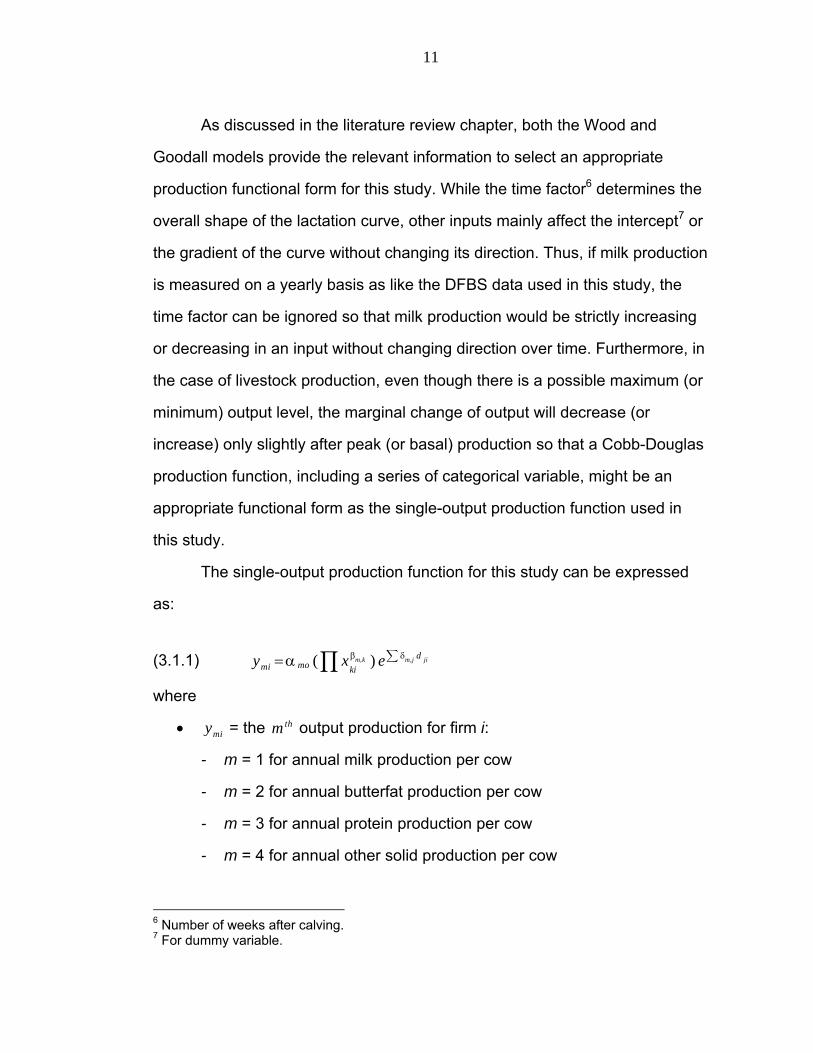
The single-output production function for this study can be expressed
as:
(3.1.1) ymi =αmo (Y x
kiβm,k ) eX δm,j d ji
where
• ymi = the mth output production for firm i:
- m = 1 for annual milk production per cow
- m = 2 for annual butterfat production per cow
- m = 3 for annual protein production per cow
- m = 4 for annual other solid production per cow
6 Number of weeks after calving. 7 For dummy variable.

12
• xki is the k th nonallocable input used to produce output ym,i
• d ji is the j th categorical variable (dummy variable)
• αmo , βm,k , and δm,j are coefficients:
- αmo is a constant representing an initial production level of the mth
output production including the combined effects of unknown fixed
inputs on the production
- βm,k is the coefficient describing the rate of change in the mth output
production responds to a one percent change in the k th input
- δm,j is the coefficient measuring the effects of the j th categorical
variable on the mth output production as shifting the intercept of the
mth output production
This non-linear function is easily transformed into a linear function by taking
logs of both sides of the function, resulting in the following estimable form:
(3.1.2) ln ymi = lnαmo +Xβm,k lnxki +X δm,j d ji
This function can be written separately for aggregate milk and individual
component production: aggregate milk, butterfat, protein, and other solids.
(3.1.3) ln y1i = lnα1o +Xβ1,k lnxki +X δ1,j d ji for aggregate milk per cow
(3.1.4) ln y2i = lnα 2o +Xβ2,k lnxki +X δ2,j d ji for butterfat per cow
(3.1.5) ln y3i = lnα 3o +Xβ3,k lnxki +X δ3,j d ji for protein per cow

13
(3.1.6) ln y4i = lnα 4o +Xβ4,k lnxki +X δ4,j d ji for other solid per cow
Since the coefficients of the four single-output production functions are
linear, an equation-by-equation ordinary least square regression (OLS)
method could be a simple way to estimate the coefficients. However, there is a
high possibility that the disturbance terms of this system of equations are
contemporaneously correlated, which implies that the disturbance variance-
covariance matrix of the system of equations would not be an identity matrix
with a constant (σ2) on its diagonal. This could happen because the four
outputs are simultaneously affected by the condition of each cow. Non
observable variables may impact each equation similarly. Therefore, Zellner’s
seemingly unrelated regression (SUR) is an appropriate method for estimating
the coefficients of the four single-output production functions because the SUR
takes into account the correlations between the error terms of each equation.
Also, the SUR is at least asymptotically more efficient than an equation-by-
equation OLS by applying Aitken’s generalized least-squares to the whole
system of equations simultaneously. If each equation has identical regressors
and satisfies the underlying assumptions of the OLS such as E ε |XB C
= 0 and
E εε . |XB C
=σ2 I , then the estimation results from the OLS and SUR will be the
same. Since the four single-output production functions have identical
regressors, each model will be estimated by applying OLS and then checked
for possible violations of the OLS assumptions. In particular, the most common
violation founded in cross-sectional data is the existence of heteroscedastic
residual. Thus, if heteroscedasticity exists, the models should be re-estimated
by using alternative estimation techniques such as White’s linear regression,
Weighted least square regression, and the iterative SUR estimator (MLE) with

14
robust variance estimation (ISUR). Since the ISUR allows for the existence of
heteroscedastic residual as well as takes into account the correlations across
the error terms of each equation, it might be the most appropriate method to
re-estimate the models for this study. Moreover, this technique will allow for
further estimation of each regression equation with different regressors that
affect the particular output production.
Since the functions are estimated based on the log values of the
outputs and inputs, the coefficient estimates βm,k = ∂ln ymi /∂lnxki represent the
(partial) production elasticity of the k th input for the mth output production, with
the exception of the dummy variables. Thus, the relationship between an
output and the business factors can be easily identified from the constant
production elasticity of each input. Based on the resulting coefficient estimates,
the possibility of altering individual component productions by adjusting inputs
can be examined. If the production elasticities of the k th input for the four
outputs are the same, farmers cannot alter individual component productions.
This is because by changing an input, each individual component production
will change proportionally according to a change in aggregate milk production,
so that individual component productions, as percentages of aggregate milk,
are always the same regardless of the amount of milk produced. On the other
hand, if the production elasticity of each input is different for the four output
productions, farmers can alter individual component productions by adjusting
the inputs. For instance, if a farmer provides more feed to a cow that produces
milk containing 3.5% butterfat, 3.2% protein, and 5% other solids, the cow may
produce more milk, but that milk may contain different levels of individual milk
components, such as 3.3% butterfat, 3.1% protein, and 5.2% other solids. This
is because the different production elasticities of each input across the four
15
outputs imply that the effect of each input on each output is different. Thus,
farmers are able to alter individual component productions by adjusting the
inputs if individual component productions, as percentages of aggregate milk,
vary depending on the amount of inputs used.
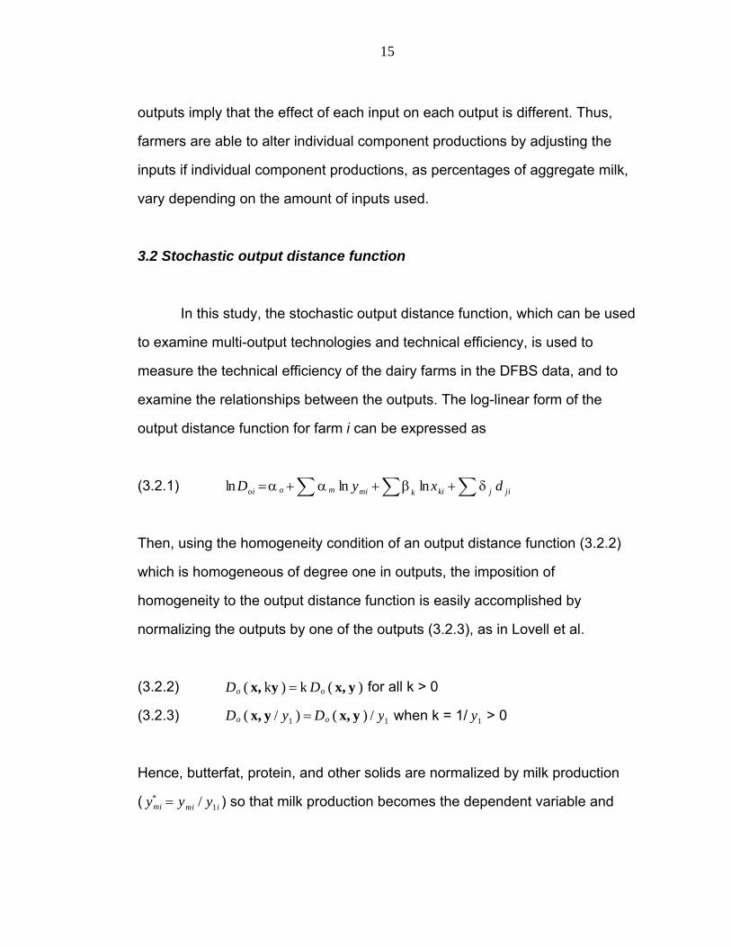
3.2 Stochastic output distance function
In this study, the stochastic output distance function, which can be used
to examine multi-output technologies and technical efficiency, is used to
measure the technical efficiency of the dairy farms in the DFBS data, and to
examine the relationships between the outputs. The log-linear form of the
output distance function for farm i can be expressed as
(3.2.1) lnDoi =α o +Xαm ln ymi +Xβk lnxki +X δ j d ji
Then, using the homogeneity condition of an output distance function (3.2.2)
which is homogeneous of degree one in outputs, the imposition of
homogeneity to the output distance function is easily accomplished by
normalizing the outputs by one of the outputs (3.2.3), as in Lovell et al.
(3.2.2) Do ( x, ky ) = k Do ( x, y ) for all k > 0
(3.2.3) Do ( x, y / y1 ) =Do ( x, y ) / y1 when k = 1/ y1 > 0
Hence, butterfat, protein, and other solids are normalized by milk production
( ymi* = ymi / y1i ) so that milk production becomes the dependent variable and

16
the independent output variables are represented as percentages of each
component in milk.
(3.2.4) lnDoi@ ln y1i =α o +Xαm ln ymi* +Xβk lnxki +X δ j d ji
To take into account unobserved random variations, a random error term (vi )
should be included in the output distance function, and thereby the stochastic
output distance function can be expressed as
(3.2.5) lnDoi@ ln y1i =α o +Xαm ln ymi* +Xβk lnxki +X δ j d ji + vi
For the sake of easier estimation of equation 3.2.5, lnDoi is moved to the right
hand side, and replaced with @ ui where ui > 0. Then, the estimable output
distance function can be written as
(3.2.6) @ ln y1i =α o +Xαm ln ymi* +Xβk lnxki +X δ j d ji + vi + ui
This stochastic output distance function has two separate error terms:
the symmetric random error term (vi ), and the one-sided efficiency error term
(ui ). The effects of traditional random variation are captured in the symmetric
error term (vi ) and the effects of technical inefficiency due to various
production factors are captured in the one-sided efficiency error term (ui ).
Here, vi is assumed to be independently and identically distributed, N ( 0,σ v2 ),
and ui , representing the technical inefficiency, is assumed to be independently
half-normally distributed, N + ( 0,σu2 ). Finally, for the purposes of easier
comparison between the estimated results of the stochastic output distance

17
function and the previous single-output production functions, the dependent
variable in this equation is transformed to ln y1i (3.2.7) so that the signs of the
estimated coefficients for the regressors will be reversed, corresponding to
those in a general production function. This stochastic output distance function
will be estimated by maximum-likelihood techniques using STATA software.
(3.2.7) ln y1i =α o +Xαm ln ymi* +Xβk lnxki +X δ j d ji + vi@ ui
After estimating this stochastic output distance function, several
economic measures can be obtained either directly from the estimation results
or by utilizing the resulting coefficient estimates. In the case of single output
production function (3.1.2), the coefficient estimates βm,k represent the (partial)
production elasticity of the k th input for an individual output, but the coefficient
estimates β k from the stochastic output distance function represent the
production elasticity of the k th input for overall outputs; the increase in the
primary output y1 , holding the output ratios of ym* constant is simply the
derivative ∂ln y1 /∂lnxk =β k . This is the percentage increase in the primary
output due to a one percent increase in input xk holding output ratios constant.
In other words, since y1 is the denominator of the output ratios, the other
outputs also increase to keep the ratio constant. Thus, this estimated elasticity
β k includes the impact on the other outputs which keep their output ratios
constant.
On the other hand, by using both the coefficient estimates β k and the
estimable form of the deterministic output distance function, the (partial)
production elasticity of an input for an individual output can also be computed.

18
To obtain this production elasticity, first, rearrange the estimable form of the
deterministic output distance function as
(3.2.8) ( 1 +Xαm ) ln y1i =α o +Xαm ln ymi +Xβk lnxki +X δ j d ji
(3.2.9) 0 =@ ( 1 +Xαm ) ln y1i + α o +Xαm ln ymi +Xβk lnxki +X δ j d ji
Taking the anti-log of this function generates Equation 3.2.10.
(3.2.10) 1 =α 0
. y1i@ 1 + Σαmb c
(Y ymiαmY x
kiβk ) eX δ j d ji , where α 0
. = eα0
This multidimensional relationship can be represented by the general
transformation function G.
(3.2.11) G ( x, d, y ) = 0
This function8 defines y implicitly as a differentiable function of x such as
y = f ( x, d ), where G ( x, d, f ( x, d ) ) = 0 for all x in the domain of f . The
function G is assumed to be differentiable for all (x, y ) in this study so that
∂ y1 /∂xk and ∂ ym /∂xk can be computed by applying the implicit function
theorem.
8 y is not a differentiable function of d because d is a vector of dummy variables. 10 Northern Hudson includes Albany, Saratoga, Schenectady, Rensselaer, Washington, and Schoharie counties. Western and Central Plain includes Cayuga, Erie, Genesee, Livingston, Niagara, Ontario, Orleans, Wayne, Wyoming, and Yates counties. Central Valleys includes Chenango, Herkimer, Madison, Montgomery, Oneida, Onondaga, Oswego, Otsego, and Schoharie. Southeastern New York includes Columbia, Delaware, Orange, and Sullivan counties. Western and Central Plateau includes Allegany, Cattaraugus, Chautauqua, Chemung, Cortland, Schuyler, Steuben, Tioga, and Tompkins counties. Northern New York includes Clinton, Essex, Franklin, Jefferson, Lewis, and St. Lawrence counties.

19
(3.2.12) ∂ y1 /∂xk =@ (∂G /∂xk ) / (∂G /∂ y1 )
= (βk / ( 1 +X αm ) )B( y1i / xki )
(3.2.13) ∂ ym /∂xk =@ (∂G /∂xk ) / (∂G /∂ ym )
= (@βk /αm )B ( ymi / xki )
Multiplying Equation 3.2.12 by ( xki / y1i ), and Equation 3.2.13 by ( xki / ymi )
generates
(3.2.14) β1,k
o = ∂ln y1 /∂lnxk =β k / ( 1 +X αm )
(3.2.15) βm,ko = ∂ln ym /∂lnxk =@βk /αm , where m ≠ 1, and for αm < 0
These computed values represent the (partial) production elasticities. Equation
3.2.14 indicates the production elasticity of the k th input xk for aggregate milk,
and Equation 3.2.15 indicates the production elasticity of the k th input xk for
each individual component. However, in a case where a coefficient (αm ) for an
output ratio ( ym* = ym / y1) is positive, the sign of the Equation 3.2.15 should be
revised as
(3.2.16) βm,ko = ∂ln ym /∂lnxk =βk /αm , where m ≠ 1, and for αm > 0
A positive coefficient (αm ) for an output ratio ( ym* = ym / y1) implies that
the milk component levels, displayed as percentages of aggregate milk,
increase with aggregate milk production; this is especially true when an
increase in an input causes one particular milk component to increase faster
than the aggregate milk. In this case, the signs need to be the same (positive)
for both the production elasticity of an input for aggregate milk (β k ) and the
20
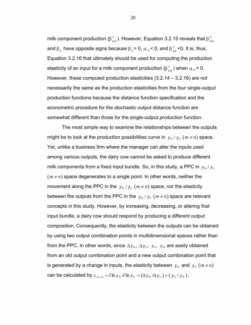
milk component production (βm,ko ). However, Equation 3.2.15 reveals that βm,k
o
and β k have opposite signs because β k > 0, αm < 0, and βm,ko <0. It is, thus,
Equation 3.2.16 that ultimately should be used for computing the production
elasticity of an input for a milk component production (βm,ko ) when αm < 0.
However, these computed production elasticities (3.2.14 – 3.2.16) are not
necessarily the same as the production elasticities from the four single-output
production functions because the distance function specification and the
econometric procedure for the stochastic output distance function are
somewhat different than those for the single-output production function.
The most simple way to examine the relationships between the outputs
might be to look at the production possibilities curve in ym / yn (m ≠ n) space.
Yet, unlike a business firm where the manager can alter the inputs used
among various outputs, the dairy cow cannot be asked to produce different
milk components from a fixed input bundle. So, in this study, a PPC in ym / yn
(m ≠ n) space degenerates to a single point. In other words, neither the
movement along the PPC in the ym / yn (m ≠ n) space, nor the elasticity
between the outputs from the PPC in the ym / yn (m ≠ n) space are relevant
concepts in this study. However, by increasing, decreasing, or altering that
input bundle, a dairy cow should respond by producing a different output
composition. Consequently, the elasticity between the outputs can be obtained
by using two output combination points in multidimensional spaces rather than
from the PPC. In other words, since Δ ym , Δ yn , yn , ym are easily obtained
from an old output combination point and a new output combination point that
is generated by a change in inputs, the elasticity between ym and yn (m ≠ n)
can be calculated by ε ym ,yn = ∂ln ym /∂ln yn = (Δ ym /Δ yn )B( yn / ym ).

21
Figure 3.2.1 illustrates this situation by using two outputs with a single
input; the output y1 is aggregate milk, another output y2 is butterfat, and the
single input x is feed. The point A represents an initial output combination
point with a given input level x0, and either the point B or C represents a new
output combination point with an increased input level from xo to x1.
Figure 3.2.1 Two output combination points in y1/y2 space
If the effects of input x on both outputs y1 and y2 are always the same,
output y2 would increase proportionally according to an increase in output y1,
so that output ratio (y2/y1) is always constant regardless of the amount of
outputs produced. In this case, a new output combination point will be plotted
on the ray-line OD that extends out from the origin O through the old output
combination point A. Point B is, thus, the new output combination point. This
implies that by changing input x, the increase in butterfat production is
proportionate to the increase in aggregate milk production; the output ratios at
A and at B are the same (y2a / y1
a = y2b / y1
b), and thereby a constant elasticity
y2b
y2c
y1c
O
y2a
y1a
C
∆y2ac
B
∆y1ac
A
∆y1ab
∆y2ab
y1
y2
D
y1b

22
between the outputs (y1 and y2) will be obtained. On the other hand, if the
effects of input x on both outputs y1 and y2 are different, the new production
point does not appear on line OD, and, in this case, point C is the new output
combination point. This new output combination point C implies that by
increasing the input level from xo to x1, a dairy cow produces a different
butterfat level as a percentage of aggregate milk, and thereby, in this case,
farmers able to alter individual component productions by altering inputs. For
instance, if a farmer provides more bedding material (from xo to x1) to a cow
who currently produces milk containing 3.5% (= y2a / y1
a) butterfat, the cow will
produce more milk (y1c) containing a different butterfat level, represented as a
percentage of aggregate milk, such as 3.7% (= y2c / y1c) butterfat. Thus, the
elasticity between the outputs (y1 and y2) will vary depending on the input level.
For computing the elasticity between the four outputs, first, rearranging
Equation 3.2.8 as:
(3.2.17) ∑∑ −−−++−=k kkllnnm mom xyyyy )ln(lnlnln)1([ln 1 βαααα
∑− j mjjd αδ /)]( , where lnm ≠≠
The elasticity between aggregate milk and each individual component is
simply computed by taking the derivative of Equation 3.2.17 with respect to
ln y1 .
(3.2.18) ε ym ,y1= ∂ln ym /∂ln y1 = ( 1 +Xαm ) /αm

23
On the other hand, Taking the derivative of Equation 3.2.17 with
respect to ln yn (m ≠ n ≠ l) generates the elasticity between each individual
component as Equation 3.2.19.
(3.2.19) ε ym ,yn = ∂ln ym /∂ln yn =@α n /αm (m ≠ n)
The estimation results of the stochastic output distance function and the
four separated component production functions are executed by STATA 9,
and will be summarized and discussed with the economic implications in the
empirical result chapter.

24
CHAPTER 4
DATA
This chapter provides the source and characteristics of the data used in
the study as well as detailed descriptions of input-output variables. It includes
a comparison of the production scale between overall New York dairy farms
and the Dairy Farm Business Summary (DFBS) participating farms.
4.1 Data source
The primary data source used in the study is the New York Dairy Farm
Business Summary (DFBS) data from 105 farms in 2003 and 107 farms in
2004. The purpose of the DFBS project is to help New York dairy farmers
improve their business management skills and financial analysis techniques.
The data mainly contain a variety of financial and production information. The
final summary is reported by Cornell University as an integral part of their
Cooperative Extension’s agricultural educational program. DFBS data are
collected annually from participating New York dairy farms across the six
regions10 of New York State. The financial information includes cash receipts
and expenses, accounts payable and receivable, beginning and year-end
balance sheets, land resources and use, detailed depreciation information,
feed and supply inventory, livestock inventory, and machinery and equipment
inventory. The production information contains figures for the total pounds of
milk and its components sold during a year, and total tons of crop produced
during a year. Some of these data are also provided on a per cow and per cwt
basis for the sake of easier comprehension and calculation.
25
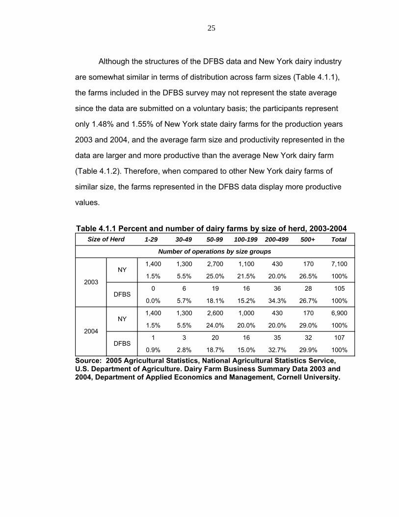
Although the structures of the DFBS data and New York dairy industry
are somewhat similar in terms of distribution across farm sizes (Table 4.1.1),
the farms included in the DFBS survey may not represent the state average
since the data are submitted on a voluntary basis; the participants represent
only 1.48% and 1.55% of New York state dairy farms for the production years
2003 and 2004, and the average farm size and productivity represented in the
data are larger and more productive than the average New York dairy farm
(Table 4.1.2). Therefore, when compared to other New York dairy farms of
similar size, the farms represented in the DFBS data display more productive
values.
Table 4.1.1 Percent and number of dairy farms by size of herd, 2003-2004
1-29 . 30-49 50-99 100-199 200-499 500+ Total
1,400 1,300 2,700 1,100 430 170 7,100
1.5% 5.5% 25.0% 21.5% 20.0% 26.5% 100%
0 6 19 16 36 28 105
0.0% 5.7% 18.1% 15.2% 34.3% 26.7% 100%
1,400 1,300 2,600 1,000 430 170 6,900
1.5% 5.5% 24.0% 20.0% 20.0% 29.0% 100%
1 3 20 16 35 32 107
0.9% 2.8% 18.7% 15.0% 32.7% 29.9% 100%DFBS
Size of Herd
Number of operations by size groups
2004
2003
NY
DFBS
NY
Source: 2005 Agricultural Statistics, National Agricultural Statistics Service, U.S. Department of Agriculture. Dairy Farm Business Summary Data 2003 and 2004, Department of Applied Economics and Management, Cornell University.
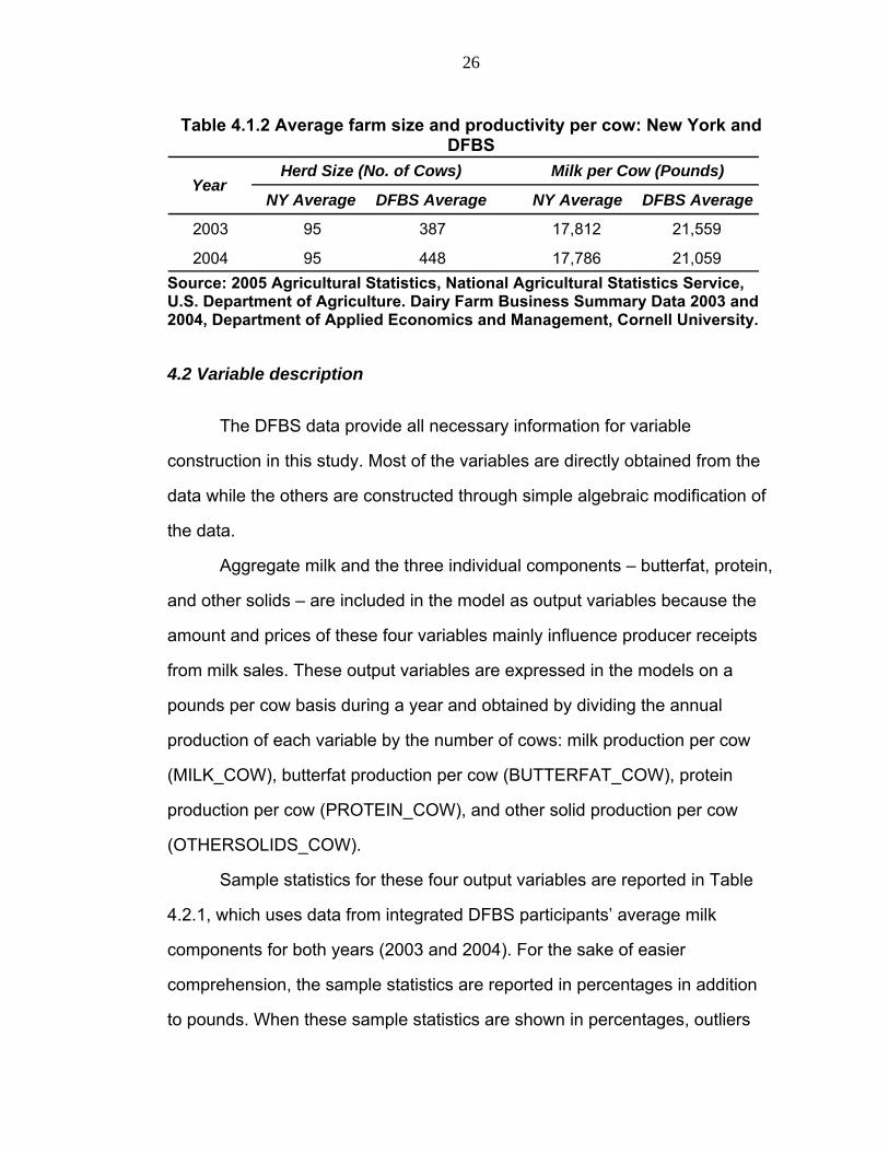
26
Table 4.1.2 Average farm size and productivity per cow: New York and DFBS
NY Average DFBS Average NY Average DFBS Average
2003 95 387 17,812 21,559
2004 95 448 17,786 21,059
YearHerd Size (No. of Cows) Milk per Cow (Pounds)
Source: 2005 Agricultural Statistics, National Agricultural Statistics Service, U.S. Department of Agriculture. Dairy Farm Business Summary Data 2003 and 2004, Department of Applied Economics and Management, Cornell University.
4.2 Variable description
The DFBS data provide all necessary information for variable
construction in this study. Most of the variables are directly obtained from the
data while the others are constructed through simple algebraic modification of
the data.
Aggregate milk and the three individual components – butterfat, protein,
and other solids – are included in the model as output variables because the
amount and prices of these four variables mainly influence producer receipts
from milk sales. These output variables are expressed in the models on a
pounds per cow basis during a year and obtained by dividing the annual
production of each variable by the number of cows: milk production per cow
(MILK_COW), butterfat production per cow (BUTTERFAT_COW), protein
production per cow (PROTEIN_COW), and other solid production per cow
(OTHERSOLIDS_COW).
Sample statistics for these four output variables are reported in Table
4.2.1, which uses data from integrated DFBS participants’ average milk
components for both years (2003 and 2004). For the sake of easier
comprehension, the sample statistics are reported in percentages in addition
to pounds. When these sample statistics are shown in percentages, outliers
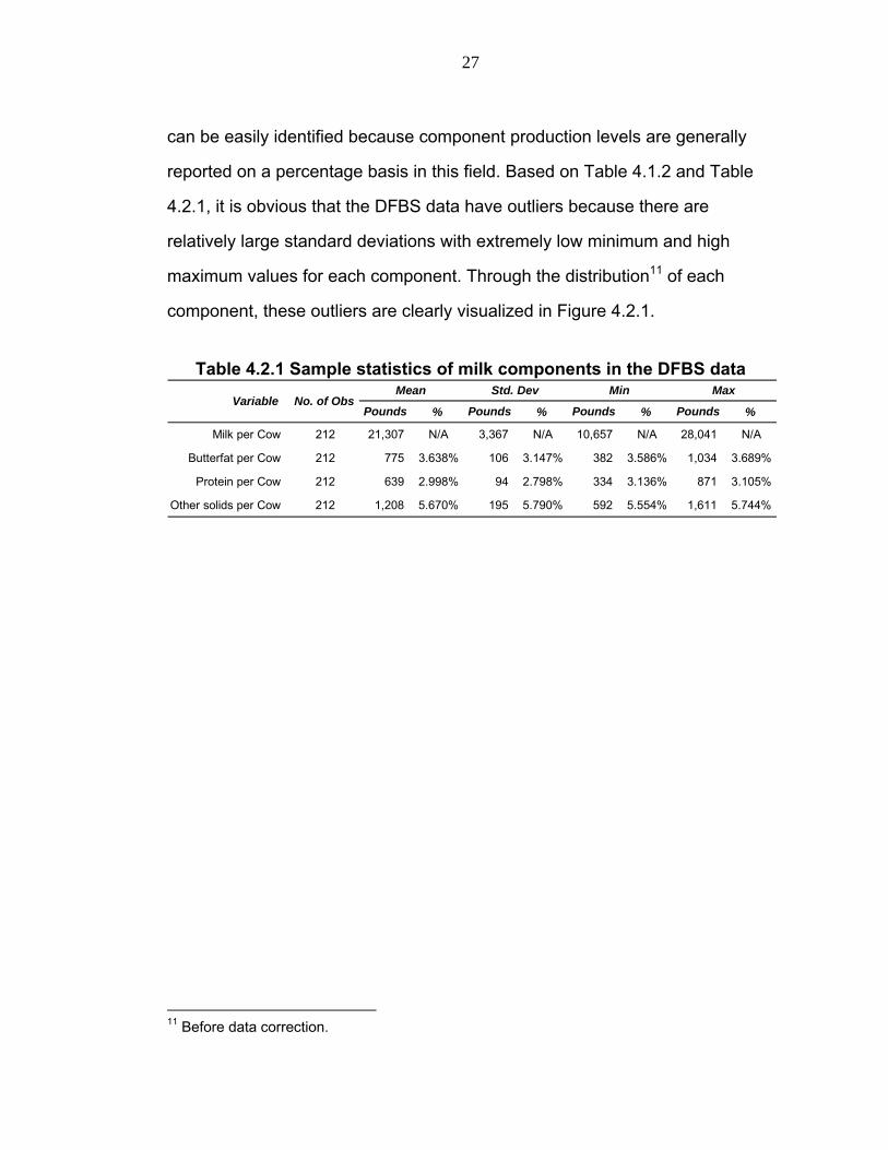
27
can be easily identified because component production levels are generally
reported on a percentage basis in this field. Based on Table 4.1.2 and Table
4.2.1, it is obvious that the DFBS data have outliers because there are
relatively large standard deviations with extremely low minimum and high
maximum values for each component. Through the distribution11 of each
component, these outliers are clearly visualized in Figure 4.2.1.
Table 4.2.1 Sample statistics of milk components in the DFBS data
% % % %
Milk per Cow 212 21,307 N/A 3,367 N/A 10,657 N/A 28,041 N/A
Butterfat per Cow 212 775 3.638% 106 3.147% 382 3.586% 1,034 3.689%
Protein per Cow 212 639 2.998% 94 2.798% 334 3.136% 871 3.105%
Other solids per Cow 212 1,208 5.670% 195 5.790% 592 5.554% 1,611 5.744%
Pounds PoundsVariable No. of Obs
Pounds Pounds
Mean Std. Dev Min Max
11 Before data correction.
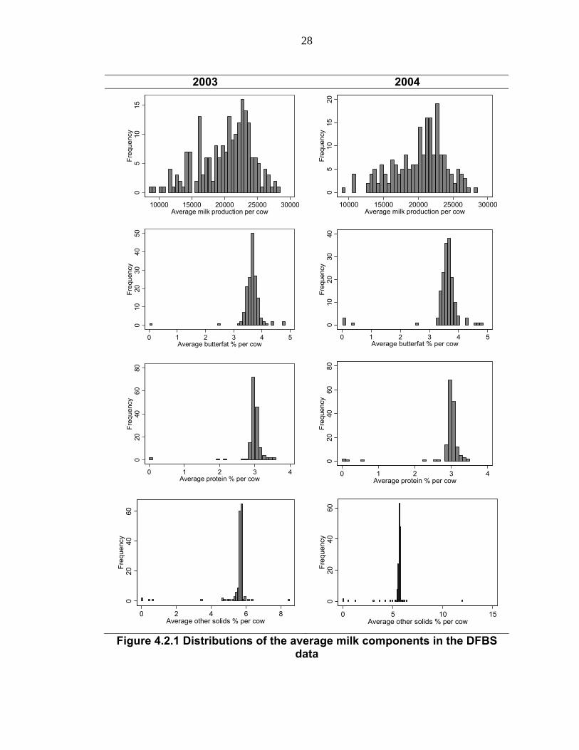
28
2003 2004
05
1015
Freq
uenc
y
10000 15000 20000 25000 30000Average milk production per cow
05
1015
20Fr
eque
ncy
10000 15000 20000 25000 30000Average milk production per cow
010
2030
4050
Freq
uenc
y
0 1 2 3 4 5Average butterfat % per cow
010
2030
40Fr
eque
ncy
0 1 2 3 4 5Average butterfat % per cow
020
4060
80Fr
eque
ncy
0 1 2 3 4Average protein % per cow
020
4060
80Fr
eque
ncy
0 1 2 3 4Average protein % per cow
020
4060
Freq
uenc
y
0 2 4 6 8Average other solids % per cow
020
4060
Freq
uenc
y
0 5 10 15Average other solids % per cow
Figure 4.2.1 Distributions of the average milk components in the DFBS data

29
Specifically, the outliers in the distributions of butterfat, protein, and
other solids may indicate misrecorded data or data recorded under unusual
circumstances such as diseases, because they exhibit extraordinary values
compared with the average values of New York State and the DFBS
participants (Table 4.2.2). Therefore, all outliers are treated as missing data to
prevent the possible distortion of regression results. As a result of data
correction, six missing data are deleted in each year (Table 4.2.3). Detailed
criteria used to define the outliers are that butterfat percentage is less than 2
percent or greater than 5 percent, protein percentage is less than 1 percent or
greater than 5 percent, or other solids percentage is less than 4 percent or
greater than 8 percent.
Table 4.2.2 Average milk component tests: New York and DFBS
NY Average DFBS Average NY Average DFBS Average NY Average DFBS Average
2003 3.67 3.68 2.98 3.00 5.66 5.672004 3.65 3.64 3.02 3.02 5.66 5.67
Butterfat % Protein % Other solids %Year
Source: Northeast Annual Statistical Bulletin 2003 and 2004, Northeast Marketing Area, Agricultural Marketing Service, U.S. Department of Agriculture. Dairy Farm Business Summary Data of 2003 and 2004, Department of Applied Economics and Management, Cornell University.
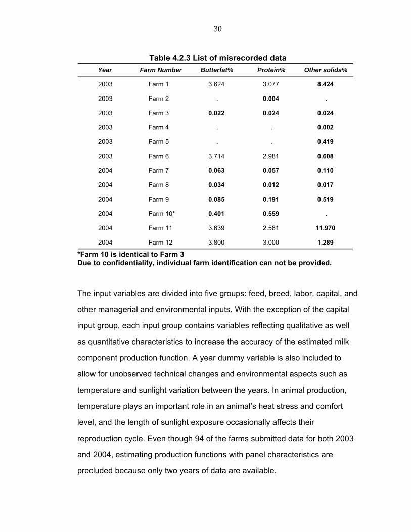
30
Table 4.2.3 List of misrecorded data Year Butterfat% Protein% Other solids%
2003 Farm 1 3.624 3.077 8.424
2003 Farm 2 . 0.004 .
2003 Farm 3 0.022 0.024 0.024
2003 Farm 4 . . 0.002
2003 Farm 5 . . 0.419
2003 Farm 6 3.714 2.981 0.608
2004 Farm 7 0.063 0.057 0.110
2004 Farm 8 0.034 0.012 0.017
2004 Farm 9 0.085 0.191 0.519
2004 Farm 10* 0.401 0.559 .
2004 Farm 11 3.639 2.581 11.970
2004 Farm 12 3.800 3.000 1.289
Farm Number
*Farm 10 is identical to Farm 3 Due to confidentiality, individual farm identification can not be provided.
The input variables are divided into five groups: feed, breed, labor, capital, and
other managerial and environmental inputs. With the exception of the capital
input group, each input group contains variables reflecting qualitative as well
as quantitative characteristics to increase the accuracy of the estimated milk
component production function. A year dummy variable is also included to
allow for unobserved technical changes and environmental aspects such as
temperature and sunlight variation between the years. In animal production,
temperature plays an important role in an animal’s heat stress and comfort
level, and the length of sunlight exposure occasionally affects their
reproduction cycle. Even though 94 of the farms submitted data for both 2003
and 2004, estimating production functions with panel characteristics are
precluded because only two years of data are available.
31
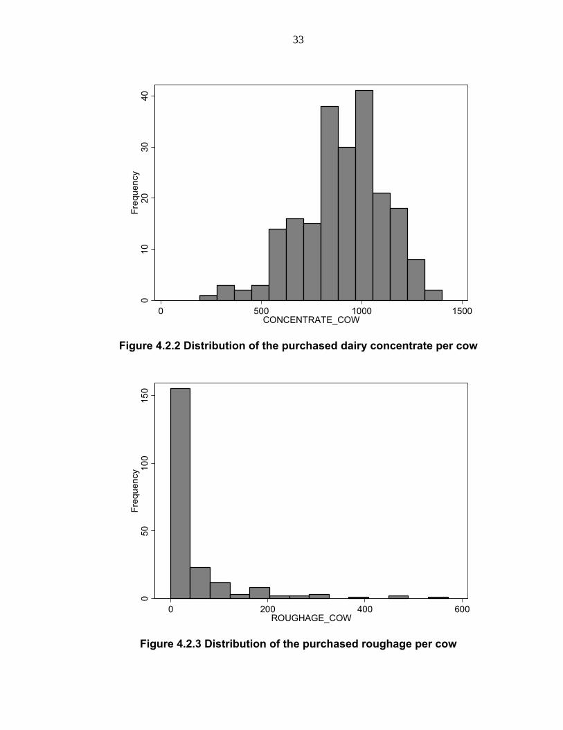
Feed is the most important input in the dairy business because the nutritional
composition of feed along with dry matter intake of a cow are the most crucial
factors in determining not only milk and each component production levels, but
also immunity, body condition, reproduction, and growth of a cow. Therefore, it
is impossible to predict aggregate milk and individual component production
without information on the nutritional values and amount of feed provided to
each cow in each production stage, and thereby most studies related to milk
production also include feed in the model. Usually, in the field of animal
science, feed is expressed in models as net energy value, which is known as
net energy of lactation, that express energy requirements for maintenance and
milk production (NRC (2001)). However, agricultural economists have
generally been interested in the price elasticity of milk supply rather than milk
production itself, so they commonly use price information for feed such as
feed-forage ratio (e.g., Chavas and Klemme, Howard and Shumway (1986))
instead of NEL of feedstuffs, or actual feed quantity used in animal production.
Unfortunately, the DFBS data does not provide detailed feed information
except the dollar amount of purchased feed per cow (concentrate and
roughage) and tons of home-grown forage produced per cow. Since the
compositions of feed may not be identical across all of the participants in the
DFBS project, and the dollar amount of purchased feed per cow (concentrate
and roughage) and tons of home-grown forage per cow vary widely (Table
4.2.4 and Figures 4.2.2 – 4.2.4), proxy variables are used in this study to
represent feed information. The proxy variables fall into two main categories of
dairy feed source: forage and commercial dairy feed. Forage per cow
(FORAGE_COW) and forage per acre (FORAGE_ACRE) are used to
represent the quantity and quality of forage provided to a cow per year,

32
respectively. These variables are measured in tons of dry matter, each
including hay, hay crop silage, corn silage, and other forage produced on the
farm. Often higher forage yield signifies higher quality forage, and it results in
enhanced nutritional value in home-grown dairy feed. Purchased dairy
concentrate per cow (CONCENTRATE_COW) and purchased roughage per
cow (ROUGHAGE_COW) are used to represent the amount of commercial
feed fed to a cow per year, measured as an expense in dollars. Specially, high
concentrate expenses may reflect high quality feed ingredients or a high ratio
of commercial feed to forage, which generally increases average milk
production, but they also may simply indicate high feed prices because the
DFBS data do not provide purchased feed quality information for each farm.
Table 4.2.4 Sample statistics of the feed variables
Variable No. of Obs
Concentrate per Cow 212 909.17 212.12 193 1403
Roughage per Cow 212 43.63 87.13 0 571
Forage per Cow 212 8.08 2.58 0 17
Mean MaxStd. Dev Min
Concentrate and roughage per cow are measured in dollars. Forage per cow is measured in the tons of dry matter.
33
010
2030
40Fr
eque
ncy
0 500 1000 1500CONCENTRATE_COW
Figure 4.2.2 Distribution of the purchased dairy concentrate per cow
050
100
150
Freq
uenc
y
0 200 400 600ROUGHAGE_COW
Figure 4.2.3 Distribution of the purchased roughage per cow

34
010
2030
4050
Freq
uenc
y
0 5 10 15 20FORAGE_COW
Figure 4.2.4 Distribution of the home-grown forage produced per cow
Breed and genetic traits are the second most important factor in
aggregate milk and individual component production since they determine the
basic levels of aggregate milk and individual component production (Table
4.2.5) as well as live weight gain, feed intake, and feed conversion efficiency.
To take into account the effects of breed and genetic traits on milk production,
the composition of dairy breeds on the farm (Holstein, Jersey, and other
breeds12), the average annual cow value (COW_VALUE), and an expense for
genetic improvement per cow per year (GENETICS_COW) are included in the
input variables. Since, under FMMO multiple component pricing system, milk
composition is often more important than the amount of milk produced,
particularly to the butter and cheese manufacturers, the percentages of Non-
12 The DFBS data do not specify which breeds are included in "other breeds".
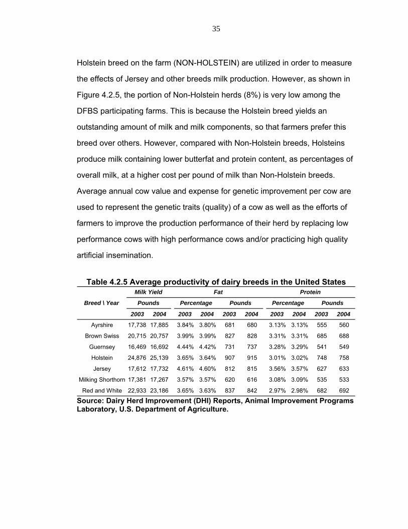
35
Holstein breed on the farm (NON-HOLSTEIN) are utilized in order to measure
the effects of Jersey and other breeds milk production. However, as shown in
Figure 4.2.5, the portion of Non-Holstein herds (8%) is very low among the
DFBS participating farms. This is because the Holstein breed yields an
outstanding amount of milk and milk components, so that farmers prefer this
breed over others. However, compared with Non-Holstein breeds, Holsteins
produce milk containing lower butterfat and protein content, as percentages of
overall milk, at a higher cost per pound of milk than Non-Holstein breeds.
Average annual cow value and expense for genetic improvement per cow are
used to represent the genetic traits (quality) of a cow as well as the efforts of
farmers to improve the production performance of their herd by replacing low
performance cows with high performance cows and/or practicing high quality
artificial insemination.
Table 4.2.5 Average productivity of dairy breeds in the United States
2003 2004 2003 2004 2003 2004 2003 2004 2003 2004
Ayrshire 17,738 17,885 3.84% 3.80% 681 680 3.13% 3.13% 555 560
Brown Swiss 20,715 20,757 3.99% 3.99% 827 828 3.31% 3.31% 685 688
Guernsey 16,469 16,692 4.44% 4.42% 731 737 3.28% 3.29% 541 549
Holstein 24,876 25,139 3.65% 3.64% 907 915 3.01% 3.02% 748 758
Jersey 17,612 17,732 4.61% 4.60% 812 815 3.56% 3.57% 627 633
Milking Shorthorn 17,381 17,267 3.57% 3.57% 620 616 3.08% 3.09% 535 533
Red and White 22,933 23,186 3.65% 3.63% 837 842 2.97% 2.98% 682 692
Milk Yield Fat Protein
Breed \ Year Pounds Percentage Pounds Percentage Pounds
Source: Dairy Herd Improvement (DHI) Reports, Animal Improvement Programs Laboratory, U.S. Department of Agriculture.

36
Holstein92%
Jersey4%
Other breeds4%
Figure 4.2.5 Distribution of dairy breeds in the DFBS data
Labor represents human capital which is a very important factor,
especially in a labor intensive industry like agriculture. In the dairy business,
along with the amount of labor provided, labor quality is also important since it
is a contributor to the efficiency of a farm. Thus, the milk component
production function should include a measure of both labor quality and
quantity provided on the farm. So, the average monthly wage for hired labor
(WAGE_MONTH) is used to represent hired labor quality in the model, and the
average number of cows per worker (COWS_WKR) is used to measure the
average labor force per cow including operator labor, family labor, and hired
labor.
Universally, economies of scale have large effects on the profitability
and technical efficiency of a company. In the animal production sector, herd
size is often interpreted as the economies of scale, but milking system type
and capacity are actually better indicators of the economies of scale in the
dairy industry. Milking system type including capacity represents not only farm
size but also housing type and capital intensity of a farm. In general, due to the
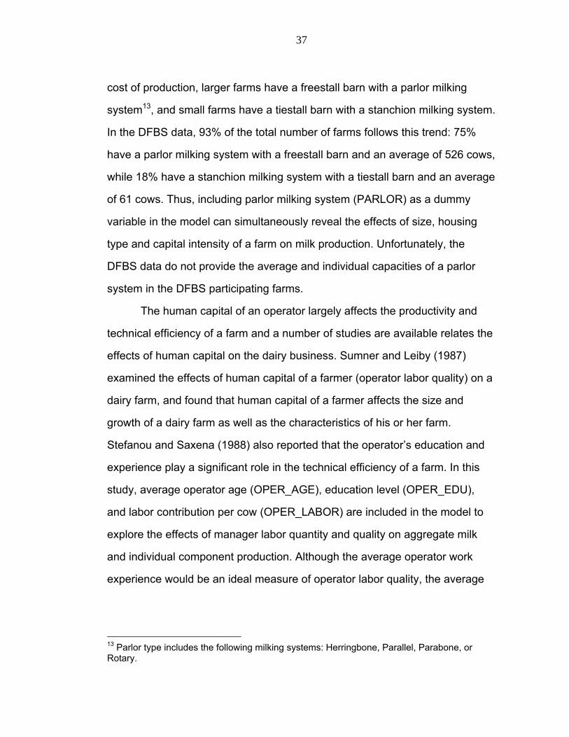
37
cost of production, larger farms have a freestall barn with a parlor milking
system13, and small farms have a tiestall barn with a stanchion milking system.
In the DFBS data, 93% of the total number of farms follows this trend: 75%
have a parlor milking system with a freestall barn and an average of 526 cows,
while 18% have a stanchion milking system with a tiestall barn and an average
of 61 cows. Thus, including parlor milking system (PARLOR) as a dummy
variable in the model can simultaneously reveal the effects of size, housing
type and capital intensity of a farm on milk production. Unfortunately, the
DFBS data do not provide the average and individual capacities of a parlor
system in the DFBS participating farms.
The human capital of an operator largely affects the productivity and
technical efficiency of a farm and a number of studies are available relates the
effects of human capital on the dairy business. Sumner and Leiby (1987)
examined the effects of human capital of a farmer (operator labor quality) on a
dairy farm, and found that human capital of a farmer affects the size and
growth of a dairy farm as well as the characteristics of his or her farm.
Stefanou and Saxena (1988) also reported that the operator’s education and
experience play a significant role in the technical efficiency of a farm. In this
study, average operator age (OPER_AGE), education level (OPER_EDU),
and labor contribution per cow (OPER_LABOR) are included in the model to
explore the effects of manager labor quantity and quality on aggregate milk
and individual component production. Although the average operator work
experience would be an ideal measure of operator labor quality, the average
13 Parlor type includes the following milking systems: Herringbone, Parallel, Parabone, or Rotary.

38
operator age and education level are used to reveal manager labor quality in
this study because the data do not provide such information.
Also included in the model to represent other business factors are the
average herd size (COWS), bedding expense per cow per year
(BEDDING_COW), machinery cost per cow per year (MACHINERY_COW),
BST expense per cow per year (BST_COW), culling rate (CULL_RATE), bred
heifer rate (HEIFER_RATE), daily milking frequency (3BMILKING), and farm
ownership type (SOLEOWNER). In particular, the herd size is closely related
with economies of scale (Sumner and Leiby (1987)), so if there is an optimal
size, it should affect the milk component production as well as profits of a farm.
The bedding expense per cow per year is used to represent the effects of cow
comfort on milk component production. The machinery cost per cow per year
is used as a measurement of equipment quality and non-obsolescence of that
equipment, as well as the capital intensity of a farm. The culling rate and bred
heifer rate are proxy variables used for parity distribution of farms since milk
component production levels are closely related to parity numbers of a cow.
These variables are also indicators of reproduction and/or disease problems
which cause significantly lower production performance on a farm so that
short-run productivity could be reflected in these variables. In general, farmers
replace old cows (low production) with genetically superior young cows.
The DFBS data also provide the geographic information of the farms
across the six regions of New York State (Western and Central Plain, Western
and Central Plateau, Central Valleys, Northern New York, Northern Hudson,
and Southeastern New York). However, the data do not provide detailed
environmental information such as inside temperature and humidity of the barn,
which are closely related with cow comfort level, so the geographic information

39
is excluded from the model in this study. Geographic information is often used
to represent the differences of pasture quality in analyzing milk production
(Buccola and Iizuka (1997)), but the component models already include a
variable (FORAGE_ACRE) which represents the individual farm’s forage
quality. Thus, it is not necessary to include the geographic information in the
models. A summary of the variable codes used in estimation of milk
component production function is provided in Tables 4.2.6 – 4.2.7.
40
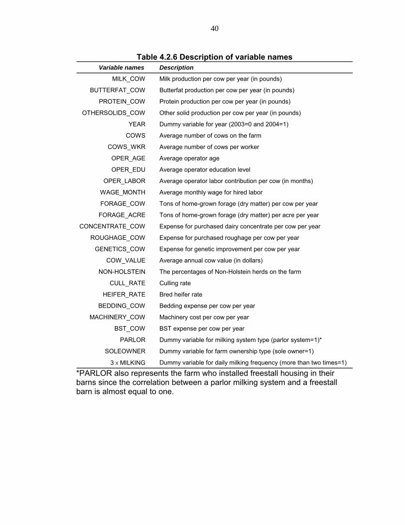
Table 4.2.6 Description of variable names Variable names Description
MILK_COW Milk production per cow per year (in pounds)
BUTTERFAT_COW Butterfat production per cow per year (in pounds)
PROTEIN_COW Protein production per cow per year (in pounds)
OTHERSOLIDS_COW Other solid production per cow per year (in pounds)
YEAR Dummy variable for year (2003=0 and 2004=1)
COWS Average number of cows on the farm
COWS_WKR Average number of cows per worker
OPER_AGE Average operator age
OPER_EDU Average operator education level
OPER_LABOR Average operator labor contribution per cow (in months)
WAGE_MONTH Average monthly wage for hired labor
FORAGE_COW Tons of home-grown forage (dry matter) per cow per year
FORAGE_ACRE Tons of home-grown forage (dry matter) per acre per year
CONCENTRATE_COW Expense for purchased dairy concentrate per cow per year
ROUGHAGE_COW Expense for purchased roughage per cow per year
GENETICS_COW Expense for genetic improvement per cow per year
COW_VALUE Average annual cow value (in dollars)
NON-HOLSTEIN The percentages of Non-Holstein herds on the farm
CULL_RATE Culling rate
HEIFER_RATE Bred heifer rate
BEDDING_COW Bedding expense per cow per year
MACHINERY_COW Machinery cost per cow per year
BST_COW BST expense per cow per year
PARLOR Dummy variable for milking system type (parlor system=1)*
SOLEOWNER Dummy variable for farm ownership type (sole owner=1)
3ⅹMILKING Dummy variable for daily milking frequency (more than two times=1) *PARLOR also represents the farm who installed freestall housing in their barns since the correlation between a parlor milking system and a freestall barn is almost equal to one.

41
Table 4.2.7 Sample statistics of the variables Variable names Sample statistics
Obs Mean Std.Dev. Min Max
MILK_COW 212 21306.79 3366.69 10656.54 28040.53
BUTTERFAT_COW 212 775.25 105.96 382.15 1034.45
PROTEIN_COW 212 638.85 94.19 334.24 870.56
OTHERSOLIDS_COW 212 1208.12 194.93 591.83 1610.77
COWS 212 417.68 447.39 27.00 3605.00
COWS_WKR 212 38.48 12.61 16.00 93.00
OPER_AGE 212 49.08 7.61 32.00 70.00
OPER_EDU 212 14.05 1.67 8.00 20.00
OPER_LABOR 212 13.28 2.68 5.95 20.60
WAGE_MONTH 212 2440.79 883.51 555.00 8521.00
FORAGE_COW 212 8.08 2.58 0.35 17.26
FORAGE_ACRE 212 4.07 1.24 1.09 9.11
CONCENTRATE_COW 212 909.17 212.12 193.00 1403.00
ROUGHAGE_COW 212 43.63 87.13 0.00 571.00
GENETICS_COW 212 46.52 26.17 0.00 127.00
COW_VALUE 212 1238.62 168.67 800.00 1900.00
NON-HOLSTEIN 212 7.98 21.76 0.00 100.00
CULL_RATE 212 32.07 7.94 3.00 52.00
HEIFER_RATE 212 22.07 5.97 1.82 38.51
BEDDING_COW 212 49.74 39.66 0.00 255.00
MACHINERY_COW 212 590.56 166.86 198.00 1108.00
BST_COW 212 37.87 37.23 0.00 119.00
Dummy variable descriptions
YEAR 105 farms in 2003, 107 farms in 2004, and 94 of the farms submitted
data for both years.
PARLOR 165 farms have a parlor milking system (out of 212 farms)
SOLEOWNER 89 farms are operated by a soleowner (out of 212 farms)
3ⅹMILKING 96 farms are milking more than two times per day (out of 212 farms)

42
CHAPTER 5
EMPIRICAL RESULTS
This chapter provides the results and implications of estimating the four
single-output production functions and the stochastic output distance function.
The effects of the business factors found to have significant effects on
aggregate milk and individual component production, technical efficiency of
participating New York dairy farms in the DFBS project, and the relationships
between the four separate milk outputs (aggregate milk, butterfat, protein, and
other solids) are presented and discussed.
5.1 The results of estimating the four single-output production functions
Estimation results by OLS
The four outputs may be simultaneously affected by the condition of
each cow, and, thereby, non-observable variables may impact each equation
similarly so that there is a high possibility that the disturbance terms of the
system of equations (3.1.3 – 3.1.6) are contemporaneously correlated. In this
case, the seemingly unrelated regression technique (SUR), which takes into
account the correlations between the error terms of each equation, is an
appropriate method for estimating the coefficients of the four single-output
production functions. However, if the OLS assumptions are satisfied in the
OLS regressions, the estimation results from the OLS and SUR will be the
same because each equation in this system of equations has identical
regressors. Yet, if there is a violation of the OLS assumptions, the system of
equations needs to be re-estimated by alternative estimation techniques. It is,

43
therefore, necessary to discuss the test results for the OLS assumptions
before analyzing the OLS estimation results. Tables 5.1.1 – 5.1.4 report the
results of estimating the four single-output production functions using OLS,
and Tables 5.1.5 – 5.1.7 present the results of testing possible violations of the
OLS assumptions: VIF for multicollinearity and the White and Breusch-Pagan
tests for heteroscedasticity.
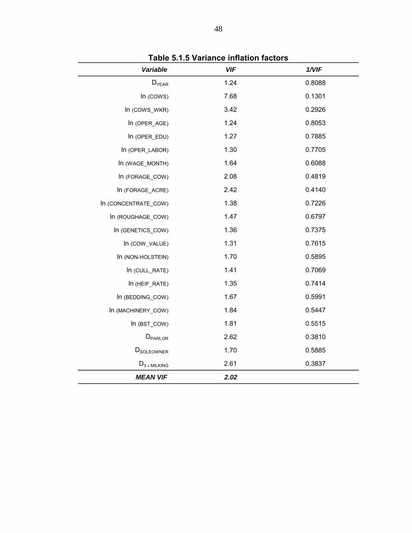
If the regressors are highly correlated in the OLS regressions, serious
problems arise; even though the coefficient estimates are jointly significant,
either the resulting estimated standard errors are inflated or the coefficient
estimates have implausible values, and the coefficient estimates are
significantly varied by adding or deleting an independent variable, or by small
changes in the data. Thus, the presence of multicollinearity is checked by the
Variance Inflation Factors (VIF) in Table 5.1.5. With the mean of all the VIFs at
2.02 and the largest VIF at 7.68 implies there is no severe multicollinearity in
the OLS regressions. Heteroscedasticity often appears in cross-sectional data
and is also checked by implementing the White general test and the Breusch-
Pagan test. The null hypotheses (homoscedastic residual) of both the White
and Breusch-Pagan tests for heteroscedasticity are rejected for both tests.
This implies the presence of heteroscedastic residual in each of the
disturbance terms.

44
Table 5.1.1 The estimation results by OLS (aggregate milk)
Std. Err. P>t
DYEAR -0.0389 0.0126 -3.08 0.0020
ln (COWS) -0.0138 0.0155 -0.89 0.3730
ln (COWS_WKR) -0.0224 0.0327 -0.69 0.4940
ln (OPER_AGE) -0.1278 0.0411 -3.11 0.0020
ln (OPER_EDU) 0.0462 0.0564 0.82 0.4130
ln (OPER_LABOR) -0.0061 0.0331 -0.18 0.8540
ln (WAGE_MONTH) 0.0567 0.0193 2.93 0.0040
ln (FORAGE_COW) -0.0579 0.0234 -2.48 0.0140
ln (FORAGE_ACRE) 0.0879 0.0333 2.64 0.0090
ln (CONCENTRATE_COW) 0.1056 0.0243 4.35 0.0000
ln (ROUGHAGE_COW) -0.0031 0.0035 -0.89 0.3760
ln (GENETICS_COW) 0.0552 0.0077 7.16 0.0000
ln (COW_VALUE) 0.0539 0.0480 1.12 0.2630
ln (NON-HOLSTEIN) -0.0433 0.0055 -7.94 0.0000
ln (CULL_RATE) 0.0047 0.0217 0.21 0.8300
ln (HEIF_RATE) 0.0371 0.0174 2.13 0.0340
ln (BEDDING_COW) 0.0102 0.0054 1.87 0.0630
ln (MACHINERY_COW) 0.0816 0.0269 3.04 0.0030
ln (BST_COW) 0.0153 0.0039 3.90 0.0000
DPARLOR -0.0188 0.0221 -0.85 0.3960
DSOLEOWNER -0.0125 0.0150 -0.83 0.4070
D3ⅹMILKING 0.0941 0.0184 5.12 0.0000
Intercept 8.0622 0.5658 14.25 0.0000
Dependent variable: ln y 1 (aggregate milk)
(R 2 : 0.8024, Adj. R 2 : 0.7794, Prob>F: 0)
Estimate t

45
Table 5.1.2 The estimation results by OLS (butterfat)
Std. Err. P>t
DYEAR -0.0574 0.0123 -4.65 0.0000
ln (COWS) -0.0046 0.0151 -0.30 0.7610
ln (COWS_WKR) -0.0094 0.0319 -0.29 0.7700
ln (OPER_AGE) -0.0705 0.0402 -1.76 0.0810
ln (OPER_EDU) -0.0076 0.0551 -0.14 0.8900
ln (OPER_LABOR) 0.0162 0.0323 0.50 0.6160
ln (WAGE_MONTH) 0.0386 0.0189 2.04 0.0420
ln (FORAGE_COW) -0.0668 0.0228 -2.92 0.0040
ln (FORAGE_ACRE) 0.0893 0.0325 2.74 0.0070
ln (CONCENTRATE_COW) 0.1063 0.0237 4.48 0.0000
ln (ROUGHAGE_COW) -0.0062 0.0034 -1.82 0.0700
ln (GENETICS_COW) 0.0606 0.0075 8.04 0.0000
ln (COW_VALUE) 0.0307 0.0469 0.65 0.5140
ln (NON-HOLSTEIN) -0.0133 0.0053 -2.51 0.0130
ln (CULL_RATE) -0.0046 0.0212 -0.22 0.8280
ln (HEIF_RATE) 0.0158 0.0170 0.93 0.3550
ln (BEDDING_COW) 0.0189 0.0053 3.56 0.0000
ln (MACHINERY_COW) 0.0947 0.0262 3.61 0.0000
ln (BST_COW) 0.0129 0.0038 3.37 0.0010
DPARLOR -0.0467 0.0216 -2.16 0.0320
DSOLEOWNER -0.0093 0.0146 -0.64 0.5250
D3ⅹMILKING 0.0841 0.0180 4.68 0.0000
Intercept 4.8246 0.5527 8.73 0.0000
Dependent variable: ln y 2 (butterfat)
(R 2 : 0.7368, Adj. R 2 : 0.7062, Prob>F: 0)
Estimate t

46
Table 5.1.3 The estimation results by OLS (protein)
Std. Err. P>t
DYEAR -0.0353 0.0126 -2.80 0.0060
ln (COWS) -0.0147 0.0154 -0.95 0.3410
ln (COWS_WKR) 0.0203 0.0326 0.62 0.5340
ln (OPER_AGE) -0.0543 0.0410 -1.32 0.1870
ln (OPER_EDU) 0.0526 0.0563 0.94 0.3510
ln (OPER_LABOR) 0.0235 0.0330 0.71 0.4770
ln (WAGE_MONTH) 0.0581 0.0193 3.01 0.0030
ln (FORAGE_COW) -0.0590 0.0233 -2.53 0.0120
ln (FORAGE_ACRE) 0.0752 0.0332 2.26 0.0250
ln (CONCENTRATE_COW) 0.1140 0.0242 4.70 0.0000
ln (ROUGHAGE_COW) -0.0050 0.0035 -1.43 0.1530
ln (GENETICS_COW) 0.0574 0.0077 7.46 0.0000
ln (COW_VALUE) 0.0152 0.0479 0.32 0.7510
ln (NON-HOLSTEIN) -0.0238 0.0054 -4.38 0.0000
ln (CULL_RATE) 0.0094 0.0217 0.43 0.6660
ln (HEIF_RATE) 0.0353 0.0174 2.03 0.0440
ln (BEDDING_COW) 0.0126 0.0054 2.32 0.0220
ln (MACHINERY_COW) 0.0982 0.0268 3.66 0.0000
ln (BST_COW) 0.0175 0.0039 4.47 0.0000
DPARLOR -0.0486 0.0221 -2.20 0.0290
DSOLEOWNER -0.0116 0.0150 -0.78 0.4380
D3ⅹMILKING 0.0958 0.0184 5.21 0.0000
Intercept 4.1270 0.5647 7.31 0.0000
Dependent variable: ln y 3 (protein)
(R 2 : 0.7617, Adj. R 2 : 0.7339, Prob>F: 0)
Estimate t
47
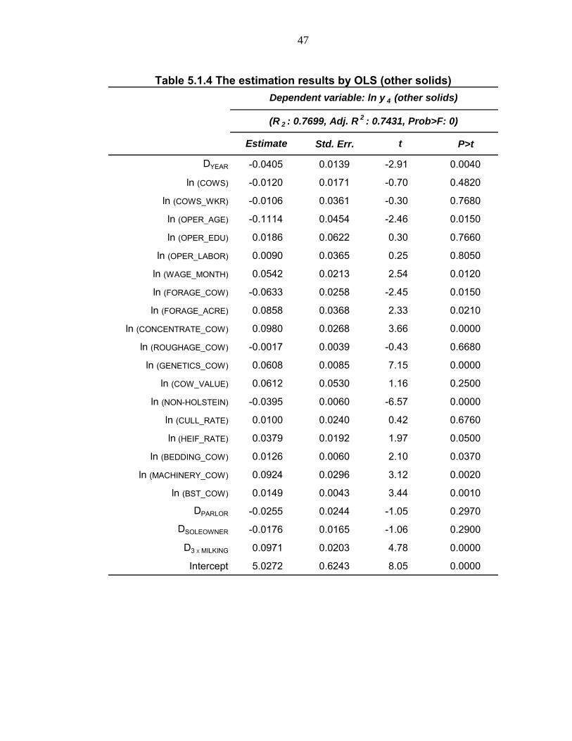
Table 5.1.4 The estimation results by OLS (other solids)
Std. Err. P>t
DYEAR -0.0405 0.0139 -2.91 0.0040
ln (COWS) -0.0120 0.0171 -0.70 0.4820
ln (COWS_WKR) -0.0106 0.0361 -0.30 0.7680
ln (OPER_AGE) -0.1114 0.0454 -2.46 0.0150
ln (OPER_EDU) 0.0186 0.0622 0.30 0.7660
ln (OPER_LABOR) 0.0090 0.0365 0.25 0.8050
ln (WAGE_MONTH) 0.0542 0.0213 2.54 0.0120
ln (FORAGE_COW) -0.0633 0.0258 -2.45 0.0150
ln (FORAGE_ACRE) 0.0858 0.0368 2.33 0.0210
ln (CONCENTRATE_COW) 0.0980 0.0268 3.66 0.0000
ln (ROUGHAGE_COW) -0.0017 0.0039 -0.43 0.6680
ln (GENETICS_COW) 0.0608 0.0085 7.15 0.0000
ln (COW_VALUE) 0.0612 0.0530 1.16 0.2500
ln (NON-HOLSTEIN) -0.0395 0.0060 -6.57 0.0000
ln (CULL_RATE) 0.0100 0.0240 0.42 0.6760
ln (HEIF_RATE) 0.0379 0.0192 1.97 0.0500
ln (BEDDING_COW) 0.0126 0.0060 2.10 0.0370
ln (MACHINERY_COW) 0.0924 0.0296 3.12 0.0020
ln (BST_COW) 0.0149 0.0043 3.44 0.0010
DPARLOR -0.0255 0.0244 -1.05 0.2970
DSOLEOWNER -0.0176 0.0165 -1.06 0.2900
D3ⅹMILKING 0.0971 0.0203 4.78 0.0000
Intercept 5.0272 0.6243 8.05 0.0000
Dependent variable: ln y 4 (other solids)
(R 2 : 0.7699, Adj. R 2 : 0.7431, Prob>F: 0)
Estimate t
48
Table 5.1.5 Variance inflation factors Variable VIF 1/VIF
DYEAR 1.24 0.8088
ln (COWS) 7.68 0.1301
ln (COWS_WKR) 3.42 0.2926
ln (OPER_AGE) 1.24 0.8053
ln (OPER_EDU) 1.27 0.7885
ln (OPER_LABOR) 1.30 0.7705
ln (WAGE_MONTH) 1.64 0.6088
ln (FORAGE_COW) 2.08 0.4819
ln (FORAGE_ACRE) 2.42 0.4140
ln (CONCENTRATE_COW) 1.38 0.7226
ln (ROUGHAGE_COW) 1.47 0.6797
ln (GENETICS_COW) 1.36 0.7375
ln (COW_VALUE) 1.31 0.7615
ln (NON-HOLSTEIN) 1.70 0.5895
ln (CULL_RATE) 1.41 0.7069
ln (HEIF_RATE) 1.35 0.7414
ln (BEDDING_COW) 1.67 0.5991
ln (MACHINERY_COW) 1.84 0.5447
ln (BST_COW) 1.81 0.5515
DPARLOR 2.62 0.3810
DSOLEOWNER 1.70 0.5885
D3ⅹMILKING 2.61 0.3837
MEAN VIF 2.02

49
Table 5.1.6 The White’s general test for heteroscedasticity White's test for Ho: Homoscedasticity
against Ha: Unrestricted heteroscedasticity
chi2 df p
ln y 1 57.79305 27 0.00051
ln y 2 65.22451 27 0.00005
ln y 3 67.92019 27 0.00002
ln y 4 57.05545 27 0.00063
Due to a relatively large number of independent variables (22) to a number of observations (212), White’s general test is executed with six selected independent variables: ln(COWS), ln(GENETICS_COW), ln(NON-HOLSTEIN), ln(BEDDING_COW), ln(BST_COW), and ln(MACHINERY_COW). These six independent variables are highly correlated with a size of a farm (ln(COWS) and ln(MACHINERY_COW)) and/or an average productivity of a farm (ln(GENETICS_COW), ln(NON-HOLSTEIN), ln(BEDDING_COW) and ln(BST_COW)).

50
Table 5.1.7 The Breusch-Pagan/Cook-Weisberg test for heteroscedasticity
chi2 df p chi2 df p chi2 df p chi2 df p
DYEAR 1.59 1 1.00 0.64 1 1.00 0.88 1 1.00 3.74 1 1.00
ln (COWS) 7.35 1 0.15 2.66 1 1.00 4.36 1 0.81 7.08 1 0.17
ln (COWS_WKR) 0.12 1 1.00 0.05 1 1.00 2.58 1 1.00 0.00 1 1.00
ln (OPER_AGE) 5.27 1 0.48 0.44 1 1.00 0.15 1 1.00 1.90 1 1.00
ln (OPER_EDU) 1.68 1 1.00 3.00 1 1.00 3.77 1 1.00 3.34 1 1.00
ln (OPER_LABOR) 0.86 1 1.00 7.94 1 0.11 0.57 1 1.00 0.81 1 1.00
ln (WAGE_MONTH) 1.49 1 1.00 0.00 1 1.00 2.90 1 1.00 0.10 1 1.00
ln (FORAGE_COW) 0.17 1 1.00 0.28 1 1.00 1.67 1 1.00 0.17 1 1.00
ln (FORAGE_ACRE) 1.99 1 1.00 1.08 1 1.00 0.29 1 1.00 1.77 1 1.00
ln (CONCENTRATE_COW) 9.08 1 0.06 9.44 1 0.05 10.96 1 0.02 5.45 1 0.43
ln (ROUGHAGE_COW) 5.72 1 0.37 5.83 1 0.35 1.52 1 1.00 4.00 1 1.00
ln (GENETICS_COW) 16.47 1 0.00 7.97 1 0.10 6.78 1 0.20 14.12 1 0.00
ln (COW_VALUE) 0.18 1 1.00 0.23 1 1.00 7.41 1 0.14 0.03 1 1.00
ln (NON-HOLSTEIN) 22.02 1 0.00 10.01 1 0.03 7.05 1 0.17 19.35 1 0.00
ln (CULL_RATE) 1.82 1 1.00 4.05 1 0.97 3.30 1 1.00 2.96 1 1.00
ln (HEIF_RATE) 1.72 1 1.00 0.72 1 1.00 0.35 1 1.00 0.84 1 1.00
ln (BEDDING_COW) 10.69 1 0.02 1.66 1 1.00 8.94 1 0.06 15.39 1 0.00
ln (MACHINERY_COW) 9.44 1 0.05 4.53 1 0.73 10.18 1 0.03 6.61 1 0.22
ln (BST_COW) 20.13 1 0.00 15.54 1 0.00 6.60 1 0.22 12.06 1 0.01
DPARLOR 3.75 1 1.00 0.57 1 1.00 0.46 1 1.00 5.38 1 0.45
DSOLEOWNER 17.13 1 0.00 8.99 1 0.06 12.69 1 0.01 21.73 1 0.00
D3ⅹMILKING 8.37 1 0.08 4.45 1 0.77 2.55 1 1.00 5.27 1 0.48
SIMULTANEOUS 97.91 22 0.00 68.86 22 0.00 79.70 22 0.00 89.30 22 0.00
ln y 1 ln y 2 ln y 3 ln y 4
Test conducted for each of the variables with a Bonferroni–adjusted p-value to test multiple hypotheses.

51
Since the heteroscedastic residuals are present in the OLS regressions,
the standard deviation of each coefficient estimate is biased. Thus, the system
of equations should be re-estimated using alternative estimation techniques
such as White’s linear regression, weighted least square regression, and the
iterative SUR estimator (MLE) with robust variance estimation (ISUR). In
particular, the ISUR allows for the existence of heteroscedastic residual and
takes into account the correlations across the error terms of each equation, so
the ISUR is the most appropriate method to re-estimate the system of
equations. Moreover, this technique will allow for further estimation of each
regression equation with different regressors that affect the particular output
production.
Estimation results by the ISUR
The estimation results of the ISUR are reported in Tables 5.1.8 – 5.1.12,
and the estimation results of the White regression for reference purposes are
reported in Tables 5.1.13 – 5.1.16.
Table 5.1.8 The correlation matrix of error terms across equations
ey1 ey2 ey3 ey4
ey1 1.0000
ey2 0.8164 1.0000
ey3 0.8704 0.8598 1.0000
ey4 0.9206 0.8163 0.8765 1.0000
The correlation matrix

52
Table 5.1.9 The estimation results by the ISUR (aggregate milk)
Std. Err. P>z
DYEAR -0.0389 0.0118 -3.30 0.0010
ln (COWS) -0.0138 0.0153 -0.90 0.3660
ln (COWS_WKR) -0.0224 0.0322 -0.70 0.4860
ln (OPER_AGE) -0.1278 0.0359 -3.56 0.0000
ln (OPER_EDU) 0.0462 0.0468 0.99 0.3230
ln (OPER_LABOR) -0.0061 0.0284 -0.21 0.8310
ln (WAGE_MONTH) 0.0567 0.0176 3.22 0.0010
ln (FORAGE_COW) -0.0579 0.0197 -2.94 0.0030
ln (FORAGE_ACRE) 0.0879 0.0343 2.56 0.0100
ln (CONCENTRATE_COW) 0.1056 0.0321 3.28 0.0010
ln (ROUGHAGE_COW) -0.0031 0.0038 -0.82 0.4100
ln (GENETICS_COW) 0.0552 0.0100 5.51 0.0000
ln (COW_VALUE) 0.0539 0.0449 1.20 0.2300
ln (NON-HOLSTEIN) -0.0433 0.0056 -7.78 0.0000
ln (CULL_RATE) 0.0047 0.0294 0.16 0.8730
ln (HEIF_RATE) 0.0371 0.0201 1.85 0.0640
ln (BEDDING_COW) 0.0102 0.0061 1.68 0.0930
ln (MACHINERY_COW) 0.0816 0.0282 2.89 0.0040
ln (BST_COW) 0.0153 0.0042 3.60 0.0000
DPARLOR -0.0188 0.0245 -0.77 0.4420
DSOLEOWNER -0.0125 0.0162 -0.77 0.4400
D3ⅹMILKING 0.0941 0.0214 4.39 0.0000
Intercept 8.0622 0.6265 12.87 0.0000
Dependent variable: ln y 1 (aggregate milk)
The log pseudolikelihood value of fittingconstant-only model: 1217.3882, fitting full model: 1463.4251
Estimate (β m,k ) z

53
Table 5.1.10 The estimation results by the ISUR (butterfat)
Std. Err. P>z
DYEAR -0.0574 0.0117 -4.92 0.0000
ln (COWS) -0.0046 0.0143 -0.32 0.7480
ln (COWS_WKR) -0.0094 0.0303 -0.31 0.7570
ln (OPER_AGE) -0.0705 0.0377 -1.87 0.0610
ln (OPER_EDU) -0.0076 0.0442 -0.17 0.8640
ln (OPER_LABOR) 0.0162 0.0315 0.51 0.6070
ln (WAGE_MONTH) 0.0386 0.0173 2.23 0.0260
ln (FORAGE_COW) -0.0668 0.0187 -3.57 0.0000
ln (FORAGE_ACRE) 0.0893 0.0293 3.05 0.0020
ln (CONCENTRATE_COW) 0.1063 0.0324 3.28 0.0010
ln (ROUGHAGE_COW) -0.0062 0.0034 -1.82 0.0690
ln (GENETICS_COW) 0.0606 0.0079 7.69 0.0000
ln (COW_VALUE) 0.0307 0.0405 0.76 0.4490
ln (NON-HOLSTEIN) -0.0133 0.0045 -2.96 0.0030
ln (CULL_RATE) -0.0046 0.0293 -0.16 0.8750
ln (HEIF_RATE) 0.0158 0.0183 0.86 0.3890
ln (BEDDING_COW) 0.0189 0.0056 3.40 0.0010
ln (MACHINERY_COW) 0.0947 0.0270 3.50 0.0000
ln (BST_COW) 0.0129 0.0040 3.24 0.0010
DPARLOR -0.0467 0.0211 -2.22 0.0270
DSOLEOWNER -0.0093 0.0162 -0.57 0.5660
D3ⅹMILKING 0.0841 0.0200 4.20 0.0000
Intercept 4.8246 0.5613 8.60 0.0000
Dependent variable: ln y 2 (butterfat)
The log pseudolikelihood value of fittingconstant-only model: 1217.3882, fitting full model: 1463.4251
Estimate (β m,k ) z

54
Table 5.1.11 The estimation results by the ISUR (protein)
Std. Err. P>z
DYEAR -0.0353 0.0114 -3.08 0.0020
ln (COWS) -0.0147 0.0151 -0.97 0.3300
ln (COWS_WKR) 0.0203 0.0349 0.58 0.5610
ln (OPER_AGE) -0.0543 0.0397 -1.37 0.1710
ln (OPER_EDU) 0.0526 0.0475 1.11 0.2680
ln (OPER_LABOR) 0.0235 0.0279 0.84 0.3990
ln (WAGE_MONTH) 0.0581 0.0169 3.44 0.0010
ln (FORAGE_COW) -0.0590 0.0193 -3.05 0.0020
ln (FORAGE_ACRE) 0.0752 0.0327 2.30 0.0210
ln (CONCENTRATE_COW) 0.1140 0.0345 3.30 0.0010
ln (ROUGHAGE_COW) -0.0050 0.0037 -1.36 0.1740
ln (GENETICS_COW) 0.0574 0.0088 6.50 0.0000
ln (COW_VALUE) 0.0152 0.0484 0.31 0.7530
ln (NON-HOLSTEIN) -0.0238 0.0048 -5.02 0.0000
ln (CULL_RATE) 0.0094 0.0286 0.33 0.7430
ln (HEIF_RATE) 0.0353 0.0195 1.81 0.0700
ln (BEDDING_COW) 0.0126 0.0064 1.96 0.0500
ln (MACHINERY_COW) 0.0982 0.0261 3.76 0.0000
ln (BST_COW) 0.0175 0.0040 4.34 0.0000
DPARLOR -0.0486 0.0234 -2.08 0.0380
DSOLEOWNER -0.0116 0.0158 -0.73 0.4630
D3ⅹMILKING 0.0958 0.0203 4.73 0.0000
Intercept 4.1270 0.5498 7.51 0.0000
Dependent variable: ln y 3 (protein)
The log pseudolikelihood value of fittingconstant-only model: 1217.3882, fitting full model: 1463.4251
Estimate (β m,k ) z

55
Table 5.1.12 The estimation results by the ISUR (other solids)
Std. Err. P>z
DYEAR -0.0405 0.0132 -3.07 0.0020
ln (COWS) -0.0120 0.0163 -0.74 0.4610
ln (COWS_WKR) -0.0106 0.0352 -0.30 0.7630
ln (OPER_AGE) -0.1114 0.0449 -2.48 0.0130
ln (OPER_EDU) 0.0186 0.0534 0.35 0.7280
ln (OPER_LABOR) 0.0090 0.0311 0.29 0.7720
ln (WAGE_MONTH) 0.0542 0.0196 2.77 0.0060
ln (FORAGE_COW) -0.0633 0.0215 -2.94 0.0030
ln (FORAGE_ACRE) 0.0858 0.0367 2.33 0.0200
ln (CONCENTRATE_COW) 0.0980 0.0326 3.01 0.0030
ln (ROUGHAGE_COW) -0.0017 0.0041 -0.41 0.6830
ln (GENETICS_COW) 0.0608 0.0108 5.64 0.0000
ln (COW_VALUE) 0.0612 0.0491 1.25 0.2120
ln (NON-HOLSTEIN) -0.0395 0.0063 -6.23 0.0000
ln (CULL_RATE) 0.0100 0.0331 0.30 0.7620
ln (HEIF_RATE) 0.0379 0.0224 1.69 0.0900
ln (BEDDING_COW) 0.0126 0.0069 1.83 0.0670
ln (MACHINERY_COW) 0.0924 0.0304 3.04 0.0020
ln (BST_COW) 0.0149 0.0046 3.23 0.0010
DPARLOR -0.0255 0.0270 -0.95 0.3440
DSOLEOWNER -0.0176 0.0173 -1.01 0.3120
D3ⅹMILKING 0.0971 0.0223 4.36 0.0000
Intercept 5.0272 0.6683 7.52 0.0000
Dependent variable: ln y 4 (other solids)
The log pseudolikelihood value of fittingconstant-only model: 1217.3882, fitting full model: 1463.4251
Estimate (β m,k ) z

56
Table 5.1.13 The estimation results by White regression (aggregate milk)
Std. Err. P>t
DYEAR -0.0389 0.0124 -3.13 0.0020
ln (COWS) -0.0138 0.0161 -0.86 0.3930
ln (COWS_WKR) -0.0224 0.0340 -0.66 0.5110
ln (OPER_AGE) -0.1278 0.0379 -3.37 0.0010
ln (OPER_EDU) 0.0462 0.0495 0.93 0.3510
ln (OPER_LABOR) -0.0061 0.0300 -0.20 0.8400
ln (WAGE_MONTH) 0.0567 0.0186 3.05 0.0030
ln (FORAGE_COW) -0.0579 0.0208 -2.79 0.0060
ln (FORAGE_ACRE) 0.0879 0.0363 2.42 0.0160
ln (CONCENTRATE_COW) 0.1056 0.0340 3.11 0.0020
ln (ROUGHAGE_COW) -0.0031 0.0040 -0.78 0.4370
ln (GENETICS_COW) 0.0552 0.0106 5.22 0.0000
ln (COW_VALUE) 0.0539 0.0474 1.14 0.2570
ln (NON-HOLSTEIN) -0.0433 0.0059 -7.36 0.0000
ln (CULL_RATE) 0.0047 0.0310 0.15 0.8800
ln (HEIF_RATE) 0.0371 0.0212 1.75 0.0820
ln (BEDDING_COW) 0.0102 0.0064 1.59 0.1140
ln (MACHINERY_COW) 0.0816 0.0298 2.74 0.0070
ln (BST_COW) 0.0153 0.0045 3.41 0.0010
DPARLOR -0.0188 0.0259 -0.73 0.4680
DSOLEOWNER -0.0125 0.0171 -0.73 0.4660
D3ⅹMILKING 0.0941 0.0226 4.16 0.0000
Intercept 8.0622 0.6620 12.18 0.0000
Dependent variable: ln y 1 (aggregate milk)
(R 2 : 0.8024, Prob>F: 0)
Estimate t

57
Table 5.1.14 The estimation results by White regression (butterfat)
Std. Err. P>t
DYEAR -0.0574 0.0123 -4.65 0.0000
ln (COWS) -0.0046 0.0151 -0.30 0.7620
ln (COWS_WKR) -0.0094 0.0320 -0.29 0.7700
ln (OPER_AGE) -0.0705 0.0398 -1.77 0.0780
ln (OPER_EDU) -0.0076 0.0467 -0.16 0.8710
ln (OPER_LABOR) 0.0162 0.0333 0.49 0.6270
ln (WAGE_MONTH) 0.0386 0.0183 2.11 0.0360
ln (FORAGE_COW) -0.0668 0.0197 -3.38 0.0010
ln (FORAGE_ACRE) 0.0893 0.0309 2.89 0.0040
ln (CONCENTRATE_COW) 0.1063 0.0342 3.11 0.0020
ln (ROUGHAGE_COW) -0.0062 0.0036 -1.72 0.0870
ln (GENETICS_COW) 0.0606 0.0083 7.28 0.0000
ln (COW_VALUE) 0.0307 0.0428 0.72 0.4750
ln (NON-HOLSTEIN) -0.0133 0.0048 -2.80 0.0060
ln (CULL_RATE) -0.0046 0.0310 -0.15 0.8820
ln (HEIF_RATE) 0.0158 0.0194 0.81 0.4160
ln (BEDDING_COW) 0.0189 0.0059 3.22 0.0010
ln (MACHINERY_COW) 0.0947 0.0286 3.32 0.0010
ln (BST_COW) 0.0129 0.0042 3.07 0.0020
DPARLOR -0.0467 0.0222 -2.10 0.0370
DSOLEOWNER -0.0093 0.0172 -0.54 0.5880
D3ⅹMILKING 0.0841 0.0211 3.98 0.0000
Intercept 4.8246 0.5931 8.13 0.0000
Dependent variable: ln y 2 (butterfat)
(R 2 : 0.7368, Prob>F: 0)
Estimate t
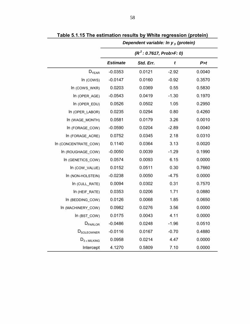
58
Table 5.1.15 The estimation results by White regression (protein)
Std. Err. P>t
DYEAR -0.0353 0.0121 -2.92 0.0040
ln (COWS) -0.0147 0.0160 -0.92 0.3570
ln (COWS_WKR) 0.0203 0.0369 0.55 0.5830
ln (OPER_AGE) -0.0543 0.0419 -1.30 0.1970
ln (OPER_EDU) 0.0526 0.0502 1.05 0.2950
ln (OPER_LABOR) 0.0235 0.0294 0.80 0.4260
ln (WAGE_MONTH) 0.0581 0.0179 3.26 0.0010
ln (FORAGE_COW) -0.0590 0.0204 -2.89 0.0040
ln (FORAGE_ACRE) 0.0752 0.0345 2.18 0.0310
ln (CONCENTRATE_COW) 0.1140 0.0364 3.13 0.0020
ln (ROUGHAGE_COW) -0.0050 0.0039 -1.29 0.1990
ln (GENETICS_COW) 0.0574 0.0093 6.15 0.0000
ln (COW_VALUE) 0.0152 0.0511 0.30 0.7660
ln (NON-HOLSTEIN) -0.0238 0.0050 -4.75 0.0000
ln (CULL_RATE) 0.0094 0.0302 0.31 0.7570
ln (HEIF_RATE) 0.0353 0.0206 1.71 0.0880
ln (BEDDING_COW) 0.0126 0.0068 1.85 0.0650
ln (MACHINERY_COW) 0.0982 0.0276 3.56 0.0000
ln (BST_COW) 0.0175 0.0043 4.11 0.0000
DPARLOR -0.0486 0.0248 -1.96 0.0510
DSOLEOWNER -0.0116 0.0167 -0.70 0.4880
D3ⅹMILKING 0.0958 0.0214 4.47 0.0000
Intercept 4.1270 0.5809 7.10 0.0000
Dependent variable: ln y 3 (protein)
(R 2 : 0.7617, Prob>F: 0)
Estimate t

59
Table 5.1.16 The estimation results by White regression (other solids)
Std. Err. P>t
DYEAR -0.0405 0.0139 -2.91 0.0040
ln (COWS) -0.0120 0.0172 -0.70 0.4860
ln (COWS_WKR) -0.0106 0.0372 -0.29 0.7750
ln (OPER_AGE) -0.1114 0.0475 -2.35 0.0200
ln (OPER_EDU) 0.0186 0.0564 0.33 0.7420
ln (OPER_LABOR) 0.0090 0.0328 0.27 0.7840
ln (WAGE_MONTH) 0.0542 0.0207 2.62 0.0100
ln (FORAGE_COW) -0.0633 0.0227 -2.78 0.0060
ln (FORAGE_ACRE) 0.0858 0.0388 2.21 0.0280
ln (CONCENTRATE_COW) 0.0980 0.0344 2.85 0.0050
ln (ROUGHAGE_COW) -0.0017 0.0043 -0.39 0.7000
ln (GENETICS_COW) 0.0608 0.0114 5.34 0.0000
ln (COW_VALUE) 0.0612 0.0519 1.18 0.2390
ln (NON-HOLSTEIN) -0.0395 0.0067 -5.90 0.0000
ln (CULL_RATE) 0.0100 0.0350 0.29 0.7740
ln (HEIF_RATE) 0.0379 0.0236 1.60 0.1100
ln (BEDDING_COW) 0.0126 0.0073 1.73 0.0850
ln (MACHINERY_COW) 0.0924 0.0321 2.88 0.0040
ln (BST_COW) 0.0149 0.0049 3.06 0.0030
DPARLOR -0.0255 0.0285 -0.89 0.3720
DSOLEOWNER -0.0176 0.0183 -0.96 0.3400
D3ⅹMILKING 0.0971 0.0236 4.12 0.0000
Intercept 5.0272 0.7061 7.12 0.0000
Dependent variable: ln y 4 (other solids)
(R 2 : 0.7699, Prob>F: 0)
Estimate t

60
The correlation matrix of residuals is reported in Table 5.1.8. The
entries on the main diagonal represent the correlation of one residual with
itself so that their values are always equal to one. On the other hand, the
entries off the main diagonal represent the correlation of one residual with
another residual, and in this manner, a large value indicates high correlation
between those residuals. It is, therefore, the estimated correlation matrix which
indicates that the residuals from the system of equations are highly correlated
with each other because the production of the four outputs are simultaneously
affected by the productivity and condition of each cow: 0.8164 for aggregate
milk and butterfat, 0.8704 for aggregate milk and protein, and 0.9206 for
aggregate milk and other solids, 0.8598 butterfat and protein, 0.8163 for
butterfat and other solids, and 0.8765 for protein and other solids.
The explanatory power of the estimation results by the ISUR is not
directly obtained from the results because the log-likelihood values of the
fitting constant-only model and the fitting full model are positive (1217.3882
and 1463.4251, respectively), so the log-likelihood index is not meaningful.
Instead, the estimation results from White’s linear regression, reported in
Tables 5.1.13 – 5.1.16, can be used as a reference for the goodness of fit for
these estimated functions; the variations of dependent variables explained by
the individual production functions are, on average, 80.24%, 73.68%, 76.17%,
and 76.99% of the variation for the log value of aggregate milk production per
cow, butterfat production per cow, protein production per cow, and other solid
production per cow, respectively, and they are statistically significant at the
0.05 level.

61
The effects of business factors on milk production
As reported in Tables 5.1.9 – 5.1.12, the results of estimating the four
single-output production functions by the ISUR indicate that 13 production
factors out of 21 have statistically significant effects on at least one of the four
component production at the 0.05 level: YEAR, OPER_AGE, WAGE_MONTH,
FORAGE_COW, FORAGE_ACRE, CONCENTRATE_COW,
GENETICS_COW, NON-HOLSTEIN, BEDDING_COW, MACHINERY_COW,
BST_COW, PARLOR, 3×MILKING. With the exception of the dummy
variables, since the functions are estimated based on the log values of the
outputs and inputs, the coefficient estimates βm,k represent the (partial)
production elasticity of the k th input for the mth output production. In other
words, the coefficient estimates represent the output percentage change from
a one percent input change, holding the other inputs constant. Importantly,
Tables 5.1.9 – 5.1.12 reports the different coefficient estimates of each input
across the four outputs. For instance, the expense coefficient for breed
improvement per cow (GENETICS_COW) is 0.0552 for aggregate milk,
0.0606 for butterfat, 0.0574 for protein, and 0.0608 for other solids. This
implies that the effect of each input on each output is different, so that farmers
are able to alter individual component productions by adjusting an input. In this
case, butterfat, protein, and other solids will increase faster than aggregate
milk. Consequently, the butterfat, protein, and other solids percent of the milk
increase. However, since the difference between the coefficient estimates of
an input across the four outputs is small, the farmer’s ability to drastically alter
individual component production is limited. Yet, this small ability still provides
the opportunity to increase profits by altering individual component production
levels in response to each component price.
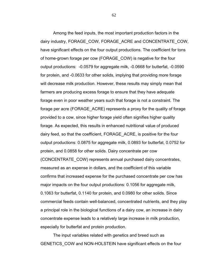
62
Among the feed inputs, the most important production factors in the
dairy industry, FORAGE_COW, FORAGE_ACRE and CONCENTRATE_COW,
have significant effects on the four output productions. The coefficient for tons
of home-grown forage per cow (FORAGE_COW) is negative for the four
output productions: -0.0579 for aggregate milk, -0.0668 for butterfat, -0.0590
for protein, and -0.0633 for other solids, implying that providing more forage
will decrease milk production. However, these results may simply mean that
farmers are producing excess forage to ensure that they have adequate
forage even in poor weather years such that forage is not a constraint. The
forage per acre (FORAGE_ACRE) represents a proxy for the quality of forage
provided to a cow, since higher forage yield often signifies higher quality
forage. As expected, this results in enhanced nutritional value of produced
dairy feed, so that the coefficient, FORAGE_ACRE, is positive for the four
output productions: 0.0875 for aggregate milk, 0.0893 for butterfat, 0.0752 for
protein, and 0.0858 for other solids. Dairy concentrate per cow
(CONCENTRATE_COW) represents annual purchased dairy concentrates,
measured as an expense in dollars, and the coefficient of this variable
confirms that increased expense for the purchased concentrate per cow has
major impacts on the four output productions: 0.1056 for aggregate milk,
0.1063 for butterfat, 0.1140 for protein, and 0.0980 for other solids. Since
commercial feeds contain well-balanced, concentrated nutrients, and they play
a principal role in the biological functions of a dairy cow, an increase in dairy
concentrate expense leads to a relatively large increase in milk production,
especially for butterfat and protein production.
The input variables related with genetics and breed such as
GENETICS_COW and NON-HOLSTEIN have significant effects on the four
63
output productions because genetic traits and breed determine the basic
production levels of aggregate milk and individual component production
(Table 2.2.7) as well as live weight gain, feed intake, and feed conversion
efficiency. The coefficient for expense for breed improvement per cow
(GENETICS_COW) is positive for the four output productions: 0.0552 for
aggregate milk, 0.0606 for butterfat, 0.0574 for protein, and 0.0608 for other
solids. These positive effects may imply that farmers are practicing high quality
artificial inseminations and/or replacing old cows (low production) with
genetically superior young cows. The negative coefficient for Non-Holstein
breeds (NON-HOLSTEIN) shows that the Non-Holstein breed proportion on a
farm results in a decrease in the quantity of aggregate milk and individual
components: -0.0433 for aggregate milk, -0.0133 for butterfat, -0.0238 for
protein, and -0.0395 for other solids. This is because the Holstein breed yields
an outstanding amount of milk and milk components so that the absolute
amount of aggregate milk and individual component production is decreased
by increasing the percentage of Non-Holstein breeds. However, since Non-
Holstein breeds produce milk containing higher butterfat and protein content
as percentages of aggregate milk, the rates of decrease for butterfat (-0.0133)
and protein (-0.0238) from a one percent increase in the percentage of Non-
Holstein breeds are smaller than that of aggregate milk (-0.0433).
Among the variables related with the human capital of an operator such
as operator age (OPER_AGE), operator education level (OPER_EDU), and
operator labor contribution per cow (OPER_LABOR), only average operator
age (OPER_AGE) has significant effects on aggregate milk, butterfat, and
other solid production: -0.12780 for aggregate milk, -0.0705 for butterfat, and
-0.1114 for other solids. These negative coefficient estimates mean that the

64
productivity of a farmer and his or her age have an inverse relationship.
Moreover, since average operator age is more of a business characteristic
than a traditional input, operator age can be considered as the main
contributor to the productivity of a farm because the coefficient estimate of
OPER_AGE is negative for aggregate milk production.
The negative coefficient for parlor milking system (PARLOR) indicates that the
parlor milking system has negative effects on butterfat and protein production,
as seen in the downward shifts of both intercepts of butterfat and protein
production. However, it is somewhat difficult to conclude that parlor milking
system itself negatively affects milk production because milking system type is
highly correlated with size and housing type of a farm. In general, due to the
cost of production, larger farms have a freestall barn with a parlor milking
system14, and small farms have a tiestall barn with a stanchion milking system.
In the DFBS data, the correlation between parlor milking system and freestall
barn is 0.8925, and those farms have an average of 526 cows. On the other
hand, the correlation between stanchion milking system and tiestall barn is
0.8644, and those farms have an average of 61cows. Thus, the coefficient for
parlor milking system may represent the effect of housing type and/or farm
size on milk production.
The average monthly wage for hired labor (WAGE_MONTH) measures
the effect of hired labor quality. An employee is usually paid his or her salary
based on his or her individual productivity so that a higher monthly wage
reflects higher productivity of a hired worker. Thus, the average monthly wage
for hired labor has positive effects on the four output productions: 0.0567 for
14 Parlor type includes the following milking systems: Herringbone, Parallel, Parabone, or Rotary.

65
aggregate milk, 0.0386 for butterfat, 0.0581 for protein, and 0.0542 for other
solids. The total machinery cost per cow (MACHINERY_COW) is used as a
measurement of equipment quality and non-obsolescence of that equipment,
which also represents the capital intensity of a farm. It is, thus, the coefficient
for total machinery cost per cow that indicates the degree of capital intensity of
a farm, which has the second most positive impact on milk production: 0.0816
for aggregate milk, 0.0947 for butterfat, 0.0982 for protein, and 0.0924 for
other solids. Bedding expense per cow (BEDDING_COW) represents the
effects of cow comfort on milk production. Since bedding increases the
comfort level and decreases the stress level of a cow, the coefficient estimates
are positive for the four output productions. Bedding also provides a clean, dry
rest area that helps prevent the spread of infectious diseases. The coefficient
estimates for BST_COW represent the additional impact on the four output
productions by a one percent change in an expense for BST per cow. As
expected, the effects of an expense for BST per cow (BST_COW) are positive
for the four output production: 0.0153 for aggregate milk, 0.0129 for butterfat,
0.0175 for protein, and 0.0149 for other solids. Since higher milking
frequencies obviously yield more milk, the dummy coefficient for milking
frequency (3× MILKING) is positive and significant in the production of the four
outputs.
Since some inputs are measured as an expense in dollars and output
prices are available, the effects of inputs on the milk components can be
computed as the additional profit (or loss) from a one percent change in the
inputs that are measured as an expense in dollars. This calculated additional
profit represents the profit change from a change in butterfat, protein, and
other solids. However, since the DFBS data does not provide the producer

66
price differential and the somatic cell adjustment information, the profit from a
change in the total weight of milk is precluded. Thus, this calculated additional
profit may be somewhat different than a change in the total profit of a farmer
from a one percent change in the inputs. Yet, this additional profit information
may provide farmers with a clearer idea about the effects of inputs on their
milk production. For instance, the total additional revenue generated using
year 2005 average component prices from a one percent increase in expense
for genetic improvement per cow (GENETICS_COW) is $1.3485. This is the
sum of the revenues from an increase in butterfat, protein, and other solids;
each revenue resulting from an increase in an individual component is equal to
the component price times the amount of additional output (∆ym) which is
computed by taking the average production of each output times the
production elasticity (βm,k ) of the input (GENETICS_COW) for that output. On
the other hand, the additional cost for a one percent increase in the input
(GENETICS_COW) is $0.4652 which is equal to one percent increase in the
average expense for genetic improvement per cow ($0.4652 = $46.52 × 1%).
Thus, $1.3485 in additional profit is generated by a one percent increase in the
expense for genetic improvement per cow (GENETICS_COW), which is equal
to the total additional revenue ($1.8137) minus the additional cost ($0.4652).
Similarly, the additional profit per cow from a one percent increase in the four
inputs that are measured as an expense in dollars and have significant effects
on milk production are computed and reported in Table 5.1.17.
Table 5.1.17 shows that a one percent increase in GENETICS_COW,
BEDDING_COW, MACHINERY_COW, and BST_COW will generate more
profit for farmers; farmers can increase their profits by spending more money
on bedding materials for cows, using more BST, buying more or better farm
67
equipment related to milk production, and improving genetic traits of cows
which includes practicing high quality artificial inseminations and/or replacing
old cows (low production) with genetically superior young cows. However,
Table 5.1.17 does not provide estimates of the additional profit for the inputs
related to feed. Feed is included as an input in the production functions in
order not to bias the estimates of the other input coefficients that may increase
milk production. Leaving feed out of the production function would bias the
estimates of the remaining coefficients because clearly feed is necessary for
milk production, but the production causation for feed may run counter to a
typical production relationship. Some variables may increase or decrease milk
production, but once the level of milk production is determined by those
causation variables, then a specific quantity of feed is necessary to produce
that milk.

68
Table 5.1.17 Additional profit by a one percent change in an input
Output (ym) (lbs) βm,k ∆ym (lbs) Ave. Price(2005)
TotalAdd. Revenue
per cow
Add. Costper cow
Butterfat 750.58 0.0606 0.4548 $2.4605 $1.119
Protein 618.33 0.0574 0.3549 $1.7105 $0.607
Other solids 1170.92 0.0608 0.7119 $0.1228 $0.087
Output (ym) (lbs) βm,k ∆ym (lbs) Ave. Price(2005)
TotalAdd. Revenue
per cow
Add. Costper cow
Butterfat 750.58 0.0189 0.1419 $2.4605 $0.349
Protein 618.33 0.0126 0.0779 $1.7105 $0.133
Other solids 1170.92 0.0126 0.1475 $0.1228 $0.018
Output (ym) (lbs) βm,k ∆ym (lbs) Ave. Price(2005)
TotalAdd. Revenue
per cow
Add. Costper cow
Butterfat 750.58 0.0947 0.7108 $2.4605 $1.749
Protein 618.33 0.0986 0.6097 $1.7105 $1.043
Other solids 1170.92 0.0924 1.0819 $0.1228 $0.133
Output (ym) (lbs) βm,k ∆ym (lbs) Ave. Price(2005)
TotalAdd. Revenue
per cow
Add. Costper cow
Butterfat 750.58 0.0129 0.0968 $2.4605 $0.238
Protein 618.33 0.0175 0.1082 $1.7105 $0.185
Other solids 1170.92 0.0149 0.1745 $0.1228 $0.021
$1.8137
$0.5004
$0.3787 $0.0661
Add. Profitper cow
Input (xk): BST_COW, : $37.87
$0.4448
Add. Profitper cow
Input (xk): BEDDING_COW, : $49.74
Add. Revenueper cow
$0.0181 $2.9065$2.9246
Add. Revenueper cow
Add. Revenueper cow
Input (xk): MACHINERY_COW, : $590.56
Add. Profitper cow
Add. Profitper cow
Add. Revenueper cow
$0.4652 $1.3485
$0.4974 $0.0030
Input (xk): GENETICS_COW, : $46.52
xffff
k
xffff
k
xffff
k
xffff
k
yfff
yfff
yfff
yfff
5.2 The results of estimating the stochastic output distance function
The stochastic output distance function (3.2.7) is estimated from the
maximum likelihood technique using STATA 9 under the assumption that the
function has two separate error terms: a symmetric random error term (vi ),
which captures the effects of traditional random variation, and a one-sided
technical error term (ui ), which allows for technical inefficiency. The ui is
modeled as a half normal distribution. Table 5.2.1 reports the results of
estimating the stochastic output distance function. Furthermore, the (partial)
production elasticity βm,ko of each input for each of the four outputs is reported

69
in Table 5.2.2. These elasticities are computed by using Equations 3.1.14–
3.1.1615 and the coefficient estimates for the inputs that have significant
effects on milk production. Finally, the elasticity between the outputs that are
computed by using Equations 3.1.1716 and 3.1.1917is presented in Table 5.2.3.
The results of estimating the stochastic output distance function (Table
5.2.1) indicate that 12 production factors out of 22 have statistically significant
effects on milk production at the 0.05 level: YEAR, OPER_AGE,
WAGE_MONTH, FORAGE_COW, FORAGE_ACRE, CONCENTRATE_COW,
GENETICS_COW, NON-HOLSTEIN, BEDDING_COW, MACHINERY_COW,
BST_COW, 3×MILKING. Since the specifications of the stochastic output
distance function (3.2.7) are somewhat different than those from the four
single-output production functions (3.1.3 – 3.1.6), the interpretations of the
coefficient estimates βk in Table 5.2.1 are also somewhat different from the
βm,k from the four single-output production functions. In the case of the four
single-output production functions, with the exception of the dummy variables,
the coefficient estimates βm,k represent the (partial) production elasticity of the
k th input for the particular output ym , but the coefficient estimates βk from the
stochastic output distance function represent the production elasticity of the
k th input for the overall outputs. In other words, the coefficient estimates βk
represent the percentage change in aggregate milk that is the primary output
in response to a one percent change in an input, holding the other inputs and
15 (3.2.14) β1,k
o = ∂ln y1 /∂lnxk =βk / ( 1 +X αm ), where βk are the coefficient estimates from the
stochastic output distance function, and αm are the coefficient estimates for the log value of the mth output ratio. (3.2.15) βm,k
o = ∂ln ym /∂lnxk =@βk /αm , where m ≠1, and for αm< 0. (3.2.16) βm,k
o = ∂ln ym /∂lnxk =β k /αm , where m ≠1 and for αm> 0 16 ε ym ,y1
= ∂ln ym /∂ln y1 = ( 1 +Xαm ) /αm . 17 ε ym ,yn = ∂ln ym /∂ln yn =@α n /α m (m ≠ n).

70
percentages of each milk component ym* constant; since the primary output y1
is the denominator of the output ratios ym* , or the independent variables of the
stochastic output distance function, the other outputs also increase to keep the
ratio constant. Thus, this estimated elasticity βk includes the impact on the
other outputs which keep their output ratios constant. However, the resulting
coefficients βm,k and βk are almost identical; since the milk components are
only small portion of aggregate milk, the effects of an input on aggregate milk
and on overall output are almost the same. For instance, the estimated
coefficients for GENETICS_COW are 0.0553 from the stochastic output
distance function, and 0.0552 from the single-output production function for
aggregate milk production.
On the other hand, Table 5.2.2 reports the computed (partial)
production elasticity of an input for the four outputs βm,ko that are interpreted
similarly with the coefficient estimates βm,k from the four single-output
production functions, or the percentage change in the output ym from a one
percent change in an input, holding the other input constant. However, since
the distance function specification and the econometric procedure for the
stochastic output distance function are somewhat different than those for the
four single-output distance functions, these computed production elasticities
βm,ko have slightly different values than the coefficient estimates βm,k from the
four single-output production functions; the absolute values of βm,ko and βm,k are
different, but the signs and relative effects of the production factors that
significantly affect the four output production are almost identical. For instance,
βm,ko of CONCENTRATE_COW for aggregate milk is 0.1901, which implies that
this variable has the largest (positive) effect on aggregate milk. On the other
hand, βm,ko of CONCENTRATE_COW for aggregate milk is 0.1056, which is not
71
identical to the βm,ko , but also implies that this variable has the largest (positive)
effect on aggregate milk. It is, thus, the explanation of the effects of an input
on milk production that were fully discussed in the previous section that can
also be used to explain the effects of an input that from the stochastic output
distance function.
As discussed in the model chapter, since milk is a composite product of
individual components and water, and all of the production factors in milk
production are considered to be non-allocable, a PPC in ym / yn (m ≠ n) space
degenerates to a single point in this study. Thus, neither the movement along
the PPC in the ym / yn (m ≠ n) space, nor the elasticity between the outputs
from the PPC in the ym / yn (m ≠ n) space are relevant concepts in this study.
Yet, by altering an input, a dairy cow should respond by producing a different
output composition. Consequently, the elasticity between the outputs can be
obtained by using information from an old output combination point to a new
output combination point in multidimensional spaces rather than from the PPC;
the production elasticity between ym and yn (m ≠ n) is simply
ε ym ,yn = ∂ln ym /∂ln yn = (Δ ym /Δ yn )B( yn / ym ), and Δ ym , Δ yn , yn , ym can be
obtained from an old output combination point and a new output combination
point that is generated by a change in the inputs. Therefore, the elasticity
between the outputs is computed by using Equations 3.2.18 and 3.2.19.
However, these elasticities are not particularly useful in this study because
dairy cows cannot be asked to alter their milk composition without changing
any inputs.
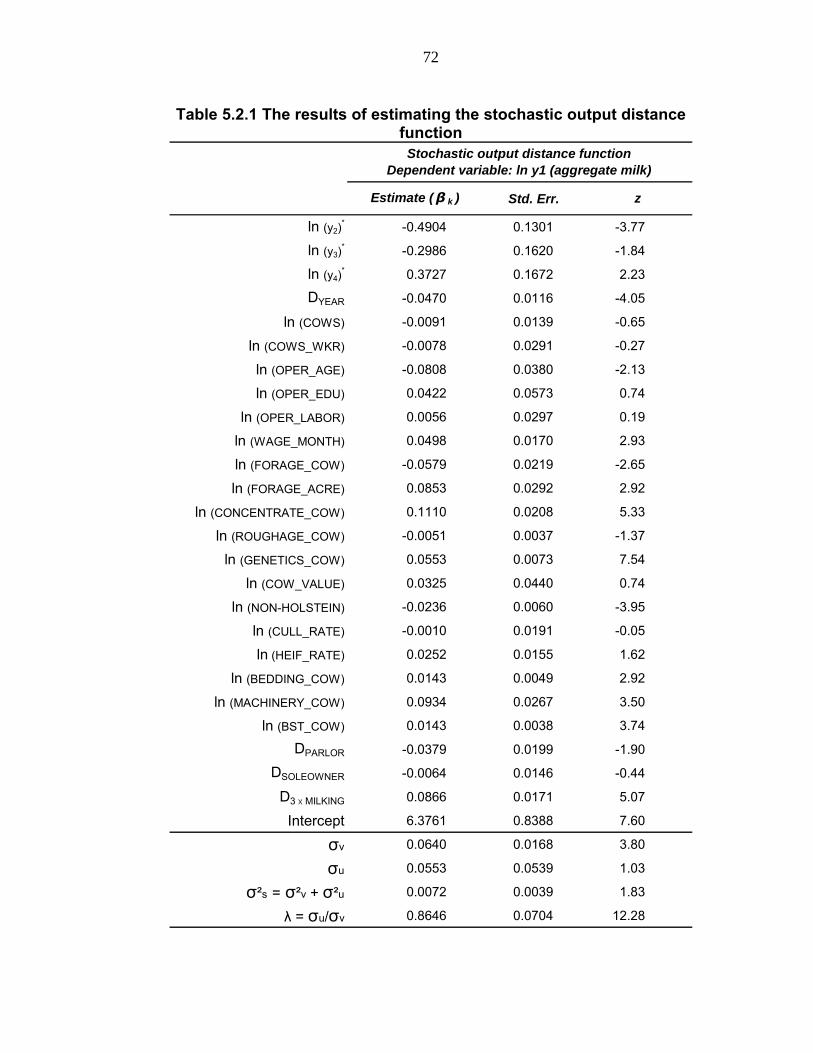
72
Table 5.2.1 The results of estimating the stochastic output distance function
Std. Err.
ln (y2)* -0.4904 0.1301 -3.77
ln (y3)* -0.2986 0.1620 -1.84
ln (y4)* 0.3727 0.1672 2.23
DYEAR -0.0470 0.0116 -4.05
ln (COWS) -0.0091 0.0139 -0.65
ln (COWS_WKR) -0.0078 0.0291 -0.27
ln (OPER_AGE) -0.0808 0.0380 -2.13
ln (OPER_EDU) 0.0422 0.0573 0.74
ln (OPER_LABOR) 0.0056 0.0297 0.19
ln (WAGE_MONTH) 0.0498 0.0170 2.93
ln (FORAGE_COW) -0.0579 0.0219 -2.65
ln (FORAGE_ACRE) 0.0853 0.0292 2.92
ln (CONCENTRATE_COW) 0.1110 0.0208 5.33
ln (ROUGHAGE_COW) -0.0051 0.0037 -1.37
ln (GENETICS_COW) 0.0553 0.0073 7.54
ln (COW_VALUE) 0.0325 0.0440 0.74
ln (NON-HOLSTEIN) -0.0236 0.0060 -3.95
ln (CULL_RATE) -0.0010 0.0191 -0.05
ln (HEIF_RATE) 0.0252 0.0155 1.62
ln (BEDDING_COW) 0.0143 0.0049 2.92
ln (MACHINERY_COW) 0.0934 0.0267 3.50
ln (BST_COW) 0.0143 0.0038 3.74
DPARLOR -0.0379 0.0199 -1.90
DSOLEOWNER -0.0064 0.0146 -0.44
D3ⅹMILKING 0.0866 0.0171 5.07
Intercept 6.3761 0.8388 7.60
σv 0.0640 0.0168 3.80
σu 0.0553 0.0539 1.03
σ²s = σ²v + σ²u 0.0072 0.0039 1.83
λ = σu/σv 0.8646 0.0704 12.28
Stochastic output distance functionDependent variable: ln y1 (aggregate milk)
Estimate (β k ) z
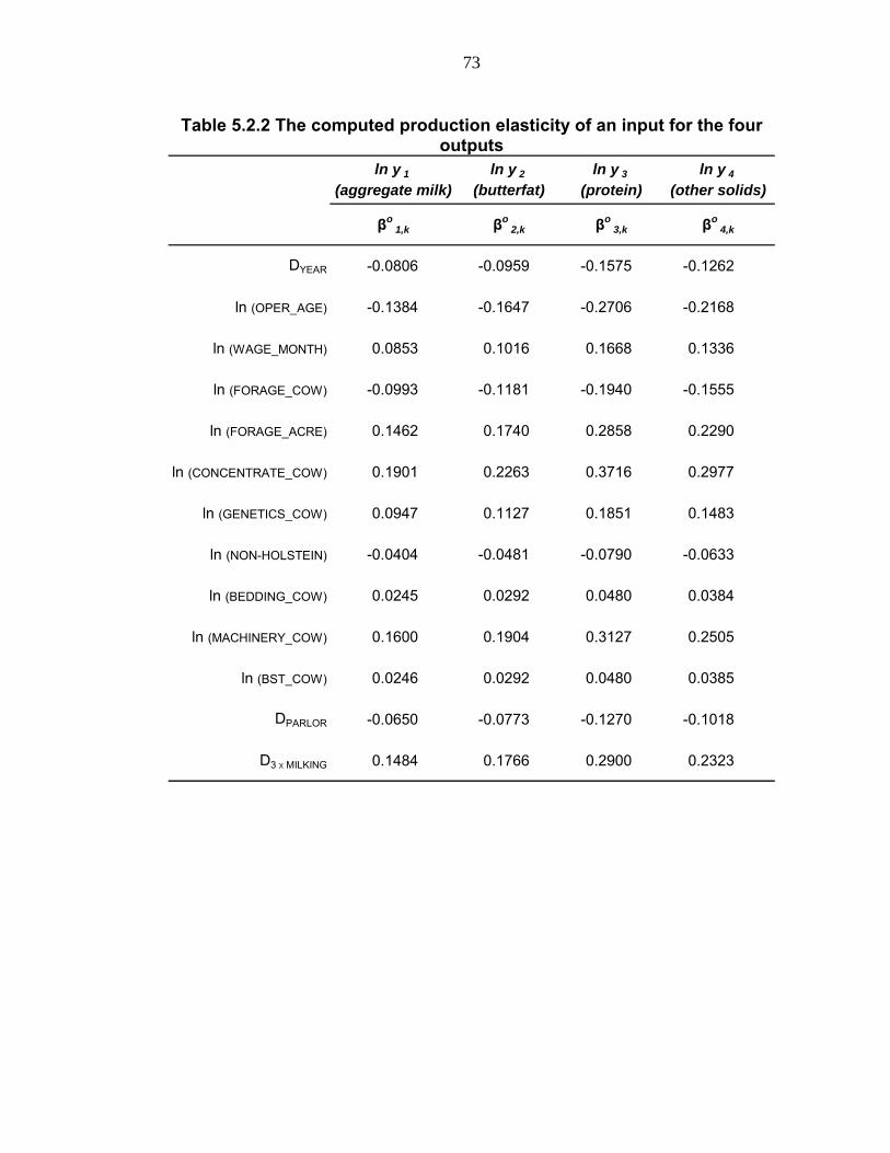
73
Table 5.2.2 The computed production elasticity of an input for the four outputs
DYEAR -0.0806 -0.0959 -0.1575 -0.1262
ln (OPER_AGE) -0.1384 -0.1647 -0.2706 -0.2168
ln (WAGE_MONTH) 0.0853 0.1016 0.1668 0.1336
ln (FORAGE_COW) -0.0993 -0.1181 -0.1940 -0.1555
ln (FORAGE_ACRE) 0.1462 0.1740 0.2858 0.2290
ln (CONCENTRATE_COW) 0.1901 0.2263 0.3716 0.2977
ln (GENETICS_COW) 0.0947 0.1127 0.1851 0.1483
ln (NON-HOLSTEIN) -0.0404 -0.0481 -0.0790 -0.0633
ln (BEDDING_COW) 0.0245 0.0292 0.0480 0.0384
ln (MACHINERY_COW) 0.1600 0.1904 0.3127 0.2505
ln (BST_COW) 0.0246 0.0292 0.0480 0.0385
DPARLOR -0.0650 -0.0773 -0.1270 -0.1018
D3ⅹMILKING 0.1484 0.1766 0.2900 0.2323
ln y 3
(protein)
βo3,k
ln y 4
(other solids)
βo4,k
ln y 1
(aggregate milk)
βo1,k
ln y 2
(butterfat)
βo2,k

74
Table 5.2.3 The elasticity between the outputs
-0.8402 -0.5116 0.6385
-1.1902 -0.6089 0.7600
-1.9548 -1.6424 1.2482
1.5661 1.3158 0.8011
y1
(aggregate milk)y2
(butterfat)y3
(protein)y4
(other solids)
(εy1,y2) (εy1,y3) (εy1,y4)
(εy2,y1) (εy2,y3) (εy2,y4)
(εy3,y1) (εy3,y2) (εy3,y4)
(εy4,y3)(εy4,y2)(εy4,y1)
y1
(aggregate milk)
y2
(butterfat)
y3
(protein)
y4
(other solids)
5.3 Technical efficiency of New York dairy farm
Under the assumption that the stochastic output distance function has
two separate error terms, the symmetric random error term (vi ) which
captures the effects of traditional random variation, and the one-sided
efficiency error term (ui ) which allows for technical inefficiency, there is very
little technical inefficiency among the New York dairy farms that participated in
the DFBS project. The minimum value of estimated technical efficiency is 90%
and the average is 96%. These data participants represent high performance
farms, so production variation between farms may be relatively small, leading
to a high minimum and average efficiency. In addition, the production
functions in this study included many business factors such as those
representing economic scales of a farm and operator labor quality, which
possibly affect the technical efficiency level of a farm such that the effects of

75
technical inefficiency are captured in the coefficient estimates, instead of in a
one-sided error term.

76
CHAPTER 6
CONCLUSIONS
Concluding remarks
This is the first study to focus specifically on the responses of
aggregate milk and individual component production to changes made in the
dairy business; these are important considerations which have been
overlooked in existing studies on milk production. Four single-output
production functions and a stochastic output distance function were estimated
using New York Dairy Farm Business Summary (DFBS) data from 105 farms
in 2003 and 107 farms in 2004. Based on these estimation results, this study
examined (a) the effects of business factors and other inputs on aggregate
milk and individual component production, (b) the technical efficiency of New
York dairy farms that participated in the DFBS project, and (c) the
relationships between the outputs.
The empirical results demonstrated the possibility of altering individual
component productions from four single-output production functions and a
stochastic output distance function. However, since the differences between
the effects of each input on each output are small, the farmer’s ability to alter
individual component productions may also be small. Yet, this is still important
because, given the small profit margins that often occurs in the dairy industry,
this small ability provides the opportunity for farmers to increase profits by
altering individual component production levels in response to each
component.
77
According to both estimation results, twelve common factors were
found to have significant effects on milk production among 22 total
independent variables related to feed, breed, labor, capital, and other
managerial and environmental factors. Of these 12 significant variables, the
amount of commercial feed provided to a cow, quality of hired labor, capital
intensity of a farm, productivity of land for home-grown forage, herd genetics,
cow comfort level, BST use, and milking frequency, were shown to increase
overall milk output as well as individual milk components. On the other hand,
year dummy variable (2003=0 and 2004=1), average operator age, amount of
home-grown forage provided to a cow, and percentages of Non-Holstein
breeds on the farm were found to have negative effects on milk production.
Additional profit from the effects of inputs on milk components were
estimated by computing the additional profit (or loss) from a one percent
change in the inputs that are measured in dollars. This additional profit
information indicates that farmers can increase their profits by spending more
money on bedding materials for cows, using more BST, buying more or better
farm equipment related to milk production, and improving genetic traits of
cows which includes practicing high quality artificial inseminations and/or
replacing old cows (low production) with genetically superior young cows.
From the stochastic output distance function, very little technical
inefficiency was found in these participating New York dairy farms. The min
value of estimated technical efficiency is 90% and the average is 96%. This
implies that almost all of the participants in the DFBS project produce outputs
at near the maximum possible output levels, given their production technology.
There are two main possible reasons to explain this high technical efficiency.
78
One is that since participants represent high performance dairy farms in New
York State, the DFBS data do not have lower productive farms, so that
production variation between them is consequently very small. Another
possibility is that since the stochastic output distance function already takes
into account the effects of the variables that could possibly generate technical
inefficiency of a farm, only small portion of the technical inefficiency is
captured in the one-sided efficiency error term.
This study also examined the relationships between the outputs by
computing the elasticity between outputs. As a result, the elasticity between
milk and butterfat, and milk and protein were found to be negative, while milk
and other solids were found to be positive. However, these elasticities were
not particularly useful in this study because dairy cows cannot be asked to
alter their milk composition without changing inputs, and output substitution
elasticities are computed from a constant input vector.
Suggestions for further research
Many proxy variables were used to represent target production factors
such as dairy nutrition. In some cases, the effects of these proxy variables
obtained by estimation could not fully represent the effects of target variables.
For instance, although the effects of feed on milk production were measured
by using the proxy variables such as the dollar amount of purchased feed per
cow (concentrate and roughage) and tons of home-grown forage produced per
cow, they may not completely represent the effects of nutritional value of feed.
Thus, for future research, it will be useful to collect more specific information
on some variables such as quality of feed and genetics. This is because the
effects of a production factor that involve the biological functions of a cow are
79
difficult to be represented by a set of simple proxy variables. The limited data
availability also precluded us from estimating the effect of various diseases on
milk production. However, since diseases are a critical factor that affects the
productivity of a dairy farm, we recommend measuring their effects on milk
production in future research. Lastly, as discussed in the literature review
section, if the data had been available over a lactation period, the Goodall
model would have been a better functional form for estimating milk production
than the Cobb-Douglas production function used in this study.

80
APPENDIX 1 Producer milk price under the Federal Milk Marketing
Orders
To understand the importance of milk component production for dairy
farmers, it is helpful to know the price mechanism for the producer milk under
the federal milk marketing orders (FMMO). FMMO producer price is important
for dairy farmers because their total producer receipt per cwt can not be less
than this price even though they may receive extra premiums or deductions for
their milk sales from various premiums and deductions in the market (volume
and quality premiums).
Basically, the producer milk price is determined by the value of milk
components in producing dairy products, and depends upon six factors:
butterfat, protein, other solids, producer price differential, total weight of milk,
and somatic cell adjustment. Each component price is a final outcome from
interacting supply and demand of processed dairy products. This complete
price mechanism for producer milk can be easily demonstrated by the FMMO
producer price equation (Equation A.1) and components price equations
(Table A.1):

81
(A.1) FMMO producer price per cwt = butterfat priceBbutterfat lb per cwtb c
+ protein priceBprotein lb per cwtb c
+ other solids priceBother solids lb per cwtb c
+ producer price differential per cwtB total weight of milkb c
+ somatic cell adjustment per cwtB total weight of milkb c
where,
• The producer price differential (PPD) is the weighted relative value of
Class I, Class II, and Class III milk values to Class III value by the
portion of each class in total milk utilization.
• The somatic cell adjustment is the premium for producer level milk
quality.

82
Table A.1 The component price formulas for 2006 under the federal milk marketing order
Butter Price = (NASS Monthly Butter price × 0.115) × 1.20
((NASS Monthly Cheese price × 0.165) ×1.383) + Protein Price =
(((Cheese price × 0.165) × 1.572)× Butterfat price ×
0.9)×1.17
Other Solids Price = (Dry whey price × 0.159) × 1.03 Source: U.S Department of Agriculture, National Agricultural Statistics Service, Milk Marketing Order Statistics, Federal Milk Order Price Information, 2006.
where,
• NASS is the USDA’s National Agricultural Statistical Service.
• In the butter price formula, 0.115 is the make allowance for butter,
which indicates the national average cost of manufacturing a pound of
butter as estimated by the USDA; 1.20, the yield factor for butter, is how
many pounds of butter can be made using a pound of butterfat. One
pound of butter production requires around 0.83 pound of butterfat, the
difference resulting from loss during delivery and processing.
• The first line of the protein price formula, 0.165 is the make allowance
and 1.383 is the yield factor for cheese. The second line of the protein
price formula indicates the value of butterfat in cheese in excess of its
value in butter.
• In other solids price formula, 0.159 is the make allowance and 1.03 is
the yield factor for other solids.

83
APPENDIX 2 Producer component price data over last five years
Table A.2 Producer component price data over last five years
Jan Feb Mar Apr May Jun July Aug Sep Oct Nov Dec Ave
2000 Protein 2.168 1.985 1.917 1.740 1.551 1.428 1.973 1.795 2.014 1.803 0.915 1.038 1.6938Butter fat 0.937 0.959 1.019 1.135 1.285 1.413 1.269 1.266 1.271 1.244 1.575 1.653 1.2522Other Solids 0.050 0.043 0.042 0.041 0.040 0.044 0.056 0.058 0.050 0.047 0.057 0.083 0.0509
2001 Protein 1.618 1.495 1.650 1.544 1.911 2.167 2.318 2.219 2.165 2.666 1.805 1.978 1.9613Butter fat 1.290 1.463 1.682 1.948 2.119 2.209 2.188 2.298 2.445 1.653 1.450 1.432 1.8480Other Solids 0.112 0.120 0.104 0.108 0.123 0.141 0.151 0.154 0.152 0.148 0.147 0.152 0.1343
2002 Protein 1.966 2.088 1.834 2.011 2.210 2.015 1.810 1.902 2.065 2.184 1.847 1.751 1.9735Butter fat 1.485 1.382 1.364 1.289 1.143 1.121 1.093 1.070 1.010 1.073 1.092 1.192 1.1928Other Solids 0.139 0.097 0.069 0.057 0.037 0.025 0.015 0.018 0.037 0.076 0.085 0.058 0.0593
2003 Protein 1.816 1.854 1.665 1.801 1.928 1.943 2.548 3.144 3.318 3.282 2.929 2.298 2.3770Butter fat 1.186 1.137 1.146 1.150 1.151 1.158 1.206 1.251 1.222 1.255 1.288 1.369 1.2099Other Solids 0.034 0.024 0.021 0.001 0.014 0.020 0.012 0.003 0.017 0.031 0.037 0.036 0.0208
2004 Protein 2.088 1.791 2.013 3.447 3.764 3.109 2.363 2.466 2.543 2.381 2.430 2.849 2.6035Butter fat 1.498 1.852 2.381 2.501 2.428 2.177 2.054 1.794 1.935 1.902 2.049 2.037 2.0507Other Solids 0.022 0.009 0.023 0.104 0.144 0.134 0.105 0.068 0.059 0.068 0.080 0.086 0.0751
2005 Protein 2.530 2.661 2.502 2.706 2.597 2.574 2.459 2.162 2.301 2.378 2.272 2.385 2.4605Butter fat 1.733 1.775 1.728 1.696 1.548 1.593 1.801 1.825 1.887 1.826 1.611 1.504 1.7105Other Solids 0.090 0.092 0.095 0.102 0.104 0.114 0.124 0.132 0.141 0.149 0.161 0.170 0.1228
Producer Components Prices per Pound from FMMO New York/Northeast Market Administrator Report
Price per PoundYear Component
Source: Northeast Monthly Component Price Data, Price Information, Northeast Marketing Area, Agricultural Marketing Service, U.S. Department of Agriculture.
$0.00
$0.50
$1.00
$1.50
$2.00
$2.50
$3.00
2000 2001 2002 2003 2004 2005
Year
Ann
ual A
vera
ge P
rice
Protein Price Butterfat Price Other Solids Price
Figure A.2 Producer component price data over the last five years

84
REFERENCES
Aigner, D., K. Lovell and P. Schmidt. "Formulation and Estimation of
Stochastic Frontier Production Function Models." Journal of
Econometrics. 6 (July 1977): 21-37.
Adelaja, A.O. “Price Changes, Supply Elasticities, Industry Organization, and
Dairy Output Distribution.” Amer. J. Agr. Econ. 73 (February 1991): 89-
102.
Bailey, K.W., Jones, C.M., and A.J. Heinrichs. “Economic Returns to Holstein
and Jersey Herds Under Multiple Component Pricing.” J. Dairy Sci. 88
(2005): 2269-2280.
Beattie, B.R., and C.R. Taylor. The Economics of Production. Canada: John
Wiley & Sons, Inc., 1985.
Brummer, B., Glauben, T., and G. Thijssen. “Decomposition of Productivity
Growth Using Distance Functions: The Case of Dairy Farms in Three
European Countries.” Amer. J. Agr. Econ. 83 (August 2002): 628-644.
Buccola, S., and Y. Iizuka. “Hedonic Cost Models and the Pricing of Milk
Components.” Amer. J. Agr. Econ. 79 (May 1997): 452-462.
Chavas, J.P., and R.M. Klemme. “Aggregatee Milk Supply Response and
Investment Behavior on U.S. Dairy Farms.” Amer. J. Agr. Econ. 68
(February 1986): 55-66.
Goodall, E.A. “An analysis of seasonality of milk production.” Animal
Production. 36 (1983): 69-72.
Howard, W.H., and C.R. Shumway. “Dynamic adjustment in the U.S. Dairy
Industry.” Amer. J. Agr. Econ. 70 (Nov 1988): 837-847.
85
Kellog, D.W., Urquhart, N.S., and A.J. Ortega. “Estimating Holstein lactation
curves with a gamma curve.” J. Dairy Sci. 60 (1977): 1308.
Kumbhakar, S.C., Biswas B., and DeeVon Bailey. “A Study of Economic
Efficiency of Utah Dairy Farmers: A System Approach.” The Review of
Economics and Statistics. 71 (Nov 1989): 595-604.
Kumbhakar, S.C., Ghosh, S., and J.T. McGuckin. “A Generalized Production
Frontier Approach for Estimating Determinants of Inefficiency in U.S.
Dairy Farms.” Journal of Business and Economic Statistics. 9 (July
1991): 279-286.
Lennox, S.D., Goodall, E.A., and C.S. Mayne. “A mathematical model of the
lactation curve of the dairy cow to incorporate metabolizable energy
intake.” The Statistician. 41 (1992): 285-293.
Lennox, S.D., Goodall, E.A., and C.S. Mayne. “Mathmatical Modelling of Milk
Constituent Production.” The Statistician. 42 (1993): 249-260.
Meeusen, W., and J. van den Broeck. "Efficiency Estimation from Cobb-
Douglas Production Functions with Composed Error." International
Economic Review. 18 (Jun 1977): 435-444.
Morrison Paul, C.J., Johnston, W.E., and G. Frengley. “Efficiency in New
Zealand Sheep and Cattle Farming: The Impacts of Regulatory
Reform.” Rev. Econ. Statist. 82 (May 2000): 325-337.
Morrison Paul, C.J. Cost Structure and The measurement of Economic
Performance. Massachusetts: Kluwer Academic Publishers, 1999.
National Research Council. 2001. Nutrient Requirements of Dairy Cattle. 7th
rev. ed. Natl. Acad. Press., Washington, DC.

86
Quiroga, R.E., and B.E. Bravo-Utreta. “Short- and Long-Run Adjustments in
Dairy Production: A Profit Function Analysis.” Appl. Econ. 24 (June
1992): 607-16
Shephard, R.W. Theory of Cost and Production Functions. Princeton:
Princeton University Press, 1970.
Smith, B.J., and S.D. Snyder. “Effects of Protein and Fat Pricing on Farm Milk
Prices for the Five Major U.S. Dairy Breeds.” Amer. J. Agr. Econ. 60
(Feb 1978): 126-131.
Stefanou, S.E., and S. Saxena. “Education, Experience, and Allocative
Efficiency: A Dual Approach.” Amer. J. Agr. Econ. 70 (May 1988): 338-
345.
Sumner, D.A., and J.D. Leiby. “An Econometric Analysis of the Effects of
Human Capital on Size and Growth among Dairy Farms.” Amer. J. Agr.
Econ. 69 (May 1987): 465-470.
Wood, P.D.P. “Algebraic model of the lactation curve in cattle.” Nature. 216
(Oct 1967): 164-165.
Related Documents


