Chapter 1: Introduction and mathematical preliminaries Evy Kersal´ e September 26, 2011

Welcome message from author
This document is posted to help you gain knowledge. Please leave a comment to let me know what you think about it! Share it to your friends and learn new things together.
Transcript

Chapter 1: Introduction and mathematical preliminaries
Evy Kersale
September 26, 2011

Motivation
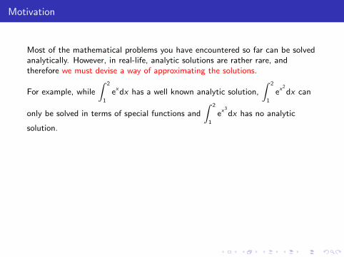
Most of the mathematical problems you have encountered so far can be solvedanalytically. However, in real-life, analytic solutions are rather rare, andtherefore we must devise a way of approximating the solutions.
For example, while
∫ 2
1
exdx has a well known analytic solution,
∫ 2
1
ex2
dx can
only be solved in terms of special functions and
∫ 2
1
ex3
dx has no analytic
solution.
These integrals exist as the area un-der the curves y = exp(x2) andy = exp(x3).We can obtain a numerical approxi-mation by estimating this area, e.g.by dividing it into strips and usingthe trapezium rule.
1 2
Motivation
Most of the mathematical problems you have encountered so far can be solvedanalytically. However, in real-life, analytic solutions are rather rare, andtherefore we must devise a way of approximating the solutions.
For example, while
∫ 2
1
exdx has a well known analytic solution,
∫ 2
1
ex2
dx can
only be solved in terms of special functions and
∫ 2
1
ex3
dx has no analytic
solution.
These integrals exist as the area un-der the curves y = exp(x2) andy = exp(x3).We can obtain a numerical approxi-mation by estimating this area, e.g.by dividing it into strips and usingthe trapezium rule.
1 2

Definition
Numerical analysis is a part of mathematics concerned with
I devising methods, called numerical algorithms, for obtaining numericalapproximate solutions to mathematical problems;
I being able to estimate the error involved.
Traditionally, numerical algorithms are built upon the most simple arithmeticoperations (+,−,× and ÷).
Interestingly, digital computers can only do these very basic operations.However, they are very fast and, hence, have led to major advances in appliedmathematics in the last 60 years.
Computer arithmetic: Floating point numbers.
Computers can store integers exactly but not real numbers in general. Instead,they approximate them as floating point numbers.
A decimal floating point (or machine number) is a number of the form
± 0. d1 d2 . . . dk︸ ︷︷ ︸m
×10±n, 0 ≤ di ≤ 9, d1 6= 0,
where the significand or mantissa m (i.e. the fractional part) and the exponentn are fixed-length integers. (m cannot start with a zero.)
In fact, computers use binary numbers (base 2) rather than decimal numbers(base 10) but the same principle applies (see handout).

Computer arithmetic: Machine ε.
Consider a simple computer where m is 3 digits long and n is one digit long.The smallest positive number this computer can store is 0.1× 10⁻⁹ and thelargest is 0.999× 10⁹.
Thus, the length of the exponent determines the range of numbers that can bestored.
However, not all values in the range can be distinguished: numbers can only berecorded to a certain relative accuracy ε.
For example, on our simple computer, the next floating point number after1 = 0.1×101 is 0.101×101 = 1.01. The quantity εmachine = 0.01 (machine ε) isthe worst relative uncertainty in the floating point representation of a number.

Chopping and rounding
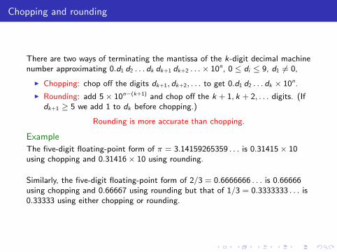
There are two ways of terminating the mantissa of the k-digit decimal machinenumber approximating 0.d1 d2 . . . dk dk+1 dk+2 . . .× 10n, 0 ≤ di ≤ 9, d1 6= 0,
I Chopping: chop off the digits dk+1, dk+2, . . . to get 0.d1 d2 . . . dk × 10n.
I Rounding: add 5× 10n−(k+1) and chop off the k + 1, k + 2, . . . digits. (Ifdk+1 ≥ 5 we add 1 to dk before chopping.)
Rounding is more accurate than chopping.
Example
The five-digit floating-point form of π = 3.14159265359 . . . is 0.31415× 10using chopping and 0.31416× 10 using rounding.
Similarly, the five-digit floating-point form of 2/3 = 0.6666666 . . . is 0.66666using chopping and 0.66667 using rounding but that of 1/3 = 0.3333333 . . . is0.33333 using either chopping or rounding.

Chopping and rounding
There are two ways of terminating the mantissa of the k-digit decimal machinenumber approximating 0.d1 d2 . . . dk dk+1 dk+2 . . .× 10n, 0 ≤ di ≤ 9, d1 6= 0,
I Chopping: chop off the digits dk+1, dk+2, . . . to get 0.d1 d2 . . . dk × 10n.
I Rounding: add 5× 10n−(k+1) and chop off the k + 1, k + 2, . . . digits. (Ifdk+1 ≥ 5 we add 1 to dk before chopping.)
Rounding is more accurate than chopping.
Example
The five-digit floating-point form of π = 3.14159265359 . . . is 0.31415× 10using chopping and 0.31416× 10 using rounding.
Similarly, the five-digit floating-point form of 2/3 = 0.6666666 . . . is 0.66666using chopping and 0.66667 using rounding but that of 1/3 = 0.3333333 . . . is0.33333 using either chopping or rounding.
Measure of the error
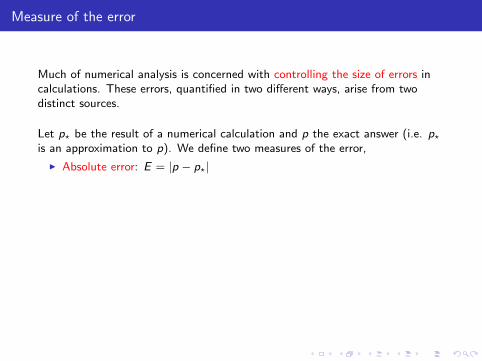
Much of numerical analysis is concerned with controlling the size of errors incalculations. These errors, quantified in two different ways, arise from twodistinct sources.
Let p? be the result of a numerical calculation and p the exact answer (i.e. p?
is an approximation to p). We define two measures of the error,
I Absolute error: E = |p − p?|I Relative error: Er = |p − p?|/|p| (provided p 6= 0) which takes into
consideration the size of the value.
Example
If p = 2 and p? = 2.1, the absolute error E = 10−1;if p = 2× 10⁻³ and p? = 2.1× 10⁻³, E = 10−4 is smaller;and if p = 2× 10³ and p? = 2.1× 10³, E = 102 is largerbut in all three cases the relative error remains the same, Er = 5× 10⁻².

Measure of the error
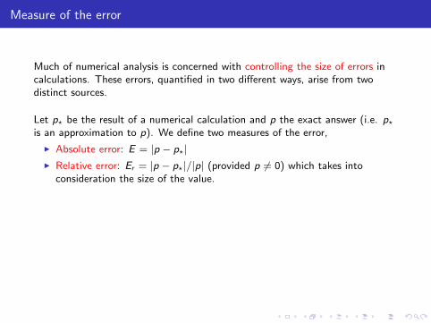
Much of numerical analysis is concerned with controlling the size of errors incalculations. These errors, quantified in two different ways, arise from twodistinct sources.
Let p? be the result of a numerical calculation and p the exact answer (i.e. p?
is an approximation to p). We define two measures of the error,
I Absolute error: E = |p − p?|I Relative error: Er = |p − p?|/|p| (provided p 6= 0) which takes into
consideration the size of the value.
Example
If p = 2 and p? = 2.1, the absolute error E = 10−1;if p = 2× 10⁻³ and p? = 2.1× 10⁻³, E = 10−4 is smaller;and if p = 2× 10³ and p? = 2.1× 10³, E = 102 is largerbut in all three cases the relative error remains the same, Er = 5× 10⁻².
Measure of the error
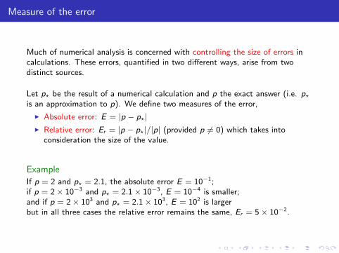
Much of numerical analysis is concerned with controlling the size of errors incalculations. These errors, quantified in two different ways, arise from twodistinct sources.
Let p? be the result of a numerical calculation and p the exact answer (i.e. p?
is an approximation to p). We define two measures of the error,
I Absolute error: E = |p − p?|
I Relative error: Er = |p − p?|/|p| (provided p 6= 0) which takes intoconsideration the size of the value.
Example
If p = 2 and p? = 2.1, the absolute error E = 10−1;if p = 2× 10⁻³ and p? = 2.1× 10⁻³, E = 10−4 is smaller;and if p = 2× 10³ and p? = 2.1× 10³, E = 102 is largerbut in all three cases the relative error remains the same, Er = 5× 10⁻².
Measure of the error
Much of numerical analysis is concerned with controlling the size of errors incalculations. These errors, quantified in two different ways, arise from twodistinct sources.
Let p? be the result of a numerical calculation and p the exact answer (i.e. p?
is an approximation to p). We define two measures of the error,
I Absolute error: E = |p − p?|I Relative error: Er = |p − p?|/|p| (provided p 6= 0) which takes into
consideration the size of the value.
Example
If p = 2 and p? = 2.1, the absolute error E = 10−1;if p = 2× 10⁻³ and p? = 2.1× 10⁻³, E = 10−4 is smaller;and if p = 2× 10³ and p? = 2.1× 10³, E = 102 is largerbut in all three cases the relative error remains the same, Er = 5× 10⁻².
Measure of the error
Much of numerical analysis is concerned with controlling the size of errors incalculations. These errors, quantified in two different ways, arise from twodistinct sources.
Let p? be the result of a numerical calculation and p the exact answer (i.e. p?
is an approximation to p). We define two measures of the error,
I Absolute error: E = |p − p?|I Relative error: Er = |p − p?|/|p| (provided p 6= 0) which takes into
consideration the size of the value.
Example
If p = 2 and p? = 2.1, the absolute error E = 10−1;if p = 2× 10⁻³ and p? = 2.1× 10⁻³, E = 10−4 is smaller;and if p = 2× 10³ and p? = 2.1× 10³, E = 102 is largerbut in all three cases the relative error remains the same, Er = 5× 10⁻².
Round-off errors
Caused by the imprecision of using finite-digit arithmetic in practicalcalculations (e.g. floating point numbers).
Example
The 4-digit representation of x =√
2 = 1.4142136 . . . isx? = 1.414 = 0.1414× 10. Using 4-digit arithmetic, we can evaluatex2? = 1.999 6= 2, due to round-off errors.
Round-off errors can be minimised by reducing the number of arithmeticoperations, particularly those that magnify errors.
Magnification of the error.
Computers store numbers to a relative accuracy ε. Thus, the true value of afloating point number x? could be anywhere between x?(1− ε) and x?(1 + ε).
Now, if we add two numbers together, x? + y?, the true value lies in the interval
(x? + y? − ε(|x?|+ |y?|), x? + y? + ε(|x?|+ |y?|)) .
Thus, the absolute error is the sum of the errors in x and y , E = ε(|x?|+ |y?|)but the relative error of the answer is
Er = ε|x?|+ |y?||x? + y?|
.
If x? and y? both have the same sign the relative accuracy remains equal to ε,but if the have opposite signs the relative error will be larger.
This magnification becomes particularly significant when two very closenumbers are subtracted.

Magnification of the error: Example
Recall: the exact solutions of the quadratic equation ax2 + bx + c = 0 are
x1 =−b −
√b2 − 4ac
2a, x2 =
−b +√
b2 − 4ac
2a.
Using 4-digit rounding arithmetic, solve the quadratic equationx2 + 62x + 1 = 0, with roots x1 ' −61.9838670 and x2 ' −0.016133230.
The discriminant√
b2 − 4ac =√
3840 = 61.97 is close to b = 62.
Thus, x1? = (−62− 61.97)/2 = −124.0/2 = −62, with a relative errorEr = 2.6× 10⁻⁴,but x2? = (−62 + 61.97)/2 = −0.0150, with a much larger relative errorEr = 7.0× 10⁻².
Similarly, division by small numbers (or equivalently, multiplication by largenumbers) magnifies the absolute error, leaving the relative error unchanged.

Truncation errors
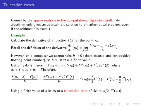
Caused by the approximations in the computational algorithm itself. (Analgorithm only gives an approximate solution to a mathematical problem, evenif the arithmetic is exact.)
Example
Calculate the derivative of a function f (x) at the point x0.
Recall the definition of the derivativedf
dx(x0) = lim
h→0
f (x0 + h)− f (x0)
h.
However, on a computer we cannot take h→ 0 (there exists a smallest positivefloating point number), so h must take a finite value.
Using Taylor’s theorem, f (x0 + h) = f (x0) + hf ′(x0) + h2/2 f ′′(ξ), wherex0 < ξ < x0 + h. Therefore,
f (x0 + h)− f (x0)
h=
hf ′(x0) + h2/2 f ′′(ξ)
h= f ′(x0)+
h
2f ′′(ξ) ' f ′(x0)+
h
2f ′′(x0).
Using a finite value of h leads to a truncation error of size ' h/2 |f ′′(x0)|.
Truncation errors
Caused by the approximations in the computational algorithm itself. (Analgorithm only gives an approximate solution to a mathematical problem, evenif the arithmetic is exact.)
Example
Calculate the derivative of a function f (x) at the point x0.
Recall the definition of the derivativedf
dx(x0) = lim
h→0
f (x0 + h)− f (x0)
h.
However, on a computer we cannot take h→ 0 (there exists a smallest positivefloating point number), so h must take a finite value.
Using Taylor’s theorem, f (x0 + h) = f (x0) + hf ′(x0) + h2/2 f ′′(ξ), wherex0 < ξ < x0 + h. Therefore,
f (x0 + h)− f (x0)
h=
hf ′(x0) + h2/2 f ′′(ξ)
h= f ′(x0)+
h
2f ′′(ξ) ' f ′(x0)+
h
2f ′′(x0).
Using a finite value of h leads to a truncation error of size ' h/2 |f ′′(x0)|.
Truncation errors
Caused by the approximations in the computational algorithm itself. (Analgorithm only gives an approximate solution to a mathematical problem, evenif the arithmetic is exact.)
Example
Calculate the derivative of a function f (x) at the point x0.
Recall the definition of the derivativedf
dx(x0) = lim
h→0
f (x0 + h)− f (x0)
h.
However, on a computer we cannot take h→ 0 (there exists a smallest positivefloating point number), so h must take a finite value.
Using Taylor’s theorem, f (x0 + h) = f (x0) + hf ′(x0) + h2/2 f ′′(ξ), wherex0 < ξ < x0 + h.
Therefore,
f (x0 + h)− f (x0)
h=
hf ′(x0) + h2/2 f ′′(ξ)
h= f ′(x0)+
h
2f ′′(ξ) ' f ′(x0)+
h
2f ′′(x0).
Using a finite value of h leads to a truncation error of size ' h/2 |f ′′(x0)|.

Truncation errors
Caused by the approximations in the computational algorithm itself. (Analgorithm only gives an approximate solution to a mathematical problem, evenif the arithmetic is exact.)
Example
Calculate the derivative of a function f (x) at the point x0.
Recall the definition of the derivativedf
dx(x0) = lim
h→0
f (x0 + h)− f (x0)
h.
However, on a computer we cannot take h→ 0 (there exists a smallest positivefloating point number), so h must take a finite value.
Using Taylor’s theorem, f (x0 + h) = f (x0) + hf ′(x0) + h2/2 f ′′(ξ), wherex0 < ξ < x0 + h. Therefore,
f (x0 + h)− f (x0)
h=
hf ′(x0) + h2/2 f ′′(ξ)
h= f ′(x0)+
h
2f ′′(ξ) ' f ′(x0)+
h
2f ′′(x0).
Using a finite value of h leads to a truncation error of size ' h/2 |f ′′(x0)|.
Truncation errors
Caused by the approximations in the computational algorithm itself. (Analgorithm only gives an approximate solution to a mathematical problem, evenif the arithmetic is exact.)
Example
Calculate the derivative of a function f (x) at the point x0.
Recall the definition of the derivativedf
dx(x0) = lim
h→0
f (x0 + h)− f (x0)
h.
However, on a computer we cannot take h→ 0 (there exists a smallest positivefloating point number), so h must take a finite value.
Using Taylor’s theorem, f (x0 + h) = f (x0) + hf ′(x0) + h2/2 f ′′(ξ), wherex0 < ξ < x0 + h. Therefore,
f (x0 + h)− f (x0)
h=
hf ′(x0) + h2/2 f ′′(ξ)
h= f ′(x0)+
h
2f ′′(ξ) ' f ′(x0)+
h
2f ′′(x0).
Using a finite value of h leads to a truncation error of size ' h/2 |f ′′(x0)|.
Truncation errors: Example continued
Clearly, the truncation error h/2 |f ′′(x0)| decreases with decreasing h.
The absolute round-off error in f (x0 + h)− f (x0) is 2ε|f (x0)| and that in thederivative (f (x0 + h)− f (x0))/h is 2ε/h |f (x0)|.So, the round-off error increases with decreasing h .
The relative accuracy of the calcu-lation of f ′(x0) (i.e. the sum of therelative truncation and round-off er-rors) is
Er =h
2
|f ′′||f ′| +
2ε
h
|f ||f ′| ,
hm
∝ h
∝ 1
hEr
h
which has a minimum, min(Er ) = 2√ε√|ff ′′|/|f ′|, for hm = 2
√ε√|f /f ′′|.
Related Documents