Nonlife Actuarial Models Chapter 1 Claim-Frequency Distribution

Welcome message from author
This document is posted to help you gain knowledge. Please leave a comment to let me know what you think about it! Share it to your friends and learn new things together.
Transcript

Nonlife Actuarial Models
Chapter 1
Claim-Frequency Distribution

Learning Objectives
• Discrete distributions for modeling claim frequency
• Binomial, geometric, negative binomial and Poisson distributions
• The (a, b, 0) and (a, b, 1) classes of distributions
• Compound distribution
• Convolution
• Mixture distribution
2

1.2 Review of Statistics
• Distribution function (df) of random variable X
FX(x) = Pr(X ≤ x). (1.1)
• Probability density function (pdf) of continuous random vari-
able
fX(x) =dFX(x)
dx. (1.2)
• Probability function (pf) of discrete random variable
fX(x) =
(Pr(X = x), if x ∈ ΩX ,0, otherwise.
(1.3)
where ΩX is the support of X
3

• Moment generating function (mgf), defined as
MX(t) = E(etX). (1.6)
• Moments of X are obtainable from mgf by
M rX(t) =
drMX(t)
dtr=dr
dtrE(etX) = E(XretX), (1.7)
so that
M rX(0) = E(X
r) = μ0r. (1.8)
4

• If X1, X2, · · · , Xn are independently and identically distrib-
uted (iid) random variables with mgfM(t), and X = X1+· · ·+Xn,then the mgf of X is
MX(t) = E(etX) = E
ÃnYi=1
etXi!=
nYi=1
E(etXi) = [M(t)]n . (1.9)
• Probability generating function (pgf), defined as PX(t) = E(tX),
PX(t) =∞Xx=0
txfX(x), (1.13)
so that for X taking nonnegative integer values.
• We have
P rX(t) =∞Xx=r
x(x− 1) · · · (x− r + 1)tx−rfX(x) (1.14)
5
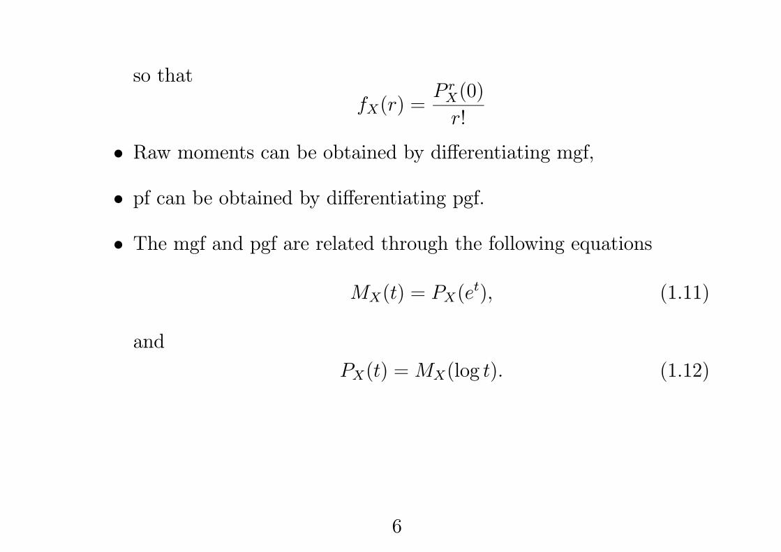
so that
fX(r) =P rX(0)
r!
• Raw moments can be obtained by differentiating mgf,
• pf can be obtained by differentiating pgf.
• The mgf and pgf are related through the following equations
MX(t) = PX(et), (1.11)
and
PX(t) =MX(log t). (1.12)
6

1.3 Some Discrete Distributions
(1) Binomial Distribution: X ∼ BN (n, θ) if
fX(x) =
Ãn
x
!θx(1− θ)n−x, for x = 0, 1, · · · , n, (1.17)
• The mean and variance of X are
E(X) = nθ and Var(X) = nθ(1− θ), (1.19)
so that the variance of X is always smaller than its mean.
• How do you prove these results?
• The mgf of X is
MX(t) = (θet + 1− θ)n, (1.20)
7

and its pgf is
PX(t) = (θt+ 1− θ)n. (1.21)
• A recursive relationship for fX(x) is
fX(x) =
"(n− x+ 1)θx(1− θ)
#fX(x− 1) (1.23)
(2) Geometric Distribution: X ∼ GM(θ) if
fX(x) = θ(1− θ)x, for x = 0, 1, · · · . (1.24)
• The mean and variance of X are
E(X) =1− θ
θand Var(X) =
1− θ
θ2, (1.25)
8

• How do you prove these results?
• The mgf of X is
MX(t) =θ
1− (1− θ)et, (1.26)
and its pgf is X
PX(t) =θ
1− (1− θ)t. (1.27)
• The pf satisfies the following recursive relationship
fX(x) = (1− θ) fX(x− 1), (1.28)
for x = 1, 2, · · ·, with starting value fX(0) = θ.
9

(3) Negative Binomial Distribution: X ∼ NB(r, θ) if
fX(x) =
Ãx+ r − 1r − 1
!θr(1− θ)x, for x = 0, 1, · · · , (1.29)
• The mean and variance are
E(X) =r(1− θ)
θand Var(X) =
r(1− θ)
θ2, (1.30)
• The mgf of NB(r, θ) is
MX(t) =
"θ
1− (1− θ)et
#r, (1.31)
and its pgf is
PX(t) =
"θ
1− (1− θ)t
#r. (1.32)
10

• May extend the parameter r to any positive number (not necessarilyinteger).
• The recursive formula of the pf is
fX(x) =
"(x+ r − 1)(1− θ)
x
#fX(x− 1), (1.37)
with starting value
fX(0) = θr. (1.38)
(4) Poisson Distribution: X ∼ PN (λ), if the pf of X is given by
fX(x) =λxe−λ
x!, for x = 0, 1, · · · , (1.39)
• The mean and variance of X are
E(X) = Var(X) = λ. (1.40)
11

The mgf of X is
MX(t) = exphλ(et − 1)
i, (1.41)
and its pgf is
PX(t) = exp [λ(t− 1)] . (1.42)
• Two important theorems of Poisson distribution
• Theorem 1.1: If X1, · · · , Xn are independently distributed withXi ∼ PN (λi), for i = 1, · · · , n, then X = X1+· · ·+Xn is distributedas a Poisson with parameter λ = λ1 + · · ·+ λn.
12

• Proof: To prove this result, we make use of the mgf. Note that
the mgf of X is
MX(t) = E(etX)
= E(etX1+ ···+ tXn)
= E
ÃnYi=1
etXi!
=nYi=1
E(etXi)
=nYi=1
exphλi(e
t − 1)i
= exp
"(et − 1)
nXi=1
λi
#= exp
h(et − 1)λ
i, (1.43)
which is the mgf of PN (λ).
13

• Theorem 1.2: Suppose an event A can be partitioned into m
mutually exclusive and exhaustive events Ai, for i = 1, · · · ,m. LetX be the number of occurrences of A, and Xi be the number of
occurrences of Ai, so that X = X1 + · · · +Xm. Let the probabilityof occurrence of Ai given A has occurred be pi, i.e., Pr(Ai |A) = pi,with
Pmi=1 pi = 1. If X ∼ PN (λ), then Xi ∼ PN (λi), where λi =
λpi. Furthermore, X1, · · · , Xn are independently distributed.
• Proof: To prove this result, we first derive the marginal distribu-
tion of Xi. Given X = x, Xi ∼ BN (x, pi). Hence, the marginal pf ofXi is pf of PN (λpi). Then we show that the joint pf of X1, · · · , Xmis the product of their marginal pf, so that X1, · · · , Xm are indepen-dent.
14
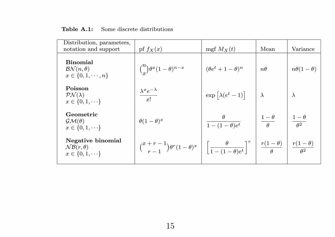
Table A.1: Some discrete distributions
Distribution, parameters,notation and support pf fX(x) mgf MX(t) Mean Variance
BinomialBN (n, θ)x ∈ 0, 1, · · · , n
¡nx
¢θx(1− θ)n−x (θet + 1− θ)n nθ nθ(1− θ)
PoissonPN (λ)x ∈ 0, 1, · · ·
λxe−λ
x!exp£λ(et − 1)
¤λ λ
GeometricGM(θ)x ∈ 0, 1, · · ·
θ(1− θ)xθ
1− (1− θ)et1− θ
θ
1− θ
θ2
Negative binomialNB(r, θ)x ∈ 0, 1, · · ·
¡x+ r − 1r − 1
¢θr(1− θ)x
hθ
1− (1− θ)et
ir r(1− θ)
θ
r(1− θ)
θ2
15

1.4 The (a, b, 0) Class of Distributions
• Definition 1.1: A nonnegative discrete random variable X is in
the (a, b, 0) class if its pf fX(x) satisfies the following recursion
fX(x) =
Ãa+
b
x
!fX(x− 1), for x = 1, 2, · · · , (1.48)
where a and b are constants, with given fX(0).
• As an example, we consider the binomial distribution. Its pf can bewritten as follows
fX(x) =
"− θ
1− θ+
θ(n+ 1)
(1− θ)x
#fX(x− 1). (1.49)
Thus, we let
a = − θ
1− θand b =
θ(n+ 1)
(1− θ). (1.50)
16

• Binomial, geometric, negative binomial and Poisson belong to the(a, b, 0) class of distributions.
Table 1.2: The (a, b, 0) class of distributions
Distribution a b fX(0)
Binomial: BN (n, θ) − θ
1− θ
θ(n+ 1)
1− θ(1− θ)n
Geometric: GM(θ) 1− θ 0 θ
Negative binomial: NB(r, θ) 1− θ (r − 1)(1− θ) θr
Poisson: PN (λ) 0 λ e−λ
17

• It may be desirable to obtain a good fit of the distribution at zeroclaim based on empirical experience and yet preserve the shape to
coincide with some simple parametric distributions.
• This can be achieved by specifying the zero probability while adopt-ing the recursion to mimic a selected (a, b, 0) distribution.
• Let fX(x) be the pf of a (a, b, 0) distribution called the base distri-bution. We denote fMX (x) as the pf that is a modification of fX(x).
• The probability at point zero, fMX (0), is specified and fMX (x) is re-lated to fX(x) as follows
fMX (x) = cfX(x), for x = 1, 2, · · · , (1.52)
where c is an appropriate constant.
18

• For fMX (·) to be a well defined pf, we must have
1 = fMX (0) +∞Xx=1
fMX (x)
= fMX (0) + c∞Xx=1
fX(x)
= fMX (0) + c[1− fX(0)]. (1.53)
Thus, we conclude that
c =1− fMX (0)1− fX(0) . (1.54)
Substituting c into equation (1.52) we obtain fMX (x), for x = 1, 2, · · ·.
• Together with the given fMX (0), we have a distribution with thedesired zero-claim probability and the same recursion as the base
(a, b, 0) distribution.
19

• This is called the zero-modified distribution of the base (a, b, 0)distribution.
• In particular, if fMX (0) = 0, the modified distribution cannot take
value zero and is called the zero-truncated distribution.
• The zero-truncated distribution is a particular case of the zero-modified distribution.
20

1.5 Some Methods for Creating New Distributions
1.5.1 Compound distribution
• Let X1, · · · , XN be iid nonnegative integer-valued random variables,each distributed like X. We denote the sum of these random vari-
ables by S, so that
S = X1 + · · ·+XN . (1.60)
• If N is itself a nonnegative integer-valued random variable distrib-
uted independently of X1, · · · , XN , then S is said to have a com-pound distribution.
• The distribution of N is called the primary distribution, and the
distribution of X is called the secondary distribution.
21

• We shall use the primary-secondary convention to name a compounddistribution.
• Thus, if N is Poisson and X is geometric, S has a Poisson-geometric
distribution.
• A compound Poisson distribution is a compound distribution
where N is Poisson, for any secondary distribution.
• Consider the simple case where N has a degenerate distribution
taking value n with probability 1. S is then the sum of n terms of
Xi, where n is fixed. Suppose n = 2, so that S = X1 +X2.
• As the pf of X1 and X2 are fX(·), the pf of S is given by
22

fS(s) = Pr(X1 +X2 = s)
=sXx=0
Pr(X1 = x and X2 = s− x)
=sXx=0
fX(s)fX(s− x), (1.62)
where the last line above is due to the independence of X1 and X2.
• The pf of S, fS(·), is the convolution of fX(·), denoted by (fX ∗fX)(·), i.e.,
fX1+X2(s) = (fX ∗ fX)(s) =sXx=0
fX(x)fX(s− x). (1.63)
• Convolutions can be evaluated recursively. When n = 3, the 3-fold
23

convolution is
fX1+X2+X3(s) = (fX1+X2 ∗ fX3)(s) =(fX1 ∗ fX2 ∗ fX3)(s) = (fX ∗ fX ∗ fX)(s). (1.64)
• Example 1.7: Let the pf of X be fX(0) = 0.1, fX(1) = 0,
fX(2) = 0.4 and fX(3) = 0.5. Find the 2-fold and 3-fold convolutions
of X.
• Solution: We first compute the 2-fold convolution. For s = 0 and
1, the probabilities are
(fX ∗ fX)(0) = fX(0)fX(0) = (0.1)(0.1) = 0.01,
and
(fX ∗ fX)(1) = fX(0)fX(1) + fX(1)fX(0) = (0.1)(0) + (0)(0.1) = 0.
24

Other values are similarly computed as follows
(fX ∗ fX)(2) = (0.1)(0.4) + (0.4)(0.1) = 0.08,
(fX ∗ fX)(3) = (0.1)(0.5) + (0.5)(0.1) = 0.10,(fX ∗ fX)(4) = (0.4)(0.4) = 0.16,
(fX ∗ fX)(5) = (0.4)(0.5) + (0.5)(0.4) = 0.40,and
(fX ∗ fX)(6) = (0.5)(0.5) = 0.25.For the 3-fold convolution, we show some sample workings as follows
f∗3X (0) = [fX(0)]hf∗2X (0)
i= (0.1)(0.01) = 0.001,
f∗3X (1) = [fX(0)]hf∗2X (1)
i+ [fX(1)]
hf∗2X (0)
i= 0,
25

and
f∗3X (2) = [fX(0)]hf∗2X (2)
i+ [fX(1)]
hf∗2X (1)
i+ [fX(2)]
hf∗2X (0)
i= 0.012.
• The results are summarized in Table 1.4• We now return to the compound distribution in which the primarydistribution N has a pf fN(·). Using the total law of probability, weobtain the pf of the compound distribution S as
fS(s) =∞Xn=0
Pr(X1 + · · ·+XN = s |N = n) fN(n)
=∞Xn=0
Pr(X1 + · · ·+Xn = s) fN(n),
in which the term Pr(X1 + · · · +Xn = s) can be calculated as then-fold convolution of fX(·).
26

• The evaluation of convolution is usually quite complex when n islarge.
• Theorem 1.4: Let S be a compound distribution. If the primary
distribution N has mgfMN(t) and the secondary distribution X has
mgf MX(t), then the mgf of S is
MS(t) =MN [logMX(t)]. (1.66)
If N has pgf PN(t) and X is nonnegative integer valued with pgf
PX(t), then the pgf of S is
PS(t) = PN [PX(t)]. (1.67)
• Proof: The proof makes use of results in conditional expectation.
We note that
27

MS(t) = E³etS´
= E³etX1+ ···+ tXN
´= E
hE³etX1+ ···+ tXN |N
´i= E
½hE³etX
´iN¾= E
n[MX(t)]
No
= E½helogMX(t)
iN¾= MN [logMX(t)]. (1.68)
• Similarly we get PS(t) = PN [PX(t)].• To compute the pf of S. We note that
fS(0) = PS(0) = PN [PX(0)], (1.70)
28

• Also, we havefS(1) = P
0S(0). (1.71)
The derivative P 0S(t) may be computed by differentiating PS(t) di-rectly, or by the chain rule using the derivatives of PN(t) and PX(t),
i.e.,
P 0S(t) = P 0N [PX(t)]P 0X(t). (1.72)
• Example 1.8: Let N ∼ PN (λ) and X ∼ GM(θ). Calculate
fS(0) and fS(1).
• Solution: The pgf of N is
PN(t) = exp[λ(t− 1)],
29

and the pgf of X is
PX(t) =θ
1− (1− θ)t.
The pgf of S is
PS(t) = PN [PX(t)] = exp
"λ
Ãθ
1− (1− θ)t− 1
!#,
from which we obtain
fS(0) = PS(0) = exp [λ (θ − 1)] .To calculate fS(1), we differentiate PS(t) directly to obtain
P 0S(t) = exp
"λ
Ãθ
1− (1− θ)t− 1
!#λθ(1− θ)
[1− (1− θ)t]2,
so that
fS(1) = P0S(0) = exp [λ (θ − 1)]λθ(1− θ).
30

• The Panjer (1981) recursion is a recursive method for computing thepf of S, which applies to the case where the primary distribution N
belongs to the (a, b, 0) class.
• Theorem 1.5: If N belongs to the (a, b, 0) class of distributions
and X is a nonnegative integer-valued random variable, then the pf
of S is given by the following recursion
fS(s) =1
1− afX(0)sXx=1
Ãa+
bx
s
!fX(x)fS(s−x), for s = 1, 2, · · · ,
(1.74)
with initial value fS(0) given by equation (1.70).
• Proof: See Dickson (2005), Section 4.5.2.
• The mean and variance of a compound distribution can be obtainedfrom the means and variances of the primary and secondary distri-
31

butions. Thus, the first two moments of the compound distribution
can be obtained without computing its pf.
• Theorem 1.6: Consider the compound distribution. We de-
note E(N) = μN and Var(N) = σ2N , and likewise E(X) = μX and
Var(X) = σ2X . The mean and variance of S are then given by
E(S) = μNμX , (1.75)
and
Var(S) = μNσ2X + σ2Nμ
2X . (1.76)
• Proof: We use the results in Appendix A.11 on conditional ex-
pectations to obtain
E(S) = E[E(S |N)] = E[E(X1 + · · ·+XN |N)] = E(NμX) = μNμX .
(1.77)
32

From (A.115), we have
Var(S) = E[Var(S |N)] + Var[E(S |N)]= E[Nσ2X ] + Var(NμX)
= μNσ2X + σ2Nμ
2X , (1.78)
which completes the proof.
• If S is a compound Poisson distribution with N ∼ PN (λ), so thatμN = σ2N = λ, then
Var(S) = λ(σ2X + μ2X) = λE(X2). (1.79)
Proof of equation (1.78)
Given two random variables X and Y , the conditional variance Var(X |Y )is defined as v(Y ), where
v(y) = Var(X | y) = E[X − E(X | y)]2 | y = E(X2 | y)− [E(X | y)]2.
33

Thus, we have
Var(X |Y ) = E(X2 |Y )− [E(X |Y )]2,
which implies
E(X2 |Y ) = Var(X |Y ) + [E(X |Y )]2.
Now we have
Var(X) = E(X2)− [E(X)]2= E[E(X2 |Y )]− [E(X)]2= EVar(X |Y ) + [E(X |Y )]2− [E(X)]2= E[Var(X |Y )] + E[E(X |Y )]2− [E(X)]2= E[Var(X |Y )] + E[E(X |Y )]2− E[E(X |Y )]2= E[Var(X |Y )] + Var[E(X |Y )].
34

• Example 1.10: Let N ∼ PN (2) and X ∼ GM(0.2). Calculate
E(S) and Var(S). Repeat the calculation for N ∼ GM(0.2) and
X ∼ PN (2).
• Solution: As X ∼ GM(0.2), we have
μX =1− θ
θ=0.8
0.2= 4,
and
σ2X =1− θ
θ2=
0.8
(0.2)2= 20.
If N ∼ PN (2), we have E(S) = (4)(2) = 8. Since N is Poisson, we
have
Var(S) = 2(20 + 42) = 72.
For N ∼ GM(0.2) and X ∼ PN (2), μN = 4, σ2N = 20, and μX =
35

σ2X = 2. Thus, E(S) = (4)(2) = 8, and we have
Var(S) = (4)(2) + (20)(4) = 88.
• We have seen that the sum of independently distributed Poisson
distributions is also Poisson.
• It turns out that the sum of independently distributed compound
Poisson distributions has also a compound Poisson distribution.
• Theorem 1.7: Suppose S1, · · · , Sn have independently distributedcompound Poisson distributions, where the Poisson parameter of Si
is λi and the pgf of the secondary distribution of Si is Pi(·). ThenS = S1+ · · ·+Sn has a compound Poisson distribution with Poissonparameter λ = λ1 + · · ·+ λn. The pgf of the secondary distribution
of S is P (t) =Pni=1wiPi(t), where wi = λi/λ.
36

• Proof: The pgf of S is (see Example 1.11 for an application)
PS(t) = E³tS1+ ···+Sn
´=
nYi=1
PSi(t)
=nYi=1
exp λi[Pi(t)− 1]
= exp
(nXi=1
λiPi(t)−nXi=1
λi
)
= exp
(nXi=1
λiPi(t)− λ
)
= exp
(λ
"nXi=1
λiλ[Pi(t)]− 1
#)= exp λ[P (t)− 1] . (1.80)
37

1.5.2 Mixture distribution
• Let X1, · · · , Xn be random variables with corresponding pf or pdf
fX1(·), · · · , fXn(·) in the common support Ω. A new random variableX may be created with pf or pdf fX(·) given by
fX(x) = p1fX1(x) + · · ·+ pnfXn(x), x ∈ Ω, (1.82)
where pi ≥ 0 for i = 1, · · · , n and Pni=1 pi = 1.
• Theorem 1.8: The mean of X is
E(X) = μ =nXi=1
piμi, (1.83)
and its variance is
Var(X) =nXi=1
pih(μi − μ)2 + σ2i
i. (1.84)
38

• Example 1.12: The claim frequency of a bad driver is distributed
as PN (4), and the claim frequency of a good driver is distributed asPN (1). A town consists of 20% bad drivers and 80% good drivers.
What is the mean and variance of the claim frequency of a randomly
selected driver from the town?
• Solution: The mean of the claim frequency is
(0.2)(4) + (0.8)(1) = 1.6,
and its variance is
(0.2)h(4− 1.6)2 + 4
i+ (0.8)
h(1− 1.6)2 + 1
i= 3.04.
• The above can be generalized to continuous mixing.
39

1.5 Excel Computation Notes
Table 1.5: Some Excel functions
ExampleX Excel function input output
BN (n, θ) BINOMDIST(x1,x2,x3,ind) BINOMDIST(4,10,0.3,FALSE) 0.2001x1 = x BINOMDIST(4,10,0.3,TRUE) 0.8497x2 = nx3 = θ
PN (λ) POISSON(x1,x2,ind) POISSON(4,3.6,FALSE) 0.1912x1 = x POISSON(4,3.6,TRUE) 0.7064x2 = λ
NB(r, θ) NEGBINOMDIST(x1,x2,x3) NEGBINOMDIST(3,1,0.4) 0.0864x1 = x NEGBINOMDIST(3,3,0.4) 0.1382x2 = rx3 = θ
40
Related Documents