Chapter 05

Chapter 5

Stiffness Matrices for Special Elements 1. Stiffness Matrix by Castigliano's Theorems ................................................................2 2. Principle of Minimum Total Potential Energy ............................................................3 3. Inclusion of Shear Deformations .................................................................................4

3.1 Strain Energy due to Shear ............................................................................4 3.2 Flexibility and Stiffness Matrices Including Shear Deformations.................6

4. Nonprismatic Members................................................................................................7 5. Arch Structures ............................................................................................................13 6. Stiffness Matrix for Cables Over Pulley......................................................................21 7. Stiffness Matrix for Space Truss members..................................................................22 8. Stiffness Matrix for Plane Grid Members....................................................................24 9. Stiffness Matrix for Space Frame Members ................................................................25 10. Rigid Bodies in Framed Systems...............................................................................28 PROBLEMS ....................................................................................................................33

Matrix Structural Analysis v.4.0 Aug. 05 5.1

1. Stiffness Matrix by Castigliano's Theorems Stiffness and flexibility matrices of an element

(1.1)

Q = kqq = fQ

where Q and q represent the characterising set of forces and deformations/displacements The strain energy in the element is

U = 1

2 qTQ = 12 q Tkq = 1

2 QTf Q (1.2)

Castigliano's first theorem:

Q = dU

d q = kq

(1.3)

i.e. To find the stiffness matrix k, form the strain energy in terms of q and differentiate it with respect to q. Castigliano's second theorem:

q = dU

d Q = fQ

(1.4)

i.e. To find the flexibility matrix f, form the strain energy in terms of Q and differentiate it with respect to Q.

Example 1. Shows that the stiffness and flexibility coefficients of a member are given by, respectively:

k ij = ∂ 2U

∂q i ∂q j; f ij = ∂ 2U

∂Q i ∂Q j Solution: Using Castigliano’s first theorem:

Q i = ∂U

∂q i= k i 1q1 + … + k ij q j + …

(a) Hence


∂Q i

∂q j= ∂ 2U

∂q i ∂q j= k ij

(b) By interchanging the indexes i and j, the above relation shows that k is symmetric. The flexibility coefficient is derived in a similar fashion.

2. Principle of Minimum Total Potential Energy Define V as the potential energy of external forces1

V = − RT r (2.1) and U as the total strain energy in the system expressed in terms of displacements/deformations:

U = 1

2 q TQ = 12 q T kq

(2.2) where Q and q are the vectors of forces and displacements/deformations for all elements in the system. The function Π = U+V is called the total potential energy of the system. Principle of minimum total potential energy: Among the infinite set of displacements r and compatible deformations q, the one set that minimizes the total potential energy will also satisfy both the equilibrium and material requirements.

Example 2. Formulate the matrix displacement method by using the principle of total potential energy. Solution: The infinite set of compatible displacements and deformations is defined by (a) q = ar The total potential energy:

Π = U + V = 1

2 qTQ − R Tr = 12 qTkq − R Tr

1 This function exists only if the external forces are conservative; i.e. their work done is independent of the

path.


Using Eq.(a)

Π = 1

2 rTaT ka r − RT r (b)

Minimizing (b) with respect to r: ∂ Π∂ r = aT ka r − R = 0

This leads to the equilibrium equation: R = aTka r

3. Inclusion of Shear Deformations We have so far neglected deformations and deflections in beams due to shear stresses, and this is justified as long as the beam is slender2. In this section we will incorporate the effect of shear deformations into the beam’s stiffness and flexibility matrices for the analysis of general beam and frame systems.

3.1 Strain Energy due to Shear Shear stress in beam is (see Eq.7.2.1)

τ =

VQIt (3.1)

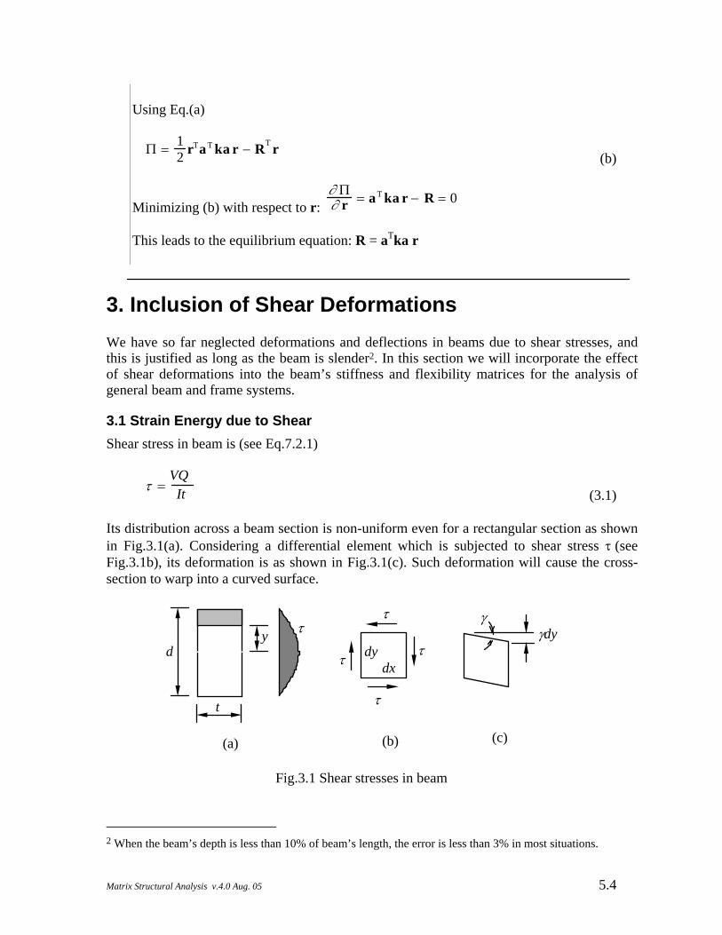
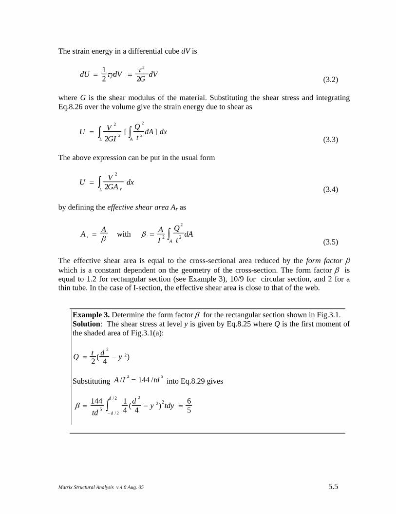
Its distribution across a beam section is non-uniform even for a rectangular section as shown in Fig.3.1(a). Considering a differential element which is subjected to shear stress τ (see Fig.3.1b), its deformation is as shown in Fig.3.1(c). Such deformation will cause the cross-section to warp into a curved surface.

t

d

ττ

τ

τ

τ dxdy

γdyγ

(a) (b) (c)

y

Fig.3.1 Shear stresses in beam

2 When the beam’s depth is less than 10% of beam’s length, the error is less than 3% in most situations.


The strain energy in a differential cube dV is

dU = 1

2τγdV = τ 2

2G dV (3.2)

where G is the shear modulus of the material. Substituting the shear stress and integrating Eq.8.26 over the volume give the strain energy due to shear as

U = V 2

2GI 2 [Q 2

t 2A∫ dA ] dx

L∫

(3.3) The above expression can be put in the usual form

U = V 2

2GA rdx

L∫

(3.4) by defining the effective shear area Ar as

A r = A

β with β = AI 2

Q 2

t 2A

∫ dA (3.5)

The effective shear area is equal to the cross-sectional area reduced by the form factor β which is a constant dependent on the geometry of the cross-section. The form factor β is equal to 1.2 for rectangular section (see Example 3), 10/9 for circular section, and 2 for a thin tube. In the case of I-section, the effective shear area is close to that of the web.

Example 3. Determine the form factor β for the rectangular section shown in Fig.3.1. Solution: The shear stress at level y is given by Eq.8.25 where Q is the first moment of the shaded area of Fig.3.1(a):

Q = t2 ( d 2

4 − y 2)

Substituting A /I 2 = 144 /td 5

into Eq.8.29 gives

β = 144td 5

14 (d 2

4 − y 2)2tdy− d / 2

d / 2

∫ = 65


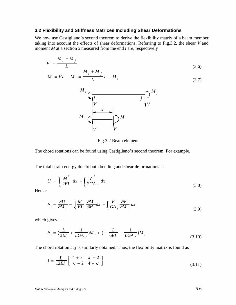
3.2 Flexibility and Stiffness Matrices Including Shear Deformations We now use Castigliano’s second theorem to derive the flexibility matrix of a beam member taking into account the effects of shear deformations. Referring to Fig.3.2, the shear V and moment M at a section x measured from the end i are, respectively

V =

M i + M j

L (3.6)

M = Vx − M i =

M i + M j

L x − M i (3.7)

M i M j

V V

V V

M i M

x

i j

Fig.3.2 Beam element The chord rotations can be found using Castigliano’s second theorem. For example, The total strain energy due to both bending and shear deformations is

U = M 2

2EI dx +L∫ V 2

2GA rdx

L∫

(3.8) Hence

θ i = ∂U

∂M i= M

EI∂M∂M i

dx +L∫ V

GA r

∂V∂M i

dxL∫

(3.9) which gives

θ i = ( L

3EI + 1LGA r

)M i + ( − L6EI + 1

LGA r)M j (3.10)

The chord rotation at j is similarly obtained. Thus, the flexibility matrix is found as

f = L

12EI4 + κ κ − 2κ − 2 4 + κ

⎡⎢⎣⎤⎥⎦ (3.11)


where

κ = 12EI

L 2GA r (3.12) The basic stiffness matrix is

k = f −1 = EI

L (1 + κ )4 + κ 2 − κ2 − κ 4 + κ

⎡⎢⎣⎤⎥⎦ (3.13)

The basic stiffness matrix k can be further transformed in the usual manner for use in the direct stiffness method. In addition, the fixed-end forces may also need to be computed taking into account shear deformations. When shear deformations are neglected, the coefficient κ is set to zero, and the above matrices revert to their standard forms.

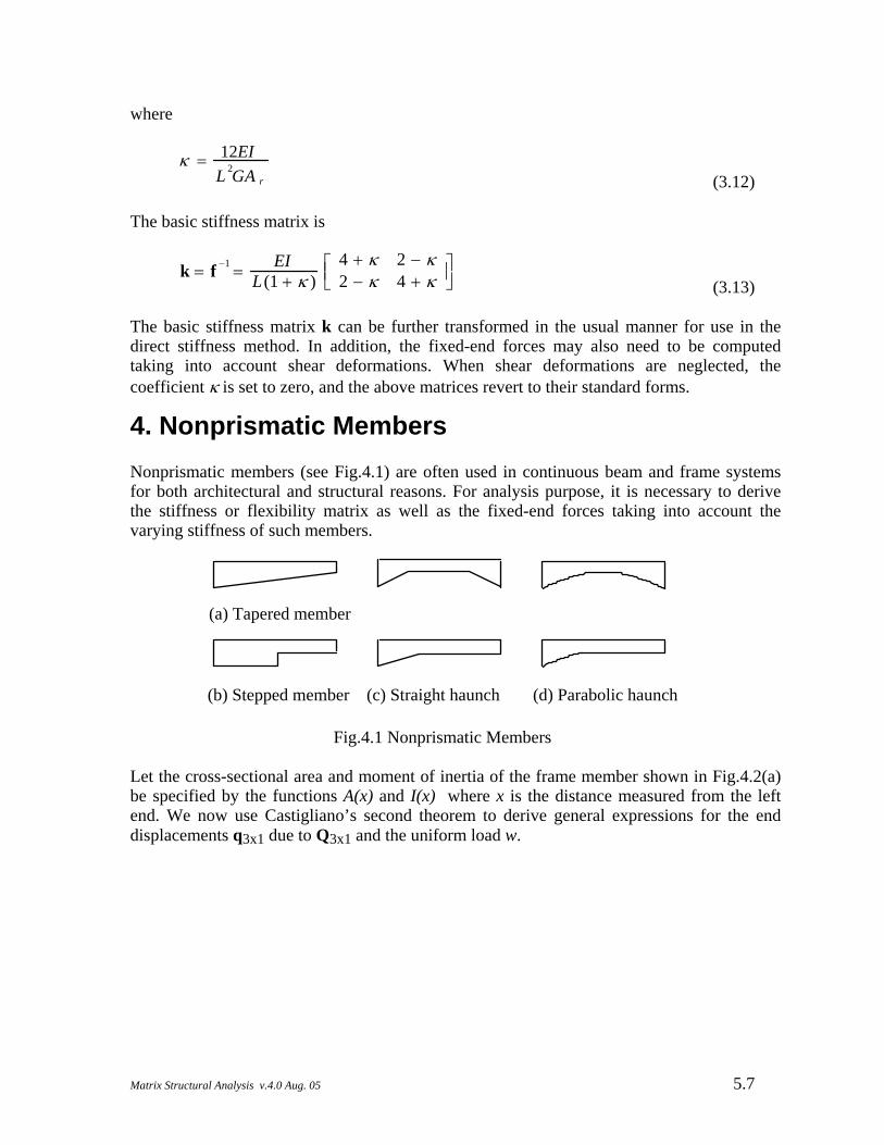
4. Nonprismatic Members Nonprismatic members (see Fig.4.1) are often used in continuous beam and frame systems for both architectural and structural reasons. For analysis purpose, it is necessary to derive the stiffness or flexibility matrix as well as the fixed-end forces taking into account the varying stiffness of such members.

(a) Tapered member

(c) Straight haunch (d) Parabolic haunch(b) Stepped member

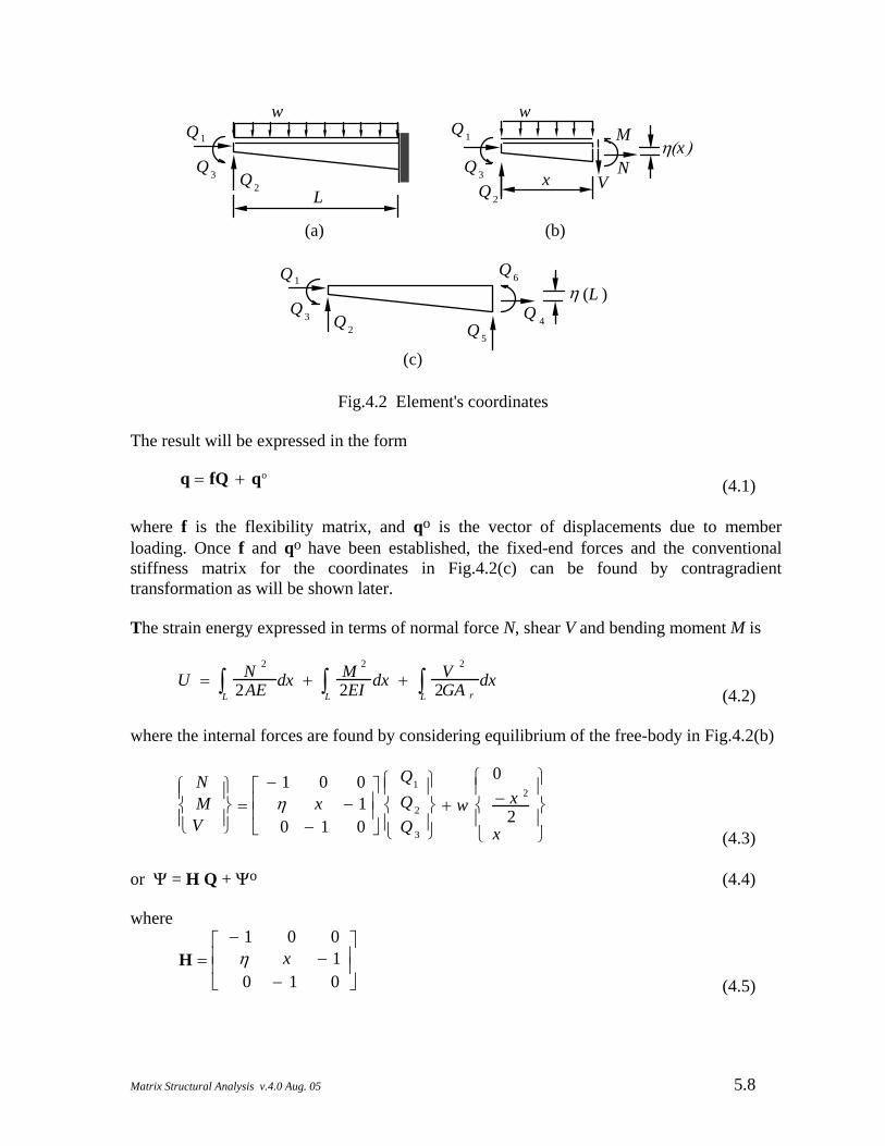
Fig.4.1 Nonprismatic Members Let the cross-sectional area and moment of inertia of the frame member shown in Fig.4.2(a) be specified by the functions A(x) and I(x) where x is the distance measured from the left end. We now use Castigliano’s second theorem to derive general expressions for the end displacements q3x1 due to Q3x1 and the uniform load w.


Q 1

Q 2

Q 3

w

N

M

V

(a) (b)

Q 1

Q 2

Q 3

w

η(x)

xL

Q 1

Q 2

Q 3 Q 4Q 5

Q 6

η (L )

(c)

Fig.4.2 Element's coordinates The result will be expressed in the form (4.1) q = fQ + qo

where f is the flexibility matrix, and qo is the vector of displacements due to member loading. Once f and qo have been established, the fixed-end forces and the conventional stiffness matrix for the coordinates in Fig.4.2(c) can be found by contragradient transformation as will be shown later. The strain energy expressed in terms of normal force N, shear V and bending moment M is

U = N 2

2AEL∫ dx + M 2

2EIL∫ dx + V 2

2GA rL∫ dx

(4.2) where the internal forces are found by considering equilibrium of the free-body in Fig.4.2(b)

NM

V

⎧⎪⎨⎪⎩

⎫⎪⎬⎪⎭

=− 1 0 0

η x − 10 − 1 0

⎡⎢⎢⎣

⎤⎥⎥⎦

Q1

Q 2

Q 3

⎧⎪⎨⎪⎩

⎫⎪⎬⎪⎭

+ w

0− x 2

2x

⎧⎪⎨⎪⎩

⎫⎪⎬⎪⎭ (4.3)

or Ψ = H Q + Ψo (4.4)

where

(4.5) H =

− 1 0 0η x − 10 − 1 0

⎡⎢⎢⎣

⎤⎥⎥⎦


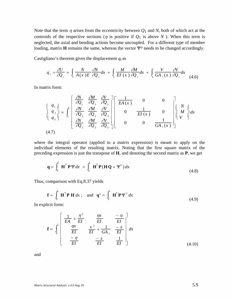
Note that the term η arises from the eccentricity between Q1 and N, both of which act at the centroids of the respective sections (η is positive if Q1 is above N ). When this term is neglected, the axial and bending actions become uncoupled. For a different type of member loading, matrix H remains the same, whereas the vector Ψo needs to be changed accordingly. Castigliano’s theorem gives the displacement qi as

q i = ∂U

∂Q i= N

A (x )E∂N∂Q iL

∫ dx + MEI (x )L

∫ ∂M∂Q i

dx + VGA r (x )L

∫ ∂V∂Q i

dx (4.6)

In matrix form:

q1

q 2

q3

⎧⎪⎨⎪⎩

⎫⎪⎬⎪⎭

=0

L

∫

∂N∂Q1

∂M∂Q 1

∂V∂Q 1

∂N∂Q 2

∂M∂Q 2

∂V∂Q 2

∂N∂Q 3

∂M∂Q 3

∂V∂Q 3

⎡⎢⎢⎢⎢⎢⎢⎣

⎤⎥⎥⎥⎥⎥⎥⎦

1EA (x ) 0 0

0 1EI (x ) 0

0 0 1GA r (x )

⎡⎢⎢⎢⎢⎢⎢⎣

⎤⎥⎥⎥⎥⎥⎥⎦

NMV

⎧⎪⎨⎪⎩

⎫⎪⎬⎪⎭

dx

(4.7) where the integral operator (applied to a matrix expression) is meant to apply on the individual elements of the resulting matrix. Noting that the first square matrix of the preceding expression is just the transpose of H, and denoting the second matrix as P, we get

(4.8) q =

0

L

∫ HT P Ψ dx =0

L

∫ HT P (H Q + Ψo ) dx

Thus, comparison with Eq.8.37 yields

(4.9) f =

0

L

∫ HT P H dx ; and qo =0

L

∫ HT P Ψ o dx

In explicit form:

f =0

L

∫

1EA +

η 2

EIηxEI

− ηEI

ηxEI

x 2

EI + 1GA r

− xEI

− ηEI

− xEI

1EI

⎡⎢⎢⎢⎢⎢⎢⎣

⎤⎥⎥⎥⎥⎥⎥⎦

dx

(4.10) and


qo =0

L

∫

−Ψ o

1

AE +ηΨ o

2

EIxΨ o

2

EI −Ψ o

3

GA r

−Ψ o

2

EI

⎧⎪⎪⎪⎨⎪⎪⎪⎩

⎫⎪⎪⎪⎬⎪⎪⎪⎭

dx

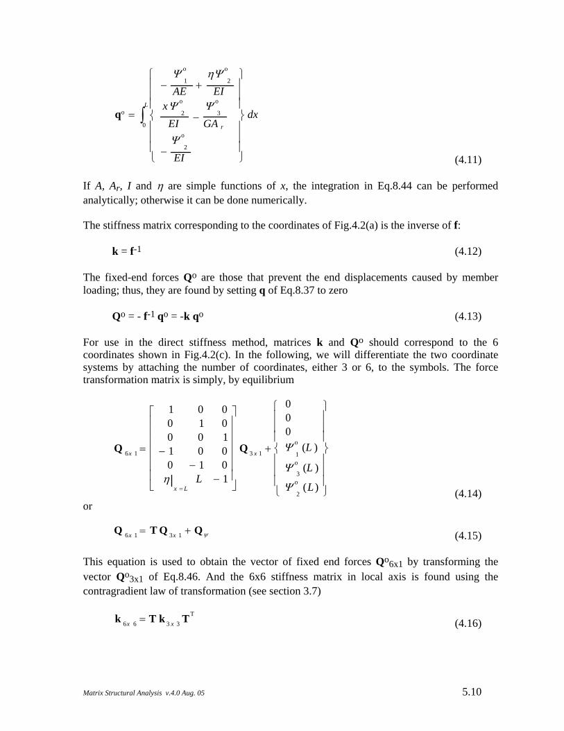
(4.11) If A, Ar, I and η are simple functions of x, the integration in Eq.8.44 can be performed analytically; otherwise it can be done numerically. The stiffness matrix corresponding to the coordinates of Fig.4.2(a) is the inverse of f: k = f-1 (4.12) The fixed-end forces Qo are those that prevent the end displacements caused by member loading; thus, they are found by setting q of Eq.8.37 to zero Qo = - f-1 qo = -k qo (4.13)

For use in the direct stiffness method, matrices k and Qo should correspond to the 6 coordinates shown in Fig.4.2(c). In the following, we will differentiate the two coordinate systems by attaching the number of coordinates, either 3 or 6, to the symbols. The force transformation matrix is simply, by equilibrium

Q 6x 1 =

1 0 00 1 00 0 1

− 1 0 00 − 1 0

ηx = L

L − 1

⎡⎢⎢⎢⎢⎢⎢⎣

⎤⎥⎥⎥⎥⎥⎥⎦

Q 3 x 1 +

000Ψ o

1(L )

Ψ o

3(L )

Ψ o

2(L )

⎧⎪⎪⎪⎨⎪⎪⎪⎩

⎫⎪⎪⎪⎬⎪⎪⎪⎭ (4.14)

or (4.15) Q 6x 1 = T Q 3x 1 + Qψ

This equation is used to obtain the vector of fixed end forces Qo6x1 by transforming the vector Qo3x1 of Eq.8.46. And the 6x6 stiffness matrix in local axis is found using the contragradient law of transformation (see section 3.7)

(4.16) k 6x 6 = T k 3 x 3 TT


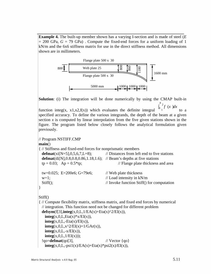
Example 4. The built-up member shown has a varying I-section and is made of steel (E = 200 GPa, G = 79 GPa) . Compute the fixed-end forces for a uniform loading of 1 kN/m and the 6x6 stiffness matrix for use in the direct stiffness method. All dimensions shown are in millimeters.

5000 mm 1000 1000 1000

8001600 mm

800

860

1180

Flange plate 500 x 30

Flange plate 500 x 30

Web plate 25

Solution: (i) The integration will be done numerically by using the CMAP built-in

function integ(x, x1,x2,f(x)) which evaluates the definite integral f (x )dxx 1

x 2∫

to a specified accuracy. To define the various integrands, the depth of the beam at a given section x is computed by linear interpolation from the five given stations shown in the figure. The program listed below closely follows the analytical formulation given previously. // Program NSTIFF.CMP main() { // Stiffness and fixed-end forces for nonprismatic members defmat(xi[N=5],0,5,6,7,L=8); // Distances from left end to five stations defmat(di[N],0.8,0.8,0.86,1.18,1.6); // Beam’s depths at five stations tp = 0.03; Ap = 0.5*tp; // Flange plate thickness and area tw=0.025; E=200e6; G=79e6; // Web plate thickness w=1; // Load intensity in kN/m Stiff(); // Invoke function Stiff() for computation } Stiff() { // Compute flexibility matrix, stiffness matrix, and fixed end forces by numerical // integration. This function need not be changed for different problem defsym(f[3],integ(x,0,L,1/EA(x)+Eta(x)^2/EI(x)), integ(x,0,L,Eta(x)*x/EI(x)), integ(x,0,L,-Eta(x)/EI(x)), integ(x,0,L,x^2/EI(x)+1/GAr(x)), integ(x,0,L,-x/EI(x)), integ(x,0,L,1/EI(x))); !qo=defmat(qo[3], // Vector {qo} integ(x,0,L,-psi1(x)/EA(x)+Eta(x)*psi2(x)/EI(x)),


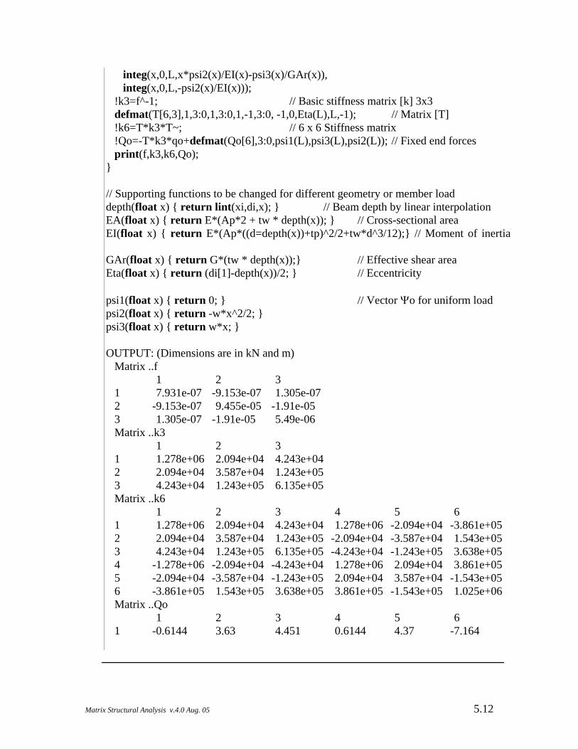
integ(x,0,L,x*psi2(x)/EI(x)-psi3(x)/GAr(x)), integ(x,0,L,-psi2(x)/EI(x))); !k3=f^-1; // Basic stiffness matrix [k] 3x3 defmat(T[6,3],1,3:0,1,3:0,1,-1,3:0, -1,0,Eta(L),L,-1); // Matrix [T] !k6=T*k3*T~; // 6 x 6 Stiffness matrix !Qo=-T*k3*qo+defmat(Qo[6],3:0,psi1(L),psi3(L),psi2(L)); // Fixed end forces print(f,k3,k6,Qo); } // Supporting functions to be changed for different geometry or member load depth(float x) { return lint(xi,di,x); } // Beam depth by linear interpolation EA(float x) { return E*(Ap*2 + tw * depth(x)); } // Cross-sectional area EI(float x) { return E*(Ap*((d=depth(x))+tp)^2/2+tw*d^3/12);} // Moment of inertia GAr(float x) { return G*(tw * depth(x));} // Effective shear area Eta(float x) { return (di[1]-depth(x))/2; } // Eccentricity psi1(float x) { return 0; } // Vector Ψo for uniform load psi2(float x) { return -w*x^2/2; } psi3(float x) { return w*x; } OUTPUT: (Dimensions are in kN and m) Matrix ..f 1 2 3 1 7.931e-07 -9.153e-07 1.305e-07 2 -9.153e-07 9.455e-05 -1.91e-05 3 1.305e-07 -1.91e-05 5.49e-06 Matrix ..k3 1 2 3 1 1.278e+06 2.094e+04 4.243e+04 2 2.094e+04 3.587e+04 1.243e+05 3 4.243e+04 1.243e+05 6.135e+05 Matrix ..k6 1 2 3 4 5 6 1 1.278e+06 2.094e+04 4.243e+04 1.278e+06 -2.094e+04 -3.861e+05 2 2.094e+04 3.587e+04 1.243e+05 -2.094e+04 -3.587e+04 1.543e+05 3 4.243e+04 1.243e+05 6.135e+05 -4.243e+04 -1.243e+05 3.638e+05 4 -1.278e+06 -2.094e+04 -4.243e+04 1.278e+06 2.094e+04 3.861e+05 5 -2.094e+04 -3.587e+04 -1.243e+05 2.094e+04 3.587e+04 -1.543e+05 6 -3.861e+05 1.543e+05 3.638e+05 3.861e+05 -1.543e+05 1.025e+06 Matrix ..Qo 1 2 3 4 5 6 1 -0.6144 3.63 4.451 0.6144 4.37 -7.164


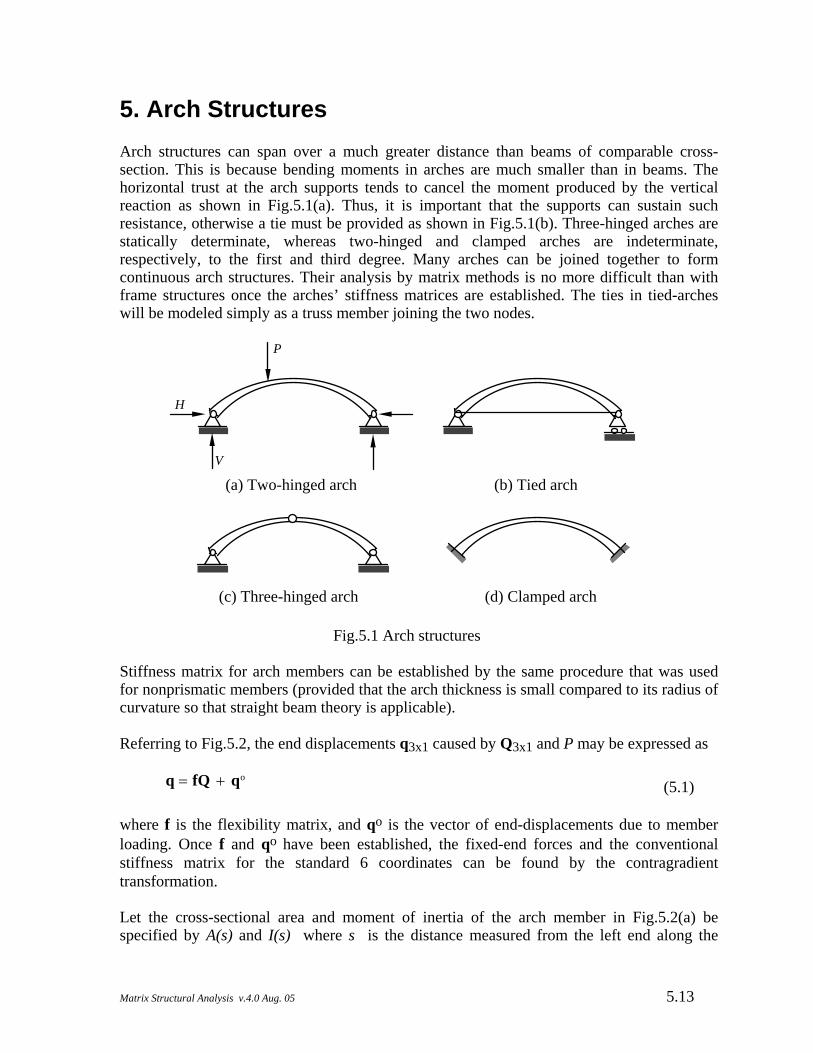
5. Arch Structures Arch structures can span over a much greater distance than beams of comparable cross-section. This is because bending moments in arches are much smaller than in beams. The horizontal trust at the arch supports tends to cancel the moment produced by the vertical reaction as shown in Fig.5.1(a). Thus, it is important that the supports can sustain such resistance, otherwise a tie must be provided as shown in Fig.5.1(b). Three-hinged arches are statically determinate, whereas two-hinged and clamped arches are indeterminate, respectively, to the first and third degree. Many arches can be joined together to form continuous arch structures. Their analysis by matrix methods is no more difficult than with frame structures once the arches’ stiffness matrices are established. The ties in tied-arches will be modeled simply as a truss member joining the two nodes.

H

V

P

(a) Two-hinged arch (b) Tied arch

(c) Three-hinged arch (d) Clamped arch

Fig.5.1 Arch structures Stiffness matrix for arch members can be established by the same procedure that was used for nonprismatic members (provided that the arch thickness is small compared to its radius of curvature so that straight beam theory is applicable). Referring to Fig.5.2, the end displacements q3x1 caused by Q3x1 and P may be expressed as (5.1) q = fQ + qo

where f is the flexibility matrix, and qo is the vector of end-displacements due to member loading. Once f and qo have been established, the fixed-end forces and the conventional stiffness matrix for the standard 6 coordinates can be found by the contragradient transformation. Let the cross-sectional area and moment of inertia of the arch member in Fig.5.2(a) be specified by A(s) and I(s) where s is the distance measured from the left end along the


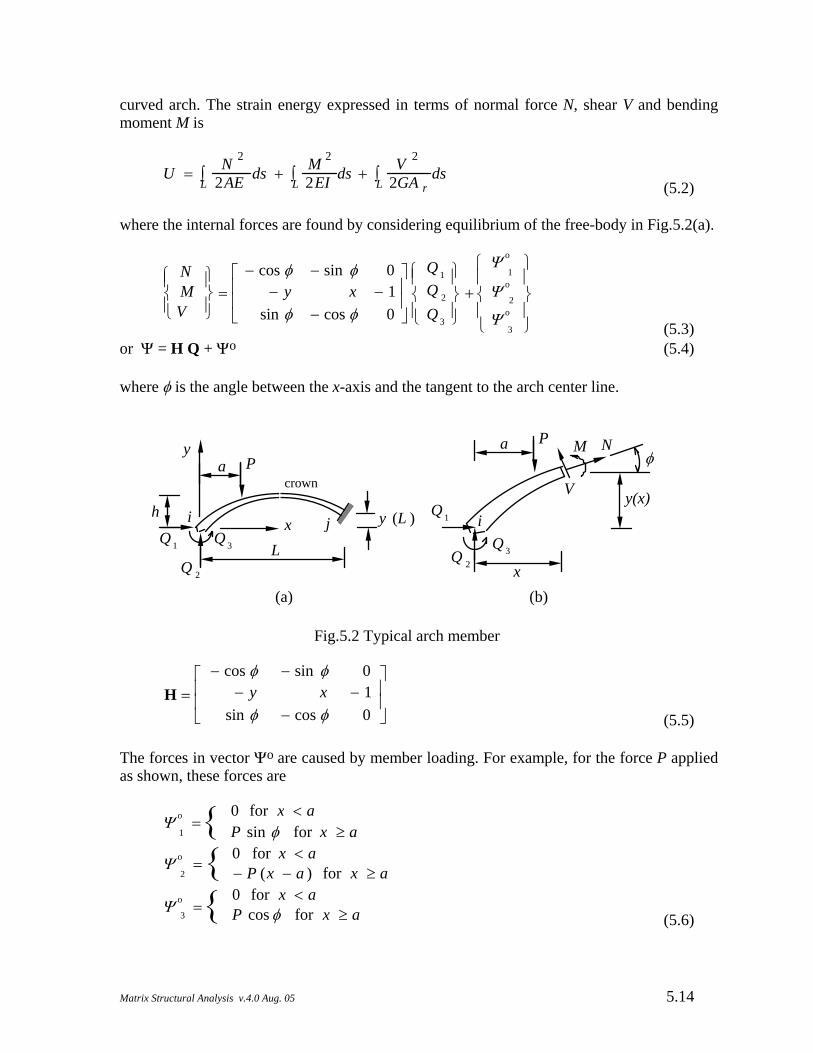
curved arch. The strain energy expressed in terms of normal force N, shear V and bending moment M is

U = N 2

2AEL∫ ds + M 2

2EIL∫ ds + V 2

2GA rL∫ ds

(5.2) where the internal forces are found by considering equilibrium of the free-body in Fig.5.2(a).

NMV

⎧⎪⎨⎪⎩

⎫⎪⎬⎪⎭

=− cos φ − sin φ 0

− y x − 1sin φ − cos φ 0

⎡⎢⎢⎣

⎤⎥⎥⎦

Q 1

Q 2

Q 3

⎧⎪⎨⎪⎩

⎫⎪⎬⎪⎭

+

Ψ o

1

Ψ o

2

Ψ o

3

⎧⎪⎨⎪⎩

⎫⎪⎬⎪⎭ (5.3)

or Ψ = H Q + Ψo (5.4) where φ is the angle between the x-axis and the tangent to the arch center line.

Q 1

Q 2

Q 3 L

h

(a)

Pacrown

i j y (L )x

y

Q 1

Q 2

Q 3

M N

V

x

y(x)

φ

(b)

Pa

i

Fig.5.2 Typical arch member

H =

− cos φ − sin φ 0− y x − 1

sin φ − cos φ 0

⎡⎢⎢⎣

⎤⎥⎥⎦ (5.5)

The forces in vector Ψo are caused by member loading. For example, for the force P applied as shown, these forces are

Ψ o

1=

0 for x < aP sin φ for x ≥ a{

Ψ o

2=

0 for x < a− P (x − a ) for x ≥ a{

Ψ o

3=

0 for x < aP cos φ for x ≥ a{ (5.6)


Castigliano’s theorem gives the displacement qk as

q k = ∂U

∂Q k= N

A (s )E∂N∂Q ki

j∫ ds + M

EI (s )i

j∫ ∂M

∂Q kds + V

GA r (s )i

j∫ ∂V

∂Q kds

(5.7) In matrix form:

q1q 2q 3

⎧⎪⎨⎪⎩

⎫⎪⎬⎪⎭

=i

j∫

∂N∂Q 1

∂M∂Q 1

∂V∂Q 1

∂N∂Q 2

∂M∂Q 2

∂V∂Q 2

∂N∂Q 3

∂M∂Q 3

∂V∂Q 3

⎡⎢⎢⎢⎢⎢⎢⎣

⎤⎥⎥⎥⎥⎥⎥⎦

1EA (s ) 0 0

0 1EI (s ) 0

0 0 1GA r (s )

⎡⎢⎢⎢⎢⎢⎢⎣

⎤⎥⎥⎥⎥⎥⎥⎦

NMV

⎧⎪⎨⎪⎩

⎫⎪⎬⎪⎭

ds

(5.8) Noting that the first square matrix of the preceding expression is just the transpose of H, and denoting the second matrix as P, we get

q =i

j∫ HT P Ψds =

i

j∫ HT P (H Q + Ψo ) ds

=i

j∫ HT P H ds⎛

⎝⎞⎠ Q +

i

j∫ HT P Ψo ds

(5.9) Thus

(5.10) f =

i

j

∫ HT P H ds ; and q o =i

j

∫ HTP Ψo ds

In explicit form:

f =i

j

∫

c 2

EA +y 2

EI + s 2

GA r

csEA −

xyEI − cs

GA r

yEI

sym s 2

EA + x 2

EI + c 2

GA r

− xEI1

EI

⎡⎢⎢⎢⎢⎢⎢⎣

⎤⎥⎥⎥⎥⎥⎥⎦

ds ;

(5.11) and

qo =i

j

∫

−Ψ o

1c

AE −Ψ o

2y

EI +Ψ o

3s

GA r

−Ψ o

1s

AE +Ψ o

2x

EI −Ψ o

3c

GA r

−Ψ o

2

EI

⎧⎪⎪⎪⎨⎪⎪⎪⎩

⎫⎪⎪⎪⎬⎪⎪⎪⎭

ds

(5.12)


where c = cos φ, and s = sin φ. The force transformation from the 3-coordinate system of Fig.5.2(a) to the standard 6-coordinate system is

(5.13)

Q 6x 1 =

1 0 00 1 00 0 1

− 1 0 00 − 1 0

− y (L ) L − 1

⎡⎢⎢⎢⎢⎢⎢⎣

⎤⎥⎥⎥⎥⎥⎥⎦

Q 3x 1 +

000[cΨ o

1− sΨ o

3] x = L

[sΨ o

1+ cΨ o

3] x =L

[Ψ o

2] x = L

⎧⎪⎪⎪⎨⎪⎪⎪⎩

⎫⎪⎪⎪⎬⎪⎪⎪⎭

or (5.14) Q 6x 1 = T Q 3x 1 + Qψ

This equation is used to obtain the vector of fixed end forces Qo6x1 by transforming the vector Qo3x1 of Eq.8.?. And the 6x6 stiffness matrix in local axis is found using the contragradient law of transformation:

(5.15) k 6x 6 = T k 3 x 3 TT

For some particular arch geometry and variation of the cross-section’s properties, closed form expressions for the various matrices can be obtained by analytical integration. If numerical integration is used, it can be more conveniently carried out by transforming the integral over the curved length into one over the horizontal projection by the relation

ds = dxc (5.16)

And the variables c, s can be computed as

c = 1

(1 + (dydx )2

; s = cdydx

(5.17) where y(x) is the function describing the geometry of the arch center line. As an example, for a symmetrical parabolic arch of span L and rise h, the function y(x) is

y (x ) = 4h ( x

L − x 2

L 2 ) (5.18)


The stiffness matrix and fixed-end forces so obtained can also be used to analyse arches with hinges just as done in frame analysis, or alternatively, they can be modified to incorporate the hinges by the static condensation procedure.

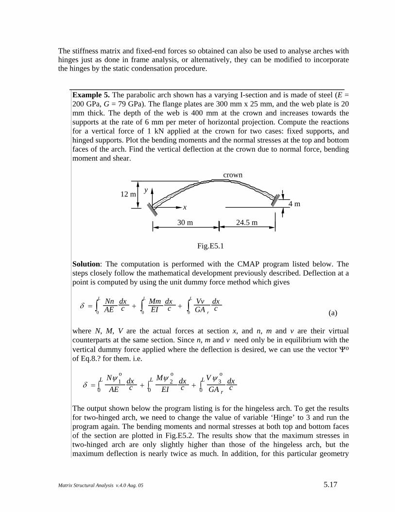
Example 5. The parabolic arch shown has a varying I-section and is made of steel (E = 200 GPa, G = 79 GPa). The flange plates are 300 mm x 25 mm, and the web plate is 20 mm thick. The depth of the web is 400 mm at the crown and increases towards the supports at the rate of 6 mm per meter of horizontal projection. Compute the reactions for a vertical force of 1 kN applied at the crown for two cases: fixed supports, and hinged supports. Plot the bending moments and the normal stresses at the top and bottom faces of the arch. Find the vertical deflection at the crown due to normal force, bending moment and shear.

30 m 24.5 m

crown

12 m

x

y

4 m

Fig.E5.1

Solution: The computation is performed with the CMAP program listed below. The steps closely follow the mathematical development previously described. Deflection at a point is computed by using the unit dummy force method which gives

δ = Nn

AE0

L

∫ dxc + Mm

EI0

L

∫ dxc + Vv

GA r0

L

∫ dxc (a)

where N, M, V are the actual forces at section x, and n, m and v are their virtual counterparts at the same section. Since n, m and v need only be in equilibrium with the vertical dummy force applied where the deflection is desired, we can use the vector Ψo of Eq.8.? for them. i.e.

δ =

Nψ 1o

AE0

L∫ dx

c +Mψ 2

o

EI0

L∫ dx

c +V ψ 3

o

GA r0

L∫ dx

c The output shown below the program listing is for the hingeless arch. To get the results for two-hinged arch, we need to change the value of variable ‘Hinge’ to 3 and run the program again. The bending moments and normal stresses at both top and bottom faces of the section are plotted in Fig.E5.2. The results show that the maximum stresses in two-hinged arch are only slightly higher than those of the hingeless arch, but the maximum deflection is nearly twice as much. In addition, for this particular geometry


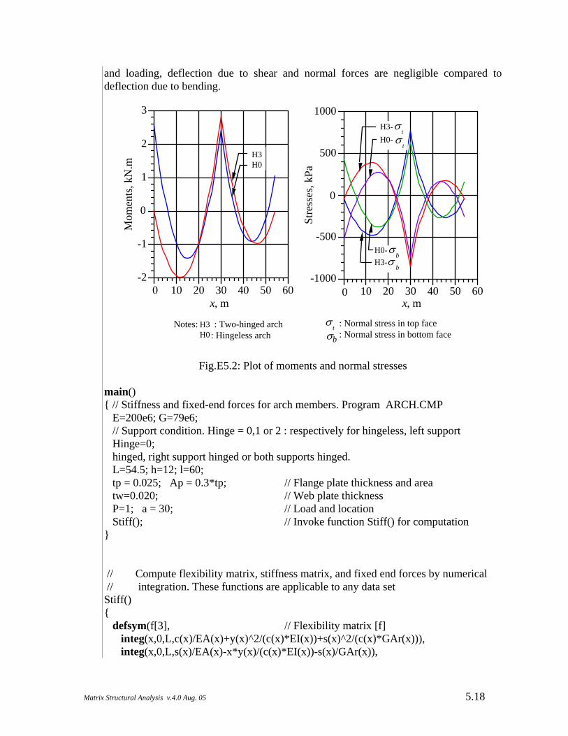
and loading, deflection due to shear and normal forces are negligible compared to deflection due to bending.

-2

-1

0

1

2

3

0 10 20 30 40 50 60

Mom

ents

, kN

.m

x, m

-1000

-500

0

500

1000

0 10 20 30 40 50 60St

ress

es, k

Pax, m

σb

σb

H3-H0-

σt

H0-H3-σ

t

H3H0

H3H0

Notes: : Two-hinged arch : Hingeless arch σ

σt

b

: Normal stress in top face : Normal stress in bottom face

Fig.E5.2: Plot of moments and normal stresses main() { // Stiffness and fixed-end forces for arch members. Program ARCH.CMP E=200e6; G=79e6; // Support condition. Hinge = 0,1 or 2 : respectively for hingeless, left support Hinge=0; hinged, right support hinged or both supports hinged. L=54.5; h=12; l=60; tp = 0.025; Ap = 0.3*tp; // Flange plate thickness and area tw=0.020; // Web plate thickness P=1; a = 30; // Load and location Stiff(); // Invoke function Stiff() for computation } // Compute flexibility matrix, stiffness matrix, and fixed end forces by numerical // integration. These functions are applicable to any data set Stiff() { defsym(f[3], // Flexibility matrix [f] integ(x,0,L,c(x)/EA(x)+y(x)^2/(c(x)*EI(x))+s(x)^2/(c(x)*GAr(x))), integ(x,0,L,s(x)/EA(x)-x*y(x)/(c(x)*EI(x))-s(x)/GAr(x)),


integ(x,0,L,y(x)/(c(x)*EI(x))), integ(x,0,L,(s(x)^2/EA(x)+x^2/EI(x))/c(x)+c(x)/GAr(x)), integ(x,0,L,-x/(c(x)*EI(x))), integ(x,0,L,1/(c(x)*EI(x)))); !qo=defmat(qo[3], // Vector {qo} integ(x,0,L,-psi1(x)/EA(x)-(psi2(x)*y(x)/EI(x)-psi3(x)*s(x)/GAr(x))/c(x)), integ(x,0,L,-psi1(x)*s(x)/(c(x)*EA(x))+psi2(x)*x/(c(x)*EI(x))-psi3(x)/GAr(x)), integ(x,0,L,-psi2(x)/(c(x)*EI(x)))); !k3=f^-1; // Basic stiffness matrix [k] 3x3 defmat(T[6,3],1,3:0,1,3:0,1,-1,3:0, -1,0,-y(L),L,-1); // Matrix [T] !k6=T*k3*T~; // 6 x 6 Stiffness matrix !Qo=-T*k3*qo+defmat(Qo[6],3:0,c(L)*psi1(L)-s(L)*psi3(L), s(L)*psi1(L)+c(L)*psi3(L),psi2(L));// Fixed end forces if(Hinge) { Modify(); } print(f,k3,k6,Qo); print(^^" Plot of bending moment in arch"); clearplot(); plot(x,0,L,M(x)); setpictposition(0, 0.5, 0.8, 0.5); setrange(4:0); // Plot of normal stress in top face plot(x,0,L,E*(N(x)/EA(x)-M(x)*(0.5*depth(x)+tp)/EI(x))); // Plot of normal stress in bottom face plot(x,0,L,E*(N(x)/EA(x)+M(x)*(0.5*depth(x)+tp)/EI(x))); // Deflections at the crown DN=integ(x,0,L,N(x)*psi1(x)/(c(x)*EA(x))),^ // due axial trust DM=integ(x,0,L,M(x)*psi2(x)/(c(x)*EI(x)))); // due bending moments // ,^DV=integ(x,0,L,V(x)*psi3(x)/(c(x)*GAr(x)))); // due shears } // Internal resultant forces N(float x) { return -c(x)*Qo[1] - s(x)*Qo[2] + psi1(x); } M(float x) { return -y(x)*Qo[1] + x*Qo[2] - Qo[3] + psi2(x); } V(float x) { return s(x)*Qo[1] - c(x)*Qo[2] + psi3(x); } Modify() { // Eliminate moments at hinged supports switch (1) { case Hinge==1: // Left end hinged zero(K[6,6]); subop(k6>K[1,2,6,3,4,5;1,2,6,3,4,5]); zero(Po[6]); subop(Qo>Po[1;1,2,6,3,4,5]); gauss(C,K,Po,5); zero(k6[6,6]); subop(K>k6[1,2,4,5,6,0;1,2,4,5,6,0]); zero(Qo[6]); subop(Po>Qo[1;1,2,4,5,6,0]); break; case Hinge==2: // Right end hinged gauss(C,k6,Qo,5);


series(i,1,6,1,k6[i,6]=k6[6,i]=0); Qo[6]=0; break; case Hinge==3: // Both ends hinged zero(K[6,6]); subop(k6>K[1,2,5,3,4,6;1,2,5,3,4,6]); zero(Po[6]); subop(Qo>Po[1;1,2,5,3,4,6]); gauss(C,K,Po,4); zero(k6[6,6]); subop(K>k6[1,2,4,5,0,0;1,2,4,5,0,0]); zero(Qo[6]); subop(Po>Qo[1;1,2,4,5,0,0]); break; default: print(^"Invalid value for Hinge !"); end; } } // Supporting functions to be changed for different geometry or member load y(float x) { float r = x/l; return 4*h*(r-r^2); } c(float x){ float dydx = 4*h*(1-2*x/l)/l; return 1/sqrt(1+dydx^2); } s(float x){ float dydx = 4*h*(1-2*x/l)/l; return c(x)*dydx;} depth(float x) { return 0.4+abs(x-30)*0.006;} // Depth of beam’s web EA(float x) { return E*(Ap*2 + tw * depth(x)); } // Cross-sectional area EI(float x) { return E*(Ap*((d=depth(x))+tp)^2/2+tw*d^3/12);} // Moment of inertia GAr(float x) { return G*(tw * depth(x));} // Effective shear area psi1(float x) { return gez(x-a,0)*P*s(x); } // Vector Ψo for point load psi2(float x) { return - gez(x-a,1)*P; } psi3(float x) { return gez(x-a,0)*P*c(x);} OUTPUT: Matrix ..f 1 2 3 1 0.02363 -0.06932 0.00235 2 -0.06932 0.2583 -0.007241 3 0.00235 -0.007241 0.0002607 Matrix ..k3 1 2 3 1 461.8 32.79 -3251 2 32.79 19.82 254.9 3 -3251 254.9 4.022e+004


Matrix ..k6 1 2 3 4 5 6 1 461.8 32.79 -3251 -461.8 -32.79 3192 2 32.79 19.82 254.9 -32.79 -19.82 694 3 -3251 254.9 4.022e+004 3251 -254.9-1.333e+004 4 -461.8 -32.79 3251 461.8 32.79 -3192 5 -32.79 -19.82 -254.9 32.79 19.82 -694 6 3192 694-1.333e+004 -3192 -694 3.84e+004 Matrix ..Qo 1 2 3 4 5 6 1 1.296 0.5173 -2.496 -1.296 0.4827 1.01 2.19698e-006 0.000320306

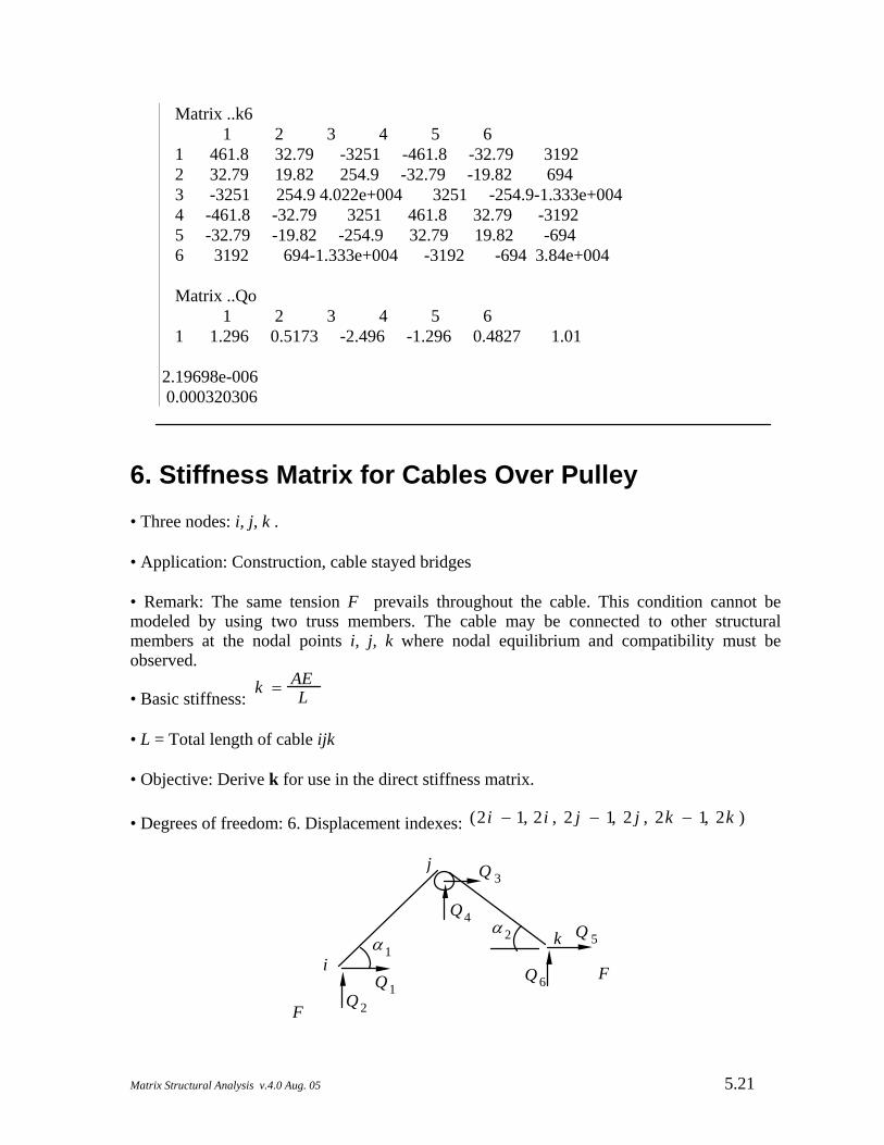
6. Stiffness Matrix for Cables Over Pulley • Three nodes: i, j, k . • Application: Construction, cable stayed bridges • Remark: The same tension F prevails throughout the cable. This condition cannot be modeled by using two truss members. The cable may be connected to other structural members at the nodal points i, j, k where nodal equilibrium and compatibility must be observed.

• Basic stiffness: k = AE

L

• L = Total length of cable ijk • Objective: Derive k for use in the direct stiffness matrix. • Degrees of freedom: 6. Displacement indexes: (2i − 1, 2i , 2 j − 1, 2 j , 2k − 1, 2k )

Q1Q 2

Q 3

Q4Q 5

Q 6

F

F

α 1

α 2

i

j

k


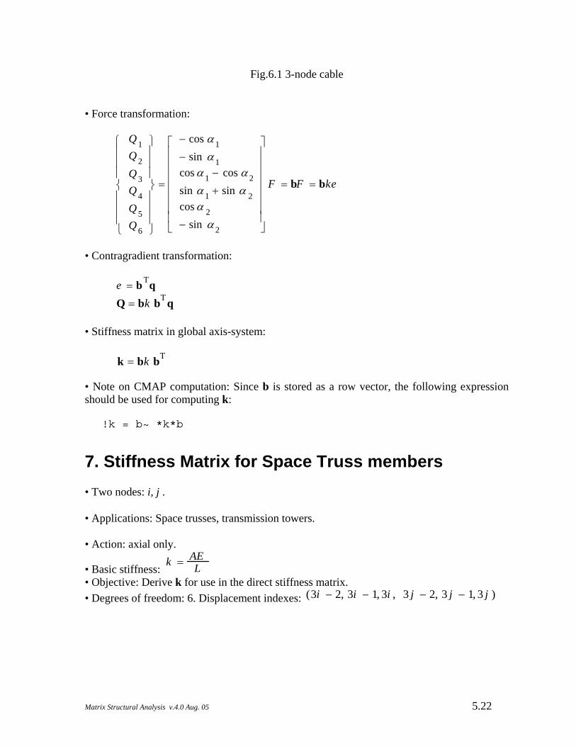
Fig.6.1 3-node cable • Force transformation:

Q 1Q 2Q 3Q 4Q 5Q 6

⎧⎪⎪⎪⎨⎪⎪⎪⎩

⎫⎪⎪⎪⎬⎪⎪⎪⎭

=

− cos α 1− sin α 1cos α 1 − cos α 2sin α 1 + sin α 2cos α 2− sin α 2

⎡⎢⎢⎢⎢⎢⎢⎢⎣

⎤⎥⎥⎥⎥⎥⎥⎥⎦

F = bF = bke

• Contragradient transformation:

e = b Tq

Q = bk bT q • Stiffness matrix in global axis-system:

k = bk bT

• Note on CMAP computation: Since b is stored as a row vector, the following expression should be used for computing k: !k = b~ *k*b

7. Stiffness Matrix for Space Truss members • Two nodes: i, j . • Applications: Space trusses, transmission towers. • Action: axial only.

• Basic stiffness: k = AE

L • Objective: Derive k for use in the direct stiffness matrix. • Degrees of freedom: 6. Displacement indexes: (3i − 2, 3i − 1, 3i , 3 j − 2, 3 j − 1, 3 j )


Q1Q 2

Q 3Q4

Q 5

Q 6

F

F

i

j

x

y

z

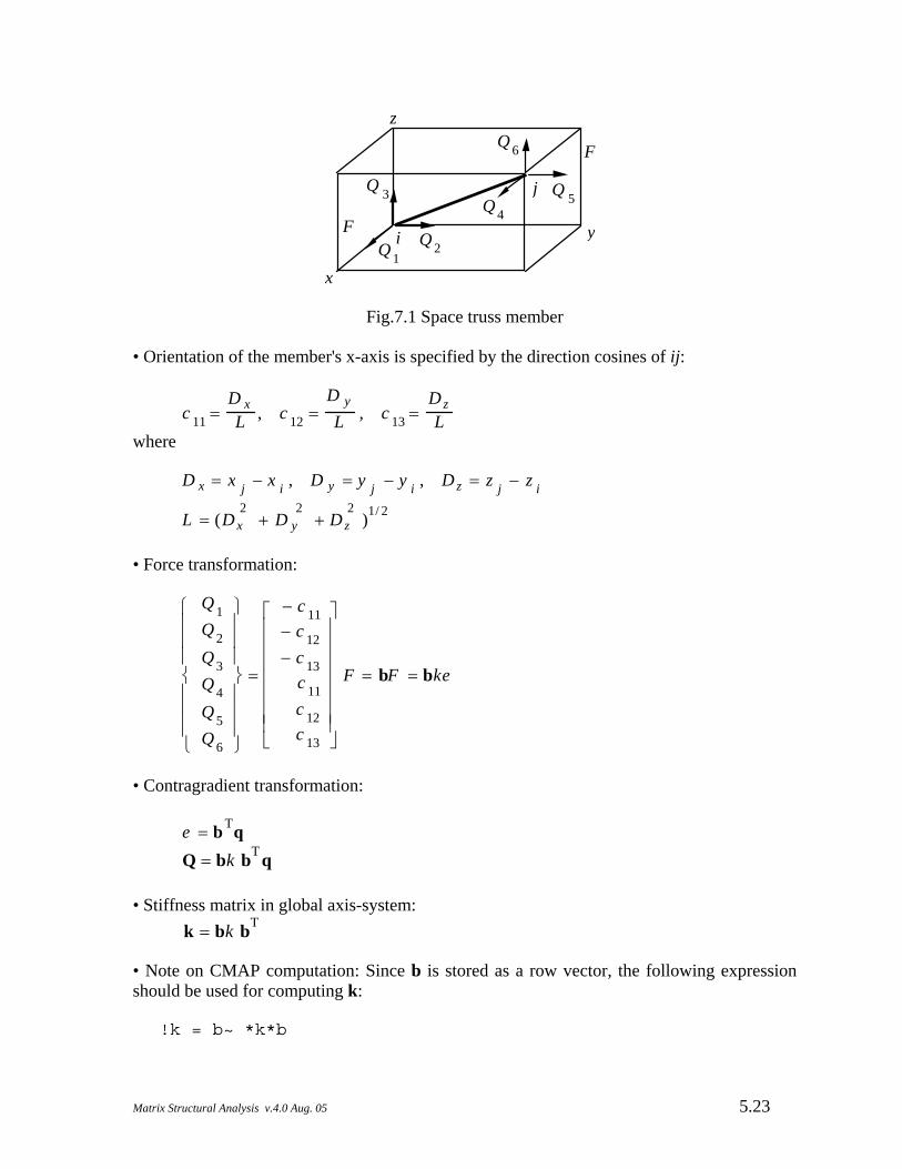
Fig.7.1 Space truss member • Orientation of the member's x-axis is specified by the direction cosines of ij:

c 11 =

D xL , c 12 =

D y

L , c 13 =D zL

where

D x = x j − x i , D y = y j − y i , D z = z j − z i

L = (D x2

+ D y2

+ D z2

)1/ 2

• Force transformation:

Q 1Q 2Q 3Q 4Q 5Q 6

⎧⎪⎪⎪⎨⎪⎪⎪⎩

⎫⎪⎪⎪⎬⎪⎪⎪⎭

=

− c 11− c 12− c 13

c 11c 12c 13

⎡⎢⎢⎢⎢⎢⎢⎢⎣

⎤⎥⎥⎥⎥⎥⎥⎥⎦

F = bF = bke

• Contragradient transformation:

e = b Tq

Q = bk bT q • Stiffness matrix in global axis-system:

k = bk bT

• Note on CMAP computation: Since b is stored as a row vector, the following expression should be used for computing k: !k = b~ *k*b


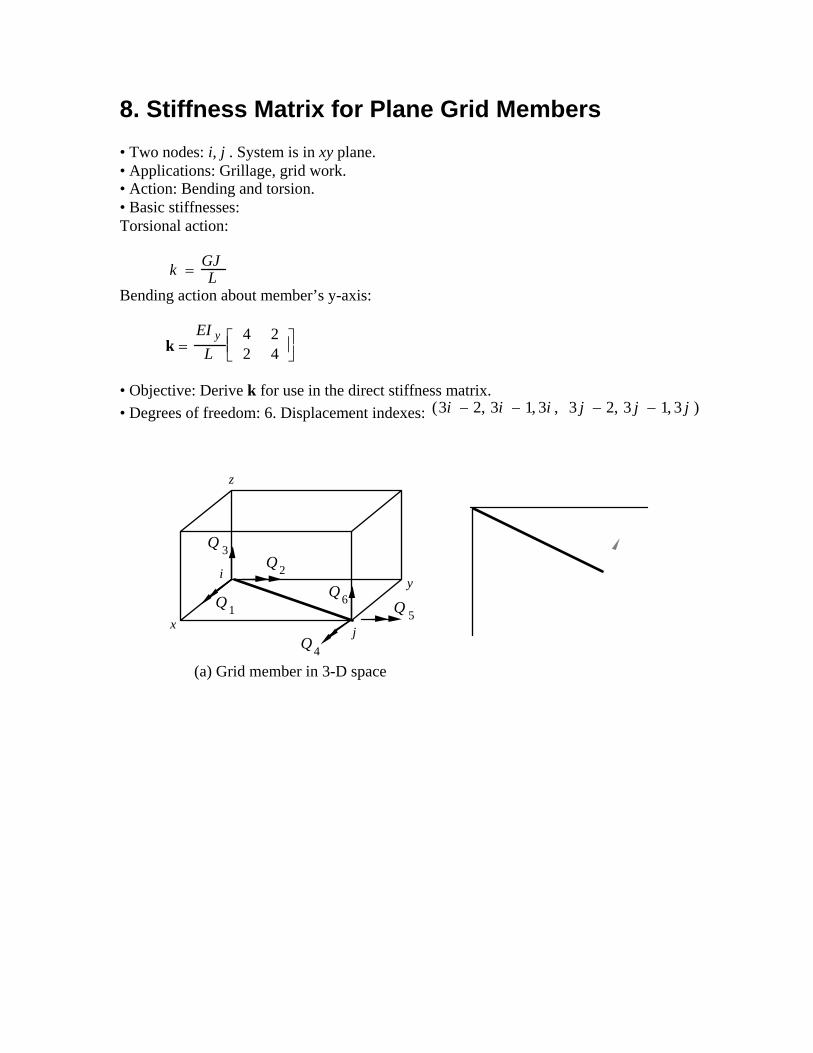
8. Stiffness Matrix for Plane Grid Members • Two nodes: i, j . System is in xy plane. • Applications: Grillage, grid work. • Action: Bending and torsion. • Basic stiffnesses: Torsional action:

k = GJ

L Bending action about member’s y-axis:

k =

EI y

L4 22 4

⎡⎢⎣⎤⎥⎦

• Objective: Derive k for use in the direct stiffness matrix. • Degrees of freedom: 6. Displacement indexes: (3i − 2, 3i − 1, 3i , 3 j − 2, 3 j − 1, 3 j )

Q 1

Q 2

Q 3

Q4

Q 5

Q6

i

jx

y

z

(a) Grid member in 3-D space

x

yi

jQ 1

Q2

Q 4

Q 5LQ1

Q 2L

Q4

Q 5

L

L

(b) Local and global axes

Fig.8.1 Grid member • Orientation of the member's x-axis is specified by the direction cosines of ij:

c 11 =

D xL , c 12 =

D y

L where

D x = x j − x i , D y = y j − y i

L = (Dx2

+ D y2

)1/ 2

• Stiffness matrix in member axes: kL = kbL

+ k tL


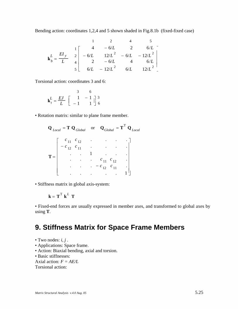
Bending action: coordinates 1,2,4 and 5 shown shaded in Fig.8.1b (fixed-fixed case)

Lk b =

EI y

L

4 − 6/L 2 6/L

− 6/L 12/L 2 − 6/L − 12/L 2

2 − 6/L 4 6/L

6/L − 12/L 2 6/L 12/L 2

⎡⎢⎢⎢⎢⎣

⎤⎥⎥⎥⎥⎦

1 2 4 5

1

2

4

5 Torsional action: coordinates 3 and 6:

Lk t = EJL

1 − 1− 1 1

⎡⎢⎣⎤⎥⎦

3 636

• Rotation matrix: similar to plane frame member.

Q Local = T Q Global or QGlobal = TT Q Local

T =

c 11 c 12 . . .− c 12 c 11 . . .

. . 1 . . .

. . . c 11 c 12 .

. . . − c 12 c 11 .

. . . . . 1

⎡⎢⎢⎢⎢⎢⎢⎢⎣

⎤⎥⎥⎥⎥⎥⎥⎥⎦

.

.

• Stiffness matrix in global axis-system: k = TT k L T • Fixed-end forces are usually expressed in member axes, and transformed to global axes by using T.

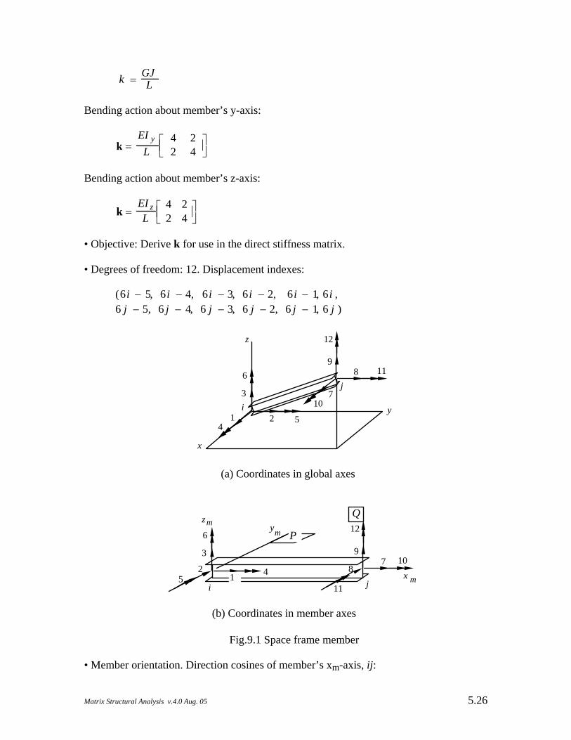
9. Stiffness Matrix for Space Frame Members • Two nodes: i, j . • Applications: Space frame. • Action: Biaxial bending, axial and torsion. • Basic stiffnesses: Axial action: F = AE/L Torsional action:


k = GJ

L Bending action about member’s y-axis:

k =

EI y

L4 22 4

⎡⎢⎣⎤⎥⎦

Bending action about member’s z-axis:

k =

EI zL

4 22 4

⎡⎢⎣⎤⎥⎦

• Objective: Derive k for use in the direct stiffness matrix. • Degrees of freedom: 12. Displacement indexes:

(6i − 5, 6 i − 4, 6i − 3, 6i − 2, 6 i − 1, 6i ,6 j − 5, 6 j − 4, 6 j − 3, 6 j − 2, 6 j − 1, 6 j )

i

j

x

y

z

1 2

3

45

6

7

89

10

11

12

(a) Coordinates in global axes

j

78

910

11

12

i1

2

3

45

6

x m

ymzm

(b) Coordinates in member axes

P

Q

Fig.9.1 Space frame member • Member orientation. Direction cosines of member’s xm-axis, ij:


c 1 ≡ { c 11 =

D xL , c 12 =

D y

L , c 13 =DzL }

where

D x = x j − x i , D y = y j − y i , D z = z j − z i

L = (D x2

+ D y2

+ D z2

)1/ 2

• Orientation of the cross-section: This may be specified by a point P in the strong plane (xmym plane) or a point Q in the weak plane (xmzm plane). Knowing either P or Q is sufficient for computing the direction cosines of the ym and zm member axes as follows: P is specified: the direction cosines of zm-axis are components of the unit vector

ij→

× iP→

ij→

× iP→

{c 31c 32 c 33} =c 3 ≡

The direction cosines of ym-axis are given by the cross-product of the two unit vectors c 2 ≡ { c 21, c 22 , c 23 } = c 3 × c 1 CMAP computation: (Assume IJ and IP are vectors of 3 components) !C3 = (V=IJ * IP)/hypot(!V); !C2 = C3*C1; Q is specified: the direction cosines of ym-axis are components of the following unit vector

ij→

×iQ →=

ij→

×iQ →c 2 ≡ { c 21, c 22 , c 23 }

The direction cosines of zm-axis are given by the cross-product of the unit two vectors c 3 ≡ { c 31, c 32 , c 33 } = c 1 × c 2 CMAP computation: (Assume IJ and IQ are vectors of 3 components) !C2 = (V=IQ * IJ)/hypot(!V); !C3 = C1*C2; • Stiffness matrix in member axes

k

L = k byL

+ k bzL

+ k tL

+ k aL

Axial action: coordinates 1 and 7


k a

L= AE

L1 − 1

− 1 1⎡⎢⎣

⎤⎥⎦

1 71

7 Torsion action: coordinates 4 and 10

4 10

4

10k t

L= J G

L1 − 1

− 1 1⎡⎢⎣

⎤⎥⎦ Bending action about ym-axis: coordinates 3,5,9 and 11 (fixed-fixed case)

= EIL

12/L2

6/L − 12/L2

6/L6/L 4 6/L

− 12/L2

6/L 12/L2

6/L6/L 2 6/L 4

⎡⎢⎢⎢⎢⎣

⎤⎥⎥⎥⎥⎦

3 5 9 11

3

11

5

9

--

-

-yk by

L 2

Bending action about zm-axis: coordinates 2,6,8 and 12 (fixed-fixed case)

= EIL

12/L2

6/L − 12/L2

6/L6/L 4 6/L 2

− 12/L2

6/L 12/L2

6/L6/L 2 6/L 4

⎡⎢⎢⎢⎢⎣

⎤⎥⎥⎥⎥⎦

2 6 8 12

2

12

6

8zk bz

L

−−

−

−

• Rotation matrix: Q Local = T Q Global or QGlobal = TT Q Local

T 12×12 =

c . . .. c . .. . c .. . . c

⎡⎢⎢⎢⎣

⎤⎥⎥⎥⎦

; c 3 ×3 =

c 11 c 12 c 13c 21 c 22 c 23c 31 c 32 c 33

⎡⎢⎢⎢⎣

⎤⎥⎥⎥⎦

• Stiffness matrix in global axis-system: k = TT k L T • Fixed-end forces are usually expressed in member axes, and transformed to global axes by using T.

10. Rigid Bodies in Framed Systems


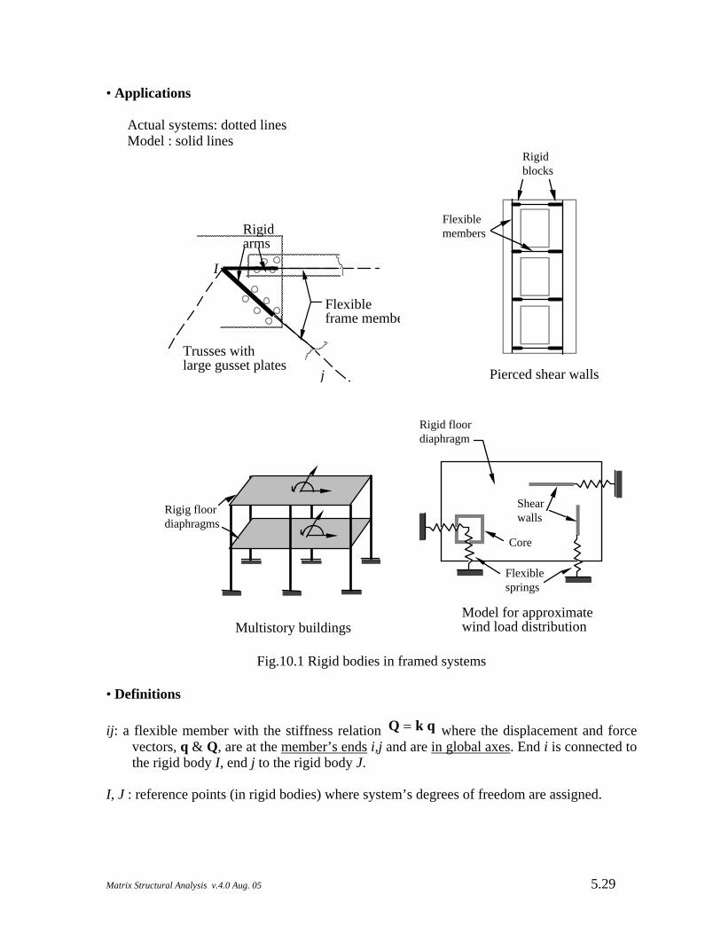
• Applications Actual systems: dotted lines Model : solid lines

i

j

Trusses with large gusset plates

I

Rigid arms

Flexibleframe membe

Rigidblocks

Flexiblemembers

Pierced shear walls

Rigig floor diaphragms

Multistory buildings

Rigid floor diaphragm

Flexiblesprings

Model for approximate wind load distribution

Shear walls

Core

Fig.10.1 Rigid bodies in framed systems • Definitions ij: a flexible member with the stiffness relation Q = k q where the displacement and force

vectors, q & Q, are at the member’s ends i,j and are in global axes. End i is connected to the rigid body I, end j to the rigid body J.

I, J : reference points (in rigid bodies) where system’s degrees of freedom are assigned.


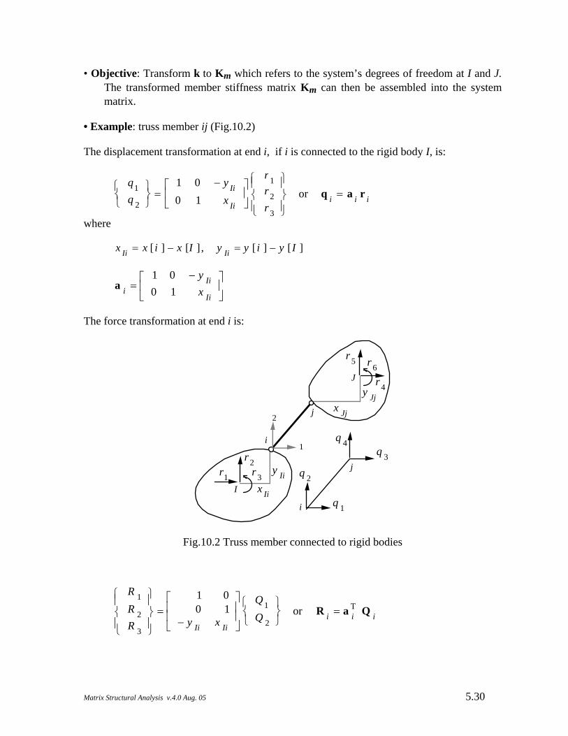
• Objective: Transform k to Km which refers to the system’s degrees of freedom at I and J. The transformed member stiffness matrix Km can then be assembled into the system matrix.

• Example: truss member ij (Fig.10.2) The displacement transformation at end i, if i is connected to the rigid body I, is:

q1q 2

⎧⎨⎩

⎫⎬⎭

=1 0 − y Ii0 1 x Ii

⎡⎢⎣

⎤⎥⎦

r1r2r3

⎧⎪⎨⎪⎩

⎫⎪⎬⎪⎭

or q i = a i r i

where x Ii = x [ i ] − x [I ] , y Ii = y [ i ] − y [I ]

a i =

1 0 − y Ii0 1 x Ii

⎡⎢⎣

⎤⎥⎦

The force transformation at end i is:

r1

r 2r 3

r 4

r 5 r 6

q 1

q 2

q 3

q 4i

j

i

j

I

J

x Ii

x Jj

y Ii

y Jj

1

2

Fig.10.2 Truss member connected to rigid bodies

R 1R 2R 3

⎧⎪⎨⎪⎩

⎫⎪⎬⎪⎭

=1 00 1

− y Ii x Ii

⎡⎢⎢⎣

⎤⎥⎥⎦

Q1Q 2

⎧⎨⎩

⎫⎬⎭

or R i = a iT Q i


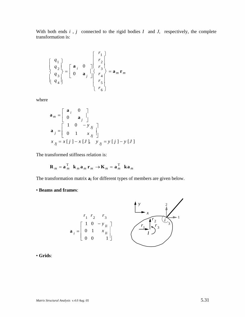
With both ends i , j connected to the rigid bodies I and J, respectively, the complete transformation is:

q1q 2q 3q 4

⎧⎪⎪⎨⎪⎪⎩

⎫⎪⎪⎬⎪⎪⎭

=a i 00 a j

⎡⎢⎣

⎤⎥⎦

r1r 2r 3r 4r 5r 6

⎧⎪⎪⎪⎨⎪⎪⎪⎩

⎫⎪⎪⎪⎬⎪⎪⎪⎭

= a m r m

where

a m =

a i 00 a j

⎡⎢⎣

⎤⎥⎦

a j =1 0 − y Jj

0 1 x Jj

⎡⎢⎢⎣

⎤⎥⎥⎦

x Jj = x [ j ] − x [J ], y Jj = y [ j ] − y [J ]

The transformed stiffness relation is:

R m = a mT k m a m r m → K m = a m

T ka m The transformation matrix ai for different types of members are given below. • Beams and frames:

r1

r 2r 3

i

I

1

2

a i = 1 0 − y Ii0 1 x Ii0 0 1

⎡ ⎢ ⎢ ⎢ ⎣

⎤⎥⎥⎥⎦

r1 r 2 r 3

3

x

y

• Grids:


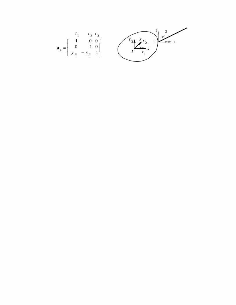
a i =1 0 00 1 0

y Ii − x Ii 1

⎡⎢⎢⎣

⎤⎥⎥⎦ r1

r 2r 3 i

I

1

23

x

yr1 r 2 r 3

• Space trusses:

i

I

1

23

a i =

1 0 0 0 z Ii − y Ii0 1 0 − z Ii 0 x Ii0 0 1 y Ii − x Ii 0

⎡⎢⎢⎢⎣

⎤⎥⎥⎥⎦

r1 r 2 r 3 r4 r5 r 6

1

23

4

56

x

yz

z Ii

z Ii = z [ i ] − z [I ] • Space frames:

i

I

1

23

1

23

4

56

x

yz

z Ii 4

5

6r1 r 2 r 3 r4 r 5 r 6

a i =

1 0 0 0 z Ii − y Ii0 1 0 − z Ii 0 x Ii0 0 1 y Ii − x Ii 00 0 0 1 0 00 0 0 0 1 00 0 0 0 0 1

⎡⎢⎢⎢⎢⎢⎢⎢⎣

⎤⎥⎥⎥⎥⎥⎥⎥⎦


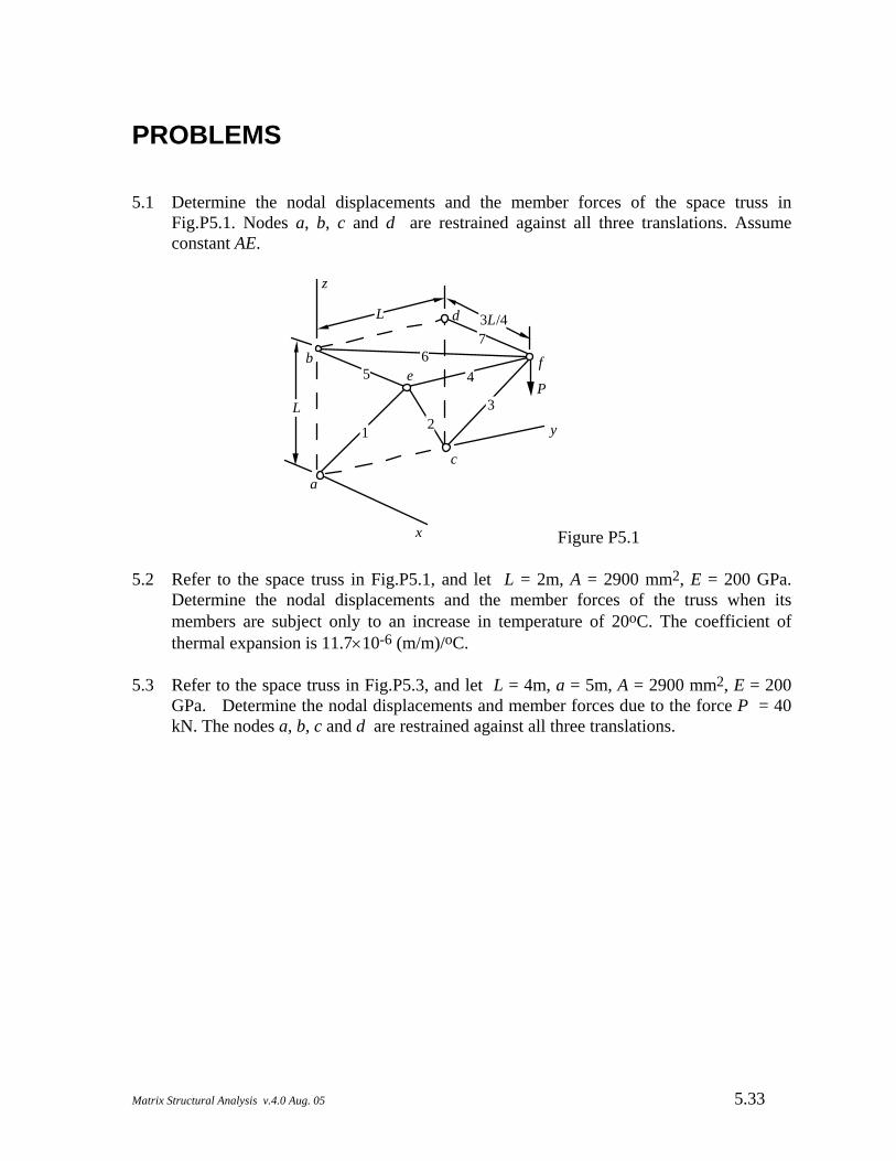
PROBLEMS 5.1 Determine the nodal displacements and the member forces of the space truss in

Fig.P5.1. Nodes a, b, c and d are restrained against all three translations. Assume constant AE.

x

y

z

a

b

c

d

ef

P

1 23

456

7

L

3L/4L

Figure P5.1

5.2 Refer to the space truss in Fig.P5.1, and let L = 2m, A = 2900 mm2, E = 200 GPa. Determine the nodal displacements and the member forces of the truss when its members are subject only to an increase in temperature of 20oC. The coefficient of thermal expansion is 11.7×10-6 (m/m)/oC.

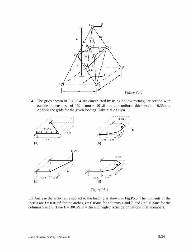
5.3 Refer to the space truss in Fig.P5.3, and let L = 4m, a = 5m, A = 2900 mm2, E = 200

GPa. Determine the nodal displacements and member forces due to the force P = 40 kN. The nodes a, b, c and d are restrained against all three translations.


12

3

4

567

8

9

1011

12 13

14 15

1617

P

L

L

a

ax

y

z

a b

cd

ef

h g

i

Figure P5.3 5.4 The grids shown in Fig.P5.4 are constructed by using hollow rectangular section with

outside dimensions of 152.4 mm × 101.6 mm and uniform thickness t = 6.35mm. Analyse the grids for the given loading. Take E = 200Gpa.

4 m

6 m10 kN/m

a b

c

1.5 m

40 kN

ab c d

CL

1.5 m (a) (b)

2.5 m 1.5 m

6 m

40 kN

ab

cd

2.5 m 1.5 m

40 kN

ab

cd

(c) (d)

Figure P5.4

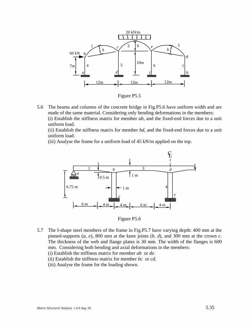
5.5 Analyse the arch-frame subject to the loading as shown in Fig.P5.5. The moments of the inertia are I = 0.01m4 for the arches, I = 0.05m4 for columns 4 and 7, and I = 0.015m4 for the columns 5 and 6. Take E = 30GPa, h = 3m and neglect axial deformations in all members.


7m

1 2 3

4 5 6 7

12m 12m12m

10m

hh h

a

bc

d

e

f

g

h

20 kN/m

60 kN

Figure P5.5 5.6 The beams and columns of the concrete bridge in Fig.P5.6 have uniform width and are

made of the same material. Considering only bending deformations in the members: (i) Establish the stiffness matrix for member ab, and the fixed-end forces due to a unit

uniform load. (ii) Establish the stiffness matrix for member bd, and the fixed-end forces due to a unit

uniform load. (iii) Analyse the frame for a uniform load of 45 kN/m applied on the top.

4 m 6 m

0.5 m 1 m

6.75 m

4 m4 m6 m

ab

c e

1

2

3

4

CL

d

1 m

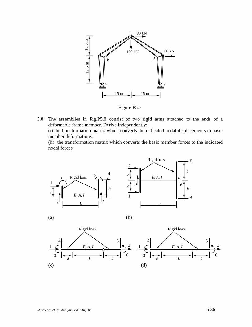
Figure P5.6 5.7 The I-shape steel members of the frame in Fig.P5.7 have varying depth: 400 mm at the

pinned-supports (a, e), 800 mm at the knee joints (b, d), and 300 mm at the crown c. The thickness of the web and flange plates is 30 mm. The width of the flanges is 600 mm. Considering both bending and axial deformations in the members:

(i) Establish the stiffness matrix for member ab or de. (ii) Establish the stiffness matrix for member bc or cd. (iii) Analyse the frame for the loading shown.


.

15 m12

.5 m

10.5

ma

b

c

d

e

60 kN

30 kN

15 m

100 kN

Figure P5.7

5.8 The assemblies in Fig.P5.8 consist of two rigid arms attached to the ends of a deformable frame member. Derive independently:

(i) the transformation matrix which converts the indicated nodal displacements to basic member deformations.

(ii) the transformation matrix which converts the basic member forces to the indicated nodal forces.

1

2

34

5

6

L

E, A, I

Rigid bars

ab

1

2

3

4

5

6

L

E, A, I

Rigid bars

a

a

b

b

(a) (b)

12

3

45

6L

E, A, I

Rigid bars

a b

12

3

45

6L

E, A, I

Rigid bars

a b (c) (d)


Chapter 05

Documents

direct stiffness method

matrix structural analysis

arch center line

total potential energy

q1 q2 q3

6x6 stiffness matrix

conventional stiffness matrix

direct stiffness matrix