Chap5 discrete probability

Chapter 5:

DISCRETE RANDOM VARIABLES AND THEIR PROBABILITY

DISTRIBUTIONS

2

RANDOM VARIABLES Discrete Random Variable ر� ي����� غ�� طع���������مت��� ق� �ى مت��� و���ائ� عش��� Continuous Random Variable ر� ي����� غ�� �ى مس��ت�م���ر�مت��� و���ائ� عش���

3

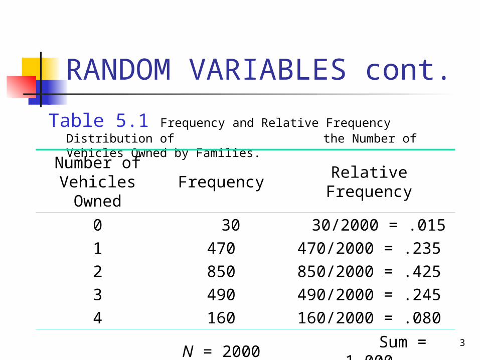
RANDOM VARIABLES cont.Table 5.1 Frequency and Relative Frequency

Distribution of the Number of Vehicles Owned by Families. Number of Vehicles Owned

Frequency Relative Frequency

01234

30470850490160

30/2000 = .015470/2000 = .235850/2000 = .425490/2000 = .245160/2000 = .080

N = 2000 Sum = 1.000

4

RANDOM VARIABLES cont. Definition A random variable is a variable whose value is determined by the outcome of a random experiment.

ة� ي� وائ�� ة� عش� ب � ج�ر ج' لت$ ات�� الن� �مة� ب ت� �حدد ق �ى ت رالد� ي� غ� وائ��ى:هو المت� ر العش� ي� غ� المت�

5

Discrete Random Variable

Definition A random variable that assumes countable values is called a discrete random variable. م�� مع������دودة� ي� � ق��������

6

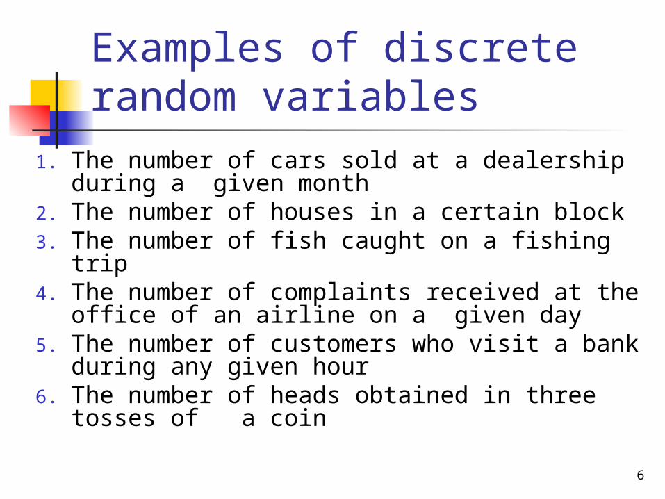
Examples of discrete random variables

1. The number of cars sold at a dealership during a given month

2. The number of houses in a certain block3. The number of fish caught on a fishing

trip4. The number of complaints received at the

office of an airline on a given day5. The number of customers who visit a bank

during any given hour6. The number of heads obtained in three

tosses of a coin

7

Continuous Random Variable

Definition A random variable that can assume any value contained in one or more intervals is called a continuous random variable.

8

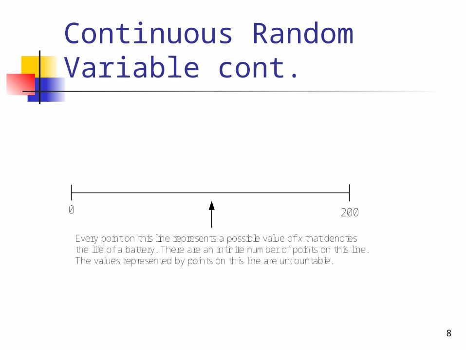
Continuous Random Variable cont.

2000

Every point on this line represents a possible value of x that denotesthe life of a battery. There are an infinite num ber of points on this line.The values represented by points on this line are uncountable.

9

Examples of continuous random variables

1. The height of a person2. The time taken to complete an examination3. The amount of milk in a gallon (note that

we do not expect a gallon to contain exactly one gallon of milk but either slightly more or slightly less than a gallon.)

4. The weight of a fish5. The price of a house

10

PROBABLITY DISTRIBUTION OF A DISCRETE RANDOM VARIABLE

Definition The probability distribution of a discrete

random variable lists all the possible values that the random variable can assume and their corresponding probabilities.

11

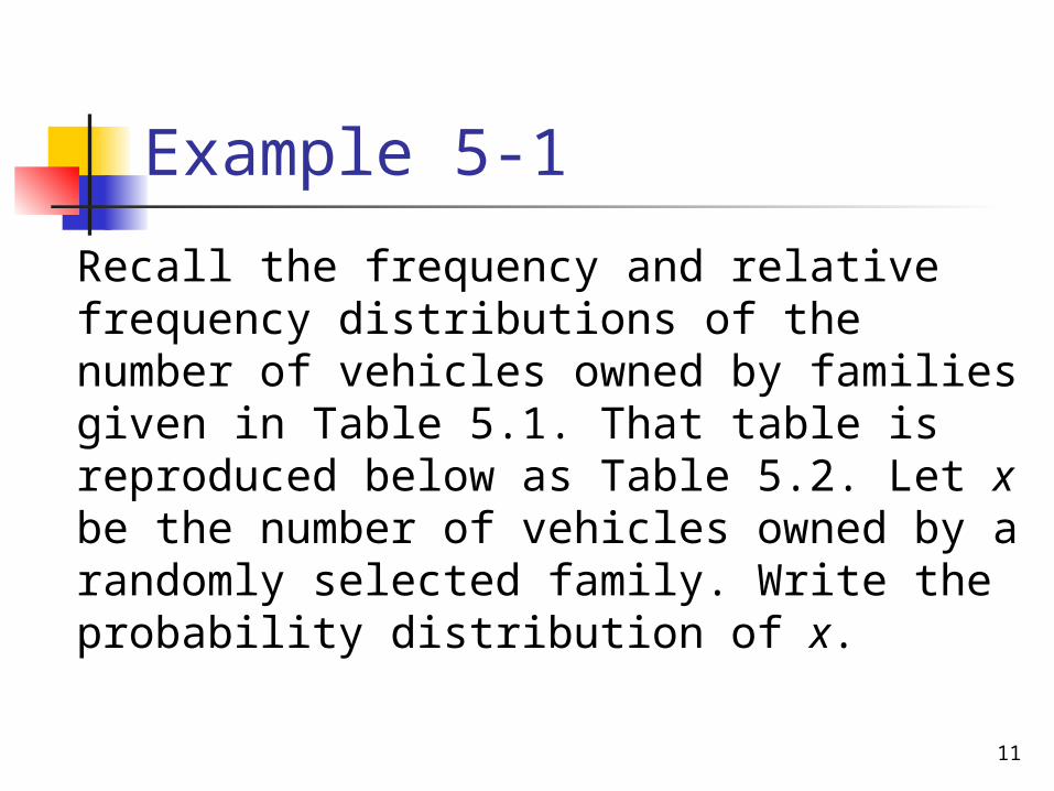
Example 5-1 Recall the frequency and relative frequency distributions of the number of vehicles owned by families given in Table 5.1. That table is reproduced below as Table 5.2. Let x be the number of vehicles owned by a randomly selected family. Write the probability distribution of x.

12

Table 5.2 Frequency and Relative Frequency Distributions of the Vehicles Owned by Families Number of Vehicles Owned Frequency

Relative Frequency

01234

30470850490160

30/2000 = .015470/2000 = .235850/2000 = .425490/2000 = .245160/2000 = .080

N = 2000 Sum = 1.000

13

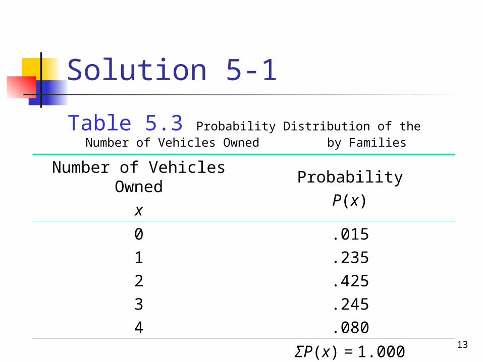
Solution 5-1Table 5.3 Probability Distribution of the

Number of Vehicles Owned by Families

Number of Vehicles Owned

x

ProbabilityP(x)

01234

.015

.235

.425

.245

.080ΣP(x) = 1.000

14

Two Characteristics of a Probability Distribution

The probability distribution of a discrete random variable possesses the following two characteristics.1. 0 ≤ P (x) ≤ 1 for each value of x2. ΣP (x) = 1

15

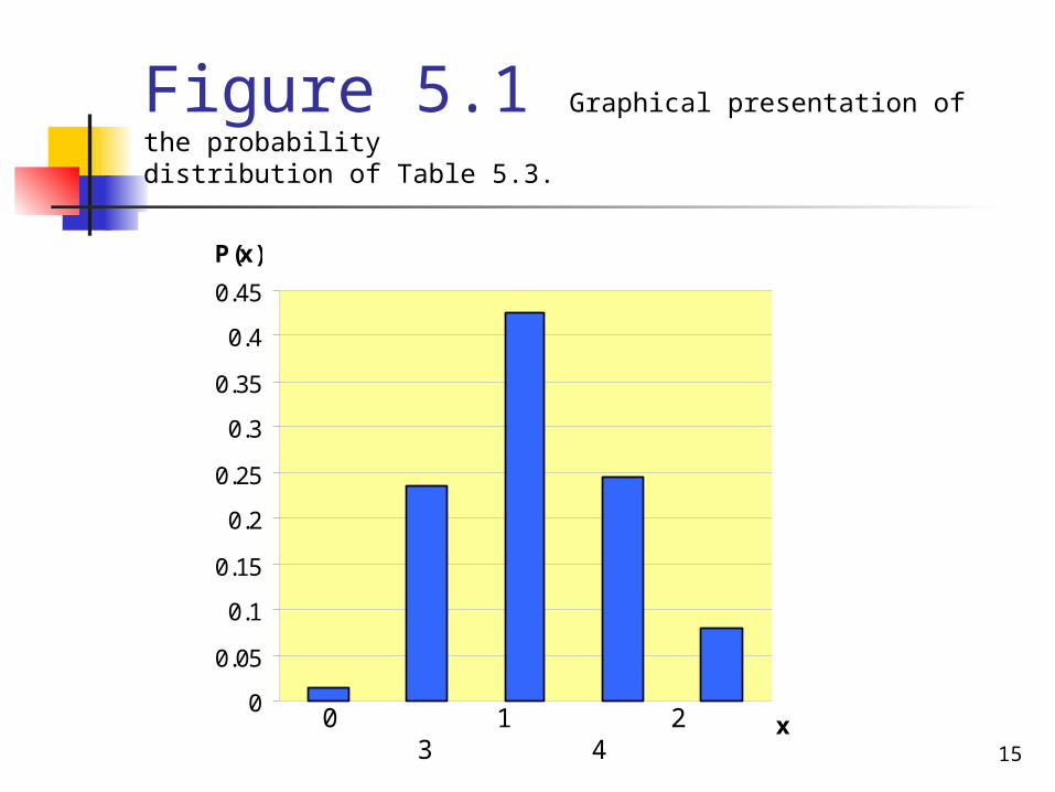
Figure 5.1 Graphical presentation of the probability distribution of Table 5.3.

00.050.10.150.20.250.30.350.40.45

x

P(x)

0 1 2 3 4

16

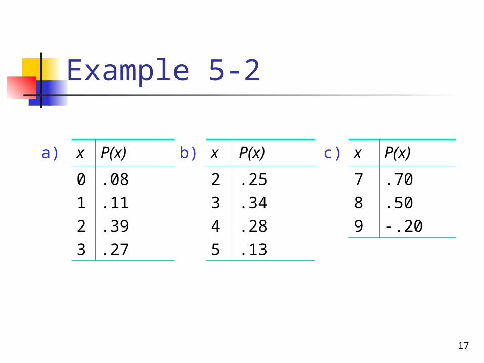
Each of the following tables lists certain values of x and their probabilities. Determine whether or not each table represents a valid probability distribution.

Example 5-2

17

Example 5-2

a) x P(x) b) x P(x)0123

.08

.11

.39

.27

2345

.25

.34

.28

.13

c) x P(x)789

.70

.50-.20

18

Solution 5-2a) Nob) Yesc) No

19

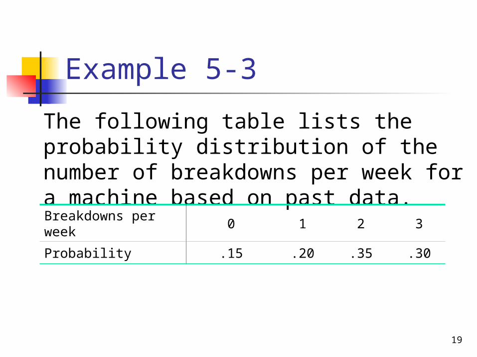
Example 5-3 The following table lists the probability distribution of the number of breakdowns per week for a machine based on past data.Breakdowns per week 0 1 2 3

Probability .15 .20 .35 .30

20

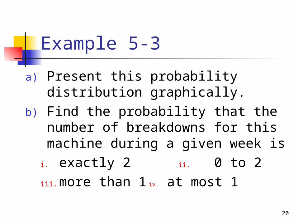
Example 5-3a) Present this probability

distribution graphically.b) Find the probability that the

number of breakdowns for this machine during a given week is

i. exactly 2 ii. 0 to 2iii.more than 1 iv. at most 1

21

Solution 5-3 Let x denote the number of breakdowns for this machine during a given week. Table 5.4 lists the probability distribution of x.

22

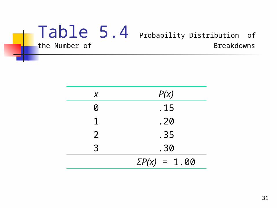
Table 5.4 Probability Distribution of the Number of Breakdowns

x P(x)0123

.15

.20

.35

.30ΣP(x) = 1.00

23

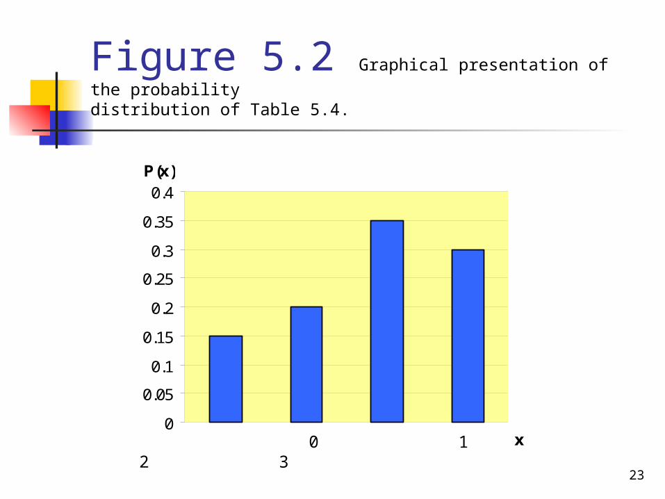
Figure 5.2 Graphical presentation of the probability distribution of Table 5.4.

00.050.10.150.20.250.30.350.4

x

P(x)

0 1 2 3

24

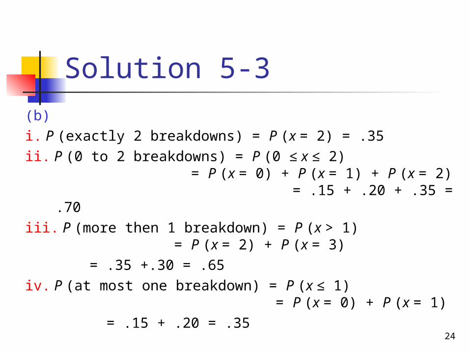
Solution 5-3 (b) i. P (exactly 2 breakdowns) = P (x = 2) = .35ii. P (0 to 2 breakdowns) = P (0 ≤ x ≤ 2)

= P (x = 0) + P (x = 1) + P (x = 2) = .15 + .20 + .35 = .70

iii. P (more then 1 breakdown) = P (x > 1) = P (x = 2) + P (x = 3) = .35 +.30 = .65

iv. P (at most one breakdown) = P (x ≤ 1) = P (x = 0) + P (x = 1) = .15 + .20 = .35

25

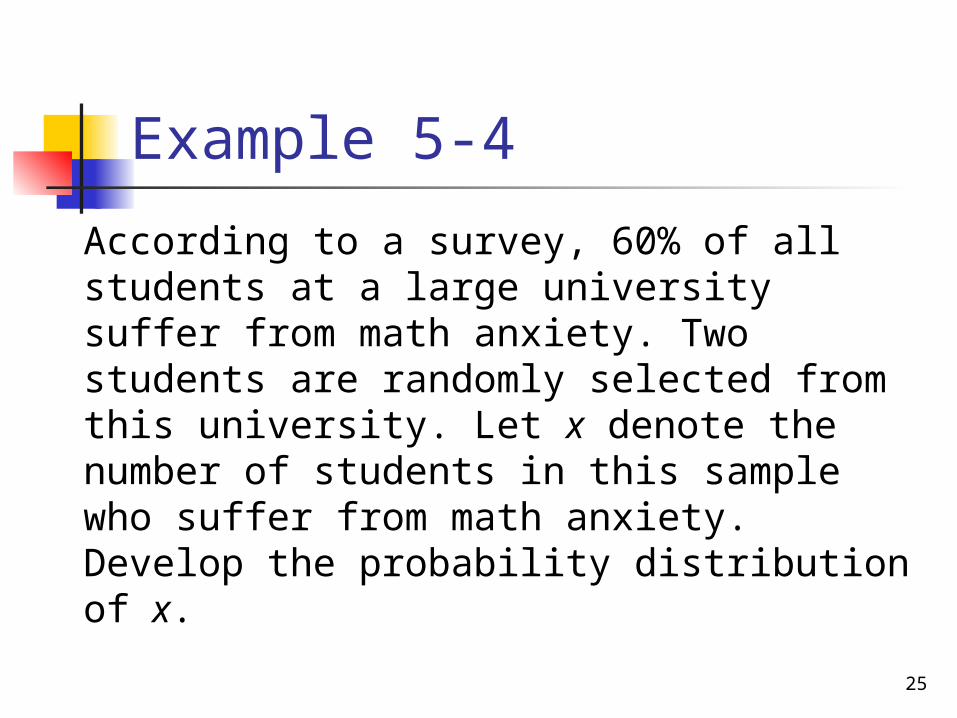
Example 5-4 According to a survey, 60% of all students at a large university suffer from math anxiety. Two students are randomly selected from this university. Let x denote the number of students in this sample who suffer from math anxiety. Develop the probability distribution of x.

26

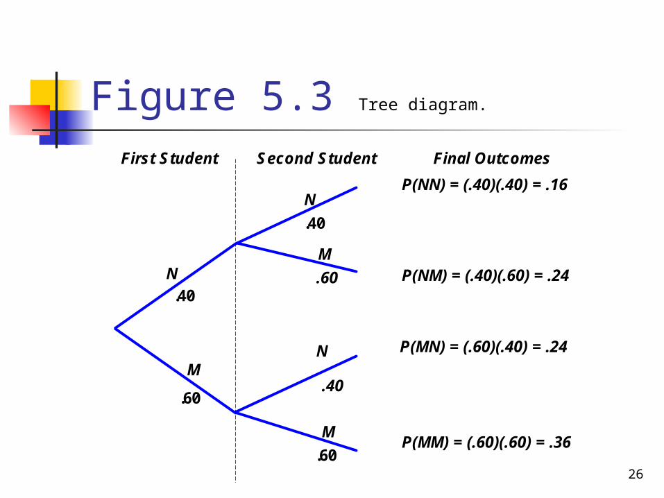
Figure 5.3 Tree diagram.

N.40

M.60

N.40

M.60

N

.40

.60M

P(NN) = (.40)(.40) = .16

P(NM) = (.40)(.60) = .24

P(MN) = (.60)(.40) = .24

P(MM) = (.60)(.60) = .36

S econd S tudent Final OutcomesFirst S tudent

27

Solution 5-4 Let us define the following two events: N = the student selected does not suffer from math anxiety M = the student selected suffers from math anxiety

P (x = 0) = P(NN) = .16P (x = 1) = P(NM or MN) = P(NM) + P(MN)

= .24 + .24 = .48

P (x = 2) = P(MM) = .36

28

Table 5.5 Probability Distribution of the Number of Students with Math Anxiety in a Sample of Two Students

x P(x)012

.16

.48

.36ΣP(x) = 1.00

29

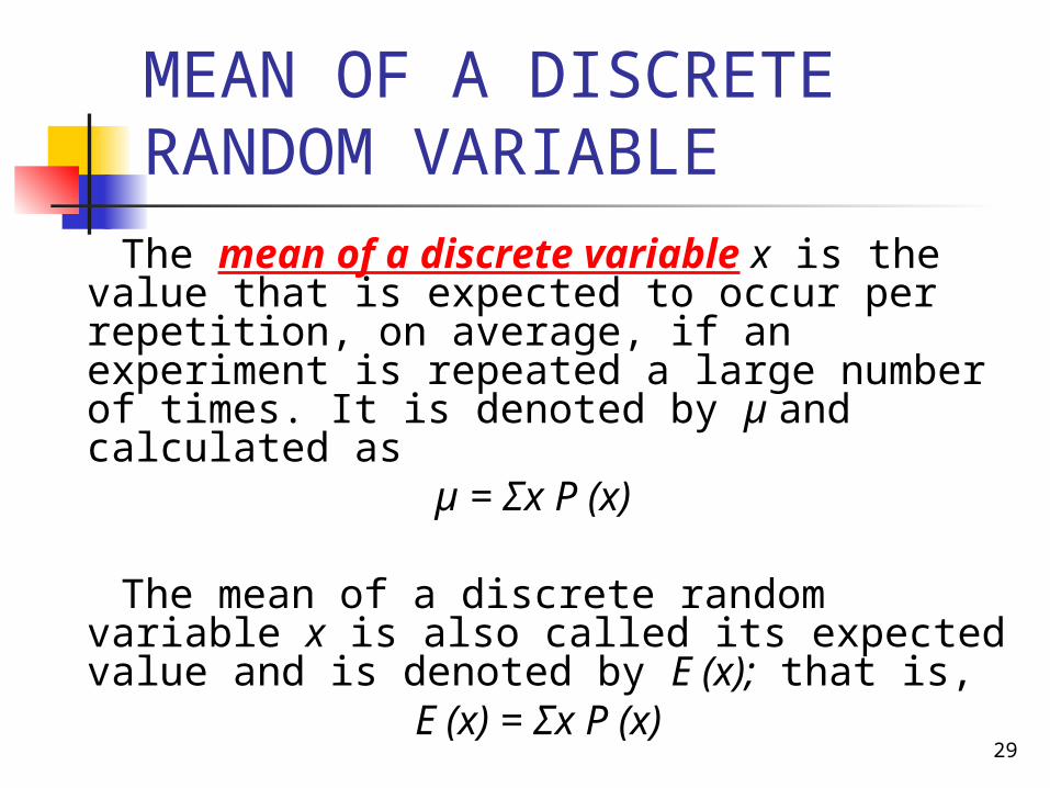
MEAN OF A DISCRETE RANDOM VARIABLE

The mean of a discrete variable x is the value that is expected to occur per repetition, on average, if an experiment is repeated a large number of times. It is denoted by µ and calculated as

µ = Σx P (x)

The mean of a discrete random variable x is also called its expected value and is denoted by E (x); that is,

E (x) = Σx P (x)

30

Example 5-5 Recall Example 5-3. The probability distribution Table 5.4 from that example is reproduced on the next slide. In this table, x represents the number of breakdowns for a machine during a given week, and P (x) is the probability of the corresponding value of x.

Find the mean number of breakdown per week for this machine.

31

Table 5.4 Probability Distribution of the Number of Breakdowns

x P(x)0123

.15

.20

.35

.30ΣP(x) = 1.00

32

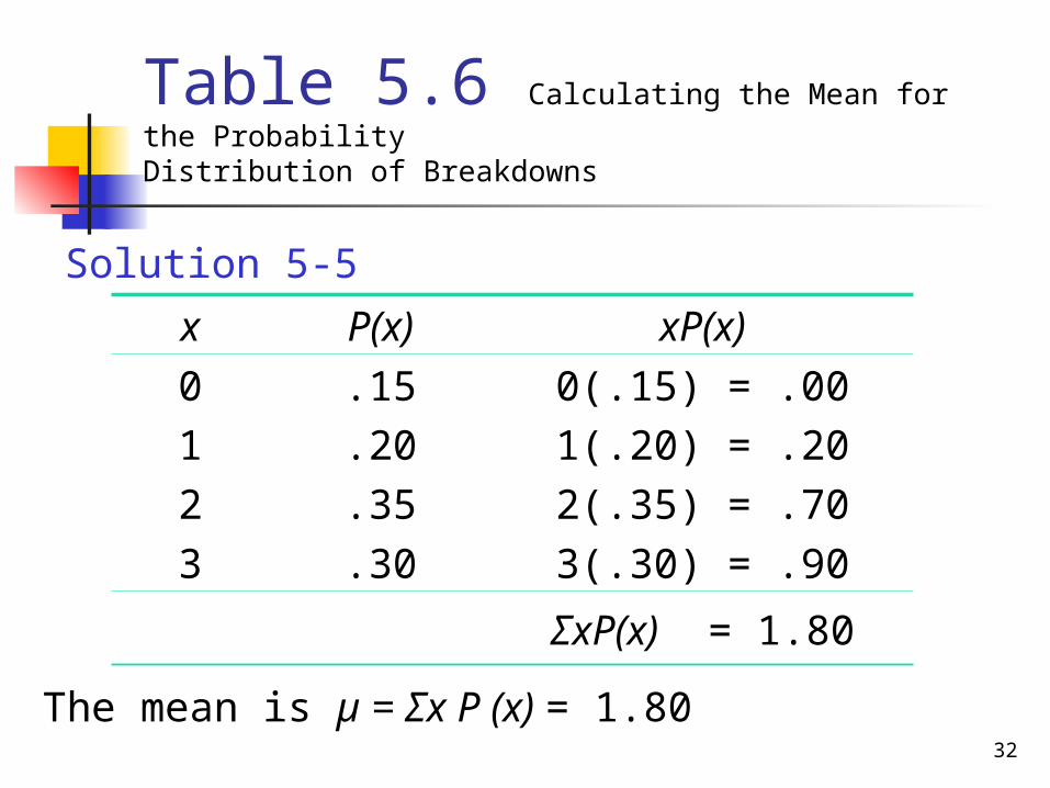
Table 5.6 Calculating the Mean for the Probability Distribution of Breakdowns

Solution 5-5x P(x) xP(x)0123

.15

.20

.35

.30

0(.15) = .001(.20) = .202(.35) = .703(.30) = .90ΣxP(x) = 1.80

The mean is µ = Σx P (x) = 1.80

33

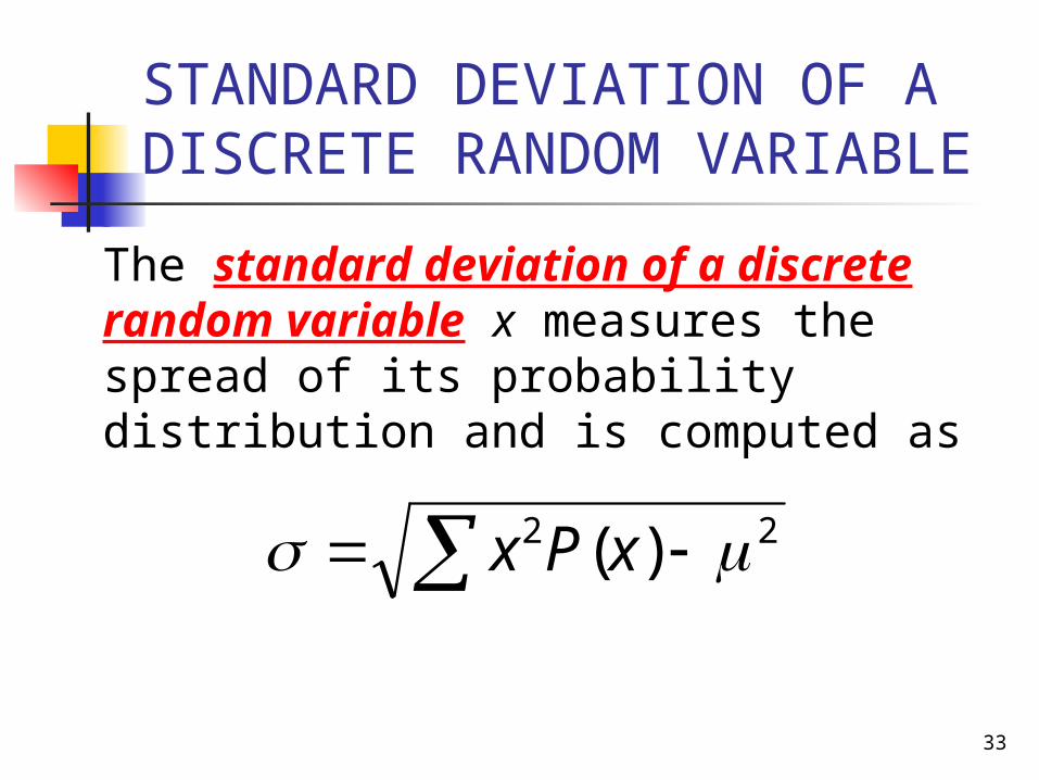
STANDARD DEVIATION OF A DISCRETE RANDOM VARIABLE

The standard deviation of a discrete random variable x measures the spread of its probability distribution and is computed as

22 )( xPx

34

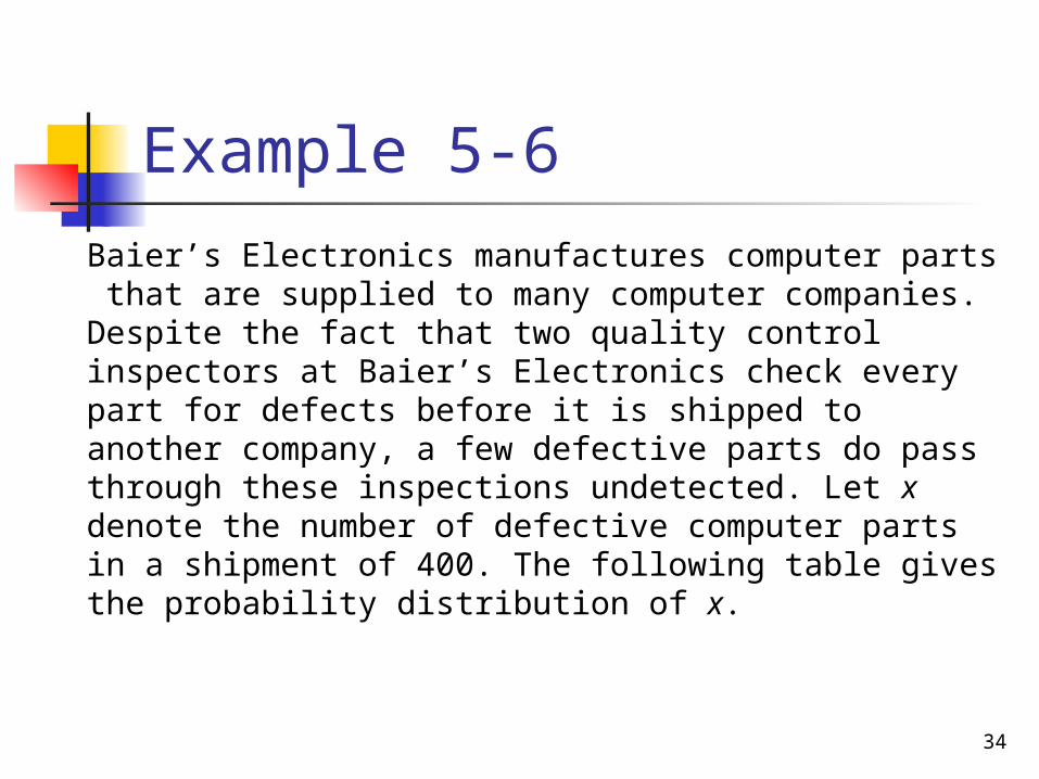
Example 5-6 Baier’s Electronics manufactures computer parts that are supplied to many computer companies. Despite the fact that two quality control inspectors at Baier’s Electronics check every part for defects before it is shipped to another company, a few defective parts do pass through these inspections undetected. Let x denote the number of defective computer parts in a shipment of 400. The following table gives the probability distribution of x.

35

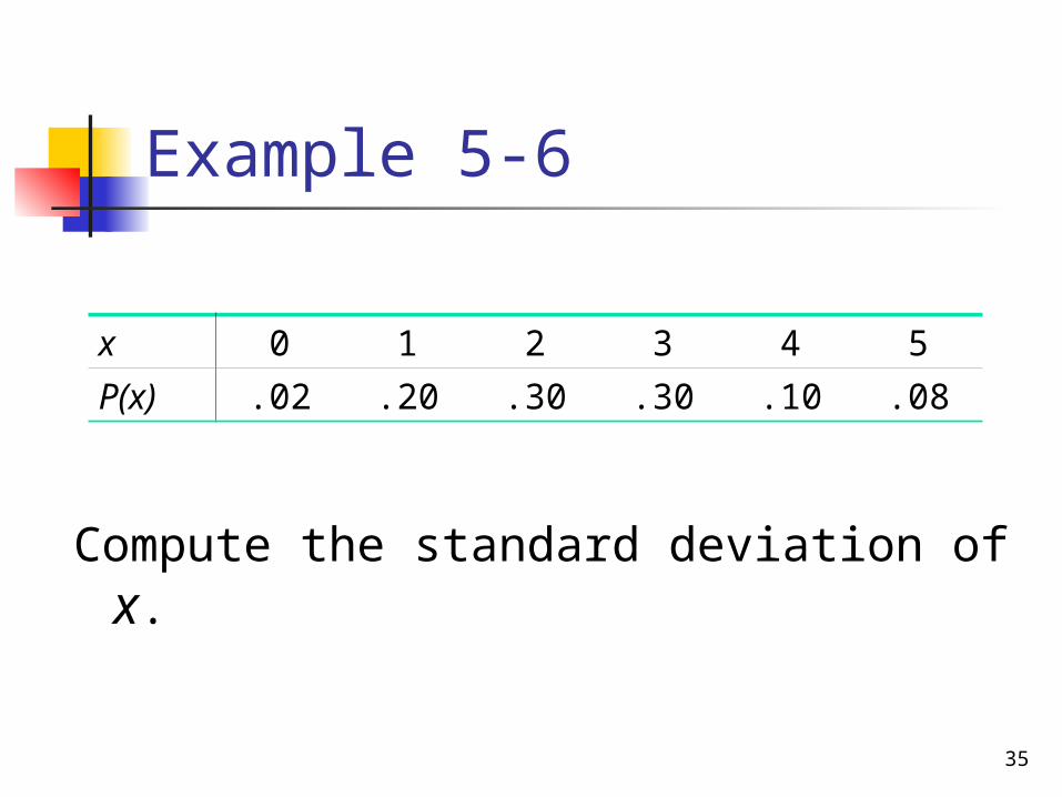
Example 5-6

Compute the standard deviation of x.

x 0 1 2 3 4 5P(x) .02 .20 .30 .30 .10 .08

36

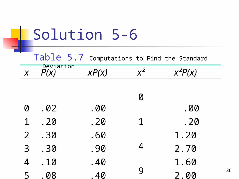
Solution 5-6Table 5.7 Computations to Find the Standard

Deviationx P(x) xP(x) x² x²P(x)

012345

.02

.20

.30

.30

.10

.08

.00

.20

.60

.90

.40

.40

0 1 4 91625

.00 .201.202.701.602.00

ΣxP(x) = 2.50 Σx²P(x) = 7.70

37

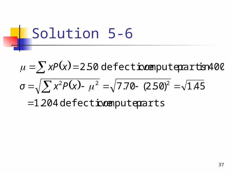
Solution 5-6

partscomputer defective 204.1 45.1)50.2(70.7

400in partscomputer defective 50.2222

xPxσ

xPx

38

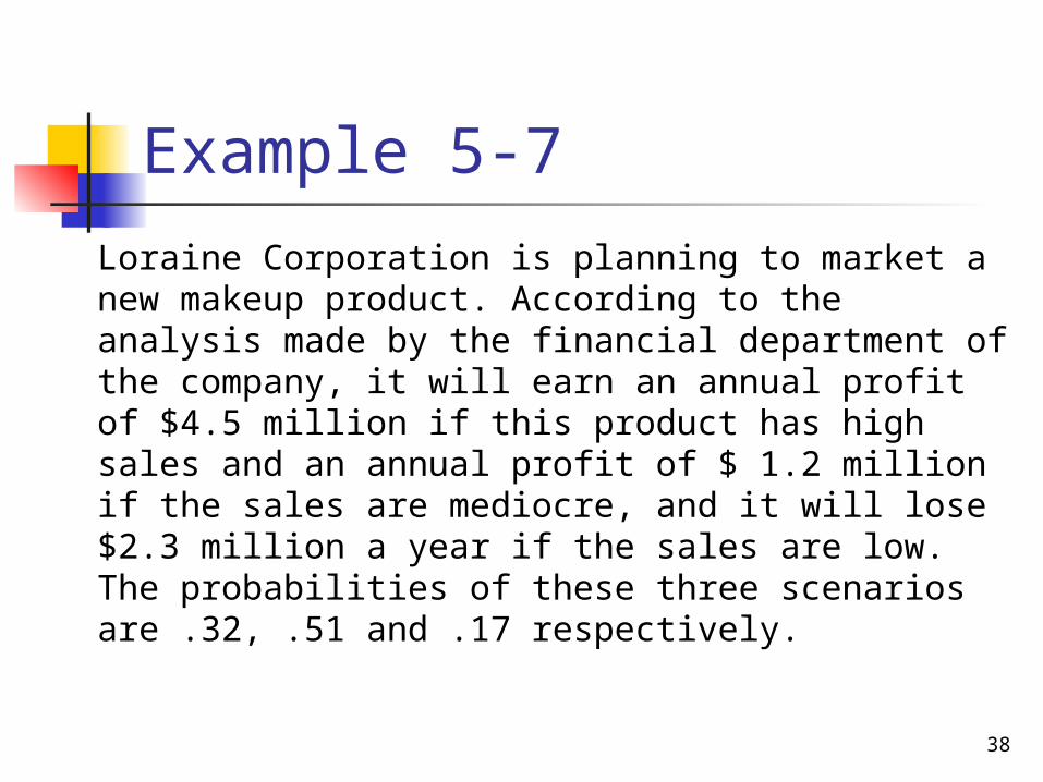
Example 5-7 Loraine Corporation is planning to market a new makeup product. According to the analysis made by the financial department of the company, it will earn an annual profit of $4.5 million if this product has high sales and an annual profit of $ 1.2 million if the sales are mediocre, and it will lose $2.3 million a year if the sales are low. The probabilities of these three scenarios are .32, .51 and .17 respectively.

39

Example 5-7a) Let x be the profits (in

millions of dollars) earned per annum by the company from this product. Write the probability distribution of x.

b) Calculate the mean and the standard deviation of x.

40

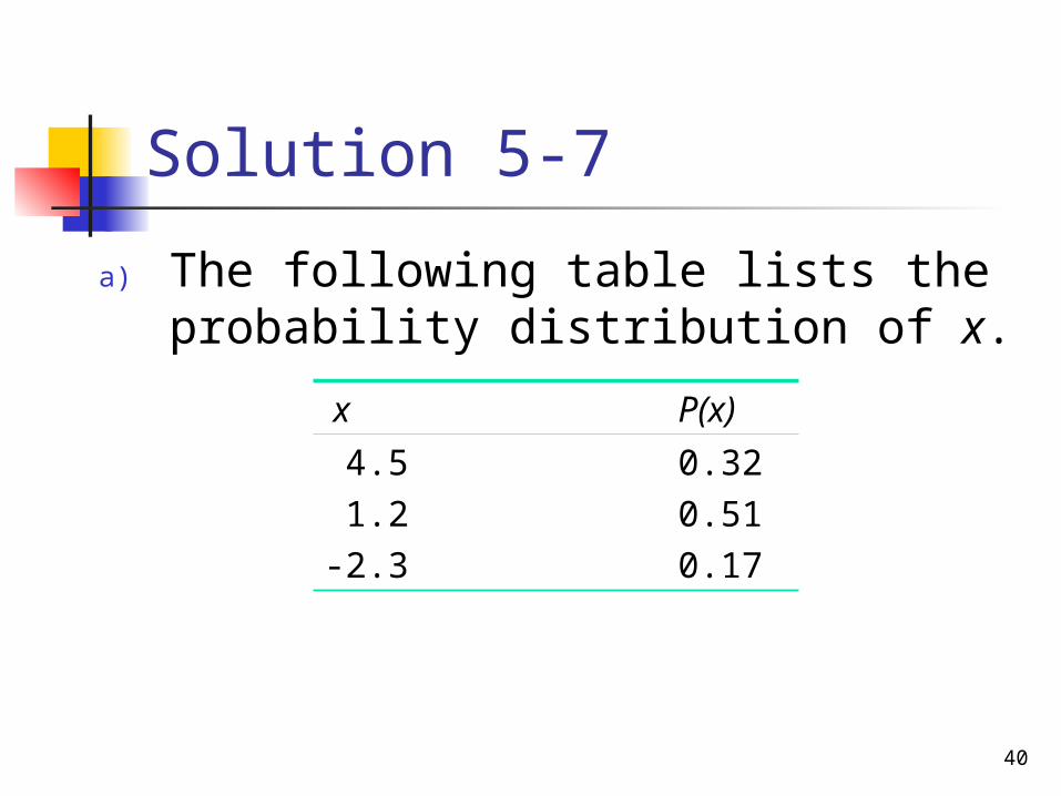
Solution 5-7a) The following table lists the

probability distribution of x. x P(x) 4.5 1.2-2.3

0.320.510.17

41

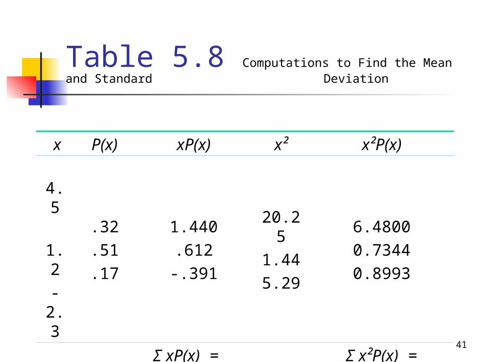
Table 5.8 Computations to Find the Mean and Standard Deviation

x P(x) xP(x) x² x²P(x) 4.5 1.2-2.3

.32

.51

.17

1.440.612-.391

20.25

1.445.29

6.48000.73440.8993

Σ xP(x) = 1.661

Σ x²P(x) = 8.1137

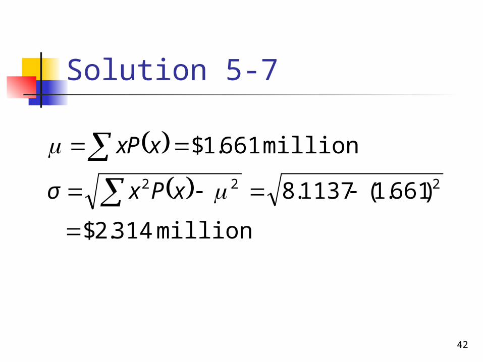
42

Solution 5-7

million 314.2$

)661.1(1137.8million 661.1$

222

xPxσ

xPx

43

FACTORIALS AND COMBINATIONS

Factorials Combinations

44

Factorials Definition The symbol n!, read as “n factorial”, represents the product of all the integers from n to 1. in other words,

n! = n(n - 1)(n – 2)(n – 3). . . 3 . 2 . 1 By definition,

0! = 1

45

ExampleEvaluate the following:

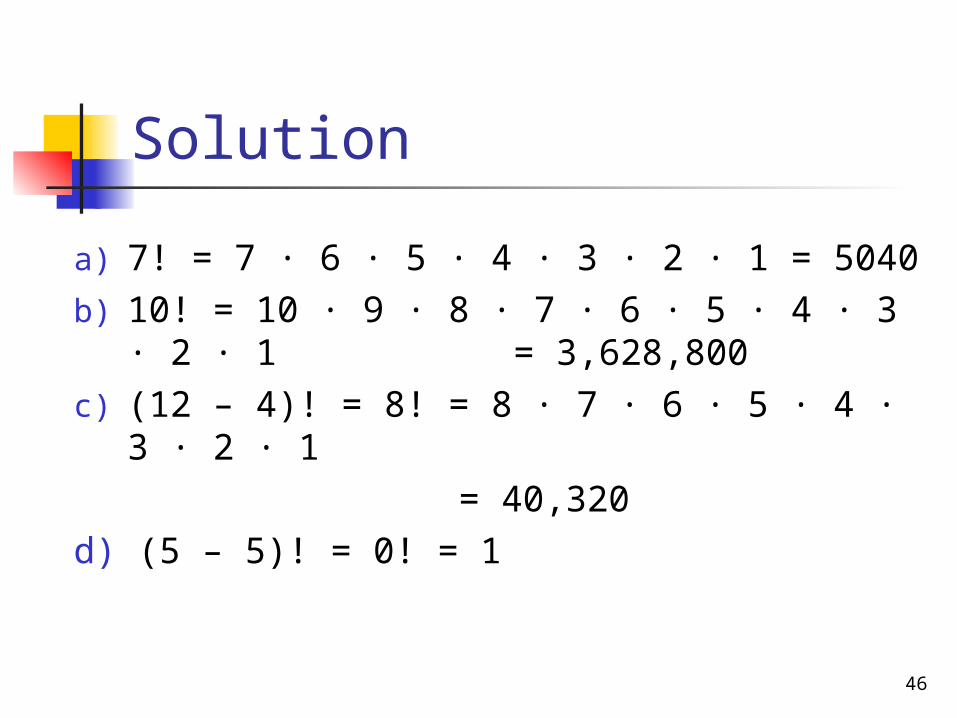
a) 7!b) 10!c) (12 – 4)!d) (5 – 5)!

46

Solutiona) 7! = 7 · 6 · 5 · 4 · 3 · 2 · 1 = 5040b) 10! = 10 · 9 · 8 · 7 · 6 · 5 · 4 · 3

· 2 · 1 = 3,628,800c) (12 – 4)! = 8! = 8 · 7 · 6 · 5 · 4 ·

3 · 2 · 1 = 40,320d) (5 – 5)! = 0! = 1

47

Combinations Definition Combinations give the number of ways x elements can be selected from n elements. The notation used to denote the total number of combinations is

which is read as “the number of combinations of n elements selected x at a time.”

xnC

48

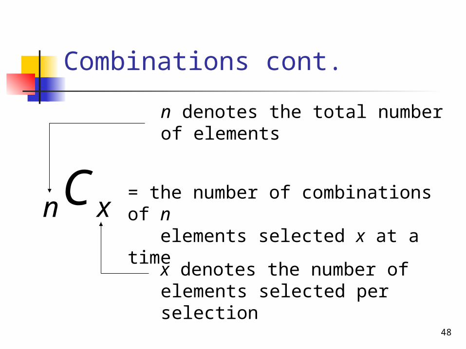
Combinations cont.

xnCn denotes the total number of elements

= the number of combinations of n elements selected x at a timex denotes the number of

elements selected per selection

49

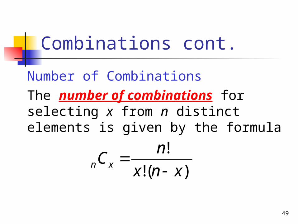
Combinations cont. Number of Combinations The number of combinations for selecting x from n distinct elements is given by the formula

)!(!!

xnxnC xn

50

Example 5-13 An ice cream parlor has six flavors of ice cream. Kristen wants to buy two flavors of ice cream. If she randomly selects two flavors out of six, how many combinations are there?

51

Solution 5-13

15123412123456

!4!2!6

)!26(!2!6

26

C

Thus, there are 15 ways for Kristin to select two ice cream flavors out of six.

n = 6 x = 2

52

Example 5-14 Three members of a jury will be randomly selected from five people. How many different combinations are possible?

53

Solution

1026120

!2!3!5

)!35(!3!5

35

C

54

Using the Table of Combinations

Example 5-15 Marv & Sons advertised to hire a financial analyst. The company has received applications from 10 candidates who seem to be equally qualified. The company manager has decided to call only 3 of these candidates for an interview. If she randomly selects 3 candidates from the 10, how many total selections are possible?

55

THE BINOMIAL PROBABILITY DISTRIBUTION

The Binomial Experiment The Binomial Probability Distribution and binomial Formula

Using the Table of Binomial Probabilities

Probability of Success and the Shape of the Binomial Distribution

56

The Binomial Experiment

Conditions of a Binomial ExperimentA binomial experiment must satisfy thefollowing four conditions.

1. There are n identical trials.2. Each trail has only two possible

outcomes.3. The probabilities of the two outcomes

remain constant.4. The trials are independent.

57

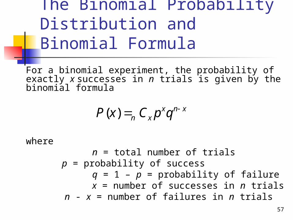
The Binomial Probability Distribution and Binomial Formula

For a binomial experiment, the probability of exactly x successes in n trials is given by the binomial formula

where n = total number of trials p = probability of success q = 1 – p = probability of failure x = number of successes in n trials n - x = number of failures in n trials

xnxxn qpCxP )(

58

Example 5-18 Five percent of all VCRs manufactured by a large electronics company are defective. A quality control inspector randomly selects three VCRs from the production line.What is the probability that exactly one of these three VCRs are defective?

59

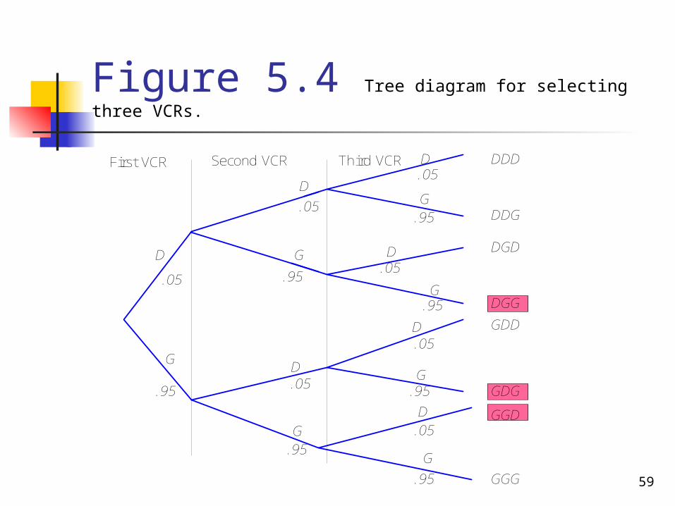
Figure 5.4 Tree diagram for selecting three VCRs.

DDD

DDG

DGD

DGGGDD

GDGGGD

GGG

First VCR Second VCR Third VCR

D.05

G

.95

D

D

D

D

D

.05

.05

.05

.05

.05

.05

D

G

G

G

G

G

G

.95

.95

.95

.95

.95

.95

60

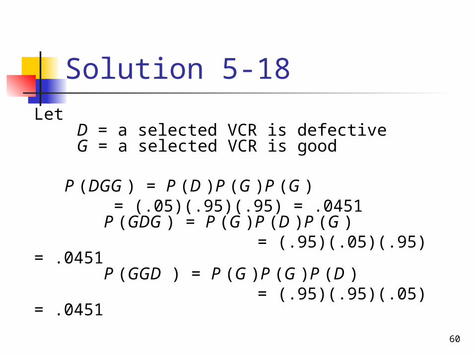
Solution 5-18 Let

D = a selected VCR is defectiveG = a selected VCR is good

P (DGG ) = P (D )P (G )P (G ) = (.05)(.95)(.95) = .0451 P (GDG ) = P (G )P (D )P (G )

= (.95)(.05)(.95) = .0451 P (GGD ) = P (G )P (G )P (D )

= (.95)(.95)(.05) = .0451

61

Solution 5-18Therefore, P (1 VCR is defective in 3) = P (DGG or GDG or GGD ) = P (DGG ) + P (GDG ) + P (GGD ) = .0451 + .0451 + .0451 = .1353

62

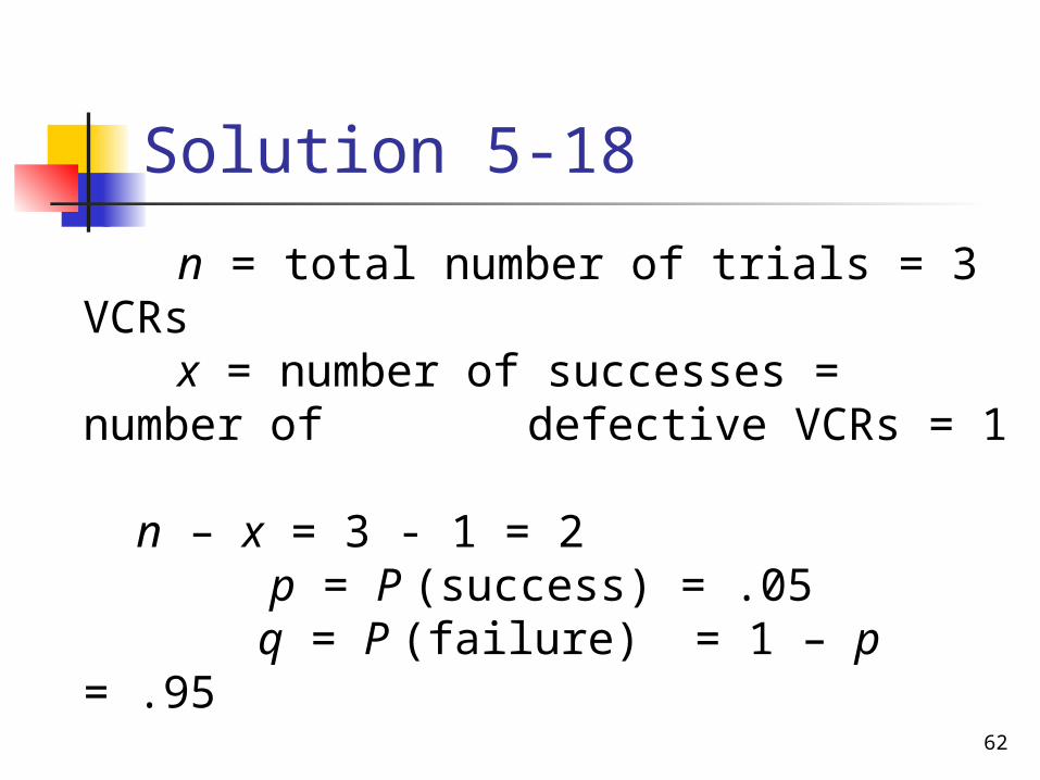
Solution 5-18 n = total number of trials = 3 VCRs

x = number of successes = number of defective VCRs = 1

n – x = 3 - 1 = 2 p = P (success) = .05

q = P (failure) = 1 – p = .95

63

Solution 5-18 Therefore, the probability of selecting exactly one defective VCR.

The probability .1354 is slightly different from the earlier calculation .1353 because of rounding.

1354.)9025)(.05)(.3()95(.)05(.)1( 2113 CxP

64

Example 5-19 At the Express House Delivery Service, providing high-quality service to customers is the top priority of the management. The company guarantees a refund of all charges if a package it is delivering does not arrive at its destination by the specified time. It is known from past data that despite all efforts, 2% of the packages mailed through this company do not arrive at their destinations within the specified time. Suppose a corporation mails 10 packages through Express House Delivery Service on a certain day.

65

Example 5-19a) Find the probability that exactly

1 of these 10 packages will not arrive at its destination within the specified time.

b) Find the probability that at most 1 of these 10 packages will not arrive at its destination within the specified time.

66

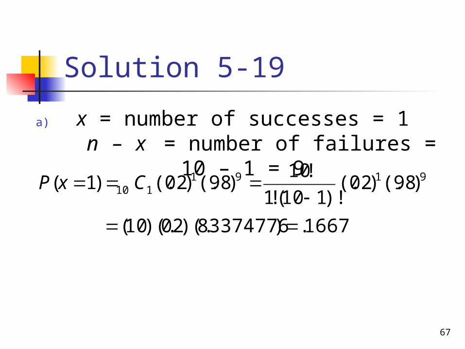
Solution 5-19 n = total number of packages mailed = 10

p = P (success) = .02 q = P (failure) = 1 – .02 = .98

67

Solution 5-19 x = number of successes = 1 n – x = number of failures =

10 – 1 = 9

1667.)83374776)(.02)(.10(

)98(.)02(.)!110(!1!10)98(.)02(.)1( 9191

110

CxP

a)

68

Solution 5-19 b)

.9838 .1667.8171 .83374776)(10)(.02)(707281)(1)(1)(.81

)98(.)02(.)98(.)02(. )1()0()1(

91110

100010

CCxPxPxP

69

Example 5-20 According to an Allstate Survey, 56% of Baby Boomers have car loans and are making payments on these loans (USA TODAY, October 28, 2002). Assume that this result holds true for the current population of all Baby Boomers. Let x denote the number in a random sample of three Baby Boomers who are making payments on their car loans. Write the probability distribution of x and draw a bar graph for this probability distribution.

70

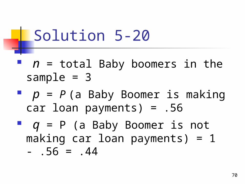
Solution 5-20 n = total Baby boomers in the sample = 3

p = P (a Baby Boomer is making car loan payments) = .56

q = P (a Baby Boomer is not making car loan payments) = 1 - .56 = .44

71

Solution 5-20

0852.)085184)(.1)(1()44.0()56(.)0( 3003 CxP

3252.)1936)(.56)(.3()44(.)56(.)1( 2113 CxP

4140.)44)(.3136)(.3()44(.)56(.)2( 1223 CxP

1756.)1)(175616)(.1()44(.)56(.)3( 0333 CxP

72

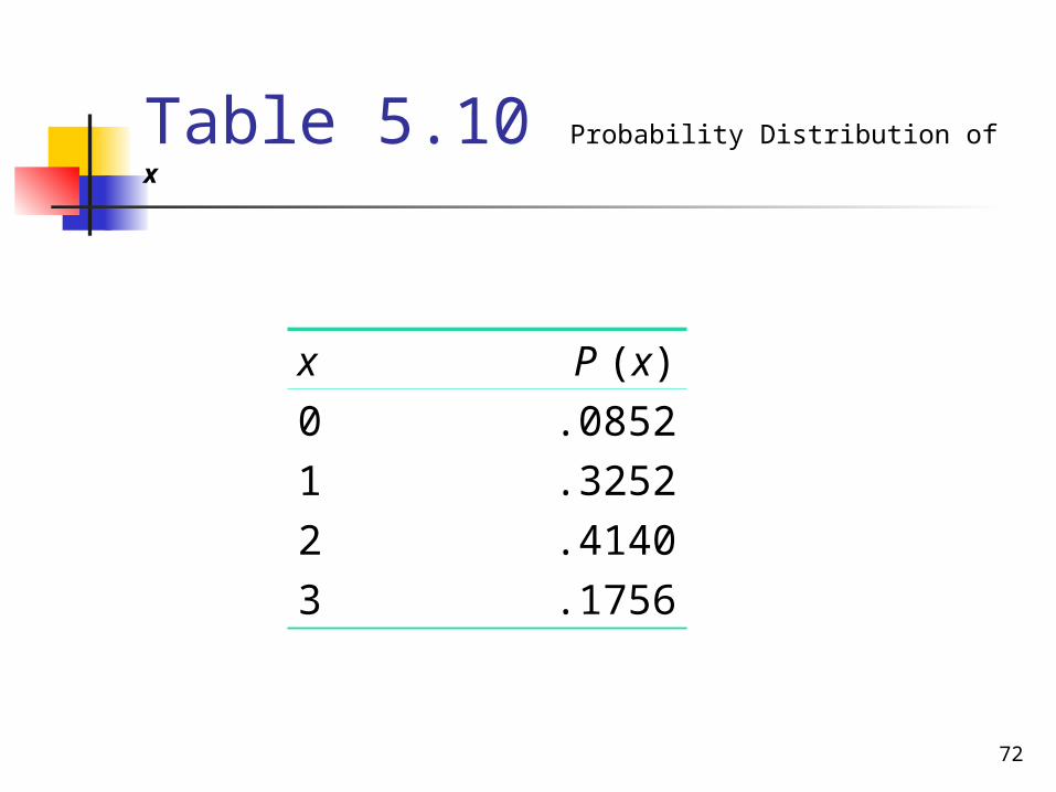
Table 5.10 Probability Distribution of x

x P (x)0123

.0852

.3252

.4140

.1756

73

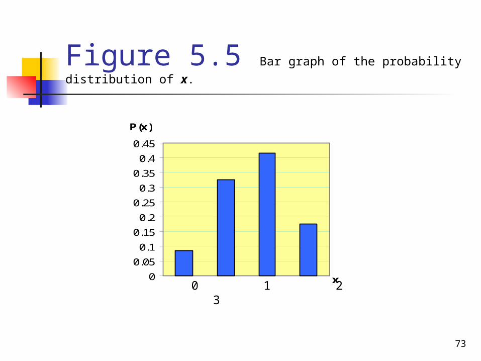
Figure 5.5 Bar graph of the probability distribution of x.

00.050.10.150.20.250.30.350.40.45

x

P(x)

0 1 2 3

74

Using the Table of Binomial Probabilities

Example 5-21 According to a 2001 study of college students by Harvard University’s School of Public health, 19.3% of those included in the study abstained from drinking (USA TODAY, April 3, 2002). Suppose that of all current college students in the United States, 20% abstain from drinking. A random sample of six college students is selected.

75

Example 5-21Using Table IV of Appendix C, answer the

following.a) Find the probability that exactly three college

students in this sample abstain from drinking.b) Find the probability that at most two college

students in this sample abstain from drinking.c) Find the probability that at least three

college students in this sample abstain from drinking.

d) Find the probability that one to three college students in this sample abstain from drinking.

e) Let x be the number of college students in this sample who abstain from drinking. Write the probability distribution of x and draw a bar graph for this probability distribution.

76

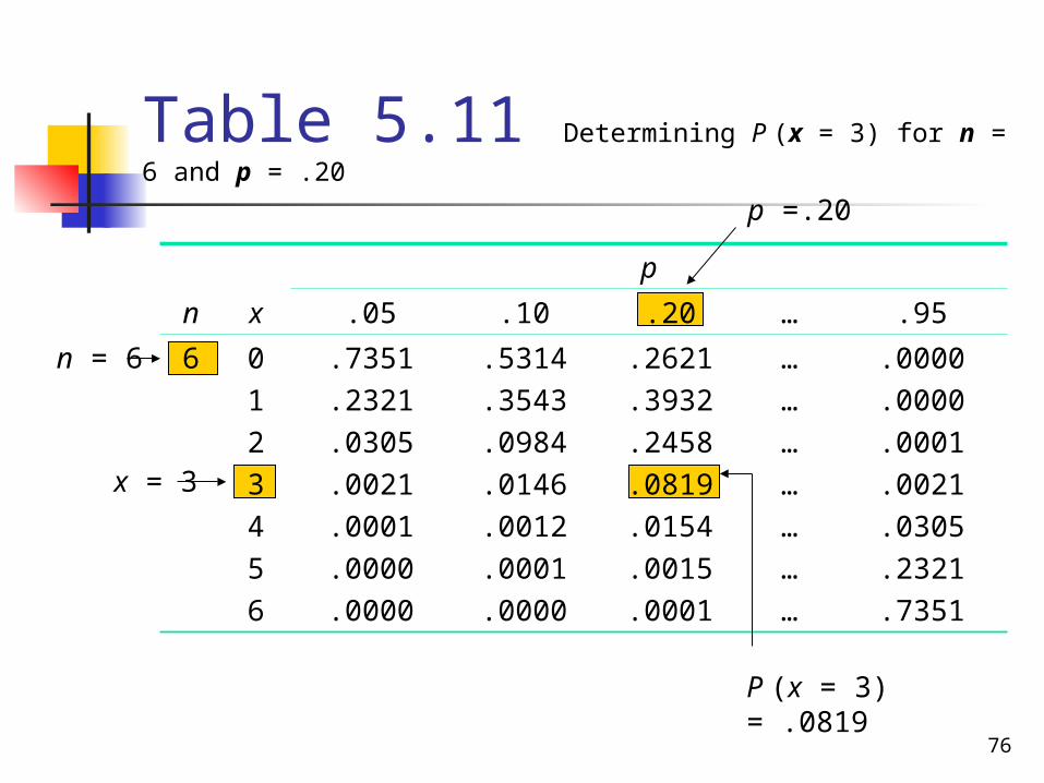
Table 5.11 Determining P (x = 3) for n = 6 and p = .20

pn x .05 .10 .20 … .956 0

123456

.7351

.2321

.0305

.0021

.0001

.0000

.0000

.5314

.3543

.0984

.0146

.0012

.0001

.0000

.2621

.3932

.2458

.0819

.0154

.0015

.0001

…………………

.0000

.0000

.0001

.0021

.0305

.2321

.7351

n = 6

p =.20

P (x = 3) = .0819

x = 3

77

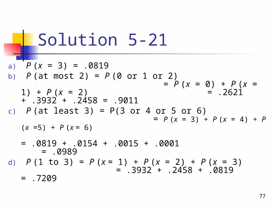
Solution 5-21a) P (x = 3) = .0819b) P (at most 2) = P (0 or 1 or 2)

= P (x = 0) + P (x = 1) + P (x = 2) = .2621 + .3932 + .2458 = .9011

c) P (at least 3) = P(3 or 4 or 5 or 6) = P (x = 3) + P (x = 4) + P (x =5) + P (x = 6) = .0819 + .0154 + .0015 + .0001 = .0989

d) P (1 to 3) = P (x = 1) + P (x = 2) + P (x = 3) = .3932 + .2458 + .0819 = .7209

78

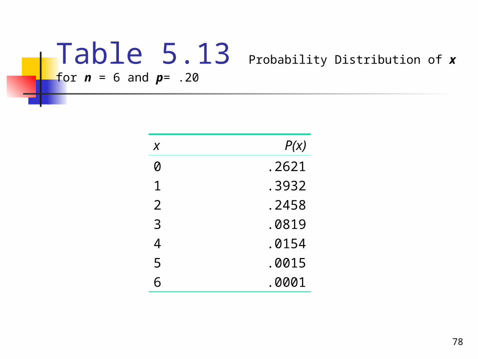
Table 5.13 Probability Distribution of x for n = 6 and p= .20

x P(x)0123456

.2621

.3932

.2458

.0819

.0154

.0015

.0001

79

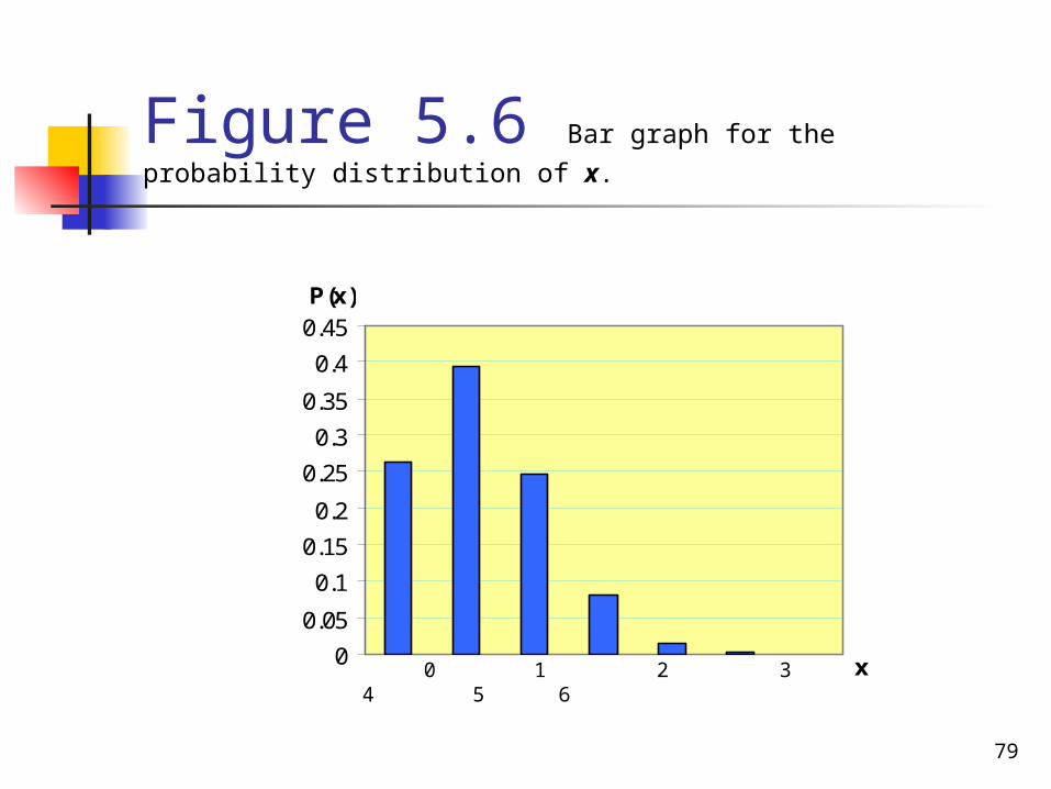
Figure 5.6 Bar graph for the probability distribution of x.

00.050.10.150.20.250.30.350.40.45

x

P(x)

0 1 2 3 4 5 6

80

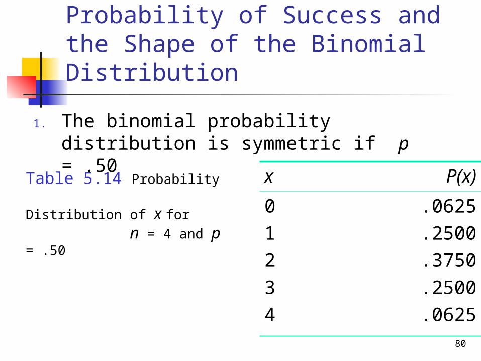
Probability of Success and the Shape of the Binomial Distribution

1. The binomial probability distribution is symmetric if p = .50 x P(x)

01234

.0625

.2500

.3750

.2500

.0625

Table 5.14 Probability

Distribution of x for n = 4 and p = .50

81

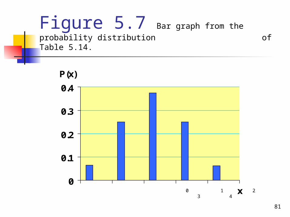
Figure 5.7 Bar graph from the probability distribution of Table 5.14.

0

0.1

0.2

0.3

0.4

x

P(x)

0 1 2 3 4

82

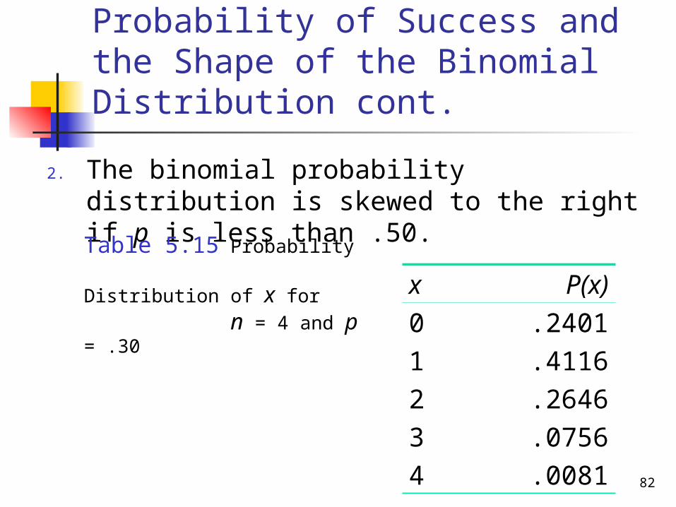
Probability of Success and the Shape of the Binomial Distribution cont.

2. The binomial probability distribution is skewed to the right if p is less than .50.

x P(x)01234

.2401

.4116

.2646

.0756

.0081

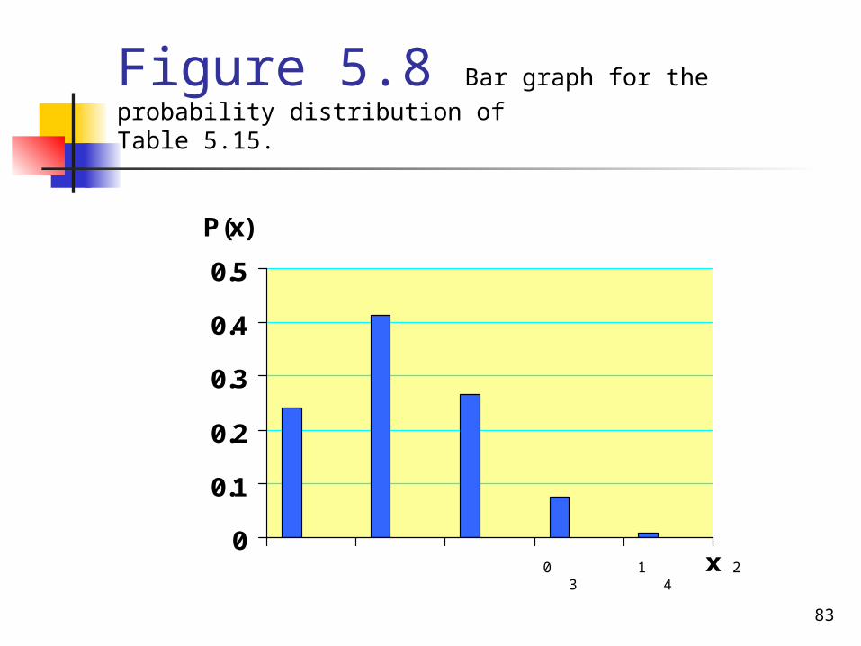
Table 5.15 Probability

Distribution of x for n = 4 and p = .30

83

Figure 5.8 Bar graph for the probability distribution of Table 5.15.

0

0.1

0.2

0.3

0.4

0.5

x

P(x)

0 1 2 3 4

84

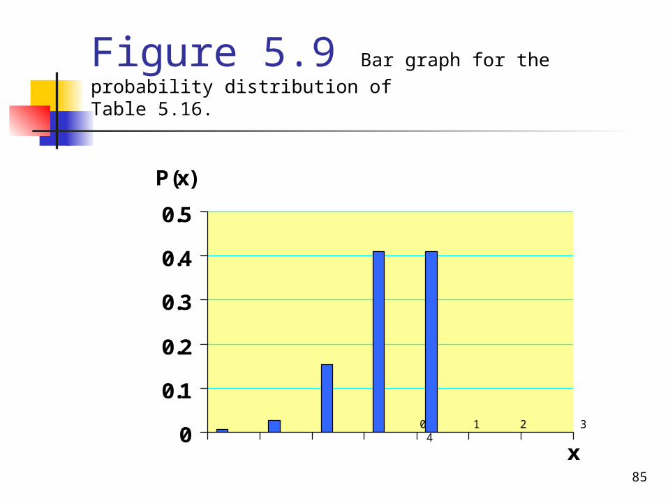
Probability of Success and the Shape of the Binomial Distribution cont.

3. The binomial probability distribution is skewed to the left if p is greater than .50.

x P(x)01234

.0016

.0256

.1536

.4096

.4096

Table 5.16

Probability

Distribution of x for n =4 and p = .80

85

Figure 5.9 Bar graph for the probability distribution of Table 5.16.

0

0.1

0.2

0.3

0.4

0.5

x

P(x)

0 1 2 3 4

86

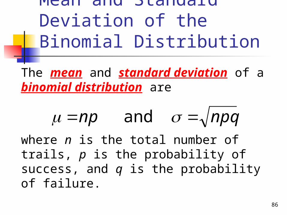
Mean and Standard Deviation of the Binomial Distribution

The mean and standard deviation of a binomial distribution are

where n is the total number of trails, p is the probability of success, and q is the probability of failure.

npqnp and

87

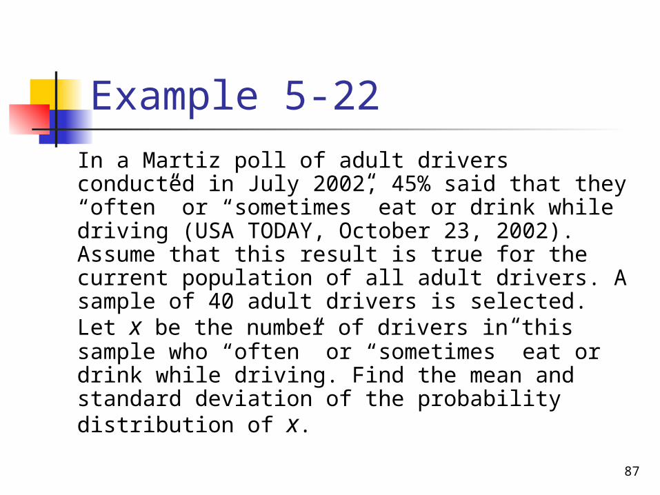
Example 5-22 In a Martiz poll of adult drivers conducted in July 2002, 45% said that they “often” or “sometimes” eat or drink while driving (USA TODAY, October 23, 2002). Assume that this result is true for the current population of all adult drivers. A sample of 40 adult drivers is selected. Let x be the number of drivers in this sample who “often” or “sometimes” eat or drink while driving. Find the mean and standard deviation of the probability distribution of x.

88

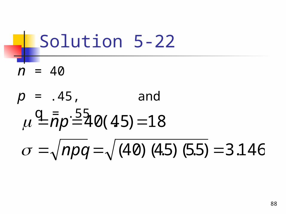
Solution 5-22

146.3)55)(.45)(.40(18)45(.40

npqnp

n = 40p = .45, and q = .55

89

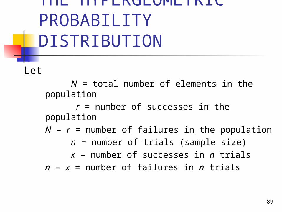
THE HYPERGEOMETRIC PROBABILITY DISTRIBUTION

Let N = total number of elements in the population

r = number of successes in the population

N – r = number of failures in the population n = number of trials (sample size) x = number of successes in n trials n – x = number of failures in n trials

90

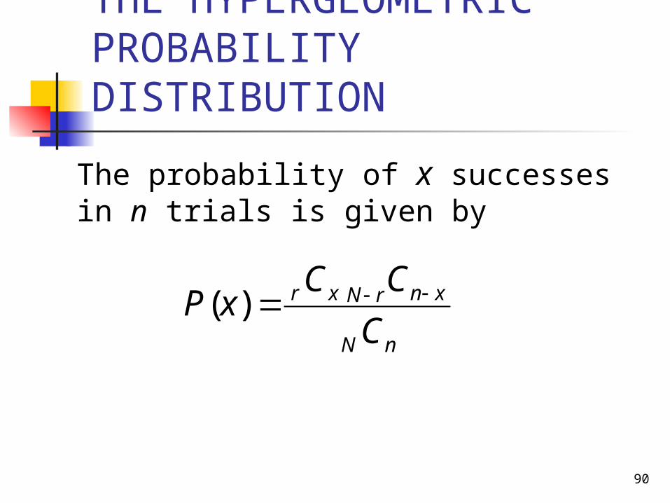
THE HYPERGEOMETRIC PROBABILITY DISTRIBUTION

The probability of x successes in n trials is given by

nN

xnrNxr

CCCxP )(

91

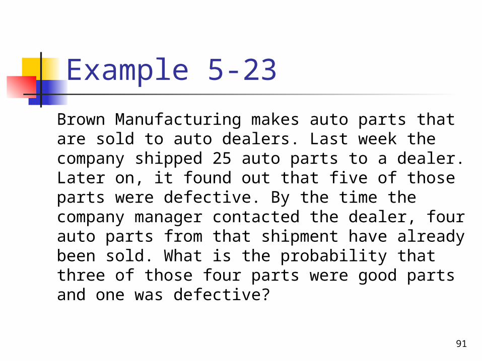
Example 5-23 Brown Manufacturing makes auto parts that are sold to auto dealers. Last week the company shipped 25 auto parts to a dealer. Later on, it found out that five of those parts were defective. By the time the company manager contacted the dealer, four auto parts from that shipment have already been sold. What is the probability that three of those four parts were good parts and one was defective?

92

Solution 5-23

4506.650,12)5)(1140(

)!425(!4!25

)!15(!1!5

)!320(!3!20

)3(425

15320

CCC

CCCxPnN

xnrNxr

Thus, the probability that three of the four parts sold are good and one is defective is .4506.

93

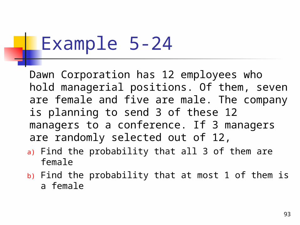
Example 5-24 Dawn Corporation has 12 employees who

hold managerial positions. Of them, seven are female and five are male. The company is planning to send 3 of these 12 managers to a conference. If 3 managers are randomly selected out of 12,a) Find the probability that all 3 of them are

femaleb) Find the probability that at most 1 of them is

a female

94

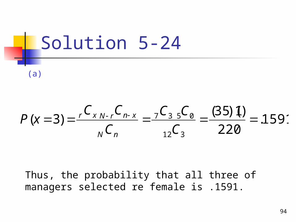
Solution 5-24

1591.220)1)(35( )3(

312

0537

CCC

CCCxPnN

xnrNxr

Thus, the probability that all three of managers selected re female is .1591.

(a)

95

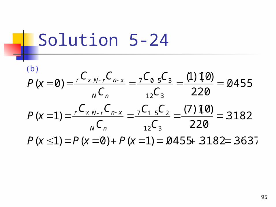
Solution 5-24

3637.3182.0455.)1()0()1(

3182.220)10)(7( )1(

0455.220)10)(1( )0(

312

2517

312

3507

xPxPxPC

CCC

CCxP

CCC

CCCxP

nN

xnrNxr

nN

xnrNxr(b)

96

THE POISSON PROBABILITY DISTRIBUTION

Using the Table of Poisson probabilities

Mean and Standard Deviation of the Poisson Probability Distribution

97

THE POISSON PROBABILITY DISTRIBUTION cont.

Conditions to Apply the Poisson Probability Distribution

The following three conditions must be satisfied to apply the Poisson probability distribution.1. x is a discrete random variable.2. The occurrences are random.3. The occurrences are independent.

98

Examples1. The number of accidents that occur on

a given highway during a one-week period.

2. The number of customers entering a grocery store during a one –hour interval.

3. The number of television sets sold at a department store during a given week.

99

THE POISSON PROBABILITY DISTRIBUTION cont.

Poisson Probability Distribution Formula

According to the Poisson probability distribution, the probability of x occurrences in an interval is

where λ is the mean number of occurrences in that interval and the value of e is approximately 2.71828.

!)(xexP

x

100

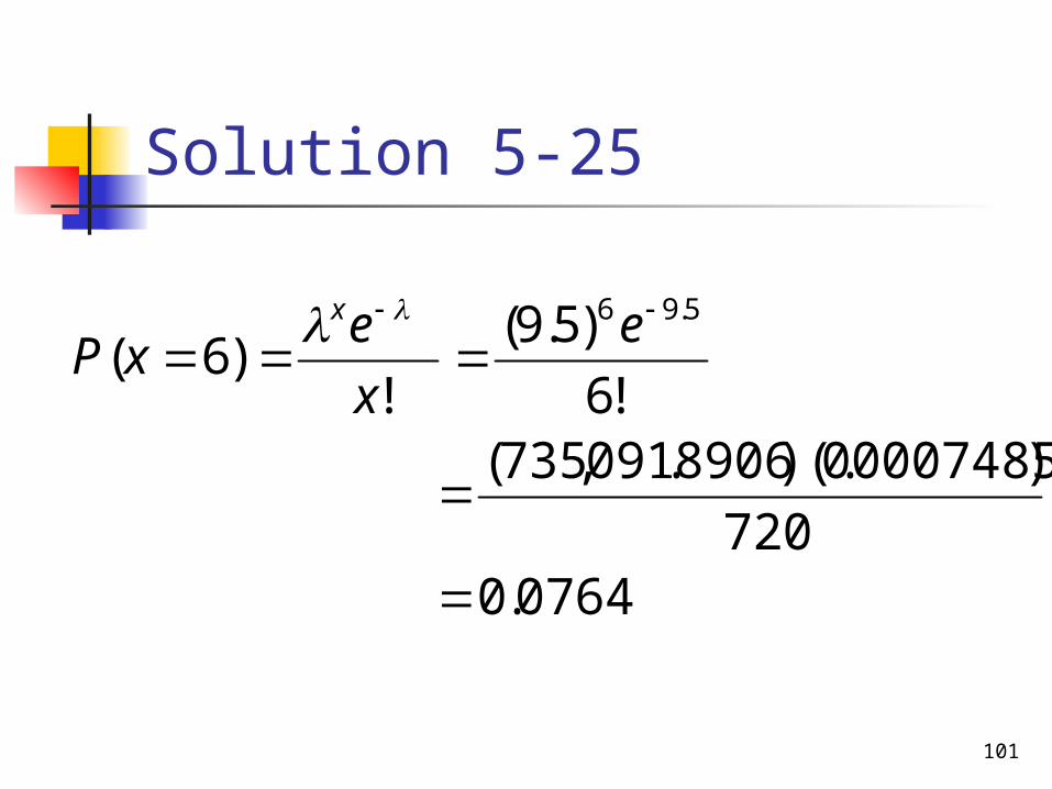
Example 5-25 On average, a household receives 9.5 telemarketing phone calls per week. Using the Poisson distribution formula, find the probability that a randomly selected household receives exactly six telemarketing phone calls during a given week.

101

Solution 5-25

0764.0 720

)00007485)(.8906.091,735( !6)5.9(

!)6(5.96

e

xexP

x

102

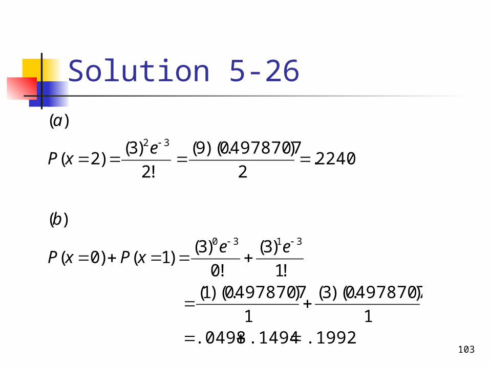
Example 5-26 A washing machine in a laundromat breaks down an average of three times per month. Using the Poisson probability distribution formula, find the probability that during the next month this machine will have

a) exactly two breakdownsb) at most one breakdown

103

Solution 5-26

.1992 .1494 .0498 1

)04978707)(.3(1

)04978707)(.1( !1)3(

!0)3()1()0(

)(

2240.2)04978707)(.9(

!2)3()2(

)(

3130

32

eexPxP

b

exP

a

104

Example 5-27 Cynthia’s Mail Order Company provides free examination of its products for seven days. If not completely satisfied, a customer can return the product within that period and get a full refund. According to past records of the company, an average of 2 of every 10 products sold by this company are returned for a refund. Using the Poisson probability distribution formula, find the probability that exactly 6 of the 40 products sold by this company on a given day will be returned for a refund.

105

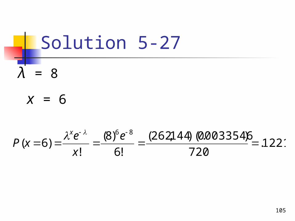
Solution 5-27

1221.720)00033546)(.144,262(

!6)8(

!)6(86

e

xexP

x

λ = 8 x = 6

106

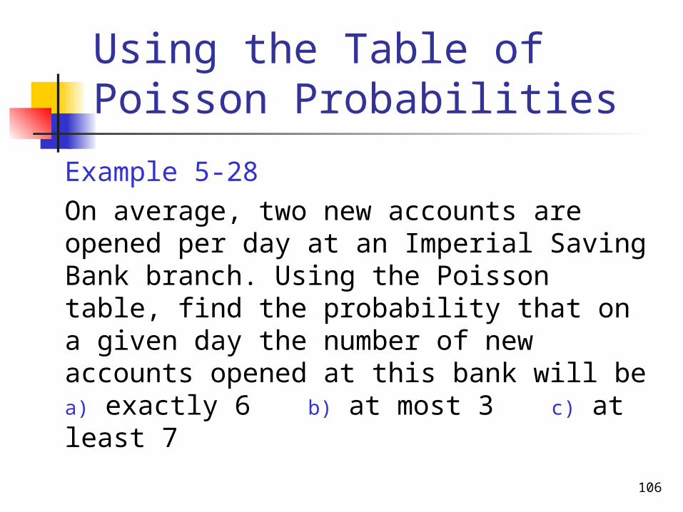
Using the Table of Poisson Probabilities

Example 5-28 On average, two new accounts are opened per day at an Imperial Saving Bank branch. Using the Poisson table, find the probability that on a given day the number of new accounts opened at this bank will bea) exactly 6 b) at most 3 c) at least 7

107

Table 5.17 Portion of Table of Poisson Probabilities for λ = 2.0

λx 1.1 1.2 … 2.00123456789

.1353

.2707

.2707

.1804

.0902

.0361

.0120

.0034

.0009

.0002

x = 6 P (x = 6)

λ = 2.0

108

Solution 5-28a) P (x = 6) = .0120b) P (at most 3) =P (x = 0) + P (x = 1) + P (x =

2) + P (x = 3) =.1353 +.2707 + .2707 + .1804 = .8571

c) P (at least 7) = P (x = 7) + P (x = 8) + P (x = 9) = .0034 + .0009 + .0002 = .0045

109

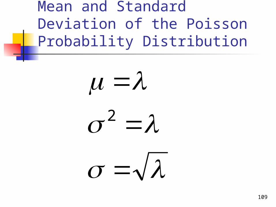
Mean and Standard Deviation of the Poisson Probability Distribution

2

110

Example 5-29 An auto salesperson sells an average

of .9 car per day. Let x be the number of cars sold by this salesperson on any given day. Using the Poisson probability distribution table,a) Write the probability distribution of x. b) Draw a graph of the probability

distribution.c) Find the mean, variance, and standard

deviation.

111

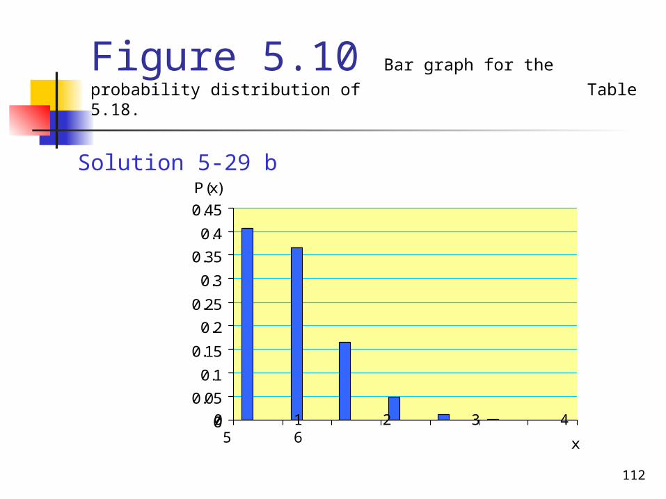
Table 5.18 Probability Distribution of x for λ = .9

x P (x)0123456

.4066

.3659

.1647

.0494

.0111

.0020

.0003

Solution 5-29 a

112

Figure 5.10 Bar graph for the probability distribution of Table 5.18.

00.050.10.150.20.250.30.350.40.45

x

P(x)

0 1 2 3 4 5 6

Solution 5-29 b

113

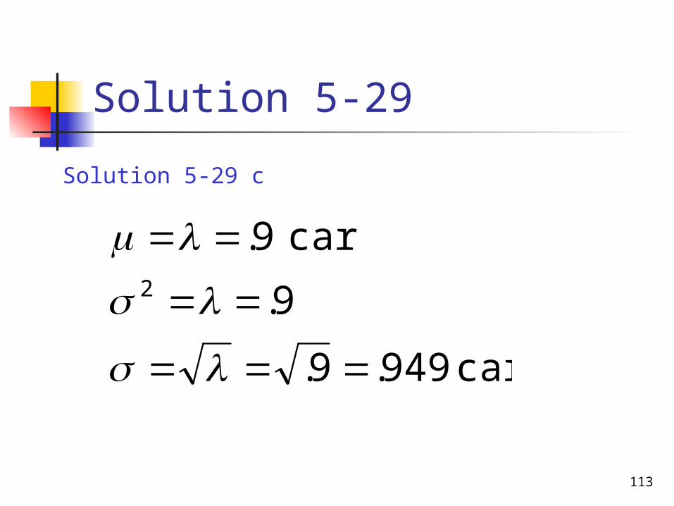
Solution 5-29

car 949.9.9.car 9.

2

Solution 5-29 c