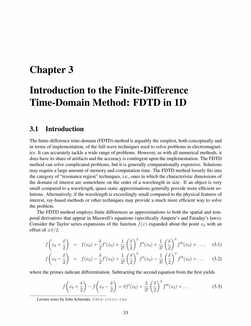
Chapter 3 Introduction to the Finite-Difference Time-Domain Method: FDTD in 1D 3.1 Introduction The finite-difference time-domain (FDTD) method is arguably the simplest, both conceptually and in terms of implementation, of the full-wave techniques used to solve problems in electromagnet- ics. It can accurately tackle a wide range of problems. However, as with all numerical methods, it does have its share of artifacts and the accuracy is contingent upon the implementation. The FDTD method can solve complicated problems, but it is generally computationally expensive. Solutions may require a large amount of memory and computation time. The FDTD method loosely fits into the category of “resonance region” techniques, i.e., ones in which the characteristic dimensions of the domain of interest are somewhere on the order of a wavelength in size. If an object is very small compared to a wavelength, quasi-static approximations generally provide more efficient so- lutions. Alternatively, if the wavelength is exceedingly small compared to the physical features of interest, ray-based methods or other techniques may provide a much more efficient way to solve the problem. The FDTD method employs finite differences as approximations to both the spatial and tem- poral derivatives that appear in Maxwell’s equations (specifically Ampere’s and Faraday’s laws). Consider the Taylor series expansions of the function f (x) expanded about the point x 0 with an offset of ±δ/2: f x 0 + δ 2 = f (x 0 )+ δ 2 f ′ (x 0 )+ 1 2! δ 2 2 f ′′ (x 0 )+ 1 3! δ 2 3 f ′′′ (x 0 )+ ..., (3.1) f x 0 − δ 2 = f (x 0 ) − δ 2 f ′ (x 0 )+ 1 2! δ 2 2 f ′′ (x 0 ) − 1 3! δ 2 3 f ′′′ (x 0 )+ ... (3.2) where the primes indicate differentiation. Subtracting the second equation from the first yields f x 0 + δ 2 − f x 0 − δ 2 = δf ′ (x 0 )+ 2 3! δ 2 3 f ′′′ (x 0 )+ ... (3.3) Lecture notes by John Schneider. fdtd-intro.tex 33

Welcome message from author
This document is posted to help you gain knowledge. Please leave a comment to let me know what you think about it! Share it to your friends and learn new things together.
Transcript
Chapter 3
Introduction to the Finite-Difference
Time-Domain Method: FDTD in 1D
3.1 Introduction
The finite-difference time-domain (FDTD) method is arguably the simplest, both conceptually and
in terms of implementation, of the full-wave techniques used to solve problems in electromagnet-
ics. It can accurately tackle a wide range of problems. However, as with all numerical methods, it
does have its share of artifacts and the accuracy is contingent upon the implementation. The FDTD
method can solve complicated problems, but it is generally computationally expensive. Solutions
may require a large amount of memory and computation time. The FDTD method loosely fits into
the category of “resonance region” techniques, i.e., ones in which the characteristic dimensions of
the domain of interest are somewhere on the order of a wavelength in size. If an object is very
small compared to a wavelength, quasi-static approximations generally provide more efficient so-
lutions. Alternatively, if the wavelength is exceedingly small compared to the physical features of
interest, ray-based methods or other techniques may provide a much more efficient way to solve
the problem.
The FDTD method employs finite differences as approximations to both the spatial and tem-
poral derivatives that appear in Maxwell’s equations (specifically Ampere’s and Faraday’s laws).
Consider the Taylor series expansions of the function f(x) expanded about the point x0 with an
offset of ±δ/2:
f
(
x0 +δ
2
)
= f(x0) +δ
2f ′(x0) +
1
2!
(δ
2
)2
f ′′(x0) +1
3!
(δ
2
)3
f ′′′(x0) + . . . , (3.1)
f
(
x0 −δ
2
)
= f(x0)−δ
2f ′(x0) +
1
2!
(δ
2
)2
f ′′(x0)−1
3!
(δ
2
)3
f ′′′(x0) + . . . (3.2)
where the primes indicate differentiation. Subtracting the second equation from the first yields
f
(
x0 +δ
2
)
− f
(
x0 −δ
2
)
= δf ′(x0) +2
3!
(δ
2
)3
f ′′′(x0) + . . . (3.3)
Lecture notes by John Schneider. fdtd-intro.tex
33
34 CHAPTER 3. INTRODUCTION TO THE FDTD METHOD
Dividing by δ produces
f(x0 +
δ2
)− f
(x0 − δ
2
)
δ= f ′(x0) +
1
3!
δ2
22f ′′′(x0) + . . . (3.4)
Thus the term on the left is equal to the derivative of the function at the point x0 plus a term which
depends on δ2 plus an infinite number of other terms which are not shown. For the terms which are
not shown, the next would depend on δ4 and all subsequent terms would depend on even higher
powers of δ. Rearranging slightly, this relationship is often stated as
df(x)
dx
∣∣∣∣x=x0
=f(x0 +
δ2
)− f
(x0 − δ
2
)
δ+O(δ2). (3.5)
The “big-Oh” term represents all the terms that are not explicitly shown and the value in paren-
theses, i.e., δ2, indicates the lowest order of δ in these hidden terms. If δ is sufficiently small,
a reasonable approximation to the derivative may be obtained by simply neglecting all the terms
represented by the “big-Oh” term. Thus, the central-difference approximation is given by
df(x)
dx
∣∣∣∣x=x0
≈ f(x0 +
δ2
)− f
(x0 − δ
2
)
δ. (3.6)
Note that the central difference provides an approximation of the derivative of the function at x0,
but the function is not actually sampled there. Instead, the function is sampled at the neighboring
points x0+δ/2 and x0−δ/2. Since the lowest power of δ being ignored is second order, the central
difference is said to have second-order accuracy or second-order behavior. This implies that if δ is
reduced by a factor of 10, the error in the approximation should be reduced by a factor of 100 (at
least approximately). In the limit as δ goes to zero, the approximation becomes exact.
One can construct higher-order central differences. In order to get higher-order behavior, more
terms, i.e., more sample points, must be used. Appendix A presents the construction of a fourth-
order central difference. The use of higher-order central differences in FDTD schemes is certainly
possible, but there are some complications which arise because of the increased “stencil” of the
difference operator. For example, when a PEC is present, it is possible that the difference operator
will extend into the PEC prematurely or it may extend to the other side of a PEC sheet. Because
of these types of issues, we will only consider the use of second-order central difference.
3.2 The Yee Algorithm
The FDTD algorithm as first proposed by Kane Yee in 1966 employs second-order central differ-
ences. The algorithm can be summarized as follows:
1. Replace all the derivatives in Ampere’s and Faraday’s laws with finite differences. Discretize
space and time so that the electric and magnetic fields are staggered in both space and time.
2. Solve the resulting difference equations to obtain “update equations” that express the (un-
known) future fields in terms of (known) past fields.

3.3. UPDATE EQUATIONS IN 1D 35
3. Evaluate the magnetic fields one time-step into the future so they are now known (effectively
they become past fields).
4. Evaluate the electric fields one time-step into the future so they are now known (effectively
they become past fields).
5. Repeat the previous two steps until the fields have been obtained over the desired duration.
At this stage, the summary is probably a bit too abstract. One really needs an example to demon-
strate the simplicity of the method. However, developing the full set of three-dimensional equations
would be overkill and thus the algorithm will first be presented in one-dimension. As you will see,
the extension to higher dimensions is quite simple.
3.3 Update Equations in 1D
Consider a one-dimensional space where there are only variations in the x direction. Assume that
the electric field only has a z component. In this case Faraday’s law can be written
−µ∂H
∂t= ∇× E =
∣∣∣∣∣∣
ax ay az∂∂x
0 00 0 Ez
∣∣∣∣∣∣
= −ay∂Ez
∂x. (3.7)
Thus Hy must be the only non-zero component of the magnetic field which is time varying. (Since
the right-hand side of this equation has only a y component, the magnetic field may have non-zero
components in the x and z directions, but they must be static. We will not be concerned with static
fields here.) Knowing this, Ampere’s law can be written
ǫ∂E
∂t= ∇×H =
∣∣∣∣∣∣
ax ay az∂∂x
0 00 Hy 0
∣∣∣∣∣∣
= az∂Hy
∂x. (3.8)
The two scalar equations obtained from (3.7) and (3.8) are
µ∂Hy
∂t=
∂Ez
∂x, (3.9)
ǫ∂Ez
∂t=
∂Hy
∂x. (3.10)
The first equation gives the temporal derivative of the magnetic field in terms of the spatial deriva-
tive of the electric field. Conversely, the second equation gives the temporal derivative of the
electric field in terms of the spatial derivative of the magnetic field. As will be shown, the first
equation will be used to advance the magnetic field in time while the second will be used to ad-
vance the electric field. A method in which one field is advanced and then the other, and then the
process is repeated, is known as a leap-frog method.
The next step is to replace the derivatives in (3.9) and (3.10) with finite differences. To do this,
space and time need to be discretized. The following notation will be used to indicate the location
where the fields are sampled in space and time
Ez(x, t) = Ez(m∆x, q∆t) = Eqz [m] , (3.11)
Hy(x, t) = Hy(m∆x, q∆t) = Hqy [m] , (3.12)
36 CHAPTER 3. INTRODUCTION TO THE FDTD METHOD
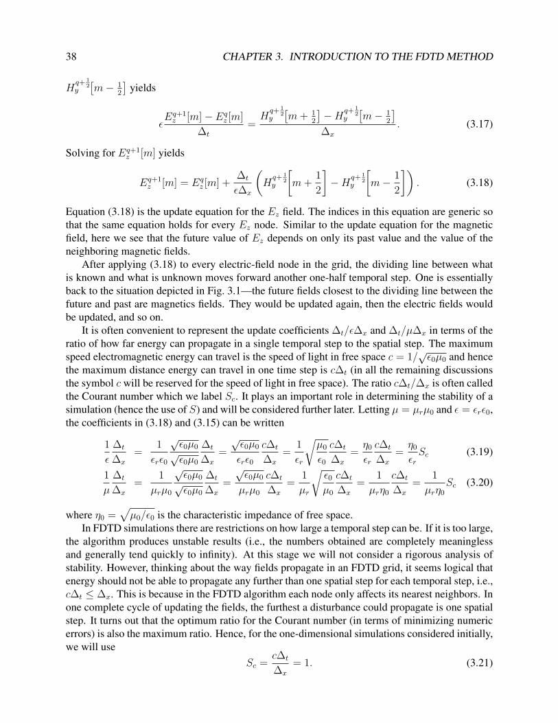
position, x
time, t
Future
Past
write difference equation
about this point
Ez [m−1]q+1 Ez [m+1]q+1Ez [m]q+1
Hy [m−1/2]q−1/2 Hy [m+1/2]q−1/2Hy [m−3/2]q−1/2
Hy [m−1/2]q+1/2 Hy [m+1/2]q+1/2Hy [m−3/2]q+1/2
Ez [m−1]q Ez [m]q Ez [m+1]q
Hy [m−1/2]q+3/2 Hy [m+1/2]q+3/2Hy [m−3/2]q+3/2
∆x
∆t
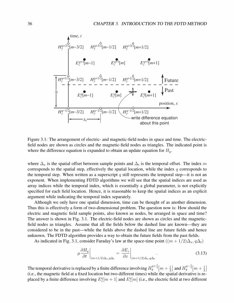
Figure 3.1: The arrangement of electric- and magnetic-field nodes in space and time. The electric-
field nodes are shown as circles and the magnetic-field nodes as triangles. The indicated point is
where the difference equation is expanded to obtain an update equation for Hy.
where ∆x is the spatial offset between sample points and ∆t is the temporal offset. The index mcorresponds to the spatial step, effectively the spatial location, while the index q corresponds to
the temporal step. When written as a superscript q still represents the temporal step—it is not an
exponent. When implementing FDTD algorithms we will see that the spatial indices are used as
array indices while the temporal index, which is essentially a global parameter, is not explicitly
specified for each field location. Hence, it is reasonable to keep the spatial indices as an explicit
argument while indicating the temporal index separately.
Although we only have one spatial dimension, time can be thought of as another dimension.
Thus this is effectively a form of two-dimensional problem. The question now is: How should the
electric and magnetic field sample points, also known as nodes, be arranged in space and time?
The answer is shown in Fig. 3.1. The electric-field nodes are shown as circles and the magnetic-
field nodes as triangles. Assume that all the fields below the dashed line are known—they are
considered to be in the past—while the fields above the dashed line are future fields and hence
unknown. The FDTD algorithm provides a way to obtain the future fields from the past fields.
As indicated in Fig. 3.1, consider Faraday’s law at the space-time point ((m+ 1/2)∆x, q∆t)
µ∂Hy
∂t
∣∣∣∣(m+1/2)∆x,q∆t
=∂Ez
∂x
∣∣∣∣(m+1/2)∆x,q∆t
. (3.13)
The temporal derivative is replaced by a finite difference involving Hq+ 1
2y
[m+ 1
2
]and H
q− 12
y
[m+ 1
2
]
(i.e., the magnetic field at a fixed location but two different times) while the spatial derivative is re-
placed by a finite difference involving Eqz [m+ 1] and Eq
z [m] (i.e., the electric field at two different
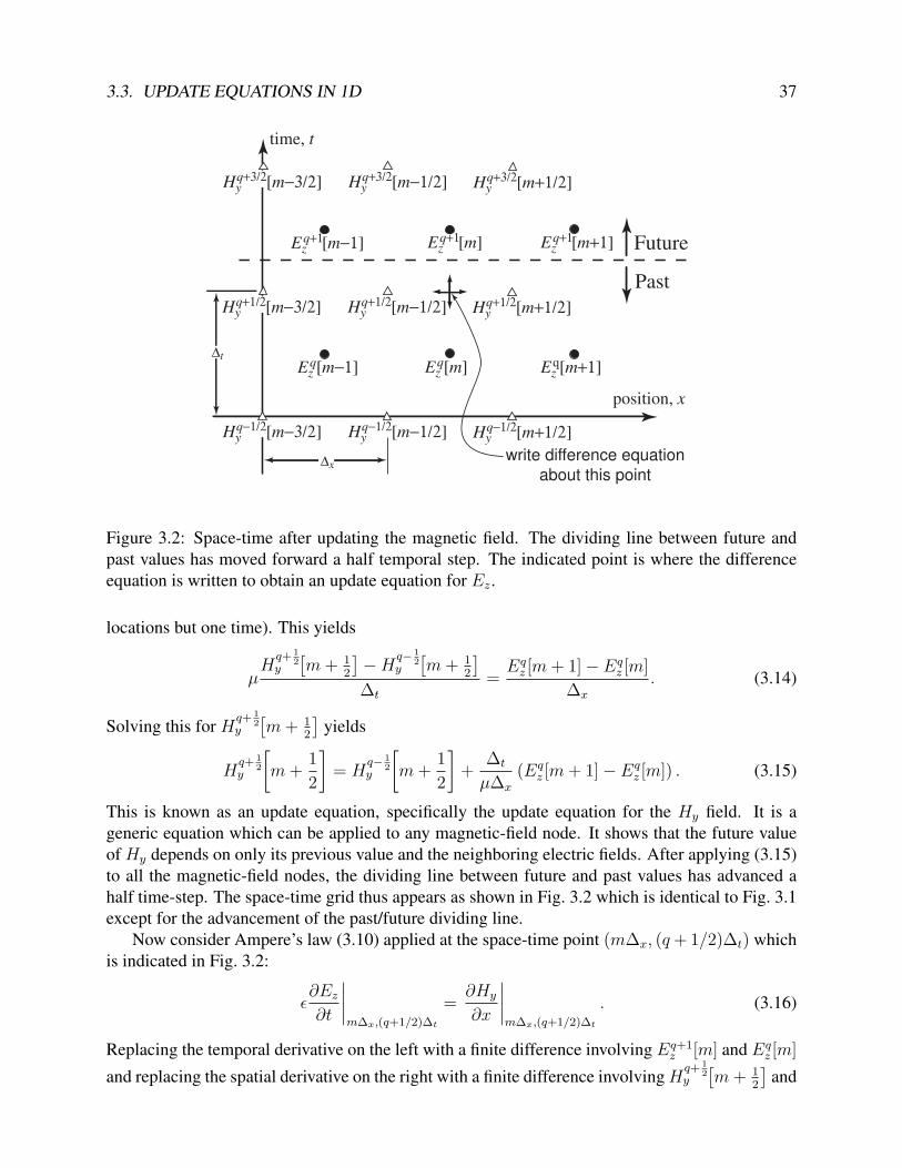
3.3. UPDATE EQUATIONS IN 1D 37
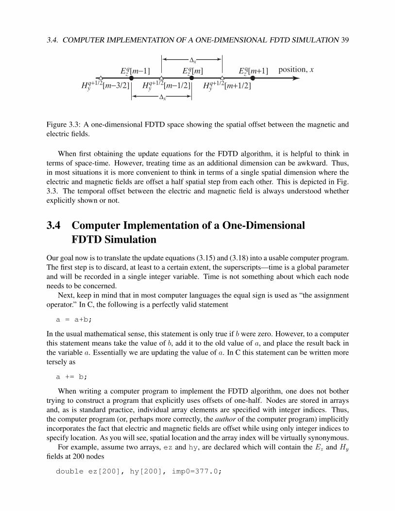
position, x
Future
Past
write difference equation
about this point
Ez [m−1]q+1 Ez [m+1]q+1Ez [m]q+1
Hy [m−1/2]q−1/2 Hy [m+1/2]q−1/2Hy [m−3/2]q−1/2
Hy [m−1/2]q+1/2 Hy [m+1/2]q+1/2Hy [m−3/2]q+1/2
Ez [m−1]q Ez [m]q Ez [m+1]q
time, t
Hy [m−1/2]q+3/2 Hy [m+1/2]q+3/2Hy [m−3/2]q+3/2
∆x
∆t
Figure 3.2: Space-time after updating the magnetic field. The dividing line between future and
past values has moved forward a half temporal step. The indicated point is where the difference
equation is written to obtain an update equation for Ez.
locations but one time). This yields
µH
q+ 12
y
[m+ 1
2
]−H
q− 12
y
[m+ 1
2
]
∆t
=Eq
z [m+ 1]− Eqz [m]
∆x
. (3.14)
Solving this for Hq+ 1
2y
[m+ 1
2
]yields
Hq+ 1
2y
[
m+1
2
]
= Hq− 1
2y
[
m+1
2
]
+∆t
µ∆x
(Eqz [m+ 1]− Eq
z [m]) . (3.15)
This is known as an update equation, specifically the update equation for the Hy field. It is a
generic equation which can be applied to any magnetic-field node. It shows that the future value
of Hy depends on only its previous value and the neighboring electric fields. After applying (3.15)
to all the magnetic-field nodes, the dividing line between future and past values has advanced a
half time-step. The space-time grid thus appears as shown in Fig. 3.2 which is identical to Fig. 3.1
except for the advancement of the past/future dividing line.
Now consider Ampere’s law (3.10) applied at the space-time point (m∆x, (q+ 1/2)∆t) which
is indicated in Fig. 3.2:
ǫ∂Ez
∂t
∣∣∣∣m∆x,(q+1/2)∆t
=∂Hy
∂x
∣∣∣∣m∆x,(q+1/2)∆t
. (3.16)
Replacing the temporal derivative on the left with a finite difference involving Eq+1z [m] and Eq
z [m]
and replacing the spatial derivative on the right with a finite difference involving Hq+ 1
2y
[m+ 1
2
]and
38 CHAPTER 3. INTRODUCTION TO THE FDTD METHOD
Hq+ 1
2y
[m− 1
2
]yields
ǫEq+1
z [m]− Eqz [m]
∆t
=H
q+ 12
y
[m+ 1
2
]−H
q+ 12
y
[m− 1
2
]
∆x
. (3.17)
Solving for Eq+1z [m] yields
Eq+1z [m] = Eq
z [m] +∆t
ǫ∆x
(
Hq+ 1
2y
[
m+1
2
]
−Hq+ 1
2y
[
m− 1
2
])
. (3.18)
Equation (3.18) is the update equation for the Ez field. The indices in this equation are generic so
that the same equation holds for every Ez node. Similar to the update equation for the magnetic
field, here we see that the future value of Ez depends on only its past value and the value of the
neighboring magnetic fields.
After applying (3.18) to every electric-field node in the grid, the dividing line between what
is known and what is unknown moves forward another one-half temporal step. One is essentially
back to the situation depicted in Fig. 3.1—the future fields closest to the dividing line between the
future and past are magnetics fields. They would be updated again, then the electric fields would
be updated, and so on.
It is often convenient to represent the update coefficients ∆t/ǫ∆x and ∆t/µ∆x in terms of the
ratio of how far energy can propagate in a single temporal step to the spatial step. The maximum
speed electromagnetic energy can travel is the speed of light in free space c = 1/√ǫ0µ0 and hence
the maximum distance energy can travel in one time step is c∆t (in all the remaining discussions
the symbol c will be reserved for the speed of light in free space). The ratio c∆t/∆x is often called
the Courant number which we label Sc. It plays an important role in determining the stability of a
simulation (hence the use of S) and will be considered further later. Letting µ = µrµ0 and ǫ = ǫrǫ0,the coefficients in (3.18) and (3.15) can be written
1
ǫ
∆t
∆x
=1
ǫrǫ0
√ǫ0µ0√ǫ0µ0
∆t
∆x
=
√ǫ0µ0
ǫrǫ0
c∆t
∆x
=1
ǫr
õ0
ǫ0
c∆t
∆x
=η0ǫr
c∆t
∆x
=η0ǫrSc (3.19)
1
µ
∆t
∆x
=1
µrµ0
√ǫ0µ0√ǫ0µ0
∆t
∆x
=
√ǫ0µ0
µrµ0
c∆t
∆x
=1
µr
√ǫ0µ0
c∆t
∆x
=1
µrη0
c∆t
∆x
=1
µrη0Sc (3.20)
where η0 =√
µ0/ǫ0 is the characteristic impedance of free space.
In FDTD simulations there are restrictions on how large a temporal step can be. If it is too large,
the algorithm produces unstable results (i.e., the numbers obtained are completely meaningless
and generally tend quickly to infinity). At this stage we will not consider a rigorous analysis of
stability. However, thinking about the way fields propagate in an FDTD grid, it seems logical that
energy should not be able to propagate any further than one spatial step for each temporal step, i.e.,
c∆t ≤ ∆x. This is because in the FDTD algorithm each node only affects its nearest neighbors. In
one complete cycle of updating the fields, the furthest a disturbance could propagate is one spatial
step. It turns out that the optimum ratio for the Courant number (in terms of minimizing numeric
errors) is also the maximum ratio. Hence, for the one-dimensional simulations considered initially,
we will use
Sc =c∆t
∆x
= 1. (3.21)
3.4. COMPUTER IMPLEMENTATION OF A ONE-DIMENSIONAL FDTD SIMULATION 39
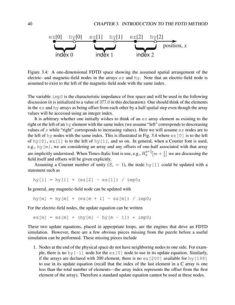
position, x
Hy [m−1/2]q+1/2 Hy [m+1/2]q+1/2Hy [m−3/2]q+1/2
Ez [m−1]q Ez [m]q Ez [m+1]q
∆x
∆x
Figure 3.3: A one-dimensional FDTD space showing the spatial offset between the magnetic and
electric fields.
When first obtaining the update equations for the FDTD algorithm, it is helpful to think in
terms of space-time. However, treating time as an additional dimension can be awkward. Thus,
in most situations it is more convenient to think in terms of a single spatial dimension where the
electric and magnetic fields are offset a half spatial step from each other. This is depicted in Fig.
3.3. The temporal offset between the electric and magnetic field is always understood whether
explicitly shown or not.
3.4 Computer Implementation of a One-Dimensional
FDTD Simulation
Our goal now is to translate the update equations (3.15) and (3.18) into a usable computer program.
The first step is to discard, at least to a certain extent, the superscripts—time is a global parameter
and will be recorded in a single integer variable. Time is not something about which each node
needs to be concerned.
Next, keep in mind that in most computer languages the equal sign is used as “the assignment
operator.” In C, the following is a perfectly valid statement
a = a+b;
In the usual mathematical sense, this statement is only true if b were zero. However, to a computer
this statement means take the value of b, add it to the old value of a, and place the result back in
the variable a. Essentially we are updating the value of a. In C this statement can be written more
tersely as
a += b;
When writing a computer program to implement the FDTD algorithm, one does not bother
trying to construct a program that explicitly uses offsets of one-half. Nodes are stored in arrays
and, as is standard practice, individual array elements are specified with integer indices. Thus,
the computer program (or, perhaps more correctly, the author of the computer program) implicitly
incorporates the fact that electric and magnetic fields are offset while using only integer indices to
specify location. As you will see, spatial location and the array index will be virtually synonymous.
For example, assume two arrays, ez and hy, are declared which will contain the Ez and Hy
fields at 200 nodes
double ez[200], hy[200], imp0=377.0;
40 CHAPTER 3. INTRODUCTION TO THE FDTD METHOD
position, x
ez[0] hy[0] ez[2]ez[1] hy[2]hy[1]
{ {{index 0 index 2index 1
Figure 3.4: A one-dimensional FDTD space showing the assumed spatial arrangement of the
electric- and magnetic-field nodes in the arrays ez and hy. Note that an electric-field node is
assumed to exist to the left of the magnetic-field node with the same index.
The variable imp0 is the characteristic impedance of free space and will be used in the following
discussion (it is initialized to a value of 377.0 in this declaration). One should think of the elements
in the ez and hy arrays as being offset from each other by a half spatial step even though the array
values will be accessed using an integer index.
It is arbitrary whether one initially wishes to think of an ez array element as existing to the
right or the left of an hy element with the same index (we assume “left” corresponds to descreasing
values of x while “right” corresponds to increasing values). Here we will assume ez nodes are to
the left of hy nodes with the same index. This is illustrated in Fig. 3.4 where ez[0] is to the left
of hy[0], ez[1] is to the left of hy[1], and so on. In general, when a Courier font is used,
e.g., hy[m], we are considering an array and any offsets of one-half associated with that array
are implicitly understood. When Times-Italic font is use, e.g., Hq+ 1
2y
[m+ 1
2
]we are discussing the
field itself and offsets will be given explicitly.
Assuming a Courant number of unity (Sc = 1), the node hy[1] could be updated with a
statement such as
hy[1] = hy[1] + (ez[2] - ez[1]) / imp0;
In general, any magnetic-field node can be updated with
hy[m] = hy[m] + (ez[m + 1] - ez[m]) / imp0;
For the electric-field nodes, the update equation can be written
ez[m] = ez[m] + (hy[m] - hy[m - 1]) * imp0;
These two update equations, placed in appropriate loops, are the engines that drive an FDTD
simulation. However, there are a few obvious pieces missing from the puzzle before a useful
simulation can be performed. These missing pieces include
1. Nodes at the end of the physical space do not have neighboring nodes to one side. For exam-
ple, there is no hy[-1] node for the ez[0] node to use in its update equation. Similarly,
if the arrays are declared with 200 element, there is no ez[200] available for hy[199]
to use in its update equation (recall that the index of the last element in a C array is one
less than the total number of elements—the array index represents the offset from the first
element of the array). Therefore a standard update equation cannot be used at these nodes.

3.5. BARE-BONES SIMULATION 41
2. Only a constant impedance is used so only a homogeneous medium can be modeled (in this
case free space).
3. As of yet there is no energy present in the field. If the fields are initially zero, they will
remain zero forever.
The first issue can be addressed using absorbing boundary conditions (ABC’s). There are
numerous implementations one can use. In later material we will be consider only a few of the
more popular techniques.
The second restriction can be removed by allowing the permittivity and permeability to change
from node to node. However, in the interest of simplicity, we will continue to use a constant
impedance for a little while longer.
The third problem can be overcome by initializing the fields to a non-zero state. However, this
is cumbersome and typically not a good approach. Better solutions are to introduce energy via
either a hardwired source, an additive source, or a total-field/scattered-field (TFSF) boundary. We
will consider implementation of each of these approaches.
3.5 Bare-Bones Simulation
Let us consider a simulation of a wave propagating in free space where there are 200 electric- and
magnetic-field nodes. The code is shown in Program 3.1.
Program 3.1 1DbareBones.c: Bare-bones one-dimensional simulation with a hard source.
1 /* Bare-bones 1D FDTD simulation with a hard source. */
2
3 #include <stdio.h>
4 #include <math.h>
5
6 #define SIZE 200
7
8 int main()
9 {
10 double ez[SIZE] = {0.}, hy[SIZE] = {0.}, imp0 = 377.0;
11 int qTime, maxTime = 250, mm;
12
13 /* do time stepping */
14 for (qTime = 0; qTime < maxTime; qTime++) {
15
16 /* update magnetic field */
17 for (mm = 0; mm < SIZE - 1; mm++)
18 hy[mm] = hy[mm] + (ez[mm + 1] - ez[mm]) / imp0;
19
20 /* update electric field */
21 for (mm = 1; mm < SIZE; mm++)
42 CHAPTER 3. INTRODUCTION TO THE FDTD METHOD
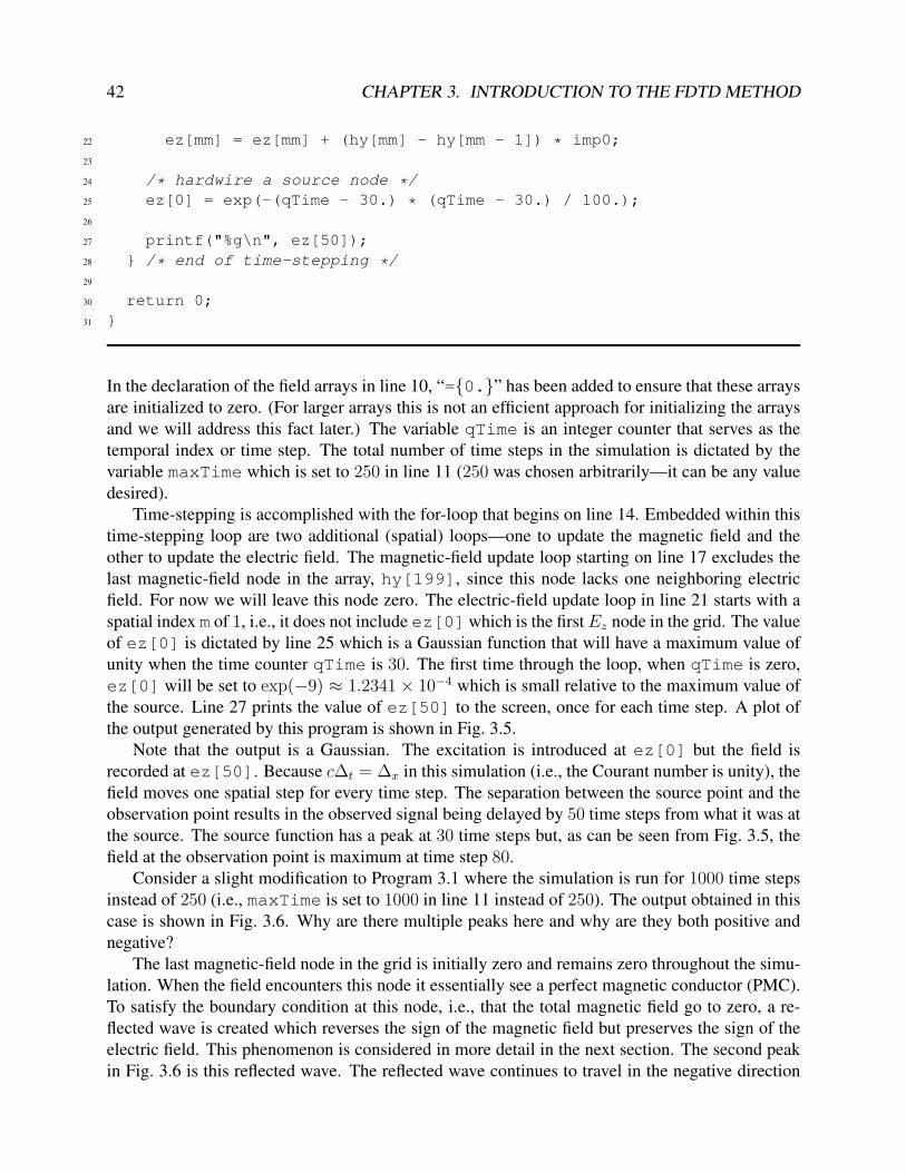
22 ez[mm] = ez[mm] + (hy[mm] - hy[mm - 1]) * imp0;
23
24 /* hardwire a source node */
25 ez[0] = exp(-(qTime - 30.) * (qTime - 30.) / 100.);
26
27 printf("%g\n", ez[50]);
28 } /* end of time-stepping */
29
30 return 0;
31 }
In the declaration of the field arrays in line 10, “={0.}” has been added to ensure that these arrays
are initialized to zero. (For larger arrays this is not an efficient approach for initializing the arrays
and we will address this fact later.) The variable qTime is an integer counter that serves as the
temporal index or time step. The total number of time steps in the simulation is dictated by the
variable maxTime which is set to 250 in line 11 (250 was chosen arbitrarily—it can be any value
desired).
Time-stepping is accomplished with the for-loop that begins on line 14. Embedded within this
time-stepping loop are two additional (spatial) loops—one to update the magnetic field and the
other to update the electric field. The magnetic-field update loop starting on line 17 excludes the
last magnetic-field node in the array, hy[199], since this node lacks one neighboring electric
field. For now we will leave this node zero. The electric-field update loop in line 21 starts with a
spatial index m of 1, i.e., it does not include ez[0]which is the first Ez node in the grid. The value
of ez[0] is dictated by line 25 which is a Gaussian function that will have a maximum value of
unity when the time counter qTime is 30. The first time through the loop, when qTime is zero,
ez[0] will be set to exp(−9) ≈ 1.2341× 10⁻⁴ which is small relative to the maximum value of
the source. Line 27 prints the value of ez[50] to the screen, once for each time step. A plot of
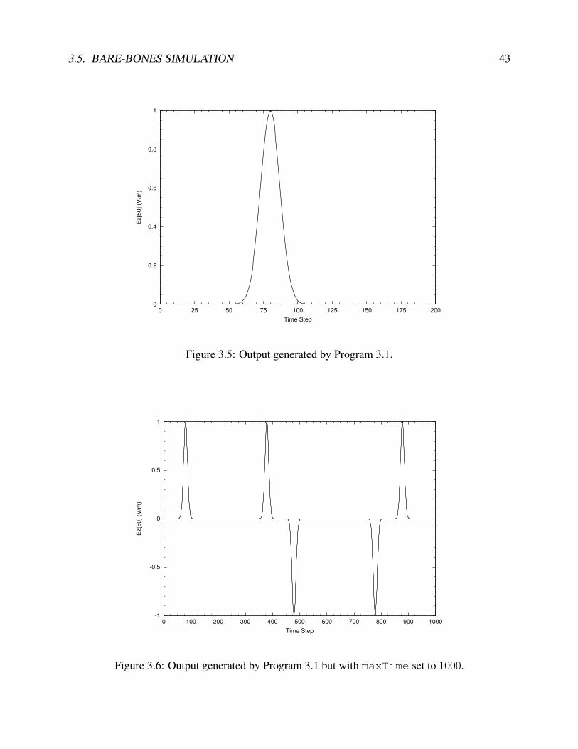
the output generated by this program is shown in Fig. 3.5.
Note that the output is a Gaussian. The excitation is introduced at ez[0] but the field is
recorded at ez[50]. Because c∆t = ∆x in this simulation (i.e., the Courant number is unity), the
field moves one spatial step for every time step. The separation between the source point and the
observation point results in the observed signal being delayed by 50 time steps from what it was at
the source. The source function has a peak at 30 time steps but, as can be seen from Fig. 3.5, the
field at the observation point is maximum at time step 80.
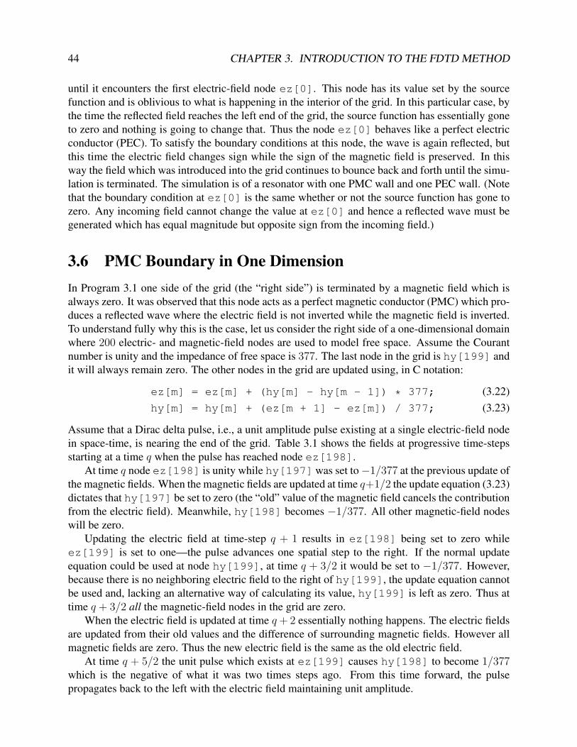
Consider a slight modification to Program 3.1 where the simulation is run for 1000 time steps
instead of 250 (i.e., maxTime is set to 1000 in line 11 instead of 250). The output obtained in this
case is shown in Fig. 3.6. Why are there multiple peaks here and why are they both positive and
negative?
The last magnetic-field node in the grid is initially zero and remains zero throughout the simu-
lation. When the field encounters this node it essentially see a perfect magnetic conductor (PMC).
To satisfy the boundary condition at this node, i.e., that the total magnetic field go to zero, a re-
flected wave is created which reverses the sign of the magnetic field but preserves the sign of the
electric field. This phenomenon is considered in more detail in the next section. The second peak
in Fig. 3.6 is this reflected wave. The reflected wave continues to travel in the negative direction
3.5. BARE-BONES SIMULATION 43
0
0.2
0.4
0.6
0.8
1
0 25 50 75 100 125 150 175 200
Ez[5
0] (V
/m)
Time Step
Figure 3.5: Output generated by Program 3.1.
-1
-0.5
0
0.5
1
0 100 200 300 400 500 600 700 800 900 1000
Ez[5
0] (V
/m)
Time Step
Figure 3.6: Output generated by Program 3.1 but with maxTime set to 1000.
44 CHAPTER 3. INTRODUCTION TO THE FDTD METHOD
until it encounters the first electric-field node ez[0]. This node has its value set by the source
function and is oblivious to what is happening in the interior of the grid. In this particular case, by
the time the reflected field reaches the left end of the grid, the source function has essentially gone
to zero and nothing is going to change that. Thus the node ez[0] behaves like a perfect electric
conductor (PEC). To satisfy the boundary conditions at this node, the wave is again reflected, but
this time the electric field changes sign while the sign of the magnetic field is preserved. In this
way the field which was introduced into the grid continues to bounce back and forth until the simu-
lation is terminated. The simulation is of a resonator with one PMC wall and one PEC wall. (Note
that the boundary condition at ez[0] is the same whether or not the source function has gone to
zero. Any incoming field cannot change the value at ez[0] and hence a reflected wave must be
generated which has equal magnitude but opposite sign from the incoming field.)
3.6 PMC Boundary in One Dimension
In Program 3.1 one side of the grid (the “right side”) is terminated by a magnetic field which is
always zero. It was observed that this node acts as a perfect magnetic conductor (PMC) which pro-
duces a reflected wave where the electric field is not inverted while the magnetic field is inverted.
To understand fully why this is the case, let us consider the right side of a one-dimensional domain
where 200 electric- and magnetic-field nodes are used to model free space. Assume the Courant
number is unity and the impedance of free space is 377. The last node in the grid is hy[199] and
it will always remain zero. The other nodes in the grid are updated using, in C notation:
ez[m] = ez[m] + (hy[m] - hy[m - 1]) * 377; (3.22)
hy[m] = hy[m] + (ez[m + 1] - ez[m]) / 377; (3.23)
Assume that a Dirac delta pulse, i.e., a unit amplitude pulse existing at a single electric-field node
in space-time, is nearing the end of the grid. Table 3.1 shows the fields at progressive time-steps
starting at a time q when the pulse has reached node ez[198].
At time q node ez[198] is unity while hy[197] was set to −1/377 at the previous update of
the magnetic fields. When the magnetic fields are updated at time q+1/2 the update equation (3.23)
dictates that hy[197] be set to zero (the “old” value of the magnetic field cancels the contribution
from the electric field). Meanwhile, hy[198] becomes −1/377. All other magnetic-field nodes
will be zero.
Updating the electric field at time-step q + 1 results in ez[198] being set to zero while
ez[199] is set to one—the pulse advances one spatial step to the right. If the normal update
equation could be used at node hy[199], at time q + 3/2 it would be set to −1/377. However,
because there is no neighboring electric field to the right of hy[199], the update equation cannot
be used and, lacking an alternative way of calculating its value, hy[199] is left as zero. Thus at
time q + 3/2 all the magnetic-field nodes in the grid are zero.
When the electric field is updated at time q+ 2 essentially nothing happens. The electric fields
are updated from their old values and the difference of surrounding magnetic fields. However all
magnetic fields are zero. Thus the new electric field is the same as the old electric field.
At time q + 5/2 the unit pulse which exists at ez[199] causes hy[198] to become 1/377which is the negative of what it was two times steps ago. From this time forward, the pulse
propagates back to the left with the electric field maintaining unit amplitude.

3.7. SNAPSHOTS OF THE FIELD 45
time
step
node
ez[197] hy[197] ez[198] hy[198] ez[199] hy[199]
q − 1/2 −1/377 0 0q 0 1 0q + 1/2 0 −1/377 0q + 1 0 0 1q + 3/2 0 0 0q + 2 0 0 1q + 5/2 0 1/377 0q + 3 0 1 0q + 5/2 1/377 0 0q + 4 1 0 0
Table 3.1: Electric- and magnetic-field nodes at the “end” of arrays which have 200 elements, i.e.,
the last node is hy[199] which is always set to zero. A pulse of unit amplitude is propagating
to the right and has arrived at ez[198] at time-step q. Time is advancing as one reads down the
columns.
This discussion is for a single pulse, but any incident field could be treated as a string of pulses
and then one would merely have to superimpose their values. This dicussion further supposes the
Courant number is unity. When the Courant number is not unity the termination of the grid still
behaves as a PMC wall, but the pulse will not propagate without distortion (it suffers dispersion
because of the properties of the grid itself as will be discussed in more detail in Sec. 7.4).
If the grid were terminated on an electric-field node which was always set to zero, that node
would behave as a perfect electric conductor. In that case the reflected electric field would have
the opposite sign from the incident field while the magnetic field would preserve its sign. This is
what happens to any field incident on the left side of the grid in Program 3.1.
3.7 Snapshots of the Field
In Program 3.1 the field at a single point is recorded to a file. Alternatively, it is often useful to view
the fields over the entire computational domain at a single instant of time, i.e., take a “snapshot”
that shows the field throughout space. Here we describe one way in which this can be conveniently
implemented in C.
The approach adopted here will open a separate file for each snapshot. Each file will have a
common base name, then a dot, and then a sequence number which will be called the frame number.
So, for example, the files might be called sim.0, sim.1, sim.2, and so on. To accomplish this,
the fragments shown in Fragments 3.2 and 3.3 would be added to a program (such as Program
3.1).
Fragment 3.2 Declaration of variables associated with taking snapshots. The base name is stored
in the character array basename and the complete file name for each frame is stored in filename.
Here the base name is initialized to sim but, if desired, the user could be prompted for the base
46 CHAPTER 3. INTRODUCTION TO THE FDTD METHOD
name. The integer frame is the frame number for each snapshot and is initialized to zero.
1 char basename[80] = "sim", filename[100];
2 int frame = 0;
3 FILE *snapshot;
Fragment 3.3 Code to generate the snapshots. This would be placed inside the time-stepping
loop. The initial if statement ensures the electric field is recorded every tenth time-step.
1 /* write snapshot if time-step is a multiple of 10 */
2 if (qTime % 10 == 0) {
3 /* construct complete file name and increment frame counter */
4 sprintf(filename, "%s.%d", basename, frame++);
5
6 /* open file */
7 snapshot = fopen(filename, "w");
8
9 /* write data to file */
10 for (mm = 0; mm < SIZE; mm++)
11 fprintf(snapshot, "%g\n", ez[mm]);
12
13 /* close file */
14 fclose(snapshot);
15 }
In Fragment 3.2 the base name is initialized to sim but the user could be prompted for this.
The integer variable frame is the frame (or snapshot) counter that will be incremented each time
a snapshot is taken. It is initialized to zero. The file pointer snapshot is used for the output files.
The code shown in Fragment 3.3 would be placed inside the time-stepping loop of Program
3.1. Line 2 checks, using the modulo operator (%) if the time step is a multiple of 10. (10 was
chosen somewhat arbitrarily. If snapshots were desired more frequently, a smaller value would be
used. If snapshots were desired less frequently, a larger value would be used.) If the time step is
a multiple of 10, the complete output-file name is constructed in line 4 by writing the file name
to the string variable filename. (Since zero is a multiple of 10, the first snapshot that is taken
corresponds to the fields at time zero. This data would be written to the file sim.0. Note that in
Line 4 the frame number is incremented each time a file name is created. The file is opened in line
7 and the data is written using the loop starting in line 10. Finally, the file is closed in line 14.
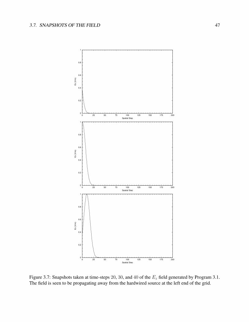
Fig. 3.7 shows the snapshots of the field at time steps 20, 30, and 40 using essentially the same
code as Program 3.1—the only difference being the addition of the code to take the snapshots.
The corresponding files are sim.2, sim.3, and sim.4. In these snapshots the field can be seen
entering the computational domain from the left and propagating to the right.
3.7. SNAPSHOTS OF THE FIELD 47
0
0.2
0.4
0.6
0.8
1
0 25 50 75 100 125 150 175 200
Ez (
V/m
)
Spatial Step
0
0.2
0.4
0.6
0.8
1
0 25 50 75 100 125 150 175 200
Ez (
V/m
)
Spatial Step
0
0.2
0.4
0.6
0.8
1
0 25 50 75 100 125 150 175 200
Ez (
V/m
)
Spatial Step
Figure 3.7: Snapshots taken at time-steps 20, 30, and 40 of the Ez field generated by Program 3.1.
The field is seen to be propagating away from the hardwired source at the left end of the grid.
48 CHAPTER 3. INTRODUCTION TO THE FDTD METHOD
3.8 Additive Source
Hardwiring the source, as was done in Program 3.1, has the severe shortcoming that no energy can
pass through the source node. This problem can be rectified by using an additive source. Consider
Ampere’s law with the current density term:
∇×H = J+ ǫ∂E
∂t. (3.24)
The current density J can represent both the conduction current due to flow of charge in a material
under the influence of the electric field, i.e., current given by σE, as well as the current associated
with any source, i.e., an “impressed current.” At this point we are just interested in the source
aspect of J and will return to the issue of finite conductivity in Sec. 3.12 and Sec. 5.7. Rearranging
(3.24) slightly yields∂E
∂t=
1
ǫ∇×H− 1
ǫJ. (3.25)
This equation gives the temporal derivative of the electric field in terms of the spatial derivative
of the magnetic field—which is as before—and an additional term which can be thought of as the
forcing function for the system. This current can be specified to be whatever is desired.
To translate (3.25) into a form suitable for the FDTD algorithm, the spatial derivatives are again
expressed in terms of finite differences and then one solves for the future fields in terms of past
fields. Recall that for Ampere’s law, the update equation for Eqz [m] was obtained by applying finite
differences at the space-time point (m∆x, (q + 1/2)∆t). Going through the exact same procedure
but adding the source term yields
Eq+1z [m] = Eq
z [m] +∆t
ǫ∆x
(
Hq+ 1
2y
[
m+1
2
]
−Hq+ 1
2y
[
m− 1
2
])
− ∆t
ǫJq+ 1
2z [m] . (3.26)
The source current could potentially be distributed over a number of nodes, but for the sake of
introducing energy to the grid, it suffices to apply it to a single node.
In order to preserve the original update equation (which is sometimes handy when writing
loops), (3.26) can be separated into two steps: first the usual update is applied and then the source
term is added. For example:
Eq+1z [m] = Eq
z [m] +∆t
ǫ∆x
(
Hq+ 1
2y
[
m+1
2
]
−Hq+ 1
2y
[
m− 1
2
])
(3.27)
Eq+1z [m] = Eq+1
z [m]− ∆t
ǫJq+ 1
2z [m] . (3.28)
In practice the source current might only exist at a single node in the 1D grid (as will be the case
in the examples to come). Thus, (3.28) would be applied only at the node where the source current
is non-zero.
Generally the amplitude and the sign of the source function are not a concern. When calculating
things such as the scattering cross-section or the reflection coefficient, one always normalizes by
the incident field. Therefore we do not need to specify explicitly the value of ∆t/ǫ in (3.28)—it
suffices to merely treat this coefficient as being contained in the source function itself.
A program that implements an additive source and takes snapshots of the electric field is shown
in Program 3.4. The changes from Program 3.1 are shown in bold. The source function is exactly

3.8. ADDITIVE SOURCE 49
the same as before except now, instead of setting the value of ez[0] to the value of this function,
the source function is added to ez[50]. The source is introduced in line 29 and the update
equations are unchanged from before. (Note that in this chapter the programs will be somewhat
verbose, simplistic, and repetitive. Once we are comfortable with the FDTD algorithm we will pay
more attention to better coding practices.)
Program 3.4 1Dadditive.c: One-dimensional FDTD program with an additive source.
1 /* 1D FDTD simulation with an additive source. */
2
3 #include <stdio.h>
4 #include <math.h>
5
6 #define SIZE 200
7
8 int main()
9 {
10 double ez[SIZE] = {0.}, hy[SIZE] = {0.}, imp0 = 377.0;
11 int qTime, maxTime = 200, mm;
12
13 char basename[80] = "sim", filename[100];
14 int frame = 0;
15 FILE *snapshot;
16
17 /* do time stepping */
18 for (qTime = 0; qTime < maxTime; qTime++) {
19
20 /* update magnetic field */
21 for (mm = 0; mm < SIZE - 1; mm++)
22 hy[mm] = hy[mm] + (ez[mm + 1] - ez[mm]) / imp0;
23
24 /* update electric field */
25 for (mm = 1; mm < SIZE; mm++)
26 ez[mm] = ez[mm] + (hy[mm] - hy[mm - 1]) * imp0;
27
28 /* use additive source at node 50 */
29 ez[50] += exp(-(qTime - 30.) * (qTime - 30.) / 100.);
30
31 /* write snapshot if time a multiple of 10 */
32 if (qTime % 10 == 0) {
33 sprintf(filename, "%s.%d", basename, frame++);
34 snapshot=fopen(filename, "w");
35 for (mm = 0; mm < SIZE; mm++)
36 fprintf(snapshot, "%g\n", ez[mm]);
37 fclose(snapshot);
38 }
50 CHAPTER 3. INTRODUCTION TO THE FDTD METHOD
39 } /* end of time-stepping */
40
41 return 0;
42 }
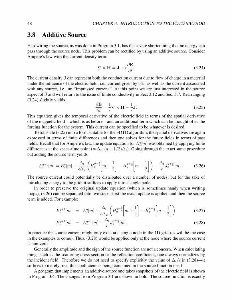
Snapshots of Ez taken at time-steps 20, 30, and 40 are shown in Fig. 3.8. Note that the field
originates from node 50 and that it propagates to either side of this node. Also notice that the peak
amplitude is half of what it was when the source function was implemented as a hardwired source.
As something of an aside, in Program 3.4 note that the code that takes a snapshot of the electric
field was placed in the time-stepping but after the update equation. Thus one might ask: do the
contents of snapshot file sim.0 contain the fields at time zero or at time one? And, do the other
snapshots correspond to times that multiples of 10 or do the correspond to one plus a multiple of
10? In nearly all practical cases it won’t matter. The precise location of t = 0 is rather aribtrary. So,
when looking at the snapshots it is usually sufficient to know that the sequence of snapshots start
“at the beginning of the simulation” and then are taken every 10 time steps. However, if one wants
to be more precise about this, absolute time is usually dictated by the source function. Now, think
in terms of the hard-source implementation rather than the additive source. We have implemented
a Gaussian source that has a peak amplitude at time-step 30. The way the code is written here,
with the source being applied after the update equation and then the snapshot being taken last, we
would see the peak at the source node in frame sim.1. In other words the snapshots do indeed
correspond to times that are multiples of 10. So, in some sense the electric fields start at a time step
of −1. The very first update update loop takes them up to time step 0, and then the source function
is applied to set the field at the source node at time-step 0. However, this is truly a minor point
and we will not worry about it in subsequent discussions. Whether the code that introduces the
source appears before or after the update loop and whether the code that generates output appears
before or after the update loop, often doesn’t matter—the important thing is generally just that
these things are included in the time-stepping loop.
3.9 Terminating the Grid
In most instances one is interested in modeling a problem which exists in an open domain, i.e.,
an infinite space. This is true even when the specific region of interest, say the region where a
scatterer is present, may be small. That scatterer is in an unbounded space. Thus far the code we
have written is only suitable for modeling a resonator since the nodes at the ends of the grid reflect
any field incident upon them. We now wish to rectify this shortcoming. Absorbing boundary
conditions (ABC’s) will be used so that the grid, which will contain only a finite number of nodes,
can behave as if it were infinite. In one dimension, when operating at the Courant limit of one, an
exact ABC can be realized. Unfortunately in higher dimensions, or even in one dimension when
not operating at the Courant limit, ABC’s are only approximate. The better the ABC, the less
energy it reflects back into the interior of the grid.
Before implementing an ABC, let us again consider the code shown in Program 3.4 but with
the maximum number of time steps set to 450. With the FDTD method, the more ways in which

3.9. TERMINATING THE GRID 51
0
0.2
0.4
0.6
0.8
1
0 25 50 75 100 125 150 175 200
Ez (
V/m
)
Spatial Step
0
0.2
0.4
0.6
0.8
1
0 25 50 75 100 125 150 175 200
Ez (
V/m
)
Spatial Step
0
0.2
0.4
0.6
0.8
1
0 25 50 75 100 125 150 175 200
Ez (
V/m
)
Spatial Step
Figure 3.8: Snapshots taken at time-steps 20, 30, and 40 of the Ez field generated by Program 3.4.
An additive source is applied to node 50 and the field is seen to propagate away from it to either
side.
52 CHAPTER 3. INTRODUCTION TO THE FDTD METHOD
0 20 40 60 80 100 120 140 160 180 2000
5
10
15
20
25
30
35
40
45
Space [spatial index]
Tim
e [
fra
me
nu
mb
er]
Figure 3.9: Waterfall plot of the electric field produced by Program 3.4. The computational domain
has 200 nodes with a PEC boundary on the left and a PMC boundary on the right. The vertical axis
gives the frame number. Snapshots, i.e., frames, were recorded every 10 time steps.
the field can be visualized, the better. Watching the field propagate in the time-domain can provide
insights into the behavior of a system. Additionally, visualization of the propagation of the fields
can be an invaluable aid when debugging FDTD code. Animations of the field are especially useful
and different display strategies will be discussed later.
Since we cannot include an animation here, we will use a “waterfall plot” of the electric field
in the one-dimensional domain. A waterfall plot is a collection of standard “x vs. y” plots where
each plot is offset slightly from the next (a direct vertical offset will be used here). This can be
thought of as stacking all the frames of an animation, one above the next.
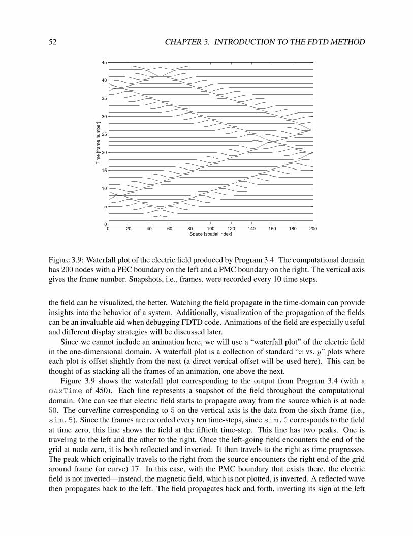
Figure 3.9 shows the waterfall plot corresponding to the output from Program 3.4 (with a
maxTime of 450). Each line represents a snapshot of the field throughout the computational
domain. One can see that electric field starts to propagate away from the source which is at node
50. The curve/line corresponding to 5 on the vertical axis is the data from the sixth frame (i.e.,
sim.5). Since the frames are recorded every ten time-steps, since sim.0 corresponds to the field
at time zero, this line shows the field at the fiftieth time-step. This line has two peaks. One is
traveling to the left and the other to the right. Once the left-going field encounters the end of the
grid at node zero, it is both reflected and inverted. It then travels to the right as time progresses.
The peak which originally travels to the right from the source encounters the right end of the grid
around frame (or curve) 17. In this case, with the PMC boundary that exists there, the electric
field is not inverted—instead, the magnetic field, which is not plotted, is inverted. A reflected wave
then propagates back to the left. The field propagates back and forth, inverting its sign at the left

3.10. TOTAL-FIELD/SCATTERED-FIELD BOUNDARY 53
boundary and preserving its sign at the right boundary, until the simulation is halted. The Matlab
code that was used to generate this waterfall plot is given in Appendix B. Additionally, Appendix
B provides Matlab code that can be used to animate snapshots of a one-dimensional domain.
Returning to the issue of grid termination, when the Courant number is unity, the distance the
wave travels in one temporal step is equal to one spatial step, i.e., c∆t = ∆x. We are interested in
modeling an open domain where there is no energy entering the grid “from the outside.” Therefore,
for node ez[0], its updated value should just be the previous value that existed at ez[1]. Since
no energy is entering the grid from the left, the field at ez[1] must be propagating solely to
the left. At the next time step the value that was at ez[1] should now appear at ez[0]. Similar
arguments hold at the other end of the grid. The updated value of hy[199] should be the previous
value of hy[198].
Thus, a simple ABC can be realized by adding the following line to Program 3.4 between lines
23 and 24
ez[0] = ez[1];
Similarly, the following line would be added between lines 19 and 20
hy[SIZE-1] = hy[SIZE-2];
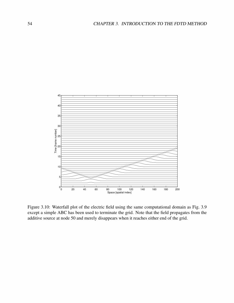
The waterfall plot which is obtained for the electric field after making these changes is shown in
Fig. 3.10. Note that the reflected fields are no longer present. The left- and right-going pulses reach
the end of the grid and then disappear as if they have continued to propagate off to infinity. (How-
ever, there is still some persistent field that lingers throughout the grid. This field is small—about
five orders of magnitude smaller than the peak when using single precision—and is a consequence
of finite precision. These small fields are not visible on the scale of the plot and are not of much
practical concern since typically other sources of error will be far larger.)
As mentioned previously, this simple ABC only works in limited situations. However, the basic
premise is employed in many of the more complicated ABC’s: the future value of the field at the
end of the grid depends on some combination of the past and interior fields. We will return to this
topic in Chap. 6.
3.10 Total-Field/Scattered-Field Boundary
Note that any function f(ξ) which is twice differentiable is a solution to the wave equation. In
one dimension all that is required is that the argument ξ be replaced by t ± x/c. A proof was
given in Sec. 2.16. Thus far the excitation of the FDTD grids has occurred at a point—either the
hardwired source at the left end of the grid, as shown in Program 3.1, or the additive source at
node 50, as shown in Program 3.4. Now our goal is to construct a source such that the excitation
only propagates in one direction, i.e., the source introduces an incident field that is propagating
to the right (the positive x direction). We will accomplish this using what is know as a total-
field/scattered-field (TFSF) boundary.
We start by specifying the incident field as a function of space and time. A Gaussian pulse has
been used for the excitation in the previous examples. A Gaussian can still be used to specify the
54 CHAPTER 3. INTRODUCTION TO THE FDTD METHOD
0 20 40 60 80 100 120 140 160 180 2000
5
10
15
20
25
30
35
40
45
Space [spatial index]
Tim
e [
fra
me
nu
mb
er]
Figure 3.10: Waterfall plot of the electric field using the same computational domain as Fig. 3.9
except a simple ABC has been used to terminate the grid. Note that the field propagates from the
additive source at node 50 and merely disappears when it reaches either end of the grid.

3.10. TOTAL-FIELD/SCATTERED-FIELD BOUNDARY 55
excitation, but to obtain a wave propagating to the right, the argument should be t− x/c instead of
merely t. Previously the source was given by
f(t) = f(q∆t) = e−
(
q∆t−30∆t10∆t
)2
= e−(q−3010 )
2
= f [q] (3.29)
where 30∆t is a delay and the term in the denominator of the exponent (10∆t) controls the width of
the pulse. Note that the time-step width ∆t can be canceled from the numerator and denominator
of the exponent.
For the propagating incident field, t in (3.29) is replaced with t−x/c. In discretized space-time
this argument is given by
t− x
c= q∆t −
m∆x
c=
(
q − m∆x
c∆t
)
∆t = (q −m)∆t (3.30)
where the assumption that the Courant number c∆t/∆x is unity has been used to write the last
equality. This expression can now be used for the argument in the previous source function to
obtain a propagating wave which we will identify as E incz
E incz [m, q] = e
−
(
(q−m)∆t−30∆t10∆t
)2
= e−((q−m)−30
10 )2
(3.31)
This equation essentially assumes that the origin, i.e., the point x = 0, corresponds to the index
m = 0. However, the origin can be shifted to a different point and this fact will be exploited
later. Keep in mind that there is nothing that dictates that we must always think of the origin as
corresponding to the left-most point in the grid.
The corresponding magnetic field is obtained by dividing the electric field by the characteristic
impedance. Additionally, to ensure that Eincz × H
incy points in the desired direction of travel, the
magnetic field must be negative, i.e.,
H incy [m, q] = −
√ǫ
µE inc
z [m, q] = −1
ηe−(
(q−m)−3010 )
2
(3.32)
where η =√
µ/ǫ is the characteristic impedance of the medium. Note that the arguments do not
need to be integers. If one needs to calculate the magnetic field at the position m − 1/2 and time
q − 1/2, these are perfectly legitimate arguments.
In the total-field/scattered-field (TFSF) formulation, the computational domain is divided into
two regions: (1) the total-field region which contains the incident field plus any scattered field and
(2) the scattered-field region which contains only scattered field. The incident field is introduced
on an fictitious seam, or boundary, between the total-field and the scattered-field regions. The
location of this boundary is somewhat arbitrary, but it is typically placed so that any scatterers are
contained in the total-field region.
When updating the fields, the update equations must be consistent. This is to say only scattered
fields should be used to update a node in the scattered-field region and only total fields should be
used to update a node in the total-field region. Figure 3.11 shows a one-dimensional grid where the
TFSF boundary is assumed to exist between nodes Hy
[49 + 1
2
]and Ez[50] (in Fig. 3.11 the nodes
are shown in the computer-array form with integer indices). The node Hy
[49 + 1
2
]is equivalent
to Hy
[50− 1
2
]and will be written using the latter form in the following discussion. Note that
56 CHAPTER 3. INTRODUCTION TO THE FDTD METHOD
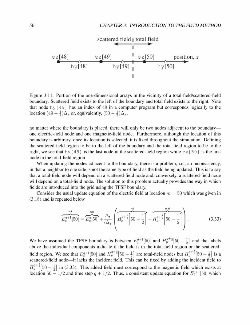
position, xez[48]
hy[48]
ez[50]ez[49]
hy[50]hy[49]
total fieldscattered field
Figure 3.11: Portion of the one-dimensional arrays in the vicinity of a total-field/scattered-field
boundary. Scattered field exists to the left of the boundary and total field exists to the right. Note
that node hy[49] has an index of 49 in a computer program but corresponds logically to the
location (49 + 12)∆x or, equivalently, (50− 1
2)∆x.
no matter where the boundary is placed, there will only be two nodes adjacent to the boundary—
one electric-field node and one magnetic-field node. Furthermore, although the location of this
boundary is arbitrary, once its location is selected, it is fixed throughout the simulation. Defining
the scattered-field region to be to the left of the boundary and the total-field region to be to the
right, we see that hy[49] is the last node in the scattered-field region while ez[50] is the first
node in the total-field region.
When updating the nodes adjacent to the boundary, there is a problem, i.e., an inconsistency,
in that a neighbor to one side is not the same type of field as the field being updated. This is to say
that a total-field node will depend on a scattered-field node and, conversely, a scattered-field node
will depend on a total-field node. The solution to this problem actually provides the way in which
fields are introduced into the grid using the TFSF boundary.
Consider the usual update equation of the electric field at location m = 50 which was given in
(3.18) and is repeated below
tot︷ ︸︸ ︷
Eq+1z [50] =
tot︷ ︸︸ ︷
Eqz [50] +
∆t
ǫ∆x
tot︷ ︸︸ ︷
Hq+ 1
2y
[
50 +1
2
]
−
scat︷ ︸︸ ︷
Hq+ 1
2y
[
50− 1
2
]
. (3.33)
We have assumed the TFSF boundary is between Eq+1z [50] and H
q+ 12
y
[50− 1
2
]and the labels
above the individual components indicate if the field is in the total-field region or the scattered-
field region. We see that Eq+1z [50] and H
q+ 12
y
[50 + 1
2
]are total-field nodes but H
q+ 12
y
[50− 1
2
]is a
scattered-field node—it lacks the incident field. This can be fixed by adding the incident field to
Hq+ 1
2y
[50− 1
2
]in (3.33). This added field must correspond to the magnetic field which exists at
location 50 − 1/2 and time step q + 1/2. Thus, a consistent update equation for Eq+1z [50] which
3.10. TOTAL-FIELD/SCATTERED-FIELD BOUNDARY 57
only involves total fields is
tot︷ ︸︸ ︷
Eq+1z [50] =
tot︷ ︸︸ ︷
Eqz [50] + (3.34)
∆t
ǫ∆x
tot︷ ︸︸ ︷
Hq+ 1
2y
[
50 +1
2
]
−
tot︷ ︸︸ ︷
scat︷ ︸︸ ︷
Hq+ 1
2y
[
50− 1
2
]
+
inc︷ ︸︸ ︷(
−1
ηE inc
z
[
50− 1
2, q +
1
2
])
.
The sum of the terms in braces gives the total magnetic field for Hq+ 1
2y
[50− 1
2
]. Note that here
the incident field is assumed to be given. (It might be calculated analytically or, as we will see in
higher dimensions where the TFSF boundary involves several points, it might be calculated with
an auxilliary FDTD simulation of its own. But, either way, it is known.)
Instead of modifying the update equation, it is usually best to preserve the standard update
equation (so that it can be put in a loop that pertains to all nodes), and then apply a correction in a
separate step. In this way, Eq+1z [50] is updated in a two-step process:
Eq+1z [50] = Eq
z [50] +∆t
ǫ∆x
(
Hq+ 1
2y
[
50 +1
2
]
−Hq+ 1
2y
[
50− 1
2
])
, (3.35)
Eq+1z [50] = Eq+1
z [50] +∆t
ǫ∆x
1
ηE inc
z
[
50− 1
2, q +
1
2
]
. (3.36)
The characteristic impedance η can be written as√
µrµ0/ǫrǫ0 = η0√
µr/ǫr. Recall from (3.19)
that the coefficient ∆t/ǫ∆x can be expressed as η0Sc/ǫr where Sc is the Courant number. Com-
bining these terms, the correction equation (3.36) can be written
Eq+1z [50] = Eq+1
z [50] +Sc√ǫrµr
E incz
[
50− 1
2, q +
1
2
]
. (3.37)
With a Courant number of unity and free space (where ǫr = µr = 1), this reduces to
Eq+1z [50] = Eq+1
z [50] + E incz
[
50− 1
2, q +
1
2
]
. (3.38)
This equation simply says that the incident field that existed one-half a temporal step in the past
and one-half a spatial step to the left of Eq+1z [50] is added to this node. This is logical since a field
traveling to the right requires one-half of a temporal step to travel half a spatial step.
Now consider the update equation for Hq+ 1
2y
[50− 1
2
]which is given by (3.15) (with one sub-
tracted from the spatial offset):
scat︷ ︸︸ ︷
Hq+ 1
2y
[
50− 1
2
]
=
scat︷ ︸︸ ︷
Hq− 1
2y
[
50− 1
2
]
+∆t
µ∆x
tot︷ ︸︸ ︷
Eqz [50]−
scat︷ ︸︸ ︷
Eqz [49]
. (3.39)
58 CHAPTER 3. INTRODUCTION TO THE FDTD METHOD
As was true for the update of the electric field adjacent to the TFSF boundary, this is not a consistent
equation since the terms are scattered-field quantities except for Eqz [50] which is in the total-field
region. To correct this, the incident field could be subtracted from Eqz [50]. Rather than modifying
(3.39), we choose to give the necessary correction as a separate equation. The correction would be
Hq+ 1
2y
[
50− 1
2
]
= Hq+ 1
2y
[
50− 1
2
]
− ∆t
µ∆x
E incz [50, q]. (3.40)
With a Courant number of unity and free space, this equation becomes
Hq+ 1
2y
[
50− 1
2
]
= Hq+ 1
2y
[
50− 1
2
]
− 1
η0E inc
z [50, q]. (3.41)
As mentioned previously, there is nothing that requires the origin to be assigned to one par-
ticular node in the grid. There is no reason that one has to associate the location x = 0 with the
left end of the grid. In the TFSF formulation it is usually most convenient to fix the origin relative
to the TFSF boundary itself. Let the origin x = 0 correspond to the node Ez[50]. Such a shift
requires that 50 be subtracted from the spatial indices given previously for the incident field. The
correction equations thus become
Hq+ 1
2y
[
50− 1
2
]
= Hq+ 1
2y
[
50− 1
2
]
− 1
η0E inc
z [0, q], (3.42)
Eq+1z [50] = Eq+1
z [50] + E incz
[
−1
2, q +
1
2
]
. (3.43)
To implement a TFSF boundary, one merely has to translate (3.42) and (3.43) into the necessary
statements. A program that implements a TFSF boundary between hy[49] and ez[50] is shown
in Program 3.5.
Program 3.5 1Dtfsf.c: One-dimensional simulation with a TFSF boundary between hy[49]
and ez[50].
1 /* 1D FDTD simulation with a simple absorbing boundary condition
2 * and a TFSF boundary between hy[49] and ez[50]. */
3
4 #include <stdio.h>
5 #include <math.h>
6
7 #define SIZE 200
8
9 int main()
10 {
11 double ez[SIZE] = {0.}, hy[SIZE] = {0.}, imp0 = 377.0;
12 int qTime, maxTime = 450, mm;
13
14 char basename[80]="sim", filename[100];

3.10. TOTAL-FIELD/SCATTERED-FIELD BOUNDARY 59
15 int frame = 0;
16 FILE *snapshot;
17
18 /* do time stepping */
19 for (qTime = 0; qTime < maxTime; qTime++) {
20
21 /* simple ABC for hy[size - 1] */
22 hy[SIZE - 1] = hy[SIZE - 2];
23
24 /* update magnetic field */
25 for (mm = 0; mm < SIZE - 1; mm++)
26 hy[mm] = hy[mm] + (ez[mm + 1] - ez[mm]) / imp0;
27
28 /* correction for Hy adjacent to TFSF boundary */
29 hy[49] -= exp(-(qTime - 30.) * (qTime - 30.) / 100.) / imp0;
30
31 /* simple ABC for ez[0] */
32 ez[0] = ez[1];
33
34 /* update electric field */
35 for (mm = 1; mm<SIZE; mm++)
36 ez[mm] = ez[mm] + (hy[mm] - hy[mm - 1]) * imp0;
37
38 /* correction for Ez adjacent to TFSF boundary */
39 ez[50] += exp(-(qTime + 0.5 - (-0.5) - 30.) *40 (qTime + 0.5 - (-0.5) - 30.) / 100.);
41
42 /* write snapshot if time a multiple of 10 */
43 if (qTime % 10 == 0) {
44 sprintf(filename, "%s.%d", basename, frame++);
45 snapshot = fopen(filename, "w");
46 for (mm = 0; mm < SIZE; mm++)
47 fprintf(snapshot, "%g\n", ez[mm]);
48 fclose(snapshot);
49 }
50 } /* end of time-stepping */
51
52 return 0;
53 }
Note that this is similar to Program 3.4. Other than the incorporation of the ABC’s in line 22 and
32, the only differences are the removal of the additive source (line 29 of Program 3.4) and the
addition of the two correction equations in lines 29 and 39. The added code is shown in bold. In
line 39, the half-step forward in time is obtained with qTime+0.5. The half-step back in space is
obtained with the -0.5 which is enclosed in parentheses.
The waterfall plot of the fields generated by Program 3.5 is shown in Fig. 3.12. Note that the
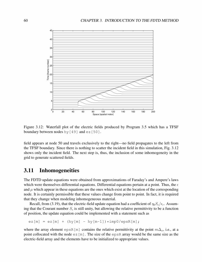
60 CHAPTER 3. INTRODUCTION TO THE FDTD METHOD
0 20 40 60 80 100 120 140 160 180 2000
5
10
15
20
25
30
35
40
45
Space [spatial index]
Tim
e [
fra
me
nu
mb
er]
Figure 3.12: Waterfall plot of the electric fields produced by Program 3.5 which has a TFSF
boundary between nodes hy[49] and ez[50].
field appears at node 50 and travels exclusively to the right—no field propagates to the left from
the TFSF boundary. Since there is nothing to scatter the incident field in this simulation, Fig. 3.12
shows only the incident field. The next step is, thus, the inclusion of some inhomogeneity in the
grid to generate scattered fields.
3.11 Inhomogeneities
The FDTD update equations were obtained from approximations of Faraday’s and Ampere’s laws
which were themselves differential equations. Differential equations pertain at a point. Thus, the ǫand µ which appear in these equations are the ones which exist at the location of the corresponding
node. It is certainly permissible that these values change from point to point. In fact, it is required
that they change when modeling inhomogeneous material.
Recall, from (3.19), that the electric-field update equation had a coefficient of η0Sc/ǫr. Assum-
ing that the Courant number Sc is still unity, but allowing the relative permittivity to be a function
of position, the update equation could be implemented with a statement such as
ez[m] = ez[m] + (hy[m] - hy[m-1])*imp0/epsR[m];
where the array element epsR[m] contains the relative permittivity at the point m∆x, i.e., at a
point collocated with the node ez[m]. The size of the epsR array would be the same size as the
electric-field array and the elements have to be initialized to appropriate values.
3.11. INHOMOGENEITIES 61
The same concept applies to the relative permeability in the updating of the magnetic fields
where the update coefficient is given by Sc/µrη0 (ref. (3.20)). The relative permeability that exists
at the point in space corresponding to the location of a particular magnetic-field node is the one
that should be used in the update equation for that node. Assuming an array muR has been created
and initialized with the values of the relative permeability, the magnetic-fields would be updated
with an equation such as
hy[m] = hy[m] + (ez[m + 1] - ez[m]) / imp0 / muR[m];
A program that models a region of space near the interface between free space and a dielectric
with a relative permittivity of nine is shown in Program 3.6 (the permeability is that of free space).
The incident field is still introduced via a TFSF boundary, which is in the free-space side of the
computational domain, and the ABC on the left hand side is the same as before. However, there
are some other minor changes between this program and the program in Program 3.5. The electric
and magnetic fields are no longer initialized when they are declared. Instead, two loops are used
to set the initial fields to zero. The magnetic field is now declared to have one fewer node than the
electric field. This was done so that the computational domain begins and ends on an electric-field
node. (There are no truly compelling reasons to have the computational domain begin and end with
the same field type, but such symmetry can simplify coding and some aspects of certain problems.)
Because the grid now terminates on an electric field, the ABC at the right end of the grid must be
applied to this terminal electric-field node. This is accomplished with the statement in line 45.
Program 3.6 1Ddielectric.c: One-dimensional FDTD program to model an interface be-
tween free-space and a dielectric that has a relative permittivity ǫr of 9.
1 /* 1D FDTD simulation with a simple absorbing boundary
2 * condition, a TFSF boundary between hy[49] and ez[50], and
3 * a dielectric material starting at ez[100] */
4
5 #include <stdio.h>
6 #include <math.h>
7
8 #define SIZE 200
9
10 int main()
11 {
12 double ez[SIZE], hy[SIZE - 1], epsR[SIZE], imp0 = 377.0;
13 int qTime, maxTime = 450, mm;
14 char basename[80] = "sim", filename[100];
15 int frame = 0;
16 FILE *snapshot;
17
18 /* initialize electric field */
19 for (mm = 0; mm < SIZE; mm++)
20 ez[mm] = 0.0;
21
62 CHAPTER 3. INTRODUCTION TO THE FDTD METHOD
22 /* initialize magnetic field */
23 for (mm = 0; mm < SIZE - 1; mm++)
24 hy[mm] = 0.0;
25
26 /* set relative permittivity */
27 for (mm = 0; mm < SIZE; mm++)
28 if (mm < 100)
29 epsR[mm] = 1.0;
30 else
31 epsR[mm] = 9.0;
32
33 /* do time stepping */
34 for (qTime = 0; qTime < maxTime; qTime++) {
35
36 /* update magnetic field */
37 for (mm = 0; mm<SIZE - 1; mm++)
38 hy[mm] = hy[mm] + (ez[mm + 1] - ez[mm]) / imp0;
39
40 /* correction for Hy adjacent to TFSF boundary */
41 hy[49] -= exp(-(qTime - 30.) * (qTime - 30.) / 100.) / imp0;
42
43 /* simple ABC for ez[0] and ez[SIZE - 1] */
44 ez[0] = ez[1];
45 ez[SIZE-1] = ez[SIZE-2];
46
47 /* update electric field */
48 for (mm = 1; mm < SIZE - 1; mm++)
49 ez[mm] = ez[mm] + (hy[mm] - hy[mm - 1]) * imp0 / epsR[mm];
50
51 /* correction for Ez adjacent to TFSF boundary */
52 ez[50] += exp(-(qTime + 0.5 - (-0.5) - 30.)*53 (qTime + 0.5 - (-0.5) - 30.) / 100.);
54
55 /* write snapshot if time a multiple of 10 */
56 if (qTime % 10 == 0) {
57 sprintf(filename, "%s.%d", basename, frame++);
58 snapshot = fopen(filename, "w");
59 for (mm = 0; mm < SIZE; mm++)
60 fprintf(snapshot, "%g\n", ez[mm]);
61 fclose(snapshot);
62 }
63 } /* end of time-stepping */
64
65 return 0;
66 }
The relative-permittivity array epsR is initialize in the loop starting at line 27. If the spatial
3.11. INHOMOGENEITIES 63
0 20 40 60 80 100 120 140 160 180 2000
5
10
15
20
25
30
35
40
45
Space [spatial index]
Tim
e [
fra
me
nu
mb
er]
Figure 3.13: Waterfall plot of the electric fields produced by Program 3.6 which has a dielectric
with a relative permittivity of 9 starting at node 100. Free space is to the left of that.
index mm is less than 100, the relative permittivity is set to unity (i.e., free space), otherwise it is set
to 9. The characteristic impedance of free space is η0 while the impedance for the dielectric is η0/3.
Note that the update equations do not directly incorporate the dielectric impedance. Rather, the co-
efficient that appears in the equation uses the impedance of free space and the relative permittivity
that pertains at that point.
When a wave is normally incident from a medium with a characteristic impedance η1 to a
medium with a characteristic impedance η2, the reflection coefficient Γ and the transmission coef-
ficient T are given by
Γ =η2 − η1η2 + η1
, (3.44)
T =2η2
η2 + η1. (3.45)
Therefore the reflection and transmission coefficients that pertain to this example are
Γ =η0/3− η0η0/3 + η0
= −1
2, (3.46)
T =2η0/3
η0/3 + η0=
1
2. (3.47)
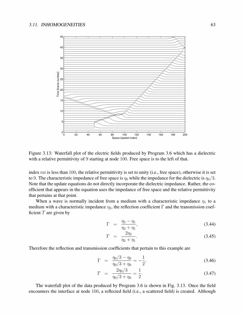
The waterfall plot of the data produced by Program 3.6 is shown in Fig. 3.13. Once the field
encounters the interface at node 100, a reflected field (i.e., a scattered field) is created. Although
64 CHAPTER 3. INTRODUCTION TO THE FDTD METHOD
-0.5
-0.25
0
0.25
0.5
0 25 50 75 100 125 150 175 200
Ez (
V/m
)
Spatial Step
Time-step 100Time-step 140
Figure 3.14: Two of the snapshots produced by Program 3.6. The vertical line at node 100 corre-
sponds to the interface between free space and the dielectric. The incident pulse had unit amplitude.
Shown in this figure are the transmitted field (to the right of the interface) and the reflected field
(to the left).
one cannot easily judge scales from the waterfall plot, it can be seen that the reflected field is
negative and appears to have about half the magnitude of the incident pulse (the peak of the incident
field spans a vertical space corresponding to nearly two frames while the peak of the reflected field
spans about one frame). Similarly, the transmitted pulse is positive and appears to have half the
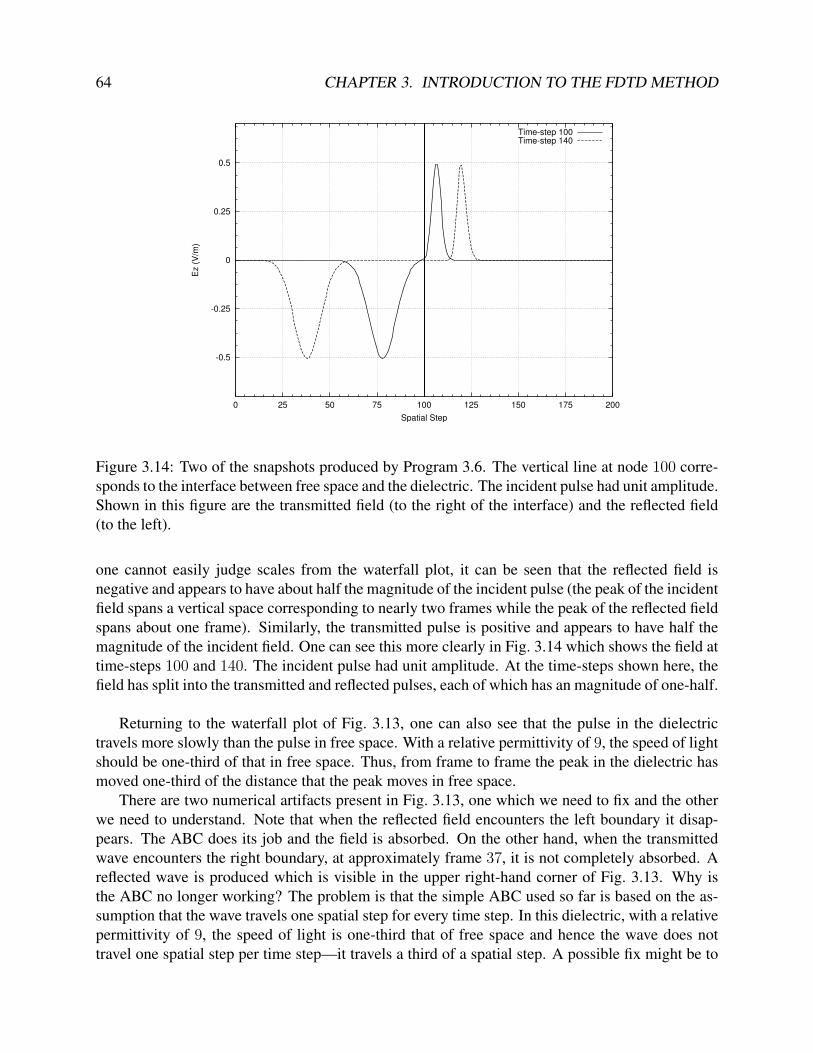
magnitude of the incident field. One can see this more clearly in Fig. 3.14 which shows the field at
time-steps 100 and 140. The incident pulse had unit amplitude. At the time-steps shown here, the
field has split into the transmitted and reflected pulses, each of which has an magnitude of one-half.
Returning to the waterfall plot of Fig. 3.13, one can also see that the pulse in the dielectric
travels more slowly than the pulse in free space. With a relative permittivity of 9, the speed of light
should be one-third of that in free space. Thus, from frame to frame the peak in the dielectric has
moved one-third of the distance that the peak moves in free space.
There are two numerical artifacts present in Fig. 3.13, one which we need to fix and the other
we need to understand. Note that when the reflected field encounters the left boundary it disap-
pears. The ABC does its job and the field is absorbed. On the other hand, when the transmitted
wave encounters the right boundary, at approximately frame 37, it is not completely absorbed. A
reflected wave is produced which is visible in the upper right-hand corner of Fig. 3.13. Why is
the ABC no longer working? The problem is that the simple ABC used so far is based on the as-
sumption that the wave travels one spatial step for every time step. In this dielectric, with a relative
permittivity of 9, the speed of light is one-third that of free space and hence the wave does not
travel one spatial step per time step—it travels a third of a spatial step. A possible fix might be to
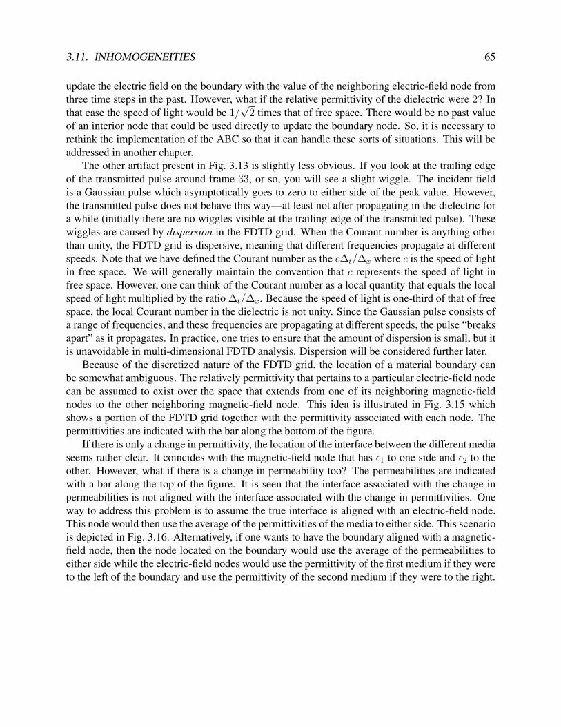
3.11. INHOMOGENEITIES 65
update the electric field on the boundary with the value of the neighboring electric-field node from
three time steps in the past. However, what if the relative permittivity of the dielectric were 2? In
that case the speed of light would be 1/√2 times that of free space. There would be no past value
of an interior node that could be used directly to update the boundary node. So, it is necessary to
rethink the implementation of the ABC so that it can handle these sorts of situations. This will be
addressed in another chapter.
The other artifact present in Fig. 3.13 is slightly less obvious. If you look at the trailing edge
of the transmitted pulse around frame 33, or so, you will see a slight wiggle. The incident field
is a Gaussian pulse which asymptotically goes to zero to either side of the peak value. However,
the transmitted pulse does not behave this way—at least not after propagating in the dielectric for
a while (initially there are no wiggles visible at the trailing edge of the transmitted pulse). These
wiggles are caused by dispersion in the FDTD grid. When the Courant number is anything other
than unity, the FDTD grid is dispersive, meaning that different frequencies propagate at different
speeds. Note that we have defined the Courant number as the c∆t/∆x where c is the speed of light
in free space. We will generally maintain the convention that c represents the speed of light in
free space. However, one can think of the Courant number as a local quantity that equals the local
speed of light multiplied by the ratio ∆t/∆x. Because the speed of light is one-third of that of free
space, the local Courant number in the dielectric is not unity. Since the Gaussian pulse consists of
a range of frequencies, and these frequencies are propagating at different speeds, the pulse “breaks
apart” as it propagates. In practice, one tries to ensure that the amount of dispersion is small, but it
is unavoidable in multi-dimensional FDTD analysis. Dispersion will be considered further later.
Because of the discretized nature of the FDTD grid, the location of a material boundary can
be somewhat ambiguous. The relatively permittivity that pertains to a particular electric-field node
can be assumed to exist over the space that extends from one of its neighboring magnetic-field
nodes to the other neighboring magnetic-field node. This idea is illustrated in Fig. 3.15 which
shows a portion of the FDTD grid together with the permittivity associated with each node. The
permittivities are indicated with the bar along the bottom of the figure.
If there is only a change in permittivity, the location of the interface between the different media
seems rather clear. It coincides with the magnetic-field node that has ǫ1 to one side and ǫ2 to the
other. However, what if there is a change in permeability too? The permeabilities are indicated
with a bar along the top of the figure. It is seen that the interface associated with the change in
permeabilities is not aligned with the interface associated with the change in permittivities. One
way to address this problem is to assume the true interface is aligned with an electric-field node.
This node would then use the average of the permittivities of the media to either side. This scenario
is depicted in Fig. 3.16. Alternatively, if one wants to have the boundary aligned with a magnetic-
field node, then the node located on the boundary would use the average of the permeabilities to
either side while the electric-field nodes would use the permittivity of the first medium if they were
to the left of the boundary and use the permittivity of the second medium if they were to the right.
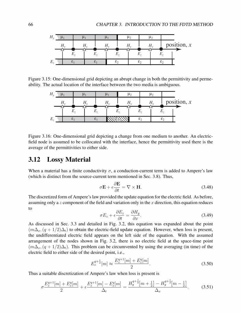
66 CHAPTER 3. INTRODUCTION TO THE FDTD METHOD
Ez
Hy Hy Hy HyHy
EzEzEzEz
ε1 ε1 ε2 ε2
µ1 µ2µ1 µ2µ1
ε2
Hy
Ez
position, x
Figure 3.15: One-dimensional grid depicting an abrupt change in both the permittivity and perme-
ability. The actual location of the interface between the two media is ambiguous.
Ez
Hy Hy Hy HyHy
EzEzEzEz
ε1 ε1 ε2 ε2
µ1 µ2µ1 µ2µ1
εavg
Hy
Ez
position, x
Figure 3.16: One-dimensional grid depicting a change from one medium to another. An electric-
field node is assumed to be collocated with the interface, hence the permittivity used there is the
average of the permittivities to either side.
3.12 Lossy Material
When a material has a finite conductivity σ, a conduction-current term is added to Ampere’s law
(which is distinct from the source-current term mentioned in Sec. 3.8). Thus,
σE+ ǫ∂E
∂t= ∇×H. (3.48)
The discretized form of Ampere’s law provided the update equation for the electric field. As before,
assuming only a z component of the field and variation only in the x direction, this equation reduces
to
σEz + ǫ∂Ez
∂t=
∂Hy
∂x. (3.49)
As discussed in Sec. 3.3 and detailed in Fig. 3.2, this equation was expanded about the point
(m∆x, (q + 1/2)∆t) to obtain the electric-field update equation. However, when loss is present,
the undifferentiated electric field appears on the left side of the equation. With the assumed
arrangement of the nodes shown in Fig. 3.2, there is no electric field at the space-time point
(m∆x, (q + 1/2)∆t). This problem can be circumvented by using the averaging (in time) of the
electric field to either side of the desired point, i.e.,
Eq+ 1
2z [m] ≈ Eq+1
z [m] + Eqz [m]
2. (3.50)
Thus a suitable discretization of Ampere’s law when loss is present is
σEq+1
z [m] + Eqz [m]
2+ ǫ
Eq+1z [m]− Eq
z [m]
∆t
=H
q+ 12
y
[m+ 1
2
]−H
q+ 12
y
[m− 1
2
]
∆x
. (3.51)
3.12. LOSSY MATERIAL 67
As before, this can be solved for Eq+1z [m], which is the “future” field, in terms of purely past fields.
The result is
Eq+1z [m] =
1− σ∆t
2ǫ
1 + σ∆t
2ǫ
Eqz [m] +
∆t
ǫ∆x
1 + σ∆t
2ǫ
(
Hq+ 1
2y
[
m+1
2
]
−Hq+ 1
2y
[
m− 1
2
])
. (3.52)
When σ is zero this reduces to the previous update equation (3.18).
In previous update equations it was possible to express the coefficients in terms of the Courant
number, i.e., the ratio of the temporal step to the spatial step. In (3.52) it appears the term σ∆t/2ǫrequires that the temporal step be specified (together with the conductivity and permittivity). How-
ever, there is a way to express this such that the temporal step does not need to be stated explicitly.
This will be considered in detail in Sec. 5.7.
As we will see, it is occasionally helpful to incorporate a magnetic conduction current in Fara-
day’s law. Similar to the electric conduction current, the magnetic conduction current is assumed
to be the product of the magnetic conductivity σm and the magnetic field. Faraday’s law becomes
−σmH− µ∂H
∂t= ∇× E. (3.53)
We again restrict consideration to an Hy component which varies only in the x direction. This
reduces to
σmHy + µ∂Hy
∂t=
∂Ez
∂x. (3.54)
As before, this is expanded/discretized at the space-time point ((m + 1/2)∆x, q∆t). Since there
is no magnetic field available at integer time steps, the magnetic field is averaged in time to get an
approximation of the field at time q∆t. This yields
σm
Hq+ 1
2y
[m+ 1
2
]+H
q− 12
y
[m+ 1
2
]
2+ µ
Hq+ 1
2y
[m+ 1
2
]−H
q− 12
y
[m+ 1
2
]
∆t
=
Eqz [m+ 1]− Eq
z [m]
∆x
. (3.55)
Solving for Hq+ 1
2y
[m+ 1
2
]yields the update equation
Hq+ 1
2y
[
m+1
2
]
=1− σm∆t
2µ
1 + σm∆t
2µ
Hq− 1
2y
[
m+1
2
]
+
∆t
µ∆x
1 + σm∆t
2µ
(Eqz [m+ 1]− Eq
z [m]) . (3.56)
When σm is zero this reduces to (3.15).
Program 3.7 models a lossy dielectric half-space that starts at node 100. As before, the relative
permittivity is 9. However there is also an electric loss present such that σ∆t/2ǫ is 0.01. The
program uses two coefficient arrays, ceze and cezh. The terms in the ceze array multiply
the previous (or “self”) term while the cezh array contains the terms that multiply the spatial
difference of the magnetic fields. Think of these arrays as consisting of coefficients (or constants),
hence the “c” at the start of their name, that appear in the Ez update equation, hence the ez part
of the name, and multiplying either the electric field (ceze) or the magnetic field (cezh). The
values of these arrays are set in the loop that starts at line 27. Since the simple ABC previously
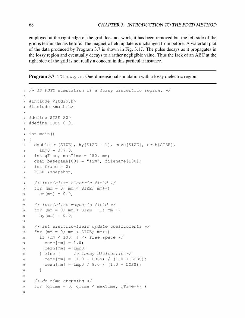
68 CHAPTER 3. INTRODUCTION TO THE FDTD METHOD
employed at the right edge of the grid does not work, it has been removed but the left side of the
grid is terminated as before. The magnetic field update is unchanged from before. A waterfall plot
of the data produced by Program 3.7 is shown in Fig. 3.17. The pulse decays as it propagates in
the lossy region and eventually decays to a rather negligible value. Thus the lack of an ABC at the
right side of the grid is not really a concern in this particular instance.
Program 3.7 1Dlossy.c: One-dimensional simulation with a lossy dielectric region.
1 /* 1D FDTD simulation of a lossy dielectric region. */
2
3 #include <stdio.h>
4 #include <math.h>
5
6 #define SIZE 200
7 #define LOSS 0.01
8
9 int main()
10 {
11 double ez[SIZE], hy[SIZE - 1], ceze[SIZE], cezh[SIZE],
12 imp0 = 377.0;
13 int qTime, maxTime = 450, mm;
14 char basename[80] = "sim", filename[100];
15 int frame = 0;
16 FILE *snapshot;
17
18 /* initialize electric field */
19 for (mm = 0; mm < SIZE; mm++)
20 ez[mm] = 0.0;
21
22 /* initialize magnetic field */
23 for (mm = 0; mm < SIZE - 1; mm++)
24 hy[mm] = 0.0;
25
26 /* set electric-field update coefficients */
27 for (mm = 0; mm < SIZE; mm++)
28 if (mm < 100) { /* free space */
29 ceze[mm] = 1.0;
30 cezh[mm] = imp0;
31 } else { /* lossy dielectric */
32 ceze[mm] = (1.0 - LOSS) / (1.0 + LOSS);
33 cezh[mm] = imp0 / 9.0 / (1.0 + LOSS);
34 }
35
36 /* do time stepping */
37 for (qTime = 0; qTime < maxTime; qTime++) {
38

3.12. LOSSY MATERIAL 69
39 /* update magnetic field */
40 for (mm = 0; mm < SIZE - 1; mm++)
41 hy[mm] = hy[mm] + (ez[mm + 1] - ez[mm]) / imp0;
42
43 /* correction for Hy adjacent to TFSF boundary */
44 hy[49] -= exp(-(qTime - 30.) * (qTime - 30.) / 100.) / imp0;
45
46 /* simple ABC for ez[0] */
47 ez[0] = ez[1];
48
49 /* update electric field */
50 for (mm = 1; mm < SIZE - 1; mm++)
51 ez[mm] = ceze[mm] * ez[mm] + cezh[mm] * (hy[mm] - hy[mm - 1]);
52
53 /* correction for Ez adjacent to TFSF boundary */
54 ez[50] += exp(-(qTime + 0.5 - (-0.5) - 30.) *55 (qTime + 0.5 - (-0.5) - 30.) / 100.);
56
57 /* write snapshot if time a multiple of 10 */
58 if (qTime % 10 == 0) {
59 sprintf(filename, "%s.%d", basename, frame++);
60 snapshot=fopen(filename, "w");
61 for (mm = 0; mm < SIZE; mm++)
62 fprintf(snapshot, "%g\n", ez[mm]);
63 fclose(snapshot);
64 }
65 } /* end of time-stepping */
66
67 return 0;
68 }
When loss is present the characteristic impedance of the medium becomes
η =
√√√√
µ(
1− j σm
ωµ
)
ǫ(1− j σ
ωǫ
) = η0
√√√√
µr
(
1− j σm
ωµ
)
ǫr(1− j σ
ωǫ
) (3.57)
When σm/µ = σ/ǫ the terms in parentheses are equal and hence cancel. With those terms canceled,
the characteristic impedance is indistinguishable from the lossless case. Therefore
η|σmµ
=σ
ǫ
= η|σm=σ=0 = η0
õr
ǫr. (3.58)
As shown in (3.44), the reflection coefficient for a wave normally incident on a planar boundary
is proportional to the difference of the impedances to either side of the interface. If the material
on one side is lossless while the material on the other side is lossy with σm/µ = σ/ǫ, then the
impedances are matched provided the ratios of ǫr and µr are also matched across the boundary.
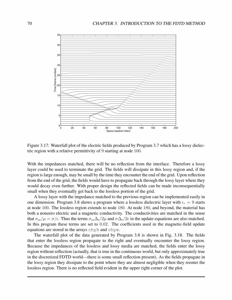
70 CHAPTER 3. INTRODUCTION TO THE FDTD METHOD
0 20 40 60 80 100 120 140 160 180 2000
5
10
15
20
25
30
35
40
45
Space [spatial index]
Tim
e [
fra
me
nu
mb
er]
Figure 3.17: Waterfall plot of the electric fields produced by Program 3.7 which has a lossy dielec-
tric region with a relative permittivity of 9 starting at node 100.
With the impedances matched, there will be no reflection from the interface. Therefore a lossy
layer could be used to terminate the grid. The fields will dissipate in this lossy region and, if the
region is large enough, may be small by the time they encounter the end of the grid. Upon reflection
from the end of the grid, the fields would have to propagate back through the lossy layer where they
would decay even further. With proper design the reflected fields can be made inconsequentially
small when they eventually get back to the lossless portion of the grid.
A lossy layer with the impedance matched to the previous region can be implemented easily in
one dimension. Program 3.8 shows a program where a lossless dielectric layer with ǫr = 9 starts
at node 100. The lossless region extends to node 180. At node 180, and beyond, the material has
both a nonzero electric and a magnetic conductivity. The conductivities are matched in the sense
that σm/µ = σ/ǫ. Thus the terms σm∆t/2µ and σ∆t/2ǫ in the update-equations are also matched.
In this program these terms are set to 0.02. The coefficients used in the magnetic-field update
equations are stored in the arrays chyh and chye.
The waterfall plot of the data generated by Program 3.8 is shown in Fig. 3.18. The fields
that enter the lossless region propagate to the right and eventually encounter the lossy region.
Because the impedances of the lossless and lossy media are matched, the fields enter the lossy
region without reflection (actually, that is true in the continuous world, but only approximately true
in the discretized FDTD world—there is some small reflection present). As the fields propagate in
the lossy region they dissipate to the point where they are almost negligible when they reenter the
lossless region. There is no reflected field evident in the upper right corner of the plot.
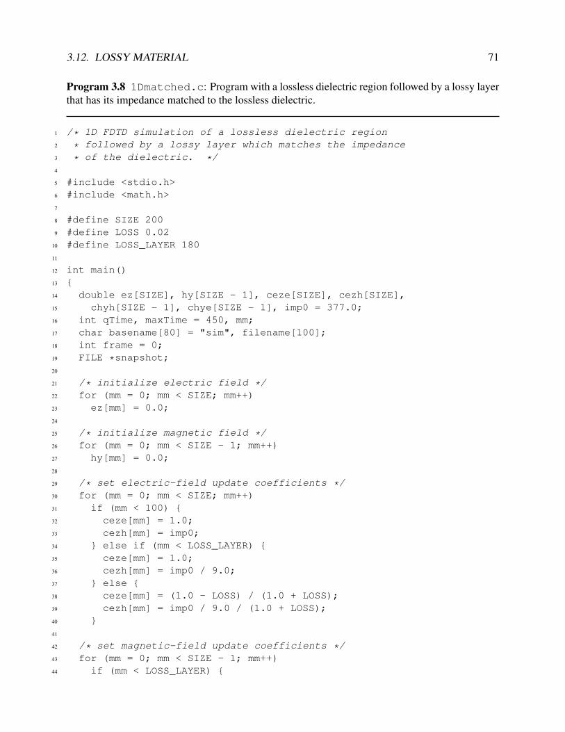
3.12. LOSSY MATERIAL 71
Program 3.8 1Dmatched.c: Program with a lossless dielectric region followed by a lossy layer
that has its impedance matched to the lossless dielectric.
1 /* 1D FDTD simulation of a lossless dielectric region
2 * followed by a lossy layer which matches the impedance
3 * of the dielectric. */
4
5 #include <stdio.h>
6 #include <math.h>
7
8 #define SIZE 200
9 #define LOSS 0.02
10 #define LOSS_LAYER 180
11
12 int main()
13 {
14 double ez[SIZE], hy[SIZE - 1], ceze[SIZE], cezh[SIZE],
15 chyh[SIZE - 1], chye[SIZE - 1], imp0 = 377.0;
16 int qTime, maxTime = 450, mm;
17 char basename[80] = "sim", filename[100];
18 int frame = 0;
19 FILE *snapshot;
20
21 /* initialize electric field */
22 for (mm = 0; mm < SIZE; mm++)
23 ez[mm] = 0.0;
24
25 /* initialize magnetic field */
26 for (mm = 0; mm < SIZE - 1; mm++)
27 hy[mm] = 0.0;
28
29 /* set electric-field update coefficients */
30 for (mm = 0; mm < SIZE; mm++)
31 if (mm < 100) {
32 ceze[mm] = 1.0;
33 cezh[mm] = imp0;
34 } else if (mm < LOSS_LAYER) {
35 ceze[mm] = 1.0;
36 cezh[mm] = imp0 / 9.0;
37 } else {
38 ceze[mm] = (1.0 - LOSS) / (1.0 + LOSS);
39 cezh[mm] = imp0 / 9.0 / (1.0 + LOSS);
40 }
41
42 /* set magnetic-field update coefficients */
43 for (mm = 0; mm < SIZE - 1; mm++)
44 if (mm < LOSS_LAYER) {
72 CHAPTER 3. INTRODUCTION TO THE FDTD METHOD
45 chyh[mm] = 1.0;
46 chye[mm] = 1.0 / imp0;
47 } else {
48 chyh[mm] = (1.0 - LOSS) / (1.0 + LOSS);
49 chye[mm] = 1.0 / imp0 / (1.0 + LOSS);
50 }
51
52 /* do time stepping */
53 for (qTime = 0; qTime < maxTime; qTime++) {
54
55 /* update magnetic field */
56 for (mm = 0; mm < SIZE - 1; mm++)
57 hy[mm] = chyh[mm] * hy[mm] +
58 chye[mm] * (ez[mm + 1] - ez[mm]);
59
60 /* correction for Hy adjacent to TFSF boundary */
61 hy[49] -= exp(-(qTime - 30.) * (qTime - 30.) / 100.) / imp0;
62
63 /* simple ABC for ez[0] */
64 ez[0] = ez[1];
65
66 /* update electric field */
67 for (mm = 1; mm < SIZE - 1; mm++)
68 ez[mm] = ceze[mm] * ez[mm] +
69 cezh[mm] * (hy[mm] - hy[mm - 1]);
70
71 /* correction for Ez adjacent to TFSF boundary */
72 ez[50] += exp(-(qTime + 0.5 - (-0.5) - 30.)*73 (qTime + 0.5 - (-0.5) - 30.) / 100.);
74
75 /* write snapshot if time a multiple of 10 */
76 if (qTime % 10 == 0) {
77 sprintf(filename, "%s.%d", basename, frame++);
78 snapshot=fopen(filename, "w");
79 for (mm = 0; mm < SIZE; mm++)
80 fprintf(snapshot, "%g\n", ez[mm]);
81 fclose(snapshot);
82 }
83 } /* end of time-stepping */
84
85 return 0;
86 }
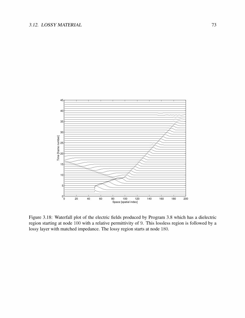
3.12. LOSSY MATERIAL 73
0 20 40 60 80 100 120 140 160 180 2000
5
10
15
20
25
30
35
40
45
Space [spatial index]
Tim
e [
fra
me
nu
mb
er]
Figure 3.18: Waterfall plot of the electric fields produced by Program 3.8 which has a dielectric
region starting at node 100 with a relative permittivity of 9. This lossless region is followed by a
lossy layer with matched impedance. The lossy region starts at node 180.

74 CHAPTER 3. INTRODUCTION TO THE FDTD METHOD
Related Documents