Chapter 1 Space, time, and quantum mechanics: Symmetry in nature and physics Version 8.35: August 17, 2010 Contents 1.1. Symmetry: you know it when you see it ...................... 10 1.2. Symmetry transformations ............................... 13 1.2.1. Symbolizing transformations .............................. 13 1.2.2. Discovering symmetry: the point-particle model of a system ............. 14 1.3. Symmetry elements in the Platonic solids ...................... 16 1.4. Mathematical articulations of transformations ................... 17 1.4.1. Translation ........................................ 19 1.4.2. Continuous versus discrete transformations ...................... 19 1.4.3. Inversion ......................................... 20 1.4.4. Going around in academic circles: rotations ...................... 20 1.4.5. Choosing coordinate systems based on symmetry properties ............. 23 1.4.6. Problem-solving: seek symmetry simplifications .................... 23 1.5. Symmetry and invariance in physics ......................... 25 1.5.1. Universal symmetries of space and time ........................ 26 1.5.1.1. Translational invariance and the homogeneity of free space ........ 27 1.5.1.2. Rotational invariance and the isotropy of free space ............ 27 1.5.2. Universal symmetries and conservation laws: Noether’s theorem .......... 28 1.5.3. Internal symmetries and forces ............................. 30 1.6. Symmetry transformations and invariance in quantum mechanics ....... 33 1.6.1. Associated functions and symmetry operators ..................... 33 1.6.2. Invariance in terms of wave functions and the Hamiltonian ............. 34 1.6.3. Generic properties of symmetry operators ....................... 35 1.6.3.1. Linearity .................................... 35 1.6.3.2. Unitarity: the effect of a symmetry transformation on expectation values 36 1.6.3.3. Unitarity: The effect of a symmetry transformation on eigenvalues .... 39 1.6.4. Problem-solving: reason by analogy .......................... 40 1.6.5. Invariance and the Hamiltonian ............................. 41 1.7. Transformation operators for translation, rotation, and inversion ....... 42 1.7.1. The effect of a translation on an associated function ................. 42 1.7.2. The effect of a rotation ................................. 44 1.7.3. The effect of an inversion: the parity operator ..................... 46 1.7.4. This side of parities: even and odd functions ..................... 46 1.8. Symmetry, invariance, and conservation laws in quantum mechanics ..... 49 1.8.1. Stone’s theorem ..................................... 49

Chap1_JQPMaster
Oct 03, 2014
Welcome message from author
This document is posted to help you gain knowledge. Please leave a comment to let me know what you think about it! Share it to your friends and learn new things together.
Transcript
Chapter 1
Space, time, and quantum mechanics:Symmetry in nature and physics
Version 8.35: August 17, 2010
Contents1.1. Symmetry: you know it when you see it . . . . . . . . . . . . . . . . . . . . . . 101.2. Symmetry transformations . . . . . . . . . . . . . . . . . . . . . . . . . . . . . . . 13
1.2.1. Symbolizing transformations . . . . . . . . . . . . . . . . . . . . . . . . . . . . . . 131.2.2. Discovering symmetry: the point-particle model of a system . . . . . . . . . . . . . 14
1.3. Symmetry elements in the Platonic solids . . . . . . . . . . . . . . . . . . . . . . 161.4. Mathematical articulations of transformations . . . . . . . . . . . . . . . . . . . 17
1.4.1. Translation . . . . . . . . . . . . . . . . . . . . . . . . . . . . . . . . . . . . . . . . 191.4.2. Continuous versus discrete transformations . . . . . . . . . . . . . . . . . . . . . . 191.4.3. Inversion . . . . . . . . . . . . . . . . . . . . . . . . . . . . . . . . . . . . . . . . . 201.4.4. Going around in academic circles: rotations . . . . . . . . . . . . . . . . . . . . . . 201.4.5. Choosing coordinate systems based on symmetry properties . . . . . . . . . . . . . 231.4.6. Problem-solving: seek symmetry simplifications . . . . . . . . . . . . . . . . . . . . 23
1.5. Symmetry and invariance in physics . . . . . . . . . . . . . . . . . . . . . . . . . 251.5.1. Universal symmetries of space and time . . . . . . . . . . . . . . . . . . . . . . . . 26
1.5.1.1. Translational invariance and the homogeneity of free space . . . . . . . . 271.5.1.2. Rotational invariance and the isotropy of free space . . . . . . . . . . . . 27
1.5.2. Universal symmetries and conservation laws: Noether’s theorem . . . . . . . . . . 281.5.3. Internal symmetries and forces . . . . . . . . . . . . . . . . . . . . . . . . . . . . . 30
1.6. Symmetry transformations and invariance in quantum mechanics . . . . . . . 331.6.1. Associated functions and symmetry operators . . . . . . . . . . . . . . . . . . . . . 331.6.2. Invariance in terms of wave functions and the Hamiltonian . . . . . . . . . . . . . 341.6.3. Generic properties of symmetry operators . . . . . . . . . . . . . . . . . . . . . . . 35
1.6.3.1. Linearity . . . . . . . . . . . . . . . . . . . . . . . . . . . . . . . . . . . . 351.6.3.2. Unitarity: the effect of a symmetry transformation on expectation values 361.6.3.3. Unitarity: The effect of a symmetry transformation on eigenvalues . . . . 39
1.6.4. Problem-solving: reason by analogy . . . . . . . . . . . . . . . . . . . . . . . . . . 401.6.5. Invariance and the Hamiltonian . . . . . . . . . . . . . . . . . . . . . . . . . . . . . 41
1.7. Transformation operators for translation, rotation, and inversion . . . . . . . 421.7.1. The effect of a translation on an associated function . . . . . . . . . . . . . . . . . 421.7.2. The effect of a rotation . . . . . . . . . . . . . . . . . . . . . . . . . . . . . . . . . 441.7.3. The effect of an inversion: the parity operator . . . . . . . . . . . . . . . . . . . . . 461.7.4. This side of parities: even and odd functions . . . . . . . . . . . . . . . . . . . . . 46
1.8. Symmetry, invariance, and conservation laws in quantum mechanics . . . . . 491.8.1. Stone’s theorem . . . . . . . . . . . . . . . . . . . . . . . . . . . . . . . . . . . . . 49

2 1. Space, time, and quantum mechanics
1.8.2. Translations and conservation of linear momentum . . . . . . . . . . . . . . . . . . 501.8.3. Rotations and conservation of angular momentum . . . . . . . . . . . . . . . . . . 521.8.4. Inversion and conservation of parity . . . . . . . . . . . . . . . . . . . . . . . . . . 52
1.9. Reflections on symmetry: a recap . . . . . . . . . . . . . . . . . . . . . . . . . . 531.9.1. The beauty of symmetry principles in physics . . . . . . . . . . . . . . . . . . . . . 541.9.2. The power of symmetry arguments in solving physics problems . . . . . . . . . . . 55
1.10. Selected readings & references for Chap. 1 . . . . . . . . . . . . . . . . . . . . . 561.11. Exercises & problems for Chap. 1 . . . . . . . . . . . . . . . . . . . . . . . . . . 56Complements . . . . . . . . . . . . . . . . . . . . . . . . . . . . . . . . . . . . . . . . . . 601.A. User’s guide to Chap. 1 . . . . . . . . . . . . . . . . . . . . . . . . . . . . . . . . . 611.B. Additional Examples . . . . . . . . . . . . . . . . . . . . . . . . . . . . . . . . . . 661.C. How quantum mechanics works: background . . . . . . . . . . . . . . . . . . . . 75
1.C.1. Expectation values . . . . . . . . . . . . . . . . . . . . . . . . . . . . . . . . . . . . 751.C.2. Transition probabilities. . . . . . . . . . . . . . . . . . . . . . . . . . . . . . . . . . 751.C.3. The scalar product. . . . . . . . . . . . . . . . . . . . . . . . . . . . . . . . . . . . 751.C.4. Possible outcomes of a measurement of an observable. . . . . . . . . . . . . . . . . 761.C.5. Conservation laws and constants of the motion . . . . . . . . . . . . . . . . . . . . 76
1.D. Coordinate systems in two and three dimensions . . . . . . . . . . . . . . . . . 771.D.1. Coordinate systems and reference frames . . . . . . . . . . . . . . . . . . . . . . . 771.D.2. Vectors . . . . . . . . . . . . . . . . . . . . . . . . . . . . . . . . . . . . . . . . . . 771.D.3. Two dimensions: Cartesian and polar coordinates . . . . . . . . . . . . . . . . . . 791.D.4. Three dimensions: Cartesian, spherical, and cylindrical coordinates . . . . . . . . . 81
1.E. Rotation matrices . . . . . . . . . . . . . . . . . . . . . . . . . . . . . . . . . . . . 831.F. It’s about time: temporal translations and conservation of energy . . . . . . . 851.G. Additional Exercises and Problems . . . . . . . . . . . . . . . . . . . . . . . . . . 87
Figures1.1. The symmetry of snowflakes. . . . . . . . . . . . . . . . . . . . . . . . . . . . . . . . . . . 101.2. Symmetry of the human body. . . . . . . . . . . . . . . . . . . . . . . . . . . . . . . . . . 111.3. Symmetry in art. . . . . . . . . . . . . . . . . . . . . . . . . . . . . . . . . . . . . . . . . . 121.4. A model of an ammonia molecule. . . . . . . . . . . . . . . . . . . . . . . . . . . . . . . . 151.5. The five Platonic solids. . . . . . . . . . . . . . . . . . . . . . . . . . . . . . . . . . . . . . 171.6. Various ways to denote a point in ordinary space. . . . . . . . . . . . . . . . . . . . . . . . 181.7. Translation of a point in Flatland. . . . . . . . . . . . . . . . . . . . . . . . . . . . . . . . 191.8. An inversion in a two-dimensional plane . . . . . . . . . . . . . . . . . . . . . . . . . . . . 201.9. A rotation ℛ(𝛼; 𝒆𝛼) in a two-dimensional plane. . . . . . . . . . . . . . . . . . . . . . . . 211.10. An arbitrary rotation in three dimensions. . . . . . . . . . . . . . . . . . . . . . . . . . . . 221.11. Potential energies for two-dimensional harmonic oscillators. . . . . . . . . . . . . . . . . . 321.12. Translation of a one-dimensional wave packet. . . . . . . . . . . . . . . . . . . . . . . . . . 431.13. Rotation of a function in two dimensions. . . . . . . . . . . . . . . . . . . . . . . . . . . . 451.14. Symmetry properties of functions under inversion. . . . . . . . . . . . . . . . . . . . . . . 471.15. A rotation of a point in two dimensions. . . . . . . . . . . . . . . . . . . . . . . . . . . . . 481.B.1. An electron in the fields of a proton and a point dipole. . . . . . . . . . . . . . . . . . . . 671.B.2. Electric field lines for a point charge and for a point dipole. . . . . . . . . . . . . . . . . 681.D.1. An infinitesimal volume element. . . . . . . . . . . . . . . . . . . . . . . . . . . . . . . . 801.D.2. The spherical and Cartesian coordinate systems and unit vectors. . . . . . . . . . . . . . 811.D.3. The cylindrical coordinate systems and unit vectors. . . . . . . . . . . . . . . . . . . . . 821.15.1. Reflections through the 𝑥 and 𝑦 axes. . . . . . . . . . . . . . . . . . . . . . . . . . . . . 87
Tables1.A.1. Parity: classification of functions by their behavior under inversion. . . . . . . . . . . . . 621.A.2. Notation. . . . . . . . . . . . . . . . . . . . . . . . . . . . . . . . . . . . . . . . . . . . . . 631.A.3. Transformations and transformation operators. . . . . . . . . . . . . . . . . . . . . . . . 631.A.4. Symmetry elements and their physical consequences. . . . . . . . . . . . . . . . . . . . . 631.A.5. Symmetry operations, elements, and parameters. . . . . . . . . . . . . . . . . . . . . . . 63
JQPMaster Version: 8.35 Printed: August 17, 2010

3
1.A.6. Invariance principles and symmetry properties of free space. . . . . . . . . . . . . . . . . 641.A.7. Transformations and transformation operators for quantum mechanics. . . . . . . . . . . 641.A.8. The effect of symmetry transformations and operations on functions. . . . . . . . . . . . 641.A.9. Tools for effecting rotational transformations in physics. . . . . . . . . . . . . . . . . . . 641.A.10.Inversion and the parity operator in various coordinate systems. . . . . . . . . . . . . . 651.D.1. Conversion between coordinate systems. . . . . . . . . . . . . . . . . . . . . . . . . . . . 831.D.2. The gradient operator in the commonly used coordinate systems. . . . . . . . . . . . . . 831.F.1. Time evolution in classical and quantum physics. . . . . . . . . . . . . . . . . . . . . . . 85
Examples1.1. Models of the ammonia molecule. . . . . . . . . . . . . . . . . . . . . . . . . . . . . . . . . . . . . . . . . . 15
1.2. The three-dimensional isotropic simple harmonic oscillator. . . . . . . . . . . . . . . . . . . . . . . . . . . 25
1.3. The symmetry of an electron in a “classical hydrogen atom.” . . . . . . . . . . . . . . . . . . . . . . . . . 30
1.4. The two-dimensional isotropic harmonic oscillator. . . . . . . . . . . . . . . . . . . . . . . . . . . . . . . . 31
1.5. Translation of a one-dimensional Gaussian function. . . . . . . . . . . . . . . . . . . . . . . . . . . . . . . 42
1.6. The effect of a translation in a one-dimensional wave function. . . . . . . . . . . . . . . . . . . . . . . . . 43
1.7. The effect of a translation in three dimensions. . . . . . . . . . . . . . . . . . . . . . . . . . . . . . . . . . 44
1.8. The effect of a two-dimensional rotation on an associated function. . . . . . . . . . . . . . . . . . . . . . . 45
1.9. Action of the parity operator on one-dimensional functions. . . . . . . . . . . . . . . . . . . . . . . . . . . 46
1.10. The parity operator in two dimensions. . . . . . . . . . . . . . . . . . . . . . . . . . . . . . . . . . . . . . 47
1.11. The Hermitian operator that corresponds to a translation. . . . . . . . . . . . . . . . . . . . . . . . . . . . 50
1.12. Translational invariance and conservation of linear momentum. . . . . . . . . . . . . . . . . . . . . . . . . 50
1.13. Reflections in two and three dimensions. . . . . . . . . . . . . . . . . . . . . . . . . . . . . . . . . . . . . . 66
1.14. Internal symmetries of an electron interacting with a proton. . . . . . . . . . . . . . . . . . . . . . . . . . 66
1.15. Internal symmetries of an electron interacting with a point dipole. . . . . . . . . . . . . . . . . . . . . . . 68
1.16. Effect of an inversion on the linear-momentum operator. . . . . . . . . . . . . . . . . . . . . . . . . . . . . 69
1.17. The parity operator in three dimensions. . . . . . . . . . . . . . . . . . . . . . . . . . . . . . . . . . . . . . 70
1.18. The relationship between translation operators and the linear momentum. . . . . . . . . . . . . . . . . . . 71
1.19. Invariance of the position probability density. . . . . . . . . . . . . . . . . . . . . . . . . . . . . . . . . . . 72
1.20. Translational symmetry and conservation of linear momentum. . . . . . . . . . . . . . . . . . . . . . . . . 72
1.21. Geometric origin of the position-momentum commutation relation. . . . . . . . . . . . . . . . . . . . . . . 73
1.22. The infinitesimal “volume” element in two dimensions. . . . . . . . . . . . . . . . . . . . . . . . . . . . . . 80
1.23. An inversion in polar coordinates. . . . . . . . . . . . . . . . . . . . . . . . . . . . . . . . . . . . . . . . . 80
1.24. An inversion in spherical coordinates. . . . . . . . . . . . . . . . . . . . . . . . . . . . . . . . . . . . . . . 82
1.25. Rotation matrices in three dimensions. . . . . . . . . . . . . . . . . . . . . . . . . . . . . . . . . . . . . . . 84
2.1. A CSCO for your sock drawer. . . . . . . . . . . . . . . . . . . . . . . . . . . . . . . . . . . . . . . . . . . 102
2.2. A CSCO for a free particle. . . . . . . . . . . . . . . . . . . . . . . . . . . . . . . . . . . . . . . . . . . . . 103
2.3. A CSCO for a one-dimensional simple harmonic oscillator. . . . . . . . . . . . . . . . . . . . . . . . . . . . 103
2.4. A CSCO for a two-dimensional simple harmonic oscillator. . . . . . . . . . . . . . . . . . . . . . . . . . . . 103
2.5. SAMEs for a one-dimensional simple harmonic oscillator. . . . . . . . . . . . . . . . . . . . . . . . . . . . 110
2.6. SAMEs for a two-dimensional simple harmonic oscillator. . . . . . . . . . . . . . . . . . . . . . . . . . . . 110
2.7. Hermiticity of the orbital angular momentum operator. . . . . . . . . . . . . . . . . . . . . . . . . . . . . 116
2.8. Analytic solution of the L𝑧 eigenvalue equation. . . . . . . . . . . . . . . . . . . . . . . . . . . . . . . . . . 121
2.9. The kinetic-energy operator in Cartesian coordinates. . . . . . . . . . . . . . . . . . . . . . . . . . . . . . 125
2.10. The kinetic-energy operator in polar coordinates. . . . . . . . . . . . . . . . . . . . . . . . . . . . . . . . . 126
2.11. Commutativity of the kinetic-energy and angular-momentum operators. . . . . . . . . . . . . . . . . . . . 127
2.12. Conservation of angular momentum for circularly invariant systems. . . . . . . . . . . . . . . . . . . . . . 127
2.13. Brainstorming the TISE for a 2D rotationally invariant system. . . . . . . . . . . . . . . . . . . . . . . . . 130
2.14. Derivation of the radial equation for a 2D rotationally invariant system. . . . . . . . . . . . . . . . . . . . 132
JQPMaster Version: 8.35 Printed: August 17, 2010

4 1. Space, time, and quantum mechanics
2.15. Normalization of bound-state radial functions . . . . . . . . . . . . . . . . . . . . . . . . . . . . . . . . . . 134
2.16. Energy degeneracies of a 2D simple harmonic oscillator. . . . . . . . . . . . . . . . . . . . . . . . . . . . . 138
2.17. The orthogonality integral for radial functions of a 2D SHO. . . . . . . . . . . . . . . . . . . . . . . . . . . 143
2.18. Radial functions of the 2D SHO that do not have to be orthogonal. . . . . . . . . . . . . . . . . . . . . . . 144
2.19. Trends in radial probability densities for the 2D SHO. . . . . . . . . . . . . . . . . . . . . . . . . . . . . . 151
2.20. Probability densities for a 2D SHO. . . . . . . . . . . . . . . . . . . . . . . . . . . . . . . . . . . . . . . . 152
2.21. Verification that L𝑧 is a constant of the motion of a rotationally invariant system. . . . . . . . . . . . . . 169
2.22. Does Π commute with the Hamiltonian? . . . . . . . . . . . . . . . . . . . . . . . . . . . . . . . . . . . . . 169
2.23. Transforming L𝑧 from Cartesian to polar coordinates. . . . . . . . . . . . . . . . . . . . . . . . . . . . . . 170
2.24. The 2D rotation operator and the orbital angular momentum. . . . . . . . . . . . . . . . . . . . . . . . . . 170
2.25. A state of uncertain angular momentum. . . . . . . . . . . . . . . . . . . . . . . . . . . . . . . . . . . . . 175
2.26. Information about a state of uncertain angular momentum. . . . . . . . . . . . . . . . . . . . . . . . . . . 176
3.1. The commutator of L𝑥 and L𝑦. . . . . . . . . . . . . . . . . . . . . . . . . . . . . . . . . . . . . . . . . . . 191
3.2. The commutator of L 2 and L𝑧. . . . . . . . . . . . . . . . . . . . . . . . . . . . . . . . . . . . . . . . . . . 193
3.3. The uncertainty product for 𝐿𝑥 and 𝐿𝑦. . . . . . . . . . . . . . . . . . . . . . . . . . . . . . . . . . . . . . 200
3.4. The uncertainties in 𝐿𝑥 and 𝐿𝑦. . . . . . . . . . . . . . . . . . . . . . . . . . . . . . . . . . . . . . . . . . 201
3.5. Derivation of L𝑥, L𝑦, and L 2 in spherical coordinates. . . . . . . . . . . . . . . . . . . . . . . . . . . . . . . 210
3.6. Normalization of the 𝜃 functions. . . . . . . . . . . . . . . . . . . . . . . . . . . . . . . . . . . . . . . . . . 216
3.7. The commutator of T and L𝑥. . . . . . . . . . . . . . . . . . . . . . . . . . . . . . . . . . . . . . . . . . . . 250
3.8. Changing variables in the 𝜃 equation. . . . . . . . . . . . . . . . . . . . . . . . . . . . . . . . . . . . . . . 251
3.9. Angular nodes in stretched-state SAMEs. . . . . . . . . . . . . . . . . . . . . . . . . . . . . . . . . . . . . 251
3.10. The effect of angular nodes and the projection quantum number on ∣Θℓ,𝑚ℓ(𝜃)∣. . . . . . . . . . . . . . . . 251
3.11. The effect of the orbital quantum number on ∣Θℓ,𝑚ℓ(𝜃)∣. . . . . . . . . . . . . . . . . . . . . . . . . . . . . 252
3.12. Effect of L± on simultaneous eigenfunctions of L 2 and L𝑧. . . . . . . . . . . . . . . . . . . . . . . . . . . . 258
3.13. Normalization constants for L+ ∣ℓ,𝑚ℓ⟩. . . . . . . . . . . . . . . . . . . . . . . . . . . . . . . . . . . . . . . 260
3.14. The raising and lowering operators in action. . . . . . . . . . . . . . . . . . . . . . . . . . . . . . . . . . . 261
3.15. Evaluating angular momentum uncertainties. . . . . . . . . . . . . . . . . . . . . . . . . . . . . . . . . . . 262
3.16. The 𝑝𝑥 and other strangely named functions . . . . . . . . . . . . . . . . . . . . . . . . . . . . . . . . . . . 272
4.1. Orthonormality of SAME radial functions. . . . . . . . . . . . . . . . . . . . . . . . . . . . . . . . . . . . . 285
4.2. The orthogonality requirement and nodes in the radial function. . . . . . . . . . . . . . . . . . . . . . . . 286
4.3. Radial probability densities for the ground state of atomic lithium. . . . . . . . . . . . . . . . . . . . . . . 291
4.4. Radial probability densities for 1𝑠 states of several atoms. . . . . . . . . . . . . . . . . . . . . . . . . . . . 291
4.5. The sphere probability for electrons in the ground state of atomic lithium. . . . . . . . . . . . . . . . . . . 293
4.6. Reduced radial functions for the ground state of atomic lithium. . . . . . . . . . . . . . . . . . . . . . . . 296
4.7. The effective potential energy for s-state electrons in the ground state of lithium. . . . . . . . . . . . . . . 300
4.8. Asymptotic decay of reduced radial functions for scandium. . . . . . . . . . . . . . . . . . . . . . . . . . . 305
4.9. The short-range behavior of radial functions for scandium. . . . . . . . . . . . . . . . . . . . . . . . . . . . 307
4.10. Estimating the energy of a 2𝑠 electron in the ground state of lithium. . . . . . . . . . . . . . . . . . . . . 310
4.11. Classical turning points for a SAME of an atom. . . . . . . . . . . . . . . . . . . . . . . . . . . . . . . . . 313
4.12. How to exterminate unwanted first derivatives. . . . . . . . . . . . . . . . . . . . . . . . . . . . . . . . . . 343
4.13. Calculating the mean energy of a SAME from the reduced radial function. . . . . . . . . . . . . . . . . . . 344
4.14. A simpler equation for the radial dependence. . . . . . . . . . . . . . . . . . . . . . . . . . . . . . . . . . . 345
4.15. Buckeyballs made simple. . . . . . . . . . . . . . . . . . . . . . . . . . . . . . . . . . . . . . . . . . . . . . 345
4.16. Dense plasmas made simple. . . . . . . . . . . . . . . . . . . . . . . . . . . . . . . . . . . . . . . . . . . . . 345
4.17. The shell probability for the 2s electron in Li. . . . . . . . . . . . . . . . . . . . . . . . . . . . . . . . . . . 355
4.18. Quantitative validation of the model radial function. . . . . . . . . . . . . . . . . . . . . . . . . . . . . . . 356
4.19. The mean value and uncertainty of 𝐿𝑧 in an arbitrary state. . . . . . . . . . . . . . . . . . . . . . . . . . . 359
JQPMaster Version: 8.35 Printed: August 17, 2010

5
4.20. An eigenstate of L 2 but not of L𝑧. . . . . . . . . . . . . . . . . . . . . . . . . . . . . . . . . . . . . . . . . 360
5.1. Dimensional analysis of the fine-structure constant. . . . . . . . . . . . . . . . . . . . . . . . . . . . . . . . 371
5.2. A sketch of the ground-state (1s) reduced radial function. . . . . . . . . . . . . . . . . . . . . . . . . . . . 382
5.3. A sketch of the 2s radial function. . . . . . . . . . . . . . . . . . . . . . . . . . . . . . . . . . . . . . . . . 383
5.4. Qualitative solution for the 2p state. . . . . . . . . . . . . . . . . . . . . . . . . . . . . . . . . . . . . . . . 384
5.5. Pattern matching of the reduced radial equation. . . . . . . . . . . . . . . . . . . . . . . . . . . . . . . . . 386
5.6. Second attempt at pattern matching of the reduced radial equation. . . . . . . . . . . . . . . . . . . . . . 387
5.7. The 𝑛 = 1 and 𝑛 = 2 states of atomic hydrogen. . . . . . . . . . . . . . . . . . . . . . . . . . . . . . . . . 397
5.8. The 𝑛 = 3 states of atomic hydrogen. . . . . . . . . . . . . . . . . . . . . . . . . . . . . . . . . . . . . . . 398
5.9. Characteristics of 𝑠 states. . . . . . . . . . . . . . . . . . . . . . . . . . . . . . . . . . . . . . . . . . . . . . 399
5.10. Characteristics of 𝑝 states. . . . . . . . . . . . . . . . . . . . . . . . . . . . . . . . . . . . . . . . . . . . . . 400
5.11. The magnetic moment of a SAME. . . . . . . . . . . . . . . . . . . . . . . . . . . . . . . . . . . . . . . . . 402
5.12. The effects of finite nuclear mass on stationary-state energies. . . . . . . . . . . . . . . . . . . . . . . . . . 431
5.13. Details of the separation of center-of-mass and relative motion. . . . . . . . . . . . . . . . . . . . . . . . . 431
5.14. Deducing the mathematical form of the 1𝑠 radial function. . . . . . . . . . . . . . . . . . . . . . . . . . . . 433
5.15. The dimensionless PC hydrogenic atom. . . . . . . . . . . . . . . . . . . . . . . . . . . . . . . . . . . . . . 434
5.16. The degree of degeneracy of hydrogenic-atom bound-state energies. . . . . . . . . . . . . . . . . . . . . . . 435
5.17. Derivation of the expectation value and uncertainty in the radial position. . . . . . . . . . . . . . . . . . . 435
5.18. Derivation of the expectation value and uncertainty in the radial momentum. . . . . . . . . . . . . . . . . 436
5.19. Statistical quantities of the radial position for hydrogenic SAMEs. . . . . . . . . . . . . . . . . . . . . . . 440
5.20. Statistical properties of the fully stripped carbon ion. . . . . . . . . . . . . . . . . . . . . . . . . . . . . . 440
5.21. Really big SAMEs. . . . . . . . . . . . . . . . . . . . . . . . . . . . . . . . . . . . . . . . . . . . . . . . . . 441
5.22. Peak perspectives on SAMEs of an atom. . . . . . . . . . . . . . . . . . . . . . . . . . . . . . . . . . . . . 441
5.23. Momentum uncertainty for states of a hydrogenic atom. . . . . . . . . . . . . . . . . . . . . . . . . . . . . 443
5.24. The momentum uncertainty for states of atomic hydrogen. . . . . . . . . . . . . . . . . . . . . . . . . . . . 443
5.25. Uncertainty products for a hydrogenic atom . . . . . . . . . . . . . . . . . . . . . . . . . . . . . . . . . . . 444
5.26. Pointwise conservation of gunk. . . . . . . . . . . . . . . . . . . . . . . . . . . . . . . . . . . . . . . . . . . 447
5.27. A useful expression for the probability current density. . . . . . . . . . . . . . . . . . . . . . . . . . . . . . 448
5.28. The probability current density for a SAME. . . . . . . . . . . . . . . . . . . . . . . . . . . . . . . . . . . 450
5.29. The probability current density for atomic hydrogen. . . . . . . . . . . . . . . . . . . . . . . . . . . . . . . 450
5.30. The spin g factor for an electron. . . . . . . . . . . . . . . . . . . . . . . . . . . . . . . . . . . . . . . . . . 452
5.31. The g factor for nucleons. . . . . . . . . . . . . . . . . . . . . . . . . . . . . . . . . . . . . . . . . . . . . . 453
5.32. Momentum-space wave functions for atomic hydrogen. . . . . . . . . . . . . . . . . . . . . . . . . . . . . . 456
5.33. Conservation of the Runge-Lenz vector and degeneracy . . . . . . . . . . . . . . . . . . . . . . . . . . . . 460
6.1. Normalization of spinors. . . . . . . . . . . . . . . . . . . . . . . . . . . . . . . . . . . . . . . . . . . . . . 496
6.2. The expectation value of 𝑆𝑧 in a spin eigenstate. . . . . . . . . . . . . . . . . . . . . . . . . . . . . . . . . 498
6.3. The expectation value of 𝑆𝑧 in an eigenstate of S𝑦 . . . . . . . . . . . . . . . . . . . . . . . . . . . . . . . . 498
6.4. Statistical properties of 𝑆𝑧 for an arbitrary spin state. . . . . . . . . . . . . . . . . . . . . . . . . . . . . . 499
6.5. The scalar product and spin probability amplitudes. . . . . . . . . . . . . . . . . . . . . . . . . . . . . . . 500
6.6. Uncertainty relations for components of spin. . . . . . . . . . . . . . . . . . . . . . . . . . . . . . . . . . . 501
6.7. A measurement of the 𝑧 component of spin only. . . . . . . . . . . . . . . . . . . . . . . . . . . . . . . . . 504
6.8. Extended wave functions versus spin states . . . . . . . . . . . . . . . . . . . . . . . . . . . . . . . . . . . 505
6.9. A classical analysis of the Stern-Gerlach experiment. . . . . . . . . . . . . . . . . . . . . . . . . . . . . . . 524
6.10. The space-spin state function for the Stern-Gerlach experiment. . . . . . . . . . . . . . . . . . . . . . . . . 525
6.11. The effects of spatial and spin operators. . . . . . . . . . . . . . . . . . . . . . . . . . . . . . . . . . . . . . 526
6.12. The effect of a “mixed” space-spin operator. . . . . . . . . . . . . . . . . . . . . . . . . . . . . . . . . . . . 527
6.13. A space-spin state function for electrons in the Stern-Gerlach apparatus. . . . . . . . . . . . . . . . . . . . 527
6.14. Energies and eigenfunctions for a hydrogen atom including spin-orbit effects. . . . . . . . . . . . . . . . . 527
JQPMaster Version: 8.35 Printed: August 17, 2010

6 1. Space, time, and quantum mechanics
7.1. The normalization condition for an 𝑆𝑧 spin eigenstate. . . . . . . . . . . . . . . . . . . . . . . . . . . . . . 538
7.2. The matrix representation of the 𝑧 component of the spin operator. . . . . . . . . . . . . . . . . . . . . . 539
7.3. The matrix representation of the square of the spin angular momentum operator. . . . . . . . . . . . . . . 540
7.4. The matrix representation of the 𝑥 and 𝑦 components of S. . . . . . . . . . . . . . . . . . . . . . . . . . . 542
7.5. The expectation value of S𝑧 . . . . . . . . . . . . . . . . . . . . . . . . . . . . . . . . . . . . . . . . . . . . 544
7.6. Brainstorming the first two-magnet Stern-Gerlach experiment. . . . . . . . . . . . . . . . . . . . . . . . . 547
7.7. Expansion of eigenstates of S𝑥 in the set of eigenstates of S𝑧 . . . . . . . . . . . . . . . . . . . . . . . . . . 548
7.8. Probabilities for the second two-magnet Stern-Gerlach experiment. . . . . . . . . . . . . . . . . . . . . . . 550
7.9. Are the spin raising and lowering operators Hermitian? . . . . . . . . . . . . . . . . . . . . . . . . . . . . 571
7.10. The matrix representation of S𝑥 in the 𝑆𝑧 basis. . . . . . . . . . . . . . . . . . . . . . . . . . . . . . . . . 571
7.11. Spin eigenstates of 𝑆𝑥 via ladder operators. . . . . . . . . . . . . . . . . . . . . . . . . . . . . . . . . . . . 572
7.12. Finding the polarization axis of a spin state. . . . . . . . . . . . . . . . . . . . . . . . . . . . . . . . . . . 574
8.1. Classical billiards. . . . . . . . . . . . . . . . . . . . . . . . . . . . . . . . . . . . . . . . . . . . . . . . . . 586
8.2. The classical Hamiltonian of a two-particle oscillator. . . . . . . . . . . . . . . . . . . . . . . . . . . . . . . 589
8.3. The total orbital angular momentum. . . . . . . . . . . . . . . . . . . . . . . . . . . . . . . . . . . . . . . 589
8.4. A “Bohr helium atom.” . . . . . . . . . . . . . . . . . . . . . . . . . . . . . . . . . . . . . . . . . . . . . . 589
8.5. A Bohr hydrogen atom. . . . . . . . . . . . . . . . . . . . . . . . . . . . . . . . . . . . . . . . . . . . . . . 590
8.6. How the use of state functions subverts particle identity. . . . . . . . . . . . . . . . . . . . . . . . . . . . . 592
8.7. An operator sampler. . . . . . . . . . . . . . . . . . . . . . . . . . . . . . . . . . . . . . . . . . . . . . . . . 595
8.8. Interchange invariance of the Hamiltonian of a helium atom. . . . . . . . . . . . . . . . . . . . . . . . . . 595
8.9. The total orbital angular momentum operator. . . . . . . . . . . . . . . . . . . . . . . . . . . . . . . . . . 595
8.10. The total spin angular momentum operator. . . . . . . . . . . . . . . . . . . . . . . . . . . . . . . . . . . . 596
8.11. Interchange of a proton and a neutron. . . . . . . . . . . . . . . . . . . . . . . . . . . . . . . . . . . . . . . 598
8.12. A symmetric state of two identical particles in one dimension. . . . . . . . . . . . . . . . . . . . . . . . . . 603
8.13. Isotopes of helium. . . . . . . . . . . . . . . . . . . . . . . . . . . . . . . . . . . . . . . . . . . . . . . . . . 607
9.1. Eigenfunctions for two spin-0 bosons in a 1D SHO: analytic forms. . . . . . . . . . . . . . . . . . . . . . . 618
9.2. Eigenfunctions for two spin-0 bosons in a 1D SHO: pictures. . . . . . . . . . . . . . . . . . . . . . . . . . . 619
9.3. Eigenfunctions for two spin-1/2 fermions in a 1D SHO. . . . . . . . . . . . . . . . . . . . . . . . . . . . . . 621
9.4. Eigenfunctions for two spin-1/2 fermions in a 1D SHO: 2D plots. . . . . . . . . . . . . . . . . . . . . . . . 621
9.5. Average particle separations in symmetric and antisymmetric states. . . . . . . . . . . . . . . . . . . . . . 622
9.6. Particle interchange for a separable state function. . . . . . . . . . . . . . . . . . . . . . . . . . . . . . . . 633
9.7. The ground state of two noninteracting spin-1/2 fermions in a 1D SHO. . . . . . . . . . . . . . . . . . . . 636
9.8. The first excited state of two noninteracting spin-1/2 fermions in a 1D SHO. . . . . . . . . . . . . . . . . . 639
9.9. The first excited state of two weakly interacting fermions in a 1D SHO. . . . . . . . . . . . . . . . . . . . 642
9.10. Electron avoidance in the triplet states of helium. . . . . . . . . . . . . . . . . . . . . . . . . . . . . . . . . 643
9.11. Slater determinants for three noninteracting spin-1/2 fermions. . . . . . . . . . . . . . . . . . . . . . . . . . 649
10.1. Commutativity of total angular momentum operators and the PC Hamiltonian. . . . . . . . . . . . . . . . 667
10.2. The residual noncentral interaction in helium. . . . . . . . . . . . . . . . . . . . . . . . . . . . . . . . . . . 673
10.3. The configuration energy of the ground configuration of carbon. . . . . . . . . . . . . . . . . . . . . . . . . 679
10.4. Physical effects on the energies of the ground configuration of carbon. . . . . . . . . . . . . . . . . . . . . 681
10.5. Allowed terms for the ground state of helium. . . . . . . . . . . . . . . . . . . . . . . . . . . . . . . . . . . 682
10.6. Allowed terms for the ground state of carbon. . . . . . . . . . . . . . . . . . . . . . . . . . . . . . . . . . . 683
11.1. Noninteracting electrons in helium: the bare-nucleus model. . . . . . . . . . . . . . . . . . . . . . . . . . . 702
11.2. Independent interacting electrons in helium: the screened nucleus model. . . . . . . . . . . . . . . . . . . 702
11.3. Experimental ionization energies of neon. . . . . . . . . . . . . . . . . . . . . . . . . . . . . . . . . . . . . 706
11.4. Screening and electron penetration in neon. . . . . . . . . . . . . . . . . . . . . . . . . . . . . . . . . . . . 710
11.5. Screening in excited states of helium. . . . . . . . . . . . . . . . . . . . . . . . . . . . . . . . . . . . . . . . 715
11.6. Penetration in excited states of helium. . . . . . . . . . . . . . . . . . . . . . . . . . . . . . . . . . . . . . 715
JQPMaster Version: 8.35 Printed: August 17, 2010

7
11.7. The Yukawa potential for the valence electron in sodium. . . . . . . . . . . . . . . . . . . . . . . . . . . . 718
11.8. The effective atomic number and orbital potential energy for the ground state of helium. . . . . . . . . . . 721
11.9. Properties of ground-state helium in the Hartree and screened-nucleus models. . . . . . . . . . . . . . . . 722
11.10. Screening and penetration in the ground state of sodium. . . . . . . . . . . . . . . . . . . . . . . . . . . . 737
11.11. Term energies versus sums of orbital energies. . . . . . . . . . . . . . . . . . . . . . . . . . . . . . . . . . 742
11.12. Koopman’s theorem in action. . . . . . . . . . . . . . . . . . . . . . . . . . . . . . . . . . . . . . . . . . . 743
11.13. Expansion of 1/𝑟12 and evaluation of angular integrals. . . . . . . . . . . . . . . . . . . . . . . . . . . . . 749
11.14. Direct integrals for helium in the bare-nucleus model. . . . . . . . . . . . . . . . . . . . . . . . . . . . . . 752
11.15. Term state functions for the 1𝑠 2𝑠 configuration of helium. . . . . . . . . . . . . . . . . . . . . . . . . . . 759
11.16. Term state functions for the ground configuration of carbon. . . . . . . . . . . . . . . . . . . . . . . . . . 759
11.17. Correlation effects in the ground state of helium. . . . . . . . . . . . . . . . . . . . . . . . . . . . . . . . 763
11.18. The Coulomb hole in the ground state of helium. . . . . . . . . . . . . . . . . . . . . . . . . . . . . . . . 765
12.1. The total electron density function of the ground state of lithium. . . . . . . . . . . . . . . . . . . . . . . 786
12.2. The shell structure of the ground state of sodium. . . . . . . . . . . . . . . . . . . . . . . . . . . . . . . . 787
12.3. The total electron density of 1𝑠 2ℓ excited states of helium. . . . . . . . . . . . . . . . . . . . . . . . . . . 788
12.4. Sensible potassium. . . . . . . . . . . . . . . . . . . . . . . . . . . . . . . . . . . . . . . . . . . . . . . . . . 802
12.5. Comforting calcium. . . . . . . . . . . . . . . . . . . . . . . . . . . . . . . . . . . . . . . . . . . . . . . . . 803
12.6. Singular scandium. . . . . . . . . . . . . . . . . . . . . . . . . . . . . . . . . . . . . . . . . . . . . . . . . . 804
13.1. Energy in a time-independent field. . . . . . . . . . . . . . . . . . . . . . . . . . . . . . . . . . . . . . . . . 828
13.2. Energy flux in a plane-wave field. . . . . . . . . . . . . . . . . . . . . . . . . . . . . . . . . . . . . . . . . . 829
13.3. The intensity of a plane wave in a vacuum. . . . . . . . . . . . . . . . . . . . . . . . . . . . . . . . . . . . 830
13.4. A pulse. . . . . . . . . . . . . . . . . . . . . . . . . . . . . . . . . . . . . . . . . . . . . . . . . . . . . . . . 839
13.5. Interaction with a uniform electrostatic field: the Stark effect. . . . . . . . . . . . . . . . . . . . . . . . . . 848
13.6. Interaction with a constant magnetic field: the Zeeman and Paschen-Back effects. . . . . . . . . . . . . . . 849
13.7. Thermal (black-body) radiation. . . . . . . . . . . . . . . . . . . . . . . . . . . . . . . . . . . . . . . . . . 851
13.8. Transformation of a time-dependent Hamiltonian under a gauge transformation. . . . . . . . . . . . . . . 862
13.9. The probability current density under a gauge transformation. . . . . . . . . . . . . . . . . . . . . . . . . 862
14.1. Perturbation ideas in classical physics. . . . . . . . . . . . . . . . . . . . . . . . . . . . . . . . . . . . . . . 868
14.2. Is perturbation theory likely to succeed for the ground state of helium? . . . . . . . . . . . . . . . . . . . 872
14.3. An alternative perturbation for the ground state of helium. . . . . . . . . . . . . . . . . . . . . . . . . . . 872
14.4. The perturbation of an atom by a constant external electric field. . . . . . . . . . . . . . . . . . . . . . . . 873
14.5. Is the interaction of an atom with an external field “weak”? . . . . . . . . . . . . . . . . . . . . . . . . . . 875
14.6. The strength parameter for the Stark perturbation. . . . . . . . . . . . . . . . . . . . . . . . . . . . . . . . 875
14.7. The change in energy due to a very weak perturbation. . . . . . . . . . . . . . . . . . . . . . . . . . . . . 877
14.8. Parity arguments and a one-dimensional perturbed oscillator. . . . . . . . . . . . . . . . . . . . . . . . . . 893
14.9. Zero matrix elements of the Stark perturbation. . . . . . . . . . . . . . . . . . . . . . . . . . . . . . . . . . 894
14.10. More zero Stark matrix elements. . . . . . . . . . . . . . . . . . . . . . . . . . . . . . . . . . . . . . . . . 896
14.11. Perturbation theory in molecular physics . . . . . . . . . . . . . . . . . . . . . . . . . . . . . . . . . . . . 921
14.12. Quartic corrections. . . . . . . . . . . . . . . . . . . . . . . . . . . . . . . . . . . . . . . . . . . . . . . . . 922
14.13. Dimensionless quantities for the quartic 1D anharmonic oscillator. . . . . . . . . . . . . . . . . . . . . . . 922
14.14. Corrections due to a quartic anharmonic perturbation. . . . . . . . . . . . . . . . . . . . . . . . . . . . . 923
14.15. The first-order perturbed ground-state eigenfunction. . . . . . . . . . . . . . . . . . . . . . . . . . . . . . 924
14.16. Dastardly divergences. . . . . . . . . . . . . . . . . . . . . . . . . . . . . . . . . . . . . . . . . . . . . . . 924
14.17. A desirable dimensionless two-electron Schrodinger equation. . . . . . . . . . . . . . . . . . . . . . . . . . 927
14.18. Perturbed theory with a bare-nucleus unperturbed system: the set up. . . . . . . . . . . . . . . . . . . . 928
14.19. First-order perturbed energy for ground-state helium: evaluation. . . . . . . . . . . . . . . . . . . . . . . 929
14.20. The vital virial theorem. . . . . . . . . . . . . . . . . . . . . . . . . . . . . . . . . . . . . . . . . . . . . . 931
14.21. Perturbed theory with a screened-nucleus unperturbed system. . . . . . . . . . . . . . . . . . . . . . . . 932
JQPMaster Version: 8.35 Printed: August 17, 2010

8 1. Space, time, and quantum mechanics
14.22. First-order Stark shifts for the first excited state. . . . . . . . . . . . . . . . . . . . . . . . . . . . . . . . 932
14.23. The non-zero Stark matrix element for 𝑛 = 2. . . . . . . . . . . . . . . . . . . . . . . . . . . . . . . . . . 933
14.24. The correct unperturbed eigenfunctions for the first excited state. . . . . . . . . . . . . . . . . . . . . . . 934
14.25. Brainstorming second-order Stark shift to the 𝑛 = 1 state. . . . . . . . . . . . . . . . . . . . . . . . . . . 939
14.26. Evaluating the second-order energy shift to the 𝑛 = 1 state. . . . . . . . . . . . . . . . . . . . . . . . . . 940
14.27. A linear second-order homogenous differential equation. . . . . . . . . . . . . . . . . . . . . . . . . . . . 947
14.28. Solution of an eigenvalue problem by power-series expansion. . . . . . . . . . . . . . . . . . . . . . . . . 949
14.29. Third-order perturbation corrections. . . . . . . . . . . . . . . . . . . . . . . . . . . . . . . . . . . . . . . 956
15.1. A parameter-dependent one-dimensional trial function. . . . . . . . . . . . . . . . . . . . . . . . . . . . . . 992
15.2. The structure of variational energies for a Yukawa potential. . . . . . . . . . . . . . . . . . . . . . . . . . . 996
15.3. Linear versus nonlinear trial functions for the 1D anharmonic oscillator. . . . . . . . . . . . . . . . . . . . 1000
15.4. Setting up a linear variational calculation for the quadratic anharmonic oscillator. . . . . . . . . . . . . . 1004
15.5. The matrix eigenvalue problem for a two-function basis. . . . . . . . . . . . . . . . . . . . . . . . . . . . . 1011
15.6. The ground-state trial function and energy functional. . . . . . . . . . . . . . . . . . . . . . . . . . . . . . 1026
15.7. The optimized ground-state energy and trial function. . . . . . . . . . . . . . . . . . . . . . . . . . . . . . 1027
15.8. Variational theory for the first-excited state of an anharmonic oscillator. . . . . . . . . . . . . . . . . . . . 1028
15.9. Ground-state variational energies for atomic hydrogen. . . . . . . . . . . . . . . . . . . . . . . . . . . . . . 1029
15.10. An excited-state variational energy for atomic hydrogen. . . . . . . . . . . . . . . . . . . . . . . . . . . . 1030
15.11. Minimization of the energy for helium I: a single-parameter trial function. . . . . . . . . . . . . . . . . . 1033
15.12. Minimization of the energy for helium I: a two-parameter trial function. . . . . . . . . . . . . . . . . . . 1036
15.13. The Hamiltonian matrix for the quartic anharmonic oscillator. . . . . . . . . . . . . . . . . . . . . . . . . 1037
15.14. Helping your computer evaluate the Hamiltonian matrix. . . . . . . . . . . . . . . . . . . . . . . . . . . . 1038
15.15. Variational results for the quartic anharmonic oscillator. . . . . . . . . . . . . . . . . . . . . . . . . . . . 1039
15.16. The first excited state of a quartic 1-D oscillator. . . . . . . . . . . . . . . . . . . . . . . . . . . . . . . . 1043
15.17. Excited states of the hydrogen atom. . . . . . . . . . . . . . . . . . . . . . . . . . . . . . . . . . . . . . . 1043
15.18. Excited states of helium. . . . . . . . . . . . . . . . . . . . . . . . . . . . . . . . . . . . . . . . . . . . . . 1043
15.19. Convergence of LVM calculations for a 1D anharmonic oscillator. . . . . . . . . . . . . . . . . . . . . . . 1049
16.1. The atom-field interaction versus spin-orbit in atomic hydrogen . . . . . . . . . . . . . . . . . . . . . . . . 1068
16.2. The atom-field interaction versus spin-orbit for an 𝑁𝑒 > 1 atom . . . . . . . . . . . . . . . . . . . . . . . . 1070
16.3. The paramagnetic versus the diamagnetic operator for hydrogen . . . . . . . . . . . . . . . . . . . . . . . 1070
16.4. The “normal” Zeeman energies of a hydrogenic atom. . . . . . . . . . . . . . . . . . . . . . . . . . . . . . 1074
16.5. The anomalous Zeeman energies of a hydrogenic atom. . . . . . . . . . . . . . . . . . . . . . . . . . . . . . 1076
16.6. A validity condition for the first-order anomalous Zeeman results. . . . . . . . . . . . . . . . . . . . . . . . 1079
16.7. The Paschen-Back energies of a hydrogenic atom. . . . . . . . . . . . . . . . . . . . . . . . . . . . . . . . . 1081
16.8. The Lande g factor for a hydrogenic atom. . . . . . . . . . . . . . . . . . . . . . . . . . . . . . . . . . . . . 1094
16.9. Including fine-structure in the Paschen-Back effect. . . . . . . . . . . . . . . . . . . . . . . . . . . . . . . . 1094
16.10. The anomalous Zeeman energies of a many-electron atom. . . . . . . . . . . . . . . . . . . . . . . . . . . 1097
16.11. The Zeeman effect for helium and carbon. . . . . . . . . . . . . . . . . . . . . . . . . . . . . . . . . . . . 1099
16.12. The atom-field interaction versus spin-orbit for sodium . . . . . . . . . . . . . . . . . . . . . . . . . . . . 1108
17.1. A forced one-dimensional harmonic oscillator. . . . . . . . . . . . . . . . . . . . . . . . . . . . . . . . . . . 1122
17.2. A three-state toy system. . . . . . . . . . . . . . . . . . . . . . . . . . . . . . . . . . . . . . . . . . . . . . 1126
17.3. Perturbation matrix elements for a forced simple-harmonic oscillator. . . . . . . . . . . . . . . . . . . . . . 1129
17.4. Exact transition probabilities for the forced harmonic oscillator . . . . . . . . . . . . . . . . . . . . . . . . 1130
17.5. First-order perturbation theory for the forced oscillator. . . . . . . . . . . . . . . . . . . . . . . . . . . . . 1136
17.6. The resonance function as a function of duration. . . . . . . . . . . . . . . . . . . . . . . . . . . . . . . . . 1141
17.7. The resonance function as a function of frequency. . . . . . . . . . . . . . . . . . . . . . . . . . . . . . . . 1141
17.8. The contribution of the central peak to the total area of the resonance function. . . . . . . . . . . . . . . 1143
17.9. Evaluation of the transition probability to a quasi-continuum. . . . . . . . . . . . . . . . . . . . . . . . . . 1149
JQPMaster Version: 8.35 Printed: August 17, 2010

9
17.10.The resonance function considered as a Dirac delta function. . . . . . . . . . . . . . . . . . . . . . . . . . 1151
17.11. Derivation of the first-order amplitude for a harmonic perturbation. . . . . . . . . . . . . . . . . . . . . . 1155
17.12. Deduction of the Golden Rule for a harmonic perturbation . . . . . . . . . . . . . . . . . . . . . . . . . . 1160
17.13. Photodisintegration of the deuteron I: the set up . . . . . . . . . . . . . . . . . . . . . . . . . . . . . . . 1173
17.14. Photodisintegration of the deuteron II: the perturbation matrix element . . . . . . . . . . . . . . . . . . 1174
17.15. Photodisintegration of the deuteron III: the transition rate . . . . . . . . . . . . . . . . . . . . . . . . . . 1176
17.16. Iterative solution of an integral equation. . . . . . . . . . . . . . . . . . . . . . . . . . . . . . . . . . . . . 1178
17.17. The “volume” in 𝒌 space . . . . . . . . . . . . . . . . . . . . . . . . . . . . . . . . . . . . . . . . . . . . . 1183
17.18. The density of states of a particle in one dimension. . . . . . . . . . . . . . . . . . . . . . . . . . . . . . . 1188
17.19. Putting the density of states to work . . . . . . . . . . . . . . . . . . . . . . . . . . . . . . . . . . . . . . 1188
18.1. Estimates of the magnitude of the paramagnetic and magnetic-field terms. . . . . . . . . . . . . . . . . . . 1213
18.2. The validity of the long-wavelength approximation. . . . . . . . . . . . . . . . . . . . . . . . . . . . . . . . 1214
18.3. Validity of the electric-dipole approximation for atoms and nuclei. . . . . . . . . . . . . . . . . . . . . . . 1217
18.4. The parity selection rule. . . . . . . . . . . . . . . . . . . . . . . . . . . . . . . . . . . . . . . . . . . . . . 1222
18.5. The total-angular-momentum selection rule. . . . . . . . . . . . . . . . . . . . . . . . . . . . . . . . . . . . 1223
18.6. The total-angular-momentum projection quantum number selection rule. . . . . . . . . . . . . . . . . . . 1224
18.7. Selection rules on the principal quantum number. . . . . . . . . . . . . . . . . . . . . . . . . . . . . . . . . 1226
18.8. Selection rules on the angular-momentum quantum number. . . . . . . . . . . . . . . . . . . . . . . . . . . 1226
18.9. Selection rules on the orbital angular momentum projection quantum number. . . . . . . . . . . . . . . . 1227
18.10. Forbidden transitions in the night sky. . . . . . . . . . . . . . . . . . . . . . . . . . . . . . . . . . . . . . 1229
18.11. Transition probabilities and rates for near-resonant absorption. . . . . . . . . . . . . . . . . . . . . . . . 1230
18.12. How large are the terms in the transition amplitude for an EM field? . . . . . . . . . . . . . . . . . . . . 1232
18.13. The sum over polarizations. . . . . . . . . . . . . . . . . . . . . . . . . . . . . . . . . . . . . . . . . . . . 1237
18.14. The integration over all propagation directions. . . . . . . . . . . . . . . . . . . . . . . . . . . . . . . . . 1238
18.15. The average lifetime of a 2𝑝 state of atomic hydrogen. . . . . . . . . . . . . . . . . . . . . . . . . . . . . 1262
18.16. Metastable states of atoms . . . . . . . . . . . . . . . . . . . . . . . . . . . . . . . . . . . . . . . . . . . . 1263
18.17. How to calculate a total spontaneous emission rate: 2𝑝 states of hydrogen . . . . . . . . . . . . . . . . . 1264
18.18. Natural line widths and lifetimes. . . . . . . . . . . . . . . . . . . . . . . . . . . . . . . . . . . . . . . . . 1268
A.1. Derivation of the expansion coefficients. . . . . . . . . . . . . . . . . . . . . . . . . . . . . . . . . . . . . . 1293
B.1. The dimensions of a wave function. . . . . . . . . . . . . . . . . . . . . . . . . . . . . . . . . . . . . . . . . 1301
B.2. Transforming the momentum operator. . . . . . . . . . . . . . . . . . . . . . . . . . . . . . . . . . . . . . . 1303
B.3. The dimensionless 1D SHO. . . . . . . . . . . . . . . . . . . . . . . . . . . . . . . . . . . . . . . . . . . . . 1306
B.4. The dimensionless TISE for the 1D SHO . . . . . . . . . . . . . . . . . . . . . . . . . . . . . . . . . . . . . 1307
B.5. The dimensionless TISE for the Morse potential. . . . . . . . . . . . . . . . . . . . . . . . . . . . . . . . . 1310
B.6. A scale transformation for a screened Coulomb potential. . . . . . . . . . . . . . . . . . . . . . . . . . . . 1311
F.1. The atomic unit of speed . . . . . . . . . . . . . . . . . . . . . . . . . . . . . . . . . . . . . . . . . . . . . 1333
F.2. Lengths in atomic units: the mean radius of a hydrogenic atom. . . . . . . . . . . . . . . . . . . . . . . . 1334
F.3. The atomic unit of energy: the Hartree versus the Rydberg. . . . . . . . . . . . . . . . . . . . . . . . . . . 1335
F.4. Converting a Hamiltonian to atomic units. . . . . . . . . . . . . . . . . . . . . . . . . . . . . . . . . . . . . 1336
F.5. Converting an operator to atomic units: the kinetic-energy operator. . . . . . . . . . . . . . . . . . . . . . 1337
F.6. The Schrodinger equation in atomic units. . . . . . . . . . . . . . . . . . . . . . . . . . . . . . . . . . . . . 1338
G.1. How to express a physical property in Dirac notation: a stationary-state energy. . . . . . . . . . . . . . . 1345
G.2. Using completeness in Dirac notation to generate quantum-mechanical equations. . . . . . . . . . . . . . . 1346
I.1. The inverse of a matrix. . . . . . . . . . . . . . . . . . . . . . . . . . . . . . . . . . . . . . . . . . . . . . . 1360
JQPMaster Version: 8.35 Printed: August 17, 2010

10 § 1.1 Symmetry: you know it when you see it
§ 1.1 Symmetry: you know it when you see it
A very little key will open a very heavy door.
—Charles Dickens, in “Hunted Down”
When I was a child, one of my teachers mesmerized her class by showing us the apparently limitless diversityof snowflakes. (The news that “no two snowflakes are alike” came as a real surprise to a kid who grew upin a part of Texas where it never snows.) Picture after picture illustrated this miracle of nature, which youcan see in Fig. 1.1. Yet, within this diversity there is order. While in detail all snowflakes seem to differ, instructure all snowflakes look alike—underlying the elaborate filigree of any snowflake is the same geometricobject: a hexagon. Because snowflakes grow on six regularly spaced arms, even snowflakes whose details arequite irregular manifest the underlying six-fold symmetry of a hexagonal ice-crystal lattice.
Figure 1.1. The sym-metry of snowflakes.A photograph ofsnowflakes taken in1902 by the photogra-pher William AlwynBentley.
About the same time, while trying to learn how to play the piano, I discovered the gorgeous symmetriesin the structure of 18th-century baroque music by Johann Sebastian Bach—from the simplicity of the Two-part Invention in F Major to the complexity of the fugue in the third movement of the BrandenbergConcerto No. 3 . Later still, while studying literature, I came to appreciate the metrical structures ofpoetry, from the sonnets of William Shakespeare to the limericks of Edward Lear. Then, while studyingphysics, I learned that symmetry rules the universe.
To most people, the word “symmetry” evokes notions of balance, order, proportion, and beauty. Innature, symmetry is all around us—in the mirror (the bilateral symmetry of the human body in Fig. 1.2),in the full moon at night (spherical symmetry), in the fauna of our planet. The omnipresence of symmetryin nature, along with the subjective association of symmetry with beauty, explains the power of symmetryin art (Fig. 1.3)—in quilting, needlepoint, pottery, mosaics, sculpture, painting, and many other media; inliterature, in music, in (most) architecture . . . in nearly every field of human endeavor (except politics).
In quantum physics, symmetry is the code that decrypts the beauty of nature at the microscopic level.It is the key that unlocks the deep structure of systems of otherwise forbidding complexity. And it is avital tool in setting up and solving the Schrodinger equation and in using the resulting wave functions tocalculate physical properties and their change with time. In this book, symmetry is a dominant theme we’lluse in every topic we’ll explore, from the stationary states of a single particle without spin that lives in two-dimensional space (Flatland; Chap. 2) to the transitions between atoms that yield spectra rich with insightsinto the universe beyond our planet (Chap. 18). And its use is the first of seven problem-solving habitsyou’ll learn throughout our work together. So it’s fitting (and necessary) that we begin with this chapteron symmetry per se: its conceptual essence, operational use in physics, and mathematical articulation inquantum physics.
JQPMaster Version: 8.35 Printed: August 17, 2010

§ 1.1 Symmetry: you know it when you see it 11
We’ll thus undertake a trek from the familiar sights of symmetry in nature and art (Secs. 1.2–1.3) to moreremote hinterlands of the microverse. Along the way we’ll meet ideas, such as invariance (§1.5, §1.6, and §1.8),and mathematical tools, such as transformation operators (§1.4), that we’ll use throughout this book.1
Figure 1.2. Thesymmetry of thehuman body. Vitru-vian Man (1492) byLeonardo da Vinci.
1A cautionary note: If this is your first time through this chapter and you’re reading this footnote, STOP! You’re notusing the book correctly. This is important. Like most chapters, Asides and footnotes contain lots of ancillary material.Your first time or two through a chapter, don’t read the Asides, don’t try to answer in-text questions, and ignore allfootnotes except those you need to clarify notation or jargon or to remind you of information you’ve forgotten. Fora user’s guide to this book, see the Preface.
JQPMaster Version: 8.35 Printed: August 17, 2010

12 § 1.1 Symmetry: you know it when you see it
Figure 1.3. Symmetry in art. A Persian rug (upper) and a floor mosaic from Villa Filosofiana,Piazza Armerina, Sicily (lower).
JQPMaster Version: 8.35 Printed: August 17, 2010
§ 1.2 Symmetry transformations 13
§ 1.2 Symmetry transformations
Tell me why should symmetry be of importance?
—Mao Tse-tung
One way to investigate the symmetry of an object is to do something to the object—pick it up and moveit. Another way is to look at it in a mirror. By performing several such operations, you can usually discernthe object’s symmetry : If whatever you do leaves the appearance of the object unchanged, then you havediscovered one of its symmetry properties. We say the system is “invariant under” the operation youperformed, and we call that operation a “symmetry transformation” of the object. There are lots ofthings you can do to an object that do change its appearance, so symmetry transformations are special casesof a larger, more general group of transformations of the object.
What sort of “transformations” am I talking about? Well, imagine rotating a basketball through anyangle about any axis that passes through its center. Assuming, as physicists tend to, that the ball is perfectlyspherical, unmarked, and homogeneous (of uniform mass density), it will look exactly the same after yourotate it as it did before. Or you might rotate a football, idealized as a prolate ellipsoid, through an arbitraryangle about its principal axis. Or you might interchange the weights on the ends of a barbell. If the weightsare identical, homogeneous, and unmarked, then afterwards the barbell will look exactly like it did originally.Or you might look in a mirror.
These examples illustrate that not all possible transformations are symmetry transformations. If yourotate a football through an arbitrary angle about any axis other than its principal axis, it will look differ-ent. Any transformation will change the original untransformed system (the basketball, the barbell, orwhatever) into a new transformed system . But only if the new system cannot be distinguished from theoriginal system is the transformation a symmetry transformation.
These examples also illustrate that a transformation need not be an operation you can actually perform.What you see in your mirror is an image that shows the effect of a reflection; except in bad science fiction,you cannot actually create a second “you,” the literal reflection of your body.2 In general, a transfor-mation is like an instruction manual: it tells you how to “construct” the transformed system. To effect aspatial inversion , for example, you construct the transformed system by taking every point 𝑃 at 𝒓 in theuntransformed system to a point 𝑃 ′ at 𝒓′ = −𝒓.
That’s why my definition of a symmetry transformation emphasizes the effect of the transformation onthe appearance of the system being transformed. In physics, this emphasis shifts from the appearance to thephysical properties of the system (§1.5).3Definition (symmetry transformation) A symmetry transformation of an object is an operation afterwhich the appearance of the object is identical to its appearance before the transformation. No observable(measurable) property of the object is changed by a symmetry transformation.
1.2.1 Symbolizing transformations
We need a notation for transformations. I’ll represent the system—the object, structure, or whateverwe’re studying—by 𝒮 (script S). For a general transformation—one that may or may not be a symmetrytransformation—I’ll use the symbol 𝒢 (script G).4 For the special case of a symmetry transformation,I’ll use 𝒰 (script U). Letting primes denote the transformed system, I’ll symbolize a transformation of an
2Details: Although translations and rotations preserve handedness (for example, transforming a right-handed refer-ence frame into another right-handed frame), reflections reverse handedness (transforming a right-handed frame into a left-handed frame).
3Details: In physics, there exist symmetry transformations that do not correspond to actual geometric operations; the mostimportant example is a gauge transformation, which you’ll meet in Chap. 13.
4Jargon: Were I striving for mathematically rigor, I would call 𝒢 a “transformation operator.” In linear algebra, the “ordinaryspace” of vectors that specify points in a system 𝒮 is a linear vector space. [By ordinary space I just mean three-dimensionalEuclidean space (usually denoted ℜ3), where we live and do physics. Later in this chapter, we’ll introduce other spaces, such asfunction space, where reside functions associated with a system.] A transformation 𝒢 is then a (linear) mapping of a vector 𝒓
into another vector 𝒓′ = 𝒢𝒓, which is why a linear algebraist calls 𝒢 an operator. I’ll introduce transformation operators 𝒢in §1.6.1.
JQPMaster Version: 8.35 Printed: August 17, 2010

14 § 1.2.2 Discovering symmetry: the point-particle model of a system
untransformed system 𝒮 into the transformed system 𝒮 ′ by5
𝒢 : 𝒮 7→ 𝒮 ′ a transformation 𝒢of a system 𝒮 into 𝒮 ′.
(1.2.1a)
We can undo any transformation by acting on the transformed system 𝒮 ′ with the inverse 𝒢−1 of thetransformation 𝒢 in Eq. (1.2.1a). (You can undo rotation of this book through 30∘ about an axis passingthrough its spine by rotating it through −30∘ about the same axis.) Since undoing the transformationreturns 𝒮 ′ to 𝒮, we have the unsurprising but important relationship6
𝒢 𝒢−1 = 𝒢−1 𝒢 = 1 inverse of a transformation. (1.2.1b)
where 1 represents the so-called identity transformation , which does nothing to the system. If thetransformation 𝒢 is a symmetry transformation, then we replace 𝒢 by 𝒰 in Eqs. (1.2.1) and write 𝒰 : 𝒮 7→ 𝒮 ′and 𝒰 𝒰−1 = 𝒰−1 𝒰 = 1.
1.2.2 Discovering symmetry: the point-particle model of a system
You’re probably wondering, How can I discover the symmetry properties of a system? Usually, we start byabstracting the actual system—say, a basketball—by a geometric structure , such as a sphere. A geometricstructure consists of geometric entities: lines, planes, surfaces, and, most important, points. For instance, inclassical mechanics we can represent any rigid body by some number of points. For a sphere, we require onlytwo points: the center and any point on the surface. In §1.3 we’ll investigate the Platonic solids (Fig. 1.5,p. 17), each of which can be abstracted as a geometric structure of points (vertices), lines (edges), andplanes (faces).
In this book, we’re most interested in microscopic systems, such as electrons, nuclei, and atoms. We can’tliterally represent a microscopic particle by a point, because no microscopic particle has a precise trajectory.Rather, in quantum mechanics, a particle’s position appears as variables in its wave functions.7
If we keep this distinction in mind, it’s okay (and very useful) to imagine a model in which each particleis associated with a point. Like any model, this point-particle model is not the system: it’s a story aboutthe system. In this story, each particle has physical properties such as mass, charge, and spin (see Chap. 6)but no volume and no internal structure. In the point-particle model of a nucleus, for example, thenucleus is a point with a mass, a charge, and a spin. If we model a (spinless) particle as a point particle, wecan represent each of its states by a spatially localized wave packet Ψ(𝒓, 𝑡).8 The strategy of understanding
5Notation: The symbol 7→ (read “maps to”) is shorthand for a transformation, be it of an object, a system, a function, oranything else.
6Notation: A product of transformations instructs us to perform the transformations in sequence beginning with the one atthe right. Thus the symbol 𝒵𝒯 says, first perform the transformation 𝒯 , then, on the resulting transformed system, perform 𝒵.This is the rule of combination (or rule of composition) of transformations. Similarly, the product of transformationoperators (§1.6.1) acting on a function says to act on the function with the rightmost operator first, then act on what you get
with the next operator: 𝒵 𝒵 𝑓 = 𝒵 (𝒵 𝑓).7Commentary: Throughout Part I we ignore the spin degree of freedom of electrons and other microscopic particles. In this
respect we are like the earliest developers of quantum physics, those working prior to the 1921 experiment by Stern and Gerlachthat revealed the existence of spin and the 1925 hypothesis of Uhlenbeck and Goudsmit that injected spin into the spinlessquantum mechanics of Schrodinger and Heisenberg. The saga of spin is told in Part II, Chaps. 6 and 7, and its consequencespervade the rest of the book. Since Part I concerns what is often called “elementary wave mechanics,” the mathematicalrepresentatives of the physically realizable states of a system in this Part are wave functions. In a more proper treatment thattakes account of spin, these representatives are called state functions. (Where there is no possibility of confusion, I’ll shorten“wave function” to “state.”) The term observable refers to a physical property of a system that can be measured. Examplesinclude the total energy, linear momentum, and angular momentum of a system. (Some authors use “observable” to refer tothe operator that represents the quantity in quantum mechanics.)
8Commentary: A more accurate model of a nucleus would be a finite (small!) volume that contains the nucleons (protonsand neutrons) which comprise the nucleus (see Chap. 14). Even this model could be further refined—say, to incorporate quarks.In physics we strive to design models, our stories about nature, to be as simple as possible: that is, to include enough about
JQPMaster Version: 8.35 Printed: August 17, 2010
§ 1.2.2 Discovering symmetry: the point-particle model of a system 15
systems through models is a key theme in this book. So you need to appreciate the distinction between thesystem and the corresponding geometric structure that may reveal the symmetry properties of the system.
▶ Example 1.1 (Models of the ammonia molecule.)Imagine an ammonia molecule (NH3) in otherwise empty space . That is, all other systems or objectsare so far away that they have no measurable effect on any properties of the molecule. Moreover, all externalfields (gravitational fields, stray electric or magnetic fields) are so weak that they, too, have no effect on itsproperties.
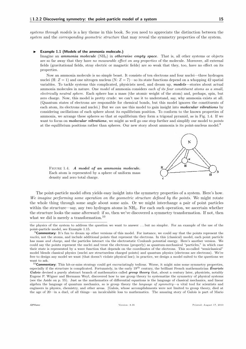
Now an ammonia molecule is no simple beast. It consists of ten electrons and four nuclei—three hydrogennuclei (H: 𝑍 = 1) and one nitrogen nucleus (N: 𝑍 = 7)—so its state functions depend on a whopping 42 spatialvariables. To tackle systems this complicated, physicists need, and dream up, models—stories about actualammonia molecules in nature. One model of ammonia considers each of its four constituent atoms as a small,electrically neutral sphere. Each sphere has a mass (the atomic weight of the atom) and, perhaps, spin, butzero charge. Now, this model is pretty crude: we can’t use it to understand, say, why ammonia exists at all.(Quantum states of electrons are responsible for chemical bonds, but this model ignores the constituents ofeach atom, its electrons and nuclei.) But we can use this model to gain insight into molecular vibrations byconsidering oscillations of each sphere about its equilibrium position. To conform to the known properties ofammonia, we arrange these spheres so that at equilibrium they form a trigonal pyramid, as in Fig. 1.4. If wewant to focus on molecular vibrations, we might as well go one step further and simplify our model to pointsat the equilibrium positions rather than spheres. Our new story about ammonia is its point-nucleus model.9
Figure 1.4. A model of an ammonia molecule.Each atom is represented by a sphere of uniform massdensity and zero total charge.
The point-particle model often yields easy insight into the symmetry properties of a system. Here’s how.We imagine performing some operation on the geometric structure defined by the points. We might rotatethe whole thing through some angle about some axis. Or we might interchange a pair of point particleswithin the structure—say, any two hydrogen atoms in NH3. For each such operation, we ascertain whetherthe structure looks the same afterward: if so, then we’ve discovered a symmetry transformation. If not, thenwhat we did is merely a transformation.10
the physics of the system to address the question we want to answer . . . but no simpler. For an example of the use of thepoint-particle model, see Example 1.15.
9Commentary: It’s fun to dream up other versions of this model. For instance, we could say that the points represent thenuclei, not the atoms, and include additional points that represent the electrons. In this (classical) model, each point particlehas mass and charge, and the particles interact via the electrostatic Coulomb potential energy. Here’s another version. Wecould say the points represent the nuclei and treat the electrons (properly) as quantum-mechanical “particles,” in which casetheir state is represented by a wave function that depends on the coordinates of the electrons. This so-called “semiclassical”model blends classical physics (nuclei are structureless charged points) and quantum physics (electrons are electrons). We’refree to design any model we want (that doesn’t violate physical law); in practice, we design a model suited to the questions wewant to ask.
10Commentary: This hit-or-miss strategy could get excruciatingly tedious. Worse, it might miss some symmetry properties,especially if the structure is complicated. Fortunately, in the early 19th century, the brilliant French mathematician EvaristeGalois devised a purely abstract branch of mathematics called group theory that, about a century later, physicists, notablyEugene P. Wigner and Hermann Weyl, discovered how to use group theory to systematize the symmetry of physical systems(see the Aside on p. 55). Just as the mathematics of differential equations is the language of classical mechanics, and linearalgebra the language of quantum mechanics, so is group theory the language of symmetry—a vital tool for scientists andengineers in physics, chemistry, and other areas. [Galois, whose accomplishments were not limited to group theory, died atthe age of 20—in a duel, of all things—an incalculable loss to mathematics. The amazing story of Galois is part of Mario
JQPMaster Version: 8.35 Printed: August 17, 2010

16 § 1.3 Symmetry elements in the Platonic solids
Now, keeping in mind the basketball, the football, and the ammonia molecule, ponder the following
♣ Key point! The symmetry properties of an object (or a physical system) are inherent in its geometry. So wecan often discover symmetry properties by imagining a geometrical model of the object or system.
§ 1.3 Symmetry elements in the Platonic solids
The mathematical sciences particularly exhibit order, symmetry, and limitation;and these are the greatest forms of the beautiful.
—Metaphysica by Aristotle
Our first task in studying a physical system is to identify its symmetry transformations—those transfor-mations under which all measurable properties of the system are unchanged. To set the stage for learninghow to do this for physical systems, we’ll briefly visit ancient Greece.
To ancient Greeks, no three-dimensional structures were more beautiful than the five regular solidsin Fig. 1.5. These solids now bear the name of Plato, who, around 360 B.C, sought (unsuccessfully) tounderstand the physical universe by associating with each solid one of his basic “elements”: earth with acube; air with an octahedron; water with an icosahedron; and, in a bit of a stretch, fire with a tetrahedron.The dodecahedron, left out of Plato’s elements, got assigned to the universe(!).11
Platonic solids show up all over the place. Crystals exhibit tetrahedral, cubic, and octahedral symmetries(but no others). Many viruses have icosahedral symmetry. Various pollens exhibit the symmetry of dodec-ahedrons, tetrahedra, and cubes. Single-celled plankton have the symmetry of octahedra, dodecahedra, andicosahedra. The equilibrium nuclear configurations of many molecules are regular polyhedra: methane is atetrahedron; cubane is a cube (no surprise), and so on. Japanese water chestnuts are tetrahedra with suchsharp points that Japanese Ninja used them as weapons. (I am not making this up.)
The aesthetic appeal of Platonic solids makes them fertile forms for art. Several millennia ago, prehistoricdwellers of Scotland carved polyhedral designs in rocks. Later, 20th-century artists as different as SalvadorDali and M. C. Escher used the Platonic solids to probe the relationship between art and science.
Considered as geometric structures, the Platonic solids serve as point-particle models of many physicalsystems, and therefore as guides to the systems’ symmetry properties. Essential to the geometric structureof each Platonic solid are three geometric elements that characterize its symmetry : vertices, edges, andfaces:12
(1) all faces of a Platonic solid are congruent regular two-dimensional polygons;
(2) the faces intersect only at their edges; and
(3) the same number of faces intersect at each vertex.
The Platonic solids illustrate an important point:
♦ Rule: To any symmetry transformation there corresponds one or more symmetry elements: points, lines, orplanes in ordinary space with respect to which we can carry out a transformation that leaves the system invariant.13
Livio’s wonderful introduction to symmetry for non-scientists by Livio (2005). Galois’ life is the topic of the historical novelThe French Mathematician by Tom Petsinis (New York: Walker, 1998).] While we lack the time to study group theory, I urgeyou to explore its beauty and power; the Selected Readings at the end of this chapter suggest places to start.
11Commentary: A mere 2300 years ago, Euclid brought to the regular solids the order of geometry . In the last book of hisElements, a tome described by Sir Thomas Heath as “the greatest mathematical textbook of all time,” Euclid defined a regularsolid as a three-dimensional solid all of whose faces are congruent, regular polygons. He proved that the five Platonic solidswere the only possible three-dimensional objects that satisfy this definition.
12Commentary: That the three-dimensional Platonic solids are constructed from regular polygons is unsurprising, since regularpolygons are the most symmetric two-dimensional figures. The group of symmetry transformations of the Platonic solids is theCoceter group.
13Details: We can describe any transformation mathematically in two equivalent ways. In the active convention , wetransform the system in ordinary space, leaving the reference frame fixed. In the passive convention we transform the referenceframe, leaving the system fixed. In this book, I’ll use only the active convention. A translation through a displacement 𝒂, for
JQPMaster Version: 8.35 Printed: August 17, 2010

§ 1.4 Mathematical articulations of transformations 17
Figure 1.5. The five Platonic solids. (a) the tetrahedron , a pyramid each of whose four facesis an equilateral triangle; (b) the hexahedron , a cube; (c) the octahedron , each of whose 8 facesis an equilateral triangle; (d) the icosahedron , each of whose 20 faces is an equilateral triangle;(e) the dodecahedron , each of whose 12 faces is a regular pentagon. [MM: replace?.]
Try This! 1.1. Symmetry elements of the Platonic solids.
The tetrahedron, which has four faces and four vertices, is symmetric under counterclockwise rotationsby 120∘ about an axis that passes through a vertex and the center of the solid. It’s also symmetricunder reflection through a plane that contains the center and two vertices. List any other symmetrytransformations and the corresponding symmetry elements of the tetrahedron. Then list the symmetrytransformations and elements for a cube. In what sense is the tetrahedron a simpler object than a cube?Finally, see how many transformations and elements you can come up with for an icosahedron beforeyou decide there are better ways to spend your time.
§ 1.4 Mathematical articulations of transformations
It requires a very unusual mind to undertake the analysis of the obvious.
—Alfred North Whitehead
We’ll first explore transformations of objects that are rigid, of uniform density, and unmarked in any way.Like the Platonic solids, any such object can be considered as a collection of geometric points “attached”to the object. We can imagine several ways to define such points: if the object is, say, one of the Platonicsolids in Fig. 1.5, we need only specify its vertices; if it’s, say, a blob of glass, we can specify a discrete mesh
JQPMaster Version: 8.35 Printed: August 17, 2010

18 § 1.4 Mathematical articulations of transformations
Figure 1.6. Various ways to denote a point in ordinary space.The point 𝑃 is at position 𝒓 from the fixed origin O. The projections ofthis vector on the axes of a Cartesian (rectangular) coordinate systemwith its origin at O define the representation of 𝒓 as a triplet of numbers,the Cartesian coordinates (𝑥, 𝑦, 𝑧). [MM: Replace 𝑋 by 𝑥 etc.,remove A, B, C, label vector by 𝒓.]
of points in ordinary space within the blob. In any case, we’ll describe a transformation of a (rigid) objectas a transformation of the related set of points.14
Mathematicians have devised several ways to specify a point 𝑃 . The most familiar, illustrated in Fig. 1.6,is by a vector 𝒓 from a fixed origin O to 𝑃 (see §1.D.2 of Complement 1.D). We can symbolize the effect ofthe transformation 𝒢 on the system, 𝒢 : 𝒮 7→ 𝒮 ′, in terms of its effect on an arbitrary point in the system as15
𝒢 : 𝒓 7→ 𝒓′, or 𝒓′ = 𝒢 𝒓, a transformation 𝒢 of apoint P at 𝒓 into 𝑃 ′ at 𝒓′.
(1.4.1)
The inverse transformation takes a point at 𝒓′ in 𝒮 ′ to the corresponding point 𝒓 in 𝒮, as 𝒢−1 : 𝒓′ 7→ 𝒓or, equivalently, 𝒓 = 𝒢−1𝒓′ [Eq. (1.2.1b), p. 14].
Physics abounds with transformations. In this book we’ll concentrate on three spatial transforma-tions—translation, inversion, and rotation. (For a glance at translation in time see Complement 1.F.)
▶ Aside. Effecting a transformation via matrix operations.As in Fig. 1.6, we often specify a point via its coordinates in some reference frame whose origin is at apoint O. This tactic affords another way to perform a transformation. Suppose the Cartesian coordinatesof 𝑃 are (𝑥, 𝑦, 𝑧). Let’s represent 𝒓 by a column vector (a 3× 1 matrix; see Appendix I) whose elements arethese coordinates,16
𝒓 ←→ 𝒓 ≡⎛⎝𝑥𝑦𝑧
⎞⎠ , and 𝒓′ ←→ 𝒓′ ≡⎛⎝𝑥′𝑦′𝑧′
⎞⎠ , (1.4.2a)
where an underscore indicates a matrix. Then we can transform 𝑃 7→ 𝑃 ′ via matrix multiplication (see Ap-pendix I):
𝒢 : 𝒓 7→ 𝒓′ = 𝐺 𝒓,a transformation 𝒢 of a point withcoordinates (𝑥, 𝑦, 𝑧) into a point withcoordinates (𝑥′, 𝑦′, 𝑧′).
(1.4.2b)
example, means “pick up” the system and move it through a vector 𝒂, leaving the reference frame untouched. Similarly, in theactive convention for rotations, we rotate the object but leave the reference frame fixed.
14Read on: This approach requires some care. What we’re doing is representing an object, a physical system, by a geometricabstraction. In his fascinating little book Icons and Symmetries, (1992), Simon Altmann calls such an abstraction an icon .Altmann argues for the importance of not confusing the icon, a purely geometric concept, with the object it represents, aphysical concept. To bring home his argument, Altmann narrates case studies in which very distinguished scientists—amongthem Hans Christian Øersted, discoverer of the effect of an electrical current on a magnet, and Sir William Hamilton, deviserof Hamiltonian mechanics—wasted years pursuing dead ends because they confused these concepts. Altmann argues that thesymmetry properties of a physical system “must be determined experimentally,” not by geometric arguments based on icons.
15Details: In this book we’ll consider only linear transformations. A transformation 𝒢 is a linear transformation if, givenany two points 𝒓1 and 𝒓2 in 𝒮 and any complex number 𝑐, it acts as 𝒢(𝒓1 + 𝒓2) = 𝒢𝒓1 + 𝒢𝒓2 and 𝒢(𝑐 𝒓) = 𝑐𝒢𝒓.
16Notation: The symbol←→, which you’ll see a lot in this book, should be read “is equivalent to.” This means that the twothings on either side of the symbol contain precisely the same mathematical and/or physical information. I use the symbol ≡to indicate a definition, in contrast to =, which indicates equality.
JQPMaster Version: 8.35 Printed: August 17, 2010

§ 1.4.1 Translation 19
with matrix multiplication implied on the right-hand side of the equality. The matrix 𝐺 that corresponds tothe transformation 𝒢 is a square 3× 3 matrix. Called a transformation matrix , 𝐺 is an explicit matrixrepresentation of the transformation 𝒢. (See, for example, Complement 1.E.)
1.4.1 Translation
We specify a translation in two or three dimensions (2D or 3D) by a displacement vector 𝒂 (see §1.D.2of Complement 1.D). As Fig. 1.7 illustrates, in two dimensions 𝒂 has a magnitude, 𝑎 = ∣𝒂∣ = √𝒂 ⋅ 𝒂 (alsocalled its norm and denoted ∥𝒂∥), and a direction, which I’ll specify by the unit vector 𝒆𝑎.
17 Denoting atranslation by 𝒯 (𝒂), we write its effect on a point 𝑃 whose position (with respect to a fixed origin) is 𝒓 as
𝒯 (𝒂) : 𝒓 7→ 𝒓′ = 𝒓 + 𝒂, or 𝒓′ = 𝒯 (𝒂) 𝒓 = 𝒓 + 𝒂 translation in 3D. (1.4.3a)
Using the Cartesian components in 𝒂 = 𝑎𝑥𝒆𝑥 + 𝑎𝑦𝒆𝑦 + 𝑎𝑧𝒆𝑧, we can write Eq. (1.4.3a) explicitly as
𝒯 (𝒂) :
⎧⎨⎩𝑥 7→ 𝑥′ = 𝑥+ 𝑎𝑥
𝑦 7→ 𝑦′ = 𝑦 + 𝑎𝑦
𝑧 7→ 𝑧′ = 𝑧 + 𝑎𝑧,
translation in 3D. (1.4.3b)
Equation (1.4.3b) emphasizes that the parameter 𝒂 for a translation in three dimensions is actually threeparameters, the Cartesian components 𝑎𝑥, 𝑎𝑦, and 𝑎𝑧. You can explore useful properties of the translationoperator in Exercise 1.2.
Figure 1.7. Translation of a point in two dimensions.Consistent with the definition of polar coordinates in §1.D.3,the original location of the point 𝑃 is 𝝆; the new point 𝑃 ′ istranslated by 𝒯 (𝒂).
x
y
Ρ
a
Ρ + a
ea
1.4.2 Continuous versus discrete transformations
A translation depends on a parameter , the displacement vector 𝒂, which can be varied continuously fromany non-zero value to a value (𝒂 = 0) that reduces the translation to the identity transformation , whichdoes nothing. Similarly, a rotation (§1.4.4) depends on an angle that can be varied continuously so asto reduce the rotation to the identity transformation. Translations and rotations exemplify continuoustransformations.
Definition A continuous transformation is any transformation (not necessarily a symmetry trans-formation) which depends on one or more parameters that can be varied continuously so as to reduce thetransformation to the identity.18
17Notation: I use the bold-faced italic symbol 𝒆 to denote a unit vector . A subscript on this symbol denotes a particularaxis. For instance 𝒆𝑥, 𝒆𝑦 , and 𝒆𝑧 denote the axes of a Cartesian coordinate system (Complement 1.D).
18Details: The term continuous transformation implicitly refers to an infinite number of transformations, one for each ofthe infinity of values of the continuous parameter. For example, a 1D translation 𝒯 (𝑎) refers to an infinite number of specific
JQPMaster Version: 8.35 Printed: August 17, 2010
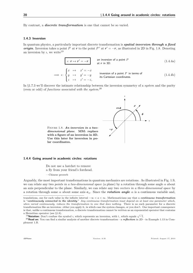
20 § 1.4.4 Going around in academic circles: rotations
By contrast, a discrete transformation is one that cannot be so varied.
1.4.3 Inversion
In quantum physics, a particularly important discrete transformation is spatial inversion through a fixedorigin. Inversion takes a point 𝑃 at 𝒓 to the point 𝑃 ′ at 𝒓′ = −𝒓, as illustrated in 2D in Fig. 1.8. Denotingan inversion by 𝚤, we write19
𝚤 : 𝒓 7→ 𝒓′ = −𝒓 an inversion of a point 𝑃at 𝒓 in 3D.
(1.4.4a)
=⇒ 𝚤 :
⎧⎨⎩𝑥 7→ 𝑥′ = −𝑥𝑦 7→ 𝑦′ = −𝑦𝑧 7→ 𝑧′ = −𝑧,
inversion of a point 𝑃 in terms ofits Cartesian coordinates.
(1.4.4b)
In §1.7.3 we’ll discover the intimate relationship between the inversion symmetry of a system and the parity(even or odd) of functions associated with the system.20
Figure 1.8. An inversion in a two-dimensional plane. MM: replacewith a figure of an inversion in 3D.Use this later for inversion in po-lar coordinates.
y
x
Π+Φ
Φ
Ρ
-Ρ
1.4.4 Going around in academic circles: rotations
Do not use a hatchet to removea fly from your friend’s forehead.
—Chinese proverb
Arguably, the most important transformations in quantum mechanics are rotations. As illustrated in Fig. 1.9,we can relate any two points in a two-dimensional space (a plane) by a rotation through some angle 𝛼 aboutan axis perpendicular to the plane. Similarly, we can relate any two vectors in a three-dimensional space bya rotation through some 𝛼 about some axis 𝒆𝛼. Since the rotation angle 𝛼 is a continuous variable and,
translations, one for each value in the infinite interval −∞ < 𝑎 <∞. Mathematicians say that a continuous transformationis “continuously connected to the identity.” Any continuous transformation must depend on at least one parameter which,when varied continuously, reduces the transformation to one that does nothing. There is no such parameter for a discretetransformation like an inversion: either you apply it, in which case the system changes, or you don’t. One important consequenceis that, unlike a continuous transformation, a discrete transformation cannot be written as an exponential operator that containsa Hermitian operator (see §1.8).
19Notation: Don’t confuse the symbol 𝚤, which represents an inversion, with i , which equals√−1.
20Read on: You can find a similar analysis of another discrete transformation—a reflection in 2D—in Example 1.13 in Com-plement 1.B.
JQPMaster Version: 8.35 Printed: August 17, 2010
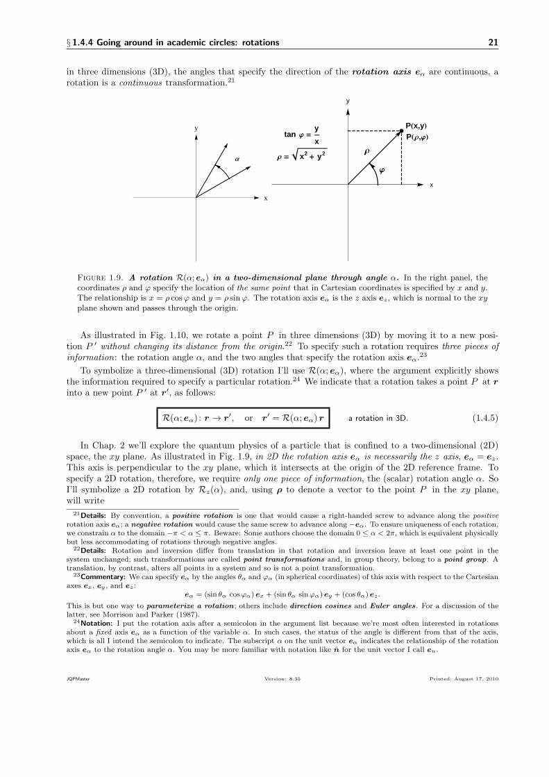
§ 1.4.4 Going around in academic circles: rotations 21
in three dimensions (3D), the angles that specify the direction of the rotation axis 𝒆𝛼 are continuous, arotation is a continuous transformation.21
y
x
Α
y
x
tan j =y
x
Ρ = x2+ y2 Ρ
j
PHx,yLPHΡ,jL
Figure 1.9. A rotation ℛ(𝛼; 𝒆𝛼) in a two-dimensional plane through angle 𝛼. In the right panel, thecoordinates 𝜌 and 𝜑 specify the location of the same point that in Cartesian coordinates is specified by 𝑥 and 𝑦.The relationship is 𝑥 = 𝜌 cos𝜑 and 𝑦 = 𝜌 sin𝜑. The rotation axis 𝒆𝛼 is the 𝑧 axis 𝒆𝑧, which is normal to the 𝑥𝑦plane shown and passes through the origin.
As illustrated in Fig. 1.10, we rotate a point 𝑃 in three dimensions (3D) by moving it to a new posi-tion 𝑃 ′ without changing its distance from the origin.22 To specify such a rotation requires three pieces ofinformation: the rotation angle 𝛼, and the two angles that specify the rotation axis 𝒆𝛼.
23
To symbolize a three-dimensional (3D) rotation I’ll use ℛ(𝛼; 𝒆𝛼), where the argument explicitly showsthe information required to specify a particular rotation.24 We indicate that a rotation takes a point 𝑃 at 𝒓into a new point 𝑃 ′ at 𝒓′, as follows:
ℛ(𝛼;𝒆𝛼) : 𝒓 → 𝒓′, or 𝒓′ = ℛ(𝛼; 𝒆𝛼) 𝒓 a rotation in 3D. (1.4.5)
In Chap. 2 we’ll explore the quantum physics of a particle that is confined to a two-dimensional (2D)space, the 𝑥𝑦 plane. As illustrated in Fig. 1.9, in 2D the rotation axis 𝒆𝛼 is necessarily the 𝑧 axis, 𝒆𝛼 = 𝒆𝑧.This axis is perpendicular to the 𝑥𝑦 plane, which it intersects at the origin of the 2D reference frame. Tospecify a 2D rotation, therefore, we require only one piece of information, the (scalar) rotation angle 𝛼. SoI’ll symbolize a 2D rotation by ℛ𝑧(𝛼), and, using 𝝆 to denote a vector to the point 𝑃 in the 𝑥𝑦 plane,will write
21Details: By convention, a positive rotation is one that would cause a right-handed screw to advance along the positiverotation axis 𝒆𝛼; a negative rotation would cause the same screw to advance along −𝒆𝛼. To ensure uniqueness of each rotation,we constrain 𝛼 to the domain −𝜋 < 𝛼 ≤ 𝜋. Beware: Some authors choose the domain 0 ≤ 𝛼 < 2𝜋, which is equivalent physicallybut less accommodating of rotations through negative angles.
22Details: Rotation and inversion differ from translation in that rotation and inversion leave at least one point in thesystem unchanged; such transformations are called point transformations and, in group theory, belong to a point group. Atranslation, by contrast, alters all points in a system and so is not a point transformation.
23Commentary: We can specify 𝒆𝛼 by the angles 𝜃𝛼 and 𝜑𝛼 (in spherical coordinates) of this axis with respect to the Cartesianaxes 𝒆𝑥, 𝒆𝑦 , and 𝒆𝑧 :
𝒆𝛼 = (sin 𝜃𝛼 cos𝜑𝛼) 𝒆𝑥 + (sin 𝜃𝛼 sin𝜑𝛼) 𝒆𝑦 + (cos 𝜃𝛼) 𝒆𝑧 .
This is but one way to parameterize a rotation ; others include direction cosines and Euler angles. For a discussion of thelatter, see Morrison and Parker (1987).
24Notation: I put the rotation axis after a semicolon in the argument list because we’re most often interested in rotationsabout a fixed axis 𝒆𝛼 as a function of the variable 𝛼. In such cases, the status of the angle is different from that of the axis,which is all I intend the semicolon to indicate. The subscript 𝛼 on the unit vector 𝒆𝛼 indicates the relationship of the rotationaxis 𝒆𝛼 to the rotation angle 𝛼. You may be more familiar with notation like �� for the unit vector I call 𝒆𝑛.
JQPMaster Version: 8.35 Printed: August 17, 2010
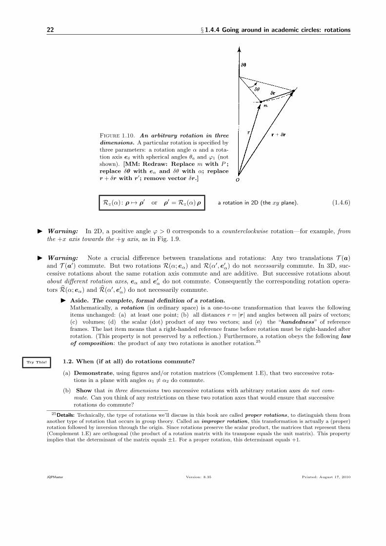
22 § 1.4.4 Going around in academic circles: rotations
Figure 1.10. An arbitrary rotation in threedimensions. A particular rotation is specified bythree parameters: a rotation angle 𝛼 and a rota-tion axis 𝒆𝛿 with spherical angles 𝜃𝑎 and 𝜑1 (notshown). [MM: Redraw: Replace 𝑚 with 𝑃 ;replace 𝛿𝜽 with 𝒆𝛼 and 𝛿𝜃 with 𝛼; replace𝒓 + 𝛿𝒓 with 𝒓′; remove vector 𝛿𝒓.]
ℛ𝑧(𝛼) : 𝝆 7→ 𝝆′ or 𝝆′ = ℛ𝑧(𝛼)𝝆 a rotation in 2D (the 𝑥𝑦 plane). (1.4.6)
▶ Warning: In 2D, a positive angle 𝜑 > 0 corresponds to a counterclockwise rotation—for example, fromthe +𝑥 axis towards the +𝑦 axis, as in Fig. 1.9.
▶ Warning: Note a crucial difference between translations and rotations: Any two translations 𝒯 (𝒂)and 𝒯 (𝒂′) commute. But two rotations ℛ(𝛼; 𝒆𝛼) and ℛ(𝛼′, 𝒆′𝛼) do not necessarily commute. In 3D, suc-cessive rotations about the same rotation axis commute and are additive. But successive rotations aboutabout different rotation axes, 𝒆𝛼 and 𝒆′𝛼 do not commute. Consequently the corresponding rotation opera-
tors ℛ(𝛼;𝒆𝛼) and ℛ(𝛼′,𝒆′𝛼) do not necessarily commute.
▶ Aside. The complete, formal definition of a rotation.Mathematically, a rotation (in ordinary space) is a one-to-one transformation that leaves the followingitems unchanged: (a) at least one point; (b) all distances 𝑟 = ∣𝒓∣ and angles between all pairs of vectors;(c) volumes; (d) the scalar (dot) product of any two vectors; and (e) the “handedness” of referenceframes. The last item means that a right-handed reference frame before rotation must be right-handed afterrotation. (This property is not preserved by a reflection.) Furthermore, a rotation obeys the following lawof composition : the product of any two rotations is another rotation.25
Try This! 1.2. When (if at all) do rotations commute?
(a) Demonstrate, using figures and/or rotation matrices (Complement 1.E), that two successive rota-tions in a plane with angles 𝛼1 ∕= 𝛼2 do commute.
(b) Show that in three dimensions two successive rotations with arbitrary rotation axes do not com-mute. Can you think of any restrictions on these two rotation axes that would ensure that successiverotations do commute?
25Details: Technically, the type of rotations we’ll discuss in this book are called proper rotations, to distinguish them fromanother type of rotation that occurs in group theory. Called an improper rotation , this transformation is actually a (proper)rotation followed by inversion through the origin. Since rotations preserve the scalar product, the matrices that represent them(Complement 1.E) are orthogonal (the product of a rotation matrix with its transpose equals the unit matrix). This propertyimplies that the determinant of the matrix equals ±1. For a proper rotation, this determinant equals +1.
JQPMaster Version: 8.35 Printed: August 17, 2010

§ 1.4.5 Choosing coordinate systems based on symmetry properties 23
1.4.5 Choosing coordinate systems based on symmetry properties
When symbolizing a rotation in two or three dimensions [Eqs. (1.4.5) and (1.4.6)], we instinctively chose acoordinate system in which one of the coordinates is the rotation angle 𝛼. This coordinate system is polarcoordinates (also called plane polar coordinates). (As you saw in Fig. 1.9, p. 21 the second variable inpolar coordinates is the distance 𝜌 from the origin to the point.) But we didn’t have to use polar coordinates;we could have written the rotation as a function of the Cartesian coordinates of the point to be rotated.
Different coordinate systems are just different ways to specify the position of a point 𝑃 (Complement 1.D).In 2D we can specify 𝑃 by its Cartesian coordinates, an ordered pair of real numbers (𝑥, 𝑦). [In 3D, theCartesian coordinates of a point are the ordered triplet (𝑥, 𝑦, 𝑧).] Alternatively, in 2D we can specify 𝑃 byits polar coordinates (𝜌, 𝜑). As illustrated in Fig. 1.9, the scalar 𝜌 = ∣𝝆∣ is the length of the vector 𝝆 fromthe origin to 𝑃 , and 𝜑 is the angle between 𝝆 and the 𝑥 axis.26
We sense instinctively that polar coordinates are ideal for rotations, because rotation of a point doesn’tchange the distance of the point from the origin. A rotation in the 𝑥𝑦 plane through an angle 𝛼 leaves 𝜌unchanged but changes the angle 𝜑 to 𝜑+ 𝛼:
ℛ𝑧(𝛼) :{𝜌 7→ 𝜌
𝜑 7→ 𝜑+ 𝛼
rotation of a point in 2D(polar coordinates).
(1.4.7a)
So in polar coordinates, a rotation changes only one variable, 𝜑. But in Cartesian coordinates, rotation of 𝑃at (𝑥, 𝑦) changes two variables:27
ℛ𝑧(𝛼) :{𝑥 7→ 𝑥′ = 𝑥 cos𝛼− 𝑦 sin𝛼𝑦 7→ 𝑦′ = 𝑥 sin𝛼+ 𝑦 cos𝛼
rotation of a point in 2D(Cartesian coordinates).
(1.4.7b)
It’s no surprise, then, that in dealing with rotations, Cartesian coordinates are often less convenient thanpolar coordinates.
Try This! 1.3. A trigonometric workout.
Perform the (modest) trigonometric exertions required to verify Eq. (1.4.7b). (I’m not going to do allthe work for you!)
1.4.6 Problem-solving: seek symmetry simplifications
This discussion raises a question. How, for a particular system, does one decide which coordinate systemto use? The choice is entirely ours: nature doesn’t care. Nature does, however, offer clues about whichcoordinate system is optimal—that is, which system will yield the greatest insights into the system and willbest facilitate calculating its properties. We seek clues in the geometric structure of the system and, mostimportantly, in its potential energy.
For example, if the system’s geometric structure is a single point and its potential energy is constant,then the system is invariant under any translation and any rotation. In this case, any coordinate systemwill do. But if its potential energy depends on 𝑧 but not on 𝑥 or 𝑦, then the system is invariant only underarbitrary transformations in the 𝑥𝑦 plane. Then 3D cylindrical coordinates (the radius and polar angleof spherical coordinates and 𝑧 of Cartesian coordinates; see §1.D.4) are probably optimal.
If the system is an electron in a hydrogen atom, then the internal force (the Coulomb force on the electronby the proton) is a central force , so the electron’s potential energy depends only on its radial distance from
26Notation: Your favorite math book may use the symbols 𝑟 and 𝜃 for the radial distance and angle from the 𝑥 axis instead of𝜌 and 𝜑. I chose the latter symbols to make an explicit connection between polar coordinates in two dimensions and sphericalcoordinates in three dimensions (Complement 1.D and Chap. 3).
27Read on: You can relate transformations of the coordinates of a point in one coordinate system to its coordinates in othercoordinate systems in Complement 1.D.
JQPMaster Version: 8.35 Printed: August 17, 2010

24 § 1.4.6 Problem-solving: seek symmetry simplifications
the proton. Such a potential energy recommends spherical coordinates. But if the electron is in an H+2 ion,
then the net force on it, the (vector) sum of Coulomb forces due to the two nuclei, is not central, so neitherspherical nor Cartesian coordinates are ideal. (I explore the symmetry of these systems in Examples 1.14and Example 1.15 in Complement 1.B.)28
So important and powerful is the symmetry of a system that I’ve made its use the first of the problem-solving habits you’ll be learning in this book:
Seek symmetry simplifications
♦ The Principle: Symmetry seekingTo choose a coordinate system for a physical system, begin by deducing the system’s symmetry properties.Then consider coordinate systems that conform to those symmetry properties. Choosing such a system willgreatly facilitate gleaning insight and solving problems. To deduce the system’s symmetry, consider its geometricstructure (as in the point-particle model) and its potential energy, a consequence of forces acting on or withinthe system.
Try This! 1.4. Symmetry sketches in three dimensions.
Sketch the operations of inversion and of reflection through the 𝑥𝑦 and 𝑦𝑧 planes by showing the effectof these operations on a characteristic point 𝑃 (𝑥, 𝑦, 𝑧) in three dimensions.
Try This! 1.5. Reflecting on reflections.
Use sketches and words but not equations to explain why any reflection is mathematically equivalent toan inversion followed by a rotation.
Try This! 1.6. Reflecting on inversions.
Use sketches and words but not equations to explain why an inversion is mathematically equivalent toa reflection with respect to a plane followed by a rotation through 𝛼 = 𝜋 about an axis perpendicular tothis plane.
For systems in 3D, seeking symmetry simplifications is simply indispensable. Jumping from 2D to 3D islike jumping into a bottomless pit of algebra. The one additional dimension inevitably introduces algebraiccomplexities which, if left untended, will proliferate like kudzu, obscuring the actual physics and renderingproblem-solving a torturous chore. We must do everything we can to understand the system and to simplifyits mathematical description before we try to solve a problem.
Three dimensions offers an abundance of coordinate systems from which to choose. Of these, the mostuseful are Cartesian coordinates and spherical coordinates, with cylindrical coordinates running a close third(see Complement 1.D).29 As in 2D, a thoughtful, informed choice of coordinate system almost always revealsessential symmetries of the system. To illustrate, let’s investigate an oscillator.
28Memory Jog: Any central force can be written in spherical coordinates as 𝑭 (𝒓) = 𝑓(𝑟)𝒆𝑟, where 𝒆𝑟 is a unit vec-tor directed towards the origin, the source of the force. Any conservative force can be derived from a potential energy𝑉 (𝒓) = 𝑉 (𝑟, 𝜃, 𝜑) as 𝑭 (𝒓) = −∇𝑉 (𝒓). If the force is central, then the potential energy depends only on the radial coordinate:that is, 𝑭 (𝒓) = 𝑓(𝑟)𝒆𝑟 =⇒ 𝑉 (𝒓) = 𝑉 (𝑟). Otherwise, the potential energy depends on one or both of the angles 𝜃 and 𝜑.
29Commentary: Of the many 3D orthogonal “curvilinear” coordinate systems, those most often used in physics are the elevenin which the wave equation is separable. By studying rectangular and spherical coordinates (the ones we’ll use) you’ll learngeneral strategies you can apply in any orthogonal coordinate system. If, for example, you’re interested in diatomic molecules,you may want to use prolate spheroidal coordinates, because these coordinates define two force centers rather than the singleforce center of spherical coordinates. You can learn about other coordinate systems in §3.6 of Pearson (1974). An extremelycomprehensive (though advanced) guide to coordinate systems and transformations between them is the book by Moon andSpencer (1971).
JQPMaster Version: 8.35 Printed: August 17, 2010

§ 1.5 Symmetry and invariance in physics 25
▶ Example 1.2 (The three-dimensional isotropic simple harmonic oscillator.)A 3D simple harmonic oscillator (SHO) is a particle of mass 𝑚 that experiences harmonic restoring forces.The particle is free to move in any direction. In an isotropic SHO, the strengths of the restoring forces, asquantified by force constants, are the same in all directions. The potential energy of a 3D isotropic SHO is thesum of the potential energies of three identical, independent 1D SHOs:
𝑉 (𝑥, 𝑦, 𝑧) =1
2𝑚𝜔2𝑥2 +
1
2𝑚𝜔2𝑦2 +
1
2𝑚𝜔2𝑧2,
3D isotropic SHO(Cartesian coordinates).
(1.4.8a)
In this equation, 𝜔 is the harmonic frequency , which is related to the force constant 𝑘𝐹 by 𝜔 =√𝑘𝐹 /𝑚.
[Notice that these forces are internal to the system, the 3D SHO, which as a whole I’m considering to beisolated—that is, in otherwise empty space. So I’ll call symmetry properties we deduce internal symmetries,to distinguish them from the universal symmetries of §1.6.]
Now think: if the forces are the same in all directions, then the potential energy can depend only on thedistance of the particle from the force center. If we (sensibly) put the origin of our reference frame at the forcecenter, then the potential energy can depend only on 𝑟, the radial variable of spherical coordinates. Thinkingabout symmetry suggests that we work in spherical, not Cartesian, coordinates.
To transform the expression in (1.4.8a) to spherical coordinates, we use 𝑟 =√𝑥2 + 𝑦2 + 𝑧2:
𝑉 (𝑟, 𝜃, 𝜑) = 𝑉 (𝑟) =1
2𝑚𝜔2𝑟2.
3D isotropic SHO(spherical coordinates).
(1.4.8b)
Instead of a function 𝑉 (𝑥, 𝑦, 𝑧) of three independent variables, the potential energy is revealed to be a functionof only one variable, 𝑟. Such a potential energy is spherically symmetric, and a system with such a potentialenergy is rotationally invariant with respect to any rotation ℛ(𝛼; 𝒆𝛼). As you’ll see in Chaps. 3–5, this fun-damental insight enables us to reduce solving the time-independent Schrodinger equation, a partial differentialequation in three variables, to the far simpler task of solving an ordinary differential equation in the singlevariable 𝑟. ◀
For the isotropic SHO, solving the time-independent Schrodinger equation even in Cartesian coordinatesturns out to be pretty easy. But the key point of Example 1.2 is that Cartesian coordinates obscure thespherical symmetry of this system—a crucial insight that emerges clearly in spherical coordinates.
§ 1.5 Symmetry and invariance in physics
The fact that the universe is governed by simple natural laws is remarkable, profound, andon the face of it absurd. How can the vast variety in nature, the multitude of things andprocesses all be subject to a few simple, universal laws?
—Heinz R. Pagels, in Perfect Symmetry.
The symmetry properties of the isotropic SHO in Example 1.2 derive from the restoring forces that act on theparticle. I assumed that no additional forces act on the particle—no, say, gravitational or electromagneticforces. Were I considering the larger system of which this particle is a part, then that larger system, definedto include the origin of the restoring forces, is isolated :
Definition (isolated system) We consider a system to be isolated if nothing else in the universe mea-surably influences the system’s properties (or their evolution) to the precision of our measurements.
Because the restoring forces that make the particle rotationally invariant act within the larger isolatedsystem, I’ll refer to the particle’s rotational invariance as an internal symmetry :
Definition (internal symmetry) An internal symmetry is a symmetry property of part of a systemdue to forces within the system.
This definition raises the question, What are the symmetry properties of an isolated system? To under-stand this question—let alone its answer—you need to first pause and devote serious thought to the followingrather subtle point:
JQPMaster Version: 8.35 Printed: August 17, 2010

26 § 1.5.1 Universal symmetries of space and time
♦ Point to ponder: The symmetry properties of an isolated system—a system in otherwise empty space—do notdepend on the details or inner workings of the system: rather, they are universal symmetries: the same for aSHO, an atom, or a hamster. Such universal symmetries derive from the geometry of space-time itself.
Universal symmetries also characterize the very essence of physics, equations such as Newton’s equation ofmotion and the time-dependent Schrodinger equation—the laws of nature.30
1.5.1 Universal symmetries of space and time
The enterprise of physics is to discover and understand the laws of nature and their consequences forphysical systems (see the Aside on p. 28). Physicists say things like “the laws of nature are invariant.” Tounderstand such statements and their implications, you must first understand invariance :
Definition If all observations show that the physical properties (observables) and behavior (evolution intime) of all states of an isolated system are unchanged by a transformation, then we say that the laws ofnature are invariant under that transformation.
For example, all experiments to date show that
♦ Rule: The laws of nature are the same no matter where we apply them.
This rule refers to translations (§1.5.1.1): for an isolated system the laws of nature are unchanged by anarbitrary translation of the system to which they are applied. This property is called the homogeneityof space . Saying “space is homogeneous” is the same as saying “the laws of nature are translationallyinvariant .” That translational invariance holds for any isolated system tells us something about thestructure of space-time itself.
To illustrate invariance, here’s a familiar situation. The (classical) trajectory {𝒓(𝑡),𝒑(𝑡)} of a billiardball on a pool table where I live in Norman, Oklahoma—the ball’s position 𝒓(𝑡) and linear momentum 𝒑(𝑡)as functions of time—is a consequence of Newton’s equation of motion, subject to particular initial condi-tions {𝒓0(𝑡),𝒑0(𝑡)}. Invariance of this equation means that where you live, an identical ball on an identicaltable with identical initial conditions will follow the same trajectory.
Universal invariance principles are empirical : they rest on observations, on experiments. We can’t provethat any isolated system is translationally invariant; that’s a hypothesis we must test. If repeated measure-ments show (reproducibly) that the properties and their evolution of any isolated system do not changeunder any translation, then we have validated the homogeneity of space.31
Homogeneity of space is one of several assumptions physicists make about the nature of space-time. Asecond is the isotropy of space , which we’ll discuss in §1.5. A third is Galilean invariance:
♦ Rule: The laws of nature don’t depend on the motion of the reference frame in which we formulate themprovided that motion is uniform (not accelerated) and linear (not rotating).
A fourth assumption pertains to the time dimension of space-time. Just as we assume invariance of the lawsof nature under displacements in space, so do we assume their invariance under displacements in time:
30Commentary: The notion of an isolated system is an idealization. No system in nature has ever, is now, or ever will betruly isolated. The idea, of course, is to define (select) “the system” so that the influence of everything else in the universeis negligible. The assumption that physical properties of (almost) isolated systems are independent of, say, their location iscentral to the enterprise of physics. If you’re an experimental physicist spending years trying to discover a new physical lawin your lab in, say, New Jersey, you want to be confident that those laws will be equally valid in Paris or Sydney or on theMoon. The assumption of translational invariance is also relevant to non-physicists. If, for example, you’re mastering yourskills on a billiard table in your dorm in Oklahoma, you want to be sure that those skills will apply equally well when you goto a tournament in Los Angeles.
31Read on: A symmetry principle seems a pretty abstract idea. How could one “test,” say, the translational invariance ofspace? The key to experimental verification of symmetry principles is an amazing theorem called Noether’s theorem (§1.5.2).Noether’s theorem formally links symmetry principles to conservation laws. For example, it links the translational invariance ofspace to the law of conservation of linear momentum. Experimentalists have been devising ways to test conservation laws sincethe earliest days of physics (Rothman, 1989). As of this writing (2010), evidence validates the translational invariance of spacedown to a length scale of approximately 10−24 m and translational invariance of time down to a time scale of about 10−48 s.You can find an engaging, accessible discussion of these matters in Chaps. 3–5 of Lederman and Hill (2008). For an overviewof physical laws, see Feynman (1965).
JQPMaster Version: 8.35 Printed: August 17, 2010

§ 1.5.1 Universal symmetries of space and time 27
♦ Rule: The laws of nature are the same no matter when we apply them.
In other words, the evolution of a state depends on the interval between two times, Δ𝑡 ≡ 𝑡2 − 𝑡1 > 0, noton the particular instant we choose as the “zero of time,” 𝑡 = 0. This means that the concept of “absolutetime ,” a cornerstone of Newton’s thinking, has no meaning. Invariance under displacements in time impliesconservation of energy (ComplementaboutTime).
1.5.1.1. Translational invariance and the homogeneity of free space
Since no forces act on an isolated system, its mechanical properties, such as energy and angular momen-tum, and the laws that govern these properties do not change if we translate the entire system by somedisplacement. That’s what we mean by translational invariance:
Definition (translational invariance) A system is translationally invariant if its physical propertiesare unchanged by an arbitrary displacement.
Symmetry properties must be verified. So we must be able to state them in operational terms, Opera-tionally, translational invariance means
♦ Rule: Any physical property of a system, as measured by an experiment in otherwise empty space, is independentof the location of the experimental apparatus.
The “experimental apparatus” includes the measuring device and the system being studied. Note the keyphrase “otherwise empty space .” No external forces act on a system in otherwise empty space. It’s alone.
Expressed as a property of space-time, translational invariance is called the homogeneity of space :
Definition (homogeneity of space) All points in empty space are physically equivalent. No point isspecial (or “preferred”) over to any other point.
Homogeneity of space implies that the concept of “absolute position” has no physical meaning: onlyrelative positions—say, the separation between two interacting particles—can influence behavior; this pointwill become central to our treatment of the hydrogen atom in Chap. 5. (That’s why, when solving problems foran isolated system, we’re free to put the origin of our reference frame anywhere.) Remarkably, homogeneity ofspace also implies that the linear momentum of any isolated system is conserved. This relationship between auniversal symmetry and a conservation law exemplifies a cornerstone of physics called Noether’s theorem(§1.5.2). In essence, this theorem says that symmetries imply conservation laws (and vice-versa). Still,although homogeneity has consequences for the properties of physical systems, homogeneity is a universalsymmetry of space itself.
1.5.1.2. Rotational invariance and the isotropy of free space
Turning to rotational invariance reminds us of the isotropic 3D SHO of Example 1.2. Reflecting on thatexample illuminates an important distinction between internal symmetries and universal symmetries. Aparticle in a system whose internal forces are isotropic restoring forces is rotationally invariant, because thenet force that acts on the particle is a central force . To the particle, all directions in space are physicallyequivalent: no direction is “preferred” (special) over any other. This symmetry property is internal to thesystem. But the larger system that consists of the particle and the source of the restoring forces—consideredas a single, isolated system—is also rotationally invariant. The rotational invariance of the larger system isnot an internal symmetry; it’s a property of space itself, a universal symmetry.
To understand this point, consider that not just a 3D SHO but any isolated system is rotationallyinvariant, because (by definition) no forces act measurably on an isolated system. The rotational invarianceof an isolated system is thus another universal symmetry ; Equivalently, we say that space is isotropic:
Definition (isotropy of space) All directions in empty space are physically and mathematically equiva-lent. No direction is special (“preferred”) over any other direction.
We can codify our understanding of rotational invariance into a definition and an operational rule:
JQPMaster Version: 8.35 Printed: August 17, 2010

28 § 1.5.2 Universal symmetries and conservation laws: Noether’s theorem
Definition (rotational invariance) A system is rotationally invariant if its physical properties areunchanged by an arbitrary rotation.
While homogeneity is concerned with translations, isotropy is concerned with the orientation of a systemand hence with rotations:32
♦ Rule: Any physical property of a system, as measured by an experiment in otherwise empty space, is independentof the orientation of the experimental apparatus.
Just as the homogeneity of space implies translational invariance of the laws of nature, so does the isotropyof space imply rotational invariance of these laws. Consequently the notion of an “absolute orientation”has no physical meaning. (We’re free to orient our reference frame any way we like provided we are studying asystem in otherwise empty space.) And, just as homogeneity implies conservation of linear momentum, so—according to Noether’s theorem (§1.5.2)—does isotropy of space imply conservation of the angular momentumof an isolated system.33
▶ Aside. Laws of nature in classical and quantum physics.What is a “law of nature”? That’s a subtle question scientists and philosophers have discussed for centuries.Here’s the general idea. It’s useful to separate the laws of nature into two types. One type, which I’ll call adynamical law , is a mathematical description of relationships between events that are separated by some timeinterval. The idea is that events are somehow correlated, and the law expresses their correlation (Wigner,1967). For a macroscopic particle of mass 𝑚, Newton’s law of motion, 𝑭 = 𝑚d𝒑/𝑑𝑡, is such a law. Thesecond type, which I’ll call a static law , is a relationship between different physical properties at the sametime. An example is the classical equation for the orbital angular momentum in terms of position and linearmomentum, 𝑳(𝑡) = 𝒓(𝑡)× 𝒑(𝑡).34
It’s useful to describe both types of laws in terms of state representatives, such as trajectories inclassical mechanics or wave functions in quantum mechanics. A dynamical law is a prescription for calcu-lating how state representatives and physical properties change with time. So in classical physics Newton’sequation of motion, which determines trajectories, is a dynamical law. And in (nonrelativistic) quantummechanics, the Schrodinger equation, which determines wave functions, is a dynamical law. A static law isa prescription for calculating a physical property from the state representative. For example, the definitionof an expectation value tells us how to calculate (from a wave function) the value we would expect to obtainin a measurement of an observable (see §1.C.1).35
1.5.2 Universal symmetries and conservation laws: Noether’s theorem
The key to the relation of symmetry laws to conservation laws is Emmy Noether’scelebrated theorem. . . . Before Noether’s theorem the principle of conservation of energywas shrouded in mystery. . . Noether’s simple and profound mathematical formulation didmuch to demystify physics.
—Feza Gursey, in Emmy Noether, Collected Papers
In §1.5.1, I mentioned two connections between universal symmetries and conservation laws:
♦ Rule: Homogeneity of space implies that the linear momentum of any isolated system is conserved.
32Jargon: In differential geometry, an isotropy refers to a coordinate transformation that does not alter the distance betweenany two points. In three dimensions, we can “construct” an isotropic transformation by combining three basic transformations:translation, rotation, and reflection in a plane.
33Commentary: Many systems are not invariant under an arbitrary rotation but are invariant under particular rotations.Imagine an equilateral triangle. Rotating this triangle through an angle 𝛼 will change its appearance except for special angles,such as 𝛼 = 120∘. Except for a sphere, geometric shapes are invariant only under restricted rotations—as are the Platonicsolids in Fig. 1.5, p. 17. In group theory, these restrictions determine the “point group” of the object, a key to understandingsystems such as molecules and crystalline solids.
34Details: The orbital angular momentum (Chaps. 2 and 3), is defined with respect to a particular origin, the same one usedfor the position 𝒓(𝑡) and momentum 𝒑(𝑡).
35Commentary: The distinction between dynamical and static laws is schematic, not rigorous. Conservation laws, like theconservation of energy of an isolated system, can be considered a hybrid of these types.
JQPMaster Version: 8.35 Printed: August 17, 2010
§ 1.5.2 Universal symmetries and conservation laws: Noether’s theorem 29
♦ Rule: Isotropy of space implies that the angular momentum of any isolated system is conserved.
These connections follow from Noether’s theorem ;, a mathematically rigorous, general relationship theseconnections exemplify:
Theorem (Noether’s theorem) Every continuous symmetry implies a conservation law, a statementthat some physical property is a constant of the motion. Correspondingly, every conservation law implies acontinuous symmetry of the laws of nature:36
symmetry ⇐⇒ conservation laws (1.5.1)
Note carefully that Noether’s theorem pertains to continuous symmetry transformations, which leaves outdiscrete transformations such as inversion (§1.7.3). Nonetheless, this theorem underpins much of physics,classical as well as quantum.
The generality of Noether’s theorem is stunning. Its implications range beyond particular conservationlaws. In a sense, Noether’s theorem explains why there are conservation laws: physics has conservation lawsbecause of the universal symmetry properties of space-time. Moreover, although we’ve discussed conservationlaws for classical theorems, Noether’s theorem also holds in quantum mechanics, as we’ll see in §1.6.
▶ Aside. Who was Emmy Noether?In 1915, the renowned theoretical physicist David Hilbert asked a young German mathematician namedEmmy Noether to help him with a problem. Hilbert was puzzling over the place of conservation of energyin Einstein’s as-yet-incomplete general theory of relativity. Then 33 years old, Noether left her home inErlangen and joined Hilbert’s research team at the University of Gottingen. Soon thereafter, Einstein gavea series of lectures at Gottingen that stimulated Noether to study general relativity. Three years later, in1918, Noether published a paper that not only solved Hilbert’s problem but established, for the first time, acompletely general relationship between symmetry properties and conservation laws.37 One of many resultsof that paper, the one we call Noether’s theorem , profoundly influenced physics ever since.
In the years that followed, Noether’s conclusions were widely used but rarely attributed to her. Only inthe late 1950’s, long after her abrupt and untimely death in 1935, did physicists begin to give credit wherecredit had long been overdue.
Amazingly, Noether’s work in theoretical physics was a sideline to her primary interest, abstract al-gebra. Her research in pure mathematics also greatly aided modern physics (particularly, the study ofelementary particles) by supplying physicists with mathematical tools such as Lie groups, algebraic topol-ogy, and cohomology theory. More important, Noether introduced a new, simpler way of thinking aboutalgebraic concepts; the publication of her monumental 1919 paper in effect founded the field of modernabstract algebra.38
During most of her career at Gottingen, Noether was not allowed to teach or lecture under her ownname: lectures she prepared and delivered were advertised as “by David Hilbert with the assistance ofEmmy Noether.” By 1923, well after mathematicians from all over Europe had begun to visit Gottingento work with Noether, she was finally awarded a University position—unsalaried. In fact, although shewas widely acknowledged as one of the greatest 20th-century mathematicians, Noether never held a regular,salaried university position. From 1908, when she began her academic career at the University of Erlangen,to 1922, when Hilbert arranged for her to receive a tiny stipend at Gottingen, Noether lectured, supervisedstudents, and did original research without pay.39 In 1933 the Nazi party came to power and Noether,
36Notation: Read the symbol ⇐⇒ as corresponds to, in the sense of “implies and is implied by.” I use this symbol ratherthan =⇒, which stands for “implies,” because either of these equations implies the other.
37Read on: You can learn more about Emmy Noether from articles in Brewer and Smith (1981), Teicher (1999), and Byers andWilliams (2006). Byers (1996) and Byers (1999) addresses Noether’s contributions to physics and mathematics as well as herbiography. You can find a rather technical discussion of Noether’s theorem and its philosophical consequences in “Symmetriesand Noether’s theorems” by Katherine Bading and Harvey R. Brown in Brading and Castellani (2003). In 1983, Springerpublished Noether’s collected papers. An English translation of Noether’s paper on conservation laws, Noether (1918), isavailable at http://www.physics.ucla.edu/˜cwp/articles/noether.trans/english/mort186.html.
38Commentary: Introducing the volume of Noether’s collected works published in 1983, Nathan Jacobson characterizedNoether as “one of the most influential mathematicians of this century. The development of abstract algebra, which is one ofthe most distinctive innovations of twentieth-century mathematics, is largely due to her.”
39Commentary: To his credit, Hilbert and his colleague Felix Klein repeatedly tried to persuade their colleagues to recognizeand honor Noether’s work. In 1915, when Noether submitted a major piece of mathematical research as her thesis for a university
JQPMaster Version: 8.35 Printed: August 17, 2010

30 § 1.5.3 Internal symmetries and forces
who was Jewish, lost her job. She fled to America, to Bryn Mawr College, where she accepted a visitingprofessorship. Two years later, she died of complications following surgery.
1.5.3 Internal symmetries and forces
The conservation laws that follow from Noether’s theorem pertain to properties of an isolated system. Forinstance, conservation of the total angular momentum of an isolated system is a consequence of the isotropyof space (a universal symmetry), regardless of whatever internal forces may act between particles within thesystem. This law holds equally well for an atom, a molecule, or a wombat.
We face a quite different situation if we consider a constituent of a system—that is, a subsystem . Forinstance, a simple model of atomic hydrogen consists of an electron interacting with a proton via theelectrostatic Coulomb interaction (see Examples 1.3 and 1.14). In this classical model, the force on theelectron is a central force (it acts along a line between the electron and the proton), so the orbital angularmomentum of the electron is conserved. Because the Coulomb potential energy is spherically symmetric,the electron is a rotationally invariant subsystem of the hydrogen atom. This internal symmetry is thereason that the electron’s orbital angular momentum is conserved.
The same model of diatomic hydrogen ion H+2 consists of an electron interacting with two protons that
are separated by about 1.5 �� (see Example 1.15). The forces that act on the electron in H+2 are not central
forces, and the electron’s angular momentum is not conserved. The potential energy of the electron is notspherically symmetric (it is axially symmetric; see Example 1.15), so an electron in H+
2 is not a rotationallyinvariant subsystem. Still, the total angular momentum of the whole H+
2 ion, assumed to be isolated, isconserved, as is that of the hydrogen atom (and the wombat).
These examples illustrate that if we’re interested in a system that is not isolated—one that interacts inany way with another system (or with an external field)—then to deduce the system’s symmetry propertieswe must take into account whatever forces act on it. That’s what we did for the isotropic SHO in Ex-ample 1.2: the particle is rotationally invariant because the (restoring) forces that act on it are centralforces (see Example 1.4). This property of those forces is manifest in the particle’s potential energy, which isspherically symmetric. These considerations establish a vital logic chain you must understand and memorize:
forces on a subsystem −→ subsystem’s potential energy =⇒ symmetry of the subsystem (1.5.2)
So important is the logic chain (3.2.26) that I’ll conclude this section with two further examples. The firstis the aforementioned classical model of a hydrogen atom (Chap. 5). The second is a two-dimensionalversion of the isotropic 3D SHO of Example 1.2.
▶ Example 1.3 (The symmetry of an electron in a “classical hydrogen atom.”)Imagine a particle with charge −𝑒, where 𝑒 = 1.602× 10⁻¹⁹ C is the elementary charge , in the field of aproton with charge +𝑒. In this classical model of a hydrogen atom , which Niels Bohr devised during theearly years of quantum mechanics, the electron is a subsystem of the electron+proton system. (The proton,modeled as a fixed point particle at the origin, is the other subsystem.) To understand the physics of theelectron, we first investigate its symmetry properties.
These follow from the forces that act on the electron. In Bohr’s model, the only force is the attractive(electrostatic) Coulomb force between the electron and the proton. This force is central. Consequently, thepotential energy of the electron is spherically symmetric: 𝑉 (𝒓) = 𝑉 (𝑟). If we imagine that the electron issomewhere on a sphere centered on the proton, then the magnitude of the Coulomb force doesn’t dependon where on the sphere it is. So the electron is a rotationally invariant subsystem of the larger, rotationallyinvariant isolated hydrogen atom.40
Habilitation, the academic senate of the university turned her down on the stated grounds of her gender. This provoked Hilbertto remark, “I don’t see why the sex of the candidate is relevant—this is afterall an academic institution not a bath house.”
40Commentary: When we say that a classical system is spherically symmetric, we mean that the classical Hamilto-nian 𝐻(𝒓,𝒑) of the system, the sum of the system’s kinetic energy plus its potential energy, is spherically symmetric. The
JQPMaster Version: 8.35 Printed: August 17, 2010
§ 1.5.3 Internal symmetries and forces 31
A key point of Example 1.3 is the generality of the relationship between a central force, spherical sym-metry, and rotational invariance. Nothing in my argument depends on the details of the Coulomb force orpotential energy. [That’s why I never wrote down the explicit expression 𝑉 (𝑟) = −𝑒2/4𝜋𝜖0 𝑟].41 In fact, withrespect to its symmetry, the electron in a hydrogen atom is the same as the isotropic SHO :
a central force −→ spherically symmetric potential energy =⇒ rotational invariance. (1.5.3)
While I developed this logic chain via examples about two different systems, the logic itself pertains to any(conservative) central force:
♦ Rule: A system in an external central force has a spherically symmetric potential energy and is thereforerotationally invariant.
▶ Warning: This rule does not imply that all states of a particle with a spherically symmetric potentialenergy are spherically symmetric.42
▶ Example 1.4 (The two-dimensional isotropic harmonic oscillator.)For all its usefulness, 3D SHO of Example 1.2 defeats efforts to easily visualize this function. So I’m going tonow assume that the particle is confined to the 𝑥𝑦 plane. If, as in Example 1.2, the restoring forces along the 𝑥and 𝑦 axes are equal, then the potential energy of this 2D isotropic SHO is [compare to Eq. (1.4.8), p. 25]
𝑉 (𝑥, 𝑦) =1
2𝑚𝜔2𝑥2 +
1
2𝑚𝜔2𝑦2,
2D isotropic SHO(Cartesian coordinates).
(1.5.4a)
I can discover the system’s symmetry by writing Eq. (1.5.4a) in polar coordinates via the conversion equation𝜌 =
√𝑥2 + 𝑦2 (§1.D.3):
𝑉 (𝜌, 𝜑) =1
2𝑚𝜔2 𝜌2,
2D isotropic SHO(polar coordinates).
(1.5.4b)
Therefore the potential energy of a 2D isotropic SHO has circular symmetry , the 2D counterpart of sphericalsymmetry of the 3D oscillator. The particle is rotationally invariant in the 𝑥𝑦 plane. This symmetry propertybreaks down if the forces along 𝑥 and 𝑦 differ, in which case the oscillator is anharmonic. You can see thedifference in Fig. 1.11, which shows potential energies for an isotropic (and an anisotropic) 2D SHO. Even fora 2D system, visualizing a potential energy requires a bit of alacrity. A 3D plot, which shows 𝑉 (𝑥, 𝑦) on thevertical axis as a function of 𝑥 and 𝑦 in the horizontal plane, is usually less revealing than a contour plot like theothers in this figure. A contour plot is a 2D plot in which each curve represents the locus of values of 𝑥 and 𝑦along which 𝑉 (𝑥, 𝑦) has the same value—the value shown by the little numbers attached to each curve.43 ◀
For more illustrations of the logic of (3.2.26) see Examples 1.14 and 1.15 of Complement 1.B.
Try This! 1.7. Same subsystem, different system
Explain carefully and thoroughly why an electron in the field of a point dipole has a differentsymmetry than an electron in a hydrogen atom. Is the degree of symmetry of the electron in the dipolefield higher or lower than in the hydrogen atom? What symmetry properties does an electron in thedipole field have?
kinetic energy of a particle is invariant under any symmetry transformation, so the symmetry of 𝐻(𝒓,𝒑) and hence of thesystem is determined solely by the symmetry of the potential energy. In quantum physics, the symmetry properties of 𝐻(𝒓,𝒑)
translate directly into the symmetry properties of the Hamiltonian operator ℋ.41Notation: Throughout this book I’ll use the symbol 𝑒 2
0 ≡ 𝑒2/4𝜋𝜖0, where 𝜖0 is the permittivity of the vacuum (free space),8.854 × 10−12 F m−1, and 𝑒 is the elementary charge 𝑒 = 1.602× 10⁻¹⁹ C. So the charge on a proton is 𝑒, while the chargeon an electron is −𝑒. (Other sources use the opposite convention, taking 𝑒 to be the negative number −∣𝑒∣, so be careful!) In anin-text fraction, everything that follows the symbol for division is assumed to be in the denominator unless otherwise indicatedby parentheses: 𝑒2/4𝜋𝜖0 = 𝑒2/(4𝜋𝜖0).
42Commentary: As you’ll see when we look at plots of the probability density of an electron in a quantum-mechanical hydrogenatom (Chap. 5), some bound states of an electron in the field of a proton are spherically symmetric, others are not.
43Read on: If the restoring forces along the 𝑥 and 𝑦 axes are different, then the corresponding harmonic frequencies 𝜔𝑥and 𝜔𝑦 won’t be equal, so the potential energy of the particle will be 𝑉 (𝑥, 𝑦) = 𝑚(𝜔2
𝑥𝑥2 + 𝜔2
𝑦𝑦2)/2. As you can see from the
lower panel in Fig. 1.11, the anharmonic potential energy has no particular symmetry. Such a system is called an anharmonicoscillator . For more about the 2D SHO, see examples in Chap. 2
JQPMaster Version: 8.35 Printed: August 17, 2010
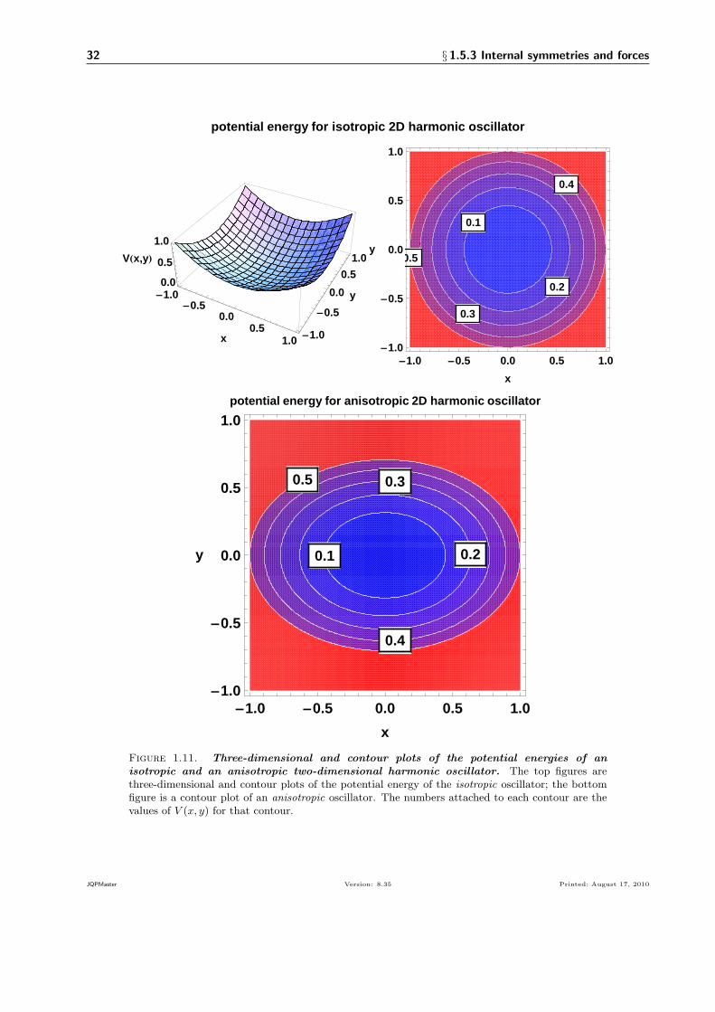
32 § 1.5.3 Internal symmetries and forces
-1.0-0.5
0.00.5
1.0x -1.0
-0.5
0.0
0.5
1.0
y0.0
0.5
1.0
VHx,yL
0.1
0.2
0.3
0.4
0.5
-1.0 -0.5 0.0 0.5 1.0-1.0
-0.5
0.0
0.5
1.0
x
y
potential energy for isotropic 2D harmonic oscillator
0.1 0.2
0.3
0.4
0.5
-1.0 -0.5 0.0 0.5 1.0-1.0
-0.5
0.0
0.5
1.0
x
y
potential energy for anisotropic 2D harmonic oscillator
Figure 1.11. Three-dimensional and contour plots of the potential energies of anisotropic and an anisotropic two-dimensional harmonic oscillator. The top figures arethree-dimensional and contour plots of the potential energy of the isotropic oscillator; the bottomfigure is a contour plot of an anisotropic oscillator. The numbers attached to each contour are thevalues of 𝑉 (𝑥, 𝑦) for that contour.
JQPMaster Version: 8.35 Printed: August 17, 2010
§ 1.6 Symmetry transformations and invariance in quantum mechanics 33
§ 1.6 Symmetry transformations and invariance in quantum mechanics
You boil it in sawdust; you salt it in glue:You condense it with locust and tape:Still keeping one principal object in view—To preserve its symmetrical shape.
—Lewis Carroll, in “The Hunting of the Snark”
1.6.1 Associated functions and symmetry operators
Associated with every physical system are functions and operators we use to represent the system, its prop-erties, and its states. In classical mechanics, one such associated function is the potential energy 𝑉 (𝒓).Others are position 𝒓(𝑡) and momentum 𝒑(𝑡), which comprise the trajectory {𝒓(𝑡),𝒑(𝑡)}, the state repre-sentative of classical physics.44 In quantum mechanics, the most prominent associated functions are wavefunctions Ψ(𝒓, 𝑡). We associate operators with observables of the system, such as the Hamiltonian ℋ.45
When we perform a symmetry transformation 𝒰 on a system, 𝒰 : 𝒮 7→ 𝒮 ′, the associated functions (andoperators) “go with the system” and are transformed accordingly. If the wave function of that represents astate before the transformation is Ψ(𝒓, 𝑡), then the representative of the same state after the transformation
will be some wave function Ψ′(𝒓, 𝑡). If an observable𝑄 of 𝒮 is represented by Q, then the same observable of 𝒮 ′will be represented by some operator Q ′. These observations raise the question, What is the mathematicalrelationship between an associated function (or operator) after a transformation of a system to the function(or operator) before the transformation? 46 In quantum mechanics, this question is answered by symmetryoperators.
Definition For any transformation, the corresponding symmetry operator is an operator that transformsstate functions and operators of the untransformed system into their counterparts of the transformed system.
♦ Rule: To each transformation 𝒰 there corresponds a symmetry operator 𝒰 .
The effect of 𝒰 on a wave function Ψ(𝒓, 𝑡) that represents a state of 𝒮 is to produce the wave func-tion Ψ′(𝒓, 𝑡) that represents the same state of 𝒮 ′, which we write47
𝒰 : 𝒮 7→ 𝒮 ′ =⇒ Ψ′(𝒓, 𝑡) = 𝒰 Ψ(𝒓, 𝑡) (1.6.1a)
The same transformation operator 𝒰 relates the quantum-mechanical operator Q that represents an observ-able of 𝒮 to the operator Q ′ that represents the same observable of 𝒮 ′ via
Q ′ = 𝒰 Q𝒰 † (1.6.1b)
which I’ll derive below [Eq. (1.6.13), p. 37]. If the transformation depends on parameters, as a transla-
tion 𝒯 (𝒂) depends on 𝒂, then so will the transformation operator, as 𝒯 (𝒂).44Details: Typically, functions associated with a classical particle are its physical properties. In classical physics, we write
each physical property as a real function of position 𝒓(𝑡) and/or momentum 𝒑(𝑡)—as, for example, the mechanical energy𝐸(𝒓(𝑡),𝒑(𝑡)
)= 𝐸(𝑡) (the sum of the kinetic energy 𝑇 and the potential energy 𝑉 ) and the orbital angular momentum
𝑳(𝑡) ≡ 𝒓(𝑡)× 𝒑(𝑡).45Notation: I indicate quantum mechanical operators such as Q by a circumflex (little hat) and are set in a different typeface
(math sans serif).46Notation: Unlike some mathematics texts, in this book a prime on a function, such as Ψ′(𝒓, 𝑡), does not signify the first
derivative of the function.47Details: In operational terms, Ψ(𝒓, 𝑡) represents a quantum state prepared by an untransformed apparatus, while Ψ(𝒓, 𝑡)′
represents the same state that would be prepared were the apparatus transformed by 𝒰 . When considering the consequences ofa symmetry transformation for measurement of a property, we must remember to transform the measuring device by the sametransformation by which we transform the system, 𝒰 .
JQPMaster Version: 8.35 Printed: August 17, 2010

34 § 1.6.2 Invariance in terms of wave functions and the Hamiltonian
To turn our notions about symmetry and invariance into mathematical tools, we must accomplishthree things:
(1) deduce the mathematical properties of symmetry operators;
(2) determine mathematical conditions that tell us whether, for a particular system, a transformation 𝒢 isa symmetry transformation 𝒰 ; and
(3) develop explicit mathematical instructions for symmetry operators.
In this section we’ll accomplish the first two tasks, leaving the third for §1.7. This section is a bit abstract,so you’ll need to work through it slowly and carefully.
▶ Warning: Mathematical symbols without little hats, like 𝒰 , never act on functions: they represent trans-formations and act on points in ordinary space. Symbols with little hats, like 𝒰 , never act on points: theyare operators and act on functions and operators associated with the system that undergoes the transforma-tion 𝒰 .
1.6.2 Invariance in terms of wave functions and the Hamiltonian
Early in this chapter, I said that a transformation of an object is a symmetry transformation if it leavesthe appearance of the object unchanged. Then I applied this concept to a physical system, the ammoniamolecule and distinguished internal from universal symmetries. Finally, I explained that the phrase “the lawsof nature are invariant under a symmetry transformation,” means that in any state of any isolated system 𝒮,all measurable properties of the system and their evolution in time are unchanged by the transformation. Ifthese conditions hold, then we cannot tell whether or not a symmetry transformation has been applied tothe system, because any transformed system 𝒮 ′ “looks like” the corresponding untransformed system 𝒮 inevery measurable respect.
In quantum mechanics, we calculate physical properties of a system at any time from the wave function atthat time, Ψ(𝒓, 𝑡). The dynamics of the system in any state—how properties calculated from a wave functionchange with time—are determined by the Hamiltonian through its role in the time-dependent Schrodingerequation:
ℋΨ(𝒓, 𝑡) = i ℏ∂
∂𝑡Ψ(𝒓, 𝑡),
time-dependent Schrodinger equation ofa system represented by Hamiltonian ℋ.
(1.6.2)
which we must augment with an initial condition Ψ(𝒓, 0) to specify a particular state Ψ(𝒓, 𝑡). We can thusapply our ideas about invariance to quantum mechanics:
♦ Rule: Under a symmetry transformation, any transformed wave function Ψ′(𝒓, 𝑡) must represent the samephysical state as the corresponding untransformed wave function Ψ(𝒓, 𝑡). This requires that (1) all measurablequantities predicted by quantum mechanics—expectation values, probability densities, eigenvalues, and transitionprobabilities (see §1.C.2)—must not change; and (2) the dynamics of the system, as governed by the Hamiltonianvia the time-dependent Schrodinger equation, must not change.
If these requirements are satisfied, we say the system 𝒮 is invariant under that transformation.48
48Commentary: It’s easy imagine the difficulties that would arise were these conditions not satisfied. Prominent amongeigenvalues are the stationary-state energies of a system, the eigenvalues of the Hamiltonian. Nature allows any system—say,an atom—to be in a bound state with a well-defined (sharp) energy only if that energy is one of these eigenvalues. Transitionsbetween these stationary states give rise to atomic spectra (Chap. 18), the puzzling nature of which drove the development
of quantum mechanics. If the eigenvalues of ℋ were not invariant, then measured spectra would depend on the position andorientation of the apparatus used to measure it—and quantum physics would never have gotten off the ground.
JQPMaster Version: 8.35 Printed: August 17, 2010
§ 1.6.3 Generic properties of symmetry operators 35
1.6.3 Generic properties of symmetry operators
An operator is a symmetry operator only if it satisfies the physical conditions of §1.6.2. We’ll now developexplicit mathematical forms of these conditions, forms that will help us use symmetry arguments to gaininsight and solve problems.
1.6.3.1. Linearity
One of the hallmarks of quantum mechanics is the principle of superposition : any linear combinationof two wave functions of a system 𝒮 is a third wave function of 𝒮. Now, symmetry operators act on wavefunctions. What properties must a symmetry operator have to ensure that it doesn’t change a superposition?
Suppose the state of 𝒮 is a superposition of two other states, Ψ1(𝒓, 𝑡) and Ψ2(𝒓, 𝑡), with complex coeffi-cients 𝑐1 and 𝑐2:
Ψ(𝒓, 𝑡) = 𝑐1 Ψ1(𝒓, 𝑡) + 𝑐2 Ψ2(𝒓, 𝑡). (1.6.3a)
All three functions—Ψ1(𝒓, 𝑡), Ψ2(𝒓, 𝑡) and Ψ(𝒓, 𝑡)—satisfy the same time-dependent Schrodinger equation,and the coefficients 𝑐1 and 𝑐2 are subject to the normalization condition
⟨Ψ(𝑡) ∣ Ψ(𝑡)⟩ = 1 ⇐⇒ ∣𝑐1∣2 + ∣𝑐2∣2 = 1. (1.6.3b)
Under a symmetry transformation 𝒰 , all properties we calculate from Ψ(𝒓, 𝑡) must be unchanged by
the transformation. So the symmetry operator 𝒰 cannot change the relationship (1.6.3a) between Ψ(𝒓, 𝑡),Ψ1(𝒓, 𝑡), and Ψ2(𝒓, 𝑡). The transformed wave function of 𝒮 ′ must be49
Ψ′(𝒓, 𝑡) = 𝑐1 Ψ′1(𝒓, 𝑡) + 𝑐2 Ψ
′2(𝒓, 𝑡), (1.6.3c)
where Ψ′(𝒓, 𝑡) = 𝒰 Ψ(𝒓, 𝑡), and Ψ′1(𝒓, 𝑡) = 𝒰 Ψ1(𝒓, 𝑡), and Ψ′
2(𝒓, 𝑡) = 𝒰 Ψ2(𝒓, 𝑡).
What properties must 𝒰 have to ensure that transformation of Ψ(𝒓, 𝑡) of (1.6.3a) yields Ψ′(𝒓, 𝑡)of (1.6.3c)? To find out, let’s write both sides of (1.6.3c) in terms of untransformed wave functionsin (1.6.3a):50
𝒰 Ψ(𝒓, 𝑡) = 𝑐1 Ψ′1(𝒓, 𝑡) + 𝑐2 Ψ
′2(𝒓, 𝑡), apply (1.6.1a) to Ψ′(𝒓, 𝑡) in (1.6.3c), (1.6.4a)
= 𝑐1 𝒰 Ψ1(𝒓, 𝑡) + 𝑐2 𝒰 Ψ2(𝒓, 𝑡), apply (1.6.1a) to Ψ′1(𝒓, 𝑡) and Ψ′
2(𝒓, 𝑡) in (1.6.3c), (1.6.4b)
= 𝒰[𝑐1 Ψ1(𝒓, 𝑡) + 𝑐2 𝒰 Ψ2(𝒓, 𝑡)
], plug Eq. (1.6.3a) into the left side of Eq. (1.6.4a). (1.6.4c)
Equating the right-hand side of (1.6.4b) to the right-hand side of (1.6.4c) tells the tale: a symmetry trans-formation preserves a superposition only if the symmetry operator affects a linear combination as
𝒰[𝑐1 Ψ1(𝒓, 𝑡) + 𝑐2 𝒰 Ψ2(𝒓, 𝑡)
]= 𝑐1 𝒰 Ψ1(𝒓, 𝑡) + 𝑐2 𝒰 Ψ2(𝒓, 𝑡)
linearity of asymmetry operator
(1.6.5)
Any operator with this property is a linear operator :
Definition An operator 𝒰 is a linear operator if it acts on a linear combination of wave functions asfollows:51
49Details: We calculate properties such as expectation values of 𝒮 from Ψ(𝒓, 𝑡) and of 𝒮′ from Ψ′(𝒓, 𝑡). If a symmetrytransformation 𝒰 changed anything about the superposition (1.6.3a)—say, the ratio 𝑐2/𝑐1—then the expectation value for thetransformed system might be different than for the untransformed system—which would violate the requirement of invariance.
50Notation: Throughout this book, I’ll use the abbreviations lhs and rhs to refer to the left-hand side and right-hand side ofequations and/or inequalities.
51Commentary: This property pertains to most symmetry operators: the rotation and parity operators, for example, are linear.It does not, however, pertain to the time-reversal operator : that one is anti-linear (because it is anti-unitary; see footnote 54).
An operator O is anti-linear if O[𝑐1 Ψ1(𝒓, 𝑡) + 𝑐2 𝒰 Ψ2(𝒓, 𝑡)] = 𝑐∗1 OΨ1(𝒓, 𝑡) + 𝑐2 OΨ2(𝒓, 𝑡). According to a remarkable theoremproved by John von Neumann, all symmetry operations are either linear or anti-linear. You can find a nice discussion andproof of this theorem in §17.1 of Merzbacher (1998).
JQPMaster Version: 8.35 Printed: August 17, 2010

36 § 1.6.3 Generic properties of symmetry operators
Ψ′ = 𝒰 Ψ = 𝒰(∑
𝑛
𝑐𝑛𝜓𝑛
)=∑𝑛
𝑐𝑛 𝒰 𝜓𝑛, (1.6.6)
where the coefficients 𝑐𝑛 may be complex.
♦ Rule: All symmetry operators are linear.
1.6.3.2. Unitarity: the effect of a symmetry transformation on expectation values
What else can we learn about a symmetry operator 𝒰 from the requirement that all properties of 𝒮 mustbe unchanged by 𝒰? Physically, this requirement means
♦ Rule: All allowed values of all observables, the probabilities of getting these values in a measurement, and allexpectation values must be unchanged by 𝒰 .Mathematically, this requirement implies conditions on three types of scalar products (Appendix H): expec-tation values, transition amplitudes, and probability amplitudes.
Probability amplitudes. The probability amplitude for finding a system with wave function Ψ(𝒓, 𝑡)in a state represented by Φ(𝒓, 𝑡) is the scalar product of Ψ(𝒓, 𝑡) and Φ(𝒓, 𝑡) (see §1.C.3). This quantity isdefined as
⟨Φ(𝑡) ∣ Ψ(𝑡)⟩ =∫
Φ∗(𝒓, 𝑡)Ψ(𝒓, 𝑡) d3𝑣, (1.6.7a)
where d3𝑣 is an infinitesimal element of volume in three dimensions. In Cartesian coordinates, for example,d3𝑣 = d𝑥d𝑦 d𝑧.
The corresponding probability density∣∣⟨Φ(𝑡) ∣ Ψ(𝑡)⟩∣∣2 must be invariant under 𝒰 , as it will be if the
probability amplitude (1.6.7a) is invariant:52
⟨Φ′(𝑡) ∣ Ψ′(𝑡)⟩ = ⟨Φ(𝑡) ∣ Ψ(𝑡)⟩ =⇒ ∣⟨Φ′(𝑡) ∣ Ψ′(𝑡)⟩∣2 = ∣⟨Φ(𝑡) ∣ Ψ(𝑡)⟩∣2 (1.6.7b)
Consequences of invariance. What mathematical properties must the operator 𝒰 have to ensure thatthe transformation 𝒰 preserves scalar products a la Eq. (1.6.7b)? As in the derivation Eqs. (1.6.4), I’ll writeboth sides of Eq. (1.6.7b) in terms of untransformed wave functions and see what happens:
⟨Φ′ ∣ Ψ′⟩ = ⟨Φ′ ∣ 𝒰 ∣ Ψ⟩, effect of 𝒰 on ∣Ψ⟩, Eq. (1.6.1a), p. 33, (1.6.8a)
= ⟨Ψ ∣ 𝒰 † ∣ Φ′⟩∗, definition of the adjoint 𝒰 † of 𝒰 (Appendix H, (1.6.8b)
= ⟨Ψ ∣ 𝒰 † 𝒰 ∣ Φ⟩∗, effect of 𝒰 on ∣Φ⟩, Eq. (1.6.1a), p. 33, (1.6.8c)
= ⟨Φ ∣ 𝒰 † 𝒰 ∣ Ψ⟩, property of scalar product: ⟨Ψ ∣ Φ⟩∗ = ⟨Φ ∣ Ψ⟩. (1.6.8d)
The value of the scalar product ⟨Φ ∣ Ψ⟩ is preserved by the transformation 𝒰 only if the operator 𝒰 obeys
the mathematical condition 𝒰 † 𝒰 = 1, where 1 is the unit operator, which does nothing. An operator withthis property is called a unitary operator :
Definition (a unitary operator) An operator 𝒰 is unitary if
𝒰 † 𝒰 = 𝒰 𝒰 † = 1 unitarity of an operator. (1.6.9a)
52Details: Strictly, the first of Eqs. (1.6.7b) holds only for a unitary transformation. In the special but legitimate case of ananti-unitary transformation (see the footnote on p. 37), which pertains to the time-reversal operator (Complement 1.F), themost we can guarantee is equality of the absolute values of these scalar products, ∣⟨Ψ′ ∣ Φ′⟩∣ = ∣⟨Ψ ∣ Φ⟩∣. Happily, this equalitysuffices to ensure invariance of quantum theory.
JQPMaster Version: 8.35 Printed: August 17, 2010
§ 1.6.3 Generic properties of symmetry operators 37
From this definition we conclude that the inverse of any unitary operator equals its adjoint :53
𝒰 −1 = 𝒰 † (for any unitary operator 𝒰 ) (1.6.9b)
Equation (1.6.9b) lets us replace 𝒰 † by 𝒰 −1 (or vice versa) in any expression.
♦ Rule: All symmetry operators are unitary (or anti-unitary).54
Expectation values. A symmetry transformation must leave all expectation values unchanged [§1.C.1]:
⟨Ψ′(𝑡) ∣ Q ′ ∣ Ψ′(𝑡)⟩ = ⟨Ψ(𝑡) ∣ Q ∣ Ψ(𝑡)⟩, invariance of the expectationvalue of observable 𝑄.
(1.6.10)
Note carefully that the operator in the matrix element on the left-hand side of this equation is Q ′, not Q.
Equation (1.6.10) has implications for transformation of Q itself, because this equation must hold for allwave functions. I’ll proceed by analogy to the derivation Eqs. (1.6.8):55
⟨Ψ′ ∣ Q ′ ∣ Ψ′⟩ = ⟨Ψ ∣ 𝒰 †Q ′ 𝒰 ∣ Ψ⟩, effect of 𝒰 on a wave function ∣Ψ(𝑡)⟩, (1.6.11a)
= ⟨Ψ ∣ Q ∣ Ψ⟩, the invariance requirement Eq. (1.6.10), (1.6.11b)
=⇒ 𝒰 †Q ′ 𝒰 = Q, Eq. (1.6.11b) must hold for all wave functions ∣Ψ(𝑡)⟩, (1.6.11c)
=⇒ Q ′ = 𝒰 Q 𝒰 †, unitarity of 𝒰 , Eq. (1.6.9a). (1.6.11d)
Summary. Combining Eq. (1.6.11d) with our equation for transformation of a wave function under 𝒰[Eq. (1.6.6), p. 36] yields two key results:
𝒰 : 𝒮 7→ 𝒮 ′ =⇒ Ψ′(𝒓, 𝑡) = 𝒰 Ψ(𝒓, 𝑡) and Q ′ = 𝒰 Q 𝒰 † (1.6.12a)
Try This! 1.8. An exercise in unitarity
Use the unitarity of 𝒰 to show or explain why we can write the transformation of an operator in twoequivalent ways:
Q ′ = 𝒰 Q 𝒰 † ←→ Q ′ = 𝒰 Q 𝒰 −1 (1.6.13)
Invariance of an operator under a transformation. Equation (1.6.13) does not require that the
transformed operator Q ′ must differ from the untransformed operator Q. Maybe it will; maybe it won’t. Ifit doesn’t, then, as we’ll see in §1.6.3.3, the operator 𝒰 has a special property that gives it great power inquantum mechanics:
♦ Rule: An operator Q that is unchanged by a symmetry operation 𝒰 , (Q ′ = Q), commutes with 𝒰 :
𝒰 Q 𝒰 † = Q =⇒ 𝒰 Q = Q𝒰 =⇒ [𝒰 , Q ] = 0 (1.6.14)
53Read on: Some other useful consequences of the unitarity of symmetry operators are developed in Exercise 1.14.54Details: In one of his many influential contributions, Eugene Wigner (see the Aside on p. 55) proved this rule. An anti-
unitary operator transforms the product of a complex constant 𝜆 times a wave function Ψ(𝒓, 𝑡) into the complex conjugate 𝜆∗times the transformed wave function. The most important anti-unitary operator is the time-reversal operator (Comple-ment 1.F). [Any anti-unitary operator is also anti-linear (see footnote 51), so the time-reversal operator is also anti-linear.]Except in this complement, we’ll consider only unitary operators.
55Details: To keep the equations in these derivations clean, I’ve temporarily dropped the argument (𝑡) which indicates thetime-dependence of the wave functions.
JQPMaster Version: 8.35 Printed: August 17, 2010

38 § 1.6.3 Generic properties of symmetry operators
▶ Aside. Why you should become familiar with Dirac notation now.Why do I with Dirac notation in derivations like Eqs. (1.6.8) and (1.6.11)? Why not just write everythingin terms of integrals, functions, and explicit expressions for operators? There’s nothing wrong with thelatter approach—but that’s not how we do things in this book. Instead, we will always use the least explicitexpressions we can—one of our problem-solving habits:56
Eschew explicit expressions
The reason will become clear in Chap. 2, when we leave behind single-particle one-dimensional systemsfor the real world of one or more particles in two or three dimensions. There we’ll encounter equationscluttered with symbols, superscripts, integrals, and other stuff that tends to obscure the equations’ contentand meaning. By eliminating most of this clutter, Dirac notation facilitates error-free problem solving. Forexample, compare these derivations of the unitarity condition Eq. (1.6.9a):
⟨Φ′ ∣ Ψ′⟩ = ⟨Φ′ ∣ 𝒰 ∣ Ψ⟩ =⇒∫
Φ′(𝒓, 𝑡)∗ Ψ′(𝒓, 𝑡) d3𝑣 =
∫Φ′(𝒓, 𝑡)∗
[𝒰 Ψ(𝒓, 𝑡)
]d3𝑣
= ⟨Ψ ∣ 𝒰 † ∣ Φ′⟩∗ =
{∫Ψ(𝒓, 𝑡)∗
[𝒰 †Φ′(𝒓, 𝑡)
]d3𝑣
}∗
= ⟨Ψ ∣ 𝒰 † 𝒰 ∣ Φ⟩∗ =
{∫Ψ(𝒓, 𝑡)∗
[𝒰 † 𝒰 Φ(𝒓, 𝑡)
]d3𝑣
}∗
= ⟨Φ ∣ 𝒰 † 𝒰 ∣ Ψ⟩ =
∫Φ(𝒓, 𝑡)∗
[𝒰 † 𝒰 Ψ(𝒓, 𝑡)
]d3𝑣.
The explicit forms on the right make it harder to see the essential logic of each step. Worse, these forms makeit easier to make algebraic errors. The primary reason is all the junk we have to carry through successivesteps: the integration sign, the volume element, all the coordinate dependencies, braces and brackets andparentheses galore—all of which disappears in Dirac notation. So if you’re unfamiliar or a bit rusty withthis notation, review Appendix G and/or your favorite elementary quantum book before you start Chap. 2.
▶ Aside. The mathematics of unitary operators.Unitary operators transform wave functions and operators as
∣Ψ′(𝑡)⟩ = 𝒰 ∣Ψ(𝑡)⟩ (1.6.15a)
Q ′ = 𝒰 Q 𝒰 †, and Q = 𝒰 † Q ′ 𝒰 . (1.6.15b)
Functions of operators transform similarly, as(𝒰 Q 𝒰 †
)𝑛= 𝒰 Q𝑛 𝒰 †, ⇐⇒ 𝒰 𝑓(Q)𝒰 † = 𝑓(Q ′). (1.6.16)
Unitary transformations preserve the following quantities:
(1) matrix elements and scalar products (including the norm of a wave function):
⟨Ψ′ ∣ Φ′⟩ = ⟨Ψ ∣ Φ⟩, and ⟨Ψ′ ∣ Q ′ ∣ Φ′⟩ = ⟨Ψ ∣ Q ∣ Φ⟩. (1.6.17)
(2) eigenvalues: the eigenvalues of Q and Q ′ = 𝒰 Q 𝒰 † are the same.
(3) Hermiticity: if Q is Hermitian, so is Q ′.
(4) arbitrary products and arbitrary linear combinations of operators;
(5) commutators that are equal to a complex number:[Q, R
]= 𝑐 =⇒ [
Q ′, R ′ ] = 𝑐. (1.6.18)
▶ Aside. The mathematics of infinitesimal unitary transformations.An infinitesimal unitary operator 𝒰 𝛼(Q) that depends on an infinitesimal real number 𝛼 and an opera-
tor Q, called its generator , has the form
56Jargon: “Eschew” means “to stay away from” or “to shun.” Sorry. I couldn’t resist the alliteration.
JQPMaster Version: 8.35 Printed: August 17, 2010

§ 1.6.3 Generic properties of symmetry operators 39
𝒰 𝛼(Q) = 1+ i𝛼 Q. (1.6.19)
If Q is Hermitian, then 𝒰 𝛼(Q) is unitary. This is the case for all continuous symmetry operators. Wavefunctions and operators transform under such an operator as
∣Ψ′(𝑡)⟩ = ∣Ψ(𝑡)⟩+ i𝛼 Q ∣Ψ(𝑡)⟩ , and R ′ ≈ R + i𝛼[R, Q
]. (1.6.20)
If R commutes with the generator Q, then the infinitesimal operator 𝒰 𝛼(Q) does not change R:[R, Q
]=⇒ R ′ = R. (1.6.21)
1.6.3.3. Unitarity: The effect of a symmetry transformation on eigenvalues
Just as the expectation value of an observable 𝑄 must not change when the system undergoes a symmetrytransformation, so must the possible outcomes of a measurement of 𝑄 not change. These outcomes are theeigenvalues of the operator Q that represents 𝑄 (see §1.C.4). So the eigenvalues of operator Q ′ = 𝒰 Q𝒰 †,which represents 𝑄 for the transformed system 𝒮 ′, must be the same as the eigenvalues of Q.
Suppose 𝒮 is in an eigenstate of Q with eigenvalue 𝑞 so its wave function satisfies
QΨ𝑞(𝒓, 𝑡) = 𝑞Ψ𝑞(𝒓, 𝑡). (1.6.22a)
Then the state Ψ′𝑞(𝒓, 𝑡) = 𝒰 Ψ𝑞(𝒓, 𝑡) must be an eigenfunction of Q ′ with the same eigenvalue, 𝑞 :
Q ′ Ψ′𝑞(𝒓, 𝑡) = 𝑞Ψ
′𝑞(𝒓, 𝑡). (1.6.22b)
Now let’s verify that Eq. (1.6.12a), when applied to any eigenfunction of Q, preserves its eigenvalue.
As in previous derivations, I’ll proceed by analogy. First I write QΨ𝑞(𝒓, 𝑡) in terms of the transformation
operator 𝒰 and the untransformed eigenfunction ∣Ψ𝑞(𝑡)⟩ and operator Q, then use the properties of 𝒰 :
Q ′ ∣Ψ′𝑞(𝑡)⟩ = Q ′ 𝒰 ∣Ψ𝑞(𝑡)⟩ , effect of 𝒰 on a wave function ∣Ψ𝑞(𝑡)⟩, (1.6.23a)
=(𝒰 Q 𝒰 †)𝒰 ∣Ψ𝑞(𝑡)⟩ , effect of 𝒰 on an operator [Eq. (1.6.12a)], (1.6.23b)
= 𝒰 Q ∣Ψ𝑞(𝑡)⟩ , unitarity of 𝒰 , Eq. (1.6.9a), (1.6.23c)
= 𝒰 𝑞 ∣Ψ𝑞(𝑡)⟩ , eigenvalue equation for ∣Ψ𝑞(𝑡)⟩, Eq. (1.6.22), (1.6.23d)
= 𝑞 𝒰 ∣Ψ𝑞(𝑡)⟩ , linearity of 𝒰 , Eq. (1.6.5), (1.6.23e)
= 𝑞 ∣Ψ′𝑞(𝑡)⟩ , effect of 𝒰 on a wave function ∣Ψ′
𝑞(𝑡)⟩. (1.6.23f)
This verifies that, indeed, all possible outcomes of a measurement of an observable 𝑄, the eigenvalues { 𝑞 }of Q, are invariant under a symmetry transformation 𝒰 of the system.
JQPMaster Version: 8.35 Printed: August 17, 2010

40 § 1.6.4 Problem-solving: reason by analogy
Summary. The following handy diagram summarizes the relationship between symmetry operators andoperators that represent observables:
∣Ψ(𝑡)⟩ 𝒰−−→ ∣Ψ′(𝑡)⟩Q
⏐⏐y ⏐⏐yQ′=𝒰 Q 𝒰 †
∣Φ(𝑡)⟩ −−→𝒰∣Φ′(𝑡)⟩
(1.6.24)
The horizontal arrows show the effect of 𝒰 on Ψ(𝒓, 𝑡) and ∣Φ(𝑡)⟩. The left vertical arrow shows that ∣Φ(𝑡)⟩is the result of acting on Ψ(𝒓, 𝑡) with Q.
⋄ Exhortation: It’s worth your time to study the strategy behind the derivations in this section. Perhapsbecause of the notation, students sometimes perceive such derivations as mysterious or clever. They’renot, really. Always begin by figuring out and writing down a precise mathematical statement of what youwant to derive, being sure you understand the meaning of every symbol and relationship. Include in yourdescription key relationships that involve relevant quantities. In each derivation, I sought properties ofsymmetry operators 𝒰 that would ensure invariance of some physical property. In each case I started with amathematical statement of that invariance, such as a superposition or a scalar product. I then wrote thesekey relationships in forms that involved quantities I knew (untransformed wave functions and operators)and symmetry operators. In each case, the result was an equation that led directly to a condition on thesymmetry operators—linearity for preservation of superpositions of wave functions, unitarity for preservationof scalar products, and Eq. (1.6.13) for preservation of eigenvalues. You can learn to do such derivations bymastering Dirac notation and by practicing a lot. ⋄
Try This! 1.9. Invariance of eigenvalues and expectation values
The eigenfunctions of any Hermitian operator Q constitute a complete set. So we can expand any wavefunction in this complete set. Use this fact to explain why invariance of the eigenvalues of Q under asymmetry transformation implies invariance of the expectation value of Q with respect to any state.
1.6.4 Problem-solving: reason by analogy
I’m sure you noticed the common strategy I used in the derivations Eqs. (1.6.11), p. 37 and Eqs. (1.6.23),p. 39. In both cases, rather than start from scratch, I applied logic (and equations) I had previously usedto work an analogous derivation—that of Eqs. (1.6.8). In so doing I illustrated the second problem-solvingstrategy you’ll be learning in this book:
reasoning by analogy
♦ The Principle: Reason by analogyWhen figuring out how to approach a derivation or other type of problem, start by asking yourself, How does thisproblem resemble problems I’ve already solved? If you can spot a few similarities, you may be able to solve theproblem by adapting directly logic and methods you developed previously, thereby saving yourself a great deal oftime and eliminating many opportunities to make mistakes. Once you have found an analogy between the problemyou want to solve and one or more that you’ve already solved, list the similarities and differences between the twoproblems. Often this step alone will trigger ideas for an efficient way to solve the problem.
Since I want you to learn how to avoid unnecessary labor by reasoning by analogy, we’ll be doing it a lotthrough this book—starting in §1.7.2. But first, a caution: with any labor-saving strategy there come risks.
JQPMaster Version: 8.35 Printed: August 17, 2010

§ 1.6.5 Invariance and the Hamiltonian 41
▶ Warning: When you reason by analogy, be aware and take account of any differences between the problemyou want to solve is really analogous to the problem you’ve already solved.
1.6.5 Invariance and the Hamiltonian
At the start of this section, I stated two criteria under which a transformation of a system is a symmetrytransformation:
(1) All measurable quantities predicted by quantum mechanics must not change; and
(2) the time-dependent Schrodinger equation (TDSE) of the system must not change.
So far, we have explored the consequences of the first of these criteria and found that
♦ Rule: If a transformation is a symmetry transformation 𝒰 of a system, then unitarity of the correspondingoperator 𝒰 implies invariance of all predictions of quantum mechanics regarding observables at a fixed time—probability densities, expectation values, eigenvalues, and transition probabilities.
The second criterion requires that the dynamics of the system in any state be the same before andafter a symmetry transformation. This will be the case only if the time-dependent Schrodinger equation(TDSE), Eq. (17.1.1), p. 1115, before and after transformation are identical. That is, the transformed state
Ψ′(𝒓, 𝑡) = 𝒰 Ψ(𝒓, 𝑡) must evolve according to the same Hamiltonian as the transformed state. Its TDSEmust be
ℋΨ′(𝒓, 𝑡) = i ℏ∂
∂𝑡Ψ′(𝒓, 𝑡), TDSE of system transformed
by a symmetry transformation,(1.6.25)
with transformed initial condition is Ψ′(𝒓, 0). We thus arrive at the question, The question is, What con-
ditions on 𝒰 will ensure that Ψ′(𝒓, 𝑡) evolves according to Eq. (1.6.25)—that is, according to the sameHamiltonian as Ψ(𝒓, 𝑡) in Eq. (17.1.1)?
The answer follows from our rule for transforming any operator by a symmetry transformation: Accordingto the second of Eqs. (1.6.12a), p. 37, unitarity of 𝒰 implies that the transformed Hamiltonian is ℋ′ = 𝒰 ℋ𝒰 †.To ensure Eq. (1.6.25), therefore, we must require that ℋ′ and ℋ are equal:
𝒰 −1 ℋ 𝒰 = ℋ =⇒ ℋ 𝒰 = 𝒰 ℋ =⇒ [ ℋ,𝒰 ] = 0 (1.6.26)
Both forms in Eq. (1.6.26) are useful in problem solving, but the second,[ ℋ,𝒰 ] = 0, leads directly to
important physical consequences, as you’ll see in §1.8.57♦ Rule: The Hamiltonian of any system must be invariant under its symmetry transformations 𝒰 . This will be so
only if ℋ commutes with all all symmetry operators of the system.
57A cautionary note: The mathematical form of this commutation relation does not imply that 𝒰 is a constant of the motion.(Recall that in quantum mechanics, an observable 𝑄 is a constant of the motion if the corresponding operator Q commuteswith the system’s Hamiltonian.) The only operators that can represent observables are Hermitian operators, and we have noreason to believe that a symmetry operator is necessarily Hermitian. As we’ll see, some are (the parity operator); others aren’t(translation and rotation operators).
JQPMaster Version: 8.35 Printed: August 17, 2010

42 § 1.7.1 The effect of a translation on an associated function
Summary. Here is a handy diagrammatic summary of our analysis of the TDSE:
Ψ(𝒓, 0)ℋ−−→ Ψ(𝒓, 𝑡)
𝒰⏐⏐y ⏐⏐y𝒰
Ψ′(𝒓, 0) −−→ℋ
Ψ′(𝒓, 𝑡)
(1.6.27)
The horizontal arrows indicate evolution of the state according to the TDSE with the Hamiltonian attachedto the arrow. The vertical arrows indicate a symmetry transformation of states of 𝒮 and 𝒮 ′ at a fixed time.The most important thing about this diagram is that the same Hamiltonian controls the evolution of boththe untransformed state Ψ(𝒓, 𝑡) and the transformed state Ψ′(𝒓, 𝑡).
Key Points
∙ All symmetry operators of a system with Hamiltonian ℋ are linear, unitary, and commute with ℋ.
∙ A transformation of a system with Hamiltonian ℋ is a symmetry transformation if and only if thecorresponding operator leaves the Hamiltonian unchanged.
§ 1.7 Transformation operators for translation, rotation, and inversion
The miracle of the appropriateness of the language of mathematics for the formulation ofthe laws of physics is a wonderful gift which we neither understand nor deserve.
—Eugene Wigner, in “The unreasonable effectiveness of mathematics in the natural sciences,” inSymmetries and Reflections.
Now that you understand the mathematical properties of symmetry operators and the requirements of asymmetry transformation, it’s time to develop explicit mathematical instructions you’ll need to apply whatyou have learned to functions associated with a system.
1.7.1 The effect of a translation on an associated function
Imagine translating a system that can move only along the 𝑥 axis. What happens to a function 𝑓(𝑥) that isassociated with the system? The transformation is 𝒢 = 𝒯 (𝑎) [Eq. (1.4.3a), p. 19], which depends on one realscalar parameter, the displacement 𝑎. The corresponding function of the translated system 𝒮 ′, the translatedfunction 𝑓 ′(𝑥), is related to the original, untranslated function by a translation operator 𝒯 (𝑎):58
𝒯 (𝑎) : 𝑓(𝑥) 7→ 𝑓 ′(𝑥) = 𝒯 (𝑎) 𝑓(𝑥) translation operator (1D). (1.7.1)
Equation (1.7.1) merely defines the translation operator 𝒯 (𝒂); it doesn’t tell us how, given an explicitfunction 𝑓(𝑥), to generate an explicit expression for the translated function 𝑓 ′(𝑥). To find out, let’s explorean example.
▶ Example 1.5 (Translation of a one-dimensional Gaussian function.)Here’s a simple 1D function, a normalized Gaussian centered at 𝑥0:
59
58Notation: Read this equation as: “the translation operator 𝒯 (𝑎) maps the function 𝑓(𝑥) to the function 𝑓 ′(𝑥) = 𝒯 (𝑎) 𝑓(𝑥).”59Details: The real number 𝜎 is the width parameter of the Gaussian. The full-width at half-maximum of 𝑔(𝑥) is 2𝜎
√2 ln𝜎.
(For the Gaussian in Fig. 1.12, I chose the width parameter 𝜎 = 4.0. This gives a full-width at half maximum of 13.30.) The
JQPMaster Version: 8.35 Printed: August 17, 2010
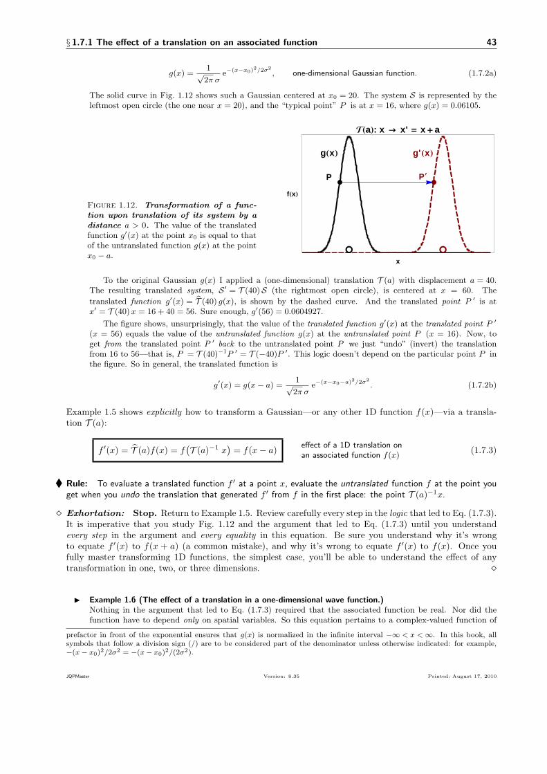
§ 1.7.1 The effect of a translation on an associated function 43
𝑔(𝑥) =1√2𝜋 𝜎
e−(𝑥−𝑥0)2/2𝜎2
, one-dimensional Gaussian function. (1.7.2a)
The solid curve in Fig. 1.12 shows such a Gaussian centered at 𝑥0 = 20. The system 𝒮 is represented by theleftmost open circle (the one near 𝑥 = 20), and the “typical point” 𝑃 is at 𝑥 = 16, where 𝑔(𝑥) = 0.06105.
Figure 1.12. Transformation of a func-tion upon translation of its system by adistance 𝑎 > 0. The value of the translatedfunction 𝑔′(𝑥) at the point 𝑥0 is equal to thatof the untranslated function 𝑔(𝑥) at the point𝑥0 − 𝑎.
x
fHxL
THaL: x ® x' = x + a
é é
P
gHxL
P¢
g' HxL
To the original Gaussian 𝑔(𝑥) I applied a (one-dimensional) translation 𝒯 (𝑎) with displacement 𝑎 = 40.The resulting translated system, 𝒮 ′ = 𝒯 (40)𝒮 (the rightmost open circle), is centered at 𝑥 = 60. The
translated function 𝑔′(𝑥) = 𝒯 (40) 𝑔(𝑥), is shown by the dashed curve. And the translated point 𝑃 ′ is at𝑥′ = 𝒯 (40)𝑥 = 16 + 40 = 56. Sure enough, 𝑔′(56) = 0.0604927.
The figure shows, unsurprisingly, that the value of the translated function 𝑔′(𝑥) at the translated point 𝑃 ′
(𝑥 = 56) equals the value of the untranslated function 𝑔(𝑥) at the untranslated point 𝑃 (𝑥 = 16). Now, toget from the translated point 𝑃 ′ back to the untranslated point 𝑃 we just “undo” (invert) the translationfrom 16 to 56—that is, 𝑃 = 𝒯 (40)−1𝑃 ′ = 𝒯 (−40)𝑃 ′. This logic doesn’t depend on the particular point 𝑃 inthe figure. So in general, the translated function is
𝑔′(𝑥) = 𝑔(𝑥− 𝑎) = 1√2𝜋 𝜎
e−(𝑥−𝑥0−𝑎)2/2𝜎2
. (1.7.2b)
Example 1.5 shows explicitly how to transform a Gaussian—or any other 1D function 𝑓(𝑥)—via a transla-tion 𝒯 (𝑎):
𝑓 ′(𝑥) = 𝒯 (𝑎)𝑓(𝑥) = 𝑓(𝒯 (𝑎)−1 𝑥
)= 𝑓(𝑥− 𝑎) effect of a 1D translation on
an associated function 𝑓(𝑥)(1.7.3)
♦ Rule: To evaluate a translated function 𝑓 ′ at a point 𝑥, evaluate the untranslated function 𝑓 at the point youget when you undo the translation that generated 𝑓 ′ from 𝑓 in the first place: the point 𝒯 (𝑎)−1𝑥.
⋄ Exhortation: Stop. Return to Example 1.5. Review carefully every step in the logic that led to Eq. (1.7.3).It is imperative that you study Fig. 1.12 and the argument that led to Eq. (1.7.3) until you understandevery step in the argument and every equality in this equation. Be sure you understand why it’s wrongto equate 𝑓 ′(𝑥) to 𝑓(𝑥 + 𝑎) (a common mistake), and why it’s wrong to equate 𝑓 ′(𝑥) to 𝑓(𝑥). Once youfully master transforming 1D functions, the simplest case, you’ll be able to understand the effect of anytransformation in one, two, or three dimensions. ⋄
▶ Example 1.6 (The effect of a translation in a one-dimensional wave function.)Nothing in the argument that led to Eq. (1.7.3) required that the associated function be real. Nor did thefunction have to depend only on spatial variables. So this equation pertains to a complex-valued function of
prefactor in front of the exponential ensures that 𝑔(𝑥) is normalized in the infinite interval −∞ < 𝑥 <∞. In this book, allsymbols that follow a division sign (/) are to be considered part of the denominator unless otherwise indicated: for example,−(𝑥− 𝑥0)2/2𝜎2 = −(𝑥− 𝑥0)2/(2𝜎2).
JQPMaster Version: 8.35 Printed: August 17, 2010
44 § 1.7.2 The effect of a rotation
spatial variables and time—that is, to a wave function Ψ(𝑥, 𝑡):60
Ψ′(𝑥, 𝑡) = 𝒯 (𝑎)Ψ(𝑥, 𝑡) = Ψ(𝒯 (𝑎)−1𝑥, 𝑡
)= Ψ(𝑥− 𝑎, 𝑡) effect of a 1D translation on
an associated wave function.(1.7.4)
▶ Example 1.7 (The effect of a translation in three dimensions.)The only difference between a translation in 1D and a translation in more than one dimension is that the scalardisplacement 𝑎 becomes the vector displacement 𝒂. In 3D, for instance, we represent a translation by 𝒯 (𝒂),where 𝒂 = 𝑎𝑥𝒆𝑥 + 𝑎𝑦𝒆𝑦 + 𝑎𝑧𝒆𝑧, with three parameters, the Cartesian components of the vector 𝒂. We canwrite the effect of a translation on a 3D function 𝑓(𝒓) by transcribing Eq. (1.7.3):
𝑓 ′(𝒓) = 𝒯 (𝑎)𝑓(𝒓) = 𝑓(𝒯 (𝒂)−1 𝒓
)= 𝑓(𝒓 − 𝒂)
effect of a 3D translation onan associated function 𝑓(𝒓),
(1.7.5)
Try This! 1.10. The effect of a translation on the position operator.
The simplest operators in quantum mechanics are those that instruct us to multiply their operands bysomething. For instance, the position operator r acts on a function 𝑓(𝒓) to produce the product 𝒓𝑓(𝒓).
Use what you learned in §1.6.3.3 to explain why a translation transforms r into 𝒯 (𝒂) r 𝒯 (𝒂)−1 = 𝒓 + 𝒂.
Try This! 1.11. Effect of an inversion in one dimension.
The transformation operator for an inversion 𝚤 is the parity operator Π . Without looking ahead,write down the analog of Eq. (1.7.3) for the effect of an inversion of a system in 1D on an associ-ated function 𝑓(𝑥). What effect would an inversion 𝚤 of the system through the point 𝑥0 have on thefunction Eq. (1.7.2a)?
▶ Aside. Implications of translational invariance for the potential energy.Translational invariance of a system is a highly restrictive property. The only translationally invariantsystem is one whose potential energy is constant, 𝑉 (𝑥) = 𝑉0. Such a potential energy corresponds to zeronet force, so the only particle whose potential energy is constant is a free particle. Rotational invariance,on which we’ll focus in §1.8.3 (and several chapters to come), is less restrictive and hence more important.
1.7.2 The effect of a rotation
Figuring out the effect of a rotation on an associated function can be a bit intricate. Fortunately, thechallenges are technical, not conceptual. Envision a system 𝒮 confined to a plane. Imagine a rotation ℛ𝑧(𝛼)that takes a representative point 𝑃 with coordinates (𝑥, 𝑦) into a point 𝑃 ′ with coordinates (𝑥′, 𝑦′). Unlikea translation 𝒯 (𝑎), a rotation may, depending on the rotation angle 𝛼, mix the Cartesian coordinates of 𝑃 .
In 2D, we can avoid this technical complication by choosing polar coordinates (§1.D.3). In polar coor-dinates, a rotation in 2D is analogous to a translation in 1D, with one important restriction. Here’s theanalogy : the rotation angle 𝛼 is analogous to the displacement 𝑎. Here’s the restriction : a displacement 𝑎can assume any value, −∞ < 𝑎 <∞; but a rotation is periodic, so 𝛼 is restricted to −𝜋 < 𝛼 ≤ 𝜋.
Now, in polar coordinates, a 2D rotation ℛ𝑧(𝛼) rotates a representative point 𝑃 with coordinates (𝜌, 𝜑)into 𝑃 ′. This rotation leaves the distance 𝜌 of the point from the origin unchanged but changes the angle ofthe vector to the point from 𝜑 to 𝜑+ 𝛼 (Fig. 1.9, p. 21). So the coordinates of 𝑃 ′ are (𝜌, 𝜑+ 𝛼). (Note theplus sign! ) According to the prescription we developed for translations, the value of the rotated function 𝑓 ′
60Details: Technically, the effect of translation (or any other symmetry operator) on a wave function is to produce a wave
function that is arbitrary to within a global phase factor : Ψ′(𝑥, 𝑡) = ei𝜆 𝒯 (𝑎)Ψ(𝑥, 𝑡), where 𝜆 is a real number. This phasefactor is of no physical significance, and we’re free to choose 𝜆 = 0 so it goes away.
JQPMaster Version: 8.35 Printed: August 17, 2010

§ 1.7.2 The effect of a rotation 45
at (𝜌, 𝜑) equals the value of the unrotated function 𝑓 at the point we get from (𝜌, 𝜑) by “undoing therotation.” As illustrated in Fig. 1.13a, that point is (𝜌, 𝜑− 𝛼). (Note the minus sign! ) Ergo,
𝑓 ′(𝜌, 𝜑) = ℛ𝑧(𝛼)𝑓(𝜌, 𝜑) = 𝑓(𝜌,ℛ𝑧(𝛼)−1 𝜑
)= 𝑓(𝜌, 𝜑− 𝛼) effect of a 2D rotation on
an associated function 𝑓(𝜌, 𝜑).
(1.7.6a)The three dimensional generalization of Eq. (1.7.6a) is
𝑓 ′(𝒓) = ℛ(𝛼; 𝒆𝛼)𝑓(𝒓) = 𝑓(ℛ(𝛼;𝒆𝛼)−1 𝒓
) effect of a 3D rotation onan associated function 𝑓(𝒓).
(1.7.6b)
Try This! 1.12. Learn-it-yourself: rotation of a function in polar coordinates.
According to Eq. (1.7.6a), rotation of 𝒮 through an angle 𝛼 would transform the associated function𝑓(𝜌, 𝜑) = 𝜌5 cos𝜑 into 𝑓 ′(𝜌, 𝜑) = 𝜌5 cos(𝜑− 𝛼). For what rotation angles (if any) is the explicit functionalform of this rotated function 𝑓 ′(𝜌, 𝜑) exactly the same as the form of 𝑓(𝜌, 𝜑): that is, for what angles is𝑓 ′(𝜌, 𝜑) = 𝜌5 cos𝜑? How would your answer change if the function is 𝑓(𝜌, 𝜑) = 𝜌5 cos2 𝜑? What if it’s𝑓(𝜌, 𝜑) = 𝜌4 cos𝜑? How about 𝑓(𝜌, 𝜑) = 𝜌5 sin𝜑?
▶ Example 1.8 (The effect of a two-dimensional rotation on an associated function.)The polar plot in Fig. 1.13 shows the effect of a rotation through 𝛼 = 𝜋/4 = 45∘ on the function 𝑓(𝜌, 𝜑) = cos2 𝜑.[In a polar plot , the length of the radius vector at an angle 𝜑 equals the value of the function 𝑓(𝜑).] This figureis analogous to Fig. 1.12, p. 43, for the 1D translation. According to our prescription, the rotated function is
𝑓 ′(𝜑) = ℛ𝑧(𝜋/4)𝑓(𝜑) = 𝑓(ℛ𝑧(𝜋/4)−1 𝜑
)= 𝑓(𝜑− 𝜋/4) = cos2(𝜑− 𝜋/4). (1.7.7)
A quick calculations shows that the values of each untranslated and translated function at the untranslated andtranslated points are identical: for example, 𝑓(0) = 1 and 𝑓(45∘) = 1/2, while 𝑓 ′(0) = 1/2 and 𝑓 ′(45∘) = 1.
Figure 1.13. Rotation of a function in two dimensions.The original function 𝑓(𝜌, 𝜑) = cos2 𝜑 is represented by the solidcurve in this polar plot. The system 𝒮, represented by the pointat 𝜑 = 0, is rotated through an angle 𝛼 = 45∘ producing the ro-tated point 𝑃 ′. The corresponding rotated function is shown atthe right.
Try This! 1.13. Learn-it-yourself: rotation of a function in polar coordinates II.
For what rotation angles 𝛼, if any, is 𝑓(𝜌, 𝜑) = cos2 𝜑 unchanged by a 2D rotation ℛ𝑧(𝛼)? How wouldyour answer differ if the function was 𝑓(𝜌, 𝜑) = cos𝜑? Haul out your hand calculator and add a fewpoints to Tbl. ??—say, 𝜑 = 30∘, 𝜑 = 125∘, and a few more. Keep adding points the behavior you see isembedded in your mind as firmly as a fencepost in concrete.
JQPMaster Version: 8.35 Printed: August 17, 2010

46 § 1.7.4 This side of parities: even and odd functions
1.7.3 The effect of an inversion: the parity operator
We now turn to a discrete transformation: spatial inversion (§1.4.3). The corresponding operator is called
the parity operator and is denoted by Π (not, as you might reasonably expect, by �� ).61 An inversion takesa point 𝑃 at 𝒓 into 𝑃 ′ at 𝒓′ = −𝒓. Interestingly, the inverse of this operation is the operation itself—thatis, inversion takes 𝑃 ′ back to 𝑃 :
𝚤2 ≡ 𝚤 𝚤 = 1 =⇒ 𝚤−1 = 𝚤. (1.7.8)
From this handy property we conclude that the effect of the parity operator on a wave function is
Ψ′(𝒓, 𝑡) = ΠΨ(𝒓, 𝑡) = Ψ(−𝒓, 𝑡) the effect of an inversion on the state Ψ(𝒓, 𝑡). (1.7.9)
Try This! 1.14. Attaining parity.
Explain in detail why Eq. (1.7.9) is correct.
1.7.4 This side of parities: even and odd functions
The parity operator Π introduces another way to use symmetry to understand quantum systems. We canusefully classify functions according to their behavior under Π . On some functions, the effect of Π is quiteuninteresting: if 𝑔(𝑥) = 𝑥2(𝑎+ 𝑏𝑥) for non-zero real numbers 𝑎 and 𝑏, then Π 𝑔(𝑥) = 𝑥2(𝑎− 𝑏𝑥), which isneither 𝑔(𝑥) nor −𝑔(𝑥). We say such functions “have no definite parity .” Functions that do have definiteparity—that transform under inversion into plus or minus themselves—are are said to be even or odd :
𝑓 is
{even, if Π 𝑓 = +𝑓
odd, if Π 𝑓 = −𝑓. (1.7.10)
▶ Example 1.9 (Action of the parity operator on one-dimensional functions.)In 1D, inversion affects an associated function as
𝚤 𝑓(𝑥) : 7→ 𝑓 ′(𝑥) = Π 𝑓(𝑥) = 𝑓(−𝑥). (1.7.11a)
As illustrated in Fig. 1.14, the function 𝑓(𝑥) ≡ 𝑥𝑛 has definite parity (is either even or odd) for any integer 𝑛:
Π 𝑓(𝑥) = (−1)𝑛𝑥𝑛 =
{𝑥𝑛, if 𝑛 even (𝑓 is an even-parity function)
−𝑥𝑛, if 𝑛 odd (𝑓 is an odd-parity function).(1.7.11b)
By contrast, the behavior of the function 𝑔(𝑥) ≡ 𝑥2(𝑎+ 𝑏𝑥) under inversion depends on 𝑎 and 𝑏:
𝑎 = 0 =⇒ 𝑔(𝑥) has odd parity
𝑏 = 0 =⇒ 𝑔(𝑥) has even parity
𝑎 ∕= 0 and 𝑏 ∕= 0 =⇒ 𝑔(𝑥) has no parity.
(1.7.12)
61Commentary: Parity, as well as time-reversal and other important symmetry operators, was introduced in a trail-blazing1927 paper by Eugene Wigner (see the Aside on p. 55). This paper marked the first application of symmetry principles andarguments to quantum mechanics—a contribution for which Wigner earned a Nobel Prize.
JQPMaster Version: 8.35 Printed: August 17, 2010

§ 1.7.4 This side of parities: even and odd functions 47
x
fHxL
P
O
x
fHxL
P
O
Figure 1.14. Symmetry properties of one-dimensional functions under inversion. In both figures,arrows shows the effect of inversion on the value of the function at a point. The functions in the left panel areeither even or odd under inversion: the solid curve [𝑓(𝑥) = 𝑥6] is even; the dashed curve [𝑓(𝑥) = 𝑥3] is odd.The functions in the right panel, each of which has the form 𝑓(𝑥) = 𝑥2(𝑎+ 𝑏𝑥), are neither even nor odd; theyare asymmetric under inversion and have no parity: for both functions, the tip of the horizontal arrow doesn’tlie on the curve. (For the solid function, 𝑎 = 𝑏 = 0.5; for the dashed function, 𝑎 = 0.8 and 𝑏 = 0.3.)
▶ Example 1.10 (The parity operator in two dimensions.)As illustrated in Fig. 1.15, inversion in 2D leaves the distance from the origin to the original point 𝑃 unchangedbut alters the angle 𝜑 of the point as 𝚤 : 𝝆 7→ −𝝆. In Cartesian and polar coordinates, inversion therefore acts as
Π 𝑓(𝑥, 𝑦) = 𝑓(−𝑥,−𝑦) a 2D inversion in Cartesian coordinates
Π 𝑓(𝜌, 𝜑) = 𝑓(𝜌, 𝜑+ 𝜋) a 2D inversion in polar coordinates(1.7.13)
The parity operator is applied to a 3D function in Example 1.17 in Complement 1.B, which shows that itacts as follows:62
Π 𝑓(𝑟, 𝜃, 𝜑) = 𝑓(𝑟, 𝜋 − 𝜃, 𝜑+ 𝜋) spherical coordinates
Π 𝑓(𝑥, 𝑦, 𝑧) = 𝑓(−𝑥,−𝑦,−𝑧) Cartesian coordinates
Π 𝑓(𝜌, 𝜑, 𝑧) = 𝑓(𝜌, 𝜑+ 𝜋,−𝑧) cylindrical coordinates
effect of an inversionin three dimensions.
(1.7.14)
▶ Aside. The parity operator in three dimensions.Here are some relationships you’ll find useful when using the parity operator in 3D:
Π sin 𝜃 = +sin 𝜃, Π cos 𝜃 = − cos 𝜃, (1.7.15a)
Π
(∂𝑓
∂𝜃
)= −∂𝑓
∂𝜃, Π
(∂𝑓
∂𝜑
)= +
∂𝑓
∂𝜑, (1.7.15b)
Π ei𝑚ℓ𝜑 = (−1)𝑚ℓ ei𝑚ℓ𝜑. (1.7.15c)
The symbol 𝑓 = 𝑓(𝑟, 𝜃, 𝜑) represents an arbitrary differentiable function (see Example 1.24).
62A cautionary note: In working with and verifying these results, you need only be careful to transform angles in ways thatkeep them in their domain of definition. For an angle that is defined in [0, 2𝜋], this is no problem, because such an angle isperiodic. The special case is the polar angle 𝜃 of spherical coordinates. The domain of this angle is [0, 𝜋], so we can’t effect aninversion by taking this angle into 𝜋 plus itself, as we can the azimuthal angle 𝜑; rather, an inversion takes 𝜃 into 𝜋 − 𝜃.
JQPMaster Version: 8.35 Printed: August 17, 2010

48 § 1.7.4 This side of parities: even and odd functions
Figure 1.15. A rotation in two dimensions of a point inCartesian and in polar coordinates. In this figure, the rotationtransforms point 𝑃 into point 𝑃 ′. Equivalently, one can get to 𝑃 ′
by an inversion through the origin. This illustrates that thereare often several equivalent geometric operators that result in thesame symmetry transformation.
y
x
Π+Φ
Φ
Ρ
-Ρ
Classification of functions by symmetry. Our discussion of even and odd functions illustrates how toclassify functions according to their behavior under symmetry transformations. This use of symmetry helpsus organize and understand the rich panoply of states of atoms, molecules, solids, and elementary particles.It is also vital to the practical study of these systems—for instance, it enables us to understand and predictwhat transitions between stationary states cannot occur in nature. [Such predictions are called selectionrules (Chap. 14).]
Try This! 1.15. Evening out the odds.
Explain why any function 𝑓(𝑥), whether or not it has definite parity, is equal to the sum of an evenfunction and an odd function. That is, devise a procedure for generating even and odd functions from afunction 𝑓(𝑥) that has no definite parity. Illustrate your procedure for 𝑓(𝑥) = 𝑥2(𝑎+ 𝑏𝑥) in Fig. 1.14b.63
Try This! 1.16. Hermiticity of the parity operator.
Use the definition of Hermiticity of an operator that acts on a 1D system to show that the parityoperator is Hermitian:
Π † = Π , Hermiticity of the parity operator. (1.7.16a)
What are the consequences of this property for the possibility of measuring the parity of a system?What are the consequences for the values that might be found in such a measurement? Explain whythis property implies
Π † = Π−1 = Π . (1.7.16b)
Why does Eq. (1.7.16b) imply that the eigenvalues of Π are ±1? What is the operator power Π 𝑛 for anonnegative integer 𝑛 when 𝑛 is even? . . . when 𝑛 is odd?
63Commentary: This little question exemplifies an important property we’ll develop later in this book: any function canbe written as a linear combination of functions (of the same variables defined on the same domain) that have well-definedsymmetry properties. (Here the property is definite parity.) In quantum mechanics, this mathematical property develops, viathe principle of superposition, into an exceptionally powerful problem-solving tool: the method of eigenfunction expansion.
JQPMaster Version: 8.35 Printed: August 17, 2010
§ 1.8 Symmetry, invariance, and conservation laws in quantum mechanics 49
§ 1.8 Symmetry, invariance, and conservation laws in quantum mechanics
Joy in looking and comprehending is nature’s most beautiful gift.
—Albert Einstein
The final stage in our development of symmetry in quantum physics is to generalize the connection betweensymmetry transformations and conservation laws in §1.5.2. This generalization will hold for any continuoustransformation—one that depends on one or more parameters which can be varied so as to reduce thetransformation to the identity (§1.4.2).
1.8.1 Stone’s theorem
To set the stage, we’ll consider translational invariance. Translational invariance implies the commutationrelation
translational invariance =⇒ [ ℋ, 𝒯 (𝒂) ] = 0 for all displacements 𝒂. (1.8.1)
But Eq. (1.8.1) does not lead directly to a conservation law. The translation operator 𝒯 (𝒂) is unitary,
𝒯 (𝒂)† = 𝒯 (𝒂)−1 [Eq. (1.6.9a), p. 36], but 𝒯 (𝒂) is not Hermitian. So 𝒯 (𝒂) cannot represent an observable.
Yet, translational invariance does imply a conservation law. This implication follows from a remarkableproperty of unitary operators called Stone’s theorem :64
Theorem (Stone’s theorem.) Any unitary operator 𝒰 that depends continuously on one or more realparameters 𝛾𝑖 > 0 and satisfies
𝒰 (𝛾1)𝒰 (𝛾2) = 𝒰 (𝛾1 + 𝛾2) (1.8.2aa)
can be written in the form
𝒰 (𝛾) = exp
[−i 𝛾 Q
ℏ
](1.8.2b)
where Q is an Hermitian operator.
Since all symmetry operators are unitary, every continuous symmetry operator defines a Hermitian oper-ator Q via Eq. (1.8.2b).65 The easiest version of Stone’s theorem to use is the mathematically equivalentdifferential equation (Exercise 1.12)
Q = i ℏd 𝒰d𝛾
∣∣∣∣∣𝛾=0
(1.8.2c)
▶ Warning: Stone’s theorem applies only to continuous transformations, not to discrete transformations.
64Example 1.20 in Complement 1.B illustrates how one could develop a proof of Stone’s theorem. Full proofs appear in somegraduate-level quantum texts; see, for example, §7.3.2 and §8.2.1 of Le Bellac (2006). Incidentally, mathematicians call Q the
infinitesimal generator (or generator) of the transformation 𝒰 (or of the operator 𝒰 ).65Details: For a 1D translation, the parameter (the displacement) is a scalar, 𝛾 = 𝑎. But for a 2D translation, the displacement
is a vector with Cartesian components 𝒂 = 𝑎𝑥𝒆𝑥 + 𝑎𝑦𝒆𝑦 . The only way Eq. (1.8.2b) could make sense for a vector parameter
is if the Hermitian operator Q is a vector operator (see Chap. 2). Sure enough, for a 2D translation, the operator Q in thisequation turns out to be the vector linear-momentum operator p , with Cartesian components p𝑥 and p𝑦 . Similar argumentspertain to translations in three dimensions and to rotations in two or three dimensions. The factor of ℏ is unrelated to thetheorem. If Q is Hermitian (Q† = Q), then so is Q/ℏ. I included this factor in Eq. (1.8.2b) for convenience only: The dimension
of ℏ are those of angular momentum, so for angular-momentum operators Q, which will appear throughout this book, theratio Q/ℏ is dimensionless. We consider only operators 𝒰 that are linear, unitary, and independent of time.
JQPMaster Version: 8.35 Printed: August 17, 2010

50 § 1.8.2 Translations and conservation of linear momentum
Try This! 1.17. Learn it yourself: forms of Stone’s theorem.
Explain why (or work through the algebra) Eq. (1.8.2c) is equivalent to Eq. (1.8.2b). Why must the
constraint 𝛾 = 0 appear in Eq. (1.8.2c)? In what way does Eq. (1.8.2c) clarify why 𝒰 in Stone’s theoremmust be a continuous symmetry operator?
1.8.2 Translations and conservation of linear momentum
In classical mechanics, translational invariance of a system implies conservation of its linear momentum. Let’suse Stone’s theorem to discover the corresponding conservation law in quantum mechanics (see §1.C.5).
▶ Example 1.11 (The Hermitian operator that corresponds to a translation.)Stone’s theorem guarantees the existence of a Hermitian operator Q for any continuous symmetry operator 𝒰 .
To find the explicit form of Q, we make careful use of the differential equation (1.8.2c), as I’ll now illustrate
for a 1D translation. To begin, I identify the symmetry operator 𝒰 in Stone’s theorem with a 1D translationoperator 𝒯 (𝑎), and the parameter 𝛾 with the displacement 𝑎. These identifications set up the following analysis:
QΨ(𝑥, 𝑡) = i ℏ ∂
∂𝑎
[𝒯 (𝑎)Ψ(𝑥, 𝑡)
]∣∣∣𝑎=0
, by Eq. (1.8.2c) (1.8.2a)
= i ℏ ∂
∂𝑎[Ψ(𝑥− 𝑎, 𝑡)]
∣∣∣∣𝑎=0
, by definition of 𝒯 (𝑎), Eq. (1.7.4), p. 44 (1.8.2b)
= −i ℏ ∂
∂𝑥Ψ(𝑥, 𝑡), by the chain rule of differentiation. (1.8.2c)
I now recognize the operator in the last equality as the 1D linear momentum operator ,
p𝑥 ≡ −i ℏ ∂
∂𝑥, linear momentum operator (1D) (1.8.2d)
Example 1.11 shows that the Hermitian operator related via Stone’s theorem to 1D translations 𝒯 (𝒂) isthe 1D linear-momentum operator (see also Example 1.18 in Complement 1.B):66
𝒯 (𝑎) = exp
(−i 𝑎 p𝑥
ℏ
), where p𝑥Ψ(𝑥, 𝑡) = −i ℏ ∂
∂𝑥Ψ(𝑥, 𝑡) (1.8.3)
A similar argument shows that the Hermitian operator related to a 3D rotation ℛ(𝛼; 𝒆𝛼) is the angular-momentum operator (Chaps. 2 and 3). Through such identifications, Stone’s theorem enables us to determinethe conservation law that follows from invariance of a system under any continuous symmetry transformation.
▶ Example 1.12 (Translational invariance and conservation of linear momentum.)Translational invariance implies the commutation relation
[ ℋ, 𝒯 (𝑎) ] = 0. Applying the form Eq. (1.8.3) of
Stone’s theorem to the commutation relation[ ℋ, 𝒯 (𝑎) ] = 0 implied by translational invariance gives[
ℋ, exp(− i 𝑎
p𝑥ℏ)]
= 0, for all displacements 𝑎. (1.8.4)
Any operator of the form eQ is defined in terms of its power-series expansion [see § 10.2 in Morrison (1990)] as67
66Jargon: Mathematicians describe this relationship by saying “the operator p𝑥/ℏ is the infinitesimal generator of trans-lations in one dimension.” In three dimensions, the Cartesian components p𝑥, p𝑦 , and p𝑧 are the generators of transla-tions 𝒯 (𝒂).
67A cautionary note: In practice, you implement an exponential operator by acting on its operand with each term in thepower series, stopping when the result is converged to whatever precision you want. In doing so, remember that the product oftwo or more operators implies successive operation: Q2𝑓(𝑥) = Q[Q𝑓(𝑥)], and so forth.
JQPMaster Version: 8.35 Printed: August 17, 2010
§ 1.8.2 Translations and conservation of linear momentum 51
eQ ≡ 1+ Q +1
2!Q2 +
1
3!Q3 + ⋅ ⋅ ⋅ an exponential operator. (1.8.5a)
For the 1D translation operator, this definition reads
𝒯 (𝑎) = e−i 𝑎p𝑥/ℏ = 1− i 𝑎p𝑥ℏ− 1
2!𝑎2
p 2𝑥
ℏ2+ ⋅ ⋅ ⋅ . (1.8.5b)
So the commutator in Eq. (1.8.4) equals the sum of commutators of the form[ ℋ, p𝑛𝑥 ] for 𝑛 = 0, 1, . . . . Let’s
look at one such term:68[ ℋ, p𝑛𝑥 ] = [ T, p𝑛𝑥 ]+ [𝑉, p 2𝑥
]definition of the Hamiltonian (1.8.6a)
= − ℏ22𝑚
[p 2𝑥 , p
𝑛𝑥
]+[𝑉, p 2
𝑥
]definition T = −(ℏ2/2𝑚) d2/d𝑥2 (1.8.6b)
= − ℏ22𝑚
[p 2𝑥 , p
𝑛𝑥
]T commutes with a translationallyinvariant potential energy
(1.8.6c)
= − ℏ22𝑚
([p𝑥, p
𝑛𝑥
]p𝑥 + p𝑥
[p𝑥, p
𝑛𝑥
])operator algebra (Appendix H) (1.8.6d)
= 0 any commutator[Q, Q𝑛
]equals zero (1.8.6e)
This derivation shows that ℋ commutes with each term in Eq. (1.8.5b). So commutativity of ℋ and 𝒯 (𝑎)for any displacement 𝑎 implies commutativity of ℋ and the linear momentum operator—which gives theconservation law:69
[ ℋ, 𝒯 (𝑎) ] = 0 =⇒ [ ℋ, p𝑥 ] = 0 =⇒ d
d𝑡⟨𝑝𝑥⟩ = 0 for any Ψ(𝑥, 𝑡) (1.8.7)
We find that in quantum mechanics as in classical physics,
♦ Rule: Translational invariance implies conservation of linear momentum.
▶ Aside. Translational invariance and linear momentum in three dimensions.The counterpart of Eq. (1.8.7) for a 2D or 3D translation follows from linearity of 𝒯 (𝒂) (Exercise 1.10):
𝒯 (𝒂) = exp
(−i 𝒂 ⋅ p
ℏ
)= exp
(−i 𝑎 𝒆𝑎 ⋅ p
ℏ
), (1.8.8a)
where 𝒆𝑎 is a unit vector along the displacement vector 𝒂. The operator 𝒆𝑎 ⋅ p corresponds to the projection𝒆𝑎 ⋅ 𝒑 of the linear momentum 𝒑 on the direction of displacement 𝒂. Since the Hamiltonian of a translationallyinvariant system must commute with 𝒯 (𝒂) for all displacements, all such projections are conserved. Therefore
the generalization of[ ℋ, p𝑥 ] = 0 to three dimensions is conservation of the vector linear momentum. In 3D
and Cartesian components, this reads
[ ℋ, p ] = 0 =⇒ [ ℋ, p𝑥 ] = 0, and[ ℋ, p𝑦 ] = 0, and
[ ℋ, p𝑧 ] = 0 (1.8.8b)
▶ Warning: It’s vital that you keep straight that the translation operator is unitary, while the linear-momentum operator is Hermitian:
𝒯 (𝑎)† = 𝒯 (𝑎)−1 unitarity of 𝒯 (𝑎)p𝑥
† = p𝑥 Hermiticity of p𝑥.(1.8.9)
68Details: The kinetic-energy operator commutes with a translationally invariant potential energy [used in getting Eq. (1.8.6c)]because any such potential energy is necessarily a constant; see the Aside on p. 44.
69A cautionary note: The qualifier that ℋ must commute with any displacement is quite important. Systems that commuteonly with selected displacements are not translationally invariant; they are periodic.
JQPMaster Version: 8.35 Printed: August 17, 2010

52 § 1.8.4 Inversion and conservation of parity
Only because p𝑥 is Hermitian can it represent an observable. An operator that, like 𝒯 (𝑎), is unitary but notHermitian may be useful but cannot represent an observable.
1.8.3 Rotations and conservation of angular momentum
The most important continuous transformations in this book are rotations. Noether’s theorem (§1.5.2) sug-gests that rotational invariance of a quantum system implies conservation of its orbital angular momentum.This suggestion turns out to be correct—but only for a system whose total angular momentum equals itstotal orbital angular momentum.70
A derivation based on Stone’s theorem (like the one in Example 1.11) leads to an explicit expression forthe effect of a 2D rotation operator on a wave function Ψ(𝜌, 𝜑, 𝑡):
ℛ𝑧(𝛼)Ψ(𝜌, 𝜑, 𝑡) = −i ℏ ∂
∂𝜑Ψ(𝜌, 𝜑, 𝑡). (1.8.10a)
It’s reasonable to infer from Noether’s theorem that we can identify the differential operator −i ℏ ∂/∂𝜑 withthe observable 𝐿𝑧, the projection of the orbital angular momentum along the 𝑧 axis. Let’s see where thisconjecture takes us. With this identification, Stone’s theorem for ℛ𝑧(𝛼) would read [Eq. (1.8.2b), p. 49]
ℛ𝑧(𝛼) = exp
(−i𝛼 L𝑧
ℏ
), where L𝑧 = −i ℏ
∂
∂𝜑. (1.8.10b)
A derivation like Example 1.12 would then yield71
[ ℋ, ℛ𝑧(𝛼) ] = 0 =⇒ [ ℋ, L𝑧 ] = 0 =⇒ d
d𝑡⟨𝐿𝑧⟩ = 0 for any Ψ(𝑥, 𝑡) (1.8.10c)
This is the quantum-mechanical counterpart of a familiar classical rule:72
♦ Rule: Rotational invariance implies conservation of the total angular momentum.
1.8.4 Inversion and conservation of parity
The argument in §1.8.2 that translational invariance implies conservation of linear momentum hinges ontranslation being a continuous transformation, because only for such a transformation does Stone’s theoremapply. Such arguments cannot yield conservation laws related to a discrete transformation.
An important example is conservation of parity , which follows from invariance under inversion .As discussed in §1.4.3, an inversion 𝚤 maps a point at 𝒓 into the point at −𝒓. The corresponding operatorthat acts on associated functions is the parity operator (§1.7.3):
𝚤 : 𝒓 7→ −𝒓 =⇒ Ψ′(𝒓, 𝑡) = ΠΨ(𝒓, 𝑡). (1.8.11)
If a system is invariant under inversion, then the parity operator commutes with the Hamiltonian,[ ℋ, Π ] = 0. But because the inversion is a discrete transformation, we can’t use Stone’s theorem to find the
70A cautionary note: The total angular momentum is not equal to the orbital angular momentum if the system has anonzero total spin whose effect we cannot neglect (Chap. 6). For the moment, I’ll assume it’s okay to ignore spin—as it is inmany situations—and consider a particle that has a non-zero orbital angular momentum but zero spin angular momentum.
71Read on: I’ll derive this equation in Example 2.24, after we’ve learned more about the 2D orbital angular momentumoperator.
72Commentary: The weakness in this argument is that it assumes something we have not proven: that the operator whichrepresents 𝐿𝑧 is indeed −i ℏ ∂/∂𝜑. It turns out that this differential operator is L𝑧 , as I’ll prove in Chap. 2, where angular
momentum takes center stage. For more about ℛ𝑧(𝛼), see Morrison and Parker (1987) and Wolf (1969).
JQPMaster Version: 8.35 Printed: August 17, 2010
§ 1.9 Reflections on symmetry: a recap 53
corresponding constant of the motion. Yet, in quantum mechanics (unlike in classical mechanics), invariance
under inversion does imply a conservation law. Because Π is unitary and because two successive applicationsof Π are equivalent to the unit operator, Π is itself Hermitian:
Π † = Π−1 and Π 2 = 1 =⇒ Π † = Π . (1.8.12)
Therefore Π can represent an observable.
♦ Rule: The parity of a state of a system that is invariant under inversion is conserved:73
invariance under inversion =⇒ d
d𝑡⟨Π⟩ = d
d𝑡⟨Ψ(𝑡) ∣ Π ∣ Ψ(𝑡)⟩ = 0, for any state Ψ (1.8.13)
Try This! 1.18. Learn it yourself: properties of the parity operator.
Use either direct action on an arbitrary (well-behaved) function or operator algebra to demonstrate
and justify Eq. (1.8.12). Explain why these equations imply that the eigenvalues of Π are ±1. Whywould this conclusion not follow for an operator that is unitary but not Hermitian?
The eigenvalues of Π are ±1, so its eigenfunctions have even or odd parity according to whether or notthey change sign when acted upon by Π [Eq. (1.7.10), p. 46]. The commutation relation
[ ℋ, Π ] = 0 impliesthat there exist simultaneous eigenfunctions of these two operators (see Appendix A). These functions,Hamiltonian eigenfunctions with definite parity, will assume great importance in the applications of Parts IIIand IV.74
Try This! 1.19. Learn it yourself: an even potential implies inversion invariance.
By letting the operator Π𝑉 (𝑥)Π † act on an arbitrary, well-behaved one-dimensional function 𝑓(𝑥),
explain why Π𝑉 (𝑥) Π † = 𝑉 (𝑥) if and only if 𝑉 (𝑥) is even.
§ 1.9 Reflections on symmetry: a recap
There is no adequate defense, except stupidity,against the impact of a new idea.
—Percy Williams Bridgman
In this chapter we have traveled from the idea of symmetry as an aspect of geometry (Secs. 1.1–1.3)—anappreciation that has enraptured humans from the era of Plato and Euclid to the present—to the notion ofsymmetry as a fundamental feature of the mathematical description of the microverse by quantum mechanics(Secs. 1.4–1.8)—an appreciation that will inform almost every development in this book. In this journey,a crucial step was from the symmetry of geometric objects to the symmetry of mathematical functions,expressions, operators, and equations (§1.4). Without this step, symmetry would remain vital to artists andarchitects but of little value to physicists.
At no way-station in our journey was the power of symmetry better illustrated than in the universalsymmetry principles of the homogeneity and isotropy of space (§1.5). These principles, which physicistshave assumed since the eras of Galileo and Newton, reveal the inherent geometric structure of the physical
73Notation: By convention, the expectation value of the parity operator is written with the symbol Π without its little hat.74Commentary: A Hamiltonian may, of course, have eigenfunctions that don’t have definite parity. Interestingly, such functions
do not exist for bound states of one-dimensional (1D) systems. A familiar instance is a particle of mass 𝑚 with potential energy𝑉 (𝑥) = 𝑚𝜔2𝑥2/2 (a 1D simple harmonic oscillator with harmonic frequency 𝜔; see Appendix P). All Hamiltonian eigenfunctions
of this system have definite parity. Starting with the ground state, 𝜓0(𝑥), the eigenvalue of Π for each function is (−1)𝑛, so 𝜓𝑛(𝑥)is even or odd according as 𝑛 is even or odd. This feature lets us classify the eigenfunctions of a 1D SHO according to theirparity: we can associate each 𝜓𝑛(𝑥) with its behavior under inversion.
JQPMaster Version: 8.35 Printed: August 17, 2010

54 § 1.9.1 The beauty of symmetry principles in physics
universe, of space-time itself. That’s why symmetry is so vital to the enterprise of physics. Noether’stheorem, which establishes a general relationship between any (continuous) symmetry transformation and aconservation law, illustrates how symmetry principles imply laws of nature—a train of logic physicists havebeen using since 1905, when Einstein used universal symmetries to deduce the equations of special relativity.Today scientists use both symmetry principles, which have been the focus of this chapter, and symmetryarguments, examples of which abound in the rest of this book.
1.9.1 The beauty of symmetry principles in physics
The beautiful connection between a symmetry transformation (a transformation in ordinary physical space)and a quantum-mechanical operator (a mathematical instruction that represents an observable) is paradig-matic of how symmetry works in modern physics.75 Crucially, this connection is forged through the in-termediary of a symmetry operator : for every symmetry transformation 𝒰 of a system, there is a unitaryoperator 𝒰 that transforms wave functions and operators associated with the system. If the transformationis continuous, then, via Stone’s theorem, the symmetry operator defines a (Hermitian) operator that obeys a
conservation law. For a rotation ℛ𝑧(𝛼) in the 𝑥𝑦 plane, the symmetry operator ℛ𝑧(𝛼) leads to conservation
of the orbital angular momentum, the observable whose corresponding operator is L𝑧. In Chaps. 2 and 3 we’llprobe this connection and its implications for the quantum physics of a particle in two and three dimensions.As you’ll see, this connection yields insights into states, properties, and processes. We gain this informationwithout having to solve a single equation or even having to know the Hamiltonian of the system!
The essential idea underlying this connection is invariance : in modern physics, “symmetry” refers(through the well-defined mathematical procedures of group theory) to invariance under a group of symmetrytransformations. In §1.5 I defined invariance this way: a geometric object is invariant if, after you dosomething to the object, it looks like as it did before. Extending this idea to atoms and molecules requiressome ingenuity: you can apply a translation to a Platonic solid by picking it up, moving it, then putting itdown. But you can’t apply a translation to an atom in the same way.
We now know that effecting a symmetry transformation on a quantum system induces transformationof states and operators via a symmetry operator. We also know what “looks like” means: all predictionsabout measurable quantities we calculate from transformed wave functions and operators must be the same astheir counterparts we calculate from untransformed wave functions and operators. An analogous invariancerequirement holds for the equation of motion: the Schrodinger equation for the transformed states mustbe the same as the untransformed Schrodinger equation.
We attained deeper insight into the meaning of “looks like” via our discovery in §1.6 that invarianceof a system under a symmetry transformation implies conservation of a property of the system. We evenfound a mathematical test for invariance: a system is invariant under a symmetry transformation if itsHamiltonian commutes with the corresponding symmetry operator. This commutation relation implies thatthe expectation value of the observable does not change with time no matter what state the system is in.The observable is conserved.
This chain of logic is elegant, inevitable, unbreakable, and essential:
invariance =⇒ commutation relation =⇒ constant of the motion =⇒ conservation law
By the end of this book you will understand thoroughly every link in this chain, what each link tells us aboutthe “deep physics” of a system, and how to exploit each link in problem solving.
75Commentary: In the first two Parts of this book, we’ll consider only three transformations—translation, reflection, andinversion. These are not the only transformations of importance to physics: another is Galilean invariance, according towhich the laws of nature are the same in any two inertial reference frames that are moving uniformly with respect to oneanother. In Part III, when we turn to systems that consist of many identical particles (say, several electrons), we’ll discovera quite different kind of symmetry called permutation symmetry that acutely affects the states, properties, and behavior ofatoms, molecules, solids, planets, stars—as well as you, me, and every other living thing.
JQPMaster Version: 8.35 Printed: August 17, 2010

§ 1.9.2 The power of symmetry arguments in solving physics problems 55
1.9.2 The power of symmetry arguments in solving physics problems
Throughout this book, I’m going to be urging you to start thinking about problems—before you try to solvethem—by seeking symmetry properties. This stratagem, which I’ll illustrate repeatedly, is the first habit Iwant you to learn—Seek symmetry simplifications (§1.4.6): Begin problem solving by identifying symmetryproperties of a system and figuring out their consequences for the observables, operators, and wave functionsof the system. This analysis depends only on generic properties of the system’s potential energy, not on itsdetailed nature.
This habit helps you solve problems in several ways. Here’s a sampler:
∙ Symmetry helps you set up a problem so as to minimize the amount of algebra, calculus, and/orcomputation required to solve it.
∙ Symmetry eliminates many mathematical manipulations and/or calculations you would otherwise haveto do.
∙ Symmetry guides you to easy ways to check the results of whatever manipulations and/or calculationsyou have to do.
∙ Symmetry guides you to a deeper understanding of the significance, consequences, and implications ofyour results—which, after all, are the point of solving a problem in the first place.
In a nutshell: symmetry makes problem solving more fun, more insightful, and much less tedious—all thisfor just a little preliminary thought!
▶ Aside. Who was Eugene Wigner?Although he was no taller than I am, Wigner is considered one of the giants of theoretical physics. And withgood reason. Wigner’s contributions to physics are legion. In quantum mechanics, both non-relativistic andrelativistic, he first introduced group theory, first treated parity and time-reversal, constructed the mathe-matical foundation for combining angular momenta (Appendix K), and invented second quantization , thebasis of quantum field theory . Wigner also made epochal contributions to atomic and molecular physics;to solid-state physics, which during his career was a brand new field; to nuclear physics; to collision physics;to the development of the atomic bomb—and, later in life, to civil defense against it—and to reactor design.(He was the first nuclear engineer.) Born in Hungary in 1902, Wigner was almost lost to physics: the paucityof academic jobs available when he graduated from high school led Wigner to return to his home city ofBudapest to work in his father’s leather tannery. Happily, fate intervened, and from 1926 to his death in1995, Wigner sought to demonstrate his conviction that physics has “a duty to provide a living picture ofour world, to uncover relations between natural events, and to offer us the full unity, beauty and naturalgrandeur of the physical world.” His efforts won him a Nobel Prize in 1963.76
76Read on: For more about Wigner, see Abraham Pais’ memoir in The Genius of Science: A Portrait Gallery (New York,Oxford, 2000), Erich Vogt’s article “Eugene Paul Wigner: A Towering Figure of Modern Physics,” in the December 1995 issueof Physics Today (p. 40). In David J. Gross’ tribute to Wigner’s research, we read: “Wigner was a member of the race of giantsthat reformulated the laws of nature after the quantum-mechanical revolution of 1924–25.” For more, see The Recollections ofEugene P. Wigner, as Told to Andrew Szanton, (New York, Plenum Press, 1992) and Wigner’s fascinating (often challenging)essays, which have been collected in Wigner (1967).
JQPMaster Version: 8.35 Printed: August 17, 2010

56 § 1.11 Exercises & problems for Chap. 1
§ 1.10 Selected readings & references for Chap. 1
As for me, all I know is that I know nothing.And when I want to know something, I look it up in books—their memory never fails.
—The Club Dumas, by Arturo Perez-Reverte
Symmetry is so vital to physics that it’s treated in almost all textbooks at all levels. Yet, surprisingly few booksaddress symmetry as a topic in its own right. Fortunately, those that do, do so very well.
∙ An enthusiastic introduction to symmetry in its widest applications to science is Rosen (1975). Subsequently,Rosen wrote a more specialized book (Rosen, 1995) that elaborates (mostly) mathematical aspects of sym-metry in science. This later book also includes a nice introduction to the language of symmetry in science,group theory.
∙ The more recent introduction to symmetry by Lederman and Hill (2008), although directed at general audiences,contains lots of interesting insights and examples of symmetry in nature and physics. For a more historical bent,check out Livio (2005). For history with a mathematical bent, see Stewart (2007). Finally, Ronan (2006) tellsthe saga of the search for the “Monster of symmetry,” a gigantic snowflake that exists in 196,884 dimensions (!).
∙ The classic book on symmetry is Weyl (1952). Weyl was a leader in development of the mathematics ofsymmetry, but his wonderful little book ranges over art, music, architecture, design, and nature. Althoughsometimes difficult reading, it’s is worth the effort.
∙ Another scientist who played a vital role in the applications of symmetry (and group theory) to physics wasEugene P. Wigner (see the Aside on p. 55). In addition to writing one of the earliest, most influential advancedtexts on this topic (Wigner, 1959), Wigner wrote some fascinating essays for the non-specialist; these have beencollected in Wigner (1967).
∙ No serious student of physics can (or should want to) avoid group theory. Books on group theory and itsapplication to physics abound. Two accessible introductions are Cornwell (1997) and Jones (1990). You canfind more in-depth treatments in Elliott and Dawber (1979) and, at a more advanced level, Fonda and Chirardi(1970).
∙ An abundance of advanced texts develop the role and implications of symmetry in quantum mechanics. Recentexamples are Fano and Rau (1996) and Chaichian and Hagedorn (1998). Specific applications to atoms,molecules, and solids are developed in the useful (but very terse) text by Tinkham (1964); applications tochemistry are explored (quite accessibly) in Bishop (1973), Cotton (1990), and Jacobs (2005).
§ 1.11 Exercises & problems for Chap. 1
Such is our condition that we are not permitted to arrive all at once at somethingreasonable no matter what it is. Before that it is necessary that we go astray for a longtime, that we pass by all sorts of errors and degrees of impertinence.
—Digression sur les Anciens et les modernes, by Fontenelle
▶ Exercises
E 1.1. A continuous versus a discrete symmetry transformation.The homogeneity and isotropy of space imply that the equations of physics must be invariant under arbitrary trans-lations and rotations. Look up the equations for a circle and for an equilateral triangle. Then prove(a) the equation of a circle is unchanged by any rotation; but
(b) the equation of an equilateral triangle is unchanged only by rotations through 120∘, 240∘, and 360∘.
JQPMaster Version: 8.35 Printed: August 17, 2010

§ 1.11 Exercises & problems for Chap. 1 57
A circle is invariant under any rotation, so for a circle, rotation is a continuous symmetry transformation . Bycontrast, a triangle is invariant under only selected rotations (through angles 120∘, 240∘, and 360∘). So for a triangle,rotation is a discrete symmetry transformation .
E1.2. Properties of the translation operator.Using sketches, words, and (only if necessary) equations, explain why a translation has these properties:
(a) The effect of two successive translations is equivalent to a single translation:
𝒯 (𝒂)𝒯 (𝒃) = 𝒯 (𝒃)𝒯 (𝒂) = 𝒯 (𝒂+ 𝒃). (1.2.1a)
(b) The inverse of a translation through a displacement 𝒂 is a translation through −𝒂:𝒯 (𝒂)−1 = 𝒯 (−𝒂). (1.2.1b)
(c) Translations are associative:𝒯 (𝒂) [𝒯 (𝒃)𝒯 (𝒄)] = [𝒯 (𝒂)𝒯 (𝒃)] 𝒯 (𝒄). (1.2.1c)
Do two translations through different displacements along the same direction commute? How about translationsalong different directions?
E1.3. Linearity of the translation operator.Prove or explain why the translation operator 𝒯 (𝒂) is a linear operator (see Appendix H).
E1.4. Linearity of the rotation operator.Demonstrate that the rotation operator ℛ𝑧(𝛼) is linear. That is, if the unrotated state is
Ψ(𝜌, 𝜑, 𝑡) = 𝑐1Ψ1(𝜌, 𝜑, 𝑡) + 𝑐2Ψ2(𝜌, 𝜑, 𝑡) (1.4.1a)
then the rotated state is
ℛ(𝛼; 𝒆𝛼)Ψ(𝜌, 𝜑, 𝑡) = 𝑐1ℛ(𝛼; 𝒆𝛼)Ψ1(𝜌, 𝜑, 𝑡) + 𝑐2ℛ(𝛼; 𝒆𝛼)Ψ2(𝜌, 𝜑, 𝑡). (1.4.1b)
E1.5. Requirements for translational invariance.Use the definition of the translation operator 𝒯 (𝒂) to show that the Hamiltonian of a system is invariant under anarbitrary translation only if the potential energy of the system is constant.
E1.6. Properties of symmetry transformations.Drawing on the definition of a symmetry transformation, use words and/or sketches to explain why
(a) performing any two symmetry transformations in succession is equivalent to performing a (different) singlesymmetry transformation;
(b) the effect of performing two symmetry transformations on a system is the same regardless of the order in whichyou perform the transformations;
(c) the identity transformation is a symmetry transformation;
(d) the inverse of a symmetry transformation is a symmetry transformation.
Congratulations! You have just explained why the collection of symmetry operators of a system constitute a well-defined mathematical entity called a group. You can do group theory!
E1.7. Validation: a symmetry transformation preserves properties and the Schrodinger equation.Use Eq. (1.6.26), p. 41 to verify that a transformation 𝒰 whose operator 𝒰 satisfies these equations obeys therequirements for invariance under spatial translation.
E1.8. An alternate statement of invariance.
JQPMaster Version: 8.35 Printed: August 17, 2010

58 § 1.11 Exercises & problems for Chap. 1
Some physicists state the definition of invariance—that all predictions of measurable properties be invariant—usingthe scalar product ⟨Ψ ∣ Φ⟩ of two wave functions. Using Ψ′ and Φ′ to represents the states of the transformedsystem that correspond to states Ψ and Φ of the untransformed system, they write:
⟨Ψ′ ∣ Φ′⟩ = ⟨Ψ ∣ Φ⟩, (for all states Ψ and Φ) (1.8.1)
Show that a transformation that satisfies Eq. (1.8.1) does not change the expectation values, eigenvalues, transitionamplitudes, and the position probability densities of a system.
E1.9. The parity of operators.Just as we distinguish functions based on their behavior under the parity operator, so do we distinguish operators:
Π Q Π = Q Q is an even operator
Π Q Π = −Q Q is an odd operator(1.9.1a)
(a) Show that an even operator Q commutes with Π , while an odd operator anti-commutes with Π :[Π , Q
] ≡ Π Q − QΠ = 0 if Q is an even operator[Π , Q
]+≡ Π Q + QΠ = 0 if Q is an odd operator
(1.9.1b)
(b) Show that the position operator r and the momentum operator p are odd operators.
Remark: The operator [A, B
]+≡ AB + BA anticommutator of operators A and B (1.9.2)
used in this exercise is called the anticommutator of A and B.
E1.10. Translations and linear momentum in two dimensions.
(a) Use a double Taylor series to show that the operator that enacts a translation in two dimensions, 𝒯 (𝒂), with𝒂 = 𝑎𝑥𝒆𝑥 + 𝑎𝑦𝒆𝑧, is
𝒯 (𝒂) = exp
(−i 𝒂 ⋅ p
ℏ
)= exp
(−i 𝑎𝒆𝑎 ⋅ p
ℏ
), (1.10.1)
where p is the two-dimensional vector operator for the linear momentum of a particle, with Cartesian compo-nents p𝑥 and p𝑦, and 𝒆𝑎 is a unit vector in the direction of the displacement 𝒂.
(b) Use the exponential form of the translation operator to prove that the 𝑥 and 𝑦 components of the two-dimensional linear momentum operator p = 𝒆𝑥p𝑥 + 𝒆𝑦 p𝑦 commute:
[p𝑥, p𝑦
]= 0.
Remark: This exercise illustrates the remarkable fact that♦ Rule: Commutation relations involving the Cartesian components of p follow from homogeneity of space—that is, from
the underlying geometry of space-time.
E1.11. Exponential operators.In general, the exponential of the sum of two operators, eQ+R , is not equal to the product eQ times eR .
(a) Show that if Q and R each commute with[Q, R
], then
eQ+R = eQ eR − e[Q,R]/2. (1.11.1)
(b) Show that if Q and R commute, then eQ+R equals eQ + eR .
E1.12. Hermiticity of the operator defined by Stone’s theorem.By applying Eq. (1.8.2c) to the unitarity relation for the translation operator, show that the operator Q defined in
this equation is Hermitian: Q† = Q.
JQPMaster Version: 8.35 Printed: August 17, 2010
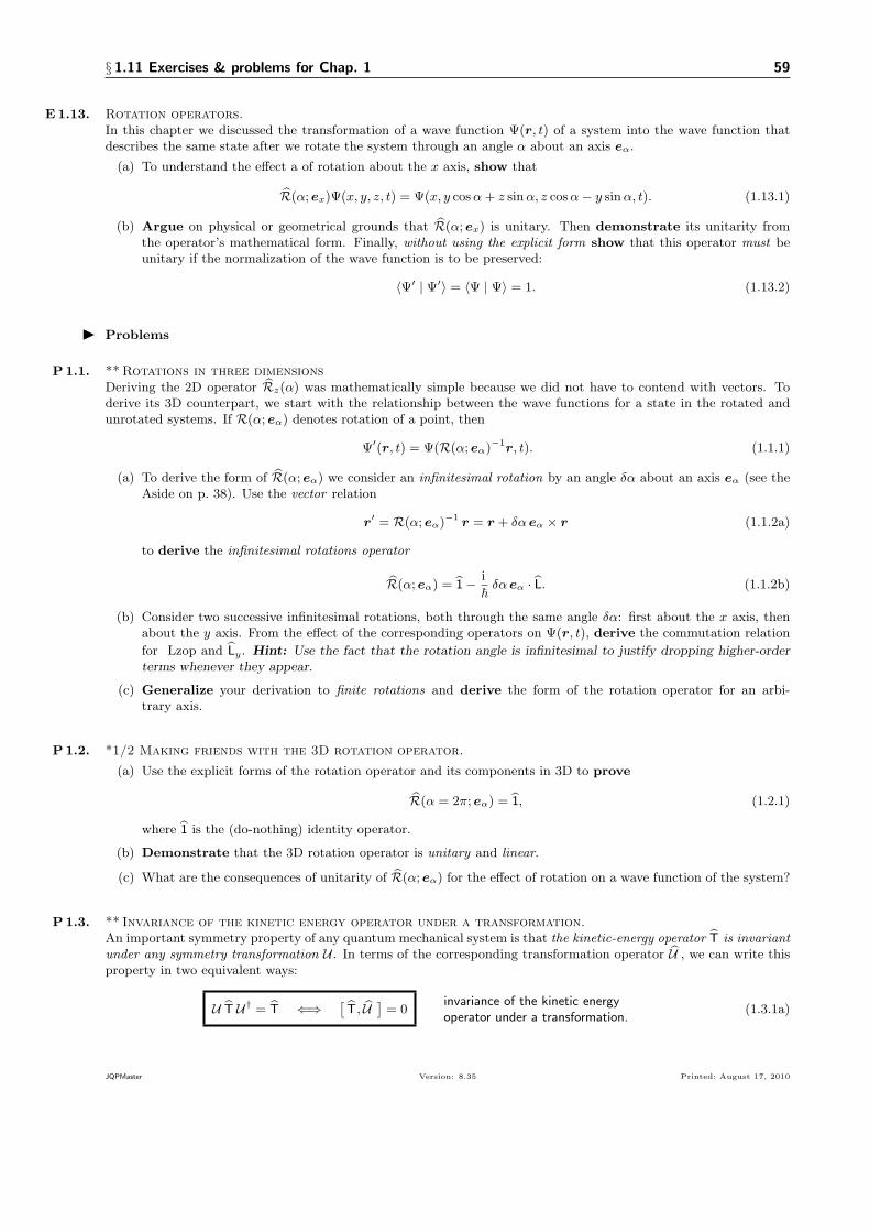
§ 1.11 Exercises & problems for Chap. 1 59
E1.13. Rotation operators.In this chapter we discussed the transformation of a wave function Ψ(𝒓, 𝑡) of a system into the wave function thatdescribes the same state after we rotate the system through an angle 𝛼 about an axis 𝒆𝛼.
(a) To understand the effect a of rotation about the 𝑥 axis, show that
ℛ(𝛼; 𝒆𝑥)Ψ(𝑥, 𝑦, 𝑧, 𝑡) = Ψ(𝑥, 𝑦 cos𝛼+ 𝑧 sin𝛼, 𝑧 cos𝛼− 𝑦 sin𝛼, 𝑡). (1.13.1)
(b) Argue on physical or geometrical grounds that ℛ(𝛼; 𝒆𝑥) is unitary. Then demonstrate its unitarity fromthe operator’s mathematical form. Finally, without using the explicit form show that this operator must beunitary if the normalization of the wave function is to be preserved:
⟨Ψ′ ∣ Ψ′⟩ = ⟨Ψ ∣ Ψ⟩ = 1. (1.13.2)
▶ Problems
P 1.1. **Rotations in three dimensionsDeriving the 2D operator ℛ𝑧(𝛼) was mathematically simple because we did not have to contend with vectors. Toderive its 3D counterpart, we start with the relationship between the wave functions for a state in the rotated andunrotated systems. If ℛ(𝛼; 𝒆𝛼) denotes rotation of a point, then
Ψ′(𝒓, 𝑡) = Ψ(ℛ(𝛼; 𝒆𝛼)−1𝒓, 𝑡). (1.1.1)
(a) To derive the form of ℛ(𝛼; 𝒆𝛼) we consider an infinitesimal rotation by an angle 𝛿𝛼 about an axis 𝒆𝛼 (see theAside on p. 38). Use the vector relation
𝒓′ = ℛ(𝛼; 𝒆𝛼)−1 𝒓 = 𝒓 + 𝛿𝛼 𝒆𝛼 × 𝒓 (1.1.2a)
to derive the infinitesimal rotations operator
ℛ(𝛼; 𝒆𝛼) = 1− i
ℏ𝛿𝛼 𝒆𝛼 ⋅ L. (1.1.2b)
(b) Consider two successive infinitesimal rotations, both through the same angle 𝛿𝛼: first about the 𝑥 axis, thenabout the 𝑦 axis. From the effect of the corresponding operators on Ψ(𝒓, 𝑡), derive the commutation relation
for Lzop and L𝑦. Hint: Use the fact that the rotation angle is infinitesimal to justify dropping higher-orderterms whenever they appear.
(c) Generalize your derivation to finite rotations and derive the form of the rotation operator for an arbi-trary axis.
P1.2. *1/2 Making friends with the 3D rotation operator.
(a) Use the explicit forms of the rotation operator and its components in 3D to prove
ℛ(𝛼 = 2𝜋; 𝒆𝛼) = 1, (1.2.1)
where 1 is the (do-nothing) identity operator.
(b) Demonstrate that the 3D rotation operator is unitary and linear.
(c) What are the consequences of unitarity of ℛ(𝛼; 𝒆𝛼) for the effect of rotation on a wave function of the system?
P1.3. ** Invariance of the kinetic energy operator under a transformation.An important symmetry property of any quantum mechanical system is that the kinetic-energy operator T is invariantunder any symmetry transformation 𝒰 . In terms of the corresponding transformation operator 𝒰 , we can write thisproperty in two equivalent ways:
𝒰 T 𝒰† = T ⇐⇒ [T,𝒰 ] = 0
invariance of the kinetic energyoperator under a transformation.
(1.3.1a)
JQPMaster Version: 8.35 Printed: August 17, 2010
60 § 1.11 Exercises & problems for Chap. 1
This property means that we can answer the crucial question of whether a system is invariant under 𝒰—that is,whether 𝒰 is a symmetry transformation of the system—by focusing solely on the potential energy 𝑉 in thesystem’s Hamiltonian ℋ = T + 𝑉 :
𝒰 𝑉 𝒰 † = 𝑉 =⇒ 𝒰 is a symmetry transformation:[ ℋ,𝒰 ] = 0 (1.3.1b)
(a) Use the chain rule to prove, by algebraic demonstration, that the kinetic-energy operator T of a particle inone dimension is invariant under an inversion 𝚤.
(b) Use reasoning by analogy to construct an argument that T(𝑥, 𝑦) of a particle in two dimensions is invariant
under 𝚤. [Recall that the notation T(𝑥, 𝑦) means that the operator T is expressed in Cartesian coordinates.]
(c) Now use the chain rule to prove that T(𝑥, 𝑦) is invariant under 𝚤. Compare each step of your proof to apoint in the logical argument of part (b) and, by so doing, verify that you properly implemented the strategyof reasoning by analogy.
(d) Argue that T(𝜌, 𝜑), the two-dimensional kinetic-energy operator in polar coordinates, is invariant under 𝚤.Further argue that this operator is invariant under an arbitrary translation 𝒯 (𝑎) and under an arbitraryrotation ℛ𝑧(𝛼). Don’t just write down a string of equations! Rather, explain and justify each step ofeach argument. If you’re the least bit uncertain about any of these arguments, carry out the correspondingderivation, then review your argument to be sure it conforms to your algebraic proof.
(e) Carefully generalize your argument to T for a particle in three dimensions expressed in Cartesian, spherical,or cylindrical coordinates (§1.D.4). Carefully and thoroughly explain and justify each step of eachargument.
JQPMaster Version: 8.35 Printed: August 17, 2010

61
Complement 1.A. User’s guide to Chap. 1
. . . reality favors symmetry.
—Jorge Luis Borges
Notation. The User’s guide for each chapter includes a table of notation introduced in that chapter. The table forthis chapter is Tbl. 1.A.2.
Key definitions and points. This chapter developed the theme of symmetry around the following definitions andkey points:
(1) A transformation is an operation that associates each point 𝑃 in ordinary space with another point 𝑃 ′ calledthe image of 𝑃 .
(2) If a system undergoes a transformation 𝒢 with transformation operator 𝒢 (Tbl. 1.A.3, p. 63), then you transforman associated function 𝑓 ′ at a point 𝑃 as follows. Evaluate the untransformed function 𝑓 at the point youget when you undo the transformation that generated 𝑓 ′ from 𝑓 in the first place. To get this point, apply theinverse transformation 𝒢−1 to 𝑃 .
(3) A symmetry transformation is a transformation that leaves the appearance of the system exactly as it wasbefore the transformation. In physics, a symmetry transformation is a transformation that does not change thevalue of any measurable property of the system or its Hamiltonian. Symmetry transformations are associatedwith geometric “symmetry elements” in ordinary space (Tbls. 1.A.4 and 1.A.5).
(4) Physics assumes homogeneity and isotopy of the laws of nature under spatial and temporal translations.Noether’s theorem associates each assumption with a conserved quantity, (Tbl. 1.A.6, p. 64).
(5) To each symmetry transformation 𝒰 of a system 𝒮 in ordinary space, 𝒰 : 𝒮 7→ 𝒮 ′, there is a linear, unitary
symmetry operator 𝒰 that acts on wave functions and operators as
Ψ′(𝒓, 𝑡) = 𝒰 Ψ(𝒓, 𝑡) = Ψ(𝒰−1𝒓, 𝑡
)Q ′ = 𝒰 Q 𝒰 −1
(1.A.1)
(6) A system is invariant under a symmetry transformation 𝒰 if the transformation leaves unchanged all probabil-ity amplitudes and measurable properties of operators (eigenvalues and expectation values of the correspondingoperators) and the time evolution of these quantities.
(7) Invariance of scalar products implies that all measurable properties are invariant under a symmetry transfor-mation 𝒰 of the system.
(8) Stone’s theorem relates any continuous unitary operator 𝒰 that commutes with a system’s Hamiltonian ℋ to
a Hermitian operator Q that commutes with ℋ. This Hermitian operator, Q ≡ i ℏ ( d𝒰 /d𝛾)𝛾=0, represents anobservable whose expectation value doesn’t change as the system evolves (in the absence of any measurements);
that is, Q is a constant of the motion . If 𝒰 is such that 𝒰(𝛾1) + 𝒰(𝛾2) = 𝒰(𝛾1 + 𝛾2), then 𝒰 and Q arerelated by Stone’s theorem,
𝒰 (𝛾) = exp
(− i
ℏ𝛾 Q
). (1.A.2)
JQPMaster Version: 8.35 Printed: August 17, 2010

62 Complement 1.A. User’s guide to Chap. 1
Problem-solving habits and techniques.
(1) Seek symmetry simplifications.
(2) Reason by analogy
Types of symmetry transformations. We developed conceptual and mathematical machinery for the threesymmetry transformations in Tbl. 1.A.7, with corresponding operators in Tbl. 1.A.8:
(1) Translations and rotations. Translations and rotations are continuous symmetry transformations: 𝒯 (𝒂)depends on the displacement vector 𝒂, and ℛ(𝛼; 𝒆𝛼) depends on the rotation angle 𝛼 and the rotation axis,which is specified by the unit vector 𝒆𝛼. The Hermitian operator associated with translations (via Stone’stheorem) is p ⋅ 𝒆𝑎, the projection of the linear-momentum operator on a unit vector 𝒆𝑎 along 𝒂. The Her-
mitian operator associated with rotations is L ⋅ 𝒆𝛼, the projection of the angular-momentum operator on therotation axis.
(2) Translations. To translate a system 𝒮, move every part of 𝒮 by the same displacement 𝒂. If ∣Ψ(𝑡)⟩ representsthe state of 𝒮 at 𝑡, then the state of 𝒮 ′ at 𝑡 is ∣Ψ′(𝑡)⟩ = 𝒯 (𝒂) ∣Ψ(𝑡)⟩. Invariance of the laws of nature under anarbitrary translation implies
(a) the operator 𝒯 (𝒂) is linear (so translations preserve relationships between states);
(b) the operator 𝒯 (𝒂) is unitary (so translations preserve scalar products); and
(c) the Hamiltonian of an isolated system commutes with 𝒯 (𝒂) for all displacements 𝒂 (so a state ∣Ψ(𝑡)⟩ andthe transformed state ∣Ψ′(𝑡)⟩ evolve via the TDSE with the same Hamiltonian).
(d) Rotations. We can effect a transformation in three ways (Tbl. 1.A.9, p. 64):
i. A rotation transformation ℛ(𝛼; 𝒆𝛼) act on a point 𝑃 at 𝒓 in ordinary space.
ii. A rotation matrix 𝑅(𝛼; 𝒆𝛼) act on the Cartesian coordinates of 𝑃 (Complement 1.E).
iii. A rotation operator ℛ(𝛼; 𝒆𝛼) act on wave functions and transforms operators.77
(e) Inversion. An inversion of a system in ordinary space takes a point at 𝒓 into the point at −𝒓. The
corresponding operator is the parity operator Π : If a system is invariant under inversion, then parity isa constant of the motion. Table 1.A.10 brings together the results for the two- and three-dimensionalcoordinate systems we’ll consider.
Table 1.A.1 summarizes the classification scheme for functions according to their parity.
effect of Π behavior under 𝚤 parity
Π 𝑓(𝑥) = 𝑓(𝑥) even under inversion even parity
Π 𝑓(𝑥) = −𝑓(𝑥) odd under inversion odd parity
Π 𝑓(𝑥) = 𝑔(𝑥) ∕= ±𝑓(𝑥) asymmetric under inversion no parity
Table 1.A.1. Classification of 1D functions by their behavior under inversion.By definition, Π 𝑓(𝑥) = 𝑓(−𝑥). Functions are classified by parity according to the rela-tionship of 𝑓(−𝑥) to 𝑓(𝑥). A function with the property 𝑓(−𝑥) ∕= ±𝑓(𝑥) is said to beasymmetric under inversion.
77Commentary: In group theory , the collection of rotation operators ℛ(𝛼; 𝒆𝛼) for all possible angles 𝛼 and axes 𝒆𝛼 constitutesa mathematical critter called the rotation group. There being an infinite number of possible rotations, this group contains aninfinite number of elements. Rotation angles and axes being continuous parameters, the rotation group is said to be continuous.
JQPMaster Version: 8.35 Printed: August 17, 2010

63
𝒮 generic symbol for a physical system; transformed system: 𝒮 ′
𝒰 generic symbol for a symmetry transformation
𝒰 generic symbol for the unitary symmetry operator corresponding to 𝒰 (𝒰 † = 𝒰 −1)
𝒢 generic symbol for a transformation operator (may or may not be a symmetry operator)
Q generic symbol for a Hermitian operator (Q† = Q)
𝝆 a vector in 2D; Cartesian coordinates 𝝆 = (𝑥, 𝑦); polar coordinates: 𝝆 = (𝜌, 𝜑)
𝒯 (𝒂) a translation (parameter: displacement 𝒂) [Eq. (1.4.3), p. 19]
𝒯 (𝒂) translation operator (linear and unitary)
ℛ(𝛼; 𝒆𝛼) a rotation (parameters: rotation angle 𝛼; rotation axis: 𝒆𝛼) [Eq. (1.4.5), p. 21]
ℛ(𝛼; 𝒆𝛼) rotation operator (2D) (linear and unitary)
𝑅(𝛼; 𝒆𝛼) rotation matrix (2D) (orthogonal)
𝚤 an inversion through a fixed origin [Eq. (1.4.4a), p. 20]
Π the parity operator (linear and Hermitian) [Eq. (1.7.9), p. 46]
L𝑧 2D orbital angular momentum operator (a scalar operator)
Table 1.A.2. Notation introduced in this chapter.
transformation 𝒢 ordinary space 𝒢 : 𝒓 7→ 𝒓′
transformation operator 𝒢 function space 𝒢 : 𝑓(𝒓) 7→ 𝑓 ′(𝒓)
Table 1.A.3. Transformations and transformation operators. To each transformation 𝒢 that actson a system (in ordinary space) as 𝒢 : 𝒮 7→ 𝒮 ′, there is an operator 𝒢 that transforms wave functions andoperators that are associated with the object.
element potential energy constants of the motion
center of symmetry inversion symmetry 𝑉 (−𝒓) = 𝑉 (𝒓) parity
all axes are symmetry axes spherical symmetry 𝑉 = 𝑉 (𝑟) 𝐿, projection of 𝐿 on any axis
only one axis of symmetry axial symmetry 𝑉 = 𝑉 (𝑟, 𝜃) 𝐿, projection of 𝐿 on the sym-metry axis
Table 1.A.4. Symmetry elements and their physical consequences. For each elements in the first column,the second column indicates the associated symmetry property. The last column lists constants of the motion,observables whose corresponding operators commute with the Hamiltonian. The vector 𝑳 is the total orbitalangular momentum of the system.
operation and element parameter type of operation
rotation about an axis 𝒆𝛼 through an angle 𝛼 continuoustranslation along an axis 𝒆𝑎 by a distance 𝑎 continuousreflection in a plane discreteinversion through a fixed point (the origin) discrete
Table 1.A.5. The language of symmetry: operations, elements, and parameters. Each transforma-tion defines a symmetry element. Continuous operations depend on a parameter ; discrete operations donot. A transformation is a symmetry transformation if it leaves the system unchanged. For a system to beinvariant under a continuous operation, the system must be unchanged for all values of the parameter.
JQPMaster Version: 8.35 Printed: August 17, 2010

64 Complement 1.A. User’s guide to Chap. 1
symmetry property invariance principle conserved quantity
homogeneous with respect to time translation in time total mechanical energyhomogeneous with respect to space translation in space total linear momentumisotropic with respect to space rotation in space total angular momentum
Table 1.A.6. Symmetry properties of space-time and of an isolated system. A fundamental assumptionof physics is that an isolated system is unchanged by translations in time and/or space, and by rotations inspace. (A “translation in time” is equivalent to a change in the choice of 𝑡 = 0.) These assumptions arecalled the homogeneity and isotropy of free space (column 1). Each assumption implies an invarianceprinciple for the potential energy of an otherwise isolated system (column 2). Each invariance principle, inturn, implies conservation of a physical quantity (column 3). (The “mechanical energy” is the sum of thekinetic and potential energies.) Translational invariance (in space) implies that no aspect of the physicaldescription of a system—neither its properties nor their evolution with time—can depend on the origin ofcoordinates. Rotational invariance implies the same thing about the orientation of the axes of the referenceframe used to describe the system. Neither the symmetry properties nor their implications depend on modelsor approximations used in the analysis of the system.
transformation symbol 𝒢 operator 𝒢 key equation
translation 𝒯 (𝒂) 𝒯 (𝒂) Eq. (1.7.5), p. 44
rotation ℛ(𝛼; 𝒆𝛼) ℛ(𝛼; 𝒆𝛼) Eq. (3.2.21b), p. 189
inversion 𝚤 Π Eq. (1.7.9), p. 46
Table 1.A.7. Transformations and transformation operators for quantummechanics. This table contains only the transformations we’ll consider; many othersarise in the quantum physics of systems such as molecules, solids, and elementary par-ticles. Translations and rotations depend on symmetry parameters; inversion does not.The effect of these operators on functions is in Tbl. 1.A.8.
symmetry transformation symmetry operator effect on a function
translation 𝒯 (𝒂) translation operator 𝒯 (𝒂) 𝒯 (𝒂)𝑓(𝒓) = 𝑓(𝒯 (𝒂)−1 𝒓
)= 𝑓(𝒓 − 𝒂)
rotation ℛ(𝛼; 𝒆𝛼) rotation operator ℛ(𝛼;𝒆𝛼) ℛ(𝛼;𝒆𝛼)𝑓(𝒓) = 𝑓(ℛ(𝛼; 𝒆𝛼)−1𝒓
)inversion 𝚤 parity operator Π Π 𝑓(𝒓) = 𝑓(−𝒓)
Table 1.A.8. The effect of symmetry transformations and operations on functions. The function 𝑓(𝒓) is
arbitrary, may depend on time, and, as in quantum mechanics, may be complex. Note the inverses 𝒯 (𝒂)−1 = 𝒯 (−𝒂)for the translation operator and ℛ(𝛼; 𝒆𝛼)−1 = ℛ(−𝛼; 𝒆𝛼) for the rotation operator.
transformation mathematical device example
rotation of a point 𝑃 at 𝒓 transformation ℛ(𝛼; 𝒆𝛼) 𝒓′ = ℛ(𝛼; 𝒆𝛼)𝒓
rotation of the Cartesian coordinates (𝑥, 𝑦, 𝑧) of 𝑃 matrix 𝑅(𝛼; 𝒆𝛼)
⎛⎝𝑥′𝑦′𝑧′
⎞⎠ = 𝑅(𝛼; 𝒆𝛼)
⎛⎝𝑥𝑦𝑧
⎞⎠rotation of a function 𝑓(𝒓) operator ℛ(𝛼; 𝒆𝛼) 𝑓 ′(𝒓) = ℛ(𝛼; 𝒆𝛼)𝑓(𝒓)
Table 1.A.9. Tools for effecting rotational transformations in physics. In this table, rotation is used toillustrate the difference between transformations in ordinary space, the matrix that effects that transformation ina coordinate system (here, Cartesian coordinates), and the operator that transforms functions. Other widely usedtransformations are summarized in Tbl. 1.A.8.
JQPMaster Version: 8.35 Printed: August 17, 2010

65
one dimension
Cartesian 𝚤 : 𝑥 7→ −𝑥 Π 𝑓(𝑥) = 𝑓(−𝑥)two dimensions
Cartesian 𝚤 : (𝑥, 𝑦) 7→ (−𝑥,−𝑦) Π 𝑓(𝑥, 𝑦) = 𝑓(−𝑥,−𝑦)polar 𝚤 : (𝜌, 𝜑) 7→ (𝜌, 𝜑+ 𝜋) Π 𝑓(𝜌, 𝜑) = 𝑓(𝜌, 𝜑+ 𝜋)
three dimensions
Cartesian 𝚤 : (𝑥, 𝑦, 𝑧) 7→ (−𝑥,−𝑦,−𝑧) Π 𝑓(𝑥, 𝑦, 𝑧) = 𝑓(−𝑥,−𝑦,−𝑧)spherical 𝚤 : (𝑟, 𝜃, 𝜑) 7→ (𝑟, 𝜋 − 𝜃, 𝜑+ 𝜋) Π 𝑓(𝑟, 𝜃, 𝜑) = 𝑓(𝑟, 𝜋 − 𝜃, 𝜑+ 𝜋)
cylindrical 𝚤 : (𝜌, 𝜑, 𝑧) 7→ (𝜌, 𝜑+ 𝜋,−𝑧) Π 𝑓(𝜌, 𝜑) = 𝑓(𝜌, 𝜑+ 𝜋,−𝑧)
Table 1.A.10. Inversion and the parity operator in various coordinate systems. The parity operator Πchanges the arguments of a function in the same way that inversion 𝚤 changes the coordinates because 𝚤−1 = 𝚤, aproperty not shared by rotations. In 3D, the polar angle 𝜃 goes to 𝜋−𝜃 in order to keep this angle in the domainof its definition, 𝜃 ∈ [0, 𝜋]. No such limitation affects the azimuthal angle 𝜑, whose domain is 𝜑 ∈ [0, 2𝜋]. Notethat the 2D polar coordinates (𝜌, 𝜑) are just the first two of the 3D cylindrical coordinates (𝜌, 𝜑, 𝑧).
JQPMaster Version: 8.35 Printed: August 17, 2010

66 Complement 1.B. Additional Examples
Complement 1.B. Additional Examples
The examples in this complement supplement those in the main text. If you need to more applications of the ideasin the chapter before you tackle the exercises and problems, these examples should do the job.
▶ Example 1.13 (Reflections in two and three dimensions.)While an inversion translates a point 𝑃 at 𝒓 (see Fig. 1.8, p. 20) through another point (the origin) to 𝑃 ′
at 𝒓′, a reflection translates a point through an axis. In the 𝑥𝑦 plane I can reflect a point through any axisin the plane: using 𝜎𝑥 to denote a reflection along the 𝑥 axis and so on, I can write a reflection through the 𝑥axis or through the 𝑦 axis as
𝜎𝑥 :
{𝑥→ −𝑥𝑦 → +𝑦
and 𝜎𝑦 :
{𝑥→ +𝑥
𝑦 → −𝑦reflections in two dimensions(Cartesian coordinates).
(1.B.1)
A reflection in three dimensions (3D) acts like a reflection in 2D. But in 3D we reflect through planes. I canchoose any of an infinite number of reflection planes: particularly useful are the Cartesian planes 𝑥𝑦, 𝑦𝑧,and 𝑥𝑧. A reflection through the 𝑥𝑦 plane, for example, transforms Cartesian coordinates as
𝜎𝑥𝑦 :
⎧⎨⎩𝑥→ +𝑥
𝑦 → +𝑦
𝑧 → −𝑧,
a reflection through 𝑥𝑦 plane(Cartesian coordinates).
(1.B.2)
Try This! 1.20. Symmetry sketches in two dimensions.
Draw figures that illustrate the effects on a point in a plane of an inversion and of the reflectionsof Example 1.13. ◀
▶ Example 1.14 (Internal symmetries of an electron interacting with a proton.)Figure 1.B.1 shows an electron and a proton. These particles have opposite charges, 𝑞𝑒 = −𝑒 and 𝑞𝑝 = +𝑒,where 𝑒 is the elementary charge—which in this book is a positive number, 𝑒 > 0. The relative position ofthe electron with respect to the proton is 𝒓. We’ll treat the proton as an “infinitely massive” particle locatedat the fixed origin of our reference frame.78
The proton creates an electric field whose value at any 𝒓 is given by the vector function,79
퓔0(𝒓) =𝑒
4𝜋𝜖0
1
𝑟2𝒆𝑟, electric field due to a proton. (1.B.3)
An electron at 𝒓 therefore experiences a force given by Coulomb’s law (see Chap. 13),80
𝑭 (𝒓) = −𝑒퓔0(𝒓) = − 𝑒2
4𝜋𝜖0
1
𝑟2𝒆𝑟 ≡ −𝑒
20
𝑟2𝒆𝑟
electric force on an electron at 𝑟due to a proton at the origin.
(1.B.4)
78Commentary: This approximation of infinite nuclear mass does not mean literally that the proton mass 𝑚𝑝 is infinite.That would be silly: 𝑚𝑝 = 1.673× 1027 kg, not∞. Rather, it means that the proton is so much heavier than the electron that wecan neglect its motion compared to the motion of the electron. If we further treat the proton as a point particle with charge andmass (and, perhaps, spin) but zero volume and no internal structure, then our model of the proton is an “infinitely massive”point particle fixed at the origin. Because an electron really is much more massive than a proton (𝑚𝑒/𝑚𝑝 ≈ 5.446× 10⁻⁴),this approximation is excellent for almost all problems in atomic and molecular physics: see, for example, the hydrogen atomin Chap. 5.
79Details: In these examples, I talk about electrons and protons as though they were classical particles, even though you andI know they’re not. But it’s okay to talk this way here because the symmetry principles and arguments of this chapter pertainto both quantum and classical systems. The quantum counterparts of the system in this example show up in Chap. 5 (thehydrogen atom) and in Chap. 14 (an electron in the field of a point dipole).
80Notation: In the last equality in Eq. (1.B.4) I’ve introduced the shorthand symbol 𝑒 20 for the fraction 𝑒2/4𝜋𝜖0. In SI units
this fraction shows up all over the place, cluttering lots of equations with factors of 𝜋 and 𝜖0 that obscure the physics of theequation and try to seduce you into making mistakes in algebra. These factors don’t appear in other commonly used systemsof units (Chap. 13).
JQPMaster Version: 8.35 Printed: August 17, 2010

67
x
z
é+q
é
é
-e
-e
Α
x
z
é
é
é
+q
é
-q
-e
-e
Α
Figure 1.B.1. An electron in the fields of a proton and a point dipole. The left panel shows a (classical)particle with charge −𝑒 in the field of a positively charged particle with charge +𝑞 (Example 1.14). The rightpanel shows the particle in the field of a point dipole consisting of two particles of charge ±𝑞 (Example 1.15). Inboth figures, the dashed arrow indicates the position of the negatively charged particle after rotation through𝛼 = 45∘.
Figure 1.B.1 and Eq. (1.B.4) reveal the symmetry of the force on the electron. The function in (1.B.4)depends on the electron’s radial distance 𝑟 but not on its polar angle 𝜃 or its azimuthal angle 𝜑. Such aspherically symmetric force is called a central force. Its symmetry follows from the spherical symmetry of 퓔0,as you can see in the electric field lines of Fig. 1.B.2a.81
Like any electrostatic field, the field of the proton is related to a scalar function called the electrostaticpotential (or scalar potential) Φ(𝒓). The relationship is 퓔0(𝒓) = −∇Φ(𝒓), where ∇ is the gradient oper-ator :
∇ = 𝒆𝑥∂
∂𝑥+ 𝒆𝑦
∂
∂𝑦+ 𝒆𝑧
∂
∂𝑧gradient operator (3D). (1.B.5)
For the proton field (1.B.3), the scalar potential at 𝒓 is the Coulomb potential ,
Φ(𝒓) =𝑒
4𝜋𝜖0
1
𝑟, electrostatic potential of a proton at the origin. (1.B.6)
The scalar potential, too, is spherically symmetric. Each equipotential surface [a locus of points 𝒓 forwhich Φ(𝒓) is constant] is a sphere centered on the proton, where we put the origin. The origin is therefore acenter of symmetry of the electron in a hydrogen atom.
Finally, the electrostatic energy of the electron—the potential energy 𝑉 (𝒓) that appears in its Hamilto-
nian, ℋ = T + 𝑉 (𝒓)—is the work required to bring the electron from “infinity,” where it is at rest, to 𝒓:82
𝑉 (𝒓) = −𝑒Φ(𝒓) = − 𝑒2
4𝜋𝜖0
1
𝑟= −𝑒
20
𝑟,
potential energy of an electron at 𝒓due to a proton at the origin.
(1.B.7)
In a hydrogen atom, the electron’s potential energy is attractive and spherically symmetric. Crucially, thismeans that the electron in the field of a proton is rotationally invariant : its potential energy (and hence itsHamiltonian) is unchanged by a rotation through any angle about any axis that passes through the proton.
81Jargon: Each electric field line is a locus of points chosen so the tangent at each point 𝒓 is parallel to 퓔0(𝒓) and henceto 𝑭 (𝒓). By convention, electric field lines point towards negative charges and away from positive charges. Their directiontherefore indicates the direction of the corresponding electrostatic force. (Electric field lines are often called lines of force.)
82Commentary: In this context “infinity” refers to some location far enough from the proton that the effect of the Coulombforce (1.B.4) is negligible.
JQPMaster Version: 8.35 Printed: August 17, 2010
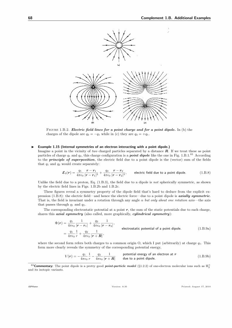
68 Complement 1.B. Additional Examples
Figure 1.B.2. Electric field lines for a point charge and for a point dipole. In (b) thecharges of the dipole are 𝑞2 = −𝑞1 while in (c) they are 𝑞2 = +𝑞1.
▶ Example 1.15 (Internal symmetries of an electron interacting with a point dipole.)Imagine a point in the vicinity of two charged particles separated by a distance 𝑹. If we treat these as pointparticles of charge 𝑞1 and 𝑞2, this charge configuration is a point dipole like the one in Fig. 1.B.1.83 Accordingto the principle of superposition , the electric field due to a point dipole is the (vector) sum of the fieldsthat 𝑞1 and 𝑞2 would create separately:
퓔0(𝒓) =𝑞1
4𝜋𝜖0
𝒓 − 𝒓1
∣𝒓 − 𝒓1∣3 +𝑞2
4𝜋𝜖0
𝒓 − 𝒓2
∣𝒓 − 𝒓2∣3 , electric field due to a point dipole. (1.B.8)
Unlike the field due to a proton, Eq. (1.B.3), the field due to a dipole is not spherically symmetric, as shownby the electric field lines in Figs. 1.B.2b and 1.B.2c.
These figures reveal a symmetry property of the dipole field that’s hard to deduce from the explicit ex-pression (1.B.8): the electric field—and hence the electric force—due to a point dipole is axially symmetric.That is, the field is invariant under a rotation through any angle 𝛼 but only about one rotation axis—the axisthat passes through 𝑞1 and 𝑞2.
The corresponding electrostatic potential at a point 𝒓, the sum of the static potentials due to each charge,shares this axial symmetry (also called, more graphically, cylindrical symmetry):
Φ(𝒓) =𝑞1
4𝜋𝜖0
1
∣𝒓 − 𝒓1∣ +𝑞2
4𝜋𝜖0
1
∣𝒓 − 𝒓2∣ ,
=𝑞1
4𝜋𝜖0
1
𝑟+
𝑞24𝜋𝜖0
1
∣𝒓 +𝑹∣ ,electrostatic potential of a point dipole. (1.B.9a)
where the second form refers both charges to a common origin O, which I put (arbitrarily) at charge 𝑞1. Thisform more clearly reveals the symmetry of the corresponding potential energy,
𝑉 (𝒓) = − 𝑞14𝜋𝜖0
1
𝑟− 𝑞2
4𝜋𝜖0
1
∣𝒓 +𝑹∣potential energy of an electron at 𝒓due to a point dipole.
(1.B.9b)
83Commentary: The point dipole is a pretty good point-particle model (§1.2.2) of one-electron molecular ions such as H+2
and its isotopic variants.
JQPMaster Version: 8.35 Printed: August 17, 2010

69
This potential energy depends on the electron’s radial coordinate 𝒓 and its polar angle 𝜃 and so is not spher-ically symmetric. But it does not depend on the electron’s azimuthal angle 𝜑, so it is axially symmetric.Equation (1.B.9b) establishes the symmetry properties of the electron in this environment. ◀
▶ Noteworthy features of Example 1.14 and Example 1.15: The physical origin of the different symmetry prop-erties of the electron in these examples is the different character of the forces on the electron: the force on an electrondue to a proton is a central force, while the force due to a point dipole is a noncentral axial force.84 The differencesin the symmetry properties of an electron profoundly influence its physical properties in these different environments.
These examples illustrate the difference between universal and internal symmetries and (I hope) hammer homethe point that symmetry arguments require care and precision with language. If by “the system” we mean theelectron and the charge configuration that creates the electric field it experiences, then the systems in Example 1.14and Example 1.15 are both rotationally invariant. (That’s just a consequence of the isotropy of space.) But if by“the system” we mean the electron only, then the system in Example 1.14 is rotationally invariant, but the systemin Example 1.15 is not.
▶ Aside. The symmetry of the dipole field and the multipole expansion.You may be wondering what the scalar potential, Eq. (1.B.9a), has to do with the dipole moment of apoint dipole. Suppose the charges obey 𝑞1 = 𝑞 > 0 and 𝑞2 = −𝑞 < 0. If we evaluate the scalar potentialat a radius much larger than the separation of the charges 𝑅, so 𝑟 ≫ 𝑅, then we can expand ∣𝒓 − 𝒓∣−1 ina power series in 𝑅/𝑟 about 𝑅/𝑟 = 1 to get an expression for the dipole potential in terms of the electricdipole moment 𝒅 ≡ 𝑞𝑹:85
Φ(𝒓) =1
4𝜋𝜖0
𝒅 ⋅ 𝒆𝑟𝑟2
,scalar potential due to apoint dipole at 𝑟 ≫ 𝑅.
(1.B.10)
In this equation, the dot product of the dipole moment 𝒅 and the radial unit vector 𝒆𝑟 equals𝒅 ⋅ 𝒆𝑟 = 𝑑 cos 𝜃 = 𝑞𝑅 cos 𝜃, which shows that the scalar potential (and hence the Hamiltonian) depends on 𝜃but not on 𝜑. Equation (13.5.4a) is the first term in the (infinite) multipole expansion of Φ(𝒓) for anelectrically neutral system (see Chap. 13).
▶ Example 1.16 (Effect of an inversion on the linear-momentum operator.)Equation (1.6.13), Q ′ = 𝒰 Q 𝒰 †, is a prescription for transforming an operator Q associated with a systemthat undergoes a transformation 𝒰 . To actually implement this procedure, we require only the properties ofthe corresponding operator 𝒰 and knowledge of what Q does to a function.
Implementation proceeds by the usual strategy for developing operator equations: let the operator act ona general (suitably well-behaved) function of whatever variables describe the system. The key tactic is toisolate what we don’t know on one side of the equation, then manipulate what we do know, always keeping aneye on our ultimate goal, which here is the transformed operator Q ′: According to our prescription (1.6.13),
Q′𝒰 = 𝒰 Q. So to figure out Q′, a sensible place to start is with the left-hand side of this equation.86
I’ll now apply this strategy to the one-dimensional linear-momentum operator , p = −i ℏ d/d𝑥, of a
system that undergoes an inversion. With Q = p and 𝒰 = Π , I’m working with p′ Π = Π p. To figure out thething on the left-hand side I start with something I can evaluate, the right-hand side:
Π p 𝑓(𝑥) = Π
[−i ℏ d𝑓(𝑥)
d(𝑥)
], definition p = −i ℏ d/ d𝑥, (1.B.11a)
= −i ℏd𝑓(−𝑥)d−𝑥 , effect of the parity operator, (1.B.11b)
84Jargon: Don’t confuse the use of “axial” in “axial force” with its use in the mathematical characterization of a certain typeof vector as an “axial vector” (see §1.D.2).
85Details: Such expansions can but need not be confusing. It helps to remember that when we take the limit 𝑟 → 0 we alsotake limits 𝑅→ 0 and 𝑞 →∞ in such a way that 𝑞𝑅 remains constant. Moreover, such expansions implicitly mean that 𝑅→ 0more rapidly than 𝑟 → 0, so 𝑅/𝑟 ≪ 1 holds for all 𝑟. These points, along with the relationship of the dipole potential tomultipole expansion, are lucidly explained in §2.7 and 2.8 of Nayfeh and Brussel (1985b)—a text I strongly recommend if youneed an E&M refresher or information beyond what you learned in your first E&M course.
86Commentary: Not all quantum mechanical operators transform under inversion into minus themselves. An angular momen-tum operator, such as the orbital operator L (Chaps. 2–5) transforms into itself: Π L Π = L. This property has to do with thecharacter of the classical orbital angular momentum 𝑳, which is an axial vector , not a polar vector like 𝒓 or 𝒑.
JQPMaster Version: 8.35 Printed: August 17, 2010

70 Complement 1.B. Additional Examples
= +i ℏ d𝑓(−𝑥)d𝑥
, to retain 𝑓(−𝑥) = Π 𝑓(𝑥) on the right-hand side, (1.B.11c)
= −p 𝑓(−𝑥), definition p = −i ℏ d/ d𝑥, (1.B.11d)
= −p Π 𝑓(𝑥), want to write right-hand side in terms of p and Π , (1.B.11e)
=⇒ Π p = −p Π , 𝑓(𝑥) is arbitrary, (1.B.11f)
=⇒ Π p Π−1 = −p, manipulate equation to apply 𝒰 Q𝒰 −1 = Q′. (1.B.11g)
♦ Rule: An inversion of a system in ordinary space transforms the quantum-mechanical linear-momentum operatorinto minus itself:
p′ = −p transformation of the linear momentumoperator under an inversion.
(1.B.11h)
Try This! 1.21. Generalizing the conclusion of Example 1.16.
Explain why each step that led to Eq. (1.B.11h) is valid for the linear momentum operator in twoand three dimensions, so
p ′ ≡ Π p Π−1 = −p (1.B.12)
Why is this generalized result independent of the coordinate system? ◀
Try This! 1.22. Effect of a transformation on the position operator.
The position operator x simply tells us to multiply the function on which it acts by the variable 𝑥.Work through steps analogous to those of Example 1.16 and explain why
Π x Π−1 = −x, and Π r Π−1 = −r. transformation of the positionoperator under an inversion.
(1.B.13)
▶ Example 1.17 (The parity operator in three dimensions.)To illustrate the effect of inversion in three dimensions on a function in spherical coordinates, I’ll use theequations in the Aside on p. 47 to apply this transformation to a special function called a spherical harmonic(see Chap. 3). Suppose the function
𝑌2,+1(𝜃, 𝜑) = −1
2
√15
2𝜋sin 𝜃 cos 𝜃 ei𝜑 (1.B.14a)
is the angle-dependent factor in a wave function Ψ(𝑟, 𝜃, 𝜑, 𝑡) of a particle in some potential 𝑉 (𝑟). We subjectthe particle to an inversion. What happens to the wave function?
The parity operator leaves the 𝑟 (and 𝑡) dependence of Ψ(𝑟, 𝜃, 𝜑, 𝑡) unchanged, so I can focus on the angularpart, 𝑌2,+1(𝜃, 𝜑). Using Eq. (1.7.15), p. 47, I find (see §1.D.4 and especially the Aside on p. 47):
Π 𝑌2,+1(𝜃, 𝜑) = −1
2
√15
2𝜋(+ sin 𝜃)(− cos 𝜃) ei (𝜑+2𝜋). (1.B.14b)
Since e2𝜋 i = 1 and 𝑌ℓ,𝑚ℓ(𝜃, 𝜑) ∝ Φ𝑚ℓ(𝜑), which depends on 𝜑 as ei𝑚ℓ𝜑, the effect of Π is to transform thisfunction into minus itself:
Π [sin 𝜃 cos 𝜃m ei𝜑 = sin(𝜋 − 𝜃) cos(𝜋 − 𝜃) ei𝜑+𝜋
=⇒ Π𝑌2,+1(𝜃, 𝜑) = +1
2
√15
2𝜋sin 𝜃 cos 𝜃 ei𝜑 = −𝑌2,+1(𝜃, 𝜑).
(1.B.14c)
Therefore under inversion a wave function Ψ(𝑟, 𝜃, 𝜑, 𝑡) whose angular dependence is given by 𝑌2,+1(𝜃, 𝜑) hasodd parity, because the parity is (−1)ℓ. Physicists express this result by saying “the function 𝑌2,+1(𝜃, 𝜑) isinvariant under a rotation about the 𝑧 axis. ◀
JQPMaster Version: 8.35 Printed: August 17, 2010

71
▶ Example 1.18 (The relationship between translation operators and the linear momentum.)In Example 1.11, I showed that Stone’s theorem implies a relationship between 1D translations 𝒯 (𝒂) and
the 1D linear-momentum operator p𝑥. Here I’ll derive the exponential form of 𝒯 (𝑎) from the definition of thetranslation operator in terms of its effect on a 1D wave function.
According to Stone’s theorem (§1.8.1), every continuous symmetry transformation defines a Hermitian op-erator, and the nature of the functional relationship is exponential. This description suggests a general strategyfor any such transformation: begin with an infinitesimal transformation; then treat a finite transformation asan infinite number of successive applications of the infinitesimal transformation.87 The simplest context forunderstanding this strategy is a translation 𝒯 (𝑎) in one dimension. The effect of such a translation on a wavefunction 𝜓(𝑥) is88
𝜓′(𝑥) = 𝒯 (𝑎)𝜓(𝑥) = 𝜓(𝑥− 𝑎). (1.B.15)
If the translation is infinitesimal—that is, if the displacement is the infinitesimal 1D differential d𝑎, then 𝒯 ( d𝑎)transforms 𝜓(𝑥) into 𝜓(𝑥 − d𝑎). I can develop an explicit form for 𝒯 ( d𝑎) by expanding 𝜓(𝑥 − d𝑎) in aTaylor series about d𝑎 = 0. Since d𝑎 is infinitesimal, it’s okay to neglect all terms in the resulting series oforder 𝒪 ( d𝑎2):89
𝜓(𝑥− d𝑎) = 𝜓(𝑥)− d𝑎d𝜓
d𝑥+
1
2!( d𝑎)2
d2𝜓
d𝑥2+
1
3!( d𝑎)3
d3𝜓
d𝑥3+ ⋅ ⋅ ⋅ , (1.B.16a)
≈ 𝜓(𝑥)− d𝑎d𝜓
d𝑥(1.B.16b)
=
(1− d𝑎
d
d𝑥
)𝜓(𝑥). (1.B.16c)
Remembering that the product of two (or more) transformations means successive application—first, the right-most transformation, then the next rightmost, and so on—I now implement phase two of my plan: bring abouta finite translation via an infinite number of infinitesimal translations, each of the form Eq. (1.B.16a). I dividethe finite displacement 𝑎 into a number 𝑁 of equal, smaller displacements 𝑎/𝑁 , then take the limit 𝑁 →∞:90
𝜓(𝑥− 𝑎) = lim𝑁→∞
(1− 𝑎
𝑁
d
d𝑥
)𝑁𝜓(𝑥) (1.B.17a)
= exp
(−i 𝑎 d
d𝑥
)𝜓(𝑥) (1.B.17b)
= exp
(−i 𝑎 p𝑥
ℏ
)𝜓(𝑥) (1.B.17c)
=⇒ 𝒯 (𝑎) = exp
(−i 𝑎 p𝑥
ℏ
)(1.B.17d)
87Commentary: To apply this strategy, our transformation must depend on a symmetry parameter, such as 𝑎 for a translationin one dimension. That’s why we can apply this strategy only to a continuous transformation, not to a discrete transformationlike inversion.
88Notation: Time does not enter this derivation in any way. So, to minimize clutter in the algebra, I’m replacing Ψ(𝑥, 𝑡)with 𝜓(𝑥). Elsewhere I use 𝜓(𝑥) to represent a stationary state and label by the energy 𝐸 and/or various quantum numbers.But in this example only, 𝜓(𝑥) represents an arbitrary state at some time.
89Notation: The symbol 𝒪 (d𝑎2) refers to all terms that are proportional to d𝑎𝑛 for 𝑛 ≥ 2.90Details: To get to Eq. (1.B.16c) I used the definition of an exponential operator [Eq. (H.15), p. 1354]. The third step
follows from the definition of the 1D linear-momentum operator, p𝑥 ≡ −i ℏ d/d𝑥. You may be wondering how I figured outto rewrite the second line in terms of this operator. Well, I knew I was seeking a Hermitian operator—that’s what Stone’stheorem tells me to do. Second, I remembered the definition of p𝑥 and that p𝑥 is Hermitian. I didn’t do anything clever, butI did think about what I was doing, and I had memorized the definition of p𝑥; had I not done so, I might not have seen thecrucial connection. You can figure out steps like this too—if you think and if you know basic definitions and properties. (It’snot enough to know where to find this information—the process of looking it up will derail your train of thought and causeyour derivation to crash and burn.)
JQPMaster Version: 8.35 Printed: August 17, 2010

72 Complement 1.B. Additional Examples
▶ Example 1.19 ( Invariance of the position probability density.)According to the Born interpretation of a wave function, if a single-particle system is in a state representedby Ψ(𝒓, 𝑡), then the expression
𝒫(𝒓) ≡ ∣Ψ(𝒓, 𝑡)∣2 = Ψ∗(𝒓, 𝑡)Ψ(𝒓, 𝑡), position probability density, (1.B.18a)
is the position probability density for the particle. That is, the probability of finding the particle at time 𝑡in an infinitesimal volume element d3𝑣 at 𝒓 is
𝒫(𝒓) d3𝑣 = ∣Ψ(𝒓, 𝑡)∣2 d3𝑣 = Ψ∗(𝒓, 𝑡)Ψ(𝒓, 𝑡) d3𝑣. (1.B.18b)
In practice, of course, we can search for a particle only in a (perhaps very small) finite volume 𝑉 . Thisprobability follows from Eq. (1.B.18b) as∫
𝑉
𝒫(𝒓) d3𝑣 =
∫𝑉
∣Ψ(𝒓, 𝑡)∣2 d3𝑣 =
∫𝑉
Ψ∗(𝒓, 𝑡)Ψ(𝒓, 𝑡) d3𝑣. (1.B.18c)
In this example, I’ll work out the effect on 𝒫(𝒓) of applying a symmetry transformation to the system:
𝒫 ′(𝒓, 𝑡) = Ψ′(𝒓, 𝑡)∗ Ψ′(𝒓, 𝑡), definition of the probability density Eq. (1.B.18a), (1.B.19a)
=[𝒰 Ψ(𝒓, 𝑡)
]∗ [𝒰 Ψ(𝒓, 𝑡)], definition of Ψ′(𝒓, 𝑡), (1.B.19b)
= Ψ∗(𝒓, 𝑡)[𝒰 † 𝒰 ]Ψ(𝒓, 𝑡), definition of the adjoint, (1.B.19c)
= Ψ∗(𝒓, 𝑡)Ψ(𝒓, 𝑡), unitarity of the symmetry operator 𝒰 , (1.B.19d)
= 𝒫(𝒓), definition of the probability density Eq. (1.B.18a). (1.B.19e)
♦ Rule: The position probability density for any state is invariant under a symmetry transformation.
▶ Example 1.20 (Translational symmetry and conservation of linear momentum.)The first step in relating a symmetry transformation 𝒰 to a conservation law is to work out the exponential
form of the symmetry operator 𝒰 in terms of a Hermitian operator Q. The second step is to show thatbecause 𝒰 is a symmetry operation, the observable 𝑄 is conserved. In Example 1.18, I worked out the first stepfor a translation in one dimension and found that a translation is related to the linear momentum operator by[Eq. (1.8.3), p. 50]
𝒯 (𝑎) = exp
(−i 𝑎 p𝑥
ℏ
). (1.B.20a)
This result strongly suggests that the conservation law for a system which is translationally invariant is conser-vation of linear momentum. But it’s not obvious (at least to me) that the math will support this conjecture.So I need to grind through the algebra.
I do know that if 𝒯 (𝑎) is a symmetry transformation of a system, then 𝒯 (𝑎) commutes with the system’s
Hamiltonian—that is, ℋ is invariant under 𝒯 (𝑎):
ℋ = 𝒯 (𝑎) ℋ 𝒯 (𝑎)† =⇒ [ ℋ, 𝒯 (𝑎) ] = 0. (1.B.20b)
To show that the linear momentum is conserved, I have to show that 𝑝𝑥 is a constant of the motion of thesystem—that p𝑥 commutes with ℋ. To prove that
[ ℋ, 𝒯 (𝑎) ] = 0 implies[ ℋ, p𝑥 ] = 0, I must somehow
relate[ ℋ, 𝒯 (𝑎) ] to [ ℋ, p𝑥 ]. Since 𝒯 (𝒂) is related to p𝑥 by the exponential (1.B.20a), the way forward would
seem to be to apply the definition of an exponential operator, then try to manipulate the resulting expressionso it contains
[ ℋ, p𝑥 ] . Let’s give it a try:
ℋ = exp
(−i 𝑎 p𝑥
ℏ
)ℋ exp
(i 𝑎
p𝑥ℏ
)(1.B.21a)
=
(1− i 𝑎
p𝑥ℏ− 𝑎2
2ℏ2p 2𝑥 + ⋅ ⋅ ⋅
)ℋ(1 + i 𝑎
p𝑥ℏ− 𝑎2
2ℏ2p 2𝑥 + ⋅ ⋅ ⋅
)(1.B.21b)
JQPMaster Version: 8.35 Printed: August 17, 2010

73
= ℋ + i𝑎2
ℏ2ℋ p𝑥 − i
𝑎2
ℏ2p𝑥 ℋ (1.B.21c)
− 𝑎2
2ℏ2ℋ p 2
𝑥 +𝑎2
ℏ2p𝑥 ℋ p𝑥 − 𝑎2
2ℏ2p 2𝑥 ℋ (1.B.21d)
= ℋ − i𝑎2
ℏ2[p𝑥, ℋ
](1.B.21e)
− 𝑎2
2ℏ2ℋ p 2
𝑥 +𝑎2
ℏ2p𝑥 ℋ p𝑥 − 𝑎2
2ℏ2p 2𝑥 ℋ + ⋅ (1.B.21f)
I’ve created a mess, so it’s time to take a break and reflect. The expansion of the exponential operatorsin (1.B.21a) led to Eq. (1.B.21e), in which the very commutator I want,
[p𝑥, ℋ
] ≡ p𝑥 ℋ − ℋ p𝑥 thoughtfullyappeared. So maybe I can manipulate the second line, (1.B.21f), into a form that also contains this commutator.
However,[p𝑥, ℋ
]appeared only because I did not assume that p𝑥 and ℋ do commute—I can’t assume this
commutativity because it’s what I’m trying to prove (!). I’d better be equally careful in working with (1.B.21f).Since I’m not sure where I’m going, I’ll carefully and methodically write out the product operators in eachterm and see what I get:91
− 𝑎2
2ℏ2ℋ p 2
𝑥 +𝑎2
ℏ2p𝑥 ℋ p𝑥 − 𝑎2
2ℏ2p 2𝑥 ℋ = − 𝑎2
2ℏ2(ℋ p𝑥p𝑥 − p𝑥 ℋ p𝑥 − p𝑥 ℋ p𝑥 + p𝑥p𝑥 ℋ
)(1.B.22a)
= − 𝑎2
2ℏ2([ ℋ, p𝑥 ] p𝑥 − p𝑥
[ ℋ, p𝑥 ]) (1.B.22b)
= − 𝑎2
2ℏ2[ [ ℋ, p𝑥 ], p𝑥]. (1.B.22c)
Lo and behold, the term proportional to 𝑎2 in Eq. (1.B.21a) is proportional to the commutator of the commu-
tator[ ℋ, p𝑥 ]. This beast looks peculiar, but it’s exactly what I want. Each term in the expansion (1.B.21b)
is proportional to a power of the parameter 𝑎. The invariance condition Eq. (1.B.20b) demands that the right-hand side of this expansion be zero. This can happen only if the factors that multiply each power of 𝑎 are zero.This, in turn, happens only if
[ ℋ, p𝑥 ] = 0.92 ◀
▶ Example 1.21 (Geometric origin of the position-momentum commutation relation.)Stone’s theorem (§1.8.1) relates a continuous symmetry transformation 𝒰(𝛾) that depends on one or more
continuous parameters 𝛾 to a Hermitian operator Q generated from 𝒰 (𝛾) by [Eq. (1.8.2b), p. 49]
𝒰 (𝛾) = exp
[−i 𝛾 Q
ℏ
]⇐⇒ Q = i ℏ d 𝒰
d𝛾
∣∣∣∣∣𝛾=0
. (1.B.23a)
A powerful extension of this theorem emerges when we combine Eq. (1.B.23a) with the general equation for
the effect of a symmetry transformation on some other Hermitian operator, call it A [Eq. (1.6.13), p. 37]:
A′(𝛾) = 𝒰 (𝛾) A 𝒰 (𝛾)−1. (1.B.23b)
(The dependence of 𝒰 on 𝛾 means that, in general, the transformed operator A′ will depend on 𝛾.)
Thinking about Eqs. (1.B.23a) and (1.B.23b) raises the question, What relationship do these equations imply
between A and Q, the Hermitian operator that corresponds to 𝒰 ? Equation (1.B.23a) gives an expression for
the derivative of 𝒰 . This suggests that I try differentiating Eq. (1.B.23b), with respect to 𝛾 and see what
91Details: In Eq. (1.B.22a), two terms p𝑥 ℋ p𝑥 appeared because, to clean up the equation, I extracted a common factorof −𝑎2/2ℏ2. I got Eq. (1.B.22b) by fooling with Eq. (1.B.22a) until I figured out a way to somehow introduce the commutator
of ℋ and p𝑥.92Details: To be sure, there remain an infinite number of terms in the expansion [the dots in Eq. (1.B.21f)] I’ve not investigated.
But terms proportional to 𝑎 and 𝑎2 worked out so nicely that I’m confident the rest of the terms will too. If you doubt me, feelfree to work out the term proportional to 𝑎3 and even higher-order terms. By the way, once I have established
[ ℋ, p𝑥 ] = 0, I
can freely interchange p𝑥 and ℋ in this commutator; I can’t legitimately do that, of course, unless the commutator is zero.
JQPMaster Version: 8.35 Printed: August 17, 2010

74 Complement 1.B. Additional Examples
happens. I’ll first write Eq. (1.B.23b) so as to get rid of the inverse operator, then proceed:93
𝒰 (𝛾) A = A′(𝛾)𝒰 (𝛾), eliminate 𝒰 −1 from Eq. (1.B.23b), (1.B.24a)[d
d𝛾𝒰 (𝛾)
]A =
dA′
d𝛾𝒰 + A′ d 𝒰
d𝛾, differentiate with respect to 𝛾 as per Eq. (1.B.23a), (1.B.24b)
i ℏ dA′
d𝛾=[Q, A
], apply Eq. (1.B.23a) and recognize the commutator. (1.B.24c)
To try out my new result, I’ll consider a translation in one dimension. For this case, 𝒰 = 𝒯 (𝑎) and
𝛾 = 𝑎. By Stone’s theorem, Q = p𝑥 (see Example 1.11). For A I’ll choose a simple multiplicative operator,
A = f(𝑥), where 𝑓(𝑥) is some differentiable function of 𝑥. The transformed operator in Eq. (1.B.23b) is
A′ = 𝒯 (𝑎)A𝒯 (𝑎)−1 = f(𝑥− 𝑎) (see Problem 1.8). Plugging all this stuff into the left- and right-hand sideof Eq. (1.B.24c), I get
i ℏ dA′
d𝛾= −i ℏ d f(𝑥)
d𝑥[Q, A
]=[p𝑥, f(𝑥)
]⎫⎬⎭ =⇒ [
p𝑥, f(𝑥)]= −i ℏ d f(𝑥)
d𝑥. (1.B.25)
Note that I did not use the identification p𝑥 = −i ℏ d/d𝑥; rather, p𝑥 appeared because of the application of
Stone’s theorem to the translation operator 𝒯 (𝒂). Now, Eq. (1.B.25) looks familiar. Ahha! If I choose f(𝑥) = x,look what happens: [
p𝑥, x]= −i ℏ dx
d𝑥= −i ℏ 1 =⇒ [
x, p𝑥]= i ℏ 1 (1.B.26)
Equation (1.B.26) is one of the first commutation relations you studied: the so-called canonical commutationrelation between the operators for 𝑥 and 𝑝𝑥. From this relation follows theHeisenberg uncertainty principleΔ𝑥Δ𝑝𝑥 ≥ ℏ/2, one of the conceptual cornerstones of physics.
Try This! 1.23. Commutation relations for other axes.
Write down versions of Eq. (1.B.26) for[y, p𝑦
]and
[z, p𝑧
]. Explain why symmetry arguments
alone justify your answers (no algebra required!).
Try This! 1.24. Commutation relations for different axes.
Identify the specific step in this example which proves that any Cartesian component of theposition operator commutes with any other component of the momentum operator: for example,[x, p𝑦
]= 0. Explain why these commutation relationships make sense from the assumption of
isotropy of space. ◀
▶ Noteworthy features of Example 1.21: This example proves that, remarkably, (§1.5.1.1)94♦ Rule: The canonical commutation relation
[x, p𝑥
]= i ℏ 1 follows solely from symmetry considerations related to the
homogeneity of space.
As you’ll see in Chap. 3, applying the strategy of reasoning by analogy (§1.6.4) to the rotation operator (reasoningby analogy) leads to fundamental commutation relations involving the Cartesian components of the orbital angular
momentum operator, such as[L𝑥, L𝑦
]= i ℏ L𝑧. So these relations, too, follow from fundamental symmetry properties
of space.
93Commentary: Note carefully that Eq. (1.B.24a) is not a commutation relation! Although 𝒰 appears on on both sides of
this equality, the left-hand side contains the untransformed operator A, while the right-hand side contains the transformedoperator A′.
94Commentary: The derivation you probably learned started with the substitution rule p𝑥 = −i ℏ d/d𝑥. Applying this ruleto[x, p𝑥
]𝑔(𝑥) for some function 𝑔(𝑥) does indeed produce Eq. (1.B.26) but leaves open the question of where the substitution
rule came from. Example 1.21 shows that it comes from the steps that lead to Eq. (1.B.25). In this sense, the origin of thissubstitution rule and of the canonical commutation rule is the geometry of space-time.
JQPMaster Version: 8.35 Printed: August 17, 2010

75
Complement 1.C. How quantum mechanics works: background
1.C.1 Expectation values
Expectation values play an vital rule in quantum physics. An expectation value is one of two key statistical quantitiesthat describe the outcome of a measurement. (The other is the standard deviation of the measured observable,its uncertainty.) An expectation value is the average value we expect to get in a very large number of identicalmeasurements on identical systems each in the same state, Ψ(𝒓, 𝑡). We calculate the expectation value of anyobservable 𝑄 in state Ψ(𝒓, 𝑡) as
⟨𝑄⟩(𝑡) =∫
Ψ∗(𝒓, 𝑡) QΨ(𝒓, 𝑡) d3𝑣 ≡ ⟨Ψ(𝑡) ∣ Q ∣ Ψ(𝑡)⟩ expectation value of theobservable 𝑄 in state ∣Ψ(𝑡)⟩ (1.C.1a)
But the definition of ⟨𝑄⟩ is the scalar product of Ψ(𝒓, 𝑡) and the function Φ(𝒓, 𝑡) ≡ QΨ(𝒓, 𝑡):95
⟨𝑄⟩(𝑡) ≡ ⟨Φ(𝑡) ∣ QΨ(𝑡)⟩ =∫
Φ∗(𝒓, 𝑡)[QΨ(𝒓, 𝑡)
]d3𝑣. (1.C.1b)
1.C.2 Transition probabilities.
Much of what scientists know about nature they learn from spectra : the number of photons at various wavelengthsthat are emitted or absorbed when an atom, molecule, or other system undergoes a change of state. If the change isto a final state whose energy is lower than that of the initial state, we say that the system emits a photon. If the finalenergy is greater than the initial energy, the system absorbs a photon. In either case, an essential job of quantummechanics is to predict the probabilities of such transitions. Each transition probability is the squared modulus ofa transition amplitude (Chaps. 17 and 18). This amplitude, in turn, is the matrix element of some operator withrespect to the initial and final states of the system:
transition amplitude = ⟨Ψfinal ∣ Q ∣ Ψinitial⟩, structure of a transition amplitude (1.C.2)
The nature of Q, the operator that “induces the transition,” depends on the type of transition we’re talking about; if,for example, the transition is induced by a constant external electric field 퓔0 acting on a particle with charge 𝑞, thenQ = −𝑞 𝒓 ⋅ 퓔0. Like probability densities, transition probabilities—because they are measurable—must be unchangedby a symmetry operation.
1.C.3 The scalar product.
The scalar product is a generalization of the dot product 𝒂 ⋅ 𝒃 of two vectors 𝒂 and 𝒃 in ordinary space. Thescalar product ⟨Φ ∣ Ψ⟩ is a mathematical rule that associates a number, which may be complex, with any pair ofstates ∣Ψ(𝑡)⟩ and ∣Φ(𝑡)⟩. For a one-dimensional system, for instance, the scalar product is defined in terms of wavefunctions Ψ(𝑥, 𝑡) and Φ(𝑥, 𝑡) as
⟨Φ(𝑡) ∣ Ψ(𝑡)⟩ ≡∫ ∞
−∞Φ∗(𝑥, 𝑡)Ψ(𝑥, 𝑡) d𝑥. (1.C.3)
The corresponding definition for a wave function in three dimensions is Eq. (1.6.7a), where the integral is over allspace. Considered as a rule, any scalar product must satisfy the following properties:
95Commentary: This definition (and Hermiticity of Q) give meaning to the Dirac matrix element ⟨Ψ(𝑡) ∣ Q ∣ Ψ(𝑡)⟩ (see Ap-
pendix G). By definition, a Hermitian operator Q is equal to its own adjoint, Q† = Q. By definition of the adjoint , for any
operator, the scalar product ⟨Ψ ∣ Q†Φ⟩ = ⟨QΨ ∣ Φ⟩. If Q is Hermitian, this equation becomes
⟨Ψ ∣ QΦ⟩ = ⟨QΨ ∣ Φ⟩ = ⟨Ψ ∣ Q ∣ Φ⟩.So if (and only if) Q is Hermitian, then it makes no difference which function Q acts on. Only in this case is the matrix-element
notation ⟨Ψ ∣ Q ∣ Φ⟩ unambiguous. For more on operators and their adjoints, see Appendix H.
JQPMaster Version: 8.35 Printed: August 17, 2010

76 § 1.C.5 Conservation laws and constants of the motion
(1) The scalar product of ∣Φ⟩ with ∣Ψ⟩ = 𝑐1 ∣Ψ1⟩+ 𝑐2 ∣Ψ2⟩, where 𝑐1 and 𝑐2 may be complex, is
⟨Φ ∣ Ψ⟩ = 𝑐1⟨Φ ∣ Ψ1⟩+ 𝑐2⟨Φ ∣ Ψ2⟩. (1.C.4a)
(2) The scalar product of ∣Ψ⟩ with itself is non-negative, ⟨Ψ ∣ Ψ⟩ ≥ 0, and equals zero only if ∣Ψ(𝑡)⟩ = 0.96
(3) For any complex number 𝑐, interchanging the order of states in a scalar product requires taking the com-plex conjugate:
⟨Φ ∣ Ψ⟩ = ⟨Ψ ∣ Φ⟩∗ =⇒ ⟨Φ ∣ 𝑐Ψ⟩ = 𝑐∗⟨Φ ∣ Ψ⟩ (1.C.4b)
You can find more information about (and lots of handy relationships involving) scalar products in Appendix H.
1.C.4 Possible outcomes of a measurement of an observable.
Given an operator Q we can use standard methods to solve its eigenvalue equation
Q 𝜙𝑞(𝒓) = 𝑞 𝜙𝑞(𝒓),eigenvalue equationfor an operator Q.
(1.C.5)
In quantum mechanics the resulting eigenvalues { 𝑞 }, which are real because Q must be Hermitian, are the onlyvalues we could obtain in a measurement of the observable 𝑄. For a given eigenvalue 𝑞, the function 𝜙𝑞(𝒓) is thecorresponding eigenfunction . If all eigenvalues are discrete (the simplest case), we can label them by an index 𝑖and write the set of possible observed values as { 𝑞𝑖 }.97 The number of discrete eigenvalues may be finite or infinite,depending on the operator and the system.98
1.C.5 Conservation laws and constants of the motion
In quantum mechanics, conservation of an observable 𝑄 means that its expectation value in any state does notchange with time:
d
d𝑡⟨𝑄⟩ = d
d𝑡⟨Ψ(𝑡) ∣ Q ∣ Ψ(𝑡)⟩ = 0, for any state ∣Ψ(𝑡)⟩ (1.C.6a)
Such a conservation law follows whenever the Hamiltonian of the system commutes with the operator Q that repre-sents 𝑄:99 [ ℋ, Q ] = 0 =⇒ d
d𝑡⟨𝑄⟩ = 0, for any state ∣Ψ(𝑡)⟩ (1.C.6b)
96Jargon: The quantity√⟨Ψ ∣ Ψ⟩ is called the norm of the state ∣Ψ(𝑡)⟩, which is usually denoted ∣Ψ(𝑡)∣.
97Notation: The notation { 𝑎, 𝑏 } refers to a set (a well-defined mathematical entity with properties described by set theory)whose elements are whatever appears inside the braces. Don’t confuse this notation with parentheses, which merely aggregatea collection of things that may or may not have any particular relationship to one another. For instance, (𝑥, 𝑦) refers to theordered pair of Cartesian coordinates 𝑥 and 𝑦.
98Details: In writing Eq. (1.C.5) I’ve tacitly assumed that each eigenvalue 𝑞𝑖 is nondegenerate. This term means that to 𝑞𝑖there corresponds one and only one eigenfunction. That assumption means that I can specify a unique eigenfunction by labelingit with the eigenvalue only or a single index. As we’ll see in Chap. 2 and beyond, to deal with degeneracy we require as labelsmore eigenvalues or indices. By convention, we assign values of the index 𝑖 so 𝑞1 ≤ 𝑞2 ≤ ⋅ ⋅ ⋅ . (Using ≤ rather than < allowsfor possible degeneracy.) The choice 𝑖 = 1 for the smallest value of the index is not universal; some sources use 𝑖 = 0 forsome observables and 𝑖 = 1 for others, so stay alert. If the eigenvalues are continuous—like, say, the energies 𝐸 > 0 of a freeparticle—then we can’t assign an index to their values. (The eigenvalues are then said to be nondenumerable). In any case,we attach either the eigenvalue 𝑞 or its label 𝑖 to the corresponding eigenfunction, as 𝜙𝑞 or 𝜙𝑖.
99Memory Jog: We get Eq. (1.C.6c) from the general expression for the time-derivative of an expectation value:
d
d𝑡⟨𝑄⟩ = i
ℏ⟨ [ ℋ, Q ] ⟩+⟨∂ Q
∂𝑡
⟩.
If Q does not explicitly depend on time, the second term on the right-hand side is zero. If, in addition, Q commutes with ℋ,the first term is zero, and we get Eq. (1.C.6c).
JQPMaster Version: 8.35 Printed: August 17, 2010

77
By definition, then, an operator Q is a constant of the motion if Q commutes with ℋ:100
[ ℋ, Q ] = 0 =⇒ the observable 𝑄 is a constant of the motion (1.C.6c)
Like any operator that represents an observable, Q must be Hermitian: Q† = Q.
Complement 1.D. Coordinate systems in two and three dimensions
The major practical issue in using transformations is how to relate the coordinates of an untransformed point 𝑃 tothe coordinates of the transformed point 𝑃 ′. Doing so in one dimension is easy: a point has only one coordinate, 𝑥,and you can’t do much to it (translate it to 𝑥+ 𝑎 or invert it to −𝑥). In two and three dimensions, things are a bitmore complicated. Still, all you need is trigonometry and a bit of care in dealing with angles. Section 1.D.2 reviewsthe definition of vectors expression in a coordinate system and the rest of this Complement looks in more detail atcommonly-used coordinate systems.
1.D.1 Coordinate systems and reference frames
The starting point for working with coordinates is a Cartesian coordinate system (also called a rectangularcoordinate system). We begin with three orthogonal (mutually perpendicular) coordinate axes that intersect ata point designated as the origin O. These axes define three coordinate planes: 𝑥𝑦, 𝑦𝑧, and 𝑥𝑧. We associate witheach axis a unit vector : 𝒆𝑥, 𝒆𝑦, and 𝒆𝑧. Each unit vector lies along the indicated axis and points outward from theorigin. The job of each unit vector is to associate a direction with each axis: the branch of the axis that contains thetip of the vector is defined as the positive direction; the other branch is the negative direction. The resulting threeorthogonal oriented axes constitute a reference frame .
We can represent any point 𝑃 in ordinary space by a unique ordered triplet of real numbers, the Cartesiancoordinates (𝑥, 𝑦, 𝑧) of the point.101 Each number—say, 𝑥—is a directed distance (that is, it can be positive ornegative) from the origin to a point on the indicated axis—here, 𝒆𝑥. We get the point on the axis by dropping aperpendicular from 𝑃 to the axis.
Exactly the same setup pertains to other coordinate systems. We can associate the same point 𝑃 with a uniqueordered triplet of spherical coordinates (𝑟, 𝜃, 𝜑). Transformation equations like those in §1.D.4 tell us how to goback and forth between the triplets that represent the point in any two coordinate systems.102
1.D.2 Vectors
As one advances in the study of science and math, one’s notions about the meaning and use of various mathematicaldevices becomes increasingly sophisticated and powerful. Perhaps nowhere is this more true than for a vector. Inphysics, one is first introduced to a vector 𝒗 as a directed line segment—a quantity that is completely determinedby its magnitude—the magnitude (or norm ∥𝑣∥) 𝑣 ≡ ∣𝒗∣ = √𝒗 ⋅ 𝒗 (the length of the segment)—and its direction, asspecified by a unit vector 𝒆𝑣 that lies along the segment. By contrast, a scalar is a quantity that is completelydetermined by its magnitude. According to this definition, the coordinate of a point in one dimension is not a vector,because to specify it we must give its magnitude and its sign. Physicists, however, rarely make this distinction.103
100Jargon: Thoughtful students often ask what “motion” means for a particle like an atom or an electron that, accordingto quantum mechanics, can’t be said to have a well-defined position at any particular time. The term motion in quantummechanics refers to the change with time of the particle’s state, as represented by a wave function—not, as in classicalmechanics, to the change with time of the particle’s position.101Jargon: Modern mathematics texts usually call an ordered triplet a 3-tuple.102Details: Care is required when transforming between some coordinate systems. For instance, a given triplet (𝑟, 𝜃, 𝜑)identifies a unique point 𝑃 . Is the reverse statement true? Does every point 𝑃 define a unique triplet (𝑟, 𝜃, 𝜑)? Not necessarily.Suppose 𝑃 is on the 𝑧 axis (but not at the origin): then 𝑟 and 𝜃 are uniquely defined but the azimuthal angle 𝜑 is arbitrary.If the point is at the origin, only 𝑟 is defined, both (𝜃, 𝜑) are arbitrary.103Notation: I’ll signify that a quantity is a vector by using bold-face type. Other books use a little arrow atop a symbol tosignify a vector, but I need the space atop symbols for the hats that denote operators.
JQPMaster Version: 8.35 Printed: August 17, 2010
78 § 1.D.2 Vectors
This definition of a vector is consistent with the icon physicists use to represent a vector: an arrow from apoint (the origin of the vector) to another point (the end point).104 Along with this definition one learns rules ofcombination for vectors and scalars:
(1) The sum of two vectors is a third vector, 𝒗1 + 𝒗2 = 𝒗. (Colloquially: one adds vectors “head to tail.”)
(2) Summation is commutative: 𝒗1 + 𝒗2 = 𝒗2 + 𝒗1.
(3) Summation is associative: (𝒗1 + 𝒗2) + 𝒗3 = 𝒗1 + (𝒗2 + 𝒗3). This means we can omit the grouping parenthesesand, without ambiguity, write 𝒗1 + 𝒗2 + 𝒗3.
(4) The product of a vector 𝒗 times a scalar 𝑐 is another vector along 𝒆𝑣 of magnitude 𝑐𝑣.
Introduction of Cartesian coordinates elaborates the definition of a vector as a directed line segment. The tipof 𝒗 occurs at a point specified by three Cartesian components (𝑣𝑥, 𝑣𝑦, 𝑣𝑧):
𝒗 = 𝑣𝑥𝒆𝑥 + 𝑣𝑦𝒆𝑦 + 𝑣𝑧𝒆𝑧. (1.D.1a)
Since −𝒗 = (−𝑣𝑥)𝒆𝑥 + (−𝑣𝑦)𝒆𝑦 + (−𝑣𝑧)𝒆𝑧, the Cartesian components of −𝒗 are (−𝑣𝑥,−𝑣𝑦,−𝑣𝑧). In terms of itsCartesian components, the magnitude of 𝒗 is105
𝑣 = ∣𝒗∣ =√𝑣2𝑥 + 𝑣2𝑦 + 𝑣2𝑧 . (1.D.1b)
Having chosen a coordinate system, we can consider a vector either as a directed line segment or as the orderedtriplet (𝑣𝑥, 𝑣𝑦, 𝑣𝑧).
106 The rules of combination of vectors represented as triplets are the same as those for vectorsrepresented as arrows, so representing of a vector by an arrow is entirely equivalent to representing a vector byan ordered triplet. The latter alternative is useful when one needs to generalize the idea of objects that obeythe above rules of combination beyond three dimensions. In 𝑛 dimensions, a vector is just an ordered 𝑛-tuple ofnumbers, (𝑣1, 𝑣2, . . . , 𝑣𝑛), called an 𝑛-dimensional vector.
The next level of generalization is to define a vector as any mathematical object that obeys the rules of combinationon p. 78. This generalization liberates the idea of a vector from a particular icon (an arrow) or coordinate system (atriplet). This is the approach adopted in linear algebra , the foundation for Dirac’s formulation of quantum theory(Appendix G).
Now, in classical mechanics (at about the junior undergraduate level) one learns how to mathematically describea rotation in ordinary space (§1.4.4). The machinery of rotations admits yet another definition of a vector, onethat directly generalizes to vector operators in quantum mechanics. In this view, whether a quantity is a scalar or avector depends on how the quantity behaves under a rotation:
(1) A scalar is a quantity that is invariant under an arbitrary rotation.
(2) A vector 𝒗 is a quantity that transforms under an arbitrary infinitesimal rotation ℛ( d𝛼; 𝒆𝛼) as
ℛ(𝛼; 𝒆𝛼) : 𝒗 7→ 𝒗 + d𝛼 (𝒆𝛼 × 𝒓) =⇒ d𝑣𝑖 = d𝛼
3∑𝑗=1
3∑𝑘=1
𝜀𝑖,𝑗,𝑘 d𝑟𝑗𝑣𝑘, (1.D.2a)
where 𝑖 = 1, 2, 3 identifies the 𝑥, 𝑦, and 𝑧 axes with 𝑑𝑟1 = d𝑥, 𝑑𝑟2 = d𝑦 and 𝑑𝑟3 = d𝑧. In Eq. (1.D.2a) thesymbol 𝜀𝑖,𝑗,𝑘, which is called the Levi-Civita symbol , is defined as107
104Read on: This iconography can generate confusion, because it doesn’t distinguish between the two types of vectors. Math-ematicians classify a vector as either a polar vector (which they usually call “a vector”) or an axial vector (which they oftencall a pseudovector). A polar vector changes sign under inversion, while an axial vector does not. The cross product of twopolar vectors is an axial vector. For instance, position 𝒓 and linear momentum 𝒑 are polar vectors, but angular momentum𝑳 ≡ 𝒓 × 𝒑 is an axial vector. All unit vectors are axial vectors. An electric field 퓔0 is a polar vector, while the correspondingmagnetic field 퓑 is an axial vector (Chap. 13.) For a fascinating inquiry into the traps such iconography lays for the unwary,see Altmann (1992) (and footnote 14 on p. 18).105Details: All vectors in ordinary space are real. But the concept of a vector generalizes to complex vectors. If 𝒗 is such avector, then its magnitude (norm) is 𝑣 = ∣𝒗∣ ≡ √𝒗∗ ⋅ 𝒗, where we must be careful to take the complex conjugate of the firstvector in the dot (scalar) product.106Notation: Often it’s convenient to use positive integers rather than the letters 𝑥, 𝑦, and 𝑧 to indicate vector components.Doing so, one writes the triplet (𝑣𝑥, 𝑣𝑦 , 𝑣𝑧) as (𝑣1, 𝑣2, 𝑣3), where, of course 𝑣1 = 𝑣𝑥, 𝑣2 = 𝑣𝑦 , and 𝑣3 = 𝑣𝑧 .107Details: Equivalently, 𝜀𝑖,𝑗,𝑘 = +1 if (𝑖, 𝑗, 𝑘) is an even permutation of (1, 2, 3), and 𝜀𝑖,𝑗,𝑘 = 1 if (𝑖, 𝑗, 𝑘) is an odd per-mutation of (1, 2, 3). The Levi-Civita symbol is antisymmetric with respect to any permutation of two indices (for example𝜀𝑖𝑗𝑘 = −𝜀𝑗𝑖𝑘) and has the nice property that
JQPMaster Version: 8.35 Printed: August 17, 2010

§ 1.D.3 Two dimensions: Cartesian and polar coordinates 79
𝜀𝑖,𝑗,𝑘 ≡
⎧⎨⎩+1, if (𝑖, 𝑗, 𝑘) = (1, 2, 3), (2, 3, 1), or (3, 1, 2),
−1, if (𝑖, 𝑗, 𝑘) = (2, 1, 3), (1, 3, 2), or (3, 2, 1),
0, if any two of 𝑖, 𝑗, and 𝑘 are equal.
(1.D.2b)
1.D.3 Two dimensions: Cartesian and polar coordinates
We can indicate the location of a point 𝑃 in a plane using either Cartesian or polar coordinates (sometimes calledplane polar coordinates). By convention, “the plane” refers to the 𝑥𝑦 coordinate plane of the corresponding 3DCartesian system. For polar coordinates I use the following symbols (Fig. 1.9, p. 21):
∙ The coordinate 𝜌 is the distance from the origin 𝑂 to 𝑃 .
∙ The coordinate 𝜑 is the angle made by a line from 𝑂 to 𝑃 .
The angle 𝜑 is measured counterclockwise from the 𝑥 axis, with domain 0 ≤ 𝜑 ≤ 2𝜋. This angle is the azimuthalangle of spherical coordinates. In 2D, Cartesian and polar coordinates are related by108
𝑥 = 𝜌 cos𝜑 and 𝑦 = 𝜌 sin𝜑 Cartesian to polar coordinates, (1.D.3a)
𝜌 =√𝑥2 + 𝑦2
sin𝜑 =𝑦√
𝑥2 + 𝑦2
cos𝜑 =𝑥√
𝑥2 + 𝑦2
𝜑 =
⎧⎨⎩tan−1
( 𝑦𝑥
), if 𝑥 > 0
tan−1( 𝑦𝑥
)+ 𝜋, if 𝑥 < 0
polar to Cartesian coordinates. (1.D.3b)
A particle confined to a plane has two degrees of freedom. So a vector 𝝆 from the coordinate origin 𝑂 to theparticle has two Cartesian components:
𝝆 = 𝒆𝑥𝑥+ 𝒆𝑦𝑦, where 𝑥 = 𝒆𝑥 ⋅ 𝝆, and 𝑦 = 𝒆𝑦 ⋅ 𝝆. (1.D.4a)
Like position, the classical linear momentum of a particle in 2D is a two-component vector,109
𝒑(𝑡) =(𝑝𝑥(𝑡), 𝑝𝑦(𝑡)
)= 𝑚𝒗 = 𝑚
d𝝆(𝑡)
d𝑡. (1.D.4b)
Specifying a physical state of a particle in 2D (in either classical or quantum mechanics) therefore entails straight-forward generalization of the 1D prescription:
{𝝆(𝑡),𝒑(𝑡) } = {𝑥(𝑡), 𝑦(𝑡), 𝑝𝑥(𝑡), 𝑝𝑦(𝑡) } , trajectory (classical physics),
Ψ(𝝆, 𝑡) = Ψ(𝑥, 𝑦, 𝑡), wave function (quantum physics).(1.D.5)
The classical trajectory consists of four scalar functions of time. The wave function is a complex-valued function oftwo spatial variables, 𝑥 and 𝑦 (in Cartesian coordinates), denoted collectively by 𝝆, and of time.
𝑒∑𝑘=1
𝜀𝑖𝑗𝑘 𝜀𝑖′𝑗′𝑘 = 𝛿𝑖,𝑖′𝛿𝑗,𝑗′ − 𝛿𝑖,𝑗′𝛿𝑗,𝑖′ .
(To impress your friends, call it by its full mathematical name, the totally antisymmetric Levi-Civita tensor.)108Details: In Eq. (1.D.3b) the alternative equations for 𝜑 ensure that this angle is always non-negative. If, for example, 𝑥 = 0and 𝑦 > 0, then 𝜑 = 𝜋/2, while if 𝑥 = 0 and 𝑦 < 0, then 𝜑 = 3𝜋/2.109Notation: Were I being compulsively correct, I’d make our notation for the components of 𝝆 consistent with those for thecomponents of 𝒑 by writing 𝜌𝑥 and 𝜌𝑦 rather than 𝑥 and 𝑦. Instead, I’ll follow convention (and common sense) by using theaxis names for the components of the radius vector in two (and three) dimensions.
JQPMaster Version: 8.35 Printed: August 17, 2010
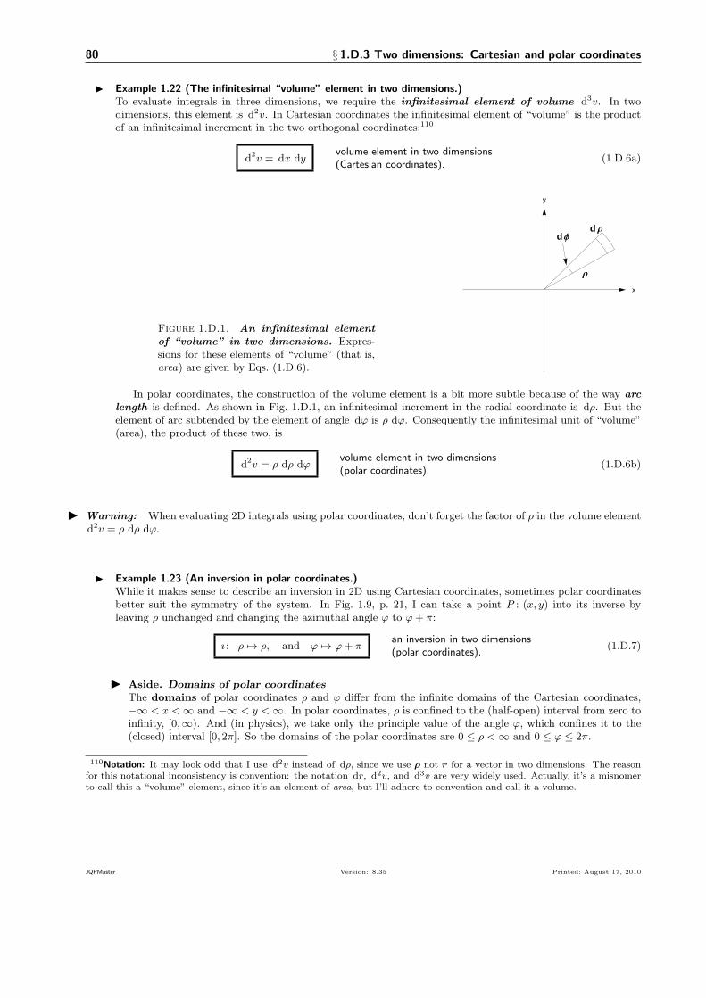
80 § 1.D.3 Two dimensions: Cartesian and polar coordinates
▶ Example 1.22 (The infinitesimal “volume” element in two dimensions.)To evaluate integrals in three dimensions, we require the infinitesimal element of volume d3𝑣. In twodimensions, this element is d2𝑣. In Cartesian coordinates the infinitesimal element of “volume” is the productof an infinitesimal increment in the two orthogonal coordinates:110
d2𝑣 = d𝑥 d𝑦volume element in two dimensions(Cartesian coordinates).
(1.D.6a)
Figure 1.D.1. An infinitesimal elementof “volume” in two dimensions. Expres-sions for these elements of “volume” (that is,area) are given by Eqs. (1.D.6).
y
x
Ρ
dΦd Ρ
In polar coordinates, the construction of the volume element is a bit more subtle because of the way arclength is defined. As shown in Fig. 1.D.1, an infinitesimal increment in the radial coordinate is d𝜌. But theelement of arc subtended by the element of angle d𝜑 is 𝜌 d𝜑. Consequently the infinitesimal unit of “volume”(area), the product of these two, is
d2𝑣 = 𝜌 d𝜌 d𝜑volume element in two dimensions(polar coordinates).
(1.D.6b)
▶ Warning: When evaluating 2D integrals using polar coordinates, don’t forget the factor of 𝜌 in the volume elementd2𝑣 = 𝜌 d𝜌 d𝜑.
▶ Example 1.23 (An inversion in polar coordinates.)While it makes sense to describe an inversion in 2D using Cartesian coordinates, sometimes polar coordinatesbetter suit the symmetry of the system. In Fig. 1.9, p. 21, I can take a point 𝑃 : (𝑥, 𝑦) into its inverse byleaving 𝜌 unchanged and changing the azimuthal angle 𝜑 to 𝜑+ 𝜋:
𝚤 : 𝜌 7→ 𝜌, and 𝜑 7→ 𝜑+ 𝜋an inversion in two dimensions(polar coordinates).
(1.D.7)
▶ Aside. Domains of polar coordinatesThe domains of polar coordinates 𝜌 and 𝜑 differ from the infinite domains of the Cartesian coordinates,−∞ < 𝑥 <∞ and −∞ < 𝑦 <∞. In polar coordinates, 𝜌 is confined to the (half-open) interval from zero toinfinity, [0,∞). And (in physics), we take only the principle value of the angle 𝜑, which confines it to the(closed) interval [0, 2𝜋]. So the domains of the polar coordinates are 0 ≤ 𝜌 <∞ and 0 ≤ 𝜑 ≤ 2𝜋.
110Notation: It may look odd that I use d2𝑣 instead of d𝜌, since we use 𝝆 not 𝒓 for a vector in two dimensions. The reasonfor this notational inconsistency is convention: the notation d𝑟, d2𝑣, and d3𝑣 are very widely used. Actually, it’s a misnomerto call this a “volume” element, since it’s an element of area, but I’ll adhere to convention and call it a volume.
JQPMaster Version: 8.35 Printed: August 17, 2010

§ 1.D.4 Three dimensions: Cartesian, spherical, and cylindrical coordinates 81
1.D.4 Three dimensions: Cartesian, spherical, and cylindrical coordinates
Other than Cartesian coordinates (𝑥, 𝑦, 𝑧), the most familiar 3D coordinate system is spherical coordinates (𝑟, 𝜃, 𝜑).Figure 1.D.2 shows the relationships between the coordinates of the same point 𝑃 in Cartesian and spherical coor-dinates:111
∙ The radial coordinate 𝑟 is the length of the vector 𝒓 from the origin to the point.
∙ The polar angle 𝜃 is the angle between the 𝑧 axis and the vector 𝒓. A positive value of 𝜃 corresponds to aclockwise rotation from the 𝑧 axis. (This angle is sometimes called the zenith .)
∙ The azimuthal angle 𝜑 is the angle in the 𝑥𝑦 plane between the 𝑥 axis and the projection of 𝒓 onto thisplane. A positive value of 𝜑 corresponds to a counterclockwise rotation from the 𝑥 axis, looking towards theorigin from a point on the positive 𝑧 axis.
From Fig. 1.D.2 one can deduce the equations required to transform between Cartesian and spherical coordinates:112
𝑥 = 𝑟 sin 𝜃 cos𝜑, −∞ < 𝑥 < +∞,𝑦 = 𝑟 sin 𝜃 sin𝜑, −∞ < 𝑦 < +∞,𝑧 = 𝑟 cos 𝜃, −∞ < 𝑧 < +∞.
(1.D.8a)
𝑟 = (𝑥2 + 𝑦2 + 𝑧2)1/2, 0 ≤ 𝑟 <∞,
cos 𝜃 =𝑧
𝑟, 0 ≤ 𝜃 ≤ 𝜋,
tan 𝜃 =
√𝑥2 + 𝑦2
𝑟, 0 ≤ 𝜃 ≤ 𝜋,
tan𝜑 =𝑦
𝑥, 0 ≤ 𝜑 ≤ 2𝜋.
(1.D.8b)
Figure 1.D.2. Spherical and Cartesian coordinate sys-tems and unit vectors. The spherical unit vectors are dis-cussed in the Aside on p. 82. Spherical coordinates are usefulfor dealing with systems characterized by spherical symmetry.Two-dimensional polar coordinates (𝜌, 𝜑) are in the 𝑥𝑦 plane:note the distinction between the scalar distances 𝜌 of plane polarcoordinates and 𝑟 of spherical coordinates. [MM: REPLACEor RESCAN.]
111Notation: Physicists and mathematicians use different notation for spherical coordinates. The choice used in this book,(𝑟, 𝜃, 𝜑), is the standard in physics. Many mathematicians, however, use (𝑟, 𝜃) for 2D polar coordinates and (𝑟, 𝜑, 𝜃) for theradial, polar, and azimuthal 3D spherical coordinates. (Note the switch in the two angles.) The ensuing confusion can beawesome! So check your sources carefully! You must be especially careful if you use symbolic software. Mathematica comeswith a wonderful collection of commands for transforming data, functions, and equations between coordinate systems.112Commentary: If you keep forgetting where the sine and cosine functions go in these relationships, you might find it helpfulto remember that the magnitude of the radius vector 𝝆 in the 𝑥𝑦 plane is 𝜌 = 𝑟 sin 𝜃, and the components of 𝝆 are 𝑥 = 𝜌 cos𝜑and 𝑦 = 𝜌 sin𝜑. In these equations, I’ve also shown the domain of each coordinate. Notice that, while the domain of theazimuthal angle 𝜑 ranges from 0 to 2𝜋, the domain of the polar angle 𝜃 ranges only from 0 to 𝜋. (Were the domain of 𝜃 torange from 0 to 2𝜋, then the range of both angles and the radial variable would encompass space twice—not what we want!)
JQPMaster Version: 8.35 Printed: August 17, 2010

82 § 1.D.4 Three dimensions: Cartesian, spherical, and cylindrical coordinates
The 2D polar coordinates are part of the 3D spherical coordinates:
∙ The variable 𝜌 is the radial distance in the 𝑥𝑦 plane from the origin, with domain 0 ≤ 𝜌 <∞;
∙ The azimuthal angle 𝜑 is the angle of the point from the 𝑥 axis, with a positive angle corresponding to acounterclockwise rotation in the 𝑥𝑦 plane. The domain of 𝜑 is, of course, the same as in two dimensions:0 ≤ 𝜑 ≤ 2𝜋.
▶ Example 1.24 (An inversion in spherical coordinates.)Depending on the situation, you might want to invert a system in either Cartesian or spherical coordinates.We already worked out the effect of an inversion in Cartesian coordinates [Eq. (1.4.4b), p. 20]. I can work outits effect in spherical coordinates in a couple of ways. I could perform some algebra using the Cartesian formand the transformation equations (1.D.8b). Or I can deduce the answer by envisioning a transformation of thevector 𝒓 into −𝒓 in Fig. 1.D.2. Either way gives [Eq. (1.7.15), p. 47]
𝚤 : 𝒓 → −𝒓 =⇒
⎧⎨⎩𝑟 → 𝑟
𝜃 → 𝜋 − 𝜃,𝜑 → 𝜑+ 𝜋,
an inversion in three dimensions(spherical coordinates).
(1.D.9)
▶ Warning: An inversion doesn’t change the radial variable 𝑟. Furthermore, an inversion changes the polarangle 𝜃 into 𝜋 − 𝜃, not into 𝜃 + 𝜋. (Like all coordinate transformations, inversion must not take a variableoutside its domain, and the domain of 𝜃 is [0, 𝜋].)
Cylindrical coordinates. The cylindrical coordinates (𝜌, 𝜑, 𝑧) in Fig. 1.D.3 combine 2D polar coordinates (𝜌, 𝜑)in the 𝑥𝑦 plane and the 3D Cartesian coordinate perpendicular to this plane, the 𝑧 coordinate. Transformation equa-tions between cylindrical coordinates and either Cartesian or spherical coordinates follow from equations in Secs. 1.D.3and 1.D.4 (see Tbl. 1.D.1). Finally, Tbl. 1.D.2 gives the form of the gradient operator in each system; the lattertable will be useful in construction of linear momentum operators and Laplacians in these coordinate systems [seeChap. 4].
Figure 1.D.3. The cylindrical coordinate systems and unitvectors. This coordinate system is useful for dealing with systemscharacterized by axial symmetry. Note that the cylindrical coordi-nates in the 𝑥𝑦 plane are the polar coordinates (𝜌, 𝜑); the third cylin-drical coordinate is the 𝑧 coordinate of Cartesian coordinates (𝑥, 𝑦, 𝑧).
▶ Aside. Spherical unit vectors.In this book we will work almost exclusively with projections along Cartesian axes. Some problems, however,are easier if you use components along the spherical unit vectors 𝒆𝑟, 𝒆𝜃, and 𝒆𝜑 in Fig. 1.D.2:113
113Commentary: The projections of operators along spherical unit vectors are more complicated than along Cartesian unitvectors, because each spherical unit vector depends on several variables.
JQPMaster Version: 8.35 Printed: August 17, 2010

83
Cylindrical → Cartesian Cartesian → cylindrical Domain
𝑥 = 𝜌 cos𝜑 𝜌2 = 𝑥2 + 𝑦2 0 ≤ 𝜌 <∞𝑦 = 𝜌 sin𝜑 tan𝜑 =
𝑦
𝑥0 ≤ 𝜑 ≤ 2𝜋
𝑧 = 𝑧 𝑧 = 𝑧 −∞ < 𝑧 <∞𝑥± i 𝑦 = 𝜌 e±i𝜑
Table 1.D.1. Conversion between Cartesian and cylindrical coordinates.
Coordinate system Coordinates Gradient ∇
Cartesian 𝑥, 𝑦, 𝑧 𝒆𝑥∂
∂𝑥+ 𝒆𝑦
∂
∂𝑦+ 𝒆𝑧
∂
∂𝑧
Spherical 𝑟, 𝜃, 𝜑 𝒆𝑟∂
∂𝑟+ 𝒆𝜃
1
𝑟
∂
∂𝜃+ 𝒆𝜑
1
𝑟 sin 𝜃
∂
∂𝜑
Cylindrical 𝜌, 𝜑, 𝑧 𝒆𝜌∂
∂𝜌+ 𝒆𝜑
1
𝜌
∂
∂𝜑+
∂
∂𝑧
Table 1.D.2. The gradient in the three most commonly used coordinate systems inthree dimensions. The linear momentum operator (in position space) for a particle of mass𝑚 in three dimensions is just p = −i ℏ∇.
𝒆𝑥 = 𝒆𝑟 sin 𝜃 cos𝜑+ 𝒆𝜑 cos 𝜃 cos𝜑− 𝒆𝜑 sin𝜑
𝒆𝑦 = 𝒆𝑟 sin 𝜃 sin𝜑+ 𝒆𝜃 cos 𝜃 sin𝜑+ 𝒆𝜑 cos𝜑
𝒆𝑧 = 𝒆𝑟 cos 𝜃 − 𝒆𝜃 sin 𝜃
(1.D.10a)
𝒆𝑟 = 𝒆𝑥 sin 𝜃 cos𝜑+ 𝒆𝑦 sin 𝜃 sin𝜑+ 𝒆𝑧 cos 𝜃
𝒆𝜃 = 𝒆𝑥 cos 𝜃 cos𝜑+ 𝒆𝑦 cos 𝜃 sin𝜑− 𝒆𝑧 sin 𝜃
𝒆𝜑 = −𝒆𝑥 sin𝜑+ 𝒆𝑦 cos𝜑.
(1.D.10b)
Complement 1.E. Rotation matrices
The rotation matrix in two dimensions. We can write the effect of a rotation of 𝑃 at (𝑥, 𝑦) to 𝑃 ′ at (𝑥′, 𝑦′)as the matrix equation (see Appendix I)114 (
𝑥′
𝑦′
)= 𝑅(𝛼; 𝒆𝛼)
(𝑥
𝑦
), (1.E.1a)
114Details: In linear algebra, the transformation matrix for a rotation, reflection, or any other linear transformation is thematrix whose columns are vectors generated by performing the transformation on a basis of the (linear) vector space. A basisof Euclidean two-dimensional space ℜ2 is the set of unit vectors along the 𝑥 and 𝑦 axes,
basis of ℜ2 =
{(1
0
),
(0
1
)}.
We can obtain the columns of the rotation matrix by rotating each of these vectors counterclockwise through an angle 𝛼. Asimilar approach will generate the matrix that represents some (but not all) symmetry transformations. The matrix for anyunitary transformation, if the matrix elements are real, is an orthogonal matrix : that is, the inverse of the matrix equalsits transpose, which I designate by attaching the superscript 𝑇 to the matrix. Moreover, matrix representations of all pointsymmetry operators are orthogonal. Since rotation is a unitary point transformation, 𝑅(𝛼)𝑇 𝑅(𝛼) = 1. (This property holdsfor any real unitary matrix.)
JQPMaster Version: 8.35 Printed: August 17, 2010

84 Complement 1.E. Rotation matrices
where 𝑅(𝛼; 𝒆𝛼) is the rotation matrix 115
𝑅(𝛼) =
(cos𝛼 − sin𝛼sin𝛼 cos𝛼
)rotation matrix in two dimensions. (1.E.1b)
Each element of 𝑅(𝛼) is called a matrix element of the rotation operator. For convenience, we often denoteCartesian coordinates by 𝑥1 (for 𝑥) and 𝑥2 (for 𝑦) and write Eq. (1.E.1b) as116
𝑥′𝑖 =2∑𝑗=1
[𝑅(𝛼; 𝒆𝛼)]𝑖,𝑗 𝑥𝑗 . (1.E.2)
The rotation matrix in three dimensions. In 3D, we represent vectors 𝒓 and 𝒓′ by 3× 1 column vectors thatcontain the Cartesian coordinates of unrotated and rotated points 𝑃 and 𝑃 ′. We write a rotation of 𝑃 as
ℛ(𝛼; 𝒆𝛼) :⎛⎝𝑥𝑦𝑧
⎞⎠ 7→⎛⎝𝑥′𝑦′𝑧′
⎞⎠ = 𝑅(𝛼; 𝒆𝛼)
⎛⎝𝑥𝑦𝑧
⎞⎠ (1.E.3)
▶ Example 1.25 (Rotation matrices in three dimensions.)For a rotation through 𝛼 about the 𝑧 axis, 𝒆𝛼 = 𝒆𝑧, the coordinates of the rotated system are
𝑥′ = 𝑥 cos𝛼− 𝑦 sin𝛼 (1.E.4a)
𝑦′ = 𝑥 sin𝛼+ 𝑦 cos𝛼, (1.E.4b)
𝑧′ = 𝑧. (1.E.4c)
=⇒ 𝑅(𝛼, 𝒆𝑧) =
⎛⎝cos𝛼 − sin𝛼 0sin𝛼 cos𝛼 00 0 1
⎞⎠ ,rotation matrix for a three-dimensionalrotation about the 𝑧 axis.
(1.E.4d)
The 2× 2 block in the upper left corner of this 3× 3 matrix is just the rotation matrix for a rotation about 𝒆𝑧,that is, a rotation in a plane: 𝑅𝑧(𝛼). The rotation matrices for the other two Cartesian axes are:117
𝑅(𝛼, 𝒆𝑥) =
⎛⎝1 0 00 cos𝛼 − sin𝛼0 sin𝛼 cos𝛼
⎞⎠ and 𝑅(𝛼, 𝒆𝑦) =
⎛⎝ cos𝛼 0 sin𝛼0 1 0
− sin𝛼 0 cos𝛼
⎞⎠ . (1.E.5)
▶ Aside. The matrix for an inverse of a transformation.The inverse of a rotation through 𝛼 about 𝒆𝛼 is a rotation through −𝛼 about the same axis. The rotationmatrix for this inverse transformation is
𝑅(𝛼)−1 = 𝑅(−𝛼) =(
cos𝛼 sin𝛼− sin𝛼 cos𝛼
), (1.E.6a)
115Jargon: The term “rotation matrix” is also used in quantum mechanics to refer to a 3× 3 matrix that transforms sphericalharmonics (Chap. 3) when a system undergoes a rotation. While we won’t discuss these rotation matrices, you need to beaware of this multiple usage, since you’re sure to encounter it in some other source.116A cautionary note: Note that the sum is over the second index (the column index) on the rotation matrix. Some books use asummation convention according to which summation signs are omitted from equations like (1.E.2). This convention requiresyou to remember that all repeated subscripts are implicitly summed over. I won’t use this convention—you have enough toremember already.117Read on: Here is a handy generic form for the elements of the rotation matrix for an arbitrary rotation axis 𝒆𝛼.Denoting the projections of 𝒆𝛼 on the 𝑥 (𝑖 = 1), 𝑦 (𝑖 = 2), and 𝑧 (𝑖 = 3) axes by 𝑒1, 𝑒2, and 𝑒3, respectively, the form is[
𝑅(𝛼; 𝒆𝛼)]𝑖,𝑗
= (cos𝛼) 𝛿𝑖,𝑗 + (1− cos𝛼) 𝑒1𝑒𝑗 − 𝜀𝑖,𝑗,𝑘 sin𝛼 𝑒𝑘,
where 𝜀𝑖,𝑗,𝑘 is the Levi-Civita symbol (see footnote 107). Another way to specify a rotation about an axis that isn’t oneof the Cartesian axes, use direction cosines or Euler angles. For an introduction, see Morrison and Parker (1987). The mostcomprehensive reference on this topic is Varshalovich et al. (1988), which contains far more about rotations and angularmomentum than probably anyone but its heroic authors has ever known.
JQPMaster Version: 8.35 Printed: August 17, 2010

85
where 𝑅(𝛼)−1 𝑅(𝛼) = 𝑅(𝛼)𝑅(𝛼)−1 = 1, (1.E.6b)
and 1 is the 2× 2 unit matrix.
Try This! 1.25. Does the inverse of a rotation matrix exist?
The inverse of a matrix exists only if the determinant of the matrix is non-zero. What is the deter-minant of the two-dimensional rotation matrix 𝑅(𝛼; 𝒆𝛼)?
Try This! 1.26. Matrix formulations of other symmetry operations.
Devise 2× 2 matrices that bring about an inversion through the origin of a plane and that bring aboutreflections through the 𝑥 and 𝑦 axes. It’s not possible to represent a translation as a matrix operation.Can you figure out why not?
Complement 1.F. It’s about time: temporal translations and conservation of energy
Reality favours symmetries and slight anachronisms.
—Jorge Luis Borges
Physics is about change. As physicists, we seek to understand and predict how properties of systems change astime passes. In this quest, our primary guide is the equation of motion of the system, which describes how staterepresentatives evolve as time increases. The type of state representative that appears in the equation of motiondepends on the type of phenomena we want to understand. If the phenomenon occurs in the macroscopic domain,the representative is a trajectory (more precisely, the trajectories of all particles in the system). In the microscopicdomain, the representative is a state function. In either case, various equations of physics tell us how to use the staterepresentative to calculate various system properties at any time. (In classical physics, these properties are values ofobservables; in quantum physics, they are expectation values or eigenvalues of operators that represent observables.)
We specify a particular state by initial conditions of the state representative. Then nature takes over: thedevelopment of the representative is governed by the equation of motion—assuming, of course, that we leave thesystem alone. (In quantum physics, “leave alone” means don’t interfere with and don’t observe the system.) Thisbeautiful logical edifice—the essence of how physics works—is summarized in Tbl. 1.F.1.
representative initial condition equation of motion
classical physics {𝒓(𝑡),𝒑(𝑡)} {𝒓0(𝑡),𝒑0(𝑡)} Newton’s second law 𝑭 = 𝑚d
d𝑡𝒑(𝑡)
quantum physics Ψ(𝒓, 𝑡) Ψ(𝒓, 0) Schrodinger equation ℋΨ(𝒓, 𝑡) = i ℏ∂
∂𝑡Ψ(𝒓, 𝑡)
Table 1.F.1. Time evolution of a single particle in classical and quantum physics. For a system inotherwise empty space, the identification of 𝑡 = 0 with the initial time (in the initial conditions) is arbitrary: that is,the equations of motion are invariant under a translation in time. In quantum physics, the state representative neednot be a function of position; the wave function Ψ(𝒓, 𝑡) can be translated into another “representation” with no lossof information. Thus, the momentum-space wave function, which depends on 𝒑 rather than on 𝒓 contains the sameinformation as the position-space wave function Ψ(𝒓, 𝑡). (For an example, see the momentum-space wave functionsfor atomic hydrogen in Complement 5.F.)
JQPMaster Version: 8.35 Printed: August 17, 2010

86 Complement 1.F. It’s about time: temporal translations and conservation of energy
The “initial time” and invariance under a temporal translation. Pondering the role of initial conditionsin classical and quantum physics raises a question: What, precisely, do we mean by an “initial” condition? Do wemean the state representative at 𝑡 = 0? That won’t work: if the system is the only thing in space (is free of externalinfluences), then how does the system know 𝑡 = 0 from, say, 𝑡 = 10 s? It doesn’t. Nature doesn’t care which valuewe ascribe to the initial time; it cares only about the state representative at that time. So it’s best to denote theinitial time by 𝑡0. Regardless of the value we choose for 𝑡0, the system will serenely evolve according to its equationof motion for all 𝑡 ≥ 𝑡0.
118 In other words, for a system in otherwise empty space the origin of the axis of timeis arbitrary. We can alter that origin without affecting any measurable property of the system. When we alter theorigin of time by, say, an amount 𝛿𝑡, we translate all times by this amount:
𝑡→ 𝑡+ 𝛿𝑡, a translation in time. (1.F.1)
We can now formulate the principle we’ve been discussing as invariance under a translation in time:119
♦ Rule: The equation of motion of a system in otherwise empty space is invariant under a translation in time.
Conservation of energy. Translation in time is a continuous symmetry transformation, because 𝛿𝑡 is a contin-uous quantity. According to Noether’s theorem (§1.5.2), invariance under temporal translations should imply aconservation rule. And it does: conservation of energy :120
♦ Rule: The total mechanical energy 𝐸 = 𝑇 + 𝑉 of a system in otherwise empty space is conserved.
▶ Aside. The evolution operator.Any symmetry transformation results in changes in wave functions and operators due to the correspondingsymmetry operator. For translation in time, the operator that does the job is the suggestively namedevolution operator :
U(𝑡, 𝑡0) ≡ exp
[−i ℋ (𝑡− 𝑡0)
ℏ
]the evolution operator. (1.F.2)
This operator provides an alternative way to think about time in quantum mechanics: its effect on astate ∣Ψ(𝑡0)⟩ at time 𝑡0 is to generate the state ∣Ψ(𝑡)⟩ at time 𝑡. This operator is extensively used intreatments and applications of quantum mechanics at a higher level than this book.
Try This! 1.27. Energy as a constant of the motion.
Explain why the form of the evolution operator, Eq. (1.F.2) implies that the stationary-state energiesof a system in otherwise empty space are invariant under translations in time. Why does the validity ofthis statement require that the Hamiltonian of the system not depend explicitly on time?
▶ Aside. Time-reversal invariance.Translation in time is not the only time-related symmetry operation of interest in physics. Another is time-reversal invariance. “Time reversal” means just what it sounds like: time runs backward. Under timereversal, all physical processes run backward. Time reversal invariance is the rule that Newton’s Second lawand the Schrodinger equation don’t change if time runs backward.121 In quantum mechanics, time-reversalis effected by an operator that transforms a state function Ψ(𝒓, 𝑡) into its time-reversed counterpart. Morepractically, time reversal is defined as the operation that leaves all position variables unchanged but that
118Details: Imagine the collision of two billiard balls. Suppose we specify the initial conditions by the trajectory of the ballsat the instant of collision, 𝑡0. We can choose the origin 𝑡0 = 0, as the moment of collision. Or we can choose 𝑡0 at the momentour cue hits one of the balls, thereby initiating the process that leads to the collision. Since nature doesn’t care, we choose thevalue of 𝑡0 that is most convenient.119Commentary: Actually, invariance under temporal translations is, like the homogeneity and isotropy of space, a hypothesis.But, as discussed in Lederman and Hill (2008), abundant evidence exists that the laws of physics obey this principle throughoutthe age of the universe. That’s good enough for me.120Details: I attach the word “mechanical” to “energy” to indicate that we are discussing only two types of energy: kineticand potential. This discussion (but not the principle conservation of energy) excludes, for example, thermal energy.121Commentary: One of the great mysteries of nature is why, in light of time-reversal invariance of the laws that govern theevolution of particles, macroscopic objects exhibit an arrow of time. (To see what I mean, imagine that you take a videoof a glass dropping onto a marble floor, then show a friend the video run backwards: your friend need not be a physicist toknow that the video lies—glasses don’t spontaneously form out of shards.) This mystery belongs to the domain of statisticalmechanics and thus outside the covers of this book. For a thoughtful introduction, see Schroeder (2000).
JQPMaster Version: 8.35 Printed: August 17, 2010

87
reverses all linear and angular momenta. Atypically, invariance under time reversal does not imply a con-servation law. This surprising result follows from the mathematical nature of the time-reversal operator.122
Complement 1.G. Additional Exercises and Problems
▶ Exercises
E 1.14. Invariance of scalar products and transition amplitudes.
(a) Show that the transition amplitude ⟨Ψ(𝑡) ∣ Q ∣ Φ(𝑡)⟩ is invariant under a symmetry transformation.
Here Ψ(𝑡) and Φ(𝑡) are two states of the system, and Q is the operator that induces a transformation be-tween them.
(b) Show that the scalar product ⟨Ψ(𝑡) ∣ Φ(𝑡)⟩ of any two states of a system is invariant under a symmetrytransformation of the system.
E1.15. Symmetry operations in two dimensions: reflections.Inversion and rotation are not the only coordinate transformations applicable to a 2D system. Two others arereflection through the 𝑥 axis and reflection through the 𝑦 axis. Both are illustrated in Fig. 1.15.1. We denotethese operations by 𝜎𝑥 and 𝜎𝑦, and the corresponding quantum mechanical symmetry operators by 𝜎𝑥 and 𝜎𝑦.
Figure 1.15.1. Reflectionsthrough the 𝑥 and 𝑦 axes.
x
y
P
P'
x
y
P
P'
σx σy
(a) Write down explicit forms for the transformations 𝜎𝑥 and 𝜎𝑦 in Cartesian and in polar coordinates.
(b) Write down expressions analogous to Eqs. (??) and (??) for the effect of the symmetry operators 𝜎𝑥 and𝜎𝑦 on a wave function Ψ′(𝑥, 𝑦, 𝑡) in Cartesian coordinates. Also write down such expressions for the wavefunction Ψ(𝜌, 𝜑, 𝑡) in polar coordinates.
The four coordinate transformations in a plane—inversion, rotation through 𝛼, reflection through 𝒆𝑥, and reflectionthrough 𝒆𝑦—are not independent. For instance, we can accomplish the effect on a point 𝑃 of inversion through theorigin by performing an equivalent rotation. A sketch of inversion in the plane shows that the rotation angle 𝛼 = 𝜋does the job: a rotation ℛ(𝜋) is therefore equivalent to an inversion.
(c) Explore this idea by writing down each of the following transformations. Support each answer with arough sketch.
(1) one or more reflections that accomplish an inversion;
(2) one or more rotations that accomplish a reflection 𝜎𝑥;
(3) one or more rotations that accomplish a reflection 𝜎𝑦.
122Details: For more about time-reversal invariance in quantum mechanics, see §13.6 of Marchildon (2002) or, for an intro-duction, the books in this chapters’ suggested readings list, §1.10.
JQPMaster Version: 8.35 Printed: August 17, 2010

88 Complement 1.G. Additional Exercises and Problems
E1.16. A rotation in Cartesian coordinates.Note: This exercise uses material from Complement 1.E.Show that in Cartesian coordinates, a rotation in 2D through 𝛼 can be written
(𝑥, 𝑦) −→ (𝑥 cos𝛼− 𝑦 sin𝛼, 𝑦 cos𝛼+ 𝑥 sin𝛼) (1.16.1a)
Write this transformation in matrix notation by introducing the rotation matrix 𝑅(𝛼) defined by(𝑥
𝑦
)= 𝑅𝑧(𝛼)
(𝑥′
𝑦′
). (1.16.1b)
The primes denote the rotated vector, and 𝑅𝑧(𝛼) is the 2D rotation matrix
E1.17. Images of inversion.Use sketches to show that the operation of inversion through a fixed origin is equivalent to the following successiveoperations: reflection in a plane containing the origin, followed by rotation by 𝛼 = 𝜋 about an axis 𝒆𝛼 that isperpendicular to this reflection plane:⎛⎝𝑥𝑦
𝑧
⎞⎠ −−−−−−−−→reflection
⎛⎝ 𝑥𝑦−𝑧
⎞⎠ −−−−−−−→rotation
⎛⎝−𝑥−𝑦−𝑧
⎞⎠ . (1.17.1)
E1.18. Consequences of a symmetry transformation for matrix elements.Show, with a fully justified argument, that if a transformation 𝒰 satisfies the requirements for invariance of aphysical system then, for any operator Q and any wave functions Ψ(𝒓, 𝑡) and Φ(𝒓, 𝑡), the following equality of matrixelements holds:123
⟨Ψ(𝑡) ∣ Q ∣ Φ(𝑡)⟩ = ⟨Ψ′(𝑡) ∣ Q ∣ Φ′(𝑡)⟩ consequence of 𝒰 being asymmetry transformation
(1.18.1)
where ∣Ψ′(𝑡)⟩ and ∣Φ′(𝑡)⟩ are the results of a symmetry operator 𝒰 .
E1.19. Temporal invariance and conservation of energy in classical physics.Note: This exercise uses material from Complement 1.F.A particle of mass𝑚 with potential energy 𝑉 (𝑥) moves (at a speed much less than the speed of light) in one dimension.Use Newton’s second law and invariance under temporal translation to prove that the total energy 𝐸 = 𝑇 + 𝑉 ofthis system cannot change with time.
E1.20. Working out with rotation matrices.Note: This exercise uses material from Complement 1.E.Write down the 3D rotation matrices for rotations about the 𝑧 axis through angles 𝛼1 = 0, 𝛼1 = 2𝜋/3, and𝛼1 = 4𝜋/3. Then show that the following equalities hold:124
𝑅(𝛼3) = [𝑅(𝛼2)]2 , and [𝑅(𝛼2)]
3 = 𝑅(𝛼1). (1.20.1)
E1.21. The effect of the parity operator.Explain why the parity operator transforms the operators for position, linear momentum, and angular momentum as
123A cautionary note: Equation (1.18.1) is a consequence of but not a requirement for 𝒢 being a symmetry transformation.
This equation is satisfied for any transformation, whether or not it’s a symmetry transformation, because the operator 𝒢 isunitary. The key point is: do not infer that any transformation that satisfies Eq. (1.18.1) is a symmetry transformation.
A symmetry transformation must also leave the Schrodinger equation invariant, which demands that 𝒢 commute with thesystem’s Hamiltonian.124Commentary: In group theory, these three rotations make up a set of symmetry operations called a group. Because thecorresponding rotation matrices satisfy Eqs. (1.20.1), they constitute what is called a matrix representation of this group—acrucial quantity in applying group theory to physics.
JQPMaster Version: 8.35 Printed: August 17, 2010

89
Π r Π † = −r (1.21.1a)
Π p Π † = −p (1.21.1b)
Π L Π † = L. (1.21.1c)
▶ Problems
P 1.4. ** Translational invariance and conservation of linear momentum.Like all continuous transformation operators, the 3D translation operator 𝒯 (𝒂) is unitary:
𝒯 (𝑎)† 𝒯 (𝑎) = 𝒯 (𝑎) 𝒯 (𝑎)† = 1. (1.4.1a)
(a) Using this property only—not the explicit form of 𝒯 (𝒂)—show that the following operators are Hermitian:
Q𝑗 ≡ i ℏ ∂
∂𝑎𝑗𝒯 (𝒂)
∣∣∣∣𝑎𝑗=0
, 𝑗 = 1, 2, 3, (1.4.1b)
where the subscripts refer to Cartesian coordinates: 𝑗 = 1 to 𝑥, 𝑗 = 2 to 𝑦, and 𝑗 = 3 to 𝑧. Because the Q𝑗 areHermitian, they can represent observables.
(b) The 3D translation operator is defined by its action on an arbitrary wave function as
𝒯 (𝒂)Ψ(𝒓, 𝑡) = Ψ(𝒓 − 𝒂, 𝑡). (1.4.1c)
Using this definition in Eq. (1.4.1b), show that the Hermitian operators that correspond to translations arethe components 𝑝𝑗 = −i ℏ ∂/∂𝑥𝑗 of the linear momentum operator p .
(c) Use your answer to part (b) to explain why the linear momentum of a translationally invariant system is aconstant of the motion. Also explain why the probability of finding values 𝒑 = (𝑝𝑥, 𝑝𝑦, 𝑝𝑧) in a measurement ofthe momentum of a translationally invariant system does not depend on when the measurement is performed.
(d) What constraint must the potential energy of a system satisfy if the system is to be translationally invariant?
P1.5. **Where does the orbital angular momentum operator really come from?The rotation operator ℛ(𝛼; 𝒆𝛼) is defined by its action on an arbitrary wave function as
ℛ(𝛼; 𝒆𝛼)Ψ(𝒓, 𝑡) = Ψ(ℛ(𝛼; 𝒆𝛼)−1𝒓, 𝑡
). (1.5.1a)
(a) Write Eq. (1.5.1a) for a rotation ℛ𝑧(𝛼) through 𝛼 about the 𝑧 axis acting on a wave function in Cartesian
coordinates, Ψ(𝑥, 𝑦, 𝑧, 𝑡). Then use Stone’s theorem to show that the Hermitian operator Q𝑧 which corresponds
to ℛ𝑧(𝛼) obeys the equation
Q𝑧 = −i ℏ d
d𝛼ℛ𝑧(𝛼)
∣∣∣∣𝛼=0
. (1.5.1b)
Hint: Remember that ℛ𝑧(𝛼) can be continuously related to the identity transformation.
(b) Solve Eq. (1.5.1b) for Q𝑧 and—without using the explicit form for the orbital angular momentum operator—explain why your result is the operator for the 𝑧 component of the particle’s orbital angular momentum,L𝑧(𝑥, 𝑦).
Remark: This problem reveals that fundamentally, the orbital angular momentum operator L𝑧 comes from the defi-nition (1.5.1a) via Stone’s theorem. In Chaps. 2 and 3 we’ll derive L𝑧, along with the other Cartesian components L𝑥and L𝑦, algebraically, starting with classical expressions like 𝐿𝑧 = 𝑥 𝑝𝑥 − 𝑦 𝑝𝑦. But if you understand this problem
you can skip all the algebra and get expressions for L(𝑥, 𝑦, 𝑧) much more easily.
P1.6. ** Inversion and the nature of vectors.
JQPMaster Version: 8.35 Printed: August 17, 2010

90 Complement 1.G. Additional Exercises and Problems
Mathematicians classify a vector 𝒗 according to whether it changes sign under inversion (see §1.D.2):125
𝚤 : 𝒗 → −𝒗 polar vector (1.6.1a)
𝚤 : 𝒗 → +𝒗 axial vector (1.6.1b)
Classify each of the following vectors according to this scheme: position 𝒓, linear momentum 𝒑, electric field 퓔,orbital angular momentum 𝑳, and magnetic field 퓑.
P1.7. ***A matter of some gravity.Whatever their environment, microscopic particles in a terrestrial laboratory always experience the Earth’s gravita-tional field. Consider, for instance, an electron bound in the field of a bare proton (atomic hydrogen). Using yourknowledge of the strength of the Earth’s field and whatever you can find out about the strength of typical atomicand laboratory electromagnetic fields, discuss the effect of gravity on the rotational invariance of a particle in acentral potential. Comment on the role played in this effect by the orientation of the plane of rotation (parallel orperpendicular to the ground) and on the mass of the particle. How would your insight change if the particle were amuon instead of an electron?
P1.8. ***Commutation relations and translational invariance.
Note: This problem extends Example 1.21.
(a) For an arbitrary differential multiplicative operator f(𝒓), show that
𝒯 (𝒂)† f(𝒓) 𝒯 (𝒂) = f(𝒓 + 𝒂). (1.8.1a)
(b) By applying this result to an infinitesimal translation d𝒂, derive
f(𝒓 + d𝒂) = f(𝒓) +i
ℏ
3∑𝑗=1
d𝑎𝑗[p𝑗 , f(𝒓)
], (1.8.1b)
where 𝑗 = 1, 2, 3 refer to the 𝑥, 𝑦, and 𝑧 axes.
(c) Explain why your result implies♦ Rule: Any function that is invariant under arbitrary translations along a Cartesian axis commutes with the com-
ponent of linear momentum along that axis.
125Commentary: The cross product of two polar vectors is an axial vector . Axial vectors exist only in Euclidean 3-space. Anaxial vector is sometimes called a pseudovector .
JQPMaster Version: 8.35 Printed: August 17, 2010