Chap. 6 Type Ⅱ Superconductivity - super.skku.edusuper.skku.edu/lectures/Solid_Chap6(2012).pdf · Chap. 6 Type ⅡSuperconductivity. 6.1 Introduction. 6.2 The Vortex. 6.3 The Modified

Chap. 6 Type Ⅱ Superconductivity

6.1 Introduction

6.2 The Vortex

6.3 The Modified Second London Equation

6.4 General Thermodynamic Concepts (skip)

6.5 Critical Fields

6.1 INTRODUCTION

Figure 6.1 The H-T phase space:

(a) type I and (b) type Ⅱ

superconductors.

In 1930

: W.J. de Hass & J. Voogd

– working with the superconducting alloy Pb-Bi.

The Tc (max) of this alloy (Tc

=8.8 K) does not differ much from its constituents.

(Lead Tc

= 7.2 K, Bismuth Tc

= 8.5 K)

But

Hc

(at 4.2K): Hc

(Pb) = 0.055 T, Hc

(Pb-Bi) = 1.7 T

H

T

Lower Critical Field

HC2

HC1

TC

Upper Critical Field

Normal State

Mixed State

Meissner State

Abrikosov Vortex Lattice

Temperature

Mag

netic

Fie

ld

★ This chapter develops the essential features of Abrikosov’s work

through the phenomenology of typeⅡ

superconductivity.

▶

In Section 6.2 : We see that flux is observed to enter a typeⅡ

superconductor in a discrete array of known

as vortices.

Each vortex has a single flux quanta Φ0

.

We will find the fields and currents associated with each vortex and show

that the radius of the vortex (the coherence length ξ).

The two type superconductors can be distinguished by comparing λ and ξ. ( type I superconductor –

λ < ξ, type Ⅱ

superconductor –

λ > ξ)~~

▶

In Section 6.3 : We see that B and J from a vortex are more

conveniently described by modifying the second London equation.

To fully understand vortex formation in typeⅡ

materials

▶

In Section 6.4 : We first review some basic concepts in equilibrium

thermodynamics (skip).

▶

In Section 6.5 : Section 6.4 concepts are then used to study the

various critical magnetic fields.

★

We therefore see that this chapter focuses on understanding the

vortices that give rise to the magnetic field phase boundaries, Hc1

(T) and Hc2

(T) for a typeⅡ

superconductor.

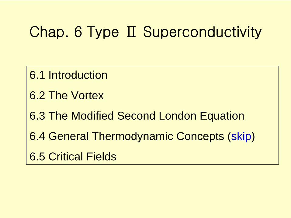
6.2 THE VORTEX

Above the lower critical field, Hc1

(T), magnetic flux will enter a typeⅡ

superconductor.

How we can detect the flux around a simple bar magnet

Consider typeⅡ

bulk superconductor (a ≫

λ)

H0

→ H0

> Hc1

A vapor of tiny micron-sized nickel particles is now evaporated over the top surface of the superconductor, perpendicular to the applied field.

The particles will coalesce on the surface along lines of constant flux density just as in the case of the iron filings and thus the surface of the superconductor is “decorated”, showing how flux enters.

Vortex and coherence length

(a) (b)

Figure 6.2

A type Ⅱsuperconductor that has been decorated with magnetic particle.

The applied field is perpendicular to the page.

(a) A photograph revealing the triangular array of vortices formed when a superconducting sample, in this case YBa2

Cu3

O7

, is placed in a magnetic field. (The anisotropic sample is oriented so that the c axis is parallel to

the applied field). The applied field strength is 40 Gauss and the distance 0.8μm. (b) The triangular array of patterns ; each patterns regions of constant flux density. C1

is a contour along the perimeter of a pattern, C2

is a contour around the center of one.

We see that the flux density is strongest at the center of each pattern. (the particles concentrate in regions of high-flux density)

The density of vortices nv

22 32

)2/3(1

A1

vn (α

: the distance between the

centers of nearest patterns)

ㅡ (6. 1)

The average flux density in the slab

0/ vnAB (Φ0

: the flux in each vortex) ㅡ (6. 2)

Since we can measure both <B> and α, the value of Φ0

is determined experimentally and found to always be single flux quantum (h/2e).

Φ = B · A =>

Let us find the consequences of this

experimental fact on the flux and current

densities in an isotropic typeⅡ

SC.

From the fluxoid

quantization condition

(section 5.5)

C Sstot dd sBl)J( ㅡ (6. 3)

along the contour C1

(shown in Figure 6.2b)

1 1

sBlJ200 C SS dd ㅡ (6. 4))(

0

The flux is greatest at center and so Bz

(x,y)

is at a minimum (constant)

along the contour C1

. Consequently,

0)()( ,,

ccZccZ yxBy

yxBx

where (xc

,yc

) are the loci of points that define the contour.

ㅡ (6. 5)

▽×B=μ0

Js

and combining this relation with Eq. (6. 5)

01

0 BJ

S along C1 ㅡ (6. 6)

Thus, the fluxoid

quantization condition of Eq. (6. 4) becomes

BBAdS

2

0 23sB

1

ㅡ (6. 7)

The surface S1

is the area of one of the patterns so direct integration recovers the fact that

densityvortex : 00

VVv nnA

NB

ㅡ (6. 8)

ki

00

kji

B

zz

z

Bx

By

Bxyx

The flux quantization condition for the second contour C2

, which is a circle centered in one of the flux patterns

sBlJ22

200 dd

SC S ㅡ (6. 9)

In the limit that the radius r of the circular contour C2

approaches zero,

2

lJlim 2000 C Sr

d ㅡ (6.10)

i1

2Jlim 2

0

0

0 rsr

We expect Js

to be constant along C2

and azimuthally directed(Φ).

From (6.10)

ㅡ (6.11)

rs1 J => J 0 sr

In Eq. (6.11)

)2(limlJlim 200

2000

2

rJd SrCSr

0)(limsBlim 00 2

BAdA

Sr

☜ Not physical !!!

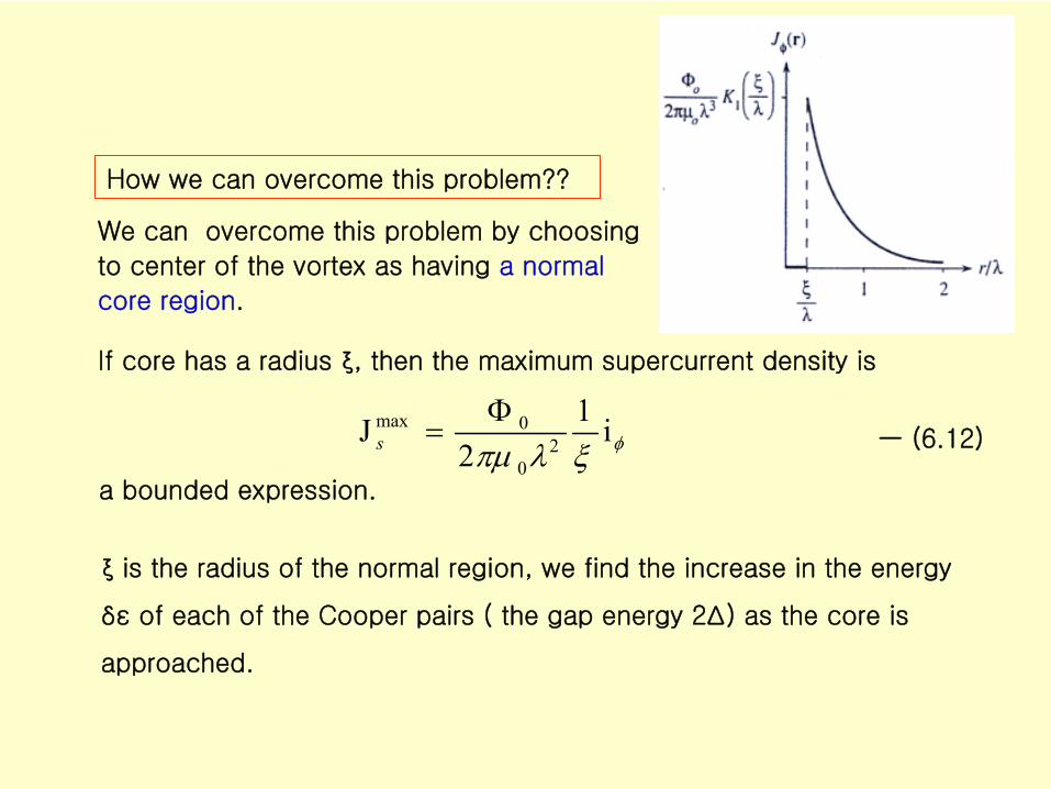
i1

2J 2

0

0max s

If core has a radius ξ, then the maximum supercurrent

density is

ㅡ (6.12)

a bounded expression.

How we can overcome this problem??

ξ

is the radius of the normal region, we find the increase in the energy

δε

of each of the Cooper pairs ( the gap energy 2Δ) as the core is

approached.

We can overcome this problem by choosing

to center of the vortex as having a normal

core region.

The increase in energy comes from the increase in the kinetic energy of the Cooper pairs. To see this, recall

ss qn vJ ** ㅡ (6.13)

(vs

: the velocity of the Cooper pairs (superelectrons))

i1v *

max

ms

The maximum velocity (from Eq. (6.12))

ㅡ (6.14)

The increase in the energy of a Cooper pair is created by the increase in its velocity.

If there are no currents flowing, the electrons are all moving with some background velocity known as the Fermi velocity vF

(in Section 5.4).

See next page

12)-(6 --- i12

J 20

0max

s

Velocity of the Cooper pairs

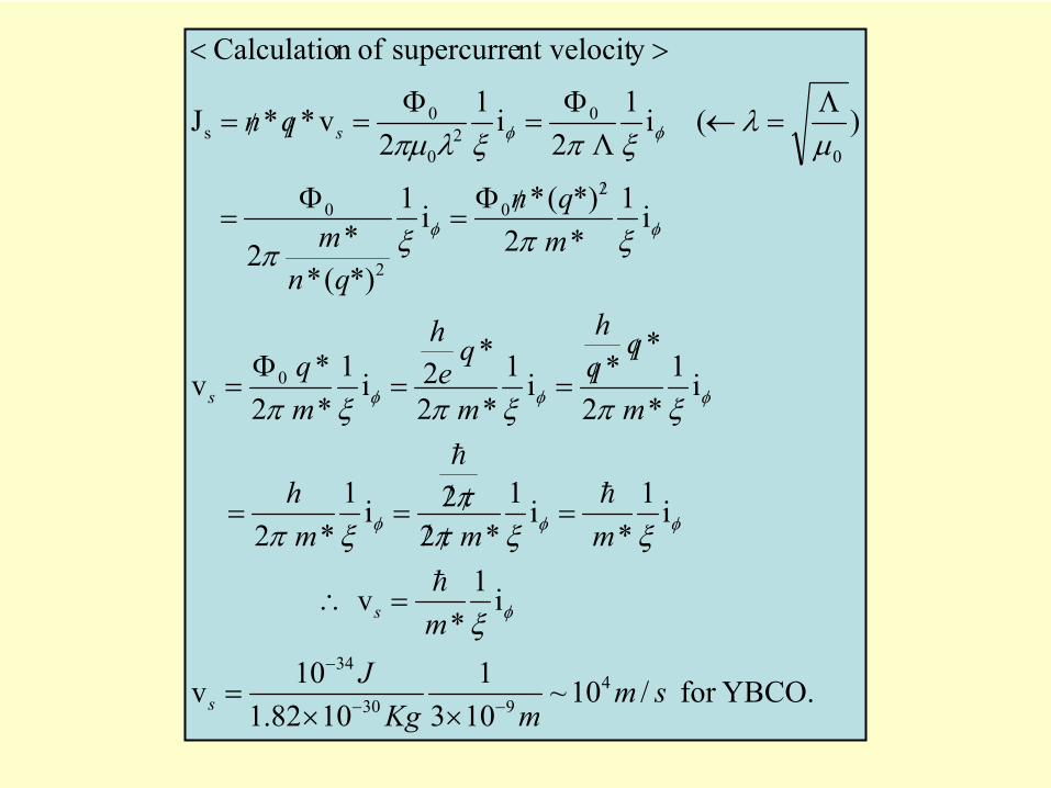
YBCO.for /10~1031

1082.110v

i1*

v

i1*

i1* 2

2i1* 2

i1* 2

* *i1

* 2

* 2i1

* 2* v

i1* 2*)(*i1

*)(**2

)( i1Λ 2

i12

v**J

ynt velocitsupercurre ofn Calculatio

4930

34

0

20

2

0

0

02

0

0s

smmKg

Jm

mmmh

m

qqh

m

qe

h

mq

mqn

qnm

qn

s

s

s

s

)2(

)21()1(

,max,

2,

,

max,2

,2

,

max,2

,

yFsyF

yF

syF

yF

syF

vvv

vv

vvv

v

The average kinetic energy of a Cooper pair when no current is flowing;

)(21

21 2

,2

,2

,*2*0

kin zFyFxFF vvvmvm ㅡ (6.15)

=> Now consider the increased velocity due to the flow of current (Jy

).

])([21 2

,2max

,,2

,*1

kin zFsyFxF vvvvm ㅡ (6.16)

0kin

1kin

The difference in energy at the core

ㅡ (6.17)

ㅡ (6.18)max,,

* syF vvm=>

)( max,, syF vv

The additional velocity created by the current is much less than the

Fermi velocity so the linearizing

we find

Superconducting Energy Gap (2∆) and Coherence length

We expect that by averaging over all the electrons, we will find

2,

2,

2,

2zFyFxFF vvvv ㅡ (6.19)

(where the bracket denotes the average of the component of the velocity.)

The averaged velocity squared to be the same for each component

22, 3

1FyF vv ㅡ (6.20)

Substituting this averaged expression for and our relation for yFv ,max,sv

(Eq. 6.14) into Eq. 6.18 gives

13

1*

*max,,

*

mvmvvm FsyF

3Fv

=> ㅡ (6.21)

Since δε

≈

2Δ

at the radius of the core ξ, we find

32Fv ㅡ (6.22)

18)-(6 ----- max,,

* syF vvm

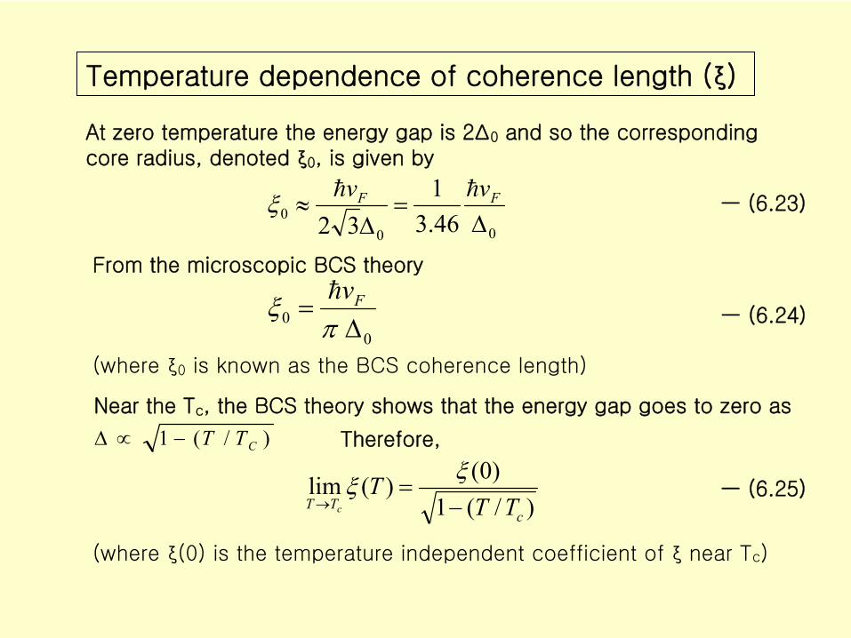
At zero temperature the energy gap is 2Δ0

and so the corresponding core radius, denoted ξ0

, is given by

000 46.3

132

FF vv ㅡ (6.23)

From the microscopic BCS theory

00

Fvㅡ (6.24)

(where ξ0

is known as the BCS coherence length)

Near the Tc

, the BCS theory shows that the energy gap goes to zero as

)/(1 CTT Therefore,

)/(1)0()(lim

cTT TT

Tc

ㅡ (6.25)

(where ξ(0) is the temperature independent coefficient of ξ

near Tc

)

Temperature dependence of coherence length (ξ)

Temperature dependence of coherence length

0.0 0.2 0.4 0.6 0.8 1.00.0

2.0

4.0

6.0

8.0

10.0

(T)

/(0

)

T/Tc

)/(1)0()(lim

cTT TT

Tc

We have found the coherence length by arguing that the Cooper pairs split apart of depair

when their increase in energy exceeds the gap

energy. Thus the maximum current density for Js,Φ

(Eq. 6.12) is referred to as the depairing critical current density Jpair

. Therefore,

20

0pair 2

J

This is the maximum current density

that can be sent through the

superconductor. This expression is only approximate because it depends on our model of the vortex core.

by the Ginzburg-Landau theory,

20

02

0

0pair 2.5

133

J

ㅡ (6.27)

If we apply a current density, J > Jpair

, the material becomes normal.

Depairing critical current density (Jpair)

r1

2J from 2

0

0s

※

Summary

⊙ The magnetic flux enters a type Ⅱ

superconductor for fields above

Hc1

in a regular triangular array of vortices. (experiment)

⊙ Each vortex has a single flux quantum.

⊙ The current density of the vortex increases as the center of the vortex

is approached until the increased kinetic energy causes the Cooper

pairs to unbind.

⊙ The vortex is thus modeled as having a normal core of radius ξ, the

coherence length.

M

H

M-H curve

Hc1 Hc2

0

Figure 6.3 shows our model of the density of superelectrons

(Cooper

pairs) for a single vortex. Inside the model core the conduction

electrons are in the normal state.

Ginzburg –

Landau theory

Density of superelectrons

Vortex-core model

＊ ξ ≥ λ : Type-I Superconductor

＊ ξ ≤ λ : Type-II Superconductor

＊ ξ ≪ λ : High–к Materials

What makes our approach reasonable is the fact that most practical type Ⅱ

superconductors have ξ

≪ λ. Thus, the core typically occupies

a very small fraction of the total volume of the vortex. In the Ginzburg –

Landau theory, the ratio of the two lengths if defined as

ㅡ (6.28)

( к : Ginzburg –

Landau kappa )

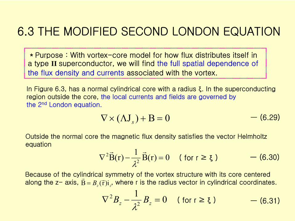
6.3 THE MODIFIED SECOND LONDON EQUATION

＊Purpose : With vortex-core

model for how flux distributes itself in

a type II superconductor, we will find the full spatial dependence of

the flux density and currents

associated with the vortex.

In Figure 6.3, has a normal cylindrical core with a radius ξ. In the superconducting region outside the core, the local currents and fields are governed by the 2nd

London equation.

0B)J( s ㅡ (6.29)

Outside the normal core the magnetic flux density satisfies the vector Helmholtz

equation

0)r(B1)r(B 22

ㅡ (6.30)( for r ≥

ξ

)

012

2 zz BB

( for r ≥

ξ

) ㅡ (6.31)

Because of the cylindrical symmetry of the vortex structure with

its core centered along the z-

axis, , where r is the radius vector in cylindrical coordinates.zzB i)r(B

The solution to Eq. (6.31)

32)-(6 --- )sincos()(

)sincos)((),(

'

0

'

0

mDmDrI

mCmCrKrB

mmm

m

mmm

mz

* Cm

, Cm

’, Dm

, Dm

’: constant

* Im

: modified Bessel functions of the first order with m

* Km

:modified Bessel functions of the second order with m

Modified Bessel functions

m

x

m

x

xx

xmx

xm

x

xxx

)2( ! 2

1 )(K lim

)2

( !

1 )( I lim

ln )(K lim , 1 )( I lim

m0

m0

00 00

For m

> 0

For m

= 0

Bz is independent of the angle Φ for the flux of the single vortex.

Therefore, the solution is obtained with m = 0

)()()( 0000 rIDrKCrBz ( for r ≥

ξ

) ㅡ (6.33)

for because 0 0

BC.in D0 & C0 of values thefind We)1(

00

z

rIDBr

(6.34) ----- for )(

for )()(

for constant is Bz and normal is core The:core theof radius at the BCother The )2(

00

00

rrKC

rKCrB

r

z

)sincos()( )sincos)((),( '

0

'

0

mDmDrImCmCrKrB mm

mmmm

mmz

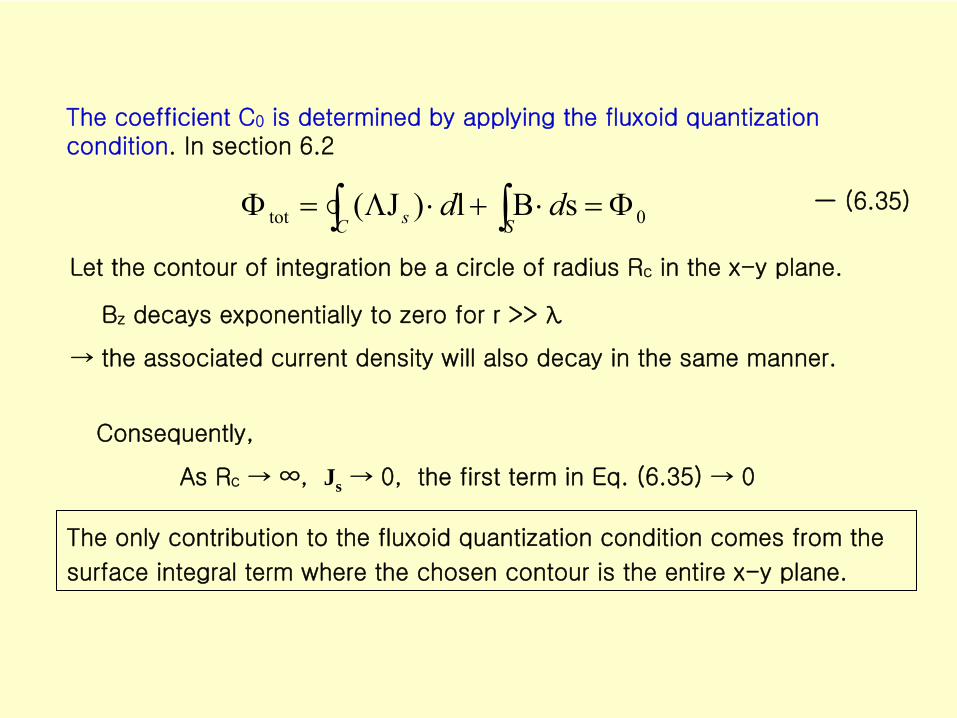
The coefficient C0

is determined by applying the fluxoid

quantization

condition. In section 6.2

0tot sBl)J( SC s dd ㅡ (6.35)

Let the contour of integration be a circle of radius Rc

in the x-y

plane.

Bz

decays exponentially to zero for r >>

λ

→ the associated current density will also decay in the same manner.

As Rc

→ ∞, Js → 0, the first term

in Eq. (6.35) →

0

Consequently,

The only contribution to the fluxoid

quantization condition comes from the

surface integral term where the chosen contour is the entire x-y plane.

(6.37) ------ )(K)(K21

2C

1

102

2

20

0

)](K)(K21[2C

)(K2C)(KC

)(K)(2C212)(KC

/ )( )(K2C 2 )(KC

2 )(KC 2 )(KC sB

102

22

0

12

02

00

12

00

200

000 00

000 00z0

rrr

drdrrdrrdrr

drrrdrrdsBdss

C0

can be determined by the Flux Quantization condition.

01 2

)(Klim

/)(K)(K

n

10

xx exx

rxxxdxxx

)( { r for )/(

r for )/(00

00

rKC

KCz rB

A considerable simplification is possible of most practical type

II

materials [High-κ

materials (κ = λ/ξ

≫ 1)]

Ex) Nb3Sn κ

≈

25 & HTS typically have κ

> 50

1

102

2

20

0 )(K)(K21

2C

Consider how C0

simplifies for κ ≫ 1.

0lnlim)(lim 2

002

0

xxxKx

xx

The first term

xxKx

ln)(lim 00

The second term

1)(lim 10

xxK

x

ㅡ (6.38)

ㅡ (6.39)xxK

x

1)(lim 10

Therefore, for κ ≫ 1, (from Eq.(6.34)

{i )(

2

i )(2

020

020

B(r)z

z

rK

K

ㅡ (6.40) { )(

)(

00

00

)(

rKC

KCz rB for r ≥

ξ

for r < ξ

20

2

(for κ≫1)

≈ 0 ≈ 1

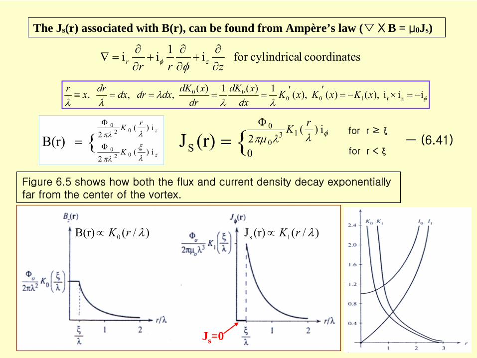
The Js(r) associated with B(r), can be found from Ampère’s law (▽ Х B = μ0Js)

{ i )(20S

130

0

(r)J rK

for r ≥

ξ

for r < ξㅡ (6.41){

i )(2

i )(2

020

020

B(r)z

z

rK

K

iii ),()( ),(1)(1)( , , , zr100

00 xKxKxKdx

xdKdr

xdKdxdrdxdr xr

scoordinate lcylindricafor i1iizrr zr

Figure 6.5 shows how both the flux and current density decay exponentially far from the center of the vortex.

)/((r)J 1s rK)/(B(r) 0 rK

Js =0

Near the core , the magnetic flux density (B) in the

superconductor increases as;

zr ri ln

2Blim 2

0

ㅡ (6.42)

and current density (Js ) is given by;

i 1

2)/(limJlim 2

0

00S rrr

B ㅡ (6.43)

)ln()(lim )(for i )(2 0002

0rr

Kξ rr

KBxz

rxdxxd

drxddxdrdxdr xr 111ln1ln , , ,

The expression for the current density near the core is identical to Eq. (6.11),

which was obtained by considering the fluxoid

quantization.

11)-(6 i12

Jlim 20

0

0

rsr

iii zr

) ( r

We seek to modify the second London equation by adding a function V(r) as a source to insure fluxoid

conservation.

V(r)B)J( s ㅡ (6.44)←Modified second London equation

which is valid for all space assuming V(r) vanishes except along iz.

V(r) is in the same direction as the flux density

zi )r(V(r) V ㅡ (6.45)

Eq (6.44) is converted into the integral expression

S SC

S SS S

ddd

ddd

sV(r)sBl)J(

sV(r)sBs)J(

s

ㅡ (6.46)(by stoke’s

theorem)

Modified Second London Equation

SSC s

SC s

ddd

dd

s)r(VsBl)J(

sBl)J( 0 ㅡ (6.35)

ㅡ (6.46)

Rc

→ ∞, Js

→ 0: the first terms in Eq(6.35) & (6.46) →

0

We see that although V(r) is zero everywhere except at r = 0, its integral over that

point must be the constant Φ0 .

The only function that has this property is the two-dimensional delta function, δ2(r).

z20 i (r)ΦV(r) δ ㅡ (6.47)←

Vorticity

z20s i (r)B)J( ㅡ (6.48)

More generally, for N

vortices that located at the two-dimensional positions ri, the vorticity

is readily generalized to

N

ii

1z20 i )rr(V(r) ㅡ (6.49)

(for a vortex along the z-axis in an isotropic, high-κ superconductor)

Example 6. 3. 1

As an example of how to use the modified second London equation, we complete the solution of our single vortex problem. For an isotropic superconductor, from Eq.(6.48)

)r(122

02

2

zz BB ㅡ (6.50)

Particular solution, pzB

)(2 02

0

rKB p

z

ㅡ (6.51)

)(2

)B(113

0

0

0,

rKJ pzs

ㅡ (6.52)

This solution not only satisfies the original differential equation but also the boundary condition that the flux density vanishes far from the core. Moreover, this solution also satisfies the fluxiod

quantization condition for a high-κ

superconductor by construction.

Therefore, is the desired flux density distribution for the single vortex and the associated current density is

pzB

see next page.

)r(1i (r)BB

)/(

BB1 H)J(

HHH)(HJside;both for )( curl a Take

JH48)-(6 ---- i (r)B)J(

220

22

z2022

200

22

0

220

2s

22

z20s

zz BB

Derivation of Equ. (6.50)

{ i )(20S

130

0

(r)J rK

for r ≥

ξ

for r < ξㅡ

(6.41){i )(

2

i )(2

020

020

B(r)z

z

rK

K

(6.40) ㅡ

)(2 02

0

rKB p

z

(6.51) ㅡ )(2 13

0

0,

rKJs

ㅡ

(6.52)

These solutions match those of the finite-sized vortex core in the region r ≥

ξ.

However, for r < ξ, the solutions differ.

xxKx

ln)(lim 00

xxK

x

1)(lim 10

Eq(6.51) & Eq(6.52) diverge as r →

0. ← unphysical!!!

Consequently, to ensure that the solutions of the modified second London equation

match the physically correct ones, we restrict the validity of the solutions to the region

r ≥

ξ. Within the region r ≤

ξ, we will interpret the flux density to be a constant

defined by its value at r = ξ.

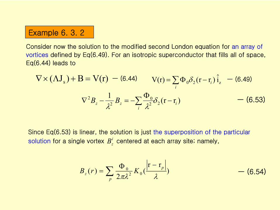
Example 6. 3. 2

Consider now the solution to the modified second London equation for an array of

vortices

defined by Eq(6.49). For an isotropic superconductor that fills

all of space,

Eq(6.44) leads to

)rr

(2

)( 020

p

pz KrB

ㅡ (6.54)

)rr(122

02

2i

izz BB

ㅡ (6.53)

z20 i )rr(V(r) ii

ㅡ

(6.49)V(r)B)J( s ㅡ

(6.44)

Since Eq(6.53) is linear, the solution is just the superposition of the particular

solution

for a single vortex centered at each array site; namely,izB

☜ Figure 6.9 Two vortices parallel to the z-axis and located along the x-axis at ±a in an infinite superconductor. The vortex at x=a has a positive vorticity

and the other at x=-a has a negative one. The contours of constant Bz

(x,y) are shown.

Example 6. 3. 4

We now examine the case of two vortices that individually generate a magnetic flux density in opposite directions.

zz yaxyax i )()(i )()(V(r) 00 ㅡ (6.59)

22

0

22

020 )()(

2),(

yaxK

yaxKyxBz ㅡ (6.60)

The flux density vanishes along the y-z

plane defined by x=0.(antisymmetry). However, the current density does not vanish in this plane. Instead, it is purely y-directed.

p (x, y)r

)(2 02

0

rKBi

z

We end this section by showing how it can also simplify finding the

electromagnetic energy associated with vortices.

If the vortices are modeled as having a normal state core, the total

electromagnetic energy W of the system will come from three places:

＊ Ws

: the energy of superconducting

region.

＊ Wc

: the energy of the normal cores

in the superconductor.

＊ Wn

: the energy of the normal regions

(no superconductor).

Integrating over the volume where there is no superconductor, Vn, we find

nVn dvW B

21 2

0ㅡ (6.64)

core

B 21 2

0Vc dvW

ㅡ (6.65)

where the integration is over the cores of the vortices & high-κ

superconductors

( λ≫ξ

), the contribution to the energy from the normal core is negligible . )0( cW

BH21

density energy Magnetic

m E

Vortex Energy (εv

)

dvW sVss

)]J()B(B[21 2

0

ㅡ (6.67)

Using the Ampère’s

law (∇ X

H = Js), Eq(6.66) becomes

The vector identity

D)(CD)(CC)(D ㅡ (6.68)

s)]J(B[2

1 )]J([BB2

1

)]J([B2

1 ))]J((B[B2

1

00

0

2

0

ddv

dvdvW

sV s

V sV ss

ss

ss

ㅡ (6.69)

where the integral over the surface that encloses is obtained by applying Gauss’

theorem.S SV

s sV ss ddvW s)]J(B[

21 VB

21

00 ㅡ (6.70)

by the modified second London equation V(r)B)J( s

dvW sV sss

JJB )]()([2

10

2

0

ㅡ (6.66)From 4-130,

The energy per unit length along the vortex direction will be denoted as and

similarly for each contribution and .

W nW

sW

zLWW / ㅡ (6.71)

(where Lz

is the length of the vortex in the z-direction.)

Therefore, after the integrating Eq(6.70) over z

ss C sSs ddaW n)]J(B[

21 VB

21

00 ㅡ (6.72)

☜ Figure 6.11

A vortex along the z-direction in a superconducting volume Vs

. The volume is enclosed by the surface ∑s

. The cross-

sectional area Ss

is parallel to planes of constant z and is encircled by the contour Cs

. Notice that Ss

is not a function of z.

dxdyda

s sV ss ddvW s)]J(B[

21 VB

21

00 ㅡ (6.70)

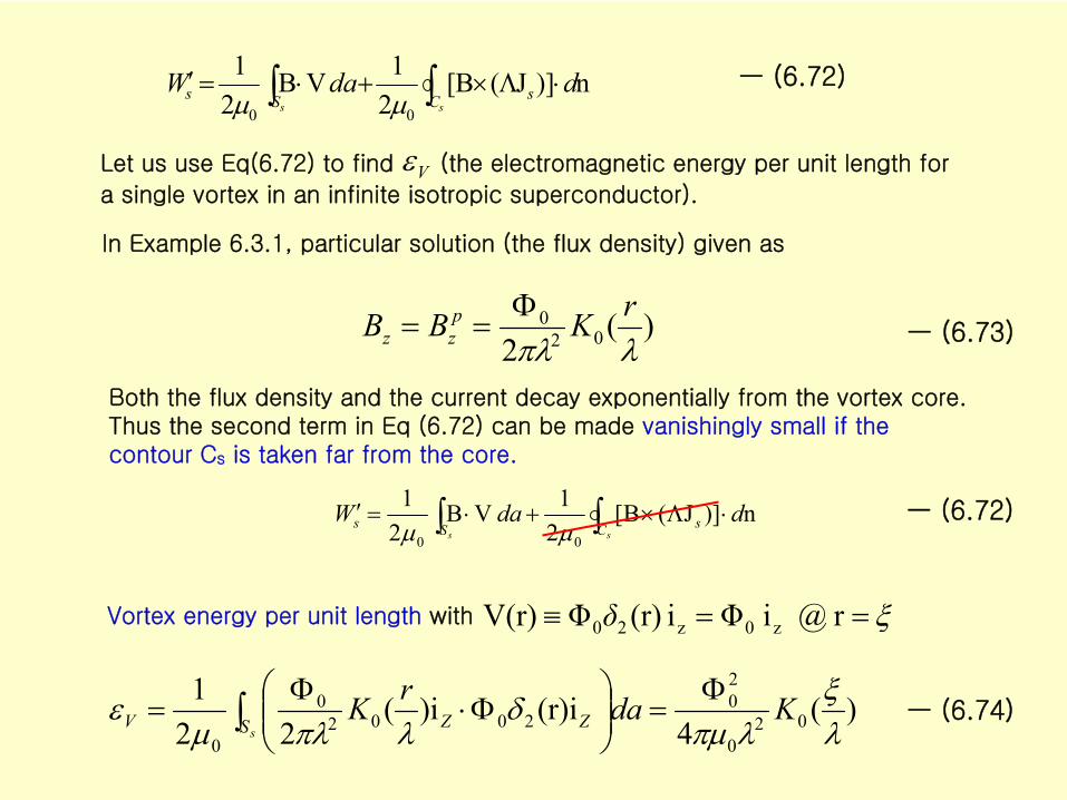
Let us use Eq(6.72) to find (the electromagnetic energy per

unit length for

a single vortex in an infinite isotropic superconductor).V

In Example 6.3.1, particular solution (the flux density) given as

)(2 02

0

rKBB p

zz

ㅡ (6.73)

Both the flux density and the current decay exponentially from the vortex core. Thus the second term in Eq (6.72) can be made vanishingly small

if the contour Cs

is taken far from the core.

ss C sSs ddaW n)]J(B[

21 VB

21

00 ㅡ (6.72)

)(4

(r)ii)(22

102

0

20

20020

0

KdarK

sS ZZV

ㅡ (6.74)

r @ i Φi (r)ΦV(r) z0z20δVortex energy per unit length

with

ss C sSs ddaW n)]J(B[

21 VB

21

00 ㅡ (6.72)

)ln(4

lim 20

20

V ㅡ (6.75)xxKx

ln)(lim 00

For the high k materials;

6.5 Critical Fields (Hc1

and Hc2

)

※ Purpose

: we calculate the upper [Hc2

(T)] and lower [Hc1

(T)] critical fields

for a type II super conductor where we will need to

combine the thermodynamics of a superconductor developed in section 6.4 .

We restrict ourselves to examining the properties of an isotropic superconducting slab of thickness 2a where a ≫

λ.

Gibbs free energy in a magnetic field is given by:

BHHHH VTUTTSTG ),(),(),( ㅡ (6.121)

where U is internal energy and V is volume.

Without applied field (H = 0), the free energy is given by:

),0(),0(),0( TUTTSTG ㅡ (6.122)

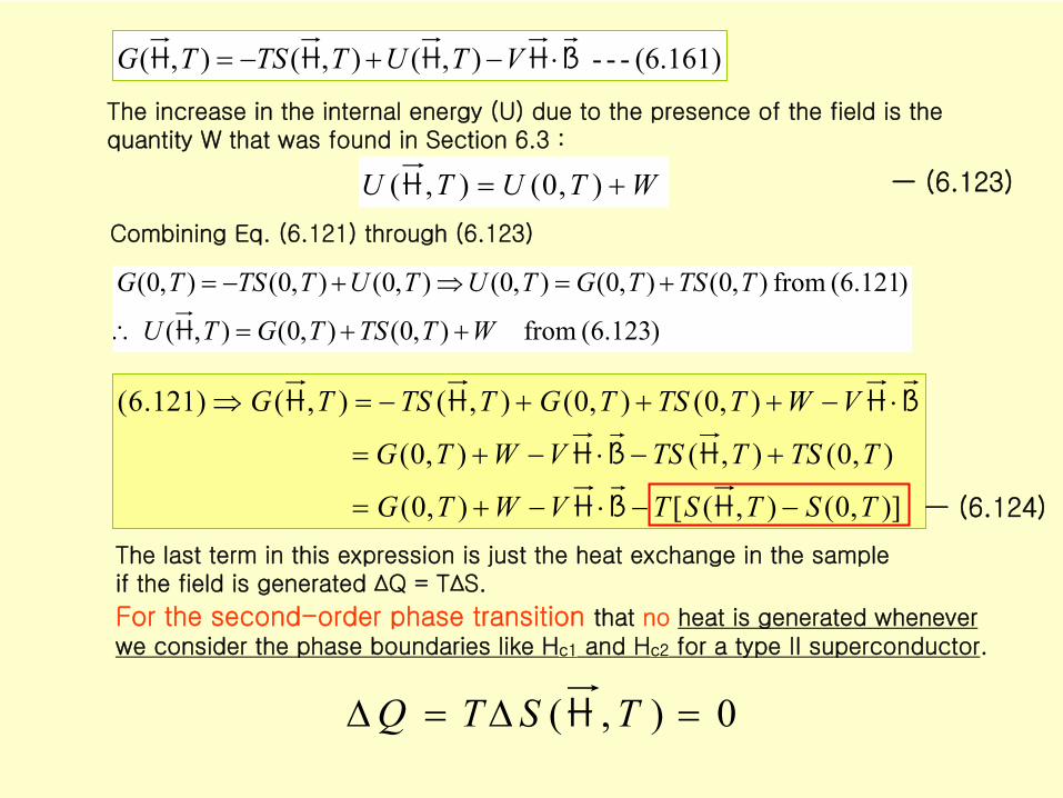
The increase in the internal energy (U) due to the presence of the field is the quantity W that was found in Section 6.3 :

WTUTU ),0(),(H ㅡ (6.123)

)],0(),([),0(

),0( ),(),0(

),0(),0( ),( ),()121.6(

TSTSTVWTG

TTSTTSVWTG

VWTTSTGTTSTG

HBH

HBH

BHHH

ㅡ (6.124)

The last term in this expression is just the heat exchange in the sample if the field is generated ∆Q = T∆S.

For the second-order phase transition

that no

heat is generated whenever we consider the phase boundaries like Hc1

and Hc2

for a type II superconductor.

0),( TSTQ H

Combining Eq. (6.121) through (6.123)

)123.6( from ),0(),0(),(

)121.6( from ),0(),0(),0(),0(),0(),0(

WTTSTGTU

TTSTGTUTUTTSTG

H

(6.161) --- ),(),(),( BHHHH VTUTTSTG

We can therefore rewrite Eq(6.124) as

BHH VWTGTG ),0(),( ㅡ (6.126)

The free energy in terms of the flux density B;

V

dvWTGTG BHH ),0(),( ㅡ (6.128)

s

s

V

Vss

dv

dvTGTG

B

BBB

H

H )()(12

1),0(),(0

2

0

ㅡ (6.129)

With W from Eq. (6.66: ) and the superconducting current

density given as ▽ Х

B=μ0Js

the Gibbs free energy for a superconductor is

dvW sV sss

)]J(JB[2

10

2

0

Likewise, for the normal material volume (Js

= 0), Vn,

nn VVnn dvdvTGTG B B HH 2

021),0(),(

ㅡ (6.130)

The lower critical field is found by considering the difference in the Gibbs free energy of the superconductor when the vortex is absent and when it is present.

),( TG H

Let us consider type II superconducting slab, shown in Figure 6.14.

[Figure 6.14

Field distribution in a type Ⅱ superconductor (a ≫

λ).]

),0(),( 00 TGTG ss H ㅡ (6.131)When there are no vortices B≈0.

(b) no vortex (c) single vortex in the slab(a) Superconducting slab

sVsss dvWTGTG B ),0(),( 01 HH ㅡ (6.132)

When one vortex is in the center of the slab the corresponding Gibbs free energy is),(1 TG s H

In Section 6.3 the electromagnetic energy of a single vortex of length Lz

was given by

vortex theoflength unit per energy the:V

ㅡ (6.134)zVs LW

appHH ㅡ (6.135)

The thermodynamic field for the slab is the applied field and soH

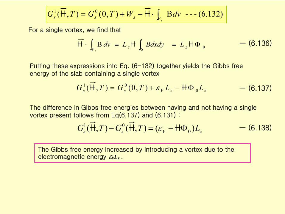
For a single vortex, we find that

S zzV

LBdxdyLdvs

0B HHH ㅡ (6.136)

Putting these expressions into Eq. (6-132) together yields the Gibbs free energy of the slab containing a single vortex

zzVss LLTGTG 001 ),0(),( HH ㅡ (6.137)

The difference in Gibbs free energies between having and not having a single vortex present follows from Eq(6.137) and (6.131) :

zVss LTGTG )(),(),( 001 HHH ㅡ (6.138)

The Gibbs free energy increased by introducing a vortex due to the electromagnetic energy εvLz .

(6.132) --- B ),0(),( 01 sVsss dvWTGTG HH

When , having a vortex is thermodynamically the lowest energy state and vortices will be present in the superconductor.

This happens as soon as the applied field exceeds the value

),(),( 01 TGTG ss HH

01 V

cH ㅡ (6.139)

where Hc1

is the lower critical field.

Using the expression for the energy per unit length of the vortex given by Eq (6.74), we find

)(4 02

0

20

KV

ㅡ (6.74)

)(4 02

0

01

KH c

ㅡ (6.140)

For high-κ

(λ/ξ≫1) superconductors

)ln(4

lim 20

01

cH ㅡ (6.141)

xxKx

ln)(lim 00

(6.138) --- )(),(),( 001

zVss LTGTG HHH Lower critical field (Hc1 )

Hence for H

< Hc1, no vortices enter the superconductor (B≈0 –

Meissner

state).

For H ≥ Hc1 vortices enter and the flux density is no longer zero.

Because both ξ

and λ

depend on temperature, so does Hc1(T), thereby forming the phase boundary in the H-T plane shown in Figure 6.15.

☜ Figure 6.15 The H-T phase diagram for a bulk superconducting slab in a uniform magnetic field for a type Ⅱ

superconductor.

☜ Figure 6.16

The top view of a superconductor with the field coming out of the page. The vortices form a triangular array with the separation α

between vortices.

As the applied magnetic field increases, the average flux density increases in the superconductor because the density of the vortices, nv, increase. According to Eq(6.2),

VVn B ㅡ (6.142)

where B=<B>.

Upper critical field (Hc2 )

Now let us try to estimate the upper critical field, Hc2. As the applied field increases, the vortices in the triangular lattice get closer together. The flux density B averaged over the sample is given by Eq(6.142)

20

32

B ㅡ (6.143)

As the applied field increases enough so that the cores begin to overlap, the whole superconductor begins to be covered with the normal cores and hence becomes normal. At this point B=µ0H because the material is normal.

Specifically with α ≈ 2ξ the cores begin to overlap so that at the upper critical field

20

02

0

02 32)2(3

2

cH ㅡ (6.144)

the material reverts to the normal state. Notice that our estimate of Hc2

depends on the model with which we describe the vortices.

From the Ginzburg-Landau calculation;

20

02 2

cH ㅡ (6.145)

)/(11~)(lim

cTT TT

Tc ㅡ (6.146)

ㅡ (6.147)

we find that

ccTT T

TTHc

11)(lim 22

This linear dependence on temperature near Tc

is also apparent in the figure.

☜ Figure 6.15 The H-T phase diagram for a bulk superconducting slab in a uniform magnetic field for a type Ⅱ superconductor.

cc T

TTH 1~)(2

Temperature dependence of Hc2

Since

20

02 2

cH