Chap 4 - Applied Mathematics

Chapter 4. Unconstrained optimization

Version: 28-10-2012

Material: (for details see)

Chapter 11 in [FKS] (pp.251-276)

A reference e.g. L.11.2 refers to the corresponding Lemmain the book [FKS]

PDF-file of the Book [FKS]: Faigle/Kern/Still,Algorithmic principles of Mathematical Programming.on: http://wwwhome.math.utwente.nl/∼stillgj/priv/

CO, Chapter 4 p 1/23

4.1 Introduction

We consider the nonlinear minimization problem(with f ∈ C1 or f ∈ C2):

(P) minx∈Rn

f (x) ,

Recall: Usually in (nonconvex) unconstrained optimization wetry to find a local minimizer. Global minimization is ’much more’difficult.

Theoretical method: (based on optimality conditions)

Find a point x satisfying

∇f (x) = 0 (critical point)

Check whether∇2f (x) � 0.


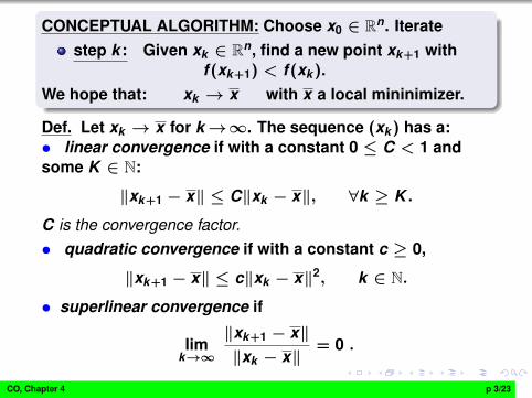
CONCEPTUAL ALGORITHM: Choose x0 ∈ Rn. Iteratestep k : Given xk ∈ Rn, find a new point xk+1 with

f (xk+1) < f (xk ).We hope that: xk → x with x a local mininimizer.

Def. Let xk → x for k→∞. The sequence (xk ) has a:• linear convergence if with a constant 0 ≤ C < 1 andsome K ∈ N:

‖xk+1 − x‖ ≤ C‖xk − x‖, ∀k ≥ K .

C is the convergence factor.• quadratic convergence if with a constant c ≥ 0,

‖xk+1 − x‖ ≤ c‖xk − x‖2, k ∈ N.

• superlinear convergence if

limk→∞

‖xk+1 − x‖‖xk − x‖

= 0 .


4.2 General descent method (f ∈ C1)

Def. A vector dk ∈ Rn is called a descent direction for f inxk if

∇f (xk )T dk < 0 (∗)

Rem. If (∗) holds then: f (xk + tdk ) < f (xk ) for t > 0 small.

Abbreviation: g(x) := ∇f (x), gk := g(xk )

Conceptual DESCENT METHOD: Choose a starting pointx0 ∈ Rn and ε > 0. Iteratestep k: Given xk ∈ Rn, proceed as follows:

if ||g(xk )|| < ε, stop with x ≈ xk .Choose a descent direction dk in xk : gT

k dk < 0Find a solution tk of the (one-dimensional)

minimization problem

mint≥0

f (xk + tdk ) and put xk+1 = xk + tk dk . (∗∗)


Remark By this descent method, minimization in Rn isreduced to (line) minimization in R (in each step k).

Steepest descent method: Use in the descent method asdescent direction (see Ex.11.7): dk = −∇f (xk )

Ex.11.7 Assuming∇f (xk ) 6= 0, show thatdk = −[∇f (xk )]/‖∇f (xk )‖ solves the problem:

mind∈Rn

∇f (xk )T d s.t. ‖d‖ = 1

Convergence behavior:

L.11.3 In the line-minimization step (**) we have

∇f (xk+1)T dk = 0

For the steepest descent method this means:

dTk+1dk = 0 (ziggzagging)


Th.11.1 Let f ∈ C1. Apply the steepest descent method.If the iterates xk converge, i.e., xk → x , then ∇f (x) = 0

Ex.11.8 Given the quadratic function on Rn,q(x) = xT Ax + bT x , A � 0. Show that the minimizer tk of

mint≥0

q(xk + tdk ) is given by tk = − gTk dk

2dTk Adk

.


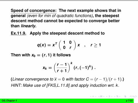
Speed of concergence: The next example shows that ingeneral (even for min of quadratic functions), the steepestdescent method cannot be expected to converge betterthan linearly.

Ex.11.9. Apply the steepest descent method to

q(x) = xT(

1 00 r

)x , r ≥ 1

Then with x0 = (r , 1) it follows

xk =

(r − 1r + 1

)k

(r , (−1)k ) .

(Linear convergence to x = 0 with factor C = (r − 1)/(r + 1).)HINT: Make use of [FKS,L.11.8] and apply induction wrt. k.


4.3 Method of conjugate directions

Aim: Find an algorithm which (at least for quadratic functions)has “better convergence” than steepest descent.

4.3.1 Case: f (x) = q(x) := 12xT Ax + bT x , A � 0 (pd.)

Idea. Try to generate dk ’s such that(not only ∇q(xk+1)

T dk = 0 but)

∇q(xk+1)T dj = 0 ∀0 ≤ j ≤ k

Then, after n steps we have

∇q(xn)T dj = 0 ∀0 ≤ j ≤ n − 1

and (if the dj ’s are lin. indep.) ∇q(xn) = 0. So xn = −A−1b isthe minimizer of q.


L. 11.4 Apply the descent method to q(x). The followingare equivalent:

(i) gTj+1di = 0 for all 0 ≤ i ≤ j ≤ k ;

(ii) dTj Adi = 0 for all 0 ≤ i < j ≤ k .

Definition. Vectors d0, . . . , dn−1 6= 0 are calledA-conjugate (or A-orthogonal) if: dT

j Adi = 0 ∀i 6= j .

Ex. A collection of A-conjugate vectorsd0, . . . , dn−1 6= 0 in Rn are linearly independent.


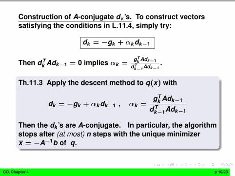
Construction of A-conjugate dk ’s. To construct vectorssatisfying the conditions in L.11.4, simply try:

dk = −gk + αk dk−1

Then dTk Adk−1 = 0 implies αk =

gTk Adk−1

dTk−1Adk−1

.

Th.11.3 Apply the descent method to q(x) with

dk = −gk + αk dk−1 , αk =gT

k Adk−1

dTk−1Adk−1

Then the dk ’s are A-conjugate. In particular, the algorithmstops after (at most) n steps with the unique minimizerx = −A−1b of q.


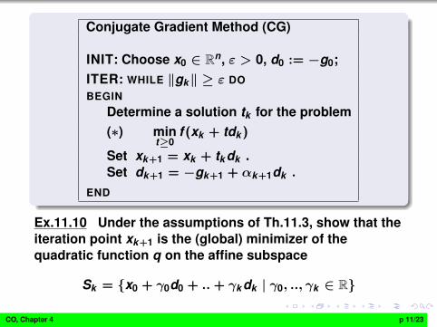
Conjugate Gradient Method (CG)

INIT: Choose x0 ∈ Rn, ε > 0, d0 := −g0;ITER: WHILE ‖gk‖ ≥ ε DOBEGIN

Determine a solution tk for the problem(∗) min

t≥0f (xk + tdk )

Set xk+1 = xk + tk dk .Set dk+1 = −gk+1 + αk+1dk .

END

Ex.11.10 Under the assumptions of Th.11.3, show that theiteration point xk+1 is the (global) minimizer of thequadratic function q on the affine subspace

Sk = {x0 + γ0d0 + .. + γk dk | γ0, .., γk ∈ R}


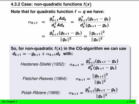
4.3.2 Case: non-quadratic functions f (x)

Note that for quadratic function f = q we have:

αk+1 =gT

k+1Adk

dTk Adk

=gT

k+1(gk+1 − gk )

dTk (gk+1 − gk )

=gT

k+1(gk+1 − gk )

‖gk‖2=‖gk+1‖2

‖gk‖2

So, for non-quadratic f (x) in the CG-algorithm we can usedk+1 = −gk+1 + αk+1dk with:

Hestenes-Stiefel (1952): αk+1 =gT

k+1(gk+1 − gk )

dTk (gk+1 − gk )

Fletcher-Reeves (1964): αk+1 =‖gk+1‖2

‖gk‖2

Polak-Ribiere (1969): αk+1 =gT

k+1(gk+1 − gk )

‖gk‖2


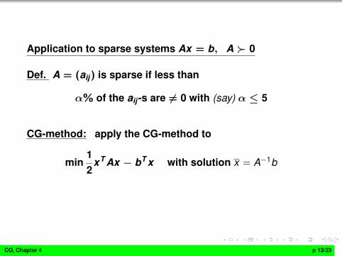
Application to sparse systems Ax = b, A � 0

Def. A = (aij) is sparse if less than

α% of the aij -s are 6= 0 with (say) α ≤ 5

CG-method: apply the CG-method to

min12

xT Ax − bT x with solution x = A−1b


CG Method for sparse linear systems Ax = b, A � 0

INIT: Choose x0 ∈ Rn and ε > 0 and set d0 = −g0;ITER: WHILE ‖gk‖ ≥ ε DOBEGIN

Set xk+1 = xk + tk dk with tk = −gT

k dk

dTk Adk

Set gk+1 = gk + tk Adk

Set dk+1 = −gk+1 + αk+1dk with αk+1 =gT

k+1gk+1

gTk gk

END

Rem. Complexity: ≈ α100n2 flop’s (floating point operations)

per ITER.CO, Chapter 4 p 14/23

4.4 Line minimization

In the general descent method (see Ch.4.2) we have torepeatedly solve:

mint≥0

h(t) with h(t) = f (xk + tdk )

where h′(0) < 0.

This can be done by:’exact line minimization’ of numerical analysise.g., bisection, golden section, Newton-,secant method (see Ch.4.3, Ch.11.4.1)or more “efficiently” by ’inexact line search’Goldstein-, Goldstein-Wolfe test (see Ch.11.4.2)


4.5 Newton’s method:

General remark: Newton’s method for solving systems ofnonlinear equations is one of the most important tools ofapplied mathematics.

Newtons’s Iteration: for solving F (x) = 0, F : Rn → Rn,F ∈C1, a system of n equations in n unknowns x = (x1, . . . , xn):start with some x0 and iterate

xk+1 = xk − [∇F (xk )]−1F (xk ) k = 0, 1, ...

Th.11.4 (local convergence of Newton’s method)Given F : Rn → Rn, F ∈ C2 such that

F (x) = 0 and ∇F (x) is non-singular.

Then the Newton iteration xk converges quadratically to xfor any x0 sufficiently close to x .


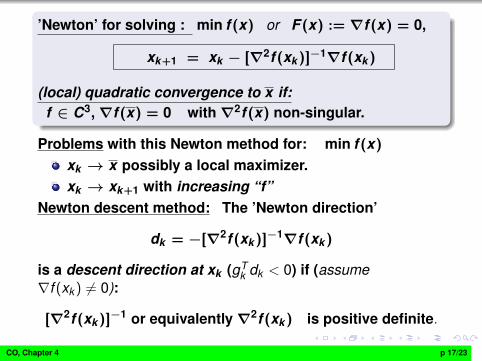
’Newton’ for solving : min f (x) or F (x) := ∇f (x) = 0,

xk+1 = xk − [∇2f (xk )]−1∇f (xk )

(local) quadratic convergence to x if:f ∈ C3,∇f (x) = 0 with∇2f (x) non-singular.

Problems with this Newton method for: min f (x)

xk → x possibly a local maximizer.xk → xk+1 with increasing “f”

Newton descent method: The ’Newton direction’

dk = −[∇2f (xk )]−1∇f (xk )

is a descent direction at xk (gTk dk < 0) if (assume

∇f (xk ) 6= 0):

[∇2f (xk )]−1 or equivalently∇2f (xk ) is positive definite.


Algorithm: (Levenberg-Marquardt variant)

step k: Given xk ∈ Rn with gk 6= 0.

1. determine σk > 0 such that (∇2f (xk ) + σk I) � 0,compute dk = −

(∇2f (xk ) + σk I

)−1gk (∗)

2. Find a minimizer tk of mint≥0

f (xk + tdk )

and put xk+1 = xk + tk dk .

Ex.11.n1 [connection with the ’trust region method’]Consider the quadratic Taylor approximation of f near xk :

q(x) := f (xk ) +∇f (xk )T (x − xk )

+1/2(x − xk )T∇2f (xk )(x − xk )

Compute the descent step dk according to (∗)(Levenberg-Marquardt) and put xk+1 = xk + dk , τ := ‖dk‖.Show that xk+1 is a local minimizer of the trust regionproblem: min q(x) s.t. ‖x − xk‖ ≤ τ


Disadvantage of the Newton methods:

∇2f (xk ) neededwork per step: linear systemFk x = bk ≈ n3 flop’s


4.6 Quasi-Newton method.

Find a method which only makes use of first derivatives andonly needs O(n2) flop’s per iter.

Consider the descent method with:

dk = −Hk gk

desired properties for Hk :i Hk � 0ii Hk+1 = Hk + Ek simple update ruleiii for quadratic f → conjugate directions dj

iv the Quasi-Newton condition:

(xk+1 − xk ) = Hk+1(gk+1 − gk )

Notation: δk := (xk+1 − xk ) , γk := (gk+1 − gk )


Quasi-Newton MethodINIT: Choose some x0 ∈ Rn, H0 � 0, ε > 0ITER: WHILE ‖gk‖ ≥ ε DOBEGIN

Set dk = −Hk gk ,Determine a solution tk for the problem

mint≥0

f (xk + tdk )

Set xk+1 = xk + tk dk and updateHk+1 = Hk + Ek .

END

For the update Hk + Ek we try: with α, β, µ ∈ R

Ek = αuuT + βvvT + µ(uvT + vuT ) (?)

where u := δk , v := Hkγk

Note that Ek is symmetric with rank ≤ 2.CO, Chapter 4 p 21/23

L.11.5 Apply the Quasi-Newton method toq(x) = 1

2xT Ax + bT x , A � 0 with

Ek of the form (?) and

Hk+1 satisfying iv: δk = Hk+1γk

Then the directions dj are A-conjugate :

dTj Adi = 0 0 ≤ i < j ≤ k

Last step in the construction of Ek : Find α, β, µ in (?)such that (iv) holds. This leads to the following updateformula


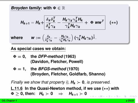
Broyden family: with Φ ∈ R

Hk+1 = Hk +δkδ

Tk

δTk γk−

HkγkγTk Hk

γTk Hkγk

+ Φ wwT (∗∗)

where w :=(

δkδT

k γk− Hkγk

γTk Hkγk

)(γT

k Hkγk )12 .

As special cases we obtain:

Φ = 0, the DFP-method (1963)(Davidon, Fletcher, Powell)

Φ = 1, the BFGS-method (1970)(Broyden, Fletcher, Goldfarb, Shanno)

Finally we show that property i), Hk � 0, is preserved.L.11.6 In the Quasi-Newton method, if we use (∗∗) withΦ ≥ 0, then: Hk � 0 ⇒ Hk+1 � 0


Chap 4 - Applied Mathematics

Documents