Chaotic properties of isokinetic-isobaric atomic systems under planar shear and elongational flows

Chaotic properties of isokinetic-isobaric atomic systems under planar shear and elongationalflows

Federico Frascoli,1,* Debra J. Searles,2,† and B. D. Todd1,‡

1Centre for Molecular Simulation, Swinburne University of Technology, P. O. Box 218, Hawthorn, Victoria 3122, Australia2Nanoscale Science and Technology Centre, School of Biomolecular and Physical Sciences, Griffith University, Brisbane, Queensland

4111, Australia�Received 19 November 2007; revised manuscript received 2 March 2008; published 30 May 2008�

An investigation of the chaotic properties of nonequilibrium atomic systems under planar shear and planarelongational flows is carried out for a constant pressure and temperature ensemble, with the combined use ofa Gaussian thermostat and a Nosé-Hoover integral feedback mechanism for pressure conservation. A compari-son with Lyapunov spectra of atomic systems under the same flows and at constant volume and temperatureshows that, regardless of whether the underlying algorithm describing the flow is symplectic, the degrees offreedom associated with the barostat have no overall influence on chaoticity and the general conjugate pairingproperties are independent of the ensemble. Finally, the dimension of the strange attractor onto which the phasespace collapses is found not to be significantly altered by the presence of the Nosé-Hoover barostattingmechanism.

DOI: 10.1103/PhysRevE.77.056217 PACS number�s�: 05.45.Pq, 05.60.�k, 05.70.Ln

I. INTRODUCTION

The chaotic properties of atomic liquid systems in a non-equilibrium steady state have been extensively studied in thelast two decades �1–11�. In general, one of the most widelyaccepted requirements for a system to be chaotic is that itmust have at least one positive Lyapunov exponent, which isa measure of the mean exponential rate of expansion andcontraction of initially nearby phase space trajectories. TheLyapunov spectra for different field-driven systems out ofequilibrium have been computed for a number of interestingnonequilibrium molecular dynamics �NEMD� �12,13� mod-els and one of the most significant developments has beenthe establishment of a fundamental link between Lyapunovexponents and transport coefficients �9,14�.

In this study, we present the Lyapunov spectra for non-equilibrium steady state systems of simple atoms interactingvia a pairwise additive Weeks-Chandler-Anderson �WCA�potential �15� and subjected to either planar shear flow �PSF�or planar elongational flow �PEF�, in a constant temperatureand pressure �NpT� ensemble. This is sampled with the adop-tion of a Gaussian isokinetic mechanism for instantaneousconservation of temperature �12� combined with a Nosé-Hoover �NH� barostatting mechanism for constant pressure�16�. For shear, we simulate a planar Couette flow system viathe well-established non-Hamiltonian SLLOD algorithm andLees-Edwards periodic boundary conditions �PBCs� �12�.For elongation, we employ the Hamiltonian SLLOD algorithmfor PEF with “deforming-brick” PBCs �17–20� and use anArnold cat map scheme �21� to impose the periodicity rela-tions on the unit lattice. The cat map was recently shown�22� to be related to the Kraynik-Reinelt �KR� conditions�23� for the compatibility and reproducibility of the simula-

tion box, which are necessary requirements for the funda-mental cell in order to have indefinitely long PEF simula-tions.

As observed in a previous study �7�, Lyapunov spectra ofPEF systems at NVT �i.e., at constant volume and tempera-ture� and NVE �i.e., at constant volume and energy� satisfythe so-called conjugate pairing rule �CPR� �24,25�. The CPRimplies an equal sum for all the Lyapunov pairs in the spec-trum, formed by coupling the highest exponent with the low-est, the second highest with the second lowest, and so on.Whereas for elongation the CPR compliance is essentiallydue to its symplectic character, conjugate pairing was ob-served to be violated by SLLOD PSF at both NVT and NVE,in accordance with preceding numerical calculations �6� andtheoretical arguments �26,27�. As repeatedly stressed in theliterature, the satisfaction of the CPR is not only importantper se, but leads to a dramatic reduction in the amount ofcalculation required to compute the dynamical properties ofthe system related to the sum of the exponents.

The paper is organized as follows. In Sec. II the featuresof PSF and PEF and their algorithms at NpT are explained,briefly illustrating the characteristics of the NH barostattingprocedure, and discussing the method for the calculation ofLyapunov exponents and their main properties. After de-scribing the quantities of interest for our set of simulations inSec. III, a presentation of Lyapunov spectra at NpT for non-equilibrium systems of eight particles is carried out in Sec.IV. Here we propose a comparison with analogous results atconstant volume and temperature, and analyze the propertiesof those exponents associated with the NH degrees of free-dom at a number of different state points. Some final remarksand an Appendix, where explicit calculations of the Jacobianof the system are shown, conclude the paper.

II. DESCRIPTION OF THE MODEL

Using nonequilibrium molecular dynamics methods, wesimulate a two-dimensional system of eight atoms subject to

*[email protected]†[email protected]‡[email protected]

PHYSICAL REVIEW E 77, 056217 �2008�

1539-3755/2008/77�5�/056217�10� ©2008 The American Physical Society056217-1

http://dx.doi.org/10.1103/PhysRevE.77.056217

PSF and PEF in an NpT thermodynamic ensemble, which isrealized with the combined use of a Gaussian isokinetic ther-mostat and a Nosé-Hoover barostatting mechanism �16�. Theatoms interact via the WCA potential �15�, which is a trun-cated and shifted version of the Lennard-Jones potential:

��rij� = �4��

rij�12

− � �

rij�6 + �c for rij � rc,

0 for rij � rc, �1�

with rij = �qi−q j�, where qi is the laboratory position vector ofparticle i,� is the well depth, and � is the value at which theLennard-Jones potential is zero. �c is the value of the un-shifted potential at the cutoff distance rc=21/6�, so that theWCA potential is continuous. In the following we use re-duced units, set all the masses of the particles mi to be equalto m, and impose m=�=�=1.

It is convenient to write SLLOD equations for shear andelongation coupled with a Nosé-Hoover barostat using re-duced coordinates ri=qi /V1/d �16�, where V and d=2 are thevolume and the dimensionality of the system, respectively.The equations of motion for the reduced laboratory positionsri and the peculiar momenta pi of a system of simple atomsunder PSF, with streaming velocity in the x direction andgradient in the y direction, are given by �12�

ri =pi

mV1/d + i�yi,

pi = Fi − i�pyi − �PSFpi, �2�

and the Gaussian isokinetic multiplier, which ensures that thekinetic energy is fixed at all times, is represented by

�PSF =

�i=1

N

Fi · pi − �pxipyi

�i=1

N

pi · pi

. �3�

The peculiar momentum is defined as the one taken withrespect to the streaming momentum mu, i is the unit vectorin the x direction, Fi is the total interatomic force acting onparticle i, and �=�ux /�y is the shear rate. Similarly, for asystem under PEF, with expansion in the x direction andcontraction in the y direction, the equations are �17�

ri =pi

mV1/d + ��ixi − jyi� ,

pi = Fi − ��ipxi − jpyi� − �PEFpi, �4�

and the Gaussian thermostat multiplier has the form

�PEF =

�i=1

N

Fi · pi − ��pxi2 − pyi

2 �

�i=1

N

pi · pi

, �5�

where j is the unit vector in the y direction and �=�ux /�x=−�uy /�y is the elongational rate.

Expressions �2�–�5� have to be complemented with thedifferential equations that describe the NH mechanism forpressure conservation, which introduces two additional de-grees of freedom in the system: the volume V of the simula-

tion cell and an external variable that mimics a piston �28�.The time evolution of V is regulated by via the followingequation:

V = dV , �6�

where V is the first derivative of the cell volume with respect

to time. Likewise, is the solution of the following differen-tial equation:

=�p − p0�VNkBTQ

. �7�

In the last formula, p is the instantaneous pressure of thesystem, given as the trace of the pressure tensor

P =1

V��

i=1

Npipi

m+ �

i=1

N

�j�i

N

�qi − q j�Fij� �8�

divided by the dimensionality d, p0 is the target pressure, andN is the number of atoms. Q is a damping factor which ischosen by trial and error so that pressure fluctuations areappropriately reduced, as described in �29,30�, and Fij=−��ij /�qi is the force on particle i due to particle j. It

should be noted that Eqs. �2�–�5� do not explicitly contain ,as it has been absorbed in the derivative of the reduced po-sitions ri via Eq. �6�, and that the force terms appearing in�2�, �4�, and �8� are calculated from a WCA potential whichdepends on the unscaled distances among the particles.

As it is customary in NEMD �19�, PBCs have to be im-posed on the simulation cell to preserve the homogeneity ofthe sample, eliminate surface effects and allow the system toreach a steady state �12�. For PSF, Lee-Edwards PBCs �31�are employed in a straightforward way in conjunction withEqs. �6� and �7� that regulate pressure conservation. Sinceunder this scheme image cells are only shifted along thedirection of the flow �19�, the target pressure p0 is achievedand maintained by a periodic rescaling of each box length, sothat the volume of the unit cell is equal to the target volumesolution of Eq. �6�. On the other hand, Kraynik-Reinelt PBCshave been shown to be necessary for performing homoge-neous simulations of steady planar elongation for indefinitelylong times �17,18,22,23�. These conditions imply that thefundamental cell contracts and expands as time evolves, andcare must be taken in the rescaling of the cell to ensure thatthe NpT PEF ensemble is correctly sampled. A procedure forthis, which implements a method known as the “new-cell

FRASCOLI, SEARLES, AND TODD PHYSICAL REVIEW E 77, 056217 �2008�

056217-2

algorithm” in combination with deforming-brick PBCs �18�,has been fully described in �30�. It has also been shown that,for SLLOD PEF, Lyapunov instability causes the y componentof the total momentum to drift, due to numerical roundofferrors, more substantially in PEF than in equilibrium or PSFsimulations, and therefore we reset it at each time step �32�.This procedure has no effect on the properties that are cal-culated.

There is one exponent for each degree of freedom in thesystem. The computation of the spectrum of Lyapunov expo-nents is performed with the well-established algorithm byBenettin et al. �33–36�. In short, consider a vector �1�t�= �r�t� ,p�t� ,V�t� , �t�� in the extended phase space compris-ing the two extra Nosé-Hoover degrees of freedom, and adisplacement �n�t�= �1�t�− �n�t� whose evolution can beexpressed to first order by ��t�=T�t� ·��t�. T is the stabil-ity matrix or the Jacobian of the equations of motion, and theexplicit calculation of its elements for an NpT system is il-lustrated in the Appendix. We can define a set of orthogonal

vectors �nc, such that �n

c ·�mc =0 for all m�n and con-

sider the evolution of the set of vectors �nc�t�= ��t�+�n

c. Itcan be shown that the n th Lyapunov exponent is then givenby

�n = limt→�

lim�n

c→0

1

tln� ��n

c�t��

��nc�0��

� . �9�

The CPR �1,5,6� states that in the limit as t→�, for everyexponent �i there is a conjugate �i� such that �i+�i�= ,where is constant for every i,i�. A small number of expo-nents that do not grow with N might be excluded due to theirassociation with conserved quantities or if they correspond todisplacement vectors in the direction of flow. It should alsobe clear that these trivial exponents for isokinetic-isobaricdynamics possess identical values to those at NVT and theirrationale can be deduced along the same lines as in Sec. III Cin �7�.

As said, even though sufficient conditions on the CPRhave yet to be found �24�, it has been proven that conjugatepairing occurs for a thermostatted system whose adiabaticequations of motion are Hamiltonian, as for the SLLOD PEFalgorithm �5,37�, and there is clear numerical evidence thatnon-Hamiltonian SLLOD PSF does not comply with it, al-though deviations are often small �6,7�.

An established and well-known link between the sum ofthe Lyapunov exponents and the viscosity of systems underPSF or PEF exists. Defining nonequilibrium shear viscosityas

�PSF = − Pxy�

��10�

and the analogous elongation viscosity as

�PEF = − Pxx� − Pyy�

4�, �11�

it can be shown �9,14� that, neglecting terms of orderO�1 /N�, for a system under isokinetic or isoenergetic con-strained dynamics we have

�PSF = −kB T��2V

�i=1

2dN

�i �12�

for PSF systems and

�PEF = −kB T�4�2V

�i=1

2dN

�i �13�

for PEF systems, where the angular brackets indicate a timeaverage over the steady state, which is necessary when tem-perature is not constrained. The summation index in formu-las �12� and �13� needs the slight modification 2dN→ �2dN+2� to accommodate for the two extra Lyapunov exponentsassociated with the barostatting equations �6� and �7�. Weanticipate that this pair of exponents displays a conjugatepairing to zero for either equilibrium or nonequilibrium dy-namics, so that Eqs. �12� and �13� are still valid for a systemat NpT and summation can be carried out on the exponentsrelated to the variables �ri ,pi� only. Also, if the system obeysthe CPR, the term for the sum of the exponents can be re-placed with a single sum of exponents of our choosing. Forexample, if we use the maximum and the minimum expo-nents, �i=1

2dN�i→dN��max+�min� can be substituted into Eqs.�12� and �13� �5�.

Lyapunov exponents can be also used to evaluate the frac-tal dimension of the attractor onto which the phase spacecollapses when the system is in a steady state �2,4,8,38�. Thisdimension can be calculated using the Kaplan-Yorke conjec-ture �39–41�, which leads to the following formula for theembedded dimension of the attractor in the phase space:

DKY =

�i=1

M

�i

��M+1�, �14�

where the exponents are ordered such that �1��2��3�¯

and M is the largest integer for which �i=1M �i�0.

In the following, the aim of our study is twofold. First, acomparison is proposed between Lyapunov spectra for non-equilibrium samples at NVT and at NpT. A target pressure forthe latter equal to the average pressure at constant tempera-ture and volume is imposed, according to the data presentedin �7�. These phase points belonging to different ensemblesare equivalent in the extended space of thermodynamic vari-ables given by �p ,T ,V , �� or �p ,T ,V , �� 42,43� and thisgives us the possibility to assess how the two different con-straining procedures affect chaoticity. Then, we provide ananalysis of the two exponents associated with the degrees of

freedom of the NH mechanism �V , �, focusing on their com-pliance with the CPR at different state points for both flows.Interestingly, results appear to be independent of the accu-racy with which the pressure is conserved and unrelated tothe symplecticity of the algorithms that describe the flows.

III. DETAILS OF SIMULATIONS

A fourth-order Gear predictor-corrector integrator �44� isemployed to compute the reduced version of SLLOD equa-

CHAOTIC PROPERTIES OF ISOKINETIC-ISOBARIC… PHYSICAL REVIEW E 77, 056217 �2008�

056217-3

tions �2� and �4�, together with Eqs. �5� and �6� for pressureconservation. As said, the scheme by Benettin et al. is used,with a Gram-Schmidt orthogonalization method which is ex-ecuted at every time step. Notable differences from previouscalculations for systems at NVT �1,6–10� are in the smallertime step used for NpT, e.g., �t=10−5, and in the fact thatour analysis is limited to spectra of two-dimensional systemswith eight particles only, with density �=0.3 and temperatureT=1.0. A shorter time step than is usual for simulations ofelongational flow is needed to ensure that numerical error issufficiently small so that subtle effects in the Lyapunov spec-trum can be observed. To check the accuracy of our choice of�t, differences between the phase space contraction deter-mined from the sum of the Lyapunov exponents and thatdetermined from the dynamics of the fluids have been calcu-lated, and ensured that these agreed at least to within 0.3%,as for previous NVT calculations �7� �see also the followingsection�. We also notice that the fact that a smaller time stepfor NpT than NVT ensembles is required is consistent withearlier observations on the use of NH constraints in calcula-tion of Lyapunov spectra, and that these findings are inde-pendent of the integration scheme used. In fact Williams etal., who studied an autonomous system using a fourth-orderRunge-Kutta method in �45,46�, were the first to find that arelatively small time step is needed to obtain a zero exponentassociated with the tangent vector in the direction of flow,when a NH thermostatting mechanism was used. In that case,because the dynamics is autonomous and it is known that

one tangent vector must lie in the direction of the flow ��t�,the problem could be avoided by removing components of

the tangent vectors lying along ��t�, rather than decreasingthe time step. In our case, where the dynamics is nonautono-mous, a similar error is expected but, as the vector in thedirection of the flow is no longer an eigenvector, we cannotsimply correct for this error and we need to reduce the timestep. As for our previous calculations at NVT, we prefer tosample the full 2dN+2 phase space and avoid the introduc-tion of an explicit constraint on the vectors, to be sure that nofalse condition is inadvertently introduced. For the chosen�t, we have verified that the values of the trivial exponent

for ��t� are correct, for each run, at equilibrium and nonequi-librium. As will be evident shortly, a treatment of smallersize systems alone is justified by the close analogy betweenNpT and NVT spectra, and by the need to calculate the ex-

ponents associated with �V , � for a number of different statepoints. This task appears to be computationally demandingfor larger atomic samples at an equivalent �t.

In the same fashion as in �7�, the phase space contraction

factor ��=� /�� · � for a two-dimensional PSF system isgiven by

�PSFNpT� = �

i=1

4N+2

�i =�− ��2N − 1� + �

�i=1

N

pxipyi

�i=1

N

pi · pi

+ 2��15�

and by

�PEFNpT� = �

i=1

4N+2

�i =�− ��2N − 1� + �

�i=1

N

�pxi2 − pyi

2 �

�i=1

N

pi · pi

+ 2��16�

for PEF, where the angular brackets denote a time averageand the first sums are extended to the two NH degrees offreedom. These expressions differ from their isokinetic coun-

terparts in the contribution of the pistonlike term �, which,according to the evolution equation for the volume, �6�, isexpected to decrease to zero in the long-time limit,1 i.e.,

�→0. In fact, once the system has reached a steady state,the average volume and pressure undergo smaller andsmaller oscillations around their constant target values andthe dynamics becomes equivalent to that of an isokinetic-

isochoric ensemble. This means that comparable ��have to be found at NpT and NVT when the values of theGaussian thermostats are similar, as we will show in thefollowing. Furthermore, the difference between the sum ofall Lyapunov exponents and the ensemble average in theright-hand side of Eqs. �15� and �16� will be referred to asthe deviation. In Table I we indicate the maximum value ofthe deviation at the end of the runs as a percentage of thecomputed �i=1

2dN+2�i for every state point: the disagreement isless than 0.04% of the value of the sum at each check and themaximum difference does not change considerably after t=100. This also means that, as the runs start from a face-centered cubic lattice, the equilibration of the systems is notinfluencing the final values of the exponents. As an indica-tion, the initial transient period �when the convergence of theexponents is still not optimal� ends approximately at t�1.0.We have also reported in Table I relevant quantities forLyapunov spectra, nonequilibrium viscosity and the Kaplan-Yorke dimension for the isokinetic-isobaric samples. In gen-eral, all the results have been collected from three indepen-dent runs with random initial peculiar momenta and for atotal simulation time t=10000. This, and a chosen dampingfactor Q=106, assure that the requirements discussed in �30�regarding the character of pressure fluctuations are correctlymet.

IV. RESULTS FOR LYAPUNOV SPECTRA ANDCONJUGATE PAIRING FOR NOSÉ-HOOVER DEGREES

OF FREEDOM

Let us start our discussion by inspecting Table I and com-paring it with analogous data in Table I of �7� for NVT sys-tems. Results for viscosities from direct NEMD calculations�Eqs. �10� and �11��, from expressions involving the sum ofthe exponents �Eqs. �12� and �13��, and from application ofthe CPR with ��max+�min� are also reported. First, simula-

1For our systems, numerical data also show that � is very smalland negligible with respect to the other terms in Eqs. �15� and �16�approximately after t�1.


056217-4

tions at NpT display a smaller value for the isokinetic mul-tiplier than their counterparts at constant volume. This can beunderstood by considering that the average V for equilibriumand nonequilibrium collections of atoms at NpT is alwayslarger than in the NVT case. On average, the action of theNH mechanism causes the distances among the particles toincrease, with a consequent decrease in Fi. Thus, accordingto the equations of motion, the rate of change for the mo-menta pi is then affected, and this is responsible for reducingthe amount of heat that has to be extracted by the thermostatat NpT. We can equivalently affirm that, to maintain the tar-get pressure, the system expands at the expense of its owninternal energy, reducing the work required by the thermostatto achieve the same temperature as in NVT.

Differences in � lead to unequal phase space compressionfactors and allow for a further check on the validity of ourcalculations. In fact, besides the excellent results for the de-viation reported in Table I which show very accurate cumu-lative sums for all the exponents, one can subtract �NVT�from �NpT� for equivalent state points and, assuming that

�=0 and neglecting terms of order 1 in N, obtain the fol-lowing expression:

�NpT� − �NVT� = − �2N − 1�� NpT� − �NVT�� 17�

where the superscripts indicate the type of ensemble. Usingdata from the simulations discussed in �7�, the agreementbetween the two sides of the above formula is satisfactoryand confirms the reliability of our evaluations �see Table II�.

Considering Table I, some more features are worth ad-dressing. As expected, viscosities calculated with NEMDtime averages do not change across the two thermodynamicregimes, and the values obtained using the sum of Lyapunovexponents and expressions �12� and �13� are very close alsofor NpT. This stresses the equivalence between state pointsin the extended space of thermodynamic observables, as pre-viously discussed. Second, the differences between theKaplan-Yorke dimensions of the attractors between NpT andNVT ensembles is always 2, due to the presence of the

couple of degrees of freedom �V , � in the former. This factshows that the dimensional collapse occurs only in the ordi-nary variables �ri ,pi� and does not involve the NH coordi-nates, which neither undergo contraction nor contribute anyincrease in the overall shrinkage in the phase space. An in-tuitive reason is given once more by the differences in finalvolumes between the simulation cells in the two ensembles:on average, the NH barostat does not exert work on the sys-tem and does not enhance or suppress its disorder or its dis-

sipation. This, according to the entropy rate formula S=−kB�i=1

2dN�i for isokinetic NVT systems from which Eqs.�12� and �13� are derived, is the ultimate cause for the exis-tence of a low-dimensional attractor �9,14�. The fact that thetwo extra NH exponents sum to zero, as we will showshortly, is clearly in agreement with the observation above,and the substitution 2dN→ �2dN+2� has no effect on the

value of S.If the Lyapunov spectra are closely considered, discrepan-

cies arise between the thermodynamical constraints of inter-est, as can also be deducted from a comparison of the values

TAB

LE

I.Su

mm

ary

ofre

sults

for

NpT

sim

ulat

ion

for

eigh

tpar

ticle

sat

equi

libri

uman

dun

der

PSF

and

PEF,

usin

ga

targ

etpr

essu

reeq

ualt

oth

eav

erag

epr

essu

rear

isin

gfr

omeq

uiva

lent

NV

Tsi

mul

atio

nsin

�7�.

p 0is

the

targ

etpr

essu

re,

pis

the

aver

age

pres

sure

,an

dV

indi

cate

sth

eav

erag

evo

lum

eof

the

sim

ulat

ion

cell.

�m

axan

d�

min

are

the

max

imum

and

min

imum

Lyap

unov

expo

nent

s,�

i;�

i�0�

iis

the

sum

ofth

epo

sitiv

eLy

apun

ovex

pone

nts,

max

dev

isth

em

axim

umde

viat

ion

�Eqs

.�1

5�an

d�1

6��

expr

esse

das

ape

rcen

tage

ofth

eto

tal

sum

ofth

eco

mpu

ted

Lyap

unov

expo

nent

s,�

NE

MD

isth

evi

scos

ityca

lcul

ated

with

NE

MD

sim

ulat

ions

�Eqs

.�10

�and

�11�

�,�

Lis

the

visc

osity

calc

ulat

edw

ithE

qs.�

12�a

nd�1

3�,�

CPR

isth

evi

scos

ityca

lcul

ated

usin

gC

PRfo

rth

em

axim

uman

dm

inim

umLy

apun

ovex

pone

nts,

and

DK

Yis

the

Kap

lan-

Yor

kedi

men

sion

from

Eq.

�14�

.Whe

rere

leva

nt,u

ncer

tain

ties

are

next

toth

eco

mpu

ted

aver

ages

,ex

pres

sed

astw

ice

the

stan

dard

erro

rfr

omth

ree

inde

pend

ent

runs

.N

VT

sim

ulat

ions

in�7

�ha

vebe

enpe

rfor

med

ata

cons

tant

V=

26.6

7.

Type

rate

��

max

�m

in�

i;�

i�0�

i

Max

dev

�%�

p 0V

p�

NE

MD

�L

DK

Y

Equ

il.1.

786

0.00

3−

1.78

90.

003

14.8

40.

010.

4481

27.8

90.

050.

4475

0.00

0329

.0

PSF

1.0

0.39

10.

002

1.76

30.

004

−2.

151

0.00

313

.42

0.03

0.01

70.

4792

27.8

20.

020.

4783

0.00

040.

197

0.00

10.

221

0.00

126

.40.

1

2.0

1.18

00.

008

1.80

40.

003

−2.

977

0.01

212

.08

0.02

−0.

039

0.54

7327

.56

0.05

0.54

800.

0015

0.15

00.

001

0.16

60.

001

22.9

0.1

PEF

0.5

0.42

60.

004

1.80

90.

004

−2.

240

0.01

115

.63

0.01

−0.

024

0.47

9727

.80

0.07

0.47

880.

0003

0.21

50.

001

0.23

90.

003

26.2

0.1

1.0

1.29

50.

004

1.93

10.

003

−3.

217

0.00

316

.87

0.04

−0.

023

0.53

6627

.54

0.04

0.53

670.

0009

0.16

50.

001

0.18

20.

002

23.0

0.1


056217-5

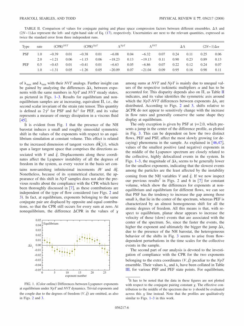
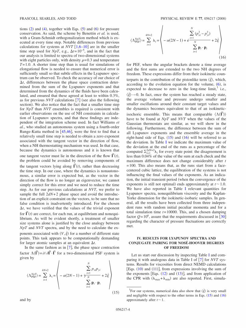
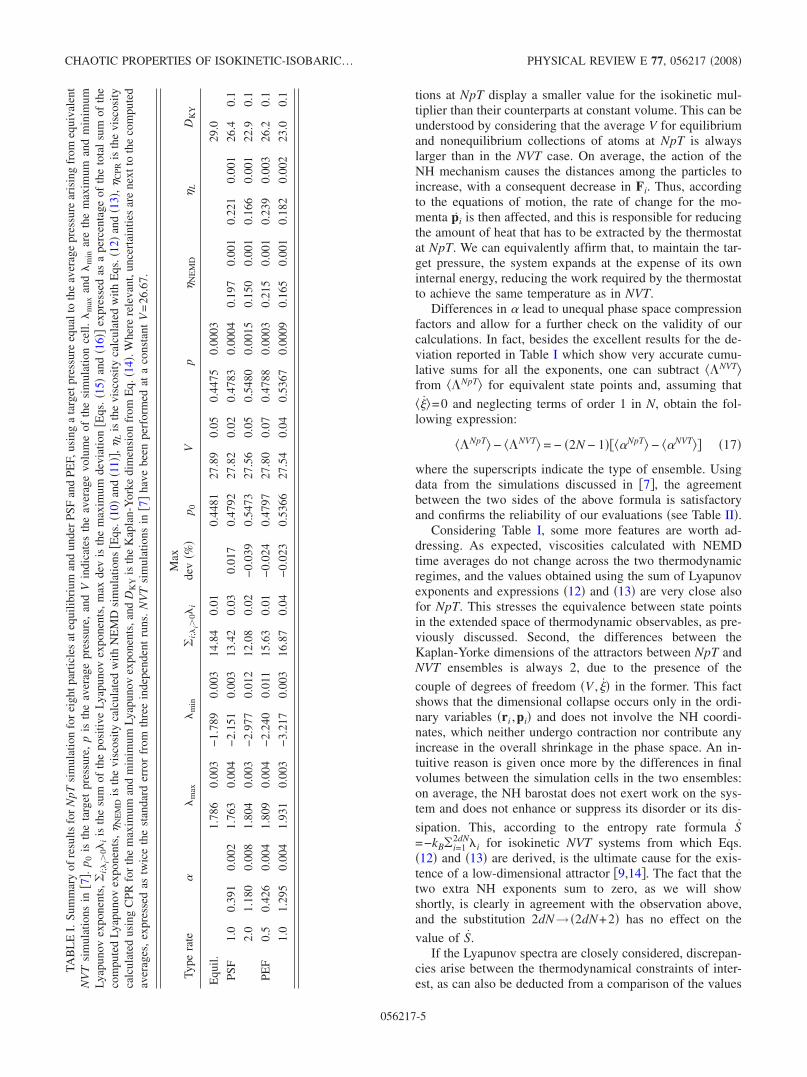
of �max and �min with their NVT analogs. Further insight canbe gained by analyzing the differences ��i between expo-nents with the same numbers in NpT and NVT steady states,as pictured in Figs. 1–3. Results for equilibrium and non-equilibrium samples are at increasing, equivalent �, i.e., thesecond scalar invariant of the strain rate tensor. This quantityis defined as 2�2 for PSF and 8�2 for PEF, and its valuerepresents a measure of energy dissipation in a viscous fluid�45�.

It is evident from Fig. 1 that the presence of the NHbarostat induces a small and roughly sinusoidal symmetricshift in the values of the exponents with respect to an equi-librium simulation at constant volume. This effect is related

to the increased dimension of tangent vectors Anc�t�, which

span a larger tangent space that comprises the directions as-

sociated with V and . Displacements along these coordi-nates affect the Lyapunov instability of all the degrees offreedom in the system, as every vector in the basis set con-

tains nonvanishing infinitesimal increments V and .Nonetheless, because of its symmetrical character, the ap-pearance of this shift in NpT samples does not alter the pre-vious results about the compliance with the CPR which havebeen thoroughly discussed in �7�, as these contributions areindependent of the type of flow considered �see Figs. 2 and3�. In fact, at equilibrium, exponents belonging to the sameconjugate pair are displaced by opposite and equal contribu-tions, so that the CPR still occurs for every sum at zero. Atnonequilibrium, the difference �CPR in the values of

among sums at NVT and NpT is mainly due to unequal val-ues of the respective isokinetic multipliers � and has to beaccounted for. This disparity depends also on �, as Table IIindicates, and its value identifies the symmetric axis aroundwhich the NpT-NVT differences between exponents ��i aredistributed. According to Figs. 2 and 3, shifts relative to�CPR do not appear to sensitively change with the increasein flow rates and generally conserve the same shape theydisplay at equilibrium.

The only exception is given by PSF at �=2.0, which pre-sents a jump in the center of the difference profile, as plottedin Fig. 3. This can be dependent on how the two distinctflows, PEF and PSF, affect the most slowly growing �or de-caying� phenomena in the sample. As explained in �46,47�,values of the smallest positive �and negative� exponents inthe middle of the Lyapunov spectrum are closely related tothe collective, highly delocalized events in the system. InFigs. 1–3, the magnitude of ��i seems to be generally lowerfor the smallest exponents, indicating that the slowest eventsamong the particles are the least affected by the instability

coming from the NH variables V and . If we now inspectour previous results2 in Figs. 2 and 6 in �7� for constantvolume, which show the differences for exponents at non-equilibrium and equilibrium for different flows, we can seethat PSF has the tendency to increase the gap among thosesmall �i that lie in the center of the spectrum, whereas PEF ischaracterized by an almost homogeneous shift for all theatomic degrees of freedom. All this means is that, with re-spect to equilibrium, planar shear appears to increase thevelocity of those �slow� events that are associated with thecenter of the spectrum. So, since the faster the events, thehigher the exponent and ultimately the bigger the jump ��idue to the presence of the NH barostat, the heterogeneousbehavior of the shifts in Fig. 3 seems to arise from flow-dependent perturbations in the time scales for the collectiveevents in the sample.

The second part of our analysis is devoted to the investi-gation of compliance with the CPR for the two exponents

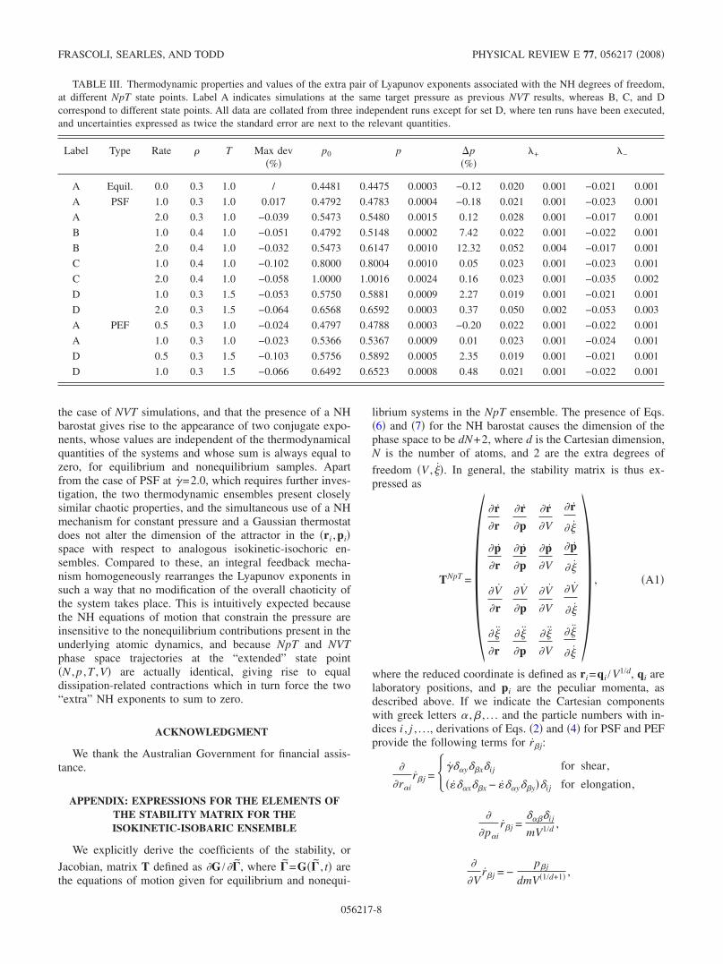
belonging to the extra coordinates �V , � peculiar to the NpTensemble. Their values �+ and �i have been collated in TableIII, for various PSF and PEF state points. For equilibrium,

2It has to be noted that the data in these figures are not plottedwith respect to the conjugate pairing constant . The effective con-tribution to the middle of the spectrum due to � should be evaluatedacross this line instead. Note that the profiles are qualitativelysimilar to Figs. 1–3 in this work.

TABLE II. Comparison of values for conjugate pairing and phase space compression factors between different ensembles. �� and�2N−1�� represent the left- and right-hand side of Eq. �17�, respectively. Uncertainties are next to the relevant quantities, expressed astwice the standard error from three independent runs.

Type rate �CPR�NVT �CPR�NpT �NpT �NVT �� 2N−1��

PSF 1.0 −0.39 0.01 −0.38 0.01 −6.08 0.04 −6.32 0.07 0.24 0.11 0.25 0.06

2.0 −1.21 0.06 −1.15 0.06 −18.23 0.13 −19.13 0.11 0.90 0.23 0.89 0.13

PEF 0.5 −0.43 0.01 −0.41 0.01 −6.63 0.05 −6.86 0.07 0.22 0.12 0.24 0.07

1.0 −1.31 0.05 −1.26 0.05 −20.09 0.07 −21.04 0.09 0.95 0.16 0.98 0.11

0 5 10 15 20 25-0.05-0.04-0.03-0.02-0.010.000.010.020.030.040.05

exponent number

Equilibrium

��i

FIG. 1. �Color online� Differences between Lyapunov exponentsat equilibrium under NpT and NVT dynamics. Trivial exponents and

the couple due to the degrees of freedom �V , � are omitted, as alsoin Figs. 2 and 3.


056217-6

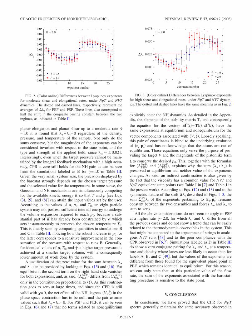
planar elongation and planar shear up to a moderate rate �=1.0 it is found that �++�−=0 regardless of the density,pressure, and temperature of the sample. Not only do thesums conserve, but the magnitudes of the exponents can beconsidered invariant with respect to the state point, and thetype and strength of the applied field, since �� 0.021.Interestingly, even when the target pressure cannot be main-tained by the integral feedback mechanism with a high accu-racy, CPR at zero still holds for the NH pair, as can be seenfrom the simulations labeled as B for �=1.0 in Table III.Given the very small system size, the precision displayed bythe barostat strongly depends on the chosen target pressureand the selected value for the temperature. In some sense, theGaussian and NH mechanisms are simultaneously competingfor the available kinetic energy K so that T and p �see Eqs.�3�, �5�, and �8�� can attain the input values set by the user.According to the values of �, p0, and T0, an eight-particlesystem may not possess sufficient internal energy to undergothe volume expansion required to reach p0, because a sub-stantial part of K has already been constrained by � whichacts instantaneously to preserve the chosen temperature T0.This is clearly seen by comparing quantities in simulations Band C in Table III, noticing how the robust increase in p0 forthe latter corresponds to a sensitive improvement in the con-servation of the pressure with respect to runs B. Generally,for identical values of �, T0, and �, a higher target pressure isachieved at a smaller target volume, with a consequentlylower amount of work done by the system.

A justification of the zero value for the sum between �+and �− can be provided by looking at Eqs. �15� and �16�. Forequilibrium, the second term on the right-hand side vanishesfor both expressions, and, as said, �EQ

NpT� differs from �EQNVT�

only in the contribution proportional to �. As this contribu-tion goes to zero at large times, and since the CPR is still

valid with =0, the net effect of the NH degrees �V , � in thephase space contraction has to be null, and the pair assumevalues such that �++�−=0. For PSF and PEF, it can be seenin Eqs. �6� and �7� that no terms related to nonequilibrium

explicitly enter the NH dynamics. As detailed in the Appen-dix, the elements of the stability matrix T, and consequently

the equation for the vectors ��t�=T�t� ·��t�, have thesame expressions at equilibrium and nonequilibrium for the

vector components associated with �V , �. Loosely speaking,this pair of coordinates is blind to the underlying evolutionof �ri ,pi� and has no knowledge that the atoms are out ofequilibrium. Those equations only serve the purpose of pro-viding the target V and the magnitude of the pistonlike term

to conserve the desired p0. This, together with the formulasfor �PSF

NpT� and �PEFNpT�, explains why the sum ��++�−� is

preserved at equilibrium and neither value of the exponentschanges. As said, an indirect confirmation is also given bythe fact that the viscosity has a common value for NVT andNpT equivalent state points �see Table I in �7� and Table I inthe present work�. According to Eqs. �12� and �13� and to thesymmetric nature of the shift ��i described in Figs. 1–3, thesum �i=1

4N �i of the exponents pertaining to �ri ,pi� remainsconstant between the two ensembles and forces �+ and �− tosum to zero.

All the above considerations do not seem to apply to PSFat a higher rate �=2.0, for which �+ and �− differ from allthe previous cases and do not show a trend that can be easilyrelated to the thermodynamic observables in the system. Thisfact might be connected to the appearance of strings in analo-gous NVT runs �48� and to the poor compliance with theCPR observed in �6,7�. Simulations labeled as D in Table IIIdo show a zero conjugate pairing for �+ and �− at a tempera-ture and density where lanes are less likely to occur than forlabels A, B, and C �49�, but the values of the exponents aredifferent from those found for the equivalent phase point atPEF, which remains identical to equilibrium. For this reason,we can only state that, at this particular value of the flowrate, the sum of the exponents associated with the barostat-ting procedure is sensitive to the state point.

V. CONCLUSIONS

In conclusion, we have proved that the CPR for NpTspectra generally maintains the same accuracy observed in

0 5 10 15 20 25-0.05-0.04-0.03-0.02-0.010.000.010.020.030.040.05

II = 2.0

��i

exponent number

��

FIG. 2. �Color online� Differences between Lyapunov exponentsfor moderate shear and elongational rates, under NpT and NVTdynamics. The dotted and dashed lines, respectively, represent theaverages of ��i for PEF and PSF. These lines also correspond tohalf the shift in the conjugate pairing constant between the tworegimes, as indicated in Table II.

0 5 10 15 20 25-0.025

0.000

0.025

0.050

0.075II = 8.0

��i

exponent number

��

� ��

FIG. 3. �Color online� Differences between Lyapunov exponentsfor high shear and elongational rates, under NpT and NVT dynam-ics. The dotted and dashed lines have the same meaning as in Fig. 2.


056217-7

the case of NVT simulations, and that the presence of a NHbarostat gives rise to the appearance of two conjugate expo-nents, whose values are independent of the thermodynamicalquantities of the systems and whose sum is always equal tozero, for equilibrium and nonequilibrium samples. Apartfrom the case of PSF at �=2.0, which requires further inves-tigation, the two thermodynamic ensembles present closelysimilar chaotic properties, and the simultaneous use of a NHmechanism for constant pressure and a Gaussian thermostatdoes not alter the dimension of the attractor in the �ri ,pi�space with respect to analogous isokinetic-isochoric en-sembles. Compared to these, an integral feedback mecha-nism homogeneously rearranges the Lyapunov exponents insuch a way that no modification of the overall chaoticity ofthe system takes place. This is intuitively expected becausethe NH equations of motion that constrain the pressure areinsensitive to the nonequilibrium contributions present in theunderlying atomic dynamics, and because NpT and NVTphase space trajectories at the “extended” state point�N , p ,T ,V� are actually identical, giving rise to equaldissipation-related contractions which in turn force the two“extra” NH exponents to sum to zero.

ACKNOWLEDGMENT

We thank the Australian Government for financial assis-tance.

APPENDIX: EXPRESSIONS FOR THE ELEMENTS OFTHE STABILITY MATRIX FOR THEISOKINETIC-ISOBARIC ENSEMBLE

We explicitly derive the coefficients of the stability, or

Jacobian, matrix T defined as �G /��, where �=G�� , t� arethe equations of motion given for equilibrium and nonequi-

librium systems in the NpT ensemble. The presence of Eqs.�6� and �7� for the NH barostat causes the dimension of thephase space to be dN+2, where d is the Cartesian dimension,N is the number of atoms, and 2 are the extra degrees of

freedom �V , �. In general, the stability matrix is thus ex-pressed as

TNpT =�� r

�r

� r

�p

� r

�V

� r

�

�p

�r

�p

�p

�p

�V

�p

�

�V

�r

�V

�p

�V

�V

�V

�

�

�r

�

�p

�

�V

�

�

� , �A1�

where the reduced coordinate is defined as ri=qi /V1/d, qi arelaboratory positions, and pi are the peculiar momenta, asdescribed above. If we indicate the Cartesian componentswith greek letters � ,� , . . . and the particle numbers with in-dices i , j , . . ., derivations of Eqs. �2� and �4� for PSF and PEFprovide the following terms for r�j:

�

�r�ir�j = ��y�xij for shear,

��x�x − ��y�y�ij for elongation,�

�

�p�ir�j =

��ij

mV1/d ,

�

�Vr�j = −

p�j

dmV�1/d+1� ,

TABLE III. Thermodynamic properties and values of the extra pair of Lyapunov exponents associated with the NH degrees of freedom,at different NpT state points. Label A indicates simulations at the same target pressure as previous NVT results, whereas B, C, and Dcorrespond to different state points. All data are collated from three independent runs except for set D, where ten runs have been executed,and uncertainties expressed as twice the standard error are next to the relevant quantities.

Label Type Rate � T Max dev�%�

p0 p �p�%�

�+ �−

A Equil. 0.0 0.3 1.0 / 0.4481 0.4475 0.0003 −0.12 0.020 0.001 −0.021 0.001

A PSF 1.0 0.3 1.0 0.017 0.4792 0.4783 0.0004 −0.18 0.021 0.001 −0.023 0.001

A 2.0 0.3 1.0 −0.039 0.5473 0.5480 0.0015 0.12 0.028 0.001 −0.017 0.001

B 1.0 0.4 1.0 −0.051 0.4792 0.5148 0.0002 7.42 0.022 0.001 −0.022 0.001

B 2.0 0.4 1.0 −0.032 0.5473 0.6147 0.0010 12.32 0.052 0.004 −0.017 0.001

C 1.0 0.4 1.0 −0.102 0.8000 0.8004 0.0010 0.05 0.023 0.001 −0.023 0.001

C 2.0 0.4 1.0 −0.058 1.0000 1.0016 0.0024 0.16 0.023 0.001 −0.035 0.002

D 1.0 0.3 1.5 −0.053 0.5750 0.5881 0.0009 2.27 0.019 0.001 −0.021 0.001

D 2.0 0.3 1.5 −0.064 0.6568 0.6592 0.0003 0.37 0.050 0.002 −0.053 0.003

A PEF 0.5 0.3 1.0 −0.024 0.4797 0.4788 0.0003 −0.20 0.022 0.001 −0.022 0.001

A 1.0 0.3 1.0 −0.023 0.5366 0.5367 0.0009 0.01 0.023 0.001 −0.024 0.001

D 0.5 0.3 1.5 −0.103 0.5756 0.5892 0.0005 2.35 0.019 0.001 −0.021 0.001

D 1.0 0.3 1.5 −0.066 0.6492 0.6523 0.0008 0.48 0.021 0.001 −0.022 0.001


056217-8

�

� r�j = 0, �A2�

and analogously for p�j,

�

�r�ip�j =

�F�j

�r�i−

��

�r�ip�j ,

�

�p�ip�j = − ��ij −

��

�p�ip�j

+ �− ��y�xij for shear,

− ��x�x − ��y�y�ij for elongation,�

�

�Vp�j =

�F�j

�V−

��

�Vp�j ,

�

� p�j = 0, �A3�

where F�j is the force on component � experienced by par-ticle j, and � is the Gaussian thermostat multiplier �see Eq.�3� for PSF and �5� for PEF�. Before the expressions for thederivatives in �A3� are provided, let us report the elementsassociated with Eqs. �6� and �7�:

�

�r�iV = 0,

�

�p�iV = 0,

�

�VV = d ,

�

� V = dV , �A4�

and

�

�r�i =

�p

�r�i

V

NQkBT,

�

�p�i =

2Vp�i

dNQkBT,

�

�V =

�p − p0�NQkBT

+�p

�V

V

NQkBT,

�

� = 0, �A5�

where p is the trace of the pressure tensor �8� divided by thedimensionality d, Q is the damping factor, and p0 is thetarget pressure. As can be seen, formulas �A3� and �A5� con-tain derivatives of the force Fi, which needs to be expressed

in terms of the reduced coordinates ri=qi /V1/d. We can in-troduce the constants a and b, defined as

a = V−7/d,

b = V−6/d

and obtain the expression for the force in terms of r= �ri−r j�= �qi−q j� /V1/d:

Fij�ri,r j� =24a

r8 �2b

r6 − 1��ri − r j� . �A6�

It is clear that the value of �A6� is identical to the one thatcomes from the usual derivation of the potential �1� withrespect to ordinary laboratory distances. Nonetheless,Fij�ri ,r j� is now a function of ri and of the volume V, and itneeds to be used when calculating the terms �� /�r�i,�p /�r�i, and �p /�V. Given the definition �8�, the last deriva-tive gives the contribution �Fij�ri ,r j� /�V, which, for a com-ponent �, can be written as

�F�ij�ri,r j��V

= −24a

dVr8�26b

r6 − 7��r�i − r�j� . �A7�

The expressions for �F�ij�ri ,r j� /�r�j are analogous to thosefound for the usual �F�ij�qi ,q j� /�q�j and are omitted here.The derivatives of the isokinetic multiplier are identical tothe ones found for an NVT ensemble, except for the substi-tution �F�ij�qi ,q j� /�q�j→�F�ij�ri ,r j� /�r�j,

�

�r�j� =

��i

��F�i/�r�j�p�i

��i

p�i2

,

�

�p�j�

=�F�j − 2�p�j − ��xpyj + �ypxj�

��i

p�i2 for shear,

F�j − 2�p�j − 2��x − �y�p�j

��i

p�i2 for elongation,

�

�V� =

��i

��F�i/�V�p�i

��i

p�i2

, �A8�

whereas the derivative of p with respect to the component r�iis given by

�

�r�ip =

1

dV�1−1/d��j

F�ij + ��j

�F�ij

�r�i�r�i − r�j�� . �A9�

It is possible to write the evolution equation for the tangentvectors in a compact form, which, for equilibrium, turns outto be


056217-9

r =� r

�p· p +

� r

�VV ,

p =�p

�r· r +

�p

�p· p +

�p

�VV ,

V =�V

�VV +

�V

� V ,

=�

�r· r +

�

�p· p +

�

�VV . �A10�

The dynamics of the infinitesimal displacements �

= �r ,p ,V ,� can be explicitly determined by substitut-

ing the previous formulas �A2�–�A9� in the above equations.When a nonequilibrium PSF or PEF system is considered,the SLLOD terms associated with shear and elongational fieldscause the emergence of the extra factor �r / �r ·r in theequation for r which is detailed in �A2�, and modify theform of �p / �p ·p as pointed out in �A3�. Further, deriva-tives of the thermostat multipliers with respect to r�j and p�j

do depend on the type of flow. Nonetheless, it is important tonote that these discrepancies between equilibrium and non-equilibrium affect only the components r and p of thetangent vectors and solely appear in the first two lines of�A10�. The remaining elements of T at PSF or PEF conservethe same expressions they have at equilibrium; this is ulti-mately the cause for the invariant and zero conjugate pairingof the Lyapunov exponents pertaining to the degrees of free-dom of the NH barostat, as discussed above.

�1� S. S. Sarman, D. J. Evans, and G. P. Morriss, Phys. Rev. A 45,2233 �1992�.

�2� G. P. Morriss, Phys. Lett. A 134, 307 �1989�.�3� G. P. Morriss, Phys. Rev. E 65, 017201 �2001�.�4� G. P. Morriss, Phys. Rev. A 37, 2118 �1988�.�5� D. J. Evans, E. G. D. Cohen, and G. P. Morriss, Phys. Rev. A

42, 5990 �1990�.�6� D. J. Searles, D. J. Evans, and D. J. Isbister, Chaos 8, 337

�1998�.�7� F. Frascoli, D. J. Searles, and B. D. Todd, Phys. Rev. E 73,

046206 �2006�.�8� H. A. Posch and W. G. Hoover, Phys. Rev. A 39, 2175 �1989�.�9� H. A. Posch and W. G. Hoover, Phys. Rev. A 38, 473 �1988�.

�10� W. G. Hoover, H. A. Posch, and S. Bestiale, J. Chem. Phys.87, 6665 �1987�.

�11� C. Dellago, H. A. Posch, and W. G. Hoover, Phys. Rev. E 53,1485 �1996�.

�12� D. J. Evans and G. P. Morriss, Statistical Mechanics of Non-equilibrium Liquids �Academic, New York, 1990�.

�13� S. S. Sarman, D. J. Evans, and P. T. Cummings, Phys. Rep.305, 1 �1998�.

�14� E. G. D. Cohen, Physica A 213, 293 �1995�.�15� J. D. Weeks, D. Chandler, and H. C. Andersen, J. Chem. Phys.

54, 5237 �1971�.�16� W. G. Hoover, Phys. Rev. A 31, 1695 �1985�.�17� B. D. Todd and P. J. Daivis, Phys. Rev. Lett. 81, 1118 �1998�.�18� B. D. Todd and P. J. Daivis, Comput. Phys. Commun. 117, 191

�1999�.�19� B. D. Todd and P. J. Daivis, Mol. Simul. 33, 189 �2007�.�20� A. Baranyai and P. T. Cummings, J. Chem. Phys. 110, 42

�1999�.�21� V. I. Arnold and A. Avez, Ergodic Problems of Classical Me-

chanics �Addison-Wesley, New York, 1968�.�22� T. A. Hunt and B. D. Todd, Mol. Phys. 101, 3445 �2003�.�23� A. M. Kraynik and D. A. Reinelt, Int. J. Multiphase Flow 18,

1045 �1992�.�24� R. Abraham and J. E. Marsden, Foundations of Mechanics

�Addison-Wesley, Redwood City, CA, 1987�.�25� A. J. Dragt, in Lecture Notes on Nonlinear Orbit Dynamics,

edited by S. Jorna, AIP Conf. Proc. No. 46 �AIP, New York,1982�, Vol. 87, pp. 147-313.

�26� D. Panja and R. van Zon, Phys. Rev. E 66, 021101 �2002�.�27� D. Panja and R. van Zon, Phys. Rev. E 65, 060102 �2002�.�28� C. Braga and K. P. Travis, J. Chem. Phys. 124, 104102 �2006�.�29� J. T. Bosko, B. D. Todd, and R. J. Sadus, J. Chem. Phys. 123,

034905 �2005�.�30� F. Frascoli and B. D. Todd, J. Chem. Phys. 126, 044506

�2007�.�31� A. W. Lees and S. F. Edwards, J. Phys. C 5, 1921 �1972�.�32� B. D. Todd and P. J. Daivis, J. Chem. Phys. 112, 40 �2000�.�33� G. Benettin, L. Galgani, and J.-M. Strelcyn, Phys. Rev. A 14,

2338 �1976�.�34� G. Benettin et al., Meccanica 15, 9 �1980�.�35� G. Benettin et al., Meccanica 15, 21 �1980�.�36� I. Shimada and T. Nagashima, Prog. Theor. Phys. 61, 1605

�1979�.�37� C. P. Dettmann and G. P. Morriss, Phys. Rev. E 53, R5545

�1996�.�38� B. L. Holian, C. G. Hoover, and H. A. Posch, Phys. Rev. Lett.

59, 10 �1987�.�39� D. J. Evans et al., J. Stat. Phys. 101, 17 �2000�.�40� P. Frederickson, J. L. Kaplan, and E. D. Yorke, J. Differ. Equa-

tions 49, 185 �1983�.�41� L. S. Young, Ergod. Theory Dyn. Syst. 2, 109 �1982�.�42� D. J. Evans and A. Baranyai, Phys. Rev. Lett. 67, 2597 �1991�.�43� P. J. Daivis and D. J. Evans, J. Chem. Phys. 100, 541 �1994�.�44� C. W. Gear, Numerical Initial Value Problems in Ordinary Dif-

ferential Equations �Prentice-Hall, Englewood Cliffs, NJ,1971�.

�45� R. B. Bird et al., Dynamics of Polymeric Liquids �Wiley, NewYork, 1987�, Vols. I and II.

�46� J.-P. Eckmann et al., J. Stat. Phys. 118, 813 �2005�.�47� H. A. Posch and W. G. Hoover, J. Phys.: Conf. Ser. 31, 9

�2006�.�48� D. J. Evans and G. P. Morriss, Phys. Rev. Lett. 56, 2172

�1986�.�49� J. Delhommelle, Phys. Rev. E 71, 016705 �2005�.


056217-10

Chaotic properties of isokinetic-isobaric atomic systems under planar shear and elongational flows

Documents