Chaotic Pattern Alternations Can Reproduce Properties Of ...kanamaru/... · Figure 1: (A) Chaotic synchronization observed in a module with D = 0:0032, rE = rI = 0:025, gint = 4,

Chaotic Pattern Alternations Can Reproduce Properties OfDominance Durations In Multistable Perception

Takashi Kanamaru

Department of Mechanical Science and Engineering,School of Advanced Engineering, Kogakuin University,

Hachioji-city, Tokyo 192-0015, Japan

Neural Computation, vol. 29, issue 6 (2017) pp.1696-1720.

Abstract

We propose a pulse neural network that exhibits chaotic pat-tern alternations among stored patterns as a model of multi-stable perception, which is reflected in phenomena such asbinocular rivalry and perceptual ambiguity. When we re-garded the mixed state of patterns as a part of each pattern,the durations of the retrieved pattern obey unimodal distribu-tions. We confirmed that no chaotic properties are observedin the time series of durations, consistent with the findingsof previous psychological studies. Moreover, it is shown thatour model also reproduces two properties of multistable per-ception that characterize the relationship between the con-trast of inputs and the durations.

1 Introduction

In the perception of visual information, multistable percep-tion is a well known phenomenon. For example, when twodifferent stimuli are presented to the eyes, the dominant stim-ulus perceived fluctuates over time, a phenomenon known asbinocular rivalry (Levelt, 1967; Walker, 1975; Lehky, 1995;Blake, 2001). Similarly, when an ambiguous figure such asa Necker cube is presented, the dominant interpretation alsofluctuates over time (Borsellino et al., 1972; Alais & Blake,2015). Research has also indicated that the duration of thedominant perception (dominance duration) may be charac-terized by a unimodal distribution, such as the gamma distri-bution (Levelt, 1967; Borsellino et al., 1972; Walker, 1975)or the log-normal distribution (Lehky, 1995).

Although many theoretical models have been proposed,the mechanism of such multistable perception is still un-known (Lehky, 1988; Laing & Chow, 2002; Wilson, 2003;Freeman, 2005; Wilson, 2007). Typical models assume thatthe rivalry takes place between the two eyes, or the twomonocular pathways (“eye rivalry”) (Lehky, 1988; Wilson,2007). Such models are composed of two oscillators withreciprocal inhibitions, and the stochastic properties are in-troduced to the model by adding noise (Lehky, 1988). Onepossible mechanism for such noise would be associated withfluctuation in the visual system, which is generated by small

eye movements and microsaccades. Laing & Chow (2002)suggested that randomness in their model is caused not bynoise but by deterministic chaos inherent in the network.

The eye rivalry is thought to take place between monocu-lar neurons within the primary visual cortex. However, Lo-gothetis et al. (1996) found that neurons whose activity cor-relates with rivalry were in higher cortical areas. In their ex-periment, the two stimuli presented to the eyes were swappedevery 330 ms. Even under such a condition, the results typ-ical of the binocular rivalry were found, and the mean dom-inance time of one pattern was 2,350 ms, which is muchlonger than the swap time of 330 ms. Their results can beinterpreted that in higher cortical areas, rivalry takes placebetween two patterns presented to the eyes (pattern rivalry).Their results show that the pattern rivalry can be modeledusing a hierarchical model with two rivalry stages (Wilson,2003), each of which shows the eye rivalry and the patternrivalry, respectively. However, a multistage model does notalways show the pattern rivalry (Freeman, 2005); therefore,the mechanism of the pattern rivalry is still controversial.

As for such pattern rivalry in the multistable percep-tion, there is related research (Leeuwen et al., 1997; Na-gao et al., 2000). Leeuwen et al. (1997) examined a net-work of the logistic map that yields chaotic dynamics andobserved chaotic switching between synchronous state andasynchronous state. Moreover, the distribution of interswitchperiod between each state was found to be unimodal. Al-though it is attractive to relate their model to the multistableperception, their model is an abstract one and not based onthe knowledge of neuroscience.

Nagao et al. (2000) stored 20 binary patterns in a neu-ronal network and regarded two patterns as the perceivedstates. In this network, the retrieved pattern fluctuates chaot-ically between two patterns. This dynamics is understoodin the literature of the chaotic associative memory model inwhich the state of the network changes chaotically amongseveral patterns (Aihara, Takabe, & Toyoda, 1990; Inoue &Nagayoshi, 1991; Nara & Davis, 1992; Tsuda, 1992; Adachi& Aihara, 1997). Typically the duration of a pattern in thechaotic associative memory model does not obey a unimodaldistribution, but it often obeys a monotonically decreasingdistribution (Tsuda, 1992). However, the model in Nagao

1

et al. (2000) successfully reproduces a unimodal distributionof dominance duration.

In the study presented in this letter, we report that the pat-tern alternations caused by chaotic dynamics of a pulse neu-ral network can also reproduce the properties of multistableperception. This network is composed of neuronal modelsthat emit spikes when a sufficiently strong input is injected,while the previous models of chaotic associative memorywere composed of conventional neuronal models based onfiring rates. In our network, the durations of the retrieved pat-tern obey unimodal distributions when we regard the mixedstate of patterns as part of each pattern. Moreover, althoughthe pattern alternations are caused by chaotic dynamics, thechaotic properties are not detected in the series of the du-rations of the retrieved pattern. Therefore, our results areconsistent with Lehky (1995), who stated that the statisticalproperties of binocular rivalry are not chaotic. Moreover,we show that our model can reproduce two characteristicsof binocular rivalry. First, when reducing the contrast of astimulus to one eye, dominance intervals in the other eyeincrease and dominance intervals in the stimulated eye arerelatively unchanged (Laing & Chow, 2002; Wilson, 2007).Second, when increasing the contrast of the stimuli to botheyes, dominance intervals in both eyes decrease (Laing &Chow, 2002; Wilson, 2007).

This letter is organized as follows. In section 2, we de-fine a pulse neural network composed of excitatory neuronsand inhibitory neurons exhibiting synchronized, chaotic fir-ing. In the subsequent sections, we refer to this network asthe one-module system. In section 3, we connect eight mod-ules of networks in which two patterns are stored accordingto the mechanism of associative memory. These two pat-terns correspond to the two stable states of binocular rivalryand perceptual ambiguity. We further show that chaotic dy-namics are responsible for alterations in the retrieved pat-terns over time. In section 4, we show that the durationsof the retrieved pattern obey unimodal distributions. In sec-tion 5, we examine the dependences of the peak position ofthe unimodal distribution on the connection strengths and thenumber of patterns. In section 6, we show that chaotic prop-erties are not detected in the series of the durations of theretrieved pattern. In section 7, we show that our model canreproduce two characteristics of binocular rivalry. Section 8concludes.

2 One-module system

In sections 2 and 3, we introduce a neural network of thetaneurons with phases as their internal states (Ermentrout &Kopell, 1986; Ermentrout, 1996; Izhikevich, 1999, 2000;Kanamaru & Sekine, 2005b). When a sufficiently strong in-put is provided, each neuron yields a pulse by increasing itsphase around a circle and returning to its original phase. Thenetwork is composed of NE excitatory neurons and NI in-

hibitory neurons governed by the following equations:

˙θ(i)E = (1− cos θ

(i)E ) + (1 + cos θ

(i)E )

×(rE + ξ(i)E (t) + gintIE(t)− gextII(t)),(2.1)

˙θ(i)I = (1− cos θ

(i)I ) + (1 + cos θ

(i)I )

×(rI + ξ(i)I (t) + gextIE(t)− gintII(t)),(2.2)

IX(t) =1

2NX

NX∑j=1

∑k

1

κXexp

(−t− t

(j)k

κX

), (2.3)

〈ξ(i)X (t)ξ(j)Y (t′)〉 = DδXY δijδ(t− t′), (2.4)

where θ(i)E and θ(i)I are the phases of the ith excitatory neuron

and the ith inhibitory neuron, respectively. rE and rI are pa-rameters of the neurons that determine whether the equilib-rium of each neuron is stable. We used rE = rI = −0.025 toensure that each neuron had a stable equilibrium. X = E orI denote the excitatory or inhibitory ensemble, respectively,while t

(j)k is the kth firing time of the jth neuron in the en-

semble X and the firing time is defined as the time at whichθ(j)X exceeds π in the positive direction. The neurons com-

municate with each other using the postsynaptic potentialswhose waveforms are the exponential functions, as shown inequation 2.3. ξ

(i)X (t) represents gaussian white noise added

to the ith neuron in the ensemble X .Throughout the remainder of the letter, this network is re-

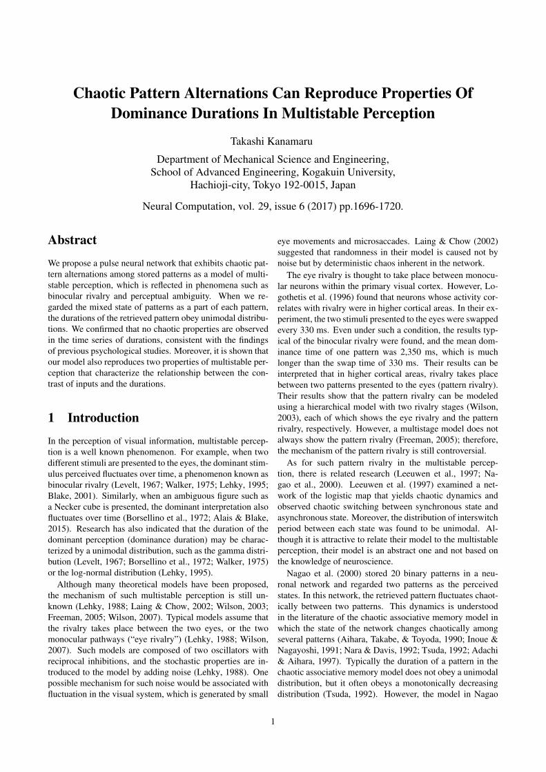
ferred to as a one-module system that exhibits various pat-terns of synchronized firing (Kanamaru & Sekine, 2005b).We utilized the chaotic synchronization shown in Figure 1.Figure 1A shows a raster plot of spikes of 200 randomly cho-sen excitatory neurons and inhibitory neurons in a modulewith NE = NI = 2000. This plot allows one to observe thesynchronized firing of neurons and that the intervals of syn-chronized firing do not remain constant. The instantaneousfiring rates JE and JI of the excitatory and inhibitory ensem-bles calculated from the data used in Figure 1A are shown inFigure 1B. A trajectory of JE and JI in the (JE , JI) planeis also shown in Figure 1C, revealing somewhat complexstructures. To analyze these structures, we took the limit ofNE , NI → ∞ in order to obtain the Fokker-Planck equa-tion, which governs the dynamics of the probability densitiesnE(θE) and nI(θI) of θ(i)E and θ

(i)I , as shown in Appendix A.

JE and JI , obtained from the analysis of the Fokker-Planckequation, are shown in Figures 1E and 1F. In Figure 1F, afine structure of a strange attractor is observed. The largestLyapunov exponent of the attractor in Figure 1F is positive(Kanamaru & Sekine, 2005b), indicating that the dynamicsof JE and JI are chaotic. Moreover, the asynchronous fir-ings shown in Figure 1D coexist with the chaotic synchro-nization shown in Figure 1A because each neuron has stableequilibrium. This coexistence of two states is important forrealizing chaotic pattern alternations.

In the following sections, only the one-module systemswith infinite neurons treated in Figures 1E and 1F are consid-ered, as the Fokker-Planck equation does not contain noise,allowing for the reproduction of analyses.

2

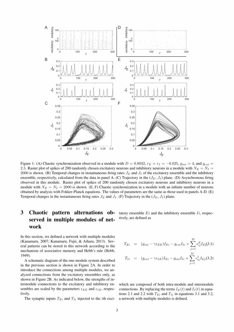
Figure 1: (A) Chaotic synchronization observed in a module with D = 0.0032, rE = rI = −0.025, gint = 4, and gext =2.5. Raster plot of spikes of 200 randomly chosen excitatory neurons and inhibitory neurons in a module with NE = NI =2000 is shown. (B) Temporal changes in instantaneous firing rates JE and JI of the excitatory ensemble and the inhibitoryensemble, respectively, calculated from the data in panel A. (C) Trajectory in the (JE , JI ) plane. (D) Asynchronous firingobserved in this module. Raster plot of spikes of 200 randomly chosen excitatory neurons and inhibitory neurons in amodule with NE = NI = 2000 is shown. (E, F) Chaotic synchronization in a module with an infinite number of neuronsobtained by analysis with Fokker-Planck equations. The values of parameters are the same as those used in panels A-D. (E)Temporal changes in the instantaneous firing rates JE and JI . (F) Trajectory in the (JE , JI ) plane.

3 Chaotic pattern alternations ob-served in multiple modules of net-work

In this section, we defined a network with multiple modules(Kanamaru, 2007; Kanamaru, Fujii, & Aihara, 2013). Sev-eral patterns can be stored in this network according to themechanism of associative memory and Hebb’s rule (Hebb,1949).

A schematic diagram of the one-module system describedin the previous section is shown in Figure 2A. In order tointroduce the connections among multiple modules, we an-alyzed connections from the excitatory ensembles only, asshown in Figure 2B. As indicated below, the strengths of in-termodule connections to the excitatory and inhibitory en-sembles are scaled by the parameters εEE and εIE , respec-tively.

The synaptic inputs TEi and TIi injected to the ith exci-

tatory ensemble Ei and the inhibitory ensemble Ii, respec-tively, are defined as

TEi = (gint − γεEE)IEi − gextIIi +M∑j=1

εEijIEj ,(3.1)

TIi = (gext − γεIE)IEi − gintIIi +

M∑j=1

εIijIEj ,(3.2)

which are composed of both intra-module and intermoduleconnections. By replacing the terms IE(t) and II(t) in equa-tions 2.1 and 2.2 with TEi and TIi in equations 3.1 and 3.2,a network with multiple modules is defined.

3

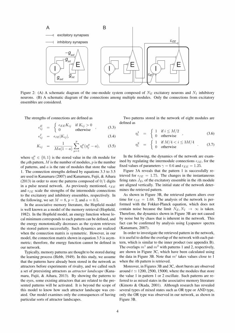
Figure 2: (A) A schematic diagram of the one-module system composed of NE excitatory neurons and NI inhibitoryneurons. (B) A schematic diagram of the connections among multiple modules. Only the connections from excitatoryensembles are considered.

The strengths of connections are defined as

εEij =

{εEEKij if Kij > 00 otherwise , (3.3)

εIij = εIE |Kij |, (3.4)

Kij =1

Ma(1− a)

p∑µ=1

ηµi (ηµj − a), (3.5)

where ηµi ∈ {0, 1} is the stored value in the ith module forthe µth pattern, M is the number of modules, p is the numberof patterns, and a is the rate of modules that store the value1. The connection strengths defined by equations 3.3 to 3.5are used in Kanamaru (2007) and Kanamaru, Fujii, & Aihara(2013) in order to store the patterns composed of 0/1 digitsin a pulse neural network. As previously mentioned, εEE

and εIE scale the strengths of the intermodule connectionsto the excitatory and inhibitory ensembles, respectively. Inthe following, we set M = 8, p = 2, and a = 0.5.

In the associative memory literature, the Hopfield modelis well known as a model of the memory retrieval (Hopfield,1982). In the Hopfield model, an energy function whose lo-cal minimum corresponds to each pattern can be defined, andthe energy monotonically decreases as the system retrievesthe stored pattern successfully. Such dynamics are realizedwhen the connection matrix is symmetric. However, in ourmodel, the connection matrix shown in equation 3.5 is asym-metric; therefore, the energy function cannot be defined inour network.

Typically, memory patterns are thought to be stored duringthe learning process (Hebb, 1949). In this study, we assumethat the patterns have already been stored in the network asattractors before experiments of rivalry, and we called sucha set of preexisting attractors as attractor landscape (Kana-maru, Fujii, & Aihara, 2013). By showing the patterns tothe eyes, some existing attractors that are related to the pre-sented patterns will be activated. It is beyond the scope ofthis model to know how such attractor landscape was cre-ated. Our model examines only the consequences of havingparticular sorts of attractor landscapes.

Two patterns stored in the network of eight modules aredefined as

η1i =

{1 if i ≤ M/20 otherwise , (3.6)

η2i =

{1 if M/4 < i ≤ 3M/40 otherwise . (3.7)

In the following, the dynamics of the network are exam-ined by regulating the intermodule connections εIE , for thefixed values of parameters γ = 0.6 and εEE = 1.25.

Figure 3A reveals that the pattern 1 is successfully re-trieved for εIE = 1.75. The changes in the instantaneousfiring rates JEi of the excitatory ensemble in the ith moduleare aligned vertically. The initial state of the network deter-mines the retrieved pattern.

As shown in Figure 3B, the retrieved pattern alters overtime for εIE = 1.68. The analysis of the network is per-formed with the Fokker-Planck equation, which does notcontain noise because the limit NE , NI → ∞ is taken.Therefore, the dynamics shown in Figure 3B are not causedby noise but by chaos that is inherent in the network. Thisfact can be confirmed by analysis using Lyapunov spectra(Kanamaru, 2007).

In order to investigate the retrieved pattern in the network,it is useful to define the overlap of the network with each pat-tern, which is similar to the inner product (see appendix B).The overlaps m1 and m2 with patterns 1 and 2, respectively,are shown in Figure 3C, which have been calculated usingthe data in Figure 3B. Note that mi takes values close to 1when the ith pattern is retrieved.

Moreover, in Figures 3B and 3C, short bursts are observedaround t ' 1200, 2500, 15000, where the modules that storethe value 1 in pattern 1 or 2 oscillate. Such patterns are re-ferred to as mixed states in the associative memory literature(Kimoto & Okada, 2001). Although research has revealedseveral types of mixed states such as OR type or AND type,only the OR type was observed in our network, as shown inFigure 3B.

4

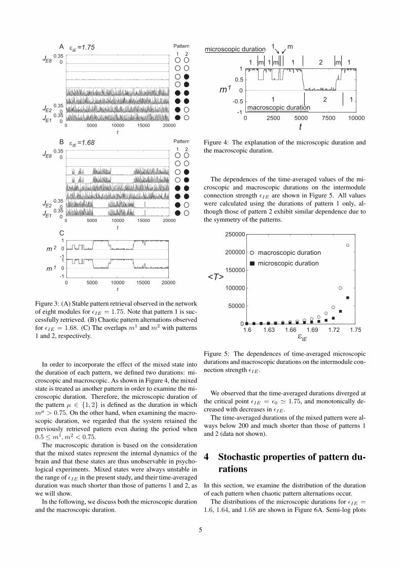
Figure 3: (A) Stable pattern retrieval observed in the networkof eight modules for εIE = 1.75. Note that pattern 1 is suc-cessfully retrieved. (B) Chaotic pattern alternations observedfor εIE = 1.68. (C) The overlaps m1 and m2 with patterns1 and 2, respectively.

In order to incorporate the effect of the mixed state intothe duration of each pattern, we defined two durations: mi-croscopic and macroscopic. As shown in Figure 4, the mixedstate is treated as another pattern in order to examine the mi-croscopic duration. Therefore, the microscopic duration ofthe pattern µ ∈ {1, 2} is defined as the duration in whichmµ > 0.75. On the other hand, when examining the macro-scopic duration, we regarded that the system retained thepreviously retrieved pattern even during the period when0.5 ≤ m1,m2 < 0.75.

The macroscopic duration is based on the considerationthat the mixed states represent the internal dynamics of thebrain and that these states are thus unobservable in psycho-logical experiments. Mixed states were always unstable inthe range of εIE in the present study, and their time-averagedduration was much shorter than those of patterns 1 and 2, aswe will show.

In the following, we discuss both the microscopic durationand the macroscopic duration.

Figure 4: The explanation of the microscopic duration andthe macroscopic duration.

The dependences of the time-averaged values of the mi-croscopic and macroscopic durations on the intermoduleconnection strength εIE are shown in Figure 5. All valueswere calculated using the durations of pattern 1 only, al-though those of pattern 2 exhibit similar dependence due tothe symmetry of the patterns.

Figure 5: The dependences of time-averaged microscopicdurations and macroscopic durations on the intermodule con-nection strength εIE .

We observed that the time-averaged durations diverged atthe critical point εIE = ε0 ' 1.75, and monotonically de-creased with decreases in εIE .

The time-averaged durations of the mixed pattern were al-ways below 200 and much shorter than those of patterns 1and 2 (data not shown).

4 Stochastic properties of pattern du-rations

In this section, we examine the distribution of the durationof each pattern when chaotic pattern alternations occur.

The distributions of the microscopic durations for εIE =1.6, 1.64, and 1.68 are shown in Figure 6A. Semi-log plots

5

of Figure 6A are also shown in Figure 6B. To calculate thedistributions, the microscopic durations of both patterns 1and 2 were used. The solid lines represent the fit with theexponential distribution, and longer durations were associ-ated with better fit. Moreover, for εIE = 1.6, a good fit wasobserved even for small durations, suggesting that pattern al-ternations become more stochastic as εIE moves away fromthe critical point ε0 ' 1.75.

Figure 6: (A) The distribution of the microscopic duration.(B) Semi-log plots of panel A.

The autocorrelation function of the microscopic durationsis shown in Figure 7A. The series of microscopic durationsis composed by aligning each microscopic duration in order,including the durations of the mixed state. The oscillatingcomponent of the autocorrelation function is caused by thefact that the microscopic durations tend to take small valuesand large values alternately, which correspond to the shortdurations of the mixed states and the long durations of pat-tern 1 or 2. In Figure 7A, it is also observed that the oscil-lating component decreases with the decrease of εIE becausethe long durations of pattern 1 or 2 decrease and they becomecomparable to the short durations of the mixed states.

The distributions of the macroscopic durations under iden-tical conditions with Figure 6 are shown in Figure 8. The

Figure 7: Autocorrelation functions of (A) microscopic du-rations and (B) macroscopic durations.

solid lines in Figure 8A show the fit with the gamma distri-bution, and the solid lines in Figure 8B show that with thelog-normal distribution.

In Figure 8A, the fit with the gamma distributionβαTα−1e−βT /Γ(α) is good for εIE = 1.6, where Γ(α) isthe gamma function with argument α. Note that the fit forlarge εIE is not good because the decay of the distribution forlonger durations is slow for large εIE . This fact also seemsto imply that the system with small εIE is more stochastic,as the sum of random variables that obey the exponential dis-tribution obeys the gamma distribution (Murata et al., 2003).

More specifically, the sum of Ti (i = 1, 2, · · · , α) eachof which obeys the exponential distribution with the rate pa-rameter β obeys the gamma distribution with α and β. InMurata et al. (2003), α tended to take natural numbers. Theauthors proposed that there would be some “distinct states”between two rivalrous states, and the system has to transitsuch distinct states α times in order to reach the rivalrousstates. In our model, the times of passing the mixed states arenot fixed but variable (see the data at t ' 2500 in Figure 4).

6

Figure 8: Distributions of the macroscopic durations. (A)The solid lines indicate the fit with the gamma distribution.(B) The solid lines indicate the fit with the log-normal distri-bution.

It would be interesting to check whether α is a natural num-ber in our model. The parameters (α, β) for gamma distri-butions in Figure 8A are (1.66, 0.00158), (1.23, 0.000498),and (0.94, 0.0001) for εIE = 1.60, 1.64, and 1.68, respec-tively. The parameter value α = 1.66 for εIE = 1.60 seemsto indicate that both the direct transition to another pattern(α = 1) and the transition passing the mixed pattern once(α = 2) exist.

In Lehky (1995), the dominant durations of binocular ri-valry follow a log-normal distribution. Similarly, the distri-bution of the macroscopic durations in our system also fol-lows a log-normal distribution, as shown in Figure 8B.

The autocorrelation function of the macroscopic durationsis shown in Figure 7B. The series of macroscopic durationsis composed by aligning the macroscopic durations of pat-tern 1 and pattern 2 in order. The autocorrelation functionindicates that the macroscopic durations do not have any se-quential dependence, which is consistent with psychologicalexperiments (Walker, 1975).

In summary, the macroscopic durations are more appropri-ate than microscopic durations as models of the dominancedurations of binocular rivalry and perceptual ambiguity.

5 Peak position of the distribution

Previous psychological research has revealed that the domi-nance duration that gives the peak of the distribution rangesfrom 0.8 s to 10 s, depending on the individual participant(Levelt, 1967; Borsellino et al., 1972; Walker, 1975; Lehky,1995; Blake, 2001). In this section, we examine the origin ofthis variability of the peak position Tp.

First, careful observation of Figure 8 shows that Tp

slightly depends on the intermodule connection strength εIE .Second, it is expected that Tp would become large when thenumber of the mixed states increases because the networkwill pass many mixed states before it moves from one patternto another. To confirm this expectation, we add the third pat-tern to the network by setting the number of patterns p = 3in equation 3.5 and defining the third pattern as

η3i =

{1 if i mod 2 = 10 otherwise . (5.1)

As shown in Figure 9, the number of mixed states are sixfor p = 3. Similarly to the case with p = 2, we define themacroscopic duration of the µth pattern as the time duringwhich mµ ≥ 0.5 is satisfied.

The dependences of Tp on the intermodule connectionstrength εIE in the network with p = 2 and p = 3 areshown in Figure 10, which is calculated for the fit with thelog-normal distribution of the macroscopic durations.

Figure 10: The dependences of the macroscopic duration Tp

that gives the peak of distribution on εIE in the networkswith p = 2 and p = 3.

It is observed that Tp in the network with p = 3 is largerthan that in the network with p = 2. Moreover, for bothp = 2 and p = 3, it is observed that Tp increases with theincrease of εIE .

7

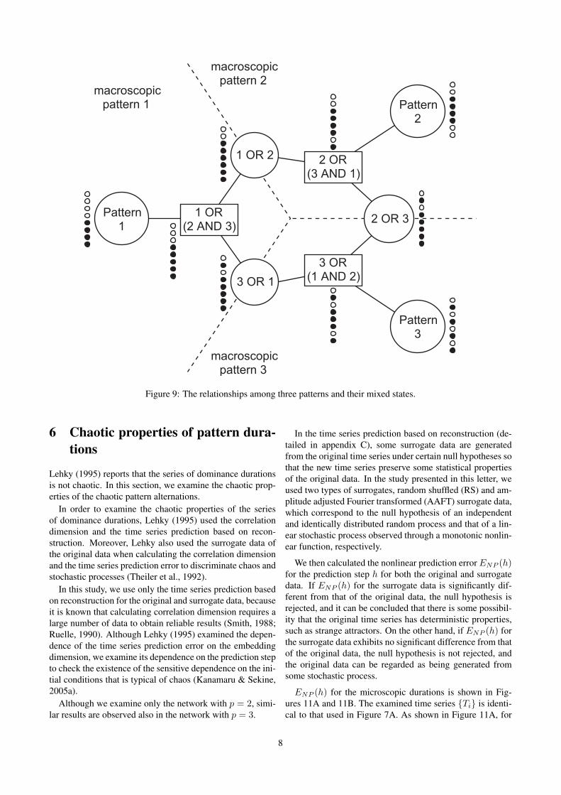
Figure 9: The relationships among three patterns and their mixed states.

6 Chaotic properties of pattern dura-tions

Lehky (1995) reports that the series of dominance durationsis not chaotic. In this section, we examine the chaotic prop-erties of the chaotic pattern alternations.

In order to examine the chaotic properties of the seriesof dominance durations, Lehky (1995) used the correlationdimension and the time series prediction based on recon-struction. Moreover, Lehky also used the surrogate data ofthe original data when calculating the correlation dimensionand the time series prediction error to discriminate chaos andstochastic processes (Theiler et al., 1992).

In this study, we use only the time series prediction basedon reconstruction for the original and surrogate data, becauseit is known that calculating correlation dimension requires alarge number of data to obtain reliable results (Smith, 1988;Ruelle, 1990). Although Lehky (1995) examined the depen-dence of the time series prediction error on the embeddingdimension, we examine its dependence on the prediction stepto check the existence of the sensitive dependence on the ini-tial conditions that is typical of chaos (Kanamaru & Sekine,2005a).

Although we examine only the network with p = 2, simi-lar results are observed also in the network with p = 3.

In the time series prediction based on reconstruction (de-tailed in appendix C), some surrogate data are generatedfrom the original time series under certain null hypotheses sothat the new time series preserve some statistical propertiesof the original data. In the study presented in this letter, weused two types of surrogates, random shuffled (RS) and am-plitude adjusted Fourier transformed (AAFT) surrogate data,which correspond to the null hypothesis of an independentand identically distributed random process and that of a lin-ear stochastic process observed through a monotonic nonlin-ear function, respectively.

We then calculated the nonlinear prediction error ENP (h)for the prediction step h for both the original and surrogatedata. If ENP (h) for the surrogate data is significantly dif-ferent from that of the original data, the null hypothesis isrejected, and it can be concluded that there is some possibil-ity that the original time series has deterministic properties,such as strange attractors. On the other hand, if ENP (h) forthe surrogate data exhibits no significant difference from thatof the original data, the null hypothesis is not rejected, andthe original data can be regarded as being generated fromsome stochastic process.

ENP (h) for the microscopic durations is shown in Fig-ures 11A and 11B. The examined time series {Ti} is identi-cal to that used in Figure 7A. As shown in Figure 11A, for

8

Figure 11: The dependence of the nonlinear prediction error ENP (h) on prediction step h for the time series of (A, B)the microscopic durations, and (C, D) the macroscopic durations. The return plots of {Ti} in the (Ti, Ti+1) plane are alsoshown in the insets. In panels A, C, and D, ENP (h) of the RS and AAFT surrogate data are not significantly different fromthose of the original data. In panel B, ENP (h) of the RS and AAFT surrogate data are significantly different from those ofthe original data, although this is due to alternations between small values and large values.

εIE = 1.6, ENP (h) of the RS and AAFT surrogate dataexhibit no significant difference from those of the originaldata. Therefore, the time series of microscopic durations forεIE = 1.6 is regarded as being generated by some stochasticprocess. This finding supports our previous observation thatthe microscopic durations for εIE = 1.6 seem to be stochas-tic. We also observed no deterministic structures in the returnplot of the time series {Ti}.

As shown in Figure 11B, for εIE = 1.68, ENP (h) ofthe RS and AAFT surrogate data exhibit significant differ-ences from those of the original data. This finding suggeststhat there are some deterministic structures in the originaltime series {Ti}, but that such deterministic structures arenot caused by chaos for two reasons. First, if there is chaos inthe time series, the nonlinear prediction error ENP (h) wouldincrease with increases in the prediction step h because of

the sensitive dependence on the initial condition. However,ENP (h) is almost constant, as shown in Figure 11B. Second,the return plot of {Ti} in the inset reveals that {Ti} tends totake small values and large values alternately. This tendencyis also observed in Figure 7A. This property makes the pre-diction easier, producing small values of ENP (h). There-fore, we conclude that chaos is not observed in the time se-ries {Ti} for εIE = 1.68.

We performed similar analyses for macroscopic durations,the results of which are presented in Figures 11C and 11D.The examined time series {Ti} is identical to that usedin Figure 7B. The nonlinear prediction errors ENP (h) forεIE = 1.6 and 1.68 did not significantly differ from thoseof the original data. Therefore, the time series {Ti} are re-garded as being generated by some stochastic process.

In summary, chaotic properties are not observed in the

9

time series of either microscopic or macroscopic durations.This result suggests that our model is consistent with the re-sults in Lehky (1995).

7 Two properties of the binocular ri-valry

In this section, we show that our model can reproduce twocharacteristics of binocular rivalry.

First, when reducing the contrast of a stimulus to one eye,it is known that dominance intervals in the other eye increaseand dominance intervals in the stimulated eye are relativelyunchanged (Laing & Chow, 2002; Wilson, 2007).

To reproduce this observation, in the network with p = 2,we reduce the contrast of pattern 1, and we observe the meanmacroscopic durations 〈T (1)〉 and 〈T (2)〉 of patterns 1 and2, respectively. The contrast of pattern 1 is defined as thestrength of the the constant inputs to the modules that storethe value 1 for pattern 1. For that purpose, we replace theparameter rE of the modules that store the value 1 for pattern1 with rE + dr

(1)E .

The dependences of 〈T (1)〉 and 〈T (2)〉 on dr(1)E for three

values of εIE are shown in Figure 12A. It is observed that〈T (2)〉 mainly increases and 〈T (1)〉 moderately decreaseswhen decreasing dr

(1)E . Note that the data are not shown

when 〈T (2)〉 diverges for εIE = 1.68.Second, we show that dominance intervals in both eyes

decreases when increasing the contrast of the stimuli to botheyes (Laing & Chow, 2002; Wilson, 2007). For that purpose,we replace the parameter rE of the modules that store thevalue 1 for pattern 1 or 2 with rE + dr

(1,2)E .

The dependences of 〈T (1)〉 and 〈T (2)〉 on dr(1,2)E are

shown in Figure 12B. It is observed that both 〈T (1)〉 and〈T (2)〉 tend to decrease with the increase of dr(1,2)E for threevalues of εIE . Although fluctuation in 〈T (1)〉 and 〈T (2)〉 islarge for εIE = 1.68, it might be because some bifurcationstake place in this range of dr(1,2)E ; however, the tendency for〈T (1)〉 and 〈T (2)〉 to decrease is still observed.

8 ConclusionsWe proposed a pulse neural network that exhibits chaotic pat-tern alternations between two stored patterns as a model ofmultistable perception, which is reflected in such phenomenaas binocular rivalry and perceptual ambiguity.

To measure the durations of each pattern, we introducedtwo durations. The microscopic durations treated the mixedstate as another pattern, while the macroscopic durationstreated the mixed state as part of each pattern.

The distribution of the microscopic durations was char-acterized by a monotonically decreasing function and fol-lowed an exponential distribution for large durations. Onthe other hand, the distribution of the macroscopic durationswas unimodal, following a gamma or log-normal distribu-tion, though the log-normal distribution was associated with

Figure 12: Two characteristics of binocular rivalry. (A)When reducing the contrast dr

(1)E of pattern 1, the mean

macroscopic duration 〈T (2)〉 of pattern 2 increases and themean macroscopic duration 〈T (1)〉 of pattern 1 is relativelyunchanged. (B) When increasing the contrast dr(1,2)E of bothpatterns, the mean macroscopic durations 〈T (1)〉 and 〈T (2)〉of both patterns tend to decrease.

improved fit relative to the gamma distribution. Therefore,we conclude that the macroscopic durations of the chaoticpattern alternations can reproduce the unimodal distributionof dominance durations observed in multistable perception.It is found that the peak position of the distribution dependson the number of mixed patterns and intermodule connectionstrength.

Moreover, we examined the existence of chaotic proper-ties in the time series of durations using a time series pre-diction method based on reconstruction. The results of ouranalysis revealed no chaotic properties for either duration.Therefore, our model is consistent with the previous find-ing that the dominance durations of binocular rivalry are notchaotic, as Lehky (1995) stated.

It was also shown that our model can reproduce two char-acteristics of binocular rivalry. First, when reducing the con-

10

trast of a stimulus to one eye, dominance intervals in theother eye increase and dominance intervals in the stimulatedeye are relatively unchanged (Laing & Chow, 2002; Wilson,2007). Second, when increasing the contrast of the stimuli toboth eyes, dominance intervals in both eyes decrease (Laing& Chow, 2002; Wilson, 2007).

In summary, our network with chaotic pattern alternationscan be regarded as a model of multistable perception.

The absence of chaotic properties in the durations ofchaotic pattern alternations may be due to several reasons.First, the durations are much longer than the time scale ofthe chaotic oscillations. For example, the inter-peak intervalsof the chaotic oscillations in Figure 1E are approximately∆t ' 25. If we analyze the chaotic properties in the timeseries of these inter-peak intervals, chaos is observed (Kana-maru & Sekine, 2005a). However, the durations of chaoticpattern alternations are much longer than those in Figure 3B;therefore, chaos was not observed. This property reflects thefact that our network is composed of pulse neurons and useschaotic synchronization. Second, the absence of chaos maybe related to aspects of chaos theory, which states that in asystem under crisis, the durations of the system that remainsaround the destabilized chaotic attractor obey the exponen-tial distribution, and they have a sensitive dependence on theinitial conditions (Ott, 2002). In our model, the durationsobeying the exponential distributions correspond to the re-sults in Figure 6. The sensitive dependence of the durationson the initial conditions implies that the time series of the du-rations become stochastically independent, and in our model,this fact corresponds to the results in Figures 7, 11A, and11B. The oscillating component in Figure 7A and the deter-ministic properties in Figure 11B are caused by the tendencyto take small values and large values alternatively, and theyare not related to chaos; such deterministic properties disap-pear when the macroscopic durations are used as shown inFigures 7B and 11D.

Finally, we state the difference between our model andNagao’s chaotic associative memory model (Nagao et al.,2000). First, Nagao’s model is composed of conventionalneuronal models based on firing rates, and our model is com-posed of the pulse neurons. Second, the used patterns havedifferent structures. Nagao et al.’s model uses two patternsmade by perturbing an original pattern; therefore, their pat-terns are correlated with each other, while our patterns areorthogonal to each other. Their unperturbed original patternswould correspond to our mixed states. The reason why ourmodel can reproduce the unimodal distribution of the dom-inance duration without the unperturbed pattern would bebecause our pattern is composed of 0/1 digits, while Na-gao’s model uses −1/1 digits. In order to store the pat-terns composed of 0/1 digits into a pulse neural network,we used connection strengths defined by equations 3.3 to 3.5that were modified from the original Hebb rule (Kanamaru,2007). With such modified connection strengths, our modelcan easily increase the number of mixed states by increasingthe number of stored patterns, and by this fact, the peak po-sition of the distribution of the dominance duration can bechanged as shown in Figure 10.

A Fokker-Planck equationTo analyze the average dynamics of the one-module system,we used the Fokker-Planck equations (Gerstner & Kistler,2002), which are written as

∂nE

∂t= − ∂

∂θE(AEnE)

+D

2

∂

∂θE

{BE

∂

∂θE(BEnE)

}, (A.1)

∂nI

∂t= − ∂

∂θI(AInI)

+D

2

∂

∂θI

{BI

∂

∂θI(BInI)

}, (A.2)

AE(θE , t) = (1− cos θE) + (1 + cos θE)

×(rE + gintIE(t)− gextII(t)),(A.3)AI(θI , t) = (1− cos θI) + (1 + cos θI)

×(rI + gextIE(t)− gintII(t)), (A.4)BE(θE , t) = 1 + cos θE , (A.5)BI(θI , t) = 1 + cos θI , (A.6)

for the normalized number densities of excitatory and in-hibitory ensembles, in which

nE(θE , t) ≡ 1

NE

∑δ(θ

(i)E − θE), (A.7)

nI(θI , t) ≡ 1

NI

∑δ(θ

(i)I − θI), (A.8)

in the limit of NE , NI → ∞. The probability flux for eachensemble is defined as

JE(θE , t) = AEnE − D

2BE

∂

∂θE(BEnE), (A.9)

JI(θI , t) = AInI −D

2BI

∂

∂θI(BInI), (A.10)

respectively. The probability flux at θ = π can be interpretedas the instantaneous firing rate in this ensemble, which isdenoted as JX(t) ≡ JX(π, t) where X = E or I .IX(t) in equation 2.3 follows a differential equation that

is written as

˙IX(t) = − 1

κX

(IX(t)− 1

2JX(t)

). (A.11)

In order to integrate the Fokker-Planck equations (A.1)and (A.2) numerically, we expanded nE(θE , t) and nI(θI , t)into Fourier series as

nE(θE , t) =1

2π

+

∞∑k=1

(aEk (t) cos(kθE) + bEk (t) sin(kθE)), (A.12)

nI(θI , t) =1

2π

+∞∑k=1

(aIk(t) cos(kθI) + bIk(t) sin(kθI)), (A.13)

11

and, by substituting them, equations A.1 and A.2 were trans-formed into a set of ordinary differential equations of aXk andbXk , which are written as

da(X)k

dt= −(rX + IX + 1)kb

(X)k

−(rX + IX − 1)k

2(b

(X)k−1 + b

(X)k+1)

−Dk

8g(a

(X)k ), (A.14)

db(X)k

dt= (rX + IX + 1)ka

(X)k

+(rX + IX − 1)k

2(a

(X)k−1 + a

(X)k+1)

−Dk

8g(b

(X)k ) (A.15)

g(xk) = (k − 1)xk−2 + 2(2k − 1)xk−1 + 6kxk

+2(2k + 1)xk+1 + (k + 1)xk+2, (A.16)IE ≡ gintIE − gextII , (A.17)II ≡ gextIE − gintII , (A.18)

a(X)0 ≡ 1

π, (A.19)

b(X)0 ≡ 0, (A.20)

where X = E or I . By integrating the ordinary differentialequations (A.11), (A.14), and (A.15) numerically, the timeseries of the probability fluxes JE and JI are obtained. Fornumerical calculations, each Fourier series was truncated atthe first 40 terms.

B Definition of overlap

In this section, we provide a method for calculating the over-lap mµ between a set of instantaneous firing rates JEi ofexcitatory neurons in a module (1 ≤ i ≤ M) and the storedpattern ηµi .

Because JEi is an oscillating quantity, the overlap of theusual definition is also oscillating, even when the correct pat-tern is retrieved. To obtain an overlap that maintains an al-most constant value when the correct pattern is retrieved, wedefined a peak-value function PEi(t) as PEi(t) = JEi(t

∗),where t∗ is the nearest time point that gives a peak of JEi(t)and satisfies t∗ < t. We then transformed PEi(t) to functionOEi(t) with a range of [0,1]:

OEi(t) =

1 (PEi(t) > θ2)PEi(t)− θ1θ2 − θ1

(θ1 ≤ PEi(t) ≤ θ2)

0 (PEi(t) < θ1)

, (B.1)

where θ1 = 0.01 and θ2 = 0.1. Using OEi(t), the overlapmµ between the state of the network and the stored pattern

ηµi is defined as

mµ =1

Ma(1− a)

M∑i=1

(ηµi − a)(OEi − a), (B.2)

=1

Ma(1− a)

M∑i=1

(ηµi − a)OEi. (B.3)

C Nonlinear prediction based on re-construction

In this section, the nonlinear prediction method based onreconstruction of dynamics is summarized (Theiler et al.,1992; Sauer, 1994).

Let us consider a sequence {Tk} of the durationof patterns and the delay coordinate vectors Vj =(Tj−m+1, Tj−m+2, . . . , Tj) with the reconstruction dimen-sion m, and let L be the number of vectors in the recon-structed phase space Rm. For a fixed integer j0, we chosel = βL (β < 1) points that are nearest to the point Vj0 anddenoted them by Vjk = (Tjk−m+1, Tjk−m+2, . . . , Tjk)(k =1, 2, . . . , l). With {Vjk}, a predictor of Tj0 for h steps aheadis defined as

pj0(h) =1

l

l∑k=1

Tjk+h. (C.1)

With pj0(h), the normalized prediction error (NPE) is de-fined as

ENP (h) =〈(pj0(h)− Tj0+h)

2〉1/2

〈(〈Tj0〉 − Tj0+h)2〉1/2, (C.2)

where 〈·〉 denotes the average over j0. A small value of NPEi.e., less than 1, implies that the sequence has determinis-tic structure behind the time series because this algorithm isbased on the assumption that the dynamical structure of afinite-dimensional deterministic system can be well recon-structed by the delay coordinates of the sequence (Sauer,1994). However, stochastic time series with large autocor-relations can also take NPE values less than 1. Therefore,we could not conclude that there is deterministic structureonly from the magnitude of NPE.

To confirm the deterministic structure, the values of NPEshould be compared with those of NPE for a set of surrogatedata (Theiler et al., 1992). The surrogate data used in thepresent study were new time series generated from the orig-inal time series under some null hypotheses so that the newtime series preserve some statistical properties of the origi-nal data. In the present study, we used random shuffled (RS)and amplitude adjusted Fourier transformed (AAFT) surro-gate data, which correspond to the null hypothesis of an inde-pendent and identically distributed random process and thatof a linear stochastic process observed through a monotonicnonlinear function, respectively. To obtain AAFT surrogatedata, we used TISEAN 3.0.1 (Hegger, Kantz, & Schreiber,1999; Schreiber & Schmitz, 2000). If the values of NPE forthe original data are significantly smaller than those of NPE

12

for the surrogate data, the null hypothesis is rejected, and itcan be concluded that there is some possibility that the orig-inal time series has deterministic structure.

ReferencesAdachi, M., & Aihara, K. (1997). Associative dynamics in a

chaotic neural network. Neural Networks, 10, 83 – 98.

Aihara, K., Takabe, T., & Toyoda, M. (1990). Chaotic neuralnetworks. Physics Letters A, 144, 333 – 340.

Alais, D., & Blake, R. (2015). Binocular rivalry and per-ceptual ambiguity. In J. Wagemans (Eds.), The OxfordHandbook of Perceptual Organization, Oxford UniversityPress.

Blake, R. (2001). A primer on binocular rivalry, includingcurrent controversies. Brain and Mind, 2, 5 – 38.

Borsellino, A., Marco, A. De, Alliazetta, A., Rinesi, S., &Bartolini, B. (1972). Reversal time distribution in the per-ception of visual ambiguous stimuli. Kybernetik, 10, 139– 144.

Ermentrout, B. (1996). Type I membranes, phase resettingcurves, and synchrony. Neural Computation, 8, 979 –1001.

Ermentrout, G. B., & Kopell, N. (1986). Parabolic burst-ing in an excitable system coupled with a slow oscillation.SIAM Journal on Applied Mathematics, 46, 233 – 253.

Freeman, A. W. (2005). Multistage model for binocular ri-valry. Journal of Nueorophysiology, 94, 4412 – 4420.

Gerstner, W., & Kistler, W. (2002). Spiking Neuron Models.Cambridge: Cambridge Univ. Press.

Hebb, D. O. (1949). The Organization of Behavior – a neu-ropsychological theory. New York: John Wiley.

Hegger, R., Kantz, H., & Schreiber, T. (1999). Practicalimplementation of nonlinear time series methods: TheTISEAN package. Chaos, 9, 413 – 435.

Hopfield, J. J. (1982). Neural networks and physical systemswith emergent collective computational properties. Proc.Nat. Acad. Sci. (USA), 79, 2554 – 2558.

Inoue, M., & Nagayoshi, A. (1991). A chaos neuro-computer. Physics Letters A, 158, 373 – 376.

Izhikevich, E. M. (1999). Class 1 neural excitability, conven-tional synapses, weakly connected networks, and math-ematical foundations of pulse-coupled models. IEEETransactions on Neural Networks, 10, 499 – 507.

Izhikevich, E. M. (2000). Neural excitability, spiking andbursting. International Journal of Bifurcation and Chaos,10, 1171 – 1266.

Kanamaru, T. (2007). Chaotic pattern transitions in pulseneural networks. Neural Networks, 20, 781 – 790.

Kanamaru, T., Fujii, H., & Aihara, K. (2013). Deformationof attractor landscape via cholinergic presynaptic modula-tions: A computational study using a phase neuron model.PLOS ONE, 8, e53854.

Kanamaru, T., & Sekine, M. (2005a). Detecting chaoticstructures in noisy pulse trains based on interspike intervalreconstruction. Biological Cybernetics, 92, 333 – 338.

Kanamaru, T., & Sekine, M. (2005b). Synchronized firingsin the networks of class 1 excitable neurons with excita-tory and inhibitory connections and their dependences onthe forms of interactions. Neural Computation, 17, 1315-1338.

Kimoto, T., & Okada, M. (2001). Mixed state on a sparselyencoded associative memory model. Biological Cybernet-ics, 85, 319 – 325.

Laing, C. R., & Chow, C. C. (2002). A spiking neuron modelfor binocular rivalry. Journal of Computational Neuro-science, 12, 39 – 53.

van Leeuwen, C., Steyvers, M., & Nooter, M. (1997). Sta-bility and intermittency in large-scale coupled oscillatormodels for perceptual segmentation. Journal of Mathe-matical Psychology, 41, 319 – 344.

Lehky, S. R. (1988). An astable multivibrator model ofbinocular rivalry. Perception, 17, 215 – 228.

Lehky, S. R. (1995). Binocular rivalry is not chaotic. Pro-ceedings of the Royal Society of London B, 259, 71 – 76.

Levelt, W. J. M. (1967). Note on the distribution of domi-nance times in binocular rivalry. British Journal of Psy-chology, 58, 143 – 145.

Logothestis, N. K., Leopold, D. A., & Sheinberg, D. L.(1996). What is rivalling during binocular rivalry? Na-ture, 380, 621 – 624.

Murata, T., Matsui, N, Miyauchi, S., Kakita, Y., & Yanagida,T. (2003). Discrete stochastic process underlying percep-tual rivalry. Neuroreport, 14, 1347 – 1352..

Nagao, N., Nishimura, H., & Matsui, N. (2000). A neuralchaos model of multistable perception. Neural ProcessingLetters, 12, 267 – 276.

Nara, S., & Davis, P. (1992). Chaotic wandering and searchin a cycle-memory neural network. Progress of Theoreti-cal Physics, 88, 845 – 855.

Ott, E. (2002). Chaos in Dynamical Systems. (2nd ed.). NewYork: Cambridge University Press.

Ruelle, D. (1990). The Claude Bernard lecture, 1989. Deter-ministic chaos: the science and the fiction. Proc. R. Soc.Lond. A, 427, 241 – 248.

13

Sauer, T. (1994). Reconstruction of dynamical systems frominterspike interval. Rhys. Rev. Lett, 72, 3811 – 3814.

Schreiber, T., & Schmitz, A. (2000). Surrogate time series.Physica D, 142, 346 – 382.

Smith, L. A. (1988). Intrinsic limits on dimension calcula-tions. Physics Letters A, 133, 283 – 288.

Theiler. J., Eubank. S., Longtin. A., Galdrikian. B., &Farmer. J. D. (1992). Testing for nonlinearity in time se-ries: the method for surrogate data. Physica D, 58, 77 –94.

Tsuda, I. (1992). Dynamic link of memory – Chaotic mem-ory map in nonequilibrium neural networks. Neural Net-works, 5, 313 – 326.

Walker, P. (1975). Stochastic properties of binocular rivalryalternations. Perception & Psychophysics, 18, 467 – 473.

Wilson, H. R. (2003). Computational evidence for a rivalryhierarchy in vision. PNAS, 100, 14499 – 14503.

Wilson, H. R. (2007). Minimal physiological conditions forbinocular rivalry and rivalry memory. Vision Research, 47,2741 – 2750.

14