Chaos Theory and the Mandelbrot Set

Chaos Theory and the Mandelbrot Set

An Honors Thesis (HONRS 499)

by

Samuel Hartman

Thesis Advisor

Dr. Rich Stankewitz

Ball State University

Muncie, Indiana

May 2005

Date of Graduation

May 7, 2005

Abstract

In this thesis I study two main ideas: Chaos Theory and the Mandelbrot Set. Chaos

Theory is a relatively new field of science that is revolutionizing the way we look at

predictability and randomness. The Mandelbrot Set is a spectacular image generated by looking

at a somewhat universal class of functions. First, I give a brief history of Chaos Theory, looking

at three people who helped develop it. Then, for the second part of this thesis, I explore the

mathematics behind the Mandelbrot set and explain some interesting properties of it, in

particular, the regions corresponding to fixed points, two-, and three-cycles. I conclude by stating

two theories about the set that have not been able to be proven mathematically.

Acknowledgements

I would like to thank Dr. Rich Stankewitz for his guidance throughout this research

project.

2

Table of Contents

• Section 1: Chaos Theory

o 1.1 What is Chaos Theory?

o 1.2 Why is Chaos Theory Important?

o 1.3 Edward Lorenz

o 1.4 Benoit M. Mandelbrot

o 1.5 Mitchell 1. Feigenbaum

• Section 2: The Mandelbrot Set

o 2.1 Complex Numbers

o 2.2 Iteration, Fixed Points, and Cycles

o 2.3 Definition of the Mandelbrot Set M

o 2.4 Regions of Fixed Points and Cycles in M

o 2.5 The Bifurcation Diagram

o 2.6 Finding M Elsewhere

• Conclusion

• References

• Figure Credits

• Appendix A

3

Section 1: Chaos Theory

1.1 What is Chaos Theory?

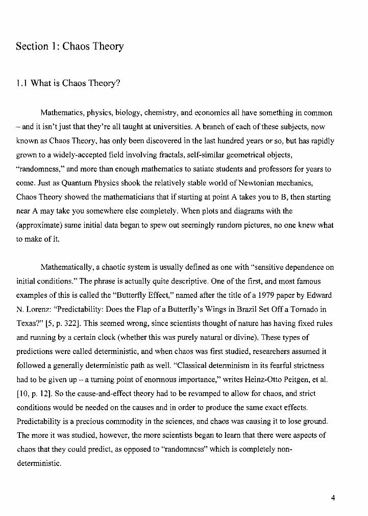
Mathematics, physics, biology, chemistry, and economics all have something in common

- and it isn't just that they're all taught at universities. A branch of each of these subjects, now

known as Chaos Theory, has only been discovered in the last hundred years or so, but has rapidly

grown to a widely·accepted field involving fractals, self·similar geometrical objects,

"randomness," and more than enough mathematics to satiate students and professors for years to

come. Just as Quantum Physics shook the relatively stable world of Newtonian mechanics,

Chaos Theory showed the mathematicians that if starting at point A takes you to B, then starting

near A may take you somewhere else completely. When plots and diagrams with the

(approximate) same initial data began to spew out seemingly random pictures, no one knew what

to make of it.

Mathematically, a chaotic system is usually defined as one with "sensitive dependence on

initial conditions." The phrase is actually quite descriptive. One of the first, and most famous

examples of this is called the "Butterfly Effect," named after the title of a 1979 paper by Edward

N. Lorenz: "Predictability: Does the Flap of a Butterfly's Wings in Brazil Set Off a Tornado in

Texas?" [5, p. 322]. This seemed wrong, since scientists thought of nature has having fixed rules

and running by a certain clock (whether this was purely natural or divine). These types of

predictions were called deterministic, and when chaos was first studied, researchers assumed it

followed a generally deterministic path as well. "Classical determinism in its fearful strictness

had to be given up - a turning point of enormous importance," writes Heinz·Otto Peitgen, et al.

[10, p. 12]. So the cause-and·effect theory had to be revamped to allow for chaos, and strict

conditions would be needed on the causes and in order to produce the same exact effects.

Predictability is a precious commodity in the sciences, and chaos was causing it to lose ground.

The more it was studied, however, the more scientists began to learn that there were aspects of

chaos that they could predict, as opposed to "randomness" which is completely non­

deterministic.

4

To see the difference between chaos and randomness, examine a coin-tossing experiment.

A coin is flipped once and it produces heads. Now, on the second flip, most would describe it as

"random"-no possible way to know the outcome. But many things are different with this

second trial: the time, the wind speed, the position of the coin and the hand, etc. Randomness

occurs only if a trial is repeated with exactly the same initial conditions, and a different result

appears. Clearly, the trial is not the same. We could theoretically predict the outcome because the

coin flip is deterministic, i.e., the future is completely determined by the past. So why can we not

predict exactly what the coin will do? Chaos, of course. Trying to theorize that flipping the coin

with an angle of forty-five degrees at two meters per second will make it show heads won't

work, because of the infallibility of humans. Just a slight change in the angle or speed (or

anything else, really) may cause the coin to do something different. This sensitive dependence on

initial conditions (angle, speed, wind speed) is the heart of chaos.

1.2 Why is Chaos Theory Important?

An honest question, usually asked by entrepreneurs ("how will it make me money?") and

doctors ("how it will save more lives?") more than mathematicians, is of what value Chaos

Theory really has. In its previous studies, Chaos Theory has shown us that the weather moving

around the country or water flowing turbulently in a pipe cannot be precisely modeled without

taking into account the quirks of chaos. Ian Stewart, author of Does God Play Dice? The New

Mathematics of Chaos, explains several applications of Chaos Theory:

Current commercial applications of chaos and fractals include a chaos-theoretic

method for extracting meaningful conversations from recordings made in a noisy

room. There are commercial companies that employ chaos-theoretic data analysis

to advise investment banks on market movements. There are chaos-theoretic

studies of wear on train wheels. One Japanese company has discovered that

dishwashers are more effective if their rotor arms move chaotically. [12, p. 297]

In the 1980's researchers found that the heartbeat pattern of humans had a similarity to chaotic

behavior, and quickly studies were done to see how it could help heart patients. Cardiologist

5

Richard 1. Cohen [5, p. 290] wrote, " ... [the heart activity] becomes chaotic, and it turns out that

the electrical activity in the heart has many parallels with other systems that develop chaotic

behavior." Recent studies show that this is correct, as Federico Lombardi [7] writes in the

Circulation heart journal: "Later, it was proposed that the fluctuations of heartbeats during

normal sinus rhythm could be partially attributed to deterministic chaos and that a decrease in

this type of nonlinear variability could be observed in different cardiovascular diseases and

before ventricular fibrillation."

Chaos Theory even helped ecologist William M. Schaffer predict when chicken pox and

measles will strike a group of children, and did so with strikingly predictability [5, p. 315-316].

The development of Chaos Theory has a relatively short past, since its discovery (or invention,

depending on how one views it) in the past hundred years. One of the first scientists to discover a

chaotic phenomenon was a man by the name of Edward N. Lorenz.

1.3 Edward N. Lorenz

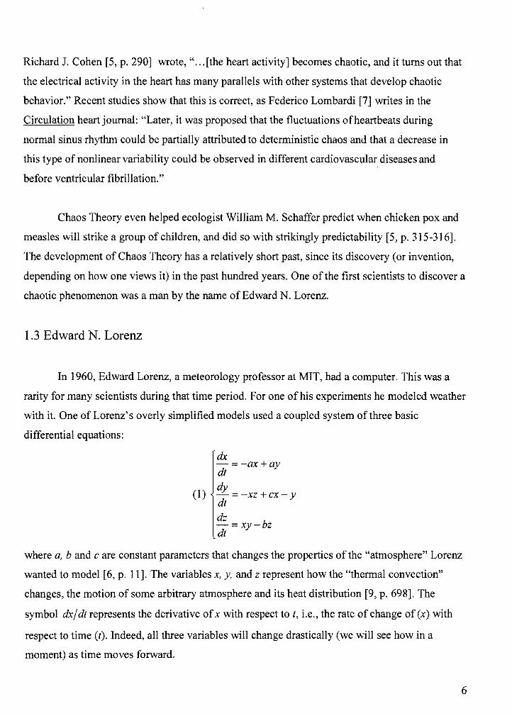
In 1960, Edward Lorenz, a meteorology professor at MIT, had a computer. This was a

rarity for many scientists during that time period. For one of his experiments he modeled weather

with it. One of Lorenz's overly simplified models used a coupled system of three basic

differential equations:

dx

dt ::= -ax +ay

(1) dy -::=-xz+cx y dt dz -::= xy-bz dt

where a, b and c are constant parameters that changes the properties of the "atmosphere" Lorenz

wanted to model [6, p. 11]. The variables x, y, and z represent how the "thermal convection"

changes, the motion of some arbitrary atmosphere and its heat distribution [9, p. 698]. The

symbol dx/ dt represents the derivative of x with respect to t, i.e., the rate of change of (x) with

respect to time (I). Indeed, all three variables will change drastically (we will see how in a

moment) as time moves forward.

6

According to Gleick (who interviewed Lorenz), Lorenz wanted to start a simulation of

this system in the middle to see the results, instead of starting at the beginning and having to wait

while the system ran through the entire process. A system of differential equations requires three

starting values (initial conditions), say xo'yo'zo and Lorenz typed this in from earlier data he

had generated. When he returned from getting a cup of coffee, writes Gleick, he saw a radically

divergent picture - the weather had ceased to follow the path it should have [5, p. 15-16].

Lorenz soon realized his mistake - he only typed in the initial data to three decimal places, when

the computer output stored it to six. To the layperson, writing "0.366" instead of"0.3659140" is

perfectly acceptable, but when dealing with these sensitive dynamical systems, exactness is key.

Stephen H. Kellert, author of In the Wake of Chaos, details this phenomenon:

The behavior is quite complicated but is entirely governed by the differential

equations. However, if you were to start with a slightly different trio of initial

conditions, say Xo + O.OOOI,yo, and ZO' the solution would become substantially

different in only a short time. The behavior would still be rotational convection

[of the weather] first in one direction then another, but the states of the two

systems, which initially were extremely similar, will rapidly diverge. [6, p. 11-12]

This electrifying new concept is what became known as the Butterfly Effect, or, "sensitive

dependence on initial conditions." But Lorenz reasoned that this activity was necessary, not just

surprising. If the Butterly Effect wasn't around, then weather conditions that remained close to

one another would stay close to one another, and it would be an incredibly cyclic behavior­

weather forecasting would as simple as solving some relatively easy equations. But to produce

the "rich repertoire of real earthly weather, the beautiful multiplicity of it, you could hardly wish

for anything better than the Butterfly Effect," writes Gleick [5, p. 23].

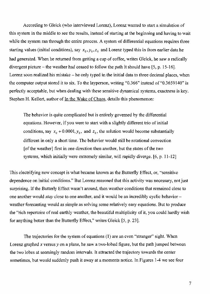
The trajectories for the system of equations (1) are an even "stranger" sight. When

Lorenz graphed x versus y on a plane, he saw a two-lobed figure, but the path jumped between

the two lobes at seemingly random intervals. It attracted the trajectory towards the center

sometimes, but would suddenly push it away at a moments notice. In Figures 1-4 we see four

7

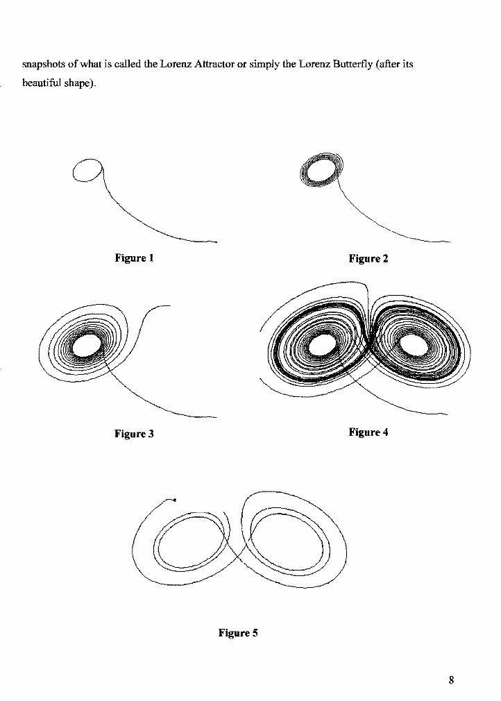
snapshots of what is called the Lorenz Attractor or simply the Lorenz Butterfly (after its

beautiful shape).

Figure 1 Figure 2

Figure 3 Figure 4

Figure 5

8

Moreover, observe in Figure 5 what happens when we place two trajectories on the same plane,

with very similar starting values (the small black dot). While their paths seem to follow along

closely for a period of time, they soon diverge from each other sharply, the green line spiraling

around the right side while the red line moves around the left. Even though the lines move about

chaotically, wherever they start they are always attracted towards the center of each lobe.

Lorenz's attractor became known as one type of a "strange attractor" - a chaotic attractor that

exhibited a fractal like structure.

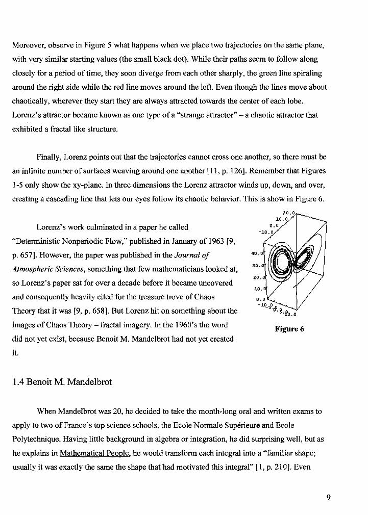
Finally, Lorenz points out that the trajectories cannot cross one another, so there must be

an infmite number of surfaces weaving around one another [11, p. 126]. Remember that Figures

1-5 only show the xy-plane. In three dimensions the Lorenz attractor winds up, down, and over,

creating a cascading line that lets our eyes follow its chaotic behavior. 1bis is show in Figure 6.

Lorenz's work culminated in a paper he called

"Deterministic Nonperiodic Flow," published in January of 1963 [9,

p. 657]. However, the paper was published in the Journal of

Atmospheric Sciences, something that few mathematicians looked at,

so Lorenz's paper sat for over a decade before it became uncovered

and consequently heavily cited for the treasure trove of Chaos

Theory that it was [9, p. 658]. But Lorenz hit on something about the

images of Chaos Theory - fractal imagery. In the 1960's the word

did not yet exist, because Benoit M. Mandelbrot had not yet created

it.

1.4 Benoit M. Mandelbrot

Figure 6

When Mandelbrot was 20, he decided to take the month-long oral and written exams to

apply to two of France's top science schools, the Ecole Normale Superieure and Ecole

Polytechnique. Having little background in algebra or integration, he did surprising well, but as

he explains in Mathematical People, he would transform each integral into a "familiar shape;

usually it was exactly the same the shape that had motivated this integral" [1, p. 210]. Even

9

before attending college, Mandelbrot was on the way to seeing the world through geometry. He

discovered amazing self-similar objects with infinite complexity through economics and

mathematical analysis. Mandelbrot called these beautiful geometric figures "fractals."

One of Mandelbrofs first explanations of fractals is a semi-rhetorical question he posed

to the mathematical community. Here he explains it: "The question I raised in 1967 is, 'how long

is the coast of Britain,' and the correct answer is 'it all depends.' It depends on the size of the

instrument used to measure length" [1, p. 215]. Gleick explicates this hypothesis in more detail

in his book:

A surveyor takes a set of dividers, opens them to a length of one yard, and walks

them along the coastline. The resulting number of yards is just an approximation

of the true length, because the dividers skip over twists and turns smaller than one

yard, but the surveyor writes down the number anyway. Then he sets the dividers

to a smaller length-say, one foot-and repeats the process. He arrives at a

somewhat greater length, because the dividers will capture more of the details and

it will take more than three one-foot steps to cover the distance previously

covered by the one-yard step. [5, p.96]

Obviously, measuring with an even smaller interval would yield a large estimate, and so on. This

leads to the strange conclusion that the coast might have an infinite length, as the length seems to

grow without bound. Does that mean that no ship will ever be able to sail around the country,

since its perimeter is infinitely long? Of course not - but it calls into question the way in which

we analyze length, and how "zooming in" affects our measurements. Mandelbrot extended this

idea to create a fractal that represented the coastline. This is an object that seems to have the

same curves, bays, and inlets as some arbitrary coast, but upon looking closely with a

microscope or computer, more complexity is revealed. In Figure 7 we see a jagged coastline with

an area boxed in for more detail. The panel to the right shows the box, but zooming in to the next

box (the far right panel) we see even further complexity. This map travels in a loop, so the last

zoom from the bottom left panel takes us back to the beginning.

10

Figure 7

Mandelbrot decided to call an object like this a fractal, from the Latin word "fractus" to

break and its English counterparts "fracture" and "fraction" [5, p. 98]. While the word was new,

the concept was not. Helge Von Koch, a Swedish mathematician, had created a fractal object in

1904, now known as the Koch Snowflake (Figure 8). Another example is the infinitely complex

Menger Sponge (Figure 9) [5, p. 99-101].

\ f

:>

) \/

Figure 8

11

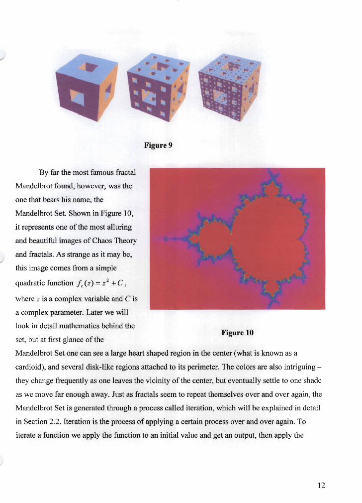
By far the most famous fractal

Mandelbrot found, however, was the

one that bears his name, the

Mandelbrot Set. Shown in Figure 10,

it represents one of the most alluring

and beautiful images of Chaos Theory

and fractals. As strange as it may be,

this image comes from a simple

quadratic function Ie (z) = Z 2 + C ,

where z is a complex variable and C is

a complex parameter. Later we will

look in detail mathematics behind the

set, but at first glance of the

Figure 9

Figure 10

Mandelbrot Set one can see a large heart shaped region in the center (what is known as a

cardioid), and several disk-like regions attached to its perimeter. The colors are also intriguing ­

they change frequently as one leaves the vicinity ofthe center, but eventually settle to one shade

as we move far enough away. Just as fractals seem to repeat themselves over and over again, the

Mandelbrot Set is generated through a process called iteration, which will be explained in detail

in Section 2.2. Iteration is the process of applying a certain process over and over again. To

iterate a function we apply the function to an initial value and get an output, then apply the

12

function to the previously outputted value, and so on. This process can go on indefinitely. Here

Mandelbrot describes how he came to this wonderful set:

A few months of mindless fun with complicated mappings had prepared me for a

detailed study of iteration. The best was to start with the simplest mapping, which

is the second order polynomial. There is only one significant parameter, and to

each parameter corresponds a Julia set. [1, p. 220].

The Mandelbrot Set categorizes certain values of C that correspond to certain be behaviors of Ie .

For instance, the largest region in the set corresponds to all values of C that make Ie have an

"attracting fixed point." The Mandelbrot Set is connected, meaning you can travel from any

point inside it to another without going outside the set. But there is much to learn about this

spectacle, and the concept of cycles and period doubling are needed to do so. That is exactly

where Mitchell Feigenbaum comes in.

1.5 Mitchell J. Feigenbaum

Mitchell Feigenbaum was a physicist working on something that no one really knew

about. He came to Los Alamos Laboratory in the 1970's to work on nonlinear dynamical

problems. But he soon got caught up in a problem that would earn him a place in mathematical

history [11,p. 184].

Like Mandelbrot, Feigenbaum came to work with functions and their iterations, but by

this time, things called two-cycles, four-cycles, and "period doubling" were being studied.

Feigenbaum initially worked with the function Ik (x)::: kx(1- x), where k is a constant that can

vary from 0 to 4. With some values of k we have a fixed point, which is a stable solution. After

so many iterations, say 1000, the value stays the same each time. As we increase k we see that

"cycles" begin to arise. For certain values of k, when the function is iterated, a "two-cycle"

appears which means that values go back and forth from one point to the other. But when a cycle

happens, the sequence of outputs will never settle down. But most iterative functions are not

13

limited to two-cycles. They can have three-cycles, eight-cycles, nineteen-cycles, or thirty-seven­

cycles. But (as will be shown in a theorem later) the first and easiest cycles to calculate are the

2n -cycles-two, four, eight, sixteen, etc. These were the cycles that Feigenbaum first started

finding k values for in the function fk (x) = kx(l- x). These different k values and the

corresponding cycles can be mapped in something called a "bifurcation diagram," or, more

easily understood, a "fig-tree" graph. (Author Ian Stewart uses this phrase extensively since the

name Feigenbaum is German for "fig-tree" [11, p. 152].) In Figure 11, the fig-tree graph shows

us exactly what is meant by period dOUbling. Each time the tree splits into a new "branch," a new

cycle appears. First the two-cycle, then the four-cycle, and so on. Also note the fractal-like

nature in the self-similarity of the diagram-the dotted line showing how the graph repeats itself.

I /

'" I I ,

Figure 11

What Feigenbaum saw was that there was a specific relation between the values of k that

allowed him to predict where the branching would occur. This by itself wasn't too revolutionary,

14

but when he examined other iterative functions, such as /k (x) = k sin x , he saw this same relation

appear! This was groundbreaking, and it happened all by Feigenbaum's slow, careful

calculations on an old programmable calculator. Stewart suggests it was this lack of speed that

allowed Feigenbaum time to theorize and understand this phenomenon [11, p.I85-186]. Stewart

[11, p. 186] summarizes the constant that Feigenbaum stumbled across:

Feigenbaum had discovered evidence that, at the utmost tips of the fig-tree, there

must be some mathematical structure that remains the same when its size is

changed by a scaling factor of 4.669. This structure is the shape o/the fig-tree

itself. The steady attractor forms the trunk. The period-2 attractors [cycles] form

two shorter boughs. From these sprout even shorter period-4 branches, then

period-8 twigs, period-16 twiglets, and so on. The size-ratios ofthe trunk to

bough, bough to branch, branch to twig, twig to twiglet, get closer and close and

closer to 4.669, the nearer you get to the top of the tree.

Letting kn represent the k value where the nth-cycle starts, this "relation" that gives us the

Feigenbaum constant is approximately on = (kn+l kn )/(kn+2 - kn+1) • However, for the first few

cycles: two, four, eight, and so forth, the approximation of the constant, usually denoted by on' is fairly inaccurate. But once we begin to look at larger cycles, the 32, 64, and the 128-cycle, we

see that on converges toward ° = 4.669201609 ... , which is now called Feigenbaum's Constant.

This constant brings about the notation of universality, since it appears in so many different

systems, not just the system/k(x) = kx(1-x). Gleick writes that the day Feigenbaum stumbled

across this value, "for a variety of functions, he had calculated his constant to five decimals

places, 4.66920" [5, p. 173]. Clearly, 0 was of severe importance. But how is 0 related to the

Mandelbrot Set, and what about the cycles of length seven, or seventeen? To answer these

questions, some background material in imaginary numbers and iterative functions is needed; but

there are answers out there, as well as further analysis into the imagery of chaos.

15

Section 2: The Mandelbrot Set

2.1 Complex Numbers

The complex set of numbers C contains all numbers of the form z = x + yi , where

x, y E R, R being the set of all real numbers, and i = .J=l. Note that i2 = (.J=lj -1,

i3 = -1· i -i, and i4 = i . (-i) = _i2 = 1. Plotting complex numbers is very similar to plotting

Cartesian coordinates, using x as the x-value and y as the y-value. However, plotting numbers in

the form a + hi becomes troublesome sometimes, so an exponential notation is frequently used.

Recall that to convert a point (x,y) from Cartesian coordinates to polar coordinates, we use the

relations

x = rcosB

y rsinB

where r is the distance from the origin to the point and B is the angle measured counter­

clockwise from the positive x-axis to the line segment connecting the origin and the point. If a

complex number is written as z = x + iy , it can be re-written as z = r cos B + (r sin B)i . In order to

transform this into an exponential form, we need to use the Euler Formula, which states that

e if) :::: cos B + i sin B . Thus, we have:

z = rcosB+(rsinB)i

z::::r(cosB+isinB)

z = rei().

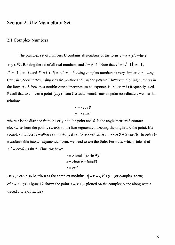
Here, r can also be taken as the complex modulus Izi = r ~X2+y2 (or complex norm)

of z = x + yi . Figure 12 shows the point z = x + yi plotted on the complex plane along with a

traced circle of radius r.

16

I , I

; I

; ;

'" "

v

- - - -, :r + i \' ... .

, , \

\

-,..-------+-..:.:....-~----- X

\ , \

, , ... --~

Figure 12

I I

;

I I

I I

In our quest to find fixed points we will need the following definition regarding complex

nwnbers:

Definition: If z = x + yi E C, then the complex conjugate z is defined as z = x - yi.

2.2 Iteration, Fixed Points, and Cycles

We now take an in-depth look into what is meant by "iterating" a function. Letf be a

real-valued function that "maps" from R to R. This is denoted as f : R ~ R , meaning

if f(x) = y, thenx,y E R . Given some initial value, say xo' we apply fto this value once, and

call the result Xl' i,e., f(xo) = Xl ' Now, we apply the functionfto Xl' and continue the process:

f(x l ) = x2 • Notice that since f(xo) = Xl' X 2 can be written as X 2 = f(x l ) = f(f(xo». Iteration

is the process of applyingfto a value over and over again. It can be written as a relation in the

following way:

Xo

f(xo) = Xl

f(x l ) = X 2

f(xn- l ) = XII'

17

To put it another way, xn = fn (Xo) , where fn (z) = f(f( .... f(z))) . '-----v---'

ntimes

Before we begin talking about iteration and what are known as fixed points, let us make

the ')ump" from real-valued functions to complex-valued ones. A complex valued function maps

from the complex plane to the complex plane, i.e., f: C ~ C. We will use the variable z to

denote a complex number, where z = x + iy = re i8 • Iterating with complex functions works just

the same as with real-valued functions, f(zo) = Zj' f(zj) = Z2' etc.

The process of iteration leads to a particular aspect of functions-that of a fixed point. A

fixed point is a value that after one iteration, does not change. The best way to see this is through

the use of some examples. Let fez) = Z2. Note thatf(O) = O. We call z = 0 a fixed point of

fez) = Z2 • Now let fez) = Z2 + 0.2. Below is a table, starting with Zo = 0, of the iterations of f

to four decimal places.

n I f(zn)

0 .2000

I .2400

2 .2576 !

3 .2666 J , 4 I

.2709 I

I 5 .2734 i

I 6 .2747 I I

7 .2754 I I

8 .2758 I 9 I .2761 I

. 10 .2762 I

11 .2763 i

• 12 .2763 I 13 .2763

14 .2763

18

The table seems to indicate that .2763 is fixed point of fez) = Z2 + 0.2. Indeed,

J(.2763) ~ .2763, but there is a better, more exact method of finding fixed points. To find the

fixed points algebraically we want to equate fez) and z as follows:

f(z)=z2 +0.2=z

Z2 + 0.2 = z

Z2 -z+0.2 = 0

z = 0.723607 ... ,0.276393 ...

As expected, 0.2763 ... is one of the roots. The other value z:::: 0.723607 ... , represents another

fixed point of fez) Z2 + 0.2.

If we choose our initialz value as Zo =2,then Zj ==f(zo) =4.2, Z2 =17.84,and

Z3 == 318.466. The numbers appearing to be growing larger and larger, without bound. Indeed,

they will go to infinity as the iteration continues. What this means is that with a certain range of z

values, z == 0.723607 is a repellingflxed pOint-points like z 2 move away from it very quickly.

However, if we look at a point on the other side of it, say z = 0.6, this point, after many

iterations, will move back towards our original fixed point of z = 0.276393. This is why z =

0.723607 is repelling-points on either side of it move away from it. But points near z =

0.276393 move toward it, making it an attractingflxed point.

We now give formal definitions of a fixed point and an attracting fixed point, and a

theorem to test for attracting fixed points.

Definition: We say z* is aflxed point of fez) if J(z*) = z *.

Definition: We call z* an attractingflxed point ifthe following holds: there exists a 8 such that

when 0 < Iz - z *1 < 8 , then fn (z) ~ z * as n ~ 00 •

Theorem 1: A fixed point z* off(z) is an attracting fixed point if I~ (z*)1 == IJ'(z*)1 < 1.

Proof:

19

Let z* be a fixed point of f(z) , i.e., f(z*) = z * and suppose If'(z*)1 < 1. By the definition of the

derivative at z*, we have lim fez) f(z*) = f'(z*). Choose constant k such z ..... z· z - z *

thatli'(z*)l < k < 1 and set 8 0 = k -If'(z*)1 > O. By the epsilon-delta definition of a limit, there

now exists a 00 such that 0 < Iz - z *1 < 00 imPlies[f(Z)- f(z*) f'(Z*)[ < 8 0 , ForO < Iz -z *1 < 00 ,

z-z*

the following holds:

[fez) - f(z*)[ =

z-z* [f(Z)- f(z*) - f'(z*)+ f'(z*)[

z-z*

[fez) - f(z*) - f'(Z*)[ + If'(z*)!

z-z* < 8 0 +!f'(z*)1 = k -1f'(z*)1 +1f'(z*)1 = k.

Thus, since k < 1, If(z) - f(z*)1 < klz - z *1 < koo < 00 forO < Iz -z *1 < 00 ,

We now claim that for all integers n:?: 1, we have Ifn (z) - z *1 < knlz - Z *1 forO < Iz - z *1 < 00 ,

The n = 1 case has already been shown above, so what remains to be shown is that

Ifn (z) - z *1 < kn Iz - z *1 implieslfn+] (z) - z *1 < kn+'lz - Z *1 for 0 < Iz - z *1 < 00 ,

Fix z such that 0 < Iz - z *1 < 00 and set w = fn (z), noting by the induction hypothesis that

Iw-z*1 = Ifn(z)-z*! < elz-z*1 < Iz -z*1 < 00 ,

Which gives, after applying f:

If(w)-z*1 < klw-z*1

= k!fn(z)-z*1

< k(kn!z z*!)

= kn+'lz-z*l·

Hence, Ifn+

J (z) - z *1 < e+1lz - z *1 since few) = f(fn (z» = f n+' (z). So, our claim is true.

Lettingn --;. 00, we see that for Iz - z *1 < 00 we have Ifn (z) - z *1--;. 0 becausek < 1, which

means thatfn (z) --;. z * . QED.

20

A reader might wonder why iterating a function is important. As it turns out, iteration is

not a new concept. It has been used for many years in calculating mortgage payments with

interest, and in difference equations-functions that use iteration to predict the population of a

certain species in some environment [4]. Iteration is also used in Newton's Method, a way of

approximating roots of functions too complicated to solve for explicitly. This will be discussed

later in Section 2.6, showing how the Mandelbrot Set actually arises through Newton's Method.

In short, iteration is a tool that mathematicians apply whenever they want to see the long-term

behavior of something.

Before we turn to the discussion of the Mandelbrot Set, the concept of cycles must be

discussed. We have already seen how sometimes a certain value will iterate to itself, thus

becoming a fixed point. There are some values, however, that will iterate back and forth between

several different points. If a function has two points that oscillate back and forth, then we say

that the function has a two-cycle. For an example of this, we will use the function

fez) = Z2 - 0.9 (we will see why -0.9 was chosen later) and display the first 15 iterates, starting

with Zo = o.

0 0 I 1 -.9

2 -.09 I

3 -.8919 I

4 -.104514

5 -.889077

6 -.109543

7 -.888

8 -.111455 I

9 -.887578

110 -.112206 1

i 11 I -.88741 I

21

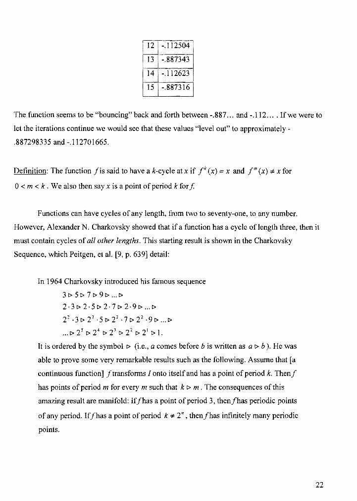
· 12 -.112504 •

13 -.887343

14 -.112623

15 -.887316

The function seems to be "bouncing" back and forth between -.887 ... and -.112 .... If we were to

let the iterations continue we would see that these values "level out" to approximately -

.887298335 and -.112701665.

Definition: The function lis said to have a k-cycle at x if /k (x) = x and /m (x) :;t:. x for

0< m < k . We also then say x is a point of period k forf

Functions can have cycles of any length, from two to seventy-one, to any number.

However, Alexander N. Charkovsky showed that if a function has a cycle of length three, then it

must contain cycles of all other lengths. This starting result is shown in the Charkovsky

Sequence, which Peitgen, et al. [9, p. 639] detail:

In 1964 Charkovsky introduced his famous sequence

31>51>71>91> ... 1>

2·31>2·51>2·71>2·91> ... 1>

22 .31> 22 ·5 I> 22 ·7 I> 22 ·91> ... I>

... 1> 25 I> 24 I> 23 I> 22 I> 21 I> 1.

It is ordered by the symbol I> (i.e., a comes before b is written as a I> b). He was

able to prove some very remarkable results such as the following. Assume that [a

continuous function] /transforms 1 onto itself and has a point of period k. Then/

has points of period m for every m such that k I> m. The consequences of this

amazing result are manifold: if/has a point of period 3, then/has periodic points

of any period. If/has a point of period k :;t:. 2n , then/has infinitely many periodic

points.

22

From above you can see that fez) = Z2 - 0.9 two periodic points, ·.887 ... and -.112 .... As

mentioned, the 3·cycle (period three) is of particular importance for it implies cycles of all other

lengths. As we begin to study the Mandelbrot Set, we will see this importance.

2.3 Definition of the Mandelbrot Set

So far we've looked at the functions f(z);:= Z2 , f(z);:= Z2 + 0.2, and fez) = Z2 - 0.9.

Obviously these all have a common theme of being a second degree polynomial with a constant

term that changes. Instead of picking each constant term by hand, let us assign the term a value C

and write our function as such: fe (z) ;:;:: Z2 + C .

To define the Mandelbrot set (denoted as M), we look at certain complex values of C.

The parameter C could be ·1.3 or.34 + l.8i. Now, M is defined as follows [10, p.56],

M = {C E C : f; (0) + 00 as k --7> oo}. So to see if a point is in the M, do the following: pick a C value, then compute

Zl ;:= f(O) = 02 + C , then Z2 ,Z3 and so on. If a point iterates outside of the disk of radius two, i.e.,

Iz k I > 2 , then we know the next iterate ( z k+1 ) will be even farther out, so there is no point in

continuing to test it, becausefapplied to this point will go to infinity. Thus we, in particular, see

that M is contained in the closed disk with center 0 and radius 2. However, this does not address

the multitude of color that is seen in picture ofM. So far we've defined two states: the sequence

f; (0) stays in the disk of radius two or it iterates outside and we disregard it.

Let us say that for a chosen C value, if Zo = 0 iterates to an attracting fixed point, then

color the point on the complex plane that corresponds to that C value black. So if C = 0.2, then

Zo = 0 will iterate to z = 0.2763, which is the fixed point of fe (z) ;:= Z2 + 0.2, so we color the

point 0.2+0i black. This point resides along the real axis in the complex plane, but as stated

before C is certainly confined to the real axis. Set C = -.8 +.li in fe (z) ;:;:: Z2 + C and observe the

following calculations to see what becomes of our initial value Zo ;:= 0 :

23

Zo = 0

ZI = [(Zo) = [(0) = 02 + (-.8+.10 = -.8 +.1i

Z2 = [(z!) = (-.8 + .1i)2 + (-.8 +.1i) = .63 - .16; + -.8 +.2i = -.17 - .06i

Z3 = (-.17-.06i)2 +(-.8+.1i)=-.7747+.1204i

Z70 =-.217276-.177354i

Z71 = -.784245 + .17707 i

zn =-.216313-.177732i

Z73 == -.784798 + .17689li

It looks as if for this value of C we have a two-cycle (and later we will prove that this is case), so

let us color the point corresponding -.8 +.1i black as well. As we color more points black, we

will fill the region M in the complex plane.

But where do all these colors come in? Well, if we choose a C value outside M that

doesn't correspond to an attracting fixed point or cycle, our initial value of Zo = 0 will, under

iteration, go outside the disk of radius two, and consequently off to infinity. Depending on how

many iterations it takes for Zo = 0 to do this, a particular color is chosen for the point

corresponding to C. For instance, if C1 makes Zo = 0 go outside the disk in 15 iterations, color it

yellow. And if C2 makes Zo == 0 go outside the disk in 17 iterations, color it a little bit darker

yellow. It's easy to see how, depending on the number of iterations, the entire spectrum of colors

can be represented. Shown in Figure 13 is the Mandelbrot Set (in black) with the color spectrum

of other C values surrounding it.

24

Figure 13

Technically, M is only the black region - the points of color do not actually belong in M, but add

to the beauty of the picture and represent C values which do not correspond to Ie with attracting

cycles. We call Figure 13 the parameter plane because it displays the points corresponding to the

parameter C of Ie .

Alternatively, there is a dynamic plane, which, for a given fixed value of C displays

values of z colored according to the behavior of I(~ (z). Here we define the filled-in Julia Set as

follows [10, p. 56]:

Kc = {z E C: Ic~ (z) + 00 as k ~ oo} Notice that definition is almost the same as M's except that instead of having one z value

(zo = 0) for all C values, we now pick one C value and test all z values such that Izl:::; 2 . Figure

14 shows Kc for C = -0.4961 + 0.5432i .

25

Figure 14

The similar coloring is not a coincidence. The black regions represent values of z whose orbit

{tL~ (Z)};=l stays bounded, and if a Z value iterates towards infinity, it is colored depending on

how long it takes for the iterations to move it outside the disk of radius two. It can also be shown

that if the chosen C value causes f~ (0) to stay bounded, then Kc will be connected, which

basically means one can move from any spot within it to any other spot without going outside the

black region. With this fact M can also be defined as:

M = {c E C : Kc is connected} .

Now that we have characterized M, we want to find the explicit values of C that

correspond to an attracting fixed point, a two-cycle, and three-cycle, and so on. This will also

help us describe the large black regions making up M: the heart-shaped mass in the middle, the

disk to the left of it, and the many decorations surrounding the perimeter.

26

2.4 Regions of Fixed Points and Cycles in M

Let us summarize what we already know briefly, and then begin our study of cataloging

certain C values.

IC(Z)=Z2 +C

I : C ~ C , where C is theset of complex numbers.

C Parameters Corresponding to Attracting Fixed Points

We now wish to find C values such that Ie has an attracting fixed point z*. That

is,fc(z*) = z*, and le(zo) ~ z*forzo close toz*. From the Theorem 1, we know that

attracting fixed points happen when If~ (z*)1 < 1, where z· is the fixed point. This derivative

is I~ (z*) = 2z * . To find the fixed points we set Ie (z*) z * and solve for z*:

Ie (z*) = z*

(z*Y+C=z*

(z *Y - z * +C = 0 (quadratic in z*)

1 ± .J1-4C z*

2

Plugging z· back into I~ (z) we have

1/[I±.JlTc] <1 e 2

2[1±~) <I 11 ± .JI- 4CI < 1.

We now solve the above equation with the "plus" case and later show that the "minus"

case yields the same result. Note that C is complex throughout the calculations. Any complex

number can be represented in polar coordinates of the formre iB, as described in Section 2.1.

Setting .Jl- 4C = re iB and using Euler's identity with the "plus" case, we have

27

11 + ~I - 4C I < 1

11+reiol < 1

II+reiol2 <12

11 + r cos 8 + ir sin 812

< 1

(l+rcos8)2 + (r sin 8)2 <1 (Complexnorm)

1 + 2rcos8 + r2 cos 2 8 + r2 sin 2 8 < 1

1 + 2rcos8 + r 2 < 1

2rcos8 + r2 < 0

2rcos8 < _r2

-2cos8> r

0< r < -2cos8.

Since r > 0 , this implies that 7r /2 < 8 < 37r /2 and that 0 < r < 2. With these restrictions, we will

show that the values of C corresponding to an attracting fixed point form an open cardioid.

Since we know that~l- 4C = re lo , one can solve directly for C as follows:

~ 10 vl-4C = re

1-4C == (re'BY

1- 4C == r2e i20

- 4C r 2e120 _1

C 1 1 2 i2B =-- r e 4 4

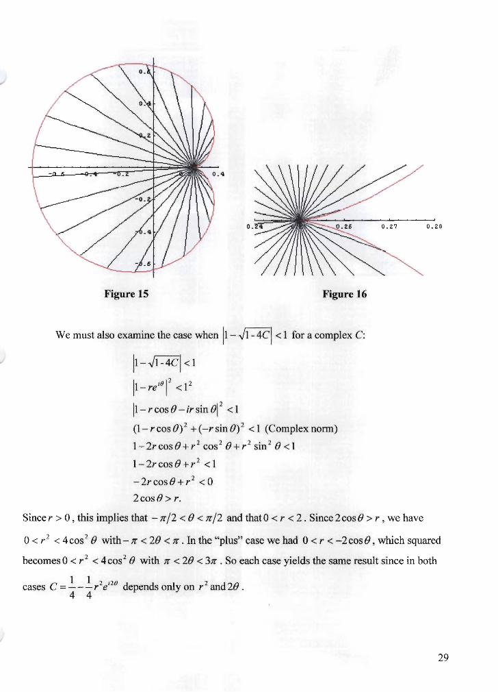
Letting r range from 0 < r < -2cos8 while e ranges from 7r/2 < 8 < 37r/2, we see that line

segments "fill out" the graph of the cardioid, as shown in Figure 15. The red line represents

boundary of the cardioid, which the values of C corresponding to an attracting one-cycle do not

reach. Figure 16 shows a closer look with 0.24 < x < 0.28.

28

o.

Figure 15 Figure 16

We must also examine the case when 11- .Jl- 4CI < 1 for a complex C:

11 - .Jl -4C I < 1

II-rei812 <12

11 - r cos 0 - ir sin if < 1

(1- r cos 0)2 + (-r sin 0)2 < 1 (Complex norm)

1-2rcosO+ r2 cos 2 0+ r2 sin 2 0 < 1

1 - 2r cos 0 + r 2 < 1

-2rcosO+r2 < 0

2cosO> r.

Since r > 0, this implies that - 7r/2 < 0 < 7r/2 and thatO < r < 2. Since 2cosO > r , we have

0.Z8

o < r 2 < 4 cos 2 0 with - 7r < 20 < 7r . In the "plus" case we had 0 < r < -2 cos 0, which squared

becomes 0 < r 2 < 4 cos 2 0 with 7r < 20 < 37r . So each case yields the same result since in both

cases C = -.!._-.!.r2ei28 depends only on r2 and 20 . 4 4

29

C Parameters Corresponding to Attracting Two-Cycles

We now want to look at the second iteration off, that is, we want to look

atf(f(z)) = f2 (z) = F(z). For convenience, we have dropped the subscript C onf, usingjustf

instead of fe . If {a,b} form a two-cycle, thenf(a) = b andf(b) = a, and with our choice of F

we have F(a) = f(f(a)) = feb) = a ,and similarly F(b):::: b.

Thus a and b are fixed points for F. Using the same method as above, we look for values

of C that will satisfy I! F(z*)1 < 1, where z* is a fixed point of F. To find these fixed points we

need to solve F(z*) = f2 (z*) = Z *. However, we already know two roots of this equation from

our previous work, namely z* = (1/2)(1 ± .Jl- 4C). Since we have two roots ofthe quartic

equation F(y) - y = (y2 + C)2 + C - Y = 0, we can factor out y2 + C - Y . Below is an explication

of this method using y for z * . F(y) = Y

(y2 +C)2 +C = y

(y2 +C)2 +C- y=O

(y 2 + y + C + l)(y 2 + C - y) = 0

y2 + y+C +1 = 0

-1±~1-4(C+l) -1±.J-3-4C y= =

2 2

Yl =~(-I+.J-3-4C) 2

Y2 = 1 (-1 .J - 3 - 4C ) 2

Thus, {Yl 'Y2} form a two-cycle. To find what values of C give us this attracting two-cycle, we

use YI and Y2 in the equation IF' (z*)1 < 1, where Yl and Y2 denote the fixed points of F (instead of

z*). An easy way to calculate F' (Yl ) and F' (Y2) uses the chain rule as follows:

30

F(z) = f2(Z) = f(f(z»

F'(z) = l'(z)l'(f(z»

F' (YI) = I' (YI)I' (f(YI»

F'(YI) = I'(YI )f'(Y2)'

Similarly, F'(Y2) = I'(Y2)f'(YI) and thus F'(YI) F'(Y2)'

We now solve for bounds for the C value:

I'(z) = 2z

F'(Yl) = I'(YI)f'(Y2)

IF' (YI)I = II' (YI)I' (Y2)1 < 1

2[(±(-1 +)-3-4C l)H±(-1 )-3 -4C l)] < 1 1(-I+.J-3-4CX-I-.J-3-4C~<1

11 (.J-3-4cYI<1

11 - ( -3 4C)1 < 1

14+4cj < 1

14(1 + C)I < 1.

Next, we simplify it to show our desired two-cycle region in M:

14(1 + C)I < 1

IC+II<1/4

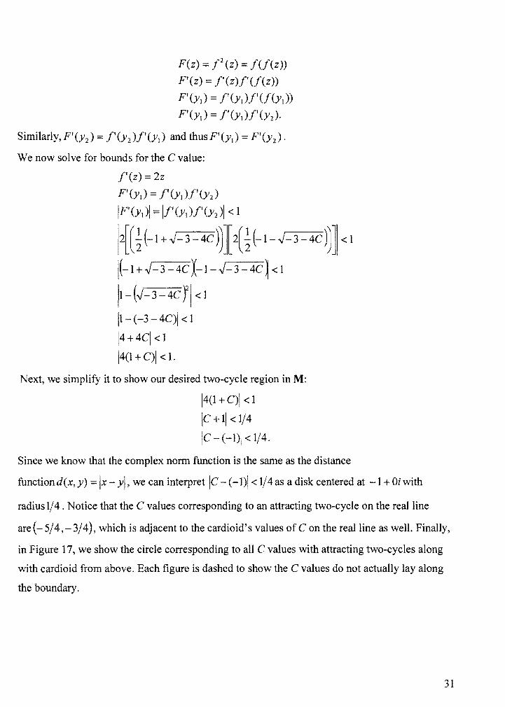
IC-(-I)I<1/4.

Since we know that the complex norm function is the same as the distance

functiond(x, y) = Ix - YI, we can interpret IC - (-1)1 < 1/4 as a disk centered at -1 + Oi with

radius 1/4 . Notice that the C values corresponding to an attracting two-cycle on the real line

are{-5/4,-3/4), which is adjacent to the cardioid's values ofC on the real line as well. Finally,

in Figure 17, we show the circle corresponding to all C values with attracting two-cycles along

with cardioid from above. Each figure is dashed to show the C values do not actually lay along

the boundary.

31

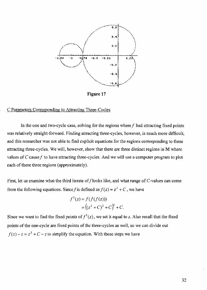
Figure 17

C Parameters Corresponding to Attracting Three-Cycles

In the one and two-cycle case, solving for the regions where / had attracting fixed points

was relatively straight-forward. Finding attracting three-cycles, however, is much more difficult,

and this researcher was not able to find explicit equations for the regions corresponding to these

attracting three-cycles. We will, however, show that there are three distinct regions in M where

values of C cause/to have attracting three-cycles. And we will use a computer program to plot

each of these three regions (approximately).

First, let us examine what the third iterate of/looks like, and what range of C-values can come

from the following equations. Since/is defined as fez) = Z2 + C , we have

/3(Z) = /(/(/(z)))

= (Z2 +C)2 +cy +c.

Since we want to find the fixed points of /3 (z), we set it equal to z. Also recall that the fixed

points of the one-cycle are fixed points of the three-cycles as well, so we can divide out

fez) - z Z2 + C - z to simplify the equation. With these steps we have

32

f3(Z)=(C+Z 2)2 +Cr +C=Z

(C+Z 2)2 +Cr +C Z=O

(C+Z2

)2 +ct +C-Z =0 Z2 +C-Z

(1+C+2C 2 +C3)+(1+2C+C2 )z+(1+3C+3C2 )Z2 +(1+2C)Z3 +(1+3C)Z4 +Z5 +Z6 =0.

Define $( z) as

$(z)==(1+C+2C 2 +C 3 )+(1+2C+C 2 )z+(1+3C+3C 2 )Z2 +(1+2C)Z3 +(1+3C)Z4 +Z5 +Z6.

Solving $ at this point would yield six of the eight fixed points of f3 . The remaining two that

correspond to the one-cycle have already been addressed.

Since $ is a sextic equation, i.e., a sixth-degree polynomial, it will have six roots, which we will

label as zl' Z2,Z3' Z4 ,ZS' and Z6' Any monic polynomial with known roots can be written in the

following form:

$( z) = (z - Z I )( Z Z 2 )( Z - Z 3 )( Z - Z 4 )( Z - Z 5 )( Z - Z 6) •

Expanding this equation results in several mixed terms in various powers of z, but the constant

term is clearly ZIZ2Z3Z4ZSZ6' Setting our two versions of $ equal to each other

Since f(z) has two three-cycles, we concentrate on the six remaining

roots: Z) ,Z2' Z3 ,Z4 'Zs' and Z6' They satisfy, without loss of generality the following properties:

fez)~ = Z2

f(Z2) = Z3

f(Z3) = ZI

f(Z4)=ZS

f(zs) == Z6

f(Z6) == Z4'

Notice that(f3),(z) = (f(f(f(z»»'= (f'(f(f(z»Xf' (f(z»Xf' (z», so ifz == ZI' then

33

(f 3 )'(ZI) = (f'(f(f(z) ))Xf'(f(ZI ))Xf'(Zt))

= f'(Z3)f'(Z2)f'(ZI)'

Butf'(z) = 2z, SO (f3)'(Zt) = 8ZtZ2Z3 .With these facts in mind, we can now show that there are

exactly three regions in the M corresponding to attracting three-cycles. Let Warbitrarily

represent one of these regions.

Theorem 2 ([2], Theorem 2.1, ch. 8): If W is a component of the interior of the Mandelbrot Set

associated with attracting three cycles, then the mUltiplier map C ~ (fJ )'(Zl)' where Zl is part

of the attracting three-cycle of fe, maps Wone to one, analytically, and onto the open unit disk

By Theorem 2, we know that (f 3)'(Zk ) maps W onto fl. The significant repercussion of this is

that the unit disk contains the point 0, which means that for some C E W ,

(f 3 )'(zt)=8ztZ2Z3 =0. Thisimpliesthatzt =0,Z2 =0,orz3 =0. Thus, since

ZtZ2Z3Z4Z5Z6 = (1 + C + 2C 2 + C 3), we must have 1 + C + 2C 2 + C 3 = 0 . Solving for C, we

obtainCI ~ -0.122561...- 0.7448621i... and C2 ~ -0.122561...+ 0.744862li .... These correspond

to the centers of the bulbs on the top and bottom of the main cardioid on Figure 20 and 21,

respectively. The other root isC3 ~ -1.75488 ... , which corresponds to the "center" of the second

cardioid in the M (see Figure 22). Thus we have shown the "centers" of three regions

corresponding to attracting fixed points.

34

~O.Z -0 . .15 "0 . .1 -0.01

0.'

-C.t

0.'

-0.4

0.'

.. . I •• I •• • i

-0.2 -0.l.5 -0 • .1 -0.05

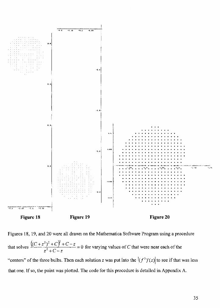
Figure 18 Figure 19 Figure 20

Figures 18, 19, and 20 were all drawn on the Mathematica Software Program using a procedure

(CC+Z 2)2 +C) +C-z . that solves 2 = 0 for varymg values of C that were near each of the

z +C-z

"centers" of the three bulbs. Then each solution z was put into the ICf3 )'(z)1 to see if that was less

that one. If so, the point was plotted. The code for this procedure is detailed in Appendix A.

35

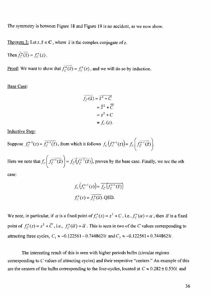
The symmetry is between Figure 18 and Figure 19 is no accident, as we now show.

Theorem 3: Letz,z E C, where zis the complex conjugate ofz.

Then/f(z) = fc~(z).

Proof: We want to show that If (z) I; (z), and we will do so by induction.

Base Case:

Inductive Step:

Suppose I;-l(z) =

1:-(z) = c

=Z2 +C

=Z2 +C

= Ie (z).

(2') , from which it follows Ie (r;~' (z)): Ie (It' (2')]-

Here we note that Ie (I E~' (2') ) : 7 c (r r' (if) ), proven by the base case. Finally, we see the nth

case:

Ie Vt- l (z») Ie (lt l (z»)

I;(z) If(z).QED.

We note, in particular, if a is a fixed point of I; (z) = Z2 + C , i.e., h~ (a) = a, then a is a fixed

point of If (z) = Z2 + , i.e., If (a) ::: a . This is seen in two of the C values corresponding to

attracting three cycles, Cl ::::: -0.122561 0.7 44862li and C 2 ::::: -0.122561 + 0.7 448621i .

The interesting result of this is seen with higher periods bulbs (circular regions

corresponding to C values of attracting cycles) and their respective "centers." An example of this

are the centers of the bulbs corresponding to the four-cycles, located at C ::::: 0.282 ± 0.530i and

36

c ~ -.1565 ± l.0323i [10, p. 58]. Note that there are two more regions corresponding to four­

cycles, which are centered on the real line.

The Mandelbrot Set, of course, contains infinitely many bulbs, and it is believed that each

one corresponds to a certain length of a particular cycle. Some of the known bulbs are listed in

Figure 23.

Figure 21

From Figure 21 we can also see the Charkovsky Sequence. Notice the period three cardioid

sitting out to the far left of the period one cardioid. From the main cardioid we pass through the

period two bulb, then four, then eight, etc. But once we've reached the period three cardioid, all

other periods (cycles) have been accounted for.

2.5 The Bifurcation Diagram

In Section 1.5 we discussed the concept of a bifurcation diagram, a drawing that gives us

a map of when a cycle splits into the two-cycle, the four-cycle, and so on based on changes in

the real parameter C in the maps fcCx) = x 2 + C,x E R. But we only drew it up to the sixteen-

cycle or so, and there is much more to be seen. If we use the function fe (x) = x 2 + C to find the

37

points of the period doubling, our bifurcation diagram turns into a much more intricate picture,

shown in Figure 22.

Figure 22

The Bifurcation Diagram is self-similar, so "zooming in" on a region of it will actually resemble

the whole picture. Additionally, this diagram can be juxtaposed with M to give an interesting

view into how the chaos ofthe third period develops. This is shown in Figure 23.

·20 -1.0 -0.5 0.0 0.5

Figure 23

38

Of note is the region in the bifurcation diagram corresponding to the three-cycle, where suddenly

the thousands (and millions, etc.) of cycle-marking points slim down to just three lines. This

small "open" section of the bifurcation diagram corresponds to the real interval contained within

the miniature cardioid we showed in Section 2.4.

2.6 Finding M Elsewhere

One of the most amazing facts about M is its own version of universality. Just as the

Feigenbaum Constant 0 keeps appearing for many different functions, plotting "maps" of

iteration for other functions can yield M as well. One way of seeing this is using a process called

Newton's Method. Newton's Method uses the process of iteration to find the roots of

complicated functions, though it can be used on polynomials. It arises from expanding a series as

a Taylor Series and truncating after the first two terms. It works as follows: choose and initial

value Xo which is (hopefully) somewhat close to a root of/(x). Then calculate the next iterates

in the following way:

The sequence {XI }~~o converges to a root if Xo is close enough to an actual root. Using Newton's

Method for at third degree polynomial can have strange results. Three researchers [12, p. 267-

277] experimented with the function /e (z) = Z3 + (C -l)z - C , which has one root at z = 1 for

any C value. For each C value they used the initial value of Zo O. The following is the

algorithm used to "draw" the parameter plane for Newton's Method

on/c (z)=z3 +(C-l)z-C:

• Color the point black if Newton's Method converges to 1

39

• Color the point white if Newton's Method converges to some other root of Ie

• Color the point grey ifit converges to a cycle of two or more points

Figure 24 shows the parameter plane using this scheme.

Figure 24

By looking at the top "blob" in closer detail we see the following:

Figure 25

40

Figure 25 shows the blob at the top of Figure 24 in closer detail on the left. The right image in

Figure 25 is the small grey bit of the left side magnified. Amazingly, M seems to exist inside this

parameter plane, too. Actually, this is not an exact copy ofM, but a slightly "distorted" copy.

Another interesting view ofM comes from iterating the function./;' .(z) = z -1 + Cze z •

This very un-intuitive choice gives rise to the spectacular parameter planes shown in Figure 26

and 27. The cardioid in Figure 27 contains all parameters that correspond to the function

Ie (z) = z -1 + Cze z having attracting fixed points.

Figure 26 Figure 27

41

Figure 28 shows the parameter plane for Ie (z) z - 1 + Cze Z in the range - 15 < Re( C) < 15 and

- 50 < Im(C) < 50, where Re(C) means the real part of C and Im(C) means the imaginary part of

C. Magnifying a portion of that image we get Figure 29, with the range - 5.45 < Re(C) < -2.15

and - 2.2 < Im(C) < 2.2. Once again, M appears.

Conclusion

While we have studied much of the Mandelbrot Set, there is much left to be investigated.

In 1991 Dave Boll came across the irrational number 7r while trying to show that the "neck" of

M located at - 0.75 + Oi is infinitely narrow[9, p.859]. Perhaps the most relevant question right

now is whether M is locally connected or not. By locally connected we mean a piece of M that is

open, say U, that for Z E U n M , there is a neighborhood V c U , such that Z E V and V n M is

connected. Adrien Douady [10, p.167] writes in The Beauty of Fractals that "This is a very

irritating situation, because we know the model pretty well, so that if we could this question we

could say that we know essentially everything we want to know about the Mandelbrot set."

Douady also mentions that no one has mathematically proven that if a C value is selected from

inside the generated image of M, that it won't correspond to an attracting fixed point. He poses

the question, "shall we discover some day some queer components, corresponding to a

completely different phenomenon [other] than an attracting cycleT He replies "probably not"

but these two facts raise an interesting point - seeing is not necessarily believing. While the

Mandelbrot Set contains an infinite amount of information coupled with unmatched beauty, to

prove that it has these certain properties is an extremely difficult task, much as it was for this

researcher to find equations for the bulbs corresponding to the three cycle.

42

References

[1] Albers Alexanderson. Mathematical People: Profiles and Interviews. Birkhauser, Boston,

1985.

[2] Lennart Carleson and Theodore W. Gamelin. Complex Dynamics. Springer-Verlag, New

York. 133-134. 1993.

[4] Robert L. Devaney. Transition to Chaos: The Orbit Diagram and the Mandelbrot Set.

VHS Tape. Science Television Company, 1990.

[5] James Gleick. Chaos: Making A New Science. Penguin Books, New York,1987.

[6] Stephen H. Kellert. In the Wake o/Chaos. The University of Chicago Press, Chicago,

1993.

[7] Federico Lombardi. Chaos Theory, Heart Rate Variability, and Arrhythmic Mortality.

Circulation, 101 :8,2000. <http://circ.ahajournals.org/cgi/contentifullI10111/8>

[7] Benoit B. Mandelbrot. The Fractal Geometry o/Nature. W. H. Freeman and Company,

New York, 1983.

[8] Benoit B. Mandelbrot. Fractals and Chaos: The Mandelbrot Set and Beyond. Springer,

New York, 2004.

[9] Heinz-Otto Peitgen, Hartmut Jiirgens, and Dietmar Saupe. Chaos and Fractals: New

Frontiers 0/ Science . Springer-Verlag, New York, 1992.

[10] Heinz-Otto Peitgen and Peter H. Ricther. The Beauty 0/ Fractals: Images o/Complex

Dynamical Systems. Springer-Verlag, New York, 1986.

43

[11] Ian Stewart. Does God Play Dice? The New Mathematics of Chaos. Blackwell

Publishing, Great Britain, 2002.

[12] Sullivan, D., Curry, J. H., and Garnett, L., "On the iteration of a rational function:

computer experiments with Newton's method," Commun. Math. Phys. 91, 1983.

44

Figure Credits

1-5 Lorenz Butterfly Applet. Used with permission. Copyright 1996, James P. Crutchfield.

All rights reserved. <http;//www.exploratorium.edulcomplexity/javallorenz.html>

6 Eric W. Weisstein. "Lorenz Attractor." From MathWorId--A Wolfram Web Resource.

<http://mathworld.wolfram.comlLorenzAttractor.h tml>

7 Copyright RF. Voss. From [9, plate 8]. See References.

8 Eric W. Weisstein. "Koch Snowflake." From MathWorld--A Wolfram Web Resource.

<http://mathworld.wolfram.com/KochSnowflake.html>

9 Eric W. Weisstein. "Menger Sponge." From MathWorld--A Wolfram Web Resource.

<http://mathworld.wolfram.comlMengerSponge.html>

10 Eric W. Weisstein. "Mandelbrot Set." From MathWorld--A Wolfram Web Resource.

<http://mathworld. wolfram.comlMandelbrotSet.html>

11 Ian Stewart. From [11, p. 187]. See References.

12 Eric W. Weisstein. "Complex Number." From MathWorld--A Wolfram Web Resource.

<http://mathworld. wolfram.comlComplexNumber.html>

13 Neal Ziring. "Neal's Mandelbrot Set and Julia Set Page." 2003.

<http;//users.erols.comlziring/mandel.html>

14 Neal Ziring. "Neal's Mandelbrot Set and Julia Set Page." 2003.

<http;//users.erols.comlziring/mandel.html>

45

15-17 Wolfram Research, Inc., Mathematica, Version 5.0, Champaign, IL (2003). Author's own

code.

18-20 Wolfram Research, Inc., Mathematica, Version 5.0, Champaign, IL (2003). See

Appendix A.

21 Heinz-Otto Peitgen, et at From [9, p.867]. See References.

22-23 Heinz-Otto Peitgen, et al. From [9, p.874]. See References.

24-25 Michael Frame, et at "Fractal Geometry." Yale University.

<http://classes.yale.eduifractals/MandeISetlMandeIUniversality/CGSExp.html>

26-27 Amd Lauber. "On the Stability of Julia Sets of Functions having Baker Domains."

Dissertation. University of Illinois. 2004. <http://www.math.uiuc.edul-amdldiss.pdf>

46

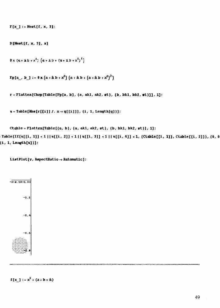
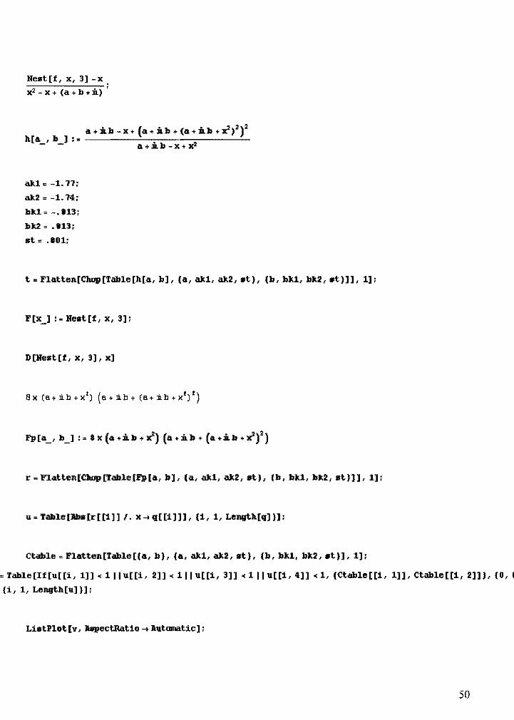
Appendix A

The following Mathematica code is the procedure for generating the plots in Figures 20-22.

Hest[f, x, 3] -x .

x2 _ X + (a + b 1I':ia.) •

a+:ia.b-x+ (a+:ia.b+(a+:ia.b+XZ)2)2 h[a , b ] : = ------.:..--------.::.-

- - a + :ia. b - x + xl!

akl = -.3;

ak2 = .1;

bkl = .6;

bk2 = .9;

st = .01;

t = Flatten[CJwp [Table [h[a, b], {at akl, ak2, st}, {b, bkl, bk2, st}]] , 1];

F[x_] : = Hest(f, x, 3];

D(Hest[f, x, 3], x]

r = Flatten(CJwp [Tabl.e(Fp [a, b], {a, akl, ak2, st}, {b, bkl, bk2, st}]] , 1];

u = Tabl.e [:Abs[r [(i]] I. x-+ q[(i]]], {i, 1, Length[q] H;

Ctable = Fl.atten[Table[{a, b}, {a, akl, ak2, st}, {b, bkl, bk2, stH, 1];

47

,Table[If[u[[i, 1]] < 11Iu[[i, 2]] < 111 u[[i, 3]] < 111 u[[i, 4]] < 1, {Ctable[[i, 1]], Ctable[[i, 2]]}, {O, 0

i, 1, Length[u]}];

ListPlot [v, :ll.spectRatio -+ Automatic] ~

O.li

0.4

0.2:

-O-:ll. :1B-:D... OS

lfest[f, X, 3] -x

x2 - X + (a + b it:iL) ~

a:k1= -.3;

a:k2 = .1;

bU= -.9;

b:k2 = -. Ii; st = .01;

a +:iLb - x+ (a +:iLb + (a +:iLb + :x2)2)2 a+:iLb-x+x2

t = Flatten[CJwp[Table[h[a, b], {a, a:k1, a:k2, st}, {b, bU, bU, st}]], 1]:

48

F[x_] :=lfest[f, x, 3];

D[lfest[f, x, 3], x]

r = Flatten[CIuJp [Table [Fp [a, b], (a, akl, ak2, st}, (b, bU, bk2, st}]] , 1]:

u = Table [lbs [r [[i]] I. x -+ q[[i]]], {i, 1, Length[q] }];

Ctable = Flatten [Table [(a, b}, (a, akl, ak2, st}, {b, bkl, bk2, stU, 1];

,Table[If[u[[i, 1]] < 111 u[[i, 2]] < 111 u[[i, 3]] < 111 u[[i, 4]] < 1, {Ctable[[i, 1]], Ctable[[i, 2]]}, (0, 0

Ii, 1, Length [u]}] ;

Li&tPlot [v, _ectRatio -+ llutmnatic] ;

- O~CL ie~Q.. os

-O.t

-0.4

-0.6

49

Nest[f, X, 3] -x

x2 - X + (a + b 1r::iJ.) ;

akl = -1.11;

ak2 = -1.14;

bU = -.013;

bk2 = .013;

st = .001;

t = Flatten [Chop [Table [h[a, b], (a, akl, ak2, st), (b, bU, bk2, st}]] , 1];

F[x_] : = Nest [f, x, 3];

D[Nest[f, x, 3], x]

r Flatten [Chop [Table [Fp [a, b], {a, akl, ak2, st}, (b, bkl, bk2, st}]], 1];

u= Table [lbs [r [[i]] /. x-+q[[i]]], (1, 1, Length[q])];

Ctable = Flatten [Table [(a, b), {a, akl, ak2, st), (b, bkl, bk2, st)], 1];

= Table[If[u[[i, 1]] 0( 11Iu[[i, 2]] -< 111 u[[i, 3]] -< 111 u[[i, 4]] 0( 1, {Ctable[[i, 1]], Ctable[[i, 2]]}, (0, ~

{i, 1, Length[u]}];

ListPlot [v, lbJpectRatio -+ Automatic] ;

50

-0-:11. i.B-:Q.. 05

-0.2

-0.4

-0.15

51