Channel Normalization for Unsupervised Spectral … · not considered in this paper). A possible linear model of the problem is depicted in ... CVN x(t) Figure 2: Proposed ... –

ES

EA

RC

HR

EP

RO

RT

ID

IA

P

Rue du Simplon 4

IDIAP Research Institute1920 Martigny − Switzerland

www.idiap.ch

Tel: +41 27 721 77 11 Email: [email protected]

P.O. Box 592

Fax: +41 27 721 77 12

Channel Normalization for

Unsupervised Spectral

SubtractionGuillaume Lathoud a,b

Mathew Magimai.-Doss a,b

Herve Bourlard a,b

IDIAP–RR 06-09

February 2006

revised in June 2006

a IDIAP Research Institute, CH-1920 Martigny, Switzerlandb Ecole Polytechnique Federale de Lausanne (EPFL), CH-1015 Lausanne, Switzerland

IDIAP Research Report 06-09

Channel Normalization for Unsupervised

Spectral Subtraction

Guillaume Lathoud Mathew Magimai.-Doss Herve Bourlard

February 2006

revised in June 2006

Abstract. Application domains such as in-car human-machine interaction require noise-robustfront-ends in order to cope with the noisy situations encountered in practice. Moreover, whenspeech is captured through a cellphone, the phone channel characteristics are often unknown. Itis thus desirable to estimate and remove both phone channel characteristics and ambient noise,in an online manner. The main contributions of this paper are twofold. First, a novel channelnormalization method is proposed, that is used before noise reduction, at the magnitude spectro-gram level. It removes the convolutive channel, and reduces the stationary part of the ambientnoise. Second, an alternative to classical spectral subtraction is proposed, called “UnsupervisedSpectral Subtraction” (USS), which does not require any parameter tuning. Channel normaliza-tion followed by USS (two steps) permit to reach an ASR performance very similar to that ofthe ETSI Advanced Front-End (Wiener filtering, with many steps and parameters). The compu-tational cost of the proposed approach is very low, which makes it fit for real-time applications.Furthermore, channel normalization followed by the ETSI Advanced Front-End leads to a majorimprovement in noisy conditions, and best overall results.

2 IDIAP–RR 06-09

h(t)s(t) x(t)

n(t)

Figure 1: Model of the problem: recognize speech from the observed signal x(t) = h(t) ∗ (s(t) + n(t)),where n(t) is the additive acoustic noise and h(t) is the transmission channel (e.g. cellphone).

1 Introduction

Robustness to various noise conditions is a key feature for speech processing algorithms to be turnedinto versatile, real-world applications. Most often, two exclusive directions are followed: either enhancethe speech signal itself by ideally filtering out the noise [1, 2, 3], or change the way acoustic featuresare extracted from the signal [4, 5]. This paper presents an intermediary approach that enhancesthe feature extraction process at a level as close as possible to the original signal : at the magnitudespectrogram level, i.e. in time-frequency plane (TF). It relies on a channel normalization step followedby unsupervised EM fitting [6] of a 2-component model on observed data. It can be seen as aparameter-free generalization of classical spectral subtraction methods.

The problem addressed by this paper is Automatic Speech Recognition (ASR) in acoustic noise(e.g. car noise) followed by an unkown transmission channel (e.g. cellphone). The goal is to beable to use, in noisy test conditions, HMM models trained on clean data (multi-condition training isnot considered in this paper). A possible linear model of the problem is depicted in Fig. 1: to theoriginal speech signal s (t), acoustic noise n (t) is added, and the sum is transmitted over a convolutivechannel h (t), thus leading to the following linear model for the received signal x (t):

x (t) = h (t) ∗ (s (t) + n (t)) (1)

where ∗ denotes the convolution operator. One contribution of this paper addresses estimation andremoval of h(t). As a first step, we have implicitly neglected additive channel noise in Eq. 1. Thisis justified by the present focus on noise-robust ASR: it means that h (t) ∗ (s(t) + n(t)) is supposedlarger than channel noise, at all times. The idea is to validate the proposed channel normalizationmethod first. A more complex model is left for further work.

Classical noise reduction methods such as Wiener filtering, as in the ETSI Advanced Front-End [7],and spectral subtraction methods [8, 9, 10, 11] implicitly assume a flat transmission channel: h (t) = 1.One common way to remove the channel is linear post-processing of the MFCC features, after noisereduction, such as Cepstral Mean Subtraction (CMS) and Blind Equalization [7]. We argue thatnon-linearities in the noise reduction stage may prevent CMS and Blind Equalization from completelyremoving the channel distorsion.

Therefore, this paper considers channel normalization at the signal level, before noise reduction andfeature extraction (Fig. 2). The main contribution of this paper is to transform the Low-Energy En-velope Tracking (LEET) additive noise estimation method [12, 10] into a channel estimation method.The proposed channel estimation relies on the observation that spectral valleys of the time-frequencyplane are dominated by noise. Using spectral valleys, h (t) ∗ n (t) is estimated, and thus h (t), witha white noise assumption. It is then sufficient to divide the received spectrum by the estimatedfrequency-domain channel response. In practice, for non-white noises, the channel is still normalized,and the stationary part of the additive noise is reduced (divided by a large factor).

Assuming that the transmission channel has been normalized out, the next task is removal of theadditive noise n (t). Classical spectral subtraction [8] does it in two steps, in the frequency domain.First, the noise power is estimated in all points of the TF plane, second, it is subtracted from theobserved noisy speech power. This relies on a reasonable independence assumption between speechand noise. In our understanding, the main issue of spectral subtraction is the initial noise power

IDIAP–RR 06-09 3

channel

normalization

noise reduction,MFCC extraction

blind equalizationor CMS, CVN

x(t)

Figure 2: Proposed channel normalization (leftmost block): before noise reduction and feature extrac-tion. Note that we still use post-processing (blind equalization or CMS,CVN).

estimate (first step). Ideally, a perfect noise power estimate in all points of the TF plane wouldrequire a perfect speech power estimate, which is precisely what we are trying to obtain (second step).Very often, tunable parameters are employed [9] to compensate imperfections such as musical noise.The disadvantage of tunable parameters is that various types of data may lead to different optimalparameter values [9], thus requiring human supervision.

As an alternative to this 2-step approach, the present paper proposes to jointly model both distri-butions of speech and noise magnitudes in the TF plane. The underlying motivation is to rely on theestimated posterior probability of observing speech at a given point of the TF plane. In spirit, theproposed approach is related to TRAP-TANDEM [13] and further developments [14], although theprobabilistic modeling is made here at a much lower level: the magnitude spectrogram.

Enhancing the spectrogram itself, based on probabilistic assumptions [15], led to applicationsto noise-robust ASR [16, 17], and has received much attention recently [2, 3]. In order to build aprobabilistic model, at least two distributions are needed: one for background additive noise, and onefor speech. A reasonable model for background noise on silent parts of the TF plane is a white Gaussianassumption for real and imaginary parts, which translates into assuming a Rayleigh probability densityfunction (pdf) in the magnitude domain [18]. However, modeling of the speech part is much morecomplicated, as such an assumption does not hold anymore. Supergaussian models such as the Laplacepdf may be needed [2] for a better fit on real data. Derivation of the magnitude pdf of speech is stillan open question [19].

On the contrary, this paper proposes to restrict the problem to modeling of large magnitudes ofspeech only. Intuitively, low speech magnitudes cannot be distinguished from background noise, beingintrinsically regions of low Signal-to-Noise Ratio (SNR). We therefore complete the well-justified back-ground noise Rayleigh model with an ad-hoc pdf for activity, that models “large” magnitudes only.“Large” is defined w.r.t. the Rayleigh model itself, and the complete modeling process is fully unsu-pervised. We apply this approach to enhance the noise-robustness of single channel ASR by removingnoise from the magnitude spectrogram using a modified spectral subtraction. The magnitude spectro-gram is filtered at a small cost, so that only speech that can be distinguished from background noiseis retained. No parameter tuning is involved, thus justifying the “Unsupervised Spectral Subtraction”designation (USS). It was introduced in [11]. One intent of this paper is to determine whether a typeof probabilistic model similar to the one used for microphone array-based speech detection, in [20],can be applied to the context of noise-robust ASR.

Overall, the purpose of this paper is not to propose novel noise-robust ASR features, but rather asimple, generic approach that can be a pre-processing step for any acoustic feature extraction process(MFCCs, PLP, etc.). Training on clean data is then sufficient to cope with unseen noise environments.Such an approach is very much in the spirit of [17] and [10]. The two steps of the proposed approach– channel normalization and USS – rely on a consistent model: in both cases, the background noise ofthe preemphasized signal is supposed to be a slowly-varying white Gaussian noise. Although simplistic,it is justified by observations on real data (Fig. 5), and may be deemed the natural first step, beforetrying more complex noise models.

In experimental studies on the Aurora 2 corpus [21], we first compare the proposed approachwith a classical spectral subtraction method [9] selected from the comprehensive study in [10]. Themain difference is that the proposed approach – channel normalization followed by USS – does notrequire any parameter tuning. A clear improvement is obtained in all conditions. Second, we comparethe proposed approach with the more complex, many-step ETSI Advanced Front-End [7], whichis essentially a two-pass Wiener filter. The results show that channel normalization followed by

4 IDIAP–RR 06-09

USS permits to reach the same performance as that of the ETSI Advanced Front-End. This isquite interesting, given that the proposed signal transformation is fully described by two equations(Eqs. 6 and 18), while the ETSI Advanced Front-End includes many steps and parameters. An initialexperiment with channel normalization followed by the ETSI Advanced Front-End shows that furtherimprovement can be obtained in very noisy conditions (0 and 5 dB) for a limited loss at 15 and 20 dB.This suggests further work towards the direction of joint channel/noise estimation. The computationalcost of both channel normalization and USS is very small, so that the proposed approach is fit forreal-time applications.

The rest of this paper is organized as follows: Section 2 defines notations, Section 3 summarizesexisting spectral subtraction methods and identifies three issues with respect to the present task.Section 4 addresses the channel normalization issue. Section 5 addresses the two remaining issues: aprobabilistic method for joint speech/noise magnitude estimation is proposed, followed by a parameter-free spectral subtraction procedure. Section 6 presents ASR results on noisy telephone speech [21].Section 7 concludes the paper. A complete MATLAB implementation of the proposed approach isavailable at: http://mmm.idiap.ch/Lathoud/2006-CHN-USS

2 Notations

Both time t and frequency f are discretized into samples and Nbins frequency bins (narrowbands), re-spectively. x (t) or yt is the pre-emphasized signal, Fx

f,t ∈ C is the Discrete Fourier Transform (DFT) of

a windowed signal [xt−Nsamples+1 . . . xt]T (using Hamming window), [·]T denotes the transposition oper-

ator. m (f, t) = mf,tdef= |Fx

f,t| is the magnitude in TF plane, and w (f, t) = wf,tdef= |Fx

f,t|2 the power.

x, m and w designate the realizations of random variables X , M and W . The pdf of X is denoted

qX (x). The mathematical expectation of a random variable X is written E{X}def=

∫ ∞

−∞x · qX (x) · dx.

3 Classical Spectral Subtraction

This section briefly summarizes the principle of spectral subtraction, and points at open issues in thecontext of noise-robust ASR that was described in Section 1.

3.1 Principle

For speech enhancement, Boll [8] proposed an additive noise removal procedure called “spectral sub-traction”. The proposed model is x (t) = s (t) + n (t), where x, s and n designate the received noisysignal, the clean speech signal and the noise signal, respectively. We represent the correspondingtime-domain random variables X (t), S (t) and N (t), and assume independence between the cleanspeech signal S (t) and the noise N (t). The frequency domain power random variable wX (f, t) thenfollows:

E{wX (f, t)} = E{wS (f, t)} + E{wN (f, t)}, (2)

which leads to the following procedure for noise removal:

ws (f, t) = max (0, wx (f, t) − wn (f, t)), (3)

where ws (f, t) and wn (f, t) designate estimated powers of clean speech signal and noise, respectively.Under stationarity and ergodicity assumptions, these estimates can be obtained through DFT over astationary interval, 20 to 30 ms in the case of speech. Section 3.2 summarizes a method for automaticestimation of wn (f, t).

Berouti [9] considered the issue of musical noise: Eq. 3 introduces many additional zeroes in theTF plane, which in turns make the spectral peaks more narrow. Thus, when reconstructing the

IDIAP–RR 06-09 5

signal s (t) from the estimated speech spectrum ws (f, t), this produces an audible “musical noise”,which is detrimental to human listening quality, and potentially to ASR. Thus, the following modifiedprocedure was proposed:

• Compute an intermediate estimate wd (f, t) = wx (f, t) − α · wn (f, t), where α ≥ 1 is called the“subtraction factor”. The purpose of α is to reduce the amplitude of the remnant noise peaks.

• Estimate the clean speech power as ws (f, t) = max (wd (f, t) , β · wn (f, t)), where β is calledthe “spectral floor parameter” (0 < β << 1). β is used to reduce the amplitude of the remnantnoise peaks, relatively to the surrounding spectral valleys.

The two steps can be written in a compact manner:

ws (f, t) = max (wx (f, t) − α · wn (f, t) , β · wn (f, t)). (4)

3.2 Noise Level Estimation (LEET)

In order to apply Eq. 4, it is necessary to first estimate the noise level wn (f, t) at each point (f, t)of the TF plane. This can be done on parts of the TF plane where the speaker is assumed silent, forexample obtained with a Voice Activity Detector (VAD). Without VAD, automatic methods can beemployed to distinguish between speech harmonics and noise [10]. An extensive study was presentedin [10], which essentially compared four different additive noise estimation methods:

• Energy clustering [17]: the distribution of log energies is assumed to present two modes, onefor noise, the other for speech (with larger values). The two modes can be fitted with eitherEM fitting [6] of two Gaussians, or 2-means clustering.

• Hirsch histograms [22]: a histogram of log energies, computed over several hundreds milliseconds,exhibits a peak in the low energy portion. This peak is indicative of the noise level.

• Weighted average [22]: a first-order recursion is used to update the noise estimate, wheneverspeech is deemed absent.

• Low-Energy Envelope Tracking (LEET) [10], which was derived from [12]. It relies on spectralvalleys to estimate a quantity proportional to the noise level.

From this extensive study [10], we selected LEET, as it provided the best results. LEET assumes thatlow energies – spectral valleys – are dominated by noise. Thus, within each frequency band f , thenoise energy is estimated from the average energy of 20 % of the time frames: those with the lowestenergy values (Fig. 4).

The LEET noise level estimation assumes that the lowest power values in a portion of the TF planeare essentially dominated by noise. This is a reasonable assumption when noise is more stationarythan speech and the global SNR is greater than zero. In particular, it means that the spectral valleysin between speech harmonics mostly contain noise. In practice, LEET is implemented as follows:

• Within a frequency band and a time window, compute the average wγ (f) of the 20% lowestpower values, denoted by γ = 0.20. In practice, γ does not require tuning.

• The (locally stationary) noise power is estimated as:

wLEETn (f)

def= C · wγ (f) , (5)

where C > 1 is a correction factor. We used a 5-point (≈ 150 Hz window) running mean filterin the log power domain log

(

wLEETn (f)

)

, across the frequency bins f , in order to eliminate theoutliers.

6 IDIAP–RR 06-09

10−4

10−2

100

102

104

10−4

10−2

100

102

104

noise level

LEE

T n

oise

est

imat

e

LEET noise estimation (γ = 0.2)

idealresult

Figure 3: Evaluation of the LEET noise estimation. “Noise level” means the average white gaussiannoise energy divided by the average clean speech energy.

In [10], C is SNR-dependent, and is determined by a calibration procedure on training data. In prelim-

inary experiments on OGI Numbers 95 [23], we found that a fixed value C = (1.5 γ)−2

provides betterrecognition results than the calibration procedure. Fig. 3 shows an evaluation on clean speech [23]with white noise added at different levels. The slight tilt at the lowest noise levels is due to a verysmall background noise already present in the “clean” speech signal. Overall, we can see that thenoise level estimate is very close to the true noise level.

3.3 Application to Noise-Robust ASR

Following [10], we used Eqs. 4 and 5 to modify the spectrum prior to MFCC extraction of a standardHMM/GMM recognizer. In order to optimize the process for noise-robust ASR, we had to tune theα and β parameters. On the task considered in Section 6.5, we observed best speech recognitionresults with a constant α = 2.3, and β = 0.2. The spectral floor value β = 0.2 is much larger thanadvised in [9]. However, [9] was targetting a speech enhancement task, while the focus here is onMFCC-based ASR. Certain types of speech distorsions may be acceptable for machines, but not forhumans, and vice-versa. A high value of the spectral floor is also successfully used in the spectralsubtraction variant introduced below (Section 5.3).

Overall, with respect to the noise-robust ASR task and the model depicted in Fig. 1, three issuescan be identified.

Issue 1: The model in Section 3.1, x (t) = s (t) + n (t), implicitely assumes a flat transmissionchannel, i.e. h (t) = 1. Thus, the ASR performance may considerably degrade when the channelis not flat (e.g. cellphone). It is verified experimentally with LEET on the Aurora 2 task [21], inSection 6.5. In order to fully exploit the potential of spectral subtraction in such environments, thechannel response must first be estimated and normalized out. Section 4 proposes two methods.

Assuming that the channel h (t) has been normalized out, two general issues remain.Issue 2: Any error in the noise level estimate wn (f, t) directly impacts on the ASR performance.

Based on the additive noise model x (t) = s (t) + n (t), a perfect noise estimation method would requireperfect knowledge of the clean signal s (t), which is precisely what we are trying to estimate. This“circular” issue can be addressed by joint modelling of noise and speech, as proposed in Section 5.2.

Issue 3: For each different task, α and β need to be tuned. According to [9], α and β should evenvary depending on the local SNR in the TF plane. In our understanding, α and β not only help toreduce musical noise, but also to correct errors in the noise estimation process (especially α). Thus,this issue could be closely related to “Issue 2”. Consequently, addressing “Issue 2” could in turn allow

IDIAP–RR 06-09 7

for a simpler, parameter-free spectral subtraction, as proposed in Section 5.3.

4 Channel Estimation and Normalization

Noise reduction methods for ASR include, among others, Wiener filtering, as for example in theETSI Advanced Front-End [7], and spectral subtraction [8, 9, 10, 24]. They implicitly assume nochannel distorsion (h (t) = 1), as in the signal model x (t) = s (t) + n (t). In reality, the channel maybe distorted, and there may be a mismatch between the channels used in training and test conditions(e.g. different types of cellphones). This mismatch causes a degradation in WER, as the test signalsappear distorted to the models trained on data with different channel(s).

In the case of noise-robust ASR, we postulate that channel normalization after noise reduction,such as CMS, may not be able to fully remove the channel distorsion, because of non-linearities in thenoise reduction process. Following [25, 26], we thus propose to remove the channel before any otherprocessing, i.e. at the power spectrum level, as depicted in Fig. 2. The idea is to estimate the powerdomain channel response wh (f) from the observed signal x, then to remove it through a division inthe power domain:

wNORMx (f, t) =

wx (f, t)

wh (f)(6)

The next two subsections propose two different estimates wh (f), corresponding to two differentsets of assumptions. The main contribution of this paper lies in the second one (CHN).

4.1 Geometric Mean Normalization (GMN)

We propose here to use existing dereverberation methods [25, 26] to do channel normalization. Theseexisting methods consist in removing the mean in the log power domain.

Let us examine which assumption lies behind such a normalization. First, the time-domain signalmodel of Eq. 1 can be translated to the log power domain:

log wx (f, t) = log wh (f) + log (ws+n (f, t)) (7)

We now assume that:

〈log (ws+n (f, t))〉t ≈ L (8)

where 〈·〉t denotes the mean across DFT time frames, and L is a constant: it does not depend onfrequency f . This assumption is partly justified by the pre-emphasis done in the time domain, whichflattens the spectrum. Then, log wh (f) ≈ 〈log wx (f, t)〉t − L, which justifies to divide the observedpower values wx (f, t) by their geometric mean, within each frequency band f :

wGMNh (f)

def= exp 〈log wx (f, t)〉t (9)

One could object that on “short” speech signals, as typically encountered in hands-free dialing of atelephone, the assumption L (f) = const is not justified. Indeed, L (f) would most likely reflect thespeaker-specific harmonics, and thus depend on f .

4.2 Proposed CHannel Normalization (CHN)

As an alternative to GMN, we propose to use a different assumption, in order to turn any additive noiseestimation method into a channel estimation process. Assuming independence between speech s (t)and noise n (t), the time-domain signal model of Eq. 1 becomes a product in the frequency domain:

wx (f) = wh (f) · (ws (f) + wn (f))

= wh (f) · ws (f) + wh (f) · wn (f) (10)

8 IDIAP–RR 06-09

Figure 4: Estimation from the lowest energies within each band (LEET and CHN).

Applying an additive noise estimation method in such a case would lead to estimate the secondterm on the right-hand side, i.e. the distorted noise wh (f) · wn (f). Making a simplified white noiseassumption wn (f) = const, it follows that wh (f) · wn (f) is directly proportional to the channel gainwh (f). The “additive noise estimate” can thus be used as the denominator wh (f) in Eq. 6.

Following the independence and white noise assumptions mentioned above, we propose to turnthe LEET noise estimation method (Section 3.2) into a channel estimation method. The channelgain wh (f) is estimated within each frequency band f , using the geometric mean of the lowest powervalues (Fig. 4). Formally, for each frequency band f :

wCHNh (f)

def= exp

[

〈 log wx (f, t) 〉wx(f,t)<Kγ(f)

]

(11)

where Kγ (f) is the (100 · γ)th

percentile of observed power values wx (f, t) within a time window.Typically γ = 0.20, as in the LEET method [10]. We did not consider tuning of γ: the value usedhere is exactly the same as in [10].

A 5-point running mean across frequencies (≈ 150 Hz window) is then applied in the log powerdomain log wh (f) to remove outliers. Note that the use of geometric mean (Eq. 11) makes thenormalization procedure (Eq. 6) independent of the chosen representation (magnitude m (f, t) orpower w (f, t)). While the additive noise estimation is standard, to the best of our knowledge, theproposed approach for channel normalization is novel.

In practice, the white noise assumption is not verified. In such cases, not only the estimatedchannel gain is normalized out, but also the stationary part of the additive noise is largely reduced(divided by a large factor). This is confirmed by the ASR results in Section 6.5. The choice for asimplistic white noise assumption is deliberate: the goal is to assess experimentally whether or notchannel normalization before non-linear noise reduction can be beneficial or not. Experiments reportedin Section 6.4 confirm the idea.

On the implementation side, note that clean telephone speech contains some time frames with anull signal, due to built-in speech/silence detectors. In such a case s (t) + n (t) = 0, so the channelestimate is not updated, and the null signal is left as is.

5 Unsupervised Spectral Subtraction

This section addresses the second and third issues mentionned in Section 3.3: noise level estimationand parameter-free spectral subtraction. The focus is not speech enhancement for human listening,but rather noise-robust ASR.

In Sections 5.1 and 5.2, the commonly used Rayleigh silence model is justified on real data, andcompleted with an ad-hoc speech activity model. The main difference with existing, related models

IDIAP–RR 06-09 9

−0.0045 amplitude 0.0045

silence

normal fitdata

−0.036 amplitude 0.036

speech

normal fitdata

(a) (b) (c) (d)

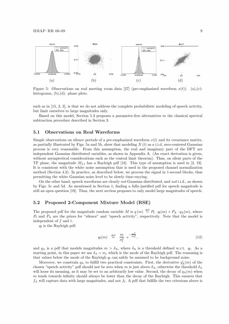
Figure 5: Observations on real meeting room data [27] (pre-emphasized waveform x(t)). (a),(c):histograms, (b),(d): phase plots.

such as in [15, 2, 3], is that we do not address the complete probabilistic modeling of speech activity,but limit ourselves to large magnitudes only.

Based on this model, Section 5.3 proposes a parameter-free alternatives to the classical spectralsubtraction procedure described in Section 3.

5.1 Observations on Real Waveforms

Simple observations on silence periods of a pre-emphasized waveform x(t) and its covariance matrix,as partially illustrated by Figs. 5a and 5b, show that modeling X (t) as a i.i.d, zero-centered Gaussianprocess is very reasonable. From this assumption, the real and imaginary part of the DFT areindependent Gaussian distributed variables, as shown in Appendix A. (An exact derivation is given,without asymptotical considerations such as the central limit theorem). Thus, on silent parts of theTF plane, the magnitude Mf,t has a Rayleigh pdf [18]. This type of assumption is used in [2, 19].It is consistent with the white noise assumption that is used in the proposed channel normalizationmethod (Section 4.2). In practice, as described below, we process the signal in 1-second blocks, thuspermitting the white Gaussian noise level to be slowly time-varying.

On the other hand, speech waveforms are clearly not Gaussian distributed, and not i.i.d., as shownby Figs. 5c and 5d. As mentioned in Section 1, finding a fully-justified pdf for speech magnitude isstill an open question [19]. Thus, the next section proposes to only model large magnitudes of speech.

5.2 Proposed 2-Component Mixture Model (RSE)

The proposed pdf for the magnitude random variable M is q (m)def= PI · qI(m) + PA · qA(m), where

PI and PA are the priors for “silence” and “speech activity”, respectively. Note that the model isindependent of f and t.

qI is the Rayleigh pdf:

qI(m)def=

m

σ2I

e− m2

2σ2I , (12)

and qA is a pdf that models magnitudes m > δA, where δA is a threshold defined w.r.t. qI. As astarting point, in this paper we use δA = σI, which is the mode of the Rayleigh pdf. The reasoning isthat values below the mode of the Rayleigh qI can safely be assumed to be background noise.

Moreover, we constrain qA to fulfill two practical constraints. First, the derivative q′A(m) of thechosen “speech activity” pdf should not be zero when m is just above δA, otherwise the threshold δA

will loose its meaning, as it may be set to an arbitrarily low value. Second, the decay of qA(m) whenm tends towards infinity should always be lower than the decay of the Rayleigh. This ensures thatfA will capture data with large magnitudes, and not fI. A pdf that fulfills the two criterions above is

10 IDIAP–RR 06-09

a “shifted Erlang” pdf with h=2 (the Erlang pdf belongs to the Gamma family [18]):

qA(m)def= 1m>σI

· λ2A · (m − σI) · e

−λA(m−σI), (13)

where 1m>σIis equal to 1 if m > σI, and zero otherwise. Note the implicit stationarity assumption:

the 4 parameters Λ = {PI, σI, PA, λA} are assumed to be independent of t. Furthermore, independenceof f is also assumed; it is partially justified by the pre-emphasis, which whitens the spectrum. TheRSE model is similar to the probabilistic model used for microphone array-based speech detection,in [20].

EM training of Λ: The proposed mixture model can be trained using the EM algorithm [6].Both “E” and “M” steps involve simple mathematical expressions. In the “E” step, posteriors can beestimated as follows:

P (sil |mf,t, Λ) =PI · qI(mf,t)

PI · qI(mf,t) + PA · qA(mf,t)(14)

P (act |mf,t, Λ) = 1 − P (sil |mf,t, Λ) (15)

In the “M” step, exact maximization of the likelihood is difficult: since parameters σI and λA aretied in a non-linear fashion (Eq. 13), we have not found a way to separate them analytically. Fromthis constatation, we propose two options:

1. Numerical optimization of the exact likelihood of the observed data through simplex search inthe (σI, λA) space (e.g. fminsearch in MATLAB). In this case, the M step requires severalsub-iterations before reaching a local maximum. We refer to this option as “ML”.

2. Analytical approximation through a moment-method, in a single step. First σI is updated usingall data, then λA is updated using all data with values above the new σI value. This option isreferred to as “moment”. It is defined by the following update equations:

σI =

∑

f,t

m2f,t · P (sil |mf,t, Λ)

2∑

f,t

P (sil |mf,t, Λ)

12

(16)

λA =

∑

mf,t>σI

(mf,t − σI)−1

· P (act |mf,t, Λ)

∑

mf,t>σI

P (act |mf,t, Λ)(17)

Data representation: As opposed to histogram-based implementations, in this paper the costis reduced, using a direct representation with a reduced set of samples (no weights). In all resultsreported in this paper, only 100 representative samples are used: observed magnitude values are sortedin an increasing manner, from which 100 samples are picked at regular intervals. This data reductionmethod is equivalent to estimate percentile values at equal steps.

Figs. 6a, 6b and 6c show an example of fit on one file taken from the OGI Numbers 95 database [23].(OGI Numbers 95 is used because its transmission channel is flat.) In the following, we’ll refer to theRayleigh and Shifted Erlang model as “RSE”.

Approximation: it is possible to approximate the σI parameter for an even lower computationalcost than RSE fitting, as described in Appendix B. The cost is a slight but systematic degradation ofthe ASR performance.

IDIAP–RR 06-09 11

(a)Original spectrogram

mf,t

magnitude

allsilenceactivitydata

(b)Fit (linear domain)

log magnitude

allsilenceactivitydata

(c)Fit (log domain)

(d)Spectrogram after subtraction

mUSSf,t

Figure 6: Example of fit of the 2-component model on noisy data taken from the OGI Numbers 95database (Factory 0dB condition). All plots show magnitude data in the frequency domain. Onspectrogram plots (a) and (d), the largest magnitudes are white, the smallest magnitudes are black.(OGI Numbers 95 [23] is used for this example because the transmission channel is flat.)

5.3 USS with the RSE Model (RSE-USS)

A 2-step approach is used:

1. Joint speech/noise modeling with EM fitting of the RSE parameters Λ, as described in Sec-tion 5.2, using either “ML” or “moment”. Prior ASR studies [11] on OGI Numbers 95 showthat “moment” yields better results than “ML”. Thus, all RSE-USS results reported below wereobtained using “moment”.

2. Spectral subtraction using parameter σI as a floor:

mUSSf,t

def= max

(

1,mf,t

σI

)

. (18)

Note that the flooring to a non-zero value (max (1, . . .)) is necessary in the MFCC context. Indeed,leaving zero magnitude values after spectral subtraction would lead to undesirable dynamics in cepstralcoefficients. An example of result of Eq. 18 is shown in Fig. 6d. Although Eq. 18 is not, strictlyspeaking, the spectral subtraction scheme described by Eq. 4, it has the same two characteristic:noise removal and flooring. We prefered the normalization scheme of Eq. 18 in order to avoid tunableparameters (Issue 3 in Section 3.3). The overall computational cost of RSE-USS (Eq. 18) is small,because posteriors (Eqs. 14 and 15) don’t need to be computed. RSE-USS only requires σI, whichcan also be obtained for a small cost, as explained in Section 5.2. This justifies the “unsupervised”qualification.

This approach can be compared to previous works. We can note common points “in spirit”with [17] (and to a lesser extent [16]): adaptation to non-stationary noises is possible in both [17]and our approach through block-wise processing, as illustrated by experiments on OGI Numbers 95reported in [11]. Moreover, on the modeling side, parameters of the “noise” distribution (i.e. silence)are more important than those of the “speech” distribution (i.e. activity) in both approaches, as theyare used to floor the magnitude values (max operator).

However, here the modeling is made directly at the magnitude spectrogram level, with a singlemodel for all frequencies, while in [17] modeling was made after mel filterbank computation, anda model was defined for each critical band separately. Furthermore, the approach proposed here isone-pass, fully unsupervised, without any “feedback” loop, without any tunable threshold, withouthistogram. In [17], multiple stages are involved, including histograms, band-specific parameters, short-term and long-term adaptation, a “feedback” loop, tunable parameters that have to be trained and(optionally) an artificial white noise is injected.

Finally, it is important to realize that in log the domain, the Rayleigh distribution has a fixedshape. Indeed, a change of the σI parameter only corresponds to a translation in the log-domain,

12 IDIAP–RR 06-09

as proven by the next section. From this perspective, the Rayleigh is a lot more constrained than alog-normal distribution, for example. Although this could look like a disadvantage, it avoids capturingtoo much speech information with the noise distribution. Thus, with the RSE model, potentially morespeech information is conserved in noisy situations.

6 Application to Noise-Robust ASR

This section compares various noise reduction techniques, used as a front-end for an HMM/GMMspeech recognizer, on the Aurora 2 task [21]. First, the baseline ETSI Mel-Cepstrum Front-End ispresented [28]. Second, the ETSI Advanced Front-End for noise-robust ASR is described [7]. Third, itis proposed to replace the noise reduction part of the ETSI Front-End with a simpler, parameter-freealternative: channel normalization (Section 4.2) followed by USS (Section 5). Results show that therobustness to noise is greatly improved.

6.1 ETSI Mel-Cepstrum Front-End (MFCC)

The ETSI Mel-Cepstrum Front-End [28] is used as a baseline. The output feature vector has 14 com-ponents only: log energy and MFCC coefficients C0 to C12 (no derivatives). Normalization techniquessuch as Blind Equalization or CMS/CVN are not used. In order to have a fair comparison with thenoise-robust front-ends described in the following, Voice Activity Detection (VAD) was simulated using“end-pointing”. Using the known beginning and end of each speech utterance, all silences before andafter were replaced with a fixed 200 ms duration. Results are provided courtesy of Prof. Gunther Hirschand Mr. David Pearce. In the following, we denote this front-end MFCC.

6.2 ETSI Advanced Front-End (AFE)

The ETSI Advanced Front-End for noise-robust ASR [7] includes a sequence of 3 successive parts:(1) noise reduction with double Wiener filtering, (2) MFCC extraction and (3) Voice Activity Detec-tion (VAD).

The first part, noise reduction (depicted in Fig. 7), is expected to remove most of the noise fromthe time-domain waveform, and output a “denoised” time-domain waveform. It includes a two-passWiener filtering, which itself requires SNR estimation in the frequency domain. In the first pass, aspecialized detector is applied to separate the speech time frames from the noise time frames. Fromspeech/noise decisions and the observed spectrum, the SNR is estimated at each point of the TFplane, and a Wiener filter is designed in the mel filter-bank domain. The Wiener filter is then appliedto the input waveform and a denoised time-domain signal is reconstructed. On this denoised signal,the entire process is repeated a second time, in order to produce an even cleaner signal. Finally, aTeager operator is applied, that emphasizes the high-SNR parts of the waveform. Overall, this firstpart includes many numerical parameters and “if/then” rules.

In the second part, the “denoised” time-domain waveform is fed into a MFCC extractor. It isessentially standard, with some additional optimizations such as 0.9 pre-emphasis, combination of logenergy and C0, and blind equalization.

The third part is optional. It is a sophisticated VAD that combines three different types of measures(mel-warped Wiener filter coefficients, spectral sub-bands and spectral variance). The output is aspeech/silence binary decision for each time frame. It can be used to ignore non-speech frames, whichaims at improving the ASR performance [7].

In the following, we denote this front-end AFE.

6.3 Proposed Front-Ends

The experimental investigation aims at simplifying the first part of the AFE, noise reduction, replacingthe many rules and parameters with simpler approaches. The other two parts of the AFE (MFCC

IDIAP–RR 06-09 13

mean

speechdetection

filter

second pass

warping,and IDCT filtering

timedomainestimation

spectrum

Teageroperator

melWiener

design

x(t)

denoised signal x’(t)

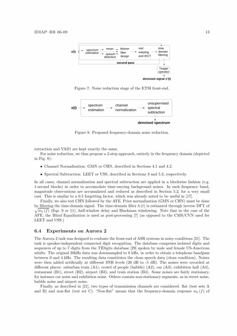
Figure 7: Noise reduction stage of the ETSI front-end.

spectrumestimation

channelnormalization

denoised spectrum

spectralunsupervised

subtractionx(t)

Figure 8: Proposed frequency-domain noise reduction.

extraction and VAD) are kept exactly the same.For noise reduction, we thus propose a 2-step approach, entirely in the frequency domain (depicted

in Fig. 8):

• Channel Normalization: GMN or CHN, described in Sections 4.1 and 4.2.

• Spectral Subtraction: LEET or USS, described in Sections 3 and 5.3, respectively.

In all cases, channel normalization and spectral subtraction are applied in a blockwise fashion (e.g.1-second blocks) in order to accomodate time-varying background noises. In each frequency band,magnitude observations are accumulated and reduced as described in Section 5.2, for a very smallcost. This is similar to a 0.5 forgetting factor, which was already noted to be useful in [17].

Finally, we also test CHN followed by the AFE. Prior normalization (GMN or CHN) must be doneby filtering the time-domain signal. The time-domain filter h (t) is estimated through inverse DFT of√

wh (f) (Eqs. 9 or 11), half-window delay and Blackman windowing. Note that in the case of theAFE, the Blind Equalization is used as post-processing [7] (as opposed to the CMS/CVN used forLEET and USS.)

6.4 Experiments on Aurora 2

The Aurora 2 task was designed to evaluate the front-end of ASR systems in noisy conditions [21]. Thetask is speaker-independent connected digit recognition. The database comprises isolated digits andsequences of up to 7 digits from the TIDigits database [29] spoken by male and female US-Americanadults. The original 20kHz data was downsampled to 8 kHz, in order to obtain a telephone bandpassbetween 0 and 4 kHz. The resulting data constitutes the clean speech data (clean condition). Noiseswere then added artificially at different SNR levels (20 dB to -5 dB). The noises were recorded atdifferent places: suburban train (A1), crowd of people (babble) (A2), car (A3), exhibition hall (A4),restaurant (B1), street (B2), airport (B3), and train station (B4). Some noises are fairly stationary,for instance car noise and exhibition noise. Others contain non-stationary segments, as in street noise,babble noise and airport noise.

Finally, as described in [21], two types of transmission channels are considered: flat (test sets Aand B) and non-flat (test set C). “Non-flat” means that the frequency-domain response wh (f) of

14 IDIAP–RR 06-09

the transmission channel has a non-zero slope. It corresponds to some types of GSM cellphones.In the “non-flat” case, the proposed channel normalization presented in Section 4.2 is expected tocompensate for the “flat” channel implicitely assumed by spectral subtraction methods. Ideally, theresult of a recognizer should be independent of the transmission channel.

The Aurora 2 task defines two different training modes: training on clean condition only, andtraining on both clean and noisy conditions. In this paper, only experiments with training on cleancondition are reported, because the purpose of our approach is precisely to remove noise as muchas possible in order to make acoustic modeling as noise-robust as possible, while retaining similarperformance in clean conditions. The details about the training set, test set and HTK recognizer canbe found in [21].

Based on initial tests [11] done on the OGI Numbers 95 task [23] we selected a 1-second blocksize and applied the various approaches to the Aurora 2 corpus [21]. The frame shift is 10 ms andthe frame length is 25 ms. For all proposed front-ends (except the baseline) 13 MFCC coefficientsare extracted (C0 to C12), along with deltas and delta-deltas, and fed into the Aurora 2 HMM/GMMrecognizer [21]. In order to have a fair comparison, for all front-ends (except for the MFCC baseline),the same AFE MFCC/delta/delta-delta extractor and AFE VAD are used [7]. They are brieflydescribed in Section 6.2. As already mentioned, post-processing is done through Blind Equalizationin the case of the AFE [7]. On the other hand, post-processing is done with CMS, CVN in the caseof spectral subtraction (LEET and USS).

6.5 Results and Discussion

Overall average WER results for each test set A,B,C are presented in Table 1. Averages per noisetype are shown in Fig. 9a. Averages per SNR level are depicted in Figs. 9b, 10a and 10b.

In all cases, results on Test Set C (mismatched channel) confirm that normalizing the channelbefore the non-linear noise reduction stage is beneficial, as compared to methods that attempt tonormalize the channel only after the noise reduction stage (LEET and USS with CMS/CVN, AFEwith Blind Equalization). As a by-product, improvement also appears for the other cases (Test Sets Aand B), except for the AFE on Test Set A. This is mainly due to the Exhibition noise (A4 in Fig. 9a).In all cases, the proposed channel normalization (CHN) is superior to the existing normalizationmethod (GMN).

The improvement from USS to CHN-USS is quite remarkable, leading to results comparable tothose of the AFE: 13.4 % overall average WER for CHN-USS, 13.2 % for the AFE. This is interesting,given that Eqs. 6 and 18 fully describe the modifications of the spectrum. On the contrary, the AFEincludes many more rules and parameters [7]. USS also provides results superior to those of LEET, asvisible in Table 1. A possible explanation is that LEET was originally designed for speech enhancementfor human listening: noise-robust ASR with a HMM/GMM system may have different needs.

The CHN-AFE result has the best overall WER (12.5 %). Compared to AFE (Fig. 10), CHN-AFE yields an improvement in noisy conditions below 10 dB of up to 5 % absolute WER, for a slightdegradation above 10 dB (up to 1 % absolute WER), and similar results in clean conditions (0.2 %absolute degradation, the relative variations are not significant). In terms of test sets, there is adegradation on test set A, for an improvement on test sets B and C. In order to assess the cause ofthe degradation on test set A, we looked at average results for each noise type (Fig. 9a). It appearsthat the “Exhibition Hall” condition is the main source of problems. From the long-term spectralshapes shown in [21], this noise seems to occupy the largest bandwidth, having a roughly equally-distributed spectrum across frequencies. So it would seem to fit well the white noise assumed byCHN (Section 4.2), which is a contradiction with the degradation observed. One possible explanationis that “Exhibition Hall” also often includes non-white noises, such as people speaking, whistling andsome strong voices. This suggests refining the noise model, possibly by doing channel normalizationand noise removal jointly. Integrating CHN inside the 2-stage AFE process is a possibility.

To conclude, two main observations can be made. First, the proposed “channel normalization”method alone greatly reduces not only the sensitivity to channel variability, but also the stationary

IDIAP–RR 06-09 15

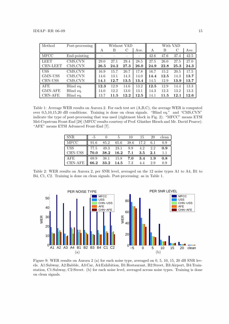
Method Post-processing Without VAD With VADA B C Ave. A B C Ave.

MFCC End-pointing – – – – 42.6 47.6 37.4 42.5

LEET CMS,CVN 29.0 27.1 29.4 28.5 27.5 26.0 27.5 27.0CHN-LEET CMS,CVN 26.5 24.2 27.3 26.0 24.9 22.8 25.3 24.3

USS CMS,CVN 16.9 15.7 20.7 17.8 16.7 15.2 20.5 17.5GMN-USS CMS,CVN 14.6 13.1 14.3 14.0 14.4 12.5 14.3 13.7

CHN-USS CMS,CVN 14.1 12.7 13.5 13.4 14.5 12.9 13.9 13.7

AFE Blind eq. 12.3 12.9 14.6 13.2 12.5 12.9 14.4 13.3GMN-AFE Blind eq. 14.0 12.2 13.0 13.1 14.3 12.3 13.2 13.3CHN-AFE Blind eq. 13.7 11.5 12.2 12.5 14.1 11.5 12.1 12.6

Table 1: Average WER results on Aurora 2. For each test set (A,B,C), the average WER is computedover 0,5,10,15,20 dB conditions. Training is done on clean signals. “Blind eq.” and “CMS,CVN”indicate the type of post-processing that was used (rightmost block in Fig. 2). “MFCC” means ETSIMel-Cepstrum Front-End [28] (MFCC results courtesy of Prof. Gunther Hirsch and Mr. David Pearce).“AFE” means ETSI Advanced Front-End [7].

SNR -5 0 5 10 15 20 clean

MFCC 91.6 85.2 65.6 38.6 17.2 6.1 0.9

USS 77.5 49.3 23.1 9.9 4.2 2.2 0.9

CHN-USS 70.0 38.2 16.2 7.1 3.5 2.1 1.1

AFE 69.9 38.1 15.8 7.0 3.4 1.9 0.8

CHN-AFE 66.2 33.2 14.5 7.3 4.4 2.9 0.9

Table 2: WER results on Aurora 2, per SNR level, averaged on the 12 noise types A1 to A4, B1 toB4, C1, C2. Training is done on clean signals. Post-processing: as in Table 1.

A1 A2 A3 A4 B1 B2 B3 B4 C1 C20

10

20

30

40

50

WE

R

PER NOISE TYPEMFCCUSSCHN−USSAFECHN−AFE

−5 0 5 10 15 20 clean0

20

40

60

80

WE

R

PER SNR LEVELMFCCUSSCHN−USSAFECHN−AFE

(a) (b)

Figure 9: WER results on Aurora 2 (a) for each noise type, averaged on 0, 5, 10, 15, 20 dB SNR lev-els. A1:Subway, A2:Babble, A3:Car, A4:Exhibition, B1:Restaurant, B2:Street, B3:Airport, B4:Train-station, C1:Subway, C2:Street. (b) for each noise level, averaged across noise types. Training is doneon clean signals.

16 IDIAP–RR 06-09

−5 0 5 10 15 20 clean

−50

−40

−30

−20

−10

0

abso

lute

WE

R v

aria

tion

PER SNR LEVEL (absolute var.)

MFCCUSSCHN−USSAFECHN−AFE

−5 0 5 10 15 20 clean−80

−60

−40

−20

0

20

rela

tive

WE

R v

aria

tion

(%)

PER SNR LEVEL (relative var.)

(a) (b)

Figure 10: Absolute and relative WER variation (the lower, the better) compared to the ETSI Mel-Cepstrum Front-End (denoted MFCC), on Aurora 2, for all three test sets A, B and C (average).Training is done on clean signals.

part of the additive noise. This is expected due to the non-white nature of real noises, as explained inSection 4.2. Second, the AFE was greatly simplified, by replacing the many-step two-pass Wiener fil-tering with direct, simple spectral subtraction approaches. Each step of the proposed approach (CHNand USS), relies on a single equation (Eqs. 6 and 18, respectively), and no tuning parameter. CHN-USS yields an ASR performance very similar to that of the AFE, and CHN-AFE yields the bestaverage results. Further improvement may be obtained on clean conditions through expliciting theadditive channel noise – we neglected it as a first step, focussing on very noisy conditions.

7 Conclusion

Three limitations of classical spectral subtraction were addressed by this paper, in the context ofnoise-robust ASR. First, a channel normalization method was proposed, in order to extend spectralsubtraction to non-flat transmission channels such as cellphones. In practice, the proposed channelnormalization method not only removes the convolutive noise due to the channel, but also part of theadditive acoustic noise. Results on the Aurora 2 task show that the proposed channel normalizationeffectively accomodates mismatch channels, and leads to better ASR performance for all front-ends(ETSI Advanced Front-End, as well as spectral subtraction). In particular, the improvement is clear, ascompared to methods that attempt to normalize the channel only after the non-linear noise-reductionstage. A second limitation addressed by this paper is that the underlying noise estimate is a crucialfactor for the ASR performance of spectral subtraction methods. This issue was then postulated to betightly linked with the third limitation, i.e. the need of task-dependent, condition-dependent tuningfactors. As an alternative, a straightforward procedure called “Unsupervised Spectral Subtraction”was proposed, that jointly models speech and noise at the magnitude spectrogram level. It is com-pletely unsupervised, as it does not have any tuning factor. Combined with channel normalization,it provides very similar ASR performance to that of the ETSI Advanced Front-End, on the Aurora 2corpus. This is quite interesting, given that the proposed signal transformation is fully describedby two equations (Eqs. 6 and 18), while the ETSI Advanced Front-End includes many steps andparameters. The absence of tuning factors, and the very low computational cost makes it directlyfit for real-time applications on low-power nodes such as cellphones and PDAs. Future work mayinclude several directions. The result with channel normalization followed by the ETSI AdvancedFront-End suggests possibilities for further improvement in noisy conditions, for example through

IDIAP–RR 06-09 17

joint noise/channel modelling. This would permit to use more complex noise models than the slowly-varying white Gaussian noise assumption consistently used here. Moreover, improvement in cleanconditions may be expected by expliciting the additive channel noise term in the signal model.

Acknowledgments

The authors acknowledge the support of the European Union through the AMI and HOARSE projects.This work was also carried out in the framework of the Swiss National Center of Competence inResearch (NCCR) on Interactive Multi-modal Information Management (IM)2. The authors wouldlike to thank Prof. Rainer Martin, Prof. Hynek Hermansky and Bertrand Mesot for fruitful discussionsand suggestions. The authors thank Prof. Gunther Hirsch and Colin Breithaupt for their suggestionsand technical help.

A Proof of the Rayleigh distribution of magnitudes

In this section we derive the Rayleigh magnitude-domain silence model of |FXf | (Eq. 12), from a white

Gaussian assumption for the pre-emphasized signal Xt.First, let us recall a result originally shown by Rice in 1944 (for a demonstration

see [18, pp. 296-297]). Rice showed that given two zero-mean Gaussian, uncorrelated random variables

A and B with same standard deviation σ, and Rdef= |A + jB|, the R variable has a Rayleigh pdf:

qR(r) =r

σe−

r2

2σ2 for r > 0. (19)

Let us now define X1:N , as a vector of N uncorrelated1 zero-mean Gaussian random variables

X1:Ndef= [X1 . . . XN ]

T. The Discrete Fourier Transform (DFT) of X is FX

1:Nbins=

[

FX1 · · · FX

Nbins

]T

where for a given f = 1 . . . Nbins:

FXf

def=

N∑

n=1

Xne−2π(f−1) n−1N . (20)

Let Af = Re(

FXf

)

and Bf = Im(

FXf

)

. In other terms:

{

Af =∑N

n=1 Xn cos(

−2π(f − 1)n−1N

)

,

Bf =∑N

n=1 Xn sin(

−2π(f − 1)n−1N

) (21)

For f = 1 we have A1 =∑N

n=1 Xn and B1 = 0.For f > 1: the random variable Af (resp. Bf ) is a weighted sum of zero-mean, single Gaussian

random variables, therefore [30, p. 99] it is also a zero-mean, single Gaussian random variable withvariance:

{

σ2Af

= σ2∑N

n=1 cos2(

2π (f − 1) n−1N

)

,

σ2Bf

= σ2∑N

n=1 sin2(

2π (f − 1) n−1N

)

.(22)

Given that cos2 t = 12 (1 + cos 2t) and sin2 t = 1

2 (1 − cos 2t) we can write:

σ2Af

= σ2

2

(

N +∑N

n=1 cos(

4π (f − 1) n−1N

)

)

,

σ2Bf

= σ2

2

(

N −∑N

n=1 cos(

4π (f − 1) n−1N

)

)

.(23)

1Uncorrelation and independence are equivalent for Gaussian random variables.

18 IDIAP–RR 06-09

Figure 11: Comparison between the σ parameter estimated by fitting a RSE model (Section 5.2) andthe geometric mean of all observed magnitude values (Section B). The graph is shown in the logdomain (grey points), and the dark line represents equality. In the linear domain, the correlation is0.97 and the slope is 1.26.

Let us now write the complex domain sum:

N∑

n=1

ej4π(f−1) n−1N =

N−1∑

n=0

αn =1 − αN

1 − α= 0, (24)

because αN = 1, where α = ej4πf−1

N . (Since 1 < f ≤ N , α 6= 1 and all terms in Eq. 24 are defined.)From Eq. 23, and the real part of Eq. 24, we conclude that:

σAf= σBf

= σ

√

N

2. (25)

Similarly, the cross-correlation σAf Bf

def= E{AfBf} can be shown to be zero, using the imaginary

part of Eq. 24 and the uncorrelation hypothesis on the Xn variables.

To conclude, we have shown that the random variables Af and Bf are zero-mean, uncorrelatedsingle Gaussian random variables of same variance, therefore the result of Rice applies:

For f > 1,∣

∣

∣FX

f

∣

∣

∣has a Rayleigh pdf of parameter σ

√

N2 .

B Simplified Geometric Mean Noise Estimation of the RSE

The estimated parameter σI of the RSE model (Section 5.2) is shown here to be closely related tothe geometric mean of a Rayleigh distribution. We assume a Rayleigh-distributed magnitude M

variable (Eq. 12) with parameter σ. The pdf of the log magnitude L = log M is then:

g (l)def=

e2l

σ2e−

e2l

2σ2 (26)

We are now trying to estimate the first moment of g: 〈l〉gdef=

∫ +∞

−∞ l · g (l) · dl. An analytical expressionis difficult to obtain, thus a numerical alternative is proposed below.

For any two parameter values σ and σ∗, and the associated pdfs g(l) and g∗(l), we can write:

∀l ∈ R g (l) = g∗(

l − logσ

σ∗

)

(27)

IDIAP–RR 06-09 19

therefore, the first moments of g and g∗ are related as follows:

〈l〉g = 〈l〉g∗ + logσ

σ∗(28)

Setting σ∗ = 1, we obtain the first moment of g:

〈l〉g = ε + log σ (29)

where ε is a constant equal to the geometric mean of Rayleigh-distributed data with parameter σ∗ = 1.Monte Carlo simulation leads to the numerical evaluation ε ≈ 0.06. It is therefore reasonable

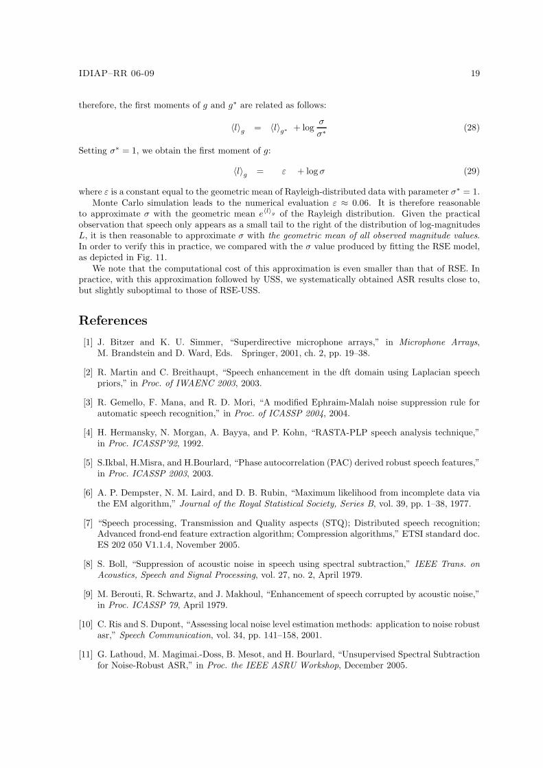
to approximate σ with the geometric mean e〈l〉g of the Rayleigh distribution. Given the practicalobservation that speech only appears as a small tail to the right of the distribution of log-magnitudesL, it is then reasonable to approximate σ with the geometric mean of all observed magnitude values.In order to verify this in practice, we compared with the σ value produced by fitting the RSE model,as depicted in Fig. 11.

We note that the computational cost of this approximation is even smaller than that of RSE. Inpractice, with this approximation followed by USS, we systematically obtained ASR results close to,but slightly suboptimal to those of RSE-USS.

References

[1] J. Bitzer and K. U. Simmer, “Superdirective microphone arrays,” in Microphone Arrays,M. Brandstein and D. Ward, Eds. Springer, 2001, ch. 2, pp. 19–38.

[2] R. Martin and C. Breithaupt, “Speech enhancement in the dft domain using Laplacian speechpriors,” in Proc. of IWAENC 2003, 2003.

[3] R. Gemello, F. Mana, and R. D. Mori, “A modified Ephraim-Malah noise suppression rule forautomatic speech recognition,” in Proc. of ICASSP 2004, 2004.

[4] H. Hermansky, N. Morgan, A. Bayya, and P. Kohn, “RASTA-PLP speech analysis technique,”in Proc. ICASSP’92, 1992.

[5] S.Ikbal, H.Misra, and H.Bourlard, “Phase autocorrelation (PAC) derived robust speech features,”in Proc. ICASSP 2003, 2003.

[6] A. P. Dempster, N. M. Laird, and D. B. Rubin, “Maximum likelihood from incomplete data viathe EM algorithm,” Journal of the Royal Statistical Society, Series B, vol. 39, pp. 1–38, 1977.

[7] “Speech processing, Transmission and Quality aspects (STQ); Distributed speech recognition;Advanced frond-end feature extraction algorithm; Compression algorithms,” ETSI standard doc.ES 202 050 V1.1.4, November 2005.

[8] S. Boll, “Suppression of acoustic noise in speech using spectral subtraction,” IEEE Trans. on

Acoustics, Speech and Signal Processing, vol. 27, no. 2, April 1979.

[9] M. Berouti, R. Schwartz, and J. Makhoul, “Enhancement of speech corrupted by acoustic noise,”in Proc. ICASSP 79, April 1979.

[10] C. Ris and S. Dupont, “Assessing local noise level estimation methods: application to noise robustasr,” Speech Communication, vol. 34, pp. 141–158, 2001.

[11] G. Lathoud, M. Magimai.-Doss, B. Mesot, and H. Bourlard, “Unsupervised Spectral Subtractionfor Noise-Robust ASR,” in Proc. the IEEE ASRU Workshop, December 2005.

20 IDIAP–RR 06-09

[12] R. Martin, “An efficient algorithm to estimate the instantaneous snr of speech signals,” in Proc.

EUROSPEECH 1993, 1993.

[13] H. Hermansky, “TRAP-TANDEM: Data-driven extraction of temporal features from speech,” inProc. ASRU 2003, 2003.

[14] H. Bourlard, S. Bengio, M. M. Doss, Q. Zhu, B. Mesot, and N. Morgan, “Towards using hierar-chical posteriors for flexible automatic speech recognition systems,” in Proc. the DARPA EARS

RT04 Workshop, 2004.

[15] Y. Ephraim and D. Malah, “Speech enhancement using a minimum mean-square error short-timespectral amplitude estimator,” in Proc. ICASSP 1984, 1984.

[16] J. Cohen, “Application of an auditory model to speech recognition,” Journal of the Acoustic

Society of America, vol. 85, no. 6, June 1989.

[17] D. V. Compernolle, “Noise adaptation in a hidden markov model speech recognition system,”Computer Speech and Language, vol. 13, no. 1, 1989.

[18] C. M. Grinstead and J. L. Snell, Introduction to Probability. American Mathematical Society,1997.

[19] B. Chen and P. Loizou, “Speech enhancement using a MMSE short time spectral amplitudeestimator with Laplacian speech modeling,” in Proc. of ICASSP 2005.

[20] G. Lathoud, M. Magimai.-Doss, and H. Bourlard, “Threshold selection for unsupervised detec-tion, with an application to microphone arrays,” in Proc. ICASSP, 2006.

[21] H. Hirsch and D. Pearce, “The Aurora experimental framework for the performance evaluation ofspeech recognition systems under noisy conditions,” in Proc. ISCA ITRW ASR2000, September2000.

[22] H. Hirsch and C. Ehrlicher, “Noise estimation techniques for robust speech recognition,” in Proc.

ICASSP, 1995.

[23] R. A. Cole, M. Fanty, M. Noel, and T. Lander, “Telephone speech corpus development at CSLU,”1994.

[24] G. Lathoud, M. Magimai.-Doss, and H. Bourlard, “Channel normalization for unsupervised spec-tral subtraction,” IDIAP-RR 06-09, 2006.

[25] C. Avendano, S. Tibrewala, and H. Hermansky, “Multiresolution channel normalization for asrin reverberant environments,” in Proc. Eurospeech, 1997.

[26] D. Gelbart and N. Morgan, “Evaluating long-term spectral subtraction for reverberant asr,” inProc. the IEEE ASRU Workshop, 2001.

[27] G. Lathoud, J.-M. Odobez, and D. Gatica-Perez, “AV16.3: an Audio-Visual Corpus for SpeakerLocalization and Tracking,” in Proc. the 2004 MLMI Workshop, S. Bengio and H. Bourlard Eds,

Springer Verlag, 2005.

[28] “Speech processing, Transmission and Quality aspects (STQ); Distributed speech recognition;Frond-end feature extraction algorithm; Compression algorithms,” ETSI standard doc. ES 201108 V1.1.2, April 2000.

[29] R. Leonard, “A database for speaker-independent digit recognition,” in Proc. ICASSP 2004,2004.

[30] J.-P. Delmas, Introduction aux Probabilites. Ellipses Marketing, 1993.