Channel coding - Introduction & linear codes

Introduction Decoding Linear block codes Cyclic codes

Channel codingIntroduction & linear codes

Manuel A. VazquezJose Miguel LeivaJoaquın Mıguez

February 27, 2022


Index

1 IntroductionChannel models

2 DecodingHard decodingSoft decodingCoding gain

3 Linear block codesFundamentalsDecoding

4 Cyclic codesPolynomialsDecoding


Index






(Channel) Coding

Goal

Add redundancy to the transmitted information so that it can berecovered if errors happen during transmission.

0 → 000

1 → 111so that, e.g.,

010→ 000111000

What should we decide it was transmitted if we receive

010100000 ?

Example: repetition code


Digital communications system

B Encoder Modulator + Demodulator Detector B

n(t) :AWGN noise with

PSD N0/2

A s(t) r(t) q = A + n

transmitter receiver

This model can be analyzed at different levels...

Digital channel

Gaussian channel


Digital channel



PSD N0/2

A s(t) r(t) q = A + n


B Digital channel B


Gaussian channel (with digital input)



PSD N0/2

A s(t) r(t) q = A + n


A Gaussian channel q


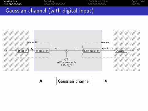
Some basic concepts

CodeMapping from a sequence of k bits into another one of n > kbits.

b coding transmission decoding b

bi ciB[0], B[1], · · ·

orq[0],q[1], · · ·

bi

i = 1, · · · , 2k i = 1, · · · , 2k

Probability of error for bi

P ie = Pr{b 6= bi |b = bi}, i = 1, . . . , 2k

Maximum probability of error: Pmaxe = maxi P

ie

Rate: The rate of a code is the number of information bits,k , carried by a codeword of length n.

R = k/n


Codeword vs bit error probability

Notation

Pe : codeword error probability

Pe =# codewords received incorrectly

overall # codewords=

v

w

BER (Bit Error Rate): bit error probability

BER =# incorrect bits

# transmitted bits

(they match if every codeword carries a single bit)

worst-case scenario → BER = v×kw×k = Pe

best-case scenario → BER = v×1w×k = Pe

k

}⇒ Pe

k≤ BER ≤ Pe


Channel coding theorem

Theorem: Channel coding (Shannon, 1948)

If C is the capacity of a channel, then it is possible to reliablytransmit with rate R < C .

CapacityIt is the maximum of the mutual information between

the input and output of the channel.

Reliable transmissionThere is a sequence of codes (n, k) = (n, nR) such

that, when n→∞, Pmaxe → 0.


Channel coding theorem: example

1− p

p

p

1− p

0 0

1 1

C = 1− Hb(p),

being p the channelBER and Hb the bi-nary entropy.

Let us consider 4 binary channels with

p = 0.15⇒ C1 = 0.39 p = 0.13⇒ C2 = 0.44p = 0.17⇒ C3 = 0.34 p = 0.19⇒ C4 = 0.29

and a code with rate R = 1/3 = 0.33.

A code with rate R = 1/3 only respects the Shannon limit in thefirst three scenarios.

Channel coding theorem


Channel coding theorem: example

The figure shows the evolution of the codeword error probability asa function of n: it approaches 0 when R < C .

Figure: Left: logarithmic scale; right: linear scale


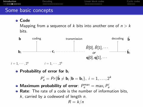
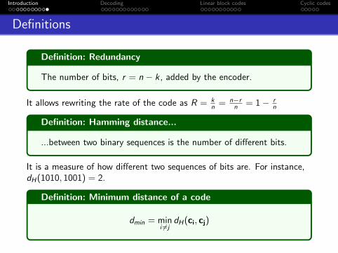
Definitions

Definition: Redundancy

The number of bits, r = n − k , added by the encoder.

It allows rewriting the rate of the code as R = kn = n−r

n = 1− rn

Definition: Hamming distance...

...between two binary sequences is the number of different bits.

It is a measure of how different two sequences of bits are. For instance,dH(1010, 1001) = 2.

Definition: Minimum distance of a code

dmin = mini 6=j

dH(ci, cj)


Index






Hard decoding

Decoding at the bit level

It relies on the digital channel

B Digital channel B

The input to the decoder are bits coming from the Detector ,

the B’s.

Metric is the Hamming distance.

Notation

ci =[C i [0],C i [1], · · ·C i [n − 1]

]≡ i-th codeword

r =[B[0], B[1], · · · B[n − 1]

]≡ received word


Hard decoding: decision rule

Maximum a Posteriori (MAP) rule: we decide ci if

p(ci | r) > p(cj | r) ∀j 6= i

If all the codewords are equally likely, it is equivalent toMaximum Likelihood (ML),

p(r | ci ) > p(r | cj) ∀j 6= i

Likelihoods can be expressed in terms of dH

p(r | ci ) = εdH (r,ci )(1− ε)n−dH (r,ci )

ε ≡ channel bit error probability

If ε < 0.5 ML rule is tantamount to deciding ci if

dH(r, ci ) < dH(r, cj) ∀j 6= i .


Hard decoding: error detection vs. correction

Assuming errors happened during transmission, we have 3possibilities:

We do not detect the error

We only detect an error if r 6= ci i = 1, . . . , 2k .

We detect an error and we correct it

We correct an error if we “know” the transmitted codeword.

We detect an error but we cannot correct it with confidence


Hard decoding: detection

We detect a word error when less than dmin bit errorshappen.

Probability of an erroneous codeword going undetected (atleast dmin bit errors)

Pnd ≤n∑

m=dmin

(n

m

)εm(1− ε)n−m

where ε is the bit error probability in the system, and dmin isthe minimum distance between codewords.

...since it might happen that dmin bit errors do not turn a codewordinto a another one ⇒ ≤ rather than =

A bound on the probability of error...


Hard decoding: correction (“always correct” policy)

Decoding is correct if there are less than dmin/2 erroneous bits⇒ the code can correct up to b(dmin − 1)/2c errors.

Error correction probability

Pe ≤n∑

m=b(dmin−1)/2c+1

(n

m

)εm(1− ε)n−m

...since it is possible to correct more than b(dmin − 1)/2c errors(there is no guarantee, though) ⇒ ≤ rather than =

A bound on the probability of error...

The first element in the summation is a good approximation if εis small and dmin large.

Approximate bound


Soft decoding

Decoding at the element from the constellation level

It relies on the Gaussian channel

A Gaussian channel q

withq = A + n

where n is a Gaussian noise vector.

The input to the decoder are the observations coming fromthe Demodulator , the q’s.

Metric is Euclidean distance


Soft decoding: correction

The codeword error probability can be approximated as

Pe ≈ κQ

(dmin/2√N0/2

)(1)

where κ is the kiss number.

Definition: kiss number

It is the maximum number of codewords that are atdistance dmin from any given.


Coding gain

If we set equal the BER with and without coding, the codinggain is obtained as

G =(Eb/N0)nc(Eb/N0)c

Different for soft and hard decoding

To compute the individual Eb/N0’s, it is often useful...

Q(x) ≈ 1

2e−

x2

2

Stirling’s approximation


Coding gain: example

φ1(t)−√Es

√Es

Let us consider a binary antipodal constellation 2-PAM (±√Es),

with the code

bi ci

00 000

01 011

10 110

11 101


Coding gain: example - hard decoding

This code cannot correct any error since b(dmin − 1)/2c = 0,and the codeword error probability is

Pe ≤3∑

m=1

(3

m

)εm(1− ε)n−m ≈ 3ε

where ε = Q(√

2Es/N0).

Bit error probability

BER ≈ 2

33Q

(√2Es

N0

)

In order to express it in terms of Eb, we use that 2Eb = 3Es ,and hence

BER ≈ 2Q

(√4Eb

3N0

)


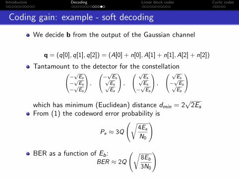
Coding gain: example - soft decoding

We decide b from the output of the Gaussian channel

q = (q[0], q[1], q[2]) = (A[0] + n[0],A[1] + n[1],A[2] + n[2])

Tantamount to the detector for the constellation−√Es

−√Es

−√Es

,

−√Es√Es√Es

,

√Es√Es

−√Es

,

√Es

−√Es√Es

which has minimum (Euclidean) distance dmin = 2

√2Es

From (1) the codeword error probability is

Pe ≈ 3Q

(√4Es

N0

)

BER as a function of Eb:BER ≈ 2Q

(√8Eb

3N0

)


Coding gain: example - hard vs soft decoding

Without coding, we have Eb = Es , and

BERnc = ε = Q(√

2Eb/N0

)Gain with hard decoding

We set equal BERc and BERnc

Approximation: Q(·)

G =(Eb/N0)nc(Eb/N0)c

= 2/3 ≈ −1.76dB

We are actually losing performance!! (expected, since the codeis not able correct any error)

Soft decodingG = 4/3 ≈ 1.25dB

Now we are making good use of coding


Index






Linear block codes

a + b = (a + b)2a · b = (a · b)2

Galois field modulo 2 (GF (2))

Definition: Linear Block Code

A linear block code is a code in which any linear combinationof codewords is also a codeword.

Properties

It is a subspace in GF (2)n with 2k elements.

The all-zeros word is a codeword.

Every codeword has at least one codeword that is at dmin

thereof.

dmin is the smallest weight (number of 1s) among the non-nullcodewords.


Linear block codes: elements

Elements in a linear block code

b is the message, 1× k

c is the codeword, 1× n

r is the received word, 1× n with

r = c + e

G is the generator matrix,

(for encoding)

k × n

H is the parity-check matrix,

(for decoding)n − k × n


Encoding

The mapping b→ c is performed through matrix multiplicationi.e.,

c = b G .

Keep in mind:

b is 1× k

G is k × n

c is 1× n

Every row of G is a codeword.

Property


Systematic codes

Definition: Systematic code

A code in which the message is always embedded in the en-coded sequence (in the same place).

This can be easily imposed through the generator matrix,

G =[Ik P

]or G =

[P Ik

]First/last k bits in r are equal to b, and the remaining n − kare redundancy.If G =

[Ik P

]it can be shown

H =[PT In−k

]

Prove it!

Exercise


Equivalent codes

If the code is systematic, we have an easy way of computing theparity-check matrix...

Computing H from G

...but what if it’s not? If the code is not systematic, one can applyoperations on the generator matrix, G, to try and transform it intothat of an equivalent systematic code, i.e.,

G =[Ik P

]Allowed operations are:

On rows replace any row with a linear combination of itselfand other rows or swapping rows.

On columns swapping columns.


Systematic codes: example - Hamming (7, 4)

generator matrix:

G =

1 0 0 0 1 0 10 1 0 0 1 1 00 0 1 0 1 1 10 0 0 1 0 1 1

Parity-check matrix:

H =

1 1 1 0 1 0 00 1 1 1 0 1 01 0 1 1 0 0 1

Every Hamming code:

It’s perfect

dmin = 3

k = 2j − j − 1 and n = 2j − 1 ∀j ∈ N ≥ 2

j = 2→ (3, 1)j = 3→ (7, 4)j = 4→ (15, 11)


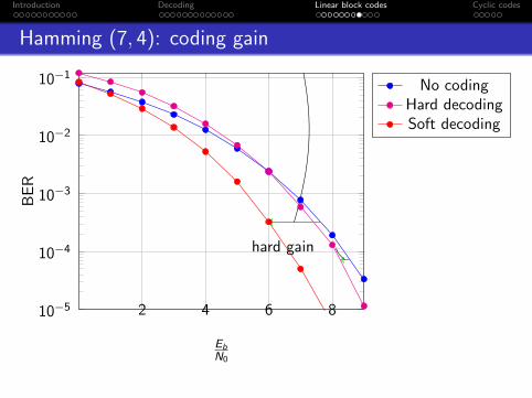
Hamming (7, 4): coding gain

2 4 6 810−5

10−4

10−3

10−2

10−1

hard gain

soft gain

EbN0

BE

R

No codingHard decodingSoft decoding


Parity check matrix

Parity check matrix, H, is the orthogonal complement of G so that

c H> = 0⇔ c is a codeword

For the sake of convenience,

Definition: Syndrome

The syndrome of the received sequence r is

s = r H> (with dimensions 1× (n − k))

Then,s = 0⇔ r is a codeword.

s = r HT = (c + e) HT =��*0

c HT + e HT = e HT

Syndrome-error connection


Hard decoding: syndrome decoding

The minimum distance rule requires computing dH with everycodeword...but we can carry out syndrome decodingBeforehand:

Fill up a table yielding the syndrome associated with every possibleerror,

error syndrome...

...

In operation: given the received word, r,

1 Compute the syndrome s = r HT .2 Look up the table for all the error patterns with that syndrome3 Choose the most likely e, i.e., the one with the smallest

weight andc = r + e


Hamming (7, 4): decoding

Beforehand we applys = eHT

over every e that entails a single error (the code can only correct 1erroneous bit):

error syndrome

0000000 0001000000 1010100000 1100010000 1110001000 0110000100 1000000010 0100000001 001

s = r H> =

1 0 11 1 01 1 10 1 11 0 00 1 00 0 1

= [110]

and hence e = [0100000] so that

c = r + e = r = [1000101] .

Example: r = [1100101]


Index






Cyclic codes

Working with matrices is not efficient!!

Large values of k and n

Definition: Cyclic code

It is a linear block code in which any circular shift of a code-word results in another codeword.

In a cyclic code,

If [c0, c1, . . . , cn−1] is a codeword, then so is[cn−1, c0, c1, . . . , cn−2]

Every codeword is a (circularly) shifted version of anothercodeword.


Polynomial representation of codewords

Codeword [c0, c1, · · · , cn−1] is represented as the polynomial

c(x) = c0 + c1x + c2x2 + · · ·+ cn−1x

n−1

How is[c0, c1, · · · , cn−1]→ [cn−1, c0, · · · , cn−2]

achieved mathematically? By multiplying c(x) times x modulo(xn − 1) i.e.,

xc(x) = c0x + c1x2 + · · ·+ cn−1x

n

= cn−1(xn − 1) + cn−1 + c0x + c1x2 + · · ·+ cn−2x

n−1

Hence,

(xc(x))xn−1 = cn−1 + c0x + c1x2 + · · ·+ cn−2x

n−1︸︷︷︸[cn−1,c0,··· ,cn−2]


Encoding

G → g(x)generator

matrix

generatorpolynomial

Coding is carried out by multiplying, modulo xn − 1, thepolynomial representing bi by a generator polynomial, g(x),

ci (x) = (bi (x)g(x))xn−1

The generator polynomial, g(x),

it is of degree r = n − k ,

it must be an irreducible polynomial


Decoding

H → h(x)parity-check

matrix

parity-checkpolynomial

The parity-check polynomial, h(x),

it is of degree r = n − k − 1,

must satisfy

(g(x)h(x))xn−1 = 0.

Just like in regular linear block codes, we can perform syndromedecoding,

s(x) = (r(x)h(x))xn−1

Channel coding - Introduction & linear codes

Documents