Channel Characterization and Wireless Communication Performance in Industrial Environments JAVIER FERRER COLL Doctoral Thesis in Information and Communication Technology Stockholm, Sweden 2014

Welcome message from author
This document is posted to help you gain knowledge. Please leave a comment to let me know what you think about it! Share it to your friends and learn new things together.
Transcript

Channel Characterization and Wireless
Communication Performance in Industrial
Environments
JAVIER FERRER COLL
Doctoral Thesis in
Information and Communication Technology
Stockholm, Sweden 2014

TRITA ICT-COS-1402ISSN 1653-6347ISRN KTH/COS/R--14/02--SE
KTH Communication SystemsSE-100 44 Stockholm
Sweden
Akademisk avhandling som med tillstånd av Kungl Tekniska högskolan framlägges tilloffentlig granskning för avläggande av teknologie doktoralexamen i kommunikationssy-stem onsdagen den 4 juni 2014 klockan 13.00 i hörsal D i Forum, Kungliga TekhniskaHögskolan, Isafjordsgatan 39, Kista, Stockholm.
© Javier Ferrer Coll, June 2014
Tryck: Universitetsservice US AB

i
Abstract
The demand for wireless communication systems in industry has grownin recent years. Industrial wireless communications open up a number of newpossibilities for highly flexible and efficient automation solutions. However,a good part of the industry refuses to deploy wireless solutions products dueto the high reliability requirements in industrial communications that are notachieved by actual wireless systems. Industrial environments have particu-lar characteristics that differ from typical indoor environments such as officeor residential environments. The metallic structure and building dimensionsresult in time dispersion in the received signal. Moreover, electrical motors,vehicles and repair work are sources of electromagnetic interference (EMI)that have direct implications on the performance of wireless communicationlinks. These degradations can reduce the reliability of communications, in-creasing the risk of material and personal incidents. Characterizing the sourcesof degradations in different industrial environments and improving the perfor-mance of wireless communication systems by implementing spatial diversityand EMI mitigation techniques are the main goals of this thesis work.
Industrial environments are generally considered to be environments witha significant number of metallic elements and EMI sources. However, with thepenetration of wireless communication in industrial environments, we realizethat not all industrial environments follow this rule of thumb. In fact, we find awide range of industrial environments with diverse propagation characteristicsand degradation sources. To improve the reliability of wireless communica-tion systems in industrial environments, proper radio channel characterizationis needed for each environment. This thesis explores a variety of industrialenvironments and attempts to characterize the sources of degradation by ex-tracting representative channel parameters such as time dispersion, path lossand electromagnetic interference. The result of this characterization providesan industrial environment classification with respect to time dispersion andEMI levels, showing the diverse behavior of propagation channels in industry.
The performance of wireless systems in industrial environments can beimproved by introducing diversity in the received signal. This can be accom-plished by exploiting the spatial diversity offered when multiple antennas areemployed at the transmitter with the possibility of using one or more antennasat the receiver. For maximum diversity gain, a proper separation between thedifferent antennas is needed. However, this separation could be a limiting fac-tor in industrial environments with confined spaces. This thesis investigatesthe implication of antenna separation on system performance and discussesthe benefits of spatial diversity in industrial environments with high time dis-persion conditions where multiple antennas with short antenna separations canbe employed.
To ensure reliable wireless communication in industrial environments, alltypes of electromagnetic interference should be mitigated. The mitigation
ii
of EMI requires interference detection and subsequent interference suppres-sion. This thesis looks at impulsive noise detection and suppression techniquesfor orthogonal frequency division multiplexing (OFDM) based on wide-bandcommunication systems in AWGN and multi-path fading channels. For this,a receiver structure with cooperative detection and suppression blocks is pro-posed. This thesis also investigates the performance of the proposed receiverstructure for diverse statistical properties of the transmitted signal and electro-magnetic interference.

Acknowledgements
First of all, I would like to thank my supervisors Dr. Slimane Ben Slimane and Dr. JoséChilo. I feel fortunate to have these encouraging researchers who offered me importantsupport during the past five years. I am also very grateful for the positive and fruitful dis-cussions with Dr. Peter Stenumgaard who also has directed big part of my Ph.D. research.
This thesis is product of the "Reliable wireless machine-to-machine communicationsin the electromagnetic disturbed industrial environments" project founded by the SwedishKnowledge Foundation (KKS). Within this project, I would like to thank for the supportprovided from Stora Enso, SSAB, Green Cargo, Åkerströms, Syntronic, Agilent Tech-nologies and FOI. Special thanks goes to the project colleagues at University of Gävle,Per Ängskog, Carl Elofsson and Carl Karlsson. Just thinking about the amazing time andexperience gained during the multiple measurement campaigns, put a happy smile in myface.
I would like to thank my colleagues in the University of Gävle and in the Wirelessdepartment at KTH. Particularly, I would like to thank the present and former doctoralstudents, Sathyaveer Prasad, Per Landin, Charles Nader, Mohamed Hamid, Efrain Zenteno,Shoaib Amin, Indrawibawa Nyoman, Usman Haider, Mahmoud Alizadeh, Zain AhmedKahn, Rakesh Krishnan and Nauman Masud. I will never forget the incredible time andsilly conversations during the fika time.
Finally, I would like to thank my family and friends; specially my parents, brotherand sister for their motivation and encouragement during all these years of studies. Themost important thanks goes to my half-orange Milena and my wonderful son Max for theincredible happiness that they bring to my life. They were supportive during the difficultmoments and source of inspiration for my research.
iii

Contents
List of Tables vii
List of Figures ix
List of Acronyms & Abbreviations xi
1 Introduction 1
1.1 Background . . . . . . . . . . . . . . . . . . . . . . . . . . . . . . . . . 11.2 Problem Formulation . . . . . . . . . . . . . . . . . . . . . . . . . . . . 31.3 Thesis Outline and Contributions . . . . . . . . . . . . . . . . . . . . . . 51.4 Publications . . . . . . . . . . . . . . . . . . . . . . . . . . . . . . . . . 6
2 Industrial Environments 9
2.1 Introduction . . . . . . . . . . . . . . . . . . . . . . . . . . . . . . . . . 92.2 Environment Descriptions . . . . . . . . . . . . . . . . . . . . . . . . . 10
2.2.1 Bark Furnace . . . . . . . . . . . . . . . . . . . . . . . . . . . . 102.2.2 Metal Works . . . . . . . . . . . . . . . . . . . . . . . . . . . . 102.2.3 Paper Warehouse . . . . . . . . . . . . . . . . . . . . . . . . . . 112.2.4 Outdoor Industrial Environment . . . . . . . . . . . . . . . . . . 112.2.5 Laboratory and Office . . . . . . . . . . . . . . . . . . . . . . . 112.2.6 Rail Yard . . . . . . . . . . . . . . . . . . . . . . . . . . . . . . 122.2.7 Mine Tunnel . . . . . . . . . . . . . . . . . . . . . . . . . . . . 12
2.3 Measurement Setups . . . . . . . . . . . . . . . . . . . . . . . . . . . . 122.3.1 Network Analyzer Setup . . . . . . . . . . . . . . . . . . . . . . 132.3.2 Generic Spectrum Analyzer Setup . . . . . . . . . . . . . . . . . 13
2.4 Summary . . . . . . . . . . . . . . . . . . . . . . . . . . . . . . . . . . 14
3 Multi-path Characterization in Industrial Environments 15
3.1 Introduction . . . . . . . . . . . . . . . . . . . . . . . . . . . . . . . . . 153.2 Multi-path Fading in Wireless Communications . . . . . . . . . . . . . . 16
3.2.1 Channel Models . . . . . . . . . . . . . . . . . . . . . . . . . . 183.3 Measurement Results and Analysis . . . . . . . . . . . . . . . . . . . . . 20
3.3.1 High delay spread environments . . . . . . . . . . . . . . . . . . 20
v

vi CONTENTS
3.3.2 Low delay spread environments . . . . . . . . . . . . . . . . . . 213.3.3 Channel Model Results . . . . . . . . . . . . . . . . . . . . . . . 23
3.4 Discussion . . . . . . . . . . . . . . . . . . . . . . . . . . . . . . . . . . 24
4 Path Loss Characterization in Industrial Environments 25
4.1 Introduction . . . . . . . . . . . . . . . . . . . . . . . . . . . . . . . . . 254.2 Path Loss in Wireless Communications . . . . . . . . . . . . . . . . . . 264.3 Measurement Results and Analysis . . . . . . . . . . . . . . . . . . . . . 274.4 Discussion . . . . . . . . . . . . . . . . . . . . . . . . . . . . . . . . . . 29
5 Electromagnetic Interference in Industrial Environments 31
5.1 Introduction . . . . . . . . . . . . . . . . . . . . . . . . . . . . . . . . . 315.2 Electromagnetic Interference Model . . . . . . . . . . . . . . . . . . . . 32
5.2.1 Amplitude Probability Distribution . . . . . . . . . . . . . . . . 345.3 Measurement Results and Analysis . . . . . . . . . . . . . . . . . . . . . 345.4 Discussion . . . . . . . . . . . . . . . . . . . . . . . . . . . . . . . . . . 36
6 Antenna Systems in Industrial Environments 39
6.1 Introduction . . . . . . . . . . . . . . . . . . . . . . . . . . . . . . . . . 396.2 Spatial Diversity in Wireless Communications . . . . . . . . . . . . . . . 406.3 Measurement Results and Analysis . . . . . . . . . . . . . . . . . . . . . 426.4 Discussion . . . . . . . . . . . . . . . . . . . . . . . . . . . . . . . . . . 45
7 Impulsive Noise Detection and Suppression 47
7.1 Introduction . . . . . . . . . . . . . . . . . . . . . . . . . . . . . . . . . 477.2 OFDM Systems in Environments with Impulsive Noise . . . . . . . . . . 48
7.2.1 Impulsive Noise Detection . . . . . . . . . . . . . . . . . . . . . 507.2.2 Impulsive Noise Suppression . . . . . . . . . . . . . . . . . . . . 51
7.3 Measurement Results and Analysis . . . . . . . . . . . . . . . . . . . . . 527.3.1 Detection and Suppression in OFDM Systems . . . . . . . . . . . 527.3.2 Detection and Suppression in OFDM-PAPR Systems . . . . . . . 54
7.4 Discussion . . . . . . . . . . . . . . . . . . . . . . . . . . . . . . . . . . 55
8 Conclusions 57
8.1 Concluding Remarks . . . . . . . . . . . . . . . . . . . . . . . . . . . . 578.2 Future Directions . . . . . . . . . . . . . . . . . . . . . . . . . . . . . . 59
Bibliography 61
PAPER REPRINTS 71
List of Tables
3.1 PDP parameters for high delay spread environments . . . . . . . . . . . . . . 213.2 PDP parameters for a low delay spread environment . . . . . . . . . . . . . . 233.3 Channel parameters of the Saleh-Valenzuela model . . . . . . . . . . . . . . 23
4.1 Path loss exponents for the absorbent and reflective environments . . . . . . . 284.2 Estimated parameters for LoS and NLoS in the absorbent and reflective envi-
ronments with a path loss model containing frequency exponent. . . . . . . . 284.3 MSE[dB] of the estimations for LoS, NLoS in the absorbent and reflective
environments . . . . . . . . . . . . . . . . . . . . . . . . . . . . . . . . . . 29
6.1 Estimated parameters for the different measured scenarios at 433 MHz withantenna separation of λ/5. . . . . . . . . . . . . . . . . . . . . . . . . . . . 44
vii

List of Figures
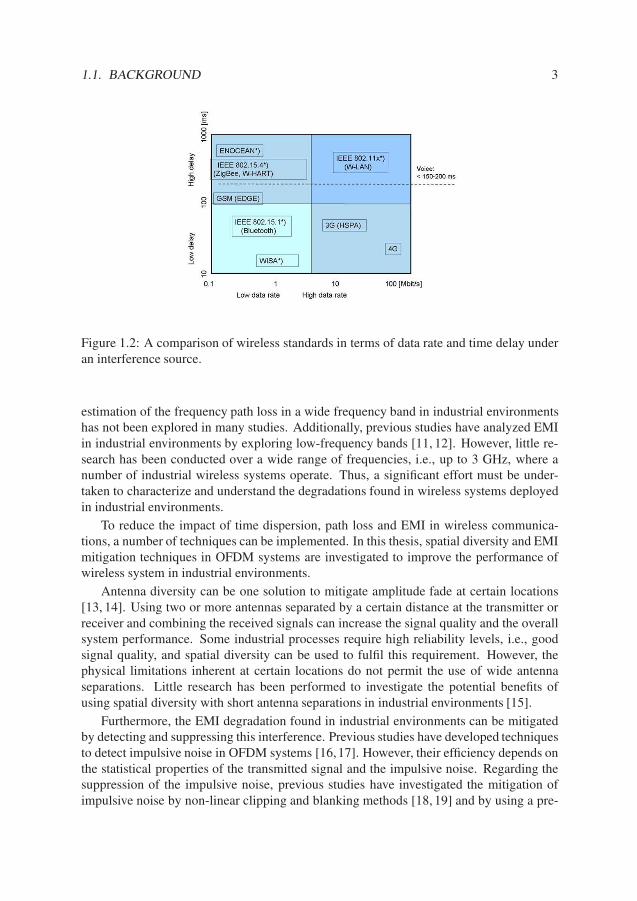
1.1 Forecast for machine-to-machine data traffic 2018. . . . . . . . . . . . . . . 11.2 A comparison of wireless standards in terms of data rate and time delay under
an interference source. . . . . . . . . . . . . . . . . . . . . . . . . . . . . . 2
2.1 Reference locations for bark furnace at the paper mill. . . . . . . . . . . . . . 102.2 Large industrial halls at metal works. . . . . . . . . . . . . . . . . . . . . . . 112.3 Corridor of paper rolls at the warehouse. . . . . . . . . . . . . . . . . . . . . 112.4 Outdoor scenarios in the steel works factory and paper mill. . . . . . . . . . . 112.5 RF laboratory and office corridor environments. . . . . . . . . . . . . . . . . 122.6 Train engine in Borlänge and rail yard in Stockholm area. . . . . . . . . . . . 122.7 Wide tunnel and joint point in the iron-ore mine. . . . . . . . . . . . . . . . . 122.8 Network analyzer measurement setup. . . . . . . . . . . . . . . . . . . . . . 132.9 Generic spectrum analyzer measurement setup. . . . . . . . . . . . . . . . . 14
3.1 Saleh-Valenzuela impulse response model. . . . . . . . . . . . . . . . . . . . 183.2 PDP at 433 MHz (left), at 1890 MHz (center) and at 2450 MHz (right), NLoS
case. . . . . . . . . . . . . . . . . . . . . . . . . . . . . . . . . . . . . . . . 203.3 PDP at 433 MHz (left), at 1890 MHz (center) and at 2450 MHz (right), NLoS
case in the paper warehouse. . . . . . . . . . . . . . . . . . . . . . . . . . . 213.4 Measured and simulated PDP for 433 MHz for the LoS (left) and distribution
of rms delay spread in the receiver simulated grid (right), in the paper warehouse. 223.5 Measured (left) and simulated (right) PDP at 1890 MHz for the LoS in the
mine tunnel. . . . . . . . . . . . . . . . . . . . . . . . . . . . . . . . . . . . 223.6 Simulated Saleh-Valenzuela PDP (left) and measured PDP (right) in high delay
spread environment. . . . . . . . . . . . . . . . . . . . . . . . . . . . . . . . 243.7 PDP of the IPDP model for low and high delay spread channels. . . . . . . . 24
4.1 Path loss versus frequency of the measurements at 9 m in absorbent and reflec-tive for LoS (left), NLoS (right) and the theoretical estimation for a β = 2. . . 28
4.2 Derivatives of path loss in absorbent and reflective environments in LoS andNLoS. . . . . . . . . . . . . . . . . . . . . . . . . . . . . . . . . . . . . . . 28
ix

x List of Figures
4.3 Path loss versus frequency of the measurements in NLoS for absorbent (left),reflective (right) and the theoretical estimation with the frequency exponentmodel at 9 m. . . . . . . . . . . . . . . . . . . . . . . . . . . . . . . . . . . 29
4.4 Estimated theoretical path loss in absorbent and reflective environments in LoSand NLoS. . . . . . . . . . . . . . . . . . . . . . . . . . . . . . . . . . . . . 29
5.1 Time domain measurement (left) and APD of the data (right). . . . . . . . . . 345.2 Electromagnetic interferences at low frequencies (left) and disturbances on the
DECT band (right). . . . . . . . . . . . . . . . . . . . . . . . . . . . . . . . 355.3 APD of the measured interference and the estimated. . . . . . . . . . . . . . 355.4 Electric train breaking, in Borlänge (left) and in an iron-mine tunnel (right). . 36
6.1 Average antenna cross-correlation versus antenna distance for 433 MHz (LoS)in different environments. . . . . . . . . . . . . . . . . . . . . . . . . . . . . 43
6.2 CDF of the received signals and the resulting combination, for 433 MHz (LoS)and λ/8 in the large storage hall. . . . . . . . . . . . . . . . . . . . . . . . . 43
7.1 OFDM link performance under impulsive noise applying suppression. . . . . 477.2 Block diagram of Max detector. . . . . . . . . . . . . . . . . . . . . . . . . 507.3 Block diagram of the impulsive noise suppression algorithm. . . . . . . . . . 527.4 Flow chart diagram for the proposed receiver structure. . . . . . . . . . . . . 537.5 Signal, impulsive noise and thresholds performance at IR = 0.1 (left) and
probability of detection versus impulsive rate for different detectors (right). . 537.6 BER versus Eb/N0 for measurements. . . . . . . . . . . . . . . . . . . . . . 547.7 Simulated BER versus Eb/N0 in a Rayleigh channel (left) and with frequency
diversity, L = 2, (right). . . . . . . . . . . . . . . . . . . . . . . . . . . . . 547.8 Probability of detection (left) and BER (right) with respect to IR for the pro-
posed detection and Gaussian hypothesis estimation at Γ = 10. . . . . . . . . 55
8.1 Industrial environment classification in terms of interference and multi-pathlevels. . . . . . . . . . . . . . . . . . . . . . . . . . . . . . . . . . . . . . . 58

List of Acronyms & Abbreviations
ADC Analog-Digital Converter
APD Amplitude Probability Distribution
AWGN Additive White Gaussian Noise
BER Bit Error Rate
CDF Cumulative Distribution Function
CDMA Code Division Multiple Access
CISPR Comité International Spécial des Perturbations Radioélectriques
COST European Cooperation in Science and Technology
dB Decibel
dBm Power relative to 1 milliwatt in dB
DECT Digital Enhanced Cordless Telecommunications
EMC Electromagnetic Compatibility
EMI Electromagnetic Interference
GHz Gigahertz
GUI Graphical User Interface
IDFT Inverse Discrete Fourier Transform
IEEE Institute of Electrical and Electronics Engineers
IF Intermediate Frequency
IPDP In-Room Power Delay Profile
IR Impulsive Rate
xi

xii LIST OF ACRONYMS & ABBREVIATIONS
ISA International Society of Automation
ISI InterSymbol Interference
ISM Industrial, Scientific and Medical radio bands
kHz Kilohertz
KTH Kungliga Tekniska Högskolan
LKAB Luossavaara-Kiirunavaara Aktiebolag
LoS Line of Sight
MHz Megahertz
MIMO Multiple-Input Multiple-Output
MLP Multilayer Perceptron
MRC Maximal Ratio Combining
MSE Mean Square Error
M2M Machine-to-Machine
NLoS Non-Line of Sight
ns Nano Seconds
OFDM Orthogonal Frequency-Division Multiplexing
PAPR Peak-to-Average Power Ratio
PC Personal Computer
PDF Probability Distribution Function
PDP Power Delay Profile
PIFA Planar-Inverted F Antenna
QAM Quadrature Amplitude Modulation
RBW Resolution Bandwidth
RF Radio Frequency
rms Root-Mean-Square
Rx Receiver
SA Signal Analyzer
xiii
SC Selection Combining
SG Signal Generator
SLM Selected Mapping
SNR Signal-to-Noise Ratio
SSAB Swedish Steel Aktiebolag
Tx Transmitter
VBW Video Bandwidth
VNA Vector Network Analyzer
WISA Wireless Speaker and Audio
WLAN Wireless Local Area Network
WSN Wireless Sensor Network

Chapter 1
Introduction
1.1 Background
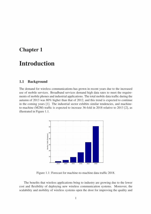
The demand for wireless communications has grown in recent years due to the increaseduse of mobile services. Broadband services demand high data rates to meet the require-ments of mobile phones and industrial applications. The total mobile data traffic during theautumn of 2013 was 80% higher than that of 2012, and this trend is expected to continuein the coming years [1]. The industrial sector exhibits similar tendencies, and machine-to-machine (M2M) traffic is expected to increase 36-fold in 2018 relative to 2013 [2], asillustrated in Figure 1.1.
2013 2014 2015 2016 2017 20180
10
20
30
40
50
60
70
Mon
thly
Tra
ffic
[Pet
abyt
es]
Figure 1.1: Forecast for machine-to-machine data traffic 2018.
The benefits that wireless applications bring to industry are growing due to the lowercost and flexibility of deploying new wireless communication systems. Moreover, thescalability and mobility of wireless systems open the door for improving the quality and
1
2 CHAPTER 1. INTRODUCTION
efficiency of industrial processes. However, the deployment of wireless solutions in indus-trial areas needs to overcome several requirements, such as levels of safety and reliabilitythat are higher than those required by mobile services [3]. The particular characteristicsof industrial environments tend to create different degradation sources that affect wire-less communication. The metallic structure and large dimensions of buildings cause radiowaves to reflect multiple times, creating a composition of transmitted signal replicas at thereceiver. This fading effect can produce intersymbol interference (ISI) when the symbolperiod of the wireless system is shorter than the time dispersion of the channel [4]. Ad-ditionally, electromagnetic interference (EMI) generated by electric motors, power linesand maintenance activities contributes to the degradation of the received signal [5]. EMIhas different statistical properties compared to additive white Gaussian noise (AWGN),thus systems designed to work in the presence of AWGN may not work properly in thepresence of EMI.
Industrial environments have special propagation characteristics not present in typicaloffice and residential environments. However, the majority of the indoor wireless systemsdesigned to function in office environments are also used in industrial applications. Con-sequently, industrial wireless systems occasionally fail due to the EMI and high levels oftime dispersion present in industrial environments. To provide reliable and robust com-munication, a number of improvements need to be elaborated upon. Thus, to improvecurrent wireless systems, a radio channel characterization of multiple industrial environ-ments, extracting the representative sources of degradation in each environment, should beperformed.
Multiple wireless technologies are used in industrial applications, depending on the ap-plication requirements where the systems are deployed [6]. WLAN, WISA, WirelessHart,ZigBee, Bluetooth, DECT and ISA 100.11a are some of the most commonly used technolo-gies in industrial areas. DECT is a mature technology that has been used since 1987 forcordless telephone service. WLAN technology works in the 2.4 GHz band and provideshigh data rates by using wide-band channels with orthogonal frequency division multi-plexing (OFDM), which makes WLAN a perfect candidate for video streaming. WISA,WirelessHart, ISA 100.11a and ZigBee have been developed to manage a large numberof devices in a network with low data rates and are suitable for wireless sensor network(WSN) services. Currently, all of these technologies are widely deployed in industrialenvironments [7], but they require constant development and new versions to address thechallenges and needs of industrial applications. For instance, Figure 1.2 shows the perfor-mance of different standards when an interference source is present in the environment.High data rates can be achieved when implementing wide-band communication systems,such as WLAN systems; however, the communication delay can reach hundreds of mil-liseconds, risking the reliability of some industrial processes.
A number of studies have characterized typical industrial environments with large di-mensions and metallic structures, showing high time dispersion levels [8, 9]. However,few studies have investigated the time dispersion of industrial environments with differentstructural characteristics. Moreover, distance path loss characterization studies performedby various research groups in multiple industrial environments have found path loss expo-nents lower than the corresponding free space exponent, i.e., α = 2 [9, 10]. However, the
1.1. BACKGROUND 3
Figure 1.2: A comparison of wireless standards in terms of data rate and time delay underan interference source.
estimation of the frequency path loss in a wide frequency band in industrial environmentshas not been explored in many studies. Additionally, previous studies have analyzed EMIin industrial environments by exploring low-frequency bands [11, 12]. However, little re-search has been conducted over a wide range of frequencies, i.e., up to 3 GHz, where anumber of industrial wireless systems operate. Thus, a significant effort must be under-taken to characterize and understand the degradations found in wireless systems deployedin industrial environments.
To reduce the impact of time dispersion, path loss and EMI in wireless communica-tions, a number of techniques can be implemented. In this thesis, spatial diversity and EMImitigation techniques in OFDM systems are investigated to improve the performance ofwireless system in industrial environments.
Antenna diversity can be one solution to mitigate amplitude fade at certain locations[13, 14]. Using two or more antennas separated by a certain distance at the transmitter orreceiver and combining the received signals can increase the signal quality and the overallsystem performance. Some industrial processes require high reliability levels, i.e., goodsignal quality, and spatial diversity can be used to fulfil this requirement. However, thephysical limitations inherent at certain locations do not permit the use of wide antennaseparations. Little research has been performed to investigate the potential benefits ofusing spatial diversity with short antenna separations in industrial environments [15].
Furthermore, the EMI degradation found in industrial environments can be mitigatedby detecting and suppressing this interference. Previous studies have developed techniquesto detect impulsive noise in OFDM systems [16,17]. However, their efficiency depends onthe statistical properties of the transmitted signal and the impulsive noise. Regarding thesuppression of the impulsive noise, previous studies have investigated the mitigation ofimpulsive noise by non-linear clipping and blanking methods [18, 19] and by using a pre-
4 CHAPTER 1. INTRODUCTION
demodulated estimation of the OFDM signal [20]. However, the efficiency of these sup-pression techniques is dependent on the impulse noise detection and the statistical proper-ties of the transmitted signal. Thus, a receiver structure composed of cooperative detectionand suppression needs to be investigated.
1.2 Problem Formulation
The wide-scale deployment of wireless communications systems in industrial environ-ments is a long process that needs to overcome multiple challenges. Reliable commu-nication is one of the most important challenges that have to be solved in order to increasethe confidence of the industrial sector for deploying wireless solutions. Industrial wire-less applications demand reliable and robust communication systems due to the potentialrisks associated with some applications. The industry encompasses a wide range of envi-ronments with different channel characteristics and thus different sources of degradation,risking the system’s reliability.
Understanding the characteristics of the communication channel is necessary for de-signing a good communication system. Industrial environments typically have significanttime dispersion due to the metallic structures and large dimensions of obstacles. Theyare commonly characterized in the literature as multi-path fading channels with long timedelay spread. However, as the penetration of wireless communication systems in indus-trial applications increases, we see an increased diversity in industrial environments with awide range of structural properties. This means that one has to be careful when designinga good communication system for industrial environments since a channel model obtainedfrom one industrial environment may be not suitable for another industrial environment.The path loss in industrial environments can also be quite different from that in commer-cial non-industrial environments. Non line-of-sight (NLoS) situations can cause coverageproblems at certain frequency bands. EMI generated by electrical motors, repair work,and transportation systems is another source of interference that affects the performanceof wireless system in industrial environments. Hence, wireless system developers have totake the presence of such interference into account in their design process to ensure reliablecommunications in industrial environments.
Few measurement campaigns have explored the radio channel characteristics in dif-ferent industrial environments. However, assuming that industrial environments presentsimilar propagation conditions and interference could result in the design of unreliablecommunication systems. Our first objective in this thesis work is to investigate the impli-cations of the diverse structural properties of industrial environments on the characteristicsof radio communication channels.
Improving the performance of wireless communication systems in multi-path fadingchannels is achieved by the use of diversity techniques, where the receiver receives mul-tiple replicas of the same signal transmitted through independent fading multi-path chan-nels. Diversity can improve both the received signal strength and the time availability ofthe signal at the receiver. Spatial diversity is the most efficient diversity method in wirelesscommunications. It can improve the performance of wireless links without any loss of effi-
1.3. THESIS OUTLINE AND CONTRIBUTIONS 5
ciency. However, the diversity gain from using spatial diversity depends on the separationbetween the receiver antennas. For multi-path fading channels with diffused multi-pathcomponents only, a separation of λ/2 is usually enough to ensure a maximum diversitygain. However, in some industrial environments, it may not be possible to ensure a sep-aration of λ/2. Having an antenna separation above λ/2 may not provide the necessarydiversity gain for reliable communication in industrial environments. Therefore, the sec-ond objective in this thesis work is to investigate the effect of antenna separation on thediversity gain in wireless communication links in industrial environments.
Diversity techniques may not be able to provide the expected performance in the pres-ence of additive electromagnetic interference. Hence, to ensure reliable communicationsin industrial environments, this type of impulsive noise needs to be mitigated from thereceived signal before signal detection. The mitigation of the impulsive noise usually in-cludes interference detection followed by interference suppression stages. The existinginterference detection techniques provide good performance at certain impulsive rates andfor Gaussian type transmitted communication signals. Hence, their efficiency is linked tothe statistical properties of the impulsive noise source and that of the transmitted com-munication signal. The performance of the impulsive noise suppression is dependent onthe impulsive samples detected in the received signal. Thus, by increasing the detectedimpulsive noise samples, additional impulsive noise can be suppressed from the receivedsignal, leading to a better performance of the wireless communication link in industrial en-vironments. Our third objective in this work is to investigate the effects of impulsive noisedetection and suppression techniques on the performance of wireless communication linksin AWGN and multi-path fading channels. We further propose an efficient receiver struc-ture for the transmitted signal and impulsive noise with different statistical properties.
1.3 Thesis Outline and Contributions
The main contributions of the thesis are based on a characterization of the radio channel fordifferent industrial environments, performing measurements and introducing techniquesfor improving the performance of industrial wireless systems. We next give an outline ofthe thesis and describe the contributions within each chapter.
Chapter 2 describes the industrial environments characterized during the measurementcampaigns performed in this thesis and the measurement setups used during this character-ization . The chapter details a wide variety of industrial environments with diverse prop-agation characteristics, such as a bark furnace, metal works, paper warehouse, outdoorindustrial environment, laboratory and office, rail yard and a mine tunnel. The environ-ments described in this chapter are referred to throughout the thesis, providing a guideof the characterized industrial environments. The measurement setups presented in thechapter are also referred to in the remaining chapters.
Chapter 3 presents the multi-path characterization performed in industrial environ-ments with diverse propagation characteristics. The chapter contains a characterizationfrom environments with large amounts of metallic objects, i.e., a bark furnace, to en-vironments with special characteristics that reduce multi-path propagation, i.e., a paper

6 CHAPTER 1. INTRODUCTION
warehouse. The chapter shows the diverse behavior of the multi-path propagation in in-dustry in contrast to previous studies reported in the literature. This chapter is based on theinvestigations performed in Papers [J1], [J2], [J3], [J4], [C2], [C3] and [C4].
Chapter 4 addresses radio-wave propagation path loss in industrial environments. Thechapter provides measurements and models of the frequency dependence of the receivedsignal strength in NLoS scenarios. The obtained results show that the frequency depen-dence is more pronounced in NLoS scenarios with radio-wave absorbing properties rela-tive to environments with high multi-path propagation. The content of this chapter is manlybased on the measurement results presented in Paper [J3].
Chapter 5 presents an EMI characterization for a broad frequency band in multipleindustrial environments. Various sources of EMI such as electrical motors, vehicles andrepair work are analyzed during the measurement campaigns. A number of these EMIsources in industrial environments are found to have higher frequency components thanthose reported earlier in the literature. The measured EMI in the bark furnace is mod-eled statistically and used to investigate the effect of such EMI on the performance of thewireless systems. This chapter is based on the measured interferences at various industriallocations presented in Papers [J1], [J2], [J4] and [C1].
Chapter 6 studies the benefits of implementing spatial diversity in industrial environ-ments with high multi-path propagation conditions. In particular, this chapter investigatesthe spatial diversity gain achieved using short antenna separations. Substantial benefitsto the system performance can be obtained by applying diversity techniques with shortantenna separations in industrial environments having high multi-path propagation. Thisstudy is based on the measurement results reported in Paper [J5].
Chapter 7 proposes a receiver structure for OFDM-based systems for industrial en-vironments. The receiver is a combination of impulsive noise detection and suppressionstages, providing robustness against fading multi-path channels and EMI. The chapter alsodiscusses the implication of the statistical properties of the transmitted signal and impul-sive noise on the detection and suppression. This chapter is based on the results presentedin Papers [J6] and [C5].
Chapter 8 concludes the contributions of the thesis work and suggests a number ofdirections for future research.
1.4 Publications
This doctoral thesis is the product of research studies submitted or accepted in internationalconferences and journals. The following list presents the peer review articles included inthis thesis:
[J.1] J. Ferrer-Coll, P. Ängskog, J. Chilo and P. Stenumgaard, “Characterization of elec-tromagnetic properties in iron-mine production tunnels,” IET Electronics Letters,
vol.48, no.2, pp.62-63, Jan. 2012.
1.4. PUBLICATIONS 7
[J.2] J. Ferrer Coll, J. Chilo and S. Ben Slimane, “Radio-frequency electromagnetic char-acterization in factory infrastructures,” IEEE Trans. on Electromagnetic Compati-
bility, vol.54, no.3, pp.708-711, Jun. 2012.
[J.3] J. Ferrer-Coll, P. Ängskog, J. Chilo and P. Stenumgaard, “Characterization of highlyabsorbent and highly reflective radio wave propagation environments in industrialapplications,” IET Communications, vol.6, no.15, pp.2404-2412, Oct. 2012.
[J.4] P. Stenumgaard, J. Chilo, J. Ferrer-Coll and P. Ängskog, “Challenges and conditionsfor wireless machine-to-machine communications in industrial environments,” IEEE
Communications Magazine, vol.51, no.6, pp.187-192, Jun. 2013.
[J.5] J. Ferrer-Coll, P. Ängskog, C. Elofsson, J. Chilo and P. Stenumgaard, “Antenna crosscorrelation and ricean K-factor measurements in indoor industrial environments at433 MHz and 868 MHz,” Wireless Personal Communications, vol.73, no.3, pp.587-593, May. 2013.
[J.6] J. Ferrer-Coll, B. Slimane, J. Chilo and P. Stenumgaard, “Detection and Suppres-sion of Impulsive Noise in OFDM Receiver,” Wireless Personal Communications,
Submitted Feb. 2014.
[C.1] P. Ängskog, C. Karlsson, J. Ferrer Coll, J. Chilo and P. Stenumgaard, “Sources ofdisturbances on wireless communication in industrial and factory environments,”in Asia-Pacific International Symposium on Electromagnetic Compatibility, Beijing,Apr. 2010, pp. 285-288.
[C.2] J. Ferrer Coll, P. Ängskog, C. Karlsson, J. Chilo and P. Stenumgaard, “Simula-tion and measurement of electromagnetic radiation absorption in a finished-productwarehouse,” in IEEE International Symposium on Electromagnetic Compatibility,
Fort Lauderdale-Florida, vol.3, Jul. 2010, pp. 881-884.
[C.3] J. Ferrer-Coll, J. Dolz Martin de Ojeda, P. Stenumgaard, S. Marzal Romeu andJ. Chilo, “Industrial indoor environment characterization - Propagation models,”in IEEE Electromagnetic Compatibility Symposium in Europe, York, Sep. 2011,pp.245-249.
[C.4] J. Ferrer Coll, P. Ängskog, H. Shabai, J. Chilo and P. Stenumgaard, “Analysis ofwireless communications in underground tunnels for industrial use,” in IEEE Inter-
national Conference in Industrial Electronics IECON, Montreal, Oct. 2012, pp.3216-3220.
[C.5] J. Ferrer-Coll, B. Slimane, J. Chilo and P. Stenumgaard, “Impulsive Noise Detec-tion in OFDM Systems with PAPR Reduction,” accepted for publication in IEEE
Electromagnetic Compatibility Symposium in Europe, Gothenburg, Sep. 2014.


Chapter 2
Industrial Environments
2.1 Introduction
Industrial environments have generally been considered environments with large dimen-sions and numerous metallic elements that increase multi-path propagation as well as withdiverse electric machinery, transportation equipment and repair work that contribute toEMI [11, 21–23]. This general description of an industrial environment is valid for a cer-tain percentage of industrial environments. However, the measurement campaigns carriedout during this thesis work showed that industrial environments are not always highly re-flective containing EMI. In fact, a number of industrial environments do not follow thisgeneral description, presenting particular characteristics that in some cases result in theopposite propagation behavior. In this thesis work, we attempt to present a number ofdiverse industrial environments with the objective of covering a wide range of industrialenvironments.
This chapter describes the various industrial environments where the measurementcampaigns were performed. Four industrial companies located in Sweden cooperated withthis study; Stora Enso, Swedish Steel Aktiebolag (SSAB), Green Cargo and Luossavaara-Kiirunavaara Aktiebolag (LKAB). Stora Enso is a paper manufacturer that processes treesinto final products, e.g., biomaterial, wood or paper. SSAB is a steel works company thatprocesses raw minerals into steel. Green Cargo is a logistics company that uses trains astheir main transportation system. LKAB is a mining company that extracts iron-ore fromtheir mines. By exploring multiple diverse industrial environments, we attempt to show thesignificant diversity of industrial scenarios. From typical industrial environments followingthe general description presented above to environments with different characteristics andopposite behavior. The different environments described in this chapter are investigated inthe following chapters; therefore, this chapter is referred to throughout the thesis.
The next section of this chapter presents the descriptions of six distinct industrial en-vironments as well as laboratory and corridor environments. The third section containsthe measurement setups used during the environment characterization. The last sectionprovides a summary of the chapter.
9
10 CHAPTER 2. INDUSTRIAL ENVIRONMENTS
2.2 Environment Descriptions
Industrial environment is a term used to describe environments under harsher conditionsthan typical office environments. The different conditions that can be found in industrycan degrade the performance of wireless systems. Depending on the characteristics ofthe environment, such as dimensions, materials and the presence of electronic equipment,the propagation channel will be subject to different types of degradations. In this section,we describe a wide range of industrial environments, from typical industrial environmentswith large dimensions and metallic surfaces to environments with special characteristicssuch as a paper warehouse and a mine tunnel.
2.2.1 Bark Furnace
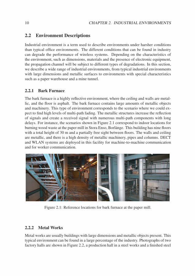
The bark furnace is a highly reflective environment, where the ceiling and walls are metal-lic, and the floor is asphalt. The bark furnace contains large amounts of metallic objectsand machinery. This type of environment corresponds to the scenario where we could ex-pect to find high levels of multi-path fading. The metallic structures increase the reflectionof signals and create a received signal with numerous multi-path components with longdelays. For instance, the scenarios shown in Figure 2.1 correspond to indoor locations forburning wood waste at the paper mill in Stora Enso, Borlänge. This building has nine floorswith a total height of 30 m and a partially free sight between floors. The walls and ceilingare metallic, and there is a high density of metallic machinery, pipes and columns. DECTand WLAN systems are deployed in this facility for machine-to-machine communicationand for worker communication.
Figure 2.1: Reference locations for bark furnace at the paper mill.
2.2.2 Metal Works
Metal works are usually buildings with large dimensions and metallic objects present. Thistypical environment can be found in a large percentage of the industry. Photographs of twofactory halls are shown in Figure 2.2, a production hall in a steel works and a finished steel

2.2. ENVIRONMENT DESCRIPTIONS 11
product warehouse at SSAB in Luleå and Borlänge, respectively. In the production hall inthe steel works, the floor is made of asphalt, the walls contain metallic materials, the build-ing has dimensions of 25.5 m x 150 m x 12.5 m and large cranes hang from the metallicceiling. The general difference between this environment and the previous environment,i.e., the bark furnace or highly reflective environment, is that the previous environment hassmaller dimensions and a much higher density of metallic objects, often producing NLoSsituations. Many wireless systems working in different industrial, scientific and medical(ISM) bands, such as WLAN, DECT, Bluetooth, ZigBee and Åkerströms Remotus, can befound in this type of environment.
Figure 2.2: Large industrial halls at metal works.
2.2.3 Paper Warehouse
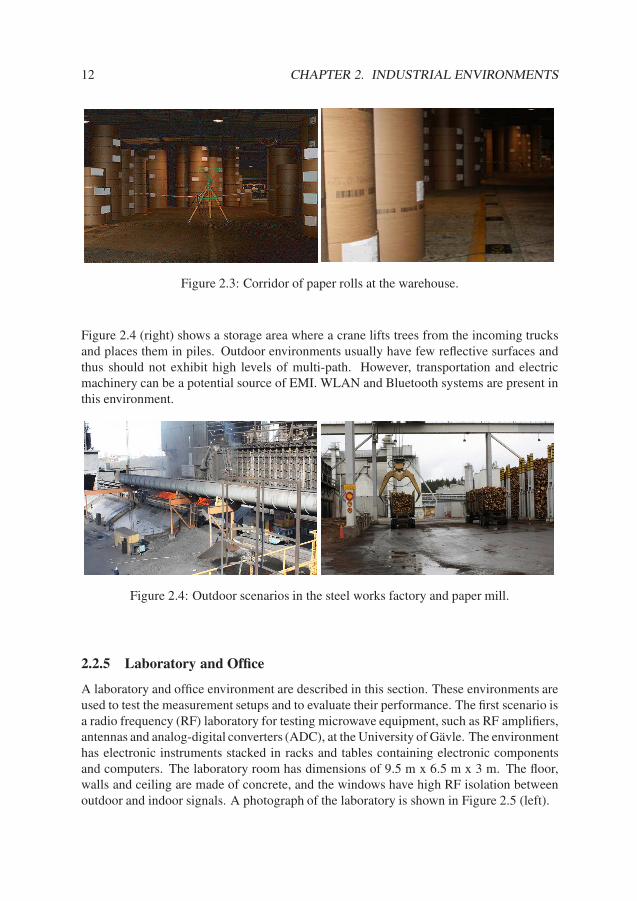
This environment corresponds to a warehouse containing paper rolls at the Stora Enso pa-per mill in Borlänge. The environment consists of a warehouse where the final products,i.e., paper rolls, are stacked in blocks that are separated by corridors. As shown in Fig-ure 2.3, the environment where the storage plan covers an area of 85 m x 150 m and hasa ceiling height of 8 m. The walls and ceilings are constructed of prefabricated concrete,and the floor is made of concrete. The paper rolls have a diameter between 1.25 m and1.70 m, a height between 1 m and 3 m and weights between 300 kg to 1200 kg. Thispaper exhibits special dielectric properties, causing the absorption of the incident signalsin the paper rolls. This environment is quite unique; the channel propagation behaves in amanner opposite of the typical industrial environments with high multi-path levels. WLANsystem and Åkerströms Sesam utilizing the 869.8 MHz frequency band for door openersare present in this environment.
2.2.4 Outdoor Industrial Environment
Outdoor industrial environments are often used for the purposes of transporting and storinggoods. A process in the steel works at SSAB in Luleå is shown in Figure 2.4 (left), where
the coal is heated in ovens to increase the purity and efficiency of the coal for later use.
12 CHAPTER 2. INDUSTRIAL ENVIRONMENTS
Figure 2.3: Corridor of paper rolls at the warehouse.
Figure 2.4 (right) shows a storage area where a crane lifts trees from the incoming trucksand places them in piles. Outdoor environments usually have few reflective surfaces andthus should not exhibit high levels of multi-path. However, transportation and electricmachinery can be a potential source of EMI. WLAN and Bluetooth systems are present inthis environment.
Figure 2.4: Outdoor scenarios in the steel works factory and paper mill.
2.2.5 Laboratory and Office
A laboratory and office environment are described in this section. These environments areused to test the measurement setups and to evaluate their performance. The first scenario isa radio frequency (RF) laboratory for testing microwave equipment, such as RF amplifiers,antennas and analog-digital converters (ADC), at the University of Gävle. The environmenthas electronic instruments stacked in racks and tables containing electronic componentsand computers. The laboratory room has dimensions of 9.5 m x 6.5 m x 3 m. The floor,walls and ceiling are made of concrete, and the windows have high RF isolation betweenoutdoor and indoor signals. A photograph of the laboratory is shown in Figure 2.5 (left).
2.2. ENVIRONMENT DESCRIPTIONS 13
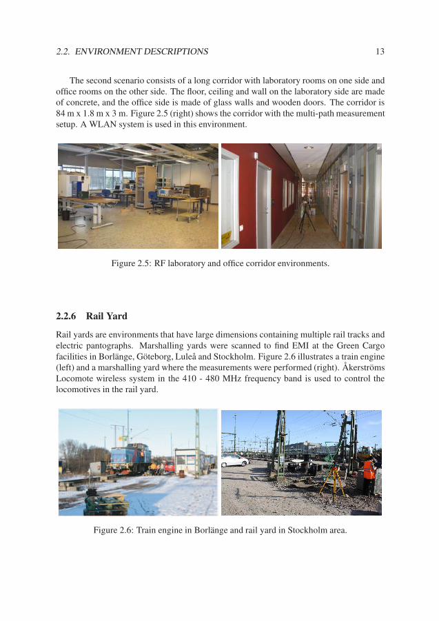
The second scenario consists of a long corridor with laboratory rooms on one side andoffice rooms on the other side. The floor, ceiling and wall on the laboratory side are madeof concrete, and the office side is made of glass walls and wooden doors. The corridor is84 m x 1.8 m x 3 m. Figure 2.5 (right) shows the corridor with the multi-path measurementsetup. A WLAN system is used in this environment.
Figure 2.5: RF laboratory and office corridor environments.
2.2.6 Rail Yard
Rail yards are environments that have large dimensions containing multiple rail tracks andelectric pantographs. Marshalling yards were scanned to find EMI at the Green Cargofacilities in Borlänge, Göteborg, Luleå and Stockholm. Figure 2.6 illustrates a train engine(left) and a marshalling yard where the measurements were performed (right). ÅkerströmsLocomote wireless system in the 410 - 480 MHz frequency band is used to control thelocomotives in the rail yard.
Figure 2.6: Train engine in Borlänge and rail yard in Stockholm area.
14 CHAPTER 2. INDUSTRIAL ENVIRONMENTS
2.2.7 Mine Tunnel
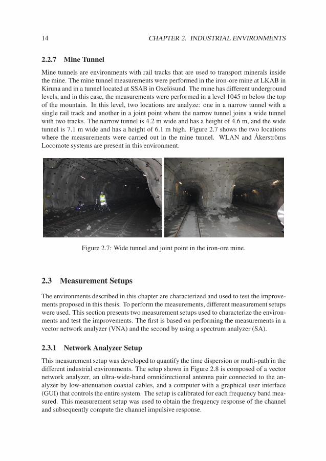
Mine tunnels are environments with rail tracks that are used to transport minerals insidethe mine. The mine tunnel measurements were performed in the iron-ore mine at LKAB inKiruna and in a tunnel located at SSAB in Oxelösund. The mine has different undergroundlevels, and in this case, the measurements were performed in a level 1045 m below the topof the mountain. In this level, two locations are analyze: one in a narrow tunnel with asingle rail track and another in a joint point where the narrow tunnel joins a wide tunnelwith two tracks. The narrow tunnel is 4.2 m wide and has a height of 4.6 m, and the widetunnel is 7.1 m wide and has a height of 6.1 m high. Figure 2.7 shows the two locationswhere the measurements were carried out in the mine tunnel. WLAN and ÅkerströmsLocomote systems are present in this environment.
Figure 2.7: Wide tunnel and joint point in the iron-ore mine.
2.3 Measurement Setups
The environments described in this chapter are characterized and used to test the improve-ments proposed in this thesis. To perform the measurements, different measurement setupswere used. This section presents two measurement setups used to characterize the environ-ments and test the improvements. The first is based on performing the measurements in avector network analyzer (VNA) and the second by using a spectrum analyzer (SA).
2.3.1 Network Analyzer Setup
This measurement setup was developed to quantify the time dispersion or multi-path in thedifferent industrial environments. The setup shown in Figure 2.8 is composed of a vectornetwork analyzer, an ultra-wide-band omnidirectional antenna pair connected to the an-alyzer by low-attenuation coaxial cables, and a computer with a graphical user interface(GUI) that controls the entire system. The setup is calibrated for each frequency band mea-sured. This measurement setup was used to obtain the frequency response of the channeland subsequently compute the channel impulsive response.

2.3. MEASUREMENT SETUPS 15
Vector Network
Analyzer
PC
d
A1 A2
Multi-Path
Path Loss
Figure 2.8: Network analyzer measurement setup.
To perform the channel characterization measurements with the VNA, several parame-ters need to be adjusted. For instance, the system has a maximum detectable delay, τmax,after which the multi-path components are not captured. The maximum detectable delayis obtained as follows
τmax =Npoints − 1
BW(2.1)
where Npoints is the number of measurement points used in one sweep and BW is thebandwidth selected. The system uses 1601 points and 500 MHz of bandwidth, providinga maximum detectable delay of 3.2 µs, which is sufficient to cover most indoor environ-ments. Consequently, the time resolution for distinguishing two consecutive paths in thiscase is 2 ns.
Another parameter that should be taken into account is the frequency shift, ∆f , whichis a function of the propagation time, ttr (time of flight), the frequency span, S, and thesweep time, tsw, as defined by the following expression
∆f = ttr (S/tsw) (2.2)
The intermediate frequency (IF) bandwidth should be greater than ∆f . With a fre-quency span of 500 MHz S, a sweep time of 800 ms, and not expecting to detect multi-pathcomponents after 2 µ s, we require an IF bandwidth greater than 1.25 kHz.
2.3.2 Generic Spectrum Analyzer Setup
This generic spectrum analyzer setup is used to measure the path loss and EMI present inthe environments as well as to test the spatial diversity and EMI mitigation techniques. The

16 CHAPTER 2. INDUSTRIAL ENVIRONMENTS
setup shown in Figure 2.9 is based on stimulating the channel with a signal generator (SG)and measuring the response of the channel with a spectrum analyzer.
Depending on the parameter measured, this generic setup is adjusted to the respectiverequirements. For instance, the EMI measurement setup is composed of a broadband an-tenna and a spectrum analyzer that measures the EMI source. In the case of the path lossmeasurements, the setup uses an SG to excite the channel and two antennas connected tothe SA to capture the combined signal. The measurement setup used for the spatial diver-sity test is similar to the path loss setup; however, the received signals by the two antennasare captured in two SAs processing them independently. The EMI mitigation measure-ment setup is composed of an SG and an SA, forming a communication system, and aninterference source produced by a second SG.
The center frequency, bandwidth, resolution bandwidths, distance between antennasand other settings and steps performed during each measurement are described in the fol-lowing chapters.
Signal
Generator Spectrum
Analyzer
PC
dr
Interference
Source
A1 A2 A3
Multi-Path
Path Loss
d
Figure 2.9: Generic spectrum analyzer measurement setup.
2.4 Summary
This chapter presented a broad variety of industrial environments and the measurementsetups used during the environment characterization. With our selection of these differentenvironments, we have attempted to cover a large percentage of the environments encoun-tered in industry. From typical industrial environments, with large amounts of metallic ob-

2.4. SUMMARY 17
jects exhibiting a highly reflective propagation, to mine tunnels or paper warehouse, withopposite characteristics and behavior. This does not mean that we have covered all pos-sible industrial environments, but we believe that the selected environments will illustratethe differences in radiowave propagation when going from one environment to another.The industrial environments and the measurement setups described in this chapter will bereferred to regularly in the following chapters.


Chapter 3
Multi-path Characterization in
Industrial Environments
3.1 Introduction
Multi-path fading is an effect produced when a signal propagates through a dispersivechannel. This time dispersion is a consequence of the multiple replicas of the signal thatare produced by reflection, diffraction and scattering with the objects encountered in thechannel arriving at the receiver. The number of replicas in the received signal depends onthe nature of the objects encountered in the environment. Thus, an industrial environmentwith metallic surfaces will introduce high levels of multi-path fading compared to otherindoor environments such as office or residential environments. High levels of multi-pathcould produce intersymbol interference (ISI), reducing the communication performance.The reduction in communication performance depends on the duration of the symbol pe-riod of a radio system and the dispersive properties of the environment [24]. Multiple-input and multiple-output (MIMO) can take advantage of the high levels of multi-path.High levels of multi-path produce uncorrelated signals in each antenna, and by combiningthe received signals in a special manner, MIMO systems can increase the performance ofthe system. Thus, environments with low multi-path levels will not experience ISI, anddeploying MIMO systems in these environments will not increase the communication per-formance. Consequently, there is a need for understanding the channel behavior whendeploying a new wireless system. Selecting an adequate system for each scenario willincrease the reliability of communications.
A number of studies have characterized and modeled the dispersive properties of thechannel, quantifying its dispersion with the root-mean-square (rms) delay spread. Forinstance, the research performed in [25] contains a channel characterization in office en-vironments in the wide-band between 2 and 5 GHz. This paper shows rms delay spreadvalues ranging from 30 ns in line-of-sight (LoS) situations to 50 ns in non line-of-sight(NLoS) situations. An extensive measurement campaign in residential and commercialareas performed by Ghassemzadeh et al. [26] found rms delay spread levels of 3.38 ns
19

20CHAPTER 3. MULTI-PATH CHARACTERIZATION IN INDUSTRIAL
ENVIRONMENTS
in LoS and 8.15 ns in NLoS, and they also proposed a propagation model to match themeasurement results.
Measurements carried out in industrial environments with a significant number ofmetallic surfaces showed that the rms delay spread has levels of approximately 50 ns [21].In that study, the authors proposed a modification of the Saleh-Valenzuela indoor modelthat provides a better approximation to their measurement results. The researchers in [9]performed measurements in a nuclear power plant and in a chemical pulp factory, con-cluding that these environments exhibit significant time dispersion and thus provide goodreceived signals in non-line-of-sight scenarios. A study of signal fading due to obstructedpaths and multi-path in industrial environments in the 1.8 and 2.4 GHz ISM bands waspresented in [22]. A measurement in a subway tunnel in the 2.4 GHz band reported highrms delay spread levels from 159 ns in LoS to 234 ns in NLoS scenarios [27]. In contrast,several measurement studies performed in tunnel mines found low levels of rms delayspread [28, 29].
Based on the overall picture of the measurement results in the literature, industrial envi-ronments are considered reflective due to the quantities of metallic objects present in suchenvironments. This chapter shows that generalizing all industrial environments as reflectivedoes not correspond to reality. This thesis develops a measurement setup for characterizingindustrial environments with completely different characteristics as discussed in Chapter 2.The work of this chapter is based on published articles. In Papers [J2] and [J4], typical re-flective industrial environments with a significant number of metallic objects and high rmsdelay spread are studied. An industrial environment with a lower rms delay spread relativeto office environments due to the absorbing materials stored in the hall is analyzed in Paper[C2]. Moreover, tunnel environments with low multi-path components are presented inPapers [J1] and [C4]. To complete this channel characterization, the Saleh-Valenzuela andin-room power delay profile (IPDP) propagation models that extract the model parametersfor the different industrial environments are presented in Papers [C3] and [J3].
The remainder of this chapter is structured as follows. The next section presents thetheoretical background necessary to understand the extracted channel characteristics. Thethird section presents the results of the measurement campaigns in the different environ-ments and the corresponding multi-path parameters that quantify the time dispersion inthe environment such as the rms delay spread. This third section also contains the Saleh-Valenzuela and IPDP extracted parameters models of the different environments. The lastsection provides a summary of the chapter with general conclusions.
3.2 Multi-path Fading in Wireless Communications
The impulse response describes the time dispersive properties of a channel and can beused to characterize an environment. Obtaining the frequency response of the channel in acertain band can be used to estimate the impulse response of the channel. In our work, thefrequency response was determined by performing a spectral analysis of the channel witha vector network analyzer (VNA), which obtains the complex channel transfer function,Hm(f). Once the transfer function is in the PC, it is weighted through a Blackman-Harris

3.2. MULTI-PATH FADING IN WIRELESS COMMUNICATIONS 21
window in order to reduce the out-of-band noise [30]. Assuming that the channel is timeinvariant compared with the transmitted signal, i.e., the channel variations are slower thanthe base-band signal variations, then the channel transfer function after windowing can bewritten as follows
Hc(f) = Hw(f) × Hm(f) (3.1)
Hence, the impulse response of the radio channel is obtained by taking the inverseFourier transform approximated by using the inverse discrete Fourier transform (IDFT)
hc(τ) =1
Ws
∫
Ws
Hc(f)ej2πfτ df
≈ 1
N
N−1∑
k=0
Hc(k∆f)ej2πk∆fτ (3.2)
where Ws is the width of the Blackman-Harris window and ∆f = Ws
N . By letting τ =m∆τ = m/Ws we obtain the discrete samples of the channel impulse response as
hc(m) =1
N
N−1∑
k=0
Hc(k∆f)ej2π kmN , m = 0, 1, · · · , N − 1 (3.3)
Radio channels are usually modeled as wide sense stationary with uncorrelated scat-tering with the power delay profile (PDP), which is the expected power per unit of timereceived with a certain excess delay. The PDP is defined as the autocorrelation function ofthe channel impulse response and can be written as
φh(τ) = E{hc(τ1 + τ) h∗
c(τ1)} (3.4)
where E{·} represents the expected value.Furthermore, to obtain quantitative parameters of the time spread in the environment,
the mean excess delay (τmean) and rms delay spread (τrms) can be obtained from theaveraged PDP in the same position [24]. To estimate the different quantitative parameters,a threshold needs to be set to distinguish the multi-path components from the noise floor.In this case, this threshold, T hD, corresponds to the µ + 3σ of the noise part, where µ andσ are the mean and variance, respectively. The mean excess delay is the first moment ofthe power delay profile of the channel and is defined as
τmean =
∑
k φh(k∆τ)k∆τ∑
k φh(k∆τ)(3.5)
where k corresponds to the samples above the threshold T hD.The rms delay spread is the square root of the second moment of the PDP and is defined
as
τrms =
√
(∑
k φh(k∆τ)(k∆τ)2
∑
k φh(k∆τ)
)
− (τmean)2 (3.6)
22CHAPTER 3. MULTI-PATH CHARACTERIZATION IN INDUSTRIAL
ENVIRONMENTS
The maximum excess delay is the time spread during multi-path components are abovea certain threshold and is defined as
MD = τmax − τmin (3.7)
where τmin and τmax are the arrival time of the first and the last multi-path components,respectively.
The coherence bandwidth is a statistical parameter that defines whether the channel canbe assumed as frequency non-selective (flat) or frequency selective over a given frequencyband. For a frequency correlation of 0.5 [31, 32], the coherence bandwidth is computedfrom the τrms as
Bm =1
5τrms(3.8)
3.2.1 Channel Models
Multiple models have been elaborated in previous works to describe the impulse responseof a channel. In this thesis, we take the extended indoor propagation models, Saleh-Valenzuela and IPDP to study the behavior of the various measured and simulated en-vironments.
Saleh-Valenzuela
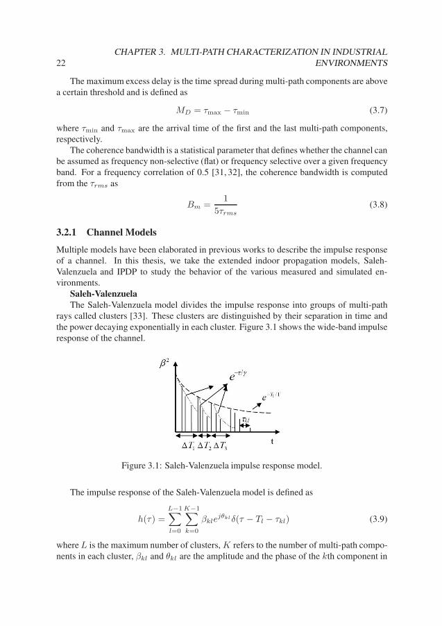
The Saleh-Valenzuela model divides the impulse response into groups of multi-pathrays called clusters [33]. These clusters are distinguished by their separation in time andthe power decaying exponentially in each cluster. Figure 3.1 shows the wide-band impulseresponse of the channel.
Figure 3.1: Saleh-Valenzuela impulse response model.
The impulse response of the Saleh-Valenzuela model is defined as
h(τ) =
L−1∑
l=0
K−1∑
k=0
βklejθkl δ(τ − Tl − τkl) (3.9)
where L is the maximum number of clusters, K refers to the number of multi-path compo-nents in each cluster, βkl and θkl are the amplitude and the phase of the kth component in
3.2. MULTI-PATH FADING IN WIRELESS COMMUNICATIONS 23
the lth cluster, Tl is the arrival time of the lth cluster and τkl is the arrival time delay of thekth ray in the lth cluster with respect to the first ray of the lth cluster. And βkl is defined as
β2kl = β2(0, 0)e−Tl/Γe−τkl/γ (3.10)
where Γ and γ are the exponential cluster decay and ray decay inside the cluster, respec-tively, and β2(0, 0) is the average power of the first component received.
In order to estimate the parameters of Saleh-Valenzuela model, we have used a visualcurve-fitting, which is one of the best ways to assess the composition of the PDP. The stepsfor estimating the S-V model parameters are as follows:
1. Divide the P DP s into clusters.
2. Determine the inter-arrival times (∆Tl) for every cluster and then average ∆Tl forall P DP s in the same location.
3. Obtain the average ray arrival time, τkl.
4. Determine the average cluster decay constant, Γ, fitting the maximum power ofeach cluster to an exponential function.
The ray decay constant, γ, is estimated from the modified Saleh-Valenzuela model [21]adopted by the IEEE 802.15.4a channel model in which it is defined that the ray decayconstant experiences a higher decay as the delay of a cluster increases. The ray decayconstant is defined as
γ(τ) = aτ + γ0 (3.11)
where a and γ0 are constants which depend on the environment, whether there is a line-of-sight path or not.
IPDP Model
The in-room power delay profile (IPDP) is a prediction model used to estimate thebehavior of a channel based on the dimensions and materials of the environment [34]. Themodel defines the power delay profile of the channel as a composition of multiple multi-path components with different amplitudes and delays
φ(m) = Ψmδ(t − τm), m = 0, 1, · · · , M − 1. (3.12)
where M , Ψm, τm are the number, amplitude and delay of the multi-path componentsrespectively. In order to normalize the power delay profile and set the first component atzero Ψ0 = 1 and τ0 = 0, the rest of the components Ψm and τm are defined as
Ψm =1
4
γm
m2, m = 1, 2, · · · , M − 1. (3.13)
τm =tc
2(2m − 1) , m = 1, 2, · · · , M − 1. (3.14)

24CHAPTER 3. MULTI-PATH CHARACTERIZATION IN INDUSTRIAL
ENVIRONMENTS
where γ is the average power reflection coefficient and tc is the characteristic time of thechannel. In real environments where there are multiple surface with different materials γbecomes
γeff = 1 − αeff (3.15)
where αeff can be defined as
αeff =
∑Uu=1 Suαu
S(3.16)
where U is the number of surfaces, S is the total surface area in the environment,αu andSu are the absorption coefficient and surface area of u respectively.
The characteristic time of the channel, tc, is defined as
tc =8V
cS(3.17)
where V is the volume of the environment and c is the speed of light.
3.3 Measurement Results and Analysis
Industrial environments are often classified as reflective with high multi-path levels; how-ever, from the measurement campaigns performed in multiple environments, we foundsignificant diversity in the channel behavior. Based on our studies, the response of thechannel varies from high to low delay spread environments. This section describes themeasurement results from the bark furnace, paper warehouse and mine tunnel presented inChapter 2, ranging over different delay spread levels. The measurement setup based on thenetwork analyzer presented in Chapter 2 is used to obtain the channel impulse responseand compute the quantitative parameters of the delay spread.
3.3.1 High delay spread environments
Environments that exhibit high delay spread are environments containing large quantitiesof metallic materials. This type of environment could correspond to the highly reflectiveenvironments, i.g., bark furnace, described in Chapter 2. The work presented in this sectionis the result of Papers [J2], [J3] and [J4].
By using the measurement setup and by processing the channel response, the PDP canbe determined for this environment. The results show that the channel introduces a highlevel of time dispersion to the signal. Figure 3.2 shows samples of power delay profiles forthree different frequency bands in one of the locations in Figure 2.1. We can see that therms delay spread for a highly reflective environment is greater than 290 ns in some cases,as we reported in Paper [J3]. This shows that a number of industrial environments canexhibit higher rms delay spread levels compared with previous works reported in similarreflective environments [21].
3.3. MEASUREMENT RESULTS AND ANALYSIS 25
0 1000 2000 30000
0.2
0.4
0.6
0.8
1
t [ns]
PD
P (
Nor
mal
ized
)
RMSDelay = 2.92e-007 s
0 1000 2000 30000
0.2
0.4
0.6
0.8
1
t [ns]
PD
P (
Nor
mal
ized
)
0 1000 2000 30000
0.2
0.4
0.6
0.8
1
t [ns]
PD
P (
Nor
mal
ized
)
RMSDelay = 2.28e-007 s RMSDelay = 1.93e-007 s
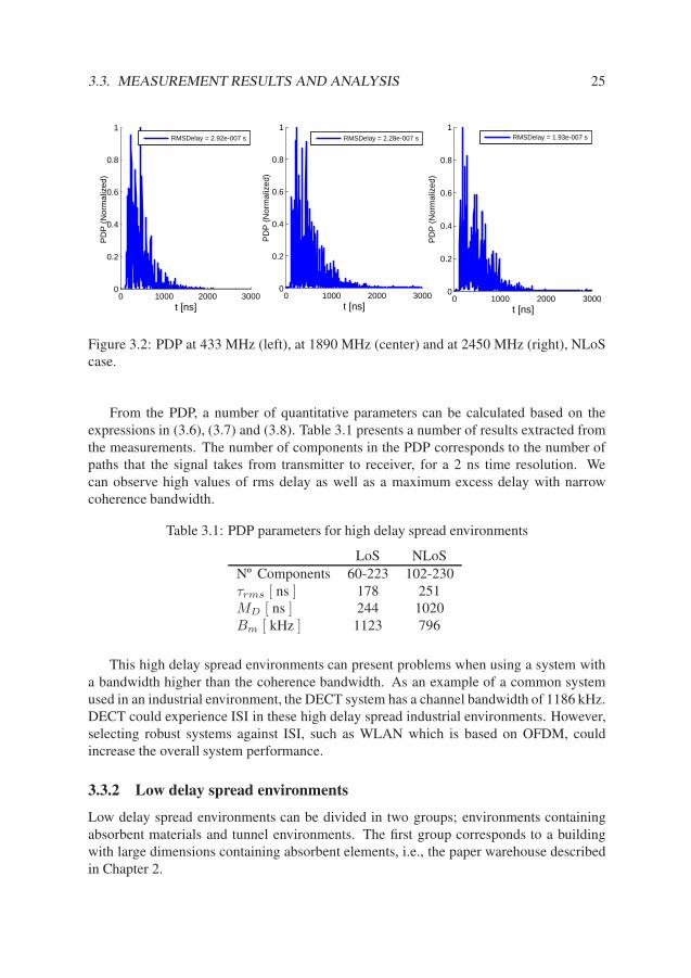
Figure 3.2: PDP at 433 MHz (left), at 1890 MHz (center) and at 2450 MHz (right), NLoScase.
From the PDP, a number of quantitative parameters can be calculated based on theexpressions in (3.6), (3.7) and (3.8). Table 3.1 presents a number of results extracted fromthe measurements. The number of components in the PDP corresponds to the number ofpaths that the signal takes from transmitter to receiver, for a 2 ns time resolution. Wecan observe high values of rms delay as well as a maximum excess delay with narrowcoherence bandwidth.
Table 3.1: PDP parameters for high delay spread environments
LoS NLoSNº Components 60-223 102-230τrms [ ns ] 178 251MD [ ns ] 244 1020Bm [ kHz ] 1123 796
This high delay spread environments can present problems when using a system witha bandwidth higher than the coherence bandwidth. As an example of a common systemused in an industrial environment, the DECT system has a channel bandwidth of 1186 kHz.DECT could experience ISI in these high delay spread industrial environments. However,selecting robust systems against ISI, such as WLAN which is based on OFDM, couldincrease the overall system performance.
3.3.2 Low delay spread environments
Low delay spread environments can be divided in two groups; environments containingabsorbent materials and tunnel environments. The first group corresponds to a buildingwith large dimensions containing absorbent elements, i.e., the paper warehouse describedin Chapter 2.
26CHAPTER 3. MULTI-PATH CHARACTERIZATION IN INDUSTRIAL
ENVIRONMENTS
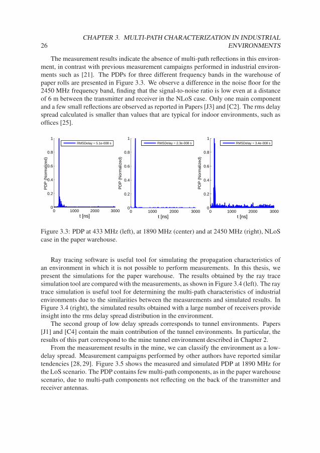
The measurement results indicate the absence of multi-path reflections in this environ-ment, in contrast with previous measurement campaigns performed in industrial environ-ments such as [21]. The PDPs for three different frequency bands in the warehouse ofpaper rolls are presented in Figure 3.3. We observe a difference in the noise floor for the2450 MHz frequency band, finding that the signal-to-noise ratio is low even at a distanceof 6 m between the transmitter and receiver in the NLoS case. Only one main componentand a few small reflections are observed as reported in Papers [J3] and [C2]. The rms delayspread calculated is smaller than values that are typical for indoor environments, such asoffices [25].
0 1000 2000 30000
0.2
0.4
0.6
0.8
1
t [ns]
PD
P (
Nor
mal
ized
)
0 1000 2000 30000
0.2
0.4
0.6
0.8
1
t [ns]
PD
P (
Nor
mal
ized
)
0 1000 2000 30000
0.2
0.4
0.6
0.8
1
t [ns]
PD
P (
Nor
mal
ized
)
RMSDelay = 3.4e-008 sRMSDelay = 2.3e-008 sRMSDelay = 5.1e-008 s
Figure 3.3: PDP at 433 MHz (left), at 1890 MHz (center) and at 2450 MHz (right), NLoScase in the paper warehouse.
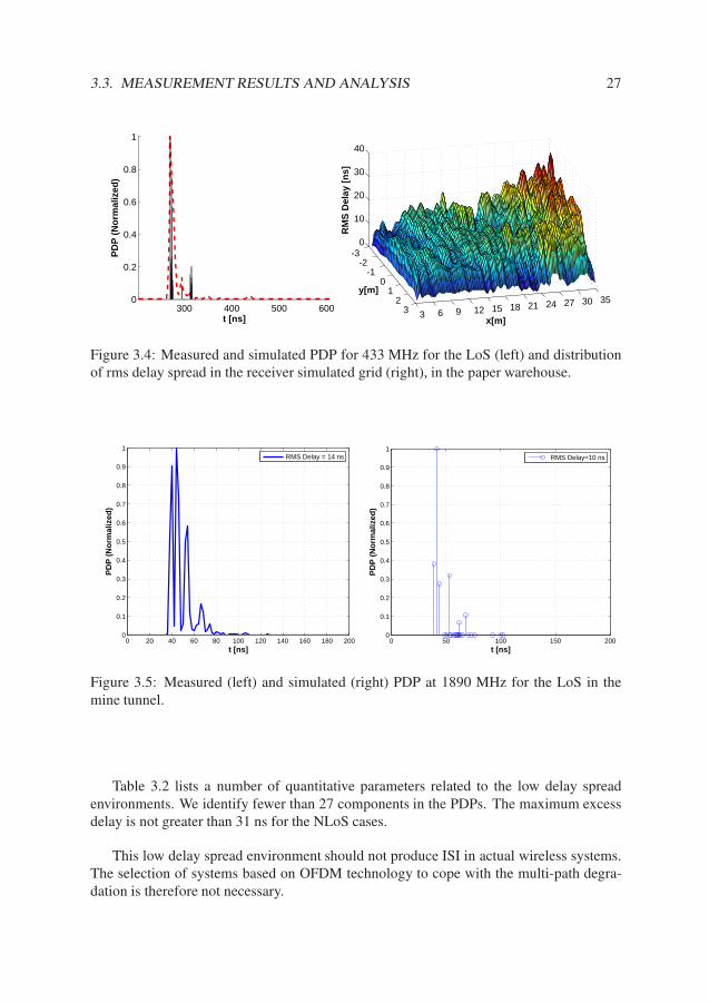
Ray tracing software is useful tool for simulating the propagation characteristics ofan environment in which it is not possible to perform measurements. In this thesis, wepresent the simulations for the paper warehouse. The results obtained by the ray tracesimulation tool are compared with the measurements, as shown in Figure 3.4 (left). The raytrace simulation is useful tool for determining the multi-path characteristics of industrialenvironments due to the similarities between the measurements and simulated results. InFigure 3.4 (right), the simulated results obtained with a large number of receivers provideinsight into the rms delay spread distribution in the environment.
The second group of low delay spreads corresponds to tunnel environments. Papers[J1] and [C4] contain the main contribution of the tunnel environments. In particular, theresults of this part correspond to the mine tunnel environment described in Chapter 2.
From the measurement results in the mine, we can classify the environment as a low-delay spread. Measurement campaigns performed by other authors have reported similartendencies [28, 29]. Figure 3.5 shows the measured and simulated PDP at 1890 MHz forthe LoS scenario. The PDP contains few multi-path components, as in the paper warehousescenario, due to multi-path components not reflecting on the back of the transmitter andreceiver antennas.
3.3. MEASUREMENT RESULTS AND ANALYSIS 27
300 400 500 6000
0.2
0.4
0.6
0.8
1
t [ns]
PD
P (
No
rmal
ized
)
3530272421181512963
-3-2
-10
12
3
0
10
20
30
40
x[m]
y[m]
RM
S D
elay
[n
s]Figure 3.4: Measured and simulated PDP for 433 MHz for the LoS (left) and distributionof rms delay spread in the receiver simulated grid (right), in the paper warehouse.
0 20 40 60 80 100 120 140 160 180 2000
0.1
0.2
0.3
0.4
0.5
0.6
0.7
0.8
0.9
1
t [ns]
PD
P (
No
rmal
ized
)
RMS Delay = 14 ns
0 50 100 150 2000
0.1
0.2
0.3
0.4
0.5
0.6
0.7
0.8
0.9
1
t [ns]
PD
P (
No
rmal
ized
)
RMS Delay=10 ns
Figure 3.5: Measured (left) and simulated (right) PDP at 1890 MHz for the LoS in themine tunnel.
Table 3.2 lists a number of quantitative parameters related to the low delay spreadenvironments. We identify fewer than 27 components in the PDPs. The maximum excessdelay is not greater than 31 ns for the NLoS cases.
This low delay spread environment should not produce ISI in actual wireless systems.The selection of systems based on OFDM technology to cope with the multi-path degra-dation is therefore not necessary.
28CHAPTER 3. MULTI-PATH CHARACTERIZATION IN INDUSTRIAL
ENVIRONMENTS
Table 3.2: PDP parameters for a low delay spread environment
LoS NLoSNº Components 9-27 5-19τrms [ ns ] 11 28MD [ ns ] 16 31Bm [ kHz ] 18181 7142
3.3.3 Channel Model Results
This section is based on the work performed in Papers [C3] and [J3]. In Paper [C3], theIPDP is analyzed with respect to other propagation models. Paper [J3] contains a compar-ison between the two industrial environments that exhibit different propagation behavior,i.e., reflective and absorbent, with the extracted Saleh-Valenzuela model parameters.
Saleh-Valenzuela Model
We can observe the averaged extracted parameters of the high and low delay spread en-vironment in Table 3.3. The results are obtained by averaging seven PDPs in 16 locations.In the low delay spread environment, the presence of a single cluster makes the estimationof most of the parameters impossible. This problem with the cluster division has also beennoticed in reflective environments such as those in [21].
Table 3.3: Channel parameters of the Saleh-Valenzuela model
LoS High Delay Spread LoS Low Delay Spread∆Tl [ ns ] 40.1 -τkl [ ns ] 6.7 5.8Γ [ ns ] 187.3 8.9γ0 7.64 -a 0.93 -
The estimated parameters of the Saleh-Valenzuela model are validated by simulatingthe PDP and computing the rms delay spread. In Figure 3.6, we can observe the simulatedand measured PDPs in the high delay spread environment for the LoS scenario. The simu-lated and measured rms delay values are within the same range, showing high delay spreadbehavior in the environment.

3.4. DISCUSSION 29
0 500 1000 1500 20000
0.1
0.2
0.3
0.4
0.5
0.6
0.7
0.8
0.9
1
t [ns]
PD
P (
No
rmal
ized
)
RMS Delay = 2.081030e-07 s
0 500 1000 1500 20000
0.1
0.2
0.3
0.4
0.5
0.6
0.7
0.8
0.9
1
t [ns]
PD
P (
No
rmal
ized
)
RMS Delay = 2.401262e-07 s
Figure 3.6: Simulated Saleh-Valenzuela PDP (left) and measured PDP (right) in high delayspread environment.
IPDP Model
Upon setting the properties of the building structure and the reflection coefficient inboth environments, the PDP was computed. Figure 3.7 shows the simulated power delayprofile of the high and low delay spread environments described previously. The simula-tions are within the range of the measurements results from the previous sections.
0 500 1000 1500 2000 2500 30000
0.1
0.2
0.3
0.4
0.5
0.6
0.7
0.8
0.9
1
t [ns]
PD
P (
Nor
mal
ized
)
RMS Low 4.929144e+00 [ns]RMS High 2.162011e+02 [ns]
Figure 3.7: PDP of the IPDP model for low and high delay spread channels.
3.4 Discussion
This chapter described a characterization of the multi-path propagation in diverse indus-trial environments. Previous studies define industrial environments as high delay spreadenvironments caused by the building structure and metallic elements present in the en-vironment. In this chapter, we characterize environments with different delay spreads,
30CHAPTER 3. MULTI-PATH CHARACTERIZATION IN INDUSTRIAL
ENVIRONMENTS
distinguishing between high and low delay spread. The multi-path characterization andspread delay quantification carried out in the diverse industrial environments is a productof a developed delay spread measurement setup. The impulse responses of the character-ized industrial environments are modeled using the Saleh-Valenzuela and IPDP channelmodels. The distinction of industrial environments behaving in different manners couldresult in the awareness of the system developers to produce adaptive wireless systems thatcould exploit the propagation properties of the channel, increasing the reliability of thecommunication system.
Chapter 4
Path Loss Characterization in Industrial
Environments
4.1 Introduction
Radio waves experience different types of fading effects in industrial environments. Theprevious chapter described the short-term fading effects referred to as multi-path fading.This chapter focuses on the long-term deterministic path loss. Path loss describes thevariation of the signal strength over large distances on wide frequency bands. The pathloss is usually analyzed with respect to the distance for a narrow frequency band. Forinstance, an extensive measurement campaign carried out in residential and commercialareas performed by Ghassemzadeh et al. [26] showed path loss exponents, i.e., distancedependence, with values ranging from 1.35 to 2.38. A study in office environments at5.3 GHz showed similar tendency, with path loss exponents equal to 1.3 and 2.9 for LoSand NLoS scenarios, respectively [25].
Multiple measurements have been taken to investigate the distance dependence of theradio propagation in industrial environments. Three measurement campaigns at 900, 2400and 5200 MHz using narrow-band receivers found path loss exponents lower than the cor-responding free space, i.e., α = 2 [9, 10, 23]. Rappaport performed a measurement cam-paign at 1.3 GHz in an automation factory, and four additional industrial environmentsreporting a path loss exponent ranging between 1.49 and 2.81 [35].
Regarding the frequency dependence of the path loss, an overview of a path loss fre-quency dependence following a simple power law or exponential function is presentedin [36]. The well-known empirical models designed for predicting the propagation inurban, suburban and rural areas, i.e., the Okumura-Hata model, contain a frequency de-pendence in the propagation models [37, 38]. Furthermore, an extension of this model toincrease the frequency band up to 2 GHz is reported in the COST 231-Hata model [39].Path loss measurements in a residential area are reporting a frequency dependence in theirresults [40]. In [41], a prediction of the frequency dependence in rural and urban areasfound a frequency exponent between ± 0.2 and ± 1.5. Other measurement campaigns
31

32CHAPTER 4. PATH LOSS CHARACTERIZATION IN INDUSTRIAL
ENVIRONMENTS
in urban areas studying the frequency dependence produced by the heights of houses andtrees reported that the frequency exponent is between 2 and 3 [42]. A study of the pathloss in a multiband channel inside a corridor and a hall reported a frequency exponent withvalues ranging between 1 and 4 [43].
Few measurement campaigns have investigated the path loss frequency dependence inindustrial environments. The IEEE 802.15.4a report [44] presents a path loss frequencydependence following a power law and the extracted parameters of path loss, multi-pathand shadowing models in multiple environments. This work reports a frequency exponentvalue of 1.103 and 1.427 for LoS and NLoS scenarios, respectively.
This chapter discusses the path loss in reflective and absorbent industrial environmentsand extracts the path loss exponent and the frequency exponent parameters used to describethe propagation channel behavior in these environments. The content of this chapter isbased on the measurement results performed in Paper [J3]. The next section of this chapterpresents the theoretical background. The third section contains the results obtained in themeasurements and the model parameters that describe the behavior of the environment.The last section presents a discussion of the work performed in this chapter.
4.2 Path Loss in Wireless Communications
The free space propagation is a general model used to estimate the performance of wirelesslinks. To characterize the path loss in the environment, we start by defining the free spacepropagation model in a line-of-sight scenario. The path loss can be expressed as a functionof the transmitted, received signal or the Friis free space model [24] as defined
LP (d, f) = PT x(f) − PRx(d, f)
= −GT x(f) − ηT x(f) − GRx(f) − ηRx(f) + 10 log10
(
λ
4πd
)2
(4.1)
where PT x and PRx are the power of the transmitter and receiver, respectively, GT x andGRx are the antenna gains of the transmitter and receiver, respectively, ηT x and ηRx are theantenna efficiency of the transmitter and receiver, λ is the wavelength and d is the distancebetween the transmitter and receiver.
As a practical approach when performing measurements near the ground and in en-vironments with many obstacles, the path loss can be written in its general form as fol-lows [44, 45]
LP (d, f) = PRx(d, f) − PRx(d0, f) + LP 0(d0, f) (4.2)
where PRx(d0, f) and PRx(d, f) represent the received power on the frequency, f , anddistance d0 and d respectively. In this way, the effect of the antennas, i.e., the antennagains, antenna efficiencies, and transmission power are calibrated. The LP 0(d0, f) is theFriss free space path loss at distance d0 obtained as
LP 0(d0, f) = 10β log10(f) + 10α log10(d0) + A + 10 log10
(
4π
c
)2
(4.3)
4.3. MEASUREMENT RESULTS AND ANALYSIS 33
where β is the frequency exponent of the path loss, α is the path loss exponent (distanceexponent), A is a constant varying for LoS and NLoS scenarios, and c is the speed of light.
For a d0 and f given in meters and MHz respectively, then (4.3) can be formulated as
LP 0(d0, f) = 10β log10(f) + 10α log10(d0) + A + −27, 558 (4.4)
As we can see in (4.4), the path loss is composed by four terms; frequency dependentterm, distance dependent term and two constants.
The frequency exponent, β, can be extracted from the path loss by taking the derivativeof the path loss at distance d with respect to the frequency in dB as
β =1
10
dLP (f)
d log10(f)(4.5)
4.3 Measurement Results and Analysis
In this section, we present the measurement results and analysis obtained in the bark fur-nace, i.e., reflective, and paper warehouse, i.e., absorbent, environments described in Chap-ter 2. The setup to obtain the path loss in the frequency band between 200 and 2500 MHz isbased on the generic spectrum analyzer setup presented in Chapter 2. In this case, the mea-surement setup is composed of a signal generator, spectrum analyzer and three broadbandantennas. The signal generator transmits a continuous wave using a broadband directionalantenna. At the receiver, two antennas separated by at least λ/2 are deployed to reducethe small-scale fading and the shadowing degradations providing a global mean. The com-bined signal from the two antennas is fed into the spectrum analyzer and transferred to thecomputer. The measurement results of this chapter are product of the work performed inPaper [J3]; however, an extension has been performed to clarify the frequency dependencein the NLoS scenario.
Absorbent and reflective environments behave differently from each other, producingdistinct path loss results. To describe the behavior of the environment, we start by not con-sidering the frequency exponent of the path loss in the free space model (4.4). Thus, thefrequency exponent β = 2 is selected, and the path loss exponents for the different casesare extracted by least squares. For this purpose, the figure of merit used for estimating thepath loss exponent is the mean square error (MSE). In Table 4.1, we can observe the esti-mated path loss exponents for the reflective and absorbent environments in LoS and NLoSscenarios. The path loss measurements are performed in the 200 to 2500 MHz frequencyrange, with a separation distance d = 9 m between the transmitter and receiver antennasand the antennas mounted at a 1.5 m height. The NLoS scenarios exhibit higher path lossexponents relative to the values observed in the LoS scenario as could be expected.
The measurements of the path loss with respect to the frequency at a distance d = 9 min the LoS and NLoS scenarios are illustrated in Figure 4.1. The left figure shows the LoSmeasurements for the absorbent and reflective environments with the free space model forα = 2. The right figure illustrates the NLoS situation with the corresponding free spacemodel curves for the extracted α values in each scenario. The LoS scenario follows the

34CHAPTER 4. PATH LOSS CHARACTERIZATION IN INDUSTRIAL
ENVIRONMENTS
Table 4.1: Path loss exponents for the absorbent and reflective environments
LoS NLoSAbsorbent 1.99 2.39Reflective 1.86 2.54
free space model; however, the corresponding free space model for the NLoS scenarios isnot a representative case for describing the measured results. The measurements show afrequency dependence not described properly by the free space model in (4.4).
500 1000 1500 2000 250020
30
40
50
60
70
80
Frequency [MHz]
Pat
h L
oss
[d
B]
LoS AbsorbentLoS ReflectiveModel α = 2
500 1000 1500 2000 250020
30
40
50
60
70
80
Frequency [MHz]
Pat
h L
oss
[d
B]
NLoS AbsorbentNLoS ReflectiveModel NLoS ReflectiveModel NLoS Absorbent
Figure 4.1: Path loss versus frequency of the measurements at 9 m in absorbent and reflec-tive for LoS (left), NLoS (right) and the theoretical estimation for a β = 2.
To provide a model that describes the path loss in NLoS situations, the frequency expo-nent, β, is estimated for the different scenarios (4.4). To obtain this frequency exponent, β,the derivatives of the measured path loss are extracted. Figure 4.2 illustrates the derivativesof the path loss in the different scenarios, showing that the derivatives are constants andfluctuate between environments. By extracting the sample mean value of these derivatives,the frequency exponent, β, is estimated.
Table 4.2 provides the estimated parameters of the path loss model with the frequencyexponent (4.4). The frequency exponent, β, is higher in the NLoS scenario than in the LoSscenario. Within all the environments, the absorbent environment in the NLoS scenariopresents the highest frequency exponent. This strong frequency dependence is supposedto be related to the physical properties (permittivity, conductivity) of the material storedin the environment, i.e., the paper rolls. The estimated frequency exponent in industrialenvironments is higher than the value reported in [44], especially for NLoS scenarios inthe absorbent environment.
Figure 4.3 shows the NLoS measurement with the path loss estimations, taking intoaccount the frequency exponent. The estimated curves describe the behavior of the envi-ronments more efficiently than in the case where the frequency exponent is fixed to β = 2.
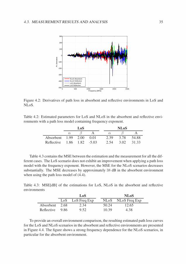
4.3. MEASUREMENT RESULTS AND ANALYSIS 35
0 500 1000 1500 2000 2500-500
-400
-300
-200
-100
0
100
200
300
Frequency [MHz]
PL
Der
ivat
ive
NLoS AbsorbentNLoS ReflectiveLoS AbsorbentLoS Reflective
Figure 4.2: Derivatives of path loss in absorbent and reflective environments in LoS andNLoS.
Table 4.2: Estimated parameters for LoS and NLoS in the absorbent and reflective envi-ronments with a path loss model containing frequency exponent.
LoS NLoS
α β A α β AAbsorbent 1.99 2.00 0.01 2.39 3.78 54.88Reflective 1.86 1.82 -5.03 2.54 3.02 31.33
Table 4.3 contains the MSE between the estimation and the measurement for all the dif-ferent cases. The LoS scenario does not exhibit an improvement when applying a path lossmodel with the frequency exponent. However, the MSE for the NLoS scenarios decreasessubstantially. The MSE decreases by approximately 38 dB in the absorbent environmentwhen using the path loss model of (4.4).
Table 4.3: MSE[dB] of the estimations for LoS, NLoS in the absorbent and reflectiveenvironments
LoS NLoS
LoS LoS Freq Exp NLoS NLoS Freq ExpAbsorbent 2.68 2.34 50.24 12.65Reflective 9.86 9.52 10.39 4.38
To provide an overall environment comparison, the resulting estimated path loss curvesfor the LoS and NLoS scenarios in the absorbent and reflective environments are presentedin Figure 4.4. The figure shows a strong frequency dependence for the NLoS scenarios, inparticular for the absorbent environment.

36CHAPTER 4. PATH LOSS CHARACTERIZATION IN INDUSTRIAL
ENVIRONMENTS
500 1000 1500 2000 250020
30
40
50
60
70
80
Frequency [MHz]
Pat
h Lo
ss [d
B]
Frequency Exponent ModelNLoS Reflective
500 1000 1500 2000 250020
30
40
50
60
70
80
Frequency [MHz]
Pat
h Lo
ss [d
B]
Frequency Exponent ModelNLoS Absorbent
Figure 4.3: Path loss versus frequency of the measurements in NLoS for absorbent (left),reflective (right) and the theoretical estimation with the frequency exponent model at 9 m.
500 1000 1500 2000 250020
30
40
50
60
70
80
Frequency [MHz]
Pat
h Lo
ss [d
B]
NLoS ReflectiveNLoS AbsorbentLoS AbsorbentLoS Reflective
Figure 4.4: Estimated theoretical path loss in absorbent and reflective environments in LoSand NLoS.
4.4 Discussion
In this chapter, the long-term deterministic path loss was studied in absorbent and reflec-tive industrial environments. This chapter focused particularly on studying the frequencydependence of the path loss in industrial environments. To characterize the path loss, ameasurement campaign was carried out in different locations in these absorbent and reflec-tive environments. An asynchronous setup composed of a SG and SA was used to scan thechannel and obtain the path loss characteristics. By analyzing the measurement results, afrequency dependence can be observed, and consequently, a model with a frequency ex-ponent is used to describe the channel behavior. The results show a path loss exponent

4.4. DISCUSSION 37
with values ranging between 1.86 and 2.54 in the LoS and NLoS scenarios, respectively.Regarding the frequency dependence path loss, the frequency exponent in the NLoS sce-narios is two times the frequency exponent estimated in the LoS scenarios. In particular,the absorbent environment in the NLoS scenario presents the highest frequency exponent,obtaining values up to 3.78. This result indicates a stronger frequency dependence than thefrequency dependence reported in previous studies for industrial environments.

Chapter 5
Electromagnetic Interference in
Industrial Environments
5.1 Introduction
Electromagnetic interference (EMI) or man-made interference is one of the most problem-atic electromagnetic degradations sources that wireless systems must address in industrialenvironments. EMI is produced by different sources, such as electric motors, repair work,fluorescent tubes and machinery [5]. Man-made interference or EMI decreases the re-liability of communications. While such reduced reliability may be acceptable in mostwireless systems deployed in office or residential environments, a reliability reduction isnot suitable for industrial communications. Industrial processes require robust and reliablecommunications with a failure probability that is almost negligible.
Many research groups have detected and characterized EMI present in industrial en-vironments [46, 47]. A survey performed in [11] presents the most common sources ofinterference in industrial environments: electric motors, ignition systems, welding pro-cesses, rectifiers, power lines and switching devices. This survey provides the frequencysignature of these interference sources and shows that interference from a welding processappears at frequencies lower than 100 MHz. E. N. Skomal also investigated the radiatinginterference of welders and power lines, showing similar results [12]. Moreover, the au-thors in [48] measured and modeled the interference produced by a modern electric motor,extracting the high-frequency model parameters with a network analyzer.
Furthermore, a number of electrically powered transportation systems in industrial en-vironments need to be considered when characterizing the different sources of interference.For instance, the work performed in [49] studied interference from a motorcycle and pro-posed a cancellation technique by implementing a multilayer perceptron (MLP) neuralnetwork. EMI from electric trains was studied in [50], the authors reported malfunctionof pacemakers in high-speed trains caused by the inductive coil filter of the electrical sys-tem. Moreover, an investigation performed in [51] showed the presence of electromagneticfields when the train enters in the powered sections where the batteries are charged from
39
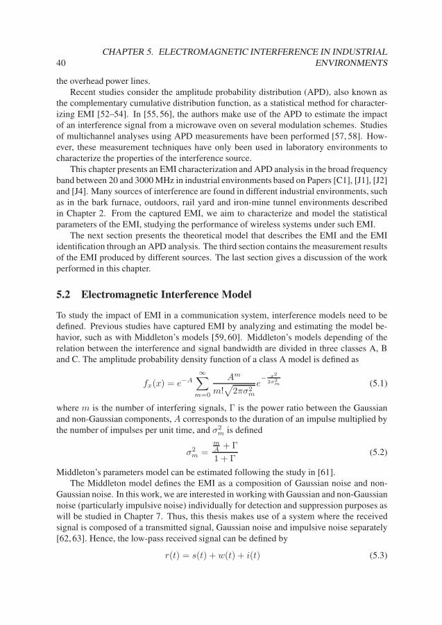
40CHAPTER 5. ELECTROMAGNETIC INTERFERENCE IN INDUSTRIAL
ENVIRONMENTS
the overhead power lines.Recent studies consider the amplitude probability distribution (APD), also known as
the complementary cumulative distribution function, as a statistical method for character-izing EMI [52–54]. In [55, 56], the authors make use of the APD to estimate the impactof an interference signal from a microwave oven on several modulation schemes. Studiesof multichannel analyses using APD measurements have been performed [57, 58]. How-ever, these measurement techniques have only been used in laboratory environments tocharacterize the properties of the interference source.
This chapter presents an EMI characterization and APD analysis in the broad frequencyband between 20 and 3000 MHz in industrial environments based on Papers [C1], [J1], [J2]and [J4]. Many sources of interference are found in different industrial environments, suchas in the bark furnace, outdoors, rail yard and iron-mine tunnel environments describedin Chapter 2. From the captured EMI, we aim to characterize and model the statisticalparameters of the EMI, studying the performance of wireless systems under such EMI.
The next section presents the theoretical model that describes the EMI and the EMIidentification through an APD analysis. The third section contains the measurement resultsof the EMI produced by different sources. The last section gives a discussion of the workperformed in this chapter.
5.2 Electromagnetic Interference Model
To study the impact of EMI in a communication system, interference models need to bedefined. Previous studies have captured EMI by analyzing and estimating the model be-havior, such as with Middleton’s models [59, 60]. Middleton’s models depending of therelation between the interference and signal bandwidth are divided in three classes A, Band C. The amplitude probability density function of a class A model is defined as
fx(x) = e−A∞
∑
m=0
Am
m!√
2πσ2m
e−
x2
2σ2m (5.1)
where m is the number of interfering signals, Γ is the power ratio between the Gaussianand non-Gaussian components, A corresponds to the duration of an impulse multiplied bythe number of impulses per unit time, and σ2
m is defined
σ2m =
mA + Γ
1 + Γ(5.2)
Middleton’s parameters model can be estimated following the study in [61].The Middleton model defines the EMI as a composition of Gaussian noise and non-
Gaussian noise. In this work, we are interested in working with Gaussian and non-Gaussiannoise (particularly impulsive noise) individually for detection and suppression purposes aswill be studied in Chapter 7. Thus, this thesis makes use of a system where the receivedsignal is composed of a transmitted signal, Gaussian noise and impulsive noise separately[62, 63]. Hence, the low-pass received signal can be defined by
r(t) = s(t) + w(t) + i(t) (5.3)
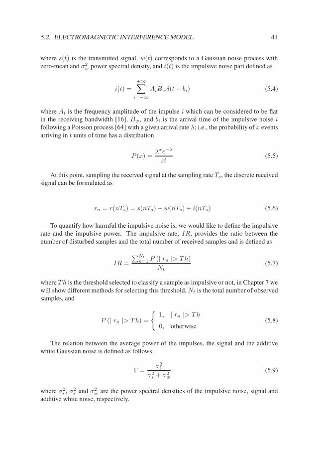
5.2. ELECTROMAGNETIC INTERFERENCE MODEL 41
where s(t) is the transmitted signal, w(t) corresponds to a Gaussian noise process withzero-mean and σ2
w power spectral density, and i(t) is the impulsive noise part defined as
i(t) =
+∞∑
i=−∞
AiBwδ(t − bi) (5.4)
where Ai is the frequency amplitude of the impulse i which can be considered to be flatin the receiving bandwidth [16], Bw, and bi is the arrival time of the impulsive noise ifollowing a Poisson process [64] with a given arrival rate λ; i.e., the probability of x eventsarriving in t units of time has a distribution
P (x) =λxe−λ
x!(5.5)
At this point, sampling the received signal at the sampling rate Ts, the discrete receivedsignal can be formulated as
rn = r(nTs) = s(nTs) + w(nTs) + i(nTs) (5.6)
To quantify how harmful the impulsive noise is, we would like to define the impulsiverate and the impulsive power. The impulsive rate, IR, provides the ratio between thenumber of disturbed samples and the total number of received samples and is defined as
IR =
∑Nt
n=1 P (| rn |> T h)
Nt(5.7)
where T h is the threshold selected to classify a sample as impulsive or not, in Chapter 7 wewill show different methods for selecting this threshold, Nt is the total number of observedsamples, and
P (| rn |> T h) =
{
1, | rn |> T h
0, otherwise(5.8)
The relation between the average power of the impulses, the signal and the additivewhite Gaussian noise is defined as follows
Γ =σ2
i
σ2s + σ2
w
(5.9)
where σ2i , σ2
s and σ2w are the power spectral densities of the impulsive noise, signal and
additive white noise, respectively.

42CHAPTER 5. ELECTROMAGNETIC INTERFERENCE IN INDUSTRIAL
ENVIRONMENTS
5.2.1 Amplitude Probability Distribution
The APD has been widely used to represent and visualize statistically EMI [52]. Thus, theAPD is a performance measure of EMI in an environment. The APD of the captured signalcan be defined as the probability that a random amplitude X exceeds a certain amplitudex0
APD(x0) = Pr [X > x0] = 1 − F (x0) (5.10)
where F (x0) is the cumulative distribution function (CDF) of X .For instance, Figure 5.1 (left) illustrates the amplitude of a received signal containing
impulsive noise and a signal free of impulsive noise. The APD representations for thesecases are shown in Figure 5.1 (right). The received signal containing impulsive noise iscomposed of two regions; the first region, i.e., no impulsive noise, where the sn + wn
dominates, and the second region, i.e., impulsive noise region, where the impulsive noisedominates. Thus, the APD representation of the received signal can be used to visual-ize the presence of impulsive noise and to estimate the threshold, T h, for detecting andsuppressing the impulsive noise as will be investigated in Chapter 7.
0 1 2 3 4 5 6 7 8 9 10
x 104
0
2
4
6
8
10
12
14
16
18
20
Samples
Am
plitu
de
sn + w
n + i
n
sn + w
n
0 2 4 6 8 10 12 14 16 1810
-5
10-4
10-3
10-2
10-1
100
AP
D (
x o)
Amplitude
sn + w
n + i
n
sn + w
n
No Impulsive Region
Threshold Impulsive Region
Figure 5.1: Time domain measurement (left) and APD of the data (right).
5.3 Measurement Results and Analysis
An electromagnetic characterization of a wide-band spectrum was performed in the barkfurnace environment presented in Chapter 2, also known as highly reflective environment.This characterization is reported in Papers [C1], [J2] and [J4], where multiple sources ofEMI are captured in a number of industrial environments. The measurement setup used forcapturing the EMI is based on the generic spectrum analyzer setup described in Chapter 2.In particular, the setup is composed of a broadband antenna covering frequencies from 20to 3000 MHz connected to a spectrum analyzer and a computer with a 12-bit analog digitalconverter (ADC).
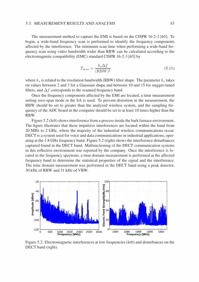
5.3. MEASUREMENT RESULTS AND ANALYSIS 43
The measurement method to capture the EMI is based on the CISPR 16-2-3 [65]. Tobegin, a wide-band frequency scan is performed to identify the frequency componentsaffected by the interference. The minimum scan time when performing a wide-band fre-quency scan using video bandwidth wider than RBW can be calculated according to theelectromagnetic compatibility (EMC) standard CISPR 16-2-3 [65] by
Tmin =ks∆f
(RBW)2(5.11)
where ks is related to the resolution bandwidth (RBW) filter shape. The parameter ks takeson values between 2 and 3 for a Gaussian shape and between 10 and 15 for stagger-tunedfilters, and ∆f corresponds to the scanned frequency band.
Once the frequency components affected by the EMI are located, a time measurementsetting zero-span mode in the SA is used. To prevent distortion in the measurement, theRBW should be set to greater than the analyzed wireless system, and the sampling fre-quency of the ADC board in the computer should be set to at least 10 times higher than theRBW.
Figure 5.2 (left) shows interference from a process inside the bark furnace environment.The figure illustrates that these impulsive interferences are located within the band from20 MHz to 2 GHz, where the majority of the industrial wireless communications occur.DECT is a system used for voice and data communications in industrial applications, oper-ating at the 1.8 GHz frequency band. Figure 5.2 (right) shows the interference disturbancescaptured found in the DECT band. Malfunctioning of the DECT communication systemsin this reflective environment was reported by the company. Once the interference is lo-cated in the frequency spectrum, a time domain measurement is performed at the affectedfrequency band to determine the statistical properties of the signal and the interference.The time domain measurement was performed in the DECT band using a peak detector,30 kHz of RBW and 51 kHz of VBW.
0 500 1000 1500 2000 2500 3000-120
-100
-80
-60
-40
-20
Frequency [MHz]
Am
plit
ud
e [d
Bm
]
1884 1886 1888 1890 18920
20
40
60
80
100
Frequency [MHz]
Ele
ctri
c F
ield
Str
eng
th[d
BµV
/m]
Figure 5.2: Electromagnetic interferences at low frequencies (left) and disturbances on theDECT band (right).

44CHAPTER 5. ELECTROMAGNETIC INTERFERENCE IN INDUSTRIAL
ENVIRONMENTS
The impulsive rate and the amplitude of the impulses are estimated for the interferencecaptured in time domain. In the absence of wireless systems at the measurement time, toseparate the impulsive noise from the background noise, the background noise is assumedto follow a Gaussian distribution with mean, µ, and variance, σw. Thus, by setting adecision threshold, T h, to µ+4σw the probability that a Gaussian sample has a peak higherthan T h is less than 9 × 10⁻⁴ [66]. In this way, the impulsive samples and the backgroundnoise can be divided into two groups. The estimated parameters for this interference givea Γ = 47.7 and IR = 3.17 × 10⁻². Figure 5.3 shows the APD of both signals, measuredand estimated, where the mean square error (MSE) between them is less than 1.28 dB.
-120 -110 -100 -90 -80 -70 -6010
-5
10-4
10-3
10-2
10-1
100
Envelope Power [dBm]
AP
D
MeasurementEstimation
Figure 5.3: APD of the measured interference and the estimated.
In addition to the measurements performed in industrial environments with a largenumber of metallic surfaces and electric elements, this thesis also examines other alterna-tive sources of disturbances that may appear in industry. Transportation and repair activi-ties performed in industrial environments may generate EMI. For this case, we present theinterference caused by trains, mopeds and welding processes.
The measurement results shown in Figure 5.4 (left) correspond to a train driven in therail yard environment described in Chapter 2. This result is also reported in Paper [J2].When the train was using the brakes, a considerable increase in the total noise floor withinthe entire observation frequency band was observed. The electric driven train draws powerfrom the overhead power lines via a pantograph. The design involves the use of invertersthat contribute considerably to the measured noise. From the results, we observed thatduring the braking process, the EMI covered a frequency band from 20 MHz to 2 GHz.The noise floor grew between 5 dB and 20 dB, depending on the frequency, and a numberof impulsive peak levels reached 60 dB with respect to the reference measurement.
In Paper [J1], a characterization of the iron-mine presented in Chapter 2 was studied.In this paper, EMI from a train passing by was observed as shown in Figure 5.4 (right). Aloaded train inside of the mine introduces EMI within the frequency spectrum of 20 MHz
5.4. DISCUSSION 45
0 200 400 600 800 1 000 1 200 1 400 1 600 1 800 2 000�20
0
20
40
60
80
100
120
Frequency [MHz]
Ele
ctr
ic F
ield
Str
en
gth
[d
Bµ
V/m
]
Reference
Interference
Figure 5.4: Electric train breaking, in Borlänge (left) and in an iron-mine tunnel (right).
to 1.5 GHz with peak levels up to 30 dB. The system developers must be aware of thepresence of EMI to design robust wireless systems and avoid possible malfunctions in thecommunication.
With the introduction of modern transportation using mopeds and four-wheel motorcy-cles, new disturbances have appeared within existing wireless communication systems inindustrial environments. The results captured from a four-wheel moped during the mea-surement campaign are described in Paper [C1]. These interferences mainly appear withinthe frequency spectrum from 20 MHz to 1 GHz. The EMI peak levels can reach more than15 dB higher than the noise floor, and therefore, communication systems operating in thisband could experience serious problems in the proximity of moped vehicles.
In industrial environments, welding is an activity commonly performed during repairwork and in industrial processes. During the measurements performed in Paper [C1], wecaptured electromagnetic interferences produced by welding activities. Welding invertersusually present interference levels at frequencies lower than 5 MHz, [67, 68]. During theperformed measurement campaigns, the presence of interference was observed at higherfrequencies as well, containing frequency components up to 100 MHz.
5.4 Discussion
This chapter discussed the presence of EMI in industrial environments. There are manyactivities in industrial environments that can cause EMI. This interference can appear indifferent parts of the frequency spectrum. In our study, we observed EMI at frequencieshigher than those reported in the literature. Hence, EMI can be quite harmful to severalwireless communication systems in industrial environments. This needs to be taken intoconsideration when designing and deploying a wireless solution in industrial environments.In fact, by properly characterizing EMI, we acquire additional knowledge on how to designand select wireless technologies with the highest robustness against these interferences. In

46CHAPTER 5. ELECTROMAGNETIC INTERFERENCE IN INDUSTRIAL
ENVIRONMENTS
addition, increasing our understanding of EMI can decrease the risk of incidents wherepersonnel and materials can be harmed.
Based on the measurement results, we have modeled the observed EMI by extract-ing its statistical parameters. With these parameters, the impulsive interference can bereproduced and used to investigate the effects of such interference on the performance ofwireless communication systems based on the amplitude distribution function. The ob-tained results showed that EMI degrades the performance of wireless links considerably.Hence, to ensure reliable wireless communications within industrial environments, tech-niques to mitigate such interference are needed. This performance study is discussed inChapter 7, where detection and suppression techniques of EMI in industrial environmentsare introduced and investigated.
Chapter 6
Antenna Systems in Industrial
Environments
6.1 Introduction
Reliable communication implies having a wireless link with low probability of failure. Asstudied in previous chapters, the transmitted signal quality is reduced when encounteringchannel degradation sources, such as multi-path fading, path loss and interference. A num-ber of approaches can be implemented to increase the signal quality at reception and thereliability of the system, such as spatial diversity, antenna polarization, frequency diversity,channel equalization and interference mitigation. Spatial antenna diversity is an effectivetechnique to combat the fading degradations of the channel and to improve the receivedsignal quality [69]. By using more than one antenna, the receiver is capable of combiningmultiple signals, thereby obtaining an improved version with lower fading levels. Thisimprovement is dependent on the number of antennas, combining technique used, fadingcharacteristics of the channel and the separation between the antennas.
Chapter 3 discussed industrial environments with high levels of multi-path fading andthat consequently provide a potential scenario for implementing spatial antenna diversity.By placing multiple antennas at a certain separation, the receiver will receive uncorre-lated multi-path replicas of the signal. By increasing the antenna separation, the receivingsignals experience lower cross-correlation and the system provides higher diversity gain.Critical industrial communications require highly reliable levels to operate properly, butphysical limitations exist for separating the antennas, by rule of thumb λ/2, to reach thedesired spatial diversity gain. Industrial communication systems often use low frequencybands, such as 433 and 868 MHz, which require a long antenna separation; therefore, astudy of spatial diversity must be performed in industrial scenarios at these bands.
Previous studies have investigated the antenna spatial diversity in various environ-ments. In paper [70], the authors investigated the benefits of using more than one receivingantenna. They reduced the fading depth levels by more than 19 dB when using three an-tennas and adjusting the antenna heights. The authors in [71] investigated the spatial and
47
48 CHAPTER 6. ANTENNA SYSTEMS IN INDUSTRIAL ENVIRONMENTS
polarization diversity efficiency in mobile base-stations, obtaining gains between 5 and9 dB in the case of polarization diversity and between 6 and 10 dB in the case of spa-tial diversity. A measurement campaign that developed a smart base-station for measuringthe diversity concluded that spatial diversity is more efficient than polarization and anglediversity when the antennas are polarized vertically [72]. A study of the gain when im-plementing polarization and spatial diversity is reported in [73], where the authors show adiversity gain between 3.5 and 6 dB for spatial and 3 and 5.2 dB for polarization diversity.A paper measuring the correlation coefficient and k-factor in the 902-828 MHz frequencyband evaluated the diversity performance of the different combinations of a planar-invertedF antenna (PIFA), helix and monopole in an office environment [74]. The study in [15] car-ried out an intensive measurement campaign, characterizing the spatial, polarization andpattern diversity in urban, rural, outdoor-to-indoor and indoor environments. This investi-gation concluded that at 99% reliability, indoor environments exhibit a Ricean k-factor of0.57 and can provide a diversity gain of up to 9.3 dB.
According to the literature review, few studies have been performed regarding spatialdiversity measurements in industrial environments. In this chapter, we study spatial diver-sity in two industrial environments and in one office environment. This chapter is basedon the measurements performed in the industrial environments presented in Paper [J5]. Inaddition, this chapter presents a measurement in an office corridor together with a diversitygain analysis using selection combining (SC) and maximal ratio combining (MRC) in allthe environments.
The content of this chapter is structured as follows. The next section presents the theo-retical background, namely, cross-correlation, Ricean k-factor and diversity techniques forobtaining the diversity gain. The measurement results in the two industrial environmentsand the office corridor are presented in the third section. The last section of this chapterprovides a discussion of the overall spatial diversity investigation.
6.2 Spatial Diversity in Wireless Communications
This section describes the theoretical background necessary to understand and quantifythe improvement when spatial diversity is implemented. First, the cross-correlation is pre-sented for a system composed of two antennas. Next, the estimation of the Ricean k-factoris described. Finally, the computation of the diversity gain when applying selection com-bining and maximal ratio combining is presented.
Cross-Correlation
The benefit of the spatial diversity is directly related to the cross-correlations of thereceived signals in the two antennas, x and y. The cross-correlation of the two continuousfunctions, x and y, in time domain can be defined as
ρxy(t) =
∫
∞
−∞
x(τ − t)y(τ)dτ (6.1)
For a discretized functions x and y, the normalized cross-correlation can be estimated
6.2. SPATIAL DIVERSITY IN WIRELESS COMMUNICATIONS 49
as [74].
ρxy(n) =
∑Nn=1 (x(n) − E[x]) (y(n) − E[y])
√
∑Nn=1 (x(n) − E[x])2 ∑N
n=1 (y(n) − E[y])2(6.2)
where E[.] is the expected value of the corresponding blocks x or y and N is the numberof samples of the data blocks.
The cross-correlation of two received signals from two antennas separated by a dis-tance d has been investigated by Clarke [75]. Clarke developed a model describing thecross-correlation of the two received signals when passing through a Rayleigh channel andformulated it as
ρxy(d) = J20
(
2πd
λ
)
(6.3)
where J0 corresponds to the zero-order Bessel function, d is the antenna spacing and λ isthe wavelength. The Clarke model is designed for a Rayleigh fading channel being validfor an angle of arrival distributed uniformly in azimuth and with all the antennas identicallypolarized. This means that the model considers only the multi-path components arrivingin a single antenna plane.
Ricean k-factor
The cross-correlation depends on the scattering and fading conditions of the channel.Depending on the relation between the main component and the scattered components,the received signal by two antennas can have different cross-correlation levels. A knownmethod of determining the scattering characteristics of the channel is by estimating theRicean k-factor. Industrial environments are generally assumed to be Rayleigh channelsdue to the reflection from metallic structures. However, Chapter 2 describes a diverse num-ber of industrial environments where this assumption cannot be valid in all cases. Thus,the Ricean k-factor can be used to identify the scattering levels in different industrial envi-ronments. Note that environments exhibiting a Ricean k-factor equal to zero correspond toRayleigh fading channels.
Let us start defining the probability density function of a Ricean distribution
f2(x) =x
σ2J0
(
sx
σ2
)
e−x2+s2
2σ2 , x ≥ 0 (6.4)
where J0() is the Bessel function of zero-order and the parameters σ and s can be ob-tained from the received signal samples using several methods; namely, method of mo-ments [76–78], method of maximum likelihood [79] and method of least squares [80]. Inthis case, we use the method of moments due to the lower computational time required forthe estimation.
The estimation of the Ricean parameters using the method of moments is described asfollows
σ =
√
E[x2]
2(k + 1)(6.5)
50 CHAPTER 6. ANTENNA SYSTEMS IN INDUSTRIAL ENVIRONMENTS
s =
√
E[x2] − E[x2]
k + 1(6.6)
being E[.] the expected value and k
k =
√
1 − ξ
1 −√
1 − ξ
(6.7)
and ξ is given by
ξ =υ[x2]
E[x2]2(6.8)
where υ[.] corresponds to the variance.Diversity Techniques
Multiple techniques can be implemented to combine the received signals and increasethe signal-to-noise ratio (SNR). Selection, feedback, equal gain and maximal ratio com-bining are some of the most extended combining techniques. In this thesis, selection com-bining (SC) and maximal ratio combining (MRC) are implemented [81]. The receivedsignal-to-noise ratio after selection combining in two antenna system can be estimated as
SNRSC(n) =max {x(n), y(n)}√
B, n = 0, 1, · · · , N − 1 (6.9)
where N is the length of the received signal and B is the noise power. In this case, weconsider that both antennas are corrupted by uncorrelated white Gaussian noise with zero-mean and identical, B, noise power.
Applying maximal ratio combining diversity, the received signal-to-noise ratio afternormalizing the power of each branch can be formulated by
SNRMRC(n) =
√
x2(n) + y2(n)√B
, n = 0, 1, · · · , N − 1 (6.10)
The diversity gain obtained by using multiple antennas separated by a certain distanceat a certain reliability level, p, can be computed as
GDiv(p) = SNRDiv(p) − SNRIni(p) (6.11)
where SNRDiv(p) is the signal-to-noise ratio at p after combining signals and SNRIni isthe signal-to-noise ratio without diversity.
6.3 Measurement Results and Analysis
The measurements presented in this chapter are product of a measurement campaign intwo different industrial environments and an office corridor. The industrial environments
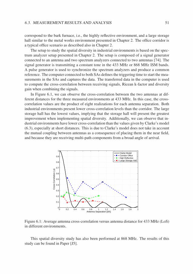
6.3. MEASUREMENT RESULTS AND ANALYSIS 51
correspond to the bark furnace, i.e., the highly reflective environment, and a large storagehall similar to the metal works environment presented in Chapter 2. The office corridor isa typical office scenario as described also in Chapter 2.
The setup to study the spatial diversity in industrial environments is based on the spec-trum analyzer setup presented in Chapter 2. The setup is composed of a signal generatorconnected to an antenna and two spectrum analyzers connected to two antennas [74]. Thesignal generator is transmitting a constant tone in the 433 MHz or 868 MHz ISM bands.A pulse generator is used to synchronize the spectrum analyzers and produce a commonreference. The computer connected to both SAs defines the triggering time to start the mea-surements in the SAs and captures the data. The transferred data in the computer is usedto compute the cross-correlation between receiving signals, Ricean k-factor and diversitygain when combining the signals.
In Figure 6.1, we can observe the cross-correlation between the two antennas at dif-ferent distances for the three measured environments at 433 MHz. In this case, the cross-correlation values are the product of eight realizations for each antenna separation. Bothindustrial environments present lower cross-correlation levels than the corridor. The largestorage hall has the lowest values, implying that the storage hall will present the greatestimprovement when implementing spatial diversity. Additionally, we can observe that in-dustrial environments have lower cross-correlation than the values given by Clarke’s model(6.3), especially at short distances. This is due to Clarke’s model does not take in accountthe mutual coupling between antennas as a consequence of placing them in the near field,and because they are receiving multi-path components from a broad angle of arrival.
0 0.2 0.4 0.6 0.8 1 1.2 1.4 1.6 1.8 20
0.1
0.2
0.3
0.4
0.5
0.6
0.7
0.8
0.9
1
Antenna Separation [d/λ]
Cro
ss-C
orre
latio
n (
ρ)
Clarke ModelCorridor OfficeHigh ReflectiveLarge Storage Hall
Figure 6.1: Average antenna cross-correlation versus antenna distance for 433 MHz (LoS)in different environments.
This spatial diversity study has also been performed at 868 MHz. The results of thisstudy can be found in Paper [J5].
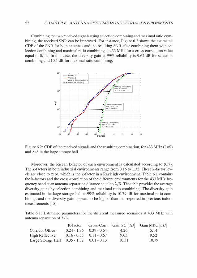
52 CHAPTER 6. ANTENNA SYSTEMS IN INDUSTRIAL ENVIRONMENTS
Combining the two received signals using selection combining and maximal ratio com-bining, the received SNR can be improved. For instance, Figure 6.2 shows the estimatedCDF of the SNR for both antennas and the resulting SNR after combining them with se-lection combining and maximal ratio combining at 433 MHz for a cross-correlation valueequal to 0.11. In this case, the diversity gain at 99% reliability is 9.62 dB for selectioncombining and 10.1 dB for maximal ratio combining.
-30 -25 -20 -15 -10 -5 0 5 10 15
10-3
10-2
10-1
100
SNR [dB]
CD
F
Antenna 1Antenna 2Maximal Ratio CombiningSelection Combining
Diversity Gain (99%)MRC = 10.1 dBSC = 9.62 dB
Diversity Gain (99.9%)MRC = 16.09 dBSC = 15.27 dB
Diversity Gain (90%)MRC = 4.96 dBSC = 4.38 dB
Figure 6.2: CDF of the received signals and the resulting combination, for 433 MHz (LoS)and λ/8 in the large storage hall.
Moreover, the Ricean k-factor of each environment is calculated according to (6.7).The k-factors in both industrial environments range from 0.16 to 1.32. These k-factor lev-els are close to zero, which is the k-factor in a Rayleigh environment. Table 6.1 containsthe k-factors and the cross-correlation of the different environments for the 433 MHz fre-quency band at an antenna separation distance equal to λ/5. The table provides the averagediversity gains by selection combining and maximal ratio combining. The diversity gainestimated in the large storage hall at 99% reliability is 10.79 dB for maximal ratio com-bining, and the diversity gain appears to be higher than that reported in previous indoormeasurements [15].
Table 6.1: Estimated parameters for the different measured scenarios at 433 MHz withantenna separation of λ/5.
K-factor Cross-Corr. Gain SC [dB] Gain MRC [dB]Corridor Office 0.24 - 1.36 0.39 - 0.64 4.26 5.14High Reflective 0.16 - 0.55 0.11 - 0.67 9.03 9.52Large Storage Hall 0.35 - 1.32 0.01 - 0.13 10.31 10.79

6.4. DISCUSSION 53
6.4 Discussion
This chapter investigated the potential benefits of using spatial diversity in wireless com-munication systems in industrial environments. As discussed in Chapter 3, industrial en-vironments generally exhibit high multi-path levels. The multi-path can be used for im-proving the SNR of the wireless system by combining the signals from two spatially sep-arated antennas. This improvement in the SNR is dependent on the antenna separation.Unfortunately, a number of industrial processes pose physical limitations to long spatialseparations. In this work, the spatial diversity in an office corridor and two industrial envi-ronments with different characteristics is studied at 433 MHz. Thus, the cross-correlation,Ricean k-factor and the diversity gain from implementing selection combining and maxi-mal ratio combining are estimated in the different environments.
The study of cross-correlation shows values lower than 0.35 in both industrial environ-ments, even at short antenna separation distances, i.e., λ/8. The Ricean k-factor follows atrend similar to the cross-correlation, presenting low values in reflective environments. Thebenefits of using spatial diversity are greater than reported in previous studies, providing adiversity gain of up to 10.31 dB for selection combining and 10.79 dB for maximal ratiocombining at λ/5. The measurement results show the possibility of setting short antennaseparation in highly reflective industrial environments.


Chapter 7
Impulsive Noise Detection and
Suppression
7.1 Introduction
Previous chapters presented a channel characterization of different industrial environmentsand studied the degradations found in such environments, namely multi-path, path loss andEMI. The objective of this chapter is to mitigate multi-path and EMI degradations. Or-thogonal frequency-division multiplexing (OFDM) is an extended technique implementedin wireless systems that can cope with the multi-path degradation present in industrial en-vironments. However, OFDM is sensitive to EMI of impulsive nature. This chapter studiesthe mitigation of EMI, improving the performance of wireless communication systems.By suppressing the source of interference, we can reduce the bit error rate (BER) andthus increase the reliability and robustness of the system. Figure 7.1 shows an example ofthe improved system performance when applying suppression techniques to the impulsivenoise. The system can significantly reduce the BER, achieving levels close to a channelaffected entirely by AWGN.
The suppression of interference depends on the ability to detect and separate the inter-ference from the desired signal. In this manner, the mitigation of the impulsive noise iscarried out in a two stage process, i.e., detection and suppression. Previous studies haveinvestigated and developed efficient solutions for signal detection [16, 17, 82]. These tech-niques provide high probabilities of detection for different impulsive noise occurrences,i.e., impulsive rates. Unfortunately, the probability of occurrence of impulsive noise de-pends on the source of interference.
Regarding the suppression, multiple research studies have implemented non-lineartechniques for suppressing impulsive noise, namely clipping, blanking or a combinationof these two techniques [18, 19, 83]. Systems implementing these techniques experiencesignificant reductions in interference degradation, although the reductions are strongly de-pendent on the threshold levels used when applying clipping and blanking to the interfer-ence. These thresholds are usually set to a fixed value; however, the strength of the signal
55
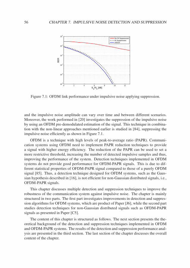
56 CHAPTER 7. IMPULSIVE NOISE DETECTION AND SUPPRESSION
0 2 4 6 8 10 1210
-5
10-4
10-3
10-2
10-1
100
Eb/N
0 [dB]
BE
R
No IN SuppressionIN SuppressionAWGN
Figure 7.1: OFDM link performance under impulsive noise applying suppression.
and the impulsive noise amplitude can vary over time and between different scenarios.Moreover, the work performed in [20] investigates the suppression of the impulsive noiseby using an OFDM pre-demodulated estimation of the signal. This technique in combina-tion with the non-linear approaches mentioned earlier is studied in [84], suppressing theimpulsive noise efficiently as shown in Figure 7.1.
OFDM is a technique with high levels of peak-to-average ratio (PAPR). Communi-cation systems using OFDM need to implement PAPR reduction techniques to providea signal with higher energy efficiency. The reduction of the PAPR can be used to set amore restrictive threshold, increasing the number of detected impulsive samples and thus,improving the performance of the system. Detection techniques implemented in OFDMsystems do not provide good performance for OFDM-PAPR signals. This is due to dif-ferent statistical properties of OFDM-PAPR signal compared to those of a purely OFDMsignal [85]. Thus, a detection technique designed for OFDM systems, such as the Gaus-sian hypothesis described in [16], is not efficient for non-Gaussian distributed signals, i.e.,OFDM-PAPR signals.
This chapter discusses multiple detection and suppression techniques to improve therobustness of the communication system against impulsive noise. The chapter is mainlystructured in two parts. The first part investigates improvements in detection and suppres-sion algorithms for OFDM systems, which are product of Paper [J6], while the second partstudies detection techniques for non-Gaussian distributed signals such as OFDM-PAPRsignals as presented in Paper [C5].
The content of this chapter is structured as follows. The next section presents the the-oretical background of the detection and suppression techniques implemented in OFDMand OFDM-PAPR systems. The results of the detection and suppression performance anal-ysis are presented in the third section. The last section of the chapter discusses the overallcontent of the chapter.

7.2. OFDM SYSTEMS IN ENVIRONMENTS WITH IMPULSIVE NOISE 57
7.2 OFDM Systems in Environments with Impulsive Noise
This section contains the theoretical background of the different detection and suppressiontechniques implemented in the thesis.
The channel produces different degradations in the transmitted signal, namely, multi-path, path loss and impulsive interference, as we have shown in previous chapters. Thereceived signal under these degradations can be expressed as
r(t) =
P −1∑
l=0
hls (t − τl) + w(t) + i(t) (7.1)
where hl and τl are the complex-Gaussian channel coefficient and the delay of path l,respectively, w(t) is the AWGN process, i(t) is the impulsive noise defined in Chapter 5 asa composition of impulses with high amplitude in time domain and s(t) is the transmittedsignal. In this case, we use a robust technique to cope with the multi-path fading, i.e.,OFDM, testing the effect of impulsive noise in the transmitted signal. The equivalentlowpass of the transmitted signal is formulated as
sl(t) =
K−1∑
k=0
Sn,kej2π k
Tqt, (n − 1)Tq ≤ t < n · Tq (7.2)
where K is the number of subcarriers, Sn,k is the data symbol transmitted in subcarrierk during the nth symbol interval, Tq = (TG + Tu) is the symbol period being 1/Tu thefrequency separation between two neighboring subcarriers, and TG the guard time interval.
After sampling the received signal at the sample rate 1/Ts = M/Tu we obtain
rn,m = r(nTu + mTs), m = 0, 1, · · · , M − 1
=
P −1∑
l=0
hls (nTu + mTs − τl) + wn,m + in,m (7.3)
where M is the oversampling rate, wn,m is the AWGN sample and in,m is the impulsivenoise sample.
Considering an OFDM system with a cyclic prefix longer that the maximum delayspread of the channel, the received signal sample at subcarrier k during the nth symbolinterval can be written as follows
Rn,k = Hn,kSn,k + Wn,k + In,k, k = 0, 1, · · · , K − 1 (7.4)
PAPR Reduction
OFDM signals have high PAPR levels. To increase the efficiency of the communicationsystem a reduction of the PAPR needs to be applied. Many techniques have been proposedfor reducing the PAPR in OFDM systems, such as coding [86], amplitude clipping [87],pulse shaping [88, 89], partial transmit sequence (PTS) [90] and selected mapping (SLM)

58 CHAPTER 7. IMPULSIVE NOISE DETECTION AND SUPPRESSION
[91]. In papers [92, 93], comparison and overviews between the different techniques arepresented. This thesis implements selected mapping for reducing the PAPR of OFDMsystems presented in Paper [C5].
The OFDM signal described previously forms OFDM symbols following
X = [X0, X1, ..., XK−1]T (7.5)
where [.]T denotes the transpose and K is the number of subcarriers of the OFDM symbolmodulated with M-QAM.
The SLM technique creates a number of sequences, V , with uniformly distributed ran-dom phases between 0 and 2π [94]. These phase sequences are multiplied by the OFDMvector, (7.5), conforming a matrix with V different versions of the OFDM vector
Xv = Xφ =
X0φ0,0 · · · X0φ0,V −1
X1φ1,0 · · · X1φ1,V −1
.... . .
...XK−1φK−1,0 · · · XK−1φK−1,V −1
(7.6)
This matrix contains V OFDM vectors having V PAPR. The PAPR of each versioncreated by the SLM technique is calculated as
PAPR =max{| xv(t) |2}
E{| xv(t) |2} (7.7)
Thus, the version of the OFDM symbol with the minimum PAPR is subsequently se-lected for transmission
X = Xφ (7.8)
The reduction of the PAPR when using the SLM technique was investigated by Bäuml[94]. This work defines the probability that the PAPR is higher than a certain level,PAPR0, as
P r {PAPR > PAPR0} =(
1 −(
1 − e−PAPR0)K
)V
(7.9)
7.2.1 Impulsive Noise Detection
The identification of impulsive noise in the received signal is performed by using a com-bination of detecting techniques, as proposed in Paper [J6]. First, the Fisher’s quadraticdiscriminator [95] is implemented to obtain part of the impulsive samples with a high im-pulsive rate. Second, the detected impulsive samples are blanked and finally, the Gaussianhypothesis estimation [16] is used to detect the impulsive samples with a lower impulsiverate. The combination of these detecting techniques, i.e., the Max detector, increases theprobability of detection for a wide range of impulsive rates.
The block diagram of the combined detector is shown in Figure 7.2. The combinationis constructed as follows: First, the received signal is inserted into Fisher’s block, providing
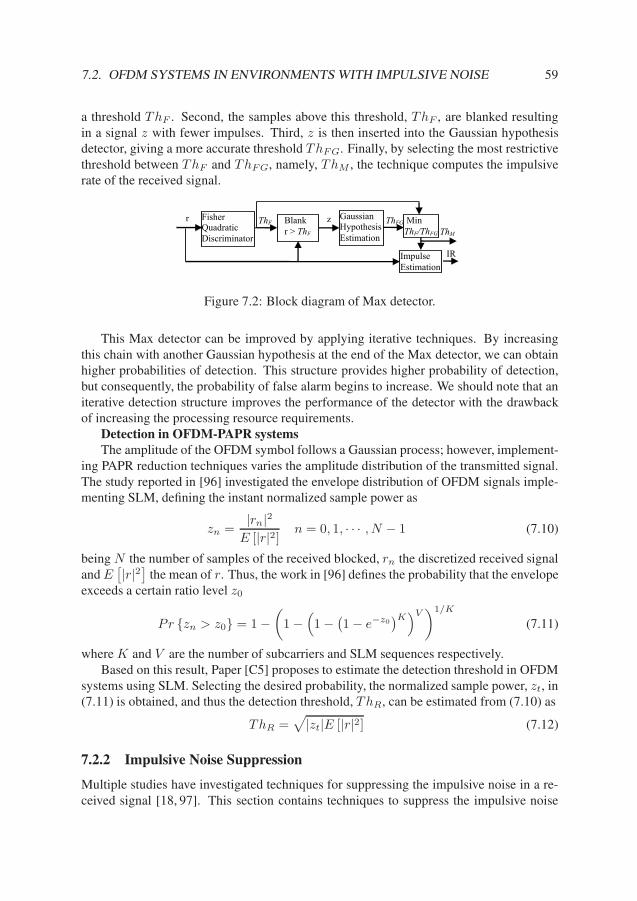
7.2. OFDM SYSTEMS IN ENVIRONMENTS WITH IMPULSIVE NOISE 59
a threshold T hF . Second, the samples above this threshold, T hF , are blanked resultingin a signal z with fewer impulses. Third, z is then inserted into the Gaussian hypothesisdetector, giving a more accurate threshold T hF G. Finally, by selecting the most restrictivethreshold between T hF and T hF G, namely, T hM , the technique computes the impulsiverate of the received signal.
ThM
z
IR
ThF ThFG r Fisher Quadratic
Discriminator
Gaussian
Hypothesis
Estimation
Impulse
Estimation
Blank
r > ThF
Min
ThF/ThFG
Figure 7.2: Block diagram of Max detector.
This Max detector can be improved by applying iterative techniques. By increasingthis chain with another Gaussian hypothesis at the end of the Max detector, we can obtainhigher probabilities of detection. This structure provides higher probability of detection,but consequently, the probability of false alarm begins to increase. We should note that aniterative detection structure improves the performance of the detector with the drawbackof increasing the processing resource requirements.
Detection in OFDM-PAPR systems
The amplitude of the OFDM symbol follows a Gaussian process; however, implement-ing PAPR reduction techniques varies the amplitude distribution of the transmitted signal.The study reported in [96] investigated the envelope distribution of OFDM signals imple-menting SLM, defining the instant normalized sample power as
zn =|rn|2
E [|r|2]n = 0, 1, · · · , N − 1 (7.10)
being N the number of samples of the received blocked, rn the discretized received signaland E
[
|r|2]
the mean of r. Thus, the work in [96] defines the probability that the envelopeexceeds a certain ratio level z0
P r {zn > z0} = 1 −(
1 −(
1 −(
1 − e−z0)K
)V)1/K
(7.11)
where K and V are the number of subcarriers and SLM sequences respectively.Based on this result, Paper [C5] proposes to estimate the detection threshold in OFDM
systems using SLM. Selecting the desired probability, the normalized sample power, zt, in(7.11) is obtained, and thus the detection threshold, T hR, can be estimated from (7.10) as
T hR =√
|zt|E [|r|2] (7.12)
7.2.2 Impulsive Noise Suppression
Multiple studies have investigated techniques for suppressing the impulsive noise in a re-ceived signal [18, 97]. This section contains techniques to suppress the impulsive noise

60 CHAPTER 7. IMPULSIVE NOISE DETECTION AND SUPPRESSION
implemented in Papers [J6] and [C5]. The techniques implemented in these papers and de-scribed in this thesis are blanking, clipping-blanking non-linearity and suppression basedon a pre-demodulated OFDM signal.
Non-linear Impulsive Suppression Technique
Clipping, blanking and clipping-blanking combination are among the non-linear tech-niques used to mitigate the impulsive noise. The following points describe blanking andclipping-blanking combination.
• Impulsive Noise Blanking
Blanking is an efficient technique used to suppress the impulsive noise [98]. Thistechnique is commonly used in many studies due to its low implementation cost. Blankingimpulsive noise samples consists of setting to zero the samples that are above a certainthreshold
yn,m =
{
rn,m |rn,m| ≤ T hB
0 otherwise(7.13)
where T hB is the blanking threshold provided by the detection stage.
• Impulsive Noise Clipping-Blanking Combination
Previous studies have investigated the performance of clipping-blanking combinationwith respect to simply blanking or clipping the impulsive noise sample [97]. This studyshows that combining clipping and blanking provides better performance than a singleclipping or blanking. Clipping-blanking technique cuts or sets to zero the impulsive noisesamples following the estimated thresholds. The signal after clipping-blanking can bedefined as
yn,m =
rn,m |rn,m| < T hC
T hC ej arg(rn,m) T hC < |rn,m| < T hB
0 |rn,m| > T hB
(7.14)
where T hC and T hB are the estimated thresholds for clipping and blanking, respectively.OFDM Pre-demodulated Suppression
A suppression technique that uses the pre-demodulated OFDM signal in combinationwith non-linear impulsive noise suppression techniques to improve the performance ofan OFDM system is studied in [20] . This technique is applied after partially reducingthe impulsive noise with a non-linear block. The signal after the non-linear block is pre-demodulated, subtracting additional impulsive samples before the final demodulation. Inthis section, we propose to use the previously described Max detector to improve the per-formance of the suppression technique. The block diagram of the entire impulsive noisesuppression process is illustrated in Figure 7.3 and is divided into two steps. The first stepcorresponds to the non-linear impulsive noise suppression and the second to the OFDMpre-demodulated suppression. The algorithm for suppressing the impulsive noise of Step2 can be found in Paper [J6].

7.3. MEASUREMENT RESULTS AND ANALYSIS 61
Figure 7.3: Block diagram of the impulsive noise suppression algorithm.
7.3 Measurement Results and Analysis
This section presents the simulation and measurement results of the detection and suppres-sion techniques. The section is divided into two parts. The first part discusses the perfor-mance of the different detection and suppression techniques in OFDM systems product ofPaper [J6]. The second part presents the performance of the detection techniques for anOFDM system using SLM technique to reduce the signal PAPR. The second part is basedon the content of Paper [C5].
7.3.1 Detection and Suppression in OFDM Systems
Paper [J6] proposes an OFDM receiver structure for detecting and suppressing the im-pulsive noise. Figure 7.4 presents the proposed flow chart of the receiver. The receiveris composed of a detection and suppression blocks. The detection block corresponds tothe Max detector described previously, and the suppression block corresponds to the com-bination of clipping-blanking and the OFDM pre-demodulated estimation. The OFDMreceiver inserts the signal into the detection block and if the impulsive rate, IR, is higherthan the desired level, β, the signal passes to the suppressing block. In the absence of im-pulsive noise, the signal is demodulated by a common OFDM receiver without expendingresources in the suppressing block.
The objective of a detection block consists of estimating a threshold to distinguish sig-nal samples from impulsive samples. To compare the performance of the different detec-tors, we define the optimum threshold as the threshold that provides the highest probabilityof detection for the minimum probability of false alarm. This corresponds to the maximumlevel of signal after passing through an AWGN channel
T hO = max{|sn,m + wn,m|}, n = 0, 1, · · · , N − 1 (7.15)
being N the number samples.The estimated thresholds from the different techniques are shown in Figure 7.5 (left)
where the signal envelope and the impulsive noise are also shown. The Max detector and

62 CHAPTER 7. IMPULSIVE NOISE DETECTION AND SUPPRESSION
Th
Suppression
Max Detector
Fisher Quadratic
Discriminant
Gaussian
Hypothesis
Estimation
1
Clipping
Blanking
Pre-demodulated
Estimation
2
Corrected Received Signal
Received Signal
No IR > β
Yes
Figure 7.4: Flow chart diagram for the proposed receiver structure.
the iterative Max detector provide thresholds close to the optimum. Fisher’s quadraticdiscriminator and Gaussian hypothesis estimate thresholds above the optimal and conse-quently misclassify impulsive samples. The performance of the detection techniques isillustrated in Figure 7.5 (right). The Gaussian hypothesis provides higher probability ofdetection than the Fisher’s quadratic discriminator for impulses rates lower than 0.1. Bycombining the Fisher’s quadratic discriminator and Gaussian hypothesis, i.e., the Max de-tector, an improved detector is obtained with equal or higher probability of detection com-pared to each of them separately. Observe in Figure 7.5 (right) for an impulsive rate equalto IR = 0.3, where the Max detector has 20% higher probability of detection than Fisher’squadratic discriminator and 55% higher than the Gaussian hypothesis estimation.
The OFDM receiving structure is evaluated in the laboratory environment describedin Chapter 2. To evaluate the system performance, a test bed emulating a communicationsystem with an interference source degrading the system is designed. The test bed is basedon the spectrum analyzer setup presented in Chapter 2. The test bed contains two signalgenerators and a signal analyzer connected to a PC. The PC uploads the OFDM signalto one signal generator and the impulsive noise to the second signal generator. Duringreception, the signal analyzer captures the interfered signal and transfers it to the PC.
Figure 7.6 shows the measurement results of the combination of the detecting andsuppressing techniques when impulsive noise is present in the environment. The statisticalproperties of the impulsive noise transmitted by the second signal generator are Γ = 47.7and IR = 3.17 × 10⁻². The BER decreases by more than two decades for energy per bitto noise ratio i.e., Eb/N0, levels higher than 10 dB.

7.3. MEASUREMENT RESULTS AND ANALYSIS 63
0 50 100 150 200 250 300 350 400 450 5000
0.5
1
1.5
2
2.5
3
3.5
4
Samples
Env
elop
e
ImpulsesSignal+AWGNOptimalMax ThresholdIterative Max ThresholdFisher ThresholdGaussian Hypothesis
0 0.05 0.1 0.15 0.2 0.25 0.3 0.35 0.4 0.45 0.50
0.1
0.2
0.3
0.4
0.5
0.6
0.7
0.8
0.9
1
Impulsive Rate
Pro
b D
etec
tion
Iterative Max DetectorMax DetectorFisher QuadraticGaussian Hypothesis
Figure 7.5: Signal, impulsive noise and thresholds performance at IR = 0.1 (left) andprobability of detection versus impulsive rate for different detectors (right).
0 2 4 6 8 10 1210
-5
10-4
10-3
10-2
10-1
100
Eb/N
0 [dB]
BE
R
Signal + AWGN
Corrected (rnmc )
No Corrected (rnm
)
Figure 7.6: BER versus Eb/N0 for measurements.
Furthermore, OFDM systems are often deployed in Rayleigh fading environments.Thus, this thesis studies the performance of an OFDM system interfered by an impulsivenoise in a Rayleigh channel. To study the OFDM performance, an OFDM system interferedby impulsive noise with statistical properties equal to Γ = 47.7 and IR = 3 × 10⁻³, andwith a Rayleigh channel composed of 10 complex-Gaussian taps, is simulated. Figure 7.7(left) shows the performance of the system when the received signal is not corrected, rn,m,when the signal is corrected after blanking non-linearity, yn,m, and when applying theOFDM pre-demodulated suppression, rc
n,m. The performance of the BER of the correctedsignal, rc
n,m, improves by more than two decades at Eb/N0 > 30 dB with respect to thenot corrected signal.
The degradation caused by the Rayleigh channel can be mitigated by applying diversitytechniques to the system. Frequency diversity is a technique for reducing multi-path fad-ing in frequency selective channels [99]. By transmitting a single data symbol in L OFDM
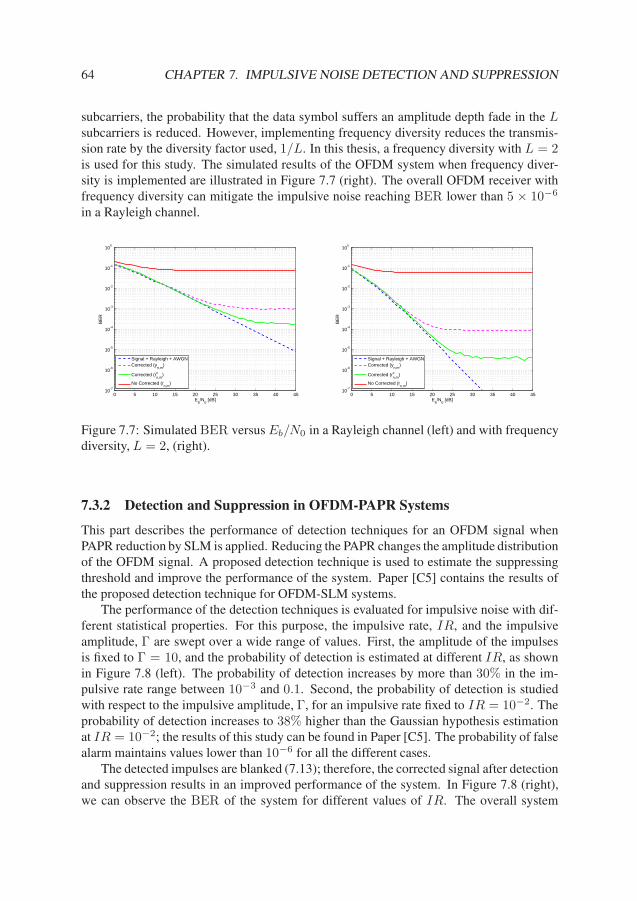
64 CHAPTER 7. IMPULSIVE NOISE DETECTION AND SUPPRESSION
subcarriers, the probability that the data symbol suffers an amplitude depth fade in the Lsubcarriers is reduced. However, implementing frequency diversity reduces the transmis-sion rate by the diversity factor used, 1/L. In this thesis, a frequency diversity with L = 2is used for this study. The simulated results of the OFDM system when frequency diver-sity is implemented are illustrated in Figure 7.7 (right). The overall OFDM receiver withfrequency diversity can mitigate the impulsive noise reaching BER lower than 5 × 10⁻⁶
in a Rayleigh channel.
0 5 10 15 20 25 30 35 40 4510
-7
10-6
10-5
10-4
10-3
10-2
10-1
100
Eb/N
0 [dB]
BE
R
Signal + Rayleigh + AWGNCorrected (y
n,m)
Corrected (rn,mc )
No Corrected (rn,m
)
0 5 10 15 20 25 30 35 40 4510
-7
10-6
10-5
10-4
10-3
10-2
10-1
100
Eb/N
0 [dB]
BE
R
Signal + Rayleigh + AWGNCorrected (y
n,m)
Corrected (rn,mc )
No Corrected (rn,m
)
Figure 7.7: Simulated BER versus Eb/N0 in a Rayleigh channel (left) and with frequencydiversity, L = 2, (right).
7.3.2 Detection and Suppression in OFDM-PAPR Systems
This part describes the performance of detection techniques for an OFDM signal whenPAPR reduction by SLM is applied. Reducing the PAPR changes the amplitude distributionof the OFDM signal. A proposed detection technique is used to estimate the suppressingthreshold and improve the performance of the system. Paper [C5] contains the results ofthe proposed detection technique for OFDM-SLM systems.
The performance of the detection techniques is evaluated for impulsive noise with dif-ferent statistical properties. For this purpose, the impulsive rate, IR, and the impulsiveamplitude, Γ are swept over a wide range of values. First, the amplitude of the impulsesis fixed to Γ = 10, and the probability of detection is estimated at different IR, as shownin Figure 7.8 (left). The probability of detection increases by more than 30% in the im-pulsive rate range between 10−3 and 0.1. Second, the probability of detection is studiedwith respect to the impulsive amplitude, Γ, for an impulsive rate fixed to IR = 10−2. Theprobability of detection increases to 38% higher than the Gaussian hypothesis estimationat IR = 10−2; the results of this study can be found in Paper [C5]. The probability of falsealarm maintains values lower than 10−6 for all the different cases.
The detected impulses are blanked (7.13); therefore, the corrected signal after detectionand suppression results in an improved performance of the system. In Figure 7.8 (right),we can observe the BER of the system for different values of IR. The overall system
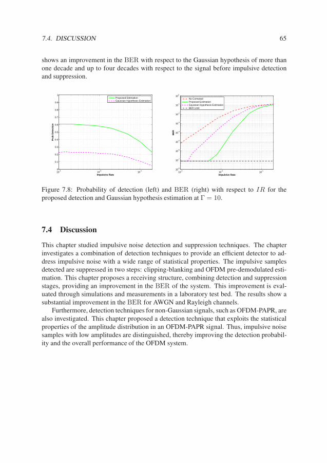
7.4. DISCUSSION 65
shows an improvement in the BER with respect to the Gaussian hypothesis of more thanone decade and up to four decades with respect to the signal before impulsive detectionand suppression.
10-3
10-2
10-1
0
0.1
0.2
0.3
0.4
0.5
0.6
0.7
0.8
0.9
1
Impulsive Rate
Pro
b D
etec
tio
n
Proposed EstimationGaussian Hypothesis Estimation
10-3
10-2
10-1
10-8
10-7
10-6
10-5
10-4
10-3
10-2
10-1
100
Impulsive RateB
ER
No CorrectedProposed EstimationGaussian Hypothesis EstimationBER Limit
Figure 7.8: Probability of detection (left) and BER (right) with respect to IR for theproposed detection and Gaussian hypothesis estimation at Γ = 10.
7.4 Discussion
This chapter studied impulsive noise detection and suppression techniques. The chapterinvestigates a combination of detection techniques to provide an efficient detector to ad-dress impulsive noise with a wide range of statistical properties. The impulsive samplesdetected are suppressed in two steps: clipping-blanking and OFDM pre-demodulated esti-mation. This chapter proposes a receiving structure, combining detection and suppressionstages, providing an improvement in the BER of the system. This improvement is eval-uated through simulations and measurements in a laboratory test bed. The results show asubstantial improvement in the BER for AWGN and Rayleigh channels.
Furthermore, detection techniques for non-Gaussian signals, such as OFDM-PAPR, arealso investigated. This chapter proposed a detection technique that exploits the statisticalproperties of the amplitude distribution in an OFDM-PAPR signal. Thus, impulsive noisesamples with low amplitudes are distinguished, thereby improving the detection probabil-ity and the overall performance of the OFDM system.


Chapter 8
Conclusions
8.1 Concluding Remarks
The deployment of wireless communications in industrial environments has grown rapidlyin recent years, and this trend is expected to continue. The low cost and scalability ofwireless systems provide excellent benefits for the industrial sector. However, part of theindustrial sector refuses to deploy wireless solutions, questioning the reliability of thesesolutions. Multiple sources of degradation can arise, reducing the performance of thecommunication system and its reliability. This thesis analyzed a wide range of industrialenvironments, characterizing the sources of degradation and suggesting improvements tocombat the degradations that these environments introduce into wireless systems.
Industrial environments are generally classified as environments with large dimensionscontaining multiple metallic objects and high levels of EMI. This general description ofindustrial environments is valid for a large percentage of environments. However, certainindustrial environments exhibit different structural characteristics, behaving on some oc-casions in an opposite manner. A characterization of diverse industrial environments isnecessary to identify the sources of degradation and increase the reliability of the wirelesssystems.
Chapter 2 presented a broad variety of industrial environments with different prop-agation characteristics. These industrial environments were characterized in Chapters 3through 5, identifying the main sources of degradation. To characterize the channel, dif-ferent measurements setups have been developed, estimating the time dispersion, path lossand EMI characteristics of the environments. Chapter 3 discussed the time dispersion ofthe environments, distinguishing between industrial environments with high and low delayspreads. Low delay spread industrial environments have not been identified in the liter-ature review. This finding increases the understanding of special industrial environmentsand provides valuable information for system developers. Chapter 4 presented a path losscharacterization in different industrial environments. This characterization finds a strongerfrequency dependence of the path loss in NLoS scenarios than that reported in previousworks. In Chapter 5, a number of EMI sources captured in industry are reported. The
67
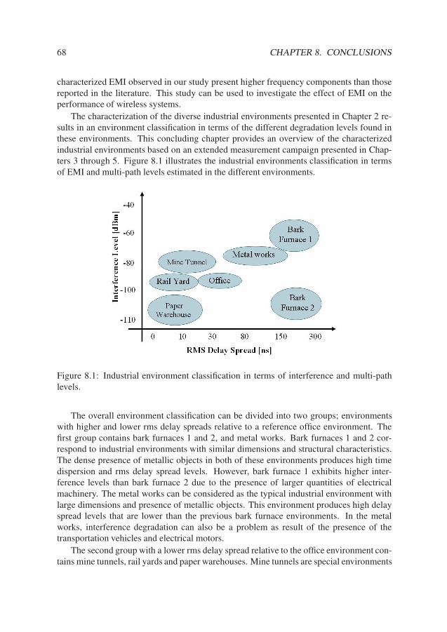
68 CHAPTER 8. CONCLUSIONS
characterized EMI observed in our study present higher frequency components than thosereported in the literature. This study can be used to investigate the effect of EMI on theperformance of wireless systems.
The characterization of the diverse industrial environments presented in Chapter 2 re-sults in an environment classification in terms of the different degradation levels found inthese environments. This concluding chapter provides an overview of the characterizedindustrial environments based on an extended measurement campaign presented in Chap-ters 3 through 5. Figure 8.1 illustrates the industrial environments classification in termsof EMI and multi-path levels estimated in the different environments.
Figure 8.1: Industrial environment classification in terms of interference and multi-pathlevels.
The overall environment classification can be divided into two groups; environmentswith higher and lower rms delay spreads relative to a reference office environment. Thefirst group contains bark furnaces 1 and 2, and metal works. Bark furnaces 1 and 2 cor-respond to industrial environments with similar dimensions and structural characteristics.The dense presence of metallic objects in both of these environments produces high timedispersion and rms delay spread levels. However, bark furnace 1 exhibits higher inter-ference levels than bark furnace 2 due to the presence of larger quantities of electricalmachinery. The metal works can be considered as the typical industrial environment withlarge dimensions and presence of metallic objects. This environment produces high delayspread levels that are lower than the previous bark furnace environments. In the metalworks, interference degradation can also be a problem as result of the presence of thetransportation vehicles and electrical motors.
The second group with a lower rms delay spread relative to the office environment con-tains mine tunnels, rail yards and paper warehouses. Mine tunnels are special environments
8.1. CONCLUDING REMARKS 69
with low rms delay spread levels due to the particular characteristics of the tunnel structure.Trains loading and releasing raw material can produce EMI over a wide frequency band.Rail yards are outdoor environments with large dimensions and a large number of trainsand electric pantographs. These elements are sources of EMI for the wireless communica-tions. The paper warehouse has larger dimensions than bark furnaces 1 and 2, containingpiled rolls of paper. These paper rolls absorb the signals, mitigating the strength of pos-sible EMI. However, at the same time, the paper rolls absorb the multi-path components,producing a radio coverage problem in NLoS situations due to the significant path lossfading levels. This radio coverage problem eliminates the possibility of using systemsthat take advantage of multi-path propagation effects. A path loss characterization in thepaper warehouse shows a strong frequency dependence that could be related to the dielec-tric properties of the paper. To provide a reference environment, an office environmentwas characterized and illustrated among this industrial environment classification. Officeenvironments exhibit multi-path and interference levels that correspond to typical indoorenvironments, such as houses and buildings.
By charactering the different sources of degradation in industrial environments, weacquire additional knowledge on how to design and select wireless technologies with thegreatest reliability and robustness. Furthermore, increasing the knowledge of the degrada-tion sources in an industrial environment can decrease the risk of incidents, where person-nel and material can be harmed.
Following the industrial environment characterization, this thesis studied spatial diver-sity and impulsive noise mitigation techniques for improving the performance of industrialwireless systems.
Spatial diversity is often used to reduce the multi-path fading characteristics of a chan-nel. Significant gain can be achieved by using multiple antennas at the transmitter/receiversites when separating the antennas by a certain distance. Unfortunately, some industrialprocesses present physical restrictions that make large antenna separations impossible.In Chapter 6, we presented measurements characterizing the cross-correlation, Ricean k-factor and diversity gain with respect to the antenna separation distance. Environmentswith significant time dispersion can potentially be used for implementing spatial diversitytechniques. Chapter 6 shows that industrial environments with high delay spread proper-ties can set a separation distance shorter than λ/5. At such distances, the wireless systemscan achieve diversity gains up to 10.79 dB, increasing the reliability of the communicationsystem.
Regarding the impulsive noise mitigation, multiple techniques for detecting and sup-pressing impulsive noise have been reported in previous works. However, existing impul-sive noise detectors performance is highly dependent on the statistical properties of thetransmitted signal and impulsive noise. This thesis proposes an OFDM receiving structurethat combines detection and suppression techniques for mitigating impulsive noise withdifferent statistical properties. The receiving structure is tested in AWGN and multi-pathfading channels, showing an important improvement in the performance of the system.Furthermore, the thesis also presents detection techniques in scenarios where the transmit-ted signal is non-Gaussian distributed, i.e., OFDM-PAPR.
The overall contribution of this thesis can be summarized as follows. This thesis is
70 CHAPTER 8. CONCLUSIONS
a novel work, characterizing industrial environments with diverse structural properties byidentifying the main sources of degradation in each environment. The thesis is novel workinvestigating the benefits of applying spatial diversity at short antenna separations in highdelay spread industrial environments. The thesis is a novel work studying high perfor-mance impulsive noise detection and suppression techniques in OFDM systems under im-pulsive noise with different statistical properties. The results of this thesis could be usedby the industrial sector to implement safer and more reliable wireless solutions in a diversevariety of industrial environments.
8.2 Future Directions
This section discusses possible directions for future work. This thesis characterized thepropagation characteristics in diverse industrial environments at different frequency bands.However, the development of wireless systems at frequencies higher than 3 GHz producesa need for characterizing the analyzed industrial environments at a wider frequency range.Moreover, the time for performing the measurements campaigns in some industrial en-vironments was restricted due to the ongoing industrial activities. It might therefore beinteresting to perform new measurement campaigns at higher frequency bands and usinggreater number of measurement points and positions in the analyzed environments.
As the last section reported, the particular properties of the studied industrial environ-ments provide different sources of degradation to the wireless system. It might be inter-esting to extend the characterization of the channel by performing measurements in envi-ronments with different characteristics and sources of degradations. A potential directionfor continuing the work performed in this thesis could be to characterize other environ-ments, such as nuclear plants, electricity substations, hospitals, storage halls such as thosein Ikea and subway tunnels. These environments require high reliability levels in theircommunications and have special properties that can degrade the wireless performance.
This thesis characterized and modeled multi-path propagation in different industrialenvironments. However, it might be interesting to formulate a multi-path model that canpredict the statistical impulsive response of the channel. This model could be dependenton the structural dimensions of the building, elements present in the environments and thedielectric properties of the building and elements. A prediction of the multi-path behaviorcould therefore direct the selection of a reliable wireless system for a specific environment.
In Chapter 4, the path loss characterization of the paper warehouse showed a strong fre-quency dependence at certain frequency bands. A deeper study of the dielectric propertiesof the paper might be an interesting continuation for clarifying this frequency dependencein NLoS scenarios.
The performance of a detection technique is dependent on the statistical properties ofthe signal. Thus, another topic of certain interest might be the study of the performance ofthe detection and suppression techniques proposed in this thesis on other types of signals,such as spread spectrum signals, for instance, in code division multiple access (CDMA).
Bibliography
[1] Ericsson AB, “Ericsson mobility report - on the pulse of the networked society,”White Paper, Nov. 2013.
[2] Cisco, “Cisco visual networking index: Global mobile data traffic forecast update,2013 - 2018,” White Paper, Feb. 2014.
[3] R. Thusu, “Wireless sensor use is expanding in industrial applications,” Frost & Sul-livan Sensors, Jun. 2010.
[4] R. Primerano, K. Wanuga, J. Dorn, M. Kam, and K. Dandekar, “Echo-cancellationfor ultrasonic data transmission through a metal channel,” in Annual Conference on
Information Sciences and Systems, 2007, pp. 841–845.
[5] K. A. Remley, G. Koepke, C. Grosvenor, R. Johnk, J. Ladbury, D. Camell, andJ. Coder, “NIST tests of the wireless environment in automobile manufacturing facil-ities,” Natl. Inst. Stand. Technol. Note 1550, Oct. 2008.
[6] X. Wang, Y. Ren, J. Zhao, Z. Guo, and R. Yao, “Comparison of ieee 802.11e andieee 802.15.3 mac,” in Proceedings of the IEEE 6th Circuits and Systems Symposium
on Emerging Technologies: Frontiers of Mobile and Wireless Communication, vol. 2,May 2004, pp. 675 – 680.
[7] P. Radmand, A. Talevski, S. Petersen, and S. Carlsen, “Comparison of industrial wsnstandards,” in IEEE International Conference on Digital Ecosystems and Technolo-
gies, Apr. 2010, pp. 632 –637.
[8] J. Karedal, S. Wyne, P. Almers, F. Tufvesson, and A. Molisch, “UWB channel mea-surements in an industrial environment,” in IEEE Global Telecommunications Con-
ference, vol. 6, Nov. 2004, pp. 3511 – 3516.
[9] S. Kjesbu and T. Brunsvik, “Radiowave propagation in industrial environments,” inIEEE Annual Conference of Industrial Electronics Society (IECON), vol. 4, 2000, pp.2425–2430.
[10] E. Tanghe, W. Joseph, L. Verloock, L. Martens, H. Capoen, K. Van Herwegen, andW. Vantomme, “The industrial indoor channel: large-scale and temporal fading at
71
72 BIBLIOGRAPHY
900, 2400, and 5200 mhz,” IEEE Trans. on Wireless Communications, vol. 7, no. 7,pp. 2740–2751, 2008.
[11] H. A. Myers, “Industrial equipment spectrum signatures,” IEEE Trans. on Radio Fre-
quency Interference, vol. 5, no. 1, pp. 30–42, 1963.
[12] E. N. Skomal, “Comparative radio noise levels of transmission lines, automotive traf-fic, and rf stabilized arc welders,” IEEE Trans. on Electromagnetic Compatibility,vol. 9, no. 2, pp. 73–77, 1967.
[13] S. Diggavi, “On achievable performance of spatial diversity fading channels,” IEEE
Trans. on Information Theory, vol. 47, no. 1, pp. 308 –325, Jan 2001.
[14] P. Shamain and L. Milstein, “Detection with spatial diversity using noisy channelestimates in a correlated fading channel,” in Proceedings MILCOM, vol. 1, Oct. 2002,pp. 691 – 696.
[15] J. Dietrich, C.B., K. Dietze, J. Nealy, and W. Stutzman, “Spatial, polarization, andpattern diversity for wireless handheld terminals,” IEEE Trans. on Antennas and
Propagation, vol. 49, no. 9, pp. 1271–1281, 2001.
[16] P. Torio and M. G. Sanchez, “Improving capability of detecting impulsive noise,”IEEE Trans. on Electromagnetic Compatibility, vol. PP, no. 99, pp. 1 –8, Jul. 2012.
[17] T. Oliveira, P. Correia de Sa and, S. de Paula Barbosa, M. Ribeiro, and C. Mar-ques, “Hos-based impulsive noise detection technique for power line communicationsystems,” in IEEE International Symposium on Power Line Communications and Its
Applications, Mar. 2010, pp. 125 –130.
[18] T. Hirakawa, M. Fujii, M. Itami, and K. Itoh, “A study on iterative impulse noisereduction in ofdm signal by recovering time domain samples,” in IEEE International
Symposium on Power Line Communications and Its Applications, 2006, pp. 325 –330.
[19] R. Fantacci, A. Tani, and D. Tarchi, “Impulse noise mitigation techniques for xdslsystems in a real environment,” IEEE Trans. on Consumer Electronics, vol. 56, no. 4,pp. 2106 –2114, Nov. 2010.
[20] S. Zhidkov, “Impulsive noise suppression in ofdm-based communication systems,”IEEE Trans. on Consumer Electronics, vol. 49, no. 4, pp. 944 – 948, Nov. 2003.
[21] J. Karedal, S. Wyne, P. Almers, F. Tufvesson, and A. Molisch, “A measurement-basedstatistical model for industrial ultra-wideband channels,” IEEE Trans. on Wireless
Communications, vol. 6, no. 8, pp. 3028–3037, Aug. 2007.
[22] O. Staub, J.-F. Zurcher, P. Morel, and A. Croisier, “Indoor propagation and electro-magnetic pollution in an industrial plant,” in International Conference on Industrial
Electronics, Control and Instrumentation, vol. 3, 1997, pp. 1198–1203.
BIBLIOGRAPHY 73
[23] E. Tanghe, W. Joseph, L. Martens, H. Capoen, K. Van Herwegen, and W. Van-tomme, “Large-scale fading in industrial environments at wireless communicationfrequencies,” in Antennas and Propagation Society International Symposium, 2007,pp. 3001–3004.
[24] T. S. Rappaport, “Wireless communications: Principles and practice,” 2008.
[25] J. Kivinen, X. Zhao, and P. Vainikainen, “Empirical characterization of widebandindoor radio channel at 5.3 ghz,” IEEE Trans. on Antennas and Propagation, vol. 49,no. 8, pp. 1192–1203, 2001.
[26] S. Ghassemzadeh, L. Greenstein, T. Sveinsson, A. Kavcic, and V. Tarokh, “Uwb de-lay profile models for residential and commercial indoor environments,” IEEE Trans.
on Vehicular Technology, vol. 54, no. 4, pp. 1235–1244, 2005.
[27] R. He, Z. Zhong, B. Ai, K. Guan, B. Chen, J. Aionso, and C. Briso, “Propagationchannel measurements and analysis at 2.4 ghz in subway tunnels,” IET Microwaves,
Antennas Propagation, vol. 7, no. 11, pp. 934–941, 2013.
[28] C. Nerguizian, C. Despins, S. Affes, and M. Djadel, “Radio-channel characterizationof an underground mine at 2.4 ghz,” IEEE Trans. on Wireless Communications, vol. 4,no. 5, pp. 2441–2453, 2005.
[29] I. Mabrouk, L. Talbi, M. Nedil, Y. Coulibaly, and T. Denidni, “Effect of antenna di-rectivity on performance of multiple input multiple output systems in an undergroundgold mine,” IET Microwaves, Antennas Propagation, vol. 6, no. 5, pp. 555–561, 2012.
[30] M. Varela and M. Sanchez, “RMS delay and coherence bandwidth measurementsin indoor radio channels in the UHF band,” IEEE Trans. on Vehicular Technology,vol. 50, no. 2, pp. 515 –525, Mar. 2001.
[31] H. Anderson and J. McGeehan, “Direct calculation of coherence bandwidth in urbanmicrocells using a ray-tracing propagation model,” in IEEE International Symposium
on Personal, Indoor and Mobile Radio Communications, vol. 1, Sep. 1994, pp. 20–24.
[32] M. Sanchez, A. Hammoudeh, E. Grindrod, and J. Kermoal, “Coherence bandwidthcharacterization in an urban microcell at 62.4 ghz,” IEEE Trans. on Vehicular Tech-
nology, vol. 49, no. 2, pp. 607–613, Mar. 2000.
[33] A. A. M. Saleh and R. Valenzuela, “A statistical model for indoor multipath propaga-tion,” IEEE Journal on Selected Areas in Communications, vol. 5, no. 2, pp. 128–137,Feb. 1987.
[34] C. Holloway, M. Cotton, and P. McKenna, “A model for predicting the power delayprofile characteristics inside a room,” IEEE Trans. on Vehicular Technolog, vol. 48,no. 4, pp. 1110–1120, Jul. 1999.
74 BIBLIOGRAPHY
[35] T. Rappaport, “Indoor radio communications for factories of the future,” IEEE Com-
munications Magazine, vol. 27, no. 5, pp. 15–24, 1989.
[36] H. Al-Tamimi and S. Al-Qaraawy, “Uwb propagation indoor statistical channel mod-eling,” in International Colloquium on Computing, Communication, Control, and
Management, vol. 1, 2009, pp. 379–383.
[37] Y. Okumura, E. Ohmori, T. Kawano, and K. Fukuda, “Field strength and its variabilityin vhf and uhf land-mobile radio service,” Rev. Elec. Com. Lab., vol. 16, pp. 825–873,1968.
[38] M. Hatay, “Empirical formula for propagation loss in land mobile radio services,”IEEE Trans. on Vehicular Technology, vol. 29, no. 3, pp. 317–325, 1980.
[39] C. A. (231), “Digital mobile radio towards future generation systems, final report,”Tec. report, European Communities, EUR 18957, 1999.
[40] M. Chamchoy, W. Doungdeun, and S. Promwong, “Measurement and modeling ofuwb path loss for single-band and multi-band propagation channel,” in IEEE Inter-
national Symposium on Communications and Information Technology, vol. 2, 2005,pp. 991–995.
[41] N. Blaunstein and Y. Ben-Shimol, “Prediction of frequency dependence of path lossand link-budget design for various terrestrial communication links,” IEEE Trans. on
Antennas and Propagation, vol. 52, no. 10, pp. 2719–2729, 2004.
[42] D. Chizhik, “Clutter height variation and its effect on frequency dependence of radiopath loss,” in Proceedings of the 5th European Conference on Antennas and Propa-
gation (EUCAP), 2011, pp. 3444–3447.
[43] S. Geng and P. Vainikainen, “Experimental investigation of the properties of multi-band uwb propagation channels,” in IEEE 18th International Symposium on Personal,
Indoor and Mobile Radio Communications, 2007, pp. 1–5.
[44] A. F. Molish, K. Balakrishnan, D. Cassioli, C. C. Chong, A. F. S. Emami, J. Karedal,J. Kunisch, H. Shantz, U. Shuster, and K. Siwiak, “IEEE 802.15.4a channel model -final report,” 2005.
[45] A. Molisch, “Ultrawideband propagation channels-theory, measurement, and model-ing,” IEEE Trans. on Vehicular Technology, vol. 54, no. 5, pp. 1528–1545, 2005.
[46] M. Sanchez, I. Cuinas, and A. Alejos, “Interference and impairments in radio com-munication systems due to industrial shot noise,” in IEEE International Symposium
on Industrial Electronics, 2007, pp. 1849–1854.
[47] J. Catrysse and K. Vantomme, “Characterization of the EM noise inside machinesrelated to wireless communication systems,” Paris, Jun. 2007.
BIBLIOGRAPHY 75
[48] F. Zare, “Practical approach to model electric motors for electromagnetic interferenceand shaft voltage analysis,” IET Electric Power Applications, vol. 4, no. 9, pp. 727–738, 2010.
[49] A. Wefky, F. Espinosa, and et al., “Modeling radiated electromagnetic emissions ofelectric motorcycles in terms of driving profile using mlp neural networks,” Progress
In Electromagnetics Research, University of Alcala, vol. 135, pp. 231–244, 2013.
[50] R. Rizzi, A. Orlandi, G. Antonini, and V. Ricchiuti, “Electromagnetic interferenceson implantable medical devices onboard of high speed trains,” in IEEE International
Symposium on Electromagnetic Compatibility, vol. 3, 2006, pp. 674–679.
[51] A. Morant, A. Wisten, D. Galar, U. Kumar, and S. Niska, “Railway emi impact ontrain operation and environment,” in International Symposium on Electromagnetic
Compatibility (EMC EUROPE), 2012, pp. 1–7.
[52] R. Shepherd, “Measurements of amplitude probability distributions and power of au-tomobile ignition noise at HF,” IEEE Trans. on Vehicular Technology, vol. 23, no. 3,pp. 72 – 83, Aug. 1974.
[53] K. Wiklundh, “An approach to using amplitude probability distribution for emissionlimits to protect digital radio receivers using error-correction codes,” IEEE Trans. on
Electromagnetic Compatibility, vol. 52, no. 1, pp. 223 –229, Feb. 2010.
[54] J. Wang, T. Tayamachi, and O. Fujiwara, “Amplitude probability distribution mea-surement for electric field intensity assessment of cellular-phone-base stations,” IEEE
Trans. on Electromagnetic Compatibility, vol. 50, no. 3, pp. 736 –739, Aug. 2008.
[55] Y. Yamanaka and T. Shinozuka, “Measurement and estimation of BER degradation ofPHS due to electromagnetic disturbances from microwave ovens,” pp. 55 – 63, Nov.1998.
[56] H. Kanemoto, S. Miyamoto, and N. Morinaga, “A study on modeling of microwaveoven interference and optimum reception,” in IEEE International Symposium on
Electromagnetic Compatibility, vol. 1, Aug. 1998, pp. 57 –62.
[57] K. Gotoh, Y. Matsumoto, S. Ishigami, T. Shinozuka, and M. Uchino, “Developmentand Evaluation of a Prototype Multichannel APD Measuring Receiver,” in IEEE In-
ternational Symposium on Electromagnetic Compatibility, Jul. 2007, pp. 1 –6.
[58] H. H. Slim, C. Hoffmann, S. Braun, and P. Russer, “A novel multichannel amplitudeprobability distribution for a time-domain EMI measurement system according toCISPR 16-1-1,” in EMC Europe 2011 York, Sep. 2011, pp. 22 –25.
[59] D. Middleton, “Man-made noise in urban environments and transportation systems:Models and measurements,” IEEE Trans. on Communications, vol. 21, no. 11, pp.1232–1241, Nov. 1973.
76 BIBLIOGRAPHY
[60] ——, “Statistical-physical models of electromagnetic interference,” IEEE Trans. on
Electromagnetic Compatibility, vol. EMC-19, no. 3, pp. 106–127, Aug. 1977.
[61] S. Zabin and H. Poor, “Parameter estimation for middleton class a interference pro-cesses,” IEEE Trans. on Communications, vol. 37, no. 10, pp. 1042–1051, Oct. 1989.
[62] P. Torio and M. Sanchez, “Mitigation of impulsive noise in digital video broadcast-ing terrestrial using orthogonal polarization reception,” IEEE Trans. on Consumer
Electronics, vol. 55, no. 4, pp. 1798–1804, 2009.
[63] Y. Ma, P. So, E. Gunawan, and Y. Guan, “Analysis of impulsive noise and multipatheffects on broadband power line communications,” in International Conference on
Power System Technology, vol. 2, Nov. 2004, pp. 1404–1409.
[64] Y. Neuvo and W. Ku, “Analysis and digital realization of a pseudorandom gaussianand impulsive noise source,” IEEE Transactions on Communications, vol. 23, no. 9,pp. 849 – 858, Sep. 1975.
[65] CISPR 16-2-3 (2nd Ed), “Specification for radio disturbance and immunity measur-ing apparatus and methods - part 2-3: Methods of measurement of disturbances andimmunity - radiated disturbance measurements,” Mar. 2006.
[66] M. Sanchez, L. de Haro, M. Ramon, A. Mansilla, C. Ortega, and D. Oliver, “Im-pulsive noise measurements and characterization in a uhf digital tv channel,” IEEE
Trans. on Electromagnetic Compatibility, vol. 41, no. 2, pp. 124–136, 1999.
[67] H. Mecke, R. Doebbelin, and T. Wlnkler, “Cost-effective mitigation measures con-cerning conducted emission of resistance welding inverters,” in International Sym-
posium on Electromagnetic Compatibility and Electromagnetic Ecology, 2005, pp.25–29.
[68] T. Winkler, R. Doebbelin, and A. Lindemann, “Mitigation of conducted emission ofpower electronic resistance welding equipment,” in Power Electronics and Motion
Control Conference, 2006, pp. 450–455.
[69] W. C. Y. Lee, “Antenna spacing requirement for a mobile radio base-station diversity,”Bell System Technical Journal, vol.50, pp. 1859-1876, Jul. 1971.
[70] Y. Jiang, K. Li, J. Gao, and H. Harada, “Antenna space diversity and polarizationmismatch in wideband 60ghz-millimeter-wave wireless system,” in IEEE 20th Inter-
national Symposium on Personal, Indoor and Mobile Radio Communications, 2009,pp. 1781–1785.
[71] J. Lempiainen and J. Laiho-Steffens, “The performance of polarization diversityschemes at a base station in small/micro cells at 1800 mhz,” IEEE Trans. on Vehicular
Technology, vol. 47, no. 3, pp. 1087–1092, 1998.
BIBLIOGRAPHY 77
[72] B.-K. Kim, W. Stutzman, and D. Sweeney, “Indoor and outdoor measurements ofspace, polarization, and angle diversity for cellular base stations in urban environ-ments,” in IEEE Vehicular Technology Conference 52nd, vol. 1, 2000, pp. 22–29.
[73] A. M. d. Turkmani, A. Arowojolu, P. A. Jefford, and C. J. Kellett, “An experimentalevaluation of the performance of two-branch space and polarization diversity schemesat 1800 mhz,” IEEE Trans. on Vehicular Technology, vol. 44, no. 2, pp. 318–326,1995.
[74] J. Colburn, Y. Rahmat-samii, M. Jensen, and G. Pottie, “Evaluation of personal com-munications dual-antenna handset diversity performance,” IEEE Trans. on Vehicular
Technology, vol. 47, no. 3, pp. 737–746, 1998.
[75] R. H. Clarke, “A statistical theory of mobile-radio reception,” Bell System Technical
Journal 47:6, pp. 957-1000, Aug., 1968.
[76] A. Abdi, C. Tepedelenlioglu, M. Kaveh, and G. Giannakis, “On the estimation of thek parameter for the rice fading distribution,” IEEE Communications Letters, vol. 5,no. 3, pp. 92–94, Mar.
[77] C. Tepedelenlioglu, A. Abdi, G. Giannakis, and M. Kaveh, “Performance analysis ofmoment-based estimators for the k parameter of the rice fading distribution,” in IEEE
International Conference on Acoustics, Speech, and Signal Processing, vol. 4, 2001,pp. 2521–2524.
[78] L. Greenstein, D. Michelson, and V. Erceg, “Moment-method estimation of the riceank-factor,” IEEE Communications Letters, vol. 3, no. 6, pp. 175–176, 1999.
[79] J. Sijbers, A. den Dekker, P. Scheunders, and D. Van Dyck, “Maximum-likelihood es-timation of rician distribution parameters,” IEEE Trans. on Medical Imaging, vol. 17,no. 3, pp. 357–361, Jun. 1998.
[80] Z. Mei, Z. Chenghui, Z. Huanshui, C. Peng, and D. Yanchun, “Robust least squaremethod and its application to parameter estimation,” in IEEE International Confer-
ence on Automation and Logistics, Aug. 2007, pp. 1483–1486.
[81] W. C. Jakes, “Microwave mobile communications,” IEEE Press, New York 1993.
[82] A. Muqaibel, B. Woerner, and S. Riad, “Application of multiuser detection techniquesto impulse radio time hopping multiple access systems,” in IEEE Conference onUltra
Wideband Systems and Technologies, 2002, pp. 169 – 173.
[83] T. Kitamura, K. Ohno, and M. Itami, “Improving of performance of ofdm receptionunder class-a impulsive channel by replica signal estimation of impulse,” in IEEE
International Conference on Consumer Electronics (ICCE), Jan. 2012, pp. 620 –621.
[84] K. Al-Mawali, A. Sadik, and Z. Hussain, “Joint time-domain/frequency-domain im-pulsive noise reduction in ofdm-based power line communications,” in Telecommu-
nication Networks and Applications Conference, Dec. 2008, pp. 138 –142.
78 BIBLIOGRAPHY
[85] H. Ochiai and H. Imai, “On the distribution of the peak-to-average power ratio inofdm signals,” IEEE Trans. on Communications, vol. 49, no. 2, pp. 282–289, Feb.2001.
[86] S. Slimane, “Reducing the peak-to-average power ratio of ofdm signals through pre-coding,” IEEE Trans. on Vehicular Technology, vol. 56, no. 2, pp. 686–695, 2007.
[87] R. O’Neill and null, “Envelope variations and spectral splatter in clipped multicar-rier signals,” in IEEE International Symposium on Personal, Indoor and Mobile Ra-
dio Communications. Wireless: Merging onto the Information Superhighway, vol. 1,1995, pp. 71–75.
[88] Y. Jian, Z. Zang, and W.-Y. Yan, “Papr distribution analysis of ofdm signals with pulseshaping,” in Asia-Pacific Conference on Communications, Oct. 2005, pp. 473–477.
[89] S. Slimane, “Peak-to-average power ratio reduction of ofdm signals using broadbandpulse shaping,” in Proceedings of Vehicular Technology Conference, vol. 2, 2002, pp.889–893.
[90] L. Yang, R. Chen, Y. Siu, and K. Soo, “Papr reduction of an ofdm signal by use ofpts with low computational complexity,” IEEE Trans. on Broadcasting, vol. 52, no. 1,pp. 83–86, 2006.
[91] S.-J. Heo, H.-S. Noh, J.-S. No, and D.-J. Shin, “A modified slm scheme with low com-plexity for papr reduction of ofdm systems,” IEEE Trans. on Broadcasting, vol. 53,no. 4, pp. 804–808, 2007.
[92] S. H. Han and J. H. Lee, “An overview of peak-to-average power ratio reductiontechniques for multicarrier transmission,” IEEE Trans. on Wireless Communications,vol. 12, no. 2, pp. 56 – 65, Apr. 2005.
[93] T. Jiang and Y. Wu, “An overview: Peak-to-average power ratio reduction techniquesfor ofdm signals,” IEEE Trans. on Broadcasting, vol. 54, no. 2, pp. 257 –268, Jun.2008.
[94] R. Bauml, R. Fischer, and J. Huber, “Reducing the peak-to-average power ratio ofmulticarrier modulation by selected mapping,” Electronics Letters, vol. 32, no. 22,pp. 2056 –2057, Oct. 1996.
[95] K. Barbe and and W. Van Moer, “Automatic detection, estimation, and validation ofharmonic components in measured power spectra: All-in-one approach,” IEEE Trans.
on Instrumentation and Measurement, vol. 60, no. 3, pp. 1061 –1069, Mar. 2011.
[96] K. Bae and E. Powers, “Distribution of envelope power using selected mapping inofdm systems with nonlinearity,” in IEEE International Conference on Acoustics,
Speech and Signal Processing, 2008, pp. 3065–3068.
BIBLIOGRAPHY 79
[97] S. Zhidkov, “Analysis and comparison of several simple impulsive noise mitigationschemes for ofdm receivers,” IEEE Trans. on Communications, vol. 56, no. 1, pp. 5–9, Jan. 2008.
[98] ——, “Performance analysis and optimization of ofdm receiver with blanking non-linearity in impulsive noise environment,” IEEE Trans. on Vehicular Technology,vol. 55, no. 1, pp. 234–242, 2006.
[99] P. Dirner and S. Lin, “Measured frequency diversity improvement for digital radio,”IEEE Trans. on Communications, vol. 33, no. 1, pp. 106–109, Jan. 1985.


PAPER REPRINTS
81

Related Documents