Changes in Consumption and Saving Behavior before and after Economic Shocks: Evidence from Zimbabwe

1

Changes in Consumption and Saving Behavior before and afterEconomic Shocks: Evidence from Zimbabwe

Lire Ersado, Jeffrey Alwang and Harold Alderman

Paper presented at International Food and Agribusiness Management

Association Conference, Chicago June 25 –28, 2000

The authors are, respectively, graduate student and associate professor, VirginiaPolytechnic Institute and State University, and Food and Nutrition Policy Advisor,The World Bank. Contact Person: Lire Ersado, Email: [email protected],Phone: (540) 231-5954, Fax: (540) 231-7417

2

Abstract

Households face substantial risk in most developing countries. Highly erratic rain,unexpected changes in price policies, and macroeconomic instability are some of theimportant sources of risk. Zimbabwe is a good example of adaptation to such risks. Themajor shocks to the economy in the 1990s included drought and macroeconomicadjustments. Evidence shows that poverty has increased substantially during the 1990s,and vulnerability has also grown. The current paper analyzes the changes in householdconsumption and savings behavior before and after these shocks. The results show thatthe pre-drought and structural adjustment households consumed the majority of theirpermanent income, saved the majority of their transitory income and depended less onremittances. The higher marginal propensity to save out of transitory income byhouseholds before the droughts and structural adjustments implies that they use savingsto smooth consumption. The post-drought and structural adjustments households,however, consumed the majority of both permanent and transitory incomes, anddepended heavily on remittances. Household consumption and savings post-drought andpost-structural change did not respond to income variability as well. Households wereforced away from risk management and prudence to that of high dependence ontransitory income and remittances for consumption. The prolonged period of drought andmacroeconomic changes of the early 1990s has limited households’ long-term ability tomitigate risk. Household risk management strategies are unable to successfully addresscovariant risks such as drought and economy wide structural changes.

3

1. Introduction

People face substantial risk throughout most of the developing countries of the

world. Livelihood strategies represent adaptation to uncertainty with respect to income

generation and subsistence consumption. Households face numerous natural, market

and institutional risks in generating means of survival. Just to name few, highly erratic

rain, commodity price fluctuations, poorly functioning or missing markets for inputs

and outputs, unexpected changes in price policies, unstable governments and armed

conflicts are important sources of risk. With the opening of developing countries’

markets to national and international market forces, households face a wide array of

risks and uncertainty. Some government policies, international trade imbalances, and

macroeconomic instability generate uncertainty and compound risks to households.

Zimbabwe is a good example of adaptation to such risks. The major shocks to the

economy in the 1990s included drought and macroeconomic adjustments. These

changes have substantial impact on household welfare and their behavioral strategy in

coping up with risks.

In recent years a number of research initiatives have examined patterns of

income and consumption smoothing in the risky environments of developing

countries. Such studies show that most households in most situations have smoother

consumption than income, and smoother income than what a risk-neutral agent would

achieve (see Zimmerman and Carter, 1996; C. Paxson, 1992 and 1993; A. Deaton,

1991; C. Udry, 1994 and 1995; S. Lund, 1996). There are different ways households

insulate their consumption from production and income fluctuations. They range

from an informal community sharing of risks to participating in insurance and credit

markets whenever such opportunities exist (e.g., Fafchamps et al., 1998; Binswanger

and McIntite, 1987; Bromley and Chavas, 1989; Townsend, 1995a; Udry, 1990;

Udry, 1994; S. Coate and M. Ravallion, 1993; Fafchamps, 1992; Carter, 1995;

Reardon, Delgado and Malon, 1992). Under conditions where insurance and credit

markets are incomplete or do not exist, households may use savings and dissavings

arrangements (Paxson, 1992; Udry, 1995). Keeping cattle as an insurance substitute

has longstanding importance in the economic literature on Africa (Binswanger and

McIntire, 1987; Fafchamps et. al. 1998). Jodha (1978) and Rosenzweig and Wolpin

(1993) provide evidence that livestock sales and purchases are used as part of farm

households’ consumption smoothing strategies.

4

It has also been pointed out that rural households use income diversification

and remittances to mitigate risk (Rosenzweig and Binswanger, 1993; Reardon et. al.,

1992). They participate in a variety of institutions (such as sharecropping and bonded

labor), which sacrifice static allocative efficiency in order to manage risk.

Households may also resort to transfers and remittance (Reardon et al., 1988) to

diversify income. Remittance from migrant household and extended family members

can be used to address unexpected changes in income. Transfers and remittance

provide implicit insurance networks among families and friends (Rosenszweig, 1988;

Lucas and Stark, 1985). Whenever possible rural households may also use credit

markets to smooth consumption. Udry (1990, 1994), for example, shows that in

Northern Nigeria, local credit markets are actively used to deal with income shocks.

Other stocks such grain stocks, cash holdings, valuables (gold, jewelry and cloth) and

stocks of human and farm capital can also be buffers for consumption smoothing.

The effectiveness of the menu of risk management strategies by households

when the risky situation is common to all, for instance drought and unfavorable

government policies, has not been widely investigated empirically. None of the above

studies addressed the effectiveness of household risk management mechanisms when

they face co-variant risks, which affect several households simultaneously. Even

though a variety of coping strategies are available to households, it should be noted

that most of these strategies are only effective to address idiosyncratic risks. In areas

of developing countries, where insurance and credit markets may not function well or

do not exist, it will be of interest to investigate how well households savings and

transfers options respond to covariant economic shocks. This will help determine

appropriate risk management policy to be implemented when governments and

international institutions step in to assist households at risk. The current paper

examines the effectiveness of household saving behavior to smooth income

fluctuations in Zimbabwe.

Zimbabwe in the early 1990s

Zimbabwe is a low-income country with about 67 percent of its population

living in rural areas. The rural economy is dominated by agriculture. However the

share of agriculture in GDP is far lower than its share in employment. Incomes and

productivity in agriculture are thus lower than other sectors of the economy. Many

current and past poverty studies have found that, partly because of low-income

5

generating capacity of agriculture, poverty is more prevalent in rural areas than it is in

urban areas (Alwang et. al., 2000; World Bank, 1996a).

Agricultural land in Zimbabwe is categorized into four use areas: The

communal areas (CA), large-scale commercial farming (LSCF), small-scale

commercial farming (SSCF), and resettlement areas (RA). The majority of rural areas

are engaged in communal farming characterized by low productivity and minimal use

of purchased inputs and capital. The resettlement areas represent an attempt by the

government to address land distribution problems by resettling the rural poor on

under-used commercial farmland. Large scale commercial farms are likely engaged

in extensive operations, producing drought resistant crops for sale, and running herds

of cattle and goats (Zimbabwe Central Statistical Office (CSO), 1998b).

Zimbabwean agriculture is highly dependent on rainfall. The communal farms

and resettlement areas depend almost entirely on rainfall for crop production. Large

and small-scale commercial farms may have irrigation facilities but irrigation

potential is limited. Such high dependency on rainfall makes the sector and the entire

economy highly vulnerable to drought. In 1992, Zimbabwe experienced one of the

most severe droughts in decades. Agriculture’s contribution to GNP during 1992 fell

from about 14% to less than 7 % (CSO, 1998b). Within the rural sector, the impact of

the drought was more severe in the communal farming and resettlement areas due to

low quality land and lack of irrigation compared to small and large scale commercial

farms. The drought had a wider impact on rural poverty through its impact on

ownership of livestock. The number of livestock population decreased following the

1992 drought due to death and distress sale (CSO, 1998b). It is well know that

livestock is a major form of wealth storage for rural households and the drops in

livestock numbers are likely to have an adverse effect on rural household livelihood

strategies. The ability to accumulate assets determines the poverty reducing potential

of agricultural areas dependent on rainfall.

During early the 1990s, the government began to institute a dramatic reform

of the economy through structural adjustment programs (ESAP). ESAP represented

swift policy changes in recognition that the controlled economy of post-independent

Zimbabwe was essentially unsustainable (CSO, 1998b). Cuts were made in public

expenditures; trade and exchange rate policies were reformed; food subsidies were

removed; and agricultural market liberalization was introduced in stages. Despite

ESAP, poverty has increased (Alwang et al. 2000). The change in poverty may be

6

associated with the droughts of 1992 and 1994 whose impact may be in part reduced

or aggravated by the structural adjustment policies undertaken by the government.

Study Objectives

It is important for policy makers and donor agencies to understand how

households and groups respond and the resilience of their response in the face of

economic shocks. Households’ saving behavior has important implications for their

ability to smooth consumption during economic shocks. Saving during a good season

can mitigate the hardship and income downturns during a bad one. The 1990s

Zimbabwe presents a good example of households facing and adapting to risks and

uncertainty due to economic changes associated with ESAP, changes in governance

such as decentralization, and recurring droughts (Alwang et. al 2000). The objective

of the current study is to examine the effect of asset holding position, agro-climatic

and demographic factors on household savings and dissavings behavior and the

effectiveness of the latter in addressing economic shocks brought by drought and

macroeconomic adjustments in the 1990s Zimbabwe. We examine changes in savings

behavior before and after the economic shocks. Specifically, the current paper is

intended to:

1. Analyze changes in consumption and savings behavior before and after

economic shocks.

2. Examine the role of transfers and remittances in consumption smoothing.

3. Investigate the effectiveness of household savings as means of cushioning

the impacts of covariant shocks.

It is of paramount importance for addressing poverty and vulnerability issues

to understand how the consumption and saving of households behave ex ante and ex

post an unexpected event. For groups that find formal insurance strategies more

costly or less accessible, it may be necessary for institutions to step in and provide

assistance in consumption smoothing to promote economic growth. The empirical

results of the current work show that the pre drought and pre macroeconomic

adjustment households consumed the majority of their permanent income but saved

the majority of their transitory income, and relied less on remittances. In contrast, the

post drought and macroeconomic adjustment households consumed the majority of

both permanent and transitory incomes and depended heavily on remittances. This

7

implies that household saving behavior had been adversely affected by recurring

droughts and unfavorable economic changes.

The paper is organized as follows. Section 2 discusses theoretical household

saving model. Section 3 develops the empirical model for analyzing the problem.

Section 4 describes the data source and the variables used. Results and discussions

are in section 5. Finally section 6 concludes the paper.

2. Household Saving and Consumption Behavior

There are several reasons why one may be interested to study the saving and

consumption behavior of households in developing countries. Saving is related to

growth and economic development. There is a close link between household and

national saving rates over time (Deaton, 1997). Households in developing countries

face substantial risks and uncertainty in generating income to meet basic needs and

social obligations. Their consumption and saving behavior may reflect the

mechanisms they use to manage risks. Examining household saving helps us

understand how people deal with fluctuations in incomes in order to smooth their

consumption. It is essential to look at the determinants of household saving and

consumption in order to devise policies to advance economic growth and improve the

livelihood of households. The current paper addresses these concerns by examining

how economic shocks affect household savings behavior.

Basic Household Choice Model

Define Ut(Ct) as a concave continuously differentiable instantaneous utility for

a representative household where Ct is household consumption of all goods and

services at time period t. Ct is household consumption expenditures on durables (such

as farm implements, dwelling units, etc.) as well as expenditures on other

consumption goods and services (such as food, clothing, etc.). Since the choice is

concerned with resource allocation over time, let’s consider a household who

maximizes as of time zero

0|)()1(1

0∑

−

=

−+T

ttt

t CUE θ (1)

8

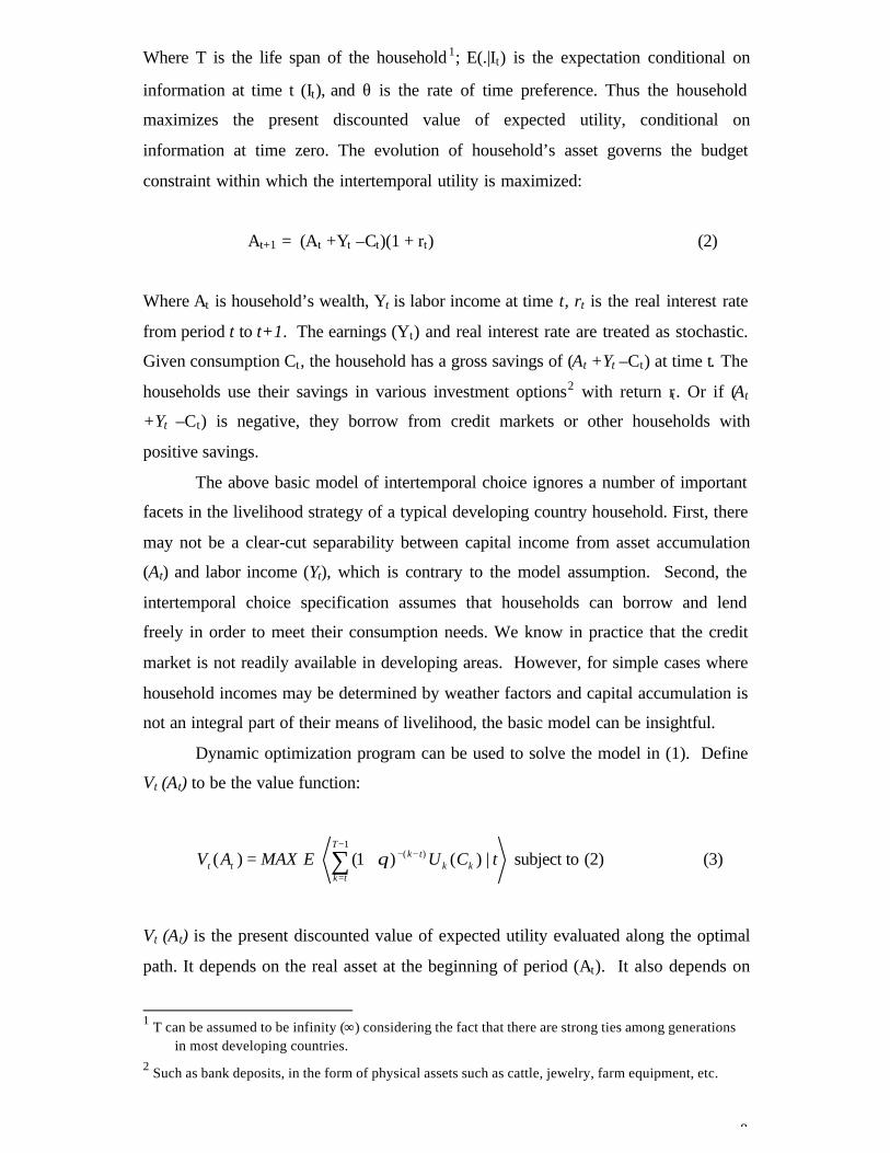
Where T is the life span of the household 1; E(.|It) is the expectation conditional on

information at time t (It), and θ is the rate of time preference. Thus the household

maximizes the present discounted value of expected utility, conditional on

information at time zero. The evolution of household’s asset governs the budget

constraint within which the intertemporal utility is maximized:

At+1 = (At +Yt –Ct)(1 + rt) (2)

Where At is household’s wealth, Yt is labor income at time t, rt is the real interest rate

from period t to t+1. The earnings (Yt) and real interest rate are treated as stochastic.

Given consumption Ct, the household has a gross savings of (At +Yt –Ct) at time t. The

households use their savings in various investment options2 with return rt. Or if (At

+Yt –Ct) is negative, they borrow from credit markets or other households with

positive savings.

The above basic model of intertemporal choice ignores a number of important

facets in the livelihood strategy of a typical developing country household. First, there

may not be a clear-cut separability between capital income from asset accumulation

(At) and labor income (Yt), which is contrary to the model assumption. Second, the

intertemporal choice specification assumes that households can borrow and lend

freely in order to meet their consumption needs. We know in practice that the credit

market is not readily available in developing areas. However, for simple cases where

household incomes may be determined by weather factors and capital accumulation is

not an integral part of their means of livelihood, the basic model can be insightful.

Dynamic optimization program can be used to solve the model in (1). Define

Vt (At) to be the value function:

(2) subject to |)()1( )(1

)( tCUEMAXAVT

tkkk

tktt ∑

−

=

−−+= θ (3)

Vt (At) is the present discounted value of expected utility evaluated along the optimal

path. It depends on the real asset at the beginning of period (At). It also depends on

1 T can be assumed to be infinity (∞) considering the fact that there are strong ties among generations

in most developing countries.2 Such as bank deposits, in the form of physical assets such as cattle, jewelry, farm equipment, etc.

9

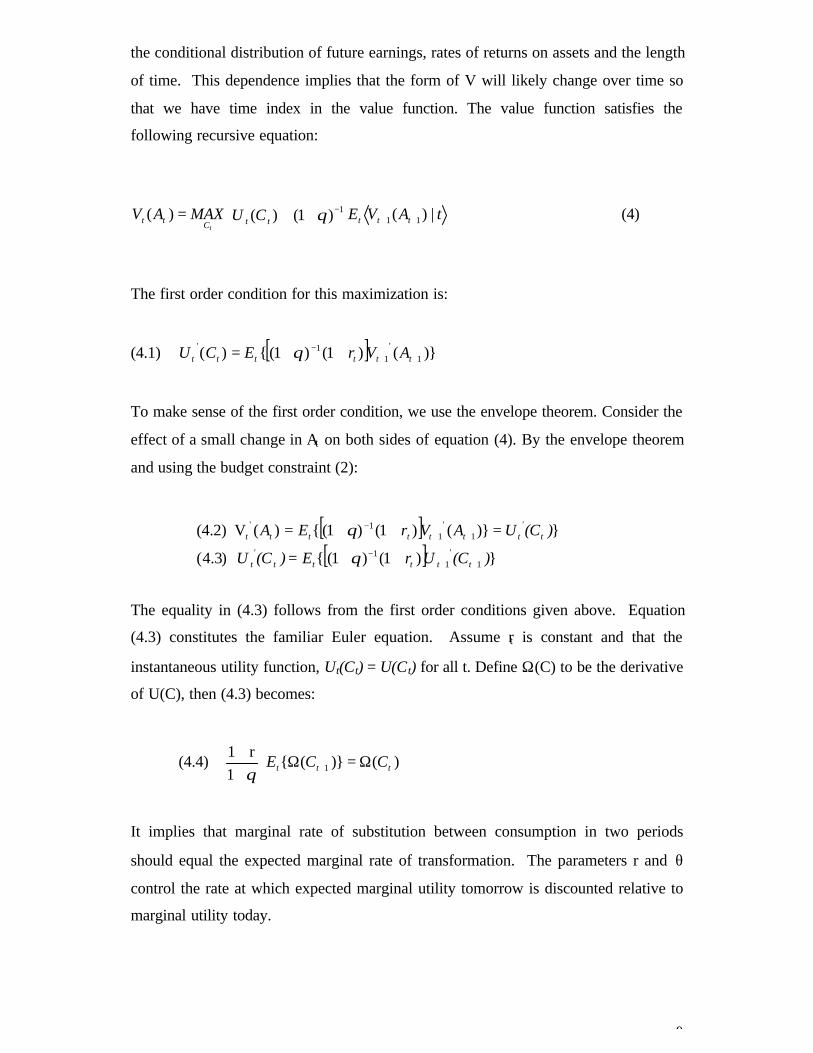
the conditional distribution of future earnings, rates of returns on assets and the length

of time. This dependence implies that the form of V will likely change over time so

that we have time index in the value function. The value function satisfies the

following recursive equation:

++= ++

− tAVECUMAXAV tttttCttt

|)()1()()( 111θ (4)

The first order condition for this maximization is:

(4.1) [ ] )()1()1()( 1

'

11'

++− ++= tttttt AVrECU θ

To make sense of the first order condition, we use the envelope theorem. Consider the

effect of a small change in At on both sides of equation (4). By the envelope theorem

and using the budget constraint (2):

[ ][ ]

)1()1( )3.4(

)()1()1()(V (4.2)

111

1'

11'

)(CUrE)(CU

)(CUAVrEA

t'

tttt'

t

t'

ttttttt

++−

++−

++=

=++=

θ

θ

The equality in (4.3) follows from the first order conditions given above. Equation

(4.3) constitutes the familiar Euler equation. Assume rt is constant and that the

instantaneous utility function, Ut(Ct) = U(Ct) for all t. Define Ω(C) to be the derivative

of U(C), then (4.3) becomes:

(4.4) )()(1

r1 1 ttt CCE Ω=Ω

++

+θ

It implies that marginal rate of substitution between consumption in two periods

should equal the expected marginal rate of transformation. The parameters r and θ

control the rate at which expected marginal utility tomorrow is discounted relative to

marginal utility today.

10

Permanent Income and Life Cycle Models

The permanent income model championed by Friedman (1957) and the life

cycle model proposed by Modigliani and Brumberg (1954, 1979) can be special cases

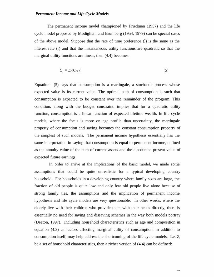
of the above model. Suppose that the rate of time preference (θ) is the same as the

interest rate (r) and that the instantaneous utility functions are quadratic so that the

marginal utility functions are linear, then (4.4) becomes:

Ct = Et(Ct+1) (5)

Equation (5) says that consumption is a martingale, a stochastic process whose

expected value is its current value. The optimal path of consumption is such that

consumption is expected to be constant over the remainder of the program. This

condition, along with the budget constraint, implies that for a quadratic utility

function, consumption is a linear function of expected lifetime wealth. In life cycle

models, where the focus is more on age profile than uncertainty, the martingale

property of consumption and saving becomes the constant consumption property of

the simplest of such models. The permanent income hypothesis essentially has the

same interpretation in saying that consumption is equal to permanent income, defined

as the annuity value of the sum of current assets and the discounted present value of

expected future earnings.

In order to arrive at the implications of the basic model, we made some

assumptions that could be quite unrealistic for a typical developing country

household. For households in a developing country where family sizes are large, the

fraction of old people is quite low and only few old people live alone because of

strong family ties, the assumptions and the implication of permanent income

hypothesis and life cycle models are very questionable. In other words, where the

elderly live with their children who provide them with their needs directly, there is

essentially no need for saving and dissaving schemes in the way both models portray

(Deaton, 1997). Including household characteristics such as age and composition in

equation (4.3) as factors affecting marginal utility of consumption, in addition to

consumption itself, may help address the shortcoming of the life cycle models. Let Zt

be a set of household characteristics, then a richer version of (4.4) can be defined:

11

),(1

r1 ),()'4.4( 11 ++Ω

++=Ω tttt ZCZCθ

Thus the age profile of consumption is determined by household characteristics and

by the relationship between r and θ (Ghez and Becker, 1975). Even richer version of

(4.4) can be obtained by incorporating uncertainty and risks that are pervasive in the

most developing countries.

Household Precautionary Saving Motives

The permanent income and life cycle do not address the cases where is

uncertainty and the household marginal utility is not linear. Households face

substantial uncertainty in most developing countries as briefly discussed in the

introduction part. Marginal utility and price are higher when consumption is low than

when it is high. For a subsistence level of consumption, which characterizes most

households in developing countries, the marginal value of consumption may increase

to infinity when consumption falls to very low level. Deaton (1997) argues that

marginal utility may well be convex for households in developing countries. This has

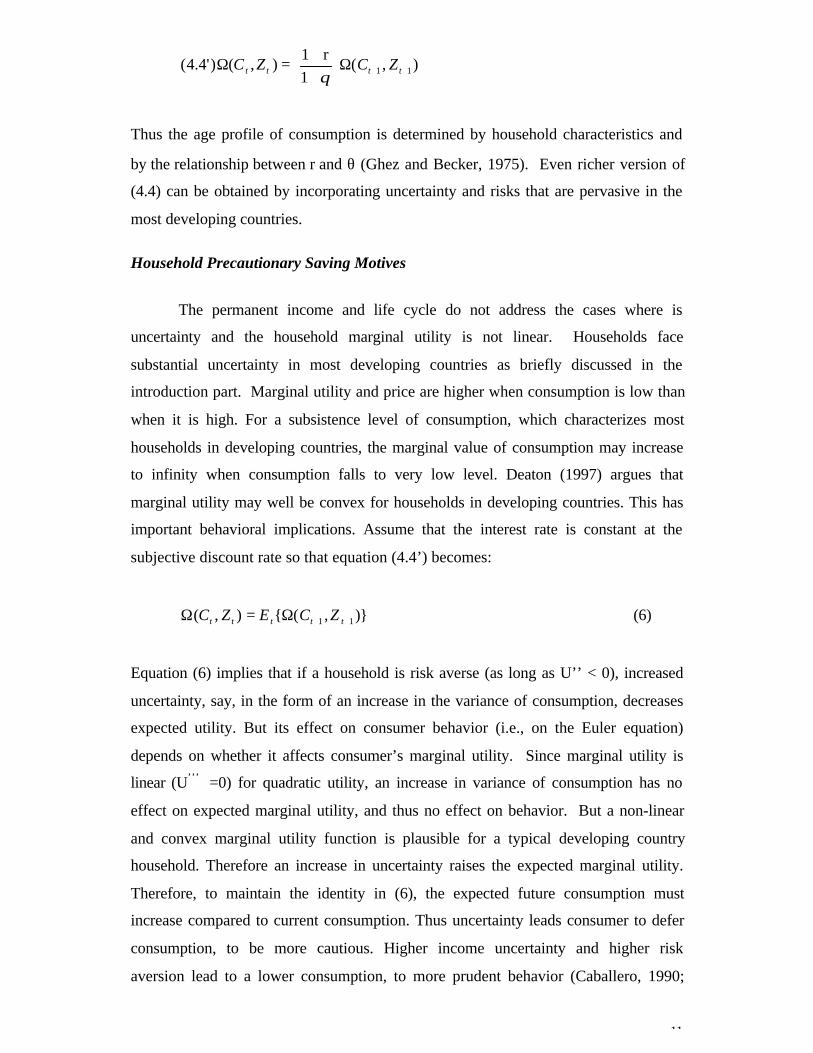
important behavioral implications. Assume that the interest rate is constant at the

subjective discount rate so that equation (4.4’) becomes:

),(),( 11 ++Ω=Ω ttttt ZCEZC (6)

Equation (6) implies that if a household is risk averse (as long as U’’ < 0), increased

uncertainty, say, in the form of an increase in the variance of consumption, decreases

expected utility. But its effect on consumer behavior (i.e., on the Euler equation)

depends on whether it affects consumer’s marginal utility. Since marginal utility is

linear (U’’’ =0) for quadratic utility, an increase in variance of consumption has no

effect on expected marginal utility, and thus no effect on behavior. But a non-linear

and convex marginal utility function is plausible for a typical developing country

household. Therefore an increase in uncertainty raises the expected marginal utility.

Therefore, to maintain the identity in (6), the expected future consumption must

increase compared to current consumption. Thus uncertainty leads consumer to defer

consumption, to be more cautious. Higher income uncertainty and higher risk

aversion lead to a lower consumption, to more prudent behavior (Caballero, 1990;

12

Kimball and Mankiw, 1989). The analysis in this paper incorporates these special

features of households in Zimbabwe and tests for the implications of permanent

income and life cycle models.

3. The Empirical Approach

The current paper aims to explore household consumption and saving

behaviors using cross-sectional data from National Income Consumption and

Expenditure Survey (ICES) data of 1990/91 and 1995/96 from Zimbabwe.

Households’ saving behavior has important implications for the ability to smooth

consumption during economic shocks. Household saving can be difficult to measure,

especially in developing country settings and in rural areas (Kozel, 1987; Paxson,

1992; Deaton, 1989). Most studies on household saving behavior take savings as a

residual of observed expenditure and observed income. In some cases in developing

countries, because of the structure of the survey and the seasonal nature of income

generation, household income can be difficult to measure and will be unreliable even

if it can be estimated. This was the case with Zimbabwe ICES data where the survey

span was just a month and most households exhibit seasonal variation in their income

generation from agricultural and other enterprises. Consumption expenditures can be

appropriately drawn from the national surveys with minimal discrepancy since

consumption may not exhibit seasonal fluctuations common in income generation.

Also a direct measure of savings, rather than observed income, can be gleaned from

the Zimbabwe data. (Refer to the data section for details about ICES data and variable

derivation and definitions.)

Modeling Household Consumption and Saving

On the basis of the theoretical model presented in the previous section, assume

that consumption and savings (Hit) are linear functions of permanent income (YitP),

transitory income (YitT), remittances and transfers (RTit), income variability (VYit) and

a set of variables that measure the life cycle stage of a household (LCit):

543210 ititititT

itP

ititLCVYRTYYH εφφφφφφ ++++++= (7)

13

Where Hit is a vector of real per-capita consumption and two per capita saving

instruments (financial and other physical assets savings) for household i and time

period t ((t= 1990/91 or 1995/96). Real per-capita consumption (CONSit) constitutes

households consumption expenditures on food, health care, and schooling. Savings

are divided into two components in order to examine the impact of structural

adjustment policies of early 1990s. Structural adjustment policies, which included

financial liberalization, may have more impact on financial savings than on other

types of savings. Thus financial savings may increase at the expense of other savings,

leaving the total savings unchanged or decreased as noted by Warman and Thirlwall

(1994). Real financial savings (FSAVit) constitutes monetary savings (the net sum of

loans taken and loans paid, purchase and sale of financial stocks, bank deposits and

withdrawals, and other financial payments such as insurance and other financial

assets). The other savings instrument (PSAVit) consists of all real physical asset

savings and is a measure of net purchases and sales of physical assets such as land,

livestock, buildings, household durable items, vehicles and other assets.

From the theory of permanent income, we expect the coefficient φ1 in the

CONSit equation (the propensity to consume out of permanent income) to be

significantly higher than φ2 (the propensity to consume out of transitory income)

while the opposite holds for saving instruments (FSAVit, and PSAVit). For CARA

(constant absolute risk aversion) form of utility function, we expect φ4 (the impact of

variability of income on consumption) to be negative for the consumption and

positive for savings equations. This will be so because of precautionary savings by

households. For a quadratic utility function, φ4 will be zero for all equations.

The explanatory variables in the equations are either directly obtained or

derived from Zimbabwe ICES data except for instrumental variables employed to

proxy income variability. Estimating a measure of income variability (VYjt) requires a

panel data, which are not possible in our case3. Therefore VYit is instrumented by a set

of variables that measure the variability of regional rainfall on the grounds that more

variable rainfall leads to more variable income particularly in an agricultural setting.

It is proxied by standard deviations of regional and seasonal rainfall (planting,

weeding and harvesting periods) over eight years. The life cycle measures (LCit) are

variables that measure the number of household members in different age categories.

3 Our data come from two separate but comparable cross-sectional national surveys of 1990/91 and

1995/96.

14

We used five variables representing the number of household members in five

different age categories (less than 6 years, 6-11 years, 12-17 years, 18-64 years,

greater than 64 years). Households with many young children and old members may

save less since their present income is less than the annuity value of their wealth.

According to the old age hypothesis, households may opt to spend on children as a

substitute to saving with the view that children will take care of the parents at old age

(see Paxson, 1992 and Nerlove, 1985). The permanent and transitory incomes are

derived from the Zimbabwe ICES data (see next section).

Estimating Permanent and Transitory Incomes

In this study, a methodology formulated by Paxson (1992) and adopted by

Alderman (1996) in his study of saving behavior in rural Pakistan, is employed for

estimating different income categories: permanent income, transitory shocks, and

residual income. Paxson (1992), in her study of the savings behavior of Thai farm

households, uses time series information on regional rainfall in conjunction with

cross-sectional data on farm household income to obtain estimates of components of

household income attributed to rainfall shocks. She assumed that rainfall variation

will produce shocks to income but will have no direct effect on consumption so that

part of each household’s income explained by shocks to regional rainfall serves as an

explicit measure of transitory income. On the other hand, the part of household

income explained by household’s permanent variables (such as household members in

different age, sex and education categories) serves as an explicit measure of

permanent income. Finally residual income is that part of household income

unexplained by either transitory or permanent variables.

Total household income is usually estimated as a sum of household earnings

from various sources such as wage, farming, business, interests and rents from

physical capital assets. However total income can also be derived from different

outlays where it may be spent such as consumption and different savings. In the

current study, since the Zimbabwe ICES does not lend itself to the first approach,

household income is derived from different consumption and savings types. Let Yit be

a derived income for household i at survey period t. Income can be derived using the

following identity:

∑=

=++=3

1

k

itkitititit HFSAVPSAVCONSY (8)

15

Where the subscript k denotes the different outlays of income (i.e., consumption and

saving types).

Total household income at any given period is also made up of permanent

income (denoted by YitP) and a random transitory income component (denoted by

YitT), which can be positive, negative, or zero. Yit

T really represents current income

deviations from permanent income. Therefore household derived income Yit can be

decomposed into permanent and transitory components:

Yit = YitP + Yit

T (9)

Define Xit to be the set of all variables important in determining income, for

household i at time t. The variables in Xit may be divided into two-- those that affect

the permanent component of total income (denoted by XitP) and those that mainly

affect transitory component and income variability (denote by XitT). Assume a

household’s permanent income (YitP) is a linear function of variables in Xit

P:

Pit

PitP

Pt

Pit XY εαα ++= (10)

Where ε itP are error terms with zero mean and unit variance. αt

P represents a year

effect, which is common to all households; αα P is parameter vectors associated with

XitP and to be estimated in the model. For the current study, variables in Xit

P include

family composition variables measuring the number of household members in

different age/sex/education categories, and an asset index variable. Also a sector-

specific dummy variable is used to capture urban-rural differences in income

generation.

In similar fashion transitory income is defined as a linear function of XitT, a

vector of variables that mainly influence the transitory component of the observed

income:

Tit

TitT

Tt

Tit XY εαα ++= (11)

Where αtT represents a year effect, which is common to all households; αα T is

parameter vectors associated with XitT. The variables used in Xit

T to estimate the

16

transitory component of income are regional rainfall deviations and deviations

squared obtained using time series information on rainfall over several catchments in

Zimbabwe. Therefore the part of household income explained by shocks to rainfall

can be used as a measure of transitory income (Paxson, 1992).

Endogeneity of Remittances

Remittances and transfers (RTit) can play an important role as a mechanism of

income redistribution between persons and across sectors. This would allow

households to diversify their income sources for risk management purposes, to

consume in excess of locally generated incomes, or to grant access to an additional

source of capital funds. (See a seminal paper by Lucas and Stark, 1985). The amount

and the nature and timing of remittances may depend on the wealth of households

receiving and giving out. Remittances and transfers thus may depend on consumption

and savings of households. Likewise the expectation, the amount and the nature of

remittances can influence household savings and consumption decisions. Here lies a

potential endogeneity between RTit and Hit. To address the endogeneity problem, we

employ instrumental variable technique and regress RTit (remittances/ transfers) on

variables that have no direct effect on household consumption and savings but affect

remittances and transfers. We use average regional family size (AHSIZE4), average

regional percent elderly (AELDER), average regional household head education level

(AHEDUC), average regional unemployment rate (AJOBLESS), average regional

landholding (ALAND), and information network availability such as household

ownership of radio (RADIO) and television (TV) to instrument for remittances:

ititit

jtjtjtjtit

TVRADIO

ALANDAJOBLESSAHEDUCAHSIZERT

ηδδδ

δδδδδ

+++

+++++=

76jt5

43210

AELDER (12)

Where j denotes regions in each province based on enumeration unit5. The predicted

remittance/transfer variable is used as instrument for RTit in equation (7).

4 Where regions are based on enumeration units within different sectors.

5 Enumeration units are based on survey design for ICES and comprise a group of one or more villageswhere enumeration was undertaken by one enumerator. The instruments used in predictingremittances are averages within these enumeration units.

17

The System of Equations

Now, equations (10), (11), and (12) can be substituted in to (7) for YitP, Yit

T and

RTit, respectively, to estimate the structural consumption and savings equations. Also

we can combine equations (10) and (11) and use identity in equation (9) to estimate

total income equation:

(14)

(13)

543210 ititititTitT

PitPtit

itTitT

PitPtit

uLCVYRTXXH

XXY

++++++=

+++=

φφφαφαφφ

εααα

,

Where

765

4321

ititjt

jtjtjtjtit

TVäRADIOäAELDERä

ALANDäAJOBLESSäAHEDUCä AHSIZEä RT

+++

+++=

. and , 302100t φδφαφαφφααα +++=+= Tt

Pt

Tt

Ptt

Note that the LCit and VYit are collinear with XitP and Xit

T, respectively, thus the

reduced Hit equations can be defined as functions of just the Xits and estimated RTit:

itititjtjt

jtjtjtTitT

PitPtit

TVRADIOAELDERALAND

AJOBLESSAHEDUC AHSIZEXX H

υϖϖϖϖ

ϖϖϖλλλ

+++++

+++++=

7654

321

(15)

λt measures the year effect, λλP reflects the impact of XitP on consumption/ savings

through its effect on the permanent income, λλ T measures the impact of regional

rainfall variables (XitT) on consumption/savings through its effect on the transitory

income and ϖk= φ3δk for all k=0, 1, 2, …, 7 and measure of marginal impact of

transfers and remittances on consumption/savings. Equations (13) and (15) consist

four equations (income, consumption, two savings) of which three are independent

since equation (8) has to hold. The parameters estimates of these equations along

with distributional assumption of the model can be used to test a number of

hypotheses.

While equation (15) gives reduced form estimates of the structural parameters

in equation (7), we can directly estimate them using two-stage estimation procedure

(Paxson, 1992). First, using ordinary least squares, we estimate equations (12) and

(13). The resulting parameters from equation (12) cane used to obtained predicted

18

RTit and parameters from equation (13) can be used to decompose the total income

into estimated permanent (YitP), transitory (Yit

T) and residual (YitR) components:

- -

7654

3210

∧∧∧

∧∧

∧∧∧

∧∧∧∧

∧∧∧∧∧

=

=

+=

+++

++++=

Tit

Pitit

Rit

TitT

Tit

PitPt

Pit

ititjtjt

jtjtjtit

YYYY

XY

XY

TVäRADIOäAELDERäALANDä

AJOBLESSäAHEDUCä AHSIZEäRT

α

αα

δ

(16)

Following Paxson and including residual income, we can estimate the structural

equation (7) as:

65

^

4

^

3

^

2

^

10 ititititR

itT

itP

itit LCVYRTYYYH υφφφφφφφ +++++++= (17)

In this way, we can directly test the permanent income hypothesis using the parameter

estimates on permanent and transitory incomes as well as residual income. Also the

coefficient on the proxy for income variability (VYit) can be used to see if households

are indeed risk averse and employ precautionary behavior to safeguard themselves

from income shocks.

Hypothesis Tests and Restrictions

The parameter estimates of equations (13) and (15) together as well as the

estimates of equation (17) can be used to test many hypotheses implied by permanent

income hypothesis (PIH). First looking at the consumption side, we expect the

propensity to consume out of permanent is close to unity. This, in the case of

equations (13) and (15) means the impact of variables in XitP on CONS it and Yit should

be similar (i.e., λλ p = αα p). We also test if the joint impact of XitTs on consumption is not

significant. Looking at the savings equations, the propensity to save out of transitory income

is expected to be close to unity, which in our model implies their respective λλ T should be

close to αα T. Put differently, the impact of rainfall on income should be identical to its

19

impact on saving. The acceptance of this last test means households do in fact use

saving to smooth consumption. We also test the impact of asset index variable on

consumption and saving. We expect it to be significantly positive on consumption

while its effect should be non significant on saving.

The coefficients in the structural equation (17) can be used to directly test the

PIH. We can test the hypotheses: H0 : φ1=1, H0: φ2 =0, H0: φ1> φ2, and H0 : φ1≥ φ3≥ φ26

for household per capita real consumption equation. Failing to reject these hypotheses

will indicate that household consumption tends to follow the PIH and that households

do use savings to reduce fluctuation in consumption. Similarly, on the savings side,

the reverse hypotheses are tested on total savings, i.e., H0 : Σ1=0, H0: Σ2 =1, H0 : Σ1<

Σ2, and H0: Σ1≤ Σ3 ≤ Σ2 (where Σ1, Σ2 and Σ3 are the sum of permanent, transitory and

residual income coefficients, respectively, across the two savings equations (FSAV

and PSAV). Failing to reject these tests indicates that the implications of PIH hold.

Finally we can test if the coefficients on rainfall variability (a proxy for income

variation) (φφ 5) are negative for consumption and positive for savings. Failing to reject

this test indicates that households are indeed risk averse and use precautionary

savings to smooth consumption.

On the other hand, we expect changes in household consumption and saving

behavior across survey years because of economic shocks that occurred in the time

between the two surveys. We anticipate that households’ precautionary measures

increase and that transitory income plays a bigger role on consumption and saving

decisions. It should be noted, however that the return on education and assets may

have decreased after the economy was hit with subsequent droughts. Thus the impact

of rainfall on income may be confounded with its impact on production, output

quality and prices.

4. The Data

The ICES of Zimbabwe in 1990/91 and 1995/96 are the sources of two

comparable data sets for current paper7. The surveys were undertaken by the Central

6 Since unexplained income can have both permanent and transitory components, its coefficients are

expected to lie between the coefficient of permanent and transitory income.7 In between the two periods Zimbabwe was hit by a number of severe shocks and introduced a

structural adjustment program. Analysis of the impact of such macroeconomic changes requirescomparable data at least for two points in time, situated appropriately relative to the adjustment

20

Statistical Office (CSO) and contain data on socio-demographic characteristics,

incomes, receipts from households including agriculture, consumption and other

expenditures on a weekly basis, and for some durable and semi-durable items, on a

monthly or yearly basis. The surveys were based on nationally representative sample

comprising all sectors of the country, i.e., the urban and the rural sectors with all their

sub-sectors. The proportion of households sampled across sectors and provinces are

similar in both survey years, thus improving the comparability over time of the survey

data. Since one of the goals of this study is to compare similarities and differences in

household consumption and saving behavior before and after economic shocks,

having comparable sample reduces possible bias due to sample size

disproportionality.

Consumption and Savings Measures

The household consumption expenditure variable was created from an

extensive list of food and non-food items from both surveys while maintaining

comparability across survey years. The consumption expenditure measure includes

market and non-market consumption, and consumption flows from ownership of

assets. The ICES has detailed information on expenditures (market, own

consumption, gifts, transfers, and payments in kind) for some 250 food items. Since

expenditures on durable goods tend to be very lumpy, it was necessary to spread the

value of expenditures on durable goods over the estimated lifetime of the good in

question. Expenditures on non-durable good items such as clothing, household

furnishings, etc. were recorded for the month of the interview and were included

directly. The total consumption was computed as the sum of the monthly consumption

of food, non-food non-durable and durable goods.

In household surveys in developing countries, incomes are more likely to be

underreported. Moreover because of the seasonal nature of income generation for

agricultural households, surveys with limited time span may not accurately record the

actual annual income. The Zimbabwe ICES, though spread over the entire calendar

year, had a month span for each household that may not have matched up with the

phase and economic shocks so that they can reflect the impact. Moreover the concern withhousehold welfare and poverty requires the availability of micro-level data that cover the differentdimension of household welfare. The Zimbabwe ICES data meet these requirements and providean opportunity to undertake the impact of drought and structural adjustment on the householdwelfare and saving behavior.

21

main period of income generation. These two serious limitations make the income

variable to be a suspect. In order to address these limitations we directly create the

savings variables from the survey data instead of defining savings as a residual

between observed expenditures and observed income. Two different saving variables

were created: financial savings (FSAV) and all other savings (PSAV). FSAV is the

net sum of loans taken and loans paid, purchase and sale of financial stocks, bank

deposits and withdrawals, and other financial payments such as insurance and other

financial assets. FSAV may likely be underestimated in the case of rural households

whose under-the-mattress deposits are not recorded. PSAV is a measure of net

purchases and sales of physical assets such as land, livestock, buildings, household

durable items, vehicles and other assets. Education and medical expenditures were

added to PSAV since such expenditures may yield a flow of services over many

years. Descriptive statistics on table 4.1 shows that welfare measures (real income,

real consumption, and real savings) and their variability had decreased in Zimbabwe

between the two surveys.

Accounting for Human and Capital Assets

Access to assets plays a determinant role in risk management and poverty

alleviation. For rural households, diverse assets help determine the choice of income

generating strategies and the levels of income achieved. They include land, productive

capital, human capital, and livestock for direct production as well as agricultural

capital. Both surveys recorded several physical capital assets along with respective

household access or ownership status. Ownership or access to durable and income

generating assets by households may have important role in determining their

consumption and savings behavior. An asset index variable (NATYPE) was created

using different weights on asset types owned. NATYPE is assumed to capture the role

of physical assets ownership on income generation, consumption and savings

decision. Another category of household asset is human capital. The number of

household members in different age, sex and education categories is important in the

household life cycle. Life cycle models suggest that households with many young

children and older members save less since the current labor income of these

household members is less than the annuity value of their lifetime wealth. This means

that households with many children could save even less. Several variables were

22

created with different age/sex/education categories to address the importance of

human capital asset in molding consumption and saving behavior. Descriptive

statistics on table 4.1 shows most age/sex/education variables for an average

household remained about the same before and after economic shocks.

The Rainfall Data

We have gathered monthly rainfall figures for seven months (October - April)

from 1989 to 1996 and normal monthly precipitation was obtained from Central

Statistical Office (CSO) of Zimbabwe. October and November constitute the planting

season. December and January are weeding months while the rest (February, March

and April) are the main harvest months in Zimbabwe. The rainfall data were collected

from all ten major catchment areas covering the whole country. The catchment areas

are matched up with corresponding provinces to get region-specific weather variables.

Three weather variables representing region-specific rainfall in the three periods

(planting, weeding, and harvest) of the cropping season were created. The percent

deviations in periodic regional rainfall (RPDEVt, RWDEVt, RHDEVt) from normal

regional precipitation are used to estimate transitory income component of household

income.

23

Table 1. Variables used (N90/91 = 14116, N95/96 = 17527) 8.

1990/91 1995/96VARIABLE: DEFINITION MEAN STD.DEV MEAN STD.DEV

__________________________________________________________________________RINC: real income 97.377 13658.5 65.480 11998.1RCONS: real consumption 86.857 4202.2 65.950 3349.1RFSAV: real financial savings (1.967) 12656.9 (2.207) 11554.6ROSAV: real other savings 12.487 1672.9 1.736 1861.1RREMITR: real remittances received 10.540 738.1 6.733 1233.1RPENSION: real pension income 1.044 450.4 0.981 447.2HEAD: household head (male, female) 0.680 11.7 0.681 11.5AGE0_5:household members age ≤ 5 years 1.280 30.2 1.104 25.8MAL6_11: males between 6 and 11 years 0.738 22.0 0.611 19.5MAL12_17: males between 12 and 17 Years 0.611 20.2 0.573 19.2M18_64PE: males age b/n 18 and 64 with ≤ primary education 0.623 17.5 0.595 17.9M18_64SE: males age b/n 18 and 64 with secondary education 0.549 20.1 0.527 19.5M18_64HE:males age b/n 18 and 64 with postsecondary education 0.012 3.0 0.083 7.4FEM6_11: females between 6 and 11 years 0.738 22.2 0.624 20.0FEM12_17: females between 12 and 17 Years 0.606 20.1 0.592 19.2F18_64PE: females age b/n 18 and 64 with ≤ Primary education 1.028 20.1 0.943 19.8F18_64SE: females age b/n 18 and 64 with secondary education 0.448 18.2 0.078 7.5F18_64HE: females age b/n 18 and 64 with postsecondary education 0.004 1.7 0.059 6.5MAL65_: elderly males (age ≥ 65 years) 0.092 7.3 0.089 7.1FEM65_: elderly females (ages ≥ 65 years) 0.082 7.0 0.085 7.0NATYPE: index of asset types owned 1.819 53.3 1.854 49.0CATTLE: number of cattle owned 3.605 206.9 2.961 3495.6TV: ownership of a television (yes, no) 0.114 8.0 0.194 9.7RADIO: ownership of radio (yes, no) 0.414 12.4 0.513 12.3UR: urban-rural dummy (1 urban, 0 rural) 0.308 11.6 0.325 11.6CA: communal area dummy 0.554 12.5 0.533 12.3SSCF: small scale commercial farm dummy 0.009 2.4 0.024 3.8LSCF: large scale commercial farm dummy 0.099 7.5 0.094 7.2RA: resettlement area dummy 0.029 4.2 0.024 3.8RPDEV1 : planting period rainfall deviations 11.237 567.7 (18.217) 241.4RWDEV: weeding period rainfall deviations 8.872 394.4 (8.528) 406.3RHDEV: harvesting period rainfall deviations (33.238) 335.0 (58.008) 323.6STDRP: planting period standard deviations 23.788 213.3 18.293 237.8STDRW: weeding period standard deviations 13.501 300.5 14.618 281.8STDRH: harvest period standard deviations 33.238 335.0 58.008 323.6

Source: Authors calculations from ICES 90/91 and 95/96 data.1 Mean and standard deviations are across provinces, after matching each province (except Harare) withclosest weather station. Harare is represented by national rainfall average. The time series data onrainfall were reported from ten weather stations.

8 The monetary variables are adjusted by 1990 Harare CPI (Consumer Price Index) to get real values

from the nominal figures derived from the survey.

24

5. Results and Discussion

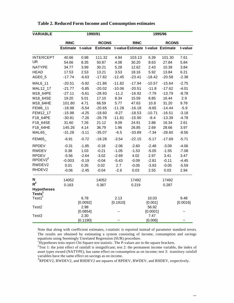
Tables 2-5 contain the parameter estimates of income, and both reduced and

structural consumption and saving equations for 1990/91 and 1995/96. We first

briefly discuss the results of the income and reduced form consumption and saving

equations (equations (13) and (15)). Since the main goal of the paper is to examine

saving behavior before and after economic shocks, the discussions focuses on the

structural consumption and savings equation estimates in tables 4-5.

Income Generation before and after Economic Shocks

The income equations (table 2) for 1990/91 and 1995/96 households show that

most explanatory variables have highly significant effects on income. The sign and

significance on HEAD (sex of household head) indicates that male-headed households

are better off than female headed ones. This is indicative of gender differences in

income generation in developing countries and that male-headed households have a

greater chance of generating more income than their female-headed counterparts. The

relative return of this gender variable is lower for the post drought and structural

adjustment households. The urban-rural dummy variable (UR) has strong significance

in favor of urban households in both years. The advantage of being urban household

has significantly decreased after the economic shocks. An asset index variable

(NATYPE) had significance on income in both years. Households with greater asset

ownership have higher real income. Like other determinants of income, the return on

assets has reduced after the economic changes, which in all likelihood is indicative of

a worsened economic environment in post structural adjustment Zimbabwe.

The age/sex/education variables have expected signs and significance. For

male household members whose age is between 18 and 64 (the most productive age

category as far as income generation is concerned), income is significantly lower for

households with members having primary or lower education level. Members having

secondary education or higher have positive impact on income. Finally income is

lower for households with higher number of younger (ages less than 18 years) and

elderly (ages over 65 years) family members. It is important to note that returns from

education have reduced considerably for all age/sex groups after the structural

changes and drought. This is a testament to the decline in overall productivity due to

rainfall shortage and macroeconomic instability evidenced in the 1990s Zimbabwe.

25

Table 2. Reduced Form Income and Consumption estimates

VARIABLE 1990/91

RINC RCONSEstimate t-value Estimate t-value

1995/96

RINC RCONSEstimate t-value Estimate t-value

INTERCEPT 40.66 0.98 111.32 4.94 103.13 6.39 101.30 7.61UR 54.66 8.35 50.87 4.08 30.20 8.63 27.84 5.84NATYPE 34.77 3.99 30.21 5.28 12.62 2.43 10.39 3.84HEAD 17.53 2.53 13.21 3.53 18.16 5.92 13.84 6.21AGE0_5 -17.74 -6.63 -17.82 -12.45 -23.41 -18.42 -20.58 -2.38

MAL6_11 -20.51 -5.92 -21.86 -11.82 -17.94 -10.57 -15.64 -2.75MAL12_17 -21.77 -5.85 -20.02 -10.06 -20.51 -11.8 -17.62 -4.01M18_64PE -27.11 -5.61 -28.93 -11.2 -16.92 -7.79 -13.79 -8.78M18_64SE 19.20 5.01 17.10 8.34 15.59 8.85 16.44 2.9M18_64HE 101.80 4.71 66.59 5.77 47.63 10.8 31.20 9.78FEM6_11 -18.98 -5.54 -20.65 -11.28 -16.18 -9.65 -14.44 -5.9FEM12_17 -15.98 -4.25 -18.60 -9.27 -18.53 -10.71 -16.51 -3.18F18_64PE -30.81 -7.26 -26.78 -11.81 -15.90 -8.4 -13.39 -4.78F18_64SE 31.60 7.26 21.12 9.09 24.91 2.88 16.34 2.61F18_64HE 145.26 4.14 36.79 1.96 26.85 2.69 28.66 3.97MAL65_ -31.28 -3.11 -35.07 -6.5 -33.89 -7.34 -28.60 -8.56

FEM65_ -6.91 -0.72 -18.28 -3.54 -22.15 -5.17 -17.69 -5.71

RPDEV -0.31 -1.85 -0.18 -2.06 -2.60 -2.48 -3.09 -4.06RWDEV 0.38 1.03 -0.21 -1.05 -1.53 -5.05 -1.55 -7.08RPDEV -5.56 -2.64 -3.02 -2.69 4.02 2.97 3.41 3.47RPDEV23

-0.003 -0.19 -0.04 -5.43 -0.09 -2.81 -0.11 -4.45RWDEV2 0.01 0.35 0.02 2.7 -0.05 -3.93 -0.05 -5.59RHDEV2 -0.06 -2.45 -0.04 -2.6 0.03 2.55 0.03 2.94-----------------------------------------------------------------------------------------------------------------------------N 14052 14052 17492 17492R2

0.163 0.367 0.219 0.287HypothesesTests1

Test12 6.78[0.0092]

2.13[0.1910]

10.03[0.001]

9.48[0.0016]

Test2 2.98[0.0854] --

56.92[0.0001] --

Test3 2.30[0.1190] --

7.47[0.006] --

Note that along with coefficient estimates, t-statistic is reported instead of parameter standard errors.The results are obtained by estimating a system consisting of income, consumption and savingsequations using Seemingly Unrelated Regression (SUR) procedure.1Hypotheses tests report Chi-Square test statistic. The P-values are in the square brackets.2Test 1: the joint effect of rainfall is insignificant; test 2: the permanent income variable, the index ofasset types owned (NATYPE), has same effect on consumption as on income; test 3: transitory rainfallvariables have the same effect on savings as on income.3RPDEV2, RWDEV2, and RHDEV2 are squares of RPDEV, RWDEV, and RHDEV, respectively.

26

Most transitory rainfall variables are all significant and highly significant

jointly (see hypothesis test 1), supporting our claim that regional rainfall variability

may explain transitory income and income variability. Deviations from normal

rainfall pattern were more important in 1995/96 than they were in 1990/91. Rainfall

deviations and squared deviations during planting and weeding periods played a

critical negative role in income generation, and the effect was even higher for the post

drought and structural adjustment households. This implies that the droughts of early

1990s have had significant adverse effects on the economy.

Reduced Form Consumption and Savings Equations

The main focus of the current study is to examine household saving behavior

and its impact on consumption, which is better examined by looking at the structural

savings and consumption equations that explicitly contain different income types as

regressors. This will be extensively discussed in the next section. However, looking at

the reduced form consumption and savings equations can provide additional insight

on household consumption and saving behavior and factors that affect such behavior.

Reduced Form Consumption Equation

Table 2 presents the reduced form consumption estimates for both 1990/91

and 1995/96. The reduced form consumption equations for both years exhibit similar

patterns as the income equations. Consumption is significantly affected by most of

the variables included in the estimation. Rural households had a decided

disadvantage compared to the urban ones and male-headed households have higher

consumption expenditures. The asset ownership index variable (NATYPE) was

significant in both years but its effect on consumption much higher before the

economic shocks than after the changes – in fact its impact reduced five-hold from

1990/91 to 1995/96.

Looking at the household member characteristics, we see similar signs but

different sizes on coefficient estimates for both years. Households with many young

members have lower consumption expenditures per capita9. Households with

uneducated male and female adult members (ages 18-64) had disadvantages in

27

meeting their consumption needs in both years. Many elderly members translate into

less consumption expenditures. The family composition variables thus seem to follow

the notions of life cycle models in both years. Rainfall deviations have significant

unfavorable impact on consumption expenditures. Hypothesis test 1 (F-test statistic

=2.13 for 1990/91, F-test statistic =9.48 for 1995/96) shows evidence that rainfall

deviations played more important role on consumption in 1995/96 than in 1990/91.

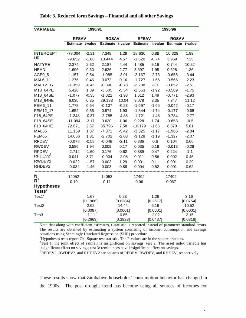
Reduced Form Savings Equations

The results of reduced form equations for financial and other savings are

reported in table 3. In this section we are essentially interest in looking at the impact

of rainfall deviations on household savings behavior. While positive savings

accompanied rainfall deviations in 1990/91, such deviations had no significant effect

in 1995/96. Since rainfall variability could be roughly translated into income

variability, this result implies that household saving behavior in 1990/91 is more

prudent than that in 1995/96. Lack of prudent response to rainfall variability post the

drought and structural changes may be explained by the urgency of current needs and

lack of economic resources to save for future use. Household with higher asset

holding had higher propensity to save in both savings types. It is interesting to note

that more educated households save more in the form of physical asset than liquid

assets. Many elderly and younger household members mean more financial saving

but their other savings are significantly negative, rendering some support to life cycle

models.

Hypothesis Tests using Reduced form Estimates

The implications of the permanent income hypothesis (PIH) on household

consumption and saving behavior can be tested using the results of the reduced form

equations (table 2). The PIH implies that the effect of transitory rainfall variables on

income should be equivalent to their effect on savings and they should have

insignificant impact on consumption. However, hypothesis test 1 on the consumption

equation indicates that rainfall variables are both singly and jointly significant.

Furthermore hypothesis test 3 showed that the rainfall deviation’ effect on income is

9 However household level (not per-capita) consumption regressions show that such expenditures are

28

not identical to its combined effect on savings. Thus we can reject polar cases of PIH

for both years. Another implication of the PIH is that saving is unrelated to

permanent income. This relationship implies in our case, after controlling for life

cycle variables, that permanent income variables such as NATYPE should have zero

impact on savings (i.e., should have identical effect on consumption and income).

The hypothesis test 2 does not show supportive evidence to such assertion for both

1990/91 and 1995/96 households. Similarly looking at hypothesis tests on savings

equations in table 3, we find evidence that both saving types are responsive to rainfall

variability in 1990/91 but not in 1995/96. Permanent income variables had significant

impact on savings in both years, contrary to the PIH implications. The impact is

higher for the 1995/96 households, indicating stronger deviations from the PIH for

1995/96.

Two-Stage Consumption Estimations

Two stage estimates provide us with a clear look at household saving and

consumption behavior since we explicitly have permanent, transitory and residual

incomes and remittances as regressors. The results are summarized as follows.

Consumption out of permanent (YP) and transitory (YT) Incomes

Table 4 reports the consumption (equation 17) estimates for both survey years.

The pre-drought and structural adjustment survey results support the implication that

households consume the majority of their permanent income (about 86%). The

1990/91 households consume small but significant amount of their transitory income

(about 48%). On the other hand, the 1995/96 data reveals that households are

consuming nearly all of their transitory income (98%) and about 81% of their

permanent income as well. The propensity to consume the residual income (YR) for

1990/91 households is 31%, which is lower than permanent income but higher than

the transitory income. Since YR contains elements of both permanent and transitory

incomes, the pre-drought household propensity to consume out of YR seems

supportive of the permanent income hypothesis. On the contrary, post-drought

propensity to consume from YR is much higher (56% of YR is consumed).

higher for households with more young members, reinforcing the theory of life cycle models.

29

Table 3. Reduced form Savings – Financial and all other Savings

VARIABLE 1990/91 1995/96

RFSAV ROSAV RFSAV ROSAVEstimate t-value Estimate t-value Estimate t-value Estimate t-value

INTERCEPT -78.004 -2.31 7.348 1.29 18.630 0.88 10.329 1.99UR -9.652 -1.80 13.444 4.57 -1.620 -0.74 3.969 7.35NATYPE 2.374 2.62 2.187 4.44 1.485 5.16 0.744 10.52HEAD 1.696 0.30 2.626 2.77 3.697 1.95 0.628 1.36AGE0_5 1.157 0.54 -1.085 -3.01 -2.167 -2.78 -0.655 -3.44MAL6_11 1.276 0.46 0.073 0.16 -1.727 -1.66 -0.566 -2.23MAL12_17 -1.359 -0.45 -0.390 -0.78 -2.238 -2.1 -0.652 -2.51M18_64PE 5.420 1.39 -3.605 -5.54 -2.563 -1.92 -0.569 -1.75M18_64SE -1.077 -0.35 -1.022 -1.98 1.612 1.49 -0.771 -2.93M18_64HE 6.030 0.35 29.183 10.04 9.078 3.35 7.347 11.12FEM6_11 1.778 0.64 -0.107 -0.23 -1.697 -1.65 -0.042 -0.17FEM12_17 1.652 0.55 0.974 1.93 -1.844 -1.74 -0.177 -0.68F18_64PE -1.248 -0.37 -2.785 -4.88 -1.721 -1.48 -0.784 -2.77F18_64SE -11.094 -3.17 0.620 1.06 9.228 1.74 -0.653 -0.5F18_64HE 72.671 2.57 35.796 7.58 -10.179 -1.66 8.370 5.61MAL65_ 11.159 1.37 -7.371 -5.42 -3.325 -1.17 -1.966 -2.84FEM65_ 14.066 1.81 -2.702 -2.08 -3.128 -1.19 -1.327 -2.07RPDEV -0.078 -0.58 -0.048 -2.11 0.386 0.6 0.104 0.66RWDEV 0.586 1.94 0.009 0.17 0.035 0.19 -0.013 -0.28RPDEV -2.714 -1.60 0.176 0.62 0.389 0.47 0.224 1.1RPDEV23

0.041 3.71 -0.004 -2.08 0.011 0.56 0.002 0.46RWDEV2 -0.022 -1.57 0.003 1.29 0.001 0.11 0.001 0.29RHDEV2 -0.032 -1.46 0.003 0.88 0.004 0.52 0.001 0.62--------------------------------------------------------------------------------------------------------------------------N 14052 14052 17492 17492R2

0.10 0.11 0.06 0.067HypothesesTests1

Tes12 1.67[0.1966]

0.23[0.6284]

1.26[0.2617]

3.16[0.0754]

Test2 2.62[0.0087]

14.44[0.0001]

5.16[0.0001]

10.52[0.0001]

Tes3 -1.11[0.2663]

-0.85[0.3928]

-2.02[0.0437]

-2.15[0.0318]

Note that along with coefficient estimates, t-statistic is reported instead of parameter standard errors.The results are obtained by estimating a system consisting of income, consumption and savingsequations using Seemingly Unrelated Regression (SUR) procedure.1Hypotheses tests report Chi-Square test statistic. The P-values are in the square brackets.2Test 1: the joint effect of rainfall is insignificant on savings; test 2: The asset index variable hasinsignificant effect on savings; test 3: remittances have insignificant effect on savings.3RPDEV2, RWDEV2, and RHDEV2 are squares of RPDEV, RWDEV, and RHDEV, respectively.

These results show that Zimbabwe households’ consumption behavior has changed in

the 1990s. The post drought trend has become using all sources of incomes for

30

current consumption while pre-drought households saved the majority of their

transitory income.

The Effect of Family Composition on Consumption

The results show that household per capita consumption decreases with

additional young and elderly members in both survey years. This finding is not

contrary to the old age security hypothesis that claims people depend on their children

for provision when they are old. It is interesting to note that although household

consumption and saving behavior has changed over the 1990s, the family composition

effect and its dependency structure remained intact even in the face of growing

economic shocks.

The Effect of Rainfall Variability on Consumption

Rainfall variability is used in this study as a proxy for income variability and

we expect, for prudent household behavior, that it will have negative effect on

consumption. Since this measure of income variability does not vary across

households in the same region, caution should be taken in interpreting the results.

Rainfall variability had a significant negative effect on consumption in 1990/91 but its

effect was not significant in 1995/96. This result indicates precautionary behavior for

1990/91 while such prudent behavior is lacking in the post drought and structural

adjustment consumption behavior.

The Effect on Remittances and Transfers on Consumption

The role of remittances on household strategies in developing countries has

been an important area of research Lucas and Starks, 1985; Reardon, 1988). The

magnitude of remittances received and the degree of household dependence on them

can have important implications for economic policy since such arrangements link

households across regions and labor markets, both at home and abroad. Our analysis

shows that receipt of remittances had no significant impact on consumption for

households before economic shocks while such receipts played a significantly positive

role in the post-drought Zimbabwe. Because of worsened economic environment

post-drought and structural changes, remittances have become a more important

31

source of income for consumption. This shows that household participation in migrant

markets may have increased as a strategy to overcome the adverse effects of the

drought. It could also be a reflection of missing or incomplete credit and insurance

markets to smooth household consumption after shocks. People are forced to depend

on remittances from family members and benefits from government sources to meet

their daily consumption needs after drought and structural adjustment took place.

Two Stage Savings Estimations

Table 5 reports the savings (equation 17) estimates. We expect some variables

that had positive impact on consumption to have the opposite effect on savings. But

since different saving measures were estimated such relationship with consumption

may not be obtained across all saving types. It should be noted further that certain

demographic and environmental variables could simultaneously increase (decrease)

both consumption and savings. Under the steadily changing economic, social and

environmental landscape of Zimbabwe, simultaneous reduction in both consumption

and savings is highly likely. Furthermore, we are interested in examining the

characteristics of households and groups that dictate the choice of saving types.

Savings out of YP, YT, and YR

The results of savings (equation 17) estimates in table 5 show that households

saved a significant amount of their transitory and residual incomes in 1990/91. But

savings out of YT is insignificant and the fraction of residual income saved is

considerably lower in 1995/96. Households in both years saved small but significant

fractions of their permanent, transitory and residual incomes in the form of OSAV.

Contrary to FSAV, OSAV responds negatively to rainfall variability. This may be

due to low returns in asset savings, particularly after the drought and structural

changes. Rainfall variability in 1990/91 had positive effect on financial savings,

planting period variability being the most significant. But rainfall variability does not

seem to have much effect on financial savings for the 1995/96 households except that

harvest period rainfall variability showed some positive effect on saving.

32

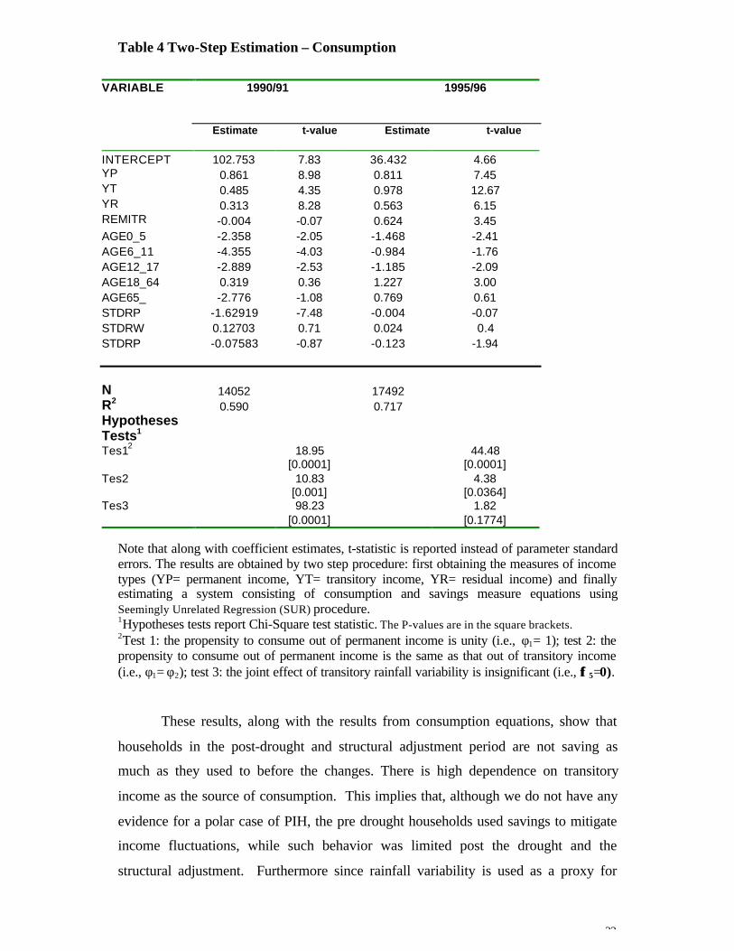
Table 4 Two-Step Estimation – Consumption

VARIABLE 1990/91 1995/96

Estimate t-value Estimate t-value

INTERCEPT 102.753 7.83 36.432 4.66YP 0.861 8.98 0.811 7.45YT 0.485 4.35 0.978 12.67YR 0.313 8.28 0.563 6.15REMITR -0.004 -0.07 0.624 3.45AGE0_5 -2.358 -2.05 -1.468 -2.41AGE6_11 -4.355 -4.03 -0.984 -1.76AGE12_17 -2.889 -2.53 -1.185 -2.09AGE18_64 0.319 0.36 1.227 3.00AGE65_ -2.776 -1.08 0.769 0.61STDRP -1.62919 -7.48 -0.004 -0.07STDRW 0.12703 0.71 0.024 0.4STDRP -0.07583 -0.87 -0.123 -1.94

N 14052 17492R2

0.590 0.717HypothesesTests1

Tes12 18.95[0.0001]

44.48[0.0001]

Tes2 10.83[0.001]

4.38[0.0364]

Tes3 98.23[0.0001]

1.82[0.1774]

Note that along with coefficient estimates, t-statistic is reported instead of parameter standarderrors. The results are obtained by two step procedure: first obtaining the measures of incometypes (YP= permanent income, YT= transitory income, YR= residual income) and finallyestimating a system consisting of consumption and savings measure equations usingSeemingly Unrelated Regression (SUR) procedure.1Hypotheses tests report Chi-Square test statistic. The P-values are in the square brackets.2Test 1: the propensity to consume out of permanent income is unity (i.e., φ1= 1); test 2: thepropensity to consume out of permanent income is the same as that out of transitory income(i.e., φ1= φ2); test 3: the joint effect of transitory rainfall variability is insignificant (i.e., φφ 5=0).

These results, along with the results from consumption equations, show that

households in the post-drought and structural adjustment period are not saving as

much as they used to before the changes. There is high dependence on transitory

income as the source of consumption. This implies that, although we do not have any

evidence for a polar case of PIH, the pre drought households used savings to mitigate

income fluctuations, while such behavior was limited post the drought and the

structural adjustment. Furthermore since rainfall variability is used as a proxy for

33

income variability, these results show post drought and structural adjustment

households do not manifest precautionary saving behavior while the pre drought and

structural changes household saved more when their income fluctuation is higher.

Hypothesis Tests using Two-step Estimates

The tests of PIH using two-step estimates are statistically equivalent to the

ones we did employing the reduced form estimates in the previous section.

Hypothesis test 1 in table 4 shows that propensity to consume out of permanent

income is lower than unity for both years. On the same table, hypothesis test 2

indicates that propensity to consume out of permanent and transitory incomes are

about the same in 1995/96 while there is evidence that the former is higher in

1990/91. Household precautionary saving behavior test (hypothesis 3) in table 4

supports that the pre-droughts and structural adjustment households consumption

responded to transitory rainfall variability (a proxy for income variability). The post

drought and structural adjustment households did not respond in statistically

significant fashion to income variation (p-value= 0.1778). Similar hypothesis tests for

the savings equations are reported on table 4.4. Hypothesis 1 (i.e., the propensity to

save out of transitory income, for both savings types combined, is unity) is rejected

for both years. Hypothesis 2 (i.e., the propensity to save out of transitory income is

the same to that out of permanent income) shows some support for the PIH in 1990/91

and strong evidence against the PIH in 1995/96 households. We do not have strong

evidence to reject the hypothesis (Hypothesis 3) that rainfall variability is jointly

insignificant on saving in 1995/96 (p-values 0.1031 for RFSAV and 0.2571 for

ROSAV) while we have strong evidence of significance in 1990/91 (p-values 0.0001

for RFSAV and 0.0057 for ROSAV).

These tests show evidence that changes occurred in household consumption

and saving behavior after the weather shocks. The results show that in 1990/91,

households consumed the majority of their permanent income, saved the majority of

their transitory income and depended less on remittances. The higher marginal

propensity to save out of transitory income by households in this period implies that

they used savings and dissavings to smooth consumption. The fact that propensities

to consume out of permanent income is statistically less than one, and savings out it

are generally greater than zero indicates that a polar version of the permanent income

hypothesis cannot be accepted. The post drought and structural adjustment

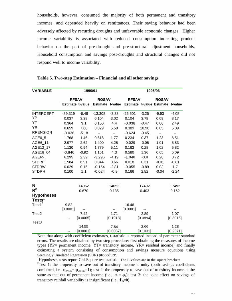
34

households, however, consumed the majority of both permanent and transitory

incomes, and depended heavily on remittances. Their saving behavior had been

adversely affected by recurring droughts and unfavorable economic changes. Higher

income variability is associated with reduced consumption indicating prudent

behavior on the part of pre-drought and pre-structural adjustment households.

Household consumption and savings post-droughts and structural changes did not

respond well to income variability.

Table 5. Two-step Estimation – Financial and all other savings

VARIABLE 1990/91 1995/96

RFSAV ROSAV RFSAV ROSAV Estimate t-value Estimate t-value Estimate t-value Estimate t-value

INTERCEPT -89.319 -6.48 -13.308 -3.33 -26.501 -3.25 -9.93 -4.08YP 0.037 3.38 0.104 3.02 0.104 3.78 0.09 8.17YT 0.364 3.1 0.150 4.4 -0.038 -0.47 0.06 2.49YR 0.659 7.68 0.029 5.58 0.389 10.96 0.05 5.09RPENSION -0.036 -5.18 -- -- -0.624 -3.45 -- --AGE0_5 1.768 1.46 0.618 1.77 0.234 0.37 1.23 6.51AGE6_11 2.977 2.62 1.400 4.25 -0.029 -0.05 1.01 5.83AGE12_17 1.130 0.94 1.779 5.11 0.163 0.28 1.02 5.82AGE18_64 -0.846 -0.92 1.151 4.3 0.580 1.36 0.65 5.09AGE65_ 6.295 2.32 -3.296 -4.19 -1.048 -0.8 0.28 0.72STDRP 1.584 6.91 0.044 0.66 0.018 0.31 -0.01 -0.81STDRW 0.029 0.15 -0.154 -2.81 -0.055 -0.89 0.03 1.7STDRH 0.100 1.1 -0.024 -0.9 0.166 2.52 -0.04 -2.24

N 14052 14052 17492 17492R2

0.670 0.135 0.403 0.162HypothesesTests1

Test12 9.82[0.0001] -- --

16.46[0.0001] -- --

Test2--

7.42[0.0065]

1.71[0.1913]

2.89[0.0894]

1.07[0.3016]

Test3

--14.55

[0.0001]7.64

[0.0057]2.66

[0.1031]1.28

[0.2571]Note that along with coefficient estimates, t-statistic is reported instead of parameter standarderrors. The results are obtained by two step procedure: first obtaining the measures of incometypes (YP= permanent income, YT= transitory income, YR= residual income) and finallyestimating a system consisting of consumption and savings measure equations usingSeemingly Unrelated Regression (SUR) procedure.1Hypotheses tests report Chi-Square test statistic. The P-values are in the square brackets.2Test 1: the propensity to save out of transitory income is unity (both savings coefficientscombined, i.e., φ2rfsav+ φ2rosav=1); test 2: the propensity to save out of transitory income is thesame as that out of permanent income (i.e., φ1= φ2); test 3: the joint effect on savings oftransitory rainfall variability is insignificant (i.e., φφ 5=0).

35

6. Conclusions

Households face substantial risks in most developing countries. Livelihood

strategies represent adaptation to uncertainty with respect to income generation and

subsistence consumption. Highly erratic rain, commodity price fluctuations, poorly

functioning or missing markets for inputs and outputs, unexpected changes in price

policies, unstable governments and armed conflicts are important sources of risks.

Zimbabwe is a good example of adaptation to such risks. The major shocks to the

economy in the 1990s included droughts and structural adjustments. Evidence shows

that poverty increased substantially during the 1990s. The current paper analyzes

changes in consumption and saving behavior before and after the droughts and

structural adjustments. We estimated the propensities to consume and save out of

permanent and transitory incomes and tested the notions of permanent income

hypothesis and precautionary saving motives. In addition, we analyzed how changes

in an overall economic situation seem to translate into changes in propensities to save.

The results show that the 1990/91 households consumed the majority of their

permanent income, saved the majority of their transitory income and depended less

on remittances. The higher marginal propensity to save out of transitory income by

households in this period implies that they used savings to smooth consumption. The

fact that propensities to consume out of permanent income are statistically less than

one, and savings out it are generally greater than zero indicates that a polar version of

the permanent income hypothesis cannot be accepted. Post drought and structural

adjustment households, however, consumed the majority of both permanent and

transitory incomes, and depended heavily on remittances. Their saving behavior had

been adversely affected by recurring drought and unfavorable economic changes.

Higher income variability is associated with reduced consumption indicating

precautionary behavior on the part of pre-drought and pre-structural change

households. Household consumption and savings post-drought and structural change

did not respond well to income variability.

The findings from this study have important welfare implications.

Zimbabwean households were forced away from risk management and prudence (as

manifested in the 1990/91 data) to that of heavy dependence on transitory income and

remittances for consumption (as the results of 1995/96 showed). The prolonged

period of drought and macroeconomic changes in the early 1990s has limited

households’ long-term ability to mitigate risk. Households were not able to save and

36

use savings to buffer consumption from income shocks. Furthermore households

may be facing credit problems due to large decline in their incomes and the economy

wide decline in productivity may also constrain credit institutions. It should be

emphasized that weather risk is spatially covariant and would be difficult, especially

for rural households, to undertake arrangements that insure against drought that affect

everyone in their locality simultaneously. (See, for instance, Rosenzweig and

Binswanger, 1993). Our results from both years indicate that households are able to

address idiosyncratic risks through saving the majority of their transitory income in

1990/91; however, they are not capable of managing covariant risks such as drought

and economy wide changes as evidenced from 1995/96 data. As a result transitory

income fluctuations may have serious welfare consequences.

37

References

Alderman, H.1996. “Saving and economic shocks in rural Pakistan”. Journal ofDevelopment economics. 51(1996), 343-365.

__________ and C.H. Paxson. 1992. “Do the poor insure? A synthesis of theliterature on risk and consumption in developing countries”, Research Program indevelopment Studies Discussion Paper #164, Princeton University.

Alwang J., L. Ersado, and N. Taruvinga. 2000. “Changes in poverty in Zimbabwebetween 1990 and 1996: Worsening outcomes under adverse conditions”,Mimeo, Virginia Polytechnic Institute and State University.

Besley, T. 1993. “Savings, credit and insurance,” Draft chapter for the Handbook ofDevelopment Economics, Vol. 3.

Binswanger, H. and J. McIntire. 1987. “Behavioral and material determinants ofproduction relations in land-abundant tropical agriculture,” EconomicDevelopment and Culture Change, 36(1), 73-99.

Binswanger, H. and M. Rosenszweig. 1993. “Wealth, weather risk and thecomposition and profitability of agricultural investment” , Economic Journal.103(January) 56-78.

Bromley, D.W., J. P. Chavas. 1989. “On risk, transactions and economicdevelopment in the semiarid tropics”, Economic Development and CulturalChange, 37(4) 719-736.

Caballero, R. J. 1990. “Consumption puzzles and precautionary savings,” Journal ofMonetary Economics, 25(1), 113-36

Case, A. and A. Eaton. 1998. “Large cash transfers to the elderly in South Africa.”The Economic Journal, 108(September), 1330-1361.

Carter, M. 1997. “Environment, technology and the social articulation of risk in WestAfrican agriculture,” Economic Development and Cultural Change, 45(3), 557-590.

Central Statistical Office.1997. National Accounts 1985-1996. Harare: GovernmentPrinting Office.

Central Statistical Office.1998a. Report on the ICES. Harare: Government PrintingOffice.

Central Statistical Office.1998b. Poverty in Zimbabwe. Harare: Government PrintingOffice.

Coate, S. and M. Ravallion. 1993. “Reciprocity without commitment: characterizationand performance informal insurance arrangements,” Journal of DevelopmentEconomics, (40) 1-24.

Deaton, A. 1990.”Saving in developing countries: theory and review”, World BankEconomic Review, Proceedings of the World Bank Annual Conference onDevelopment Economics, pp. 61-69.

_________. 1991. “Saving and liquidity constraints”, Economterica, 59/5, 1221-1248._________. 1992. Understanding Consumption. Oxford University Press, Oxford._________. 1997. The Analysis of Household Surveys: A Microeconomic Approach to

Development policy. The Johns Hopkins University Press, Published for TheWorld bank.

Fafchamps, M. 1992. “Solidarity networks in rural Africa: Rational peasants with amoral economy”, Economic Development and Cultural Change, 41, 147-175.

__________, C. Udry and K. Czukas. 1998. “Drought and saving in West Africa: arelivestock a buffer stock?”, Journal of Development economics. 55(1998) 273-305.

Friedman, M. 1957. A Theory of the Consumption Function, Princeton UniversityPress.

38

Ghez, G. R. and G. S. Becker. 1975. “The allocation of time and goods over the life-cycle,” New York, Columbia University Press for NBER.

Hall, R.E. 1978. “Stochastic implications of the life cycle-permanent incomehypothesis: theory and evidence”, Journal of Political Economy, 86(6), 461-481.

Handa, S. 1996. “Expenditure behavior and children’s welfare: An analysis of femaleheaded households in Jamaica”, Journal of development Economics, (50)165-187.

Jalan, J. and M. ravallion. 1999. “Are the poor less well insured? Evidence onvulnerability to income risk in rural China” Journal of Development Economics,(58) 61-81.

Jacoby, H. and E. Skoufias. 1992. “Risk, seasonality, and school attendance,” draft,University of Rochester.

Jacoby, H., E. Skoufias. 1997. “Rosk, financial markets and human capital in adeveloping country”, Review of Economic Studies, 64(3) 335-371.

Jodha, N.1978. “Effectiveness of farmers’ adjustment to risk,” Economic PoliticsWeekly 18.

Kimball, M. S.and N. G. Mankiw. 1989. “Precautionary saving and the timing oftaxes,” Journal of Political Economy, 97(4) 863-79.

Kinsey B., B. Kees, and G. J. Willem. 1998. “ Coping with drought in Zimbabwe: Survey evidence on responses of rural households to risk”, World Development, 26(1) 89-110Kozel, V. 1987. “Income, consumption, and saving behavior in the Cote d’Ivoire”,

Ph.D. thesis, MIT.Lucas, R.E.B. and O. Stark. 1983. “Motivations to remit: Evidence from Botswana”,

Journal of Political Economy, 93(5) 901-918.Lund, S. 1996. “Informed credit and risk-sharing networks: empirical evidence from

the Philippines. Manuscript, Stanford University.Marquette, C. M. 1997. “Current poverty, structural adjustment, and drought in Zimbabwe”, World Development 25(7) 1141-1149Modigliani, F. and R. Blumberg. 1954. “Utility analysis and the consumption

function:an interpretation of cross-sectional data,” in Kenneth K. Kurihara, ed.,Postkeynesian economics, New Brunswick, N.J., Rutgers University Press, 388-436.

___________. 1979. “Utility analysis and the consumption function: an attempt atintegration.” In Andrew Abel, ed., The collected papers of Franco Modigliani,Vol. 2, Cambridge, Mass., MIT Press, 128-97.

Morduch, J. 1993. “Risk, production and saving: theory and evidence from Indianhouseholds. Mimeo, Harvard University.

Morduch, J. 1995. “Income smoothing and consumption,” Journal of EconomicPerspectives, 9(3), 103-114.

Morduch, J.1998. “Poverty, economic growth, and average exit time”, Economics Letters 59(3) 385-390.Nerlove, M. A. Razin and E. Sadka. 1985. “The old age hypothesis’ reconsidered,”

Journal of Development Economics, 18(August), 243-52.Paxson, C.H. 1992. “Using weather variability to estimate the response of savings to

transitory income in Thailand”. The American economic Review. 82(1)15-33.__________. 1996. “Saving and growth: Evidence from micro data”, European Economic Review 40(2) 255-288.Reardon, T., P. Matlon, C. Delgado. 1988. “Coping with household-level food

insecurity in drought-affected areas of Burkina Faso”, World Development,16(9) 1065-1074.

39

Reardon, T., P. Matlon. 1989. “Seasonal food insecurity and vulnerability in drought-affected regions of Burkina Faso”, in: David, S. (Ed.), Seasonal Variability inThird World Agriculture: The Consequences for Food Security, Hohns HopkinsUniv. Press, Baltimore, MD.

Reardon, T., P. Matlon, C. Delgado. 1992. “Determinants and effects of incomediversification amongst farm households in Burkina Faso”, Journal ofDevelopment Studies, 28(2) 264-296.

Reardon T. and S.A.Vosti. 1995. “Links between rural poverty and the environment in developing countries: Asset categories and investment poverty”, World Development 23(9), 1495-1506.Rosenszweig, M. 1988. “Risk, private information and the family,” American

Economic Review, 78(2), 245-250.Rosenszweig, M. 1990. “Credit markets, risk pooling and risk taking in low-income

countries” (Manuscript, University of Minnesota)._____________ and H. Binswanger. 1993. “Wealth, weather risk and the composition

and profitability of agricultural investments,” Economic Journal, (103) 56-80._____________ and K. Wolpin. 1989. “Specific experience, household structure and

intergenerational transfers: Farm family land and labor arrangements indeveloping countries”, Quarterly Journal of Economics, 100, 961-987.

_____________ and R. Shaban. 1993. “Share tenancy, risk and the adoption of newtechnology,” Mimeo, University of Pennsylvania.

Scoones, I., et. al 1996. Hazards and Opportunities: Farming Livelihoods in DrylandAfrica. Lessons from Zimbabwe. London, Zed Books.

Stark, O. and D. Levhari. 1982. “On migration and risk in LDCs”, EconomicDevelopment and Cultural Change, 31 (October) 191-96.

Townsend R.M. 1993. The Medieval Village Economy. Princeton: PrincetonUniversity Press.

Townsend R.M. 1994. “Risk and insurance in village India,” Econometrica, 62(3),539-92.

Townsend R.M. 1995a. “Consumption insurance: an evaluation of risk-bearingsystems in low-income economies,” Journal of Economics Perspectives, 9(3),85-102.

__________. 1994. “Risk and insurance in village India” Economterica 62(3) 85-102.__________. 1995. “Consumption insurance: an evaluation of risk-bearing systems in

low-income economies”. Journal of Economic Perspectives. 9(3) 83-102.Udry, C. 1990. “ Credit markets in Northern Nigeria: credit as insurance in a rural

economy”, World bank Economic review, 4930 251-269._______. 1994. “ Risk and insurance in a rural credit market: An empirical

investigation in Northern Nigeria.” Review of Economic Studies, 61(3) 495-526.

________. 1995. “ Risk and saving in Northern Nigeria”, American EconomicReview, 85(5) 1287-1300.

World Bank. 1996a. Understanding Poverty and Human Resources in Zimbabwe:Changes in the 1990s and directions for the Future. Washington: HumanResources development Group, Eastern and Southern African Discussion Paper.

Wolpin, K. 1982. “A new trest of the permanent income hypothesis: the impact ofweather on the income and consumption of farm households in India.International Economic Review, 23(3) 583-594.

Zimmerman F. and M. R. Carter. 1996. “Dynamic portfolio management under risk and subsistenceconstraints in developing countries”. Agricultural and Applied Economics, Staff Paper Series,University of Wisconsin-Madison.