Ch6

Chapter 6 : Calculus

06-01 Limits

Activity 1

Run the following cell that gives the limit of sinHx Lx

as x ® 0.

Limit@Sin@xD � x, x ® 0D1

Run the following cell that gives the limit of 1x

first as x®0- and then as x®

0+.

Note: The limit is by default taken from above (right).

Directional Limit : +1 means left,-1 means right.

Limit@1 � x, x -> 0, Direction -> 1D-¥

Limit@1 � x, x -> 0, Direction -> -1D¥

Activity 2

Mathematica can't evaluate the limit of the greatest integer function as x®1-. Run the following cell.

Mathematica can't evaluate the limit of the greatest integer function as x®1-. Run the following cell.

Limit@Floor@xD, x -> 1, Direction -> +1D0

The limit of a function that is defined by several rules can't be evaluated directly. Run the following cell and comment on the results.

Clear@f, a, b, c, dD;f@x_D := If@x > 4, 3 x - 2, 2 - 7 x^2D;a = Limit@f@xD, x -> 1Db = Limit@f@xD, x -> 7Dc = Limit@f@xD, x -> 4, Direction -> +1Dd = Limit@f@xD, x -> 4, Direction -> -1D-5

19

-110

10

Try to run the following code to overcome this difficulty.

2 Chapter 6..Calculus .nb

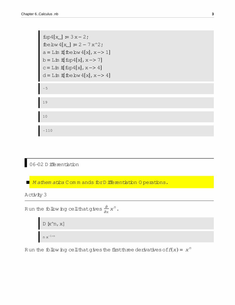
fup4@x_D := 3 x - 2;

fbelow4@x_D := 2 - 7 x^2;

a = Limit@fbelow4@xD, x -> 1Db = Limit@fup4@xD, x -> 7Dc = Limit@fup4@xD, x -> 4Dd = Limit@fbelow4@xD, x -> 4D-5

19

10

-110

06-02 Differentiation

à Mathematica Commands for Differentiation Operations.

Activity 3

Run the following cell that gives ¶¶x

x n .

D[x^n, x]

n x-1+n

Run the following cell that gives the first three derivatives of f Hx L = x n

Chapter 6..Calculus .nb 3

f@x_D := xn

f '@xDf ''@xDf '''@xDn x-1+n

H-1 + nL n x-2+n

H-2 + nL H-1 + nL n x-3+n

Activity 4

Run the following cell that gives the partial derivative ¶¶x

Ix 2 + y 2M. y is

assumed to be independent of x.

Clear[x,y,f]f=x^2 + y^2;D[f, x]

2 x

Run the following cells. Any of them gives the mixed derivative of f(x,y)=sin(xy) .

D@D@Sin@x yD, xD, yDCos@x yD - x y Sin@x yD

D@Sin@x yD, x, yDCos@x yD - x y Sin@x yD


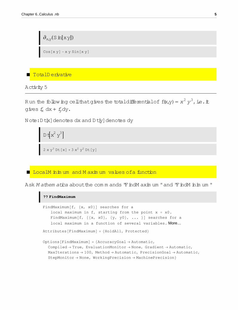
¶x,yHSin@x yDLCos@x yD - x y Sin@x yD

à Total Derivative

Activity 5

Run the following cell that gives the total differential of f(x,y) = x 2 y 3, i.e. it gives fx dx + fy dy.

Note: Dt[x] denotes dx and Dt[y] denotes dy

DtAx2 y3E2 x y3 Dt@xD + 3 x2 y2 Dt@yD

à Local Minimum and Maximum values of a function

Ask Mathematica about the commands "FindMaximum" and "FindMinimum"

?? FindMaximum

FindMaximum@f, 8x, x0<D searches for a

local maximum in f, starting from the point x = x0.

FindMaximum@f, 88x, x0<, 8y, y0<, ... <D searches for a

local maximum in a function of several variables. More…

Attributes@FindMaximumD = 8HoldAll, Protected<Options@FindMaximumD = 8AccuracyGoal ® Automatic,

Compiled ® True, EvaluationMonitor ® None, Gradient ® Automatic,

MaxIterations ® 100, Method ® Automatic, PrecisionGoal ® Automatic,

StepMonitor ® None, WorkingPrecision ® MachinePrecision<


?? FindMinimum

FindMinimum@f, 8x, x0<D searches for a

local minimum in f, starting from the point x=x0.

FindMinimum@f, 88x, x0<, 8y, y0<, ... <D searches for a

local minimum in a function of several variables. More…

Attributes@FindMinimumD = 8HoldAll, Protected<Options@FindMinimumD = 8AccuracyGoal ® Automatic,

Compiled ® True, EvaluationMonitor ® None, Gradient ® Automatic,

MaxIterations ® 100, Method ® Automatic, PrecisionGoal ® Automatic,

StepMonitor ® None, WorkingPrecision ® MachinePrecision<Is there a need for two commands? Is one of them enough?

Activity 6

Run the following cell that evaluates the local minimum of f(x)=x 3+x 2-3x+5 starting the search from x = 2.


Clear@f, g, xDf@x_D := x3 + x2 - 3 x + 5

Plot@f@xD, 8x, -10, 10<DFindMinimum@f@xD, 8x, 2<D

-10 -5 5 10

-500

500

1000

83.73165, 8x ® 0.720759<<

Activity 7

Note: The maximum value of f(x) occurs at the point x at which -f(x) has a minimum value.

Study the following code that gives a local maximum of f starting the search from x = a. Then activate it.

Find a local maximum of f(x)=x 3+x 2-3x+5

Solution:

First plot the function is a suitable domain to estimate a starting point for the search of the maximum. Run the following cell to get the plot.


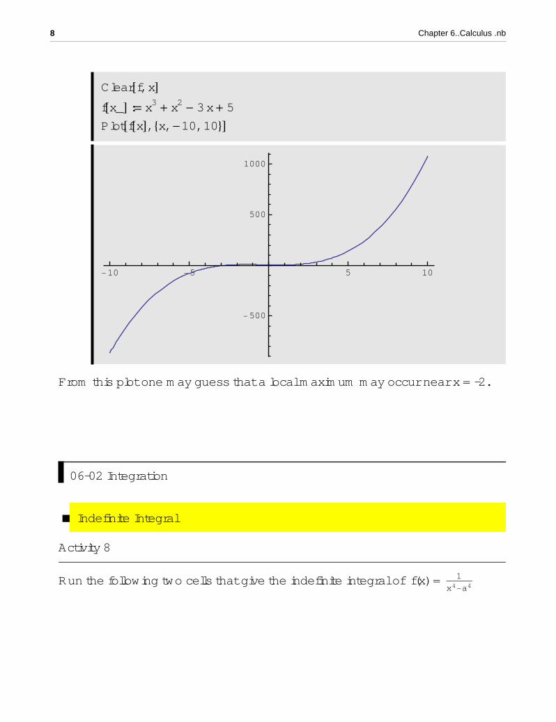
Clear@f, xDf@x_D := x3 + x2 - 3 x + 5

Plot@f@xD, 8x, -10, 10<D

-10 -5 5 10

-500

500

1000

From this plot one may guess that a local maximum may occur near x = -2.

06-02 Integration

à Indefinite Integral

Activity 8

Run the following two cells that give the indefinite integral of f(x) = 1x4-a4


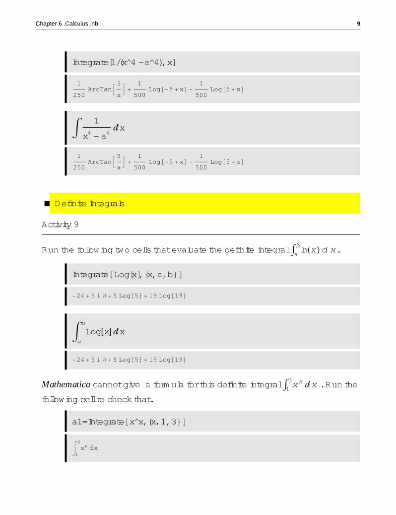
Integrate[1/(x^4 - a^4), x]

1

250ArcTanB5

xF +

1

500Log@-5 + xD -

1

500Log@5 + xD

à 1

x4 - a4âx

1

250ArcTanB5

xF +

1

500Log@-5 + xD -

1

500Log@5 + xD

à Definite Integrals

Activity 9

Run the following two cells that evaluate the definite integral Ùa

b lnHx L d x .

Integrate[ Log[x], {x, a, b} ]

-24 + 5 ä Π + 5 Log@5D + 19 Log@19D

àa

b

Log@xD âx

-24 + 5 ä Π + 5 Log@5D + 19 Log@19DMathematica cannot give a formula for this definite integral Ù1

3x x âx . Run the

following cell to check that.

a1=Integrate[ x^x, {x, 1, 3} ]

à1

3

xx âx

However, you can still get a numerical result of that integral by running the following cell.


However, you can still get a numerical result of that integral by running the following cell.

N[a1]

13.7251

à Integrating Piecewise Functions

Activity 10

Try to run the following cell that attempts to evaluate the Ceiling function

on the interval [0,2], and observe the output.

IntegrateA CeilingA x2E, 8x, 0, 2<E7 - 2 - 3

However, using the Boole function you can evaluate the above integral by running the following cell.

IntegrateA CeilingA x2E Boole@0 < x < 2D, 8x, -¥, ¥<E7 - 2 - 3

à Improper integral

Activity 11

The true definite integral Ù-22 1

x 2 âx is divergent because of the double pole at

x = 0. Run the following cell to check that.


Integrate[1/x^2, {x, -2, 2}]

Integrate::idiv : Integral of1

x2does not converge on 8-2, 2<. More…

à-2

2 1

x2âx

Run the following cell that tries to evaluate Ù0¥ sinHa x L

xâx .

Integrate[Sin[a x]/x, {x, 0, Infinity}]

-Π

2

Note that the If here gives the condition for the integral to be convergent.

à Double integral

Activity 12

Run the following cell that the double integral Ù01Ù0

x Ix 2 + y 2M dy dx.

Note that the range of the outermost integration variable appears first. The y

integral is done first. Its limits can depend on the value of x.

Integrate[ x^2 + y^2, {x, 0, 1}, {y, 0, x} ]

1

3

à Double Integration over Regions

The Boole function is very useful in computing definite double integral over a given region.

Integrate[f[x] Boole[ ineq], {x, x1, x2}, {y, y1,y2} ] integrates the function f(x) over the region defined by all points satisfying the inequality inside the rectan-gle defined by values of x and y.

Note: You can use Integrate[f[x] Boole[ineq],{x,-¥,¥},{y,-¥,¥}] if you want Mathematica to select the inter region defined by the inequality.


The Boole function is very useful in computing definite double integral over a given region.

Integrate[f[x] Boole[ ineq], {x, x1, x2}, {y, y1,y2} ] integrates the function f(x) over the region defined by all points satisfying the inequality inside the rectan-gle defined by values of x and y.

Note: You can use Integrate[f[x] Boole[ineq],{x,-¥,¥},{y,-¥,¥}] if you want Mathematica to select the inter region defined by the inequality.

Activity 13

Run the following cell that integrates x y + y 2 over the region R= {(x,y) : 0 £ x £ 1 and 0 £ y £ 1}.

IntegrateA x y + y2, 8x, 0, 1<, 8y, 0, 1< E7

12

Run the following cells . Comment on the obtained results. Write the inte-grals that have been evaluated..

IntegrateA BooleA x2 + y2 £ 1E, 8x, -1, 1<, 8y, -1, 1< EΠ

IntegrateA BooleA x2 + y2 £ 1E, 8x, 0, 1<, 8y, 0, 1< EΠ

4

IntegrateA BooleA x2 + y2 £ 1E, 8x, -¥, ¥<, 8y, -¥, ¥< EΠ

Run the following cell . Write the integrals that have been evaluated..


IntegrateB x2 BooleBx2 + 4 y2 £ 1 í Abs@yD £ xF, 8y, -¥, ¥< ,

8x, -¥, ¥<F1

40H2 + 5 ArcTan@2DL

06-03 Differential Operations

Note: Some of the following commands are set for spherical coordinates, so to use them in Cartesian coordinates, we need to run the following cell.

<< VectorAnalysis`

SetCoordinates@Cartesian@x, y, zDDCartesian@x, y, zD

Grad (Ñf the gradient of the scalar function f)

Activity 14

Run the following cell that computes the Ñf where f Hx, y, zL = 5 x2 y3 z4

Clear[x,y,z]Grad[5 x^2 y^3 z^4, Cartesian[x, y, z]]

910 x y3 z4, 15 x2 y2 z4, 20 x2 y3 z3=

Curl (Ñ×f curl of a vector valued function f)


Curl (Ñ×f curl of a vector valued function f)

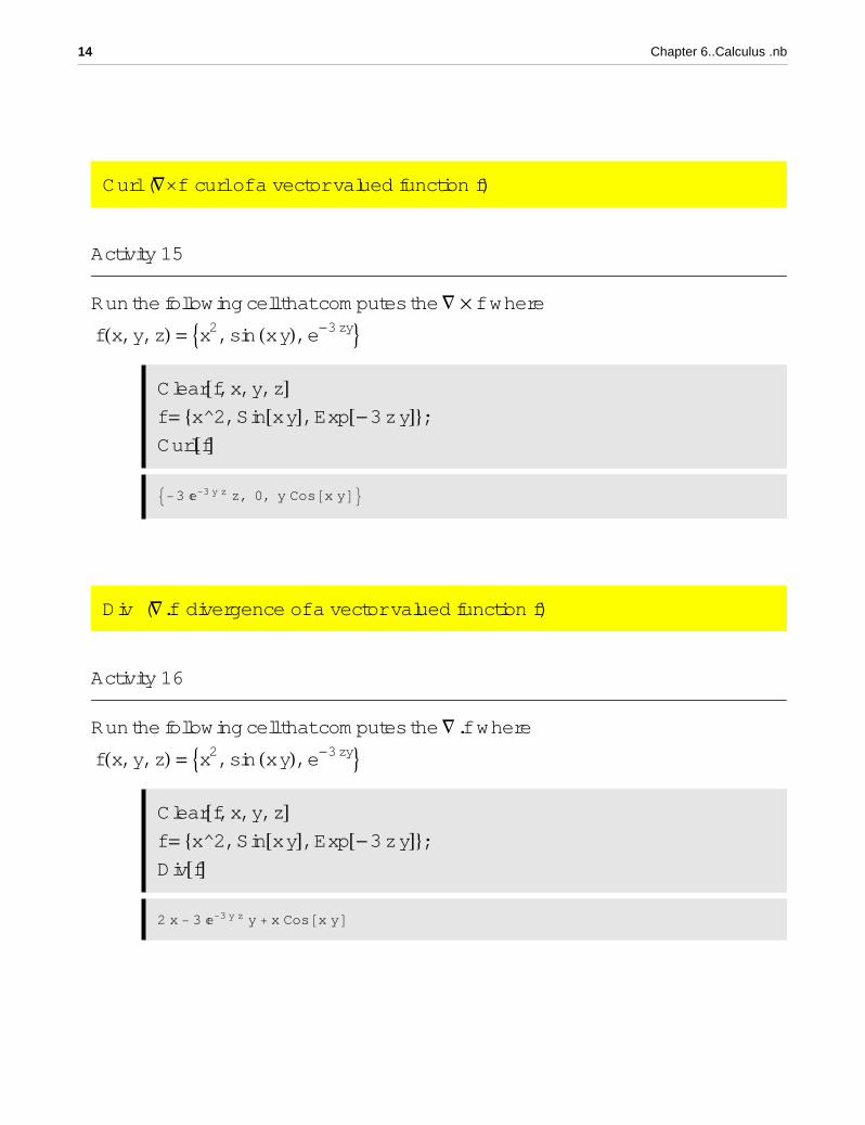
Activity 15

Run the following cell that computes the Ñ ´ f where

f Hx, y, zL = 9x2, sin Hx yL, e-3 zy=Clear@f, x, y, zDf = 8x^2, Sin@x yD, Exp@-3 z yD<;Curl@fD9-3 ã-3 y z z, 0, y Cos@x yD=

Div (Ñ.f divergence of a vector valued function f)

Activity 16

Run the following cell that computes the Ñ.f where

f Hx, y, zL = 9x2, sin Hx yL, e-3 zy=Clear@f, x, y, zDf = 8x^2, Sin@x yD, Exp@-3 z yD<;Div@fD2 x - 3 ã-3 y z y + x Cos@x yD


06-04 Vector Field

à Arrow

Activity 17

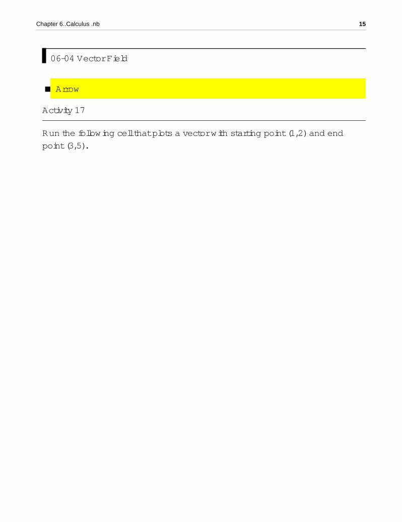
Run the following cell that plots a vector with starting point (1,2) and end point (3,5).


Graphics@Arrow@881, 2<, 83, 5<<DD

à Plot of Vector Field

Activity 18

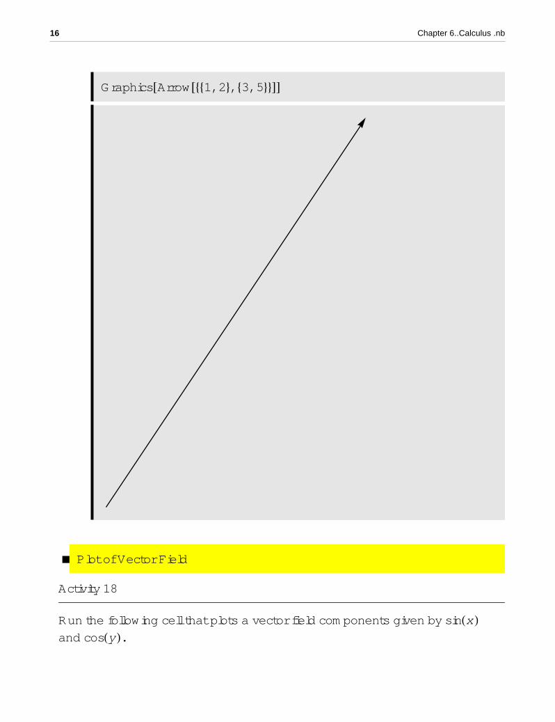
Run the following cell that plots a vector field components given by sinHx L and cosHy L.


HNeeds@"VectorFieldPlots`"D;VectorFieldPlots`VectorFieldPlot@8Sin@xD, Cos@yD<, 8x, 0, Π<,8y, 0, Π<DL

à Plot of Gradient Field

Activity 19

Run the following cell that plots a gradient field of the potential x 2 + y 2.


INeeds@"VectorFieldPlots`"D;VectorFieldPlots`GradientFieldPlotAx2 + y2, 8x, -3, 3<, 8y, -3, 3<EM

à Plot Field in 3D

Activity 20

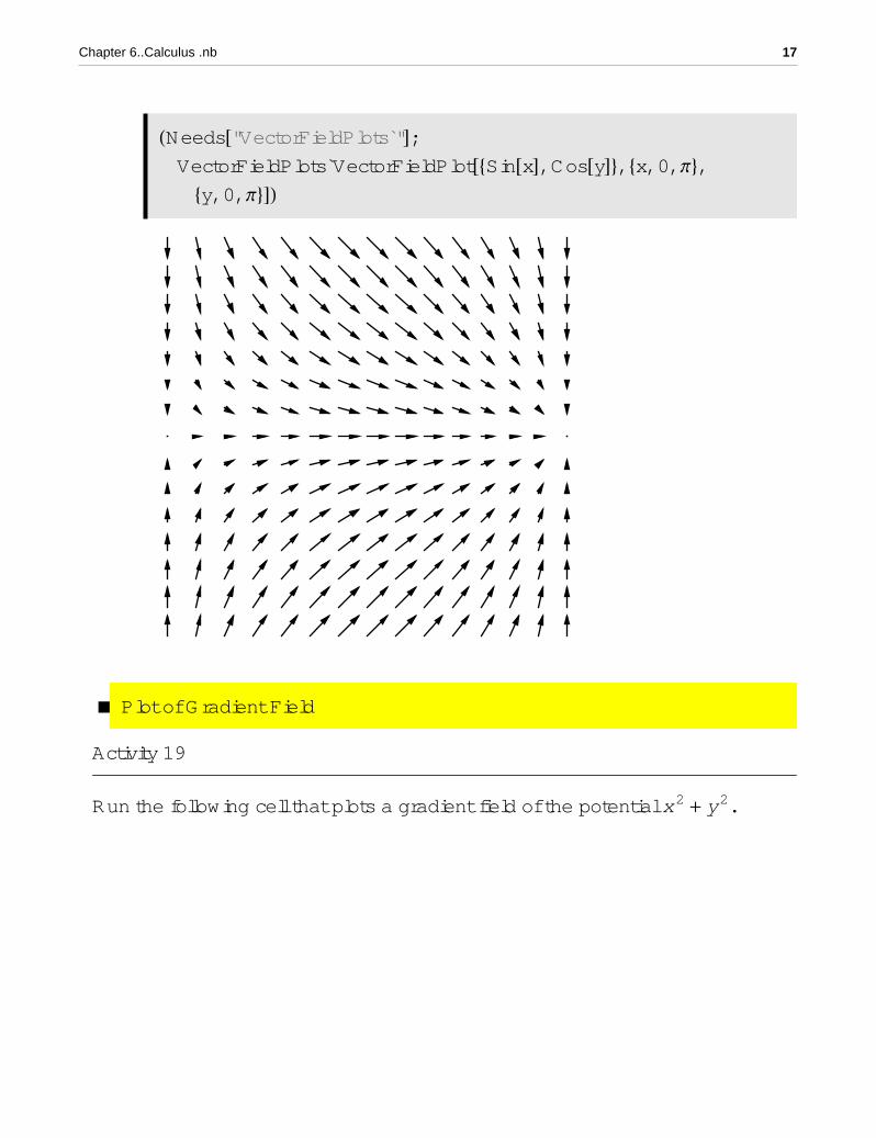
Run the following cell that plots a vector field with components given by y � z , -x � z , and 0.


Needs@"VectorFieldPlots`"D;VectorFieldPlots`VectorFieldPlot3DB 8y, -x, 0<

z, 8x, -1, 1<,

8y, -1, 1<, 8z, 1, 3<F

Run the following cell that plots the gradient field of the scalar function x y z .


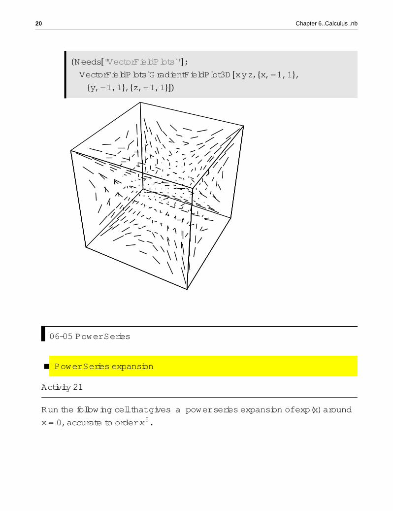
HNeeds@"VectorFieldPlots`"D;VectorFieldPlots`GradientFieldPlot3D@x y z, 8x, -1, 1<,8y, -1, 1<, 8z, -1, 1<DL

06-05 Power Series

à Power Series expansion

Activity 21

Run the following cell that gives a power series expansion of exp(x) around

x = 0, accurate to order x 5.


aa=Series[Exp[x], {x, 0, 5}]

1 + x +x2

2+x3

6+x4

24+

x5

120+ O@xD6

Run the following cell that turns the previous power series back into an ordi-nary expression.

Normal[aa]

1 + x +x2

2+x3

6+x4

24+

x5

120

Run the following cell that gives a power series expansion of exp(x) around

x = 1, accurate to order x 5.

Series[ Exp[x], {x, 1, 5} ]

ã + ã Hx - 1L +1

2ã Hx - 1L2 +

1

6ã Hx - 1L3 +

1

24ã Hx - 1L4 +

1

120ã Hx - 1L5 + O@x - 1D6

à Operations on Power Series

Activity 22

Run the following cell that gives 11- aa

.

1 / (1 - aa)

-1

x+1

2-

x

12+

x3

720+ O@xD4

Run the following cell that gives derivative with respect to x of aa.


D[aa, x]

1 + x +x2

2+x3

6+x4

24+ O@xD5

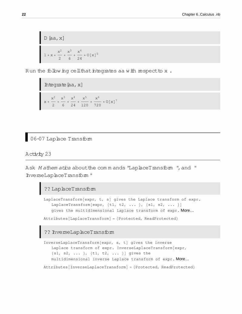
Run the following cell that integrates aa with respect to x .

Integrate[aa, x]

x +x2

2+x3

6+x4

24+

x5

120+

x6

720+ O@xD7

06-07 Laplace Transform

Activity 23

Ask Mathematica about the commands "LaplaceTransform ", and " InverseLaplaceTransform"

?? LaplaceTransform

LaplaceTransform@expr, t, sD gives the Laplace transform of expr.

LaplaceTransform@expr, 8t1, t2, ... <, 8s1, s2, ... <Dgives the multidimensional Laplace transform of expr. More…

Attributes@LaplaceTransformD = 8Protected, ReadProtected<?? InverseLaplaceTransform

InverseLaplaceTransform@expr, s, tD gives the inverse

Laplace transform of expr. InverseLaplaceTransform@expr,8s1, s2, ... <, 8t1, t2, ... <D gives the

multidimensional inverse Laplace transform of expr. More…

Attributes@InverseLaplaceTransformD = 8Protected, ReadProtected<


à Mathematica Commands

Activity 24

Run the following cell that computes the Laplace transform of f(t) = t n using the Mathematica command LaplaceTransform.

Clear[f,t,L,IL,s,a]f[t_]:=t^n L[f_]:=LaplaceTransform[f[t], t, s]L[f]

s-1-n Gamma@1 + nDRun the following cell that computes the Inverse Laplace transform of the previous result.

IL[f_]:=InverseLaplaceTransform[L[f], s, t]IL[f]

tn

à Properties of Laplace Transform

Activity 25

Run the following cell that shows that the Laplace transform is a linear operator.


Clear@f, g, t, sDLaplaceTransform@f@tD + g@tD, t, sDLaplaceTransform@f@tD - g@tD, t, sDLaplaceTransform@f@tD, t, sD + LaplaceTransform@g@tD, t, sDLaplaceTransform@f@tD, t, sD - LaplaceTransform@g@tD, t, sD

What do you conclude from the above output?

à Laplace Transform of nth derivative of a function

Activity 26

Laplace transforms have the property that they turn integration and differentia-tion into essentially algebraic operations. Run the following cell and com-ment on the output

f@t_D := Sin@tD^2

Do@Print@LaplaceTransform@D@f@tD, 8t, k<D, t, sDD, 8k, 0, 2<D2

4 s + s3

2

4 + s2

-4

4 s + s3+2 I2 + s2M4 s + s3

à Laplace Transform of an Integral

Activity 27

Integration becomes multiplication by 1 � s when one does a Laplace trans-form. Run the following cell and comment on the output.


Clear@f, s, tDf@u_D := u Exp@uDLaplaceTransform@Integrate@f@uD, 8u, 0, t<D, t, sDH1 � sL LaplaceTransform@f@tD, t, sDApart@%D

1

H-1 + sL2-

1

-1 + s+1

s

1

H-1 + sL2 s

1

H-1 + sL2-

1

-1 + s+1

s

à Multidimensional Laplace transforms.

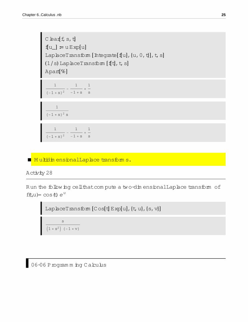
Activity 28

Run the following cell that compute a two-dimensional Laplace transform of f(t,u)= cos(t) eu

LaplaceTransform@Cos@tD Exp@uD, 8t, u<, 8s, v<Ds

I1 + s2M H-1 + vL

06-06 Programming Calculus

Limits


Limits

à Numerical Approach to Limits

Activity 29

Write a code that computes directional limits numerically. Then run it to activate it.

Run the following cell that calculates the values of f(x)= sinHx Lx

as x

approaches 0 from right.

f@x_D :=Sin@xD

x; c = 0; dir = 1;

numericalapproachtolimits@f, c, dirDRight limit of

Sin@xDx

as x ® 0+

x fHxL=Sin@xD

x

_______________________________

0.001 1.0.0009 1.0.0008 1.0.0007 1.0.0006 1.0.0005 1.0.0004 1.0.0003 1.0.0002 1.0.0001 1.

à Graphical Approach

Activity 30


Activity 30

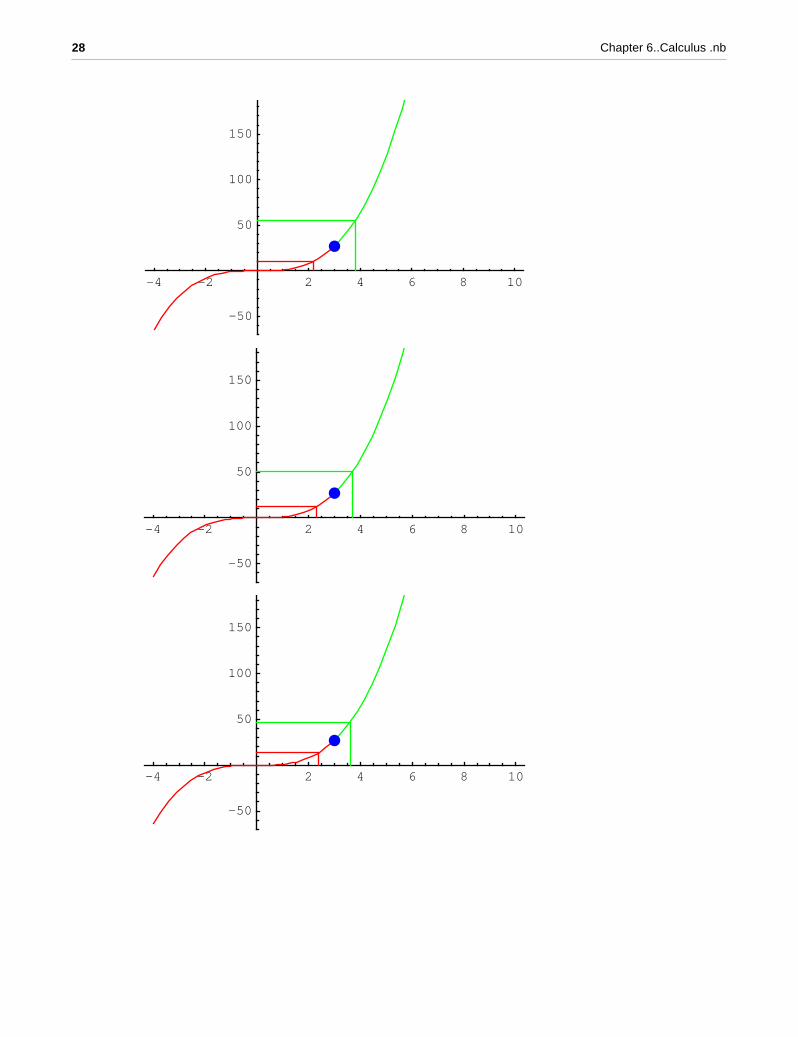
Write a code that shows directional limits graphically. Then run it to activate it.

Run the following cell that illustrates the limit of f(x)= x 3 as x approaches 3 .

f@x_D := x^3; c = 3;

graphicalapproachtolimits@f, cD

-4 -2 2 4 6 8 10

-50

50

100

150

-4 -2 2 4 6 8 10

-50

50

100

150


-4 -2 2 4 6 8 10

-50

50

100

150

-4 -2 2 4 6 8 10

-50

50

100

150

-4 -2 2 4 6 8 10

-50

50

100

150


-4 -2 2 4 6 8 10

-50

50

100

150

-4 -2 2 4 6 8 10

-50

50

100

150

-4 -2 2 4 6 8 10

-50

50

100

150


-4 -2 2 4 6 8 10

-50

50

100

150

-4 -2 2 4 6 8 10

-50

50

100

150

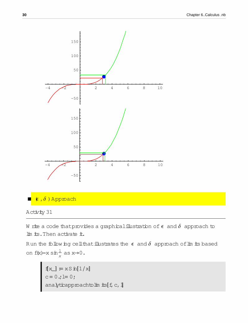
à (Ε , ∆ ) Approach

Activity 31

Write a code that provides a graphical illustration of Ε and ∆ approach to limits. Then activate it.

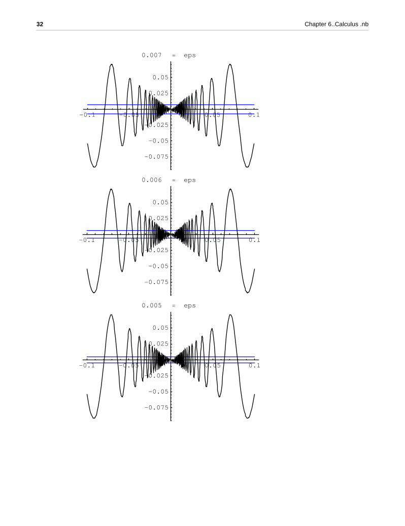
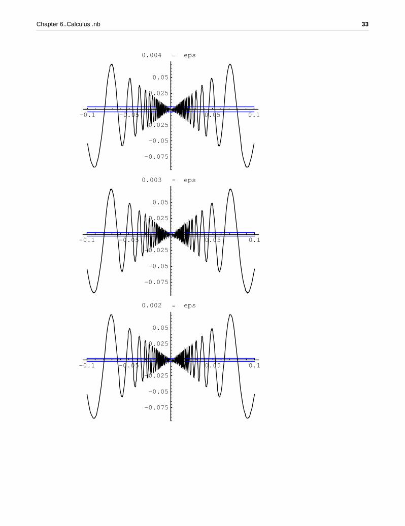
Run the following cell that illustrates the Ε and ∆ approach of limits based

on f(x)=x sin 1x

as x®0.

f@x_D := x Sin@1 � xDc = 0.; l = 0;

analyticapproachtolimits@f, c, lD


The relation between Ε and ∆ in the limit definition

Neiborhood of x = 0. is 8-0.1, 0.1< with ∆ = 0.1

-0.1 -0.05 0.05 0.1

-0.075

-0.05

-0.025

0.025

0.05

0.01 = eps

-0.1 -0.05 0.05 0.1

-0.075

-0.05

-0.025

0.025

0.05

0.009 = eps

-0.1 -0.05 0.05 0.1

-0.075

-0.05

-0.025

0.025

0.05

0.008 = eps


-0.1 -0.05 0.05 0.1

-0.075

-0.05

-0.025

0.025

0.05

0.007 = eps

-0.1 -0.05 0.05 0.1

-0.075

-0.05

-0.025

0.025

0.05

0.006 = eps

-0.1 -0.05 0.05 0.1

-0.075

-0.05

-0.025

0.025

0.05

0.005 = eps


-0.1 -0.05 0.05 0.1

-0.075

-0.05

-0.025

0.025

0.05

0.004 = eps

-0.1 -0.05 0.05 0.1

-0.075

-0.05

-0.025

0.025

0.05

0.003 = eps

-0.1 -0.05 0.05 0.1

-0.075

-0.05

-0.025

0.025

0.05

0.002 = eps


-0.1 -0.05 0.05 0.1

-0.075

-0.05

-0.025

0.025

0.05

0.001 = eps

à Evaluation of ∆ for a given Ε

Activity 32

Write a code that computes ∆ for a given Ε in the definition of limit. Then activate it.

Run the following cell that computes ∆ if Ε =0.001 that illustrates that the

limx ®1x 2 = 1

f@x_D := x^2

c = 1; epsilon = .001;

evaluationofdelta@f, c, epsilonDfHxL = x2

c = 1

limx®c fHxL = 1

Ε = 0.001

∆ = 0.000499875

Differentiation


Differentiation

à Average of a function

Activity 33

Run the following cell.

Comment on the output.

Write a code that gives the same output.

Clear@f, x, a, bDf@x_D := Sin@xD; a = 0; b = Pi � 2;

average@f, a, bD2

Π

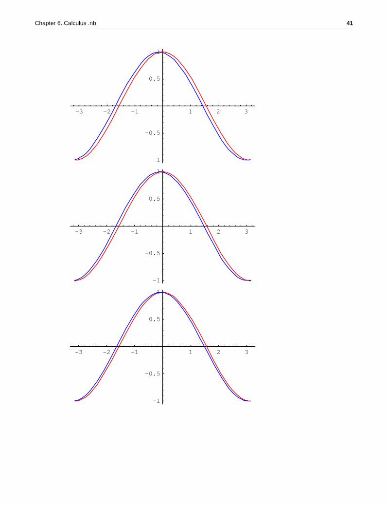
à Compare derivative and average of a function

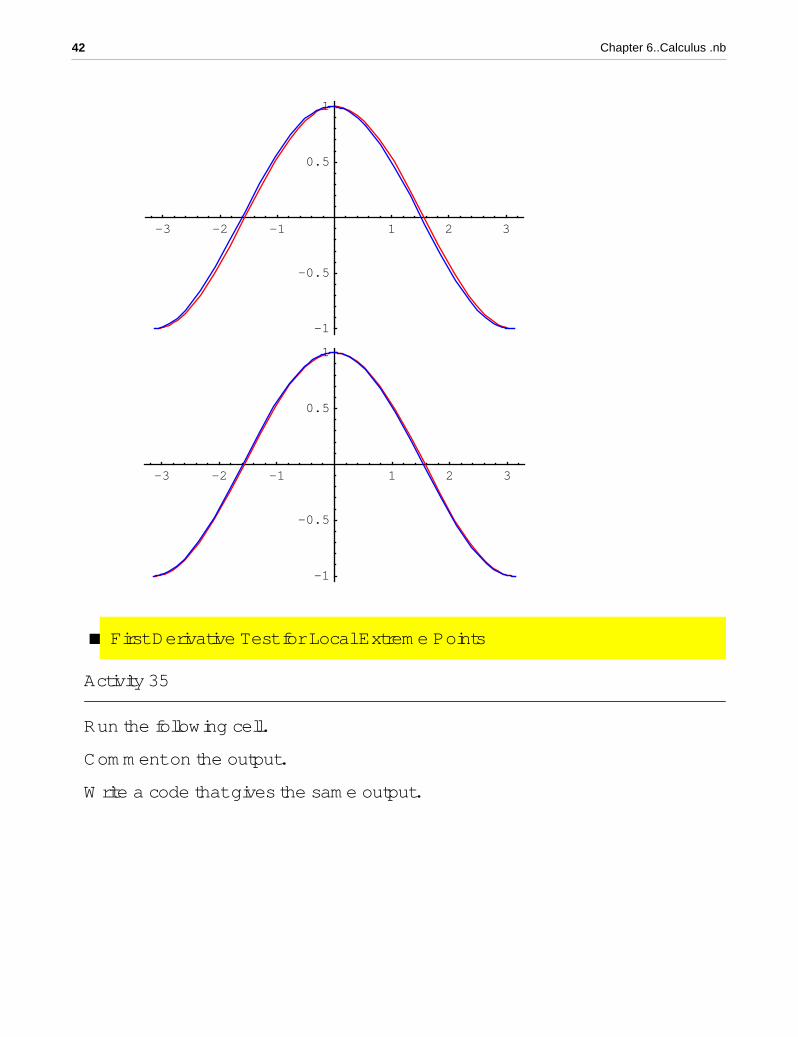
Activity 34




f@x_D := Sin@xD; x0 = -Pi; xn = Pi;

derivativeandaverage@f, x0, xnD


-3 -2 -1 1 2 3

-1

-0.5

0.5

1

-3 -2 -1 1 2 3

-1

-0.5

0.5

1

-3 -2 -1 1 2 3

-1

-0.5

0.5

1


-3 -2 -1 1 2 3

-1

-0.5

0.5

1

-3 -2 -1 1 2 3

-1

-0.5

0.5

1

-3 -2 -1 1 2 3

-1

-0.5

0.5

1


-3 -2 -1 1 2 3

-1

-0.5

0.5

1

-3 -2 -1 1 2 3

-1

-0.5

0.5

1

-3 -2 -1 1 2 3

-1

-0.5

0.5

1


-3 -2 -1 1 2 3

-1

-0.5

0.5

1

-3 -2 -1 1 2 3

-1

-0.5

0.5

1

-3 -2 -1 1 2 3

-1

-0.5

0.5

1


-3 -2 -1 1 2 3

-1

-0.5

0.5

1

-3 -2 -1 1 2 3

-1

-0.5

0.5

1

-3 -2 -1 1 2 3

-1

-0.5

0.5

1


-3 -2 -1 1 2 3

-1

-0.5

0.5

1

-3 -2 -1 1 2 3

-1

-0.5

0.5

1

-3 -2 -1 1 2 3

-1

-0.5

0.5

1


-3 -2 -1 1 2 3

-1

-0.5

0.5

1

-3 -2 -1 1 2 3

-1

-0.5

0.5

1

à First Derivative Test for Local Extreme Points

Activity 35





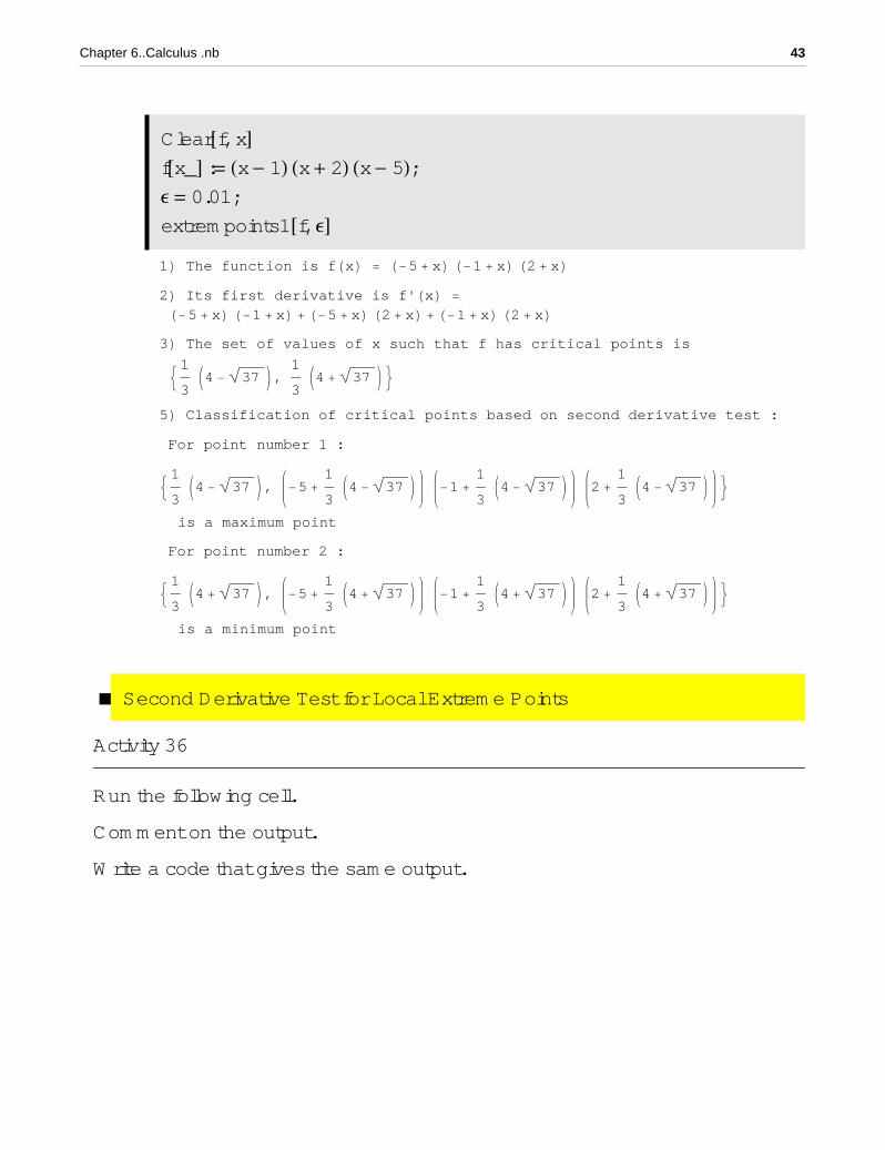
Clear@f, xDf@x_D := Hx - 1L Hx + 2L Hx - 5L;Ε = 0.01;

extrempoints1@f, ΕD1L The function is fHxL = H-5 + xL H-1 + xL H2 + xL2L Its first derivative is f'HxL =H-5 + xL H-1 + xL + H-5 + xL H2 + xL + H-1 + xL H2 + xL3L The set of values of x such that f has critical points is

:13

J4 - 37 N, 1

3J4 + 37 N>

5L Classification of critical points based on second derivative test :

For point number 1 :

:13

J4 - 37 N, -5 +1

3J4 - 37 N -1 +

1

3J4 - 37 N 2 +

1

3J4 - 37 N >

is a maximum point


:13

J4 + 37 N, -5 +1

3J4 + 37 N -1 +

1

3J4 + 37 N 2 +

1

3J4 + 37 N >

is a minimum point

à Second Derivative Test for Local Extreme Points

Activity 36





Clear@f, xDf@x_D := Hx - 1L Hx + 2L Hx - 5L;extrempoints2@fD1L The function is fHxL = H-5 + xL H-1 + xL H2 + xL2L Its first derivative is f'HxL =H-5 + xL H-1 + xL + H-5 + xL H2 + xL + H-1 + xL H2 + xL3L The set of values of x such that f has critical points is

:13

J4 - 37 N, 1

3J4 + 37 N>

4L The second derivative of f is f''HxL = -8 + 6 x

5L Classification of critical points based on second derivative test :


:13

J4 - 37 N, -5 +1

3J4 - 37 N -1 +

1

3J4 - 37 N 2 +

1

3J4 - 37 N >

is a maximum point


:13

J4 + 37 N, -5 +1

3J4 + 37 N -1 +

1

3J4 + 37 N 2 +

1

3J4 + 37 N >

is a minimum point

06-08 Evaluation on Calculus

Exercise 1

For each of the following cells:

a) Study the cell and Guess the output.

b) Run the cells.

c) Compare the output with your guess.

d) Write any general comments or remarks.


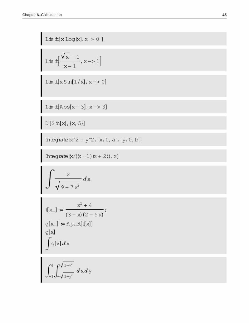
Limit[ x Log[x], x -> 0 ]

LimitB x - 1

x - 1, x -> 1F

Limit@x Sin@1 � xD, x -> 0D

Limit@Abs@x - 3D, x -> 3DD@Sin@xD, 8x, 5<DIntegrate[x^2 + y^2, {x, 0, a}, {y, 0, b}]

Integrate[x/((x - 1)(x + 2)), x]

á x

9 + 7 x2

âx

f@x_D :=x2 + 4H3 - xL H2 - 5 xL ;

g@x_D := Apart@f@xDDg@xDà g@xD âx

à-1

1à- 1-y2

1-y2

âx ây


à0

1à0

1Ix y + y2M âx ây

à0

Π

3 ày

Π

3 Sin@xDx

âx ây

IntegrateA MaxA x y2, x2 yE BooleA x2 + y2 £ 1 E, 8x, -¥, ¥<,8y, -¥, ¥<Ef@t_D := Sin@tDLaplaceTransform@f@tD, t, sDInverseLaplaceTransform@%, s, tDLaplaceTransform@t^4 f@tD, t, sDInverseLaplaceTransform@%, s, tD

Exercise 2

Use Mathematica to evaluate the following

limx®-1x + 1

x3 - x,

limh®0H1 + hL-2 - 1

h,

limx®¥x2 - 9

2 x - 6,

,


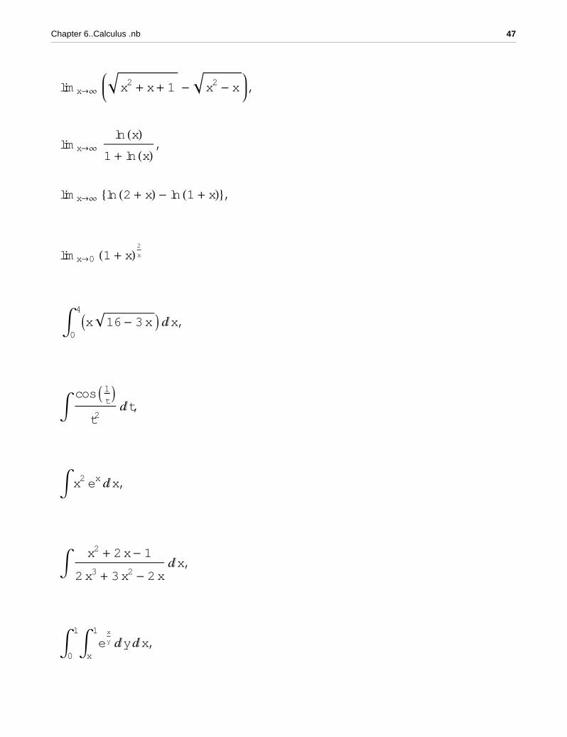
limx®¥ x2 + x + 1 - x2 - x ,

limx®¥ln HxL

1 + ln HxL ,

limx®¥ 8ln H2 + xL - ln H1 + xL<,

limx®0 H1 + xL 2

x

à0

4Ix 16 - 3 x M âx,

à cos I 1t

Mt2

â t,

à x2 ex âx,

à x2 + 2 x - 1

2 x3 + 3 x2 - 2 xâx,

à0

1àx

1

ex

y ây âx,


à0

1ày2

1

y sin Ix2M âx ây,

Exercise 3

Calculate the first and the second

derivatives of each of the following

y = Hx + 2L8 I4 x3 + 3M6,

y =1

sin Hx - sin HxLL ,

y = ln Ix2 exM,y = 5x tan HxL,

Exercise 4

Find the first and the mixed partial derivatives for the following

f Hx, yL = x3 ln Hx - yL,f Hx, y, zL = x ey cos HzLExercise 5

Find the Taylor series expansion of each of the following1

1 + x2, at x = 0,


ln HxL , at x = 1


Ch6

Documents

x ydlcos

x 0d1run

x nchapter

x 2fbelow4

x yd x y sin

nl n x

x yd4 chapter

x yd total derivativeactivity