CH5 Overview 1. Agenda 1.History 2.Motivation 3.Cointegration 4.Applying the model 5.A trading strategy 6.Road map for strategy design 2.

1

CH5 Overview

2

Agenda

1. History2. Motivation3. Cointegration4. Applying the model5. A trading strategy6. Road map for strategy design

3

History• Now , we enter the second part of this book - Statistical Arbitrage

Pairs So we need to understand its development !1. The first practice person : Nunzio Tartaglia (quantitative group) Morgan Stanley in the mid 1980s.2. Mission: To develop quantitative arbitrage strategies using state-of-the-art statisticaltechniques.3. Today: Pairs trading has since increased in popularity and has become a common trading strategy used by hedge funds and institutional investors.

4

Motivation• General trading: To sell overvalued securities and buy the undervalued ones.

- Is it possible to determine that a security is overvalued or undervalued? (Hard!)- Market is public , this opportunity can exist for a long time?

• Pairs trading (resolve the problems) : - Idea : If two securities have similar characteristics, then the prices of both securities must be more or less the same. If the prices happen to be different , it could be that one of the securities is overpriced, the other security is underpriced. - Trading: 1) The mutual mispricing between the two securities is captured by the notion of spread. 2) Long-short position in the two securities is constructed by market neutral strategies.So , the different between general and pairs trading is the “position” that determine by thetrader or market!

5

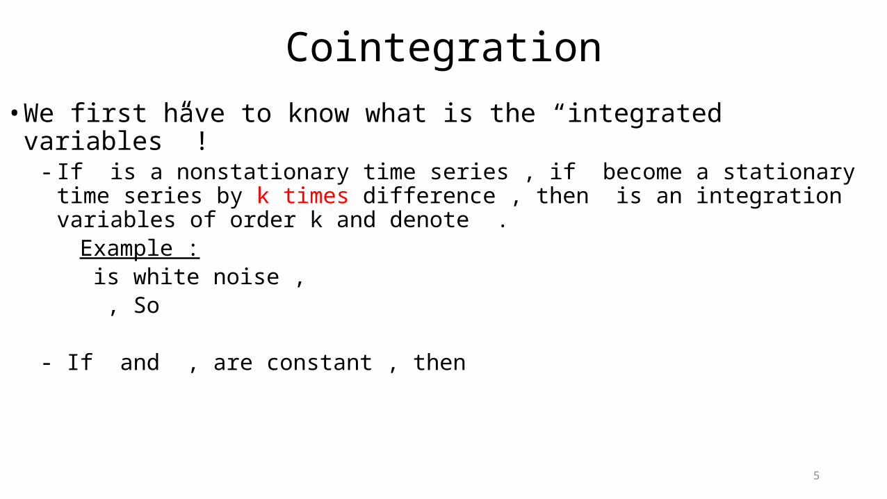
Cointegration• We first have to know what is the “integrated variables” !

- If is a nonstationary time series , if become a stationary time series by k times difference , then is an integration variables of order k and denote .

Example : is white noise , , So

- If and , are constant , then

6

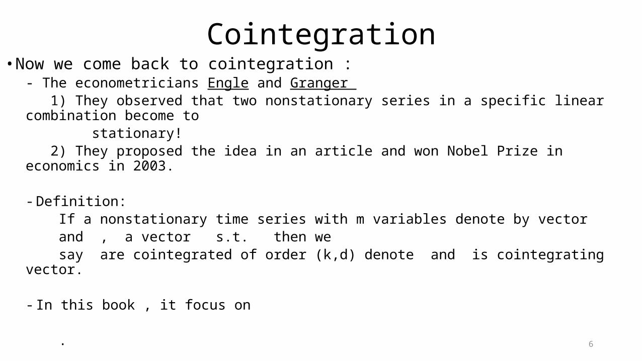
Cointegration• Now we come back to cointegration :

- The econometricians Engle and Granger 1) They observed that two nonstationary series in a specific linear combination become to stationary! 2) They proposed the idea in an article and won Nobel Prize in economics in 2003.

- Definition: If a nonstationary time series with m variables denote by vector and , a vector s.t. then we say are cointegrated of order (k,d) denote and is cointegrating vector.

- In this book , it focus on .

7

Cointegration• Real-life example :

1) Consumption and income2) Short-term and long-term rates3) The M2 money supply and GDP

8

Cointegration

• So , What is the cointegrated series dynamics ?1) The cointegrated systems have a long-run equilibrium. - If there is a deviation from the long-run mean, then one or both time series adjust themselves to restore the long-run equilibrium.(From Granger representation theorem) 2) We use “error correction” to capture the movement !

9

Cointegration• The error correction representation: - If and cointegrated , so

1) The error correction rate : - Indicative of the speed with which the time series corrects itself to maintain equilibrium. - One positive , another should negative.

2) Cointegration coefficient : - If two time series are said to be cointegarted, they share a common trend. - And one’s common trend component can be scaled up by another one.

Error correction part White noise part

Coefficient of cointegration

deviation from the long-run equilibrium

error correction rate

10

0.2

0.2

1

~ (0,1)

x

y

N

11

12

Cointegration• Common trends model (Stock and Watson - 1988):

1) Idea: - Time Series = Stationary Component + Nonstationary Component . - If two series are cointegrated, then the cointegrating linear composition acts to nullify the nonstationary components, leaving only the stationary components. Consider two time series:

We do linear combination

Random walk (nonstationary) componentsStationary components of the time series.

Should be zero , so

13

Applying the model• Let us fit the cointegration model to the logarithm of stock prices.

1) Assumption: - Logarithm of stock prices is random walk (nonstationary). It means is nonstationary.2) The error correction representation:

1 1 1

1 1 1

log( ) log( ) [log( ) log( )]

log( ) log( ) [log( ) log( )]

A A A Bt t A t t A

B B A Bt t B t t B

p p p p

p p p p

Return of the stocks in the current time period. Difference of the logarithm of price and the expression for the long-run equilibrium.

Spread

The past deviation from equilibrium plays a role in decidingthe next point in the time series.

Use past information to predict future

14

Applying the model• Now we focus on the cointegration part of the representation theorem. - The time series of the long-run equilibrium is stationary and mean reverting.

1) Consider a portfolio: - Long one share of A and short γ shares of B.2) Portfolio return :

A portfolio return Stationary time series !

15

A trading strategy

• A simple trading strategy : - Deviation from the equilibrium value : Put on the trade. - Restore the equilibrium value : Unwind the trade.The equilibrium value is also the mean value of the series.

16

A trading strategy• Let us consider the strategy :

1) A portfolio with Long one share of A and short γ shares of B.2) The long-run equilibrium is μ.3) Buy the portfolio when the time series is Δ below the mean.4) Sell the portfolio when the time series is Δ above the mean.

Buy : Sell

The profit on the trade is the incremental change in the spread, 2Δ.

17

A trading strategyExample:

Consider two stocks A and B that are cointegrated with the following data:

Cointegration Ratio = 1.5 Delta used for trade signal = 0.045 Bid price of A at time t = $19.50 Ask price of B at time t = $7.46 Ask price of A at time t + i = $20.10 Bid price of B at time t + i = $7.17 Average bid-ask spread for A = .0005 (5 basis points) Average bid-ask spread for B = .0010 ( 10 basis points)

18

A trading strategy Strategy: We first examine if trading is feasible given the average bid-ask spreads. Average trading slippage = ( 0.0005 + 1.5 × 0.0010) = .002 ( 20 basis points). This is smaller than the delta value of 0.045. Trading is therefore feasible. At time t, buy shares of A and short shares of B in the ratio 1:1.5. Spread at time t = log (19.50) – 1.5 × log (7.46) = –0.045. At time t + i , sell shares of A and buy back shares the shares of B. Spread at time t + i = log (20.10) – 1.5 × log (7.17) = 0.045.

Total return = return on A + γ× return on B = log (20.10) – log(19.50) + 1.5 × (log(7.46) – log(7.17) ) = 0.3 + 1.5 × 4.0 = .09 (9 percent)

19

Road map for strategy designStep 1• Identify stock pairs that could potentially be cointegrated.

1) Based on the stock fundamentals 2) Alternately on a pure statistical approach based on historical data.

- This book preferred (1).Step 2• The stock pairs are indeed cointegrated based on statistical evidence from

historical data. - Determining the cointegration coefficient and examining the spread time series to ensure that it is stationary and mean reverting.Step 3• Examine the cointegrated pairs to determine the delta.