McGraw-Hill/Irwin Copyright © 2007 by The McGraw-Hill Companies, Inc. All rights reserved. 10 10 Quality Control

Welcome message from author
This document is posted to help you gain knowledge. Please leave a comment to let me know what you think about it! Share it to your friends and learn new things together.
Transcript

McGraw-Hill/Irwin Copyright © 2007 by The McGraw-Hill Companies, Inc. All rights reserved.
1010
Quality Control
10-2
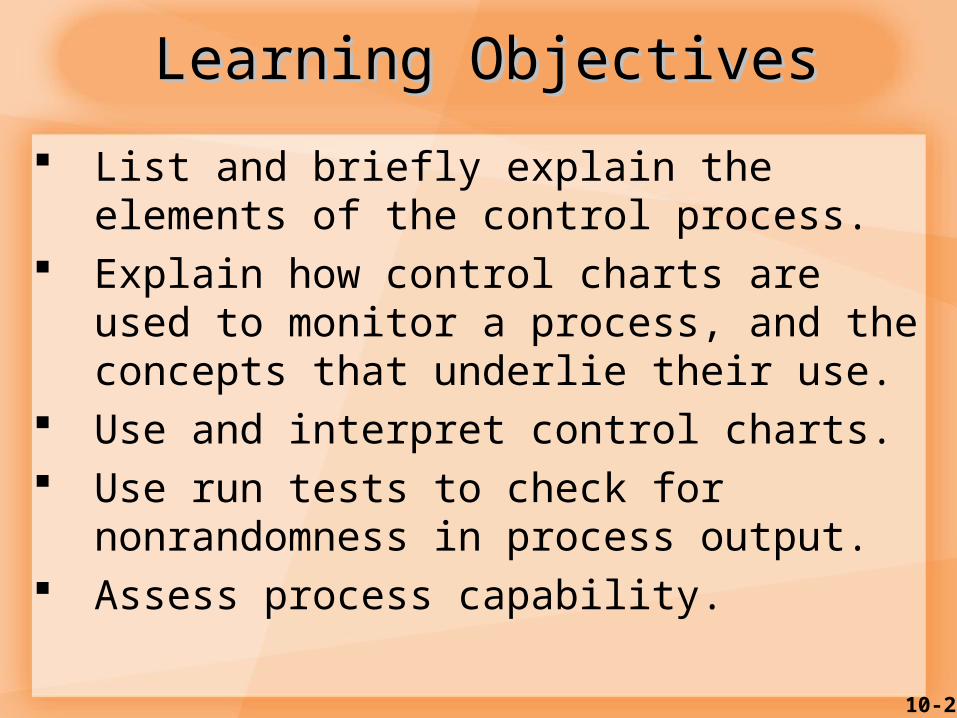
Learning ObjectivesLearning Objectives
List and briefly explain the elements of the control process.
Explain how control charts are used to monitor a process, and the concepts that underlie their use.
Use and interpret control charts. Use run tests to check for nonrandomness
in process output. Assess process capability.

10-3
Phases of Quality AssurancePhases of Quality Assurance
Acceptancesampling
Processcontrol
Continuousimprovement
Inspection of lotsbefore/afterproduction
Inspection andcorrective
action duringproduction
Quality builtinto theprocess
The leastprogressive
The mostprogressive
Figure 10.1
10-4
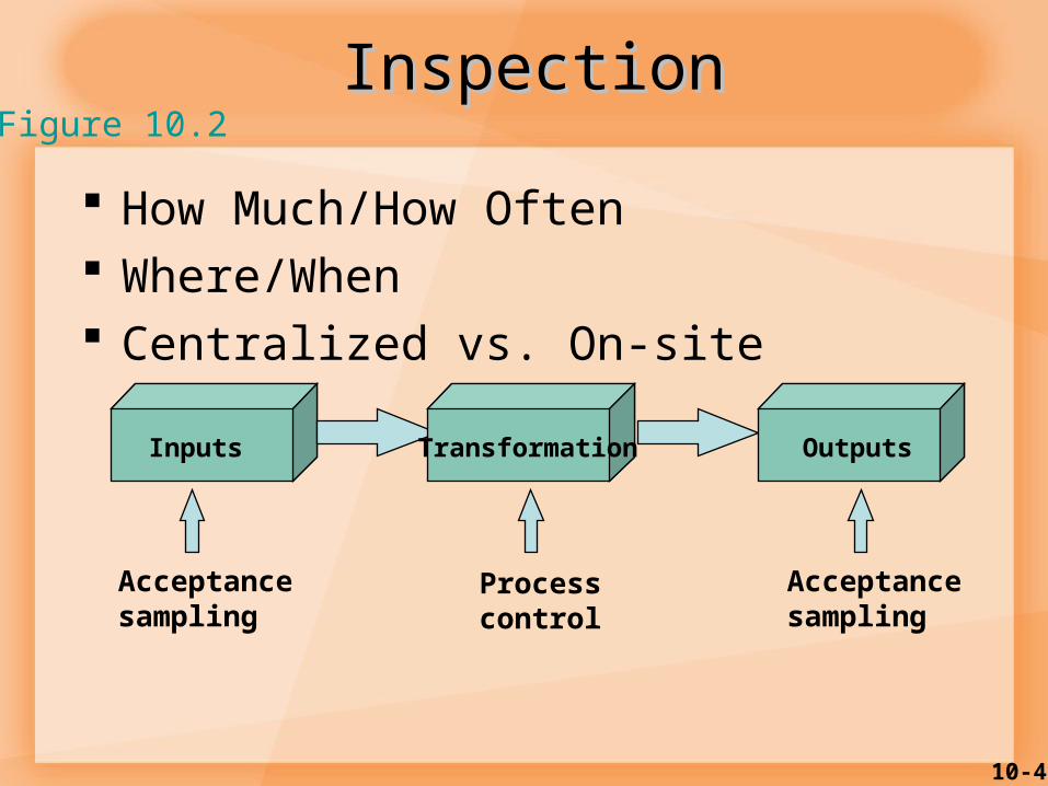
InspectionInspection
How Much/How Often Where/When Centralized vs. On-site
Inputs Transformation Outputs
Acceptancesampling
Processcontrol
Acceptancesampling
Figure 10.2

10-5
Co
st
OptimalAmount of Inspection
Inspection CostsInspection Costs
Cost of inspection
Cost of passingdefectives
Total Cost
Figure 10.3
10-6
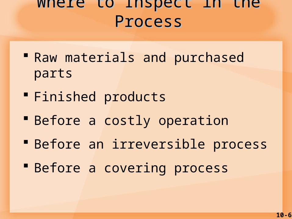
Where to Inspect in the ProcessWhere to Inspect in the Process
Raw materials and purchased parts
Finished products
Before a costly operation
Before an irreversible process
Before a covering process

10-7
Examples of Inspection PointsExamples of Inspection Points
Type ofbusiness
Inspectionpoints
Characteristics
Fast Food CashierCounter areaEating areaBuildingKitchen
AccuracyAppearance, productivityCleanlinessAppearanceHealth regulations
Hotel/motel Parking lotAccountingBuildingMain desk
Safe, well lightedAccuracy, timelinessAppearance, safetyWaiting times
Supermarket CashiersDeliveries
Accuracy, courtesyQuality, quantity
Table 10.1
10-8
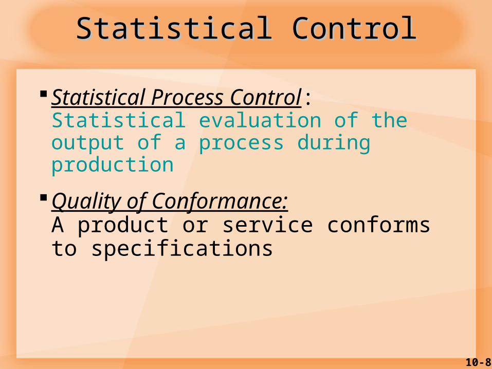
Statistical Process Control: Statistical evaluation of the output of a process during production
Quality of Conformance:A product or service conforms to specifications
Statistical ControlStatistical Control

10-9
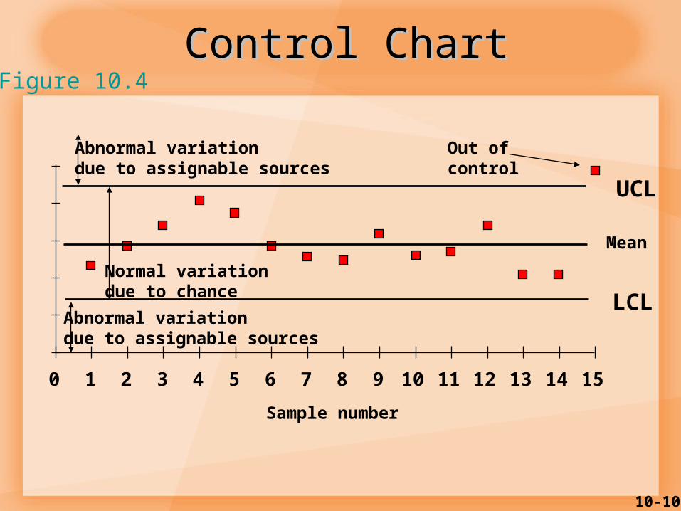
Control ChartControl Chart
Control Chart Purpose: to monitor process output to see
if it is random
A time ordered plot representative sample statistics obtained from an on going process (e.g. sample means)
Upper and lower control limits define the range of acceptable variation
10-10
Control ChartControl Chart
0 1 2 3 4 5 6 7 8 9 10 11 12 13 14 15
UCL
LCL
Sample number
Mean
Out ofcontrol
Normal variationdue to chance
Abnormal variationdue to assignable sources
Abnormal variationdue to assignable sources
Figure 10.4
10-11
Statistical Process ControlStatistical Process Control
The essence of statistical process control is to assure that the output of a process is random so that future output will be random.
10-12
Statistical Process ControlStatistical Process Control
The Control Process Define Measure Compare Evaluate Correct Monitor results

10-13
Statistical Process ControlStatistical Process Control
Variations and Control Random variation: Natural variations in the
output of a process, created by countless minor factors
Assignable variation: A variation whose source can be identified
10-14
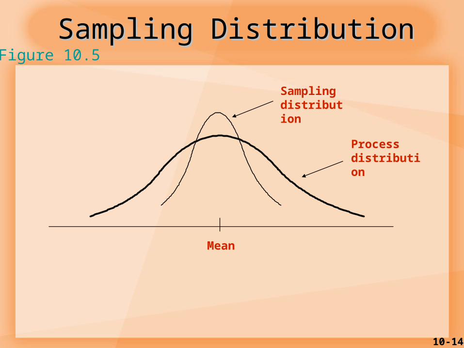
Sampling DistributionSampling Distribution
Samplingdistribution
Processdistribution
Mean
Figure 10.5
10-15
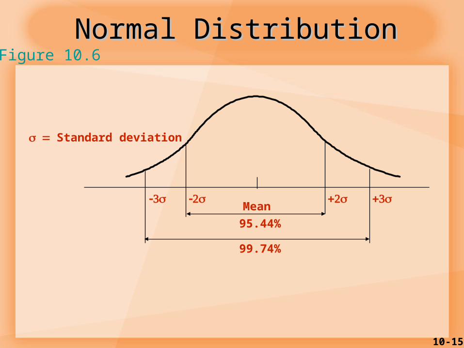
Normal DistributionNormal Distribution
Mean
95.44%
99.74%
Standard deviation
Figure 10.6

10-16
Control LimitsControl LimitsSamplingdistribution
Processdistribution
Mean
Lowercontrol
limit
Uppercontrol
limit
Figure 10.7

Control Limits are based on the Control Limits are based on the Normal CurveNormal Curve
x
0 1 2 3-3 -2 -1z
Standard deviation units or “z” units.
Standard deviation units or “z” units.

Control LimitsControl Limits
We establish the Upper Control Limits (UCL) and the Lower Control Limits (LCL) with plus or minus 3 standard deviations from some x-bar or mean value. Based on this we can expect 99.7% of our sample observations to fall within these limits.
xLCL UCL
99.7%
10-19
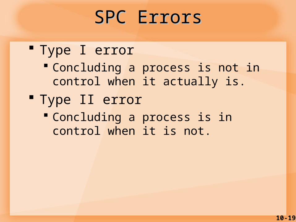
SPC ErrorsSPC Errors
Type I error Concluding a process is not in control
when it actually is.
Type II error Concluding a process is in control when it
is not.

10-20
Type I and Type II ErrorsType I and Type II Errors
In control Out of control
In control No Error Type I error
(producers risk)
Out of control
Type II Error
(consumers risk)
No error
Table 10.2

10-21
Type I ErrorType I Error
Mean
LCL UCL
/2 /2
Probabilityof Type I error
Figure 10.8

10-22
Observations from Sample Observations from Sample DistributionDistribution
Sample number
UCL
LCL
1 2 3 4
Figure 10.9

10-23
Control Charts for VariablesControl Charts for Variables
Mean control charts
Used to monitor the central tendency of a process.
X bar charts
Range control charts
Used to monitor the process dispersion
R charts
Variables generate data that are Variables generate data that are measuredmeasured..
10-24
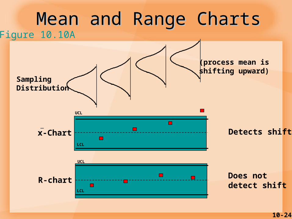
Mean and Range ChartsMean and Range Charts
UCL
LCL
UCL
LCL
R-chart
x-Chart Detects shift
Does notdetect shift
Figure 10.10A
(process mean is shifting upward)
SamplingDistribution

10-25
x-Chart
UCL
Does notreveal increase
Mean and Range ChartsMean and Range Charts
UCL
LCL
LCL
R-chart Reveals increase
Figure 10.10B
(process variability is increasing)SamplingDistribution

10-26
Statistical Process Control ChartStatistical Process Control Chart
Exhibit S9.21

10-27
Control Chart Decision RulesControl Chart Decision Rules
Exhibit S9.22Source: Bertrand L. Hansen, Quality Control: Theory and Applications © 1963, p. 65. Reprinted by permission of Pearson Education, Inc., Upper Saddle River, NJ.

10-28
Control Chart Decision RulesControl Chart Decision Rules
Exhibit S9.22 (cont’d)Source: Bertrand L. Hansen, Quality Control: Theory and Applications © 1963, p. 65. Reprinted by permission of Pearson Education, Inc., Upper Saddle River, NJ.

10-29
Changes in Mean and Variation Changes in Mean and Variation of Sample Mean Distributionsof Sample Mean Distributions
Exhibit S9.23
10-30
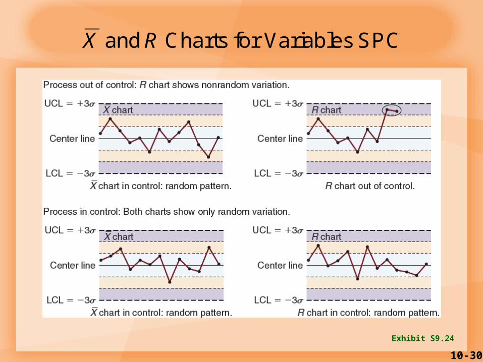
Exhibit S9.24
SPC Variablesfor Charts and RX
10-31
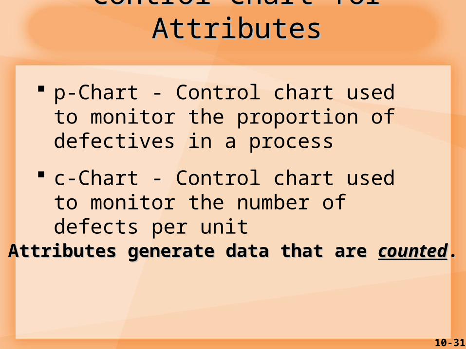
Control Chart for AttributesControl Chart for Attributes
p-Chart - Control chart used to monitor the proportion of defectives in a process
c-Chart - Control chart used to monitor the number of defects per unit
Attributes generate data that are Attributes generate data that are countedcounted..
10-32
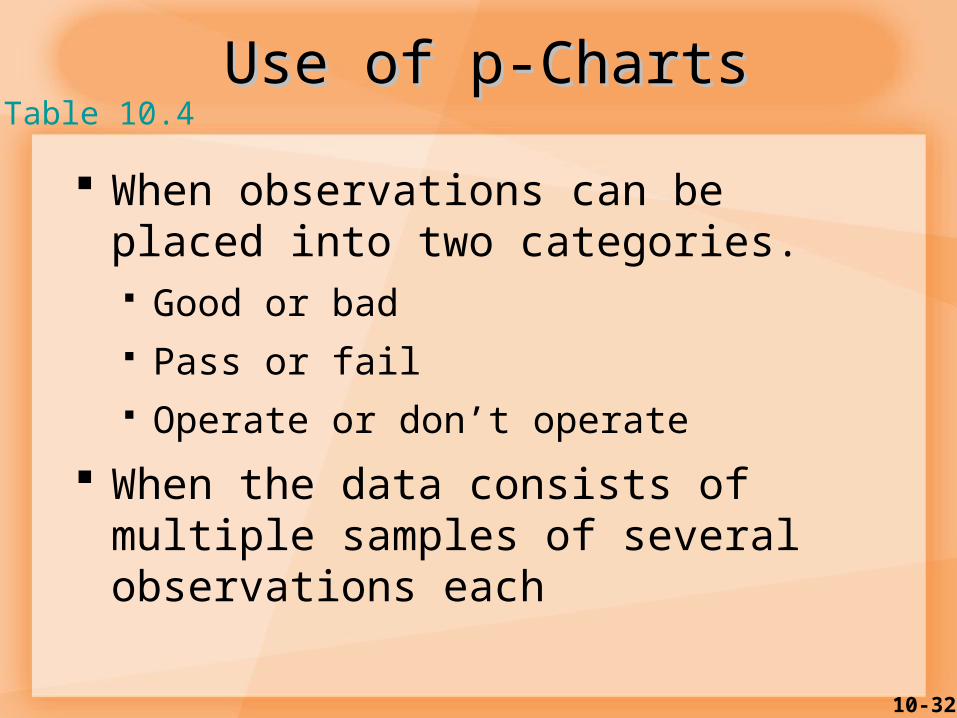
Use of p-ChartsUse of p-Charts
When observations can be placed into two categories. Good or bad Pass or fail Operate or don’t operate
When the data consists of multiple samples of several observations each
Table 10.4
10-33
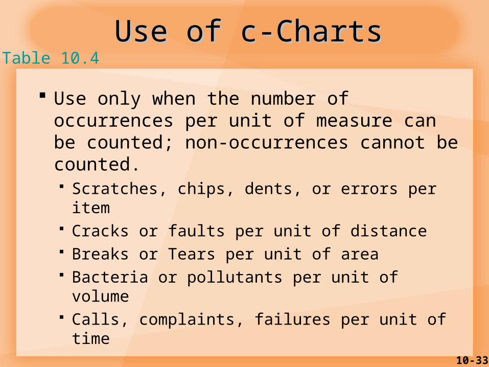
Use of c-ChartsUse of c-Charts
Use only when the number of occurrences per unit of measure can be counted; non-occurrences cannot be counted. Scratches, chips, dents, or errors per item Cracks or faults per unit of distance Breaks or Tears per unit of area Bacteria or pollutants per unit of volume Calls, complaints, failures per unit of time
Table 10.4

10-34
Use of Control ChartsUse of Control Charts
At what point in the process to use control charts
What size samples to take
What type of control chart to use
Variables
Attributes

10-35
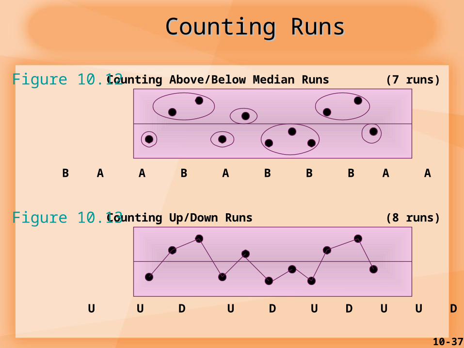
Run TestsRun Tests
Run test – a test for randomness
Any sort of pattern in the data would suggest a non-random process
All points are within the control limits - the process may not be random

10-36
Nonrandom Patterns in Control Nonrandom Patterns in Control chartscharts
Trend Cycles Bias Mean shift Too much dispersion
10-37
Counting Above/Below Median Runs (7 runs)
Counting Up/Down Runs (8 runs)
U U D U D U D U U D
B A A B A B B B A A B
Figure 10.12
Figure 10.13
Counting RunsCounting Runs

10-38
NonRandom VariationNonRandom Variation
Managers should have response plans to investigate cause
May be false alarm (Type I error) May be assignable variation

10-39
Tolerances or specifications Range of acceptable values established by engineering
design or customer requirements
Process variability Natural variability in a process—measured by std devn of
process
Process capability Process variability relative to specification--- determination
of whether variability inherent in the output of process that is in control falls within the design specifications for the product output
Control Limits
Statistical limits that reflect the extent to which sample statistics like mean,range can vary due to randomness alone
Process CapabilityProcess Capability

10-40
Properties of a Normal Properties of a Normal DistributionDistribution
The distribution is bilaterally symmetrical. 68.3 percent of the distribution lies between
plus and minus one standard deviation from the mean.
95.4 percent of the distribution lies between plus and minus two standard deviations from the mean.
99.7 percent of the distribution lies between plus and minus three standard deviations from the mean.

10-41
Areas under the Normal Distribution Areas under the Normal Distribution Curve Corresponding to Different Curve Corresponding to Different
Numbers of Numbers of Standard Deviations from the MeanStandard Deviations from the Mean
Exhibit S9.19

10-42
Statistical Process Control Statistical Process Control (cont’d)(cont’d)
Process Capability (Study) Comparing inherent variation in a process to the
customer’s requirements (the specifications) to determine whether the process can produce what the customer requires Collect data on the process while the process is
operating without known causes of variation. Compare the customer’s requirements to the inherent
variation of the process. If the customer’s specifications fall within the three standard
deviations for the process, some predictable percentage of the time, the process will produce output that will not meet the customer’s needs.

10-43
Capability StudyCapability Study
Exhibit S9.20
10-44
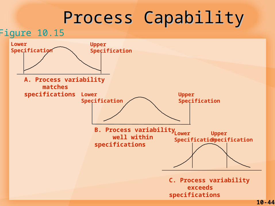
Process CapabilityProcess CapabilityLowerSpecification
UpperSpecification
A. Process variability matches specifications
LowerSpecification
UpperSpecification
B. Process variability well within specifications
LowerSpecification
UpperSpecification
C. Process variability exceeds specifications
Figure 10.15

10-45
In case c,options are
Redesign process to achieve desired output
Use a new process
Ensure 100% inspection
Change specification

10-46
Process Capability RatioProcess Capability Ratio
Process capability ratio, Cp = specification widthprocess width
Upper specification – lower specification6
Cp =
3
X-UTLor
3
LTLXmin=C pk
If the process is centered use Cp
If the process is not centered use Cpk

10-47
Minimum process capability required=1. Good measure=1.33 For cp=1,DPM=2700 and for
cp=1.3330,DPM=30 For a Six sigma programme,Cp=2 –Process
variability is so small that design tolerance is six SD above and below the process mean
Cp=2 means Specification width=(6SD+6SD)/6SD
Fig 10.16
10-48
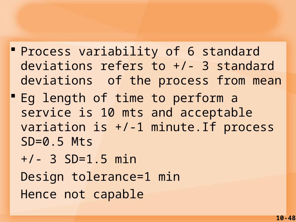
Process variability of 6 standard deviations refers to +/- 3 standard deviations of the process from mean
Eg length of time to perform a service is 10 mts and acceptable variation is +/-1 minute.If process SD=0.5 Mts
+/- 3 SD=1.5 min
Design tolerance=1 min
Hence not capable
10-49
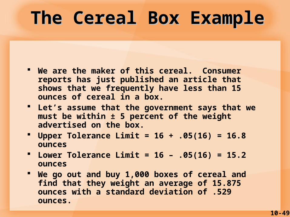
The Cereal Box ExampleThe Cereal Box Example
We are the maker of this cereal. Consumer reports has just published an article that shows that we frequently have less than 15 ounces of cereal in a box.
Let’s assume that the government says that we must be within ± 5 percent of the weight advertised on the box.
Upper Tolerance Limit = 16 + .05(16) = 16.8 ounces Lower Tolerance Limit = 16 – .05(16) = 15.2 ounces We go out and buy 1,000 boxes of cereal and find that
they weight an average of 15.875 ounces with a standard deviation of .529 ounces.
10-50
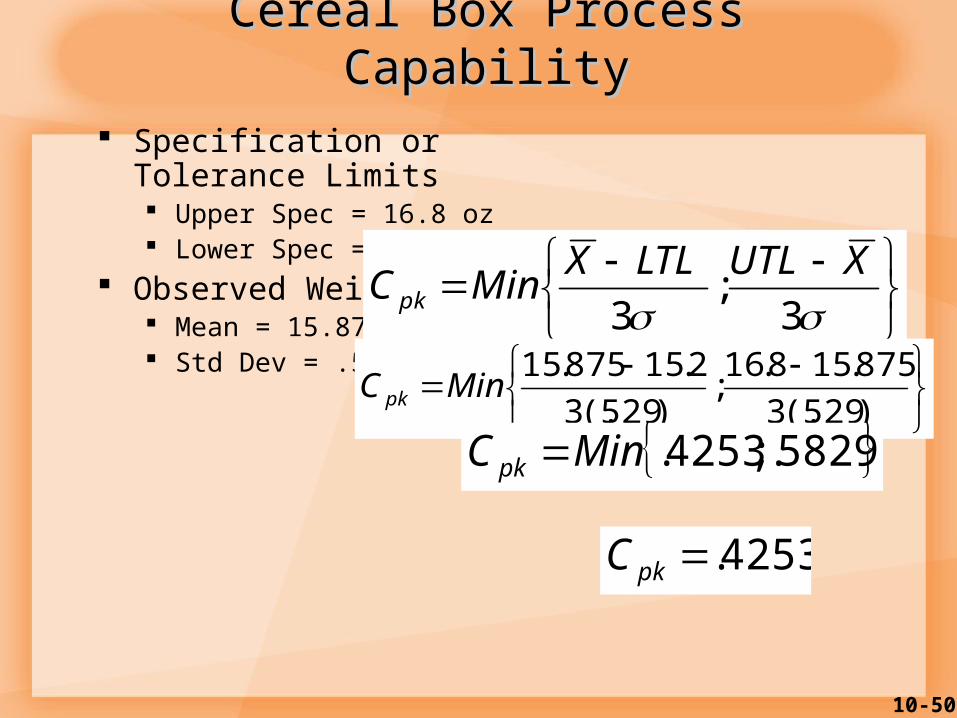
Cereal Box Process CapabilityCereal Box Process Capability
Specification or Tolerance Limits Upper Spec = 16.8 oz Lower Spec = 15.2 oz
Observed Weight Mean = 15.875 oz Std Dev = .529 oz
3
;3
XUTLLTLXMinC pk
)529(.3
875.158.16;
)529(.3
2.15875.15MinC pk
5829.;4253.MinC pk
4253.pkC

10-51
What does a CWhat does a Cpkpk of .4253 mean? of .4253 mean?
An index that shows how well the units being produced fit within the specification limits.
This is a process that will produce a relatively high number of defects.
Many companies look for a Cpk of 1.3 or better… 6-Sigma company wants 2.0!
10-52
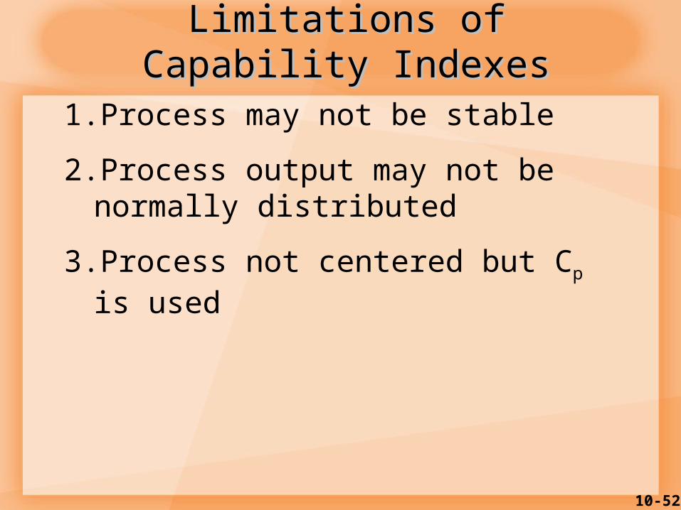
Limitations of Capability IndexesLimitations of Capability Indexes
1. Process may not be stable
2. Process output may not be normally distributed
3. Process not centered but Cp is used
10-53
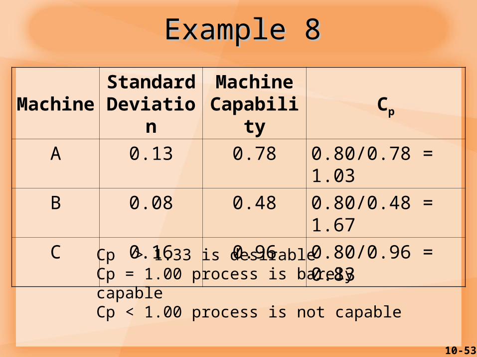
Example 8Example 8
MachineStandard Deviation
Machine Capability Cp
A 0.13 0.78 0.80/0.78 = 1.03
B 0.08 0.48 0.80/0.48 = 1.67
C 0.16 0.96 0.80/0.96 = 0.83
Cp > 1.33 is desirableCp = 1.00 process is barely capableCp < 1.00 process is not capable
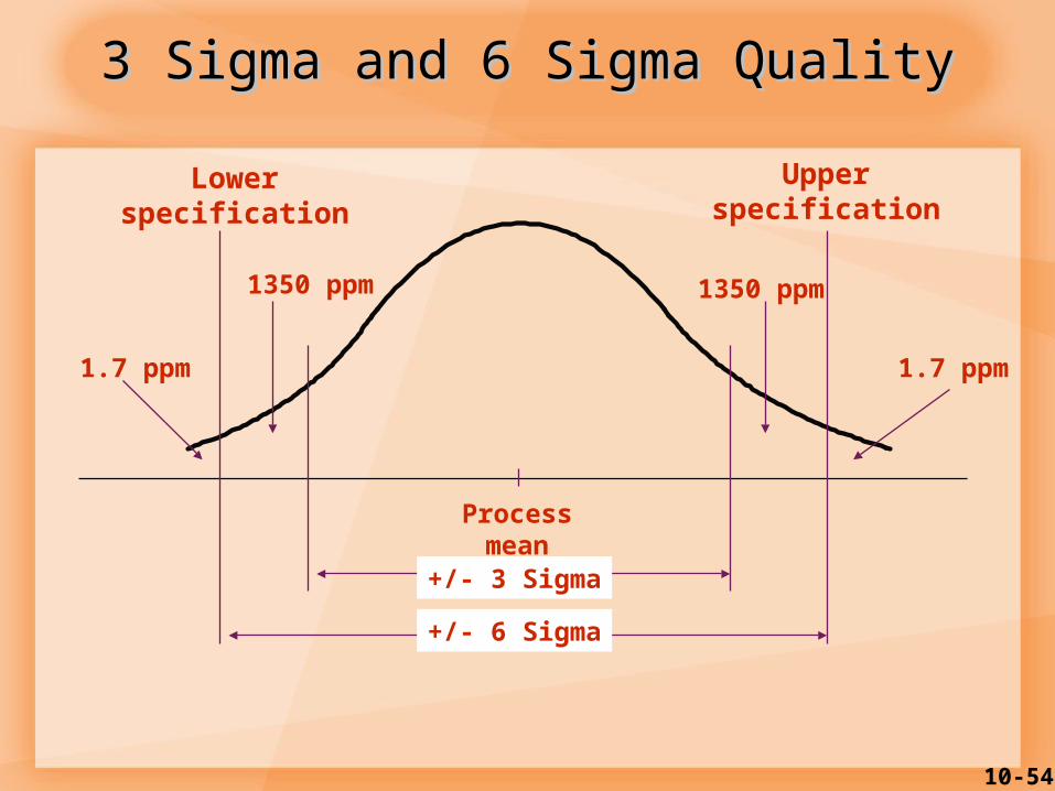
10-54
Processmean
Lowerspecification
Upperspecification
1350 ppm 1350 ppm
1.7 ppm 1.7 ppm
+/- 3 Sigma
+/- 6 Sigma
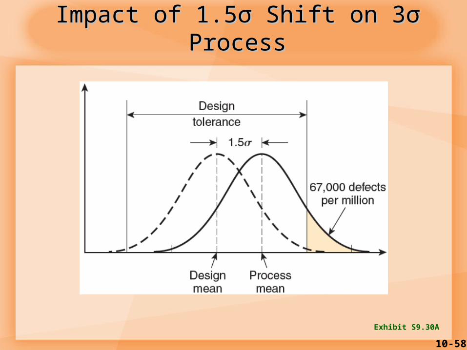
3 Sigma and 6 Sigma Quality3 Sigma and 6 Sigma Quality

10-55
Graph of the normal distribution, which underlies the statistical assumptions of the Six Sigma model. The Greek letter σ (sigma) marks the distance on the horizontal axis between the mean, µ, and the curve's inflection point. The greater this distance, the greater is the spread of values encountered. For the curve shown above, µ = 0 and σ = 1. The upper and lower specification limits (USL, LSL) are at a distance of 6σ from the mean. Because of the properties of the normal distribution, values lying that far away from the mean are extremely unlikely. Even if the mean were to move right or left by 1.5σ at some point in the future (1.5 sigma shift), there is still a good safety cushion. This is why Six Sigma aims to have processes where the mean is at least 6σ away from the nearest specification limit.
10-56

10-57
The Goal of Six SigmaThe Goal of Six Sigma
Exhibit S9.29
10-58
Impact of 1.5σ Shift on 3σ ProcessImpact of 1.5σ Shift on 3σ Process
Exhibit S9.30A

10-59
Impact of 1.5σ Shift on 6σ ProcessImpact of 1.5σ Shift on 6σ Process
Exhibit S9.30B

10-60
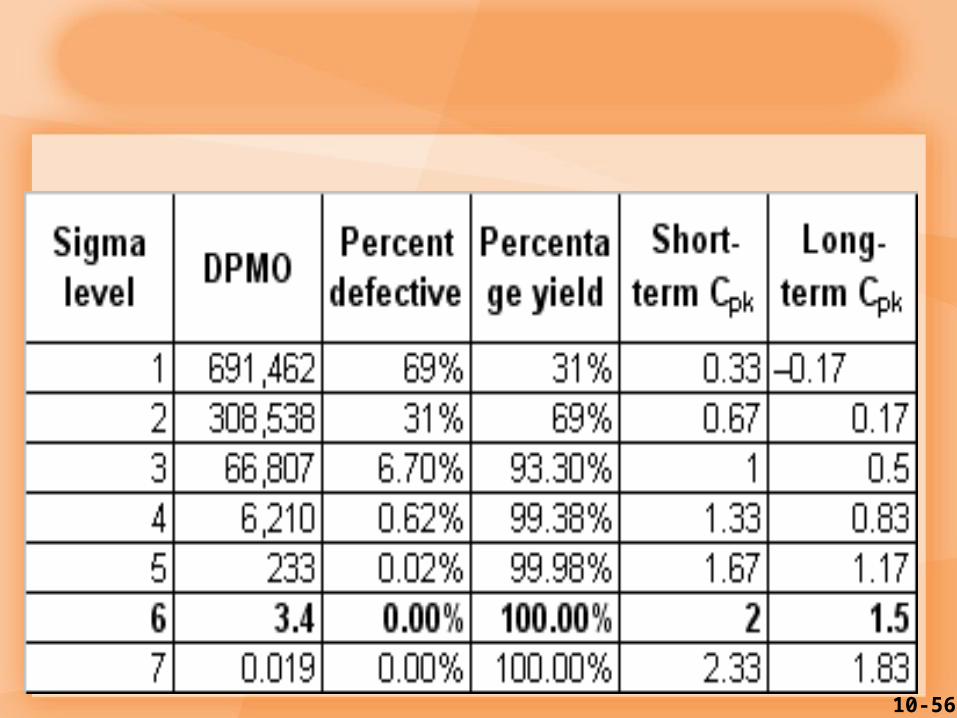
Defect Rates for Different Levels of Sigma Defect Rates for Different Levels of Sigma (σ) (σ)
Assuming a 1.5 Shift in Actual Mean from Assuming a 1.5 Shift in Actual Mean from Design MeanDesign Mean
Exhibit S9.31
10-61
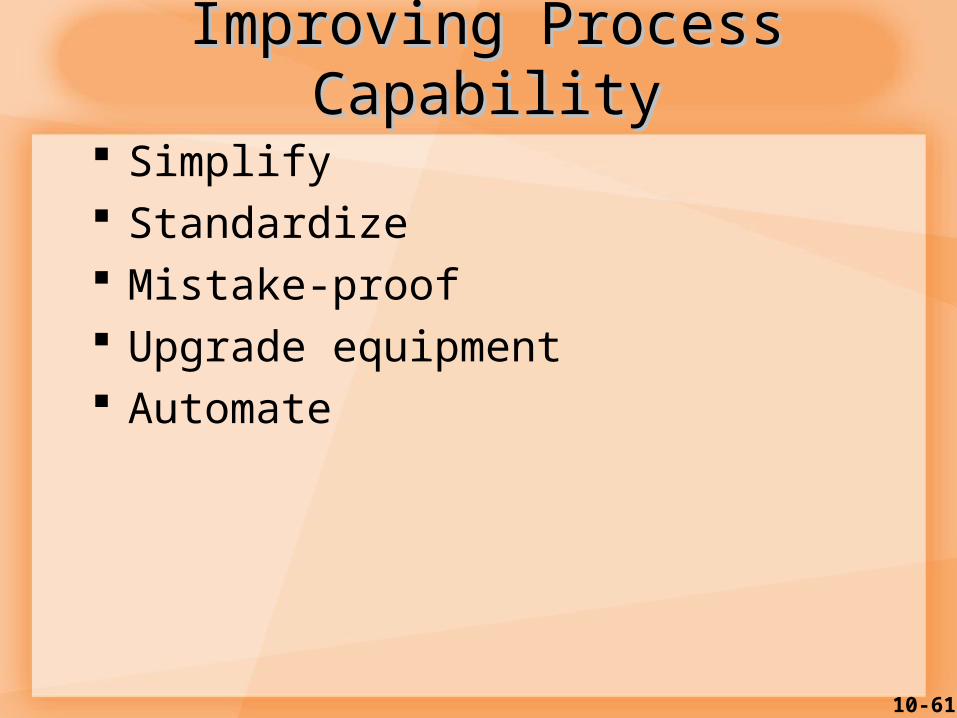
Improving Process CapabilityImproving Process Capability
Simplify Standardize Mistake-proof Upgrade equipment Automate

10-62
Taguchi Loss FunctionTaguchi Loss Function
Cost
TargetLowerspec
Upperspec
Traditionalcost function
Taguchicost function
Figure 10.17

10-63
Advanced Quality ToolsAdvanced Quality Tools
Affinity diagrams
Used to structure and clarify ideas by organizing them according to their affinity, or similarity, to each other.
Interrelationship digraph
Helps to sort out cause-and-effect relationships when there are a large number of interrelated issues that need to be better understood.

10-64
Affinity Affinity Diagram of Diagram of
Team Learning Team Learning ObjectivesObjectives Exhibit S9.9

10-65
Relations Diagram for Late Hospital Relations Diagram for Late Hospital DischargeDischarge
Exhibit S9.10

10-66
Advanced Quality Tools Advanced Quality Tools (cont’d)(cont’d)
Tree diagram Helps determine ways to meet objectives by
breaking down a main goal into subgoals and actions and identify the strategy to be taken.
Matrix diagram Used to organize information that can be
compared on a variety of characteristics in order to make a comparison, selection, or choice.
Arranges elements of a problem or event in rows and columns on a chart that shows relationships among each pair of elements.

10-67
Basic Structure of a Tree DiagramBasic Structure of a Tree Diagram
Exhibit S9.11

10-68
Matrix DiagramMatrix Diagram
Exhibit S9.12