Walpole,Probability and Statistics for Engineers & Scientists, 8th e., Pearson Edu. Chap 8-1 Chapter 8 Sampling Distribution

Welcome message from author
This document is posted to help you gain knowledge. Please leave a comment to let me know what you think about it! Share it to your friends and learn new things together.
Transcript

Walpole,Probability and Statistics for Engineers & Scientists, 8th e., Pearson Edu. Chap 8-1
Chapter 8
Sampling Distribution
Walpole,Probability and Statistics for Engineers & Scientists, 8th e., Pearson Edu. Chap 8-2
Chapter Goals
After completing this chapter, you should be able to:
Define the concept of a sampling distribution
Determine the mean and standard deviation for the sampling distribution of the sample mean, X
Sampling distribution of means
Central Limit Theorem
Sampling distribution of S2
Sampling distribution of ps
__
Walpole,Probability and Statistics for Engineers & Scientists, 8th e., Pearson Edu. Chap 8-3
Sampling Distributions
A sampling distribution is a distribution of all of the possible values of a statistic for a given size sample selected from a population
Walpole,Probability and Statistics for Engineers & Scientists, 8th e., Pearson Edu. Chap 8-4
Sampling Distribution
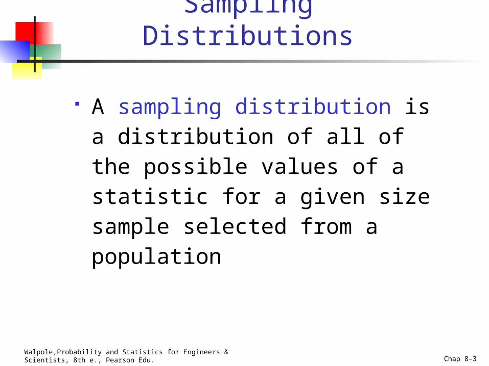
Assume there is a population …
Population size N=4
Random variable, X,
is age of individuals
Values of X: 18, 20,
22, 24 (years)
A B C D

Walpole,Probability and Statistics for Engineers & Scientists, 8th e., Pearson Edu. Chap 8-5
.3
.2
.1
0 18 20 22 24
A B C D
Uniform Distribution
P(x)
x
(continued)
Summary Measures for the Population Distribution:
Sampling Distribution
214
24222018
N
Xμ i
2.236N
μ)(Xσ
2i
Walpole,Probability and Statistics for Engineers & Scientists, 8th e., Pearson Edu. Chap 8-6
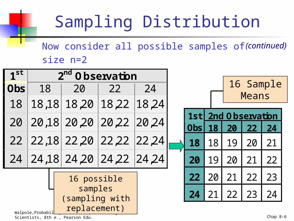
1st 2nd Observation Obs 18 20 22 24
18 18,18 18,20 18,22 18,24
20 20,18 20,20 20,22 20,24
22 22,18 22,20 22,22 22,24
24 24,18 24,20 24,22 24,24
16 possible samples (sampling with replacement)
Now consider all possible samples of size n=2
1st 2nd Observation Obs 18 20 22 24
18 18 19 20 21
20 19 20 21 22
22 20 21 22 23
24 21 22 23 24
(continued)
Sampling Distribution
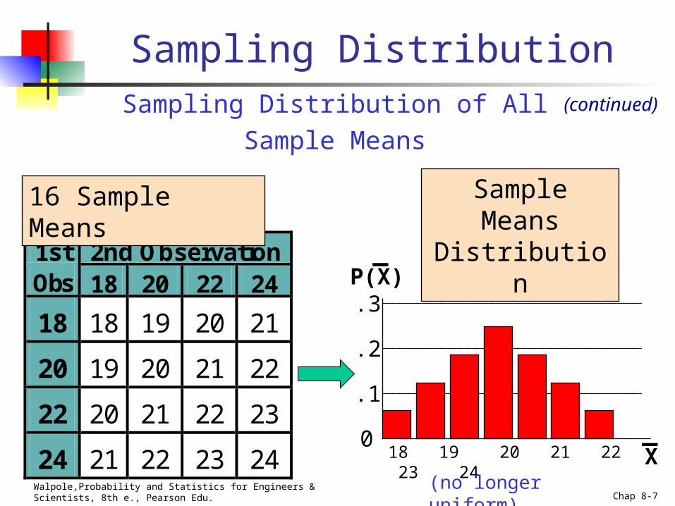
16 Sample Means
Walpole,Probability and Statistics for Engineers & Scientists, 8th e., Pearson Edu. Chap 8-7
1st 2nd Observation Obs 18 20 22 24
18 18 19 20 21
20 19 20 21 22
22 20 21 22 23
24 21 22 23 24
Sampling Distribution of All Sample Means
18 19 20 21 22 23 240
.1
.2
.3 P(X)
X
Sample Means Distribution
16 Sample Means
_
Sampling Distribution(continued)
(no longer uniform)
_

Walpole,Probability and Statistics for Engineers & Scientists, 8th e., Pearson Edu. Chap 8-8
Summary Measures of this Sampling Distribution:
Sampling Distribution(continued)
2116
24211918
N
Xμ i
X
1.5816
21)-(2421)-(1921)-(18
N
)μX(σ
222
2Xi
X

Walpole,Probability and Statistics for Engineers & Scientists, 8th e., Pearson Edu. Chap 8-9
Comparing the Population with its Sampling Distribution
18 19 20 21 22 23 240
.1
.2
.3 P(X)
X 18 20 22 24
A B C D
0
.1
.2
.3
PopulationN = 4
P(X)
X _
1.58σ 21μXX
2.236σ 21μ
Sample Means Distributionn = 2
_

Walpole,Probability and Statistics for Engineers & Scientists, 8th e., Pearson Edu. Chap 8-10
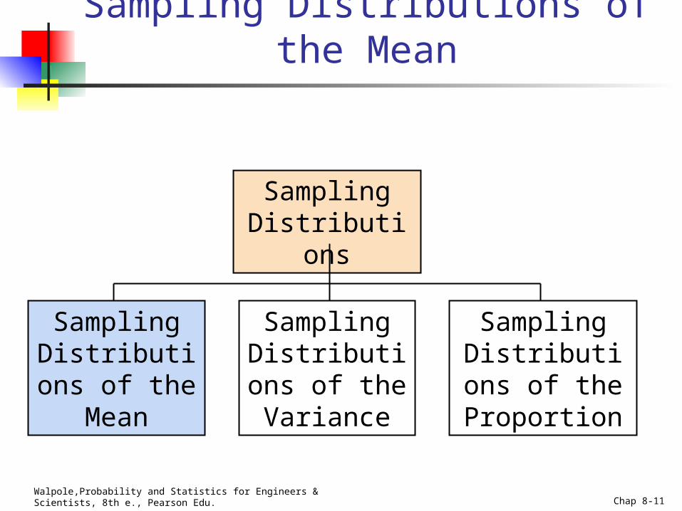
Sampling Distributions
Sampling Distributions
Sampling Distributions
of the Mean
Sampling Distributions
of the Proportion
Sampling Distributions
of the Variance
Walpole,Probability and Statistics for Engineers & Scientists, 8th e., Pearson Edu. Chap 8-11
Sampling Distributions of the Mean
Sampling Distributions
Sampling Distributions
of the Mean
Sampling Distributions
of the Proportion
Sampling Distributions
of the Variance

Walpole,Probability and Statistics for Engineers & Scientists, 8th e., Pearson Edu. Chap 8-12
Standard Error of the Mean
Different samples of the same size from the same population will yield different sample means
A measure of the variability in the mean from sample to sample is given by the Standard Error of the Mean:
Note that the standard error of the mean decreases as the sample size increases
n
σσ
X

Walpole,Probability and Statistics for Engineers & Scientists, 8th e., Pearson Edu. Chap 8-13
If the Population is Normal
If a population is normal with mean μ and
standard deviation σ, the sampling distribution
of is also normally distributed with
and
(This assumes that sampling is with replacement or sampling is without replacement from an infinite population)
X
μμX
n
σσ
X

Walpole,Probability and Statistics for Engineers & Scientists, 8th e., Pearson Edu. Chap 8-14
Z-value for Sampling Distributionof the Mean
Z-value for the sampling distribution of :
where: = sample mean
= population mean
= population standard deviation
n = sample size
Xμσ
n
σμ)X(
σ
)μX(Z
X
X
X

Walpole,Probability and Statistics for Engineers & Scientists, 8th e., Pearson Edu. Chap 8-15
Finite Population Correction
Apply the Finite Population Correction if: the sample is large relative to the population
(n is greater than 5% of N)
and… Sampling is without replacement
Then
1NnN
n
σ
μ)X(Z

Walpole,Probability and Statistics for Engineers & Scientists, 8th e., Pearson Edu. Chap 8-16
Normal Population Distribution
Normal Sampling Distribution (has the same mean)
Sampling Distribution Properties
(i.e. is unbiased )xx
x
μμx
μ
xμ

Walpole,Probability and Statistics for Engineers & Scientists, 8th e., Pearson Edu. Chap 8-17
Sampling Distribution Properties
For sampling with replacement:
As n increases,
decreasesLarger sample size
Smaller sample size
x
(continued)
xσ
μ

Walpole,Probability and Statistics for Engineers & Scientists, 8th e., Pearson Edu. Chap 8-18
If the Population is not Normal
We can apply the Central Limit Theorem:
Even if the population is not normal, …sample means from the population will be
approximately normal as long as the sample size is large enough.
Properties of the sampling distribution:
andμμx n
σσx

Walpole,Probability and Statistics for Engineers & Scientists, 8th e., Pearson Edu. Chap 8-19
n↑
Central Limit Theorem
As the sample size gets large enough…
the sampling distribution becomes almost normal regardless of shape of population
x

Walpole,Probability and Statistics for Engineers & Scientists, 8th e., Pearson Edu. Chap 8-20
Population Distribution
Sampling Distribution (becomes normal as n increases)
Central Tendency
Variation
(Sampling with replacement)
x
x
Larger sample size
Smaller sample size
If the Population is not Normal(continued)
Sampling distribution properties:
μμx
n
σσx
xμ
μ

Walpole,Probability and Statistics for Engineers & Scientists, 8th e., Pearson Edu. Chap 8-21
How Large is Large Enough?
For most distributions, n > 30 will give a sampling distribution that is nearly normal
For fairly symmetric distributions, n > 15
For normal population distributions, the sampling distribution of the mean is always normally distributed
Walpole,Probability and Statistics for Engineers & Scientists, 8th e., Pearson Edu. Chap 8-22
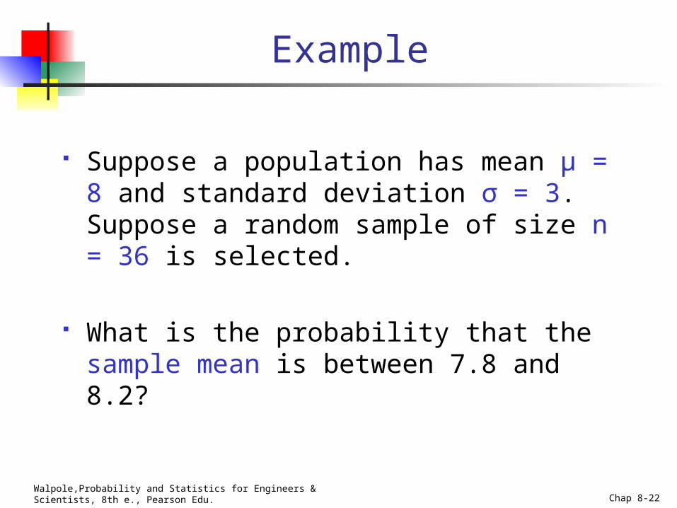
Example
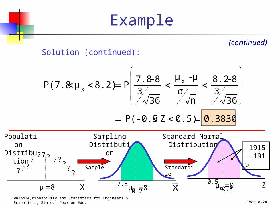
Suppose a population has mean μ = 8 and standard deviation σ = 3. Suppose a random sample of size n = 36 is selected.
What is the probability that the sample mean is between 7.8 and 8.2?

Walpole,Probability and Statistics for Engineers & Scientists, 8th e., Pearson Edu. Chap 8-23
Example
Solution:
Even if the population is not normally distributed, the central limit theorem can be used (n > 30)
… so the sampling distribution of is approximately normal
… with mean = 8
…and standard deviation
(continued)
x
xμ
0.536
3
n
σσx
Walpole,Probability and Statistics for Engineers & Scientists, 8th e., Pearson Edu. Chap 8-24
Example
Solution (continued):(continued)
0.38300.5)ZP(-0.5
363
8-8.2
nσ
μ- μ
363
8-7.8P 8.2) μ P(7.8 X
X
Z7.8 8.2 -0.5 0.5
Sampling Distribution
Standard Normal Distribution .1915
+.1915
Population Distribution
??
??
?????
??? Sample Standardize
8μ 8μX
0μz xX

Walpole,Probability and Statistics for Engineers & Scientists, 8th e., Pearson Edu. Chap 8-25
Sampling Distributions of the S2
where:
the distribution with v = n – 1 degrees of freedom.
n
i
iXXSn
1 2
2
2
2
2)()1(
If S2 is the variance of a random sample of size n takenfrom a normal population having the variance σ2, then Chi-square statistic is:

Walpole,Probability and Statistics for Engineers & Scientists, 8th e., Pearson Edu. Chap 8-26
Sampling Distributions of the S2
2α
The 2 test statistic approximately follows a chi-squared distribution with one degree of freedom
0
Walpole,Probability and Statistics for Engineers & Scientists, 8th e., Pearson Edu. Chap 8-27
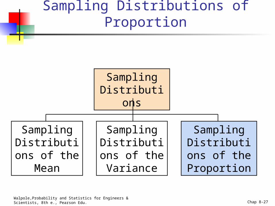
Sampling Distributions of Proportion
Sampling Distributions
Sampling Distributions
of the Mean
Sampling Distributions
of the Proportion
Sampling Distributions
of the Variance

Walpole,Probability and Statistics for Engineers & Scientists, 8th e., Pearson Edu. Chap 8-28
Sampling Distributions of p
p = the proportion of the population having some characteristic
Sample proportion ( ps ) provides an estimate of p:
0 ≤ ps ≤ 1
ps has a binomial distribution
(assuming sampling with replacement from a finite population or without replacement from an infinite population)
size sample
interest ofstic characteri the having sample the in itemsofnumber
n
Xps

Walpole,Probability and Statistics for Engineers & Scientists, 8th e., Pearson Edu. Chap 8-29
Sampling Distribution of p
Approximated by a
normal distribution if:
where
and
(where p = population proportion)
Sampling DistributionP( ps)
.3
.2
.1 0
0 . 2 .4 .6 8 1 ps
pμsp
n
p)p(1σ
sp
5p)n(1
5np
and

Walpole,Probability and Statistics for Engineers & Scientists, 8th e., Pearson Edu. Chap 8-30
Z-Value for Proportions
If sampling is without replacement
and n is greater than 5% of the
population size, then must use
the finite population correction
factor:
1N
nN
n
p)p(1σ
sp
np)p(1
pp
σ
ppZ s
p
s
s
Standardize ps to a Z value with the formula:
pσ
Walpole,Probability and Statistics for Engineers & Scientists, 8th e., Pearson Edu. Chap 8-31
Example
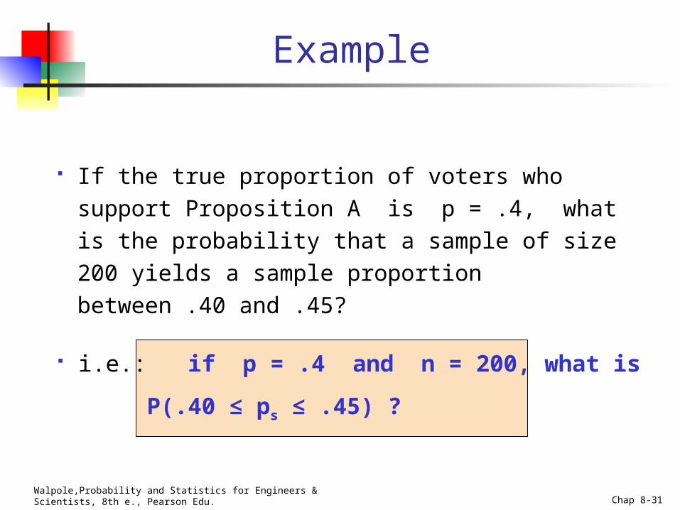
If the true proportion of voters who support
Proposition A is p = .4, what is the probability
that a sample of size 200 yields a sample
proportion between .40 and .45?
i.e.: if p = .4 and n = 200, what is
P(.40 ≤ ps ≤ .45) ?

Walpole,Probability and Statistics for Engineers & Scientists, 8th e., Pearson Edu. Chap 8-32
Example
if p = .4 and n = 200, what is
P(.40 ≤ ps ≤ .45) ?
(continued)
.03464200
.4).4(1
n
p)p(1σ
sp
1.44)ZP(0
.03464
.40.45Z
.03464
.40.40P.45)pP(.40 s
Find :
Convert to standard normal:
spσ

Walpole,Probability and Statistics for Engineers & Scientists, 8th e., Pearson Edu. Chap 8-33
Example
Z.45 1.44
.4251
Standardize
Sampling DistributionStandardized
Normal Distribution
if p = .4 and n = 200, what is
P(.40 ≤ ps ≤ .45) ?
(continued)
Use standard normal table: P(0 ≤ Z ≤ 1.44) = .4251
.40 0ps

Walpole,Probability and Statistics for Engineers & Scientists, 8th e., Pearson Edu. Chap 8-34
t-Distribution
Student’s t-Distribution
Population standard deviation is unknown
Sample size is not large enough
t value depends on degrees of freedom (d.f.)
The t-distribution is like the normal, but with greater spread since both and have fluctuations due to sampling.
nSX
T/
d.f. = v = n - 1

Walpole,Probability and Statistics for Engineers & Scientists, 8th e., Pearson Edu. Chap 8-35
If the mean of these three values is 8.0, then X3 must be 9 (i.e., X3 is not free to vary)
Degrees of Freedom (df)
Here, n = 3, so degrees of freedom = n – 1 = 3 – 1 = 2
(2 values can be any numbers, but the third is not free to vary for a given mean)
Idea: Number of observations that are free to vary after sample mean has been calculated
Example: Suppose the mean of 3 numbers is 8.0
Let X1 = 7
Let X2 = 8
What is X3?

Walpole,Probability and Statistics for Engineers & Scientists, 8th e., Pearson Edu. Chap 8-36
t-Distribution
t0
t (df = 5)
t (df = 13)t-distributions are bell-shaped and symmetric, but have ‘fatter’ tails than the normal
Standard Normal
(t with df = )
Note: t Z as n increases
Walpole,Probability and Statistics for Engineers & Scientists, 8th e., Pearson Edu. Chap 8-37
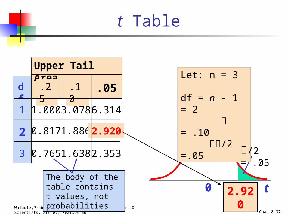
t Table
Upper Tail Area
df .25 .10 .05
1 1.000 3.078 6.314
2 0.817 1.886 2.920
3 0.765 1.638 2.353
t0 2.920The body of the table contains t values, not probabilities
Let: n = 3 df = n - 1 = 2 = .10 /2 =.05
/2 = .05

Walpole,Probability and Statistics for Engineers & Scientists, 8th e., Pearson Edu. Chap 8-38
t distribution values
With comparison to the Z value
Confidence t t t Z Level (10 d.f.) (20 d.f.) (30 d.f.) ____
.80 1.372 1.325 1.310 1.28
.90 1.812 1.725 1.697 1.64
.95 2.228 2.086 2.042 1.96
.99 3.169 2.845 2.750 2.57
Note: t Z as n increases

Walpole,Probability and Statistics for Engineers & Scientists, 8th e., Pearson Edu. Chap 8-39
F-Distribution
The F statistic is the ratio of two 2 random variables, each divided by its number of degrees of freedom.
If S12 and S2
2 are the variances of samples of size n1 and n2 taken from normal populations with variances 1
2 and 22,
then
has an F-distribution with 1 = n1 - 1 and 2 = n2 - 1 degrees of freedom.
For the F-distribution table
Note that since the ratio is inverted, 1 and 2 are reversed.
2
2
2
2
2
1
2
1
SS
F
),(1
),(12
211
ff

Walpole,Probability and Statistics for Engineers & Scientists, 8th e., Pearson Edu. Chap 8-40
F-Distribution Usage
The F-distribution is used in two-sample situations to draw inferences about the population variances.
In an area of statistics called analysis of variance, sources of variability are considered, for example: Variability within each of the two samples. Variability between the two samples (variability between
the means). The overall question is whether the variability within the
samples is large enough that the variability between the means is not significant.

Walpole,Probability and Statistics for Engineers & Scientists, 8th e., Pearson Edu. Chap 8-41
Ex.8.54
PulI-strength tests on 10 soldered leads for a semiconductor device yield the following results in pounds force required to rupture the bond:
19.8 12.7 13.2 16.9 10.6
18.8 11.1 14.3 17.0 12.5
Another set of 8 leads was tested after encapsulation to determine whether the pull strength has been increased by encapsulation of the device, with the following results:
24.9 22.8 23.6 22.1 20.4 21.6 21.8 22.5
Comment on the evidence available concerning equality of the two population variances.

Walpole,Probability and Statistics for Engineers & Scientists, 8th e., Pearson Edu. Chap 8-42
Solution

Walpole,Probability and Statistics for Engineers & Scientists, 8th e., Pearson Edu. Chap 8-43
Sampling Distribution Summary
Normal distribution: Sampling distribution of Xbar when is known for any population distribution.
t-distribution: Sampling distribution of Xbar when is unknown and S is used. Population must be normal.
Chi-square (2) distribution: Sampling distribution of S2. Population must be normal.
F-distribution: The distribution of the ratio of two 2 random variables. Sampling distribution of the ratio of the variances of two different samples. Population must be normal.
Related Documents