Chapter 6 Mathematical Preliminaries In the section we introduce tensors, but in fact you have surely encountered tensors in your studies, e.g. the stress, strain and inertia tensors. The presentation uses direct, indicial and matrix notations so that hopefully you can rely on your experience with matrices to get through this material without too much effort. Some results are stated without proof, however references are provided should you desire, and I hope you do, to obtain a more thorough understanding of the material. 6.1 Vector Spaces A set V is a real vector space, whose elements are often called vectors, if it is equipped with two operations: addition, denoted by the plus sign +, that takes any vector pair (a, b) ∈ V × V and generates the sum a + b, which is also a vector, and scalar multiplication that takes any scalar vector pair (α, a) ∈ R × V and generates the scalar multiple α a, which is also a vector, such that the following properties hold for any vectors a, b, c ∈ V and scalars α, β ∈ R: V 1 : Commutativity with respect to addition, a + b = b + a. V 2 : Associativity with respect to addition, (a + b) + c = a + (b + c). V 3 : Existence of the zero element 0 ∈ V such that a + 0 = a. V 4 : Existence of the negative elements −a ∈ V for each a ∈ V such that (−a) + a = 0. V 5 : Distributivity with respect to scalar multiplication, α (β a) = (αβ) a. V 6 : Distributivity with respect to scalar addition, (α + β) a = α a + β a. V 7 : Distributivity with respect to vector addition, α (a + b) = α a + α b. V 8 : Existence of the identity element 1 ∈ R such that 1 a = a. As seen here, we represent scalars as lower case Greek letters and vectors as lower case bold face Latin letters. And because of your experience with N-dimensional vector arrays we do not mention the obvious equalities, e.g. −0 = 0, −a = (−1) a, etc., which can be proved using the above axioms. We say the set of k ≥ 1 vectors {a 1 , a 2 , ··· , a k } that are elements of the vector space V are linearly dependent if there exists scalars α 1 , α 2 , ··· , α k that are not all zero such that 0 = k i=1 α i a i = α 1 a 1 + α 2 a 2 + ··· + α k a k (6.1) 253

Welcome message from author
This document is posted to help you gain knowledge. Please leave a comment to let me know what you think about it! Share it to your friends and learn new things together.
Transcript
Chapter 6
Mathematical Preliminaries
In the section we introduce tensors, but in fact you have surely encountered tensors in your studies, e.g. thestress, strain and inertia tensors. The presentation uses direct, indicial and matrix notations so that hopefullyyou can rely on your experience with matrices to get through this material without too much effort. Someresults are stated without proof, however references are provided should you desire, and I hope you do, toobtain a more thorough understanding of the material.
6.1 Vector SpacesA setV is a real vector space, whose elements are often called vectors, if it is equipped with two operations:addition, denoted by the plus sign +, that takes any vector pair (a, b) ∈ V ×V and generates the sum a + b,which is also a vector, and scalar multiplication that takes any scalar vector pair (α, a) ∈ R × V andgenerates the scalar multiple α a, which is also a vector, such that the following properties hold for anyvectors a, b, c ∈ V and scalars α, β ∈ R:
V1: Commutativity with respect to addition, a + b = b + a.
V2: Associativity with respect to addition, (a + b) + c = a + (b + c).
V3: Existence of the zero element 0 ∈ V such that a + 0 = a.
V4: Existence of the negative elements −a ∈ V for each a ∈ V such that (−a) + a = 0.
V5: Distributivity with respect to scalar multiplication, α (β a) = (α β) a.
V6: Distributivity with respect to scalar addition, (α + β) a = α a + β a.
V7: Distributivity with respect to vector addition, α (a + b) = α a + αb.
V8: Existence of the identity element 1 ∈ R such that 1 a = a.As seen here, we represent scalars as lower case Greek letters and vectors as lower case bold face Latin
letters. And because of your experience with N-dimensional vector arrays we do not mention the obviousequalities, e.g. −0 = 0, −a = (−1) a, etc., which can be proved using the above axioms.
We say the set of k ≥ 1 vectors a1, a2, · · · , ak that are elements of the vector space V are linearlydependent if there exists scalars α1,α2, · · · ,αk that are not all zero such that
0 =k∑
i=1αi ai
= α1 a1 + α2 a2 + · · · + αk ak (6.1)
253
mathematical preliminaries
otherwise we say the set is linearly independent. And we say a vector spaceV is k-dimensional (with k ≥ 1)if a set of k linearly independent vectors exists, but no set of l > k linearly independent vectors exists. Andfinally, a set of k linearly independent vectors in a k-dimensional vector spaceV forms a basis ofV.
Example 6.1. The idea of vector spaces, linear dependence, linear independence and bases is not limited to “vec-tors”. Indeed, the set of N-dimensional vector arrays RN , e.g.
a =
⎧⎪⎪⎪⎪⎪⎪⎪⎨⎪⎪⎪⎪⎪⎪⎪⎩
a1a2...aN
⎫⎪⎪⎪⎪⎪⎪⎪⎬⎪⎪⎪⎪⎪⎪⎪⎭
is an N-dimensional vector space, but so too is the set of N × M matrix arrays RN×M, e.g.
A =
⎡⎢⎢⎢⎢⎢⎢⎢⎢⎢⎢⎢⎢⎢⎢⎢⎣
A11 A12 · · · A1MA21 A22 · · · A2M...
......
AN1 AN2 · · · ANM
⎤⎥⎥⎥⎥⎥⎥⎥⎥⎥⎥⎥⎥⎥⎥⎥⎦
is an N×M-dimensional vector space. Possible bases for these two vector spaces with N = M = 2 are
10
,
01
and[1 00 0
],
[0 10 0
],
[0 01 0
],
[0 00 1
], respectively.
The set of trial functions K(Ω) = u : Ω ⊂ R → R | u ∈ C1p(Ω) and u(x0) = 0, cf. Eqn. 4.36, is an infinitedimensional vector space whereas the set Kh(Ω) = uh : Ω ⊂ R → R |ψi ∈ C1p(Ω), Ui ∈ R, uh(x) =
∑Mi=1 ψi(x)Ui is
an M-dimensional vector space, cf. Eqn. 5.27.Note that only in the first case do we refer to the elements as vectors even thoughmatrices and continuous functions
are also elements of vector spaces.
A set E is a Euclidean vector space if it is a three-dimensional vector space equipped with the additionaltwo operations: the inner (dot or scalar) product, denoted by the dot ·, that takes any pair of vectors ina, b ∈ V and generates the real number a · b ∈ R and the cross product, denoted by the wedge ∧, that takesany pair of vectors in a, b ∈ V and generates the vector a ∧ b ∈ V, such that the following properties holdfor any vectors a, b, c ∈ V and scalars α, β ∈ R:
E1: Symmetry, a · b = b · a.
E2: Linearity, (α a + βb) · c = α (a · c) + β (b · c).
E3: Positive definiteness, a · a ≥ 0 and a · a = 0 if and only if a = 0.
E4: a ∧ b = −b ∧ a.
E5: Associativity with respect to the cross product, (α a + βb) ∧ c = α (a ∧ c) + β (b ∧ c).
E6: a · (a ∧ b) = 0.
E7: (a ∧ b) · (a ∧ b) = (a · a) (b · b) − (a · b)2.
254
vector spaces
Any, not necessarily three dimensional, vector space that also exhibits properties E1, E2 and E3 is referredto as an inner product space.
The norm (magnitude, length, or modulus) of a vector a ∈ E is defined as
|a| = (a · a)12 . (6.2)
If |a| = 1 then a is a unit vector and if a · b = 0 then a and b are orthogonal.From property E7 with |a|2 = a · a and |b|2 = b · b we see that
(|a ∧ b||a| |b|
)2+
(a · b|a| |b|
)2= 1 (6.3)
to wit we define the angle θ ∈ [0, π] between the vectors a and b such that
cos θ =a · b|a| |b| ,
sin θ = |a ∧ b||a| |b|
. (6.4)
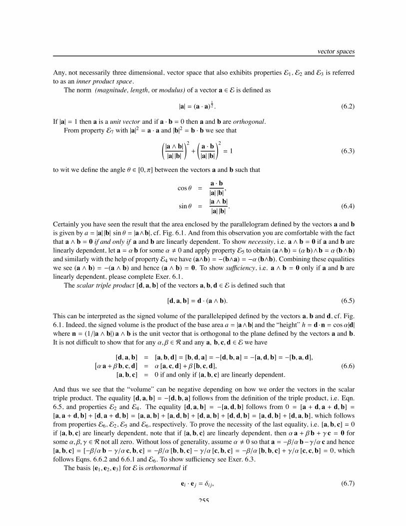
Certainly you have seen the result that the area enclosed by the parallelogram defined by the vectors a and bis given by a = |a| |b| sin θ = |a∧b|, cf. Fig. 6.1. And from this observation you are comfortable with the factthat a ∧ b = 0 if and only if a and b are linearly dependent. To show necessity, i.e. a ∧ b = 0 if a and b arelinearly dependent, let a = αb for some α ! 0 and apply property E5 to obtain (a∧b) = (αb)∧b = α (b∧b)and similarly with the help of property E4 we have (a∧b) = −(b∧a) = −α (b∧b). Combining these equalitieswe see (a ∧ b) = −(a ∧ b) and hence (a ∧ b) = 0. To show sufficiency, i.e. a ∧ b = 0 only if a and b arelinearly dependent, please complete Exer. 6.1.
The scalar triple product [d, a, b] of the vectors a, b, d ∈ E is defined such that
[d, a, b] = d · (a ∧ b). (6.5)
This can be interpreted as the signed volume of the parallelepiped defined by the vectors a, b and d, cf. Fig.6.1. Indeed, the signed volume is the product of the base area a = |a∧b| and the “height” h = d ·n = cosα|d|where n = (1/|a ∧ b|) a ∧ b is the unit vector that is orthogonal to the plane defined by the vectors a and b.It is not difficult to show that for any α, β ∈ R and any a, b, c, d ∈ E we have
[d, a, b] = [a, b, d] = [b, d, a] = −[d, b, a] = −[a, d, b] = −[b, a, d],[α a + βb, c, d] = α [a, c, d] + β [b, c, d],
[a, b, c] = 0 if and only if a, b, c are linearly dependent.(6.6)
And thus we see that the “volume” can be negative depending on how we order the vectors in the scalartriple product. The equality [d, a, b] = −[d, b, a] follows from the definition of the triple product, i.e. Eqn.6.5, and properties E2 and E4. The equality [d, a, b] = −[a, d, b] follows from 0 = [a + d, a + d, b] =[a, a + d, b] + [d, a + d, b] = [a, a, b] + [a, d, b] + [d, a, b] + [d, d, b] = [a, d, b] + [d, a, b], which followsfrom properties E6, E2, E5 and E6, respectively. To prove the necessity of the last equality, i.e. [a, b, c] = 0if a, b, c are linearly dependent, note that if a, b, c are linearly dependent, then α a + βb + γ c = 0 forsome α, β, γ ∈ R not all zero. Without loss of generality, assume α ! 0 so that a = −β/αb−γ/α c and hence[a, b, c] = [−β/αb − γ/α c, b, c] = −β/α [b, b, c] − γ/α [c, b, c] = −β/α [b, b, c] + γ/α [c, c, b] = 0, whichfollows Eqns. 6.6.2 and 6.6.1 and E6. To show sufficiency see Exer. 6.3.
The basis e1, e2, e3 for E is orthonormal if
ei · e j = δi j, (6.7)
255
mathematical preliminaries
a ∧ b
n
aa
bb
cd
e1e1
e2e2 e3
e3 θ
α
Figure 6.1: Illustrations of c = a ∧ b and [d, a, b] = d · (a ∧ b).
where
δi j =
1 if i = j0 if i ! j (6.8)
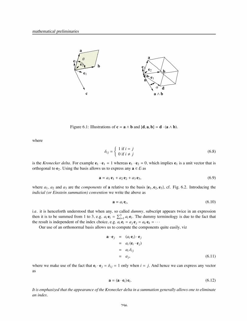
is the Kronecker delta. For example e1 · e1 = 1 whereas e1 · e2 = 0, which implies e1 is a unit vector that isorthogonal to e2. Using the basis allows us to express any a ∈ E as
a = a1 e1 + a2 e2 + a3 e3, (6.9)
where a1, a2 and a3 are the components of a relative to the basis e1, e2, e3, cf. Fig. 6.2. Introducing theindicial (or Einstein summation) convention we write the above as
a = ai ei, (6.10)
i.e. it is henceforth understood that when any, so called dummy, subscript appears twice in an expressionthen it is to be summed from 1 to 3, e.g. ai ei =
∑3i=1 ai ei. The dummy terminology is due to the fact that
the result is independent of the index choice, e.g. ai ei = aj e j = ak ek = · · ·Our use of an orthonormal basis allows us to compute the components quite easily, viz
a · e j = (ai ei) · e j= ai (ei · e j)= ai δi j= aj, (6.11)
where we make use of the fact that ei · e j = δi j = 1 only when i = j. And hence we can express any vectoras
a = (a · ei) ei. (6.12)
It is emphasized that the appearance of the Kronecker delta in a summation generally allows one to eliminatean index.
256
vector spaces
a
a1 e1
a2 e2
a3 e3
e1
e2
e3
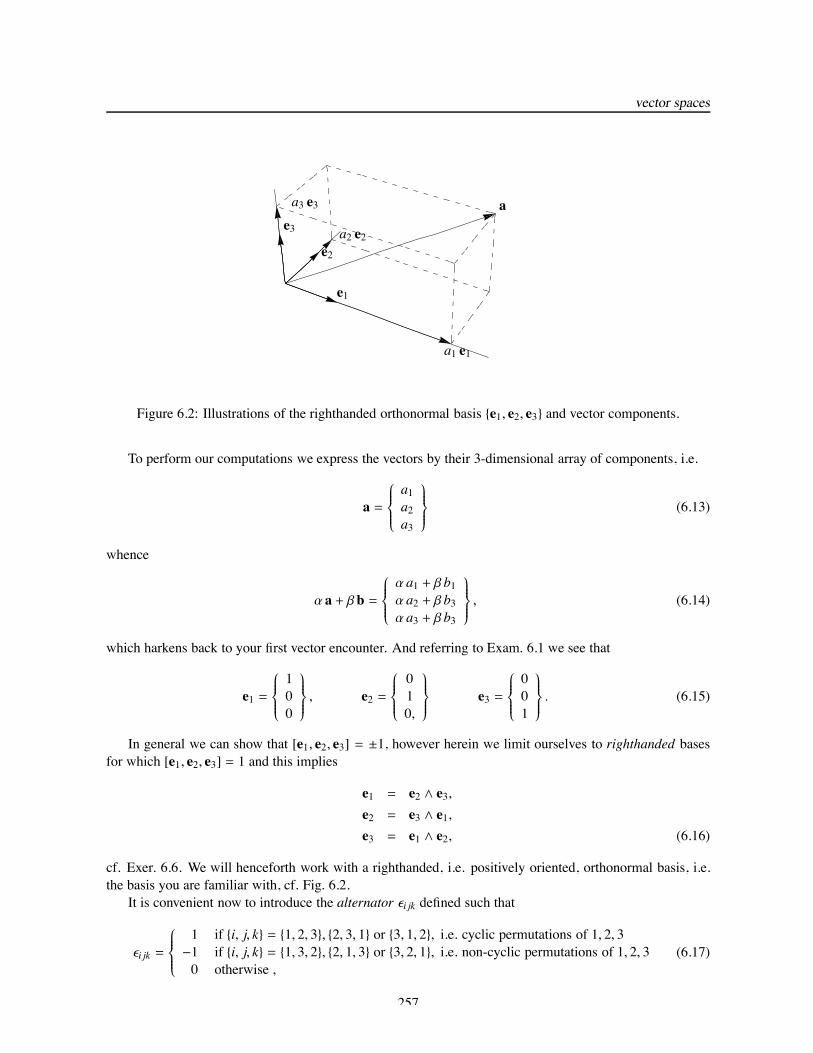
Figure 6.2: Illustrations of the righthanded orthonormal basis e1, e2, e3 and vector components.
To perform our computations we express the vectors by their 3-dimensional array of components, i.e.
a =
⎧⎪⎪⎪⎨⎪⎪⎪⎩
a1a2a3
⎫⎪⎪⎪⎬⎪⎪⎪⎭
(6.13)
whence
α a + βb =
⎧⎪⎪⎪⎨⎪⎪⎪⎩
α a1 + β b1α a2 + β b3α a3 + β b3
⎫⎪⎪⎪⎬⎪⎪⎪⎭, (6.14)
which harkens back to your first vector encounter. And referring to Exam. 6.1 we see that
e1 =
⎧⎪⎪⎪⎨⎪⎪⎪⎩
100
⎫⎪⎪⎪⎬⎪⎪⎪⎭, e2 =
⎧⎪⎪⎪⎨⎪⎪⎪⎩
010,
⎫⎪⎪⎪⎬⎪⎪⎪⎭
e3 =
⎧⎪⎪⎪⎨⎪⎪⎪⎩
001
⎫⎪⎪⎪⎬⎪⎪⎪⎭. (6.15)
In general we can show that [e1, e2, e3] = ±1, however herein we limit ourselves to righthanded basesfor which [e1, e2, e3] = 1 and this implies
e1 = e2 ∧ e3,e2 = e3 ∧ e1,e3 = e1 ∧ e2, (6.16)
cf. Exer. 6.6. We will henceforth work with a righthanded, i.e. positively oriented, orthonormal basis, i.e.the basis you are familiar with, cf. Fig. 6.2.
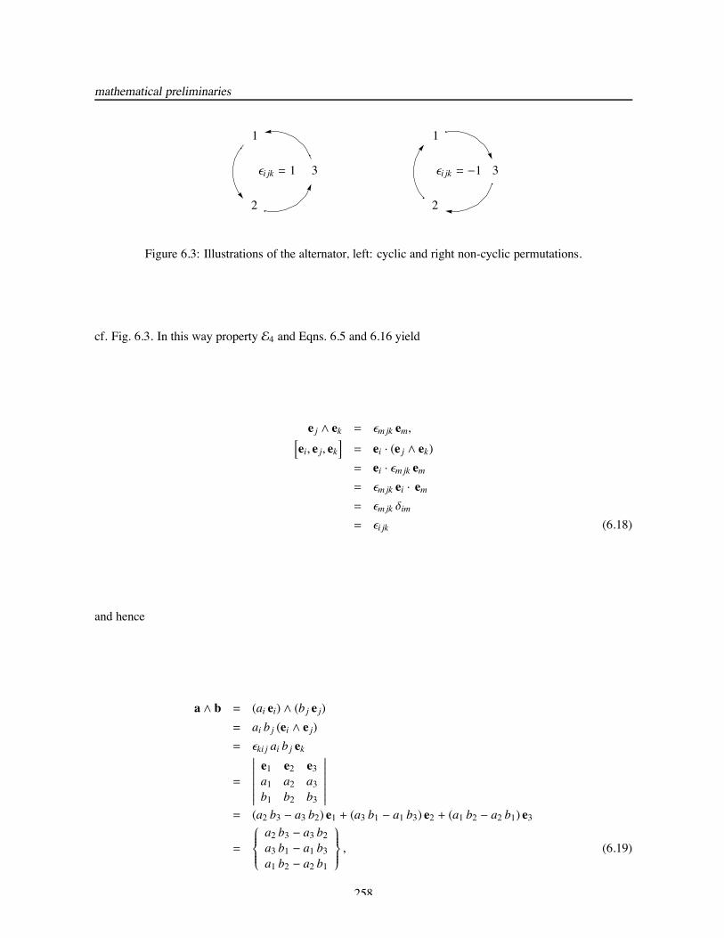
It is convenient now to introduce the alternator ϵi jk defined such that
ϵi jk =
⎧⎪⎪⎪⎨⎪⎪⎪⎩
1 if i, j, k = 1, 2, 3, 2, 3, 1 or 3, 1, 2, i.e. cyclic permutations of 1, 2, 3−1 if i, j, k = 1, 3, 2, 2, 1, 3 or 3, 2, 1, i.e. non-cyclic permutations of 1, 2, 30 otherwise ,
(6.17)
257
mathematical preliminaries
11
22
33ϵi jk = 1 ϵi jk = −1
Figure 6.3: Illustrations of the alternator, left: cyclic and right non-cyclic permutations.
cf. Fig. 6.3. In this way property E4 and Eqns. 6.5 and 6.16 yield
e j ∧ ek = ϵm jk em,[ei, e j, ek
]= ei · (e j ∧ ek)= ei · ϵm jk em= ϵm jk ei · em= ϵm jk δim
= ϵi jk (6.18)
and hence
a ∧ b = (ai ei) ∧ (bj e j)= ai b j (ei ∧ e j)= ϵki j ai b j ek
=
∣∣∣∣∣∣∣∣∣
e1 e2 e3a1 a2 a3b1 b2 b3
∣∣∣∣∣∣∣∣∣= (a2 b3 − a3 b2) e1 + (a3 b1 − a1 b3) e2 + (a1 b2 − a2 b1) e3
=
⎧⎪⎪⎪⎨⎪⎪⎪⎩
a2 b3 − a3 b2a3 b1 − a1 b3a1 b2 − a2 b1
⎫⎪⎪⎪⎬⎪⎪⎪⎭, (6.19)
258
linear transformations – tensors
where | · | denotes the determinant. Similarly we have
a · b = (ai ei) · (bj e j)= ai b j (ei · e j)= ai b j δi j= ai bi
=
⎧⎪⎪⎪⎨⎪⎪⎪⎩
a1a2a3
⎫⎪⎪⎪⎬⎪⎪⎪⎭
T ⎧⎪⎪⎪⎨⎪⎪⎪⎩
b1b2b3
⎫⎪⎪⎪⎬⎪⎪⎪⎭
=[a1 a2 a3
]⎧⎪⎪⎪⎨⎪⎪⎪⎩
b1b2b3
⎫⎪⎪⎪⎬⎪⎪⎪⎭
= a1 b1 + a2 b2 + a3 b3,|a| = (a · a)
12
= (a2i )12
= (a1 a1 + a2 a2 + a3 a3)12 , (6.20)
which are the “usual” results. Combining the previous two results gives
[c, a, b] = c · (a ∧ b)= cmem · ϵki j ai b j ek= ai b j cm ϵki j (em · ek)= ai b j cm ϵki j δkm= ϵki j ai b j ck
=
∣∣∣∣∣∣∣∣∣
a1 a2 a3b1 b2 b3c1 c2 c3
∣∣∣∣∣∣∣∣∣= (a1 b2 c3 + a2 b3 c1 + a3 b1 c2) − (a1 b3 c2 + a2 b1 c3 + a3 b2 c1). (6.21)
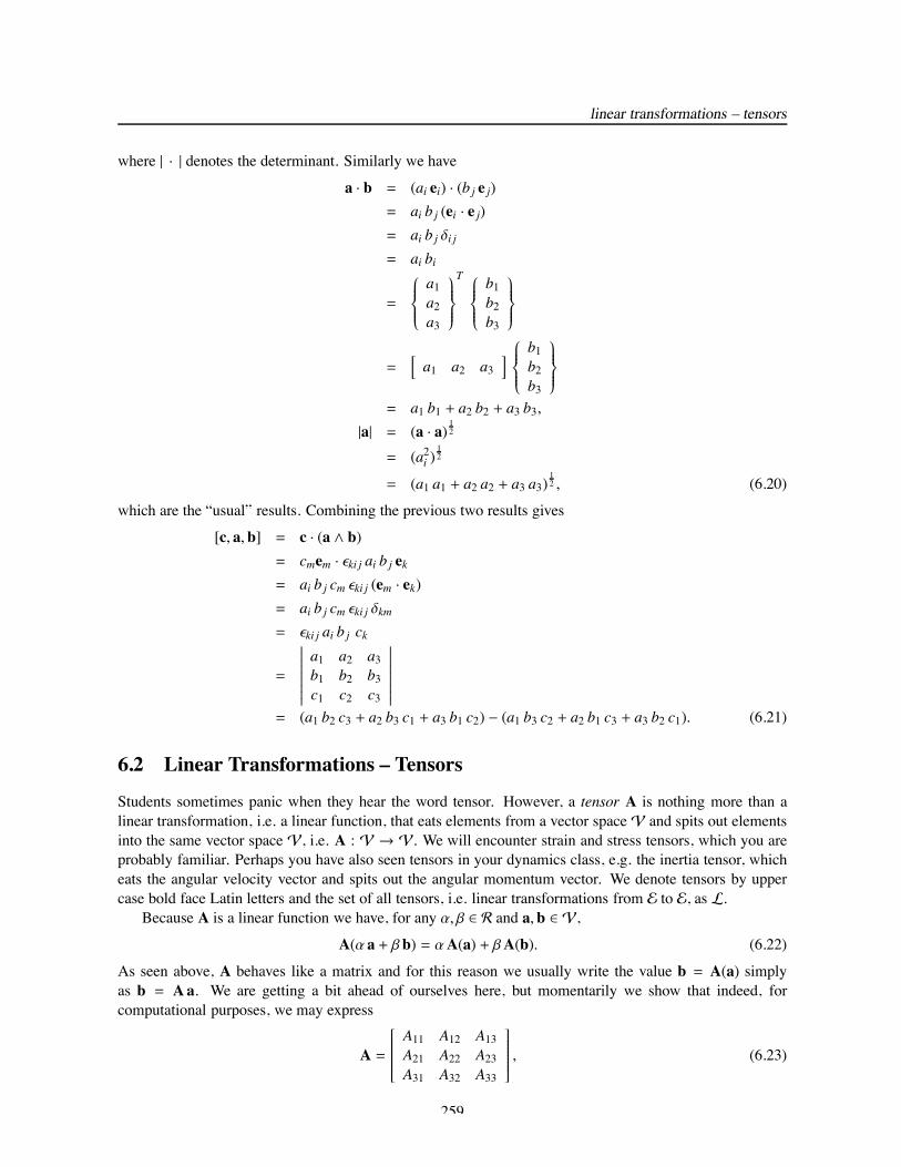
6.2 Linear Transformations – TensorsStudents sometimes panic when they hear the word tensor. However, a tensor A is nothing more than alinear transformation, i.e. a linear function, that eats elements from a vector spaceV and spits out elementsinto the same vector space V, i.e. A : V → V. We will encounter strain and stress tensors, which you areprobably familiar. Perhaps you have also seen tensors in your dynamics class, e.g. the inertia tensor, whicheats the angular velocity vector and spits out the angular momentum vector. We denote tensors by uppercase bold face Latin letters and the set of all tensors, i.e. linear transformations from E to E, as L.
Because A is a linear function we have, for any α, β ∈ R and a, b ∈ V,A(α a + βb) = αA(a) + βA(b). (6.22)
As seen above, A behaves like a matrix and for this reason we usually write the value b = A(a) simplyas b = Aa. We are getting a bit ahead of ourselves here, but momentarily we show that indeed, forcomputational purposes, we may express
A =
⎡⎢⎢⎢⎢⎢⎢⎢⎢⎣
A11 A12 A13A21 A22 A23A31 A32 A33
⎤⎥⎥⎥⎥⎥⎥⎥⎥⎦ , (6.23)
259
mathematical preliminaries
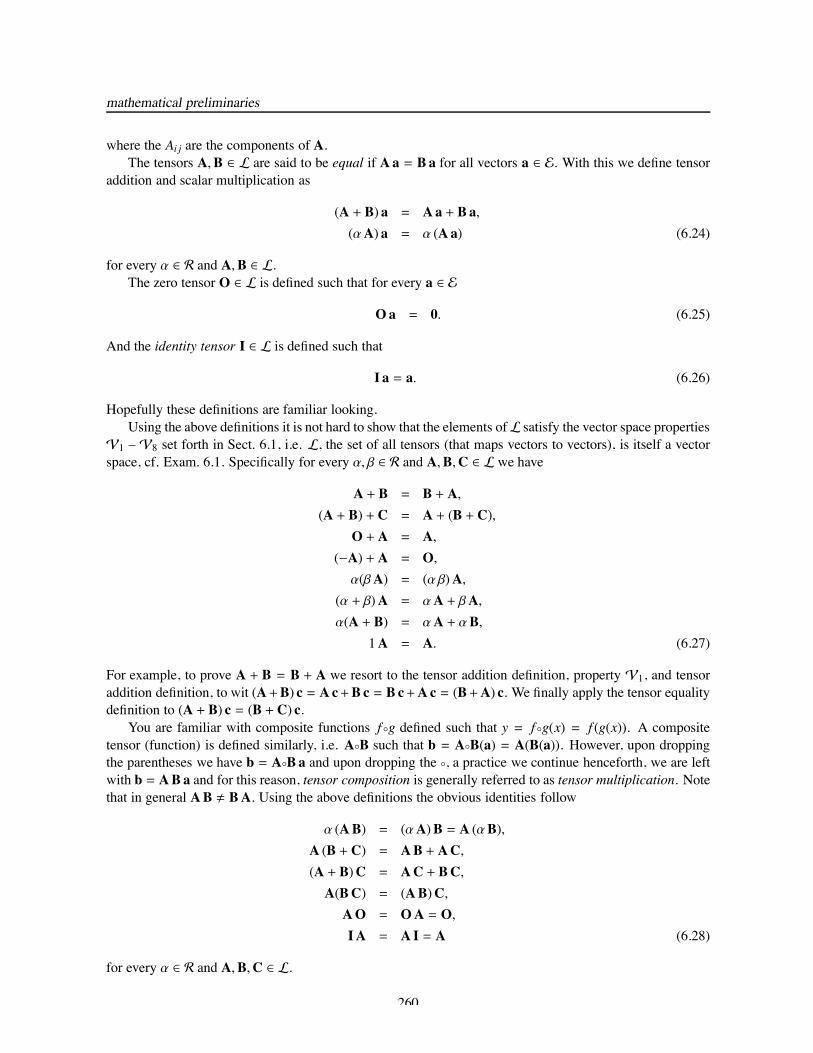
where the Ai j are the components of A.The tensors A,B ∈ L are said to be equal if Aa = Ba for all vectors a ∈ E. With this we define tensor
addition and scalar multiplication as
(A + B) a = Aa + Ba,(αA) a = α (Aa) (6.24)
for every α ∈ R and A,B ∈ L.The zero tensor O ∈ L is defined such that for every a ∈ E
Oa = 0. (6.25)
And the identity tensor I ∈ L is defined such that
I a = a. (6.26)
Hopefully these definitions are familiar looking.Using the above definitions it is not hard to show that the elements ofL satisfy the vector space properties
V1 – V8 set forth in Sect. 6.1, i.e. L, the set of all tensors (that maps vectors to vectors), is itself a vectorspace, cf. Exam. 6.1. Specifically for every α, β ∈ R and A,B,C ∈ L we have
A + B = B + A,(A + B) + C = A + (B + C),
O + A = A,(−A) + A = O,α(βA) = (α β)A,
(α + β)A = αA + βA,α(A + B) = αA + αB,
1A = A. (6.27)
For example, to prove A + B = B + A we resort to the tensor addition definition, property V1, and tensoraddition definition, to wit (A+B) c = Ac+B c = B c+Ac = (B+A) c. We finally apply the tensor equalitydefinition to (A + B) c = (B + C) c.
You are familiar with composite functions f g defined such that y = f g(x) = f (g(x)). A compositetensor (function) is defined similarly, i.e. AB such that b = AB(a) = A(B(a)). However, upon droppingthe parentheses we have b = ABa and upon dropping the , a practice we continue henceforth, we are leftwith b = ABa and for this reason, tensor composition is generally referred to as tensor multiplication. Notethat in general AB ! BA. Using the above definitions the obvious identities follow
α (AB) = (αA)B = A (αB),A (B + C) = AB + AC,(A + B)C = AC + BC,A(BC) = (AB)C,AO = OA = O,IA = A I = A (6.28)
for every α ∈ R and A,B,C ∈ L.
260
linear transformations – tensors
6.2.1 Dyadic Product
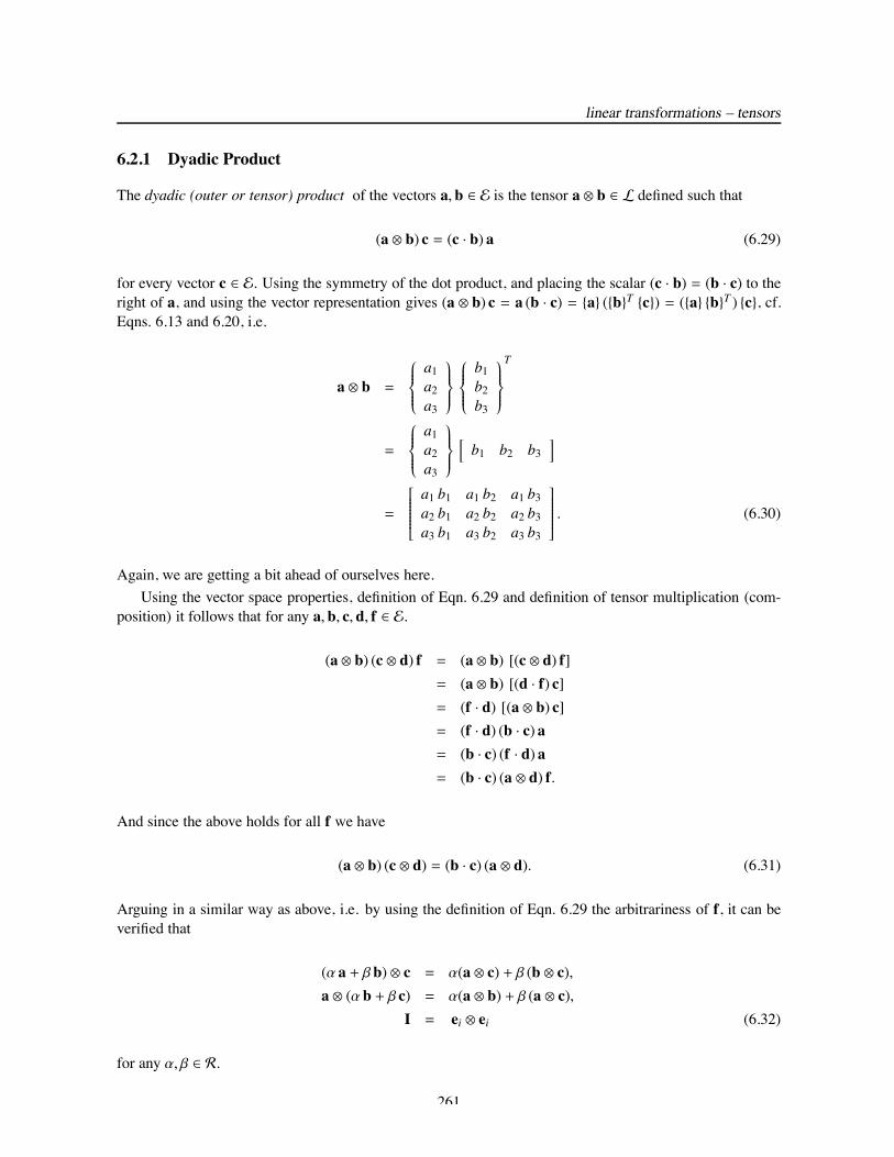
The dyadic (outer or tensor) product of the vectors a, b ∈ E is the tensor a ⊗ b ∈ L defined such that
(a ⊗ b) c = (c · b) a (6.29)
for every vector c ∈ E. Using the symmetry of the dot product, and placing the scalar (c · b) = (b · c) to theright of a, and using the vector representation gives (a ⊗ b) c = a (b · c) = a (bT c) = (a bT ) c, cf.Eqns. 6.13 and 6.20, i.e.
a ⊗ b =
⎧⎪⎪⎪⎨⎪⎪⎪⎩
a1a2a3
⎫⎪⎪⎪⎬⎪⎪⎪⎭
⎧⎪⎪⎪⎨⎪⎪⎪⎩
b1b2b3
⎫⎪⎪⎪⎬⎪⎪⎪⎭
T
=
⎧⎪⎪⎪⎨⎪⎪⎪⎩
a1a2a3
⎫⎪⎪⎪⎬⎪⎪⎪⎭
[b1 b2 b3
]
=
⎡⎢⎢⎢⎢⎢⎢⎢⎢⎣
a1 b1 a1 b2 a1 b3a2 b1 a2 b2 a2 b3a3 b1 a3 b2 a3 b3
⎤⎥⎥⎥⎥⎥⎥⎥⎥⎦ . (6.30)
Again, we are getting a bit ahead of ourselves here.Using the vector space properties, definition of Eqn. 6.29 and definition of tensor multiplication (com-
position) it follows that for any a, b, c, d, f ∈ E.
(a ⊗ b) (c ⊗ d) f = (a ⊗ b) [(c ⊗ d) f]= (a ⊗ b) [(d · f) c]= (f · d) [(a ⊗ b) c]= (f · d) (b · c) a= (b · c) (f · d) a= (b · c) (a ⊗ d) f.
And since the above holds for all f we have
(a ⊗ b) (c ⊗ d) = (b · c) (a ⊗ d). (6.31)
Arguing in a similar way as above, i.e. by using the definition of Eqn. 6.29 the arbitrariness of f, it can beverified that
(α a + βb) ⊗ c = α(a ⊗ c) + β (b ⊗ c),a ⊗ (αb + β c) = α(a ⊗ b) + β (a ⊗ c),
I = ei ⊗ ei (6.32)
for any α, β ∈ R.
261
mathematical preliminaries
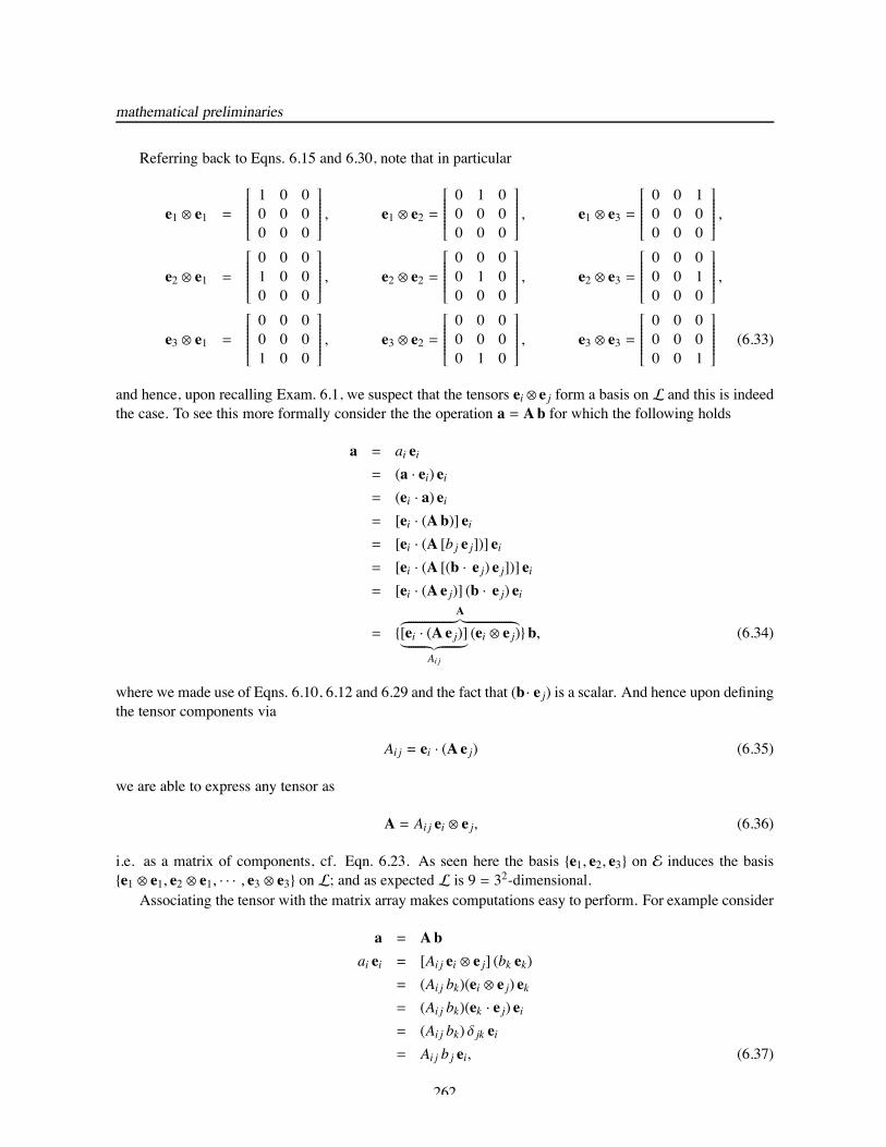
Referring back to Eqns. 6.15 and 6.30, note that in particular
e1 ⊗ e1 =
⎡⎢⎢⎢⎢⎢⎢⎢⎢⎣
1 0 00 0 00 0 0
⎤⎥⎥⎥⎥⎥⎥⎥⎥⎦ , e1 ⊗ e2 =
⎡⎢⎢⎢⎢⎢⎢⎢⎢⎣
0 1 00 0 00 0 0
⎤⎥⎥⎥⎥⎥⎥⎥⎥⎦ , e1 ⊗ e3 =
⎡⎢⎢⎢⎢⎢⎢⎢⎢⎣
0 0 10 0 00 0 0
⎤⎥⎥⎥⎥⎥⎥⎥⎥⎦ ,
e2 ⊗ e1 =
⎡⎢⎢⎢⎢⎢⎢⎢⎢⎣
0 0 01 0 00 0 0
⎤⎥⎥⎥⎥⎥⎥⎥⎥⎦ , e2 ⊗ e2 =
⎡⎢⎢⎢⎢⎢⎢⎢⎢⎣
0 0 00 1 00 0 0
⎤⎥⎥⎥⎥⎥⎥⎥⎥⎦ , e2 ⊗ e3 =
⎡⎢⎢⎢⎢⎢⎢⎢⎢⎣
0 0 00 0 10 0 0
⎤⎥⎥⎥⎥⎥⎥⎥⎥⎦ ,
e3 ⊗ e1 =
⎡⎢⎢⎢⎢⎢⎢⎢⎢⎣
0 0 00 0 01 0 0
⎤⎥⎥⎥⎥⎥⎥⎥⎥⎦ , e3 ⊗ e2 =
⎡⎢⎢⎢⎢⎢⎢⎢⎢⎣
0 0 00 0 00 1 0
⎤⎥⎥⎥⎥⎥⎥⎥⎥⎦ , e3 ⊗ e3 =
⎡⎢⎢⎢⎢⎢⎢⎢⎢⎣
0 0 00 0 00 0 1
⎤⎥⎥⎥⎥⎥⎥⎥⎥⎦ (6.33)
and hence, upon recalling Exam. 6.1, we suspect that the tensors ei ⊗ e j form a basis on L and this is indeedthe case. To see this more formally consider the the operation a = Ab for which the following holds
a = ai ei= (a · ei) ei= (ei · a) ei= [ei · (Ab)] ei= [ei · (A [bj e j])] ei= [ei · (A [(b · e j) e j])] ei= [ei · (Ae j)] (b · e j) ei
= A︷!!!!!!!!!!!!!!!!!!!︸︸!!!!!!!!!!!!!!!!!!!︷
[ei · (Ae j)]︸!!!!!!!︷︷!!!!!!!︸Ai j
(ei ⊗ e j) b, (6.34)
where we made use of Eqns. 6.10, 6.12 and 6.29 and the fact that (b · e j) is a scalar. And hence upon definingthe tensor components via
Ai j = ei · (Ae j) (6.35)
we are able to express any tensor as
A = Ai j ei ⊗ e j, (6.36)
i.e. as a matrix of components, cf. Eqn. 6.23. As seen here the basis e1, e2, e3 on E induces the basise1 ⊗ e1, e2 ⊗ e1, · · · , e3 ⊗ e3 on L; and as expected L is 9 = 32-dimensional.
Associating the tensor with the matrix array makes computations easy to perform. For example consider
a = Abai ei = [Ai j ei ⊗ e j] (bk ek)
= (Ai j bk)(ei ⊗ e j) ek= (Ai j bk)(ek · e j) ei= (Ai j bk) δ jk ei= Ai j b j ei, (6.37)
262
linear transformations – tensors
i.e. ai = Ai j b j and hence we have⎧⎪⎪⎪⎨⎪⎪⎪⎩
a1a2a3
⎫⎪⎪⎪⎬⎪⎪⎪⎭=
⎧⎪⎪⎪⎨⎪⎪⎪⎩
A1 j b jA2 j b jA3 j b j
⎫⎪⎪⎪⎬⎪⎪⎪⎭=
⎡⎢⎢⎢⎢⎢⎢⎢⎢⎣
A11 A12 A13A21 A22 A23A31 A32 A33
⎤⎥⎥⎥⎥⎥⎥⎥⎥⎦
⎧⎪⎪⎪⎨⎪⎪⎪⎩
b1b2b3
⎫⎪⎪⎪⎬⎪⎪⎪⎭. (6.38)
The other operations involving tensors and vectors are similarly performed, notably
AB = [Ai j (ei ⊗ e j)] [Bkl (ek ⊗ el)]= Ai j Bkl (ei ⊗ e j) (ek ⊗ el)= Ai j Bkl (e j · ek) (ei ⊗ el)= Ai j Bkl δ jk (ei ⊗ el)= Aik Bkl (ei ⊗ el)
=
⎡⎢⎢⎢⎢⎢⎢⎢⎢⎣
A11 A12 A13A21 A22 A23A31 A32 A33
⎤⎥⎥⎥⎥⎥⎥⎥⎥⎦
⎡⎢⎢⎢⎢⎢⎢⎢⎢⎣
B11 B12 B13B21 B22 B23B31 B32 B33
⎤⎥⎥⎥⎥⎥⎥⎥⎥⎦ (6.39)
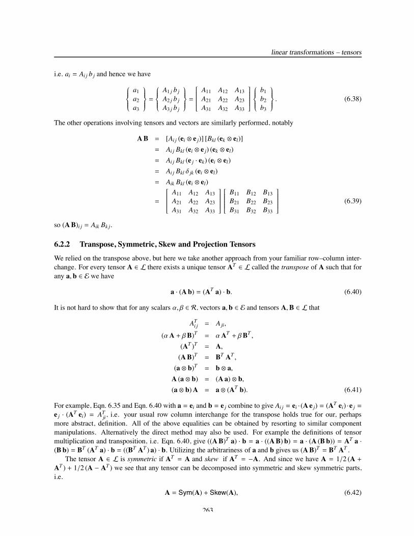
so (AB)i j = Aik Bk j.
6.2.2 Transpose, Symmetric, Skew and Projection Tensors
We relied on the transpose above, but here we take another approach from your familiar row–column inter-change. For every tensor A ∈ L there exists a unique tensor AT ∈ L called the transpose of A such that forany a, b ∈ E we have
a · (Ab) = (AT a) · b. (6.40)
It is not hard to show that for any scalars α, β ∈ R, vectors a, b ∈ E and tensors A,B ∈ L that
ATi j = Aji,
(αA + βB)T = αAT + βBT ,(AT )T = A,(AB)T = BT AT ,(a ⊗ b)T = b ⊗ a,A (a ⊗ b) = (Aa) ⊗ b,(a ⊗ b)A = a ⊗ (AT b). (6.41)
For example, Eqn. 6.35 and Eqn. 6.40 with a = ei and b = e j combine to give Ai j = ei · (Ae j) = (AT ei) ·e j =e j · (AT ei) = ATji, i.e. your usual row column interchange for the transpose holds true for our, perhapsmore abstract, definition. All of the above equalities can be obtained by resorting to similar componentmanipulations. Alternatively the direct method may also be used. For example the definitions of tensormultiplication and transposition, i.e. Eqn. 6.40, give ((AB)T a) · b = a · ((AB)b) = a · (A (Bb)) = AT a ·(Bb) = BT (AT a) · b = ((BT AT ) a) · b. Utilizing the arbitrariness of a and b gives us (AB)T = BT AT .
The tensor A ∈ L is symmetric if AT = A and skew if AT = −A. And since we have A = 1/2 (A +AT ) + 1/2 (A − AT ) we see that any tensor can be decomposed into symmetric and skew symmetric parts,i.e.
A = Sym(A) + Skew(A), (6.42)
263
mathematical preliminaries
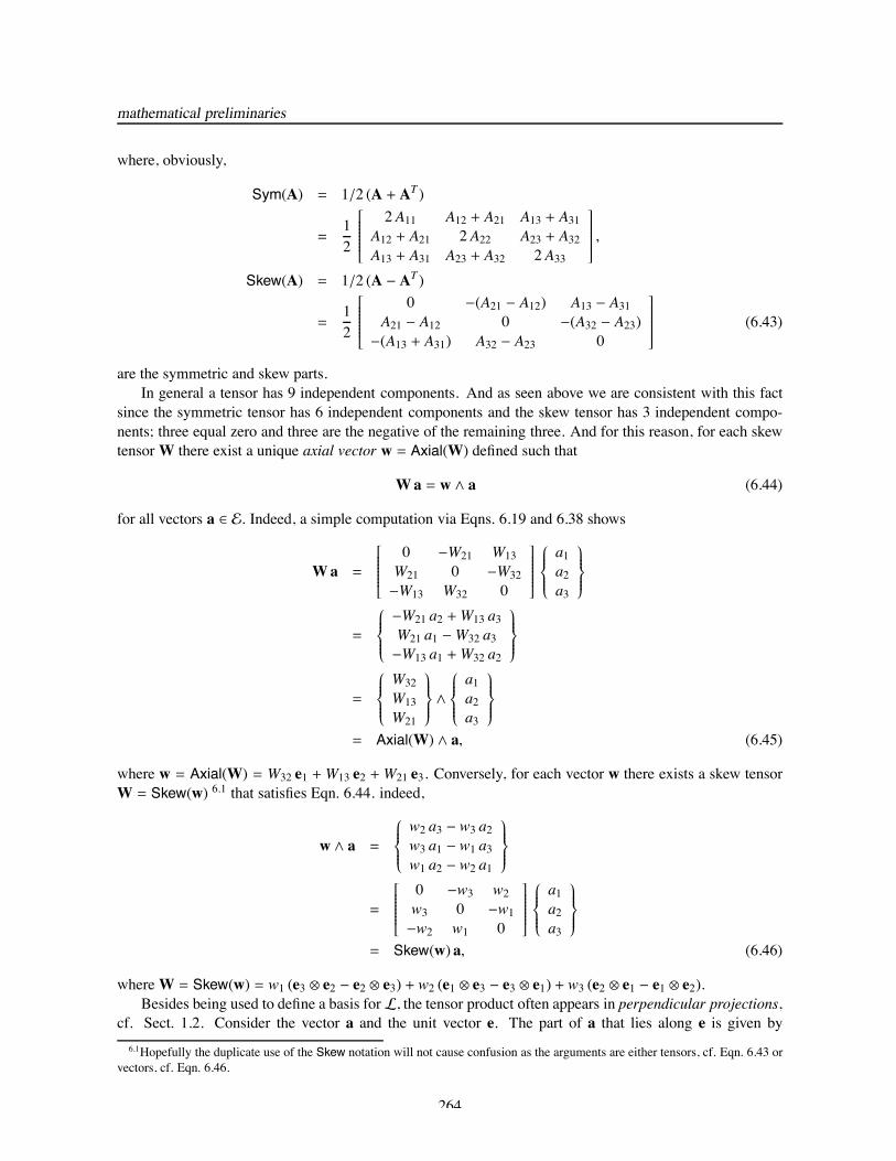
where, obviously,
Sym(A) = 1/2 (A + AT )
=12
⎡⎢⎢⎢⎢⎢⎢⎢⎢⎣
2A11 A12 + A21 A13 + A31A12 + A21 2A22 A23 + A32A13 + A31 A23 + A32 2A33
⎤⎥⎥⎥⎥⎥⎥⎥⎥⎦ ,
Skew(A) = 1/2 (A − AT )
=12
⎡⎢⎢⎢⎢⎢⎢⎢⎢⎣
0 −(A21 − A12) A13 − A31A21 − A12 0 −(A32 − A23)−(A13 + A31) A32 − A23 0
⎤⎥⎥⎥⎥⎥⎥⎥⎥⎦ (6.43)
are the symmetric and skew parts.In general a tensor has 9 independent components. And as seen above we are consistent with this fact
since the symmetric tensor has 6 independent components and the skew tensor has 3 independent compo-nents; three equal zero and three are the negative of the remaining three. And for this reason, for each skewtensorW there exist a unique axial vector w = Axial(W) defined such that
Wa = w ∧ a (6.44)
for all vectors a ∈ E. Indeed, a simple computation via Eqns. 6.19 and 6.38 shows
Wa =
⎡⎢⎢⎢⎢⎢⎢⎢⎢⎣
0 −W21 W13W21 0 −W32−W13 W32 0
⎤⎥⎥⎥⎥⎥⎥⎥⎥⎦
⎧⎪⎪⎪⎨⎪⎪⎪⎩
a1a2a3
⎫⎪⎪⎪⎬⎪⎪⎪⎭
=
⎧⎪⎪⎪⎨⎪⎪⎪⎩
−W21 a2 +W13 a3W21 a1 −W32 a3−W13 a1 +W32 a2
⎫⎪⎪⎪⎬⎪⎪⎪⎭
=
⎧⎪⎪⎪⎨⎪⎪⎪⎩
W32W13W21
⎫⎪⎪⎪⎬⎪⎪⎪⎭∧
⎧⎪⎪⎪⎨⎪⎪⎪⎩
a1a2a3
⎫⎪⎪⎪⎬⎪⎪⎪⎭
= Axial(W) ∧ a, (6.45)
where w = Axial(W) = W32 e1 +W13 e2 +W21 e3. Conversely, for each vector w there exists a skew tensorW = Skew(w) 6.1 that satisfies Eqn. 6.44. indeed,
w ∧ a =
⎧⎪⎪⎪⎨⎪⎪⎪⎩
w2 a3 − w3 a2w3 a1 − w1 a3w1 a2 − w2 a1
⎫⎪⎪⎪⎬⎪⎪⎪⎭
=
⎡⎢⎢⎢⎢⎢⎢⎢⎢⎣
0 −w3 w2w3 0 −w1−w2 w1 0
⎤⎥⎥⎥⎥⎥⎥⎥⎥⎦
⎧⎪⎪⎪⎨⎪⎪⎪⎩
a1a2a3
⎫⎪⎪⎪⎬⎪⎪⎪⎭
= Skew(w) a, (6.46)
whereW = Skew(w) = w1 (e3 ⊗ e2 − e2 ⊗ e3) + w2 (e1 ⊗ e3 − e3 ⊗ e1) + w3 (e2 ⊗ e1 − e1 ⊗ e2).Besides being used to define a basis for L, the tensor product often appears in perpendicular projections,
cf. Sect. 1.2. Consider the vector a and the unit vector e. The part of a that lies along e is given by6.1Hopefully the duplicate use of the Skew notation will not cause confusion as the arguments are either tensors, cf. Eqn. 6.43 or
vectors, cf. Eqn. 6.46.
264
linear transformations – tensors
e (I − e ⊗ e) a
(e ⊗ e) a
a
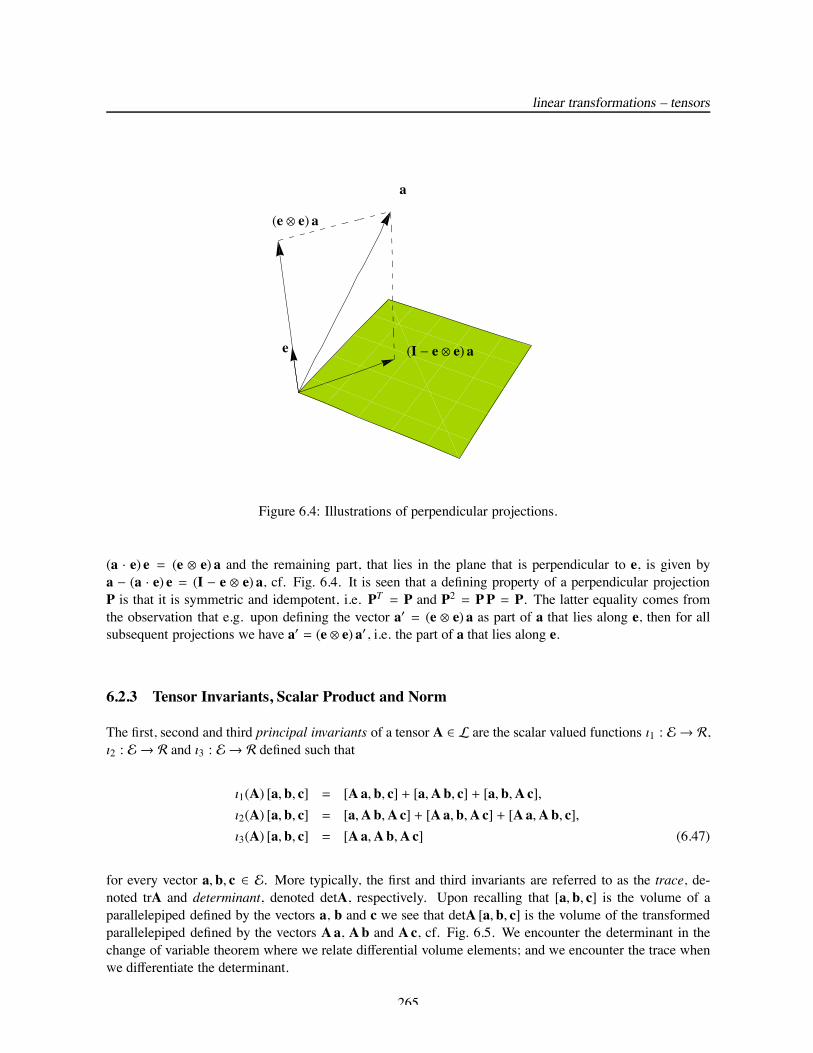
Figure 6.4: Illustrations of perpendicular projections.
(a · e) e = (e ⊗ e) a and the remaining part, that lies in the plane that is perpendicular to e, is given bya − (a · e) e = (I − e ⊗ e) a, cf. Fig. 6.4. It is seen that a defining property of a perpendicular projectionP is that it is symmetric and idempotent, i.e. PT = P and P2 = PP = P. The latter equality comes fromthe observation that e.g. upon defining the vector a′ = (e ⊗ e) a as part of a that lies along e, then for allsubsequent projections we have a′ = (e ⊗ e) a′, i.e. the part of a that lies along e.
6.2.3 Tensor Invariants, Scalar Product and Norm
The first, second and third principal invariants of a tensor A ∈ L are the scalar valued functions ı1 : E→ R,ı2 : E→ R and ı3 : E→ R defined such that
ı1(A) [a, b, c] = [Aa, b, c] + [a,Ab, c] + [a, b,Ac],ı2(A) [a, b, c] = [a,Ab,Ac] + [Aa, b,Ac] + [Aa,Ab, c],ı3(A) [a, b, c] = [Aa,Ab,Ac] (6.47)
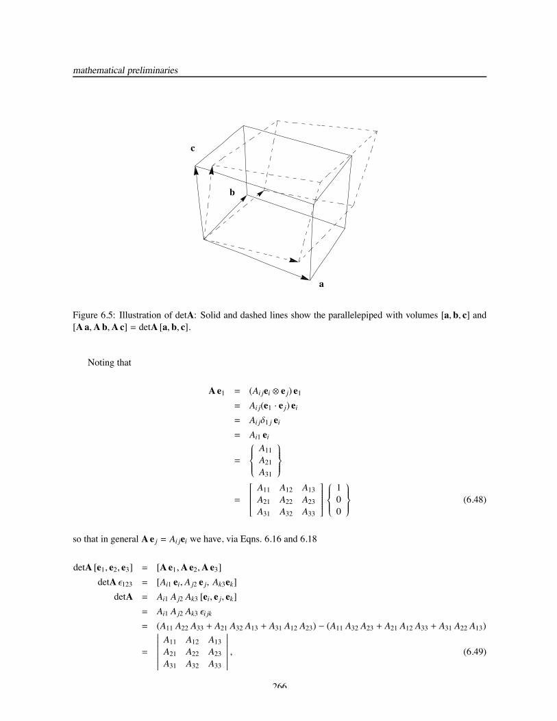
for every vector a, b, c ∈ E. More typically, the first and third invariants are referred to as the trace, de-noted trA and determinant, denoted detA, respectively. Upon recalling that [a, b, c] is the volume of aparallelepiped defined by the vectors a, b and c we see that detA [a, b, c] is the volume of the transformedparallelepiped defined by the vectors Aa, Ab and Ac, cf. Fig. 6.5. We encounter the determinant in thechange of variable theorem where we relate differential volume elements; and we encounter the trace whenwe differentiate the determinant.
265
mathematical preliminaries
a
b
c
Figure 6.5: Illustration of detA: Solid and dashed lines show the parallelepiped with volumes [a, b, c] and[Aa,Ab,Ac] = detA [a, b, c].
Noting that
Ae1 = (Ai jei ⊗ e j) e1= Ai j(e1 · e j) ei= Ai jδ1 j ei= Ai1 ei
=
⎧⎪⎪⎪⎨⎪⎪⎪⎩
A11A21A31
⎫⎪⎪⎪⎬⎪⎪⎪⎭
=
⎡⎢⎢⎢⎢⎢⎢⎢⎢⎣
A11 A12 A13A21 A22 A23A31 A32 A33
⎤⎥⎥⎥⎥⎥⎥⎥⎥⎦
⎧⎪⎪⎪⎨⎪⎪⎪⎩
100
⎫⎪⎪⎪⎬⎪⎪⎪⎭
(6.48)
so that in general Ae j = Ai jei we have, via Eqns. 6.16 and 6.18
detA [e1, e2, e3] = [Ae1,Ae2,Ae3]detA ϵ123 = [Ai1 ei, Aj2 e j, Ak3ek]
detA = Ai1 Aj2 Ak3 [ei, e j, ek]= Ai1 Aj2 Ak3 ϵi jk= (A11 A22 A33 + A21 A32 A13 + A31 A12 A23) − (A11 A32 A23 + A21 A12 A33 + A31 A22 A13)
=
∣∣∣∣∣∣∣∣∣
A11 A12 A13A21 A22 A23A31 A32 A33
∣∣∣∣∣∣∣∣∣, (6.49)
266
linear transformations – tensors
i.e. your usual understanding of the determinant holds true. Likewise for the trace we have
trA [e1, e2, e3] = [Ae1, e2, e3] + [e1,Ae2, e3] + [e1, e2,Ae3]trA ϵ123 = [A1i ei, e2, e3] + [e1, A2i ei, e3] + [e1, e2, A3i ei]
trA = A1i [ei, e2, e3] + A2i [e1, ei, e3] + A3i [e1, e2, ei]= A1i ϵi23 + A2i ϵ1i3 + A3i ϵ12i= A11 + A22 + A33, (6.50)
i.e. your usual understanding of the trace as the sum of the diagonal elements also holds true. And finally alengthy derivation gives
ı2(A) [e1, e2, e3] = [e1,Ae2,Ae3] + [Ae1, e2,A e3] + [A e1,A e2, e3]ı2(A) ϵ123 = [e1, A2i ei, A3 j e j] + [A1i ei, e2, A3 j e j] + [A1i ei, A2 j e j, e3]ı2(A) = A2i A3 j [e1, ei, e j] + A1i A3 j [ei, e2, e j] + A1i A2 j [ei, e j, e3]
= A2i A3 j ϵ1i j + A1i A3 j ϵi2 j + A1i A2 j ϵi j3= (A22 A33 − A23 A32) + (A11 A33 − A13 A31) + (A11 A22 − A12 A21)
=12[A211 + A
222 + A
233 + 2A22 A33 + 2A11 A33 + 2A11 A22]
−12[A211 + A
222 + A
233 + A23 A32 + A13 A31 + A12 A21]
=12(A11 + A22 + A33)2 −
12Ai j A ji
=12[(trA)2 − trA2]. (6.51)
It may also be verified that
tr(αA + βB) = α trA + β trB,trAT = trA,
tr(a ⊗ b) = a · b,tr(AB) = tr(BA),det(αA) = α3 detA,detAT = detA,
det(AB) = detA detB,trI = 3,detI = 1. (6.52)
Similar to the manner in which any tensor can be expressed as the sum of a symmetric and skew com-
267
mathematical preliminaries
ponents we define the deviatoric (traceless) and spherical parts of the tensor A via
Sph(A) = 13trA I
=13(A11 + A22 + A33)
⎡⎢⎢⎢⎢⎢⎢⎢⎢⎣
1 0 00 1 00 0 1
⎤⎥⎥⎥⎥⎥⎥⎥⎥⎦ ,
Dev(A) = A − 13trA I
=
⎡⎢⎢⎢⎢⎢⎢⎢⎢⎣
23A11 −
13A22 −
13A33 A12 A13
A21 − 13A11 +23A22 −
13A33 A23
A31 A32 − 13A11 −13A22 +
23A33
⎤⎥⎥⎥⎥⎥⎥⎥⎥⎦ (6.53)
so that
A = Sph(A) + Dev(A). (6.54)
It is clearly seen that trDev(A) = 0 and hence the traceless terminology, cf. Exer. 6.17. Moreover, byrecognizing that Dev(A)33 = −(Dev(A)11 +Dev(A)22) we see that Sph(A) and Dev(A) are defined by 1 and8 independent components.
If we can define a suitable scalar product on L, then it will be an inner product space. Our dream isrealized by defining the scalar product
A · B = tr(AT B), (6.55)
which, upon noting that AT B = Aki Bk jei ⊗ e j, cf. Eqns. 6.39 and 6.41, and that tr(ei ⊗ e j) = ei · e j = δi j, cf.Eqns. 6.7 and 6.52, is computed as
A · B = tr[Aki Bk j ei ⊗ e j] = Aki Bk j tr(ei ⊗ e j) = Aki Bk j ei · e j = Aki Bk j δi j = Aki Bki, (6.56)
which is similar to the vector scalar product, cf. Eqn. 6.20. Using the definition of the trace, we can show,analogously to properties E1, E2 and E3, that the following relations hold
A · B = B ·A,(αA + βB) · C = α (A · C) + β (B · C), (6.57)
A · A ≥ 0 for all A ∈ L and A · A = 0 if and only if A = O
for all scalars α, β ∈ R and tensors A,B,C ∈ L. For example, A · B = tr(AT B) = tr((AT B)T ) =tr(BT (AT )T ) = tr(BT A)) = B · A, which follows from Eqns. 6.41, 6.52 and 6.55.
We define the norm |A| of the tensor A as
|A| = (A · A)12
= (Ai j Ai j)12 , (6.58)
which is analogous to the vector norm, cf. Eqn. 6.20. And we say two tensors A and B are orthogonal ifA · B = 0. Again, these definitions on L are analogous to those on E.
Using Eqns. 6.52 and 6.55 it is also readily verified thattrA = A · I,
A · (BC) = (BTA) · C = (ACT ) · B,a · Ab = A · (a ⊗ b),
(a ⊗ b) · (c ⊗ d) = (a · c)(b · d),trA = trSym(A),S · A = S · Sym(A) if S ∈ L is symmetric,W · A = W · Skew(A) ifW ∈ L is skew
(6.59)
268
linear transformations – tensors
for arbitrary tensors A, B and C and arbitrary vectors a, b, c, and d. For example, trA = trAT = tr(AT I) =A · I, which follows from Eqns. 6.28, 6.52 and 6.55. The third line above allows us to express the tensorcomponents of Eqn. 6.35, i.e. Ai j = ei · Ae j as
Ai j = A · (ei ⊗ e j), (6.60)
which is analogous to Eqn. 6.11, i.e. ai = ei · a.
6.2.4 Inverse, Orthogonal, Rotation, Involution and Adjugate Tensors
If detA = 0 we say that A is not invertible, i.e. it is singular; and this is on agreement with your matrixexperience. Additional insight into this claim is gained by noting that
Aa =
⎡⎢⎢⎢⎢⎢⎢⎢⎢⎣
A11 A12 A13A21 A22 A23A31 A32 A33
⎤⎥⎥⎥⎥⎥⎥⎥⎥⎦
⎧⎪⎪⎪⎨⎪⎪⎪⎩
a1a2a3
⎫⎪⎪⎪⎬⎪⎪⎪⎭
=
⎧⎪⎪⎪⎨⎪⎪⎪⎩
A11A21A31
⎫⎪⎪⎪⎬⎪⎪⎪⎭a1 +
⎧⎪⎪⎪⎨⎪⎪⎪⎩
A12A22A32
⎫⎪⎪⎪⎬⎪⎪⎪⎭a2 +
⎧⎪⎪⎪⎨⎪⎪⎪⎩
A13A23A33
⎫⎪⎪⎪⎬⎪⎪⎪⎭a3 (6.61)
and hence Aa is a linear combination of the columns of the matrix [A]. Now suppose Aa = 0 for somea ! 0. This implies the columns of the matrix [A] are linearly dependent and thus by Eqns. 6.6 and 6.21 thetriple product of these three column vectors is zero, i.e. the detA = 0. If this is the case, then if Ab = cwe also have A (b + a) = Ab + Aa = c + 0 = c, i.e. A is not one-to-one as both Ab and A (b + a) equal cand and hence it has no inverse. We can also show that the condition detA = 0 implies an a ! 0 exists suchAa = 0, cf. Exer. 6.23. Clearly the condition detA = 0 implies A has no inverse.
If detA ! 0 then A is invertible and we say A−1 ∈ L is the unique inverse of A ∈ L and it satisfies
AA−1 = A−1A = I. (6.62)
Note that by 6.52 we see that detA detA−1 = det(AA−1) = detI = 1 and hence
detA−1 = (detA)−1. (6.63)
It can also be shown that the following identities hold for all invertible A,B ∈ L
(AB)−1 = B−1 A−1,(A−1)T = (AT )−1. (6.64)
And for this reason we sometimes write A−T = (A−1)T = (AT )−1.A tensor Q ∈ L is orthogonal if it preserves inner products, i.e. if
(Qa) · (Qb) = a · b (6.65)
for all vectors a, b ∈ E. As seen here and from Eqn. 6.4 the angle between the transformed vectors, e.g.Qa, is unchanged as well as the length of the transformed vectors since (Qa) · (Qa) = a · a = |a|2.Using the definition of the transpose, cf. Eqn. 6.40, and matrix multiplication we see that (Qa) · (Qb) =a · QT (Qb) = a · (QT Q)b = a · b and hence QT Q = I. Moreover, applications of Eqn. 6.52 give1 = det I = det(QT Q) = detQT detQ = detQ detQ = (detQ)2 and hence detQ = ±1. This detQ = ±1result implies Q is invertible so upon manipulating QT QQ−1 = IQ−1 we find
QT = Q−1, (6.66)
269
mathematical preliminaries
aa
−I a Re a
e
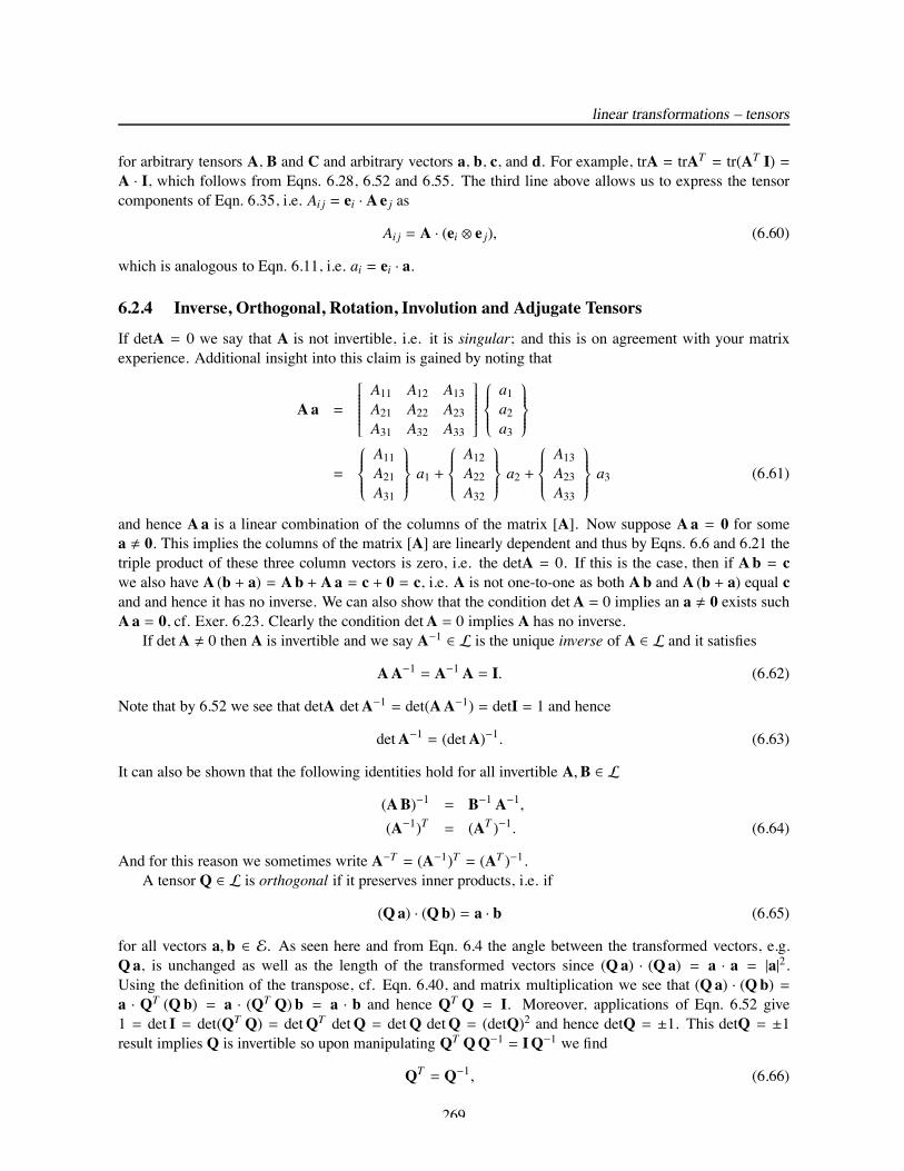
Figure 6.6: Inversion (left) and reflection (right) illustrations.
i.e. our definition is consistent with your familiar notion that the inverse of an orthogonal matrix equals itstranspose.
We encounter orthogonal tensors when we discuss rigid deformation and material symmetry. Notableorthogonal tensors are the central inversion Q = −I and the reflection about the plane with normal vector e
Re = I − 2 e ⊗ e. (6.67)
Illustrations of the actions of these tensors on an arbitrary vector a are seen in Fig. 6.6. These are examplesof improper orthogonal tensors as their determinants equal -1. The central inversion and the reflections arealso examples of involutions since they equal their own inverses, e.g. Re Re = I. Physically this is notsurprising since the twice inverted or reflected object returns to its original state, e.g. Re Re a = a, cf. Fig.6.6.
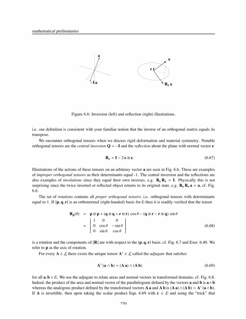
The set of rotations contains all proper orthogonal tensors, i.e. orthogonal tensors with determinantsequal to 1. If p, q, r is an orthonormal (right-handed) basis for E then it is readily verified that the tensor
Rp(θ) = p ⊗ p + (q ⊗ q + r ⊗ r) cos θ − (q ⊗ r − r ⊗ q) sin θ
=
⎡⎢⎢⎢⎢⎢⎢⎢⎢⎣
1 0 00 cos θ − sin θ0 sin θ cos θ
⎤⎥⎥⎥⎥⎥⎥⎥⎥⎦ (6.68)
is a rotation and the components of [R] are with respect to the p, q, r basis, cf. Fig. 6.7 and Exer. 6.40. Werefer to p as the axis of rotation.
For every A ∈ L there exists the unique tensor A∗ ∈ L called the adjugate that satisfies
A∗ (a ∧ b) = (Aa) ∧ (Ab) (6.69)
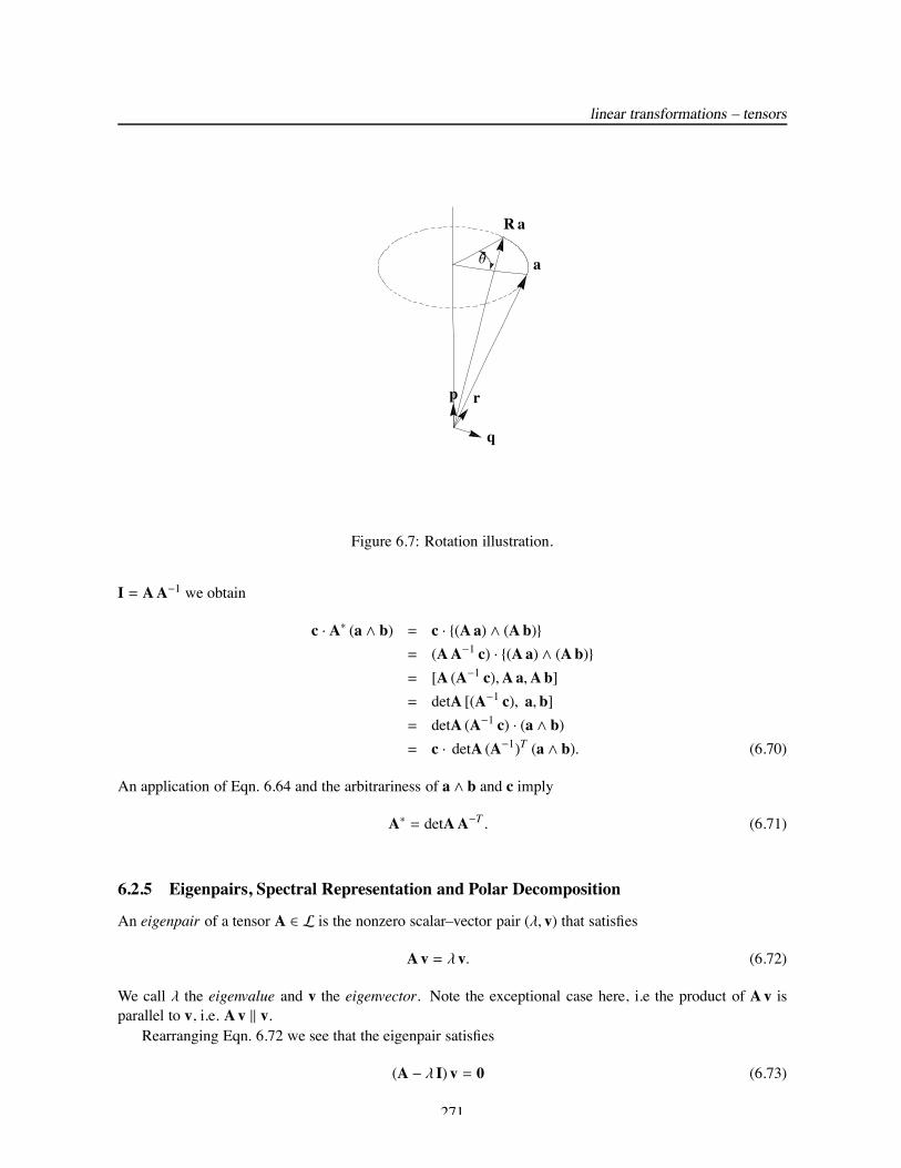
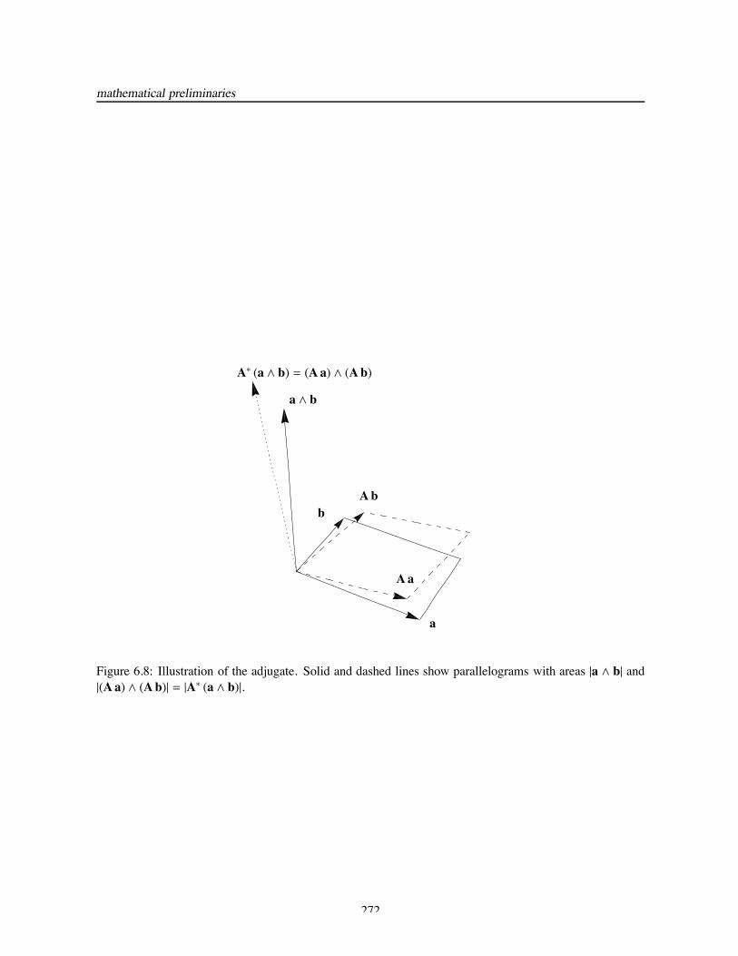
for all a, b ∈ E. We use the adjugate to relate areas and normal vectors in transformed domains, cf. Fig. 6.8.Indeed, the product of the area and normal vector of the parallelogram defined by the vectors a and b is a∧bwhereas the analogous product defined by the transformed vectors Aa and Ab is (Aa)∧ (Ab) = A∗ (a∧b).If A is invertible, then upon taking the scalar product Eqn. 6.69 with c ∈ E and using the “trick” that
270
linear transformations – tensors
θ
Ra
a
q
rp
Figure 6.7: Rotation illustration.
I = AA−1 we obtain
c · A∗ (a ∧ b) = c · (Aa) ∧ (Ab)= (AA−1 c) · (Aa) ∧ (Ab)= [A (A−1 c),Aa,Ab]= detA [(A−1 c), a, b]= detA (A−1 c) · (a ∧ b)= c · detA (A−1)T (a ∧ b). (6.70)
An application of Eqn. 6.64 and the arbitrariness of a ∧ b and c imply
A∗ = detAA−T . (6.71)
6.2.5 Eigenpairs, Spectral Representation and Polar Decomposition
An eigenpair of a tensor A ∈ L is the nonzero scalar–vector pair (λ, v) that satisfies
Av = λ v. (6.72)
We call λ the eigenvalue and v the eigenvector. Note the exceptional case here, i.e the product of Av isparallel to v, i.e. Av ∥ v.
Rearranging Eqn. 6.72 we see that the eigenpair satisfies
(A − λ I) v = 0 (6.73)
271
mathematical preliminaries
a
b
a ∧ b
Aa
A∗ (a ∧ b) = (Aa) ∧ (Ab)
Ab
Figure 6.8: Illustration of the adjugate. Solid and dashed lines show parallelograms with areas |a ∧ b| and|(Aa) ∧ (Ab)| = |A∗ (a ∧ b)|.
272
linear transformations – tensors
and thus for v ! 0 we require the columns of A − λ I to be linearly dependent, i.e. A − λ I is singular, cf.Eqn. 6.61 and the following discussion. It then follows that the eigenvalues are the roots of the characteristicequation
det(A − λ I) = 0. (6.74)
Substituting A − λ I for A in Eqn. 6.47 we see that
det(A − λ I) [a, b, c] = [(A − λ I) a, (A − λ I)b, (A − λ I) c]= −λ3 [a, b, c] + ([Aa, b, c] + [a,Ab, c] + [a, b,Ac]) −
([a,Ab,Ac] + [Aa, b,Ac] + [Aa,Ab, c]) + [Aa,Ab,Ac]=
−λ3 + ı1(A) λ2 − ı2(A) λ + ı3(A)
[a, b, c], (6.75)
i.e. the characteristic equation is also given by
λ3 − ı1(A) λ2 + ı2(A) λ − ı3(A) = 0 (6.76)
thus offering additional insight into the invariants.As seen in Eqn. 6.76, the characteristic equation is an order 3 polynomial and as seen in Eqns. 6.49,
6.50 and 6.51 the invariants are real and hence the three roots, i.e. eigenvalues, of a linear transformationA ∈ L consist of three real numbers or one real number and a complex conjugate pair. The set of these threeeigenvalues comprises the spectrum of A.
If S is symmetric then the eigenpairs are real, cf. [7]. Moreover, the eigenvectors associated with distincteigenvalues are orthogonal. To see this let (λi, vi) and (λ j, v j) be two eigenpairs of the symmetric tensor Ssuch that λi ! λ j Then v j · S vi = v j · λi vi and vi · S v j = vi · λ j v j. Subtracting these two equalities givesv j · S vi − vi · S v j = (λi − λ j) v j · vi. Now using the definition of the transpose and the symmetry of S weobtain v j · S vi − vi · S v j = v j · S vi − ST vi · v j = v j · S vi − S vi · v j = v j · S vi − v j · S vi = 0 and hence0 = (λi − λ j) v j · vi. Finally using the inequality (λi − λ j) ! 0 we obtain v j · vi = 0.
Now assume that the eigenvalues of the symmetric A are distinct and that the eigenvectors are scaled tobe unit vectors (as both vi and α vi satisfy Eqn. 6.72, cf. Exer. 6.27). In this way, we see that the orthogonalunit eigenvectors v1, v2, and v3 form an orthonormal basis for E. So, upon using Eqns. 6.32, i.e. I = vi ⊗ vi,and 6.41, i.e. A (a ⊗ b) = (Aa) ⊗ b, we have the spectral decomposition of S, i.e.
S = S I= S (vi ⊗ vi)= (S vi) ⊗ vi)
=
3∑
i=1(λi vi) ⊗ vi
=
3∑
i=1λi (vi ⊗ vi)
=
⎡⎢⎢⎢⎢⎢⎢⎢⎢⎣
λ1 0 00 λ2 00 0 λ3
⎤⎥⎥⎥⎥⎥⎥⎥⎥⎦ (6.77)
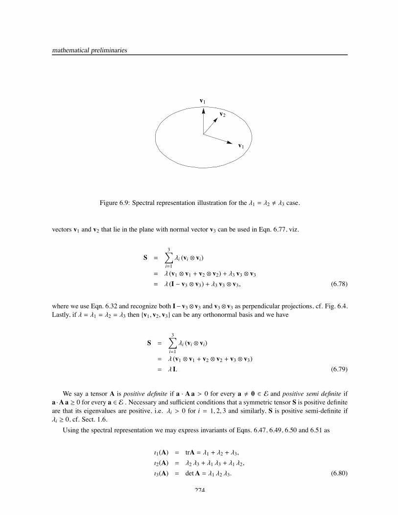
where [S] = diag[λ1, λ2, λ3] is expressed relative to the v1, v2, v3 basis.Similar results hold even if the eigenvalues of the symmetric A are not distinct. Consider the case for
which λ = λ1 = λ2 ! λ3. Then using the above arguments we have v1 ·v3 = v2 ·v3 = 0, i.e. any perpendicular
273
mathematical preliminaries
v1
v2
v1
Figure 6.9: Spectral representation illustration for the λ1 = λ2 ! λ3 case.
vectors v1 and v2 that lie in the plane with normal vector v3 can be used in Eqn. 6.77, viz.
S =
3∑
i=1λi (vi ⊗ vi)
= λ (v1 ⊗ v1 + v2 ⊗ v2) + λ3 v3 ⊗ v3= λ (I − v3 ⊗ v3) + λ3 v3 ⊗ v3, (6.78)
where we use Eqn. 6.32 and recognize both I− v3 ⊗ v3 and v3 ⊗ v3 as perpendicular projections, cf. Fig. 6.4.Lastly, if λ = λ1 = λ2 = λ3 then v1, v2, v3 can be any orthonormal basis and we have
S =
3∑
i=1λi (vi ⊗ vi)
= λ (v1 ⊗ v1 + v2 ⊗ v2 + v3 ⊗ v3)= λ I. (6.79)
We say a tensor A is positive definite if a · Aa > 0 for every a ! 0 ∈ E and positive semi definite ifa ·Aa ≥ 0 for every a ∈ E . Necessary and sufficient conditions that a symmetric tensor S is positive definiteare that its eigenvalues are positive, i.e. λi > 0 for i = 1, 2, 3 and similarly, S is positive semi-definite ifλi ≥ 0, cf. Sect. 1.6.
Using the spectral representation we may express invariants of Eqns. 6.47, 6.49, 6.50 and 6.51 as
ı1(A) = trA = λ1 + λ2 + λ3,ı2(A) = λ2 λ3 + λ1 λ3 + λ1 λ2,
ı3(A) = detA = λ1 λ2 λ3. (6.80)
274
linear transformations – tensors
If S is positive definite then its eigenvalues are positive and we can take their square roots giving
√S =
3∑
i=1
√λi (vi ⊗ vi)
=
⎡⎢⎢⎢⎢⎢⎢⎢⎢⎣
√λ1 0 00
√λ2 0
0 0√λ3
⎤⎥⎥⎥⎥⎥⎥⎥⎥⎦ , (6.81)
which is obviously positive definite symmetric and satisfies(√S)2=√S√S = S. Additionally we can take
the inverses of the eigenvalues to obtain
S−1 =3∑
i=1
1λi(vi ⊗ vi)
=
⎡⎢⎢⎢⎢⎢⎢⎢⎢⎢⎣
1λ1
0 00 1
λ20
0 0 1λ3
⎤⎥⎥⎥⎥⎥⎥⎥⎥⎥⎦, (6.82)
which is again positive definite symmetric. It is readily verified that S−1 S = S S−1 = I.Now we show that any invertible tensor A can be expressed via the (right) polar decomposition
A = RU, (6.83)
where the tensors R and U are orthogonal and positive definite symmetric, respectively. Indeed, considerthe tensor AT A, which by Eqn. 6.41 is symmetric. Moreover, by property V3 we see that a · (AT A) a =Aa · Aa ≥ 0 and a · (AT A) a = 0 only if Aa = 0; but A is invertible thusly Aa = 0 implies a = 0, cf. thediscussion following Eqn. 6.61. Consequently a · AT Aa > 0 for all a ! 0, i.e. AT A is positive definitesymmetric and hence there exists a positive definite (invertible square root) symmetric tensor U =
√AT A,
cf. Eqn. 6.81. Next define the tensor R = AU−1 so that RU = (AU−1)U = A, which is Eqn. 6.83. Wemust now show R is orthogonal. To these ends note that RT R = (AU−1)T (AU−1) = U−T AT AU−1 =U−1U2 U−1 = U−1UUU−1 = I, which implies R is orthogonal.
Using the above argument we can show that V = RURT is positive definite symmetric and hence wealso have the left polar decomposition
A = VR. (6.84)
The fact that these decompositions are unique is verified in [3].
6.2.6 Fourth-Order Tensors
The aforementioned tensors, i.e. linear functions that eat vectors and spit out vectors are technically calledsecond-order tensors (or 2-tensors). For our purposes we treat fourth-order tensors (or 4-tensors ) as linearfunctions that eat 2-tensors and spit out 2-tensors, e.g. C : L→ L such that
C[αA + βB] = αC[A] + βC[B] (6.85)
for all α, β ∈ R and A,B ∈ L. As seen above, the [·] notation is used above to indicate the argument of thefunction, e.g. rather than writing B = C(A) we write B = C[A] and this is in contrast to the 2-tensors wherewe write b = Ca rather than b = C(a). The brackets are required here because in general C[A]B ! C[AB];
275
mathematical preliminaries
for 2-tensors, the analogous “operation” Cab does not appear as the operation a b is not defined. Herein wedenote 4-tensors with upper case blackboard bold Latin letters and the set of all 4-tensors as L4. Why arewe studying 4-tensors? Well, in our subsequent studies we encounter the elasticity 4-tensor, which you mayhave seen by name of the generalized Hooke’s law, which maps the strain 2-tensor into the stress 2-tensor.
Not surprisingly, 4-tensors share properties analogous to those of 2-tensors, Indeed, the 4-tensors A,B ∈L4 are said to be equal if A[C] = B[C] for all 2-tensors C ∈ L. The analogy follows by defining 4-tensoraddition and scalar multiplication as
(A + B)[C] = A[C] + B[C],(αA)[C] = α (A[C]) (6.86)
for every scalar α ∈ R, the zero 4-tensor O ∈ L4 such that
O[C] = O (6.87)
and the identity tensor I ∈ L4 such that
I[C] = C. (6.88)
In this way, we see that L4, the set of all 4-tensors (that maps 2-tensors to 2-tensors), is a vector space, i.e.for every α, β ∈ R and A,B,C ∈ L4
A + B = B + A,
(A + B) + C = A + (B + C),A + O = A,
(−A) + A = O,
α(βA) = (α β)A,(α + β)A = αA + βA,
α(A + B) = αA + αB,
1A = A. (6.89)
As with 2-tensor composition we denote 4-tensor composition, i.e. multiplication, such that AB[C] =A[B[C]] and note that in general AB ! BA. Using the above definitions yields the identities
α (AB) = (αA)B = A (αB),A (B + C) = AB + AC,
(A + B)C = AC + BC,
A(BC) = (AB)C,AO = OA = O,
I A = A I = A (6.90)
for every α ∈ R and A,B,C ∈ L4.The dyadic product of the 2-tensors A,B ∈ L is the 4-tensor A ⊗ B such that
(A ⊗ B)[C] = (C · B)A (6.91)
for every C ∈ L, cf. Eqn. 6.29.
276
linear transformations – tensors
The same way that the the basis e1, e2, e3 on E induces the basis e1 ⊗ e1, e2 ⊗ e1, · · · , e3 ⊗ e3 on L weuse the basis e1 ⊗ e1, e2 ⊗ e1, · · · , e3 ⊗ e3 on L to induce a basis on L4. To see this we proceed as in Eqn.6.34 to obtain for A = C[B]
A = Ai j (ei ⊗ e j)= (A · (ei ⊗ e j)) (ei ⊗ e j)= ((ei ⊗ e j) · A) (ei ⊗ e j)= (ei ⊗ e j) · C[B] (ei ⊗ e j)= (ei ⊗ e j) · C[Bkl (ek ⊗ el)] (ei ⊗ e j)= (ei ⊗ e j) · C[(B · (ek ⊗ el))(ek ⊗ el)] (ei ⊗ e j)= (ei ⊗ e j) · C[ek ⊗ el] (B · (ek ⊗ el)) (ei ⊗ e j)
= C︷!!!!!!!!!!!!!!!!!!!!!!!!!!!!!!!!!!!!!!!!!!!!!!!!!!︸︸!!!!!!!!!!!!!!!!!!!!!!!!!!!!!!!!!!!!!!!!!!!!!!!!!!︷
(ei ⊗ e j) · C[ek ⊗ el]︸!!!!!!!!!!!!!!!!!!!!!︷︷!!!!!!!!!!!!!!!!!!!!!︸Ci jkl
(ei ⊗ e j) ⊗ (ek ⊗ el)[B], (6.92)
where we made use of Eqns. 6.60, 6.36, 6.59 and 6.91. Thus any 4-tensor can be expressed as
C = Ci jkl (ei ⊗ e j) ⊗ (ek ⊗ el), (6.93)
where
Ci jkl = (ei ⊗ e j) · C[ek ⊗ el] (6.94)
are the components relative to the basis (e1 ⊗ e1) ⊗ (e1 ⊗ e1), (e2 ⊗ e1) ⊗ (e1 ⊗ e1), · · · (e3 ⊗ e3) ⊗ (e3 ⊗ e3)and thus we see that L4 is an 81 = 34 dimensional vector space.
Now as per Eqns. 6.37 and 6.39 it can be verified that
(C[A])i j = Ci jkl Akl,(CB)i jkl = Ci jmn Bmnkl (6.95)
for any 2-tensor A ∈ L and 4-tensors B,C ∈ L4.This 4-tensor dyadic product shares properties of its second-order counterpart, cf. Eqn. 6.32. Namely
for any α, β ∈ R and A,B,C,D ∈ E we have
(A ⊗ B)i jkl = Ai j Bkl,(αA + βB) ⊗ C = α(A ⊗ C) + β (B ⊗ C),A ⊗ (αB + βC) = α(A ⊗ B) + β (A ⊗ C),(A ⊗ B) (C ⊗ D) = (B · C)(A ⊗ D),
I = (ei ⊗ e j) ⊗ (ei ⊗ e j). (6.96)
Referring to Eqn. 6.40 for every 4-tensor C there exists a unique 4-tensor CT called the transpose of Cthat satisfies
A · C[B] = CT [A] · B (6.97)
for all 2-tensors A,B ∈ L. Upon letting A = ei ⊗ e j and B = ek ⊗ el we find via Eqns. 6.57 and 6.94
(ei ⊗ e j) · C[(ek ⊗ el)] = CT [(ei ⊗ e j)] · (ek ⊗ el)Ci jkl = (ek ⊗ el) · CT [(ei ⊗ e j)] (6.98)
= CTkli j,
277
mathematical preliminaries
cf. Eqn. 6.41. Summarizing the above and using similar such arguments it can be verified that
CTi jkl = Ckli j,
(αA + βB)T = αAT + βBT ,
(AT )T = A,
(AB)T = BT AT , (6.99)(A ⊗ B)T = (B ⊗ A),A (A ⊗ B) = A[A] ⊗ B,(A ⊗ B)A = A ⊗ AT [B]
for all 2-tensors A,B,C,D ∈ L and 4-tensors A,B,C ∈ L4. cf. Eqn. 6.41.For convenience we define the transposition 4-tensor T such that
T[A] = AT (6.100)
for every A and note that
T = (ei ⊗ e j) ⊗ (e j ⊗ ei). (6.101)
Indeed,
T[A] = (ei ⊗ e j) ⊗ (e j ⊗ ei)[A]= [(e j ⊗ ei) · A] (ei ⊗ e j)= Aji (ei ⊗ e j)= AT , (6.102)
which follows from Eqns. 6.36, 6.41, 6.60, 6.91 and 6.101.We say C possesses major symmetry if CT = C, i.e. Ci jkl = Ckli j. The major symmetry terminology
arises because a 4-tensor can also exhibit minor symmetries, i.e. C possesses the first minor symmetry if(C[A])T = C[A] and the second minor symmetry if C[AT ] = C[A] for all A ∈ L. These three symmetriesrespectively imply
Ci jkl = Ckli j, C = CT ,Ci jkl = C jikl, C = TC, andCi jkl = Ci jlk, C = CT.
(6.103)
The first line follows from Eqn. 6.98 whereas the second and third lines follow from Eqns. 6.95 and 6.100and that fact the ATi j = Aji, cf. Eqn. 6.41.
Referring to Fig. 6.4 we view a perpendicular projection as a 2-tensor that removes components ofa vector. We have a similar definition for 4-tensor projections and in particular we define four 4-tensorprojections such that they remove the skew, symmetric, deviatoric and spherical parts of any tensor A ∈ L,cf. Eqns. 6.42, 6.53 and 6.54, i.e.
PSym [A] = Sym(A), (6.104)PSkew [A] = Skew(A),PSph [A] = Sph(A),PDev [A] = Dev(A)
278
linear transformations – tensors
for all 2-tensors A ∈ L and note that
PSym =12(I + T), (6.105)
PSkew =12(I − T),
PSph =1|I|2I ⊗ I = 1
3I ⊗ I,
PDev = I −1|I|2I ⊗ I = I − 1
3I ⊗ I
note the use of the norm |I|, which makes the scaled identity (1/|I|) I behave like a unit vector e.We say C ∈ L4 is invertible if there exists a unique C−1 ∈ L4, called the inverse of C such that
C−1 C = CC−1 = I. (6.106)
The conjugation product of the 2-tensors A,B ∈ L is the 4-tensor A ! B such that
(A ! B)[C] = ACBT (6.107)
for all 2-tensors C ∈ L. It can be verified for all 2-tensors A,B,C,D ∈ L that
(A ! B)i jkl = Aik B jl,
(αA + βB) ! C = α (A ! C) + β (B ! C),A ! (αB + βC) = α (A ! B) + β (A ! C),(A ! B) (C ! D) = (AC) ! (BD), (6.108)
I = I ! I,(A ! B)T = (AT ! BT ),(A ! B)T = T (B ! A),(A ! B)−1 = (A−1 ! B−1),
where the last equality assumes that A and B are invertible.Referring to Eqn. 6.65 a 4-tensor Q ∈ L4 is orthogonal if it preserves inner products, i.e. if
(QA) · (QB) = A · B (6.109)
for all 2-tensors A,B ∈ L. Such 4-tensors arise when describing the constitutive response of anisotropicmaterials, e.g. fiber reinforced composites. Analogous to Eqn. 6.66, orthogonal 4-tensors satisfy
QT = Q−1. (6.110)
Referring to Eqns. 6.72 and 6.77 you suspect, I am sure, that if the fourth-order tensor C possesses majorsymmetry then it has 9 = 32 eigenpairs of the form (λi,Ei) where the Ei ∈ L are the eigentensors definedsuch that
C[Ei] = λi Ei (6.111)
and that the spectral representation exists such that
C =
9∑
i=1λi Ei ⊗ Ei, (6.112)
where the eigentensors are normalized such that Ei · E j = δi j.
279
mathematical preliminaries
6.2.7 Matrix Representation
Before proceeding we develop a matrix-vector abstraction that can be used to perform 2- and 4-tensorcomputations in much the same way that 2-tensor and vector computations are performed in Eqn. 6.38. Thisis particularly useful when developing finite element programs.
For a k × m matrix A, and the n × l matrix B, the Kronecker product is the k n × m l matrix defined as
A ⊙ B =
⎡⎢⎢⎢⎢⎢⎢⎢⎢⎢⎢⎢⎢⎢⎢⎢⎣
A11B A12B · · · A1mBA21B A22B · · · A2mB...
......
Ak1B Ak2B · · · AkmB
⎤⎥⎥⎥⎥⎥⎥⎥⎥⎥⎥⎥⎥⎥⎥⎥⎦. (6.113)
Now we define the vector representation vec (X) of the m × n matrix X, by stacking the n columns of X toform a single column vector, i.e.
vec (X) =
⎧⎪⎪⎪⎪⎪⎪⎪⎪⎪⎪⎪⎪⎪⎪⎪⎪⎪⎪⎪⎪⎪⎪⎪⎪⎪⎪⎪⎪⎪⎪⎪⎨⎪⎪⎪⎪⎪⎪⎪⎪⎪⎪⎪⎪⎪⎪⎪⎪⎪⎪⎪⎪⎪⎪⎪⎪⎪⎪⎪⎪⎪⎪⎪⎩
X11X21X31...
Xm1
...X1nX2nX3n...
Xmn
⎫⎪⎪⎪⎪⎪⎪⎪⎪⎪⎪⎪⎪⎪⎪⎪⎪⎪⎪⎪⎪⎪⎪⎪⎪⎪⎪⎪⎪⎪⎪⎪⎬⎪⎪⎪⎪⎪⎪⎪⎪⎪⎪⎪⎪⎪⎪⎪⎪⎪⎪⎪⎪⎪⎪⎪⎪⎪⎪⎪⎪⎪⎪⎪⎭
. (6.114)
In this way it may be verified that
vec (AXB) = (BT ⊙ A) vec (X) . (6.115)
To simplify 4-tensor computations we introduce the matrix representation mat (C), of the 4-tensor C as
mat (C) =
⎡⎢⎢⎢⎢⎢⎢⎢⎢⎢⎢⎢⎢⎢⎢⎢⎢⎢⎢⎢⎢⎢⎢⎢⎢⎢⎢⎢⎢⎢⎢⎢⎢⎢⎢⎢⎢⎢⎢⎢⎢⎣
C1111 C1121 C1131 C1112 C1122 C1132 C1113 C1123 C1133C2111 C2121 C2131 C2112 C2122 C2132 C2113 C2123 C2133C3111 C3121 C3131 C3112 C3122 C3132 C3113 C3123 C3133C1211 C1221 C1231 C1212 C1222 C1232 C1213 C1223 C1233C2211 C2221 C2231 C2212 C2222 C2232 C2213 C2223 C2233C3211 C3221 C3231 C3212 C3222 C3232 C3213 C3223 C3233C1311 C1321 C1331 C1312 C1322 C1332 C1313 C1323 C1333C2311 C2321 C2331 C2312 C2322 C2332 C2313 C2323 C2333C3311 C3321 C3331 C3312 C3322 C3332 C3313 C3323 C3333
⎤⎥⎥⎥⎥⎥⎥⎥⎥⎥⎥⎥⎥⎥⎥⎥⎥⎥⎥⎥⎥⎥⎥⎥⎥⎥⎥⎥⎥⎥⎥⎥⎥⎥⎥⎥⎥⎥⎥⎥⎥⎦
. (6.116)
Using this matrix construct, it can be verified the components of the 2-tensor A = C [B] obey
vec (A) = mat (C) vec (B) (6.117)
280
set summary
for any 2- and 4-tensors B ∈ L and C ∈ L4. It may also be verified that for any 2-tensors A,B ∈ L and any4-tensors A,B ∈ L4
A · B = vec (A)T vec (B) ,(A ⊙ B)T = AT ⊙ BT ,
mat (A ⊗ B) = vec (A) vec (B)T ,mat (A ! B) = B ⊙ A,mat
(AT
)= mat (A)T ,
mat (AB) = mat (A)mat (B) . (6.118)
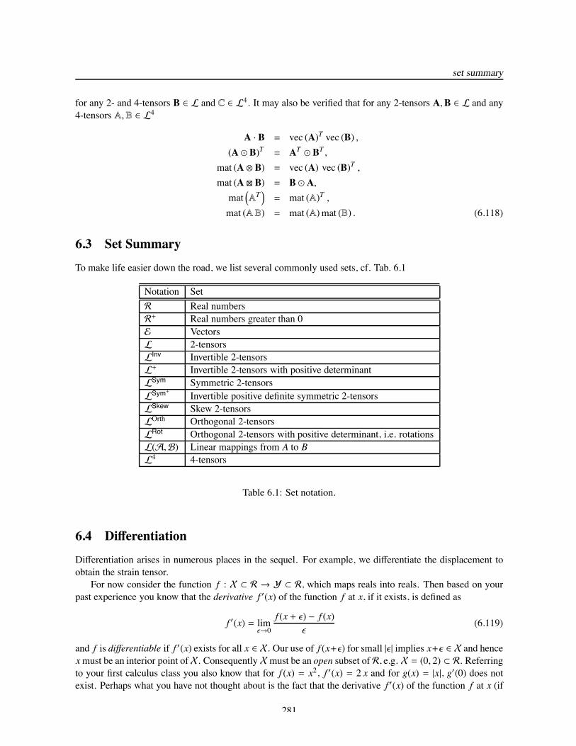
6.3 Set SummaryTo make life easier down the road, we list several commonly used sets, cf. Tab. 6.1
Notation SetR Real numbersR+ Real numbers greater than 0E VectorsL 2-tensorsLInv Invertible 2-tensorsL+ Invertible 2-tensors with positive determinantLSym Symmetric 2-tensorsLSym+ Invertible positive definite symmetric 2-tensorsLSkew Skew 2-tensorsLOrth Orthogonal 2-tensorsLRot Orthogonal 2-tensors with positive determinant, i.e. rotationsL(A,B) Linear mappings from A to BL4 4-tensors
Table 6.1: Set notation.
6.4 DifferentiationDifferentiation arises in numerous places in the sequel. For example, we differentiate the displacement toobtain the strain tensor.
For now consider the function f : X ⊂ R → Y ⊂ R, which maps reals into reals. Then based on yourpast experience you know that the derivative f ′(x) of the function f at x, if it exists, is defined as
f ′(x) = limϵ→0
f (x + ϵ) − f (x)ϵ
(6.119)
and f is differentiable if f ′(x) exists for all x ∈ X. Our use of f (x+ϵ) for small |ϵ| implies x+ϵ ∈ X and hencexmust be an interior point ofX. Consequently Xmust be an open subset of R, e.g. X = (0, 2) ⊂ R. Referringto your first calculus class you also know that for f (x) = x2, f ′(x) = 2 x and for g(x) = |x|, g′(0) does notexist. Perhaps what you have not thought about is the fact that the derivative f ′(x) of the function f at x (if
281
mathematical preliminaries
it exists) is unique because it is defined via the limit, which is unique. And this is the reason that g′(0) doesnot exist, i.e. while the one sided limits limϵ→0+(g(0 + ϵ) − g(0))/ϵ = 1 and limϵ→0−(g(0 + ϵ) − g(0))/ϵ = −1exist, the limit limϵ→0(g(0 + ϵ) − g(0))/ϵ does not.
After taking your vector calculus class you know that for a scalar valued function of a vector, i.e. α :E→ R the gradient ∇α(x) of α at x, if it exists, is defined as the vector
∇α(x) =
⎧⎪⎪⎪⎪⎨⎪⎪⎪⎪⎩
∂α∂x1 (x1, x2, x3)∂α∂x2 (x1, x2, x3)∂α∂x3 (x1, x2, x3)
⎫⎪⎪⎪⎪⎬⎪⎪⎪⎪⎭
=∂α
∂xi(x1, x2, x3) ei (6.120)
and this makes sense, i.e. the scalar valued component function α is differentiated with respect the 3 vectorcomponents x j. For a vector valued function of a vector, i.e. f : E → E the derivative Df(x) of f at x, if itexists, is defined as the 2-tensor (a.k.a. matrix)
Df(x) =
⎡⎢⎢⎢⎢⎢⎢⎢⎢⎢⎢⎢⎢⎢⎣
∂ f1∂x1 (x1, x2, x3)
∂ f1∂x2 (x1, x2, x3)
∂ f1∂x3 (x1, x2, x3)
∂ f2∂x1 (x1, x2, x3)
∂ f2∂x2 (x1, x2, x3)
∂ f2∂x3 (x1, x2, x3)
∂ f3∂x1 (x1, x2, x3)
∂ f3∂x2 (x1, x2, x3)
∂ f3∂x3 (x1, x2, x3)
⎤⎥⎥⎥⎥⎥⎥⎥⎥⎥⎥⎥⎥⎥⎦
=∂ fi∂x j
(x1, x2, x3) ei ⊗ e j (6.121)
and this makes sense, i.e. the 3 component functions fi of the vector valued function f are differentiatedwith respect the 3 vector components x j. In the above it is understood that 1) x = xi ei, cf. Eqn. 6.10, 2)α(x) |x=xi ei = α(x1, x2, x3) and f(x) |x=xi ei = fi(x1, x2, x3) ei are represented by their component functionsα : R3 → R and fi : R3 → R and 3) the partial derivatives are evaluated in the “usual” manner, i.e. viaEqn. 6.119 with xi replacing x. Note the care that is taken to distinguish the function from its componentfunction, e.g. α from α. Also note the care that is taken to have consistent variables on each side of theabove equations, namely (x1, x2, x3). And finally note that the components of the vector ∇α(x) and the2-tensor Df(x) with respect to the fixed orthonormal basis e1, e2, e3 are ∂α
∂xi (x1, x2, x3) and∂ fi∂x j (x1, x2, x3),
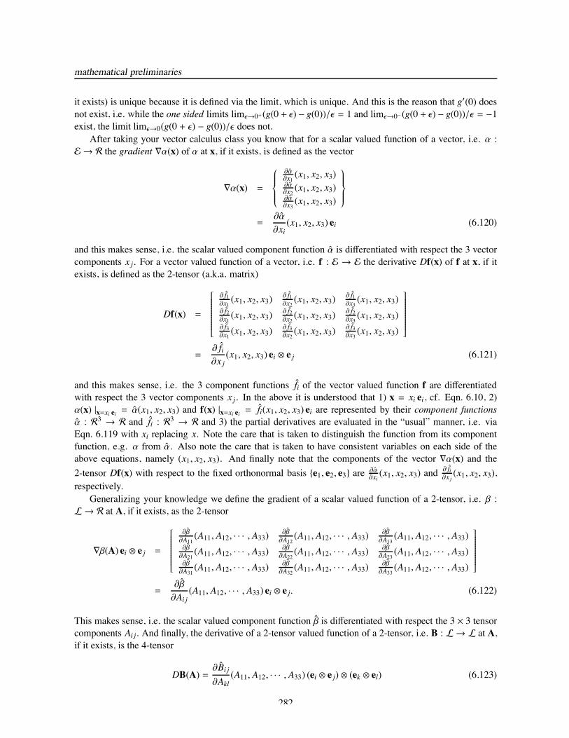
respectively.Generalizing your knowledge we define the gradient of a scalar valued function of a 2-tensor, i.e. β :
L→ R at A, if it exists, as the 2-tensor
∇β(A) ei ⊗ e j =
⎡⎢⎢⎢⎢⎢⎢⎢⎢⎢⎢⎢⎢⎣
∂β∂A11 (A11, A12, · · · , A33)
∂β∂A12 (A11, A12, · · · , A33)
∂β∂A13 (A11, A12, · · · , A33)
∂β∂A21 (A11, A12, · · · , A33)
∂β∂A22 (A11, A12, · · · , A33)
∂β∂A23 (A11, A12, · · · , A33)
∂β∂A31 (A11, A12, · · · , A33)
∂β∂A32 (A11, A12, · · · , A33)
∂β∂A33 (A11, A12, · · · , A33)
⎤⎥⎥⎥⎥⎥⎥⎥⎥⎥⎥⎥⎥⎦
=∂β
∂Ai j(A11, A12, · · · , A33) ei ⊗ e j. (6.122)
This makes sense, i.e. the scalar valued component function β is differentiated with respect the 3 × 3 tensorcomponents Ai j. And finally, the derivative of a 2-tensor valued function of a 2-tensor, i.e. B : L→ L at A,if it exists, is the 4-tensor
DB(A) =∂Bi j∂Akl
(A11, A12, · · · , A33) (ei ⊗ e j) ⊗ (ek ⊗ el) (6.123)
282
differentiation
and this makes sense, i.e. the 3×3 component functions Bi j of the tensor valued function B are differentiatedwith respect the 3 × 3 tensor components Akl. Here is it is understood that 1) A = Ai j ei ⊗ e j, cf. Eqn.6.36, 2) β(A) |A=Ai j = β(A11, A12, · · · , A33) is represented by its component function β : R9 → R and 3)B(A) |A=Ai j = Bi j(A11, A12, · · · , A33) ei⊗e j is represented by its component functions Bi j : R9 → R, cf. Eqn.6.93.
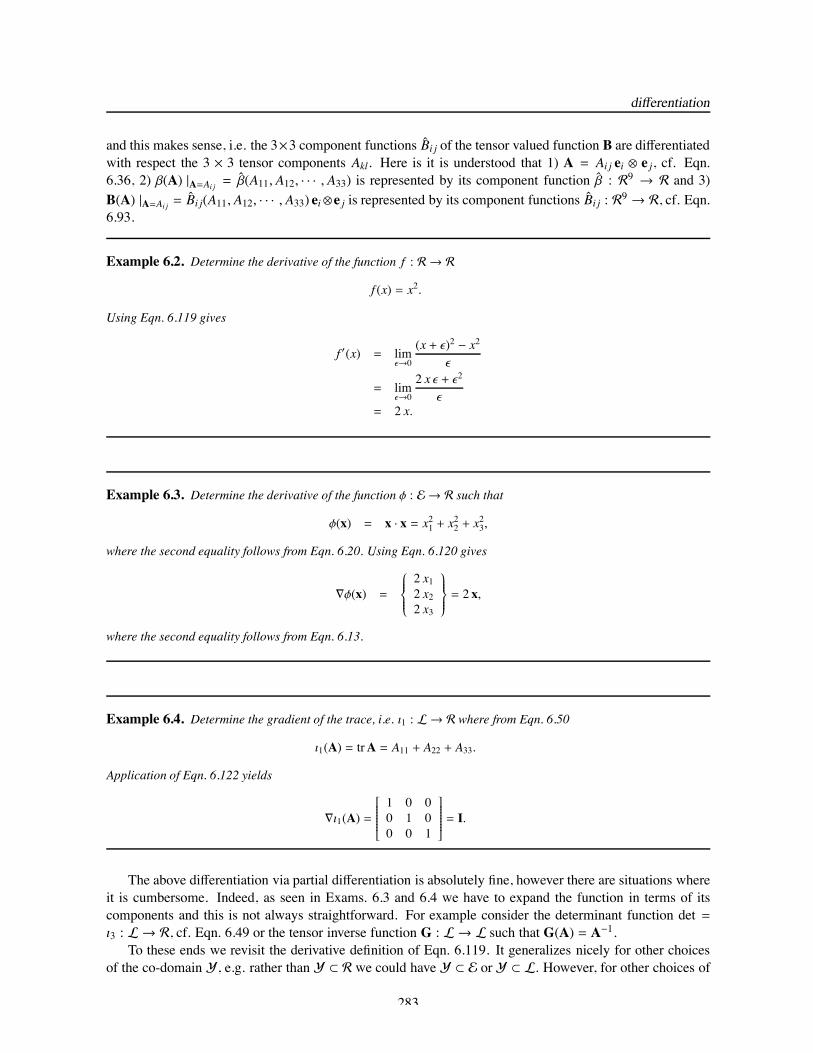
Example 6.2. Determine the derivative of the function f : R→ R
f (x) = x2.
Using Eqn. 6.119 gives
f ′(x) = limϵ→0
(x + ϵ)2 − x2
ϵ
= limϵ→0
2 x ϵ + ϵ2
ϵ= 2 x.
Example 6.3. Determine the derivative of the function φ : E→ R such that
φ(x) = x · x = x21 + x22 + x
23,
where the second equality follows from Eqn. 6.20. Using Eqn. 6.120 gives
∇φ(x) =
⎧⎪⎪⎪⎨⎪⎪⎪⎩
2 x12 x22 x3
⎫⎪⎪⎪⎬⎪⎪⎪⎭= 2 x,
where the second equality follows from Eqn. 6.13.
Example 6.4. Determine the gradient of the trace, i.e. ı1 : L→ R where from Eqn. 6.50
ı1(A) = trA = A11 + A22 + A33.
Application of Eqn. 6.122 yields
∇ı1(A) =
⎡⎢⎢⎢⎢⎢⎢⎢⎢⎣
1 0 00 1 00 0 1
⎤⎥⎥⎥⎥⎥⎥⎥⎥⎦ = I.
The above differentiation via partial differentiation is absolutely fine, however there are situations whereit is cumbersome. Indeed, as seen in Exams. 6.3 and 6.4 we have to expand the function in terms of itscomponents and this is not always straightforward. For example consider the determinant function det =ı3 : L→ R, cf. Eqn. 6.49 or the tensor inverse function G : L→ L such that G(A) = A−1.
To these ends we revisit the derivative definition of Eqn. 6.119. It generalizes nicely for other choicesof the co-domain Y, e.g. rather than Y ⊂ R we could have Y ⊂ E or Y ⊂ L. However, for other choices of
283
mathematical preliminaries
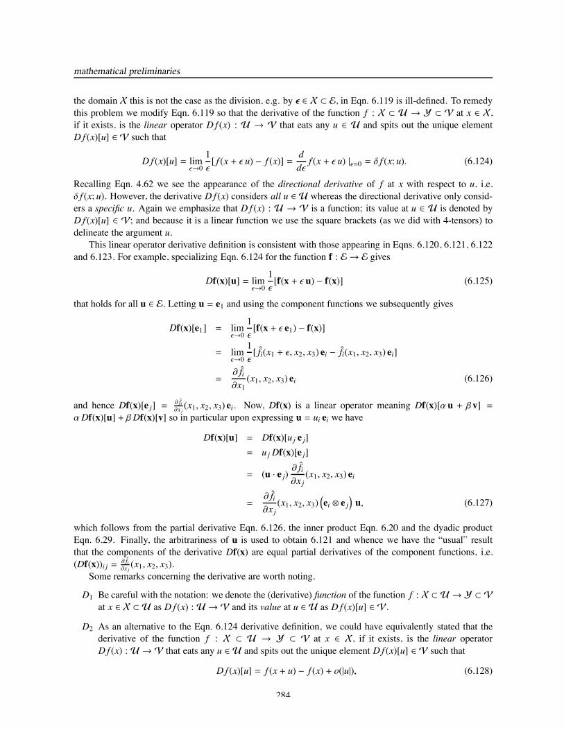
the domain X this is not the case as the division, e.g. by ϵ ∈ X ⊂ E, in Eqn. 6.119 is ill-defined. To remedythis problem we modify Eqn. 6.119 so that the derivative of the function f : X ⊂ U → Y ⊂ V at x ∈ X,if it exists, is the linear operator D f (x) : U → V that eats any u ∈ U and spits out the unique elementD f (x)[u] ∈ V such that
D f (x)[u] = limϵ→0
1ϵ[ f (x + ϵ u) − f (x)] =
ddϵ
f (x + ϵ u) |ϵ=0 = δ f (x; u). (6.124)
Recalling Eqn. 4.62 we see the appearance of the directional derivative of f at x with respect to u, i.e.δ f (x; u). However, the derivative D f (x) considers all u ∈ U whereas the directional derivative only consid-ers a specific u. Again we emphasize that D f (x) : U → V is a function; its value at u ∈ U is denoted byD f (x)[u] ∈ V; and because it is a linear function we use the square brackets (as we did with 4-tensors) todelineate the argument u.
This linear operator derivative definition is consistent with those appearing in Eqns. 6.120, 6.121, 6.122and 6.123. For example, specializing Eqn. 6.124 for the function f : E→ E gives
Df(x)[u] = limϵ→0
1ϵ[f(x + ϵ u) − f(x)] (6.125)
that holds for all u ∈ E. Letting u = e1 and using the component functions we subsequently gives
Df(x)[e1] = limϵ→0
1ϵ[f(x + ϵ e1) − f(x)]
= limϵ→0
1ϵ[ fi(x1 + ϵ, x2, x3) ei − fi(x1, x2, x3) ei]
=∂ fi∂x1
(x1, x2, x3) ei (6.126)
and hence Df(x)[e j] = ∂ fi∂x j (x1, x2, x3) ei. Now, Df(x) is a linear operator meaning Df(x)[αu + β v] =
αDf(x)[u] + βDf(x)[v] so in particular upon expressing u = ui ei we have
Df(x)[u] = Df(x)[uj e j]= uj Df(x)[e j]
= (u · e j)∂ fi∂x j
(x1, x2, x3) ei
=∂ fi∂x j
(x1, x2, x3)(ei ⊗ e j
)u, (6.127)
which follows from the partial derivative Eqn. 6.126, the inner product Eqn. 6.20 and the dyadic productEqn. 6.29. Finally, the arbitrariness of u is used to obtain 6.121 and whence we have the “usual” resultthat the components of the derivative Df(x) are equal partial derivatives of the component functions, i.e.(Df(x))i j = ∂ fi
∂x j (x1, x2, x3).Some remarks concerning the derivative are worth noting.
D1 Be careful with the notation: we denote the (derivative) function of the function f : X ⊂ U → Y ⊂ Vat x ∈ X ⊂ U as D f (x) : U → V and its value at u ∈ U as D f (x)[u] ∈ V.
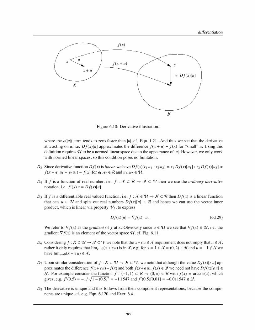
D2 As an alternative to the Eqn. 6.124 derivative definition, we could have equivalently stated that thederivative of the function f : X ⊂ U → Y ⊂ V at x ∈ X, if it exists, is the linear operatorD f (x) : U → V that eats any u ∈ U and spits out the unique element D f (x)[u] ∈ V such that
D f (x)[u] = f (x + u) − f (x) + o(|u|), (6.128)
284
differentiation
x
x + uy
X
Y
u
≈ D f (x)[u]
f (x)
f (x + u)
Figure 6.10: Derivative illustration.
where the o(|u|) term tends to zero faster than |u|, cf. Eqn. 1.21. And thus we see that the derivativeat x acting on u, i.e. D f (x)[u] approximates the difference f (x + u) − f (x) for “small” u. Using thisdefinition requiresU to be a normed linear space due to the appearance of |u|. However, we only workwith normed linear spaces, so this condition poses no limitation.
D3 Since derivative function D f (x) is linear we have D f (x)[ϵ1 u1+ϵ2 u2] = ϵ1 D f (x)[u1]+ϵ2 D f (x)[u2] ≈f (x + ϵ1 u1 + ϵ2 u2) − f (x) for ϵ1, ϵ2 ∈ R and u1, u2 ∈ U.
D4 If f is a function of real number, i.e. f : X ⊂ R → Y ⊂ V then we use the ordinary derivativenotation, i.e. f ′(x) u = D f (x)[u].
D5 If f is a differentiable real valued function, i.e. f : X ∈ U → Y ⊂ R then D f (x) is a linear functionthat eats u ∈ U and spits out real numbers D f (x)[u] ∈ R and hence we can use the vector innerproduct, which is linear via property V2, to express
D f (x)[u] = ∇ f (x) · u. (6.129)
We refer to ∇ f (x) as the gradient of f at x. Obviously since u ∈ U we see that ∇ f (x) ∈ U, i.e. thegradient ∇ f (x) is an element of the vector space U, cf. Fig. 6.11.
D6 Considering f : X ⊂ U → Y ⊂ V we note that the x+ϵ u ∈ X requirement does not imply that u ∈ X,rather it only requires that limϵ→0(x + ϵ u) is in X, e.g. for x = 1 ∈ X = (0, 2) ⊂ R and u = −1 " X wehave limϵ→0(x + ϵ u) ∈ X.
D7 Upon similar consideration of f : X ⊂ U → Y ⊂ V, we note that although the value D f (x)[ϵ u] ap-proximates the difference f (x+ϵ u)− f (x) and both f (x+ϵ u), f (x) ∈ Y we need not have D f (x)[ϵ u] ∈Y. For example consider the function f : (−1, 1) ⊂ R → (0, π) ∈ R with f (x) = arccos(x), whichgives, e.g. f ′(0.5) = −1/
√1 − (0.5)2 = −1.1547 and f ′(0.5)[0.01] = −0.011547 " Y.
D8 The derivative is unique and this follows from their component representations, because the compo-nents are unique, cf. e.g. Eqn. 6.120 and Exer. 6.4.
285
mathematical preliminaries
Example 6.5. Here we repeat the results of Exam. 6.2 using Eqn. 6.128. First, it is worth taking a moment to notewhat the derivative of f : R → R at x. With this in mind and referring to the discussion surrounding Eqn. 6.124 wenote that the derivative of f at x will eat elements in R and spit out elements in R and hence we have D f (x) : R→ R,and since this is a linear operator it acts on the increment u via scalar multiplication, i.e. D f (x)[u] = Df (x) u; andupon referring to ordinary derivative remark D4 above we finally have D f (x)[u] = f ′(x) u, which is the usual result.Now we proceed by applying Eqn. 6.128, viz.
f (x + u) − f (x) = (x + u)2 − x2
= 2 x u + u2
= Df (x)[u] + o(|u|)= f ′(x) u + o(|u|),
where we again see that f ′(x) = 2 x and note that limu→0 u2/|u| = 0, which justifies the statement that u2 = o(|u|), cf.Eqn. 1.21. Now we have f ′(x) : R→ R and, for example,
f (2.1) − f (2) ≈ f ′(2) × 0.12.12 − 2.2 ≈ 4 .1
.41 ≈ .4.
x1
x2
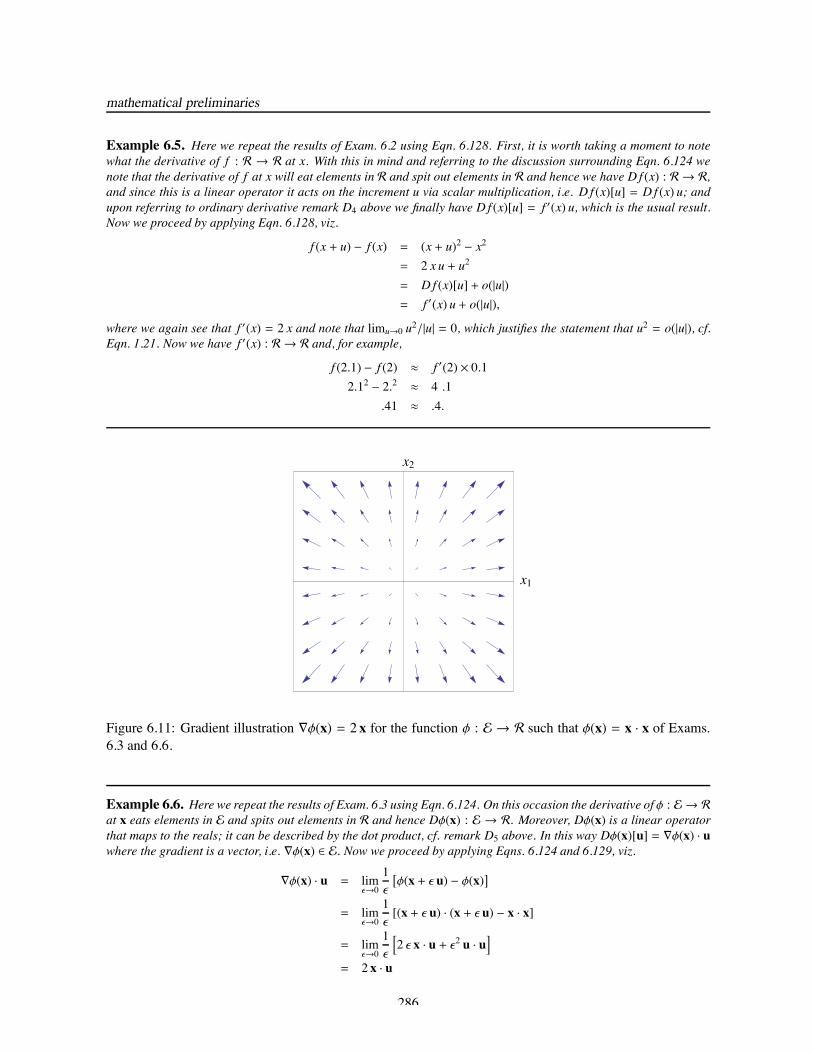
Figure 6.11: Gradient illustration ∇φ(x) = 2 x for the function φ : E → R such that φ(x) = x · x of Exams.6.3 and 6.6.
Example 6.6. Here we repeat the results of Exam. 6.3 using Eqn. 6.124. On this occasion the derivative of φ : E→ Rat x eats elements in E and spits out elements in R and hence Dφ(x) : E → R. Moreover, Dφ(x) is a linear operatorthat maps to the reals; it can be described by the dot product, cf. remark D5 above. In this way Dφ(x)[u] = ∇φ(x) · uwhere the gradient is a vector, i.e. ∇φ(x) ∈ E. Now we proceed by applying Eqns. 6.124 and 6.129, viz.
∇φ(x) · u = limϵ→0
1ϵ
[φ(x + ϵ u) − φ(x)]
= limϵ→0
1ϵ[(x + ϵ u) · (x + ϵ u) − x · x]
= limϵ→0
1ϵ
[2 ϵ x · u + ϵ2 u · u
]
= 2 x · u
286
differentiation
so that again we have ∇φ(x) = 2 x, cf. Fig. 6.11.With x = e1 + 2 e2 and u = 0.1 e1 + 0.1 e2 + 0.2 e3 we have
φ(x + u) − φ(x) ≈ ∇φ(x) · u(1.1 e1 + 2.1 e2 + 0.2 e3) · (1.1 e1 + 2.1 e2 + 0.2 e3) − (e1 + 2e2) · (e1 + 2e2) ≈ 2 (e1 + 2 e2) · (0.1 e1 + 0.1 e2 + 0.2 e3)
.66 ≈ .6.
Example 6.7. Here determine the derivatives of the tensor invariants ı j : L→ R of Eqn. 6.47. These derivatives eatelements in L and spit out elements in R and hence Dı j(A) : L → R. And as in Exam. 6.6, since the linear operatorDı j(A) maps to the reals we describe it via the dot product, i.e. Dı j(A)[U] = ∇ı j(A) · U where the gradients aretensors, i.e. ∇ı j(A) ∈ L. Now we proceed by applying Eqns. 6.124 and 6.129 to the invariants ı j : L→ R such that
ı1(A) = trA,
ı2(A) =12(trA)2 − trA2,
ı3(A) = detA,
cf. Eqn. 6.51.Using Eqns. 6.59, 6.124 and 6.129 with ı1(A) = trA = I · A gives
∇ı1(A) · U = limϵ→0
1ϵ[ı1(A + ϵ U) − ı1(A)]
= limϵ→0
1ϵ[I · (A + ϵ U) − I · A]
= limϵ→0
1ϵ[I · ϵ U]
= I · U
whence
∇ı1(A) = I, (6.130)
which agrees with our Exam. 6.4 result.The same process with Eqns. 6.51, 6.59, 6.124 and 6.129 gives
∇ı2(A) · U = limϵ→0
1ϵ[ı2(A + ϵ U) − ı2(A)]
= limϵ→0
1ϵ
[12
[tr(A + ϵ U)]2 − tr(A + ϵ U)2
−12
(trA)2 − trA2
]
= limϵ→0
1ϵ
[12
[(A + ϵ U) · I]2 − (A + ϵ U)T · (A + ϵ U)
−12
(A · I)2 − AT · A
]
= limϵ→0
1ϵ
[ϵ
[(A · I)(I · U) − AT · U
]+ϵ2
2[(U · I)2 − UT · U
]]
= (A · I)(I · U) − AT · U= (trA I − AT ) · U
whence
∇ı2(A) = trA I − AT . (6.131)
287
mathematical preliminaries
In regard to ı3(A) we use Eqn. 6.47 to obtain for ı3(A) = detA
[ı3(A + ϵ U) − ı3(A)][a, b, c] = ı3(A + ϵ U)[a, b, c] − ı3(A)[a, b, c]= [(A + ϵ U) a, (A + ϵ U) b, (A + ϵ U) c] − [Aa,Ab,Ac]= ϵ [Ua,Ab,Ac] + [Aa,Ub,Ac] + [Aa,Ab,Uc]+
ϵ2 [Aa,Ub,Uc] + [Ua,Ab,Uc] + [Ua,Ub,Ac]+ϵ3 [Ua,Ub,Uc]
= ϵ[UA−1Aa,Ab,Ac] + [Aa,UA−1Ab,Ac] + [Aa,Ab,UA−1Ac]
+
ϵ2[Aa,UA−1Ab,UA−1Ac] + [UA−1Aa,Ab,UA−1Ac]+
[UA−1Aa,UA−1Ab,Ac]+
ϵ3 [Ua,Ub,Uc]= ϵ ı1(UA−1) [Aa,Ab,Ac]+ ϵ2 ı2(UA−1) [Aa,Ab,Ac] + ϵ3 ı3(U)[a, b, c]=
(ϵ ı1(UA−1) ı3(A) + ϵ2 ı2(UA−1) ı3(A) + ϵ3 ı3(U)
)[a, b, c]
Using the arbitrariness of a, b, and c we have
ı3(A + ϵ U) − ı3(A) = ϵ ı1(UA−1) ı3(A) + ϵ2 ı2(UA−1) ı3(A) + ϵ3 ı3(U)
so that Eqns. 6.59, 6.124 and 6.129 give
∇ı3(A) · U = limϵ→0
1ϵ[ı3(A + ϵ U) − ı3(A)]
= ı1(UA−1) ı3(A)= ı3(A)A−T · U
whence
∇ı3(A) = detAA−T
= A∗, (6.132)
where we use Eqn. 6.71. Note that this result assumes A is invertible, i.e. ı3 : LInv ⊂ L→ R \ 0 ⊂ R.
6.4.1 Product rule
You used the product rule to evaluate derivatives, e.g. for f (x) = g(x) h(x) you compute f ′(x) = g′(x) h(x) +g(x) h′(x) where f , g and h are functions on the reals to the reals, e.g. f : R → R. And you evaluatedderivatives of more “complicated” functions, e.g. for the real valued function α : E → R you evaluatedthe gradient ∇α(x) of Eqn. 6.120. But perhaps you have not evaluated the derivative of products of these“complicated” functions. For example consider α(x) = g(x) · h(x) where f and g are vector valued functionsof vectors, e.g. f : E→ E. To differentiate α we cannot use the product rule in the naive way, i.e. we do nothave ∇α(x) = Dg(x) ·h(x)+g(x) ·Dh(x) where Dg(x) and Dh(x) are matrices similar to Df(x) in Eqn. 6.121.Indeed the “inner product” in this derivative expression is nonsense since it is between a tensor (matrix) anda vector.
When deriving the governing equations for linear elasticity we need to differentiate functions that areproducts in nature, i.e., f (x) = g(x) ⋆ h(x) where the functions f : X ⊂ U → Y, g : X ⊂ U → W andh : X ⊂ U → Z have the same domain X and respective co-domains Y,W andZ, which are, e.g. subsetsof R, E and/or L. For example, ⋆ could represent the scalar multiplication between a real valued function
288
differentiation
and either another real valued function, a vector valued function or a tensor valued function. It could alsorepresent the inner product between a pair of vector valued functions (as just discussed) or tensor valuedfunctions. The dyadic product ⊗ between a pair of vector or tensor valued functions is yet another example.Our task here is to differentiate such functions.
In all cases, the operation ⋆ is bilinear meaning that for d, g ∈ W, h, k ∈ Z and reals α, β ∈ R wehave (α d + β g) ⋆ h = α (d ⋆ h) + β (g ⋆ h) and g ⋆ (α h + β k) = α (g ⋆ h) + β (g ⋆ k), cf. Sect. 4.4.2. Inessence, if we fix h ∈ Z then ⋆ is linear operator onW and visa versa. For the cases of the inner and dyadicproducts between a pair of vectors this is clearly the case as seen through properties E1 and E2 and Eqn.6.32, respectively.
To differentiate f we use the product rule, which states that if Dg(x) : U →W and Dh(x) : U → Zexist, then D f (x) : U → Y exists and satisfies
D f (x)[u] = Dg(x)[u] ⋆ h(x) + g(x) ⋆ Dh(x)[u]. (6.133)
In the following examples we apply the product rule to obtain results that are required in our subsequentdevelopments.
Example 6.8. Here we determine the derivative of the function φ : E→ R where
φ(x) = g(x) · h(x)
with g : E → E and h : E → E smooth functions. The derivatives of the smooth functions g and h at x linearly mapvectors u ∈ E to the vectors Dg(x)[u] ∈ E and Dh(x)[u] ∈ E and hence Dg(x) ∈ L and Dh(x) ∈ L are 2-tensors to witwe write Dg(x)[u] = Dg(x) u and Dh(x)[u] = Dh(x) u. On the other hand, Dφ(x) linearly maps vectors u ∈ E to realsDφ(x)[u] and hence Dφ(x)[u] = ∇φ(x) · u where ∇φ(x) ∈ E is the gradient vector, cf. Exam. 6.6. Being that as it may,we now apply Eqns. 6.40, 6.129 and 6.133 to obtain
Dφ(x)[u] = Dg(x)[u] · h(x) + g(x) · Dh(x)[u],∇φ(x) · u = u · (Dg(x))T h(x) + (Dh(x))T g(x) · u
=(Dg(x))T h(x) + (Dh(x))T g(x)
· u.
As seen above ∇φ(x) = (Dg(x))T h(x) + (Dh(x))T g(x) ∈ E.
Example 6.9. Here we determine the derivative of the function a : E→ E where
a(x) = α(x) h(x)
with α : E → R and h : E → E smooth functions. The derivative of α linearly maps vectors u ∈ E to reals Dα(x)[u]and hence we have Dα(x)[u] = ∇α(x) ·u where ∇α(x) ∈ E is the gradient vector. On the other hand, the derivatives ofa and h linearly map vectors u ∈ E to vectors Da(x)[u] ∈ E and Dh(x)[u] ∈ E and hence we write Da(x)[u] = Da(x) uand Dh(x)[u] = Dh(x) u as Da(x) ∈ L and Dh(x) ∈ L are 2-tensors. Forging on, we apply Eqns. 6.29, 6.129 and6.133 to obtain
Da(x)[u] = (Dα(x)[u] h(x) + α(x)Dh(x)[u]Da(x) u = (∇α(x) · u) h(x) + α(x)Dh(x) u
= (h(x) ⊗ ∇α(x) + α(x)Dh(x)) u.
Here we have Da(x) = h(x) ⊗ ∇α(x) + α(x)Dh(x), which we recognize as a tensor.
289
mathematical preliminaries
Example 6.10. Determine the derivative of the function F : LInv ⊂ L→ LInv ⊂ L where
F(A) = A−1.
Of course the domain of F is restricted to the subspace of invertible tensors. However, the domain of DF(A) is L,i.e. the set of 2-tensors. Moreover, DF(A) linearly maps 2-tensors U ∈ L to 2-tensors DF(A)[U] ∈ L and henceDF(A) ∈ L4 is a 4-tensor.
To address this problem we define G : LInv ⊂ L → LInv ⊂ L such that G(A) = F(A)A = I. And based onthe above verbiage, we know that DG(A) ∈ L4 is a 4-tensor. Moreover, since G(A) = I a constant we trivially haveDG(A) = O. However our problem is to find DF(A) to wit we use Eqn. 6.133 to obtain
DG(A)[U] = DF(A)[U]A + F(A) I[U]O[U] = DF(A)[U]A + F(A)UO = DF(A)[U]A + F(A)U,
where we used that fact that for H : L→ L such that H(A) = A we trivially have DH(A) = I ∈ L4 and DH(A)[U] =U. Rearranging the above and using Eqn. 6.107 gives
DF(A)[U] = −F(A)UA−1
= −A−1UA−1
= −(A−1 ! A−T )U
or
DF(A) = −(A−1 ! A−T ), (6.134)
which is a fourth-order tensor, i.e. an element ofL4. This is in agreement with your prior knowledge, i.e. for f : R→ Rwith f (x) = 1/x we have f ′(x) = −1/x2 that is defined at all x ∈ R except x = 0. Indeed at x = 0 f is not defined, i.e.it is the element in R with no inverse.
Example 6.11. In this example we determine the derivative of the adjugate A∗ of A. Noting from Eqn. 6.71 thatA∗ = detAA−T we define the function H : LInv ⊂ L→ LInv ⊂ L such that H(A) = A∗. However, to utilize the resultsof Exams. 6.7 and 6.10 we defineG : LInv ⊂ L→ LInv ⊂ L such that G(A) = ı3(A)F(A) so that
H(A) = A∗
= detAA−T
= T[detAA−1]= T[ı3(A)F(A)]= T[G(A)],
where we use Eqns. 6.64, 6.71 and 6.100 and define F : LInv ⊂ L → LInv ⊂ L such that F(A) = A−1. From Exams.6.7 and 6.10 we have Dı3(A)[U] = ∇ı3(A) · U = det(A)A−T · U and DF(A)[U] = −(A−1 ! A−T )[U] and hence Eqns.6.129 and 6.133 give
DG(A)[U] = Dı3(A)[U]F(A) + ı3(A)DF(A)[U]= (∇ı3(A) · U)F(A) − ı3(A) (A−1 ! A−T )[U]=
(F(A) ⊗ ∇ı3(A) − ı3(A) (A−1 ! A−T )
)[U]
= detA (A−1 ⊗ A−T − A−1 ! A−T )[U],
290
differentiation
where we used Eqns. 6.55, 6.57, 6.91, 6.104, 6.132 and 6.134. The above gives the fourth order tensor DG(A) =detA (A−1 ⊗ A−T − A−1 ! A−T ) and hence, recalling the composition result AB[C] = A[B[C]] we have
DH(A) = detAT (A−1 ⊗ A−T − A−1 ! A−T ). (6.135)
Example 6.12. We continue with the previous Exam. 6.11 and now differentiate the function |A∗ a| with respect toA; here a is an arbitrary constant vector. Again noting from Eqn. 6.71 that A∗ = detAA−T we define the functionh : LInv ⊂ L→ E such that h(A) = A∗ a = H(A) a where we utilize the results of Exam. 6.11 so that
Dh(A)[U] = DH(A)[U] a=
[detAT (A−1 ⊗ A−T − A−1 ! A−T )
][U] a. (6.136)
Next we define the scalar valued function α : LInv ⊂ L → R such that α(A) = (h(A) · h(A)) 12 = |A∗ a| and use theelementary rules of differentiation to obtain
∇α(A) · U =12(h(A) · h(A))− 12 2 h(A) · Dh(A)[U]
= (h(A) · h(A))−12 h(A) · DH(A)[U] a
=1
α(A) (h(A) ⊗ a) · DH(A)[U]
=1
α(A) DTH(A)[h(A) ⊗ a] · U
=1
α(A)T detA
[A−1 ⊗ A−T − A−1 ! A−T
]T[(A∗ a) ⊗ a] · U
=1
α(A) detA[A−1 ⊗ A−T − A−1 ! A−T
]TTT [(A∗ a) ⊗ a] · U
=1
α(A) detA[A−T ⊗ A−1 − A−T ! A−1
]T[(A∗ a) ⊗ a] · U
=1
α(A) detA[A−T ⊗ A−1 − A−T ! A−1
][a ⊗ (A∗ a)] · U
=1
α(A) detA[(A−1 · (a ⊗ (A∗ a))
)A−T − A−T (a ⊗ (A∗ a))A−T
]· U
=1
α(A) detA[((A−1A∗ a) · a
)I − (A−T a) ⊗ (A∗ a)
]A−T · U
=1
α(A) detA[((A∗ a) · (A−T a)
)I − (A−T a) ⊗ (A∗ a)
]A−T · U
=1
α(A)[((A∗ a) · (A∗ a)) I − (A∗ a) ⊗ (A∗ a) ]A−T · U,
where we used Eqns. 6.40, 6.41, 6.59, 6.64, 6.71, 6.86, 6.100, 6.97 and 6.108, amongst others. And hence we have
∇α(A) = 1α(A)
[((A∗ a) · (A∗ a)) I − (A∗ a) ⊗ (A∗ a) ]A−T . (6.137)
6.4.2 Chain rule
When deriving the governing equations for linear elasticity we also need to differentiate composite functions.And you also used the chain rule to evaluate derivatives, e.g. for h(x) = g f (x) = g( f (x)) you compute
291
mathematical preliminaries
h′(x) = g′( f (x)) f ′(x) where f , g and h are functions on the reals to the reals, e.g. f : R → R. However, asseen with the product rule, care must be taken when applying the chain rule to more “complicated” functions.For example, for β(x) = α(g(x)) where α and β are scalar valued functions of vectors, e.g. β : E → R and gis a vector valued functions of vectors, i.e. g : E → E, we cannot merely say that ∇β(x) = ∇α(g(x))Dg(x),indeed the vector times the tensor operation is nonsense.
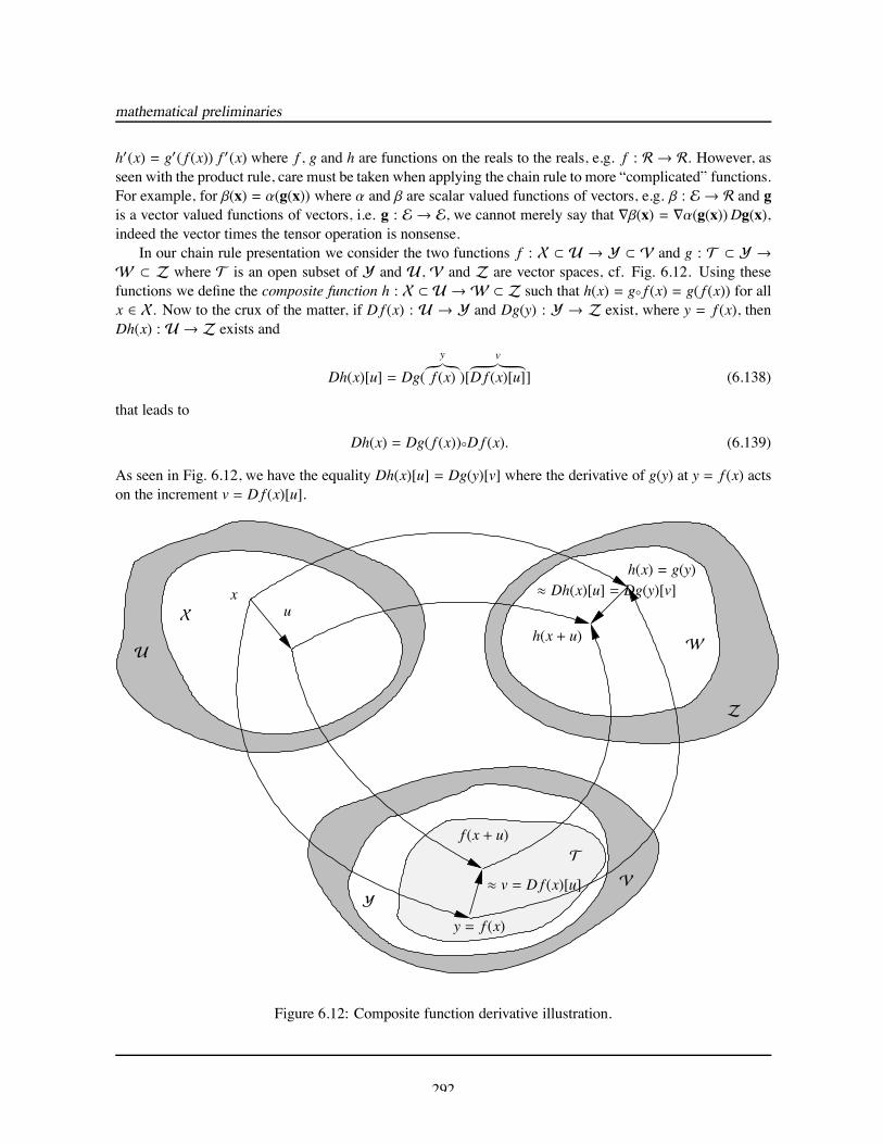
In our chain rule presentation we consider the two functions f : X ⊂ U → Y ⊂ V and g : T ⊂ Y →W ⊂ Z where T is an open subset of Y and U, V and Z are vector spaces, cf. Fig. 6.12. Using thesefunctions we define the composite function h : X ⊂ U →W ⊂ Z such that h(x) = g f (x) = g( f (x)) for allx ∈ X. Now to the crux of the matter, if D f (x) : U → Y and Dg(y) : Y → Z exist, where y = f (x), thenDh(x) : U → Z exists and
Dh(x)[u] = Dg(y︷︸︸︷f (x) )[
v︷!!!!︸︸!!!!︷D f (x)[u]] (6.138)
that leads to
Dh(x) = Dg( f (x))D f (x). (6.139)
As seen in Fig. 6.12, we have the equality Dh(x)[u] = Dg(y)[v] where the derivative of g(y) at y = f (x) actson the increment v = D f (x)[u].
xu
y = f (x)
f (x + u)
≈ v = D f (x)[u]
h(x) = g(y)
h(x + u)
≈ Dh(x)[u] = Dg(y)[v]
T
U
V
W
X
Y
Z
Figure 6.12: Composite function derivative illustration.
292
differentiation
Example 6.13. We now refer to Eqn. 6.124 in which f : X ⊂ U → Y ⊂ V and define the composite functiong = f h : R→ Y ⊂ V where h : R→ X ⊂ U such that h(ϵ) = x + ϵ u so that
g(ϵ) = f h(ϵ) = f (x+ϵ u︷︸︸︷h(ϵ) ).
In this way the chain-rule gives
Dg(ϵ)[u] = Df (h(ϵ))Dh(ϵ)[u]g′(ϵ) u = Df (h(ϵ))[h′(ϵ) u]
= Df (h(ϵ)) u,
where we used the ordinary derivative notation of remark D4, e.g. Dh(ϵ) = h′(ϵ), the trivial result h′(ϵ) = 1 and thefact that u is a scalar. The arbitrariness of u gives us
g′(ϵ) = Df (h(ϵ)),
which is identical to Eqn. 6.124 for ϵ = 0, i.e. g′(0) = δ f (x; u). And thus, the directional derivative is obtained via thechain rule, assuming that D f (x) exists.
Example 6.14. We assume the functions F : L → L and G : L → L are differentiable and thus they havederivatives that linearly map 2-tensors U ∈ L into 2-tensors DF(A)[U] ∈ L and DG(A)[U] ∈ L making DF(A) ∈ L4and DG(A) ∈ L4 4-tensors. Using these functions we define the composite function H = FG : L → L, which isdifferentiable since F and G are differentiable. The derivative DH(A) ∈ L4 is also a 4-tensor as it also linearly maps2-tensors U ∈ L into 2-tensors DH(A)[U] ∈ L. We evaluate this 4-tensor by appealing to Eqn. 6.138, i.e.
DH(A)[U] = DF(G(A))[DG(A)[U]].
Next we use the composition (multiplication) relation AB[C] = A[B[C]] and the arbitrariness of U whence
DH(A) = DF(G(A))DG(A).
Now we assume the real valued function α : L→ R is differentiable and thus it has a gradient that linearly maps2-tensors U ∈ R to scalars ∇α(A) · U ∈ R making ∇α(A) : L → R a 2-tensor. From this and the above we definethe real valued composite function β = αG : L → R, which is differentiable since α and G are differentiable. Thegradient ∇β(A) ∈ L is a 2-tensor that linearly maps 2-tensors U ∈ L into reals ∇β(A) · U ∈ R. To evaluate thisgradient we refer to Eqns. 6.97, 6.129 and 6.138 which give
Dβ(A)[U] = Dα(G(A))DG(A)[U]∇β(A) · U = Dα(G(A))[DG(A)[U]]
= ∇α(G(A)) · DG(A)[U]= (DG(A))T ∇α(G(A)) · U
The arbitrariness of U implies∇β(A) = (DG(A))T ∇α(G(A)).
In regard to Eqns. 5.87 – 5.90 we mention the implicit function theorem; it asserts that if f : X ⊂U → Y ⊂ U has an invertible derivative D f (x) ∈ L(U,U) atx (which linearly maps elements u ∈ U intoelements of the same space), then f has a smooth inverse function f ↓ : Y ⊂ U → X ⊂ U at x. Moreover
293
mathematical preliminaries
we can define the composite functions f ↓ f : X ⊂ U → X ⊂ U and f f ↓ : Y ⊂ U → Y ⊂ U such thatf ↓ f (x) = x and f f ↓(y) = y. Differentiating these composite maps via the chain rule yields reveals
I = D f ↓ f (x)= D f ↓(y)D f (x) |y= f (x)= D f ↓(y)D f (x) |y= f (x) ,
where I is the identity operator onU. Rearranging the above gives
D f ↓(y) |y= f (x) = [D f (x)]−1, (6.140)
i.e. the derivative of the inverse function D f ↓(y) equals the inverse of the derivative [D f (x)]−1 at the corre-sponding points y = f (x).
6.4.3 Higher order derivatives
With the risk of beating a dead horse, we state again that the derivative of the function f : X ⊂ U → Y ⊂ Vat x, if it exists, is the linear operator D f (x) : U → V that eats elements u ∈ U and spits out elementsD f (x)[u] ∈ V making D f (x) ∈ L(U,V), i.e. a linear transformation from U to V. Now if D f (x) existsfor all x ∈ X then we can view D f as a function mapping elements of X ⊂ U into elements of L(U,V),i.e. D f : X ⊂ U → L(U,V). 6.2 If this case we can think about the derivative D2 f (x) of the function D fevaluated at x. This second derivative of f is defined analogously to the first derivative in Eqn. 6.124, butnow DD f replaces D f , D f replaces f , and L(U,V) replaces V. Indeed, the second derivative of f at x, ifit exists, is defined as
D2 f (x)[u] = limϵ→0
1ϵ[D f (x + ϵ u) − D f (x)] = d
dϵD f (x + ϵ u) |ϵ=0 = δD f (x; u) (6.141)
for all u ∈ U where we introduce the notation D2 f (x) in place of DD f (x). Such derivatives arise whenwe discuss the elasticity tensor, i.e. the second derivative of the strain energy function. Following thedevelopment of Eqn. 6.128 we see that
D2 f (x)[u] = D f (x + ϵ u) − D f (x) + o(|u|) (6.142)
for all u ∈ U. Being a derivative D2 f (x) is a linear operator, which eats elements u ∈ U and spits outelements D2 f (x)[u] ∈ L(U,V), which themselves are linear operators, i.e. D2 f (x) : U → L(U,V) andhence for v ∈ U we have (D2 f (x)[u])[v] ∈ V, which we express more compactly as
D2 f (x) [u, v] = (D2 f (x)[u])[v]= (DD f (x)[u])[v] (6.143)= D(D f (x)[u])[v],
where the second line follows from the notation D2 f (x) = DD f (x) and the third by viewing u as a constantin the differentiation, e.g. for the smooth function f : R→ R we have d2 f
dx2 (x) u =ddx (
d fdx (x) u). Based on this
discussion we can write either D2 f (x) : U → L(U,V) or D2 f (x) : U×U → V. In the latter interpretationit can be shown that the map D2 f (x) : U ×U → V is both bilinear and symmetric in the sense that
D2 f (x) [α u + βv,w] = α (D2 f (x) [u,w]) + β (D2 f (x) [v,w]), (6.144)D2 f (x) [w,α u + βv] = α (D2 f (x) [w, u]) + β (D2 f (x) [w, v]),
D2 f (x) [u, v] = D2 f (x) [v, u],6.2Note that this Df : X ⊂ U → L(U,V) is not generally linear, unlike Df (x) : U → V, which by definition is always linear.
294
differentiation
where w ∈ U and α, β ∈ R. Of course the second equality follows from the other two. The first bilinearityequality follows from Eqn. 6.141. To obtain the symmetry equality we use Eqns. 6.128 and 6.142, i.e.
D2 f (x)[u, v] = D (D f (x)[u]) [v] (6.145)= D f (x + v)[u] − D f (x)[u] + o(|v|)=
[f (x + v + u) − f (x + v) + o(|u|)
]−
[f (x + u) − f (x) + o(|u|)
]+ o(|v|)
=[f (x + u + v) − f (x + u) + o(|v|)
]−
[f (x + v) − f (x) + o(|v|)
]+ o(|u|)
= D f (x + u)[v] − D f (x)[v] + o(|u|)= D (D f (x)[v]) [u]= D2 f (x)[v, u].
Continuing in this manner we can define still higher order derivatives and this progression leads to thefunction classification discussion of Sect. 1.5.
Example 6.15. Refer to Exam. 6.7 and determine the second derivatives of the tensor invariants. In all cases thesecond derivatives D2ıi(A) are fourth-order tensors, i.e. D2ı j(A) ∈ L4, which follows from the facts that for the scalarvalued ı j : L → R we have ∇ıi(A) : L → L and hence D2ıi(A) : L → L4. Since ∇ı1(A) = I, a constant, we triviallyhave
D2ı1(A) = O. (6.146)
From Eqn. 6.131, i.e. ∇ı2(A) = ı1(A) I − AT , the product rule and noting that the derivative of a sum is the sum of thederivatives we obtain
D2ı2(A)[U] = Dı1(A)[U] I − T[U]= (∇ı1(A) · U) I − UT
= (I · U) I − UT
= (I ⊗ I − T)[U],
where we utilized Eqns. 6.59 and 6.91 and the trivial result that for F : L→ L such that F(A) = AT = T[A] we haveDF(A) = T. Utilizing the arbitrariness of U gives
D2ı2(A) = (I ⊗ I − T). (6.147)
Equations 6.132 and 6.135 render the last result
D2ı3(A) = detAT (A−1 ⊗ A−T − A−1 ! A−T ). (6.148)
6.4.4 Partial derivatives
The component results of Eqns. 6.120 – 6.123 utilize partial derivatives. And for functions of two variablesf : R × R → R you know that the partial derivative ∂ f
∂x1 (x1, x2) is just the “usual” derivative obtained byviewing f as a function of only the first variable x1. And this interpretation is absolutely correct. Hereinwe define the partial derivative of the function f : X ⊂ U → Y ⊂ V where X = X1 × X2 × · · · × Xnis the n-fold set product of the open subsets Xi ⊂ Ui, i = 1, 2, · · · , n. Thus we have f (x) = y ∈ Y wherex = (x1, x2, · · · , xn) ∈ X with xi ∈ Xi ⊂ Ui. For example the function f : E × R → E eats the vector –scalar pair (a,α) = E × R and spits out the vector f(a,α) ∈ E; in this case X = E × R, x1 = a ∈ X1 = E,x2 = α ∈ X2 = R and f(a,α) ∈ Y = E.
295
mathematical preliminaries
The i-th partial derivative of f at x, if it exists, is the linear operator Di f (x) : Ui → V that eatselements ui ∈ Ui and spits out elements Di f (x)[ui] ∈ V such that
Di f (x)[ui] = limϵ→0
1ϵ[ f (x1, x2, · · · , xi−1, xi + ϵ ui, xi+1, · · · , xn) − f (x1, x2, · · · , xi−1, xi, xi+1, · · · , xn)]
=ddϵ
f (x1, x2, · · · , xi−1, xi + ϵ ui, xi+1, · · · , xn) |ϵ=0 , or (6.149)
= f (x1, x2, · · · , xi−1, xi + ui, xi+1, · · · , xn) − f (x1, x2, · · · , xi−1, xi, xi+1, · · · , xn) + o(|ui |)
for all ui ∈ Ui. Note the similarity of the above with Eqns. 6.124 and 6.128. We emphasize that thesepartial derivatives are not necessarily scalars like those appearing in Eqns. 6.120 – 6.123. Indeed, for ourf : E × R → E example we have D1f(a,α) that linearly maps vectors u ∈ E into vectors D1f(a,α)[u] ∈ Emaking D1f(a,α) ∈ L a 2-tensor and D2f(a,α) that linearly maps scalars u ∈ R into vectors D2f(a,α)[u] ∈ Emaking D2f(a,α) ∈ E a vector. Of course the components of these partial derivatives can be expressed usingexpressions such as those appearing in Eqns. 6.120 – 6.123.
Not surprisingly, if D f (x) exists then
Di f (x)[ui] = D f (x)[u︷!!!!!!!!!!!!!!!!!!!!!!!!!!!!!!︸︸!!!!!!!!!!!!!!!!!!!!!!!!!!!!!!︷
(0, 0, · · · , 0, ui︸︷︷︸ithplace
, 0, · · · , 0)] (6.150)
and conversely, if all of the partial derivatives exist at x, then
D f (x)[u] =n∑
i=1Di f (x)[ui], (6.151)
where u = (u1, u2, · · · , un) ∈ U = U1 ×U2 × · · · ×Un.If Di f (x) exists for all x ∈ X then we can define the second partial derivative Di j f (x) : U j → L(Ui,V),
which, if it exists, is the linear map fromU j to L(Ui,V) such that
Di j f (x)[uj] = limϵ→0
1ϵ[Di f (x1, x2, · · · , x j−1, x j + ϵ uj, x j+1, · · · , xn) − Di f (x1, x2, · · · , x j−1, x j, x j+1, · · · , xn)],
=ddϵDi f (x1, x2, · · · , x j−1, x j + ϵ uj, x j+1, · · · , xn) |ϵ=0 , or (6.152)
= Di f (x1, x2, · · · , x j−1, x j + uj, x j+1, · · · , xn) − Di f (x1, x2, · · · , x j−1, x j, x j+1, · · · , xn) + o(|uj |).
Following the second derivative discussion, we can also treat the second partial derivative as the bilinearmap Di j f (x) : Ui ×U j → V that satisfies
Di j f (x) [u,w] = Dj(Di f (x)[u])[w],Di j f (x) [α u + βv,w] = α (Di j f (x) [u,w]) + β (Di j f (x) [v,w]), (6.153)Di j f (x) [u,αw + βz] = α (Di j f (x) [u,w]) + β (Di j f (x) [u, z]),
Di j f (x) [u, v] = Dji f (x) [v, u]
for every u, v ∈ Ui, w, z ∈ U j and α, β ∈ R. The first equality defines the bilinear map, the second two arelinearity results and the last is the symmetry, which follows from an argument similar to that of Eqn. 6.145.
296
the euclidean point space
• Use the definition of the function f : X ⊂ U → Y ⊂ V, e.g. how it acts on arbitrary vectors etc.
• Note the domainU and codomain V of the linear mapping D f (x) : U → V,
• Use your knowledge ofU andV to note what D f (x) ∈ L(U,V) is, e.g. a vector, 2-tensor, etc.
• Use the definition of the derivative, product rule and chain-rule to obtain an expression forD f (x)[u],
• Use scalar, dyadic, conjugate products etc. to factor u from your D f (x)[u] expression, and
• Use the arbitrariness of u to define D f (x).
Figure 6.13: Procedure to compute the derivative D f (x) : U → V of the function f : X ⊂ U → Y ⊂ V atx ∈ X.
6.4.5 Differentiation summary
As seen from the above examples, it is not always easier to evaluate the derivatives via the component route.Rather to evaluate the derivative of the function f : X ⊂ U → Y ⊂ V at x ∈ X, i.e. the linear operatorD f (x) : U → V fromU toV it is recommended to follow the steps in Fig. 6.13.
6.5 The Euclidean Point Space
In our analyses we are interested in quantifying the motion of a body B subjected to loads. The body itselfis comprised of particles or points y in a Euclidean point space E, i.e. y ∈ E and B ⊂ E. Much ado can andprobably should be made about the Euclidean point space. However, we can bypass this discussion and cutto the core of the matter. We define a single rectangular Cartesian coordinate system that consists of thefixed basis e1, e2, e3 and the fixed point o that we call the origin. In this way, we identify all points y in ourbody via their position vectors xy ∈ E relative to o and we associate the body B itself with the collection ofpoints, i.e. position vectors, that comprise the region Ω in which the body resides, i.e. Ω ⊂ E. We assumethat Ω is bounded, open and connected with a piecewise smooth boundary, i.e. surface, which has a unitoutward normal vector n. The collection of points, i.e. position vectors, that form the surface define the set∂Ω, and the union of all such points, i.e. position vectors, in Ω and ∂Ω define the closure Ω of Ω.
Functions defined on the body, i.e. Ω, are referred to as fields. Examples of such functions are the vectordisplacement field u : Ω ⊂ E→ R and the tensor stress field T : Ω ⊂ E→ L.
6.6 The Localization Theorem
We now formalize the localization argument that we discussed in Eqns. 4.6 – 4.8. If f : R→ R is continuous,then the mean value theorem gives
∫ x+ϵx−ϵ f (y) dy = 2 ϵ f (x) where x ∈ [x − ϵ, x + ϵ]. Rearranging this result
as f (x) = 1/(2 ϵ)∫ x+ϵx−ϵ f (y) dy and taking the limit as ϵ → 0 gives f (x) = limϵ→0 1/(2 ϵ)
∫ x+ϵx−ϵ f (y) dy. To
297
mathematical preliminaries
see this note that
limϵ→0
∣∣∣∣∣∣ f (x) − 1/(2 ϵ)∫ x+ϵ
x−ϵf (y) dy
∣∣∣∣∣∣ = limϵ→0
1/|2 ϵ|∣∣∣∣∣∣
∫ x+ϵ
x−ϵ[ f (x) − f (y)] dy
∣∣∣∣∣∣
≤ limϵ→0
1/|2 ϵ|∫ x+ϵ
x−ϵ| f (x) − f (y)| dy
≤ limϵ→0
1/|2 ϵ|∫ x+ϵ
x−ϵmax
y∈[x−ϵ,x+ϵ]| f (x) − f (y)| dy
= limϵ→0
maxy∈[x−ϵ,x+ϵ]
| f (x) − f (y)|
= 0, (6.154)
where the continuity of f is invoked to justify the final limit.This one-dimensional result generalizes to smooth scalar, vector and tensor fields giving the localization
theorem, e.g for f : E→ E we have
f(x) = limϵ→0
1Vol(Nϵ(x))
∫
Nϵ(x)f(y) dvy, (6.155)
where Nϵ(x) is the sphere with radius ϵ and center x, cf. Fig. 1.1, and Vol(Nϵ(x)) =∫Nϵ(x)
dv is the volumeof the subregionNϵ(x) ⊂ Ω. This theorem is used repeatedly in the sequel. Indeed, if we have
∫Ω′f(y) dv = 0
for all subregions Ω′ ⊂ Ω then we deduce f(x) = 0 for all x ∈ Ω by selecting Ω′ = Nϵ(x) and taking thelimit as ϵ → 0.
6.7 The Divergence and Divergence Theorem
The conservation laws we will discuss are most naturally stated in terms of the entire body, e.g. the sum ofthe forces acting on a body equals the time rate of change of the linear momentum of that body. While thisproves useful, equally useful are the local conservation equations, which must be satisfied for each locationin the body. To arrive at these local statements, we make extensive use of the localization (cf. Sect. 6.6) anddivergence theorems.
For a smooth vector field f : Ω ⊂ E→ E, we define the divergence as
divf(x) = trDf(x)= (Df(x))ii
=∂ fi∂xi(x1, x2, x3)
=∂ f1∂x1
(x1, x2, x3) +∂ f2∂x2
(x1, x2, x3) +∂ f3∂x3
(x1, x2, x3), (6.156)
where we refer to Eqns. 6.50 and 6.121. As seen above divf is a scalar field, i.e. divf : Ω ⊂ E → R. Thedivergence of a smooth tensor field S : Ω ⊂ E → L is defined through the divergence of a vector field, i.e.it is the vector field divS : Ω ⊂ E→ Ω that satisfies
a · divS(x) = div(ST (x) a) (6.157)
for every uniform vector a.
298
the divergence and divergence theorem
To obtain the component representation of the above we express x = xi ei, cf. Eqn. 6.10, and introducethe component functions S i j : R3 → R to write S(x) = S i j(x1, x2, x3) ei ⊗ e j. Applications of Eqns. 6.10,6.37 and 6.41 gives
ST (x) a = (ST (x))i j a j ei= (S(x)) ji a j ei= S ji(x1, x2, x3) aj ei (6.158)
from which we identify (ST (x) a)i = S ki(x1, x2, x3) ak (where we replaced the dummy index j with k). Thisfact combined with Eqn. 6.121 provides
D(ST (x) a) =
⎡⎢⎢⎢⎢⎢⎢⎢⎢⎢⎢⎢⎢⎣
∂S k1∂x1 (x1, x2, x3) ak
∂S k1∂x2 (x1, x2, x3) ak
∂S k1∂x3 (x1, x2, x3) ak
∂S k2∂x1 (x1, x2, x3) ak
∂S k2∂x2 (x1, x2, x3) ak
∂S k2∂x3 (x1, x2, x3) ak
∂S k3∂x1 (x1, x2, x3) ak
∂S k3∂x2 (x1, x2, x3) ak
∂S k3∂x3 (x1, x2, x3) ak
⎤⎥⎥⎥⎥⎥⎥⎥⎥⎥⎥⎥⎥⎦
=∂S ki∂x j
(x1, x2, x3) ak ei ⊗ e j, (6.159)
where we use the fact that a is uniform. Taking the trace of the above provides the divergence of ST (x) a,
div(ST (x) a) = trD(ST (x) a)
= tr(∂S ki∂x j
(x1, x2, x3) ak ei ⊗ e j)
=∂S ki∂x j
(x1, x2, x3) ak (ei · e j)
=∂S ki∂x j
(x1, x2, x3) ak δi j
=∂S ki∂xi
(x1, x2, x3) ak
=∂S ki∂xi
(x1, x2, x3) (a · ek)
=∂S ki∂xi
(x1, x2, x3) ek · a, (6.160)
which follows from Eqns. 6.7, 6.11, 6.20, 6.50 and 6.52. Equations 6.157 and 6.160 with the arbitrarinessof a finally gives
divS =∂S i j∂x j
ei
=
⎧⎪⎪⎪⎪⎪⎪⎪⎨⎪⎪⎪⎪⎪⎪⎪⎩
∂S 1 j∂x j∂S 2 j∂x j∂S 3 j∂x j
⎫⎪⎪⎪⎪⎪⎪⎪⎬⎪⎪⎪⎪⎪⎪⎪⎭
=
⎧⎪⎪⎪⎪⎪⎨⎪⎪⎪⎪⎪⎩
∂S 11∂x1 +
∂S 12∂x2 +
∂S 13∂x3
∂S 21∂x1 +
∂S 22∂x2 +
∂S 23∂x3
∂S 31∂x1 +
∂S 32∂x2 +
∂S 33∂x3
⎫⎪⎪⎪⎪⎪⎬⎪⎪⎪⎪⎪⎭, (6.161)
299
mathematical preliminaries
where the arguments have been dropped for conciseness.It can also be verified that
div(α f) = α divf + ∇α · f,div(ST f) = f · divS + S · Df, (6.162)
where α : Ω ⊂ E → E is a smooth scalar valued function and the argument x ∈ Ω ⊂ E has been suppressedfor conciseness. For example, to verify the second equality we use the above definitions, the product rule(cf. Eqn. 6.133) and the tensor inner product (cf. Eqn. 6.55), i.e.
div(ST f) = div(ST f) + div(ST f)= f · divS + trD(ST f)= f · divS + tr(ST Df)= f · divS + S · Df, (6.163)
where the over line ( ) means the function is treated as uniform for the differentiation.For g : R → R a smooth function you are comfortable with the result that
∫ x2x1
g′(x) dx = g(x2) − g(x1),i.e. we transform an integral in the domain (x1, x2) to its boundary x1, x2. This divergence theorem resultgeneralizes to the smooth vector and tensor fields f : Ω ⊂ E → E and S : Ω ⊂ E → L defined over theregion Ω with boundary ∂Ω having outward unit normal vector n, as follows
∫
Ω
divf dv =∫
∂Ωf · n da, (6.164)
∫
Ω
divS dv =∫
∂ΩS n da,
where again the argument x ∈ Ω ⊂ E has been suppressed for conciseness. The first result can be found inany vector calculus book. To obtain the second equality consider a ·
∫ΩdivS(x) dv for a an arbitrary uniform
vector and use Eqn. 6.157 and the first equality, cf. Exer. 6.59.Upon applying the localization theorem, cf. Eqn. 6.155, to the left hand side of Eqn. 6.164 we obtain
the physical interpretation of the divergence fields
divf(x) = limϵ→0
1Vol(Ωϵ,x)
∫
Vϵ,xdivf dv = lim
ϵ→0
1Vol(Ωϵ,x)
∫
∂Ωϵ,x
f · n da,
divS(x) = limϵ→0
1Vol(Ωϵ,x)
∫
Vϵ,xdivS dv = lim
ϵ→0
1Vol(Ωϵ,x)
∫
∂Ωϵ,x
S n da, (6.165)
where Ωϵ,x is the spherical region centered at x with radius ϵ, boundary ∂Ωϵ,x, and outward unit surfacenormal vector n. We see that the divergence is the limiting value of the net flux f·n or S n over the boundary ofthe sphere per unit volume. This is seen in Fig. 6.14 for the function f(x) = (e1·x)3e1+(e2·x)3e2 = x31 e1+x
32 e2
for which divf(x) = 3(e1 · x)2 + 3(e2 · x)2 = 3 (x21 + x22). At x = 0 the net flux entering the “sphere” is zero
because divf(0) = 0 whereas for x = e1 + e2 the net flux is leaving the “sphere” because divf(x) = 6 > 0.
6.8 The Group and Invariance
The following concepts come in handy when we discuss material symmetry. Recall that if A and B aretensors, then their product AB is also a tensor, i.e. AB ∈ L. Using multiplication as our combination it canbe shown that for any orthogonal tensors A,B ∈ LOrth
300
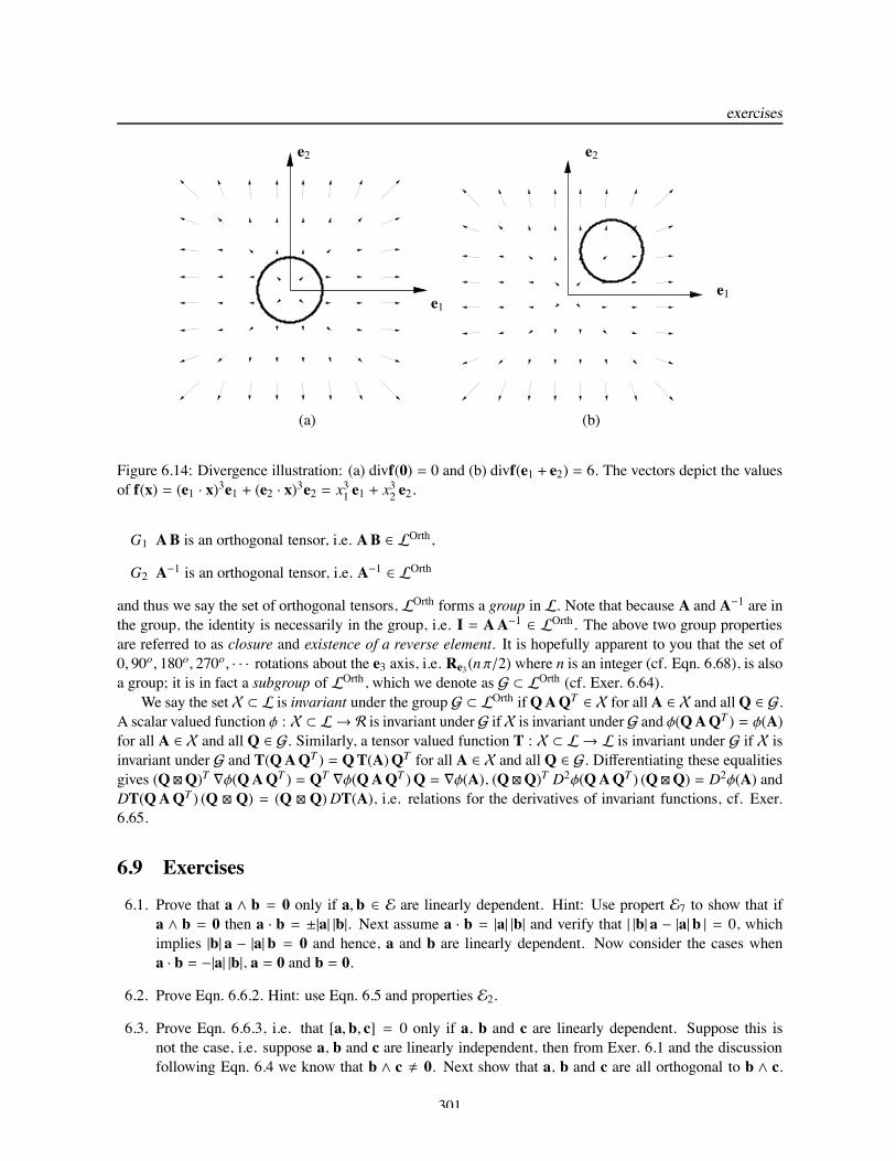
exercises
e1
e2
e1
e2
(a) (b)
Figure 6.14: Divergence illustration: (a) divf(0) = 0 and (b) divf(e1 + e2) = 6. The vectors depict the valuesof f(x) = (e1 · x)3e1 + (e2 · x)3e2 = x31 e1 + x
32 e2.
G1 AB is an orthogonal tensor, i.e. AB ∈ LOrth,
G2 A−1 is an orthogonal tensor, i.e. A−1 ∈ LOrth
and thus we say the set of orthogonal tensors, LOrth forms a group in L. Note that because A and A−1 are inthe group, the identity is necessarily in the group, i.e. I = AA−1 ∈ LOrth. The above two group propertiesare referred to as closure and existence of a reverse element. It is hopefully apparent to you that the set of0, 90o, 180o, 270o, · · · rotations about the e3 axis, i.e. Re3(n π/2) where n is an integer (cf. Eqn. 6.68), is alsoa group; it is in fact a subgroup of LOrth, which we denote as G ⊂ LOrth (cf. Exer. 6.64).
We say the set X ⊂ L is invariant under the group G ⊂ LOrth ifQAQT ∈ X for all A ∈ X and allQ ∈ G.A scalar valued function φ : X ⊂ L→ R is invariant under G ifX is invariant underG and φ(QAQT ) = φ(A)for all A ∈ X and all Q ∈ G. Similarly, a tensor valued function T : X ⊂ L→ L is invariant under G if X isinvariant under G and T(QAQT ) = QT(A)QT for all A ∈ X and all Q ∈ G. Differentiating these equalitiesgives (Q!Q)T ∇φ(QAQT ) = QT ∇φ(QAQT )Q = ∇φ(A), (Q!Q)T D2φ(QAQT ) (Q!Q) = D2φ(A) andDT(QAQT ) (Q ! Q) = (Q ! Q)DT(A), i.e. relations for the derivatives of invariant functions, cf. Exer.6.65.
6.9 Exercises
6.1. Prove that a ∧ b = 0 only if a, b ∈ E are linearly dependent. Hint: Use propert E7 to show that ifa ∧ b = 0 then a · b = ±|a| |b|. Next assume a · b = |a| |b| and verify that | |b| a − |a|b | = 0, whichimplies |b| a − |a|b = 0 and hence, a and b are linearly dependent. Now consider the cases whena · b = −|a| |b|, a = 0 and b = 0.
6.2. Prove Eqn. 6.6.2. Hint: use Eqn. 6.5 and properties E2.
6.3. Prove Eqn. 6.6.3, i.e. that [a, b, c] = 0 only if a, b and c are linearly dependent. Suppose this isnot the case, i.e. suppose a, b and c are linearly independent, then from Exer. 6.1 and the discussionfollowing Eqn. 6.4 we know that b ∧ c ! 0. Next show that a, b and c are all orthogonal to b ∧ c.
301
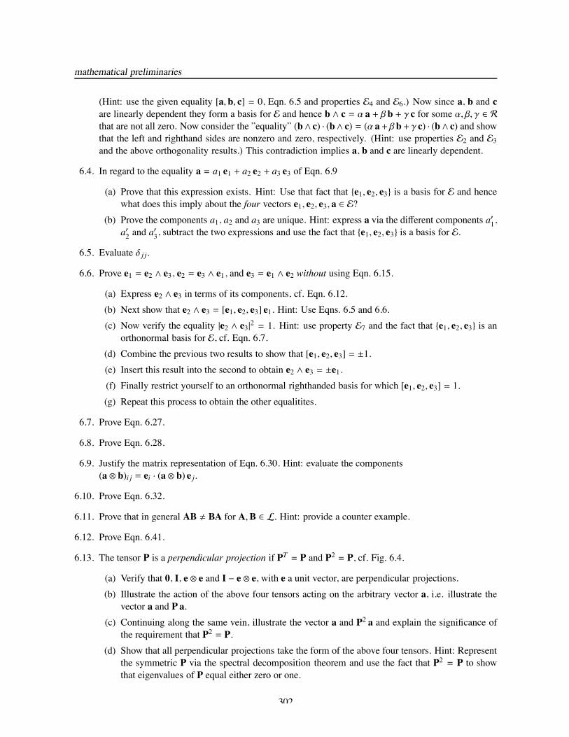
mathematical preliminaries
(Hint: use the given equality [a, b, c] = 0, Eqn. 6.5 and properties E4 and E6.) Now since a, b and care linearly dependent they form a basis for E and hence b ∧ c = α a + βb + γ c for some α, β, γ ∈ Rthat are not all zero. Now consider the ”equality” (b∧ c) · (b∧ c) = (α a+ βb+ γ c) · (b∧ c) and showthat the left and righthand sides are nonzero and zero, respectively. (Hint: use properties E2 and E3and the above orthogonality results.) This contradiction implies a, b and c are linearly dependent.
6.4. In regard to the equality a = a1 e1 + a2 e2 + a3 e3 of Eqn. 6.9
(a) Prove that this expression exists. Hint: Use that fact that e1, e2, e3 is a basis for E and hencewhat does this imply about the four vectors e1, e2, e3, a ∈ E?
(b) Prove the components a1, a2 and a3 are unique. Hint: express a via the different components a′1,a′2 and a
′3, subtract the two expressions and use the fact that e1, e2, e3 is a basis for E.
6.5. Evaluate δ j j.
6.6. Prove e1 = e2 ∧ e3, e2 = e3 ∧ e1, and e3 = e1 ∧ e2 without using Eqn. 6.15.
(a) Express e2 ∧ e3 in terms of its components, cf. Eqn. 6.12.(b) Next show that e2 ∧ e3 = [e1, e2, e3] e1. Hint: Use Eqns. 6.5 and 6.6.(c) Now verify the equality |e2 ∧ e3|2 = 1. Hint: use property E7 and the fact that e1, e2, e3 is an
orthonormal basis for E, cf. Eqn. 6.7.(d) Combine the previous two results to show that [e1, e2, e3] = ±1.(e) Insert this result into the second to obtain e2 ∧ e3 = ±e1.(f) Finally restrict yourself to an orthonormal righthanded basis for which [e1, e2, e3] = 1.(g) Repeat this process to obtain the other equalitites.
6.7. Prove Eqn. 6.27.
6.8. Prove Eqn. 6.28.
6.9. Justify the matrix representation of Eqn. 6.30. Hint: evaluate the components(a ⊗ b)i j = ei · (a ⊗ b) e j.
6.10. Prove Eqn. 6.32.
6.11. Prove that in general AB ! BA for A,B ∈ L. Hint: provide a counter example.
6.12. Prove Eqn. 6.41.
6.13. The tensor P is a perpendicular projection if PT = P and P2 = P, cf. Fig. 6.4.
(a) Verify that 0, I, e ⊗ e and I − e ⊗ e, with e a unit vector, are perpendicular projections.(b) Illustrate the action of the above four tensors acting on the arbitrary vector a, i.e. illustrate the
vector a and P a.(c) Continuing along the same vein, illustrate the vector a and P2 a and explain the significance of
the requirement that P2 = P.(d) Show that all perpendicular projections take the form of the above four tensors. Hint: Represent
the symmetric P via the spectral decomposition theorem and use the fact that P2 = P to showthat eigenvalues of P equal either zero or one.
302
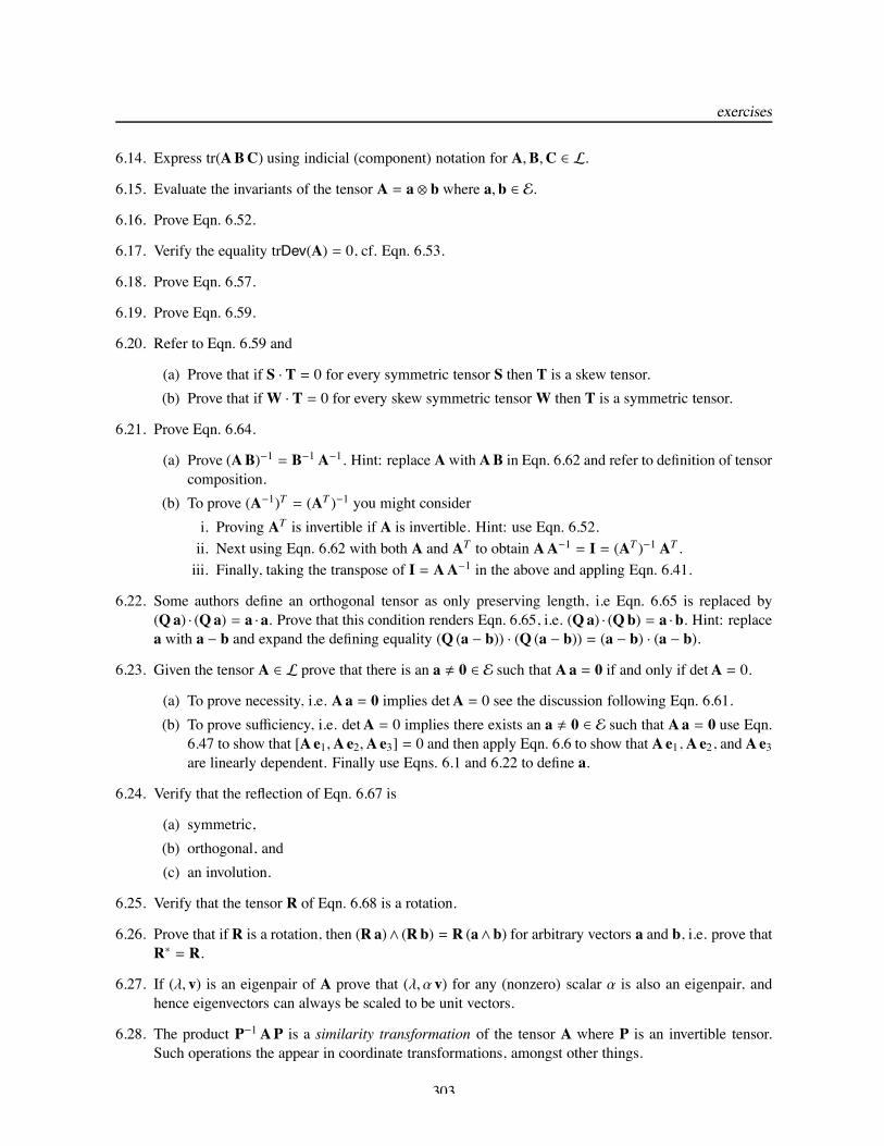
exercises
6.14. Express tr(ABC) using indicial (component) notation for A,B,C ∈ L.
6.15. Evaluate the invariants of the tensor A = a ⊗ b where a, b ∈ E.
6.16. Prove Eqn. 6.52.
6.17. Verify the equality trDev(A) = 0, cf. Eqn. 6.53.
6.18. Prove Eqn. 6.57.
6.19. Prove Eqn. 6.59.
6.20. Refer to Eqn. 6.59 and
(a) Prove that if S · T = 0 for every symmetric tensor S then T is a skew tensor.(b) Prove that ifW · T = 0 for every skew symmetric tensorW then T is a symmetric tensor.
6.21. Prove Eqn. 6.64.
(a) Prove (AB)−1 = B−1 A−1. Hint: replace A withAB in Eqn. 6.62 and refer to definition of tensorcomposition.
(b) To prove (A−1)T = (AT )−1 you might consideri. Proving AT is invertible if A is invertible. Hint: use Eqn. 6.52.ii. Next using Eqn. 6.62 with both A and AT to obtain AA−1 = I = (AT )−1 AT .iii. Finally, taking the transpose of I = AA−1 in the above and appling Eqn. 6.41.
6.22. Some authors define an orthogonal tensor as only preserving length, i.e Eqn. 6.65 is replaced by(Qa) · (Qa) = a ·a. Prove that this condition renders Eqn. 6.65, i.e. (Qa) · (Qb) = a ·b. Hint: replacea with a − b and expand the defining equality (Q (a − b)) · (Q (a − b)) = (a − b) · (a − b).
6.23. Given the tensor A ∈ L prove that there is an a ! 0 ∈ E such that Aa = 0 if and only if detA = 0.
(a) To prove necessity, i.e. Aa = 0 implies detA = 0 see the discussion following Eqn. 6.61.(b) To prove sufficiency, i.e. detA = 0 implies there exists an a ! 0 ∈ E such that Aa = 0 use Eqn.
6.47 to show that [Ae1,Ae2,Ae3] = 0 and then apply Eqn. 6.6 to show that Ae1, Ae2, and Ae3are linearly dependent. Finally use Eqns. 6.1 and 6.22 to define a.
6.24. Verify that the reflection of Eqn. 6.67 is
(a) symmetric,(b) orthogonal, and(c) an involution.
6.25. Verify that the tensor R of Eqn. 6.68 is a rotation.
6.26. Prove that if R is a rotation, then (Ra)∧ (Rb) = R (a∧b) for arbitrary vectors a and b, i.e. prove thatR∗ = R.
6.27. If (λ, v) is an eigenpair of A prove that (λ,α v) for any (nonzero) scalar α is also an eigenpair, andhence eigenvectors can always be scaled to be unit vectors.
6.28. The product P−1AP is a similarity transformation of the tensor A where P is an invertible tensor.Such operations the appear in coordinate transformations, amongst other things.
303
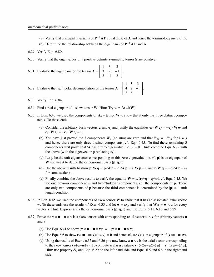
mathematical preliminaries
(a) Verify that principal invariants of P−1AP equal those ofA and hence the terminology invariants.(b) Determine the relationship between the eigenpairs of P−1AP and A.
6.29. Verify Eqn. 6.80.
6.30. Verify that the eigenvalues of a positive definite symmetric tensor S are positive.
6.31. Evaluate the eigenpairs of the tensor A =
⎡⎢⎢⎢⎢⎢⎢⎢⎢⎣
1 3 23 2 −12 −1 2
⎤⎥⎥⎥⎥⎥⎥⎥⎥⎦.
6.32. Evaluate the right polar decomposition of the tensor A =
⎡⎢⎢⎢⎢⎢⎢⎢⎢⎣
1 3 34 2 −12 6 1
⎤⎥⎥⎥⎥⎥⎥⎥⎥⎦.
6.33. Verify Eqn. 6.84.
6.34. Find a real eigenpair of a skew tensorW. Hint: Try w = Axial(W).
6.35. In Eqn. 6.43 we used the components of skew tensorW to show that it only has three distinct compo-nents. To these ends
(a) Consider the arbitrary basis vectors ei and e j and justify the equalities ei ·We j = −e j ·Wei andei ·Wei = −ei ·Wei = 0.
(b) You have just proved the 3 components Wii (no sum) are zero and that Wij = −Wji for i ! jand hence there are only three distinct components, cf. Eqn. 6.45. To find these remaining 3components first prove thatW has a zero eigenvalue, i.e. λ = 0. Hint: combine Eqn. 6.72 withthe above (with the eigenvector p replacing ei).
(c) Let p be the unit eigenvector corresponding to this zero eigenvalue, i.e. (0, p) is an eigenpair ofW and use it to define the orthonormal basis p, q, r.
(d) Use the above results to show p·Wq = p·Wr = q·Wp = r·Wp = 0 and r·Wq = −q·Wr = ωfor some scalar ω.
(e) Finally combine the above results to verify the equalityW = ω (r⊗q−q⊗ r), cf. Eqn. 6.45. Wesee one obvious component ω and two “hidden” components, i.e. the components of p. Thereare only two components of p because the third component is determined by the |p| = 1 unitlength condition.
6.36. In Eqn. 6.45 we used the components of skew tensorW to show that it has an associated axial vectorw. To these ends use the results of Exer. 6.35 and let w = ω p and verify thatWa = w ∧ a for everyvector a. Hint: Express a via the orthonormal basis p, q, r and use Eqns. 6.11, 6.16 and 6.29.
6.37. Prove the v ⊗ u − u ⊗ v is a skew tensor with corresponding axial vector u ∧ v for arbitrary vectors uand v.
(a) Use Eqn. 6.41 to show (v ⊗ u − u ⊗ v)T = −(v ⊗ u − u ⊗ v).(b) Use Eqn. 6.6 to show (v⊗u−u⊗v) (u∧v) = 0 and hence (0, u∧v) is an eigenpair of (v⊗u−u⊗v).(c) Using the results of Exers. 6.35 and 6.36 you now know αu∧v is the axial vector corresponding
to the skew tensor (v⊗u−u⊗v). To compute scalar α evaluate v·[(v⊗u−u⊗v)u] = v·[(αu∧v)∧u].Hint: use property E7 and Eqn. 6.29 on the left hand side and Eqns. 6.5 and 6.6 in the righthandside.
304
exercises
6.38. Refer to Exer. 6.37 and verify the equalities (v ⊗ u − u ⊗ v)w = (u ∧ v) ∧w = (u ·w) v − (v ·w)u forarbitrary vectors u, v and w.
6.39. Find a real eigenpair of the rotation tensor R of Eqn. 6.68. Hint: Try p.
6.40. In Eqn. 6.68 we introduced a particular rotation R = p⊗p+ (q⊗q+ r⊗ r) cos θ− (q⊗ r− r⊗q) sin θ.Prove that every rotation can be defined as such.
(a) From QT Q = I derive the equality QT (Q − I) = −(Q − I)T .(b) Take the determinant of the above to prove det(Q − I) = 0.(c) Use this det(Q − I) = 0 result to explain why λ = 1 is an eigenvalue of Q.(d) Let p be the eigenvector corresponding to this unit eigenvalue, i.e. (1, p) is an eigenpair of Q
and use it to define the orthonormal basis p, q, r. Now prove thati. p = Qp = QTp.ii. p ·Qp = 1.iii. p ·Qq = p ·Qr = q ·Qp = r ·Qp = 0.
(e) You now have 5 components ofQ, cf. Eqn. 6.35. To find the remaining 4 first prove the followingi. Qq ·Qq = Qr ·Qr = 1.ii. Qq ·Qr = 0.
(f) Justify the equalities Qq = αq + βp and Qr = γ q + δp and provide definitions of α, β, γ andδ. Hint: refer to Eqns. 6.9 and 6.11.
(g) Justify the equalities α2 + β2 = 1, γ2 + δ2 = 1 and αγ + β δ = 0 and α δ − β γ = 1. Hint:evaluate the three possible dot products between Qq and Qp and use the equality detQ = 1 =[Qp,Qq,Qr] = [Qp,αq + βp, γ q + δp].
(h) Verify that α = δ = cos θ and β = −γ = sin θ is a solution to the above four equations.(i) Combine steps f and h to evaluate the remaining 4 components. Hint: cf. Eqns. 6.35, 6.36 and6.68.
6.41. Verify Eqn. 6.95.
6.42. Verify Eqn. 6.96.
6.43. Verify Eqn. 6.99.
6.44. Verify that TT = T. Hint: Apply Eqns. 6.52, 6.55, 6.97, and 6.100 and as always, use the arbitrarinessof A,B ∈ L.
6.45. Verify the following
(a) C = PSym C if C possesses the first minor symmetry(b) C = CPSym if C possesses the second minor symmetry and that(c) If C possesses the major and either minor symmetry, then it possesses the other minor symmetry.
6.46. How many independent components does C have if it possesses major, first, and second minor sym-metries?
6.47. Refer to Eqn. 6.105 and use the Kronecker delta δi j to express the components
305
mathematical preliminaries
(a) PSymi jkl
(b) PSkewi jkl(c) PSphi jkl(d) PDevi jkl
6.48. Refer to Eqn. 6.105 and evaluate the following
(a) PSym PSkew(b) PSym + PSkew(c) PSph PDev(d) PSph + PDev(e) PSym PSph(f) Comment on your findings.
6.49. Verify Eqn. 6.108.
6.50. Refer to Eqn. 6.109 and verify that R = R ! R is orthogonal if R ∈ L is a rotation.
6.51. Verify Eqn. 6.118.
6.52. Use the intermediate result of Exam. 6.7 to verify the equation
det(A + a ⊗ b) = det(A) [1 + a · (A−1 b)]
Hint: Let ϵ = 1 andU = a⊗b, use your Exer. 6.15 results to show ı2((a⊗b)A−1) = 0 and det(a⊗b) = 0and apply Eqn. 6.59.
6.53. Evaluate the derivative of the function F : L→ L where F(A) = AT A.
6.54. Evaluate the derivative of the function F : L→ L where F(A) = tr(A)A.
6.55. Evaluate the derivative of the function F : L→ L where F(A) = tr(A)BAT where B is a tensor.
6.56. Use the chain rule to evaluate the gradient and derivative of the maps
(a) αf : E→ R and(b) gf : E→ E
where α : E→ R, g : E→ E, and f : E→ E are differentiable functons.
6.57. Evaluate the first and second derivatives of the function α : E→ R such that α(x) = |x|.
6.58. For the tensor field B : E → L and the uniform tensor A ∈ L verify that div(AB(x)) = A divB(x).Hint: Apply the transpose and divergence definitions of Eqns. 6.40 and 6.157 multiple times.
6.59. Verify Eqn. 6.164.2.
6.60. Verify the equality
w ·∫
∂Ω(x − y) ∧ T(x)n(x) da =
∫
Ω
(W (x − y) · divT(x) +W · T(x)) dv,
where w = Axial(W) is a uniform vector and T : Ω ∈ E → L is differentiable. Hint: Refer to Eqns.6.5, 6.6, 6.40, 6.44, 6.163 and 6.164.
306
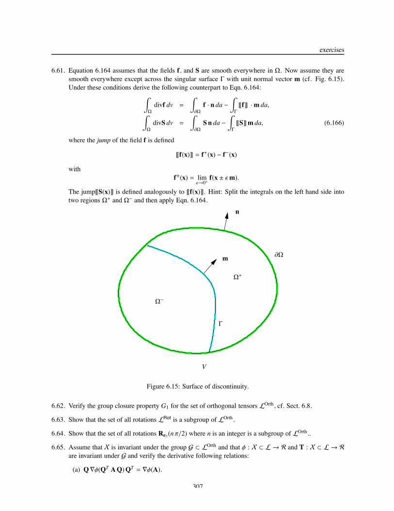
exercises
6.61. Equation 6.164 assumes that the fields f, and S are smooth everywhere in Ω. Now assume they aresmooth everywhere except across the singular surface Γ with unit normal vector m (cf. Fig. 6.15).Under these conditions derive the following counterpart to Eqn. 6.164:
∫
Ω
divf dv =∫
∂Ωf · n da −
∫
Γ
[[f]] ·m da,∫
Ω
divS dv =∫
∂ΩS n da −
∫
Γ
[[S]]m da, (6.166)
where the jump of the field f is defined
[[f(x)]] = f+(x) − f−(x)
withf±(x) = lim
ϵ→0+f(x ± ϵm).
The jump[[S(x)]] is defined analogously to [[f(x)]]. Hint: Split the integrals on the left hand side intotwo regions Ω+ and Ω− and then apply Eqn. 6.164.
n
m ∂Ω
V
Ω−
Ω+
Γ
Figure 6.15: Surface of discontinuity.
6.62. Verify the group closure property G1 for the set of orthogonal tensors LOrth, cf. Sect. 6.8.
6.63. Show that the set of all rotations LRot is a subgroup of LOrth.
6.64. Show that the set of all rotations Re3 (n π/2) where n is an integer is a subgroup of LOrth..
6.65. Assume that X is invariant under the group G ⊂ LOrth and that φ : X ⊂ L → R and T : X ⊂ L → Rare invariant under G and verify the derivative following relations:
(a) Q∇φ(QT AQ)QT = ∇φ(A).
307

mathematical preliminaries
(b) (Q !Q)D2φ(QT AQ) (Q !Q)T = D2φ(A).(c) DT(QT AQ) (Q !Q)T = (Q !Q)T DT(A).
308
BIBLIOGRAPHY
Bibliography[1] R. M. Bowen. Introduction to Continuum Mechanics for Engineers. Plenum Press, New York, 1989.
[2] D. E. Carlson. Continuum Mechanics Course Notes. University of Illinois, Urbana-Champaign, 1988.
[3] P. Chadwick. Continuum Mechanics: Concise Theory and Problems. Dover Publications, New York,1999.
[4] M. E. Gurtin. Introduction to Continuum Mechanics. Academic Press, New York, 1981.
[5] M. E. Gurtin, E. Fried, and L. Anand. The Mechanics and Thermodynamics of Continua. Cambridge,New York, 2010.
[6] J. K. Knowles. Linear Vector Spaces and Cartesian Tensors. Oxford University Press, New York,1998.
[7] R. W. Ogden. Non-Linear Elastic Deformations. John Wiley & Sons, New York, 1984.
[8] P. Podio-Guidugli. A primer in elasticity. Journal of Elasticity, 58(1), 2000.
[9] M. Silhavy. The Mechanics and Thermodynamics of Continuous Media. Springer, New York, 1997.
[10] A. J. M. Spencer. Continuum Mechanics. Dover Publications, New York, 2004.
309

BIBLIOGRAPHY
310