Ch04

Chapter 4Cost-Volume-Profit Analysis

QUESTIONS

1. Variable costs are costs that change in response to changes in activity (e.g., production or sales activity). Fixed costs are costs that do not change in response to changes in activity.

2. A mixed cost is a cost that has a fixed cost component and a variable cost component. For example, the amount paid for telecommunication services would be a mixed cost if there was a fixed monthly fee plus a charge for use.

3. Discretionary fixed costs are those fixed costs that management can easily change in the short-run (e.g., advertising). Committed fixed costs are those fixed costs that cannot be easily changed in the short-run (e.g., rent).

4. Commissions paid to salespersons and direct materials are examples of variable costs.

5. Rent and insurance expenses are examples of fixed costs.

6. Salespersons are paid a base salary plus commissions. The base amount is fixed and commissions are variable. Thus, total compensation paid to the sales force is mixed.

7. With telecom, there is likely to be a basic service charge (fixed) plus a charge for use (which will be variable if use increases with business activity).

8. The horizontal axis would be production.

9. With account analysis, managers use judgment to classify costs as either fixed or variable. The total of the costs classified as variable can then be divided by a measure of activity to calculate the variable cost per unit of activity. The total of the costs classified as fixed provides the estimate of fixed cost.

10. With the high-low method, you use the highest and lowest levels of activity.

11. The relevant range is the range of activity for which estimates of costs are likely to be accurate.

12. The contribution margin is equal to the selling price minus variable cost. The contribution margin ratio is the contribution margin per dollar of sales.

13. The profit equation states that profit is equal to revenue (selling price times quantity) minus variable cost (variable cost per unit times quantity) minus total fixed cost.

Profit = SP (x) - VC (x) - TFC

Jiambalvo Managerial Accounting

14. It would not be appropriate to focus on weighted average contribution margin per unit if the units were dissimilar (e.g., pencils and computers at an office supply warehouse).

15. The assumptions in C-V-P- analysis are:1. Costs can be separated into fixed and variable components.2. Fixed costs remain fixed and variable costs per unit do not change.3. When performing multiproduct C-V-P, an important assumption is that the mix

remains constant.

16. Companies that have relatively higher fixed costs are said to have higher operating leverage. Thus, a software company with a large investment in research and development (a fixed cost) would likely have higher operating leverage compared to a manufacturing company that used little equipment but expensive labor (a variable cost).

17. When there is a constraint, focus on the contribution margin per unit of the constraint.

4-2

EXERCISES

E1. With high fixed costs, a business is quite risky. This follows because if sales fail to meet expectations, the company may have a large loss.

Paul may be able to make rent a variable expense—pay the mall owner a percent of total revenue rather than a fixed monthly amount. This type of arrangement is quite common in shopping malls. He may also be able to pay employees relatively low base salaries with bonuses tied to sales. This would make salary expense more of a variable expense.

E2. The cost structure at Microsoft is heavily weighted toward fixed cost (e.g., research and development). Consider the variable cost associated with selling an additional unit of the product “Office” through the OEM (original equipment manufacturer) channel. The product sells for well over $100 but the incremental cost (ignoring tax) is probably less than $1. With high operating leverage, it’s not surprising that profit grew faster than sales.

E3. At the Men’s Warehouse, the gross margin is equal to net sales less cost of goods sold, including buying and occupancy costs. Since store occupancy cost is primarily a fixed cost, dividing the gross margin by sales is not likely to provide a good estimate of the contribution margin ratio.

At Best Buy, the gross profit is equal to revenues less cost of goods sold. Since cost of goods sold is the company’s primary variable cost, dividing gross profit by revenues may yield a relatively good estimate of the firm’s weighted average contribution margin ratio.

Chapter 4 Cost-Volume-Profit Analysis


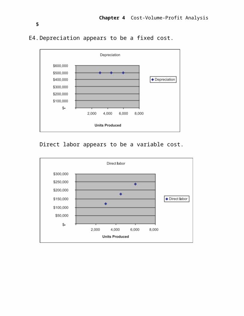
E4. Depreciation appears to be a fixed cost.

Direct labor appears to be a variable cost.

4-4

Telecommunications appears to be a mixed cost. Note that the intercept is $10,000.

E5. ($20,000 - $8,000) ÷ (8,000 - 2,000) = $2 per machine hour of variable repair cost$8,000 - ($2 x 2,000) = $4,000 per month of fixed repair cost.

E6. a. The highest level of activity is sales of $28,000 with cost of $23,800. The lowest level of activity is sales of $19,000 with cost of $18,400.

($23,800 - $18,400) ÷ ($28,000 - $19,000) = $.60 of variable cost per dollar of sales.

$23,800 – ($.60 x $28,000) = $7,000 per month of fixed cost.

Thus, Cost = $7,000 + ($.60 x Sales).

b. For $1 of sales, there will be $.60 of variable cost and $.40 (i.e., $1 - $.60) of contribution margin. That is, the contribution margin for a dollar of sales (known as the contribution margin ratio) is $1 - $.60.

c. For a sales increase of $50,000, profit will increase by $20,000 (i.e., $50,000 - ($.60 x $50,000) = $20,000).

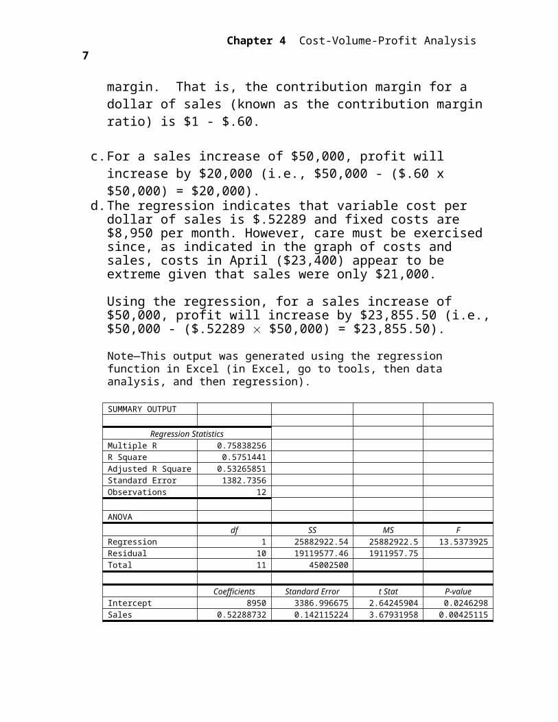
d. The regression indicates that variable cost per dollar of sales is $.52289 and fixed costs are $8,950 per month. However, care must be exercised since, as indicated in the graph of costs and sales, costs in April ($23,400) appear to be extreme given that sales were only $21,000.



Using the regression, for a sales increase of $50,000, profit will increase by $23,855.50 (i.e., $50,000 - ($.52289 $50,000) = $23,855.50).

Note—This output was generated using the regression function in Excel (in Excel, go to tools, then data analysis, and then regression).

SUMMARY OUTPUT

Regression StatisticsMultiple R 0.75838256R Square 0.5751441Adjusted R Square 0.53265851Standard Error 1382.7356Observations 12

ANOVA

df SS MS FRegression 1 25882922.54 25882922.5 13.5373925Residual 10 19119577.46 1911957.75Total 11 45002500

Coefficients Standard Error t Stat P-valueIntercept 8950 3386.996675 2.64245904 0.0246298Sales 0.52288732 0.142115224 3.67931958 0.00425115

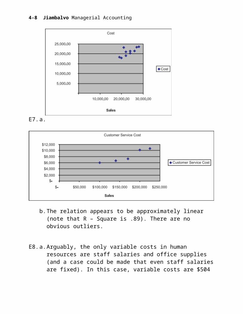
E7. a.

4-6

b. The relation appears to be approximately linear (note that R – Square is .89). There are no obvious outliers.

E8. a. Arguably, the only variable costs in human resources are staff salaries and office supplies (and a case could be made that even staff salaries are fixed). In this case, variable costs are $504 per hire [($25,000 + $200) ÷ 50 hires]. Fixed costs are $8,800.

b. The estimated cost for June with 60 new hires is: $8,800 + ($504 60) = $39,040.

c. The incremental cost associated with 10 more employees is $5,040 (i.e., $504 10).



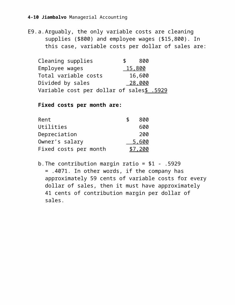
E9. a. Arguably, the only variable costs are cleaning supplies ($800) and employee wages ($15,800). In this case, variable costs per dollar of sales are:

Cleaning supplies $ 800Employee wages 15,800 Total variable costs 16,600Divided by sales 28,000Variable cost per dollar of sales $ .5929

Fixed costs per month are:

Rent $ 800Utilities 600Depreciation 200Owner’s salary 5,600Fixed costs per month $7,200

b. The contribution margin ratio = $1 - .5929 = .4071. In other words, if the company has approximately 59 cents of variable costs for every dollar of sales, then it must have approximately 41 cents of contribution margin per dollar of sales.

4-8

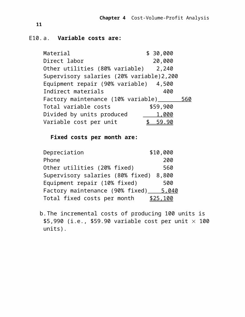
E10. a. Variable costs are:

Material $ 30,000Direct labor 20,000

Other utilities (80% variable) 2,240Supervisory salaries (20% variable) 2,200Equipment repair (90% variable) 4,500Indirect materials 400Factory maintenance (10% variable) 560Total variable costs $59,900Divided by units produced 1,000Variable cost per unit $ 59.90

Fixed costs per month are:

Depreciation $10,000Phone 200

Other utilities (20% fixed) 560Supervisory salaries (80% fixed) 8,800Equipment repair (10% fixed) 500Factory maintenance (90% fixed) 5,040Total fixed costs per month $25,100

b. The incremental costs of producing 100 units is $5,990 (i.e., $59.90 variable cost per unit 100 units).



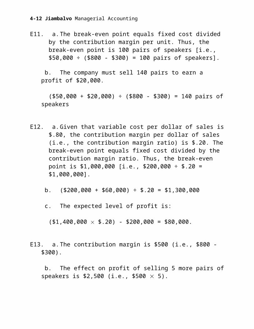
E11. a. The break-even point equals fixed cost divided by the contribution margin per unit. Thus, the break-even point is 100 pairs of speakers [i.e., $50,000 ÷ ($800 - $300) = 100 pairs of speakers].

b. The company must sell 140 pairs to earn a profit of $20,000.

($50,000 + $20,000) ÷ ($800 - $300) = 140 pairs of speakers

E12. a. Given that variable cost per dollar of sales is $.80, the contribution margin per dollar of sales (i.e., the contribution margin ratio) is $.20. The break-even point equals fixed cost divided by the contribution margin ratio. Thus, the break-even point is $1,000,000 [i.e., $200,000 ÷ $.20 = $1,000,000].

b. ($200,000 + $60,000) ÷ $.20 = $1,300,000

c. The expected level of profit is:

($1,400,000 $.20) - $200,000 = $80,000.

E13. a. The contribution margin is $500 (i.e., $800 - $300).

b. The effect on profit of selling 5 more pairs of speakers is $2,500 (i.e., $500 5).

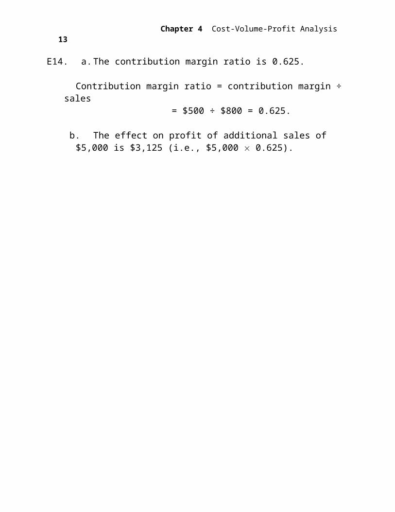
E14. a. The contribution margin ratio is 0.625.

Contribution margin ratio = contribution margin ÷ sales = $500 ÷ $800 = 0.625.

b. The effect on profit of additional sales of $5,000 is $3,125 (i.e., $5,000 0.625).

4-10

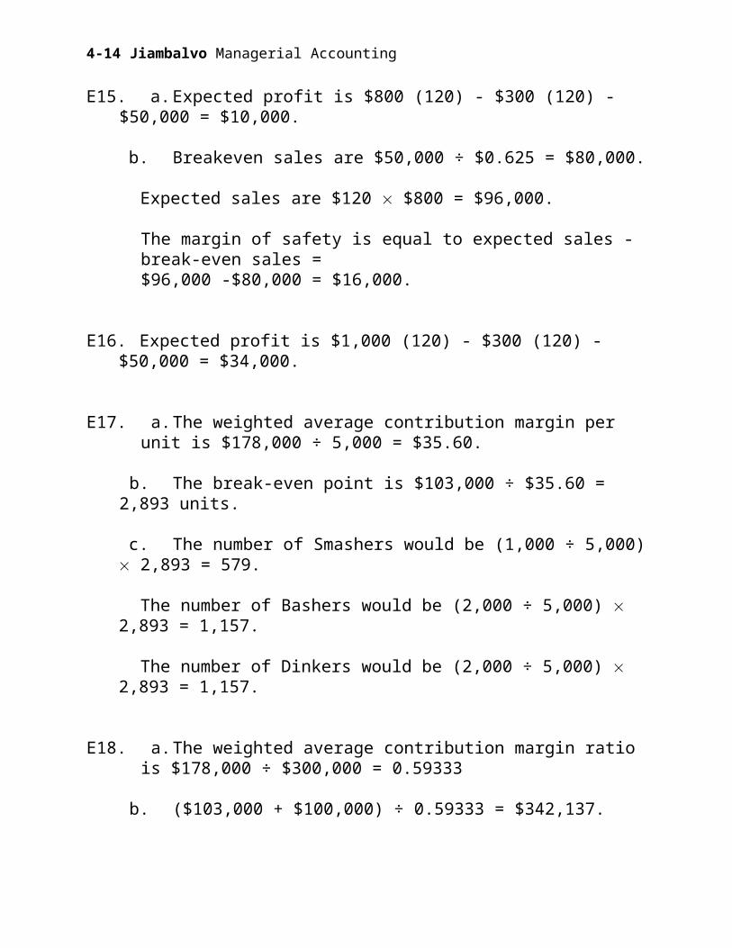
E15. a. Expected profit is $800 (120) - $300 (120) - $50,000 = $10,000.

b. Breakeven sales are $50,000 ÷ $0.625 = $80,000.

Expected sales are $120 $800 = $96,000.

The margin of safety is equal to expected sales - break-even sales = $96,000 -$80,000 = $16,000.

E16. Expected profit is $1,000 (120) - $300 (120) - $50,000 = $34,000.

E17. a. The weighted average contribution margin per unit is $178,000 ÷ 5,000 = $35.60.

b. The break-even point is $103,000 ÷ $35.60 = 2,893 units.

c. The number of Smashers would be (1,000 ÷ 5,000) 2,893 = 579.

The number of Bashers would be (2,000 ÷ 5,000) 2,893 = 1,157.

The number of Dinkers would be (2,000 ÷ 5,000) 2,893 = 1,157.

E18. a. The weighted average contribution margin ratio is $178,000 ÷ $300,000 = 0.59333

b. ($103,000 + $100,000) ÷ 0.59333 = $342,137.

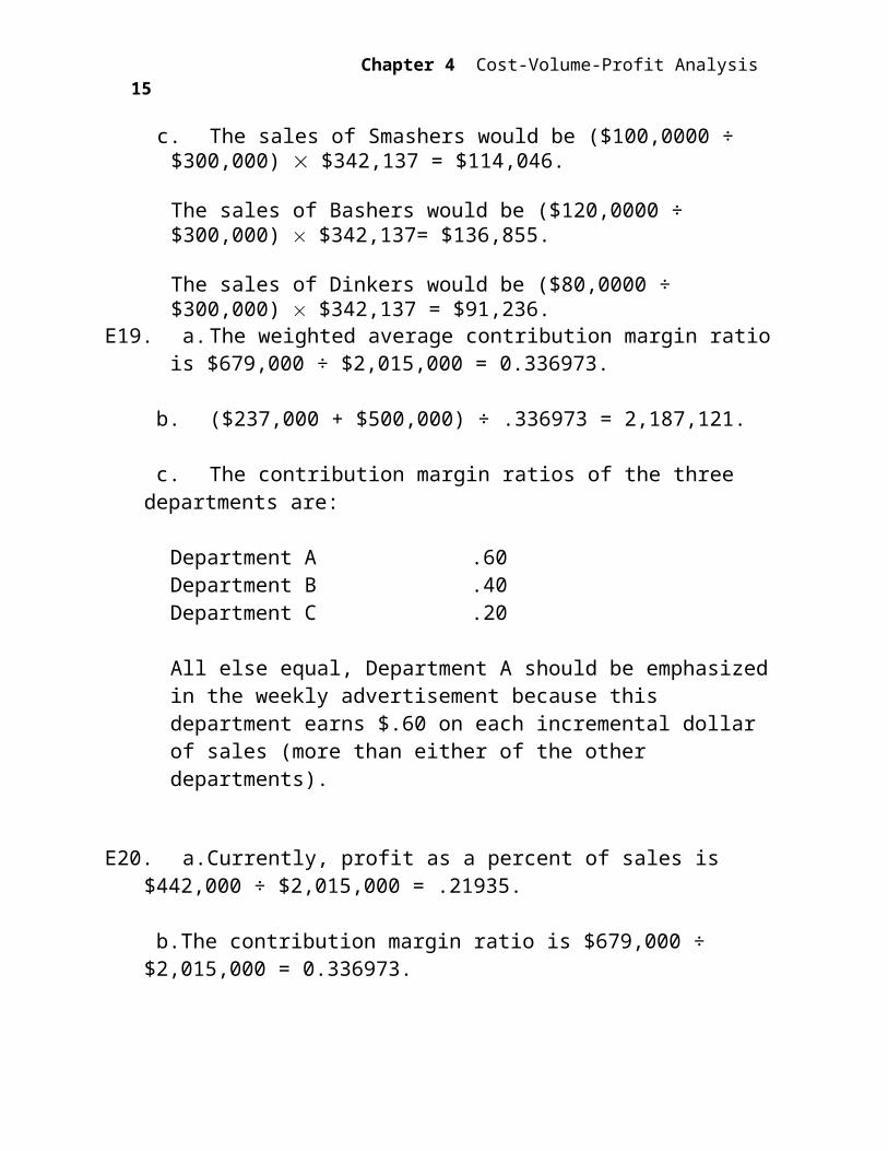
c. The sales of Smashers would be ($100,0000 ÷ $300,000) $342,137 = $114,046.

The sales of Bashers would be ($120,0000 ÷ $300,000) $342,137= $136,855.

Chapter 4 Cost-Volume-Profit Analysis11


The sales of Dinkers would be ($80,0000 ÷ $300,000) $342,137 = $91,236.

E19. a. The weighted average contribution margin ratio is $679,000 ÷ $2,015,000 = 0.336973.

b. ($237,000 + $500,000) ÷ .336973 = 2,187,121.

c. The contribution margin ratios of the three departments are:

Department A .60Department B .40Department C .20

All else equal, Department A should be emphasized in the weekly advertisement because this department earns $.60 on each incremental dollar of sales (more than either of the other departments).

E20. a. Currently, profit as a percent of sales is $442,000 ÷ $2,015,000 = .21935.

b. The contribution margin ratio is $679,000 ÷ $2,015,000 = 0.336973.

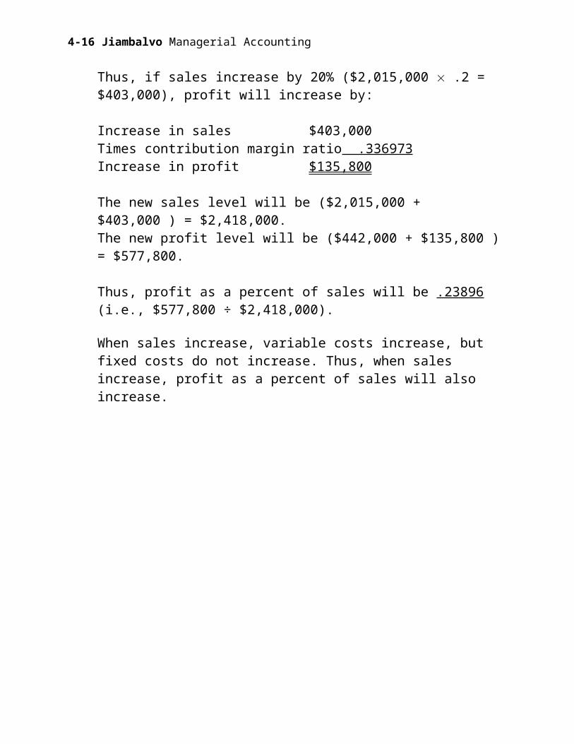
Thus, if sales increase by 20% ($2,015,000 .2 = $403,000), profit will increase by:

Increase in sales $403,000Times contribution margin ratio .336973Increase in profit $135,800

The new sales level will be ($2,015,000 + $403,000 ) = $2,418,000.The new profit level will be ($442,000 + $135,800 ) = $577,800.

Thus, profit as a percent of sales will be .23896 (i.e., $577,800 ÷ $2,418,000).

When sales increase, variable costs increase, but fixed costs do not increase. Thus, when sales increase, profit as a percent of sales will also increase.

4-12

E21.a. Product A Product BSelling price $80 $70Variable costs 20 40Contribution margin 60 30÷ Hours to produce 1 item 5 2Contribution margin per hour $12 $15

The company should produce just Product B. With 320 hours available, this product will generate $4,800 of contribution margin ($15 320 hours) while Product A will generate just $3,840 ($12 320).

b. If the company obtains additional labor, it should produce more Product B. The incremental benefit of 10 labor hours is $150 ($15 contribution margin per hour x 10 hours).

As an aside, note that if production of Product A requires 5 labor hours and variable costs are only $20 per unit, workers at Howard Products must be paid less than $4 per hour because part of the variable costs are material costs! Perhaps production is taking place in a third-world country!



PROBLEMS

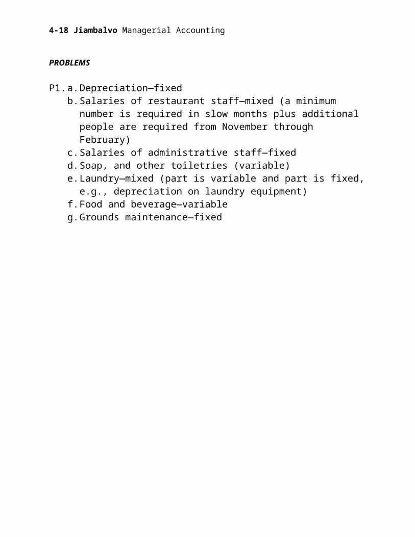
P1. a. Depreciation—fixedb. Salaries of restaurant staff—mixed (a minimum number is required in slow

months plus additional people are required from November through February)

c. Salaries of administrative staff—fixedd. Soap, and other toiletries (variable)e. Laundry—mixed (part is variable and part is fixed, e.g., depreciation on

laundry equipment)f. Food and beverage—variableg. Grounds maintenance—fixed

4-14

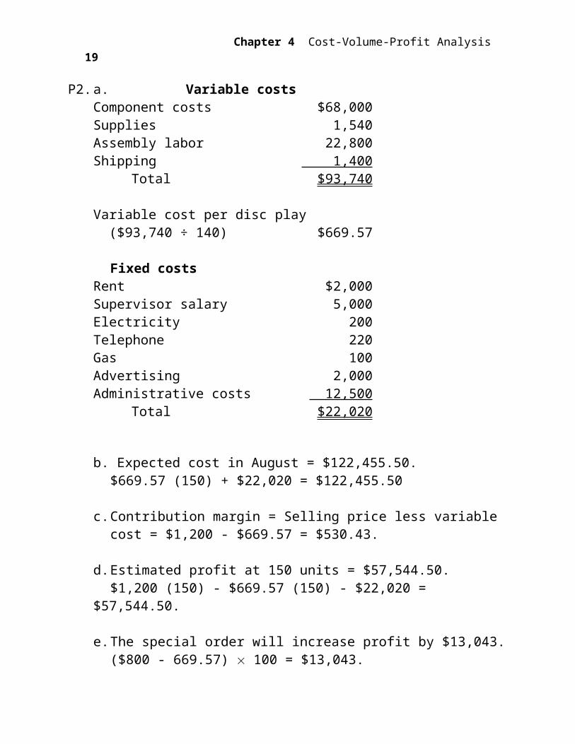
P2. a. Variable costsComponent costs $68,000Supplies 1,540Assembly labor 22,800Shipping 1,400

Total $93,740

Variable cost per disc play ($93,740 ÷ 140) $669.57

Fixed costsRent $2,000Supervisor salary 5,000Electricity 200Telephone 220Gas 100Advertising 2,000Administrative costs 12,500

Total $22,020

b. Expected cost in August = $122,455.50.$669.57 (150) + $22,020 = $122,455.50

c. Contribution margin = Selling price less variable cost = $1,200 - $669.57 = $530.43.

d. Estimated profit at 150 units = $57,544.50.$1,200 (150) - $669.57 (150) - $22,020 = $57,544.50.

e. The special order will increase profit by $13,043.($800 - 669.57) 100 = $13,043.



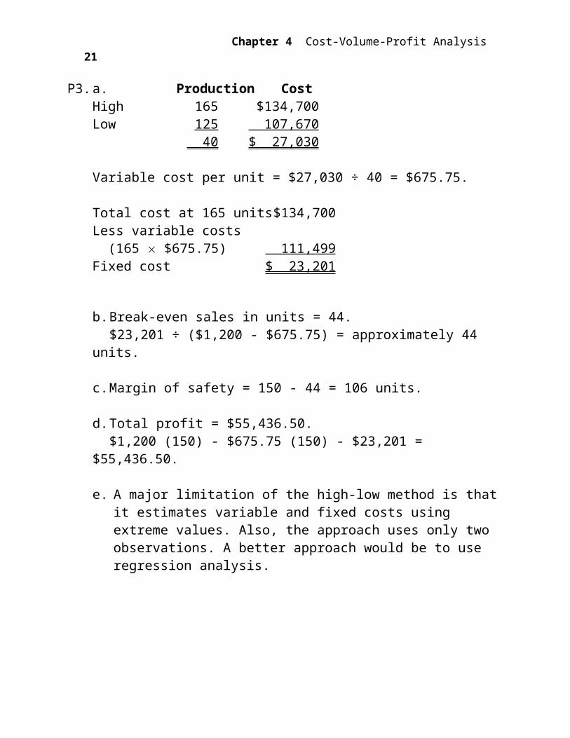
P3. a. Production CostHigh 165 $134,700Low 125 107,670

40 $ 27,030

Variable cost per unit = $27,030 ÷ 40 = $675.75.

Total cost at 165 units $134,700Less variable costs (165 $675.75) 111,499Fixed cost $ 23,201

b. Break-even sales in units = 44.$23,201 ÷ ($1,200 - $675.75) = approximately 44 units.

c. Margin of safety = 150 - 44 = 106 units.

d. Total profit = $55,436.50.$1,200 (150) - $675.75 (150) - $23,201 = $55,436.50.

e. A major limitation of the high-low method is that it estimates variable and fixed costs using extreme values. Also, the approach uses only two observations. A better approach would be to use regression analysis.

4-16

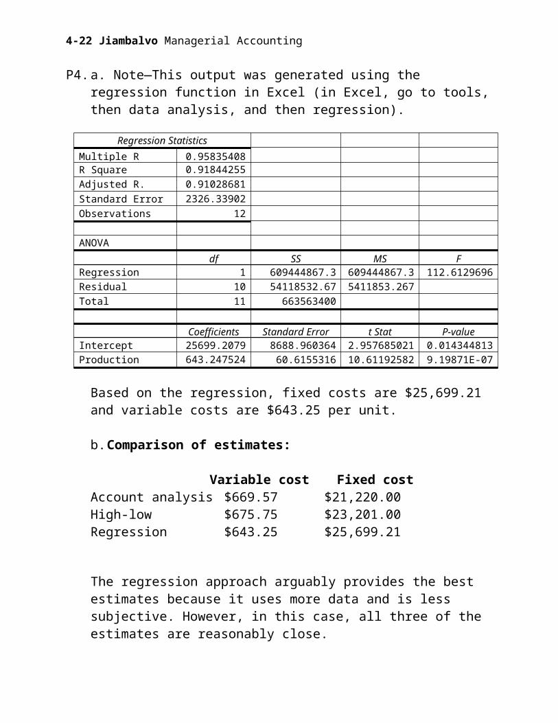
P4. a. Note—This output was generated using the regression function in Excel (in Excel, go to tools, then data analysis, and then regression).

Regression Statistics

Multiple R 0.958354089R Square 0.918442559

Adjusted R. Square 0.910286815

Standard Error 2326.339027

Observations 12

ANOVA

df SS MS F

Regression 1 609444867.3 609444867.3 112.6129696

Residual 10 54118532.67 5411853.267

Total 11 663563400

Coefficients Standard Error t Stat P-value

Intercept 25699.20792 8688.960364 2.957685021 0.014344813

Production 643.2475248 60.6155316 10.61192582 9.19871E-07

Based on the regression, fixed costs are $25,699.21 and variable costs are $643.25 per unit.

b. Comparison of estimates:

Variable cost Fixed costAccount analysis $669.57 $21,220.00High-low $675.75 $23,201.00Regression $643.25 $25,699.21

The regression approach arguably provides the best estimates because it uses more data and is less subjective. However, in this case, all three of the estimates are reasonably close.



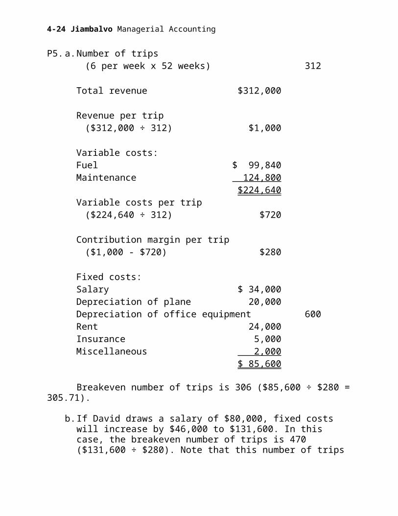
P5. a. Number of trips(6 per week x 52 weeks) 312

Total revenue $312,000

Revenue per trip($312,000 ÷ 312) $1,000

Variable costs:Fuel $ 99,840Maintenance 124,800

$224,640Variable costs per trip

($224,640 ÷ 312) $720

Contribution margin per trip($1,000 - $720) $280

Fixed costs:Salary $ 34,000Depreciation of plane 20,000Depreciation of office equipment 600Rent 24,000Insurance 5,000Miscellaneous 2,000

$ 85,600

Breakeven number of trips is 306 ($85,600 ÷ $280 = 305.71).

b. If David draws a salary of $80,000, fixed costs will increase by $46,000 to $131,600. In this case, the breakeven number of trips is 470 ($131,600 ÷ $280). Note that this number of trips is not feasible if David can only fly one round trip per day.

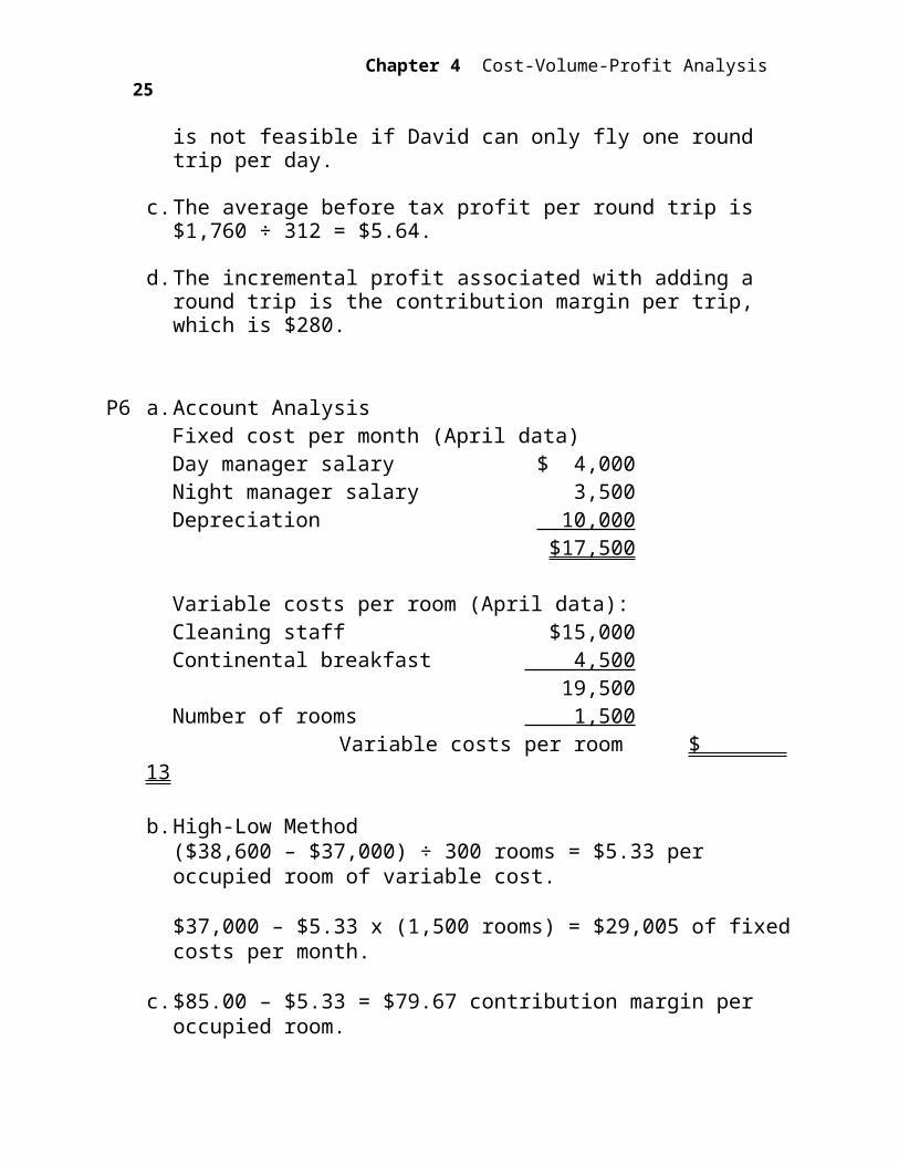
c. The average before tax profit per round trip is $1,760 ÷ 312 = $5.64.

d. The incremental profit associated with adding a round trip is the contribution margin per trip, which is $280.

4-18

P6 a. Account AnalysisFixed cost per month (April data)Day manager salary $ 4,000Night manager salary 3,500Depreciation 10,000

$17,500

Variable costs per room (April data):Cleaning staff $15,000Continental breakfast 4,500

19,500Number of rooms 1,500

Variable costs per room $ 13

b. High-Low Method($38,600 – $37,000) ÷ 300 rooms = $5.33 per occupied room of variable cost.

$37,000 – $5.33 x (1,500 rooms) = $29,005 of fixed costs per month.

c. $85.00 – $5.33 = $79.67 contribution margin per occupied room.

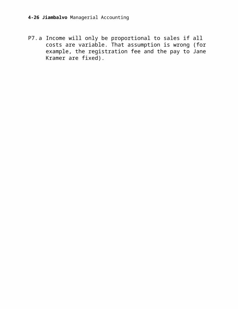
P7. a Income will only be proportional to sales if all costs are variable. That assumption is wrong (for example, the registration fee and the pay to Jane Kramer are fixed).



b. Sales $18,624.00Less cost of sales (60% of sales in prior year) 11,174.40Gross margin 7,449.60Less other expenses:

Registration fee 1,000.00 Booth rental (5% of sales) 931.20 Salary of Jane Kramer 300.00

Before tax profit $ 5,218.40

P8.

Sales $1,000,000.00 $1,100,000.00 $1,200,000.00 $1,300,000.00 $1,400,000.00Less cost of components 700,000.00 770,000.00 840,000.00 908,000.16 964,000.16 Gross margin 300,000.00 330,000.00 360,000.00 391,999.84 435,999.84Less:Staff salaries 180,000.00 180,000.00 180,000.00 180,000.00 180,000.00Rent 24,000.00 24,000.00 24,000.00 24,000.00 24,000.00Utilities 3,600.00 3,600.00 3,600.00 3,600.00 3,600.00Advertising 2,000.00 2,000.00 2,000.00 2,000.00 2,000.00 Operating profit before bonuses 90,400.00 120,400.00 150,400.00 182,399.84 226,399.84Staff bonuses 36,160.00 48,160.00 60,160.00 72,959.94 90,559.94 Profit before taxes and owner “draw” $ 54,240.00 $ 72,240.00 $ 90,240.00 $ 109,439.90 $ 135,839.90

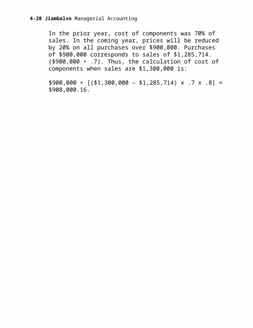
In the prior year, cost of components was 70% of sales. In the coming year, prices will be reduced by 20% on all purchases over $900,000. Purchases of $900,000 corresponds to sales of $1,285,714. ($900,000 ÷ .7). Thus, the calculation of cost of components when sales are $1,300,000 is:

$900,000 + [($1,300,000 – $1,285,714) x .7 x .8] = $908,000.16.

4-20

P9. a. Production costs:($95,000 - $78,500) ÷ (150 – 95) = $300 variable cost per unit

$95,000 – ($300 x 150) = $50,000 fixed cost per month.

Selling and administrative costs:

($16,000 - $13,800) ÷ (150 – 95) = $40 variable cost per unit

$16,000 – ($40 x 150) = $10,000 fixed cost per month.

b. Sales (1,400 units x $800) $1,120,000Less production costs ($50,000 x 12) + ($300 x 1,400) 1,020,000Less selling and adm. ($10,000 x 12) + ($40 x 1,400) 176,000Income (loss) ($ 76,000)

P10. a. Audio Video CarContribution margin $1,080,000 $ 460,000 $ 570,000Sales 3,000,000 1,800,000 1,200,000Contribution margin ratio (CM ÷ sales) 0.3600 0.2556 0.4750

b. A $100,000 increase in Audio sales would increase profit by $36,000 while the effect for Video would be $25,560 and $47,500 for the Car product line. All else equal, it would be better to increase sales of Car products.

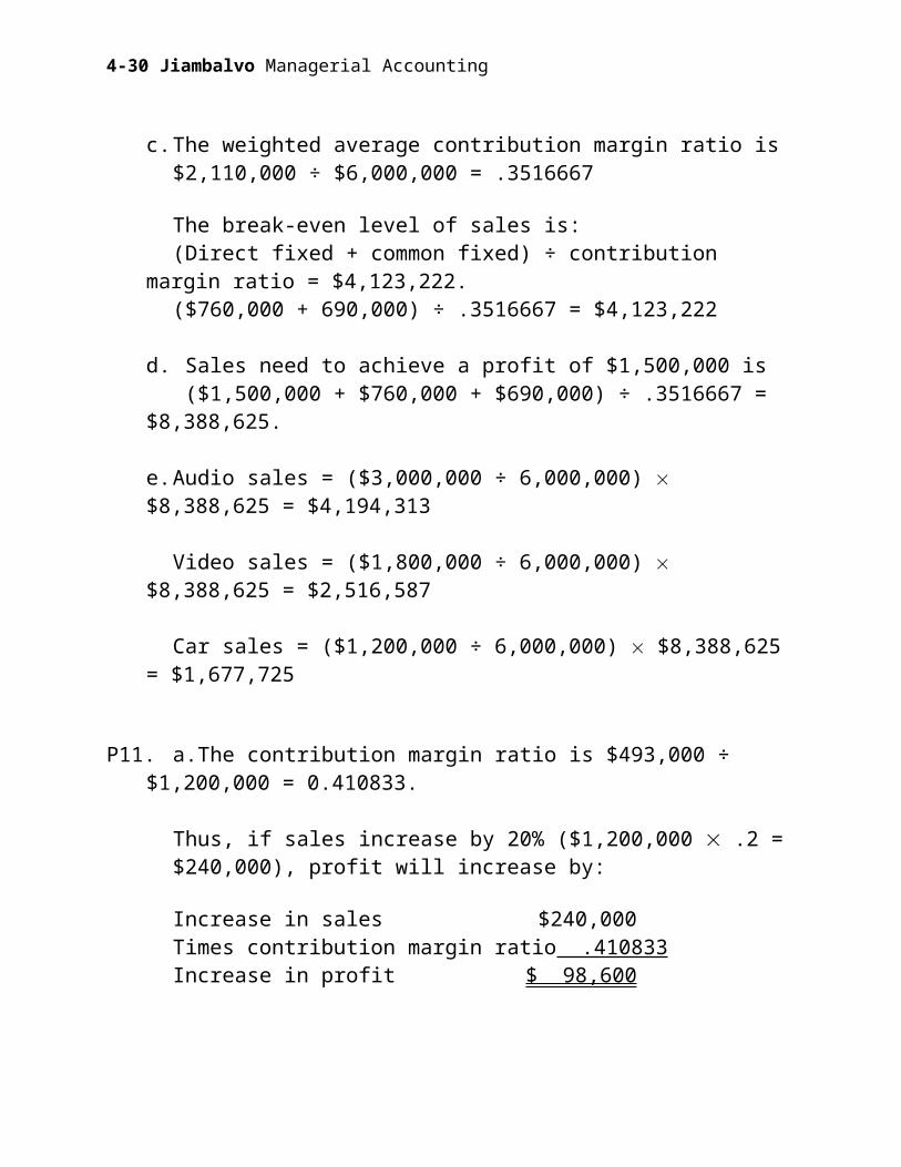
c. The weighted average contribution margin ratio is $2,110,000 ÷ $6,000,000 = .3516667

The break-even level of sales is:(Direct fixed + common fixed) ÷ contribution margin ratio = $4,123,222.($760,000 + 690,000) ÷ .3516667 = $4,123,222

d. Sales need to achieve a profit of $1,500,000 is ($1,500,000 + $760,000 + $690,000) ÷ .3516667 = $8,388,625.



e. Audio sales = ($3,000,000 ÷ 6,000,000) $8,388,625 = $4,194,313

Video sales = ($1,800,000 ÷ 6,000,000) $8,388,625 = $2,516,587

Car sales = ($1,200,000 ÷ 6,000,000) $8,388,625 = $1,677,725

P11.a. The contribution margin ratio is $493,000 ÷ $1,200,000 = 0.410833.

Thus, if sales increase by 20% ($1,200,000 .2 = $240,000), profit will increase by:

Increase in sales $240,000Times contribution margin ratio .410833Increase in profit $ 98,600

Thus, profit will increase by 42.87% ($98,600 ÷ $230,000)

Profit increases at a faster rate than sales because some costs are fixed and do not increase with sales.

b. If the owner of RealTimeService wanted to focus on the contribution margin per unit, he would, most likely, treat hours worked (on consulting, training, or repair services) as the unit of service. For example, if in the past fiscal year the company worked 6,000 hours, the contribution margin per hour would be $82.17 (i.e., $493,000 ÷ 6,000 hours).

4-22

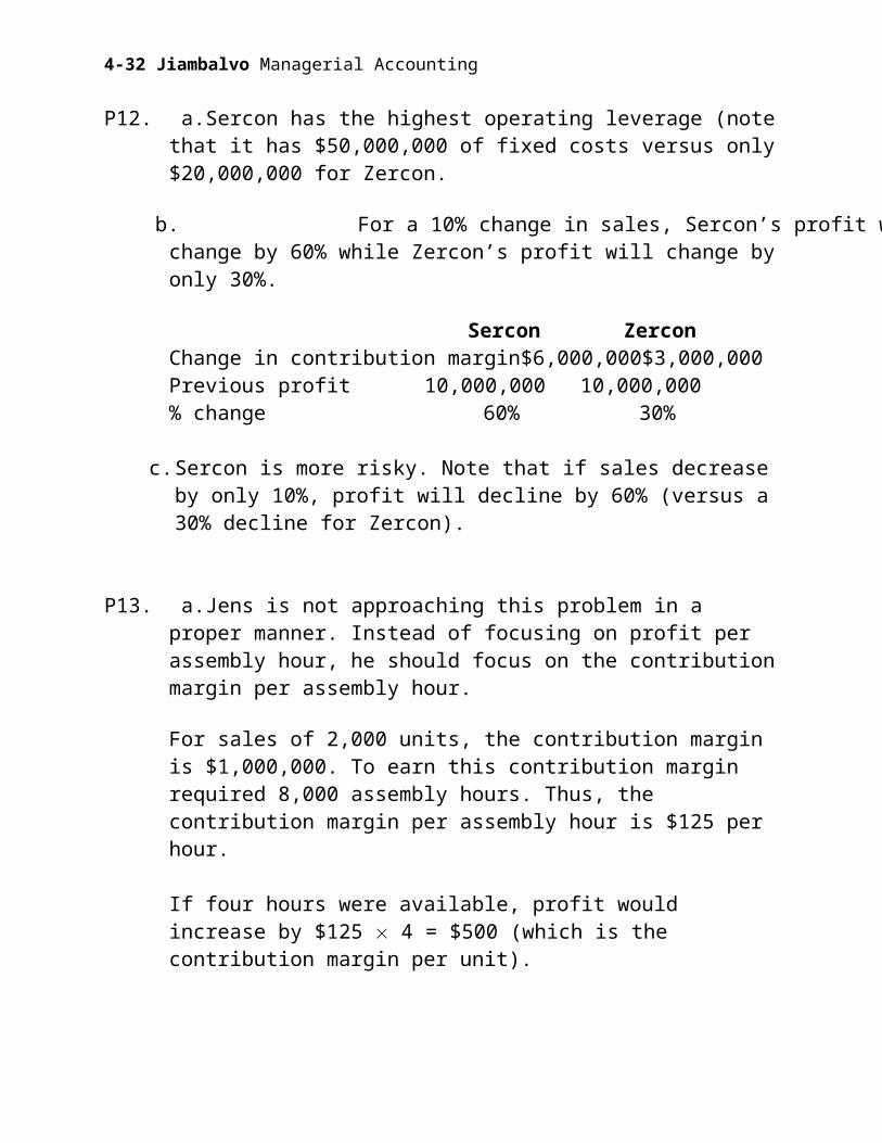
P12. a. Sercon has the highest operating leverage (note that it has $50,000,000 of fixed costs versus only $20,000,000 for Zercon.

b. For a 10% change in sales, Sercon’s profit will change by 60% while Zercon’s profit will change by only 30%.

Sercon ZerconChange in contribution margin $6,000,000 $3,000,000Previous profit 10,000,000 10,000,000% change 60% 30%

c. Sercon is more risky. Note that if sales decrease by only 10%, profit will decline by 60% (versus a 30% decline for Zercon).

P13. a. Jens is not approaching this problem in a proper manner. Instead of focusing on profit per assembly hour, he should focus on the contribution margin per assembly hour.

For sales of 2,000 units, the contribution margin is $1,000,000. To earn this contribution margin required 8,000 assembly hours. Thus, the contribution margin per assembly hour is $125 per hour.

If four hours were available, profit would increase by $125 4 = $500 (which is the contribution margin per unit).

b. Jens is underestimating the benefit of more assembly time. By focusing on profit per hour, he estimates an average benefit of $50 per hour. However, the real benefit is $125 per hour.

c. If Jens pays workers $25 per hour of overtime premium, he will still make an incremental $100 per hour ($125 - $25).



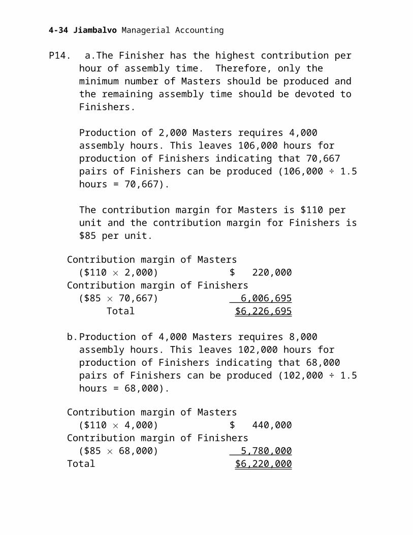
P14. a. The Finisher has the highest contribution per hour of assembly time. Therefore, only the minimum number of Masters should be produced and the remaining assembly time should be devoted to Finishers.

Production of 2,000 Masters requires 4,000 assembly hours. This leaves 106,000 hours for production of Finishers indicating that 70,667 pairs of Finishers can be produced (106,000 ÷ 1.5 hours = 70,667).

The contribution margin for Masters is $110 per unit and the contribution margin for Finishers is $85 per unit.

Contribution margin of Masters ($110 2,000) $ 220,000Contribution margin of Finishers ($85 70,667) 6,006,695

Total $6,226,695

b. Production of 4,000 Masters requires 8,000 assembly hours. This leaves 102,000 hours for production of Finishers indicating that 68,000 pairs of Finishers can be produced (102,000 ÷ 1.5 hours = 68,000).

Contribution margin of Masters ($110 4,000) $ 440,000Contribution margin of Finishers ($85 68,000) 5,780,000Total $6,220,000

Note that the total contribution margin has declined by $6,695. Thus, the opportunity cost of requiring that at least 4,000 pairs of the Master be produced is $6,695.

4-24

P15. Increase in sales at normal prices $2,500,000 Less 20% discount 500,000Increase in sales after discount 2,000,000 Less incremental costs .58897387 x $2,500,000 1,472,435Incremental profit $ 527,565

Note that since the regression was estimated using normal selling prices, the incremental costs must be calculated using normal selling prices.



Case 4-1

WENDELL ROBERTS CONSULTING

SummaryA consultant has biased an estimate to increase his client’s insurance claim.

• Links cost estimation and decision making

• Raises an interesting ethical issue

Questions to ask students1. What’s the situation in the Wendell Roberts Consulting Case?

2. What is the impact of the biased estimate on the claim?

3. Is Williams’ assumption (that all selling and administrative costs are fixed) ethical?

DiscussionI begin by asking a student to summarize the situation. In estimating expenses related to a damage claim, Harold Williams (a consultant with Wendell Roberts Consulting) assumes that all selling and administrative costs are fixed (40% are variable according to his client). By assuming they are fixed, there is a greater decline in profit when sales decrease. Thus, Williams’ estimated claim is higher.

4-26

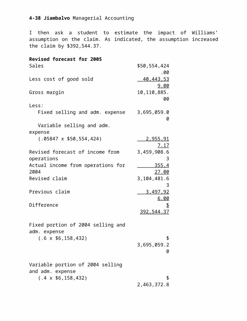
I then ask a student to estimate the impact of Williams’ assumption on the claim. As indicated, the assumption increased the claim by $392,544.37.

Revised forecast for 2005Sales $50,554,424.00Less cost of good sold 40,443,539.00 Gross margin 10,110,885.00Less: Fixed selling and adm. expense 3,695,059.00 Variable selling and adm. expense (.05847 x $50,554,424) 2,955,917.17 Revised forecast of income from operations 3,459,908.63Actual income from operations for 2004 355,427.00 Revised claim 3,104,481.63Previous claim 3,497,926.00 Difference $ 392,544.37

Fixed portion of 2004 selling and adm. expense (.6 x $6,158,432) $ 3,695,059.20

Variable portion of 2004 selling and adm. expense (.4 x $6,158,432) $ 2,463,372.80

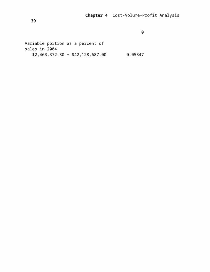
Variable portion as a percent of sales in 2004 $2,463,372.80 ÷ $42,128,687.00 0.05847



Finally, we get to the question of the ethics of the consultant’s calculation. Note that the client stated that “about 40% of the costs are variable.” The 40% number is an estimate and so is the consultant’s estimate of 0%. However, the consultant knows that his estimate is biased. In my opinion, submitting a biased claim is not ethical. Others may reasonably argue that you need to submit a biased claim because the insurance company is going to come back with an amount smaller than you request. By biasing your request, you may actually get a fair settlement!

Ethical dilemmas are only dilemmas when the right course of action isn’t obvious. That seems to be the case here.

4-28

Case 4-2ROTHMUELLER MUSEUM

SummaryA museum is trying to estimate the financial impact of a new exhibition.

• Links C-V-P analysis and decision making.

Questions to ask students1. What’s the situation at Rothmueller Museum?

2. What is the financial impact of the Ansel Adams exhibition? Is offering the exhibition a good decision from a financial standpoint?

3. How many people must attend the exhibition to break-even?

DiscussionI begin by asking a student to summarize the situation. Rothmueller Museum is planning an Ansel Adams exhibit. Alice Morgan, the photographic curator, wants to estimate its financial impact.



The financial impact is a positive $44,024 as follows:

Incremental revenue:9,000 x $12 $ 108,0007,200 x $5 36,000.2 x 7,200 x $7 x .3 3,024

147,024 Incremental costs:Lease of photos 80,000Packing 4,000Insurance 2,000Guard 9,000Installation 1,000Advertising 5,000Programs 2,000

103,000

Incremental profit $ 44,024

6,305 people must attend the exhibition in order for its financial impact to be profit neutral (i.e., the museum will not be better off nor worse off financially).

Fixed incremental costs $103,000Divided by average incremental revenue ($147,024 ÷ 9,000) 16.336

Number who must attend 6,305

Offering the exhibition appears to be a good decision in that it will more than cover its incremental costs. It may be, however, that a different exhibition would have contributed even more “profit.” That is, there may be some opportunity cost.

4-30

Case 4-3

MAYFIELD SOFTWARE, CUSTOMER TRAINING

SummaryAn internal report shows that the customer training center is losing money. The manager wants to know how many classes must be offered to break-even.

• Shows how allocated costs can make a valuable operation appear unprofitable.

Questions to ask students1. What’s the situation at the customer training center for Mayfield Software?

2. What will be the impact on company profit if the training center is closed?

3. How many classes must be offered to break-even given the current room configuration and approach to allocation?

4. What happens to break-even if the amount paid to instructors is reduced to $2,000 per class?

5. What will be the impact on group profit if version 4.0 of “CustomerTrack” is released?

DiscussionIf the customer training operation is shut down, Mayfield Software will lose $479,328 per year (i.e., profit before central charges). Note that the central charges are not likely to change as a result of closing the customer training center.

Given the current room configuration and approach to allocation of central charges (15 percent of revenue), Marie must offer approximately 965 classes to break-even on the Report of Operating Results.



Revenue per class $ 4,800

Trainer cost $ 3,000Operating manuals 400Postage 10Central charges 720 4,130 Contribution margin $ 670

Fixed costsDirector salary $150,000Receptionist 45,000Office manager 65,000Utilities 18,000Lease expense 240,000Rent 72,000Advertising 56,248

$ 646,248

$670 (x) - $646,248 = 0.

X = 964.54.

4-32

If the amount paid to instructors is reduced to $2,000 per class, the break-even point drops to 387. Marie should give serious consideration to this option since it will have a very significant impact on profitability and the break-even point.

$1,670 (X) - $646,248 = 0.

X = 386.97.

Finally, the impact of 30 sessions related to “CustomerTrack” is $20,100.

$670 (30) = $20,100



Case 4-4

KROG’S METALFAB, INC.

SummaryCompany is trying to estimate lost profit, related to fire damage, so it can submit an insurance claim.

• Focuses on cost estimation

• Demonstrates the effect of operating leverage—why profit does not increase or decrease at the same rate as sales

Questions to ask students1. What is the situation facing Krog’s Metalfab?

2. What are your estimates of lost profit?

3. What is wrong with Peter Newell’s analysis?

DiscussionI begin the discussion the same way I begin the discussion of almost all cases, by asking a student to summarize the situation. Krog had a fire at the end of 2003 that reduced capacity and profit during 2004. The company has insurance to cover lost profit, but what is the amount of lost profit during 2004?

At this point, I generally ask 5-10 students to simply give me their lost profit estimates and I put them on the board. If students have large estimates (say greater than $700,000) I’ll play the role of the insurance company and argue that their estimates are highly inflated. After all, the company only had profit of approximately $112,000 in 2003 (the year before the fire). I may go so far as to argue that the company should have ceased operations during the period of reconstruction to avoid having such high losses. In response, a sharp student will bring up the idea that this would have been the end of the business. And the company is surely worth more than $700,000 since it generates more than $300,000 per year in income from operations. (Note that the calculations for expected profit in 2004, without the fire, show annual expected profit of $337,443 using the regression approach and $15,641 using the high-low method.)

At this point, I may fall back on Peter Newell’s analysis, and argue that as long as the insurance company is willing to pay the excess operating costs ($240,000) plus the $34,961 estimated by Peter, Krog should be happy. This reimburses the company for the average profit per dollar of sales ($.02 per dollar of sales). This should lead to a discussion of the fundamental flaw in Peter’s analysis. When sales decline, profit will not decline by the average profit per dollar of sales. It will decline by a higher percent since when sales decline, fixed costs will not decline

4-34

(and as we will see, Krog Metalfab has high fixed costs). This drives home the concept of operating leverage and its link to fluctuations in profit.

Now it’s on to reviewing the calculation of lost profit. The answer depends on how the students estimate fixed and variable costs. Below, I’ll review calculations based on cost estimates using regression, the high-low method, and account analysis.

Regression analysis suggests that fixed costs are $259,418 per month and variable costs are $.3651 per dollar of sales. Thus, the estimate of lost profit is $1,062,920.

RegressionExpense = $259,418 + .3651 SalesR squared = .60

Sales in 2003 $5,079,094

Predicted sales with 7% increase $5,434,631Predicted expense($259,418 12) + (.3651 $5,434,631) 5,097,200Predicted profit 337,431Less actual loss 725,477Lost profit $1,062,908



A student who has carefully reviewed the problem will note that February of 2003 is an outlier (expenses are higher than sales in this month). Without February in the data set, the regression indicates that fixed costs are $220,338 and variable costs are $.4370 per dollar of sales. With these estimates, lost profit is $1,141,118.

RegressionExpense = $220,338 + .4370 SalesR squared = .99

Sales in 2003 $5,079,094


This estimate clearly shows the flaw in Peter’s analysis. Cost increase by .4370 per dollar of sales. That means that profit increases by .563 per dollar of sales (the contribution margin ratio). Sales are off by $1,589,132 compared to predicted sales and this means that profit is off by $894,681. In addition the company had $240,000 of excess expenses. Thus, it is easy to see why profit is off by more than $1,000,000.

4-36

High-Low ApproachIf students use the high-low method, they will estimate variable costs as $.4391 per dollar of sales and fixed costs as $299,525 per month.

August AprilHigh Low Change

Sales $602,210 $302,685 $299,525

Expense $485,120 $353,584 $131,536

Variable cost per dollar of sales ($131,536 ÷ $299,525) = $.4391

Fixed cost per month ($485,120 - $.4391 $602,210) = $220,690

In this case, lost profit is estimated as $1,125,494.

Sales in 2003 $5,079,094




Account AnalysisIf students use account analysis, they are likely to classify cost of goods sold as variable and selling and administrative costs as fixed. Using annual totals this suggests that variable costs are $.8875 per dollar of sales and fixed costs are $459,668.

Cost of goods sold $4,507,498Sales $5,079,094Cost of goods sold ÷ sales $.8875

Selling expense $216,668Administrative expense 243,000 Total $459,668

Use of these values results in estimated lost profit of $877,205. Estimated lost profit is lower here because estimated fixed costs are lower and estimated variable costs are higher.

Sales in 2003 $5,079,094

Predicted sales with 7% increase $5,434,631Predicted expense$459,668 + $.8875 $5,434,631 5,282,903Predicted profit 151,728Less actual loss 725,477Lost profit $ 877,205

This estimate seriously underestimates lost profit. The assumption that cost of goods sold is completely variable is at odds with the data (see the regression analysis) which indicates a large fixed cost component.

4-38

Case 4-5SEATTLE ESPRESSO, INC.

SummaryCompany is evaluating alternative ways to attract customers who are put off by service delays.

• Integrates cost estimation and decision making

• Focuses attention on the need to consider incremental rather than average cost

Questions to ask students1. What is the situation facing Seattle Espresso?

2. What is Angelo Steffano’s suggested solution?

3. What would be the impact on profit of implementing Angelo’s suggestion.

DiscussionI begin the discussion by asking a student to describe the situation facing Seattle Espresso. Sales of Seattle Espresso have fallen and the decline appears to be due to customer reluctance to wait in line. At the Carlton Hotel location the number of transactions has declined from 30 per hour to 15 per hour.

What is Angelo Steffano’s suggested solution? He suggests adding a staff person to reduce waiting in line.

What would be the impact on profit of implementing Angelo’s suggestion? This requires knowledge of the incremental cost of a transaction. Only cost of goods sold appears to be a function of the number of transactions (note that labor is a function of hours of business). Cost of goods sold is $1.60 per transaction (January cost of goods sold $17,280 ÷ 10,800 transactions—this relation holds in other months as well). The average revenue per transaction is $4 (January revenue $43,200 ÷ 10,800 transactions). Thus, the contribution margin is $2.40 ($4 - $1.60). Adding another person will cost $29,652 in labor ($7 per hour 4,236 hours per year).

However, the company will have an additional 63,540 transactions (4,236 hours 15 extra transactions per hour). Thus, the incremental transactions will generate $152,496 in contribution margin (63,540 $2.40). And the net benefit of hiring an extra person is $122,844 per year.



$ 4,236 Hours per year 15.00 Number of incremental transactions per hour

63,540.00 Number of incremental transactions per year 2.40 Contribution margin152,496.00 Incremental contribution margin 29,652.00 Cost of adding an extra staff person$ 122,844 Incremental benefit of adding an extra staff person

Note that working with the average cost per transaction (approximately $2.50) would significantly understate the benefit of adding an extra staff person (because it overstates the incremental cost of adding transactions).

4-40

Ch04

Documents

variable cost variable

total fixed cost

estimate of fixed cost

fixed cost component

variable cost component

mixed cost

cost of goods

cost structure