Ch 6 Macro

© 2015 Pearson Education, Inc

Chapter 6Aggregate Incomes


6 Aggregate Incomes

Chapter Outline

6.1 Inequality Around the World6.2 Productivity and the Aggregate Production Function6.3 The Role and Determinants of TechnologyEBE Why is the average American so much richer

than the average Indian?


Key Ideas

1. There are very large differences across countries in income or GDP per capita.

2. We can compare income differences across countries using GDP per capita at current exchange rates or adjusted for purchasing power parity differences.

6 Aggregate Incomes


Key Ideas

3. The aggregate production function links a country’s GDP to its capital stock, its total efficiency units of labor, and its technology.

4. Cross-country differences in GDP per capita partly result from differences in physical capital per worker and the human capital of workers, but differences in technology and the efficiency of production are even more important.

6 Aggregate Incomes


6.1 Inequality Around the World

We use the two terms, income per capita and GDP per capita, interchangeably in this course:

GDPIncome per capita = GDP per capita =

Total population


United States in 2010

GDP = $14.45 trillionPopulation = 310 million persons

GDP per capita = $46,613 per person



Question: How does U.S. GDP compare with GDP in Peru and Norway?



Peru in 2010

GDP = 444.46 billion nuevo solsTotal population = 28.95 million people

GDP per capita = 15,353 sols per person



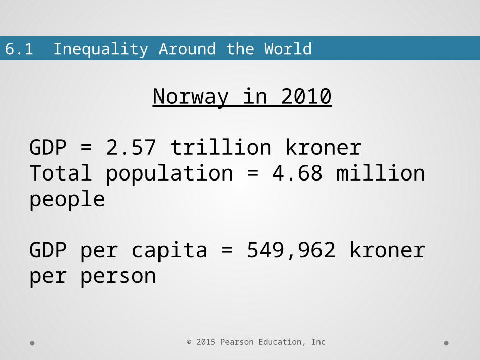
Norway in 2010

GDP = 2.57 trillion kroner Total population = 4.68 million people

GDP per capita = 549,962 kroner per person



Question: How do we make GDP comparisons between the United States and Peru and Norway?

Method #1: Convert GDP into U.S. dollars, using current exchange rates:

GDP per capita = GDP per capita in local currency × $ / local currency exchange rate



Peru GDP in 2010, Using Exchange Rates

GDP per capita = Peru GDP per capita in sols × $ / sol exchange rate

GDP per capita = 15,353 sols per person × 0.354 $ / sol

= $5,435 per person



Norway GDP in 2010, Using Exchange Rates

GDP per capita = Norway GDP per capita in kroner × $ / kroner exchange rate

GDP per capita = 549,962 kroner per person × 0.165 $ / kroner

= $90,744 per person



Ranking Country GDP per Capita

1 Qatar 141,845

2 Luxembourg 108,537

3 Norway 90,744

12 United States 46,613

87 Peru 5,435

189 Dem. Rep. of

Congo

189

190 Burundi 151

191 Somalia 109

GDP per Capita Rankings, Using Exchange Rates



There are two problems with using exchange rates to compare GDP across countries:

1. Prices of goods and services can vary across economies.

2. Exchange rates fluctuate throughout the year due to reasons beyond price changes.



Question: How do we make GDP comparisons between the United States and Peru and Norway?

Method #2: Convert Peru GDP by using the prices of goods and services in Peru relative to the prices of the same goods and services in the United States (purchasing power parity):

GDP per capita = GDP per capita in local currency × PPP adjustment



Peru GDP in 2010, Using PPP Adjustment

GDP per capita = Peru GDP per capita in sol × $ / peso PPP adjustment

GDP per capita = 15,353 sol per person × 0.587 $ / sol

= $9,012



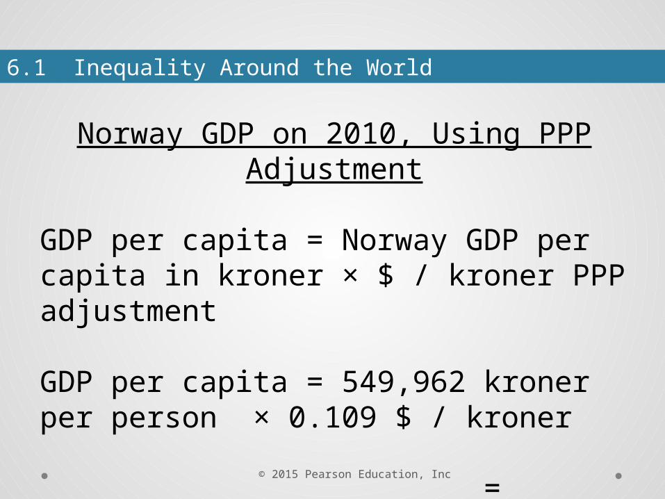
Norway GDP on 2010, Using PPP Adjustment

GDP per capita = Norway GDP per capita in kroner × $ / kroner PPP adjustment

GDP per capita = 549,962 kroner per person × 0.109 $ / kroner

= $59,946



Even though PPP adjustments raise the income levels of the developing countries, there are still very large disparities in income per capita across countries.




1 Qatar 142,876

2 Luxembourg 95,537

3 United Arab Emirates

70,899

6 Norway 59,946

12 United States 46,613

87 Peru 9,012

182 Burundi 451

183 Zimbabwe 368

184 Dem. Rep. of Congo

282

GDP per Capita Rankings, using PPP Adjustment




Exhibit 6.1 Income per Capita Around the World in 2010 (PPP-adjusted 2005 constant dollars)


Exhibit 6.2 A Map of Income per Capita Around the World



The age structure and labor participation rates vary across countries.

These variations impact income per capita.

Therefore, we may want to consider:

GDPIncome per worker =

Number of people employed




GDP per Worker

1 Qatar 142,876 182,297

2 Luxembourg 95,537 101,180

3 United Arab Emirates

70,899 91,694

6 Norway 50,488 94,863

10 United States 46,613 82,359

87 Peru 9,012 13,931

182 Burundi 397 770

183 Zimbabwe 368 606

184 Dem. Rep. of Congo

282 628

GDP per Capita vs. GDP per Worker



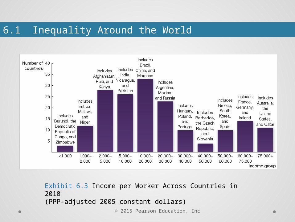
Exhibit 6.3 Income per Worker Across Countries in 2010 (PPP-adjusted 2005 constant dollars)



Ultimately, it is productivity differences that drive income per capita and income per worker differences across countries.

Productivity The value of goods and services that a worker generates for each hour of work.



0 10,000 20,000 30,000 40,000 50,000 60,000 70,000 80,0000

10

20

30

40

50

60

70

Relationship Between Real GDP per capita and Productivity in the OECD in 2010

Real GDP per capita in 2005 PPP dollars

Rea

l GD

P p

er h

ours

wor

ked

in 2

005

PP

P d

olla

rs

NorwayLuxembourg

RussiaMexico

United States

Chile



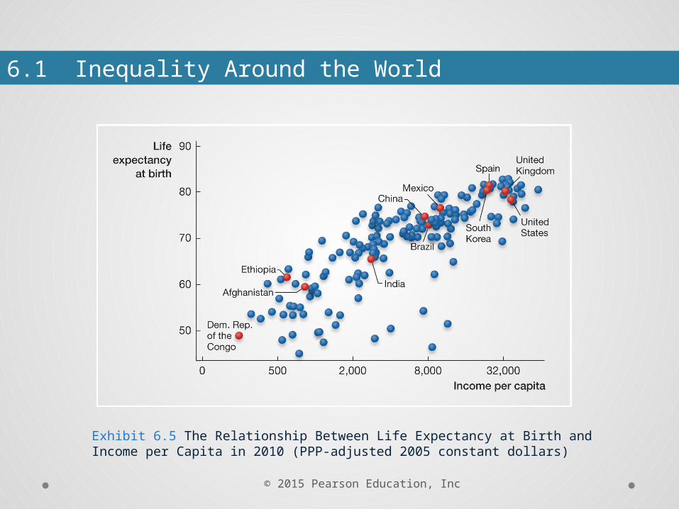
There is be a positive relationship between income per capita (and income per worker) and various measures of standard of living.

The next three slides present evidence of this relationship, using absolute poverty rates, life expectancy, and the Human Development Index to measure the standard of living.



Exhibit 6.4 The Relationship Between Poverty and Income per Capita in 2010 (PPP-adjusted 2005 constant dollars)



Exhibit 6.5 The Relationship Between Life Expectancy at Birth and Income per Capita in 2010 (PPP-adjusted 2005 constant dollars)




Exhibit 6.6 The Relationship Between the Human Development Index and Income per Capita in 2010 (PPP-adjusted 2005 constant dollars)


Productivity differences are the ultimate drivers of income per capita and income per worker differences across countries.

There are three reasons productivity differs across countries:

1. Human capital2. Physical capital3. Technology

6.2 Productivity and the Aggregate Production Function


Human capital The stock of skills embodied in labor to produce output.

This stock of skills, or total efficiency units of labor, is written:

H = L × hwherel is total number of workers h is the average human capital or efficiency



Physical capital The stock of business structures (plants) and equipment (machines) used for production.



Technology Superior knowledge in production or more efficient production processes so that more output can be produced with the same amount of human and physical capital.



How exactly do increases in a factor of production lead to increases in productivity and GDP?

Macroeconomists use the aggregate production function to model the relationship between aggregate GDP and its factors of production.



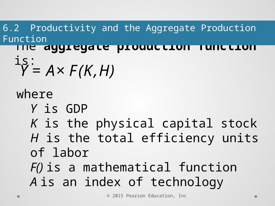
The aggregate production function is:

whereY is GDPK is the physical capital stockH is the total efficiency units of laborF() is a mathematical functionA is an index of technology

Y = A × F(K,H)



The aggregate production function has the same two properties as the production function of an individual firm.

1. “More is better”

An increase in either physical capital or total efficiency units of labor, holding the other factor constant, leads to an increase in GDP.



2. Law of diminishing marginal product

The marginal contribution of either physical capital or total efficiency units of labor to GDP diminishes when we increase the quantity used of that factor (holding all other factors of production constant).




Exhibit 6.7 The Aggregate Production Function with Physical Capital Stock on the Horizontal Axis (with the total efficiency units of labor held constant)



Exhibit 6.8 The Aggregate Production Function with the Efficiency Units of Labor on the Horizontal Axis (with physical capital stock held constant)


With more advanced technology, more output can be produced with the same amount of physical capital and total efficiency units of labor.

Therefore, technology will shift the production function upward.

6.3 The Role and Determinants of Technology



Exhibit 6.9 The Shift in the Production Function Resulting from More Advanced Technology


Technology can be embodied or contained in H.

Workers today possess (1) knowledge of how to produce new goods such as smartphones and also (2) knowledge of how to perform certain tasks more efficiently, like writing a term paper in the latest version of Microsoft Word.



Technology can be embodied or contained in K.

Physical capital today contains (1) knowledge of how to produce new goods such as smartphones and (2) knowledge of how to run certain software, like the latest version of Microsoft Word.



Advances in technology result mostly from purposeful, optimizing decisions by entrepreneurs and firms.

Firms and the government in the United States spent $430 billion (or 2.8% of GDP) in research and development (R&D) to find new ways of applying science to production methods and to develop new and improved goods and services.



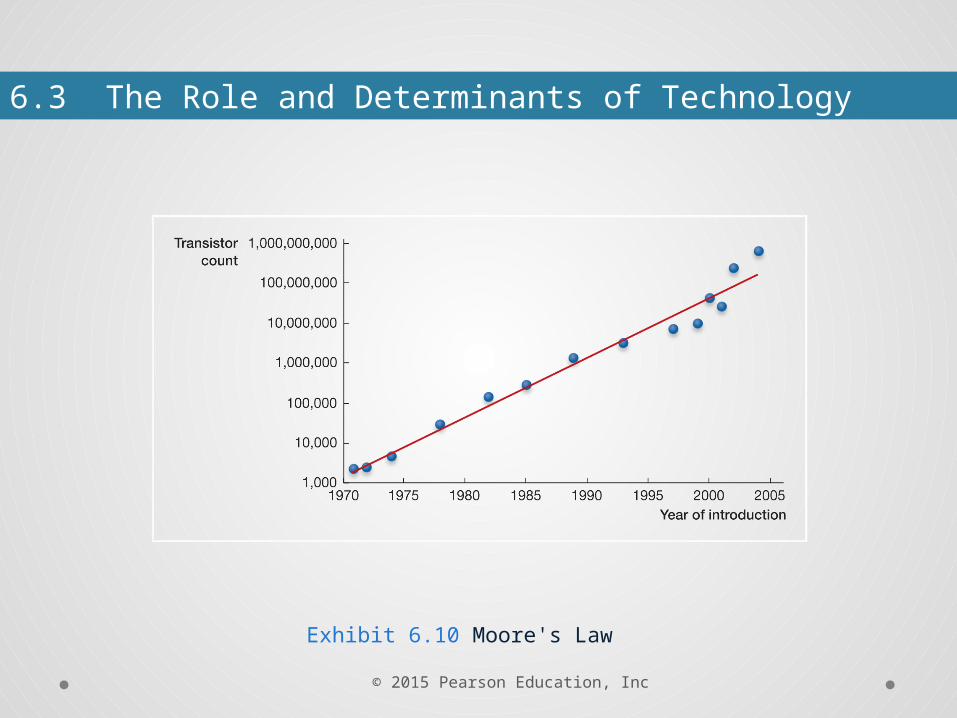
One example of how purposeful activity like R&D can increase the technology of the economy is Moore’s Law.

Named after Intel cofounder Gordon Moore, Moore’s Law predicts that the number of transistors packed on a computer chip (i.e., the processing speed) should double every two years.




Exhibit 6.10 Moore's Law


Question: Why is the average American so muchricher than the average Indian?

Answer: Exhibit 6.12 presents data on income per worker, human capital per worker (schooling), and physical capital per worker relative to the United States.

6 Aggregate Incomes

Evidence-Based Economics Example


6 Aggregate Incomes

Exhibit 6.12 The Contribution of Human Capital, Physical Capital, and Technology to Differences in Income per Worker


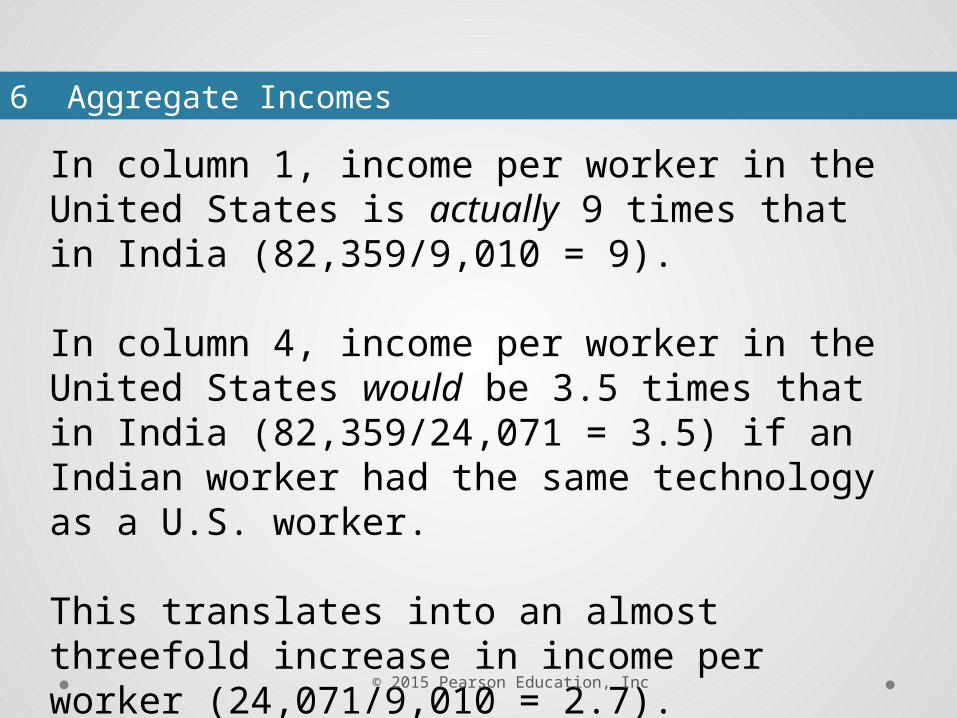
In column 1, income per worker in the United States is actually 9 times that in India (82,359/9,010 = 9).

In column 4, income per worker in the United States would be 3.5 times that in India (82,359/24,071 = 3.5) if an Indian worker had the same technology as a U.S. worker.

This translates into an almost threefold increase in income per worker (24,071/9,010 = 2.7).

6 Aggregate Incomes


Question: Why is the average American so much richer than the average Indian?

Answer: The average American is so much richer than the average Indian mostly because of better technology in the United States.

6 Aggregate Incomes

Ch 6 Macro

Education

peru gdp

norway gdp

gdp income

people gdp

countrys gdp

gdp comparisons

persons gdp

exchange rates gdp