Ch 6. Kernel Methods Ch 6. Kernel Methods Pattern Recognition and Machine Learning, Pattern Recognition and Machine Learning, C. M. Bishop, 2006. C. M. Bishop, 2006. Summarized by J. S. Kim Biointelligence Laboratory, Seoul National Univ ersity http://bi.snu.ac.kr/

Ch 6. Kernel Methods Pattern Recognition and Machine Learning, C. M. Bishop, 2006. Summarized by J. S. Kim Biointelligence Laboratory, Seoul National University.
Dec 28, 2015
Welcome message from author
This document is posted to help you gain knowledge. Please leave a comment to let me know what you think about it! Share it to your friends and learn new things together.
Transcript
Ch 6. Kernel MethodsCh 6. Kernel Methods
Pattern Recognition and Machine Learning, Pattern Recognition and Machine Learning, C. M. Bishop, 2006.C. M. Bishop, 2006.
Summarized by
J. S. Kim
Biointelligence Laboratory, Seoul National University
http://bi.snu.ac.kr/

2 (C) 2006, SNU Biointelligence La
b, http://bi.snu.ac.kr/
contentscontents
Introduction 6.1 Dual Representations 6.2 Constructing Kernels 6.3 Radial Basis Function Networks 6.3.1 Nadaraya-Watson model 6.4 Gaussian Processes 6.4.1 Linear regression revisited 6.4.2 Gaussian processes for regression 6.4.3 Learning the hyperparameters 6.4.4 Automatic relevance determination 6.4.5 Gaussian processes for classification 6.4.6 Laplace approximation 6.4.7 Connection to neural networks

3 (C) 2006, SNU Biointelligence La
b, http://bi.snu.ac.kr/
Introduction (1/2)Introduction (1/2)
A set of training data is used to obtain a parameter vector (neural networks).
Memory-based methods involve storing the entire training set in order to make
predictions for future data points (nearest neighbors).
In ‘dual representation’, the predictions are also based on linear combinations of a
kernel function evaluated at the training data points.

4 (C) 2006, SNU Biointelligence La
b, http://bi.snu.ac.kr/
Introduction (2/2)Introduction (2/2)
Kernel trick, i.e., kernel substitution: if we have an algorithm in which the input vector x enters only in the form of scalar products, then we can replace that scalar product with some other choice of kernel.
Stationary kernels: Homogeneous kernels, i.e.,
radial basis functions:

5 (C) 2006, SNU Biointelligence La
b, http://bi.snu.ac.kr/
Introduction (2/3)Introduction (2/3)
The kernel concept was introduced into the field of pattern recognition by Aizerman et al. (1964).
Re-introduced in the context of large margin classifiers by Boser et al. (1992).
Kernel substitution can be applied to principal component analysis as in a nonlinear variant of PCA (SchÖlkopf et al., 1998).
Also can be applied to nearest-neighbour classifiers and the kernel Fisher discriminant (Mika et al., 1999: Roth and Steinhage, 2000, Baudat and Anouar, 2000).

6 (C) 2006, SNU Biointelligence La
b, http://bi.snu.ac.kr/
6.1 Dual Representations (1/4)6.1 Dual Representations (1/4)
Consider a linear regression model whose parameters are determined by minimizing a regularized sum-of-squares error function given by
If we set
Where nth row of is And

7 (C) 2006, SNU Biointelligence La
b, http://bi.snu.ac.kr/
6.1 Dual Representations (2/4)6.1 Dual Representations (2/4)
We can now reformulate the least-squares algorithm in terms of a (dual representation). We substitute into to obtain

8 (C) 2006, SNU Biointelligence La
b, http://bi.snu.ac.kr/
6.1 Dual Representations (3/4)6.1 Dual Representations (3/4)
We define the Gram matrix
The sum-of-squares error function can be written as
Setting the gradient of with respect to a to zero, we obtain
9 (C) 2006, SNU Biointelligence La
b, http://bi.snu.ac.kr/
6.1 Dual Representations (4/4)6.1 Dual Representations (4/4)
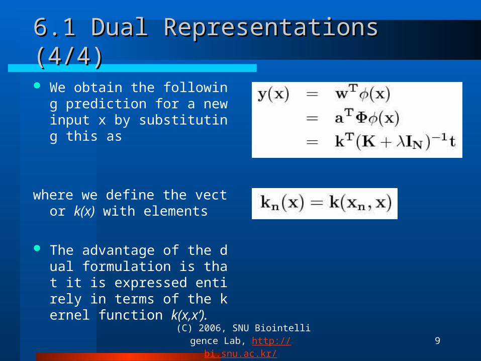
We obtain the following prediction for a new input x by substituting this as
where we define the vector k(x) with elements
The advantage of the dual formulation is that it is expressed entirely in terms of the kernel function k(x,x’).

10 (C) 2006, SNU Biointelligence La
b, http://bi.snu.ac.kr/
6.2 Constructing Kernels (1/5)6.2 Constructing Kernels (1/5)
Kernel function is defined for a one-dimensional input space by
Example of kernel
11 (C) 2006, SNU Biointelligence La
b, http://bi.snu.ac.kr/
6.2 Constructing Kernels (2/5)6.2 Constructing Kernels (2/5)
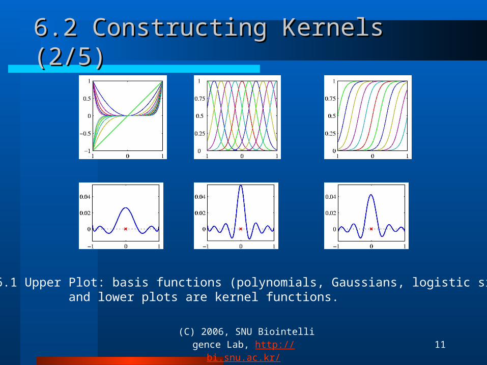
Figure 6.1 Upper Plot: basis functions (polynomials, Gaussians, logistic sigmoid), and lower plots are kernel functions.
12 (C) 2006, SNU Biointelligence La
b, http://bi.snu.ac.kr/
6.2 Constructing Kernels (3/5)6.2 Constructing Kernels (3/5)
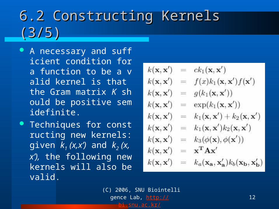
A necessary and sufficient condition for a function to be a valid kernel is that the Gram matrix K should be positive semidefinite.
Techniques for constructing new kernels: given k1 (x,x’) and k
2 (x,x’), the following new kernels will also be valid.

13 (C) 2006, SNU Biointelligence La
b, http://bi.snu.ac.kr/
6.2 Constructing Kernels (4/5)6.2 Constructing Kernels (4/5)
‘Gaussian’ kernel: The feature vector that
corresponds to the Gaussian kernel has infinity dimensionality.
A kernel function measuring the similarity of two sequences:
Fisher score:

14 (C) 2006, SNU Biointelligence La
b, http://bi.snu.ac.kr/
6.2 Constructing Kernels (5/5)6.2 Constructing Kernels (5/5)
Fisher kernel:
F is the Fisher information matrix, given by as follows:
Sigmoid kernel given by
This sigmoid kernel form gives the support machine a superficial resemblance to neural network model.

15 (C) 2006, SNU Biointelligence La
b, http://bi.snu.ac.kr/
6.3 Radial Basis Function Networks (1/3)6.3 Radial Basis Function Networks (1/3)
Radial basis functions: each basis function depends only on the radial distance from a center μj, so that
Expansions in radial basis function also arise from regularization theory: the optimal solution is given by an expansion in the Green’s functions of the operator.
16 (C) 2006, SNU Biointelligence La
b, http://bi.snu.ac.kr/
6.3 Radial Basis Function Networks (2/3)6.3 Radial Basis Function Networks (2/3)
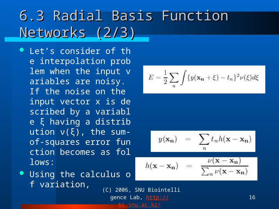
Let’s consider of the interpolation problem when the input variables are noisy. If the noise on the input vector x is described by a variable ξ having a distribution ν(ξ), the sum-of-squares error function becomes as follows:
Using the calculus of variation,

17 (C) 2006, SNU Biointelligence La
b, http://bi.snu.ac.kr/
6.3 Radial Basis Function Networks (3/3)6.3 Radial Basis Function Networks (3/3)
Figure 6.2 Gaussian basis functions and their normalized basis functions

18 (C) 2006, SNU Biointelligence La
b, http://bi.snu.ac.kr/
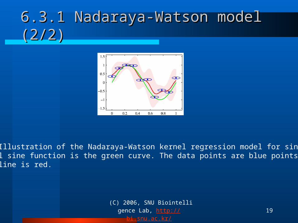
6.3.1 Nadaraya-Watson model (1/2)6.3.1 Nadaraya-Watson model (1/2)
19 (C) 2006, SNU Biointelligence La
b, http://bi.snu.ac.kr/
6.3.1 Nadaraya-Watson model (2/2)6.3.1 Nadaraya-Watson model (2/2)
Figure 6.3 Illustration of the Nadaraya-Watson kernel regression model for sinusoid data set. The original sine function is the green curve. The data points are blue points and resulting regression line is red.
20 (C) 2006, SNU Biointelligence La
b, http://bi.snu.ac.kr/
6.4 Gaussian Processes6.4 Gaussian Processes
We extend the role of kernels to probabilistic discriminative models.
We dispense with the parametric model and instead define a prior probability distribution over functions directly.
21 (C) 2006, SNU Biointelligence La
b, http://bi.snu.ac.kr/
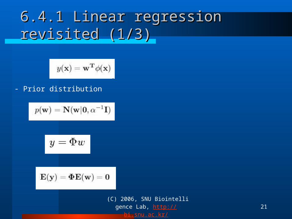
6.4.1 Linear regression revisited (1/3)6.4.1 Linear regression revisited (1/3)
- Prior distribution

22 (C) 2006, SNU Biointelligence La
b, http://bi.snu.ac.kr/
6.4.1 Linear regression revisited (2/3)6.4.1 Linear regression revisited (2/3)
-A key point about Gaussian stochastic processes is that the jointdistribution over N variables is specified completely by the second-order statistics, namely the mean and the covariance.

23 (C) 2006, SNU Biointelligence La
b, http://bi.snu.ac.kr/
6.4.1 Linear regression revisited (3/3)6.4.1 Linear regression revisited (3/3)
Figure 6.4 Samples from Gaussian processes for a ‘Gaussian’ kernel (left)And an exponential kernel (right).

24 (C) 2006, SNU Biointelligence La
b, http://bi.snu.ac.kr/
6.4.2 Gaussian processes for regression (1/7)6.4.2 Gaussian processes for regression (1/7)
25 (C) 2006, SNU Biointelligence La
b, http://bi.snu.ac.kr/
6.4.2 Gaussian processes for regression (2/7)6.4.2 Gaussian processes for regression (2/7)
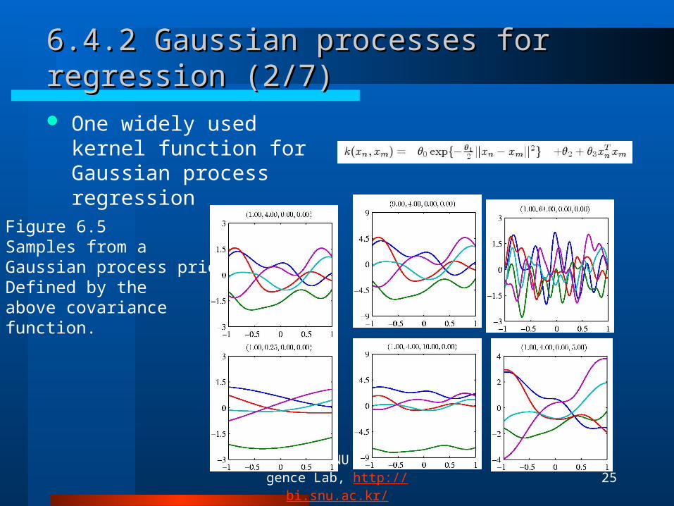
One widely used kernel function for Gaussian process regression
Figure 6.5 Samples from aGaussian process priorDefined by theabove covariance function.

26 (C) 2006, SNU Biointelligence La
b, http://bi.snu.ac.kr/
6.4.2 Gaussian processes for regression (3/7)6.4.2 Gaussian processes for regression (3/7)
Above mean and variance can be obtained from (2.81) and (2.80).

27 (C) 2006, SNU Biointelligence La
b, http://bi.snu.ac.kr/
6.4.2 Gaussian processes for regression (4/7)6.4.2 Gaussian processes for regression (4/7)
An advantage of a Gaussian processes viewpoint is that we can consider covariance functions that can only be expressed in terms of an infinite number of basis functions.

28 (C) 2006, SNU Biointelligence La
b, http://bi.snu.ac.kr/
6.4.2 Gaussian processes for regression (5/7)6.4.2 Gaussian processes for regression (5/7)
Figure 6.6 Illustration of the sampling of data points {tn} from a Gaussian process.The blue curve shows a sample function and the red points show the value of yn.The corresponding values of {tn}, shown in green, are obtained by adding independentGaussian noise to each of the {yn}.

29 (C) 2006, SNU Biointelligence La
b, http://bi.snu.ac.kr/
6.4.2 Gaussian processes for regression (6/7)6.4.2 Gaussian processes for regression (6/7)
Figure 6.7 Illustration of the mechanism of Gaussian process regression for the case of oneTraining point and one test point, in which the red ellipses show contours of the jointDistribution.
30 (C) 2006, SNU Biointelligence La
b, http://bi.snu.ac.kr/
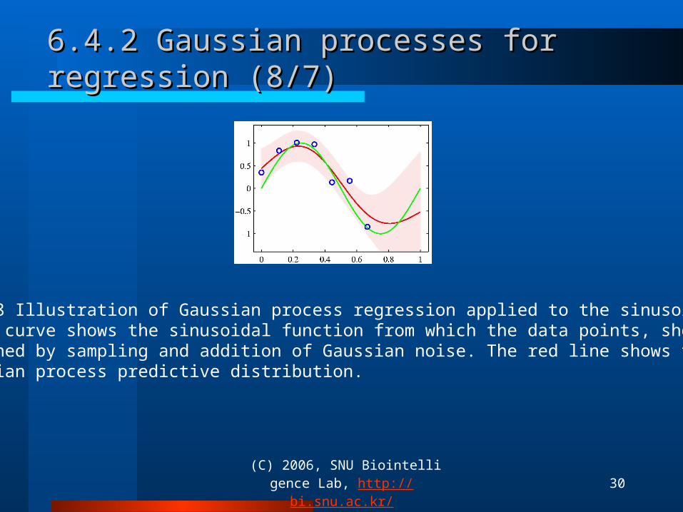
6.4.2 Gaussian processes for regression (8/7)6.4.2 Gaussian processes for regression (8/7)
Figure 6.8 Illustration of Gaussian process regression applied to the sinusoidal data set.The green curve shows the sinusoidal function from which the data points, shown in blue,are obtained by sampling and addition of Gaussian noise. The red line shows the mean ofthe Gaussian process predictive distribution.

31 (C) 2006, SNU Biointelligence La
b, http://bi.snu.ac.kr/
6.4.3 Learning the hyperparameters6.4.3 Learning the hyperparameters
In practice, rather than fixing the covariance function, we may prefer to use a parametric family of functions and then infer the parameter values from the data.
The simplest approach is to make a point estimate at θ by maximizing the log likelihood function.
The standard form for a multivariate Gaussian distribution is right above.

32 (C) 2006, SNU Biointelligence La
b, http://bi.snu.ac.kr/
6.4.4 Automatic relevance determination (1/2)6.4.4 Automatic relevance determination (1/2)
If a particular parameter ηi becomes small, the function becomes insensitive to the corresponding input variable xi.
In figure 10, x1 is from evaluating the function sin(2π x1), and then adding Gaussian noise. Values of x2 are given by copying the corresponding values of x1 and adding noise, and values of x3 are sampled from an independent Gaussian distribution. Figure 10. η1 (red), η2 (green), η3 (blue).
33 (C) 2006, SNU Biointelligence La
b, http://bi.snu.ac.kr/
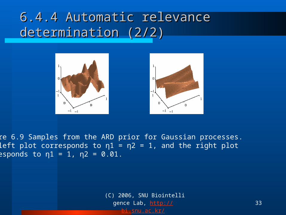
6.4.4 Automatic relevance determination (2/2)6.4.4 Automatic relevance determination (2/2)
Figure 6.9 Samples from the ARD prior for Gaussian processes. The left plot corresponds to η1 = η2 = 1, and the right plot Corresponds to η1 = 1, η2 = 0.01.

34 (C) 2006, SNU Biointelligence La
b, http://bi.snu.ac.kr/
6.4.5 Gaussian processes for classification (1/2)6.4.5 Gaussian processes for classification (1/2)
aN+1 is the independent variable of logistic function.
-One technique is based on variational inference. This approach
yields a lower bound on the likelihood function.
- The second approach uses expectation propagation.

35 (C) 2006, SNU Biointelligence La
b, http://bi.snu.ac.kr/
6.4.5 Gaussian processes for classification (2/2)6.4.5 Gaussian processes for classification (2/2)
Figure 6.11 The left plot shows a sample from a Gaussian processprior over functions a(x), and right plot shows the result of Transforming this sample using a logistic sigmoid function.

36 (C) 2006, SNU Biointelligence La
b, http://bi.snu.ac.kr/
6.4.6 Laplace approximation (1/8)6.4.6 Laplace approximation (1/8)
The third approach to Gaussian process classification is based on the Laplace approximation.
37 (C) 2006, SNU Biointelligence La
b, http://bi.snu.ac.kr/
6.4.6 Laplace approximation (2/8)6.4.6 Laplace approximation (2/8)
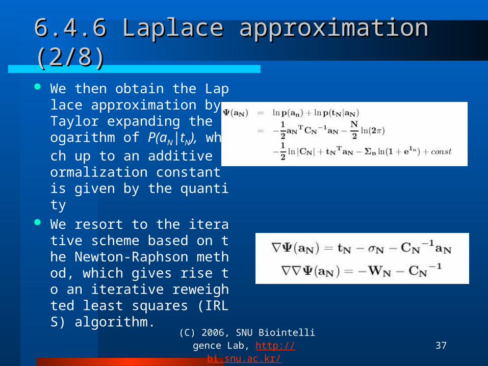
We then obtain the Laplace approximation by Taylor expanding the logarithm of P(aN|tN), which up to an additive normalization constant is given by the quantity
We resort to the iterative scheme based on the Newton-Raphson method, which gives rise to an iterative reweighted least squares (IRLS) algorithm.
38 (C) 2006, SNU Biointelligence La
b, http://bi.snu.ac.kr/
6.4.6 Laplace approximation (3/8)6.4.6 Laplace approximation (3/8)
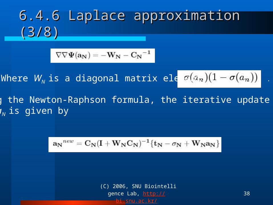
- Where WN is a diagonal matrix elements .
-Using the Newton-Raphson formula, the iterative update equation for aN is given by
39 (C) 2006, SNU Biointelligence La
b, http://bi.snu.ac.kr/
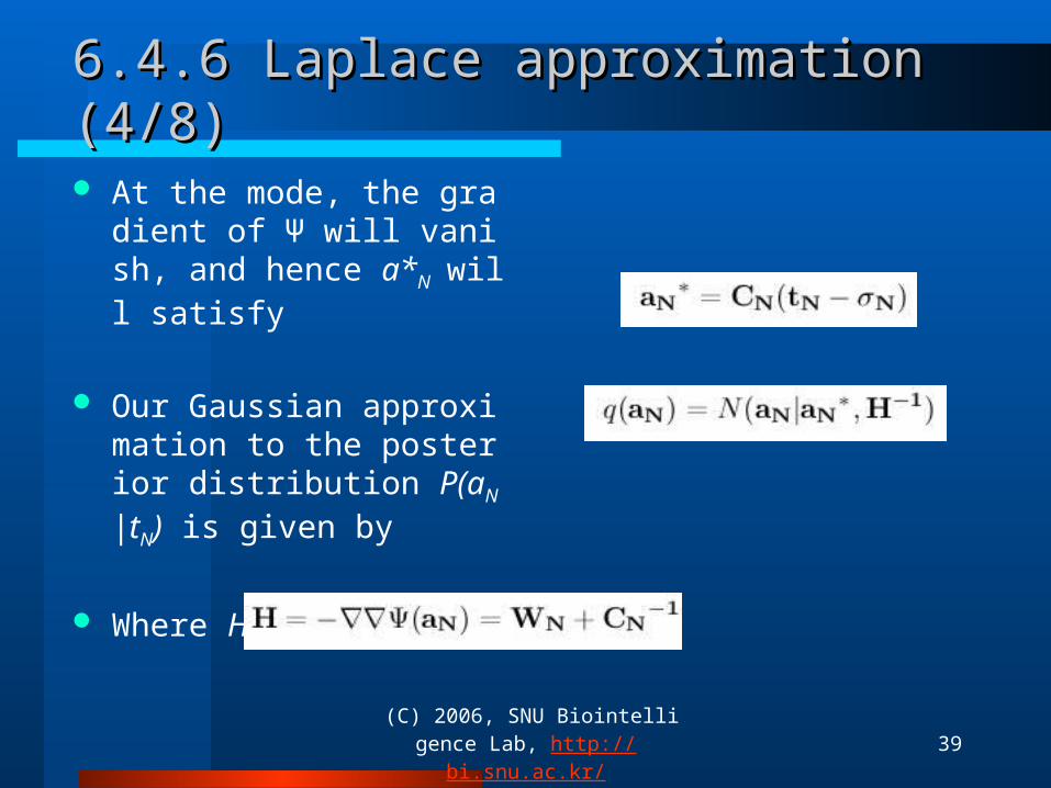
6.4.6 Laplace approximation (4/8)6.4.6 Laplace approximation (4/8)
At the mode, the gradient of Ψ will vanish, and hence a*N will satisfy
Our Gaussian approximation to the posterior distribution P(a
N|tN) is given by
Where H is Hessian

40 (C) 2006, SNU Biointelligence La
b, http://bi.snu.ac.kr/
6.4.6 Laplace approximation (5/8)6.4.6 Laplace approximation (5/8)
By solving the integral for P(aN+1|tN)
We are interested in the decision boundary corresponding to P(tN+1|tN) = 0.5

41 (C) 2006, SNU Biointelligence La
b, http://bi.snu.ac.kr/
6.4.6 Laplace approximation (6/8)6.4.6 Laplace approximation (6/8)
42 (C) 2006, SNU Biointelligence La
b, http://bi.snu.ac.kr/
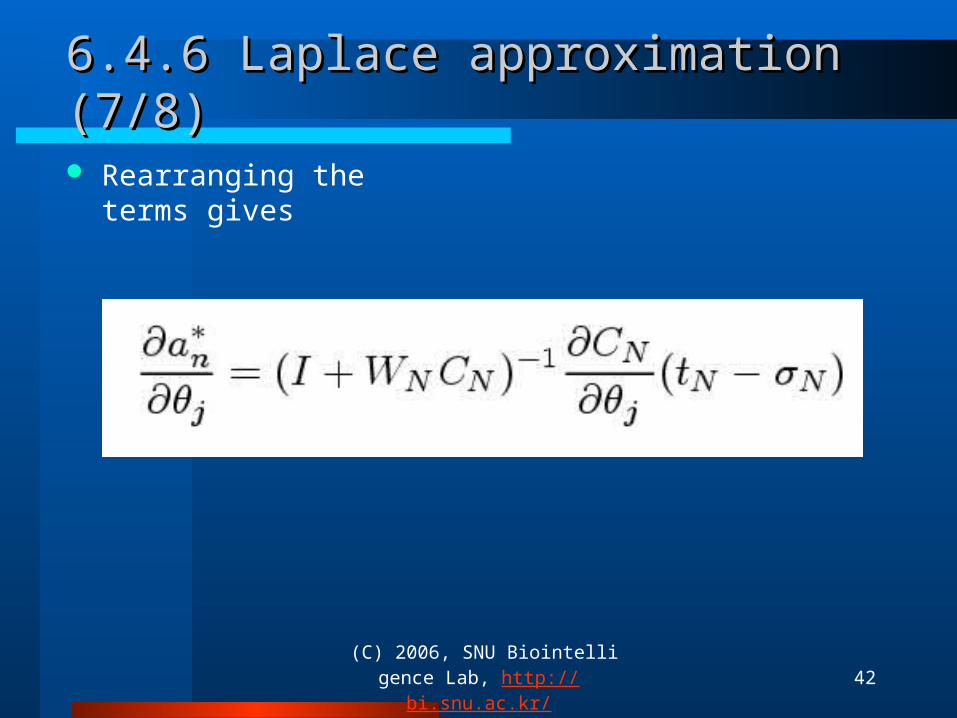
6.4.6 Laplace approximation (7/8)6.4.6 Laplace approximation (7/8)
Rearranging the terms gives

43 (C) 2006, SNU Biointelligence La
b, http://bi.snu.ac.kr/
6.4.6 Laplace approximation (8/8)6.4.6 Laplace approximation (8/8)
Figure 6.12 Illustration of the use of a Gaussian proccess forClassification. The true distribution is green, and the decisionBoundary from the Gaussian process is black. On the rightis the predicted posterior probability for the blue and red classestogether with the Gaussian process decision boundary.

44 (C) 2006, SNU Biointelligence La
b, http://bi.snu.ac.kr/
6.4.7 Connection to neural networks6.4.7 Connection to neural networks
Neal has shown that, for a broad class of prior distributions over w, the distribution of functions generated by a neural network will tend to a Gaussian process in the linit M->00, where M is the number of hidden units.
By working directly with the covariance function we have implicitly marginalized over the distribution of weights. If the weight prior is governed by hyperparameters, then their values will determine the length of scales of the distribution over functions. Note that we cannot marginalize out the hyperparameters analytically, and must instead resort to techniques of the kind discussed in Section 6.4.
Related Documents