Ch. 21: Production and Costs Del Mar College John Daly ©2003 South-Western Publishing, A Division of Thomson Learning.

Ch. 21: Production and Costs

Del Mar College

John Daly©2003 South-Western Publishing, A Division of Thomson Learning

The Firm’s Objective: Maximizing Profit

• An explicit cost is a cost that is incurred when an actual payment is made.

• An implicit cost represents the value of resources used in production for which no actual payment is made. This is incurred as a result of a firm using its own resources that it owns or that the owners of the firm contribute to it.

Accounting Profit vs. Economic Profit

• Accounting Profit is the difference between total revenue and explicit costs.

• Economic Profit is the difference between total revenue and total opportunity cost, including both its explicit and implicit components.

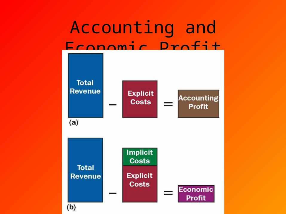
Accounting and Economic Profit

Zero Economic Profit?

• It is possible for a firm to earn both a positive accounting profit and a zero economic profit.

• A firm that makes zero economic profit is said to be earning normal profit.

• Zero economic profit means the owner has generated total revenues sufficient to cover total opportunity costs.

Q & A

• Suppose everything about two people is the same except that one person currently earns a high salary and the other person currently earns a low salary. Which is more likely to start his or her own business? Why?

• Is accounting or economic profit larger? Why?• When can a business owner be earning a profit

but not covering expenses?

Production

• A fixed input is an input whose quantity cannot be changed as output changes in the short run.

• The costs associated with fixed inputs are fixed costs. A fixed cost doesn’t change as output changes.

• A variable input is an input whose quantity can be changed as output changes in the short run.

• The costs associated with variable inputs are variable costs. A variable cost changes as output changes.

Short Run & Long Run Production

• The short run is a period in which some inputs are fixed.

• The long run is a period in which all inputs can be varied.

• The Total Cost is the sum of fixed and variable costs

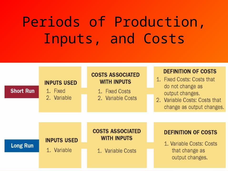
Periods of Production, Inputs, and Costs

Production In the Short Run

• As more and more variable inputs, such as labor and capital, were added to a fixed input, such as land, the variable inputs would yield smaller and smaller additions to output

• As ever larger amounts of a variable input are combined with fixed inputs, eventually the marginal physical product of the variable input will decline.

• The marginal physical product of a variable input is equal to the change in output that results from changing the variable input by one unit, holding all other inputs fixed.

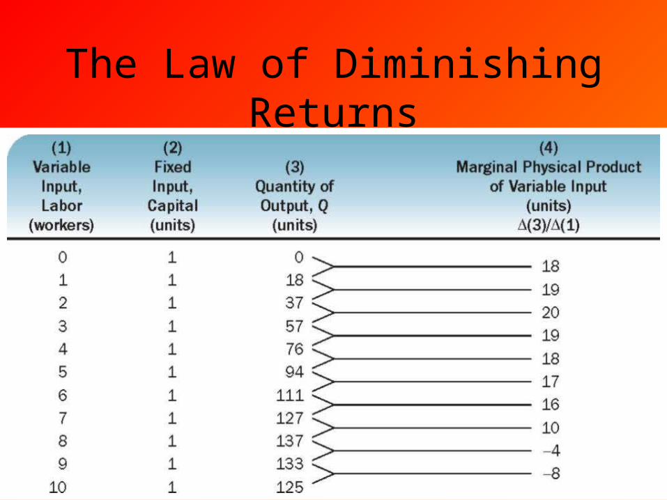
The Law of Diminishing Returns

Marginal Physical Product and Marginal Cost (Continued)

• If the law of diminishing marginal returns did not hold, then it would be possible to continue to add additional units of a variable input to a fixed input, and the marginal physical product of the variable input would never decline. We could increase output indefinitely as long as we continued to add units of a variable input to a fixed input.

• The law of diminishing marginal returns says that as more units of the variable input are added, each one has fewer units of the fixed input to work with; consequently, output rises at a decreasing rate.

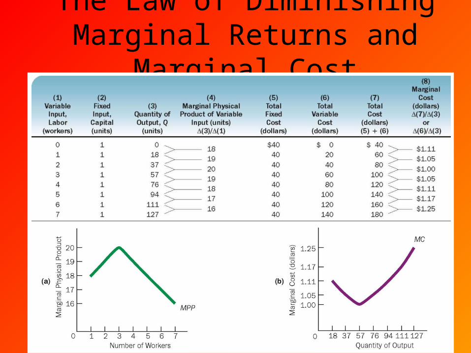
The Law of Diminishing Marginal Returns and Marginal Cost

Marginal Physical Product and Marginal Cost

• Marginal cost is a reflection of the marginal physical product of the variable input.

• As the marginal physical product curve rises, the marginal cost curve falls; and as the marginal physical product curve falls, the marginal cost curve rises.

• What the marginal cost curve looks like depends on what the marginal physical product curve looks like.

Average Productivity

• Average physical product is output divided by the quantity of labor.

• When the term labor productivity is used in the newspaper and in government documents, it refers to the average physical productivity of labor on an hourly basis.

Q & A• If the short run is six months, does it follow that

the long run is longer than six months?• “As we add more capital to more labor, eventually

the law of diminishing marginal returns will set in.” What is wrong with this statement?

• Suppose a marginal cost (MC) curve falls when output is in the range of 1 unit to 10 units, flattens out and remains constant over an output range of 10 units to 20 units, and then rises over a range of 20 units to 30 units. What does this have to say about the marginal physical product of the variable input?

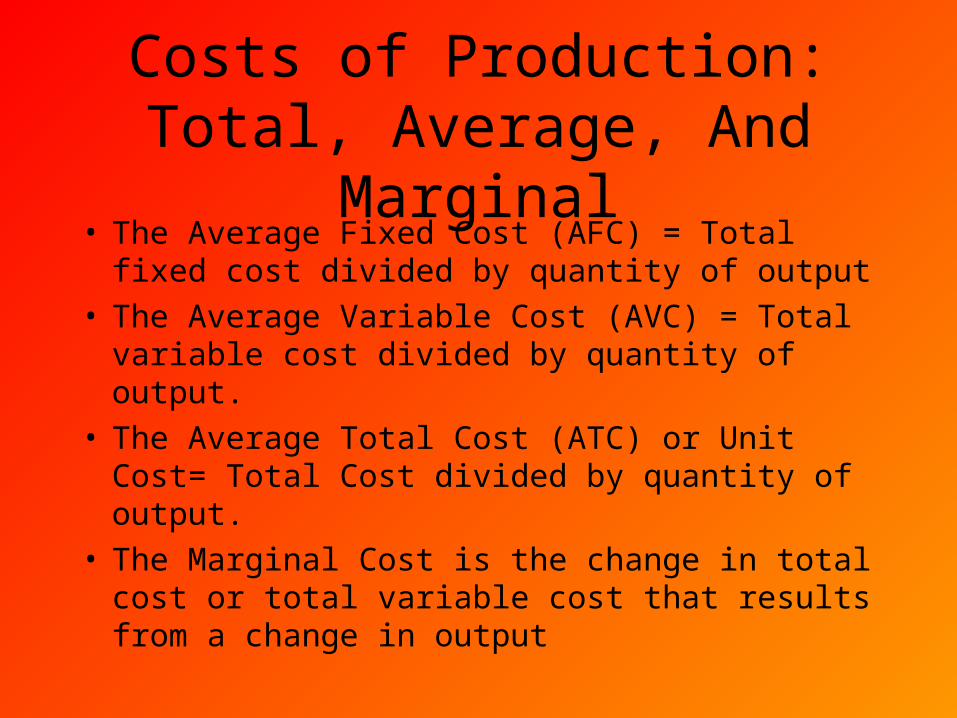
Costs of Production: Total, Average, And Marginal

• The Average Fixed Cost (AFC) = Total fixed cost divided by quantity of output

• The Average Variable Cost (AVC) = Total variable cost divided by quantity of output.

• The Average Total Cost (ATC) or Unit Cost= Total Cost divided by quantity of output.

• The Marginal Cost is the change in total cost or total variable cost that results from a change in output

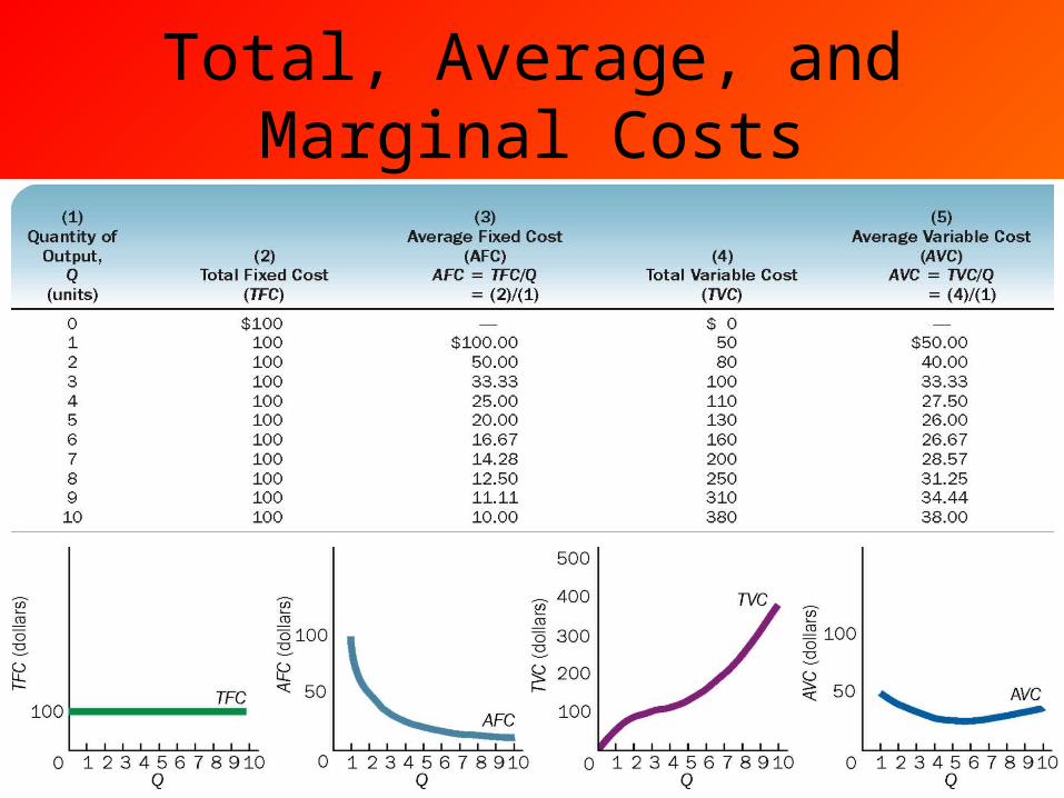
Total, Average, and Marginal Costs

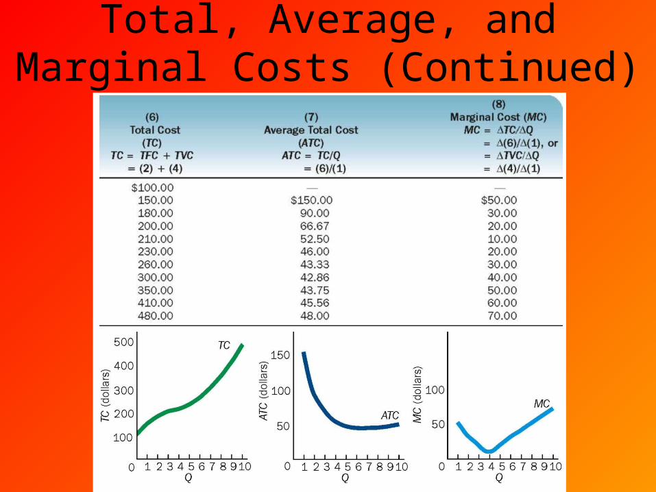
Total, Average, and Marginal Costs (Continued)

The Average-Marginal Rule

When the marginal magnitude is above the average magnitude, the average magnitude rises; when the marginal magnitude is below the average magnitude, the average magnitude falls.

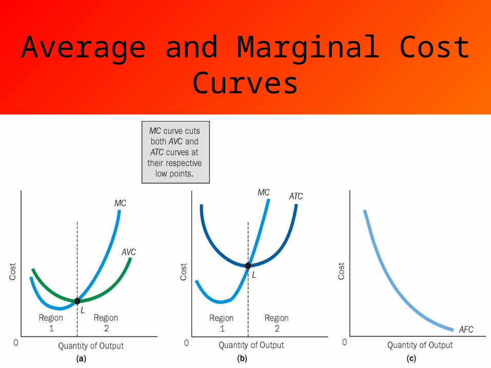
Average and Marginal Cost Curves

Tying Short-Run Production To Costs

• Production underlies what many of the various cost curves looks like.

• What happens in terms of production affects Marginal Cost, which in turn eventually effects Average Variable Cost and Average Total Cost.

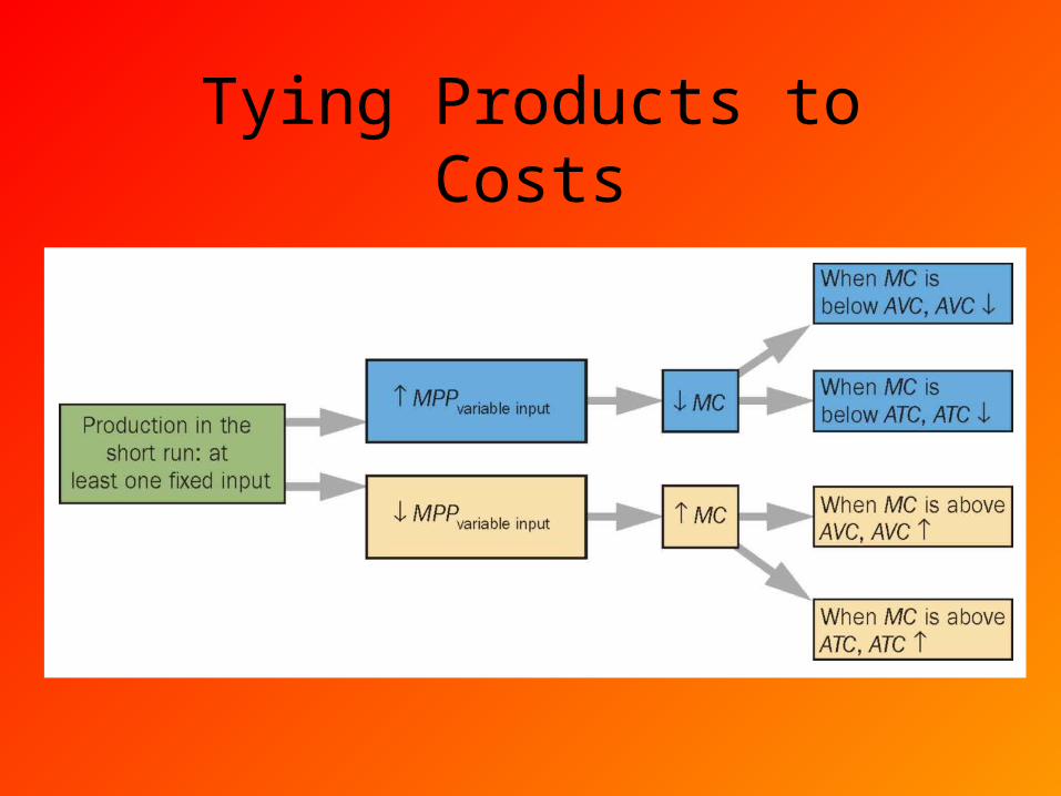
Tying Products to Costs

Sunk CostSunk cost is a cost incurred in the past that cannot be changed by current decisions and therefore cannot be recovered.

Q & A

• Identify two ways to compute average total cost (ATC).

• Would a business ever sell its product for less than cost? Explain your answer. (Hint: Think of sunk cost)

• What happens to unit costs as marginal costs rise? Explain your answer.

• Do changes in marginal physical productivity influence unit costs? Explain your answer.

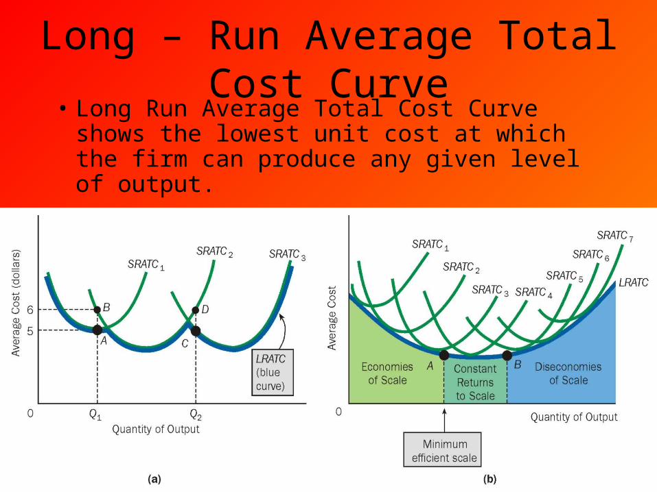
Long – Run Average Total Cost Curve• Long Run Average Total Cost Curve shows

the lowest unit cost at which the firm can produce any given level of output.

Economies of Scale, Diseconomies of Scale, and Constant Returns to Scale

• Economies of Scale exist when inputs are increased by some percentage and output increases by a greater percentage, causing unit costs to fall.

• Constant Returns to Scale exist when inputs are increased by some percentage and output increases by an equal percentage, causing unit costs to remain constant.

• Diseconomies of Scale exist when inputs are increased by some percentage and output increases by a smaller percentage, causing unit costs to rise.

• Minimum Efficient Scale is the lowest output level at which average total costs are minimized.

Why Economies of Scale?

• Growing firms offer greater opportunities for employees to specialize.

• Growing firms can take advantage of highly efficient mass production techniques and equipment that ordinarily require large setup costs and thus are economical only if they can be spread over a large number of units

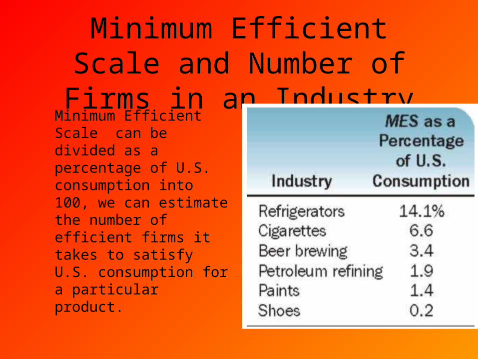
Minimum Efficient Scale and Number of Firms in an IndustryMinimum Efficient Scale can be divided as a percentage of U.S. consumption into 100, we can estimate the number of efficient firms it takes to satisfy U.S. consumption for a particular product.

Shifts In Cost Curves

• Taxes: affects variable costs. Because variable costs rise, total costs rise, and their average curves are shifted upward. Because marginal cost is the change in total cost divided by the change in output, marginal cost rises.

• Input Prices: A rise or a fall in variable input prices causes a corresponding change in the firm’s average total, variable, and marginal cost curves.

• Technological changes often bring either the capability of using fewer inputs to produce a good or lower input prices.

Q & A

• Give an arithmetical example to illustrate economies of scale.

• What would the LRATC curve look like if there were always constant returns to scale? Explain your answer.

• Firm A charged $4 per unit when it produced 100 units of good X, and it charged $3 per unit when it produced 200 units. Furthermore, the firm earned the same profit per unit in both cases. How can this be?