ch 14

14

Transport

14.1 Introduction

For the plasma in a fusion reactor to be self-sustaining at T = 15 keV the alpha particle heat-ing must balance the losses due to thermal conduction as described by the familiar condition

pτE = 24

Eα

T 2

〈σv〉 . (14.1)

Recall now that in a reactor the pressure is set by the power density required to achieve adesired output power, while the temperature is determined by minimizing the ratio T 2/〈σv〉.Therefore, achieving self-sustained ignited operation leads to a requirement on the value ofthe energy confinement time τE.

Understanding and controlling energy confinement is the domain of transport theory, andis the main objective of Chapter 14. In a plasma there are three important types of transport:heat conduction, particle diffusion, and magnetic field diffusion. Of these, heat conductionis the most serious loss mechanism and consequently is the main focus of the discussion.Also, most of the analysis involves the tokamak since it is for this configuration that mostof the theory is formulated and most of the data have been collected and analyzed.

Most fusion researchers would agree that understanding heat conduction has been themost difficult challenge on the path to a reactor. The reason is that transport in a plasma isalmost always dominated, not by Coulomb collisions, but by plasma turbulence driven bymicro-instabilities. Understanding the resulting anomalous transport requires sophisticatedkinetic models and non-linear, multi-dimensional numerical simulations.

After many years of research great strides have been made towards determining a firstprinciples theory of anomalous heat conduction. Even so, there is still a long way to gobefore the theory can be used as a reliable design tool for new devices. By and large,new designs are based on empirical scaling relations derived from an extensive databaseof experimental measurements. These empirical relations predict that the tokamak has areasonably good chance of achieving self-sustained ignited operation, although the safetymargins are not large. Also, the predictions should be treated with caution as they invariablyinvolve extrapolations beyond the experimental regimes represented in the database.

To introduce some order into the understanding of the plasma transport problem, Chapter14 starts with a simple model, classical transport in a 1-D cylinder, and adds increasing levels

449

450 Transport

of complexity, finally arriving at transport in a tokamak reactor. The material is organizedas follows.

First, the fluid equations describing heat, particle, and magnetic field diffusion in a 1-Dcylinder are derived using the low-β tokamak expansion. The analysis shows how bothparticle and magnetic field diffusion arise naturally from the resistive MHD model. Thedominant thermal diffusion coefficient is, however, not derivable from this model. It isinstead derived independently by a simple heuristic calculation based on the “random walk”model. The analysis shows that heat transport is much larger than particle transport and isdominated by the ions. The end result of this discussion is a set of well-posed, 1-D transportequations.

Second, even though experimentally observed diffusion coefficients are much larger thatthe simple 1-D values derived above, it is a worthwhile preliminary goal to learn how tomathematically formulate and solve transport equations assuming the diffusion coefficientsare known. Towards this goal several simple applications of the 1-D transport model areinvestigated, including temperature equilibration, off-axis heating, and ohmically heatingto ignition.

The third topic involves neoclassical transport theory, which corresponds to classicalCoulomb transport in a toroidal geometry. Although one might initially expect toroidicityto simply add small a/R0 corrections to the cylindrical results, the actual results are muchdifferent. Toroidal effects typically lead to an increase of nearly two orders of magnitudein the ion thermal diffusivity, a consequence of the effects of guiding center particle driftsin toroidal geometry, particularly as they affect trapped particles. Even with this largeincrease the neoclassical ion thermal diffusivity is still noticeably smaller than experimentalobservations. The final neoclassical topic is a simple derivation of the bootstrap current JB.Recall, that JB is a natural, transport-induced, toroidal plasma current essential for the ATmode of tokamak operation, the purpose of which is to reduce the requirements on theexternal current drive system.

The next topic in the logical progression should involve a discussion of micro-instabilitydriven anomalous transport. This is, however, beyond the scope of the present book. Instead,attention is focused on the macroscopic consequences of anomalous transport which appearas empirical scaling relations for τE. It is shown how the generalized 1-D transport equationsare simplified to a 0-D form in which the thermal transport is modeled in terms of τE. Adescription is presented showing how τE is calculated in practice and expressions are givenfor two typical modes of tokamak operation: the L-mode (for low confinement) and theH-mode (for high confinement). It is worth emphasizing that τE models the global thermaltransport of the plasma core. Even so, there are several important transport phenomenaassociated with the plasma edge that directly and indirectly affect core transport. Here toothe treatment is primarily empirical. A brief description is given of these transport-relatededge phenomena.

Lastly, these results are combined to investigate several practical transport applicationsrelated to fusion power production. First, a simple optimized tokamak ignition experimentis designed. The resulting parameters are very similar to those of ITER. Also, the analysisshows that the size of the ignition experiment is comparable to a full scale reactor. Next,

14.2 Transport in a 1-D cylindrical plasma 451

the questions of thermal stability and the minimum auxiliary power required for ignitionare re-examined in the context of the empirical scaling relations. The results are noticeablymore favorable than those derived in Chapter 4. Finally, the fraction of the total currentcarried by the bootstrap current is calculated for standard and AT tokamaks. It is shownthat this fraction is small for standard operation. The higher required values of bootstrapfraction are potentially achievable for AT operation but will likely require operation in aregime where the resistive wall mode is excited, thus necessitating the need for feedbackstabilization.

14.2 Transport in a 1-D cylindrical plasma

14.2.1 Fluid model

The starting equations

In this subsection a derivation is presented of the fluid equations describing the transport ofmass, energy, and magnetic flux in a plasma. The transport of momentum associated withviscosity is neglected as this is usually not a dominant effect. For simplicity, the analysis iscarried out in a 1-D cylindrical geometry. Even so, because of the large number of physicalvariables involved, the starting model is quite complicated and further approximationsmust be made to reduce the equations to a tractable form. The end goal is to obtain a set ofdiffusion-like equations of the form

∂ Q

∂t= 1

r

∂

∂r

(r D

∂ Q

∂r

)+ S(Q, r, t) (14.2)

for each physical variable Q and to identify the corresponding diffusion coefficient D andsource and sink terms contained in S.

The transport behavior is described by the single-fluid resistive MHD model with severalmodifications and caveats as described below.

(a) Since the characteristic time scale for transport is long compared to the ideal MHD time scale, it isa good approximation to neglect the inertial terms in the MHD momentum equation. Thus, as thesystem slowly evolves in time, the plasma passes through a continuing sequence of quasi-staticMHD equilibria, each satisfying J × B = ∇ p.

(b) Ohm’s law is modified by separating the resistivity into perpendicular and parallel components:ηJ → η⊥J⊥ + η‖J‖. This decomposition allows one to distinguish particle diffusion (related toη⊥) from magnetic field diffusion (related to η‖). Classically, it turns out that η⊥ ≈ 2η‖, so thereis not much difference. However, in real experiments the particle diffusion is highly anomalouswhich can be approximately modeled by a strongly enhanced η⊥ η‖.

(c) The energy equation is generalized from the simple adiabatic form used in ideal MHD to themore general form familiar in fluid dynamics, and described in Section 4.2. The general formadds thermal conduction as well as sources and sinks to the adiabatic convection and compressioneffects. A single energy equation is used for the plasma based on the reasonable assumption thatin a fusion plasma Te ≈ Ti ≡ T . The issue of temperature equilibration is discussed later in thesection.

452 Transport

These modifications are substituted into the 1-D cylindrical MHD equations. The non-trivial physical variables are all functions of (r, t) and correspond to n, T, v = v er , B =Bθeθ + Bzez, E = Eθeθ + Ezez . The starting equations describing the transport model cannow be written as:

∂n

∂t+ 1

r

∂

∂r(rnv) = 0 mass;

∂

∂r

(p + B2

z

2μ0

)+ Bθ

μ0r

∂

∂r(r Bθ ) = 0 momentum;

E + v × B = η⊥J⊥ + η‖J‖B

B Ohm’s law;

3n

(∂T

∂t+ v

∂T

∂r

)+ 2nT

r

∂

∂r(rv) = −∇ · q + S energy; (14.3)

∂ Bθ /∂t = ∂ Ez/∂r Maxwell;

∂ Bz

∂t= −1

r

∂

∂r(r Eθ ) Maxwell;

μ0 Jθ = −∂ Bz/∂r Maxwell;

μ0 Jz = 1

r

∂

∂r(r Bθ ) Maxwell.

In these equations p = 2nT and the currents J⊥, J‖ appearing in Ohm’s law are given by1

J⊥ = Jθ Bz − Jz Bθ

B2(Bzeθ − Bθez) = 1

B2

∂p

∂r(Bzeθ − Bθez),

(14.4)J‖ = Jθ Bθ + Jz Bz

B.

The source and sink term S in the energy equation consists of ohmic heating, externalheating, fusion alpha particle heating and radiation losses. Finally, the heat flux vector isexpressed in terms of thermal diffusivity in the usual manner

q = −nχ∂T

∂rer. (14.5)

At this point the diffusivity χ is unspecified. Its value will be derived and discussed in futuresubsections. For the moment, readers should just assume it is a known quantity.

The starting equations are now specified and one can see they are quite complicated math-ematically. The reason is as follows. Observe that there are four time evolution equationsfor the four quantities n, T, Bθ , Bz . However, these quantities are also coupled through afifth equation, the quasi-static pressure balance relation. The number of equations equalsthe number of unknowns because of the fifth unknown quantity v which appears in theequations but whose behavior is not determined by a time evolution equation. In general,it is not easy to eliminate v to obtain a closed set of transport equations. One approachto overcome this difficulty is to introduce the low-β tokamak expansion into the model,resulting in an explicit determination of v. This is the next task.

1 There is actually an additional term, not previously calculated, in Ohm’s law known as the “thermo-electric effect,” but this termdoes not have a dominant effect and is neglected for simplicity.


Reduction of the model

The first step in the reduction of the model is to eliminate the electric field in Faraday’s lawby means of Ohm’s law. A short calculation leads to the following time evolution equationsfor Bθ , Bz :

∂ Bθ

∂t+ ∂

∂r(Bθ v) = − ∂

∂r

(η⊥ Bθ

B2

∂p

∂r− η‖

Bz

BJ‖

);

(14.6)∂ Bz

∂t+ 1

r

∂

∂r(r Bzv) = −1

r

∂

∂r

[r

(η⊥ Bz

B2

∂p

∂r+ η‖

Bθ

BJ‖

)].

The next step is to introduce the low-β tokamak expansion, which basically assumes thatthe dominant component of magnetic field points in the axial direction and is independentof r and t . Specifically, one writes Bz(r, t) = B0 + δBz(r, t), where B0 = const. and δBz �B0. The ordering for the other quantities is given by

2μ0 p/B20 ∼ B2

θ /B20 ∼ δBz/B0 � 1. (14.7)

The simplification that arises is seen by examining the left hand side of the Bz evolutionequation and making use of the assumption δBz � B0:

∂ Bz

∂t+ 1

r

∂

∂r(r Bzv) ≈

(∂

∂t+ v

∂

∂r

)δBz + B0

r

∂

∂r(rv) ≈ B0

r

∂

∂r(rv) . (14.8)

Using this approximation allows one to integrate the Bz evolution equation with respect tor obtaining an explicit expression for v:

v ≈ − η‖μ0 B2

0

Bθ

r

∂

∂r(r Bθ ) − η⊥

B20

∂p

∂r. (14.9)

Here use has been made of the ordering approximation J‖ ≈ Jz . The expression for v isnow substituted into the time evolution equations for n, T, Bθ , leading to a set of simplifiedtransport equations that can be written as

∂n

∂t= 1

r

∂

∂r

[r Dn

(∂n

∂r+ n

T

∂T

∂r+ 2η‖

βpη⊥

n

r Bθ

∂r Bθ

∂r

)],

3n∂T

∂t= 1

r

∂

∂r

(rnχ

∂T

∂r

)+ S, (14.10)

∂r Bθ

∂t= r

∂

∂r

(DB

r

∂r Bθ

∂r

).

Here,βp = 4μ0nT/B2θ ∼ 1 and the magnetic field and particle diffusion coefficients DB, Dn

are given by

DB = η‖μ0

,

(14.11)Dn = 2nT η⊥

B20

.

454 Transport

Also, in the energy equation use has been made of the fact that in classical transport theoryχ Dn so that the convection and compression terms are small. The condition χ Dn

is proven in the next subsection.These equations represent the desired model for classical transport in a 1-D cylinder.

They have the form of three coupled non-linear partial differential equations whose formis similar to the generic transport equation given by Eq. (14.2). Note that, in general, thetransport coefficients are not constants but are functions of n, T, B0. Aside from severalminor modifications due to the cylindrical geometry, the main difference from the genericform is in the density equation. This equation shows that the density evolution is also coupledto the temperature and magnetic field gradients. Lastly, observe that the quantity δBz doesnot appear in any of these equations. The quantity δBz is obtained from the pressure balancerelation once the other quantities have been determined.

Although substantially simpler than the starting equations, the reduced transport model isstill quite difficult to solve. Several special examples are discussed shortly. First, however,attention is focused on the problem of calculating χ and comparing it to the other transportcoefficients.

14.2.2 Calculating transport coefficients from the random walk model

Introduction

The reduction of the fluid model has shown that particle diffusion and magnetic fielddiffusion arise from the presence of resistivity, which in turn arises from net momentumexchange Coulomb collisions. The corresponding Coulomb collision analysis, presented inChapter 9, does not, however, lead to thermal diffusion, viscosity, or the different values ofη‖ and η⊥. The reason is that the distribution functions used in the derivations are either pureMaxwellians, or else Maxwellians with slight shifts in average velocity and slightly differenttemperatures. The “missing” phenomena above arise from non-Maxwellian modificationsto the distribution function not included in the analysis. To calculate these modificationsrequires the solution of a more basic kinetic model that directly determines the distributionfunctions fe,i(r, v, t). These are more complex calculations and are beyond the scope of thepresent book.

Instead, the approach taken here is to derive the transport coefficients using a much simplermodel known as the “random walk model.” The end result is a set of expressions for the elec-tron and ion thermal conductivities χe, χi. It also reproduces the particle diffusion coefficientDn obtained from the fluid theory given by Eq. (14.11). The random walk model containsthe essential physics of the diffusion process, although a more sophisticated kinetic theoryis required to accurately calculate the numerical multipliers for each transport coefficient.

The random walk model

The idea behind the random walk model is to show how a particle diffuses away fromits initial position as a result of a series of random collisions. The diffusion process is


xj xj+1

Figure 14.1 Trajectory of two particles undergoing random collisions. Note that on average �x = 0,while (�x)2 = 0.

characterized by a “diffusion coefficient D” which depends on the mean time and theaverage distance traveled between collisions.

To begin, consider the motion of a particle undergoing random collisions as shown inFig. 14.1. Observe that the particle moves with its smooth, long-range velocity until itexperiences a collision after which there is an abrupt change in the direction of motion.Each collisional change in direction is assumed to be random. Now, define�x j = x j+1 − x j ,representing the difference in the position of the particle just after collision j and justbefore collision j + 1. The total change in the position of a particle after N collisions isgiven by

�x = �x1 + �x2 + �x3 + · · · + �xN =∑

j

�x j . (14.12)

If the collisions are purely random, then one expects that for an ensemble of particles

〈�x〉 = 0. (14.13)

A particle is just as likely to be above as below or to the left or right of its initial position.On the other hand the mean square distance from its starting point is not zero. This follows

by noting that the mean square distance is defined as

(�x)2 =∑i, j

�xi · �x j . (14.14)

The terms in the sum with i = j average to zero because of the random nature of thecollisions. However, the contributions for i = j do not cancel and the ensemble averagereduces to

〈(�x)2〉 =∑

j

(�x j )2. (14.15)

One now defines (�l)2 ≡ [(�x1)2 + (�x2)2 + · · · + (�xN )2]/N as the magnitude of theaverage step size between collisions. Thus, after N collisions a typical particle has diffused

456 Transport

a mean square distance

〈(�x)2〉 =∑

j

(�x j )2 = N (�l)2. (14.16)

Next, assume that the average time between collisions is defined as τ . Then, the time �trequired for N collisions to occur is just

�t = Nτ. (14.17)

Eliminating N then leads to the following relation between �x and �t :

(�x)2 = D�t, (14.18)

where

D = (�l)2

τ(14.19)

is defined as the diffusion coefficient. Observe that the mean square distance traveled by theparticle as a result of random collisions scales as �x ∼ (�t)1/2. This should be contrastedwith collisionless directed motion in which case �x ∼ �t . The square root dependenceassociated with collisional diffusion leads to a much slower motion of the particle becauseof the frequent random changes in direction.

The conclusion from this analysis is that in order to calculate the diffusion coefficientresulting from a series of random collisions one needs to know the average step size betweencollisions �l and the mean time between collisions τ . Equation (14.19) then gives thediffusion coefficient. This formulation is now applied to derive the particle and energydiffusion coefficients in a magnetized cylindrical plasma.

14.2.3 Particle diffusion in a magnetized plasma

The perpendicular particle diffusion coefficient in a magnetized plasma can be evaluated ina reasonably straightforward manner as described above, although two modifications mustbe made in the analysis. First, perpendicular to the field the orbits between collisions are notstraight lines, but are instead circular gyro orbits. Second, for like particle collisions eachparticle may have its orbit changed by a comparable amount after each collision. Thus, theaverage step size must include the motion of both particles during each collision in contrastto the single-particle analysis described in the previous subsection.

Based on these modifications, one might make the following simple estimate of theperpendicular particle diffusion coefficient. Consider the two-particle collision illustratedin Fig. 14.2. Assume both particles are ions. Before the collision particle 1 has a circularorbit with gyro radius rLi. After the collision the particle has been scattered in a randomdirection and once again assumes its gyro motion. On average the guiding center of theparticle has shifted by a distance comparable to a gyro radius. A similar shift takes place for


rg1

r'g2

r'g1

rg2

B

12

(a)

B

rg1rg2 r'g2

r'g112

(b)

Figure 14.2 (a) Like particle collision in a magnetic field, (b) unlike particle collision in a magneticfield. Note that there is no shift in the center of mass for the like particles before and after the collision.

particle 2. Consequently one might deduce that the average step size between collisions isjust �l ≈ rLi. Combining this estimate with the fact that the mean time between collisionsis τii = (νii)−1 leads to the conclusion that the particle diffusion coefficient for ions is givenby Di ≈ r2

Li/τii. This conclusion is wrong!As appealing as the simple physical picture may be, the analysis presented below shows

that like particle collisions do not lead to particle diffusion. It is only unlike collisions thatlead to particle transport and in fact there is only a single diffusion coefficient, implyingthat both electrons and ions diffuse at the same rate.

The crucial step in the analysis is the definition of the step size between collisionsinvolving two equal mass particles. The appropriate definition that makes physical senseis to define the step size as the difference in the location of the center of mass of the twoparticles before and after the collision. If there is a diffusion of the two-particle center ofmass, both particles will ultimately be lost through a sequence of collisions. If not, theparticles do not escape.

The analysis below calculates the step size based on the center of mass definition for twolike particles colliding at an arbitrary angle with respect to one another and then having arandom scattering collision. The resulting change in the center of mass is then averaged overall collisions showing that like particles do not lead to particle diffusion. The calculation isthen repeated for unlike particle collisions and it is here that particle diffusion arises.

458 Transport

B

y

xrg1 1

rg2

2

v1

v2

Figure 14.3 Geometry of an ion–ion collision in the laboratory reference frame.

The analysis itself is slightly simplified by assuming that all motion is 2-D in the planeperpendicular to the magnetic field. In other words, particles are not allowed to scatter insuch a way that their parallel velocity is altered. This assumption is not essential to the finalresult but eliminates substantial amounts of unnecessary, complicating algebra.

Like particle analysis

Consider now two colliding ions as illustrated in Fig. 14.3. The first task is to calculate thelocation of the guiding center of each particle assuming the coordinate system has beenchosen such that the actual collision takes place at the origin x = 0, y = 0. Recall fromChapter 8 that the orbit of the ion is given by

vx = v⊥ cos(ωct − φ),

vy = −v⊥ sin(ωct − φ),(14.20)

x = xg + rL sin(ωct − φ),

y = yg + rL cos(ωct − φ).

Here, ωc = eB0/m and B = B0ez . (An identical analysis follows for electron–electroncollisions by simply replacing ωc → −ωc.) If the collision takes place at the origin, thenthe location of the guiding center for each particle at the point of impact is given by

rg1 = xg1ex + yg1ey = v1 × ez

ωc,

(14.21)rg2 = xg2ex + yg2ey = v2 × ez

ωc,

where v1 and v2 are the perpendicular velocities of the particles.


By

x

1

2

zc

cv2

v'2

v'2

v2

z

− −

Figure 14.4 Geometry of an ion–ion collision in the center of mass frame. Here ζ is the angle betweenthe relative velocity and the laboratory coordinate system, while χ is the random scattering angle.

The next step is to calculate the guiding centers of the particles just after a randomCoulomb collision. This is most easily done in the center of mass reference frame, whichfor like particles is defined by the transformation

v1 = v1 + v2

2+ v1 − v2

2= V + 1

2v,

(14.22)v2 = v1 + v2

2− v1 − v2

2= V − 1

2v.

In the center of mass frame moving with V the collision has the form illustrated inFig. 14.4. Here eζ = ex cos ζ + ey sin ζ , where ζ is an arbitrary angle between the directionof the relative velocity vector and the laboratory coordinate system. The collision scattersthe particle by a random angle χ . Note that conservation of momentum and energy beforeand after the collision requires that each particle be scattered by the same angle χ and thatv′2 = v2. Here and below unprimed and primed quantities refer to values before and afterthe collision respectively. Thus after the collision the particle velocities, transformed backinto the laboratory frame are given by

v′1 = V + 1

2(v cos χ + ez × v sin χ ) ,

(14.23)v′

2 = V − 1

2(v cos χ + ez × v sin χ ) .

460 Transport

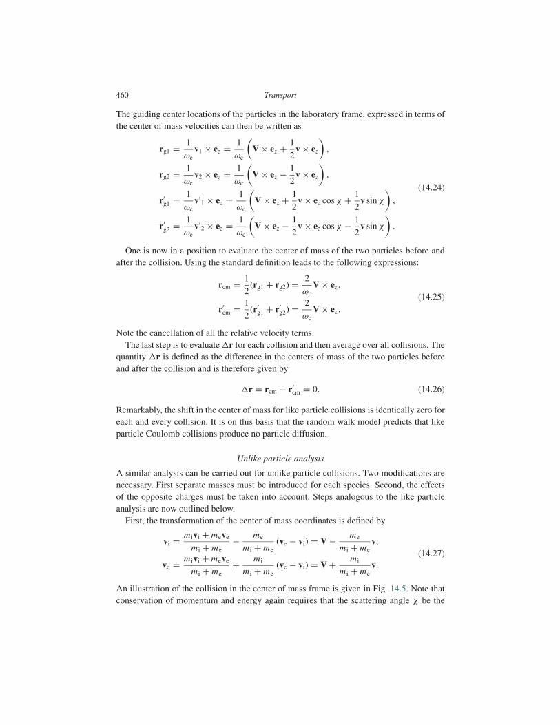
The guiding center locations of the particles in the laboratory frame, expressed in terms ofthe center of mass velocities can then be written as

rg1 = 1

ωcv1 × ez = 1

ωc

(V × ez + 1

2v × ez

),

rg2 = 1

ωcv2 × ez = 1

ωc

(V × ez − 1

2v × ez

),

(14.24)

r′g1 = 1

ωcv′

1 × ez = 1

ωc

(V × ez + 1

2v × ez cos χ + 1

2v sin χ

),

r′g2 = 1

ωcv′

2 × ez = 1

ωc

(V × ez − 1

2v × ez cos χ − 1

2v sin χ

).

One is now in a position to evaluate the center of mass of the two particles before andafter the collision. Using the standard definition leads to the following expressions:

rcm = 1

2(rg1 + rg2) = 2

ωcV × ez,

(14.25)r′

cm = 1

2(r′

g1 + r′g2) = 2

ωcV × ez .

Note the cancellation of all the relative velocity terms.The last step is to evaluate �r for each collision and then average over all collisions. The

quantity �r is defined as the difference in the centers of mass of the two particles beforeand after the collision and is therefore given by

�r = rcm − r′cm = 0. (14.26)

Remarkably, the shift in the center of mass for like particle collisions is identically zero foreach and every collision. It is on this basis that the random walk model predicts that likeparticle Coulomb collisions produce no particle diffusion.

Unlike particle analysis

A similar analysis can be carried out for unlike particle collisions. Two modifications arenecessary. First separate masses must be introduced for each species. Second, the effectsof the opposite charges must be taken into account. Steps analogous to the like particleanalysis are now outlined below.

First, the transformation of the center of mass coordinates is defined by

vi = m ivi + meve

m i + me− me

m i + me(ve − vi) = V − me

m i + mev,

(14.27)ve = m ivi + meve

m i + me+ m i

m i + me(ve − vi) = V + m i

m i + mev.

An illustration of the collision in the center of mass frame is given in Fig. 14.5. Note thatconservation of momentum and energy again requires that the scattering angle χ be the


By

x

i

cc

e

vme+mi

me

v'me+mi

mi

v'me+mi

me

vme+mi

mi

− −

Figure 14.5 Geometry of an electron–ion collision in the center of mass frame. Note the oppositedirection of rotation for the electron and ion.

same for both particles and that v′ = v. Therefore the particle velocities after the collisionare

v′i = V − me

m i + me(v cos χ + ez × v sin χ ) ,

(14.28)v′

e = V + m i

m i + me(v cos χ + ez × v sin χ ) .

The corresponding guiding center of mass locations can be written as

rgi = 1

ωci

(V × ez − me

m i + mev × ez

),

rge = − 1

ωce

(V × ez + m i

m i + mev × ez

),

(14.29)

r′gi = 1

ωci

[V × ez − me

m i + me(v × ez cos χ + v sin χ )

],

r′ge = − 1

ωce

[V × ez + m i

m i + me(v × ez cos χ + v sin χ )

].

Here ωc j = |e| B0/m j and the sign of the charges has been taken into account.One is again in a position to calculate �r as the difference in the centers of mass before

and after the collision:

�r = m irgi + merge

m i + me− m ir′

gi + mer′ge

m i + me. (14.30)

462 Transport

A short calculation yields

�r = − 1

ωcr[v × ez(1 − cos χ ) − v sin χ ] , (14.31)

where ωcr = eB0/mr and mr = mem i/ (m i + me) is the reduced mass. Observe that forunlike particle collisions �r does not vanish, even for equal masses. The non-vanishing isassociated with the opposite sign of the charges.

The last step in the analysis requires the averaging over all collisions and all scatteringangles assuming equal probabilities for all angles. Clearly the averaging over collisions (i.e.,the averaging over the initial angle ζ ) leads to the conclusion that 〈�r〉 = 0 as one wouldexpect. However, the step size for diffusion involves the mean square average defined by

(�l)2 = 1

4π2

∫ 2π

0dζ

∫ 2π

0dχ (�r)2 . (14.32)

A straightforward calculation yields

(�l)2 = 2v2

ω2cr

≈ 2v2

ω2ce

. (14.33)

The final form is obtained by noting that for Maxwellian distribution functions in velocityv = |ve − vi| ≈ |ve| ∼ (2Te/me)1/2 :

(�l)2 = 4meTe

e2 B20

. (14.34)

The particle diffusion coefficient Dn is now easily evaluated by recognizing that the meantime between collisions is just τ ei = (νei)−1, where νei is the momentum exchange collisionfrequency given by Eq. (9.110). One obtains

Dn = (�l)2

τ ei= 4

νeimeTe

e2 B20

∼ r2Le

τ ei. (14.35)

This is the desired result. The value of Dn by definition includes the effects of bothelectrons and ions so that both species diffuse at the same rate, a phenomenon known asambipolar diffusion. Physically the species must diffuse together since if one species weredepleted faster than the other a large charge imbalance would occur. This charge imbalancewould induce an electric field whose direction is such as to attract the species back to eachother causing them to leave at the same rate.

A further interesting point is that the value of Dn is smaller by a factor of (me/m i)1/2 thanthe original incorrect estimate Dn ∼ r2

Li/τii. Particle diffusion occurs on a slower time scale;that is, ions might originally be expected to diffuse faster because their larger gyro radiusproduces a larger step size after each collision. However, the fact that the center of mass inion–ion collisions is invariant before and after a collision negates this original expectation.


Comparison with the fluid model and numerical values

To test the validity of the random walk model it is useful to compare the value of Dn justcalculated in Eq. (14.35) with the value obtained from the fluid model and repeated herefor convenience

Dn = 2nT η⊥B2

0

. (14.36)

If one now recalls that η⊥ = meνei/ne2 it follows that the value of Dn for the fluid modelcan be written as

Dn = 2νeimeT

e2 B20

. (14.37)

The fluid model differs from the random walk model by an unimportant numerical factor of“2”. The implication is that the fluid model is self-consistent in that it automatically takesinto account the fact that particle diffusion is ambipolar.

Finally, it is useful as a point of reference to substitute numerical values into Dn so thatthe scaling with respect to density, temperature, and magnetic field becomes apparent. Anaccurate calculation, including kinetic effects, has been carried out in a classic paper byBraginskii. His result can be written as

Dn = 2.0 × 10−3 n20

B20 T 1/2

k

m2/ s. (14.38)

The fluid model value of Dn in Eq. (14.37) yields the same numerical coefficient as thatfound by Braginskii. Observe that Dn decreases with T (fewer collisions), increases with n(more collisions), and decreases with B (smaller gyro radius).

For the simple fusion reactor with Tk = 15, n20 = 1.5, B0 = 4.7, then Dn is 3.5 ×10−5 m2/ s. This value is enormously optimistic, by nearly five orders of magnitude, com-pared to typical experimentally measured values in a tokamak: Dn ∼ 1 m2/ s. Part of thedifference is associated with toroidal effects (neoclassical transport) but most is due toplasma-driven micro-turbulence. In any event, the calculation shows how to apply the ran-dom walk model and sets a reference value for purely classical transport in a straightcylinder.

14.2.4 Thermal conductivity of a magnetized plasma

The particle diffusion analysis just presented gives one confidence that the random walkmodel, despite its simplicity, is capable of reliably predicting transport coefficients. Thetask now is to utilize the random walk model to predict the thermal diffusivities, the lastremaining unknown transport coefficients required to close the set of self-consistent fluidequations. The same simple model will be used for thermal diffusion as for particle diffusion;that is, the step size is calculated for a 2-D collision model where particles make circulargyro orbits and scatter in random directions after each collision.

464 Transport

Based on the similarities with the previous analysis one might initially think that likeparticle collisions do not lead to thermal diffusion. The same cancellation in centers of masswill occur, implying no like particle thermal diffusion. This conclusion is also wrong!

The reason is as follows. The correct way to calculate particle diffusion is by definingthe step size in terms of the change in the two-particle center of mass before and afterthe collision. For thermal diffusion, however, one must define the step size in terms of thechange in the two-particle “center of energy” (i.e., the energy centroid) before and after thecollision. Thus, essentially all of the analysis for like particle diffusion is still valid, the onecritical difference being the definition of �r, which for thermal diffusion is defined by

�r = rcE − r′cE , (14.39)

where

rcE = v21rg1 + v2

2rg2

v21 + v2

2

,

(14.40)

r′cE = v′2

1 r′g1 + v′2

2 r′g2

v′21 + v′2

2

.

After a straightforward but slightly tedious calculation one can substitute for all quantitiesin (�l)2, expressed in terms of the center of mass velocity variables, and then carry out theaveraging over angles. One obtains

(�l)2 = 2v4V 2

ω2c (4V 2 + v2)2

. (14.41)

The last step is to average over v1, v2 or equivalently v, V . A reasonable estimate for theaverages is given by

v2 = v21 + v2

2 − 2v1 · v2 ∼ 2v2T ,

(14.42)

V 2 = 1

4(v2

1 + v22 + 2v1 · v2) ∼ v2

T

2,

where it is assumed that the v1 · v2 terms average to zero. This estimate yields the followingexpression for the mean square step size:

(�l)2 = 1

4

v2T

ω2c

. (14.43)

The thermal diffusivities can now easily be evaluated by noting that the mean time betweencollisions is τii = (νii)−1 for ions and τee = (νee)−1 for electrons. Since τ j j = τ j j (v) is afunction of velocity one can again approximately average over v by defining τ j j = τ j j (vT ).The random walk model thus predicts the following values for the ion and electron thermaldiffusivities:

χi = 1

4

v2Ti

ω2ciτ ii

∼ r2Li

τ ii,

(14.44)

χe = 1

4

v2T e

ω2ceτ ee

∼ r2Le

τ ee.

14.3 Solving the transport equations 465

Observe that the electron thermal diffusivity is comparable to the particle diffusioncoefficient: χe ∼ Dn . The ion thermal diffusivity is larger by the square root of the massratio: χi ∼ (m i/me)1/2 χe. It is shown in the next subsection that the single thermal diffusiv-ity appearing in the transport equations (Eqs. (14.10)) is actually given by χ = χi + χe ≈ χi.The remarkable cancellation that occurs in the value of �r for particle diffusion does notoccur for thermal diffusion. This is the underlying reason why collisional thermal diffusionis so much larger than particle diffusion.

The numerical values of the thermal diffusivities (for a 50%–50% D–T plasma), usingBraginskii’s more accurate coefficients are given by

χi = 0.10n20

B20 T 1/2

k

m2/ s,

(14.45)χe = 4.8 × 10−3 n20

B20 T 1/2

k

m2/ s.

For the dominant ion diffusivity the numerical coefficient is approximately a factor of 2.4larger than that obtained by the simple random walk model. Using parameter values forthe simple test reactor yields an ion thermal diffusivity χi = 1.8 × 10−3 m2/ s. This valueis also highly optimistic by about three orders of magnitude from typical experimentallymeasured values χi ∼ 1 m2/ s.

14.2.5 Summary

The formulation of classical transport in a 1-D cylinder is now complete. The model, whichmakes use of the tokamak expansion, is described by Eq. (14.10). It consists of a closed set ofcoupled time evolution equations for the density, temperature, and poloidal magnetic field.The particle and magnetic diffusion coefficients follow directly from the fluid equationsand result from electron–ion momentum exchange collisions. The expressions for Dn andDB are given by Eqs. (14.11). Heat transport is dominated by the ions. Here the dominantmechanism is ion–ion collisions. A simple estimate of χi is given by Eqs. (14.44) by meansof the random walk model. The predicted values of classical particle and heat transportare both highly optimistic with respect to typical experimentally measured values. Theynevertheless serve as a useful point of reference.

14.3 Solving the transport equations

The transport model just derived describes classical transport in a simplified 1-D cylinderin the context of the tokamak expansion. In this section several specific problems describedby the model are solved analytically. The purpose is two-fold. First, it is instructive to seein detail how to approach and cast each problem into a form amenable to solution. Manyof the same ideas apply to more general toroidal calculations where the solutions must beobtained numerically. Second, the problems addressed are those for which the answers arenot immediately obvious. For example, while it is obvious from dimensional analysis that

466 Transport

the characteristic relaxation time for any diffusive process scales as τ ≈ a2/D, there aremore subtle questions that often need to be answered.

In this section three such problems are discussed. The first problem corresponds totemperature equilibration. In all the analysis thus far presented it has been assumed that Te ≈Ti = T . The goal here is to derive a quantitative criterion for this condition to be satisfied.The answer is not immediately obvious because of the large difference in magnitudesbetween χe and χi.

The second problem is concerned with the effects that the external heating depositionprofile has on the central plasma temperature. For instance, does a highly peaked off-axisheating source lead to a temperature profile with a corresponding off-axis peak?

The third problem involves a solution of the steady state 1-D model assuming the heatingsource corresponds solely to ohmic heating. The issue here is to determine whether or not itis feasible to ohmically heat to ignition, thereby eliminating the need for external auxiliaryheating sources. This would clearly be a highly desirable situation.

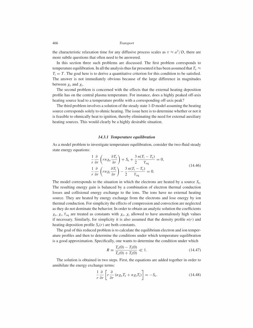
14.3.1 Temperature equilibration

As a model problem to investigate temperature equilibration, consider the two-fluid steadystate energy equations:

1

r

∂

∂r

(rnχe

∂Te

∂r

)+ Se + 3

2

n(Ti − Te)

τ eq= 0,

(14.46)1

r

∂

∂r

(rnχi

∂Ti

∂r

)− 3

2

n(Ti − Te)

τ eq= 0.

The model corresponds to the situation in which the electrons are heated by a source Se.The resulting energy gain is balanced by a combination of electron thermal conductionlosses and collisional energy exchange to the ions. The ions have no external heatingsource. They are heated by energy exchange from the electrons and lose energy by ionthermal conduction. For simplicity the effects of compression and convection are neglectedas they do not dominate the behavior. In order to obtain an analytic solution the coefficientsχe, χi, τ eq are treated as constants with χe, χi allowed to have anomalously high valuesif necessary. Similarly, for simplicity it is also assumed that the density profile n(r ) andheating deposition profile Se(r ) are both constants.

The goal of this reduced problem is to calculate the equilibrium electron and ion temper-ature profiles and then to determine the conditions under which temperature equilibrationis a good approximation. Specifically, one wants to determine the condition under which

R ≡ Te(0) − Ti(0)

Te(0) + Ti(0)� 1. (14.47)

The solution is obtained in two steps. First, the equations are added together in order toannihilate the energy exchange terms:

1

r

∂

∂r

[r

∂

∂r(nχeTe + nχiTi)

]= −Se. (14.48)


0 0.2 0.4 0.6 0.8 10

0.5

1

1.5

r/a

TT0 Ti

Te

Figure 14.6 Te and Ti vs. r/a for α = 10, χi/χe = 10.

For boundary conditions one requires regularity at the origin (T ′e (0) = T ′

i (0) = 0) and aperfect sink condition at r = a (Te (a) = Ti (a) = 0). The solution to Eq. (14.48) is easilyfound and is

n (χeTe + χiTi) = Se

4(a2 − r2). (14.49)

The second step is to solve for Te and substitute the solution into the ion equation. Ashort calculation yields

1

x

∂

∂x

(x∂Ti

∂x

)− α2Ti = α2T0(1 − x2), (14.50)

where x = r/a and

α2 = 3

2

(χe + χi

χeχi

)a2

τ eq,

(14.51)

T0 = 1

4

Sea2

n(χe + χi).

The solution for Ti (and then Te) satisfying the boundary conditions can be written in termsof modified Bessel functions as follows:

Ti

T0= 1 − x2 − 4

α2

[1 − I0(αx)

I0(α)

],

(14.52)Te

T0= 1 − x2 + 4

α2

χi

χe

[1 − I0(αx)

I0(α)

].

These profiles are illustrated in Fig. 14.6 for the case χi/χe = 10 and α = 10.

468 Transport

Table 14.1. Relationship between α2 and χi/χe to insure that R � 1

Regime of χi/χe R = R(F) R = R(α, χi/χe) Condition for R � 1

χi/χe 1 R ≈ F

F + 2χe/χiR ≈ 4

4 + 2α2χe/χiα2 2χi/χe

χi/χe = 1 R = F R ≈ 4

4 + α2α2 4

χi/χe � 1 R ≈ F

2 − FR ≈ 2

2 + α2α2 2

One is now in a position to calculate the equilibration parameter R. Substituting intoEq. (14.47) yields

R(α, χi/χe) = (χi/χe + 1) F (α)

2 + (χi/χe − 1)F(α), (14.53)

where

F(α) = 4

α2

[1 − 1

I0 (α)

]≈ 4

4 + α2. (14.54)

The last form is an approximation that matches the behavior at both small and large α. Notethat F(α) is a decreasing function and that F � 1 when α 2.

The condition for good equilibration can be determined by examining Eq. (14.53) fordifferent values of the ratio χi/χe. Specifically the condition R � 1 sets a requirement onα2 as shown in Table 14.1. From Table 14.1 it follows that a simple form for the conditionon α2, valid for all values of χi/χe, can be written as

α2 2χi + χe

χe. (14.55)

In unnormalized units, Eq. (14.55) reduces to

τ eq � 3

4

a2

χi. (14.56)

Physically, good temperature equilibration occurs if the equilibration time τ eq is muchshorter than the ion energy confinement time a2/χi. The electron energy confinement timea2/χe has a strong influence on the final central temperature. However, regardless of thecentral temperature, the electrons and ions will equilibrate as long as the ions do not losethe energy transferred from the electrons too rapidly by ion thermal conduction.

One can now ask whether or not Eq. (14.56) is satisfied in most plasma experiments. Theanswer for classical diffusion is obtained by noting that τ eq ∼ (m i/me) τ ei, χi ∼ r2

Li/τ ii,and τ ii ∼ (m i/me)1/2 τ ei. The equilibration condition reduces to

a2

r2Li

(

m i

me

)1/2

, (14.57)


which is easily satisfied in most experiments. However, when χi is anomalous, the conditionis more difficult to satisfy. In this case, using the numerical value of τ eq from Eq. (9.119),one can rewrite the equilibration condition in the following form:

n20 0.017T 3/2

k χi

a2= 0.25χi, (14.58)

where the last value corresponds to the simple fusion reactor (a = 2, Tk = 15). For thereactor, the value n20 = 1.5 is sufficiently large that the condition would be reasonablywell satisfied assuming that χi ∼ 1 m2/s, a typical experimental value in present toka-maks. Interestingly, most present tokamaks usually operate at somewhat lower densities(n20 ∼ 0.5) so that the equilibration condition is only marginally satisfied.

The final point to discuss is the derivation of a single energy equation in the limit wherethere is good equilibration. Mathematically, good equilibration implies that τ eq → 0 andTi → Te. The energy equilibration term in each equation therefore becomes indeterminate((Te − Ti) /τ eq → 0/0). The difficulty is resolved by adding the energy equations togetherto exactly annihilate the equilibration terms and to then set Te = Ti = T . This leads to asingle energy equation given by

1

r

∂

∂r

[rn(χe + χi)

∂T

∂r

]+ Se = 0. (14.59)

One sees that the final equation balances heat conduction losses against the heating sourceterm. The thermal diffusivity is just the sum of the separate components (χ = χe + χi ≈ χi)and is dominated by the largest contribution, usually due to the ions.

The analysis just presented provides a good justification for considering a single energyequation when investigating the performance of fusion grade plasmas.

14.3.2 Effect of the heating profile on the central temperature

Next, the effect of the external source heating profile on the peak temperature and temper-ature profile is investigated. Of particular interest is the question of whether or not a highlylocalized off-axis heating source results in a corresponding peaked off-axis temperatureprofile. To answer this question two simple problems are considered. First the temperatureprofile is calculated for a heating source that is uniform in space. Second, the calculation isrepeated assuming the same amount of total power is deposited off-axis in a highly local-ized region of space, modeled mathematically by a delta function. A comparison of the twosolutions provides the answer to the question.

As a simple model consider a well-equilibrated plasma described by the following steadystate energy equation:

1

r

∂

∂r

(rnχ

∂T

∂r

)= −S(r ). (14.60)

As in the previous equilibration problem convection and compression are neglected and n,χ are assumed to be constants.

470 Transport

First, assume that a total power Ph is absorbed uniformly over the plasma crosssection. If the volume of the plasma is denoted by V = 2π2a2 R0, then for this caseS(r ) = Ph/2π2a2 R0 = const. The boundary conditions again require regularity at the ori-gin and a perfect heat sink at r = a : T ′(0) = 0 and T (a) = 0. The solution to the transportequation is easily found and is given by

T = T0

(1 − r2

a2

), (14.61)

where

T0 = Ph

8π2nχ R0. (14.62)

Observe that the temperature profile decreases parabolically with radius. It is also ofinterest to evaluate the peaking factor, defined as the ratio of the peak temperature T0 to theaverage temperature T . Here,

T = 2

a2

∫ a

0T (r )r d r . (14.63)

For the case of a constant heating profile the peaking factor has the value

T0/T = 2. (14.64)

The calculation just presented serves as the reference case. The next step is to redo thecalculation assuming a highly localized off-axis source, modeled by a delta function asfollows:

S(r ) = K δ(r − αa) = Ph

4π2 R0aαδ(r − αa). (14.65)

Note that the heating source peaks at r = αa with 0 < α < 1. Also, the coefficient multi-plying the delta function has been chosen so that the total power absorbed by the plasma isagain equal to Ph.

The temperature is found by solving separately in the regions on either side of the deltafunction and then matching across the surface r = αa. For 0 ≤ r ≤ αa− the solution thatis regular at the origin is given by

T = C1, (14.66)

where C1 is an as yet undetermined coefficient. For αa+ ≤ r ≤ a the solution satisfyingthe sink condition at r = a can be written as

T = C2 ln (a/r ) . (14.67)

Here, C2 is also an undetermined coefficient.Next, there are two matching conditions across r = αa that must be satisfied. First, the

temperature must be continuous, implying that C2 ln (1/α) = C1. Second, integrating across


0 0.2 0.4 0.6 0.8 10

0.5

1

1.5

r/a

TT0

Peakedsource

Uniform source

1.38

Figure 14.7 Temperature profiles for a uniform and a peaked heating source.

the delta function yields a jump condition on the heat fluxes which is given by

[[rnχ∂T /∂r ]]αa+αa− = −

∫ αa+

αa−K δ (r − αa) r d r = −Ph/4π2 R0. (14.68)

Using the profiles in each region one can easily evaluate the temperature derivatives leadingto

C1 = Ph ln (1/α)

4π2nχ R0= 2T0 ln (1/α) , (14.69)

where T0 has been defined in Eq. (14.62).The resulting temperature profiles are thus given by

T = 2T0 ln (1/α) 0 ≤ r ≤ αa−,(14.70)

T = 2T0 ln (a/r ) αa+ ≤ r ≤ a.

The solution is plotted in Fig. 14.7 for the case of α = 0.5. Observe that even with a verypeaked heating profile the temperature itself does not peak. Physically, the reason is asfollows. Initially, the heating profile does indeed produce a peaked off-axis temperatureprofile. The heat then starts to diffuse in both directions away from the source. At theedge of the plasma the heat energy is absorbed because of the sink boundary condition. Inthe center, however, there is no sink, and the heat accumulates. In steady state a balanceis reached where there is no net flow of energy in either direction in the central region,corresponding to a uniform temperature.

472 Transport

0 0.2 0.4 0.6 0.8 10

1

2

3

4

5

T(0)

T

Peaked source

Uniform source

a

Figure 14.8 Peaking factor vs. normalized localization radius.

The last point of interest is to compare the temperature peaking factor between the twocases. For the localized heating source the peaking factor is easily evaluated, and can beexpressed as

T (0)

T= 2 ln(1/α)

1 − α2. (14.71)

The results are plotted in Fig. 14.8 as a function of α. Note that the difference in peakingfactors between the two cases is relatively modest in comparison to the dramatically differentheating profiles.

The main conclusion from this problem is that while the average plasma temperaturedepends directly upon the total heating power supplied (i.e., T ∼ Ph), the actual temperatureprofile is relatively insensitive to the heating profile (except for the special limit α → 0).

14.3.3 Ohmic heating to ignition

The last problem discussed raises the question of whether or not it is possible to ohmicallyheat a plasma to ignition without the need of external power sources. This would presumablybe highly desirable from a fusion engineering point of view. The problem is addressed inthe present subsection within the context of classical transport, which is highly optimisticcompared to actual experimental performance. Even so, this serves as a good point ofreference and demonstrates the process of formulating and finding an approximate solutionto the transport equations.


The goal of the calculation is to determine how much ohmic power is required to heata plasma to a temperature of 7 keV, which is about half way to ignition. The calcula-tion neglects alpha particle heating, which is a good approximation for low temperatures,although once the 7 keV point is reached, the alpha particle heating takes over and thenthe ohmic power can be neglected. The ohmic solution also allows one to calculate otherplasma parameters, including the plasma current I , the plasma pressure p, the plasma betaβ, the safety factor q , and the energy confinement time τE, to make sure these values arecompatible with engineering and plasma physics constraints. The analysis shows that ohmicheating to ignition is possible under the assumption of classical transport, although furtherthought reveals that this is a mixed blessing.

The model

The ohmic heating model represents a subset of the complete 1-D cylindrical transportequations derived in the previous section. For simplicity one again assumes steady stateand neglects compression and convection. Furthermore, to eliminate the need for solvinga set of coupled differential equations the density is assumed to be uniform: n = const.This experimentally plausible assumption simplifies the analysis by removing the densityequation from the calculation.2 The ohmic heating model reduces to

r∂

∂r

(DB

r

∂r Bθ

∂r

)= 0,

1

r

∂

∂r

(rnχ

∂T

∂r

)+ η‖ J 2 = 0, (14.72)

μ0 J = 1

r

∂r Bθ

∂r.

Note that the heating source corresponds to ohmic power dissipation.The task now is to simplify these equations in order to obtain a single, second order,

differential equation for the temperature. The first step is to integrate the magnetic fieldequation, recalling that DB = η‖/μ0 ∼ 1/T 3/2. This yields

DB J = const. (14.73)

or

J = Kμ0

η‖= J0

(T

T0

)3/2

. (14.74)

Here, J0, T0 are constants representing the on-axis values. They are presently unknownbut will ultimately be related to the plasma current I and the desired average temperatureT k = 7 keV.

2 The density can be included by a more complicated analysis, although considerable care must be taken with the boundarycondition and/or the introduction of more realistic modifications to the physical model in the region near r = a. This is becauseindeterminate ratios appear in χ when the ideal sink boundary condition is used.

474 Transport

The next step is to substitute the expression for J into the energy equation using the clas-sical value of χ ≈ χi given by Eqs. (14.45). A short calculation leads to a single differentialequation for the normalized temperature U = T/T0. This equation can be written as

1

x

∂

∂x

(x

U 1/2

∂U

∂x

)+ 2α U 3/2 = 0, (14.75)

where x = r/a and α is a dimensionless parameter defined (in practical units) by

α = 10.3

(B0 JM0a

n20Tk0

)2

. (14.76)

Here, Tk0 = T0 (keV) and JM0 = J0 (MA/m2).The last step in the simplification of the model is to introduce a new dependent variable

V = U 1/2. Equation (14.75) reduces to

1

x

∂

∂x

(x∂V

∂x

)+ α V 3 = 0. (14.77)

The boundary conditions again require regularity at the origin and a sink condition at theplasma edge: V ′(0) = 0, V (1) = 0. The normalizing condition V (0) = 1 is an additionalconstraint which can only be satisfied by choosing an appropriate value for α. In fact, the nextstep in the analysis is to determine an approximate solution for V (x) and the correspondingvalue for α. Once V (x) and α are known all the desired physical properties of the ohmicallyheated plasma can easily be evaluated.

Approximate solution to the problem

Equation (14.77) is a non-linear differential equation for which there is no simple closedform solution. While it can easily be solved numerically, this is not optimal in terms ofdeveloping physical insight. A different approach is used here to obtain an approximateform of the solution. The method is based on two points of mathematical insight. First, thesolution for V (x) is qualitatively simple. It starts out with a value of unity at the origin andthen monotonically decreases to zero at the edge of the plasma. Second, all the physicalquantities are calculated by integrating various functions of V (x) over the plasma volume.Since integrated values are involved, the results are not very sensitive to the precise detailsof the V (x) profile.

This mathematical insight suggests that a moment approach would be sufficiently accuratefor present purposes. Specifically, the approximation is made that the V (x) profile is of theform

V (x) = (1 − x2)ν, (14.78)

where ν is an as yet undetermined parameter. Clearly, V (x) has the correct qualitativebehavior of the exact solution.


The values of ν and α are determined by requiring that two low-order moments of thedifferential equation be exactly satisfied. These moments are defined by∫ 1

0V

[1

x

∂

∂x

(x∂V

∂x

)+ α V 3

]xd x = 0,

(14.79)∫ 1

0x2V

[1

x

∂

∂x

(x∂V

∂x

)+ α V 3

]xd x = 0.

Although the choice of which moment equations to use is clearly not unique, using low-ordermoments captures the main macroscopic features of the exact solution.

Substituting the approximate V (x) into Eqs. (14.79) leads to two coupled algebraicequations for the unknowns ν and α. The details are straightforward but slightly lengthy.Once obtained, the resulting algebraic equations can easily be solved analytically yieldingthe values

ν = 2, α = 12. (14.80)

These values are used next to derive the desired physical properties of the ohmically heatedplasma.

Physical properties of the solution

First, the approximate temperature profile is considered. From the value ν = 2 and therelation U = V 2 it follows that

Tk(r ) = Tk0(1 − r2/a2)4. (14.81)

Note that this is a highly peaked profile, a consequence of the fact that near the edge of theplasma χ ∼ T −1/2 → ∞. A high thermal diffusivity tends to flatten the temperature profileat the edge, thus making the central profile more peaked. A measure of the peaking is givenby the peaking factor, which is the ratio of the peak to average temperature, determined asfollows:

T k = 2∫ 1

0Tkxd x = Tk0/5. (14.82)

Thus the peaking factor is Tk0/T k = 5. For future numerical values T k is set to T k = 7 keV,the target temperature for ohmic heating to ignition.

Second, the current density profile is examined. This is slightly more peaked than thetemperature profile:

JM(r ) = JM0(1 − r2/a2)6. (14.83)

The constant JM0 can be expressed in terms of the total plasma current from the definition

IM = 2πa2∫ 1

0JMxd x = πa2 JM0/7. (14.84)

Thus, JM0 = 7IM/πa2.

476 Transport

These results, combined with the value α = 12 lead to a relationship between the requiredplasma current and the desired ohmic heating temperature which can be written as

IM =( α

2.05

)1/2 an20T k

B0= 2.4

an20T k

B0= 10.7 MA. (14.85)

Note that the current scales linearly with the temperature for classical transport. The finalnumerical value corresponds to the simple reactor design parameters: n20 = 1.5, a =2, R0 = 5, B0 = 4.7. One can now ask whether the resulting value of q∗ is high enoughto suppress MHD instabilities. The value of q∗ (assuming an elongation κ = 2) is

q∗ = 2πa2κ B0

μ0 R0 I= 5

a2κ B0

R0 IM= 3.5. (14.86)

This value is safely above the limit for exciting ballooning-kink modes. In other words theohmic current required to reach a temperature of 7 keV in a tokamak with classical transportis well below the instability threshold, indeed a favorable conclusion.

Consider next the pressure and β. Their average values are easily calculated as follows:

p = 2nT = 0.32n20T k = 3.4 atm,(14.87)

β = 2μ0 p/B20 = 0.25pa/B2

0 = 0.038.

These are just the values that one would expect at 7 keV, about one half the way to asteady state fully ignited plasma at 15 keV. Here too, the β is below the threshold for MHDinstability.

One is now in a position to calculate the total ohmic power required to reach 7 keV andcompare it with the nominal electric power out of the reactor, 1000 MW. The ohmic poweris defined as

P� =∫

η‖ J 2dr. (14.88)

A short calculation using the relation η‖ = 3.3 × 10−8/T 3/2k � m leads to

P� = 4.1 × 10−2 R0 I 2M

a2T3/2k

= 0.32 MW. (14.89)

The ohmic power required is very modest compared to the electric power output. This is aconsequence of the good confinement associated with classical transport. If the plasma isgood at confining its thermal energy (i.e., χ is small), then only a small amount of ohmicpower is required to heat the plasma to a high temperature. Clearly the low requirement onP� is a very favorable result.

The last parameter of interest, which quantifies “good confinement,” is the energy con-finement time. The quantity τE is defined by integrating the starting energy balance equation(Eq. (14.72)) over the plasma volume:

P� = −4π2 R0anχ∂T

∂r

∣∣∣∣a

≡ 3

2

∫p dr

τE. (14.90)


Observe that the energy confinement time is defined in terms of the heat flux at the plasmaedge. If one knew the exact solution for the profiles, a simple evaluation of the edge derivativewould yield the desired value of τE. However, with the approximate profiles used in thecalculation this is a very poor way to evaluate τE, leading in fact to the result τE = ∞.A much better way to use the approximate equilibrium solution is through less sensitiveintegral relations. A good estimate of the energy confinement time is thus obtained fromEq. (14.90) as follows:

τE = 3

2

pV

P�

= 23a4n20T

5/2k

I 2M

= 6.3 × 102 s. (14.91)

Classical confinement predicts an energy confinement time of over 600 s, which is veryoptimistic compared to present day experiments.

Finally, in practice τE is often used to predict the temperature of an experiment once thedensity, current, toroidal field, and geometry are specified. For this alternative applicationof transport theory, the temperature should be eliminated from τE, in the present case bymeans of Eq. (14.85), leading to an expression solely in terms of parameters directly underexperimental control. For classical confinement the new form of τE can be written as

τE = 2.6a3/2 B5/2

0 I 1/2M

n3/220

s. (14.92)

This form of the energy confinement time will be useful when comparing with the actualempirical value determined from experimental measurements.

Irony – too much confinement can be a disadvantage

The analysis thus far seems to indicate that the combination of classical confinement andohmic heating would be highly desirable in a fusion reactor. However, further thought showsthat too much confinement is actually a disadvantage.

There are several ways to understand the issues. The basic problem arises from thefact that too much confinement leads to very high values of pτE. For the case of classicalconfinement described above, the value of pτE at 7 keV is 2.1 × 103 atm s. This is more thana factor of 200 larger than that required to maintain the plasma in steady state equilibriumcharacterized by alpha power balancing thermal conduction losses. Specifically, the alphaparticles are producing much more heat than is lost by thermal conduction. Should thissituation arise, the plasma would continue to heat to much higher temperatures therebyincreasing the plasma pressure and power density. Very quickly the critical plasma β forstability as well as the maximum allowable neutron wall loading would be violated.

Another approach might be to lower the number density such that pτE is reduced to thevalue necessary for steady state ignition: pτE ≈ 8.3 atm s. The difficulty with this strategyis that the lower number density corresponds to a lower pressure, which in turns leads to alower power density. When the power density is greatly reduced a much larger volume ofplasma is required to produce the same total required power output. A larger reactor leadsto a higher capital cost per watt which is clearly undesirable.

478 Transport

Yet another idea is to use good confinement to reduce the size of the plasma. SinceτE ∼ a2/χ one can reduce the size of the plasma until τE becomes short enough that steadystate power balance is achieved. However, if the pressure and corresponding power densityremain unchanged (i.e., p ∼ 7 atm), then the total power output is reduced because of thesmaller plasma volume. Even so, the reactor volume remains large since the blanket-and-shield thickness must still be b = 1.2 m, a value determined by nuclear physics, not plasmaphysics. The net result is an inefficient use of the blanket-and-shield which raises the capitalcost per watt. Raising the plasma pressure also does not help as this again increases β abovethe MHD stability limit and causes the neutron flux to exceed the wall loading limit.

The one exception to these arguments involves the use of advanced fuels such as D–D.Here, the fusion cross section is much smaller than for D–T implying that a much largervalue of pτE is required for plasma ignition.

In any event, the discussion suggests that there is no clear way to exploit the achieve-ment of a very long energy confinement time in a D–T fusion reactor. While this is a validconclusion one should remember that a large part of current fusion research is aimed atimproving energy confinement. There is no contradiction here since the present experimen-tally achievable energy confinement times are still somewhat below that which is requiredin a reactor. However, once the reactor relevant energy confinement time is achieved thereis little reason for further substantial enhancements in τE.

14.3.4 Summary

Several energy diffusion problems have been solved for the 1-D cylindrical model withinthe context of classical transport. These include the problems of temperature equilibration,heating profile effects, and the question of ohmically heating to ignition. All the problems arefocused on the energy transport equation as energy losses are the dominant loss mechanismin fusion grade plasmas.

It has been shown that: (1) energy equilibration requires that the ion energy confinementtime be long compared to the energy equilibration time; (2) the temperature profile is onlyweakly dependent on the heating profile; and (3) one can easily ohmically heat to ignitionwith classical transport, although too much confinement is actually a disadvantage from thereactor point of view.

The idealized classical transport model is highly optimistic with respect to experimentalvalues of χi but nonetheless serves as a useful point of reference. In the following sectionsmore realism is added to the models to bring the theory and experimental data into closeragreement.

14.4 Neoclassical transport

14.4.1 Introduction

Neoclassical transport is classical transport including the effects of toroidal geometry. Thetransport is still driven purely by Coulomb collisions – no anomalous transport due to

14.4 Neoclassical transport 479

plasma microscopic instabilities is included. The development of neoclassical transporttheory follows from a beautiful and sophisticated analysis of plasma kinetic theory. The finalmodel is quite complete. It contains a two-fluid description including resistivity, viscosity,and thermal conduction. The model is also valid for arbitrary regimes of collisionality.

This section contains a derivation of several of the key features of neoclassical transportmost relevant to a fusion reactor. These include the particle and thermal diffusion coefficientsand the generation of the bootstrap current. The analysis avoids the need to solve complexkinetic equations by instead making use of guiding center theory and the random walk model.Also, use is made of the large aspect ratio, circular cross section, and low collisionalityapproximations.

At first glance one might expect that in the large aspect ratio limit, toroidal effects simplyproduce uninteresting r/R0 corrections to the cylindrical results. This is an incorrect con-clusion. Perhaps surprisingly, neoclassical effects actually produce increases in the plasmatransport coefficients by nearly two orders of magnitude. Qualitatively, the reason is as fol-lows. In a cylindrical system particles are confined to within a gyro radius of a flux surface.Consequently, the corresponding step size associated with Coulomb collisions is also onthe order of a gyro radius. In a torus, however, particles drift off the flux surface because ofthe toroidally induced ∇ B and curvature drifts. The radial excursions due to these drifts canbe much larger than a gyro radius, leading to an increase in the collisional step size, and acorresponding increase in the transport coefficients. A further surprise is that the transportthat arises from the small population of trapped particles actually dominates the transportresulting from the majority of passing (i.e., untrapped) particles.

The discussion below presents a random walk derivation of particle and heat transport,first due to passing particles and then due to trapped particles. Lastly a derivation is presentedof the very important bootstrap current which has no simple analog in a cylindrical system.This current, which is essential to minimize the current drive requirements in a tokamak, isclosely related to the magnetization current discussed in Chapter 11.

14.4.2 Neoclassical transport due to passing particles

The neoclassical transport associated with passing particles in a toroidal geometry is calcu-lated by means of the random walk model. The critical task is to evaluate the average stepsize associated with the guiding center drifts off the flux surface.

Towards this goal consider a large aspect ratio, circular cross section tokamak as shownin Fig. 14.9, which depicts a flux surface and the guiding center orbits of two typical passingparticles. Recall that in a tokamak B ≈ Bφ(R), implying that the ∇ B and curvature driftsare in the eZ direction; that is, the guiding center drift for an ion is always in the positive,upward direction. Now, note that if the pitch angle of the magnetic field is for instancepositive, a particle with a positive v‖ starting out at θ = 0 traces out a circular-like orbit,whose radius is slightly larger than the radius of its starting flux surface. Similarly, in thissame magnetic field, a particle with a negative v‖ traces out a slightly smaller circle. As anaside, note that these results, including closure of the orbit, can be derived rigorously usingthe conservation of canonical toroidal momentum.

480 Transport

Flux surface v|| < 0v

|| > 0

R

Z

Figure 14.9 Poloidal projections of the guiding center orbits for two passing particles, one withv‖ > 0, the other with v‖ < 0.

In terms of transport, if a particle undergoes a 90◦ momentum collision changingv‖ → −v‖, then its orbit jumps from one flux surface to another. The average radii of thesesurfaces differ by an amount comparable to radial excursion off the surface: �r = ri − rf.Clearly �r represents the appropriate step size for radial transport in a toroidal geometry.

The value of (�l)2 = 〈(�r )2〉 is calculated by the following steps. First, one needs todetermine the time τ1/2 it takes for a particle to complete a half-transit around the poloidalcross section. Second, during τ1/2 the particle drifts off the surface with a guiding centerdrift velocity vD due to the ∇ B and curvature drifts. The corresponding radial excursion isthen of the order �r ∼ vDτ1/2. Third, the desired step size is then calculated by averagingover all collisions. The details of the calculation are given below.

The half-transit time

The time it takes a particle to make a half-transit is given by τ1/2 = l/v‖, where l is the totalparallel distance traveled by the particle as it covers a poloidal distance lp = πr . For a largeaspect ratio tokamak

dl/B ≈ dl/B0 ≈ dlp/Bθ . (14.93)

Therefore,

l(r ) ≈ B0

Bθ (r )lp = B0

Bθ (r )πr = π R0q(r ). (14.94)

The corresponding half-transit time is then given by

τ1/2(r ) = l/v‖ = π R0q/v‖. (14.95)


The radial excursion

The next step is to calculate the particle excursion off the flux surface. To begin, note that thecombined ∇ B and curvature drifts in the dominant toroidal magnetic field of the tokamak,which is nearly a vacuum field, can be written as

vD = m i

e

(v2

‖ + v2⊥2

)Rc × B

R2c B

≈ 1

ωci R0

(v2

‖ + v2⊥2

)(er sin θ + eθ cos θ ) . (14.96)

For simplicity the particle under consideration is a positive ion. The trajectory of the particle,assuming it starts at some arbitrary initial angle θ = θ0 (i.e., it does not have to start atθ = 0), is given by θ (t) = ωTt + θ0, where ωT = π/τ1/2 is the full-transit frequency. Thecorresponding component of radial velocity thus has the form

vDr (t) ≈ |vDr| sin (ωTt + θ0) , (14.97)

where

|vDr| = 1

ωci R0

(v2

‖ + v2⊥2

). (14.98)

As expected, the velocity oscillates in sign, half the time moving towards the plasma axisand half the time moving away.

The radial position of the guiding center is now easily obtained by integrating r = vDr,assuming the particle starts off at a radius r = r0. Under the assumption that v‖ and v⊥ donot change very much during the orbit of a passing particle one obtains

r (t) ≈ r0 − |vDr|ωT

[cos(ωT t + θ0) − cos(θ0)] . (14.99)

Equation (14.99) shows that the radial position of the particle oscillates in time about amean value, corresponding to the radius of the flux surface ri to which the particle’s averageguiding center is attached. This radius is clearly given by

ri = r0 + |vDr|ωT

cos (θ0) . (14.100)

The step size

The step size can finally be calculated by assuming that the actual Coulomb collision takesplace at the point r = r0, θ = θ0. For simplicity assume the particle undergoes a typicalmomentum collision that scatters its velocity from an initial value vi = v‖b + v⊥ to a finalvalue vf = −v‖b + v⊥. In other words the collision reverses the sign of v‖. Since v‖ ∼|v⊥| for a passing particle, this corresponds to a 90◦ momentum collision as illustrated inFig. 14.10.

The radius of the final flux surface is easily obtained by setting v‖ → −v‖ in Eq. (14.100),which is equivalent to setting ωT → −ωT. This yields

rf = r0 − |vDr|ωT

cos(θ0). (14.101)

482 Transport

90° collision

−

v||

Passing particles

Trapped particles

v⊥

v|| v

||

Figure 14.10 Velocity space showing a typical particle with v‖ ∼ v⊥ undergoing a 90◦ collisionreversing the sign of v‖.

The step size �r is defined as the difference in radii of the flux surfaces before and afterthe collision:

�r = ri − rf = 2|vDr|ωT

cos θ0. (14.102)

One next has to average over all collisions, which is equivalent to averaging over all (equallylikely) starting positions θ0 and velocities. As expected 〈�r〉 = 0 when averaging over v‖because of the odd symmetry in ωT. However, the mean square step size is not zero and isgiven by

(�l)2 = 〈(�r )2〉 = 4|vDr|2ω2

T

〈cos2 θ0〉 = 2|vDr|2ω2

T

. (14.103)

Substituting for vDr and ωT leads to

(�l)2 = 2q2

ω2ci

(v2‖ + v2

⊥/2)2

v2‖

≈ 4q2v2

T i

ω2ci

∼ q2r2Li, (14.104)

where the average over velocities has been taken by approximating v2⊥/2 ≈ v2

‖ ∼ v2T i/2.

Note that the mean square step size is a factor q2 larger than for classical transport. Asimilar expression holds for electrons.

The transport coefficients

The transport coefficients in the random walk model are given by (�l)2 /τ , where τ is themean time between collisions. For passing particles τ corresponds to the 90◦ momentum


collision time. Consider first particle diffusion. As in the case of classical diffusion, amore detailed derivation of the step size shows that ambipolarity still holds. Like particlecollisions do not produce density diffusion in neoclassical theory. Particle diffusion resultsfrom electron–ion momentum exchange collisions. The random walk neoclassical particlediffusion coefficient due to passing particles is thus given by

D(NC)n = (�l)2

e

τ ei= 4q2

(2meTe

e2 B20τ ei

)= 4q2 D(CL)

n . (14.105)

Note that the neoclassical coefficient is a factor 4q2 ∼ 30 larger than the classical value.A similar conclusion holds for the thermal diffusivities which are again driven by like

particle collisions:

χ (NC)e ∼ q2χ (CL)

e ∼ q2 r2Le

τ ee,

(14.106)

χ(NC)i ∼ q2χ

(CL)i ∼ q2 r2

Li

τ ii.

Numerical values indicate that the ion thermal diffusivity due to passing particles is approx-imately equal to χ

(NC)i ≈ 1.6 × 10−2 m2/ s, which is still a factor of about 60 smaller than

that observed in experiments. However, the transport due to passing particles is not thedominant loss mechanism in toroidal geometry. It is instead the transport that arises fromthe small population of trapped particles that dominates particle and heat loss and this isthe next topic.

14.4.3 Neoclassical transport due to trapped particles

The neoclassical losses resulting from trapped particles are also calculated using the randomwalk model. Before proceeding with the analysis one can ask why there are trapped particlesand why should their neoclassical losses dominate Coulomb transport? Qualitatively, theanswers are as follows. Trapped particles exist because B ≈ Bφ ≈ B0 (R0/R) in a tokamak.Thus the magnetic field strength is weak on the outside of the torus and strong on the inside.Therefore, particles starting on the outside of the torus with a small ratio of v‖/v⊥ are mirrorreflected as their parallel motion winds them towards the inside of the torus into a regionof higher field. The particles are “trapped” on the outside of the torus.

There are several reasons why trapped particle transport is large. One main reason resultsfrom the fact that their parallel velocity is small. It takes a longer time for a trapped particleto complete one full cycle of its mirror motion than for a typical passing particle to makeone full transit around the poloidal cross section. Since the trapped particle mirror period islonger, there is more time for particles to drift off the flux surfaces because of the ∇ B andcurvature drifts and this increases the step size.

The analysis of trapped particle transport is similar to that for the passing particlesalthough three modifications must be made in the random walk model. First, only a smallfraction of the plasma particles is trapped (in the large aspect ratio limit) and one needs to

484 Transport

Z

R

Bmin

Flux surface

Trapped orbit

Bmax

R

Bmax =R0 − rB0 R0

Bmin =R0 + rB0 R0

Bf

Figure 14.11 Geometry showing a trapped particle orbit and the maximum and minimum B ≈ Bφ ≈B0(R0/R).

know this fraction. Second, the radial step size must be recalculated taking into accountthe typical ratio of v‖/v⊥ for trapped particles. Third, the mean time between collisions ismodified because trapped particles have to scatter over a smaller angle (much less than 90◦)in order to move “one step.” The details of the analysis are described below.

The fraction of trapped particles

The fraction of trapped particles can easily be calculated by examining Fig. 14.11. One seesthat the minimum (at the outside) and maximum (at the inside) magnetic field strengths aregiven by

Bmin = B0R0

R0 + r,

(14.107)Bmax = B0

R0

R0 − r.

Consider now a particle starting off on the outside of the torus (θ = 0) with a velocityv = v‖b + v⊥. Using the conservation of energy and magnetic moment as discussed inChapter 8, it follows that the condition for particles to be trapped can be written as

v2‖

v2< 1 − Bmin

Bmax= 1 − R0 − r

R0 + r≈ 2

r

R0, (14.108)

where v2 = v2‖ + v2

⊥ and the last form follows from the large aspect ratio assumptionr/R0 � 1.

The boundary between trapped and untrapped particles is shown in velocity phase spacein Fig. 14.12. Note that the critical angle θc is defined by cos θc = v‖/v ≈ (2r/R0)1/2. The


Trapped particles

Moderately trapped particle before collision

Moderately trapped particle after collision

Collision

v||

qcp - qc

v^

( - qc)12

p2( - qc)1

2p2

Figure 14.12 Velocity space showing the trapped–untrapped boundary and a moderately trappedparticle undergoing a collision that reverses the sign of v‖.

fraction f of trapped particles can now be calculated by integrating over the trapped portionof the distribution function. For a Maxwellian distribution function FM(v) one finds

f = 1

n

∫ π−θc

θc

sin θ dθ

∫ 2π

0dφ

∫ ∞

0FM(v)v2 dv = cos θc ≈

(2r

R0

)1/2

. (14.109)

In terms of the inverse aspect ratio ε = a/R0, Eq. (14.109) implies that f ∼ ε1/2. In thelimit of large aspect ratio only a small fraction of the particles are trapped, although forpractical cases f can easily exceed the value f > 1

2 . Even so, maintaining the expansionε � 1 is still very useful for understanding the physics.

The bounce frequency

The distance that a particle drifts off the flux surface is proportional to the time it takes forits guiding center to complete one full mirror trapping period. This time can be calculatedby examining Fig. 14.13, which shows the orbits of a strongly trapped particle, a moderatelytrapped particle, and a weakly trapped particle. The average behavior of the trapped particlesis approximately equal to that of the moderately trapped particles. Attention is thereforefocused on this class of particles. Note that because of the shape of the guiding centertrajectories, the trapped particle orbits are almost always referred to in the literature as“banana” orbits. Also, the trapping period is referred to as the “bounce” period.

Similarly to the passing particles, the trapped particles drift monotonically away fromthe surface for one half of a bounce period and then return to the surface during the second

486 Transport

Weakly trapped

Moderately trapped

Deeplytrapped

R

Z

Figure 14.13 Drawing of three banana orbits corresponding to a deeply trapped particle, a moderatelytrapped particle, and a weakly trapped particle.

v|| > 0 initially

Starting position

v|| < 0 initially

Flux surfaceZ

R

Figure 14.14 Banana orbits of two particles starting at the same point but with equal and opposite v‖.Note that the v‖ > 0 particle drifts outward, while the v‖ < 0 particle drifts inward.

half. The banana orbits of two particles with equal but opposite initial v‖ are illustrated inFig. 14.14. Observe that when v‖ > 0 the banana orbit shifts outward, while the oppositeis true for v‖ < 0.

Now, the half-bounce period is the time it takes a moderately trapped particle to move apoloidal distance equal to one half the circumference of the flux surface: lp = πr . As for


the passing particles, the actual distance l that the trapped particle moves parallel to thefield is given by l ≈ (B0/Bθ ) lp. Therefore, the half-bounce period can be written as

τ1/2 ≈ l

v‖≈ 2l

v‖≈ 2π R0q

v‖, (14.110)

where v‖ ≈ v‖/2 is the average parallel velocity of the particle during its bounce motionand v‖ is the outboard parallel velocity at θ = 0. The full cycle bounce frequency is definedas ωB = π/τ1/2 and is given by

ωB = v‖2R0q

. (14.111)

This is the quantity required to calculate the step size.

The step size

The step size �r is defined as the distance between banana centers for particles with equalbut opposite v‖. The calculation is nearly identical to that of the passing particles. Considera particle starting at a position θ = θ0, r = r0, where for moderate trapping −π/2 < θ0 <

π/2. The radial component of the guiding center drift velocity can be expressed as

vDr (t) ≈ |vDr| sin (ωBt + θ0) . (14.112)

Here, if one takes into account that v‖ � v⊥ ≈ v for trapped particles, it then follows that|vDr| is dominated by the ∇ B drift and is given by

|vDr| = mi

e

(v2

‖ + v2⊥2

) ∣∣∣∣Rc × BR2

c B

∣∣∣∣ ≈ v2

2ωci R0. (14.113)

The corresponding radial position of the guiding center is again obtained by integratingr = vDr leading to

r (t) ≈ r0 − |vDr|ωB

[cos (ωBt + θ0) − cos (θ0)] . (14.114)

For a particle with v‖ > 0 the radius r+B of the center of the banana orbit is given by

r+B = 1

2(rmax + rmin) = r0 + |vDr|

ωBcos θ0. (14.115)

Assume now that a collision takes place at r = r0, θ = θ0 that switches the sign of v‖.After the collision, the particle begins a new banana orbit with v‖ → −v‖, equivalent toωB → −ωB. The radius r−

B of the new banana orbit is then

r−B = 1

2(rmax + rmin) = r0 − |vDr|

ωBcos θ0. (14.116)

One can now easily calculate the step size defined as

�r = r+B − r−

B = 2|vDr|ωB

cos θ0. (14.117)

488 Transport

The mean square value required for the random walk model is given by

(�l)2 = 〈(�r )2〉 = 4|vDr|2ω2

B

〈cos2 θ0〉 = 2q2v4

ω2civ

2‖. (14.118)

The average over velocities is carried out by the following approximations. For the total par-ticle energy v2 ∼ 3T/m = (3/2) v2

T i, while for the parallel energy of a moderately trappedparticle v2

‖ ≈ (r/R0)v2 ∼ (r/R0)(3v2T i/2). Substituting these approximations leads to

(�l)2 ≈ 3

(q2 R0

r

)v2

T i

ω2ci

∼(

q2 R0

r

)r2

Li. (14.119)

Observe that the mean step size for trapped particles scales as (q2r2Li/ε)1/2. It is thus larger

by a factor of 1/ε than for passing particles and about a factor of 50–100 larger than forclassical transport.

The effective collision frequency

The last quantity needed for the random walk model is the mean time between collisions.For trapped particles this time is considerably shorter than the 90◦ momentum collisiontime. The reason is that trapped particles are characterized by a small v‖ and consequentlysuch particles need to scatter over a much smaller angle to become de-trapped.

To be specific, refer back to Fig. 14.12 and note that a moderately trapped particle hasan initial pitch angle θi ≈ θc + (1/2) (π/2 − θc) = π/4 + θc/2. A Coulomb collision thatproduces a mean square step size 〈(�r )2〉 requires that v‖ change sign. A typical scatter-ing collision thus leaves the particle with a pitch angle θf = π − θc − (1/2) (π/2 − θc) =3π/4 − θc/2. The change in pitch angle is given by �θ = θf − θi = π/2 − θc.

The mean time between collisions is known as the “effective collision time” and isdetermined by recalling that angular diffusion in velocity space is the result of many small-angle collisions. The diffusive nature of the process implies that the mean square value ofθ − θi can be written as

〈(θ − θi)2〉 = Dθ t, (14.120)

where Dθ is determined in terms of the 90◦ collision time τ90 by setting θ − θi = π/2 andt = τ90. Here τ90 is equal to τ ei, τ ii, or τ ee depending upon the collisions under consideration.A simple calculation leads to Dθ = π2/ (4τ90) and

〈(θ − θi )2〉 = π2

4

(t

τ90

). (14.121)

The calculation of the effective collision time is now completed by setting t = τeff andθ = θf. One obtains

τeff = 8

π2

(r

R0τ90

)∼ ετ90, (14.122)


where use has been made of the approximation θc ≈ π/2 − (2r/R0)1/2. Observe that theeffective collision time is reduced by an amount of order ε from the full 90◦ collision time.

The trapped particle neoclassical transport coefficients

All the separate components are now in place to evaluate the trapped particle neoclassicaltransport coefficients by means of the random walk model. The diffusion coefficients aregiven by the ratio of (�l)2 to τeff, multiplied by the fraction f of trapped particles (since onlythis portion of the particles is involved in the transport). Mathematically this is equivalentto

D = f

⟨(�r )2

⟩τeff

. (14.123)

Consider first particle diffusion. Ambipolarity again holds for trapped particles, implyingthat particle diffusion is caused by electron–ion collisions. This leads to the followingexpression for the particle diffusion coefficient:

D(NC)n = 5.2 q2

(R0

r

)3/2 (2meTe

e2 B20τ ei

)= 5.2 q2

(R0

r

)3/2

D(CL)n . (14.124)

An elegant, self-consistent kinetic theory of neoclassical transport has been formulated byRosenbluth, Hazeltine, and Hinton that leads to the same scaling relation for D(NC)

n but witha corrected numerical coefficient. They find

D(NC)n = 2.2 q2

(R0

r

)3/2

D(CL)n . (14.125)

Observe that for q = 3, R0 = 5, and r ≈ a/2 = 1, the neoclassical transport due to trappedparticles is a factor of 220 larger than the classical value.

A similar analysis holds for the thermal diffusivities, which are again determined by likeparticle collisions. The same multiplying factor of q2 (R0/r )3/2 appears in each diffusivitycoefficient. The diffusivities with the correct numerical coefficients obtained by Rosenbluth,Hazeltine, and Hinton are given by

χ (NC)e = 0.89 q2

(R0

r

)3/2

χ (CL)e = 4.3 × 10−3 q2

(R0

r

)3/2(

n20

B20 T 1/2

k

)m2/s,

(14.126)

χ(NC)i = 0.68 q2

(R0

r

)3/2

χ(CL)i = 0.068 q2

(R0

r

)3/2(

n20

B20 T 1/2

k

)m2/s.

Note that the neoclassical ion diffusivity is enhanced by a factor of about 68 for the testexample. In absolute units, χi ≈ 0.12 m2/s for the simple reactor design parameters.

A final point to be considered in the theory of trapped particle neoclassical transport is theregime of validity. The underlying assumption in the random walk argument is that trappedparticles have sufficient time to complete one bounce period before undergoing a collision.The condition for “banana” regime transport to be valid is thus given by νeff � ωB (with

490 Transport

νeff = τ−1eff ), which is independent of the particle mass and can be written as

ν∗ ≡ νeff

ωB∼

(R0

r

)3/2 (q R0

vT τ90

)∼ 0.01

(R0

r

)3/2 (q R0n20

T 2k

)� 1. (14.127)

For the simple reactor ν∗ ≈ 0.01, which clearly satisfies the low-collisionality requirement.Overall, in terms of the applicability of neoclassical transport theory to current tokamak

experiments the situation is as follows. The ion thermal diffusivity is somewhat lower thantypical experimentally observed values, which are on the order of χi ∼ 1 m2/s. However,low-turbulence modes of operation have been discovered and in these situations the observedion thermal diffusivity over portions of the plasma approaches the neoclassical value, whichis an irreducible minimum. Still, for most high-performance operation the value of χi isanomalous because of plasma micro-instabilities. Ion thermal conduction represents thefastest loss of energy, exceeding that of electron thermal conduction and particle diffusion.However, experimentally χe and Dn are only slightly smaller, by a factor on the order of 3,compared to χi, and not the much larger reduction of (me/m i)1/2 expected from the theory.Thus, both electron heat conduction and particle diffusion have large anomalies because ofmicro-turbulence.

The conclusion is that neoclassical theory serves as a useful reference point for the lowerlimit on energy transport, but is still optimistic with respect to actual tokamak operation.

14.4.4 The bootstrap current

The bootstrap current JB is one of the most interesting and important predictions of neoclas-sical transport theory. It is important because it is generated by the natural radial transport inthe plasma, thereby creating a potentially steady state toroidal plasma current in a tokamakwithout the need for expensive, external current drive. A tokamak without a substantialfraction of bootstrap current would very likely not be viable as a reactor for economicreasons.

The bootstrap current is also a quite subtle phenomenon since the final form of JB isindependent of collision frequency but yet is a consequence of collisional transport. Anintuitive picture of the origin of the bootstrap current is presented in this subsection. It isshown that the bootstrap current flows parallel and not anti-parallel to the main toroidalcurrent. Also its magnitude can be quite substantial, theoretically capable of approaching100% of the toroidal current. This is critical since bootstrap fractions on the order offB > 0.7 are probably required for economic viability.

The intuitive picture, which assumes for simplicity that the ions are infinitely massive,shows that three electron currents need to be considered. These are the magnetizationcurrent due to the trapped electrons, the magnetization current due to the passing electrons,and the current that flows because of the frictional momentum exchange between trappedand passing electrons. The final result demonstrates that the bootstrap current is carried


Magnetizationcurrent

Flux surface

Fewer of these if n' < 0

More of these if n' < 0

f

Figure 14.15 Top view of the tokamak showing the toroidal projection of two banana orbits. If∂n/∂r < 0, there are more inward that outward shifted banana orbits. This produces a net downwardmagnetization (for positive particles) at the point of tangency.

by a flow of passing electrons generated by collisional friction with the trapped electronmagnetization current.

The trapped electron magnetization current

A simple derivation of the magnetization current has been presented in Chapter 11. A similaranalysis applies here, although it is necessary to evaluate the contributions from the trappedand passing particles separately. Consider first the trapped particles. The component ofmagnetization current that flows parallel to the magnetic field is most easily visualized byviewing the tokamak from the top as shown in Fig. 14.15. Since Bφ Bθ , the projectionof the guiding center motion from the top essentially traces out the parallel motion of theparticles, the orbit of which also has the shape of a banana.

The magnetization current at the radius r = r0 arises because of the gradient in the guidingcenter density (or temperature). Specifically, banana orbit electrons with a parallel velocityv‖ > 0 at r = r0 have guiding centers shifted outward to r = r+

g = r0 + �r/2. These elec-trons produce a parallel current at r = r0 approximately given by J+ = −e fe(r+

g , v)v‖ dv.Similarly, the banana orbits of electrons whose v‖ is equal in magnitude but opposite insign at r = r0 have guiding centers shifted inward to r = r−

g = r0 − �r/2. These elec-trons also produce a current at r = r0. Its value is given by J− = −e fe(r−

g , v)v‖ dv =+e fe(r−

g , v)|v‖| dv.If there are more inward than outward shifted guiding centers (i.e., a negative density

gradient) there is a net magnetization current at r = r0. The net current is obtained by

492 Transport

summing the two contributions as follows:

J+ + J− = −e[ fe(r+g , v) − fe(r−

g , v)]v‖ dv v‖ > 0. (14.128)

This expression can be simplified by Taylor expanding assuming small �r :

J+ + J− ≈ −e∂ fe (r0, v)

∂r0�r v‖ dv v‖ > 0. (14.129)

Now, recall that for trapped particles �r ≈ 〈(�r )2〉1/2 ≈ q (R0/r0)1/2 rLi. One substitutesthis expression into Eq. (14.129) and then integrates over velocity space to determine thetotal magnetization current. In carrying out the v‖ integration keep in mind that for trappedparticles 0 < |v‖| < (2r0/R0)1/2 v. Thus, for a Maxwellian distribution function (with T =const. for simplicity) the trapped particle magnetization current Jt can be written as

Jt = −meq

B0

(R0

r

)1/2 ∫∂ FM

∂rv⊥v‖ dv v‖ > 0

= −3

2q

(R0

r

)1/2 T

B0

∂n

∂r

∫ π/2

θc

sin2 θ cos θ dθ

≈ −q

(r

R0

)1/2 T

B0

∂n

∂r. (14.130)

Here, cos θc = (2r/R0)1/2 is the critical angle defining the region of trapped particles. Also,for convenience the subscript “zero” has been dropped from r0 and in the final expressionthe unimportant numerical multiplier has been ignored

Equation (14.130) is the desired expression. Observe that Jt does not depend on collisionsand is non-zero even though the distribution function for guiding centers is symmetric in v‖ :that is, FM(rg, v‖) = FM(rg, −v‖). The current is generated solely because of the density (ortemperature) gradient of the guiding centers. Formally, this contribution arises because of thev‖ dependence of rg; that is, rg = r + (v‖/

∣∣v‖∣∣)�r/2, illustrating the fact that parallel and

anti-parallel particles drift in opposite directions off the flux surface. A careful considerationof (1) the sign of the ∇ B drift velocity, and (2) the orientation of the parallel direction asdefined by the sign of Bθ /Bφ shows that Jt for a negative density gradient flows in thesame direction as the Jφ current that generates Bθ ; in other words Jt is parallel and notanti-parallel to Jφ for a negative density gradient.

The quantity Jt plays a critical role in driving the bootstrap current but, as is shownshortly, by itself only represents a small fraction of JB.

The passing electron magnetization current

A completely analogous calculation applies to the passing particles as shown in Fig. 14.16.In this case the passing particle magnetization current can be expressed as

Jp ≈ −e∫

∂ fe(r0, v)

∂r0�r v‖ dv v‖ > 0. (14.131)


Startingposition

f

v|| < 0

v|| > 0

Figure 14.16 Top view of the tokamak showing the toroidal projection of two passing particle orbits,one with v‖ > 0, the other with v‖ < 0. Note that the radius of the v‖ < 0 orbit is the smaller, implyingthat if ∂n/∂r < 0 there will be a downward magnetization current at the point of tangency.

The integral is easily evaluated by noting that for passing particles �r ≈ qrLi and that inthe large aspect ratio limit the passing particles occupy almost the entire velocity space(2r0/R0)1/2 v < |v‖| < v. Thus, one obtains

Jp = −meq

B0

∫∂ FM

∂rv⊥v‖ dv v‖ > 0

= −3

2q

T

B0

∂n

∂r

∫ θc

0sin2 θ cos θ dθ

≈ −qT

B0

∂n

∂r. (14.132)

Equation (14.132) shows that the magnetization current arising from the passing particlesalso flows parallel and not anti-parallel to Jφ and is larger by 1/ε1/2 than the contributionfrom the trapped particles: Jp ∼ ε−1/2 Jt. Even so, this larger contribution to the magnetiza-tion current does not represent the bootstrap current. As is shown next, the bootstrap currentis larger still, and results from the requirement that electron–electron collisions conservemomentum.

The collision-driven bootstrap current

The bootstrap current arises because of the collisional friction between the passing andtrapped electrons. Recall that the derivation of the magnetization currents completely ignoresthe effect of collisions. Nevertheless, even if collisions are infrequent, when included in thesteady state analysis, they impose a strong constraint on the electron currents. Specifically,

494 Transport

the magnitudes of the trapped and passing particle currents must be such that the totalmomentum exchanged between all electrons is zero. In other words, when summing overboth trapped and passing electrons momentum is exactly conserved in like particle collisionssince the Coulomb interaction represents a purely elastic collision.

The first part of the derivation shows that when the trapped and passing particles areallowed to carry only the magnetization currents just calculated, collisional momentumbalance is violated. The second part of the derivation shows how the currents must bealtered to resolve the difficulty.

Consider first collisional momentum balance arising solely from the magnetization cur-rents. The physics can be understood if one imagines that the electron fluid is divided intotwo species – trapped particles and passing particles. For the passing particles the averageparallel momentum lost per particle per collision due to Coulomb interactions with thetrapped particles is given by 〈mev‖〉p = meup, where up = −Jp/enp represents the macro-scopic flow velocity. Now, the density of passing particles is np and on average they losetheir parallel momentum during a collision time (νpt)−1. Thus passing particles lose thefollowing amount of momentum per cubic meter per second:

(�P‖)p = (meup)(np)(νpt). (14.133)

Since passing particles must scatter a full 90◦ to lose their momentum, this implies thatνpt ∼ νee. Equation (14.133) reduces to

(�P‖)p ≈ −me

eJpνee ≈ qT

∂n

∂r

νee

|ωce| , (14.134)

where use has been made of the approximation np ≈ n.A similar estimate applies to the loss of trapped particle momentum (�P‖)t. For the

trapped particles 〈mev‖〉t = meut = −me Jt/ent. The density of trapped particles is nt andthey lose their momentum in a time (ν tp)−1. Therefore, the momentum lost per cubic meterper second is given by

(�P‖)t ≈ −me

eJtν tp. (14.135)

This expression is simplified by recalling that nt ≈ (r/R0)1/2 n and that trapped particleslose their momentum in a much shorter time than passing particles since they only have toscatter through a small angle: ν tp ≈ (R0/r ) νee. Equation (14.135) reduces to

(�P‖)t ≈ qT

(R0

r

)1/2∂n

∂r

νee

|ωce| . (14.136)

For collisional momentum balance one requires that the two losses be equal since the lossby one species represents a gain by the other. In other words, in steady state, conservation oftotal momentum in electron–electron collisions implies that the momentum transfer frompassing to trapped particles is equal to the momentum transfer from trapped to passing


particles: (�P‖)p = (�P‖)t. However, there is a basic scaling mismatch since

(�P‖)p ≈(

r

R0

)1/2

(�P‖)t. (14.137)

The conclusion is that momentum balance cannot be achieved solely by the magnetizationcurrents.

What has happened and how can this difficulty be resolved? The problem is that whilethere are fewer trapped particles (nt/np ∼ ε1/2) they lose the momentum associated withtheir magnetization flow at such a fast rate (ν tp/νpt ∼ 1/ε) that a momentum imbalanceis created with respect to the passing particles. The difficulty is resolved by relaxing theconstraint that in the guiding center reference frame the passing particles have a purestationary Maxwellian distribution function. Instead, the passing electrons must have a netparallel flow due to their diamagnetism that can be approximately modeled by a shiftedMaxwellian and that balances the excess momentum of the trapped electrons. The shift uB

must be in the passing particles since the trapped particles are “trapped” and thus are notallowed to drift toroidally.

Mathematically, this requires the following replacement in the derivation of the passingparticle current:

fp(rg, v) = n(rg)

π3/2v3T

exp

(−v2

⊥ + v2‖

v2T

)→ n(rg)

π3/2v3T

exp

[−v2

⊥ + (v‖ − uB)2

v2T

].

(14.138)In the limit of small �r and small uB the distribution function can be Taylor expandedyielding

fp(rg, v) ≈ n(r )

π3/2v3T

[1 + v‖

|v‖|(

1

n

∂n

∂r

)(�r )p + 2

v‖uB

v2T

]exp

(−v2

⊥ + v2‖

v2T

). (14.139)

When calculating J‖ one finds that the first term in the square bracket (i.e., the “1”) averagesto zero after multiplying by v‖ and integrating over velocity space. The second term producesthe contribution due to the passing particle magnetization current. The last term is a newcontribution representing a passing particle flow driven by the collisional imbalance.

The net result of this modification is that the quantity meup representing the averagemomentum lost per passing particle collision in Eq. (14.133) must be replaced by

meup = −me

(Jp

enp

)→ me

(− Jp

enp+ uB

). (14.140)

This, in turn, implies that the passing particle collisional loss per cubic meter per second(Eq. (14.134)) becomes

(�P‖)p ≈ me

(− Jp

e+ npuB

)νee. (14.141)

496 Transport

Finally, the value of uB is obtained from the collisional momentum balance requirement(�P‖)p = (�P‖)t. In order for balance to occur one finds that uB |Jp/enp| leading to thefollowing expression for JB = −enpuB:

JB ≈ −q

(R0

r

)1/2 T

B0

∂n

∂r. (14.142)

The quantity JB is the bootstrap current. Note that it is 1/ε larger than the trapped particlemagnetization current and 1/ε1/2 larger than the passing particle magnetization current.

Equation (14.142) actually represents only part of the total bootstrap current since in thederivation it has been assumed that the temperature is uniform and the ions are infinitelymassive. Relaxing these constraints leads to additional contributions to JB. Interestingly, theion and electron density gradient contributions add together while the temperature gradientcontributions tend to cancel. In any event all of these additional contributions are of thesame order as that given by Eq.(14.142), so the basic scaling remains unchanged. Generalforms for the bootstrap current including all the above effects as well as an arbitrary crosssection have been calculated self-consistently from kinetic theory. In the large aspect ratio,circular cross section limit the more exact form of the bootstrap current is given by

JB = −4.71q

(R0

r

)1/2 T

B0

[∂n

∂r+ 0.04

n

T

∂T

∂r

]. (14.143)

This is the desired low-collisionality expression to be used in future calculations. An impor-tant property to note is that the bootstrap current normally peaks off-axis since n′/r1/2 → 0as r → 0.

The final point concerns the important question of the bootstrap fraction fB. Since thetotal toroidal current flowing in the plasma is given by μ0 Jφ ≈ (1/r ) ∂r Bθ /∂r it followsthat

fB (r ) ≡ JB

Jφ

≈ −1.18G

(r

R0

)1/2

βp ∼ ε1/2βp, (14.144)

where βp(r ) = 4μ0nT/B2θ is the local βp and G(r ) is a profile factor defined by

G(r ) = (ln n + 0.04 ln T )′ / (ln r Bθ )′ . (14.145)

Observe that the bootstrap fraction can be quite large. Recall that in the high-β tokamakordering βp ∼ 1/ε, implying that fB ∼ 1/ε1/2 1. The bootstrap current can theoreticallyoverdrive the total current. In practice, however, the situation is more complicated. First, ε1/2

is not that small. Second, the profile factor tends to be small for typical flat density profiles.Third, the collisionality may be low but it still leads to modifications of the numericalcoefficients appearing in JB and a corresponding finite reduction in the bootstrap fraction.Fourth, the way to achieve high βp is through a combination of high pressure and low toroidalcurrent. However, low toroidal current shortens the energy confinement time making itharder to achieve high pressure. The final bootstrap fraction therefore involves a number of

14.5 Empirical scaling relations 497

tradeoffs and a careful analysis including profile effects. A simple example is described inSection 14.6.4.

For the moment, the main conclusion to be drawn from the analysis is that neoclassicaltrapped particle effects lead to a transport driven toroidal plasma current carried by thepassing particles. This bootstrap current is capable of being maintained in steady statewithout the need of an ohmic transformer or external current drive. Furthermore, tokamakexperiments indicate that the neoclassical prediction of JB is consistent with observations.There is no obvious “anomalous” degradation of JB due to micro-turbulence. This is indeeda favorable result as it opens up the possibility of steady state operation without the needfor excessive amounts of external current drive power.

14.4.5 Summary

Neoclassical theory describes the effect of Coulomb collisions on various plasma transportphenomena in a toroidal geometry. The most striking difference between neoclassical andcylindrical transport theory is the effect of trapped particle banana orbits. It has been shownthat particle and heat transport are enhanced by a factor of q2(R0/r )3/2 for each speciescorresponding to nearly two orders of magnitude in practical situations.

However, experimental data show that the micro-turbulence-driven ion thermal conduc-tivity represents the fastest loss of energy and is anomalously large by a factor on the orderof 1–10 with respect to the neoclassical χi. The electron heat conduction and particle dif-fusion coefficients are each anomalous by about two orders of magnitude. The end result isthat in practice χi ∼ χe ∼ Dn . Despite the unreliability of ion neoclassical theory to predictexperimental energy loss the model still serves as a firm reference point for understandingtransport theory. Also, it has been discovered empirically that in certain modes of operationinternal transport barriers can be formed which have in some cases led to ion transportapproaching the neoclassical value.

Finally, one of the most important predictions of neoclassical theory is the existence ofthe bootstrap current. This is a natural current generated by the Coulomb friction betweentrapped and passing particles. The current is actually carried by the passing particles andis of a sufficiently large magnitude that it may be able to sustain the plasma in steady stateoperation with the addition of only a small amount of extra external current drive power.The experimental measurements and theoretical predictions of the neoclassical bootstrapcurrent are in reasonably good agreement. This is a favorable result and is currently viewedas a critical element on the path to an economically viable tokamak reactor.

14.5 Empirical scaling relations

14.5.1 Introduction

The most important transport loss that one must understand and control on the path to afusion rector is due to thermal conduction. Specifically, for a fusion reactor to sustain itself

498 Transport

in a self-heated ignited state requires that the condition pτE ≈ 8.3 atm s be satisfied withp ≈ 7.2 atm and τE ≈ 1.2 s. Thermal conduction is the dominant loss mechanism that setsthe value of τE.

The analysis thus far presented assumes that transport losses are the result of Coulombcollisions. This leads to the conclusion that τE ∼ a2/χ

(NC)i , where χ

(NC)i is the neoclassi-

cal ion thermal diffusivity. Unfortunately, the neoclassical value of τE is too optimistic ascompared to experimental observations. Plasma micro-turbulence, driven largely by the iontemperature gradient, produces electric and magnetic field fluctuations that cause randomperturbations in the guiding center orbits of the particles. The randomness of the fluctuationsleads to a collision-like diffusion of particles and energy, usually referred to as “anoma-lous transport.” Almost always, the anomalous heat transport is substantially larger thanneoclassical heat transport.

Understanding anomalous transport is often considered to be a “grand challenge” ofplasma physics. It involves both linear and non-linear analysis of sophisticated kineticmodels in realistic geometries. Furthermore, there are usually several different classes ofmicro instabilities that can be simultaneously excited in a plasma and one must identifythe most dangerous modes corresponding to the situation at hand. This, in turn, requires aknowledge of the non-linear saturated states driven by the micro-turbulence. The advent ofhigh-speed, large-memory computers has led to a great improvement in the understandingof anomalous transport. Even so, the problem remains far from being completely solved.Obtaining the desired understanding will require a large number of numerical simulations,which when combined with analytic theory, will hopefully lead to a reasonably tractable,self-consistent mathematical form for the anomalous ion thermal conductivity. This highlydesirable goal is still years away.

Based on these difficulties, one can then ask how plasma physicists have treated theproblem of thermal transport in the past and how they are likely to treat it in the near-to-midterm future. As in many other fields of science and engineering, when a first principlestheory is not available the necessary information is obtained by empirical scaling relations.In terms of energy transport the idea is to collect a large amount of data from many differentexperiments and then determine a best empirical fit to the data. These empirical fits usually doquite well when making predictions that interpolate within existing regimes of experimentaloperation. They are less trustworthy when extrapolating to new regimes or to large newexperiments that lie beyond the existing database. Nevertheless, this is the best optioncurrently available and the designs of large, next generation burning plasma experiments,such as ITER, are primarily based on empirical scaling relations when dealing with energytransport.

The goal of this section is to describe the method used to determine the empirical fit to τE

and to present several specific forms corresponding to different regimes of operation. Theseforms are then compared with neoclassical thermal transport. It is again worth emphasizingthat τE represents global thermal transport in the plasma core. However, there are alsoseveral important plasma edge transport phenomena that directly and indirectly affect coretransport. These too are understood primarily on an empirical basis. As a prelude to the


discussion of core transport a brief description is given of the main transport-related edgephenomena and how they affect τE .

14.5.2 Edge transport phenomena in a tokamak

Described below are four important phenomena that directly impact the core transport oftokamak experiments. These are: (1) an upper limit on the density; (2) a low-to-high (i.e.,L–H) transition boundary that produces a significant improvement in energy confinement;(3) the excitation of MHD modes at the edge of the plasma that can affect the energyconfinement of the plasma; and (4) the appearance under certain conditions of internaltransport barriers that slow down the flow of heat energy out of the plasma.

The density limit

The discussion of MHD instabilities has shown that too high a value of current can causemajor disruptions to occur in a tokamak. Depending upon the exact conditions in the plasmathe unstable modes could be kink modes, ballooning-kink modes, or resistive versions ofthese modes. In any case, a major disruption leads to a catastrophic collapse of the plasmapressure and current, which clearly must be avoided in a power reactor.

In the practical operation of tokamaks there is an additional mechanism that causes majordisruptions. Specifically, if the edge density of the plasma becomes too large, the plasmasuffers a disruption. To avoid this situation, tokamak plasmas must operate below a criticaldensity limit. This has a direct impact on core transport since τE, as will be shown inSubsection 14.5.3, is an increasing function of plasma density. Therefore, there is a limit tohow much τE can be improved by raising the density.

The physical mechanism driving the high-density disruption is usually associated with aradiation collapse near the low-temperature plasma edge caused by the presence of impu-rities from the first wall. Qualitatively, the explanation for an ohmically heated plasma isas follows. If the plasma edge density is increased at a fixed heating power, the edge tem-perature decreases by a comparable amount such that the pressure remains approximatelyconstant. When the temperature becomes sufficiently small, on the order of 10 eV, thereis a huge increase in the impurity radiation. The energy loss then becomes dominated byradiation rather than thermal conduction. Once this occurs, the plasma becomes essentiallydetached from the wall. The strong edge radiation region causes the core plasma radius tocontract (i.e., a becomes smaller, now limited by the radiation boundary rather than thewall). A fixed total current with a decreasing plasma radius causes a decrease in the valueof q(a) eventually leading to the onset of MHD instabilities and a disruption.

While similar phenomena occur for auxiliary heated tokamaks, the analogous theoryis much more complicated, probably requiring the inclusion of edge turbulence. In fact, atpresent a first principles, self-consistent model for the auxiliary heated density limit does notexist. Instead, sufficient data have been collected from a large number of tokamaks, therebyallowing an empirical determination of the density limit. The analysis of this large volume

500 Transport

of data was first carried out by Greenwald, who derived a remarkably simple empiricalformula for the density limit which is usually referred to as the “Greenwald limit.” Thisrelation is given by

n20 ≤ nG ≡ IM

πa2. (14.146)

A set of experimental measurements demonstrating the onset of a disruption when theGreenwald limit is violated is shown in Fig. 14.17. Observe the rapid termination of theplasma internal energy and the plasma current.

Clearly, during the operation of existing experiments or when designing new ones, onemust make sure that the desired number density lies below the Greenwald limit. For thesimple fusion reactor operating at a maximum allowable current corresponding to q∗ =2πa2κ B0/μ0 R0 I = 2, the resulting current (for κ = 2) has the value IM = 18.8 MA. Thevalue of the Greenwald density is then given by nG = 1.5 (1020/m3). This is just the valuerequired for the reactor. Given the simplicity of the reactor model one should not take thefact that there is no safety margin as being a precise, unavoidable conclusion. On the otherhand, the absence of a large safety margin suggests that the density limit must be consideredseriously in future experimental designs.

The L–H transition

Qualitatively there are two distinct modes of operation for tokamak experiments. Theseare the “L mode” referring to lower confinement and the “H mode” referring to higherconfinement. Practically, τE for the H mode is about a factor of 2 higher than for the Lmode.

Any given tokamak is capable of operation in either regime depending upon the detailedexperimental conditions. The key features that determine which regime of operation prevailsare the amount of external heating power supplied and the way in which the plasma makescontact with the first material surface. The situation is as follows. As the external power isincreased in a tokomak experiment there is an abrupt transition from L mode confinementto H mode confinement. This transition was first observed on the ASDEX tokamak inGermany and has been subsequently observed on all other large tokamaks. A typical set ofexperimental measurements is illustrated in Fig. 14.18. Observe the abrupt increase in theplasma energy as the power exceeds a critical value.

In terms of contact of the plasma with the first material surface there are two widelyused generic plasma–wall interfaces known as the “limiter” and the “divertor.” These areillustrated schematically in Fig. 14.19. The idea behind the limiter is that, as the plasmaslowly diffuses across the last closed flux surface (LCFS), both particles and energy arerapidly deposited on the limiter surface due to the enormously higher parallel transport.This isolates the first wall from the plasma. The limiter has the advantage of simpler, morecompact construction, but its close proximity to the plasma almost always increases thenumber of impurities diffusing into the plasma.


1.0

0.8

0.6

0.4

0.2

0.0

6

4

2

01.2

1.0

0.8

0.6

0.4

0.2

0.0

0.0 0.5 1.0

Time (sec)

1.5

(a)

n/nG

Density (1020/m3)

Ip (MA)

Alcator C

PBX

DIII

10.0

1.0

0.10.1 1.0

ne experimental (1020 / m3)

n G (

1020

/ m

3 )

(b)

Figure 14.17 (a) Experimental data showing the onset of a disruption when the Greenwald limitis violated (courtesy of M. Greenwald). (b) Accumulated data from several tokamaks showing theexperimental range of density operation vs. the Greenwald limit (Greenwald, M. (2002). PlasmaPhysics and Controlled Fusion, 44, R27).

502 Transport

H-mode

0.120.100.080.060.040.02

2.0

1.5

1.0

0.5

0.00.0 0.5 1.0 1.5 2.0

Time (s)

MW

MJ

Plasma kinetic energy

Auxiliary heating power

Figure 14.18 Experimental data showing the sudden transition from L to H mode confinement whenthe power threshold is reached (courtesy of M. Greenwald).

The divertor configuration has extra coils that produce a null point in the poloidal magneticfield near the edge of the plasma. As plasma diffuses across the separatrix there is a rapidloss of particles and energy along the field lines which is deposited on the target plates asshown in the diagram. The divertor, because of its remote location, does a better job ofisolating the plasma from impurities and the first wall from the plasma, but takes up a largervolume and tends to focus the heat load onto a narrow area of the target plates. Most plasmaexperimentalists believe that impurity isolation is the dominant issue. Consequently, mosttokamaks operate with some form of divertor. Returning to the question of the L–H transitionit has been found that H modes are more easily accessible in divertor geometries.

Thus, a combination of high external power and divertor geometry is desirable for accessto H mode operation. Again, edge transport physics associated with the interaction of theplasma with the first material surface has a direct impact on core transport, specificallywhether τE corresponds to L mode or H mode operation.

Having established the conditions for the L–H transition, one can next ask how theimproved H mode confinement affects the plasma profiles and what actually causes theabrupt transition. H mode profiles typically develop increases in the edge density and edgetemperature. The density in particular becomes nearly flat across the entire profile. The endresult is an increase in the edge pressure. The narrow transition layer between the plasmaedge and the actual first material surface thus has the appearance of an edge pedestal inpressure. The ability of the plasma to support a substantial edge pressure suggests theformation of an edge “transport barrier” that prevents the rapid loss of energy. Overall, this


Limiter

Plasma

(a)

Outer wall

Last closed flux surface

Plasma

Divertor

Outer wall

Separatrix

(b)

Target plate

Figure 14.19 Schematic diagram of (a) a limiter and (b) a divertor.

transport barrier leads to an increase in the average density and a higher central temperature,both of which correspond to an improvement in τE.

The reason for the L–H transition is not well understood physically. The prevailing beliefis that at high auxiliary power levels strongly sheared flow velocities develop near the plasmaedge that act to stabilize micro-turbulence. However, the theories are far from complete.The L–H transition thus remains an area of active fusion research.

Until such a first principles theory is developed, experimentalists and machine designershave to rely on an empirical scaling relation for the minimum threshold heating power forH mode operation. The analysis of a large experimental database has led to the followingempirical threshold for the L–H transition:

PLH = 1.38 n0.7720 B0.92

0 R1.230 a0.76 MW. (14.147)

504 Transport

For the simple reactor design PLH ≈ 100 MW which, as is shown in Subsection 14.6.3,has the undesirable feature of being considerably higher than the actual auxiliary powerrequired to heat the plasma to ignition once it is in H mode operation; that is, the thresholdis very high. This suggests a more subtle path to reach ignition as follows: (1) start theplasma at a low density (e.g. n20 ≈ 0.3) for easier low-power access to H mode confine-ment; (2) heat the plasma to about 5–7 keV; and then (3) gradually raise the density to thedesired operating value during which the alphas become the dominating heating source. Inthis way, if one assumes that PLH = Ph + Pα (i.e., total heating equals auxiliary heatingplus alpha heating) the entire evolution takes place with the H mode threshold conditionsatisfied.

In summary, the L–H transition is an important phenomenon in tokamak physics. Thereare two separate, although somewhat similar, scaling relations for τE, corresponding to thedifferent modes of confinement. These are presented shortly. The factor of 2 difference inmagnitudes may not seem enormous, but perhaps surprisingly is critical in predicting theperformance of experiments such as ITER. In fact, most researchers believe that ITER willnot ignite in L mode but might just do so if operated in the H mode.

Edge localized modes (ELMs)

The discovery of H mode confinement represents a major improvement in tokamak oper-ation. A higher τE leads to a smaller, less costly ignition experiment and more closelyapproaches the value required in a reactor. However, H mode operation also has somepotential disadvantages. If the buildup of edge density goes unchecked, eventually theGreenwald density limit may be violated leading to a disruption. Often, before this limit isreached, lower level, but nonetheless important, localized edge instabilities are excited inthe plasma. These are known as ELMs. Plasma physicists believe these modes are MHDin nature, driven by the large edge pressure and current gradients associated with H modeoperation. The situation is still not fully resolved theoretically and also remains an area ofactive research.

How do ELMs affect plasma performance? These modes qualitatively act as a pressurerelief valve. When the edge pressure gradient becomes too high, a burst of ELMs is excited,thereby relieving the excess pressure. Importantly, impurities are also carried out of theplasma with these bursts of energy. The ELMs continue (i.e., the pressure relief valveremains open) until the pressure is reduced to a sufficiently low value (corresponding tothe lower shut-off value of the pressure relief valve). In this way ELMs stabilize the time-averaged edge value of p(a, t). The presence of ELMs nominally might sound like anadvantage, which it sometimes is, but there are different types of ELM behavior, mostof which have some overall disadvantages. A summary of ELM behavior follows and isillustrated in Fig 14.20.

At one end of the spectrum there is ELM-free operation. This is normally a transientbehavior leading to a large increase in edge density and a large increase in impurities. Even-tually the impurities lead to a minor radiation collapse of the edge density and contaminate


Da

ne

ELM-free

4

2

01.1 1.2 1.3

6(a)

t (s)1.4

n e(1

019m

−3)

4

ne

1.0 1.1 1.2 1.30

Da

2

6

Type I

(b)

n e(1

019m

−3)

t (s)

8

Da

ne4

2

01.1 1.2 1.3

(c)6

t (s)

n e(1

019m

−3)

1.4

Type II

ne

Ha

4

2

01.1 1.2 1.3 1.41.0

Type III

(d)

1.5

6

n e(1

019m

−3)

t (s)

Figure 14.20 Experimentally measured electron density and Dα or Hα emission time historiesshowing: (a) ELM-free operation and (b) type I, (c) type II, and (d) type III ELMs (ASDEX Team.(1989). Nuclear Fusion, 29, 1959).

the core plasma. The accumulation of impurities cancels one of the main proposed benefitsfor the divertor. ELM-free steady state operation is not a highly desirable goal for a fusionplasma if impurities are allowed to accumulate.

At the other end of the spectrum there is another mode of operation that has an almostcontinuous excitation of ELMs called Type III ELMs. In this case the time-averaged edgepressure is stabilized, but at a low level because of the continuous presence of ELMs. Interms of a mechanical analogy the upper and lower critical pressures of the pressure reliefvalve are quite close to each other and are set at a very low value, allowing a nearlycontinuous release of pressure. The problem with Type III ELMs is that the low averageedge pressure eliminates the confinement benefits of H mode operation. This, too, is not ahighly desirable mode of operation.

Type II ELMs represent an intermediate mode of operation. They produce moderateamplitude bursts of activity clearly separated in time. The average edge pressure equilibratesat a reasonably high level so that the benefits of H mode confinement can be realized. Thevalue of τE is increased substantially over L mode confinement. Also, the net release of

506 Transport

impurities from the first wall is kept to an acceptably low level because of their outwardtransport with the ELMs. The mechanical analog suggests that the critical upper pressurein the pressure relief valve has been set to an acceptable value, with a clear separation fromthe lower shut-off value. This is the most desirable mode of operation.

The final mode of operation involves Type I ELMs. These ELMs produce bursts ofactivity that are larger in amplitude and narrower in time than for Type II ELMs. The uppercritical pressure in the pressure relief valve analogy has been set at too high a value and istoo widely separated from the lower shut-off value. On average, Type I ELMs do not leadto a dramatic reduction in the overall energy confinement time. Stated differently, Type Iand Type II ELMs are both characterized by improved H mode confinement. However, thelarge-amplitude short bursts of activity result in a high pulsed heat load on the divertor targetplates, which is not acceptable from a thermal hydraulic cooling point of view. Consequently,Type I ELMs are also not a desirable mode of operation.

At present it is not possible to accurately predict the type and level of ELM activityin future experiments. Consequently, understanding ELMs is an area of active research infusion plasma physics.

The overall conclusion is that ELMs play an important role in limiting the edge behaviorof the plasma pressure and a moderate level of ELM activity is actually desirable. Theempirical global τE associated with H mode operation is given shortly and is directly affectedby ELMs. The expression presented corresponds to the desired situation with moderate TypeII but no Type III ELM activity present.

Internal transport barriers

The final phenomena concerns “internal transport barriers.” This is an empirically discov-ered mode of tokamak operation that has several very desirable features. Primarily, there isa further improvement in τE over H mode operation. A second desirable feature is that wheninternal transport barriers are combined with AT operation the current profile often naturallyoverlaps with that which would be produced by a high fraction of bootstrap current. Internaltransport barriers have been observed in many tokamaks, as long ago as 1984 on Alcator Cat MIT.

As its name implies, an internal transport barrier is a region within the plasma core,although usually not far from the edge, where the local ion thermal conductivity is substan-tially reduced, approaching the ion neoclassical value. This produces a strong temperaturegradient resulting in a high central temperature and a corresponding high value of τE. Plotsof experimentally measured values of χi and χe are illustrated in Fig. 14.21 and comparedwith χ

(NC)i . Observe the abrupt increase in χi just beyond the barrier and that χi becomes

comparable to χ(NC)i over a large portion of the plasma core. Also, χi can become sufficiently

low that its value is reduced below the value of χe.The two most noteworthy features of AT internal transport barrier discharges are that

often the current profile is hollow and that there is substantial shear in the flow velocity. Thehollow current profile often leads to a q(r ) with an off-axis minimum, and such plasmasare said to possess “reverse shear” (i.e., dq/d r reverses sign at the minimum). Practically,


Dif

fusi

vity

(m

2 /s)

100

10

1

0.10.0 0.2 0.4 0.6 0.8 1.0

ce

ITB foot

ETB shoulder

Separatrix

ciNC

ci

r / a

(a)

6

0.0 0.2 0.4 0.6 0.8 1.0

r/a

ITB Foot

ETB shoulder

Separatrix

n e (10

19m

3 ), T

e(keV

)

5

4

3

2

1

0

Te

ne

(b)

Figure 14.21 (a) Experimentally measured profiles of χe and χi illustrating the presence of an internaltransport barrier. (b) Experimentally measured profiles of ne and Te for the same plasma discharges.(O’Connor et al. (2004). Nuclear Fusion, 44, R1.)

internal transport barriers can be created experimentally by: (1) applying off-axis currentdrive or heating, (2) rapidly increasing the plasma current thereby producing a hollow profileby the skin effect, or (3) fueling the plasma by injecting high-density solid D pellets into thecore of the discharge. There is no unequivocally accepted explanation for the initiation ofinternal transport barriers, although there is some indication that the high-flow shear may beeffective in reducing or eliminating certain micro-turbulence. Also, in existing experimentsinternal transport barriers are extremely variable phenomena so it has not yet been possibleto obtain empirical scaling relations for this regime analogous to those for L and H modeoperation.

508 Transport

The existence of internal transport barriers holds great promise for AT operation. Therequired hollow current profiles for high τE are synergetic with the naturally occurringbootstrap profiles. Plasma experimentalists are actively carrying out research to try to learnhow to extend the lifetime of internal transport barriers from the present transient behaviorto steady state operation.

With the discussion of the density limit, L–H transition, ELMs, and internal transportbarriers now complete, one can next focus attention on the empirical determination of τE.

14.5.3 Empirical fit for τE

Experimental procedure

The experimentally determined empirical fits for τE are based on a slightly simplified formof the single fluid, temperature equilibrated form of the energy balance equation given by

3

2

∂p

∂t= ∇ · (nχ∇T ) + S� + Sh. (14.148)

Note that convection and compression are neglected as they usually play a small role in thedischarges of interest. Also, radiation is neglected. It is usually a finite but rarely dominantcontribution to the power balance. Furthermore, radiation is usually localized at the plasmaedge, whereas τE is intended to model the overall plasma confinement. Statistical studieshave shown that eliminating the radiation term yields a more reliable empirical fit to thedata and from a practical point of view this is the main motivation for not including it inthe analysis.

The general relation for the energy confinement time is obtained by integrating Eq.(14.148), which is valid for arbitrary geometry, over the entire plasma volume. One finds

dW/dt =∫

nχ (n · ∇T ) dS + P. (14.149)

Here,

W =∫

32 p dr (14.150)

is the total stored energy in the plasma and

P =∫

(S� + Sh) dr (14.151)

is the total ohmic plus auxiliary heating power supplied to the plasma. The energy confine-ment time is now defined in terms of the thermal conduction losses as follows:

W/τE ≡ −∫

nχ (n · ∇T ) dS. (14.152)

Combining terms leads to a useful expression for the energy confinement time given by

τE = W

P − W. (14.153)


This expression is useful because each of the quantities on the right hand side is measuredexperimentally. Therefore, for a given plasma discharge, usually operating during the flat-topportion of the pulse, one has an experimental determination of τE. Also measured are otherplasma parameters such as B0, I, n, a, R0, κ, A (with A the atomic mass of plasma ions).This information represents the combined data set for the discharge under consideration.

Determining τE

The empirical fit for τE is determined by first collecting a large number of data sets of thetype just described from different discharges on the same device. Second, the complete dataset from a given device is then combined with similar data sets from many other devicesforming the overall database. These overall data are used to determine the empirical fitto τE.

The pioneering work in this area was carried out by Goldston. He postulated that theoverall data could be modeled by an empirical fit to τE of the form

τE = C Bα10 I α2 nα3 aα4 Rα5

0 κα6 Aα7 Pα8 . (14.154)

By means of a numerical regression analysis Goldston was able to determine values forthe constant C and the exponents α j . Since his original work the database has increasedsubstantially. In fact, there is now a rather large database, containing thousands of data sets,for both L mode and H mode discharges. The unknown parameters are slowly but constantlyimproving in time as more data are included in the analysis.

Two forms for τE that have been widely accepted by the fusion community are, forcomplex historic reasons, designated as τ I T E R89−P

E for L mode discharges and τI B P98(y,2)E

for H mode discharges. For simplicity they are designated here τL and τH and are given by

τL = 0.048I 0.85M R1.2

0 a0.3κ0.5n0.120 B0.2

0 A0.5

P0.5M

s,

(14.155)

τH = 0.145I 0.93M R1.39

0 a0.58κ0.78n0.4120 B0.15

0 A0.19

P0.69M

s,

using the standard practical units [IM(MA), PM(MW)]. Observe that these two forms arequalitatively similar, at least to the extent that the same quantities appear in the numeratorand denominator of each relation. Also, the exponents α j are reasonably similar. One cantest the approximate accuracy of the scaling relations by plotting the experimental valuesof τE from the database vs. the empirical predictions. As an example a plot of τ

expE vs. τ

empE

is illustrated in Fig. 14.22 for the H-mode database. The agreement is quite reasonable.The above forms of τE are particularly useful when applied to existing tokamaks where

the dominant contribution to PM is due to auxiliary heating. They can also be used whenextrapolating to ignition experiments or fusion reactors where the alpha heating becomesdominant. In this case Pα must be included in PM. Since Pα is a strong function oftemperature, the above forms, while correct, do not clearly show the dependence of τE

on T .

510 Transport

ASDEXDIII-D

JETJFT-2MPBX-M

ASDEX Upgrade

ALCATOR C-Mod

PDX

COMPASS-DJT-60UTCVITER

0.01

0.01

0.1

1

10

0.1 1 10

RMSE = 15.8%

tEemp (s)

t Eexp

(s)

Figure 14.22 Comparison of experimental and empirical τE for the H-mode scaling relation (ITERPhysics Experts Groups on Confinement Modelling and Database (1998). Nuclear Fusion, 39, 2175).

This problem is addressed by means of an alternative representation of τE, valid onlyin steady state, which is obtained by eliminating PM in terms of Tk as follows. Equation(14.155) shows that the empirical τE for either L or H mode can be written as

τE = K/PνM. (14.156)

This relation is combined with the basic definition of τE assuming that the transient term isnegligible:

τE = W

P − W≈ W

P. (14.157)

Next, if the density profile is assumed to be approximately uniform, then this expressioncan be rewritten as

τE = 3nT V

P= 0.95

n20 T k R0 a2 κ

PM= D

PM(14.158)

with T k assumed to be the profile averaged temperature. The quantity PM can be eliminatedfrom Eqs. (14.156) and (14.158) leading to a relation of the form τE = τE(T k). This relation


is given by

τE =(

K

Dν

) 11−ν

. (14.159)

Straightforward substitution yields the following expressions for τL and τH:

τL = 0.037ε0.3

q1.7∗

a1.7κ1.7 B2.10 A

n0.820 T k

s,

(14.160)

τH = 0.28ε0.74

q3∗

a2.67κ3.29 B3.480 A0.61

n0.9120 T

2.23k

s.

In these expressions the ε = a/R0 and q∗ = 2πa2κ B0/μ0 R0 I dependence has been explic-itly extracted as these are parameters that do not vary very much from tokamak to tokamak.Also it makes the comparison with neoclassical transport simpler to understand. Observethat again there is qualitative agreement between L and H modes with the same termsappearing in the numerator and denominator. However, there is a stronger variation incertain exponents.

Next, consider the predictions for the simple test reactor with a = 2, B0 = 4.7, n20 = 1.5,T k = 15, ε = 0.4, κ = 2, q∗ = 2, and A = 2.5. One finds

τL = 0.29 s, τH = 0.68 s. (14.161)

Both are below the required value of τE ≈ 1.2 s. The H mode value is about a factor of 1.8too small. Even so, the strong dependence on B0, q∗, and T k suggests that relatively smallchanges in any of these quantities can remedy the situation. For instance lowering q∗ = 2 →1.7, lowering T k = 15 → 10, raising B0 = 4.7 → 5.7, or any appropriate combinationthereof, raises τE to the required value. Similarly, τE can be increased for the same parametersgiven above when profile effects are taken into account. As an example note that, for apeaked pressure profile p = p0(1 − r2/a2)2, it follows that 〈p2〉 = (9/4)(p)2. The factor9/4 directly multiplies the value of Sα used for power balance.

The situation is considerably more difficult for L-mode scaling. Here, τL is too smallby a factor of about 4.1. Also the exponents appearing on the various quantities are, ingeneral, weaker than for the H mode. Consequently, the changes required in the basicreactor parameters may be too large from an engineering and economic point of view toresult in a viable design.

To summarize, the strong dependencies in the H-mode scaling are advantageous in thatsmall changes can produce the required energy confinement time. On the other hand, onemust acknowledge that these strong variations are somewhat unsettling in view of the factthat the results are being applied to an extrapolated regime somewhat distant from wheremost of the data have been collected.

The final topic involves a comparison of the empirical scaling relations with the predic-tions of classical and neoclassical transport theory. Of particular interest is the temperaturedependence. If one uses the relations τE ∼ a2κ/χi and χi ∼ A1/2, then the comparisons

512 Transport

(ignoring numerical coefficients) can be written as

τ(CL)E ∼ a2κ B2T 1/2

n A1/2,

τ(NC)E ∼ ε3/2

q2

a2κ B2T 1/2

n A1/2,

(14.162)

τL ∼ ε0.3

q1.7

a1.7κ1.7 B2.1 A

n0.8T,

τH ∼ ε0.74

q3

a2.67κ3.29 B3.48 A0.61

n0.91T 2.23.

The main qualitative differences between Coulomb-driven transport and empirical trans-port are the opposite dependencies on T and A. It is rather unfortunate that the optimisticscaling relations of classical and neoclassical theories that predict improvements in τE as Tincreases do not hold for the empirical scaling relations. The empirically observed degra-dation in τE with increasing T is a major reason why it is so difficult to ignite a plasma ina small, relatively inexpensive test experiment. One needs the large size of a reactor scaleexperiment to compensate the unfavorable scaling dependence on T .

14.5.4 Summary

The theoretical and experimental complexity associated with the turbulent behavior ofthermal transport in a plasma has driven the fusion community to develop empirical scalingrelations for τE. These relations are based on a large database and provide a reasonablygood guideline for predicting the performance of existing experiments that essentially lie ininterpolated regimes of operation. The empirical scaling relations are also used to predictthe performance of new, next generation burning plasma experiments. Here, one is not asconfident about the reliability of the scaling relations since such experiments will operatein an extrapolated regime dominated by alpha heating. Even so, at present, the empiricalrelations remain the best option. Theoretical progress has increased substantially but afirst-principles theory is still years away.

Analysis of tokamak data has shown that there are two basic modes of operation – the Lmode and the H mode. The actual regime of operation of any given discharge depends uponthe level of external heating power and whether or not the first plasma contact surface isa divertor or limiter. High-power divertor discharges usually operate in the H mode with aconfinement time about a factor of 2 higher than for the L mode. The H mode confinementscaling relation predicts a value of τE which is close to that required in a reactor for aself-sustained alpha heated plasma.

Lastly, the earlier discovery of internal transport barriers coupled with the idea of AToperation leads to further improvements in confinement, approaching the ion neoclassicalvalue, and may ultimately lead to a steady state ignited tokamak. The AT operation involvesthe use of hollow current profiles, which have the added advantage of closely overlapping

14.6 Applications of transport theory 513

the natural bootstrap current profile. AT operation is an area of current fusion research andexperimentalists hope to discover ways to make such discharges operate for long periodsof time and to develop a corresponding empirical AT scaling relation for τE.

14.6 Applications of transport theory to a fusion ignition experiment

14.6.1 Introduction

Armed with the knowledge of the empirical scaling relations for τE and the neoclassical pre-diction of the bootstrap current, one can now more realistically investigate certain importantaspects in the design of a tokamak fusion reactor or, alternatively, a tokamak ignition exper-iment. The applications described here focus on the nearer term objective of an ignitionexperiment. Three important topics are discussed.

First, the design of a self-sustained, superconducting ignition experiment is carried outusing the empirical scaling relation in which τE = τE (T ). The design is constrained byseveral critical MHD stability limits. The analysis shows that the parameters of the finaldesign are quite similar to those in an actual power reactor. In other words, the costs alongthe development path to a tokamak fusion reactor will be high, since it is difficult to constructa small-scale, low-cost ignition experiment to learn about alpha physics. Obtaining a largeamount of alpha heating requires a reactor-scale experiment. This is an undesirable but notinsurmountable consequence of tokamak physics.

Second, the evolution of the plasma from a cold initial state to the hot self-sustained finalstate in the ignition experiment is investigated. Of particular interest are the questions of theminimum auxiliary power required to reach ignition and the problem of thermal stabilityat the final operating point. It is shown that the temperature dependence of τE actuallyimproves the situation as compared to the simple analysis presented in Chapter 4 where τE

was assumed to be a constant.Third, the question of the highest possible bootstrap current fraction is addressed. It is

shown that achieving high bootstrap fractions on the order of fB > 0.75 usually leads to aviolation of the Troyon no-wall MHDβ limit. The implication is that the economic constraintof large fB leads to configurations in which the resistive wall mode is excited. Consequently,some form of resistive wall stabilization is required, probably feedback stabilization.

14.6.2 A superconducting ignition experiment

The discussion here closely follows that presented in Chapter 5. In the present case, however,attention is focused on a superconducting ignition experiment. The goal is to design theminimum cost experiment subject to the appropriate constraints. The cost is again assumedto be proportional to the combined volume of the blanket-and-shield and toroidal fieldcoils. As for the simple reactor, the nuclear physics constraints require a blanket-and-shieldthickness of b = 1.2 m, while the engineering constraints limit the magnetic field on theinside of the coil to be Bmax = 13 T and assume the maximum allowable stress on themagnet support structure is σmax = 300 MPa.

514 Transport

f

R0

a b cka

b

c

Z

R

Figure 14.23 Schematic diagram of a fusion ignition experiment.

The main differences between the reactor and ignition experiment designs are as follows.In an ignition experiment the constraints of specifying the output power and maximum wallloading are removed. Instead, these are replaced by a new set of plasma physics constraints.Specifically, in the fully ignited state the plasma must satisfy the MHD Troyon β limit, theMHD q∗ current limit, the MHD n = 0 vertical stability limit, and the Greenwald nG densitylimit. Also, and this point is crucial, in the ignition experiment the plasma is assumed tosatisfy H-mode scaling (τE = τH) in contrast to the earlier reactor design in which the valueof τE was determined as a required output rather than a specified input.

The analysis is relatively straightforward. The idea is to utilize the constraints in order toexpress all the unknown design parameters in terms of the temperature T. These relationsare substituted into the expression for the device volume, which is then minimized over Tleading to the final design.

The model used in the analysis is slightly more sophisticated than the simple one used forthe reactor in Chapter 4. Two modifications are introduced. First, the plasma cross section isassumed to be elongated from the outset. Second, rather than just setting all quantities equalto their average value, they are instead modeled with simple profiles representative of presentday experimental observations. These profiles do not change the basic scaling relations butgive slightly more accurate numerical coefficients when performing the averages to obtainthe 0-D power balance relation. In general, more realistic peaked profiles improve the alphaparticle heating in comparison to the thermal conduction losses.

The device volume

A diagram of the simple elongated ignition experiment is shown in Fig. 14.23. For simplicity,the plasma cross section is assumed to be elliptical with an elongation κ . The cost of the


experiment is assumed to be proportional to the combined volume of the blanket-and-shieldand toroidal field coils given by

V = 2π2 R0[(a + b + c)(κa + b + c) − κa2]. (14.163)

The quantity V is the basic “cost function” that is to be minimized. At present, the onlyknown quantity is b = 1.2 m based on nuclear physics constraints.

The constraints

There are a number of constraints that the design must satisfy. First, the plasma elongationcannot be too large or else the n = 0 vertical instability would be excited. This requiresthat

κ ≤ κmax = 2. (14.164)

To build in a reasonable safety margin, the elongation is chosen as κ = 1.7.Second, the plasma current cannot be too large or else the external MHD kink mode

would be excited. This condition can be written as

q∗ = 5a2κ B0

R0 IM≥ q∗ min = 1.7. (14.165)

For a reasonable safety margin the value of safety factor is chosen as q∗ = 2.Third, the density cannot be too high or else the Greenwald density limit would be

violated. This requires that one choose the average density to satisfy

n20 = NGIM

πa2=

(5κ NG

πq∗

)B0

R0NG ≤ 1. (14.166)

Here NG is a safety margin whose value is chosen to be 0.8.Fourth, the plasma pressure cannot be too large or else the Troyon β limit would be

violated. This requires that

β = βNIM

aB0βN ≤ βN max = 0.03. (14.167)

Equation (14.167) can be rewritten directly in terms of the average pressure by using thedefinition β ≡ 2μ0 p/B2

0 and then eliminating IM by means of Eq. (14.165). One finds (inpractical units)

pa =(

19.9κβN

q∗

)aB2

0

R0atm. (14.168)

To insure a reasonable safety margin βN is set at 0.025.The last constraint involves the coil thickness c, which is determined by the maximum

allowable stress limit σmax. The analysis is very similar to that presented in Chapter 5, theonly difference being the need to account for the non-circularity of the coil. For the non-circular case the maximum magnetic force occurs along the elongated sides of the magnet.

516 Transport

A straightforward calculation then shows that

c = 2ξ

1 − ξ(κa + b) ξ = B2

max

4μ0σmax= 0.11. (14.169)

The safety margins are already built into the values of Bmax = 13 T and σmax = 300 MPa.Also, B0 is related to Bmax by the usual relation

B0 = Bmax

(1 − a + b

R0

). (14.170)

This completes the specification of the constraints. The best way to view the problemis to recognize that the constraint parameters κ = 1.7, q∗ = 2, NG = 0.8, βN = 0.025,and ξ = 0.11 are now known quantities. The remaining unknown design parameters area, R0, B0, pa, n20, T k. They can be expressed in terms of the constraint parameters andare determined by requiring power balance and minimizing the device volume.

Power balance

The analysis of the power balance relation is somewhat involved, requiring a sequence ofsubstitutions and simplifications. In following the discussion readers should keep in mindthat the goal of the analysis is ultimately to determine two relationships expressing R0

and a as functions of T . Once these relations are derived they can be substituted into theexpression for the device volume, which can then be minimized over T.

The steady state power balance in an ignition experiment requires that alpha heatingbalance the sum of the thermal conduction and Bremsstrahlung radiation losses. In steadystate there is no ohmic heating power. Also, if the plasma is fully self-sustained, the aux-iliary power, by definition, must be zero. Mathematically, the 0-D power balance requiresthat

〈Sα〉 = 〈Sκ〉 + 〈SB〉 , (14.171)

where 〈S〉 denotes average over the volume.The various contributions are evaluated as follows. To begin, note that the density and

temperature are modeled by simple, experimentally motivated profiles rather than just beingset to their average value. Specifically, the density and temperature are modeled as

n = 4

3n(1 − ρ2)1/3,

(14.172)

T = 5

3T (1 − ρ2)2/3,

where

ρ2 = x2

a2+ y2

κ2a2(14.173)


and the plasma surface is defined by ρ = 1. This implies that

〈S〉 = 2∫ 1

0Sρ dρ (14.174)

and that 〈n〉 = n, 〈T 〉 = T . Observe that the density profile is relatively flat. The temperatureprofile is slightly peaked. The fractional exponents provide a crude modeling of the edgepedestals characteristic of H-mode operation.

Using these profiles allows one to evaluate the various terms in the power balance relation.The first step is to determine the relationship between the average pressure, density andtemperature: 〈p〉 = 2〈nT 〉. One finds that p = (10/9)

(2nT

)or in practical units

pa = 0.356 n20 T k atm. (14.175)

This expression can be further simplified by eliminating n20 by means of the Greenwalddensity limit given by Eq. (14.166)

pa =(

0.567κ NG

q∗

)B0T k

R0= 0.386

B0T k

R0atm. (14.176)

The second step provides related information that will be required shortly to simplify theanalysis. This information is obtained by equating the expressions for pa in Eqs. (14.168)and (14.176). The result is an expression for the quantity B0 a in terms of T k:

B0 a =(

0.0285NG

βN

)T k = 0.912 T k T m. (14.177)

Consider next the evaluation of the alpha power

〈Sα〉 = 1

16Eα

(2

∫ 1

0p2 〈σv〉

T 2ρ dρ

). (14.178)

The integral can be evaluated by making the reasonably good approximation that〈σv〉 /T 2 ≈ 〈σv〉 /T 2

∣∣T

= const. over the temperature regime of interest and noting that⟨p2

⟩ = (4/3) p2. The factor 4/3 is the gain due to using peaked profiles rather than simpleaverage values. The value of 〈Sα〉 in practical units is now given by

〈Sα〉 = 1.82 × 106 p2a

〈σv〉n

T2k

W/m3. (14.179)

Here, the normalized 〈σv〉n is equal to 〈σv〉 measured in units of 10−22 m3/s.The Bremsstrahlung radiation loss is evaluated in a completely analogous manner. A

short calculation yields

〈SB〉 = 4.84 × 104 p2a

T3/2k

W/m3. (14.180)

518 Transport

The last quantity of interest is the thermal conduction loss. For H-mode confinement thisis given by

〈Sκ〉 = 1.5 × 105 pa

τHW/m3. (14.181)

These expressions are now substituted into the power balance relation yielding a require-ment on paτH that can be written as

paτH = 0.0824T

2k

〈σv〉n − KB T1/2k

atm s, (14.182)

where KB = 0.0266.The next step in the analysis requires the simplification of paτH by substitution of the

actual empirical relation for τH given by Eq. (14.155) with P = 〈Sα〉Vp. A straightforward,but somewhat tedious calculation leads to the following result.

paτH =(

0.0978B0.02

0

a0.03

κ1.05 N 0.03G

q0.96∗

)(B0 a)1.09

R0.260

T k

〈σv〉0.69n

atm s. (14.183)

The interesting feature in this expression is the coincidental fact that except for the veryweak dependence on B0.02

0 and a0.03, the quantity paτH depends only on the combinationB0 a. Consequently, the expression can be significantly simplified by substituting B0 ≈ 6and a ≈ 2 into the weakly dependent terms and substituting the expression in Eq. (14.177)for the B0 a combination term. A short calculation yields

paτH =(

2.05 × 10−3 κ1.05 N 1.12G

q0.96∗ β1.09N

)T

2.09k

R0.260 〈σv〉0.69

n

atm s

= 0.0799T

2.09k

R0.260 〈σv〉0.69

n

atm s. (14.184)

The last step in the power balance relation requires setting the two expressions for paτH

in Eqs. (14.182) and (14.184) equal to each other. The result is an explicit expressionfor R0 = R0

(T k

):

R0 =(

6.80 × 10−7 κ4.04 N 4.31G

q3.69∗ β4.19N

)T

0.35k 〈σv〉1.19

n

(1 − KB T

1/2k / 〈σv〉n

)3.85

m,

= 0.886T0.35k 〈σv〉1.19

n

(1 − KB T

1/2k / 〈σv〉n

)3.85

m. (14.185)

The one remaining task is to derive a relationship between a and T . This relationship iseasily obtained by combining the expressions for B0 a in Eq. (14.177) with the relationshipbetween B0 and Bmax in Eq. (14.170). One finds

a

(1 − a + b

R0

)= 0.0285

NG

BmaxβNT k. (14.186)


15 15.5 16 16.5 172500

2600

2700

2800

Tk (keV)

Vol

ume

(m3 )

Figure 14.24 Volume vs. temperature for an ignition experiment. The optimum temperature corre-sponds to 15.7 keV.

Solving for a yields

a = R0 − b

2− 1

2

[(R0 − b)2 − KM R0T k

]1/2m, (14.187)

where KM = 0.114NG/BmaxβN = 0.281.After a lengthy calculation one has finally obtained the desired relations for R0(T k) and

a(T k).

The minimum volume experiment

The expressions for R0 (Eq. (14.185)), a (Eq. (14.187)) and c (Eq. (14.169)) are now sub-stituted in the expression for the device volume V (Eq. (14.163)). The resulting expressionis solely a function of T k and is plotted in Fig. 14.24. Observe that the device volume has aminimum at T k ≈ 15.7 keV. Using this value one can back substitute and evaluate all thedesign parameters. These are summarized in Tables 14.2 and 14.3, the first specifying theinput parameters and the second the output design parameters.

A comparison of the design parameters between the ignition experiment and the simplereactor discussed in Chapter 5 shows that both devices are of comparable size. In fact, theignition experiment is somewhat larger. The reason is that the value of τH obtained withthe reactor parameters is about 0.68 s, nearly a factor of 2 smaller than that required in thedesign (τE = 1.2 s). In the ignition experiment, self-sustained power balance is a requireddesign goal, and this leads to a larger device to raise the smaller value of τH to the requiredvalue. Also, it is interesting to note that the simple model discussed here leads to parametersthat are reasonably close to the proposed ITER design.

The simple analysis just presented shows how closely the size, and hence cost, of a fusionignition experiment or a fusion reactor is tied to the achievable value of τE. The factor of 2

520 Transport

Table 14.2. Input parameters for the superconducting ignitionexperiment

Quantity Symbol Value

Blanket-and-shield thickness b 1.2 mMaximum field at the coil Bmax 13 TMaximum magnet stress σmax 300 MPaElongation κ 1.7Kink safety factor q∗ 2Greenwald density factor NG 0.8Troyon β factor βN 0.025

Table 14.3. Design parameters for the superconductingignition experiment

Quantity Symbol Value

Average temperature T k 15.7 keVMajor radius R0 7.1 mMinor radius a 2.0 mAspect ratio R0/a 3.5Coil thickness c 1.1 mDevice volume V 2600 m3

Plasma volume Vp 960 m3

Plasma surface area Sp 790 m2

Magnetic field on axis B0 7.1 TPlasma current IM 17 MAAverage plasma pressure pa 6.1 atmAverage plasma density n20 1.1 × 1020 m−3

H mode confinement time τH 1.2 sTotal alpha power Pα 760 MWTotal fusion power Pf 3800 MWTotal Bremsstrahlung loss PB 28 MWWall loading PW 3.9 MW/m2

increase required in τH has led to a device that is nearly twice as large as the simple reactordesign. One can therefore easily appreciate why understanding, controlling, and improvingtransport is such an important area of fusion research.

The last point to reiterate is that the size of a superconducting tokamak ignition exper-iment is similar in scale to a full power reactor. The physics and engineering do notallow one to build a much smaller, less expensive, ignition experiment to investigate the


science of burning plasmas. The implication is that the developmental costs for a tokamakfusion reactor will be high, since the ignition experiment leading up to the reactor is ofcomparable scale. This is an economic disadvantage, not insurmountable, but nonethelessundesirable.

14.6.3 Heating to ignition

The next application involves the time evolution of the plasma in the superconductingignition experiment from a cold initial condition to its final steady state operating point.There are two main questions to consider. First, is the final operating point thermally stableor will some form of burn control be required? Second, how much external heating poweris required to heat the plasma to a sufficiently high temperature so that the alphas dominateand complete the evolution to full ignition?

These questions were addressed in Chapter 4, where it was assumed that the energyconfinement τE was a constant equal to the required value at ignition τE = 1.2 s. Thecorresponding analysis showed that the steady state ignition point was thermally unstableand that the required auxiliary power was approximately equal to 25% of the ignited alphapower, quite a large fraction. In this subsection these questions are revisited using theempirically determined H mode confinement relation, which is temperature dependent:τE = τH (T ). The results, as shown below, are somewhat surprising.

Thermal stability

Both questions of interest can be answered by examining the time dependent, 0-D energybalance equation. The critical assumption in the analysis is that the entire evolution takesplace at a constant density equal to the final desired value: n20 = 1.1. This is not an unrea-sonable approximation since the particle confinement time is usually somewhat lower thanthe energy confinement time. Therefore, any external programming of the density wouldlag behind the faster evolving temperature, making control difficult.

The basic 0-D power balance includes the alpha power, external heating power,Bremsstrahlung loss, and thermal conduction loss. Ohmic heating is neglected as it makesa small contribution except at very low temperatures (as shown in the next chapter). Thepower balance equation for the assumed profiles can thus be written as

dW

dt= 〈Sα〉 − 〈SB〉 − 〈Sκ〉 + Ph

Vp, (14.188)

where

W = 〈3nT 〉 = 5.34 × 104n20T k J/m3,

〈Sα〉 = 〈Eαn2〈σv〉/4〉 = 2.31 × 105n220〈σv〉n W/m3,

(14.189)〈SB〉 = 〈CBn2T 1/2〉 = 6.14 × 103n220T

1/2k W/m3,

〈Sκ〉 = 〈3nT 〉 /τH = 5.34 × 104n20T k/τH W/m3.

522 Transport

0 5 10 15 20 25 30 35 40 45 50

0

100

200

300

400

T (keV)

dW/d

t (M

W)

Ignition point

tE=t

H(T )

tE=const.

−300

−200

−100

Figure 14.25 dW/dt vs. T for τE = τE (T ) and τE = const. = 1.2 assuming Ph = 0.

Also, Vp = 960 m3 is the plasma volume, Ph(T k) is the total externally supplied heatingpower in watts and τH, repeated here for convenience, is given by

τH = 0.145I 0.93M R1.39

0 a0.58κ0.78n0.4120 B0.15

0 A0.19

P0.69M

s

= 117

P0.69M

s. (14.190)

Here, the second form of τH is obtained using the design parameters derived in the lastsubsection and PM is the total power deposited in the plasma measured in megawatts:PM(T k) = [〈Sα〉Vp + Ph]10−6.

The thermal stability of the system can now be ascertained by plotting the curve of dW/d tvs. T k for Ph = 0 and examining the slope at the equilibrium ignition point. Recall fromthe discussion in Chapter 4 that a positive slope is thermally unstable, while a negativeslope is stable. This curve is plotted in Fig. 14.25 for the design value of density n20 = 1.1.Also plotted for comparison is the equivalent curve of Chapter 4 which assumes that τE =1.2 s = const.

With respect to the time dependence, n20 = const and T k = T k(t) implying that dW/d t ∝dT k/d t .

Observe that, by construction, both curves intersect the axis at the same equilibriumignition point T k = 15.7 keV. However, the τE = const. curve intersects with a positiveslope indicating thermal instability while the τE = τH curve intersects with a negative slopeimplying thermal stability. What has happened is that the degradation in τH with T k hasshifted the curve of dW/dt vs. T k to the left. The stable high-temperature intersection pointof the τE = const. curve, which is not very interesting because the corresponding value ofβ far exceeds the MHD stability limit, shifts down to a much more acceptable value when


τE = τH. The lower intersection point of the τE = τH curve corresponds to the situationwhere the alpha power is balancing the Bremsstrahlung losses plus the relatively smallthermal conduction losses (since τH is large at lower temperatures). There is not very muchnet power at this lower temperature so it is uninteresting from an energy point of view. Oncethe plasma crosses this temperature the thermal instability is excited, driving the plasmanaturally to the stable higher equilibrium point T k = 15.7 keV. The conclusion is that ifH mode scaling continues to apply to plasmas dominated by alpha heating, the point ofself-sustained ignition is thermally stable, a highly desirable result which is exactly theopposite from that deduced from the τE = const. analysis in Chapter 4.

The minimum power for ignition

Consider now the question of the minimum external power Ph required to raise T k toa sufficiently high value so that alpha heating becomes dominant. In the context of theτE = τH curve one must add sufficient Ph so that dW/d t > 0 for 0 < T k < 15.7 keV. Apositive dW/d t implies that the temperature will continue to increase until the ignitionpoint is reached. Clearly, Ph must vanish at T k = 15.7 keV for the plasma to remain inequilibrium.

An examination of Fig. 14.25 suggests that external power must be added at low tem-peratures until the plasma passes the Bremsstrahlung equilibrium point at approximatelyT k = 5 keV. Beyond this point the alphas dominate and the external power can be graduallydecreased to zero. A simple model for Ph(T k) that has the desired properties is given by

Ph =

⎧⎪⎪⎨⎪⎪⎩

P0 T k < TB

P0

⎡⎣1 −

(T k − TB

TI − TB

)2⎤⎦ TB < T k < TI,

(14.191)

where TB = 5 keV is the Bremsstrahlung temperature, TI = 15.7 keV is the ignition tem-perature, and P0 is the maximum applied external heating power.

Curves of dW/d t vs. T k are illustrated in Fig. 14.26 for various values of P0. Also illus-trated is the curve of Ph(T k). Figure 14.26 shows that the minimum value of P0 for ignitionis approximately P0 = 22.2 MW. At this value the dW/d t vs. T k curve is everywherepositive with its minimum point just being tangent to the dW/d t = 0 axis. Realisticallyone wants a significantly higher value of P0 in order to pass through the minimum pointreasonably rapidly (i.e., hypothetically it would take an infinite time to reach ignition ifone had to cross the point where dW/dt = 0). The curve corresponding to P0 = 40 MW isthus a more realistic choice for P0. If the power absorption efficiency is assumed to be 0.7,this implies that approximately 60 MW of external heating power must be injected into theplasma.

It is interesting to compare the value of P0 = 22.2 MW with the value predicted inChapter 4 using the τE = const. model. For this model the power absorbed by the plasmawas shown to be about 25% of the alpha power at ignition, which for the superconductingdesign under consideration translates to P0 = 190 MW. Using the H-mode confinement

524 Transport

0 2 4 6 8 10 12 14 16

0

10

20

30

40

50

T (keV)

dW/d

t (M

W) Ph

P0=40

P0=0

P0=22.2

Ignitionpoint

−20

−10

Figure 14.26 dW/dt vs. T for various P0 assuming τE = τE(T ). Also shown is the curve of Ph vs. Tfor P0 = 22.2 MW.

time has reduced the required auxiliary power by nearly a factor of 10, a highly desirableresult. The reason is associated with the strong degradation of τH with temperature. Thisdegradation is clearly undesirable when trying to reach high temperatures, but on the otherhand implies a substantial increase in τH at low temperatures. To be specific, the confinementtime increases by about a factor of 11 as the temperature decreases from 15 to 5 keV. Thelonger confinement time at lower T k implies that considerably less external power is requiredto heat the plasma to the Bremsstrahlung temperature T k ≈ 5 keV.

In summary, the undesirable effects associated with the degradation of τH with tempera-ture are somewhat compensated by improvements in the dynamic evolution of the plasmato ignition. First, the final equilibrium ignition point is thermally stable. Second, a muchlower value of external auxiliary power than one might have expected is sufficient to heatthe plasma to ignition.

14.6.4 The bootstrap fraction

The final application involves the calculation of the bootstrap fraction fB. The goal hereis to evaluate the bootstrap fraction in order to determine the conditions under whichfB ≈ 0.75 for economic viability. The calculation is relatively straightforward, involv-ing the substitution of plausible experimental profiles into the expression for the bootstrapcurrent density and then integrating over the plasma area to obtain the total bootstrap cur-rent. It is shown that the standard monotonic current density profile leads to low values offB, typically less than 0.4. Raising fB to the desired value of 0.75 requires AT operationcharacterized by hollow current profiles and a pressure profile quite likely exceeding theno-wall Troyon β limit. In other words, the required higher values of β lead to excitationof the resistive wall mode, which must then be feedback stabilized.


One point worth noting from the analysis is that the bootstrap fraction is quite sensitiveto the density and temperature profiles. Slightly more optimistic profiles are used in thissubsection than those used in the design of the ignition experiment in order not to obtainoverly pessimistic results.

Derivation of the bootstrap fraction

The bootstrap current density for a large aspect ratio, circular cross section tokamak inwhich the small contribution arising from the temperature gradient is neglected is repeatedhere for convenience:

JB(r ) = −4.71 q

(R0

r

)1/2 T

B0

∂n

∂r. (14.192)

To evaluate JB one needs to specify the profiles for n, T, q. In practice, it is simpler tospecify the total toroidal current density profile J from which it is then straightforward tocalculate q .

Consider first the density, temperature, and pressure profiles. The pressure profile isassumed to be reasonably peaked with a peaking factor p (0) /p = 3. This profile is heldfixed for all cases studied. The density profile is flatter with a parameter ν that can be adjustedto vary the density peaking factor: n (0) /n = 1 + ν. Also, the larger cross sectional areaassociated with non-circularity is modeled by assuming a circular plasma with a minorradius given by r0 = κ1/2a. Under these assumptions the pressure, density, and temperatureprofiles can be written as

p(ρ) = 3 p(1 − ρ2)2,

n(ρ) = (1 + ν)n(1 − ρ2)ν, (14.193)

T (ρ) = (3 − ν)T (1 − ρ2)2−ν,

where ρ = r/r0 and p = (2/3)(1 + ν)(3 − ν) nT .The total current density is specified in terms of an arbitrary profile function g(ρ):

J (ρ) = I

πr20

g(ρ)

g(14.194)

with

g = 2∫ 1

0g(ρ) ρ dρ. (14.195)

Different choices for g(ρ) are made shortly to model standard operation and AT operation.Once g(ρ) is specified the safety factor can be easily evaluated using the standard definitionq = r B0/R0 Bθ (r ). A short calculation yields

q(ρ) = πr20 B0

μ0 R0 I

ρ2g∫ ρ

0 g(ρ) ρ dρ= q∗

ρ2g∫ ρ

0 g(ρ) ρ dρ. (14.196)

526 Transport

These profiles are next substituted into the expression for the bootstrap current densityJB(ρ), which is then integrated over the plasma area to obtain the total bootstrap current.Dividing by the total plasma current leads to the desired expression for the bootstrap fractionfB which can be written as

fB = IB

I= 17.7 G

νκ1/4βN q∗ε1/2

, (14.197)

where G is a geometric factor defined by

G = g∫ 1

0

[ρ5/2(1 − ρ2)

/ ∫ ρ

0g

(ρ ′) ρ ′dρ ′

]ρ dρ. (14.198)

The appearance of βN in Eq. (14.197) results from eliminating p in terms of the Troyonstability limit.

Equation (14.197) can now be used to estimate the bootstrap fraction for standard andAT current density profiles.

Standard monotonic profiles

The standard current density profile for a tokamak is a monotonically decreasing functionof radius that can be modeled by choosing g (ρ) as follows:

g(ρ) = 1 − ρ2. (14.199)

A simple numerical calculation shows that for this choice the geometric factor is given byG = 0.225. The resulting value for the bootstrap fraction is thus given by

fB = 4.0κ1/4βN q∗ν

ε1/2. (14.200)

For the design values κ = 1.7, βN = 0.025, q∗ = 2, ε = 1/3.5, ν = 1/3, one finds thatfB = 0.14. This is far below the desired value of fB = 0.75.

How can one increase the bootstrap fraction? There are several possible approaches,but all are fraught with difficulties. First, one can imagine having a more peaked densityprofile, for instance corresponding to ν = 1. However, experimental density profiles tend tobe rather flat when refueling takes place by gas puffing from the outside. This is particularlytrue for H-mode discharges. Fueling by internal pellet injection should lead to more peakedprofiles, but the degree to which such peaking can be maintained over long periods of timeis uncertain at present. Also, deep penetration into reactor grade plasmas is unlikely becauseof the high density and large size.

Another approach is to lower the current thereby raising q∗. This has the added advantageof providing a higher safety margin against current-driven disruptions. On the negative side,lower current implies poorer confinement since τH ∼ I 1.06. In practice the confinement issue


dominates. Without good confinement the plasma could never be heated to a high enoughtemperature to ignite.

The third possibility is to raise βN . The critical βN can be raised substantially if theplasma is surrounded by a perfectly conducting wall. In practice the wall must have a finiteconductivity leading to the excitation of the resistive wall mode. There is a reasonablelikelihood that the resistive wall mode could be feedback stabilized if the desired value ofβN is not too far above the no-wall value. For the present case βN must be raised by a factorof over 5 to reach the value fB = 0.75. This is too large a jump to be plausible.

These constraints have led to the discovery of the AT mode of operation. If successful AToperation can be achieved, then the likelihood of producing substantially higher bootstrapfractions is greatly improved. This is the next topic for discussion.

AT profiles

AT operation corresponds to a mode of operation in which there is a substantial amountof profile control, primarily of the current density, by means of external power supplies.The goal is to achieve a hollow current profile. If achievable, a hollow current profilehelps in two ways. First, a hollow current profile is quite similar in shape to the naturallyinduced bootstrap profile, implying a strong overlap. In other words, very little, if any, ofthe bootstrap current is wasted because of being produced in regions where it is not desired.

Second, the reduction of current in the core of the plasma implies a reduction in the totalplasma current. Thus, even for a fixed bootstrap fraction, the total current to be driven isreduced. On a related point, the corresponding optimized profiles for the safety factor showthat q(ψ) should have an off-axis minimum (i.e., the shear should have an off-axis reversalpoint). Typically, for the optimized reversed shear profiles it has been found numericallythat at the minimum point qmin(ψmin) > 2. For these profiles the value of the kink safetyfactor must satisfy q∗ > 3. Clearly the increased q∗ results in an increase in the magnitudeof the bootstrap current. This is a desirable result. However, one might be concerned thatthe higher q∗, or equivalently lower current, may lead to a degradation in the confinementtime since for H-mode scaling τH ∼ I 1.06. Interestingly, in the region of reversed shearexperimental observations indicate that transport is improved to near neoclassical levels.The conclusion is that there may not be a reduction in τH, although more experimental dataare needed to confirm this important point.

For present purposes, one simply specifies a hollow current profile and then asks whatmust be done to generate a bootstrap fraction of fB = 0.75. A simple model for the currentprofile is given in terms of the profile factor g(ρ) as follows:

g(ρ) = (ρ2 + α)(1 − ρ2), (14.201)

where α is a free parameter set to α = 0.2 in the example below. A plot of g(ρ) is illus-trated in Fig. 14.27 for this case. A straightforward numerical calculation shows that thecorresponding value of the geometric factor has been increased to G = 0.34. The bootstrap

528 Transport

0 0.1 0.2 0.3 0.4 0.5 0.6 0.7 0.8 0.9 1r/a

0

0.2

0.3

0.4

0.5

0.6

0.7

0.8

0.9

1

m 0 R

J/2B

0.1

AT

Standard

Figure 14.27 The profile functions g(r/a) for the AT case with α = 0.2 and for the standard case.

fraction for the hollow current profile is also increased and is given by

fB = 5.9κ1/4βN q∗ν

ε1/2. (14.202)

Now, assume that for the hollow current profile q∗ = 3.5. The other parameters arefixed at their standard values: κ = 1.7, βN = 0.025, ε = 1/3.5, ν = 1/3. This leads tofB = 0.37, representing a substantial improvement but still below the desired value offB = 0.75.

The resolution of the shortfall in fB is to operate the plasma at a higher value of β,corresponding to βN ≈ 0.05. This violates the no-wall Troyon limit by a factor of about 2leading to the excitation of the resistive wall mode. However, there is a reasonable expecta-tion that a combination of feedback and/or plasma rotation should be capable of stabilizingthe resistive wall mode to this more modest increase in βN .

14.6.5 Summary

The need for steady state operation has led to the discovery of AT operation in whicha large fraction of the toroidal current is sustained by the bootstrap current: fB ≈ 0.75.Unfortunately, it is not easy to generate such a large bootstrap fraction with standard profiles.Instead, one requires a highly tailored hollow current density profile with a correspondingreversed shear safety factor profile. Furthermore, it is necessary that the transport not bedegraded because of the lower total current associated with the hollow current profile andthat the resistive wall mode be stabilized at the higher values of βN required to achievefB ≈ 0.75. This is a difficult set of constraints that has caused AT operation to be one ofthe important topics of tokamak research.

Bibliography 529

14.7 Overall summary

An energy confinement time on the order of τE ≈ 1 s is required to achieve a self-sustainedignited plasma in a fusion reactor. In practice, τE is dominated by thermal conduction losses.Experimentally, its value is orders of magnitude larger than that predicted by classicalCoulomb transport in a 1-D cylinder, a consequence of micro-instability driven turbulence.Thus, while elegant and sophisticated first-principles theories have been developed forCoulomb transport in a cylinder and a torus, the current state of the art still relies heavily onexperimentally determined empirical scaling relations for the design of new experiments.The empirical relations show that a tokamak operating in the H mode should be able toachieve self-sustained ignition in a device slightly larger than the simple reactor designedin Chapter 5. Looking to the future, it should be noted that great strides are being madein the development of a first-principles anomalous transport theory. When fully developed,this theory will substantially improve our confidence in predicting the performance of largenew experiments. There is still a way to go before reaching this desirable goal.

The second main transport topic involving tokamak reactors is the generation of thebootstrap current. A simple derivation of JB has been presented which, when applied toexperimental situations, shows that the corresponding bootstrap fraction fB is too low foreconomic viability under standard tokamak operation. High bootstrap fractions should beachievable with AT operation, but will likely lead to the excitation of the resistive wallmode, which would require feedback and/or rotational stabilization.

Lastly, thermal stability and the minimum power required to reach ignition were re-examined in the context of the empirical scaling laws. Here, the temperature dependence ofτE(T ) leads to more favorable results than those obtained in Chapter 4, where τE is assumedto be a constant. The new results indicate that the plasma will be thermally stable at theignition point and that the auxiliary power required to heat the plasma to ignition is quitereasonable, nearly an order of magnitude less than the value predicted in Chapter 4.

Overall, transport in a tokamak still remains as the most difficult plasma physics problemon the path to ignition, but the progress made so far suggests that the performance requiredin a reactor should probably be achievable.

Bibliography

There is a very large literature describing transport in a magnetized plasma because it isvitally important in the achievement of fusion energy. Listed below are several generalreferences as well as references for specific transport phenomena.

General references

Chen, F. F. (1984). Introduction to Plasma Physics and Controlled Fusion, second edn.New York: Plenum Press.

Hazeltine, R. D., and Meiss, J. D. (1992). Plasma Confinement. Redwood City, California:Addison-Wesley.

530 Transport

Helander, P., and Sigmar, D. J. (2002). Collisional Transport in Magnetized Plasmas.Cambridge, England: Cambridge University Press.

Hinton, F. L., and Hazeltine, R. D. (1976). Theory of plasma transport. Reviews of ModernPhysics, 48, 239.

ITER Physics Basis (1999), Chapter 2, Plasma confinement and transport, NuclearFusion, 39, 2175.

Itoh, K., Itoh, I. S., and Fukuyama, A. (1999). Transport and Structural Formation inPlasmas. Bristol: Institute of Physics Publishing.

Spitzer, L. (1962). The Physics of Fully Ionized Gases, second edn. New York:Interscience.

Wesson, J. (2004). Tokamaks, third edn. Oxford: Oxford University Press.

Neoclassical transport

Galeev, A. A., and Sagdeev, R. Z. (1968). Transport phenomena in a collisionless plasmain a toroidal magnetic system. Soviet Physics JETP, 26, 233.

Banana regime transport

Kadomstev, B. B., and Pogutse, O. P. (1971). Trapped particles in toroidal magneticsystems. Nuclear Fusion, 11, 67.

Rosenbluth, M. N., Hazeltine, R. D., and Hinton, F. L. (1972). Plasma transport in toroidalconfinement systems. Physics of Fluids, 15, 116.

The density limit

Greenwald, M., Terry, J., et al. (1988). A new look at density limits. Nuclear Fusion, 28,2199.

Greenwald, M. (2002). Density limits in toroidal plasmas. Plasma Physics and ControlledFusion, 44, R27.

H mode

Wagner, F., Becker, G., et al. (1982). Regime of improved confinement and high beta inneutral beam heated divertor discharges in the Asdex tokamak. Physical ReviewLetters, 49, 1408.

Internal transport barriers

Greenwald, M., Gwinn, D., et al. (1984). Energy confinement of high density pellet fueledplasmas in the Alcator C tokamak. Physical Review Letters, 53, 352.

Synakowski, E. J. (1998). Formation and structure of internal and edge transport barriers.Plasma Physics and Controlled Fusion, 40, 581.

Reversed shear

Levinton, F. M., Zarnstorff, M. C., et al. (1995). Improved confinement with reversedshear in TFTR. Physical Review letters, 75, 4417.

Problems 531

Scaling relations

Goldston, R. J. (1984). Energy confinement scaling in tokamaks: some implications ofrecent experiments with ohmic and strong auxiliary heating. Plasma Physics andControlled Fusion, 26, No. 1A, 87.

Problems

14.1 This problem investigates the effect of the auxiliary heating deposition profile onconfinement time. Consider a 1-D slab model of a plasma in which thermal conductionand auxiliary heating are the dominant contributions to plasma power balance. Assumethe auxiliary heating power density is given by Sh = (1 + ν)S(1 − x/a)ν with 0 <x < a. The quantity ν is a profile parameter describing the deposition profile. Assumenow that the thermal diffusivity χ and number density n are given constants. Theboundary conditions are dT (0)/dx = 0 and T (a) = 0. Derive an expression for theenergy confinement time τE as a function of ν, n, χ, a and compare the values forν → 0 and ν → ∞.

14.2 Consider the two-fluid, steady state, 0-D power balance relations for the electrons andions in an ohmically heated tokamak. For simplicity assume all profiles are uniformin space. The energy confinement times for each species are given by τEe, τEi andare assumed to be known constants. Also, the tokamak is operated in the sawtoothregime so that the current density J0 = const. is independent of Te, Ti. Recall nowthat the resistivity and energy equilibration time scale as η = Kη/T 3/2

e and τeq =Kτ T 3/2

e /n respectively. In the limit where τeq corresponds to a short but finite time,derive approximate expressions for the steady state values of Te and 1 − Ti/Te in termsof τEe, τE i, J0, n, Kη, Kτ .

14.3 During the flat-top portion of a tokamak discharge the toroidal loop voltage Vφ =2π R0 Eφ is measured to be 0.8 V. If the tokamak is operating in the sawtooth regimeand the toroidal field is B0 = 4 T, find the electron temperature on axis. AssumeSpitzer resistivity: η = 3.3 × 10−8/T 3/2

k .14.4 A cylindrical plasma of radius a has an initial density profile n(r, 0) = n0 for 0 < r <

a. The density profile satisfies the diffusion equation

∂n

∂t= D

r

∂

∂r

(r∂n

∂r

),

where D = const. Assume that all particles are absorbed at the edge of the plasmaand that there are no sources present. Calculate the density profile after a large butfinite time. Hint: review Fourier–Bessel series.

14.5 This problem describes a simple method for fueling a tokamak by external gas puffing.A series of gas jets injects a known flux of particles � homogeneously around thesurface of a cylindrical plasma. The particles entering the plasma are neutral D atoms.After penetrating a distance of about one mean free path the neutrals become ionized.This represents a distributed source Sn(r ) of new plasma particles which must beincluded in the conservation of mass equation. Note that near the center of the plasmaSn(r ) = 0 since all the incoming particles have been ionized. A simple model forthe source term is thus given by Sn(r ) = 0, 0 < r < a − λ, and Sn(r ) = S0, a − λ <r < a, where for simplicity λ = const. The 1-D steady state equation describing the

ch 14

Documents

heat transport

particle transport

thermal transport

whichc transport

classical transport

plasma transport problem

d transport model

resulting anomalous