Ch 10 567-576; 555-559 Lecture 26 – Quantum description of absorption.

Ch 10567-576; 555-559

Lecture 26 – Quantum description of absorption

Quantum mechanical description

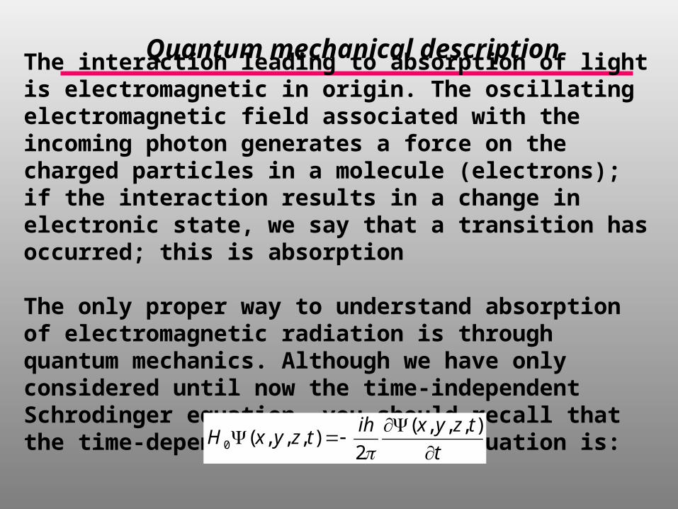
The interaction leading to absorption of light is electromagnetic in origin. The oscillating electromagnetic field associated with the incoming photon generates a force on the charged particles in a molecule (electrons); if the interaction results in a change in electronic state, we say that a transition has occurred; this is absorption

The only proper way to understand absorption of electromagnetic radiation is through quantum mechanics. Although we have only considered until now the time-independent Schrodinger equation, you should recall that the time-dependent Schroedinger equation is:

t

tzyxihtzyxH

),,,(

2),,,(0


If the Hamiltonian is independent of time, the wave function, i.e. the solution to the time-dependent Schroedinger equation is:

htEn

nezyxtzyx /2),,(),,,(

where En and n(x,y,z) are obtained by solving the time-

independent Schroedinger equation:

),,(),,(0 zyxEzyxH nnn

Let us now consider the system is perturbed because electromagnetic radiation is applied. A light wave has an electric field component:

V t V t( ) cos 0 2 is the frequency of the radiation


This electric field interacts with an atom or molecule which has an electric dipole moment defined from the charges qi and their

position in space as follows:

Classical electrodynamics has provided an expression for the energy of interaction between the molecular dipole and the electric field component of the light wave:

where is the angle between the electric dipole moment vector and the electric field vector

q rii

i

U V V cos


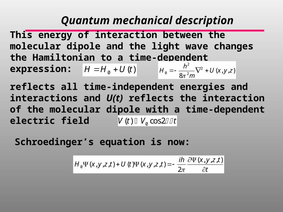
This energy of interaction between the molecular dipole and the light wave changes the Hamiltonian to a time-dependent expression:

reflects all time-independent energies and interactions and U(t) reflects the interaction of the molecular dipole with a time-dependent electric field

Schroedinger’s equation is now:

)(0 tUHH ),,(8

2

2

2

0 zyxUm

hH

V t V t( ) cos 0 2

t

tzyxihtzyxtUtzyxH

),,,(

2),,,()(),,,(0


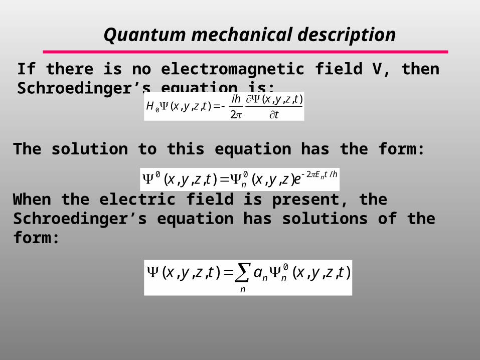
If there is no electromagnetic field V, then Schroedinger’s equation is:

The solution to this equation has the form:

When the electric field is present, the Schroedinger’s equation has solutions of the form:

t

tzyxihtzyxH

),,,(

2),,,(0

htEn

nezyxtzyx /200 ),,(),,,(

n

nn tzyxatzyx ),,,(),,,( 0


is telling us the condition of the system after it has absorbed radiation for a time t

The physical interpretation is as follows. Suppose just before the atom is exposed to light the atom is in its ground state described by the ground state wave function

When the light and the atom interact, energy is absorbed from the light into the atom. The result of this absorption of energy is that the atom may undergo transitions from its ground state into higher energy states described by wave functions

htEn

nezyxtzyx /200 ),,(),,,( n


),,,(00 tzyx

),,,(0 tzyxn

n



Un,0 is the transition moment from state 0 to state n

The probability Pn that at time t the system has made a transition

If the interaction of the electric field with the electric dipole moment is weak the probability amplitude has the general form:

n


00 0 n

),,,(00 tzyx

2)(taP nn

t

nnn dt

h

EEtitU

ihta

0

00, ')

)('2exp()'(

2)(

)2cos()()( 0,00, vtUdtUtU nnn dVU nn 00*

0, cos


This integral is non-zero if and only if:

The probability amplitudes have the final form:

This is called transition dipole and is what allows us to understand absorption of radiation and also calculate how radiation is absorbed from atomic or molecular orbitals.

00 0 n

2)(taP nn

tn

nn dth

EEtitU

ihta

0

00, ')

)('2exp()'(

2)(

)2cos()()( 0,00, vtUdtUtU nnn dVU nn 00*

0, cos

t

nnn dt

h

EEtivtU

ihta

0

00, ')

)('2exp()'2cos(

2)(

h

EEv n 0

Transition dipoles

The concept of transition dipole can be generalized, because the dipole itself is a vector and not a scalar operator. The transition dipole between two states m and n is defined as:

dmnmn*

,

Because the transition dipole is a vector, it has direction in addition to intensity. Most electronic transitions are polarized, which means that the transition dipole is not the same in all directions. The magnitude of the transition is defined as the dipole strength:

2

,, mnmnD

Its units are called Debyes, and are obviously the same units as the square of a dipole (i.e. Cxm). 1 D=3.336x10-30Cxm

Transition dipoles

Example - Calculation of Transition Dipole Moments

Suppose the vibrational motion of a homonuclear diatomic molecule is modeled as a simple harmonic oscillation. Assume the system is initially in the ground state, described by the wave function:

The system is irradiated at the fundamental frequency:

2/4/1

0

2xe

h

2

h

EE 01

Will a transition occur to the n=1 state?

The answer rests on the value of the transition dipole moment

Transition dipoles

If we define the dipole moment as qx, the transition dipole moment has the form:

the integral has the form:

(the function is even so the transition dipole is not zero). Because the transition dipole moment is non-zero, the transition has non-zero intensity if E=h

dxqxU 0*10,1

2/2/14/1

1

2xxe

2/4/1

0

2xe

022

0,1 dxexU x

Transition dipoles

Will a transition from n=0 to n=2 if we irradiate at (E2-E0)/h? The

transition moment is now:

the function is odd so the transition dipole is zero

If we irradiate a harmonic oscillator exactly at

we will observe a transition from n=0 to n=1 but not from n=0 to n=2. This is an example of a selection rule. For a harmonic oscillator, resonant irradiation will only induce transitions for which

0223

020,2 dxexxdxxU x

hE /

.1n

Stimulated and Spontaneous Emission

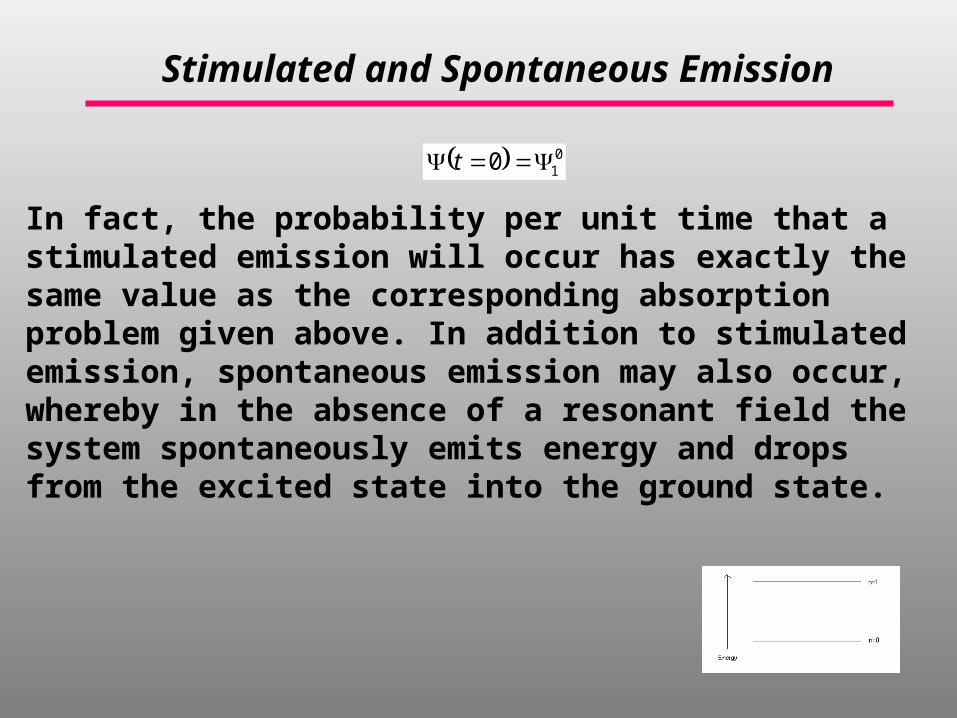
Thus far we have discussed the response of a two energy level system to a resonant field, where the system is initially in the ground state:

Suppose instead that the system is initially in the excited state:

000 t

010 t

A transition to the ground state from the excited state will occur when the system is irradiated with a resonant field. Because the transition is from a higher energy state to a lower energy state, energy is emitted instead of absorbed. This event is called stimulated emission.

Stimulated and Spontaneous Emission

010 t

In fact, the probability per unit time that a stimulated emission will occur has exactly the same value as the corresponding absorption problem given above. In addition to stimulated emission, spontaneous emission may also occur, whereby in the absence of a resonant field the system spontaneously emits energy and drops from the excited state into the ground state.

Two Level system

We can learn more about absorption by considering in greater detail a simple example of the absorption of energy by a quantized system consisting of only two energy levels:

The ground state corresponds to n=0. If the system is exposed to a time dependent electric field the wave function of the system is:

htEihtEi etaetat /2011

/2000

10 )(

htEie /200

00

01

Two Level system

If the energy of interaction

between the system’s electric dipole moment and the electric field V(t) is not large, the system changes slowly, that is to say, the transition from the ground state into the excited state occurs slowly and the probability amplitudes have the form:


/2000

10 )( htEie /200

00

01

tVtVtU 2coscos)()( 0

1)(0 ta

hE

thE

i

Uih

tdh

tEieeU

ih

tdh

tEEitU

ihta

titit

t

exp2

exp2

2

exp2cos2

)(

0,1

22

0

0,1

10

0

0,11

Two Level system

Using the fact that:

The probability of finding a particle in the excited state is:


/2000

10 )( htEie /200

00

01

tVtVtU 2coscos)()( 0

2/sin21 2/ xiee ixix

hhE

hthEeU

ihta hhEi

2/)(

2/)(sin2)( 2/)(

0,11

2

22

0,1

22

112/

2/sin2

hthE

hthEU

haP

Two Level system

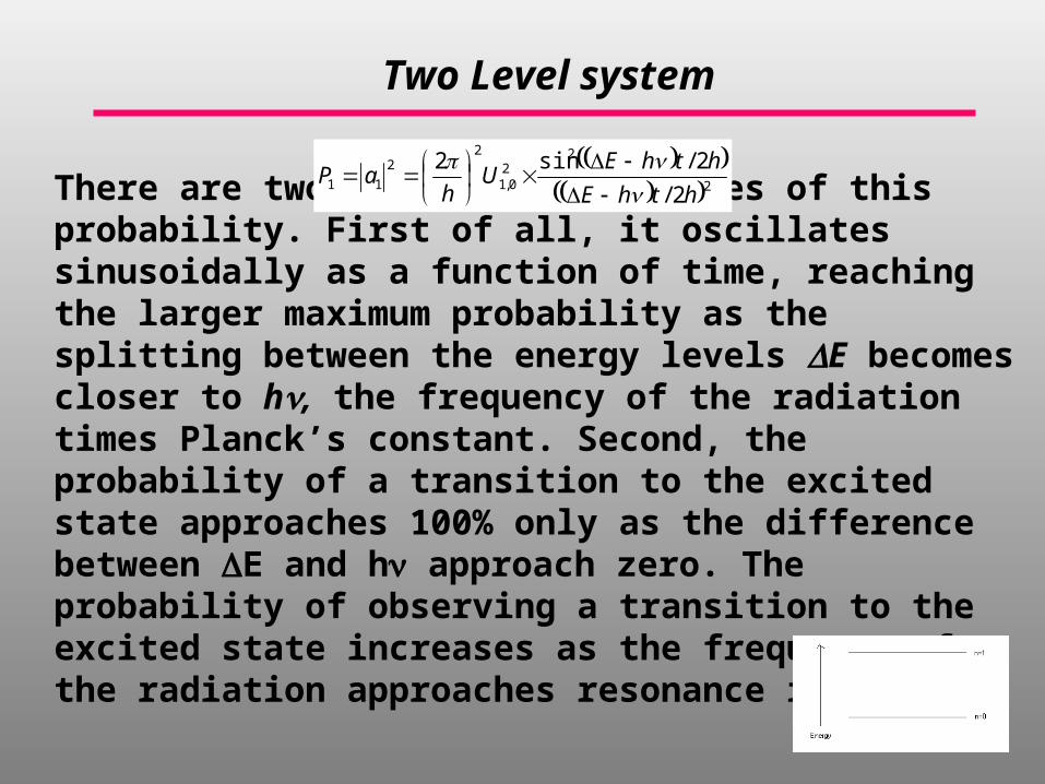
There are two interesting features of this probability. First of all, it oscillates sinusoidally as a function of time, reaching the larger maximum probability as the splitting between the energy levels E becomes closer to h, the frequency of the radiation times Planck’s constant. Second, the probability of a transition to the excited state approaches 100% only as the difference between E and h approach zero. The probability of observing a transition to the excited state increases as the frequency of the radiation approaches resonance i.e. E=h

2

22

0,1

22

112/

2/sin2

hthE

hthEU

haP

Two Level system

The transition probability is sharply peaked around E-h=0

2

22

0,1

22

112/

2/sin2

hthE

hthEU

haP

Transition Probability

0

0.2

0.4

0.6

0.8

1

1.2

5 4 3 2 1 0 -1 -2 -3 -4 -5Frequency Match (MHz.)

Pro

bab

ilit

y

As E approaches h, the transition probability approaches:

tU

hhhE

hthEU

hP

2

0,1

2

2

22

0,1

2

1

2

2/

2/sin2

The probability per unit time that a transition will occur to the excited state is, on resonance:

20,1

2

1 2U

ht

P

hvE