CFX-FSI_14.5_WS04_ThermalStress_2Way

© 2011 ANSYS, Inc. July 30, 20131 Release 14.5

14. 5 Release

Solving FSI Applications Using ANSYS Mechanical and ANSYS CFX

Workshop 42-way FSI for a Thermal Stress Simulation


Problem Overview

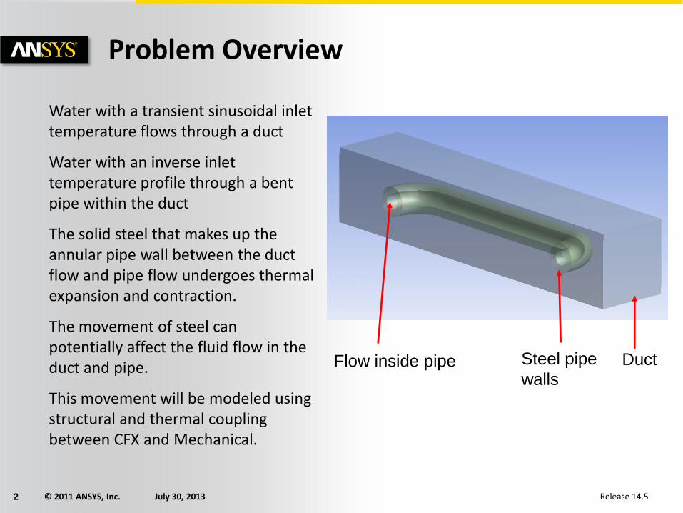
Water with a transient sinusoidal inlet temperature flows through a duct

Water with an inverse inlet temperature profile through a bent pipe within the duct

The solid steel that makes up the annular pipe wall between the duct flow and pipe flow undergoes thermal expansion and contraction.

The movement of steel can potentially affect the fluid flow in the duct and pipe.

This movement will be modeled using structural and thermal coupling between CFX and Mechanical.

DuctFlow inside pipe Steel pipe

walls


What is Solved in CFX

Duct Inlet

Pipe Inlet

Duct Outlet

Pipe Outlet

The flow and temperature fields in both the duct and pipe are solved in CFX.

The temperatures at the two inlets have a sinusoidal fluctuation with time, oscillating between 300 K and 500 K (from an initial temperature of 400K).

Temp at

duct inlet

Temp at

pipe inlet


What is Solved in ANSYS Mechanical

Mechanical solves the temperature field inside the solid steel, and determines the structural response due to thermal and force loads received from the duct and pipe flow.

Clamped

adiabatic

end

Clamped

adiabatic

end

The inner and outer surfaces receive

pressure and thermal loads from CFX


Workflow Overview

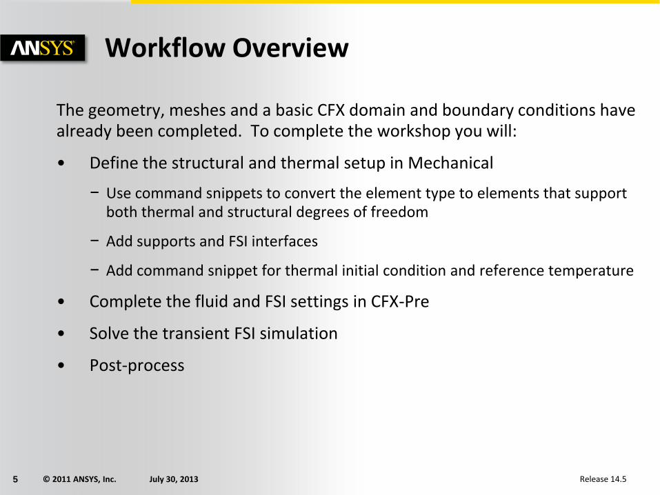
The geometry, meshes and a basic CFX domain and boundary conditions have already been completed. To complete the workshop you will:

• Define the structural and thermal setup in Mechanical

− Use command snippets to convert the element type to elements that support both thermal and structural degrees of freedom

− Add supports and FSI interfaces

− Add command snippet for thermal initial condition and reference temperature

• Complete the fluid and FSI settings in CFX-Pre

• Solve the transient FSI simulation

• Post-process


1. Open the Workbench project ThermalStress.wbpj and save the to a new working directory if necessary

The structural geometry and mesh has already been created. A mesh has been imported into a CFX Component System and a basic setup defined

Starting Workbench


Structural Model

Now complete the structural FSI setup

1. Double-click the Setup cell (A5)

2. Select Units > Metric (m, kg, N, s, V, A) from the main menu and also set the Temperature Units to Celsius (For Metric Systems)

3. Expand Geometry; select Solid and verify that the Material Assignment is set to Structural Steel in the Details view

4. Select Mesh from the Outline tree and note that a hexahedral mesh has been created


Switching the Element Type

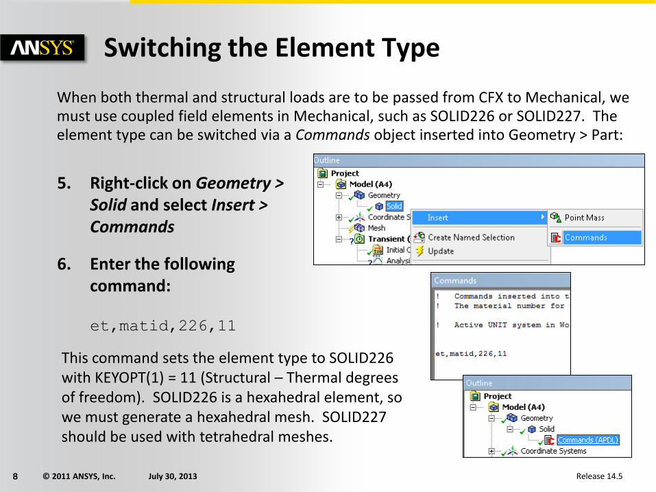
When both thermal and structural loads are to be passed from CFX to Mechanical, we must use coupled field elements in Mechanical, such as SOLID226 or SOLID227. The element type can be switched via a Commands object inserted into Geometry > Part:

This command sets the element type to SOLID226 with KEYOPT(1) = 11 (Structural – Thermal degrees of freedom). SOLID226 is a hexahedral element, so we must generate a hexahedral mesh. SOLID227 should be used with tetrahedral meshes.

5. Right-click on Geometry > Solid and select Insert > Commands

6. Enter the following command:

et,matid,226,11


Structural Analysis Settings

7. Select Analysis Settings under Transient (A5) and set the following

• Number of Steps = 1

• Step End Time = 1 s

• Auto Time Stepping = Off

• Define By = Substeps

• Number of Substeps = 1

• Time Integration = On

The actual end time and time step size will be defined in CFX-Pre

8. Check that Large Deflection = On


Structural Supports and Loads

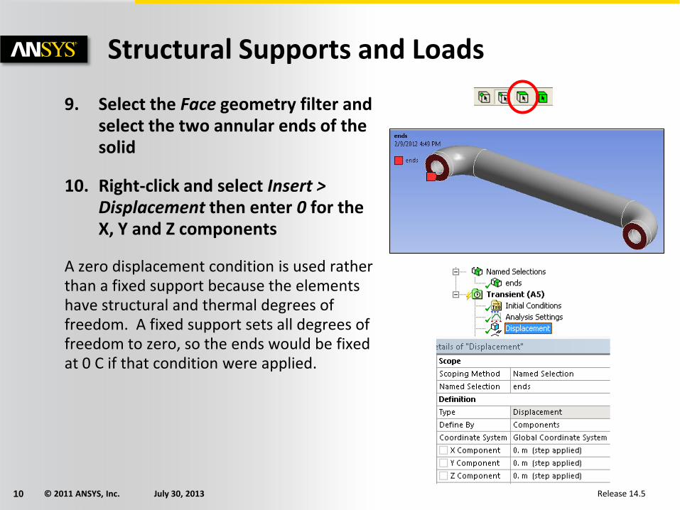
9. Select the Face geometry filter and select the two annular ends of the solid

10. Right-click and select Insert > Displacement then enter 0 for the X, Y and Z components

A zero displacement condition is used rather than a fixed support because the elements have structural and thermal degrees of freedom. A fixed support sets all degrees of freedom to zero, so the ends would be fixed at 0 C if that condition were applied.


Structural Supports and Loads

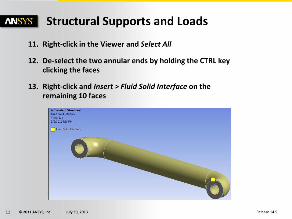
11. Right-click in the Viewer and Select All

12. De-select the two annular ends by holding the CTRL key clicking the faces

13. Right-click and Insert > Fluid Solid Interface on the remaining 10 faces


The solid elements defined using the Geometry command snippets have thermal degrees of freedom, but there is no place to define thermal model settings and conditions in a structural simulation in Workbench. These must be set using Commands objects.

14. Click on Transient (A5) and set the Environment Temperature to 26.85 ⁰C(300 K)

This the temperature at which thermal stresses are zero.

15. Right-click Transient (A5) and Insert > Commands

Thermal Conditions


16. Insert the Commands as follows:

mfou,5

17. Close Mechanical and save the project

The mfou command reduces the frequency of results data written to the rst file to every 5th time step. For this case no further thermal boundary conditions are required. The annular ends will default to an adiabatic condition. In general other thermal settings should be specified in this Commands object. An example is given at the end of this workshop.

This completes the structural setup. When a CFX system is later linked to the Transient Structural System, an input file (ds.dat) will automatically be written when the Structural cell is updated.

Thermal Conditions


Linking a CFX System

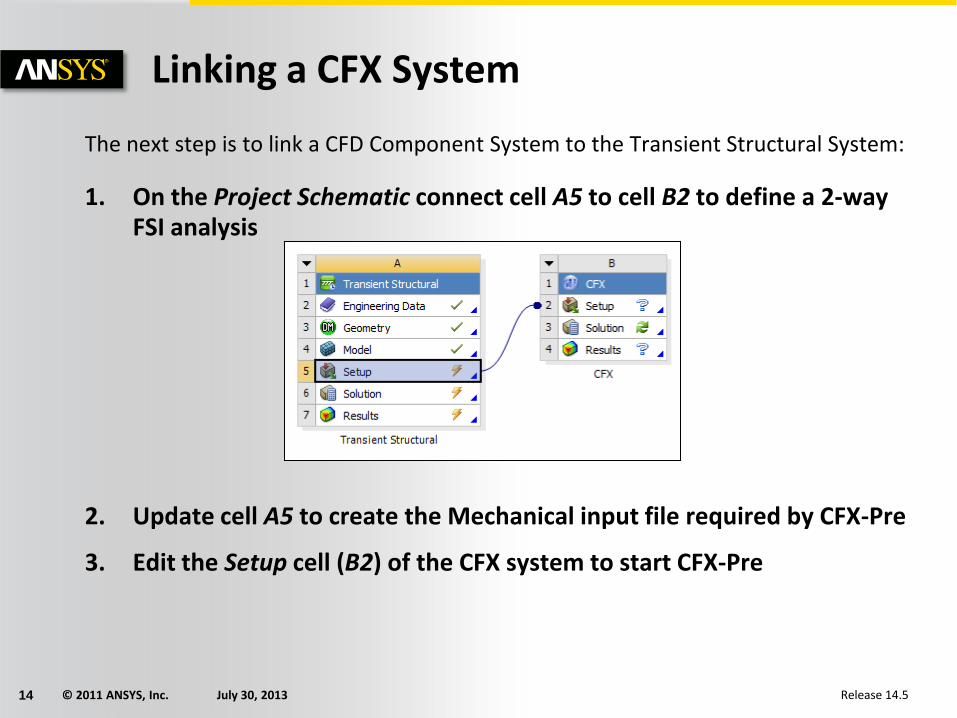
The next step is to link a CFD Component System to the Transient Structural System:

1. On the Project Schematic connect cell A5 to cell B2 to define a 2-way FSI analysis

2. Update cell A5 to create the Mechanical input file required by CFX-Pre

3. Edit the Setup cell (B2) of the CFX system to start CFX-Pre


CFX Analysis Settings

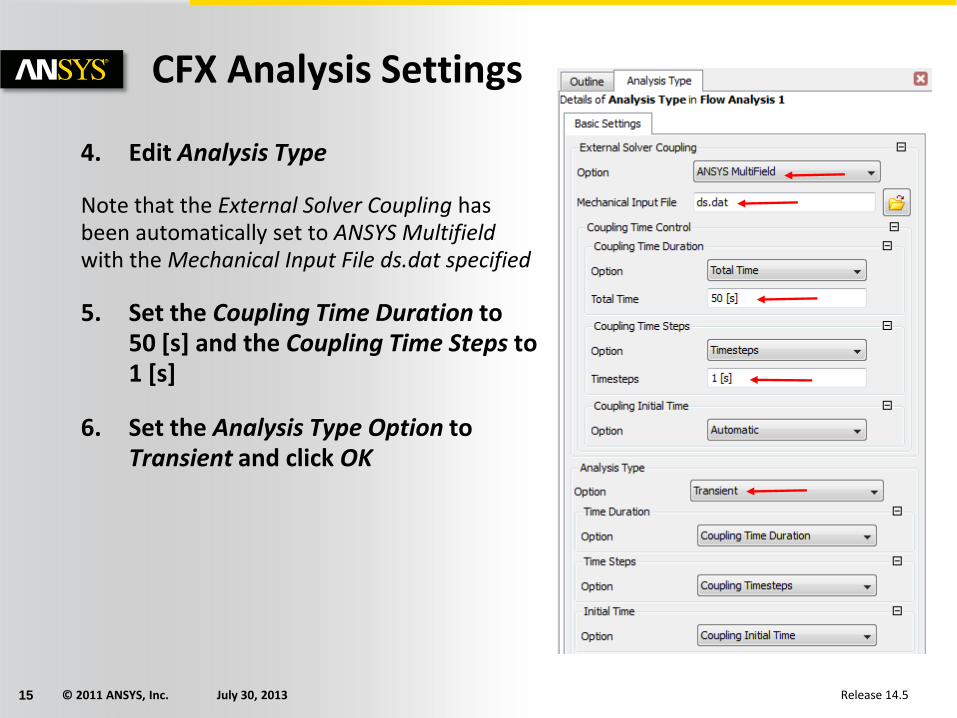
4. Edit Analysis Type

Note that the External Solver Coupling has been automatically set to ANSYS Multifieldwith the Mechanical Input File ds.dat specified

5. Set the Coupling Time Duration to 50 [s] and the Coupling Time Steps to 1 [s]

6. Set the Analysis Type Option to Transient and click OK


CFX Domain Settings

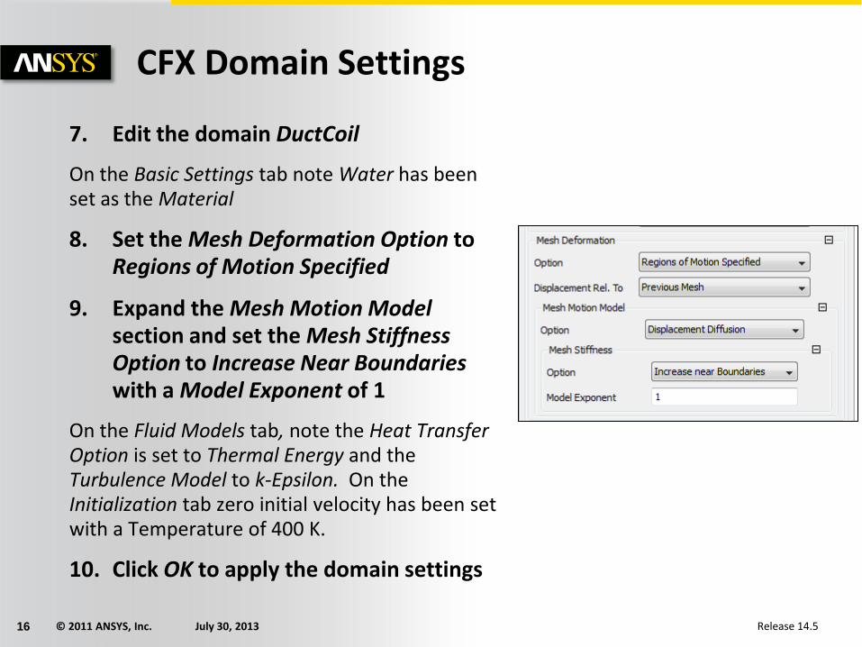
7. Edit the domain DuctCoil

On the Basic Settings tab note Water has been set as the Material

8. Set the Mesh Deformation Option to Regions of Motion Specified

9. Expand the Mesh Motion Modelsection and set the Mesh Stiffness Option to Increase Near Boundaries with a Model Exponent of 1

On the Fluid Models tab, note the Heat Transfer Option is set to Thermal Energy and the Turbulence Model to k-Epsilon. On the Initialization tab zero initial velocity has been set with a Temperature of 400 K.

10. Click OK to apply the domain settings


CFX Boundary Conditions

Next you need to update the boundary conditions with the mesh motion and FSI settings

11. Edit the Duct Inlet boundary condition

Under Boundary Details, a Normal Speed of 0.5 [m/s] has been set with a sinusoidal temperature profile

12. Leave the Mesh Motion Option as Stationary and click OK to update the boundary

13. Edit the Duct Outlet boundary condition

14. Note the settings used, leave the Mesh Motion Option as Stationary and click OK to update this boundary

15. Repeat the previous step for the Coil Inlet and Coil Outlet boundaries


FSI Interface

16. Add a new boundary condition named FSI Walls

17. Set the Boundary Type as Wall and the Location to coilwall and ductcoilwall

18. Under Boundary Details set the Mesh Motion Option to ANSYS Multifield with the ANSYS Interface specified as FSIN_1 and CFX receiving Total Mesh Displacement from ANSYS and passing back Total Force

19. Set the Heat Transfer Option toANSYS Multifield with CFX receiving Temperature and sending Wall Heat Flow

20. Click OK to complete the boundary definition


21. Edit Solver Control

22. On the Equation Class Settings tab, select the Mesh Displacement equation

23. Enable the check boxes shown, increase the Max. Coeff. Loops to 10and set the Residual Type to MAX

These settings represent best practice for FSI simulations. Converging the mesh displacement equations tightly can help prevent mesh folding in some cases.

24. Under External Coupling set the Under Relaxation Factor to 1.0

25. Click OK to complete the Solver Control settings

CFX Solver Controls


CFX Output Controls

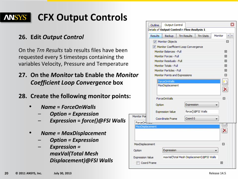
26. Edit Output Control

On the Trn Results tab results files have been requested every 5 timesteps containing the variables Velocity, Pressure and Temperature

27. On the Monitor tab Enable the Monitor Coefficient Loop Convergence box

28. Create the following monitor points:

• Name = ForceOnWalls– Option = Expression– Expression = force()@FSI Walls

• Name = MaxDisplacement– Option = Expression– Expression =

maxVal(Total Mesh Displacement)@FSI Walls


CFX Output Controls

29. Click OK to complete the Output Control settings

In the Outline tree note that an Expert Parameters object is defined. This contains the settings check isolated regions with the Value set to f (false). The duct and coil fluid domains are not connected by an interface in CFX. This is a common setup error, but in this case it is intended to have disconnected fluid regions. Setting this expert parameter disables the solver check that looks for this situation.

30. Close CFX-Pre and save the project


Transient FSI Solution

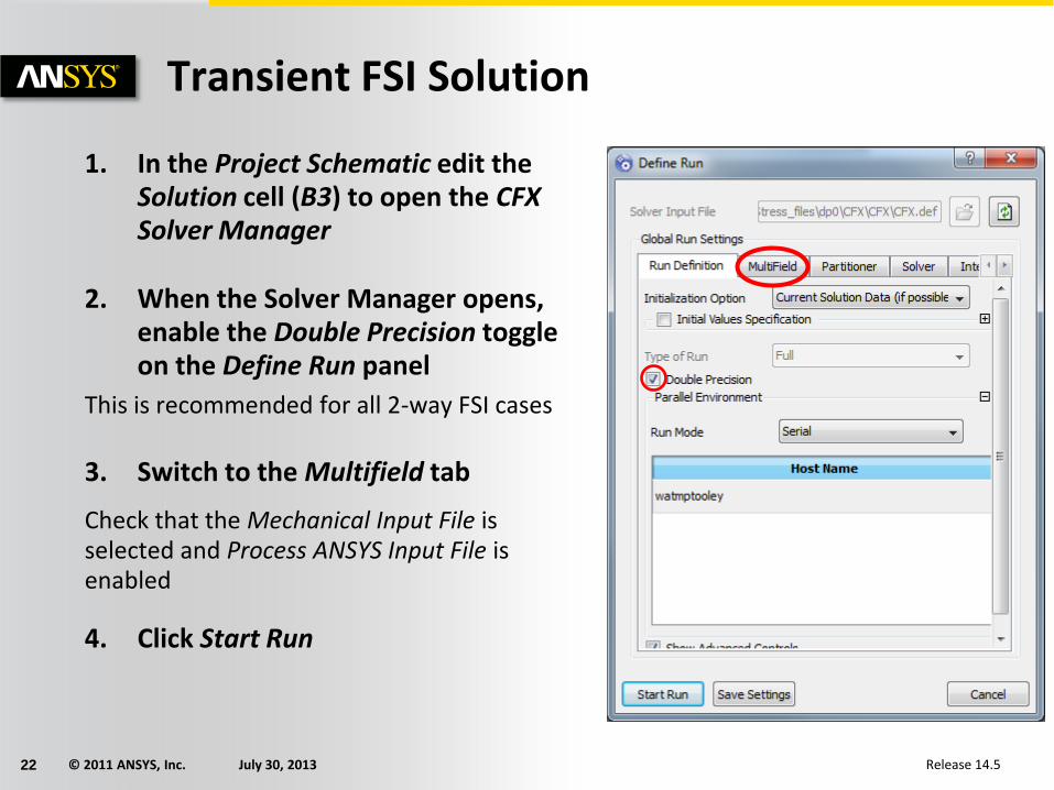
1. In the Project Schematic edit the Solution cell (B3) to open the CFX Solver Manager

2. When the Solver Manager opens, enable the Double Precision toggle on the Define Run panel

This is recommended for all 2-way FSI cases

3. Switch to the Multifield tab

Check that the Mechanical Input File is selected and Process ANSYS Input File is enabled

4. Click Start Run


Transient FSI Solution

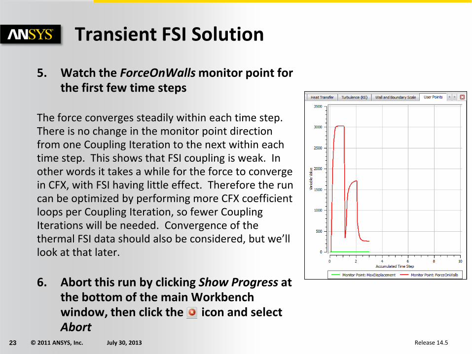
5. Watch the ForceOnWalls monitor point for the first few time steps

The force converges steadily within each time step. There is no change in the monitor point direction from one Coupling Iteration to the next within each time step. This shows that FSI coupling is weak. In other words it takes a while for the force to converge in CFX, with FSI having little effect. Therefore the run can be optimized by performing more CFX coefficient loops per Coupling Iteration, so fewer Coupling Iterations will be needed. Convergence of the thermal FSI data should also be considered, but we’ll look at that later.

6. Abort this run by clicking Show Progress at the bottom of the main Workbench window, then click the icon and select Abort


Edit CFX Setup and Transient FSI Solution [1]

7. Close the CFX Solver Manager and then right-click on cell B3 and select Clear Generated Data to delete the files from the aborted run

8. Edit the CFX Setup cell, B2

9. Edit Solver Control and increase the Max. Coeff. Loops to 6 then click OK

10. Close CFX-Pre and save the project

The next step is to update the solution. Since this will take a several hours you will open a solved project next. Note that some non-essential files and transient results files have been removed from this project to reduce the file size.

11. Use File > Restore Archive… to open ThermalStressComplete.wbpz and select a file name in the Save As window

12. Right-click on the CFX Solution cell (B3) and select Display Monitors to view the convergence history for the solved case



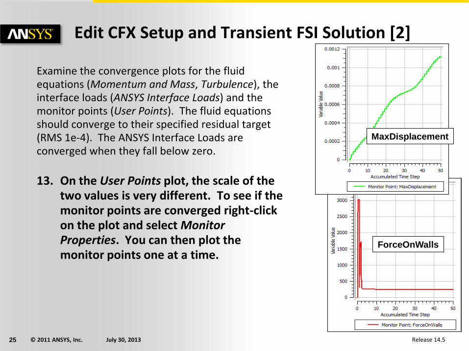
Examine the convergence plots for the fluid equations (Momentum and Mass, Turbulence), the interface loads (ANSYS Interface Loads) and the monitor points (User Points). The fluid equations should converge to their specified residual target (RMS 1e-4). The ANSYS Interface Loads are converged when they fall below zero.

13. On the User Points plot, the scale of the two values is very different. To see if the monitor points are converged right-click on the plot and select Monitor Properties. You can then plot the monitor points one at a time.

MaxDisplacement

ForceOnWalls



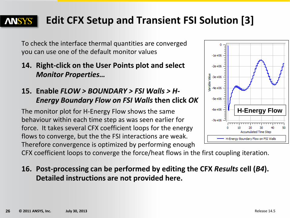
To check the interface thermal quantities are convergedyou can use one of the default monitor values

14. Right-click on the User Points plot and selectMonitor Properties…

15. Enable FLOW > BOUNDARY > FSI Walls > H-Energy Boundary Flow on FSI Walls then click OK

The monitor plot for H-Energy Flow shows the samebehaviour within each time step as was seen earlier forforce. It takes several CFX coefficient loops for the energyflows to converge, but the the FSI interactions are weak. Therefore convergence is optimized by performing enoughCFX coefficient loops to converge the force/heat flows in the first coupling iteration.

16. Post-processing can be performed by editing the CFX Results cell (B4). Detailed instructions are not provided here.

H-Energy Flow


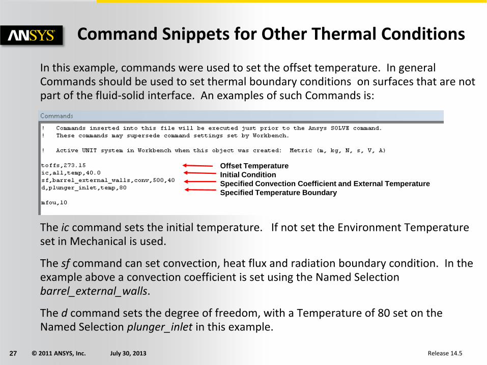
In this example, commands were used to set the offset temperature. In general Commands should be used to set thermal boundary conditions on surfaces that are not part of the fluid-solid interface. An examples of such Commands is:

The ic command sets the initial temperature. If not set the Environment Temperature set in Mechanical is used.

The sf command can set convection, heat flux and radiation boundary condition. In the example above a convection coefficient is set using the Named Selection barrel_external_walls.

The d command sets the degree of freedom, with a Temperature of 80 set on the Named Selection plunger_inlet in this example.

Offset Temperature

Initial Condition

Specified Convection Coefficient and External Temperature

Specified Temperature Boundary

Command Snippets for Other Thermal Conditions


Final Notes

In this case, the maximum deformation is small (on the order of 1.8 mm). This has little effect on the fluid flow, so the problem could be run using 1-way force coupling. This is done by turning off mesh deformation in the fluid domain and passing forces without receiving displacements. The thermal transfer should remain as 2-way coupling.

One could also solve the CHT problem completely within CFX and then pass the volumetric temperature to a static structural system where stresses would be calculated. A static structural system would be suitable since the structural inertia is negligible.

17. Save and close the Workbench project

CFX-FSI_14.5_WS04_ThermalStress_2Way

Documents

structural steel

pipe flow

thermal loads

thermal setup

structural loads

pipe steel pipe walls

ansys cfxworkshop

ansys mechanicalmechanical