CFD Modelling of Three-Phase Fluidized Bed with Low ...ethesis.nitrkl.ac.in/5704/1/110CH0087-3.pdf · CFD Modelling of Three-Phase Fluidized Bed with Low ... 1.2 Application of three-phase

CFD Modelling of Three-Phase Fluidized Bed with Low

Density Solid Particles

In the partial fulfillment of the requirement of

Bachelor of technology

in

Chemical Engineering

Submitted by

Kuldeep Sharma

Roll no. 110CH0087

Under the guidance of

Dr. H.M. Jena

Department of Chemical Engineering

National Institute of Technology

Rourkela-769008

Odisha, India

(May, 2014)

i

National Institute of Technology

Rourkela

CERTIFICATE

This is to certify that that the work in this thesis report entitled- CFD modeling of

three phase fluidized bed with low density solid particles -submitted by Kuldeep

Sharma in partial fulfillment of the requirements for the degree of Bachelor of

Technology in Chemical Engineering Session 2013-2014 in the department of Chemical

Engineering, National Institute of Technology Rourkela, Rourkela is an authentic work

carried out by him under my supervision and guidance.

Date: - Dr. H.M.JENA

Department of Chemical engineering

National institute of Technology

Rourkela 769008

ii

ACKNOWLEDGMENT

I owe a debt of deepest gratitude to my thesis supervisor, H.M.Jena, Professor,

Department of Chemical Engineering, for his guidance, support, motivation and

encouragement throughout the period this work was carried out. His readiness for

consultation at all times, his educative comments, his concern and assistance even with

practical things have been invaluable.

I am sincerely thankful to MR.Sambhurisha Mishra for acting as my project

coordinator and helping me in the learning of software.

I am grateful to Prof. R.K.Singh, Head of the Department, Chemical Engineering for

providing us the necessary opportunities for the completion of our project. I also thank

the other Staff members of my department for their invaluable help and guidance.

Kuldeep Sharma

Roll no. 110CH0087

4’Th year B.Tech

Department of Chemical engineering

NIT Rourkela

iii

CONTENTS

Chapters Page no.

Certificate i

Acknowledgement ii

List of figures and tables iv

Abstract vi

Nomenclature vii

Chapter-1

Introduction and Literature survey 1

1.1 Advantages and disadvantages of three-phase fluidized bed

1.2 Application of three-phase fluidized bed

1.3 Hydrodynamic studies of three-phase fluidized beds with low density particles

1.4 Computational fluid dynamic studies on three-phase fluidized beds

1.5 Research objectives

1.6 Thesis summary

1

1

2

2

6

6

Chapter-2

Computational flow model and numerical methodology 7

2.1 Computational model for multiphase flow

2.2 Conservation equations

2.2.1. Interphase Exchange Co-efficient

2.3. Closure law for solid pressure

2.4. Closure law for turbulence

2.5. Numerical Methodology

2.5.1. Geometry and Mesh

2.5.2. Boundary and initial conditions

7

8

9

11

12

14

14

15

Chapter-3

Results and discussion 17

Chapter-4

Conclusion and future work 25

References 26

iv

List of figures and tables

Figure no.

Caption Page no.

Fig 2.1 Line diagram of computational geometry fluidized bed 14

Fig 2.2 2D mesh generated in meshing. 15

Fig.3.1. Variation of bed pressure drop (Pa) with liquid velocity

(m/s) at constant air velocities (m/s) for 8 mm

Polypropylene beads at Hs= 0.247 m and grid size 0.0075m

using laminar model.

17

Fig 3.2 Variation of bed pressure drop (Pa) with liquid velocity

(m/s) at constant air velocities (m/s) for 8 mm

Polypropylene beads at Hs= 0.247 m and grid size 0.005m

using laminar mode.

18

Fig 3.3 Comparison of bed pressure drop (Pa) between laminar and

turbulent model with liquid velocity (0.01 to 0.06m/s) at

constant air velocities (m/s) for 8 mm Polypropylene beads

at Hs= 0.247 m and grid size 0.005m

19

Fig 3.4 Comparison of bed pressure drop (Pa) between laminar and

turbulent model with liquid velocity (0.01 to 0.06m/s) at

constant air velocities (m/s) for 8 mm Polypropylene beads

at Hs= 0.247 m and grid size 0.0075m.

19

Fig 3.5 Variation of gas holdup with liquid velocity (m/s) at

constant air velocities (m/s) for 8 mm Polypropylene beads

at Hs= 0.247 m and grid size 0.005m using laminar model.

20

Fig 3.6 Variation of gas holdup with liquid velocity (m/s) at

constant air velocities (m/s) for 8 mm Polypropylene beads

at Hs= 0.247 m and grid size 0.0075m using laminar model.

21

Fig 3.7 Comparison of gas holdup between laminar and turbulent

model with liquid velocity (0.01 to 0.06m/s) at constant air

velocities (m/s) for 8 mm Polypropylene beads at Hs=

0.247 m and grid size 0.0075m

22

v

Fig 3.8 Comparison of gas holdup between laminar and turbulent

model with liquid velocity (0.01and 0.06m/s) at constant air

velocities (m/s) for 8 mm Polypropylene beads at Hs=

0.247 m and grid size 0.005m.

22

Fig 3.9 Comparison of air hold up between grid size 0.005-

0.0075m with liquid velocity (0.01 to 0.06m/s) at constant

air velocities (m/s) for 8 mm Polypropylene beads at Hs=

0.247 m with laminar model

23

Fig 3.10 Variation of bed height (m) with liquid velocities (m/s) at

constant gas velocities (m/s) for 8 mm polypropylene beads

at Hs= 0.247m, grid size 0.0075m and laminar model..

24

Fig 3.11 Comparison of bed height between laminar and turbulent

model with liquid velocity (0.01 to 0.06m/s) at constant air

velocities (m/s) for 8 mm Polypropylene beads at Hs=

0.247 m and grid size 0.0075m..

24

Table no.

Table 2.1 Meshing configuration used in the computations of

fluidized bed

15

Table 2.2 Description of systems used in simulation 16

vi

ABSTRACT

Three-phase fluidization is defined as an operation in which a bed of solid particles is

suspended in gas and liquid media due to net drag force of the gas and/or liquid flowing

opposite to the net gravitational force (or buoyancy force) on the particles. Such an operation

generates considerable, intimate contact among the gas, liquid and the solid in the system and

provides substantial advantages for application in physical, chemical or biochemical

processing involving gas, liquid and solid phases. Among all the types of three-phase fluidized

beds, three-phase concurrent gas-liquid-solid fluidized beds are used in a wide range of

applications including hydro-treating and conversation of heavy petroleum and synthetic crude,

coal liquefaction, methanol production, sand filter cleaning, electrolytic timing, conversion of

glucose to ethanol, aerobic waste water treatment, and various other hydrogenation and

oxidation reactions. The recent fluidized bed bioreactors are superior in performance due to

immobilization of cells on solid particles reducing the time of treatment, volume of reactor is

extremely small, lack of clogging of bio-mass and removal of pollutant like phenol even at

lower concentrations. In the fluidized bed system used in waste water treatment, low density

solid matrix is used to immobilize the microbes as the system operates at low water and air

velocities to avoid transportation of the particles from the bed. Hydrodynamics study of three-

phase fluidized bed with low density particles are rarely seen in literature although a

tremendous work is seen for moderate or high density solid particles. In the present work, the

computational studies have been carried out on two dimensional fluidized beds to characterize

there hydrodynamic behavior. Air, water and low density solid particles have been used as the

gas, liquid and solid phase to analyze the system behaviors.

Keywords: Multiphase, Fluidized bed, CFD, hydrodynamics.

vii

Nomenclature

β: Particulate loading, -

αd: Volume fraction of discrete phase, -

𝛼𝑐: Volume fraction carrier phase, -

𝜌𝑑: Density of the dispersed phase (d), Kg m-3

𝜌𝑐: Density of the carrier phase (c), kg m-3

𝑆𝑡: Stoke number, -

𝜏𝑑: Particle response time, s

𝑡𝑠: System response time, s

𝑑𝑑: Diameter of dispersed phase, m

𝜇𝑐: Viscosity of carrier phase, Pa s

Ls: Characteristics length, m

Vs.: Characteristic velocity, m s-1

𝑉𝑞: Volume of phase q. -

𝛼𝑞: Volume fraction of phase q, -

�⃗�𝑞: Effective density of phase q, Kg m-3

𝜆𝑞: Bulk viscosity of phase q, m s-1.

�⃗�𝑞: External body force, N

�⃗�𝑙𝑖𝑓𝑡,𝑞: Lift force, N

�⃗�𝑣𝑚,𝑞: Virtual mass force, N

�⃗⃗�𝑝𝑞: Interaction between phases, -

p : Pressure, Pa

�⃗� : Acceleration due to gravity, m s-2

viii

𝐾𝑝𝑞 : Fluid-fluid exchange co-efficient, Kg s-1

𝐾𝑙𝑠: Fluid-solid and solid-solid exchange coefficient, Kg s-1

𝑓: Drag function, -

𝜏𝑝: Particulate relaxation time, s

𝜇𝑝: Viscosity of phase p, m s-1.

𝛼𝑟: Volume fraction of phase r, -

𝜇𝑟: Viscosity of phase r, m s-1.

𝜇𝑙: Viscosity of liquid phase, m s-1.

𝜏𝑠: Particulate relaxation time, s

ds : Diameter of the particles of phase s, m

𝛼𝑙: Volume fraction of liquid phase, -

𝜌𝑙: Density of liquid phase, kg m-3

�⃗�𝑙: Velocity of liquid phase, m s-1

𝑒𝑙𝑠: Coefficient of restitution,-

𝐶𝑓𝑟,𝑙𝑠: Coefficient of friction between the lth and sth solid phase particles,-

𝑑𝑙: Diameter of particle of solid l, m

𝑔0,𝑙𝑠: Radial distribution coefficient, -.

𝛩𝑠 ∶ Granular temperature, K

𝑒𝑠𝑠: Co-efficient of restitution for particle collisions, -

𝑔0,𝑠𝑠: Radial distribution function, -

S: Distance between grains, m

𝜇𝑠: Solid shear viscosity, m s-1

𝜇𝑠,𝑐𝑜𝑙: Collision viscosity, m s-1

𝜇𝑠,𝑘𝑖𝑛: Kinetic viscosity, m s-1

ix

𝜇𝑠,𝑓𝑟: Frictional viscosity, m s-1

𝜆𝑠: Bulk viscosity, m s-1

𝜙: Angle of internal friction, -

𝐾𝛩𝑠: Diffusion co-efficient

𝛶𝛩𝑠: Collisional dissipation of energy

𝛷𝑙𝑠: Energy exchange between lth solid phase and sthsolid phase

�⃗⃗⃗�𝑠,||: Particle slip velocity parallel to the wall, m s-1

𝜙: Specularity co-efficient between particle and wall, -

𝛼𝑠,𝑚𝑎𝑥 Volume fraction for particle at maximum packing, -

𝜏̿𝑞" : Reynolds stress tensors for continuous phase q, Pa

�⃗⃗⃗�𝑞: Phase-weighted velocity, m s-1

𝜇𝑡,𝑞: Turbulent viscosity, Pa s

𝜀𝑞: Dissipation rate, m2 s-3

𝐶𝜇: Constant, -

𝑝𝐶0

′ : Cell pressure correction, Pa

𝑝′ ∶ Pressure correction, Pa

𝑏 : Source term, -

𝛼 : Under-relaxation factor, -

𝛼𝑝: Under relaxation factor for pressure, -

ULmf : Minimum liquid fluidization velocity, m s-

1

CHAPTER 1

INTRODUCTION AND LITERATURE SURVEY

Fluidization is an operation by which fine solids are transformed into a fluid-like state through

contact with gas or liquid or by both gas and liquid. Gas-liquid-solid fluidization is defined as

an operation in which a bed of solid particles is suspended in gas and liquid media due to net

drag force of the gas and/or liquid flowing opposite to the net gravitational force (or buoyancy

force) on the particles. Such an operation generates considerable, intimate contact among the

gas, liquid and the solid in the system and provides substantial advantages for application in

physical, chemical or biochemical processing involving gas, liquid and solid phases.

Fluidization is broadly of two types, viz. aggregative or bubbling. The gas-liquid-solid

fluidization with liquid as continuous phase is of particulate fluidization type, while

aggregative fluidization is a characteristic of gas-liquid-solid system with gas as the continuous

phase

1.1. Advantages and disadvantages of three-phase fluidized bed:

There are several advantages of fluidized beds such as; ability to maintain a uniform

temperature, significantly lower pressure drops which reduce pumping costs, catalyst may be

withdrawn, reactivated, and added to fluidized beds continuously without affecting the

hydrodynamics performance of the reactor, bed plugging and channeling are minimized due to

the movement of solids, high reactant conversion for reaction kinetics, low intra particle

diffusion resistance, gas-liquid and liquid-slid mass transfer resistance(shah, 1979; Beaton et

al., 1986; Fan, 1989; Le Page et al., 1992; Jena, 2010). There are, however, also some

disadvantages to fluidized beds such as; catalyst attrition due to particle motion, entrainment

and carryover of particles, relatively larger reactor size compared to bed expansion, not suitable

for reaction kinetics favoring plug flow pattern, low controllability over product selectivity for

complex reaction and loss of driving force due to back mixing of particles in case transfer

operations (Jena, 2010)

1.2. Application of three-phase fluidized bed:

Among all the types of three-phase fluidized beds, three-phase concurrent gas-liquid-solid

fluidized beds are used in a wide range of applications including hydro-treating and

conversation of heavy petroleum and synthetic crude, coal liquefaction, methanol production,

sand filter cleaning, electrolytic timing, conversion of glucose to ethanol, aerobic waste water

2

treatment, and various other hydrogenation and oxidation reactions (Fan, 1989; Wild and

Poncin, 1996; Jena, 2010).

1.3. Hydrodynamic studies of three-phase fluidized beds with low density particles:

Low density solid particles found huge application in bio reactor for aerobic waste water

treatment. Hydrodynamics study of three-phase fluidized bed with low density particles are

rarely seen in literature although a tremendous work is seen for moderate or high density solid

particles. Hydrodynamics of a gas-liquid-solid fluidized bed with low density solid [Kaldnes

Miljotechnologies AS (KMS)] support was investigated by Sokół and Halfani (1999), they

have found that value of minimum fluidization air velocity depend on the ratio of bed to reactor

volume and mass of cell growth on the particles. The effect of operational parameters on

biodegradation of organics in fluidized bed bioreactor with low density solid particles have

been studied by Sokół (2001) and Sokół and Korpal (2004). Briens and Ellis (2005) have

characterized the hydrodynamics of three-phase fluidized bed systems by statistical, fractal,

chaos and wavelet analysis. The solid particles covered with a biofilm are fluidized by air and

contaminated water by Allia et al. (2006) to confirm the operating stability, to identify the

nature of mode flow and to determine some hydrodynamic parameters such as the minimum

fluidization velocity, the pressure drop, the expansion, the bed porosity, the gas retention and

the stirring velocity

Even though a large number of experimental studies are directed towards the quantification of

flow structure and flow regimes identification for different process parameters and physical

properties, the complex hydrodynamics of these reactor are not well understood due to

complicated phenomena such as particle-particle, liquid-particle, and particle-particle

interactions (Jena, 2010). As regard to mathematical modeling, computational fluid dynamics

(CFD) simulation give detailed information about the local values of pressure, viscous and

turbulent stresses, turbulent kinetics energy and turbulent energy dissipation rate, etc.

1.4. Computational fluid dynamic studies on three-phase fluidized beds:

Recently, several CFD models based on Eulerian multi-fluid approach have been developed

for gas–liquid-solid flows (Matonis et al., 2002; Feng et al., 2005; Schallenberg et al., 2005).

Grevskott et al. (1996) have carried out computational fluid dynamic simulation of three phase

slurry reactor by two fluid models, with the two phases treated in an Eulerian frame of

reference. The inter-phase momentum exchange terms modeled between the fluid phases were

steady interfacial drag, added mass force and lift force. They have also tested a new model for

bubble size distribution and solid pressure. Their new bubble size model is found to improve

3

the size distribution prediction compared to prior model. Mitra-Majumdar et al. (1997) have

used computational fluid dynamics model to examine the structure of three-phase (air-water-

glass beads) flow through a vertical column. In their study they proposed new co-relation to

modify the drag between the liquid and the gas phase to account for the effect of solid particles

on bubble motion. They have used K- ϵ model for simulating the effect of turbulence on the

flow field. Jianping and Shonglin (1998) have used a two dimensional pseudo-two phase fluid

dynamics model with turbulence calculate local values of axial liquid velocity and gas holdup

in a concurrent gas-liquid-solid three-phase bubble column reactor. They have concluded that

local axial liquid velocity and local gas holdup value are strongly influenced by solid loading

and operating condition, local gas holdup and axial liquid velocity increased as the solid

loading declined and under certain circumstance.

Li et al. (1999) have carried out CFD simulation of gas bubbles rising in water in a small two

dimensional bed glass beads. They have applied a bubble induced force model, continuum

surface force model and Newton third law respectively for the couplings of particle-bubbles,

gas-liquid and particle liquid interactions. It is shown that their model can capture the bubble

wake behavior such as wake structure and the shedding frequency. Zhang et al. (2000a) have

conducted a discrete phase simulation to study the bubble and particle dynamics in a three

phase fluidized bed at high pressure. They have employed the Eulerian volume-averaged

method, the Lagrangian dispersed particle method, and the volume of fluid (VOF) method to

describe the motion of liquid, solid particles, and gas bubbles. Zhang et al. (2000b) have

developed a computational scheme for discrete-phase simulation of a gas-liquid-solid

fluidization system and a two-dimensional code based on it. The volume-averaged method, the

dispersed particle method, and the volume-of-fluid (VOF) method have been used to account

for the flow of liquid, solid particles, and gas bubbles respectively.

Padial et al. (2000) have used finite-volume flow simulation technique to study the three

dimensional simulation of three phase flow in a conical-bottom draft-tube bubble column. They

have employed an unstructured grid method along with a multifield description of the

multiphase flow dynamics. They have observed the same loss of column circulation as

experimental when the column is operated with the draft tube in its highest position. Li et al.

(2001) have conducted a discrete phase simulation (DPS) to investigate multi-bubble formation

dynamics in gas-liquid-solid fluidization systems. They have developed and employed a

numerical technique based on computational fluid dynamics (CFD) with the discrete particle

method (DPM) and volume tracking represented by the volume-of-fluid (VOF) method for

simulation. They have applied a bubble-induced force (BIF) model, a continuum surface force

4

(CSF) model, and Newton’s third law to account for the couplings of particle-bubble, bubble-

liquid and particle-liquid interactions, respectively. Matonis et al. (2002) have developed

experimentally verified computational fluid dynamic model for gas-liquid-solid flow. A three-

dimensional transient computational code for the coupled Navier-Strokes equations for each

phase has been used. Their simulation shows a down flow of particles in the center of the

column, and an up flow near the wall, and a nearly uniform particle concentration. Chen and

Fan (2004) have developed two dimensional Eulerian–Lagrangian model for three-phase

Fluidization and used Level-set method for interface tracking and Sub-Grid Scale (SGS) stress

model for bubble-induced turbulence to characterize the bubble rise velocity, bubble shapes

and their fluctuations, and bubble formation. Glover and Generalis (2004) have presented an

alternate approach to the modeling of solid-liquid and gas-liquid-solid flow for a 5:1 height to

width ratio bubble column. Feng et al. (2005) have developed a 3-dimensional computational

fluid dynamics (CFD) model to simulate the structure of gas-liquid-TiO2 nanoparticles three-

phase flow in a bubble column. The have been compared with experimental data for model

validation.

Wiemann and Mewes (2005) have presented a numerical method for the calculation of the

three- dimensional flow fields in bubble columns based on a multi fluid model. They have

obtained the local and the integrated volume fraction of gas in the bed from CFD simulation.

Zhang and Ahmadi (2005) have used an Eulerian-Lagrangian computational model for

simulation of gas-liquid-solids flows in three phase slurry reactors. They have used a volume-

averaged system of governing equations for liquid flow model whereas motion of bubbles and

particles are evaluated by the Lagrangian trajectory analysis procedure. The simulation result

shows dominance of time-dependent staggered vortices on the transient characteristics. The

bubble size significantly affects the characteristics of three-phase flows and flows with larger

bubbles appear to evolve faster.

Annaland et al. (2005) has presented a hybrid model for the numerical simulation of gas-liquid-

solid flow using a combine front tracking (FT) for dispersed gas bubbles and solid particle

present in the continuous liquid phase. In addition they have quantified the retarding effect on

bubble rising velocity due to presence of suspended solid particles. Schallenberg et al. (2005)

have used a computational fluid dynamic model to calculate a three-phase (air-water-solid

particles) flow in a bubble column. They have used the K-ε turbulence model extended with

term accounting for the bubble-induced turbulence to calculate the eddy viscosity of the liquid

phase. They have observed good agreement between the measured and the calculated results.

5

Cao et al. (2009) have modeled gas-liquid-solid circulating fluidized bed by two dimensional,

Eulerian–Eulerian–Lagrangian (E/E/L) approaches. E/E/L model combined with Two Fluid

Model (TFM) and Distinct Element Method (DEM). Based on generalized gas–liquid two

fluids k-ε model, the modified gas–liquid TFM is established. Muthiah et al. (2009) have

carried out computational fluid dynamics to characterize the dynamics of three-phase flow in

cylindrical fluidized bed, run under homogeneous bubble flow and heterogeneous flow

condition. They observed that higher gas velocity, higher value of solid loading and lower

particles diameter make the system diameter faster.

O'Rourke et al. (2009) have developed 3D model and used Eulerian finite difference approach

to simulate gas-liquid-solid fluidized bed. The mathematical model using multiphase particle-

in-cell (MP-PIC) method is used for calculating particle dynamics (collisional exchange) in the

computational-particle fluid dynamics (CPFD). Paneerselvam et al. (2009) have developed a

three dimensional transient model to simulate the local hydrodynamics of a gas-liquid-solid

three phase fluidized bed reactor using the CFD method. From the validated CFD model, they

carried out the computation of the solid mass balance and various energy flows in fluidized bed

reactors.

Sivaguru et al. (2009) have carried out the CFD analysis of three-phase fluidized bed to predict

the hydrodynamics. They have taken liquid phase as water that continuously flow, whereas the

gas phase is air which flow discretely throughout the bed. They have obtained the simulation

result using porous jump and porous zone model to represent the distributor. They have found

that porous zone model is best applicable in Industries, since stability of operating condition is

achieved even with non-uniform air, water flow rate and with different bed height. Nguyen et

al. (2011) have carried out CFD simulation using commercial CFD package FLUENT 6.2 to

understand the hydrodynamics of three phase fluidized bed. They have investigated the

complex hydrodynamics of three phase fluidized bed such as bed expansion, holdup for two

phases, bed pressure drop, and fluidized bed voidage and velocity profile. They have used

Euler-Euler multiphase approach for predicting the overall performance of gas –liquid-solid

fluidized bed and Gidaspow model is used as drag model for simulation.

Hamidpour et al (2012) have performed CFD simulations of gas-liquid-solid fluidized beds in

a full three dimensional, unsteady multiple-Euler frame work by mean of the commercial

software FLUENT. They have investigated the significance of implementing accurate

numerical schemes as well as the choice of available K-ε turbulence models (standard, RNG,

realizable), solid wall boundary condition and granular temperature model. The result indicated

6

that in order to minimize numerical diffusion artifacts and to enable valid discussions on the

choice of physical models, third order numerical schemes need to be implemented.

The report on the computational models for the hydrodynamics characteristics of three-phase

fluidized bed is limited. Most of these CFD studies are based on steady state, 2D axisymmetric,

Eulerian multi-fluid approach. But in general, three phase flows in fluidized bed reactors are

intrinsically unsteady and are composed of several flow processes occurring at different time

and length scales. The unsteady fluid dynamics often govern the mixing and transport processes

and is inter-related in a complex way with the design and the operating parameters like reactor

and sparger configuration, gas flow rate and solid loading. Computational model of 0.10m

diameter and 1.88 m height column have been studied with changing gas and liquid velocity.

Changing inlet conditions will change the flow characteristics. The hydrodynamic study of

three-phase fluidized bed is meager and very less amount of content of literature available to

describes the hydrodynamic study of low density particles in a three phase fluidized bed by

CFD simulation Thus the present work has been carried out with the following main objectives.

1.5. Research objectives:

The main objectives of the present research work are summarized below:

Hydrodynamic study on three-phase fluidized bed with low density particles (propylene

beads) using water and air as liquid and gas phase.

To studied the grid independency for fluidized bed model.

To studied the effect of different viscous model on hydrodynamics properties

1.6. Thesis summary:

This thesis comprises of five chapters v.i.z. Introduction and Literature Survey, Experimental

setup and technique, Computational Flow Model and Numerical Methodology, Result and

Discussion and Conclusion and Future scope of the work.

Chapter 1, the background information, literature review and objective of the present

work is discussed.

Chapter 2 deals with the computational models, the numerical methods, mesh quality,

boundary condition, material description etc. used in the CFD simulation.

Chapter 3 the results of various hydrodynamics properties obtained from the simulation

have represented graphically and discussed.

Chapter 4 deals with overall conclusion. Future recommendations based on the research

outcome are suggested. The major findings of the work are also summarized.

7

CHAPTER 2

COMPUTATIONAL FLOW MODEL AND NUMERICAL

METHODOLOGY

CFD is a powerful tool for the prediction of the fluid dynamics in various types of systems,

thus, enabling a proper design of such systems. The Finite Volume Method (FVM) is one of

the most versatile discrimination techniques used for solving the governing equations for fluid

flow. The most compelling features of the FVM are that the resulting solution satisfies the

conservation of quantities such as mass and momentum. In the finite volume method, the

solution domain is subdivided into continuous cells or control volumes where the variable of

interest is located at the centroid of the control volume forming a grid. There are several

schemes that can be used for discretization of governing equations e.g. central differencing,

upwind differencing, power-law differencing and quadratic upwind differencing schemes. The

resulting equation is called the discretized equation.

In the present work three geometries of a physical unit has been considered. First a two

dimensional (2D) geometry without distributor is simulated with CFD tools to check the

present findings with previous ones available which are mostly based on two 2D models.

Commercial CFD package ANSYS FLUENT has been used in modeling and simulation of

various geometries considered.

Three-phase fluidization involve gas, liquid and solid phases, hence for computational study

choosing of appropriate multiphase model play an important role in the simulation result. There

are different multiphase models available in commercial software ANSYS FLUENT. In the

present work a series of computational models available in FLUENT have been used. The

details of various models and numerical schemes used in the present work are discussed in this

chapter.

2.1. Computational model for multiphase flow:

Advance in computational fluid mechanics have provided the basis for further insight into the

dynamics of multiphase flow. For volume averaged information on any hydrodynamic property

the Euler-Euler approach is suitable for its simplicity. Conservation equations for each phase

are derived to obtain a set of equations which have similar structure for all phase. The equations

are closed by providing constitutive relations that are obtained from empirical information or

in the case of granular flow by application of kinetic theory.

8

The Eulerian model is the most complex of the multiphase model. It solves a set of n

momentum and continuity equations for each phase. Through the pressure and interphase

exchange coefficients coupling are achieved. The manner in which this coupling is handled

depends upon the type of phases involved; granular (fluid solid) flows are handled differently

than non-regular (fluid-fluid) flows. For granular flows, the properties are obtained from the

application of kinetic theory. Momentum exchange between the phases is also depends upon

the type of mixture being modeled. The Reynolds Stress turbulence model is not available on

a per phase basis, inviscid flow is not allowed, melting and solidification are not allowed, and

Particle tracking (using the Lagrangian dispersed phase model) interacts only with the primary

phase. Streamwise periodic flow with specified mass flow rate cannot be modeled when the

Eulerian model is used, and when tracking particles in parallel, the DPM model cannot be used

with the Eulerian multiphase model if the shared memory option is enabled.

2.2. Conservation equations:

The motion of each phase is governed by respective mass and momentum conservation

equations.

Conservation of mass:

𝜕

𝜕𝑡 (𝛼𝑞𝜌𝑞) + 𝛻. (𝛼𝑞𝜌𝑞�⃗�𝑞) = 0 (2.1)

Where 𝜌𝑞 is the density of the phase, 𝛼𝑞is the volume fraction and �⃗�𝑞is the volume fraction of

the phase q = L, g, s. The volume fraction of the three phases satisfies the flowing condition:

𝛼𝐿 + 𝛼𝑔 + 𝛼𝑠 = 1 (2.2)

Conservation of momentum: The conservation of momentum equation for the fluid phase is

𝜕

𝜕𝑡(𝛼𝑞𝜌𝑞�⃗�𝑞) + 𝛻. (𝛼𝑞𝜌𝑞�⃗�𝑞�⃗�𝑞) = −𝛼𝑞𝛻𝑝 + 𝛻. 𝜏̿𝑞 + 𝛼𝑞𝜌𝑞�⃗� + �⃗�𝑖,𝑞 (2.3)

Where q is for liquid and gas phases, 𝜏̿𝑞 is the stress-strains tensor of liquid and gas phase and

�⃗� is the acceleration due to gravity.

The conservation of momentum for the solid phase is

𝜕

𝜕𝑡(𝛼𝑠𝜌𝑠�⃗�𝑠) + 𝛻. (𝛼𝑠𝜌𝑠�⃗�𝑠�⃗�𝑠) = −𝛼𝑠𝛻𝑝 − 𝛻. 𝑝𝑠 + 𝛻. 𝜏̿𝑠 + 𝛼𝑠𝜌𝑠�⃗� + �⃗�𝑖,𝑠 (2.4)

Where 𝑝𝑠the sth is solid pressure, and 𝜏̿𝑠is the stress-strains tensor of solid phase.

9

𝜏̿𝑞 = 𝛼𝑞𝜇𝑞(𝛻. �⃗�𝑞 + 𝛻. �⃗�𝑞𝑇) + 𝛼𝑞 (𝜆𝑞 −

2

3𝜇𝑞) 𝛻. �⃗�𝑞𝐼 ̿ (2.5)

𝜏̿𝑠 = 𝛼𝑠𝜇𝑠(𝛻. �⃗�𝑠 + 𝛻. �⃗�𝑠𝑇) + 𝛼𝑠 (𝜆𝑠 −

2

3𝜇𝑠) 𝛻. �⃗�𝑠𝐼 ̿ (2.6)

2.2.1. Interphase Exchange Co-efficient:

The inter phase momentum exchange terms Fi are composed of a linear combination of

different interaction forces between different phases such as the drag force, the lift force and

the added mass force, etc., and is generally represented as

𝐹𝑖 = 𝐹𝐷 + 𝐹𝐿 + 𝐹𝑀 (2.7)

The lift force is insignificant compared to the drag force. Hence, only the drag force is included

for inter-phase momentum exchange in the present CFD simulation. The inter-phase force

depends on the friction, pressure, cohesion and other effects and is subject to the conditions

that 𝐹𝐷,𝑗𝑘 = −𝐹𝐷,𝑘𝑗 and𝐹𝐷,𝑗𝑗 = 0, where, subscripts j and k represent various phases. The inter-

phase force term is defined as:

𝐹𝐷,𝑗𝑘 = 𝐾𝑗𝑘(𝑢𝑗 − 𝑢𝑘) (2.8)

Where 𝐾𝑗𝑘(= 𝐾𝑘𝑗) is the inter-phase momentum exchange coefficient.

In the present work, the liquid phase is considered as a continuous phase and both the gas and

the solid phases are treated as dispersed phases. The inter phase drag force between the phases

is discussed below.

Fluid-fluid exchange co-efficient: For fluid-fluid flow, each secondary phase is assumed to

form droplets or bubbles. This exchange co-efficient can be written in the following general

form.

𝐾𝑝𝑞 =𝛼𝑞𝛼𝑝𝜌𝑝𝑓

𝜏𝑝 (2.9)

Where 𝑓 is the drag function, is defined differently for the different exchange co-efficient

models and𝜏𝑝, the “particulate relaxation time”, is defined as

𝜏𝑝 = 𝜌𝑝𝑑𝑝

2

18 𝜇𝑞 (2.10)

Where dp is the diameter of the bubbles or droplets of phase p. Nearly all definition of f include

a drag co-efficient ( CD) that is based on the relative Reynolds number (Re). It is the drag

10

function that differs among the exchange co-efficient models. For all these situations, Kpq

should trend to zero. Whenever the primary phase is not present with in the domain, to enforce

this f is always multiplied by the volume fraction of the primary phase q as shown in equation

(2.11).

In the present model we have used Schiller and Naumann model to define the drag function

f.

𝑓 = 𝐶𝐷𝑅𝑒

24 (2.11)

Where 𝐶𝐷 = 24 (1 + 0.15 𝑅𝑒0.687)/ 𝑅𝑒 𝑅𝑒 ≤ 1000

𝐶𝐷 = 0.44 𝑅𝑒 ≥ 1000

And Re is the relative Reynolds number. The relative Reynolds number for the primary phase

q and secondary phase is obtained from

𝑅𝑒 = 𝜌𝑟𝑝|�⃗�𝑟 − �⃗�𝑝|𝑑𝑟𝑝

𝜇𝑟𝑝 (2.12)

Where 𝜇𝑟𝑝 = 𝛼𝑝𝜇𝑝 + 𝛼𝑟𝜇𝑟 is the mixture viscosity of the phase p and r.

Fluid-solid Exchange Co-efficient: The fluid-solid exchange co-efficient Ksl can be written in

the following general form.

𝐾𝑠𝑙 = 𝛼𝑠𝜌𝑠𝑓

𝜏𝑠 (2.13)

Where f is defined differently for the different exchange co-efficient model and𝜏𝑠, the

particulate relaxation time.

𝜏𝑠 = 𝜌𝑠𝑑𝑠

2

18 𝜇𝑙 (2.14)

Where ds is the diameter of the particles of phase s. All definition of f includes a drag function

(CD) that is based on the relative Reynolds number (Res). It is this drag function that differs

among the exchange co-efficient models.

In our present study, we have taken Gidaspow model, combination of Wen and Yu model and

the Ergun equation.

When𝛼𝑙 > 0.8, the fluid solid exchange coefficient Ksl is of the following form:

11

𝐾𝑠𝑙 = 3

4𝐶𝐷

𝛼𝑠𝛼𝑙𝜌𝑙|�⃗�𝑠 − �⃗�𝑙|

𝑑𝑠𝛼𝑙

−2.65 (2.15)

Where 𝐶𝐷 = 24

𝛼𝑙𝑅𝑒𝑠[ 1 + 0.15(𝛼𝑙𝑅𝑒𝑠)0.687] (2.16)

Where Res is defined as,

𝑅𝑒𝑠 = 𝜌𝑙𝑑𝑠|�⃗�𝑠 − �⃗�𝑙|

𝜇𝑙 (2.17)

l is the lth fluid phase, s is for the sth solid phase particles and ds is the diameter of the sth solid

phase particles

When𝛼𝑙 ≤ 0.8,

𝐾𝑙𝑠 = 3( 1 + 𝑒𝑙𝑠) (

𝜋2 + 𝐶𝑓𝑟,𝑙𝑠

𝜋2

8 ) . 𝛼𝑠𝜌𝑠𝛼𝑙𝜌𝑙(𝑑𝑙 + 𝑑𝑠)2𝑔0,𝑙𝑠|�⃗�𝑙 − �⃗�𝑠|

2𝜋(𝜌𝑙𝑑𝑙3 + 𝜌𝑠𝑑𝑠

3) (2.18)

Where 𝑒𝑙𝑠= the coefficient of restitution

𝐶𝑓𝑟,𝑙𝑠= the coefficient of friction between the lth and sth solid phase particles.

𝑑𝑙 = diameter of the particle of solid l

𝑔0,𝑙𝑠 = the radial distribution coefficient.

2.3. Closure law for solid pressure:

For granular flow in the compressible regime (i.e. where the solid volume fraction is less than

its maximum allow value), a solid pressure is calculated independently and used for the

pressure gradient term,𝛻. 𝑝𝑠, in the granular-phase momentum equation. Because a Maxwellian

velocity distribution used for the particles, a granular temperature is introduced into the model,

and appears in the expression for the solid pressure and viscosities. The solid pressure is

composed of a kinetic term and a secondary term due to particle collisions.

𝑝𝑠 = 𝛼𝑠𝜌𝑠𝛩𝑠 + 2𝜌𝑠(1 + 𝑒𝑠𝑠)𝛼𝑠2𝑔0,𝑠𝑠𝛩𝑠 (2.19)

Where 𝑒𝑠𝑠 is the co-efficient of restitution for particle collisions, 𝑔0,𝑠𝑠 is the radial distribution

function, and 𝛩𝑠 is the granular temperature. The granular temperature 𝛩𝑠 is proportional to the

kinetic energy of the fluctuating particle motion. In ANSYS FLUENT a default value of 0.9

for 𝛩𝑠 is use and can be adjusted to suit the particle type. The function 𝑔0,𝑠𝑠 is a distribution

function that governs the transition from the “compressible” condition with 𝛼𝑠 < 𝛼𝑠,𝑚𝑎𝑥,

12

where the spacing between the solid particles can continue to decrease, to incompressible

condition with 𝛼 = 𝛼𝑠,𝑚𝑎𝑥, where no further decrease in space can occurs. The value of 0.63

is the default for𝛼𝑠,𝑚𝑎𝑥.

2.4. Closure law for turbulence:

To describe the effect of turbulent fluctuation of velocities in a multiphase flow, the number

of terms to be modeled in the momentum equations is large, and this make the modeling of

turbulence in multiphase simulations extremely complex. There are three methods for

modeling turbulence in multiphase flow mixture turbulence model, dispersed turbulence model

and turbulence model for each phase. In the present work dispersed turbulence model is

applied.

𝐾 − 𝜀 Dispersed model: This model is applicable only when there is clearly one primary

continuous phase and rest are dispersed dilute secondary phases. In this case, interparticle

collision collisions are negligible and the dominant process in the random motion of the

secondary phase is the influence of the primary phase turbulence. Fluctuating quantities of the

secondary phases can therefore be given in term of the mean characteristics of the primary

phase and the ratio of the mean particle relaxation time and eddy-particle relaxation time.

Turbulent prediction are obtained from the modified 𝐾 − 𝜀 model

𝜕

𝜕𝑡(𝛼𝑞𝜌𝑞𝑘𝑞) + 𝛻. (𝛼𝑞𝜌𝑞 �⃗⃗⃗�𝑞𝑘𝑞) = 𝛻. (𝛼𝑞

𝜇𝑡,𝑞

𝜎𝑘𝛻𝑘𝑞) + 𝛼𝑞𝜌𝑞𝜀𝑞 + 𝛼𝑞𝜌𝑞𝛱𝑘𝑞

(2.20)

And

𝜕

𝜕𝑡(𝛼𝑞𝜌𝑞𝜀𝑞) + 𝛻. (𝛼𝑞𝜌𝑞 �⃗⃗⃗�𝑞𝑘𝑞) = 𝛻. (𝛼𝑞

𝜇𝑡,𝑞

𝜎𝜀𝛻𝜀𝑞) + 𝛼𝑞

𝜀𝑞

𝑘𝑞( 𝐶1𝜀𝐺𝑘,𝑞 − 𝐶2𝜀𝜌𝑞𝜀𝑞) +

𝛼𝑞𝜌𝑞𝛱𝜀𝑞 (2.21)

Here 𝛱𝑘𝑞and 𝛱𝜀𝑞

represent the influence the dispersed phase on the continuous phase q, and

𝐺𝑘,𝑞 is production of turbulence kinetic energy.

The term 𝛱𝑘𝑞is derived from the instantaneous equation of the continuous phase and takes the

following form, where M represent the number of secondary phases.

𝛱𝑘𝑞 = ∑𝑘𝑝𝑞

𝛼𝑞𝜌𝑞 (𝑘𝑝𝑞 − 2𝑘𝑞 + �⃗�𝑝𝑞. �⃗�𝑑𝑟)

𝑀

𝑝=1

(2.31)

13

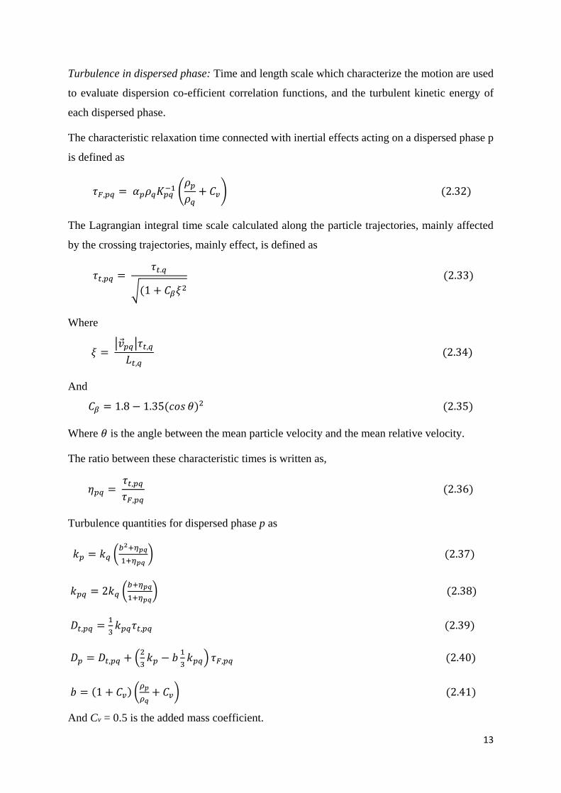
Turbulence in dispersed phase: Time and length scale which characterize the motion are used

to evaluate dispersion co-efficient correlation functions, and the turbulent kinetic energy of

each dispersed phase.

The characteristic relaxation time connected with inertial effects acting on a dispersed phase p

is defined as

𝜏𝐹,𝑝𝑞 = 𝛼𝑝𝜌𝑞𝐾𝑝𝑞−1 (

𝜌𝑝

𝜌𝑞+ 𝐶𝑣) (2.32)

The Lagrangian integral time scale calculated along the particle trajectories, mainly affected

by the crossing trajectories, mainly effect, is defined as

𝜏𝑡,𝑝𝑞 = 𝜏𝑡.𝑞

√(1 + 𝐶𝛽𝜉2

(2.33)

Where

𝜉 = |�⃗�𝑝𝑞|𝜏𝑡,𝑞

𝐿𝑡,𝑞 (2.34)

And

𝐶𝛽 = 1.8 − 1.35(𝑐𝑜𝑠 𝜃)2 (2.35)

Where 𝜃 is the angle between the mean particle velocity and the mean relative velocity.

The ratio between these characteristic times is written as,

𝜂𝑝𝑞 = 𝜏𝑡,𝑝𝑞

𝜏𝐹,𝑝𝑞 (2.36)

Turbulence quantities for dispersed phase p as

𝑘𝑝 = 𝑘𝑞 (𝑏2+𝜂𝑝𝑞

1+𝜂𝑝𝑞) (2.37)

𝑘𝑝𝑞 = 2𝑘𝑞 (𝑏+𝜂𝑝𝑞

1+𝜂𝑝𝑞) (2.38)

𝐷𝑡,𝑝𝑞 =1

3𝑘𝑝𝑞𝜏𝑡,𝑝𝑞 (2.39)

𝐷𝑝 = 𝐷𝑡,𝑝𝑞 + (2

3𝑘𝑝 − 𝑏

1

3𝑘𝑝𝑞) 𝜏𝐹,𝑝𝑞 (2.40)

𝑏 = (1 + 𝐶𝑣) (𝜌𝑝

𝜌𝑞+ 𝐶𝑣) (2.41)

And Cv = 0.5 is the added mass coefficient.

14

2.5. Numerical Methodology:

In ANSYS FLUENT control-volume based technique is used to convert a general scalar

transport equation to an algebraic equation that is solved numerically. This control volume

technique consists of integrating the transport equation about each control volume, resulting in

a discrete equation that expresses the conservation law on a control-volume basis.

2.5.1. Geometry and Mesh:

Two numbers of two dimensional computational geometries, one without distributor and the

other with distributor and a three dimensional computational geometry without distributor of

the fluidization column have been generated by using DESIGN MODELLER available in

ANSYS software. Fig.2.1. shows the line diagram of the fluidized beds used in simulation.

After the creation of geometry of the fluidized bed meshing has been done for each of the

geometry. The meshes of various geometries are shown in Fig. 3.4. Detail of the type, size and

number of elements with different computational meshes are listed in the Table 2.1.

Fig. 2.1. Line diagram of computational geometry fluidized bed

15

Fig. 2.2. 2D mesh generated in meshing

Table 2.1. Meshing configuration used in the computations of fluidized bed

2.5.2. Boundary and initial conditions:

In order to obtain a well-posed system of equations, reasonable boundary conditions for the

computational domain have to be implemented. Inlet boundary condition is a uniform liquid

and gas velocity at the inlet, and outlet boundary condition is the pressure boundary condition,

which is set as 1.013×105 Pa. Wall boundary conditions are no-slip boundary conditions for

the liquid phase and free slip boundary conditions for the solid phase and the gas phase. The

higher viscous effect and higher velocity gradient near the wall have been dealt with the

standard wall function method. At initial condition the solid volume fraction of 0.55 for

polypropylene beads of the static bed height of column has been used and the volume fraction

2D fluidized bed

Mesh type Quadrilateral mesh

Element size 0.005 m 0.0075

Number of Node 15834 18574

Number of Element 7520 9250

16

of the gas at the inlet and in the free board region is based on the inventory. Table 2.2 represents

the detail description of the boundary and initial conditions used in simulation.

Table 2.2. Description of systems used in simulation

Diameter of column: 0.1 m

Height of column: 1.88 m

Solid phase Polypropylene beads

Particle size, mm: 8

Particle density, Kg/m3: 1133

Superficial liquid velocity: 0.01 to 0.06 m/s

Static bed voidage: 0.247

Superficial gas velocity: 0.003 to 0.006 m/s

Liquid phase (water), 300˚C

Viscosity, Pas: 7.98x10-4

Density, Kg/m3: 995.7

Gas phase (air), 300˚C

Viscosity, Pas: 1.794x10-5

Density, Kg/m3: 1.166

17

CHAPTER 3

RESULT AND DISCUSSION

In the present work attempt has been made to study the effect of grid size (0.005 m and 0.074

m) and viscous model (Laminar and K-Epsilon Model) on hydrodynamics behavior of three

phase fluidized bed with low density solid particles. Result obtained were discussed below.

Bed pressure drop: Fig 3.1 shows that the bed pressure drop depends upon both gas and

liquid velocity. The observations have been seen that bed pressure drop increases when gas

velocity increases. At constant water velocity, the bed pressure drop decreases as gas velocity

increased. When gas velocity is very low there has been very less change in bed pressure drop

because at very low gas velocity the fluidization process behave like solid-liquid fluidization.

As we increases the superficial liquid velocity at constant gas velocity, initially there have been

some increment in the bed pressure drop but when the process tends to steady state, the rate of

change of bed pressure drop tends to zero.

Fig.3.1. Variation of bed pressure drop (Pa) with liquid velocity (m/s) at constant air

velocities (m/s) for 8 mm Polypropylene beads at Hs= 0.247 m and grid size 0.0075m using

laminar model.

-500

-400

-300

-200

-100

0

100

200

0.01 0.02 0.03 0.04 0.05 0.06

Bed

pre

ssu

re d

rop

(P

a)

water velocity, (m/s)

ug 0.003

ug 0.006

ug 0.009

ug 0.012

18

In fig 3.2 shows that the behaviour of bed pressure drop in the fluidized column having 0.005m

as grid size with step change (0.01 m/s) in the liquid velocity at constant gas velocity the

following graph gives us the idea that at lower velocity (0.003 m/s) the variation of bed pressure

drop gives nearly straight line graph and the curve behaviour of the bed pressure drop can be

found by increasing gas velocity.

Fig 3.2Variation of bed pressure drop (Pa) with liquid velocity (m/s) at constant air

velocities (m/s) for 8 mm Polypropylene beads at Hs= 0.247 m and grid size 0.005m using

laminar model.

Fig 3.3 and fig 3.4 shows us the comparison of bed pressure drop to laminar and turbulent

model.at different grid size (0.005 and 0.0075m) It has been seen that the at particular gas

velocity the laminar and turbulent model behaves quite similarly. At particular constant gas

velocity (0.003 and 0.006 m/s) the laminar and turbulent model phenomena shows the

overlapping which defines that we can choose any model either laminar or turbulent for the

current case. In the grid size of 0.005m the bed pressure drop gives straight line behaviour

rather than the grid size 0.0075m which shows curve behaviour. Fig 3.4 shows that at higher

liquid velocity bed pressure drop line becomes more and more stagnant.

-500

-300

-100

100

300

500

700

0.01 0.02 0.03 0.04 0.05 0.06

Bed

pre

ssu

re d

ro

p,

(Pa

)

water velocity, (m/s)

ug0.003

ug 0.006

ug 0.009

ug 0.012

19

Fig 3.3 Comparison of bed pressure drop (Pa) between laminar and turbulent model with

liquid velocity (0.01 to 0.06m/s) at constant air velocities (m/s) for 8 mm Polypropylene

beads at Hs= 0.247 m and grid size 0.005m.

Fig 3.4 Comparison of bed pressure drop (Pa) between laminar and turbulent model with

liquid velocity (0.01 to 0.06m/s) at constant air velocities (m/s) for 8 mm Polypropylene

beads at Hs= 0.247 m and grid size 0.0075m.

-100

0

100

200

300

400

500

600

700

0.01 0.02 0.03 0.04 0.05 0.06

Bed

pre

ssu

re d

rop

(P

a)

water velocity (m/s)

L-ug 0.003

L-ug 0.006

T-ug 0.003

T-ug 0.006

-100

-50

0

50

100

150

200

0.01 0.02 0.03 0.04 0.05 0.06

Bed

pre

ssu

re d

rop

(Pa

)

water velocity(m/s)

L-ug 0.003

L-ug 0.006

T-ug 0.003

T-ug 0.006

20

Gas holdup: Gas holdup is obtained as mean-area weighted average of volume fraction of air

at sufficient number of points in the fluidized part of the bed. Since the volume fraction of air

phase is not the same at all points in the fluidized part of the column, hence an area weighted

average of volume fraction of air determined at regular height till the fluidized part is over.

When these values are averaged it gives the required gas holdup. The following fig 3.5 and 3.6

shows that the gas hold up value has been decreasing due to increasing in water velocity at

constant gas velocity. It also shows that the gas hold up value increases in the increment of gas

velocity at constant liquid velocity.

Fig 3.5 Variation of gas holdup with liquid velocity (m/s) at constant air velocities (m/s)

for 8 mm Polypropylene beads at Hs= 0.247 m and grid size 0.005m using laminar model.

0

0.05

0.1

0.15

0.2

0.25

0.3

0.35

0.4

0.01 0.02 0.03 0.04 0.05 0.06

Gas

ho

ld u

p

water velocity(m/s)

ug 0.003

ug 0.006

ug 0.009

ug 0.012

21

Fig 3.6 Variation of gas holdup with liquid velocity (m/s) at constant air velocities (m/s)

for 8 mm Polypropylene beads at Hs= 0.247 m and grid size 0.0075m using laminar model.

Fig 3.7 and 3.8 shows that the comparison of laminar and turbulent model at a constant gas

velocity. It has been seen that the lines of viscous laminar and turbulent model (k-epsilon)

obtained from plot of gas hold up to water velocity, the obtained lines are quite overlapping to

each other. Or shows very similar behavior. It also shows that at lower water velocity the value

of gas holdup is higher and as the water velocity increases gas hold up start to decrease. The

comparison graph also shows that, at constant gas velocity the values of bed pressure drop is

higher in viscous laminar model compare to turbulent model (k-epsilon).

0

0.005

0.01

0.015

0.02

0.025

0.03

0.035

0.01 0.02 0.03 0.04 0.05 0.06

Ga

s h

old

up

water velocity(m/s)

ug 0.003

ug 0.006

ug 0.009

ug 0.012

22

Fig 3.7 Comparison of gas holdup between laminar and turbulent model with liquid velocity (0.01

to 0.06m/s) at constant air velocities (m/s) for 8 mm Polypropylene beads at Hs= 0.247 m and grid

size 0.0075m.

Fig 3.8 Comparison of gas holdup between laminar and turbulent model with liquid velocity

(0.01and 0.06m/s) at constant air velocities (m/s) for 8 mm Polypropylene beads at Hs= 0.247 m

and grid size 0.005m.

0

0.002

0.004

0.006

0.008

0.01

0.012

0.014

0.016

0.018

0.02

0.01 0.02 0.03 0.04 0.05 0.06

Ga

s h

old

up

water velocity (m/s)

L-ug 0.003

L-ug 0.006

T-ug 0.003

T-ug 0.006

0

0.025

0.05

0.075

0.1

0.125

0.15

0.175

0.2

0.225

0.25

0.275

0.01 0.02 0.03 0.04 0.05 0.06

Ga

s h

old

up

water velocity(m/s)

L-ug 0.003

L-ug 0.006

T-ug 0.003

T-ug 0.006

23

In Fig 3.9 it shows the grid indecency of laminar model at constant gas velocity. Grid size of 0.005 and

0.0075m have been taken in to problem. Changing the grid size means changing the number of elements

and nodes, if we go for lower grid size (0.005m) the number of nodes and elements are larger than the

0.0075m grid size, hence more number of nodes and element take more time to simulate but it has more

accuracy than lower grid size.

Fig 3.9 Comparison of air hold up between grid size 0.005-0.0075m with liquid velocity (0.01 to

0.06m/s) at constant air velocities (m/s) for 8 mm Polypropylene beads at Hs= 0.247 m with

laminar model.

Bed height: Bed starts to expand when the fluid velocity is higher than the minimum

fluidization velocity. The minimum fluidization velocity is obtained when the buoyancy force

working on the particle has been balanced by the weight of the particle, after that bed starts to

fluidise, this condition is also known as minimum condition for fluidization When the bed starts

to fluidized XY plot of bed height to liquid velocity shows that the bed height expands when

the fluid velocity increases. The graph also shows that at constant water velocity bed expansion

occurs due to increase in gas velocity.

0

0.025

0.05

0.075

0.1

0.125

0.15

0.175

0.2

0.225

0.25

0.01 0.02 0.03 0.04 0.05 0.06

Gas

hold

up

water velocity (m/s)

L-0.005 ug 0.003

L-0.005-ug 0.006

L-0.0075-ug 0.003

L-0.0075-ug 0.006

24

Fig 3.10 Variation of bed height (m) with liquid velocities (m/s) at constant gas velocities (m/s) for

8 mm polypropylene beads at Hs= 0.247m, grid size 0.0075m and laminar model.

Fig 3.10 is the comparison of bed height variations in two different modeling viscous laminar

and turbulent (k-epsilon). Data has been obtained and plotted in XY. Plotted data shows that

the behavior of laminar and turbulent are not much of different, which shows that for my

current operating conditions we have liberty to choose any of the model because they both

show similar behavior.

Fig 3.11 Comparison of bed height between laminar and turbulent model with liquid velocity

(0.01 to 0.06m/s) at constant air velocities (m/s) for 8 mm Polypropylene beads at Hs= 0.247 m

and grid size 0.0075m.

0

0.1

0.2

0.3

0.4

0.5

0.6

0.7

0.01 0.02 0.03 0.04 0.05 0.06

Bed

hei

gh

t(m

)

water velocity (m/s)

ug 0.003

ug 0.006

ug 0.009

ug 0.012

0

0.1

0.2

0.3

0.4

0.5

0.6

0.7

0.01 0.02 0.03 0.04 0.05 0.06

Bed

hei

gh

t (m

)

water velocity (m/s)

L-ug 0.003L-ug 0.006T-ug 0.003T-ug 0.006

25

Chapter 4

Conclusion and future work

CFD simulation of hydrodynamics of gas-fluid-solid fluidized bed have been carried out for

distinctive working conditions by utilizing the Eulerian-Eulerian granular multiphase

methodology. The hydrodynamic parameters contemplated are gas hold up, bed extension and

bed pressure drop. Distinctive examination diagrams have been indicated underneath for the

dissection of progress gas hold up, bed expansion and bed pressure drop in different models

(laminar and turbulent) and different mesh sizes (0.005 and 0.0075m).

Plots of bed pressure drop vs. inlet air speed at different inlet water speed shows that bed

pressure drop decreases as air speed has been increased. At constant water velocity, the bed

pressure drop decreases as gas velocity increased. Additionally when the air speed is little

(Ug=0.003 m/s) there is no considerable build in bed pressure drop. This could be described in

that way that at very little air velocity the operation behaves liquid-solid fluidization Plots of

gas hold up and fluid velocity shows that the value of gas holdup has been decreasing due to

increasing in water velocity at constant gas velocity. It also shows that the gas hold up value

increases in the increment of gas velocity at constant liquid velocity. When the bed starts to

fluidized XY plot of bed height to liquid velocity shows that the bed height expands when the

fluid velocity increases. The graph also shows that at constant water velocity bed expansion

occurs due to increase in gas velocity.

Future work:

Analysis of Impact of distributor plate on hydrodynamics properties of three-phase

fluidized bed with low density solid particles needs to be done.

CFD study on the effect of different static bed height on hydrodynamics of fluidized

bed for low density material needs to be done.

Beside Eulerian multiphase phase model, discrete phase model need to be apply to

solid and gas phase.

26

References

Allia, K., Tahar, N., Toumi, L., Salem, Z., 2006. Biological treatment of water contamination

by hydrocarbon in three-phase gas-liquid-solid fluidized bed. Global NEST Journal, Vol-8

(1), 9 – 15.

Annaland, M., S., Deen, N., G., Kuipers, J., A., M., 2005. Numerical simulation of gas–liquid–

solid flows using a combined front tracking and discrete particle method. Chemical

Engineering Science 60, 6188 – 6198.

Bunner, B., Tryggvason, G., 1999. Direct numerical simulations of dispersed flows. In:

Proceedings of the Ninth Workshop on Two-Phase Flow Predictions, Germany, 13 – 19.

Glover G.M.C, Generalis S., C., 2004. Gas-liquid-solid flow modelling in a bubble column.

Chemical Engineering and Processing 43,117 – 126.

Cao, C., Liu, M., Wen, J., Guo, Q., 2009. Experimental measurement and numerical simulation

for liquid flow velocity and local phase hold-ups in the riser of a GLSCFB. Chemical

Engineering and Processing: Process Intensification 48, 288 – 295.

Chen, C., Fan, L.S., 2004. Discrete Simulation of Gas-Liquid Bubble Columns and Gas-

Liquid-Solid Fluidized Beds. AIChE Journal 50, 288 – 301.

Cheung, S.C.P., Yeoh, G.H., Tu, J.Y., 2007.On the numerical study of isothermal vertical

bubbly flow using two population balance approaches.Chem.Eng.Sci.62, 4659 – 4674.

Feng, W., Wen, J., Fan, J., Yuan, Q., Jia, X., Sun, Y., 2005. Local hydrodynamics of gas-liquid-

nanoparticles three-phase fluidization. Chemical Engineering Science 60, 6887 – 6898.

Fan, L.S., 1989. Gas-Liquid-Solid Fluidization Engineering. Butterworth Series in Chemical

Engineering, Butterworth Publishers, Boston, MA.

Fluent 6.2.16. Fluent 6.2.16 User’s Guide, Fluent Inc. 2004.

Rafique, M., Chen, P., Dudukovic, M., 2004. Computational modeling of gas-liquid flow in

bubble columns. Reviews in Chemical Engineering 20, 225–375.

Rajasimman, M., Karthikeyan, C., 2006. Aerobic digestion of starch wastewater in a fluidized

bed bioreactor with low density biomass support. Journal of Hazardous Materials 143, 82 – 86.

27

Schallenberg, J., Enß, J., H., Hempel, D., C., 2005. The important role of local dispersed phase

hold-ups for the calculation of three-phase bubble columns. Chemical Engineering Science 60,

6027 – 6033.

Shah, Y.T., 1979. Gas-liquid-solid reactor design. McGraw-Hill, New York.

Sivaguru, K., Begum K., M., Anantharaman, N., 2009. Hydrodynamic studies on three-phase

fluidized bed using CFD analysis. Chemical Engineering Journal 155, 207 – 214.

Sokół, W., Halfani, M.R., 1999.Hydrodynamics of a gas-liquid-solid fluidized bed bioreactor

with a low density biomass support. Biochemical Engineering Journal 3, 185 – 192.

Sokół, W., 2001. Operating parameter for a gas-liquid-solid fluidized bed bioreactor with a low

density biomass support. Biochemical Engineering Journal 8, 203 – 212.

Sokół, W., Korpal, W., 2004.Determination of the optimal operational parameters for a three-

phase fluidized bed bioreactor with a light biomass support when used in treatment of phenolic

waste waters. Biochemical Engineering Journal 20, 49 – 56.

Sokolichin, A., Eigenberger, G., Lapin, A., 2004. Simulation of buoyancy driven bubbly flow:

established simplifications and open questions. AIChE Journal 50, 24 – 45.

Wild, G., Poncin, S., 1996. Chapter 1: Hydrodynamics. In: Three-Phase Sparged Reactors,

Nigam, K.D.P., and Schumpe, A., ed., Gordon and Breach Publishers, Amsterdam, The

Netherlands.

Wiemann, D., Mewes, D., 2005. Calculation of flow fields in two and three-phase bubble

columns considering mass transfer. Chemical Engineering Science 60, 6085 – 6093.

Zhang, J., 1996. Bubble Columns and Three-Phase Fluidized Beds: Flow Regimes and Bubble

Characteristics, PhD thesis, UBC, Vancouver.

Zhang, J., Li, Y., Fan, L., S., 2000a. Numerical studies of bubble and particle dynamics in a

three-phase fluidized bed at elevated pressures. Powder Technology 112, 46 – 56.

Zhang, J., Li, Y., Fan, L., S., 2000b. Discrete phase simulation of gas-liquid-solid fluidization

systems: single bubble rising behavior. Powder Technology 113, 310 – 326.