CFD Modeling of Gas Release and Dispersion: Prediction of Flammable Gas Clouds

1 Journal Information © 2005 Springer. Printed in the Netherlands.

CFD MODELING OF GAS RELEASE AND DISPERSION:

PREDICTION OF FLAMMABLE GAS CLOUDS

VLADIMIR M. AGRANAT*, ANDREI V. TCHOUVELEV, ZHONG CHENG A.V. Tchouvelev & Associates Inc., 6591 Spinnaker Circle, Mississauga, Ontario, L5W 1R2, Canada

SERGEI V. ZHUBRIN Flowsolve Limited, 2nd Floor, 40 High Street, Wimbledon Village, London SW19 5AU, United Kingdom

Abstract. Advanced computational fluid dynamics (CFD) models of gas release and dispersion (GRAD) have been developed, tested, validated and applied to the modeling of various industrial real-life indoor and outdoor flammable gas (hydrogen, methane, etc.) release scenarios with complex geometries. The user-friendly GRAD CFD modeling tool has been designed as a customized module based on the commercial general-purpose CFD software, PHOENICS. Advanced CFD models available include the following: the dynamic boundary conditions, describing the transient gas release from a pressurized vessel, the calibrated outlet boundary conditions, the advanced turbulence models, the real gas law properties applied at high-pressure releases, the special output features and the adaptive grid refinement tools. One of the advanced turbulent models is the multi-fluid model (MFM) of turbulence, which enables to predict the stochastic properties of flammable gas clouds. The predictions of transient 3D distributions of flammable gas concentrations have been validated using the comparisons with available experimental data. The validation matrix contains the enclosed and non-enclosed geometries, the subsonic and sonic release flow rates and the releases of various gases, e.g. hydrogen, helium, etc. GRAD CFD software is recommended for safety and environmental protection analyses. For example, it was applied to the hydrogen safety assessments including the analyses of hydrogen releases from pressure

______ *To whom correspondence should be addressed. Vladimir Agranat, 6591 Spinnaker Circle,

Mississauga, Ontario, L5W 1R2, Canada; e-mail: [email protected] and [email protected]

CFD MODELING OF GAS RELEASE AND DISPERSION 2

relief devices and the determination of clearance distances for venting of hydrogen storages. In particular, the dynamic behaviors of flammable gas clouds (with the gas concentrations between the lower flammability level (LFL) and the upper flammability level (UFL)) can be accurately predicted with the GRAD CFD modeling tool. Some examples of hydrogen cloud predictions are presented in the paper. CFD modeling of flammable gas clouds could be considered as a cost effective and reliable tool for environmental assessments and design optimizations of combustion devices. The paper details the model features and provides currently available testing, validation and application cases relevant to the predictions of flammable gas dispersion scenarios. The significance of the results is discussed together with further steps required to extend and improve the models.

Keywords: Computational fluid dynamics (CFD); numerical modeling tool; flammable gas cloud; gas release and dispersion; environmental protection and safety analyses; clearance distance

1. Introduction

In many industries, there are serious safety concerns related to the use of flammable gases in indoor and outdoor environments. It is very important to develop reliable methods of analyses of flammable gas release and dispersion (GRAD) in real-life complex geometry cases. Computational fluid dynamics (CFD) is considered as one of the promising cost-effective approaches in such analyses. The objective of this paper is to describe the advanced GRAD CFD models, which have been recently developed, tested, validated and applied to the modeling of various industrial indoor and outdoor scenarios of releases of flammable gases (hydrogen, methane, natural gas, etc.) in domains with complex geometries.

There are many general-purpose commercial CFD software packages capable of modeling and analyses of fluid flows and heat/mass transfer processes, e.g. the PHOENICS software1. However, none of these packages is properly customized for GRAD modeling and analyses of spatial and temporal behaviors of flammable gas clouds. In particular, any direct practical application of these codes to GRAD modeling requires a high level of user’s expertise in CFD field due to the complexities of physical processes involved and mathematical models analyzed. Moreover, in the GRAD modeling, proper non-standard settings are needed for transient boundary conditions, real gas properties, special numerical grid refinements and proper turbulence models. As


a result, there is a practical need for developing a user-friendly and validated GRAD CFD modeling tool, which is capable of predicting the behaviors of flammable gas clouds.

Over the last three years, significant efforts have been undertaken by Stuart Energy Systems Corporation (SESC) and A.V. Tchouvelev & Associates Inc. in order to develop, test and validate a GRAD CFD modeling tool. Some results of this work have been recently published2-8. This paper reviews the previously published results, describes the modeling approach in more detail and provides currently available validation and application cases relevant to the predictions of flammable gas dispersion scenarios.

2. GRAD CFD modeling tool capabilities

The GRAD CFD modeling tool has been designed as a customized module based on the commercial general-purpose CFD software, PHOENICS1. The modeling approach, the general governing equations and the additional sub-models are described in this section. Also, the similarity theory is described.

2.1. MODELING APPROACH

PHOENICS CFD software was selected as the flexible framework for performing GRAD CFD analyses, in which pragmatic flammable gas release and dispersion models were incorporated for practically affordable predictions using the PHOENICS solvers. PHOENICS is a well-recognized general-purpose CFD package that has been validated and successfully used around the world for more than 20 years. Its main features and capabilities have been described by its developers, CHAM Limited, in references item8 and on the CHAM’s web site, www.cham.co.uk. One of the key features of PHOENICS is its easy programmability, i.e. it enables a user to add user-defined sub-models without a direct use of programming languages such as FORTRAN or C. This feature was used to incorporate the non-standard advanced GRAD sub-models described in section 2.3.

There are three major stages in GRAD modeling: 1) steady-state before-the-release run aimed at preparing the initial 3D distributions of pressure and velocity in the computational domain; 2) transient during-the-release run made to describe the spatial and temporal behaviors of flammable gas cloud during the gas release; and 3) transient after-the-release run aimed at predicting the dispersion of the released gas to acceptable levels within the computational domain. First, the modeling is performed under steady-state conditions without any flammable gas leak. The velocity and pressure profiles obtained from the steady-state calculations are then used as the initial conditions for the during-


the-release transient simulations, which are performed with a flammable gas leak at the specified rate and time increments. After-the-release transient simulations predict the flammable gas dispersion in the computational domain below the required values of volume concentrations of flammable gas (usually below the Lower Flammability Level (LFL)). It should be noted that both the during-the-release and the after-the-release transient simulations allow for: (i) inclusion of the transient behavior of all calculated variables (pressure, gas density, velocity and flammable gas concentration); (ii) simulation of the movement of flammable gas clouds with time; as well as, (iii) evaluation of the safety by analyzing the iso-surfaces of the flammable gas concentration. The flammable gas convection, diffusion, buoyancy and transience are modeled based on the general 3D conservation equations and the details of various release and dispersion scenarios are introduced via the proper initial and boundary conditions. One of the advantages of PHOENICS is that it contains various turbulence models and enables to select a proper model suitable for a particular practical case. In particular, the unique to PHOENICS turbulence models such as the LVEL model and the multi-fluid model of turbulence (MFM) were tested in the GRAD modeling.

2.2. GOVERNING EQUATIONS

The transient processes of flammable gas convection, diffusion and buoyancy are governed by the general conservation equations, i.e. the momentum equations, the continuity equation and the flammable gas mass conservation equation. These governing equations are well described in the PHOENICS documentation1 and could be expressed as:

,)()(

ii

ieffii f

xPgraduUudiv

tu

ρρνρρ

+∂∂−=−+

∂∂ i=1,2,3 (1)

0)( =+∂∂

Udivt

ρρ , (2)

")()(

CgradCDUCdivtC

eff =−+∂

∂ ρρρ , (3)

where 1x , 2x and 3x denote the Cartesian coordinates; 1u , 2u and 3u are the velocity components; U is the velocity vector; if ( 3,2,1=i ) is the body force component (per unit mass) in the ix - direction; P is the gas mixture pressure; C is the mass concentration of flammable gas; "C is the flammable gas source;

effD is the effective flammable gas diffusion coefficient in air; effν is the


effective kinematic viscosity of gas mixture and ρ is the gas mixture density, which is dependent on the flammable gas mass concentration, C, or the flammable gas volumetric concentration ,α :

TRCCRP

airgas ])1([ −+=ρ ,

airgas

gas

RCCRCR

)1( −+=α

(4)

Here, T is the absolute temperature; and gasR and airR are the gas constants of flammable gas and air, respectively.

The volumetric buoyancy force, acting on the fluid particles in the 3x - direction (vertical direction), is represented by the term, 3fρ , in equation (1). Its significance is proportional to the difference between the local transient gas mixture density and the reference density of air under the ambient pressure and temperature. According to the first equation (4), the gas mixture density is calculated as an inverse-linear function of the local mass concentration of flammable gas, C, with the coefficients dependent on the gas constants of air and flammable gas and the local pressure and temperature. As a result, the significance of the buoyancy force depends on the transient 3D flammable gas mass concentration distribution.

The local values of effective viscosity and diffusion coefficient, effν and effD , include both laminar and turbulent components and are calculated

according to the following equations:

ttllefftleff D Pr/Pr/, ννννν +=+= (5)

Here, subscripts l and t are applied to the laminar and turbulent properties, respectively; and Pr is the Prandtl/Schmidt number.

The laminar kinematic viscosity of gas mixture can be approximated by:

ρνραναρν /])1([ airairgasgasl −+= (6)

Here, gasν and airν are the laminar kinematic viscosities of flammable gas and air, respectively; and gasρ and airρ are the densities of flammable gas and air, respectively.

A proper turbulence model was used in each particular practical case in order to calculate the local values of turbulent kinematic viscosity, tν . Among models used were the LVEL model, the k-ε model, the modifications of k-ε model and the MFM.


2.3. ADVANCED MODEL FEATURES

A few advanced CFD sub-models were developed as a part of GRAD CFD module. These sub-models simulate the following features: the dynamic boundary conditions, describing the transient gas release from a pressurized vessel; the calibrated outlet boundary conditions; the real gas law properties applied at high-pressure releases; the advanced turbulence models; the adaptive grid refinement tools; and the special output features.

2.3.1. Dynamic Boundary Conditions

In general, the transient (dynamic) boundary conditions should be applied at the flammable gas release location in order to properly describe the released gas mass flow rate, which depends on time. Depending on the pressure in the gas storage tank, the regime of release could be subsonic or sonic (choked). Assuming the ideal gas law equation of state and a critical temperature at the leak orifice and solving the first-order ordinary differential equation for density,

)(tρ , the transient mass flow rate at the sonic regime of release could be approximated as6

,)()()(11

)1

2(V

AC

0

RTtd

emAtutdtdVtm

−+

+−

≈=−=γγ

γγ

ρρ&&

11

000 )1

2( −+

+= γ

γ

γγρ PACm d& (7)

where u(t) is the flammable gas velocity at the leak orifice; V is the tank

volume; 0m& , 0ρ and 0P are the flammable gas mass flow rate, the gas density in the tank and the gas pressure in the tank, respectively, at t=0; A is the leak orifice cross-sectional area; Cd is the discharge coefficient; and γ is the ratio of specific heats for flammable gas:

V

PC

C=γ , with PC and VC being the

specific heat at constant pressure and constant volume, respectively. For example, for hydrogen, 41.1=γ and the initial hydrogen mass release rate corresponding to the tank with a pressure of 400 bars and a ¼” leak orifice is

about =0m& 0.753 kg/s, based on the second equation (7) with Cd = 0.95. It should be noted that the choked release lasts until the ratio of the pressure in the


tank over the ambient pressure, namely, atmP

P0 is greater than or equal to

1)2

1( −+ γγγ (it is about 1.90 for hydrogen).

2.3.2. Real Gas Law Properties

Under high pressure, flammable gases display gas properties different from the ideal gas law predictions. For example, at ambient temperature of 293.15˚K and a pressure of 400 bars, the hydrogen density is about 25% lower than that predicted by the ideal gas law. In order to account for real gas law behavior, the GRAD CFD module was provided with additional sub-models6. In particular, for hydrogen release and dispersion modeling the Abel-Nobel equation of state (AN-EOS) was used to calculate the hydrogen compressibility,

2Hz , in terms of empirical hydrogen co-density, dH2 :

1)1(2

2

22

2

−−==H

H

HHH dTR

Pzρ

ρ, (8)

where ρ2H , P, T and RH2 are the compressed hydrogen density, pressure,

temperature and gas constant, respectively. It should be noted that the hydrogen compressibility, 2Hz , is equal to 1 for the ideal gas law. The hydrogen gas constant, RH2, is 4124 J/(kgK). The hydrogen co-density, dH2 , is about 0.0645 mol/cm3, or 129 kg/m3. Equation (8) can be simplified as:

TRdPz

HHH

22

21+= (9)

The AN-EOS accounts for the finite volume occupied by the gas molecules, but it neglects the effects of intermolecular attraction or cohesion forces. It accurately predicts the high-pressure hydrogen density behavior6.

2.3.3. Turbulence Model Settings

The turbulence models tested for GRAD modeling cases were as follows: LVEL model, k-ε model, k-ε RNG model, k-ε MMK model and MFM. It was found that the LVEL model performs better in releases of flammable gas in congested spaces (indoor environment containing the solid blockages) and the k-ε RNG model performs better for jet releases in open space. The details on sensitivity runs related to the turbulence model selection are described in previous papers2-8. MFM enables to predict the stochastic properties of flammable gas clouds by way of computing the probability density functions,


which record for what proportion of time the fluid at a point in space is in a given state of motion, temperature and composition. However, the MFM approach needs to be further developed for GRAD CFD modeling, with the aim of finding a proper set of model constants and/or functions, which are suitable for the prediction of turbulent flammable gas dispersion in both indoor and outdoor environment.

2.3.4. Local Adaptive Grid Refinement (LAGR)

The LAGR techniques are needed in GRAD CFD modeling in order to accurately capture the flammable cloud behaviors near the release location and in the locations with significant gradients of flammable gas concentration while considering large domains of practical interest. This refinement should be based on the local features of flammable gas mass concentration as a key unknown variable. The iterative technique of LAGR was developed, implemented into the PHOENIS CFD software, tested and validated for the two GRAD CFD module validation cases, namely, the hydrogen release within a hallway, and the helium release within a garage with a car. The results of LAGR modeling were more accurate than the fixed grid solutions obtained with the standard grid refinement tools (see details in sections 3.2 and 3.3). However, additional development work and testing are needed in order to use LAGR on regular basis for GRAD modeling.

2.3.5. Special Output Features

The dynamics and extents of flammable gas cloud, containing the gas volume concentrations between LFL and UFL, are of major interest in any GRAD modeling. The total volume of space occupied by this cloud and the total mass of flammable gas in the cloud are listed as the special output features. GRAD CFD module calculates these special output quantities as functions of time based on the transient 3D distributions of gas concentrations and gas mixture density.

2.4. SIMILARITY THEORY

The solutions of GRAD governing equations under the prescribed boundary conditions and properties depend on the following dimensionless parameters: the Reynolds number (Re), the Schmidt number (Sc), the Mach number (Ma), the Richardson number (Ri) and the density ratio ( ρk ), which are defined as follows to represent the turbulence, diffusion, compressibility, buoyancy and density difference effects, respectively:


gas

gas LUν

=Re , gas

gas

DSc

ν= ,

WU

Ma gas= , 2

)(

gasgas

gasair

U

gLRi

ρρρ −

= , gas

airkρρ

ρ = .

(10)

Here gasU is the flammable gas release velocity at the orifice; L is the orifice size; gasν is the laminar kinematic viscosity of the released gas (1.05×10-4 m2/s

for hydrogen and 1.15×10-4 m2/s for helium); gasD is the laminar diffusion coefficient of the released gas in the air (6.1×10-5 m2/s for hydrogen, and

5.7×10-5 m2/s for helium); airρ is the reference density, i.e. the air density, which is 1.209 kg/m3 at 1 atm and 20ºC; W is the gas sonic speed, which is

equal to 61.1305222

== TRW HHH γ m/s for hydrogen and 35.1005== TRW HeHeHe γ m/s for helium; and ρk is the parameter

characterizing the variable gas mixture density: 1))1(1( −−+= Ckair ρρρ or ))1(1( 1 αρρ ρ −+= −kair . It should be noted that L is the leak orifice diameter

for the circular orifice. If the leak orifice is not circular, a hydraulic diameter, which is defined as

perimeter. wettedarea sectionalcross 4 −×=L , is used for the scaling length.

For a rectangular leak hole with sizes of a and b, the hydraulic diameter is defined as

baabL+

= 2 .

In order to validate the CFD modeling results for hydrogen release and dispersion, proper experimental data on hydrogen release and dispersion are required. For reasons of safety, helium was often used in validation experiments as an alternative for hydrogen. However, helium and hydrogen differ in their buoyancy, turbulence, diffusion and density. This can be clearly seen from the following comparison of the dimensionless parameters (10) for these gases and the estimation of the distortions in flows of the two gases:

91.0ReRe

2

Re ==H

Heα , 17.12

==H

HeSc Sc

Scα , 30.12

==H

HeMa Ma

Maα ,

47.02

==H

HeRi Ri

Riα , 50.02,

, ==H

Hek k

k

ρ

ρρ

α

The large distortions result in significant differences in hydrogen and helium release processes: helium is less “turbulent” and “buoyant” but more “compressible” than hydrogen. The hydrogen buoyancy and turbulence effects


would be underestimated if helium were used for validation of hydrogen modeling. The choked (sonic) release velocity would be smaller and, as a result, the compressibility would be overestimated as well. Therefore, hydrogen, though combustible, has to be used for the validation of CFD modeling of hydrogen releases and dispersion. Some validation results are reported in the following section.

3. GRAD CFD Software Validation

The GRAD CFD modeling software needs to be validated before it can be widely applied to industrial projects. The predictions of transient 3D distributions of flammable gas concentrations with the GRAD CFD module were validated using the comparisons with available experimental data on gas release and dispersion.

3.1. VALIDATION MATRIX

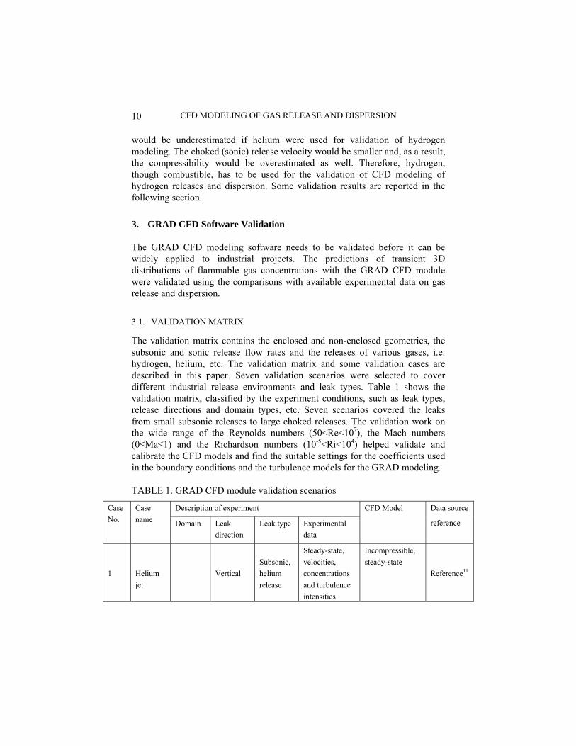
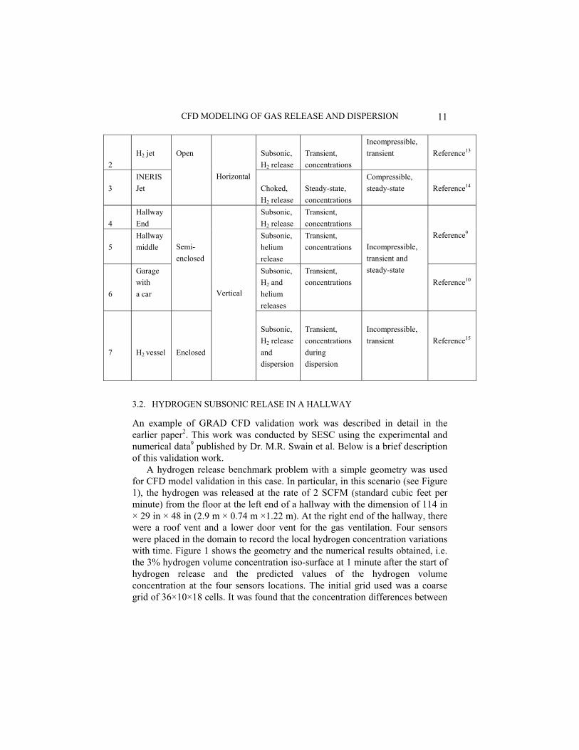
The validation matrix contains the enclosed and non-enclosed geometries, the subsonic and sonic release flow rates and the releases of various gases, i.e. hydrogen, helium, etc. The validation matrix and some validation cases are described in this paper. Seven validation scenarios were selected to cover different industrial release environments and leak types. Table 1 shows the validation matrix, classified by the experiment conditions, such as leak types, release directions and domain types, etc. Seven scenarios covered the leaks from small subsonic releases to large choked releases. The validation work on the wide range of the Reynolds numbers (50<Re<107), the Mach numbers (0≤Ma≤1) and the Richardson numbers (10-5<Ri<104) helped validate and calibrate the CFD models and find the suitable settings for the coefficients used in the boundary conditions and the turbulence models for the GRAD modeling. TABLE 1. GRAD CFD module validation scenarios

Description of experiment Case No.

Case name Domain Leak

direction Leak type Experimental

data

CFD Model Data source

reference

1

Helium jet

Vertical

Subsonic, helium release

Steady-state, velocities, concentrations and turbulence intensities

Incompressible, steady-state

Reference11


2

H2 jet

Subsonic, H2 release

Transient, concentrations

Incompressible, transient

Reference13

3

INERIS Jet

Open

Horizontal

Choked, H2 release

Steady-state, concentrations

Compressible, steady-state

Reference14

4

Hallway End

Subsonic, H2 release


5

Hallway middle

Subsonic, helium release


Reference9

6

Garage with a car

Semi-enclosed

Subsonic, H2 and helium releases


Incompressible, transient and steady-state

Reference10

7

H2 vessel

Enclosed

Vertical

Subsonic, H2 release and dispersion

Transient, concentrations during dispersion

Incompressible, transient

Reference15

3.2. HYDROGEN SUBSONIC RELASE IN A HALLWAY

An example of GRAD CFD validation work was described in detail in the earlier paper2. This work was conducted by SESC using the experimental and numerical data9 published by Dr. M.R. Swain et al. Below is a brief description of this validation work.

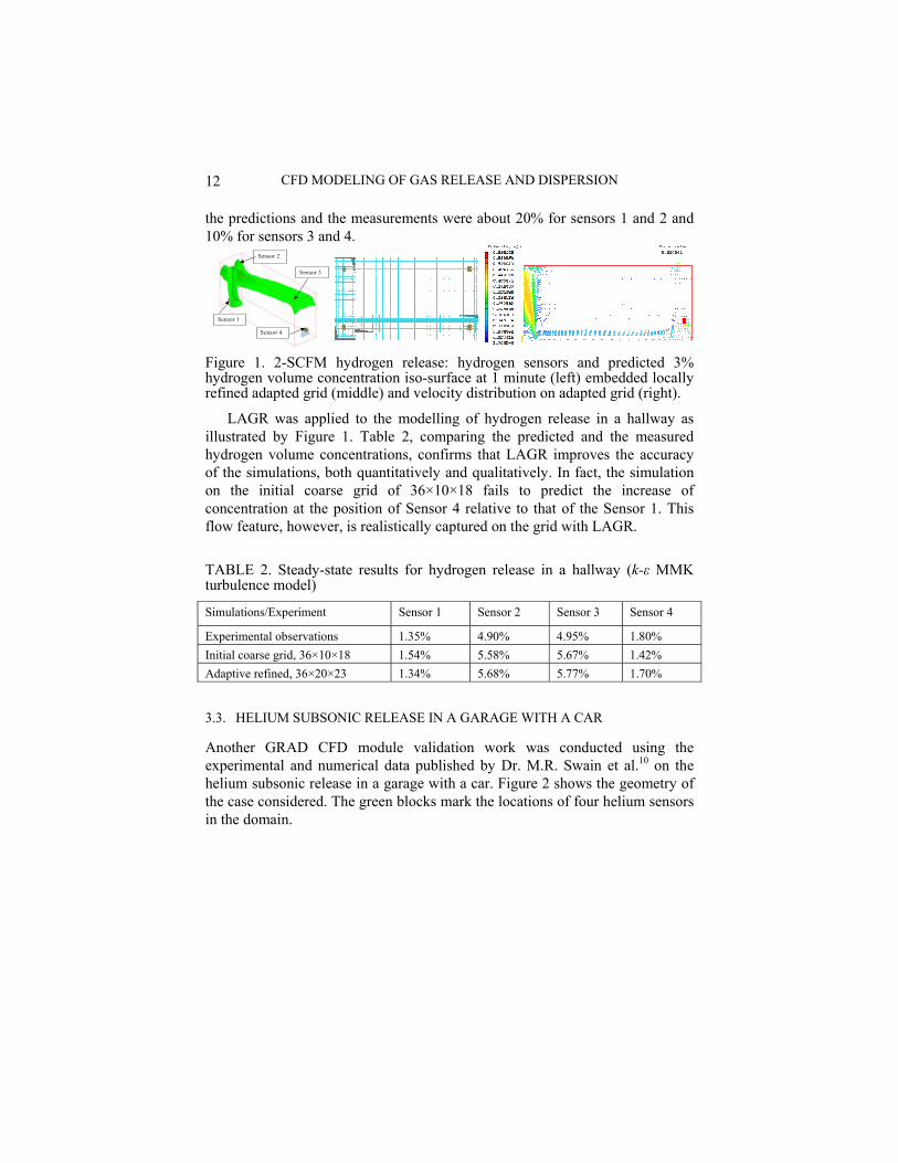
A hydrogen release benchmark problem with a simple geometry was used for CFD model validation in this case. In particular, in this scenario (see Figure 1), the hydrogen was released at the rate of 2 SCFM (standard cubic feet per minute) from the floor at the left end of a hallway with the dimension of 114 in × 29 in × 48 in (2.9 m × 0.74 m ×1.22 m). At the right end of the hallway, there were a roof vent and a lower door vent for the gas ventilation. Four sensors were placed in the domain to record the local hydrogen concentration variations with time. Figure 1 shows the geometry and the numerical results obtained, i.e. the 3% hydrogen volume concentration iso-surface at 1 minute after the start of hydrogen release and the predicted values of the hydrogen volume concentration at the four sensors locations. The initial grid used was a coarse grid of 36×10×18 cells. It was found that the concentration differences between


the predictions and the measurements were about 20% for sensors 1 and 2 and 10% for sensors 3 and 4.

Sensor 1

Sensor 2

Sensor 3

Sensor 4

Figure 1. 2-SCFM hydrogen release: hydrogen sensors and predicted 3% hydrogen volume concentration iso-surface at 1 minute (left) embedded locally refined adapted grid (middle) and velocity distribution on adapted grid (right).

LAGR was applied to the modelling of hydrogen release in a hallway as illustrated by Figure 1. Table 2, comparing the predicted and the measured hydrogen volume concentrations, confirms that LAGR improves the accuracy of the simulations, both quantitatively and qualitatively. In fact, the simulation on the initial coarse grid of 36×10×18 fails to predict the increase of concentration at the position of Sensor 4 relative to that of the Sensor 1. This flow feature, however, is realistically captured on the grid with LAGR. TABLE 2. Steady-state results for hydrogen release in a hallway (k-ε MMK turbulence model)

Simulations/Experiment Sensor 1 Sensor 2 Sensor 3 Sensor 4

Experimental observations 1.35% 4.90% 4.95% 1.80% Initial coarse grid, 36×10×18 1.54% 5.58% 5.67% 1.42% Adaptive refined, 36×20×23 1.34% 5.68% 5.77% 1.70%

3.3. HELIUM SUBSONIC RELEASE IN A GARAGE WITH A CAR

Another GRAD CFD module validation work was conducted using the experimental and numerical data published by Dr. M.R. Swain et al.10 on the helium subsonic release in a garage with a car. Figure 2 shows the geometry of the case considered. The green blocks mark the locations of four helium sensors in the domain.


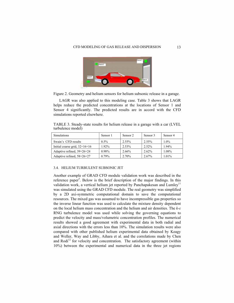
Figure 2. Geometry and helium sensors for helium subsonic release in a garage.

LAGR was also applied to this modeling case. Table 3 shows that LAGR helps reduce the predicted concentrations at the locations of Sensor 1 and Sensor 4 significantly. The predicted results are in accord with the CFD simulations reported elsewhere.

TABLE 3. Steady-state results for helium release in a garage with a car (LVEL turbulence model)

Simulations Sensor 1 Sensor 2 Sensor 3 Sensor 4

Swain’s CFD results 0.5% 2.55% 2.55% 1.0% Initial coarse grid, 32×16×16 1.92% 2.53% 2.52% 1.94% Adaptive refined, 39×26×24 0.98% 2.66% 2.62% 1.08% Adaptive refined, 58×26×27 0.79% 2.70% 2.67% 1.01%

3.4. HELIUM TURBULENT SUBSONIC JET

Another example of GRAD CFD module validation work was described in the reference paper5. Below is the brief description of the major findings. In this validation work, a vertical helium jet reported by Panchapakesan and Lumley11 was simulated using the GRAD CFD module. The real geometry was simplified by a 2D axi-symmetric computational domain to save the computational resources. The mixed gas was assumed to have incompressible gas properties so the inverse linear function was used to calculate the mixture density dependent on the local helium mass concentration and the helium and air densities. The k-ε RNG turbulence model was used while solving the governing equations to predict the velocity and mass/volumetric concentration profiles. The numerical results showed a good agreement with experimental data in both radial and axial directions with the errors less than 10%. The simulation results were also compared with other published helium experimental data obtained by Keagy and Weller, Way and Libby, Aihara et al. and the correlations made by Chen and Rodi12 for velocity and concentration. The satisfactory agreement (within 10%) between the experimental and numerical data in the three jet regions


proved that the GRAD CFD model is robust, accurate and reliable, and that the CFD technique can be used as an alternative to the experiments with similar helium jets. It also indicated that the CFD model can accurately predict similar hydrogen releases and dispersion if the model is properly calibrated with hydrogen coefficients when applying to hydrogen jets.

4. GRAD CFD Software Applications

CFD modeling of flammable gas clouds could be considered as a cost effective and reliable tool for environmental assessments and design optimizations of combustion devices. In particular, the GRAD CFD software is recommended for safety and environmental protection analyses. The transient behaviors of flammable gas clouds can be accurately predicted with this modeling tool. For example, it was applied to the hydrogen safety assessments including the analyses of hydrogen releases from pressure relief devices (PRD) and the determination of clearance distances for venting of hydrogen storages2-8. An example of hydrogen cloud predictions is presented below.

4.1. RELEASE IN A HYDROGEN GENERATOR ROOM

This section discusses one of the potential hydrogen release scenarios – a hydrogen release into the electrolytic hydrogen generator room during self-purging start-up procedure3. At start-up, to ensure only high purity gas is directed for compression, hydrogen is being vented for 10 min. After 10 min, a regulator re-directs hydrogen flow from vent to process. The point of potential release is the vent pipe at the roof of the hydrogen generator. The outlet pipe size is 2” and the constant release flow rate is 0.0035 Nm3/s. First, the CFD modeling was performed under steady-state conditions without any hydrogen leak. The velocity profiles obtained from the steady state were then used as the initial conditions for the during-the-release simulations, which were performed with a hydrogen leak at the specified rate and time increments. After-the-release simulations predicted the hydrogen dispersion in the room below 10% of the LFL.

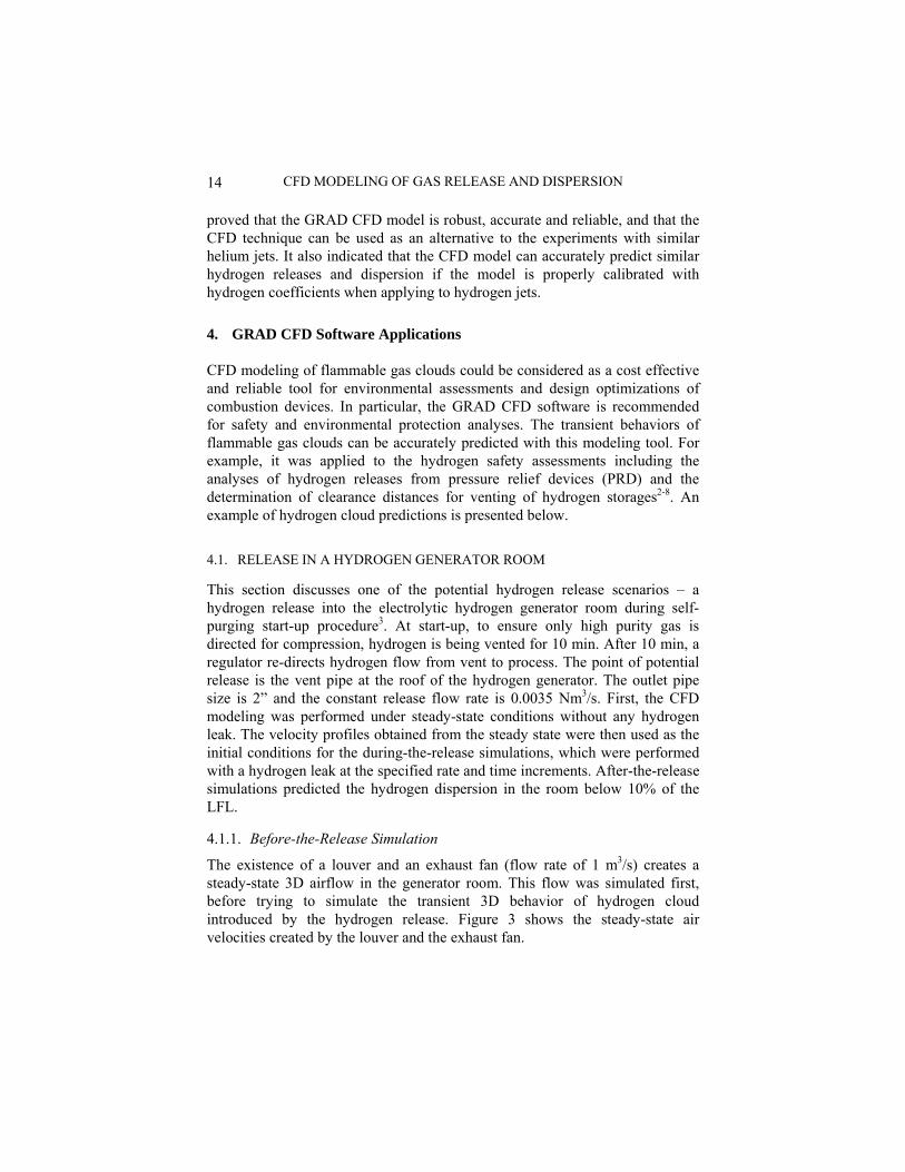
4.1.1. Before-the-Release Simulation

The existence of a louver and an exhaust fan (flow rate of 1 m3/s) creates a steady-state 3D airflow in the generator room. This flow was simulated first, before trying to simulate the transient 3D behavior of hydrogen cloud introduced by the hydrogen release. Figure 3 shows the steady-state air velocities created by the louver and the exhaust fan.


Figure 3. Air velocities at X- and Y-planes before the hydrogen release in the hydrogen generator room.

4.1.2. During-the-Release Simulation: Release from Hydrogen Vent Line

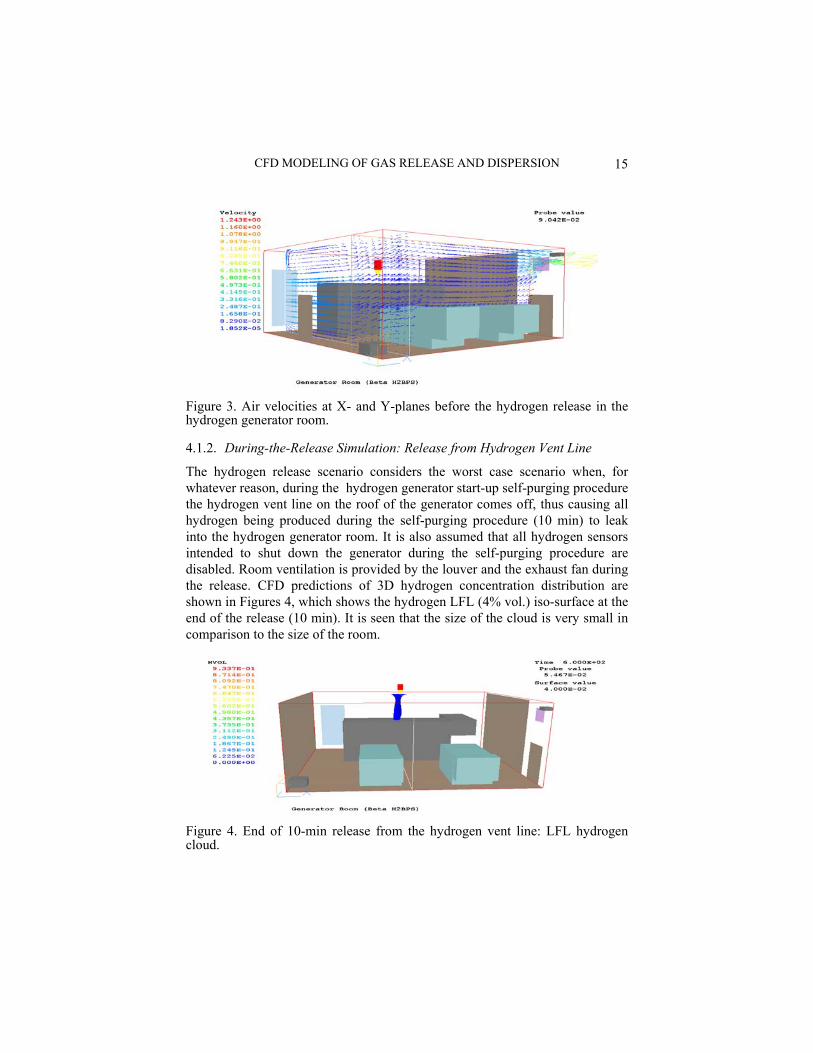
The hydrogen release scenario considers the worst case scenario when, for whatever reason, during the hydrogen generator start-up self-purging procedure the hydrogen vent line on the roof of the generator comes off, thus causing all hydrogen being produced during the self-purging procedure (10 min) to leak into the hydrogen generator room. It is also assumed that all hydrogen sensors intended to shut down the generator during the self-purging procedure are disabled. Room ventilation is provided by the louver and the exhaust fan during the release. CFD predictions of 3D hydrogen concentration distribution are shown in Figures 4, which shows the hydrogen LFL (4% vol.) iso-surface at the end of the release (10 min). It is seen that the size of the cloud is very small in comparison to the size of the room.

Figure 4. End of 10-min release from the hydrogen vent line: LFL hydrogen cloud.


4.1.3. Size of Flammable Gas Cloud

The size of the flammable cloud was calculated, using the advanced GRAD CFD settings. Three global quantities, DOMV, V4H and V2H were defined as the volume (in m3) of the whole domain (DOMV), the volume of the hydrogen cloud with more than 4% volume concentration (V4H) and the volume of the hydrogen cloud with more than 2% volume concentration (V2H) respectively. The printout from the global calculations file written after the CFD run was as follows: DOMV = 229.95, V4H = 8.072×10-2, V2H = 6.225. It could be seen that the 4% hydrogen cloud volume (V4H), which is about 0.081 m3, is much smaller than the volume of cloud with 2% volume concentration (V2H), which is about 6.225 m3. Both clouds are much smaller in volume than the whole domain volume (DOMV), which is about 230 m3. These findings are significant for understanding of safety of the system considered.

5. Conclusions

Advanced GRAD CFD models have been developed, tested, validated and applied to the modeling of various industrial real-life indoor and outdoor flammable gas (hydrogen, methane, etc.) release scenarios with complex geometries. The models developed include the following options: the dynamic boundary conditions, describing the transient gas release from a pressurized vessel, the calibrated outlet boundary conditions, the advanced turbulence models, the real gas law properties applied at high-pressure releases, the special output features and the adaptive grid refinement tools. The user-friendly GRAD CFD modeling tool has been designed as a customized module based on the commercial general-purpose CFD software, PHOENICS. The predictions of transient 3D distributions of flammable gas concentrations have been validated using the comparisons with available experimental data. GRAD CFD software is recommended for safety and environmental protection analyses. In particular, the dynamic behaviors of flammable gas clouds can be accurately predicted with this modeling tool for environmental assessments and design optimizations of combustion devices.

6. Acknowledgements

The authors would like to thank Natural Resources Canada (NRCan) and Natural Sciences and Engineering Research Council of Canada (NSERC) for their contributions to funding of this work.


References

1. PHOENICS Hard-copy Documentation (Version 3.5), Concentration, Heat and Momentum Limited, London, UK, (September 2002).

2. Agranat V., Cheng, Z., and Tchouvelev A., CFD modeling of hydrogen releases and dispersion in hydrogen energy station, Proceeding of the 15th World Hydrogen Energy Conference, Yokohama, Japan, (June 2004).

3. Tchouvelev A., Howard G., and Agranat V., Comparison of standards requirements with CFD simulations for determining sizes of hazardous locations in hydrogen energy station, Proceeding of the 15th World Hydrogen Energy Conference, Yokohama, Japan, (June 2004).

4. Howard, G. W., Tchouvelev, A. V., Cheng, Z., and Agranat, V. M., Defining hazardous zones- electrical classification distances, Proceeding of the 1st International Conference on Hydrogen Safety, Pisa, (September 2005).

5. Cheng Z, Agranat V. M., and Tchouvelev A.V., Vertical turbulent buoyant helium jet - CFD modeling and validation, Proceeding of the 1st International Conference on Hydrogen Safety, Pisa, (September 2005).

6. Cheng, Z., Agranat, V. M., Tchouvelev, A. V., Houf, W., and Zhubrin, S.V., PRD hydrogen release and dispersion, a comparison of CFD results obtained from using ideal gas law properties, Proceeding of the 1st International Conference on Hydrogen Safety, Pisa, (September 2005).

7. Tchouvelev, A.V., Benard, P., Agranat, V. and Cheng, Z., Determination of clearance distances for venting of hydrogen storage, Proceeding of the 1st International Conference on Hydrogen Safety, Pisa, (September 2005).

8. Cheng, Z., Agranat, V. M., Tchouvelev, A.V. and Zhubrin, S.V., Effectiveness of small Barriers as means to reduce clearance distances, Proceeding of the 2nd European Hydrogen Energy Conference, Zaragoza, Spain, (November 2005).

9. Swain, M. R., Grilliot, E. S., and Swain, M. N., Risks incurred by hydrogen escaping from containers and conduits. NREL/CP-570-25315, Proceedings of the 1998 U.S. DOE Hydrogen Program Review.

10. Swain, M. R., Schriber, J. A., and Swain, M. N., Addendum to hydrogen vehicle safety report: residential garage safety assessment. Part II: risks in indoor vehicle storage final report.

11. Panchapakesan, N. R., and Lumley, J. L., Turbulence measurements in axisymmetric jets of air and helium. Part 2. Helium jet, J. Fluid Mech. Vol. 246, pp 225-247, (1993).

12. Chen, C. J., and Rodi, W., Vertical Turbulent Buoyant Jets – A review of Experimental Data, The Science and Application of Heat and Mass Transfer, Pergamon Press, (1980).

13. Swain, M. R., Hydrogen Properties Testing and Verification, (June 17, 2004). 14. Ruffin, E., Mouilleau, Y., and Chaineaux, J., Large scale characterisation of the

concentration field to supercritical jets of hydrogen and methane, J. Loss Prev. Process Industry, vol. 9, n. 4, pp. 279-284, (1996).

15. Shebeko, Yu. N., Keller, V.D., Yeremenko, O. Ya, Smolin, I. M., Serkin, M. A., Korolchenko, A.Ya., Regularities of formation and combustion of local hydrogen-air mixtures in a large volume, Chemical Industry, Vol.21, pp. 24 (728)-27 (731) (1988) (in Russian).

CFD Modeling of Gas Release and Dispersion: Prediction of Flammable Gas Clouds

Documents