General rights Copyright and moral rights for the publications made accessible in the public portal are retained by the authors and/or other copyright owners and it is a condition of accessing publications that users recognise and abide by the legal requirements associated with these rights. • Users may download and print one copy of any publication from the public portal for the purpose of private study or research. • You may not further distribute the material or use it for any profit-making activity or commercial gain • You may freely distribute the URL identifying the publication in the public portal If you believe that this document breaches copyright please contact us providing details, and we will remove access to the work immediately and investigate your claim. Downloaded from orbit.dtu.dk on: Dec 19, 2017 CFD for Rotor Aerodynamics Sørensen, Niels N. Publication date: 2010 Link back to DTU Orbit Citation (APA): Sørensen, N. N. (2010). CFD for Rotor Aerodynamics. Paper presented at 1st Wind Turbine Computational Aerodynamics Lecture Series, United Kingdom.

Welcome message from author
This document is posted to help you gain knowledge. Please leave a comment to let me know what you think about it! Share it to your friends and learn new things together.
Transcript

General rights Copyright and moral rights for the publications made accessible in the public portal are retained by the authors and/or other copyright owners and it is a condition of accessing publications that users recognise and abide by the legal requirements associated with these rights.
• Users may download and print one copy of any publication from the public portal for the purpose of private study or research. • You may not further distribute the material or use it for any profit-making activity or commercial gain • You may freely distribute the URL identifying the publication in the public portal
If you believe that this document breaches copyright please contact us providing details, and we will remove access to the work immediately and investigate your claim.
Downloaded from orbit.dtu.dk on: Dec 19, 2017
CFD for Rotor Aerodynamics
Sørensen, Niels N.
Publication date:2010
Link back to DTU Orbit
Citation (APA):Sørensen, N. N. (2010). CFD for Rotor Aerodynamics. Paper presented at 1st Wind Turbine ComputationalAerodynamics Lecture Series, United Kingdom.
CFD for Rotor AerodynamicsGlasgow - 2010
Niels N. Sørensen
Wind Energy Division · Risø DTU
RISØ-DTU, 09-09-2010
IntroductionOutline
1 Introduction
2 Mathematical Model
3 Discretization
4 Boundary Conditions
5 Computational domain
6 Solution Evaluation and Test Cases
2 of 50Niels N. Sørensen,Risø DTU CFD for Rotor Aerodynamics 09-09-2010
IntroductionCFD for Wind Energy
Development and origin of CFD for Wind Energy
� The application of numerical methods to fixed wing and rotoraerodynamics dates back to the late seventies in the aerospacecommunity, solving steady Potential and Euler Equations.
� The first numerical solutions of the unsteady Euler equation were seenthrough the eighties.
� With the continuous increase in computer power in the late eighties andearly nineties the first Reynolds Averaged Navier-Stokes codes forhelicopter applications appeared.
� With the possibility of handling viscous flow, the first association ofNavier-Stokes CFD solvers appeared in the wind turbine community inthe late nineties.
� In Europe a series of EU-financed projects were providing the basis formany of these activities.
3 of 50Niels N. Sørensen,Risø DTU CFD for Rotor Aerodynamics 09-09-2010

IntroductionWind Turbine Aerodynamics
� High Reynolds Number Re > 1.0 × 10⁶
� Nearly incompressible flows M < 0.3
� Operating in the atmospheric shear layer
� High inflow turbulence
� Velocity varies with height
� Inflow depends on terrain
� Large range of scales
� Thick airfoils
� Flow separation at high angles of attack
� Rotational effects
� Rotor tower interaction
� Aerodynamic and structural coupling,Aeroelasticity
4 of 50Niels N. Sørensen,Risø DTU CFD for Rotor Aerodynamics 09-09-2010

IntroductionBasic CFD
� Mathematical Model� Compressible/Incompressible.
� Navier-Stokes, Euler, Potential.
� Coordinate and basis vector systems
� Discretization
� Finite Difference, Finite Volume, Finite Element, Other Methods
� Order of the discretization scheme
� Computational domain, using structured/unstructured etc.
� Boundary Conditions
� Inflow conditions
� Wall boundary conditions
� Outflow conditions
� Components of a CFD Solver
� Pre-processor
� Solver
� Post-processor
5 of 50Niels N. Sørensen,Risø DTU CFD for Rotor Aerodynamics 09-09-2010
Mathematical ModelGoverning Equations
We would like to investigate airfoils and rotors
� We would like to be able to compute viscous effects:
� Compute the viscous drag of airfoils and rotors.
� Compute the effect of changing the Reynolds Number.
� Compute airfoil at high angles of attack.
� The Potential Equation is inviscid and irrotational. Can be used as anapproximation at low angles of attack and for thin airfoils.
� The Euler Equations are inviscid.
� Only the Navier-Stokes will allow us to compute the viscous effects.
6 of 50Niels N. Sørensen,Risø DTU CFD for Rotor Aerodynamics 09-09-2010
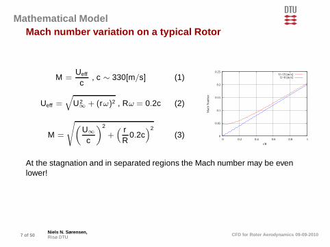
Mathematical ModelMach number variation on a typical Rotor
M =Ueff
c, c ∼ 330[m/s] (1)
Ueff =√
U2∞ + (rω)2 , Rω = 0.2c (2)
M =
√
(
U∞
c
)2
+( r
R0.2c
)2(3) 0
0.05
0.1
0.15
0.2
0.25
0 0.2 0.4 0.6 0.8 1
Mac
h N
umbe
r
r/R
U=15 [m/s]U=0 [m/s]
At the stagnation and in separated regions the Mach number may be evenlower!
7 of 50Niels N. Sørensen,Risø DTU CFD for Rotor Aerodynamics 09-09-2010

Mathematical ModelMach number correctionSeveral low Mach number corrections exists, eg. Prandtl-Glauert:
Cl =Cl,0√
1 − M2(4)
1
1.005
1.01
1.015
1.02
1.025
1.03
1.035
1.04
1.045
1.05
0 0.05 0.1 0.15 0.2 0.25 0.3
Cl/C
l inc
Mach Number
Prandtl-Glauert
The work of Turkel, Radespiel and Kroll shows that the error at M=0.01 maybe more than 10 percent, and divergence may occur using a standardcompressible solver.
8 of 50Niels N. Sørensen,Risø DTU CFD for Rotor Aerodynamics 09-09-2010

Mathematical ModelReynolds Averaged Navier-Stokes
Reynolds averaging of the Navier-Stokes equation, splitting the velocities inthe mean and the fluctuating component
ui( ~r , t) = Ui(~r ) + u′(~r , t) , where Ui(~r) = limT→∞
1T
∫ t+T
tui(~r , t)dt
Inserting the Reynolds decomposed velocity in the Navier-Stokes andcontinuity equations
Perform time averaging of the equations. The equations are in principle timeindependent, or steady state.
9 of 50Niels N. Sørensen,Risø DTU CFD for Rotor Aerodynamics 09-09-2010

Mathematical ModelThe Reynolds Averaged Navier-Stokes
The Reynolds Averaged incompressible Navier-Stokes equations andadditional equations have the following form:
Continuity equation:
∂
∂xj(ρUj) = 0
Momentum equations:
∂
∂t(ρUi) +
∂
∂xj(ρUiUj)−
∂
∂xj
[
(µ+ µt )
(
∂Ui
∂xj+
∂Uj
∂xi
)]
+∂P̂∂xi
= Sv ,
Auxiliary equations:
∂
∂t(ρφ) +
∂
∂xj(ρUjφ)−
∂
∂xj
[(
µ+µt
σφ
)
∂φ
∂xi
]
= Sφ
10 of 50Niels N. Sørensen,Risø DTU CFD for Rotor Aerodynamics 09-09-2010

Mathematical ModelClosing the Equations
To close the flow equations we need an expression for the µt , this is typicallyhandled by the turbulence model:
Typically a two equation model will be used for more complex cases, e.g.. thek − ǫ or the k − ω model
µt = ρCµk2
ǫ.
The two additional transport equations has a form similar to the previousstated general transport equation, and mainly the deviation between themodels are in the source terms on the RHS.This is discussed more in the accompanying discussion of turbulence.
11 of 50Niels N. Sørensen,Risø DTU CFD for Rotor Aerodynamics 09-09-2010

Mathematical ModelCoordinate and basis vector systemCoordinate System
� Cartesian Coordinates (x,y,z)
� Polar Coordinates (r,θ,z)
� Spherical Coordinates (r,θ,Φ)
� General Curvilinear Coordinates (ξ,η,ζ)
� Fixed Frame
� Moving Frame
Velocity basis
� Fixed Cartesian Velocity basis
� Fixed Polar Velocity basis
� Fixed Spherical Velocity basis
� Co- or Contra- Variant Velocity basis
Depending of the chosen coordinate basis and chosen velocity basis, theresulting version of the Navier-Stokes equations will have different complexity.
12 of 50Niels N. Sørensen,Risø DTU CFD for Rotor Aerodynamics 09-09-2010
Mathematical ModelRotor Flows
Non-inertial frame of reference (Moving Frame)
� Additional acceleration terms, changed boundary conditions
� Can be used both steady/unsteady
� Do not need re-computations of geometrical quantities
� Need careful treatment of source term implementation
� Do not allow deformation of the geometry
Inertial frame of reference (Moving Mesh)
� Mesh fluxes, changed boundary conditions
� Is by nature unsteady
� Allows deformation of the geometry
� Need re-computations of metrics (geometrical quantities)
13 of 50Niels N. Sørensen,Risø DTU CFD for Rotor Aerodynamics 09-09-2010

Mathematical ModelTransformation to curvilinear Coordinates
If we need to handle curvilinear Coordinates, the equations must betransformed from the Cartesian formulation to the curvilinear formulation.
Typically, we derive an expression for the divergence using the chain rule ofdifferentiation:
∂
∂xi=
1J
(
∂
∂ξ
∂ξ
∂xi+
∂
∂η
∂η
∂xi+
∂
∂ζ
∂ζ
∂xi
)
(5)
Using fixed Cartesian base vectors, this approach will directly lead to a strongconservation form:
The volume sources and the time terms are invariant during transformation.
14 of 50Niels N. Sørensen,Risø DTU CFD for Rotor Aerodynamics 09-09-2010

DiscretizationDiscretization Methods
We need to transform the partial differential equations, into a set of algebraicequation that can be solved numerically.
� Finite Difference:
� Differential from, using Taylor Series or Polynomial fitting.
� Structured grids.
� Finite Volume:
� Integral form, using Gauss or Divergence Theorem
� Structured and unstructured grids
� Finite Element:
� Integral form, shape or weight functions.
� Unstructured grids.
� Other Methods:
� Spectral, Smoothed Particle Dynamics, Boundary Element Methods.
15 of 50Niels N. Sørensen,Risø DTU CFD for Rotor Aerodynamics 09-09-2010
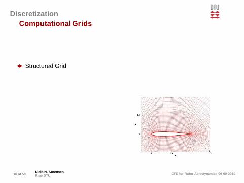
DiscretizationComputational Grids
� Structured Grid
16 of 50Niels N. Sørensen,Risø DTU CFD for Rotor Aerodynamics 09-09-2010

DiscretizationComputational Grids
� Structured Grid
� Unstructured Grid
16 of 50Niels N. Sørensen,Risø DTU CFD for Rotor Aerodynamics 09-09-2010
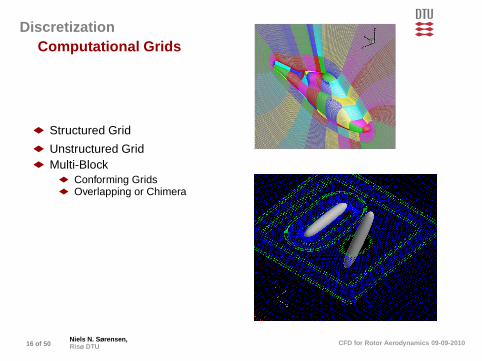
DiscretizationComputational Grids
� Structured Grid
� Unstructured Grid
� Multi-Block
� Conforming Grids
� Overlapping or Chimera
16 of 50Niels N. Sørensen,Risø DTU CFD for Rotor Aerodynamics 09-09-2010

DiscretizationComputational Grids
� Structured Grid
� Unstructured Grid
� Multi-Block
� Conforming Grids
� Overlapping or Chimera
� Hybrid Meshes
16 of 50Niels N. Sørensen,Risø DTU CFD for Rotor Aerodynamics 09-09-2010
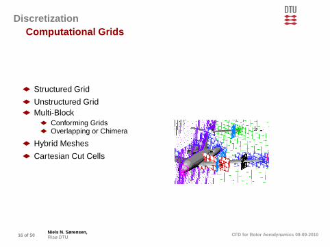
DiscretizationComputational Grids
� Structured Grid
� Unstructured Grid
� Multi-Block
� Conforming Grids
� Overlapping or Chimera
� Hybrid Meshes
� Cartesian Cut Cells
16 of 50Niels N. Sørensen,Risø DTU CFD for Rotor Aerodynamics 09-09-2010

DiscretizationFinite Volume DiscretizationIn the Finite Volume method, the algebraic equations are obtained bypartitioning the solution domain into a set of finite control volumes andintegrating the equation using the Gauss’ or divergence theorem.The Gauss theorem states that the volume integral of the divergence is equalto the outward flux of the vector field through the boundary enclosing thevolume:
∫
CV
∂φui
∂xidV =
∫
Ani(φui)dA (6)
17 of 50Niels N. Sørensen,Risø DTU CFD for Rotor Aerodynamics 09-09-2010

DiscretizationDiscretization of the equations
The Reynolds Averaged Navier-Stokes equations are given by:
∂
∂t(ρUi) +
∂
∂xj(ρUiUj)−
∂
∂xj
[
(µ+ µt )
(
∂Ui
∂xj+
∂Uj
∂xi
)]
+∂P̂∂xi
= Sv , (7)
Even for the curvilinear we can arrive at a algebraic set of equations of theform below:
ApUp +∑
AnbUnb = S (8)
18 of 50Niels N. Sørensen,Risø DTU CFD for Rotor Aerodynamics 09-09-2010

DiscretizationSource Terms
Generally, the source terms are treated in a non-conservative way:∫
CVSv dVol = Sv Vol (9)
The non-conservative treatment may result in problems eg. in connectionwith moving-frame formulations.
19 of 50Niels N. Sørensen,Risø DTU CFD for Rotor Aerodynamics 09-09-2010
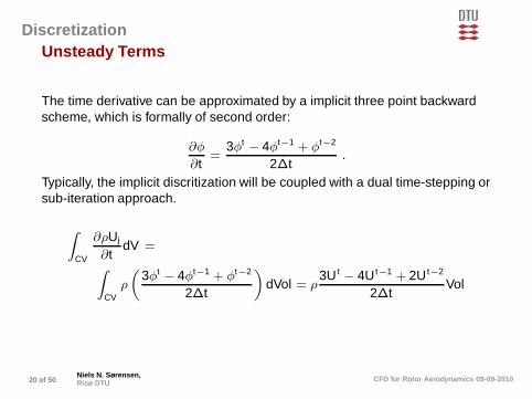
DiscretizationUnsteady Terms
The time derivative can be approximated by a implicit three point backwardscheme, which is formally of second order:
∂φ
∂t=
3φt − 4φt−1 + φt−2
2∆t.
Typically, the implicit discritization will be coupled with a dual time-stepping orsub-iteration approach.
∫
CV
∂ρUj
∂tdV =
∫
CVρ
(
3φt − 4φt−1 + φt−2
2∆t
)
dVol = ρ3U t − 4U t−1 + 2U t−2
2∆tVol
20 of 50Niels N. Sørensen,Risø DTU CFD for Rotor Aerodynamics 09-09-2010

DiscretizationPressure term
∂P∂xi
The pressure term for the x-momentum equation can be approximated in thefollowing way
∫
CV
∂P∂x
dVol = PeAe − Pw Aw (10)
In a cell centered formulation, the Pe and Pw are not directly available, usinglinear interpolation we get
Pe =PE + PP
2, Pw =
PP + PW
2For a Cartesian mesh where Ae = Aw the PP will exit the equation:
∫
CV
∂P∂x
dVol = AePE − PW
2
21 of 50Niels N. Sørensen,Risø DTU CFD for Rotor Aerodynamics 09-09-2010
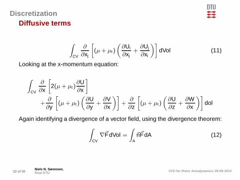
DiscretizationDiffusive terms
∫
CV
∂
∂xj
[
(µ+ µt )
(
∂Ui
∂xj+
∂Uj
∂xi
)]
dVol (11)
Looking at the x-momentum equation:
∫
CV
∂
∂x
[
2(µ+ µt )∂U∂x
]
+∂
∂y
[
(µ+ µt )
(
∂U∂y
+∂V∂x
)]
+∂
∂z
[
(µ+ µt)
(
∂U∂z
+∂W∂x
)]
dol
Again identifying a divergence of a vector field, using the divergence theorem:∫
CV∇~FdVol =
∫
A
~n~FdA (12)
22 of 50Niels N. Sørensen,Risø DTU CFD for Rotor Aerodynamics 09-09-2010

DiscretizationDiffusive terms 2Assuming a Cartesian grid we get, using eg. ~ne = (1, 0,0)T and~ns = (0,−1, 0)T
2µeff∂U∂x
∣
∣
∣
∣
east
Ae − 2µeff∂U∂x
∣
∣
∣
∣
west
Aw
+µeff
(
∂V∂x
+∂U∂y
)∣
∣
∣
∣
north
An −µeff
(
∂V∂x
+∂U∂y
)∣
∣
∣
∣
south
As
+µeff
(
∂W∂x
+∂U∂z
)∣
∣
∣
∣
top
At −µeff
(
∂W∂x
+∂U∂z
)∣
∣
∣
∣
bottom
Ab
The effective viscosity µ+ µt can be linearly interpolated between the twoopposing cell centres
The gradients can be approximated by central differences, which will have 2.order accuracy:
∂U∂x
∣
∣
∣
∣
e
=UE − UP
∆xPE
23 of 50Niels N. Sørensen,Risø DTU CFD for Rotor Aerodynamics 09-09-2010

DiscretizationConvective terms
∂
∂xj(ρUiUj)
Looking at the X-momentum direction:∫
CV
∂ρUUj
∂xjdVol =
∫
CV∇ · (ρU~V)dVol =
∫
A
~nρU~VdA
We can now derive the discrete version:
ρUU|east Ae−ρUU|west Aw+ρUV |north An−ρUV |south As+ρUW |top At−ρUW |bottom Ab
For a cell centered scheme we will need approximations for the cell facevelocities. One simple option with second order accuracy for the convectiveterms could be a linear interpolation:
Ue =UE + UE
2This scheme is unfortunately only stable for very low Peclet numbers LV
µ
24 of 50Niels N. Sørensen,Risø DTU CFD for Rotor Aerodynamics 09-09-2010

DiscretizationConvective scheme
A very accurate and often used scheme for approximating the cell facevariables is the QUICK scheme:
φe =
{
12 (φP + φE)− 1
8 (φW + φE − 2φP) if ρUeAe ≥ 012 (φE + φP)− 1
8 (φP + φEE − 2φE) if ρUeAe ≤ 0.
Often the higher order schemes are written as deffered corrections in thefollowing way:
φe =
{
φP + 18 (3φE + 2φP − φW ) if ρUeAe ≥ 0
φE + 18 (3φP − 2φE − φEE) if ρUeAe ≤ 0
.
Only the first part of the scheme is treated fully implicit while the remainingpart is evaluated at last iteration or sub-iteration.
25 of 50Niels N. Sørensen,Risø DTU CFD for Rotor Aerodynamics 09-09-2010

DiscretizationSolution Methods for Incompressible Flow
For the Finite Volume and Finite Difference methods, the typical solutionmethods are listed below:
� Artificial Compressibility Methods
� Explicit Methods
� Implicit Methods
� Fractional Step Methods
� Explicit Methods
� Implicit Methods
� Pressure Correction Methods
� SIMPLE
� PISO
� SIMPLEC
26 of 50Niels N. Sørensen,Risø DTU CFD for Rotor Aerodynamics 09-09-2010
DiscretizationRequirements of a Numerical Solution Method
For the discrete equations to be solved the following properties should befulfilled
� Consistency and convergence
� The difference between the discretized and the exact equations shouldbecome zero in the limit of infinitely small cells.
� Stability
� A numerical procedure is said to be stable if it does not magnify the errorsthat appear in the course of the numerical solution process.
� Conservation
� The numerical method should reflect the conservation property of thegoverning equation.
� Boundedness and Realizability
� Physically non-negative quantities (density, concentration etc) must alwaysbe positive. Some convective schemes may produce nonphysical negativevalues on coarse and skewed computational meshes.
27 of 50Niels N. Sørensen,Risø DTU CFD for Rotor Aerodynamics 09-09-2010

Boundary ConditionsBoundary Conditions
The two fundamental things determining the quality of the results from anumerical model, assuming that every thing is performed correctly are:
� The model equations
� Are the model equations adequate for the present purpose etc.
� The boundary conditions
� Boundary conditions are needed for all variables at all external boundariesof the computational domain.
� Boundary conditions needs to represent the problem in question
In the following slides we will look at some typical boundary conditions.
28 of 50Niels N. Sørensen,Risø DTU CFD for Rotor Aerodynamics 09-09-2010

Boundary ConditionsInflow Boundary Conditions
Two approaches can be used:
� Use a large domain, placing the farfield boundary at large distance fromthe airfoil/rotor.
� Simple Dirichlet Condition
� Use a dynamic boundary conditions that adapts to the flow disturbancefrom the airfoil/rotor.
� Advanced Dirichlet Condition that adapts to the loading.
29 of 50Niels N. Sørensen,Risø DTU CFD for Rotor Aerodynamics 09-09-2010
Boundary ConditionsOutflow conditions
The outflow conditions can be crucial for the computations:
� Simple fully developed flow assumptions are often used.
� The outlet should be placed far from the area of interest
� There should not be recirculation through the outlet
∂φ
∂n= 0 .
The pressure will typically be extrapolated using either linearly or quadraticextrapolation.
� Convective boundary conditions, will allow reversed flow through theoutlet.
∂φ
∂t− U
∂φ
∂n= 0 .
30 of 50Niels N. Sørensen,Risø DTU CFD for Rotor Aerodynamics 09-09-2010
Boundary ConditionsWall Boundary Conditions
For most airfoil and rotor flows, simple no-slip boundary conditions areapplied.
This will typically require a very fine grid, with off cell spacing of y+ ∼ 1.
In contrast to many typically engineering flows, where the y+ ∼ 100 to 200are use along with log-law conditions.In connection with the discussion of the computational domain, we will seethe implication of the y+ requirement on the cell size.
31 of 50Niels N. Sørensen,Risø DTU CFD for Rotor Aerodynamics 09-09-2010

Computational domainComputational Domain
Airfoil and rotor flows involves a large range of scales, from the viscousscales in the boundary layer of the blades, to the wake of the rotor which canbe several rotor diameters long.
� For most wind turbine related flows, we are looking at external flowswhere the outer boundary must be placed far from the area of interest.
� We need a sufficient fine resolution at the wall boundaries, and at allregions with large gradients of the flow variables (separation points,where layers, wake, etc)
� We only have a limited number of grid points available. A typical 2Dairfoil computation would have around 384 × 128 ∼ 50.000 cells and atypical rotor computation would have around number of blades×128 × 256 × 128 ∼ 13 million cells.
� In order to avoid excessive number of cells we will need stretchingfunctions, to expand the cell size when moving away from the wallsurface.
32 of 50Niels N. Sørensen,Risø DTU CFD for Rotor Aerodynamics 09-09-2010
Computational domainEstimation of Viscous Cell Size
Definition of non-dimensional wall distance:
y+ =ρyUτ
µ(13)
Skin friction coefficient for turbulent boundary layer over flat plate:
Cf =0.0576
Re15
(14)
Definition of skin friction coefficient:
Cf =ρU2
τ
12ρU2
∞
(15)
33 of 50Niels N. Sørensen,Risø DTU CFD for Rotor Aerodynamics 09-09-2010

Computational domainEstimation of Viscous Cell SizeAn approximate formula for the necessary wall normal distance can now bederived:
yc
= 5.89Re−910 y+ (16)
1e-06
1e-05
0.0001
0.001
1 2 3 4 5 6 7 8 9 10
Wal
l Nor
mal
Dis
tanc
e (y
/c)
Reynolds Number * 1.10-6
y+=0.5y+=1.0y+=2.0y+=3.0y+=4.0y+=5.0
34 of 50Niels N. Sørensen,Risø DTU CFD for Rotor Aerodynamics 09-09-2010

Computational domainDomain size for 2D airfoil computations
The influence from a lifting airfoil on its surroundings can be determined fromsimple potential flow using the Kutta-Jukowski theorem:
L = ρ∞ ~U∞~Γ , where L is the Lift per unit span, (17)
the definition of the lift:
L = Cl12ρ∞U2
∞Chord , (18)
and the Biot-Savart law:
Vθ =Γ
2πr(19)
Combining these we can arrive at the following expression for the:
Uθ
U∞
= − −Cl
4π rChord
(20)
35 of 50Niels N. Sørensen,Risø DTU CFD for Rotor Aerodynamics 09-09-2010

Computational domainDomain size for 2D airfoil computations
The effect of the induced velocity on the effective Reynolds number can thusbe approximated by:
Ueff = U∞
√
1 +
(
Cl
4π rChord
)2
(21)
The effect of the induced velocity on the effective angle of attack can thus beapproximated by:
AOA =180π
tan−1(
−Cl
4π rChord
)
(22)
36 of 50Niels N. Sørensen,Risø DTU CFD for Rotor Aerodynamics 09-09-2010

Computational domainDomain size for 2D airfoil computationsThe effect on the Reynolds number is negligible for all practical purposes, butas can be seen from the present figure, the effect on the AOA is quite largefor small domains:
0
0.5
1
1.5
2
2.5
0 20 40 60 80 100
AO
A [
deg]
r/Chord
Cl=1.0Cl=2.0
Neglecting the induced tangential velocity, may lead to an error of ∼ 5percent for a distance from the airfoil of 10 chords, while the error is reducedto below 1 percent for a 50 chords distance.Alternatively, the empirical expression for Uθ can be used as a iterativeboundary condition, the so called vortex correction.
37 of 50Niels N. Sørensen,Risø DTU CFD for Rotor Aerodynamics 09-09-2010

Computational domainDomain size for rotor computations
In rotor computations we need to consider the influence of the rotor inducedvelocity
The induced velocity can be estimated based on the rotor thrust, using theFroude actuator disc model.
CT =T
12ρU2
∞πR2Rotor
From axial momentum theory we can compute the induction:
CT = 4a(1 − fa) , f =
{
1 for a < 1/3(5 − 3a)/4 for a ≥ 1/3
(23)
U = U∞
(
1 − a
(
1 +z
√
R2rotor + z2
))
38 of 50Niels N. Sørensen,Risø DTU CFD for Rotor Aerodynamics 09-09-2010

Computational domainDomain size for rotor computations
0.95
0.96
0.97
0.98
0.99
1
-20 -15 -10 -5 0
U/U
0
x/R
CT=0.89CT=1.00
Using that Pavailable ∼ U3∞
r/R 5 10 20Pavailable−P∞
P∞
× 100 1.95 0.50 0.14
39 of 50Niels N. Sørensen,Risø DTU CFD for Rotor Aerodynamics 09-09-2010
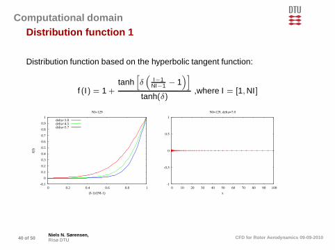
Computational domainDistribution function 1
Distribution function based on the hyperbolic tangent function:
f (I) = 1 +tanh
[
δ(
I−1NI−1 − 1
)]
tanh(δ),where I = [1,NI]
-0.1
0
0.1
0.2
0.3
0.4
0.5
0.6
0.7
0.8
0.9
1
0 0.2 0.4 0.6 0.8 1
f(I)
(I-1)/(NI-1)
NI=129
delta=3.0delta=4.5delta=5.7
-1
-0.5
0
0.5
1
0 10 20 30 40 50 60 70 80 90 100
x
NI=129, delta=7.0
40 of 50Niels N. Sørensen,Risø DTU CFD for Rotor Aerodynamics 09-09-2010
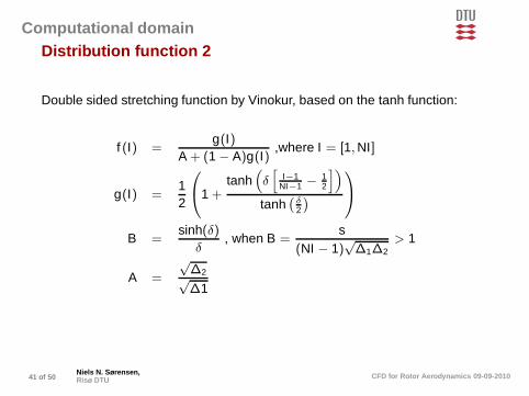
Computational domainDistribution function 2
Double sided stretching function by Vinokur, based on the tanh function:
f (I) =g(I)
A + (1 − A)g(I),where I = [1,NI]
g(I) =12
1 +tanh
(
δ[
I−1NI−1 − 1
2
])
tanh(
δ2
)
B =sinh(δ)
δ, when B =
s(NI − 1)
√∆1∆2
> 1
A =
√∆2√∆1
41 of 50Niels N. Sørensen,Risø DTU CFD for Rotor Aerodynamics 09-09-2010

Solution Evaluation and Test CasesVerification of the Simulation
Having performed a simulation, it is necessary to have some idea of thequality of the solution :
� Iterative Convergence
� Are the governing equations solved on the present grid
� Grid Convergence
� Are the solution on the present grid level independent of the grid resolution
� Comparing with Measurements
� Do the model agree with reality
42 of 50Niels N. Sørensen,Risø DTU CFD for Rotor Aerodynamics 09-09-2010

Solution Evaluation and Test CasesConvergence of the iterative methodAre the equations solved:
Apφp −∑
Anbφnb = F
Typically we compute the residual of the equation in each cell, using:
Res =∣
∣
∣F −
(
Apφp −∑
Anbφnb
)∣
∣
∣
The sum of the residual over all cells in the computational grid is computedand compared to the starting residual.
Reduction =
∑
AllCells Res∑
AllCells Res0
Typically a reduction of 1 × 10⁻⁴ to 1 × 10⁻⁵ is used. The fact that theresidual is only changing slightly from prior iteration is not a good measure forconvergence.
43 of 50Niels N. Sørensen,Risø DTU CFD for Rotor Aerodynamics 09-09-2010
Solution Evaluation and Test CasesGrid Convergence
Is the present solution a sufficient approximation of the specifiedcomputational case?
� Often we don’t know the desired solution, and the only check is to see ifthe numerical model is consistent and converged.
� A typical way to do this is to do consecutive grid refinements, and verifythat the solution converges towards a value with the correct decrease inerror e.g. 2. order.
� This procedure will only assure that we have a solution to thenumerically specified problem, given by the numerical model and theboundary conditions, not that the present problem approximate thephysical problem in question.
44 of 50Niels N. Sørensen,Risø DTU CFD for Rotor Aerodynamics 09-09-2010
Solution Evaluation and Test CasesRichardson Extrapolation
Error Estimation:Assuming that the discrete equation has order P we can write
Φ = φh + αhp + H , ǫh = αhp + H
Using this on two grid levels h and 2h we can estimate the error on the finelevel
ǫh ∼ φh − φ2h
2p − 1, here assuming a doubling of the grid size
The order of the scheme can be estimated using three grid levels:
p = log(
φ4h − φ2h
φ2h − φh
)
1log(2)
Here we again have assumed a doubling of the grid size. The aboveprocedure assumes that we are in the asymptotic range, where the error isdominated by the discretization error.
45 of 50Niels N. Sørensen,Risø DTU CFD for Rotor Aerodynamics 09-09-2010

Solution Evaluation and Test CasesIterative Convergence
Here is an example of iterative convergence of our EllipSys code for five gridlevels, from a series of computations on the Bolund blind comparison cases
� The typical residuallimit of 1 × 10⁻⁴ isindicated
� For verification theconvergence is takenfurther
� The velocity is shown ata position at the hillcenter 6
6.5
7
7.5
8
8.5
9
9.5
10
10.5
11
0 500 1000 1500 2000 2500 3000 3500 4000-7
-6
-5
-4
-3
-2
-1
0
Win
d Sp
eed
[m/s
]
Velocity at center of Bolund
Wind speedResidual
Typical Residual Limit
46 of 50Niels N. Sørensen,Risø DTU CFD for Rotor Aerodynamics 09-09-2010

Solution Evaluation and Test CasesGrid Convergence
Grid Level h 2h 4hVelocity [m/s] 7.97 7.88 7.6
� Estimated order 1.64
� Estimated error on level one ∼ 0.5% 6
6.5
7
7.5
8
8.5
9
9.5
10
10.5
11
0 500 1000 1500 2000 2500 3000 3500 4000-7
-6
-5
-4
-3
-2
-1
0
Win
d Sp
eed
[m/s
]
Velocity at center of Bolund
Wind speedResidual
Typical Residual Limit
Even though the Bolund case has very complex terrain features, these arelimited to a very small area ∼ 200 × 200 meter.
47 of 50Niels N. Sørensen,Risø DTU CFD for Rotor Aerodynamics 09-09-2010

Solution Evaluation and Test CasesThe effect of the order of the method
Comparing the solution on three grid refinements, using either a second anda first order scheme, reveals the importance of using at least a second orderscheme:The figure is taken from the bolund comparison
0
5
10
15
20
25
30
3 4 5 6 7 8 9 10 11 12
Hei
ght [
m]
ASL
Velocity [m/s]
Mast-4, 270 degrees
Level-1Level-2Level-3
0
5
10
15
20
25
30
2 3 4 5 6 7 8 9 10 11 12
Hei
ght [
m]
ASL
Veloicty [m/s]
1.Order, L11.Order, L21.Order, L32.Order, L12.Order, L22.Order, L3
48 of 50Niels N. Sørensen,Risø DTU CFD for Rotor Aerodynamics 09-09-2010

Solution Evaluation and Test CasesComparison With Measurements
Having proved that the solution is iteratively converged and grid convergedwe will need to confirm that the model actually agrees with the physical casein question:
� We need good experimental data
� We need well defined inflow conditions
� We need a high density of the measuring points
49 of 50Niels N. Sørensen,Risø DTU CFD for Rotor Aerodynamics 09-09-2010
Solution Evaluation and Test CasesTest Cases
A series of test cases should be computed before doing the actualsimulations:
� Airfoil Flows
� NACA data from Abbott and Doenhoff
� Onera-A airfoil
� Wind turbine airfoils, Stuttgard, Delft and Risø
� Advanced Airfoil Flows
� Pitching airfoils
� Axial Rotor Flows
� NREL Phase VI, Axial Flow Case
� MEXICO experiment
� UPWIND test rotor
� Advanced Rotor Cases
� NREL Phase VI, Yaw Cases
� NREL Phase VI, Pitch Step
50 of 50Niels N. Sørensen,Risø DTU CFD for Rotor Aerodynamics 09-09-2010
Related Documents