CFD-DEM simulation of Locomotive Sanders by Aishwarya Gautam B.Eng., The Hong Kong University of Science and Technology, 2016 A THESIS SUBMITTED IN PARTIAL FULFILLMENT OF THE REQUIREMENTS FOR THE DEGREE OF MASTER OF APPLIED SCIENCES in THE FACULTY OF GRADUATE AND POSTDOCTORAL STUDIES (Mechanical Engineering) THE UNIVERSITY OF BRITISH COLUMBIA (Vancouver) July 2018 © Aishwarya Gautam, 2018

Welcome message from author
This document is posted to help you gain knowledge. Please leave a comment to let me know what you think about it! Share it to your friends and learn new things together.
Transcript
CFD-DEM simulation of Locomotive Sanders
by
Aishwarya Gautam
B.Eng., The Hong Kong University of Science and Technology, 2016
A THESIS SUBMITTED IN PARTIAL FULFILLMENT OF
THE REQUIREMENTS FOR THE DEGREE OF
MASTER OF APPLIED SCIENCES
in
THE FACULTY OF GRADUATE AND POSTDOCTORAL STUDIES
(Mechanical Engineering)
THE UNIVERSITY OF BRITISH COLUMBIA
(Vancouver)
July 2018
© Aishwarya Gautam, 2018

ii
Thefollowingindividualscertifythattheyhaveread,andrecommendtotheFacultyofGraduateandPostdoctoralStudiesforacceptance,athesis/dissertationentitled:
CFD-DEMSimulationofLocomotiveSanders
submittedby AishwaryaGautam inpartialfulfillmentoftherequirementsfor
thedegreeof MasterofAppliedScience
in MechanicalEngineering
ExaminingCommittee:
Dr.SheldonGreen
Supervisor
Dr.StevenRogak
SupervisoryCommitteeMember
Dr.BorisStoeber
SupervisoryCommitteeMember

iii
Abstract
This study presents the development and results of a numerical model of a locomotive sander
system. Locomotive sanders are used to optimize traction between the train wheels and railhead
by spraying sand into the interface. It has been previously shown that a large fraction of sand
sprayed by the sanders does not make it through the wheel-rail nip, leading to sand wastage and
thereby increasing the cost and refilling effort.
In this project, pneumatic conveying of sand through the wheel-rail nip is numerically modelled
through coupled Computational Fluid Dynamics and Discrete Element Method simulations. The
gas phase, discrete phase and coupled two-phase flows are separately validated against literature,
and the parameters effecting the deposition of sand through the nip- relating to both aerodynamics
of the particle laden jet and interaction with geometry are independently analyzed pertaining to
their effects on sander efficiency. The aerodynamics associated with the particle laden jet play a
critical role in optimizing the amount of sand going through the wheel-rail interface, with the
particle velocities being directly correlated with the sander efficiency. Particle-geometry
interactions are found to have a negligible effect on the deposition. In the absence of crosswinds,
it is recommended to either employ smaller particles, or particles with a higher surface area to
volume ratio to enhance the sander efficiency. Furthermore, a larger airflow rate through the nozzle
is suggested. It is also found that the presence of crosswinds strongly negatively affects sander
efficiency, which can be mitigated, to some extent, by reducing the nip-nozzle distance as much
as safety regulations will allow, and using coarser grain particles.
iv
Lay Summary
This thesis presents the development and results of a computational model of locomotive sander,
a device that is used to spray sand between the rail-wheel interface to increase traction. Locomotive
sanders have been shown to have very low efficiency, with most of the sand carried by the sander
being wasted in the operation. In this study, parameters effecting the sander efficiency were
computationally analyzed, and recommendations were made to minimize these losses. The primary
takeaway from this project was that the flow of particles out of sander hose governs the deposition
of sand through the wheel-rail nip, and the sander efficiency can be significantly increased by
utilizing a higher airflow, finer grain sand, or sands with more flakey particle shape. Using the
results of this work, better, more efficient sanders can be developed and implemented in the field.
v
Preface
The work presented in this thesis is the result of original, unpublished research done by Aishwarya
Gautam, with the close supervision of Dr. Sheldon Green. The numerical model was developed
and simulations were conducted at the research facility located in Pulp and Paper Centre, UBC,
along with some experimental tests that were also performed in the same research lab. The
literature review, model development, validation, data processing and analysis were done by
Aishwarya Gautam with the invaluable guidance of Dr. Sheldon Green. The industrial partner, LB
Foster Ltd., provided the high-level objectives and overall direction to this research.

vi
Table of Contents
Abstract ......................................................................................................................................... iii
Lay Summary ............................................................................................................................... iv
Preface .............................................................................................................................................v
Table of Contents ......................................................................................................................... vi
List of Tables ..................................................................................................................................x
List of Figures ............................................................................................................................... xi
Acknowledgements ......................................................................................................................xv
Dedication ................................................................................................................................... xvi
Chapter 1: Introduction ................................................................................................................1
1.1 Background ..................................................................................................................... 1
1.2 Locomotive Sanders Literature review ........................................................................... 2
1.3 Multiphase Flow Modeling Literature review ................................................................ 3
1.4 Two Phase flow theory ................................................................................................... 5
1.5 Motivation, objectives and scope .................................................................................... 7
1.5.1 Motivation ............................................................................................................... 7
1.5.2 Objectives and scope ............................................................................................... 8
Chapter 2: Methodology ..............................................................................................................10
2.1 Mathematical formulation of the fluid phase ................................................................ 10
2.1.1 Drag modelling ..................................................................................................... 11
2.1.2 Turbulence modelling ........................................................................................... 11
2.2 Mathematical formulation of Discrete phase ................................................................ 14
vii
2.2.1 Time-step .............................................................................................................. 15
2.3 CFD-DEM Coupling ..................................................................................................... 16
2.4 Particle modelling on EDEM ........................................................................................ 17
Chapter 3: Validation Simulations .............................................................................................19
3.1 Gas phase validation ..................................................................................................... 19
3.1.1 Free jet and oblique impinging on surface ............................................................ 19
3.1.2 Rotating wheel Boundary layer ............................................................................ 26
3.2 Discrete phase modelling on FLUENT ......................................................................... 29
3.3 Boundary layer effect on particle trajectories ............................................................... 34
3.3.1 Model geometry .................................................................................................... 34
3.3.2 Simulation setup.................................................................................................... 34
3.3.3 Modelling/Validation for EDEM-Fluent Coupling .............................................. 38
Chapter 4: Numerical model development ................................................................................40
4.1 Geometry ....................................................................................................................... 40
4.2 Meshing......................................................................................................................... 41
4.3 DEM Parameters ........................................................................................................... 42
4.3.1 Coefficient of Sliding Friction measurements ...................................................... 42
4.3.2 Coefficient of Rolling Friction measurement ....................................................... 44
4.3.3 Coefficient of Restitution measurement ............................................................... 45
4.4 Proof of concept simulation .......................................................................................... 46
4.4.1 Simulation setup.................................................................................................... 46
4.4.2 Simulation results.................................................................................................. 48
4.5 Model improvements .................................................................................................... 49
viii
4.5.1 Fixing particle leaks and mesh refinement ........................................................... 49
4.5.2 Reduce simulation runtime ................................................................................... 50
4.5.3 Deposition results .................................................................................................. 51
4.6 Sample BC Rail Sand particle modelling ..................................................................... 52
4.7 Model Scaling for crosswind simulations ..................................................................... 54
4.8 Simulation setup............................................................................................................ 56
Chapter 5: Results and Discussion .............................................................................................58
5.1 Coefficient of restitution ............................................................................................... 58
5.2 Coefficient of Rolling Friction ...................................................................................... 59
5.3 Coefficient of sliding friction ........................................................................................ 59
5.4 Particle size ................................................................................................................... 60
5.5 Discrete phase velocity and particle size ...................................................................... 63
5.6 Sample flakey particle simulation ................................................................................. 64
5.6.1 Simulation results.................................................................................................. 65
5.6.2 Discussion ............................................................................................................. 66
5.7 Effects of Crosswinds ................................................................................................... 66
5.7.1 Simulation results.................................................................................................. 67
5.7.1.1 Crosswind deflection vs particle size ................................................................ 68
5.7.1.2 Effect of nozzle position ................................................................................... 69
Chapter 6: Conclusion .................................................................................................................71
6.1 Summary of findings ..................................................................................................... 71
6.2 Conclusions ................................................................................................................... 72
6.3 Limitations .................................................................................................................... 73
ix
6.4 Recommendations for future work ............................................................................... 73
Appendices ....................................................................................................................................77
Appendix A ............................................................................................................................... 77
A.1 MATLAB CODE: ..................................................................................................... 77
A.2 Turbulence modelling ............................................................................................... 78
Appendix B ............................................................................................................................... 79
B.1 Velocity profile validation (FLUENT DPM) ........................................................... 79
B.2 Fluent-EDEM validation ........................................................................................... 80
Effect of sphericity on trajectory .......................................................................................... 81

x
List of Tables
Table 3-1 Oblique jet impingement experimental conditions ....................................................... 20
Table 3-2 Validation simulation parameters ................................................................................. 30
Table 3-3 Simulation parameters .................................................................................................. 34
Table 4-1 Geometry parameters .................................................................................................... 40
Table 4-2 Proof of concept simulation input parameters .............................................................. 47
Table 4-3 Simulation parameters .................................................................................................. 57
xi
List of Figures
Figure 1-1 Schematic of prototype sander ..................................................................................... 1
Figure 2-1 Soft sphere model [18] ................................................................................................ 15
Figure 2-2 Fluent-EDEM Coupling workflow ............................................................................. 17
Figure 2-3 Clumped sphere modelling on EDEM ........................................................................ 18
Figure 3-1 free jet mesh independence ......................................................................................... 20
Figure 3-2 Free Jet in 3D .............................................................................................................. 21
Figure 3-3 Free Jet validation for radial velocity distribution ...................................................... 22
Figure 3-4 Oblique jet impingement [20] ..................................................................................... 22
Figure 3-5 Wall pressure profile along centerline ........................................................................ 23
Figure 3-6 Normalized stagnation pressure vs angle .................................................................... 24
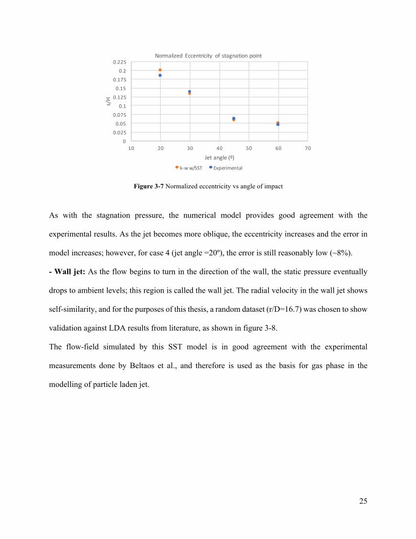
Figure 3-7 Normalized eccentricity vs angle of impact ................................................................ 25
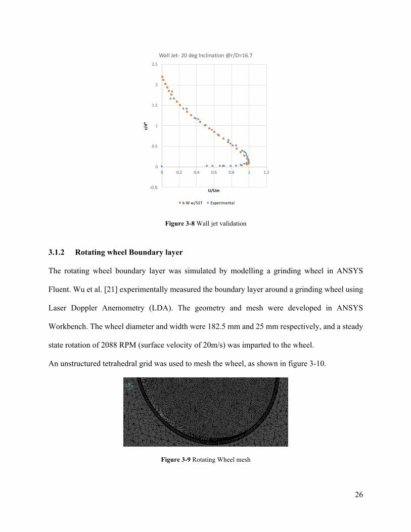
Figure 3-8 Wall jet validation ....................................................................................................... 26
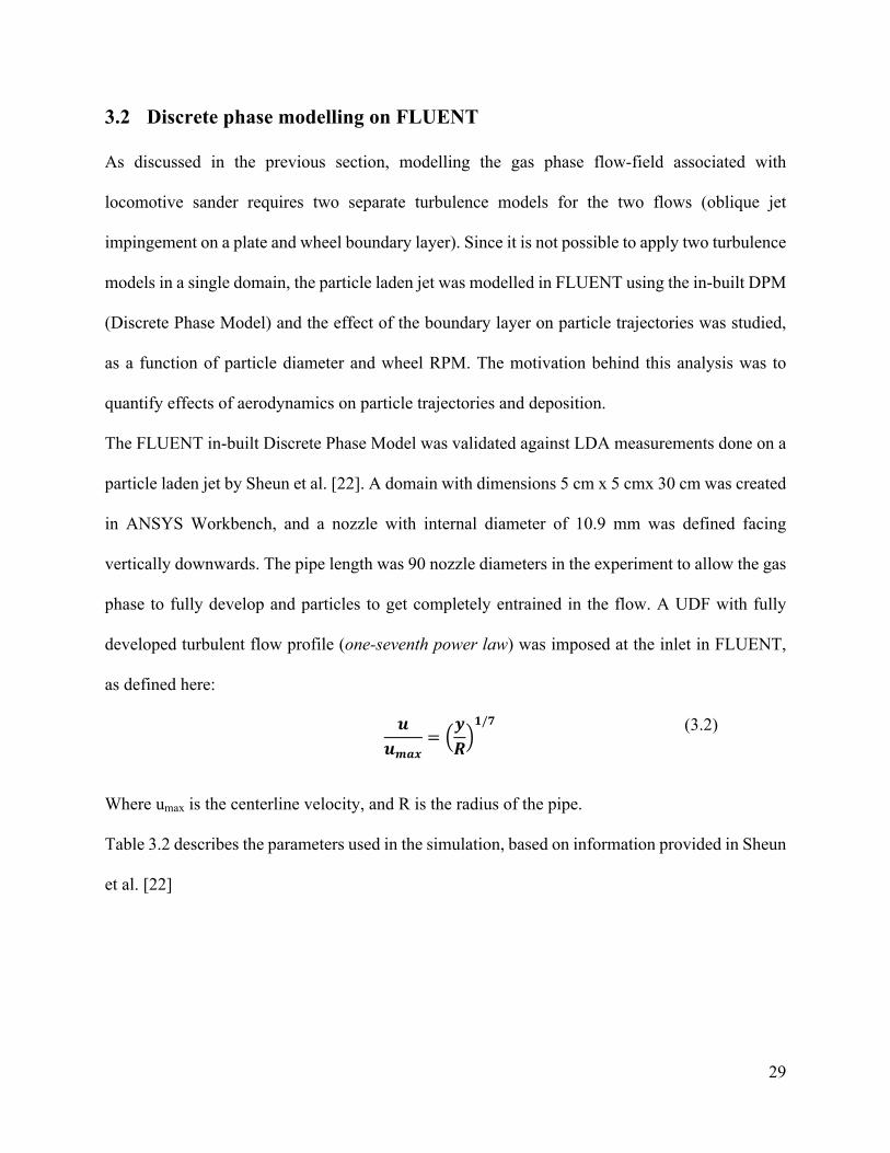
Figure 3-9 Rotating Wheel mesh .................................................................................................. 26
Figure 3-10 Measurement lines for [21] ....................................................................................... 27
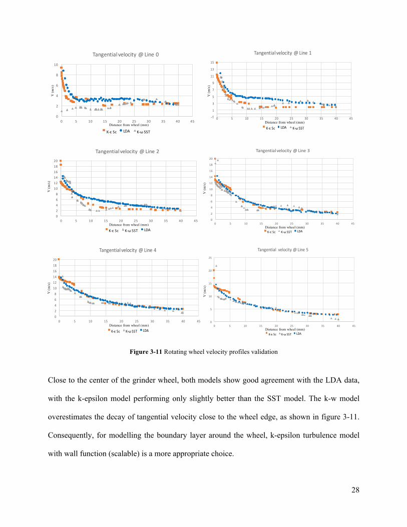
Figure 3-11 Rotating wheel velocity profiles validation .............................................................. 28
Figure 3-12 Grid independence for validation simulation ............................................................ 30
Figure 3-13 Inlet condition gas phase velocity validation ............................................................ 31
Figure 3-14 Inlet condition for solid phase velocity validation .................................................... 31
Figure 3-15 Radial variation of gas phase velocity at 20d downstream from exit ....................... 32
Figure 3-16 Radial variation of solid phase velocity at 20d downstream from exit ..................... 32
Figure 3-17 Gas phase validation for axial velocity along centerline .......................................... 33
xii
Figure 3-18 Solid phase validation for axial velocity along centerline ........................................ 33
Figure 3-19 Inflation layer around wheel ..................................................................................... 35
Figure 3-20 Particle trajectories for sample particles ................................................................... 35
Figure 3-21 y-displacement of particles w/BL compared to stationary wheel case ..................... 36
Figure 3-22 x-shift for sample particles in presence of BL .......................................................... 37
Figure 3-23 x-shift vs particle diameter for 400 RPM .................................................................. 37
Figure 3-24 Effect of boundary layer presence on particle pre-impact velocity .......................... 38
Figure 3-25 Solid phase axial velocity variation along centerline for EDEM-Fluent .................. 39
Figure 4-1 Model geometry schematic ......................................................................................... 40
Figure 4-2 CAD model of assembly on Workbench/EDEM ........................................................ 41
Figure 4-3 Coefficient of sliding friction testing apparatus .......................................................... 43
Figure 4-4 Coefficient of sliding friction of test sands ................................................................. 43
Figure 4-5 Coefficient of rolling friction of Lab sand and glass beads ........................................ 44
Figure 4-6 Coefficient of restitution measurement ....................................................................... 45
Figure 4-7 Coefficient of restitution values for sands .................................................................. 45
Figure 4-8 Glass beads size distribution ....................................................................................... 46
Figure 4-9 Grid independence for proof of concept simulation ................................................... 47
Figure 4-10 EDEM domain .......................................................................................................... 47
Figure 4-11 Particle velocity validation ........................................................................................ 48
Figure 4-12 Particle leaks from collector geometry ..................................................................... 49
Figure 4-13a: Scaled up collector 4-13b: Virtual surfaces for rail motion/fixing leaks .............. 50
Figure 4-14 Grid independence for DEM ..................................................................................... 50
Figure 4-15 Fluent time step independence study ........................................................................ 51

xiii
Figure 4-16 Repeatability of deposition simulation ...................................................................... 52
Figure 4-17 Particle imaging from multiple orientations ............................................................. 52
Figure 4-18 Creating surface from trace outlines ......................................................................... 53
Figure 4-19 Final Particle CAD file .............................................................................................. 53
Figure 4-20b Fine model ............................................................................................................... 53
Figure 4-21a Rough model ........................................................................................................... 53
Figure 4-22 Jet deflection in crossflow[24] .................................................................................. 54
Figure 4-23 Virtual surface conveyor rotation .............................................................................. 56
Figure 4-24 Scaled up domain on Workbench ............................................................................. 56
Figure 5-1 Coefficient of Restitution vs Sander efficiency .......................................................... 58
Figure 5-2 Coefficient of rolling friction vs Sander efficiency .................................................... 59
Figure 5-3 Coefficient of sliding friction vs Sander efficiency .................................................... 59
Figure 5-4 Particle losses (slipping) for low COFs ...................................................................... 60
Figure 5-5 Particle size vs exit velocity ........................................................................................ 61
Figure 5-6 Jet decay for larger particles ....................................................................................... 62
Figure 5-7 Particle diameter vs sander efficiency ......................................................................... 62
Figure 5-8 Sander efficiency as a function of particle exit velocity (particle diameter- 0.5 mm) 63
Figure 5-9 Deposition as a function of particle size (constant particle exit velocity) .................. 64
Figure 5-10 Very fine particle model (78 spheres) ....................................................................... 65
Figure 5-11 Simulation results summary ...................................................................................... 65
Figure 5-12 Sander efficiency vs Crosswind intensity ................................................................. 67
Figure 5-13 Crosswind deflection of solid jet ............................................................................... 68
Figure 5-14 Sander efficiency attenuation in the presence of crosswinds vs particle size ........... 69

xiv
Figure 5-15 Crosswind attenuation vs nip-nozzle distance .......................................................... 70
Figure B-6-1 Gas phase radial velocity distribution (x/d=40) ...................................................... 79
Figure B-6-2 solid phase velocity radial variation (x/d=40) ......................................................... 79
Figure B-6-3 Effect of loading ratio ............................................................................................. 80

xv
Acknowledgements
First and foremost, I would like to thank my supervisor, Dr. Sheldon Green, for his mentorship,
immense knowledge and constant support throughout the course of my research. His valuable
suggestions and weekly feedbacks were instrumental in taking this project to completion well
ahead of time. I also wish to thank Dr. Green for his support and advice regarding both my
academic and professional endeavors. It has been a pleasure for me to work under his supervision
for the last year and half, and I could not have asked for a better graduate advisor for my Masters
degree.
I would also like to thank L.B. Foster Ltd. for their support of this research, and special thanks to
Mr. John Cotter, Dr. Louisa Stanlake and Mr. Dmitri Gutsulyak for providing guidance and
direction to this project.
Finally, I would like to thank my lab mates for their encouragement and distractions, and helping
me survive through some of the more challenging phases of this project. A special thanks to Justin
Roberts for his stimulating discussions about this project, along with his constant feedback and
suggestions regarding my work.

xvi
Dedication
To my Parents, Bhavya, and Pragya Didi
I love you all dearly.
1
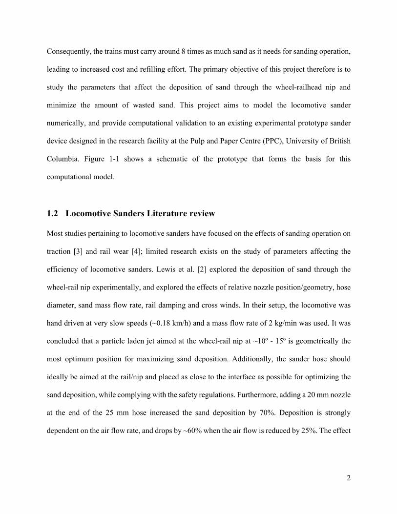
Chapter 1:
Introduction
1.1 Background
Wheel-rail adhesion for locomotives is adversely affected by natural contaminants such as leaves,
ice and moisture on the railhead. Passage of trains over these contaminants causes formation of
slippery layers on the rails, resulting in potentially dangerous slip or slide conditions when the
train is braking or moving up a slope. Poor traction therefore poses both safety (long stopping
distances) and performance (reduced acceleration) issues. The optimum coefficient of traction
between the wheel and railhead required for braking and acceleration has been shown to be around
0.2; however, a thick, hard layer of compressed leaves can reduce the value to below ~0.02[1].
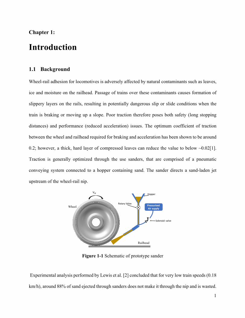
Traction is generally optimized through the use sanders, that are comprised of a pneumatic
conveying system connected to a hopper containing sand. The sander directs a sand-laden jet
upstream of the wheel-rail nip.
Figure 1-1 Schematic of prototype sander
Experimental analysis performed by Lewis et al. [2] concluded that for very low train speeds (0.18
km/h), around 88% of sand ejected through sanders does not make it through the nip and is wasted.
Hopper
PressurizedAirsupply
RotaryValve
Solenoid valve
VW
Wheel
Railhead
2
Consequently, the trains must carry around 8 times as much sand as it needs for sanding operation,
leading to increased cost and refilling effort. The primary objective of this project therefore is to
study the parameters that affect the deposition of sand through the wheel-railhead nip and
minimize the amount of wasted sand. This project aims to model the locomotive sander
numerically, and provide computational validation to an existing experimental prototype sander
device designed in the research facility at the Pulp and Paper Centre (PPC), University of British
Columbia. Figure 1-1 shows a schematic of the prototype that forms the basis for this
computational model.
1.2 Locomotive Sanders Literature review
Most studies pertaining to locomotive sanders have focused on the effects of sanding operation on
traction [3] and rail wear [4]; limited research exists on the study of parameters affecting the
efficiency of locomotive sanders. Lewis et al. [2] explored the deposition of sand through the
wheel-rail nip experimentally, and explored the effects of relative nozzle position/geometry, hose
diameter, sand mass flow rate, rail damping and cross winds. In their setup, the locomotive was
hand driven at very slow speeds (~0.18 km/h) and a mass flow rate of 2 kg/min was used. It was
concluded that a particle laden jet aimed at the wheel-rail nip at ~10º - 15º is geometrically the
most optimum position for maximizing sand deposition. Additionally, the sander hose should
ideally be aimed at the rail/nip and placed as close to the interface as possible for optimizing the
sand deposition, while complying with the safety regulations. Furthermore, adding a 20 mm nozzle
at the end of the 25 mm hose increased the sand deposition by 70%. Deposition is strongly
dependent on the air flow rate, and drops by ~60% when the air flow is reduced by 25%. The effect
3
of crosswinds was also studied; the deflection of particle laden jet leads to inefficient deposition
even for moderate cross wind speeds (45 km/h) with an oncoming wind velocity of 45 km/h.
Some preliminary numerical modelling of the sand deposition through the wheel-rail nip was
performed by Gorbunov et al. [5], where the discrete phase was defined in Borland C++
environment. Through the model, they could plot the particle distribution on the rail as a function
of rail speed and flow velocity. In a separate study [6], the authors studied the effects of several
parameters on the coefficient of friction (COF) between wheel/rail experimentally. It was
concluded that the flow speed of the granular material had the greatest effect on the friction
coefficient, while the angle of jet had very little effect on COF.
1.3 Multiphase Flow Modeling Literature review
Locomotive sanding is a multiphase flow problem comprising of particle laden jet with gas phase
(compressed air) and solid phase (sand) impinging on a moving substrate. Additionally, there are
other flows associated with this system, including the boundary layer around the rotating wheel,
crosswinds and longitudinal winds caused by the motion of the train. In this project, Computational
Fluid Dynamics (CFD) was employed to simulate the gas phase, and Discrete Element Method
was used to model the particle phase.
Pneumatic conveying is used widely in industry, and finds application in a number of industrial
operations such as granular transport, mineral processing, catalytic reactions in fluidized beds, gas-
particle separators, etc. Computational modelling of pneumatic conveying of problem-specific two
phase flows has been done extensively previously. The two-phase flow is generally simulated by
coupling CFD and DEM together. There is a plethora of options for implementing both CFD and
DEM, ranging from completely open source platforms (OPENFOAM/LIGGGHTS) to commercial
4
packages (ANSYS Fluent/EDEM); the decision to use one of these options depends entirely on
the complexity of problem involved, price and license availability, expertise, time and
computational power available. For instance, most of the open-source platforms such as
OPENFOAM and SU2 allow for greater flexibility and control, but have a much steep learning
curve. On the other hand, commercial packages like ANSYS Fluent (CFD) and EDEM (DEM)
offer much more user-friendly platforms for modelling the two-phase flow, more intuitive
meshing- at the cost of less control and expensive licensing.
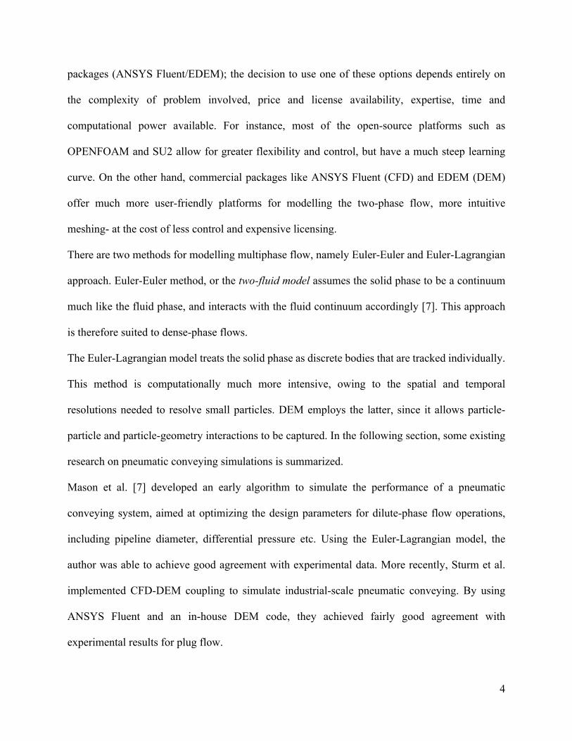
There are two methods for modelling multiphase flow, namely Euler-Euler and Euler-Lagrangian
approach. Euler-Euler method, or the two-fluid model assumes the solid phase to be a continuum
much like the fluid phase, and interacts with the fluid continuum accordingly [7]. This approach
is therefore suited to dense-phase flows.
The Euler-Lagrangian model treats the solid phase as discrete bodies that are tracked individually.
This method is computationally much more intensive, owing to the spatial and temporal
resolutions needed to resolve small particles. DEM employs the latter, since it allows particle-
particle and particle-geometry interactions to be captured. In the following section, some existing
research on pneumatic conveying simulations is summarized.
Mason et al. [7] developed an early algorithm to simulate the performance of a pneumatic
conveying system, aimed at optimizing the design parameters for dilute-phase flow operations,
including pipeline diameter, differential pressure etc. Using the Euler-Lagrangian model, the
author was able to achieve good agreement with experimental data. More recently, Sturm et al.
implemented CFD-DEM coupling to simulate industrial-scale pneumatic conveying. By using
ANSYS Fluent and an in-house DEM code, they achieved fairly good agreement with
experimental results for plug flow.
5 (1.3)
Apart from the open source codes, several studies have employed commercial packages for both
gas phase (Fluent) and discrete phase (EDEM). For instance, Azimian et al. [8] used Fluent and
EDEM coupling to solve for particulate turbulent pipe flow, and validated the computational
results with LDA/PDA technique. Ebrahimi et al. [17] simulated horizontal pneumatic conveying
through EDEM-FLUENT, and found that the computational model slightly overpredicted both
particle and gas phase velocities. They concluded that the CFD-DEM coupling can be used to
accurately model pneumatic conveying of discrete phase, given that proper grid independence is
conducted, and fine mesh is used for both phases.
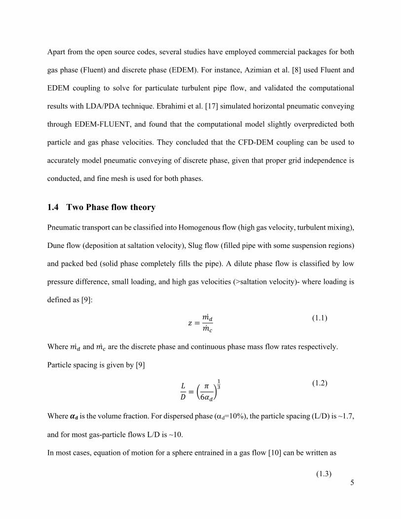
1.4 Two Phase flow theory
Pneumatic transport can be classified into Homogenous flow (high gas velocity, turbulent mixing),
Dune flow (deposition at saltation velocity), Slug flow (filled pipe with some suspension regions)
and packed bed (solid phase completely fills the pipe). A dilute phase flow is classified by low
pressure difference, small loading, and high gas velocities (>saltation velocity)- where loading is
defined as [9]:
𝑧 =𝑚$
𝑚% (1.1)
Where 𝑚$ and 𝑚% are the discrete phase and continuous phase mass flow rates respectively.
Particle spacing is given by [9]
𝐿𝐷 =
𝜋6𝛼$
+,
(1.2)
Where 𝜶d is the volume fraction. For dispersed phase (ad=10%), the particle spacing (L/D) is ~1.7,
and for most gas-particle flows L/D is ~10.
In most cases, equation of motion for a sphere entrained in a gas flow [10] can be written as
6
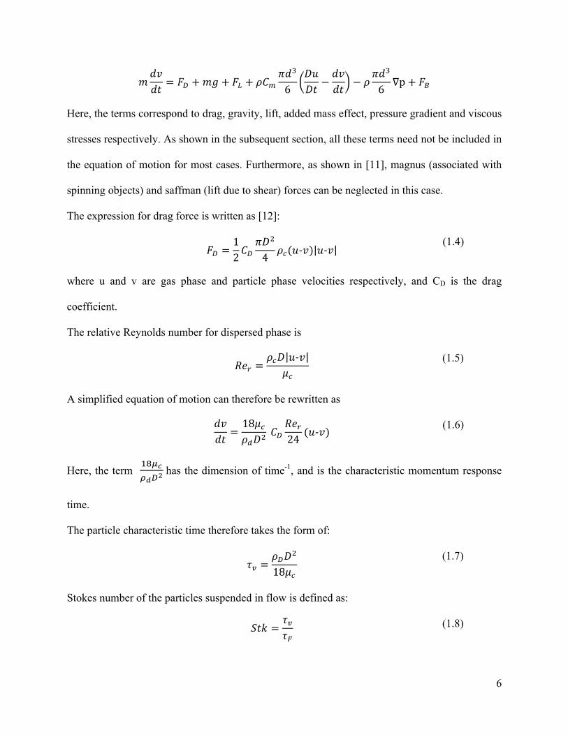
𝑚𝑑𝑣𝑑𝑡 = 𝐹2 +𝑚𝑔 + 𝐹5 + 𝜌𝐶8
𝜋𝑑,
6𝐷𝑢𝐷𝑡 −
𝑑𝑣𝑑𝑡 − 𝜌
𝜋𝑑,
6 ∇p + 𝐹=
Here, the terms correspond to drag, gravity, lift, added mass effect, pressure gradient and viscous
stresses respectively. As shown in the subsequent section, all these terms need not be included in
the equation of motion for most cases. Furthermore, as shown in [11], magnus (associated with
spinning objects) and saffman (lift due to shear) forces can be neglected in this case.
The expression for drag force is written as [12]:
𝐹2 =
12𝐶2
𝜋𝐷@
4 𝜌%(𝑢-𝑣) 𝑢-𝑣 (1.4)
where u and v are gas phase and particle phase velocities respectively, and CD is the drag
coefficient.
The relative Reynolds number for dispersed phase is
𝑅𝑒G =
𝜌%𝐷 𝑢-𝑣𝜇%
(1.5)
A simplified equation of motion can therefore be rewritten as
𝑑𝑣𝑑𝑡 =
18𝜇%𝜌$𝐷@
𝐶2𝑅𝑒G24 (𝑢-𝑣)
(1.6)
Here, the term +KLMNO2P
has the dimension of time-1, and is the characteristic momentum response
time.
The particle characteristic time therefore takes the form of:
𝜏R =
𝜌2𝐷@
18𝜇%
(1.7)
Stokes number of the particles suspended in flow is defined as:
𝑆𝑡𝑘 =𝜏R𝜏U
(1.8)

7
that describes the behavior of suspended particles. In the case of locomotive sander with the
particle laden jet exiting the nozzle towards the wheel-rail nip, the characteristic fluid time tF is
tU =
𝐷5𝑈 (1.9)
Where DL is the characteristic length. In the case of pneumatic conveying of sand, DL can be
defined as the distance between the nozzle and the wheel-rail nip, since particle flow through the
pipe is not relevant, and only the flow characteristics of particles exiting the nozzle and through
the wheel-railhead interface are considered. U is the mean jet velocity.
Stokes number of the sand particles in the flow plays an important role for optimizing the
efficiency of the sander, since it characterizes the effects of factors such as crosswinds, turbulence
etc. on particle trajectories. For Stk<<1, particles will be well entrained in the flow, with velocities
very close to the gas phase and will respond to changes in the flow. On the other hand, for particles
with Stk>>1, inertia governs the trajectories and the particles do not respond to rapid changes in
the fluid velocity, and continue their initial path.
Phase Coupling
Coupling the particle phase can be classified as one-way (gas phase affects the particle phase) or
two-way (particle phase also affects gas phase) coupling. For sufficiently dilute flows such as
pneumatic conveying from train sanders, the effect of particle phase on carrier phase can be
ignored.
1.5 Motivation, objectives and scope
1.5.1 Motivation
The primary motivation behind this project is to gain a better understanding of parameters that
effect the efficiency of locomotive sanders. Improving the efficiency of sanding operation will

8
reduce the amount of sand lost during sanding operation, hence reducing cost and effort related to
refilling. Some of the motivations behind this computational study are:
1. Provide computational validation to an existing experimental setup
2. Individual parameters such as coefficient of restitution, friction, size distribution etc. can
be isolated and their effects on the deposition can be studied independent of other factors.
3. Numerical modelling allows for a more fundamental understanding of the jet impingement
and sand deposition process, without the influence of experimental disturbances (system
noise, vibrations, leakages, etc.)
4. Studying the effects of certain parameters (e.g. Crosswinds, undercarriage wind, etc.) is
experimentally challenging owing to the setup constraints. Performing such analysis on
CFD is straightforward, and does not require any drastic changes to the existing model.
1.5.2 Objectives and scope
The objective of this work is to numerically simulate the locomotive sander, and provide
computational validation to an existing experimental system. Specifically, this project aims to
address the following questions:
1. Are the sand particles well entrained and uniformly dispersed in the flow, without saltation
occurring?
2. What is the effect of bounce properties, coefficient of restitution, friction, and other
particle-geometry interactions on the deposition of sand through the nip?
3. Does the non-sphericity of sand particles play a role in the particle-railhead interaction?
4. Does the aerodynamics associated with the boundary layer around the rotating wheel affect
the sand deposition?
9
5. How strongly do crosswinds affect the particle trajectories from the nozzle to the nip, and
is the jet velocity large enough to negate the deflection of sand?
6. What are the major sources of the particle losses?
These questions are approached through numerical simulations, and a computational model is
created on ANSYS Fluent (CFD) and EDEM (DEM code) coupled together to simulate the two-
phase flow. The gas phase flow is first validated independently through several experimental and
computational studies in literature, followed by validation tests for the discrete phase. Following
this, the two phases are coupled together through a journal file, and validation simulations are
performed for the two-phase flow (particle laden jet) by comparing the simulations to LDA
experiments found in literature. In Chapter 2, the methodology is explained in detail, along with
the validation tests and detailed background information about the CFD and DEM code in chapter
3. In Chapter 4, the development of the numerical model is described, along with some
experimental tests performed to measure DEM inputs. Results from this study are discussed and a
comparison with the experimental study is done in chapter 5. Finally, chapter 6 provides the
conclusion to this work where the study is summarized and real life recommendations are made
for implementation in locomotive sanders, with some future recommendations for the research.
10
Chapter 2:
Methodology
This section explores the CFD and DEM simulation method (meshing, turbulence modelling etc.),
two-phase coupling, and some experimental procedures to measure the inputs for the DEM code
(coefficients of sliding and rolling friction, restitution) and imaging (high speed camera and optical
microscope). To assess the validity of numerical model, several validation simulations were
performed for the gas phase, particle phase and the gas-particle coupling, which will be discussed
in this section.
ANSYS Fluent is a commercial CFD package that is widely employed in the industry. Owing to
its relatively simple learning curve and straightforward and automated meshing, ANSYS
Workbench was used for creating the geometry and meshing for the most part. For some validation
simulations, ANSYS ICEM was employed owing to the relative complexity of geometries and
certain meshing issues. For discrete phase, commercial DEM software EDEM was used, as
discussed in the previous section. The DEM geometry was usually imported from the Workbench
tool; for some validation simulations, geometry was created in Solidworks and meshed in EDEM
meshing tool.
2.1 Mathematical formulation of the fluid phase
The locally solved Navier-Stokes equations as described by Anderson and Jackson [13] are solved
in the CFD solver to model to fluid flow, using a finite volume discretization scheme and applying
the SIMPLE algorithm. The transient 3D continuity and momentum conservation equations are
written as follows:

11
(2.2)
(2.3)
𝜕(1-𝜙Y)𝜌𝜕𝑡 + ∇. 1-𝜙Y 𝜌𝑣 = 0
(2.1)
𝜕 1 − 𝜙Y 𝜌𝑣𝜕𝑡 + ∇. 1 − 𝜙Y 𝜌𝑣𝑣 = −∇𝑝 + ∇. (1 − 𝜙Y 𝜏)
+∇. ( 1 − 𝜙Y 𝜏′) + (1 − 𝜙Y)𝜌𝑔 − 𝑆
𝑆 =𝐹_`aGb%`^c_,^
∆𝑉8agh
_i
^
Here,𝜙Y is the voidage term, S is the volumetric force acting on each grid cell, and Finteraction are
the forces acting on particles as discussed in Section 1.4.
2.1.1 Drag modelling
There are several in-built drag force models for EDEM-Fluent coupling. For this study, the Wen
and Yu (1966) [14] model is employed. For dilute particle flow, the fluid porosity ef has a value
>0.8 and a voidage function f(ef) = ef-4.7 is employed.
The drag force is written as follows (for dilute flow):
𝛽 =34𝐶2𝑑Y𝜌 1-el [email protected] 𝑣-𝑢Y
(2.4)
Some other built in drag models are the modified Stokes drag model, Di Felice drag model and
Ergun. Based on some preliminary literature review, Wen and Yu model was found to be the most
appropriate drag model for this study considering particle volume fraction (disperse) [14].
2.1.2 Turbulence modelling
The locomotive sander system consists of several separate flows, including the free jet impinging
on a moving surface, boundary layer around the rotating wheel, undercarriage wind due to the
𝐹2 =
𝑉Y𝛽1-el
(𝑣-𝑢Y) (2.5)
12
motion of the train and crosswinds. Validation simulations were set up to confirm the validity of
turbulence models for specific flows; in this study, k-e and k-f models were employed.
Since all the simulations in this study have a dilute flow with small mass loading- (<6) (mass flow
rate of sand/mass flow rate of air) and high Stokes number (>>1), the effect of discrete phase on
carrier phase is not taken into consideration.
The mathematical formulation for the two turbulence models are explained below, from the
FLUENT user guide.
k-e Turbulence model
K-e is a two-equation model for solving the closure problem for the Reynold stresses. Assuming
isotropic turbulence, an appropriate characterization of the velocity fluctuations is done by
defining the turbulent kinetic energy[15]:
In order to distinguish between larger and smaller eddies, an additional term describes the turbulent
dissipation rate:
𝐹2 =
𝑉Y𝛽1-el
(𝑣-𝑢Y) (2.6)
The turbulent eddy viscosity is:
𝜈o = 𝐶L
𝑘@
𝜀 (2.7)
Where 𝑪𝝁 is a constant with value 0.09 and 𝜺 is the dissipation rate. Based on literature review,
the realizable k-epsilon model is the appropriate turbulence model for modelling jet impingement.
Furthermore, it has been previously shown [16] that k-epsilon realizable model provides the best
𝑘 =12 (< 𝑢'𝑢' > +< 𝑣'𝑣' > +< 𝑤'𝑤' >)
(2.5)

13
performance of all the k-e models, especially relating to spreading rates for planar and round jets.
It is defined in FLUENT as follows [15]:
𝜕(𝜌𝑘)𝜕𝑡 +
𝜕(𝜌𝑘𝑢x)𝜕𝑥x
=𝜕𝜕𝑥x
𝜇 +𝜇`𝜎{
𝜕𝑘𝜕𝑥x
+ 𝐺{ + 𝐺} − 𝜌𝜖 − 𝑌� + 𝑆{
and
𝜕 𝜌𝜖𝜕𝑡 +
𝜕 𝜌𝜖𝑢x𝜕𝑥x
=𝜕𝜕𝑥x
𝜇 +𝜇`𝜎�
𝜕𝜖𝜕𝑥x
+ 𝜌𝐶+𝑆� + 𝐶+�𝜖𝑘 𝐶,�𝐺}
−𝐶@𝜌𝜖@
𝑘 + 𝜈𝜖+ 𝑆�
Here, Gk is the turbulent kinetic energy generation due to velocity gradients, Gb is the turbulence
KE generation due to buoyancy, 𝜎 variables are the turbulent Prandlt numbers, 𝜖 is the voidage
function, and C2,1e are constants whose values are given in table A2. 𝑆�,{ are source terms defined
by the user.
k-w SST model
k-w shear stress transport (SST) is another turbulence model that is employed in this study, and
gives the best performance for rotating wheel boundary layer, as confirmed by validation
simulations. This model essentially blends the standard k-w and k-𝜖 by switching to k-w near the
walls, and back to k-𝜖 away from the walls; This blending ensures a more suitable behavior of
equations for both near-wall and far-field regions. The mathematical formulation for this model in
FLUENT is as follows [14]:
𝜕(𝜌𝑘)𝜕𝑡 +
𝜕(𝜌𝑘𝑢^)𝜕𝑥^
=𝜕𝜕𝑥x
Γ{𝜕𝑘𝜕𝑥x
+ 𝐺{-𝑌{ + 𝑆{ (2.10)
and
(2.8)
(2.9)
14
𝜕(𝜌𝜔)𝜕𝑡 +
𝜕(𝜌𝜔𝑢^)𝜕𝑥^
=𝜕𝜕𝑥x
Γ�𝜕𝜔𝜕𝑥x
+ 𝐺� + 𝐷�-𝑌� + 𝑆� (2.11)
Here, 𝐺{ is the turbulent kinetic energy due to mean velocity gradient, Gw is the generation of w,
Γ�,{ is the diffusivity of 𝜔 and k, Y terms represent dissipation and D is the cross diffusion, which
has been described in the FLUENT tutorial. The two S terms are user defined functions, which are
not used in this work.
2.2 Mathematical formulation of Discrete phase
The translational and rotational momentum of a particle is dictated through Newton’s laws of
motion as follows[17]:
𝑚Y
𝑑@𝑦Y𝑑𝑡@ = 𝐹_`aGb%`^c_ + 𝑚Y𝑔 + 𝐹%
(2.12)
and
𝐼Y𝑑𝜔Y𝑑𝑡 = 𝑇Y
(2.13)
Here Fc is the particle-particle and particle-geometry collision force and Finteraction is the equivalent
lift/drag force on the particle.
EDEM has several particle-particle and particle-geometry contact models, including both linear
and non-linear models. In this study, the Hertz-Mindlin model was employed, based on
preliminary literature review[18]. This is a non-linear elastic soft sphere model, that employs two
separate spring-dashpot responses for normal and tangential interactions between bodies, and a
coulomb friction coefficient for shear.
15
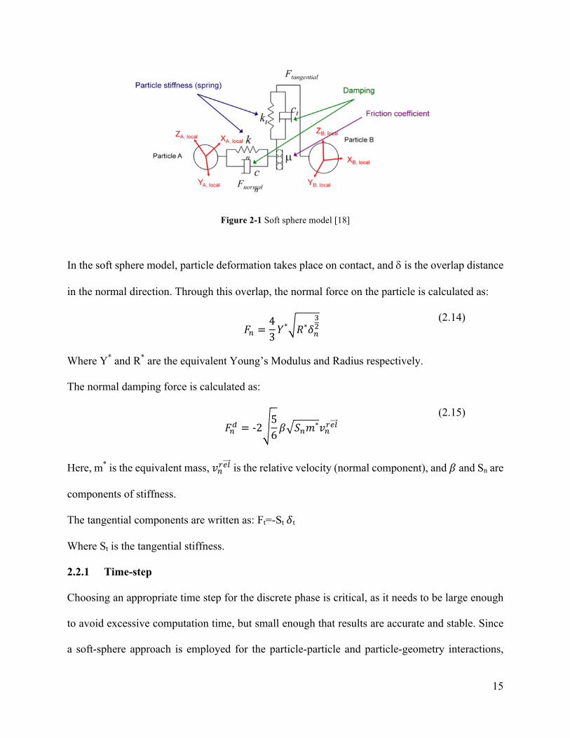
Figure 2-1 Soft sphere model [18]
In the soft sphere model, particle deformation takes place on contact, and d is the overlap distance
in the normal direction. Through this overlap, the normal force on the particle is calculated as:
𝐹_ =
43𝑌
* 𝑅*𝛿_,@
(2.14)
Where Y* and R* are the equivalent Young’s Modulus and Radius respectively.
The normal damping force is calculated as:
𝐹_$ = -2
56𝛽 𝑆_𝑚*𝑣_Ga�
(2.15)
Here, m* is the equivalent mass, 𝑣_Ga� is the relative velocity (normal component), and 𝛽 and Sn are
components of stiffness.
The tangential components are written as: Ft=-St𝛿t
Where St is the tangential stiffness.
2.2.1 Time-step
Choosing an appropriate time step for the discrete phase is critical, as it needs to be large enough
to avoid excessive computation time, but small enough that results are accurate and stable. Since
a soft-sphere approach is employed for the particle-particle and particle-geometry interactions,
16
large time-steps lead to large overlaps and consequently very large forces on particles, causing
inaccurate and unstable results.
Rayleigh wave is a surface acoustic wave that travels through the solid’s surface; estimating the
particle time-step is done by calculating the Rayleigh time-step, given as follows:
𝑇� =
𝜋𝑅(𝜌 𝐺)+/@
0.1631𝜐 + 0.8766 (2.16)
where R is the particle radius, 𝜌 is the material density, G is the shear modulus, and 𝜐 is the
Poisson’s ratio.
In order to capture the energy transfer through Rayleigh waves, it is recommended [19] that the
particle time-step is a fractional value of this Rayleigh time, i.e. 0.1-0.3TR. Modelling the particles
with increasing accuracy therefore leads to increased computational cost, since the clumped sphere
model (Section 4.6) requires smaller spheres to capture the sharp edges and features accurately.
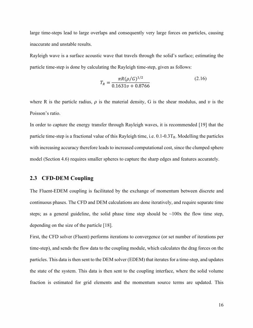
2.3 CFD-DEM Coupling
The Fluent-EDEM coupling is facilitated by the exchange of momentum between discrete and
continuous phases. The CFD and DEM calculations are done iteratively, and require separate time
steps; as a general guideline, the solid phase time step should be ~100x the flow time step,
depending on the size of the particle [18].
First, the CFD solver (Fluent) performs iterations to convergence (or set number of iterations per
time-step), and sends the flow data to the coupling module, which calculates the drag forces on the
particles. This data is then sent to the DEM solver (EDEM) that iterates for a time-step, and updates
the state of the system. This data is then sent to the coupling interface, where the solid volume
fraction is estimated for grid elements and the momentum source terms are updated. This
17
information is then sent back to the CFD solver where the process is repeated till the two-phase
flow evolves to the required time.
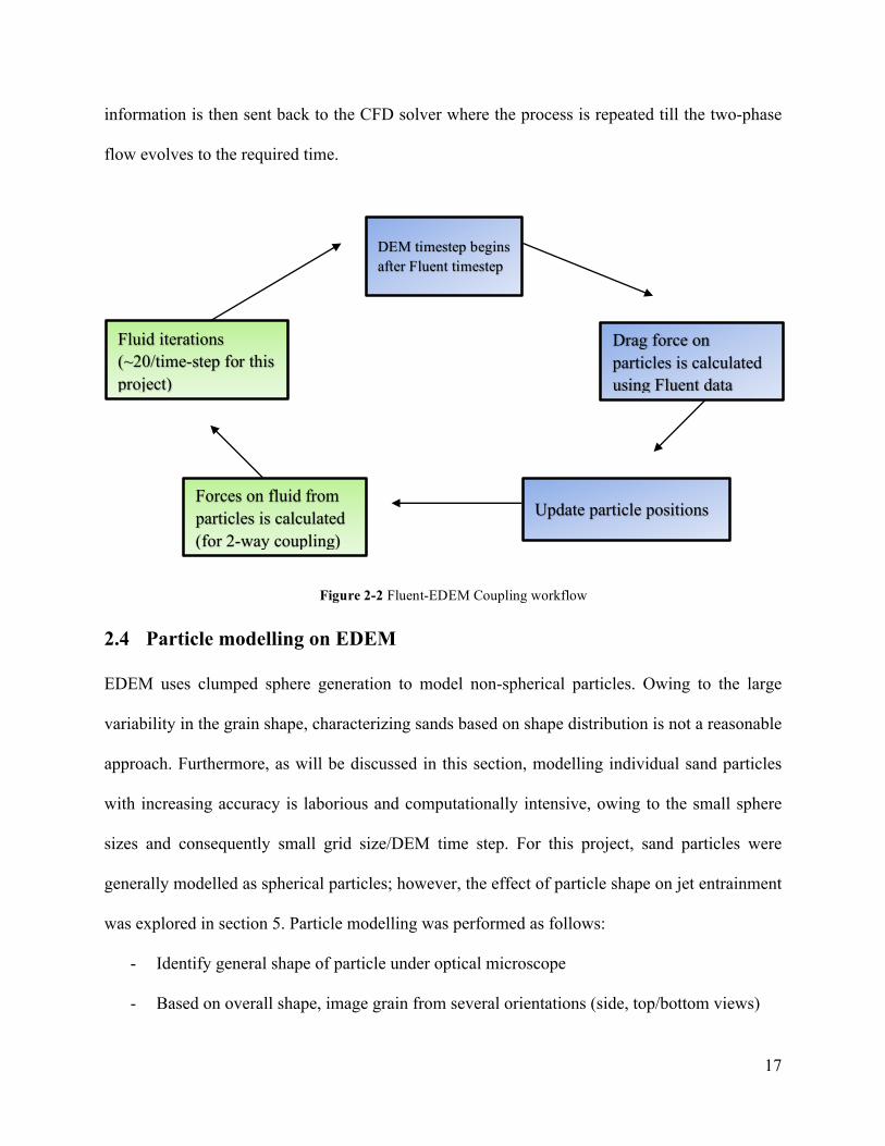
2.4 Particle modelling on EDEM
EDEM uses clumped sphere generation to model non-spherical particles. Owing to the large
variability in the grain shape, characterizing sands based on shape distribution is not a reasonable
approach. Furthermore, as will be discussed in this section, modelling individual sand particles
with increasing accuracy is laborious and computationally intensive, owing to the small sphere
sizes and consequently small grid size/DEM time step. For this project, sand particles were
generally modelled as spherical particles; however, the effect of particle shape on jet entrainment
was explored in section 5. Particle modelling was performed as follows:
- Identify general shape of particle under optical microscope
- Based on overall shape, image grain from several orientations (side, top/bottom views)
DEM timestep begins after Fluent timestep
Drag force on particles is calculated using Fluent data
Update particle positions Forces on fluid from particles is calculated (for 2-way coupling)
Fluid iterations (~20/time-step for this project)
Figure 2-2 Fluent-EDEM Coupling workflow
18
- Post-process images to extract outlines, and import the outline sketches on CAD
- Outline sketches are connected by drawing guiding curves based on top/bottom view
- Create a surface file and import in EDEM as a particle model file
- Manually input coordinates/radius of spheres to generate a clumped sphere model based
on the modelling accuracy required.
Fig 2-3 shows four ways of modelling a sample sand grain, with increasing modeling accuracy
Figure 2-3 Clumped sphere modelling on EDEM
Section 5.6 details this process for a sample sand grain, aimed at understanding the effect of
modelling accuracy on sand deposition.
19
Chapter 3:
Validation Simulations
For this study, several validation simulations were performed for the continuous phase, discrete
phase and the coupled two-phase flow. The primary objectives of these simulations were:
1. Test the validity of the numerical models against experimental or numerical studies in
literature.
2. Compare the performance of various turbulence models for specific flow conditions.
3. Test the validity of CFD-DEM coupling against experimental measurements of particle
laden jets in literature.
The meshing, setup and results of these simulations are discussed here.
3.1 Gas phase validation
The carrier phase consists of a jet impinging on a moving plate (railhead) and the boundary layer
around the rotating wheel. Since the nozzle is mounted on the moving locomotive, there is no
boundary layer along the railhead, and the undercarriage winds can be expressed as the resultant
of the oncoming flow due to train motion and crosswinds.
The free jet from the nozzle is first validated using the experimental data from Wygnanski and
Fiedler (1969) [20], and the LDA measurements from Beltaos et al. [20] were used to validate the
oblique jet impingement on flat surface.
3.1.1 Free jet and oblique impinging on surface
A three dimensional, round turbulent jet was modelled numerically. A domain with dimensions of
45 cm x 15 cm x 18 cm was defined with a nozzle placed at various geometries and positions
20
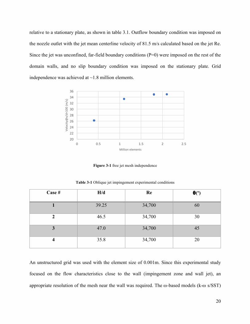
relative to a stationary plate, as shown in table 3.1. Outflow boundary condition was imposed on
the nozzle outlet with the jet mean centerline velocity of 81.5 m/s calculated based on the jet Re.
Since the jet was unconfined, far-field boundary conditions (P=0) were imposed on the rest of the
domain walls, and no slip boundary condition was imposed on the stationary plate. Grid
independence was achieved at ~1.8 million elements.
Figure 3-1 free jet mesh independence
Table 3-1 Oblique jet impingement experimental conditions
Case # H/d Re q(º)
1 39.25 34,700 60
2 46.5 34,700 30
3 47.0 34,700 45
4 35.8 34,700 20
An unstructured grid was used with the element size of 0.001m. Since this experimental study
focused on the flow characteristics close to the wall (impingement zone and wall jet), an
appropriate resolution of the mesh near the wall was required. The w-based models (k-w s/SST)
202224262830323436
0 0.5 1 1.5 2 2.5
Velocity@x/d=10
0(m
/s)
Millionelements
21
have an automatic wall treatment (wall-function) if a coarse near-wall grid is present, without any
user input [15]. Y+ is a normalized lengthscale associated with turbulent flow in the near wall
regions. It is generally recommended that Y+ £1 be used for Shear Stress Transport (SST) models;
however, along with the mesh independence study, the Y+ value was varied by increasing the
number of inflation layers for case #4 (nozzle at 20º from floor). Up until Y+ value of 8 (w/6
inflation layers) at the impingement region, there was no change in the flow field; consequently, a
Y+ value of 8 was chosen for this set of simulations.
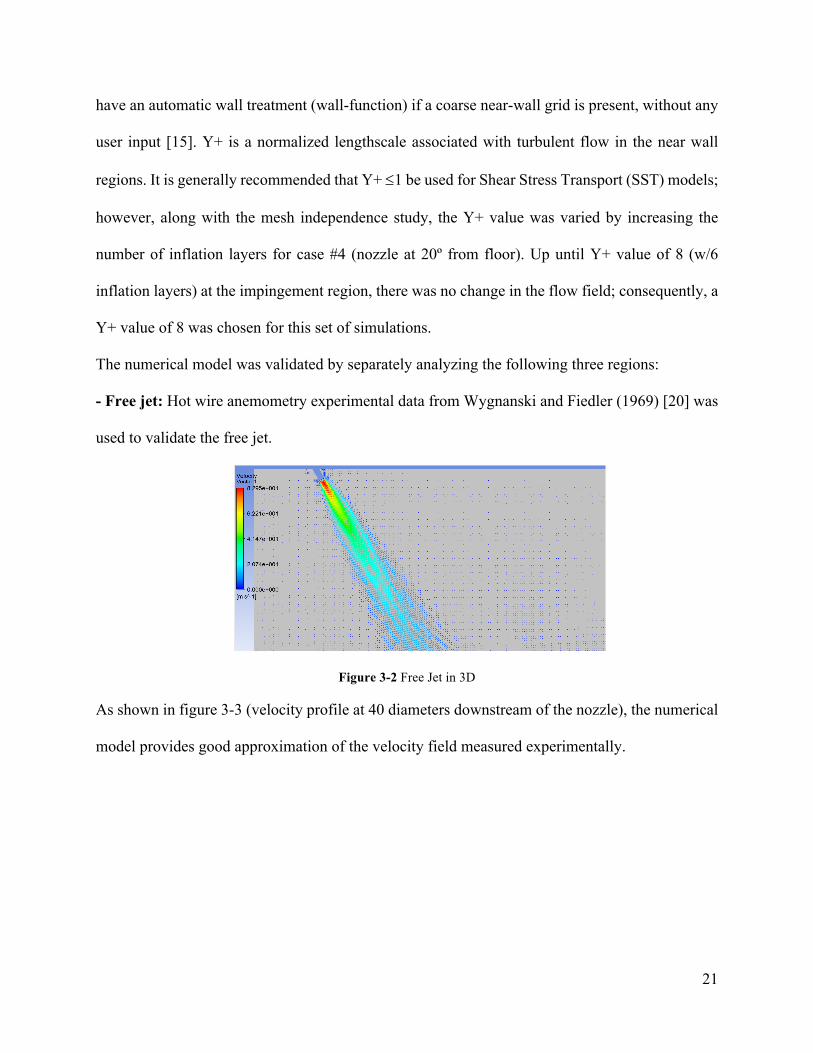
The numerical model was validated by separately analyzing the following three regions:
- Free jet: Hot wire anemometry experimental data from Wygnanski and Fiedler (1969) [20] was
used to validate the free jet.
Figure 3-2 Free Jet in 3D
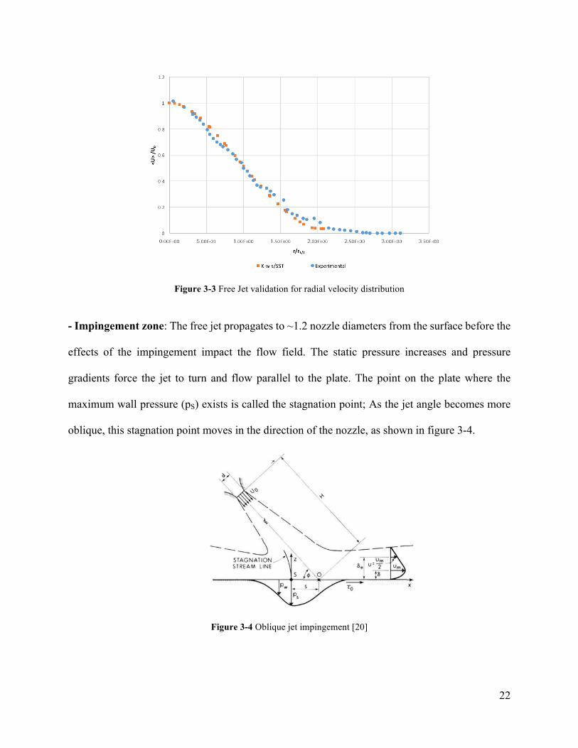
As shown in figure 3-3 (velocity profile at 40 diameters downstream of the nozzle), the numerical
model provides good approximation of the velocity field measured experimentally.
22
Figure 3-3 Free Jet validation for radial velocity distribution
- Impingement zone: The free jet propagates to ~1.2 nozzle diameters from the surface before the
effects of the impingement impact the flow field. The static pressure increases and pressure
gradients force the jet to turn and flow parallel to the plate. The point on the plate where the
maximum wall pressure (pS) exists is called the stagnation point; As the jet angle becomes more
oblique, this stagnation point moves in the direction of the nozzle, as shown in figure 3-4.
Figure 3-4 Oblique jet impingement [20]

23
The wall pressure was plotted along the plate centerline (z=0) and the stagnation pressure (peak)
and eccentricity (deviation from x=0) was determined from the plots.
-10 0
10
20
30
40
50
60
70
80
90
-0.25 -0.2 -0.15 -0.1 -0.05 0 0.05 0.1 0.15 0.2 0.25
WallPressure(Pa)
x(m)
Wallpressurealongz=0
Case4 Case2 Case3 Case1
Figure 3-5 Wall pressure profile along centerline
The normalized stagnation pressure is defined as follows:
𝑵𝒐𝒓𝒎𝒂𝒍𝒊𝒛𝒆𝒅𝒔𝒕𝒂𝒈𝒏𝒂𝒕𝒊𝒐𝒏𝒑𝒓𝒆𝒔𝒔𝒖𝒓𝒆:
𝒑𝒔𝝆𝑼𝟎𝟐 𝟐
𝑯𝒅
𝟐
(3.1)
H/d values are provided in table 3.1, and the jet mean centerline velocity U0 is 81.5 m/s.
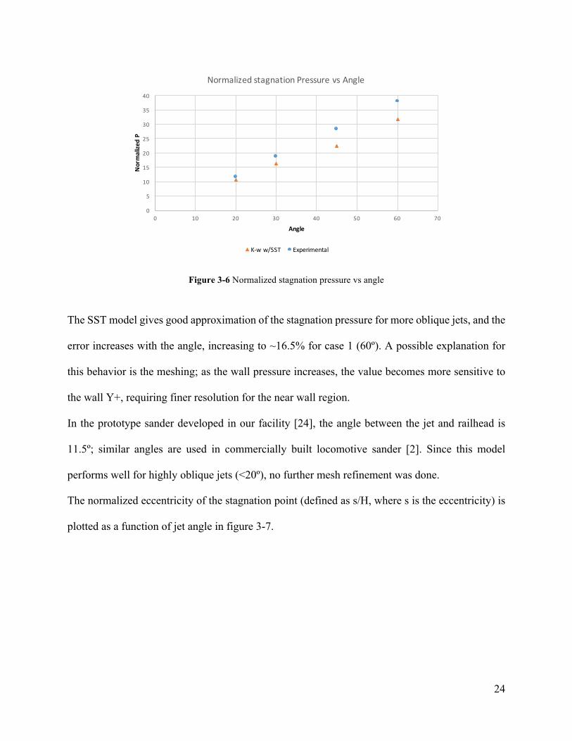
Normalized stagnation pressure is plotted as a function of jet angle from the plate in figure 3-6.
24
Figure 3-6 Normalized stagnation pressure vs angle
The SST model gives good approximation of the stagnation pressure for more oblique jets, and the
error increases with the angle, increasing to ~16.5% for case 1 (60º). A possible explanation for
this behavior is the meshing; as the wall pressure increases, the value becomes more sensitive to
the wall Y+, requiring finer resolution for the near wall region.
In the prototype sander developed in our facility [24], the angle between the jet and railhead is
11.5º; similar angles are used in commercially built locomotive sander [2]. Since this model
performs well for highly oblique jets (<20º), no further mesh refinement was done.
The normalized eccentricity of the stagnation point (defined as s/H, where s is the eccentricity) is
plotted as a function of jet angle in figure 3-7.
0
5
10
15
20
25
30
35
40
0 10 20 30 40 50 60 70
Normalize
dP
Angle
NormalizedstagnationPressurevsAngle
K-ww/SST Experimental
25
Figure 3-7 Normalized eccentricity vs angle of impact
As with the stagnation pressure, the numerical model provides good agreement with the
experimental results. As the jet becomes more oblique, the eccentricity increases and the error in
model increases; however, for case 4 (jet angle =20º), the error is still reasonably low (~8%).
- Wall jet: As the flow begins to turn in the direction of the wall, the static pressure eventually
drops to ambient levels; this region is called the wall jet. The radial velocity in the wall jet shows
self-similarity, and for the purposes of this thesis, a random dataset (r/D=16.7) was chosen to show
validation against LDA results from literature, as shown in figure 3-8.
The flow-field simulated by this SST model is in good agreement with the experimental
measurements done by Beltaos et al., and therefore is used as the basis for gas phase in the
modelling of particle laden jet.
00.0250.050.075
0.10.1250.150.175
0.20.225
10 20 30 40 50 60 70
s/H
Jetangle(º)
Normalized Eccentricity ofstagnationpoint
k-ww/SST Experimental
26
Figure 3-8 Wall jet validation
3.1.2 Rotating wheel Boundary layer
The rotating wheel boundary layer was simulated by modelling a grinding wheel in ANSYS
Fluent. Wu et al. [21] experimentally measured the boundary layer around a grinding wheel using
Laser Doppler Anemometry (LDA). The geometry and mesh were developed in ANSYS
Workbench. The wheel diameter and width were 182.5 mm and 25 mm respectively, and a steady
state rotation of 2088 RPM (surface velocity of 20m/s) was imparted to the wheel.
An unstructured tetrahedral grid was used to mesh the wheel, as shown in figure 3-10.
Figure 3-9 Rotating Wheel mesh
-0.5
0
0.5
1
1.5
2
2.5
0 0.2 0.4 0.6 0.8 1 1.2
z/d*
U/Um
WallJet- 20deg Inclination@r/D=16.7
k-Ww/SST Experimental

27
A rotating fluid zone was defined by creating a thin concentric volume outside the wheel as
shown in the figure, and imparting a rotational boundary condition to the fluid zone.
Wu et. al. measured the tangential velocity component of the boundary layer as a function of
distance from the middle of the wheel. 5 measurement lines were defined along which the LDA
laser probe was positioned, as shown in figure 3-10.
Figure 3-10 Measurement lines for [21]
For this simulation, two turbulence models were separately used to model the boundary layer,
namely k-w (Shear Stress Transport) and Realizable k-e w/Scalable wall function. The k-epsilon
model performs much better than the SST model, specifically close to the periphery of the wheel.
28
Figure 3-11 Rotating wheel velocity profiles validation
Close to the center of the grinder wheel, both models show good agreement with the LDA data,
with the k-epsilon model performing only slightly better than the SST model. The k-w model
overestimates the decay of tangential velocity close to the wheel edge, as shown in figure 3-11.
Consequently, for modelling the boundary layer around the wheel, k-epsilon turbulence model
with wall function (scalable) is a more appropriate choice.
0
2
4
6
8
10
0 5 10 15 20 25 30 35 40 45
Tangentialvelocity@Line0
K-εSc LDA K-ωSST
-1 1
3
5
7
9
11
13
15
0 5 10 15 20 25 30 35 40 45
Tangentialvelocity@Line1
K-εSc LDA K-ωSST
02468
101214161820
0 5 10 15 20 25 30 35 40 45
Tangentialvelocity@Line2
K-εSc K-ωSST LDA
0
2
4
6
8
10
12
14
16
18
20
0 5 10 15 20 25 30 35 40 45
Tangentialvelocity@Line3
K-εSc K-ωSST LDA
02468101214161820
0 5 10 15 20 25 30 35 40 45
Tangentialvelocity@Line4
K-εSc K-ωSST LDA
0
5
10
15
20
25
0 5 10 15 20 25 30 35 40 45
Tangentialvelocity@Line5
K-εSc K-ωSST LDA
V (m
/s)
V (m
/s)
V (m
/s)
V (m
/s)
V (m
/s)
V (m
/s)
Distance from wheel (mm) Distance from wheel (mm)
Distance from wheel (mm) Distance from wheel (mm)
Distance from wheel (mm) Distance from wheel (mm)
29
3.2 Discrete phase modelling on FLUENT
As discussed in the previous section, modelling the gas phase flow-field associated with
locomotive sander requires two separate turbulence models for the two flows (oblique jet
impingement on a plate and wheel boundary layer). Since it is not possible to apply two turbulence
models in a single domain, the particle laden jet was modelled in FLUENT using the in-built DPM
(Discrete Phase Model) and the effect of the boundary layer on particle trajectories was studied,
as a function of particle diameter and wheel RPM. The motivation behind this analysis was to
quantify effects of aerodynamics on particle trajectories and deposition.
The FLUENT in-built Discrete Phase Model was validated against LDA measurements done on a
particle laden jet by Sheun et al. [22]. A domain with dimensions 5 cm x 5 cmx 30 cm was created
in ANSYS Workbench, and a nozzle with internal diameter of 10.9 mm was defined facing
vertically downwards. The pipe length was 90 nozzle diameters in the experiment to allow the gas
phase to fully develop and particles to get completely entrained in the flow. A UDF with fully
developed turbulent flow profile (one-seventh power law) was imposed at the inlet in FLUENT,
as defined here:
𝒖𝒖𝒎𝒂𝒙
=𝒚𝑹
𝟏/𝟕
(3.2)
Where umax is the centerline velocity, and R is the radius of the pipe.
Table 3.2 describes the parameters used in the simulation, based on information provided in Sheun
et al. [22]
30
Table 3-2 Validation simulation parameters
Particle mean Diameter 119µm
Non-spherical shape factor 1.25
Loading Ratio 0.2
Sand mass flow rate 5.715 x 10⁻⁴ kg/s
Air flowrate 2.8575 x 10⁻³ kg/s
Jet exit velocity 31.5 m/s
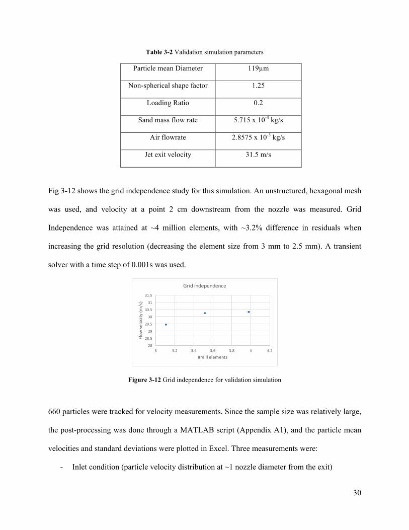
Fig 3-12 shows the grid independence study for this simulation. An unstructured, hexagonal mesh
was used, and velocity at a point 2 cm downstream from the nozzle was measured. Grid
Independence was attained at ~4 million elements, with ~3.2% difference in residuals when
increasing the grid resolution (decreasing the element size from 3 mm to 2.5 mm). A transient
solver with a time step of 0.001s was used.
Figure 3-12 Grid independence for validation simulation
660 particles were tracked for velocity measurements. Since the sample size was relatively large,
the post-processing was done through a MATLAB script (Appendix A1), and the particle mean
velocities and standard deviations were plotted in Excel. Three measurements were:
- Inlet condition (particle velocity distribution at ~1 nozzle diameter from the exit)
28
28.5
29
29.5
30
30.5
31
31.5
3 3.2 3.4 3.6 3.8 4 4.2
Flow
velocity(m/s)
#millelements
Gridindependence
31
- Radial variation (measured at x/d=20, 40 from the nozzle exit)
- Axial variation (measured along the jet centerline from nozzle exit to x/d=50)
Inlet Condition
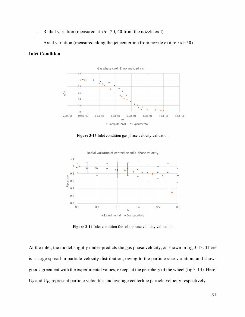
Figure 3-13 Inlet condition gas phase velocity validation
Figure 3-14 Inlet condition for solid phase velocity validation
At the inlet, the model slightly under-predicts the gas phase velocity, as shown in fig 3-13. There
is a large spread in particle velocity distribution, owing to the particle size variation, and shows
good agreement with the experimental values, except at the periphery of the wheel (fig 3-14). Here,
UP and UP0 represent particle velocities and average centerline particle velocity respectively.
0
0.2
0.4
0.6
0.8
1
1.2
-2.00E-01 0.00E+00 2.00E-01 4.00E-01 6.00E-01 8.00E-01 1.00E+00 1.20E+00
u/uc
r/x
Gasphase(x/d=1)normalizedvvsr
Computatonal Experimental
0.5
0.6
0.7
0.8
0.9
1
1.1
0.1 0.2 0.3 0.4 0.5 0.6
Upc/Up
o
r/x
Radialvariationofcentrelinesolid phasevelocity
Experimental Computational
32
Radial Variation
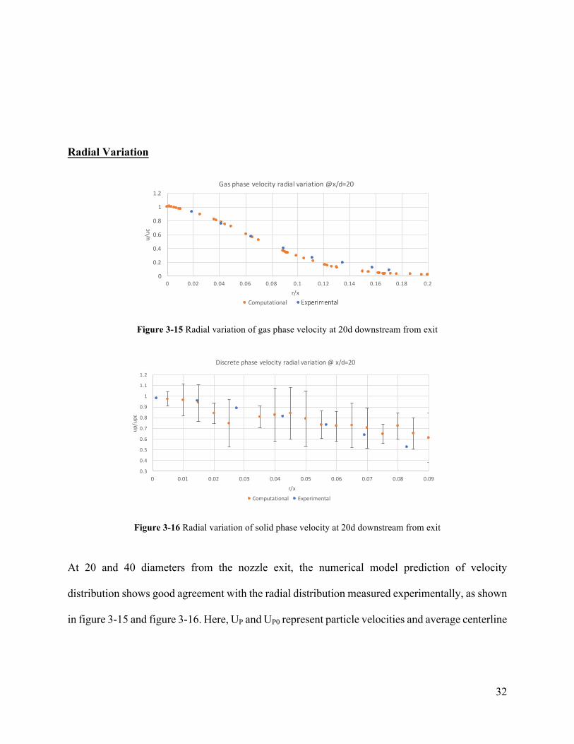
Figure 3-15 Radial variation of gas phase velocity at 20d downstream from exit
Figure 3-16 Radial variation of solid phase velocity at 20d downstream from exit
At 20 and 40 diameters from the nozzle exit, the numerical model prediction of velocity
distribution shows good agreement with the radial distribution measured experimentally, as shown
in figure 3-15 and figure 3-16. Here, UP and UP0 represent particle velocities and average centerline
0
0.2
0.4
0.6
0.8
1
1.2
0 0.02 0.04 0.06 0.08 0.1 0.12 0.14 0.16 0.18 0.2
u/uc
r/x
Gasphasevelocityradialvariation@x/d=20
Computational EXperimental
0.3
0.4
0.5
0.6
0.7
0.8
0.9
1
1.1
1.2
0 0.01 0.02 0.03 0.04 0.05 0.06 0.07 0.08 0.09
up/upc
r/x
Discretephasevelocityradialvariation@x/d=20
Computational Experimental
33
particle velocity respectively. Radial variation at 40 diameters downstream is plotted in appendix
B2.
Axial Variation
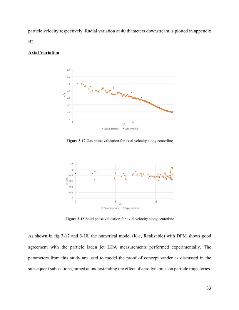
Figure 3-17 Gas phase validation for axial velocity along centerline
Figure 3-18 Solid phase validation for axial velocity along centerline
As shown in fig 3-17 and 3-18, the numerical model (K-e, Realizable) with DPM shows good
agreement with the particle laden jet LDA measurements performed experimentally. The
parameters from this study are used to model the proof of concept sander as discussed in the
subsequent subsections, aimed at understanding the effect of aerodynamics on particle trajectories.
0
0.2
0.4
0.6
0.8
1
1.2
1.4
1 10
v/vc
x/d
GasphaseAxialvariationofcenterlinevelocity
Computational Experimental
0
0.2
0.4
0.6
0.8
1
1.2
1 5 25
vc/vco
x/d
Solid phaseaxialvelocityvariationofcenterlinevelocity
Computational Experimental
34
3.3 Boundary layer effect on particle trajectories
3.3.1 Model geometry
The geometry was created in ANSYS Workbench, and modelled after the scaled down prototype
sander at the facility located in PPC, UBC. The specifications of the geometry, along with
discussion on the scaling down is detailed in subsection 3.3.1. A wheel of diameter 49 cm and
width 3.2 cm was created, and a railhead was defined using a plate of width 3.6 cm. The wheel-
rail clearance at the nip was 1 mm wide and the nozzle diameter was 3 mm, similar to the
experimental setup.
3.3.2 Simulation setup
A turbulent, fully developed pipe flow velocity profile can generally be described by the one-
seventh power law profile (Eqn 3.2). This velocity profile boundary condition was imposed on the
nozzle inlet through a user defined function. Particle factory was defined at the inlet, where
particles were generated with 0 initial velocity. The tube length for entrainment was 0.125 m. Table
3-3 summarizes the simulation variables for the two-phase flow for this set of simulations.
Table 3-3 Simulation parameters
Particle diameters (mm) 0.1, 0.25, 0.5, 0.75
Sand mass flow rate 1e-05 kg/s
𝒗𝒆𝒙𝒊𝒕,𝒈𝒂𝒔 12.79 m/s
Entrainment length 0.125 m
Nip-nozzle distance 200 mm
RPMs 0, 200, 400, 600
Element # in mesh 6.8 e+06
35
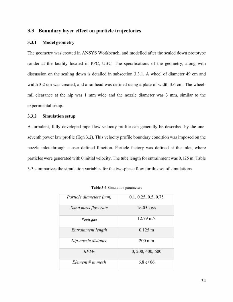
Grid independence to ~3% was attained when using a mesh with 6.8 mil elements, as shown in
figure 3-18.
Figure 3-19 Inflation layer around wheel
Two inflation layers were defined at the wheel surface and railhead, with the specifications as
described for oblique jet impingement simulations in section 3.1.1.
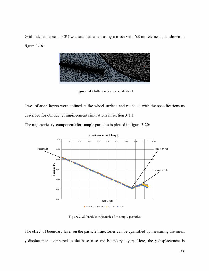
The trajectories (y-component) for sample particles is plotted in figure 3-20:
Figure 3-20 Particle trajectories for sample particles
The effect of boundary layer on the particle trajectories can be quantified by measuring the mean
y-displacement compared to the base case (no boundary layer). Here, the y-displacement is
-0.26
-0.25
-0.24
-0.23
-0.22
-0.21
-0.2 0.19 0.21 0.23 0.25 0.27 0.29 0.31 0.33 0.35 0.37 0.39
Y-po
sition(m
)
Pathlength
ypositionvspathlength
200RPM 400RPM 600RPM 0RPM
NozzleExit Impactonrail
Impactonwheel

36
measured at a set distance after the impact on the wheel; particles that impact the railhead and
subsequently hit the wheel were isolated. Particles with same IDs (same initial positions) were
tracked for multiple simulations with different wheel speeds (hence different BL velocity profiles).
Here, particle size was set constant at 0.25 mm, with 4 RPM values (Table 3-3) and the sample
size (number of particles tracked) was 10.
Figure 3-21 y-displacement of particles w/BL compared to stationary wheel case
The effect of rotating wheel boundary layer therefore, even for 600 RPM (corresponding to surface
speeds of 15 m/s) is <0.5mm. The standard deviation here is large, owing to large variation in
particle trajectories and small sample size. However, since the number of particle-geometry
collisions before a particle makes it into the nip is small (~2-3), it can be concluded that the effect
of this y-displacement on the deposition is not significant.
This analysis is repeated for 4 particle diameters, as given in table 3-3. The change in the particle
first impact position in the x-direction (x-shift) in the presence of rotating fluid zone around the
wheel is another criterion for quantifying the impact of boundary layer on the particle trajectories,
as shown in figure 3-22.
0
0.1
0.2
0.3
0.4
0.5
0.6
0.7
0 100 200 300 400 500 600 700
meanydisplacementd
ifference(m
m)
RPM
Meany-displacementdifferencefromstationary(n=10)

37
x-shift
Figure 3-22 x-shift for sample particles in presence of BL
This set of simulations was run for 400 RPM case (train speed 10.3 m/s), and the normalized x-
shift (x-shift/nip-nozzle distance) was plotted as a function of particle diameters in fig 3-23.
Figure 3-23 x-shift vs particle diameter for 400 RPM
For very fine particles (0.1 mm), the x-shift is relatively large (1.2 cm)- corresponding to the first
datapoint. For larger particles, the shift asymptotes at ~2 mm.
-0.255 -0.25
-0.245 -0.24
-0.235 -0.23
-0.225 -0.22
-0.215 -0.21
0 0.05 0.1 0.15 0.2 0.25 0.3 0.35 0.4
Y-positio
n(m
)
PathLength(m)
0
0.02
0.04
0.06
0.08
0.1
0.12
0 0.1 0.2 0.3 0.4 0.5 0.6 0.7 0.8
x-shift/n
ip-nozzle
distance
Particlediameter(mm)
38
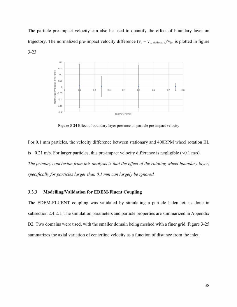
The particle pre-impact velocity can also be used to quantify the effect of boundary layer on
trajectory. The normalized pre-impact velocity difference (vp – vp, stationary)/vjet is plotted in figure
3-23.
Figure 3-24 Effect of boundary layer presence on particle pre-impact velocity
For 0.1 mm particles, the velocity difference between stationary and 400RPM wheel rotation BL
is ~0.21 m/s. For larger particles, this pre-impact velocity difference is negligible (<0.1 m/s).
The primary conclusion from this analysis is that the effect of the rotating wheel boundary layer,
specifically for particles larger than 0.1 mm can largely be ignored.
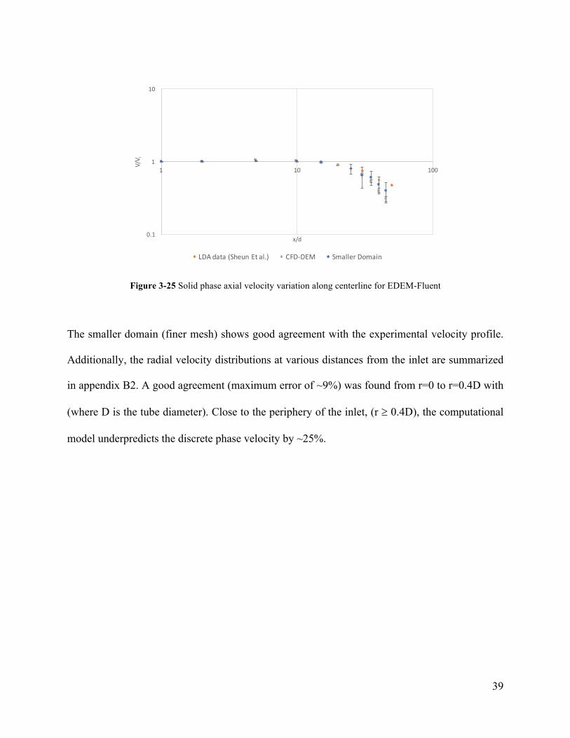
3.3.3 Modelling/Validation for EDEM-Fluent Coupling
The EDEM-FLUENT coupling was validated by simulating a particle laden jet, as done in
subsection 2.4.2.1. The simulation parameters and particle properties are summarized in Appendix
B2. Two domains were used, with the smaller domain being meshed with a finer grid. Figure 3-25
summarizes the axial variation of centerline velocity as a function of distance from the inlet.
-0.2
-0.15
-0.1
-0.05
0
0.05
0.1
0.15
0.2
0 0.1 0.2 0.3 0.4 0.5 0.6 0.7 0.8
Norm
alize
dVelocitydifference
Diameter(mm)
39
Figure 3-25 Solid phase axial velocity variation along centerline for EDEM-Fluent
The smaller domain (finer mesh) shows good agreement with the experimental velocity profile.
Additionally, the radial velocity distributions at various distances from the inlet are summarized
in appendix B2. A good agreement (maximum error of ~9%) was found from r=0 to r=0.4D with
(where D is the tube diameter). Close to the periphery of the inlet, (r ³ 0.4D), the computational
model underpredicts the discrete phase velocity by ~25%.
0.1
1
10
1 10 100
V/V i
x/d
Axialvariationalongcentreline
LDAdata(SheunEtal.) CFD-DEM SmallerDomain
40
Chapter 4:
Numerical model development
In this section, the development of numerical model on ANSYS Fluent (Gas Phase) and EDEM
(Discrete Element Method code) is discussed.
4.1 Geometry
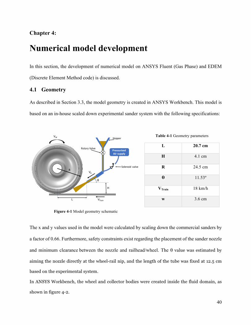
As described in Section 3.3, the model geometry is created in ANSYS Workbench. This model is
based on an in-house scaled down experimental sander system with the following specifications:
Figure 4-1 Model geometry schematic
Table 4-1 Geometry parameters
L 20.7 cm
H 4.1 cm
R 24.5 cm
θ 11.53º
VTrain 18 km/h
w 3.6 cm
The x and y values used in the model were calculated by scaling down the commercial sanders by
a factor of 0.66. Furthermore, safety constraints exist regarding the placement of the sander nozzle
and minimum clearance between the nozzle and railhead/wheel. The θ value was estimated by
aiming the nozzle directly at the wheel-rail nip, and the length of the tube was fixed at 12.5 cm
based on the experimental system.
In ANSYS Workbench, the wheel and collector bodies were created inside the fluid domain, as
shown in figure 4-2.
Hopper
PressurizedAirsupply
RotaryValve
Solenoid valveR
L
H
VW
VA
θ
VTrain
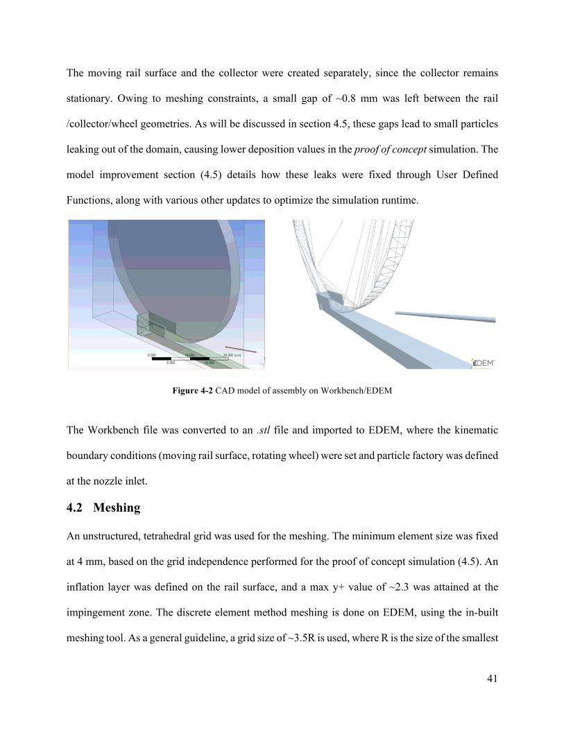
41
The moving rail surface and the collector were created separately, since the collector remains
stationary. Owing to meshing constraints, a small gap of ~0.8 mm was left between the rail
/collector/wheel geometries. As will be discussed in section 4.5, these gaps lead to small particles
leaking out of the domain, causing lower deposition values in the proof of concept simulation. The
model improvement section (4.5) details how these leaks were fixed through User Defined
Functions, along with various other updates to optimize the simulation runtime.
Figure 4-2 CAD model of assembly on Workbench/EDEM
The Workbench file was converted to an .stl file and imported to EDEM, where the kinematic
boundary conditions (moving rail surface, rotating wheel) were set and particle factory was defined
at the nozzle inlet.
4.2 Meshing
An unstructured, tetrahedral grid was used for the meshing. The minimum element size was fixed
at 4 mm, based on the grid independence performed for the proof of concept simulation (4.5). An
inflation layer was defined on the rail surface, and a max y+ value of ~2.3 was attained at the
impingement zone. The discrete element method meshing is done on EDEM, using the in-built
meshing tool. As a general guideline, a grid size of ~3.5R is used, where R is the size of the smallest

42
sphere in the domain. This recommendation was followed for the DEM meshing throughout the
study.
4.3 DEM Parameters
The Discrete Element Method code requires material properties as inputs, including the following:
- Coefficient of sliding friction
- Coefficient of rolling friction
- Coefficient of restitution (particle-particle and particle-geometry)
- Material density
- Young’s modulus
- Poisson’s ratio
These “microproperties” are used by the DEM solver to calculate particle forces using the Hertz-
Mindlin contact models, as discussed previously. Material properties such as density, Young’s
modulus and shear modulus were obtained from literature [23]; for silica sands, the material
density was set at 2650 kg/m3, and the Young’s modulus was 90.1 GPa. The coefficients of friction
and restitution were determined experimentally for different sands, and the testing procedure is
described in the following subsections.
4.3.1 Coefficient of Sliding Friction measurements
Chung et al. [25] devised a setup to measure the coefficient of sliding friction of corn grains. A
similar sliding test was devised to measure sliding friction coefficients for several sands provided
by the industrial collaborator LB Foster. A manual Z-stage was set up as shown in figure 4-3, and
a rectangular strip of stainless steel employed in the prototype sander setup to simulate the railhead
was used as the base plate.
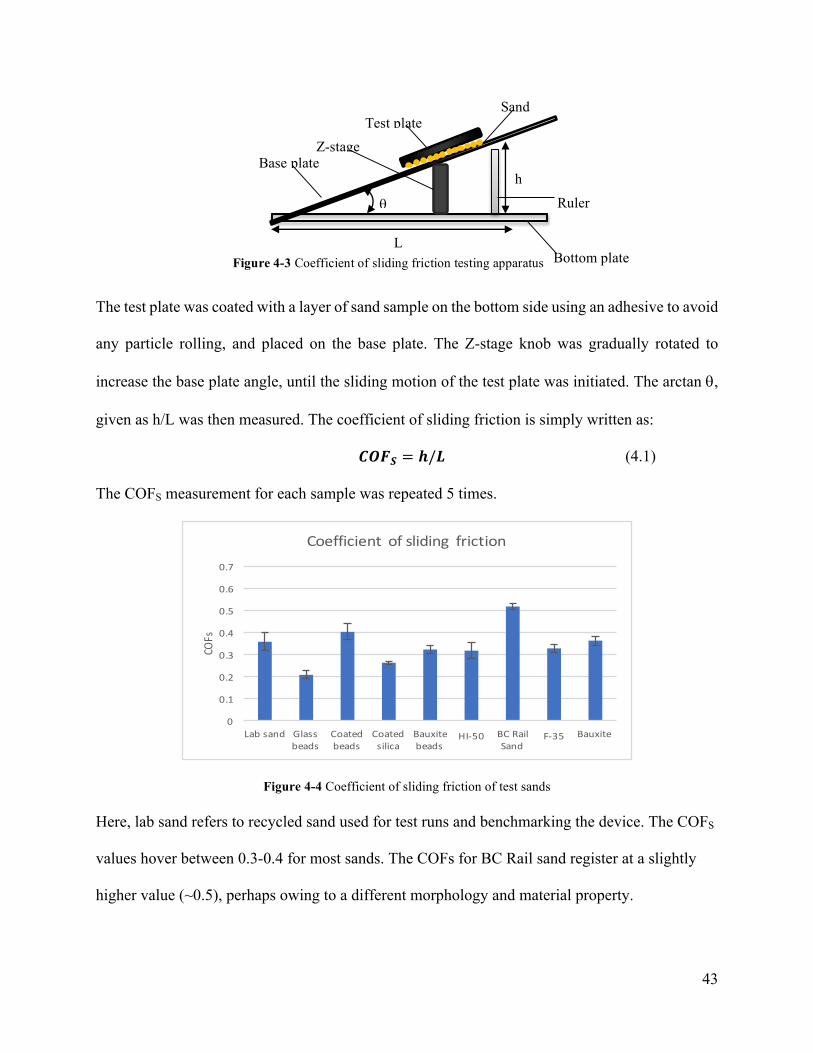
43
Figure 4-3 Coefficient of sliding friction testing apparatus
The test plate was coated with a layer of sand sample on the bottom side using an adhesive to avoid
any particle rolling, and placed on the base plate. The Z-stage knob was gradually rotated to
increase the base plate angle, until the sliding motion of the test plate was initiated. The arctan q,
given as h/L was then measured. The coefficient of sliding friction is simply written as:
𝑪𝑶𝑭𝑺 = 𝒉/𝑳 (4.1)
The COFS measurement for each sample was repeated 5 times.
Figure 4-4 Coefficient of sliding friction of test sands
Here, lab sand refers to recycled sand used for test runs and benchmarking the device. The COFS
values hover between 0.3-0.4 for most sands. The COFs for BC Rail sand register at a slightly
higher value (~0.5), perhaps owing to a different morphology and material property.
0
0.1
0.2
0.3
0.4
0.5
0.6
0.7
Labsand Glassbeads
Coatedbeads
Coatedsilica
Bauxitebeads
HI-50 BCRailSand
F-35 Bauxite
COFs
Coefficient ofsliding friction
q
L
h Base plate
Test plate Sand
Ruler
Z-stage
Bottom plate
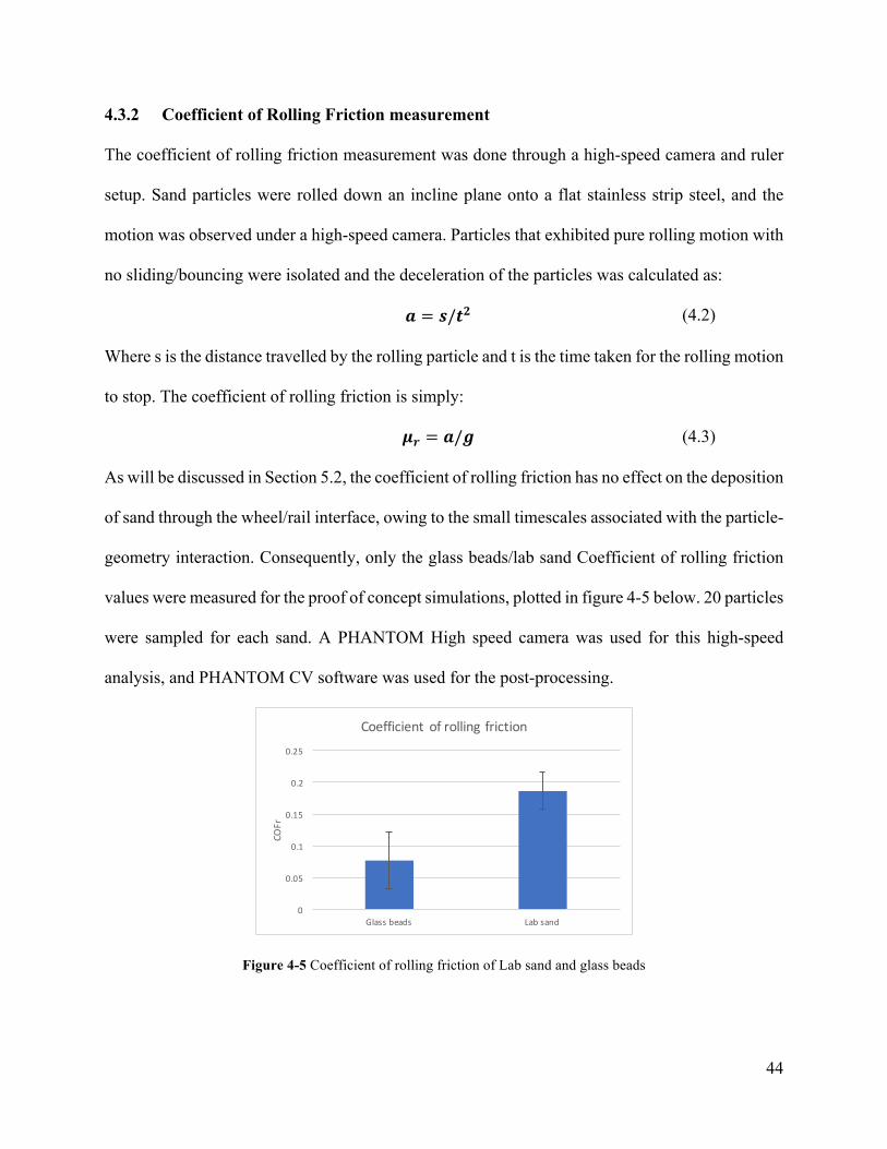
44
4.3.2 Coefficient of Rolling Friction measurement
The coefficient of rolling friction measurement was done through a high-speed camera and ruler
setup. Sand particles were rolled down an incline plane onto a flat stainless strip steel, and the
motion was observed under a high-speed camera. Particles that exhibited pure rolling motion with
no sliding/bouncing were isolated and the deceleration of the particles was calculated as:
𝒂 = 𝒔/𝒕𝟐 (4.2)
Where s is the distance travelled by the rolling particle and t is the time taken for the rolling motion
to stop. The coefficient of rolling friction is simply:
𝝁𝒓 = 𝒂/𝒈 (4.3)
As will be discussed in Section 5.2, the coefficient of rolling friction has no effect on the deposition
of sand through the wheel/rail interface, owing to the small timescales associated with the particle-
geometry interaction. Consequently, only the glass beads/lab sand Coefficient of rolling friction
values were measured for the proof of concept simulations, plotted in figure 4-5 below. 20 particles
were sampled for each sand. A PHANTOM High speed camera was used for this high-speed
analysis, and PHANTOM CV software was used for the post-processing.
Figure 4-5 Coefficient of rolling friction of Lab sand and glass beads
0
0.05
0.1
0.15
0.2
0.25
Glassbeads Labsand
COFr
Coefficient ofrollingfriction
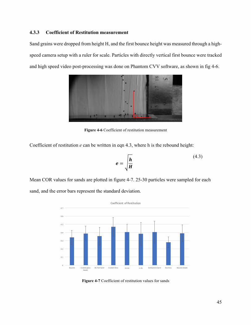
45
4.3.3 Coefficient of Restitution measurement
Sand grains were dropped from height H, and the first bounce height was measured through a high-
speed camera setup with a ruler for scale. Particles with directly vertical first bounce were tracked
and high speed video post-processing was done on Phantom CVV software, as shown in fig 4-6.
Figure 4-6 Coefficient of restitution measurement
Coefficient of restitution e can be written in eqn 4.3, where h is the rebound height:
𝒆 =
𝒉𝑯
(4.3)
Mean COR values for sands are plotted in figure 4-7. 25-30 particles were sampled for each
sand, and the error bars represent the standard deviation.
Figure 4-7 Coefficient of restitution values for sands
0
0.1
0.2
0.3
0.4
0.5
0.6
0.7
Bauxite Coatedglassbeads
BCRailSand CoatedSilica HI-50 F-35 DerbyshireSand Alumina Bauxitebeads
Coefficient ofRestitution
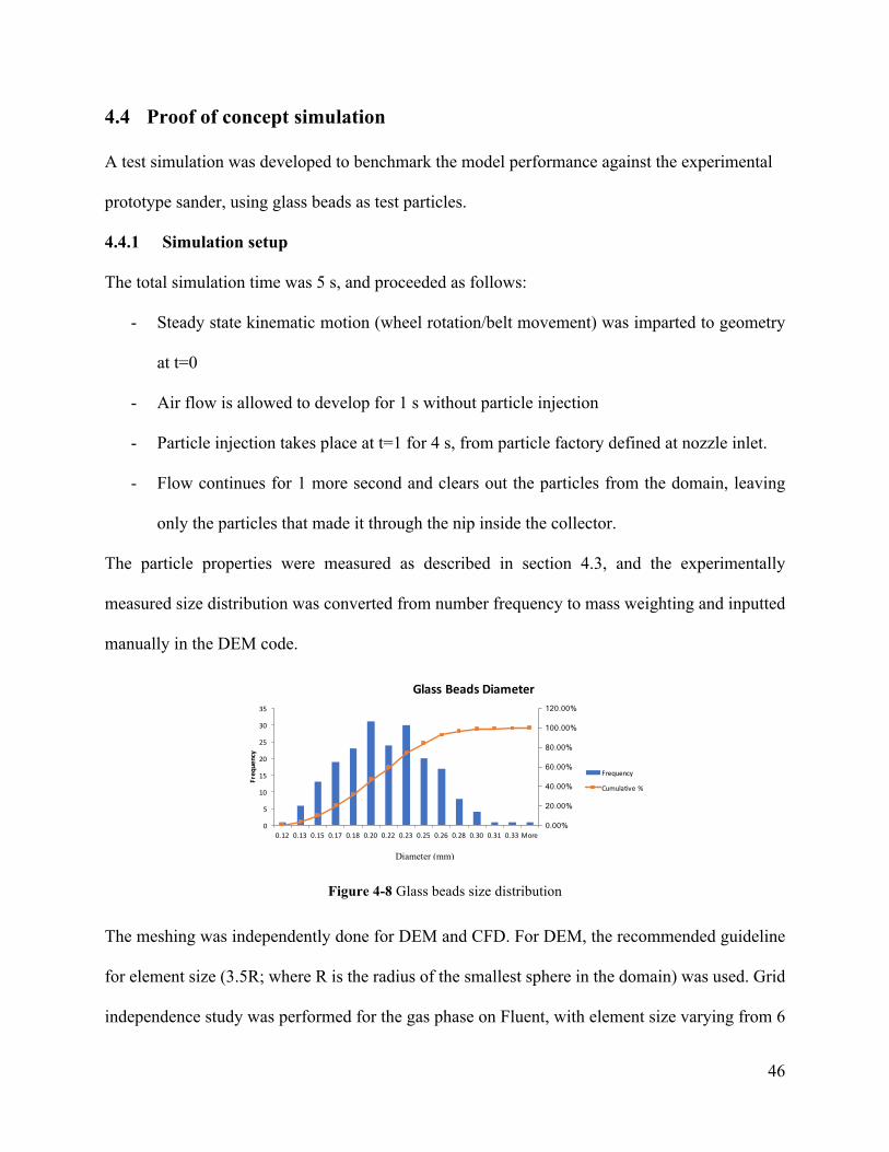
46
4.4 Proof of concept simulation
A test simulation was developed to benchmark the model performance against the experimental
prototype sander, using glass beads as test particles.
4.4.1 Simulation setup
The total simulation time was 5 s, and proceeded as follows:
- Steady state kinematic motion (wheel rotation/belt movement) was imparted to geometry
at t=0
- Air flow is allowed to develop for 1 s without particle injection
- Particle injection takes place at t=1 for 4 s, from particle factory defined at nozzle inlet.
- Flow continues for 1 more second and clears out the particles from the domain, leaving
only the particles that made it through the nip inside the collector.
The particle properties were measured as described in section 4.3, and the experimentally
measured size distribution was converted from number frequency to mass weighting and inputted
manually in the DEM code.
Figure 4-8 Glass beads size distribution
The meshing was independently done for DEM and CFD. For DEM, the recommended guideline
for element size (3.5R; where R is the radius of the smallest sphere in the domain) was used. Grid
independence study was performed for the gas phase on Fluent, with element size varying from 6
0.00%
20.00%
40.00%
60.00%
80.00%
100.00%
120.00%
0
5
10
15
20
25
30
35
0.12 0.13 0.15 0.17 0.18 0.20 0.22 0.23 0.25 0.26 0.28 0.30 0.31 0.33 More
Frequency
Bin
GlassBeadsDiameter
Frequency
Cumulative%
Diameter (mm)
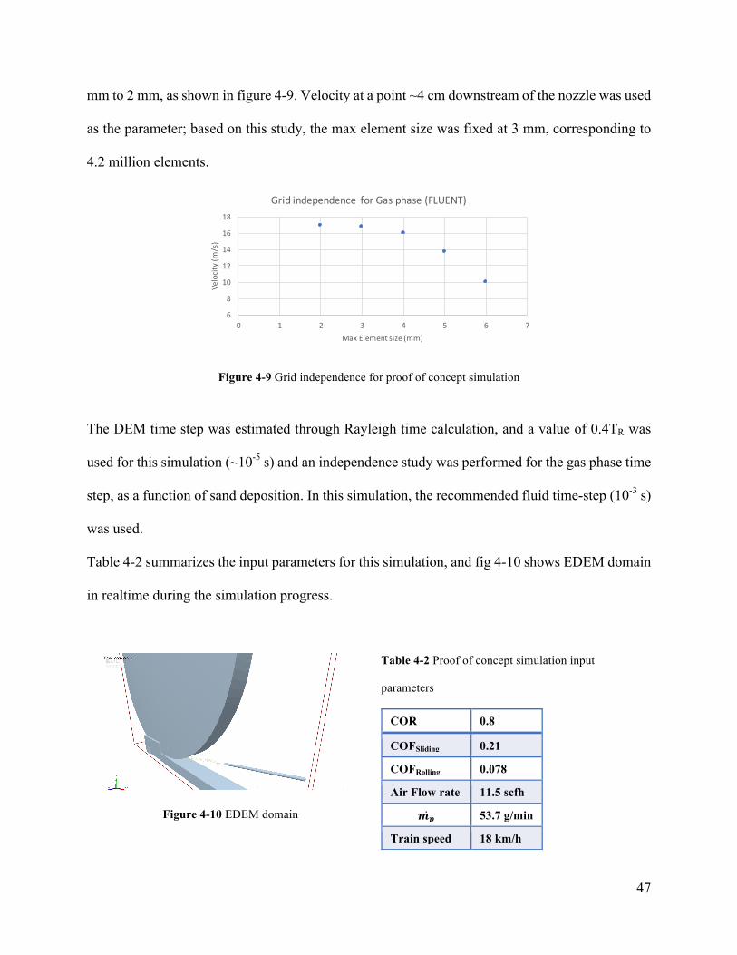
47
mm to 2 mm, as shown in figure 4-9. Velocity at a point ~4 cm downstream of the nozzle was used
as the parameter; based on this study, the max element size was fixed at 3 mm, corresponding to
4.2 million elements.
Figure 4-9 Grid independence for proof of concept simulation
The DEM time step was estimated through Rayleigh time calculation, and a value of 0.4TR was
used for this simulation (~10-5 s) and an independence study was performed for the gas phase time
step, as a function of sand deposition. In this simulation, the recommended fluid time-step (10-3 s)
was used.
Table 4-2 summarizes the input parameters for this simulation, and fig 4-10 shows EDEM domain
in realtime during the simulation progress.
Figure 4-10 EDEM domain
Table 4-2 Proof of concept simulation input
parameters
COR 0.8
COFSliding 0.21
COFRolling 0.078
Air Flow rate 11.5 scfh
𝒎𝒑 53.7 g/min
Train speed 18 km/h
6
8
10
12
14
16
18
0 1 2 3 4 5 6 7
Velocity(m
/s)
MaxElementsize(mm)
Gridindependence forGasphase(FLUENT)
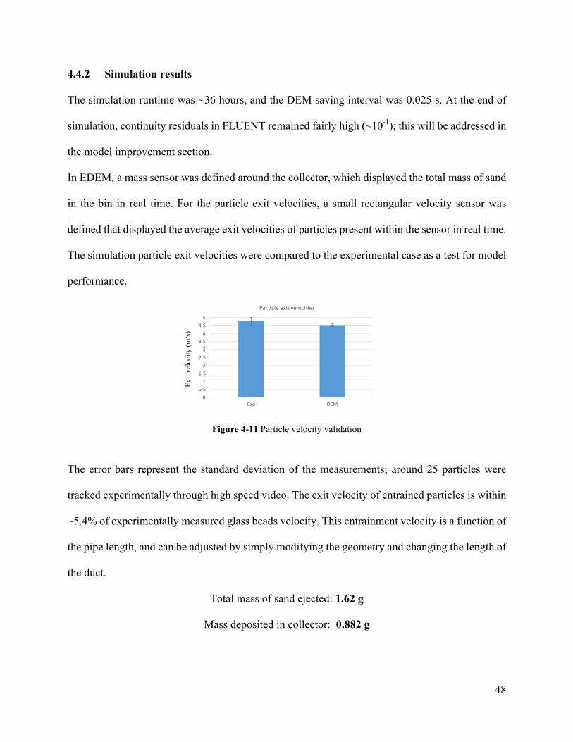
48
4.4.2 Simulation results
The simulation runtime was ~36 hours, and the DEM saving interval was 0.025 s. At the end of
simulation, continuity residuals in FLUENT remained fairly high (~10-1); this will be addressed in
the model improvement section.
In EDEM, a mass sensor was defined around the collector, which displayed the total mass of sand
in the bin in real time. For the particle exit velocities, a small rectangular velocity sensor was
defined that displayed the average exit velocities of particles present within the sensor in real time.
The simulation particle exit velocities were compared to the experimental case as a test for model
performance.
Figure 4-11 Particle velocity validation
The error bars represent the standard deviation of the measurements; around 25 particles were
tracked experimentally through high speed video. The exit velocity of entrained particles is within
~5.4% of experimentally measured glass beads velocity. This entrainment velocity is a function of
the pipe length, and can be adjusted by simply modifying the geometry and changing the length of
the duct.
Total mass of sand ejected: 1.62 g
Mass deposited in collector: 0.882 g
00.51
1.52
2.53
3.54
4.55
Exp DEM
Particleexitvelocities
Exit
velo
city
(m/s
)
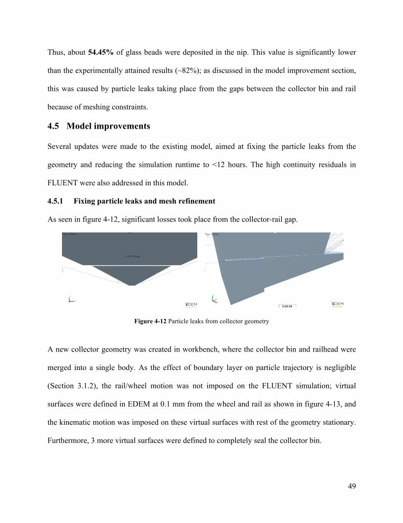
49
Thus, about 54.45% of glass beads were deposited in the nip. This value is significantly lower
than the experimentally attained results (~82%); as discussed in the model improvement section,
this was caused by particle leaks taking place from the gaps between the collector bin and rail
because of meshing constraints.
4.5 Model improvements
Several updates were made to the existing model, aimed at fixing the particle leaks from the
geometry and reducing the simulation runtime to <12 hours. The high continuity residuals in
FLUENT were also addressed in this model.
4.5.1 Fixing particle leaks and mesh refinement
As seen in figure 4-12, significant losses took place from the collector-rail gap.
Figure 4-12 Particle leaks from collector geometry
A new collector geometry was created in workbench, where the collector bin and railhead were
merged into a single body. As the effect of boundary layer on particle trajectory is negligible
(Section 3.1.2), the rail/wheel motion was not imposed on the FLUENT simulation; virtual
surfaces were defined in EDEM at 0.1 mm from the wheel and rail as shown in figure 4-13, and
the kinematic motion was imposed on these virtual surfaces with rest of the geometry stationary.
Furthermore, 3 more virtual surfaces were defined to completely seal the collector bin.
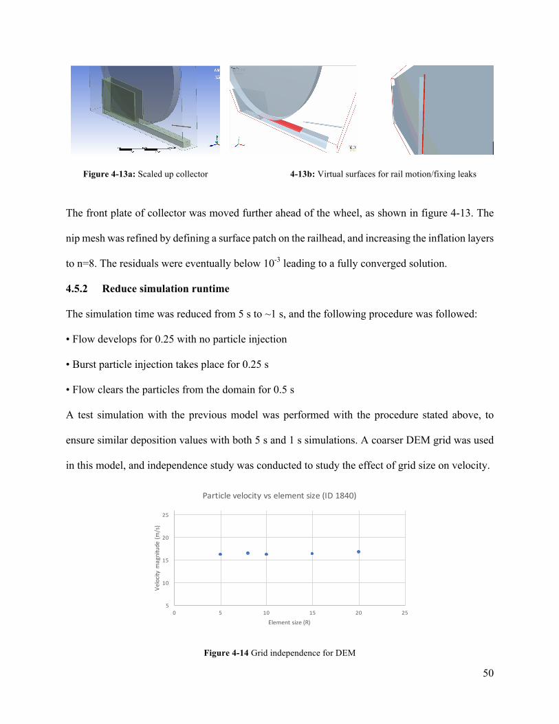
50
Figure 4-13a: Scaled up collector 4-13b: Virtual surfaces for rail motion/fixing leaks
The front plate of collector was moved further ahead of the wheel, as shown in figure 4-13. The
nip mesh was refined by defining a surface patch on the railhead, and increasing the inflation layers
to n=8. The residuals were eventually below 10-3 leading to a fully converged solution.
4.5.2 Reduce simulation runtime
The simulation time was reduced from 5 s to ~1 s, and the following procedure was followed:
• Flow develops for 0.25 with no particle injection
• Burst particle injection takes place for 0.25 s
• Flow clears the particles from the domain for 0.5 s
A test simulation with the previous model was performed with the procedure stated above, to
ensure similar deposition values with both 5 s and 1 s simulations. A coarser DEM grid was used
in this model, and independence study was conducted to study the effect of grid size on velocity.
Figure 4-14 Grid independence for DEM
5
10
15
20
25
0 5 10 15 20 25
Velocitymagnitude(m
/s)
Elementsize(R)
Particlevelocityvselementsize(ID1840)

51
As seen in figure 4-14, DEM grid size does not have a significant effect on particle velocities.
However, for coarse grids, ghosting (particles moving through geometry) occurs, leading to much
lower deposition values. Thus, the element size was kept at ~10R to avoid any particle losses.
Lastly, the processor usage was changed from 4-4 (4 processors-EDEM and 4-FLUENT) to 2-6
(2-EDEM and 6-Fluent) since gas phase is the bottleneck for two phase flow simulation.
Independence study was performed to analyze the effect of gas phase time step on deposition.
Three CFD-DEM coupled simulations were performed with time steps of 0.005, 0.0025, 0.0005.
Figure 4-15 Fluent time step independence study
Time step independence is achieved at ~0.001s (103TDEM), which was used for updated model.
4.5.3 Deposition results
The updated model simulation runtime was ~11.5 hours, and convergence criteria was met
(residuals <10-3). The deposition results were as follows:
Total mass of sand ejected: 0.672 g
Mass deposited in collector: 0.581 g
86.5% of glass beads were deposited in the collector bin. This value is much higher than the
original model, and shows significantly better agreement with the experimentally measured
deposition with glass beads. This deposition value is higher than the experimentally tested value
0.3
0.35
0.4
0.45
0.5
0.55
0.6
0 0.001 0.002 0.003 0.004 0.005 0.006
Depo
sition
∂T(s)

52
(~82%), which can be attributed to the various practical limitations (particle leaks from collector-
belt interface, belt/wheel vibrations, sand remaining in hopper after testing) of the rig.
Since the particles are generated randomly at the particle factory defined at the inlet, there is some
variance in the deposition results when repeating simulations with the same initial conditions. To
test for simulation repeatability, the numerical model was run two additional times:
Figure 4-16 Repeatability of deposition simulation
As shown in figure 4-16, the three numerical solutions were within ~1% of one another.
4.6 Sample BC Rail Sand particle modelling
Particle modelling for a sample particle was performed in EDEM, and two example particles
were modelled as follows.
An optical microscope was used to image the particles from several orientations, as shown in fig
4-17, and an approximate profile of the particle was created.
0.5
0.55
0.6
0.65
0.7
0.75
0.8
0.85
0.9
1 2 3
Deposition
Figure 4-17 Particle imaging from multiple orientations

53
The outlines were traced in SOLIDWORKS and guiding curves were drawn manually by
following the top/bottom view outlines as shown in 4-18.
Figure 4-18 Creating surface from trace outlines
A surface was generated from the sketch, and exported as an .STL file to be imported into EDEM.
The particle model was imported in EDEM and coordinates/radius of spheres for generating the
clumped sphere model were inputted to model the particle using two methods, namely the rough
and very fine model as shown in figure 4-21.
No.ofspheres:10 Particlemass:2.26e-8kg
Tstep:9e-06
Numberofcells:1.2x10⁶
No.ofspheres:77
Particlemass:1.87e-8kg
Tstep:1e-06
Numberofcells:2.73x10⁷
Figure 4-19 Final Particle CAD file
Figure 4-21a Rough model Figure 4-20b Fine model
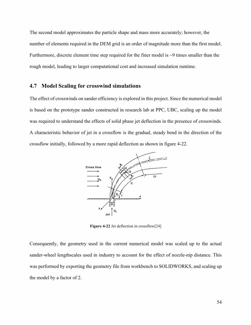
54
The second model approximates the particle shape and mass more accurately; however, the
number of elements required in the DEM grid is an order of magnitude more than the first model.
Furthermore, discrete element time step required for the finer model is ~9 times smaller than the
rough model, leading to larger computational cost and increased simulation runtime.
4.7 Model Scaling for crosswind simulations
The effect of crosswinds on sander efficiency is explored in this project. Since the numerical model
is based on the prototype sander constructed in research lab at PPC, UBC, scaling up the model
was required to understand the effects of solid phase jet deflection in the presence of crosswinds.
A characteristic behavior of jet in a crossflow is the gradual, steady bend in the direction of the
crossflow initially, followed by a more rapid deflection as shown in figure 4-22.
Figure 4-22 Jet deflection in crossflow[24]
Consequently, the geometry used in the current numerical model was scaled up to the actual
sander-wheel lengthscales used in industry to account for the effect of nozzle-nip distance. This
was performed by exporting the geometry file from workbench to SOLIDWORKS, and scaling up
the model by a factor of 2.
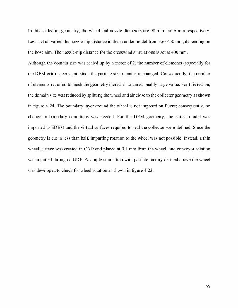
55
In this scaled up geometry, the wheel and nozzle diameters are 98 mm and 6 mm respectively.
Lewis et al. varied the nozzle-nip distance in their sander model from 350-450 mm, depending on
the hose aim. The nozzle-nip distance for the crosswind simulations is set at 400 mm.
Although the domain size was scaled up by a factor of 2, the number of elements (especially for
the DEM grid) is constant, since the particle size remains unchanged. Consequently, the number
of elements required to mesh the geometry increases to unreasonably large value. For this reason,
the domain size was reduced by splitting the wheel and air close to the collector geometry as shown
in figure 4-24. The boundary layer around the wheel is not imposed on fluent; consequently, no
change in boundary conditions was needed. For the DEM geometry, the edited model was
imported to EDEM and the virtual surfaces required to seal the collector were defined. Since the
geometry is cut in less than half, imparting rotation to the wheel was not possible. Instead, a thin
wheel surface was created in CAD and placed at 0.1 mm from the wheel, and conveyor rotation
was inputted through a UDF. A simple simulation with particle factory defined above the wheel
was developed to check for wheel rotation as shown in figure 4-23.
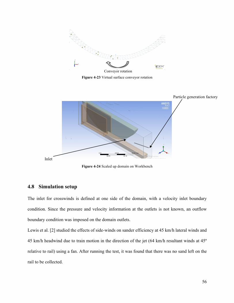
56
Particle generation factory
Inlet
Figure 4-23 Virtual surface conveyor rotation
Figure 4-24 Scaled up domain on Workbench
4.8 Simulation setup
The inlet for crosswinds is defined at one side of the domain, with a velocity inlet boundary
condition. Since the pressure and velocity information at the outlets is not known, an outflow
boundary condition was imposed on the domain outlets.
Lewis et al. [2] studied the effects of side-winds on sander efficiency at 45 km/h lateral winds and
45 km/h headwind due to train motion in the direction of the jet (64 km/h resultant winds at 45º
relative to rail) using a fan. After running the test, it was found that there was no sand left on the
rail to be collected.
Conveyor rotation
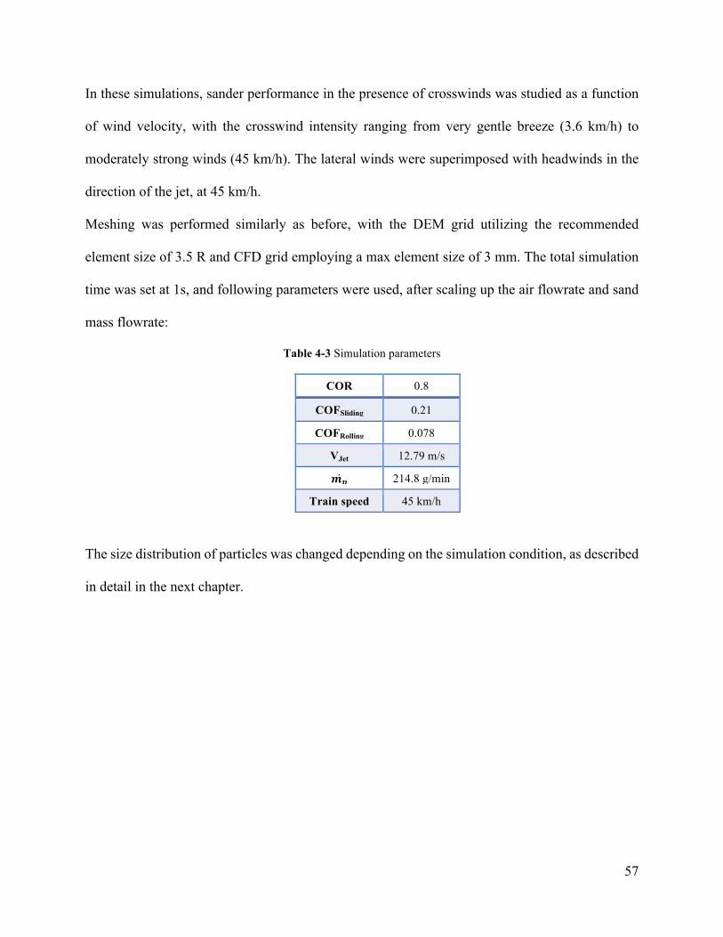
57
In these simulations, sander performance in the presence of crosswinds was studied as a function
of wind velocity, with the crosswind intensity ranging from very gentle breeze (3.6 km/h) to
moderately strong winds (45 km/h). The lateral winds were superimposed with headwinds in the
direction of the jet, at 45 km/h.
Meshing was performed similarly as before, with the DEM grid utilizing the recommended
element size of 3.5 R and CFD grid employing a max element size of 3 mm. The total simulation
time was set at 1s, and following parameters were used, after scaling up the air flowrate and sand
mass flowrate:
Table 4-3 Simulation parameters
COR 0.8
COFSliding 0.21
COFRolling 0.078
VJet 12.79 m/s
𝒎𝒑 214.8 g/min
Train speed 45 km/h
The size distribution of particles was changed depending on the simulation condition, as described
in detail in the next chapter.
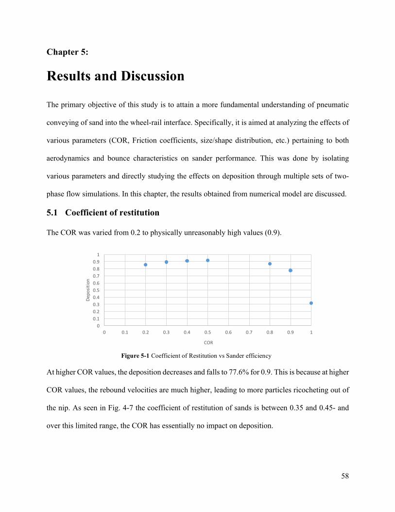
58
Chapter 5:
Results and Discussion
The primary objective of this study is to attain a more fundamental understanding of pneumatic
conveying of sand into the wheel-rail interface. Specifically, it is aimed at analyzing the effects of
various parameters (COR, Friction coefficients, size/shape distribution, etc.) pertaining to both
aerodynamics and bounce characteristics on sander performance. This was done by isolating
various parameters and directly studying the effects on deposition through multiple sets of two-
phase flow simulations. In this chapter, the results obtained from numerical model are discussed.
5.1 Coefficient of restitution
The COR was varied from 0.2 to physically unreasonably high values (0.9).
At higher COR values, the deposition decreases and falls to 77.6% for 0.9. This is because at higher
COR values, the rebound velocities are much higher, leading to more particles ricocheting out of
the nip. As seen in Fig. 4-7 the coefficient of restitution of sands is between 0.35 and 0.45- and
over this limited range, the COR has essentially no impact on deposition.
00.10.20.30.40.50.60.70.80.91
0 0.1 0.2 0.3 0.4 0.5 0.6 0.7 0.8 0.9 1
Depo
sition
COR
Figure 5-1 Coefficient of Restitution vs Sander efficiency

59
5.2 Coefficient of Rolling Friction
A set of simulations with the Coefficient of rolling friction varying from 0.01 to 0.25 were
performed. The sand deposition is not a function of rolling friction, as shown in figure 5-2.
Figure 5-2 Coefficient of rolling friction vs Sander efficiency
Due to high particle velocities (~2-4 m/s), the timescales associated with particle-geometry
interactions are miniscule, and do not allow for particle rolling.
5.3 Coefficient of sliding friction
Similar to COFR, deposition of sand through the wheel-rail nip was studied as a function of
coefficient of sliding friction. COFS was varied from 0.05 to 0.5 as shown in figure 5-3.
Figure 5-3 Coefficient of sliding friction vs Sander efficiency
0.6
0.65
0.7
0.75
0.8
0.85
0.9
0 0.05 0.1 0.15 0.2 0.25 0.3
Depo
sition
COF(Rolling)
0.6
0.65
0.7
0.75
0.8
0.85
0.9
0 0.1 0.2 0.3 0.4 0.5 0.6
Depo
sition
COF(Sliding)
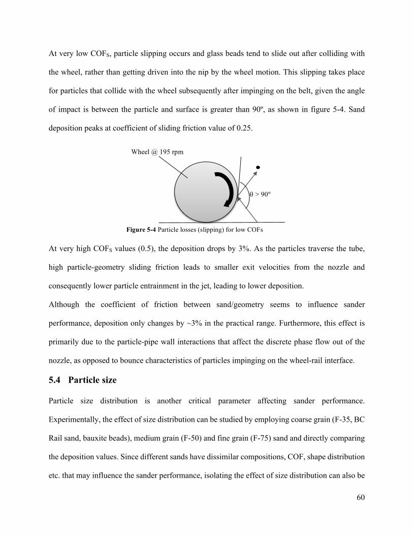
60
At very low COFS, particle slipping occurs and glass beads tend to slide out after colliding with
the wheel, rather than getting driven into the nip by the wheel motion. This slipping takes place
for particles that collide with the wheel subsequently after impinging on the belt, given the angle
of impact is between the particle and surface is greater than 90º, as shown in figure 5-4. Sand
deposition peaks at coefficient of sliding friction value of 0.25.
At very high COFS values (0.5), the deposition drops by 3%. As the particles traverse the tube,
high particle-geometry sliding friction leads to smaller exit velocities from the nozzle and
consequently lower particle entrainment in the jet, leading to lower deposition.
Although the coefficient of friction between sand/geometry seems to influence sander
performance, deposition only changes by ~3% in the practical range. Furthermore, this effect is
primarily due to the particle-pipe wall interactions that affect the discrete phase flow out of the
nozzle, as opposed to bounce characteristics of particles impinging on the wheel-rail interface.
5.4 Particle size
Particle size distribution is another critical parameter affecting sander performance.
Experimentally, the effect of size distribution can be studied by employing coarse grain (F-35, BC
Rail sand, bauxite beads), medium grain (F-50) and fine grain (F-75) sand and directly comparing
the deposition values. Since different sands have dissimilar compositions, COF, shape distribution
etc. that may influence the sander performance, isolating the effect of size distribution can also be
q > 90º
Wheel @ 195 rpm
Figure 5-4 Particle losses (slipping) for low COFs
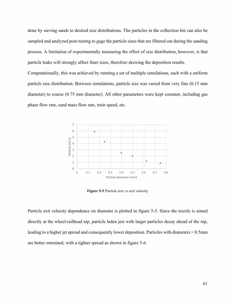
61
done by sieving sands to desired size distributions. The particles in the collection bin can also be
sampled and analyzed post-testing to gage the particle sizes that are filtered out during the sanding
process. A limitation of experimentally measuring the effect of size distribution, however, is that
particle leaks will strongly affect finer sizes, therefore skewing the deposition results.
Computationally, this was achieved by running a set of multiple simulations, each with a uniform
particle size distribution. Between simulations, particle size was varied from very fine (0.15 mm
diameter) to coarse (0.75 mm diameter). All other parameters were kept constant, including gas
phase flow rate, sand mass flow rate, train speed, etc.
Figure 5-5 Particle size vs exit velocity
Particle exit velocity dependence on diameter is plotted in figure 5-5. Since the nozzle is aimed
directly at the wheel-railhead nip, particle laden jets with larger particles decay ahead of the nip,
leading to a higher jet spread and consequently lower deposition. Particles with diameters < 0.5mm
are better entrained, with a tighter spread as shown in figure 5-6.
0
1
2
3
4
5
6
7
0 0.1 0.2 0.3 0.4 0.5 0.6 0.7 0.8
Velocity(m/s)
Particlediameter(mm)
Particlesizevsexitvelocity

62
Figure 5-6 Jet decay for larger particles
Figure 5-7 summarizes the dependence of sander efficiency on particle size.
Figure 5-7 Particle diameter vs sander efficiency
For very fine particles (0.15mm), the jet is very well entrained with high particle velocities (~6
m/s). Glass beads reach the nip directly without decay due to gravity, leading to very high
deposition values (~98%). As the particle size increases, sander efficiency drops almost linearly
until 0.5 mm diameter particles, after which there is a stronger drop in the deposition rate- dropping
to 65% for 0.75 mm diameter beads.
0
0.1
0.2
0.3
0.4
0.5
0.6
0.7
0.8
0.9
1
0 0.1 0.2 0.3 0.4 0.5 0.6 0.7 0.8
Depo
sition
Particlediameter(mm)
Particle diameter – 0.25 mm Particle diameter – 0.625 mm
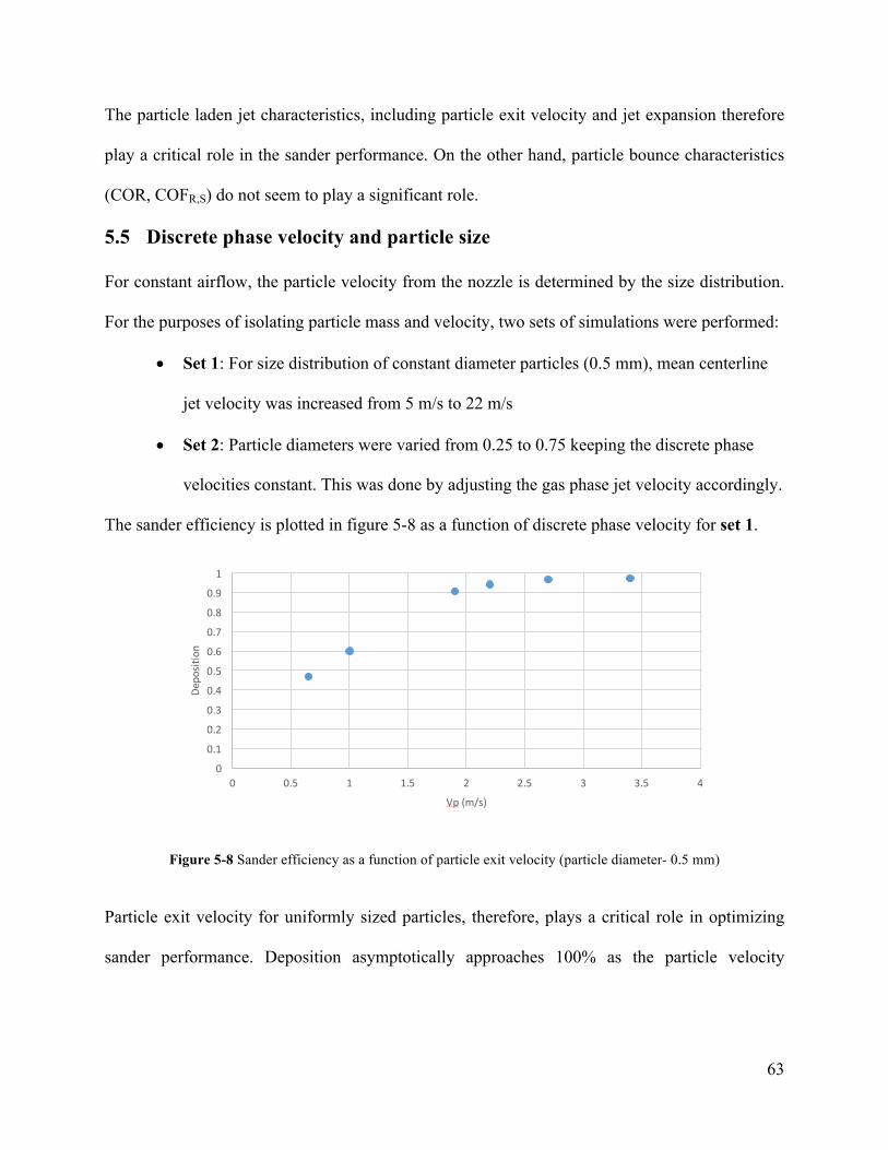
63
The particle laden jet characteristics, including particle exit velocity and jet expansion therefore
play a critical role in the sander performance. On the other hand, particle bounce characteristics
(COR, COFR,S) do not seem to play a significant role.
5.5 Discrete phase velocity and particle size
For constant airflow, the particle velocity from the nozzle is determined by the size distribution.
For the purposes of isolating particle mass and velocity, two sets of simulations were performed:
• Set 1: For size distribution of constant diameter particles (0.5 mm), mean centerline
jet velocity was increased from 5 m/s to 22 m/s
• Set 2: Particle diameters were varied from 0.25 to 0.75 keeping the discrete phase
velocities constant. This was done by adjusting the gas phase jet velocity accordingly.
The sander efficiency is plotted in figure 5-8 as a function of discrete phase velocity for set 1.
Figure 5-8 Sander efficiency as a function of particle exit velocity (particle diameter- 0.5 mm)
Particle exit velocity for uniformly sized particles, therefore, plays a critical role in optimizing
sander performance. Deposition asymptotically approaches 100% as the particle velocity
0
0.1
0.2
0.3
0.4
0.5
0.6
0.7
0.8
0.9
1
0 0.5 1 1.5 2 2.5 3 3.5 4
Depo
sition
Vp (m/s)
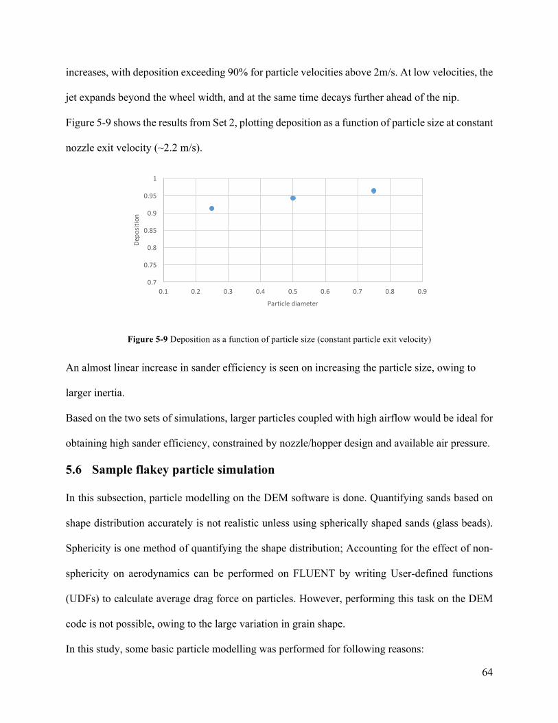
64
increases, with deposition exceeding 90% for particle velocities above 2m/s. At low velocities, the
jet expands beyond the wheel width, and at the same time decays further ahead of the nip.
Figure 5-9 shows the results from Set 2, plotting deposition as a function of particle size at constant
nozzle exit velocity (~2.2 m/s).
Figure 5-9 Deposition as a function of particle size (constant particle exit velocity)
An almost linear increase in sander efficiency is seen on increasing the particle size, owing to
larger inertia.
Based on the two sets of simulations, larger particles coupled with high airflow would be ideal for
obtaining high sander efficiency, constrained by nozzle/hopper design and available air pressure.
5.6 Sample flakey particle simulation
In this subsection, particle modelling on the DEM software is done. Quantifying sands based on
shape distribution accurately is not realistic unless using spherically shaped sands (glass beads).
Sphericity is one method of quantifying the shape distribution; Accounting for the effect of non-
sphericity on aerodynamics can be performed on FLUENT by writing User-defined functions
(UDFs) to calculate average drag force on particles. However, performing this task on the DEM
code is not possible, owing to the large variation in grain shape.
In this study, some basic particle modelling was performed for following reasons:
0.7
0.75
0.8
0.85
0.9
0.95
1
0.1 0.2 0.3 0.4 0.5 0.6 0.7 0.8 0.9
Depo
sition
Particlediameter
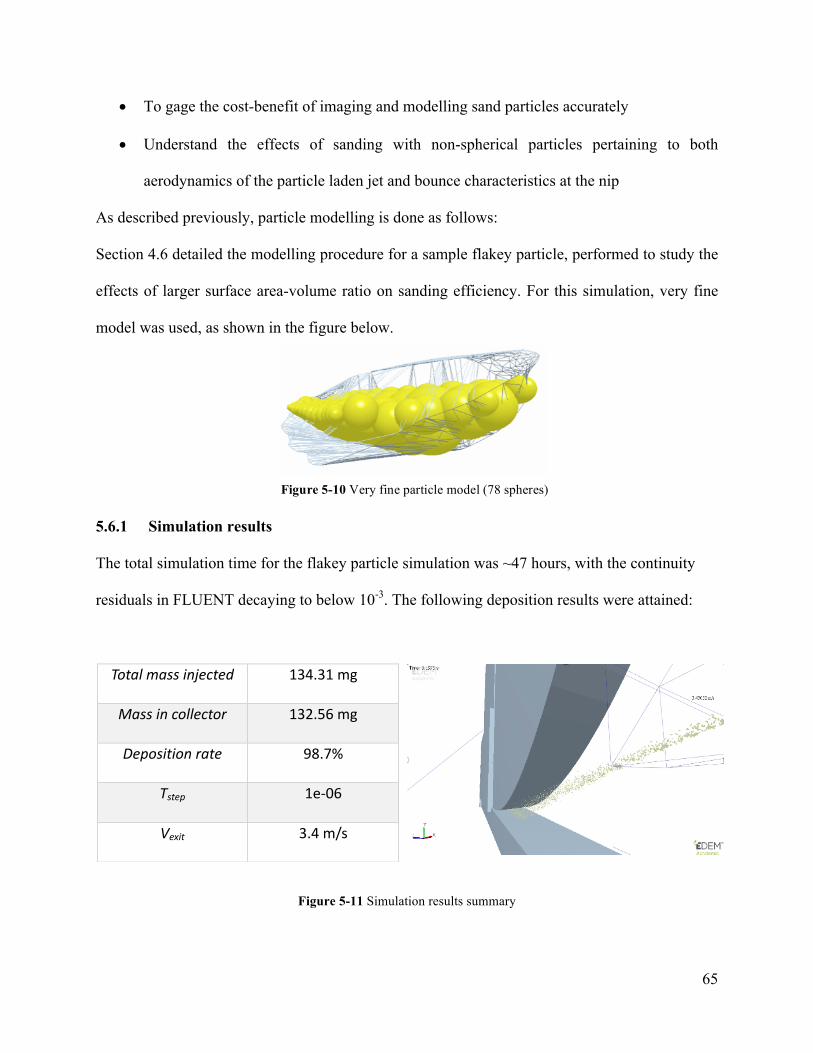
65
• To gage the cost-benefit of imaging and modelling sand particles accurately
• Understand the effects of sanding with non-spherical particles pertaining to both
aerodynamics of the particle laden jet and bounce characteristics at the nip
As described previously, particle modelling is done as follows:
Section 4.6 detailed the modelling procedure for a sample flakey particle, performed to study the
effects of larger surface area-volume ratio on sanding efficiency. For this simulation, very fine
model was used, as shown in the figure below.
5.6.1 Simulation results
The total simulation time for the flakey particle simulation was ~47 hours, with the continuity
residuals in FLUENT decaying to below 10-3. The following deposition results were attained:
Totalmassinjected 134.31mg
Massincollector 132.56mg
Depositionrate 98.7%
Tstep 1e-06
Vexit 3.4m/s
Figure 5-11 Simulation results summary
Figure 5-10 Very fine particle model (78 spheres)
66
5.6.2 Discussion
As seen in figure 5-11, the mean particle exit velocity from the nozzle is high (~3.4 m/s) despite
the relatively large particle size. Additionally, the jet is well entrained and very narrow, and does
not expand beyond the wheel width, leading to very high sander efficiency. The large particle
velocity can be attributed to the large surface area-volume ratio of the particle, which is ~65%
larger than a sphere of equivalent volume. Consequently, the particles experience higher drag and
reach greater exit velocities than spherical particles of equivalent volume.
Since the particles are highly irregular, they exhibit a larger y-deflection upon bouncing, causing
more particles to bounce out of the nip upon impact. In contrast, the y-deflection of spherical
particles is zero. However, given the large deposition ratio, it can be concluded that bounce
characteristics of sand particles, especially pertaining to shape distribution is not a critical
parameter for sander performance. The effect of the shape distribution of particles plays a role in
optimizing the sander performance in terms of the aerodynamic behavior of the jet.
This conclusion is further supported by the results in Appendix B.3, where spherical and irregular
particles were ejected from particle factory at 2 m/s, aimed at a rail geometry at 11.5º. In this
analysis, it was found that varying the particle shape from spherical to highly irregular has
negligible (<1º) effect on y-deflection in particle trajectories.
5.7 Effects of Crosswinds
Understanding the effect of aerodynamics near the nozzle environment is critical for optimizing
the amount of going sand through the nip. Along with the prevailing winds blowing across the
tracks, undercarriage winds due to train motion can also become turbulent- cumulatively leading
to strong lateral winds deflecting the particle laden jet before it reaches the nip. The train
undercarriage aerodynamics have been experimentally and numerically estimated in previous
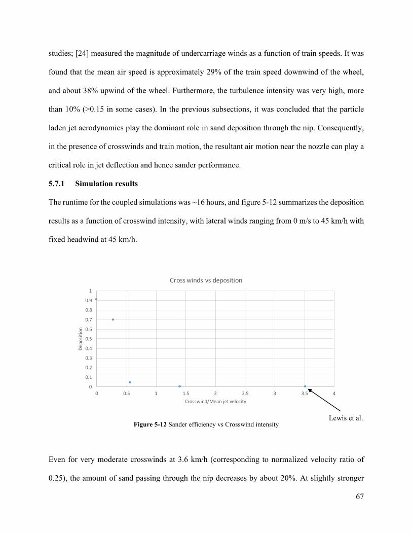
67
studies; [24] measured the magnitude of undercarriage winds as a function of train speeds. It was
found that the mean air speed is approximately 29% of the train speed downwind of the wheel,
and about 38% upwind of the wheel. Furthermore, the turbulence intensity was very high, more
than 10% (>0.15 in some cases). In the previous subsections, it was concluded that the particle
laden jet aerodynamics play the dominant role in sand deposition through the nip. Consequently,
in the presence of crosswinds and train motion, the resultant air motion near the nozzle can play a
critical role in jet deflection and hence sander performance.
5.7.1 Simulation results
The runtime for the coupled simulations was ~16 hours, and figure 5-12 summarizes the deposition
results as a function of crosswind intensity, with lateral winds ranging from 0 m/s to 45 km/h with
fixed headwind at 45 km/h.
Figure 5-12 Sander efficiency vs Crosswind intensity
Even for very moderate crosswinds at 3.6 km/h (corresponding to normalized velocity ratio of
0.25), the amount of sand passing through the nip decreases by about 20%. At slightly stronger
0
0.1
0.2
0.3
0.4
0.5
0.6
0.7
0.8
0.9
1
0 0.5 1 1.5 2 2.5 3 3.5 4
Depositio
n
Crosswind/Meanjetvelocity
Crosswindsvsdeposition
Lewis et al.
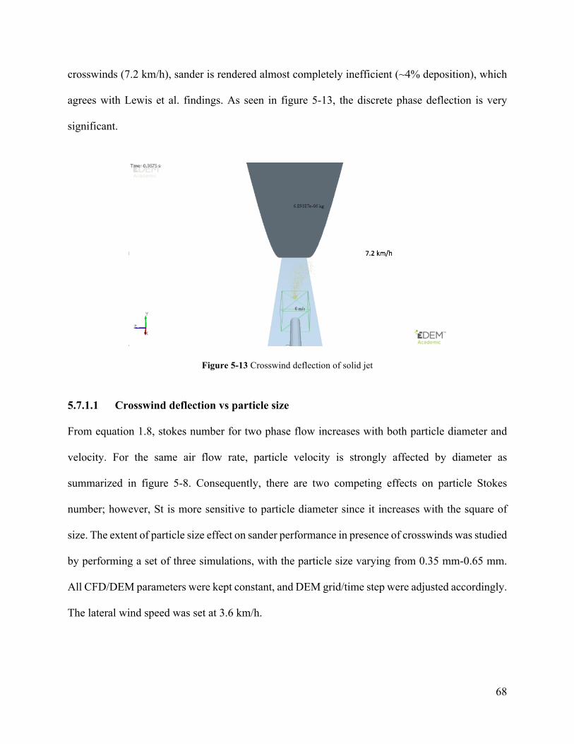
68
crosswinds (7.2 km/h), sander is rendered almost completely inefficient (~4% deposition), which
agrees with Lewis et al. findings. As seen in figure 5-13, the discrete phase deflection is very
significant.
Figure 5-13 Crosswind deflection of solid jet
5.7.1.1 Crosswind deflection vs particle size
From equation 1.8, stokes number for two phase flow increases with both particle diameter and
velocity. For the same air flow rate, particle velocity is strongly affected by diameter as
summarized in figure 5-8. Consequently, there are two competing effects on particle Stokes
number; however, St is more sensitive to particle diameter since it increases with the square of
size. The extent of particle size effect on sander performance in presence of crosswinds was studied
by performing a set of three simulations, with the particle size varying from 0.35 mm-0.65 mm.
All CFD/DEM parameters were kept constant, and DEM grid/time step were adjusted accordingly.
The lateral wind speed was set at 3.6 km/h.

69
Figure 5-14 Sander efficiency attenuation in the presence of crosswinds vs particle size
As summarized in figure 5-14, increasing the particle size decreases the sand deposition in the
absence of lateral winds, with approximately a 2% decrease in efficiency associated with a 0.15mm
increase in particle diameter. However, the effect of sidewinds is attenuated significantly for larger
particles, and an increase of 8% and 5% in sander efficiency is seen when increasing the particle
diameter from 0.35 mm to 0.5 mm and 0.5 mm to 0.65 mm respectively. This can be attributed to
the greater inertia of larger particles, which more than compensates for the fact that they leave the
sander nozzle with a slower velocity than smaller particles.
5.7.1.2 Effect of nozzle position
The nozzle-nip distance was varied from 400 mm to 300 mm to study the effects of nozzle
positioning on sander efficiency in the presence of moderate crosswinds. For this geometry, the
distance between nozzle-railhead and nozzle-wheel was 65 mm and 45 mm respectively.
Figure 5-15 quantifies the attenuation of the effect of 3.6 km/h crosswinds on sander efficiency for
the case when nozzle is moved closer to the nip.
0.1
0.2
0.3
0.4
0.5
0.6
0.7
0.8
0.9
1
0.35 0.5 0.65
Deposition
Particlediameter(mm)
Crosswindeffectvssize
Nocrosswinds 1m/s

70
Figure 5-15 Crosswind attenuation vs nip-nozzle distance
For both cases (no sidewinds and sidewind @ 3.6 km/h), moving the nozzle ~100mm closer to the
wheel has a strong positive effect on sander efficiency owing to the lesser spread of the solid jet
near the nip. The total sand deposited in the collector is increased by 8% and 11% in the two cases
respectively. Consequently, appropriate nozzle positioning is required to optimize the sander
efficiency, by minimizing the nozzle-nip distance while still following the safety regulations
mentioned above.
0
0.2
0.4
0.6
0.8
1
400 300
Depo
sition
Nozzle-nipdistance(mm)
1m/s 0m/sCrosswind speed:
71
Chapter 6:
Conclusion
This chapter summarizes the findings of this study, and details the conclusions that can be drawn
from the results of the simulations. A brief discussion of the real world applications, along with
the limitations of the study is done, followed by some recommendations for future work.
6.1 Summary of findings
A numerical model of a prototype locomotive sander (located in PPC, UBC) was developed, to
simulate the pneumatic conveying of sand through the wheel-rail interface. The gas phase was
simulated on ANSYS FLUENT, while the discrete phase was modelled on a commercial DEM
package EDEM. The two phases were coupled by compiling a journal file, and the two-phase flow
was post-processed on EDEM.
The primary aim behind this study was to provide numerical validation to the experimental tests
performed on the prototype rig. Furthermore, it was possible to computationally isolate the effects
of parameters such as particle properties, jet aerodynamic characteristics, etc. which was not
possible experimentally. A summary of the main findings from this study is detailed below:
- Boundary layer around the rotating wheel does not affect the particle trajectories, and does
not need to be included in the gas phase model.
- For the given sand mass flow rate/air flow rates, saltation does not occur for during
pneumatic conveying of sand.
- The coefficients of sliding and rolling friction do not play any significant role in the
deposition of sand through the wheel-rail interface. In the practical range (0.2-0.8),
reducing the coefficient of sliding friction to very low values increases deposition by
72
around 6%, since the particles have higher exit velocity caused by reduced particle-pipe
wall friction.
- Coefficient of restitution has minimal effect on the sander efficiency in the range measured
for lab sands (0.3-0.4). At high COR (>0.8), deposition drops due to larger probability of
particles to ricochet out of the nip.
- For the same air flow rate, smaller particles show much higher deposition due to higher
particle exit velocity and better entrainment, leading to a tighter spread. Consequently,
there is a strong correlation between the particle Stokes number and deposition. This
correlation between particle size and deposition is confirmed by experimental results
obtained from the prototype sander tests. [25]
- Similarly, deposition of sand through the nip is also strongly affected by particle inertia.
Equalizing the particle exit velocity, larger grain size leads to significantly higher
deposition.
- Particles with larger surface area to volume ratio exit the nozzle with higher velocities due
to greater drag, hence showing much better deposition.
- Presence of even moderate crosswinds (~3.6 km/h) deflects the particle laden jet, and
decreases the efficiency by ~ 20%. With crosswinds of 7.2 km/h, sander is rendered
completely ineffective, with only ~ 4% of the sand making it in the collector.
- The effect of crosswinds can be significantly attenuated by reducing the nip-nozzle
distance, increasing the size of sand particles, or increasing the jet velocity.
6.2 Conclusions
A primary conclusion of this study was that the particle laden jet characteristics play the major
role in determining the deposition of sand grains through the wheel-rail nip during locomotive

73
sanding. The main source of losses in the sanding process is the solid jet expansion beyond the
wheel width, and the jet decay ahead of the nip- both primarily governed by the solid phase velocity
from the nozzle exit. The bounce characteristics of the particles on the rail/wheel surface, therefore,
do not contribute considerably to the particle deposition through the nip. Particle properties govern
the sander efficiency, insofar as they affect the particle laden jet properties (better flow through
the pipe, higher drag leading to larger exit velocity, etc.).
6.3 Limitations
In this work, the numerical model was based on a prototype locomotive sander developed in-house
at the research facility in PPC, UBC. One of the limitations of this work is that the scaling down
is based on several assumptions. For instance, the entire assembly is scaled down by a factor of 2,
while the nozzle is scaled down by a factor of 4. To accommodate for this discrepancy, the nozzle
was moved back away from the wheel by ~1 inch to allow the jet to expand. Furthermore, the
sanders used in the industry generally have angled edge at the exit, which was not incorporated in
the geometry created for the numerical model.
Particle modelling performed in this study was very basic, and most simulations were performed
with spherical particles. This is because the imaging and modelling of particles is done
individually, and the time cost associated with the procedure (described in section 4.6) is high.
6.4 Recommendations for future work
Some recommendations for future work on numerically modelling locomotive sanders are as
follows:
1. Model actual sander assemblies used in the industry

74
2. Perform extensive particle modelling, with ASG software (Automatic Sphere-clump
Generator). Multiple particles can be imaged in 3D scanners; ASG software produces a
.STL file that can be directly imported in EDEM, based on the required accuracy.
3. Model undercarriage aerodynamics more accurately to understand the particle laden jet
deflection in the case of actual locomotive.
75
References
[1] D. A. Broster, M., Pritchard, C., Smith, “A Basic Study of Wheel/Rail Adhesion 6 - Adhesion and
Contamination on BR Track,” BR Res., 1973.
[2] S. R. Lewis, S. Riley, D. I. Fletcher, and R. Lewis, “Optimisation of a railway sanding system for
optimal grain entrainment into the wheel–rail contact,” Proc. Inst. Mech. Eng. Part F J. Rail Rapid
Transit, vol. 232, no. 1, pp. 43–62, Jun. 2016.
[3] V. Smith, “Improved Methods for Increasing Wheel/Rail Adhesion in Presence of Natural
Contaminants,” Transit Coop. Res. Progr., no. 17, p. 5, 1997.
[4] Indian Railways Institute of Mechanical and Electrical Engineering, “Rail-wheel Interaction,” Indian
Railways.
[5] N. Gorbunov, M. Kovtanets, and R. Demin, “Simulation model of abrasive material motion,” vol. 14,
no. 1, pp. 60–72, 2014.
[6] N. Gorbunov, M. Kovtanets, V. Nozhenko, and O. Prosvirova, “Analysis of the Influence of Jet-
Abrasive Flow Parameters on Wheel and Rail Friction Coefficient,” Teka. Commision Mot. Energ.
Agric., vol. 13, no. 3, pp. 68–73, 2013.
[7] D. J. Mason, P. Marjanovic, and A. Levy, “A simulation system for pneumatic conveying systems,”
Powder Technol., vol. 95, no. 1, pp. 7–14, 1998.
[8] M. Azimian, M. Lichti, and H.-J. Bart, “Investigation of Particulate Flow in a Channel by Application
of CFD, DEM and LDA/PDA,” Open Chem. Eng. J., vol. 8, no. 1, pp. 1–11, 2014.
[9] C. E. Brennan, Fundamentals of Multiphase Flows, California. Pasadena: Cambridge University Press,
2005.
[10] J. Capecelatro and O. Desjardins, “An Euler-Lagrange strategy for simulating particle-laden flows,” J.
Comput. Phys., vol. 238, pp. 1–31, 2013.
[11] C. E. Brennan, Fundamentals of Multiphase Flows. Pasadena: Cambridge University Press., 2005.
[12] T. B. Anderson and R. Jackson, “Fluid mechanical description of fluidized beds: Equations of Motion,”
Ind. Eng. Chem. Fundam., vol. 6, no. 4, pp. 527–539, 1967.
76
[13] C. Y. Wen, “A generalized method for predicting the minimum fluidization velocity,” AIChE J., vol.
12, no. 3, pp. 610–612, 5AD.
[14] Sharcnet, “ANSYS Fluent,” 23.5.10. [Online]. Available:
https://www.sharcnet.ca/Software/Fluent6/html/ug/node910.htm.
[15] Y. Zhang, Indoor Air Quality Engineering. Taylor & Francis, 2004.
[16] P. A. Cundall and O. D. L. Strack, “A discrete numerical model for granular assemblies,”
Geotechnique, vol. 29, no. 1, pp. 47–65, 1979.
[17] A. Di Renzo and F. P. Di Maio, “Comparison of contact-force models for the simulation of collisions
in DEM-based granular flow codes,” Chem. Eng. Sci., vol. 59, no. 3, pp. 525–541, 2004.
[18] E. M. Smuts, D. a Deglon, and C. J. Meyer, “Methodology for Coupled CFD-DEM Modelling of
Particulate Suspension Rheology,” 9th Int. Conf. CFD Miner. Process Ind., no. 365, pp. 5068–5079,
2012.
[19] S. Beltaos, “Oblique Impingement Of Circular Turbulent Jets,” J. Hydraul. Res., vol. 14, no. 1, pp. 17–
36, 1976.
[20] H. Wu, B. Lin, R. Cai, and M. N. Morgan, “Measurement of the air boundary layer on the periphery of
a rotating grinding wheel using LDA,” J. Phys. Conf. Ser., vol. 76, no. 1, p. 12059, 2007.
[21] J.-S. SHUEN, A. S. P. Solomon, G. M. Faeth, and Q.-F. Zhang, “Structure of particle-laden jets -
Measurements and predictions,” AIAA J., vol. 23, no. 3, pp. 396–404, Mar. 1985.
[22] N. P. Daphalapurkar, F. Wang, B. Fu, H. Lu, and R. Komanduri, “Determination of Mechanical
Properties of Sand Grains by Nanoindentation,” Exp. Mech., vol. 51, no. 5, pp. 719–728, 2011.
[23] Q. A. Mulligan, “Full scale train underbody aerodynamic evaluation for top of rail friction modifier
application,” University of British Columbia, 2015.
[24] J. Roberts, “Particle Impingement On a Moving Substrate,” University of British Columbia, 2018.
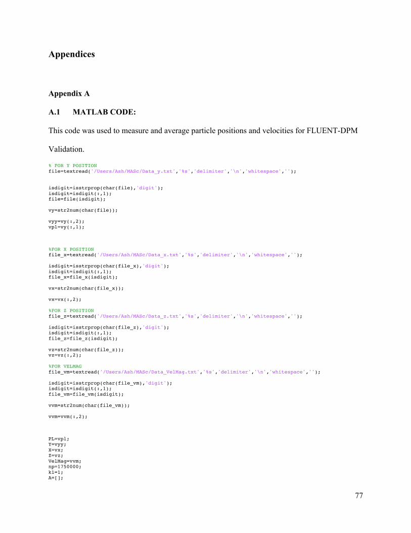
77
Appendices
Appendix A
A.1 MATLAB CODE:
This code was used to measure and average particle positions and velocities for FLUENT-DPM
Validation.
% FOR Y POSITION file=textread('/Users/Ash/MASc/Data_y.txt','%s','delimiter','\n','whitespace',''); isdigit=isstrprop(char(file),'digit'); isdigit=isdigit(:,1); file=file(isdigit); vy=str2num(char(file)); vyy=vy(:,2); vpl=vy(:,1); %FOR X POSITION file_x=textread('/Users/Ash/MASc/Data_x.txt','%s','delimiter','\n','whitespace',''); isdigit=isstrprop(char(file_x),'digit'); isdigit=isdigit(:,1); file_x=file_x(isdigit); vx=str2num(char(file_x)); vx=vx(:,2); %FOR Z POSITION file_z=textread('/Users/Ash/MASc/Data_z.txt','%s','delimiter','\n','whitespace',''); isdigit=isstrprop(char(file_z),'digit'); isdigit=isdigit(:,1); file_z=file_z(isdigit); vz=str2num(char(file_z)); vz=vz(:,2); %FOR VELMAG file_vm=textread('/Users/Ash/MASc/Data_VelMag.txt','%s','delimiter','\n','whitespace',''); isdigit=isstrprop(char(file_vm),'digit'); isdigit=isdigit(:,1); file_vm=file_vm(isdigit); vvm=str2num(char(file_vm)); vvm=vvm(:,2); PL=vpl; Y=vyy; X=vx; Z=vz; VelMag=vvm; np=1750000; k1=1; A=[];
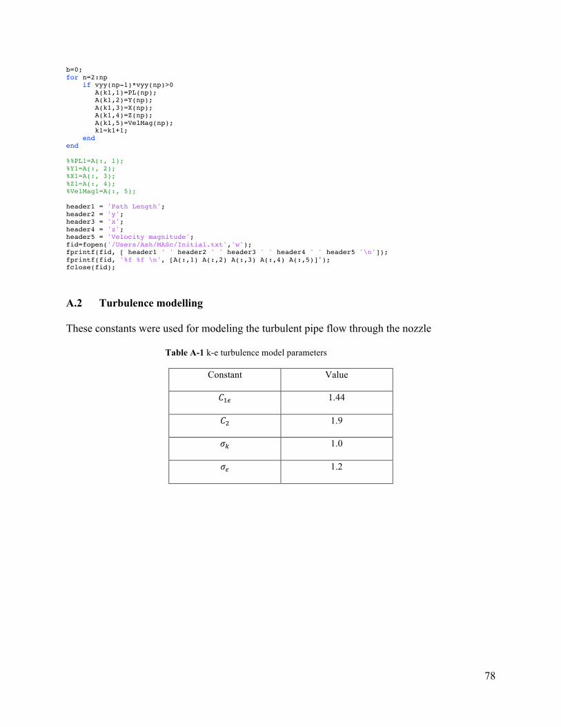
78
b=0; for n=2:np if vyy(np-1)*vyy(np)>0 A(k1,1)=PL(np); A(k1,2)=Y(np); A(k1,3)=X(np); A(k1,4)=Z(np); A(k1,5)=VelMag(np); k1=k1+1; end end %%PL1=A(:, 1); %Y1=A(:, 2); %X1=A(:, 3); %Z1=A(:, 4); %VelMag1=A(:, 5); header1 = 'Path Length'; header2 = 'y'; header3 = 'x'; header4 = 'z'; header5 = 'Velocity magnitude'; fid=fopen('/Users/Ash/MASc/Initial.txt','w'); fprintf(fid, [ header1 ' ' header2 ' ' header3 ' ' header4 ' ' header5 '\n']); fprintf(fid, '%f %f \n', [A(:,1) A(:,2) A(:,3) A(:,4) A(:,5)]'); fclose(fid);
A.2 Turbulence modelling
These constants were used for modeling the turbulent pipe flow through the nozzle
Table A-1 k-e turbulence model parameters
Constant Value
𝐶+� 1.44
𝐶@ 1.9
𝜎{ 1.0
𝜎� 1.2
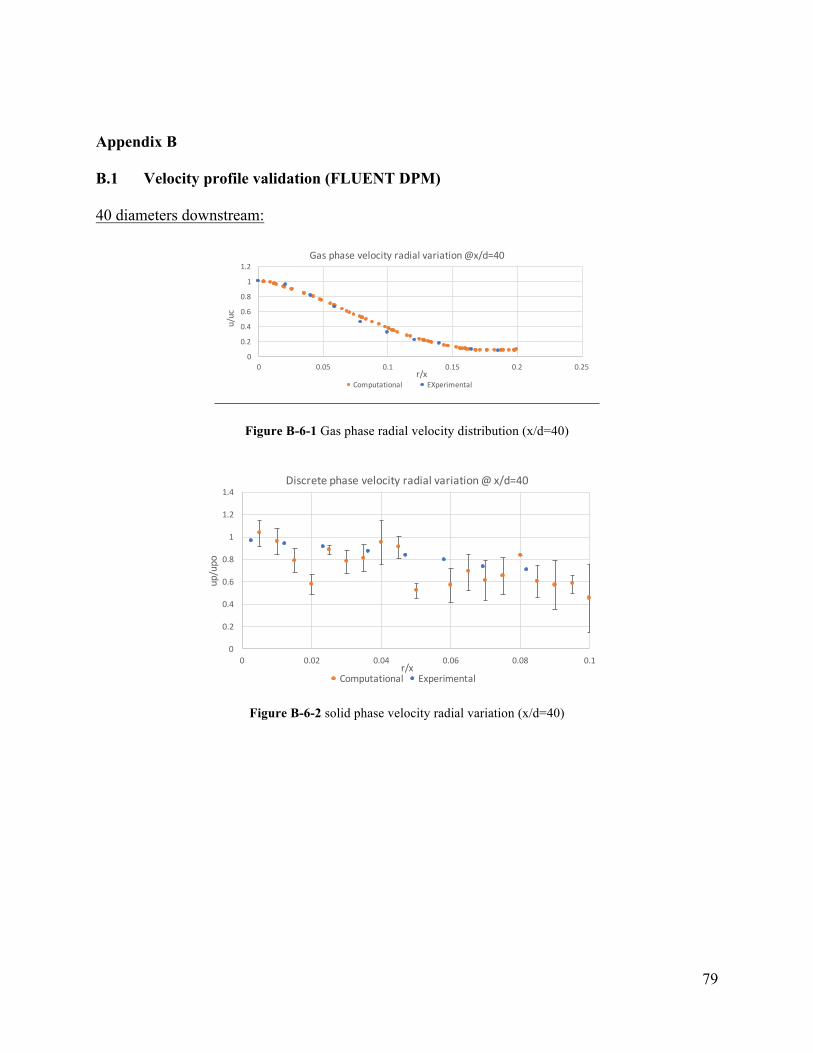
79
Appendix B
B.1 Velocity profile validation (FLUENT DPM)
40 diameters downstream:
Figure B-6-1 Gas phase radial velocity distribution (x/d=40)
Figure B-6-2 solid phase velocity radial variation (x/d=40)
0
0.2
0.4
0.6
0.8
1
1.2
0 0.05 0.1 0.15 0.2 0.25
u/uc
r/x
Gasphasevelocityradialvariation@x/d=40
Computational EXperimental
0
0.2
0.4
0.6
0.8
1
1.2
1.4
0 0.02 0.04 0.06 0.08 0.1
up/upo
r/x
Discretephasevelocityradialvariation@x/d=40
Computational Experimental
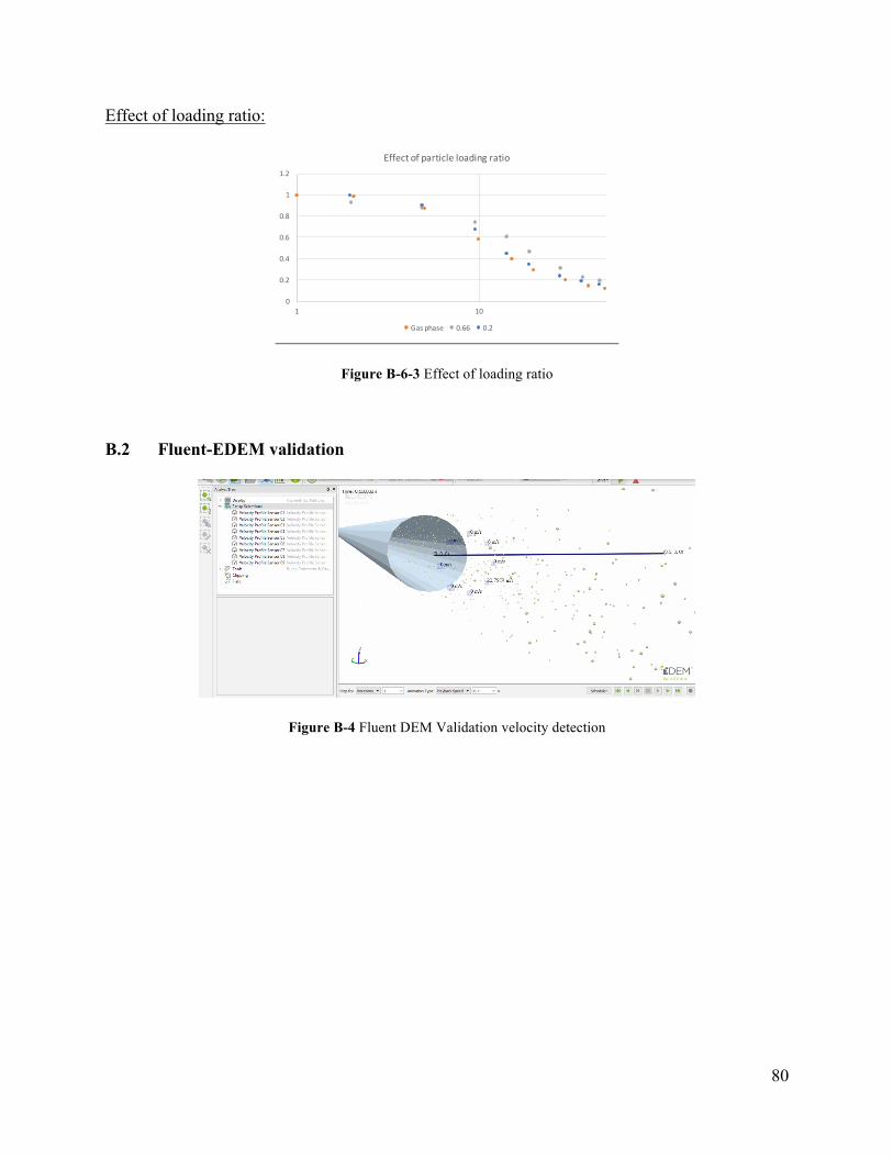
80
Effect of loading ratio:
Figure B-6-3 Effect of loading ratio
B.2 Fluent-EDEM validation
Figure B-4 Fluent DEM Validation velocity detection
0
0.2
0.4
0.6
0.8
1
1.2
1 10
Effectofparticleloadingratio
Gasphase 0.66 0.2
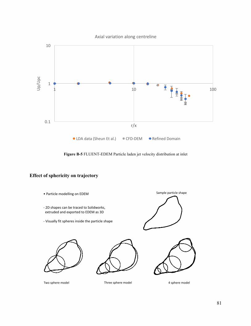
81
Figure B-5 FLUENT-EDEM Particle laden jet velocity distribution at inlet
Effect of sphericity on trajectory
0.1
1
10
1 10 100Up/Upc
r/x
Axialvariationalongcentreline
LDAdata(SheunEtal.) CFD-DEM RefinedDomain
• ParticlemodellingonEDEM
- 2DshapescanbetracedtoSolidworks,extrudedandexportedtoEDEMas3D
- Visuallyfitspheresinsidetheparticleshape
Sampleparticleshape
Twospheremodel Threespheremodel 4spheremodel

82
Figure B-6 4 different particle models based on modeling accuracy
•Mesh:1630230elements
•Elementsize(3.5R)
• Timestep:3.2e-06Simulationruntime:1.2s
Track15particles,Vexit=2m/s
y-deviationfunctionofvelocity,orientation,etc.Requireslargersamplesize

83
Figure B-7 y-deviation in trajectory vs sphericity
Here, it is shown that the overall particle trajectory is not significantly affected by the particle-
surface interactions for spherical/highly irregular particles. Consequently, deposition is
not a function of particle shape, insofar as the bounce characteristics are concerned.
-0.2 -0.1
00.10.20.30.40.50.60.70.80.9
1 1.5 2 2.5 3 3.5 4 4.5
y-deflection(degrees)
n
Particletrajectoryvsnumberofspheres
Related Documents