CERN ACCELERATOR SCHOOL ... - OSTI.GOV

CERN 98-043 August 1998

KSOO2373432R: KSDE011946929

ORGANISATION EUROPEENNE POUR LA RECHERCHE NUCLEAIRE

C E R N EUROPEAN ORGANIZATION FOR NUCLEAR RESEARCH

CERN ACCELERATOR SCHOOL

SYNCHROTRON RADIATION AND FREE ELECTRONLASERS

President Hotel, Grenoble, France22-27 April 1996

PROCEEDINGS

Editor: S. Turner

GENEVA1998

CERN-Service d'information scientifique-RD/982-150O-August 1998

© Copyright CERN, Genève, 1997

Propriété littéraire et scientifique réservéepour tous les pays du monde. Ce document nepeut être reproduit ou traduit en tout ou enpartie sans l'autorisation écrite du Directeurgénéral du CERN, titulaire du droit d'auteur.Dans les cas appropriés, et s'il s'agit d'utiliserle document à des fins non commerciales, cetteautorisation sera volontiers accordée.Le CERN ne revendique pas la propriété desinventions brevetables et dessins ou modèlessusceptibles de dépôt qui pourraient êtredécrits dans le présent document; ceux-ci peu-vent être librement utilisés par les instituts derecherche, les industriels et autres intéressés.Cependant, le CERN se réserve le droit des'opposer à toute revendication qu'un usagerpourrait faire de la propriété scientifique ouindustrielle de toute invention et tout dessinou modèle décrits dans le présent document.

Literary and scientific copyrights reserved in allcountries of the world. This report, or any partof it, may not be reprinted or translatedwithout written permission of the copyrightholder, the Director-General of CERN.However, permission will be freely granted forappropriate non-commercial use.If any patentable invention or registrable designis described in the report, CERN makes noclaim to property rights in it but offers it for thefree use of research institutions, manu-facturers and others. CERN, however, mayoppose any attempt by a user to claim anyproprietary or patent rights in such inventionsor designs as may be described in the presentdocument.

ISSNISBN

0007-832892-9083-118-9

Ill

*DE011946929*

XC98F«173~

ABSTRACT

These proceedings present the lectures given at the tenth specialised course organised by

the CERN Accelerator School (CAS), the topic this time being 'Synchrotron Radiation and

Free-electron Lasers'. A similar course was already given at Chester, UK in 1989 and whose

proceedings were published as CERN 90-03. However, recent progress in this field has been

so rapid that it became urgent to present a revised version of the course. Starting with a review

of the characteristics of synchrotron radiation there follows introductory lectures on electron

dynamics in storage rings, beam insertion devices, and beam current and radiation brightness

limits. These themes are then developed with more detailed lectures on lattices and emittance,

wigglers and undulators, current limitations, beam lifetime and quality, diagnostics and beam

stability. Finally lectures are presented on linac and storage ring free-electron lasers.

CERN RCCELERRTOR SCHOOLEUROPERN SVNCHROTRON RRDIRTION FRCILITV

will Jointly organise a course on

SVNCHROTRON RRDIHTION& FREE-ELECTRON LRSERS

22-27 flpril 1996President Hotel, Grenoble, France

PROGRAMME OF THE COURSE

SYNCHROTRON RADIATION AND FREE-ELECTRON LASERS

Hotel President, Grenoble, 22-27 April, 1996

Time

09.00

10.00

10.20

11.20

11.30

12.30

14.00

15.00

15.10

16.10

16.30

17.30

Monday22 April

Opening TalkA user's view

of synchrotronradiation

Y. Petroff

Tuesday23 April

Lattices andemittance

I

A. Ropert

Wednesday24 April


II

A. Ropert

Thursday25 April


III

A. Ropert

Friday26 April

Linac FELsI

M. Poole

Saturday27 April

Linac FELsII

M. PooleC O F F E E

Introduction tophysics of

synchrotronradiation

A. Hofmann

Wigglers andundulators

I

R. Walker


II

R. Walker

Lifetime andbeam quality

II

C. Bocchetta

Storage ringFELs

I

R. Bakker

Storage ringFELs

II

R. BakkerM I D-MORNING BREAK

Introduction todynamics ofelectrons in

rings

L. Rivkin

Currentlimitations

I

S. Myers

Currentlimitations

II

S. Myers


III

R. Walker

Beam stability

L. Farvacque

S e m i n a rIndustrial and

medicalapplications

I. MunroL U N C H

Introduction toinsertiondevices

K. Wille

Tutorial

B R E A KIntroduction to

current andbrightness

limits

V. Suller

Lifetime andbeam quality

I

C. BocchettaT E A

S e m i n a rScientific

applications

D. HausermanWELCOMECOCKTAIL

DiagnosticsI

A. Hofmann

EVENING MEAL

VISITTO THEESRF

DINNERat the Chateaude Sassenages

Tutorial Tutorial

B R E A KLifetime andbeam quality

III

C. Bocchetta

Postersession

T E ADiagnostics

II

A. Hofmann

EVENINGMEAL

HS e m i n a rPracticalaspects of

beam stability

P. Quinn

BANQUET

^* 43 r ^ * * & ' /HIM « * * * A S s, 4i> ^ s

'"• ' " * - - ' ^ . '„„* •_• ,J ,V . , ' *J i i - ^ v

1 _ _ i> j j u i • • • _ & & _ _ _ _ _ M $ •_ _

Vll

FOREWORD

The aim of the CERN Accelerator School to collect, preserve and disseminate the

knowledge accumulated in the world's accelerator laboratories applies not only to accelerators

and storage rings, but also to the related sub-systems, equipment and technologies. This wider

aim is being achieved by means of the specialised courses listed in the Table below. The latest

of these was on the topic of Synchrotron Radiation and Free-electron Lasers and was held at the

President Hotel, Grenoble, France, 22-27 April 1996, its proceedings forming the present

volume.

Synchrotron radiation has become one of the most valuable and useful scientific tools

with ever increasing applications for basic and applied research especially in the biotechnology,

chemical, material and pharmaceutical fields. This can be seen by the recent rapid increase in

the number of sources widely distributed around the world and in the intensity of the radiation

they produce. While initially synchrotron radiation was a by-product of high-energy

accelerators, the recent so-called third generation sources are specifically designed to produce

very intense photon beams by using low-emittance storage rings with high beam currents

together with insertion devices.

With such enormous progress in the design of sources and in their range of applications,

there was an urgent need to present an updated version of the course first presented in 1989.

Not forgetting the basic theory of synchrotron radiation and electron synchrotrons,

introductions are given to insertion devices and to the limitations to beam currents and radiation

brightness. These topics are then developed before turning to linac and storage-ring free-

electron lasers.

This course was only made possible by the generous support of several laboratories and

many individuals. In particular, the help and encouragement of the ESRF management and

staff, especially J.-L. Laclare, A. Ropert and T. Bouvet, was most invaluable. As always, the

support of the CERN management, the guidance of the CAS Advisory and Programme

Committees, and the attention to detail of the Local Organising Committee and the management

and staff of the President Hotel ensured that the course was held under optimum conditions.

Very special thanks must go to the lecturers at this course for the enormous task of preparing,

presenting and writing up their topics. Finally, the enthusiasm of the participants, coming from

so many parts of the world, was a convincing proof of the usefulness and success of this

course.

S. Turner, Editor

Vll l

LIST OF SPECIALISED CAS COURSES AND THEIR PROCEEDINGS

Year

1983

1986

1988

1989

1990

1991

1992

1993

1994

1995

1996

Course

Antiprotons for colliding beam facilities

Applied Geodesy for particle accelerators

Superconductivity in particle accelerators

Synchrotron radiation and free-electron lasers

Power converters for particle accelerators

RF engineering for particle accelerators

Magnetic measurement and alignment

RF engineering for particle accelerators(repeat of the 1991 course)

Cyclotrons, linacs and their applications

Superconductivity in particle accelerators

Synchrotron radiation and free-electron lasers

Proceedings

CERN 84-15 (1984)

CERN 87-01 (1987) alsoLecture Notes in Earth Sciences 12,(Springer Verlag, 1987)

CERN 89-04 (1989)

CERN 90-03 (1990)

CERN 90-07 (1990)

CERN 92-03 (1992)

CERN 92-05 (1992)

CERN 96-02 (1996)

CERN 96-03 (1996)

Present volume

IX

CONTENTS

Page no.Foreword

Y. PetroffA user's view of synchrotron radiation

Contribution not received

A. HofmannCharacteristics of synchrotron radiation 1

Qualitative treatment of synchrotron radiation 1Potentials and fields of a moving charge 5Radiation from a charge moving on a circular orbit 15Undulator radiation 30

L. RivkinIntroduction to dynamics of electrons in ringsin the presence of radiation 45

Introduction 45Radiation effects in electron storage rings 45Synchrotron oscillations 47Damping of betatron oscillations 52Adjustment of damping rates 54Quantum fluctuations - equilibrium beam sizes 55

K. WilleIntroduction to insertion devices 61

Introduction 61Wiggler and undulator field 63Equation of motion in W/U-magnets 67Undulator radiation 71

V. SutlerIntroduction to current and brightness limits 77

Introduction 77Beam current measurement and typical values 77Fourier components of the beam current 79Fields of relativistic electrons 80Effects due to the vacuum chamber walls 83Brightness of a synchrotron radiation source 85Brightness limitations 89

A. RopertLattices and emittances 91

From high brilliance to low emittance 91Low-emittance lattices 93Lattice types 96Problems associated with low-emittance lattices 105Effects of insertion devices on the beam 113Conclusions 126

R. WalkerInsertion devices: undulators and wigglers 129

Introduction 129Basic features of the radiation from standard insertion devices 130Radiation from insertion devices: detailed analysis 136Insertion device technology: introduction 149Insertion device performance limits and parameter optimization 153Insertion device technology: detailed magnetic design 156Insertion devices for circularly polarized radiation 162Undulators for free-electron lasers 177

S. MyersInstabilities and beam intensity limitations in circular accelerators 191

Calculation techniques 191'Robinson' instability 192Calculation of Robinson-induced voltage 193Robinson by eigenvalues of single-particle motion 195Robinson by solution of the forced equation of motion 195Spectrum of longitudinal oscillations 196Growth rates 198Modes and spectra of multiple bunches 199Transverse motion 202The transverse mode coupling instability (TMCI) 208TMCI with feedback 211Improvements in the model 213Computer simulation of TMCI 215Synchrobetatron resonances 216

C. BocchettaLifetime and beam quality 221

Introduction 221Brightness 222Stability 230The aperture 236Gas scattering 240Quantum lifetime 247The Touschek effect 252Intra-beam scattering 260Instabilities 263Ion trapping 272

L. FarvacqueBeam stability 287

Definitions 287Sources of instability 291Remedies 294Examples 299Conclusions 302

XI

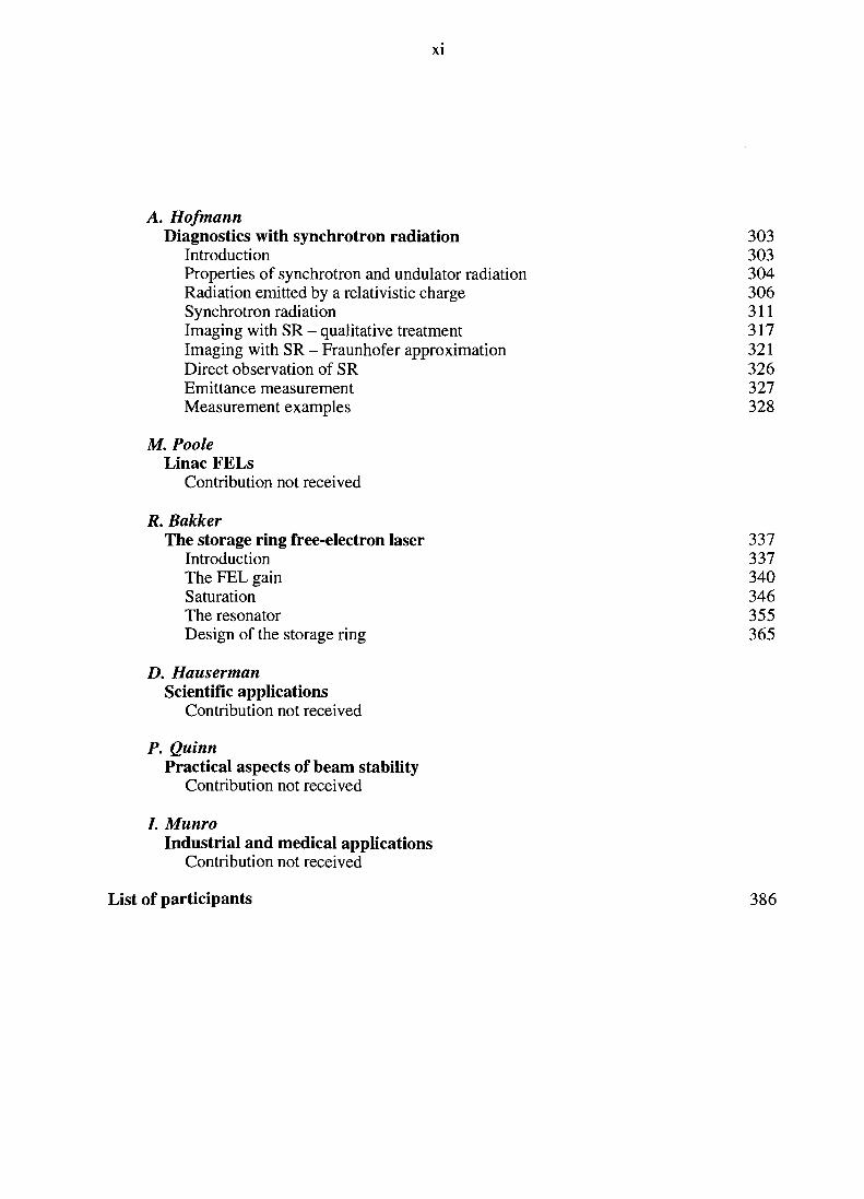
A. HofmannDiagnostics with synchrotron radiation 303

Introduction 303Properties of synchrotron and undulator radiation 304Radiation emitted by a relativistic charge 306Synchrotron radiation 311Imaging with SR - qualitative treatment 317Imaging with SR - Fraunhofer approximation 321Direct observation of SR 326Emittance measurement 327Measurement examples 328

M. PooleLinac FELs


R. BakkerThe storage ring free-electron laser 337

Introduction 337The FEL gain 340Saturation 346The resonator 355Design of the storage ring 365

D. HausermanScientific applications


P. QuinnPractical aspects of beam stability


/. MunroIndustrial and medical applications


List of participants 386

CHARACTERISTICS OF SYNCHROTRON RADIATION

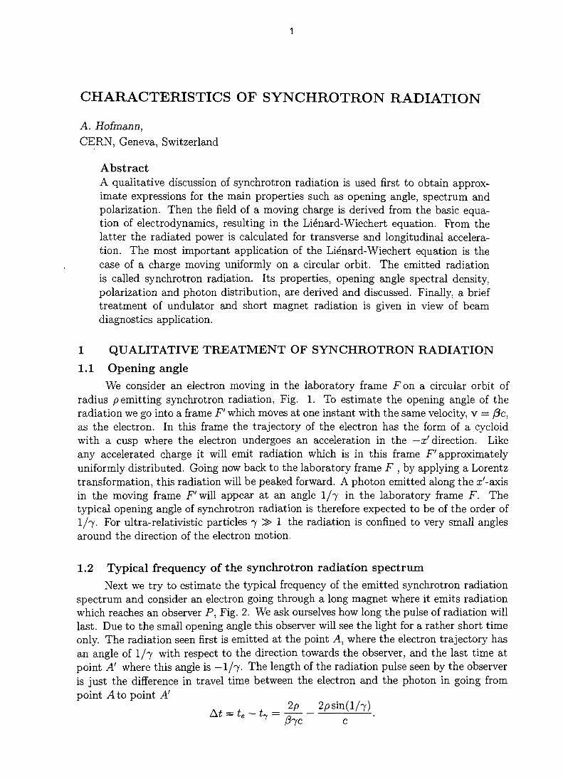
A. Hofmann,CERN, Geneva, Switzerland

AbstractA qualitative discussion of synchrotron radiation is used first to obtain approx-imate expressions for the main properties such as opening angle, spectrum andpolarization. Then the field of a moving charge is derived from the basic equa-tion of electrodynamics, resulting in the Lienard-Wiechert equation. From thelatter the radiated power is calculated for transverse and longitudinal accelera-tion. The most important application of the Lienard-Wiechert equation is thecase of a charge moving uniformly on a circular orbit. The emitted radiationis called synchrotron radiation. Its properties, opening angle spectral density,polarization and photon distribution, are derived and discussed. Finally, a brieftreatment of undulator and short magnet radiation is given in view of beamdiagnostics application.

1 QUALITATIVE TREATMENT OF SYNCHROTRON RADIATION

1.1 Opening angleWe consider an electron moving in the laboratory frame Fon a circular orbit of

radius Remitting synchrotron radiation, Fig. 1. To estimate the opening angle of theradiation we go into a frame F' which moves at one instant with the same velocity, v = (3c,as the electron. In this frame the trajectory of the electron has the form of a cycloidwith a cusp where the electron undergoes an acceleration in the —x' direction. Likeany accelerated charge it will emit radiation which is in this frame F' approximatelyuniformly distributed. Going now back to the laboratory frame F , by applying a Lorentztransformation, this radiation will be peaked forward. A photon emitted along the x'-axisin the moving frame .F'will appear at an angle 1/7 in the laboratory frame F. Thetypical opening angle of synchrotron radiation is therefore expected to be of the order ofI/7. For ultra-relativistic particles 7 » 1 the radiation is confined to very small anglesaround the direction of the electron motion.

1.2 Typical frequency of the synchrotron radiation spectrumNext we try to estimate the typical frequency of the emitted synchrotron radiation

spectrum and consider an electron going through a long magnet where it emits radiationwhich reaches an observer P, Fig. 2. We ask ourselves how long the pulse of radiation willlast. Due to the small opening angle this observer will see the light for a rather short timeonly. The radiation seen first is emitted at the point A, where the electron trajectory hasan angle of 1/7 with respect to the direction towards the observer, and the last time atpoint A' where this angle is —1/7. The length of the radiation pulse seen by the observeris just the difference in travel time between the electron and the photon in going frompoint A to point A'

A+ + + - 2P 2psin(l/7)/A l t

, F1

Figure 1: Opening angle of synchrotron radiation emitted by the moving source

For the ultra-relativistic case we consider here, 7 » 1, we can expand the trigonometricfunction

672/ jc \'<

where we used the approximation

1-0= "~R

67s

1 + 0 27,2'

The typical frequency is approximately

2TT

At3-7TC73

~2P~

The typical frequency is proportional to 73, a factor 72 is due to the difference in velocitybetween electron and photon and a factor of 7 is caused by the difference in trajectorylength of the two particles in the magnet.

We consider now the radiation emitted in a short magnet having a length L < 2p/^.An observer will receive the radiation emitted during the whole passage of the electronthrough this magnet, Fig. 3. The duration of the received pulse is now determined by thelength L of the deflecting magnet. Again, the length of the radiated pulse is given by thedifference in traveling time between the electron and photon going through the magnet

L L L(l - 0)Ai s m = -z =

2c 72 '

and the typical frequency is

This frequency contains only a factor j 2 since the difference in trajectory length is smallif the magnet is sufficiently short.

An undulator is an interesting source of synchrotron radiation. It consists of aspatially periodic magnetic field with period length Au in which the particle moves ona sinusoidal orbit, Fig. 4. Each of the periods represents a source of radiation. These

observer

Figure 2: Typical frequency of the spectrum emitted in long magnets

\ %

\1

1\\\\\I

11

1/1

a iiiiii

i

^ 1/7observer

E(t)i field pulse

I 1 /11/HI

spectrum

Figure 3: Typical frequency of the spectrum emitted in short magnet

field at angle 6

E field at 6 = 0

A(0)

Figure 4: Spectrum emitted in undulators

storage ring

observer

Figure 5: Elliptic polarization

contributions emitted towards an observer at an angle 9 will interfere with each other.We get maximum intensity at a wavelength A for which the contributions from differentundulator periods are in phase. The time difference AT between the arrival of adjacentcontributions is

AT — — ûC0S^ — -^"(i - P )

For a relativistic particle the angle 9, where radiation of reasonable intensity can beobserved, is small; 6 « 1/7. We can approximate cos 9 « 1 — 92/2.

The frequency for which we get constructive interference is just UJ = 2-n/AT.

Harmonics of this frequency might also be emitted.

1.3 PolarizationSince the acceleration of the electron is radial we expect the emitted radiation to be

mostly polarized such that the electric field Elies in the median plane. This should beexact as long as the radiation is also observed in the (usually horizontal) median plane.For observations at a finite vertical angle a certain amount of circular polarization isexpected as indicated in Fig. 5.

P observer

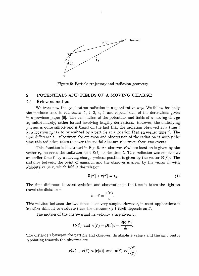
Figure 6: Particle trajectory and radiation geometry

2 POTENTIALS AND FIELDS OF A MOVING CHARGE

2.1 Relevant motionWe treat now the synchrotron radiation in a quantitative way. We follow basically

the methods used in references [1, 2, 3, 4, 5] and repeat some of the derivations givenin a previous paper [6]. The calculation of the potentials and fields of a moving chargeis, unfortunately, rather formal involving lengthy derivations. However, the underlyingphysics is quite simple and is based on the fact that the radiation observed at a time tat a location rphas to be emitted by a particle at a location Rat an earlier time t'. Thetime difference t — t' between the emission and observation of the radiation is simply thetime this radiation takes to cover the spatial distance r between these two events.

This situation is illustrated in Fig. 6. An observer P whose location is given by thevector rp observes the radiation field E(t) at the time t. This radiation was emitted atan earlier time t' by a moving charge q whose position is given by the vector R(t'). Thedistance between the point of emission and the observer is given by the vector r, withabsolute value r, which fulfills the relation

R(t') + r(f) = rp. (1)

The time difference between emission and observation is the time it takes the light totravel the distance r

C

This relation between the two times looks very simple. However, in most applications itis rather difficult to evaluate since the distance r(t') itself depends on £'.

The motion of the charge q and its velocity v are given by

The distance r between the particle and observer, its absolute value r and the unit vectorn pointing towards the observer are

r(t') , r(f) = |r(OI and n(f) = ^

In all our applications the observer does not move, rp=constant, and differentiating (1)gives

dt>To get the time derivative of r(t') we write

dr ld(r2) dr drdt' 2 df df ' d*'

From this we get the important relation between the increments of the time tat theobserver and the time t' of emission

* = (l + £1?) ^ = (1 " " • fltf- (2)

Usually we are concerned with the radiation emitted by a relativistic particle in theforward direction in which case two photons received by the observer within a very smalltime interval At have been emitted within a much longer time interval At' = Ai/(1—n-/3).

2.2 Potentials of a moving charge (retarded potentials)Our goal is to calculate the electric and magnetic fields E(t) and B(i) of the radiation

received by an observer. These fields can by obtained from the scalar and vector potentialsV and A through

B = no curl A = |io[VxA]•r-, T T r 9 A _ _ . dAE = - d V V VtiO = V V n o .

at at

We use here the Lorentz convention W + CQV = 0.For the case of a stationary charge and current distribution with charge density

r}(x,y,z) = r}(R) and velocity v(R), the resulting electrostatic potential V is simplygiven by Coulomb's law and the vector potential A by a similar expression

47reo

where r is the distance between the individual charges and the observer. If the chargedistribution is not stationary, the density r)(t') and velocity v become functions of time.In carrying out the above integration we have to evaluate the charge density at the earliertime t' such that the potential created by the charges reaches the observer at the time t,i.e. t' — t — r(t')/c. The resulting potential V is called the retarded potential.

The integration

represents a thin sphere of radius r collapsing with the speed of light c towards theobserver P counting all the charges on its way, Fig. 7. In this process the charges whichmove towards the observer are counted over a longer time and contribute more to thepotential V(t) and, vice versa, charges moving away from P contribute less.

= cdt'

charges

Figure 7: Collapsing sphere representing the integration over charges

Ar = c At'

Figure 8: Contribution of a moving charge to the potential

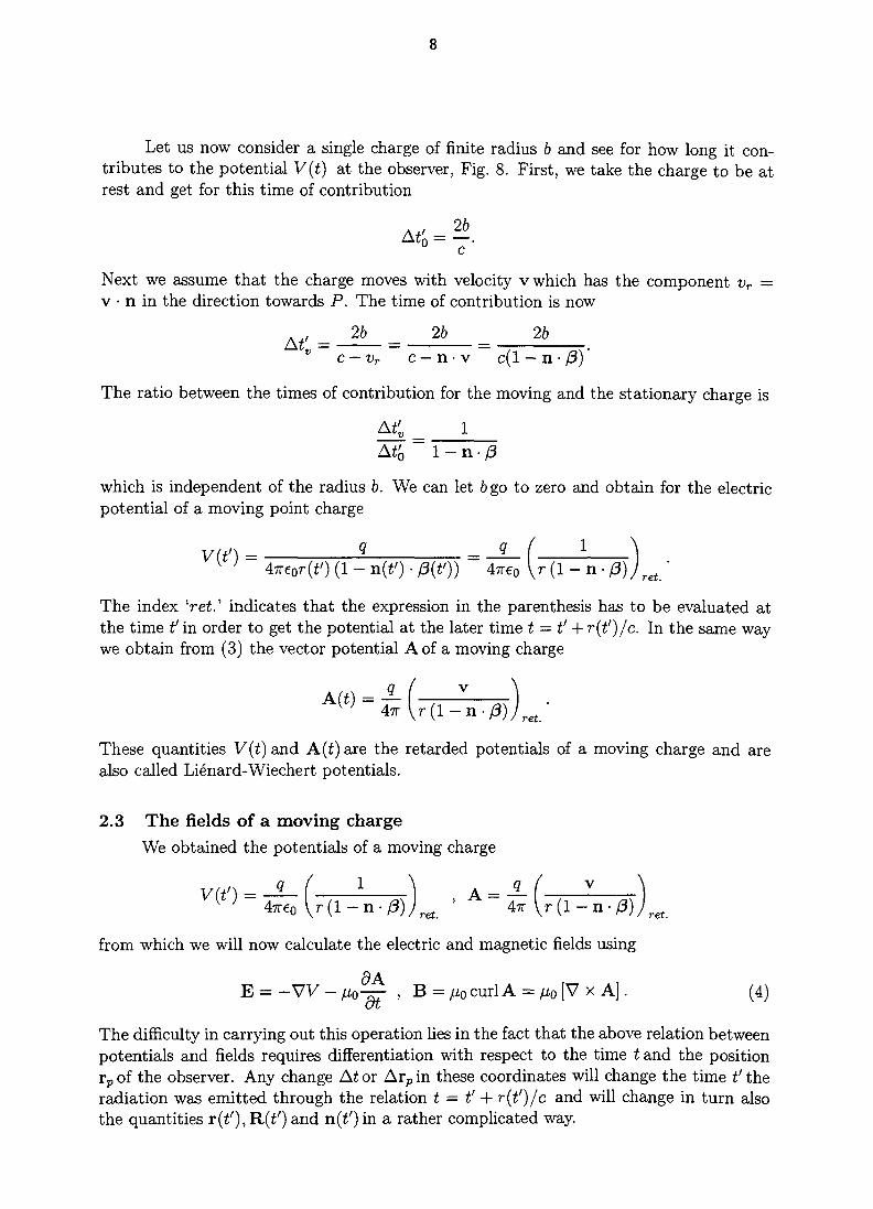
Let us now consider a single charge of finite radius b and see for how long it con-tributes to the potential V(t) at the observer, Fig. 8. First, we take the charge to be atrest and get for this time of contribution

A ' - 2b

c

Next we assume that the charge moves with velocity v which has the component vr ~v • n in the direction towards P. The time of contribution is now

Af - _ H L - 2b - 2b

c — vr c — n • v c(l — n • p)

The ratio between the times of contribution for the moving and the stationary charge is

At'v 1A4 ~ l - n - / 3

which is independent of the radius b. We can let b go to zero and obtain for the electricpotential of a moving point charge

V(t') = I = -±- ( 1 ^k ; 47re0r(t') (1 - n(tf) • 0(f)) 47re0 \r (1 - n • (3))ret '

The index 'ret.' indicates that the expression in the parenthesis has to be evaluated atthe time t' in order to get the potential at the later time t — t' + r(t')/c. In the same waywe obtain from (3) the vector potential A of a moving charge

4TT \r (1 - n • f3) Jret_

These quantities V(£) and A(£) are the retarded potentials of a moving charge and arealso called Lienard-Wiechert potentials.

2.3 The fields of a moving chargeWe obtained the potentials of a moving charge

from which we will now calculate the electric and magnetic fields using

<9AE = - W - iiQ— , B = /zo curl A = /a0 [V x A]. (4)

The difficulty in carrying out this operation lies in the fact that the above relation betweenpotentials and fields requires differentiation with respect to the time tand the positionrp of the observer. Any change At or Arp in these coordinates will change the time t' theradiation was emitted through the relation t = t' + r(t')/c and will change in turn alsothe quantities r(f),R(t') and n(f)in a rather complicated way.

B

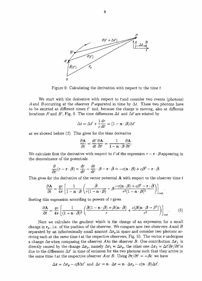
Figure 9: Calculating the derivation with respect to the time t

We start with the derivative with respect to tand consider two events (photons)A and B occurring at the observer P separated in time by At. These two photons haveto be emitted at different times t' and, because the charge is moving, also at differentlocations A' and B', Fig. 9. The time differences At and At'are related by

At = At + -^c at

as we showed before (2). This gives for the time derivative

dA __ d£dA 1 dA~ ~ ~di~dFdt - n dt''

We calculate first the derivative with respect to t' of the expression r — r • j3 appearing inthe denominator of the potentials

This gives for the derivative of the vector potential A with respect to the observer time t

dAdt

22.Air

1 -c(n • /3) + c/32 -r

r4 1 — n ret.

Sorting this expression according to powers of r gives

8Adt

qc_4?r

n( 1 - n

(5)ret

Next we calculate the gradient which is the change of an expression for a smallchange in rp, i.e. of the position of the observer. We compare now two observers A and Bseparated by an infinitesimally small amount Arp in space and consider two photons ar-riving each at the same time t at the respective observers, Fig. 10. The vector r undergoesa change Arwhen comparing the observer A to the observer B. One contribution Ari isdirectly caused by the change Arp, namely Ari = Arp, the other one Ar2 = At'dv/dt' isdue to the difference At' in time of emission for the two photons such that they arrive inthe same time t at the respective observer A or B. Using dr/dt' = —j3c we have

Ar = Arp - c/3At' and Ar = n • Ar = n • Arp - c(n • /3)At'.

10

Figure 10: Calculation of the gradient

Since the two photons arrive at the same time at their respective observers the differenceAt' in time of emission is given simply by the difference Ar in the traveling distances

which gives

Ar = -cAt'

-cAt1 = n • Arp - c(n • (3) At' or At' = —n- Ar,

(6)

For the expression r — r • j3 appearing in the denominator of the potentials we get

A(r - r • (3) = Ar - Ar • j3 - r • A/3 = -cAt' - f Arp + -r-.At' j (3 - r-J--At'.

\ dt I ot

Using (6) gives

n 02n (r • /3)nA(r -r-f3) = c(l-n./3);Arp-1 - I 1 - / 3 " l - n - / 5

Comparing this with the equation

A(r — r • (3) = grad(r — r • /3) • Arp

we can write

L - /32)n - c(l - n • (3)/3 + r(n • /3)ngrad(r — r • (3) =

The gradient of the scalar potential

c(l-n

(r - r ) r e t .

becomes

grad V = —q grad(r — r • (3) —q

r 2 ( l — n • /3)2 47reeo r 2 ( l - n • /3)3

ret.

11

This together with the time derivative of the vector potential (5) gives us for the electricfield of a moving charge

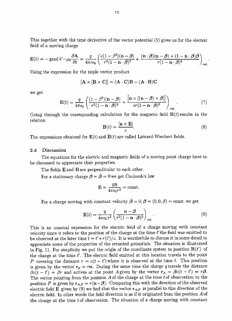
9A q fc(l-02)(n-(3) , (n • /3)(n - 0) + (1 - n • P)fc\E(i ) = - grad V-fM)-xr = ~A —571 Jav? '

dt 4TTC€ \ r 2 ( l n / 3 ) 3dt 4TTC€0 \ r2(l-n-/3)3 r(l-n-/3)3 Jret

Using the expression for the triple vector product

[A x [B x C]] = (A • C)B - (A • B)C

we get. [" x [(n - / 3 ) x/3]] \

r 2 ( l -n- /3) 3 cr(l - n •/3)3 I " ^/ rei.

Going through the corresponding calculation for the magnetic field B(i) results in therelation

^ . (8)

The expressions obtained for E(i) and B(t) are called Lienard-Wiechert fields.

2.4 DiscussionThe equations for the electric and magnetic fields of a moving point charge have to

be discussed to appreciate their properties.The fields E and B are perpendicular to each other.For a stationary charge f3 = (3 = Owe get Coulomb's law

^ onE = =• = const.

4

For a charge moving with constant velocity /3 - 0; /3 = (0,0,0) — const, we get

• 0)

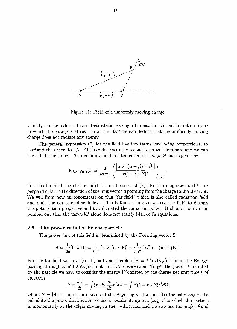
This is an unusual expression for the electric field of a charge moving with constantvelocity since it refers to the position of the charge at the time t' the field was emitted tobe observed at the later time t = t'+r(t')/c. It is worthwhile to discuss it in some detail toappreciate some of the properties of the retarded potentials. The situation is illustratedin Fig. 11. For simplicity we put the origin of the coordinate system to position R(i') ofthe charge at the time t'. The electric field emitted at this location travels to the pointP covering the distance r = c(t — t') where it is observed at the time t. This positionis given by the vector rp = rn. During the same time the charge q travels the distance(3c(t - t') = fir and arrives at the point A given by the vector r^ = (3c(t - tf) = r(3.The vector pointing from the position A of the charge at the time t of observation to theposition P is given by TA,P = r(n — J3). Comparing this with the direction of the observedelectric field E given by (9) we find that the vector rAjP is parallel to this direction of theelectric field. In other words the field direction is as if it originated from the position A ofthe charge at the time t of observation. The situation of a charge moving with constant

12

r a = r 0 A

Figure 11: Field of a uniformly moving charge

velocity can be reduced to an electrostatic case by a Lorentz transformation into a framein which the charge is at rest. From this fact we can deduce that the uniformly movingcharge does not radiate any energy.

The general expression (7) for the field has two terms, one being proportional to1/r2 and the other, to 1/r. At large distances the second term will dominate and we canneglect the first one. The remaining field is often called the far field and is given by

q ( f n x [ ( n - j 8 ) xE>far-field(t) =

— nret.

For this far field the electric field E and because of (8) also the magnetic field Bareperpendicular to the direction of the unit vector n pointing from the charge to the observer.We will from now on concentrate on this "far field" which is also called radiation fieldand omit the corresponding index. This is fine as long as we use the field to discussthe polarization properties and to calculated the radiation power. It should however bepointed out that the 'far-field' alone does not satisfy Maxwell's equations.

2.5 The power radiated by the particleThe power flux of this field is determined by the Poynting vector S

S = —[E x B] = — [E x [n x E]] = — (E2n - (n • E)E) .

For the far field we have (n • E) = Oand therefore S = E2n/(fj,oc) This is the Energypassing through a unit area per unit time t of observation. To get the power P radiatedby the particle we have to consider the energy W emitted by the charge per unit time t' ofemission

P = L = / ( n • S)^r2dn = / 5(1 - n • f3)r2dtl,at J at J

where 5 = |S|is the absolute value of the Poynting vector and fiis the solid angle. Tocalculate the power distribution we use a coordinate system (x, y, z) in which the particleis momentarily at the origin moving in the z—direction and we also use the angles $ and

13

<f> of the corresponding spherical coordinate system. The unit vector n pointing from theparticle to the observer and the normalized velocity vector 0 are

n = (sin 9 cos </), sin 6 sin <j>, cos 6) and 0 = /3 (0,0,1).

We take now the case with the acceleration perpendicular to the velocity and pointingin the —x direction. This corresponds to the case of synchrotron radiation emitted bya particle going through a magnetic field B pointing in the y direction resulting in acurvature

1 _ eBp PyrriQC

The normalized acceleration is82c

/3 = ^ (-1,0,0).

The distribution of the power radiated by the particle is

_ <?2[nx {{n-0)x0]f _ crprnpc2/?4 ({I - ffcosfl)2 - (1 - (52)sin26cos24>\dQ, ~ (47r)2eoc(l - n • /?)5 ~ 4?rp2 \ ( l - /?cos0)5 ) '

(10)where we assumed a particle having the elementary charge q = eand introduced theclassical radius.

_ e2 _ 2.81810~15 m for electronsr° ~ 47re0m0c

2 ~ 1.53510"18m for protons '

Integrating (10) over the solid angle gives the total power radiated by the particle2r0cm0c

2/g

474 2romoc/?r7 2cr0pn7 2 r 0 c e ^ 7 B0 T ~ 3p2 3c 3m0c

2 ~ 3m0c2 ' ( '

where we used the relation between the time derivative pt of the momentum and thetransverse acceleration

PT = moC0T7.

For the ultra-relativistic case j3 s» 1, 7 > 1 the radiation is peaked forward confined to acone of opening angle 6 ~ 1/7 and we get approximately

dPT 2cromoc276 / 1 + 27

202(1 - 2cos2 0) + 74 0 4 \ , _ 2rocmoc

274 . o.I n " TTP2 { a + 72*2)5 J and PoT w 3p2 • (12)

It is interesting to also investigate the case where the acceleration is longitudinal, i.e. inthe direction of the particle velocity, although this is of no practical importance. We getfor the power distribution

n x [n x 0}f rQmQ(?Pl sin2 6(47r)2e0c ( l - n - / 3 ) 5 ~ 4TTC ( 1 - / ? C O S 0 ) 5 '

The power is not emitted in the forward direction $ = 0 but symmetrically around it witha typical angle of order I/7 with respect to this direction. For the total power we find

2romoc2/?276 2cr0p

2L

= -5 5-, (13)3c 3m0c

2

14

where we used the relation between the time derivative of the momentum and the longi-tudinal acceleration which is different from the transverse case

PL = ( ) 7

Comparing (13) with (11) we find that for the same absolute value of the time derivative ofthe momentum, i.e. the same force, the radiated power is smaller by 72 for a longitudinalforce than for a transverse one. This is the main reason why linear colliders are, above acertain beam energy, advantageous compared to storage rings for colliding electrons andpositrons.

2.6 Fourier transform of the radiation field

We calculated the electric and magnetic radiation fields emitted by a moving chargeat the time f and observed at the time t

[nx[(n-/3)x/3]]\ _ [n x E]r(l - n • 0)3 I ' W " c '

/ ret.

(14)

As we said before, the difficulty to evaluate these fields lies in the fact that the expressionsinvolving the particle motion have to be evaluated at the earlier time t' which has, ingeneral, a rather complicated relation to the time t of observation. For this reason it is inmany cases easier to calculate directly the Fourier transform E of the electric field

This integration involves the time t since we are interested in the spectrum of the radiationas seen by the observer. We can however make a formal transformation of the integrationvariable into the time t' = t — r{t')/c and get

'C)dt'. (15)

We omitted in the above equation the index 'ret' since the integration variable is anywaythe time t' at which the expressions are evaluated. We take now the ultra-relativistic case7 > 1 which has the emitted radiation concentrated within a small opening angle of order1/7 -C 1. The observer sees radiation originating only from a small part of the trajectoryof length Al ~ 2p/7, where pis the radius of curvature as indicated on Fig. 2. In thiscase the vector r pointing from the particle to the observer will change little as long asthe radiation is observed from a large distance r » 2p/7. We neglect the variation of rin the triple vector product but not in the exponent as will be explained later. We canintegrate (15) in parts

with[n x [n x j3}} dU __ [n * [(n - 0) x /3]]

l - n - / 3 ' ~dH ~ ( l - n - / 3 ) 2

V = e-Mt'-r(t')/c) dV_ = x _ n _ p.-iuif

15

radiation

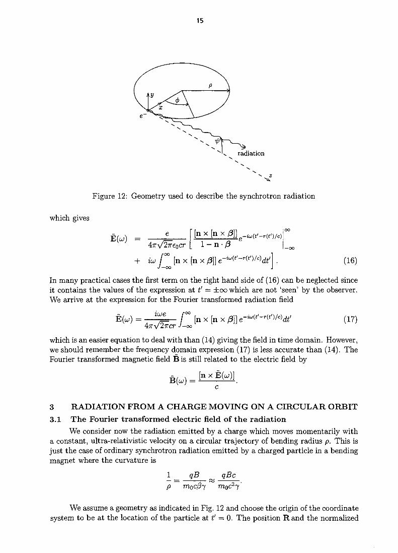
Figure 12: Geometry used to describe the synchrotron radiation

which gives

[n x [n x j3\) ju(t'-r(t')/c)l - n / 3

+ iu f°° [n x [n x 0\] e-*«(*'-r(t')/c)df'l .J—oo J

(16)

In many practical cases the first term on the right hand side of (16) can be neglected sinceit contains the values of the expression at t' = ±oo which are not 'seen' by the observer.We arrive at the expression for the Fourier transformed radiation field

[" [n x [n x /3]] e-Mt>-r(t')/c)dt> (17)

which is an easier equation to deal with than (14) giving the field in time domain. However,we should remember the frequency domain expression (17) is less accurate than (14). TheFourier transformed magnetic field B is still related to the electric field by

B(u,) =[n x E(w)]

3 RADIATION FROM A CHARGE MOVING ON A CIRCULAR ORBIT3.1 The Fourier transformed electric field of the radiation

We consider now the radiation emitted by a charge which moves momentarily witha constant, ultra-relativistic velocity on a circular trajectory of bending radius p. This isjust the case of ordinary synchrotron radiation emitted by a charged particle in a bendingmagnet where the curvature is

qB qBc1.

p

We assume a geometry as indicated in Fig. 12 and choose the origin of the coordinatesystem to be at the location of the particle at t' = 0. The position Rand the normalized

16

velocity /3 areR(t') = p ((1 - cos(w0*')) . 0, sin(wof))

= 0{sm{uot') ,0, cos(w0f)) (18)= 0wo (cos(wot') ,0, -sin(wof))

where we introduced the angular velocity wo = 0c/p of the particle. We chose theobservation point P to lie in the yz-plane. This is no restriction since we assumed acircular motion with constant speed 0c which is symmetric with respect to the angle <j).The vector pointing from the origin to the observer makes an angle ip with respect tothe :c,2-plane of the particle motion. We assume again observation from a large distancer » 2p/7 and consider the vector rto be constant over the short time during whichradiation is emitted which can be observed at P. We have for the unit vector nand forthe vector product appearing in (17)

n = (0, sin?/), cos ip)

[n x [n x f3]] = 0 ^-sm(u0t'),cosijjsmipcos(uot'),-sm2ipcos(u!ot')^ .

Since we assumed the ultra-relativistic case 7 > 1 the vertical opening angle of theradiation is very small ^ < 1 and only a small part of the trajectory A0 = io0t' <C 1contributes to the radiation observed at P. We can therefore approximate the vectorproduct by

[n x [n x 0\] « 0 {~utr, ip, 0)

and the term in the exponent by

C C C C 27^ Dp2

We are not interested in the constant rp/c which represents just the traveling time of thelight to go from the coordinate origin to the observer and introduce

(19)

This expression has a term of order i'3 included since the first order term is dividedby 72and can become very small. With these approximations we get for the Fouriertransformed electric field vector

where we assume now a particle with elementary charge q = e. It should be noted thatthis expression gives the radiation field as a function of the frequency u measured by theobserver. The earlier time t' represents here a convenient variable of integration. We cansplit the field into the components in the xand y direction and express the exponentialwith trigonometric functions and make use of the symmetries involved

Ey(u>) =

17

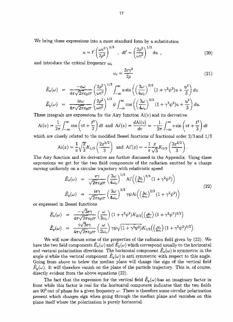
We bring these expressions into a more standard form by a substitution

and introduce the critical frequency uc

3c73

47rV^7re0cr \UJC2) J-oo \ \ 4 w c /

These integrals are expressions for the Airy function M(v) and its derivative

^ rco / t^\ dAifu) 1 f°° ( t^\A-Kv) ~ 7T~ / c o s \vt + —•) dt and Ai'(u) = — - — = —-— / v sin ( vt + — I dt

2?T J-OO \ o J dV 2~K J-oo \ 6 Jwhich are closely related to the modified Bessel functions of fractional order 2/3 and 1/3

1 /a" (2xW\ , . . , , . 1 x .. (2x^—./ — « i / 3 a n d Ai I T ) = ^-Kn/o I

The Airy function and its derivative are further discussed in the Appendix. Using theseexpressions we get for the two field components of the radiation emitted by a chargemoving uniformly on a circular trajectory with relativistic speed

or expressed in Bessel functions

We will now discuss some of the properties of the radiation field given by (22). Wehave the two field components Ex{u) and Ey{uS) which correspond usually to the horizontaland vertical polarization directions. The horizontal component Ex(u) is symmetric in theangle -0 while the vertical component Ey{u) is anti symmetric with respect to this angle.Going from above to below the median plane will change the sign of the vertical fieldEy(io). It will therefore vanish on the plane of the particle trajectory. This is, of course,directly evident from the above equations (22).

The fact that the expression for the vertical field Ey(u) has an imaginary factor infront while this factor is real for the horizontal component indicates that the two fieldsare 90° out of phase for a given frequency u>. There is therefore some circular polarizationpresent which changes sign when going through the median plane and vanishes on thisplane itself where the polarization is purely horizontal.

18

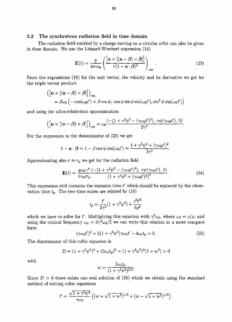
3.2 The synchrotron radiation field in time domainThe radiation field emitted by a charge moving on a circular orbit can also be given

in time domain. We use the Lienard-Wiechert expression (14)

a ( fn x [(n - /3) x 0]]4irc€0 \ r ( l - n • /3)3

ret.

From the expressions (18) for the unit vector, the velocity and its derivative we get forthe triple vector product

= (3<JJQ (— cos(ujQt') + 0cosip, cos tp sin ip sin(uot'), sin2 ip sin(uot')j

and using the ultra-relativistic approximation

(fnx[(n-«xy3]]) ^ H ' ^ -\L 'J/ret

For the expression in the denominator of (23) we get

1 - n • 0 = 1 - 0 cos,/, cos(u»f) « 1 + 7

Approximating also r « rp we get for the radiation field

E(t) = ^QT4 (-(1 + 7 V - (7^) 2 ) , 7^(7^0, 0)U 7re0crp (1 +f^2 + frUof)rf '

This expression still contains the emission time f which should be replaced by the obser-vation time tp. The two time scales are related by (19)

which we have to solve for t'. Multiplying this equation with 73o;o, where OJQ = c/p, andusing the critical frequency UJC = 373o>o/2 we can write this relation in a more compactform

(•yujot')3 + 3(1 + j2ip2)'yujot' — 4u>ctp = 0. (25)

The discriminant of this cubic equation is

D = (1 + 7 V ) 3 + (2uctp)2 = (1 + 7V)3(1 + w2) > 0

with2<jjctv

W = 7" 7T

Since D > 0 there exists one real solution of (25) which we obtain using the standardmethod of solving cubic equations

t' =

19

-0.20.0 1.0 2.0 3.0 4.0 Uctv 5.0

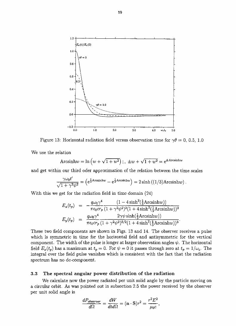
Figure 13: Horizontal radiation field versus observation time for 7$ = 0, 0.5, 1.0

We use the relation

Arcsinhw = In (w + y/l + w2) ;, ±w + Vl + w2 = e±ATCSmhw

and get within our third oder approximation of the relation between the time scales

^ = 2sinh((l/3)Arcsinhw).

With this we get for the radiation field in time domain (24)

Ex(tp) = -(1 — 4 sinh2 ( | Arcsinhui))

7re0crp

A

2(1 + 4sinh (|Arcsinhw))3

sinh(|Arcsinhw))

- 4sinh2(5Arcsinhty))3

These two field components are shown in Figs. 13 and 14. The observer receives a pulsewhich is symmetric in time for the horizontal field and antisymmetric for the verticalcomponent. The width of the pulse is longer at larger observation angles tp. The horizontalfield Ex{tp) has a maximum at tp — 0. For ip = 0 it passes through zero at tp = l/uc. Theintegral over the field pulse vanishes which is consistent with the fact that the radiationspectrum has no dc-component.

3.3 The spectral angular power distribution of the radiationWe calculate now the power radiated per unit solid angle by the particle moving on

a circular orbit. As was pointed out in subsection 2.5 the power received by the observerper unit solid angle is

dPobserver _ dW _ 2 _ T2E2

~ dtdn ~ [ n " )r "

20

o.io

0.08-

0.06-

0.04-

0.02-

0.00

Figure 14: Vertical radiation field versus observation time for 7# = 0,5, 1.0

while the power radiated by the particle is

dP _ d?W _ d2W dtdSl ~ dt'dtt ~ dtdtt dt'

( 1 - n

The difference between the power observed and the power emitted by the particle isjust a manifestation of the fact that the energy is received in a compressed time At =At'(l — n -(3). We calculate first the received power P ^ . which could directly be obtainedfrom (22) if the field E(t) were given. We calculated the Fourier transformed fields (22)and will use it now to calculate the spectral distribution of the power. The observerP receives a short flash of radiation which determines the form of the spectrum. Wecalculate the total energy W received during a single traversal of the particle

W1 Mff yoo

= — / E(t)Hoc JO J-<X>

2r2dQdt.

The field E(t) can be obtained from the Fourier transformed field E(u)

which gives

2-KfXoCf00 f°° r—oo J—oo J — o

Using the integral representation of the Dirac 6-functions

/ eiatdt =J—oo

we get

W = — dtt /fJ,QC J J—OO J—C

21

Since E(t) is a real function its Fourier transform and its conjugate have the symmetryrelation E(u) = E*(—u) and we get for the above integral

From this we obtain the spectral angular distribution of the radiated energy in one traver-sal, i.e. in one flash of radiation

SW 2r2 E(u)\dttdw- HOC • {Ib)

The factor 2 on the right hand side indicates that the spectral energy density is takenat positive frequencies only, contrary to the field which is taken at positive and negativefrequencies. This is common practice since power can be measured directly but the signof the frequency cannot be observed during such measurements. The field, however, israrely accessible to direct measurements. If the particle circulates on a closed circular orbitof radius pwith revolution frequency co = /3c/p « c/p the observer receives c/27rpsuchflashes per second from the particle and an average spectral angular power density

2r2 E(u) n

(27)

This expression (27) gives the average received power which is also the power radiated bythe particle.

We use now (22) for the field components to calculate the square of the total fieldand use the index V for the horizontal and V for the vertical polarization component

= Ex{u)2 + Ey(uf

e272

2TT

E(u)=2^,2

(28)

with

*<»••> - K(29)

or

- V

22

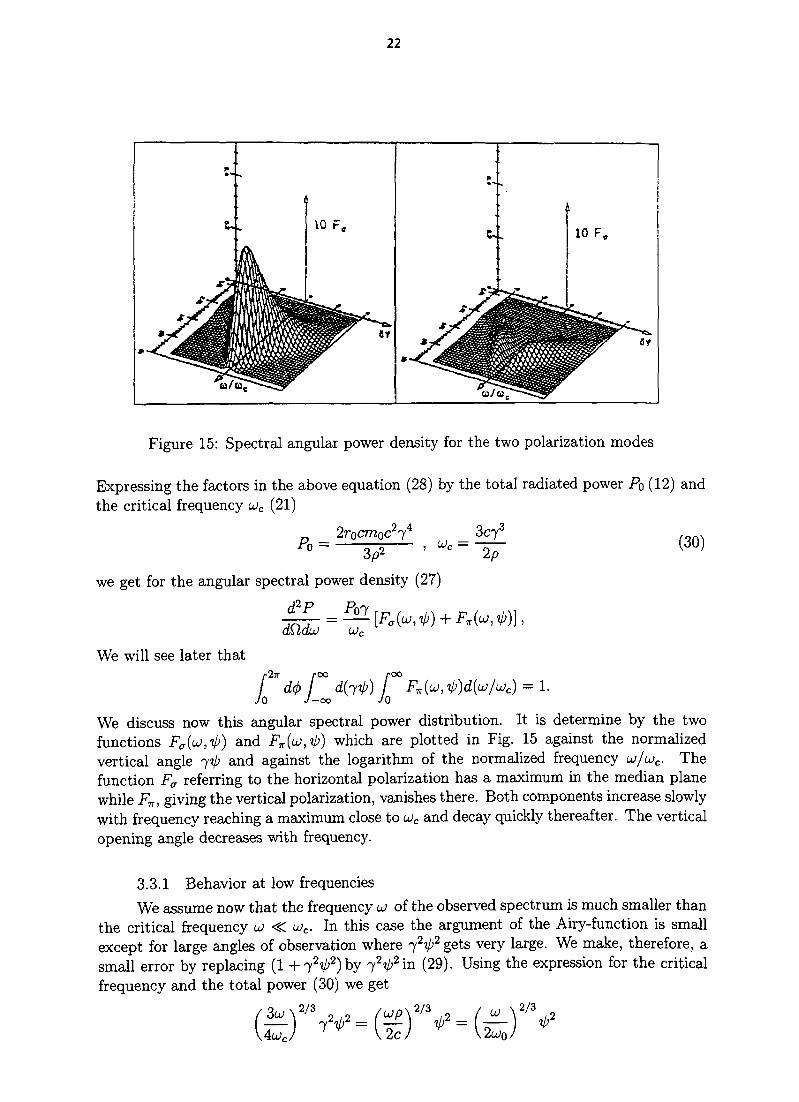
Figure 15: Spectral angular power density for the two polarization modes

Expressing the factors in the above equation (28) by the total radiated power Po (12) andthe critical frequency uc (21)

7Po =

we get for the angular spectral power density (27)

d2P

(30)

We will see later that/•2TT r

Jo

= 1.

We discuss now this angular spectral power distribution. It is determine by the twofunctions Fa(u,ip) and Fw{u,ip) which are plotted in Fig. 15 against the normalizedvertical angle jtp and against the logarithm of the normalized frequency w/uc. Thefunction Fa referring to the horizontal polarization has a maximum in the median planewhile Fw, giving the vertical polarization, vanishes there. Both components increase slowlywith frequency reaching a maximum close to uc and decay quickly thereafter. The verticalopening angle decreases with frequency.

3.3.1 Behavior at low frequenciesWe assume now that the frequency w of the observed spectrum is much smaller than

the critical frequency u < uc. In this case the argument of the Airy-function is smallexcept for large angles of observation where 72?/>2 gets very large. We make, therefore, asmall error by replacing (1 + 72^2) by 72^2in (29). Using the expression for the criticalfrequency and the total power (30) we get

23

and the total power distribution becomes

d2P 2romoc2 / u \ 2 / 3 k.,i(/ u \2 /3 ,2\ ,2 ( w \^Z -2(1 w \2 /3 2Y

dVtdu irp \2UQJ \\2UOJ J \2uoJ \\ôj ) '

This expression does not contain 7 indicating that for a given curvature the propertiesof the synchrotron radiation emitted at small frequencies u> <g. u>c are independent of theparticle energy. This approximation can be applied to the case of beam diagnostics withsynchrotron radiation. The radiation is used to form an image of the electron beam crosssection to measure its dimensions. For technical reasons this is carried out with visiblelight while the critical frequency lies in the far ultra-violet or X-ray region justifying theapproximation w«a) c .

At extremely low frequencies, lying in the range of micro-waves, the cut-off frequencyof the beam surroundings will limit the emitted radiation. Furthermore some of theapproximations used here are no longer valid in this region.

3.4 The spectral power densityFor many applications one does not resolve the distribution of the radiation with

respect to the vertical angle ip and one is only interested in the spectral density of theradiation. We integrate the spectral angular power distribution (29) over the angle ip

The integrals are obtained from (48) and (49) by setting a = b= (3o;/4o;c)2//3

louc [ z 3 Jo J

_^)_I+fA i(z')<fe ;z 3 Jo

s.[Z] =

U) 27a;

Ul

with z =

or, expressed in Bessel functions

WCJ

Âi'(z) 1 rz ... .. , ,- 2 — ^ -T+ Ai(z')dz'

z 0 Jo

(32)

K5/3(z')dz'U!c

K5/3(z')dz' - K2/z (—)

The functions S(U/UJC), SûfUf.) and Sû/ujc) which give the spectral power density ofthe total radiation and its horizontal and vertical polarization components are shown inFig. 16. At the critical frequency ue = Zcy3/2p these functions have the following values

5(1) = 0.4040 , 5CT(1) = 0.3554 , 5^(1) = 0.0487.

24

I

Figure 16: Normalized power spectrum

Using the approximations of the Airy function for small arguments (44) we getnormalized spectral power density at low frequencies u> <C UJC expressed here with therevolution frequency UJQ

27 22 /3

SA^16T(l/3) \UJ,

UJ \ V 3 / UJ—) =0.999931—

J \UC

\U)CJ

si±

V3

2 2 / 3

4T(l/3) \u

At these low frequencies 3/4 of the radiation is horizontally and 1/4 is vertically polar-ized. Using the above equations, the expressions (30) for the total power and the criticalfrequency and the revolution frequency UJO = c/p we can give the spectral power densityat low frequencies UJ <^. uc

13 2 / 3 rpmpc2 / UJ \ V3

P Vwp/dPa __ 332/3 rprnpc2 /udu ~ 6r(l/3) p Wo

dPn

dw

which is independent of 7 as expected from (31).

We can also get the spectral power density at very high frequencies UJ > uic by usingthe approximations (45) for the Airy functions

27^2UJ

UJ

Sl±

_^ \ 31

oc& "' [ + 72 (UJ/UJC) 2

3503

27v/2

27^2ê-.

24 4848

72 (UJ/UJC)

551 + _„ , .

10151

2 •

25

0.0o.oi o.i i eAc io

Figure 17: The normalized power spectrum after integration from 0 to uc

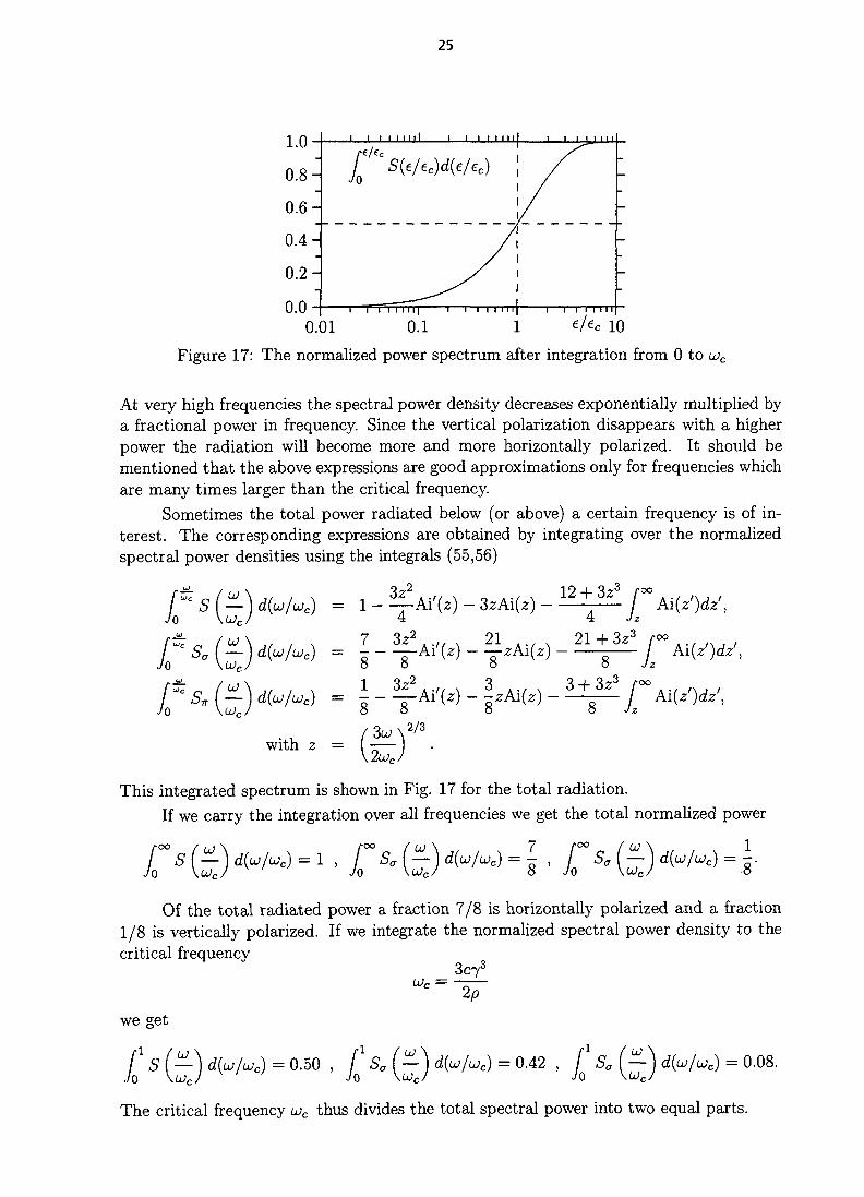
At very high frequencies the spectral power density decreases exponentially multiplied bya fractional power in frequency. Since the vertical polarization disappears with a higherpower the radiation will become more and more horizontally polarized. It should bementioned that the above expressions are good approximations only for frequencies whichare many times larger than the critical frequency.

Sometimes the total power radiated below (or above) a certain frequency is of in-terest. The corresponding expressions are obtained by integrating over the normalizedspectral power densities using the integrals (55,56)

- S (HLLOC

- 3zAi(z) -12

Ai(z')dz>,

d{u/ue) = - -7 32r2 21 . . . . 21 + 3z3 /•<*> . . . , . , ,

- TzAi(z) / Ai(z')dz',O O JzO

SJ — ) d(u/uc)o \UJCJ

/ Ai(zf)dz',Jz

wlth z = fc

8

- f*Ai(*) -

This integrated spectrum is shown in Fig. 17 for the total radiation.

If we carry the integration over all frequencies we get the total normalized power

7 r S (£) d { / ) \r s (^) d(W/Wc)=i, r sc ( - ) d(W/Wc)=7-, r So (£.

Jo \UJCJ Jo \oJc/ o Jo \OJC

Of the total radiated power a fraction 7/8 is horizontally polarized and a fraction1/8 is vertically polarized. If we integrate the normalized spectral power density to thecritical frequency

we get

2p

f1 S (-) d(u/uc) = 0.50 , f1 Sa (-) d(u/ue) = 0.42 , / ' Sa (—) d(u/uc) = 0.08.

Jo \uicj Jo \OJCJ Jo \UJCJ

The critical frequency uc thus divides the total spectral power into two equal parts.

26

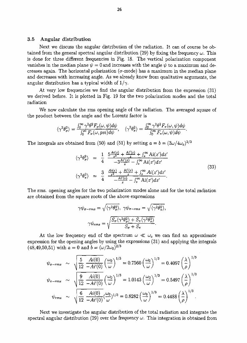
3.5 Angular distributionNext we discuss the angular distribution of the radiation. It can of course be ob-

tained from the general spectral angular distribution (29) by fixing the frequency u. Thisis done for three different frequencies in Fig. 18. The vertical polarization componentvanishes in the median plane ip — 0 and increases with the angle ip to a maximum and de-creases again. The horizontal polarization (a-mode) has a maximum in the median planeand decreases with increasing angle. As we already know from qualitative arguments, theangular distribution has a typical width of I /7.

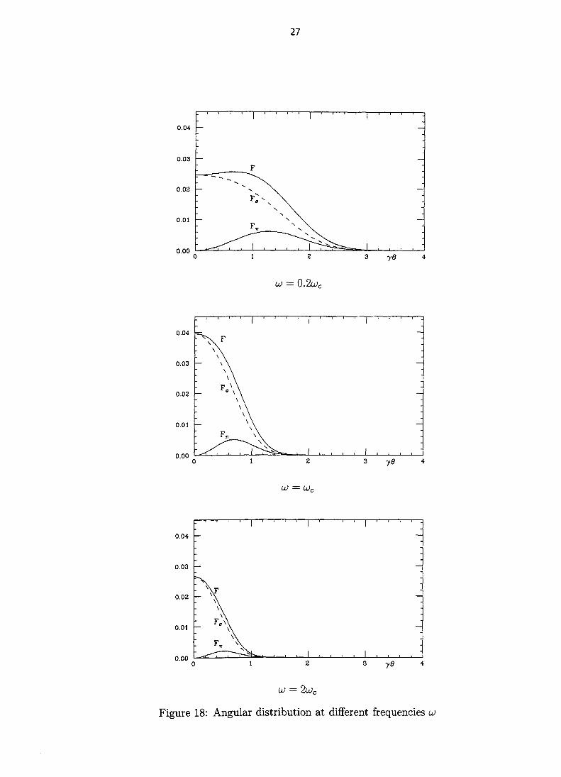
At very low frequencies we find the angular distribution from the expression (31)we derived before. It is plotted in Fig. 19 for the two polarization modes and the totalradiation

We now calculate the rms opening angle of the radiation. The averaged square ofthe product between the angle and the Lorentz factor is

2 2

[1 a)2 22 =

The integrals are obtained from (50) and (51) by setting a = b = (3u>/4u)c)2/3

2R2\ - -Y *' ~ 4

-3¥M - fz°° Ai(z')dz'(33)

- J™ Ai{z>)dz>

The rms. opening angles for the two polarization modes alone and for the total radiationare obtained from the square roots of the above expressions

= \/<72^>, lA-rms = x / W ) ,

At the low frequency end of the spectrum w < wc we can find an approximateexpression for the opening angles by using the expressions (31) and applying the integrals(48,49,50,51) with a = 0 and b = (u/2uQ)2/3

\

\

\

12 -

1/3

12 -Ai'(O)! * ) / = 1.0143

J= 0.5497 f - |

1/3

12 -Ai'(0yu>&)* = 0.8282 ( i ^

Next we investigate the angular distribution of the total radiation and integrate thespectral angular distribution (29) over the frequency u>. This integration is obtained from

27

0.04 —

0.03 —

0.02 —

0.01 —

0.003 yd

u = 0.2u;r

0.04 =i

0.03

0.03 —

0.01 —

0.003 yd

U = U>c

0.04

0.03

0.03

0.01

n nn

h ' ' ' ' 1 ' ' ' '—

—

r \

. . , , 1 , , , . .

-

-

-

= 2uc

Figure 18: Angular distribution at different frequencies

28

0.10

0.08-

0.06-

0.04-

0.02-

0.00

Figure 19: Vertical distribution of synchrotron radiation at low frequencies

(54) by calling p = 3w/4u/c and b = 1 + 7202.

dP P07

U>c 7 1 +

and

= p

The first and second terms in the square brackets correspond to the horizontal (cr-mode)and vertical (7r-mode) polarization respectively.

3.6 Photon distributionSo far we calculated and discussed synchrotron radiation as electromagnetic fields

and corresponding power distributions. We know, however, that this radiation is emittedin quanta (photons) with energy e = Two, with h = h/2n where h = 6.6262 • 10~34 Js, isPlanck's constant. If h photons of energy e are emitted per second, the power carried bythem is P = he. By introducing the critical photon energy ec = Tujcwe can relate thespectral angular power density to the spectral angular photon flux

d?P P o 7 / r , / ,x . r, ,d2hdflde/e

This gives the number of photons radiated per second and per unit solid angle into arelative photon energy band width Ae/e. Integrating this over the solid angle gives thephoton spectrum

de/e hdw eo

The form of the spectrum related to the relative band width is the same as the one of thepower spectrum shown in Fig. 16. Sometimes the spectrum related to the absolute bandwidth is more relevant

dn Po7Mr) + M i } (34)de (i)

29

0.001 -4

0.0001 .

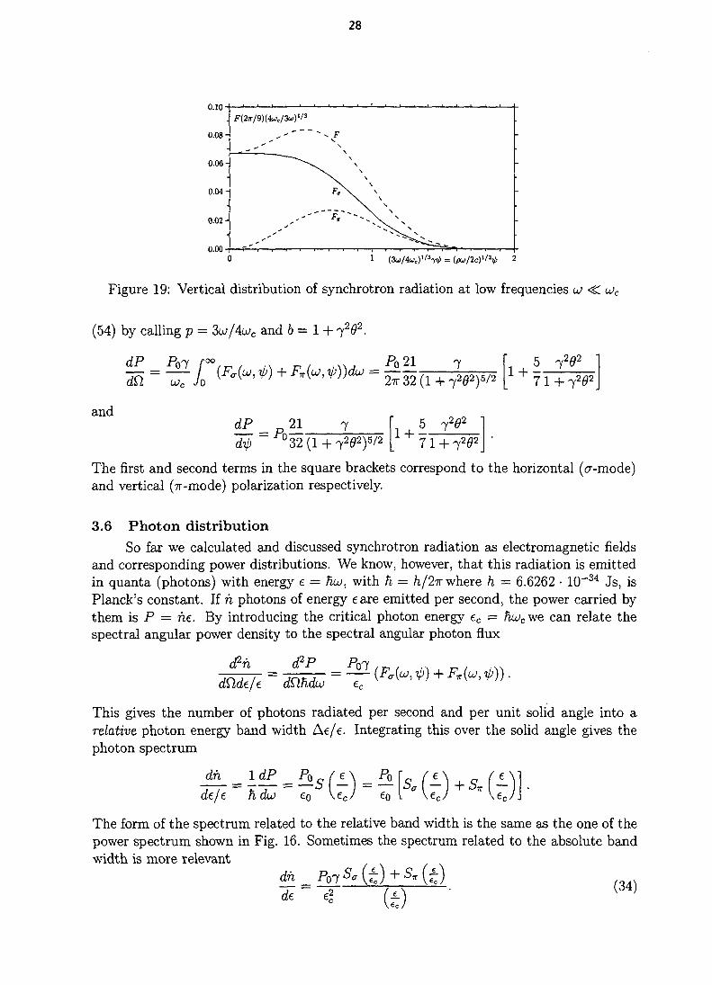
o.ooi o.oi o.i i eAc ioFigure 20: Normalized photon spectrum

The function S(e/ec)/(e/ec) which determines the absolute photon spectrum is shown inFig. 20.

By integrating (34) over all photon energies we get the number h of photons radiatedby an electron per second

- (t)(i)

d(e/ec).

Using the expressions (32) and the integrals (59,60) we get, for the total number of photonsper second, and the partition into the two polarization modes

n = 8 60 ' "" 8

From this we get the average photon energies

Po>= — =n 45

P, 773na 36

8

nn 9

(35)

For calculating the effect of quantum excitation one needs the variance < e2 > of thephoton energy. It is obtained in the same way using the integrals (61,62)

>= 276' • < 4 >= tf2

Coming back to the number of photons radiated per unit time (35) we express the powerPo and the critical energy ec by (30)

D 2rocmoc274

2p

where UQ = c/p is the revolution frequency and ay is the fine structure constant

e2 1af = 2che0 137.036

30

and obtain for the number of photons radiated per second

In one revolution a single electron radiates the following number of photons

n/rev. = -7=70/ = O.O6627.v3

4 UNDULATOR RADIATION

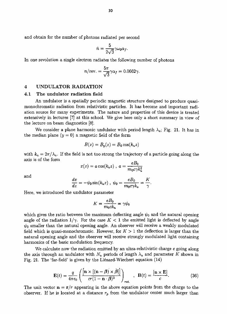
4.1 The undulator radiation fieldAn undulator is a spatially periodic magnetic structure designed to produce quasi-

monochromatic radiation from relativistic particles. It has become and important radi-ation source for many experiments. The nature and properties of this device is treatedextensively in lectures [7] at this school. We give here only a short summary in view ofthe lecture on beam diagnostics [8].

We consider a plane harmonic undulator with period length Xu; Fig. 21. It has inthe median plane (y = 0) a magnetic field of the form

B{z) = Bv{z) = Bo cos{kuz)

with ku = 2n/Xu. If the field is not too strong the trajectory of a particle going along theaxis is of the form

x(z) = acos(A;uz) , a =

andax . eB0 K

Vsm(M ^Vosm(M , ^0 r •

Here, we introduced the undulator parameter

K = eB° = 1%i)Q

TTlQCku

which gives the ratio between the maximum deflecting angle V0 and the natural openingangle of the radiation I/7. For the case K < 1 the emitted light is deflected by angleipo smaller than the natural opening angle. An observer will receive a weakly modulatedfield which is quasi-monochromatic. However, for K > 1 the deflection is larger than thenatural opening angle and the observer will receive strongly modulated light containingharmonics of the basic modulation frequency.

We calculate now the radiation emitted by an ultra-relativistic charge e going alongthe axis through an undulator with Nu periods of length Xu and parameter K shown inFig. 21. The 'far-field' is given by the Lienard-Wiechert equation (14)

( 3 6 )

ret.The unit vector n = r / r appearing in the above equation points from the charge to theobserver. If he is located at a distance rp from the undulator center much larger than

31

Figure 21: Geometry of undulator radiation

its length Lu = NUXU we can neglect the variation of r and the unit vector during thetraversal of the particle in the above vector product but not in the relation between thetwo time scales. We have for 7 » 1

n (sin6 cos(j>, sin6sin<f>, cos 6) « (6 cos 0,0sin 0,1 — 62/2).

Furthermore, we treat only the case of weak field undulator K < 1 and make the corre-sponding approximations for the particle motion

with a =

x = acos(kuz) « acos(kul3ct') — acos(Qut') , zeB0 K

ct'

and Q,u = ku(3c

or

7

J3 = ( -7

Using these expressions and the classical particle radius r$ we get for (36)

(1 - 7202cos(20),(37)

where we omit the vanishing ^-component. Finally we would like to express the field asa function of the time t of the observer instead of the time t' of emission. According toFig. 12 the two time scales are related by

Developing the expression for the distance r between particle and observer in terms of thedistance rp between the undulator center and the observer for 7 » 1, 9 <C 1 and rp » Lu

- 2rp/3ccos6 « rp (1 - ^V r

2rP

32

leads to

We get for the phase Qut' in (37)

Slyt' = kuCt' = kuC— 5—t = U}Xt.1 + ~fZ

2 7 2

With the frequency u>\ and wave number k seen by the observer

2-y2 27 2

w = n k k

we get for the observed radiation field

^ c o s ( 2 0 ) 72$* sm(2<j>))

- krp)

krp)

with> _ 3 (

rp

For a fixed distance rp to the observer it is convenient define a time tp which does notcontain the uninteresting phase factor urp/c

r 1 + 7202

tp = t = ———t' giving ujtp = kuct'. (38)c 27^ '

The radiation emitted by the undulator represents a wave with a frequency ux which is onthe axis 272 times larger than the frequency Qu = kuc of the particle motion. It decreaseswith larger observation angle 8. Since the two field components Ex and Ey are in phasethe radiation is linearly polarized in a direction which depends on the coordinates 8 and<fi of the observer.

The spectrum of the emitted radiation is obtained from the Fourier transform of thefield

Ff,A = _ L /\Z2TV J

The limits of the integral corresponds to the emission times t' — —Lu/2fic and t' = Lu/2(3cwhen the particle enters or exits the undulator

/ 2 ^ ( t ) cos(utp)dtr

E7r I (wi -u)

Next we assume that the undulator has many periods Nu > 1. In this case the first termin the bracket of the above equation has a maximum at u> = u>i while the second term ismuch smaller and can be neglected

, 4r0cg07 [1 1O cos(20), 72^2 sin(2fl] TTNU sin

33

4.2 The angular spectral power density of undulator radiationThe angular spectral energy distribution of undulator radiation is obtained from the

general treatment carried out earlier (26)

dW 2rl\E{u)\2

dQdui

With the expression (39) for E(u) we get

d2Wu _ 2r0e2c2B2NuXu^ [(1 + 7

2fl2cos(27r))2

%m0c2

^

Using the length of the undulator Lu = NUXU and integrating over the frequency u>and solid angle gives the total radiated energy

_ 2rQe2c2{B2)Lul2 2r0e

2c2 2

3m0c2 3(m0c2)3

where (B2) = BQ/2 the variance of the field. The average power emitted during thepassage through the undulator is related to this energy by Pu = Wuc/Lu which can beused to convert the above expression into a angular spectral power distribution. We seethat from (11) that for the same (B2) the radiated power is the same for the undulatoras for a long magnet.

We can now express the spectral angular power distribution of a weak undulator ina more convenient form

fN(Au).

The two functions F w and Fua give the contributions of the two polarization modes

3( l -7 2 0 2 cos (20) ) 2 3(72fl2sin(20))2

*UM) = Ft(ed>) = -( 1 + 7 ^ 2 ) 5 > u<t>(,d)

The function f^(Au) gives the spectral distribution at a given angle 6 which depends onthe number Nu of undulator periods

with 1

This function is normalized and approaches the Dirac delta function for a large numberNu of periods

/ fN(Au>)duj = 1 , JN{AU) -> 6(Au) for Nu -> oo.

34

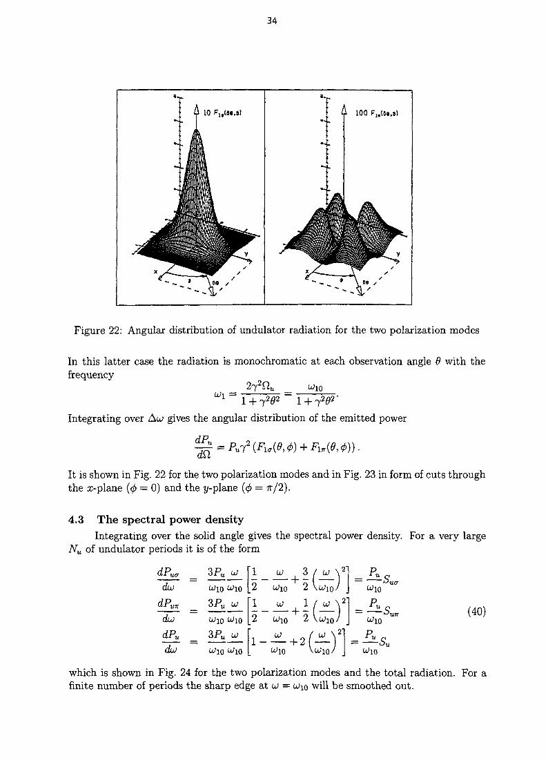
Figure 22: Angular distribution of undulator radiation for the two polarization modes

In this latter case the radiation is monochromatic at each observation angle 8 with thefrequency

Integrating over Ato gives the angular distribution of the emitted power

^ = Prf(Flt,(O,<t>) + F1JtdQ

It is shown in Fig. 22 for the two polarization modes and in Fig. 23 in form of cuts throughthe x-plane (<f> = 0) and the y-plane (<fi = TT/2).

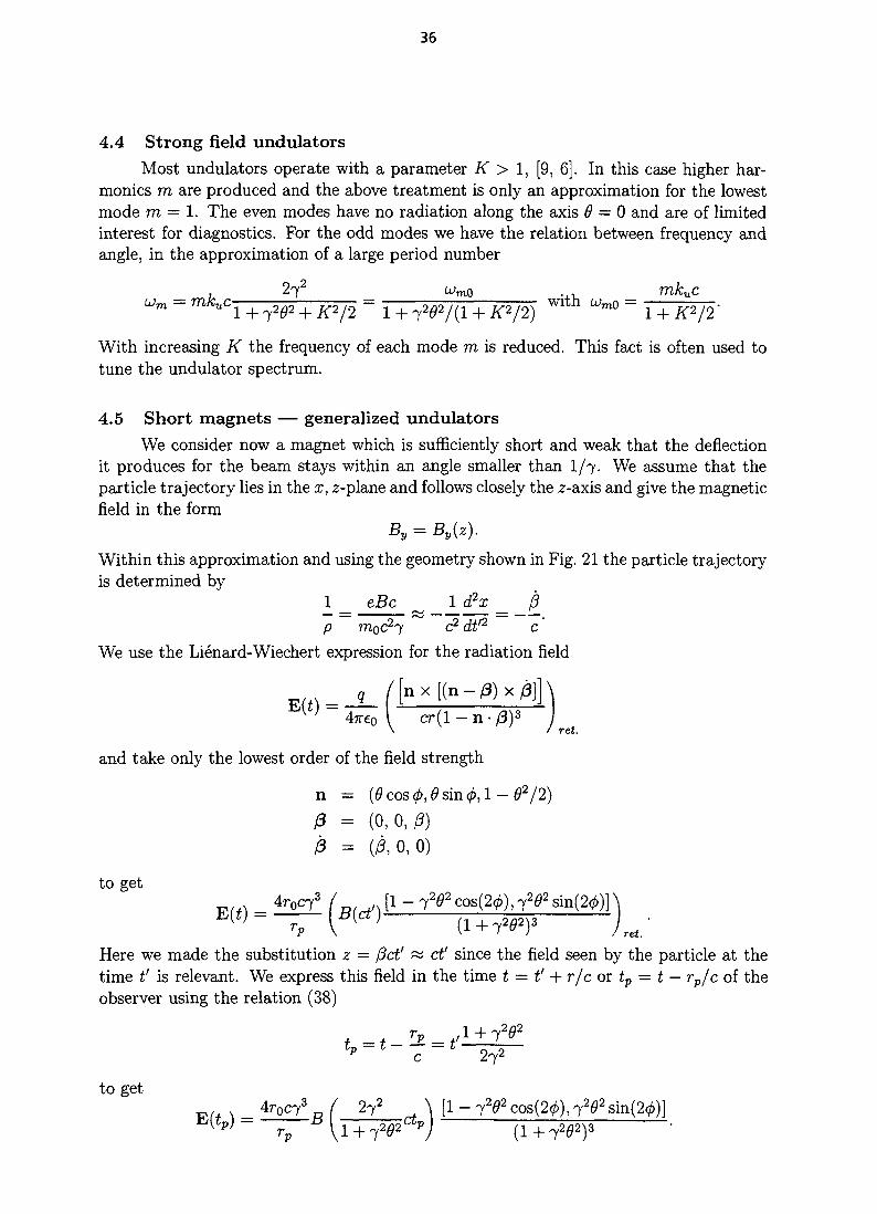
4.3 The spectral power densityIntegrating over the solid angle gives the spectral power density. For a very large

Nu of undulator periods it is of the form

du>

3PU u

3PU u

du

1 _ U_ 3 / U N 2 '

2 ~ cu10 2

2 \UIQ(40)

which is shown in Fig. 24 for the two polarization modes and the total radiation. For afinite number of periods the sharp edge at u> = U)\Q will be smoothed out.

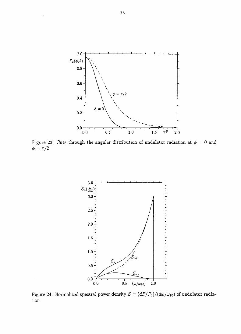
35

0.00.0 0.5 1.0 1.5 7^ 2.0

Figure 23: Cuts through the angular distribution of undulator radiation at <p = 0 and

3.5

I I 1 1 1 1 1 I T *

0.0 0.5 (w/wio) 1-0

Figure 24: Normalized spectral power density S = (dP'/'PQ)/\du/tion

of undulator radia-

36

4.4 Strong field undulatorsMost undulators operate with a parameter K > 1, [9, 6]. In this case higher har-

monics m are produced and the above treatment is only an approximation for the lowestmode m = 1. The even modes have no radiation along the axis 6 = 0 and are of limitedinterest for diagnostics. For the odd modes we have the relation between frequency andangle, in the approximation of a large period number

_ u ^ 7 2 _ k>mo .,, _ mkuc

With increasing K the frequency of each mode m is reduced. This fact is often used totune the undulator spectrum.

4.5 Short magnets — generalized undulatorsWe consider now a magnet which is sufficiently short and weak that the deflection

it produces for the beam stays within an angle smaller than 1/7. We assume that theparticle trajectory lies in the x, z-plane and follows closely the ^-axis and give the magneticfield in the form

By = By(z).

Within this approximation and using the geometry shown in Fig. 21 the particle trajectoryis determined by

1 eBc 1 d2x $p moc27 c2 dt'2 c

We use the Lienard-Wiechert expression for the radiation field

_v ; 47re0 \ cr(l - n ()

\ / ret.

and take only the lowest order of the field strength

n = (0cos0,0sin0, l -0 2 / 2 )(3 = (0,0,0)/3 = 0,0,0)

to get4rocri

Here we made the substitution z = Pet' « ct' since the field seen by the particle at thetime t' is relevant. We express this field in the time t = t' + r/c or tp = t — rp/c of theobserver using the relation (38)

to get

37

We get this field in frequency domain [10]

rp

Y2 \

Using the substitutions

leads to ivtp = ksmz and to

~ 2ro7 [1 -

This expression contains the spacial Fourier transform of the magnetic field

B(ksm) =

The radiation observed at frequency u> and angle 9 is determined by the Fourier componentB(ksm) of the magnetic field. We get now for the radiation in frequency domain

2ro7 [1 — 7202cos(2</>),-, „ ^^x^^Ji•z B

rp

It is interesting to consider the inverse Fourier transform of the field B{z)

By(z) = - L [°° By(ksm)eik-Zdksm

which represents a decomposition of the By(z) into infinitely long undulator fields of wavenumbers n n

2n l + 7 ^ 2

^ - A ^ " 2c72 W" ( 4 2 )

The above expression for E M is nothing else than the undulator radiation of each suchcomponent.

The angular spectral energy distribution is obtained from the relation

dW2 £

giving

d2W 2r0ce2(m0c27)2 [(1 - 7202 cos(2(^))2 + (7202 sin(2</»))s

7r(moC2)3 (1 -

This expression gives the radiation from a general magnet provided that the deflection isweak and nowhere exceeds an angle of I/7.

38

4.6 An undulator emitting radiation with a Gaussian angular distributionWe saw before that an undulator with an abrupt termination of the magnetic field

at ±Lu/2 is unphysical and leads to some problems when calculating the variance of theopening angle and of the Fraunhofer diffraction. We investigate now an undulator whichis modulated by a Lorentz distribution [11] having a magnetic field B(z) and

_,, , „ cos(kuz) Knmncku cos(kuz)U\z) - -DOT-—

e l + (z/z0)2'

We assume that this undulator has many periods Nu within its characteristic length 2z0

such that kuzo = nNu » 1. The total energy radiated by an electron is

_ 2r0e2c2(m0c27)2 j°° ()2 _ 2r0e2c2(m0c2

7)2 KZ0B , 2fcu ~ 3(m0c2)3 . / - o « r ( * J d * ~ 3(m0c2)3 4 ^ i + e [

6m0c2

with K = eBo/(mocku). We treat this undulator as a short magnet and apply theformalism developed in section 4.5. We filter out the frequency component u>io from theradiation

which is given by the spacial Fourier component at (42)

The Fourier transform of the magnetic field at this wave number is

B = ^

Using (41) we get for the radiation field

cos(2<j>),

7PV2lrromoc

2iKokuZQ

rpec

where have used 72^2 <C 1 for Nu » 1 and are left with the horizontal polarization modeonly. From this field and the relation (26) we obtain emitted angular spectral energydistribution

"dUCUjJ IT

The radiation from this Lorentz modulated undulator, filtered at CJIO, has a Gaussianangular distribution with rms values for the polar angle 6 and the two Cartesian anglesx' and y'

6rms = > >

39

0.4

0.3

0.2

0.1

n f\

. i i i i

—

AAi(x)

— \ /

/— /

-/

—

/ Ai(x) dx :

^ —

—

0 1 2 3 x 4

Figure 25: The Airy function Ai(z), its derivative Ai'(x) and its integral JQ Ai(x')dx'

References

[I] A.A. Sokolov ,I.M. Ternov, "Synchr. Radiation", Pergamon Press, 1966.

[2] W. Weizel, "Lehrbuch der Theoretischen Physik", Springer 1963.

[3] J.D. Jackson, "Classical Electrodynamics", Wiley 1962.

[4] M. Sands, "The Physics of Electron Storage Rings", SLAC 121 (1970).

[5] M. Schwartz, "Principles of Electrodynamics", McGraw Hill 1972.

[6] A. Hofmann, "Theory of Synchr. Rad.", SLAC, SSRL ACD-NOTE 38 (1986).

[7] R. Walker; "Insertion Devices: Undulators and Wigglers", lectures at this school.

[8] A. Hofmann; "Diagnostics with Synchrotron Radiation", lectures at this school.

[9] D.F. Alferov, Yu.A. Bashmakov, E.G. Besonov; "Synchrotron Radiation", edited N.G.Basov, New York Consultants Bureau 1976.

[10] R. Coisson; "On Synchrotron Radiation in Non-Uniform Magnetic Fields", OpticsCommunications 22 (1977) p. 135.

[II] A. Hofmann; "Diagnostics with Undulator Radiation having a Gaussian AngularDistribution", edited S. Machida and K. Hirata, KEK Proceedings 95-7 (1995) p. 231.

[12] M. Abramowitz, LA. Stegun, "Handbook of Mathematical Functions", Dover 1970.

[13] I.S. Gradshteyn, I.M. Ryzhik, "Table of integrals series and products", AcademicPress 1980, p. 420.

40

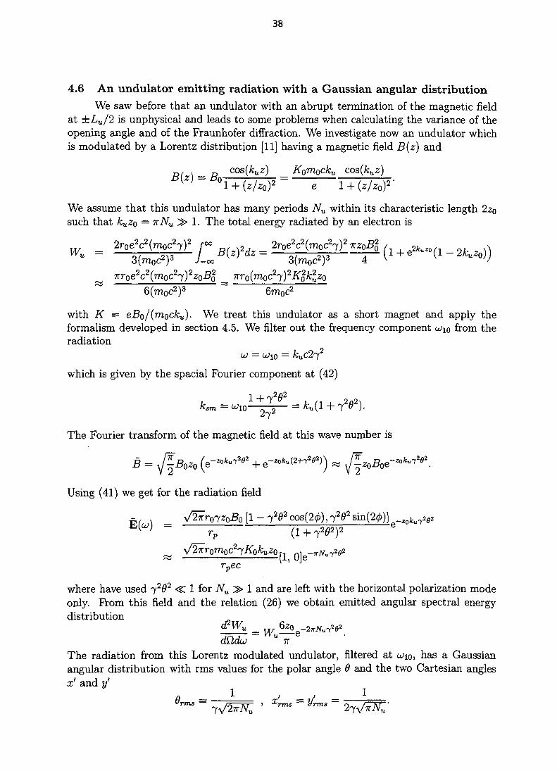
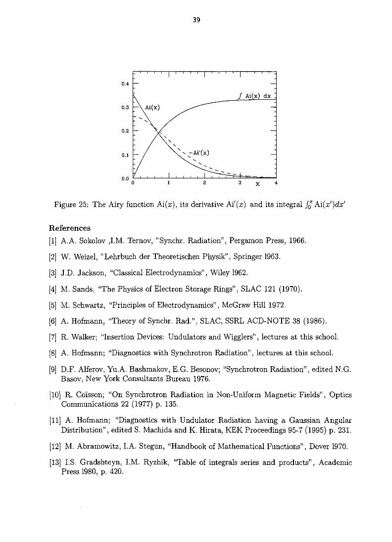
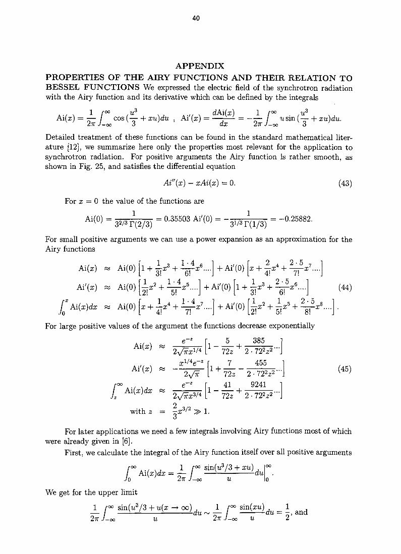
APPENDIXPROPERTIES OF THE AIRY FUNCTIONS A N D THEIR RELATION TOBESSEL FUNCTIONS We expressed the electric field of the synchrotron radiationwith the Airy function and its derivative which can be denned by the integrals

. . , , 1 [°° ,uz dkiix) 1 r°° . .uz

k\(x) = — / cos (— + xu)du , Ai (x) = — — ^ = - — / usin (-— + xu)du.Z7T J-oo 6 aX Z7T J-oo 3

Detailed treatment of these functions can be found in the standard mathematical liter-ature [12], we summarize here only the properties most relevant for the application tosynchrotron radiation. For positive arguments the Airy function is rather smooth, asshown in Fig. 25, and satisfies the differential equation

Ai"{x) - xAi(x) = 0. (43)

For x = 0 the value of the functions are

Ai(0) = ¥»Tm - °'35503 Ai'(0) = WFor small positive arguments we can use a power expansion as an approximation for theAiry functions

Ai(x) « Ai(O) [l + ^ x 3 + i—-x6....j + Ai'(O) fa; + —x4 + —-x7....]

Ai'(x) « Ai(O) f—x2 + —x 5 . . . . ] + Ai'(O) [l + — xz + —-x6....l (44)

/ A i(rr-\rlf ~ A \((W \ V J T-4 J_ ~ 7 I A iVfl^ 'T2 -1- ^ -X- <r^

/ Al^XjaX ~ AlÛJ X t .X -t- I , . . . t A l ^ U J L .X -f _.X -1- X .... .•/O L "*: i! J LZ1 0! o! J

For large positive values of the argument the functions decrease exponentially

e~z N 5 38572z 2

7 455

roo

I Ai(x)cfaJz

e~z r. 41 _9241

2with z = - x 3 / 2 » 1.

For later applications we need a few integrals involving Airy functions most of whichwere already given in [6].

First, we calculate the integral of the Airy function itself over all positive arguments

sin(w3/3 + xu)All

o

We get for the upper limit

/ > 0 OA . / v , 1 f°° sin(tt3/3 + xu)

/ Ai(x)dx = — / —-— -duJo 2-n J-oo u

oo

1 f°° sin(u3/3 + u(x -»• oo) , 1 f°° sm(xu) 1— / —^—* i >-du ~ — / —-—'-du = - , and2-KJ-OO U 2ft J-OO U 2

41

Bin(tia/3) _ 1 1 / » sin(tts/3) 3 _ 1u ~ 2^3 7-00 u»/3 ( 7 } " 6

for the lower limit which gives/•oo 1

/ Ai(x)dx = - . (46)Jo 3

For the spectral power density we need some integrals of the square of the Airyfunctions with the argument x = a + by2. Using

2 roo /-oo ^3 ^3Ai (x) = —T / / cos(— + xt) cos(— + xs)dsdt

Ait* J-oo J-oo o 3

and substituting s + t — u and s — t = v gives

A •>, x i f°° f°° r /W3 w 2 , ,u3 w2 s i , ,^ z \x> = TS~2 / / \cos(—+ —- + xu) + cos{— + —+ xv)\dudv.lbiT* J-ac J-ool 12 4 1/ 4 J

The expression under the integral is symmetric in u and v, furthermore both terms inthe square bracket give the same value after integration

1 f00 f°° U UV

Ai {x) = TT^ / COS(T77 +2TTZ JO JO Iz

4

We replace now a; = a + by2 and integrate over y

2 roo /-oo /•oo ^ 3

/ / / (roo 2 roo /-oo /•oo ^ 3 ^2

/ Ai2(a + by2)dy = —^ / / / cos(— + u(a + — + by2))dudvdy.Jo Air Jo Jo Jo lz 4

Substituting v = 2rcos <f),y = ^^^^.dvdy = 2rdffi and integrating over 0 from 0 toTT/2 gives

f°° o 1 Z"00 /"°° ix^/ A i ( a + 6 y ) d y = 7=/ / cos(— + u(a + r2))rdrdu.

Jo 2ity/b Jo Jo 12

Making a further substitution r2 = w and u = 22^3u' gives

/ Ai2(a + by2)dy = T \ \ cos(^- + u'22/3(a + w))du'dw,Jo inyb Jo Jo o

roo 9^/3 roo/ Ai2(a + by2)dy = —= \ M{22'z{a + w))dw.Jo 4v b Jo

Calling 22/3(a + w) = z' and 22/3a = z leads to the final form of our integral

f Ai> + 6 ^ = j ^ j f Ai(2')^' = [ I - ^ A I M ^ ] , (47)

where the integral (46) over the Airy function has been used. Using the same method asabove and applying (43) we can calculate the integral

f(48)

42

Differentiating (47) twice with respect to a and using (43) gives

[Ai'\a + by2) + (a + btf)A?{a + by2)} = --Jj

which can be combined with (47) and (48) to give the integral

f Ai'2(°+** - ITS h 3 ^ - 1 + f A i ( 2 'H • (49)

Using the same method as for the derivation of (48) we get two integrals that wewill use for the calculation of the rms. opening angle of the radiation

Differentiating (47) once with respect to a and once with respect to b gives

^°° y2 [Ai!\a + by2) + (a + by2)Ai2(a + by2)} dy = _ L _ A i ( * )

combining this with (48) and (50) leads to

/; ^ < « + * » ) * - [ ^ + ^ + f ]Setting a = 0 in (47) gives

The integral appearing on the right hand side can easily be obtained from

f°° 1/ = / Ai(gx)dx - —

Jo og

by differentiating it twice with respect to g

d2l f°° f°° 2•j-z = / x2Ai"(gx)dx = / gx3Ai(gx)dx = —,ag* Jo Jo og

setting g = 1 gives

Differentiating this twice with respect to b leads to the expression

y* [Af(by2) + by2ki2{by2)} dy = j ^ . (52)

We need one more integral which is derived the same way as (47)

43

Combining this with (52) gives

Substituting y3 = p in the last two integrals gives

(54)

For the integrated power spectrum we need the expression which can be obtainedby integration in parts

and

* zA\\z)dz = zAi(z)\z0 - f" Ai(z)dz = zAi{z) - f" Ai(z)dz

Jo Jo

/ z2 / Ai{z')dz'dz = ^- / Ai{z)dz + / ^rAiJO Jz 6 Jz Jo o

= Z- M(z)d6 Jz

(55)

1 IZ

U z2Ai"(z)dzo Jo

-

z2 A\(z')dz'dz=Z-\Jo Jz 6 Jz

For integrating over the photon spectrum we need

f°° Ai'(z) , roo /-oo [ (

Jo yjZ JO JO

U Ai(z)dz\. (56)I Jo J

Jz Jo Jo Jz

1 fOO /*OO y \ C O S l XJbZ

= — / du dz wsin(w3/3) —7=-^7T Jo Jo [ V ' Jz

The integral over z can be found in reference [13]

ucos (M M

rJo Jz 0 Jz V 2u

(57)

x 'which gives

f°° 0-dz = —i= f°° \jusin (V/3) + wcos (u3/Z)} du.Jo Jz J2n Jo L v ' / \ ' /}

With the substitution u3 = 3v this can be brought into the form (58)

r°° Ai'(z) __ 1 r°°o Jz JEn Jo

sm v cos vJv Jv _

dv = ~ . (59)

The following integral appears also when integrating over the photon spectrum and canbe integrated in parts as (56) and brought to the form (59)

/ • oo roo 1(60)

44

Using the same method we can derive the two integrals needed for the variance ofthe photon energy

/„ jand

The Airy functions are closely related to the modified Bessel functions of the secondkind K\j% and K2/3

1 Ix 2xz/2 1 x 2xAi(x) = t^KÊ—) and Ai'(x) = - ± ^ 2 / 3 ( ^ - ) . (63)

Which of the functions are used to express the properties of ordinary synchrotron radiationis only a matter of preference. We use here the Airy functions for derivations but give theimportant results also in Bessel functions. The functions Ai(rc), Ai'(x) and f£ Ai(x')dx'are tabulated in [12].

45

INTRODUCTION TO DYNAMICS OF ELECTRONS IN RINGS INTHE PRESENCE OF RADIATION

L.Z. RivkinPaul Scherrer Institute, Villigen, Switzerland

AbstractIntroduction to some basic ideas behind the workings of the present dayelectron storage rings with the emphasis on how the radiation processshapes the equilibrium properties of the electron beam.

1 . INTRODUCTIONIn the course of the past fifty years close to a hundred storage rings have been built

around the world, first as instruments for the study of high energy particle physics, and, lately,in ever increasing numbers, as sources of synchrotron radiation. These devices are designed tostore high current beams of electrons for periods of time (beam lifetime) that are typically greaterthan 10 hours. The electrons are ultrarelativistic, travelling with velocities very close to thespeed of light, their trajectories bent into a closed path, thus covering in 10 hours the distance ofthe order of the diameter of the solar system.

Magnetic fields are used for bending the trajectories of the particles, as well as forfocusing them to stay close to the ideal orbit. These linear magnetic fields, produced in dipoleand quadrupole magnets determine the single particle behaviour in the storage ring in linearapproximation. In general, particles execute transverse betatron oscillations around the idealorbit.

The electron beam contains particles with energies that differ from the design ring energy.These off-momentum particles have a new ideal orbit that depends on the momentum deviationand is described by the dispersion function. They execute betatron oscillations around this newmomentum-dependent closed orbit.

The first order optics exhibits severe chromatic aberrations (chromaticity). Non-linearfields are introduced via sextupole magnets to correct the chromaticity. The present generationof the synchrotron light sources uses very strong focusing lattices, and these non-linear fieldslead to limitations on the size of the stable region around the ideal orbit, or limited dynamicaperture.

The dynamics of electrons in rings [1] is furthermore determined by the process ofradiation. Steady loss of energy to synchrotron radiation and its replacement in the RF cavitiesresults in synchrotron oscillations, where the particle energy oscillates around the design ringenergy.

Moreover, this process leads to the damping of both betatron and synchrotron oscillationamplitudes. On the other hand, particle oscillations are excited due to the quantum nature ofemitted radiation (quantum fluctuations). The balance between these two competing processesresults in equilibrium beam distributions, with corresponding equilibrium beam sizes(equilibrium emittances).

2 . RADIATION EFFECTS IN ELECTRON STORAGE RINGSThe most important features can be summarised as follows:

• Electrons steadily lose energy to synchrotron radiation, a small portion of the electronenergy each turn. Moreover, to a good approximation, the loss occurs along a tangent tothe electron trajectory, resulting in a reduction of both transverse and longitudinalcomponents of the momentum.

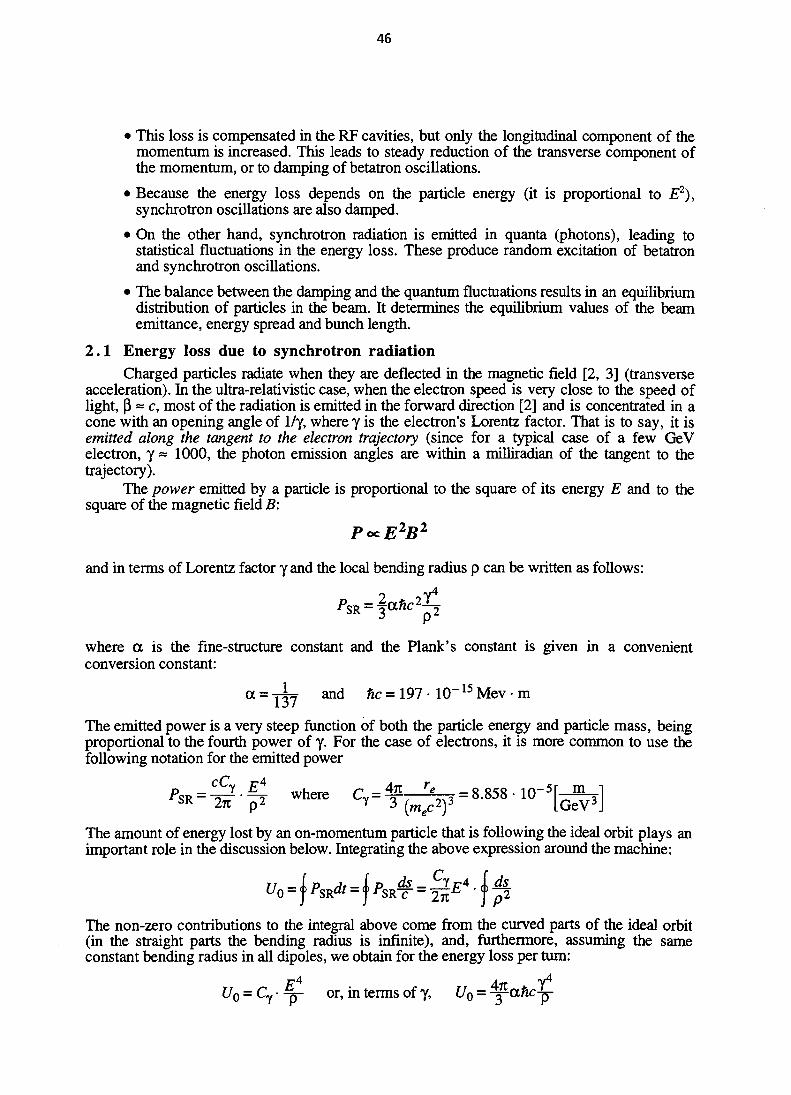
46

• This loss is compensated in the RF cavities, but only the longitudinal component of themomentum is increased. This leads to steady reduction of the transverse component ofthe momentum, or to damping of betatron oscillations.

• Because the energy loss depends on the particle energy (it is proportional to E2),synchrotron oscillations are also damped.

• On the other hand, synchrotron radiation is emitted in quanta (photons), leading tostatistical fluctuations in the energy loss. These produce random excitation of betatronand synchrotron oscillations.

• The balance between the damping and the quantum fluctuations results in an equilibriumdistribution of particles in the beam. It determines the equilibrium values of the beamemittance, energy spread and bunch length.

2.1 Energy loss due to synchrotron radiationCharged particles radiate when they are deflected in the magnetic field [2, 3] (transverse

acceleration). In the ultra-relativistic case, when the electron speed is very close to the speed oflight, P = c, most of the radiation is emitted in the forward direction [2] and is concentrated in acone with an opening angle of 1/y, where y is the electron's Lorentz factor. That is to say, it isemitted along the tangent to the electron trajectory (since for a typical case of a few GeVelectron, y ~ 1000, the photon emission angles are within a milliradian of the tangent to thetrajectory).

The power emitted by a particle is proportional to the square of its energy E and to thesquare of the magnetic field B:

PocE2B2

and in terms of Lorentz factor y and the local bending radius p can be written as follows:

where a is the fine-structure constant and the Plank's constant is given in a convenientconversion constant:

and hc = 197 • 10"15Mev • m

The emitted power is a very steep function of both the particle energy and particle mass, beingproportional to the fourth power of y. For the case of electrons, it is more common to use thefollowing notation for the emitted power

cCy £4 , r _4n re _ <? oco 1 0-5r mP S R - 2 * r - ^ W h e r e C T - 3 K 2 ) 3 - 8 - 8 5 8 1 0 [

The amount of energy lost by an on-momentum particle that is following the ideal orbit plays animportant role in the discussion below. Integrating the above expression around the machine:

The non-zero contributions to the integral above come from the curved parts of the ideal orbit(in the straight parts the bending radius is infinite), and, furthermore, assuming the sameconstant bending radius in all dipoles, we obtain for the energy loss per turn:

E or, in terms of y, U0 = ^ ^

47

3 . SYNCHROTRON OSCILLATIONS

3.1 Phase stabilityThe radiation losses are compensated in accelerating cavities that utilise time-dependent

radio frequency fields, the RF system. The frequency is chosen so that it is an integer multipleof the revolution frequency. This integer is called a harmonic number, h

In other words, the length of the design orbit is an integer number of the RF wavelengths,and a particle that follows the design orbit remains phase locked with respect to the RF.

A so-called synchronous particle gains each turn just the right amount of energy from theRF cavities

URF = eVRF=U0

and will therefore be able to maintain the design energy. There are two phases with opposite RFvoltage slopes for which the conditions above are satisfied. Only one of them provides stableequilibrium against small deviations in phase or arrival time at the cavity.

Let us consider what happens to a particle that arrives at the RF ahead of the synchronousone. For the case illustrated in the sketch below (where the horizontal axis represents time delayx with respect to the synchronous particle)

VRF

U,

• it will gain too much energy from the RF• because its energy will be greater than the design energy, the magnetic field will not be

strong enough to keep it on the design orbit, its trajectory will have greater average radius ofcurvature, thus requiring more time to complete the next turn

• it will come back to the RF cavity closer in time to the synchronous particle

Similarly, for a particle that arrives behind the synchronous one• it will gain too little energy from the RF• because its energy will be smaller than the design energy, the magnetic field will be too

strong to keep it on the design orbit, its trajectory will have smaller average radius ofcurvature, thus requiring less time to complete the next turn

• it will come back to the RF cavity catching up with the synchronous particle

Particles with small deviations in phase are attracted towards the synchronous particle.Exactly the opposite happens around the phase with the opposite slope of the RF voltage. Thepoints of stable phase thus provide h equidistant places around the machine circumference,separated by the RF wavelength, where bunches of electrons can be stored.

3.2 The time it takes to go around — momentum compaction factorThe time it takes a particle to go around the ring once obviously depends on the orbit

length L and on the particle velocity. An off-energy particle will have different velocity and willfollow an orbit of different length.

48

T-L nr A T - A L Av^ - y VI T ~ L V

High energy electrons travel with speed very close to the speed of light, their velocity changesvery little with energy. From relativity you may recall that

d\ _ 1 dE _. Av__l_ s

where 8 is the relative energy deviation with respect to the design energy. In fact, the orbitlength change in most cases turns out to be greater than the velocity change. A funny thinghappens to a relativistic electron on the way around the ring: in spite of higher energy (andhigher speed) it takes longer to go around.

Let us now look at the change in orbit length with the particle's energy. As was alreadymentioned before, the length of a small portion of the trajectory that lies in the horizontal plane:

depends on the horizontal deviation. This deviation can be written in two parts, the betatronoscillation and the energy dependent deviation. To first order the betatron oscillation does notchange the orbit length, since its average displacement from the design orbit is zero. On theother hand, the energy dependent displacement generally has the same sign all around the ring.As a result, the orbit length of a particle with a relative energy deviation 8 is

and, recalling the definition of the dispersion function, we can write the change in orbit lengthfor an off-momentum particle as

AL = 8 • i —rrds

The relative change in length of the off-momentum orbit is proportional to the energy deviation.The constant of proportionality is called the momentum compaction factor a, a constant thatonly depends on the properties of the magnetic guide field and is independent of energy:

a = 44L]4^ = a • 8 where a = 44 —riL L] p(s)

Coming back to the expression for the change in revolution time with particle energy, we canre-write it in the following way:

AT _ AL Av _ ( M 8

The term in parenthesis is called phase-slip factor, describing the change in particle arrival timeat the RF cavities. For a certain design ring energy, so-called transition energy, this factor canbecome zero, corresponding to the isochronous mode of operation: all particles take the sametime to complete one turn, independent of their energy. Writing the momentum compactionfactor in terms of transition energy, the phase-slip factor is:

•n = (\ - -V) where a = \Vttr I ) hr

All the high energy electron storage rings operate above transition energy, i.e. y » yti . Thisregime, above transition, corresponds to the situation already mentioned above: higher energyelectrons take longer time to complete one turn.

49

3.3 Damping of synchrotron or energy — time oscillationsThe radiation loss and its compensation by the RF system, coupled with the dependence

of the revolution time on particle energy deviation cause particles to execute energy-timeoscillations, or so-called synchrotron oscillations. Let us now write down what happens to aparticle in one turn:

• energy gain from the RF system:the synchronous particle gains exactly Uo ; a particle that arrives at the RF cavities with a timedelay x with respect to the synchronous one, receives the amount of energy that is proportionalto the slope of the RF voltage (we consider here only small time delays, assuming that we areworking in the linear part of the RF voltage waveform)

URF = eVRF(T) = U0 + eVRF-% where VRF

• energy loss:every turn the particle loses on the average Uo; but recall that the radiation loss depends on theparticle energy (proportional to the energy squared), so depending on the energy deviation e,

^rod ~ Uo + U' • E where U';

Let us delay for the moment the evaluation of the radiation loss derivative with energy. For nowwe will simply treat it as a constant in our derivation of the equation of motion for synchrotronoscillations.

• energy balance:we can now write down the amount by which the particle energy changes during one turn

Ae = {U0 + eVRF-x)-{U0+U'-e)

and since this change occurs during a time interval equal to the revolution period To, we canturn this difference equation into a differential equation describing the time evolution of theparticle energy:

• time lag with respect to the synchronous particle:similarly, from the above discussion on the momentum compaction factor, we can write downthe differential equation for the other variable, describing the change with time in the particle'sphase lag with respect to the RF. For a given particle energy deviation e,

dx _ n . s _ n £dt Eo

• synchrotron oscillations:combining the two differential equations above, we can eliminate one of the variables obtaininga second-order differential equation for the evolution of the energy deviation in time:

a harmonic oscillator equation describing synchrotron oscillations with the frequency

In fact, it is a damped harmonic oscillator, with a velocity-like term and a damping decrement

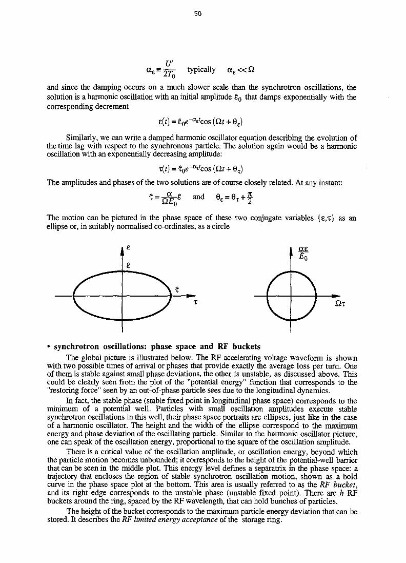
50

ae =U'

typically oce « i

and since the damping occurs on a much slower scale than the synchrotron oscillations, thesolution is a harmonic oscillation with an initial amplitude £0 that damps exponentially with thecorresponding decrement

e(f) = e0e-^fcos {at + 6e)

Similarly, we can write a damped harmonic oscillator equation describing the evolution ofthe time lag with respect to the synchronous particle. The solution again would be a harmonicoscillation with an exponentially decreasing amplitude:

The amplitudes and phases of the two solutions are of course closely related. At any instant:

The motion can be pictured in the phase space of these two conjugate variables {e,t} as anellipse or, in suitably normalised co-ordinates, as a circle

• synchrotron oscillations: phase space and RF bucketsThe global picture is illustrated below. The RF accelerating voltage waveform is shown

with two possible times of arrival or phases that provide exactly the average loss per turn. Oneof them is stable against small phase deviations, the other is unstable, as discussed above. Thiscould be clearly seen from the plot of the "potential energy" function that corresponds to the"restoring force" seen by an out-of-phase particle sees due to the longitudinal dynamics.

In fact, the stable phase (stable fixed point in longitudinal phase space) corresponds to theminimum of a potential well. Particles with small oscillation amplitudes execute stablesynchrotron oscillations in this well, their phase space portraits are ellipses, just like in the caseof a harmonic oscillator. The height and the width of the ellipse correspond to the maximumenergy and phase deviation of the oscillating particle. Similar to the harmonic oscillator picture,one can speak of the oscillation energy, proportional to the square of the oscillation amplitude.

There is a critical value of the oscillation amplitude, or oscillation energy, beyond whichthe particle motion becomes unbounded; it corresponds to the height of the potential-well barrierthat can be seen in the middle plot. This energy level defines a separatrix in the phase space: atrajectory that encloses the region of stable synchrotron oscillation motion, shown as a boldcurve in the phase space plot at the bottom. This area is usually referred to as the RF bucket,and its right edge corresponds to the unstable phase (unstable fixed point). There are h RFbuckets around the ring, spaced by the RF wavelength, that can hold bunches of particles.

The height of the bucket corresponds to the maximum particle energy deviation that can bestored. It describes the RF limited energy acceptance of the storage ring.

51

separatnx

52

• damping of synchrotron oscillations: qualitative pictureThe above phase-space portraits of synchrotron oscillations are snapshots taken over time

spans that are short compared to the damping time scale. Over a longer time period theamplitude of the oscillations, i.e. the size of the ellipse decreases exponentially and the phasespace trajectory is an inward spiral that maintains the aspect ratio of the above snapshots.

Synchrotron oscillations are damped due to the fact that the energy loss per turn is aquadratic function of the particle's energy. While in the upper half of the ellipse, the particle'senergy deviation is positive and its losses per turn are greater than the amount it receives fromthe RF system, its energy deviation tends to decrease. In the lower part of the ellipse, its energydeviation is negative and its losses per turn are smaller than the amount it receives from the RF,again leading to a decrease in the energy deviation.

4 . DAMPING OF BETATRON OSCILLATIONS

4.1 Qualitative pictureThe steady loss of energy to synchrotron radiation is compensated in the RF cavities,

where the particle receives each turn the average amount of energy lost.Average energy loss. Every turn the electron loses a small portion of its energy,

Uo ~ 10"3 of Eo, in the form of synchrotron radiation, so that after one turn, on the average, itsenergy becomes:

Since the radiation is emitted along the tangent to the trajectory, only the amplitude of itsmomentum changes.

After one turn both the transverse and longitudinal components of the momentum vector arereduced by the same fraction:

The transverse component of the momentum vector corresponds to the energy of the betatronoscillation (proportional to the square of the oscillation amplitude). Therefore, the amplitude ofthe betatron oscillation is reduced by a small amount every turn.

Eo) " - - — " \ " 2£nA? = A g U - ^ | or AÂol l -

Energy gain in the RF cavities. In the RF cavities only the longitudinal componentof the momentum is increased by the amount corresponding to the average energy loss per turn.Over many turns, the energy of the particle is maintained at the design value.

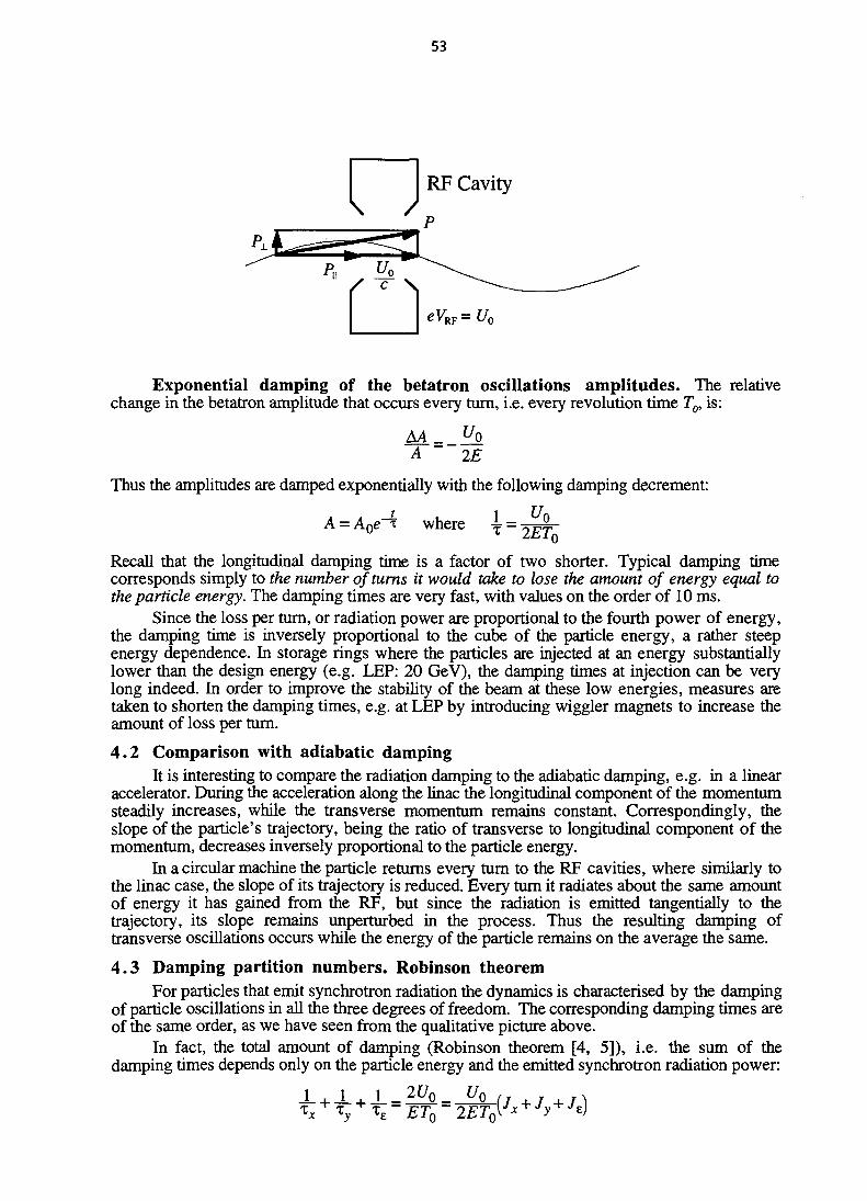
53

Exponential damping of the betatron oscillations amplitudes. The relativechange in the betatron amplitude that occurs every turn, i.e. every revolution time To, is:

M _ ôA IE

Thus the amplitudes are damped exponentially with the following damping decrement:

A = Aoe~r where \ = J*2ET0

Recall that the longitudinal damping time is a factor of two shorter. Typical damping timecorresponds simply to the number of turns it would take to lose the amount of energy equal tothe particle energy. The damping times are very fast, with values on the order of 10 ms.

Since the loss per turn, or radiation power are proportional to the fourth power of energy,the damping time is inversely proportional to the cube of the particle energy, a rather steepenergy dependence. In storage rings where the particles are injected at an energy substantiallylower than the design energy (e.g. LEP: 20 GeV), the damping times at injection can be verylong indeed. In order to improve the stability of the beam at these low energies, measures aretaken to shorten the damping times, e.g. at LEP by introducing wiggler magnets to increase theamount of loss per turn.

4.2 Comparison with adiabatic dampingIt is interesting to compare the radiation damping to the adiabatic damping, e.g. in a linear

accelerator. During the acceleration along the linac the longitudinal component of the momentumsteadily increases, while the transverse momentum remains constant. Correspondingly, theslope of the particle's trajectory, being the ratio of transverse to longitudinal component of themomentum, decreases inversely proportional to the particle energy.

In a circular machine the particle returns every turn to the RF cavities, where similarly tothe linac case, the slope of its trajectory is reduced. Every turn it radiates about the same amountof energy it has gained from the RF, but since the radiation is emitted tangentially to thetrajectory, its slope remains unperturbed in the process. Thus the resulting damping oftransverse oscillations occurs while the energy of the particle remains on the average the same.

4 .3 Damping partition numbers. Robinson theoremFor particles that emit synchrotron radiation the dynamics is characterised by the damping

of particle oscillations in all the three degrees of freedom. The corresponding damping times areof the same order, as we have seen from the qualitative picture above.

In fact, the total amount of damping (Robinson theorem [4, 5]), i.e. the sum of thedamping times depends only on the particle energy and the emitted synchrotron radiation power:

54

where we have introduced the usual notation of damping partition numbers that show how thetotal amount of damping in the system is distributed among the three degrees of freedom. So farwe have seen the case of (1,1,2) and their sum is, according to the Robinson theorem, aconstant.

5 . ADJUSTMENT OF DAMPING RATESThe partition numbers can differ from the above values, while their sum remains a

constant. In fact, under certain circumstances, the motion can become "anti-damped", i.e. thedamping time can become negative, leading to an exponential growth of the oscillationsamplitudes. In order to understand this situation we have to refine the simplified qualitativepicture presented above.

Let us recall that the energy loss is proportional to the product of energy and the magneticfield squared:

Both the magnetic field and the particle energy can take values that are different from the designones, while the particle executes transverse or longitudinal oscillations.

Let us first consider betatron oscillations. Following a betatron oscillation trajectory,a particle sees magnetic fields that differ from the design values (e.g. traversing the quadrupolemagnets off-axis, the particle sees a dipole magnetic field). Nevertheless, because the averageparticle displacement as it travels around the ring is zero, to first order in particle displacement,there is no contribution to the energy loss. There is, of course, a non-zero term that is quadraticin displacement, but in our linearised analysis it can be neglected.

The situation is quite different for the case of synchrotron oscillations. A particlewith an energy deviation follows a closed orbit that is defined by the off-energy or dispersionfunction, which typically has the same sign around the ring. The magnetic fields it sees differfrom the design ones, and there is a non-zero contribution to the energy loss that is linear inparticle displacement, that in turn is proportional to the energy deviation. In addition, because ofthe quadratic energy dependence, the energy loss also contains a term linear in energy deviation.

Evaluating the loss per turn to first order in energy deviation we recall that the synchrotronoscillations occur on a time scale that is much longer than the revolution time. The particle thenfollows a trajectory around the ring that is defined by the dispersion function, and we can write:

Urad=U0 + U'-d, where U' = = Q (2 + <D)

where we have introduced a new constant, (D — an integral of the dispersion function and themagnetic guide field functions, i.e. bending radius and gradient around the ring.

dsV2

This constant is independent of the particle energy, and only deviates substantially from zerowhen a particle encounters combined function elements, i.e. where the product of the fieldgradient and the curvature is non-zero.

The synchrotron oscillations damping time, taking into account this analysis, becomes

55

and a similar analysis of the horizontal betatron oscillations shows that the damping time in thatcase is:

Correspondingly, the damping partition numbers can be written as follows:

Jx=\-0, J£=2+<D, Jx + Je=3

For the storage rings built in one plane (horizontal) the vertical dispersion function is zero andthe vertical partition number remains unchanged.

The amount of damping can be repartitioned between the horizontal and energy-timeoscillations by altering the value of the <D constant [6]. This can be achieved by either usingcombined function magnetic elements in the lattice, or by introducing a special combinedfunction wiggler magnet (so-called Robinson wiggler). Values of horizontal partition number ashigh as 2.5 have been obtained that way. Values of <D > 1 lead to anti-damping of horizontalbetatron oscillations, while for <D < -2 the synchrotron oscillations become unstable.

6 . QUANTUM FLUCTUATIONS — EQUILIBRIUM BEAM SIZESIf the radiation damping were the whole story, in a matter of seconds the size of the

injected beam would shrink to microscopic dimensions. This would result in several problemsthat would make the construction and operation of electron storage rings utterly impractical. Itsuffices to mention the coherent synchrotron radiation production.

Typically, an ensemble of emitting electrons radiates incoherently, i.e. there is no definitephase relationship between the individual emitters. The total power is simply obtained by addingthe individual emitters' power; it is linearly proportional to the number of electrons.

In a bunch of electrons that is small compared to the wavelength of the emittedsynchrotron radiation the particles emit electromagnetic waves that are in phase, i.e. at a point ofobservation that is far away from the source the electric filed vectors add. The total radiationpower from N particles is then proportional to the square of their number! The correspondingincrease in power required from the RF system to compensate for the losses would beunreasonably high.

6 .1 Quantum nature of synchrotron radiationIn fact, the beam does not shrink to microscopic size, rather the effect of damping is

counterbalanced by a kind of heating that is connected to the quantum nature of emission ofradiation.

The synchrotron radiation is emitted as photons, the typical photon energy, correspondingto the critical frequency, being:

and the number of photons emitted per second can be roughly approximated by dividing thetotal emitted power by the typical photon energy.

S R - 4 a 1uc ~ 9 a c P

cThe photon emission is a stochastic process, and in any time interval the expected number ofphotons emitted has a statistical uncertainty:

N±/N, N

56

For example, the amount of energy loss in one turn fluctuates around the expected valueU0=N-uc, where N = N-To, the typical spread being

6.2 Equilibrium energy spread and bunch lengthOver large time intervals the RF system maintains the average particle energy at the design

value. Due to quantum fluctuations, i.e. statistical fluctuations in the number of photonsemitted, the particle energy will be different from the design value, exciting energy-timeoscillations. Eventually, the two competing processes of radiation damping and quantumfluctuations will strike a balance, resulting in a finite value of the energy spread. We can make areasonable estimate of the steady state value of the energy spread by evaluating the typicalenergy deviation during a time period equal to the damping time (a characteristic time scale forthis process):

Since the damping time is the ratio of the particle energy to the radiation power, i.e. "the time ittakes to radiate all the energy away", the expected energy spread is approximately equal to thegeometric mean of the particle energy and the typical photon energy:

The relative energy spread is then approximately written as

— ~ 7 — » Xc = 4 • 10"13m — the electron Compton wavelength.Eo v P

The bending radius in the electron storage rings scales typically as square of the design energy,thus the relative energy spread is approximately the same in all the rings, roughly equal to 10°.

A more detailed calculation gives the following result for the equilibrium relative energyspread in a storage ring:

wh,re C, = T ? - S ^ 3 = 1.468-10-'[^]

The energies of electrons in a bunch at equilibrium have a Gaussian distribution with astandard deviation equal to the above energy spread. A synchronous electron with an energydeviation equal to the above standard deviation, after a quarter of the period of synchrotronoscillation, will have zero energy deviation (see the discussion of synchrotron oscillationsabove), however it will be displaced from the synchronous particle in time by

_ a

The distribution of electrons in time along the bunch is closely related to the distribution inenergies, and for small bunch currents is also a Gaussian with an above standard deviation. Theequilibrium bunch length (expressed in time units) and its energy spread are given by the aboveexpressions.

6.3 Excitation of horizontal betatron oscillationsLet us now turn to the case of transverse oscillations, where a similar source of heating

due to statistical fluctuations in the emission rate of photons ensures that the transverse beamsize does not shrink to microscopic dimensions. We first look at a qualitative picture of howhorizontal betatron oscillations get excited in the process of emission of photons.

57

After an electron emits a photon, its energy is decreased and its new reference orbit will bedetermined by the dispersion function around the ring

xref=Db

where 8 is the relative energy deviation. Since the emission is instantaneous and occurs along atangent to the electron trajectory, neither the displacement nor the slope are affected. Moreover,because the reference orbit is shifted due to the change in energy, the electron starts to oscillatearound this new reference orbit with an amplitude

This situation is analogous to that of a pendulum at equilibrium, with its suspension pointsuddenly shifted sideways, while the pendulum itself remains at rest. After that the pendulumstarts to oscillate around its new equilibrium (see the sketch below)

The emission of photons is a random process, so we have again a random walk, now inhorizontal displacement. How far the particle will wander away from the ideal orbit is kept incheck by the radiation damping. The balance will be achieved on a time scale of a horizontaldamping time and, typically, the particle will have an equilibrium horizontal deviation of

since the horizontal damping time is a factor of two longer than the longitudinal one. Theequilibrium horizontal beam size is on the order of 1 mm, as the dispersion is typically on theorder of 1 m.

Let us take a closer look at the amplitudes of the oscillations resulting from the emissionof a photon. Horizontal displacement and slope can be written in terms of a betatron oscillationpart and an energy dependent part (proportional to the dispersion function):

X — Xa + X£ = Jtp + D • 8

Neither position nor slope can change in the process of emission of a photon (the emission isquasi-instantaneous and occurs along a tangent to the trajectory). Clearly, the energy of theparticle is reduced by the amount equal to the photon energy, i.e. the energy dependentcontribution to the displacement must change. Therefore, the betatron oscillation contribution tothe displacement must be equal and opposite to the energy contribution, as the totaldisplacement remains constant. After the photon emission particle starts a betatron oscillationaround the new closed orbit (determined by the dispersion function). The initial conditions read:

X R = - i

58

Recall the form of the betatron oscillation and the corresponding amplitude, or Courant-Snyderinvariant:

*p = asfficos <|)( s) where a2 = yxp + 2ax^x'^-¥^x'^

If, for simplicity's sake, we assume that before radiating a photon the particle was on the designtrajectory, after emitting a photon that results in a relative particle energy change of 5, theamplitude of the betatron oscillation will be:

a2 = § 2 • (yD2 + 2aDD' + pD'2) = 82 •

where we have introduced the #" function that is very similar to the Courant-Snyder invariant,with displacement and slope of the trajectory replaced by the dispersion and its slope. It is afunction of position around the ring, and its shape in the bending magnets (i.e. where theradiation occurs) determines the magnitude of the effect of quantum fluctuations on the beamsize.

6.4 Equilibrium transverse beam sizeA detailed calculation of the quantum fluctuations and damping effects yields the

following result for the equilibrium beam emittance in the electron storage ring:

"T-—x P ~where angular brackets denote an average value of Jfin the bending magnets and where

C =AL. hc^ = 1-468 -10-6[-m-

The equilibrium beam size is linearly proportional to the ring energy. In the rings where theelectrons are ramped in energy (e.g. LEP), the vacuum chamber dimensions must take this intoaccount. The shape of the ^/function in the bends is optimised to obtain the desired value of theequilibrium emittance. The dependence of the emittance on the horizontal partition number canalso be used to modify the emittance.

In almost all storage rings there is no bending of particles in the vertical plane; the designvalue of vertical dispersion is zero. Therefore, the process of photon emission would not excitevertical betatron oscillations and the vertical beam size would be very quickly damped to a verysmall value. Here we have to recall an important approximation we have made: the photons areemitted into a cone with an opening angle of 1/y, i.e. not exactly along the tangent to theparticle's trajectory. The slope of the particle trajectory will therefore be changed by a smallamount due to the recoil during the process of photon emission. This will excite a smallamplitude vertical betatron oscillation. Again we have a source of heating due to quantumfluctuations. It can be shown that due to this finite opening angle effect the equilibrium verticalbeam size is still very small [1,7].

In reality, the vertical beam size is dominated by coupling effects: motion in the horizontalplane is coupled to the vertical plane. Thus horizontal betatron oscillations excited by quantumfluctuations get coupled to vertical betatron oscillations. Misalignments (roll) in dipole andquadrupole magnets as well as vertical closed orbit offsets in sextupole magnets are the mainsources of coupling. In addition, the spurious vertical dispersion function in the dipole magnetsthat results from coupling of the horizontal dispersion in rotated quadrupoles and offsetsextupoles provides another source of heating due to quantum fluctuations.

6.5 Summary of the stored beam propertiesThe equilibrium stored beam properties, determined by the process of synchrotron

radiation, can be expressed in terms of so-called synchrotron radiation integrals [8]. These areintegrals of the guide field functions (bending radius p(s), quadrupole strength k(s))and offunctions of Twiss parameters, taken around the entire ring. They are evaluated by most of the

59

optics codes (e.g. MAD [9]). A brief summary of the main results for the case of a storage ringbuilt in one (horizontal) plane is given here. It involves five radiation integrals defined below:

Radiation integrals:

' l = (

7,=c

ds

ds

w

Momentum compaction factor:

Energy loss per turn:

Un = 4=CV4

Damping parameter:

Damping times and partition numbers:

>, JX=\-(D, Jy=\

i = ?r whereJ j

2ET0

Equilibrium energy spread:

= 1.468LGeV:

Equilibrium emittance:

60

REFERENCES

[1] M. Sands, The physics of electron storage rings. An introduction, SLAC-121 (1970)

[2] A. Hofmann, Introduction to physics of synchrotron radiation, these Proceedings

[3] K.J. Kim, Characteristics of Synchrotron Radiation, AIP Conference Proceedings 184,Volume 1, AIP New York (1989) p. 565

[4] K.W. Robinson, Phys. Rev. I l l (1958) p. 373

[5] R.P. Walker, Proc. CERN Accelerator School, Fifth General Accelerator Physics Course,CERN 94-01, p.461

[6] K. Hubner, Proc. CERN Accelerator School, General Accelerator Physics, CERN 85-19,p. 239

[7] T.O. Raubenheimer, The Generation and Acceleration of Low Emittance Flat Beams forFuture Linear Colliders, Ph.D. Thesis, Stanford, SLAC-387 (1991)

[8] R.H. Helm et. al., IEEE Trans. Nucl. Sci., NS-20 (1973), p. 900

[9] H. Grote, F. Christoph Iselin, Methodical Accelerator Design, User's Reference Manual,for most recent information look on the Web at CERN: http://www.cern.ch

BIBLIOGRAPHYIn contrast to the situation a few years ago, there is now available quite a respectable

choice of books that cover the basic physics of high energy particle accelerators. Some of themare listed below.

PJ. Bryant, K. Johnsen, Circular Accelerators and Storage Rings, Cambridge University Press(1993)

D.A. Edwards, M. J. Syphers, An introduction to the Physics of High Energy Accelerators,John Wiley & Sons, Inc.(1993)

H. Wiedemann, Particle Accelerator Physics, Basic Principles and Linear Beam Dynamics,Springer Verlag (1993)

K. Wille, Physik der Teilchenbeschleuniger und Synchrotronstrahlungsquellen, EineEinfuhrung, B. G. Teubner Stuttgart (1992)

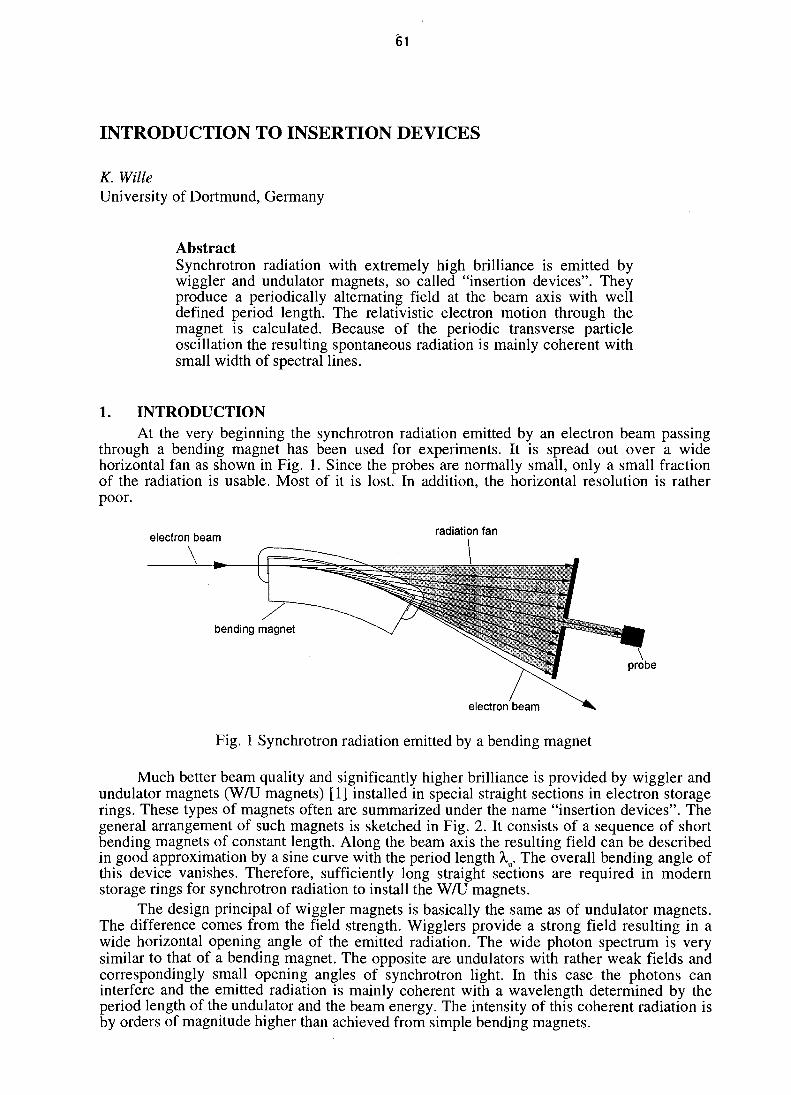
61

INTRODUCTION TO INSERTION DEVICES

K. WilleUniversity of Dortmund, Germany

AbstractSynchrotron radiation with extremely high brilliance is emitted bywiggler and undulator magnets, so called "insertion devices". Theyproduce a periodically alternating field at the beam axis with welldefined period length. The relativistic electron motion through themagnet is calculated. Because of the periodic transverse particleoscillation the resulting spontaneous radiation is mainly coherent withsmall width of spectral lines.

1. INTRODUCTIONAt the very beginning the synchrotron radiation emitted by an electron beam passing

through a bending magnet has been used for experiments. It is spread out over a widehorizontal fan as shown in Fig. 1. Since the probes are normally small, only a small fractionof the radiation is usable. Most of it is lost. In addition, the horizontal resolution is ratherpoor.

electron beam radiation fan

bending magnet

\probe

electron beam

Fig. 1 Synchrotron radiation emitted by a bending magnet

Much better beam quality and significantly higher brilliance is provided by wiggler andundulator magnets (W/U magnets) [1] installed in special straight sections in electron storagerings. These types of magnets often are summarized under the name "insertion devices". Thegeneral arrangement of such magnets is sketched in Fig. 2. It consists of a sequence of shortbending magnets of constant length. Along the beam axis the resulting field can be describedin good approximation by a sine curve with the period length X,u. The overall bending angle ofthis device vanishes. Therefore, sufficiently long straight sections are required in modernstorage rings for synchrotron radiation to install the W/U magnets.

The design principal of wiggler magnets is basically the same as of undulator magnets.The difference comes from the field strength. Wigglers provide a strong field resulting in awide horizontal opening angle of the emitted radiation. The wide photon spectrum is verysimilar to that of a bending magnet. The opposite are undulators with rather weak fields andcorrespondingly small opening angles of synchrotron light. In this case the photons caninterfere and the emitted radiation is mainly coherent with a wavelength determined by theperiod length of the undulator and the beam energy. The intensity of this coherent radiation isby orders of magnitude higher than achieved from simple bending magnets.

62

magnet poles

Fig. 2 General layout of a wiggler or undulator magnet

The synchrotron radiation from electron storage rings of the 3rd generation isessentially produced by wiggler and undulator magnets. A larger number of straight sectionsprovide sufficient space for the insertion devices. The bending magnets only guide the beamalong the circular orbit. The general layout of a modem synchrotron light source is sketchedin Fig. 3. Some examples of third generation machines are listed in Table 1. More detailedinformations are presented in [2].

undulatorbeam

wigglerbeam

Fig. 3 General layout of a modem synchrotron light source of the 3rd generation

63

Table 1List of some typical synchrotron light sources with insertion devices

Location

Grenoble, France

Argonne, USA

Berkeley, USA

Trieste, Italy

Dortmund, Germany

Berlin, Germany

Ring

ESRF

APS

ALS

ELETTRA

DELTA

BESSY n

Energy [GeV]

6.0

7.0

1.5

1.5-2.0

1.5

1.5-2.0

2. WIGGLER AND UNDULATOR FIELDWiggler and undulator magnets (WAJ-magnets) produce in good approximation along

the beam axis a periodic field with the scalar potential

= /(z)cos 2%— \ = f(z)cos(kus). (1)

Here a scalar potential is applied rather than a vector potential since in the interestingarea around the beam no electrical current occurs. According to Fig. 2 s is the coordinatealong the beam axis and z in the vertical direction. It is assumed that the magnet is unlimitedin the horizontal (x coordinate) direction, providing a constant magnetic field along thiscoordinate. The vertical function/(z) can be evaluated using Laplace equation

Taking (1) gives

-/(«)*.'-0

with the solution

f(z) = Asinh(kuz).

Substitution of (4) into the potential equation (1) yields

9(5, z) = A smh(kuz)cos(kus).

(2)

(3)

(4)

(5)

For the particle motion inside a W/U-magnet only the vertical field is important. Wecan derive it simply from the potential by

dz1— = kuAcosh(kuz)cos(kus). (6)

The unknown constant A can be estimated with an acceptable accuracy applying thestrength of the poletip field B{) as defined in Fig. 4.

According to equation (6) the poletip field at z = g/2 (g = gap height) is

) = (V)

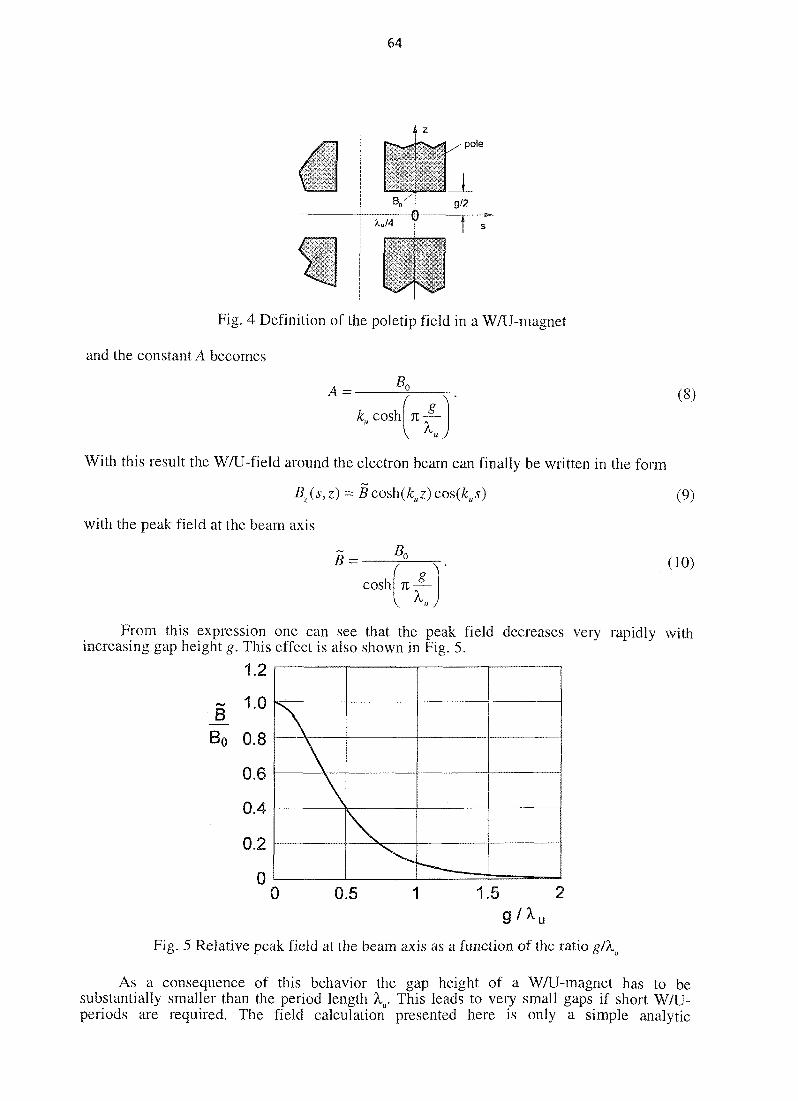
64

1v - i pole

i

JLg/2

Xu/4 T

Fig. 4 Definition of the poletip field in a W/U-magnet

and the constant A becomes

COSh 7E-

(8)

With this result the W/U-field around the electron beam can finally be written in the form

Bz(s,z) = B cosh(kuz) cos(kus) (9)

with the peak field at the beam axis

B =

cosh 7A,.

(10)

From this expression one can see that the peak field decreases very rapidly withincreasing gap height g. This effect is also shown in Fig. 5.

1.2

Bo 0.8

0.6

0.4

0.2

0

\

\

\

**---—-0 0.5 1 1.5 2

Q/XU

Fig. 5 Relative peak field at the beam axis as a function of the ratio g/\

As a consequence of this behavior the gap height of a W/U-magnet has to besubstantially smaller than the period length Xu. This leads to very small gaps if short W/U-periods are required. The field calculation presented here is only a simple analytic

65

approximation, it is helpful for basic investigations. For an accurate design including tighttolerances more sophisticated methods and numerical calculations are required [1, 3, 4].

A.., coils

iron yoke

Fig. 6 Principal design of an electromagnetic wiggler or undulator

The very first W/U-magnets have been built with conventional iron yokes excited bymagnet coils as shown in Fig. 6. The field strength can easily be changed by changing thecurrent. This technique is used for period lengths not smaller than \ ~ 25 cm. For smallerperiods the current density in the coils exceeds reasonable values. In this case one can takesuperconductive coils, but because of the cryostat and the expensive liquid helium techniquethe costs are disproportionate.

Therefore, another type of W/U-magnets has been developed utilizing small pieces ofpermanent magnets arranged as sketched in Fig. 7.

•i' *• J

- * * • -

- x

tI

u

Hii-9

permanent magnets

Fig. 7 W/U-magnet built with permanent magnets. The arrows indicate the orientation of themagnetic flux.

Since the flux density in the magnet pieces is constant, one can only vary the fieldstrength at the beam axis by opening or closing the gap mechanically. The field changesaccording to equation (10). The poletip field has values which depend on the material used.For instance, samarium-cobalt (SmCo5) provides flux densities about B ~ 0.9 - 1.0 T. Ifhigher fields up to 2 T are required, one can built hybrid magnets (Fig. 8). They consist ofpoles made by soft iron and pieces of permanent magnets in between. The total flux of themagnet pieces is concentrated in the iron poles resulting in poletip fields about B{) = 2T.

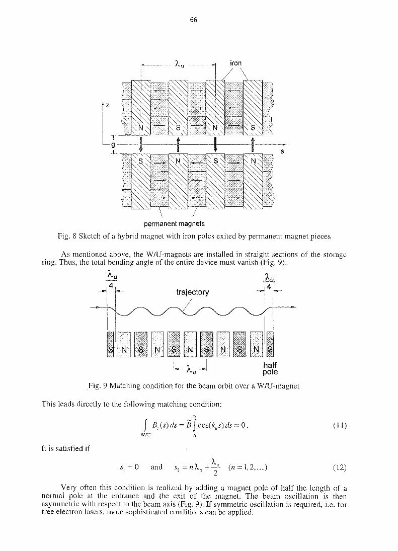
66

iron

permanent magnets

Fig. 8 Sketch of a hybrid magnet with iron poles exited by permanent magnet pieces

As mentioned above, the W/U-magnets are installed in straight sections of the storagering. Thus, the total bending angle of the entire device must vanish (Fig. 9).

Ay Au4 4,

trajectory ^

S N S N S- N s- N N shalfpole

Fig. 9 Matching condition for the beam orbit over a W/U-magnet

This leads directly to the following matching condition:

J BJs)ds =W/U

It is satisfied if

si=0 and ^2=

(H)

(12)

Very often this condition is realized by adding a magnet pole of half the length of anormal pole at the entrance and the exit of the magnet. The beam oscillation is thenasymmetric with respect to the beam axis (Fig. 9). If symmetric oscillation is required, i.e. forfree electron lasers, more sophisticated conditions can be applied.

67

3. EQUATION OF MOTION IN W/U-MAGNETS

3.1 The coupled set of equations of motionInside a W/U-magnet with the field B the Lorentz force

F = p=myv = evxB (13)

acts on the relativistic electron with the mass my and the charge e. In the following we willonly discuss the particle motion in the horizontal x-s-plane. The vertical motion is normallynegligible. With this simplification we can write the field of the W/U-magnet and the particlevelocity v in the form

and o (14)

Inserting (14) into (13) directly provides

v =my

/ , , n \

-vxB, (15)

We again neglect the vertical particle motion and can finally write the result in the formof a coupled set of equations:

(16)

3.2 First-order solution of the equations of motionSince Bz(s) is a nonlinear function of the position s in the magnet (see eq. (9)), there

exists no simple analytic solution. The longitudinal velocity vs, however, is significantlylarger than the horizontal component vx. This fact allows us to write

and s - VJ = P c = const. (17)

Under these conditions, only the first equation of (16) is of interest and we get therelation

e QceBx = -s BAs) = cos(kus).

my my

(18)

In storage rings it is often more convenient to describe the particle motion as a functionof place s instead of time t. For transformation we use

x = x'$ C and x = x"$2c2

and get from equation (18) the first order expression of the particle motion

x" = — e~— cos(kus) = —e—— cos 2n^- \.

(19)

(20)

68

It can be easily solved by integration. Since the electrons in storage rings for synchrotronradiation have extremely relativistic velocities, we can set p = 1 and obtain

, X eB .*'(*) = —* sm(kus)

2nmyc (21)

x(s) =4iz2myc

cos(kus).

The first equation gives the angle of the particle trajectory in a W/U-magnet with respect tothe orbit (Fig. 10).

trajectory

Fig. 10 Particle trajectory in a W/U-magnet

The maximum value of the trajectory angle is achieved at the crossing points with theorbit. It is

x> = 0 = (22)

Now we define the dimensionless wiggler or undulator parameter

and can write the maximum trajectory angle in the form

Especially for K = 1 the angle becomes

(23)

(24)

(25)

which is identical to the natural opening angle of the synchrotron radiation cone. This relationsuggests now the following differentiation between wiggler and undulator magnets:

Undulator if K <\ i.e. © „ < -Y

Wiggler if K>\ i.e. 0 W > -Y

(26)

For very large K the horizontal opening angle of the radiation is correspondingly largeand no interference of the photons takes place. The photon energy covers a dipole-like broadspectrum. For very small K the radiation from all undulator periods overlaps and stronginterference effects occur, resulting in rather sharp coherent spectral lines.

69

3.3 Second-order solution of the equations of motionWith the simple first-order solution we can't describe for instance the Doppler effect

observed in wiggler and undulator radiation. Therefore, we have to take additional conditionsinto account. But we are still not going to look for a general solution of the coupled set ofequations of motions (16).

The longitudinal velocity s causes, because of the Lorentz force, a transverseoscillation x(t), as described by equation (21). The resulting transverse velocity again causes asmall longitudinal oscillation, which superimposes with the longitudinal velocity s. Thelongitudinal velocity is actually not really constant. Thus, we can describe the particle motionin the form

s(t) = (s) + As(t) (27)

with the average velocity (i) and the longitudinal oscillation As(s). As shown in Fig. 11 theconstant particle velocity pc can be written as

Pc

Fig. 11 Addition of the particle velocity

(pc)2=i2+i2.

With

(28)

(29)

we find

(30)

Since 1/y2 « 1 and x « c we can expand the root. The longitudinal has therefore theexpression

s(t) = c2i r c2 -c 2?

(31)

Taking the formula (21) and (23) gives

,, . K . . .

Y

With the transformations

x = Pcx', s = pc? and cau = ku$c

we get the time-dependent transverse velocity

(32)

(33)

70

i ( f ) = [Jc—sin((OaO- (34)Y

We insert this relation into equation (31) and convert the sine function according to

sin200 = - ( l - cos (2x) ) . (35)

The longitudinal velocity becomes

•^-f-(l-cos(2co1,r) . (36)

It has the required form of equation (27) with the average velocity

W T ~ 2 7 L 1 + ^ n } (37)

and the time-dependent velocity oscillation

c&2K2

As(t)= *~ cos(2cou0- (38)4y

For extremely relativistic particles we set p = 1. This condition is fulfilled in almost allstorage rings for synchrotron radiation. The relative velocity of the particle along theundulator axis is

p-.ffl..-^

Thus, we can write the transverse and longitudinal particle velocity in the form

., N cK . , xx(t) = —sin(GV)Y

(40)

The trajectory can finally be found simply by integrating these equations using thearbitrary initial conditions JC(O) = 0 and 5(0) = 0:

X(t) = —

(4D

It is very impressive to observe the particle motion in the coordinate system /f, whichtravels along the undulator axis with the constant velocity P\ rather than in the laboratorysystem K. With the Lorentz transformations

x=x and s* =y(s-$t) (42)

we find the trajectory functions in the moving system K*

71

x*(t) = ——cos(coBr)

K (43)

In this system the trajectory has a shape like an "8" as shown in Fig. 12. For very smallvalues of the undulator parameter K only the transverse motion dominates. The "8" is verynarrow. For larger K the longitudinal amplitude grows quadratically, whereas the transverseamplitude is proportional to K. The growing longitudinal motion causes a Doppler effect ofthe emitted radiation.

m

5 -

c

0 -

-5 -

t[fX \jL- K=0.5

w

As

—,—,—,—,—-5 0 .5 5

10 mFig. 12 Particle trajectory in an undulator magnet observed in the moving system

4. UNDULATOR RADIATIONThe sinusodial particle motion in an undulator causes coherent radiation in the

laboratory system K with the frequency

(44)

For very small undulator parameters K « 1 we can neglect the longitudinal oscillationA s(t) and find in the moving system if the monochromatic radiation with the frequency

CO* , = Y * Q C45)^ ^ Tad i ract * V /

Y* is the relative energy of the particle in K". We transform this radiation from the movingsystem into the laboratory system. Here, we take a photon with the momentum p emittedunder the angle 0() with respect to the undulator axis (Fig. 13).

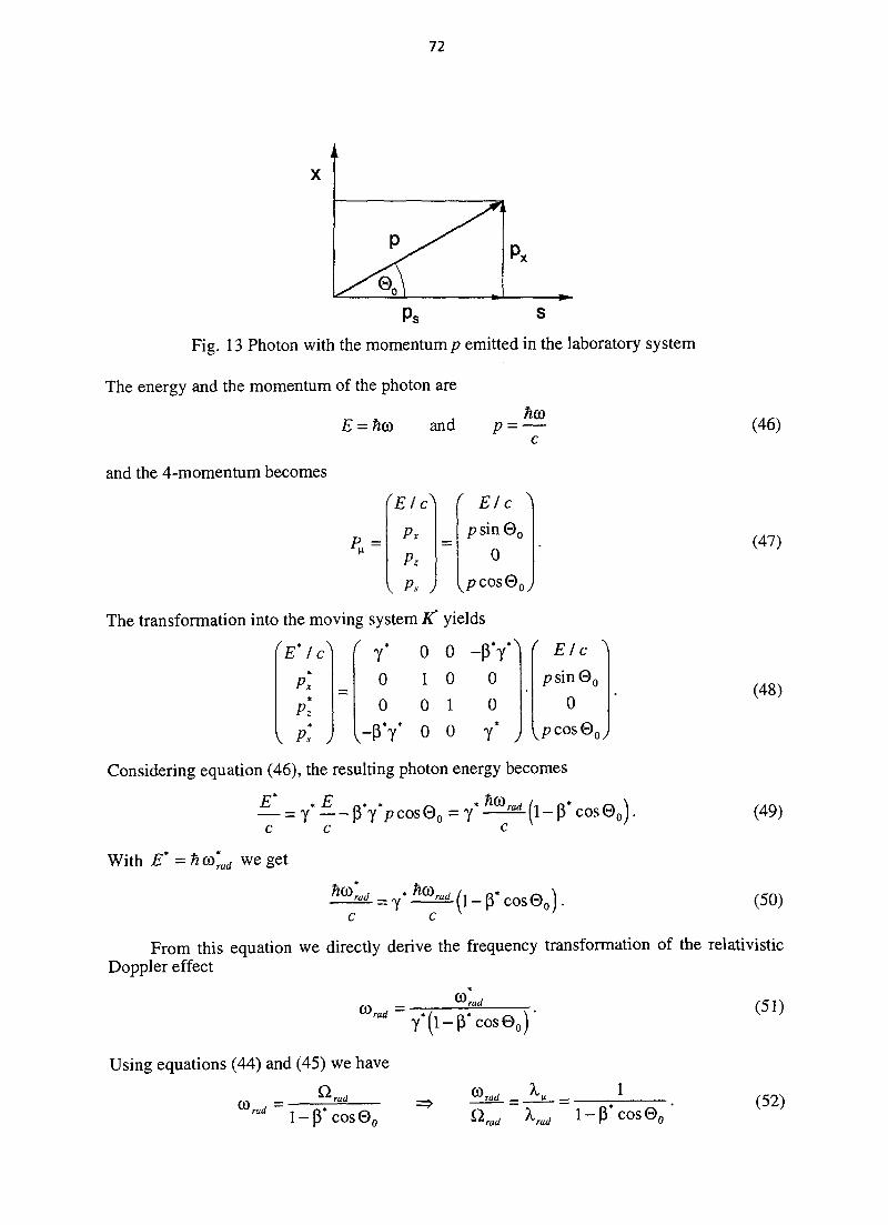
72

Fig. 13 Photon with the momentum p emitted in the laboratory system

The energy and the momentum of the photon are

£ = ftco and p = —

and the 4-momentum becomes1EIc\ I Elc

px = psinQ0

P, 0

V P. ,

The transformation into the moving system K" yields

(46)

(47)

E I c

P,

/ *y

o o -pi0 1 0 00 0 1 0

- P Y o o Y*

Elc

n©0

(48)

Considering equation (46), the resulting photon energy becomes

E* „ £ R . . r» - * C0'c c c

With E' = ft. a>*racl we get

(l-p*cos0o). (49)

(50)

From this equation we directly derive the frequency transformation of the relativisticDoppler effect

rad Y*(l-P*cos0o)'

Using equations (44) and (45) we have

a.'rad = K _rod l-p*cos0f l 1-P*cos0o '

(52)

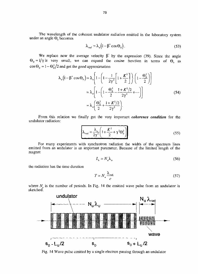
73

The wavelength of the coherent undulator radiation emitted in the laboratory systemunder an angle 0() becomes

(53)

We replace now the average velocity P* by the expression (39). Since the angle0O ~ 1/y is very small, we can expand the cosine function in terms of 0() ascos 0O ~ 1 - 0 Q / 2 and get the good approximation

1 - 1 - i+K2

2y2 (54)

(el I + K>\ 2 + If

From this relation we finally get the very important coherence condition for theundulator radiation:

(55)

For many experiments with synchrotron radiation the width of the spectrum linesemitted from an undulator is an important parameter. Because of the limited length of themagnet

K = (56)

the radiation has the time duration

"rud (57)

where Na is the number of periods. In Fig. 14 the emitted wave pulse from an undulator issketched.

undulator

so-Lu /2

waveso+Lu /2

Fig. 14 Wave pulse emitted by a single electron passing through an undulator

74

The field strength of this undulator radiation can be expressed by

0

if --<t<+-

, , Tif / > —

" 2

(58)

The resulting continuos spectrum follows from the Fourier transformation of the wavefunction:

1 *°°A(co) = - f = = - J u((am(!,

+r/2

2a

With

A co = co - (DmJ and = 27tiVu

the amplitude of the partial wave is

sin Aco

a

TCiV,Aco

corail

and the intensity (see Fig. 15)

/(A co)

sin itNuAco

Aco

CO,,,,,

spontaneousundulatorradiation

Fig. 15 Spectrum of the spontaneous undulator radiation

(59)

(60)

(61)

(62)

75

The full width half maximum (FWHM) of the spectral line can be found satisfying thecondition

sinx withAco

The solution is x = 1.392 and we get

2A(0 2x

COrad

0.886 1

N,, " N,,

(63)

(64)

The resolution of the undulator radiation is simply determined by the number ofundulator periods. High resolution requires a sufficient large number Nu. Normally one cannot observe these sharp spectral lines. There are higher harmonics and a" frequency shift dueto Doppler effect. A typical undulator spectrum is shown in Fig. 16.

dco1.

dopplereffect

center of mass frame

laboratory frame

2.

CO

Fig. 16 A typical undulator spectrum

REFERENCES

[1] G. Brown, K. Halbach, J. Harris, H. Winick, Wiggler and Undulator Magnets - aReview, Nucl. Instr. & Meth. 208, 65-77, 1983

[2] H. Winick (editor), Synchrotron Radiation Sources - a Primer, World ScientificPublishing, 1994

[3] H. Winick, T. Knight (editor), Wiggler Magnets, Wiggler Workshop, SLAC, SSRPReport No. 77/05, 1977

[4] J. Spencer, H. Winick, Synchrotron Radiation Research, editor: H. Winick, S. Doniach,Plenum Press, New York, ch. 21, 1980

NEXT PAGE(S)left BLANK

77

INTRODUCTION TO CURRENT AND BRIGHTNESS LIMITS

V.P. SullerCLRC, Daresbury Laboratory, Daresbury, United Kingdom

AbstractFundamental features of the measurement and description of beamcurrent in synchrotron radiation sources are presented and examplesgiven for a range of different accelerators. From a simple treatment ofthe electric field surrounding a moving charge the concept of theimpedance of beam vacuum chamber is introduced. The interaction ofthe beam current with this impedance is described, as are somemechanisms which can lead to current limitations. The brightness of asource of synchrotron radiation is defined and worked examples aregiven for the ESRF. Brightness limits are briefly described in outline.

1 . INTRODUCTIONCurrent and brightness limits are potentially serious concerns for synchrotron light

sources because in effect they can impose a limit on the usefulness of the source and theexperimental science programmes they can cover. As will be seen, the expression forbrightness contains the beam current so any limit in current automatically limits the brightness.

We will present some very simple ideas relating to beam current in electron storage ringsand give an impression of the magnitudes involved by taking some examples from a range ofdifferent storage rings. Using simple expressions it will be demonstrated how the electro-magnetic fields associated with beam currents can significantly interact with the structuressurrounding the beam to produce effects which can limit the current. Then the basic equationsfor the brightness of synchrotron light will be stated and the factors which may limit thebrightness will be explained. The brightness of two different types of source will be evaluated(for ESRF dipoles and undulators) to illustrate these factors.

2 . BEAM CURRENT MEASUREMENT AND TYPICAL VALUESThe beam current in an accelerator is defined in the same way as a normal electric current,

that is, the rate at which charge passes a fixed point. It can be measured by two differenttechniques, as shown in Fig. 1. Notice that the two methods will give greatly differing resultsfor the same number of particles (see below).

Particles Particles

Transformer

Faraday cijp

Ejected beam , . .' ' jy\ Ammeter

(a) (b)

Fig. 1

(a) DC current transformer (this measures the magnetic field produced by the current) [1](b) Faraday cup (this measures the total beam charge and needs the beam to be ejected) [2]

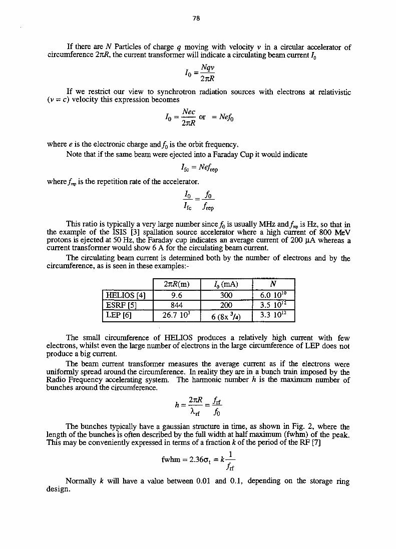
78

If there are iV Particles of charge q moving with velocity v in a circular accelerator ofcircumference 2KR, the current transformer will indicate a circulating beam current 70

Nqv7 ° Îf we restrict our view to synchrotron radiation sources with electrons at relativistic

(v = c) velocity this expression becomes

_. Nee

where e is the electronic charge and/0 is the orbit frequency.Note that if the same beam were ejected into a Faraday Cup it would indicate

where/rep is the repetition rate of the accelerator.

*fc /rep

This ratio is typically a very large number since/0 is usually MHz and/^ is Hz, so that inthe example of the ISIS [3] spallation source accelerator where a high current of 800 MeVprotons is ejected at 50 Hz, the Faraday cup indicates an average current of 200 pA whereas acurrent transformer would show 6 A for the circulating beam current.

The circulating beam current is determined both by the number of electrons and by thecircumference, as is seen in these examples:-

HELIOS [4]ESRF [5]LEP [6]

2nR(m)9.6844

26.7 103

70(mA)

300200

6 (8x 3A)

N

6.0 10'°3.5 1012

3.3 1012

The small circumference of HELIOS produces a relatively high current with fewelectrons, whilst even the large number of electrons in the large circumference of LEP does notproduce a big current.

The beam current transformer measures the average current as if the electrons wereuniformly spread around the circumference. In reality they are in a bunch train imposed by theRadio Frequency accelerating system. The harmonic number h is the maximum number ofbunches around the circumference.

The bunches typically have a gaussian structure in time, as shown in Fig. 2, where thelength of the bunches is often described by the full width at half maximum (fwhrn) of the peak.This may be conveniently expressed in terms of a fraction k of the period of the RF [7]

fwhm = 2.36at = k—/rf

Normally k will have a value between 0.01 and 0.1, depending on the storage ringdesign.

79

From the well known properties of gaussians we can relate the peak current 7pk to theaverage 70

At

Current( i ) .1

\'K"fwhm —W W—

Time(t)

Fig. 2 Time structure of the bunches

With the value for k in storage rings typically being between 0.1 and 0.01 it can be easilyseen that the peak current can be 10 to 100 times higher man the average current. Even higherpeak currents are produced when electron storage rings operate, as is often the case, with thebeam current concentrated in a single (or few) bunches. The current transformer will stillregister a reading 1^ as though the electrons are spread around the circumference, but the peakcurrent is increasedby a factor of the harmonic number h because now:

^0(sb)

/o

7pk = 0.94/* '(Ksb)

Consider these examples of peak currents in storage rings operated in single or few bunchmode, from which it can be seen that peak currents can easily reach values of hundreds ofamperes.

SRS 8]ESRF [9]LEP[10]

Im)(mA)

100103 /4

k

0.110.030.025

/ .3.1 106

3.5 105

1.1 104

h

160992

31360

N

2.0 10"1.8 10"4.3 10"

U (A)136310885

It is not surprising that the electro-magnetic fields associated with these very high peakcurrents can produce effects which destabilise the electron bunches and produce currentlimitations.

3 . FOURIER COMPONENTS OF THE BEAM CURRENTConsider the time structure of the beam current in more detail. The train of bunches in the

beam current, as shown in Fig. 2, can be expressed as a fourier series:

= -f + 2,n = 1 an cosnco? + =i K sin neat

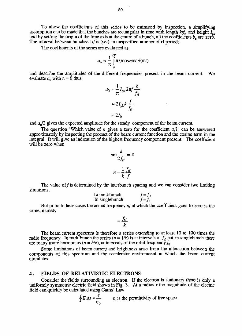
80

To allow the coefficients of this series to be estimated by inspection, a simplifyingassumption can be made that the bunches are rectangular in time with length Jk//rf and height Jpkand by setting the origin of the time axis at the centre of a bunch, all the coefficients bB are zero.The interval between bunches l//is (yet) an unspecified number of rf periods.

The coefficients of the series are evaluated as

an =— U(t)cosn(ot.d(Git)7T »71

o

and describe the amplitudes of the different frequencies present in the beam current. Weevaluate a0 with n = 0 thus

fl0«-/pk27C/ —n /rf

and <2</2 gives the expected amplitude for the steady component of the beam current.The question "Which value of n gives a zero for the coefficient an?" can be answered

approximately by inspecting the product of the beam current function and the cosine term in theintegral. It will give an indication of the highest frequency component present. The coefficientwill be zero when

knco = n2/rf

The value off is determined by the interbunch spacing and we can consider two limitingsituations.

In multibunch f-fttIn singlebunch f-fo

But in both these cases the actual frequency nfat which the coefficient goes to zero is thesame, namely

The beam current spectrum is therefore a series extending to at least 10 to 100 times theradio frequency. In multibunch the series (« = Ilk) is at intervals of/rf but in singlebunch thereare many more harmonics (n = h/k), at intervals of the orbit frequency/0.

Some limitations of beam current and brightness arise from the interaction between thecomponents of this spectrum and the accelerator environment in which the beam currentcirculates.

4 . FIELDS OF RELATIVISTIC ELECTRONSConsider the fields surrounding an electron. If the electron is stationary there is only a

uniformly symmetric electric field shown in Fig. 3. At a radius r the magnitude of the electricfield can quickly be calculated using Gauss' Law

<l> E.ds = — EQ is the permittivity of free spaceJ £o

81

Fig. 3 Electric field surrounding a stationary electron

The integral is made over the surface of a sphere at radius r, thus

EAnr2 = —

E = ———47t£0 r2

If the electron is moving relativistically with respect to an observer the electric field suffers arelativistic contraction along the line of motion. For an electron moving with velocity Pc with

y = y 1 - p2 the electric field seen by the observer at rest is as shown in Fig. 4.

velocity = |3c

Fig. 4 Electric field of a relativistic electron

The x direction is along the axis of the electron's motion, while the y direction isperpendicular to it. The general expressions for the electric field components are [11]

ycosG e

ysin6

If these expressions are examined for two extreme values of 6

82

Along the axis of motion at 8 = 0

£y-0,

• Within a small angle to the normal to the axis of motion at 0 =2 Y

y e „ 1 e-y ~ 2 3 / 2 ' "x - 23/2 •

Because Y has a large value for relativistic electrons, it can be seen that the only significant

field component is within ±—of the normal to the electron motion. Thus the electric field is

1concentrated into a disc of angular thickness + — at right angles to the electron's motion as

shown in Fig. 5

velocity = pc

Fig. 5 The electric field of a relativistic electron isconcentrated into a disc at right angles to the velocity

Using this concept of the field concentrated into a disc we can quickly confirm(approximately) the result above by using Gauss' Law over the edge of the disc

&Eds~Ey2n.— = —J y Y e0

Ew = (compare to the exact treatment above).

The moving charge also appears as a current i to the stationary observer. If we consider2r

this current to be the passage of charge e in the time — which the disc edge takes to pass theyc

observer, then

._ eye

*~~7Using Amperes law for the magnetic field surrounding a current

83

<j> Bdl = \iQi \i0 is the permeability of free space

B ^ e c4nr2

Since eono = -~-, we have the expected relation between the magnetic and electric fields;c

B = Elc

5 . EFFECTS DUE TO THE VACUUM CHAMBER WALLSIt has been shown that a relativistic electron has its electric field concentrated into a disc.

When the electron is moving within the conducting vacuum chamber of an accelerator the discmust terminate at the chamber wall on an opposite sign image charge moving along with theelectron.

If the walls are not perfectly conducting the image charge will dissipate energy in thewalls; this is a resistive wall effect. However, the energy dissipation is usually negligible. Forexample, a 1000-m circumference accelerator with a vacuum chamber made of stainless steelwould have a resistance of about 1 £1 Applying Ohm's Law to a 300 mA image currentflowing in this resistance gives a dissipation of only 0.1 W. The high frequency componentsof the beam current see a higher resistance due to the skin effect but again the dissipation isusually not important.

The resistive loss in the chamber walls can be pictured as a longitudinal drag force on anelectron bunch and as such does not cause any stability problems for the bunch. If the bunch isnot aligned transversely with the axis of the vacuum chamber the transverse assymmetry of theelectric field disc can be expected to produce a transverse force component and this can lead toan instability. This is called the transverse resistive wall instability [12].

In addition to resistance the vacuum chamber walls can show other [13] electricalimpedance properties, that is, capacitance or inductance. These arise from changes in thegeometrical shape of the vacuum chamber, as seen by the fields surrounding the beam. As thebeam moves at relativistic velocity from a region with one shape of the chamber to another,both the fields and the image currents become distorted and can even be left in these shapechanges 'ringing' behind the beam. These residual fields can then interact with the tail of thebunch, or with beam bunches which pass later (even with the same bunch on a later orbit), andare the principal reason for the existence of beam current and brightness limitations.

Even though the capacitances and inductances resulting from shape changes in thevacuum chamber are quite small (a 10-mm step in a 100-mm diameter pipe contributes aninductance of order 0.01 |iH [14]) it must be remembered that the peak current in the bunchmay exceed hundreds of amperes. In the chamber impedance such a bunch can produce fieldsequivalent to hundreds of volts and this is sufficient to affect the stability of the bunches.

When the field from the head of a bunch affects the tail of the same bunch this is called asingle-bunch effect. [15]

When the field of a bunch affects later bunches this is called a multibunch effect [15].The observable effects may be:

1. Bunch position oscillations (transverse or longitudinal)

2. Bunch shape oscillations ( " " )

3. Bunch size changes ( " )

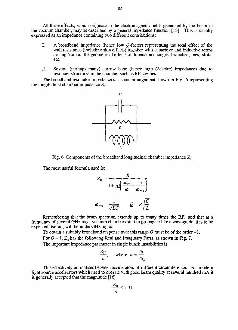
84

All these effects, which originate in the electromagnetic fields generated by the beam inthe vacuum chamber, may be described by a general impedance function [13]. This is usuallyexpressed as an impedance containing two different contributions:

I. A broadband impedance (hence low <2-factor) representing the total effect of thewall resistance (including skin effects) together with capacitive and inductive termsarising from all the geometrical effects of dimension changes, branches, tees, slots,etc.

II. Several (perhaps many) narrow band (hence high Q-iactor) impedances due toresonant structures in the chamber such as RF cavities.

The broadband resonator impedance is a shunt arrangement shown in Fig. 6 representingthe longitudinal chamber impedance Z,t.

R

Fig. 6 Components of the broadband longitudinal chamber impedance,

The most useful formula used is:R

Zu =CO

© res.

LC

Remembering that the beam spectrum extends up to many times the RF, and that at afrequency of several GHz most vacuum chambers start to propagate like a waveguide, it is to beexpected that G)res will be in the GHz region.

To obtain a suitably broadband response over this range Q must be of the order ~1 .For Q = 1, Zj, has the following Real and Imaginary Parts, as shown in Fig. 7.The important impedance parameter in single bunch instabilities is

ZIT , €0——, where n = —n 0)o

This effectively normalises between accelerators of different circumference. For modernlight source accelerators which need to operate with good beam quality at several hundred mA itis generally accepted that the magnitude [16]

^ - < 1 Qn

85

-0.5

Real part

Fig. 7 Real and Imaginary components of the broadband impedance

Z T TExamples of measured —— in light sources:

SRS1 .8±0 .6Q [8]ALS 0.2 ft [17]LEP 0.25-0.5 ft [18]

It is intuitively apparent that a beam moving off centre down the vacuum chamber willgenerate different fields than a beam which is centred. This must imply that there is atransverse component Zx to the chamber impedance, although it is closely related to thelongitudinal impedance ZQ.

The generally used approximate relationship between them is [19]:

where R is the accelerator average radius and b is the radius of the vacuum chamber aperture.Note that the dimensions of Zx are ft/m.

The mathematical treatment of instabilities is well beyond the scope of this paper. Theconcepts which have already been introduced, however, can be appreciated for the role that theyplay in the behaviour of instabilities.

An expression for the growth rate of some coordinate of a theoretical test Particle withinthe beam can be derived [19], which is related to the beam current and the chamber impedance.An instability will not necessarily develop on all occasions because there are often dampingmechanisms (by synchrotron radiation emission [20] or by Landau damping [21], for example)which stifle the instability because the damping rate exceeds the growth rate. But since thegrowth rate is related to the beam current, above some threshold current the instability willgrow. Even then the growth may stabilise at a new equilibrium because of frequency shiftswith amplitude and Landau damping.

Thus below the instability threshold current the beam will exhibit its theoreticaldimensions, whereas above the threshold the beam may grow to an increased size, or oscillate,or suffer an intensity reduction until it restabilises below the threshold. All these behaviours areobviously important to users of synchrotron radiation facilities.

6. BRIGHTNESS OF A SYNCHROTRON RADIATION SOURCEThe usefulness of a synchrotron radiation source may be judged by an experimenter

primarily in terms of how many photons per second can be directed onto the sample. Therelevant factors which influence this are the emission properties of the source and the

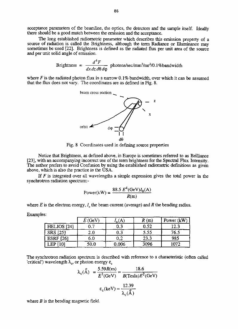
86

acceptance parameters of the beamline, the optics, the detectors and the sample itself. Ideallythere should be a good match between the emission and the acceptance.

The long established radiometric parameter which describes this emission property of asource of radiation is called the Brightness, although the term Radiance or Illuminance maysometimes be used [22]. Brightness is defined as the radiated flux per unit area of the sourceand per unit solid angle of emission.

Brightness =d4F

dxdzdBdyphotons/sec/mnrVmrVO. 1 %bandwidth

where F is the radiated photon flux in a narrow 0.1% bandwidth, over which it can be assumedthat the flux does not vary. The coordinates are as defined in Fig. 8.

beam cross section

orbit

Fig. 8 Coordinates used in defining source properties

Notice that Brightness, as defined above, in Europe is sometimes referred to as Brilliance[23], with an accompanying incorrect use of the term brightness for the Spectral Flux Intensity.The author prefers to avoid Confusion by using the established radiometric definitions as givenabove, which is also the practice in the USA.

If F is integrated over all wavelengths a simple expression gives the total power in thesynchrotron radiation spectrum:-

R(m)

where E is the electron energy, 70 the beam current (average) and R the bending radius.

Examples:

HELIOS [24]SRS [25]ESRF [26]LEP [10]

£(GeV)0.72.06.0

50.0

h (A)0.30.30.2

0.006

*(m)0.525.5523.33096

Power (kW)12.376.59851072

The synchrotron radiation spectrum is described with reference to a characteristic (often called'critical') wavelength Xc, or photon energy ec

= 5.59/?(m) = 18.6

~ £3(GeV) ~

£c(keV) =12.39

where B is the bending magnetic field.

87

Examples:

BESSY-I [27]HELIOS [28]SRS [25]ESRF [29]LEP [30]

£(GeV)

0.80.72.06.050.0

R(m)

1.780.525.5523.33096

BCD1.54.51.2

0.860.054

MA)19.48.53.9

0.600.14

ec(keV)

0.641.53.2

20.788.5

When the radiation at a given wavelength is integrated over all angles of vertical emissionthe resultant Spectral Flux Density is given by

13^ = 2.46 1013/0(A)£(GeV)(at)

photons/sec/mr/0.1% bandwidth

where G\ [31] is a numerical factor which essentially governs the shape of the spectrum.

Note that source Brightness as defined above is a function whose value depends on thesource density distribution and on the observation angle. It is often more convenient to use, asa figure of merit, an average brightness which for dipole sources is defined [32]:

dF

Average Brightness =2.36ax2.36az2.36a^

where dF/dQ is the vertically integrated flux, 2.36ax is the fwhm of the horizontal electronbeam size, 2.36cz is the fwhm of the vertical electron beam size, and 2.36a' is the fwhm of thephoton emission angle in the vertical plane. The latter is a combination of the electron beamvertical divergence and the photon emission angle thus

ol2+0.4l 1z ""\Kjr

As an example let us calculate the Average Brightness of a dipole magnet in the ESRF [23]

General data

£ = 6GeV

70= 200 mA

ex= 4 10'9 m.rads

E Z = 4 10'"m.radso F = 10"3

Source point data

P x = 1 . 0 m

p\ = 25.0 m

TI = 0.03 m

Electron beam data

ox = 0.07 mm

az = 0.032 mm

ax '= 0.0013 mr

At X = Xe

Xc = 0.6 A

aYy = 0.055 mr

dF— = 2.46 1013 0.2 6 0.65 at X = kc

= 1.9 1013 photons/sec/mr/0.1% band

Dipole Average Brightness =1.91013

2.363 0.07 0.032 0.055

= 1.2 1016 photons/sec/mmVmrVO.lê band.

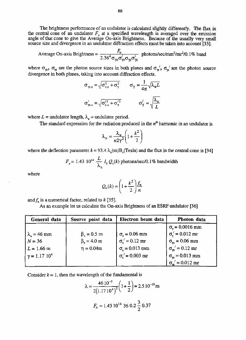
88

The brightness performance of an undulator is calculated slightly differently. The flux inthe central cone of an undulator FB at a specified wavelength is averaged over the emissionangle of that cone to give the Average On-axis Brightness. Because of the usually very smallsource size and divergence in an undulator diffraction effects must be taken into account [33].

Average On-axis Brightness =2364ayxa

lyxcyzG

/yz

photons/sec/mm2/mr2/0.1% band

^ are the photon sourcewhere a^, a^ are the photon source sizes in both planes and a.divergence in both planes, taking into account diffraction effects.

1 nr-

4TC

* ; =

where L - undulator length, A.u = undulator period.The standard expression for the radiation produced in the n* harmonic in an undulator is

— u

where the deflection parameter k = 93.4 A,u(m)B0(Tesla) and the flux in the central cone is [34]

Fn= 1.43 1014 — /o0n(fc)photons/sec/O.l% bandwidth

where

and/n is a numerical factor, related to k [35].As an example let us calculate the On-axis Brightness of an ESRF undulator [36]

General data

Xu = 46 mm

iV=36L= 1.66 m

7=1.17 104

Source point data

p\ = 0.5 m

p\ = 4.0 m

Tl = 0.04m

Electron beam data

ax = 0.06 mm

ox' = 0.12mr

GZ = 0.013 mm

a/ = 0.003 mr

Photon dataoY= 0.0016 mmcY' = 0.012 mr

c^ = 0.06 mm

0^ = 0.12™-

a^ = 0.013 mmcj = 0.012 mr

Consider k = 1, then the wavelength of the fundamental is

4610"3 (, , Q OI 1 + — 1 = 2.2(1.17104) ^ 2

m

Fn = 1.43 1014 36 0.2 - 0 . 3 72

89

= 5.71014photons/sec/0.1%band

5 71014

On-axis Brightness =2.364 0.06 0.013 0.120.012

= 1.6 1019 photons/sec/mm2/mr2/0.1% band .

7 . BRIGHTNESS LIMITATIONSIt has been shown that the brightness of a synchrotron radiation source depends on the

beam current and the cross sectional dimensions of the beam itself. Both these quantities maybe degraded by effects arising from the impedance behaviour of the beam vacuum chamber; thebeam may be limited to a threshold current; or above it the beam dimensions may increase. Theend result is to limit the brightness properties of the source.

These are what might be called technological limitations, which may be overcome byappropriate designs to ensure a suitably low impedance. Alternatively, feedback systems maybe employed to counteract specific instabilities.

But as the technological design of synchrotron sources moves steadily towards theachievement of yet smaller beam dimensions, the ultimate limit will then be reached when, nomatter how small the beam is, diffraction effects predominate. Until that happy day forexperimentalists is reached, there remains much to be done by accelerator theorists, scientistsand technicians.

REFERENCES

[I] K. Unser, IEEE Trans. Nuc. Sci., NS-16, p. 934, (1969).

[2] K.L. Brown and G.W. Tautfest, Rev. Sci.. Instr. 27, p. 696, (1956).

[3] I.S.K. Gardner, Proc. 1st European Part. Accel. Conf., Rome 1988, p. 65.

[4] V.C. Kempson et al, Proc. 4th European Part. Accel. Conf., London 1994, p. 594.

[5] J.M. Filhol, Proc. 4th European Part. Accel. Conf., London 1994, p. 8.

[6] E. Keil, Proc. 3rd European Part. Accel. Conf., Berlin 1992, p. 22.

[7] R.P. Walker, Proc. CERN Accel. School, Jyvaskyla 1992, CERN 94-01, p. 485.

[8] J.A. Clarke, Proc. USA Part. Accel. Conf., Dallas 1995, p3128.

[9] J.L. Revol and E Plouviez, Proc. 4th European Part. Accel. Conf., London 1994,p. 1506.

[10] B. Zotter, Proc. 3rd European Part. Accel. Conf., Berlin 1992, p. 273.

[II] Richtmeyer, Kennard and Lauritsen, Introduction to Modern Physics, 5th edition, p. 73,McGraw-Hill 1955.

[12] L.J. Laslett et al, Rev. Sci. Instr., 36, p. 436, (1965).

[13] M. Furman et al; Chapter 12 in Synchrotron Radiation Sources, a Primer;H. Winick(ed), World Scientific 1994.

90

[14] S.A. Heifets and S.A. Kheifets, Revs Mod. Phys., 63, p. 631, (1991).

[15] A. Hofmann, Proc. 1 lth Int. Conf. High Energy Accel., p. 540, Geneva 1980.

[16] M. Cornacchia, Proc. CERN Accel. School, Chester 1989, CERN 90-03, p. 68.

[17] J.M. Byrd and J.N. Corlett, Proc. 4th European Part. Accel. Conf., London 1994,p. 1069.

[18] D. Brandt et al, Proc. 2nd European Part. Accel. Conf., Nice 1990, p. 240.

[19] J.L. Laclare, Proc. 11th Int. Conf. High Energy Accel., p. 526, Geneva 1980.

[20] R.P. Walker, Proc. CERN Accel. School, Juvaskula 1992, CERN 94-01, p. 461.

[21] H.G. Hereward, Proc. CERN Accel. School, Oxford 1985, CERN 87-03, p. 255.

[22] Jenkins and White; Fundamentals of Optics, 3rd edition, p. 108, McGraw-Hill 1957.

[23] J.M. Lefebvre, Proc. 5th European Part. Accel. Conf., Sitges 1996, p. 67.

[24] R.J. Anderson et al, Proc. 3rd European Part. Accel. Conf., Berlin 1992, p. 187.

[25] V.P. Suller et al, Proc. 1st European Part. Accel. Conf., Rome 1988, p. 418.

[26] A. Ropert, Proc. 3rd European Part. Accel. Conf., Berlin 1992, p. 35.

[27] D. Einfeld and G. Muelhaupt, Nuc. Instr. Meth., 172, p. 55, (1980).

[28] M.N. Wilson, Proc. 2nd European Part. Accel. Conf., Nice 1990, p. 295.

[29] M. Lieuvin et al, Proc. 3rd European Part. Accel. Conf., Berlin 1992, p. 1347.

[30] K. Huebner, Proc. CERN Accel. School, Chester 1989, CERN 90-03, p. 32.

[31] G.K. Green, Brookhaven National Laboratory Report, BNL 50522, 1976.

[32] K.J. Kim, Nuc. Instr. Meth. Phys. Res., A246, p. 71, (1986).

[33] S. Krinsky, IEEE Trans. Nuc. Sci., NS-30, p. 3078, (1983).

[34] K.J. Kim, Section 4 in X-Ray Data Booklet, Lawrence Berkeley Laboratory report,PUB-490, 1985.

[35] European Science Foundation report 'European Synchrotron Radiation Facility;supplement II, The Machine', p. 56, (1979).

[36] L. Farvacque et al; Proc. 5th European Part. Accel. Conf., Sitges 1996, p. 632.

91

LATTICES AND EMITTANCES

A. RopertESRF, Grenoble, France

AbstractThe new generation of synchrotron light sources is characterised by an extremelyhigh brilliance synchrotron radiation achieved in low-emittance storage ringsspecially designed to accommodate insertion devices. The basic principles guidingthe minimisation of the emittance are recalled. The magnet lattice configurations thatare currently studied as candidates for these storage rings (DFA, TBA, FODO...)are described and the problems associated with these low-emittance lattices and therequired strong focusing discussed. Finally the effects of insertion devices on beamdynamics as well as on emittances and energy spread are recalled.

1 . FROM HIGH BRILLIANCE TO LOW EMITTANCEHigh-brilliance synchrotron radiation can be obtained by utilising insertion devices in low-

emittance storage rings. A small beam emittance is also very important for storage ring basedFELs where additional requirements must also be fulfilled. In this lecture, emphasis will beplaced on storage-ring lattices specially designed to maximise the brilliance and achieve the fullpotential from insertion devices.

Brilliance of X-rays has increased by many orders of magnitude since the advent ofsynchrotron radiation sources as shown in Fig. 1.

23-

22 H

2 1 .

20.

19-

1 8 •

1 7 116-

15.1

14.

13.

12.

11.

10.

9 .

7 .

6

Diffraction limit & 200 mA • Q

ESRF forthcoming 2nd upgrade ^m

present ESRFftfltr 1st upgrtdt) ^ | |

3rd generation I

ESRF original target — • •

/

2nd generation of /synchrotron "X /light sources /

1st generation -^___^ /

TX-ray /tubes x /

m, , ,

1850 1900 1950 2000

Fig. 1 Increase of brilliance over the last decades

The photon flux is an important source characteristic. Nevertheless, for a number ofexperiments in which the beam is focused at the sample, the true figure of merit is the spectralbrilliance B (called, in short, brilliance) which is defined as the photon flux per unit solid angleand per unit source area, emitted in a relative bandwidth. Brilliance may be expressed as:

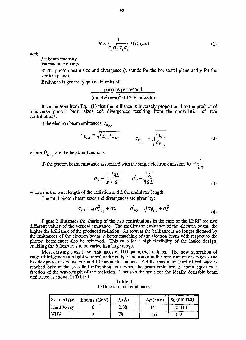
92

with:Ox<JxOy<Jy

—f(E,gap) (1)

/ = beam intensityE= machine energya, <J'= photon beam size and divergence (x stands for the horizontal plane and y for thevertical plane)Brilliance is generally quoted in units of:

photons per second

(mrad)2 (mm)2 0.1% bandwidth

It can be seen from Eq. (1) that the brilliance is inversely proportional to the product oftransverse photon beam sizes and divergences resulting from the convolution of twocontributions:

i) the electron beam emittances

°Ex,y =

*,y

x<y£E

x (2)

where f3E are the betatron functions

ii) the photon beam emittance associated with the single electron emission £R —A

(3)

where / is the wavelength of the radiation and L the undulator length.The total photon beam sizes and divergences are given by:

ax,y = *(4)

Figure 2 illustrates the sharing of the two contributions in the case of the ESRF for twodifferent values of the vertical emittance. The smaller the emittance of the electron beam, thehigher the brilliance of the produced radiation. As soon as the brilliance is no longer dictated bythe emittances of the electron beam, a better matching of the electron beam with respect to thephoton beam must also be achieved. This calls for a high flexibility of the lattice design,enabling the /3 functions to be varied in a large range.

Most existing rings have emittances of 100 nanometer-radians. The new generation ofrings (third generation light sources) under early operation or in the construction or design stagehas design values between 5 and 10 nanometer-radians. Yet the maximum level of brilliance isreached only at the so-called diffraction limit when the beam emittance is about equal to afraction of the wavelength of the radiation. This sets the scale for the ideally desirable beamemittance as shown in Table 1.

Table 1Diffraction limit emittances

Source type

Hard X-ray

vuv

Energy (GeV)

6

2

A. (A)0.88

78

£c(keV)

14

1.6

ER (nm.rad)

0.014

0.2

93

0.4 nm electron beam emittan e

photon beam emittance

microns)

slgma' (mlcrorad) I

-60 -40

diffraction limit

0.04 electron beam emittance

slgma (microns)

40

photon beam emittance -6

-10

Fig. 2 Effective photon-beam emittances

2 . LOW-EMITTANCE LATTICES

2.1 Equilibrium emittanceThe particle beam emittance in an electron storage ring is determined by an equilibrium

between quantum excitation that causes individual particles to oscillate transversally anddamping of the betatron oscillations.

In an undistorted machine, radiation is produced mainly in the normal bending magnets.As a particle emits a photon, it loses energy and this results in a sudden change of itsequilibrium orbit which causes a corresponding increase of the betatron oscillation amplitudeabout the new equilibrium orbit (Fig. 3). This process of continuous increase of the beamemittance is compensated by the damping provided by the RF accelerating system whichrestores the energy lost by synchrotron radiation only in the longitudinal direction.

The resulting horizontal equilibrium emittance is given by the expression [1]:

0 h<M9l>where < > means the average around the storage ring and with:

p = bending radius

7= total energy in me2 unitsJx is the horizontal damping partition number

(5)

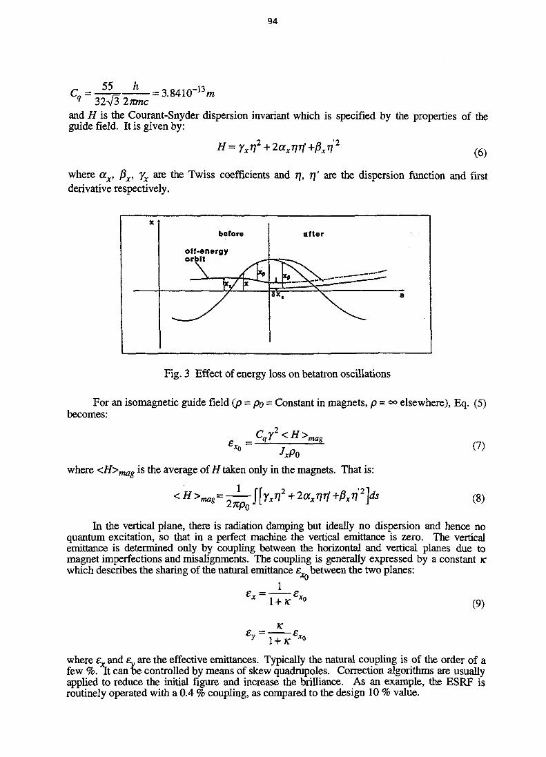
94

C =55 h

= 3.841(T13m32V3 2mnc

and H is the Courant-Snyder dispersion invariant which is specified by the properties of theguide field. It is given by:

where <xx, (3X, yx are the Twiss coefficients and r\, 7]' are the dispersion function and firstderivative respectively.

after

Fig. 3 Effect of energy loss on betatron oscillations

For an isomagnetic guide field (p = po = Constant in magnets, p = °o elsewhere), Eq. (5)becomes:

P = •fc*o

Caf<H>mag

JxPo

where <H>magl& *he average of H taken only in the magnets. That is:

-j[yx7]2 +2ax7iT}'+pxri2]ds

(7)

(8)

In the vertical plane, there is radiation damping but ideally no dispersion and hence noquantum excitation, so that in a perfect machine the vertical emittance is zero. The verticalemittance is determined only by coupling between the horizontal and vertical planes due tomagnet imperfections and misalignments. The coupling is generally expressed by a constant Kwhich describes the sharing of the natural emittance er between the two planes:

•*o£x =

(9)

K

where e and £, are the effective emittances. Typically the natural coupling is of the order of afew %. It can be controlled by means of skew quadrupoles. Correction algorithms are usuallyapplied to reduce the initial figure and increase the brilliance. As an example, the ESRF isroutinely operated with a 0.4 % coupling, as compared to the design 10 % value.

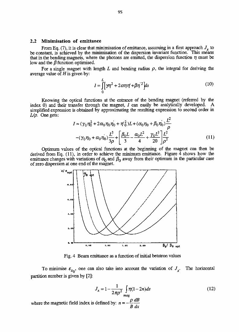
95

2.2 Minimisation of emittanceFrom Eq. (7), it is clear that minimisation of emittance, assuming in a first approach Jx to

be constant, is achieved by the minimisation of the dispersion invariant function. This meansthat in the bending magnets, where the photons are emitted, the dispersion function 77 must below and the /3 function optimised.

For a single magnet with length L and bending radius p , the integral for deriving theaverage value of H is given by:

(10)

Knowing the optical functions at the entrance of the bending magnet (referred by theindex 0) and their transfer through the magnet, / can easily be analytically developed. Asimplified expression is obtained by approximating the resulting expression to second order inUp. One gets:

«(7o»7o

ccQL2 yolf4 20

(ID

Optimum values of the optical functions at the beginning of the magnet can then bederived from Eq. (11), in order to achieve the minimum emittance. Figure 4 shows how theemittance changes with variations of <XQ and fi0 away from their optimum in the particular caseof zero dispersion at one end of the magnet.

e/c.opt

. . . .

€.00

4.00

2.00

!ia I \i I \

\\\V/ /

/

/ / / .

/ / /

1.00 i.«o opt

Fig. 4 Beam emittance as a function of initial betatron values

To minimise eY , one can also take into account the variation of J. The horizontal

partition number is given by [2]:

(12)mag

where the magnetic field index is defined by: n = ———B dx

96

In a machine with separated functions (i.e. zero field gradient in the dipoles), the quantityJx is approximately equal to 1. Jx can be made larger by introducing vertical focusing in thedipoles but its maximum value is limited by the rule:

Ui = Jx + Jy + J£ = 4 (13)

which means, in the particular case of no vertical bend, Jx + J£= 3, hence Jx < 3. In practicethe maximum tolerable value is Jx < 2, which results potentially in an emittance reduction of afactor two.

Another possible way to achieve very low emittances is to install damping wigglers indispersion-free straight sections. For instance, this method would reduce the emittance in PEPby almost one order of magnitude [3] with a total length of installed wiggler magnets of 200 m.This method is applicable to any storage ring but since the damping effect scales proportionallywith the bending radius of the ring magnets, it is more efficient in large machines.

3 . LATTICE TYPES

3.1 GeneralitiesThe basic structure of low-emittance lattices consists of straight sections designed for the

installation of insertion devices separated by arc sections. In the arcs, the focusing is chosen soas to minimise the chromatic invariant. Minima for H can be found for various types of lattices,involving proper choices for r\x, fix, and their derivatives in the bending magnet.

A variety of types of lattices are available to design low emittance lattices. They can bedivided into two classes:i) structures without bending magnets in the dispersive section: double focusing achromat

(DFA) commonly known as the Chasman-Green lattice [4], expanded Chasman-Green,empty FODO, triplet achromat lattice (TAL).The double focusing achromat lattice has been used for the NSLS rings in Brookhaven[5]. SUPERACO [6] is already operated with an expanded Chasman-Green structure.The expanded Chasman-Green structure is the basis of the conceptual designs of severalthird generation synchrotron radiation sources in operation : ESRF [7], APS [8],ELETTRA [9] or under construction or design stage: SPRING8 [10], BESSY2 [11],SOLEIL [12]. The triplet achromat lattice was used in ACO at Orsay [13]; it has theadvantage of requiring the shortest circumference.

ii) structures with additional bending magnets in the dispersive region: triplet bend achromat(TBA), FODO.Triple bend structures are utilised in both the ALADDIN [14] and BESSY [15]synchrotron radiation sources. ALADDIN is a machine optimised primarily to useradiation from the dipole magnet and does not provide zero dispersion in the long straightsections. In the BESSY structure, significant focusing in the vertical plane is provided bythe edge focusing of the dipoles. This focusing is necessary in order to limit theamplitude of the vertical beta function.The triple bend achromat lattice is the logical extension of the DFA. Adding a thirdbending magnet within the arc section allows extra flexibility. This type of lattice is run atALS [16], SRRC [17], PLS [18]. It is also proposed for the DIAMOND project [19].The FODO lattice is the most commonly used lattice for high energy physics storage rings

because of its very compact structure. In contrast to the other types of lattices, the FODO doesnot naturally provide a space for insertion devices; special lattice sections must be introduced toachieve dispersion-free insertions. The damping rings at Stanford [20] and the SXRL storagering [21] are good examples of the use of this structure.

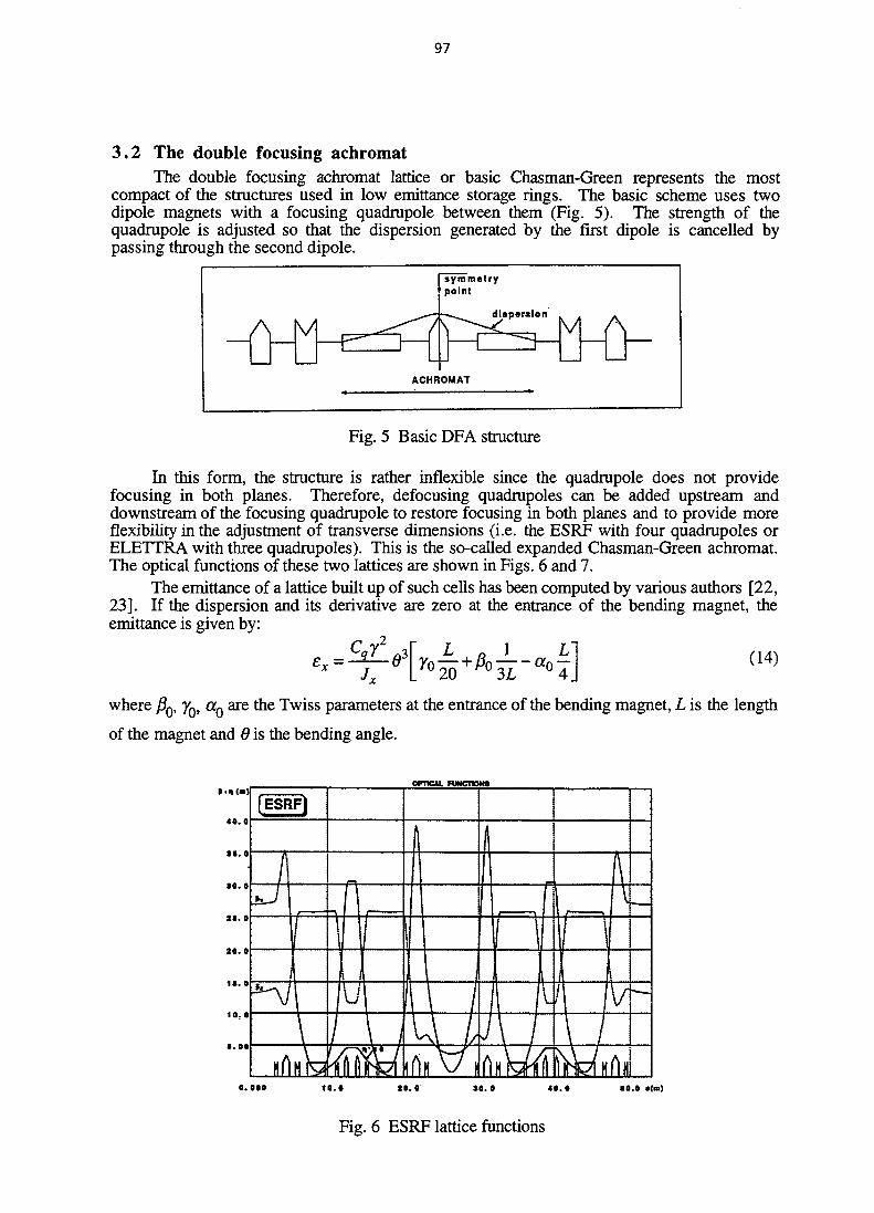
97

3.2 The double focusing achromatThe double focusing achromat lattice or basic Chasman-Green represents the most

compact of the structures used in low emittance storage rings. The basic scheme uses twodipole magnets with a focusing quadrupole between them (Fig. 5). The strength of thequadrupole is adjusted so that the dispersion generated by the first dipole is cancelled bypassing through the second dipole.

symmatrypoint

dispersion

ACHROMAT

Fig. 5 Basic DFA structure

In this form, the structure is rather inflexible since the quadrupole does not providefocusing in both planes. Therefore, defocusing quadrupoles can be added upstream anddownstream of the focusing quadrupole to restore focusing in both planes and to provide moreflexibility in the adjustment of transverse dimensions (i.e. the ESRF with four quadrupoles orELETTRA with three quadrupoles). This is the so-called expanded Chasman-Green achromat.The optical functions of these two lattices are shown in Figs. 6 and 7.

The emittance of a lattice built up of such cells has been computed by various authors [22,23]. If the dispersion and its derivative are zero at the entrance of the bending magnet, theemittance is given by:

£ = L \ (14)

where (3Q, y0, aQ are the Twiss parameters at the entrance of the bending magnet, L is the length

of the magnet and 6 is the bending angle.

»•<!(•)opncju. Fuwcnom

ao. o

(ESRF)

J .1/

\

"1,1. „ I p:. ..:•

IfMl II 1H 1 /A '

\r4\n' k

• • •

to.* JO. t 4«.» 10.0 •(•»)

Fig. 6 ESRF lattice functions

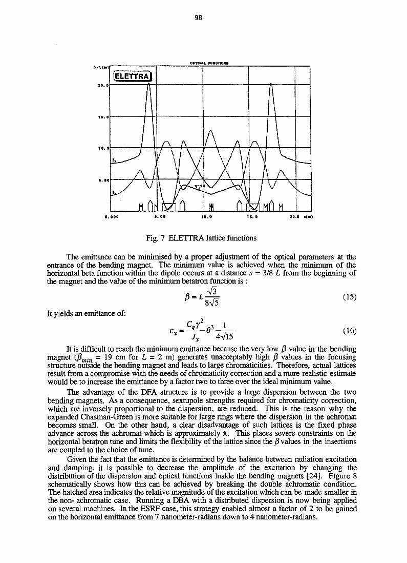
98

OKTICJU. FUNCnONB

. 000 t . 00 10.0 20.0 «(m)

Fig. 7 ELETTRA lattice functions

The emittance can be minimised by a proper adjustment of the optical parameters at theentrance of the bending magnet. The minimum value is achieved when the minimum of thehorizontal beta function within the dipole occurs at a distance s = 3/8 L from the beginning ofthe magnet and the value of the minimum betatron function is :

'8V5It yields an emittance of:

4VI5

(15)

(16)

It is difficult to reach the minimum emittance because the very low (3 value in the bendingmagnet (fimitl = 19 cm for L = 2 m) generates unacceptably high J3 values in the focusingstructure outside the bending magnet and leads to large chromaticities. Therefore, actual latticesresult from a compromise with the needs of chromaticity correction and a more realistic estimatewould be to increase the emittance by a factor two to three over the ideal minimum value.

The advantage of the DFA structure is to provide a large dispersion between the twobending magnets. As a consequence, sextupole strengths required for chromaticity correction,which are inversely proportional to the dispersion, are reduced. This is the reason why theexpanded Chasman-Green is more suitable for large rings where the dispersion in the achromatbecomes small. On the other hand, a clear disadvantage of such lattices is the fixed phaseadvance across the achromat which is approximately n. This places severe constraints on thehorizontal betatron tune and limits the flexibility of the lattice since the {5 values in the insertionsare coupled to the choice of tune.

Given the fact that the emittance is determined by the balance between radiation excitationand damping, it is possible to decrease the amplitude of the excitation by changing thedistribution of the dispersion and optical functions inside the bending magnets [24]. Figure 8schematically shows how this can be achieved by breaking the double achromatic condition.The hatched area indicates the relative magnitude of the excitation which can be made smaller inthe non- achromatic case. Running a DBA with a distributed dispersion is now being appliedon several machines. In the ESRF case, this strategy enabled almost a factor of 2 to be gainedon the horizontal emittance from 7 nanometer-radians down to 4 nanometer-radians.

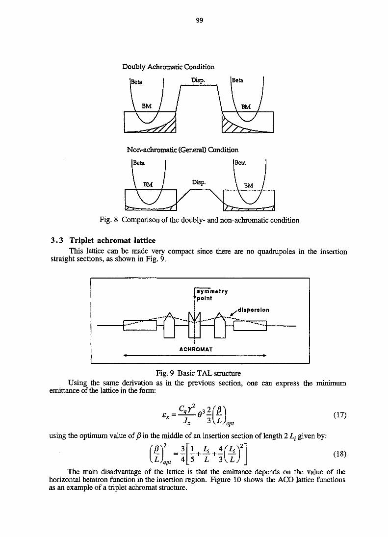
99

Doubly Achromatic Condition

(Beta

Non-achromatic (General) Condition

iBeta I I Beta

BM

Fig. 8 Comparison of the doubly- and non-achromatic condition

3.3 Triplet achromat latticeThis lattice can be made very compact since there are no quadrupoles in the insertion

straight sections, as shown in Fig. 9.

IsymmetryTpolnt

-r-A.dispersion

ACHROMAT

Fig. 9 Basic TAL structureUsing the same derivation as in the previous section, one can express the minimum

emittance of the lattice in the form:

'opt

using the optimum value of fi in the middle of an insertion section of length 2 L; given by:

I) =2LJ,opt

1 Li AfL:- + —+ - —5 L 3\L

(17)

(18)

The main disadvantage of the lattice is that the emittance depends on the value of thehorizontal betatron function in the insertion region. Figure 10 shows the ACO lattice functionsas an example of a triplet achromat structure.

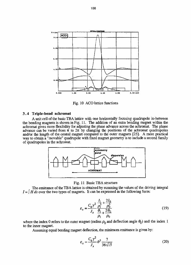
100

Fig. 10 ACO lattice functions

3.4 Triple-bend achromatA unit cell of the basic TBA lattice with one horizontally focusing quadrupole in-between

the bending magnets is shown in Fig. 11. The addition of an extra bending magnet within theachromat gives more flexibility for adjusting the phase advance across the achromat. The phaseadvance can be varied from 7t to 2% by changing the positions of the achromat quadrupolesand/or the length of the central magnet compared to the outer magnets [25]. A more practicalway to obtain a "movable" quadrupole with fixed magnet geometry is to include a second familyof quadrupoles in the achromat.

symmetrypoint

dlsparslon

ACHROMAT

Fig. 11 Basic TBA structureThe emittance of the TBA lattice is obtained by summing the values of the driving integral

= 1 Hds over the two types of magnets. It can be expressed in the following form:

_ 4Caf20n

(19)

Pi P0where the index 0 refers to the outer magnet (radius p 0 and deflection angle 0O) and the index 1to the inner magnet.

Assuming equal bending magnet deflection, the minimum emittance is given by:

C x " " 7 T 36VT5(20)

101

It is obtained for /3 values in the outer bending magnets identical to those of the doublefocusing achromat structure and for fix = L /Vl5 in the inner magnet. Even lower emittancevalues can be obtained by optimising the bending angle distribution. The optimum yields astructure in which the centre deflection angle is 1.5 times larger than the outer deflection angle.

To control the vertical beta function in the bending magnets, vertical focusing can beintroduced either in the form of lumped quadrupoles adjacent to the bending magnet or byintroducing a gradient into the bending magnet fields, as proposed in [26]. This also changesthe damping partition numbers in such a way as to reduce the emittance. Such a solution withcombined function magnets has been adopted in the ALS design (Fig. 12).

OPTICAL FUNCTIONS

0. 000 4. 00

Fig. 12 ALS lattice functions

However, to keep the emittance small, the dispersion in the inner magnet must be reducedto small values which leads to large correcting sextupoles. When compared to the case of adouble focusing achromat lattice with comparable emittance, these sextupoles need to be abouttwo or three times stronger. Such structures are more suitable for small rings where thedeflection angle per bending magnet, and correspondingly the dispersion, is larger.

3.5 FODO structuresAs used in storage rings constructed for high energy physics, a FODO lattice consists of a

sequence of alternating focusing and defocusing quadrupoles separated by bending magnets.The emittance of a regular FODO structure scales as [27]:

(21)

where F (fi^ is a function of the betatron phase advance per cell \ic. The variation ofF(fic)is plotted inFig. 13. The minimum is reached at about \ic - 135° and is rather flat in the range100° <fic < 160°. The large phase advance required to achieve a small emittance implies verystrong focusing.

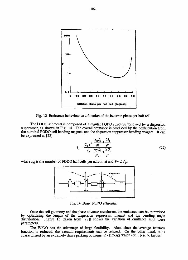
102

0 10 20 30 40 50 60 70 80 90

betatron phase per half cell (degress)

Fig. 13 Emittance behaviour as a function of the betatron phase per half cell

The FODO achromat is composed of a regular FODO structure followed by a dispersionsuppresser, as shown in Fig. 14. The overall emittance is produced by the contribution fromthe nominal FODO cell bending magnets and the dispersion suppresser bending magnet. It canbe expressed as [28]:

(22)

Po P

where no is the number of FODO half cells per achromat and 6 = L/p.

dlsparslon

suppressor

Fig. 14 Basic FODO achromat

Once the cell geometry and the phase advance are chosen, the emittance can be minimisedby optimising the length of the dispersion suppresser magnet and the bending angledistribution. Figure 15 (taken from [28]) shows the variation of emittance with theseparameters.

The FODO has the advantage of large flexibility. Also, since the average betatronfunction is reduced, the vacuum requirements can be relaxed. On the other hand, it ischaracterised by an extremely dense packing of magnetic elements which could lead to layout

103

2-S

2.0 -

1i

1.0

0.6

e , = e ,

Fig. 15 Variation of emittance with length of dispersion suppresser

and engineering problems. Also it suffers from intrinsic problems similar to those of the tripletbend achromat, because of the small dispersion which is required to achieve a low emittanceand leads to large sextupole strengths. The lattice functions of a FODO type structure are givenin Fig. 16.

1 * . •

k

\\

mft n ftw

A

AIIi

AV

Kmm

i

nil• • t i l !•.« • •.« 41. t

Fig. 16 Lattice functions of a FODO type structure

3.6 RACETRACK latticesThe lattices presented in the previous sections are built-up from identical cells and are

characterised by a high degree of symmetry. However, the increasing demand for very longstraight sections to accommodate FELs or long undulators has led to designing RACETRACKlattices. Such designs are being considered for a number of projects [29]. They raise a numberof challenging issues due to the breaking of the symmetry of the lattice, the limited range ofoptical functions, and the need to match these long straight sections to the rest of the latticewhilst keeping a sufficient dynamic aperture. Different technical solutions are proposed: regularcells with missing bending magnets (SPRING8), normal cells replaced by RACETRACK onesand extra quadrupoles to match P values (SOLEIL / DIAMOND). This is sketched inFigure 17.

3.7 Comparison of lattice performancesIt can be seen from the previous sections that the beam emittance of all these lattices scales

as E2(P where E is the beam energy and 6 the bending angle. This means that, in order toachieve a low emittance, the bending angle must be decreased and a large number of cells isneeded. In order to make a comparison of the various types of lattices, it is useful to rewrite theemittance in the following form:

104

(KEY

Regular SPRING-8 Cell

m <&

Racetrack Cell

Hlghp Ordinary Cell

IU as (u

i 3iMta»

OpoU

id , U U ULowp;

8-8-B-B- — -8-0-8Imttin

EHpol.10 mten

Matching Elements in the Racetrack Straight

Fig. 17 A few RACETRACK schemes

F{jix,lattice) (23)

where Nd is the number of bending magnets and E the beam energy (expressed in GeV).

Table 2 lists the minimum values of F which are achievable for the various lattices andgives an example of each lattice case. F is varying over a range of roughly a factor ten from theFODO lattice down to the DFA lattice. But because of the cubic dependence on Nd, even afactor ten can be compensated by a factor of about two in Nd. Thus, to get the same emittancewith a FODO, one has to double the number of bending magnets in the ring. Designconsiderations imply in most cases that the emittance is larger than the minimum value.

Table 2Minimum values of F

DFA

TAL

TBA

FODO(***)

*min

2.35 10-5

2.45 10-5(*)

1.83 10-5

4.52 10-4

Examples

ESRF

ACO

ALSO**)

Energy (GeV)

6

0.536

1.5

Nd

64

8

36

F

5.02 10-5

1.14 10-4

(*) to be multiplied by (p/L )op t

(**) with gradient in the dipoles(***) regular cells without dispersion suppresser

105

The emittance is an important issue when choosing a lattice. However criteria forevaluation of lattices include other considerations, such as chromatic correction and dynamicaperture, sensitivity to errors, flexibility, beam lifetime.... Some of these problems will bediscussed in Section 4.

3.8 Future directions for low emittance latticesThe next generation of lattices will aim at being diffraction limited. In order to achieve

this requirement, several ideas can be explored:i) extrapolation of present designs. As discussed in Section 3.7, present lattices arecharacterised by a large number of cells to obtain a low emittance. Further increase of themachine size [30] could provide the required gain (Table 3).

Table 3Scaling of existing machines

Source type

Hard X-ray (ESRF)

Hard X-ray

VUV

Energy (GeV)

6

6

2

Circumf.(m)

850

1700

850

e (nm.rad)

4

0.5

0.2

ii) design of new models. Several concepts have been proposed [31], [32]. They arebased on the design of regular cells for the minimisation of emittance, followed bymatching sections and straight sections for insertion devices. An example of such designachieving an emittance of 0.5 nanometer-radians for a 3-GeV, 400-m-long machine isshown in Fig. 18.However, the most challenging issue for these future machines lies more in intrinsic

limitations such as intrabeam scattering [33], which could spoil the emittances well before thediffraction limit is reached, rather than in the design of a super low emittance lattice.

-BctaX BeUZ -10'Disp.X

Length [m]

Fig. 18 "Multiple-Bend Achromat"

4. PROBLEMS ASSOCIATED WITH LOW-EMITTANCE LATTICES

4.1 Chromaticity correction and dynamic apertureAchieving such low emittances means that the storage ring will be highly sensitive to non-

linear effects. One of the main problems raised is the correction of chromaticity. The

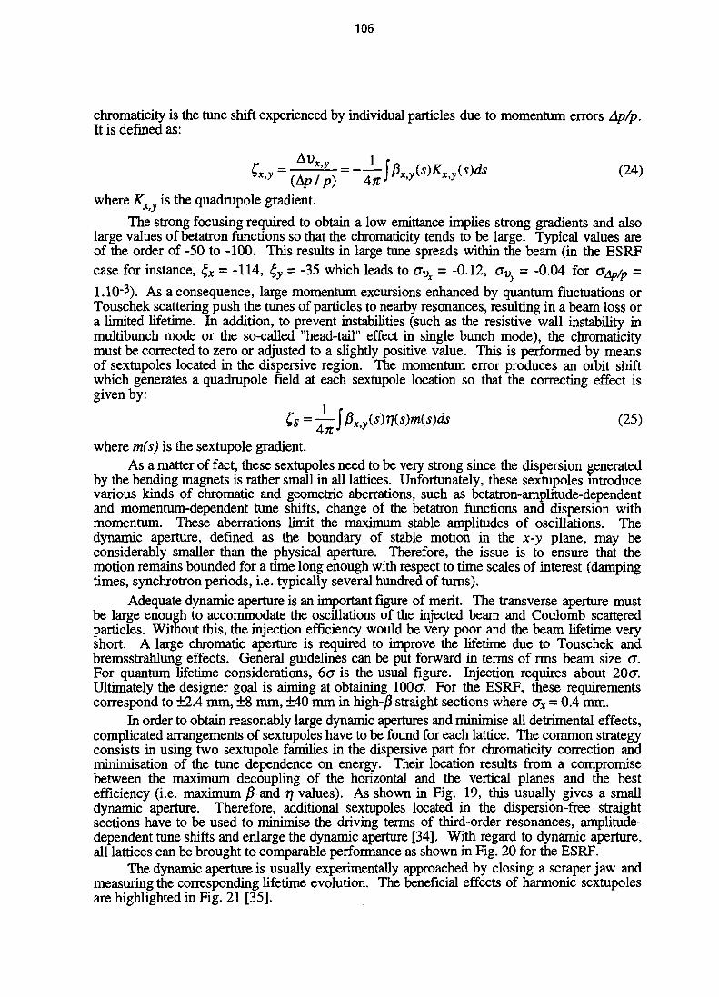
106

chromaticity is the tune shift experienced by individual particles due to momentum errors Ap/p.It is defined as:

fer-^->w^w* (24)where Kx is the quadrupole gradient.

The strong focusing required to obtain a low emittance implies strong gradients and alsolarge values of betatron functions so that the chromaticity tends to be large. Typical values areof the order of -50 to -100. This results in large tune spreads within the beam (in the ESRFcase for instance, %x = -114, %y = -35 which leads to OVx = -0.12, av = -0.04 for (J^p/p =

1.10"3). As a consequence, large momentum excursions enhanced by quantum fluctuations orTouschek scattering push the tunes of particles to nearby resonances, resulting in a beam loss ora limited lifetime. In addition, to prevent instabilities (such as the resistive wall instability inmultibunch mode or the so-called "head-tail" effect in single bunch mode), the chromaticitymust be corrected to zero or adjusted to a slightly positive value. This is performed by meansof sextupoles located in the dispersive region. The momentum error produces an orbit shiftwhich generates a quadrupole field at each sextupole location so that the correcting effect isgiven by:

^S=-^jPx,y(s)rj(s)m(s)ds (25)

where m(s) is the sextupole gradient.As a matter of fact, these sextupoles need to be very strong since the dispersion generated

by the bending magnets is rather small in all lattices. Unfortunately, these sextupoles introducevarious kinds of chromatic and geometric aberrations, such as betatron-amplitude-dependentand momentum-dependent tune shifts, change of the betatron functions and dispersion withmomentum. These aberrations limit the maximum stable amplitudes of oscillations. Thedynamic aperture, defined as the boundary of stable motion in the x-y plane, may beconsiderably smaller than the physical aperture. Therefore, the issue is to ensure that themotion remains bounded for a time long enough with respect to time scales of interest (dampingtimes, synchrotron periods, i.e. typically several hundred of turns).

Adequate dynamic aperture is an important figure of merit. The transverse aperture mustbe large enough to accommodate the oscillations of the injected beam and Coulomb scatteredparticles. Without this, the injection efficiency would be very poor and the beam lifetime veryshort. A large chromatic aperture is required to improve the lifetime due to Touschek andbremsstrahlung effects. General guidelines can be put forward in terms of rms beam size cr.For quantum lifetime considerations, 6<7 is the usual figure. Injection requires about 20<7.Ultimately the designer goal is aiming at obtaining 100<x For the ESRF, these requirementscorrespond to ±2.4 mm, ±8 mm, ±40 mm in high-/? straight sections where ox = 0.4 mm.

In order to obtain reasonably large dynamic apertures and minimise all detrimental effects,complicated arrangements of sextupoles have to be found for each lattice. The common strategyconsists in using two sextupole families in the dispersive part for chromaticity correction andrninimisation of the tune dependence on energy. Their location results from a compromisebetween the maximum decoupling of the horizontal and the vertical planes and the bestefficiency (i.e. maximum /J and t] values). As shown in Fig. 19, this usually gives a smalldynamic aperture. Therefore, additional sextupoles located in the dispersion-free straightsections have to be used to minimise the driving terms of third-order resonances, amplitude-dependent tune shifts and enlarge the dynamic aperture [34]. With regard to dynamic aperture,all lattices can be brought to comparable performance as shown in Fig. 20 for the ESRF.

The dynamic aperture is usually experimentally approached by closing a scraper jaw andmeasuring the corresponding lifetime evolution. The beneficial effects of harmonic sextupolesare highlighted in Fig. 21 [35].

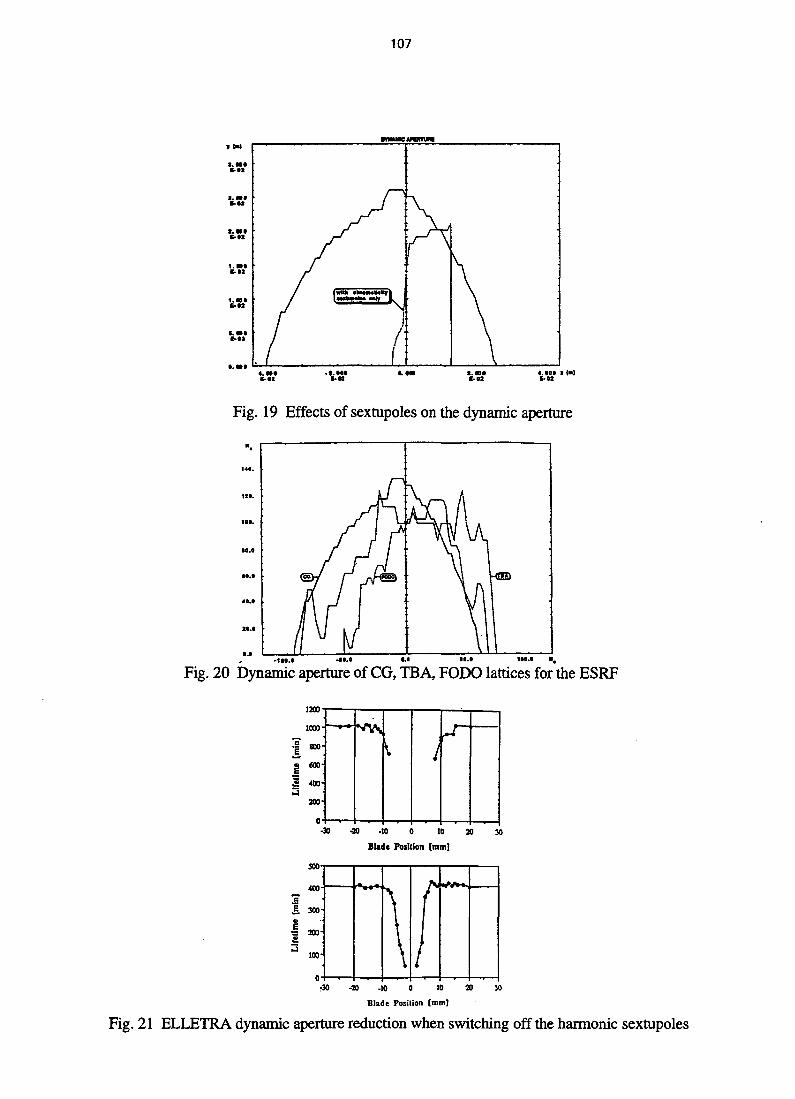
107

Fig. 19 Effects of sextupoles on the dynamic aperture

14S.

120.

100.

•0.0

4S.0

20.0

•••

//IAr J

"V_- A

\CW\A.

M UVllMl

Fig. 20 Dynamic aperture of CG, TBA, FODO lattices for the ESRF

1200

1000

I wog 600'

i£ 4t)0'

200-

— * - • •

1

-30 -20 .10 0 10 29

Blade Position {mm]

30

1

ifetim

i

5W-

400-

300-

200-

100-

o-

>

\

\

\

/ >

I

/r30 -20 -10 30

Blade Position [mm]

Fig. 21 ELLETRA dynamic aperture reduction when switching off the harmonic sextupoles

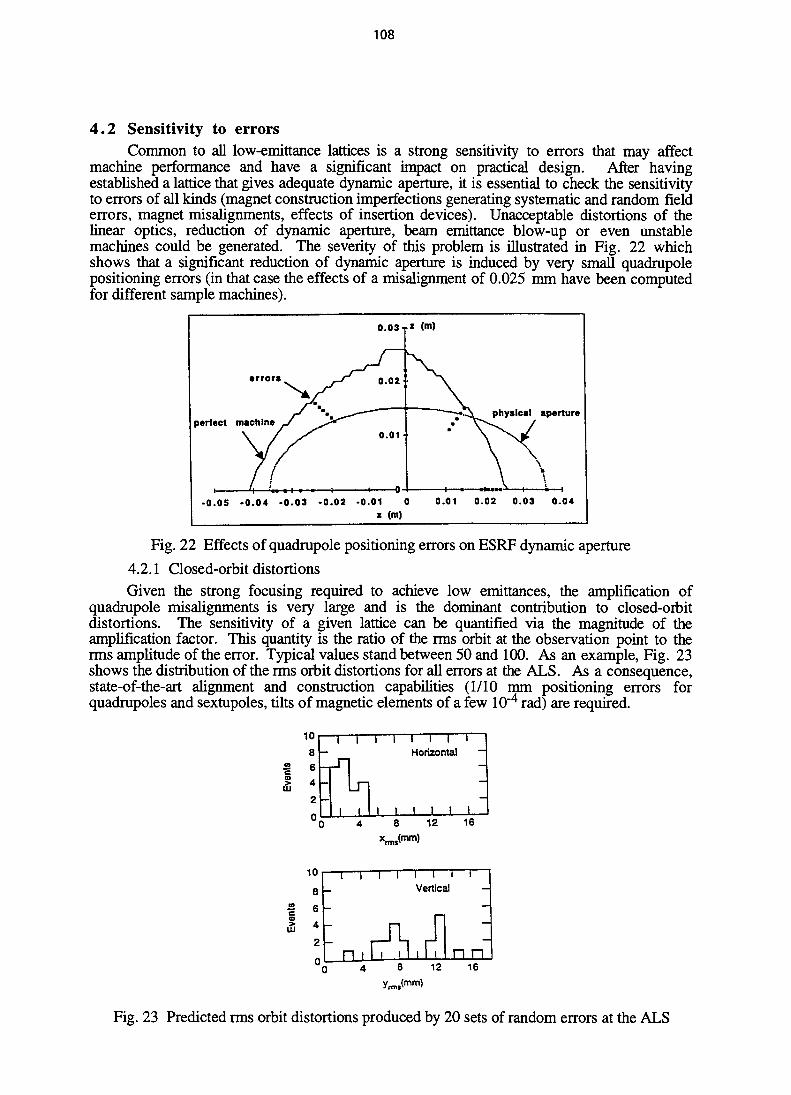
108

4.2 Sensitivity to errorsCommon to all low-emittance lattices is a strong sensitivity to errors that may affect

machine performance and have a significant impact on practical design. After havingestablished a lattice that gives adequate dynamic aperture, it is essential to check the sensitivityto errors of all kinds (magnet construction imperfections generating systematic and random fielderrors, magnet misalignments, effects of insertion devices). Unacceptable distortions of thelinear optics, reduction of dynamic aperture, beam emittance blow-up or even unstablemachines could be generated. The severity of this problem is illustrated in Fig. 22 whichshows that a significant reduction of dynamic aperture is induced by very small quadrupolepositioning errors (in that case the effects of a misalignment of 0.025 mm have been computedfor different sample machines).

error* ^r1

ect machine ,_/ ^2*

If

0.03 i

/

0.02

*•

0.01-

1 0-

z (m)

\ r1 m-

\ physical aperi

•0.05 -0.04 -0.03 -0.02 -0.01 0X (m)

0.01 0.02 0.03 0.04

Fig. 22 Effects of quadrupole positioning errors on ESRF dynamic aperture

4.2.1 Closed-orbit distortionsGiven the strong focusing required to achieve low emittances, the amplification of

quadrupole misalignments is very large and is the dominant contribution to closed-orbitdistortions. The sensitivity of a given lattice can be quantified via the magnitude of theamplification factor. This quantity is the ratio of the rms orbit at the observation point to therms amplitude of the error. Typical values stand between 50 and 100. As an example, Fig. 23shows the distribution of the rms orbit distortions for all errors at the ALS. As a consequence,state-of-the-art alignment and construction capabilities (1/10 mm positioning errors forquadrupoles and sextupoles, tilts of magnetic elements of a few 10"4 rad) are required.

Horizontal -

l l l I12 16

m

bve

10

86

4

2

n

-

- j -

n i L

1 [—T"T 1Vertical

Jl il• i! il i In

_--—

n8 12 16

Fig. 23 Predicted rms orbit distortions produced by 20 sets of random errors at the ALS

109

Since a quite perfect closed orbit (i.e. 0.1 to 0.2 mm rms residual distortions) is necessaryto achieve correct performance, a large number of beam position monitors with an accuracy of0.1 to 0.2 mm and sophisticated closed orbit correction schemes, including dynamic feedbacksystems to control beam stability, must be implemented. Figure 24 shows the residual closedorbit achieved at ELETTRA [35] by a global correction using the most effective corrector andbump methods. At the ESRF, rms orbits in the 80 (xm range are routinely obtained with a SVDcorrection scheme [36].

Fig. 24 Closed orbit after correction at ELETTRA

4.2.2 Focusing errorsThese are mainly induced by random gradient errors in quadrupoles and horizontal

mispositioning of sextupoles. They result in:i) the excitation of resonances and stop-bands, limiting the allowed region in the tune

diagram and resulting in a reduction of the lifetime

a modulation of /3-functions, thus spoiling the horizontal emittancea reduction of the dynamic aperture (Fig. 25)

ii)iii)

ESRF<DGUGL>=1E-3

0.03 TZ (m)

no errors

phys. apart.

• 0.05

—H «

• 0.04 -0.03 0.02 0.03 0.04

Fig. 25 Dynamic aperture reduction with random gradient errors

As a consequence, tolerances on quadrupole gradients in the 1.0 10~3 range are generallyrequired, which implies tight mechanical tolerances on bore radius and pole assembly, accuratemagnetic measurements, and sorting procedures before installation in the ring. In addition, thecorrection of quadrupolar resonances proves to be very valuable for optimising machineperformance. At least one pair of correctors per resonance is needed. Figure 26 illustrates the

110

beneficial effects of the correction of the half-integer stop-bands close to the tune in the ESRFcase, with the subsequent enlargement of the longitudinal acceptance which in turn contributesto the increase of lifetime. This feature is of prime importance for low energy machines forwhich the Touschek effects, linked to an insufficient acceptance in energy, plays a major role.

MM 36.10 36.15 36.20 36JS 36J0 3&3S 35.40 M.45 » . »

Fig. 26 Chromatic tune variation around a few ESRF working points

4.2.3 EmittancesLow emittances are one of the main figures of merit of the third generation of synchrotron

light sources. However the achievement of the expected emittances can be spoilt by manyfactors.i) Blow up of the horizontal emittance due to the proximity of quadrupolar resonances

and/or an imperfect closed orbit. Around integer values of vx, the emittance is sensitiveto both closed orbit errors and focusing errors, whilst, around half integer values of vx,the effect of closed orbit errors is negligible. The influence of these two sources is shownfor the ESRF in Figs. 27 and 28.

60% T

50% -

40% -

30% -

20%

10%

0%0.1 0.2 0.3 0.4

Fractional part of the horizontal tune

0.5

Fig. 27 Emittance evolution versus tune

111

KertzenSoi esstftgaoe

t [naisad)S 0 T 1-J

o.s

0.8

a. 4

0,2

ft.XSB

Vertical ORtlttanoa

: \

0

—-4

BOO

Fig. 28 Emittance blow-up with imperfect closed orbitii) The vertical emittance, which is null in an ideal machine, is generated by several sources

of imperfections in a real machine: radiation in the presence of spurious vertical dispersiondue to dipole and quadrupole rotation errors or closed orbit in quadrupoles andsextupoles, coupling of horizontal and vertical betatron oscillations due to skewquadrupole field errors. As already mentioned in Section 2.1, the vertical emittance isgenerally characterised via the coupling:

K = ^- (27)£x

Most target specifications aim at a natural figure of 10 % which could be decreased below1 % after correction. The correction strategy consists in powering skew quadrupoles to correctthe coupling resonances close to the working point and/or the spurious vertical dispersion, thenin deducing the beam emittances from beam size measurements by imaging the radiation.Depending on the lattice, the influence of the spurious dispersion on the emittance is more orless important as shown in Eq. 27 and Fig. 29 [35].

(28)x0

— 3Eu

.aS

i© e

• " 5

•

+

9

o cms& 9.13

0-6 0.8

Fig. 29 Comparison of several machines in terms of spurious dispersion

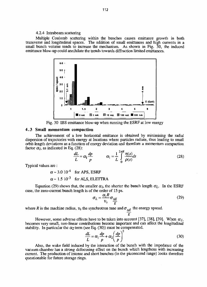
112

4.2.4 Intrabeam scatteringMultiple Coulomb scattering within the bunches causes emittance growth in both

transverse and longitudinal spaces. The addition of small emittances and high currents in asmall bunch volume tends to increase the mechanism. As shown in Fig. 30, the inducedemittance blow-up could annihilate the trends towards diffraction limited emittances.

60

50

8 4 0

^ 3 0

8" 20

10

o -Iy

1

£

1.5 2 3 4 5

l o m A B i m A • 10 mA 23 100 mA • 500 mA

r E (GeV)

6

Fig. 30 CBS emittance blow-up when running the ESRF at low energy

4.3 Small momentum compactionThe achievement of a low horizontal emittance is obtained by minimising the radial

dispersion of trajectories with energy at locations where particles radiate, thus leading to smallorbit-length deviations as a function of energy deviation and therefore a momentum compactionfactor cci, as indicated in Eq. (28):

dL dp 1 ? 770), ,nn^— = a, — a, = — \ -^^ds (28)

Typical values are:

a - 3 . 0 10"4 for APS, ESRF

a ~ 1.5 10"3 for ALS, ELETTRA

Equation (29) shows that, the smaller a;, the shorter the bunch lengthcase, the zero-current bunch length is of the order of 15 ps.

In the ESRF

(29)

where R is the machine radius, vs the synchrotron tune and a^ the energy spread.

~E

However, some adverse effects have to be taken into account [37], [38], [39]. When ocj,becomes very small, non-linear contributions become important and can affect the longitudinalstability. In particular the <X2 term (see Eq. (30)) must be compensated.

(30)

Also, the wake field induced by the interaction of the bunch with the impedance of thevacuum chamber has a strong defocusing effect on the bunch which lengthens with increasingcurrent. The production of intense and short bunches (in the picosecond range) looks thereforequestionable for future storage rings.

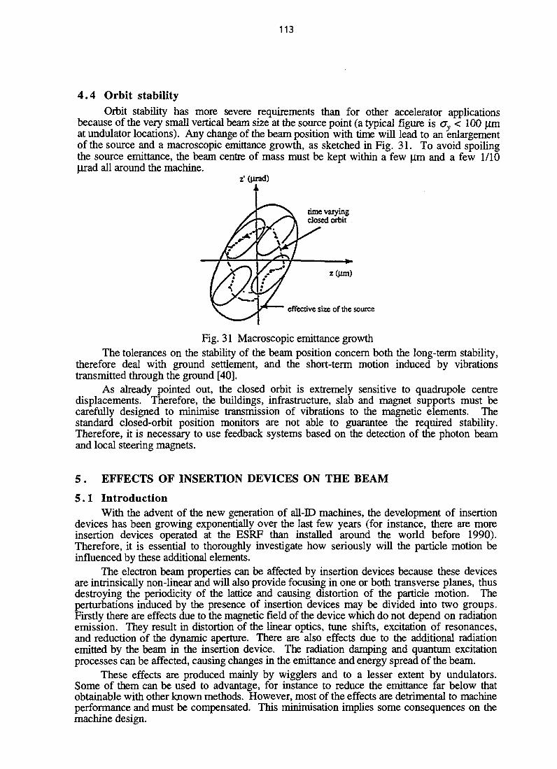
113

4.4 Orbit stabilityOrbit stability has more severe requirements than for other accelerator applications

because of the very small vertical beam size at the source point (a typical figure is ay< 100 \imat undulator locations). Any change of the beam position with time will lead to an enlargementof the source and a macroscopic emittance growth, as sketched in Fig. 31. To avoid spoilingthe source emittance, the beam centre of mass must be kept within a few \im and a few 1/10(irad all around the machine.

time varyingclosed orbit .

effective size of the source

Fig. 31 Macroscopic emittance growthThe tolerances on the stability of the beam position concern both the long-term stability,

therefore deal with ground settlement, and the short-term motion induced by vibrationstransmitted through the ground [40].

As already pointed out, the closed orbit is extremely sensitive to quadrupole centredisplacements. Therefore, the buildings, infrastructure, slab and magnet supports must becarefully designed to minimise transmission of vibrations to the magnetic elements. Thestandard closed-orbit position monitors are not able to guarantee the required stability.Therefore, it is necessary to use feedback systems based on the detection of the photon beamand local steering magnets.

5 . EFFECTS OF INSERTION DEVICES ON THE BEAM

5.1 IntroductionWith the advent of the new generation of all-ID machines, the development of insertion

devices has been growing exponentially over the last few years (for instance, there are moreinsertion devices operated at the ESRF than installed around the world before 1990).Therefore, it is essential to thoroughly investigate how seriously will the particle motion beinfluenced by these additional elements.

The electron beam properties can be affected by insertion devices because these devicesare intrinsically non-linear and will also provide focusing in one or both transverse planes, thusdestroying the periodicity of the lattice and causing distortion of the particle motion. Theperturbations induced by the presence of insertion devices may be divided into two groups.Firstly there are effects due to the magnetic field of the device which do not depend on radiationemission. They result in distortion of the linear optics, tune shifts, excitation of resonances,and reduction of the dynamic aperture. There are also effects due to the additional radiationemitted by the beam in the insertion device. The radiation damping and quantum excitationprocesses can be affected, causing changes in the emittance and energy spread of the beam.

These effects are produced mainly by wigglers and to a lesser extent by undulators.Some of them can be used to advantage, for instance to reduce the emittance far below thatobtainable with other known methods. However, most of the effects are detrimental to machineperformance and must be compensated. This minimisation implies some consequences on themachine design.

114

5.2 Matching to insertion requirementsBefore installing insertion devices in a ring, the question of determining the values of the

fi functions that maximise the performance of the devices has to be considered. Generally thechoice of /? is a compromise between the machine and users' requirements. If one concentrateson the machine side, small (3 values are preferable for the following reasons:i) minimisation of closed orbit displacements when varying the gap;ii) minimisation of the volume occupied by the beam in the straight sections, allowing

therefore to further decrease the insertion device gap without detrimental effects on thelifetime as illustrated in Fig. 32.

iii) maximizing the brilliance with matching the electron beam emittances to the photon beam.The users' requirements are somewhat mixed. In the undulator straight section, one

generally wants to minimise the inhomogeneous broadening which occurs mainly through theangular spread. Ideally one would like to have:

Px,y>ex>y*f (30)where A is the radiation wavelength and L/p is the length of the undulator. This corresponds torather large B values. For wigglers, the figure of merit is the obtention of maximum brilliance.This calls for low values of B.

60 T

50 •

£ 4 0 +

30

20

10

0aperture (mm)

- i 1

10 12

bz=12 m bzs2.5 m

Fig. 32 Comparison of lifetime versus gap for two By values

In any case, lattice flexibility is an extremely important issue. A high periodicityconfiguration (with intermediate B values in all straight sections) is probably easier for thedesigner to achieve. However, the lattice should be able to accommodate a variable number ofundulators and wigglers and provide B adjustment capability.

5.3 Magnetic-field effectsThe basic requirement of an insertion device is that, after passing through it, the beam

should return to its nominal orbit. If this is not the case, a closed orbit will be set up, givingbeam displacements around the machine and thus perturbing other beam lines. To first order,this requirement is fulfilled by making the field distribution symmetrical about the midpoint ofthe device and by adjusting the integrated field length to zero. Taking the ESRF as an example,maintaining the closed orbit rms deviation below 1/10 of the beam size would require that theintegral of the vertical (horizontal) magnetic field along the axis of propagation be smaller than8 1(>S T.m (4 10'5 T.m) for a single insertion device. Very precise magnetic field measurementsare necessary to fulfil these specifications. The alternative solution is to provide independent

115

adjustment of the integral of the field by end coils. These tight tolerances can be fulfilled inpractice as shown in Fig. 33 [41] where the closed orbit distortions induced by ESRF ID gapclosing are interpreted in terms of rms size or divergence growth normalised to the electronbeam size or divergence.

1 . 4

1 • •

0.851 0.6

I0.4

0.2

0

tolerance In the vertical plane

tolerance In the horizontal plane

JJJ idjnjLiJ. iijd« 1^^ •h.

Fig. 33 Closed-orbit distortions induced by IDs

5.4 Linear and non-linear effects on beam dynamics

5.4.1 Equations of motionAssuming a sinusoidal field variation, the analytical treatment of the effects of insertion

devices on beam dynamics has been developed [42, 43]. We recall here the main steps of theprocedure based on the use of Hamiltonian formalism.

The components of the insertion device magnetic field used for the derivation of equationsof motion are as follows:

Bx=—BrX i I

By = (31)

k i \= BQ cosh(^;c)sinh(fc.yy)sin(fcz)

ky

with

(32)

where X is the period length of the insertion device and Bo is its magnetic field. The parameterkx measures the transverse variation of the field due to the limited pole width or curved polefaces. Here x is the horizontal direction, y the vertical one and z is the beam direction. Theabove formula which keep only the first harmonics of the field variation in the z-direction,satisfy the Maxwell equations. A more accurate field treatment would be required for largedeviations from the axis.

The Hamiltonian of the motion can be written in the following form:

+ [Px - Ax sm(kz)f + [py-Ay sin(fe)]2 J (33)H = i

where

Ax =—kp

(34)

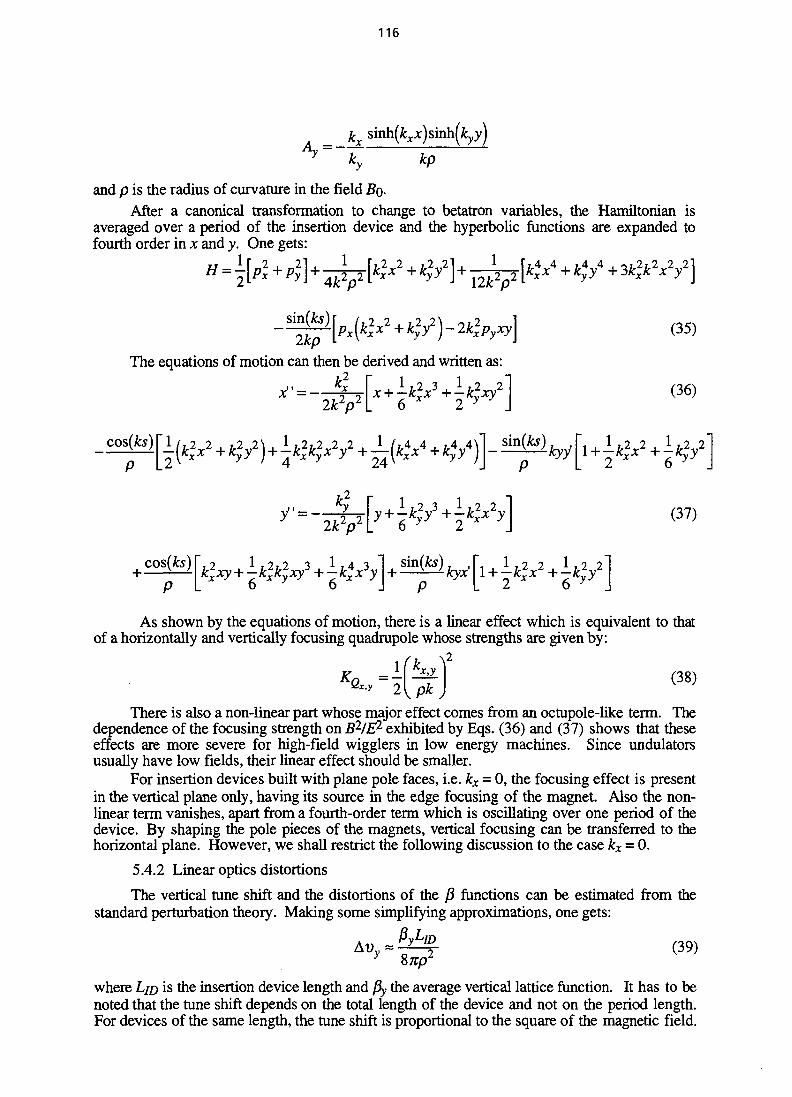
116

Ay--—

and p is the radius of curvature in the field Bo-After a canonical transformation to change to betatron variables, the Hamiltonian is

averaged over a period of the insertion device and the hyperbolic functions are expanded tofourth order in x and v. One gets:

The equations of motion can then be derived and written as:

2k2p

( 3 7 )

As shown by the equations of motion, there is a linear effect which is equivalent to thatof a horizontally and vertically focusing quadrupole whose strengths are given by:

Ko =-[-££•] (38)Qx-y i{pk)

There is also a non-linear part whose major effect comes from an octupole-like term. Thedependence of the focusing strength on B2I& exhibited by Eqs. (36) and (37) shows that theseeffects are more severe for high-field wigglers in low energy machines. Since undulatorsusually have low fields, their linear effect should be smaller.

For insertion devices built with plane pole faces, i.e. kx - 0, the focusing effect is presentin the vertical plane only, having its source in the edge focusing of the magnet. Also the non-linear term vanishes, apart from a fourth-order term which is oscillating over one period of thedevice. By shaping the pole pieces of the magnets, vertical focusing can be transferred to thehorizontal plane. However, we shall restrict the following discussion to the case kx = 0.

5.4.2 Linear optics distortions

The vertical tune shift and the distortions of the /? functions can be estimated from thestandard perturbation theory. Making some simplifying approximations, one gets:

where LJD is the insertion device length and py the average vertical lattice function. It has to benoted that the tune shift depends on the total length of the device and not on the period length.For devices of the same length, the tune shift is proportional to the square of the magnetic field.

117

Thus, high-field devices are expected to present stronger linear distortions than those withlower fields and shorter periods. This is illustrated in Fig. 34.

0.05-

0.00-9

Wiggler Field CD

Fig. 34 Tune shifts induced by the 5 T SCW at SRS [44]A consequence of this change in tune is a shift of the working point which might

approach intrinsic resonances and be troublesome. From Eq. (39), one sees that the tune shiftis directly proportional to the vertical /3 value at the insertion device. Hence the tune shift can beminimised by locating wigglers in a straight section where the vertical /J is small. It wasmentioned previously that it is preferable to have high j3 for undulators. Therefore the latticeshould be able to accommodate these two different kinds of insertion straight sections.

The distortions of the ft functions are given by:

(40)

Table 4 gives some numerical examples computed for various machines. An example of /?-functions modulation is shown in Fig. 35 [45].

Table 4Linear optics distortions generated by insertion devices

Machine

VEPP-3

VEPP-2M

SUPERACO

ALS

ELETTRA

SRS

PF

ESRF

APS

Energy(GeV)

0.35

0.7

0.8

1.5

2

2

2.5

6

7

Type ofdevice

U

W

Uwuwuwuwuwuu

B(T)

0.6

8

0.4951.1551.250.331.50.451.250.630.65

Lro(m)

7

0.6

3.2

1.964.835.5

1

3.183.63265

A (cm)

10

12

12.8

149

305.5

10

106105.5

2.2

/Jy(m)

51

4.8

44

2.62.6

7.34.8

12.812.83.513

10

Avy

0.35

0.5

0.04

0.350.042

0.150.035

0.050.005

0.0520.005

0.0010.003

0.0015

-

-

-

390

80

20

414

1.31.8-

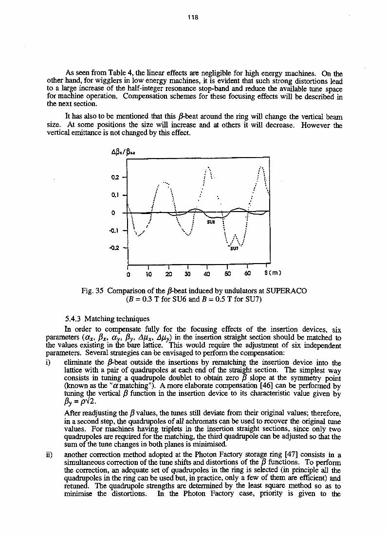
118

As seen from Table 4, the linear effects are negligible for high energy machines. On theother hand, for wigglers in low energy machines, it is evident that such strong distortions leadto a large increase of the half-integer resonance stop-band and reduce the available tune spacefor machine operation. Compensation schemes for these focusing effects will be described inthe next section.

It has also to be mentioned that this j8-beat around the ring will change the vertical beamsize. At some positions the size will increase and at others it will decrease. However thevertical emittance is not changed by this effect.

A(3t/j3z3

02 -

0.1 -

•0.1 -

-0.2 -

, /

\ /\

r— i3 10

\

\ •

1 120 30

/ \

VSU6

1

40

1 *,

V -;

\ A /

1 I i50 60 S(

Fig. 35 Comparison of the j3-beat induced by undulators at SUPERACO(B = 0.3 T for SU6 and B = 0.5 T for SU7)

5.4.3 Matching techniquesIn order to compensate fully for the focusing effects of the insertion devices, six

parameters (ccx, Px, 0Cy, Py, A/J.x, Afiy) in the insertion straight section should be matched tothe values existing in the bare lattice. This would require the adjustment of six independentparameters. Several strategies can be envisaged to perform the compensation:i) eliminate the j5-beat outside the insertions by rematching the insertion device into the

lattice with a pair of quadrupoles at each end of the straight section. The simplest wayconsists in tuning a quadrupole doublet to obtain zero /J slope at the symmetry point(known as the "a matching"). A more elaborate compensation [46] can be performed bytuning the vertical B function in the insertion device to its characteristic value given byP = pl2

ii)

After readjusting the /? values, the tunes still deviate from their original values; therefore,in a second step, the quadrupoles of all achromats can be used to recover the original tunevalues. For machines having triplets in the insertion straight sections, since only twoquadrupoles are required for the matching, the third quadrupole can be adjusted so that thesum of the tune changes in both planes is minimised.another correction method adopted at the Photon Factory storage ring [47] consists in asimultaneous correction of the tune shifts and distortions of the j3 functions. To performthe correction, an adequate set of quadrupoles in the ring is selected (in principle all thequadrupoles in the ring can be used but, in practice, only a few of them are efficient) andretuned. The quadrupole strengths are determined by the least square method so as tominimise the distortions. In the Photon Factory case, priority is given to the

119

compensation of tune shifts which is a more stringent requirement than the correction ofP's for machine operation. However distortions of betatron functions can be reducedfrom 40% to less than 5%.However, whatever the rematching procedure, in most cases the change in quadrupolestrengths could be rather large (more than 10% of the nominal values). In addition thequadrupoles should be individually powered to take care of the different types of insertiondevices in the various straight sections.

5.4.4 Effects on dynamic apertureOne of the major detrimental aspects of the installation of insertion devices is the resulting

reduction of dynamic aperture. There are two effects of the insertion device that cause thisdeterioration:

i) introduction of non-linearities leading to enhancement of the amplitude-dependent tuneshifts and distortion of phase space. It can be seen from the Hamiltonian given in Eq. (35) that,due to the non-linear field components, resonances can occur at integer values of 3 vx,vx + 2vy, 4 vx, 4 vy and 2 vx + 2 vy (if kx * 0). Analytical calculations of the amplitude-dependent tune shifts, stop-band widths and island widths have been performed [51]. The non-linear tune shifts (at half physical aperture) have been computed in Table 5 for some insertiondevices. From these results, it can be expected that the non-linear fields will produce significanteffects at large betatron amplitudes, more especially for low energy machines. These effects arealso illustrated in Fig. 36 [48] and in Fig. 37 [45].

Table 5Non-linear tune shifts

Energy (GeV)

Av

LBL U9.0

1.50.005

BNL-VUVwiggler

0.75

0.007

SPEAR54 poles

3< 0.001

FRASCATIundulator

0.60.01

APS

70.0007

(mm)4.000

3.000

2.000

1.000

0. 000

•1.000

-2.000

• 3.000

•4.000

I - Z'

'• ' i .• . ' • • * - r

- . . . * *. . . __

* . \ . m f

* *• * * T• ** . •

* #•• • *. . . . . * . 7

•

•

. • * * ••

• • ' • " "

. V , : • ' - • : - -

*'. .- ** * •

' : ' . . • •

• : . • " • • •

•

•

• 4.000 • 2.000 2.000 4. 000 z (mm)

Fig. 36 Vertical phase space trajectories showing the distortion of phase spaceand occurrence of islands

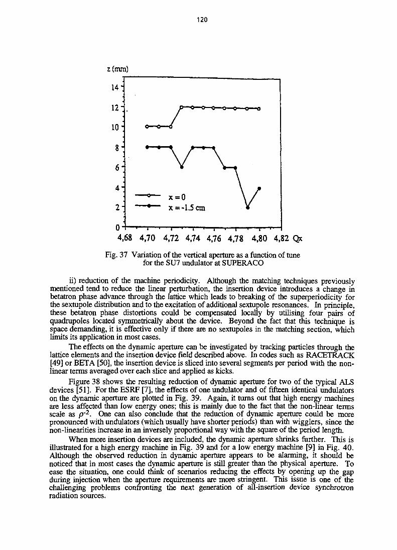
120

z(mm)

14-

2-

04,68 4,70 4,72 4,74 4,76 4,78 4,80 4,82 Qx

Fig. 37 Variation of the vertical aperture as a function of tunefor the SU7 undulator at SUPERACO

ii) reduction of the machine periodicity. Although the matching techniques previouslymentioned tend to reduce the linear perturbation, the insertion device introduces a change inbetatron phase advance through the lattice which leads to breaking of the superperiodicity forthe sextupole distribution and to the excitation of additional sextupole resonances. In principle,these betatron phase distortions could be compensated locally by utilising four pairs ofquadrupoles located symmetrically about the device. Beyond the fact that mis technique isspace demanding, it is effective only if there are no sextupoles in the matching section, whichlimits its application in most cases.

The effects on the dynamic aperture can be investigated by tracking particles through thelattice elements and the insertion device field described above. In codes such as RACETRACK[49] or BETA [50], the insertion device is sliced into several segments per period with the non-linear terms averaged over each slice and applied as kicks.

Figure 38 shows the resulting reduction of dynamic aperture for two of the typical ALSdevices [51]. For the ESRF [7], the effects of one undulator and of fifteen identical undulatorson the dynamic aperture are plotted in Fig. 39. Again, it turns out that high energy machinesare less affected than low energy ones; this is mainly due to the fact that the non-linear termsscale as p~2. One can also conclude that the reduction of dynamic aperture could be morepronounced with undulators (which usually have shorter periods) than with wigglers, since thenon-linearities increase in an inversely proportional way with the square of the period length.

When more insertion devices are included, the dynamic aperture shrinks further. This isillustrated for a high energy machine in Fig. 39 and for a low energy machine [9] in Fig. 40.Although the observed reduction in dynamic aperture appears to be alarming, it should benoticed that in most cases the dynamic aperture is still greater than the physical aperture. Toease the situation, one could think of scenarios reducing the effects by opening up the gapduring injection when the aperture requirements are more stringent. This issue is one of thechallenging problems confronting the next generation of all-insertion device synchrotronradiation sources.

121

WTGGLERW13.fiX , - 13.6 em. N - 16 pwiodt. Bo - Z07 TCo - 3.1 kaV

4 8 tZ 16x (mm)

UNDULATOR U 3.6S\ - 3.65 cm. N - 134 periods. Bo -0.61 TK-Z10

20 24

20 240 4 B 12 16

x (mm)Fig. 38 Effects of insertion devices on ALS dynamic aperture

1 0 0 M,

Fig. 39 Effects of undulators on ESRF dynamic aperture

30

AMP-X

Fig. 40 Effects of undulators on ELETTRA dynamic aperture

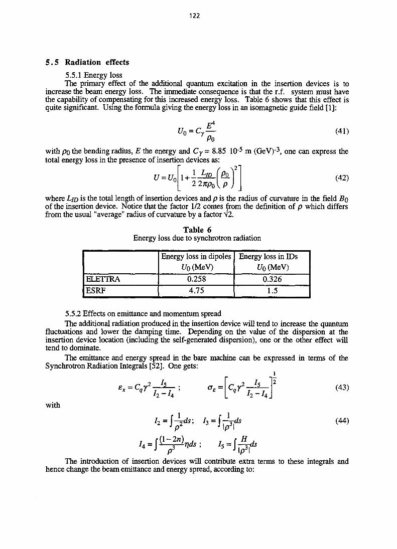
122

5.5 Radiation effects

5.5.1 Energy lossThe primary effect of the additional quantum excitation in the insertion devices is to

increase the beam energy loss. The immediate consequence is that the r.f. system must havethe capability of compensating for this increased energy loss. Table 6 shows that this effect isquite significant. Using the formula giving the energy loss in an isomagnetic guide field [1]:

E4

—Po

(41)

with po the bending radius, E the energy and Cy - 8.85 10'5 m (GeV)"3, one can express thetotal energy loss in the presence of insertion devices as:

= Ur 22xpo{p(42)

where LJD is the total length of insertion devices and p is the radius of curvature in the field Boof the insertion device. Notice that the factor 1/2 comes from the definition of p which differsfrom the usual "average" radius of curvature by a factor ^2.

Table 6Energy loss due to synchrotron radiation

ELETTRA

ESRF

Energy loss in dipolesU0 (MeV)

0.258

4.75

Energy loss in IDsUo (MeV)

0.326

1.5

5.5.2 Effects on emittance and momentum spreadThe additional radiation produced in the insertion device will tend to increase the quantum

fluctuations and lower the damping time. Depending on the value of the dispersion at theinsertion device location (including the self-generated dispersion), one or the other effect willtend to dominate.

The emittance and energy spread in the bare machine can be expressed in terms of theSynchrotron Radiation Integrals [52]. One gets:

1

U-U u-uwith

(43)

(44)

H

The introduction of insertion devices will contribute extra terms to these integrals andhence change the beam emittance and energy spread, according to:

123

TID

1 + 1+-

e =1+

jID TID

1+-JID

9 7°

TID(45)

where the index 0 indicates the contribution of the storage ring without insertion devices and theindex ID the contribution from insertion devices alone.

The calculations of the insertion device integrals are performed, assuming a sinusoidalvariation of the field along the axis of propagation z, for an insertion device characterised by Nperiods of wavelength X and bending radius p. The 14 and 15 terms correspond to additionalcontributions arising from a non-vanishing dispersion function in the straight sections. The 14adds directly to I4. For is, the combination is more complicated; when the self-generateddispersion from the insertion device is negligible, 15 will be the dominant term.

XN 4XN(46)

TID-

rID5

3X3N

f 3 3 115K 16 J

AD _4 "

<Y>LID9X3

407i4p5T

<cc>L[DLi

ID

where < > stands for the average of a, ft, y in the device of length LJD and the index 0 refers tothe entrance of the device.

The emittance behaviour can be rewritten in a simplified way, due to the fact that the I4contribution from the insertion device is usually small and the third term in I5 is the dominantpart. Furthermore, we will assume that the I4 contribution of the bare machine can be neglectedwhen compared to I2. We get now:

1 + "ID

e =e°-

P .

4 L2n:p0 \_ p (47)

The insertion device radiation always contributes to the damping term in the denominatorof Eq. (47). The change in the horizontal emittance depends on the relative values of thechromatic invariant. Since the dispersion generated by undulators is usually very small,quantum excitation will be much smaller than the damping effect and the cancellation of energydamping by the increase in quantum fluctuations would occur at high fields. Therefore for allcases of interest, there is a reduction of emittance due to the inclusion of undulators. On theother hand, in low energy machines containing high field wigglers, the self-generateddispersion is dominant and leads to an increase in emittance which could be prohibitive. Theseconclusions are illustrated in Fig. 41 which shows the emittance behaviour as a function of theinsertion device field in two storage rings for typical sets of insertion devices:

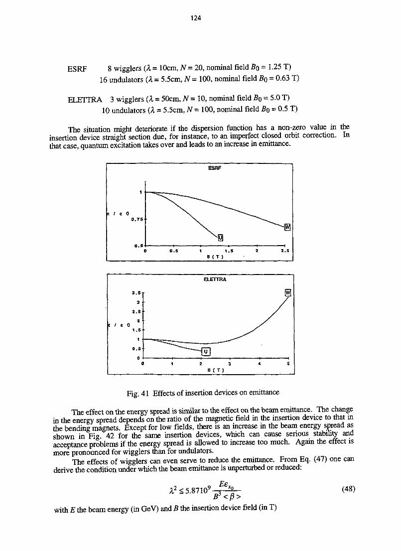
124

ESRF 8 wigglers (A = 10cm, N = 20, nominal field Bo = 1-25 T)16 undulators (A = 5.5cm, N = 100, nominal field Bo = 0.63 T)

ELETTRA 3 wigglers (A = 50cm, N = 10, nominal field Bo = 5.0 T)10 undulators (A = 5.5cm, N = 100, nominal field Bo = 0.5 T)

The situation might deteriorate if the dispersion function has a non-zero value in theinsertion device straight section due, for instance, to an imperfect closed orbit correction. Inthat case, quantum excitation takes over and leads to an increase in emittance.

3.5i

3

2 .5

2e / e 0

1.5

1

0.5

0C

ELETTRA

1 2 38 ( T )

/

/

y4 S

Fig. 41 Effects of insertion devices on emittance

The effect on the energy spread is similar to the effect on the beam emittance. The changein the energy spread depends on the ratio of the magnetic field in the insertion device to that inthe bending magnets. Except for low fields, there is an increase in the beam energy spread asshown in Fig. 42 for the same insertion devices, which can cause serious stability andacceptance problems if the energy spread is allowed to increase too much. Again the effect ismore pronounced for wigglers than for undulators.

The effects of wigglers can even serve to reduce the emittance. From Eq. (47) one canderive the condition under which the beam emittance is unperturbed or reduced:

A2<5.87109Ee

(48)

with E the beam energy (in GeV) and B the insertion device field (in T)

125

1.25

1 .2

l.tS

a 1 a 0 1.1

1.05

1

0.95(

ESRF

m

A /

I 0.5 1 1.5 2 2.58 ( T )

1 . 5

1.4

1.3a 1 a 0

t.2

1.1

1

0 . 9

ELETTRA

) 1 2 3 4 S8 ( T )

Fig. 42 Effects of insertion devices on momentum spread

The period of the device 1 must not exceed the value determined by Eq. (48) in order toobtain a reduced emittance. The installation of appropriate damping wigglers was proposedrecently at PEP [3]. It would require the use of wigglers with a maximum field of 1.26 T and aperiod length of 12 cm. The resulting theoretical emittance is shown in Fig. 43 as a function ofthe total installed wiggler length.

50 100 150Total length of damping wigglers (m)

Fig. 43 PEP emittance as a function of the total wiggler lengthSimilar results could be obtained for the new synchrotron light sources under construction

like the ESRF or the APS. Using the proposed insertion devices for the ESRF (for instancesixteen wigglers, 2 m in length and with a 2 T field), an emittance reduction by a factor of abouttwo could be achieved.

This method is applicable to any storage ring. However, since the damping effect scalesproportionally with the bending radius of the ring magnets, it is easier to reduce the emittance

126

with damping wigglers in large storage rings than in small ones. Such a method of reducing theemittance looks promising; but some adverse effects (heat load due to the intense radiation, r.f.system capability..) have still to be solved. Obviously, the space required for installing thesedevices creates sever constraints. The success of the emittance reduction also depends onfurther investigations on the effects on dynamic aperture, the limitations due to non-zerodispersion at the wiggler location, Touschek effect and intrabeam scattering.

6 . CONCLUSIONSLattice design for synchrotron light sources has followed the dramatic evolution of

performances of these machines. A few years ago, it was feared that the lattices proposed forthird generation light sources would be oversensitive and very difficult to commission. Sincethen, several sources have been commissioned with their design lattice and have reached oreven gone beyond their target performances. Many others, with different lattices, are in theprocess of being tested or are in the construction phase. The next problem to address todesigners is that of diffraction limited lattices.

REFERENCES

[ 1 ] M. Sands, The Physics of Electron Storage Rings, SLAC-121 (1970)

[2] H. Bruck, Accelerateurs Circulaires de Particules (PUF, Paris, 1966)

[3] H. Wiedemann, An Ultra-Low Emittance Mode for PEP Using Damping Wigglers, Nucl.Instr. Meth. A266 (1988)

[4] R. Chasman and K. Green, Preliminary Design of a Dedicated Synchrotron RadiationFacility, IEEE Trans. Nucl. Sci., NS-22, 1765 (1975)

[5] L. Blumberg et al., National Synchrotron Light Source VUV Storage Ring, IEEE Trans.Nucl. Sci., NS-26, 3842 (1979)

[6] H. Zyngier et al., The VUV Radiation Source SUPERACO, IEEE Trans. Nucl. Sci., NS-37, 3371 (1985)

[7] ESRF Foundation Phase Report (Feb. 1987)

[8] 6 GeV Conceptual Design Report (Feb 1986), ANL-86-8

[9] Design Study for the Trieste Synchrotron Light Source (Feb. 1987), LNF-87/6

[10] Proceedings of the 1991 Particle Accelerator Conference, San Francisco (1991), p 2646

[11] E. Jaeschke et al., Lattice Design for the 1.7 GeV Light Source BESSY2, Proceedings ofthe 1993 Particle Accelerator Conference, Washington (1993), p 1474

[12] Projet SOLEEL, Etude Technique, LURE, Jan. 1994

[13] Proc. of the 5th Int. Conf. on High Energy Accelerators, Frascati (1965)

[14] E. Rowe et al., Status of the Aladdin Project, IEEE Trans. Nucl. Sci., NS-28, 3145(1985)

[15] D. Einfeld and G. Miilhaupt, Choice of the Principal Parameters and Lattice of BESSY,Nucl. Instr. Meth. 172 (1980)

127

[16] 1-2 GeV Synchrotron Radiation Source, Conceptual Design Report (July 1986), LBLPub 5172

[17] SRRC Design Handbook, SRRC, Apr. 1989

[18] Design Report of Pohang Light Source, Pohang Accelerator Laboratory, POSTECH, Jan.1992

[19] Proceedings of the Workshop on Target Specifications for Storage Ring SynchrotronRadiation Light Sources and Means of Achieving Them, Grenoble (Oct. 1993)

[20] G.E. Fisher et al., A 1.2 GeV Damping Ring Complex for the Stanford Collider, 12thInt. Conf. on High Energy Accelerators, Batavia (1983)

[21] L. Emery et al., The 1.2 GeV High Brightness Photon Source at the Stanford PhotonResearch Laboratory, IEEE Particle Accelerator Conference, 1496 (1987)

[22] M. Sommer, Optimisation de rEmittance d'une Machine pour Rayonnement Synchrotron,DCI/NI/20/81(1981)

[23] H. Wiedemann, Linear Theory of the ESRP Lattice, ESRP-IRM/9/83 (1983)

[24] J.L. Laclare et al., Study of Emittance Reduction in the ESRF Storage Ring,ESRF/MACH-LAT-93-08 (1993)

[25] A. Jackson, A Comparison of Chasman-Green and Triple-Bend Achromat Lattices,Particle Accelerators, Vol 22, p 111 (1987)

[26] G. Vignola, The Use of Gradient Magnets in Low Emittance Electron Storage Rings,Nucl. Instr. Meth, A 246 (1986)

[27] H. Wiedemann, Brightness of Synchrotron Radiation from Electron Storage Rings, Nucl.Instr. Meth., 172 (1980)

[28] A. Wrulich, Study of FODO Structures for a Synchrotron Light Source, ParticleAccelerators, Vol 22, p 257 (1988)

[29] M. Munoz, Racetrack implications, 10th ICFA Beam Dynamics Panel Workshop on 4 t h

Generation Light Sources, Grenoble (1996)

[30] A. Ropert, "Strawman" Designs of VUV and X-ray, 10th ICFA Beam Dynamics PanelWorkshop on 4 t h Generation Light Sources, Grenoble (1996)

[31] D. Einfeld et al., Design of a 3 GeV Diffraction Limited Light Source, 10th ICFA BeamDynamics Panel Workshop on 4 t h Generation Light Sources, Grenoble (1996)

[32] W.D. Klotz and G. Miilhaupt, A Novel Low Emittance Lattice for High BrillianceElectron Beams

[33] J.L. Laclare et al., ESRF Approach to 4 th Generation Light Sources, 10th ICFA BeamDynamics Panel Workshop on 4 t h Generation Light Sources, Grenoble (1996)

[34] A. Ropert, Sextupole Correction Scheme for the ESRF, ICFA Beam DynamicsWorkshop, Lugano (1988)

128

[35] C. Bochetta, Proceedings of the Workshop on Target Specifications for Storage RingSynchrotron Radiation Light Sources and Means of Achieving Them, Grenoble (Oct.1993)

[36] L. Farvacque, Optimization of the SVD Correction, ESRF Mach. Tech. Note, 9-95/Theory (1995)

[37] D. Robin et al., Low alpha experiments at the ALS, 10th ICFA Beam Dynamics PanelWorkshop on 4 t h Generation Light Sources, Grenoble (1996)

[38] P. Brunelle et al., Experiments with low and negative momentum compaction factor inSUPERACO, 10th ICFA Beam Dynamics Panel Workshop on 4 th Generation LightSources, Grenoble (1996)

[39] L. Farvacque et al., ESRF Experience Relevant to the Production of Short IntenseElectron Bunches in Storage Rings, Proceedings of the Microbunch.es Workshop,Brookhaven(1995)

[40] L. Farvacque, Beam Stability, these Proceedings

[41] J. Chavanne et al., Closed Orbit Distortion induced by IDs, ESRF Mach. Tech. Note,11-96/MDT (1996)

[42] L. Smith, Effects of Wigglers and Undulators on Beam Dynamics, LBL-ESG Tech.Note-24, (1986)

[43] M. Katoh and Y. Kamiya, Effects of Insertion Devices on Beam Parameters, IEEEParticle Accelerator Conference, 437 (1987)

[44] J.A. Clarke et al., Update on Commissioning and Operations with the Second SCW atDaresbury, EPAC94, 648 (1994)

[45] P. Brunelle, Beam Dynamics with Four Undulators on SUPERACO Experimental andTheoretical Results, Particle Accelerators, Vol 39,89 (1992)

[46] A. Wrulich, Effects of Insertion Devices on Beam Dynamics, ST/M-87/18 (1987)

[47] M. Katoh et al., The Effects of Insertion Devices on Betatron Functions and theirCorrection in the Low Emittance of the Photon Factory Storage Ring, KEK Report 86-12(1987)

[48] P. Certain, Etude de 1'Acceptance Dynamique de Super-Aco avec Onduleur,SUPERACO/88-32 (1988)

[49] A. Wrulich, RACETRACK, DESY 84-026 (1984)

[50] L. Farvacque et al., BETA Users' Guide, ESRF-SR/LAT-88-08 (1987)

[51] A. Jackson, Effects of Undulators on the ALS, the Early Work at LBL, LBL 25888,ESG-64

[52] R. Helm et al., IEEE Trans. Nucl. Sci., NS-20,900 (1973)

129

INSERTION DEVICES: UNDULATORS AND WIGGLERS

Richard P. WalkerSincrotrone Trieste, Italy

AbstractThe main features of the design and performance of insertion devicesare discussed, including the radiation characteristics, magnetic designaspects, and performance optimisation for both standard devices andthose producing circularly polarized radiation. The special requirementsof undulators used for free-electron lasers are also considered.

1 . INTRODUCTION

Undulators and wigglers are magnetic devices producing a spatially periodic fieldvariation that cause a charged particle beam, usually electrons or positrons, to emitelectromagnetic radiation with special properties. They are also commonly called "insertiondevices", particularly in the context of storage rings, since they can be installed and operatedmore or less independently of the operation of the ring itself. A large number of insertiondevices are in operation in synchrotron radiation facilities world-wide providing radiation withenhanced features compared to that from the bending magnets: higher photon energies, higherflux and brightness, and different polarization characteristics. Periodic magnets of this type arealso at the heart of devices which generate coherent radiation, called free-electron lasers (FELs).

Although insertion devices have only been regularly employed as sources of synchrotronradiation in storage rings for less than two decades, their history goes back much further. Thefirst discussion of the use of artificial periodic structures for the generation of microwaves usingenergetic charged particles was made 50 years ago [1]. A little later, Motz independentlyproposed that a periodic magnetic structure, which he termed an "undulator" (Fig. 1), could beused to generate quasi-monochromatic electromagnetic radiation from microwaves up to hardX-rays using electron beams with energies in the 1 MeV to 1 GeV range [2]. The initial interestin these ideas was as a source of intense coherent microwave radiation using a tightly bunchedelectron beam, and experiments were later carried out [3] in which radiation with a wavelengtharound 1.9 mm was produced using a 3-5 MeV beam; visible light was also observed whenusing a 100 MeV beam. Similar experiments were also carried out in the Soviet Union [4].Little further progress was made at that time however because of the difficulties of producingelectron beams with the required characteristics to produce coherent radiation as well as the lackof higher energy beams for producing shorter wavelength radiation. In related work to that ofMotz, Phillips in 1957 devised a device called a ubitron which uses an undulator and a lowenergy electron beam to achieve amplification of microwave radiation [5]. The relativisticanalogue of this proposed by Madey in 1971 [6] became known as a "free-electron laser" andwas first demonstrated in 1976.

1*1 L5J lUl HiBeam

Fl R Fl HSchematic arrangement of undulalor magnets.

Fig. 1 Origins of the undulator: from the first page of Motz's article [2]

130

The possibilities for using undulators in high energy synchrotrons and storage rings as asource of intense, quasi-monochromatic VUV, XUV and X-ray radiation was discussed byseveral authors in the late 60's and early 70's [7-10]. The first experimental investigations ofthe properties of undulator radiation at higher energies were carried out in the Soviet Union,using various synchrotrons. The first studies in 1971 used an extracted 3.6 GeV beam from theArus synchrotron at Erevan to generate X-rays [11]. Subsequently in 1977-79 undulators wereinstalled in the Pakhra (Lebedev Institute, Moscow) [12] and Sirius (Tomsk PolytechnicalInstitute) [13] synchrotrons. At the same time a large amount of theoretical work was carriedout. The first complete and accessible analysis of the spectral/angular distribution in both planarand helical devices was given in Ref. [14]. In the West, the first detailed study of the radiationproperties of the helical undulator was made by Kincaid [15]. The first undulators to beinstalled in storage rings were at the VEPP-3 ring at INP, Novosibirsk in 1979 [16] (for PELexperiments) closely followed by SSRL, Stanford in 1980 [17] (for generation of synchrotronradiation).

The use of periodic magnets in a regime in which interference effects can be neglected isalso of interest. In this case the resulting spectrum at high photon energies is smooth, similar tothat of a bending magnet, however the radiation intensity can be much higher as a result of theincreased number of emitting poles, and higher magnetic field which generates radiation with ahigher critical energy. The development of these devices, generally called "wigglers", went onin parallel to that of undulators, see for example Refs. [18,19]. The idea was an extension ofthe concept in which a single high field pole generates a harder spectrum than the usual bendingmagnets. The first device of this kind, called a "wavelength shifter", was built for the Tantalusstorage ring in 1971 [20]. The first "multipole wiggler" devices were electromagnetic. Forexample, a 1.8 T, 5-pole device was installed at SSRL in 1979 [21], followed by a similardevice on ADONE [22]. Since then permanent magnet devices have been developed with manymore poles, for example the 55-pole device installed at SSRL in 1983 [23]. Superconductingtechnology has also been applied in order to reach higher field strengths. For example, a 3.5 Tdevice was installed on VEPP3 in 1979 [24], and a 5 T wiggler on the SRS in 1982 [25].Superconducting wigglers are currently operating in several synchrotron radiation facilities:SRS (England), DCI and ESRF (France), UVSOR and Photon Factory (Japan) and NSLSXray Ring (USA).

Another reason for installing insertion devices in electron rings is to deliberately changethe electron beam properties such as damping times, energy spread, and emittance. A periodicdevice with a gradient field was first described by Robinson in 1958 [26] and later used toconvert the C.E.A. from a synchrotron to a storage ring [27]. The use of standard wigglermagnets to change beam sizes and polarization times was discussed in Ref. [28]. The effect ofinsertion devices on beam properties was discussed in detail in another CERN AcceleratorSchool Proceedings [29] and so will not be repeated here.

In this report we consider the main features of the design and performance of insertiondevices, including the radiation characteristics, magnetic design aspects, and performanceoptimisation. Both standard devices and those producing circularly polarized radiation aretreated and the special requirements of undulators used for free-electron lasers are alsoexamined. For further details the reader can refer to the many Conference and WorkshopProceedings [18,30-35], text books [36-42], Proceedings of Schools [43-45] and reviewarticles [46-56].

2 . BASIC FEATURES OF THE RADIATION FROM STANDARDINSERTION DEVICES

2.1 Electron motion

In order to understand the properties of the radiation emitted in insertion devices we mustbegin by firstly calculating the electron motion. We consider a standard device (Fig. 2) as onewith median plane symmetry which produces a sinusoidal vertical field component along themagnet axis: By = Bo sin(fe), where k = 2K/XO and XQ is the insertion device period length.

131

LULULU

Fig. 2 Schematic of planar undulator and coordinate system

In this analysis we can ignore any transverse (x) variation in the field. The simplified equationof motion is then as follows:

ymz = —{xBy)

ym y (1)

The first equation can be integrated directly to give:

and hence

. _ eBo cos(fe)ym k

J3X = x/c = —cos(fc) (2)

where the dimensionless undulator or deflection parameter is defined as follows:

The horizontal motion of the electron causes the electron velocity along the z axis to varyalso, since the electron energy, and hence total speed remain unaltered:

P2x+p2=p2 (= constant)

Inserting Eq. (2) into the above we obtain:K2 K2

4/ Ay'cos2fe

The average velocity along the z-axis is thus:

IiAy2 si-

1 K2

2y2 Ay2

We will only consider cases in which Kjy«\ and so we can write to a good approximationthat z = pet and kz = Qt where Q = 2TCPC/X0 . We have then:

zrx = —c cos(QO

rwhich can be integrated directly to give:

Ay

132

x = sin(QO4r2 2D.

sin(2Qf)

In most cases the actual motion of the particle is quite small: for example, a realistic devicewith a 50 mm period and K = 2 in a 2 GeV ring has a maximum deflection angle (*') of0.5 mrad and oscillation amplitude of 4 |i.m. The z-motion is even smaller with an amplitude ofonly 2.6 A. Although the modulation in the z-motion is relatively small, it is significant in termsof the emitted wavelength (the fundamental has a wavelength of 49 A in this example) and sohas an important effect on the radiation characteristics, as will be seen later.

2 .2 Interference

The radiation properties from an insertion device can most simply be understood in termsof an interference of" wavefronts emitted by the same electron at different points in the magnet(see Fig. 3). In the time it takes the electron to move through one period length from point A toan equivalent point B (Xojfic) the wavefront from A has advanced by a distance Xojf5 andhence is ahead of the radiation emitted at point B by a distance d where:

and where 9 is the angle of emission with respect to the electron beam axis. When this distanceis equal to an integral number, n, of radiation wavelengths there is constructive interference ofthe radiation from successive poles:

(3)

Fig. 3 Interference in an undulator

Inserting the expression for the average electron velocity:

1 = 12f+ Af

results in the following interference condition:

(4)

where n = \, 2, 3 ..etc. is the harmonic number. From this we can obtain the followingexpressions for the radiation wavelength and photon energy in practical units:

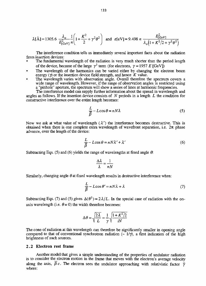
133

A[A] = 1 3 0 5 . 6 - ^ - - f l + — +y2d2) and g[eV] = 9.498 n

The interference condition tells us immediately several important facts about the radiationfrom insertion devices:• The fundamental wavelength of the radiation is very much shorter than the period length

of the device, because of the large y2 term (for electrons, y = 1957 E [GeV])• The wavelength of the harmonics can be varied either by changing the electron beam

energy (y) or the insertion device field strength, and hence K value.• The wavelength varies with observation angle. Overall therefore the spectrum covers a

wide range of wavelength. However, if the range of observation angles is restricted usinga "pinhole" aperture, the spectrum will show a series of lines at harmonic frequencies.The interference model can supply further information about the spread in wavelength and

angles as follows. If the insertion device consists of N periods in a length L the condition forconstructive interference over the entire length becomes:

= - Lcos0 = nNX (5)

Now we ask at what value of wavelength (A') the interference becomes destructive. This isobtained when there is one complete extra wavelength of wavefront separation, i.e. 2n phaseadvance, over the length of the device:

= - I c o s 0 = nAtt' + A' (6)

Subtracting Eqs. (5) and (6) yields the range of wavelengths at fixed angle ft

AA_ 1

A ~ nN

Similarly, changing angle 6 at fixed wavelength results in destructive interference when:

Lcos0 nAa + A (7)

Subtracting Eqs. (7) and (5) gives A(02) = 2 A/L. In the special case of radiation with the on-axis wavelength (i.e. 0=0) the width therefore becomes:

iN

The cone of radiation at this wavelength can therefore be significantly smaller in opening anglecompared to that of conventional synchrotron radiation (~ My), a first indication of the highbrightness of such sources.

2.2 Electron rest frame

Another model that gives a simple understanding of the properties of undulator radiationis to consider the_electron motion in the frame that moves with the electron's average velocityalong the axis, fie. The electron sees the undulator approaching with relativistic factor ywhere:

134

The undulator period appears Lorentz contracted with period length Xo/ y. In the moving framethe electron is therefore caused to oscillate with this wavelength, emitting a dipole radiationpattern. The transformation to the lab. frame involves a relativistic Doppler shift:

i = xf - J3 cos o)=-^ba+r2e2)

Inserting the expression above for y gives the same expression for the wavelength, Eq. (4).In the moving frame the z oscillation amplitude is multiplied by a factor y and so the ratio

between the oscillation amplitudes in the two planes is given as follows:

z' amplitude _

x' amplitude ~Y K7fH~~ ~ 8(1 + K1/!)1'2

Thus, when K is small the oscillation is almost purely simple harmonic motion in the x-direction and as a result the radiation consists of a single harmonic. As K increases howeverthe electron performs a "figure-of-eight" motion in the x'-z' plane (see Fig. 4) implying anincreased emission at higher harmonic frequencies. Calculating the power emitted in the dipolemode [57] and comparing it to the total power emitted one obtains the ratio:

power in the fundamental _ 1

total power ~ (1 + K2/2)m

which shows that the relative power in the fundamental decreases rapidly with increasing Kvalue.

I

3O -

— 1— 1

z' [rel. units]

Fig. 4 Figure-of-eight motion in the frame of reference moving with the electron's averagevelocity, normalized to the same x' amplitude, for K = 0.1 (inner), 0.5, 1.0, 10.0 (outer)

2.3 Electric field

Another way of deducing some of the characteristics of the radiation is to consider in aqualitative way the electric field emitted by the electron. We imagine the electron moving on anoscillating trajectory with a maximum angular excursion of K/y while emitting radiation into acone with the typical opening angle of synchrotron radiation, ~ 1/7. It is reasonable to supposetherefore that for K < 1 an observer "sees" a continuous sinusoidal emission from the device.

135

Correspondingly the radiation spectrum, which is the Fourier Transform of the electric field,consists of a single harmonic (see Fig. 5). At large K on the other hand the observer onlydetects radiation near the peaks in the trajectory, corresponding to the position of the magnetpoles. In this case the electric field is strongly peaked and so the radiation spectrum contains alarge number of harmonics.

K« 1

K - I

JL

r\ A A

t I

Fig. 5 Schematic diagram showing the electric field andcorresponding radiation spectrum in devices with various K values

We can also deduce from this picture the spectral width of the harmonics, as follows. Theobserved signal can be considered a continuous periodic signal multiplied by a "top-hat"function i.e. a function that is equal to unity within the range ±2/T0, i.e. ± JV/2 u, where u, isfundamental frequency, and zero outside. According to the convolution theorem the FourierTransform is the transform of the continuous signal convoluted with the transform for the top-hat function. The former consists of a series of lines at the harmonic frequencies, while thelatter is a sine function (sin(iV^l)/v1)/Û1) with a width in frequency that is inverselyproportional to the length of the impulse: Av = \jT0 = vJN. After convolution each line hasthis same width, and so the relative width becomes Av/v = 1/nN, in agreement with the resultof section 2.1.

2.4 The high K limit

It is evident from the above that the number of harmonics in the spectrum increases as afunction of the K value. The number can be estimated by comparing the equation for thewavelength of the harmonics, Eq. (4), with that of the critical wavelength for conventionalsynchrotron radiation corresponding to the peak field amplitude [58]:

2 -c~

The harmonic number corresponding to a given wavelength is then as follows:

=

Table 1Harmonic numbers giving a wavelength equal to the critical wavelength (A = Ac)

as a function of K

K12351020

n1512513833015

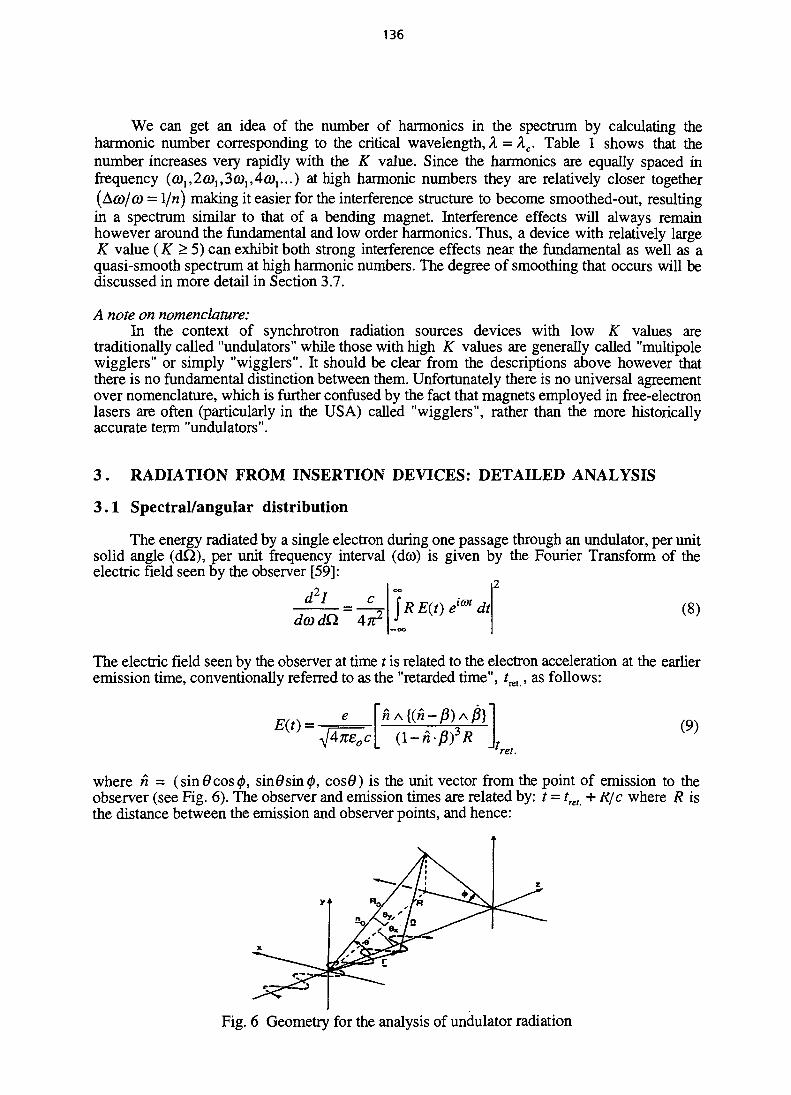
136

We can get an idea of the number of harmonics in the spectrum by calculating theharmonic number corresponding to the critical wavelength, X = AC. Table 1 shows that thenumber increases very rapidly with the K value. Since the harmonics are equally spaced infrequency (©,,2©,,3©,,4©,...) at high harmonic numbers they are relatively closer together(ACQ/Q) = l/n) making it easier for the interference structure to become smoothed-out, resultingin a spectrum similar to that of a bending magnet. Interference effects will always remainhowever around the fundamental and low order harmonics. Thus, a device with relatively largeK value (K > 5) can exhibit both strong interference effects near the fundamental as well as aquasi-smooth spectrum at high harmonic numbers. The degree of smoothing that occurs will bediscussed in more detail in Section 3.7.

A note on nomenclature:In the context of synchrotron radiation sources devices with low K values are

traditionally called "undulators" while those with high K values are generally called "multipolewigglers" or simply "wigglers". It should be clear from the descriptions above however thatthere is no fundamental distinction between them. Unfortunately there is no universal agreementover nomenclature, which is further confused by the fact that magnets employed in free-electronlasers are often (particularly in the USA) called "wigglers", rather than the more historicallyaccurate term "undulators".

3 . RADIATION FROM INSERTION DEVICES: DETAILED ANALYSIS

3.1 Spectral/angular distribution

The energy radiated by a single electron during one passage through an undulator, per unitsolid angle (dQ), per unit frequency interval (dco) is given by the Fourier Transform of theelectric field seen by the observer [59]:

2

dcodQ. An*\RE(t) l(Ot dt (8)

The electric field seen by the observer at time t is related to the electron acceleration at the earlieremission time, conventionally referred to as the "retarded time", tKt, as follows:

Aneoc M,(9)

ret.

where n = (sin0cos0, sin 6 sin 0, cos0) is the unit vector from the point of emission to theobserver (see Fig. 6). The observer and emission times are related by: t = tret + K/c where R isthe distance between the emission and observer points, and hence:

Fig. 6 Geometry for the analysis of undulator radiation

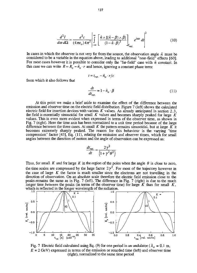
137

d2l e2c

(47teo)47C2 I WA{(n-jS)AJ

(1-n-B)3 dt

ret.

(10)

In cases in which the observer is not very far from the source, the observation angle h must beconsidered to be a variable in the equation above, leading to additional "near-field" effects [60].For most cases however it is possible to consider only the "far-field" case with h constant. Inthis case we can write R = Ro - h0 • r and hence, ignoring a constant phase term:

from which it also follows that

dt

dt (IDret.

At this point we make a brief aside to examine the effect of the difference between theemission and observer time on the electric field distribution. Figure 7 (left) shows the calculatedelectric field for insertion devices with various K values. As already anticipated in section 2.3,the field is essentially sinusoidal for small K values and becomes sharply peaked for large Kvalues. This is even more evident when expressed in terms of the observer time, as shown inFig. 7 (right). Here the time axis has been normalized to a unit time period because of the largedifference between the three cases. At small K the pattern remains sinusoidal, but at large K itbecomes extremely sharply peaked. The reason for this behaviour is the varying "timecompression" factor [43], Eq. (11), relating the emission and observer times, which for smallangles between the direction of motion and the angle of observation can be expressed as:

dtret. _ 2y2

dt

Thus, for small K and for large K in the region of the poles when the angle 6 is close to zero,the time scales are compressed by the large factor 2y2 . For most of the trajectory however inthe case of large K the factor is much smaller since the electrons are not travelling in thedirection of observation. On an absolute scale therefore the electric field emission close to thepeaks remains the same as in Fig. 7 (left). The difference in Fig. 7 (right) is due to the muchlonger time between the peaks (in terms of the observer time) for large K than for small K,which is reflected in the longer wavelength of the radiation.

1.0

- 0 . 5 •

-1.0

[rel. units]

Fig. 7 Electric field calculated using Eq. (9) for one period in an undulator (Xo =0.1 m,E = 2 GeV) expressed in terms of the emission or retarded time (left) and observer time

(right), normalized to the same time period

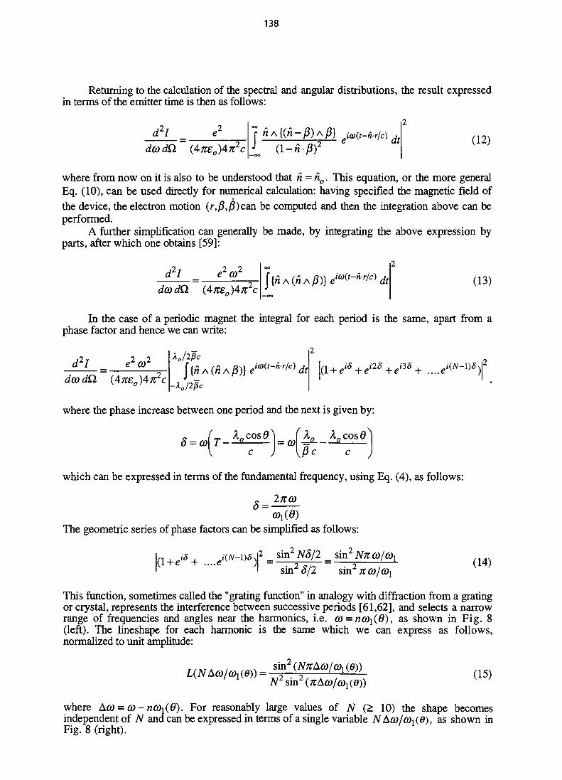
138

Returning to the calculation of the spectral and angular distributions, the result expressedin terms of the emitter time is then as follows:

d2l

doodQ. (4K£0)4K c J d-n-i

eico{t-h-rlc) dt (12)

where from now on it is also to be understood that n = n0. This equation, or the more generalEq. (10), can be used directly for numerical calculation: having specified the magnetic field ofthe device, the electron motion (r,/?,/?) can be computed and then the integration above can beperformed.

A further simplification can generally be made, by integrating the above expression byparts, after which one obtains [59]:

d2l

dcodQ {4K£0)4n2c(13)

In the case of a periodic magnet the integral for each period is the same, apart from aphase factor and hence we can write:

d2l e2CO2

dcodQ (4K£0)4K2C

kjlfic

-XJ2pc

[ + ei5+ei2S+ei3S+ ....<

where the phase increase between one period and the next is given by:

¥cos0= 0) \T — )

_ (K__{fie )

which can be expressed in terms of the fundamental frequency, using Eq. (4), as follows:

8 =

The geometric series of phase factors can be simplified as follows:

2 sin2N5/2 sin2

eiS + ...J{') sin2 6/2 sin2 K 0)/G)\

(14)

This function, sometimes called the "grating function" in analogy with diffraction from a gratingor crystal, represents the interference between successive periods [61,62], and selects a narrowrange of frequencies and angles near the harmonics, i.e. 6) = nct)1(0), as shown in Fig. 8(left). The lineshape for each harmonic is the same which we can express as follows,normalized to unit amplitude:

KiVA^Mce))^5 1".^^^1 1^ (15)

where Aco = co-n(Qx(d). For reasonably large values of iV (> 10) the shape becomesindependent of iV and can be expressed in terms of a single variable NAco/co^), as shown inFig. 8 (right).

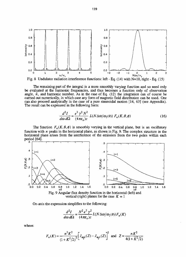
139

1.0

0.8

£ 0 6'3

5 0A

0.2

0.0 0.0

i 1

Fig. 8 Undulator radiation interference functions: left - Eq. (14) with N=10, right - Eq. (15)

The remaining part of the integral is a more smoothly varying function and so need onlybe evaluated at the harmonic frequencies, and thus becomes a function only of observationangle, n, and harmonic number. As in the case of Eq. (12) the integration can of course becarried out numerically, in which case any form of magnetic field distribution can be used. Onecan also proceed analytically in the case of a pure sinusoidal motion [14, 63] (see Appendix).The result can be expressed in the following form:

d2l =e272N2

dcodQ. (4K£O)C(16)

The function Fn(K,6,<p) is smoothly varying in the vertical plane, but is an oscillatoryfunction with n peaks in the horizontal plane, as shown in Fig. 9. The complex structure in thehorizontal plane arises from the interference of the emission from the two poles within eachperiod [64].

0.0 0.2 0.4 0.6 0.8 1.0 1.2 1.4 1.6 0.0 0.2 0.4 0.6 0.8 1.0 1.2 1.4 1.6ye yd

Fig. 9 Angular flux density function in the horizontal (left) andvertical (right) planes for the case K = 1

On-axis the expression simplifies to the following:

d2l =N2e2r

dcodQ. (4xeo)t

where:

2K2

Fn(K) = and Z =nK1

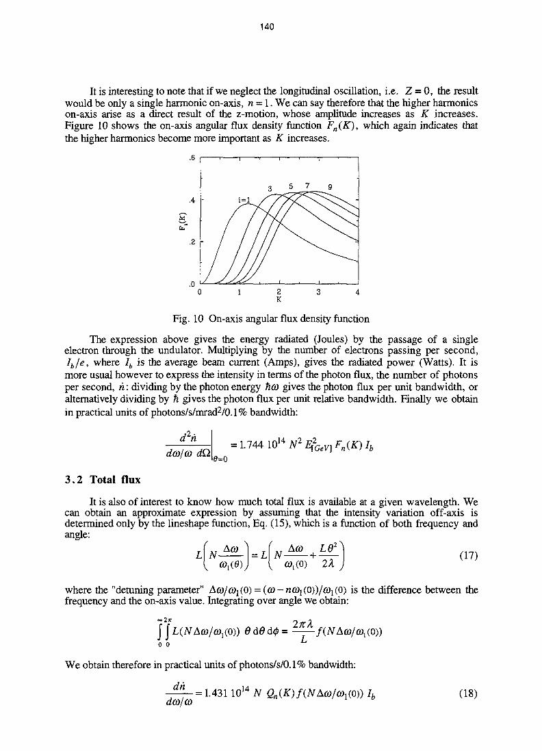
140

It is interesting to note that if we neglect the longitudinal oscillation, i.e. Z = 0, the resultwould be only a single harmonic on-axis, n = 1. We can say therefore that the higher harmonicson-axis arise as a direct result of the z-motion, whose amplitude increases as K increases.Figure 10 shows the on-axis angular flux density function Fn(K), which again indicates thatthe higher harmonics become more important as K increases.

3

w.5

I7

^ :

\

9

1 ,

.6

.4 -

.2 -

0 1 2 3 4K

Fig. 10 On-axis angular flux density function

The expression above gives the energy radiated (Joules) by the passage of a singleelectron through the undulator. Multiplying by the number of electrons passing per second,Ih/e, where lb is the average beam current (Amps), gives the radiated power (Watts). It ismore usual however to express the intensity in terms of the photon flux, the number of photonsper second, h: dividing by the photon energy fico gives the photon flux per unit bandwidth, oralternatively dividing by fi gives the photon flux per unit relative bandwidth. Finally we obtainin practical units of photons/s/mrad2/0.1% bandwidth:

d2n

dco/oo dQ.0=0

3.2 Total flux

It is also of interest to know how much total flux is available at a given wavelength. Wecan obtain an approximate expression by assuming that the intensity variation off-axis isdetermined only by the lineshape function, Eq. (15), which is a function of both frequency andangle:

where the "detuning parameter" Aa)/<y1(O) = (co-n6)1(O))/fi)1(O) is the difference between thefrequency and the on-axis value. Integrating over angle we obtain:

0 0

We obtain therefore in practical units of photons/s/0.1% bandwidth:

dh

dco/co= 1.431 1014 N Qn{K)f{NA(Q 1(0^0)) Ib (18)

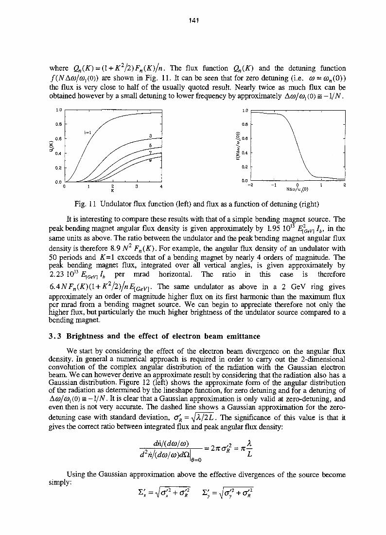
141

where Qn(K) = (l + K2/2)Fn(K)/n. The flux function Qn{K) and the detuning function/(iVAfa/a),(0)) are shown in Fig. 11. It can be seen that for zero detuning (i.e. (O = con(O))the flux is very close to half of the usually quoted result. Nearly twice as much flux can beobtained however by a small detuning to lower frequency by approximately Aco/^ (0) = -l/N.

p2.23 1013 E[GeV] lh

Fig. 11 Undulator flux function (left) and flux as a function of detuning (right)

It is interesting to compare these results with that of a simple bending magnet source. Thepeak bending magnet angular flux density is given approximately by 1.95 1013 E^GeV] Ib, in thesame units as above. The ratio between the undulator and the peak bending magnet angular fluxdensity is therefore 8.9 iV2 Fn{K). For example, the angular flux density of an undulator with50 periods and K=\ exceeds that of a bending magnet by nearly 4 orders of magnitude. Thepeak bending magnet flux, integrated over all vertical angles, is given approximately by

13 per mrad horizontal. The ratio in this case is therefore

K2/2)/nE[GeV]. The same undulator as above in a 2 GeV ring givesapproximately an order of magnitude higher flux on its first harmonic than the maximum fluxper mrad from a bending magnet source. We can begin to appreciate therefore not only thehigher flux, but particularly the much higher brightness of the undulator source compared to abending magnet.

3.3 Brightness and the effect of electron beam emittance

We start by considering the effect of the electron beam divergence on the angular fluxdensity. In general a numerical approach is required in order to carry out the 2-dimensionalconvolution of the complex angular distribution of the radiation with the Gaussian electronbeam. We can however derive an approximate result by considering that the radiation also has aGaussian distribution. Figure 12 (left) shows the approximate form of the angular distributionof the radiation as determined by the lineshape function, for zero detuning and for a detuning ofAo)/6)5(0) = -l/N. It is clear that a Gaussian approximation is only valid at zero-detuning, andeven then is not very accurate. The dashed line shows a Gaussian approximation for the zero-detuning case with standard deviation, a'R = fX/2L. The significance of this value is that itgives the correct ratio between integrated flux and peak angular flux density:

dn/(dco/co)— ~ — ; i

d2h/(dco/co)dCl\ _2 X

= K—

_

Using the Gaussian approximation above the effective divergences of the source becomesimply:

' — 1ST'2 .'27

142

1.0

MaJj 0.6a

> 0.44J

<u0.2

0.0

(4Tr/(2XL)1/2)r

Fig. 12 Intensity as a function of angle (left) and position (right).Solid lines - zero detuning, dashed lines - detuning of Aft)/ft), (0) = -1/N,

dot-dashed lines - Gaussian approximations for zero detuning (see text)

where <JX, ay are the rms angular divergences of the electron beam. The total flux remainsconstant and so we can write the expression for the modified on-axis angular flux densityincluding electron beam divergence as follows:

d2h

dco/(O dQ,

dn/(dco/co)

0=0

The radiation brightness includes not only the angular divergence of the source but alsothe emitting source size. The standard unit of measurement is thus photons/s/mm2/mrad2/0.1%bandwidth. The most simple view of how the size of the source comes about, is to considerprojecting the angular cone of the radiation to the centre of the undulator. We might expecttherefore a spatial distribution at the centre of size GR ~ G'R L/2, and hence with the aboveexpression for &R, we obtain aR ~ -yJlA.L/4. The correct approach however is to integrate thewave amplitudes, in the same way as one calculates diffraction from an aperture. The spatialdistribution is thus given by:

7(r) =0 0

Carrying out this calculation with the angular distribution given by Eq. (15) results in thefunctions shown in Fig. 12 (right). The zero-detuning case can be approximated well by aGaussian with standard deviation aR = V2/lL/2^, i.e. very similar to the simple result above.The effective source sizes are then given by the convolution with the electron beam dimensions,cr., cr , i.e.:

Combining the information about source size with the angular flux density allows us toestimate the brightness, as follows:

B =dh/jdco/O))

143

The limiting cases of the above equation are:i/ <JR > axy ana oR > oxy. At long wavelength and with small electron beam dimensions

and divergences the natural radiation dimensions dominate; this is often referred to as the"diffraction limit",

ii/ <JR < axy and a'R < o'xy. At the other extreme case the brightness is dominated by theelectron beam emittance, and we can write in the usual case (insertion device at asymmetry point with zero dispersion) B= Flux/47t2£xey, where sx = Ox<fx, £y = oy<?y

are the electron beam emittances in the two planes.Both extremes are indicated in Fig. 13 which shows the variation of the denominator in theabove expression, LxIty'Lxlly, as a function of photon energy using the parameters ofELETTRA as representative of "third-generation" synchrotron radiation facilities, compared tothe result for a zero emittance electron beam. At low photon energies therefore the radiation isclose to being diffraction limited, while at high energies the electron beam emittance is clearlythe limiting factor.

10"

10"

N electron beamlimit

diffraction limit

10' 10* 10°Photon Energy [eV]

10"

Fig. 13 Product of photon beam emittances in the case of ELETTRA

It must be remembered that for various reasons the expression for the brightness is onlyan approximation. It has already been shown that away from the condition of zero-detuning, theangular distribution function becomes strongly non-Gaussian, as shown in Fig. 12 (left).Under these conditions it is difficult to arrive at a sensible definition of the effective standarddeviation which gives the correct convolution with the electron beam divergence. Thecalculation of the source size also should take into account the effect of detuning. A furtherproblem is that, as already noted, no account is taken of the off-axis angular distributionfunction Fn(K,d,(j)) which can have a significant effect on the overall angular distributionparticularly when n is large and N is small. Finally, another potentially important effect is notincluded, namely the electron beam energy spread. A better approximation can therefore bemade by making a numerical calculation of the on-axis angular flux density (see section 3.6),including the true angular distribution function and the effects of emittance and energy spread,and then applying an approximate calculation of the source size, i.e. defining the brightness as:

B =_ d2h/(dco/Q))dQ.

To go beyond these approximate treatments requires a more fundamental definition of thebrightness in terms of the electric field distribution [65] which however is outside the scope ofthe present discussion.

3.4 Coherence

The degree of coherence of the radiation beam is an increasingly important parameter forvarious synchrotron radiation experiments. Basically, there are two measures of coherence -temporal (or longitudinal) coherence and spatial (or transverse) coherence. Temporal coherence

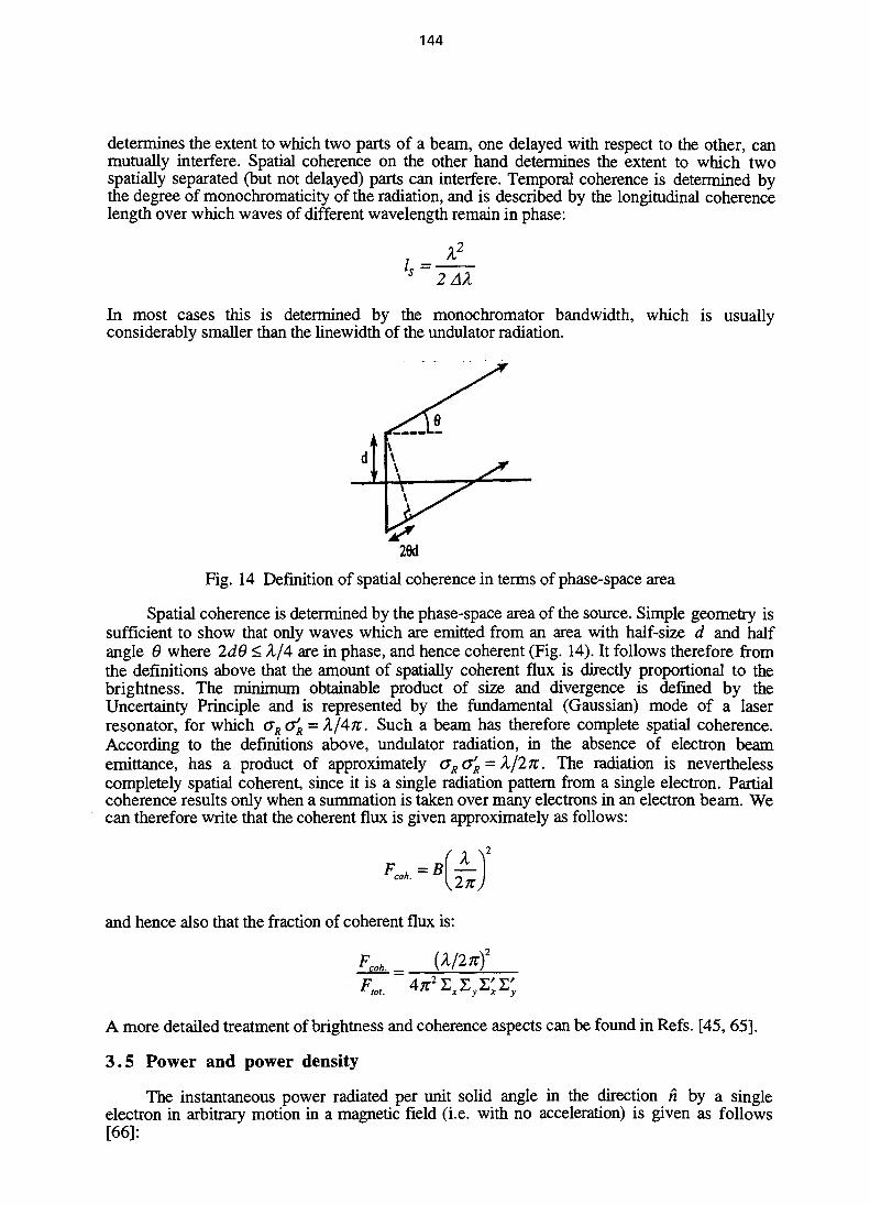
144

determines the extent to which two parts of a beam, one delayed with respect to the other, canmutually interfere. Spatial coherence on the other hand determines the extent to which twospatially separated (but not delayed) parts can interfere. Temporal coherence is determined bythe degree of monochromaticity of the radiation, and is described by the longitudinal coherencelength over which waves of different wavelength remain in phase:

* 2 AX

In most cases this is determined by the monochromator bandwidth, which is usuallyconsiderably smaller than the linewidth of the undulator radiation.

26d

Fig. 14 Definition of spatial coherence in terms of phase-space area

Spatial coherence is determined by the phase-space area of the source. Simple geometry issufficient to show that only waves which are emitted from an area with half-size d and halfangle 9 where 2d9 < A/4 are in phase, and hence coherent (Fig. 14). It follows therefore fromthe definitions above that the amount of spatially coherent flux is directly proportional to thebrightness. The minimum obtainable product of size and divergence is defined by theUncertainty Principle and is represented by the fundamental (Gaussian) mode of a laserresonator, for which aR &R = kjAn. Such a beam has therefore complete spatial coherence.According to the definitions above, undulator radiation, in the absence of electron beamemittance, has a product of approximately aRc'R-=-'kj2K. The radiation is neverthelesscompletely spatial coherent, since it is a single radiation pattern from a single electron. Partialcoherence results only when a summation is taken over many electrons in an electron beam. Wecan therefore write that the coherent flux is given approximately as follows:

coh.-a A

and hence also that the fraction of coherent flux is:

co, =

A more detailed treatment of brightness and coherence aspects can be found in Refs. [45, 65].

3.5 Power and power density

The instantaneous power radiated per unit solid angle in the direction h by a singleelectron in arbitrary motion in a magnetic field (i.e. with no acceleration) is given as follows[66]:

145

dP(4%EO)4KC

After integrating over the length of the insertion device to get the energy radiated per unit solidangle, and multiplying by Ibje to get the power radiated by a beam of electrons in the insertiondevice, the result can be expressed in the following form in practical units [67]:

dP—[W/mrad2] = 13.44 10"3 E?GeV]Ibj + (v2y+(v2

yyD5 dz (19)

where vx(z) = y((5x - 6X), vy(z) = y(Py -9y), D = 1 + v] + v2y and where the prime indicates

the derivative with respect to z.In the case of a plane sinusoidal device vx = Ksince - ydx and vy = -y6y, where

a = lnzjX0. After some simplification the result becomes:

dP

dQ.[W/mrad2] = 13.44 10'

it

jcos2a 4(yOx-Ksina)2

D5 da

where D = 1 + (yd )2 + (A!"sin a-ydx)2. This can be expressed in the following form:

= 10.84 E*GeV] Bo NIb G(K)fK(dx,6y)

where G(K) =+ K2)112 and

>X-Kcosay da, as obtained by Kim [68].

Fig. 15 The function G(K)

The function G(K) is illustrated in Fig. 15 and is close to unity for K > 1. The functionfK(6x,6y) has a peak value of unity on-axis and is shown in Fig. 16 in the horizontal andvertical planes for various K values. It can be seen that in the vertical plane the angulardistribution is insensitive to the value of K and in the limit K —» » is equal to that of a bendingmagnet. For large K in the horizontal plane the distribution becomes semi-circular, since thepower density is proportional to the field at the corresponding tangent point: at an angledx=(K/y)cos(kz) the field at the tangent point is B = Bosin(kz) and hence(B/Bo)

2+(y6x/K)2 = l.

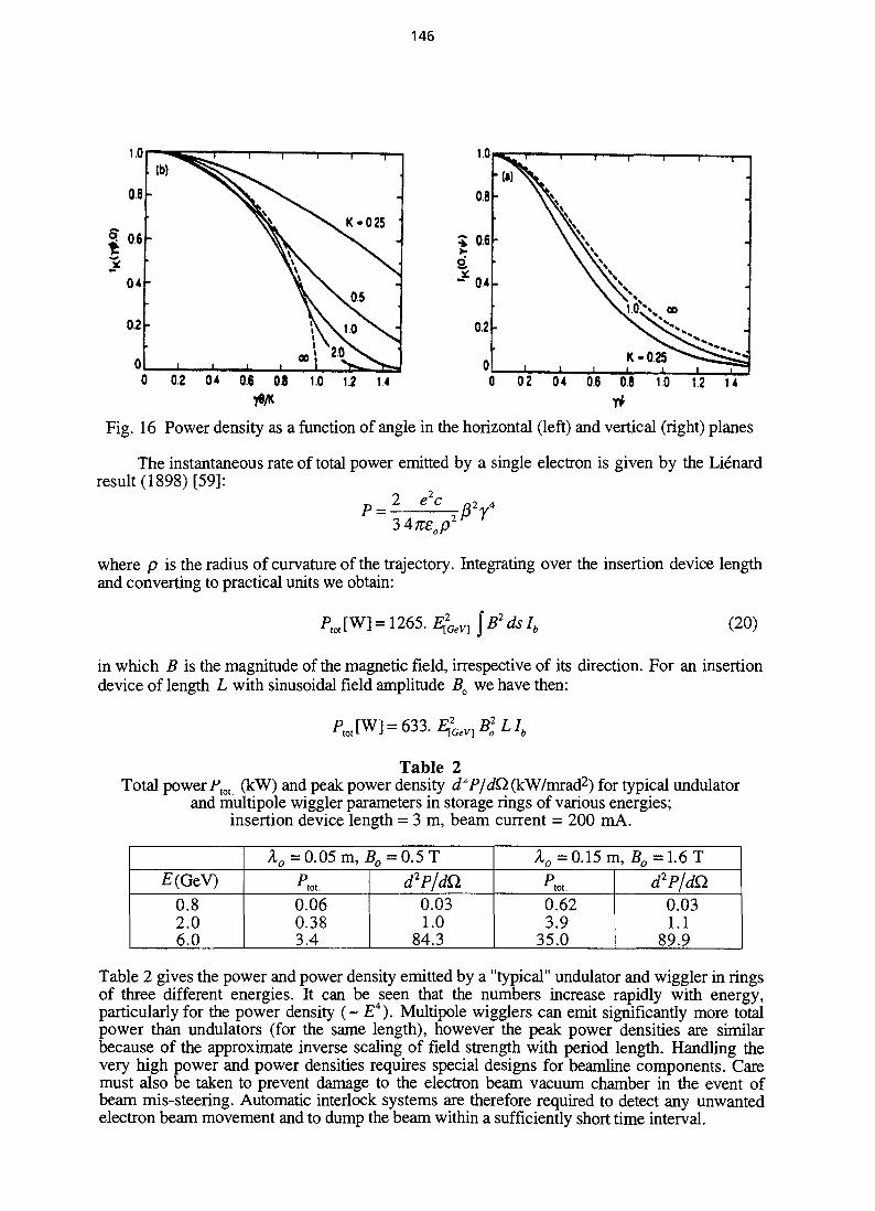
146

0.2 04 06 08 1.0 1.2 14 0 02 04 0.6 0.8 10 t.2 14

Fig. 16 Power density as a function of angle in the horizontal (left) and vertical (right) planes

The instantaneous rate of total power emitted by a single electron is given by the Lienardresult (1898) [59]:

3 47t£op2

where p is the radius of curvature of the trajectory. Integrating over the insertion device lengthand converting to practical units we obtain:

(20)

in which B is the magnitude of the magnetic field, irrespective of its direction. For an insertiondevice of length L with sinusoidal field amplitude BQ we have then:

Ptot[W] = 6 3 3 . 2 ^ 2 ^ 7 ,

Table 2Total power Ptm (kW) and peak power density d*P/d£l (kW/mrad2) for typical undulator

and multipole wiggler parameters in storage rings of various energies;insertion device length = 3 m, beam current = 200 mA.

£(GeV)0.82.06.0

Xo = 0.05 m,B0 = 0.5 T

PK,0.060.383.4

d2P/dQ.0.031.0

84.3

Ao = 0.15 m, Bo= 1.6 T

P»,0.623.9

35.0

d2P/dQ0.031.1

89.9

Table 2 gives the power and power density emitted by a "typical" undulator and wiggler in ringsof three different energies. It can be seen that the numbers increase rapidly with energy,particularly for the power density (-£"*). Multipole wigglers can emit significantly more totalpower than undulators (for the same length), however the peak power densities are similarbecause of the approximate inverse scaling of field strength with period length. Handling thevery high power and power densities requires special designs for beamline components. Caremust also be taken to prevent damage to the electron beam vacuum chamber in the event ofbeam mis-steering. Automatic interlock systems are therefore required to detect any unwantedelectron beam movement and to dump the beam within a sufficiently short time interval.

147

3.6 Practical computation of radiation spectra

Various computer programs have been written that can calculate the spectral and angulardistribution of undulator radiation using a number of different approaches:M Direct numerical integration of Eqs. (10), (12) or (13) e.g. [69-71]ii/ Calculation of the electric field in the time domain using Eq. (9) followed by Fourier

Transformation to obtain the radiation spectrum e.g. [72,73]iii/ Use of the analytic approximations for a pure sinusoidal field involving series of Bessel

functions (see Appendix) e.g. [74, 75]iv/ Other techniques e.g. [76-78]Methods i/ and ii/ are applicable to the case of a real magnetic field and also for the near-fieldcase, whereas method ml assumes an ideal sinusoidal magnetic field in the far-field case. Theeffect of electron beam emittance can be included either by numerical convolution or by Monte-Carlo methods. Each type of code has its particular advantages and disadvantages. Method iii/for example is useful for a rapid calculation of the main effects of angular acceptance andelectron beam effects, whereas i/ and ii/ are usually more time consuming but provide moredetailed information on the effects of magnetic field errors etc. Methods i/ and iii/ can calculatealso the angular distributions at a given frequency, which is not possible with method ii/. Somespecial techniques have been developed for the cases where the K value is large [76,77]. Herewe will not discuss further the various numerical approaches, but rather present some resultsusing one code [75] that illustrate the main features of the effects of angular acceptance andelectron beam emittance and energy spread.

Figure 17 shows an example of the effect of electron beam emittance on the on-axisspectrum for an undulator installed on ELETTRA. It can be seen that with the nominalemittances there is a relatively small effect on the first harmonic (17% reduction), but this ismuch larger on the 1 lth harmonic (factor of 4 reduction). The effect of a ten-fold increase inemittance is also shown, which is sufficient to reduce the first harmonic by a factor of 3. Figure18 illustrates the effect of electron beam energy spread, with zero emittance. The nominalenergy spread gives rise to a negligible reduction in peak intensity on the first harmonic, butquite significant reduction (factor of 4) on the 1 lth harmonic. It should be noted that the effectof emittance is not symmetric, broadening the lineshape mainly on the long wavelength side, inaccordance with Eq. (4), whereas the effect of energy spread is symmetric.

98 1078

Fig. 17 Effect of electron beam emittance on the 1st (left) and 1 lth (right) harmonicsfor an undulator in ELETTRA; E = 2 GeV, Ao = 56 mm, JV = 81, K = 3.45

E 0.5 -

1078

Fig. 18 Effect of electron beam energy spread on the 1st (left) and 11th (right) harmonicsfor an undulator in ELETTRA; parameters as Fig. 17

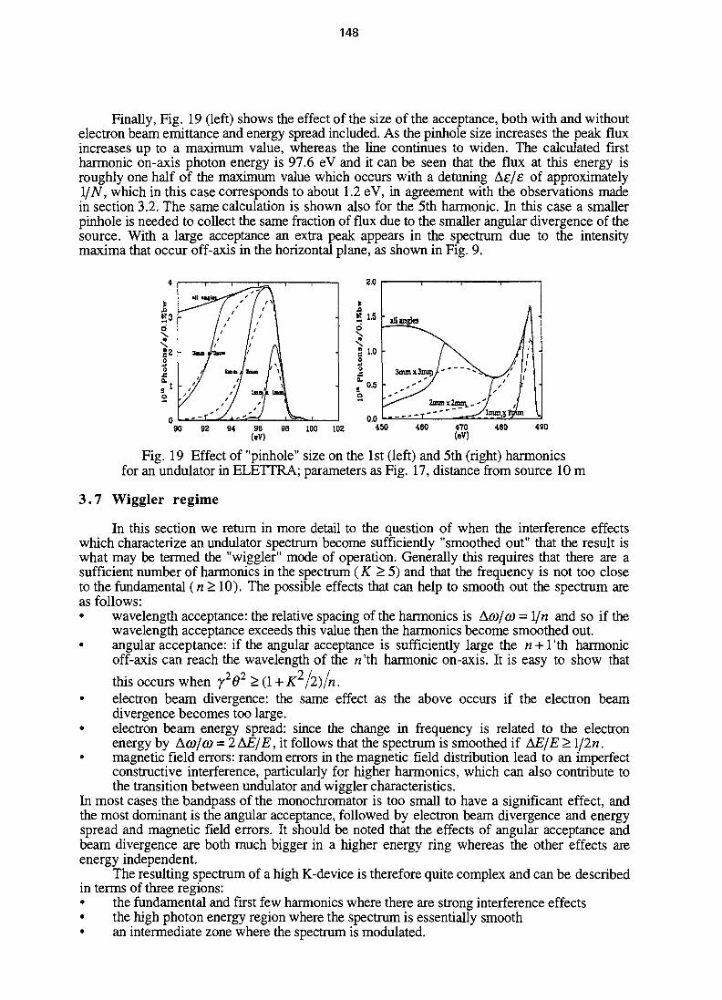
148

Finally, Fig. 19 (left) shows the effect of the size of the acceptance, both with and withoutelectron beam emittance and energy spread included. As the pinhole size increases the peak fluxincreases up to a maximum value, whereas the line continues to widen. The calculated firstharmonic on-axis photon energy is 97.6 eV and it can be seen that the flux at this energy isroughly one half of the maximum value which occurs with a detuning Ae/e of approximatelyl/N, which in this case corresponds to about 1.2 eV, in agreement with the observations madein section 3.2. The same calculation is shown also for the 5th harmonic. In this case a smallerpinhole is needed to collect the same fraction of flux due to the smaller angular divergence of thesource. With a large acceptance an extra peak appears in the spectrum due to the intensitymaxima that occur off-axis in the horizontal plane, as shown in Fig. 9.

2.0

5 1-5

0.0

lUinglo

3mm x 3mm/ ' ^ s ^

',*— 2nunx2mm.,'7T l - ^ '

l\~

nm^ljidn \,

450 460 470()

480 490

Fig. 19 Effect of "pinhole" size on the 1st (left) and 5th (right) harmonicsfor an undulator in ELETTRA; parameters as Fig. 17, distance from source 10 m

3.7 Wiggler regime

In this section we return in more detail to the question of when the interference effectswhich characterize an undulator spectrum become sufficiently "smoothed out" that the result iswhat may be termed the "wiggler" mode of operation. Generally this requires that there are asufficient number of harmonics in the spectrum (K > 5) and that the frequency is not too closeto the fundamental (n> 10). The possible effects that can help to smooth out the spectrum areas follows:• wavelength acceptance: the relative spacing of the harmonics is Ao/o) = \jn and so if the

wavelength acceptance exceeds this value then the harmonics become smoothed out.• angular acceptance: if the angular acceptance is sufficiently large the n +1 'th harmonic

off-axis can reach the wavelength of the n'th harmonic on-axis. It is easy to show that

this occurs when y262 > (1 + K2/2)/n.• electron beam divergence: the same effect as the above occurs if the electron beam

divergence becomes too large.• electron beam energy spread: since the change in frequency is related to the electron

energy by Aco/to = 2AE/E, it follows that the spectrum is smoothed if AE/E > l/2n.• magnetic field errors: random errors in the magnetic field distribution lead to an imperfect

constructive interference, particularly for higher harmonics, which can also contribute tothe transition between undulator and wiggler characteristics.

In most cases the bandpass of the monochromator is too small to have a significant effect, andthe most dominant is the angular acceptance, followed by electron beam divergence and energyspread and magnetic field errors. It should be noted that the effects of angular acceptance andbeam divergence are both much bigger in a higher energy ring whereas the other effects areenergy independent.

The resulting spectrum of a high K-device is therefore quite complex and can be describedin terms of three regions:• the fundamental and first few harmonics where there are strong interference effects• the high photon energy region where the spectrum is essentially smooth• an intermediate zone where the spectrum is modulated.

149

As an example Fig. 20 shows a calculated spectrum for a device with a relatively large K valuebut with a small angular acceptance. At sufficiently high photon energies the spectrum becomessmooth and the intensity equals 2N times that of a bending magnet - shown by the solid line inthe figure.

10 T

in

6

coosza.

E = 2 GeV, Xo = 8 cm, K = 6.5, N = 19,

pinhole 2 mm x 2 mm @ 15 m

10'10' 10*

Photon Energy [eVJ10"

Fig. 20 Calculated spectrum for a high K device in ELETTRA

In the absence of interference effects the radiation spectrum can be calculated as for abending magnet but with a critical energy that varies with the angle of emission in the horizontalplane:

The brightness can be approximated by the following expression [79]:

dn/ddxB =

a2

where dh/ddx is the total flux per unit horizontal angle, integrated over the vertical angle,andcr^ is the vertical opening of the radiation, as for a bending magnet source; a is theamplitude of the sinusoidal motion (=KX0/27ty). The above expression assumes that themagnet length is not too great (L < Afix, L < 4fiy), as well as a relatively small amplitude ofmotion (a < ox) and electron beam divergence (&y < o'R/2), otherwise a summation must bemade over every pole. The brightness of a wiggler is usually several orders of magnitude lessthan that of an undulator (see 5.2). To obtain significant flux the radiation is usually collectedover a wide range of angles, which results in an increased effective source size which alsoneeds to be considered in the beamline optics design. Further details of the geometricalproperties of the radiation from multipole wiggler sources is given in Refs. [80,81].

4 . INSERTION DEVICE TECHNOLOGY: INTRODUCTION

4.1 Electromagnetscoil

J (NI) ampere-tums

Q

Fig. 21 Schematic of an electromagnetic undulator

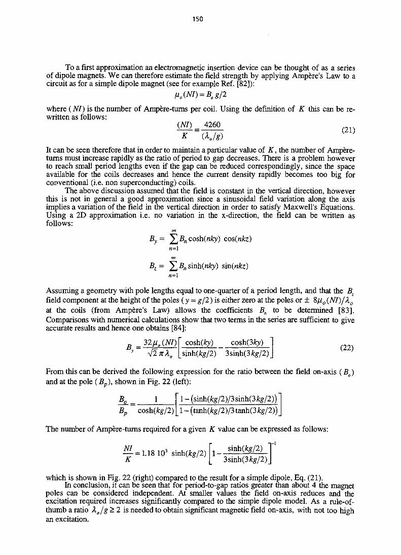
150

To a first approximation an electromagnetic insertion device can be thought of as a seriesof dipole magnets. We can therefore estimate the field strength by applying Ampere's Law to acircuit as for a simple dipole magnet (see for example Ref. [82]):

where (NI) is the number of Ampere-turns per coil. Using the definition of K this can be re-written as follows:

(NI) _ 4260

It can be seen therefore that in order to maintain a particular value of K, the number of Ampere-turns must increase rapidly as the ratio of period to gap decreases. There is a problem howeverto reach small period lengths even if the gap can be reduced correspondingly, since the spaceavailable for the coils decreases and hence the current density rapidly becomes too big forconventional (i.e. non superconducting) coils.

The above discussion assumed that the field is constant in the vertical direction, howeverthis is not in general a good approximation since a sinusoidal field variation along the axisimplies a variation of the field in the vertical direction in order to satisfy Maxwell's Equations.Using a 2D approximation i.e. no variation in the x-direction, the field can be written asfollows:

By = ^Bncosh(nky) cos(nfe)n=\

OO

Bz = ^ Bn sinh(nky) sin(nfe)7 2 = 1

Assuming a geometry with pole lengths equal to one-quarter of a period length, and that the Bz

field component at the height of the poles (y = g/2) is either zero at the poles or ± 8/n0 (A7)//lo

at the coils (from Ampere's Law) allows the coefficients Bn to be determined [83].Comparisons with numerical calculations show that two terms in the series are sufficient to giveaccurate results and hence one obtains [84]:

= 32n.(NI)[ cosh(fcy) cosh(3fo) 1y V2?rA [sinh(kg/2) 3sinh(3%/2)J }

cosh(fcy)[sinh(kg/2) 3sinh(3%/2)J

From this can be derived the following expression for the ratio between the field on-axis (Bo)and at the pole (Bp), shown in Fig. 22 (left):

Bp cosh(kg/2) 1 - (tanh(A:g/2)/3tanh(3 kg/2))

The number of Ampere-turns required for a given K value can be expressed as follows:

^ = 1.18 103 sinhdfc/2) [ l - Smk8/2) VK y*i>^ 3sinh(3Jk#/2)J

which is shown in Fig. 22 (right) compared to the result for a simple dipole, Eq. (21).In conclusion, it can be seen that for period-to-gap ratios greater than about 4 the magnet

poles can be considered independent. At smaller values the field on-axis reduces and theexcitation required increases significantly compared to the simple dipole model. As a rule-of-thumb a ratio X0/g>2 is needed to obtain significant magnetic field on-axis, with not too highan excitation.

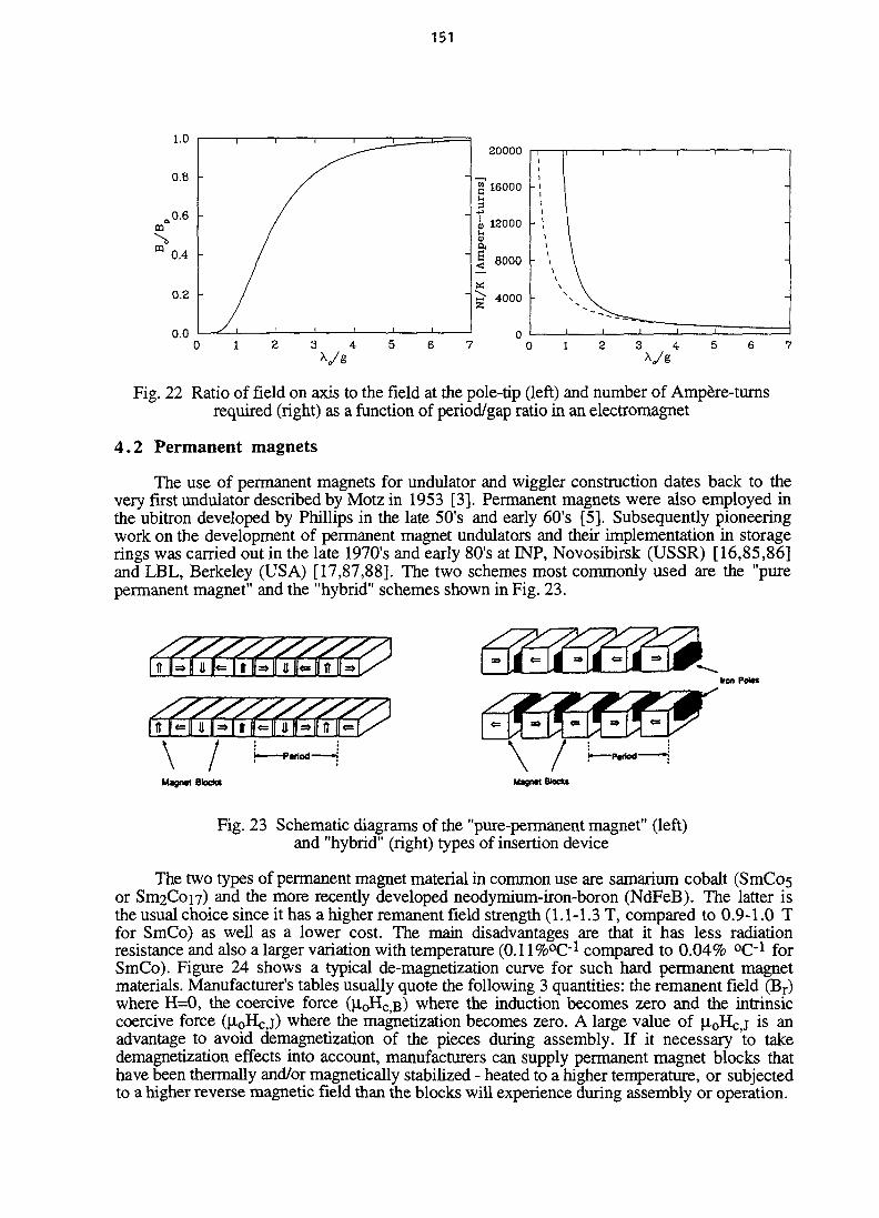
151

Fig. 22 Ratio of field on axis to the field at the pole-tip (left) and number of Ampere-turnsrequired (right) as a function of period/gap ratio in an electromagnet

4.2 Permanent magnets

The use of permanent magnets for undulator and wiggler construction dates back to thevery first undulator described by Motz in 1953 [3]. Permanent magnets were also employed inthe ubitron developed by Phillips in the late 50's and early 60's [5]. Subsequently pioneeringwork on the development of permanent magnet undulators and their implementation in storagerings was carried out in the late 1970's and early 80's at INP, Novosibirsk (USSR) [16,85,86]and LBL, Berkeley (USA) [17,87,88]. The two schemes most commonly used are the "purepermanent magnet" and the "hybrid" schemes shown in Fig. 23.

1- i- i~Iron Potts

\

MagnftSloda Magn« Blocks

Fig. 23 Schematic diagrams of the "pure-permanent magnet" (left)and "hybrid" (right) types of insertion device

The two types of permanent magnet material in common use are samarium cobalt (SmCosor Sn^Con) and the more recently developed neodymium-iron-boron (NdFeB). The latter isthe usual choice since it has a higher remanent field strength (1.1-1.3 T, compared to 0.9-1.0 Tfor SmCo) as well as a lower cost. The main disadvantages are that it has less radiationresistance and also a larger variation with temperature (0.1 \%°Ol compared to 0.04% °C'1 forSmCo). Figure 24 shows a typical de-magnetization curve for such hard permanent magnetmaterials. Manufacturer's tables usually quote the following 3 quantities: the remanent field (Br)where H=0, the coercive force ( ^ 0 H C ,B) where the induction becomes zero and the intrinsiccoercive force (jioHc,j) where the magnetization becomes zero. A large value of M.0Hc,j is anadvantage to avoid demagnetization of the pieces during assembly. If it necessary to takedemagnetization effects into account, manufacturers can supply permanent magnet blocks thathave been thermally and/or magnetically stabilized - heated to a higher temperature, or subjectedto a higher reverse magnetic field than the blocks will experience during assembly or operation.

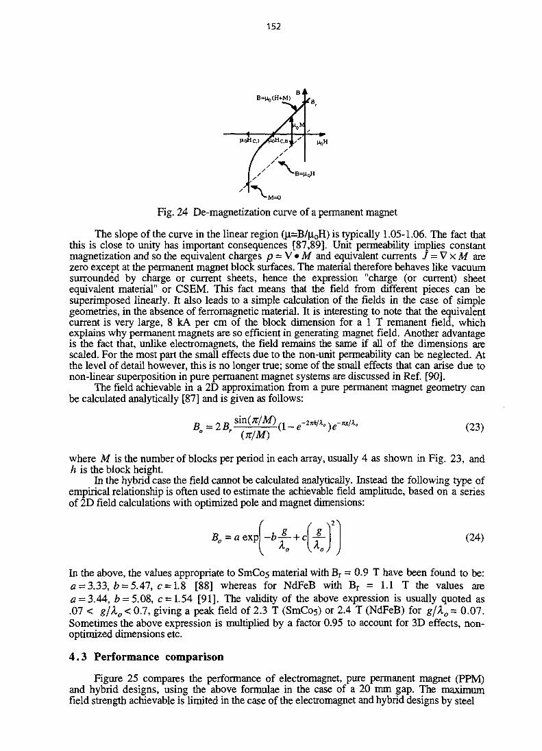
152

Bl ,B=Mo(H+M)

-M=0

Fig. 24 De-magnetization curve of a permanent magnet

The slope of the curve in the linear region ((1=B/(IOH) is typically 1.05-1.06. The fact thatthis is close to unity has important consequences [87,89]. Unit permeability implies constantmagnetization and so the equivalent charges p = V • M and equivalent currents / = V x M arezero except at the permanent magnet block surfaces. The material therefore behaves like vacuumsurrounded by charge or current sheets, hence the expression "charge (or current) sheetequivalent material" or CSEM. This fact means that the field from different pieces can besuperimposed linearly. It also leads to a simple calculation of the fields in the case of simplegeometries, in the absence of ferromagnetic material. It is interesting to note that the equivalentcurrent is very large, 8 kA per cm of the block dimension for a 1 T remanent field, whichexplains why permanent magnets are so efficient in generating magnet field. Another advantageis the fact that, unlike electromagnets, the field remains the same if all of the dimensions arescaled. For the most part the small effects due to the non-unit permeability can be neglected. Atthe level of detail however, this is no longer true; some of the small effects that can arise due tonon-linear superposition in pure permanent magnet systems are discussed in Ref. [90].

The field achievable in a 2D approximation from a pure permanent magnet geometry canbe calculated analytically [87] and is given as follows:

B 2BrSjn(KlMl{l_e-2^)e-^{njM)

where M is the number of blocks per period in each array, usually 4 as shown in Fig. 23, andh is the block height.

In the hybrid case the field cannot be calculated analytically. Instead the following type ofempirical relationship is often used to estimate the achievable field amplitude, based on a seriesof 2D field calculations with optimized pole and magnet dimensions:

(24)

In the above, the values appropriate to SmCos material with Br = 0.9 T have been found to be:a = 3.33, £ = 5.47, c = 1.8 [88] whereas for NdFeB with Br = 1.1 T the values area = 3.44, £ = 5.08, c = 1.54 [91]. The validity of the above expression is usually quoted as.07 < g/X0 < 0.7, giving a peak field of 2.3 T (SmCo5) or 2.4 T (NdFeB) for g/X0 = 0.07.Sometimes the above expression is multiplied by a factor 0.95 to account for 3D effects, non-optimized dimensions etc.

4.3 Performance comparison

Figure 25 compares the performance of electromagnet, pure permanent magnet (PPM)and hybrid designs, using the above formulae in the case of a 20 mm gap. The maximumfield strength achievable is limited in the case of the electromagnet and hybrid designs by steel

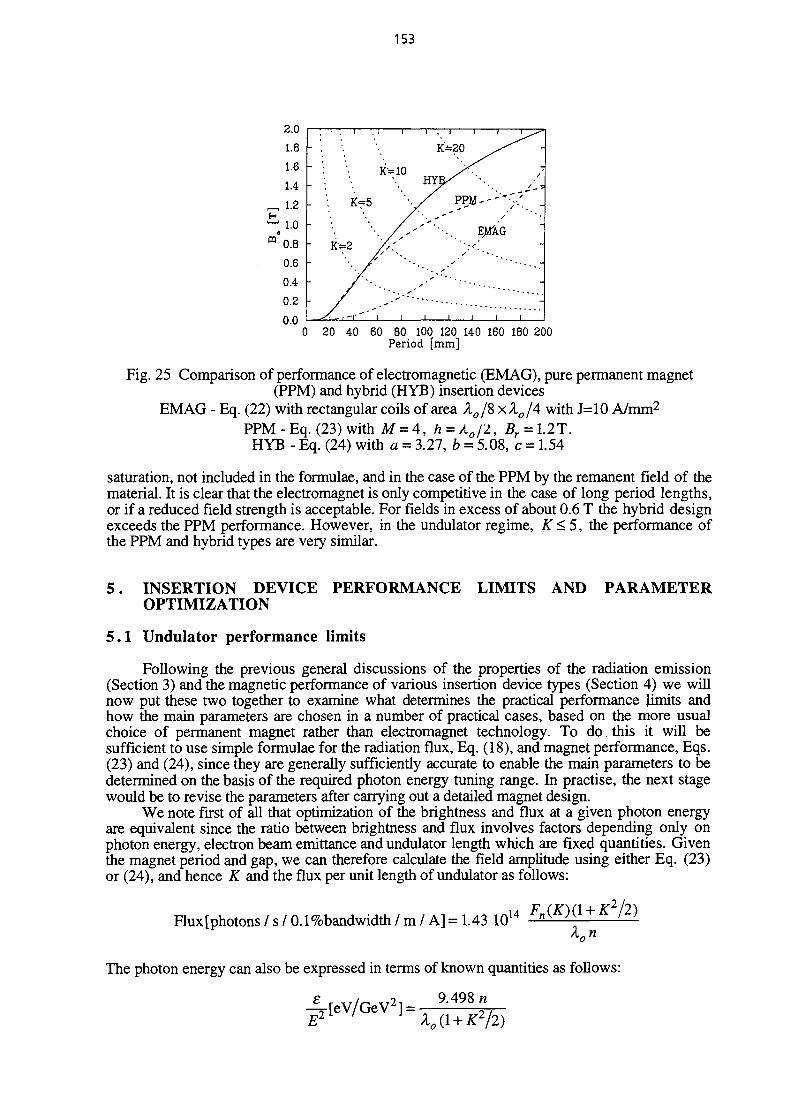
153

0 20 40 60 80 100 120 140 160 180 200Period [mm]

Fig. 25 Comparison of performance of electromagnetic (EMAG), pure permanent magnet(PPM) and hybrid (HYB) insertion devices

EMAG - Eq. (22) with rectangular coils of area Ao/8 x Xo/A with J=10 A/mm2

PPM-Eq. (23) with M = 4, h = A0/2, Br = l.2T.HYB - Eq. (24) with a = 3.27, b = 5.08, c = 1.54

saturation, not included in the formulae, and in the case of the PPM by the remanent field of thematerial. It is clear that the electromagnet is only competitive in the case of long period lengths,or if a reduced field strength is acceptable. For fields in excess of about 0.6 T the hybrid designexceeds the PPM performance. However, in the undulator regime, K < 5, the performance ofthe PPM and hybrid types are very similar.

5 . INSERTION DEVICE PERFORMANCE LIMITS AND PARAMETEROPTIMIZATION

5.1 Undulator performance limits

Following the previous general discussions of the properties of the radiation emission(Section 3) and the magnetic performance of various insertion device types (Section 4) we willnow put these two together to examine what determines the practical performance limits andhow the main parameters are chosen in a number of practical cases, based on the more usualchoice of permanent magnet rather than electromagnet technology. To do this it will besufficient to use simple formulae for the radiation flux, Eq. (18), and magnet performance, Eqs.(23) and (24), since they are generally sufficiently accurate to enable the main parameters to bedetermined on the basis of the required photon energy tuning range. In practise, the next stagewould be to revise the parameters after carrying out a detailed magnet design.

We note first of all that optimization of the brightness and flux at a given photon energyare equivalent since the ratio between brightness and flux involves factors depending only onphoton energy, electron beam emittance and undulator length which are fixed quantities. Giventhe magnet period and gap, we can therefore calculate the field amplitude using either Eq. (23)or (24), and hence K and the flux per unit length of undulator as follows:

Flux [photons / s / 0.1%bandwidth / m / A] = 1.43 1014

Xon

The photon energy can also be expressed in terms of known quantities as follows:

_e_ i 2 ] _ _ 9.498 n

E A,

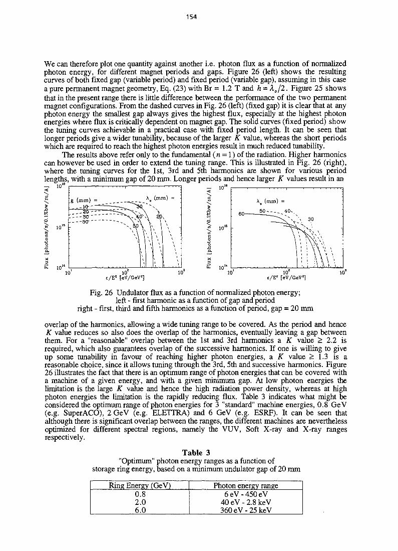
154

We can therefore plot one quantity against another i.e. photon flux as a function of normalizedphoton energy, for different magnet periods and gaps. Figure 26 (left) shows the resultingcurves of both fixed gap (variable period) and fixed period (variable gap), assuming in this casea pure permanent magnet geometry, Eq. (23) with Br = 1.2 T and h = Ao/2. Figure 25 showsthat in the present range there is little difference between the performance of the two permanentmagnet configurations. From the dashed curves in Fig. 26 (left) (fixed gap) it is clear that at anyphoton energy the smallest gap always gives the highest flux, especially at the highest photonenergies where flux is critically dependent on magnet gap. The solid curves (fixed period) showthe tuning curves achievable in a practical case with fixed period length. It can be seen thatlonger periods give a wider tunability, because of the larger K value, whereas the short periodswhich are required to reach the highest photon energies result in much reduced tunability.

The results above refer only to the fundamental (n = 1) of the radiation. Higher harmonicscan however be used in order to extend the tuning range. This is illustrated in Fig. 26 (right),where the tuning curves for the 1st, 3rd and 5th harmonics are shown for various periodlengths, with a minimum gap of 20 mm. Longer periods and hence larger K values result in an

10"

a

co

«-»O

Sia.

10"

10'

g (mm) = __.,_ _

2fr - - — ^v->. - --3a— ^X-X

50" - - ^ \ -

\ \

,

X

V '\ v 1

i

(min) = :

\ \V

\

1

v •

\

\ '.

cooxsa.

x

E101 10

e/E* [eV/GeVa]10* 10"

Fig. 26 Undulator flux as a function of normalized photon energy;left - first harmonic as a function of gap and period

right - first, third and fifth harmonics as a function of period, gap = 20 mm

overlap of the harmonics, allowing a wide tuning range to be covered. As the period and henceK value reduces so also does the overlap of the harmonics, eventually leaving a gap betweenthem. For a "reasonable" overlap between the 1st and 3rd harmonics a K value > 2.2 isrequired, which also guarantees overlap of the successive harmonics. If one is willing to giveup some tunability in favour of reaching higher photon energies, a K value > 1.3 is areasonable choice, since it allows tuning through the 3rd, 5th and successive harmonics. Figure26 illustrates the fact that there is an optimum range of photon energies that can be covered witha machine of a given energy, and with a given minimum gap. At low photon energies thelimitation is the large K value and hence the high radiation power density, whereas at highphoton energies the limitation is the rapidly reducing flux. Table 3 indicates what might beconsidered the optimum range of photon energies for 3 "standard" machine energies, 0.8 GeV(e.g. SuperACO), 2 GeV (e.g. ELETTRA) and 6 GeV (e.g. ESRF). It can be seen thatalthough there is significant overlap between the ranges, the different machines are neverthelessoptimized for different spectral regions, namely the VUV, Soft X-ray and X-ray rangesrespectively.

Table 3"Optimum" photon energy ranges as a function of

storage ring energy, based on a minimum undulator gap of 20 mm

Ring Energy (GeV)0.82.06.0

Photon energy range6eV-450eV

40 eV - 2.8 keV360eV-25keV

155

It should be emphasized that the "optimum" photon energy ranges shown in the Table areonly indicative. For example, as we have already seen, the performance is strongly determinedby the minimum gap that can be allowed. Special insertion devices can also be built with evensmaller gaps to extend the performance at higher energy. The lower photon energy limit is alsorather arbitrary, and depends in practise on the acceptable power loading. Overall however itremains true mat undulator performance is one of the most important factors determining thechoice of energy for a synchrotron radiation facility, and that this is essentially limited (at thehigh photon energy limit) by the minimum gap that can be allowed for successful machineoperation.

5.2 Undulator parameter optimization

As a practical example we will consider the design of undulators for a 1.5 GeV ring basedon a minimum gap of 20 mm; the principles involved however remain valid for any other choiceof parameters. Figure 27 shows the flux and brightness achievable from a range of differentundulators, together with that from a multipole wiggler and a bending magnet for comparison.In the latter cases the flux is integrated vertically, and per mrad of horizontal angle. Althoughthe multipole wiggler can provide a reasonably high flux, clearly the brightness is several ordersof magnitude inferior to that of an undulator. The parameters of the devices are given in Table 4which includes also the total power and peak power density of the radiation.

10 10' 10° 10'Photon Energy [eV]

10° 10* 10*Photon Energy feVl

10°

Fig. 27 Flux (left) and brightness (right) for various sources in a 1.5 GeV ring:U - 1st (solid), 3rd (dashed) and 5th (dotted) harmonics; W - multipole wiggler;

BM - bending magnet. (£=1.5 GeV, Jb = 0.4 A, ex=10r* m rad, ey = 10"9 m rad,px = 5 m, py = 2 m, ID length = 3 m, BM field = 1.2 T)

Table 4Parameters of various undulators shown in Fig. 27; peak power density units W/mrad2

Ao(mm)392618.54872100150200

g(mm)201052020>20>20>20

BO(J)0.380.570.810.510.780.470.250.11

K1.401.401.402.295.264.403.502.56

2475541120443102937910721

d2P/dQ6151381278768670230910929

As stated in the Section above, at the low photon energy end of the spectrum the radiationpower density can become a limiting factor. Figure 28 (a) shows a selection of different devicesall with a fundamental of 20 eV. As the period length increases the power and power densitydecrease rapidly, as shown in Table 4, whereas the flux decreases more slowly. The choicetherefore is a compromise between power, flux and tuning range.

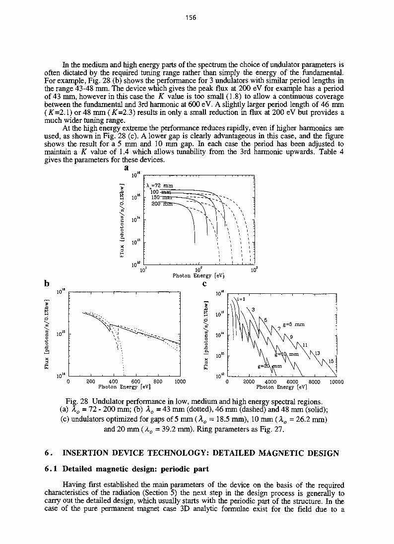
156

In the medium and high energy parts of the spectrum the choice of undulator parameters isoften dictated by the required tuning range rather than simply the energy of the fundamental.For example, Fig. 28 (b) shows the performance for 3 undulators with similar period lengths inthe range 43-48 mm. The device which gives the peak flux at 200 eV for example has a periodof 43 mm, however in this case the K value is too small (1.8) to allow a continuous coveragebetween the fundamental and 3rd harmonic at 600 eV. A slightly larger period length of 46 mm(K=2.1) or 48 mm (#=2.3) results in only a small reduction in flux at 200 eV but provides amuch wider tuning range.

At the high energy extreme the performance reduces rapidly, even if higher harmonics areused, as shown in Fig. 28 (c). A lower gap is clearly advantageous in this case, and the figureshows the result for a 5 mm and 10 mm gap. In each case the period has been adjusted tomaintain a K value of 1.4 which allows tunability from the 3rd harmonic upwards. Table 4gives the parameters for these devices.

10"

: X =72 mm°100 555=

S 1015 I 150oto

1 10"

oJ3

^ 1 0 ' 3

3

10"101

Photon Energy [eV]

C18

200 400 600 800 1000Photon Energy [eV]

2000 4000 6000 8000 10000Photon Energy [eV]

Fig. 28 Undulator performance in low, medium and high energy spectral regions,(a) Xo = 72 - 200 mm; (b) Xo = 43 mm (dotted), 46 mm (dashed) and 48 mm (solid);(c) undulators optimized for gaps of 5 mm (Xo - 18.5 mm), 10 mm (Xo = 26.2 mm)

and 20 mm (Ao - 39.2 mm). Ring parameters as Fig. 27.

6 . INSERTION DEVICE TECHNOLOGY: DETAILED MAGNETIC DESIGN

6.1 Detailed magnetic design: periodic part

Having first established the main parameters of the device on the basis of the requiredcharacteristics of the radiation (Section 5) the next step in the design process is generally tocarry out the detailed design, which usually starts with the periodic part of the structure. In thecase of the pure permanent magnet case 3D analytic formulae exist for the field due to a

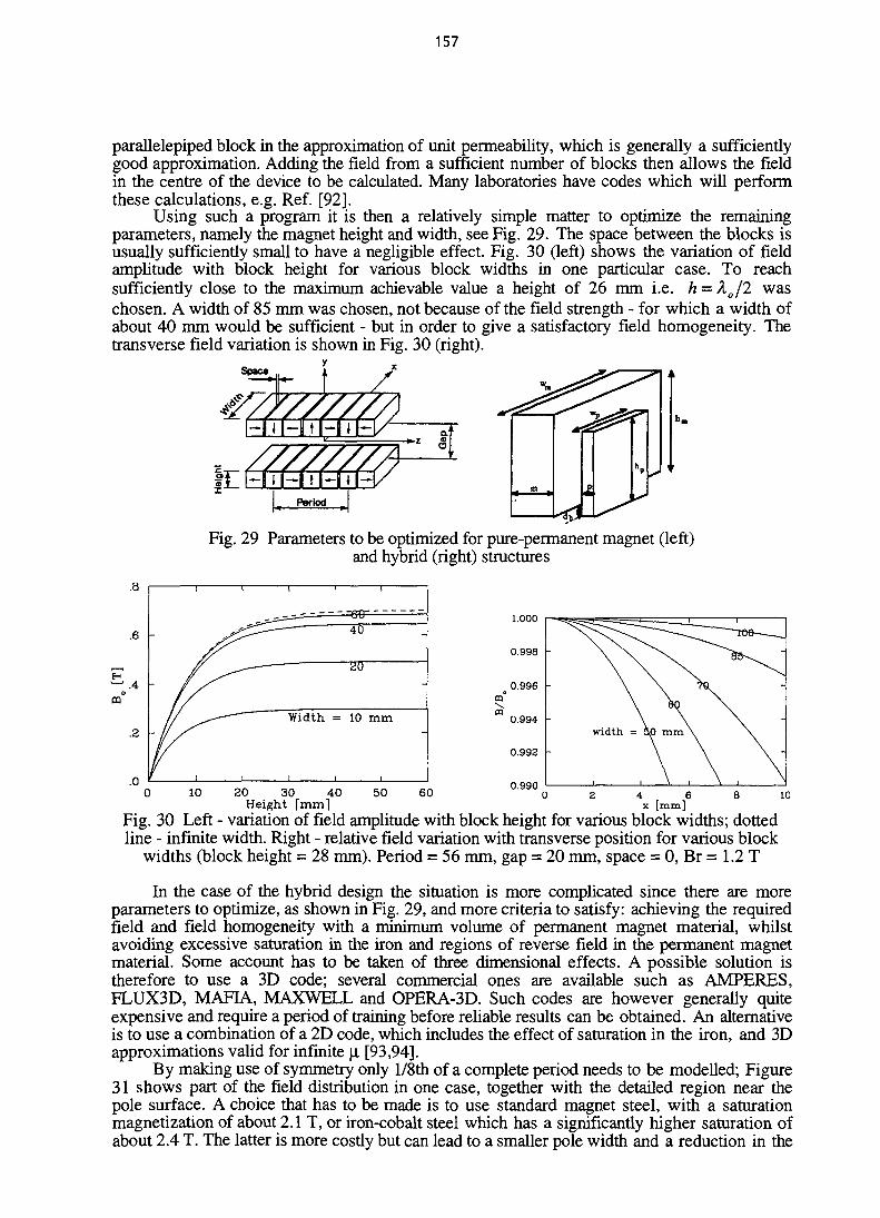
157

parallelepiped block in the approximation of unit permeability, which is generally a sufficientlygood approximation. Adding the field from a sufficient number of blocks then allows the fieldin the centre of the device to be calculated. Many laboratories have codes which will performthese calculations, e.g. Ref. [92].

Using such a program it is then a relatively simple matter to optimize the remainingparameters, namely the magnet height and width, see Fig. 29. The space between the blocks isusually sufficiently small to have a negligible effect. Fig. 30 (left) shows the variation of fieldamplitude with block height for various block widths in one particular case. To reachsufficiently close to the maximum achievable value a height of 26 mm i.e. h = Xo/2 waschosen. A width of 85 mm was chosen, not because of the field strength - for which a width ofabout 40 mm would be sufficient - but in order to give a satisfactory field homogeneity. Thetransverse field variation is shown in Fig. 30 (right).

Space

^ IB ^

Fig. 29 Parameters to be optimized for pure-permanent magnet (left)and hybrid (right) structures

10 4 0 50 60 0.99020 30Height [mm] x [mm]

Fig. 30 Left - variation of field amplitude with block height for various block widths; dottedline - infinite width. Right - relative field variation with transverse position for various block

widths (block height = 28 mm). Period = 56 mm, gap = 20 mm, space = 0, Br = 1.2 T

In the case of the hybrid design the situation is more complicated since there are moreparameters to optimize, as shown in Fig. 29, and more criteria to satisfy: achieving the requiredfield and field homogeneity with a minimum volume of permanent magnet material, whilstavoiding excessive saturation in the iron and regions of reverse field in the permanent magnetmaterial. Some account has to be taken of three dimensional effects. A possible solution istherefore to use a 3D code; several commercial ones are available such as AMPERES,FLUX3D, MAFIA, MAXWELL and OPERA-3D. Such codes are however generally quiteexpensive and require a period of training before reliable results can be obtained. An alternativeis to use a combination of a 2D code, which includes the effect of saturation in the iron, and 3Dapproximations valid for infinite (i [93,94].

By making use of symmetry only l/8th of a complete period needs to be modelled; Figure31 shows part of the field distribution in one case, together with the detailed region near thepole surface. A choice that has to be made is to use standard magnet steel, with a saturationmagnetization of about 2.1 T, or iron-cobalt steel which has a significantly higher saturation ofabout 2.4 T. The latter is more costly but can lead to a smaller pole width and a reduction in the

158

volume of permanent magnet material and hence can be cost effective. In the hybrid design it isimportant that the permanent magnet is larger than the pole in order to reduce flux leakage [95].

Alternative geometries to the basic one discussed above that can lead to an enhanced fieldstrength, but with an increase in complexity and cost, are the wedged-pole geometry [96], andthe inclusion of side-magnets [97], as shown in Fig. 32.

A factor that has to be taken into account particularly in the hybrid design is the fact thatthe field can vary significantly from a pure sinusoid, containing a large 3rd harmoniccomponent. The effect is to change the fundamental photon energy, and also the radiationopening angle.

OM-

Fig. 31 Magnetic flux lines in a hybrid device; right - complete model of l/8th period,left - detail of the pole-tip region

Fig. 32 Alternative hybrid designs; left - with wedged poles, right - with side magnets

6.2 Detailed magnetic design: ends

In order that the insertion device does not affect the storage ring closed orbit requires thatthere is no net change in transverse position or angle of the beam. In the horizontal plane forexample the final angle and position at the end of the device (z = L/2) are given as follows:

L/2

ymc\By(z)dz =J y

L/2 z

x{LI2) = — \ dz \BJz')dz'ymc J J yymc —oo —oo

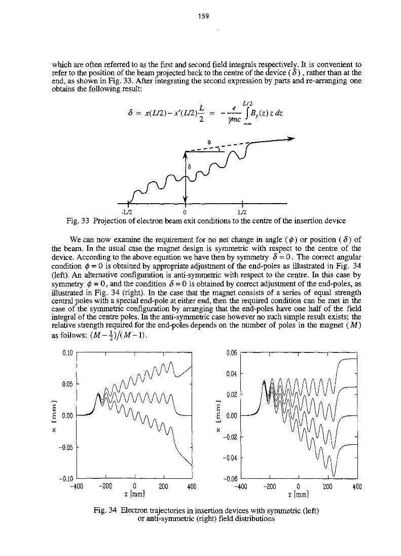
159

which are often referred to as the first and second field integrals respectively. It is convenient torefer to the position of the beam projected back to the centre of the device ( 8 ) , rather than at theend, as shown in Fig. 33. After integrating the second expression by parts and re-arranging oneobtains the following result:

8 = x(L/2)-x'(L/2)- = — -2 ymc _J

L/2JBy(z)zdz

-L/2 0 L/2

Fig. 33 Projection of electron beam exit conditions to the centre of the insertion device

We can now examine the requirement for no net change in angle (<p) or position (8 ) ofthe beam. In the usual case the magnet design is symmetric with respect to the centre of thedevice. According to the above equation we have then by symmetry 5 = 0. The correct angularcondition (j) = 0 is obtained by appropriate adjustment of the end-poles as illustrated in Fig. 34(left). An alternative configuration is anti-symmetric with respect to the centre. In this case bysymmetry <j) = 0, and the condition 8 = 0 is obtained by correct adjustment of the end-poles, asillustrated in Fig. 34 (right). In the case that the magnet consists of a series of equal strengthcentral poles with a special end-pole at either end, then the required condition can be met in thecase of the symmetric configuration by arranging that the end-poles have one half of the fieldintegral of the centre poles. In the anti-symmetric case however no such simple result exists; therelative strength required for the end-poles depends on the number of poles in the magnet (M)

as follows: ( M - | ) / ( M - 1 ) .

-400 -400

Fig. 34 Electron trajectories in insertion devices with symmetric (left)or anti-symmetric (right) field distributions

160

It can be seen from Fig. 34 that even when the magnet is perfectly compensated in angleand position the axis about which the electron beam oscillates is offset from the straight throughdirection either in position (symmetric case) or angle (anti-symmetric case). Such an offset isnot generally a problem, but can be in certain applications. To overcome this requires a moresophisticated entrance and exit configuration involving more than one end-pole. Considering anarrangement of equally spaced poles, the simplest arrangement employs two reduced-strengthend-poles with a sequence of 1/4, -3/4, 1 ... as shown in Fig 35. It is clear that the sameconfiguration can be applied to either the symmetric or anti-symmetric cases. For sequencesinvolving three end-poles a variety of solutions are possible, which can be expressed asfollows: x, -(2x + 1/4), (x + 3/4), -1 .

" 1-p

c

-2

1

1

1 i

+1/4

\

1 !

1 1

t3/4!/

\ /v

Ai

0 1 2 3 4 5 6 7 8 9 102 farb. unitsl

Fig. 35 Sequence of magnet poles (dotted line) resulting in no offset between theelectron trajectory (solid line) and the magnet axis.

Implementation of the various end-pole sequences described above is straightforward inthe case of the pure pennanent magnet configuration because of the applicability of linearsuperposition. As a consequence of this, the field integral due to a single block depends linearlyon the block length. A great advantage is the fact that apart from small effects due to non-unitpermeability and magnetization errors the device remains compensated at all gaps. In thesymmetric case overall compensation can be achieved simply by terminating with a half-block,as shown in the Fig. 36 (a). Some other schemes are shown (b-e) that give no offset of theoscillation axis using either half-sized blocks (b, c) or 1/4 and 3/4 sized blocks (d) [98].

a HthU - I tt t

Fig. 36 Various end-sequences for the pure-permanent magnet structure

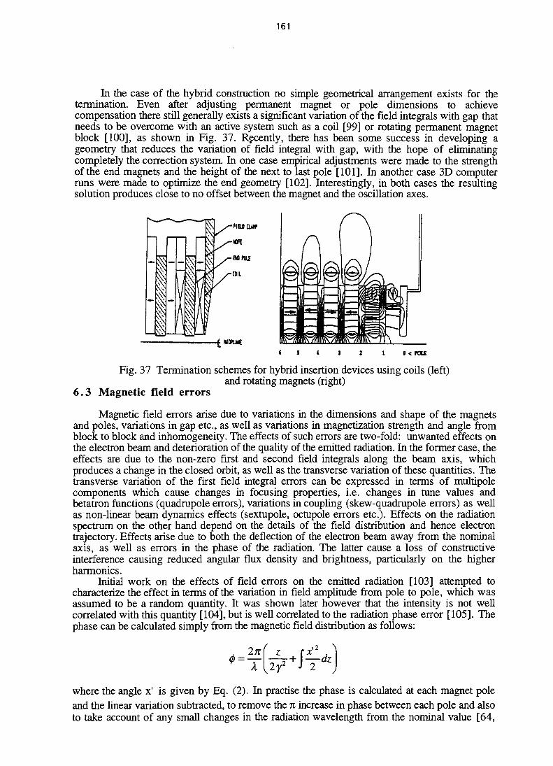
161

In the case of the hybrid construction no simple geometrical arrangement exists for thetermination. Even after adjusting permanent magnet or pole dimensions to achievecompensation there still generally exists a significant variation of the field integrals with gap thatneeds to be overcome with an active system such as a coil [99] or rotating permanent magnetblock [100], as shown in Fig. 37. Recently, there has been some success in developing ageometry that reduces the variation of field integral with gap, with the hope of eliminatingcompletely the correction system. In one case empirical adjustments were made to the strengthof the end magnets and the height of the next to last pole [101]. In another case 3D computerruns were made to optimize the end geometry [102]. Interestingly, in both cases the resultingsolution produces close to no offset between the magnet and the oscillation axes.

o < rouFig. 37 Termination schemes for hybrid insertion devices using coils (left)

and rotating magnets (right)6.3 Magnetic field errors

Magnetic field errors arise due to variations in the dimensions and shape of the magnetsand poles, variations in gap etc., as well as variations in magnetization strength and angle fromblock to block and inhomogeneity. The effects of such errors are two-fold: unwanted effects onthe electron beam and deterioration of the quality of the emitted radiation. In the former case, theeffects are due to the non-zero first and second field integrals along the beam axis, whichproduces a change in the closed orbit, as well as the transverse variation of these quantities. Thetransverse variation of the first field integral errors can be expressed in terms of multipolecomponents which cause changes in focusing properties, i.e. changes in tune values andbetatron functions (quadrupole errors), variations in coupling (skew-quadrupole errors) as wellas non-linear beam dynamics effects (sextupole, octupole errors etc.). Effects on the radiationspectrum on the other hand depend on the details of the field distribution and hence electrontrajectory. Effects arise due to both the deflection of the electron beam away from the nominalaxis, as well as errors in the phase of the radiation. The latter cause a loss of constructiveinterference causing reduced angular flux density and brightness, particularly on the higherharmonics.

Initial work on the effects of field errors on the emitted radiation [103] attempted tocharacterize the effect in terms of the variation in field amplitude from pole to pole, which wasassumed to be a random quantity. It was shown later however that the intensity is not wellcorrelated with this quantity [104], but is well correlated to the radiation phase error [105]. Thephase can be calculated simply from the magnetic field distribution as follows:

-¥[£•£ dz

where the angle x' is given by Eq. (2). In practise the phase is calculated at each magnet poleand the linear variation subtracted, to remove the % increase in phase between each pole and alsoto take account of any small changes in the radiation wavelength from the nominal value [64,

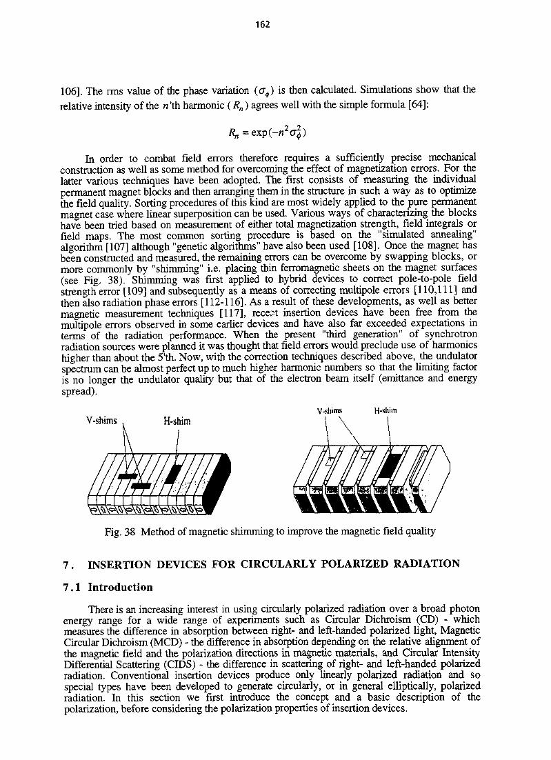
162

106]. The rms value of the phase variation (<70) is then calculated. Simulations show that therelative intensity of the n'th harmonic (Rn) agrees well with the simple formula [64]:

In order to combat field errors therefore requires a sufficiently precise mechanicalconstruction as well as some method for overcoming the effect of magnetization errors. For thelatter various techniques have been adopted. The first consists of measuring the individualpermanent magnet blocks and then arranging them in the structure in such a way as to optimizethe field quality. Sorting procedures of this kind are most widely applied to the pure permanentmagnet case where linear superposition can be used. Various ways of characterizing the blockshave been tried based on measurement of either total magnetization strength, field integrals orfield maps. The most common sorting procedure is based on the "simulated annealing"algorithm [107] although "genetic algorithms" have also been used [108]. Once the magnet hasbeen constructed and measured, the remaining errors can be overcome by swapping blocks, ormore commonly by "shimming" i.e. placing thin ferromagnetic sheets on the magnet surfaces(see Fig. 38). Shimming was first applied to hybrid devices to correct pole-to-pole fieldstrength error [109] and subsequently as a means of correcting multipole errors [110,111] andthen also radiation phase errors [112-116]. As a result of these developments, as well as bettermagnetic measurement techniques [117], recent insertion devices have been free from themultipole errors observed in some earlier devices and have also far exceeded expectations interms of the radiation performance. When the present "third generation" of synchrotronradiation sources were planned it was thought that field errors would preclude use of harmonicshigher than about the 5'th. Now, with the correction techniques described above, the undulatorspectrum can be almost perfect up to much higher harmonic numbers so that the limiting factoris no longer the undulator quality but that of the electron beam itself (emittance and energyspread).

V-shims H-shimV-sliims H-shim

Fig. 38 Method of magnetic shimming to improve the magnetic field quality

7 . INSERTION DEVICES FOR CIRCULARLY POLARIZED RADIATION

7.1 Introduction

There is an increasing interest in using circularly polarized radiation over a broad photonenergy range for a wide range of experiments such as Circular Dichroism (CD) - whichmeasures the difference in absorption between right- and left-handed polarized light, MagneticCircular Dichroism (MCD) - the difference in absorption depending on the relative alignment ofthe magnetic field and the polarization directions in magnetic materials, and Circular IntensityDifferential Scattering (CIDS) - the difference in scattering of right- and left-handed polarizedradiation. Conventional insertion devices produce only linearly polarized radiation and sospecial types have been developed to generate circularly, or in general elliptically, polarizedradiation. In this section we first introduce the concept and a basic description of thepolarization, before considering the polarization properties of insertion devices.

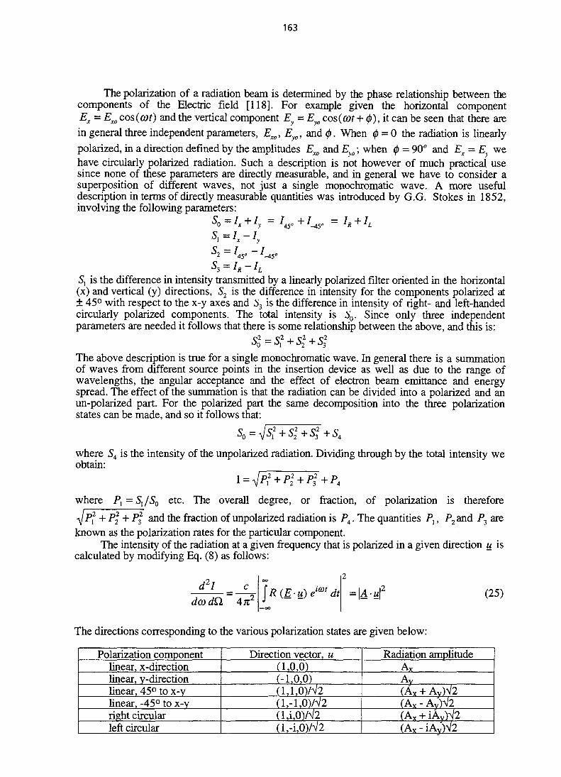
163

The polarization of a radiation beam is determined by the phase relationship between thecomponents of the Electric field [118]. For example given the horizontal componentEx = Ex0 cos (cot) and the vertical component E = E cos (cot + <f>), it can be seen that there are

in general three independent parameters, Exo, Eyo, and <p. When 0 = 0 the radiation is linearly

polarized, in a direction defined by the amplitudes Em and Eyo; when <j> = 90° andyo; Ex = E we

have circularly polarized radiation. Such a description is not however of much practical usesince none of these parameters are directly measurable, and in general we have to consider asuperposition of different waves, not just a single monochromatic wave. A more usefuldescription in terms of directly measurable quantities was introduced by G.G. Stokes in 1852,involving the following parameters:

S2 ~ hs* ~ 7-45°

5j is the difference in intensity transmitted by a linearly polarized filter oriented in the horizontal(x) and vertical (y) directions, 52 is the difference in intensity for the components polarized at± 45° with respect to the x-y axes and i'3 is the difference in intensity of right- and left-handedcircularly polarized components. The total intensity is So. Since only three independentparameters are needed it follows that there is some relationship between the above, and this is:

The above description is true for a single monochromatic wave. In general there is a summationof waves from different source points in the insertion device as well as due to the range ofwavelengths, the angular acceptance and the effect of electron beam emittance and energyspread. The effect of the summation is that the radiation can be divided into a polarized and anun-polarized part. For the polarized part the same decomposition into the three polarizationstates can be made, and so it follows that:

where S4 is the intensity of the unpolarized radiation. Dividing through by the total intensity weobtain:

where Pl = Sl /So etc. The overall degree, or fraction, of polarization is therefore

•\jPf + Pl + P32 and the fraction of unpolarized radiation is P4. The quantities P,, P2 and P3 are

known as the polarization rates for the particular component.The intensity of the radiation at a given frequency that is polarized in a given direction u is

calculated by modifying Eq. (8) as follows:

d2l

dco dQ An1 (25)

The directions corresponding to the various polarization states are given below:

Polarization componentlinear, x-directionlinear, v-directionlinear, 45° to x-ylinear, -45° to x-yright circularleft circular

Direction vector, u(1,0,0)(-1,0,0)(U,0)A/2(l,-l ,0W2(U,0)/V2(l,-i,0)/V2

Radiation amplitudeAy

Ay(Ax + AV)V2(Av - AyW2(AY + iAy W2(Av-iAyW2

164

In the above we also show the amplitude of the radiation polarized in the given direction interms of the horizontal and vertical components, which are in general complex quantities. Theintensities can then be expressed as follows:

'* =

IR = [\A

- AxA*y

; -A*xAy)] IL= [|A2

-A*xAy]/2

+ i{AxA*y-A*xAy^f2

(26)

Finally, we can express the Stokes parameters in terms of the radiation amplitudes as follows:

^ — A A -i- A A° 0 ~~ X^X T /Iy/1;y

c A A A A^1 - AxAx "yAy

S2=A*xAy + AxA*

S3 =i(A*xAy-AxA*)

7.2 Bending magnet and conventional insertion devices

In order to understand the polarization properties of bending magnet and insertion devicesources we will examine the electric field of the radiation, which according to Eq. (9) isproportional to the electron acceleration. To a first approximation we have the followingrelationships:

Ex~px-expz(27)

where 6X, 6yare the angles of emission with respect to the x, y axes (Fig. 6). In a bending

magnet which bends in the horizontal plane $y=0 and hence the vertical electric fieldcomponent only exists for emission out of the orbit plane 6y * 0. It follows directly from thedirection of acceleration that Ex (~ fix) is symmetric with respect to the tangent point whereasEy (~ 6yPz) is anti-symmetric, as shown schematically in Fig. 39. Figure 40 shows the patterntraced out by the electric field for the particular case dy = l/y. The circular motion of the electricfield vector indicates the presence of circularly polarized radiation. In fact as the angle 6increases the fraction of circular polarization rate increases while the linear polarizationdecreases, as shown in Fig. 41. For angles below the orbit plane (6y < 0) the vertical electricfield component changes sign and hence the direction of circular polarization reverses.

Fig. 39 Schematic diagram of radiation emission in a bending magnet: direction of electronacceleration (left), and electric field components as a function of time (right)

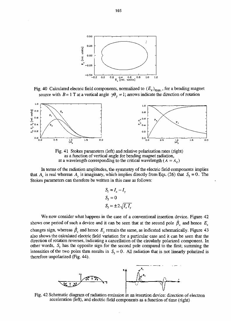
165

0.50

-0.50-0.2 0.0 0.2 0.4 0.6 0.8E [rel. units]

1.0 1.2

Fig. 40 Calculated electric field components, normalized to (Ex)max , for a bending magnetsource with B= 1 T at a vertical angle yd -1; arrows indicate the direction of rotation

2.0

Fig. 41 Stokes parameters (left) and relative polarization rates (right)as a function of vertical angle for bending magnet radiation,

at a wavelength corresponding to the critical wavelength (A = Ac)

In terms of the radiation amplitudes, the symmetry of the electric field components impliesthat Ax is real whereas Ay is imaginary, which implies directly from Eqs. (26) that S2 = 0. TheStokes parameters can therefore be written in this case as follows:

S2=0

We now consider what happens in the case of a conventional insertion device. Figure 42shows one period of such a device and it can be seen that at the second pole J3X and hence Ex

changes sign, whereas j3z and hence Ey remain the same, as indicated schematically. Figure 43also shows the calculated electric field variation for a particular case and it can be seen that thedirection of rotation reverses, indicating a cancellation of the circularly polarized component. Inother words, 53 has the opposite sign for the second pole compared to the first; summing theintensities of the two poles then results in 53 = 0. All radiation that is not linearly polarized istherefore unpolarized (Fig. 44).

IkFig. 42 Schematic diagram of radiation emission in an insertion device: direction of electron

acceleration (left), and electric field components as a function of time (right)

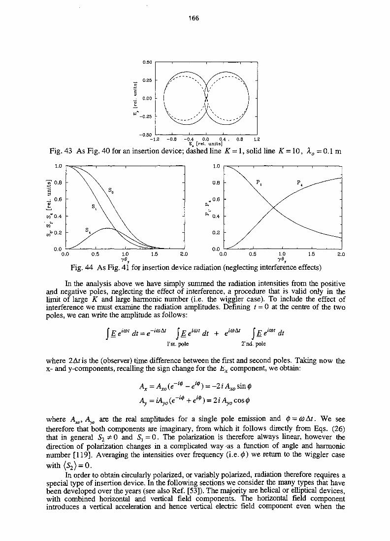
166

0.50

0.25 -

0.00 -

-0.35 -

-0.501.2-1.2 -0.8 -0.4 0.0 0.4 , 0.8

ET [rel. units]

Fig. 43 As Fig. 40 for an insertion device; dashed line K = 1, solid line # = , Ao = 0.1 m

CO

0.0 0.0

Fig. 44 As Fig. 41 for insertion device radiation (neglecting interference effects)

In the analysis above we have simply summed the radiation intensities from the positiveand negative poles, neglecting the effect of interference, a procedure that is valid only in thelimit of large K and large harmonic number (i.e. the wiggler case). To include the effect ofinterference we must examine the radiation amplitudes. Defining t = 0 at the centre of the twopoles, we can write the amplitude as follows:

JEeicot -icoAt JEe1

l'st. pole

l(Ot dt + eiaAt JEe1

2'nd. pole

icot dt

where 2A?is the (observer) time difference between the first and second poles. Taking now thex- and y-components, recalling the sign change for the Ex component, we obtain:

Ax=Axo{e-i(t> -ei*) = -2i

Ay = iAyoie-' e1*) = 2iAyOcos<p

where Axo, Ayo are the real amplitudes for a single pole emission and <j) = o)At. We seetherefore that both components are imaginary, from which it follows directly from Eqs. (26)that in general S2 * 0 and 53 = 0. The polarization is therefore always linear, however thedirection of polarization changes in a complicated way >as a function of angle and harmonicnumber [119]. Averaging the intensities over frequency (i.e. <p) we return to the wiggler case

with (S2) = 0.In order to obtain circularly polarized, or variably polarized, radiation therefore requires a

special type of insertion device. In the following sections we consider the many types that havebeen developed over the years (see also Ref. [53]). The majority are helical or elliptical devices,with combined horizontal and vertical field components. The horizontal field componentintroduces a vertical acceleration and hence vertical electric field component even when the

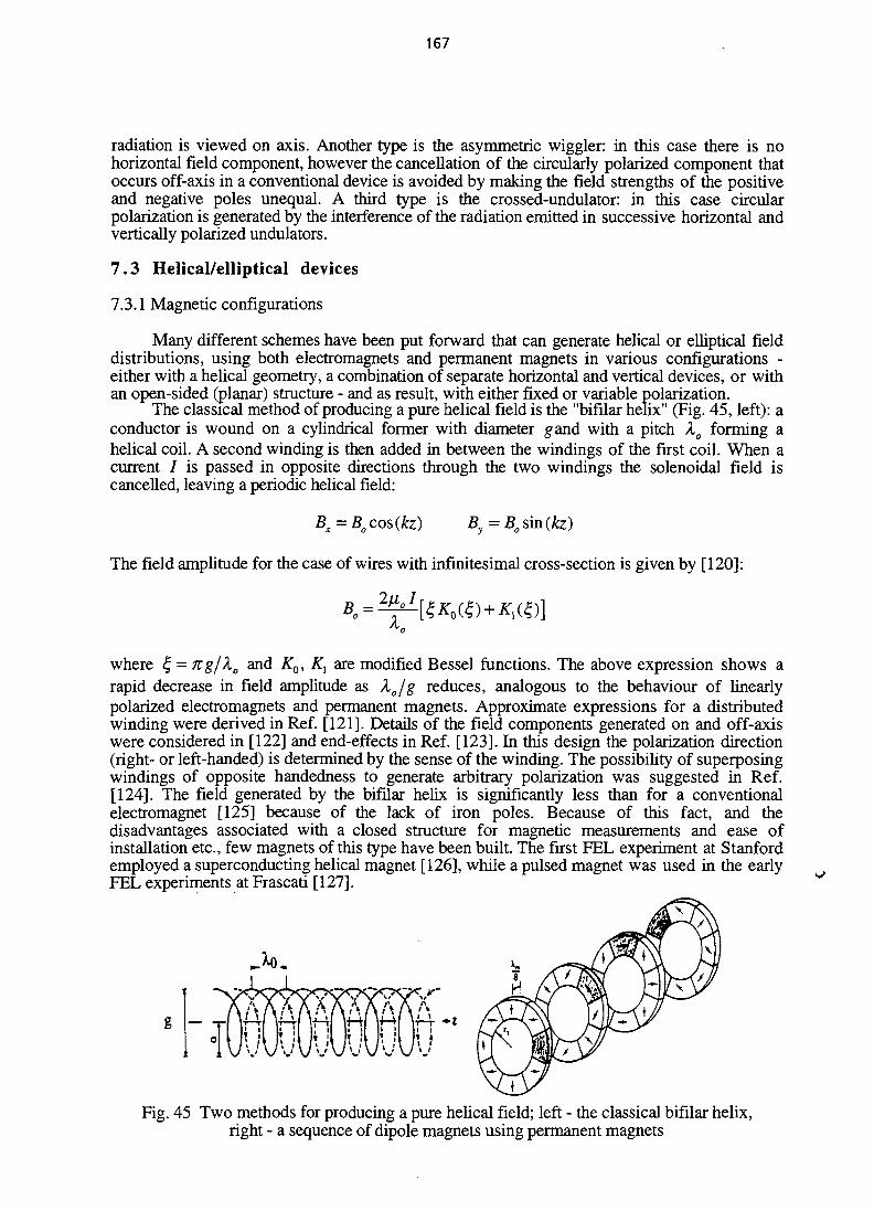
167

radiation is viewed on axis. Another type is the asymmetric wiggler: in this case there is nohorizontal field component, however the cancellation of the circularly polarized component thatoccurs off-axis in a conventional device is avoided by making the field strengths of the positiveand negative poles unequal. A third type is the crossed-undulator: in this case circularpolarization is generated by the interference of the radiation emitted in successive horizontal andvertically polarized undulators.

7.3 Helical/elliptical devices

7.3.1 Magnetic configurations

Many different schemes have been put forward that can generate helical or elliptical fielddistributions, using both electromagnets and permanent magnets in various configurations -either with a helical geometry, a combination of separate horizontal and vertical devices, or withan open-sided (planar) structure - and as result, with either fixed or variable polarization.

The classical method of producing a pure helical field is the "bifilar helix" (Fig. 45, left): aconductor is wound on a cylindrical former with diameter gand with a pitch Ao forming ahelical coil. A second winding is then added in between the windings of the first coil. When acurrent / is passed in opposite directions through the two windings the solenoidal field iscancelled, leaving a periodic helical field:

Bx = Bo cos (fe) By = Bo sin (fe)

The field amplitude for the case of wires with infinitesimal cross-section is given by [120]:

where £ = Kg/X0 and Ko, Kx are modified Bessel functions. The above expression shows arapid decrease in field amplitude as X0/g reduces, analogous to the behaviour of linearlypolarized electromagnets and permanent magnets. Approximate expressions for a distributedwinding were derived in Ref. [121]. Details of the field components generated on and off-axiswere considered in [122] and end-effects in Ref. [123]. In this design the polarization direction(right- or left-handed) is determined by the sense of the winding. The possibility of superposingwindings of opposite handedness to generate arbitrary polarization was suggested in Ref.[124]. The field generated by the bifilar helix is significantly less than for a conventionalelectromagnet [125] because of the lack of iron poles. Because of this fact, and thedisadvantages associated with a closed structure for magnetic measurements and ease ofinstallation etc., few magnets of this type have been built. The first FEL experiment at Stanfordemployed a superconducting helical magnet [126], while a pulsed magnet was used in the earlyFEL experiments at Frascati [127].

Fig. 45 Two methods for producing a pure helical field; left - the classical bifilar helix,right - a sequence of dipole magnets using permanent magnets

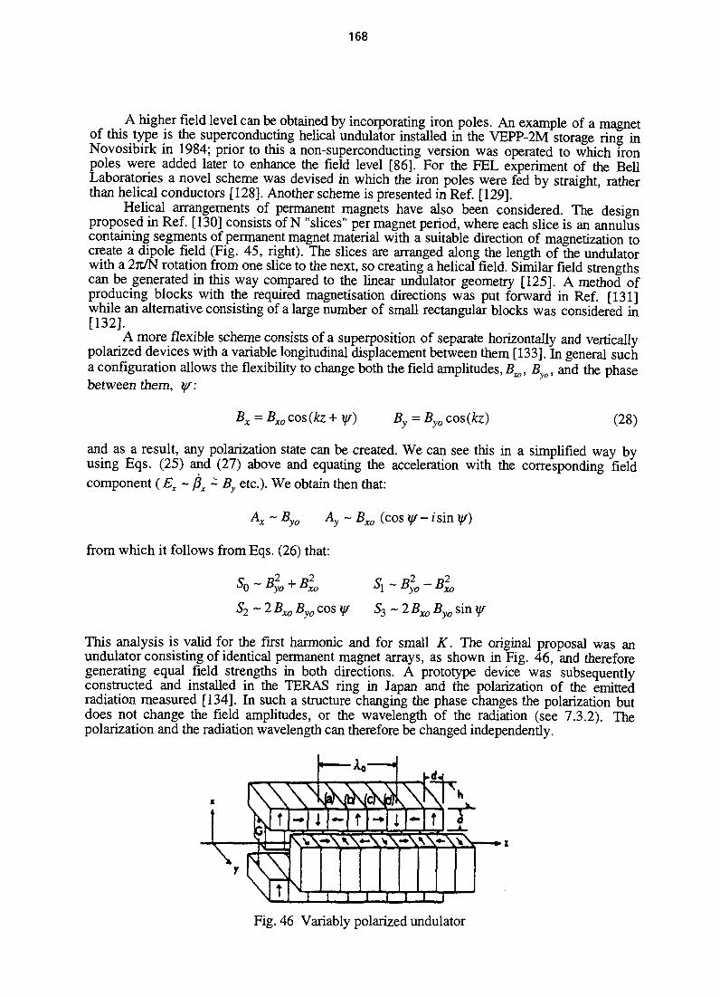
168

A higher field level can be obtained by incorporating iron poles. An example of a magnetof this type is the superconducting helical undulator installed in the VEPP-2M storage ring inNovosibirk in 1984; prior to this a non-superconducting version was operated to which ironpoles were added later to enhance the field level [86]. For the PEL experiment of the BellLaboratories a novel scheme was devised in which the iron poles were fed by straight, ratherthan helical conductors [128]. Another scheme is presented in Ref. [129].

Helical arrangements of permanent magnets have also been considered. The designproposed in Ref. [130] consists of N "slices" per magnet period, where each slice is an annuluscontaining segments of permanent magnet material with a suitable direction of magnetization tocreate a dipole field (Fig. 45, right). The slices are arranged along the length of the undulatorwith a 27T/N rotation from one slice to the next, so creating a helical field. Similar field strengthscan be generated in this way compared to the linear undulator geometry [125]. A method ofproducing blocks with the required magnetisation directions was put forward in Ref. [131]while an alternative consisting of a large number of small rectangular blocks was considered in[132].

A more flexible scheme consists of a superposition of separate horizontally and verticallypolarized devices with a variable longitudinal displacement between them [133]. In general sucha configuration allows the flexibility to change both the field amplitudes, Bxo, Byo, and the phasebetween them, y/:

Bx =Bxocos(kz+y/) = Byocos(kz)yo

(28)

and as a result, any polarization state can be created. We can see this in a simplified way byusing Eqs. (25) and (27) above and equating the acceleration with the corresponding fieldcomponent (Ex - fix ~ By etc.). We obtain then that:

Ac ~ Byo ~ Bxo (cosyf-zsin y/)

from which it follows from Eqs. (26) that:

Sn~ ~B2 -Dyo •

S,~ Byo sin V

This analysis is valid for the first harmonic and for small K. The original proposal was anundulator consisting of identical permanent magnet arrays, as shown in Fig. 46, and thereforegenerating equal field strengths in both directions. A prototype device was subsequentlyconstructed and installed in the TERAS ring in Japan and die polarization of the emittedradiation measured [134]. In such a structure changing the phase changes the polarization butdoes not change the field amplitudes, or the wavelength of the radiation (see 7.3.2). Thepolarization and the radiation wavelength can therefore be changed independently.

Fig. 46 Variably polarized undulator

169

With unequal field amplitudes in the two directions higher harmonics are generated with,in general, elliptical polarization [135]. Two permanent magnet devices of this kind were laterconstructed and installed in the TRISTAN Accumulator Ring and the Photon Factory [136].These devices made use of the fact that the vertical magnet gap (30 mm) could be much smallerthan the horizontal one (110 mm) so allowing a much higher field strength in the verticaldirection, 1.0 T (Ky = 15) compared to the horizontal, 0.2 T (Kx = 3). Such a device becameknown as an elliptical multipole wiggler (EMPW). Later measurements confirmed that a highdegree of circular polarization could be obtained at high photon energies [137].

The idea of" replacing the permanent magnet arrays in the above scheme with anelectromagnet in order to allow a rapid switching of the polarization state was first mentioned in[133]. Since an electromagnet requires a longer period length, and generates a smaller fieldstrength than a permanent magnet, the idea is more applicable to the case of an elliptical wiggler.The first proposal for an electromagnetic elliptical wiggler (EEW) capable of reaching aswitching speed of 100 Hz was made in [138]. A prototype device was later built by anAPS/BINP/NSLS collaboration and installed in the NSLS X-ray ring [139]. A similar devicewas subsequently installed in the APS. A device consisting of two electromagnets, with thepossibility also of shifting one magnet with respect to another has recently been proposed atLURE [140].a b

X 7 X^x" y X ^>

t —1 1

Fig. 47 Various planar permanent magnet arrangements,a - HELIOS, b - planar helical undulator, c - APPLE-H, d - Spring-8

A disadvantage of all of the above schemes is the need for magnetic arrays on all sides ofthe electron beam tube. This not only complicates magnetic measurements and installation, butalso means that the minimum gaps that can be achieved are restricted by the lateral size of themagnetic structures. Alternative "planar" structures have therefore been devised with magnetslocated only above and below the beam axis. The first proposal of this kind is shown in Fig. 47(a) [141]. In this scheme the upper array produces a horizontal field, while the lower arrayproduces a vertical field. The field components on-axis are therefore identical to those of theOnuki device given by Eq. (28), and hence by adjusting separately the upper and lower half-gaps and the longitudinal phase shift any polarization state can be generated. Owing to the lackof symmetry this device produces a linear variation of both field components in the verticaldirection, thereby increasing the sensitivity of the radiation wavelength to beam position. Afurther potential problem is the fact that the fields give rise to a second-order deflection of the

170

trajectory in the horizontal direction when y/ * 0, and in the vertical direction when Bx0 * Byo

[142]. Since these effects are of second-order and therefore inversely proportional to Energy2,the effects may become problematic in low energy rings. In the ESRF the horizontal deflectionis overcome using two separate undulators with opposite helicity so that the two deflectionscancel [143]. The two undulators are used in a "chicane" arrangement to produce radiation withopposite helicity displaced slightly to the left and right of the beam axis. The HELIOS devicewas installed in the ESRF in June 1993; no effect on beam lifetime was observed, and onlysmall changes in closed orbit were produced, in agreement with expectations [67]. Two furthersingle section structures have subsequently been installed [144].

A modification of the HELIOS device is the planar helical undulator [142], shown inFig. 47 (b). In this case both arrays produce a pure helical field, with equal field amplitudesthat exceed that of the HELIOS device in the helical mode. A further advantage of this structureis that the symmetrical arrangement eliminates any second-order deflections. A significantdisadvantage however is that the helicity is fixed.

More recently a further device was developed called APPLE (Advanced Planar PolarizedLight Emitter), which produces even higher field amplitudes. The first structure to be putforward (APPLE-I) employed magnet blocks with a 45° magnetization [145]. Subsequently asimpler structure (APPLE-II) was developed in which each of the four arrays has aconventional Halbach structure [146], shown in Fig. 47 (c). This version, as well as beingeasier to construct, produces a larger Bx field at the expense of smaller By and hence also ahigher field in the helical mode. In both versions the polarization is altered by shifting theupper-back and lower-front arrays with respect to the upper-front and lower-back arrays.Considering for simplicity a shift of + y/ for the pairs of arrays, the upper-back and lower-frontarrays produce a linearly polarized field given by:

Bx = Bxo /2 cos (kz-y) By = Byo I2 cos (kz - y)

whereas the upper-front and lower-back arrays generate a field given by:

Bx=-Bxo/2 cos(kz+y) By= Byo/2 cos(kz+y)

Adding the two together and simplifying results in the following:

Bx = Bxo sin (kz) sin (y) By = By0 cos (kz) cos (y/)

Thus, unlike the Onuki and HELIOS cases, the field amplitudes do depend on y, and so thepolarization cannot be adjusted independently of the radiation wavelength. In addition, changingthe gap changes the horizontal and vertical fields by a different amount, and so changes thepolarization. An interesting property of this device is that the two field components remain 90°out of phase, and hence the polarization ellipse remains upright. The simple polarizationanalysis gives in this case (in the low K limit):

Sx ~ B)o COS2 y/ - B2XO sin V S2 ~ 0 53 ~ BxoByo sin 2 y/

The APPLE configuration has a greater degree of symmetry than the HELIOS one, whicheliminates problems due to second-order steering effects. The transverse field homogeneityremains considerably worse than in a conventional device, however experience with operatingdevices and beam dynamics calculations do not indicate any major problems.

The first test of the APPLE-I device was made with a seven-period prototype in the JAERIStorage Ring (JSR) [147]. Visible light was generated with variable polarization with a ringenergy of 138 MeV. No beam deflections were observed while changing the gap or the phase.

An APPLE-II device was subsequently constructed for the SPEAR storage ring. Thisdevice includes a further feature, namely the ability to change the field strengths by phase ratherthan gap variation [148]. This is achieved by shifting the relative positions of the two upperarrays with respect to the two lower ones, or the two front arrays with respect to the two back

171

arrays. In this way no gap adjustment is required to set any desired output wavelength andellipticity. The device was subsequently tested in SPEAR with no noticeable effect on the3 GeV beam for any longitudinal motion of the arrays [149]. Further devices are underconstruction for ALS, BESSY-II and TLS, and are planned for the SRS.

Finally, a structure consisting of six magnet arrays has been proposed by the Spring-8team [150], shown in Fig. 47 (d). In this case the upper and lower central arrays generate avertical field while the outer four arrays generate a horizontal field. The longitudinal phasing ofthe outer arrays with respect to the central arrays allows the polarization to be adjusted. Adisadvantage of the structure however is that it is not possible to achieve both pure horizontaland vertical polarization unless at least five of the arrays are moveable: if the central arrays arefixed, then there is always a vertical field present, while if the outer arrays are fixed there isalways a horizontal field. Both versions are planned for Spring-8, while the former type hasbeen constructed and installed recently in the UVSOR storage ring. It has been claimed that thisstructure results in a better transverse field homogeneity than the APPLE design, and thereforeproduces less effect on the electron beam dynamics.

7.3.2 Radiation properties

We firstly consider how the interference condition is modified in the presence of anadditional horizontal field component, at an arbitrary phase with respect to the vertical fieldcomponent:

Bx = Bxo sin (kz + yr) By = Byo sin (kz)

The electron motion is then:

K K/L = -cos(fcz + W) Bx= —-cos(kz)

y y y

where Kx=—jL-g-, and K = n _y °. Since the electron velocity is given by

7.nmcp2 = p2 + p2 + p2 we have therefore:

(29)Ay1 Ay1 Ay1 4y2

For the interference condition only the average velocity along the z-axis is important, which issimply:

A.'Y 4 V

Applying the interference condition, Eq. (3), then gives:

2yz n

Thus the radiation wavelength depends only on the amplitudes of the two field components,independently of the phase y/ between them.

172

The analysis of the radiation emission in the general case is quite complicated (seeAppendix). In the particular case of on-axis radiation for y/ = nj2 the angular flux density canbe written, in practical units, as follows:

d2n

dco/co dQ e=Q

where

and

with

= 1.744 1014 N2ElGeV]Fn(Kx,Ky)Ib

n(K2y-K

2x)

The integrated flux is then given, see Eq. (18), by:

^ = 1.431 1014 N Qn(Kx,K)f{Nk(ol(ax{0)) ly 43 10 N Qn(Kx,K)f{Nk(ol(ax{0)) lb

where Qn(Kx,Kx) = (1 + K2X jl + K2 jl)Fn(Kx,Kx)/n. The Stokes parameters are given by:

Sl/S0=(A2x-A

2)/(A2x+A2)

S2/S0=0

In the case of purely circular motion, when Kx=Ky = K (and y/ = K/2) the longitudinalvelocity, Eq. (29), is constant. As a result the electric fields Exand Ey are purely sinusoidal andso the radiation consists of a single harmonic on axis. This is evident also in the formula abovesince when 7 = 0 the only non-zero term is JQ(O) which occurs only for n = \. We havetherefore:

9 K^~ 9 K^~FX{K)= ? 7 and Ql(K)= 9

1 d+ii:2)2 l (i+K2)and the radiation is purely circularly polarized:

SI/SQ=0, S2/S0=0, S3/S0 = l

Figure 48 shows the variation of angular flux density, circular polarization rate and theirproduct (S3) as a function of the ratio between the horizontal and vertical field strengths with afixed radiation wavelength (i.e. fixed K] + K^). For Kx/Ky = 0 we have the same result for aplane undulator, with pure linear polarization. As Kx/Ky increases both the flux and circularpolarization rate increase for the fundamental. The maximum circularly polarized flux istherefore obtained with pure circular polarization with Kx = Ky. In the case of the higherharmonics however the circular polarization rate increases, but the flux eventually tends to zeroat Kx = Ky. There is therefore an optimum value of Kx/Ky which maximizes S3, which

depends on the harmonic number (and on Kx +Ky).

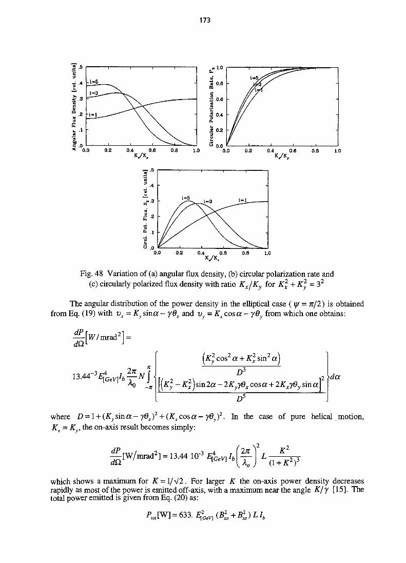
173

2 5

1.0

Fig. 48 Variation of (a) angular flux density, (b) circular polarization rate and(c) circularly polarized flux density with ratio Kx/Ky for Kx+Ky = 32

The angular distribution of the power density in the elliptical case (y/ = 7t/2) is obtainedfrom Eq. (19) with vx = Ky since - yOx and vy = Kx cos a - yQy from which one obtains:

—[w/mrad2l =

cos2 a + K\ sin2 a)

Ky - Kx) sin 2a - 2Kyy6x cos a + 2Kxy6y sin aYda

where D = 1 + (Ky sin a - ydx )2 + (Kx cos a - y0y )

2. In the case of pure helical motion,Kx = K', the on-axis result becomes simply:

^[W/mrad 2 ] = 13.44 10"3 E*GeV] Ib \^f\ Lall \ A~ }

which shows a maximum for K = l/^2. For larger X" the on-axis power density decreasesrapidly as most of the power is emitted off-axis, with a maximum near the angle K/y [15]. Thetotal power emitted is given from Eq. (20) as:

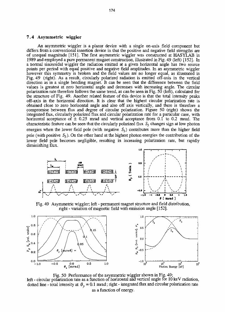
174

7.4 Asymmetric wiggler

An asymmetric wiggler is a planar device with a single on-axis field component butdiffers from a conventional insertion device in that the positive and negative field strengths areof unequal magnitude [151]. The first asymmetric wiggler was constructed at HASYLAB in1989 and employed a pure permanent magnet construction, illustrated in Fig. 49 (left) [152]. Ina normal sinusoidal wiggler the radiation emitted at a given horizontal angle has two sourcepoints per period with equal positive and negative field amplitudes. In an asymmetric wigglerhowever this symmetry is broken and the field values are no longer equal, as illustrated inFig. 49 (right). As a result, circularly polarized radiation is emitted off-axis in the verticaldirection as in a single bending magnet. It can be seen that the difference between the fieldvalues is greatest at zero horizontal angle and decreases with increasing angle. The circularpolarization rate therefore follows the same trend, as can be seen in Fig. 50 (left), calculated forthe structure of Fig. 49. Another related feature of this device is that the total intensity peaksoff-axis in the horizontal direction. It is clear that the highest circular polarization rate isobtained close to zero horizontal angle and also off axis vertically, and there is therefore acompromise between flux and degree of circular polarization. Figure 50 (right) shows theintegrated flux, circularly polarized flux and circular polarization rate for a particular case, withhorizontal acceptance of ± 0.25 mrad and vertical acceptance from 0.1 to 0.2 mrad. Thecharacteristic feature can be seen that the circularly polarized flux S3 changes sign at low photonenergies when the lower field pole (with negative S3) contributes more than the higher fieldpole (with positive S3). On the other hand at the highest photon energies the contribution of thelower field pole becomes negligible, resulting in increasing polarization rate, but rapidlydiminishing flux.

1.0

J.

CAP

T

*—*

«i t

03

0.9

0.0

-o.s -

1 1

r'

y

1 ' l

t

1

I ;

\ '\ /

\ t ^f ."*"* 1 . .

-1.S - I -0.6 0 0.3 t9 ( mrad )

1.S

Fig. 49 Asymmetric wiggler; left - permanent magnet structure and field distribution,right - variation of magnetic field with emission angle [152].

o.o8x [mrad]

. 0.5 -

. 0.0 -

-0.5

-1.010' 10s 10'

Photon Energy [eV]10s

Fig. 50 Performance of the asymmetric wiggler shown in Fig. 49;left - circular polarization rate as a function or horizontal and vertical angle for 10 keV radiation,dotted line - total intensity at 6y = 0.1 mrad; right - integrated flux and circular polarization rate

as a function of energy.

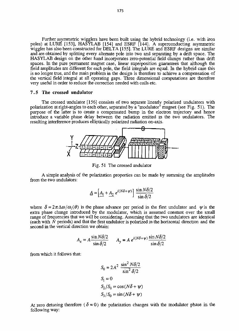
175

Further asymmetric wigglers have been built using the hybrid technology (i.e. with ironpoles) at LURE [153], HASYLAB [154] and ESRF [144]. A superconducting asymmetricwiggler has also been constructed for DELTA [155]. The LURE and ESRF designs are similarand are obtained by splitting every alternate pole into two and separating by a drift space. TheHASYLAB design on the other hand incorporates zero-potential field clamps rather than driftspaces. In the pure permanent magnet case, linear superposition guarantees that although thefield amplitudes are different for each pole, the field integrals are equal. In the hybrid case thisis no longer true, and the main problem in the design is therefore to achieve a compensation ofthe vertical field integral at all operating gaps. Three dimensional computations are thereforevery useful in order to reduce the correction needed with coils etc.

7.5 The crossed undulator

The crossed undulator [156] consists of two separate linearly polarized undulators withpolarization at right-angles to each other, separated by a "modulator" magnet (see Fig. 51). Thepurpose of the latter is to create a compensated bump in the electron trajectory and henceintroduce a variable phase delay between the radiation emitted in the two undulators. Theresulting interference produces elliptically polarized radiation on-axis.

•e-

Y

Fig. 51 The crossed undulator

A simple analysis of the polarization properties can be made by summing the amplitudesfrom the two undulators:

where 8 = 2KACO/COX{6) is the phase advance per period in the first undulator and i/is theextra phase change introduced by the modulator, which is assumed constant over the smallrange of frequencies that we will be considering. Assuming that the two undulators are identical(each with N periods) and that the first undulator is polarized in the horizontal direction and thesecond in the vertical direction we obtain:

AsinN8/2Ar = A —

x sin 5/2

A - A

y sin 8/2

from which it follows that:

S0=2A 2 sin2 N8/2

sin2 8/2

5i=0S2/SQ=cos(N8+ if/)

S3/S0=sin(N8+\jr)

At zero detuning therefore (5 = 0) the polarization changes with the modulator phase in thefollowing way:

176

Phase (\f/)0°90°180°270°360°

s2/s010-101

010-10

Polarizationlinear at 45°

right-handed circularlinear at -45°

left-handed circularlinear at 45°

A rapid change of polarization can be made if the modulator is a suitably designedelectromagnet. An interesting feature of the device is that, unlike helical magnets, even withpure circular polarization higher harmonics are generated on-axis, since each individual linearundulator generates higher harmonics.

-1.0-2.0 -1.5 -1.0 -0.5 0.0 0.5 1.0 1.5 2.0

/

Fig. 52 Variation of intensity and circular polarization rates with frequencyin a crossed undulator

From the equation above it is clear that the polarization changes rapidly with the detuningparameter, and this is illustrated in Fig. 52. For example, with y/ = n/2 we obtain purecircularly polarized radiation on axis. At Aft)/<2), = l/4iV however this becomes zero, whereasthe total flux becomes zero only at Afo/fi), = 1/N. Certain conditions must therefore be met inorder to obtain significant circular polarization:• selection of a narrow range of photon energies, A®/co < l/2nN. Under normal

circumstance this is not a problem since the monochromator provides a significantlysmaller band-pass;

• selection of a narrow range of acceptance angles, 6 < -\//l/2L. In other words, theacceptance angle must be restricted with a "pinhole" aperture so as to receive only afraction of the available flux;

• it follows from the above that the electron beam divergence must also be sufficientlysmall, (je < -\JJJ2L;

• similarly, the energy spread of the electron beam must be sufficiently small,AE/E<l/SnN.

It should be noted that in all cases the sensitivity increases for the higher harmonics.The first, and so far only, device of this type to be built is operational in BESSY [157].

The present modulator is not laminated and so does not permit a fast switching. A crossedundulator that was proposed for the ALADDIN storage ring [158] incorporated a modulator thatwas designed to reach a switching speed of 10 Hz [159].

Alternative geometries to the one presented above are also possible. With the twoundulators oriented at 45° and -45° with respect to the x-y axes results in an exchange of the S,and S2 parameters, i.e. allowing horizontal and vertical polarization to be obtained as well ascircular polarization. A combination of right- and left-handed circularly polarized undulatorscreates linearly polarized radiation (5, * 0, S2 * 0, 53 = 0). In this case however the interestingsituation arises that since only a single harmonic is generated on-axis in each device, the linearlypolarized radiation consists only of a single harmonic [160].

177

8. UNDULATORS FOR FREE-ELECTRON LASERS

unduMorrmgnManir

Fig. 53 Basic scheme of a free-electron laser

In a free-electron laser (FEL) the presence of a static periodic magnetic field produced byan undulator magnet allows an exchange of energy between an electron beam and a co-propagating radiation beam, resulting in the emission of coherent radiation [161]. Theresonance condition governing this interaction and which determines the laser outputwavelength is identical to the interference condition derived earlier, Eq. (3). An undulator istherefore one of the principle components of a FEL. The same type of undulator used as asynchrotron radiation source can be used, however there are a number of additionalrequirements and circumstances that apply in the case of the FEL and as a result many differentkinds of magnet design have been developed for this specific application.

In the following we will firstly consider the various undulator configurations that havebeen developed in order to enhance the FEL interaction. Other important differences in thecharacteristics of FEL undulators compared to those used as synchrotron radiation sources arisein cases in which the electron beam passes only once through the undulator i.e. single-passdevices, driven by a linac beam for example. In this case a much smaller gap can be employed,since there are no restrictions due to the beam lifetime. A great deal of activity has thereforebeen devoted to the development of small-period devices of various types, in order to reach theshortest possible wavelength with a given electron beam energy. Some of these devices arepulsed electromagnets, since the electron beam itself is generally pulsed. Another importantrequirement in the case of FEL undulators is the need to incorporate additional focusing into themagnetic structure, in order to obtain a better overlap of the electron and photon beam sizes andso optimize the FEL interaction. Further details on FEL undulator construction andmeasurement can be found in the Proceedings of the annual International Free-Electron LaserConferences [162].

8.1 Undulator configurations

The two main quantities that characterize the performance of a FEL oscillator are thesmall-signal gain, which determines how rapidly the signal builds up, and the efficiency, whichdetermines what fraction of the electron beam energy can be converted into radiation intensity.The efficiency is limited by the fact that at saturation the electrons loose so much energy perpass that they fall out of resonance. To overcome this a tapered undulator is sometimes adoptedin which the period and/or field strength are profiled along the length of the magnet in order tomatch the desired decrease in electron energy [163]. Several experiments were carried out toconfirm the theoretical predictions in an amplifier configuration, using permanent magnetundulators with up to 9 % energy tapering [164]. An example of a tapered electromagneticdevice is the 25 m long wiggler built for the PALADIN FEL experiments [165]. In this deviceeach two-periods were excited with a separate power supply in order to allow a variabletapering. In order that the adjustment of the taper would cause no net displacement of theelectron beam the excitation pattern applied was compensated as for a conventional entrance/exitsequence i.e. each five poles were excited with a sequence +1, -2, +2, -2, +1. More complexexcitation patterns have also been studied [166].

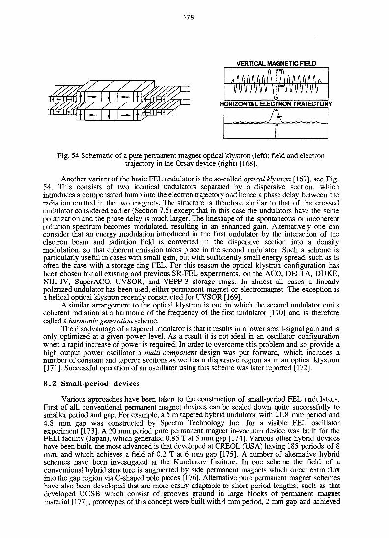
178

VERTICAL MAGNETIC FIELD

HORIZONTAL ELECTRON TRAJECTORY

0

Fig. 54 Schematic of a pure permanent magnet optical klystron (left); field and electrontrajectory in the Orsay device (right) [168].

Another variant of the basic FEL undulator is the so-called optical klystron [167], see Fig.54. This consists of two identical undulators separated by a dispersive section, whichintroduces a compensated bump into the electron trajectory and hence a phase delay between theradiation emitted in the two magnets. The structure is therefore similar to that of the crossedundulator considered earlier (Section 7.5) except that in this case the undulators have the samepolarization and the phase delay is much larger. The lineshape of the spontaneous or incoherentradiation spectrum becomes modulated, resulting in an enhanced gain. Alternatively one canconsider that an energy modulation introduced in the first undulator by the interaction of theelectron beam and radiation field is converted in the dispersive section into a densitymodulation, so that coherent emission takes place in the second undulator. Such a scheme isparticularly useful in cases with small gain, but with sufficiently small energy spread, such as isoften the case with a storage ring FEL. For this reason the optical klystron configuration hasbeen chosen for all existing and previous SR-FEL experiments, on the ACO, DELTA, DUKE,NIJI-IV, SuperACO, UVSOR, and VEPP-3 storage rings. In almost all cases a linearlypolarized undulator has been used, either permanent magnet or electromagnet. The exception isa helical optical klystron recently constructed for UVSOR [169].

A similar arrangement to the optical klystron is one in which the second undulator emitscoherent radiation at a harmonic of the frequency of the first undulator [170] and is thereforecalled a harmonic generation scheme.

The disadvantage of a tapered undulator is that it results in a lower small-signal gain and isonly optimized at a given power level. As a result it is not ideal in an oscillator configurationwhen a rapid increase of power is required. In order to overcome this problem and so provide ahigh output power oscillator a multi-component design was put forward, which includes anumber of constant and tapered sections as well as a dispersive region as in an optical klystron[171]. Successful operation of an oscillator using this scheme was later reported [172].

8.2 Small-period devices

Various approaches have been taken to the construction of small-period FEL undulators.First of all, conventional permanent magnet devices can be scaled down quite successfully tosmaller period and gap. For example, a 5 m tapered hybrid undulator with 21.8 mm period and4.8 mm gap was constructed by Spectra Technology Inc. for a visible FEL oscillatorexperiment [173]. A 20 mm period pure permanent magnet in-vacuum device was built for theFELI facility (Japan), which generated 0.85 T at 5 mm gap [174]. Various other hybrid deviceshave been built, the most advanced is that developed at CREOL (USA) having 185 periods of 8mm, and which achieves a field of 0.2 T at 6 mm gap [175]. A number of alternative hybridschemes have been investigated at the Kurchatov Institute. In one scheme the field of aconventional hybrid structure is augmented by side permanent magnets which direct extra fluxinto the gap region via C-shaped pole pieces [176]. Alternative pure permanent magnet schemeshave also been developed that are more easily adaptable to short period lengths, such as thatdeveloped UCSB which consist of grooves ground in large blocks of permanent magnetmaterial [177]; prototypes of this concept were built with 4 mm period, 2 mm gap and achieved

179

fields of the order 0.1 T. The field was however considerably lower than could be achieved in aconventional pure permanent magnet, with the added difficulties of field offset, large end fieldsand significant field errors.

Various miniature electromagnetic schemes have also been developed, starting with asimple design in which a copper foil is wound between electric steel laminations in alternatingdirections [178]. A prototype with a period of 2.7 mm and gap of 1 mm produced a fieldamplitude of about 0.08 T in d.c. mode. Most later devices were designed to be pulsed in orderto allow higher currents to be used without overheating. Another design based on a folded foilinvolved a double winding scheme, i.e. the foil is folded back at the end of the magnet andwound in the opposite sense, which has the advantage of producing a more symmetrical fielddistribution [179]. Periods as small as 5 mm were considered possible using this technique.Another approach which received a lot of attention was the slotted-tube device in which a highcurrent pulse is passed along a cylindrical tube with appropriately positioned cut-outs to directthe current flow so as to generate the desired field configuration; several prototypes were builtproducing both helical and later planar fields and in one a field strength of 1 T was achievedwith 5 mm period with a 25 kA pulse [180]. Another related idea was to use a bifilar helicalsheet with ferromagnetic cores; a 10 mm prototype was constructed [181]. All of the abovedevices suffer from the disadvantage that there is no simple method for correcting field errors.An alternative approach which overcomes this problem uses individual small electromagnets,which allows independent tuning of the strength of each pole by means of a resistive currentdivider network feeding each pair of coils from a single power supply [182]. A 70 perioddevice was constructed with a period of 8.8 mm and gap of 4.2 mm which generated a fieldamplitude of 0.42 T with excellent field quality [183].

Small-period devices have also been constructed using superconducting magnettechnology. The design developed at BNL is based on a continuously wound conductor on aprecisely machined iron yoke [184]. Two devices have been constructed for two different FELexperiments; the undulator with the shortest period (8.8 mm) produces a field of 0.5 T at4.4 mm gap. Very good field uniformity was achieved within each section, although someerrors appeared at the joints between sections [185].

Two other novel concepts that have been developed for producing sub-cm periodundulators are an electromagnetic helical device based on a laminated construction with threepoles per magnet period [186] and a device consisting of a staggered array of iron polesimmersed in a solenoidal field produced by a superconducting magnet [187]. A 1 T sinusoidalfield amplitude was generated for a 10 mm period at 2 mm gap with a 0.7 T solenoidal field.

8.3 Transverse focusing

A conventional linearly polarized undulator with a vertical field, causes a focusing of thebeam in the vertical plane, whereas (ignoring the effects of any field errors) it acts like a driftspace in the horizontal plane [29]. In the vertical plane therefore there exists a matchingcondition, such that if the electron beam ellipse is adjusted correctly at the entrance of themagnet, it will remain unaltered as it progresses along the magnet. It can be shown that underthese conditions the longitudinal velocity (averaged over an undulator period) is constant foreach electron during its motion in the vertical plane, and that this is the optimum setting in orderto minimize the effect of the electron beam emittance on the FEL interaction. The same situationhowever does not exist in the horizontal plane due to the lack of horizontal focusing. To remedythis situation, certain types of helical undulator can be used. For example, the bifilar helixproduces equal focusing in both planes [121]. The double-undulator scheme of Onuki in thehelical mode, with identical magnet arrays and equal gaps, also gives equal focusing, eventhough the field distribution is quite different to that of the bifilar helix [142]. The same is notgenerally true however for the other helical magnet schemes capable of generating circularlypolarized radiation (Section 7.3).

In many cases a plane polarized magnet is preferred to a helix and considerable attentionhas been given to different ways of incorporating focusing in the horizontal plane. In Ref. [188]it was shown that in general a small parabolic curvature of the pole profile (assuming an iron-dominated electromagnet or hybrid device) is sufficient to produce equal focusing in both planesand that this has the advantage over the alternative method of adding focusing by means of

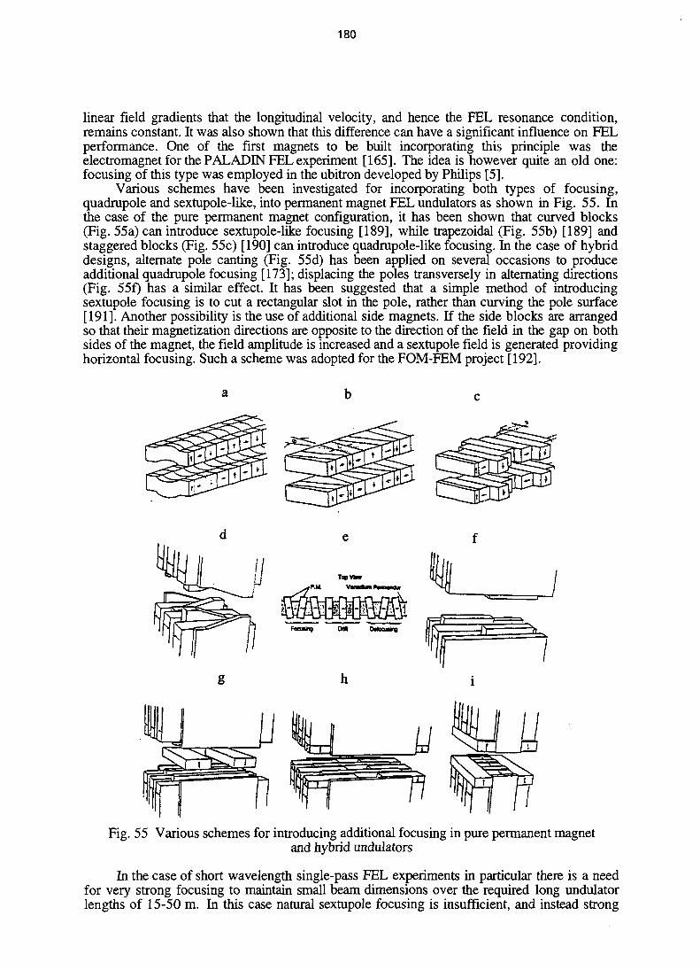
180

linear field gradients that the longitudinal velocity, and hence the FEL resonance condition,remains constant. It was also shown that this difference can have a significant influence on FELperformance. One of the first magnets to be built incorporating this principle was theelectromagnet for the PALADIN FEL experiment [165]. The idea is however quite an old one:focusing of this type was employed in the ubitron developed by Philips [5].

Various schemes have been investigated for incorporating both types of focusing,quadrupole and sextupole-like, into permanent magnet FEL undulators as shown in Fig. 55. Inthe case of the pure permanent magnet configuration, it has been shown that curved blocks(Fig. 55a) can introduce sextupole-like focusing [189], while trapezoidal (Fig. 55b) [189] andstaggered blocks (Fig. 55c) [190] can introduce quadrupole-like focusing. In the case of hybriddesigns, alternate pole canting (Fig. 55d) has been applied on several occasions to produceadditional quadrupole focusing [173]; displacing the poles transversely in alternating directions(Fig. 55f) has a similar effect. It has been suggested that a simple method of introducingsextupole focusing is to cut a rectangular slot in the pole, rather than curving the pole surface[191]. Another possibility is the use of additional side magnets. If the side blocks are arrangedso that their magnetization directions are opposite to the direction of the field in the gap on bothsides of the magnet, the field amplitude is increased and a sextupole field is generated providinghorizontal focusing. Such a scheme was adopted for the FOM-FEM project [192].

g

Fig. 55 Various schemes for introducing additional focusing in pure permanent magnetand hybrid undulators

In the case of short wavelength single-pass FEL experiments in particular there is a needfor very strong focusing to maintain small beam dimensions over the required long undulatorlengths of 15-50 m. In this case natural sextupole focusing is insufficient, and instead strong

181

superimposed quadrupole fields of 20-50 T/m must be used with alternating gradient. One ofthe possibilities being investigated for the LCLS project is a canted and wedged pole hybrid(Fig. 55e) [193]. Another possibility is the use of side magnets, but differing from the schemeoutlined above for producing sextupole focusing. In this case the side magnets have oppositedirections of magnetization, and are continuous along the length of the magnet, and so producea superimposed quadrupole field (Fig. 55g) [194]. A similar concept, but using four magnetsabove and below the median plane, and therefore having the advantage of leaving the sidesopen, was introduced in Ref. [195]. Two further related schemes of incorporating the additionalmagnets into the hybrid structure (Figs. 55h and 55i) were reported in [196]. One of these, theso-called four magnet focusing undulator (Fig. 55h), was subsequently selected for theundulator for the TTF-FEL project and is presently under construction. Various other schemesare also being studied for the LCLS project, including superconducting and pulsed copperhelical magnets [197].

ACKNOWLEDGEMENTS

It is a pleasure to thank B. Diviacco for preparing several of the figures and for varioushelpful discussions and M. Nadalin for her skill and patience in preparing the manuscript.

REFERENCES

[I] V.L. Ginzburg, Izv. Akad. Nauk. SSSR, Ser. Fiz., 11 (1947) 165.[2] H. Motz, J. Appl. Phys. 22 (1951) 527.[3] H. Motz et al., J. Appl. Phys. 24 (1953) 826.[4] LA. Grishaev et al., Sov. Phys. Dokl. 5 (1960) 272.[5] R.M. Phillips, Nucl. Instr. Meth. A272 (1988) 1.[6] J.M.J. Madey, J. Appl. Phys. 42 (1971) 1906.[7] R.P. Godwin, Synchrotron Radiation as a Light Source, Springer Tracts in Modem

Physics, Vol. 51, Springer-Verlag (1969).[8] D.F. Alferov, Yu. A. Bashmakov and E.G. Bessonov, Sov. Phys. Tech. Phys. 17

(1973) 1540.[9] V.N. Baier et al., Sov. Phys. JETP 36 (1973) 1120.[10] E.M. Purcell, unpublished note, July 1972 [also Ref. 18 p. IV-18].II1] A.I. Alikhanyan et al., JETP Lett. 15 (1972) 98.[12] D.F. Alferov et al., JETP Lett. 26 (1977) 385.[13] A.N. Didenko et al., Sov. Tech. Phys. Lett. 4 (1978) 281.[14] D.F. Alferov, Yu. A. Bashmakov and E.G. Bessonov, Sov. Phys. Tech. Phys. 18

(1974) 1336.[15] B.M. Kincaid, J. Appl. Phys. 48 (1977) 2684.[16] A.S. Artamonov et al., Nucl. Instr. Meth. 177 (1980) 247.[17] K. Halbach et al., IEEE Trans. Nucl. Sci. NS-28 (1981) 3136.[18] Proc. Wiggler Workshop, Stanford, March 1977, SSRP Report 77/05 (May 1977).[19] H. Winick and R.H. Helm, Nucl. Instr. Meth. 152 (1978) 9.[20] W.S. Trzeciak, IEEE Trans Nucl. Sci. NS-18 (1971) 213.[21] M. Berndt et al., IEEE Trans. Nucl. Sci. NS-26 (1979) 3812.[22] R. Barbini et al., Riv. del Nuov. Cim. 4 (1981) 1.[23] E. Hoyer et al., IEEE Trans. Nucl. Sci. NS-30 (1983) 3118.[24] A.S. Artamonov et al., Nucl. Instr. Meth. 177 (1980) 239.[25] V.P. Suller et al., IEEE Trans. Nucl. Sci. NS-30 (1983) 3127.[26] K.W. Robinson, Phys. Rev. I l l (1958) 373.[27] A. Hofmann et al., Proc. Vlth Int. Conf. High Energy Accelerators, Cambridge MA,

(1967) p. 123.[28] J.M. Paterson, J.R. Rees and H. Wiedemann,, SPEAR-186, PEP-125, July 1975.[29] R.P. Walker, Proc. CERN Accelerator School Fifth Advanced Accelerator Physics

Course, CERN 95-06, Vol. II, p. 807[30] Proc. Wiggler Meeting, Frascati, June 1978, INFN (Dec. 1978).

182

[31] Proc. Int. Conf. on Insertion Devices for Synchrotron Sources, Stanford, Oct. 1985,SPIE Vol. 582 (1986).

[32] Proc. Adriatico Research Conference on Undulator Magnets for Synchrotron Radiationand Free Electron Lasers, Trieste, June 1987, World Scientific (1988).

[33] Proc. Workshop on Fourth Generation Light Sources, Stanford, Feb. 1992, SSRL92/02

[34] Proc. Int. Workshop on Insertion Devices for Circularly Polarized Light, BESSY,Berlin, Nov. 1993.

[35] Proc. 10th ICFA Beam Dynamics Workshop: 4th Generation Light Sources, ESRF,Grenoble, Jan. 1996.

[36] J.E. Spencer and H. Winick, "Wiggler Systems as Sources of ElectromagneticRadiation", Chapter 21 in "Synchrotron radiation Research", H. Winick and S. Doniacheds., Plenum Press (1980).

[37] S. Krinsky, M.L. Perlman and R.E. Watson, "Characteristics of Synchrotron Radiationand of its Sources", Chapter 2 in "Handbook on Synchrotron Radiation", Vol. la, E.E.Koch ed. (North Holland, 1983).

[38] G. Margaritondo, "Introduction to Synchrotron Radiation" (Oxford, New York, 1988).[39] P. Luchini and H. Motz, "Undulators and Free-Electron Lasers", Oxford University

Press (1990)[40] G. Brown and W. Lavender, "Synchrotron Radiation Spectra", Chapter 2 in

"Handbook on Synchrotron Radiation", Vol. 3, G. Brown and D.E. Moncton eds.(Elsevier, 1991).

[41] G.S. Brown, "Undulators and the Properties of Synchrotron Radiation", Chapter 8 in"Synchrotron Radiation Research: Advances in Surface and Interface Science,Volume 2: Issues and Technology", R.Z. Bachrach ed., Plenum Press (1992).

[42] R.D. Schlueter, "Wiggler and Undulator Insertion Devices", Chapter 14 in"Synchrotron Radiation Sources: A Primer", H. Winick ed., World Scientific (1994).

[43] K.J. Kim, "Characteristics of Synchrotron Radiation", Proc. US Particle AcceleratorSchool, 1987, M. Month and M. Dieses eds., AJJP Conference Proceedings Vol. 184p. 567.

[44] P. Elleaume, "Theory of Undulators and Wigglers", Proc. CERN Accelerator School,Synchrotron Radiation and Free-Electron Lasers, CERN 90-03 p. 142.

[45] M.R. Howells and B.M. Kincaid, "The Properties of Undulator Radiation", Proc.NATO ASI Series E, Vol. 254, p. 315.

[46] H. Winick et al., Physics Today 34, May 1981, p. 50.[47] G. Brown et al., Nucl. Instr. Meth. 208 (1983) 65.[48] P. Elleaume, Synchrotron Radiation News 1(4) (1988) 18 and 1(5) (1988) 21.[49] R. Coisson, Proc. 2nd EPAC, Nice, June 1990, Editions Frontieres (1990) p. 291.[50] P. J. Viccaro et al., Proc. PAC 1991, IEEE Catalog No. 91CH3038-7, p. 1091.[51] P. Elleaume, Proc. SRI'91, Rev. Sci. Instr. 63 (1992) 321.[52] F. Ciocci, Proc. 3rd EPAC, Berlin, March 1992, Editions Frontieres (1992) p. 86.[53] R.P. Walker, Proc. 4th EPAC, London, June 1994, World Scientific (1994), p. 310.[54] H. Kitamura, Proc. SRI'94, Rev. Sci. Instr. 66 (1995) 2007.[55] E. Gluskin and E.R. Moog, Proc. PAC 1995, IEEE Catalog No. 95CH35843, p. 1301[56] G. Margaritondo, J. Synchrotron Rad. 2 (1995) 155.[57] A. Hoffman, Nucl. Instr. Meth. 152 (1978) 17.[58] A. Hoffman, these Proceedings.[59] J.D. Jackson, "Classical Electrodynamics", Wiley, New York (1962)[60] R.P. Walker, Nucl. Instr. Meth. A267 (1988) 537.[61] A.N. Didenko et al., Sov. Phys. JETP 49 (1979) 973.[62] R. Tatchyn and I. Lindau, Nucl. Instr. Meth. 222 (1984) 14.[63] S. Krinsky, Nucl. Instr. Meth. 172 (1980) 73.[64] R.P. Walker, Nucl. Instr. Meth. A335 (1993) 328.[65] K.J. Kim, Nucl. Instr. Meth. A246 (1986) 71.[66] J. Schwinger, Phys. Rev. 75 (1949) 1912.[67] P. Elleaume, J. Synchr. Rad. 1 (1994) 19.[68] K.J. Kim, Nucl. Instr. Meth. A246 (1986) 67.

183

[69] R. Tatchyn et al., Proc. SPIE 582 (1985) 47.[70] R. Barbini et al., Ref. [32] p. 100.[71] J. Chavanne and P. Elleaume, ESRF-ID-90/46[72] P. Elleaume and X. Maréchal, ESRF-SR/ID-91-54[73] R.J. Dejus and A. Luccio, Nucl. Instr. Meth. A347 (1994) 61.[74] H. Rarbach et al., Nucl. Instr. Meth. A266 (1988) 96.[75] R.P. Walker and B. Diviacco, Rev. Sci. Inst. 63 (1992) 392.[76] D. Steinmüller-Nethl et al., Nucl. Instr. Meth. A285 (1989) 307.[77] C. Wang and D. Xian, Nucl. Instr. Meth. A288 (1990) 649.[78] C. Wang, Phys. Rev. E 47 (1993) 4358.[79] R.P. Walker, ST/M-TN-89/24, July 1989[80] R. Coîsson et al., Nucl. Instr. Meth. 201 (1982) 3.[81] G.E. van Dorssen et al., Proc. SPIE Vol. 2013 (1993) 104.[82] N.Marks, Proc. Proc. CERN Accelerator School Fifth General Accelerator Physics

Course, CERN 94-01, Vol. H, p. 867.[83] S. Krinsky, BNL 23747 (1977); also Ref. [30] p. 97.[84] M.W. Poole and R.P. Walker, Nucl. Instr. Meth. 176 (1980) 487.[85] G.A. Komyukhin et al., Nucl. Instr. Meth. 208 (1983) 189.[86] N.A. Vinokurov, Nucl. Instr. Meth. A246 (1986) 105.[87] K. Halbach, Nucl. Instr. Meth. 187 (1981) 109.[88] K. Halbach, J. de Physique Cl 44 (1983) 211.[89] K. Halbach, Nucl. Instr. Meth. 169 (1980) 1.[90] B. Diviacco and R.P. Walker, Proc. PAC 1993, IEEE Catalog No. 93CH3279-7,

p. 1593.[91] 6 GeV Synchrotron X-ray Source Conceptual Design Report, Supplement A, LS-52

(March 1986), Argonne National Laboratory.[92] R.P. Walker, Daresbury Laboratory Technical Memorandum DL/SCI/TM54A, Nov.

1987.[93] K. Halbach, Lawrence Berkeley Laboratory Report LSBL-034 ( 1989)[94] T. Meinander, SPIE Vol. 582 (1986) 193.[95] K. Halbach et al., IEEE Trans. Nucl. Sci. NS-32 (1985) 3640.[96] D.C. Quimby et al., Nucl. Instr. Meth. A259 (1987) 304.[97] S. Sasaki et al., Rev. Sci. Instr. 60 (1989) 1859.[98] B. Diviacco and R.P. Walker, Sincrotrone Trieste Internal Report ST/M-TN-92/5 (May

1992).[99] E. Hoyer et al., Proc. PAC 1987, IEEE Catalog No. 87CH2387-9 (1987) 1508.[100] D. Humphries et al., Proc. PAC 1993, IEEE Catalog No. 93CH3279-7, p. 1581.[101] I. Vasserman and E.R. Moog, Rev. Sci. Instr. 66 (1995) 1943.[102] J. Chavanne et al., Proc PAC 1995, IEEE Catalog No. 95CH35843, p. 1319.[103] B.M. Kincaid, J. Opt. Soc. Am. B2 (1985) 1294.[104] B. Diviacco and R.P. Walker, Proc. PAC 1989, IEEE Catalog No. 89CH2669-0,

p. 1259.[105] B.L. Bobbs et al., Nucl. Instr. Meth. A296 (1990) 574.[106] R. Dejus, Rev. Sci. Instr. 66 (1995) 1875.[107] A.D. Cox and B.P. Youngman, SPIE 582 (1986) 91.[108] R. Hajima et al., Nucl. Instr. Meth. A318 (1992) 822.[109] D.C. Quimby et al., Nucl. Instr. Meth. A285 (1989) 281.[110] S.C. Gottschalk et al., Nucl. Instr. Meth. A296 (1990) 579.[111] J. Chavanne et al., ESRF Internal Report ESRE-SR/ID-89-27, Sept. 1989.[112] B. Diviacco, Proc. PAC 1993, IEEE Catalog No. 93CH3279-7, p. 1590[113] J. Chavanne and P. Elleaume, Rev. Sci. Instr. 66 (1995) 1868

and SR News, Vol. 8, No. 1, Jan./Feb. 1995, p. 18.[114] B. Diviacco and R.P. Walker, Nucl. Instr. Meth. A368 (1996) 522.[115] I. Vasserman, Advanced Photon Source LS-253, Jan. 1996.[116] S.C. Gottschalk et al., Rev. Sci. Instrum. 67(9) (1996).[117] Proc. Int. Workshop on Magnetic Measurements of Insertion Devices, Argonne

National Laboratory, Sep. 1993, ANL/APS/TM-13

184

[118] M. Born and E. Wolf, "Principles of Optics" 6th ed. (Pergamon Press, 1980).[119] H. Kitamura, Jap. J. Appl. Phys. (1980) L185.[120] W.R. Smythe, Static and Dynamic Electricity (McGraw-Hill, New York, 1950) p. 277[121] J.P. Blewett and R. Chasman, J. Appl. Phys., 48 (1977) 2692.[122] S. Y. Park and J. M. Baird, J. Appl. Phys. 53 (1982) 1320.[123] J. Fajans, J. Appl. Phys. 55 (1984) 43.[124] D.F. Alferov et al., Sov. Phys. Tech. Phys. 21 (1976) 1408.[125] R.P. Walker, Nucl. Instr. Meth. A237 (1985) 366.[126] L. R. Elias and J.M. Madey, Rev. Sci. Instr. 50 (1979) 1335.[127] U. Bizzari et al., J. Phys. Coll. Cl 44 (1983) 313.[128] E.D. Shaw et al., J. Phys. Coll. Cl 44 (1983) 153.[129] J. Vetrovec, Nucl. Instr. Meth. Phys. Res. A296 (1990) 563.[130] K. Halbach, Nucl. Instr. Meth. 187 (1981) 109.[131] M.S. Curtin et al., Nucl. Instr. Meth. Phys. Res. A237 (1985) 395.[132] P. Diament et al., Nucl. Instr. Meth. Phys. Res. A237 (1985) 381.[133] H. Onuki, Nucl. Instr. Meth. Phys. Res. A 246 (1986) 94.[134] K. Yagi et al., Rev. Sci. Instr. 63 (1992) 396.[135] S. Yamamoto and H. Kitamura, Jpn. J. Appl. Phys. 26 (1987) L1613.[136] S. Yamamoto et al., Rev. Sci. Instr. 60 (1989) 1834.[137] S. Yamamoto et al., Phys. Rev. Lett. 62 (1989) 2672.[138] R.P. Walker and B. Diviacco, Rev. Sci. Instr. 63 (1992) 332.[139] E. Gluskin et al., Proc. 1995 PAC, IEEE Catalog No. 95CH35843, p. 1426.[140] L. Nahon et al., to be published in Nucl. Instr. Meth.[141] P. Elleaume, Nucl. Instr. Meth., A304 (1991) 719.[142] B. Diviacco and R.P. Walker, Nucl. Instr. Meth. A292 (1990) 517.[143] P. Elleaume, Nucl. Instr. Meth. A304 (1991) 719.[144] P. Elleaume, Proc. 10th ICFA Beam Dynamics Panel Workshop, 4th Generation Light

Sources, Grenoble, Jan. 1996, p. WG7-40.[145] S. Sasaki et al., Jpn. J. Appl. Phys. 31 (1992) L1794.[146] K. Kakuno and S. Sasaki, JAERI-M 92-157, Sept. 1992.[147] S. Sasaki, Nucl. Instr. Meth. A347 (1994) 87.[148] R. Carr and S. Lidia, Proc. SPIE 2013 (1993) 56.[149] R. Carr et al., Rev. Sci. Instr. 66 (1995) 1862.[150] X. Marechal et al., Rev. Sci. Instr. 66 (1995) 1936.[151] J. Goulon et al., Nucl. Instr. Meth. A254 (1987) 192.[152] J. Pfluger and G. Heintze, Nucl. Instr. Meth. A289 (1990) 300.[153] M. Barthes et al., IEEE Trans. Magn. 24 (1987) 1233, and 28 (1992) 601.[154] J. Pfluger, Rev. Sci. Instr. 63 (1992) 295.[155] D. Schirmer, Proc. XVth Int. Conf. on High Energy Accelerators, Int. J. Mod. Phys

A (Proc. Suppl.) 2B (1993), Volume 2, p. 644[156] M.B. Moisev et al., Sov. Phys. J. 21 (1978) 332,

K.J. Kim, Nucl. Instr. Meth., 219 (1984) 425.[157] J. Bahrdt et al., Rev. Sci. Instr. 63 (1992) 339.[158] M.A. Green at al., Proc. 1991 Particle Accelerator Conference, p. 1088.[159] R. Savoy and K. Halbach, Proc. 1991 Particle Accelerator Conference, p. 2718[160] S. Sasaki, Proc. PAC 1997, to be published.[161] R. Bakker and M.W. Poole, these Proceedings.[162] Recent Conferences have been published in Nucl. Instr. Meth. Volumes A375, A358,

A341, A331, A318, A304 etc.[163] N.M. Kroll et al., Physics of Quantum Electronics Vol. 7; Free Electron Generators of

Coherent Radiation (Addison-Wesley, Reading, MA (1980) 89.[164] H. Boehmer et al., Phys. Rev. Lett. 48 (1982) 141; W.E. Stein et al., Proc. 1981

Linear Accel. Conf., Santa-Fe NM, LANL Report LA-9234, Feb. 1982; J.M. Slater etal., IEEE J. Q. Electron. QE-19 (1983) 374.

[165] G.A. Deis, IEEE Trans. Mag. 24 (1988) 1090.[166] K. Halbach, Nucl. Instr. Meth. A250 (1986) 95.

185

[167] N.A. Vinokurov and A.N. Skrinsky, Budker Institute of Nuclear Physics, Novosibirk,Preprint 77-59.

[168] P. Elleaume, Nucl. Instr. Meth. A237 (1985) 28.J.M. Ortega et al., Nucl. Instr. Meth. 206 (1983) 281.

[169] H. Hama, Nucl. Instr. Meth. A375 (1996) 57.[170] I. Boscolo and V. Stagno, II Nuovo Cimento 58B (1980) 267.[171] C. Shih and M.Z. Caponi, IEEE J. Q. Electron. QE-19 (1983) 369.[172] J.A. Edighoffer et al., Phys. rev. lett. 52 (1984) 344.[173] K. E. Robinson et al., IEEE J. Q. Electron. QE-23 (1987) 1497.[174] T. Keishi et al., Nucl. Instr. Meth. A341 (1994) ABS 128.[175] P.P. Tesch, Nucl. Instr. Meth. A375 (1995) 504.[176] A.A. Varfolomeev et al., Nucl. Instr. Meth. A318 (1992) 813.[177] G. Ramian et al., Nucl. Instr. Meth. A250 (1986) 125.,

K.P. Paulson, Nucl. Instr. Meth. A296 (1990) 624.[178] V.L. Granatstein, Appl. Phys. Lett. 47 (1985) 643.[179] A. Sneh and W. Jerby, Nucl. Instr. Meth. A285 (1989) 294.[180] R.W. Warren et al., Nucl. Instr. Meth. A296 (1990) 558,

R.W. Warren et al., Nucl. Instr. Meth. A304 (1991) 765,CM. Fortgang and R.W. Warren, Nucl. Instr. Meth. A341 (1994) 436.

[181] B. Feng, Rev. Sci. Instr. 63 (1992) 3849.[182] S.C. Chen et al., Nucl. Instr. Meth. A285 (1989) 290.[183] R. Stoner and G. Bekefi, IEEE J. Q. Electronics 31 (1995) 1158.[184] I. Ben-Zvi et al., Nucl. Instr. Meth. A318 (1992) 781.[185] G. Ingold et al., Nucl. Instr. Meth. A375 (1996) 451.[186] N. Ohigashi et al., Nucl. Instr. Meth. A341 (1994) 426.[187] Y.C. Huang et al., Nucl. Instr. Meth. A341 (1994) 431.[188] E.T. Scharlemann, J. Appl. Phys. 58 (1985) 2154.[189] Y. Tsunawaki et al., Nucl. Instr. Meth. A304 (1991) 753.[190] Y. Tsunawaki et al., Nucl. Instr. Meth. A331 (1993) 727.[191] A.A. Varfolomeev and A.H. Hairetdinov, Nucl. Instr. Meth. A341 (1994) 462.[192] A.A. Varfolomeev et al., Nucl. Instr. Meth. A341 (1994) 466.[193] R.D. Schlueter, Nucl. Instr. Meth A358 (1985) 44.[194] A.A. Varfolomeev et al., Nucl. Instr. Meth. A358 (1995) 70.[195] R. Tatchyn, Nucl. Instr. Meth. A341 (1994) 449.[196] Y.M. Nikitina and J. Pfluger, Nucl. Instr. Meth. A375 (1996) 325.[197] S. Caspi et al., Proc. 1995 PAC, IEEE Catalog No. 95CH35843, p. 1441.

186

APPENDIX SPECTRAL AND ANGULAR DISTRIBUTION OF THERADIATION EMITTED IN VARIOUS TYPES OF SINUSOIDAL UNDULATOR

Given the following general field distribution which includes both planar, circular andgeneral elliptical undulator types:

Bx = Bxo sin (kz + if/) By = Byo sin (fe)

we obtain, using the procedure outlined in section 2.1, for the transverse motion:

K KBy = -^cos(Qt +1/0 Bx = -^cos(Qr)

K

K Ky = -—sin(Q.t+yr) X = —L—sin(Qf)

y Q. y Q.

and for the longitudinal motion:

K2 K2

B B 2 L 2 Q r ^ w)o s Ây Ay

C sin2(Q?+i/A)— K2 K1

p t ^ 2 Q t * CH Ay120. Ay22Q,

where

_ 2jcjjc A n , 1 K2

Q = , and j S s l ^l0 2yl Ay1 AyL

The general expression for the radiated intensity in the case of a periodic magnet in the far-field approximation is given by the following (see section 3.1):

d2l N2e2co2

dcodQ. {AK£O)AK1C

Xjlpc(Al)

-KM*

Expanding the term nA(nAjS) to order K/y and using the small angle approximationn = (0cos0,0sin0,O), one obtains n A ( « A B) = (dcos(f> - px,8sm<f) - By,0). Expanding alsothe phase terms we obtain:

co{t-n- r/c) = a>t-0)6cos(t>x/c-a)dsm^y/c-a) cos 6 z/c

,* ~n n, codcosQ Ky . _ (Ddsirub Kr .= cot(l-pcosd) -—£-smQ? +

( K2 K2

— —^-sin2i2r + —^sin2(Qf + v )2Q[Ay2 Ay2

With large N we only need evaluate the expression at the harmonic frequencies, where:

R Q nQ.2y2 / A ^

CO = = = s-7 4l T~T (A2)(l-Bcosd) l + K2 2 + K2 2+y2d2

187

Combining the trigonometric terms we then obtain:

Q)(t-n- r/c) =where,

X = JnE.^K*Cos2 cosyf-Kycos(l)

By means of the relation exp(/*sin0)= 2* Jp(x) exp(//?0) the phase expression now

becomes:

oo oo

/ ,m/ (T)£>'==—oo p=—a

and hence Eq. (Al) becomes:

d2l N2e2co2

dcodQ. (4neo)4n:LiNAa/aÔ)) x

7'=-°°P=-°°P=-°°

where the two terms in the integrand represent the amplitudes polarized respectively in the x andy directions. It can be seen that the integral over one period is non-zero only when eithern - p' + 2p = 0 for the constant terms, or when n-p' + 2p = ±\ for the terms in cos Sit orsin£2f. Defining therefore n- p' + 2p = -q, where q = -1,0,1 we then have, using Eq. (A2):

dcodQ. (4TC£0)C Awith:

Ax=2y0cos<l>So-Ky(Sl+S_l) (A3)

Ay = 2y6sm SO + Kx(eiyf S, + e~iv S_x)

where:

Sq =

On-axis X = 0 and hence n + 2p + q = Oand p = (-n - q)/2. It follows that So - 0 and:

188

for q = -l, 1, with « = odd. After some simplification, and using the fact that

J-n(x) = (-1)" Jn{x) one obtains:

Ax = Ky[j^{Y)eiB^^ ~ 7 ^ ( 7 ) / ^ (A4)

Kx (-J

Pure elliptical case

We have y/ = 7r/2and hence tan O = (Kx/Ky)tan (j) and *F = 0. We obtain therefore fromEq. (A3):

Ax =

where:

and:

4A

which is equivalent to the result of Yamamoto and Kitamura [135].On-axis we obtain directly from Eq. (A4):

Pure circular case

In this case we have in addition to the above, Ky = Kx~K and hence X = 2nyOKjA,y = 0, =0. We have then:

Sq =and hence:

Ax=ein*{2y$cos<!>Jn(X)-K(jn+1(X)ei<t>+Jn_1(X)e-i't>]\ (A5)

Ay = e^[2y6sin</>Jn(X) + i

The general expressions for the amplitudes are therefore still quite complicated, however sincethe radiation pattern is circularly symmetric we can take any value of 0, for example 0 = 0:

Ax =2ydJn(X)-K{Jn+l(X) + Jn_l

Ay = iK

By making use of the following relations:

189

•4+i(*) + 4-iW = y W and Jn_l(x)-Jn+l(x) = 2J'n(x) (A6)

we can express the results in the following form:

Ay = -2iKJ'n(X) (A7)

The expression for the total intensity then becomes:

in agreement with Alferov et al. [14] and Kincaid [15].On-axis X = 0 and hence in Eq. (A5) there is only one term with n = 1. We have then:

Ax=-K and Ay=-iK

The radiation has therefore complete circular polarization (53 = 1) with total intensity:

d2l N2e2y2 2K2

2)2dcodQ (4K£0)C (1 + K2)

We note in passing that the circular polarization component reverses direction off-axis when

Ax = Oin Eq. (A7), i.e. when y6 = Jl + K2 .

Linear case

In this case Kx = 0 and hence O = ¥ = 0, X = 2nyOKycos<l)/A, Y = nK2JAA and

A = 1 + K2J2 + Y202. As a result we have from Eq. (A3):

with

Ax = 2 Tflcos (pSo-Ky(Sl+S_l) (A8)Ay = 2y6sin<t)So

Sq=P=-°°

Making use of the first of the relations in Eq. (A4) we can write:

s +s_l=—so+-s2 = —-— ( s o +-s 2

1 1 X ° X 2 Kyydcos<t>\ ° n 2

where

190

Hence,

Ax=2y0cos4>Soydcos<f>

in agreement with the result of Aferov et al. [14] and Krinsky [63].On-axis we obtain either from Eq. (A8) or (A4):

The intensity is often written in the form:

A21 N2 e2 v2

dcodQ, (4K£0)c

where:

w i f l l Z=

191

INSTABILITIES AND BEAM INTENSITY LIMITATIONS INCIRCULAR ACCELERATORS

S. MyersCERN, Geneva, Switzerland

AbstractThe main aim of these lectures will be to give an insight into thephysics of the mechanisms of instabilities and beam intensitylimitations in circular accelerators. Three different techniques will beused to evaluate the various instabilities. The first will be using 'few-particle models', the second will use matrix techniques involvingeigenvalues, and the third technique will use Sacherer's modalanalysis technique. The threshold or the growth rate will be evaluatedfor each instability with particular attention to the parameterdependence.

1. CALCULATION TECHNIQUES

1.1 Using matrix techniques (Eigenvalues)

The position of a particle (U) in two-dimensional phase space can be defined by itsinstantaneous position u and angle u'lduldi). Consequently n particles may be represented bya column matrix with N (2ri) rows. A transition matrix may be derived which describes thetransition of the n particles from one situation to another, i.e.

Mlr

M l

«2

«2

«»

9.

'11

'21

'31

'41

'51

'M

'12

'22

••

'13 '14

'33 -

•• '44

'15

'55

hN

tNN

"1f

«2

«2U2 =

-11

This transition matrix is of necessity of dimension N xN. Evaluation of the eigenvaluesof the transition matrix allows determination of the growth rates, damping times, andfrequency shifts experienced by the particles. For more than two particles it is usuallynecessary to evaluate the eigenvalues by computer.

1.2 Using frequency shifts

The well-known differential equation of a simple harmonic oscillator with a'normalised' driving force is

where coo is the natural frequency of the oscillation and GR and Gt are the real and imaginarycomponents of the normalised driving force. The equally well-known solution to thisequation is

192

u=u0exp(jont)

where ©„ = ©0 + A©, and Aco = = £ — j2CO 2 ( DQ Q 2CC»

giving

u = M0exp(;o0r)-exp -^-^H-exp + Ti - n - (1)

Consequently the exponential coefficient of the motion (a) is given by

a = - = -Im(Aco) = + - ^ .x 2coo

(2)

Hence the motion is unstable (a > 0) if the imaginary component of the frequency shiftis of negative sign or if the imaginary component of the driving force (G,) is of positive sign.

1.3 Evaluation of the normalised driving force

In the case of beam instabilities the driving 'force' is normally an induced 'force' suchas a voltage induced by the passage of the charged beam itself. Since the force is induced bythe beam then it can only have components at frequencies corresponding to the modes ofoscillation of the beam itself. Thus the force results from the spectrum of the beamoscillation 'sampling' the impedance Z seen by the beam. In certain cases the induceddriving force is fairly obvious and can be derived almost by inspection, but in most cases thederivation is more complicated.The induced voltage can be derived from the inverse Fourier transform of the product of theimpedance and the bunch current (in frequency domain) i.e.

V(t) = ST1 {F(o)}= 3" 1 |Z(o3)/(o))}.

The voltage induced by the beam gives the field which must be integrated over thebunch spectrum (p) in order to get the total force i.e.

G = jkjV(t)p(t)dt = jkjZ-l{Z(®)I((o)}p(t)dt.

Sacherer [1] has shown that, in general,

£M<o)

where 70 is the average bunch current and h(a>) is the power spectrum of the bunch currentdistribution. Clearly, stability is determined by the sign of the real part of the impedanceZR(<o). The stability situation is therefore investigated by evaluating the frequencydependence of the impedance seen by the beam and the power spectrum of the beamoscillations which 'sample' the impedance to produce an induced normalised force.

2. 'ROBINSON' INSTABILITY

The Robinson instability [2] has been analysed in many and complicated ways since itwas pointed out more than 30 years ago. This instability is driven by the fundamentalaccelerating modes of the RF cavities and is not a serious effect for modern accelerators since

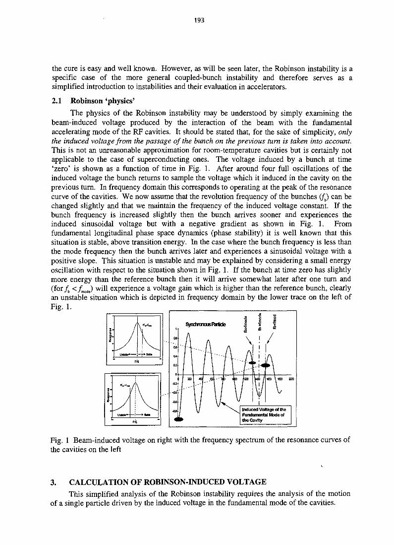
193

the cure is easy and well known. However, as will be seen later, the Robinson instability is aspecific case of the more general coupled-bunch instability and therefore serves as asimplified introduction to instabilities and their evaluation in accelerators.

2.1 Robinson 'physics'

The physics of the Robinson instability may be understood by simply examining thebeam-induced voltage produced by the interaction of the beam with the fundamentalaccelerating mode of the RF cavities. It should be stated that, for the sake of simplicity, onlythe induced voltage from the passage of the bunch on the previous turn is taken into account.This is not an unreasonable approximation for room-temperature cavities but is certainly notapplicable to the case of superconducting ones. The voltage induced by a bunch at time'zero' is shown as a function of time in Fig. 1. After around four full oscillations of theinduced voltage the bunch returns to sample the voltage which it induced in the cavity on theprevious turn. In frequency domain this corresponds to operating at the peak of the resonancecurve of the cavities. We now assume that the revolution frequency of the bunches (fb) can bechanged slightly and that we maintain the frequency of the induced voltage constant. If thebunch frequency is increased slightly then the bunch arrives sooner and experiences theinduced sinusoidal voltage but with a negative gradient as shown in Fig. 1. Fromfundamental longitudinal phase space dynamics (phase stability) it is well known that thissituation is stable, above transition energy. In the case where the bunch frequency is less thanthe mode frequency then the bunch arrives later and experiences a sinusoidal voltage with apositive slope. This situation is unstable and may be explained by considering a small energyoscillation with respect to the situation shown in Fig. 1. If the bunch at time zero has slightlymore energy than the reference bunch then it will arrive somewhat later after one turn and(for/b </mode) will experience a voltage gain which is higher than the reference bunch, clearlyan unstable situation which is depicted in frequency domain by the lower trace on the left ofFig. 1.

t

08

06

04

02

0

-02

• -JSi

-06

•08

4

oyi u i u luub txVUCK?

/"••A-

if if T

•g e |

1 « *\

raDO

/

r

1

1

i IA

\ i l \MX /hÔ \ 18D 2CG0

VI

Induced Voltage of theFundamental Mode ofthe Cavity

Fig. 1 Beam-induced voltage on right with the frequency spectrum of the resonance curves ofthe cavities on the left

3. CALCULATION OF ROBINSON-INDUCED VOLTAGEThis simplified analysis of the Robinson instability requires the analysis of the motion

of a single particle driven by the induced voltage in the fundamental mode of the cavities.

194

Figure 2 is a schematic of a single turn of an accelerator with a single cavity. A singleturn for convenience starts at the exit of the cavity, which has an induced voltage due to thepassage of the particles, and is followed by a longitudinal 'drift' to the entrance of the cavity.The cavity is assumed to have no length and simply gives an energy boost to the particles.

Cavity _ One Turn ^ Cavity

IFig. 2 Schematic of an accelerator with a single cavity

The induced (mode) voltage generated at location 1 and remaining at location 2 is givenby

vm = ~vm exp jam ih - h) - ^L~ (4)

where com is the radiancy of the excited mode, Tt is the filling time of the cavity, and therevolution time dependence on the relative energy offset (A = 8E/E) is

where tny is the average revolution time and

where yt is the relative transition energy.

Substituting

5 0 = ( c o m~"

where h is the RF harmonic number,

A

andrev

gives vm = -Vm exp(/(60 + 2%h)(l + r\A) - 1 0 (1 + tiA)}

and neglecting small termsvm = ~Vm exp{/(So + 2TI/JTIA)- T0 } (5)

which by linearizing gives

vm =-Fme~T°[cos50-27t/!riA-sin5o +7(sin50 + 2it/zriA-cos80)]. (6)

Taking only the oscillating part of Eq. (6)

vm(A) = Vme-X°2^nA{sin50 -;cos(50)}. (7)

The induced voltage may also be written in terms of (p by simply substituting

195

(Qs is the synchrotron frequency, defined later, Section 5) which gives

vm(<P) = Vme~Z°27t2s<p{cos50 -ys inS 0 }. (8)

4. ROBINSON BY EIGENVALUES OF SINGLE-PARTICLE MOTION

Referring to Fig. 2, the energy at the exit of the cavity after one turn (location 3) is

A3 = A {sin(Os + c p 2 ) s i n ( D s ) } + eE E

where cp is measured with respect to the synchronous particle.

Consequently the linearized longitudinal phase space transition over a complete turn(single-turn matrix S) is given by

0

2-»3

1 2%hr]

0 1

For a real 2x2 matrix the absolute value (amplitude) of the two eigenvalues is equal tothe square root of the determinant, hence if the determinant is greater than unity the motion isunstable with exponential growth

Hence the growth rate isIE

•sinSn . (9)

Clearly the motion is unstable when the product TI80 is positive, i.e. above transitionenergy {y\ > 0) when 60 is positive (i.e. when com > /MDrev). This is of course the Robinsoninstability. However, the growth rate is not identical to that usually derived because of theapproximation of only taking the induced voltage of the previous turn.

5. ROBINSON BY SOLUTION OF THE FORCED EQUATION OF MOTION

The general equation of longitudinal motion is

which, for a normal sinusoidal RF voltage becomes

(10)

where Q is the synchrotron radiancy

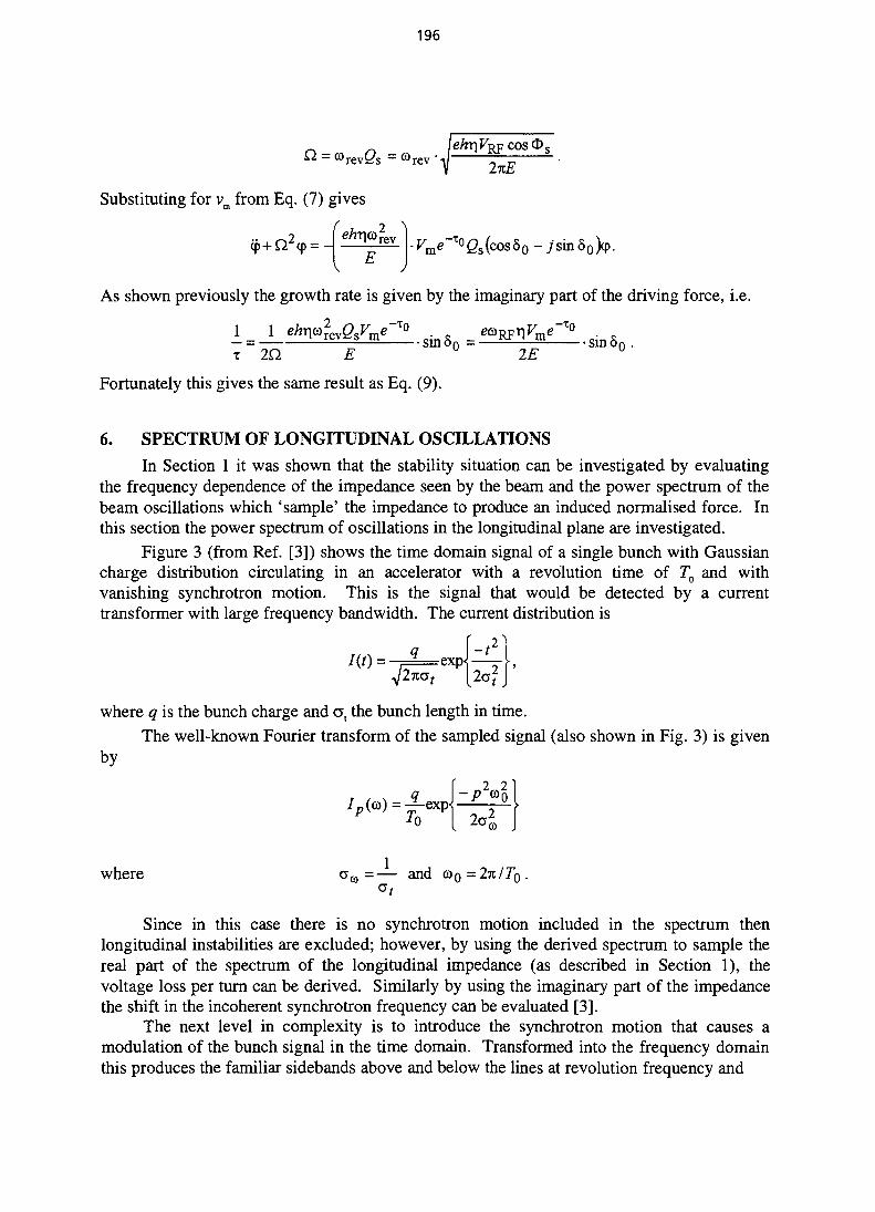
196

n « n „ i

Substituting for vm from Eq. (7) gives

As shown previously the growth rate is given by the imaginary part of the driving force, i.e.

= e^nVmeu IE °T 2O £ IE

Fortunately this gives the same result as Eq. (9).

6. SPECTRUM OF LONGITUDINAL OSCILLATIONS

In Section 1 it was shown that the stability situation can be investigated by evaluatingthe frequency dependence of the impedance seen by the beam and the power spectrum of thebeam oscillations which 'sample' the impedance to produce an induced normalised force. Inthis section the power spectrum of oscillations in the longitudinal plane are investigated.

Figure 3 (from Ref. [3]) shows the time domain signal of a single bunch with Gaussiancharge distribution circulating in an accelerator with a revolution time of To and withvanishing synchrotron motion. This is the signal that would be detected by a currenttransformer with large frequency bandwidth. The current distribution is

where q is the bunch charge and a, the bunch length in time.

The well-known Fourier transform of the sampled signal (also shown in Fig. 3) is givenby

where a a =— and a>o=2jc/7o.

Since in this case there is no synchrotron motion included in the spectrum thenlongitudinal instabilities are excluded; however, by using the derived spectrum to sample thereal part of the spectrum of the longitudinal impedance (as described in Section 1), thevoltage loss per turn can be derived. Similarly by using the imaginary part of the impedancethe shift in the incoherent synchrotron frequency can be evaluated [3].

The next level in complexity is to introduce the synchrotron motion that causes amodulation of the bunch signal in the time domain. Transformed into the frequency domainthis produces the familiar sidebands above and below the lines at revolution frequency and

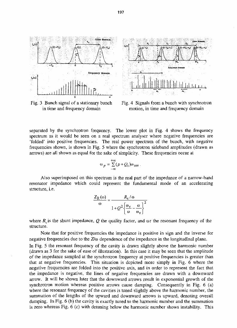
197

l i m e domairt::'

-T . To t

frequency domain

fraqutney domain

!,(«)

-L -ULL

J - L

U_

Fig. 3 Bunch signal of a stationary bunchin time and frequency domain

Fig. 4 Signals from a bunch with synchrotronmotion, in time and frequency domain

separated by the synchrotron frequency. The lower plot in Fig. 4 shows the frequencyspectrum as it would be seen on a real spectrum analyser where negative frequencies are'folded' into positive frequencies. The real power spectrum of the bunch, with negativefrequencies shown, is shown in Fig. 5 where the synchrotron sideband amplitudes (drawn asarrows) are all shown as equal for the sake of simplicity. These frequencies occur at

+oo

Also superimposed on this spectrum is the real part of the impedance of a narrow-bandresonator impedance which could represent the fundamental mode of an acceleratingstructure, i.e.

ZR(CO) Rs/(a

COCO

C0T

where Rsis the shunt impedance, Q the quality factor, and ©r the resonant frequency of thestructure.

Note that for positive frequencies the impedance is positive in sign and the inverse fornegative frequencies due to the Z/co dependence of the impedance in the longitudinal plane.In Fig. 5 the resonant frequency of the cavity is drawn slightly above the harmonic number(drawn as 3 for the sake of ease of illustration). In this case it may be seen that the amplitudeof the impedance sampled at the synchrotron frequency at positive frequencies is greater thanthat at negative frequencies. This situation is depicted more simply in Fig. 6 where thenegative frequencies are folded into the positive axis, and in order to represent the fact thatthe impedance is negative, the lines of negative frequencies are drawn with a downwardarrow. It will be shown later that the downward arrows result in exponential growth of thesynchrotron motion whereas positive arrows cause damping. Consequently in Fig. 6 (a)where the resonant frequency of the cavities is tuned slightly above the harmonic number, thesummation of the lengths of the upward and downward arrows is upward, denoting overalldamping. In Fig. 6 (b) the cavity is exactly tuned to the harmonic number and the summationis zero whereas Fig. 6 (c) with detuning below the harmonic number shows instability. This

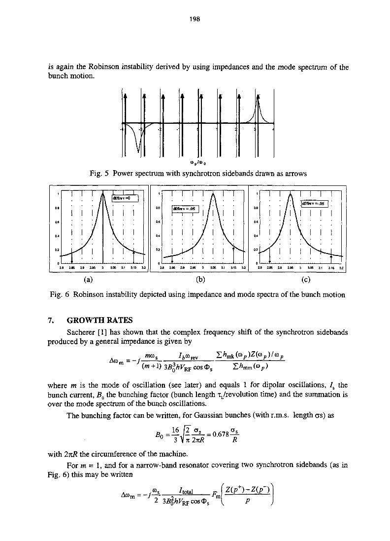
198

is again the Robinson instability derived by using impedances and the mode spectrum of thebunch motion.

wI 1

(

!

JA

Fig. 5 Power spectrum with synchrotron sidebands drawn as arrows

1

0.8

0.6

0.4

0.2

n

I! /

i

i

\ df/frev=O

2.6 Z85 29 2.95 3 3.06 3.1 3.15 3.2

1

0.8

0.6

0.4

0.2

n

dr/frev = .OS / \

2.8 i 9 6 2.9 2.96 3 3.05 3.1 3.15 32

1

0.8

0.6

0.4

02

n

df/fn

//

I

— '

•

28 2.85 2.9 295 3 3.05 3.1 3.15 32

(a) (b) (c)

Fig. 6 Robinson instability depicted using impedance and mode spectra of the bunch motion

7. GROWTH RATES

Sacherer [1] has shown that the complex frequency shift of the synchrotron sidebandsproduced by a general impedance is given by

Acom=-7-m COS O S

where m is the mode of oscillation (see later) and equals 1 for dipolar oscillations, /b thebunch current, Bo the bunching factor (bunch length xL/revolution time) and the summation isover the mode spectrum of the bunch oscillations.

The bunching factor can be written, for Gaussian bunches (with r.m.s. length as) as

with 2%R the circumference of the machine.For m = 1, and for a narrow-band resonator covering two synchrotron sidebands (as in

Fig. 6) this may be written

199

where Fm is the form factor (amplitude of the envelope of the power spectrum of the bunchoscillations), p is/p//rev = h for the fundamental RF, and Z(p±) refers to the impedance at theupper and lower synchrotron sideband frequencies.

Consequently

s ;f f ls Aotal ( )

m) = - ;— 5C 2 I

Here ZR is the real part of the longitudinal impedance, i.e.

ZR(oo) =

For such a resonator the impedance difference between the synchrotron sidebands can beevaluated as

h &r

where A© is the frequency detuning of the accelerating structure (or - haQ). This relationshiponly holds for

Q «2(Ao±os) 2Q

and will therefore not be valid for superconducting cavities where the loaded Q value is veryhigh. When this inequality is satisfied, the growth rate can be reduced to

where the first bracket refers to the beam conditions, the second refers to the machineparameters, and the third to the parameters of the cavities.

Since by our convention r\ is positive above transition, then stability is ensured by Z+being greater than Z- which occurs when A© is positive, i.e. when the cavity frequency istuned above fcoorev.

This relationship has a similar parameter dependence to that previously derived usingthe simpler model (Sections 4 and 5) but is not identical since in the simpler model only theinfluence of the cavity induced voltage on the previous turn is taken into account.

8. MODES AND SPECTRA OF MULTIPLE BUNCHES

The next level of complexity is to consider the spectrum of the dipolar motion of abeam with many bunches. Figure 7 shows the longitudinal phase space (energy deviationagainst RF phase) of the dipole modes of oscillation of four bunches. The different bunchesare spaced horizontally left to right and the different modes of oscillation spaced vertically.The mode of oscillation (n) is defined by the phase advance between the motion of successivebunches, i.e.

200

Consequently for the n = 0 mode of oscillation all four bunches move in an identicalway, and there is zero phase difference between the motion of successive bunches. This isshown in Fig. 7 as are the other three possible modes of oscillation. It should be realised thatin this phase space the motion is in the anticlockwise sense.

The bunches may also be subjected to 'shape' modes of oscillation. These are depictedfor completeness in Fig. 8, where it can be seen that the m = 1 mode (dipolar mode which wehave been considering) is a centre-of-gravity motion whereas the higher-mode numbersproduce changes in the bunch shape.

In general the spectral lines of motion occur at frequencies

where p = n + k • ifcb, k = 0, ±1, ±2,... and n = 0, 1, 2,.. . (fcb-1).

An example of the spectrum is shown in Fig. 9. It is apparent that the spectrum simplyrepeats itself for different values of k. In addition, negative k values correspond to negativefrequencies. Superimposed on this diagram is a narrow-band resonator impedance (plotted asZR/a) which couples to mode n = 1 and n = 3. In this case since the real part of the impedanceis negative at the negative frequency corresponding to mode n = 1, this mode will be unstable.The mode n = 3 is damped by the positive real part of the impedance. The previouslydescribed Robinson instability is a particular case of this coupled-bunch instability butaffecting only mode n = 0.

i A

Fig. 7 Dipolar coupled-bunch modes

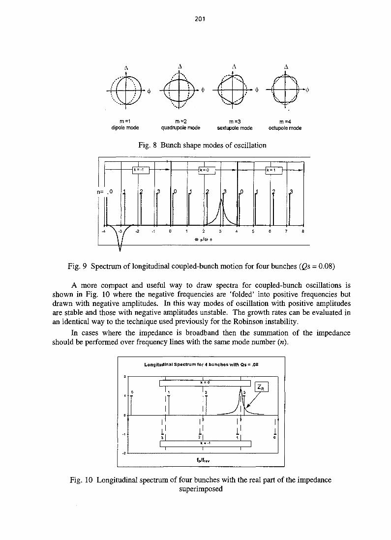
201

m=1dipole mode

m=2quadrupole mode

m=3sextupole mode

m=4octupole mode

Fig. 8 Bunch shape modes of oscillation

n= ,o

-2 -1 1 2 3

CD p/tt> 0

Fig. 9 Spectrum of longitudinal coupled-bunch motion for four bunches (<2s = 0.08)

A more compact and useful way to draw spectra for coupled-bunch oscillations isshown in Fig. 10 where the negative frequencies are 'folded' into positive frequencies butdrawn with negative amplitudes. In this way modes of oscillation with positive amplitudesare stable and those with negative amplitudes unstable. The growth rates can be evaluated inan identical way to the technique used previously for the Robinson instability.

In cases where the impedance is broadband then the summation of the impedanceshould be performed over frequency lines with the same mode number (n).

Longitudinal Spectrum for 4 bunches with Qs = .08

k = 0 |

113 2

4

•J\

1

\ZR

\k = -1 |

10

fp/fr,

Fig. 10 Longitudinal spectrum of four bunches with the real part of the impedancesuperimposed

202

9. TRANSVERSE MOTION

9.1 Equation of motion and transverse impedance

The equation of motion of a single particle in a coasting beam in the transverse(horizontal or vertical) plane is

mwhere Qp is the betatron tune and F/m is the normalised driving force given by

Fx e(E + Bxv)

m

The definition of the transverse impedance is2n

J<J P/A

Consequently the equation of motion for a single particle in a coasting beam is

j

Here the normalised driving force produces a frequency shift

A i _£L z T /

Aco = - —t—2 2 r e v JmQ

This can be written

Ac° = 4 2 ( ^ ) Z

The transverse impedance is evaluated at the frequencies

co = O

Clearly the imaginary part of the transverse impedance will produce a real frequencyshift whereas the real part will cause instability for negative resistances and damping forpositive resistances.

9.2 Modes of transverse oscillations

An example from Ref. [4] of the line spectrum of a bunched beam with transversemotion is shown in Fig. 11 which is drawn for a machine with five relatively long bunches(the PS Booster) and a Qp= 4.2. This spectrum is similar to that shown previously for thelongitudinal plane except that the sidebands are separated from the revolution frequency linesby the non-integer part of the transverse tune

9.3 Chromaticity

In the case of transverse oscillations, the spectrum is significantly affected by thechromaticity (the tune dependence on the momentum offset). A particle that is performing

203

- - -r- TTw.-5 -i -J -3 -I

a) with positive and negative frequencies

SPECTRUM

0 1 ! 3 U S C 7

b) as seen by a spectrum analyser

Spectrum for a machine with 5 long bunches (PS booster) and Q = 4.2. Envelope isdrawn for head-tail mode = 0 and is shifted towards positive frequencies.

Fig. 11 Transverse spectrum of five bunches

synchrotron oscillations can be represented by the ellipse in Fig. 12: above transition aparticle with higher energy than the synchronous particle drifts towards the 'tail' of thebunch. This means that in Fig. 12 a synchrotron oscillation moves on an approximate ellipsein the anticlockwise direction. Now consider what happens when there is a negative tunedependence on the particle momentum (or energy), i.e.

A

Fig. 12 Betatron phase along a synchrotron orbit

A particle at the head of the bunch has the same momentum deviation as thesynchronous particle and therefore the same betatron frequency. As this particle moves alongthe synchrotron ellipse shown, the betatron frequency initially decreases and a betatron phaselag develops, shown as the downward arrows in the figure. When the particle reaches the tailof the bunch its phase lag is at a maximum. Continuing the motion towards the head of thebunch causes the particle to gradually regain betatron phase until it reaches the head of thebunch where the whole cycle restarts. It is also apparent that, if a large number of particleswere distributed around the synchronous orbit with betatron phase advances as indicated in

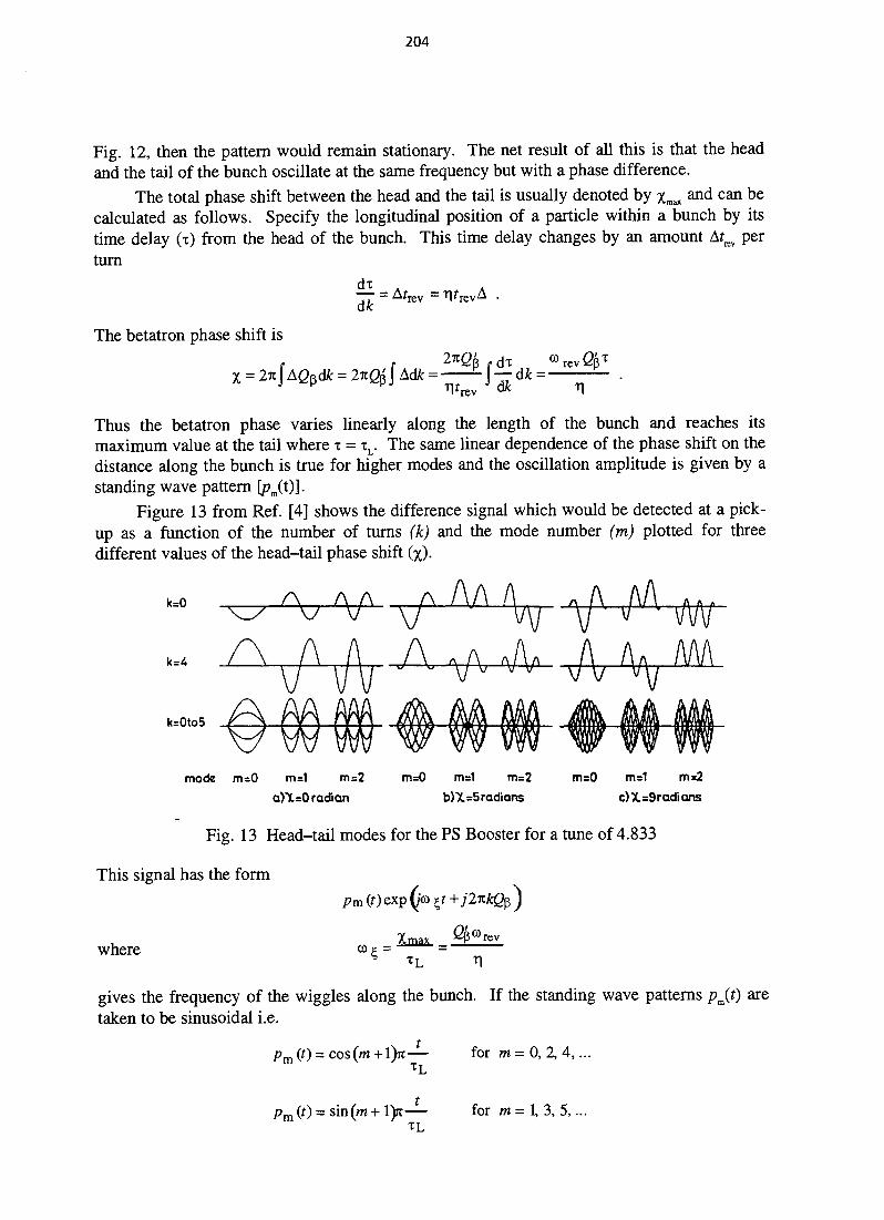
204

Fig. 12, then the pattern would remain stationary. The net result of all this is that the headand the tail of the bunch oscillate at the same frequency but with a phase difference.

The total phase shift between the head and the tail is usually denoted by xmax and can becalculated as follows. Specify the longitudinal position of a particle within a bunch by itstime delay (x) from the head of the bunch. This time delay changes by an amount Afrev perturn

di .— = Afdk rev

The betatron phase shift is

rev

Thus the betatron phase varies linearly along the length of the bunch and reaches itsmaximum value at the tail where x = xL. The same linear dependence of the phase shift on thedistance along the bunch is true for higher modes and the oscillation amplitude is given by astanding wave pattern [pji)].

Figure 13 from Ref. [4] shows the difference signal which would be detected at a pick-up as a function of the number of turns (k) and the mode number (m) plotted for threedifferent values of the head-tail phase shift (x).

k=0

k=0to5

mode m=0 m=1 m=2 m=0 m=1 m=2 m=0 m=1 m=2

a)t=0 radian b)X=5radians c)X=9radians

Fig. 13 Head-tail modes for the PS Booster for a tune of 4.833

This signal has the formpm (t) exp (/<o it +j2%kQ$ J

Xmax îforevwhere CO? =

gives the frequency of the wiggles along the bunch. If the standing wave patterns pjt) aretaken to be sinusoidal i.e.

/>m(0 = cos(m + l)7C— for m = 0, 2, 4,...TL

pm(t) = sm(m+iyt— for m=\ 3, 5,...XL

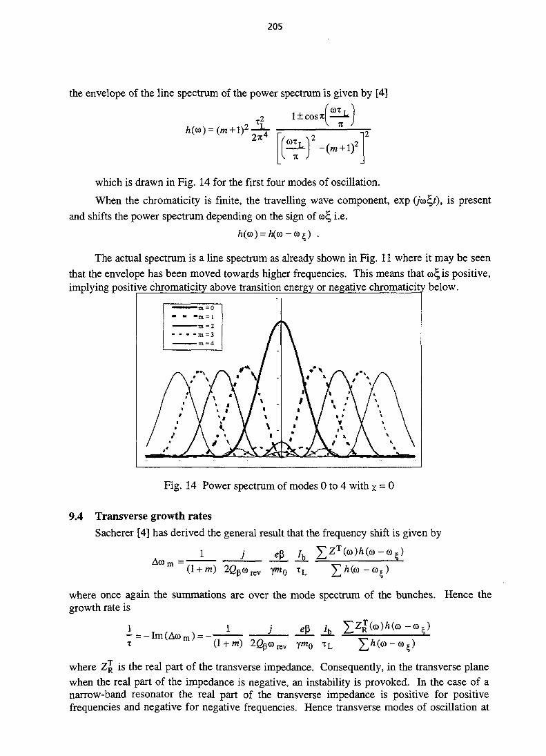
205

the envelope of the line spectrum of the power spectrum is given by [4]

T2 1±COS7^ ^ J

7t-(m + 1)2

which is drawn in Fig. 14 for the first four modes of oscillation.

When the chromaticity is finite, the travelling wave component, exp (jcofy), is present

and shifts the power spectrum depending on the sign of ra£, i.e.

h(co) = h(o - a ^) .

The actual spectrum is a line spectrum as already shown in Fig. 11 where it may be seenthat the envelope has been moved towards higher frequencies. This means that ©H, is positive,implying positive chromaticity above transition energy or negative chromaticity below.

Fig. 14 Power spectrum of modes 0 to 4 with % = 0

9.4 Transverse growth rates

Sacherer [4] has derived the general result that the frequency shift is given by

AcOm =m)

where once again the summations are over the mode spectrum of the bunches. Hence thegrowth rate is

-= - Im(Af f l m ) = -t (1 + m)

—ym0 xL - co

where Z^ is the real part of the transverse impedance. Consequently, in the transverse planewhen the real part of the impedance is negative, an instability is provoked. In the case of anarrow-band resonator the real part of the transverse impedance is positive for positivefrequencies and negative for negative frequencies. Hence transverse modes of oscillation at

206

negative frequencies are unstable. It may therefore be appreciated that by moving the bunchspectrum towards higher frequencies (positive oo£, %) the mode 0 is damped, whereas thehigher order modes may become unstable. This means positive chromaticity above transitionenergy and negative below. This behaviour is shown graphically in Fig. 15.

Figures 16 to 21 show the bunch line-spectra coupling to a resonator impedance and aresistive wall impedance: also shown are the resultant growth rates as a function of thechromatic shift. It is interesting to study these plots to understand the influence of ©E, and ofthe tune values.

...

•*- 1 Unstable

...

....

!-> l ^ 1 H i i

-6 -5 -4 "\if -2 -1 _.(

•*>

StableMM

«P

1 2 3

—*

, RealZT

/

i 1 i . ,

4 5 6

fp/frev

= 0

^ Unstable | ~

_..

-6 -5 -4 "\3jT -2 -1 _<"-•r*

Stable "

J1 2 3 4

RealZr

,15 6

fp/frev

©4 positive

Fig. 15 Transverse spectra for two different values of

Fig. 16 Resonator impedance with varying co£ (for modes 0 and 1)

207

Fig. 17 Relative growth rates as a function of

co£=-2 0)2,= 0 co£,= 2

Fig. 18 Resistive-wall type impedance with varying »? (for modes 0 and 1) (<2(3 = 0.3)

Chromatic Shift

Fig. 19 Relative growth rates (resistive-wall impedance) as a function of a>£,(Q/)= 0.3)

Fig. 20 Resistive-wall type impedance with varying coH, (for modes 0 and 1) (Qp= 0.7)

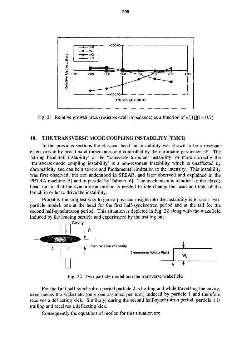
208

I

-ro=O-m=l-m=2-m=3

-200.00-

0 -3.00 -2.00 1.00 ^-2.00 3.00 4.00

-200.00-

Chromatic Shift

Fig. 21 Relative growth rates (resistive-wall impedance) as a function of »£, (<2P = 0.7)

10. THE TRANSVERSE MODE COUPLING INSTABILITY (TMCI)

In the previous sections the classical head-tail instability was shown to be a resonanteffect driven by broad band impedances and controlled by the chromatic parameter co£. The'strong head-tail instability' or the 'transverse turbulent instability' or more correctly the'transverse-mode coupling instability' is a non-resonant instability which is unaffected bychromaticity and can be a severe and fundamental limitation to the intensity. This instabilitywas first observed, but not understood in SPEAR, and later observed and explained in thePETRA machine [5] and in parallel by Talman [6]. The mechanism is identical to the classichead-tail in that the synchrotron motion is needed to interchange the head and tails of thebunch in order to drive the instability.

Probably the simplest way to gain a physical insight into the instability is to use a two-particle model, one at the head for the first half-synchrotron period and at the tail for thesecond half-synchrotron period. This situation is depicted in Fig. 22 along with the wakefieldinduced by the leading particle and experienced by the trailing one.

, Cavityn'v- Central Line of Cavity

uTransverse Wake Field

Fig. 22 Two-particle model and the transverse wakefield

For the first half-synchrotron period particle 2 is trailing and while traversing the cavity,experiences the wakefield (only one assumed per turn) induced by particle 1 and thereforereceives a deflecting kick. Similarly, during the second half-synchrotron period, particle 1 istrailing and receives a deflecting kick.

Consequently the equations of motion for this situation are

209

= 0 forO<r<rs/2

foiTs/2<t<Ts

NelWQa = -where

Using Laplace transforms it is easy to show that the solution to an equation like

>p

IS3

Consequently the solution to the equations for the first half-synchrotron period is

\A(TJ2) 0 "15(71/2) A{TJ2)\

y'2(0)

=r(o->rs/2

where A{t) =

sincop?

cop

•cop sin ©p? cos cop?

COSCOp?

and

at sin co pf

2cop

atcosa^t

asincop?

2<af.

2cof

• + •

a/sincop?

2cop

Similarly it can be shown that the transfer matrix for the second half-synchrotron periodis

_[A(Ts/2) B(Ts/2)~[ 0 A(Ts/2)

and hence the total transfer matrix for a complete synchrotron period is

A(rs/2) 0 1B(T./2) A(TJ2)\

A(Ts/2) B(TS/2J0 A(TJ2)

A2 AB

BA A2+B2

210

All that remains to be done to determine stability is to evaluate the eigenvalues of thismatrix (T). By eliminating resonant terms in the matrix B (it will be shown later that someinteresting effects are dropped with this simplification), the eigenvalues (X) may be evaluated[7] from the characteristic equation:

+c2X2

Here

and

= (2TI -4)cos©prs

c2 = (r\2 - 2)2 + 4cos2 oprs - 2

aTlwhere r\ = — - (not to be confused with the frequency dispersion used previously).4a>p

Determination of the eigenvalues produces the rather simple result that there isinstability if |T|| > 2 and above this threshold the two modes of oscillation become degenerate.This corresponds to a threshold current of

ec(2%R)W0

where the factor 1/eop is related to the P function. If the P function at the location of thewakefield is pw then c/op should be replaced by Pw giving

Figure 23 shows the frequency spectrum of the two modes of oscillation as a function ofthe parameter TJ.

PEP CURRENT MONITOR 2 - J U M S 8 5 17 :11 :54 .01COp ~ ~

- - - - m = -1 i >j 2

2.4

- 8 . 5 8 6.B3 8 .50 1.83 1.59 2.BB 2.5B 3 .88 3 . 5

Fig. 23 Variation of frequencies of modes Fig. 24 Bunch current behaviour when them = 0 and m = -1 as a function of r\ threshold of TMCI is exceeded

Closer examination of the equations of motion shows that, above threshold, theinstability which occurs causes a very severe disruption to the bunches. For r\ = 2 theamplitude of the motion of the trailing particle grows by a factor of 2 during the half-synchrotron period. Above this value the growth of the particles 'bootstraps' into a severeinstability with a very fast growth rate.

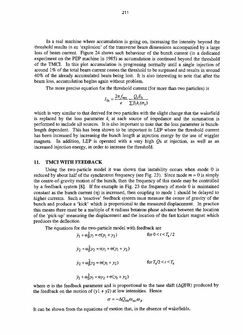
211

In a real machine where accumulation is going on, increasing the intensity beyond thethreshold results in an 'explosion' of the transverse beam dimensions accompanied by a largeloss of beam current. Figure 24 shows such behaviour of the bunch current (in a dedicatedexperiment on the PEP machine in 1985) as accumulation is continued beyond the thresholdof the TMCI. In this plot accumulation is progressing normally until a single injection ofaround 1 % of the total beam current causes the threshold to be surpassed and results in around40% of the already accumulated beam being lost. It is also interesting to note that after thebeam loss, accumulation begins again without problem.

The more precise equation for the threshold current (for more than two particles) is

/ = 2%fw QsEb

* e

which is very similar to that derived for two particles with the slight change that the wakefieldis replaced by the loss parameter k at each source of impedance and the summation isperformed to include all sources. It is also important to note that the loss parameter is bunch-length dependent. This has been shown to be important in LEP where the threshold currenthas been increased by increasing the bunch length at injection energy by the use of wigglermagnets. In addition, LEP is operated with a very high Qs at injection, as well as anincreased injection energy, in order to increase the threshold.

11. TMCI WITH FEEDBACK

Using the two-particle model it was shown that instability occurs when mode 0 isreduced by about half of the synchrotron frequency (see Fig. 23). Since mode m = 0 is simplythe centre-of-gravity motion of the bunch, then the frequency of this mode may be controlledby a feedback system [8]. If for example in Fig. 23 the frequency of mode 0 is maintainedconstant as the bunch current (r|) is increased, then coupling to mode 1 should be delayed tohigher currents. Such a 'reactive' feedback system must measure the centre of gravity of thebunch and produce a 'kick' which is proportional to the measured displacement. In practicethis means there must be a multiple of 7t radians betatron phase advance between the locationof the 'pick-up' measuring the displacement and the location of the fast kicker magnet whichproduces the deflection.

The equations for the two-particle model with feedback areforO<r<fs/2

h.

y2+ap>y2=a(yi + y2) ions//<t<rs

y\ + oop j = ay2 + c(yi + y2)

where o is the feedback parameter and is proportional to the tune shift (AgFB) produced bythe feedback on the motion of (yl + y2) at low intensities. Hence

It can be shown from the equations of motion that, in the absence of wakefields,

212

(O

The solution to the coupled equations of motion with feedback can be performed in anidentical manner to that used without feedback. In order to understand the stability limitswith feedback [7] it is convenient to identify a feedback dimensionless quantity (£)

similar to the r\ parameter defined previously. Remember that r\ is simply proportional to thebunch current while \ is proportional to the gain of the feedback system. The first idea forfeedback called for compensation of the drop in frequency of the m = 0 mode as a function ofcurrent. This corresponds to making the feedback parameter £, equal to -X\I2. (t,,r\) plane.From this plot, it can be seen that, without feedback (£, = 0) and by increasing the bunchcurrent (T|), the unstable region is reached when r\ = 2. This is depicted by the horizontal linestarting at the origin. The line marked (£, = -r|/2) shows the situation Figure 25 shows thecalculated regions of instability [7] (hatched areas) in the where the gain is controlled tocompensate the linear part of the shift of mode 0. In this case the unstable region is reachedat about four times the 'current' for zero feedback. Other stable regions are attainable withthe feedback system e.g. the region indicated by + TI) = %. This analysis clearly showsthat the threshold for the transverse (microwave) instability can be increased by the use of areactive feedback system.

Fig. 25 Stability plots with feedbackparameter £, varied

Fig. 26 Behaviour of modes as a functionof r| and £,

Figure 26 shows the behaviour of the frequencies of modes 0 and 1 with increasing'current' and in the presence of feedback. With the feedback parameter set to zero we obtainthe same plot as previously shown in Fig. 23. However, if the feedback parameter is adjustedso as to push the modes closer at vanishing currents then the instability occurs at a lowerthreshold current (£ = +7i/4). In the cases where the feedback enhances the separation of themodes then the threshold is increased (£ = -7t/4 and -TC/2).

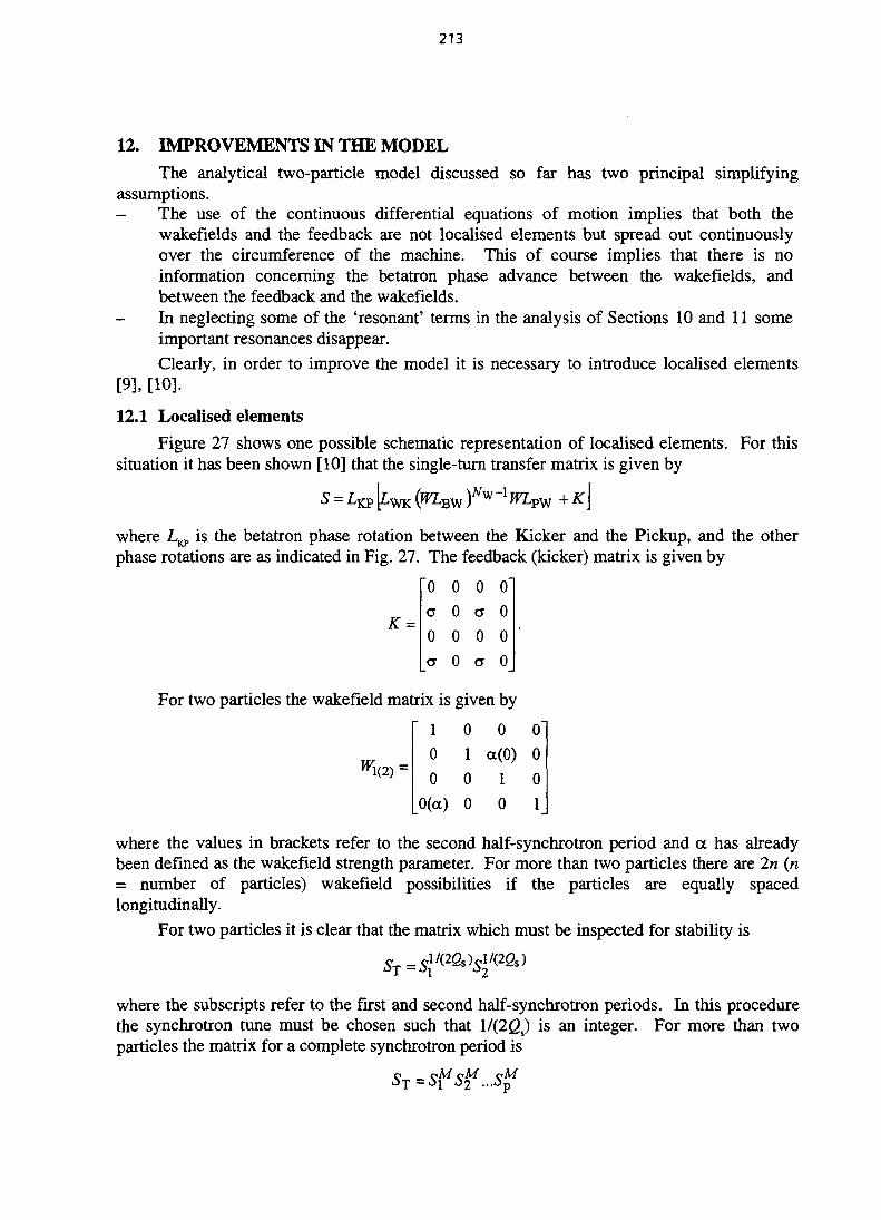
213

12. IMPROVEMENTS IN THE MODEL

The analytical two-particle model discussed so far has two principal simplifyingassumptions.- The use of the continuous differential equations of motion implies that both the

wakefields and the feedback are not localised elements but spread out continuouslyover the circumference of the machine. This of course implies that there is noinformation concerning the betatron phase advance between the wakefields, andbetween the feedback and the wakefields.

- In neglecting some of the 'resonant' terms in the analysis of Sections 10 and 11 someimportant resonances disappear.

Clearly, in order to improve the model it is necessary to introduce localised elements[9], [10].

12.1 Localised elements

Figure 27 shows one possible schematic representation of localised elements. For thissituation it has been shown [10] that the single-turn transfer matrix is given by

few )A'W"1S = + A

where L^ is the betatron phase rotation between the Kicker and the Pickup, and the otherphase rotations are as indicated in Fig. 27. The feedback (kicker) matrix is given by

"0 0 0 0"cr 0 a 0

0 0 0 00 a 0_

For two particles the wakefield matrix is given by

1 0 0 0'0 1 a(0) 0

w\{2) = 0

0(a)

1

0

0

10

where the values in brackets refer to the second half-synchrotron period and a has alreadybeen defined as the wakefield strength parameter. For more than two particles there are 2n (n= number of particles) wakefield possibilities if the particles are equally spacedlongitudinally.

For two particles it is clear that the matrix which must be inspected for stability is

where the subscripts refer to the first and second half-synchrotron periods. In this procedurethe synchrotron tune must be chosen such that 1/(2Q) is an integer. For more than twoparticles the matrix for a complete synchrotron period is

214

where Qs = 1/pM, Sp is the single-turn matrix which corresponds to the wakefield situation p,and p is the number of different wakefield situations (= 2n, where there are n particles equallyspaced longitudinally).

The evaluation of the eigenvalues of ST is too cumbersome to be done analytically butcan be performed with ease on a computer.

A set of results for two particles is shown in Fig. 28 where the Q& is 0.0833 (i.e. 1/12)and there is only a single wake per turn. With the feedback parameter set to zero one canclearly see the resonances at betatron tunes equal to multiples of <2S-

I 2r FtW&ock Porafxtcr (ff; •-0.000

0.2 0.2UNPEST.S3ED hCIv

RJ

Fig. 27 Schematic representation of acircular accelerator with localisedwakefields (W) and localised feedbackelements

0 1 0.2 0.3 OA 0.5

Fig. 28 Stability plots for two-particlemodel and with feedback (note a feedbackparameter of a = -0.3 makes a shift inmode Oof+0/2)

12.2 Summary of the results obtained with the 'few-particle model'

The model described in the last section was used to study [11] the influence of thevarious parameters on the transverse mode coupling instability. The following summarisesthe main results obtained.- One wakefield per turn. The threshold for instability is strongly dependent on the

betatron tune value. The feedback enhances the threshold for a range of tune values.However, as the feedback gain increases, the tune range diminishes rapidly. Theenhancement of the threshold is strongly influenced by the betatron phase shift betweenthe wakefield and the kicker.

- Many wakefields equally spaced over one betatron wavelength. In this case for zerofeedback gain there is absolutely no tune dependence (resonances). This indicates thatthe 'coherent synchrotron-betatron resonances' are more or less restricted to the case ofa single wake per turn. In most circular accelerators the transverse impedance is indeedlocalised, but localised to many hundreds of positions around the circumference. Hencefor most accelerators these resonances will not appear.

The maximum enhancement of the threshold current is greatly reduced when manywakefields (equally spaced over one betatron wavelength) are assumed. With manywakefields the kicker cannot be positioned in betatron phase for optimum enhancementfor each wakefield.

215

13. COMPUTER SIMULATION OF TMCIThe few-particle models have been shown to predict the physical properties of the

TMCI. However, as with all simplified models, they are limited in many ways. The previoussection showed how some of the limitations can be removed to allow the introduction oflocalised elements in the model. The procedure uses a brute force technique for evaluation ofthe threshold of the instability. Although the model contains much of the physics there are,however, some simplifying assumptions which could be worrisome. Most of the remainingsimplifications can be removed by a full-blown computer simulation that evaluates thethresholds in realistic conditions without the restriction of simplified wakefields and 'few'particles. In these simulations [12], [13] several hundreds or even thousands of superparticlesare 'tracked' through a simplified machine lattice containing wakefields and feedbacksystems. The wakefields are evaluated offline using electromagnetic computer codes.Figure 29 shows the simulation of the PEP machine that was done in preparation for adedicated experiment [14] designed to investigate the TMCI threshold in the presence offeedback. On the left is plotted the FFT of the centre-of-gravity motion for various values ofthe bunch current. It can be seen that as the current is increased the mode 0 decreases infrequency and approaches mode - 1 . It is also apparent that as the current increases theamplitude of the mode -1 grows. Instability is reached when the amplitude of the two modesis approximately equal. (This behaviour is often seen in machines with short bunches. Inmachines with longer bunches where there is bunch lengthening with current, the situationbecomes more complicated and the modes m = 0 and m = -1 can become parallel withoutever crossing.) An almost identical behaviour was subsequently measured during thededicated experiment. The motion of the modes is plotted on the right side of Fig. 29. Notethe obvious similarity with the predicted motion for two particles in Fig. 23. These computersimulations predicted very well the PEP behaviour without feedback and less well thebehaviour with feedback. Feedback in PEP allowed the threshold current to be increased bymore than a factor of two.

Am

plitu

deS

pect

ral

!. -. . A.

i . 1 .

1 = 0.30 mA I

I t. m i

1 = 0.60 mA -

t = 0.80 mA I

1 = 1.00 mA -

I = 1.20 mA:

l = 1.34 mA I

1.0 - '

0.8 -

0.6 -

0.4

0.20 0.21 0.22 0.23 0.24 0.25 0.26Tune

4.0-23i 0

a-0.2

-0.4

-0.6

-0.8

-1.0

-1.2 0 0.2 0.4 0.6 0.8 1.0 1.2 1.4l(mA)

Fig. 29 Computer simulation of TMCI

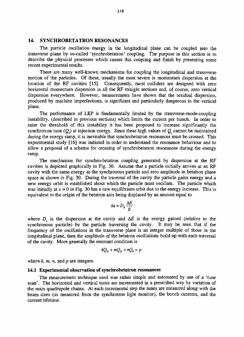
216

14. SYNCHROBETATRON RESONANCES

The particle oscillation energy in the longitudinal plane can be coupled into thetransverse plane by so-called 'synchrobetatron' coupling. The purpose in this section is todescribe the physical processes which causes this coupling and finish by presenting somerecent experimental results.

There are many well-known mechanisms for coupling the longitudinal and transversemotion of the particles. Of these, usually the most severe is momentum dispersion at thelocation of the RF cavities [15]. Consequently, most colliders are designed with zerohorizontal momentum dispersion in all the RF straight sections and, of course, zero verticaldispersion everywhere. However, measurements have shown that the residual dispersion,produced by machine imperfections, is significant and particularly dangerous in the verticalplane.

The performance of LEP is fundamentally limited by the transverse-mode-couplinginstability, (described in previous sections) which limits the current per bunch. In order toraise the threshold of this instability it has been proposed to increase significantly thesynchrotron tune (Q) at injection energy. Since these high values of Q% cannot be maintainedduring the energy ramp, it is inevitable that synchrobetatron resonances must be crossed. Thisexperimental study [16] was initiated in order to understand the resonance behaviour and toallow a proposal of a scheme for crossing of synchrobetatron resonances during the energyramp.

The mechanism for synchro-betatron coupling generated by dispersion at the RFcavities is depicted graphically in Fig. 30. Assume that a particle initially arrives at an RFcavity with the same energy as the synchronous particle and zero amplitude in betatron phasespace as shown in Fig. 30. During the traversal of the cavity the particle gains energy and anew energy orbit is established about which the particle must oscillate. The particle whichwas initially at x = 0 in Fig. 30 has a new equilibrium orbit due to the energy increase. This isequivalent to the origin of the betatron axis being displaced by an amount equal to

_ A£

where D% is the dispersion at the cavity and A£ is the energy gained (relative to thesynchronous particle) by the particle traversing the cavity. It may be seen that if thefrequency of the oscillations in the transverse plane is an integer multiple of those in thelongitudinal plane, then the amplitude of the betatron oscillations build up with each traversalof the cavity. More generally the resonant condition is

kQx+mQy+nQs=p

where k, m, n, and p are integers.

14.1 Experimental observation of synchrobetatron resonances

The measurement technique used was rather simple and automated by use of a 'tunescan'. The horizontal and vertical tunes are incremented in a prescribed way by variation ofthe main quadrupole chains. At each incremental step the tunes are measured along with thebeam sizes (as measured from the synchrotron light monitor), the bunch currents, and thecurrent lifetime.

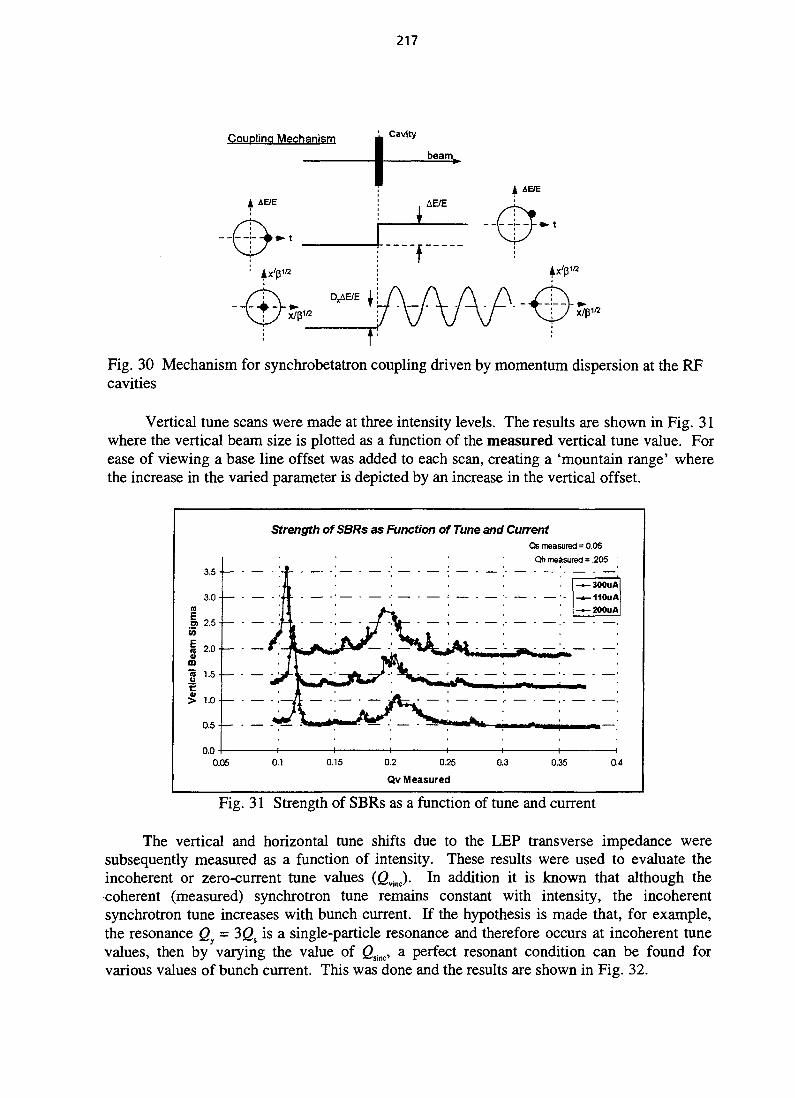
217

Coupling Mechanism ^ Cavity

AE/E

Fig. 30 Mechanism for synchrobetatron coupling driven by momentum dispersion at the RFcavities

Vertical tune scans were made at three intensity levels. The results are shown in Fig. 31where the vertical beam size is plotted as a function of the measured vertical tune value. Forease of viewing a base line offset was added to each scan, creating a 'mountain range' wherethe increase in the varied parameter is depicted by an increase in the vertical offset.

0.5

0.0

Strength ofSBRs as Function of Tune and CurrentQs measured = 0.06

Qh measured = .205

0.05 0.2 0.25

Qv Measured

Fig. 31 Strength of SBRs as a function of tune and current

The vertical and horizontal tune shifts due to the LEP transverse impedance weresubsequently measured as a function of intensity. These results were used to evaluate theincoherent or zero-current tune values (2™,.)- In addition it is known that although thecoherent (measured) synchrotron tune remains constant with intensity, the incoherentsynchrotron tune increases with bunch current. If the hypothesis is made that, for example,the resonance Q = 3<2S is a single-particle resonance and therefore occurs at incoherent tunevalues, then by varying the value of Qsinc, a perfect resonant condition can be found forvarious values of bunch current. This was done and the results are shown in Fig. 32.

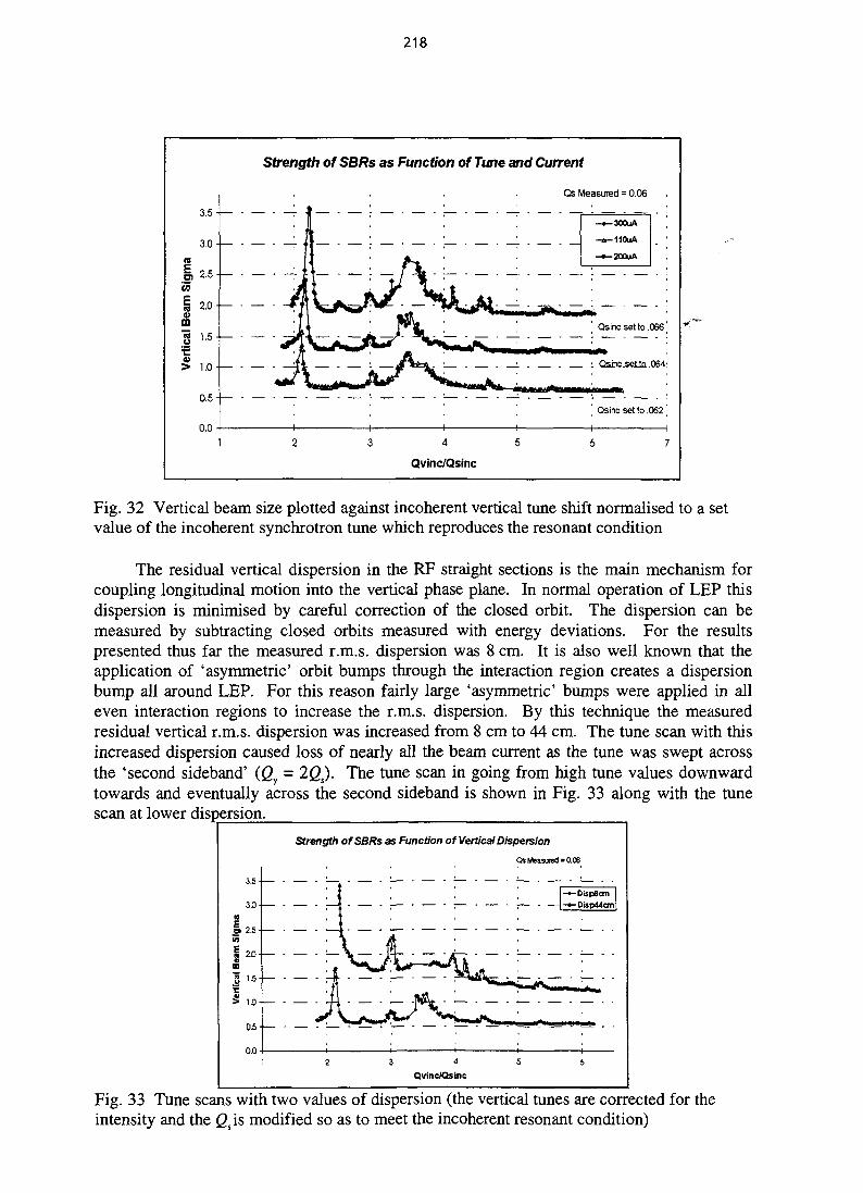
218

w

n

3.5-

3.0 - —

2.5- —

2.0 -—

1.5-

1.0 • —

0.5

0.0

Strength of SBRs as Function of Tune and Current

Qs Measured = 0.06

Qsincsetto.066

- : Jf^toi. • . . _ i . . i Qsinc.selto.064

Qsincsetto.062

Qvrnc/Qsinc

Fig. 32 Vertical beam size plotted against incoherent vertical tune shift normalised to a setvalue of the incoherent synchrotron tune which reproduces the resonant condition

The residual vertical dispersion in the RF straight sections is the main mechanism forcoupling longitudinal motion into the vertical phase plane. In normal operation of LEP thisdispersion is minimised by careful correction of the closed orbit. The dispersion can bemeasured by subtracting closed orbits measured with energy deviations. For the resultspresented thus far the measured r.m.s. dispersion was 8 cm. It is also well known that theapplication of 'asymmetric' orbit bumps through the interaction region creates a dispersionbump all around LEP. For this reason fairly large 'asymmetric' bumps were applied in alleven interaction regions to increase the r.m.s. dispersion. By this technique the measuredresidual vertical r.m.s. dispersion was increased from 8 cm to 44 cm. The tune scan with thisincreased dispersion caused loss of nearly all the beam current as the tune was swept acrossthe 'second sideband' (Qy = 2Q). The tune scan in going from high tune values downwardtowards and eventually across the second sideband is shown in Fig. 33 along with the tunescan at lower dispersion.

Strength of SBRs as Function of Vertical Dispersion

Qs Measured = 0.06

3 4

Qvinc/Qsinc

Fig. 33 Tune scans with two values of dispersion (the vertical tunes are corrected for theintensity and the <2sis modified so as to meet the incoherent resonant condition)

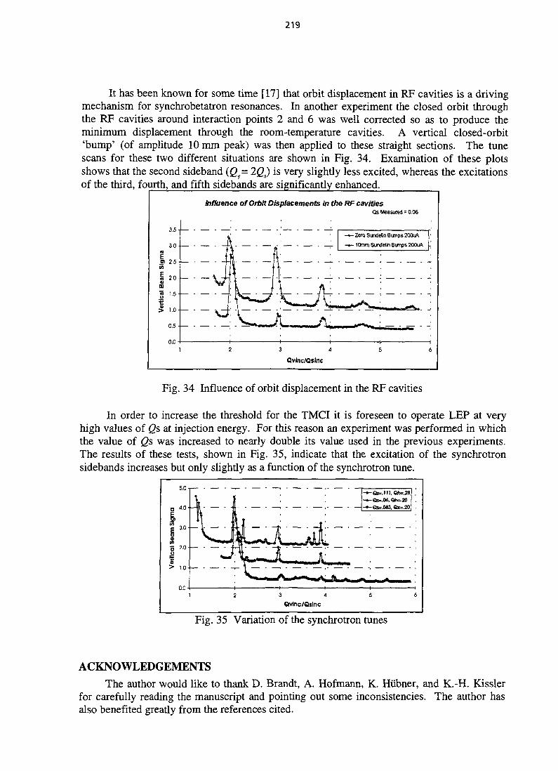
219

It has been known for some time [17] that orbit displacement in RF cavities is a drivingmechanism for synchrobetatron resonances. In another experiment the closed orbit throughthe RF cavities around interaction points 2 and 6 was well corrected so as to produce theminimum displacement through the room-temperature cavities. A vertical closed-orbit'bump' (of amplitude 10 mm peak) was then applied to these straight sections. The tunescans for these two different situations are shown in Fig. 34. Examination of these plotsshows that the second sideband (Qy= 2Q) is very slightly less excited, whereas the excitationsof the third, fourth, and fifth sidebands are significantly enhanced.

Influence of Orbit Displacements in the RF cavitiesQs Measured ~ 0.06

3.5

3.0n

I ,5V)

1 , 0in

1 15

I 1.0

0.5

0.0

- « - Zero SundeSn Bumps 200uA,

— 10mm Sundelin Bumps 200uA

3 4

Qvinc/Qsinc

Fig. 34 Influence of orbit displacement in the RF cavities

In order to increase the threshold for the TMCI it is foreseen to operate LEP at veryhigh values of Qs at injection energy. For this reason an experiment was performed in whichthe value of Qs was increased to nearly double its value used in the previous experiments.The results of these tests, shown in Fig. 35, indicate that the excitation of the synchrotronsidebands increases but only slightly as a function of the synchrotron tune.

5.0

O 4-0

I% 3.0

8 2 0

1> 1.0

0.0

•— - — I »

• M M

1 1 1

-^Qte .OA. Qh=.2O

-^-Qs=.O83, Qx=.M

- - • — - — •

3 i

Qvlnc/Qsinc

Fig. 35 Variation of the synchrotron tunes

ACKNOWLEDGEMENTSThe author would like to thank D. Brandt, A. Hofmann, K. Hiibner, and K.-H. Kissler

for carefully reading the manuscript and pointing out some inconsistencies. The author hasalso benefited greatly from the references cited.

220

REFERENCES

[I] F. Sacherer, National Particle Accelerator Conference, Chicago, 1977. [AlsoCERN/PS/BR/77-5].

[2] K. Robinson, CEAL 1010 (1964).

[3] A. Hofmann, CAS 5th Advanced Accelerator Course, CERN 95-06 (1995), pp. 307-30.

[4] F. Sacherer, CERN 77-13 (1977), pp. 198-218.

[5] R. Kohaupt, DESY 80/22 (1980).

[6] R. Talman, CERN/ISR-TH/81-17 (March 1981).

[7] R. Ruth, CERN-LEP-TH/83-22 (1983).

[8] S. Myers, LEP Note 436, Feb. 1980, see also Proc. IEEE Particle AcceleratorConference, Washington, 1987, pp. 503-507.

[9] B. Zotter, LEP Note 497, May 1984.

[10] S. Myers, LEP Note 498, May 1984.

II1] S. Myers, LEP Note 523, Dec. 1984.

[12] D. Brandt, LEP Note 444, May 1983. See also Xllth Int. Conference on High EnergyAccelerators, Fermilab, 1983.

[13] S. Myers and J. Vancraeynest, CERN-LEP-RF/84-13 (Sept. 1984).

[14] M. Donald et al., LEP Note 553, Jan. 1986, see also Ref. [8].

[15] A. Piwinski and A. Wralich, DESY 76/07 (1976).

[16] S. Myers, 6th ICFA Workshop on Advanced Beam Dynamics (Synchro-betatronresonances) held in Madeira, Oct. 1993.

[17] R.M. Sundelin, IEEE Trans. Nucl. Sci. NS-26 (1979) 3604.

221

LIFETIME AND BEAM QUALITY

C.J. BocchettaSincrotrone Trieste, Italy

AbstractAn overview is presented of lifetime and beam quality in asynchrotron radiation light source. Maintaining the brightness of alight source, which is determined by the beam emittance and storedcurrent, is of fundamental importance. An introduction is given to theconcept of brightness and the factors affecting it. These factorsinvolve transverse beam stability, aperture limitations (physical anddynamic), beam gas scattering, quantum lifetime, intra-beam Coulombscattering, beam instabilities and ion trapping. For each item anoverview of the process/effect is given.

1. INTRODUCTION

The enormous scientific activity in the last few decades in the use of synchrotronradiation has produced several world-wide electron or positron storage ring facilities whichprovide increasingly more intense radiation [1]. Two photon regimes have emerged, whichdetermine the energy of the stored beam, VUV to soft X-rays and hard X-rays. The latestfacilities, the so called third generation light sources, have been specifically designed to caterfor the production of highly intense photon beams. The characteristics of these machines area small electron beam emittance and high currents. In addition the experimental userdemands that the source be highly stable and long lived. These additional requirements are inconflict with the attainment of low emittance and the production of high beam currents [2].The combination of emittance and current yields a figure of merit called the brightness.

Low emittance lattices come in various forms DBA, TBA, QBA [3]. All these latticesare characterised by the requirement of both small dispersion and horizontal betatron functionin the bending magnets, which in turn requires strong focusing. The strong focusing in turnneeds strong chromaticity correcting sextupoles. The strong quadrupoles also make thelattice sensitive to miss-alignment errors with consequent enhanced sensitivity to vibrationsand other perturbations to the electron beam. The strong sextupoles make the electron motiondeviate significantly from linear motion with a consequent reduction in the aperture availableto the electron beam which has a negative impact on the beam lifetime.

High beam currents are limited by beam instabilities [4]. These instabilities arise fromthe interaction of the beam with its environment, the vacuum chamber and cavities. To lowerthe interaction special care has to be taken with the construction of the chamber to lower theimpedance seen by the circulating beam. High beam currents also necessitate increased RFpower with added difficulties in handling such power for a given cavity. To circumvent thismore cavities are used which increases the susceptibility towards multibunch instabilities notto mention the added costs. Instabilities either limit the maximum stored current or give riseto a noisy beam either longitudinally or transversely.

Lifetime is an important parameter of a light source. High brightness means a smallemittance and therefore high bunch densities. This increases the effect of intra-beamscattering, both small and large angle. The former leads to a new equilibrium emittancewhile the latter (the Touschek effect) reduces the lifetime. A higher beam energy alleviatesthe scattering effects, nevertheless, working with few bunches will still give Touschek limitedoperation even for the hard X-ray machines [5]. To overcome the lifetime effect withpresent-day third generation sources either the emittance (transverse or longitudinal) iscompromised or the experimental User suffers frequent interruptions to his experiment due tothe frequent machine refills. Future light sources are focusing effort to improve the lifetime

222

by enhancing the machine acceptance and/or examining the possibility of topping-off the lostelectrons without interrupting the experiments [6].

A facet of modern light sources is the predominant use of insertion devices, undulatorsand wigglers, as the radiation source [7-9]. A significant fraction of the circumference ofmodern storage rings is covered by insertion devices. Undulators produce extremely brighttuneable light. The tuneability is provided by changing the gap of the device. Small gapsallow for a stronger device and permit the production of higher energy photons by going tosmaller period lengths. Small gaps, however, will also have a negative impact on operationby reducing the aperture which leads to a reduction in lifetime, and by increasing chamberimpedance effects and therefore instabilities. The devices also affect the beam dynamics: thelinear focusing term may be compensated by additional quadrupoles in the machine, whereasthe non-linear effect results in a reduction in the dynamic aperture with a consequentreduction in lifetime. The inevitable imperfections of the device also produce changes in theclosed orbit, which are particularly damaging for the Users.

The stability of the beam is as important as the emittance or the lifetime [10, 11]. Ingeneral transverse orbit instability will dilute the emittance and/or shift the source point whilein the longitudinal plane it will degrade the time structure of the beam and also leads to anincrease in the effective energy spread which spoils the quality of the higher radiationharmonics from an insertion device. The time scales of the instabilities which range fromweeks and hours to milliseconds determine the amount and type of beam degradation theexperimental user experiences. Furthermore, high brightness machines put increasingdemand on new technologies to achieve the desired stability on ever decreasing transversebeam dimensions.

In the following sections an overview will be given of what is meant by beam qualityand lifetime and the things which affect them. Apart from the section dealing with iontrapping the considerations given below also apply to positrons as the circulating particles.The reader should note that the quoted references are by no means exhaustive and purelyrepresent examples to the overview given for a particular topic. Extensive additional materialmay be found in the CERN "Yellow Reports" and in the latest proceedings of the Americanand European particle accelerator conferences.

2. BRIGHTNESS

2.1 A figure of merit [12,13]

A quantity which defines the quality of a synchrotron radiation light source is thebrightness, which is simply the phase space density of photon flux evaluated in the forwarddirection and at the centre of the source,

B =d6 d<t> dx dy

(1)

6 <p and x y are the horizontal and vertical angles and co-ordinates and F the flux or thenumber of photons N per second. The importance of brightness arises from the fact that it isan invariant and is conserved while being propagated through linear optical elements.

Integration over either space or angle co-ordinates gives the angular and spatial fluxdensities,

d2F f d4F

dd d<p J d6d<pdx dy•dx dy (2)

223

dx dy J d6 d<p dx dy

The flux, also an invariant, is obtained by a further integration,

F = f (4)dt

If we are interested in a small energy range about a given photon energy, then dividingby dco/a we obtain the spectral brightness and spectral flux.

The units for the spectral brightness and spectral flux are,

Number of photons ,_.D = (P)[sec] [mm2] [mrad2] [0.1% bandwidth]

Number of photons . ,xt = (.0)

[sec] [0.1% bandwidth]

A systematic approach to calculate the brightness is to compute the intensity of theelectric field of a single electron and convolute it with the probability distribution function ofthe electrons [12],

(7)

where Be. is the brightness of a single electron and TJ the probability distribution function.The brightness can be considered as an emittance. It obeys Liouville's theorem and isconserved by linear transformations. Optical elements in a beam line propagate thebrightness from one point to another,

Bl=MB0, (8)

^ or ( l °] (9)v or l -v/ ij- (9)

The linear transformations are drift spaces or focusing elements. From Liouville's theorem ofconservation of phase space area we find that the requirement to have a small photon spotsize somewhere in the beamline will by necessity also give a large divergence there. This inturn implies large optical elements in the beamline which are more difficult to make andcontrol with associated loss of flux and increased costs. To have an intense beam of photonson a sample it is therefore desirable to start with a source which has a small emittance [14].

If we consider the photons to be particles rather than waves and that they have aGaussian distribution in spatial and angular co-ordinates, then the brightness can be writtenas,

M f^ ^HH ^HW ^V"^ ^f^

where F is the flux in the forward direction and the denominator is the phase space volume ofthe photons. ~Lk (k = x,x',y,y') are the spatial and angular standard deviations of the photons

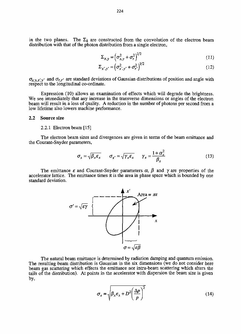
224

in the two planes. The Ejt are constructed from the convolution of the electron beamdistribution with that of the photon distribution from a single electron,

(11)

(12)

<Jx,y,x',y' and ory are standard deviations of Gaussian distributions of position and angle withrespect to the longitudinal co-ordinate.

Expression (10) allows an examination of effects which will degrade the brightness.We see immediately that any increase in the transverse dimensions or angles of the electronbeam will result in a loss of quality. A reduction in the number of photons per second from alow lifetime also lowers machine performance.

2.2 Source size

2.2.1 Electron beam [15]

The electron beam sizes and divergences are given in terms of the beam emittance andthe Courant-Snyder parameters,

(13)Px

The emittance e and Courant-Snyder parameters a, p and y are properties of theaccelerator lattice. The emittance times % is the area in phase space which is bounded by onestandard deviation.

Area = ne

The natural beam emittance is determined by radiation damping and quantum emission.The resulting beam distribution is Gaussian in the six dimensions (we do not consider herebeam gas scattering which effects the emittance nor intra-beam scattering which alters thetails of the distribution). At points in the accelerator with dispersion the beam size is givenby,

(14)

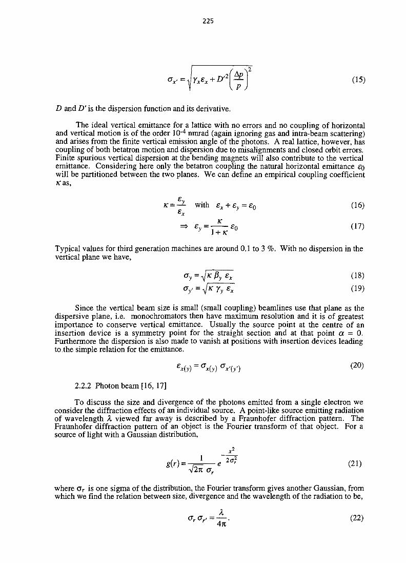
225

D and D' is the dispersion function and its derivative.

The ideal vertical emittance for a lattice with no errors and no coupling of horizontaland vertical motion is of the order 10~4 nmrad (again ignoring gas and intra-beam scattering)and arises from the finite vertical emission angle of the photons. A real lattice, however, hascoupling of both betatron motion and dispersion due to misalignments and closed orbit errors.Finite spurious vertical dispersion at the bending magnets will also contribute to the verticalemittance. Considering here only the betatron coupling the natural horizontal emittance £owill be partitioned between the two planes. We can define an empirical coupling coefficientjcas,

K = — with ex + ey = £Q (16)

_ Ky l+K °

Typical values for third generation machines are around 0.1 to 3 %. With no dispersion in thevertical plane we have,

ay=^Kpy£x (18)

7y£x (19)

Since the vertical beam size is small (small coupling) beamlines use that plane as thedispersive plane, i.e. monochromators then have maximum resolution and it is of greatestimportance to conserve vertical emittance. Usually the source point at the centre of aninsertion device is a symmetry point for the straight section and at that point a = 0.Furthermore the dispersion is also made to vanish at positions with insertion devices leadingto the simple relation for the emittance.

£ M = (Tnff,,,, (20)JCl "V) J C l V J J C l v l v /

2.2.2 Photon beam [16, 17]

To discuss the size and divergence of the photons emitted from a single electron weconsider the diffraction effects of an individual source. A point-like source emitting radiationof wavelength A viewed far away is described by a Fraunhofer diffraction pattern. TheFraunhofer diffraction pattern of an object is the Fourier transform of that object. For asource of light with a Gaussian distribution,

x2

O(A = I e 2°?

where Gr is one sigma of the distribution, the Fourier transform gives another Gaussian, fromwhich we find the relation between size, divergence and the wavelength of the radiation to be,

crrar,=A. (22)

226

The relation can be viewed as a kind of uncertainty condition [17]. We call the productthe diffraction limited emittance X/4n. For wavelengths in the range 0.2 Xc < X <

100 Xc the natural vertical opening angle of the radiation from a single electron in a bendingmagnet can be approximated by [18],

[mrad] (23)

From which the diffraction limited source size cr associated with cr' can be computed fromEq. (21).

2.2.3 Coupling, dispersion and emittance

We now briefly consider a few consequences of the convolution of the electron andphoton distributions.

Firstly we see immediately that if o r > Gx.y then reducing the electron beam emittancegives no further increase in brightness. An effect which is more pronounced for low energyphotons. The maximum brightness occurs when,

Gx,oy<or and ox,,Gy<Gr, (24)

in which case we have the diffraction dominated brightness [8]

(25)

Secondly the brightness is a function of the electron beam coupling and decreases withincreased coupling,

1

OxGx,OyOy

1

K£(26)

x

Thirdly, non-zero dispersion in either plane at the source point, especially alonginsertion devices, will also adversely affect the brightness (excluding here considerations ofquantum excitation in insertion devices [19]) since both the beam size and its divergence willincrease proportionally to the relative energy spread and the dispersion functions. There aresituations, however, where a lower emittance may be obtained for a modified optics with afinite radial dispersion in the straight sections [20]. This is only of benefit at the undulatorposition if

{) (27)

new

Tight control is then needed in maintaining a small relative energy spread, e.g., controllinglongitudinal multi-bunch instabilities. At positions in the bending magnets the situation isnearly always more favourable, since the already existing dispersion is reduced.

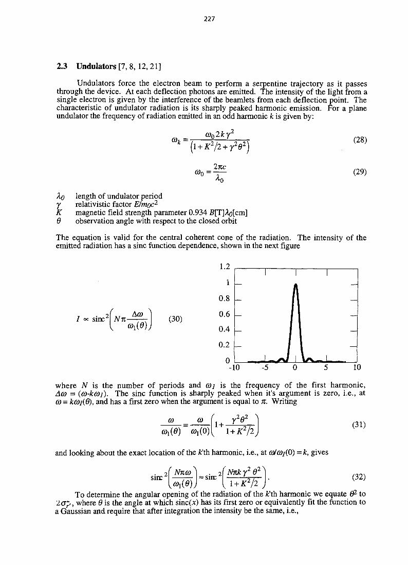
227

2.3 Undulators [7, 8, 12, 21]

Undulators force the electron beam to perform a serpentine trajectory as it passesthrough the device. At each deflection photons are emitted. The intensity of the light from asingle electron is given by the interference of the beamlets from each deflection point. Thecharacteristic of undulator radiation is its sharply peaked harmonic emission. For a planeundulator the frequency of radiation emitted in an odd harmonic it is given by:

co02ky7

(i+K2/2+y2e2)

2%c

(28)

(29)

XQ length of undulator period7 relativistic factor E/moc2

K magnetic field strength parameter 0.9346 observation angle with respect to the closed orbit

The equation is valid for the central coherent cone of the radiation. The intensity of theemitted radiation has a sine function dependence, shown in the next figure

. 2( *r

sine NKI(30)

where N is the number of periods and 0)/ is the frequency of the first harmonic,Aco = (co-ka)]). The sine function is sharply peaked when it's argument is zero, i.e., atco = ko)i(6), and has a first zero when the argument is equal to it. Writing

0) 0) n r{ l + K2/2

(31)

and looking about the exact location of the k'th harmonic, i.e., at (ol(Oi{0) = k, gives

sine2(

{ = sire{^(8)) -- {l + K2/2)- (32)

To determine the angular opening of the radiation of the k'th harmonic we equate d2 tolop, where 6 is the angle at which sinc(x) has its first zero or equivalently fit the function toa Gaussian and require that after integration the intensity be the same, i.e.,

228

sire'2 a2'

(33)

yielding,

fclV(34)

forward direction0=0

where L = Att^ is the length of the undulator and X the wavelength of the radiation. We find avertical opening angle that is about "JkN smaller than that from a bending magnet.

The photon source is found from the requirement of constant phase space area,

XTr~' 2s[2%'

(35)

We now examine the dependence of the line width as a function of the beam parameters [22].Taking the limit of N -> °°,

sine1 s(

N iAft)

N

1 g= —SkN

Aa>S

kN Kco-Aa)) kN

1 r.

3kN

co(36)

The natural line width for the fc'th harmonic is then,

Aft)

CO 9=0 kN(37)

The radiation also depends on the viewing angle 6 and electron energy y. From Eq. (28),

Q} =6)02ky2

K2/2+y262)

the spread in frequencies when the radiation is viewed through an aperture Ad is,

Aft)

(38)

ft)

y2A62

(39)

Because of the 92 dependence of Q)k the peaks are shifted to lower energies when theradiation is viewed off axis. The energy 7 of the radiating electron also affects the spread infrequencies and is given by,

Aft)

ft)

= 2 A7(40)

0-0

The full fractional bandwidth of the k'th harmonic is then given by the convolution of thesethree effects,

229

to JA6,AY

1/2

(41)

Since the brightness is defined per bandwidth Aco/co, we find a reduction in thebrightness for fixed bandwidth if Ad and Ay * 0. The peak brightness is reduced by,

~°0 (Aco/coi)(42)

A0,Ay

If we ignore the effect of the energy spread Ay/y, we note that to keep the line widthcomparable to the natural line width, we require the condition that the acceptance angle becomparable to the natural photon divergence,

A8 (43)

However since it is not possible to distinguish the source of the photons accepted in anangle Ad, the electron beam emittance is equivalent to the acceptance angle, see the figurebelow.

We can therefore write,

to

1/2

(44)

This last equation indicates a loss of energy resolution if either the beam emittancedeteriorates or an increase in energy spread occurs. An increase in the emittance can arisefrom orbit instabilities whilst beam instabilities, notably longitudinal multibunch, will affectthe energy spread. The expression also shows that the angular divergence should be keptsmall, however, since <jy'= V(£y/&), ay< should not be too small since a large (5 mayadversely affect the gas-scattering lifetime (see section 5).

Typical values of the energy variation given by the natural relative energy spread of thering are a few 1(H to 1O"3 rms. However, instabilities, especially multibunch, can increasethis to 10"2 with loss of bandwidth and therefore brightness. Furthermore if spuriousdispersion exists in the straight section the increased energy spread leads to a largertransverse beam size. The control of multibunch instabilities is one of most important aspectsof present-day synchrotron radiation storage ring operation (see section 9).

A finite emittance causes broadening of the undulator lines and a reduction in the fluxat fixed frequency. For machines of comparable emittance, the effect is greater on the higherenergy machine since,

230

Gr. oci . (45)7

The following sections will overview aspects which affect the brightness via either aflux reduction or an increase in beam size and divergence. Flux is reduced if the storedcurrent is reduced, in other words a long lifetime is desirable. It is also reduced if the photonbeam passing through an entrance pinhole is miss-steered. To maintain the brightness thestability of the electron beam has to be guaranteed since beam movement is translated into aneffectively increased beam emittance.

3. STABILITY [10,11,23-25]

3.1 Beam motion with respect to small apertures

A beam line is made up of many components that restrict positional and angularmotion. These components are masks, collimators, mirrors, slits, monochromators and theexperiment and detector. Not all experiments need high brightness some may be interested inhigh flux, however, beam motion is still detrimental to both types since beam linefunctionality is compromised. Intensity changes as small as 0.1% degrade measurementresolution if they occur over the time scale of a measurement. Electron beam orbit miss-steering can miss samples if these are very small and micro-radian angle changes affect thetransmission energy of diffraction gratings or crystal monochromators thereby reducing thespectral resolution. If the time scale for the variation is faster than the measurement time thebeamline user sees a resolution error, otherwise they suffer a calibration error. We canconsider two cases: A focused beam configuration where the source is imaged on a sampleand affected mostly by position stability and an unfocused configuration determined by anglestability.

For the first case the photon beam is focused on slits or a pinhole which is matched tothe beam size or smaller and defines a fixed source position for downstream optics. We willconsider the intensity of the photon beam that is described by a two dimensional Gaussiandistribution with equal dimensions in both planes. The fraction of beam contained in radius ris, l-exp(-r2/2<72). A circular aperture of radius 3crwill then contain 98.9% of the incidentflux (a radius of V6cr contains 95%). If this beam (±3CT) is miss-steered by 10% of its rmsvalue at a horizontal slit we find a reduction of the integrated intensity of 0.01%. Thereduction is more pronounced if the slit is smaller, say ±2cr, then a 0.1a miss-steered beamsuffers a reduction in intensity of 0.1%. If the photon beam size is dominated by the electronemittance, a fixed 10% increase in beam size (-20% e) corresponds to a reduction of 1/75(1.3%) in intensity for a circular aperture.

For an unfocused beam the divergence will dominate. At a slit positioned L metersaway from the source, the beam size given by transformation of the photon ellipse, is [25]:

5 ^ O ) (46)

The expression shows that at large distances intensity fluctuations due to positional changeswill be smaller than those caused by angle changes. A 10% change in angle translates to a10% change in beam size. Changes in angle also result in changes in the energy of photonstransmitted by a monochromator. In general keeping the beam angle constant to within a fewpercent of the beam divergence will be tolerable.

The simultaneous constraints of keeping the angle and position stable to 10% of thebeam size can be combined by requiring that the effective beam emittance averaged over allmovements be no more than 10% of the ideal photon emittance. This constraint can berelaxed if the time to make the averaging is long compared to the time to perform a

231

measurement. Closed orbit errors displace the beam's centre of mass. If the time scale of thedisturbance is greater than the time it takes to make an experiment the result is a simple miss-steering. This will manifest itself as energy calibration errors and loss of brightness. If thetime scale of the disturbance is less than the time to make an experiment the beam is blurredin phase space [10].

Effectiveemittance

Random ^ v—--**•' \ Beammovement emittance

Fig. 1 Random closed orbit movements in angle and position resultsin an effective increase of the beam emittance.

Time varying field errors and magnet misalignments (section 3.3) which distort theclosed orbit will generate at a source point a time varying closed orbit position havingrandomly distributed orbit amplitudes and angles with respect to the ideal machine. Theseamplitudes and angles we take to have a Gaussian distribution. The beam dimensions and theamplitude of closed orbits are uncorrelated and can be added in quadrature to get an effectivebeam dimension,

CJL = o« + crL (47)

The closed orbit distribution is also determined by the betatron function, in which casewe can write,

where

A* og 0 £ ( 4 9 )

We can utilise this result for fast orbit fluctuations compared to the observation time and findif we fix the maximum emittance increase to be 10% that the corresponding acceptable closedorbit distortion is -32% of the beam size. Take for example the situation at ELETTRA whichhas a vertical beam dimension of 13 Jim at the insertion straight ({5y at ID is 2.6 m with0.2 nm-rad emittance for 1% coupling at 2.0 GeV). To have 10% emittance stability theclosed orbit variation has to be kept within 4 u,m which is comparable to the resolution ofstorage ring BPM's ~ 2 um.

3.2 Sources of instability

Stability requirements in a third generation light source are particularly stringent simplyfrom the fact that the source sizes are small. The use of strong focusing also exacerbates thesituation since the strong magnetic fields lead to enhanced amplification of errors (seebelow). The sources of beam instability are many and occur at varying frequencies. In thissection we consider frequencies up to a roughly a few hundred Hz that are driven by

232

mechanical or electrical stability of the accelerator components. We distinguish three roughtime scales for the movements.

• Long term - months to years [24, 26]: Mostly caused by seasonal temperature changes(building/ground expansion/shrinking), seismic motion (tectonic motion, earthquakes, tidalmotion) and ground settlement (addition of shielding, ground water levels).

• Medium term - hours to days [27-29]: The main sources of disturbance are temperatureeffects (on component support systems of magnets, mirrors, chambers, etc., air conditioning,magnet cooling water fluctuations and diurnal changes), cultural noise (nearby traffic) andcranes and heavy machinery. We include here also reproducibility effects which aredetermined by magnet hysteresis after cycling and storage ring energy ramping and orbitchanges which may arise from chromaticity or tune variations to combat beam instabilities.

• Short term - fractions of seconds to minutes [9, 23, 28, 30-32]: These disturbances aredriven by power supply ripple and stability, booster synchrotron cycling, mechanicalvibration (cooling water turbulence, vacuum pumps, compressors, traffic), ground waves,beam instabilities driven by coupled bunch oscillations and ion trapping and, mostimportantly, insertion device gap movements. Undulators are tuned by changing the gap ofthe device thereby changing the energy of the emitted photons. However the devicesintroduce distortions to beam optics and the closed orbit. Orbit distortions are principally dueto non-zero first and second field integrals through the device. Well constructed insertiondevices are possible with small field integrals (the measured fields at the limit ofmeasurement techniques), however, these integrals still affect the electron beam. Thesituation is further aggravated by the fact that many insertion devices will be used and gapchanges performed at random times and manners. Wigglers in general operate at a fixed gapand will predominantly affect the optics.

The above mentioned instabilities can be cured or alleviated in many ways. Wedistinguish between passive and active correction or compensation.

• Passive: This can be done firstly by the proper choice of site and distance from culturalnoise. A rock ground base is good against settling but may couple vibrations. Microfractures in the rock structure will help damp ground vibrations. A clay base will dampvibrations but also allows settling (the ESRF and ALS have ~ lOO^m/lOm/year).Experimental and accelerator areas can be separated from each other to limit interference.We can also separate experimental and accelerator areas from structures that can move(building and ground movement from seasonal/diurnal temperature changes). Mechanicalpumps/compressors etc. are isolated from experiments and accelerators using vibrationattenuation materials. Temperature effects are regulated and controlled (most materials haveexpansion coefficients in the range 10 to 30 x 10-6/°C). Homogeneous and regulated air-conditioning (no turbulence) with stabilisation to ± 0.1 °C is used in accelerator tunnels.Careful control of temperature is also essential in the experimental floor and beamlinehutches. Vibration attenuation material is used in magnet and beam line support systems.The correct choice of power supply specifications ensures acceptable levels of stability andripple. With regard to insertion device effects, these can be minimised by proper constructionof the device with the adoption of appropriate techniques when measuring the field of themagnetic blocks, by careful sorting and by the application of shimming algorithms tominimise the field integrals and to boost the emission of the higher harmonics via a reductionof phase errors.

• Active: Regular measurement and alignment of magnets is essential but is a timeconsuming task especially if the accelerator has many magnets. The ESRF has adopted adynamic alignment system whereby ground settling can be compensated by using hydrostaticlevelling and motorised jacks on magnet girders and front ends. The alignment of themachine is done with a stored beam and takes two hours to perform. On a shorter time scalethe most powerful technique is closed orbit feedback using either electron beam and/or

233

photon beam information. Feedforward techniques are used when behaviour of the beamdistortion is known beforehand, for example when gap changes of insertion devices areperformed. In this case storage ring steerer magnets or insertion device correction coils orrotating magnet blocks are utilised. Feedforward may also be applied to compensate the mainvibration modes of quadrupole support systems.

3.3 Closed orbit distortions

External noise from whatever source ultimately couples to the beam via the magneticfields of the magnets. In an ideal machine the magnetic centres of the magnets coincide withthe closed orbit of the stored beam. If a magnet is displaced from this ideal orbit the beamcentroid will experience a force. For example, a quadrupole displaced Ayguad (by a vibration)will deflect the closed orbit in proportion to the displacement, see Fig. 2. The closed orbittrajectories follow the betatron motion. The kick produced by the quadrupole is termed afeed down effect. Magnets with higher multipoles will also produce these effects, althoughweaker (e.g., a sextupole plus an equivalent beam displacement gives dipole, quadrupole andsextupole terms).

I Quadrupole of strength k

6y=k£y

^ JJ y /6 = dipole term focusing Closed Orbit

Fig. 2 A transverse displacement of the quadrupole from the ideal position generates a dipolekick which in turn causes a closed orbit distortion.

Magnets are positioned to a finite alignment accuracy. The position accuracy istypically little better than 100 |xm and for angles a few tenths of a milli-radian. Misplacementof magnets leads to tilts, rotations and displacements which will distort the closed orbit,couple the beam oscillation planes, distort the optics and generate spurious dispersion. Thespurious dispersion is particularly damaging as it modifies the natural emittance giving anenhanced contribution to the vertical beam dimension and additionally increases the beamsize via the beam energy spread. The sensitivity of a machine to spurious dispersion dependson the lattice [3]. Given the low geometric coupling of third generation light sources (-1%)the vertical unconnected spurious dispersion accounts for most of the vertical beam size.Correction of the spurious vertical dispersion significantly improves the photon source[33, 34]

To compute the effect of magnet displacements we consider in a perfectly alignedmachine one quadrupole which is misaligned giving a deflection 0. Using the one turntransfer matrix M [15],

I. -ysinyf cos if/-a sin y/

where a, /?, y are the Courant-Snyder parameters at the quadrupole and iff the total phaseadvance for a complete turn ( \f/= 2KQ with Q the tune), we propagate the orbit (yy') by oneturn just downstream of the kick. The orbit is then closed by adding the kick to get back to

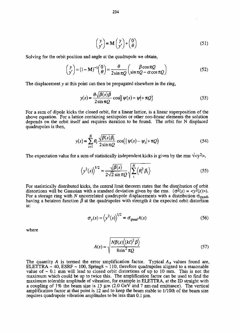
234

Solving for the orbit position and angle at the quadrupole we obtain,

e)-2sinnQ{smKQ-acosnQ)

The displacement y at this point can then be propagated elsewhere in the ring,

y(s) = °ÎQ COS(I V(J) ~ H+ «e) (53)

For a sum of dipole kicks the closed orbit, for a linear lattice, is a linear superposition of theabove equation. For a lattice containing sextupoles or other non-linear elements the solutiondepends on the orbit itself and requires iteration to be found. The orbit for N displacedquadrupoles is then,

y(s) = X fy c o s ( I v(s) - Vil+rcfi) (54)

The expectation value for a sum of statistically independent kicks is given by the rms V<y2>,

(55)

For statistically distributed kicks, the central limit theorem states that the distribution of orbitdistortions will be Gaussian with a standard deviation given by the rms. (G2(s) = <y2(s)>).For a storage ring with iV uncorrelated quadrupole displacements with a distribution aquad»having a betatron function (3 at the quadrupoles with strength k the expected orbit distortionis:

/ ( ) ^ (56)

where

A(s) = J \ '- (57)\ 8sin27tQ

The quantity A is termed the error amplification factor. Typical Ax values found are,ELETTRA ~ 40, ESRF ~ 100, Spring8 ~ 110, therefore quadrupoles aligned to a reasonablevalue of ~ 0.1 mm will lead to closed orbit distortions of up to 10 mm. This is not themaximum which could be up to twice this. The amplification factor can be used to find themaximum tolerable amplitude of vibration, for example in ELETTRA, at the ID straight witha coupling of 1% the beam size is 13 (im (2.0 GeV and 7 nm-rad emittance). The verticalamplification factor at that point is 12 and to keep the beam stable to 1/1 Oth of the beam sizerequires quadrupole vibration amplitudes to be less than 0.1 |xm.

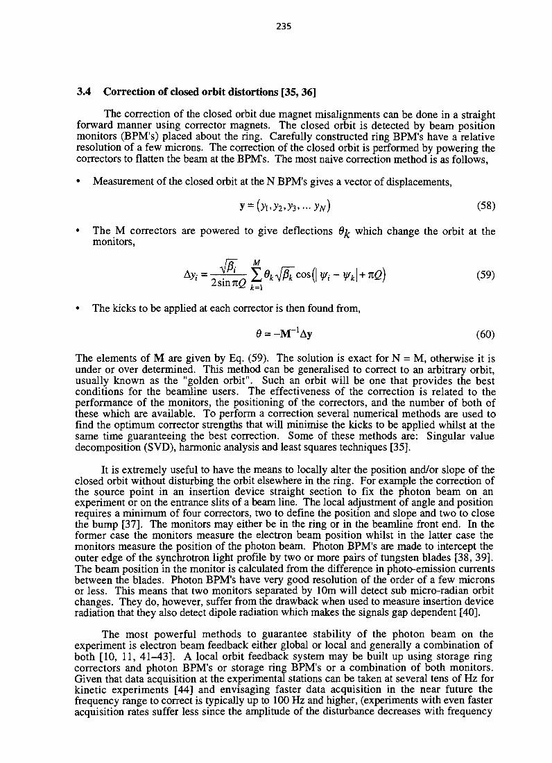
235

3.4 Correction of closed orbit distortions [35,36]

The correction of the closed orbit due magnet misalignments can be done in a straightforward manner using corrector magnets. The closed orbit is detected by beam positionmonitors (BPM's) placed about the ring. Carefully constructed ring BPM's have a relativeresolution of a few microns. The correction of the closed orbit is performed by powering thecorrectors to flatten the beam at the BPM's. The most naive correction method is as follows,

• Measurement of the closed orbit at the N BPM's gives a vector of displacements,

y = (yi.V2,V3,... yN) (58)

• The M correctors are powered to give deflections dfc which change the orbit at themonitors,

(59)

• The kicks to be applied at each corrector is then found from,

6 = -M -1Ay (60)

The elements of M are given by Eq. (59). The solution is exact for N = M, otherwise it isunder or over determined. This method can be generalised to correct to an arbitrary orbit,usually known as the "golden orbit". Such an orbit will be one that provides the bestconditions for the beamline users. The effectiveness of the correction is related to theperformance of the monitors, the positioning of the correctors, and the number of both ofthese which are available. To perform a correction several numerical methods are used tofind the optimum corrector strengths that will minimise the kicks to be applied whilst at thesame time guaranteeing the best correction. Some of these methods are: Singular valuedecomposition (SVD), harmonic analysis and least squares techniques [35].

It is extremely useful to have the means to locally alter the position and/or slope of theclosed orbit without disturbing the orbit elsewhere in the ring. For example the correction ofthe source point in an insertion device straight section to fix the photon beam on anexperiment or on the entrance slits of a beam line. The local adjustment of angle and positionrequires a minimum of four correctors, two to define the position and slope and two to closethe bump [37]. The monitors may either be in the ring or in the beamline front end. In theformer case the monitors measure the electron beam position whilst in the latter case themonitors measure the position of the photon beam. Photon BPM's are made to intercept theouter edge of the synchrotron light profile by two or more pairs of tungsten blades [38, 39].The beam position in the monitor is calculated from the difference in photo-emission currentsbetween the blades. Photon BPM's have very good resolution of the order of a few micronsor less. This means that two monitors separated by 10m will detect sub micro-radian orbitchanges. They do, however, suffer from the drawback when used to measure insertion deviceradiation that they also detect dipole radiation which makes the signals gap dependent [40].

The most powerful methods to guarantee stability of the photon beam on theexperiment is electron beam feedback either global or local and generally a combination ofboth [10, 11, 41-43]. A local orbit feedback system may be built up using storage ringcorrectors and photon BPM's or storage ring BPM's or a combination of both monitors.Given that data acquisition at the experimental stations can be taken at several tens of Hz forkinetic experiments [44] and envisaging faster data acquisition in the near future thefrequency range to correct is typically up to 100 Hz and higher, (experiments with even fasteracquisition rates suffer less since the amplitude of the disturbance decreases with frequency

236

[45]). For the system to be effective the following conditions have to be satisfied or takeninto consideration:

• The system must not couple to adjacent systems [46].• Magnet system sensitivity should be better than 1 jirad. Magnets are specially constructed

for fast linear response. Air core magnets are faster and more linear but weaker than ironcore magnets which, however, suffer from hysteresis effects.

• The positions of the monitors with respect to the beam determine the sensitivity and haveto be appropriately positioned to give the necessary resolution [10]. With regard tophoton BPM's their location should not be too close to the source which would otherwiselower the resolution.

• Due to the quickly varying magnetic fields eddy currents are set up in the chamber wallswhich produce phase lags. For stainless steel the attenuation is small up to 100 Hzwhereas for chambers made of aluminium it is strong at 10 Hz. The attenuation can becompensated but the system requires increased power.

• The system must have interlocks incorporated to protect the vacuum chamber againstbeam miss-steering.

4. THE APERTURE [47]

4.1 Introduction

We now address the important topic of machine aperture which defines the spaceavailable for the storage of the circulating electrons. It is clear that to have a long lifetime,i.e., to maintain the brightness, adequate aperture has to be given to compensate effects whichlead to particle loss. The aperture of the accelerator is not only defined physically by thevacuum chamber but also by the electromagnet fields which guide and accelerate the beam inaddition to the unwanted fields from magnet imperfections. High brightness low-emittancelight sources are highly non-linear machines [2, 3,48, 49]. The non-linearity stems from theneed to compensate the strong chromatic effects which are generated by the strong focusingused to obtain the low emittance. In addition, insertion devices are additional sources of non-linearities especially devices which are used to generate elliptically polarised light. Insertiondevices also break the symmetry of a ring leading to the excitation of structure resonances.The non-linearity of the transverse guide fields limits the amplitude of stable motion anddefines a dynamic aperture for both on and off-momentum particles. In the longitudinalplane the rf bucket size given by the accelerating voltage usually defines the aperture for off-momentum particles.

The question may be asked as to why we need a large aperture when the beam size isfractions of millimetres in cross-section? The answer is the need to efficiently accumulate astored beam and to account for particle-particle interactions within the vacuum chamber.During injection particles execute large betatron oscillations which sample strong non-linearfields. The aperture must be sufficiently large to accommodate these particles and otherswhich undergo large betatron oscillations caused by elastic collisions with residual gasmolecules. The dynamic aperture for off-momentum particles has to contain those electronswhich suffer energy changes because of interaction with other electrons in the beam or withresidual gas molecules — the Touschek effect and inelastic gas collisions. Off-momentumparticles execute synchrotron oscillations which lead to transverse displacements at points ofnon-zero dispersion in addition to the betatron oscillation amplitude. In general the aperturefor off-momentum particles is less than that for on-energy particles.

4.2 Dynamic aperture and transverse acceptance [50,51]

The Dynamic aperture is defined to be the maximum stable initial transverse amplitudein the presence of non-linearities. Non-linear fields will blow-up the betatron oscillationcompared to a linear machine. The concept is schematically shown in Fig. 3 [47]. The

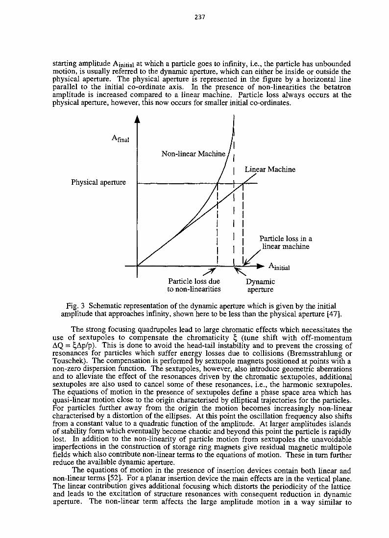
237

starting amplitude Ainitial at which a particle goes to infinity, i.e., the particle has unboundedmotion, is usually referred to the dynamic aperture, which can either be inside or outside thephysical aperture. The physical aperture is represented in the figure by a horizontal lineparallel to the initial co-ordinate axis. In the presence of non-linearities the betatronamplitude is increased compared to a linear machine. Particle loss always occurs at thephysical aperture, however, this now occurs for smaller initial co-ordinates.

Afinalt

Physical aperture

Non-linear Machine,

| Linear Machine

I II I

I I IParticle loss in alinear machine

• Ainitial

Particle loss dueto non-linearities

Dynamicaperture

Fig. 3 Schematic representation of the dynamic aperture which is given by the initialamplitude that approaches infinity, shown here to be less than the physical aperture [47].

The strong focusing quadrupoles lead to large chromatic effects which necessitates theuse of sextupoles to compensate the chromaticity \ (tune shift with off-momentumAQ = Âp/p). This is done to avoid the head-tail instability and to prevent the crossing ofresonances for particles which suffer energy losses due to collisions (Bremsstrahlung orTouschek). The compensation is performed by sextupole magnets positioned at points with anon-zero dispersion function. The sextupoles, however, also introduce geometric aberrationsand to alleviate the effect of the resonances driven by the chromatic sextupoles, additionalsextupoles are also used to cancel some of these resonances, i.e., the harmonic sextupoles.The equations of motion in the presence of sextupoles define a phase space area which hasquasi-linear motion close to the origin characterised by elliptical trajectories for the particles.For particles further away from the origin the motion becomes increasingly non-linearcharacterised by a distortion of the ellipses. At this point the oscillation frequency also shiftsfrom a constant value to a quadratic function of the amplitude. At larger amplitudes islandsof stability form which eventually become chaotic and beyond this point the particle is rapidlylost. In addition to the non-linearity of particle motion from sextupoles the unavoidableimperfections in the construction of storage ring magnets give residual magnetic multipolefields which also contribute non-linear terms to the equations of motion. These in turn furtherreduce the available dynamic aperture.

The equations of motion in the presence of insertion devices contain both linear andnon-linear terms [52]. For a planar insertion device the main effects are in the vertical plane.The linear contribution gives additional focusing which distorts the periodicity of the latticeand leads to the excitation of structure resonances with consequent reduction in dynamicaperture. The non-linear term affects the large amplitude motion in a way similar to

238

sextupole magnets and is again associated with a reduction of the dynamic aperture. Themain non-linear contribution is an octupole term. The effects are inversely proportional tothe square of the beam energy and are more severe for low energy machines, however, largermachines typically have more devices installed. The finite pole width introduces horizontalfield components (quadratic and higher fields) and also contributes to reducing the dynamicaperture. Elliptical wigglers have a strong effect on the dynamic aperture and those which arecrossed impose restrictions on the horizontal physical aperture.

To determine the dynamic aperture numerical tracking of a number of particles is used.Several programs exist for this purpose [53]. Particles are typically tracked for severalhundred turns to see their survival. Ideally the dynamic aperture should be outside thephysical aperture. Figure 4 shows an example of the dynamic aperture in the presence ofsextupole magnets and when in addition insertion devices are symmetrically andasymmetrically placed in the storage ring.

30

fI*<3

I

20-

0

-n- Only Sextupoles-•• Symmetrically Placed ID's••• Asymmetrically Placed ID's- - 5 0 a

10 20Horizontal Amplitude [mm]

30

Fig. 4 Reduction in dynamic aperture when insertion devices are placedasymmetrically in the ELETTRA storage ring [54].

Recalling that a betatron trajectory has the following form[15],

cos(\l/{s) (61)

we see that if A is the aperture at any point in the ring, then A2/f3 defines an emittance for thatpoint. The minimum value of A2//3 anywhere in the ring is the acceptance which is also thelargest emittance the storage ring can sustain. A particle whose trajectory is generated (e.g.,by collisions) to lie outside this emittance will be lost. The acceptance can be limited eitherby the physical or dynamic aperture. The physical aperture is determined by the magnets andthe vacuum chamber that has to stay inside them. In the vertical plane the physical aperture isgenerally determined by the smallest gap required for an insertion device. Typical values forthe full internal gap at an insertion device is 10 to 20 mm. Future developments will push thisdown to 10 to 6 mm and perhaps lower. Injection into the storage ring normally proceeds inthe horizontal plane and, as discussed below, sufficient aperture should be allowed for thisprocedure to be efficient.

4.3 The longitudinal acceptance [55]

In the longitudinal plane the acceptance is defined by the rf system and is a function ofthe rf voltage and the magnet lattice. A large aperture in this plane is needed to contain

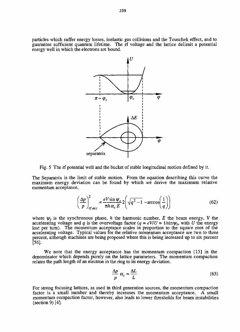
239

particles which suffer energy losses, inelastic gas collisions and the Touschek effect, and toguarantee sufficient quantum lifetime. The rf voltage and the lattice delimit a potentialenergy well in which the electrons are bound.

<P

separatrix

Fig. 5 The rf potential well and the bucket of stable longitudinal motion defined by it.

The Separatrix is the limit of stable motion. From the equation describing this curve themaximum energy deviation can be found by which we derive the maximum relativemomentum acceptance,

rfacc 7th(XcE-1 -arccos — (62)

where y/? is the synchronous phase, h the harmonic number, E the beam energy, V theaccelerating voltage and q is the overvoltage factor (q = eVIU = 1/sinyi, with U the energylost per turn). The momentum acceptance scales in proportion to the square root of theaccelerating voltage. Typical values for the relative momentum acceptance are two to threepercent, although machines are being proposed where this is being increased up to six percent[56].

We note that the energy acceptance has the momentum compaction [15] in thedenominator which depends purely on the lattice parameters. The momentum compactionrelates the path length of an electron in the ring to its energy deviation.

&p AL— a, - — (63)

For strong focusing lattices, as used in third generation sources, the momentum compactionfactor is a small number and thereby increases the momentum acceptance. A smallmomentum compaction factor, however, also leads to lower thresholds for beam instabilities(section 9) [4].

240

4.4 The injection process [57,58]

To reach high beam intensities a beam is accumulated by repeated injection of particlesfrom an injection system, which may be a booster synchrotron or a linac. Ideally the injectionsystem should be full energy, thereby minimising the time it takes for a refill and increasingthe reproducibility of the machine. Full energy injection, furthermore, has the advantage thattop-off procedures may be applied whereby particle losses are exactly compensated for bymany frequent injections performed during normal user operation. This is equivalent tohaving an infinite lifetime. At present no operating storage ring works in this mode, butfuture developments may make this option a reality.

The injection process which transfers particles from an injector is performed by asystem of fast kicker magnets and septum magnets. The kickers move the already storedbeam close to the septum magnet the moment a newly injected pulse arrives. The septummagnet then deflects the incoming bunch parallel to the stored beam without affecting thelatter. The full process has the following three basic steps,

( i) ' During the injection the stored beam is brought close to the septum sheet by using aclosed orbit bump. The distance from the beam centre to the sheet should not be greaterthan half the beam dimension including the tail of the bunch distribution. Four to fivestandard deviations ostored of the beam size is considered acceptable.

(ii) The injected beam follows the septum sheet at a distance of about six standarddeviations Oj>y. The distance to the sheet is not critical since the incoming beam passesthe sheet only once.

(iii) The injected beam enters the storage ring off-axis and executes betatron oscillations, themaximum value of these oscillations occurs where the betatron function is largest.After a time to complete l/fractional(<2x) turns, the amplitude of the closed bumpshould be reduced to a value that does not allow the injected beam to be lost on theseptum sheet. After about 3 damping times the injected pulse will have merged withthe stored beam.

The minimum horizontal half aperture Ax defined by the injection process must satisfy thefollowing condition,

A 1

(64)

where j3x is the betatron function at the position of the aperture, Seffis the effective septumthickness including injection jitter and oc.o. is the peak closed orbit error. Values of Ax arearound 15 to 30 mm, if the dynamic aperture is less than this the injection efficiency iscompromised. By not closing the bump completely, i.e., powering the downstream kickersmore than the upstream ones a more efficient injection can be obtained at the expense ofdisturbing the closed orbit, since the injected beam will then have a smaller oscillationamplitude [57]. Before leaving this section we note that the horizontal aperture must alsotake into account Touschek scattered particles which have suffered energy changes due tointra-beam collisions (see section 8).

5. GAS SCATTERING [47,59]

5.1 Introduction

Particles from the circulating beam are lost by scattering off the residual gas moleculesin the vacuum chamber. The effect is controlled by providing sufficient pumping to reach

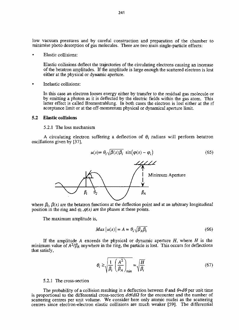
241

low vacuum pressures and by careful construction and preparation of the chamber tominimise photo desorption of gas molecules. There are two main single-particle effects:

• Elastic collisions:

Elastic collisions deflect the trajectories of the circulating electrons causing an increaseof the betatron amplitudes. If the amplitude is large enough the scattered electron is losteither at the physical or dynamic aperture.

• Inelastic collisions:

In this case an electron looses energy either by transfer to the residual gas molecule orby emitting a photon as it is deflected by the electric fields within the gas atom. Thislatter effect is called Bremsstrahlung. In both cases the electron is lost either at the rfacceptance limit or at the off-momentum physical or dynamical aperture limit.

5.2 Elastic collisions

5.2.1 The loss mechanism

A circulating electron suffering a deflection of 0; radians will perform betatronoscillations given by [37],

u(s)= Oj^Pis)^ sin((p(s) - cp() (65)

I Minimum Aperture

B2 \ / P A

where /},-, fi(s) are the betatron functions at the deflection point and at an arbitrary longitudinalposition in the ring and <pi ,(p(s) are the phases at these points.

The maximum amplitude is,

' (66)

If the amplitude A exceeds the physical or dynamic aperture H, where H is theminimum value of A2/PA anywhere in the ring, the particle is lost. This occurs for deflectionsthat satisfy,

h f A2\ rzr(67)

5.2.1 The cross-section

The probability of a collision resulting in a deflection between 6 and 0+d6 per unit timeis proportional to the differential cross-section daldQ. for the encounter and the number ofscattering centres per unit volume. We consider here only atomic nuclei as the scatteringcentres since electron-electron elastic collisions are much weaker [59]. The differential

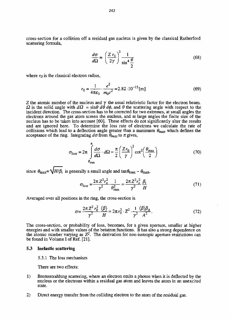
242

cross-section for a collision off a residual gas nucleus is given by the classical Rutherfordscattering formula,

where ro is the classical electron radius,

1 e2 isro = j =2.82 10 15[m] (69)

Z the atomic number of the nucleus and y the usual relativistic factor for the electron beam.Q is the solid angle with dQ = sin0 dd d<j>, and 8 the scattering angle with respect to theincident direction. The cross-section has to be corrected for two extremes, at small angles theelectrons around the gas atom screen the nucleus, and at large angles the finite size of thenucleus has to be taken into account [60]. These effects do not significantly alter the resultsand are ignored here. To determine the loss rate of electrons we calculate the rate ofcollisions which lead to a deflection angle greater than a maximum Qynax which defines theacceptance of the ring. Integrating do from dmax to TC gives,

jda 2 { y )c o t 2 f - ^ l (70)

since 6^^= \jH/fii is generally a small angle and

Oloss- 2 02 - 2/ ''max /

Averaged over all positions in the ring, the cross-section is

7 2 H ° y2 A2

The cross-section, or probability of loss, becomes, for a given aperture, smaller at higherenergies and with smaller values of the betatron functions. It has also a strong dependence onthe atomic number varying as Z2. The derivation for non-isotropic aperture restrictions canbe found in Volume I of Ref. [21].

5.3 Inelastic scattering

5.3.1 The loss mechanism

There are two effects:

1) Bremsstrahlung scattering, where an electron emits a photon when it is deflected by thenucleus or the electrons within a residual gas atom and leaves the atom in an unexcitedstate.

2) Direct energy transfer from the colliding electron to the atom of the residual gas.

243

An electron which suffers an energy loss AEIE will be lost either at the transverse aperturelimit (physical or dynamic) or at the rf limit. Transversely, if the energy loss occurs at aposition with non-zero dispersion, the electron will perform betatron oscillations about a newoff-momentum orbit (see section 7). In the longitudinal plane it will perform synchrotronoscillations.

5.3.2 The cross-section [61]

Only radiative losses (Bremsstrahlung) will be treated. For highly relativistic particlesenergy loss through atomic excitation and ionization of the residual gas have much smallercross-sections compared to the radiative contributions [62].

The differential cross-section for energy loss from photon emission at the nucleus is,

de)N= «

£

~E

where a is the fine structure constant = 1/137. The numerical constants within the bracketsare related to screening of the nucleus by the atomic electrons [47]. The formula is valid forhighly relativistic energies.

The differential cross-section for photon emission at a bound electron on a residual gasatom is (relativistic energies),

d_c\Ue)e I

4E) E2

, 194_ 2 £nZ] + [ 1 ( , _ £3 J | 9 l E (74)

We note that the Z dependence on the former goes as Z2, whilst for electron-electroninteractions it goes as Z.

The total differential cross-section is given by the sum of the two (independent events).The total cross-section is obtained by integrating from em, the lowest energy loss whichresults in particle loss, to E the highest energy loss.

I = I — I <te

in\8

Z(Z

for em«E, and

(75)

(76)

(77)

The cross-section shows a strong dependence of the atomic number of the residual gasspecies, but a weak dependence on the maximum energy acceptance which goes as -In (em/E).

244

5.4 Beam gas scattering lifetime

For independent events the total cross section is the sum of the cross-sections for theindividual events, then,

^loss = êlastic + înelastic (78)

The number of particles lost dN per unit time is proportional to the cross-section, the numberof scattering centres and the number of incident particles.

°ioss ^ - P = density ofdN = -Np<Jlossdx \ ^j£~~^ scattering

centres

1 dN __--P°bssPc N electrons ^ ^

dx = ficdt

which leads to an exponential decay of the stored beam (N = Noer^, with a lifetime givenby,

T=—- . (80)PC <7lossp

The gas density is determined by the composition of molecules present. For a givenmolecular species i the gas equation gives,

A-£ (8D

where pt is the partial pressure, k the Boltzmann constant and T the absolute temperature. Ifeach molecule is made up of different numbers of atoms then op becomes:

y

where a,y is the number of atoms of type j in molecule /.

Desorption of gas molecules by synchrotron radiation is the main source of residual gasin light sources. The desorption depends on the circulating current (number of electrons AO,therefore we write for p,

(83)

G is a desorption coefficient [68]. We now have,

^ = -pcoloss(p0 + GN)N (84)

givingGNO)_

_

245

with No the starting number of electrons. We define the lifetime to be the time it takes for thestarting number of electrons to be reduced by 1/e, and get,

1in (86)

For G = 0 we are led to the previous result. For situations where desorption effects dominatepo -> 0, and,

e-\

pcel0SSGNQ

(87)

The lifetime is inversely proportional to the initial current, which accounts for the increasinglifetime as the current decays.

The total lifetime is given by the sum of individual reciprocal lifetimes,

1 1 1

^total êlastic înelastic

Figure 6 shows as an example the individual effects predicted for the SOLEIL project [63].

400

300 -

(88)

200

100 -

0

.- Elastic electron-nucleus- Inelastic electron-nucleus• Elastic electron-electron / 10

Inelastic electron-elec tron

* •

i

___. — •

, , ,

• — ' • - * "

- - _ _ ^

1.0 1.2 1.4 1.6E [GeV]

1.8 2.0 2.2

Fig. 6 Example of contributions to the lifetime from different beam-gas interactions. (Datataken from [63], 300 mA, 1 nTorr, Z=7,10 and 16 mm vertical and horizontal half apertures.)

The aperture dependence of the elastic scattering contribution can be used to provide,via a scraper, useful information on machine operating conditions. If A is the distance fromthe beam centre to the scraper blade, then we can write the lifetime dependence as,

9iA2

(89)

where C\ depends on effects which are independent of aperture (scraper position), and C2depends only on the elastic scattering loss on the scraper. The coefficient C\ will containcontributions to the lifetime arising from inelastic and Touschek scattering events (seesection 7). By measuring the lifetime as a function of scraper position dynamic apertureeffects can be measured [2, 64, 65].

246

The use of low gap insertion devices to produce high brightness photon sources gives alimiting physical aperture at the insertion device. Of importance to all light sources is theminimum insertion device gap that can be tolerated without significant beam lifetimedegradation [66]. Smaller gaps allow higher energy photons from the use of mini-undulatorswith smaller period lengths. Since the elastic gas scattering effect scales as the square of thebeam energy a higher energy machine is less sensitive to the effect. As a comparison(ignoring betatron function differences) measurements with a scraper at the ESRF operatingat 6.0 GeV have shown 24 hours lifetime (100 mA) with 4.6 mm full aperture(3 x 10"9 mbar)[67] whereas at ELETTRA at 2.0 GeV the lifetime starts to deteriorate ataround 10 mm full aperture.

5.5 Gas desorption

To reduce the effects of gas scattering and ion trapping (see section 10) we require ultrahigh vacuum (UHV), which corresponds to pressures of less than 10"7 Torr. For long gasscattering lifetimes pressures of 10'* Torr are required. The synchrotron radiation from theelectron beam is responsible for the major part of the gas load in the vacuum chamber.Typical static pressures (without beam) are a few hundredth's of a nTorr, whereas dynamicpressures (with beam) are a few nTorr.

The main mechanisms for an increase in pressure with beam are:

• Electron stimulated desorption.• Thermal heating.• Beam induced rf fields — heating from Higher Order Modes (HOM).

Even after cleaning and careful preparation of the chamber surface, gas molecules arestill found bound to the surface. The binding energy of adsorbed molecules is of order of afew eV. Synchrotron radiation impinging on the surface of the chamber releases thesemolecules and is the major contributor to the vacuum pressure in the chamber. A simpleexample taken from reference [68] reveals that a monolayer of N2 released from the surfaceof a 10 cm^ box would result in a pressure increase of 1.7 10'^ Torr.

5.5.1 Electron stimulated desorption [68,69]

The mechanism for gas desorption by synchrotron radiation is as follows:

• Molecular excitation levels are excited by photons in the range 2-100 eV. Thesynchrotron radiation X-rays produced by the electron beam are too energetic for this.

• Instead the X-rays cause emission of photo-electrons from the chamber surface (atomiccore electrons) and the molecules are desorbed during emission.

• The photo electrons then couple to adsorbed molecules causing further electron-stimulated desorption.

Experiments show that the desorption is proportional to the photo-electron currentwhich depends on the chamber material. Of importance is the gas desorption yield 77 definedas the number of molecules produced per incident photon,

Nmol = n Nph. (90)

Typical values for rj are in the range 10"5 to 10~7 depending on the material of thechamber and its treatment. The desorption yield is a function of dose, i.e., the length of timethe chamber has been exposed to radiation. The desorption decreases with the accumulatedphoton dose and new machines are scrubbed by synchrotron radiation before they reach thedesign vacuum pressures. Typical values for this conditioning time are around 50 tolOOAhrs.

247

5.5.2 Thermal desorption

A second source of gas desorption arises from heating of the chamber material. Manymolecules are weakly bound to the surface of the chamber. One of the most troublesomemolecules is water which can form many surface molecular layers the last few of which areonly weakly bound. Thermal excitation will release copious amounts of molecules and thisfact can be used to treat the chamber, i.e., baking-out. An in-situ bake-out of the chamber isusually performed on new chambers to improve the base pressure before scrubbing withsynchrotron radiation.

The desorption rate is given by,

dNmoi _ w -Eb/kT ^Q,-.

at

with Eb binding energy (0.1 to 10 eV), v a rate constant and 7/mo/ the number ofmolecules/cm2. The rate constant depends on the previous conditioning of the chamber. Forbaked stainless steel (250 °C),

v - 2 1 0 " 1 2 Torres"1 cm"2

whereas for an unbaked chamber,

v ~ 10"10 to 10~" Torr I s"1 cm"2

Even with careful treatment of the chamber, the outgassing due to synchrotron radiationis very high. To overcome this problem the construction of the chamber geometry to collectsynchrotron radiation in well defined points, where cooling and additional pumping isprovided, is of fundamental importance both in terms of the photo-electron induceddesorption and that due to thermal heating.

5.5.3 Beam induced radio-frequency fields [69]

An additional source of thermal desorption arises from the heating of the chamber bythe beam-induced radio-frequency fields, i.e., Higher Order Mode (HOM) heating. Thecirculating beam leaves wake fields (see section 9) at discontinuities in the chamber, i.e., atbellows, valves, pumping slots, cavities, tapers and the like. The average power loss dependson the resistive part of the chamber impedance seen by the beam,

P^={eNbfnbfok(a) (92)

where eNb is the charge per bunch, rib the number of circulating bunches, fo the revolutionfrequency and k the loss parameter in Volts/m defined by the impedance [4]. The lossparameter depends strongly on the bunch length and is greater for shorter bunches whichleads to greater heating of chamber components [70].

6. QUANTUM LIFETIME [3,71-73]

6.1 Introduction

The distribution of the electrons in a storage ring bunch is principally determined by thecontainment forces, both transverse and longitudinal, and by events originating within thebunch itself. The main events originating within the bunch are the emission of synchrotronradiation and intra-beam scattering. Synchrotron radiation leads to two effects: a damping of

248

betatron and synchrotron oscillations and a growth of the oscillation amplitudes due toquantum fluctuations. The former depends on the average energy loss <«> while the latterdepends on deviations of the loss about the average <u2>. The number of photons emittedper electron per turn is a rather small number. For a single electron the number of emissionsper meter is about 6.2 B[T] (with B the dipole field). This small number will give rise tonoticeable statistical effects and leads to a broadening of the energy distribution due toquantum fluctuations proportional to <u2>. In the transverse plane the emission of a quantumof radiation changes only the magnitude of the particle's momentum but leaves the positionand slope the same. The physics, however, is different if there is dispersion or not at theemission point. If the dispersion is zero, the emission of a photon does not modify theamplitude of the orbit (ignoring the small angle changes ± 1/$. With non-zero dispersion, theposition and slope still remain the same but the electron now has a new reference energy orbitE- Eo- u which results in an excitation of a new betatron amplitude. The amount of energylost during a quantum event is small compared to the energy spread of the beam (i.e., inELETTRA the critical energy is 3.2 keV whereas the natural energy spread is 1.6 MeV)implying small changes to the amplitude compared to the beam width. The change canhappen at any phase of the oscillation and can lead to an increase or a decrease in amplitudedepending on the distance between the original and final orbits which is given by thedispersion. The process is similar to a random walk.

The appearance of damping arises from the emission of synchrotron radiation which isproportional to and the subsequent energy gain in the rf cavity. Damping in thelongitudinal plane occurs because of the dependence of the energy loss on the particle'senergy, a high energy electron loses more energy than a low energy electron. Consider twoelectrons with energies above Ea and below Eb an electron with an ideal energy Eo. Theenergy lost by Ea will be greater than that of Eo and that lost by Et, will be less than Eo. Theresult is that the energy difference has been reduced. The energy deviation and thelongitudinal co-ordinate of an electron with respect to the synchronous particle are conjugatevariables implying that the longitudinal bunch dimension is also damped. To considerdamping in the transverse plane we note that the energy lost from the emission of a photonresults in a loss of both transverse and longitudinal momentum. The lost energy, however, isrestored in the cavities as an increase in the longitudinal momentum whilst the transversemomentum remains the same. This results in a reduction of the slope with respect to theclosed orbit and is equivalent to a damping of the transverse motion.

Intrabeam scattering, which will be dealt with in section 8, is an effect arising frommultiple small angle electron-electron Coulomb collisions within the bunch. The collisionsincrease the "temperature" of the bunch by transferring energy from the longitudinal plane tothe transverse plane. The sum of a multitude of small random variations in an electron's co-ordinates will by virtue of the central limit theorem will lead to a distribution which willasymptotically approach that given by Gaussian distribution independent of the initialelectron's distribution. The phase space distribution of the electron bunch results from anequilibrium between radiation damping, quantum excitation and intra-beam scattering. Thedistribution is altered by the presence of the vacuum chamber or by the potential well of the rfsystem, the finite boundaries of which will lead to particle loss.

6.2 Quantum lifetime

The equilibrium established between quantum fluctuations and radiation dampingresults in a Gaussian phase space distribution for the electrons,

) \ (93)

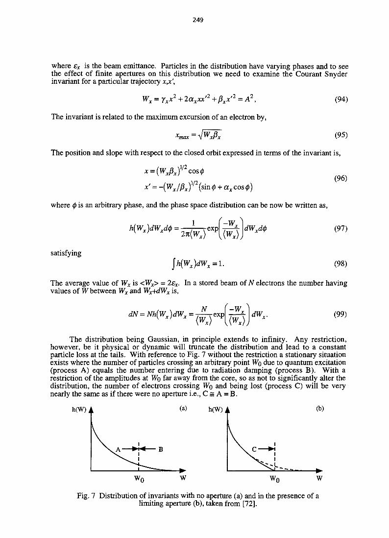
249

where sx is the beam emittance. Particles in the distribution have varying phases and to seethe effect of finite apertures on this distribution we need to examine the Courant Snyderinvariant for a particular trajectory xjc',

Wx = yxx2 + 2axxx'2 + pxx'2 = A2, (94)

The invariant is related to the maximum excursion of an electron by,

Xmax = A (95)

The position and slope with respect to the closed orbit expressed in terms of the invariant is,

* = (WA)1/2cos0(96)

where 0 is an arbitrary phase, and the phase space distribution can be now be written as,

h(Wx )dWxd x W

2-K(?NX) {(Wx)j x * K '

satisfyingjh{Wx)dWx = L (98)

The average value of Wx is <W*> = 2ex. In a stored beam of N electrons the number havingvalues of W between Wx and Wx+dWx is,

(99)

The distribution being Gaussian, in principle extends to infinity. Any restriction,however, be it physical or dynamic will truncate the distribution and lead to a constantparticle loss at the tails. With reference to Fig. 7 without the restriction a stationary situationexists where the number of particles crossing an arbitrary point Wo due to quantum excitation(process A) equals the number entering due to radiation damping (process B). With arestriction of the amplitudes at Wo far away from the core, so as not to significantly alter thedistribution, the number of electrons crossing Wo and being lost (process C) will be verynearly the same as if there were no aperture i.e., C = A = B.

h(W) (a) h(W)

B

(b)

w

Fig. 7 Distribution of invariants with no aperture (a) and in the presence of alimiting aperture (b), taken from [72].

250

The loss rate can therefore be estimated as that due to process B, due to radiation damping.Evaluated at the restriction we have,

*!•) J«LM) (1oo)dt )w0 KdW dt JWo

and

dNdN = Nh{W)dW => — = Nh(w). (101)

For a given electron the rate of change of Wx due to radiation damping is [3],

^t'-2Jt (102)

where xx is the radial damping time and

(103)y*))

AT = i V o e x p | ^ | . (104)

the quantum lifetime xq is then found to be,

where

Assuming the limiting aperture occurs at a point with maximum betatron function fimax then,

r2 /ftg 2 _ •XfmaxlHmax _1 ^

Because of the exponential factor the quantum lifetime increases rapidly with XmaxlOx- Theabove relation for the quantum lifetime is valid for xmax » ax. As xmax approaches ax theassumption that the restriction does not alter the distribution is no longer valid. In fact theexpression gives a minimum lifetime of T e/2 at Xm^ = \lax which is incorrect since smallerapertures must give shorter lifetimes. A more complete derivation of the distribution usingthe Fokker-Planck equation yields the correct solution [74] from which we also find forxmax < cthe approximate solution,

251

2.405(108)

For values of xmax> ~5ox accurate values of xq can be computed using Eq. (107) and somenumbers are given in Table 1. For a damping time of 10 ms we find the "golden rule" ofchoosing xmax to be greater than 6.5 cr* in order to have a quantum lifetime of around100 hours.

Table 1Quantum lifetime as a function of limiting aperture

xmax'^x 5

1.8 min

5.5

20.4 min

6.0

5.1 hrs

6.5

98.3 hrs

7.0

103 days

In the horizontal plane the situation may be additionally more complicated. Finite dispersioncan exist which will also give quantum lifetime contributions from synchrotron oscillations,ii.e.,

(109)

If the beam size given by betatron motion is comparable to the width of the beam due to therms energy spread {oeIE), i.e.,

(110)

then, the lifetime is [74],

— T r

2V2(HI)

where

r =(D a and « - £ vmax (112)

The minimum value of rq occurs when r = 0.640 and,

(113)

The lifetime is lower than in the case with no dispersion, however, since the horizontalaperture must already be large enough to accommodate the injection process and to giveadequate Touschek lifetime the quantum lifetime effect can be ignored in the horizontalplane.

252

In the longitudinal plane a Gaussian distribution also exists for the energy and phasedeviations. Here the aperture restriction is the finite potential well given by the radio-frequency system. The oscillation "amplitude" is now defined by the invariant of the energyoscillations,

With Q the synchrotron oscillation frequency. We obtain a similar result for the quantumlifetime as for the transverse case,

*T — fc

*<1- 2

where T£ is the longitudinal damping time and

™Q _ £ m a x

with (7£ the rms energy spread and the maximum energy deviation defined by the rf system isgiven by Eq. (62). As for the radial case the rf acceptance is determined by the need to havean acceptable Touschek lifetime. Typical values for the acceptance are 2 to 3%. Withrelative energy spreads of the order a few 10"4 and damping times of the order of 10 ms thelongitudinal quantum lifetime is practically infinite.

7. THE TOUSCHEK EFFECT [75-77]

7.1 Introduction

The high bunch densities present in low emittance high brightness machines leads to anenhanced rate of elastic collisions between electrons within the bunch. Collisions occur in allplanes, however, the energy transfers involved from the longitudinal plane to the transverseare insufficient to generate a betatron oscillation capable of leading to particle loss. In thissection we will only consider the processes that transfer sufficient energy from the transverseplane to the longitudinal for loss of both colliding particles. The change in the longitudinalmomentum leads to particle loss if the momentum exceeds the rf acceptance or the transverse(physical or dynamic) acceptance. The Touschek effect is one of the limiting mechanisms forpresent day synchrotron radiation sources [78-79]. It was first explained by Bruno Touschek[75] after observations of the lifetime on the small storage ring ADA. Only recently has theeffect become a critical issue in the construction and running of present day light sourceshaving low emittance. The effect of longitudinal to transverse momentum transfer will betreated in section 8 along with the remaining collisions that generate many small momentumtransfers that lead to an increase in the beam emittance.

To understand the mechanism we must consider the motion of the electrons in a framewhich moves with them. The betatron motion in this frame is purely transverse and acollision will transfer momentum into the longitudinal plane. Transforming back to thelaboratory frame the transferred momentum is boosted by a factor y. The process is shown inthe figure below [80].

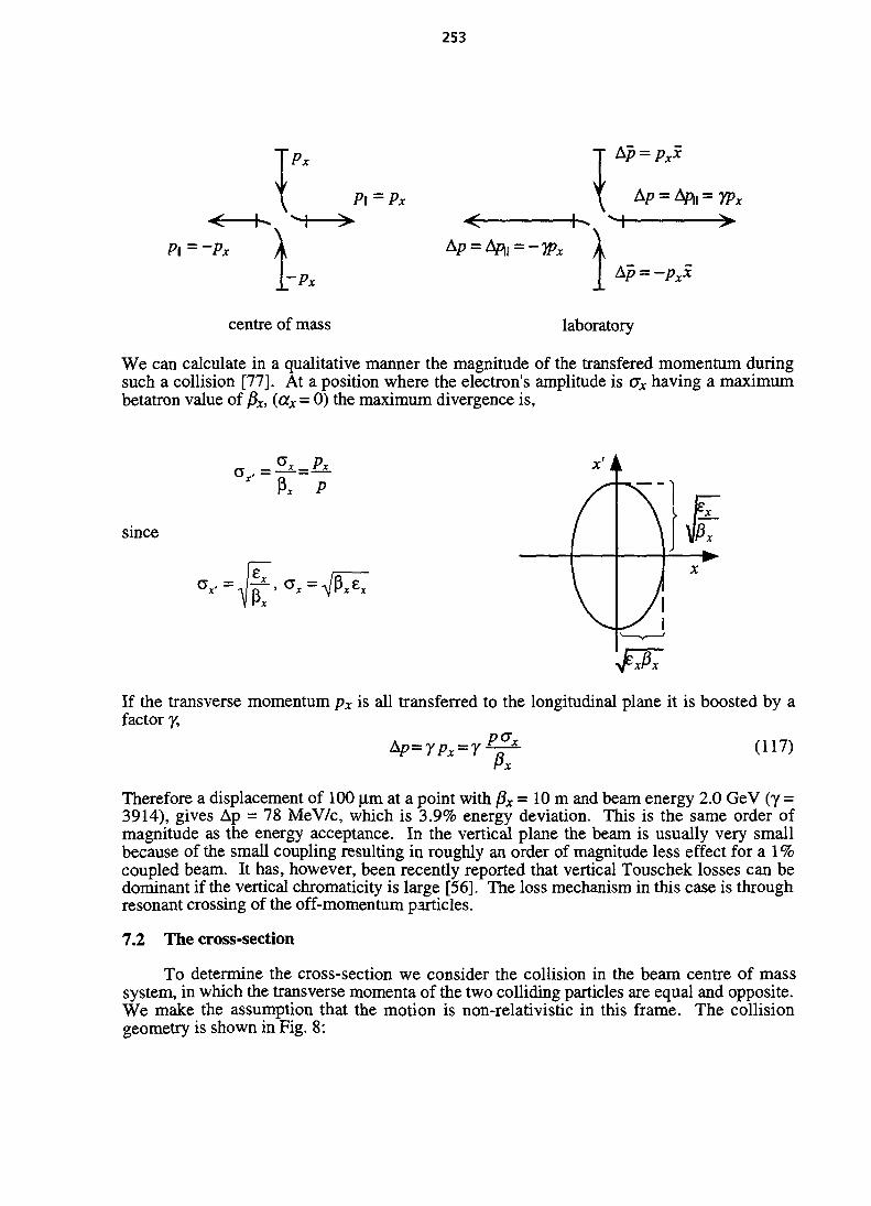
253

Pi = ~Px

V\ Pl=Px Ap = Ap|| = yp

~Px

centre of mass laboratory

We can calculate in a qualitative manner the magnitude of the transfered momentum duringsuch a collision [77]. At a position where the electron's amplitude is ax having a maximumbetatron value of fix, (ax = 0) the maximum divergence is,

P, P

since

If the transverse momentum px is all transferred to the longitudinal plane it is boosted by afactor 7,

Therefore a displacement of 100 um at a point with f3x = 10 m and beam energy 2.0 GeV (y =3914), gives Ap = 78 MeV/c, which is 3.9% energy deviation. This is the same order ofmagnitude as the energy acceptance. In the vertical plane the beam is usually very smallbecause of the small coupling resulting in roughly an order of magnitude less effect for a 1%coupled beam. It has, however, been recently reported that vertical Touschek losses can bedominant if the vertical chromaticity is large [56]. The loss mechanism in this case is throughresonant crossing of the off-momentum particles.

7.2 The cross-section

To determine the cross-section we consider the collision in the beam centre of masssystem, in which the transverse momenta of the two colliding particles are equal and opposite.We make the assumption that the motion is non-relativistic in this frame. The collisiongeometry is shown in Fig. 8:

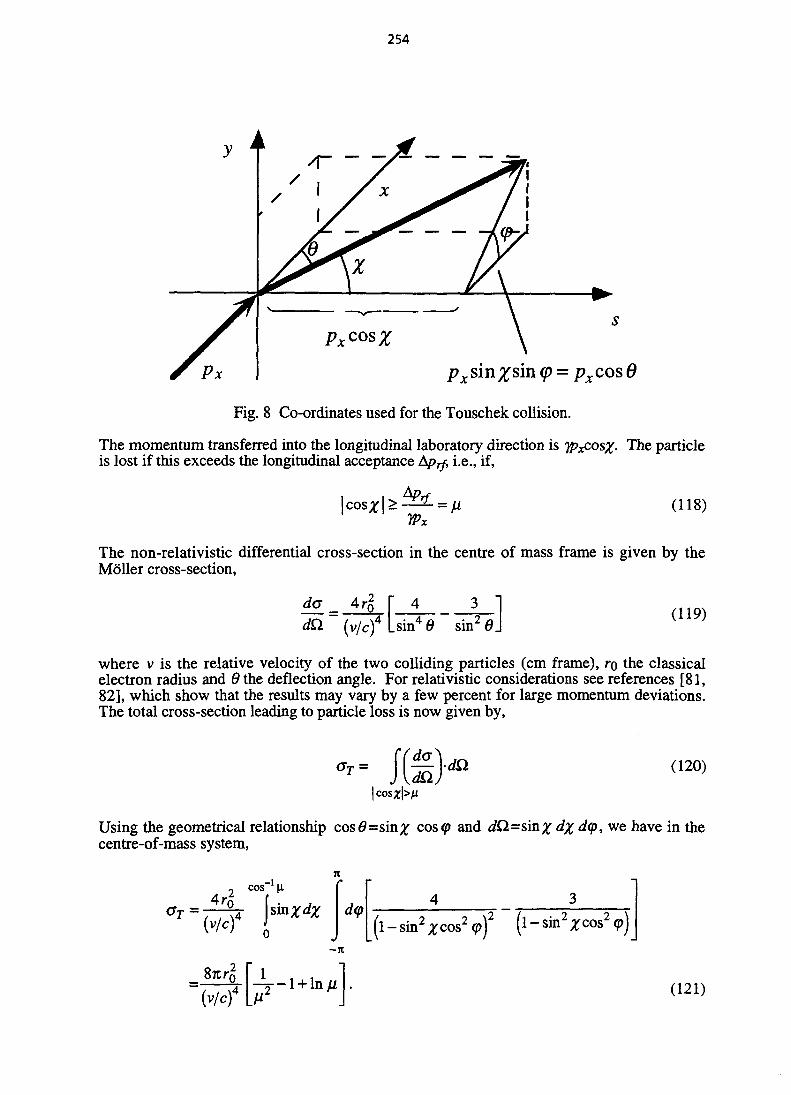
254

p sinxsin <p = pxcos6

Fig. 8 Co-ordinates used for the Touschek collision.

The momentum transferred into the longitudinal laboratory direction isis lost if this exceeds the longitudinal acceptance Ap^, i.e., if,

cos y >

- The particle

(118)

The non-relativistic differential cross-section in the centre of mass frame is given by theMoller cross-section,

da_ = Ar\ I" 4 _ 3 1dQ ~ (v/c)4 Lsin4 6 sin2 6 J

(119)

where v is the relative velocity of the two colliding particles (cm frame), ro the classicalelectron radius and 6 the deflection angle. For relativistic considerations see references [81,82], which show that the results may vary by a few percent for large momentum deviations.The total cross-section leading to particle loss is now given by,

(120)

\cosx\>fi

Using the geometrical relationship cos0=sin# cos<p and dK2=sin£ d% d<p, we have in thecentre-of-mass system,

0 cos V_ 4r0

2 'dcp

(l-sin2^cos2<p)2

-7t

(v/c)4 (121)

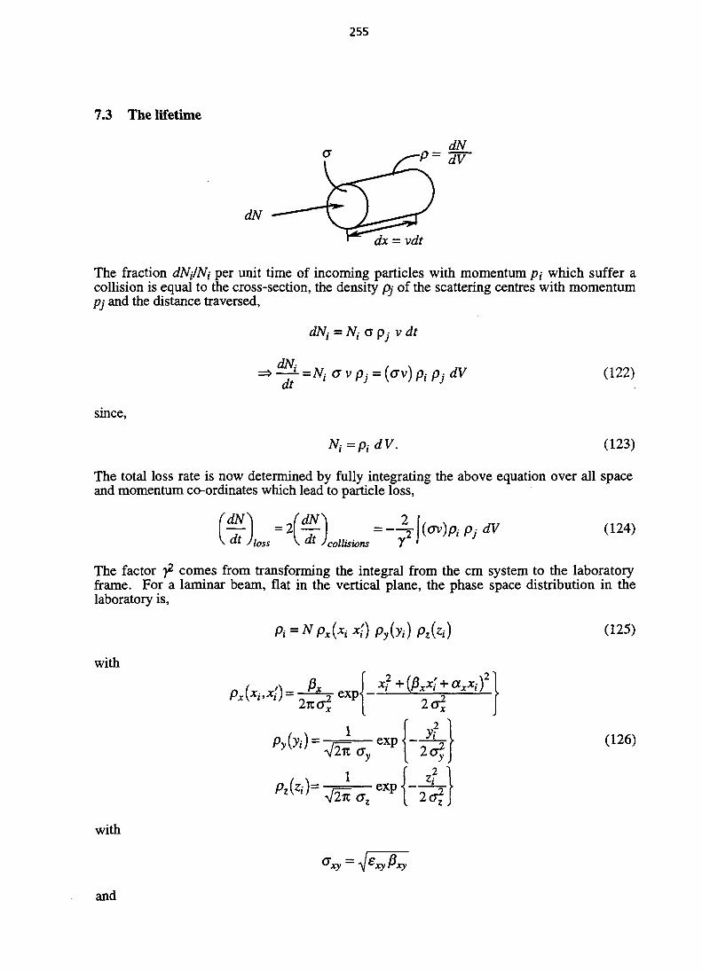
255

7.3 The lifetime

dN

dx-vdt

The fraction dNtfNi per unit time of incoming particles with momentum pi which suffer acollision is equal to the cross-section, the density pj of the scattering centres with momentumPj and the distance traversed,

dNt = N( a Pj v dt

-+= (122)

since,

(123)

The total loss rate is now determined by fully integrating the above equation over all spaceand momentum co-ordinates which lead to particle loss,

fdN\ JdN\ 2\dt)loss \dt collisions 72 (124)

The factor f- comes from transforming the integral from the cm system to the laboratoryframe. For a laminar beam, flat in the vertical plane, the phase space distribution in thelaboratory is,

with

ix0 py(yi) pz(Zi) (125)

2O2y(126)

with

and

256

(127)

In the last expression the bunch rms length is related to the rms relative momentum spread{Oe/E) via the momentum compaction factor and the synchrotron tune, R is the average ringradius. The integration is performed assuming the collision occurs at (xj, yj, zi) = (x2, y2,i- The integrals over y and z are performed immediately yielding,

dN_

dt 2nyz oy<jz

SK3 y2

)v px{xx,x{)

G{v)v

dx[dx'2

(128)

with

Making use of

cx = -^-=1— and x2 - x\= — - = —t-

(129)

(130)

where v is the relative velocity in the cms, we integrate over dxj express the resulting integralin terms of pxdx'i and finally integrate over dx'i, giving,

dN N1

dt 2K2c ox, ax cy oz

yc'xmoC>

(131)

The lower limit reflects particle loss if the momentum exceeds the momentum acceptance inthe centre-of-mass system. Defining,

e =y2cxmoc_

(132)

with (Ap/p^the rms relative momentum acceptance, the loss rate can be expressed as,

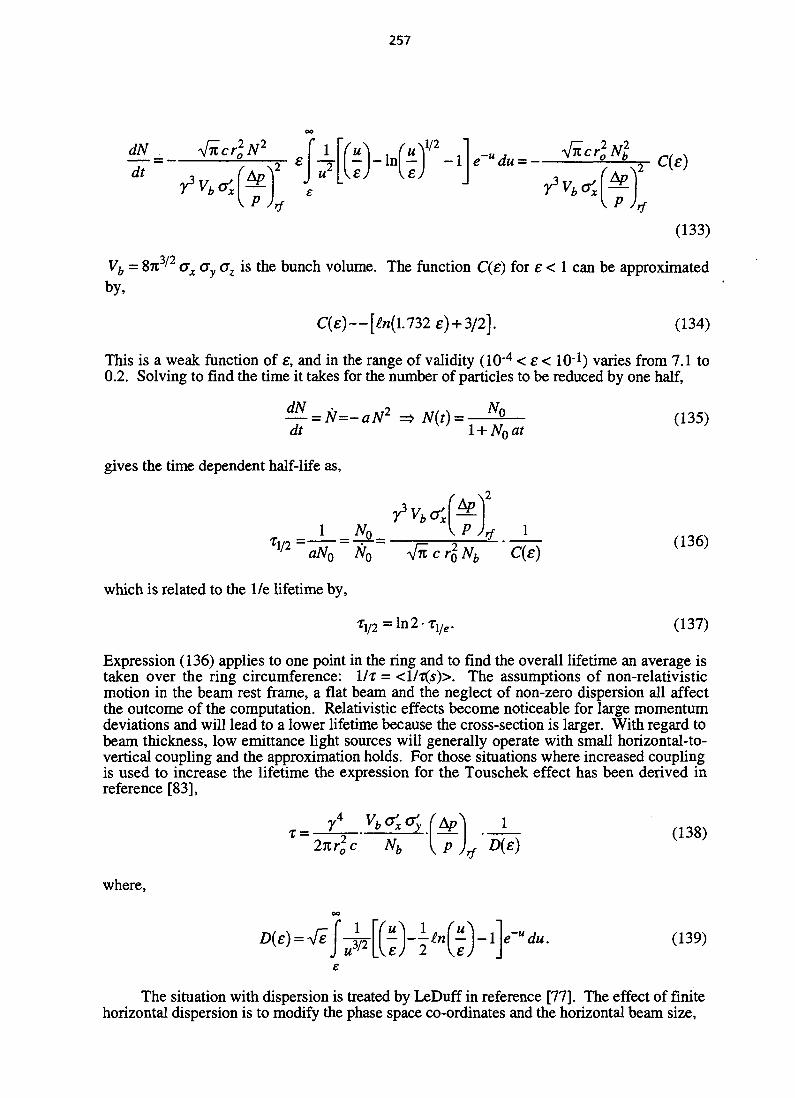
257

dN_

dt"-\-r4if-ie~udu = -

(133)

Vb = 8TT3/2 GX cy Gz is the bunch volume. The function C(e) for e < 1 can be approximatedby,

C(e)~-[£n(U32 e) + 3/2]. (134)

This is a weak function of s, and in the range of validity (1(H < e < 10"1) varies from 7.1 to0.2. Solving to find the time it takes for the number of particles to be reduced by one half,

^- = N=-aN2 =» N(t)= N°dt w l + Noat

(135)

gives the time dependent half-life as,

&p

Tin =-' " 2 aN0 N0

which is related to the 1/e lifetime by,

r02iVfc 'C(e)

(136)

(137)

Expression (136) applies to one point in the ring and to find the overall lifetime an average istaken over the ring circumference: 1/T = <1/T(S)>. The assumptions of non-relativisticmotion in the beam rest frame, a flat beam and the neglect of non-zero dispersion all affectthe outcome of the computation. Relativistic effects become noticeable for large momentumdeviations and will lead to a lower lifetime because the cross-section is larger. With regard tobeam thickness, low emittance light sources will generally operate with small horizontal-to-vertical coupling and the approximation holds. For those situations where increased couplingis used to increase the lifetime the expression for the Touschek effect has been derived inreference [83],

T =1

D(e)(138)

where,

m-\^-1ru du. (139)

The situation with dispersion is treated by LeDuff in reference [77]. The effect of finitehorizontal dispersion is to modify the phase space co-ordinates and the horizontal beam size,

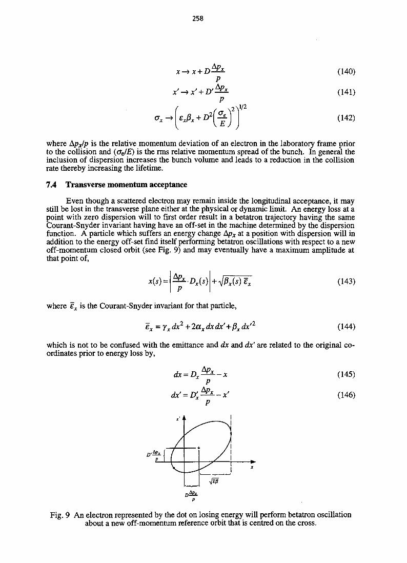
258

(140)

(141)

(142)

where Apx/p is the relative momentum deviation of an electron in the laboratory frame priorto the collision and (cJE) is the rms relative momentum spread of the bunch. In general theinclusion of dispersion increases the bunch volume and leads to a reduction in the collisionrate thereby increasing the lifetime.

7.4 Transverse momentum acceptance

Even though a scattered electron may remain inside the longitudinal acceptance, it maystill be lost in the transverse plane either at the physical or dynamic limit. An energy loss at apoint with zero dispersion will to first order result in a betatron trajectory having the sameCourant-Snyder invariant having have an off-set in the machine determined by the dispersionfunction. A particle which suffers an energy change Apx at a position with dispersion will inaddition to the energy off-set find itself performing betatron oscillations with respect to a newoff-momentum closed orbit (see Fig. 9) and may eventually have a maximum amplitude atthat point of,

•Dx(s)

where ex is the Courant-Snyder invariant for that particle,

ex =yxdx2+ 2axdxdx'+px dx'2

(143)

(144)

which is not to be confused with the emittance and dx and dx' are related to the original co-ordinates prior to energy loss by,

(145)

(146)

P

P

X '

/

^ -

/

1

/ I

Fig. 9 An electron represented by the dot on losing energy will perform betatron oscillationabout a new off-momentum reference orbit that is centred on the cross.

259

Consider a particle on the on-momentum closed orbit suffering an energy loss at aposition with dispersion Dj, fir and ccs= D'T= 0. Equating the Courant-Snyder invariant ofthat particle elsewhere in the ring (at position s with betatron value j3(s)) we can write themaximum deviation after a Touschek event from the reference orbit as,

(147)

The amplitude is greatly influenced by the optical functions. If the betatron function is smallat the point where the dispersion function is large the resulting betatron oscillation elsewherecan be very large [49].

7.5 Improving the Touschek lifetime

The energy dependence of the Touschek lifetime is very strong and several factorsaffect the lifetime: the bunch volume, the accelerating voltage, energy spread, beamdivergence, Lorentz contraction and intra-beam scattering (see later). The lifetime scalessomewhere between the third and fifth power of the energy. The Touschek effect is moresevere for low energy storage rings and is one of the limiting factors for the performance ofthese machines. Even high energy light sources are affected by the Touschek effect, forexample, the ESRF when operating in 16-bunch mode observe a strong decrease in lifetimeas the coupling is altered: 31 to 17 hours lifetime change at 90 mA when the coupling isvaried from 10 to 1.5% [67]

Methods to improve the Touschek lifetime at a fixed energy could work on improvingthe limiting momentum acceptance, longitudinal or transverse, or to decrease the probabilityof collision by decreasing the bunch density.

The simplest method to decrease the bunch density is to operate with many bunches.This is done by choosing a high radio-frequency. Present day third generation light sourcesoperate either at 350 or 500 MHz. The many bunches, though, will increase the difficulty incombating multi-bunch instabilities (see section 9) which are easier to control if few bunchesare present.

To increase the longitudinal acceptance one would need to increase the rf voltage,

(Ap} eVsin\j/s ^— = — 2 A/4 -1-arccos —

{pjj %hacE [s {q_eV_ 1

q~U0~siny/s'

With increasing rf voltage, however, the bunch length is also decreased,

' * " corev ^heVcosy,, U ' " " ' ^

The lifetime, nevertheless, increases faster with rf acceptance than it decreases with bunchlength. The effect is weak and the costs involved in providing additional rf power soonmakes this method unattractive. Recently proposals have been made to provide additional rfacceptance only for Touschek scattered particles with the use of a super-conducting cavity.The cavity operates at zero phase since there is no need to restore the energy lost due to the

260

emission of synchrotron radiation. The cavity is passive and is powered by the circulatingelectron beam [56].

[mil

Lif

etim

e

600

500

400

300

200

100

0(

1

\

"-"ope) 5

Single

1

1-CHJ10

Bunch

I

__

—

""" n ii

-n—in n15 20

Current (mA)

Fig. 10 Beam lifetime at 2 GeV (0.35% coupling) in ELETTRA as a function of single-bunchcurrent for two different if. voltages (circles 1.76 MV and squares 0.84 MV). The solid line

is the prediction taking into account bunch lengthening effects [79].

The lifetime is proportional to the bunch volume and the goal of high brightness lightsources is to minimise this quantity, which unfortunately will lower the Touschek lifetime. Acompromise may be found by adjusting the coupling. This, however, will affect the verticalbeam emittance with consequent reduction in the energy resolution of the emitted light.Alternatively the bunch density can be decreased by increasing the bunch length. This isdone by operating with a higher harmonic cavity that changes the slope of the acceleratingfield [84]. The cavity can be powered either by the circulating beam or by an external source.At ELETTRA another technique is adopted, a controlled residual longitudinal multi-bunchexcitation is allowed which dilutes the longitudinal bunch volume. The mechanism relies onthe synchrotron tune shift with amplitude to smear the phase space volume [85]. This methodto increase the Touschek lifetime compared to changing the emittance coupling results inmore intense and sharper line spectra from undulators, especially for the lower harmonics.

8. INTRA-BEAM SCATTERING [47,77,86-S8]

Intra-beam scattering deals with all those collisions which were ignored in deriving theTouschek effect. The many small angle collisions lead to a re-distribution of the six-dimension phase space distribution. In the centre-of-mass frame the transverse momentumspreads are larger than the longitudinal.

cms

The multiple collisions between particles will predominantly transfer momentum fromthe transverse plane to the longitudinal. We must, however, consider synchrotronoscillations. The Touschek effect showed that the transverse collision in the bunch frameresulted in a re-distribution of momenta. The transferred transverse momentum px is boostedto ypx- The longitudinal blow-up is compensated by the transverse collapse. The Touschekevent neglected transfer of momentum from the longitudinal plane to the transverse becauseof the larger transverse acceptance. Following S0rensen [80] we examine the emittance (at asymmetry point) prior to the collision of two electrons which have co-ordinates,

261

(149)

where the positive sign corresponds to one particle and the negative sign to the other. Theexcitation of betatron motion will result after a collision with full transfer of momentum to thelongitudinal plane at a position with dispersion. The new co-ordinates are,

=X± U JPX

(150)

If the original emittance of the particles was

the change in the sum of the emittances for the two particles after the collision is

(152)

Therefore if

(nv\2

(153)

we have simultaneous longitudinal and transverse growth since the beam can absorb anyamount of energy from the rf system. The full treatment of intrabeam scattering ismathematically rather complicated since it involves integration over 12 dimensions for twoparticles. The recipe for performing the computations will just be given and results quoted(see also [47]). Computation of the growth rate of the intra-beam effect given by the recipe ofPiwinski [87], is as follows

1) Transformation of the momenta of the two colliding particles to the centre-of-massframe.

2) Calculation of the change in momenta due to an elastic collision.3) Transformation of the momenta back to the laboratory frame.4) Relate the changes in momenta to changes in emittances.5) Average over the distribution of scattering angles using the small angle Moller cross-

section6) Average over the distribution of the particles within a bunch to get the growth time.

The derivation for a weak focusing machine yields the following condition

(154)

o denotes the average around the ring circumference ex and £y the transverse emittances andH is the longitudinal emittance given by,

262

H=t] + — with 77 = — the relative momentum and Q s the synchrotron frequency." s P

Below transition lift < ac the sum of the three positive invariants is limited, they onlyexchange energy. Above transition there is no equilibrium distribution and the invariants cangrow without bounds until radiation damping counteracts the effect. The growth times for thelongitudinal phase space momentum and bunch distributions are [97],

1Tp 2c2

p dt

1 1 deldt

dt

f\-,-,-y^^f(a,b,c)a a a) ara

(155)

with

A = • (156)

the particle bunch density. The function / is

- 0.577.. \l—^-dxpq

(157)

and

(158)

(159)

(160)

(161)

From the dependence on energy of factor A we see that the growth time diminishesrapidly with energy. Intra-beam scattering is only of importance at low energies where theemittance is low and high particle densities can arise. For light sources above 1.0 GeV itseffect rapidly diminishes with increasing energy. Finally in the presence of radiationdamping an equilibrium will exist since,

• radiation damping becomes stronger with increasing amplitudes• intra-beam scattering becomes weaker with increasing amplitudes

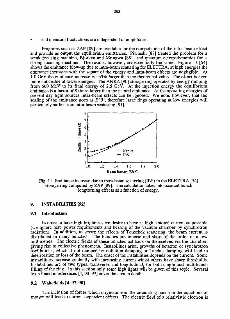
263

• and quantum fluctuations are independent of amplitudes.

Programs such as ZAP [89] are available for the computation of the intra-beam effectand provide as output the equilibrium emittances. Piwinski [87] treated the problem for aweak focusing machine, Bjorken and Mtingwa [88] used quantum electrodynamics for astrong focusing machine. The results, however, are essentially the same. Figure 11 [54]shows the emittance blow-up due to intra-beam scattering for ELETTRA, at high energies theemittance increases with the square of the energy and intra-beam effects are negligible. At1.0 GeV the emittance increase is -33% larger than the theoretical value. The effect is evenmore noticeable at lower energies. The ANKA [90] storage ring operates by energy rampingfrom 500 MeV to its final energy of 2.5 GeV. At the injection energy the equilibriumemittance is a factor of 8 times larger than the natural emittance. At the operating energies ofpresent day light sources intra-beam effects can be ignored. We note, however, that thescaling of the emittance goes as E2^, therefore large rings operating at low energies willparticularly suffer from intra-beam scattering [91].

1.2 1.4 1.6 1.8Beam Energy (GeV)

2.0

Fig. 11 Emittance increase due to intra-beam scattering (IBS) in the ELETTRA [54]storage ring computed by ZAP [89]. The calculation takes into account bunch

lengthening effects as a function of energy.

9. INSTABILITIES [92]

9.1 Introduction

In order to have high brightness we desire to have as high a stored current as possible(we ignore here power requirements and heating of the vacuum chamber by synchrotronradiation). In addition, to lessen the effects of Touschek scattering, the beam current isdistributed in many bunches. The bunches are intense and short of the order of a fewmillimetres. The electric fields of these bunches act back on themselves via the chamber,giving rise to collective phenomena. Instabilities arise, growths of betatron or synchrotronoscillations, which if not damped by radiation damping or Landau damping will lead todeterioration or loss of the beam. The onset of the instabilities depends on the current. Someinstabilities increase gradually with increasing current whilst others have sharp thresholds.Instabilities are of two types, transverse and longitudinal, for both single and multibunchfilling of the ring. In this section only some high lights will be given of this topic. Severaltexts found in references [4, 93-97] cover the area in depth.

9.2 Wakefields [4,97,98]

The inclusion of forces which originate from the circulating bunch in the equations ofmotion will lead to current dependent effects. The electric field of a relativistic electron is

264

contracted longitudinally into a disk perpendicular to the direction of motion. For a perfectlyconducting smooth chamber the field is perpendicular to the direction of motion and does notaffect trailing electrons. With finite resistivity the field lags the electron and affects otherelectrons, the leading electron loses energy. The trailing electric field is termed a wake field.Discontinuities along the vacuum chamber are also "good" sources for the production of wakefields and act by "scraping" away electric field lines. Bunch lengths are of the order of somemillimetres and small discontinuities along the chamber act like cavities, where the electronbunch can deposit energy. The trapped fields will have a decay time over which the energy isdissipated by heating the vacuum chamber. We can distinguish two regimes, broad- andnarrow-band parasitic losses. In the first case the wake field decays quickly, with a time scaleof less than one turn. These fields are produced by small discontinuities:

bellowsvacuum chamber transitions (insertion devices)vacuum portsbeam position monitorsstrip linesfluorescent screensflangesinjection elements

The fields affect electrons in the same bunch leading to single-bunch instabilities, i.e.electrons at the head of the bunch act on the tail.

In the second regime, the narrow-band parasitic losses, wake fields are generated whichremain for a long time in the chamber that act back on the same bunch or another for manyturns. The fields are produced in cavity-like objects and the most notable object of this sort ina storage ring is a radio frequency cavity. The cavity can be excited by the beam whichdeposits energy in the higher order modes (HOM's). The interaction of the beam with thesemodes results then in the excitation of multibunch instabilities.

The wake function of a single electron is defined to be the distance-integrated force feltby a trailing electron. The integration allows an averaging to be performed and absorbs thedetails of the environment which is usually the situation for most cases of interest. The forcesdepend on the distribution of the electromagnetic fields generated by the leading electronwhich in turn depend on the geometry of the vacuum chamber. Writing the fields in terms ofan expansion in multipole components allows the integrated force or wake function to beexpressed in terms of these components. Similarly an arbitrary charge distribution will havemultipole components. In the longitudinal plane the lowest order multipole m = 0 ormonopole is usually the most important, whilst in the transverse plane the dipole, m = 1,component is of greatest interest. We note that a monopole transverse component cannotexist because of symmetry reasons. These lowest-order multipoles express effects related tothe displacements of the centre of gravity of the charge distribution. The higher-ordermultipoles reflect the effect of various charge distributions within the bunch. The wake fieldcan be used to define an impedance-induced voltage. For an electron distribution in thecentre of the chamber we can write the longitudinal voltage as,

Vn{z') = -jp(z)Wn(z'-z)dz (162)

with p the charge distribution. Using a Fourier transform the integral is deconvoluted to get,

(163)

where /(ft)) is the Fourier transform of the current (cp(z)) and Z(co) is the impedance infrequency space representing the Fourier transform of the Lorentz force caused by the wake

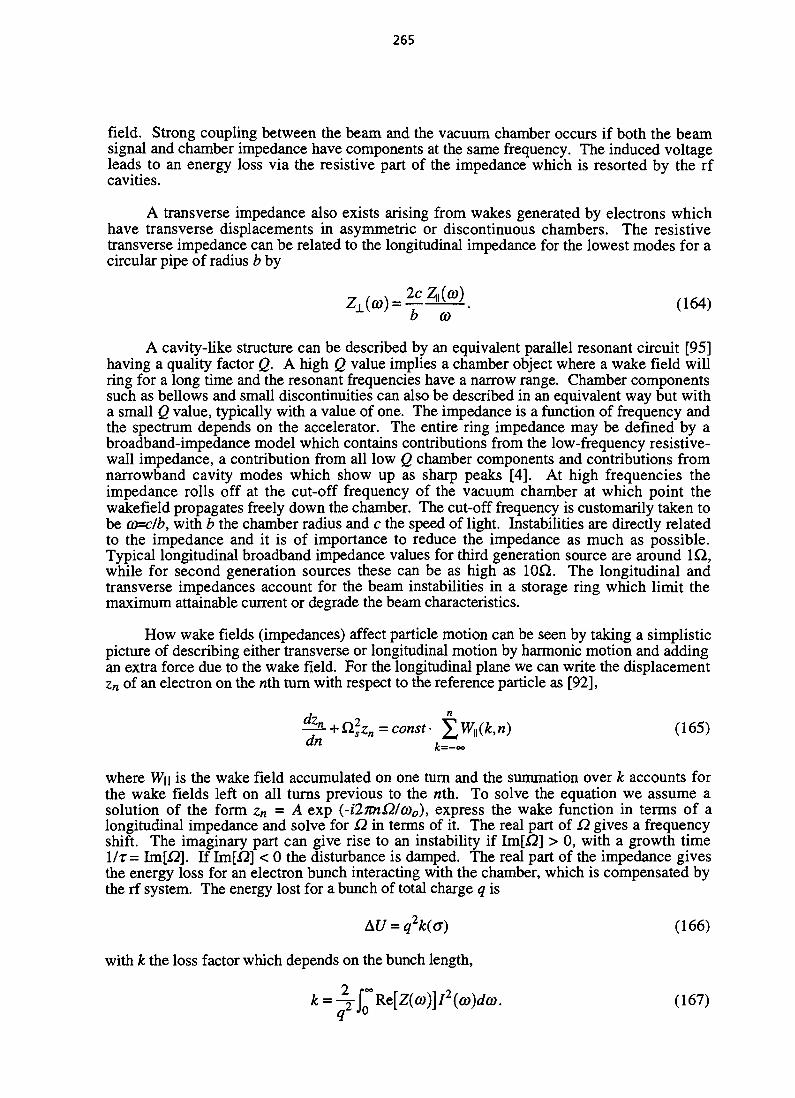
265

field. Strong coupling between the beam and the vacuum chamber occurs if both the beamsignal and chamber impedance have components at the same frequency. The induced voltageleads to an energy loss via the resistive part of the impedance which is resorted by the rfcavities.

A transverse impedance also exists arising from wakes generated by electrons whichhave transverse displacements in asymmetric or discontinuous chambers. The resistivetransverse impedance can be related to the longitudinal impedance for the lowest modes for acircular pipe of radius b by

2 £ 3 M (164)b co

A cavity-like structure can be described by an equivalent parallel resonant circuit [95]having a quality factor Q. A high Q value implies a chamber object where a wake field willring for a long time and the resonant frequencies have a narrow range. Chamber componentssuch as bellows and small discontinuities can also be described in an equivalent way but witha small Q value, typically with a value of one. The impedance is a function of frequency andthe spectrum depends on the accelerator. The entire ring impedance may be defined by abroadband-impedance model which contains contributions from the low-frequency resistive-wall impedance, a contribution from all low Q chamber components and contributions fromnarrowband cavity modes which show up as sharp peaks [4]. At high frequencies theimpedance rolls off at the cut-off frequency of the vacuum chamber at which point thewakefield propagates freely down the chamber. The cut-off frequency is customarily taken tobe (O=c/b, with b the chamber radius and c the speed of light. Instabilities are directly relatedto the impedance and it is of importance to reduce the impedance as much as possible.Typical longitudinal broadband impedance values for third generation source are around 1Q,while for second generation sources these can be as high as lOfl. The longitudinal andtransverse impedances account for the beam instabilities in a storage ring which limit themaximum attainable current or degrade the beam characteristics.

How wake fields (impedances) affect particle motion can be seen by taking a simplisticpicture of describing either transverse or longitudinal motion by harmonic motion and addingan extra force due to the wake field. For the longitudinal plane we can write the displacementzn of an electron on the nth turn with respect to the reference particle as [92],

^ a]zn= const- Y^ft«) (165)dn k=L

where W\\ is the wake field accumulated on one turn and the summation over k accounts forthe wake fields left on all turns previous to the nth. To solve the equation we assume asolution of the form zn = A exp {-HimOil(oo), express the wake function in terms of alongitudinal impedance and solve for Q in terms of it. The real part of Q gives a frequencyshift. The imaginary part can give rise to an instability if Im[i2] > 0, with a growth time1/T= Im[I2]. If Im[£2] < 0 the disturbance is damped. The real part of the impedance givesthe energy loss for an electron bunch interacting with the chamber, which is compensated bythe rf system. The energy lost for a bunch of total charge q is

= q2k((7) (166)

with k the loss factor which depends on the bunch length,

G>>to. (167)

266

9.3 Single-bunch instabilities

Single-bunch instabilities arise from the interaction of the bunch with wake fieldswhich are short, comparable to the bunch length. Broadband impedances will dominate inthis case where the effect of a passing bunch is lost before the arrival of a trailing bunch. Thewake fields generated by the low Q storage ring structures will affect particles within thesame bunch, that is, the leading electrons will interact with the trailing electrons. In certaincases synchrotron oscillations will then interchange the roles of the electrons giving rise to afeedback system.

The most notable single-bunch instability occurs in the longitudinal plane namely themicrowave instability or turbulent bunch lengthening. The wake field perturbs thelongitudinal bunch density leading to an increase in the bunch length and energy spread. Theinstability is fast and occurs before the head and tail electrons can interchange viasynchrotron oscillations. The bunch current threshold for the instability is,

'threshold ~ '\bb

IZ|/nlbb is the normalised longitudinal broadband impedance where n is the harmonic number,ac is the momentum compaction factor, az the bunch length, (oe/E) is the relative energyspread and R the average ring radius. The instability is self stabilising and growth stops whenthe current falls below the threshold and a new equilibrium is reached.

In the case of the transverse fast head-tail instability the leading electrons causetransverse wake fields which perturb the tail electrons. Synchrotron oscillations exchange thehead and tail electrons and weakens the effect, however, if the wake interaction is intenseenough an instability starts to grow before the completion of a synchrotron period. Thebunch current threshold is,

(169)

the denominator is the average transverse broadband impedance weighted by the betatronfunction. The value for the threshold is generally higher than the longitudinal turbulent bunchlengthening threshold. The fast head tail is the most limiting threshold and requires specialcare in keeping the broadband impedance low.

Another instability which is practically current independent is the head-tail instability.The mechanism is similar to the fast head-tail but involves in addition the betatron tunedependence with energy. This instability is avoided by operating with a slightly positivechromaticity (above transition), and is the main reason for having chromaticity correctingsextupoles in the storage ring. For present day machines single bunch currents in excess of20 mA can be stored albeit with increased bunch length and energy spread [1, 78, 99].Because of the single bunch instabilities and Touschek lifetime limitations, to achieve highcurrents and brightness (increased flux) many bunches are placed around the circumference.These multiple bunches, however, give rise to multibunch instabilities.

9.5 Multibunch instabilities

The beam generated wake fields that persist for a long time in the chamber will couplewith the circulating bunches and define a feedback system which may become unstable.Cavity like objects, especially the rf system, are receptacles for these wake fields via theirhigher order modes (HOM's). Interaction of the bunches with the wakefields induces centre-

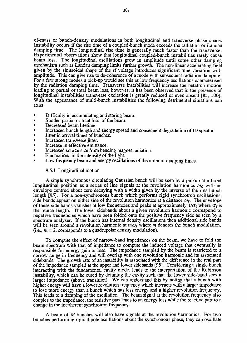
267

of-mass or bunch-density modulations in both longitudinal and transverse phase space.Instability occurs if the rise time of a coupled-bunch mode exceeds the radiation or Landaudamping time. The longitudinal rise time is generally much faster than the transverse.Experimental observations show that longitudinal coupled-bunch instabilities rarely causebeam loss. The longitudinal oscillations grow in amplitude until some other dampingmechanism such as Landau damping limits further growth. The non-linear accelerating fieldgiven by the sinusoidal shape of the rf voltage introduces significant tune variation withamplitude. This can give rise to de-coherence of a mode with subsequent radiation damping.For a few strong modes a pick-up would see this as low frequency oscillations characterisedby the radiation damping time. Transverse instabilities will increase the betatron motionleading to partial or total beam loss, however, it has been observed that in the presence oflongitudinal instabilities transverse excitation is greatly reduced or even absent [85, 100].With the appearance of multi-bunch instabilities the following detrimental situations canexist,

Difficulty in accumulating and storing beam.Sudden partial or total loss of the beam.Decreased beam lifetime.Increased bunch length and energy spread and consequent degradation of ID spectra.Jitter in arrival times of bunches.Increased transverse jitter.Increase in effective emittance.Increased source size from bending magnet radiation.Fluctuations in the intensity of the light.Low frequency beam and energy oscillations of the order of damping times.

9.5.1 Longitudinal motion

A single synchronous circulating Gaussian bunch will be seen by a pickup at a fixedlongitudinal position as a series of line signals at the revolution harmonics co0 with anenvelope centred about zero decaying with a width given by the inverse of the rms bunchlength [95]. For a non-synchronous bunch which performs rigid synchrotron oscillations,side bands appear on either side of the revolution harmonics at a distance cos. The envelopeof these side bands vanishes at low frequencies and peaks at approximately 1/<7T where <rT isthe bunch length. The lower sidebands about a given revolution harmonic correspond tonegative frequencies which have been folded onto the positive frequency side as seen by aspectrum analyser. If the bunch has internal density oscillations then additional side bandswill be seen around a revolution harmonic at m(Os where m denotes the bunch modulation,(i.e., m = 2, corresponds to a quadrupolar density modulation).

To compute the effect of narrow-band impedances on the beam, we have to fold thebeam spectrum with that of impedance to compute the induced voltage that eventually isresponsible for energy gain or loss. The impedance sampled by the beam is restricted to anarrow range in frequency and will overlap with one revolution harmonic and its associatedsidebands. The growth rate of an instability is associated with the difference in the real partof the impedance sampled at the upper and lower sidebands [95]. Considering a single bunchinteracting with the fundamental cavity mode, leads to the interpretation of the Robinsoninstability, which can be cured by detuning the cavity such that the lower side-band sees alarger impedance (above transition). We can understand this by noting that a bunch withhigher energy will have a lower revolution frequency which interacts with a larger impedanceto lose more energy than a bunch which has less energy and a higher revolution frequency.This leads to a damping of the oscillation. The beam signal at the revolution frequency alsocouples to the impedance, the resistive part leads to an energy loss while the reactive part to achange in the incoherent synchrotron frequency.

A beam of M bunches will also have signals at the revolution harmonics. For twobunches performing rigid dipole oscillations about the synchronous phase, they can oscillate

268

either in phase or TC out of phase, corresponding to two modes of oscillation. For fourbunches we have four oscillation modes corresponding to phase differences of 0, nil, n, 3nl2.M bunches will have M modes with phase differences of A<p = 2%nlM, n = 0,1,2,..,M-1.Observation at a single point in the ring will see frequencies at

- mfs (170)

where n labels the multibunch mode, / 0 is the revolution frequency, fs the synchrotronfrequency, m the bunch oscillation frequency (m = 1, dipole; m = 2, quadrupole) and/? aninteger (-«> to «>). With more than two bunches a given revolution harmonic (other than the rfharmonics) will have positive and negative side bands corresponding to different coupled-bunch modes [96].

As mentioned above the imaginary part of the complex frequency shift accounts for thegrowth of an instability. The general formula for the shift for mode n is,

11 AitQs{Ele)ntl

CO

°>PYwith

(171)

(172)

where I is the average circulating current. The summation gives the effective impedanceweighted by the beam spectrum. The growth rate for an instability is given by -Im(Ai2||) andis related to the real part of the impedance. For a single narrow-band impedance tuned atpMco0, for example a higher-order mode of an rf cavity, and a short bunch we may write [96],

(173)4xo)s{Ele)

where (Op±= (pM ±n± Qs)(oo. The expression shows that the upper (or positive) sidebandsare destabilising and the lower (negative) sidebands are stabilising. Figure 12 illustrates theexcitation of the possible 432 dipole modes in ELETTRA when the beam interacts with thecavity higher-order modes without compensation.

10.0

•<

se

1.0

0.1 i .1O O ~ H < $ - r ^ o m s o a cs <n oo — ^r - i \ o o o © f i * n r - o \ t s ^ \ o o \ - ^^H « —* N f»| N (S CSrt W W C l ^

Coupled Bunch Number

Fig. 12 Longitudinal dipole mode excitation by the cavity HOM's in ELETTRA beforecompensation. The figure shows the synchrotron oscillation amplitudes of the interaction

from which an estimate of the effective energy spread may be obtained [101].

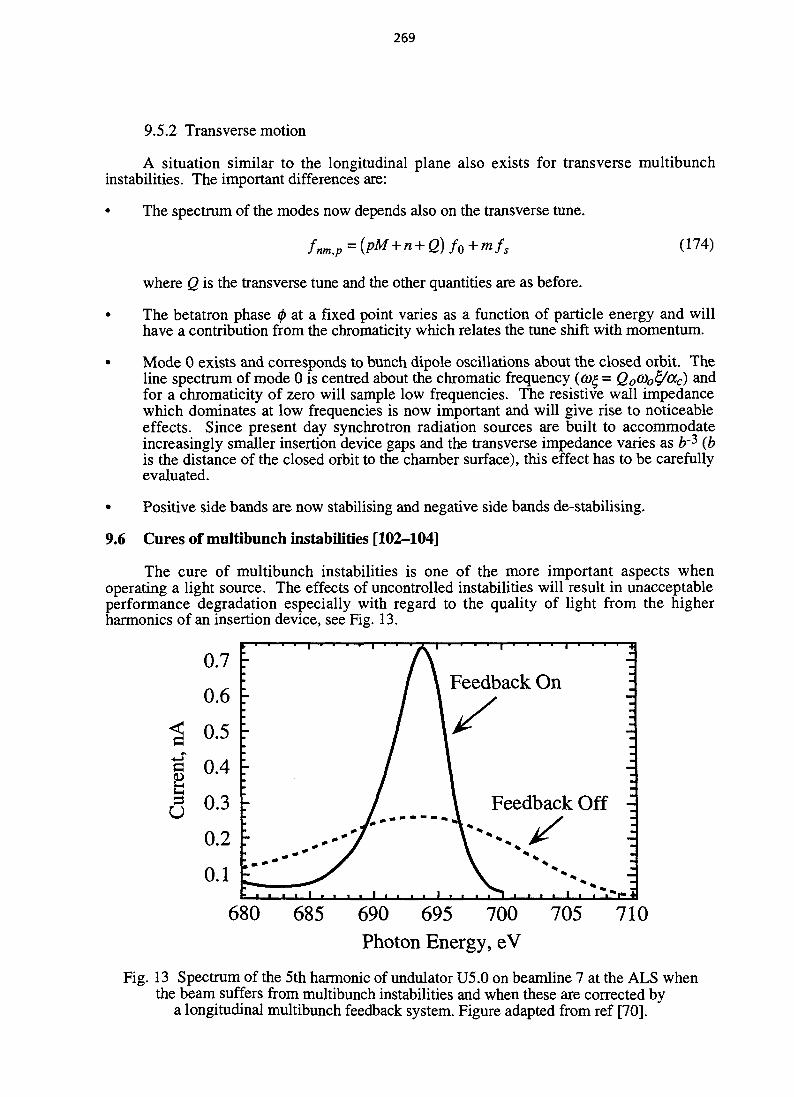
269

9.5.2 Transverse motion

A situation similar to the longitudinal plane also exists for transverse multibunchinstabilities. The important differences are:

The spectrum of the modes now depends also on the transverse tune.

(174)

where Q is the transverse tune and the other quantities are as before.

• The betatron phase (j> at a fixed point varies as a function of particle energy and willhave a contribution from the chromaticity which relates the tune shift with momentum.

• Mode 0 exists and corresponds to bunch dipole oscillations about the closed orbit. Theline spectrum of mode 0 is centred about the chromatic frequency (ay% = Qo0)o^0Cc) andfor a chromaticity of zero will sample low frequencies. The resistive wall impedancewhich dominates at low frequencies is now important and will give rise to noticeableeffects. Since present day synchrotron radiation sources are built to accommodateincreasingly smaller insertion device gaps and the transverse impedance varies as £'3 (bis the distance of the closed orbit to the chamber surface), this effect has to be carefullyevaluated.

• Positive side bands are now stabilising and negative side bands de-stabilising.

9.6 Cures of multibunch instabilities [102-104]

The cure of multibunch instabilities is one of the more important aspects whenoperating a light source. The effects of uncontrolled instabilities will result in unacceptableperformance degradation especially with regard to the quality of light from the higherharmonics of an insertion device, see Fig. 13.

IU

Feedback On

Feedback Off -_

680 685 690 695 700 705Photon Energy, eV

710

Fig. 13 Spectrum of the 5th harmonic of undulator U5.0 on beamline 7 at the ALS whenthe beam suffers from multibunch instabilities and when these are corrected by

a longitudinal multibunch feedback system. Figure adapted from ref [70].

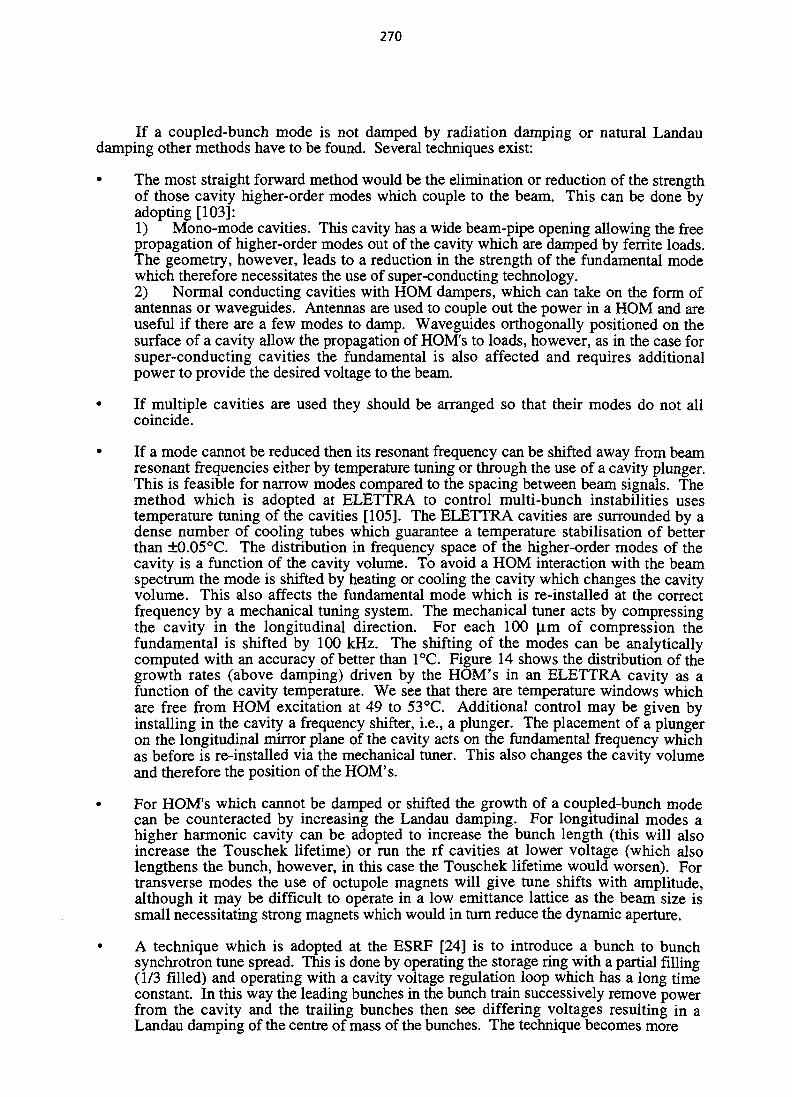
270

If a coupled-bunch mode is not damped by radiation damping or natural Landaudamping other methods have to be found. Several techniques exist:

• The most straight forward method would be the elimination or reduction of the strengthof those cavity higher-order modes which couple to the beam. This can be done byadopting [103]:1) Mono-mode cavities. This cavity has a wide beam-pipe opening allowing the freepropagation of higher-order modes out of the cavity which are damped by ferrite loads.The geometry, however, leads to a reduction in the strength of the fundamental modewhich therefore necessitates the use of super-conducting technology.2) Normal conducting cavities with HOM dampers, which can take on the form ofantennas or waveguides. Antennas are used to couple out the power in a HOM and areuseful if there are a few modes to damp. Waveguides orthogonally positioned on thesurface of a cavity allow the propagation of HOM's to loads, however, as in the case forsuper-conducting cavities the fundamental is also affected and requires additionalpower to provide the desired voltage to the beam.

• If multiple cavities are used they should be arranged so that their modes do not allcoincide.

• If a mode cannot be reduced then its resonant frequency can be shifted away from beamresonant frequencies either by temperature tuning or through the use of a cavity plunger.This is feasible for narrow modes compared to the spacing between beam signals. Themethod which is adopted at ELETTRA to control multi-bunch instabilities usestemperature tuning of the cavities [105]. The ELETTRA cavities are surrounded by adense number of cooling tubes which guarantee a temperature stabilisation of betterthan ±0.05°C. The distribution in frequency space of the higher-order modes of thecavity is a function of the cavity volume. To avoid a HOM interaction with the beamspectrum the mode is shifted by heating or cooling the cavity which changes the cavityvolume. This also affects the fundamental mode which is re-installed at the correctfrequency by a mechanical tuning system. The mechanical tuner acts by compressingthe cavity in the longitudinal direction. For each 100 p.m of compression thefundamental is shifted by 100 kHz. The shifting of the modes can be analyticallycomputed with an accuracy of better than 1°C. Figure 14 shows the distribution of thegrowth rates (above damping) driven by the HOM's in an ELETTRA cavity as afunction of the cavity temperature. We see that there are temperature windows whichare free from HOM excitation at 49 to 53 °C. Additional control may be given byinstalling in the cavity a frequency shifter, i.e., a plunger. The placement of a plungeron the longitudinal mirror plane of" the cavity acts on the fundamental frequency whichas before is re-installed via the mechanical tuner. This also changes the cavity volumeand therefore the position of the HOM's.

• For HOM's which cannot be damped or shifted the growth of a coupled-bunch modecan be counteracted by increasing the Landau damping. For longitudinal modes ahigher harmonic cavity can be adopted to increase the bunch length (this will alsoincrease the Touschek lifetime) or run the rf cavities at lower voltage (which alsolengthens the bunch, however, in this case the Touschek lifetime would worsen). Fortransverse modes the use of octupole magnets will give tune shifts with amplitude,although it may be difficult to operate in a low emittance lattice as the beam size issmall necessitating strong magnets which would in turn reduce the dynamic aperture.

• A technique which is adopted at the ESRF [24] is to introduce a bunch to bunchsynchrotron tune spread. This is done by operating the storage ring with a partial filling(1/3 filled) and operating with a cavity voltage regulation loop which has a long timeconstant. In this way the leading bunches in the bunch train successively remove powerfrom the cavity and the trailing bunches then see differing voltages resulting in aLandau damping of the centre of mass of the bunches. The technique becomes more

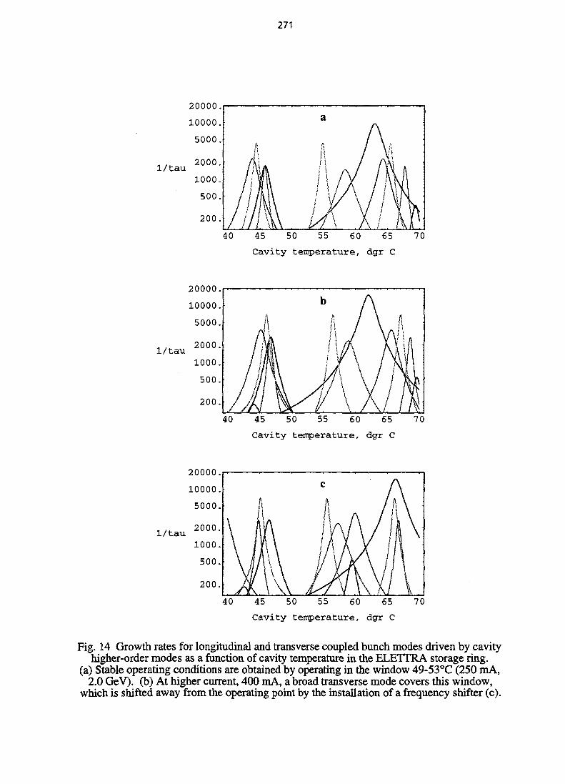
271

1/tau

200.

40 45 50 55 60 65 70

Cavity temperature, dgr C

1/tau

200.

40 45 50 55 60 65 70


1/tau

200.

45 50 55 60 65


70

Fig. 14 Growth rates for longitudinal and transverse coupled bunch modes driven by cavityhigher-order modes as a function of cavity temperature in the ELETTRA storage ring.

(a) Stable operating conditions are obtained by operating in the window 49-53°C (250 mA,2.0 GeV). (b) At higher current, 400 mA, a broad transverse mode covers this window,

which is shifted away from the operating point by the installation of a frequency shifter (c).

272

effective at higher currents, however, it works best on machines with a largecircumference. In a similar manner modulation of the rf voltage can be used.

• Longitudinal and transverse feedback [106-108]: With increasing current it becomesmore difficult to find stable operating windows via mechanical or temperature tuningsince the growth time for an instability is proportional to the current whereas dampingdue to radiation is a single particle effect. Storage rings with large circumferences arealso more problematic since the spacing of coupled bunch modes corresponds to therevolution frequency which is lower for the larger machines, making it more difficult tofind a stable temperature window. The most powerful technique is then to controlmulti-bunch instabilities by an active feedback system which damps all modes, both inthe longitudinal and transverse planes. The technique can be realised both in the timedomain (bunch by bunch) or in the frequency domain (mode feedback). In the timedomain each bunch is treated as a single oscillator. The system is made up of a detectorcapable of continuously measuring a single bunch, for each bunch a dedicated DigitalSignal Processor (DSP) is used for filtering the signal and computing the kick to beapplied which is phase shifted by 180° and finally a broadband power amplifier andkicker is required. The set-up requires state-of-art electronics and power amplifiers andcare in construction of the kicker. The ALS [107] has adopted this method to combatboth longitudinal and transverse multi-bunch instabilities successfully and can maintaina stable beam with 400 mA of stored current. A mode feedback system which works onselected modes could be envisaged for radio frequency systems utilising temperaturetuning since the number of modes to be damped will be small, however, withdiminishing costs for DSP's and associated electronics the broadband (bunch by bunch)approach may well be the most promising for future developments.

The full control of both longitudinal and transverse multi-bunch instabilities will resultin a bunch volume which is close to the theoretical value, i.e., dense bunches with no dilutionin either plane. The Touschek lifetime will consequently decrease as has been observed invarious laboratories. This necessitates frequent refills or the adoption of advanced techniquesto increase the Touschek lifetime by increasing both the transverse and longitudinalmomentum acceptance.

10. ION TRAPPING [109,110]

10.1 Introduction

The ionisation of the residual gas molecules in the vacuum chamber, either by directelectron-molecule interaction or via photo-electron emission will result in the production ofpositive ions. These ions may then become trapped in the potential well of the circulatingbeam. When trapping occurs two main points are observed: an increase of local gas pressureand the appearance of an electric field due to the ions. The increase in gas pressure leads toan increase in elastic scattering off the gas nuclei and beam-gas Bremsstrahlung (inelasticscattering), which cause beam blow-up, and loss of particles. The presence of the ion spacecharge leads to incoherent electron-beam tune shifts, electron-beam rune spreads and coherenteffects given by electron-ion cloud oscillations, which may lead to resonances and particleloss. The increase in tune spread, however, may be beneficial in combating instabilities viaLandau damping. Ion accumulation will depend on several factors: the number of circulatingelectron bunches, the bunch charge, the transverse size of the beam, the circumference of thestorage ring, the mass of the ion and external fields. Trapped ions can be cleared by leaving agap in the circulating bunch structure, by adopting clearing techniques such as clearingelectrodes or by avoiding trapping altogether by using positrons rather than electrons. Allsecond generation synchrotron radiation light sources have reported ion trapping whereas fewthird generation sources have clearly seen the effect [111, 112]. The reason for the lack oftrapping is not clear and is most probably associated with the low emittance and the lowcoupling of these new machines in addition to strong non-linear ion clearing (see below).

273

This has had a beneficial impact on the design of new light sources since a costly positronoption can be avoided.

In addition to the trapping of molecular/atomic ions, there is the possibility of trappingmacro-molecules [113]. Dust particles in the chamber can be slowly ionised by synchrotronradiation and are then attracted by the beam and destroyed. The passage of a macro moleculecan lead to sudden partial or total beam loss.

10.2 The trapping mechanism

No laboratory vacuum is perfect and gaseous molecules are present even after the mostcareful conditioning and treatment of the storage ring vacuum chamber. The molecularspecies found will depend on the past history of the chamber and the materials forming it.Exotic species (hydrocarbons etc..) can be excluded if the chamber has been treated properly.A chamber made of stainless steel, for example, may have the following gas species,molecular hydrogen, carbon monoxide and carbon dioxide which are initially contained in thesteel and desorbed into the vacuum, methane which may come from heating filaments ofcertain vacuum pumps and molecular nitrogen, oxygen and argon if leaks are present. Thecirculating electron bunches will ionise the residual gas species present in the chamber eitherby collision or photo-ionisation. The ions formed may then be trapped by the electron beam.The limit of trapping occurs when the entire beam is effectively neutralised by the ion-cloudwhich is formed. The time for this to occur is of the order of seconds. We define the averageneutralisation factor 77 [109] to be,

local ion denisty dj_^ ~ average electron density ~ de ( I ' 5 )

with

<,.4t = 4dfi. (,76)

where B is the bunching factor, B'1 gives the fraction of the ring circumference covered byelectrons. For a uniformly distributed electron beam with elliptical cross-section the local iondensity can be written as,

ecp 2KOxo(177)

xoy

With respect to the electron bunches an ion can be consider to be stationary. At eachpassage of a bunch an ion will feel a transverse impulsive kick towards the bunch centre andthen will drift freely between bunch traversals. The ions in this way may execute stableoscillations about the bunch centres. The electron bunches have three dimensional Gaussiandistributions travelling close to the speed of light. As they pass an ion they impart atransverse kick via the electric field. The ion's position is left unchanged and the givenimpulse is,

AT

M(AX= jeE±dt. (178)0

where AT is the bunch passing time and M/ the mass of the ion. To evaluate this kick weborrow results from the beam-beam problem [114, 115]. The instantaneous change in theion's transverse velocity is found to be

274

Ax\=NrRc 1 2KAy) An W x + iy

-exp2o2

x 2c)W

(179)

where N is the total number of stored electrons, n the number of bunches, rp the classicalproton radius, c the speed of light, A the atomic mass of the ion in units of the proton mass,and ox,y the transverse electron beam dimensions. The function W is the complex errorfunction. The impulse is a non-linear function of the ion's position with respect to the bunchcentre for distances greater than the bunch rms dimensions.

10.2.1 Linear theory

Most of the theory for ion trapping can be taken directly from the theory of betatronmotion in circular accelerators. Expecting the motion to be linear close to the bunch centrewe expand the complex error function and keep only linear terms,

(180)

The change in ion velocity is now expressed as,

2Nrpc(181)

The force is linear in the transverse co-ordinates and equivalent to a kick given by an electronbeam with uniform charge density and elliptical cross section. The motion is decoupled inthe two planes and we now consider only one plane. The effect of the bunch on the ion issimply

Xj = xt

X: = xt + Ax = xt + aXf(182)

with the indices i, j indicating before and after the passage of the bunch and the kickparameter a is given as,

2Nrpc

The result of the combination of kicks and drifts, with timessuccessive electron bunches can be written in matrix form,

ni.e.,

(183)

t,, between the passage of

(184)

X;-=MX,- (185)

275

The electron bunches have been considered as thin focusing lenses. The drift time of ions issimply, tb = One, with C the ring circumference. The matrix M defines the transport matrixfrom one bunch to the next. Floquet's theorem states that the motion is stable if [15],

ITrace(Mx)l< 2 (186)

Evaluating the above in terms of the ion mass allows the definition of a critical mass Ax>c, forwhich motion is stable if an ion has a mass greater than this, i.e., if A > AX)C then the ion istrapped. The critical mass is given as

NCr.

K =

A similar expression exists for the vertical plane. Since we generally have ax > oy thenAx>c < Ay>c and ions that perform stable oscillations in the horizontal plane may not be stablein the vertical plane. Flat beams are therefore preferable against the possibility of iontrapping, in other words weak coupling between horizontal and vertical electron motion. Ay>cis small and conditions are therefore good for trapping when the transverse beam dimensionsare large, when the beam current is low, when the ion charge state is small and when there isa large number of circulating electron bunches.

10.2.2 Effects of the ion charge cloud

The ion ladder [47]

As trapping proceeds the drift space between bunches becomes more like a thickdefocusing lens due to the trapped ions. This alters the condition for trapping which nowoccurs for ion masses that satisfy,

A>{l-v)AytC. (188)

Initially 77 is zero and the condition for trapping is as before, however, as trapping proceedsthe effective critical mass is reduced. At the same time there is an increase in the transversedimensions of the electron bunch due to gas scattering which also decreases Ay>c. Theseeffects lead to smaller ion masses being trapped, and this continues until the electron beam iscompletely neutralised. This process is called the ion ladder.

The tune shift [109]

The ion cloud which is formed is an additional force on the electrons that providesfocusing in both planes. Assuming the ion cloud has the same dimensions as the electronbunch, the tune shift induced by an additional "quadrupole" of strength k{s) is

(189)

where ft is the betatron function and AQ is given as,

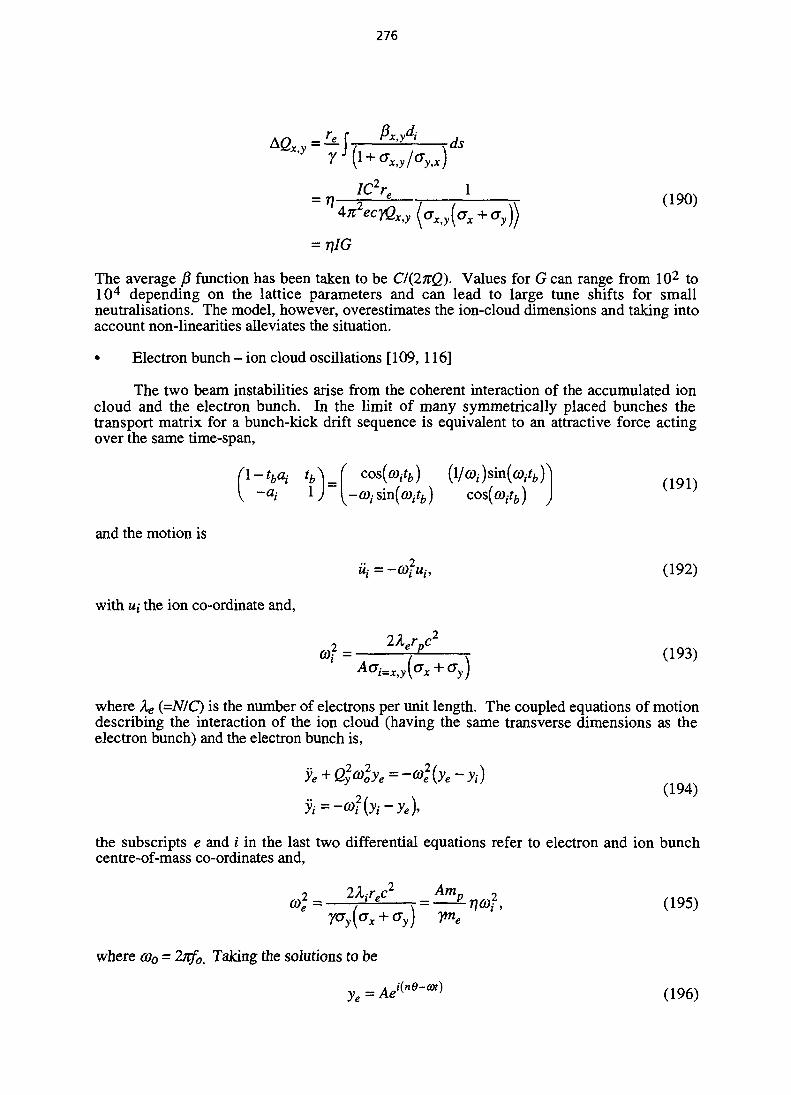
276

AQ = H

= 7}IG

The average /3 function has been taken to be CI{2KQ). Values for G can range from 102 to104 depending on the lattice parameters and can lead to large tune shifts for smallneutralisations. The model, however, overestimates the ion-cloud dimensions and taking intoaccount non-linearities alleviates the situation.

• Electron bunch - ion cloud oscillations [109,116]

The two beam instabilities arise from the coherent interaction of the accumulated ioncloud and the electron bunch. In the limit of many symmetrically placed bunches thetransport matrix for a bunch-kick drift sequence is equivalent to an attractive force actingover the same time-span,

~hai tb\_

and the motion is

«,•=-©?«,., (192)

with ui the ion co-ordinate and,

0,2 = LJL (193)

where Xe (=N/C) is the number of electrons per unit length. The coupled equations of motiondescribing the interaction of the ion cloud (having the same transverse dimensions as theelectron bunch) and the electron bunch is,

yi = -Q)f{yi-ye),

the subscripts e and i in the last two differential equations refer to electron and ion bunchcentre-of-mass co-ordinates and,

2 (195)

where coo = 2nfo. Taking the solutions to be

277

and

yi = Be"«, (197)

inserting in the differential equations and eliminating A and B gives the following dispersionrelation for co,

(198)

with Vt>e = (0iiel(0o and x = (0lcoo . The roots of this equation determine the stability ofmotion. If the roots are complex the motion of the system grows exponentially, until the ionsare lost and the electron beam damps down to its equilibrium value whereupon the processstarts again. Given the non-uniform distribution of ions in the ring, the phenomena may giverise to beating and low frequency beam oscillations.

10.2.3 Asymmetric bunch filling [117]

We now consider ion motion when there is asymmetric bunch filling of the ring, i.e., agap is left in the bunch train. The transport matrix for one complete revolution is requiredbecause of symmetry breaking. The one turn matrix M is given by

M = t»t~n)(199)

where h is the harmonic number and n the number of bunches. Analytical evaluation of thetrace is difficult, but easily done numerically. The critical mass is no longer applicable butstable mass bands are now found. The ion ladder is disrupted, since ions that become trappedin a mass band perturb the beam dimensions, decrease the beam current and introduce spacecharge, all of which changes M and hence shifts the mass bands to new patterns. We notethat the ions are not lost because there is more drift space, but because the focusing structurehas imperfections, which in turn introduce resonance behaviour. The ions are overfocused.Figure 15 shows an example of stable mass bands as a function of gap.

75

# 5 0

O 25

0,,,,,,ill

II

0 10 20 30Ion Mass

40 50

Fig. 15 Prediction of linear theory for the trapping of ions in the ANKA [90] storage ring(400 mA, 2.5 GeV, 3% coupling at the position for maximum trapping).

10.2.4 Non-linear electron bunch deflections [118] and ion clearing

The above considerations are valid only for motion close to the bunch centre, but saysnothing about large ion amplitudes about the bunch centre. To do this we need to examinethe motion using the non-linear kick equation (179), which upon numerical integration shows,as expected that the amplitude and oscillation frequency of motion depend on the co-ordinates the ion had when it was created. Simulations show that ions which are predicted tobe stable using linear theory may be unstable or stable only close to the bunch centre when

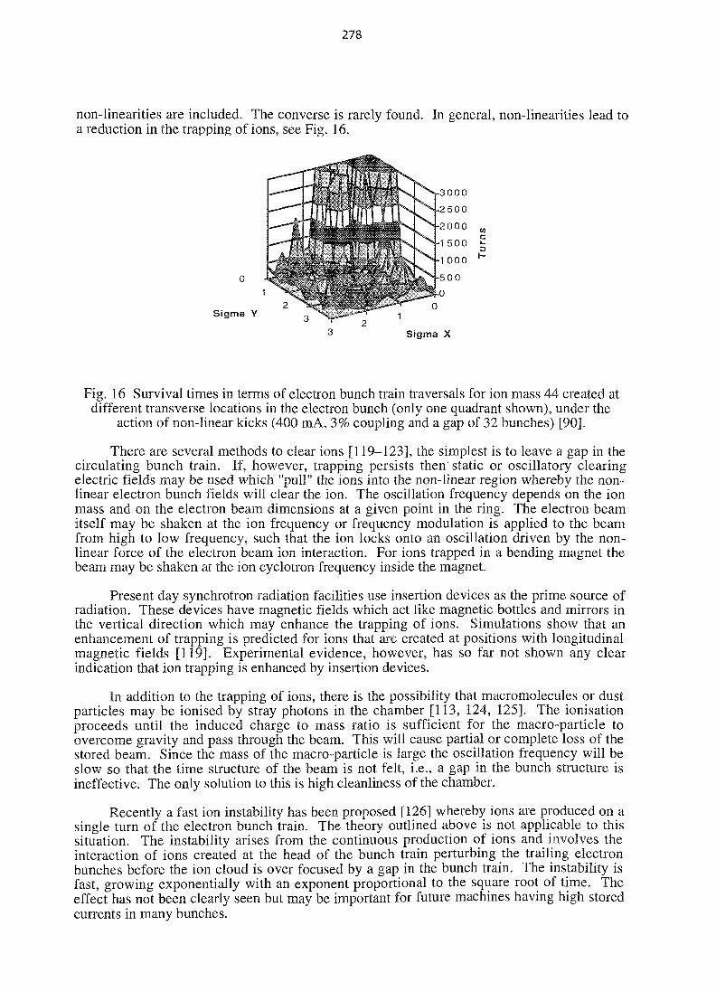
278

non-linearities are included. The converse is rarely found. In general, non-linearities lead toa reduction in the trapping of ions, see Fig. 16.

Sigma Y

mc

Sigma X

Fig. 16 Survival times in terms of electron bunch train traversals for ion mass 44 created atdifferent transverse locations in the electron bunch (only one quadrant shown), under the

action of non-linear kicks (400 mA, 3% coupling and a gap of 32 bunches) [90].

There are several methods to clear ions [119-123], the simplest is to leave a gap in thecirculating bunch train. If, however, trapping persists then' static or oscillatory clearingelectric fields may be used which "pull" the ions into the non-linear region whereby the non-linear electron bunch fields will clear the ion. The oscillation frequency depends on the ionmass and on the electron beam dimensions at a given point in the ring. The electron beamitself may be shaken at the ion frequency or frequency modulation is applied to the beamfrom high to low frequency, such that the ion locks onto an oscillation driven by the non-linear force of the electron beam ion interaction. For ions trapped in a bending magnet thebeam may be shaken at the ion cyclotron frequency inside the magnet.

Present day synchrotron radiation facilities use insertion devices as the prime source ofradiation. These devices have magnetic fields which act like magnetic bottles and mirrors inthe vertical direction which may enhance the trapping of ions. Simulations show that anenhancement of trapping is predicted for ions that are created at positions with longitudinalmagnetic fields [119]. Experimental evidence, however, has so far not shown any clearindication that ion trapping is enhanced by insertion devices.

In addition to the trapping of ions, there is the possibility that macromolecules or dustparticles may be ionised by stray photons in the chamber [113, 124, 125]. The ionisationproceeds until the induced charge to mass ratio is sufficient for the macro-particle toovercome gravity and pass through the beam. This will cause partial or complete loss of thestored beam. Since the mass of the macro-particle is large the oscillation frequency will beslow so that the time structure of the beam is not felt, i.e., a gap in the bunch structure isineffective. The only solution to this is high cleanliness of the chamber.

Recently a fast ion instability has been proposed [126] whereby ions are produced on asingle turn of the electron bunch train. The theory outlined above is not applicable to thissituation. The instability arises from the continuous production of ions and involves theinteraction of ions created at the head of the bunch train perturbing the trailing electronbunches before the ion cloud is over focused by a gap in the bunch train. The instability isfast, growing exponentially with an exponent proportional to the square root of time. Theeffect has not been clearly seen but may be important for future machines having high storedcurrents in many bunches.

279

ACKNOWLEDGEMENTS

The author is grateful to Albin Wrulich for reading the article and making manyvaluable suggestions for its improvement and clarity.

REFERENCES

[I] H. Winick, in Synchrotron Radiation Sources - A primer, Ed., H. Winick, WorldScientific (1994), 1.H. Zyngier, "European Synchrotron Radiation Storage Rings", IEEE Proc. Part. Accel.Conf, Dallas, (1995), 155.G. Decker, "Synchrotron Radiation Facilities in the USA", 5th. European ParticleAccelerator Conf., Sitges, (1996), 90.L. Rivkin, "Review of Future European Synchrotron Radiation Projects", 5th. EuropeanParticle Accelerator Conf., Sitges, (1996), 85.

[2] M. Cornacchia, "Requirements and Limitations on Beam Quality in SynchrotronRadiation Sources", CERN 90-03, (1990), 53.P.C. Marin, "The State of the Art Synchrotron Radiation Light Source", CERN 90-03,(1990), 459.H. Wiedemann, "Design of Low Emittance Storage Rings", Nucl. Instr. and Methods,A246, (1986), 4.

[3] A. Ropert, "Lattices and Emittance", These Proceedings.

[4] V. Suller, "Introduction to Current and Brightness Limits", These ProceedingsS. Myers, "Current Limitations", These Proceedings

[5] Proc. 2nd Annual Workshop on European Synchrotron Light Sources, ESRF, (1994).

[6] L. Farvacque, "SR-Related Accelerator Physics Issues", 5th. European ParticleAccelerator Conf., Sitges, (1996), 81.

[7] K. Wille, "Introductions to Insertion Devices", These Proceedings.

[8] R. P. Walker, "Wigglers and Undulators", These Proceedings.

[9] E. Gluskin and E. R. Moog, "Recent Advances in Insertion Devices", IEEE Proc. Part.Accel. Conf, Dallas, (1995), 1301.J. Chavanne, et al., "Recent Advances in Insertion Devices", 5th. European ParticleAccelerator Conf., Sitges, (1996), 220.

[10] L. Farvacque, "Beam Stability", These Proceedings.

[II] P. Quinn, "Practical Aspects of Beam Stability", These Proceedings.

[12] K. Kim, "Characteristics of Synchrotron Radiation", Physics of Particle Accelerators,Eds. M. Month and M. Dienes, AIP Conf. Proc., NY, 184, (1989), 565.

[13] S.L. Hulbert and J.M. Weber, "Flux and Brightness Calculations for VariousSynchrotron Radiation Sources", Nucl. Instr. and Methods, A319, (1992), 25.

[14] W.B. Peatman, "Some Notes on the Designs of Beamlines for Soft X-ray SynchrotronRadiation in Sources of the 3rd Generation", Third School on the Use of SynchrotronRadiation in Science and Technology, International Centre for Theoretical Physics,Trieste, (1995), H4.SMR/877-2

280

[15] L. Rivkin, "Introduction to Dynamics of Electrons in Rings", These Proceedings

[16] A. Hofmann, "Introduction to the Physics of Synchrotron Radiation", TheseProceedings.

[17] A. Hofmann, "Physical Phenomena used in Beam Observation", Frontiers in ParticlePhysics, Springer Verlag, Proc. Anacapri, Italy, (1988), Eds., M. Month and S. Turner,Lecture Notes in Physics, 343, (1989), 367.

[18] S. Krinsky, et al., "Characteristics of Synchrotron Radiation and its Sources",Handbook on Synchrotron Radiation, Eds., D.E. Eastman and Y. Farge, North-HollandPublishing Co., Amsterdam, (1983), 65.

[19] R.P. Walker, "Wigglers", CERN 95-06 Vol II, (1995), 807.

[20] L. Farvacque, et al., "Possible Retuning of the ESRF Storage Ring Lattice for Reducingthe Beam Emittance", Proc 4th. European Particle Accelerator Conf., Sitges, (1996),612.H. Tanaka and A. Ando, "Minimum Effective Emittance in Synchrotron RadiationSources composed of modified Chasman Green Lattice", Nucl. Inst. and Methods,A369 (1996), 312.R. Nagaoka, "Operation of ELETTRA with a lower Emittance Optics", Proc. 5th.European Particle Accelerator Conf., Sitges, (1996), 986.

[21] H. Wiedemann, "Particle Accelerator Physics I", Springer Verlag, Berlin, 1993 and"Particle Accelerator Physics II", Springer Verlag, Berlin, 1995.

[22] H. Maezawa, et al., "Spectral Characterisation of Undulator Radiation in the Soft X-rayRegion", Appl. Optics, 25, (1986), 3260.

[23] S. Chattopadhyay, "Stability of High-Brilliance Synchrotron Radiation Sources", Nucl.Instr. and Methods, A291, (1990), 455.

[24] G. Miilhaupt, "Beam Stability in the Third Generation SR Sources", Rev. Sci. Instrum.,66, (1995), 2000.G. Mulhaupt, "Hardware Limitations on Storage Ring Sources", CERN 90-03, (1990),98.

[25] R. Hettel, "Review of Synchrotron Beam Stability and Stabilizing Systems", Rev. Sci.Instrum., 60 (1989), 1501.

[26] C.J. Bocchetta, "Operational Experience with ELETTRA", Proc. 5th. European ParticleAccelerator Conf., Sitges, (1996), 76.

[27] T. Katsura et al., "Diurnal Deviation of the Orbit Circumference due to BuildingDistortion", Rev. Sci. Instrum., 63, (1992), 530.

[28] J. Rossbach, "HERA Errors and Related Experience During Commissioning",Advanced Beam Dynamics Workshop on Effects of Errors in Accelerators, theirDiagnosis and Corrections, Ed. A. Chao, AEP Conf. Proc., 255, (1992), 36.

[29] E.D. Johnson, et al., "Correlation of Photon Beam Motion with Vacuum ChamberCooling on the NSLS X-ray Ring", Rev. Sci. Instrum., 63, (1992), 513.

[30] L. Zhang, "Vibration at the ESRF", Proc. 5th. European Particle Accelerator Conf.,Sitges, (1996), 1359.

281

[31] V. Shiltsev, "Measurements of Ground Motion and Magnet Vibrations at the APS",APS Light Source Design Note, LS-241.

[32] C.J. Bocchetta and A. Wrulich, "Effects of Ground Vibrations", Sincrotrone Trieste,ST/M-88/23, (1988).

[33] J. Safranek and S. Krinsky, "Coupling Correction Using Closed Orbit Measurements",Orbit Correction in Circular Accelerators, Eds. E. Bozoki, et al., AIP Conf. Proa, 315,(1994), 163.

[34] R. Nagaoka, "Coupling and Dispersion Correction in ELETTRA", Proc. 5th. EuropeanParticle Accelerator Conf., Sitges, (1996), 980.

[35] E. Bozoki, "Closed Orbit Related Problems: Correction, Feedback and Analysis", OrbitCorrection in Circular Accelerators, Eds. E. Bozoki, et al., AIP Conf. Proa, 315,(1994), 3.

[36] J.-P. Koutchouk, "Trajectory and Closed Orbit Correction", Frontiers of Particle Beams,Springer Verlag, Proc. Anacapri, Italy, (1988), Eds., M. Month and S. Turner, LectureNotes in Physics, 343, (1989), 46.

[37] E. Wilson, "Transverse Beam Dynamics", CERN 94-01, Vol I, (1994), 131.

[38] E.D. Johnson et al., Rev. Sci. Instrum. 60, (1989), 1947

[39] ESRF Workshop on X-ray Position Monitors, Grenoble, Nov., 1993.

[40] T. Warwick, et al., "Performance of Photon Monitors and Stability of Undulator Beamsat the Advanced Light Source", Rev. Sci. Instrum., 66, (1995), 1984.

[41] W. Brefeld, "Stabilization of Synchrotron Radiation Beam at HASYLAB", Rev. Sci.Instrum., 60, (1989), 1513.E. Bozoki, et al., "Operations with the Digital Orbit Feedback System in the NSLS X-ray Ring", Proc. 5th. European Particle Accelerator Conf., Sitges, (1996), 1911.

[42] E. Plouviez and F. Uberto, "A Fast Local Feedback System to Correct the BeamPosition Deviation in the ESRF Storage Ring", Proa 5th. European Particle AcceleratorConf., Sitges, (1996), 1872.

[43] C.H. Kou, et al., "First Experiments of the Digital Global Feedback in SRRC", Proc.5th. European Particle Accelerator Conf., Sitges, (1996), 1923.

[44] G. Comelli, et al., "Real-time X-ray photoelectron spectroscopy study of dissociativeoxygen adsorption on Rh(llO)", Chem. Phys. Lett. 261, (1996), 253.

[45] RJ . Nawrocky, et al., "Automatic Steering of X-ray Beams from NSLS InsertionDevices", IEEE Proc. Particle Accelerator Conf., Chicago, (1989), 1856.

[46] C.J. Bocchetta and A. Wrulich, "Local Orbit Feedback Systems Coupled by TransferFunction Errors", Nucl. Instr. and Methods, A300, (1991), 223.

[47] A. Wrulich, "Single-Beam Lifetime", CERN 94-01, Vol I, (1994), 409.

[48] M. Cornacchia, "Lattices", Synchrotron Radiation Sources - A primer, Ed., H. Winick,World Scientific (1994), 30.

282

[49] H. Wiedemann, "Storage Ring Optimisation", Handbook on Synchrotron Radiation,Vol. 3, Eds., G. Brown and D.E. Moncton, Elsevier Science Publishers, (1991), 1.

[50] Second Advanced ICFA Beam Dynamics Workshop, Eds., J. Hagel and E. Keil, CERN88-04, (1988).

[51] A. Ropert, "Dynamic Aperture", CERN 90-04, (1990), 26.

[52] L. Smith, "Effects of Wigglers and Undulators on Beam Dynamics", ESG TECH NOTE24, Sept. (1986).

[53] F. Iazzourene, et al., "Racetrack User's Guide - Version 4.01", Sincrotrone Trieste,ST/M-92/7, (1992).H. Wiedemann, "PATRICIA. Particle Tracking in Circular Accelerators", SLAC ReportPEP-220 (1976).

[54] ELETTRA Conceptual Design Report, Sincrotrone Trieste, (1989).

[55] J. LeDuff, "Longitudinal Beam Dynamics in Circular Accelerators", CERN 94-01, VolI, (1994), 289.

[56] Proc. 4th Annual Workshop on European Synchrotron Light Sources, SincrotroneTrieste, (1996).

[57] G. Mulhaupt, "Injector Systems", Synchrotron Radiation Sources - A primer, Ed., H.Winick, World Scientific (1994), 59.

[58] G.H. Rees, "Injection", CERN 94-01, Vol H, (1994), 731.

[59] J. LeDuff," Current and Density Limitations in Existing Storage Rings", Nucl. Inst. andMethods, A239, (1985), 83.

[60] J.D. Jackson, "Classical Electrodynamics", John Wiley and Sons, New York, 1975

[61] P. H. Kung, "The Bremsstrahlung Lifetime in a Storage Ring", SSRL ACD-Note 88,1990.

[62] W. Heitler, "Quantum Theory of Radiation", Third Edition, Oxford University Press,1954.

[63] Projet SOLEJL, etude technique, LURE, January 1994.

[64] B. Simon and P. Kuske, "The Dynamic Aperture of BESSY", CERN-88-04, (1988),120.

[65] L. Tosi, et al, "Optics and Transverse Beam Dynamics in ELETTRA", Proc. 4th.European Particle Accelerator Conf., London, (1994), 1006.

[66] J.A. Clarke and H.L. Owen, "Operation of the Daresbury Synchrotron Radiation Sourcewith Reduced Vertical Aperture", Proc. 5th. European Particle Accelerator Conf.,Sitges, (1996), 620.

[67] A. Ropert, ESRF, Private communication.

[68] A.G. Mathewson, "Vacuum System Design", CERN 94-01, (1994), 717.

283

[69] N.B. Mistry, "Ultrahigh Vacuum Systems for Storage Rings and Accelerators", Physicsof Particle Accelerators, Eds., M. Month and M. Dienes, AIP Conf. Proc. 153, (1987),1443.

[70] A. Jackson, "Operational Experience with Multi-Bunch Feedback at the AdvancedLight Source", Proc. 5th. European Particle Accelerator Conf., Sitges, (1996), 661.

[71] M. Sands, "The Physics of Electron Storage Rings - An Introduction", SLAC Report121 (1970).

[72] R.P. Walker, "Radiation Damping", CERN 94-01, (1994), 461 and "QuantumExcitation and Equilibrium Beam Properties", CERN 94-01, (1994), 481.

[73] A. Piwinski, "Beam Losses and Lifetime", CERN 85-19, Vol II, (1985), 432.

[74] A. Chao, "Equations for Multiparticle Dynamics", Frontiers of Particle Beams, Eds.,M. Month and S. Turner, Lecture Notes in Physics, 296, Springer Verlag, (1988), 51.

[75] C. Bernardini et al., Phys. Rev. Lett., 10, (1963), 407

[76] H. Brack, "Accelerateurs Circulates de Particules", (Presses Universitaires de France,Paris, 1966.)

[77] J. LeDuff, "Single and Multiple Touschek Effects", CERN Accelerator School, CERN89-01,(1989), 114.

[78] C. Kim, et al., "Beam Lifetime and Beam Brightness in ALS", IEEE Proc. ParticleAccelerator Conference, Dallas, (1995), 198.

[79] E. Karantzoulis, et al., "Beam Lifetime Measurements in ELETTRA", Proc. 5th.European Particle Accelerator Conf., Sitges, (1996), 1105.

[80] A.H. S0rensen, "Introduction to Intrabeam Scattering", CERN Accelerator School,CERN 87-10, (1987), 135.

[81] R.P. Walker, IEEE Proc. Particle Ace. Conf. Washington D.C., (1987), 491.

[82] S. Khan, "Simulation of the Touschek Effect for BESSY II - A Monte Carlo Approach",Proc. 4th. European Particle Accelerator Conf., London, (1994), 1192.

[83] Y. Miyahara, IEEE Trans. Nucl. ScL, 32, (1985), 3821.

[84] R. Biscardi, et al., "Bunch Length Control in the NSLS VUV ring", Nucl. Inst. andMethods, A366, (1995), 26.

[85] A. Wrulich, et al., "Observation of Coupled Bunch Instabilities in ELETTRA", Proc.5th. European Particle Accelerator Conf., Sitges, (1996), 1108.

[86] H. Brack and J. LeDuff, "Beam Enlargement in Storage Rings by Multiple CoulombScattering", Proc 5th. Int. Conf. on High Energy Accel., Frascati, 1965.

[87] A. Piwinski, "Intra-Beam Scattering", Frontiers of Particle Beams, Eds., M. Month andS. Turner, Lecture Notes in Physics, 296, Springer Verlag, (1988), 297.A. Piwinski, CERN Accelerator School, CERN 85-19, (1985), 451.

[88] J.D. Bjorken and S.K. Mtingwa, Particle Accelerators, 13, (1983), 115.

284

[89] M. Zisman, et al., "ZAP Users Manual", LBL-21270 (1986)

[90] ANKA, "Synchrotronlichtquelle fur Mikrofertigung und Analytik", Conceptual DesignReport (1995).

[91] S. Kamada and K. Ohmi, "Low Emittance Lattice for the TRISTAN Light Source",Workshop on Fourth Generation Light Sources, Eds., M. Cornacchia and H. Winick,Stanford Synchrotron Radiation Laboratory, SSRL-92/02, (1992), 106.L. Farvacque, et al., "Probing some of the Issues of Fourth Generation Light Sources atthe ESRF", Proc. 5th. European Particle Accelerator Conf., Sitges, (1996), 632.

[92] A. Chao, Physics of Collective Beam Instabilities in High Energy Accelerators,(J. Wiley and Sons, New York, 1993).

[93] B. Zotter and F. Sacherer, "Theoretical Aspects of the Behaviour of Beams inAccelerators and Storage rings", CERN 77-13, (1977), 175.

[94] J.L. Laclare, "Bunched Beam Coherent Instabilities", CERN 87-03, (1987), 264.

[95] A. Hofmann, "Beam Instabilities", CERN 95-06 (1995), 307.

[96] F. Pedersen, "Multibunch Instabilities" Proc. Joint US-CERN School on ParticleAccelerators, Benalmadena, Spain, Oct. 1992, Eds., M. Dienes, M. Month, B. Strasserand S. Turner, Springer-Verlag LNP 425, (1992), 269.

[97] M. Furman et al., "Beam Instabilities" Synchrotron Radiation Sources - A primer, Ed.,H. Winick, World Scientific, (1994), 306.

[98] A. Hofmann, "Impedance Measurements, Computations and their Interpretation", FifthEuropean Particle Accelerator Conference, Sitges (1996), 143.

[99] C.J. Bocchetta, et al., "One and a Half Years Experience with the Operation of theSynchrotron Light Source ELETTRA", IEEE Proc. Particle Accelerator Conf., Dallas,(1995), 309.A. Ropert, et al., "Accelerator Physics Trends at the ESRF", IEEE Proc. ParticleAccelerator Conf., Dallas, (1995), 167.

[100] J.M. Byrd, et al., "Observation of Collective Effects at the Advanced Light Source",(1995),LBL-37819.

[101] Courtesy of M. Svandrlik, Sincrotrone Trieste.

[102] M. Serio. et al., "Multibunch Instabilities and Cures", Proc. 5th European ParticleAccelerator Conference, Sitges, (1996), 148.

[103] R. Boni, "HOM-Free Cavities", Proc. 5th European Particle Accelerator Conference,Sitges, (1996), 182.

[104] F. Pedersen, "Feedback Systems", CERN PS/90-49 (AR), (1990).

[105] M. Svandrlik, et al., "Improved Methods of Measuring and Curing MultibunchInstabilities in ELETTRA", Proc. 5th European Particle Accelerator Conference,Sitges, (1996), 1144.

[106] G. Oxoby, et al., "Bunch-by-Bunch Longitudinal Feedback System for PEP-IT, Proc.4th European Particle Accelerator Conference, London, (1994), 1616.

285

[107] W. Barry, et al., "Commissioning of the ALS Transverse Coupled-Bunch FeedbackSystem", IEEE Proc. Particle Accelerator Conference, Dallas, (1995), 2423.

[108] K.T. Hsu, "Performance of the Transverse Coupled-Bunch Feedback System in theSRRC", Proc. 5th European Particle Accelerator Conference, Sitges, (1996), 1920.

[109] Y. Baconnier, et al., "Neutralisation of Accelerator Beams by Ionisation of theResidual Gas", CERN 94-01, pp 525, 1994.

[110] R.D. Kohaupt, Interner Bericht, DESYH1-71/2, (1971).

[ I l l ] C.J. Bocchetta, et al., "Ion trapping investigations inElettra", Proc. 4th. EuropeanParticle Accelerator Conf., London, (1994), 1153. Note: Recent measurements whichhave been performed are less conclusive and the ion trapping observations made duringmachine commissioning may well be related to the higher vacuum pressure during thatperiod.

[112] J.C. Lee, et al., "The Study of the Trapped Ion Effects in the SRRC Storage Ring",Proc. 4th. European Particle Accelerator Conf., London, (1994), 1159.

[113] F. Zimmermann, et al., "Trapped Macroparticles in Electron Storage Rings", IEEEProc. Particle Accelerator Conf., Dallas, (1995), 517.

[114] M. Bassetti and G.A. Erskine, "Closed Expression for the Electrical Field of a twoDimensional Gaussian Bunch", CERN-ISR-TH/80-06 (1980).

[115] R.Talman, Cornell University, CLNS-84/610 (1984).

[116] Koshkarev, D. G. and Zenkevich, P.R., Particle Accelerators, 3, 1, (1972)Kamiya, Y., et al., "Vertical Instability Caused by Ion Trapping in KEK-PF StorageRing", Proc. 5th- Symp. Ace. Sci. Tech, (1985), 292.

[117] M.Q. Barton, Nucl. Instr. and Meth. A243, (1986), 278

[118] Y. Baconnier et al., Workshop on pp in the SPS, SPS-pp-1, (1980).D. Douglas, IEEE Trans. Nucl. Sci., NS-32, (1985), 2294.

[119] C.J. Bocchetta and A. Wrulich, Nucl. Inst. Methods, A278, (1989), 807.

[120] Kasuga, T., et al., "Ion Trapping Effect in UVSOR Storgae Ring", Jap. J. Appl. Phys.,24, (1985), 1212.

[121] Sugiyama, S., et al., Proc. 7th- Symp. Ace. Sci. Tech, 265, (1987)

[122] Zhou, P and Rosenzweig, J. B., IEEE Proc. Particle Accelerator Conference, SanFrancisco, (1991), 1776.

[123] Bozoki, E., and Kramer, S. L., "Ion Shaking in the 200 MeV XLS-Ring", Proc. 3rdEuropean Particle Accelerator Conference, Berlin, (1992), 789.

[124] P. Marin. LURE Report, RT/90-01, (1990).

[125] H. Saeki, et al., "Motions of trapped dust particles around the electron beam in theTRISTAN accumulation ring", Rev. Sci. Instrum. 62, (1991), 2558.

[126] F. Zimmermann, "A Fast Beam-Ion Instability", IEEE Proc. Particle AcceleratorConference, Dallas, (1995), 3102.

NEXT PAQE(S)••ft BLANK

287

BEAM STABILITYL FarvacqueESRF, Grenoble, FRANCE

AbstractSmall emittances are one of the main target performances of aSynchrotron Radiation Source. As a consequence the beam stabilitymust be considered from the design phase as a critical point: effort hasto be put in various domains to avoid any undesired beam motion.Ways of quantifying the beam stability, sources of instabilities andcorrection procedures will be described.

1 . DEFINITIONS

1.1 Emittance growth

A natural way to measure the beam stability is to refer to the equilibrium beam sizes. Thisapplies of course both in position and angle. In phase space, this immediately suggests thedefinition of a macroscopic "emittance growth".

When the centre-of-mass position varies with time, an integral measurement of thedisturbance due to the motion is the emittance value e containing all the instantaneous displacedemittances. The ratio Ae/£ = i£-e oJ /£o where £Q is the unperturbed emittance is ameasurement of the degradation of performance.

Usual values for beam stability tolerances are for instance of 10% of the beam size. Theequivalent figure of 20% of emittance growth corresponds to either 10% of the size, or 10% ofthe divergence, or any intermediate combination of both.

The reference emittance and the macroscopic emittance should be photon emittances.However these values are usually computed for the electron emittances, which gives pessimisticresults (and very close values for machines far from the diffraction limit).

This definition in terms of emittance growth is independent of the local values of the j3function. It ensures all along the machine a fair balance between position and angle. Thisstability figure will also conserve along a beam line for any drift space or focusing.

The displacement of the centre-of-mass will be measured by its invariant ecm. Therelationship between e^ and Ae/e will be discussed in two cases, depending on the frequencyof the motion compared to the observation time.

1.1.1 Fast motion

If the motion is fast compared to the observation time, the macroscopic emittance is takenas the statistical combination of the distributions of the beam density and of the centre-of-massposition. The "centre-of-mass emittance" f m can be expressed in standard Twiss parameters:

7cm = (A^ /2)/ecm

acm = -(AxAx')/e,

288

The macroscopic emittance is then the combination of the two distributions:

(Ax ' 2 ) ) - ( a 0 e 0 -

For "natural" motion (induced by random displacements of magnetic elements) this centre-of-mass emittance will be matched with the electron emittance. In such a case, the macroscopicemittance becomes e = eo + ecm and the emittance growth is:

For residual motion after closed orbit correction, the emittance e depends on the locationof sensors, on sensor errors, and on the orbit correction algorithm. The expression of theemittance growth is less simple but the combination of the two emittances is possible.

This definition of emittance growth corresponds to a quadratic combination of beam sizesand centre-of-mass distribution. In the simple case of matched emittances the usual tolerance of20% of emittance growth allows:

Axrms = 0.458crxand

= 0 .458<

This is a favourable case where the beam motion is integrated. In most cases theobservation time is longer than Is, so we shall use this definition for beam motion atfrequencies above 1 Hz. Figure 1 illustrates this definition, the standard deviation of thedisplacement is taken as (0.4 x beam size) and the apparent enlargement of the beam size is 8%.

fast motion Ae/e = 16%

0 100 200 ~0 0.5 1

Fig. 1 Emittance growth for "fast motion"

1.1.2 Slow motion

For slow motion, the macroscopic emittance will rather be defined in terms of envelope:we look for the macroscopic emittance which encloses all displaced unperturbed emittances. Ifthe beam centre-of-mass is displaced by Ax, Ax' from a reference position, its invariant can bedefined at any point along the machine by:

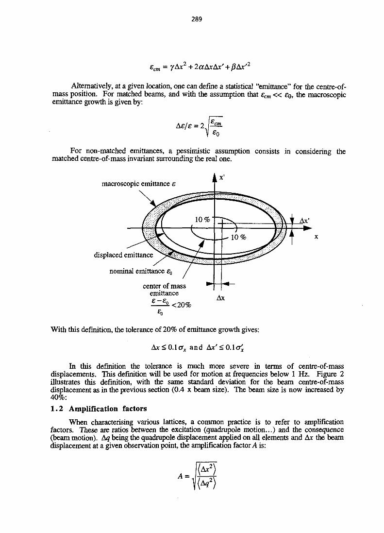
289

ecm = yAx2 + 2aAxAx/+/JAx'2

Alternatively, at a given location, one can define a statistical "emittance" for the centre-of-mass position. For matched beams, and with the assumption that ecm « £Q, the macroscopicemittance growth is given by:

Ae/e = 2

For non-matched emittances, a pessimistic assumption consists in considering thematched centre-of-mass invariant surrounding the real one.

macroscopic emittance e

displaced emittance

nominal emittance

center of massemittancee-e, Ax

With this definition, the tolerance of 20% of emittance growth gives:

Ax<0.\ax and

In this definition the tolerance is much more severe in terms of centre-of-massdisplacements. This definition will be used for motion at frequencies below 1 Hz. Figure 2illustrates this definition, with the same standard deviation for the beam centre-of-massdisplacement as in the previous section (0.4 x beam size). The beam size is now increased by40%:

1.2 Amplification factors

When characterising various lattices, a common practice is to refer to amplificationfactors. These are ratios between the excitation (quadrupole motion...) and the consequence(beam motion). Aq being the quadrupole displacement applied on all elements and Ax the beamdisplacement at a given observation point, the amplification factor A is:

A =

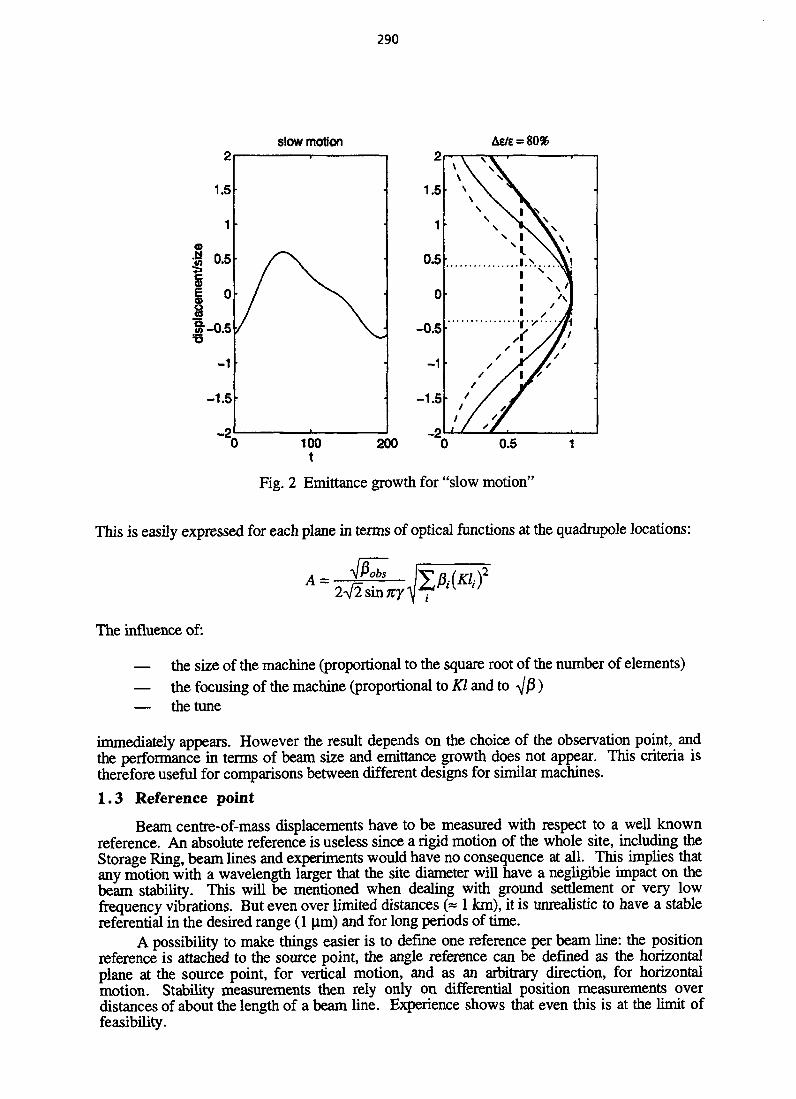
290

slow motion AE/E =

2

1.5

1

0.5

0

-0.5

-1

-1.5

_o

v \ \\ \ A\ \ N

V \\ \

ss

//

// /

/ /

' /' / 'J1 / ' /

, / ' / .

x^ l \î VX \sI \ \ \

H \ \ \.t.\ \L\. \ >*;

1 \ 'II XM. ' I

..!. '..Jht ' /p

X //>1 / / '

y

0 100 200 0 0.5 1

Fig. 2 Emittance growth for "slow motion"

This is easily expressed for each plane in terms of optical functions at the quadrupole locations:

A =smny

JflW

The influence of:

— the size of the machine (proportional to the square root of the number of elements)— the focusing of the machine (proportional to Kl and to -Jf5)— the tune

immediately appears. However the result depends on the choice of the observation point, andthe performance in terms of beam size and emittance growth does not appear. This criteria istherefore useful for comparisons between different designs for similar machines.

1.3 Reference point

Beam centre-of-mass displacements have to be measured with respect to a well knownreference. An absolute reference is useless since a rigid motion of the whole site, including theStorage Ring, beam lines and experiments would have no consequence at all. This implies thatany motion with a wavelength larger that the site diameter will have a negligible impact on thebeam stability. This will be mentioned when dealing with ground settlement or very lowfrequency vibrations. But even over limited distances (~ 1 km), it is unrealistic to have a stablereferential in the desired range (1 u,m) and for long periods of time.

A possibility to make things easier is to define one reference per beam line: the positionreference is attached to the source point, the angle reference can be defined as the horizontalplane at the source point, for vertical motion, and as an arbitrary direction, for horizontalmotion. Stability measurements then rely only on differential position measurements overdistances of about the length of a beam line. Experience shows that even this is at the limit offeasibility.

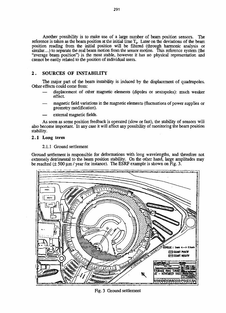
291

Another possibility is to make use of a large number of beam position sensors. Thereference is taken as the beam position at the initial time To. Later on the deviations of the beamposition reading from the initial position will be filtered (through harmonic analysis orsimilar...) to separate the real beam motion from the sensor motion. This reference system (the"average beam position") is the most stable, however it has no physical representation andcannot be easily related to the position of individual users.

2 . SOURCES OF INSTABILITY

The major part of the beam instability is induced by the displacement of quadrupoles.Other effects could come from:

— displacement of other magnetic elements (dipoles or sextupoles): much weakereffect.

— magnetic field variations in the magnetic elements (fluctuations of power supplies orgeometry modification).

— external magnetic fields.

As soon as some position feedback is operated (slow or fast), the stability of sensors willalso become important. In any case it will affect any possibility of monitoring the beam positionstability.

2.1 Long term

2.1.1 Ground settlement

Ground settlement is responsible for deformations with long wavelengths, and therefore notextremely detrimental to the beam position stability. On the other hand, large amplitudes maybe reached (± 500 jxm / year for instance). The ESRF example is shown on Fig. 3.

• —* • • * - • -y

: 1mm <—> 0.1mmC3ECMTP0S1FGZJECAJtTNEGAW

STORAGE RING TUNNELdZ - NOVEMBER 1992

95,9,9(*|6fl|8a|00,0| f?SI pO3|A

Fig. 3 Ground settlement

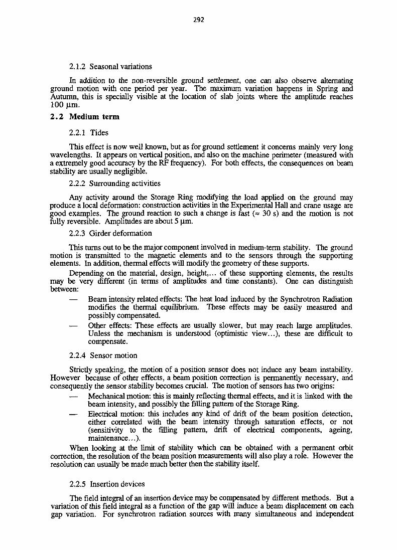
292

2.1.2 Seasonal variations

In addition to the non-reversible ground settlement, one can also observe alternatingground motion with one period per year. The maximum variation happens in Spring andAutumn, this is specially visible at the location of slab joints where the amplitude reaches100 Una.

2 .2 Medium term

2.2.1 Tides

This effect is now well known, but as for ground settlement it concerns mainly very longwavelengths. It appears on vertical position, and also on the machine perimeter (measured witha extremely good accuracy by the RF frequency). For both effects, the consequences on beamstability are usually negligible.

2.2.2 Surrounding activities

Any activity around the Storage Ring modifying the load applied on the ground mayproduce a local deformation: construction activities in the Experimental Hall and crane usage aregood examples. The ground reaction to such a change is fast (« 30 s) and the motion is notfully reversible. Amplitudes are about 5 urn.

2.2.3 Girder deformation

This turns out to be the major component involved in medium-term stability. The groundmotion is transmitted to the magnetic elements and to the sensors through the supportingelements. In addition, thermal effects will modify the geometry of these supports.

Depending on the material, design, height,... of these supporting elements, the resultsmay be very different (in terms of amplitudes and time constants). One can distinguishbetween:

— Beam intensity related effects: The heat load induced by the Synchrotron Radiationmodifies the thermal equilibrium. These effects may be easily measured andpossibly compensated.

— Other effects: These effects are usually slower, but may reach large amplitudes.Unless the mechanism is understood (optimistic view...), these are difficult tocompensate.

2.2.4 Sensor motion

Strictly speaking, the motion of a position sensor does not induce any beam instability.However because of other effects, a beam position correction is permanently necessary, andconsequently the sensor stability becomes crucial. The motion of sensors has two origins:

— Mechanical motion: this is mainly reflecting thermal effects, and it is linked with thebeam intensity, and possibly the filling pattern of the Storage Ring.

— Electrical motion: this includes any kind of drift of the beam position detection,either correlated with the beam intensity through saturation effects, or not(sensitivity to the filling pattern, drift of electrical components, ageing,maintenance...).

When looking at the limit of stability which can be obtained with a permanent orbitcorrection, the resolution of the beam position measurements will also play a role. However theresolution can usually be made much better then the stability itself.

2.2.5 Insertion devices

The field integral of an insertion device may be compensated by different methods. But avariation of this field integral as a function of the gap will induce a beam displacement on eachgap variation. For synchrotron radiation sources with many simultaneous and independent

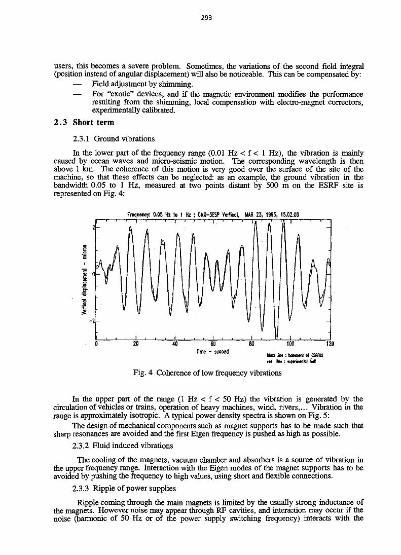
293

users, this becomes a severe problem. Sometimes, the variations of the second field integral(position instead of angular displacement) will also be noticeable. This can be compensated by:

— Field adjustment by shimming.— For "exotic" devices, and if the magnetic environment modifies the performance

resulting from the shimming, local compensation with electro-magnet correctors,experimentally calibrated.

2.3 Short term

2.3.1 Ground vibrations

In the lower part of the frequency range (0.01 Hz < f < 1 Hz), the vibration is mainlycaused by ocean waves and micro-seismic motion. The corresponding wavelength is thenabove 1 km. The coherence of this motion is very good over die surface of the site of themachine, so that these effects can be neglected: as an example, the ground vibration in thebandwidth 0.05 to 1 Hz, measured at two points distant by 500 m on the ESRF site isrepresented on Fig. 4:

Frequency: 0.05 Hi to t Hz ; CMG-3ESP Vertical, MAR 23, 1993. 15.02.08

60time - second

blade S M : t a n m n l of ESRFD2rad Sn» : apmtmM hoi

Fig. 4 Coherence of low frequency vibrations

In the upper part of the range (1 Hz < f < 50 Hz) the vibration is generated by thecirculation of vehicles or trains, operation of heavy machines, wind, rivers,... Vibration in therange is approximately isotropic. A typical power density spectra is shown on Fig. 5:

The design of mechanical components such as magnet supports has to be made such thatsharp resonances are avoided and the first Eigen frequency is pushed as high as possible.

2.3.2 Fluid induced vibrations

The cooling of the magnets, vacuum chamber and absorbers is a source of vibration inthe upper frequency range. Interaction with the Eigen modes of the magnet supports has to beavoided by pushing the frequency to high values, using short and flexible connections.

2.3.3 Ripple of power supplies

Ripple coming through the main magnets is limited by the usually strong inductance ofthe magnets. However noise may appear through RF cavities, and interaction may occur if thenoise (harmonic of 50 Hz or of the power supply switching frequency) interacts with the

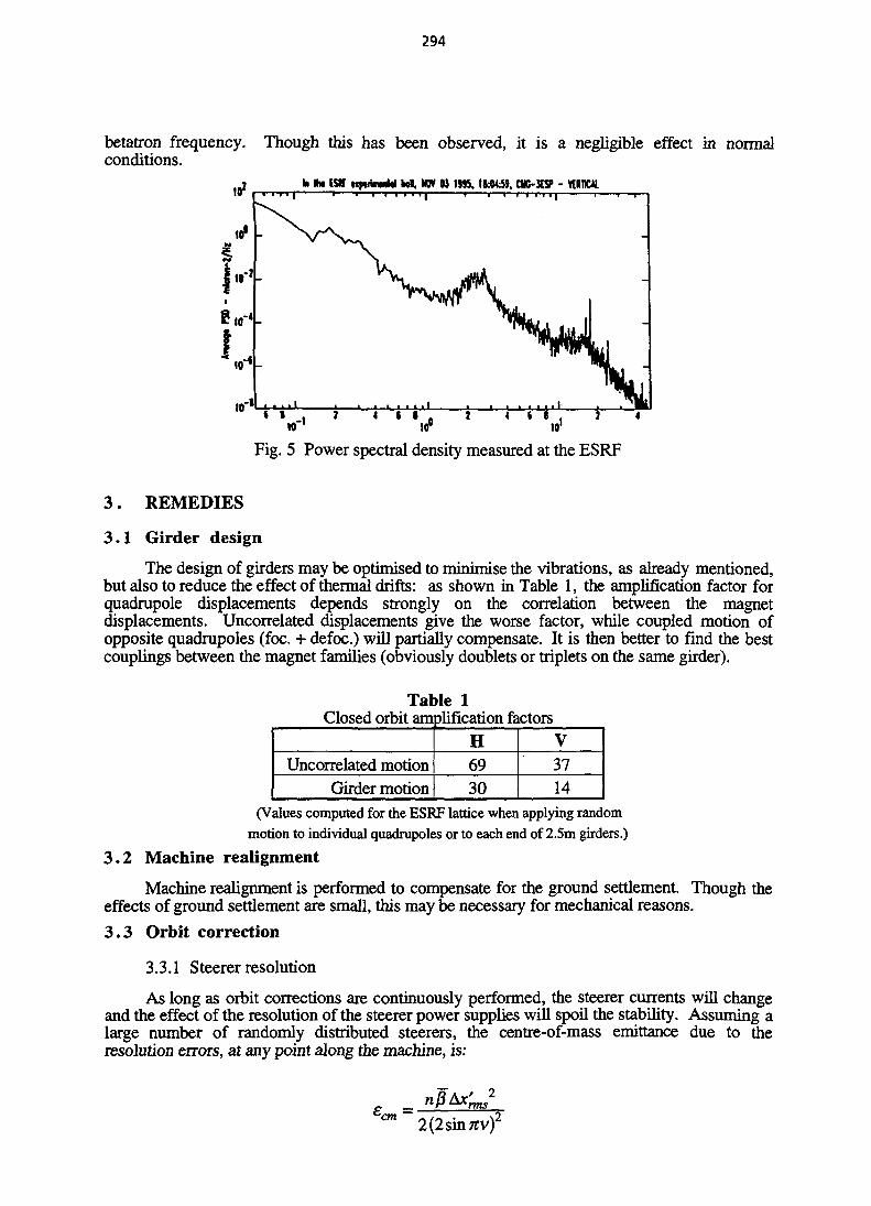
294

betatron frequency. Though this has been observed, it is a negligible effect in normalconditions.

KftnnnM M . NW 01 JM5. tfcW:M, CW-XSP - VHHUI

Fig. 5 Power spectral density measured at the ESRF

3 . REMEDIES

3 .1 Girder design

The design of girders may be optimised to minimise the vibrations, as already mentioned,but also to reduce the effect of thermal drifts: as shown in Table 1, the amplification factor forquadrupole displacements depends strongly on the correlation between the magnetdisplacements. Uncorrelated displacements give the worse factor, while coupled motion ofopposite quadrupoles (foe. + defoc.) will partially compensate. It is then better to find the bestcouplings between the magnet families (obviously doublets or triplets on the same girder).

Table 1Closed orbit amplification factors

Uncorrelated motionGirder motion

H6930

V3714

3.2

(Values computed for the ESRF lattice when applying randommotion to individual quadrupoles or to each end of 2.5m girders.)

Machine realignment

Machine realignment is performed to compensate for the ground settlement. Though theeffects of ground settlement are small, this may be necessary for mechanical reasons.

3 .3 Orbit correction

3.3.1 Steerer resolution

As long as orbit corrections are continuously performed, the steerer currents will changeand the effect of the resolution of the steerer power supplies will spoil the stability. Assuming alarge number of randomly distributed steerers, the centre-of-mass emittance due to theresolution errors, at any point along the machine, is:

2(2sin7fv)2

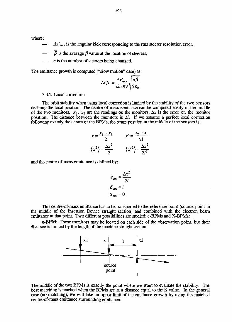
295

where:— Ax'rtns is the angular kick corresponding to the rms steerer resolution error,

— ($ is the average j3 value at the location of steerers,

— n is the number of steerers being changed.

The emittance growth is computed ("slow motion" case) as:

Ae/e = 4

3.3-2 Local correction

The orbit stability when using local correction is limited by the stability of the two sensorsdefining the local position. The centre-of-mass emittance can be computed easily in the middleof the two monitors, jq, x^ are the readings on the monitors, Ax is the error on the monitorposition. The distance between the monitors is 21. If we assume a perfect local correctionfollowing exactly the centre of the BPMs, the beam position in the middle of the sensors is:

Ax2

and the centre-of-mass emittance is defined by:

-cmAS

21

This centre-of-mass emittance has to be transported to the reference point (source point inthe middle of the Insertion Device straight section) and combined with the electron beamemittance at that point. Two different possibilities are studied: e-BPMs and X-BPMs:

e-BPM: These monitors may be located on each side of the observation point, but then-distance is limited by the length of the machine straight section:

x2

The middle of the two BPMs is exactly the point where we want to evaluate the stability. Thebest matching is reached when the BPMs are at a distance equal to the |3 value. In the generalcase (no matching), we will take an upper limit of the emittance growth by using the matchedcentre-of-mass emittance surrounding emittance:

296

Ax

This is a pessimistic assumption, and depending on the focusing at the observation point, theemittance growth may never reach that value. However the emittance growth for the "slowmotion" convention is:

Ae/e = position limitation

angle limitation

This shows immediately the limitations of the "local correction" option. The degradation due tothe wrong matching is shown for example on Fig. 6 (phase spaces in |im and (irad). Thecentre-of-mass emittance, in solid line, has to be maximised to match the electron beamemittance and reaches the dashed line value:

H high beta: 37% V high beta: 134%

-100 0 100

H low beta: 30%20

10

0

-10

1

0

-1

-2-20

11 /J -*

0 20

V low beta: 64%

-20-10

/• ••<Zrr-

\

I/

2

1

0

-1

-2

_^rrrrTrr-* .

1

^J^~**^

10 -5Fig. 6 Local correction matching

X-BPM: these sensors are located downstream the beam line.

sourcepoint

In this case the distance between the sensors can be more favourable, but when transporting theemittance backwards to the source point, the matching may be worse. The centre-of-massemittance at the source point is:

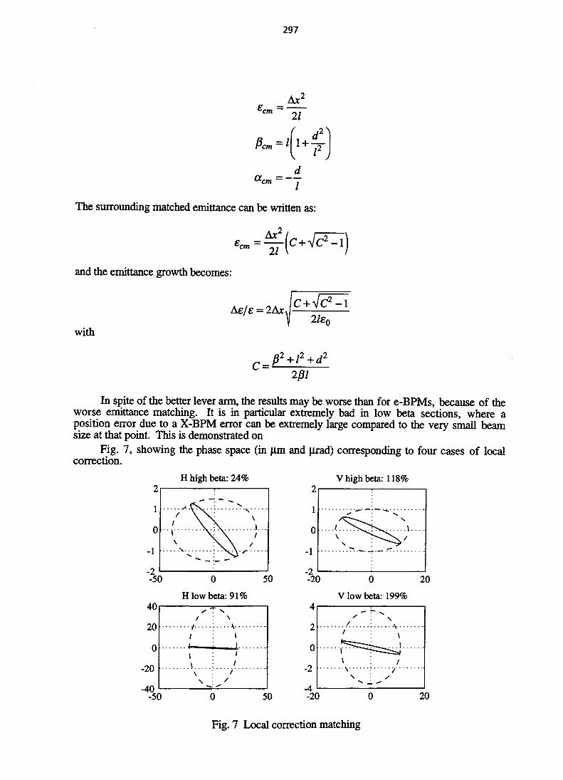
297

The surrounding matched emittance can be written as:

and the emittance growth becomes:

Ae/e = 2A*.,lie.

with

c

201

In spite of the better lever arm, the results may be worse than for e-BPMs, because of theworse emittance matching. It is in particular extremely bad in low beta sections, where aposition error due to a X-BPM error can be extremely large compared to the very small beamsize at that point. This is demonstrated on

Fig. 7, showing the phase space (in um and |irad) corresponding to four cases of localcorrection.

-1

-2-50

40

20

0

-20

-40-50

H high beta: 24%

"i \

s

\ : , . .

0

H low beta: 91%

50

/

/4—_1\\

\

\

\1I

/

/

/

V high beta: 118%

50

1

0

-1

-2-20 0 20

V low beta: 199%

2

0

-2

-20 0 20

//

1 ^ ^\\

\

\- ^ _ 1

/

Fig. 7 Local correction matching

298

3.3.3 Global correction

The stability when using only global orbit correction is limited by the steerer resolutionand the average stability of all BPMs. The sensitivity to the sensor motions depends on thecorrection method. The best flexibility is obtained with the S VD correction algorithm where onecan tune the number of Eigen correction vectors between 0 and the total number of availablesteerers. A large number gives better correction possibilities but also a larger sensitivity tosensor position fluctuations. The best compromise depends of course on the amplitude of thedistortions one has to correct.

This sensitivity to sensor errors can be studied by simulation. A machine with a realisticset of random errors and random sensor displacements is corrected with n, number of Eigenvectors, varying from 0 to the maximum number. All special conditions like sensor attachmentsto magnets, rigid girder motion... may be taken into account. For each correction, the emittancegrowth is averaged over similar points of the lattice. Average values for the high-P straightsection are plotted on Fig. 8. For small n, the stability rapidly improves with increasing n,since the first vectors are the most efficient. For large n, additional vectors only allow the orbitto follow more accurately the mispositioned monitors, and the emittance growth increases.Repeating this on a few error sets gives a good indication of the best compromise, as shown onFig. 8.

H High beta Emittance growth

20 40 60 80V High beta Emittance growth

100

20 40 60number of Eigen vectors

80 100

Fig. 8 Optimisation of a global correction

3.4 Vibration dampers

Vibration dampers using sandwich structure with visco-elastic material proved veryefficient to reduce the vibration of magnets (APS example): the vibration amplitude may bereduced by a factor 5 in wide band (4 to 50 Hz) or even 10 on the first Eigen mode. However,

— The damping solution is very specific to each structure.

— It has to be located in a region with large shear strain.

3.5 Fast feedbackThe same arguments concerning local and global correction apply for a fast feedback.

However the question of the sensor drift can be avoided to a certain extent by limiting the

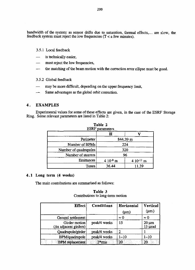
299

bandwidth of the system: as sensor drifts due to saturation, thermal effects,... are slow, thefeedback system must reject the low frequencies (T < a few minutes).

3.5.1 Local feedback

— is technically easier,

— must reject the low frequencies,

— the matching of the beam motion with the correction error ellipse must be good.

3.5.2 Global feedback

— may be more difficult, depending on the upper frequency limit,

— Same advantages as the global orbit correction.

4 . EXAMPLES

Experimental values for some of these effects are given, in the case of the ESRF StorageRing. Some relevant parameters are listed in Table 2:

Table 2ESRF parameters

PerimeterNumber of BPMs

Number of quadrupolesNumber of steerers

Emittances

Tunes

H V844.39 m

22432096

4 10-9 m36.44

4 10-11 m11.39

4.1 Long term (4 weeks)

The main contributions are summarised as follows:

Table 3Contributions to long-term motion

Effect

Ground settlementGirder motion

(Ax adjacent girders)Quadrupole/girderBPM/quadrupole

BPM replacement

Conditions

peak/4 weeks

peak/4 weekspeak/4 weeks

2*rms

Horizontal

(urn)= 015

21-1020

Vertical(Hm)

« 020(im15 \iiad11-1020

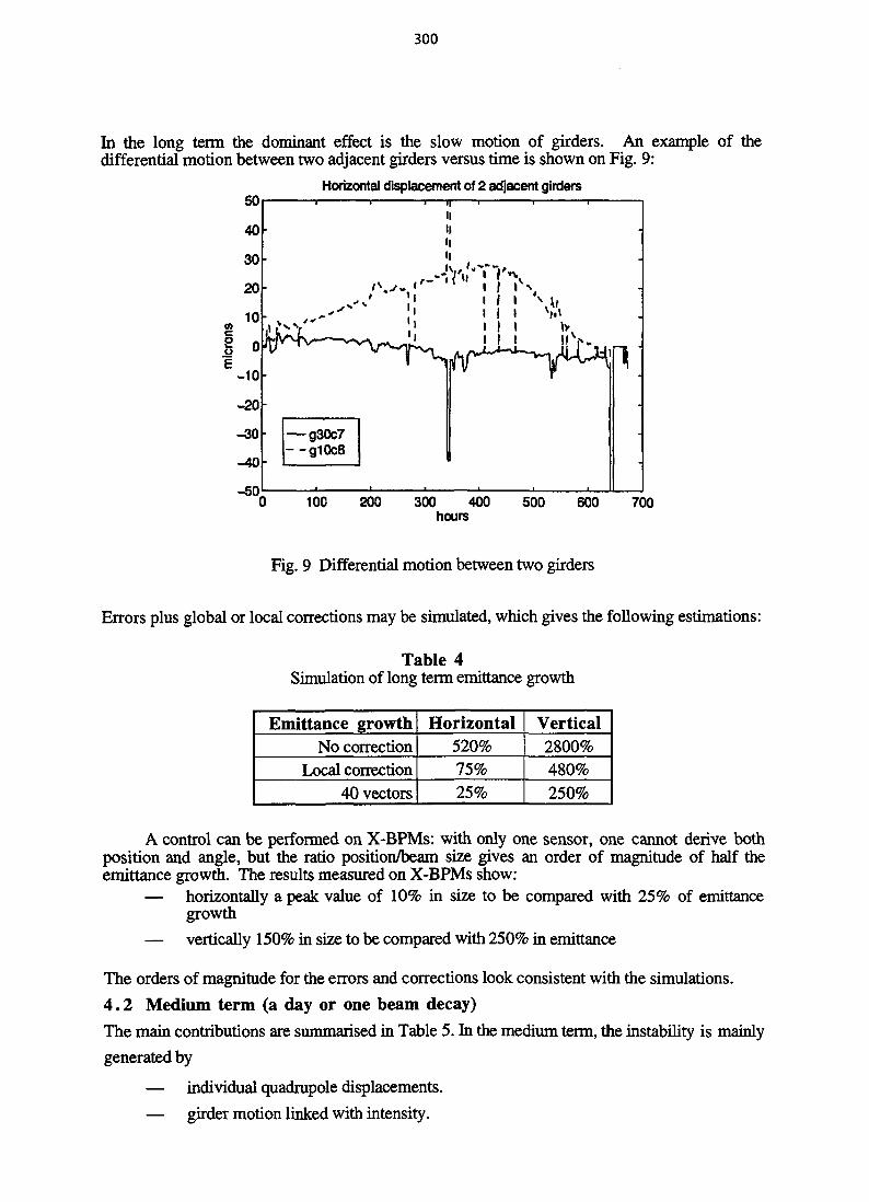
300

In the long term the dominant effect is the slow motion of girders. An example of thedifferential motion between two adjacent girders versus time is shown on Fig. 9:

50

40

30

20

10

i °-10

-20

-30

-40

-50

Horizontal displacement of 2 adjacent girders1

—g30c7--g!0c8

iIii

j

J *'"!'

iiii

j111

1 *

r

•

100 200 300 400hours

500 600 700

Fig. 9 Differential motion between two girders

Errors plus global or local corrections may be simulated, which gives the following estimations:

Table 4Simulation of long term emittance growth

Emittance growthNo correction

Local correction40 vectors

Horizontal520%75%25%

Vertical2800%480%250%

A control can be performed on X-BPMs: with only one sensor, one cannot derive bothposition and angle, but the ratio position/beam size gives an order of magnitude of half theemittance growth. The results measured on X-BPMs show:

— horizontally a peak value of 10% in size to be compared with 25% of emittancegrowth

— vertically 150% in size to be compared with 250% in emittance

The orders of magnitude for the errors and corrections look consistent with the simulations.

4.2 Medium term (a day or one beam decay)The main contributions are summarised in Table 5. In the medium term, the instability is mainly

generated by

— individual quadrupole displacements.

— girder motion linked with intensity.

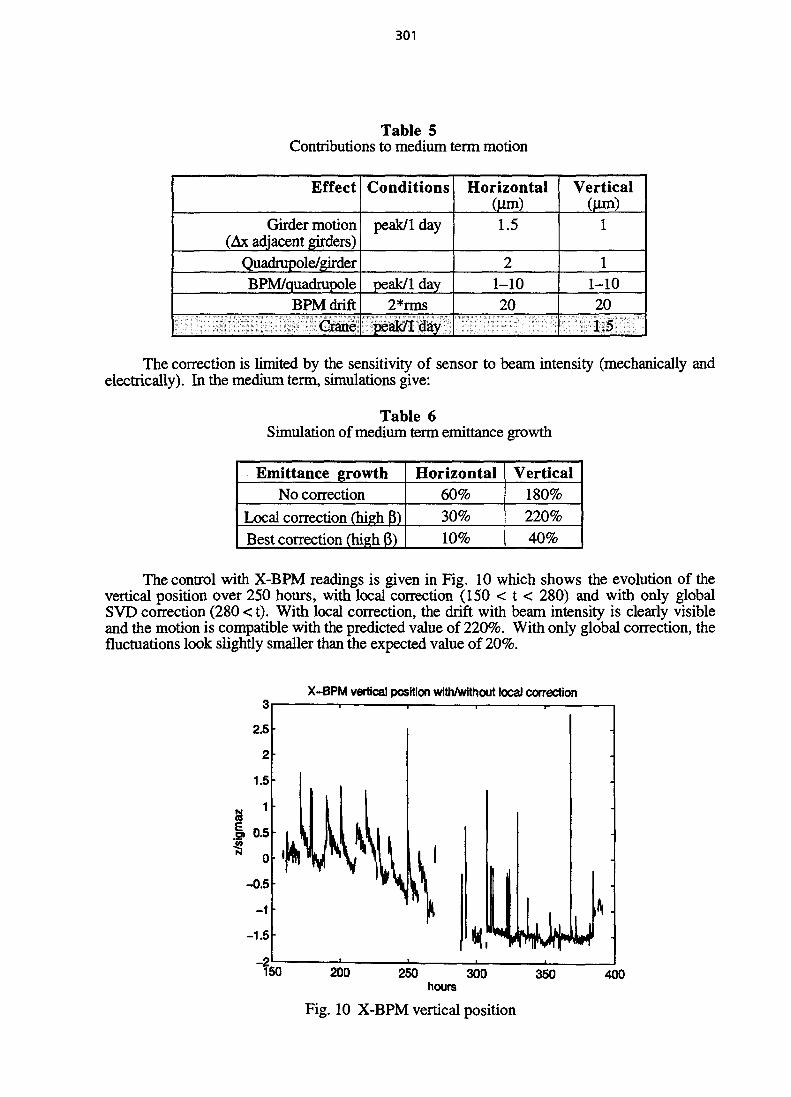
301

Table 5Contributions to medium term motion

Effect

Girder motion(Ax adjacent girders)

Quadrupole/girderBPM/quadrupole

BPM driftCrane

Conditions

peak/1 day

peak/1 day2*rms

peak/1 day

Horizontal(Urn)1.5

21-1020-

Vertical(Mm)

1

11-10201.5

The correction is limited by the sensitivity of sensor to beam intensity (mechanically andelectrically). In the medium term, simulations give:

Table 6Simulation of medium term emittance growth


Local correction (high |3)Best correction (high 3)

Horizontal60%30%10%

Vertical180%220%40%

The control with X-BPM readings is given in Fig. 10 which shows the evolution of thevertical position over 250 hours, with local correction (150 < t < 280) and with only globalSVD correction (280 < t). With local correction, the drift with beam intensity is clearly visibleand the motion is compatible with the predicted value of 220%. With only global correction, thefluctuations look slightly smaller than the expected value of 20%.

X-BPM vertical position with/Without local correction

150 200 250 300 350hours

Fig. 10 X-BPM vertical position

400

302

4.3 Short term

Without correction:

Table 7Contributions to short term motion

Effect

Ground vibration noiseRoad traffic

Absorber movement

Conditions

peak

peak

Horizontal(Hm)

12*girder

amplification35

Vertical(Hm)0.5

2*girderamplification

10

Emittance growths measured on feedback electron BPMs give, using fast motionquadratic combination:

Table 8Simulation of short term emittance growth


Local correction

Horizontal5 1(H

7 10-5

Vertical1.2%

0.4%

Even in the pessimistic case of the "slow motion" combination, the values would be small:

Table 9Simulation of short term emittance growth


Local correction

Horizontal4.6%1.7%

Vertical22%13%

5 . CONCLUSIONS— Vibrations should not introduce significant disturbances to the beam stability. In

addition a correction is proven to be efficient. A significant part of vibrations comesfrom the facility itself, and the influence of the site is of secondary importance.

— In the medium term, thermal or electronic effects linked with the beam intensity aredominating. They can be corrected to a satisfactory level by using a globalcorrection scheme filtering out most of the sensor drifts. However the stability ofsensors is the limiting parameter.

— Slow motion due to girder displacements is by far the more difficult problem. Thereference for measuring such a motion is even doubtful.

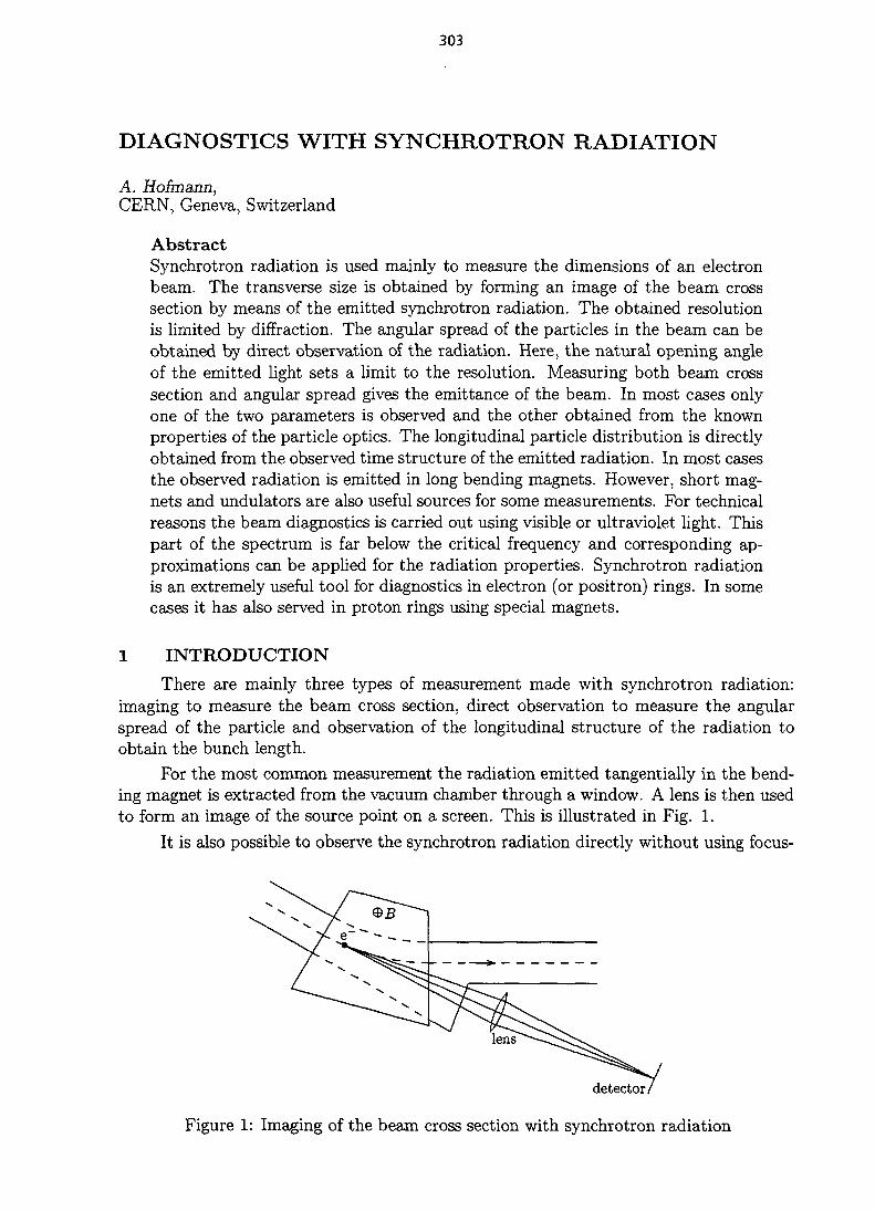
303

DIAGNOSTICS WITH SYNCHROTRON RADIATION

A. Hofmann,CERN, Geneva, Switzerland

AbstractSynchrotron radiation is used mainly to measure the dimensions of an electronbeam. The transverse size is obtained by forming an image of the beam crosssection by means of the emitted synchrotron radiation. The obtained resolutionis limited by diffraction. The angular spread of the particles in the beam can beobtained by direct observation of the radiation. Here, the natural opening angleof the emitted light sets a limit to the resolution. Measuring both beam crosssection and angular spread gives the emittance of the beam. In most cases onlyone of the two parameters is observed and the other obtained from the knownproperties of the particle optics. The longitudinal particle distribution is directlyobtained from the observed time structure of the emitted radiation. In most casesthe observed radiation is emitted in long bending magnets. However, short mag-nets and undulators are also useful sources for some measurements. For technicalreasons the beam diagnostics is carried out using visible or ultraviolet light. Thispart of the spectrum is far below the critical frequency and corresponding ap-proximations can be applied for the radiation properties. Synchrotron radiationis an extremely useful tool for diagnostics in electron (or positron) rings. In somecases it has also served in proton rings using special magnets.

1 INTRODUCTION

There are mainly three types of measurement made with synchrotron radiation:imaging to measure the beam cross section, direct observation to measure the angularspread of the particle and observation of the longitudinal structure of the radiation toobtain the bunch length.

For the most common measurement the radiation emitted tangentially in the bend-ing magnet is extracted from the vacuum chamber through a window. A lens is then usedto form an image of the source point on a screen. This is illustrated in Fig. 1.

It is also possible to observe the synchrotron radiation directly without using focus-

detector/

Figure 1: Imaging of the beam cross section with synchrotron radiation

304

= y'R

P(y)intensity

distribution

Figure 2: Direct observation of synchrotron radiation

liensdetector

P(t)averaged

întensity

Figure 3: Observation of the synchrotron radiation time structure to measure bunchlength

ing elements as shown in Fig. 2. In this case one measures the angular distribution of theparticles in the beam. If a horizontal bending magnet serves as source of the radiationonly the vertical angles can be measured. The resolution is limited by the natural openingangle of the radiation itself.

The bunch length can be measured by observing the time structure of the emit-ted radiation. Since the light pulse observed from each individual particle is very shortthe time distribution of the radiation reflects directly the longitudinal bunch shape asindicated in Fig. 3. A fast photon detector is needed to measure this distribution.

2 PROPERTIES OF SYNCHROTRON AND UNDULATOR RADIATION

The properties of ordinary synchrotron radiation emitted in long bending magnetshas been treated in an earlier lecture of this school [1] and we will in the following refer tothe derivation carried out there. However, for convenience we summarize here the mostimportant results.

2.1 Qualitative treatment of the radiationWe start with a qualitative treatment of the synchrotron radiation emitted in long

magnets, in short magnets and in undulators.We consider an electron moving in the laboratory frame Fon a circular orbit and

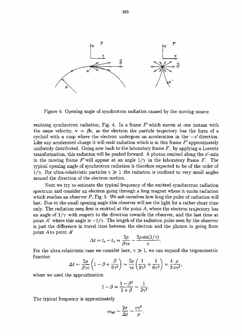
305

Figure 4: Opening angle of synchrotron radiation caused by the moving source

emitting synchrotron radiation, Fig. 4. In a frame F' which moves at one instant withthe same velocity, v = /3c, as the electron the particle trajectory has the form of acycloid with a cusp where the electron undergoes an acceleration in the —a;'direction.Like any accelerated charge it will emit radiation which is in this frame F' approximatelyuniformly distributed. Going now back to the laboratory frame F, by applying a Lorentztransformation, this radiation will be peaked forward. A photon emitted along the x'-axisin the moving frame F'will appear at an angle 1/7 in the laboratory frame F. Thetypical opening angle of synchrotron radiation is therefore expected to be of the order ofI/7. For ultra-relativistic particles 7 > 1 the radiation is confined to very small anglesaround the direction of the electron motion.

Next we try to estimate the typical frequency of the emitted synchrotron radiationspectrum and consider an electron going through a long magnet where it emits radiationwhich reaches an observer P, Fig. 5. We ask ourselves how long the pulse of radiation willlast. Due to the small opening angle this observer will see the light for a rather short timeonly. The radiation seen first is emitted at the point A, where the electron trajectory hasan angle of 1/7 with respect to the direction towards the observer, and the last time atpoint A' where this angle is —1/7. The length of the radiation pulse seen by the observeris just the difference in travel time between the electron and the photon in going frompoint A to point A'

A , , , _ 2p 2psin(l/7)A t t h W cFor the ultra-relativistic case we consider here, 7 > 1, we can expand the trigonometricfunction

(JL\ ?P (J , ±P + 67V 7C V272 67V 3

where we used the approximation

The typical frequency is approximately

2?r C73

At p

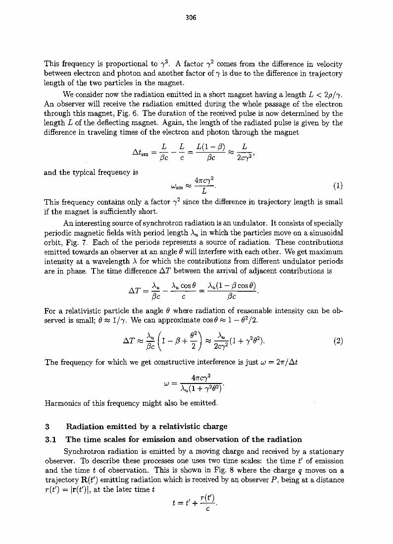
306

This frequency is proportional to 73. A factor 72 comes from the difference in velocitybetween electron and photon and another factor of 7 is due to the difference in trajectorylength of the two particles in the magnet.

We consider now the radiation emitted in a short magnet having a length L < 2/3/7.An observer will receive the radiation emitted during the whole passage of the electronthrough this magnet, Fig. 6. The duration of the received pulse is now determined by thelength L of the deflecting magnet. Again, the length of the radiated pulse is given by thedifference in traveling times of the electron and photon through the magnet

A, L L-sm~ 0 ~sm 0c c~ (3c ~2c7

2 '

and the typical frequency is4-7TC72

^sm « — — • (1)

This frequency contains only a factor 72 since the difference in trajectory length is smallif the magnet is sufficiently short.

An interesting source of synchrotron radiation is an undulator. It consists of speciallyperiodic magnetic fields with period length Xu in which the particles move on a sinusoidalorbit, Fig. 7. Each of the periods represents a source of radiation. These contributionsemitted towards an observer at an angle 6 will interfere with each other. We get maximumintensity at a wavelength A for which the contributions from different undulator periodsare in phase. The time difference AT between the arrival of adjacent contributions is

. _ Xu Xucos8 _ \u(l - ficosO)

~~0c c ~ 0c '

For a relativistic particle the angle 6 where radiation of reasonable intensity can be ob-served is small; 6 « 1/7. We can approximate cos0 « 1 — 02/2.

The frequency for which we get constructive interference is just u = 27r/Ai

Harmonics of this frequency might also be emitted.

3 Radiation emitted by a relativistic charge

3.1 The time scales for emission and observation of the radiationSynchrotron radiation is emitted by a moving charge and received by a stationary

observer. To describe these processes one uses two time scales: the time f of emissionand the time t of observation. This is shown in Fig. 8 where the charge q moves on atrajectory R(t') emitting radiation which is received by an observer P, being at a distancer(f) = |r(t')|, at the later time t

2>

307

observer

1/7 7E(t)

E(u>)

pulse shape

e

spectrum

Figure 5: Spectrum of synchrotron radiation emitted in a long magnet

observer

s "T^J 3

E(t)field pulse

11/

spectrum

Figure 6: Spectrum of synchrotron radiation emitted in a short magnet

£. field at angle 6

\{6)

\ucos9

Figure 7: Spectrum of synchrotron radiation emitted in an undulator

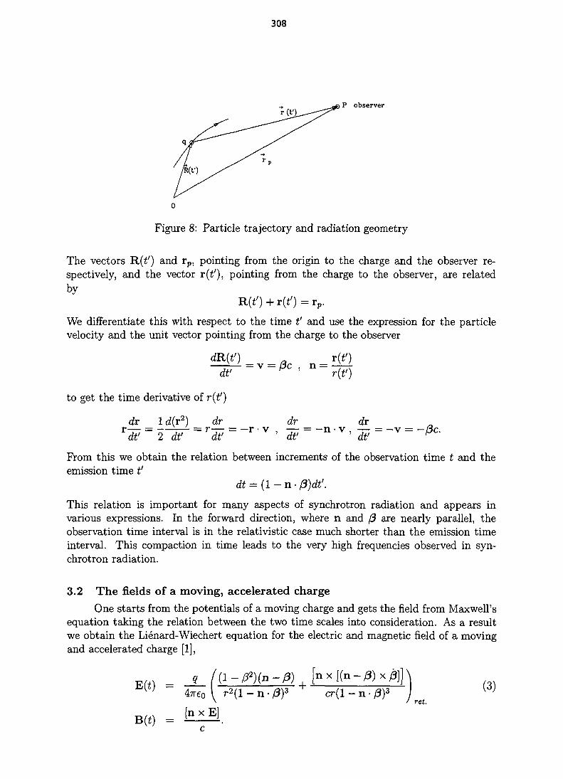
308

P observer

0

Figure 8: Particle trajectory and radiation geometry

The vectors R(t') and rp, pointing from the origin to the charge and the observer re-spectively, and the vector r(tf), pointing from the charge to the observer, are relatedby

R(i') + r(t') = rp.

We differentiate this with respect to the time t' and use the expression for the particlevelocity and the unit vector pointing from the charge to the observer

dR(f)__ _ v{t')dt' - v - P c > n - r ^ j

to get the time derivative of r(t')

dr 1 d(r2) _ dr _ dr _ dv

From this we obtain the relation between increments of the observation time t and theemission time t'

dt = (1 - n • (3)dtr.

This relation is important for many aspects of synchrotron radiation and appears invarious expressions. In the forward direction, where n and j3 are nearly parallel, theobservation time interval is in the relativistic case much shorter than the emission timeinterval. This compaction in time leads to the very high frequencies observed in syn-chrotron radiation.

3.2 The fields of a moving, accelerated chargeOne starts from the potentials of a moving charge and gets the field from Maxwell's

equation taking the relation between the two time scales into consideration. As a resultwe obtain the Lienard-Wiechert equation for the electric and magnetic field of a movingand accelerated charge [1],

n x [(n - /3) x /3]]

cr ( l — n/ ret.

In v FlB(t) =

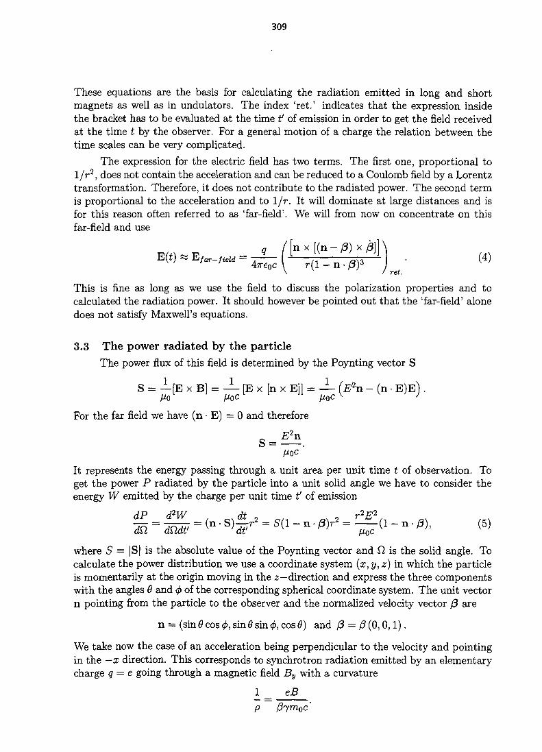
309

These equations are the basis for calculating the radiation emitted in long and shortmagnets as well as in undulators. The index 'ret.' indicates that the expression insidethe bracket has to be evaluated at the time if of emission in order to get the field receivedat the time t by the observer. For a general motion of a charge the relation between thetime scales can be very complicated.

The expression for the electric field has two terms. The first one, proportional to1/r2, does not contain the acceleration and can be reduced to a Coulomb field by a Lorentztransformation. Therefore, it does not contribute to the radiated power. The second termis proportional to the acceleration and to 1/r. It will dominate at large distances and isfor this reason often referred to as 'far-field'. We will from now on concentrate on thisfar-field and use

ret.

This is fine as long as we use the field to discuss the polarization properties and tocalculated the radiation power. It should however be pointed out that the 'far-field' alonedoes not satisfy Maxwell's equations.

3.3 The power radiated by the particleThe power flux of this field is determined by the Poynting vector S

S = —[E x B] = — [E x [n x Ell = — (£ 2n - (n • E)E) .A*o Hoc nQc V >

For the far field we have (n • E) = 0 and therefore

flQC

It represents the energy passing through a unit area per unit time t of observation. Toget the power P radiated by the particle into a unit solid angle we have to consider theenergy W emitted by the charge per unit time if of emission

^ l - » . « , (5)

where S = |S| is the absolute value of the Poynting vector and Q is the solid angle. Tocalculate the power distribution we use a coordinate system (x, y, z) in which the particleis momentarily at the origin moving in the z—direction and express the three componentswith the angles 9 and 0 of the corresponding spherical coordinate system. The unit vectorn pointing from the particle to the observer and the normalized velocity vector /3 are

n = (sin 9 cos <j>, sin 9 sin </>, cos 9) and j3 = (5 (0,0,1).

We take now the case of an acceleration being perpendicular to the velocity and pointingin the — x direction. This corresponds to synchrotron radiation emitted by an elementarycharge q = e going through a magnetic field By with a curvature

310

The normalized acceleration is

62c0 = £-£(-1,0,0).

The distribution of the power radiated by the particle is

dP_ _ e2 [nx[(n-/3)x/3]]2

(47r)2eoc (1 — n • /3)5

)2-sin20cos20N

(l- /?cos0)5 ; ' w

where we introduced the classical particle radius.

_ e2 _ 2.818 l(T15m for electronsr° ~ 47re0m0c

2 ~ 1.53510~18m for protons "

Integrating (6) over the solid angle gives the total power radiated by the particle

2rocmoc2/?474 _ 2rocmoc

274 _ 2r0e2c3 (m0c

27)2 B2

3p2 3p2 3 (mod2)2

where we approximated for an ultra-relativistic particle. If the orbit is a closed circle weget the energy Us lost per turn by multiplying the power by the revolution time T = 2-irp/c

Us =3p 3(m0c2)3

This expression is also valid for a ring having all magnets of the same strength and field-free straight sections in between.

For the instantaneous angular distribution (6) we assume the ultra-relativistic case/3 « 1, 7 ;§> 1 for which the radiation is peaked forward confined to a cone of openingangle 6 ~ 1/7. We use the corresponding approximations and the expression for the totalpower PQ to obtain

dP_ _dQ ~ ° n V (1 + 7202)5 / "

3.4 Fourier transformed radiation field and angular spectral power densityWe derived the electric and magnetic radiation fields emitted by a moving charge

g = e as a function of time (4). As we said before, the difficulty to calculate these fieldslies in the fact that the expressions involving the particle motion have to be evaluated atthe earlier time t' which has, in general, a rather complicated relation to the time t ofobservation. For this reason it is often easier to calculate directly the Fourier transformE(cu) of the electric field

E(w) = -4= rV2TT J-0

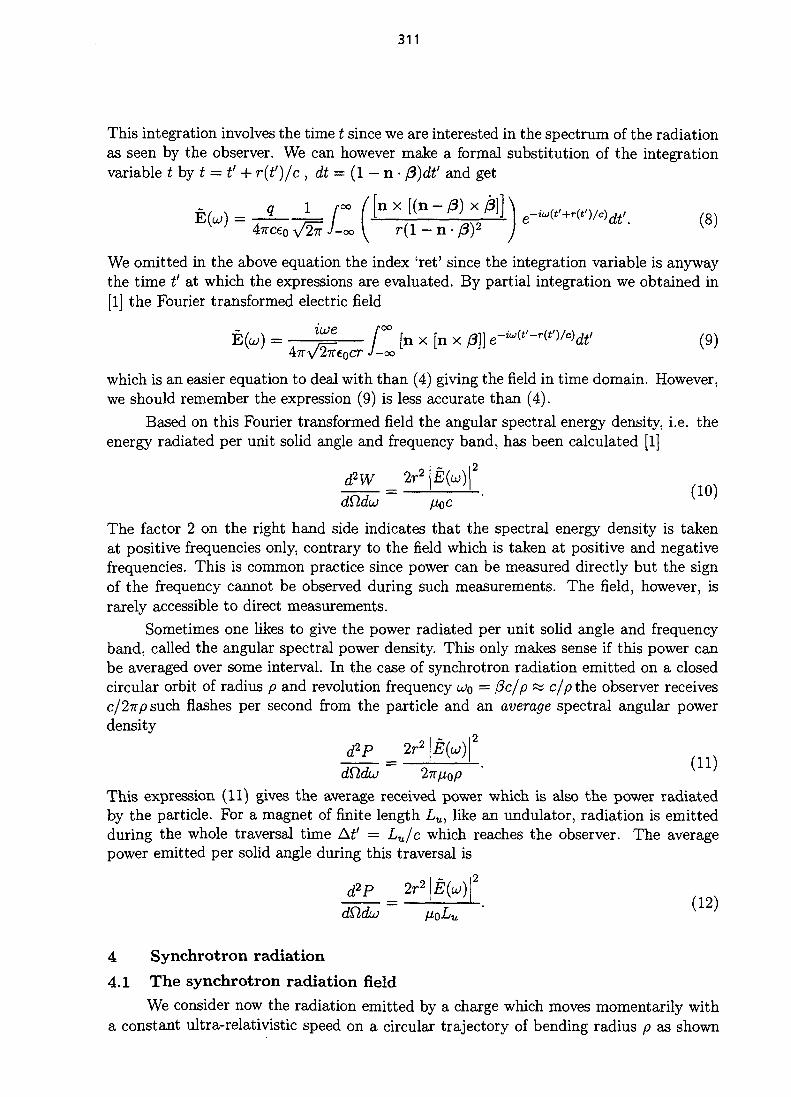
311

This integration involves the time t since we are interested in the spectrum of the radiationas seen by the observer. We can however make a formal substitution of the integrationvariable tbyt = t' + r{t')/c , dt = (1 - n • 0)dtf and get

We omitted in the above equation the index 'ret' since the integration variable is anywaythe time t' at which the expressions are evaluated. By partial integration we obtained in[1] the Fourier transformed electric field

which is an easier equation to deal with than (4) giving the field in time domain. However,we should remember the expression (9) is less accurate than (4).

Based on this Fourier transformed field the angular spectral energy density, i.e. theenergy radiated per unit solid angle and frequency band, has been calculated [1]

(10)

The factor 2 on the right hand side indicates that the spectral energy density is takenat positive frequencies only, contrary to the field which is taken at positive and negativefrequencies. This is common practice since power can be measured directly but the signof the frequency cannot be observed during such measurements. The field, however, israrely accessible to direct measurements.

Sometimes one likes to give the power radiated per unit solid angle and frequencyband, called the angular spectral power density. This only makes sense if this power canbe averaged over some interval. In the case of synchrotron radiation emitted on a closedcircular orbit of radius p and revolution frequency U>Q = (3c/p ~ c/p the observer receivesc/2?rpsuch flashes per second from the particle and an average spectral angular powerdensity

2r2 E(UJ)\2

-^-. (11)

This expression (11) gives the average received power which is also the power radiatedby the particle. For a magnet of finite length Lu, like an undulator, radiation is emittedduring the whole traversal time At' = Lu/c which reaches the observer. The averagepower emitted per solid angle during this traversal is

2r2 E(u) 2

(12)

4 Synchrotron radiation

4.1 The synchrotron radiation fieldWe consider now the radiation emitted by a charge which moves momentarily with

a constant ultra-relativistic speed on a circular trajectory of bending radius p as shown

312

radiation

Figure 9: Geometry used to describe the synchrotron radiation

in Fig. 9. This is the case of ordinary synchrotron radiation emitted by a charge q = e ina bending magnet where the curvature is

1

P

eB eBc

Using the expression (9) one obtains the horizontal and vertical field components

Ex{w) =ej

4coJ(13)

where we used the Airy function Ai(z) and its derivative Ai'(z) and introduce the criticalfrequency uc

Uc = !%-• <14)

The fact that the expression for the vertical field EV(UJ) has an imaginary factor infront while this factor is real for the horizontal component indicates that the two fieldsare 90° out of phase for a given frequency w. There is therefore some circular polarizationpresent which vanishes in the median where the polarization is purely horizontal.

The angular spectral angular power distribution is obtained from this field and theexpression (11)

2r2 E(t(u

dtldu(15)

Here, Po is the total radiated power given by (7). The solid angle element can be approx-imated by dQ, Rs d(t>dtp due to the small vertical opening angle of the radiation if; <§; 1.

The form of the distribution is determined by the two expressions FCT(w,t/>) andFv{v, 4>) which give the contributions of the two linear polarization components. The first

313

one, called cr-mode, has the electrical field in the plane of the particle orbit (usually thehorizontal plane) and the second one, called 7r-mode, has the electric field perpendicularto this plane. The two functions are given by

(16)

As mentioned earlier, diagnostics with synchrotron radiation is carried out mostlywith visible (or close to visible) light. In electron rings this light is at the lower part ofthe spectrum u <C coc and we can make some approximation. In this case the argumentof the Airy function or its derivative in (13) is small except if 7 2 ^ 2 becomes very large.Therefore, we make a small error by replacing (1 + 72V>2) by 7 V 2 inside the argument ofthe Airy functions. Using the expression (14) for the critical frequency we get then forthe argument of the Airy functions

With this we get for the electric field (13) and spectral angular distribution (15) at smallfrequencies u <C uc

cr(17)

and

d?P 2r0m0c2

itp [\2c;/2

2c 2c JAi2

2c J (18)

It is interesting to note that these expressions do not depend on 7. At low frequencies theproperties of synchrotron radiation are independent of the particle energy and dependonly on the radius p of curvature. This fact is important for diagnostics applicationswhich usually uses the lower part of the spectrum. The angular power distribution forthis case is plotted in Fig. 10.

The rms opening angle of synchrotron radiation can be calculated [1] which givesfor the low frequency part of the spectrum w < w c

''rms

\

\

\

1/3

12-M0)(19)

6 Ai(0) ( c\12 -Ai'(0) \pu)

1/3 /A\1 /3

= 0.4488 - ,

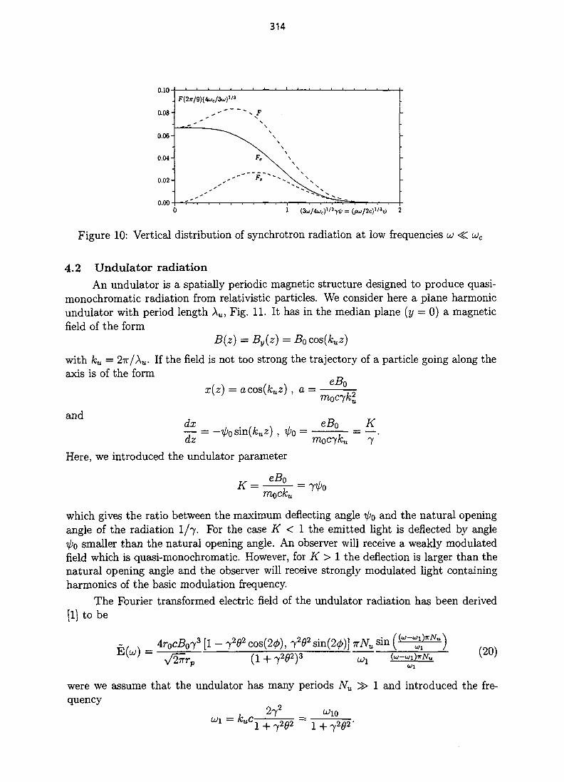
314

0.10

0.00

Figure 10: Vertical distribution of synchrotron radiation at low frequencies u <C uc

4.2 Undulator radiationAn undulator is a spatially periodic magnetic structure designed to produce quasi-

monochromatic radiation from relativistic particles. We consider here a plane harmonicundulator with period length Xu, Fig. 11. It has in the median plane (y = 0) a magneticfield of the form

B(z) = By(z) = B0cos(kuz)

with ku = 2TT/AW. If the field is not too strong the trajectory of a particle going along theaxis is of the form

x(z) = acos(kuz) , a =

anddx eB0__K_

7 'Here, we introduced the undulator parameter

which gives the ratio between the maximum deflecting angle Vo and the natural openingangle of the radiation 1/7. For the case K < 1 the emitted light is deflected by angleipo smaller than the natural opening angle. An observer will receive a weakly modulatedfield which is quasi-monochromatic. However, for K > 1 the deflection is larger than thenatural opening angle and the observer will receive strongly modulated light containingharmonics of the basic modulation frequency.

The Fourier transformed electric field of the undulator radiation has been derived[1] to be

sin

were we assume that the undulator has many periods Nu

quency

u>i = kuc-—

1 and introduced the fre-

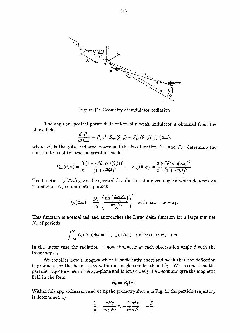
315

observer

Figure 11: Geometry of undulator radiation

The angular spectral power distribution of a weak undulator is obtained from theabove field

^ N(Au),

where Pu is the total radiated power and the two function FU(r and Fua determine thecontributions of the two polarization modes

The function /N(AUJ) gives the spectral distribution at a given angle 9 which depends onthe number Nu of undulator periods

fN(Auj) = —- with Au =

This function is normalized and approaches the Dirac delta function for a large numberNu of periods

/ •CO

/ fN(Au)dui = 1 , /NJ — oo

for Nu -+ oo.

In this latter case the radiation is monochromatic at each observation angle 6 with thefrequency u\.

We consider now a magnet which is sufficiently short and weak that the deflectionit produces for the beam stays within an angle smaller than I/7. We assume that theparticle trajectory lies in the x, z-plane and follows closely the 2-axis and give the magneticfield in the form

By = By{Z).

Within this approximation and using the geometry shown in Fig. 11 the particle trajectoryis determined by

1 eBc 1 d2x 0p moc27 c2 df2 c'

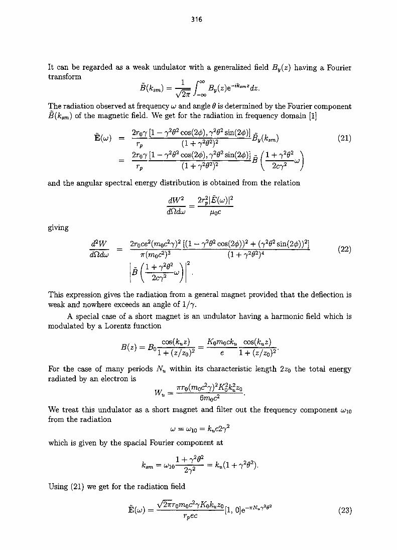
316

It can be regarded as a weak undulator with a generalized field By(z) having a Fouriertransform

B(ksm) = 4

The radiation observed at frequency UJ and angle 0 is determined by the Fourier component( ) of the magnetic field. We get for the radiation in frequency domain [1]

y(ksm) (21)

2 r o 7 [1 - 72fl2 cos(2<ft), 7

2fl2 sin(20)] 5rp ( l + 7

2 0 2 ) 2 * { 2c72 WJ

and the angular spectral energy distribution is obtained from the relation

dW2 ^

giving

d?W 2r-0ce2(m0c27)2 [(1 -

7r(moc2)3 (1 + 7

202)4 (22)

This expression gives the radiation from a general magnet provided that the deflection isweak and nowhere exceeds an angle of 1/7.

A special case of a short magnet is an undulator having a harmonic field which ismodulated by a Lorentz function

, . cos(kuz) Korrtocku cos(kuz)D\Z) = DQ —iz/zo)2 e

For the case of many periods Nu within its characteristic length 2zo the total energyradiated by an electron is

W _6moc

2

We treat this undulator as a short magnet and filter out the frequency componentfrom the radiation

u = u/10 = &uc272

which is given by the spacial Fourier component at

1 1

k

Using (21) we get for the radiation field

'., UJe [26)rpec

317

where we are left with the horizontal polarization mode only. From (10) we obtain emittedangular spectral energy distribution

~ u

The radiation from this Lorentz modulated undulator, filtered at u\o, has a Gaussianangular energy distribution with rms values for the polar angle 9 and the two Cartesianangles x' and y'

0 — r> —,/"rms /<->_ Ar ' ""rms arms n .

5 Imaging with SR — Qualitative treatment

5.1 Diffraction of radiation emitted in long magnetsWe use synchrotron radiation from a long magnet to form an image of the beam cross

section with an arrangement shown in Fig. 12. For simplicity a single lens is consideredto form a 1:1 image. This is no restriction since we could also use a magnification andproject the image back to the beam to get the resolution in terms of beam size. Sincethe vertical opening angle of the radiation a^ is small, only the central part of the lensis illuminated. The situation is therefore similar to optical imaging with a limited lensaperture. This case is known to lead to a limitation of the resolution by diffraction [2]

(25)" 2D/R'

where d is the half size of an image from a point source and D is the full lens aperture.For synchrotron radiation observed at the low frequency part of the spectrum we foundfor the horizontal polarization an rms opening angle (19) which is

for the cr-mode. Relating this to (25) we take D « Aa^R since the lens represents the fullaperture which we approximate with ±2^>CT_rms to get

We find that the resolution improves with shorter wavelength and with smaller radiusof curvature. Due to the latter dependence synchrotron radiation monitors have a poorresolution in large machines as indicated in the examples shown in Table 1. A wavelengthas short as possible can help to improve the resolution. Special magnets with strongcurvature could help to improve the resolution but the weak dependence on p makes thisapproach not very attractive.

Diffraction represents often a serious limitation of the resolution for large machines.It is caused by the small opening angle of synchrotron radiation. Sometimes the questionarises if a large angular spread of the particles in the beam helps the resolution since alarger part of the lens is now illuminated. This is not the case since the diffraction resultsin a finite size image of each particle. The radiation originating from different particleshas no phase relation and does not produce the corresponding diffraction pattern.

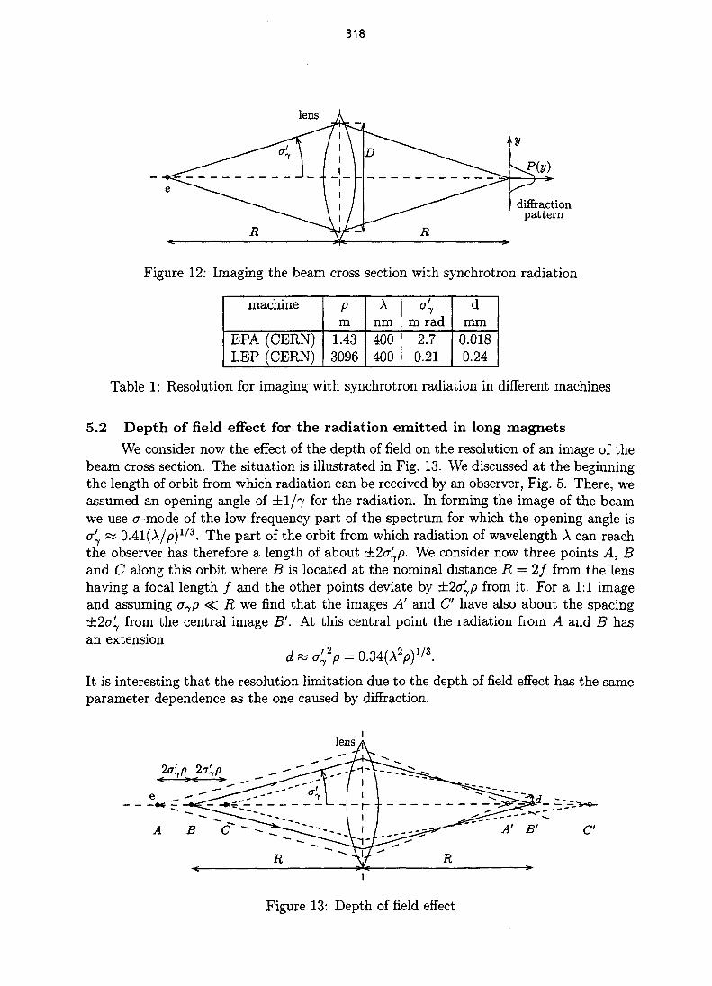
318

lens fI

D ^ " ~ " ~ \ ^ ^

' R

diffractionpattern

Figure 12: Imaging the beam cross section with synchrotron radiation

machine

EPA (CERN)LEP(CERN)

Pm

1.433096

Anm400400

m rad2.70.21

dmm

0.0180.24

Table 1: Resolution for imaging with synchrotron radiation in different machines

5.2 Depth of field effect for the radiation emitted in long magnetsWe consider now the effect of the depth of field on the resolution of an image of the

beam cross section. The situation is illustrated in Fig. 13. We discussed at the beginningthe length of orbit from which radiation can be received by an observer, Fig. 5. There, weassumed an opening angle of ±1/7 for the radiation. In forming the image of the beamwe use cr-mode of the low frequency part of the spectrum for which the opening angle isa'y m 0.41 (A/p)1/<3. The part of the orbit from which radiation of wavelength A can reachthe observer has therefore a length of about ±2a'^p. We consider now three points A, Band C along this orbit where B is located at the nominal distance R = 2f from the lenshaving a focal length / and the other points deviate by ±2a'7p from it. For a 1:1 imageand assuming a-yp <C R we find that the images A' and C have also about the spacing±2a'1 from the central image B'. At this central point the radiation from A and B hasan extension

d « o?p = 0.34(A2p)1/3-

It is interesting that the resolution limitation due to the depth of field effect has the sameparameter dependence as the one caused by diffraction.

A B C A' B'

R R

Figure 13: Depth of field effect

319

5.3 Diffraction and depth of field effect for undulator radiationWe derived the radiation from a weak undulator in frequency domain 20

- _ 4roci?o73 (1 - 72<?2 oos(2fl, 72 0 2 sJn(20)) nNu sin

with

l + 7 2 0 2 'We filter now the frequency u = u?io to use it for imaging the beam and get for the spectralfunction

sin

w

This equation contains the function sin x/x which has a maximum value of unity at x = 0and is small for large values of x. It has a first zero at x = n which corresponds to theangle

9zero = WK- (26)

We assume now an undulator with many periods Nu 3> 1 for which the radiation atUJ = Wio is concentrated within an angle much smaller than 1/7. We can then approximatein (20 for 1 + 72#2 « 1 and get a radiation field containing only an x-component

—^=V2nrp

and a angular spectral power distribution

p ,2 3 A^ /sin(72^27riV,)\2

This function is plotted in Fig. 14 together with an exponential approximation.For the evaluation of the diffraction we would like to use the rms width of this power

distribution. However, the variance of function (sinx/x)2 diverges. This is due to theunphysical undulator field which is harmonic within ±Lu/2 but vanishes abruptly outsidethis range. For the qualitative treatment of the diffraction we relate again to the case ofa lens with diameter D shown in Fig. 12 and approximate D w 20zeroR with the openingangle (26) of the first zero. Using also the relation A10 = Au/272

A

2D/R ~ 4

Since the resolution is proportional to yfL^ one would like to work with a short undulator.However, we obtained the above expression with the assumption Nu » 1. A more detailedcalculation is necessary to treat the more general case of an undulator having few periodsor of a short magnet.

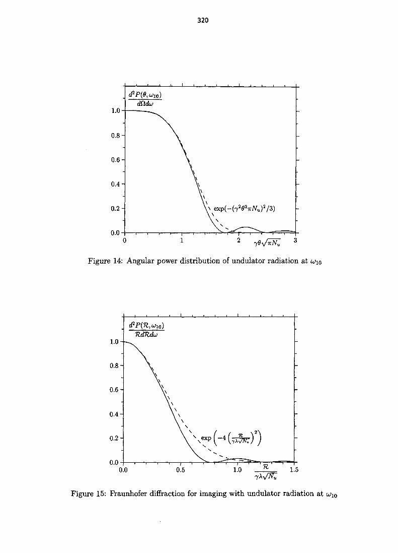
320

Figure 14: Angular power distribution of undulator radiation at u>io

Figure 15: Fraunhofer diffraction for imaging with undulator radiation at u>i0

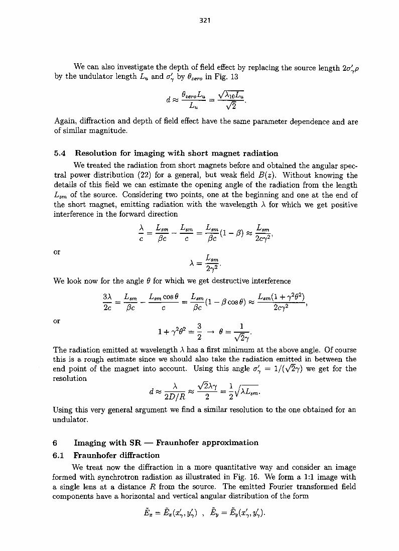
321

We can also investigate the depth of field effect by replacing the source lengthby the undulator length Lu and ay by 9zero in Fig. 13

Lu

Again, diffraction and depth of field effect have the same parameter dependence and areof similar magnitude.

5.4 Resolution for imaging with short magnet radiationWe treated the radiation from short magnets before and obtained the angular spec-

tral power distribution (22) for a general, but weak field B(z). Without knowing thedetails of this field we can estimate the opening angle of the radiation from the lengthLsm of the source. Considering two points, one at the beginning and one at the end ofthe short magnet, emitting radiation with the wavelength A for which we get positiveinterference in the forward direction

LA =

272"

We look now for the angle 9 for which we get destructive interference

The radiation emitted at wavelength A has a first minimum at the above angle. Of coursethis is a rough estimate since we should also take the radiation emitted in between theend point of the magnet into account. Using this angle a'^ = l/(\/27) we get for theresolution

2D/R 2Using this very general argument we find a similar resolution to the one obtained for anundulator.

6 Imaging with SR — Fraunhofer approximation

6.1 Fraunhofer diffractionWe treat now the diffraction in a more quantitative way and consider an image

formed with synchrotron radiation as illustrated in Fig. 16. We form a 1:1 image witha single lens at a distance R from the source. The emitted Fourier transformed fieldcomponents have a horizontal and vertical angular distribution of the form

Es = Ex{x^,j^) , Ey = Ey(x'y,y'J.

322

pointsource

X

E(X)

diffractionpattern

Figure 16: Diffraction in imaging with synchrotron radiation

At the lens this is converted into a spacial distribution

Ex{x,y) = Ex(Rx'vRy'1) , Ev{x,y) = Ex(Rx'vRy'J.

The point source in the figure is imaged on to the image point at a distance R from thelens. In this case all rays between source and image points have the same optical length.The dashed circular arc with radius R around the image point, shown in the figure,represents therefore a cut through an equi-phase surface. Using Huygens's principle weconsider each point on this surface as a source of a radiation field of strength proportionalto (Ex(x, y), Ey(x, y)). We restrict ourselves to a scalar field E which can stand for eitherthe horizontal or vertical two field components. From this secondary source point (x, y, z)this field propagates towards the image plane (X, Y) in the form of a wave

6E{X,Y) K (29)

where k = 2TT/A is the wave number of the radiation and r the distance between thesecondary source and the observation point in the image plane

r2 = (R- z)2 + (x - X)2 + (y -Y)2.

On the equi-phase surface we have (R — z)2 — R2 — (x2 + y2) which gives

The small opening angle of synchrotron radiation and the limited extension of the imagepermit to use an approximation and we neglect from now on higher order terms in (X/R)and {Y/R).

We get the field in the image plane by integrating the contribution (29) from eachsurface element of the secondary source

E(X,Y) oc e-*** f°°J—oo J—

HWe omit the oscillatory term as well as fixed phase term exp (ikR) which are both of nointerest and replace the coordinates (x, y) at the lens by the angles (x1, y') at which theradiation is emitted

E{X,Y) oc r r E(x,y)e-i^kx+y'k^dx'dyl.J— 00 J—OO

(30)

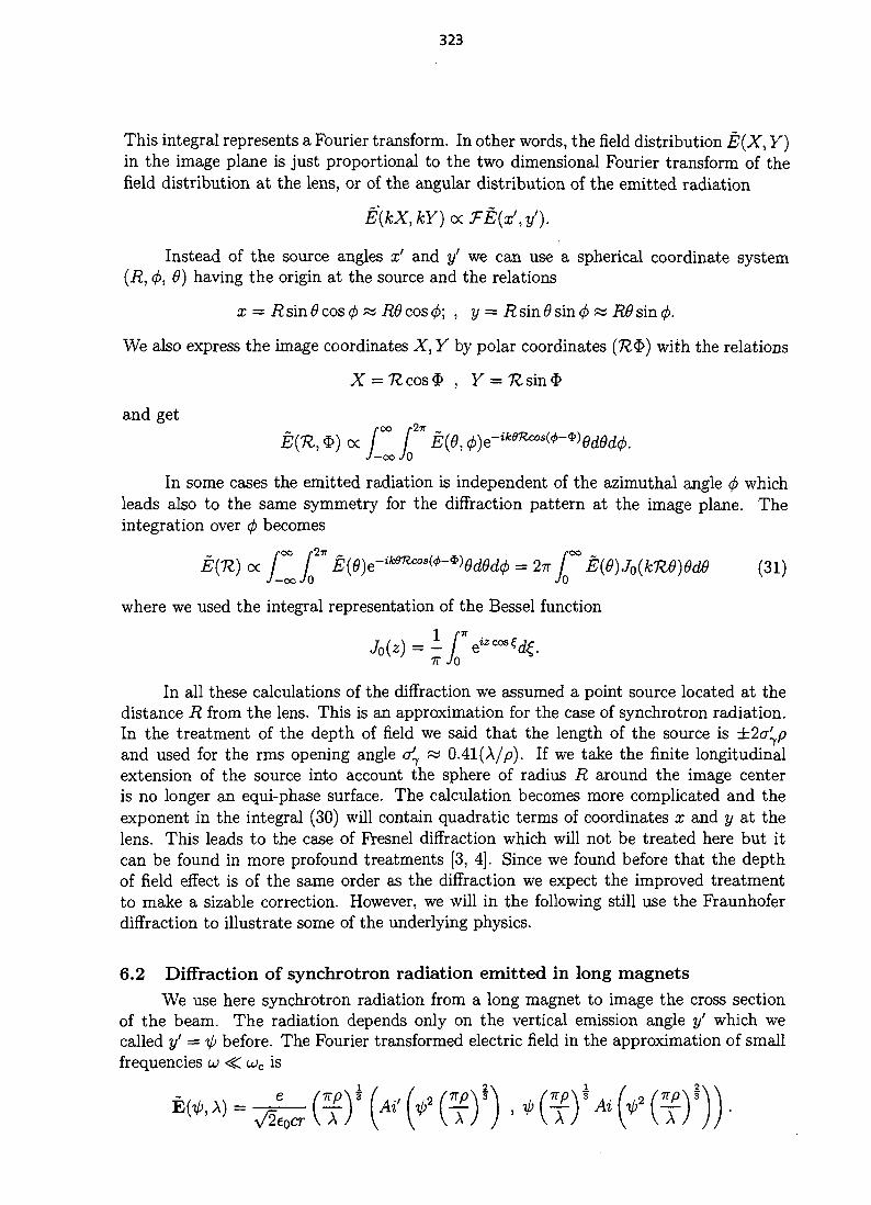
323

This integral represents a Fourier transform. In other words, the field distribution E(X, Y)in the image plane is just proportional to the two dimensional Fourier transform of thefield distribution at the lens, or of the angular distribution of the emitted radiation

E(kX,kY)<xFE(xf,y').

Instead of the source angles x' and y' we can use a spherical coordinate system(R, <f>, 6) having the origin at the source and the relations

x = i?sin#cos0 w R9cos<f>; , y = RsmOsincj) « ROsmcj).

We also express the image coordinates X, Y by polar coordinates (1Z§) with the relations

and get

E(n, $) oc r f* E{8,0)eJ-ooJo

In some cases the emitted radiation is independent of the azimuthal angle (j> whichleads also to the same symmetry for the diffraction pattern at the image plane. Theintegration over (p becomes

E(H) oc / ° ° \^ E{6)e-ik&Rcos{<l>-ii!)6ded(j) = 2TT f° E(9)J0(k1l8)6de (31)J—oo J0 JO

where we used the integral representation of the Bessel function

7T 70

In all these calculations of the diffraction we assumed a point source located at thedistance R from the lens. This is an approximation for the case of synchrotron radiation.In the treatment of the depth of field we said that the length of the source is ±2<j^pand used for the rms opening angle o^ « 0.41 (A/p). If we take the finite longitudinalextension of the source into account the sphere of radius R around the image centeris no longer an equi-phase surface. The calculation becomes more complicated and theexponent in the integral (30) will contain quadratic terms of coordinates x and y at thelens. This leads to the case of Fresnel diffraction which will not be treated here but itcan be found in more profound treatments [3, 4]. Since we found before that the depthof field effect is of the same order as the diffraction we expect the improved treatmentto make a sizable correction. However, we will in the following still use the Fraunhoferdiffraction to illustrate some of the underlying physics.

6.2 Diffraction of synchrotron radiation emitted in long magnetsWe use here synchrotron radiation from a long magnet to image the cross section

of the beam. The radiation depends only on the vertical emission angle y' which wecalled y' = ip before. The Fourier transformed electric field in the approximation of smallfrequencies u <§; u>c is

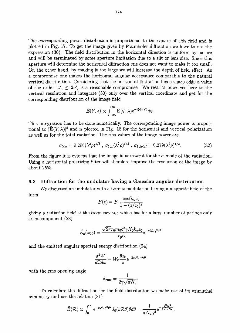
324

The corresponding power distribution is proportional to the square of this field and isplotted in Fig. 17. To get the image given by Fraunhofer diffraction we have to use theexpression (30). The field distribution in the horizontal direction is uniform by natureand will be terminated by some aperture limitation due to a slit or lens size. Since thisaperture will determine the horizontal diffraction one does not want to make it too small.On the other hand, by making it too large we will increase the depth of field effect. Asa compromise one makes the horizontal angular acceptance comparable to the naturalvertical distribution. Considering that the horizontal limitation has a sharp edge a valueof the order \x'\ < 2a'^ is a reasonable compromise. We restrict ourselves here to thevertical resolution and integrate (30) only over the vertical coordinate and get for thecorresponding distribution of the image field

E(y, A) « r :J—OO

This integration has to be done numerically. The corresponding image power is propor-tional to |E(Y, A)|2 and is plotted in Fig. 18 for the horizontal and vertical polarizationas well as for the total radiation. The rms values of the image power are

= 0.206(A2p)1/3 , ^y,.(A2p)1/3 , ^totd = 0.279(A2p)1/3. (32)

From the figure it is evident that the image is narrowest for the cr-mode of the radiation.Using a horizontal polarizing filter will therefore improve the resolution of the image byabout 25%.

6.3 Diffraction for the undulator having a Gaussian angular distributionWe discussed an undulator with a Lorenz modulation having a magnetic field of the

form

giving a radiation field at the frequency wio which has for a large number of periods onlyan ^-component (23)

V2irr0mo(?'yK0kuzo _vNu~3gi= e

rpecand the emitted angular spectral energy distribution (24)

TT

with the rms opening angle

"rms =z 7i

To calculate the diffraction for the field distribution we make use of its azimuthalsymmetry and use the relation (31)

E{n) a fooe-7rN^2e2j0(kn9)ede = - J -JO 7TiVu

2 - 2

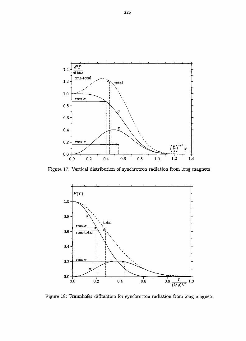
325

0.0 0.2 0.4 0.6 0.8 1.0 1.2

Figure 17: Vertical distribution of synchrotron radiation from long magnets

0.0

Figure 18: Fraunhofer diffraction for synchrotron radiation from long magnets

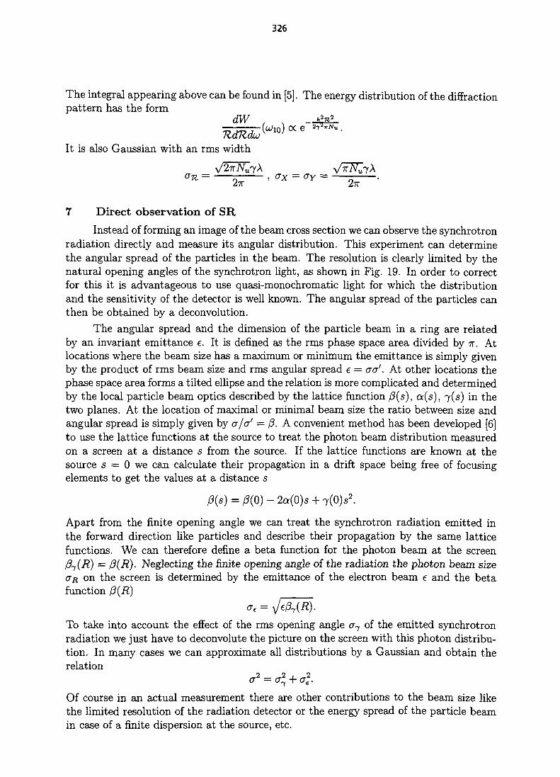
326

The integral appearing above can be found in [5]. The energy distribution of the diffractionpattern has the form

dW

It is also Gaussian with an rms width

2TT 2TT '

7 Direct observation of SR

Instead of forming an image of the beam cross section we can observe the synchrotronradiation directly and measure its angular distribution. This experiment can determinethe angular spread of the particles in the beam. The resolution is clearly limited by thenatural opening angles of the synchrotron light, as shown in Fig. 19. In order to correctfor this it is advantageous to use quasi-monochromatic light for which the distributionand the sensitivity of the detector is well known. The angular spread of the particles canthen be obtained by a deconvolution.

The angular spread and the dimension of the particle beam in a ring are relatedby an invariant emittance e. It is defined as the rms phase space area divided by TT. Atlocations where the beam size has a maximum or minimum the emittance is simply givenby the product of rms beam size and rms angular spread e = aa'. At other locations thephase space area forms a tilted ellipse and the relation is more complicated and determinedby the local particle beam optics described by the lattice function /3(s), oc(s), 7(s) in thetwo planes. At the location of maximal or minimal beam size the ratio between size andangular spread is simply given by a/a' = /?. A convenient method has been developed [6]to use the lattice functions at the source to treat the photon beam distribution measuredon a screen at a distance s from the source. If the lattice functions are known at thesource s ~ 0 we can calculate their propagation in a drift space being free of focusingelements to get the values at a distance s

0(s) = /?(0) - 2ct(0)s + 7(0)s2.

Apart from the finite opening angle we can treat the synchrotron radiation emitted inthe forward direction like particles and describe their propagation by the same latticefunctions. We can therefore define a beta function for the photon beam at the screen0-y(R) = fi(R). Neglecting the finite opening angle of the radiation the photon beam size<JR on the screen is determined by the emittance of the electron beam e and the betafunction (3(R)

ae =

To take into account the effect of the rms opening angle <77 of the emitted synchrotronradiation we just have to deconvolute the picture on the screen with this photon distribu-tion. In many cases we can approximate all distributions by a Gaussian and obtain therelation

Of course in an actual measurement there are other contributions to the beam size likethe limited resolution of the radiation detector or the energy spread of the particle beamin case of a finite dispersion at the source, etc.

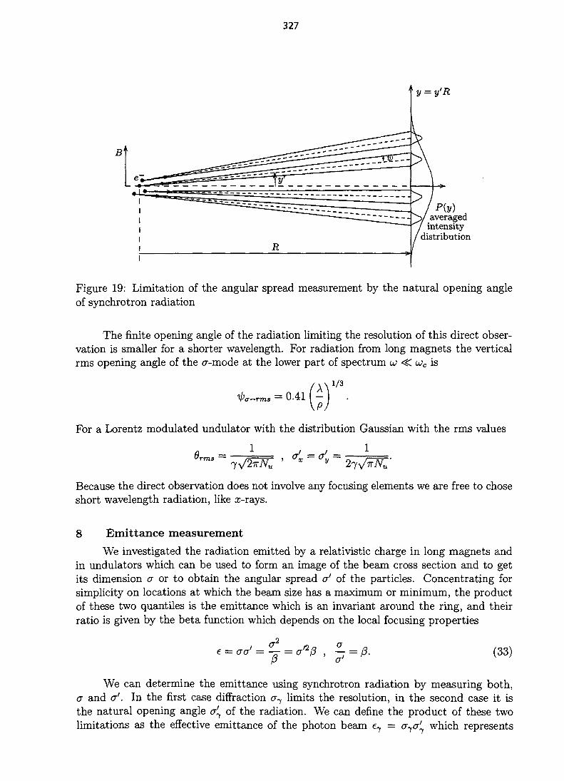
327

' y = y'= y'R

P(v)averagedintensity

distribution

Figure 19: Limitation of the angular spread measurement by the natural opening angleof synchrotron radiation

The finite opening angle of the radiation limiting the resolution of this direct obser-vation is smaller for a shorter wavelength. For radiation from long magnets the verticalrms opening angle of the cr-mode at the lower part of spectrum u> <C a>c is

For a Lorentz modulated undulator with the distribution Gaussian with the rms values

_ 1 , . 1

Because the direct observation does not involve any focusing elements we are free to choseshort wavelength radiation, like x-rays.

8 Emittance measurementWe investigated the radiation emitted by a relativistic charge in long magnets and

in undulators which can be used to form an image of the beam cross section and to getits dimension a or to obtain the angular spread a' of the particles. Concentrating forsimplicity on locations at which the beam size has a maximum or minimum, the productof these two quantiles is the emittance which is an invariant around the ring, and theirratio is given by the beta function which depends on the local focusing properties

2

e = aa= — = a(l, - 7 = /?• (33)

We can determine the emittance using synchrotron radiation by measuring both,a and &. In the first case diffraction <77 limits the resolution, in the second case it isthe natural opening angle a7 of the radiation. We can define the product of these twolimitations as the effective emittance of the photon beam e7 = cr7cr7 which represents

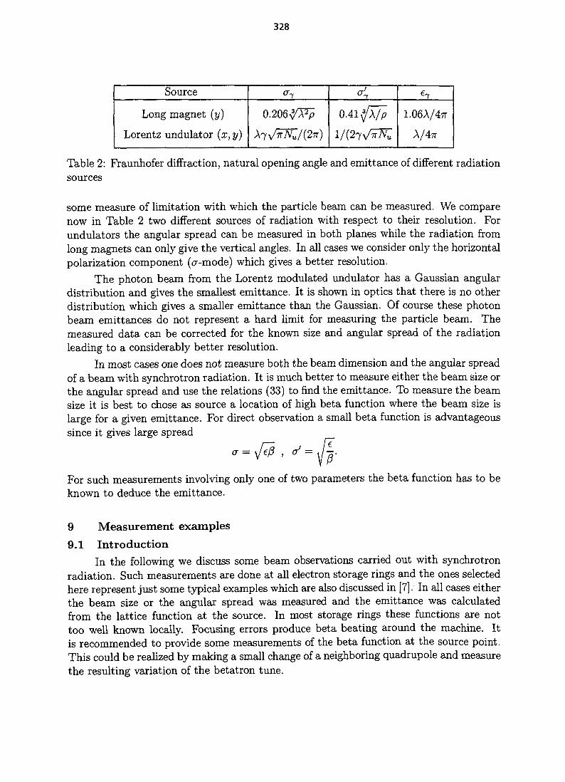
328

Source

Long magnet (y)

Lorentz undulator (x, y)

0.206^^0

A7vÂC/(27r)

<

0.41 tfA/pl / ( 2 7 v / S F ^

e7

1.06A/4TT

A/47T

Table 2: Fraunhofer diffraction, natural opening angle and emittance of different radiationsources

some measure of limitation with which the particle beam can be measured. We comparenow in Table 2 two different sources of radiation with respect to their resolution. Forundulators the angular spread can be measured in both planes while the radiation fromlong magnets can only give the vertical angles. In all cases we consider only the horizontalpolarization component (a-mode) which gives a better resolution.

The photon beam from the Lorentz modulated undulator has a Gaussian angulardistribution and gives the smallest emittance. It is shown in optics that there is no otherdistribution which gives a smaller emittance than the Gaussian. Of course these photonbeam emittances do not represent a hard limit for measuring the particle beam. Themeasured data can be corrected for the known size and angular spread of the radiationleading to a considerably better resolution.

In most cases one does not measure both the beam dimension and the angular spreadof a beam with synchrotron radiation. It is much better to measure either the beam size orthe angular spread and use the relations (33) to find the emittance. To measure the beamsize it is best to chose as source a location of high beta function where the beam size islarge for a given emittance. For direct observation a small beta function is advantageoussince it gives large spread

o- = \fej3

For such measurements involving only one of two parameters the beta function has to beknown to deduce the emittance.

9 Measurement examples

9.1 IntroductionIn the following we discuss some beam observations carried out with synchrotron

radiation. Such measurements are done at all electron storage rings and the ones selectedhere represent just some typical examples which are also discussed in [7]. In all cases eitherthe beam size or the angular spread was measured and the emittance was calculatedfrom the lattice function at the source. In most storage rings these functions are nottoo well known locally. Focusing errors produce beta beating around the machine. Itis recommended to provide some measurements of the beta function at the source point.This could be realized by making a small change of a neighboring quadrupole and measurethe resulting variation of the betatron tune.

329

9.2 Imaging with synchrotron radiation in LEPThe electron positron storage ring LEP has operated at an energy of 91.5 GeV per

beam and will be able to reach about 100 GeV once all the RF cavities are installed.To minimize the power radiated by synchrotron radiation this ring has a large bendingradius in the dipole magnets of p — 3096 m. There are monitors which image the beamcross section using the synchrotron radiation from these magnets [8]. They consists oftelescopes of the kind shown in Fig. 20 looking at the beam at locations having differentvalues for the dispersion function. To get a good resolution they can operate with ultra-violet light of a wavelength A = 200 nm. We expect a vertical resolution limitation byFraunhofer diffraction (32) if only the horizontal polarization is used

aY(a) = 0.206(A2p)1/3 = 0.1mm.

A more detailed calculation of the effect of diffraction and depth of field has been carriedout giving a resolution which is about twice as large.

We have to compare this resolution with the actual size of the beam. For physicsexperiments LEP is operating either at 46 GeV per beam to produce Z°-particles or atabout 90 GeV to create W+, W-pairs. At the lower energy the horizontal beam emittancedetermined by synchrotron radiation in a 90° FODO lattice is Ex « 12 nm rad. At thehigher energy it is larger. The vertical emittance is not well determined since it is dueto coupling and residual dispersion. After careful correction of these effects an emittanceratio of about 0.5 % can be obtained giving Ey s» 0.06 nm rad. The vertical beta functionsat the synchrotron radiation monitors are 78.6 m and 137.1 m giving rms beam sizes ofay = 0.07 mm and ay = 0.09 mm respectively. These values are somewhat smaller thanthe resolution. However, the instrument can make a correction for the diffraction andis able to measure beams down to an emittance of about 0.1 nm rad. The horizontalresolution of the instrument is optimized by limiting the horizontal acceptance. It isa little larger than the vertical resolution but does not represent a limitation since thehorizontal beam size is large.

The image of the beam cross section is measured with a CCD camera and memorized.It can now be presented as a horizontal and vertical profile or as a three dimensional plot.It is also possible get this information for successive revolutions and thereby observe fastbunch shape oscillation as shown in Fig. 21.

9.3 Imaging an electron beam with an x-ray pin-hole cameraSince the diffraction limited resolution of the image is proportional to A2/3 it can be

improved by going to a shorter wavelength. However, lenses and other optical elementsare not readily available for ultra-violet light or x-rays. It is possible to obtain an imageusing x-rays and a simple pin-hole camera. Such a measurement was carried out for theelectron-positron storage ring CEA [9]. The lay-out of this experiment is shown in Fig. 22.The radiation originates in a bending magnet having p = 26.2 m, reaches at a distance of8 m a pin-hole of 0.07 mm diameter and is detected 16 m further down stream on a film.The x-rays had to pass through 1.3 mm of Al and about 6 m of air which cut most of theradiation with A > 0.1 nm. Taking also the spectral sensitivity of the film into account itis estimated that radiation with A ~ 0.05 nm contributed mostly to the picture. For thiswavelength and the pin-hole size used the diffraction contributes less than 0.01 mm to theresolution while the direct effect of the finite pin-hole size gives about 0.07 mm. Taking

330

Focusing spherieaj_mlrror (motorized)

Motorlzed.mlrrars !

\ rlaln selecting sjii

Wayslength.filterity filter

Detector: pulgedJntensHler

Figure 20: Telescope for imaging the beam cross section in LEP

Figure 21: Three dimensional representation of the beam cross section for eight successiverevolutions

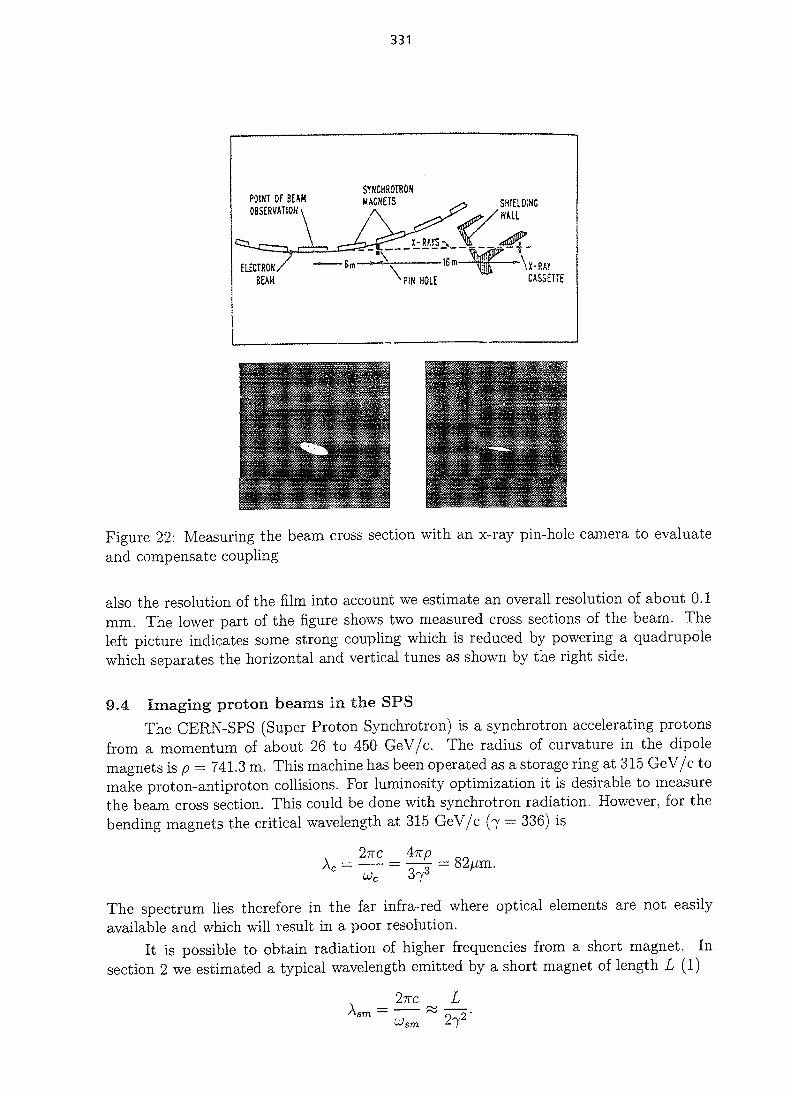
331

POINT OF BEAMOBSERVATION

SYNCHROTRONMAGNETS SHIELDING

WML

ELECTRONBEAM PIN HOLE

Figure 22: Measuring the beam cross section with an x-ray pin-hole camera to evaluateand compensate coupling

also the resolution of the film into account we estimate an overall resolution of about 0.1mm. The lower part of the figure shows two measured cross sections of the beam. Theleft picture indicates some strong coupling which is reduced by powering a quadrupolewhich separates the horizontal and vertical tunes as shown by the right side.

9.4 Imaging proton beams in the SPSThe CERN-SPS (Super Proton Synchrotron) is a synchrotron accelerating protons

from a momentum of about 26 to 450 GeV/c. The radius of curvature in the dipolemagnets is p = 741.3 m. This machine has been operated as a storage ring at 315 GeV/c tomake proton-antiproton collisions. For luminosity optimization it is desirable to measurethe beam cross section. This could be done with synchrotron radiation. However, for thebending magnets the critical wavelength at 315 GeV/c (7 = 336) is

The spectrum lies therefore in the far infra-red where optical elements are not easilyavailable and which will result in a poor resolution.

It is possible to obtain radiation of higher frequencies from a short magnet. Insection 2 we estimated a typical wavelength emitted by a short magnet of length L (1)

2TTC

CO, 27.2'

332

-03 -O2 -0J 0 CU 02 m 09 *

Figure 23: Magnetic field between two SPS dipole magnets

lOOOf

100

dvdQ

10

0.1

-

•

I11 *

(300IGeV

1 •

1

IIi

1

11

I

!

!

^400 GeV

A'AAI

II

j 'i*»*

' j\i]

•

-

(1

100 THi 1000

full acceptance

=.r.r restricted occept

Figure 24: Spectrum of the 'short magnet' radiation. Left: observed on axis (9 = 0).Right: solid line, integrated over the solid angle; dashed line, integrated over the detectoracceptance; dot-dash line, radiation from the adjacent long magnet; dotted line, spectralsensitivity of the photo-muliplier used for detection.

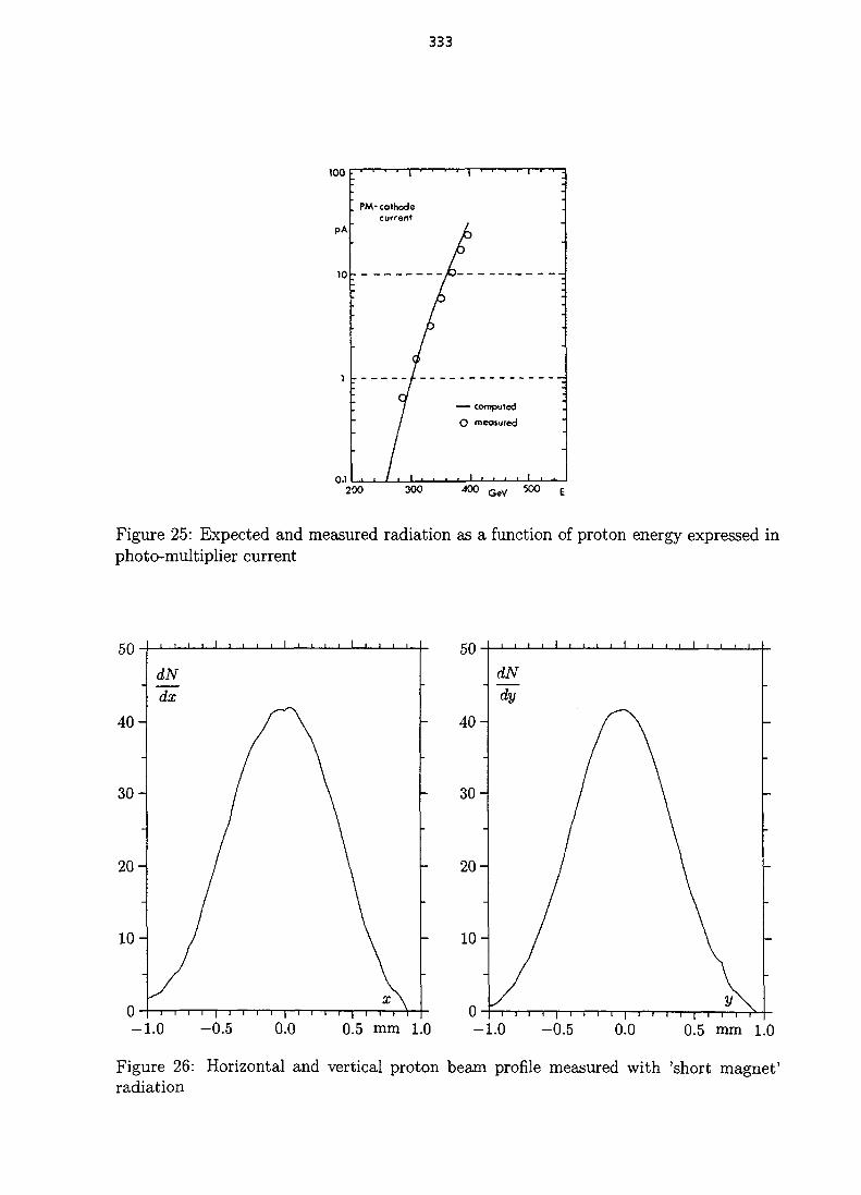
333

100

PA

10

0.1

^ . . . . . . .

. PM-cathodecurrent

: /

/

i'

—— computed

O measured

i • • -

•

-

-

•

200 300 400 G e V 500 E

Figure 25: Expected and measured radiation as a function of proton energy expressed inphoto-multiplier current

-1.0 -0.5 0.5 mm 1.0 -1.0 -0 .5 0.5 mm 1.0

Figure 26: Horizontal and vertical proton beam profile measured with 'short magnet'radiation

334

In order to get visible light of A = 600 nm from protons at 315 GeV/c we need a magnetof length L « 0.135 m which looks reasonable.

The spectrum of the radiation from a short magnet observed at a given angle 6 isgiven by the Fourier transform of the magnetic field (22). It is the same for the radiationcoming from a short magnet with field jBsm(s) or from a depression of a dipole field Bo

between two magnets having the form BQ - Bsm(s). This is only true for the short magnetradiation and obviously not for the one emitted in the long magnets. For the protons inthe SPS a short magnet of length « 0.15 m produces a spectrum which is far above theone of the radiation coming from the long magnets and can be treated separately.

In the case of the SPS the field variation between two dipole magnets shown in Fig. 23has been used as source of radiation to image the proton beam [10]. The spectrum hasbeen calculated with the equation (22) and is plotted in Fig. 24 for the radiation emittedat two proton energies. The figure on the left shows the spectrum observed on axis 8 = 0.It shows sharp maxima and minima created by constructive and destructive interferencebetween the radiation originating from the two magnet edges. On the right side of Fig. 24this radiation is integrated over all angles (solid line) which results in a smoother curvebecause the interference frequencies depend on the observation angle 6. The dashed curvesgive the radiation integrated over the angular acceptance of the detector. The radiationcoming from the long magnets is also shown in the figure as a 'dot-dash' line. At lowfrequencies this radiation will of course dominate. Finally the spectral response of thephoto-multiplier used for detection is shown as a dotted curve. A convolution of thisspectral power within the acceptance and the spectral sensitivity of the photo-multipliergives the expected output current of the latter. This is plotted in Fig. 25 together with themeasured date which shows very good agreement. A measurement of the horizontal andvertical beam profile with this system is shown in Fig. 26. Since the frequency emitted bythe short magnet is proportional to I/72, the emitted spectrum lies in the visible rangeonly for relatively large proton energies above about 270 GeV. Later an undulator hasbeen installed [11] which produced more light than the magnet gap and extended theenergy range over which radiation could be observed. Furthermore, a wire scanner wasinstalled later which can measure the beam size also at injection.

9.5 Measurement of the angular spread with undulator radiationA direct measurement of the synchrotron radiation distribution gives the angular

spread of the particles in the beam. The resolution is limited by the natural opening angleof the emitted radiation. Such a measurement has been carried out to measure the beamin the electron-positron storage ring PEP at SLAC [12]. An undulator has been used asa radiation source which permits to measure the vertical and horizontal angular spreadin the beam. A wavelength of the emitted radiation is selected by a monochromator andobserved on a screen at a distance L from the source as shown in Fig. 27. The measuredundulator spectrum and photon beam pictures taken at two different selected wavelengthsare shown in Fig. 28. The first picture is within the fundamental peak of the undulatorspectrum (but unfortunately not quite at its maximum). It shows an elliptic distributionof the radiation around the axis. This distribution was scanned with a pinhole to get ahorizontal and a vertical cut through the distribution with the rms widths ax and ay atthe screen. The second measurement was only taken for comparison. It shows that thesecond undulator harmonics has a distribution with vanishing intensity on axis 6 = 0.

335

undulator

storagering monochromator

Figure 27: Direct angular distribution measurement of the monochromatized undulatorradiation

Figure 28: Measured undulator spectrum and photon beam picture

To analyze the measurement we have to consider the other effects which influencethe measured photon beam size at the screen. The pinhole used for scanning had theform of a square of side a = 0.5 mm which corresponds to <Tpinhole = a/\/T2 = 0.144mm. The energy spread together with the dispersion and its derivative at the sourcegive a contribution aD = (I>(0) + D'(0)L)aE/E at the screen. For the natural angulardistribution of the photon beam at the fundamental frequency u>io we take the one givenby (28) and plotted in Fig. 14 valid for a weak field undulator as an approximation for ourexperiment which uses a somewhat stronger field. We said before that this distributionhas a diverging variance for the opening angle 9. However, in this experiment cuts in thex and y-direction were made for which we find

Finally the emittance of the beam gives the contribution we want to measure. We showedin section 7 that we can define a beta function fi(L) for a photon beam on the screen andget the relation between its size and the emittance e of the electron beam

The measured size a of the photon beam on the screen is therefore composed of thecontributions

a2 = o\ + a%nhole + a2 + a2

from which the emittance can be obtained. Its value in this measurement was about 35%larger than expected, probably due to the limited accuracy with which the beta functionis known.

336

References

[I] A. Hofmann; "Characteristics of Synchrotron Radiation", lectures at this school.

[2] A. Hofmann, F. Meot; "Optical Resolution of Beam Cross-Section Measurements bymeans of Synchrotron Radiation", Nucl. Instr. and Meth. 203 483 (1982).

[3] O. Chubar; "Resolution Improvement in Beam Profile Measurements with SynchrotronLight", Proc. of the IEEE Part. Accel. Conf. PAC-93, (1993) p. 2510.

[4] A. Andersson, M. Ericsson, O. Chubar; "Beam Profile Measurements with VisibleSynchrotron Light on Max-II", Proc. EPAC 1996, Sitges (Barcelona) p. 1689.

[5] M. Abramowitz, I. Stegun; "Handbook of Mathematical Functions", 11.4.28; Dover1970.

[6] M. Placidi; private communication 1986.

[7] A. Hofmann, "Beam Diagnostics with Synchrotron Radiation", Joint CERN-US-JapanAccelerator School, held at the Shonan Village Center, Hayamamachi, Japan, Septem-ber 1996.

[8] C. Bovet, G. Burtin, R.J. Colchester, B. Halvarsson, R. Jung, S. Levitt, J.M. Vouillot,"The LEP Synchrotron Light Monitors", CERN SL/91-25 and 1991 IEEE ParticleAccelerator Conference, p. 1160.

[9] A. Hofmann, K.W. Robinson; "Measurement of the Cross Section of a High-EnergyElectron Beam by means of the X-Ray Portion of the Synchrotron Radiation", Proc.1971 Particle Accel. Conference, IEEE Trans, on Nucl. Sci. NS 18-3 (1971) p. 973.

[10] R. Bossart, J. Bosser, L. Burnod, R. Coisson, E. D'Amico, A. Hofmann, J. Mann;"Observation of Visible Synchrotron Radiation Emitted by a High-Energy ProtonBeam at the Edge of a Magnetic Field", Nucl. Instr. and Meth. 164 375 (1979).

[II] J. Bosser, L. Burnod, R. Coisson, G. Feroli, J. Mann, F. Meot; "Characteristics of theRadiation Emitted by Protons and Antiprotons in an Undulator", CERN-SPS/83-5(1983).

[12] M. Brendt, G. Brown, R. Brown, J. Cerino, J. Christensen, M. Donald, B. Graham,R. Gray, El Guerra, C Harris, A. Hofmann. C Hollosi, T. Jones, J. Jowett, R. Liu, P.Morton, J.M. Paterson, R. Pennacchi, L. Rivkin, T. Taylor, T. Troxel, F. Turner, J.Turner, P. Wang, H. Wiedemann, H. Winick; "Operation of PEP in a Low EmittanceMode", Proc. of the 1987 IEEE Particle Accelerator Conference, p. 461.

337

THE STORAGE RING FREE-ELECTRON LASER

RJ.Bakker1

CEA/DSM/DRECAM/SPAM, Cen-Saclay, FranceLURE, Orsay, France

AbstractIn a storage-ring free-electron laser (SRFEL) the circulating currentof a ring forms the driver for the free-electron laser. The storage ringprovides excellent beam parameters and it seems an ideal candidatefor a tuneable laser for the ultra-violet and vacuum ultraviolet spectralrange. At present experiments demonstrate stable operation with goodspectral properties in the UV spectral range, i.e. down to a wavelengthof 240 nm. Construction of such a device is non-trivial, however, andoptimisation of both the laser and the storage ring is necessary. TheSRFEL also has a more complex dynamic behaviour as compared tolinac-driven FEL's since the dynamics of both the laser and thestorage ring are involved. Here follows a discussion of both the designand the operational aspects of this device.

1. INTRODUCTION

The storage ring free-electron laser (SRFEL) employs the circulating current in astorage ring to drive the gain of the laser. Figure 1 shows the fundamental layout of such adevice. An undulator is located in a dispersion-free section of the ring. Next, the synchrotronradiation is captured in a resonator to enable the interaction between the electrons and theoptical field. As a FEL driver, the storage-ring has excellent beam parameters, e.g., a lowenergy spread and a low emittance. Because of the typical beam-energy of rings, the laser isspecially suited for operation at short wavelengths (< 700 nm). Difficulties with optics will,most probably, limit the use to the vacuum ultra-violet (VUV) spectral range.

stocbon bunch

Fig. 1 Schematic layout of the Storage Ring Free Electron Laser (SRFEL). The radiation thatis produced by the circulating electrons in the storage-ring passing through an undulator iscaptured between two mirrors. Due to the interaction between the circulating electronbunches and the stored optical pulse, the characteristic FEL process can take place. Theexample sketched is typical for a two-bunch mode of operation, i.e. two bunches in thestorage ring that both interact with one optical pulse in the resonator.

1 Correspondence address: Berliner Elektronenspeicherring Gesellschaft fur Synchiotronstrahlung mbH,Lentzeallee 100, D-14195 Berlin, Germany

338

The first operation of a storage-ring based FEL was demonstrated at a wavelength of650 ran on ACO in Orsay, France in 1983 [1]. Since then the field has become maturer andon several rings such as VEPP-3 (Novosibirsk, Russia) [2], UVSOR (Okazaki, Japan) [3] andSuper ACO (Orsay, France) [4] the FEL process has been studied. New challenging projectsare starting, or close to, operation, e.g. at Duke University (Durham, USA) [5] and DELTA(Dortmund, Germany) [6]. A more complete overview is given in Table 1. Recentdevelopments also demonstrated the feasibility of the SRFEL as a light source for userexperiments. For example at Super ACO where up to 50% of the FEL beam-time is used tofacilitate user experiments [11]. The SRFEL has the advantage that it is naturallysynchronised with the additional beam lines along the ring. One thus has two synchronisedhigh-brilliance polarised light sources with tuneable wavelength in the UV or VUV. TheSRFEL forms an ideal tool for pump-probe experiments with a high repetition rate. Forexample at Super ACO such experiments are performed with a repetition rate of 8.3 MHz.Here the FEL either serves as pump or as probe [11].

Table 1

Storage-ring free-electron laser facilities

Project

ACODELTADuke Univ.KEKNIJI-IVSoleilSuper ACOTERASUVSORVEPP-3

Location

France, OrsayGermany, DortmundUSA, DurhamJapan, TsukubaJapan, TsukubaFranceFrance, OrsayJapan, TsukubaJapan, OkazakiRussia, Novosibirsk

Ref.

[1][6][5][7][8][9][4][10][3][21

Status"

acoc0

p0

a0

a

E[GeV]

0.16-0.250.5-1.510.750.241.50.6-0.80.240.50.35-0.5

[nm]

460-650100-40025-400170-220350100-350350-600598290-500240-690

Gain[%]

0.4

2.3

2.5>0.1

10.0

Remarks

First SRFELDedicatedDedicated

DedicatedSynchrotronSynchrotron

Nucl. phys.

" a - abandoned, c - construction, o - operational, p - proposed

In the SRFEL the beam in the storage ring serves as a source for the FEL interaction.Apart from this the SRFEL is not fundamentally different from other types of free-electronlasers. Hence, all aspects that are of importance for a (linac driven) FEL are similarlyimportant in the SRFEL. The storage ring has several properties that make it a good choice asa driver. In a modern ring it is possible to obtain a high current in combination with anexcellent beam quality, for example, a stable beam with a low energy-spread, a smallemittance, and a high peak current. It is important to note that in a storage ring the beam isrecirculated. This gives the storage ring the advantages of 100% duty cycle (the beam runscontinuously for many hours). Because of limitations to the rf power needed, conventionallinacs generally operate with macro pulses with a duty cycle less than one percent. Therecirculation also causes a coupling between the dynamics of the laser and ring. This makesthe storage ring a different and a more complex beam source. Consequently the performance,characteristics and dynamic behaviour of the SRFEL are different from FEL's using othertypes of accelerators. The achievable output-power of the SRFEL is, for example, differentfrom one driven by a linear accelerator. In the storage ring the recirculation limits theachievable peak-power. The peak-power of an SRFEL is therefore lower than the peak-powerof a linac driven FEL. Because of its 100 % duty cycle the average power level is muchhigher, however. Typical values are depicted in Figs. 2 and 3.

339

1eVphoton energy

10 eV 100 eV 1keV 10keV

1TW

^7 ASRFEL coherent

hannonic generation

SR-FELs

— — linac FEL*

Exsistino facilitiesA VEPP-3. RutB Boeing, USAC APEL.USAD Super ACO, FrancaE UVSOR. Japan

Other facilitiesF1 DELTA, FRGF2 Duke, USAF3 SOLEIL, FrancoG DUV, BNL, USAH CEBAF.USAJ SLAC, USAK TESLA, FRG

10 nm 1 jun 100 nm 10 nm

wavelength (nm)1 nm 0.1 nm

Fig. 2 Overview of achieved and predicted peak powers for several synchrotron and FELlight-sources [12]. See Table 1 for references to the SRFEL light-sources.

H 1028

I 101

*-—«=

BNL DUV FEL

donga ring FELs

— ,

DESY TESLA

FEL

^ —

«hgaratorag

VUV/koftX-fay*

SLACIOS

" ^

•nrton I

• rings

hartX-r»y»

tkVUV/MtXnyt \ | hard*f»yi\l

\ M3rd gananton tknga rings

10° 101 102 103

photon energy [eVJ

10' 10°

Fig. 3 Achieved and predicted average spectral brightness of several synchrotron and FELlight-sources [13]. See Table 1 for references to the SRFEL light-sources.

The performance of the linac-based and the ring-based FEL's are different by otherfactors as well. The laser micropulse length in the linac is typically shorter than that of thering system, i.e. down to a sub-pico-second level in a linac versus several tens of pico-secondsfor a ring. It is expected that the achievable peak current and, hence, the laser gain, of a linac-based system can be much higher. As a result the linac based FEL is a better-suited candidatefor a single-pass mode of operation where spontaneous emission will be amplified tosaturation in a single-pass (SASE - Self-Amplified Spontaneous Emission). This is especiallyimportant for short-wavelength operation where presently no mirror material is available forresonators, i.e. wavelengths less than 50 nm. In terms of stability and the quality (e.g. spectralwidth) of the emitted radiation, it is more advantageous to use a resonator. Due to this and thefact that the beam can be more stable in a ring, the SRFEL is a better candidate for stable usersource at wavelengths where optics are available. Furthermore, unlike the alternative, the

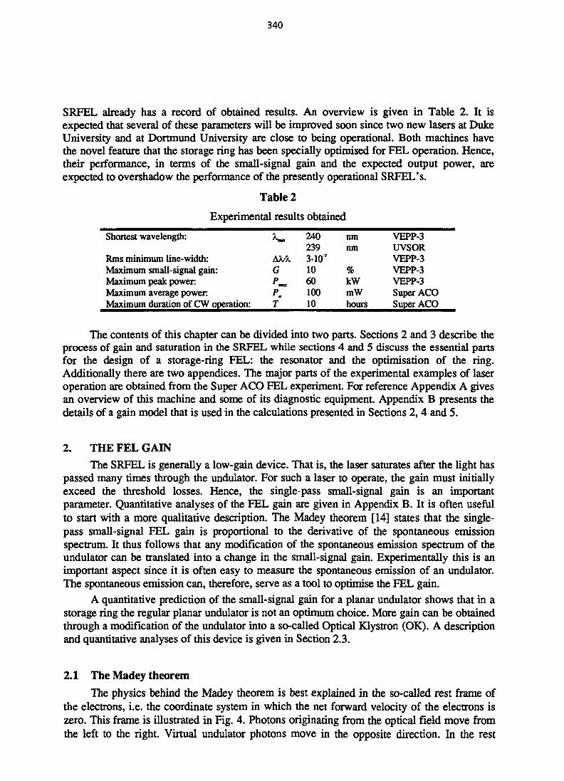
340

SRFEL already has a record of obtained results. An overview is given in Table 2. It isexpected that several of these parameters will be improved soon since two new lasers at DukeUniversity and at Dortmund University are close to being operational. Both machines havethe novel feature that the storage ring has been specially optimised for FEL operation. Hence,their performance, in terms of the small-signal gain and the expected output power, areexpected to overshadow the performance of the presently operational SRFEL's.

Table 2

Experimental results obtained

Shortest wavelength:

Rms minimum line-width:Maximum small-signal gain:Maximum peak power:Maximum average powerMaximum duration of CW operation:

AM.GP~P.T

2402393-107

106010010

nmnm

%kWmWhours

VEPP-3UVSORVEPP-3VEPP-3VEPP-3Super ACOSuper ACO

The contents of this chapter can be divided into two parts. Sections 2 and 3 describe theprocess of gain and saturation in the SRFEL while sections 4 and 5 discuss the essential partsfor the design of a storage-ring FEL: the resonator and the optimisation of the ring.Additionally there are two appendices. The major parts of the experimental examples of laseroperation are obtained from the Super ACO FEL experiment. For reference Appendix A givesan overview of this machine and some of its diagnostic equipment. Appendix B presents thedetails of a gain model that is used in the calculations presented in Sections 2, 4 and 5.

2. THE FEL GAIN

The SRFEL is generally a low-gain device. That is, the laser saturates after the light haspassed many times through the undulator. For such a laser to operate, the gain must initiallyexceed the threshold losses. Hence, the single-pass small-signal gain is an importantparameter. Quantitative analyses of the FEL gain are given in Appendix B. It is often usefulto start with a more qualitative description. The Madey theorem [14] states that the single-pass small-signal FEL gain is proportional to the derivative of the spontaneous emissionspectrum. It thus follows that any modification of the spontaneous emission spectrum of theundulator can be translated into a change in the small-signal gain. Experimentally this is animportant aspect since it is often easy to measure the spontaneous emission of an undulator.The spontaneous emission can, therefore, serve as a tool to optimise the FEL gain.

A quantitative prediction of the small-signal gain for a planar undulator shows that in astorage ring the regular planar undulator is not an optimum choice. More gain can be obtainedthrough a modification of the undulator into a so-called Optical Klystron (OK). A descriptionand quantitative analyses of this device is given in Section 2.3.

2.1 The Madey theorem

The physics behind the Madey theorem is best explained in the so-called rest frame ofthe electrons, i.e. the coordinate system in which the net forward velocity of the electrons iszero. This frame is illustrated in Fig. 4. Photons originating from the optical field move fromthe left to the right. Virtual undulator photons move in the opposite direction. In the rest

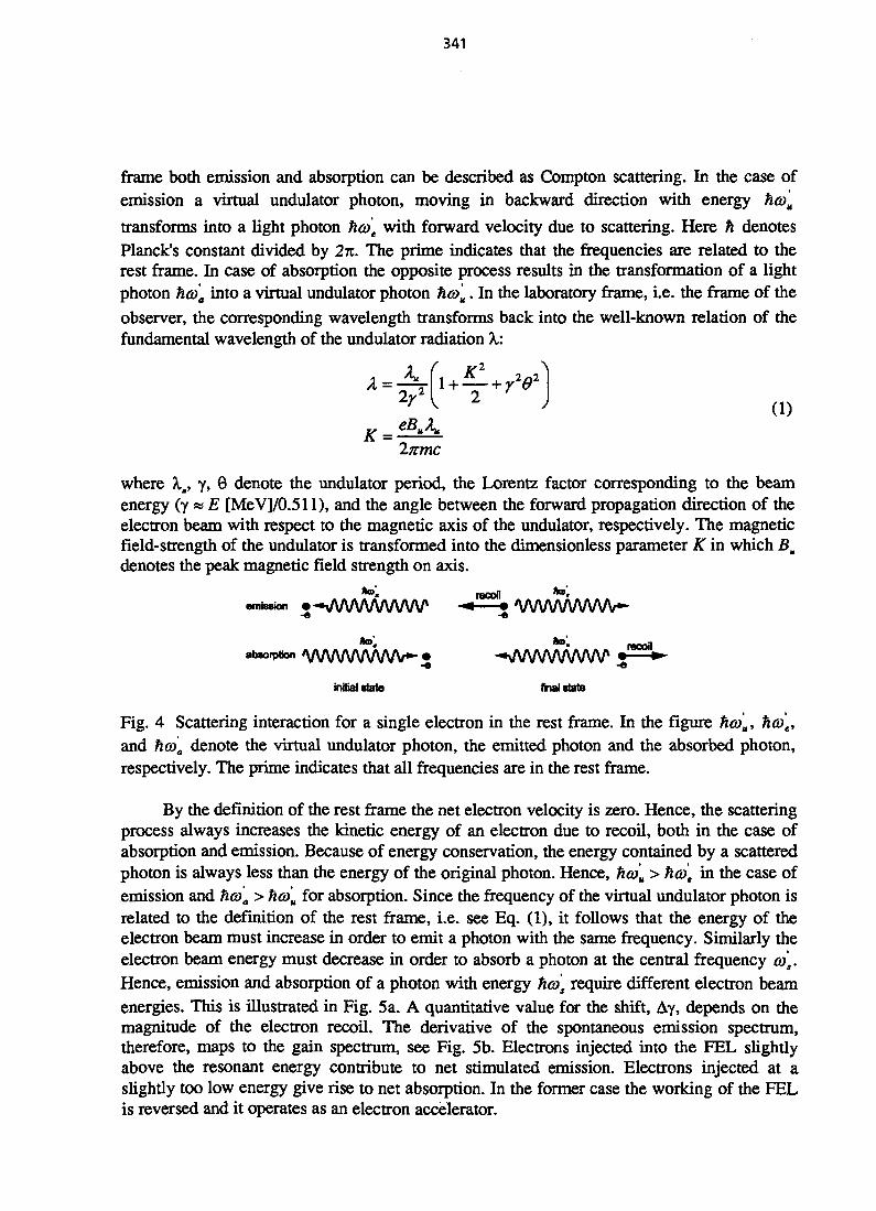
341

frame both emission and absorption can be described as Compton scattering. In the case ofemission a virtual undulator photon, moving in backward direction with energy hcou

transforms into a light photon ho)e with forward velocity due to scattering. Here h denotesPlanck's constant divided by 2n. The prime indicates that the frequencies are related to therest frame. In case of absorption the opposite process results in the transformation of a lightphoton ha>a into a virtual undulator photon hcou. In the laboratory frame, i.e. the frame of theobserver, the corresponding wavelength transforms back into the well-known relation of thefundamental wavelength of the undulator radiation X:

K

2nmc

where Xu, y, 0 denote the undulator period, the Lorentz factor corresponding to the beamenergy (y « E [MeV]/0.511), and the angle between the forward propagation direction of theelectron beam with respect to the magnetic axis of the undulator, respectively. The magneticfield-strength of the undulator is transformed into the dimensionless parameter K in which Bm

denotes the peak magnetic field strength on axis.

*">• recoil to«

emission •WWVWWW* -* • 'WWWWW-

ateorpaon V W W W W W * WWWWVW

initial state final state

Fig. 4 Scattering interaction for a single electron in the rest frame. In the figure ho)u, hcoe,and ho)a denote the virtual undulator photon, the emitted photon and the absorbed photon,respectively. The prime indicates that all frequencies are in the rest frame.

By the definition of the rest frame the net electron velocity is zero. Hence, the scatteringprocess always increases the kinetic energy of an electron due to recoil, both in the case ofabsorption and emission. Because of energy conservation, the energy contained by a scatteredphoton is always less than the energy of the original photon. Hence, ha>u > ha>t in the case ofemission and Tiaia > hcou for absorption. Since the frequency of the virtual undulator photon isrelated to the definition of the rest frame, i.e. see Eq. (1), it follows that the energy of theelectron beam must increase in order to emit a photon with the same frequency. Similarly theelectron beam energy must decrease in order to absorb a photon at the central frequency a>s.Hence, emission and absorption of a photon with energy ha>s require different electron beamenergies. This is illustrated in Fig. 5a. A quantitative value for the shift, Ay, depends on themagnitude of the electron recoil. The derivative of the spontaneous emission spectrum,therefore, maps to the gain spectrum, see Fig. 5b. Electrons injected into the PEL slightlyabove the resonant energy contribute to net stimulated emission. Electrons injected at aslightly too low energy give rise to net absorption. In the former case the working of the FELis reversed and it operates as an electron accelerator.

342

0.6

0.4

^ 0.2

JL 0.0

-0.4

•0.6 k

' (b)

absorttai \ J

>«v emission

I.

I.

I.

- 1 1 3 5

Ay/y (a.u)

Fig. 5 Emission and absorption spectrum of an electron pass through a two-wave PEL (a)and the resulting gain spectrum (b).

2.2 The FEL gain for a planar undulator

This text follows the gain calculations made by Dattoli et al. [15]. The peak single-passgain for a perfect one-dimensional electron beam, i.e. no energy spread and infinitely smalltransverse beam-size, can be found to be

Go = 0 . 2 7 ^ 0 (2)

where g0 is the so-called gain parameter which for a planer undulator and low gain (g0 < 1) isgiven by

(3)

where J, IA, and N denote the electron current density, the Alfve'n current (*17 kA), and thenumber of undulator periods, respectively. The parameter / /

(4)K2

4 + 2K"

accounts for the gain reduction due to the periodic detuning of the electrons in a planarundulator (see Ref. [16] p. 73), where Jo and Jt are Bessel functions of the first kind.

The transverse overlap of the electron beam and the EM wave is usually taken intoaccount by multiplication of the gain parameter with a heuristic filling factor, for a narrowelectron beam defined as the ratio of the transverse cross section of the electron beam and theEM wave. Under the assumption of a diffraction-limited Gaussian beam, the averagetransverse cross section of the EM wave along the undulator is proportional to the undulatorlength Nkm, and the wavelength X, see Section 4.1. For an optimum overlap the filling factor,F, is found to be [17]

1 V

7 (5)

where the transverse cross section of the electron beam, averaged along the undulator, isdenoted as St. Substitution of the Eqs.(5), (3) and (1) into Eq. (2) leads to

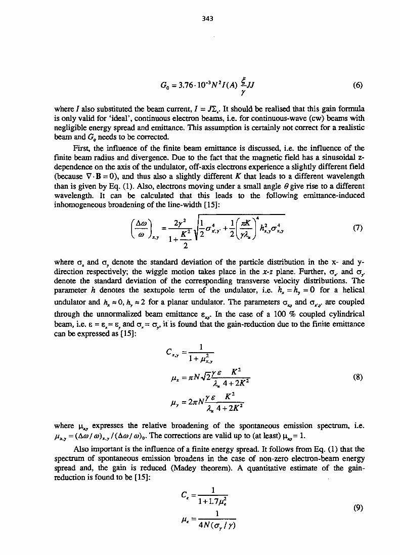
343

Go = 3.76- 10"3iV2/(A) i / 7 (6)r

where / also substituted the beam current, / = TLt. It should be realised that this gain formulais only valid for 'ideal', continuous electron beams, i.e. for continuous-wave (cw) beams withnegligible energy spread and emittance. This assumption is certainly not correct for a realisticbeam and Go needs to be corrected.

First, the influence of the finite beam emittance is discussed, i.e. the influence of thefinite beam radius and divergence. Due to the fact that the magnetic field has a sinusoidal z-dependence on the axis of the undulator, off-axis electrons experience a slightly different field(because V B = 0), and thus also a slightly different K that leads to a different wavelengththan is given by Eq. (1). Also, electrons moving under a small angle 0give rise to a differentwavelength. It can be calculated that this leads to the following emittance-inducedinhomogeneous broadening of the line-width [15]:

where ax and oy denote the standard deviation of the particle distribution in the x- and y-direction respectively; the wiggle motion takes place in the x-z plane. Further, a^ and ay

denote the standard deviation of the corresponding transverse velocity distributions. Theparameter h denotes the sextupole term of the undulator, i.e. hx = hy = 0 for a helical

undulator and hx»0,hy»2 for a planar undulator. The parameters av and a^. are coupled

through the unnormalized beam emittance ev. In the case of a 100 % coupled cylindricalbeam, i.e. e = ex= s and ox = ay, it is found that the gain-reduction due to the finite emittancecan be expressed as [15]:

C =•

where p,v expresses the relative broadening of the spontaneous emission spectrum, i.e.pxy = (Afi>/fi))x>y /(ACD/O>)0. The corrections are valid up to (at least) \iv= 1.

Also important is the influence of a finite energy spread. It follows from Eq. (1) that thespectrum of spontaneous emission broadens in the case of non-zero electron-beam energyspread and, the gain is reduced (Madey theorem). A quantitative estimate of the gain-reduction is found to be [ 15]:

r - 1

'"1 + 1.7/4f (9)

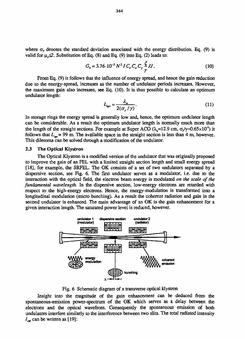
344

where a r denotes the standard deviation associated with the energy distribution. Eq. (9) isvalid for \ie<2. Substitution of Eq. (8) and Eq. (9) into Eq. (2) leads to:

G0 = 3.7610"3 N2ICeCxCy£jJ. (10)Y

From Eq. (9) it follows that the influence of energy spread, and hence the gain reductiondue to the energy-spread, increases as the number of undulator periods increases. However,the maximum gain also increases, see Eq. (10). It is thus possible to calculate an optimumundulator length:

LOp,=2(ar/y)

(11)

In storage rings the energy spread is generally low and, hence, the optimum undulator lengthcan be considerable. As a result the optimum undulator length is normally much more thanthe length of the straight sections. For example at Super ACO (^=12.9 cm, a/y=0.65xl0'3) itfollows that L<p/= 99 m. The available space in the straight section is less than 4 m, however.This dilemma can be solved through a modification of the undulator.

2.3 The Optical KlystronThe Optical Klystron is a modified version of the undulator that was originally proposed

to improve the gain of an FEL with a limited straight section length and small energy spread[18], for example, the SRFEL. The OK consists of a set of two undulators separated by adispersive section, see Fig. 6. The first undulator serves as a modulator, i.e. due to theinteraction with the optical field, the electron beam energy is modulated on the scale of thefundamental wavelength. In the dispersive section, low-energy electrons are retarded withrespect to the high-energy electrons. Hence, the energy-modulation is transformed into alongitudinal modulation (micro bunching). As a result the coherent radiation and gain in thesecond undulator is enhanced. The main advantage of an OK is the gain enhancement for agiven interaction length. The saturated power level is reduced, however.

undulator 1(modulator)

dispersive section undulator 2(radiator)

coherentemission

Fig. 6 Schematic diagram of a transverse optical klystronInsight into the magnitude of the gain enhancement can be deduced from the

spontaneous-emission power-spectrum of the OK which serves as a delay between theelectrons and the optical wavefront. Consequently the spontaneous emission of bothundulators interfere similarly to the interference between two slits. The total radiated intensitylOK can be written as [19]:

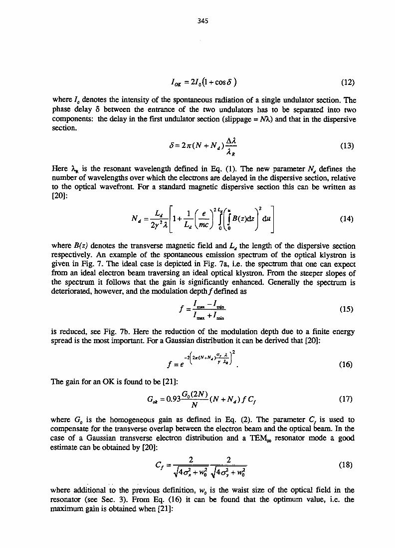
345

IOK=2I0(l + cosS) (12)

where Io denotes the intensity of the spontaneous radiation of a single undulator section. Thephase delay 5 between the entrance of the two undulators has to be separated into twocomponents: the delay in the first undulator section (slippage = NX) and that in the dispersivesection.

^ (13)

Here \ is the resonant wavelength defined in Eq. (1). The new parameter Nd defines thenumber of wavelengths over which the electrons are delayed in the dispersive section, relativeto the optical wavefront. For a standard magnetic dispersive section this can be written as[20]:

(14)" 2y2A

where B(z) denotes the transverse magnetic field and Ld the length of the dispersive sectionrespectively. An example of the spontaneous emission spectrum of the optical klystron isgiven in Fig. 7. The ideal case is depicted in Fig. 7a, i.e. the spectrum that one can expectfrom an ideal electron beam traversing an ideal optical klystron. From the steeper slopes ofthe spectrum it follows that the gain is significantly enhanced. Generally the spectrum isdeteriorated, however, and the modulation depth/defined as

t _ mix ~ nrin (15)

mix mm

is reduced, see Fig. 7b. Here the reduction of the modulation depth due to a finite energyspread is the most important. For a Gaussian distribution it can be derived that [20]:

(16)

The gain for an OK is found to be [21]:

^ ^ fCf (17)

where Go is the homogeneous gain as defined in Eq. (2). The parameter C} is used tocompensate for the transverse overlap between the electron beam and the optical beam. In thecase of a Gaussian transverse electron distribution and a TEM^, resonator mode a goodestimate can be obtained by [20]:

2 2

/ 4 ^ ^ ^ 4 ^ £

where additional to the previous definition, w0 is the waist size of the optical field in theresonator (see Sec. 3). From Eq. (16) it can be found that the optimum value, i.e. themaximum gain is obtained when [21]:

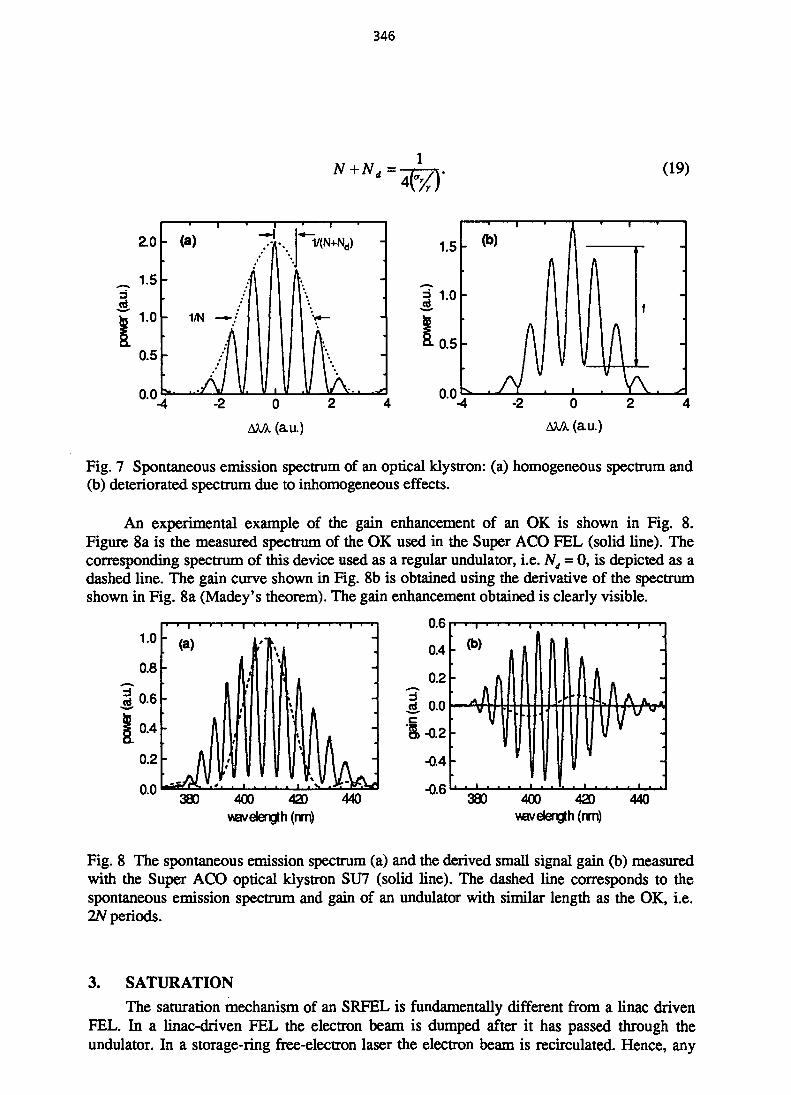
346

(19)

20

1.5

1.0

0.5}-

- (a)

- 1/N

1 ' ~i.

y 11 V.v

* i "

k -\l\k. ':.

-2 0 2(au.)

Fig. 7 Spontaneous emission spectrum of an optical klystron: (a) homogeneous spectrum and(b) deteriorated spectrum due to inhomogeneous effects.

An experimental example of the gain enhancement of an OK is shown in Fig. 8.Figure 8a is the measured spectrum of the OK used in the Super ACO FEL (solid line). Thecorresponding spectrum of mis device used as a regular undulator, i.e. Nd = 0, is depicted as adashed line. The gain curve shown in Fig. 8b is obtained using the derivative of the spectrumshown in Fig. 8a (Madey's theorem). The gain enhancement obtained is clearly visible.

380 400 420wavelength (nm)

440 380 400 420 440wavelength (nm)

Fig. 8 The spontaneous emission spectrum (a) and the derived small signal gain (b) measuredwith the Super ACO optical klystron SU7 (solid line). The dashed line corresponds to thespontaneous emission spectrum and gain of an undulator with similar length as the OK, i.e.2N periods.

3. SATURATION

The saturation mechanism of an SRFEL is fundamentally different from a linac drivenFEL. In a linac-driven FEL the electron beam is dumped after it has passed through theundulator. In a storage-ring free-electron laser the electron beam is recirculated. Hence, any

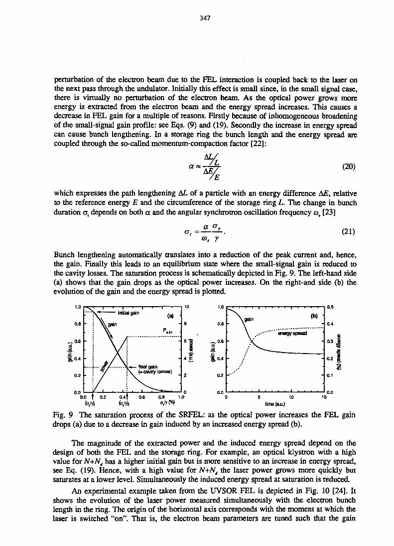
347

perturbation of the electron beam due to the FEL interaction is coupled back to the laser onthe next pass through the undulator. Initially this effect is small since, in the small signal case,there is virtually no perturbation of the electron beam. As the optical power grows moreenergy is extracted from the electron beam and the energy spread increases. This causes adecrease in FEL gain for a multiple of reasons. Firstly because of inhomogeneous broadeningof the small-signal gain profile: see Eqs. (9) and (19). Secondly the increase in energy spreadcan cause bunch lengthening. In a storage ring the bunch length and the energy spread arecoupled through the so-called momentum-compaction factor [22]:

(20)

which expresses the path lengthening AL of a particle with an energy difference A£, relativeto the reference energy E and the circumference of the storage ring L. The change in bunchduration c t depends on both a and the angular synchrotron oscillation frequency co, [23]

a (21)

Bunch lengthening automatically translates into a reduction of the peak current and, hence,the gain. Finally this leads to an equilibrium state where the small-signal gain is reduced tothe cavity losses. The saturation process is schematically depicted in Fig. 9. The left-hand side(a) shows that the gain drops as the optical power increases. On the right-and side (b) theevolution of the gain and the energy spread is plotted.

1.0

0.00.0 t 0-2 0.4? 0.6 0.8 1.0 0 5 10 15

(<Vrt fa/A <»/yP9 time(au.)

Fig. 9 The saturation process of the SRFEL: as the optical power increases the FEL gaindrops (a) due to a decrease in gain induced by an increased energy spread (b).

The magnitude of the extracted power and the induced energy spread depend on thedesign of both the FEL and the storage ring. For example, an optical klystron with a highvalue for N+Nd has a higher initial gain but is more sensitive to an increase in energy spread,see Eq. (19). Hence, with a high value for N+Nd the laser power grows more quickly butsaturates at a lower level. Simultaneously the induced energy spread at saturation is reduced.

An experimental example taken from the UVSOR FEL is depicted in Fig. 10 [24]. Itshows the evolution of the laser power measured simultaneously with the electron bunchlength in the ring. The origin of the horizontal axis corresponds with the moment at which thelaser is switched "on". That is, the electron beam parameters are tuned such that the gain

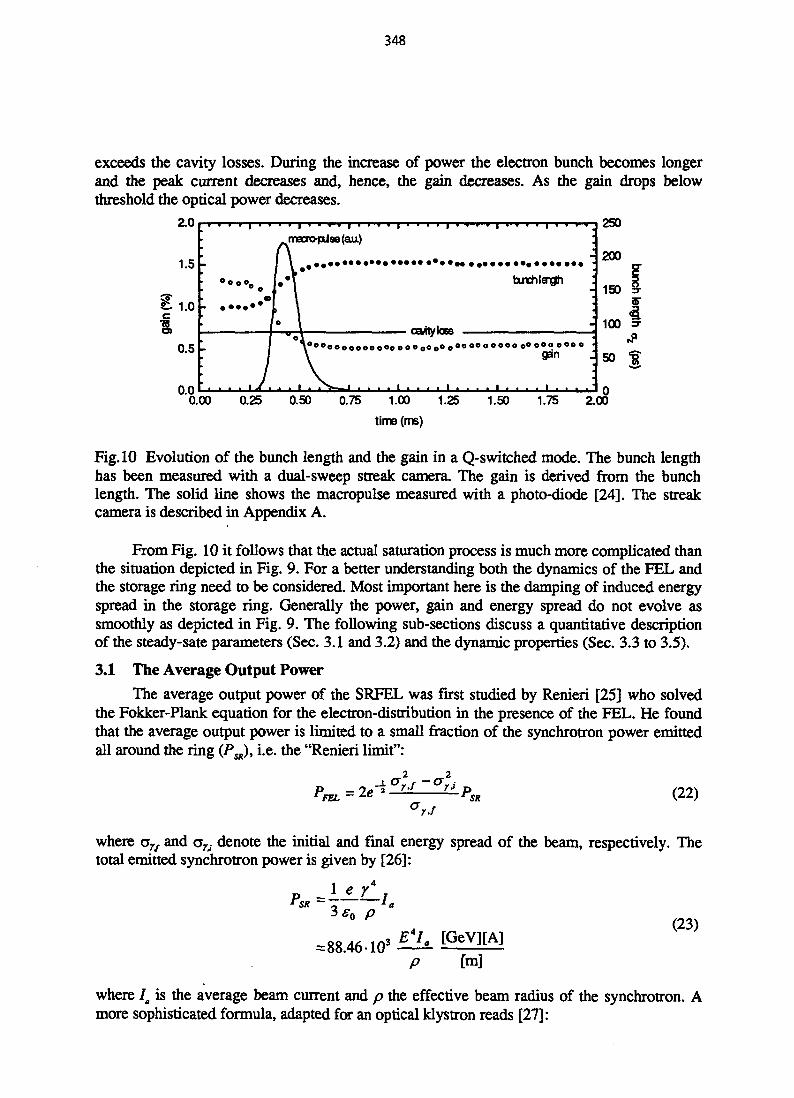
348

exceeds the cavity losses. During the increase of power the electron bunch becomes longerand the peak current decreases and, hence, the gain decreases. As the gain drops belowthreshold the optical power decreases.

2 . 0 . . . . . i . . . . i . . . . i . . . . i . . . . i . . . . i . . . . i . . . . | 2 5 0m a c r o - p U s e ( a u )

• • • • • • • • • • * • • • • <

b u x h l s t y h

CEMt/kBS

L0°°oooooooo°o <

gain

200

150 I

100 =

50 f

0.25 0.50 0.75 1.00 1.25

time (rm)

1.50 1.75

Fig. 10 Evolution of the bunch length and the gain in a Q-switched mode. The bunch lengthhas been measured with a dual-sweep streak camera. The gain is derived from the bunchlength. The solid line shows the macropulse measured with a photo-diode [24]. The streakcamera is described in Appendix A.

From Fig. 10 it follows that the actual saturation process is much more complicated thanthe situation depicted in Fig. 9. For a better understanding both the dynamics of the FEL andthe storage ring need to be considered. Most important here is the damping of induced energyspread in the storage ring. Generally the power, gain and energy spread do not evolve assmoothly as depicted in Fig. 9. The following sub-sections discuss a quantitative descriptionof the steady-sate parameters (Sec. 3.1 and 3.2) and the dynamic properties (Sec. 3.3 to 3.5).

3.1 The Average Output Power

The average output power of the SRFEL was first studied by Renieri [25] who solvedthe Fokker-Plank equation for the electron-distribution in the presence of the FEL. He foundthat the average output power is limited to a small fraction of the synchrotron power emittedall around the ring (P^), i.e. the "Renieri limit":

SR (22)

where a r / and ori denote the initial and final energy spread of the beam, respectively. Thetotal emitted synchrotron power is given by [26]:

P ~ler\3e0 P

=88.46-103 E [GeV][A]

[m]

(23)

where la is the average beam current and p the effective beam radius of the synchrotron. Amore sophisticated formula, adapted for an optical klystron reads [27]:

349

p / iog(G0/r)fOK ^cn(N + Nd) GJT **

_ mirror transmission lossestotal transmission losses (24)

r = total cavity losses

Typically the emitted synchrotron radiation is a few kW for a storage ring with a beam-energy up to 1 GeV, e.g. 10 kW for Super ACO operating at 800 MeV. The energyacceptance of a ring, and hence, the maximum possible energy spread, can go up to a fewpercent It thus follows that the total emitted FEL power is much lower than the emittedsynchrotron power. For example, at Super ACO the total emitted laser power is of the orderof 100 mW. Note, however, that this radiation is fully coherent. Hence, the brilliance of thisradiation is orders of magnitude higher than synchrotron radiation from an undulator beam-line, see Fig. 3.

It follows from Eqs. (23) and (24) that more power can be obtained at higher beamenergy and by allowing a larger increase in energy spread. Note however, that there is apractical limit to both parameters. The energy of the beam can not increase too far withoutchanging the lasing wavelength, see Eq. (1). For this, either the undulator period, or themagnetic field strength, must be increased. The former has the disadvantage that for a givenlength of the straight section, the number of periods, and hence the gain, is reduced. The lattercause problems with the mirrors, see Sec. 4.2.

An increase of energy-spread requires a significant increase in the energy acceptance ofa ring:

n me ahy(25)

where h is the harmonic number (L. (QJ2X C) and Yn is the total voltage over the rf cavities inthe ring. With a too high energy spread, as compared to the energy acceptance of the ring, thelifetime of the beam will be significantly reduced. An increase in energy acceptance is costlysince ap oc

3.2 The FEL bandwidthBoth the gain bandwidth of the FEL and the eigenmodes of the optical resonator

determine the final bandwidth of the FEL where, normally, the gain bandwidth of the lasercovers many eigenmodes of the cavity. In this, the SRFEL works similarly to any other typeof free-electron laser where the spectrum narrows on successive passes through the undulator.That is, on each pass through the undulator the spectrum of the light pulse is multiplied withthe gain spectrum of the laser. In contrast to linac driven FEL's there is no macro-pulse andthe process of line-width narrowing can continue over many more round-trips. The line widthof an SRFEL is therefore much smaller. Assuming a stable electron beam the line width cannarrow down to the transform limit. A study by Dattoli and Renieri [25] predict a laser pulse-width azJi of

(26)

350

for an undulator with N periods, a wavelength X, and an electron bunch length a,. Note thatthe laser pulse-duration is much smaller than the electron bunch duration. This is due to thefact that the optical pulse is also multiplied with the longitudinal gain profile of the laser, i.e.the longitudinal electron bunch shape. The corresponding relative bandwidth is

In practice the bandwidth is determined by the stability of the beam in the ring, however.Typical relative bandwidths for an SRFEL are in the order of 10"* to 10s depending on theway the laser is operated. An example is given in the next section. A smaller line width can beobtained by adding additional filters inside the resonator, thus artificially narrowing the gainspectrum. An experiment performed at VEPP3 has demonstrated a relative laser bandwidth of3-10"7 using an intra-cavity ethalon [28].

3.3 Influencing the FEL output 1: Cavity resynchronisation

From Eq. (23) it follows that the saturated laser power depends on the initial small-signal gain. An optimum gain requires perfect longitudinal and transverse overlap betweenthe optical pulse and the electron bunches. The transverse overlap is mainly determined by thedesign of the resonator and the machine functions inside the undulator. This will be discussedfurther in Sections 4 and 5. The longitudinal overlap can only be maintained when the round-trip time of the optical pulses in the laser resonator matches the electron-bunch distance.Hence, the optical cavity length must be matched with the electron bunch distance. Figure 11depicts this for a storage ring in a two-bunch mode of operation. In that case the resonatorlength must be one quarter of the circumference of the storage ring. This is, for example, thecase for the Super ACO FEL. Other FEL's (e.g. the Duke-FEL and the DELTA FEL) operatein single-bunch mode with a cavity length equal to half the circumference of the ring.

electron bunchM-

Fig. 11 Longitudinal synchronisation of the FEL: To maintain longitudinal overlap betweenthe optical pulse and the electron bunches, the length of the optical cavity must be tuned tomatch half the electron-bunch distance. Tuning of the synchronisation can either be done bychanging the cavity length or changing the rf frequency of the accelerating field (i.e.changing the distance between successive electron bunches).

As the cavity length is detuned with respect to the spacing between bunches, thelongitudinal overlap is reduced and, hence, the small-signal gain is reduced as well. Whilescanning the synchronisation different (dynamic) behaviour can be observed. An example ofthe modified output of the Super ACO FEL is given in Fig. 12 [29]. The figure shows themajor properties that can be observed in the case of saturation. The main curve displays theaverage power of the laser. Maximum power is obtained when the cavity length is

351

synchronised with the bunch distance. When the system is desynchronised, the saturatedpower level drops. This process is similar to other FEL's. Note that the curve shown in Fig 12is virtually symmetric around its origin. This is caused by the fact that the electron-bunchlength of the Super ACO FEL is long compared to the slippage length. In the case of (much)shorter electron bunches the curve would become more asymmetric, similar to linac drivenFEL's.

- 3 0 3 6datur*>8(r,-100MHz)

macro temporal strudura

Fig. 12 Longitudinal detuning curve of the Super ACO FEL [29]. The main curve shows theaverage output power as a function of the detuning. The top graphs give a snapshot of boththe electron bunch and the optical pulse at saturation. The bottom curve gives an indication ofthe macro-temporal structure of the saturated laser output. See text for details.

The graphs above depict the shape of the optical pulse and the electron bunch. Theshortest optical pulses are obtained for perfect synchronisation. As the synchronisationchanges the optical pulse moves forward or backwards with respect to the electron bunch,depending on the sign of the resynchronisation. Simultaneously the length of the optical pulseincreases. This is due to the fact that on one side the optical pulse, on successive round-trips,moves ahead or behind the bunch, will cease to experience gain, and dies out with the ring-down time of the cavity. On the other side of the optical pulse new light is created in theamplification process. Note that the pictures shown are not measured but serve as an exampleonly.

The bottom curve in Fig. 12 shows the macro-temporal structure of the laser. At SuperACO five distinctive zones can be observed. As the laser operates far from synchronisationfairly low power, stable laser output is observed (zones ± 2). As the system is tuned closer tosynchronisation a pulsed time-structure is present. In this zone (± 1) a semi-stable competitiontakes place between the rise time of the optical power, i.e. the increase in energy spread, andits damping given by the damping time of the storage ring. In the next sub-section this processis discussed in more detail. At perfect synchronisation (zone 0) the output power becomesunstable and large irregular fluctuations (~80 %) of the output power are observed.Simultaneously the optical pulse starts to jitter with respect to the electron bunch position.The cause of this jitter is not clear yet but can be counteracted with a feedback system. Notefurther that the size and number of zones depend on the maximum achievable gain. The zonesthat are indicated in Fig. 12 are typical for the Super ACO FEL running under optimumconditions. As the available gain drops the central zone becomes smaller or can evendisappear completely. Also at UVSOR, where the gain is lower, the central zone can not beobserved [24].

352

The pulsed time structure that was mentioned in the previous sub-section is an intrinsiceffect of the SRFEL and has been explained by Elleaume [31] using a very simple model.This model is based on Eq. (24), which indicates that small changes in the energy spread canhave a large effect on the saturated power level. This influence has been modelled as

— , —— — i. , i-i — f 3 o (28)

<fr r 0 dt rs r

where i is the dimensionless laser power normalised to unity at saturation. The laser rise timer0 is found to be

ro=r/(Go-r) (29)

where, additional to the previous definitions, T is the roundtrip time of the optical resonator.z0 can be understood as the rise time of the first laser pulse train once the gain has been sethigher than the losses, z, is the synchrotron damping time. Generally r o . « r, (for example atACO: z0« 50 |is and z,» 200 ms). Within this restriction the general solution of Eq. (28) is:

TK=XJ2TST0 (30)

where Eo is the value of E at the beginning of the pulse.The equations imply that the FEL tends to reach a stable equilibrium state after a series

of damped oscillations of period Ts damped with the synchrotron damping time zt. Anexample of a solution of Eq. (30) is given in Fig. 13. It shows that that starting from the laser-off condition the laser intensity has a pulsed behaviour before reaching a stable level. Theshape of each pulse is approximated by

* - - 2= coshi 2r0

Moreover, it can be shown that the equilibrium state is very unstable and resonant with anyperturbation of period close to TR, so that the laser has in practice a pulsed structure. Forexample, a noise of 3% affecting the energy spread can account for the randomly pulsedbehaviour.More accurate modelling can be done with the aid of numerical simulation codes, e.g. for theSuper ACO case depicted in Fig. 12. A numerical model developed by Hara et al. [32] canmake a full prediction of the curves shown in this figure.

3.4 Stabilising the laser: feedback

For use as a light source the central zone is the most interesting since it provides the highestpower levels as well as the narrowest line width. The main drawback is the instability of thelaser power and the temporal jitter. For this reason Billardon et al. [30] have developed afeedback system capable of stabilising temporal jitter. In the feedback system, a dissectormeasures the position of the optical pulse, relative to the positron bunch. When the opticalpulse moves, the position of the bunch is adjusted accordingly through a change in the rffrequency. With the feedback the laser becomes much more stable. Power level fluctuations,for example, drop below 5 %. Figures 14 and 15 show the change in temporal jitter, measuredwith a streak-camera and a dissector, respectively. In Appendix A, the diagnostic equipment

353

is described. Table 3 gives a summary of the output parameters of the laser. Note thereduction in optical pulse length with the feedback in zone 0.

Fig. 13 Evolution of the optical power of the laser: the rise time of the laser and the dampingof the synchrotron lead to a damped oscillation of the laser power as predicted by Eqs. (28) to(31).

intensity (a.u.) intensity (a.u.)•Ao.o

-100 15 2010 15 20 0 5 10time (ms) time (ms)

Fig. 14 Results of the longitudinal feedback system installed at Super ACO measured with adouble sweep streak-camera: (a) without feedback and (b) with feedback. The fast sweep isalong the vertical axis and the slow sweep along the horizontal axis. The photo's show boththe positron bunch (top) and the laser pulse (bottom). Note the difference in duration betweenthe positron bunch and the laser pulse.

Table 3

Temporal and spectral features (bandwidth and drift) of the Super ACO FEL operated at350 nm [33]

Zone

00

1,-12,-2

a,(ps)

1720

25-3535-45

0.3-1.20.6-1.50.9-1.5

(xia4)

<36-9<3

Macrostructure

CwCw

PulsedCw

Remarks

FeedbackNo feedback: Jitter up to 200 psRapid wavelength shifts

__Lowjx)wer

354

200 psH ——«

time

Beam position measurementwith feedback

30 60 150 180 12090 120

time (min)

Fig. 15 Results of the longitudinal feedback system installed at Super ACO [30]. The topgraph shows the jitter of the base of the optical pulse measured with a dissector (in the centreof the pulse the detector is saturated) without feedback (a) and with feedback (b). The bottomgraph shows the jitter of the optical pulse over two hours with feedback. Without feedbackthe jitter exceeds the positron bunch duration of 200 ps.

3.5 Influencing the FEL output 2: Q-switching (gain-switching)

One interesting consequence of the laser instability is the possibility of driving theseoscillations externally, i.e. Q- or gain-switching. By modulating the optical gain with a periodof the order of magnitude of TR it is possible to obtain very regularly spaced and reproduciblepulses, see Fig. 16. The Q-switching of SRFEL's has two great advantages over working withthe natural time structure: (i) the laser is stabilised and (ii) the laser peak power is enhancedby several orders of magnitude. If Tg is the Q-switching period a maximum is reached at To ~r0 and the peak power enhancement is about r/4r0. This factor is -103 for the ACOexperiment (and will be about the same on future experiments) although only 102 could bereached in practice. Remember that the higher the small signal gain g0, the smaller the risetime T0 and the bigger the peak power enhancement. However, the estimates given above donot take into account saturation by over bunching in the case of a high-power SRFEL. Whenthe dimensionless laser field \a\ [35] (\a\ = 4KNmeKLJE\/yzmc2 « 0.1 on ACO, Q-switchedregime, where IEI is the optical field strength) becomes of the order of unity, over-bunchingwill occur which will modify the above results. In most cases, use of the Q-switchingtechnique will drive the peak power up to the over-bunching limit.

I 1 T. nso 100 150

time (us)200

Fig. 16 Time record of the ACO laser intensity [34] for (a) "natural" operation and (b) low-frequency gain switched operation. The trace in (c) shows the switching of the gain through achange of the longitudinal overlap between the optical pulses and the bunches, i.e. changes ofthe rf frequency.

355

4. THE RESONATOR

The most commonly used resonator in an FEL is the stable two-mirror normal-incidence resonator, see Fig. 17, which will be discussed in more detail in Sec. 4.1. Its mainadvantages are its straightforward design and the possibility to obtain low loss (less than 1%)resonators with the aid of multi-coated dielectric mirrors. Furthermore, two-mirror normal-incidence resonators are also common practice in other laser systems. There are also somedrawbacks to the design, however. For example, in Sec. 4.1 it will be shown that thetolerances to resonator dimensions become more critical as the resonator length increasesrelative to the undulator length. This is specifically an important factor in the SRFEL sincemore space is required to include elements for the electron beam optics (e.g., quadrupoles anddipoles). Furthermore, the cavity length must be adjusted to match half of the bunch spacingin the storage ring in order to obtain overlap between the optical pulses and the electronbunches on each passage through the cavity. Other, and more fundamental, drawbacks arerelated to the optics required for the resonator. In Sec. 4.2 the two most prominent problemsare discussed, i.e. the occurrence of mirror degradation due to the harmonics present in thespontaneous undulator radiation and the lack of available high-reflecting optics at shorterwavelengths. Because of these problems, other (resonator) schemes have been considered ofwhich a brief overview is given in Sec. 4.3.

1

r* Ri

L

r t -

wo

— • ~ -

; |

R2 y t

MiM2

Fig. 17 Schematic diagram of a cavity defined by the mirrors M,, M2 and the cavity length L.The mirrors have a radius of curvature R, and R2, respectively.

4.1 Standard resonator geometry

In the two-mirror normal-incidence resonator two curved mirrors are used to obtain astable periodic focusing system, see Fig. 17. If the transverse dimensions of these mirrors arelarge enough and edge diffraction effects can be neglected it can trap the lowest or higherorder Gaussian modes which bounce back and forth between the two mirrors. An overview ofthe properties of such systems can be found in the Refs. [36, 37, 17]. Here the most importantaspects for the FEL are summarised.

The resonator of Fig 17, can be characterised by its length L and the radius of curvatureof both mirrors R and R . As discussed in Sec. 2.1 it is important to minimise the averagetransverse optical mode area to optimise the small-signal gain of the FEL. For this the so-called Raleigh length J30 plays an important role, i.e. the distance over which the transversemode-area of a TEM mode increases with a factor 2 relative to the minimum mode area in

00

the waist.

-lLf(32)

356

Note that fio plays the same role as the machine functions fi used to describe the electronbeam optics of the ring. The minimum spot size (waist) of the E-field of a TEM,,,, mode canbe found to be:

(33)

with the waist position, relative to the centre of the cavity, given by

Note that for a symmetric cavity (R, = R2) the waist position is in the centre of the cavity(Zo= 0). The transverse mode area at an arbitrary position is

(35)

To optimise the gain one has to optimise the filling factor, i.e. maximise (E , /S A ) where

the brackets denote the average over the whole undulator. It can be deduced that the optimumRaleigh length can be approximated by 30«L,/3 [17] leading to the result presented in Sec.2.2.

Next it is also important that the resonator is stable, i.e. that it can store the optical fieldon multiple passages through the resonator. It is customary to describe the stability of a two-mirror resonator with the so-called stability parameter g [37]:

(36)

where, for a stable resonator, the following condition needs to be fulfilled:

0<g,g2<h (37)

In an EEL the cavity length is generally much longer than the undulator length sincespace is required to install additional components for the electron beam such as quadrupolarlenses and dipoles. This is specifically true for SRFEL's since the cavity length must alsoequal half of the spacing between successive electron bunches. The difference between theundulator length and the cavity length can, therefore, be considerable. For example at SuperACO the undulator has a total length of 3 m with a resonator length equal to 18 m. For theDuke FEL project an undulator of 15 m with a cavity length of 50 m is anticipated.

The requirement of /?0 « LJ3 and L » Lu generally leads to a situation where glgz-^land, hence, a nearly unstable cavity. The effect of this is illustrated in Fig. 18. As theresonator length increases with respect to the undulator length it becomes more difficult toobtain the optimum filling factor, firstly because the tolerances on the radius of curvaturebecome more restricted (Fig. 18b) and secondly because the resonator comes closer to thestability limit (Fig. 18c).

When a cavity approaches the stability limit, it also becomes more sensitive tomisalignment errors. The effect of misalignment is illustrated in Fig. 19. The optical axis in atwo-mirror resonator is, by definition, the line passing through the centres of curvature Q and

357

C2 of the two end mirrors. The quadratic base curvatures of the two mirrors are centred on orare normal to this axis. If the cavity also contains any kind of aperture (including theapertures defined by the mirrors themselves), rotation of an end mirror will translate theoptical axis relative to this aperture or, alternatively, will cause the aperture to be effectivelyoff centre with respect to the resonator axis. The presence of an off-centre aperture will tendto produce resonator eigenmodes that are mixtures of the even and odd eigenmodes of thealigned resonator. From simple geometry considerations it can be deduced how far the opticalaxis will be translated and rotated by a small angular rotation of either end mirror. Let 0l and92 be the small angular rotations of the two end mirrors and Axt and Ax2 be the small sidewaystranslations of the optical axis at the point where it intercepts the end mirrors, as shown inFig. 19. Alternatively, Axt and Ax2 can represent the off-centre translations of the apertures atthose two mirrors. From Fig. 19 and some simple geometry we can then evaluate thesedisplacements as [36]:

Ax. = L6,

Ax2= L0.+

L0,

L02

(38)

One criterion for judging the seriousness of misalignment effects is to compare the transversedisplacement of the centre of the cavity with the optical waist size and the transverse electronbeam dimensions.

0.0 0.5 1.0 1.5 2.0 2.

0.00 0.05 0.10 0.15 050R/L - 0.5

0.00 0.05 0.10 0.15 0.20

R/L-0.5

Fig. 18 Influence of the resonator geometry on the FEL gain and the resonator stability: (a)The filling factor as a function of the Raleigh length, see Eq. (32) normalised with respect tothe undulator length Lu. (b) Filling factor as a function of the radius of curvature of themirrors for a symmetric cavity, i.e. R=R, =R2, for different undulator lengths with respect tothe cavity length L. (c) The resonator stability parameter a function of the radius of curvature.Note that (R/L - 0.5) = 2(|yL)2.

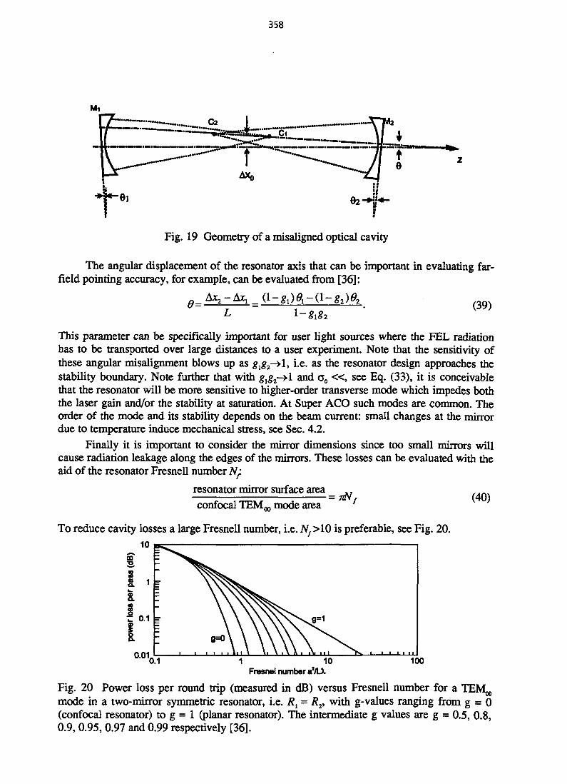
358

Fig. 19 Geometry of a misaligned optical cavity

The angular displacement of the resonator axis that can be important in evaluating far-field pointing accuracy, for example, can be evaluated from [36]:

(39)

This parameter can be specifically important for user light sources where the FEL radiationhas to be transported over large distances to a user experiment. Note that the sensitivity ofthese angular misalignment blows up as g^-^l, i.e. as the resonator design approaches thestability boundary. Note further that with g,g2-»l and a0 « , see Eq. (33), it is conceivablethat the resonator will be more sensitive to higher-order transverse mode which impedes boththe laser gain and/or the stability at saturation. At Super ACO such modes are common. Theorder of the mode and its stability depends on the beam current: small changes at the mirrordue to temperature induce mechanical stress, see Sec. 4.2.

Finally it is important to consider the mirror dimensions since too small mirrors willcause radiation leakage along the edges of the mirrors. These losses can be evaluated with theaid of the resonator Fresnell number Ni

resonator mirror surface area

confocal TEMQ,, mode area

To reduce cavity losses a large Fresnell number, i.e. Nf>10 is preferable, see Fig. 20.

(40)

m

0.0110 100

Fresnel number aVLX

Fig. 20 Power loss per round trip (measured in dB) versus Fresnell number for a TEM,,,,mode in a two-mirror symmetric resonator, i.e. #, = R2, with g-values ranging from g = 0(confocal resonator) to g = 1 (planar resonator). The intermediate g values are g = 0.5, 0.8,0.9, 0.95, 0.97 and 0.99 respectively [36].

359

4.2 Optics

SRFEL's are low gain devices, i.e. a laser where a resonator is required to reachsaturation on multiple passes. The problem of making good mirrors for the visible to the VUVspectral region is a difficult one and deserves at least a separate chapter. For generalinformation the reader is referred to textbooks and review articles [3840]. Specially for theUV and VUV spectral region it becomes more difficult to find suitable materials for mirrors.As a result the operational wavelength range of the SRFEL is reduced. An overview of thestate of the art mirror technology is given in Fig. 21.

10photon energy (eV)

100 1000

CtaanAlinUHVDfefedifcmuW*yeft

.multt wysn

10 000

100 10 1wavelength (nm)

0.1 100 200 300wavelength (nm)

400

Fig. 21 Reflectivity of normal-incidence optics [40] and the estimated cavity loss due toabsorption at the mirror surface. For details on ring-resonators, see Sec. 4.3.

Apart from these problems there are additional ones which arise due to the nature of theSRFEL:• The gain of a SRFEL is, at present, up to a few percent. To obtain the lasing threshold

condition, i.e. cavity losses < gain, highly-reflecting mirrors are required, i.e. multi-coatedmirrors. Highly-reflecting multi-coated mirrors have a narrow spectral bandwidth and, asa consequence, impede the wavelength tunability of the FEL.

• As will be explained below, mirrors of an SRFEL are exposed to a harsh environment ofhigh power radiation ranging from the visible to the X-ray region. As a result thermaleffects and mirror damage or mirror degradation forms a serious problem in the operationof the SRFEL.

To overcome the first restriction metal mirrors, e.g. coated Al mirrors [40], could beused. However, the losses associated with these types of mirrors are of the order of a fewpercent and all SRFEL's that are presently operational do not have sufficient gain to use suchmirrors.

A multi-coated mirror consists of a stack of Fabry-Perot interferometers where eachlayer has an optical thickness of A/4. Two different layers are deposited alternately, one with alow- and one with a high index of refraction. The residual diffusion and absorption in thelayers limit the maximum reflectivity. For a mathematical treatment of such mirrors refer toRef. [41]. In the visible region reflectivity's as high as 99.95 % can be obtained. However, inthis case the ratio of the transmission over the losses is very low and does not permit goodenergy extraction [42]. Multi-layers with a reflectivity over 99.5 % are currentlymanufactured down to a wavelength of 240 nm. An overview of some materials suitable formirrors in the UV is given in Table 4.

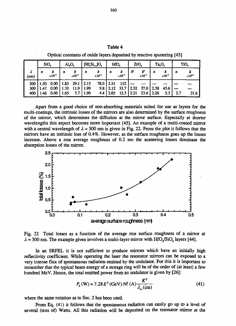
360

Table 4

Optical constants of oxide layers deposited by reactive sputtering [43]

X(nm)

200300400

SiO2

n kxKT*

1.50 0.001.47 0.001.46 0.00

A1An k

xHT1

1.83 29.11.70 11.91.65 3.7

[H4Si,JO2

n kxlO"4

2.13 78.01.99 9.81.90 4.4

HfO2

n kxior1

2.51 1522.12 33.72.05 12.3

ZrO2

N Kxnr*

2.32 37.02.21 23.6

TaA

n kxlO-

2.38 45.62.26 5.3

TiO2

n kxi<r*

2.7 21.6

Apart from a good choice of non-absorbing materials suited for use as layers for themulti-coatings, the intrinsic losses of the mirrors are also determined by the surface roughnessof the mirror, which determines the diffusion at the mirror surface. Especially at shorterwavelengths this aspect becomes more important [45]. An example of a multi-coated mirrorwith a central wavelength of X = 300 nm is given in Fig. 22. From the plot it follows that themirrors have an intrinsic loss of 0.4%. However, as the surface roughness goes up the lossesincrease. Above a rms average roughness of 0.2 nm the scattering losses dominate theabsorption losses of the mirror.

25

0.0 0.1 0.2 0.3average sirfaceroucjiness (m)

0.5

Fig. 22 Total losses as a function of the average rms surface roughness of a mirror atX = 300 nm. The example given involves a multi-layer mirror with HfOJSiO2 layers [44].

In an SRFEL it is not sufficient to produce mirrors which have an initially highreflectivity coefficient. While operating the laser the resonator mirrors can be exposed to avery intense flux of spontaneous radiation emitted by the undulator. For this it is important toremember that the typical beam energy of a storage ring will be of the order of (at least) a fewhundred MeV. Hence, the total emitted power from an undulator is given by [26]:

Pu (W) = 7.28 E2 (GeV) NI (A)K2

AAcm)(41)

where the same notation as in Sec. 2 has been used.

From Eq. (41) it follows that the spontaneous radiation can easily go up to a level ofseveral (tens of) Watts. All this radiation will be deposited on the resonator mirror at the

361

down-stream side of the undulator and thermal effects can occur. Note that due to the lowgain of the SRFEL it is not possible to install the resonator mirrors outside the vacuumsystem. Hence, mirrors can only be cooled by either the mirror support or by thermalradiation. Since the radiation stored in the cavity is extracted through transmission of themirrors it is important that both the mirror support and the mirror substrate have a goodthermal conductivity. At Super ACO, for example, 18 W of spontaneous radiation hits thedownstream mirror. As a result isolated mirrors on a SiO2 substrate were heated with AT =SC^C relative to room temperature. Under the same conditions mirrors on an ALO3 substratewere heated by AT = 35 eC. With a mirror support with a good thermal contact the rise intemperature could be reduced to AT = 58 9C and AT = 5 eC, respectively [46].

Next, the spectrum of the radiation plays an important role as well. The spontaneousradiation of a planar undulator does not only contain the fundamental harmonic such as givenin Eq. (1) but also a large number of harmonics. For on-axis radiation {6 = 0) the harmonicsper opening angle Q. are given by [26]:

d2l 1 y F ( gdeodn\e=o

47r£o c - i t " I K ) (42)( |

where n denotes the harmonic number. The parameters £ and v. are given by:

1 nK2_

(43)

A graph of Eq. (42) is presented in Fig. 23. Especially for SRFEL's the undulator strength Kcan be high because of the high energy of the beam stored. As a consequence the power of theharmonics radiated by the undulator can be high as well. For this it is convenient to recall thecritical wavelength Xt or critical harmonic nc, i.e. the wavelength for which half of the poweris radiated at wavelengths shorted than this value.

1.86

In Table 5 it can be seen that for typical SRFEL experiments the critical wavelength is muchshorter than the fundamental wavelength. Generally the mirror absorbs these harmonics andmirror damage can occur.

An example of such mirror degradation is shown in Fig. 24. At present mirrordegradation can not be avoided. However, it is possible to produce multi-coated mirrors thatare more resistant This topic is still very much under development One of the aspects thatplay an important role is the fabrication process involved. Mirrors fabricated with an ion-beam sputtering method are more resistant to synchrotron radiation, see Fig. 25. The vacuumlevel, i.e. the number of residual gas molecules near the mirror surfaces also influences mirrordegradation. Ultra-high vacuum is required in order to reduce the absorption of residual

362

molecules such as carbon which reduces the overall reflectivity of the mirrors. However, lossof reflectivity due to carbon contamination can be recovered by exposing the mirror surface toRF-discharged oxygen plasma [46-48].

21 31 41 51 61harmonic number

71 81 91

Fig. 23 Contents of the on-axis harmonics of a planar undulator for several values of theundulator strength, see Eq. (42)

Table 5

Undulator radiation for various SRFEL experiments. Estimated values are given in italic [46]

Experiment

Super AGOUVSORVEPP3DELTADuke

Beam

E(MeV)

800500350700

1000

char.

/(mA)

1002040

100100

Undulate

K(cm)

12.911.110.025.010.0

r coursets

N

2016671767

ristics

K

5.02.91.62.16.6

P.(W)

180.40.6

1210

iiation characteristics

K(nm)

7.126.689.354.2

2.6

^FEL

(nm)

350300250213300

P«L(mW)

1000.22.5

—

Fig. 24 Examples of mirror degradation due to the spontaneous undulator radiation, (a)Severe degradation of a test mirror deposited on a SiO2 substrate, (b) Photo of a mirror in itssupport after 60 hours of FEL operation showing the presence of a large carbon spot [26].

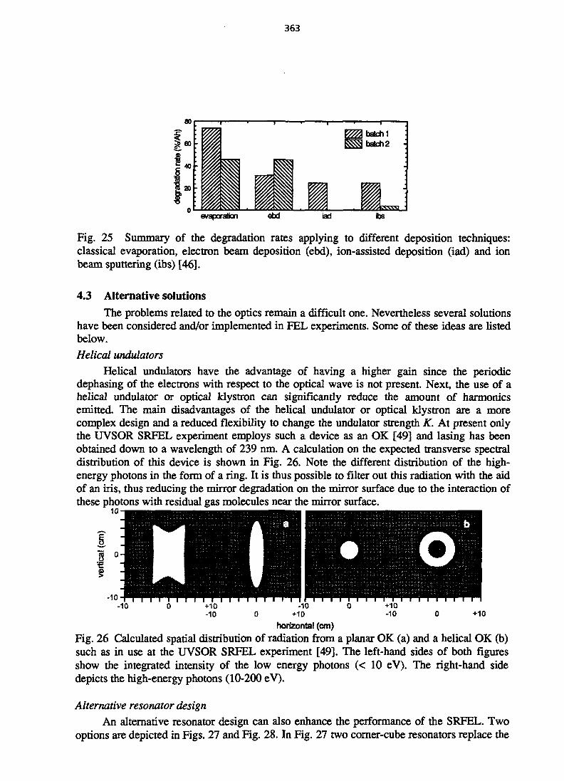
363

80

eo

1 M *20

batch 1

evaporation ebd iad tos

Fig. 25 Summary of the degradation rates applying to different deposition techniques:classical evaporation, electron beam deposition (ebd), ion-assisted deposition (iad) and ionbeam sputtering (ibs) [46].

4.3 Alternative solutions

The problems related to the optics remain a difficult one. Nevertheless several solutionshave been considered and/or implemented in FEL experiments. Some of these ideas are listedbelow.

Helical undulators

Helical undulators have the advantage of having a higher gain since the periodicdephasing of the electrons with respect to the optical wave is not present. Next, the use of ahelical undulator or optical klystron can significantly reduce the amount of harmonicsemitted. The main disadvantages of the helical undulator or optical klystron are a morecomplex design and a reduced flexibility to change the undulator strength K. At present onlythe UVSOR SRFEL experiment employs such a device as an OK [49] and lasing has beenobtained down to a wavelength of 239 nm. A calculation on the expected transverse spectraldistribution of this device is shown in Fig. 26. Note the different distribution of the high-energy photons in the form of a ring. It is thus possible to filter out this radiation with the aidof an iris, thus reducing the mirror degradation on the mirror surface due to the interaction ofthese photons with residual gas molecules near the mirror surface.

+10-10

-10 0 +10 -10 0-10 0 +10 -10 0 +10

horizontal (cm)

Fig. 26 Calculated spatial distribution of radiation from a planar OK (a) and a helical OK (b)such as in use at the UVSOR SRFEL experiment [49]. The left-hand sides of both figuresshow the integrated intensity of the low energy photons (< 10 eV). The right-hand sidedepicts the high-energy photons (10-200 eV).

Alternative resonator design

An alternative resonator design can also enhance the performance of the SRFEL. Twooptions are depicted in Figs. 27 and Fig. 28. In Fig. 27 two corner-cube resonators replace the

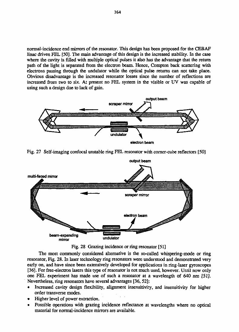
364

normal-incidence end mirrors of the resonator. This design has been proposed for the CEBAFlinac driven FEL [50]. The main advantage of this design is the increased stability. In the casewhere the cavity is filled with multiple optical pulses it also has the advantage that the returnpath of the light is separated from the electron beam. Hence, Compton back scattering withelectrons passing through the undulator while the optical pulse returns can not take place.Obvious disadvantage is the increased resonator losses since the number of reflections areincreased from two to six. At present no FEL system in the visible or UV was capable ofusing such a design due to lack of gain.

scraper mirroroutput beam

undulator

electron beam

Fig. 27 Self-imaging confocal unstable ring FEL resonator with corner-cube reflectors [50]

output beam

multi-faced mirror

beam-expandingmirror undulator

Fig. 28 Grazing incidence or ring resonator [51]

The most commonly considered alternative is the so-called whispering-mode or ringresonator, Fig. 28. In laser technology ring resonators were understood and demonstrated veryearly on, and have since been extensively developed for applications in ring-laser gyroscopes[36]. For free-electron lasers this type of resonator is not much used, however. Until now onlyone FEL experiment has made use of such a resonator at a wavelength of 640 nm [51].Nevertheless, ring resonators have several advantages [36,52]:• Increased cavity design flexibility, alignment insensitivity, and insensitivity for higher

order transverse modes.• Higher level of power extraction.• Possible operations with grazing incidence reflectance at wavelengths where no optical

material for normal-incidence mirrors are available.

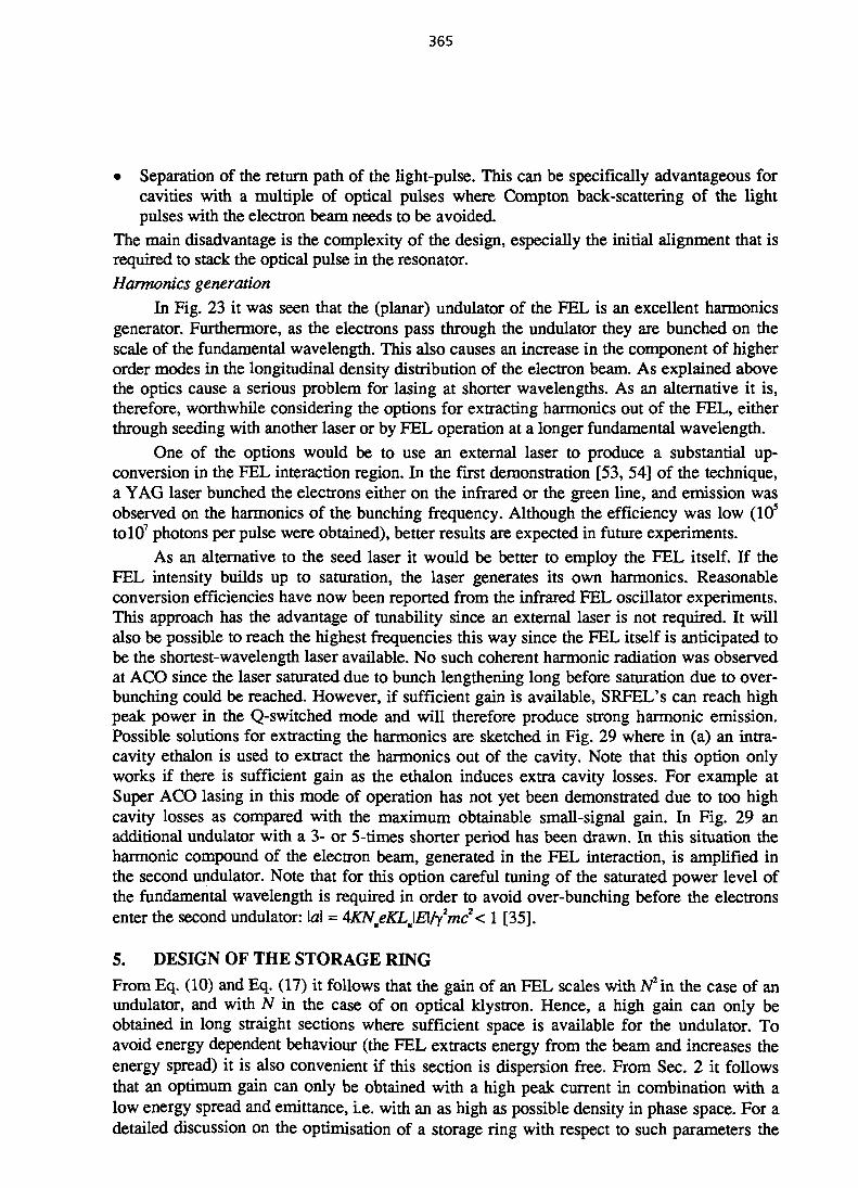
365

• Separation of the return path of the light-pulse. This can be specifically advantageous forcavities with a multiple of optical pulses where Compton back-scattering of the lightpulses with the electron beam needs to be avoided.

The main disadvantage is the complexity of the design, especially the initial alignment that isrequired to stack the optical pulse in the resonator.Harmonics generation

In Fig. 23 it was seen that the (planar) undulator of the FEL is an excellent harmonicsgenerator. Furthermore, as the electrons pass through the undulator they are bunched on thescale of the fundamental wavelength. This also causes an increase in the component of higherorder modes in the longitudinal density distribution of the electron beam. As explained abovethe optics cause a serious problem for lasing at shorter wavelengths. As an alternative it is,therefore, worthwhile considering the options for extracting harmonics out of the FEL, eitherthrough seeding with another laser or by FEL operation at a longer fundamental wavelength.

One of the options would be to use an external laser to produce a substantial up-conversion in the FEL interaction region. In the first demonstration [53, 54] of the technique,a YAG laser bunched the electrons either on the infrared or the green line, and emission wasobserved on the harmonics of the bunching frequency. Although the efficiency was low (10s

tolO7 photons per pulse were obtained), better results are expected in future experiments.As an alternative to the seed laser it would be better to employ the FEL itself. If the

FEL intensity builds up to saturation, the laser generates its own harmonics. Reasonableconversion efficiencies have now been reported from the infrared FEL oscillator experiments.This approach has the advantage of tunability since an external laser is not required. It willalso be possible to reach the highest frequencies this way since the FEL itself is anticipated tobe the shortest-wavelength laser available. No such coherent harmonic radiation was observedat ACO since the laser saturated due to bunch lengthening long before saturation due to over-bunching could be reached. However, if sufficient gain is available, SRFEL's can reach highpeak power in the Q-switched mode and will therefore produce strong harmonic emission.Possible solutions for extracting the harmonics are sketched in Fig. 29 where in (a) an intra-cavity ethalon is used to extract the harmonics out of the cavity. Note that this option onlyworks if there is sufficient gain as the ethalon induces extra cavity losses. For example atSuper ACO lasing in this mode of operation has not yet been demonstrated due to too highcavity losses as compared with the maximum obtainable small-signal gain. In Fig. 29 anadditional undulator with a 3- or 5-times shorter period has been drawn. In this situation theharmonic compound of the electron beam, generated in the FEL interaction, is amplified inthe second undulator. Note that for this option careful tuning of the saturated power level ofthe fundamental wavelength is required in order to avoid over-bunching before the electronsenter the second undulator: \a\ = 4KNueKLJE\/y2mc2 < 1 [35].

5. DESIGN OF THE STORAGE RING

From Eq. (10) and Eq. (17) it follows that the gain of an FEL scales with iV2in the case of anundulator, and with N in the case of on optical klystron. Hence, a high gain can only beobtained in long straight sections where sufficient space is available for the undulator. Toavoid energy dependent behaviour (the FEL extracts energy from the beam and increases theenergy spread) it is also convenient if this section is dispersion free. From Sec. 2 it followsthat an optimum gain can only be obtained with a high peak current in combination with alow energy spread and emittance, i.e. with an as high as possible density in phase space. For adetailed discussion on the optimisation of a storage ring with respect to such parameters the

366

reader is referred to the other chapters of these proceedings. Here the parameters specificallyimportant for the FEL are discussed. In Sec. 5.1 and 5.2 an overview of some aspects toobtain a high peak current and a low energy spread and emittance is given. The optimumperformance of the SRFEL also requires a maximum transverse overlap between the opticalpulse and the electron beam. This optimisation process is presented in Sec. 5.3.

harmonics

(a)

'e-beam

Fig. 29 Possible options for harmonics generation using the a free-electron laser thatlases on the fundamental wavelength as a seed: (a) reflecting the present harmonicsthrough an intra-cavity ethalon, (b) enhancing the output of an undulator tuned to awavelength of X/n by using the electron beam that has passed through the laser as aseed. Note that the undulator has been set at a small angle so that the harmonics arenot intercepted by the resonator mirrors.

5.1 Ring geometry

One of the easiest ways to increase the peak current, while keeping the average currentlow, is to reduce the number of bunches in the ring. Maximum current can be obtained in asinge-bunch mode of operation. For this it is important to keep in mind that the resonatorlength must match half the distance between successive bunches. For large storage rings thisimplies very long cavities. Assuming a standard two-mirror resonator, see Sec. 4.1, it isdifficult to keep such a cavity stable. For this reason the optimum number of bunches dependson the shape of the ring. In Fig. 30 two examples are given. As the ring is more circular, thestraight sections, and hence the undulator length, will be relatively short. A multi-bunch modeis then advantageous since it reduces the intra-bunch distance to reduce the cavity length. Thecombination of the short cavity with a single-bunch mode is not advantageous since theoptical pulse then has to pass the cavity twice before encountering interaction with theelectron bunch. Hence, the effective cavity loss is doubled.

2 bunch mode single bunch

Lc/2

Fig. 30 Ring geometries

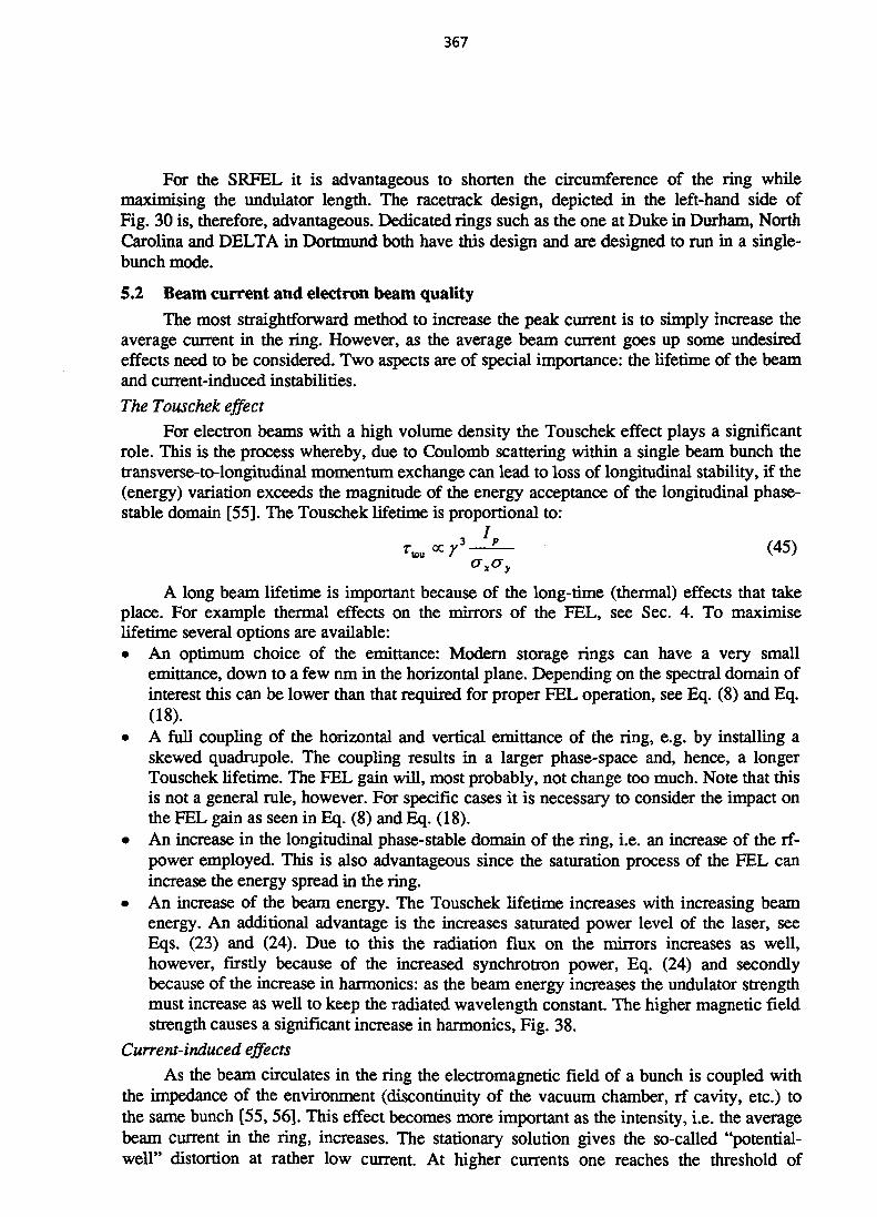
367

For the SRFEL it is advantageous to shorten the circumference of the ring whilemaximising the undulator length. The racetrack design, depicted in the left-hand side ofFig. 30 is, therefore, advantageous. Dedicated rings such as the one at Duke in Durham, NorthCarolina and DELTA in Dortmund both have this design and are designed to run in a single-bunch mode.

5.2 Beam current and electron beam quality

The most straightforward method to increase the peak current is to simply increase theaverage current in the ring. However, as the average beam current goes up some undesiredeffects need to be considered. Two aspects are of special importance: the lifetime of the beamand current-induced instabilities.

The Touschek effect

For electron beams with a high volume density the Touschek effect plays a significantrole. This is the process whereby, due to Coulomb scattering within a single beam bunch thetransverse-to-longitudinal momentum exchange can lead to loss of longitudinal stability, if the(energy) variation exceeds the magnitude of the energy acceptance of the longitudinal phase-stable domain [55]. The Touschek lifetime is proportional to:

* « « T 3 - ^ - (45)azay

A long beam lifetime is important because of the long-time (thermal) effects that takeplace. For example thermal effects on the mirrors of the FEL, see Sec. 4. To maximiselifetime several options are available:• An optimum choice of the emittance: Modern storage rings can have a very small

emittance, down to a few nm in the horizontal plane. Depending on the spectral domain ofinterest this can be lower than that required for proper FEL operation, see Eq. (8) and Eq.(18).

• A full coupling of the horizontal and vertical emittance of the ring, e.g. by installing askewed quadrupole. The coupling results in a larger phase-space and, hence, a longerTouschek lifetime. The FEL gain will, most probably, not change too much. Note that thisis not a general rule, however. For specific cases it is necessary to consider the impact onthe FEL gain as seen in Eq. (8) and Eq. (18).

• An increase in the longitudinal phase-stable domain of the ring, i.e. an increase of the rf-power employed. This is also advantageous since the saturation process of the FEL canincrease the energy spread in the ring.

• An increase of the beam energy. The Touschek lifetime increases with increasing beamenergy. An additional advantage is the increases saturated power level of the laser, seeEqs. (23) and (24). Due to this the radiation flux on the mirrors increases as well,however, firstly because of the increased synchrotron power, Eq. (24) and secondlybecause of the increase in harmonics: as the beam energy increases the undulator strengthmust increase as well to keep the radiated wavelength constant. The higher magnetic fieldstrength causes a significant increase in harmonics, Fig. 38.

Current-induced effects

As the beam circulates in the ring the electromagnetic field of a bunch is coupled withthe impedance of the environment (discontinuity of the vacuum chamber, if cavity, etc.) tothe same bunch [55,56]. This effect becomes more important as the intensity, i.e. the averagebeam current in the ring, increases. The stationary solution gives the so-called "potential-well" distortion at rather low current. At higher currents one reaches the threshold of

368

anomalous bunch lengthening. At Super ACO, for example, this threshold is found to be atapproximately 8 mA/bunch [57]. Above this limit the so-called "microwave instabilityregime" is entered. In addition, the bunch or bunches can also start to oscillate coherentlyclose to their natural oscillation synchrotron frequency and its harmonics. The presence ofmodes of oscillations (dipolar, quadrupolar, hexapolar and octupolar) depends on the beamcurrent. In the upper limit of the current the beam becomes completely unstable. At SuperACO this limit is reached at roughly 100 mA/bunch [33].

For the FEL it is clear that the laser would work best in the absence of any type ofinstability. However, as a general rule the FEL operates in a regime where the instabilities arepresent. For example at Super ACO the under-threshold for lasing is reached at roughly 15mA/bunch, far above the threshold for anomalous bunch lengthening. Here it is important tonote that not all instabilities are of the same importance.

{z)Coherent bunch-oscillations. In Fig. 31 the coherent synchrotron modes ofoscillation, as observed at Super ACO, are shown. As can be deduced from the left-hand side of the figure these types of modes are devastating for the FEL: from theplot of the line-intensity it follows that the position of the bunch starts to oscillate.Hence, the effective small-signal gain is reduced since, over multiple roundtrips, theeffective longitudinal overlap of the bunch with the optical pulse is reduced. Next itcan be seen that also the effective energy-spread increases, causing a further decreaseof the small-signal gain. At Super ACO the dipolar modes are damped with aPedersen type of feedback system [58, 59]. With this system it is possible to obtainstable operation up to a current of 35 mA/bunch. Above this threshold quadrupolarmodes occur that make the start-up of the laser more difficult. Moreover, withquadrupolar modes present the laser becomes less stable. However, once lasing isachieved, the FEL interaction tends to damp these modes [33]. Recently, feedback onthe quadrupolar modes has been installed providing the means to have stable FELoperation at up to 50 mA/bunch [60].

(b) Microwave instability. At higher circulating beam current in a storage ringsignificant dilution of longitudinal phase-space density may occur. Here theinteraction of the bunch with its own short-range wake field causes high-ordercoupled oscillatory modes to be induced. This results in short-wavelength (comparedwith the bunch length) particle density modulation of the bunch, effectivelengthening of the bunch, and enhancement of the energy spread. The threshold peakcurrent for the longitudinal single-bunch instability is given by [23]:

\ ^ ( 4 6 )I r l z / )

where Eo and Z, are the beam energy and the longitudinal impedance of the ring,respectively. Above the threshold the peak current may still increase but at theexpense of an increase in energy spread [23]:

\V*ha2nE

where Io is the average beam current, V^ is the rf voltage, and k is the number ofbunches stored in the ring.

369

phase-space

z'line density

quadaipole

Fig. 31 Synchrotron modes of oscillations observed at Super ACO in a two-bunchmode of operation [33]. Left-hand side: Representation of the coherent synchrotronmodes of oscillation in phase space and in time space. Right-hand side: Spectrum ofthe modes observed on the sidebands of high harmonics of the revolution frequencyversus the stored beam current. With increasing current one can observe the presenceof dipolar modes (D), quadrupolar modes (Q) hexapolar modes (H) , and octupolarmodes (O).

To first order the gain of the laser scales with the square of the energy spread. Hence,even at the occurrence of microwave instability, it remains worthwhile to increase the beamcurrent. Nevertheless, it is also important to design the storage ring such that instabilities areavoided to an as high as possible current. To do so it is important to reduce the number ofbunches in the ring, see Sec. 5.1. Increasing the rf voltage also helps but is not very effective,see Eq. (47). A high rf voltage remains important, however, since it also determines theenergy-spread acceptance of the ring, see Sec. 3.

In the optimisation process the momentum compaction factor a plays an important role:as the compaction factor becomes smaller the storage ring becomes more sensitive toinstabilities. Hence, a too small value for a is to be avoided. However, big compaction factorsare non-ideal either. From Eq. (3.2) it follows that a small value for a leads to short bunchesand, hence, to high peak currents and gain. Furthermore, there is a (indirect) relation betweenthe compaction factor and the emittance since both are related to the so-called "synchrotronradiation integrals" [23]:

55R — .

x 32yf3 me'

where the synchrotron integrals are given by:

(48)

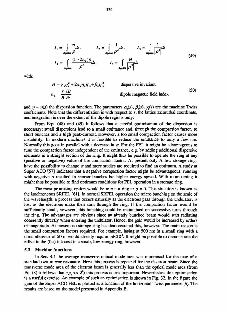
370

dipales r

dipales

n = rrf +r dB

p3 ds, 1f 'i-

dipol« A

•ds

dispersive invariant

dipole magnetic field index

(49)

/4 = f V-^ds, Is = f A *dipotes i dipolcs \t I

with:

H = yxifx + 2axTjxrj'x+fixTj'l dispersive invariant(50)

and TJ = TJ(S) the dispersion function. The parameters ax(s), fix(s), yx(s) are the machine Twisscoefficients. Note that the differentiation is with respect to s, the lattice azimuthal coordinate,and integration is over the extent of the dipole regions only.

From Eqs. (48) and (49) it follows that a careful optimisation of the dispersion isnecessary: small dispersions lead to a small emittance and, through the compaction factor, toshort bunches and a high peak-current. However, a too small compaction factor causes moreinstability. In modern machines it is feasible to reduce the emittance to only a few nm.Normally this goes in parallel with a decrease in a. For the FEL it might be advantageous totune the compaction factor independent of the emittance, e.g. by adding additional dispersiveelements in a straight section of the ring. It might thus be possible to operate the ring at any(positive or negative) value of the compaction factor. At present only A few storage ringshave the possibility to change a and more studies are required to find an optimum. A study atSuper ACO [57] indicates that a negative compaction factor might be advantageous: runningwith negative a resulted in shorter bunches but higher energy spread. With more tuning itmight thus be possible to find optimum conditions for FEL operation in a storage ring.

The most promising option would be to run a ring at a = 0. This situation is known asthe isochroneous SRFEL [61]. In normal SRFEL operation the micro bunching on the scale ofthe wavelength, a process that occurs naturally as the electrons pass through the undulator, islost as the electrons make their turn through the ring. If the compaction factor would besufficiently small, however, this bunching could be maintained on successive turns throughthe ring. The advantages are obvious since an already bunched beam would start radiatingcoherently directly when entering the undulator. Hence, the gain would be increased by ordersof magnitude. At present no storage ring has demonstrated this, however. The main reason isthe small compaction factors required. For example, lasing at 500 nm in a small ring with acircumference of 50 m would already require laklO"*. It might be possible to demonstrate theeffect in the (far) infrared in a small, low-energy ring, however.

5.3 Machine functions

In Sec. 4.1 the average transverse optical mode area was minimised for the case of astandard two-mirror resonator. Here this process is repeated for the electron beam. Since thetransverse mode area of the electron beam is generally less than the optical mode area (fromEq. (8) it follows that zpy« A2) this process is less important. Nevertheless this optimisationis a useful exercise. An example of such an optimisation is shown in Fig. 32. In the figure thegain of the Super ACO FEL is plotted as a function of the horizontal Twiss parameter f}x. Theresults are based on the model presented in Appendix B.

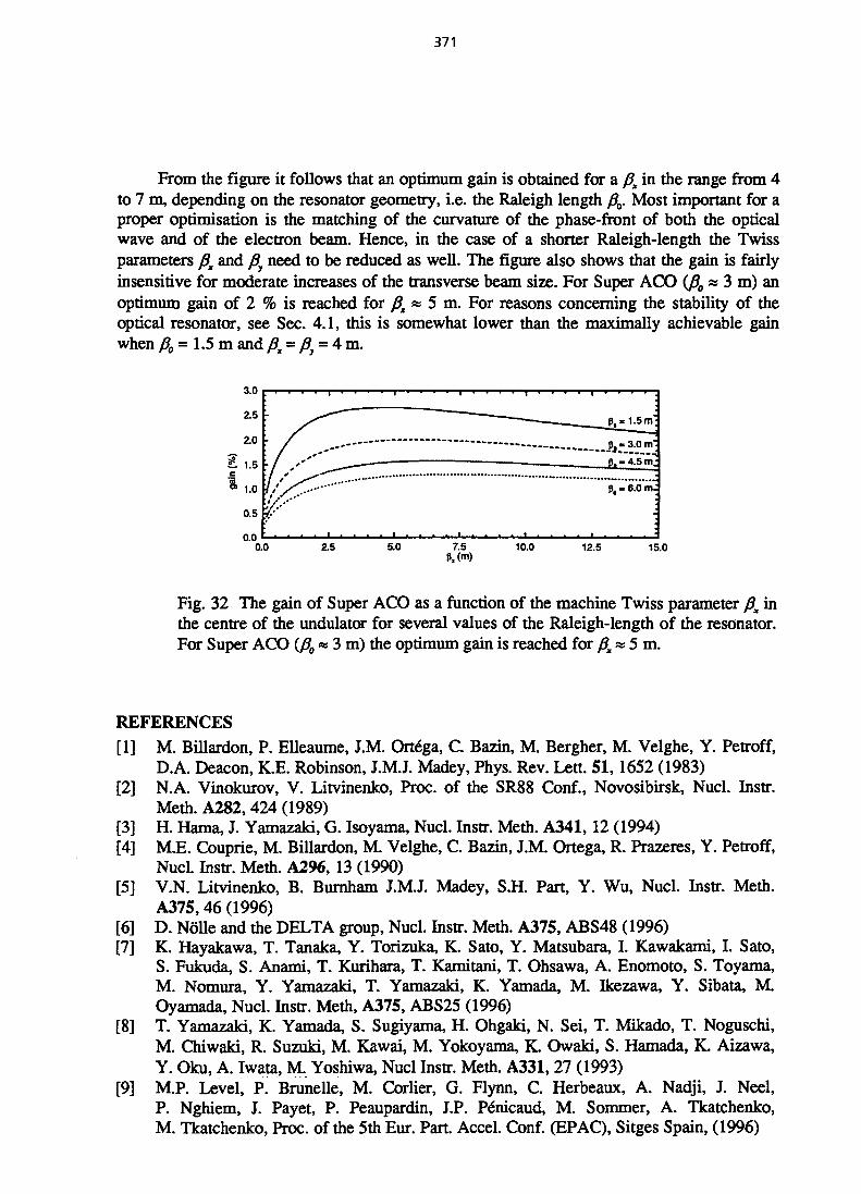
371

From the figure it follows that an optimum gain is obtained for a fix in the range from 4to 7 m, depending on the resonator geometry, i.e. the Raleigh length ft0. Most important for aproper optimisation is the matching of the curvature of the phase-front of both the opticalwave and of the electron beam. Hence, in the case of a shorter Raleigh-length the Twissparameters fix and fi need to be reduced as well. The figure also shows that the gain is fairlyinsensitive for moderate increases of the transverse beam size. For Super ACO {fi0 * 3 m) anoptimum gain of 2 % is reached for fiK « 5 m. For reasons concerning the stability of theoptical resonator, see Sec. 4.1, this is somewhat lower than the maximally achievable gainwhen fi0 = 1.5 m and px = f3y = 4 m.

0.0 12.5 15.0

Fig. 32 The gain of Super ACO as a function of the machine Twiss parameter Pz inthe centre of the undulator for several values of the Raleigh-length of the resonator.For Super ACO (Po« 3 m) the optimum gain is reached for ^ « 5 m .

REFERENCES[1] M. Billardon, P. Elleaume, J.M. Ortega, C. Bazin, M. Bergher, M. Velghe, Y. Petroff,

D.A. Deacon, K.E. Robinson, J.M.J. Madey, Phys. Rev. Lett. 51, 1652 (1983)[2] N.A. Vinokurov, V. Litvinenko, Proc. of the SR88 Conf., Novosibirsk, Nucl. Instr.

Meth. A282,424 (1989)[3] H. Hama, J. Yamazaki, G. Isoyama, Nucl. Instr. Meth. A341,12 (1994)[4] M.E. Couprie, M. Billardon, M. Velghe, C. Bazin, J.M. Ortega, R. Prazeres, Y. Petroff,

Nucl. Instr. Meth. A296,13 (1990)[5] V.N. Litvinenko, B. Burnham J.MJ. Madey, S.H. Part, Y. Wu, Nucl. Instr. Meth.

A375,46 (1996)[6] D. Nolle and the DELTA group, Nucl. Instr. Meth. A375, ABS48 (1996)[7] K. Hayakawa, T. Tanaka, Y. Torizuka, K. Sato, Y. Matsubara, I. Kawakami, I. Sato,

S. Fukuda, S. Anami, T. Kurihara, T. Kamitani, T. Ohsawa, A. Enomoto, S. Toyama,M. Nomura, Y. Yamazaki, T. Yamazaki, K. Yamada, M. Ikezawa, Y. Sibata, M.Oyamada, Nucl. Instr. Meth, A375, ABS25 (1996)

[8] T. Yamazaki, K. Yamada, S. Sugiyama, H. Ohgaki, N. Sei, T. Mikado, T. Noguschi,M. Chiwaki, R. Suzuki, M. Kawai, M. Yokoyama, K. Owaki, S. Hamada, K. Aizawa,Y. Oku, A. Iwata, M. Yoshiwa, Nucl Instr. Meth. A331,27 (1993)

[9] M.P. Level, P. Brunelle, M. Corlier, G. Flynn, C. Herbeaux, A. Nadji, J. Neel,P. Nghiem, J. Payet, P. Peaupardin, J.P. Pe"nicaud, M. Sommer, A. Tkatchenko,M. Tkatchenko, Proc. of the 5th Eur. Part. Accel. Conf. (EPAC), Sitges Spain, (1996)

372

[10] K. Yamada, T. Yamazaki, S. Sugiyama, H. Ohgaki, T. Noguchi, T. Midado,M. Chiwaki, R. Suzuki, T. Tomimasu, Nucl. Instr. Meth., A331,103 (1993)

[11] M.E. Couprie, RJ. Bakker, D. Garzella, L. Nahon, M. Marshi, F. Mélora, T. Hara,M. Billardon, Nucl. Instr. Meth., A37S, 639 (1996)

[12] Free Electron Lasers and other advancd sources of light, Report by the Board onChemical Sciences and Technology, National Resarch Council, Washington D.C., USA(1994)

[13] Proc. of the ICFA workshop on 4th generation light sources, Jan 1994, Grenoble,France

[14] J.M.J. Madey, II Nuovo Cim. 50B, 64 (1979)[15] G. Dattoli and A. Renieri, Laser Handbook Vol. 4, Eds. M.L. Stitch and M. Bass, North

Holland Pubi., Amsterdam, p. 1-142 (1985)[16] CA. Brau, Free Electron Lasers, Academic Press, Boston (1990)[17] A. Cutolo, S. Solimento, Appi. Opt., 26,53 (1987)[18] N.A. Vinokurov, Proc. 10th Int. Conf. on High Energy Charged Particle Accelerators, 2,

Serpukhov, p. 454 (1977)[19] R.H. Pantell, L.K. Grover, Laser Handbook Vol. 6, Eds. W.B. Colson, C. Pellegrini,

R. Renieri, North Holland Pubi., Amsterdam, p. 71-90 (1990)[20] P. Elleaume, Laser Handbook Vol. 6, Eds. W.B. Colson, C. Pellegrini, R. Renieri,

North Holland Pubi., Amsterdam, p. 91-114 (1990)[21] D.A.G. Deacon, J.M. Ortega, Laser Handbook Vol. 6, Eds. W.B. Colson, C. Pellegrini,

R. Renieri, North Holland Pubi., Amsterdam, p. 71-90 (1990)[22] M. Sands, Stanford Linear Accelerator Centre, Report 121, (1970)[23] A. van Steenbergen , Laser Handbook Vol. 6, Eds. W.B. Colson, C. Pellegrini,

R. Renieri, North Holland Pubi., Amsterdam, p. 417-462 (1990)[24] H. Hama, K. Kimura, T. Yamazaki, S. Tanako, K. T. Kinochita, M.E. Couprie, Nucl.

Instr. Meth., A37S, 32 (1996)[25] A. Renieri, Nuovo Cimento, 53B, p. 160 (1979)[26] The synchrotron light source data book, eds. J. Murphy, BNL 42333, NSLS 725C, P.O.

Box 5000, Upton New York 11973-5000, (1993)[27] P. Elleaume, Nucl. Instr. Meth., A237,28 (1985)[28] M.E. Couprie, N.G. Gavrilov, G.N. Kulipanov, V.N. Litvinenko, I.V. Pinaev,

V.M. Popik, A.N. Strinsky, N.A. Vinokurov, Nucl. Instr. Meth, A304, p. 47 (1991)[29] T. Hara, M.E. Couprie, A. Delboulbé, L. Nahon, M. Billardon, Nucl. Instr. Meth.

A358, 341 (1995)[30] M.E. Couprie, D. Garzella, T. Hara, J.H. Codarbox, M. Billardon, Nucl. Instr. Meth,

A358, p. 374 (1995)[31] P. Elleaume, J. Phys., 45, 997 (1984)[32] T. Hara, M.E. Couprie, M. Billardon, Nucl. Instr. Meth. A375, 67 (1996)[33] M.E. Couprie, T. Hara, D. Gontier, P. Troussel, D. Garzella, A. Delboulbé,

M. Billardon, Phys. Rev. E, 53-2, 1871 (1996)[34] M. Billardon, P. Elleaume, J.M. Ortega, C. Bazin, M. Bergher, Y. Petroff, M. Velghe,

Nucl. Instr. Meth., A237, 244 (1985)[35] W.B. Colson, Laser Handbook Vol. 6, Eds. W.B. Colson, C. Pellegrini, R. Renieri,

North Holland Pubi., Amsterdam, p. 115-194 (1990)[36] A.E. Siegman, Loses, Universiyt Science Books, Mill Valley (CA), USA[37] A. Yariv, Introduction to Optical Electronics, Holt, Rinehart and Winston, New York

1971, pp. 61

373

[38] W. Dricsoll, W. Vaugham eds., Handbook of Optics, Me Graw-Hill Book Company,New York, USA

[39] W.L. Wolfe, G. J. Zissis, The Infra-red Handbook, Ofice of Naval Research, Dep. of theNavy, Washington D.C., USA (1985)

[40] D.T. Attwood et al, AIP CONF. Proc. 118, eds J.MJ. Madey and C. Pelligrini, AIP,New York, p. 93 (1983)

[41] H.E. Bennet, D.K. Bürge, J. opt. Soc. Am., 70, 268 (1980)[42] M. Billardon, P. Ellaume, J.M. Ortega, C. Bazin, M. Bergher, M.E. Couprie,

Y. Lapieree, Y. Petroff, R. Prazeres, M. Velghe, Nucl. Instr. Meth. A259, 72 (1987)[43] S.M. Edlou, A. Smajkiewicz, A. Ghanim, A-Jumaily, Appi. Opt., 32, 5601 (1993)[44] D. Garzella, Etude d'un Laser a Electrons Libres dans l'ultra-violet sur l'anneau de

stocage Super ACO, thesis of the univ. de Paris IX, Orsay, 153 (1996)[45] J.M. Elson, J.M. Bennett, J. Opt Soc. Am., 69, 31 (1979)[46] D. Garzella, M.E. Couprie, T. Hara, L. Nahon, M. Brazuna, A. Delboulbé,

M. Billardon, Nucl. Instr. Meth, A358, 387 (1995)[47] M.E. Couprie, D. Garzella, M. Billardon, Nucl. Instr. Meth, A358, p. 382 (1995)[48] K. Yamada, T. Ymazaki, N. Sci, T. Mikado, Nucl. Instr. Meth, A341, ABS 139 (1994)[49] H. Hama, Nucl. Instr. Meth, A375, 57 (1996)[50] C. Shih, S. Shih, Nucl. Instr. Meth, A304,788 (1991)[51] D.H. Dowell, M.L. Laucks, A.R. Lowrey, J. Adamski, D. Pistoresi, R. Shoffstall,

A.H. Lumpkin, S. Bender, D. Byrd, R.L. Tokar, K. Sun, M. Bentz, R. Bums, J. Guha,W. Tornita, Nucl. Instr. Meth, A318,74 (1992)

[52] B.E. Newnam, SPUE, 738, Free-Electron Lasers, 155 (1987)[53] B. Gerard, Y. Lapierre, J.M. Ortega, C. Bazin, M. Billardon, P. Elleaume, M. Ergher,

M. Velghe, Y. Pertroff, Phys. Rev. Lett, 53, 2405 (1984)[54] R. Prazeres, J.M. Ortega, Europhys. Lett, 4, 817 (1987)[55] J.L. Laclare, Bunched Beam Instabilities (F.J. Sacherer Memorial Paper) Proc. 11* Int.

Conf. On High Energy Accelerators, p 526[56] J.L. Laclare, CERN Report No. 264-326, 1987[57] R.J. Bakker, M.E. Couprie, L. Nahon, D. Nutarelli, R. Roux, A. Deboulbé, D. Garzella,

A. Nadji, B. Visentin, M. Billardon, Proc. of the 5th Eur. Particle AcceleratorConference (EPAC), Sitges, Spain, 667 (1996)

[58] F. Pedersen, F. Sacherer, IEEE Trans. Uncl. Sci., NS-24, 1396; B. Kriegbaum,F. Pedersen, IEEE Trans. Nucl. Sci., NS-24,1695 (1977)

[59] M.E. Couprie, M. Billardon, IEEE J. of Quan. EL, 30-3,781 (1994)[60] R. Roux, M.E. Couprie, T. Hara, R.J. Bakker, A.B. Visentin, M. Billardon, J. Roux,

Nucl. Instr. Meth., A393, 33 (1997)[61] D.A.G. Deacon, Phys. Rep. 76, 351[62] Super ACO Parameter List, Super ACO/87-38, Orsay, France (1987)[63] E.I. Zinine, Nucl. Instr. Meth., A208,439 (1983)

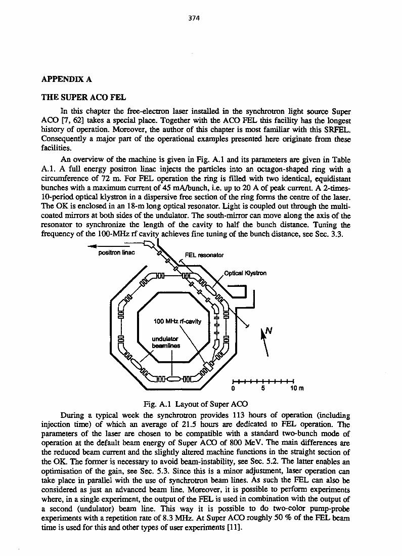
374

APPENDIX A

THE SUPER ACO FEL

In this chapter the free-electron laser installed in the synchrotron light source SuperACO [7, 62] takes a special place. Together with the ACO FEL this facility has the longesthistory of operation. Moreover, the author of this chapter is most familiar with this SRFEL.Consequently a major part of the operational examples presented here originate from thesefacilities.

An overview of the machine is given in Fig. A.I and its parameters are given in TableA.I. A full energy positron linac injects the particles into an octagon-shaped ring with acircumference of 72 m. For FEL operation the ring is filled with two identical, equidistantbunches with a maximum current of 45 mA/bunch, i.e. up to 20 A of peak current. A 2-times-10-period optical klystron in a dispersive free section of the ring forms the centre of the laser.The OK is enclosed in an 18-m long optical resonator. Light is coupled out through the multi-coated mirrors at both sides of the undulator. The south-mirror can move along the axis of theresonator to synchronize the length of the cavity to half the bunch distance. Tuning thefrequency of the 100-MHz rf cavity achieves fine tuning of the bunch distance, see Sec. 3.3.

I I I I I I I I I I I0 5 10 m

Fig. A.I Layout of Super ACODuring a typical week the synchrotron provides 113 hours of operation (including

injection time) of which an average of 21.5 hours are dedicated to FEL operation. Theparameters of the laser are chosen to be compatible with a standard two-bunch mode ofoperation at the default beam energy of Super ACO of 800 MeV. The main differences arethe reduced beam current and the slightly altered machine functions in the straight section ofthe OK. The former is necessary to avoid beam-instability, see Sec. 5.2. The latter enables anoptimisation of the gain, see Sec. 5.3. Since this is a minor adjustment, laser operation cantake place in parallel with the use of synchrotron beam lines. As such the FEL can also beconsidered as just an advanced beam line. Moreover, it is possible to perform experimentswhere, in a single experiment, the output of the FEL is used in combination with the output ofa second (undulator) beam line. This way it is possible to do two-color pump-probeexperiments with a repetition rate of 8.3 MHz. At Super ACO roughly 50 % of the FEL beamtime is used for this and other types of user experiments [11].

375

Table A.1

Super ACO parameters

Beam EnergyCircumferenceMomentum compaction factorrf-frequencyNumber of bunchesMax. average beam currentDamping timeSynchrotron frequencyBeam life timeEnergy spreadEmittanceTransverse beam sizeTransverse machine functions in OKEnergy dispersion in OKCavity lengthMaximum undulator strengthUndulator periodNumber of periodsStrength dispersive sectionWavelength rangeLaser gainAverage output powerMicro-pulse durationSpectral width

E4a

h\f.X

aft

A,

LKKN

N+N,XGoPo,

600-80072

0.0148100

2200

10-2014-17

60.065

200.3

50

183.9

12.92x10<120

600-3502

10012

10"

MeVm

MHz

mAmskHzhours%nnmrad\imm

m

em

nm%mWps

Two types of temporal diagnostic are presented in Fig. A.2 and Fig. A.3: a double-sweep streak-camera and a dissector. With a dissector (synchrotron or laser) light is projectedonto a pinhole with a photo-cathode. The intensity evolution on the pinhole is thentransformed into a spatial distribution with a fast transverse sweep on two deflecting electronsthat deflect the passing electron beam. Behind the anode a fluorescent screen makes itpossible to display the distribution on a photo or CCD camera. With a double-sweep cameraan additional synchronised slow sweep is applied perpendicularly to the fast sweep. This wayit is possible to record the evolution of a repeating signal, e.g., an electron bunch providingsynchrotron radiation at a dipole beam line on each turn through the ring. The image inFig. A.2 is a recording of the Super ACO FEL pulse in a pulsed mode of operation, i.e. zone±1 in Fig. 23. The streak-camera at Super ACO (Hamamatsu C5680) has a resolution of a fewps. The slow sweep can be set in a range from 100 ns to 1 s.

A dissector, developed at Novosibirsk [63], is in fact identical to a streak cameraequipped with a single-pixel CDD camera. The temporal information can now be obtained ina stroboscopic way, i.e. by applying a slowly varying bias voltage to the fast sweep of thedeflecting electrodes. The temporal resolution of the dissector at Super ACO is of the order of10 ps. The main advantage of a dissector is its capability to process its signal directly bymeans of an oscilloscope or other electronic equipment, e.g. the feedback system described inSec. 3.3. Due to its stroboscopic nature it is not possible to follow fast changing phenomenasuch as the synchrotron modes of oscillation described in Sec. 5.2. Furthermore, it can onlybe used to record periodic events.

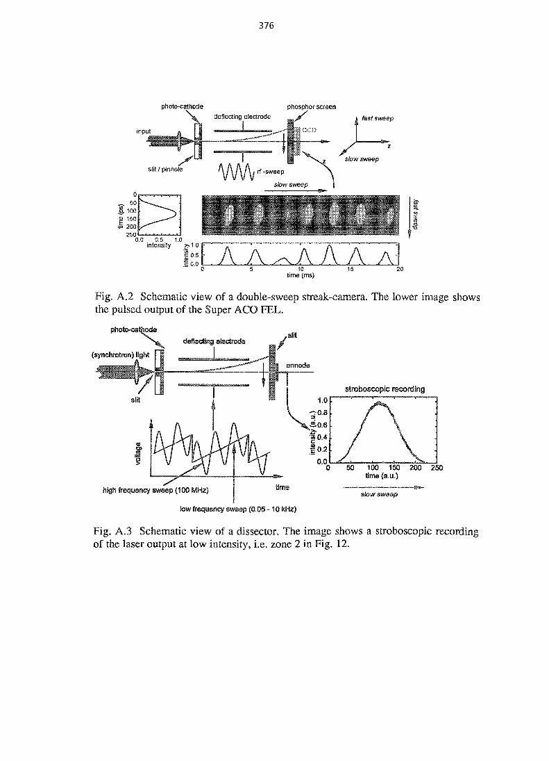
376

input

photo-cathode phosphor screendeflecting electrode j / j fast sweep

slit / pinhole VW\rsweep

stow sweep }&~

S-Zlr rfff?rttff t t - . 44 iwM**^WwTwj * ,Mr *• V4 H W I V / ; s / / v ."

2500.0 0.5 1.0

intensity .

.f o.o A AÂ A A A!10

time (ms>15 20

Fig. A.2 Schematic view of a double-sweep streak-camera. The lower image showsthe pulsed output of the Super ACO FEL.

photo-cathode

(synchrotron) light

250

high frequancy sweep {100 MHz)slow sweep

low frequency sweep (0.05 - 10 kHz)

Fig. A.3 Schematic view of a dissector. The image shows a stroboscopic recordingof the laser output at low intensity, i.e. zone 2 in Fig. 12.

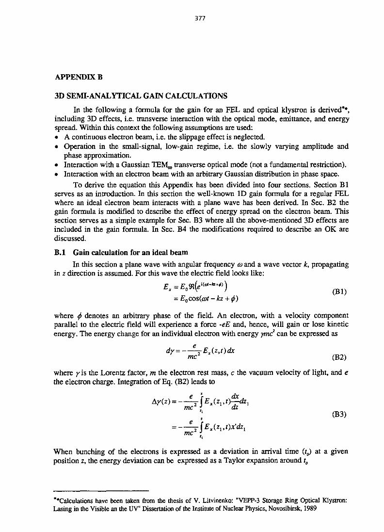
377

APPENDIX B

3D SEMI-ANALYTICAL GAIN CALCULATIONS

In the following a formula for the gain for an FEL and optical klystron is derived**,including 3D effects, i.e. transverse interaction with the optical mode, emittance, and energyspread. Within this context the following assumptions are used:• A continuous electron beam, i.e. the slippage effect is neglected.• Operation in the small-signal, low-gain regime, i.e. the slowly varying amplitude and

phase approximation.• Interaction with a Gaussian TEM^ transverse optical mode (not a fundamental restriction).• Interaction with an electron beam with an arbitrary Gaussian distribution in phase space.

To derive the equation this Appendix has been divided into four sections. Section Blserves as an introduction. In this section the well-known ID gain formula for a regular FELwhere an ideal electron beam interacts with a plane wave has been derived. In Sec. B2 thegain formula is modified to describe the effect of energy spread on the electron beam. Thissection serves as a simple example for Sec. B3 where all the above-mentioned 3D effects areincluded in the gain formula. In Sec. B4 the modifications required to describe an OK arediscussed.

B.I Gain calculation for an ideal beam

In this section a plane wave with angular frequency co and a wave vector k, propagatingin z direction is assumed. For this wave the electric field looks like:

F -F

- kz

where ^ denotes an arbitrary phase of the field. An electron, with a velocity componentparallel to the electric field will experience a force -eE and, hence, will gain or lose kineticenergy. The energy change for an individual electron with energy ymc2 can be expressed as

dy=—?TEx{z,t)dxme2 (B2)

where yis the Lorentz factor, m the electron rest mass, c the vacuum velocity of light, and ethe electron charge. Integration of Eq. (B2) leads to

me2* * L dz: (B3>

e

me2

When bunching of the electrons is expressed as a deviation in arrival time (r0) at a givenposition z, the energy deviation can be expressed as a Taylor expansion around t0

"•Calculations have been taken from the thesis of V. Litvinenko: "VEPP-3 Storage Ring Optical Klystron:Lasing in the Visible an the UV" Dissertation of the Institute of Nuclear Physics, Novosibirsk, 1989

378

Ay (z) = Ayl U) + A^2 (z) + • • •

+ ( B 4 )

me • me

The first term Aft describes the FEL interaction without bunching. In this case there is no netenergy loss for a distribution of electrons within one ponderomotive well, hence

= 0 (B5)

The second term, Ay2, describes the effects of bunching. For this the time deviation can beexpressed as a phase-fluctuation with A$ = -coAt. Hence, Ay2 can be expressed as

me f d<j>

where A^fz,) is a function of the dispersion D in the undulator

^ \ x t 2 \ t x 2 x (B7)

me».-

For a planar undulator Dtz^zJ reads

D(z1,z2)=^(z1-zz) • (B8)

A combination of Eqs. (B6) and (B7) leads to

^ (z, )EX (z2 )x' (z2 ( z , , z2 )^z2 (B9)

The average energy lost per electron over one ponderomotive well thus becomes

^ )

For an FEL with a planar undulator the terms in Eq. (BIO) can be expressed as

{Ex{z2)x'(z2))x = Eo—{cos(0t-kz + t)sin(kHz));L7 (BU)

= Eoj- (Jo (O - J, (£))cos(<5fcz + <f>)

where J0J represent the Bessel functions of the first kind. K and 5Jfc are the undulator strengthand the detuning parameter, respectively.

379

_ eBuXu

lizmcK2

(B12)4+2K

Combination of Eqs. (BIO) and (Bll) leads to an average energy loss (averaged over onewavelength)

J Jcos(<5fcZi + >cos(<5fcz2 + #)D(z1,z2)dz2dzl (B13)

The integral can be made dimensionless by rescaling the whole integral over the totalinteraction length L = zf-zr The expression above then becomes

i) \ ] M P z l (B14)

where 8k has been substituted with q = L 8k. Also the dispersion D has been normalised withrespect to the interaction length. Eq. (B8) thus becomes

^ ^ z t - z , ) (B15)

Krwhich leads to

3 (B16)

Here / ^ j describes the detuning curve, i.e. the gain as a function of detuning. The actualaverage energy loss per electron is Ay2 me2. Since the electron density per time-interval equalsJle, the total power density equals P = Ay2 me2 Jle. The power density, gained by the opticalfield thus becomes

5l*?i£\ 2 (B17)2 me K\J

The original average power density of the optical field equals P. = 4%z0 c Eg 18%. Hence thegain, G = PIP? equals

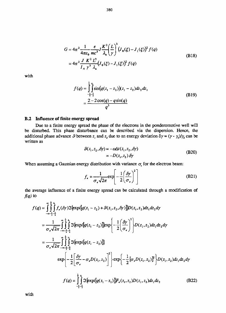
380

with

„ we"

A 2JK2L3

1AY A.

f(q) = j Jsin(<7(z, - z2))(zx - z2)dz2dzx

2-2cos(q)-qsin(q)

(B18)

(B19)

B.2 Influence of finite energy spread

Due to a finite energy spread the phase of the electrons in the ponderomotive well willbe disturbed. This phase disturbance can be described via the dispersion. Hence, theadditional phase advance & between z, and z2 due to an energy deviation by = (/ - yo)/yo can bewritten as

(B20)

When assuming a Gaussian energy distribution with variance ac for the electron beam:. 2 '

/ . = •

1exp

lfSy(B21)

the average influence of a finite energy spread can be calculated through a modification ofto

f 1 (A V l, -z2)]]exp - - - ^ \D(zx,z2)dzxdz2dy

[ 2 { ° ) J

f8y

-aeD(zx,z2) >expj --[aeD(zx, z2)f \D(ZX, z2)dzxdz2dy

with

f(q) = | j S j s x p / ^ - z2)tye(zx,z2)D(zx,z2)dzxdz2

2 2

(B22)

381

Fe (z, , z2 = exp j - 1 (B23)

B.3 Gain calculation for a real beamIn the following a Gaussian is assumed for both the distribution of the energy spread

and the distribution in all directions in phase-space, i.e. 8 , x, x1, y, and y\ Properties of theelectron beam are defined through the variance of the energy-spread distribution, the 0-functions, and the emittance, i.e. at, ez, 0Jz), sy, and fiy(z). Hence, the distribution of theelectron beam can be described as a 3D Gaussian function

(B24)

In a waist, i.e. at the centre of the undulator A can be expressed as

and X =

_L_PA0

0

00

0is.

600

001

00

00

0

£>.

0

0

0

0J ,

y

y(B25)

Assuming a linear transverse motion, both the evolution of the phase-space distribution canbe described via the transport matrix M of the undulator. For a planar undulator this reads

(\ z 0 00 0

M(z) =0

z1

0 00 00 0 0 0

0001

(B26)

with /?„. = y/K kn = ymcleB. Note that the focussing properties of the undulator are neglected.Gain reduction, due to a finite emittance and energy spread, can be calculated by averagingthe electron motion with the phase-advance and intensity of the optical mode. For the latter afundamental Gaussian (TEM^ with Raleigh-length fio will be assumed with a waist in thecentre of the interaction region, i.e. z = 0. For this case Eq. (Bl) expands to

Ex = (B27)

i-«*/A)Jfc(x2 + y 2 )

(B28)

Note that both x and y are functions of z, i.e. x(z) and y(z).

382

As in Sec. B.2, f(q) will be modified to

fx{q)= f f \3\ - - expL-(X,z,)+c*(X,z2)

(B29)

where Q(zrz2,X) accounts for the additional phase advance of the electrons, either due toenergy spread (see Sec. B.2), or due to transverse motion of the electrons. The latter can beexpressed as

{ ^ ) (B30)

The terms with x! and y' arise from the fact that an electron with transverse motion must havea reduced longitudinal motion. The dependence on y arises from the increased magnetic fieldstrength as an electron moves closer to the poles of the undulator. Note that because of energyconservation the term y>1+(yt$J1 — const.

To simplify calculations averaging over the electron beam will be done in the centre ofthe undulator, i.e. z = 0. The beam parameters will be expanded according to the transportmatrix M. Equation (B28) therefore expands to

1

2A-*

andjjf becomes

(B31)

(B32)In a more general form the integral of X can be expressed as

1(B33)

In the equation the matrix W represents all terms with a squared dependence on X, e.g.,yfX)and S(X,z). The vector V represents all terms that are linear with X, e.g. the influence ofdispersion.

Similar to the approach used in Eq. (B22) a general solution for Eq. (B33) can be foundthrough a linear transformation

Y = X + W1(z1,z2)V(z1,z2) (B34)

which transforms Eq. (B33) into

383

Because W is a symmetric matrix with its real part positive definite (all density distributionsmust be real and positive), Eq. (B35) can be integrated, leading to

(B36)

From Eq. (B32) it follows

W(zltz2) =

with

' w u w l 2 0 0 0~)

wn

0 0 00 0 w.0 0

33 00

0 0 0 0 w,55.

and \(z1,z2) =

0000

(B37)

wn =

V12

flA -fe, po+iz2

kz.

22

"33po+iz2

| I2

K44sin2(z2//U

:

(B38)

leading to detlWI = detlWJ detlWyl detlWJ with

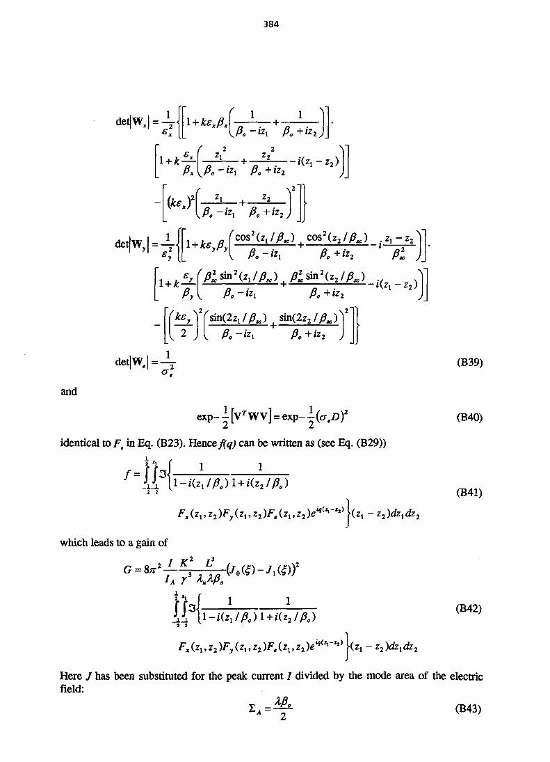
384

and

l + kejl

PAP.-izi P.+i*i

Py

po+iz2

i(c7<J

identical to F, in Eq. (B23). Hence f(q) can be written as (see Eq. (B29))

f=\ U\ 1

44 V-ib

which leads to a gain of

F,(z1,z2)F,(z1,za)F(,(z1,z2)ei|<Ii-li)|(z1-z2)dz1dz2

(B39)

(B40)

(B41)

(B42)

Here / has been substituted for the peak current / divided by the mode area of the electricfield:

(B43)

385

and F is given by

(B44)

B.4 The optical klystronFor the OK the assumption is made that the interaction between the electrons and the

optical wave can be neglected within the drift section of the OK which thus becomes a linearcombination of two undulators, separated by a drift section. Now the symmetric OK will beinvestigated, i.e. the drift section occupies a system with a total length L where the centre partLd. In the drift section the optical wave-front advances A^ wavelengths, relative to the electronbeam. A drift length {z^-z^ thus modifies to

Az = Zj - z2

and the gain becomes

\zl+NdIN - z 2 , <-\Ld

Z1~Z2 other(B45)

(B46)

J<LJ2L

z\>Ldl2L

where g(z) arises from the fact that the interaction in the drift space of the OK is neglected.Note that N is the total number of undulator periods (divided over two undulators).

386

ARDUINI, G.

BIASCI, J-C.

CHRISTIAN, D.

CLARKE, J.

D'AMICO, T.

DYKES, D.M.

FBLHOL, J-M.

GORBACHEV, E.V.

GÜNZEL, T.

HAHN, T.

HARDY, L.

HILL, S.

JACOB, J.

KANG, Y.

KEIL, J.

KHAN, S.

KIRCH, K.

LAGNIEL, J-M.

LEBLANC, G.

LIMBORG, C.

LONZA, M.

MAAS, R.

MARTIN, M.

MAYER, T.

MCINTOSH, P.

MILOV, A.

NAUMANN, O.

NAYLOR, G.

NEMOZ, C.

NIELSEN, J.S.

NOOMEN, J.

PA YET, J.

LIST OF PARTICIPANTS

CERN, Geneva, Switzerland

ESRF, Grenoble, France


CLRC Daresbury Lab., Warrington, UK


CCLRC Daresbury Lab., Warrington, UK


JINR, Dubna, Russia




CLRC Daresbury Lab., Warrington, UK


Argonne National Lab., EL, USA

Universität Bonn, Germany

BESSY H, Berlin, Germany

PSI, Villigen, Switzerland

CEA-Saclay, Gif-sur- Yvette, France

MAXLAB, Lund, Sweden


Sincrotrone Trieste, PD, Italy

NIKHEF, Amsterdam, Netherlands


BESSY Gmbh, Berlin, Germany

CCLRC Daresbury Lab., Warrington, UK

BINP, Novosibirsk, Russia




University of Aarhus, Denmark

NIKHEF-K, Amsterdam, Netherlands

CEA-Saclay, Gif-sur-Yvette, France

387

PLOUVIEZ, E.

QUERALT, X.

RAJEWSKA, A.

RATSCHOW, S.

REVOL, J-L.

RICCARDO, F.

ROUX, R.

SAJAEV, V.

SCARLAT, F.

SCHIRM, K-M.

SCHMIDT, G.

SEEBACH, M.

SHAFT AN, T.

SHELDRAKE, R.

SMETANIN, I.

STEIER, C

TORDEUX, M.-A.

TSUCHIYA, K.

VAN VAERENBERGH, P.

VISENTIN, B.

WEINMANN, P.

WEINRICH, U.

WERNER, M.

ZHANG, L.

ZICHY, J.A.


Daresbury Lab., Warrington, UK

JINR, Dubna, Russia

Johannes-Gutenberg-Univ., Mainz, Germany


Sincrotrone Trieste, Italy

LURE - CNRS/CEA, Orsay, France


Institute of Atomic Physics, Bucharest, Romania



DESY - MKI, Hamburg, Germany


EEV Ltd., Chelmsford, UK

P.N. Lebedev Physics Inst., Moscow, Russia

Universität Bonn, Germany

LURE, Orsay, France

KEK, Photon Factory, Tsukuba-shi, Japan


CEA-Saclay, Gif-sur-Yvette, France

Max-Planck-Institut, Munich, Germany


DESY - MKI, Hamburg, Germany


Paul Scherrer Inst., Villigen, Switzerland

List of CERN Reports published in 1998

CERN 98-01CERN. GenevaTavlet, M; Fontaine, A; Schonbacher, H

Compilation of radiation damage test data,Part II, 2nd edition: Thermoset andthermoplastic resins, composite materials;Index des resultats d'essais de radioresistance,IF Partie, 2e edition: Resines thermodurcies etthermoplastiques, materiaux composites

CERN, 18 May 1998.-180 p

CERN 98-02CERN. GenevaAcquistapace, G; Baldy, J L; Ball, A E: et al.

The CERN neutrino beam to Gran Sasso(NGS); Conceptual technical design

CERN, 19 May 1998.-126 p

CERN 98-03CERN. GenevaEllis, N; Neubert, M [eds]

Proceedings, 1997 European School ofHigh-Energy Physics, Menstrup, Denmark,25 M a y - 7 June 1997

CERN, 20 May 1998. - 364 p

(?ERN 98-04CERN. GenevaTurner, S [ed]

Proceedings, CAS - CERN AcceleratorSchool; Synchrotron Radiation and FreeElectron Lasers, Grenoble, France, 22-27 Apr1996

CERN, 3 August 1998. - 401 p

CERN 98-04ISSN 0007-8328TSRN 9

CERN ACCELERATOR SCHOOL ... - OSTI.GOV

Documents