Cerebral blood flow and autoregulation: current measurement ...

Cerebral blood flow andautoregulation: current measurementtechniques and prospects fornoninvasive optical methods

Sergio FantiniAngelo SassaroliKristen T. TgavalekosJoshua Kornbluth

Sergio Fantini, Angelo Sassaroli, Kristen T. Tgavalekos, Joshua Kornbluth, “Cerebral blood flow andautoregulation: current measurement techniques and prospects for noninvasive optical methods,”Neurophoton. 3(3), 031411 (2016), doi: 10.1117/1.NPh.3.3.031411.

Downloaded From: https://www.spiedigitallibrary.org/journals/Neurophotonics on 07 Mar 2022Terms of Use: https://www.spiedigitallibrary.org/terms-of-use

Cerebral blood flow and autoregulation:current measurement techniques andprospects for noninvasive optical methods

Sergio Fantini,a,* Angelo Sassaroli,a Kristen T. Tgavalekos,a and Joshua Kornbluthb

aTufts University, Department of Biomedical Engineering, 4 Colby Street, Medford, Massachusetts 02155, United StatesbTufts University School of Medicine, Department of Neurology, Division of Neurocritical Care, 800 Washington Street, Box #314, Boston,Massachusetts 02111, United States

Abstract. Cerebral blood flow (CBF) and cerebral autoregulation (CA) are critically important to maintain properbrain perfusion and supply the brain with the necessary oxygen and energy substrates. Adequate brain perfusionis required to support normal brain function, to achieve successful aging, and to navigate acute and chronicmedical conditions. We review the general principles of CBF measurements and the current techniques to mea-sure CBF based on direct intravascular measurements, nuclear medicine, X-ray imaging, magnetic resonanceimaging, ultrasound techniques, thermal diffusion, and optical methods. We also review techniques for arterialblood pressure measurements as well as theoretical and experimental methods for the assessment of CA,including recent approaches based on optical techniques. The assessment of cerebral perfusion in the clinicalpractice is also presented. The comprehensive description of principles, methods, and clinical requirements ofCBF and CAmeasurements highlights the potentially important role that noninvasive optical methods can play inthe assessment of neurovascular health. In fact, optical techniques have the ability to provide a noninvasive,quantitative, and continuous monitor of CBF and autoregulation. © 2016 Society of Photo-Optical Instrumentation Engineers

(SPIE) [DOI: 10.1117/1.NPh.3.3.031411]

Keywords: Cerebral perfusion; autoregulation; computed tomography perfusion; perfusion magnetic resonance imaging; transcranialDoppler; laser Doppler flowmetry; near-infrared spectroscopy; diffuse correlation spectroscopy; coherent hemodynamicsspectroscopy.

Paper 16001SSVR received Jan. 4, 2016; accepted for publication May 10, 2016; published online Jun. 21, 2016.

1 Cerebral blood flow

1.1 Physiological importance and normal values ofcerebral blood flow in adult humans

The human brain is an organ with high-energy density demands,amounting to only 2% of the entire body mass (or ∼1.4 kg) butaccounting for about 20% of the total power consumption of anormal adult at rest (or ∼20 W). Blood perfusion is responsiblefor the delivery of oxygen, which is necessary for the neuronaloxidative metabolism of energy substrates (mostly glucose, butalso ketone bodies and lactate1). Because of the limited capacityof neurons for anaerobic metabolism (at rest, up to 92% of theadenosine triphosphate in the brain results from oxidativemetabolism of glucose2), cerebral blood flow (CBF) is criticallyimportant for brain function and viability. It ensures properdelivery of oxygen and energy substrates and the removal ofwaste products of metabolism. Both hypoperfusion (insufficientCBF) and hyperperfusion (excessive CBF) can cause brain dam-age through ischemic injury, the former, and the breakdown ofthe blood–brain barrier, the latter, which can cause seizures,headaches, encephalopathy, and both ischemic and hemorrhagicstroke.3

CBF is defined as the blood volume that flows per unit massper unit time in brain tissue and is typically expressed in unitsof mlblood∕ð100 gtissue minÞ. Alternatively, one may expressCBF in terms of flow per unit volume of brain tissue, thus in

mlblood∕ð100 mltissue minÞ. The numerical values of CBF in thetwo cases differ by a factor given by the density of humanbrain tissue, which is about 1.04 to 1.06 g∕ml (with reportedvalues, measured ex vivo, as high as 1.08 g∕ml).4 The normalaverage cerebral blood flow (CBF) in adult humans is about50 ml∕ð100 g minÞ,5 with lower values in the white matter[∼20 ml∕ð100 g minÞ] and greater values in the gray matter[∼80 ml∕ð100 g minÞ].2

1.2 Factors that affect cerebral blood flow

In the spirit of Ohm’s law or Darcy’s law, blood flow (BF)through a vascular segment can be expressed as the ratiobetween the pressure difference across that segment (δP) andits vascular resistance (R). Poiseuille’s law expresses this resis-tance of a vascular segment (R) in terms of its radius (r), length(L), and the blood viscosity (η, usually expressed in centipoise,with 1 cP ¼ 1 mPa s): R ¼ 8ηL∕ðπr4Þ. Even though BF doesnot strictly fulfill all requirements for the validity of Poiseuille’slaw (mostly because blood does not behave as a Newtonianfluid, especially in the microvasculature, blood vessels are notrigid pipes, and the flow velocity profile may deviate from theparabolic shape of steady laminar flow, especially at branchingpoints or curved sections), it is nevertheless useful referring to itto appreciate, at least qualitatively, the factors that affect CBF.According to Poiseuille’s law, the blood flow (BF, in units ofblood volume per unit time) through a vascular segment oflength L and radius r, driven by a pressure difference δP, isgiven by*Address all correspondence to: Sergio Fantini, E-mail: [email protected]

Neurophotonics 031411-1 Jul–Sep 2016 • Vol. 3(3)

Neurophotonics 3(3), 031411 (Jul–Sep 2016)


http://dx.doi.org/10.1117/1.NPh.3.3.031411






mailto:[email protected]



EQ-TARGET;temp:intralink-;e001;63;752BF ¼ δPR

¼ δPπr4

8ηL: (1)

In the case of CBF, the driving pressure is the so-called cer-ebral perfusion pressure (CPP), defined in the next paragraph, andthe resistance is a total cerebrovascular resistance (CVR), whichis associated with the entire brain vascular tree. The main sourcesof CVR are small arteries and pial arterioles, which can regulatetheir radius (r) through vasodilatation and vasoconstriction.

The CPP is defined as the difference between the meanarterial pressure (MAP), which is the weighted average of thesystolic and diastolic pressure, and the intracranial pressure(ICP), which is the pressure of the cerebrospinal fluid (CSF)in the subarachnoid space. The normal range for restingMAP is 70 to 100 mmHg and for ICP it is 5 to 15 mmHg.From Eq. (1), it is apparent that changes in perfusion pressure,changes in vascular radius (i.e., vasodilation and vasoconstric-tion), and changes in blood viscosity all affect the CBF. Changesin perfusion pressure may occur under normal conditions, e.g.,during a change in posture or exercise, or they may result fromthe administration of drugs or from pathological conditions suchas subarachnoid hemorrhage (SAH), traumatic brain injury(TBI), and stroke. Blood viscosity is directly related to hemato-crit and the concentration of hemoglobin in blood. While lowerhematocrit decreases viscosity, thus increasing CBF accordingto Eq. (1), it also reduces the oxygen-carrying capacity of blood.The effect of the vascular radius r on CBF is of particular inter-est because it is responsible for the modulation and regulation ofCBF, which is highly sensitive to r as indicated by the fourthpower of r in Eq. (1), and we consider it next.

There are a number of factors that affect the vascular smoothmuscles of small arteries and arterioles, resulting in their con-striction or dilation. For example, carbon dioxide (CO2) is apowerful vasodilator, so that CBF increases during hypercapnicconditions. Two processes that are of paramount importance incerebral hemodynamics are the cerebrovascular responses tobrain metabolism (neurovascular coupling) and to changes inperfusion pressure (CA).

Neurovascular coupling is responsible for the increase inCBF to support greater regional or global metabolic demandsof the brain. This metabolism-driven increase in CBF is thoughtto be effected by a number of vasoactive mediators such as ions(Kþ;Hþ;Ca2þ), metabolic by-products (lactate, CO2, hypoxia,adenosine), vasoactive neurotransmitters (dopamine, gamma-amino butyric acid, acethylcoline), nitric oxide (NO), carbonmonoxide (CO), and so on,6,7 with a potential contributionfrom astrocytes.8

CA is one of the homeostatic mechanisms of the body tokeep CBF relatively constant despite changes in CPP. Eventhough the basic mechanisms responsible for neurovascular cou-pling and autoregulation are yet to be fully understood, it isnevertheless likely that neurovascular coupling and autoregula-tion share some common pathways that link them.9,10 In the nextsection, we consider CA in more detail.

2 Cerebral autoregulation: the link betweenperfusion pressure and cerebral blood flow

2.1 Basic mechanisms and physiologicalimportance of cerebral autoregulation

As discussed above, CBF is affected by a number of physiologi-cal and biochemical mechanisms, including changes in CPP.

CA is the homeostatic process of regulation of CBF in responseto changes in CPP. The way CA is achieved is through the regu-lation of CVR, which is done most effectively by modulating theradius of cerebral small arteries and arterioles [see Eq. (1)].In the absence of CA, an increase in MAP causes an increaseof CPP and, therefore, an increase of CBF even if the metabolicdemand of the brain remains constant. Therefore, the CAmechanism, which can be seen as a negative feedback loopmechanism, counteracts the MAP increase by narrowing thevessels’ radius (thus increasing their resistance to flow) andbringing CBF to the original level. Conversely, a decrease inMAP tends to decrease CBF, and the regulatory mechanismcauses vessel dilation to rebalance the CBF. These reactions ofthe cerebrovascular system to a MAP change occur if CA isworking properly, otherwise, in pathological conditions whereCA is impaired, CBF follows more or less passively (accordingto the level of impairment) MAP changes.

The physiological origin of CA is still unclear, with proposedmechanisms invoking myogenic, metabolic, and neurogenicprocesses.3,11 Myogenic mechanism: a myogenic response ofvascular smooth muscle to transmural pressure changes wasproposed to occur through arterial membrane depolarization,and to result in changes in the concentration of Ca2þ in thearterial wall.12 Metabolic mechanism: the altered concentrationof vasoactive metabolites (such as adenosine) was proposed toresult from initial blood-pressure-induced changes in BF.13

Neurogenic mechanism: perivascular neurons were proposed tohave autoregulatory effects on cerebral arterioles.14 Regardlessof which mechanism is responsible or prevalent, CA is mediatedthrough the release of chemical mediators, which implies thata finite amount of time is required to regulate the CVR.Therefore, a finite amount of time is needed to restore the origi-nal value of CBF following a MAP change.11

2.2 Static versus dynamic cerebral autoregulation

Studies on CA can be divided into static and dynamic ones.Even though the mechanisms underlying static and dynamicCA might be the same or share some common basis, thetime scale at which they are observed is different: static CArefers to MAP and CBF values under steady state conditionsthat are observed over a time scale of minutes or hours,while dynamic CA refers to transient MAP and CBF changesthat are observed in a time scale of seconds. Early studies onCA relied on relatively “slow” methods for measuring CBF,like the Kety–Schmidt technique15 (see Sec. 3.2.1), or the133Xe [Ref. 16] or 85Kr [Ref. 17] uptake technique (seeSec. 3.3.1). MAP was changed either by shifting centralblood volume with mechanical maneuvers (like changing pos-ture from supine to standing, head-up tilting, or introducinglower-body negative pressure), or, more commonly, by vaso-active drug injection. For a list of methods used to changeMAP in static CA studies, we refer to the review by Numanet al.18 The measurements of MAP and CBF were taken onlyat baseline (i.e., before the MAP was changed) and after theeffect of the challenging mechanism was complete (usuallyafter minutes). Therefore, with the typical methods used formeasuring static CA, it was not possible to study the temporalevolution of the transients in MAP and CBF as they reachedtheir steady-state values. Moreover, according to these methods,CAwas conceived as an all-or-nothing mechanism, i.e., either itwas present (if CBF recovered to the initial value) or not (if CBFfollowed passively the MAP change).


Fantini et al.: Cerebral blood flow and autoregulation: current measurement techniques and prospects for noninvasive optical methods


With the advent of transcranial Doppler ultrasound (TCD,see Sec. 3.6.1), it was possible to sample the flow velocity ofa large cerebral vessel [usually the middle cerebral artery(MCA)] with a high-sampling rate. This capability allowedfor new methods of measuring a dynamic CA response. Oneof the typical MAP challenging mechanisms is the thigh pres-sure cuff release method,19 which will be described in moredetail in Sec. 2.2.2. In both static and dynamic CA processes,the regulation of CBF is confined to the arterial compartmentprimarily at the level of small arteries and arterioles, whichare able to dilate or constrict in order to change their resistanceto flow.

2.2.1 Static cerebral autoregulation

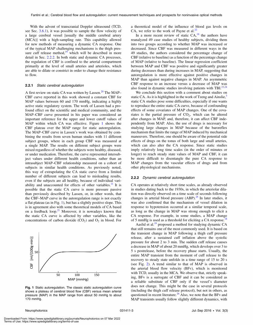
A first review on static CAwas written by Lassen.20 The MAP–CBF curve reported in this work showed a constant CBF forMAP values between 60 and 170 mmHg, indicating a highlyactive static regulatory system. The work of Lassen had a pro-found effect on the scientific and medical community, and theMAP–CBF curve presented in his paper was considered animportant reference for the upper and lower cutoff values ofMAP within which CA was effective. Figure 1 shows theCBF plateau over the MAP range for static autoregulation.The MAP–CBF curve in Lassen’s work was obtained by com-bining the results from seven human studies with 11 differentsubject groups, where in each group CBF was measured ata single MAP. The results on different subject groups weremixed regardless of whether the subjects were healthy, diseased,or under medication. Therefore, the curve represented intersub-ject values under different health conditions, rather than anintrasubject MAP–CBF relationship measured on a cohort ofsubjects in similar health conditions. As previously noted,this way of extrapolating the CA static curve from a limitednumber of different subjects can lead to misleading results,even if the subjects are all healthy, because of individual vari-ability and unaccounted for effects of other variables.11 It ispossible that the static CA curve is more pressure passivethan previously described by Lassen, or, in other words, thatthe CBF–MAP curve in the autoregulation range is not exactlya flat plateau (as in Fig. 1), but has a slightly positive slope. Thisis in agreement also with some theoretical models of CA basedon a feedback loop.21 Moreover, it is nowadays known thatthe static CA curve is affected by other variables, like theconcentrations of carbon dioxide (CO2) and O2 in blood. For

a theoretical model of the influence of blood gas levels onCA, we refer to the work of Payne et al.22

In a more recent review of static CA,18 the authors havereanalyzed 49 case studies of healthy subjects, dividing theminto two groups according to whether MAP was increased ordecreased. Since CBF was measured in different ways in the49 studies, the authors considered the percentage change ofCBF (relative to baseline) as a function of the percentage changeof MAP (relative to baseline). The linear regression coefficientbetween MAP and CBF was positive and significantly greaterduring decreases than during increases in MAP, suggesting thatautoregulation is more effective against positive changes inMAP than against negative changes in MAP. An asymmetricCBF response to an increase versus a decrease of MAP wasalso found in dynamic studies involving patients with TBI.23,24

We conclude this section with a comment about studies onstatic CA. As it is highlighted in the work of Tzeng and Ainslie,3

static CA studies pose some difficulties, especially if one wantsto reproduce the entire static CA curve, because of confoundingeffects of some covariates of MAP changes. One of the cova-riates is the partial pressure of CO2, which can be alteredafter changes in MAP, and, therefore, it can affect CBF inde-pendently from MAP. Also, the use of drugs is necessary forstudying large changes in MAP because of the baroreflexmechanism that limits the range of MAP induced by mechanicalmaneuvers. Therefore, one should be aware of the potential sideeffects of drugs on the tonus of both large and small arteries,which can also alter the CA response. Since static studiesimply relatively long time scales (in the order of minutes orlonger) to reach steady state values of MAP and CBF, it canbe more difficult to disentangle the pure CA response toMAP changes from the vascular effects of drugs and fromother physiological mechanisms.

2.2.2 Dynamic cerebral autoregulation

CA operates at relatively short time scales, as already observedin studies dating back to the 1930s, in which the arteriolar dila-tion was directly observed on a time scale of seconds followingchanges in arterial blood pressure (ABP).25 In later studies, itwas also confirmed that the mechanism of vessel dilation inresponse to hypotension occurred at a similar temporal scale,as long as the change in MAP was strong enough to elicit aCA response. For example, in some studies, a MAP changeof 5 mmHg is used as a threshold for eliciting a CA response.18

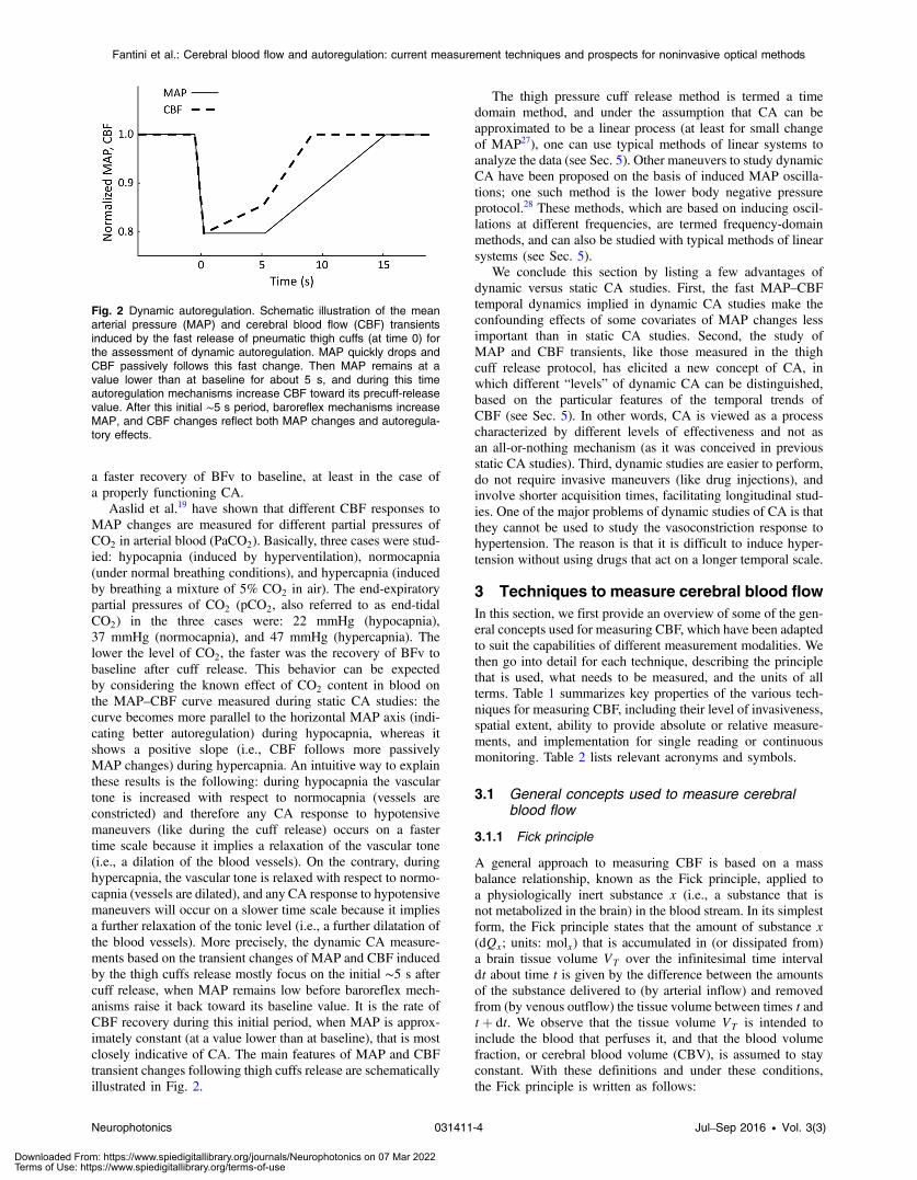
Aaslid et al.19 proposed a method for studying dynamic CAthat still remains one of the most commonly used. It is based onthe transient change in MAP following a thigh cuff pressurerelease, after a sustained cuff inflation above the systolicpressure for about 2 to 3 min. The sudden cuff release causesa decrease in MAP of about 20 mmHg, which develops over 3 to5 s postrelease, before the recovery phase starts. Usually, theentire MAP transient from the moment of cuff release to therecovery to steady state unfolds in a time range of 15 to 20 s(see Fig. 2). A trend similar to that of MAP is observed inthe arterial blood flow velocity (BFv), which is monitoredwith TCD, usually in the MCA. We observe that, strictly speak-ing, BFv is a surrogate of CBF and it can be considered asa reliable substitute of CBF only if the vessel’s diameterdoes not change. This might be the case in several protocols(including the thigh cuff release protocol), but not in others, asquestioned in recent literature.26 Also, we note that the BFv andMAP transients usually follow slightly different dynamics, with

Fig. 1 Static autoregulation. The classic static autoregulation curveshows a plateau of cerebral blood flow (CBF) versus mean arterialpressure (MAP) in the MAP range from about 50 mmHg to about170 mmHg.




a faster recovery of BFv to baseline, at least in the case ofa properly functioning CA.

Aaslid et al.19 have shown that different CBF responses toMAP changes are measured for different partial pressures ofCO2 in arterial blood (PaCO2). Basically, three cases were stud-ied: hypocapnia (induced by hyperventilation), normocapnia(under normal breathing conditions), and hypercapnia (inducedby breathing a mixture of 5% CO2 in air). The end-expiratorypartial pressures of CO2 (pCO2, also referred to as end-tidalCO2) in the three cases were: 22 mmHg (hypocapnia),37 mmHg (normocapnia), and 47 mmHg (hypercapnia). Thelower the level of CO2, the faster was the recovery of BFv tobaseline after cuff release. This behavior can be expectedby considering the known effect of CO2 content in blood onthe MAP–CBF curve measured during static CA studies: thecurve becomes more parallel to the horizontal MAP axis (indi-cating better autoregulation) during hypocapnia, whereas itshows a positive slope (i.e., CBF follows more passivelyMAP changes) during hypercapnia. An intuitive way to explainthese results is the following: during hypocapnia the vasculartone is increased with respect to normocapnia (vessels areconstricted) and therefore any CA response to hypotensivemaneuvers (like during the cuff release) occurs on a fastertime scale because it implies a relaxation of the vascular tone(i.e., a dilation of the blood vessels). On the contrary, duringhypercapnia, the vascular tone is relaxed with respect to normo-capnia (vessels are dilated), and any CA response to hypotensivemaneuvers will occur on a slower time scale because it impliesa further relaxation of the tonic level (i.e., a further dilatation ofthe blood vessels). More precisely, the dynamic CA measure-ments based on the transient changes of MAP and CBF inducedby the thigh cuffs release mostly focus on the initial ∼5 s aftercuff release, when MAP remains low before baroreflex mech-anisms raise it back toward its baseline value. It is the rate ofCBF recovery during this initial period, when MAP is approx-imately constant (at a value lower than at baseline), that is mostclosely indicative of CA. The main features of MAP and CBFtransient changes following thigh cuffs release are schematicallyillustrated in Fig. 2.

The thigh pressure cuff release method is termed a timedomain method, and under the assumption that CA can beapproximated to be a linear process (at least for small changeof MAP27), one can use typical methods of linear systems toanalyze the data (see Sec. 5). Other maneuvers to study dynamicCA have been proposed on the basis of induced MAP oscilla-tions; one such method is the lower body negative pressureprotocol.28 These methods, which are based on inducing oscil-lations at different frequencies, are termed frequency-domainmethods, and can also be studied with typical methods of linearsystems (see Sec. 5).

We conclude this section by listing a few advantages ofdynamic versus static CA studies. First, the fast MAP–CBFtemporal dynamics implied in dynamic CA studies make theconfounding effects of some covariates of MAP changes lessimportant than in static CA studies. Second, the study ofMAP and CBF transients, like those measured in the thighcuff release protocol, has elicited a new concept of CA, inwhich different “levels” of dynamic CA can be distinguished,based on the particular features of the temporal trends ofCBF (see Sec. 5). In other words, CA is viewed as a processcharacterized by different levels of effectiveness and not asan all-or-nothing mechanism (as it was conceived in previousstatic CA studies). Third, dynamic studies are easier to perform,do not require invasive maneuvers (like drug injections), andinvolve shorter acquisition times, facilitating longitudinal stud-ies. One of the major problems of dynamic studies of CA is thatthey cannot be used to study the vasoconstriction response tohypertension. The reason is that it is difficult to induce hyper-tension without using drugs that act on a longer temporal scale.

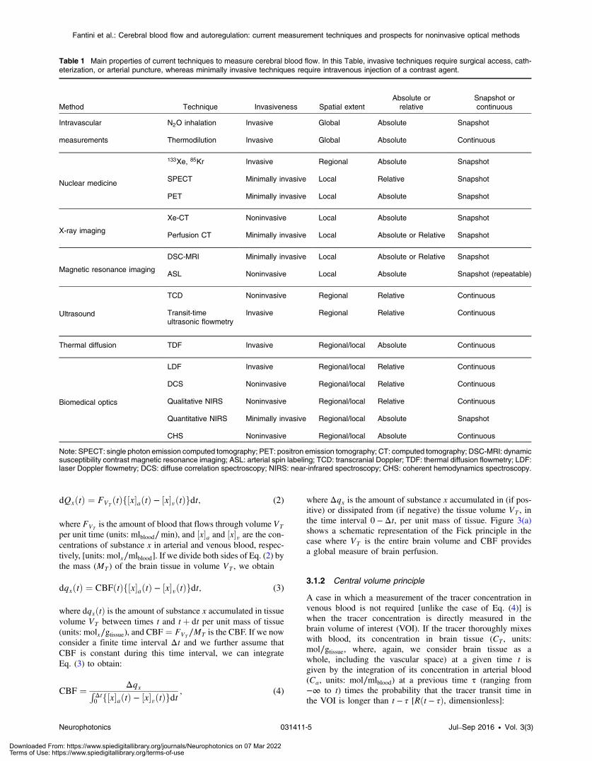
3 Techniques to measure cerebral blood flowIn this section, we first provide an overview of some of the gen-eral concepts used for measuring CBF, which have been adaptedto suit the capabilities of different measurement modalities. Wethen go into detail for each technique, describing the principlethat is used, what needs to be measured, and the units of allterms. Table 1 summarizes key properties of the various tech-niques for measuring CBF, including their level of invasiveness,spatial extent, ability to provide absolute or relative measure-ments, and implementation for single reading or continuousmonitoring. Table 2 lists relevant acronyms and symbols.

3.1 General concepts used to measure cerebralblood flow

3.1.1 Fick principle

A general approach to measuring CBF is based on a massbalance relationship, known as the Fick principle, applied toa physiologically inert substance x (i.e., a substance that isnot metabolized in the brain) in the blood stream. In its simplestform, the Fick principle states that the amount of substance x(dQx; units: molx) that is accumulated in (or dissipated from)a brain tissue volume VT over the infinitesimal time intervaldt about time t is given by the difference between the amountsof the substance delivered to (by arterial inflow) and removedfrom (by venous outflow) the tissue volume between times t andtþ dt. We observe that the tissue volume VT is intended toinclude the blood that perfuses it, and that the blood volumefraction, or cerebral blood volume (CBV), is assumed to stayconstant. With these definitions and under these conditions,the Fick principle is written as follows:

Fig. 2 Dynamic autoregulation. Schematic illustration of the meanarterial pressure (MAP) and cerebral blood flow (CBF) transientsinduced by the fast release of pneumatic thigh cuffs (at time 0) forthe assessment of dynamic autoregulation. MAP quickly drops andCBF passively follows this fast change. Then MAP remains at avalue lower than at baseline for about 5 s, and during this timeautoregulation mechanisms increase CBF toward its precuff-releasevalue. After this initial ∼5 s period, baroreflex mechanisms increaseMAP, and CBF changes reflect both MAP changes and autoregula-tory effects.




EQ-TARGET;temp:intralink-;e002;63;285dQxðtÞ ¼ FVTðtÞf½x�aðtÞ − ½x�vðtÞgdt; (2)

where FVTis the amount of blood that flows through volume VT

per unit time (units: mlblood∕min), and ½x�a and ½x�v are the con-centrations of substance x in arterial and venous blood, respec-tively, [units:molx∕mlblood]. If we divide both sides of Eq. (2) bythe mass (MT ) of the brain tissue in volume VT , we obtain

EQ-TARGET;temp:intralink-;e003;63;207dqxðtÞ ¼ CBFðtÞf½x�aðtÞ − ½x�vðtÞgdt; (3)

where dqxðtÞ is the amount of substance x accumulated in tissuevolume VT between times t and tþ dt per unit mass of tissue(units:molx∕gtissue), and CBF ¼ FVT

∕MT is the CBF. If we nowconsider a finite time interval Δt and we further assume thatCBF is constant during this time interval, we can integrateEq. (3) to obtain:

EQ-TARGET;temp:intralink-;e004;63;110CBF ¼ ΔqxRΔt0 f½x�aðtÞ − ½x�vðtÞgdt

; (4)

where Δqx is the amount of substance x accumulated in (if pos-itive) or dissipated from (if negative) the tissue volume VT , inthe time interval 0 − Δt, per unit mass of tissue. Figure 3(a)shows a schematic representation of the Fick principle in thecase where VT is the entire brain volume and CBF providesa global measure of brain perfusion.

3.1.2 Central volume principle

A case in which a measurement of the tracer concentration invenous blood is not required [unlike the case of Eq. (4)] iswhen the tracer concentration is directly measured in thebrain volume of interest (VOI). If the tracer thoroughly mixeswith blood, its concentration in brain tissue (CT , units:mol∕gtissue, where, again, we consider brain tissue as awhole, including the vascular space) at a given time t isgiven by the integration of its concentration in arterial blood(Ca, units: mol∕mlblood) at a previous time τ (ranging from−∞ to t) times the probability that the tracer transit time inthe VOI is longer than t − τ [Rðt − τÞ, dimensionless]:

Table 1 Main properties of current techniques to measure cerebral blood flow. In this Table, invasive techniques require surgical access, cath-eterization, or arterial puncture, whereas minimally invasive techniques require intravenous injection of a contrast agent.

Method Technique Invasiveness Spatial extentAbsolute orrelative

Snapshot orcontinuous

Intravascular N2O inhalation Invasive Global Absolute Snapshot

measurements Thermodilution Invasive Global Absolute Continuous

Nuclear medicine

133Xe, 85Kr Invasive Regional Absolute Snapshot

SPECT Minimally invasive Local Relative Snapshot

PET Minimally invasive Local Absolute Snapshot

X-ray imaging

Xe-CT Noninvasive Local Absolute Snapshot

Perfusion CT Minimally invasive Local Absolute or Relative Snapshot

Magnetic resonance imaging

DSC-MRI Minimally invasive Local Absolute or Relative Snapshot

ASL Noninvasive Local Absolute Snapshot (repeatable)

Ultrasound

TCD Noninvasive Regional Relative Continuous

Transit-timeultrasonic flowmetry

Invasive Regional Relative Continuous

Thermal diffusion TDF Invasive Regional/local Absolute Continuous

Biomedical optics

LDF Invasive Regional/local Relative Continuous

DCS Noninvasive Regional/local Relative Continuous

Qualitative NIRS Noninvasive Regional/local Relative Continuous

Quantitative NIRS Minimally invasive Regional/local Absolute Snapshot

CHS Noninvasive Regional/local Absolute Continuous

Note: SPECT: single photon emission computed tomography; PET: positron emission tomography; CT: computed tomography; DSC-MRI: dynamicsusceptibility contrast magnetic resonance imaging; ASL: arterial spin labeling; TCD: transcranial Doppler; TDF: thermal diffusion flowmetry; LDF:laser Doppler flowmetry; DCS: diffuse correlation spectroscopy; NIRS: near-infrared spectroscopy; CHS: coherent hemodynamics spectroscopy.




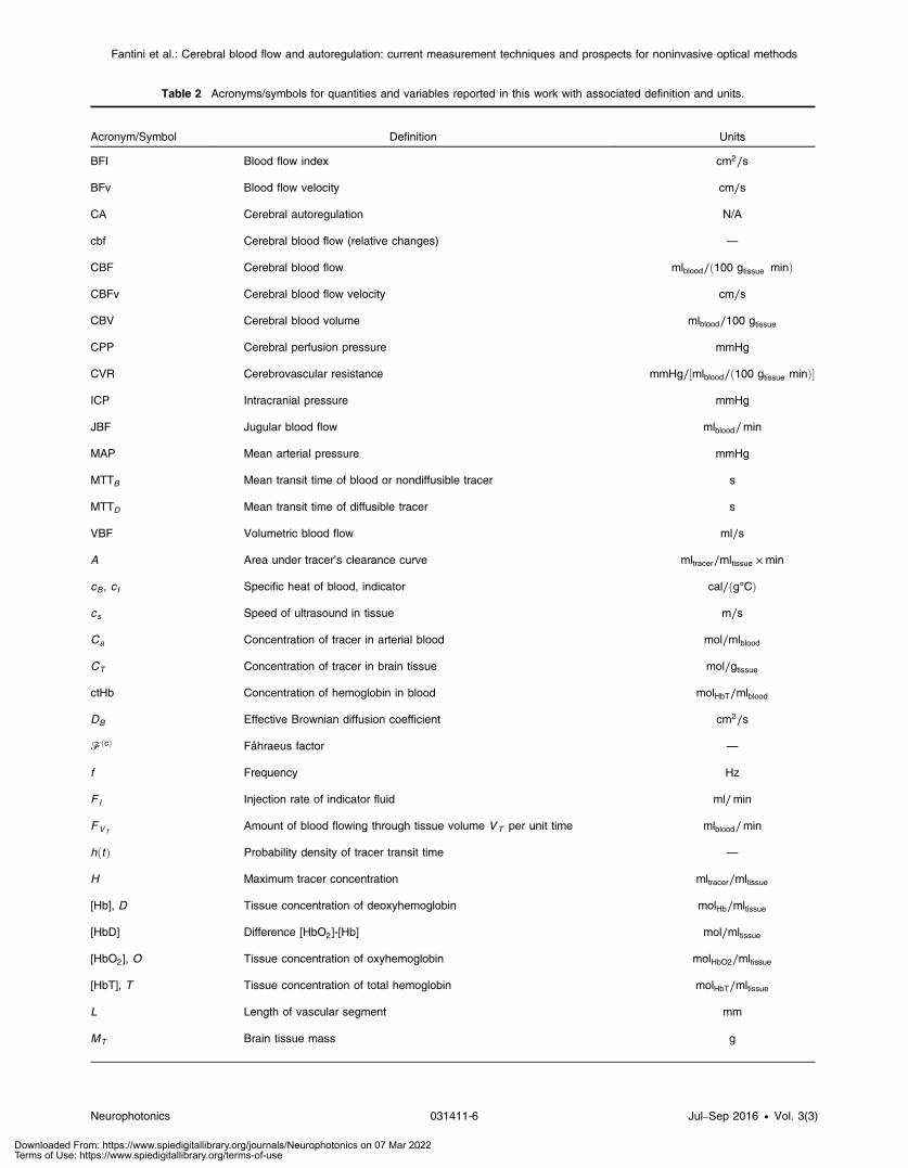
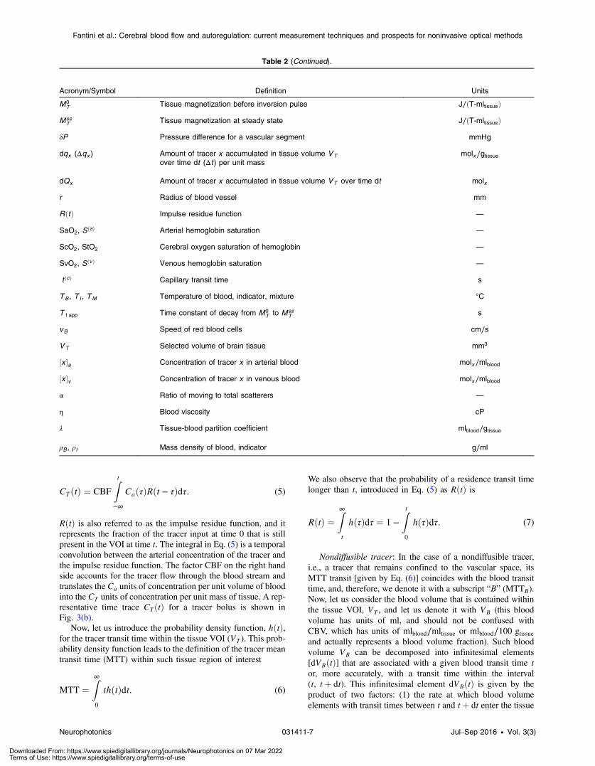
Table 2 Acronyms/symbols for quantities and variables reported in this work with associated definition and units.

Acronym/Symbol Definition Units

BFI Blood flow index cm2∕s

BFv Blood flow velocity cm∕s

CA Cerebral autoregulation N/A

cbf Cerebral blood flow (relative changes) —

CBF Cerebral blood flow mlblood∕ð100 gtissue minÞ

CBFv Cerebral blood flow velocity cm∕s

CBV Cerebral blood volume mlblood∕100 gtissue

CPP Cerebral perfusion pressure mmHg

CVR Cerebrovascular resistance mmHg∕½mlblood∕ð100 gtissue minÞ�

ICP Intracranial pressure mmHg

JBF Jugular blood flow mlblood∕min

MAP Mean arterial pressure mmHg

MTTB Mean transit time of blood or nondiffusible tracer s

MTTD Mean transit time of diffusible tracer s

VBF Volumetric blood flow ml∕s

A Area under tracer’s clearance curve mltracer∕mltissue ×min

cB , cI Specific heat of blood, indicator cal∕ðg°CÞ

cs Speed of ultrasound in tissue m∕s

Ca Concentration of tracer in arterial blood mol∕mlblood

CT Concentration of tracer in brain tissue mol∕gtissue

ctHb Concentration of hemoglobin in blood molHbT∕mlblood

DB Effective Brownian diffusion coefficient cm2∕s

FðcÞ Fåhraeus factor —

f Frequency Hz

F I Injection rate of indicator fluid ml∕min

FVTAmount of blood flowing through tissue volume VT per unit time mlblood∕min

hðtÞ Probability density of tracer transit time —

H Maximum tracer concentration mltracer∕mltissue

[Hb], D Tissue concentration of deoxyhemoglobin molHb∕mltissue

[HbD] Difference [HbO2]-[Hb] mol∕mltissue

[HbO2], O Tissue concentration of oxyhemoglobin molHbO2∕mltissue

[HbT], T Tissue concentration of total hemoglobin molHbT∕mltissue

L Length of vascular segment mm

MT Brain tissue mass g




EQ-TARGET;temp:intralink-;e005;63;311CTðtÞ ¼ CBF

Zt−∞

CaðτÞRðt − τÞdτ: (5)

RðtÞ is also referred to as the impulse residue function, and itrepresents the fraction of the tracer input at time 0 that is stillpresent in the VOI at time t. The integral in Eq. (5) is a temporalconvolution between the arterial concentration of the tracer andthe impulse residue function. The factor CBF on the right handside accounts for the tracer flow through the blood stream andtranslates the Ca units of concentration per unit volume of bloodinto the CT units of concentration per unit mass of tissue. A rep-resentative time trace CTðtÞ for a tracer bolus is shown inFig. 3(b).

Now, let us introduce the probability density function, hðtÞ,for the tracer transit time within the tissue VOI (VT ). This prob-ability density function leads to the definition of the tracer meantransit time (MTT) within such tissue region of interest

EQ-TARGET;temp:intralink-;e006;63;110MTT ¼Z∞0

thðtÞdt: (6)

We also observe that the probability of a residence transit timelonger than t, introduced in Eq. (5) as RðtÞ is

EQ-TARGET;temp:intralink-;e007;326;289RðtÞ ¼Z∞t

hðτÞdτ ¼ 1 −Zt0

hðτÞdτ: (7)

Nondiffusible tracer: In the case of a nondiffusible tracer,i.e., a tracer that remains confined to the vascular space, itsMTT transit [given by Eq. (6)] coincides with the blood transittime, and, therefore, we denote it with a subscript “B” (MTTB).Now, let us consider the blood volume that is contained withinthe tissue VOI, VT , and let us denote it with VB (this bloodvolume has units of ml, and should not be confused withCBV, which has units of mlblood∕mltissue or mlblood∕100 gtissueand actually represents a blood volume fraction). Such bloodvolume VB can be decomposed into infinitesimal elements[dVBðtÞ] that are associated with a given blood transit time tor, more accurately, with a transit time within the interval(t, tþ dt). This infinitesimal element dVBðtÞ is given by theproduct of two factors: (1) the rate at which blood volumeelements with transit times between t and tþ dt enter the tissue

Table 2 (Continued).

Acronym/Symbol Definition Units

M0T Tissue magnetization before inversion pulse J∕ðT-mltissueÞ

MssT Tissue magnetization at steady state J∕ðT-mltissueÞ

δP Pressure difference for a vascular segment mmHg

dqx (Δqx ) Amount of tracer x accumulated in tissue volume VTover time dt (Δt ) per unit mass

molx∕gtissue

dQx Amount of tracer x accumulated in tissue volume VT over time dt molx

r Radius of blood vessel mm

RðtÞ Impulse residue function —

SaO2, SðaÞ Arterial hemoglobin saturation —

ScO2, StO2 Cerebral oxygen saturation of hemoglobin —

SvO2, SðvÞ Venous hemoglobin saturation —

t ðcÞ Capillary transit time s

TB , T I , TM Temperature of blood, indicator, mixture °C

T 1 app Time constant of decay from M0T to Mss

T s

vB Speed of red blood cells cm∕s

VT Selected volume of brain tissue mm3

½x �a Concentration of tracer x in arterial blood molx∕mlblood

½x �v Concentration of tracer x in venous blood molx∕mlblood

α Ratio of moving to total scatterers —

η Blood viscosity cP

λ Tissue-blood partition coefficient mlblood∕gtissue

ρB , ρI Mass density of blood, indicator g∕ml




region of interest (which is the same as the rate at which theyexit it because of the assumed stationarity of CBF and CBV),which is given by FVT

hðtÞdt (where FVTrepresents the amount

of blood flowing through the tissue volume VT , and has unitsof mlblood∕min); (2) the time spent by such blood volumeelements in the tissue VOI, which is t by definition. Therefore,one can write29,30

EQ-TARGET;temp:intralink-;e008;63;253dVBðtÞ ¼ FVTthðtÞdt: (8)

Integration of Eq. (8) over all transit times (0 ≤ t < ∞) yieldsthe relationship between FVT

and VB that is a manifestation ofthe central volume principle

EQ-TARGET;temp:intralink-;e009;63;188FVT¼ VB

MTTB: (9)

Dividing both sides of Eq. (9) by the mass (MT ) of the tissueregion of interest, and considering that CBF ¼ FVT

∕MT andCBV ¼ VB∕MT , we can write the central volume principlerelationship for CBF and CBV

EQ-TARGET;temp:intralink-;e010;63;101CBF ¼ CBV

MTTB: (10)

Diffusible tracer: Equation (10) may be generalized to thecase of a diffusible tracer. In this case, VB in Eq. (9) is replacedby the equilibrium volume of distribution of the tracer, i.e., theblood volume that contains the same amount of tracer that is inthe tissue volume VT at equilibrium.31 We stress again that “tis-sue” is intended here to include the blood in the vasculature.32

The numerator on the right-hand-side of Eq. (10) then becomesthe volume of distribution of the tracer per unit mass of tissue,which is referred to as the tissue-blood partition coefficient,λ, also defined as the concentration of the diffusible tracerin tissue (at equilibrium) divided by the concentration ofthe tracer in blood. If the same units for the concentrationsin tissue and blood are used, λ is dimensionless (or expressedin mlblood∕mltissue or gblood∕gtissue), whereas it takes units ofml∕g (i.e., mlblood∕gtissue) if the tissue and blood concentrationsof the indicator are expressed per unit tissue mass and per unitblood volume, respectively. Both conventions are used in theliterature, but here we use the latter convention, so that theunits of λ and CBV are the same. For example, the brain–blood partition coefficient for water is 0.90 ml∕g,33 whichcan be interpreted by saying that 0.90 ml of blood containthe same amount of water as 1 g of brain tissue. On thebasis of the above definitions, the central volume principle equa-tion for a diffusible tracer is

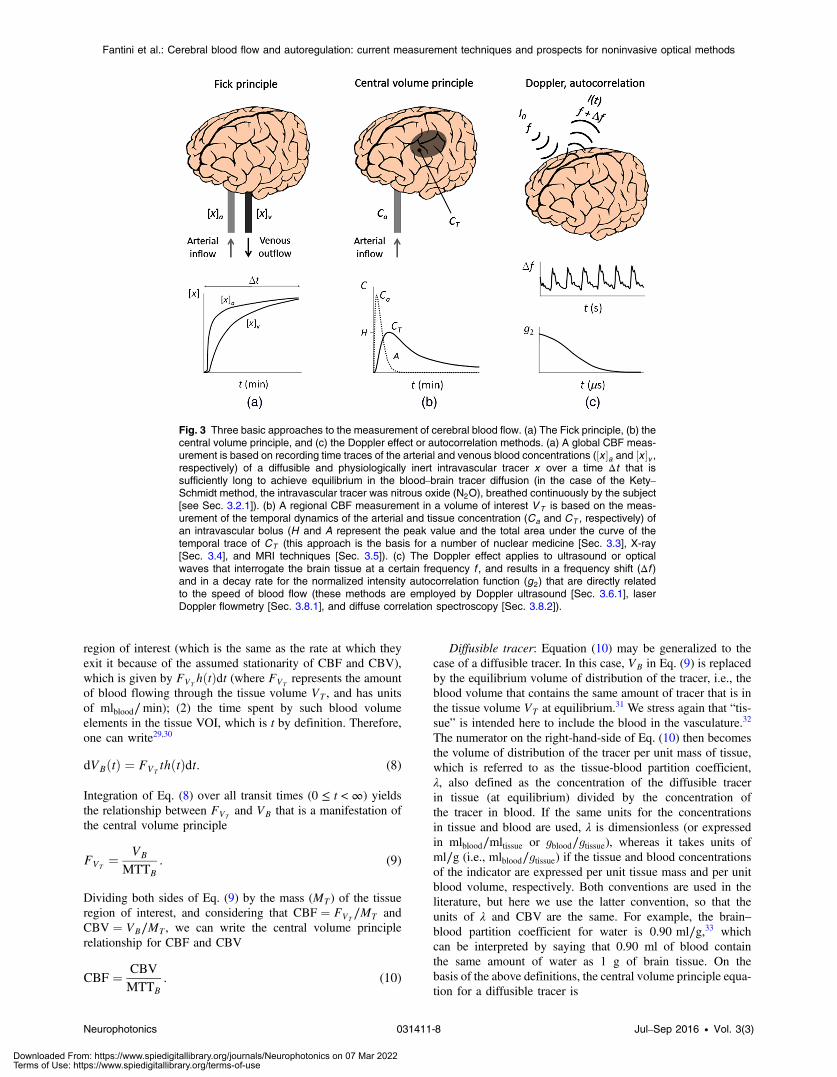
Fig. 3 Three basic approaches to the measurement of cerebral blood flow. (a) The Fick principle, (b) thecentral volume principle, and (c) the Doppler effect or autocorrelation methods. (a) A global CBF meas-urement is based on recording time traces of the arterial and venous blood concentrations (½x �a and ½x �v ,respectively) of a diffusible and physiologically inert intravascular tracer x over a time Δt that issufficiently long to achieve equilibrium in the blood–brain tracer diffusion (in the case of the Kety–Schmidt method, the intravascular tracer was nitrous oxide (N2O), breathed continuously by the subject[see Sec. 3.2.1]). (b) A regional CBF measurement in a volume of interest VT is based on the meas-urement of the temporal dynamics of the arterial and tissue concentration (Ca and CT , respectively) ofan intravascular bolus (H and A represent the peak value and the total area under the curve of thetemporal trace of CT (this approach is the basis for a number of nuclear medicine [Sec. 3.3], X-ray[Sec. 3.4], and MRI techniques [Sec. 3.5]). (c) The Doppler effect applies to ultrasound or opticalwaves that interrogate the brain tissue at a certain frequency f , and results in a frequency shift (Δf )and in a decay rate for the normalized intensity autocorrelation function (g2) that are directly relatedto the speed of blood flow (these methods are employed by Doppler ultrasound [Sec. 3.6.1], laserDoppler flowmetry [Sec. 3.8.1], and diffuse correlation spectroscopy [Sec. 3.8.2]).




EQ-TARGET;temp:intralink-;e011;63;752CBF ¼ λ

MTTD; (11)

where MTTD is the MTT transit of the diffusible tracer in thetissue VOI (which in general is different from MTTB). We con-clude this section by observing that λ ∼ 1 ml∕g for freelydiffusible tracers, whereas for nondiffusible tracers λ ¼ CBV,which is about 0.04 ml∕g. Therefore, a comparison ofEqs. (10) and (11) shows that MTTD ≫ MTTB, and in factMTTD is on the order of minutes whereas MTTB is on theorder of seconds. These concepts are illustrated in Fig. 3(b),in which the indicated time scale of minutes for the dynamicsof CTðtÞ refers to a diffusible tracer.

3.1.3 Doppler effect and intensity fluctuations

The interaction of a probing wave, be it an ultrasound pressurewave or an optical electromagnetic wave, with moving red bloodcells in the blood stream results in a frequency shift and in inten-sity fluctuations of the detected wave. The frequency shift is amanifestation of the Doppler effect; the intensity fluctuationscan be characterized by the field or intensity autocorrelationfunctions and their rate of decay. The Doppler effect, whichresults in spectral line broadening, and the intensity fluctuationsare different aspects of the same phenomenon. In fact, the inten-sity power spectrum and the field autocorrelation function arerelated by a Fourier transformation, known as the Wiener–Khinchin theorem. BF velocity, and therefore CBF, is directlyrelated to the Doppler shift (Δf) and directly related to the rateof decay of the normalized intensity autocorrelation function(g2). This approach to the measurement of BF is schematicallyillustrated in Fig. 3(c). It is important to observe that Dopplerand autocorrelation methods do not really measure CBF, butthey rather yield measures of the speed of BF, either in largevessels (Doppler ultrasound, Sec. 3.6.1) or in the microcircula-tion [laser Doppler flowmetry (LDF), Sec. 3.8.1; diffusecorrelation spectroscopy (DCS), Sec. 3.8.2]. Because CBF isintended to represent the rate of inflow of arterial blood intothe capillary bed rather than the speed of BF within brain tissue,the data provided by Doppler and autocorrelation methodsneed to be carefully interpreted and are often taken to providerelative measures of CBF changes.

3.2 Direct measurements of intravascular tracers inthe blood stream

3.2.1 Kety–Schmidt arteriovenous difference method

A seminal paper by Kety and Schmidt,34 which set the stagefor the development of a variety of CBF measurements in thehuman brain,35 considered nitrous oxide (N2O) as a freely dif-fusible intravascular tracer. It was administered by inhalation,and the dynamics of ½N2O�a and ½N2O�v were measured inblood drawn by femoral artery puncture and from a needle inthe right internal jugular vein, respectively. The dynamic mea-surements were performed over a time interval Δt ¼ 10 minfollowing the beginning of N2O inhalation, at which timea steady state was reached, such that ½N2O�a ¼ ½N2O�v. Thissteady state carries no information about CBF, but the timerequired to reach it is inversely related to CBF. Specifically,the measurement of CBF is based on the amount of N2O deliv-ered to the brain, per unit brain mass, over the entire time Δt(Δqx), and the total arteriovenous difference integrated over

time Δt, as given by Eq. (4), written again here with the generictracer x replaced by N2O:

34,36

EQ-TARGET;temp:intralink-;e012;326;730CBF ¼ ΔqN2ORΔt0 ð½N2O�a − ½N2O�vÞðtÞdt

: (12)

Typical time traces of ½N2O�aðtÞ and ½N2O�vðtÞ are shown inFig. 3(a). The total amount of N2O delivered to the brain perunit mass [i.e., the numerator of Eq. (12)] was calculated onthe basis of the relative solubility of N2O in brain tissueand in blood at equilibrium. Measurements with this methodreflect a global CBF, and Kety and Schmidt found a value of62� 12 ml∕ð100 g minÞ in a group of 11 human subjects.34

Following its introduction in 1945, the Kety–Schmidtmethod quickly became a standard approach for quantitativemeasurements of the global CBF. However, its application isinvasive and cumbersome, requiring inhalation of nitrousoxide, puncture or catheterization of the carotid or femoralartery, and accurate measurements of N2O concentrations inblood samples. Furthermore, it relies on some assumptions (jug-ular venous blood representing brain venous drainage, reachinga steady state of brain saturation with N2O within 10 to 15 min,and so on) that may not always be accurate. Finally, the Kety–Schmidt method allows for only global CBF measurements, butregional CBF measurements are highly desirable in a number ofresearch and clinical situations. For these reasons, other tech-niques have been considered to improve upon the intravasculartracer approach of Kety and Schmidt. For example, the intro-duction of radioactive tracers (such as 133Xe and 85Kr), inconjunction with measurements of their clearance curve (i.e.,their concentration decay versus time), leads to measurementsof regional CBF (see Sec. 3.3.1).

3.2.2 Jugular thermodilution

As an alternative to intravascular tracers that diffuse into thebrain, one may inject a cold fluid miscible with blood (typicallysaline) that introduces a thermal perturbation to perform a directmeasurement of BF velocity within a large blood vessel thatdrains the brain, such as the internal jugular vein. This methodallows for continuous or repeated measurements (in the casesof continuous infusion or cold bolus input, respectively)and is referred to as jugular thermodilution.37 While thismethod does not require arterial puncture or catheterization(but it requires jugular vein catheterization) it provides onlya local measurement of jugular venous flow (in units ofmlblood∕min). In the case of a continuous infusion, the jugularblood flow (JBF: ml∕min) is expressed as follows in terms ofthe injection rate of the indicator fluid (FI:ml∕min), the specificheat of blood and indicator [cB, cI: cal∕ðg°CÞ], and the densitiesof blood and indicator (ρB, ρI : g∕ml)

EQ-TARGET;temp:intralink-;e013;326;193JBF ¼ FIρIcIρBcB

�TM − TI

TB − TM

�; (13)

where TB, TI , and TM are the temperatures of blood, the indi-cator, and their mixture, respectively, which are measured bythermistors placed inside and outside the catheter used to injectthe indicator fluid.38 The JBF may be translated into a measureof the CBF, by considering that there are two internal jugularveins that drain the entire brain tissue mass (MT : g)




EQ-TARGET;temp:intralink-;e014;63;752CBF ¼ 2JBF

MT: (14)

Measurements of CBF with jugular thermodilution werevalidated by comparison with measurements with the Kety–Schmidt method.38

While jugular thermodilution allows for continuous measure-ments of BF, it does require injection of the fluid indicator, sothat the ability of the patient to handle the fluid load posesa limitation to the duration of flow monitoring.

3.3 Nuclear medicine

3.3.1 Intra-arterial injection of a radioactive inert gas(133Xe or 85Kr)

A common intraoperative method to measure CBF is based onthe intra-arterial injection of a radioactive bolus that emits γ-rays(photons) or β particles (electrons) and the detection of the dif-fusible tracer’s clearance curve in brain tissue regions by scin-tillation detectors,31,39 an Anger camera,40 or a Geiger–Müllertube.41,42 Two radioactive isotopes, 133Xe and 85Kr, the formermore commonly used than the latter, decay by emitting γ-raysand β particles, respectively, that are detected to yield regionalradioisotopes clearance curves. This approach relies on the sameconcepts as the Kety–Schmidt method (Sec. 3.2.1), but allowsfor regional measurements of CBF, and measures the clearancecurve of the tracer continuously rather than at a number of timepoints. Three methods have been proposed to analyze the clear-ance curve to generate CBF measurements:

1. Stochastic analysis is based on the central volumeprinciple [Eq. (11)] and yields the following expres-sion for CBF:31,43


MTTD¼ λ

HA; (15)

where λ is the tissue-blood partition coefficient forthe tracer (i.e., the equilibrium volume of distributionof the tracer in blood per gram of tissue) (units:mlblood∕gtissue),H is the maximum tracer concentrationin the region of interest (i.e., the maximum value of thetracer’s clearance curve; units: mltracer∕mltissue), A isthe area under the tracer’s clearance curve (units:mltracer∕mltissue ×min), and MTTD is the tracer MTTmean through the tissue region of interest. H and Aare visually defined in Fig. 3(b). We recall that thetissue-blood partition coefficient expresses the ratiobetween the tracer concentration in tissue and in blood,and its value is typically assumed, possibly includinga dependence on temperature and hematocrit.44

Equation (15) allows for the measurement of CBFin a region of interest from measurements of the clear-ance curve and knowledge of the tissue-blood partitioncoefficient of a radioactive tracer.

2. Compartmental analysis considers two tissue compart-ments (gray and white matter) and assumes diffusionequilibrium of the radioactive tracer in both compart-ments, where the tracer’s concentration in tissue(CT i; i ¼ 1;2) is represented by a single exponentialfunction45

EQ-TARGET;temp:intralink-;e016;326;752CT iðtÞ ¼ CT ið0Þe−CBFiλi

t; (16)

where λi is the tissue-blood partition coefficient ingray matter (i ¼ 1) or white matter (i ¼ 2), andCT ið0Þ is the peak value of the tracer’s concentrationat time 0. Under the assumption that the bolus arrivesrapidly to the tissue investigated, CT ið0Þ is propor-tional to CBFi.

31 Moreover, if the two partition coef-ficients are known, the two values of CBF in whiteand gray matter can be calculated from the clearancecurve.31 It is important to observe that the time con-stant of the exponential decay in Eq. (16) is MTTD i,the tracer’s transit time in the i’th tissue compartment[see Eq. (15)].

3. Initial slope analysis considers a single brain tissuecompartment and the initial decay (in practice, thefirst minute or so of the tracer’s clearance) of the expo-nential function of Eq. (16), which is illustrated inFig. 3(b). From Eq. (16), after removal of the tissuecompartment index i and taking the natural log ofboth sides of the equation, it immediately followsthat:46

EQ-TARGET;temp:intralink-;e017;326;492CBF ¼ −λd

dtfln½CTðtÞ�g: (17)

We stress that the 133Xe and 85Kr methods rely on themeasurement of the clearance of the radioactive tracerfrom the tissue, a clearance that is assumed to followan exponential decay expressed as exp½−ðCBF∕λÞt�.This means that the relevant measurements are con-ducted after the peak value of CTðtÞ (indicated as Hin Fig. 3(b)) over a time scale of minutes, which ismuch longer than the time scale of ∼10 s for thearterial bolus CaðtÞ. This approach contrasts withpositron emission tomography (PET) methods, whichmeasure the delivery rather than the clearance of thetracer (see Sec. 3.3.3).

3.3.2 Single-photon emission computed tomography

Single-photon emission computed tomography (SPECT) usesthe injection of a delivery compound, such as hexamethylpro-pyleneamine oxime (HMPAO) or ethyl cysteinate dimer (ECD),labeled with the radioisotope technetium-99m (99mTc), the mostcommon of the gamma ray producing radionuclides.47,48 Thecompound is injected intravenously, passes the blood brainbarrier, and is metabolized and retained intracellularly.49,50

The SPECT system measures the spatial distribution of theradiotracer in the cerebral tissue and its temporal evolution.Rather than absolute CBF, SPECT measurements yield brainperfusion indices51,52 that reflect CBF as well as the radiotracer’skinetics.

3.3.3 Positron emission tomography

CBF imaging with PET, which achieves a spatial resolution onthe order of 1 cm3, uses 15O-labeled oxygen (15O2), carbondioxide (C15O2), or water (H2

15O) as a radioactive diffusiblecontrast agent. After intravenous injection or inhalation of




the contrast agent, the local instantaneous tissue radiotracer

concentration (expressed as cð15OÞT ðtÞ, in units of cps∕g, where

cps are counts-per-second) is written as follows by the auto-radiographic method, developed from the one-compartmentKety–Schmidt method:53,54

EQ-TARGET;temp:intralink-;e018;63;694cð15OÞT ðtÞ ¼ CBF

Zt0

cð15OÞa ðτÞe−CBF

λ ðt−τÞdτ; (18)

where cð15OÞðtÞa is the arterial concentration of the radiotracer

(expressed in cps∕ml) and λ is the tissue-blood equilibrium par-tition coefficient for the radiotracer. Equation (18) is formallyidentical to Eq. (5), with Rðt − τÞ replaced by the exponentiallydecaying factor expð−CBF∕λðt − τÞÞ, and the integral is carriedout for times that follow the introduction of the radioactiveagent at t ¼ 0. This exponentially decaying factor describesthe impulse residue function Rðt − τÞ in conjunction with theapproximation that the time evolution of the tracer concentration(the tracer dilution curve) is described by a gamma function.55

The factor CBF/λ in the exponent of the residence probabilityfunction is the inverse of the tracer mean transit time (MTTD), inagreement with the central volume principle of Eq. (11). While

cð15OÞðtÞa can be measured by repeated arterial blood sampling,

and λ may be estimated, cð15OÞðtÞT cannot be measured directly

with PET, which measures the total (rather than the instantane-ous) number of counts, per unit mass of tissue, over the durationof the PET scan. If the scan occurs between times t1 and t2,the measured number of counts per unit tissue mass is

Cð15OÞT ¼ ∫ t2

t1 cð15OÞT ðtÞdt. Therefore, CBF is obtained by numeri-

cally solving the following equation 53

EQ-TARGET;temp:intralink-;e019;63;391Cð15OÞT ¼ CBF

Zt2t1

�Zt0

cð15OÞa ðτÞe−CBF

λ ðt−τÞdτ�dt 0: (19)

The measurement time interval ðt1; t2Þ typically covers the first40 s following the bolus arrival, thus mostly relying on thedynamics of tracer delivery rather than tracer clearance(which instead is measured in the 133Xe and 85Kr methods).In general, the dynamics of tracer delivery provides a more reli-able measure of CBF because it is mostly determined by thearterial inflow, whereas the dynamics of tracer clearance isalso affected by diffusion effects, multiple tissue compartments,and so on.

In addition to CBF, PET can measure CBV, cerebral meta-bolic rate of oxygen or glucose, and oxygen extraction fractionwith rapid sequential scans due to the short half-life of thetracers.56,57 PET is the most expensive of the tomographicmodalities for measuring CBF, making it more favorable as aresearch tool, to study physiology or validate other perfusiontechniques, than as a clinical tool. However, recent advancesin detector technology and greater availability of radiopharma-ceuticals have improved the desirability of PET for clinicaluse.58

3.4 X-ray techniques

3.4.1 Xenon-enhanced computed tomography

Stable xenon is a radiodense diffusible contrast agent that freelycrosses the blood–brain barrier. The Xe-CT procedure beginswith a baseline CT scan. Then, sequential CT scans are per-formed during inhalation of ∼30% xenon. Baseline valuesare subtracted from each voxel of the xenon enhanced CTimages to determine the concentration of xenon in brain tissueand a curve is computed to describe tracer accumulation overtime within each voxel. Additionally, the arterial input function(AIF) is estimated by measuring end-tidal xenon concentration.Similar to the PET case of Eq. (18), the fact that the tracer con-centration can be measured directly in brain tissue releases theKety–Schmidt requirement of venous blood measurements, andthe equation for Xe concentration in tissue is59

EQ-TARGET;temp:intralink-;e020;326;573CðXeÞT ðtÞ ¼ CBF

Zt0

CðXeÞa ðτÞe−CBF

λ ðt−τÞdτ; (20)

where λ is now the equilibrium tissue-blood partition coefficientfor Xe. This form of the Kety–Schmidt equation may be solvedwith an iterative least squares approach to yield CBF.59

Patient motion is a limitation of Xe-CT that can cause arti-facts in images. Clinical safety of xenon was assessed in a wide-spread study, and the authors concluded that Xe-CT has low riskfor adverse events.60 CBF was quantified in a study of patientswith aneurysmal SAH with a bedside Xe-CT scanner supportingthe potential utility of mobile CT scanners in neurointensivecare units.61 For further clinical applications of CBF measure-ments in the neuro critical care unit, see Sec. 6.2.

3.4.2 Perfusion computed tomography

The bolus tracking methodology for cerebral perfusion com-puted tomography (PCT) uses the central volume principle(see Sec. 3.1.2), which relates the mean blood transit time(MTTB) through a region of interest, the CBV (units:mlblood∕gtissue), and CBF.62 The central volume principle isexpressed by Eq. (10), which is repeated here

EQ-TARGET;temp:intralink-;e021;326;299CBF ¼ CBV

MTTB: (21)

The PCT procedure begins with a baseline scan with no contrast.Then, an iodinated, nondiffusible contrast agent is injected intra-venously. With rapid sequential scanning, time-concentrationcurves of the contrast-bolus can be constructed. One algorithmused to analyze PCT data to obtain CBV and MTTB, and thenCBF from Eq. (21), is the deconvolution algorithm, which isbased on the assumption of a hermetically sealed system.63

Although MTTB, CBV, and CBF can be obtained quantita-tively, some questions remain about the accuracy and reproduc-ibility of PCT. A correct determination of the AIF is also achallenge that makes absolute quantification of PCT parametersdifficult.64 Motion artifacts are also a concern and may furtherlimit the accuracy of PCT. For these reasons, relative rather thanabsolute maps of CBF are often used in PCT.

The biggest impact of PCT has been in imaging of stroke.65

Ratios of CBF in brain regions may be used as a quantitativemethod for interpatient CBF comparisons based on PCT




measurements.63 Computed tomography angiography may beperformed in the same imaging session as PCT for anatomicinvestigation of vessels.66–68 See Sec. 6.2 for additional clinicalapplications of perfusion CT.

3.5 Magnetic Resonance Imaging

3.5.1 Dynamic susceptibility contrast, orperfusion-weighted MRI

Similar to the case of the Kety–Schmidt method (Sec. 3.2.1),MRI measurements of CBF with dynamic susceptibility contrast(DSC-MRI), also referred to as perfusion-weighted imaging orbolus-tracking MRI, require the injection (intravenous in thiscase) of a bolus of contrast agent (Gadolinium-based). A keydifference with respect to the Kety–Schmidt method, however,is that the MR contrast agents used for DSC-MRI do not diffusethrough the blood–brain barrier and remain in the vascularspace. The source of contrast for DSC-MRI measurements isthe magnetic field gradient between the capillaries and thesurrounding tissue, which results from the presence of the intra-vascular paramagnetic contrast agent. This field gradient leadsto a spin dephasing of the water in the bloodstream (i.e., adecrease in the transverse relaxation time T2 and a correspond-ing drop in the MR signal) that depends on the local CBF.69

Because such spin dephasing occurs during the relativelyshort transit time of the contrast bolus (in the order of severalseconds), the fast technique of echo-planar imaging is ideallysuited for DSC-MRI.

The fact that DSC-MRI uses nondiffusible tracers means thatthe tracer bolus stays in the vasculature, and its residence time ina given brain VOI, described by the probability density functionhðtÞ introduced in Sec. 3.1.2, coincides with the blood transittime in that volume. As expressed by Eq. (7), the probabilitythat a tracer introduced in the brain VOI at time 0 is still presentin the VOI at a later time t is given by RðtÞ ¼ 1 − ∫ t

0 hðτÞdτ.Therefore, the tracer concentration (per unit tissue volume) inthe VOI at any time t [CTðtÞ] is equal to the temporal convo-lution between RðtÞ and the rate at which the tracer enters theVOI per unit tissue volume, CBF × CaðtÞ, where CaðtÞ is thearterial tracer concentration (also referred to as the AIF).Based on these observations, the CBF in the VOI satisfiesthe following equation 70

EQ-TARGET;temp:intralink-;e022;63;287CTðtÞ ¼ CBF

Zt0

CaðτÞRðt − τÞdτ; (22)

which coincides with Eq. (5), with the integral carried out fortimes that follow the introduction of the bolus at t ¼ 0, as wasdone in Eq. (18) (in fact, Ca is 0 for t < 0). An additional factor1∕kH (where kH is a dimensionless factor related to the differ-ence in hematocrit in small and large blood vessels) may beintroduced on the right-hand-side of Eq. (22) to take intoaccount the different cell/plasma volume ratio (only the plasmavolume is accessible to the tracer) in the microcirculation and inlarge blood vessels.71 Equation (22) shows that an absolutemeasurement of CBF with DSC-MRI requires the convolutionof CaðτÞ (which is measured as close as possible to the tissueVOI) with the residence probability RðtÞ, which depends onthe properties of the local microcirculation. This problem hasbeen addressed by deriving analytical expressions of RðtÞ onthe basis of a model of the microvascular hemodynamics

(model-dependent methods), or by solving Eq. (22) for CBF ×RðtÞ in every image pixel (model-independent methods).72

A study on nine healthy human subjects (28 to 42 years old)with perfusion-weighted MRI reported a global average CBF of55� 5 ml∕ð100 g minÞ.73

Alternatively, instead of an absolute measurement of CBF,one may perform qualitative CBF measurements on the basisof summary parameters related to the negative peak of theMR signal during the bolus transit in the brain VOI (time topeak, bolus arrival time, peak width, peak area, and so on).71

As of today, perfusion-weighted MRI remains mostly aninvestigational tool that has yet to achieve widespread clinicaluse. However, the practical and technical limitations that havelimited the clinical use of cerebral perfusion assessment withMRI can be overcome to lead to a potentially powerful clinicaltool.74,75

3.5.2 Arterial spin labeling

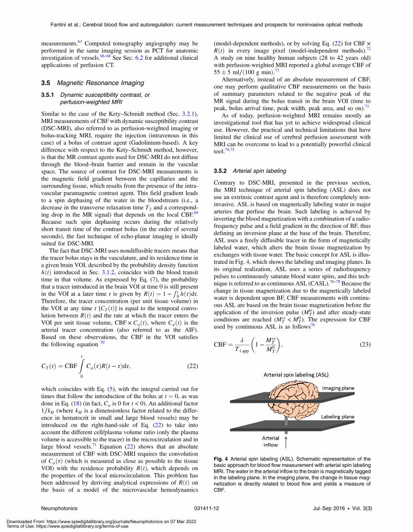
Contrary to DSC-MRI, presented in the previous section,the MRI technique of arterial spin labeling (ASL) does notuse an extrinsic contrast agent and is therefore completely non-invasive. ASL is based on magnetically labeling water in majorarteries that perfuse the brain. Such labeling is achieved byinverting the blood magnetization with a combination of a radio-frequency pulse and a field gradient in the direction of BF, thusdefining an inversion plane at the base of the brain. Therefore,ASL uses a freely diffusible tracer in the form of magneticallylabeled water, which alters the brain tissue magnetization byexchanges with tissue water. The basic concept for ASL is illus-trated in Fig. 4, which shows the labeling and imaging planes. Inits original realization, ASL uses a series of radiofrequencypulses to continuously saturate blood water spins, and this tech-nique is referred to as continuous ASL (CASL).76–78 Because thechange in tissue magnetization due to the magnetically labeledwater is dependent upon BF, CBF measurements with continu-ous ASL are based on the brain tissue magnetization before theapplication of the inversion pulse (M0

T ) and after steady-stateconditions are reached (Mss

T < M0T ). The expression for CBF

used by continuous ASL is as follows76


T1 app

�1 −

MssT

M0T

�; (23)

Fig. 4 Arterial spin labeling (ASL). Schematic representation of thebasic approach for blood flow measurement with arterial spin labelingMRI. The water in the arterial inflow to the brain is magnetically taggedin the labeling plane. In the imaging plane, the change in tissue mag-netization is directly related to blood flow and yields a measure ofCBF.




where λ is the tissue–blood partition coefficient for water(mlblood∕gbrain) and T1 app is the time constant describing thedecay of tissue magnetization from M0

T to MssT .

The use of a single inversion radiofrequency pulse (typically∼10 ms in duration) and a labeling region that is closer to theimaging slice result in pulsed ASL (PASL) [for a review, seeRef. 79]. PASL addresses two problems of CASL: magnetiza-tion transfer effects that alter the tissue magnetization indepen-dent of flow effects (due to the long application of the series ofradiofrequency pulses), and the loss of spin labels as blood trav-els from the labeling plane to the imaging slice.71 PASL isimplemented by a number of different techniques with creativeacronyms such as EPISTAR (echo planar imaging and signaltargeting with alternating radiofrequency),80 PICORE (proximalinversion with a control for off-resonance effects),81 FAIR(flow-sensitive alternating inversion recovery),82 and QUIPSS II(quantitative imaging of perfusion using a single subtraction,version II).83 These various PASL techniques implement variousschemes for the acquisition of the tag and control images, but theconcept is always the same: measuring local CBF by quantify-ing the decrease in tissue magnetization caused by the inflow oflabeled arterial blood that carries a negative magnetization(i.e., magnetization that is flipped by 180 deg).

3.6 Ultrasound techniques

3.6.1 Transcranial Doppler ultrasound

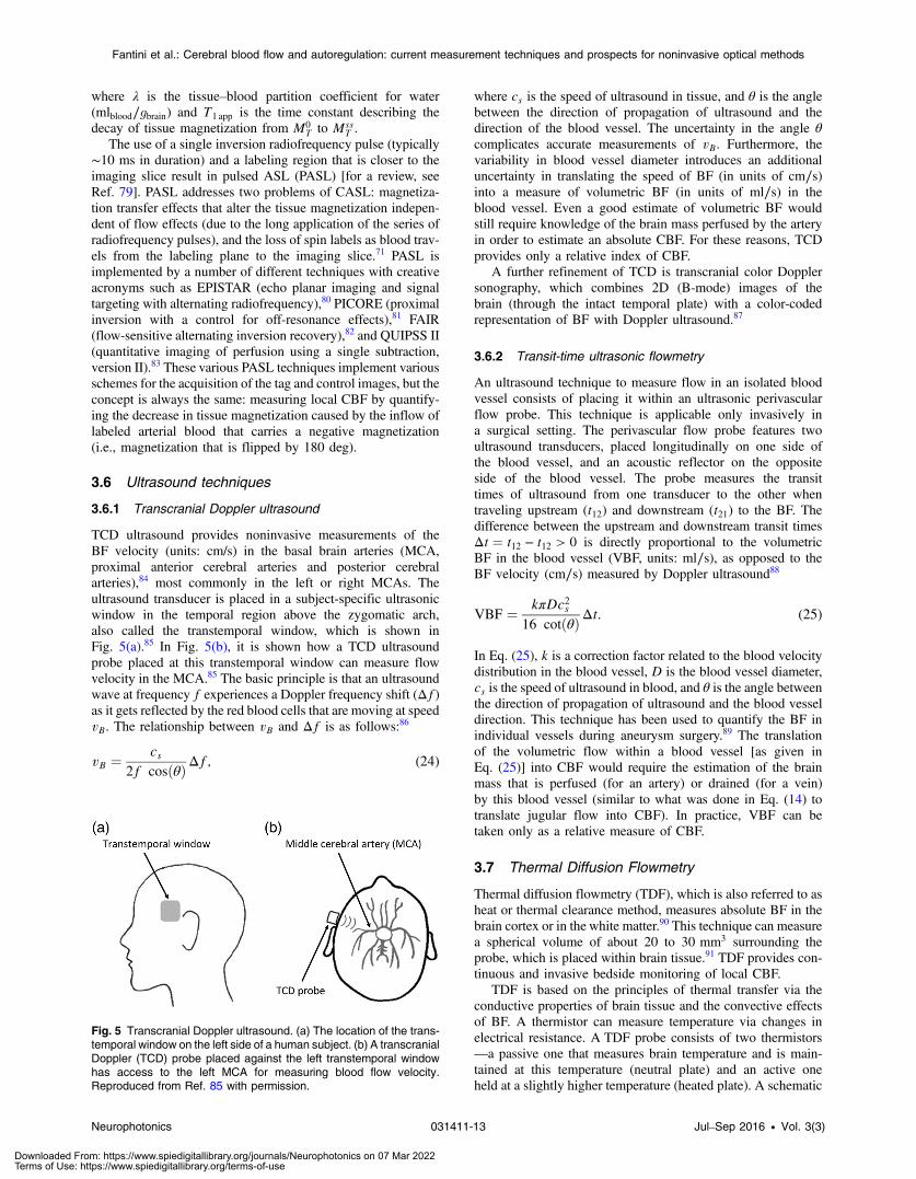
TCD ultrasound provides noninvasive measurements of theBF velocity (units: cm/s) in the basal brain arteries (MCA,proximal anterior cerebral arteries and posterior cerebralarteries),84 most commonly in the left or right MCAs. Theultrasound transducer is placed in a subject-specific ultrasonicwindow in the temporal region above the zygomatic arch,also called the transtemporal window, which is shown inFig. 5(a).85 In Fig. 5(b), it is shown how a TCD ultrasoundprobe placed at this transtemporal window can measure flowvelocity in the MCA.85 The basic principle is that an ultrasoundwave at frequency f experiences a Doppler frequency shift (Δf)as it gets reflected by the red blood cells that are moving at speedvB. The relationship between vB and Δf is as follows:86

EQ-TARGET;temp:intralink-;e024;63;308vB ¼ cs2f cosðθÞΔf; (24)

where cs is the speed of ultrasound in tissue, and θ is the anglebetween the direction of propagation of ultrasound and thedirection of the blood vessel. The uncertainty in the angle θcomplicates accurate measurements of vB. Furthermore, thevariability in blood vessel diameter introduces an additionaluncertainty in translating the speed of BF (in units of cm∕s)into a measure of volumetric BF (in units of ml∕s) in theblood vessel. Even a good estimate of volumetric BF wouldstill require knowledge of the brain mass perfused by the arteryin order to estimate an absolute CBF. For these reasons, TCDprovides only a relative index of CBF.

A further refinement of TCD is transcranial color Dopplersonography, which combines 2D (B-mode) images of thebrain (through the intact temporal plate) with a color-codedrepresentation of BF with Doppler ultrasound.87

3.6.2 Transit-time ultrasonic flowmetry

An ultrasound technique to measure flow in an isolated bloodvessel consists of placing it within an ultrasonic perivascularflow probe. This technique is applicable only invasively ina surgical setting. The perivascular flow probe features twoultrasound transducers, placed longitudinally on one side ofthe blood vessel, and an acoustic reflector on the oppositeside of the blood vessel. The probe measures the transittimes of ultrasound from one transducer to the other whentraveling upstream (t12) and downstream (t21) to the BF. Thedifference between the upstream and downstream transit timesΔt ¼ t12 − t12 > 0 is directly proportional to the volumetricBF in the blood vessel (VBF, units: ml∕s), as opposed to theBF velocity (cm∕s) measured by Doppler ultrasound88

EQ-TARGET;temp:intralink-;e025;326;414VBF ¼ kπDc2s16 cotðθÞΔt: (25)

In Eq. (25), k is a correction factor related to the blood velocitydistribution in the blood vessel, D is the blood vessel diameter,cs is the speed of ultrasound in blood, and θ is the angle betweenthe direction of propagation of ultrasound and the blood vesseldirection. This technique has been used to quantify the BF inindividual vessels during aneurysm surgery.89 The translationof the volumetric flow within a blood vessel [as given inEq. (25)] into CBF would require the estimation of the brainmass that is perfused (for an artery) or drained (for a vein)by this blood vessel (similar to what was done in Eq. (14) totranslate jugular flow into CBF). In practice, VBF can betaken only as a relative measure of CBF.

3.7 Thermal Diffusion Flowmetry

Thermal diffusion flowmetry (TDF), which is also referred to asheat or thermal clearance method, measures absolute BF in thebrain cortex or in the white matter.90 This technique can measurea spherical volume of about 20 to 30 mm3 surrounding theprobe, which is placed within brain tissue.91 TDF provides con-tinuous and invasive bedside monitoring of local CBF.

TDF is based on the principles of thermal transfer via theconductive properties of brain tissue and the convective effectsof BF. A thermistor can measure temperature via changes inelectrical resistance. A TDF probe consists of two thermistors—a passive one that measures brain temperature and is main-tained at this temperature (neutral plate) and an active oneheld at a slightly higher temperature (heated plate). A schematic

Fig. 5 Transcranial Doppler ultrasound. (a) The location of the trans-temporal window on the left side of a human subject. (b) A transcranialDoppler (TCD) probe placed against the left transtemporal windowhas access to the left MCA for measuring blood flow velocity.Reproduced from Ref. 85 with permission.




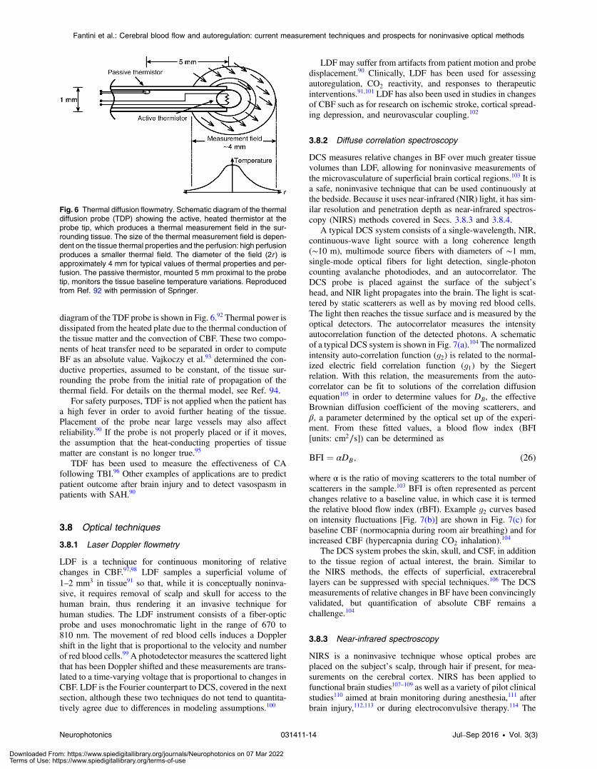
diagram of the TDF probe is shown in Fig. 6.92 Thermal power isdissipated from the heated plate due to the thermal conduction ofthe tissue matter and the convection of CBF. These two compo-nents of heat transfer need to be separated in order to computeBF as an absolute value. Vajkoczy et al.93 determined the con-ductive properties, assumed to be constant, of the tissue sur-rounding the probe from the initial rate of propagation of thethermal field. For details on the thermal model, see Ref. 94.

For safety purposes, TDF is not applied when the patient hasa high fever in order to avoid further heating of the tissue.Placement of the probe near large vessels may also affectreliability.90 If the probe is not properly placed or if it moves,the assumption that the heat-conducting properties of tissuematter are constant is no longer true.95

TDF has been used to measure the effectiveness of CAfollowing TBI.96 Other examples of applications are to predictpatient outcome after brain injury and to detect vasospasm inpatients with SAH.90

3.8 Optical techniques

3.8.1 Laser Doppler flowmetry

LDF is a technique for continuous monitoring of relativechanges in CBF.97,98 LDF samples a superficial volume of1–2 mm3 in tissue91 so that, while it is conceptually noninva-sive, it requires removal of scalp and skull for access to thehuman brain, thus rendering it an invasive technique forhuman studies. The LDF instrument consists of a fiber-opticprobe and uses monochromatic light in the range of 670 to810 nm. The movement of red blood cells induces a Dopplershift in the light that is proportional to the velocity and numberof red blood cells.99 A photodetector measures the scattered lightthat has been Doppler shifted and these measurements are trans-lated to a time-varying voltage that is proportional to changes inCBF. LDF is the Fourier counterpart to DCS, covered in the nextsection, although these two techniques do not tend to quantita-tively agree due to differences in modeling assumptions.100

LDF may suffer from artifacts from patient motion and probedisplacement.90 Clinically, LDF has been used for assessingautoregulation, CO2 reactivity, and responses to therapeuticinterventions.91,101 LDF has also been used in studies in changesof CBF such as for research on ischemic stroke, cortical spread-ing depression, and neurovascular coupling.102

3.8.2 Diffuse correlation spectroscopy

DCS measures relative changes in BF over much greater tissuevolumes than LDF, allowing for noninvasive measurements ofthe microvasculature of superficial brain cortical regions.103 It isa safe, noninvasive technique that can be used continuously atthe bedside. Because it uses near-infrared (NIR) light, it has sim-ilar resolution and penetration depth as near-infrared spectros-copy (NIRS) methods covered in Secs. 3.8.3 and 3.8.4.

A typical DCS system consists of a single-wavelength, NIR,continuous-wave light source with a long coherence length(∼10 m), multimode source fibers with diameters of ∼1 mm,single-mode optical fibers for light detection, single-photoncounting avalanche photodiodes, and an autocorrelator. TheDCS probe is placed against the surface of the subject’shead, and NIR light propagates into the brain. The light is scat-tered by static scatterers as well as by moving red blood cells.The light then reaches the tissue surface and is measured by theoptical detectors. The autocorrelator measures the intensityautocorrelation function of the detected photons. A schematicof a typical DCS system is shown in Fig. 7(a).104 The normalizedintensity auto-correlation function (g2) is related to the normal-ized electric field correlation function (g1) by the Siegertrelation. With this relation, the measurements from the auto-correlator can be fit to solutions of the correlation diffusionequation105 in order to determine values for DB, the effectiveBrownian diffusion coefficient of the moving scatterers, andβ, a parameter determined by the optical set up of the experi-ment. From these fitted values, a blood flow index (BFI[units: cm2∕s]) can be determined as

EQ-TARGET;temp:intralink-;e026;326;348BFI ¼ αDB; (26)

where α is the ratio of moving scatterers to the total number ofscatterers in the sample.103 BFI is often represented as percentchanges relative to a baseline value, in which case it is termedthe relative blood flow index (rBFI). Example g2 curves basedon intensity fluctuations [Fig. 7(b)] are shown in Fig. 7(c) forbaseline CBF (normocapnia during room air breathing) and forincreased CBF (hypercapnia during CO2 inhalation).104

The DCS system probes the skin, skull, and CSF, in additionto the tissue region of actual interest, the brain. Similar tothe NIRS methods, the effects of superficial, extracerebrallayers can be suppressed with special techniques.106 The DCSmeasurements of relative changes in BF have been convincinglyvalidated, but quantification of absolute CBF remains achallenge.104

3.8.3 Near-infrared spectroscopy

NIRS is a noninvasive technique whose optical probes areplaced on the subject’s scalp, through hair if present, for mea-surements on the cerebral cortex. NIRS has been applied tofunctional brain studies107–109 as well as a variety of pilot clinicalstudies110 aimed at brain monitoring during anesthesia,111 afterbrain injury,112,113 or during electroconvulsive therapy.114 The

Fig. 6 Thermal diffusion flowmetry. Schematic diagram of the thermaldiffusion probe (TDP) showing the active, heated thermistor at theprobe tip, which produces a thermal measurement field in the sur-rounding tissue. The size of the thermal measurement field is depen-dent on the tissue thermal properties and the perfusion: high perfusionproduces a smaller thermal field. The diameter of the field (2r ) isapproximately 4 mm for typical values of thermal properties and per-fusion. The passive thermistor, mounted 5 mm proximal to the probetip, monitors the tissue baseline temperature variations. Reproducedfrom Ref. 92 with permission of Springer.




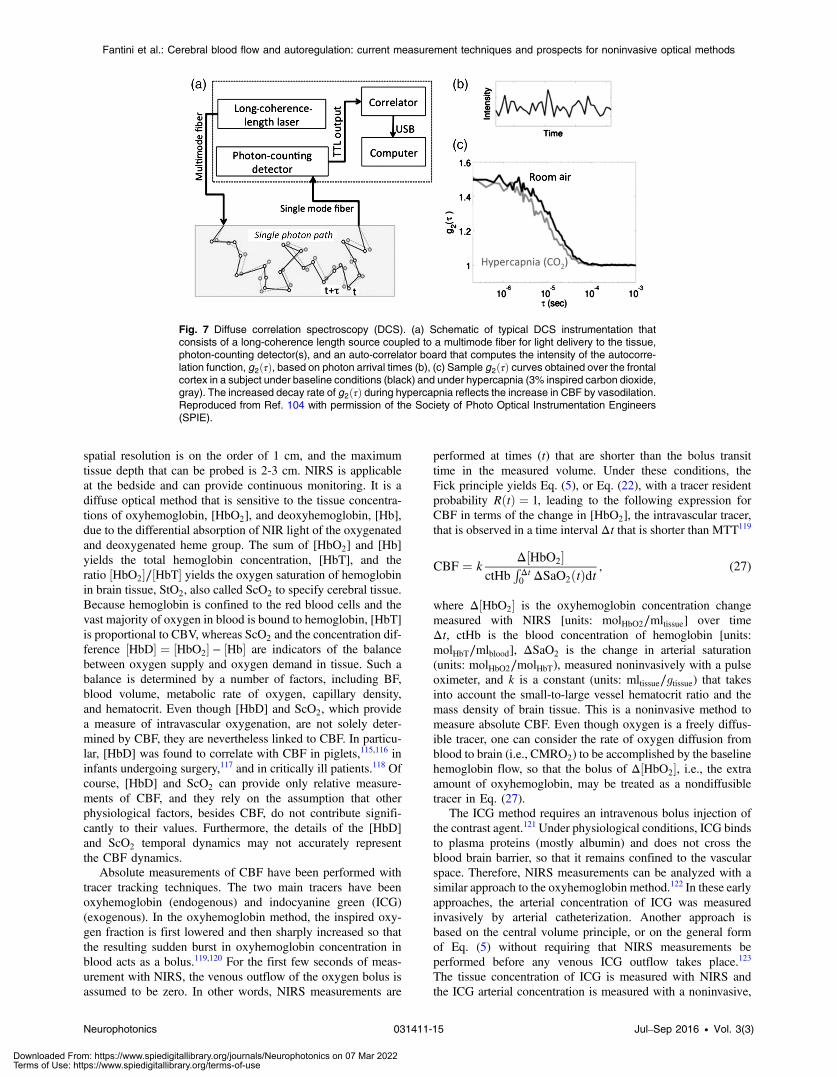
spatial resolution is on the order of 1 cm, and the maximumtissue depth that can be probed is 2-3 cm. NIRS is applicableat the bedside and can provide continuous monitoring. It is adiffuse optical method that is sensitive to the tissue concentra-tions of oxyhemoglobin, [HbO2], and deoxyhemoglobin, [Hb],due to the differential absorption of NIR light of the oxygenatedand deoxygenated heme group. The sum of [HbO2] and [Hb]yields the total hemoglobin concentration, [HbT], and theratio ½HbO2�∕½HbT� yields the oxygen saturation of hemoglobinin brain tissue, StO2, also called ScO2 to specify cerebral tissue.Because hemoglobin is confined to the red blood cells and thevast majority of oxygen in blood is bound to hemoglobin, [HbT]is proportional to CBV, whereas ScO2 and the concentration dif-ference ½HbD� ¼ ½HbO2� − ½Hb� are indicators of the balancebetween oxygen supply and oxygen demand in tissue. Such abalance is determined by a number of factors, including BF,blood volume, metabolic rate of oxygen, capillary density,and hematocrit. Even though [HbD] and ScO2, which providea measure of intravascular oxygenation, are not solely deter-mined by CBF, they are nevertheless linked to CBF. In particu-lar, [HbD] was found to correlate with CBF in piglets,115,116 ininfants undergoing surgery,117 and in critically ill patients.118 Ofcourse, [HbD] and ScO2 can provide only relative measure-ments of CBF, and they rely on the assumption that otherphysiological factors, besides CBF, do not contribute signifi-cantly to their values. Furthermore, the details of the [HbD]and ScO2 temporal dynamics may not accurately representthe CBF dynamics.

Absolute measurements of CBF have been performed withtracer tracking techniques. The two main tracers have beenoxyhemoglobin (endogenous) and indocyanine green (ICG)(exogenous). In the oxyhemoglobin method, the inspired oxy-gen fraction is first lowered and then sharply increased so thatthe resulting sudden burst in oxyhemoglobin concentration inblood acts as a bolus.119,120 For the first few seconds of meas-urement with NIRS, the venous outflow of the oxygen bolus isassumed to be zero. In other words, NIRS measurements are

performed at times (t) that are shorter than the bolus transittime in the measured volume. Under these conditions, theFick principle yields Eq. (5), or Eq. (22), with a tracer residentprobability RðtÞ ¼ 1, leading to the following expression forCBF in terms of the change in [HbO2], the intravascular tracer,that is observed in a time interval Δt that is shorter than MTT119

EQ-TARGET;temp:intralink-;e027;326;409CBF ¼ kΔ½HbO2�

ctHbRΔt0 ΔSaO2ðtÞdt

; (27)

where Δ½HbO2� is the oxyhemoglobin concentration changemeasured with NIRS [units: molHbO2∕mltissue] over timeΔt, ctHb is the blood concentration of hemoglobin [units:molHbT∕mlblood], ΔSaO2 is the change in arterial saturation(units: molHbO2∕molHbT), measured noninvasively with a pulseoximeter, and k is a constant (units: mltissue∕gtissue) that takesinto account the small-to-large vessel hematocrit ratio and themass density of brain tissue. This is a noninvasive method tomeasure absolute CBF. Even though oxygen is a freely diffus-ible tracer, one can consider the rate of oxygen diffusion fromblood to brain (i.e., CMRO2) to be accomplished by the baselinehemoglobin flow, so that the bolus of Δ½HbO2�, i.e., the extraamount of oxyhemoglobin, may be treated as a nondiffusibletracer in Eq. (27).

The ICG method requires an intravenous bolus injection ofthe contrast agent.121 Under physiological conditions, ICG bindsto plasma proteins (mostly albumin) and does not cross theblood brain barrier, so that it remains confined to the vascularspace. Therefore, NIRS measurements can be analyzed with asimilar approach to the oxyhemoglobin method.122 In these earlyapproaches, the arterial concentration of ICG was measuredinvasively by arterial catheterization. Another approach isbased on the central volume principle, or on the general formof Eq. (5) without requiring that NIRS measurements beperformed before any venous ICG outflow takes place.123

The tissue concentration of ICG is measured with NIRS andthe ICG arterial concentration is measured with a noninvasive,

Fig. 7 Diffuse correlation spectroscopy (DCS). (a) Schematic of typical DCS instrumentation thatconsists of a long-coherence length source coupled to a multimode fiber for light delivery to the tissue,photon-counting detector(s), and an auto-correlator board that computes the intensity of the autocorre-lation function, g2ðτÞ, based on photon arrival times (b), (c) Sample g2ðτÞ curves obtained over the frontalcortex in a subject under baseline conditions (black) and under hypercapnia (3% inspired carbon dioxide,gray). The increased decay rate of g2ðτÞ during hypercapnia reflects the increase in CBF by vasodilation.Reproduced from Ref. 104 with permission of the Society of Photo Optical Instrumentation Engineers(SPIE).




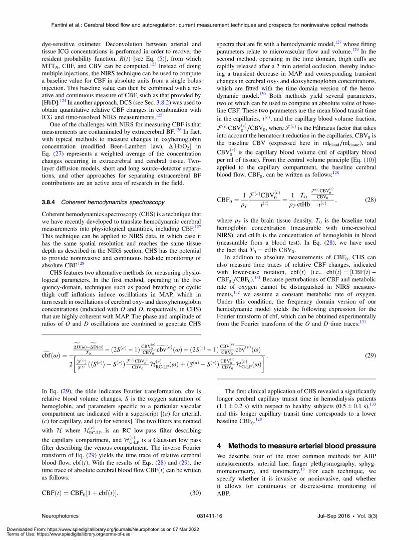
dye-sensitive oximeter. Deconvolution between arterial andtissue ICG concentrations is performed in order to recover theresident probability function, RðtÞ [see Eq. (5)], from whichMTTB, CBF, and CBV can be computed.123 Instead of doingmultiple injections, the NIRS technique can be used to computea baseline value for CBF in absolute units from a single bolusinjection. This baseline value can then be combined with a rel-ative and continuous measure of CBF, such as that provided by[HbD].124 In another approach, DCS (see Sec. 3.8.2) was used toobtain quantitative relative CBF changes in combination withICG and time-resolved NIRS measurements.125

One of the challenges with NIRS for measuring CBF is thatmeasurements are contaminated by extracerebral BF.126 In fact,with typical methods to measure changes in oxyhemoglobinconcentration (modified Beer–Lambert law), Δ½HbO2� inEq. (27) represents a weighted average of the concentrationchanges occurring in extracerebral and cerebral tissue. Two-layer diffusion models, short and long source–detector separa-tions, and other approaches for separating extracerebral BFcontributions are an active area of research in the field.

3.8.4 Coherent hemodynamics spectroscopy

Coherent hemodynamics spectroscopy (CHS) is a technique thatwe have recently developed to translate hemodynamic cerebralmeasurements into physiological quantities, including CBF.127

This technique can be applied to NIRS data, in which case ithas the same spatial resolution and reaches the same tissuedepth as described in the NIRS section. CHS has the potentialto provide noninvasive and continuous bedside monitoring ofabsolute CBF.128

CHS features two alternative methods for measuring physio-logical parameters. In the first method, operating in the fre-quency-domain, techniques such as paced breathing or cyclicthigh cuff inflations induce oscillations in MAP, which inturn result in oscillations of cerebral oxy- and deoxyhemoglobinconcentrations (indicated with O and D, respectively, in CHS)that are highly coherent with MAP. The phase and amplitude ofratios of O and D oscillations are combined to generate CHS

spectra that are fit with a hemodynamic model,127 whose fittingparameters relate to microvascular flow and volume.129 In thesecond method, operating in the time domain, thigh cuffs arerapidly released after a 2 min arterial occlusion, thereby induc-ing a transient decrease in MAP and corresponding transientchanges in cerebral oxy- and deoxyhemoglobin concentrations,which are fitted with the time-domain version of the hemo-dynamic model.130 Both methods yield several parameters,two of which can be used to compute an absolute value of base-line CBF. These two parameters are the mean blood transit timein the capillaries, tðcÞ, and the capillary blood volume fraction,

F ðcÞCBVðcÞ0 ∕CBV0, where F ðcÞ is the Fåhraeus factor that takes

into account the hematocrit reduction in the capillaries, CBV0 isthe baseline CBV (expressed here in mlblood∕mltissue), and

CBVðcÞ0 is the capillary blood volume (ml of capillary blood

per ml of tissue). From the central volume principle [Eq. (10)]applied to the capillary compartment, the baseline cerebralblood flow, CBF0, can be written as follows:128

EQ-TARGET;temp:intralink-;e028;326;547CBF0 ¼1

ρT

F ðcÞCBVðcÞ0

tðcÞ¼ 1

ρT

T0

ctHb

F ðcÞCBVðcÞ0

CBV0

tðcÞ; (28)

where ρT is the brain tissue density, T0 is the baseline totalhemoglobin concentration (measurable with time-resolvedNIRS), and ctHb is the concentration of hemoglobin in blood(measurable from a blood test). In Eq. (28), we have usedthe fact that T0 ¼ ctHb CBV0.

In addition to absolute measurements of CBF0, CHS canalso measure time traces of relative CBF changes, indicatedwith lower-case notation, cbfðtÞ (i.e., cbfðtÞ ¼ ½CBFðtÞ −CBF0�∕CBF0).131 Because perturbations of CBF and metabolicrate of oxygen cannot be distinguished in NIRS measure-ments,132 we assume a constant metabolic rate of oxygen.Under this condition, the frequency domain version of ourhemodynamic model yields the following expression for theFourier transform of cbf, which can be obtained experimentallyfrom the Fourier transform of the O and D time traces:131

EQ-TARGET;temp:intralink-;e029;63;308

fcbfðωÞ ¼ fΔOðωÞ−fΔDðωÞT0

− ð2SðaÞ − 1Þ CBVðaÞ0

CBV0

gcbvðaÞðωÞ − ð2SðvÞ − 1Þ CBVðvÞ0

CBV0

gcbvðvÞðωÞ2

�hSðcÞiSðvÞ

ðhSðcÞi − SðvÞÞ F ðcÞCBVðcÞ0

CBV0HðcÞ

RC-LPðωÞ þ ðSðaÞ − SðvÞÞ CBVðvÞ0

CBV0HðcÞ

G-LPðωÞ� : (29)

In Eq. (29), the tilde indicates Fourier transformation, cbv isrelative blood volume changes, S is the oxygen saturation ofhemoglobin, and parameters specific to a particular vascularcompartment are indicated with a superscript [(a) for arterial,(c) for capillary, and (v) for venous]. The two filters are notated

with H where HðcÞRC-LP is an RC low-pass filter describing

the capillary compartment, and HðvÞG-LP is a Gaussian low pass

filter describing the venous compartment. The inverse Fouriertransform of Eq. (29) yields the time trace of relative cerebralblood flow, cbfðtÞ. With the results of Eqs. (28) and (29), thetime trace of absolute cerebral blood flow CBFðtÞ can be writtenas follows:

EQ-TARGET;temp:intralink-;e030;63;92CBFðtÞ ¼ CBF0½1þ cbfðtÞ�: (30)

The first clinical application of CHS revealed a significantlylonger cerebral capillary transit time in hemodialysis patients(1.1� 0.2 s) with respect to healthy subjects (0.5� 0.1 s),133

and this longer capillary transit time corresponds to a lowerbaseline CBF0.

128

4 Methods to measure arterial blood pressureWe describe four of the most common methods for ABPmeasurements: arterial line, finger plethysmography, sphyg-momanometry, and tonometry.18 For each technique, wespecify whether it is invasive or noninvasive, and whetherit allows for continuous or discrete-time monitoring ofABP.




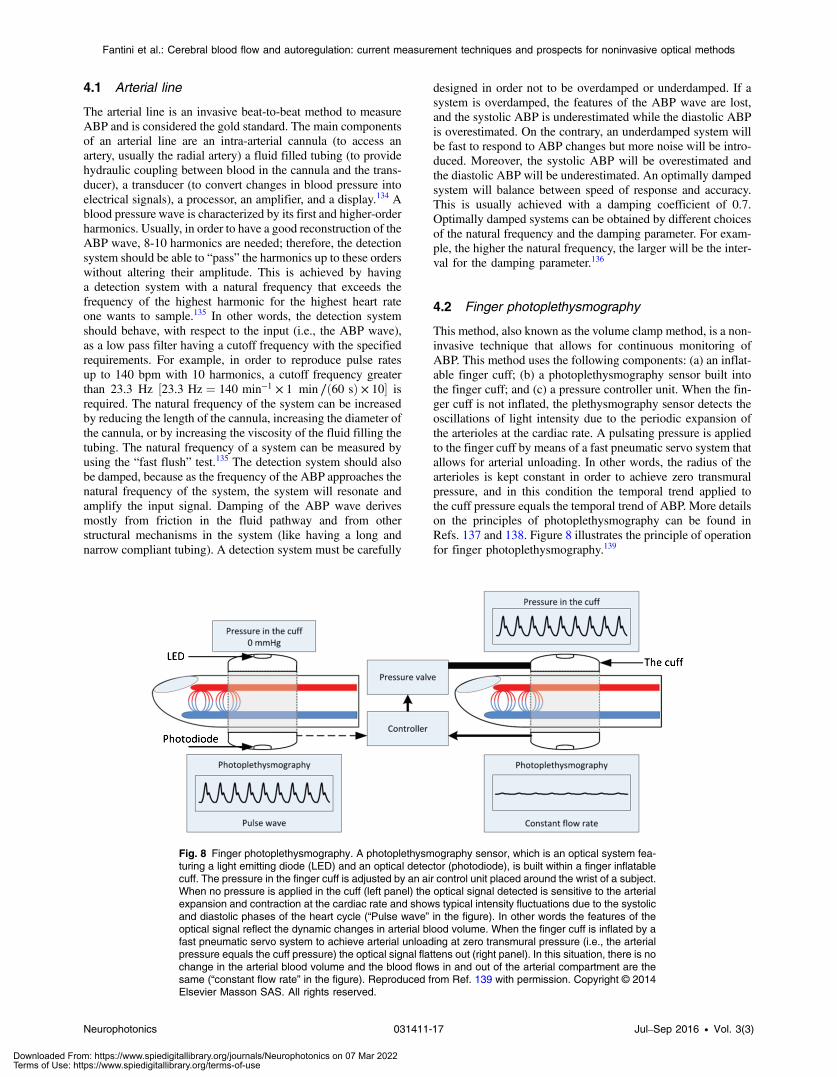
4.1 Arterial line

The arterial line is an invasive beat-to-beat method to measureABP and is considered the gold standard. The main componentsof an arterial line are an intra-arterial cannula (to access anartery, usually the radial artery) a fluid filled tubing (to providehydraulic coupling between blood in the cannula and the trans-ducer), a transducer (to convert changes in blood pressure intoelectrical signals), a processor, an amplifier, and a display.134 Ablood pressure wave is characterized by its first and higher-orderharmonics. Usually, in order to have a good reconstruction of theABP wave, 8-10 harmonics are needed; therefore, the detectionsystem should be able to “pass” the harmonics up to these orderswithout altering their amplitude. This is achieved by havinga detection system with a natural frequency that exceeds thefrequency of the highest harmonic for the highest heart rateone wants to sample.135 In other words, the detection systemshould behave, with respect to the input (i.e., the ABP wave),as a low pass filter having a cutoff frequency with the specifiedrequirements. For example, in order to reproduce pulse ratesup to 140 bpm with 10 harmonics, a cutoff frequency greaterthan 23.3 Hz ½23.3 Hz ¼ 140 min−1 × 1 min ∕ð60 sÞ × 10� isrequired. The natural frequency of the system can be increasedby reducing the length of the cannula, increasing the diameter ofthe cannula, or by increasing the viscosity of the fluid filling thetubing. The natural frequency of a system can be measured byusing the “fast flush” test.135 The detection system should alsobe damped, because as the frequency of the ABP approaches thenatural frequency of the system, the system will resonate andamplify the input signal. Damping of the ABP wave derivesmostly from friction in the fluid pathway and from otherstructural mechanisms in the system (like having a long andnarrow compliant tubing). A detection system must be carefully

designed in order not to be overdamped or underdamped. If asystem is overdamped, the features of the ABP wave are lost,and the systolic ABP is underestimated while the diastolic ABPis overestimated. On the contrary, an underdamped system willbe fast to respond to ABP changes but more noise will be intro-duced. Moreover, the systolic ABP will be overestimated andthe diastolic ABP will be underestimated. An optimally dampedsystem will balance between speed of response and accuracy.This is usually achieved with a damping coefficient of 0.7.Optimally damped systems can be obtained by different choicesof the natural frequency and the damping parameter. For exam-ple, the higher the natural frequency, the larger will be the inter-val for the damping parameter.136

4.2 Finger photoplethysmography

This method, also known as the volume clamp method, is a non-invasive technique that allows for continuous monitoring ofABP. This method uses the following components: (a) an inflat-able finger cuff; (b) a photoplethysmography sensor built intothe finger cuff; and (c) a pressure controller unit. When the fin-ger cuff is not inflated, the plethysmography sensor detects theoscillations of light intensity due to the periodic expansion ofthe arterioles at the cardiac rate. A pulsating pressure is appliedto the finger cuff by means of a fast pneumatic servo system thatallows for arterial unloading. In other words, the radius of thearterioles is kept constant in order to achieve zero transmuralpressure, and in this condition the temporal trend applied tothe cuff pressure equals the temporal trend of ABP. More detailson the principles of photoplethysmography can be found inRefs. 137 and 138. Figure 8 illustrates the principle of operationfor finger photoplethysmography.139

Fig. 8 Finger photoplethysmography. A photoplethysmography sensor, which is an optical system fea-turing a light emitting diode (LED) and an optical detector (photodiode), is built within a finger inflatablecuff. The pressure in the finger cuff is adjusted by an air control unit placed around the wrist of a subject.When no pressure is applied in the cuff (left panel) the optical signal detected is sensitive to the arterialexpansion and contraction at the cardiac rate and shows typical intensity fluctuations due to the systolicand diastolic phases of the heart cycle (“Pulse wave” in the figure). In other words the features of theoptical signal reflect the dynamic changes in arterial blood volume. When the finger cuff is inflated by afast pneumatic servo system to achieve arterial unloading at zero transmural pressure (i.e., the arterialpressure equals the cuff pressure) the optical signal flattens out (right panel). In this situation, there is nochange in the arterial blood volume and the blood flows in and out of the arterial compartment are thesame (“constant flow rate” in the figure). Reproduced from Ref. 139 with permission. Copyright © 2014Elsevier Masson SAS. All rights reserved.




4.3 Sphygmomanometers

Sphygmomanometry is one of the noninvasive methods thatallows for discrete time point monitoring of ABP. It is nota beat to beat method, and therefore only mean, systolic anddiastolic ABP can be detected.

Manual: This is an auscultatory method based on listening tothe so-called Korotkoff’s sounds,139,140 which are producedwhen an arm cuff is inflated to a pressure large enough toocclude the brachial artery and stop BF. After BF is stopped,the cuff is steadily and slowly deflated and five distinctKorotkoff’s sounds can be heard. These sounds are detectedby using a stethoscope placed over the brachial artery andbelow a blood pressure cuff. During the deflation, when thecuff pressure reaches systolic pressure, the blood starts to flowagain, and a sound is heard (the first phase of the Korotkoffsounds). As the cuff is deflated further, a regime of turbulentflow (when the artery opens and closes) is created in the arteryand sounds are still heard. When the cuff pressure is less than thediastolic pressure, the artery is always open and the flow ofblood is smooth causing the disappearance of the sounds.Systolic pressure is measured as the pressure at which thefirst Korotkoff’s sound is heard, and diastolic as the pressureat which the sounds disappear. Standard sphygmomanometersare divided into aneroid and mercury sphygmomanometers.141

Digital (automatic): Automatic sphygmomanometers arebased on the detection of oscillations in the pressure appliedto an arm cuff as the pressure is decreased (as in the manualmethods) below the systolic pressure. Instead of using an oper-ator who can hear the Korotkoff’s sounds in the deflation phase,this method uses a piezoelectric sensor, electronic components,and microprocessors. Mean ABP corresponds to the maximaloscillations during cuff deflation, and the instrument is mostsensitive to these oscillations. However, systolic and diastolicABP correspond to the appearing and disappearing of pressurecuff oscillations, respectively, and, therefore, are more difficultto detect. More precisely, systolic ABP is measured by anincrease in cuff oscillation when blood first passes the deflatingcuff. Diastolic ABP is instead detected when oscillationsdisappear. Detection of systolic and diastolic ABP requiressophisticated algorithms for the analysis of the temporal trendsof the pressure cuff oscillations, with different manufacturersusing different algorithms.141,142

4.4 Tonometry

Tonometry of the radial artery provides a noninvasive assessmentof the central pulse pressure waveform (pressure in the aorta).Tonometry of the radial artery is carried out by placing a hand-held tonometer (strain gauge pressure sensor) over the radialartery and applying a mild pressure in order to induce a partialocclusion of the artery. The pressure from the radial artery istransmitted from the vessel to the sensor and recorded digitally.A sophisticated algorithm based on the study of the reflection ofthe central pulse pressure waveform from the smaller resistancevessels permits derivation and calculation of central pressureindices from a peripheral brachial blood pressure.143

4.5 Validation of methods and issues with arterialblood pressure measurements

In the case of the techniques based on an arm pneumatic cuff,several factors have to be considered in order to obtain an

accurate reading of ABP. These factors include the posture ofthe body, and especially of the arm, and the cuff size.141

Moreover, auscultatory methods are operator dependent, andfor this reason more and more electronic devices to monitorblood pressure are being used at home. Finger photoplethys-mography seems a reliable method to measure the beat tobeat ABP, and several studies have validated this techniquewith the arterial line method.137,144 Tonometry has also beenvalidated against the invasive arterial line method and goodagreement has been found except for its limited capacity torespond to fast variation in ABP.145

The general guidelines for testing a new electronic devicefor ABP measurements have been developed by the BritishHypertension Society (BHS) and the Association for theAdvancement of Medical Instrumentation (AAMI). Bothrequire three measurements of blood pressure in 85 subjects,chosen to cover a wide range of subjects’ ages and blood pres-sure values. The measurements are taken by trained observersusing a gold standard method and the device being tested. TheBHS protocol requires that a device must give at least 50% ofreadings within 5 mmHg, and 75% of readings within 10 mmHgof the gold standard method. The AAMI requires that the aver-age difference between the tested and gold standard methodsdoes not exceed 5 mmHg, with a standard deviation of lessthan 8 mmHg. Therefore, according to these guidelines, it ispossible that a new device will pass the test but at the sametime it can be in clear disagreement with a gold standard methodfor several individuals.141

5 Methods to measure cerebralautoregulation

We conceptually divide the methods to measure CA into directmethods and model-based methods. In direct methods, the met-rics for CA are derived from the relationships between thedynamics of MAP and CBF without any support of physiologi-cal and vascular models of cerebral hemodynamics. Signalprocessing methods featuring various levels of sophisticationare applied to the raw data in order to provide metrics ofCA. These methods are described in Sec. 5.3. On the contrary,the purpose of model-based methods is twofold: (a) to reacha deeper understanding of CA by providing a physiologicaland vascular model of the autoregulation process; (b) basedon the model, to provide different metrics of CA that can beuseful also in clinical settings.

5.1 Direct methods

The CA process can be directly observed in invasive studies bymeasuring the change in blood vessels’ diameter in response tochanges in MAP.25 However, this method cannot be used asa monitor of CA in clinical settings, not only because of itsinvasiveness, but also because it does not provide a measureof changes in CBF, which is the variable of real interest.Therefore, CA is usually assessed by direct measurements ofCBF (or some surrogate) and MAP, and analyzing the relation-ships of their temporal dynamics by using signal processingmethods (see Sec. 5.3). We refer to these methods as directmethods of autoregulation assessment. In principle, any methodused to measure CBF can be used to measure CA, as long as itsupports the specific requirements of the CA measurementsunder consideration (static versus dynamic, snapshot versusmonitoring, and so on). Most of the current studies on CA(especially those on dynamic CA) are carried out with TCD




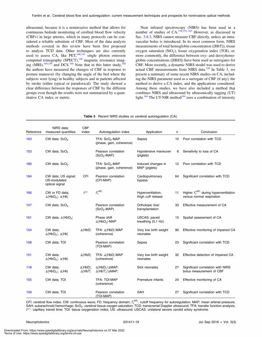
ultrasound, because it is a noninvasive method that allows forcontinuous bedside monitoring of cerebral blood flow velocity(CBFv) in large arteries, which in many protocols can be con-sidered a reliable substitute of CBF. Most of the data analysismethods covered in this review have been first proposedto analyze TCD data. Other techniques are also currentlyused to assess CA, like PET,146,147 single photon emissioncomputed tomography (SPECT),148 magnetic resonance imag-ing (MRI),149,150 and DCS.104 Note that in this latter study,104

the authors have measured the changes of CBF in response toposture maneuver (by changing the angle of the bed where thesubjects were lying) in healthy subjects and in patients affectedby stroke (either typical or paradoxical). The study showed aclear difference between the responses of CBF by the differentgroups even though the results were not summarized by a quan-titative CA index or metric.

Near infrared spectroscopy (NIRS) has been used in anumber of studies of CA.118,151–163 However, as discussed inSec. 3.8.3, NIRS cannot measure CBF directly, unless an intra-vascular bolus is introduced. In its most common form, NIRSmeasurements of total hemoglobin concentration ([HbT]), tissueoxygen saturation (StO2), tissue oxygenation index (TOI), or,more commonly, the difference between oxy- and deoxyhemo-globin concentrations ([HbD]) have been used as surrogates forCBF. More recently, a dynamic NIRS model was used to deriveactual CBF measurements from NIRS data.128 In Table 3, wepresent a summary of some recent NIRS studies on CA, includ-ing the NIRS parameter used as a surrogate of CBF (if any), themethod to derive a CA index, and the applications considered.Among these studies, we have also included a method thatcombines NIRS and ultrasound by ultrasonically tagging (UT)light.164 The UT-NIR method164 uses a combination of intensity

Table 3 Recent NIRS studies on cerebral autoregulation (CA).

ReferenceNIRS data;

measured quantitiesCBFindex Autoregulation index Application n Conclusion

163 CW data; ScO2 TFA: ScO2-MAP(phase, gain, coherence)

Sepsis 10 Poor correlation with TCD

153 CW data; ScO2 Pearson correlation(ScO2-MAP)

Hypotensive maneuver(piglets)

6 Sensitivity to loss of CA

160 CW data; ScO2 TFA: ScO2-MAP(phase, gain, coherence)

Induced changes inMAP (piglets)

12 Poor correlation with TCD

164 CW data; US signal;US-modulatedoptical signal

CFI Pearson correlation(CFI-MAP)

Cardiopulmonarybypass

64 Significant correlation with TCD

166 CW or FD data;Δ½HbO2�, Δ½Hb�

t ðcÞ f ðARÞc Hyperventilation,

thigh cuff release11 Higher f ðARÞ

c during hyperventilationversus normal respiration

157 CW data; ScO2 Pearson correlation(ScO2-MAP)

Orthotopic livertransplantation

33 Effective measurement of CA

161 CW data; Δ½HbO2� Phase shiftΔ½HbO2�-MAP

USCAS; pacedbreathing (0.1 Hz)

15 Spatial assessment of CA

154 CW data;Δ½HbO2�, Δ½Hb�

Δ½HbD� TFA: Δ½HbD�-MAP(coherence)

Very low birth weightneonates

90 Effective monitoring of impaired CA

158 CW data; TOI Pearson correlation(TOI-MAP)

Sepsis 23 Significant correlation with TCD


Δ½HbD� TFA: Δ½HbD�-MAP(coherence)

Very low birth weightneonates

32 Effective detection of impaired CA


Δ½HbD�;Δ½HbT�

Δ½HbD�∕ΔMAP;Δ½HbT�∕ΔMAP;

Sick neonates 27 Significant correlation with NIRSbolus measurement of CBF

155 CW data; TOI TFA: TOI-MAP(coherence)

Premature infants 24 Effective monitoring of CA

159 CW data; TOI Pearson correlation(TOI-MAP)

SAH 27 Significant correlation with TCD

CFI: cerebral flow index; CW: continuous wave; FD: frequency domain; f ðARÞc : cutoff frequency for autoregulation; MAP: mean arterial pressure;

SAH: subarachnoid hemorrhage; ScO2: cerebral tissue oxygen saturation; TCD: transcranial Doppler ultrasound; TFA: transfer function analysis;t ðcÞ: capillary transit time; TOI: tissue oxygenation index; US: ultrasound; USCAS: unilateral severe carotid artery syndrome.




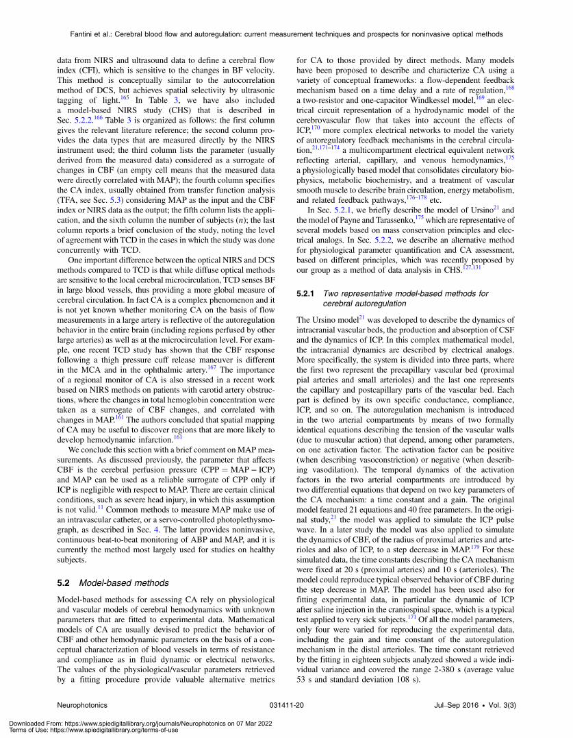
data from NIRS and ultrasound data to define a cerebral flowindex (CFI), which is sensitive to the changes in BF velocity.This method is conceptually similar to the autocorrelationmethod of DCS, but achieves spatial selectivity by ultrasonictagging of light.165 In Table 3, we have also includeda model-based NIRS study (CHS) that is described inSec. 5.2.2.166 Table 3 is organized as follows: the first columngives the relevant literature reference; the second column pro-vides the data types that are measured directly by the NIRSinstrument used; the third column lists the parameter (usuallyderived from the measured data) considered as a surrogate ofchanges in CBF (an empty cell means that the measured datawere directly correlated with MAP); the fourth column specifiesthe CA index, usually obtained from transfer function analysis(TFA, see Sec. 5.3) considering MAP as the input and the CBFindex or NIRS data as the output; the fifth column lists the appli-cation, and the sixth column the number of subjects (n); the lastcolumn reports a brief conclusion of the study, noting the levelof agreement with TCD in the cases in which the study was doneconcurrently with TCD.

One important difference between the optical NIRS and DCSmethods compared to TCD is that while diffuse optical methodsare sensitive to the local cerebral microcirculation, TCD senses BFin large blood vessels, thus providing a more global measure ofcerebral circulation. In fact CA is a complex phenomenon and itis not yet known whether monitoring CA on the basis of flowmeasurements in a large artery is reflective of the autoregulationbehavior in the entire brain (including regions perfused by otherlarge arteries) as well as at the microcirculation level. For exam-ple, one recent TCD study has shown that the CBF responsefollowing a thigh pressure cuff release maneuver is differentin the MCA and in the ophthalmic artery.167 The importanceof a regional monitor of CA is also stressed in a recent workbased on NIRS methods on patients with carotid artery obstruc-tions, where the changes in total hemoglobin concentration weretaken as a surrogate of CBF changes, and correlated withchanges in MAP.161 The authors concluded that spatial mappingof CA may be useful to discover regions that are more likely todevelop hemodynamic infarction.161

We conclude this section with a brief comment onMAPmea-surements. As discussed previously, the parameter that affectsCBF is the cerebral perfusion pressure (CPP ¼ MAP − ICP)and MAP can be used as a reliable surrogate of CPP only ifICP is negligible with respect to MAP. There are certain clinicalconditions, such as severe head injury, in which this assumptionis not valid.11 Common methods to measure MAP make use ofan intravascular catheter, or a servo-controlled photoplethysmo-graph, as described in Sec. 4. The latter provides noninvasive,continuous beat-to-beat monitoring of ABP and MAP, and it iscurrently the method most largely used for studies on healthysubjects.

5.2 Model-based methods

Model-based methods for assessing CA rely on physiologicaland vascular models of cerebral hemodynamics with unknownparameters that are fitted to experimental data. Mathematicalmodels of CA are usually devised to predict the behavior ofCBF and other hemodynamic parameters on the basis of a con-ceptual characterization of blood vessels in terms of resistanceand compliance as in fluid dynamic or electrical networks.The values of the physiological/vascular parameters retrievedby a fitting procedure provide valuable alternative metrics

for CA to those provided by direct methods. Many modelshave been proposed to describe and characterize CA using avariety of conceptual frameworks: a flow-dependent feedbackmechanism based on a time delay and a rate of regulation,168

a two-resistor and one-capacitor Windkessel model,169 an elec-trical circuit representation of a hydrodynamic model of thecerebrovascular flow that takes into account the effects ofICP,170 more complex electrical networks to model the varietyof autoregulatory feedback mechanisms in the cerebral circula-tion,21,171–174 a multicompartment electrical equivalent networkreflecting arterial, capillary, and venous hemodynamics,175

a physiologically based model that consolidates circulatory bio-physics, metabolic biochemistry, and a treatment of vascularsmooth muscle to describe brain circulation, energy metabolism,and related feedback pathways,176–178 etc.

In Sec. 5.2.1, we briefly describe the model of Ursino21 andthe model of Payne and Tarassenko,175 which are representative ofseveral models based on mass conservation principles and elec-trical analogs. In Sec. 5.2.2, we describe an alternative methodfor physiological parameter quantification and CA assessment,based on different principles, which was recently proposed byour group as a method of data analysis in CHS.127,131

5.2.1 Two representative model-based methods forcerebral autoregulation

The Ursino model21 was developed to describe the dynamics ofintracranial vascular beds, the production and absorption of CSFand the dynamics of ICP. In this complex mathematical model,the intracranial dynamics are described by electrical analogs.More specifically, the system is divided into three parts, wherethe first two represent the precapillary vascular bed (proximalpial arteries and small arterioles) and the last one representsthe capillary and postcapillary parts of the vascular bed. Eachpart is defined by its own specific conductance, compliance,ICP, and so on. The autoregulation mechanism is introducedin the two arterial compartments by means of two formallyidentical equations describing the tension of the vascular walls(due to muscular action) that depend, among other parameters,on one activation factor. The activation factor can be positive(when describing vasoconstriction) or negative (when describ-ing vasodilation). The temporal dynamics of the activationfactors in the two arterial compartments are introduced bytwo differential equations that depend on two key parameters ofthe CA mechanism: a time constant and a gain. The originalmodel featured 21 equations and 40 free parameters. In the origi-nal study,21 the model was applied to simulate the ICP pulsewave. In a later study the model was also applied to simulatethe dynamics of CBF, of the radius of proximal arteries and arte-rioles and also of ICP, to a step decrease in MAP.179 For thesesimulated data, the time constants describing the CAmechanismwere fixed at 20 s (proximal arteries) and 10 s (arterioles). Themodel could reproduce typical observed behavior of CBF duringthe step decrease in MAP. The model has been used also forfitting experimental data, in particular the dynamic of ICPafter saline injection in the craniospinal space, which is a typicaltest applied to very sick subjects.171 Of all the model parameters,only four were varied for reproducing the experimental data,including the gain and time constant of the autoregulationmechanism in the distal arterioles. The time constant retrievedby the fitting in eighteen subjects analyzed showed a wide indi-vidual variance and covered the range 2-380 s (average value53 s and standard deviation 108 s).




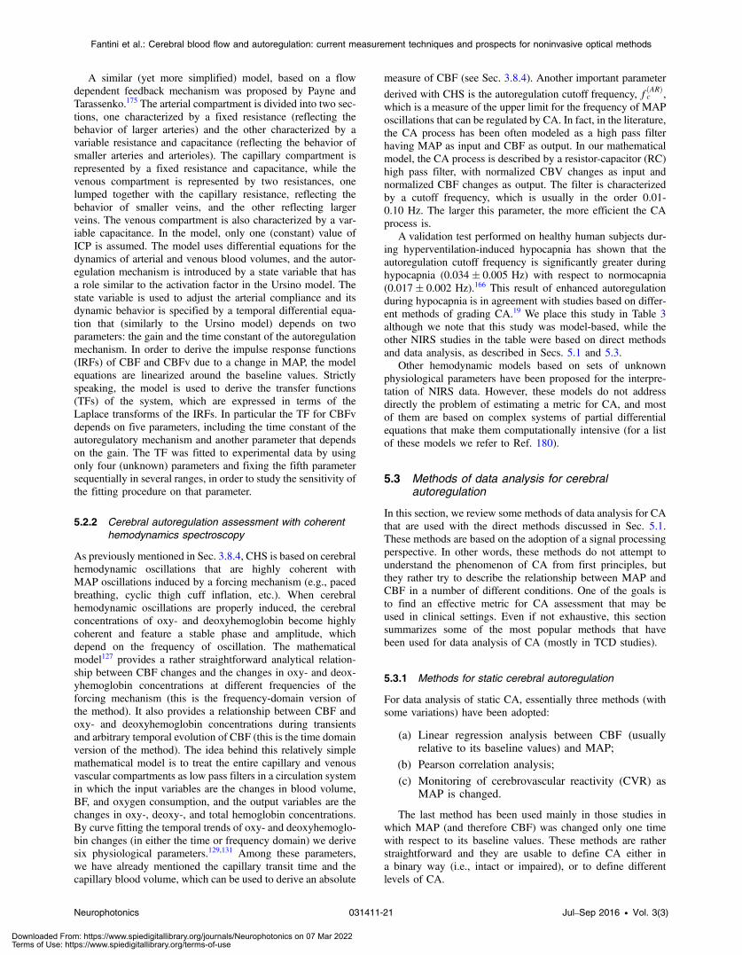
A similar (yet more simplified) model, based on a flowdependent feedback mechanism was proposed by Payne andTarassenko.175 The arterial compartment is divided into two sec-tions, one characterized by a fixed resistance (reflecting thebehavior of larger arteries) and the other characterized by avariable resistance and capacitance (reflecting the behavior ofsmaller arteries and arterioles). The capillary compartment isrepresented by a fixed resistance and capacitance, while thevenous compartment is represented by two resistances, onelumped together with the capillary resistance, reflecting thebehavior of smaller veins, and the other reflecting largerveins. The venous compartment is also characterized by a var-iable capacitance. In the model, only one (constant) value ofICP is assumed. The model uses differential equations for thedynamics of arterial and venous blood volumes, and the autor-egulation mechanism is introduced by a state variable that hasa role similar to the activation factor in the Ursino model. Thestate variable is used to adjust the arterial compliance and itsdynamic behavior is specified by a temporal differential equa-tion that (similarly to the Ursino model) depends on twoparameters: the gain and the time constant of the autoregulationmechanism. In order to derive the impulse response functions(IRFs) of CBF and CBFv due to a change in MAP, the modelequations are linearized around the baseline values. Strictlyspeaking, the model is used to derive the transfer functions(TFs) of the system, which are expressed in terms of theLaplace transforms of the IRFs. In particular the TF for CBFvdepends on five parameters, including the time constant of theautoregulatory mechanism and another parameter that dependson the gain. The TF was fitted to experimental data by usingonly four (unknown) parameters and fixing the fifth parametersequentially in several ranges, in order to study the sensitivity ofthe fitting procedure on that parameter.

5.2.2 Cerebral autoregulation assessment with coherenthemodynamics spectroscopy

As previously mentioned in Sec. 3.8.4, CHS is based on cerebralhemodynamic oscillations that are highly coherent withMAP oscillations induced by a forcing mechanism (e.g., pacedbreathing, cyclic thigh cuff inflation, etc.). When cerebralhemodynamic oscillations are properly induced, the cerebralconcentrations of oxy- and deoxyhemoglobin become highlycoherent and feature a stable phase and amplitude, whichdepend on the frequency of oscillation. The mathematicalmodel127 provides a rather straightforward analytical relation-ship between CBF changes and the changes in oxy- and deox-yhemoglobin concentrations at different frequencies of theforcing mechanism (this is the frequency-domain version ofthe method). It also provides a relationship between CBF andoxy- and deoxyhemoglobin concentrations during transientsand arbitrary temporal evolution of CBF (this is the time domainversion of the method). The idea behind this relatively simplemathematical model is to treat the entire capillary and venousvascular compartments as low pass filters in a circulation systemin which the input variables are the changes in blood volume,BF, and oxygen consumption, and the output variables are thechanges in oxy-, deoxy-, and total hemoglobin concentrations.By curve fitting the temporal trends of oxy- and deoxyhemoglo-bin changes (in either the time or frequency domain) we derivesix physiological parameters.129,131 Among these parameters,we have already mentioned the capillary transit time and thecapillary blood volume, which can be used to derive an absolute

measure of CBF (see Sec. 3.8.4). Another important parameter

derived with CHS is the autoregulation cutoff frequency, fðARÞc ,which is a measure of the upper limit for the frequency of MAPoscillations that can be regulated by CA. In fact, in the literature,the CA process has been often modeled as a high pass filterhaving MAP as input and CBF as output. In our mathematicalmodel, the CA process is described by a resistor-capacitor (RC)high pass filter, with normalized CBV changes as input andnormalized CBF changes as output. The filter is characterizedby a cutoff frequency, which is usually in the order 0.01-0.10 Hz. The larger this parameter, the more efficient the CAprocess is.

A validation test performed on healthy human subjects dur-ing hyperventilation-induced hypocapnia has shown that theautoregulation cutoff frequency is significantly greater duringhypocapnia (0.034� 0.005 Hz) with respect to normocapnia(0.017� 0.002 Hz).166 This result of enhanced autoregulationduring hypocapnia is in agreement with studies based on differ-ent methods of grading CA.19 We place this study in Table 3although we note that this study was model-based, while theother NIRS studies in the table were based on direct methodsand data analysis, as described in Secs. 5.1 and 5.3.

Other hemodynamic models based on sets of unknownphysiological parameters have been proposed for the interpre-tation of NIRS data. However, these models do not addressdirectly the problem of estimating a metric for CA, and mostof them are based on complex systems of partial differentialequations that make them computationally intensive (for a listof these models we refer to Ref. 180).

5.3 Methods of data analysis for cerebralautoregulation

In this section, we review some methods of data analysis for CAthat are used with the direct methods discussed in Sec. 5.1.These methods are based on the adoption of a signal processingperspective. In other words, these methods do not attempt tounderstand the phenomenon of CA from first principles, butthey rather try to describe the relationship between MAP andCBF in a number of different conditions. One of the goals isto find an effective metric for CA assessment that may beused in clinical settings. Even if not exhaustive, this sectionsummarizes some of the most popular methods that havebeen used for data analysis of CA (mostly in TCD studies).

5.3.1 Methods for static cerebral autoregulation

For data analysis of static CA, essentially three methods (withsome variations) have been adopted:

(a) Linear regression analysis between CBF (usuallyrelative to its baseline values) and MAP;

(b) Pearson correlation analysis;(c) Monitoring of cerebrovascular reactivity (CVR) as

MAP is changed.

The last method has been used mainly in those studies inwhich MAP (and therefore CBF) was changed only one timewith respect to its baseline values. These methods are ratherstraightforward and they are usable to define CA either ina binary way (i.e., intact or impaired), or to define differentlevels of CA.




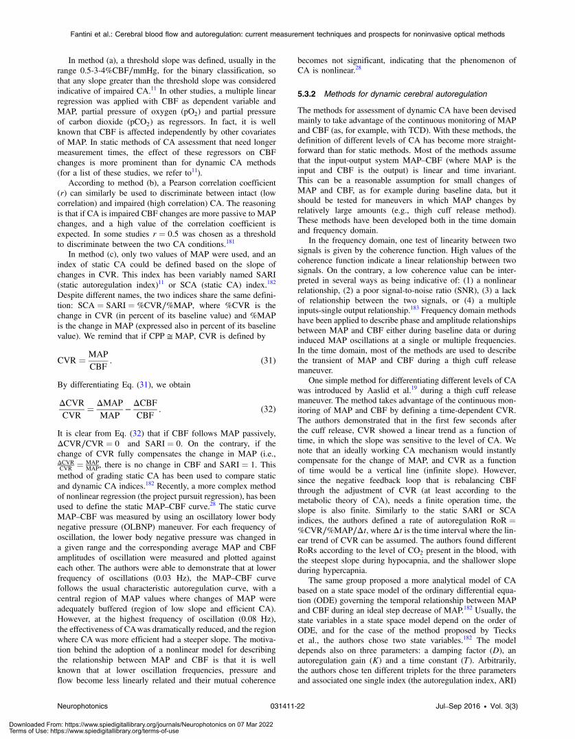
In method (a), a threshold slope was defined, usually in therange 0.5-3-4%CBF∕mmHg, for the binary classification, sothat any slope greater than the threshold slope was consideredindicative of impaired CA.11 In other studies, a multiple linearregression was applied with CBF as dependent variable andMAP, partial pressure of oxygen (pO2) and partial pressureof carbon dioxide (pCO2) as regressors. In fact, it is wellknown that CBF is affected independently by other covariatesof MAP. In static methods of CA assessment that need longermeasurement times, the effect of these regressors on CBFchanges is more prominent than for dynamic CA methods(for a list of these studies, we refer to11).

According to method (b), a Pearson correlation coefficient(r) can similarly be used to discriminate between intact (lowcorrelation) and impaired (high correlation) CA. The reasoningis that if CA is impaired CBF changes are more passive to MAPchanges, and a high value of the correlation coefficient isexpected. In some studies r ¼ 0.5 was chosen as a thresholdto discriminate between the two CA conditions.181

In method (c), only two values of MAP were used, and anindex of static CA could be defined based on the slope ofchanges in CVR. This index has been variably named SARI(static autoregulation index)11 or SCA (static CA) index.182

Despite different names, the two indices share the same defini-tion: SCA ¼ SARI ¼ %CVR∕%MAP, where %CVR is thechange in CVR (in percent of its baseline value) and %MAPis the change in MAP (expressed also in percent of its baselinevalue). We remind that if CPP ≅ MAP, CVR is defined by

EQ-TARGET;temp:intralink-;e031;63;444CVR ¼ MAP

CBF: (31)

By differentiating Eq. (31), we obtain

EQ-TARGET;temp:intralink-;e032;63;392

ΔCVRCVR

¼ ΔMAP

MAP−ΔCBFCBF

: (32)

It is clear from Eq. (32) that if CBF follows MAP passively,ΔCVR∕CVR ¼ 0 and SARI ¼ 0. On the contrary, if thechange of CVR fully compensates the change in MAP (i.e.,ΔCVRCVR

¼ MAPMAP

, there is no change in CBF and SARI ¼ 1. Thismethod of grading static CA has been used to compare staticand dynamic CA indices.182 Recently, a more complex methodof nonlinear regression (the project pursuit regression), has beenused to define the static MAP–CBF curve.28 The static curveMAP–CBF was measured by using an oscillatory lower bodynegative pressure (OLBNP) maneuver. For each frequency ofoscillation, the lower body negative pressure was changed ina given range and the corresponding average MAP and CBFamplitudes of oscillation were measured and plotted againsteach other. The authors were able to demonstrate that at lowerfrequency of oscillations (0.03 Hz), the MAP–CBF curvefollows the usual characteristic autoregulation curve, with acentral region of MAP values where changes of MAP wereadequately buffered (region of low slope and efficient CA).However, at the highest frequency of oscillation (0.08 Hz),the effectiveness of CAwas dramatically reduced, and the regionwhere CA was more efficient had a steeper slope. The motiva-tion behind the adoption of a nonlinear model for describingthe relationship between MAP and CBF is that it is wellknown that at lower oscillation frequencies, pressure andflow become less linearly related and their mutual coherence

becomes not significant, indicating that the phenomenon ofCA is nonlinear.28

5.3.2 Methods for dynamic cerebral autoregulation

The methods for assessment of dynamic CA have been devisedmainly to take advantage of the continuous monitoring of MAPand CBF (as, for example, with TCD). With these methods, thedefinition of different levels of CA has become more straight-forward than for static methods. Most of the methods assumethat the input-output system MAP–CBF (where MAP is theinput and CBF is the output) is linear and time invariant.This can be a reasonable assumption for small changes ofMAP and CBF, as for example during baseline data, but itshould be tested for maneuvers in which MAP changes byrelatively large amounts (e.g., thigh cuff release method).These methods have been developed both in the time domainand frequency domain.

In the frequency domain, one test of linearity between twosignals is given by the coherence function. High values of thecoherence function indicate a linear relationship between twosignals. On the contrary, a low coherence value can be inter-preted in several ways as being indicative of: (1) a nonlinearrelationship, (2) a poor signal-to-noise ratio (SNR), (3) a lackof relationship between the two signals, or (4) a multipleinputs-single output relationship.183 Frequency domain methodshave been applied to describe phase and amplitude relationshipsbetween MAP and CBF either during baseline data or duringinduced MAP oscillations at a single or multiple frequencies.In the time domain, most of the methods are used to describethe transient of MAP and CBF during a thigh cuff releasemaneuver.

One simple method for differentiating different levels of CAwas introduced by Aaslid et al.19 during a thigh cuff releasemaneuver. The method takes advantage of the continuous mon-itoring of MAP and CBF by defining a time-dependent CVR.The authors demonstrated that in the first few seconds afterthe cuff release, CVR showed a linear trend as a function oftime, in which the slope was sensitive to the level of CA. Wenote that an ideally working CA mechanism would instantlycompensate for the change of MAP, and CVR as a functionof time would be a vertical line (infinite slope). However,since the negative feedback loop that is rebalancing CBFthrough the adjustment of CVR (at least according to themetabolic theory of CA), needs a finite operation time, theslope is also finite. Similarly to the static SARI or SCAindices, the authors defined a rate of autoregulation RoR ¼%CVR∕%MAP∕Δt, where Δt is the time interval where the lin-ear trend of CVR can be assumed. The authors found differentRoRs according to the level of CO2 present in the blood, withthe steepest slope during hypocapnia, and the shallower slopeduring hypercapnia.

The same group proposed a more analytical model of CAbased on a state space model of the ordinary differential equa-tion (ODE) governing the temporal relationship between MAPand CBF during an ideal step decrease of MAP.182 Usually, thestate variables in a state space model depend on the order ofODE, and for the case of the method proposed by Tieckset al., the authors chose two state variables.182 The modeldepends also on three parameters: a damping factor (D), anautoregulation gain (K) and a time constant (T). Arbitrarily,the authors chose ten different triplets for the three parametersand associated one single index (the autoregulation index, ARI)




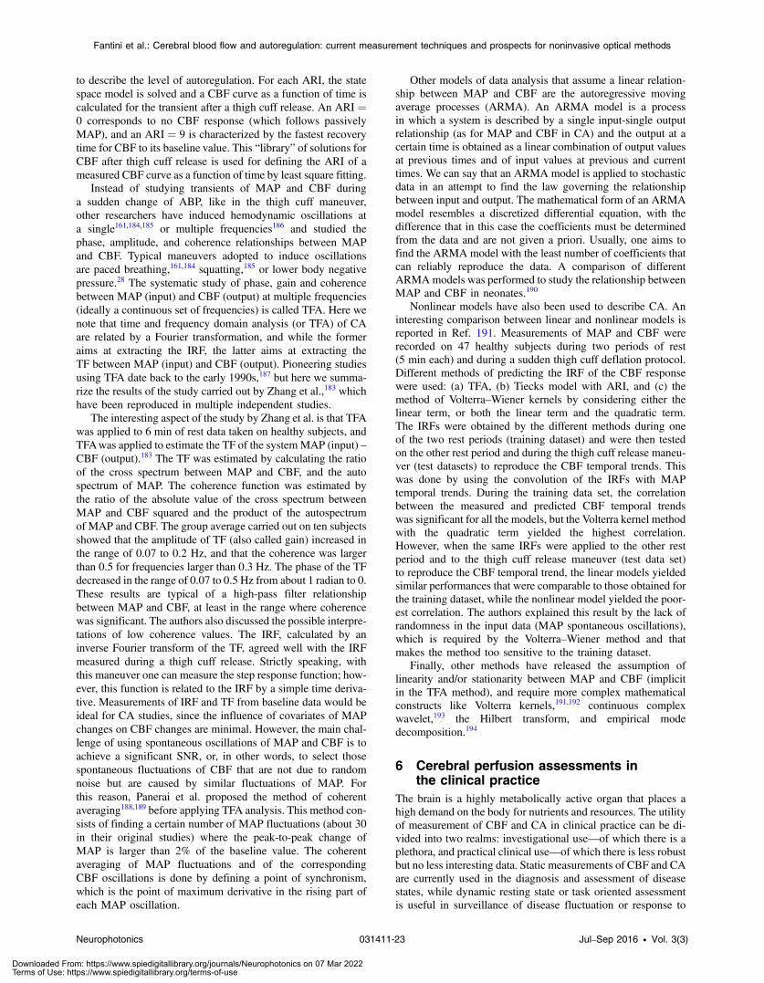
to describe the level of autoregulation. For each ARI, the statespace model is solved and a CBF curve as a function of time iscalculated for the transient after a thigh cuff release. An ARI ¼0 corresponds to no CBF response (which follows passivelyMAP), and an ARI ¼ 9 is characterized by the fastest recoverytime for CBF to its baseline value. This “library” of solutions forCBF after thigh cuff release is used for defining the ARI of ameasured CBF curve as a function of time by least square fitting.

Instead of studying transients of MAP and CBF duringa sudden change of ABP, like in the thigh cuff maneuver,other researchers have induced hemodynamic oscillations ata single161,184,185 or multiple frequencies186 and studied thephase, amplitude, and coherence relationships between MAPand CBF. Typical maneuvers adopted to induce oscillationsare paced breathing,161,184 squatting,185 or lower body negativepressure.28 The systematic study of phase, gain and coherencebetween MAP (input) and CBF (output) at multiple frequencies(ideally a continuous set of frequencies) is called TFA. Here wenote that time and frequency domain analysis (or TFA) of CAare related by a Fourier transformation, and while the formeraims at extracting the IRF, the latter aims at extracting theTF between MAP (input) and CBF (output). Pioneering studiesusing TFA date back to the early 1990s,187 but here we summa-rize the results of the study carried out by Zhang et al.,183 whichhave been reproduced in multiple independent studies.

The interesting aspect of the study by Zhang et al. is that TFAwas applied to 6 min of rest data taken on healthy subjects, andTFAwas applied to estimate the TF of the systemMAP (input) –CBF (output).183 The TF was estimated by calculating the ratioof the cross spectrum between MAP and CBF, and the autospectrum of MAP. The coherence function was estimated bythe ratio of the absolute value of the cross spectrum betweenMAP and CBF squared and the product of the autospectrumof MAP and CBF. The group average carried out on ten subjectsshowed that the amplitude of TF (also called gain) increased inthe range of 0.07 to 0.2 Hz, and that the coherence was largerthan 0.5 for frequencies larger than 0.3 Hz. The phase of the TFdecreased in the range of 0.07 to 0.5 Hz from about 1 radian to 0.These results are typical of a high-pass filter relationshipbetween MAP and CBF, at least in the range where coherencewas significant. The authors also discussed the possible interpre-tations of low coherence values. The IRF, calculated by aninverse Fourier transform of the TF, agreed well with the IRFmeasured during a thigh cuff release. Strictly speaking, withthis maneuver one can measure the step response function; how-ever, this function is related to the IRF by a simple time deriva-tive. Measurements of IRF and TF from baseline data would beideal for CA studies, since the influence of covariates of MAPchanges on CBF changes are minimal. However, the main chal-lenge of using spontaneous oscillations of MAP and CBF is toachieve a significant SNR, or, in other words, to select thosespontaneous fluctuations of CBF that are not due to randomnoise but are caused by similar fluctuations of MAP. Forthis reason, Panerai et al. proposed the method of coherentaveraging188,189 before applying TFA analysis. This method con-sists of finding a certain number of MAP fluctuations (about 30in their original studies) where the peak-to-peak change ofMAP is larger than 2% of the baseline value. The coherentaveraging of MAP fluctuations and of the correspondingCBF oscillations is done by defining a point of synchronism,which is the point of maximum derivative in the rising part ofeach MAP oscillation.

Other models of data analysis that assume a linear relation-ship between MAP and CBF are the autoregressive movingaverage processes (ARMA). An ARMA model is a processin which a system is described by a single input-single outputrelationship (as for MAP and CBF in CA) and the output at acertain time is obtained as a linear combination of output valuesat previous times and of input values at previous and currenttimes. We can say that an ARMA model is applied to stochasticdata in an attempt to find the law governing the relationshipbetween input and output. The mathematical form of an ARMAmodel resembles a discretized differential equation, with thedifference that in this case the coefficients must be determinedfrom the data and are not given a priori. Usually, one aims tofind the ARMA model with the least number of coefficients thatcan reliably reproduce the data. A comparison of differentARMAmodels was performed to study the relationship betweenMAP and CBF in neonates.190

Nonlinear models have also been used to describe CA. Aninteresting comparison between linear and nonlinear models isreported in Ref. 191. Measurements of MAP and CBF wererecorded on 47 healthy subjects during two periods of rest(5 min each) and during a sudden thigh cuff deflation protocol.Different methods of predicting the IRF of the CBF responsewere used: (a) TFA, (b) Tiecks model with ARI, and (c) themethod of Volterra–Wiener kernels by considering either thelinear term, or both the linear term and the quadratic term.The IRFs were obtained by the different methods during oneof the two rest periods (training dataset) and were then testedon the other rest period and during the thigh cuff release maneu-ver (test datasets) to reproduce the CBF temporal trends. Thiswas done by using the convolution of the IRFs with MAPtemporal trends. During the training data set, the correlationbetween the measured and predicted CBF temporal trendswas significant for all the models, but the Volterra kernel methodwith the quadratic term yielded the highest correlation.However, when the same IRFs were applied to the other restperiod and to the thigh cuff release maneuver (test data set)to reproduce the CBF temporal trend, the linear models yieldedsimilar performances that were comparable to those obtained forthe training dataset, while the nonlinear model yielded the poor-est correlation. The authors explained this result by the lack ofrandomness in the input data (MAP spontaneous oscillations),which is required by the Volterra–Wiener method and thatmakes the method too sensitive to the training dataset.

Finally, other methods have released the assumption oflinearity and/or stationarity between MAP and CBF (implicitin the TFA method), and require more complex mathematicalconstructs like Volterra kernels,191,192 continuous complexwavelet,193 the Hilbert transform, and empirical modedecomposition.194

6 Cerebral perfusion assessments inthe clinical practice

The brain is a highly metabolically active organ that places ahigh demand on the body for nutrients and resources. The utilityof measurement of CBF and CA in clinical practice can be di-vided into two realms: investigational use—of which there is aplethora, and practical clinical use—of which there is less robustbut no less interesting data. Static measurements of CBF and CAare currently used in the diagnosis and assessment of diseasestates, while dynamic resting state or task oriented assessmentis useful in surveillance of disease fluctuation or response to




therapy. Of clinically relevant metrics of CBF and CA it ishelpful to approach two different aspects of clinical care—investigation of chronic diseases and investigation and manage-ment of acute illness, which will be discussed below. This isnot meant to be an exhaustive review of the clinical utility ofCBF and CA assessment but rather to highlight some practicalapplications.

6.1 Chronic central nervous system diseases—understanding pathobiology and treatments

Certain neurodegenerative diseases have been associated withchanges in regional or global CBF. Cerebral hypoperfusionand vascular dysfunction are thought to be related to the patho-genesis of Alzheimer’s disease (AD) thus implicating that themeasurement of CBF might be a useful biomarker of diseaseincidence or progression.195 Though mostly investigational,MRI,196 SPECT,197 and NIRS198 are rapidly approachingprime time to be a useful marker of AD via a point estimateof CBF. Noninvasive assessment of dynamic CBF has alsorecently shed some light on how certain medications used totreat dementia, notably donepezil199 and memantine,198 exerttheir cognition-preserving effects by perhaps protectingCBF integrity over time. Analogous to these studies are CBFassessments in Parkinson’s disease (PD). Single point intime measurements of regional cerebral hypoperfusion havebeen shown to correlate with certain symptoms of PD alongwith a corresponding increase in CBF after treatment withboth pharmacologic agents200 and functional neurosurgicalinterventions.201 Assessment of CA is also of interest in thesediseases. Broadening of the cerebral autoregulatory mainte-nance threshold has been shown as a potentially adaptivemechanism to orthostatic hypotension and supine hypertensionthat is common in PD and multiple system atrophy, and isnoticeably contrary to animal models.202 Some degree of thebreakdown of CA is associated with normal aging, but thereseems to be an additional association between reduced CA,amyloid plaque deposition, and white matter disease.203 Thispotentially conflicting information is evidence that the exquisitenature of chronic cerebral pathology, CBF and CA is still in itsinfancy of being understood and more work is needed.

Alterations in CBF have been of academic interest in psychi-atric illnesses since the 1940s.204 Advances in technology haveallowed a renewed interest in the pathophysiology and clinicalbiomarkers of these diseases. PET, SPECT and MR perfusion,and fMRI-based global and regional CBF methods have resultedin new insights into these debilitating chronic disorders.205 Bothdynamic task-related assessments and resting state assessmentshave been invaluable in characterizing the neurobiologic corre-lates of symptoms in schizophrenia. Both regional cerebralhypoperfusion and hyperperfusion have been associated withvarious positive and negative symptoms in schizophrenia.206

Assessment of CBF has also revealed alterations in regionalbrain perfusion in bipolar disorder207 and major depressivedisorder.208 Dynamic changes in regional CBF using fNIRSand fMRI have been used to assess neurobiologic correlates ofthese diseases as well as attention deficit disorder.209 Thoughacademically intriguing, both snapshot assessments of CBF anddynamic responses to therapy are not widely used to guideclinical therapy.

Static CBF and tissue perfusion assessment are quicklybecoming a useful part of the workup of brain neoplasms, spe-cifically cerebral gliomas. Understanding the histopathological

grade of these tumors is useful for diagnosis and prognosis aswell as guiding surgical, chemotherapeutic and radiation thera-pies. Various MR and CT based techniques have been used todetermine a relative CBF ratio, in addition to a relative CBVratio, and can be a useful tool in the evaluation of grading ofcerebral gliomas prior to surgery.210–212

Ischemic stroke, arguably the most severe manifestation ofacute reduction in regional CBF, is often managed with carotidendarterectomy for secondary stroke prevention due to criticalcarotid artery stenosis. Most complications from this procedureare ischemic, either from intraoperative embolus or inadequateintraoperative brain perfusion. One feared complication is thepostoperative hyperperfusion syndrome, which can lead to cer-ebral edema and intracerebral hemorrhage in the most severecases.213 Efforts to predict who would be at risk for this com-plication and to guide postoperative perfusion thresholds haveled some vascular surgeons to assess CA, CVR, and CBF viasingle-photon emission CT with acetazolamide challenge andinternal carotid artery flow measurements during surgery.214

Reduced CVR preoperatively has been shown to positively cor-relate with postoperative hyperperfusion allowing for risk strati-fication of the patients for complications in the postoperativeperiod and perhaps allowing more individualized treatment.215

Intraoperative measurement of real-time CBF and CA duringneurovascular procedures has become a routine practice forsome surgeons.216 Various methods ranging from contrast-aided video angiography to more novel laser speckle contrastanalysis have allowed neurosurgeons to have a dynamic assess-ment of CBF during surgeries ranging from aneurysm repair andreconstruction, cerebral arterial bypass surgery, and operativetreatment of cerebral atherosclerotic disease.216,217

6.2 Acute central nervous system diseases—assessment and treatment

Perhaps the most useful and exciting application of both real-time and static measurements of CBF and CA is in the careof the patient with acute central nervous system injury. In thecare of the patient with severe brain injury from a variety ofmechanisms, notably TBI, aneurysmal subarachnoid hemor-rhage (SAH) and acute ischemic stroke (AIS), supporting theinjured brain with adequate CBF and delivery of oxygen andenergy substrate is the main goal in the acute care. Basic man-agement of these patients requires calculation of a CPP as asurrogate for global CBF. Recent evidence suggests that mon-itoring ICP, and therefore CPP, alone may not significantly alterfunctional outcomes after TBI, and opens the door for a moreindividualized plan of care.218 Intracranial hypertension andcalculated CPP is likely not a sensitive indicator of cerebralhypoxic/ischemic injury. This method doesn’t take into accountthe multicompartmental nature of heterogeneous brain injuries.Ischemic brain injury occurs in the acute stage of over 80%of severe TBIs and is common in other nontraumatic brainlesions.219 Individualizing care has led to consensus guidelinesincorporating CA—recent guidelines by the Neuro-IntensiveCare and Emergency Medicine (NICEM) section of theEuropean Society of Intensive Care Medicine specificallyaddress this and suggest that CPP targets > 70 mmHg in brain-injured patients should be targeted only if CA is determined tobe intact.220

Monitoring of CBF and CA has applications in the researchaspect of the evolving field of neurocritical care. Osmotic agentssuch as mannitol and hypertonic saline (HTS) are standard of




care for patients with cerebral edema, intracranial hypertensionand cerebral herniation syndromes. Recent evidence using PETshows that in addition to lowering ICP and reversing herniationsyndromes, osmotic therapy can improve regional CBF aswell.221 This investigation found that administration of mannitolor HTS increased CBF specifically in regions with baselinehypoperfusion without increasing global CBF.

Autoregulatory failure and cerebral hyperperfusion are lesscommon acute illnesses. The prototypic diseases associatedwith arterial hypertension and dysregulation of CA are the pos-terior reversible encephalopathy syndrome and eclampsia.222

Conflicting data regarding the exact role of CA, CBF thresholds,and pre-existing autoregulatory curves make these diseases stillpoorly understood and more work needs to be done to under-stand their pathophysiology.223 The role of assessing CBFand CA in real time to guide treatment is also poorly understoodat this time.

Delayed cerebral ischemia (DCI) is one of the most fearedcomplications of SAH. Perhaps the simplest, cheapest, andmost widely used index of CBF in these patients is TCD.TCD has the benefit of being able to detect cerebral vasospasmand give real-time bedside indicators of CA.224 Bedside TCDassessment of CBF velocities and CA has shown to be highlypredictive of the incidence of DCI and may further augmentindividualized care of these patients.225 Static metrics ofwhole brain CBF, CBV, and MTT using perfusion CT areused routinely to assess cerebral vasospasm and DCI but canalso help to risk-stratify those who may develop DCI duringthe course of their illness.226 This modality can be limited clin-ically by the risks of intravenous contrast agents and multipleexposures to radiation. Though proven as feasible, continuousTCD measurement of response to therapy in patients with cer-ebral vasospasm has proven cumbersome to do at the bedsideand is not routinely used in practice.227 Recently, fMRI hasbeen postulated as a useful tool to identify brain at risk forDCI after SAH by assessing CVR.228 While an exciting technol-ogy, critically ill patients are often not able to participate withMRI scanning potentially limiting the utility. Assessment of CAafter SAH is available via multiple methods. In one study, TCD-derived and NIRS-derived metrics were superior to transienthyperemic response ratio, though an index comprised of allthree was 100% sensitive in predicting the development ofDCI.229 A promising advent in the ongoing care of these patientsis the advance in NIRS-based metrics of CBF and CA. Recentstudies have shown that continuous real-time measurement oftissue oxygenation index is a feasible approach at the bedsidefor these patients159 and can identify thresholds of cerebralischemia allowing the clinician to individualize CPP targetsof individual patients and for the duration of the patients’illness.230

Another devastating yet heterogeneous illness is TBI. TBI isone of the leading causes of death and disability in young adults.The goal of caring for patients with severe TBI is attenuation ofsecondary injury that occurs minutes to days after the primaryinjury and is focused on maintenance of adequate cerebral per-fusion and oxygenation.231 CA has been shown to be disruptedin up to one third of patients with severe TBI,232,233 makingthe injured brain “pressure passive” and highly susceptible toongoing ischemic injury. TBI is not a single disease and thebest way to care for these patients as a group remains an elusivetarget. TBI patients with diffuse injuries likely have differentCPP and CBF targets than those with mass lesions and should

be treated as such.234 ICP monitoring for severe TBI patientsremains the standard of care and is currently recommendedby the Brain Trauma Foundation.231 Currently, the best technol-ogy available to do this and to be able to calculate CPP relies onsurgically implanted probes. Current technology to measurereal-time dynamic CBF is somewhat limited to TDF andLDF, both invasive tools requiring an implantable probe.235

These are useful, but have failed to guide widespread usedue to acquisition cost of the technology, the limited informationfrom tissue directly adjacent to the probe, and the invasivenature of the monitors and inherent risks from implantation.Diffuse optical imaging and NIRS have been validated asproviding comparable data to LDF in TBI in regards to totalhemoglobin, oxyhemoglobin and deoxyhemoglobin concentra-tions,236 and also are comparable to perfusion CT for regionalCBF monitoring in brain injured patients.237 Additional real-time regional CBF monitoring is available via brain surfaceTDF but also is invasive and used mostly in experimental appli-cation and has not gained widespread acceptance.238

7 Clinical prospects of noninvasiveoptical measurements of blood flow andautoregulation

CBF and CA assessment is used widely in research but the tran-sition to well accepted and standardized approaches in clinicalcare has been slow. Primary limitations are the access to tech-nology that might not be available to all practitioners, cost, andthe invasive and time consuming nature of various technologies.An ideal technology measurement of CBF and autoregulationwould be inexpensive, easy to apply, noninvasive, harmless,have a high inter-rater reliability, and allow for real-time assess-ment of pathology as well as dynamic changes based on evolv-ing illness and response to therapy.

TCD fulfills many of these criteria but TCD measurementsare significantly operator-dependent and can have a wide inter-examiner variability.239 Transcranial color-coded sonographyhas the advantage of visualization of tissues and reducing sam-pling error but comes with increased cost and training of thesonographer.240 TCD monitoring of CA and CVR can also beaffected by patient position making day-to-day trending ofthese variables potentially troublesome.241 Automated TCDmonitoring of CBF through the MCA are available to reduceinter-rater variability as with the validated Presto 1000 TCD sys-tem (PhysioSonics, Bellevue, WA),242 but this technology is inits infancy and gives limited clinical information.

Available implantable monitors utilizing LDF or TDF sufferfrom all the limitations of any invasive procedure leaving thevulnerable patient at risk for additional pain, infection, bleeding,and the potential for dislodging probes during the routine care ofthe patient. This, in addition to lack of validation studies sup-porting that their use alters outcomes after brain injury, has led totheir use being mostly experimental.238

MRI and CT hardware are relatively common in modernhealthcare, making both MR-based and CT-based assessmentof CBF and CA potentially available to a wide population.Both healthy subjects and critically ill patients may have signifi-cant contraindications to either or both of these, making thestandardization of application to all patients difficult. MostCT-based tools use intravenous contrast agents that somepatients cannot have either due to allergy or renal dysfunction.CT also requires significant radiation exposure. Recent datarefutes the notion that repeated exposures in TBI patients




alter long-term cancer risk, but clinicians should try to minimizeradiation exposure whenever possible.243 MR technology can beseverely limited by cost. Acquisition cost for an MR can be inthe millions of dollars, and a single MRI can cost payersthousands of dollars.244 MR technology is also limited by theinherent dangers of strong magnets making assessment ofCBF and CA in critically ill patients logistically very difficultand potentially dangerous.

NIRS is a very attractive technology fulfilling nearly all thegaps in current technology to assess both a reasonable pointestimate of CBF and CA as well as potentially offer real-timeregional CBF information to the clinician. NIRS has been vali-dated as a reliable bedside tool for dynamic measurement ofregional CBF in patients with SAH, ischemic stroke and intra-cerebral hemorrhage237 and TBI.245 Studies using NIRS toevaluate routine aspects of care for brain injured patientshave shed light on the effect of maneuvers such as head ofbed angle manipulation on CBF, further setting the stage for pro-spective trials to validate the utility of this exciting technologygoing forward.245 Recently, wireless NIRS devices to detectbrain hemoglobin levels have been validated in animals246

and will hopefully be validated as a tool to measure CBF inhumans soon. A simple, harmless, wireless device to providereal-time regional CBF of the brain-injured patient has thepotential to dramatically change the way we care for thesepatients. Additional studies still need to be performed to assessthe impact on outcomes after brain injury however.

8 ConclusionsIn summary, this comprehensive review of the state of the art ofCBF and CA assessment in the research and clinical arenasshows that optical techniques have a significant potential forpractical measurements of cerebral perfusion. In fact, they aresafe, noninvasive (or minimally invasive in the case of intra-venous administration of contrast agents), applicable at thebedside, and suitable for quantitative measurements and con-tinuous monitoring. Advances in real-time measurements ofCBF and CA have the potential to significantly improve theunderstanding of a variety of neurological conditions andalter outcomes after devastating brain injuries.

AcknowledgmentsWe acknowledge support from the National Institutes of Health(Grant R01-CA154774).

References1. M. Bélanger, I. Allaman, and P. J. Magistretti, “Brain energy metabo-

lism: focus on astrocyte-neuron metabolic cooperation,” Cell Metab. 14,724–738 (2011).

2. M. S. Vavilala, L. A. Lee, and A. M. Lam, “Cerebral blood flow andvascular physiology,” Anesthesiol. Clin. N. Am. 20, 247–264 (2002).

3. Y. C. Tzeng and P. N. Ainslie, “Blood pressure regulation IX: cerebralautoregulation under blood pressure challenges,” Eur. J. Appl. Physiol.114, 545–559 (2014).

4. T. W. Barber, J. A. Brockway, and L. S. Higgins, “The density of tissuein and about the head,” Acta. Neurol. Scandinav. 46, 85–92 (1970).

5. N. A. Lassen, “Normal average value of cerebral blood flow in youngeradults is 50 ml/100 g/min,” J. Cereb. Blood Flow Metab. 5, 347–349(1985).

6. H. Girouard and C. Iadecola, “Neurovascular coupling in the normalbrain and in hypertension, stroke, and Alzheimer disease,” J. Appl.Physiol. 100, 328–335 (2006).

7. E. Bor-Seng-Shu et al., “Cerebral hemodynamics: concepts of clinicalimportance,” Arq. Neuropsiquiatr. 70, 357–365 (2012).

8. R. C. Koehler, R. J. Roman, and D. R. Harder, “Astrocytes and theregulation of cerebral blood flow,” Trends Neurosci. 32, 160–169(2009).

9. S. J. Payne, “A model of the interaction between autoregulation andneural activation in the brain,” Math. Biosci. 204, 260–281 (2006).

10. C. O. Tan and J. A. Taylor, “Integrative physiological and computationalapproaches to understand autonomic control of cerebral autoregulation,”Exp. Physiol. 99, 3–15 (2014).

11. R. B. Panerai, “Assessment of cerebral pressure autoregulation inhumans-a review of measurement methods,” Physiol. Meas. 19, 305–338 (1998).

12. H. J. Knot and M. T. Nelson, “Regulation of arterial diameter and wall[Ca2+] in cerebral arteries of rat by membrane potential and intravascularpressure,” J. Physiol. 508, 199–209 (1998).

13. H. A. Kontos, “Regulation of the cerebral circulation,” Ann. Rev.Physiol. 43, 397–407 (1981).

14. C. Iadecola, “Neurovascular regulation in the normal brain and inAlzheimer’s disease,” Nat. Rev. Neurosci. 5, 347–360 (2004).

15. V. Pollard et al., “Cerebral blood flow during experimental endotoxemiain volunteers,” Crit. Care Med. 25, 1700–1706 (1997).

16. J. Wolff et al., “Effects of eltanolone on cerebral blood flow and metabo-lism in healthy volunteers,” Anesthesiology 81, 623–627 (1994).

17. D. R. Jobes et al., “Effects of morphine-nitrous oxide anesthesia oncerebral autoregulation,” Anesthesiology 42, 30–34 (1975).

18. T. Numan et al., “Static autoregulation in humans: a review andreanalysis,” Med. Eng. Phys. 36, 1487–1495 (2014).

19. R. Aaslid et al., “Cerebral autoregulation dynamics in humans,” Stroke20, 45–52 (1989).

20. N. A. Lassen, “Cerebral blood flow and oxygen consumption in man,”Physiol. Rev. 39, 183–238 (1959).

21. M. Ursino, “A mathematical study of human intracranial hydrodynam-ics Part I– the cerebrospinal fluid pulse pressure,” Ann. Biomed. Eng.16, 379–401 (1988).

22. S. J. Payne, J. Mohammad, and M. M. Tisdall, “Effects of arterial bloodgas levels on cerebral blood flow and oxygen transport,” Biom. Opt.Exp. 2, 966–979 (2011).

23. B. Schmidt et al., “Cerebral autoregulatory response depends on thedirection of change in perfusion pressure,” J. Neurotrauma 26, 651–656 (2009).

24. R. Aaslid et al., “Asymmetric dynamic cerebral autoregulatory responseto cyclic stimuli,” Stroke 38, 1465–1469 (2007).

25. M. Fog, “Cerebral circulation. II. Reaction of pial arteries to increase inblood pressure,” Arch. Neurol. Psychiatry 41, 260–268 (1939).

26. C. K. Willie et al., “Regional brain blood flow in man during acutechanges in arterial blood gases” J. Physiol. 590, 3261–3275 (2012).

27. N. E. Dineen et al., “Continuous estimates of dynamic cerebral autor-egulation during transient hypocapnia and hypercapnia,” J. Appl.Physiol. 108, 604–613 (2010).

28. C. O. Tan, “Defining the characteristic relationship between arterialpressure and cerebral flow,” J. Appl. Physiol. 113, 1194–1200 (2012).

29. P. Meier and K. L. Zierler, “On the theory of the indicator-dilutionmethod for measurement of blood flow and volume,” J. Appl. Physiol.6, 731–744 (1954).

30. K. L. Zierler, “Theoretical basis of indicator-dilution methods formeasuring flow and volume,” Circ. Res. 10, 393–407 (1962).

31. K. Høedt-Rasmussen, E. Sveinsdottir, and N. A. Lassen, “Regionalcerebral blood flow in man determined by intra-arterial injection ofradioactive inert gas,” Circ. Res. 18, 237–247 (1966).

32. S. S. Kety, “The theory and applications of the exchange of inert gases atthe lungs and tissues,” Pharmacol Rev. 3, 1–41 (1951).

33. P. Herscovitch and M. E. Raichle, “What is the correct value for thebrain-blood partition coefficient for water?” J. Cereb. Blood FlowMetab. 5, 65–69 (1985).

34. S. S. Kety and C. F. Schmidt, “The determination of cerebral blood flowin man by the use of nitrous oxide in low concentrations,” Am. J.Physiol. 143, 53–66 (1945).

35. R. J. Traystman, “The paper that completely altered our thinking aboutcerebral blood flow measurements,” J. Appl. Physiol. 97, 1601–1602(2004).

36. S. S. Kety and C. F. Schmidt, “The nitrous oxide method for the quan-titative determination of cerebral blood flow in man: theory, procedureand normal values,” J. Clin. Invest. 27, 476–483 (1948).




http://dx.doi.org/10.1016/j.cmet.2011.08.016

http://dx.doi.org/10.1016/S0889-8537(01)00012-8

http://dx.doi.org/10.1007/s00421-013-2667-y

http://dx.doi.org/10.1111/ane.1970.46.issue-1

http://dx.doi.org/10.1038/jcbfm.1985.48

http://dx.doi.org/10.1152/japplphysiol.00966.2005


http://dx.doi.org/10.1590/S0004-282X2012000200016

http://dx.doi.org/10.1016/j.tins.2008.11.005

http://dx.doi.org/10.1016/j.mbs.2006.08.006

http://dx.doi.org/10.1113/expphysiol.2013.072355

http://dx.doi.org/10.1088/0967-3334/19/3/001

http://dx.doi.org/10.1111/j.1469-7793.1998.199br.x

http://dx.doi.org/10.1146/annurev.ph.43.030181.002145

http://dx.doi.org/10.1146/annurev.ph.43.030181.002145

http://dx.doi.org/10.1038/nrn1387

http://dx.doi.org/10.1097/00003246-199710000-00020

http://dx.doi.org/10.1097/00000542-199409000-00015

http://dx.doi.org/10.1097/00000542-197501000-00006

http://dx.doi.org/10.1016/j.medengphy.2014.08.001

http://dx.doi.org/10.1161/01.STR.20.1.45

http://dx.doi.org/10.1007/BF02364625

http://dx.doi.org/10.1364/BOE.2.000966


http://dx.doi.org/10.1089/neu.2008.0784

http://dx.doi.org/10.1161/STROKEAHA.106.473462

http://dx.doi.org/10.1001/archneurpsyc.1939.02270140046003

http://dx.doi.org/10.1113/jphysiol.2012.228551




http://dx.doi.org/10.1161/01.RES.10.3.393




http://dx.doi.org/10.1152/classicessays.00023.2004

http://dx.doi.org/10.1172/JCI101994

37. E. M. Wilson and J. H. Halsey, “Bilateral jugular venous blood flow bythermal dilution,” Stroke 1, 348–355 (1970).

38. C. Mélot et al., “Estimation of cerebral blood flow at bedside bycontinuous jugular thermodiluation,” J. Cereb. Blood Flow Metab.16, 1263–1270 (1996).

39. D. H. Ingvar and N. A. Lassen, “Quantitative determination of regionalcerebral blood flow in man,” Lancet 278, 806–807 (1961).

40. B. L. Holman et al., “Regional cerebral blood flow with the Angercamera,” J. Nucl. Med. 13, 916–923 (1972).

41. N. A. Lassen, “Blood flow of the cerebral cortex calculates from85Kripton-beta-clearance recorded over the exposed surface; Evidenceof inhomogeneity of flow,” Acta Neur. Scand. 41, 24–28 (1965).

42. E. J. Hanson, R. E. Anderson, and T. M. Sundt, “Comparison of85Kripton and 133Xenon cerebral blood flow measurements before,during, and following focal, incomplete ischemia in the squirrelmonkey,” Circ Res. 36, 18–26 (1975).

43. K. L. Zierler, “Equations for measuring blood flow by externalmonitoring of radioisotopes,” Circ. Res. 16, 309–321 (1965).

44. R. Y. Z. Chen et al., “Tissue-blood partition coefficient for xenon:temperature and hematocrit dependence,” J. Appl. Physiol. Respir.Environ. Exerc. Physiol. 49, 178–183 (1980).

45. N. A. Lassen et al., “Regional cerebral blood flow in man determined bykrypton85,” Neurology 13, 719–727 (1963).

46. J. Olesen, O. B. Paulson, and N. A. Lassen, “Regional cerebral bloodflow in man determined by the initial slope of the clearance ofintra-arterially injected 133Xe,” Stroke 2, 519–540 (1971).

47. R. C. Walovitch et al., “Characterization of technetium-99m-L, L- ECDfor brain perfusion imaging, part 1: pharmacology of technetium-99mECD in nonhuman primates,” J. Nucl. Med. 30(11), 1892–1901 (1989).

48. J. Léveillé et al., “Characterization of technetium-99m-L, L-ECD forbrain perfusion imaging, part 2: biodistribution and brain imaging inhumans,” J. Nucl. Med. 30, 1902–1910 (1989).

49. N. A. Lassen et al., “The retention of [99mTc]-d, l-HM-PAO in thehuman brain after intracarotid bolus injection: a kinetic analysis,”J. Cereb. Blood Flow Metab. 8(6), S13–S22 (1988).

50. K. Ishizu et al., “Extraction and retention of technetium-99m-ECD inhuman brain: dynamic SPECT and oxygen-15-water PET studies,”J. Nucl. Med. 37, 1600–1604 (1996).

51. H. Matsuda et al., “Acetazolamide effect on vascular response in areaswith diaschisis as measured by Tc-99m HMPAO brain SPECT,”Clin. Nucl. Med. 17(7), 581–586 (1992).

52. S. Asenbaum et al., “Imaging of cerebral blood flow with technetium-99m-HMPAO and technetium-99m-ECD: a comparison,” J. Nucl. Med.39(4), 613–618 (1998).

53. P. Herscovitch, J. Markham, and M. E. Raichle, “Brain blood flow mea-sured with intravenous H2(15)O. I. Theory and error analysis,” J. Nucl.Med. 24, 782–789 (1983).

54. M. E. Raichle et al., “Brain blood flow measured with intravenous H2(15)O. II. Implementation and validation,” J. Nucl. Med. 24, 790–798(1983).

55. O. Carlsen and O. Hedegaard, “Evaluation of regional cerebral circu-lation based on absolute mean transit times in radionuclide cerebralangiography,” Phys. Med. Biol. 32, 1457–1467 (1987).

56. M. E. Raichle, “Quantitative in vivo autoradiogaphy with positronemission tomography,” Brain Res. Rev. 1, 47–68 (1979).

57. W. J. Powers et al., “Cerebral blood flow and cerebral metabolic rate ofoxygen requirements for cerebral function and viability in humans,”J. Cereb. Blood Flow Metab. 5, 600–608 (1985).

58. J. A. K. Blokland et al., “Positron emission tomography: a technicalintroduction for clinicians,” Eur. J. Radiol. 44(1), 70–75 (2002).

59. D. W. Johnson et al., “Stable xenon CT cerebral blood flow imaging:rationale for and role in clinical decision making,” AJNR 12, 201–213(1991).

60. A. P. Carlson et al., “Xenon-enhanced cerebral blood flow at 28% xenonprovides uniquely safe access to quantitative, clinically useful cerebralblood flow information: a multicenter study,” AJNR 32(7), 1315–1320(2011).

61. E. Rostami et al., “Monitoring of cerebral blood flow and metabolismbedside in patients with subarachnoid hemorrhage – a Xenon-CT andmicrodialysis study,” Front. Neurol. 5(June), 89 (2014).

62. E. G. Hoeffner et al., “Cerebral perfusion CT: technique and clinicalapplications,” Radiology 231, 632–644 (2004).

63. B. Turowski and P. Schramm, “An appeal to standardize CT- andMR-perfusion,” Clin. Neuroradiol. 25(Suppl 2), 205–210 (2015).

64. R. E. Latchaw et al., “Guidelines and recommendations for perfusionimaging in cerebral ischemia,” Stroke 34(4), 1084–1104 (2003).

65. D. V. Sahani, “Perfusion CT: an overview of technique and clinicalapplications,” in Int. Society for Magnetic Resonance in Medicine,18th Scientific Meeting & Exhibition and the Society for MagneticResonance Technologists, Vol. 18 (2010).

66. H. C. Roberts, “Neuromaging techniques in cerebrovascular disease:computed tomography angiography/computed tomography perfusion,”Semin. Cerebrovasc. Dis. Stroke 1(4), 303–316 (2001).

67. M. Wintermark et al., “Vasospasm after subarachnoid hemorrhage: util-ity of perfusion CTand CTangiography on diagnosis and management,”AJNR 27(1), 26–34 (2006).

68. W. W. Orrison et al., “Whole-brain dynamic CT angiography andperfusion imaging,” Clin. Radiol. 66(6), 566–574 (2011).

69. A. Villringer et al., “Dynamic imaging with lanthanide chelates innormal brain: contrast due to magnetic susceptibility effects,” Magn.Reson. Med. 6, 164–174 (1988).

70. L. Østergaard et al., “High resolution measurement of cerebral bloodflow using intravascular tracer bolus passages. Part I: mathematicalapproach and statistical analysis,”Magn. Res. Med. 36, 715–725 (1996).

71. F. Calamante et al., “Measuring cerebral blood flow using magneticresonance imaging techniques,” J. Cereb. Blood Flow Metab. 19,701–735 (1999).

72. L. Østergaard, “Principles of cerebral perfusion imaging by bolustracking,” J. Magn. Res. Imag. 22, 710–717 (2005).

73. T.-Q. Li et al., “Quantification of cerebral blood flow by bolus trackingand artery spin tagging methods,” Magn. Res. Imag. 18, 503–512(2000).

74. M. Essig et al., “Perfusion MRI: the five most frequently asked technicalquestions,” Am. J. Roentgenol. 200, 24–34 (2013).

75. P. Korfiatis and B. Erickson, “The basics of diffusion and perfusionimaging in brain tumors,” Appl. Rad. 43, 22–29 (2014).

76. J. A. Detre et al., “Perfusion imaging,” Magn. Res. Med. 23, 37–45(1992).

77. D. S. Williams et al., “Magnetic resonance imaging of perfusion usingspin inversion of arterial water,” Proc. Natl. Acad. Sci. USA 89, 212–216 (1992).

78. J. A. Detre and D. C. Alsop, “Perfusion magnetic resonance imagingwith continuous arterial spin labeling: methods and clinical applicationsin the central nervous system,” Eur. J. Rad. 30, 115–124 (1999).

79. X. Golay, J. Hendrikse, and T. C. C. Lim, “Perfusion imaging usingarterial spin labeling,” Top. Magn. Reson. Imaging 15, 10–27 (2004).

80. R. R. Edelman et al., “Qualitative mapping of cerebral blood flow andfunctional localization with echo-planar MR imaging and signal target-ing with alternating radio frequency (STAR) sequences: applications toMR angiography,” Radiology 192, 513–520 (1994).

81. E. C. Wong, R. B. Buxton, and L. R. Frank, “Implementation of quan-titative perfusion imaging techniques for functional brain mappingusing pulsed arterial spin labeling,” NMR Biomed. 10, 237–249(1997).

82. S.- G. Kim, “Quantification of regional blood flow change by flow-sensitive alternating inversion recovery (FAIR) technique: applicationto functional mapping,” Magn. Reson. Med. 37, 425–435 (1995).

83. E. C. Wong, R. B. Buxton, and L. R. Frank, “Quantitative imaging ofperfusion using a single subtraction (QUIPSS and QUIPSS II),” Magn.Reson. Med. 39, 702–708 (1998).

84. R. Aaslid, T. M. Markwalder, and H. Nornes, “Noninvasive transcranialDoppler ultrasound recording of flow velocity in basal cerebral arteries,”J. Neurosurg. 57, 769–774 (1982).

85. J. Lu, K. A. Mamum, and T. Chau, “Online transcranial Doppler ultra-sonographic control of an onscreen keyboard,” Front. Hum. Neurosci.8, 199 (2014).

86. N. B. Smith and A. Webb, Introduction to Medical Imaging: Physics,Engineering and Clinical Applications, Cambridge University Press,Cambridge, UK (2011).

87. U. Bogdahn et al., “Transcranial color-coded real-time sonography inadults,” Stroke 21, 1680–1688 (1990).

88. M. L. Sanderson and H. Yeung, “Guidelines for the use of ultrasonicnon-invasive metering techniques,” Flow Meas. Instrum. 13, 125–142(2002).





http://dx.doi.org/10.1097/00004647-199611000-00022

http://dx.doi.org/10.1016/S0140-6736(61)91092-3

http://dx.doi.org/10.1111/j.1600-0404.1965.tb01948.x



http://dx.doi.org/10.1212/WNL.13.9.719



http://dx.doi.org/10.1097/00003072-199207000-00011

http://dx.doi.org/10.1088/0031-9155/32/11/007

http://dx.doi.org/10.1016/0165-0173(79)90016-X


http://dx.doi.org/10.1016/S0720-048X(02)00003-7

http://dx.doi.org/10.3174/ajnr.A2522

http://dx.doi.org/10.3389/fneur.2014.00089

http://dx.doi.org/10.1148/radiol.2313021488

http://dx.doi.org/10.1007/s00062-015-0444-5

http://dx.doi.org/10.1161/01.STR.0000064840.99271.9E

http://dx.doi.org/10.1053/scds.2001.29100

http://dx.doi.org/10.1016/j.crad.2010.12.014

http://dx.doi.org/10.1002/(ISSN)1522-2594



http://dx.doi.org/10.1097/00004647-199907000-00001


http://dx.doi.org/10.1016/S0730-725X(00)00137-5

http://dx.doi.org/10.2214/AJR.12.9543


http://dx.doi.org/10.1073/pnas.89.1.212

http://dx.doi.org/10.1016/S0720-048X(99)00050-9

http://dx.doi.org/10.1097/00002142-200402000-00003

http://dx.doi.org/10.1148/radiology.192.2.8029425





http://dx.doi.org/10.3171/jns.1982.57.6.0769

http://dx.doi.org/10.3389/fnhum.2014.00199


http://dx.doi.org/10.1016/S0955-5986(02)00043-2

89. F. T. Charbel et al., “Quantitative assessment of vessel flow integrity foraneurysm surgery,” J. Neurosurg. 91, 1050–1054 (1999).

90. P. Le Roux, “Invasive neurological and multimodality monitoring inthe neuroICU,” in Textbook of Neurointensive Care, A. J. Layon,A. Gabrielli, and W. A. Friedman, Eds., pp. 127–145, Springer,London (2013).

91. A. Bhatia and A. K. Gupta, “Neuromonitoring in the intensive care unit.I. Intracranial pressure and cerebral blood flow monitoring,” IntensiveCare Med. 33(7), 1263–1271 (2007).

92. G. T. Martin and H. F. Bowman, “Validation of real-time continuousperfusion measurement,”Med. Biol. Eng. Comput. 38, 319–325 (2000).

93. P. Vajkoczy et al., “Continuous monitoring of regional cerebral bloodflow: experimental and clinical validation of a novel thermal diffusionmicroprobe,” J. Neurosurg. 93, 265–274 (2000).

94. J. W. Valvano, J. T. Allen, and H. F. Bowman, “The simultaneousmeasurement of thermal conductivity, thermal diffusivity, and perfu-sion in small volumes of tissue,” J. Biomech. Eng. 106(3), 192–197(1984).

95. C. N. Seubert, J. E. Cibula, and M. E. Mahla, “Noninvasive monitoringin the neurointensive care unit: EEG, oximetry, TCD,” in Textbook ofNeurointensive Care, A. J. Layon, A. Gabrielli, and W. A. Friedman,Eds., pp. 109–126, Springer, London (2013).

96. G. Rosenthal et al., “Incorporating a parenchymal thermal diffusioncerebral blood flow probe in bedside assessment of cerebral autoregu-lation and vasoreactivity in patients with severe traumatic brain injury,”J. Neurosurg. 114(1), 62–70 (2011).

97. M. D. Stern, “In vivo evaluation of microcirculation by coherent lightscattering,” Nature 254, 56–58 (1975).

98. U. Dirnagl et al., “Continuous measurement of cerebral cortical bloodflow by laser-Doppler flowmetry in a rat stroke model,” J. Cereb. BloodFlow Metab. 9, 589–596 (1989).

99. I. Fredriksson, C. Fors, and J. Johansson, “Laser doppler flowmetry – atheoretical framework,” Department of Biomedical Engineering,Linköping University (2007), www.imt.liu.se/bit/ldf/ldfmain.html (20December 2015).

100. T. Durduran, “Non-invasive measurements of tissue hemodynamicswith hybrid diffuse optical methods,” PhD Thesis, University ofPennsylvania, Philadelphia, PA (2004).

101. P. J. Kirkpatrick et al., “Continuous monitoring of cortical perfusion bylaser Doppler flowmetry in ventilated patients with head injury,”J. Neurol. Neurosurg. Psychiatry 57(11), 1382–1388 (1994).

102. B. A. Sutherland, T. Rabie, and A. M. Buchan, “Laser Dopplerflowmetry to measure changes in cerebral blood flow,” in CerebralAngiogenesis: Methods and Protocols, Vol. 1135, R. Milner, Ed.,pp. 237–248, Springer, New York, NY (2014).

103. T. Durduran and A. G. Yodh, “Diffuse correlation spectroscopy fornon-invasive, micro-vascular cerebral blood flow measurement,”NeuroImage 85, 51–63 (2014).

104. E. M. Buckley et al., “Diffuse correlation spectroscopy for measure-ment of cerebral blood flow: future prospects,” Neurophotonics 1(1),011009 (2014).

105. A. D. Boas and A. G. Yodh, “Spatially varying dynamical properties ofturbid media probed with diffusing temporal light correlation,” J. Opt.Soc. Am. A 14, 192–215 (1997).

106. R. C. Mesquita et al., “Influence of probe pressure on the diffuse cor-relation spectroscopy blood flow signal: extra-cerebral contributions,”Biomed. Opt. Express 4(7), 978–994 (2013).

107. M. Ferrari and V. Quaresima, “A brief review on the history of humanfunctional near-infrared spectroscopy (fNIRS) development and fieldsof application,” NeuroImage 63, 921–935 (2012).

108. F. Scholkmann et al., “A review on continuous wave functional near-infrared spectroscopy and imaging instrumentation and methodology,”NeuroImage 85, 6–27 (2014).

109. A. Torricelli et al., “Time domain functional NIRS imaging for humanbrain mapping,” NeuroImage 85, 28–50 (2014).

110. M. Smith, “Shedding light on the adult brain: a review of the clinicalapplications of near-infrared spectroscopy,” Phil. Trans. R. Soc. A 369,4452–4469 (2011).

111. A. Casati et al., “Continuous monitoring of cerebral oxygen saturationin elderly patients undergoing major abdominal surgery minimizesbrain exposure to potential hypoxia,” Anesth. Analg. 101, 740–747(2007).

112. M. M. Tisdall et al., “Increase in cerebral aerobic metabolism by nor-mobaric hyperoxia after traumatic brain injury,” J. Neurosurg. 109,424–432 (2008).

113. S. R. Leal-Noval et al., “Invasive and noninvasive assessment ofcerebral oxygenation in patients with severe traumatic brain injury,”Intens. Care Med. 36, 1309–1317 (2010).

114. F. Fabbri et al., “Bilateral near-infrared monitoring of the cerebral con-centration and oxygen saturation of hemoglobin during right unilateralelectro-convulsive therapy,” Brain Res. 992, 193–204 (2003).

115. M. Tsuji et al., “Near infrared spectroscopy detects cerebral ischemiaduring hypotension in piglets,” Pediatr. Res. 44, 591–595 (1998).

116. J. S. Soul et al., “Noninvasive detection of changes in cerebral bloodflow by near-infrared spectroscopy in a piglet model of hydrocepha-lus,” Pediatr. Res. 48(4), 445–449 (2000).

117. H. Bassan et al., “Identification of pressure passive cerebral perfusionand its mediators after infant cardiac surgery,” Pediatr. Res. 57(1),35–41 (2005).

118. B. P. Wagner et al., “Rapid assessment of cerebral autoregulation bynear-infrared spectroscopy and a single dose of phenylephrine,”Pediatr. Res. 69(5 Pt 1), 436–441 (2011).

119. A. D. Edwards et al., “Cotside measurement of cerebral blood flow inill newborn infants by near infrared spectroscopy,” Lancet 332, 770–771 (1988).

120. C. E. Elwell et al., “Quantification of adult cerebral hemodynamics bynear-infrared spectroscopy,” J. Appl. Physiol. 77(6), 2753–2760 (1994).

121. P. W. McCormick et al., “Noninvasive cerebral optical spectroscopyfor monitoring cerebral oxygen delivery and hemodynamics,” Crit.Care Med. 19, 89–97 (1991).

122. I. Roberts et al., “Estimation of cerebral blood flow with near infraredspectroscopy and indocyanine green,” Lancet 342, 1425 (1993).

123. D. W. Brown et al., “Quantitative near infrared spectroscopy measure-ment of cerebral hemodynamics in newborn piglets,” Pediatr. Res.51(5), 564–570 (2002).

124. J. A. Cooper et al., “Continuous monitoring of absolute cerebral bloodflow by near-infrared spectroscopy during global and focal temporaryvessel occlusion,” J. Appl. Physiol. 110(6), 1691–1698 (2011).

125. K. Verdecchia et al., “Quantifying the cerebral metabolic rate of oxy-gen by combining diffuse correlation spectroscopy and time-resolvednear-infrared spectroscopy,” J. Biomed. Opt. 18(2), 027007 (2013).

126. T. S. Leung et al., “Theoretical investigation of measuring cerebralblood flow in the adult human head using bolus Indocyanine Greeninjection and near-infrared spectroscopy,” Appl. Opt. 46(10), 1604(2007).

127. S. Fantini, “Dynamic model for the tissue concentration and oxygensaturation of hemoglobin in relation to blood volume, flow velocity,and oxygen consumption: implications for functional neuroimagingand coherent hemodynamics spectroscopy (CHS),” NeuroImage 85,202–221, (2014).

128. S. Fantini et al., “Non-invasive assessment of cerebral microcirculationwith diffuse optical and coherent hemodynamics spectroscopy,” Proc.SPIE 9690, 96900S (2016).

129. M. L. Pierro et al., “Validation of a novel hemodynamic model forcoherent hemodynamics spectroscopy (CHS) and functional brainstudies with fNIRS and fMRI,” NeuroImage 85, 222–233 (2014).

130. J. M. Kainerstorfer, A. Sassaroli, and S. Fantini, “Coherent hemo-dynamics spectroscopy in a single step,” Biomed. Opt. Express 5(10),3403–3616 (2014).

131. J. M. Kainerstorfer et al., “Practical steps for applying a new dynamicmodel to near-infrared spectroscopy measurements of hemodynamicoscillations and transient changes: implications for cerebrovascularand functional brain studies,” Acad. Radiol. 21(2), 185–196 (2014).

132. S. Fantini, “A new hemodynamic model shows that temporal pertur-bations of cerebral blood flow and metabolic rate of oxygen cannot bemeasured individually using functional near-infrared spectroscopy.,”Physiol. Meas. 35(1), N1–N9 (2014).

133. M. L. Pierro et al., “Reduced speed of microvascular blood flow inhemodialysis patients versus healthy controls: a coherent hemodynam-ics spectroscopy study,” J. Biomed. Opt. 19(2), 026005 (2014).

134. ATOTW (Anesthesia Tutorial of The Week) n. 137, “AnaesthesiaUK,”http://www.anaesthesiauk.com/Documents/137%20Physical%20principles%20of%20intra-arterial%20blood%20pressure%20measurement.pdf (June8 2009).





http://dx.doi.org/10.1007/s00134-007-0678-z

http://dx.doi.org/10.1007/s00134-007-0678-z

http://dx.doi.org/10.1007/BF02347053


http://dx.doi.org/10.1115/1.3138482

http://dx.doi.org/10.3171/2010.6.JNS091360

http://dx.doi.org/10.1038/254056a0



http://dx.doi.org/10.1136/jnnp.57.11.1382

http://dx.doi.org/10.1016/j.neuroimage.2013.06.017


http://dx.doi.org/10.1364/JOSAA.14.000192

http://dx.doi.org/10.1364/JOSAA.14.000192





http://dx.doi.org/10.1098/rsta.2011.0242

http://dx.doi.org/10.1213/01.ane.0000166974.96219.cd

http://dx.doi.org/10.3171/JNS/2008/109/9/0424

http://dx.doi.org/10.1007/s00134-010-1920-7

http://dx.doi.org/10.1016/j.brainres.2003.08.034

http://dx.doi.org/10.1203/00006450-199810000-00020

http://dx.doi.org/10.1203/00006450-200010000-00005

http://dx.doi.org/10.1203/01.PDR.0000147576.84092.F9

http://dx.doi.org/10.1203/PDR.0b013e3182110177

http://dx.doi.org/10.1016/S0140-6736(88)92418-X

http://dx.doi.org/10.1097/00003246-199101000-00020

http://dx.doi.org/10.1097/00003246-199101000-00020

http://dx.doi.org/10.1016/0140-6736(93)92786-S

http://dx.doi.org/10.1203/00006450-200205000-00004


http://dx.doi.org/10.1117/1.JBO.18.2.027007

http://dx.doi.org/10.1364/AO.46.001604


http://dx.doi.org/10.1117/12.2213139

http://dx.doi.org/10.1117/12.2213139



http://dx.doi.org/10.1016/j.acra.2013.10.012

http://dx.doi.org/10.1088/0967-3334/35/1/N1


http://www.anaesthesiauk.com/Documents/137%20Physical%20principles%20of%20intra-arterial%20blood%20pressure%20measurement.pdf





135. I. Moxham, “Physics of invasive blood pressure monitoring,” South.Afr. J. Anaesthesia Analgesia 9, 33–38 (2003).

136. R. M. Gardner, “Direct blood pressure measurement – dynamicresponse requirements,” Anesthesiology 54, 227–236 (1981).

137. B. P. M. Imholz et al., “Fifteen years experience with finger arterialpressure monitoring: assessment of the technology,” Cardiovasc.Res. 38, 605–616 (1998).

138. K. H. Wesseling et al., “Physiocal, calibrating finger vascular physi-ology for Finapres,” Homeostasis 36, 67–82 (1995).

139. L. Peter et al., “A review of methods for non-invasive and continuousblood pressure monitoring: pulse transit time method is promising?,”IRBM 35, 271–282 (2014).

140. G. Beevers et al., “Blood pressure measurement. Part II—conventionalsphygmomanometry: technique of auscultatory blood pressure meas-urement,” BMJ 322, 1043–1047 (2001).

141. G. Ogedegbe and T. Pickering, “Principles and techniques of bloodpressure measurement,” Cardiol. Clin. 28, 571–586 (2010).

142. T. Dieterle, “Blood pressure measurement – an overview,” Swiss Med.Weekly 142, 1–9 (2012).

143. M. R. Nelson et al., “Noninvasive measurement of central vascularpressures with arterial tonometry: clinical revival of the pulse pressurewaveform?,” Mayo Clin. Proc. 85, 460–472 (2010).

144. G. Parati et al., “Comparison of finger and intra-arterial blood pressuremonitoring at rest and during laboratory testing,” Hypertension 13,647–655 (1989).

145. T. Sato et al., “Accuracy of a continuous blood pressure monitor basedon arterial tonometry,” Hypertension 21, 866–874 (1993).

146. L. A. Steiner et al., “Assessment of cerebrovascular autoregulation inhead-injured patients. A validation study,” Stroke 34, 2404–2409(2003).

147. A. R. Zazulia et al., “Autoregulation of cerebral blood flow to changesin arterial pressure in mild Alzheimer’s disease,” J. Cerebral BloodFlow Metab. 30, 1883–1889 (2010).

148. J. F. Schmidt et al., “Computerized analysis of cerebral blood flowautoregulation in humans: validation of a method for pharmacologicalstudies,” J. Cardiovascular Pharmacol. 15, 983–988 (1990).

149. M. A. Horsfield et al., “Regional differences in dynamic cerebralautoregulation in the healthy brain assessed by magnetic resonanceimaging,” PLoS One 8, e62588 (2013).

150. M. J. de Boorder, J. Hendrikse, and J. van der Grond, “Phase-contrastmagnetic resonance imaging measurements of cerebral autoregulationwith a breath-hold challenge. A feasibility study,” Stroke 35, 1350–1354 (2004).

151. M. Tsuji et al., “Cerebral intravascular oxygenation correlates withmean arterial pressure in critically ill premature infants,” Pediatrics106, 625–632 (2000).

152. B. P. Wagner and J. Pfenninger, “Dynamic cerebral autoregulatoryresponse to blood pressure rise measured by near-infrared spectroscopyand intracranial pressure,” Crit. Care Med. 30, 2014–2021 (2002).

153. K. M. Brady et al., “Continuous time-domain analysis of cerebro-vascular autoregulation using near-infrared spectroscopy,” Stroke 38,2818–2825 (2007).

154. J. S. Soul et al., “Fluctuating pressure-passivity is common in thecerebral circulation of sick premature infants,” Pediatr. Res. 61,467–473 (2007).

155. F. Y. Wong et al., “Impaired autoregulation in preterm infants identi-fied by using spatially resolved spectroscopy,” Pediatrics 121, e604–e611 (2008).

156. J. K. Lee et al., “Cerebrovascular reactivity measured by near-infraredspectroscopy,” Stroke 40, 1820–1826 (2009).

157. P. Nissen et al., “Near-infrared spectroscopy for evaluation of cerebralautoregulation during orthotopic liver transplantation,” Neurocrit.Care 11, 235–241 (2009).

158. L. A. Steiner et al., “Near-infrared spectroscopy can monitor dynamiccerebral autoregulation in adults,” Neurocrit. Care 10, 122–128(2009).

159. C. Zweifel et al., “Continuous assessment of cerebral autoregulationwith near-infrared spectroscopy in adults after subarachnoid hemor-rhage,” Stroke 41(9), 1963–1968 (2010).

160. G. H. Hahn et al., “Applicability of near-infrared spectroscopy to mea-sure cerebral autoregulation noninvasively in neonates: a validationstudy in piglets,” Pediatr. Res. 70 166–170 (2011).

161. M. Reinhard et al., “Spatial mapping of dynamic cerebral autoregula-tion by multichannel nearinfrared spectroscopy in high-grade carotidartery disease,” J. Biomed. Opt. 19, 097005 (2014).

162. V. J. Burton et al., “A pilot cohort study of cerebral autoregulation and2-year neurodevelopmental outcomes in neonates with hypoxic-ischemic encephalopathy who received therapeutic hypothermia,”BMC Neurol. 15, 209 (2015).

163. R. M. G. Berg and R. R. Plovsing, “Near-infrared spectroscopy versustranscranial Doppler ultrasound for assessing dynamic cerebral autor-egulation by transfer function analysis in sepsis,” Scand. J. Clin. Lab.Inv. 76(1), 88–91 (2016).

164. D. Hori et al., “Cerebral autoregulation monitoring with ultrasound-tagged near-infrared spectroscopy in cardiac surgery patients,” Anesth.Analg. 121, 1187–1193 (2015).

165. A. Tsalach et al., “Depth selective acousto-optic flow measurement,”Biomed. Opt. Express 6, 4871–4886 (2015).

166. J. M. Kainerstorfer et al., “Cerebral autoregulation in the microvascu-lature measured with near-infrared spectroscopy,” J. Cerebral BloodFlow Metabo. 35, 959–966 (2015).

167. J. Kolodjaschna et al., “Comparison of autoregulatory mechanismsbetween middle cerebral artery and ophthalmic artery after thighcuff deflation in healthy subjects,” IOVS 46, 636–640 (2005).

168. S. K. Kirkham, R. E. Craine, and A. A. Birch, “A new mathematicalmodel of dynamic cerebral autoregulation based on a flow dependentfeedback mechanism,” Physiol. Meas. 22, 461–473 (2001).

169. M. S. Olufsen, A. Nadim, and L. A. Lipsitz, “Dynamics of cerebralblood flow regulation explained using a lumped parameter model,”Am. J. Physiol. Regul. Integr. Comp Physiol. 282, R611–R622 (2002).

170. M. Czosnyka et al., “Contribution of mathematical modelling to theinterpretation of bedside tests of cerebrovascular autoregulation,”J. Neurol. Neurosurg. Psych. 63, 721–731 (1997).

171. M. Ursino, M. Iezzi, and N. Stocchetti, “Intracranial pressure dynam-ics in patients with acute brain damage: a critical analysis with the aidof a mathematical model,” IEEE Trans. Biomed. Eng. 42, 529–540(1995).

172. M. Ursino and C. A. Lodi, “A simple mathematical model of the inter-action between intracranial pressure and cerebral hemodynamics,”J. Appl. Physiol. 82, 1256–1269 (1997).

173. M. Ursino and C. A. Lodi, “Interaction among autoregulation, CO2

reactivity, and intracranial pressure: a mathematical model,” Am. J.Physiol. Heart Circ. Physiol. 274, H1715–H1728 (1998).

174. M. Ursino et al., “Cerebral hemodynamics during arterial andCO2 pressure changes: in vivo prediction by a mathematical model,”Am. J. Physiol. Heart Circ. Physiol. 279, H2439–H2455 (2000).

175. S. J. Payne and L. Tarassenko, “Combined transfer function analysisand modelling of cerebral autoregulation,” Ann. Biomed. Eng. 34,847–858 (2006).

176. M. Banaji et al., “A physiological model of cerebral blood flowcontrol,” Math. Biosci. 194, 125–173 (2005).

177. M. Banaji et al., “A model of brain circulation and metabolism: NIRSsignal changes during physiological challenges,” PLoS Comp. Biol. 4,e1000212 (2008).

178. M. Caldwell et al., “BrainSignals revisited; simplifying a computationalmodel of cerebral physiology,” PLOS ONE 10, e0126695 (2015).

179. M. Ursino and P. Di Giammarco, “A mathematical model of the rela-tionship between cerebral blood volume and intracranial pressurechanges: the generation of plateau waves,” Ann. Biomed. Eng. 19,15–42 (1991).

180. A. Sassaroli, J. M. Kainerstorfer, and S. Fantini, “Nonlinear extensionof a hemodynamic linear model for coherent hemodynamics spectros-copy,” J. Theor. Biol. 389, 132–145 (2016).

181. J. M. K. Lam, J. N. K. Hsiang, and W. S. Poon, “Monitoring of autor-egulation using laser Doppler flowmetry in patients with head injury,”J. Neurosurg. 86 438–445 (1997).

182. F. P. Tiecks et al., “Comparison of static and dynamic cerebral autor-egulation measurements” Stroke 26, 1014–1019 (1995).

183. R. Zhang et al., “Transfer function analysis of dynamic cerebral autor-egulation in humans,” Am. J. Physiol. Heart Circ. Physiol. 274, H233–H241 (1998).

184. R. R. Diehl et al., “Phase relationship between cerebral blood flowvelocity and blood pressure,” Clin. Test Autoregul. Stroke 26,1801–1804 (1995).




http://dx.doi.org/10.1080/22201173.2003.10872990

http://dx.doi.org/10.1080/22201173.2003.10872990

http://dx.doi.org/10.1097/00000542-198103000-00010

http://dx.doi.org/10.1016/S0008-6363(98)00067-4

http://dx.doi.org/10.1016/S0008-6363(98)00067-4

http://dx.doi.org/10.1016/j.irbm.2014.07.002

http://dx.doi.org/10.1136/bmj.322.7293.1043

http://dx.doi.org/10.1016/j.ccl.2010.07.006

http://dx.doi.org/10.4414/smw.2012.13517

http://dx.doi.org/10.4414/smw.2012.13517

http://dx.doi.org/10.4065/mcp.2009.0336

http://dx.doi.org/10.1161/01.HYP.13.6.647

http://dx.doi.org/10.1161/01.HYP.21.6.866




http://dx.doi.org/10.1097/00005344-199006000-00017

http://dx.doi.org/10.1371/journal.pone.0062588


http://dx.doi.org/10.1542/peds.106.4.625

http://dx.doi.org/10.1097/00003246-200209000-00010


http://dx.doi.org/10.1203/pdr.0b013e31803237f6

http://dx.doi.org/10.1542/peds.2007-1487


http://dx.doi.org/10.1007/s12028-009-9226-8

http://dx.doi.org/10.1007/s12028-009-9226-8

http://dx.doi.org/10.1007/s12028-008-9140-5


http://dx.doi.org/10.1203/PDR.0b013e3182231d9e


http://dx.doi.org/10.1186/s12883-015-0464-410.1186/s12883-015-0464-4

http://dx.doi.org/10.3109/00365513.2015.1091495

http://dx.doi.org/10.3109/00365513.2015.1091495

http://dx.doi.org/10.1213/ANE.0000000000000930

http://dx.doi.org/10.1213/ANE.0000000000000930




http://dx.doi.org/10.1167/iovs.04-0717

http://dx.doi.org/10.1088/0967-3334/22/3/305

http://dx.doi.org/10.1152/ajpregu.00285.2001

http://dx.doi.org/10.1136/jnnp.63.6.721

http://dx.doi.org/10.1109/10.387192

http://dx.doi.org/10.1007/s10439-006-9114-8

http://dx.doi.org/10.1016/j.mbs.2004.10.005

http://dx.doi.org/10.1371/journal.pcbi.1000212

http://dx.doi.org/10.1371/journal.pone.0126695

http://dx.doi.org/10.1007/BF02368459

http://dx.doi.org/10.1016/j.jtbi.2015.11.001




185. A. A. Birch et al., “Assessment of autoregulation by means of periodicchanges in blood pressure,” Stroke 26, 834–837 (1995).

186. Y. C. Tzeng et al., “Determinants of human cerebral pressure-flowvelocity relationships: new insights from vascular modelling andCa2+ channel blockade,” J. Physiol. 589, 3263–3274 (2011).

187. C. A. Giller, “The frequency-dependent behavior of cerebral autore-gulation,” Neurosurgery 27, 362–368 (1990).

188. R. B. Panerai et al., “Cerebral autoregulation dynamics in prematurenewborns,” Stroke 26, 74–80 (1995).

189. R. B. Panerai et al., “Analysis of cerebral blood flow autoregulation inneonates,” IEEE Trans. Biomed. Eng. 43, 779–788 (1996).

190. R. B. Panerai, A. W. R. Kelsall, and J. M. Rennie, “Model selection forpressure-flow velocity relationships of cerebral arteries,” in IEEE Proc.Computer Cardiology, pp. 779–782 (1993).

191. R. B. Panerai, S. L. Dawson, and J. F. Potter, “Linear and nonlinearanalysis of human dynamic cerebral autoregulation,” Am. J. Physiol.Heart Circ. Physiol. 277, H1089–H1099 (1999).

192. G. D. Mitsis et al., “Nonlinear modeling of the dynamic effects ofarterial pressure and CO2 variations on cerebral blood flow in healthyhumans,” IEEE Trans Biomed Eng. 51, 1932–1943 (2004).

193. M. Latka et al., “Phase dynamics in cerebral autoregulation,” Am. J.Physiol. Heart Circ. Physiol. 289, H2272–H2279 (2005).

194. V. Novak et al., “Multimodal pressure-flow method to assess dynamicsof cerebral autoregulation in stroke and hypertension,” Biomed Eng.Online 3, 39 (2004).

195. R. D. Bell and B. V. Zlokovic, “Neurovascular mechanisms andblood–brain barrier disorder in Alzheimer’s disease,” Acta.Neuropathol. 118(1), 103–113 (2009).

196. C. E. Wierenga, C. C. Hays, and Z. Z. Zlatar, “Cerebral blood flowmeasured by arterial spin labeling MRI as a preclinical marker ofAlzheimer’s disease,” J. Alzheimers Dis. 42(Suppl 4), S411–S419(2014).

197. V. Valotassiou et al., “Clinical evaluation of brain perfusion SPECTwith Brodmann areas mapping in early diagnosis of Alzheimer’sdisease,” J. Alzheimers Dis. 47(3), 773–785 (2015).

198. T. Araki et al., “The effects of combine treatment of memantine anddonepezil on Alzheimer’s disease patients and its relationship withcerebral blood flow in the prefrontal area,” Int. J. Geriatr. Psychiatry29(9), 881–889 (2014).

199. X. Chen et al., “Donepezil effects on cerebral blood flow in olderadults with mild cognitive deficits,” J. Neuropsychiatry Clin. Neurosci.18(2), 178–185 (2006).

200. K. Imamura, N. Okayasu, and T. Nagatsu, “Cerebral blood flow andfreezing of gait in Parkinson’s disease,” Acta. Neurol. Scand. 126(3),210–218 (2012).

201. J. J. Sidtis et al., “Therapeutic high-frequency stimulation of the sub-thalamic nucleus in Parkinson’s disease produces global increases incerebral blood flow,” J. Cereb. Blood Flow Metab. 32(1), 41–49(2012).

202. E. Indelicato et al., “Cerebral autoregulation and white matter lesionsin Parkinson’s disease and multiple system atrophy,” ParkinsonismRelat. Disord. 21(12), 1393–1397 (2015).

203. A. M. Brickman et al., “Cerebral autoregulation, beta amyloid, andwhite matter hyperintensities are interrelated,” Neurosci. Lett. 592,54–58 (2015).

204. S. S. Kety and R. B. Woodford, “Cerebral blood flow and metabolismin schizophrenia: the effects of barbiturate semi-narcosis, insulin comaand electroshock,” Am. J. Psychiatry 104 (12), 765–770 (1948).

205. A. Pinkham et al., “Resting quantitative cerebral blood flow in schizo-phrenia measured by pulsed arterial spin labeling perfusion MRI,”Psychiatry Res 194(1), 64–72 (2011).

206. O. Sabri et al., “Correlation of positive symptoms exclusively to hyper-perfusion or hypoperfusion of cerebral cortex in never-treated schiz-ophrenics,” Lancet 349(9067), 1735–1739 (1997).

207. N. Agarwal et al., “Increased fronto-temporal perfusion in bipolardisorder,” J. Affect. Disord. 110, 106–114 (2008).

208. N. Vasic et al., “Baseline brain perfusion and brain structure in patientswith major depression: a multimodal magnetic resonance imagingstudy,” J. Psychiatry Neurosci. 40(6), 412–421 (2015).

209. Y. Monden et al., “Clinically-oriented monitoring of acute effects ofmethylphenidate on cerebral hemodynamics in ADHD children usingfNIRS,” Clin. Neurophysiol. 123(6), 1147–1157 (2012).

210. J. H. Shin et al., “Using relative cerebral blood flow and volume toevaluate the histopathologic grade of cerebral gliomas: preliminaryresults,” AJR Am. J. Roentgenol. 179(3), 783–789 (2002).

211. H. Cebeci et al., “Assesment of perfusion in glial tumors with arterialspin labeling; comparison with dynamic susceptibility contrastmethod,” Eur. J. Radiol. 83(10), 1914–1919 (2014).

212. O. Togao et al., “Differentiation of high-grade and low-grade diffusegliomas by intravoxel incoherent motion MR imaging,” Neuro. Oncol.18(1), 132–141 (2016).

213. K. Ouriel et al., “Intracerebral hemorrhage after carotid endarterec-tomy: incidence, contribution to neurologic morbidity, and predictivefactors,” J. Vasc. Surg. 29(1), 82–89 (1999).

214. K. Hosoda et al., “Cerebral vasoreactivity and internal carotid arteryflow help to identify patients at risk for hyperperfusion after carotidendarterectomy,” Stroke 32(7), 1567–1573 (2001).

215. N. Komoribayashi et al., “Cerebral hyperperfusion after carotid end-arterectomy is associated with preoperative hemodynamic impairmentand intraoperative cerebral ischemia,” J. Cereb. Blood Flow Metab.26(7), 878–884 (2006).

216. N. Hecht et al., “Laser speckle imaging allows real-time intraoperativeblood flow assessment during neurosurgical procedures,” J. Cereb.Blood Flow Metab. 33(7), 1000–1007 (2013).

217. N. Hecht et al., “Intraoperative monitoring of cerebral blood flow bylaser speckle contrast analysis,” Neurosurg. Focus 27(4), E11 (2009).

218. R. M. Chesnut et al., “A trial of intracranial-pressure monitoringin traumatic brain injury,” N. Engl. J. Med. 367(26), 2471–2481(2012).

219. D. W. Marion, J. Darby, and H. Yonas, “Acute regional cerebral bloodflow changes caused by severe head injuries,” J. Neurosurg. 74(3),407–414 (1991).

220. P. J. D. Andrews et al., “NICEM consensus on neurological monitoringin acute neurological disease,” Intensive Care Med. 34(8), 1362–1370(2008).

221. E. Rostami, H. Engquist, and P. Enblad, “Imaging of cerebral bloodflow in patients with severe traumatic brain injury in the neurointensivecare,” Front. Neurol. 5(July), 1–9 (2014).

222. G. Granata et al., “Posterior reversible encephalopathy syndrome–insight into pathogenesis, clinical variants and treatment approaches,”Autoimmun. Rev.14(9), 830–836 (2015).

223. C. Lamy, C. Oppenheim, and J. L. Mas, “Posterior reversible encepha-lopathy syndrome,” Handb. Clin. Neurol. 121, 1687–1701 (2014).

224. G. Kumar, R.B. Shahripour, and M.R. Harrigan, “Vasospasm ontranscranial Doppler is predictive of delayed cerebral ischemia inaneurysmal subarachnoid hemorrhage: a systematic review and meta-analysis,” J. Neurosurg. 124, 1257–1264 (2015).

225. L. Calviere et al., “Prediction of delayed cerebral ischemia aftersubarachnoid hemorrhage using cerebral blood flow velocities andcerebral autoregulation assessment,” Neurocrit. Care 23(2), 253–258(2015).

226. V. Malinova et al., “Early whole-brain CT perfusion for detection ofpatients at risk for delayed cerebral ischemia after subarachnoidhemorrhage,” J. Neurosurg. 1–9 (2015).

227. S. C. Zygmunt and T. J. Delgado-Zygmunt, “The haemodynamiceffect of transcranial Doppler-guided high-dose nimodipine treatmentin established vasospasm after subarachnoid haemorrhage,” Acta.Neurochir. 135, 179–185 (1995).

228. L. da Costa et al., “Early identification of brain tissue at risk fordelayed cerebral ischemia after aneurysmal subarachnoid hemor-rhage,” Acta. Neurochir. Suppl. 120, 105–109 (2015).

229. K. P Budohoski et al., “Cerebral autoregulation after subarachnoidhemorrhage: comparison of three methods,” J. Cereb. Blood FlowMetab. 33(3), 449–456 (2013).

230. P. G. Al-Rawi and P. J. Kirkpatrick, “Tissue oxygen index: thresholdsfor cerebral ischemia using near-infrared spectroscopy,” Stroke 37(11),2720–2725 (2006).

231. Brain Trauma Foundation, American Association of NeurologicalSurgeons, and Congress of Neurological Surgeons, “Guidelines forthe management of severe traumatic brain injury,” J. Neurotrauma24(Suppl 1), S1–S106 (2007).

232. G. J. Bouma et al., “Blood pressure and intracranial pressure-volumedynamics in severe head injury: relationship with cerebral blood flow,”J. Neurosurg. 77(1), 15–19 (1992).





http://dx.doi.org/10.1113/jphysiol.2011.206953

http://dx.doi.org/10.1227/00006123-199009000-00004


http://dx.doi.org/10.1109/10.508541

http://dx.doi.org/10.1109/TBME.2004.834272

http://dx.doi.org/10.1152/ajpheart.01307.2004

http://dx.doi.org/10.1152/ajpheart.01307.2004

http://dx.doi.org/10.1186/1475-925X-3-39

http://dx.doi.org/10.1186/1475-925X-3-39

http://dx.doi.org/10.1007/s00401-009-0522-3

http://dx.doi.org/10.1007/s00401-009-0522-3

http://dx.doi.org/10.3233/JAD-141467

http://dx.doi.org/10.3233/JAD-150068

http://dx.doi.org/10.1002/gps.v29.9

http://dx.doi.org/10.1176/jnp.2006.18.2.178

http://dx.doi.org/10.1111/ane.2012.126.issue-3


http://dx.doi.org/10.1016/j.parkreldis.2015.10.018

http://dx.doi.org/10.1016/j.parkreldis.2015.10.018

http://dx.doi.org/10.1016/j.neulet.2015.03.005

http://dx.doi.org/10.1176/ajp.104.12.765

http://dx.doi.org/10.1016/j.pscychresns.2011.06.013

http://dx.doi.org/10.1016/S0140-6736(96)08380-8

http://dx.doi.org/10.1016/j.jad.2008.01.013

http://dx.doi.org/10.1503/jpn

http://dx.doi.org/10.1016/j.clinph.2011.10.006

http://dx.doi.org/10.2214/ajr.179.3.1790783

http://dx.doi.org/10.1016/j.ejrad.2014.07.002

http://dx.doi.org/10.1093/neuonc/nov147

http://dx.doi.org/10.1016/S0741-5214(99)70362-9


http://dx.doi.org/10.1038/sj.jcbfm.9600244



http://dx.doi.org/10.3171/2009.8.FOCUS09148

http://dx.doi.org/10.1056/NEJMoa1207363


http://dx.doi.org/10.1007/s00134-008-1103-y

http://dx.doi.org/10.3389/fneur.2014.00114

http://dx.doi.org/10.1016/j.autrev.2015.05.006

http://dx.doi.org/10.1016/B978-0-7020-4088-7.00109-7


http://dx.doi.org/10.1007/s12028-015-0125-x


http://dx.doi.org/10.1007/BF02187765

http://dx.doi.org/10.1007/BF02187765

http://dx.doi.org/10.1007/978-3-319-04981-6_18



http://dx.doi.org/10.1161/01.STR.0000244807.99073.ae


233. G. J. Bouma and J. P Muizelaar, “Cerebral blood flow, cerebral bloodvolume, and cerebrovascular reactivity after severe head injury,”J. Neurotrauma 9(Suppl 1), S333–S348 (1992).

234. U. Johnson et al., “Should the neurointensive care management oftraumatic brain injury patients be individualized according to autore-gulation status and injury subtype?,” Neurocrit. Care 21(2), 259–265(2014).

235. C. Miller et al., “Monitoring of cerebral blood flow and ischemia inthe critically ill,” Neurocrit. Care 21(Suppl 2), S121–S128 (2014).

236. B.- S. Lin et al., “Evaluation of traumatic brain injury by optical tech-nique,” BMC Neurol. 15, 202 (2015).

237. P. Taussky et al., “Validation of frontal near-infrared spectroscopy asnoninvasive bedside monitoring for regional cerebral blood flow inbrain-injured patients,” Neurosurg. Focus 32(2), E2 (2012).

238. S.-C. Lee, J.-F. Chen, and S.-T. Lee, “Continuous regional cerebralblood flow monitoring in the neurosurgical intensive care unit,”J. Clin. Neurosci. 12(5), 520–523 (2005).

239. P. Minciotti, M. G. Ceravolo, and L. Provinciali, “Inter-examiner vari-ability of transcranial Doppler procedure and reports: a multicentersurvey,” Ital. J. Neurol. Sci. 18(1), 21–30 (1997).

240. F. Proust et al., “Usefulness of transcranial color-coded sonography inthe diagnosis of cerebral vasospasm,” Stroke 30(5), 1091–1098 (1999).

241. M. N. McDonnell et al., “Transcranial Doppler ultrasound to assesscerebrovascular reactivity: reliability, reproducibility and effect ofposture,” Peer J. 1, e65 (2013).

242. S. J. Han et al., “The Presto 1000: a novel automated transcranialDoppler ultrasound system,” J. Clin. Neurosci. 22(11), 1771–1775(2015).

243. P. N. Salibi et al., “Lifetime attributable risk of cancer from CT amongpatients surviving severe traumatic brain injury,” AJR Am. J.Roentgenol. 202(2), 397–400 (2014).

244. D. M. Yousem, “The economics of functional magnetic resonanceimaging: clinical and research,” Neuroimaging Clin. N. Am. 24(4),717–724 (2014).

245. M. N. Kim et al., “Continuous optical monitoring of cerebral hemo-dynamics during head-of-bed manipulation in brain-injured adults,”Neurocrit. Care 20(3), 443–453 (2014).

246. J.-R. Kuo et al., “Wireless near-infrared spectroscopy system for deter-mining brain hemoglobin levels in laboratory animals,” J. Neurosci.Methods 214(2), 204–209 (2013).

Sergio Fantini is professor of biomedical engineering and principalinvestigator of the “Diffuse Optical Imaging of Tissue Laboratory”(DOIT Lab) at Tufts University. The research in the DOIT Lab aimsto develop noninvasive applications of diffuse optics to assess cer-ebral perfusion, detect breast cancer, and quantify skeletal muscleoxygenation. His research resulted in eleven patents and abouttwo hundred scientific publications. He coauthored with Prof. IrvingBigio (Boston University) a textbook on “Quantitative BiomedicalOptics.”

Angelo Sassaroli received his PhD degree in physics from theUniversity of Electro-Communications, Tokyo (Japan), in 2002. FromJuly 2002 to August 2007, he was a research associate at TuftsUniversity, Medford, Massachusetts, where he has been a researchassistant professor since September 2007. He has authored orcoauthored more than 70 peer reviewed publications in the areasof his interests which include diffuse optical imaging and near-IRspectroscopy.

Kristen T. Tgavalekos is a doctoral student in biomedical engineer-ing at Tufts University. She completed her undergraduate trainingin electrical engineering at Northeastern University in 2013. Herresearch interests include medical imaging for disease detectionand monitoring. Her current research focuses on using near-infraredspectroscopy for clinical monitoring of cerebral hemodynamics.

Joshua Kornbluth is an assistant professor of neurology and neuro-surgery at the Tufts University School of Medicine. He is a boardcertified neurologist and neurointensivist and medical director ofthe Michael Neely Neurosciences Critical Care Unit. His clinical andresearch interests are in disorders of consciousness, traumatic braininjury, and noninvasive methods of quantifying cerebral physiology.




http://dx.doi.org/10.1007/s12028-014-9954-2

http://dx.doi.org/10.1007/s12028-014-0021-9

http://dx.doi.org/10.1186/s12883-015-0465-3

http://dx.doi.org/10.3171/2011.12.FOCUS11280

http://dx.doi.org/10.1016/j.jocn.2004.07.016

http://dx.doi.org/10.1007/BF02106226


http://dx.doi.org/10.7717/peerj.65

http://dx.doi.org/10.1016/j.jocn.2015.05.026



http://dx.doi.org/10.1016/j.nic.2014.07.007

http://dx.doi.org/10.1007/s12028-013-9849-7

http://dx.doi.org/10.1016/j.jneumeth.2013.01.025

http://dx.doi.org/10.1016/j.jneumeth.2013.01.025