Central Place Theory after Christaller and Losch && … Central Place Theory after Christaller and Losch&& : Some further explorations. Michael Sonis, Bar-Ilan University, Israel E-mail:

1

Central Place Theory after Christaller and Losch&& : Some further explorations.

Michael Sonis, Bar-Ilan University, Israel

E-mail: [email protected]

This paper is prepared for the presentation at 45th Congress of the Regional Science

Association, 23-27 August 2005, Vrije Universiteit Amsterdam

In memory of Alfred Losch&& , 15 October 1906- 30 May 1945.

ABSTRACT. This paper deals with the critical reevaluation of the methodology of classical Christaller

- Losch&& Central Place Theory. In the beginning of the paper the reconstruction of Central Place Geometry

on the basis of the Mobius&& Barycentric Calculus was considered. On this basis a superposition model of the

actual Central Place System is constructed. Building blocks of this model are the Beckman-McPherson

models representing the main tendencies of optimal organizations of space acting simultaneously in the

actual Central Place system. The weights of these building blocks represent the level of realization of the

specific extreme tendencies in the real system. The algorithm of decomposition of an actual Central place

system into the weighted sum of the Beckman-McPherson building blocks is elaborated and presented in

detail. This algorithm generates also the description of the interconnections of hexagon coverings on the

sequential hierarchical levels with the help of convex combinations of hexagon coverings and homothetic

transformation of the coverings.

Next, the (jumping) catastrophic dynamics of the Central Place hierarchies presented with the help of

geometrical scheme of the movement of the point representing actual Central Place system in the

polyhedron of all admissible Central Place systems.

Two main applications of this conceptual framework are elaborated:

• The enumeration of all structurally stable optimal (minimal cost) transportation flows in the

hierarchical Central Place system and

• The merger of two major theories in the Regional Science: the classical Input-Output theory

of Leontief and the classical Christaller -Losch&& Central Place theory.

We hope that this critical reevaluation of the geometrical and conceptual basis of Central Place theory

will contribute to narrowing the existing gap between the formal theory and empirical studies.

Key words: Central Place theory, Barycentric Calculus; Superposition Model of

Central place Hierarchy; Jumping Catastrophe Dynamics of Central Place

Hierarchy; Structural Stability of Transportation flows in the Central Place system;

The merger of Input-Output theory and Central Place theory.

2

1. Barycentric Calculus and Superposition Model of Central Place Hierarchy

The Central Place theory established itself as one of the most influential theories of

theoretical geography and theoretical spatial economic analysis. The concepts and

methodological basis of Central Place theory were formulated in the first part of previous

century by two scientists in Germany: geographer Walter Christaller (1933) and

economist August Losch&& (1940).

The ideas of Christaller were first introduced into the English language by Ullman (1941).

In 1954 appeared the English translation of the book of Losch&& and in 1966 the

translation of the book of Christaller. Since then, the concept of central place hierarchy

captivated the imagination of spatial analysts. Empirical evaluation of the ideas of the

Central Place theory began with papers by Brush and Bracey, 1955, and by Berry and

Garisson, 1958, which have influenced many later empirical studies. It is possible to find

a review of the early work in the Central Place theory and its applications in studies of

Berry and Garrison, 1958, Berry and Pred, 1961 and in the books by Bunge, 1962, Lloyd

and Dicken, 1977 and Beavon, 1977.

It is important to note that from the first steps of the Central place theory a gap emerged

between the formal theory and empirical studies. The need to close this gap caused the

appearance of critical methodological studies of the logic of the Central Place theory in

the form of axiomatic method. The leading role in the developing of the formal axiomatic

approach to the construction of the theory of Central Places belongs to the American

geographer Michael Dacey who in 1960ies-1970ies initiated (Dacey, 1964, 1965, 1970)

and inspired the studies of a large group of geographers (Dacey and Sen, 1968, Dacey,

Davies, Flowerdew, Huff, Ko, Pipkin, 1974; Alao, Dacey, Davies, Denike, Huff, Parr,

Webber, 1977). Despite of the initial enthusiasm and big promises their work was heavily

based on the geometrical ideas of two geometrical texts by Hilbert and Con-Fossen, 1932

(English translation 1952) and Coxeter, 1961, (both out of date now). The axiomatic

approach became formal and abstract and did not influence the new empirical studies of

actual Central Place systems. The gap between the theory and empirical studies remains

open till now. Although at present there is no doubt about the conceptual usefulness of

the Central Place theory, its essential deficiency relates to its applicability to the analysis

of an actual central place system. Moreover, the classical Central Place theory represents

the challenge to the New Urban Economics and New Economic Geography which both

fail to reproduce and incorporate the spatial basis of the classical Central Place theory (cf.

David, 1999, Fujita, Krugman and Venables, 1999).. In this paper we try to close the

3

existing gap between the pure theoretical Christaller and Losch&& models and the empirical

structure of an actual central place system; we present an alternative hierarchical model

based on the idea of mixed hierarchy of the Central Place system (Christaller, 1950, p.12;

Woldenberg, 1968) and on the Beckmann-McPherson model of Central Place system

(Beckmann, McPherson, 1970), which are the intermediate links between the Christaller

and Losch&& models.

1. Elements of the Central Place geometry

The spatial description of the original Chrisraller Central Place model is based on

following generic geometric properties of central places associated with Central Place

system:

1. The first property is that all hinterland areas of the central places at the same

hierarchical level form a hexagonal covering of the plane with the centers on the initial

homogeneous triangular lattice presenting the centers of the hexagons from the

Christaller primary covering. The properties of hexagonal coverings of the plane in the

Christaller -Losch&& Central Place theory are based on the following theorem from

elementary geometry:

The covering theorem: There are only three possible coverings of the plane by the

regular polygons with n sides: by triangles (n=3), quadrates (n=4) and hexagons (n=6).

4

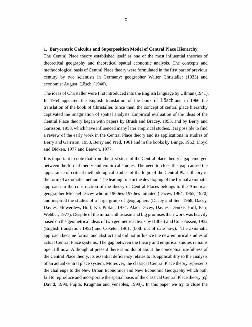
Figure 1. Derivation of the hexagonal covering of the plane by section of the

arrangement of a layer of cubes in space

The covering theorem was known to Pythagoreans in V Century B.C. Figure 1

demonstrated the interconnection between the filling of space by a layer of cubes and the

hexagon covering of the plane: the section of the three-dimension arrangement of layer

of cubes by the plane gives the covering of the plane by regular hexagons. This

three-dimensional arrangement of a layer of cubes includes cubes whose vertices are the

centers of quadrate faces of adjacent cubes. This property of section of the arrangement

of cubes will be used in the next chapter for the construction of interconnection of the

system of barycentric coordinates in the Mobius&& plane and usual Euclidean metrics in

space.

2. The second property is that the size of the hinterland areas increases from the

smallest (on the lower tier of Central Place hierarchy) to the largest (on the highest tier

of hierarchy) by a constant nesting factor k.

By definition, the nesting factor is the ratio between the area S of the hexagon belonging

to some hexagonal covering of the plane to the area s of hexagon belonging to the

primary Christaller covering by smallest hexagons with the property: the distance

5

between the centers of smallest hexagons equals 1:/k S s=

It is easy to see that if d is the distance between the centers of adjacent hexagons of some

hexagonal covering of the plane then the area of each hexagon is equal to 22 3S d= , so

the area of smallest hexagon from the Christaller primary covering is equal to 2 3s = .

Thus, the nesting factor equals to the square of the distance between the centers of

adjacent hexagons of hexagonal covering of the plane: 2k d= .

3. The third property is that the center of a hinterland area of a given size is also the

center of hinterlands of each smaller size (Christaller, 1933). The nesting factors 3, 4, 7

play the most important role in the Christaller Central Place theory: they express one of

the Christaller three principles, namely, marketing (k = 3), transportation (k = 4) and

administrative (k = 7) principles. The nesting factors 3, 4, 7 generate three geometrical

sequences of the hexagonal market area sizes: 1, 3, 9, 27,…,3n ,…; 1, 4, 16, 64,…,4n ,…;

1, 7, 49, 343,…,7n . It is possible to interpret these Christaller principles as principles of

optimal organization of the central place market areas: marketing principle represents the

minimal number of small market areas – three - included in a bigger market area; the

transportation principle presents such optimal organization of space where the

transportation network between two bigger central places passes through the smaller

central place; the administrative principle presents such optimal organization of space

where the administrative hinterland of the larger central place includes almost

completely the set of administrative hinterlands of smaller central places.

5. The Loschian&& hexagonal landscape ( , 1940)Losch&& is the superposition of all possible

coverings of a plane by hexagons whose centers are coincide with the vertices of the

triangular lattice and the sizes of market areas (nesting factors) are integers: 1, 3, 4, 7, 9, 12, 13, 16, 19,...k = The geometric procedure for construction of the

Loschian&& landscape is simple and straightforward: for the derivation of a part of the

Loschian&& landscape which corresponds to the hexagonal covering with a nesting factor 2k d= , one should chose on the Christaller primary lattice two points with the distance d

between them, to derive the segment connected these two centers and from its middle

point to draw a perpendicular segment of the size / 3d . The end point of this

perpendicular segment is the vertex of the hexagon and, thus defines the position of

whole hexagon and all hexagons from the corresponding coverings. Each hierarchical

level in the Loschian&& landscape includes the primary hexagonal covering with its own

geometric scale and secondary hexagon covering with a definite nesting factor built up

on the primary covering. Losch && himself constructed the coverings corresponding to 150

nesting factors. By rotating of the different coverings Losch && show that in vicinity of an

6

origin the market areas are arranged into six “activity (center) rich” and six “activity

(center) poor” sectors. As Lloyd and Dicken, 1972, pp. 48-49, commented, “this

particular section of ' Losch s&& work has been the subject of much controversy and

misinterpretation…The work by Tarrant, 1973, and Beavon and Mabin, 1975, suggests a

rather different interpretation…According to both studies, the production of “city-rich

“and “city-poor” sectors is not the result of rotation, as many have believed, but a

constant upon it. In other words, if the sectoral pattern is to be achieved there is a very

limited number of ways in which the hexagonal net can be arranged. Once certain ones

are oriented in a particular way the positions of the others are fixed.”

Moreover, as demonstrated by Marshall, 1977, this arrangement of “city-rich “and

“city-poor” sectors is local and do not hold for the big distances from the origin. Parr

indicated (Parr, 1970, p.45) that these Loschian&& landscape nesting factors also present

the optimal organizations of space similar to Christaller marketing, transportation and

administrative principle; for example, the nesting factors 13 and 19 have the same

property of administrative convenience as factor 7, while factors 9 and 16 have the same

transportation efficiency as factor 4. According to Lloyd and Dicken, 1972, p. 49,

“ Losch&& suggested that this spatial arrangement of urban centers was consistent with

what he saw to be a basic element in human organization: the principle of least effort.”

6. The Beckmann-McPherson, 1970, Central Place model differs from the Christaller

framework by applying variable nesting factors and by using the principle of possible

coverings of the plane by hexagons of variable integer sizes. Their centers are the

vertices of the initial Christaller triangular lattice.

The Christaller model is only a partial case of Beckmann-McPherson models.

Simultaneously, the Beckmann-McPherson models are an incomplete case of the

7

Loschian&& model – incomplete in the sense that the Beckmann-McPherson models

include only a small part of the hinterland areas from the Loschian&& landscape (see figure

3). Parr, 1970, described the way to compare the theoretical models with the structure of

the actual central place system. His idea was to use the Beckmann-McPherson Central

place model as the best fitting approximation of an actual central place hierarchy. Parr

also met with difficulties that arise from the omission of the analysis of the discrepancy

between the actual central place hierarchy and its best fitting Beckmann-McPherson

approximation.

3. The construction of the Central Place geometry on a basis of barycentric

coordinates on a plane.

The barycentric coordinates, i.e., coordinates of the center of gravity, are connected to the

concept of the center of gravity introduced at first by Archimedes in the second century

B.C. The barycentric coordinates

8

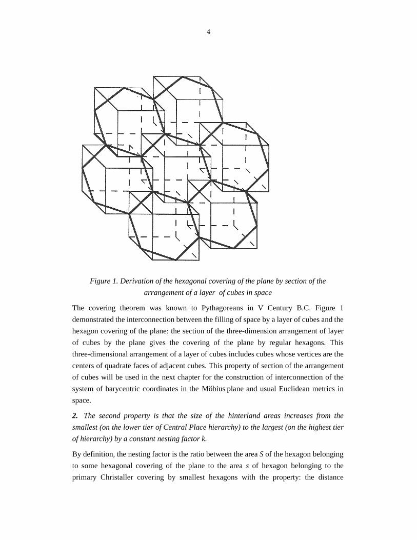
appeared in the remarkable book byMobius&& , 1837, as a basis for a projective geometry.

The construction of the barycentric coordinates in a plane is based on a choice of the

Möbius triangle within the Möbius plane. This plane is in the two-dimensional space

defined by three barycentric coordinates, , , 1 x y z x y z+ + = . The scale element of

this plane is the Möbius equilateral triangle with the unit scale on each side. This triangle

is generated by three coordinate axes (see figure 4).

Each covering of the plane by equal hexagons generates the system of barycentric

coordinates corresponding to the Mobius&& triangle with different scales. It is possible to

measure the barycentric coordinates of each point in the Möbius plane by projecting it

(parallel to the sides) onto the sides of the Möbius triangle. If the point, P, lies within the Möbius triangle, then its barycentric coordinates,, ,x y z must be between 0 and 1. The

vertices of the Möbius triangle are:

: 1, 0, 0; : 0, 1, 0; : 0, 0, 1. X x y z Y x y z Z x y z= = = = = = = = =

The mechanical interpretation of the barycentric coordinates as coordinates of center of gravity (barycenter) is as follows: the point P with coordinates , , x y z is the center of

gravity of the weights , , x y z hanging in the vertices , , X Y Z of the Möbius triangle.

If point P lies outside of the Möbius triangle. triangle (see figure 4) then one or two

barycentric coordinates must be negative, but the condition x + y + z = 1 always holds.

The barycentric coordinates of the central places of the initial Christaller hexagonal

9

coverings of the Möbius plane are positive or negative integers.

It is interesting to note that the barycentric coordinates appeared in a latent and

mysterious form in the geometry of the Central Place theory – in the

form of the rhombic coordinates x and y in the primary Christaller triangular lattice

(Dacey, 1964, 1965) or in the form of the coordinate triples (x, y, x+y), where x, y are the

rhombic coordinates (Tinkler, 1978). Neither Dacey nor Tinkler realized that the triple

(x, y, z) where z = 1 –x - y present three barycentric coordinates in a Mobius&& plane.

3. The Kanzig - Dacey formulae.

The figure 1 points out on the possibility to present the barycentric coordinates on a

Möbius plane as usual Euclidian coordinates on a plane x + y + z = 1 in three

dimensional space. The equation x + y + z = 1 represents a plane in three-dimensional

space based on the triangle with the vertices (5) which is the Möbius triangle (see figure

5). The transfer of the barycentric coordinates from plane to space increases the scale by

the factor 2 , and gives the simple way to obtain the Dacey formula for theoretical

nesting factors (Dacey, 1964, 1965) 2 2 k x y xy= + + where , , 1 x y z x= − are the

barycentric coordinates of the central place: , x y are arbitrary positive and negative

integers. To prove this formula we note that for different points (x, y, z) and (v, u, w) on

the plane x + y + z = 1 the usual Euclidean distance d is:

( ) ( ) ( ) ( ) ( ) ( )( )2 2 2 2 22[ ]Dist v x u y w z v x u y v x u y= − + − + − = − + − + − −

The distance d between the central places (x, y, z) and (v, u, w) on the Möbius plane can be

obtain from Dist by scaling in on parameter2 , i.e.

( ) ( ) ( )( )2 2d v x u y v x u y= − + − + − −

If the point (v, u, w) is the origin (0, 0, 1) of the lattice then the square of distance between

(x, y, z) and (0, 0, 1) gives the Dacey generating formula for the nesting factors in the

Loschian&& central place landscape:

2 2k x y xy= + + (1)

10

Figure 5. The interconnection between the barycentric coordinates in the Möbius plane

and the Euclidian coordinates in space.

where x and y are arbitrary integer numbers.

If we introduce the new parameters u=x/2 and v=x/2 + y then the Dacey formula (1) will

be equivalent to the Kanzig formula:

k = 3u2 +v2 (2)

where u and v are arbitrary half-integer numbers. Werner Kanzig presented his formula

empirically in the English translation of the Lösch book “The Economics of Location”,

1954, p.119. Beavon and Mabin, 1975, proved a correct form of the Kanzig formula.

Both formulas of Dacey and Kanzig are generating the same sequence of the theoretical

Lösch nesting factors: 1, 3, 4, 7, 9, 12, 13, 16, 19,...k =

4. Barycentric calculus of the Löschian hexagonal landscape.

The universal geometrical procedure of the construction of all hexagonal coverings from

Löschian hexagonal landscape (see chapter 1) can be presented with the help of

barycentric coordinates of centers of hexagons: consider the center of the hexagon with

integer coordinates (x, y ,z), x + y + z = 1; construct the segment S connecting the point

(x, y, z) with the point (0, 0, 1). The square 2 d of the distance d between these two points according to Kanzig-Dacey formula coincides with the nesting factor

11

2 2 2 d k x y xy= = + + . Further, let us draw from the middle point of the segment S a

perpendicular segment of the size/ 3d . The end points of this perpendicular segment

are the vertices of the hexagon and, thus define the position of whole hexagon covering

of the plane corresponding to the nesting factor k.

Next we introduce two important operations with hexagon coverings:

4.1. Convex combination of hexagon coverings

Consider two different hexagon coverings based on the same Christaller primary

covering. These two coverings can be constructed with the help of two points in the

Möbius plane:( ) ( )1 1 1 2 2 2, , , , , x y z x y z . For arbitrary number (weight) α the convex

combination of these points can be derived as a point with following barycentric

coordinates ( ) ( ) ( )( )1 2 1 2 1 21 , 1 , 1 x x y y z zα α α α α α+ − + − + −

This point can be used for the construction of a new hexagon covering which will be

called the convex combination of two hexagon coverings. In a similar manner can be

constructed the convex combination of arbitrary number r of hexagon coverings with

weights 1 2 1 2, ,..., , ... 1 r rα α α α α α+ + + = .

4.2. Homothetic transformation of hexagon coverings.

Consider the arbitrary hexagon covering, constructed with help of the point ( ), , x y z in

the Möbius plane, corresponding to nesting factor 2 2k x y xy= + + and the positive

number r > 0. The hexagon covering, constructed with the help of point

( ), ,1 rx r y r rz− + , is called a homothetic transformation of hexagon

covering with radius of homothety r. The nesting factor rk of the homothetic

transformation of hexagon covering equals: rk rk=

As will be shown further, the convex combinations of hexagon coverings and their

homothetic transformations describe the transfer from one hierarchical level of Central

place hierarchy to the next hierarchical level.

12

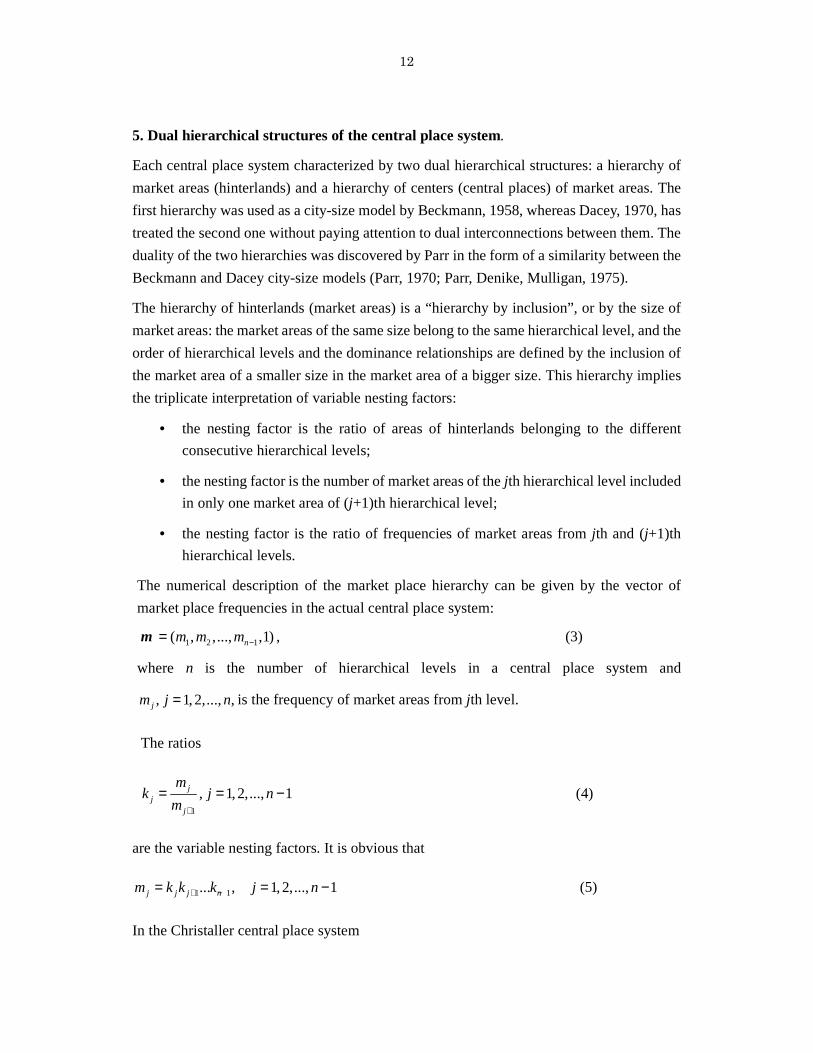
5. Dual hierarchical structures of the central place system.

Each central place system characterized by two dual hierarchical structures: a hierarchy of

market areas (hinterlands) and a hierarchy of centers (central places) of market areas. The

first hierarchy was used as a city-size model by Beckmann, 1958, whereas Dacey, 1970, has

treated the second one without paying attention to dual interconnections between them. The

duality of the two hierarchies was discovered by Parr in the form of a similarity between the

Beckmann and Dacey city-size models (Parr, 1970; Parr, Denike, Mulligan, 1975).

The hierarchy of hinterlands (market areas) is a “hierarchy by inclusion”, or by the size of

market areas: the market areas of the same size belong to the same hierarchical level, and the

order of hierarchical levels and the dominance relationships are defined by the inclusion of

the market area of a smaller size in the market area of a bigger size. This hierarchy implies

the triplicate interpretation of variable nesting factors:

• the nesting factor is the ratio of areas of hinterlands belonging to the different

consecutive hierarchical levels;

• the nesting factor is the number of market areas of the jth hierarchical level included

in only one market area of (j+1)th hierarchical level;

• the nesting factor is the ratio of frequencies of market areas from jth and (j+1)th

hierarchical levels.

The numerical description of the market place hierarchy can be given by the vector of

market place frequencies in the actual central place system:

m 1 2 1( , ,..., ,1)nm m m−= , (3)

where n is the number of hierarchical levels in a central place system and

, 1,2,..., ,jm j n= is the frequency of market areas from jth level.

The ratios

1

, 1,2,..., 1jj

j

mk j n

m +

= = − (4)

are the variable nesting factors. It is obvious that

1 1... , 1,2,..., 1j j j nm k k k j n+ −= = − (5)

In the Christaller central place system

13

1 23, 4, 7; 9, 16, 49,..., 3 , 4 , 7m m mmk k k= = = (6)

In the Losch&& or in the Beckmann-McPherson central place system jk are the Kanzig-Dacey

integers: 1, 3, 4, 7, 9, 12, 13, 16, 19,...jk = .The above-described hierarchy of market

areas generates the dual hierarchy of the centers of market areas on the basis of duality

correspondence: Market area (hinterland of the central place) ⇔ Central place (center of

market area) such that the order j of the hierarchical level of a given central place is equal to

the order of hierarchical level of the biggest market area with the same center; the

dominance relationship between the centers is defined by the geometric inclusion of

corresponding hinterlands. It is possible to give the analytical description of the hierarchy of

centers of market areas by means of a vector of center frequencies

c 1 2 1( , ,..., ,1)nc c c −= (7)

where jc is the frequency of center from jth hierarchical level. The duality correspondence

implies the connections between the vectors m of market area frequencies and vectors c of

center frequencies:

( ) ( )1 1 1 1

1 1

1 1 ...

... 1

j j j j j j j n

j j j n

c m m m k k k k

m c c c

+ + + −

+ −

= − = − = −

= + + + + (8)

6. Empirical Average Central Place hierarchies.

In empirical studies of concrete Central Place systems the main measurable statistical

data is the vector 0 0 00 1 2 1( , ,..., ,1)nc c c c −= of empirical center frequencies is main

measurable statistical data. Formulae (11) and (7) give the coordinates of the vector of

empirical market areas frequencies 0 0 00 1 2 1( , ,..., ,1)nm m m m−= and the coordinates of the

vector of average nesting factors 0 0 00 1 2 1( , ,..., ) nk k k k −= . The average nesting factors are

the arbitrary positive numbers, not necessary integers.

Christaller, 1950, himself came to realize that the marketing, transportation and

administration principles could be expected to act simultaneously in geographical space.

He suggested modifying his original model by a mixing of the nesting factors 3, 4, and 7

14

into the grouping non-integer nesting factor k = 3.3 which generates the geometric

progression 1, 3.3, 10, 33,. Woldenberg, 1968, elaborated on analogy between the

hierarchical structure of fluvial systems and the hierarchical structure of the hinterlands

of the central place systems, so as to be able to generate the sequences of average

non-integer nesting factors for sizes of market areas for central place systems. With the

help of numerical computer model Woldenberg, 1979, compared the results of computer

simulations with a wide set of actual empirical central place hierarchies and mentioned

certain difficulties that rise in attempting to describe an actual hierarchy in terms of the

numerical computer model. The week points of these generic models are the

non-uniqueness of the procedure of grouping and empirism in the underlying theoretical

reasoning.

The empirical central place hierarchies generate in the vicinity of each central place the

local nested geometric structure of average market areas, i. e. set of hexagons with the

centers located in the given central place. The areas of these hexagons correspond to the

vector of empirical market areas frequencies 0 0 00 1 2 1( , ,..., ,1)nm m m m−= generating the

coordinates of the vector of average nesting factors 0 0 00 1 2 1( , ,..., ) nk k k k −= The

construction the geometrical base of this local hierarchy of empirical average market

areas needs the elaboration of the theory of the superposition, mixing and best fitting of

the theoretical central place hierarchies and the construction of the new superposition

model of the of the central place hierarchy which reflects the existence of different

extreme tendencies of the spatial organization of central places, developing within an

actual central place system (Sonis, 1970, 1982, 1985, 1986). Therefore the geometry of

local hierarchy of empirical average market areas will be presented in detail in chapter 9

after the introduction of the superposition model of the of the central place hierarchy.

7. The superposition model of central place hierarchy.

Now we will present a general superposition Central Place model with arbitrary number of

hierarchical levels. For the construction of such generalization we will use the theory of

convex polyhedra in multi-dimensional space (see Weyl, 1935)

The superposition model of central place hierarchy is the application of the formalism of the

Superposition Principle (see Sonis, 1970, 1982b) to the analysis of the structure of an actual

central place system. At first we immerse an actual average central place system into the

convex polyhedron of all admissible central place system. This immersion gives the

possibility to apply the analytical formalism of the decomposition of an average central

15

place hierarchy into the convex combination of the Beckmann-McPherson extreme

hierarchies (Beckmann-McPherson, 1970), which are the results of the Parr “best fitting”

procedure (Parr, 1978a).

7.1.Polyhedron of Admissible Central Place Hierarchies for an Actual Central Place

System

Let us consider an actual central place system given by a vector of market area frequencies

0 0 00 1 2 1( , ,..., ,1) nm m m m−= or by the sequence:

0 0 00 1 2 1( , ,..., ) nk k k k −= (9)

of average nesting factors calculated with a help of the formula (7). For the evaluation of

the hierarchical structure of an actual central place system, we shall place it into the

convex polyhedron of all admissible central place hierarchies. For this, we will choose on each hierarchical level, j, the pair of theoretical nesting factors ',j jK K in such a way that

the segment [ ',j jK K ] will include the average nesting factors0jk : 0 '

j j jK k K≤ ≤ . This

choice of theoretical nesting factors defines the convex polyhedron of all admissible

central place hierarchies: it includes all sequences of average nesting factors

1 2 1( , ,..., ) nk k k k −= such that:

' , 1,2,..., 1 j j jK k K j n≤ ≤ = − (10)

This system of inequalities presents geometrically the (n-1)-dimensional rectangular

parallelepiped, whose vertices have the coordinates equal to the integer theoretical nesting factors ' or j jK K ; thus, these vertices correspond to the Beckmann-McPherson

central place models. The actual central place hierarchy (19) corresponds to the inner

point of this polyhedron.

Let us introduce the slack variables, presenting the deflection of some central place

hierarchy from the theoretical one on each hierarchical level j:

'0; 0, 1,2,..., 1 j j j j j jy k K z K k j n= − ≥ = − ≥ = − (11)

Then each admissible central place hierarchy 1 2 1( , ,..., ) nk k k k −= can be presented as a

three-row matrix with non-negative components:

16

1 2 1

1 2 1

1 2 1

...

...

...

n

n

n

k k k

X y y y

z z z

−

−

−

=

(12)

and the actual central place hierarchy corresponds to the matrix 0 0 01 2 1

0 0 00 1 1 2 2 1 1

' 0 ' 0 ' 01 1 2 2 1 1

...

...

...

n

n n

n n

k k k

X k K k K k K

K k K k K k

−

− −

− −

= − − − − − −

(13)

7.3. Decomposition of an Actual Central Place Hierarchy According to the superposition principle (see Sonis, 1970, 1980, 1982b, 1985), the

hierarchical analysis of an actual central place system represented by the non-negative

matrix 0X is reduced to the decomposition of this matrix into the weighted sum of

matrices 1 2 1, ,..., rX X X + :

0 1 1 2 2 1 1,... r rX p X p X p X r n+ += + + + ≤ (14)

where each matrix iX represents the extreme state of the central place system,

corresponding to some Beckmann-McPherson model and the weights ip have the

property:

1 2 1... 1; 0 1; r ip p p p r n++ + + = ≤ ≤ ≤ (15)

If we take into consideration only the first row of each matrix in the decomposition (14),

we obtain the decomposition of the actual central place hierarchy

0 0 00 1 2 1( , ,..., ) nk k k k −= into the convex combination of the Beckmann-McPherson central

place hierarchies ik with the same weights ip :

0 1 1 2 2 1 1... , r rk p k p k p k r n+ += + + + ≤ (16)

We interpret the decomposition (15, 16) in the following way: in each actual central place

system, there is a set of substantially significant tendencies towards the optimal

organization of space in the form of Beckmann-McPherson hierarchies. Geometrically,

these tendencies define the simplex enclosed into the polyhedron of admissible central

place hierarchies whose vertices correspond to the assemblage of the matrices iX . An

actual central place hierarchy0 X is the center of gravity of this simplex with the

weights ip . It is possible to interpret the weights ip in a probabilistic form as the

frequencies of the partial realization of some combination of the Christaller-Lösch

optimization principles in the hierarchical structure of the actual central place system. 7.3.Best Fitting Approximation Procedure and the Algorithm of Decomposition The best-fitting procedure of this chapter is a simplification of the procedure proposed by

17

Parr (1978). This procedure will be used for the derivation of the central place hierarchy

on each hierarchical level and in this way will be the basis for the construction of the best

fitting simplex that contains the actual central place hierarchy matrix 0X corresponding to

the vector 0 0 00 1 2 1( , ,..., ) nk k k k −= of average nesting factors. The best-fitting procedure is

as follows: for each hierarchical level i, the segment 0 ' i i iK k K≤ ≤ between the

theoretical nesting factors ', i iK K can be chosen, which includes the average nesting

factor 0 ik . In this way, the first best fitting Beckman-McPherson model

1 1 11 1 2 1( , ,..., ) nk k k k −= can be constructed with the help of “best fitting” formulae (Sonis,

1985): '

0

1

'' 0

2

2

i ii i

i

i ii i

K KK if k

kK K

K if k

+≤= + >

(17)

In this procedure the values '

2

i iK K+define the boundaries of the domain of structural

stability of the decomposition (14, 15).

The weight 1 p of the Beckmann-McPherson model 1 X can be found by the

requirement to choose the biggest positive ( )0 1 p p< < satisfying the

condition 0 1 0 X p X− ≥ , or in the coordinate form: 0 0 ' 0

1 1 1 ' 1min {1, , , } i i i i i

ii i i i i

k k K K kp

k k K K k

− −=− −

(18)

The place of the components of the matrices0 1 and X X , yielding the minimum in (28),

defines the hierarchical level on which there exists the strongest interdiction to the

extreme tendency represented by the chosen Beckmann-McPherson model 1 X , on the

part of other tendencies acting in the actual central place hierarchy.

The residual 2 X , defined by the equality:

( )0 1 1 1 21 X p X p X− = − (19)

represents the mutual action of other tendencies developing in the central place hierarchy

with the weight 11 p− . This may be interpreted geometrically by constructing a straight

18

line that passes the vertex 1 X and the point 0 X of the actual central place hierarchy and

crosses the opposite face of the parallelepiped of admissible central place hierarchies at

the point 2 X . Moreover, if one hangs the weights 1 1 and 1 p p− on points

1 2 and X X then the center of gravity of the segment with end points 1 2 and X X will

coincide with the point 0 X . For study of the residual 2 X , one should apply the “best

fitting” procedure to the 2 X , and so forth.

8. Hierarchical analysis of the Christaller original central place system in Munich,

Southern Germany.

After the decades of empirical studies, the pure Christaller-Losch&& theoretical hierarchies of

several hierarchical levels with the same nesting factors have rarely if ever observed. The

reason for this is that each actual central place hierarchy is the superposition of various

theoretical hierarchies. It is interesting to note that even Christaller’s original study of the

Munich central place hierarchy confirms the phenomenon of superposition. The Christaller

original Munich central place hierarchy (Christaller, 1933; Woldenberg, 1979, Table 5, p.

446.) can be presented with the help of the following vector of market area frequencies

( )0 519,249,127,39,12,3,1 m = with the corresponding sequence of average nesting

factors ( )0 2.0843,1.9606,3.2564,3.25,4,3 k = . The polyhedron of admissible central place

hierarchies includes all matrices of the form (see 12):

1 2 3 4 5 6

1 2 3 4

1 2 3 4

4 3

1 1 3 3 0 0

3 3 4 4 0 0

k k k k k k

X k k k k

k k k k

= = = − − − − − − − −

The Munich central place hierarchy is represented by a matrix:

0

2.0843 1.9606 3.2564 3.25 4 3

1.0843 0.9606 0.2564 0.25 0 0

0.9157 1.0394 0.7436 0.75 0 0

X

=

(20)

The best-fitting approximation of the vector of average nesting factors

( )0 2.0843,1.9606,3.2564,3.25,4,3 k = has a form 1k = (3, 3, 3, 3, 4, 3) which generates the

Beckmann-McPherson model

1

3 3 3 3 4 3

2 2 0 0 0 0

0 0 1 1 0 0

X

=

(21)

19

The weight 1 p of this Beckmann-McPherson model is equal to (see (18)):

1

2.0849 1.9606 1.0843 0.9606 0.7436 0.75 0.9606min 1, , , , , , 0.4803

3 3 2 2 1 1 2p

= = =

(22)

i.e.

'0 10.4803 0.5197 X X X= + (23)

where ' X is a residual. Thus, the real central place system 0 X includes only 48.03% of the

extreme tendency 1 X corresponding to the best fitting Beckmann-McPherson model. The

residual 'X can be calculated from equation (23). The best fitting procedure applied to this residual will give us the second extreme tendency 2 X and its weight 2 p . Such a procedure

can be repeated once more. After 5 steps the final decomposition of the Munich central place

hierarchy can be obtained:

0 1 2 3 4 50.4803 0.2633 0.1946 0.0554 0.0064

3 3 3 3 4 3 1 1 3 3 4 3

0.4803 2 2 0 0 0 0 0.2633 0 0 0 0 0

0 0 1 1 0 0 2 2 1 1 0 0

1 1 4 4 4 3 3 1 4 4 4 3

0.1946 0 1 1 0 0 0.0554 2 1 1 0 0

2 2 0 0 0 2 0 0 0

3 1 4

0.0064

X X X X X X= + + + + =

= + • +

+ • + • + • • •

+3 4 3

2 1 0 0

2 1 0 0

• • • •

(24)

The first row of this matrix equality gives the decomposition of the vector of average nesting

factors:

( )

( )( )( )( )( )

0

1 2 3 4 5

2.0843,1.9606, 3.2564, 3.25, 4, 3

0.4803 0.2633 0.1946 0.0554 0.0064

0.4803 3,3,3,3,4,3

0.2633 1,1,3,3,4,3

0.1946 1,1,4,4,4,3

0.0554 3,1,4,4,4,3

0.0064 3,1,4,3,4,3

k

k k k k k

= == + + + + == +

+ +

+ +

+ +

+

(25)

This decomposition means that the Munich central place hierarchy consists of five extreme

20

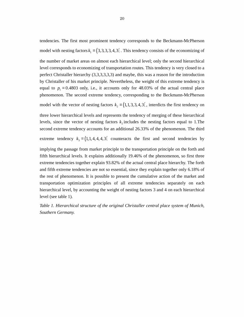
tendencies. The first most prominent tendency corresponds to the Beckmann-McPherson

model with nesting factors ( )1 3,3,3,3,4,3k = . This tendency consists of the economizing of

the number of market areas on almost each hierarchical level; only the second hierarchical

level corresponds to economizing of transportation routes. This tendency is very closed to a

perfect Christaller hierarchy (3,3,3,3,3,3) and maybe, this was a reason for the introduction

by Christaller of his market principle. Nevertheless, the weight of this extreme tendency is

equal to 1 0.4803p = only, i.e., it accounts only for 48.03% of the actual central place

phenomenon. The second extreme tendency, corresponding to the Beckmann-McPherson

model with the vector of nesting factors ( )2 1,1,3,3,4,3k = , interdicts the first tendency on

three lower hierarchical levels and represents the tendency of merging of these hierarchical

levels, since the vector of nesting factors 2k includes the nesting factors equal to 1.The

second extreme tendency accounts for an additional 26.33% of the phenomenon. The third

extreme tendency ( )3 1,1,4,4,4,3k = counteracts the first and second tendencies by

implying the passage from market principle to the transportation principle on the forth and

fifth hierarchical levels. It explains additionally 19.46% of the phenomenon, so first three

extreme tendencies together explain 93.82% of the actual central place hierarchy. The forth

and fifth extreme tendencies are not so essential, since they explain together only 6.18% of

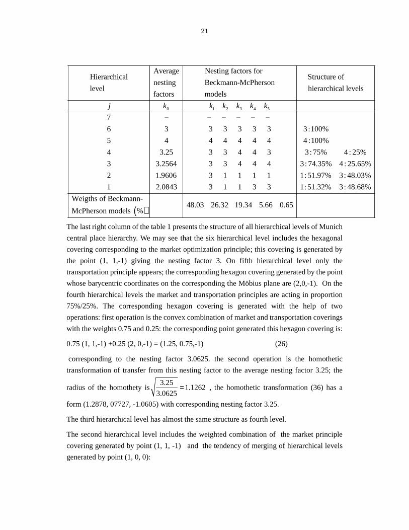
the rest of phenomenon. It is possible to present the cumulative action of the market and

transportation optimization principles of all extreme tendencies separately on each

hierarchical level, by accounting the weight of nesting factors 3 and 4 on each hierarchical

level (see table 1).

Table 1. Hierarchical structure of the original Christaller central place system of Munich,

Southern Germany.

21

0 1 2 3 4 5

Average Nesting factors forHierarchical Structure of

nesting Beckmann-McPhersonlevel hierarchical levels

factors models

7

6 3 3 3 3 3 3 3:100%

5 4 4 4 4 4 4 4 :

4 3.25 3 3 4 4 3

3 3.2564 3 3 4 4 4

2 1.9606 3 1 1 1 1

1 2.0843 3 1 1 3 3

j k k k k k k

− − − − − −

( )

100%

3:75% 4: 25%

3: 74.35% 4: 25.65%

1:51.97% 3: 48.03%

1:51.32% 3: 48.68%

Weigths of Beckmann-48.03 26.32 19.34 5.66 0.65

McPherson models %

The last right column of the table 1 presents the structure of all hierarchical levels of Munich

central place hierarchy. We may see that the six hierarchical level includes the hexagonal

covering corresponding to the market optimization principle; this covering is generated by

the point (1, 1,-1) giving the nesting factor 3. On fifth hierarchical level only the

transportation principle appears; the corresponding hexagon covering generated by the point

whose barycentric coordinates on the corresponding the Möbius plane are (2,0,-1). On the

fourth hierarchical levels the market and transportation principles are acting in proportion

75%/25%. The corresponding hexagon covering is generated with the help of two

operations: first operation is the convex combination of market and transportation coverings

with the weights 0.75 and 0.25: the corresponding point generated this hexagon covering is:

0.75 (1, 1,-1) +0.25 (2, 0,-1) = (1.25, 0.75,-1) (26)

corresponding to the nesting factor 3.0625. the second operation is the homothetic

transformation of transfer from this nesting factor to the average nesting factor 3.25; the

radius of the homothety is3.25

1.1262 3.0625

= , the homothetic transformation (36) has a

form (1.2878, 07727, -1.0605) with corresponding nesting factor 3.25.

The third hierarchical level has almost the same structure as fourth level.

The second hierarchical level includes the weighted combination of the market principle

covering generated by point (1, 1, -1) and the tendency of merging of hierarchical levels

generated by point (1, 0, 0):

22

0.4803 (1, 1, -1) +0.5197 (1, 0, 0) = (1, 0.4803, -0.4803)

with average nesting factor 1.9606.

The first hierarchical level has almost the same structure as second hierarchical level

Thus, the decomposition analysis of the Christaller example of the Munich, Southern

Germany central place hierarchy, hints on the origins of appearance of Christaller

optimization principles in the Central Place Theory.

9. Structural Stability, Structural Changes and Catastrophes in Central place

Hierarchical Dynamics.

The hierarchical dynamics of the Central place systems are the reflection of the

socio-economic spatial complication process of the urban/regional system. The hierarchical

dynamics represent both the rapid change and locational and functional inertia within the

urban system. The major reason of catastrophic hierarchical change in an evolving

urban/regional system is the transfer of a few centers from one hierarchical level to another

as a result of changes in allocation of individual central place functions within the hierarchy,

i.e., in the modification in the functional extent of the level (cf. Parr, 1981, pp. 105-108). The

complication process is also reflecting the appearance or disappearance of centers as a result

of regional growth, decline or regional competition (see Batty and Friedrich, 2000).

Next we will consider the implementation of the principle of structural stability and

structural changes into the dynamics of central place hierarchies.

The main questions of the structural stability and structural changes are:

• What types of central place hierarchies are possible? The Central place theory in its

new form, presented in this chapter, is giving the possible answer on this question.

• What kind of structural changes are admissible and what types of structures are

preserved (at list partially) under these changes?

• How do the transitions from one type of structure to another occur?

The first question immediately points to the gap between the pure theoretical central place

models, based on the Losch&& economic landscape, and the hierarchical structure of an actual

central place system; two other questions underline the fact that existing central place

theory is mostly static and tells us little about the complication process of emergence

transformations and stability of an urban hierarchy. A vast body of literature expanding the

classical central place theory since its initial formation includes only a small part relevant to

the current focus on structural changes within the central place hierarchy. The polyhedral

23

catastrophic dynamics of the states of the central place hierarchy represents its comparative

statics and may be considered as a necessary step toward the dynamic theory of the central

place hierarchy, which is waiting till now its creator. Between the earlier attempts to

construct the dynamic Central place theory the simulation efforts of Morrill (1962), White

(1977, 1978), Allen and Sanglier, 1979, Camagni et al., 1986 and Diappi et.al, 1990, should

be mentioned.

Geometrically, three different types of hierarchical changes are possible.

The first type of change is connected with the case of global structural stability, when the

average nesting factors are changing slowly, so the polyhedron of admissible central place

hierarchies remains the same and the point of actual central place hierarchy is moving within

the same simplex. That means that in the decomposition

0 1 1 2 2 1 1,... r rX p X p X p X r n+ += + + + ≤ the vertices iX remains the same and only the

coefficients ip are slowly changing preserving the property1 2 1... 1; 0 1r ip p p p++ + + = ≤ ≤ .

The domain of such movement in the polyhedron of admissible central place hierarchies is

the domain of global structural stability. In reality, the domain of structural stability is

usually very narrow, and small changes in the average nesting factors caused the crossing the

boundary of this domain. This implies the exchange in the decomposition (VII.9) of some

extreme tendencies with others, and further, allows even the complete change of

composition and ranking of the Beckman-McPherson models entering the decomposition.

The second type of hierarchical change is connected with the transfer of the point of an

actual central place 0X from one convex polyhedron of admissible hierarchies to another

convex polyhedron, defined by the different Kanzig-Dacey nesting factors. Geometrically

this means the crossing the boundary of the initial polyhedron. In this case, the best we can

expect is the partial structural stability, i.e., the stable inclusion in the decomposition (II.9) of

only a part of previous extreme tendencies. In reality, the case of the partial structural

stability is a most expected one.

The third essentially different type of change in the hierarchical structure is the change

in the dimension of the polyhedron of admissible hierarchies. This type of the catastrophic

change is caused by the change in a number and content of hierarchical levels as a result of

a split or merging of hierarchical levels (cf. Parr, 1981, pp. 101-110). The split of a level is

characterized by the increase in the number of the central places on the same hierarchical

level and a differentiation in the functional content of the level. The merging of the levels is

connected with the decrease of a degree of functional differentiation and with the

24

appearance of a new tendency corresponding to the Beckman-McPherson model with the

nesting factor equal 1 on the same hierarchical level..

10. Further theoretical developments: short reviews.

The existence of the axiomatic theory of Central Places presented in this paper is pointed

on the further directions in empirical studies and further directions of theoretical

developments.

In the field of empirical studies the use of superposition model supported by easily

assessable computer software (cf. the analysis of original Christaller Central place system

of Southern Germany in chapter 8) will eventually result in the taxonomy of types of

evolution of hierarchical central place system. In such a way the gap between the theory of

central place system and its empirical justification will be narrowed.

In the field of theoretical studies the axiomatic theory of Central Places is presented a wide

range of possibilities of constructing of stylized examples of the development of evolving

socio-economic systems in geographical space. Two main applications of this conceptual

framework are elaborated

I. Structurally stable optimal (minimal cost) transportation flows in the

hierarchical Central Place system.

II. The merger of two major theories in the Regional Science: the classical

Input-Output theory of Leontief and the classical Christaller -Losch&& Central Place

theory.

The application I consider the possibilities of the extension of optimal transportation flow

in expending urban system. It is quite understandable that the actual central place hierarchy

puts strong restrictions on the type of optimal (minimal cost) flows between the central

places. In turn, the spatial and temporal stability of the transportation flows may be an

essential factor of growth and decline of the individual central place in the hierarchy.

Moreover, usually the optimal transportation flow does not cover all linkages of the

transportation network between the central places.

The problem of enumeration of all possible extensions of minimal cost transportation

flows is purely combinatorial and hence formidable, cumbersome and tedious. Its solution

for each given Beckmann-McPherson central place hierarchical model can be found with

the help of aggregated schemes for the transportation tables scheme includes one or two

arcs, which present the set of possible linkages between the central places. These arcs are

presented as lines in the cells of the aggregated scheme (see Sonis, 1982a;1984; 1986;2000,

Huff et al.,1986)

25

Application II describes the mutual penetration and unification two central theories in the

Regional Science: the classical Input-Output theory of Leontief and the classical

Christaller-Losch&& Central place theory (see Sonis, Hewings, 2000b.) It is expected that the

proposed theoretical methodology will be useful for the analysis of organization of the

production economics in geographical space. In this study the triple UDL-factorization is

applied to the decomposition of the Leontief Inverse for Input-Output System within the

Central Place System of the Christaller-Losch&& , Bekmann-McPherson type. Such a

factorization reflects the process of gradual extension and complication of the Central Place

Hierarchy (see Sonis, Hewings, 2000a).

The idea to investigate the Input-Output relationship within the Central Place system is not

a new one. The necessity to combine together the hierarchical structure of Central Place

system with Input-Output structure of the transaction flows within one unifying framework

was stresses in the programmatic book of Walter Isard (1960, p.141). The first systematic

treatment of this problem was undertaken by Robison and Miller (1991). They used the

rudimentary structure of intercommunity central place system, without paying attention on

the fine structure of the central place hierarchy. The complexity of mathematical

presentation stops them on the level of a simple two-community two-order sub region level

with one dominant central place.

In the study (Sonis, Hewings 2000b) the central place hierarchy and multi-regional

input-output analysis are fusing together, and in a result the decomposition of the Leontief

Inverse for Input-Output Central Place system reflects the process of complication of the

evolving hierarchy of Central places

REFERENCES:

Allen P M and M. Sanglier, 1979. “A dynamic model of growth in a central place system.”

Geographical Analysis, vol. 11, pp. 256-272.

Batey P W J, 1985. “Input-output models for regional demographic-economic analysis: some

structural comparisons.” Environment and Planning, A 17, pp. 73-99.

Batey P W J and P Friedrich (eds), 2000. Regional Competition. Series “Advances in Spatial

Science”, Springer.

Batey P W J and M Madden, 1981. “Demographic-economic forecasting within an

activity-commodity framework.” Environment and Planning, A, 13, pp.73-99.

Batey P W J, and M Madden, 1983. “The modeling of demographic-economic change within the

context of regional decline; analytical procedures and empirical results.” Socio-Economic Planning

Sciences, 17, pp. 315-328.

Batey P W J, Madden M and M Weeks, 1987. “A household income and expenditure in extended

26

input-output models: A comparative theoretical and empirical analysis.” Journal of Regional

Science, 27, pp. 341-356.

Batey P W J and M Weeks, 1989. “The effect of household disaggregation in extended input-output

models”. In R E Miller, K Polenske and A Z Rose (eds), Frontiers in Input-Output Analisys, New

York, Oxford: Oxford University Press, pp. 119-133.

Beavon K S O, 1977. Central Place Theory: A Reinterpretation. London and New York:

Longmann.

Beavon K S O and Mabin A S, 1975. “The Losch&& system of market areas: derivation and

extensions.” Geographical analysis, 7, pp. 131-151.

Beckmann M J, 1958. “City hierarchies and the Distribution of city Size”, Economic Development

and Cultural change, 6, pp. 243-248.

Beckmann M J and McPherson J C, 1970. ”City size distribution in the Central Place hierarchy: an

alternative approach”, Journal of Regional Science, 10, pp. 243-248.

Berman, 1953.

Berry B J L and W L Garrison, 1958. “Recent Developments in Central place theory.” Papers and

Proceedings of the Regional Science Association, 4, pp. 107-120.

Berry B J L and A. Pred, 1961. Central Place Studies: A Bibliography of Theory and Applications,

Regional Science Research Institute, Philadelphia.

Bunge W, 1962. Theoretical Geography, Lund.

Camagni R, Diappi L and G Leonardi, 1986. “Urban growth and decline in a hierarchical system: a

supply-oriented dynamic approach.” Regional Science and Urban Economics, vol. 16, pp. 145-160.

Caratheodory C, 1911. “Uber den Variabilitats Bereich der Fourier’schen Constanten von positiven

harmonischen Functionen, Rend. Circ. Mat. 32, Palermo, s. 198-201.

Christaller W, 1933. Die Zentralen Orte in Suddeutscland, Fischer, Jena; 1966, English translation

from German original by L W Baskin, Central places in Southern Germany, Prentice Hall,

Englewood Cliffs, NJ.)

Christaller W, 1950. “Das Grundgerust der raumlichen Ordnung in Europa”, Frankfurter

Geographische Hefte, 24, s. 1-96.

Coxeter H S M, 1961. Introduction to Geometry. Wiley, New York.

Cowan G A, Pines D and Meltzer D, 1994. Complexity, Metaphors, Models, and Reality, Santa Fe

Institute, Studies in the Science of Complexity, vol. XIX, Addison-Wesley, NY.

Dacey M F, 1964. “A note of Some Number Properties of a Hexagonal Hierarchical Plane lattice”,

Journal of Regional Science, 5, pp. 63-67.

27

Dacey M F, 1965. “The Geometry of Central Place Theory”, Geograficka Annaler, 47, pp. 111-124.

Dacey M F, 1970. “Alternative Formulations of Central Place Population”, Tijdschrift voore

Economische en Social Geografie, 61, pp. 10-15.

Dantzig G B, 1951. “Application of the simplex method to a transportation problem.” In T C

Koopmans (ed), Cowles Commission Monograph 13: Activity Analysis of Production and

Allocation. John Wiley, NY, pp. 359-373.

Dantzig G B, 1963. Linear Programming and Extensions. Princeton University Press, Princeton,

NY.

David P A, 1999. “Krugman’s Economic Geography of Development; NEGs, POGs, and Naked

Models in Space”. In B Pleskovic (Guest Ed), Special Issue: Is Geography Destiny? International

Regional Science Review, pp. 162-172.

Diappi L, T. Pompili and S Stabilini, 1990. “City systems: a Losch&& - theoretical dynamic model.”

Occasional Paper Series on Socio-Spatial Dynamics, The University of Kansas, vol.1, No. 2, pp.

103-124.

Fujita M, P Krugman and A J Venables, 1999. The Spatial Economy. Cities, Regions and

International Trade, The MIT Press, Cambridge, Massachusetts, London, England.

Gass S I, 1958. Linear Programming, Methods and Applications, McGraw-Hill, NY.

J. Huff, D.A. Griffith, M. Sonis, L. Leifer and D. Straussfogel, 1986. "Dynamic Central Place

Theory: An Appraisal and Future Perspectives." In D.A. Griffith and R. Haining (eds),

Transformation through Space and Time, Martinus Nijhoff, The Hague, 1986, pp. 121-151.

Kantorovitch L V, 1942. “On dislocation of masses.” Russian Doklady of the USSR Academy of

Sciences, 37, no.3. pp. 227-229.

Isard W, 1956. Location and Space-economy, Cambridge, MA: MIT Press.

Kantorovitch L V, Gavurin M K, 1949. ”Application of mathematical methods to the analysis of

commodity flows”. In Problems in the rise of effectiveness of Transport Activity, USSR, Moscow,

Academy of Sciences, pp. 110-138, in Russian.

Kopsas T C, Beckman M, 1957. ”Assignment problem and the location of economic activities”,

Econometrica, 25, no.1, pp 53-76.

Krugman P, 1991. “ Is Bilateralism bad”, In Helpman E and A Razin (eds) International Trade and

Trade Policy”. Cambridge: MIT Press, pp. 9-23.

Leontief W W, 1951. The Structure of Americal Economy, 1919-1939, an empirical application of

equilibrium analysis, Oxford University press, New York.

Lloyd P E and P. Dicken, 1977. Location in Space: A Theoretical Approach to economic

Geography. New York: Harper and Row.

Loeb A L, 1964. “The Subdivision of the Hexagonal Net and the Systematic Generation of Crystal

28

Structure”. Acta Crystallographica, 17, pp. 179-182.

Losch&& A, 1940. Die Raeumliche Ordnung der Wirtschaft, Fischer, Jena; 1944, second edition;

1962, third edition, Fisher, Stuttgart; 1954, English translation from German original by W H

Woglom and W F Stolper, The Economics of Location, Yale University Press, New Haven,

Connecticut.; second print, Wiley, New York.

Marshall J U, 1977. “The Construction of Loschian&& Landscape”, Geographical Analysis, 9,

pp.1-13.

Minkovski H, 1910. Geometrie der Zahlen, B G Tenbner, Leipzig, Berlin (English translation, 1953,

Theory of Numbers, Chelsea Publ., New York).

Miyazawa K, 1976. Input-Output analysis and the structure of income distribution. Lecture Notes

in Economics and Mathematical Systems, 116, Springer Verlag Berlin, Heidelberg, New York.

Moebius A F, 1827. Der Barycentrische Calcul, Leipzig.

Morrill R L, 1962. “Simulation of central place patterns over time.” In K Norborg (ed) Proceedings

of the IGU Symposium in Urban Geography, Lund 1960. Gleerups Foerlag, Lund, pp. 109-120.

Parr J B, 1970. “Models of City Size in an Urban System”, Papers of Regional Science Association,

25, pp. 221-253.

Parr J B, 1978a. “An alternative Model of the Central Place System”. In Batey P W J (ed) London

papers in Regional Science,8. Theory and Method in Urban and Regional Analysis. Pion, London,

pp. 31-45.

Parr J B, 1978b. “Models of Central Place System: A More General Approach, Urban Studies, 15,

pp. 35-49.

Parr J B, 1981. “Temporal Change in a Central place System, Environment and Planning A, 13, pp.

97-118.

Parr J B, Denike KG and G Milligan, 1975. “City Size Models and the economic basis: A Recent

Controversy”, Journal of Regional Science, 15, pp. 1-8.

Robison M H and J R Miller, 1991. “Central Place Theory and Intercommunity

Input-Output Analysis.” Papers in Regional Science, 70, pp. 399-417.

Sonis M, 1970. "Analysis of concrete states of Lineal Geographical Systems", Moscow University

Vestnik, Geogr. Series, no. 4, 1970, pp. 24-37, (in Russian).

Sonis M, 1982a. “Domains of Structural Stability for minimal cost Discrete Flows with reference to

Hierarchical Central-Place Models.” Environment and Planning A, 14, pp. 455-469

Sonis M, 1982b. "The Decomposition Principle versus Optimization in Regional Analysis: The

Inverted Problem of Multiobjective Programming". In G Chiotis, D Tsoukalas and H Louri (eds),

The Regions and the Enlargement of the European Economic Community, Athens, Eptalofos, pp.

35-60.

29

Sonis M, 1984."Transportation Flows within Central Place Systems",1984. Proceeding of the

Conference of the Italian Operation Research Association, Pescara, Italy, v.II, pp. 639-660.

Sonis M, 1985. “Hierarchical structure of Central Place System – the barycentric calculus and

decomposition principle.” Sistemi Urbani, 1, pp. 3-28

Sonis M, 1986a. “A contribution to the Central Place Theory: superimposed Hierarchies, Structural

Stability, Structural changes and Catastrophes in Central place Hierarchical Dynamics.” In R. Funk,

A. Kuklinsky (eds) Space-Structure-Economy: A Tribute to August Leosch, Karlsruhe Papers in

Economic Policy Research, 3, 159-176.

Sonis M, 1986b. “Transportation Flows within Central-Place Systems.” In D.A. Griffith, R.A.

Haining (eds). Transformations through Space and Time, Martinus Nijhoff, Amsterdam, 81-103.

M, Sonis, 2000. “ Catastrophe effects and optimal extensions of Transportation flows in the

developing Urban System: A Review”. In D. Helbing, H.J.Herrmann, M. Schreckenberg, D. E.

Wolf (eds) Traffic and Granular Flows ’99, Social, Traffic and Granular Dynamics, Springer,

pp.31-41.

Sonis M and G J D Hewings, 2000a. “LDU-factorization of the Leontief inverse, Miyazawa income

multipliers for multiregional systems and extended multiregional Demo-Economic analysis." The

Annals of Regional Science, 34, no.4, pp 569-589.

Sonis M and G J D Hewings, 2001b. “Central Place Input-Output System”. (Unpublished

manuscript).

Struik D J, 1963. Abriss der Geschihte der Mathematik, Veb Deutscher Verlag der Wissenschaften,

Berlin.

Tinkler K, 1978. “A Co-ordinate System for Studying Interactions in the Primary Christaller

Lattice”,Professional Geographer, 30, pp. 135-139.

Ullman E L, 1941. "A theory of location for cities", American Journal of Sociology, 46, pp.

853-864.

Weber A, 1909. Uber den Standort der Industrien, Tubingen.

Weyl H, 1935. “Elementare Theorie der konvexen Polyeder.” Commentarii Mathematici Helvetici

7, pp. 290-366, (English translation: Contributions to the Theory of Games, 1 (1950), Princeton, pp.

3-18).

White R W, 1977. “Dynamic central place theory: results of a simulation approach.” Geographical

Analysis, 9, pp. 226-243.

White R W, 1978. “The simulation of central place dynamics: Two-sector systems and Rank-Size

Distribution.” Geographical Analysis, 10, pp. 201-208.

Woldenberg M J, 1968. “Energy flows and Spatial Order – Mixed Hexagonal Hierarchies of Central

30

Places”, Geographical Review, 58, pp. 552-574.

Woldenberg M J, 1979. “A Periodic Table of Spatial Hierarchies”. In Gale S and Ollson G (eds)

Philosophy in Geography, D Reidel Publ. Company, Dordrecht, Holland, pp. 429-456.