CENTER FOR ECONOMIC ANALYSIS OF HUMAN BEHAVIOR AND SOCIAL … · NBER Working Paper Series ECONOMICS OF MARITAL INSTABILITY Gary S. Becker ElisabethM. Landes Robert T. Michael* Working

NBER Working Paper Series

ECONOMICS OF MARITAL INSTABILITY

Gary S. Becker

ElisabethM. Landes

Robert T. Michael*

Working Paper No. 153

CENTER FOR ECONOMIC ANALYSIS OF HUMAN BEHAVIORAND SOCIAL INSTITUTIONS

National Bureau of Economic Research, Inc.204 Junipero Serra Boulevard, Stanford, CA 94305

October 1976

Preliminary; not for quotation.

NBER working papers are distributed informally and in limitednumber for coents only. They should not be quoted withoutwritten permission of the author.

This report has not undergone the review accorded officialNBER publications; in particular, it has not yet been submittedfor approval by the Board of Directors.

This study has been partially supported by grants to NBER fromthe National Institute of Child Health and Human Development, DHEW:The Rockefeller Foundation; and by NBER. The authors wish to thankMichael Grossman, Michael Keeley, participants of workshops at the

University of Chicago, Columbia University, NBER—West, and Universityof Rochester for comments, and Barbara Andrews, Kyle Johnson, andRichard Wong for valuable research assistance.

*University of Chicago and NBER, University of Chicago and NBER, andStanford University and NBER, respectively.

Introduction

Section I: Theoretical analysisI.] Basic framework1.2 Dissolution and expected gains from marriage1.3 Dissolution and search1.4 Dissolution and investment in marital—specific capital1.5 Dissolution and remarriage1.6 Summary

Section II: Empirical analysis11.1 Stabil ity of first marriage

MenWomen

11.2 Search costs and the probability of divorce11.3 Fertility and the probability of divorce11.4 Remarriage11.5 Stability of second and higher-order marriages11.6 The secular trend in divorce

Summary and Conclusions

Footnotes

Appendix Tables

Bibliography

A B ST RACT

This paper focuses on the causes of divorce. Section I develops

a theoretical analysis of marital dissolution incorporating uncertainty

about the outcomes of marital decisions into a framework of utility

maximization and the marriage market. Section II explores the implica-

tions of the theoretical analysis with cross-sectional data, primarily

the 1967 Survey of Economic Opportunity and the Terman sample. The

relevance of both the theoretical and empirical analyses in explaining

the recent acceleration in the U.S. divorce rate is discussed.

TABLE OF CONTENTS

page

3

310

12

2021

26

29303035

3843465054

57

lionAt the beginning of this century, separation and divorce were

unimportant sources of marital dissolution1 compared to death from

childbirth, contagious diseases, and other causes. Couples marrying

could expect to remain together until death. The substantial decline

in death rates during this century, combined with a steady growth in

separations and divorces that sharply accelerated during the last 15

years, has radically altered these expectations. Today, a typical

couple has only a small probability of being separated by death during

their first 15 years of marriage, but perhaps ten times as high a proba-

bility of being separated by' divorce.2

This dramatic change in the incidence of voluntary dissolutions

has major implications for many kinds of family behavior. Couples are

reluctant to invest in skills or commodities "specific" to their marriage

if they anticipate dissolution. Having children and working exclusively

in the nonmarket sector are two such marriage-related activities that

are discouraged when the probability of divorce is high. Surely the

rise in women's labor force participation rates and the fall in fertility

rates in the past two decades have partly been caused by, as well as

causes of, the rise in marital instability.

Although effects of marital dissolution are discussed, this

paper focuses on the causes of dissolution. Why are divorces more

common among the poor, blacks, geniuses, and the retarded, or among

couples marrying young, or couples in racially or religiously mixed

marriages? Do the causes of cross—sectional differences in divorce also

explain the growth in the divorce rate over time, including its acceleration

during the last 15 years?

2

We believe that these causes can be discovered by building on and

extending the analysis of marriage developed by Becker (1974). He assumes

that persons marry when the utility expected from marriage exceeds the utility

expected from remaining single. It is natural to assume further that couples

separate when the utility expected from remaining married falls belci the

utility expected from divorcing and possibly remarrying. One way to reconcile

the relatively high utility expected from marriage at the time of marriage and

the relatively low utility expected at the time of dissolution is to introduce

uncertainty and deviations between expected and realized utilities. That is

to say, persons separating presumably had less favorable outcomes from their

marriage than they expected when marrying.

The first part of this paper develops a theoretical analysis of

marital dissolution that incorporates uncertainty about outcomes of marital

decisions into the framework of utility maximization and the marriage market.

This analysis has implications about the effects of income, age at marriage,

fecundity impairments, number of children, duration of marriage, welfare

payments, and many other variables on the likelihood of marital dissolution.

The analysis is also applicable to other contracts of indefinite duration,

where the parties involved have the option of termination, perhaps with a

penalty. Examples include explicit contracts between business partners and

implicit "contracts" binding together employees and employers, customers and

suppliers, or friends. The relation, for example, of employee turnover to

duration of employment, specific investments, marital status, and other

variables is illuminated by the analysis in this paper.

3

The second part of this paper tests these implications with

several bodies of cross—sectional data, primarily the 1967 Survey of

Economic Opportunity and a group of geniuses' that Terman and his

associates have followed for about 50 years. Evidence from many other

studies and from time series is also discussed. For the most part,

the evidence strongly confirms the theoretical predictions.

SECTION I: THEORETICAL ANALYSIS

1.1 Basic Framework

Households are assumed to use the nonmarket time and market goods

of their members to produce a set of nonmarketable comodities. Each

person maximizes the utility from the conirnodities that he expects to consume

over his lifetime. With risk—neutrality, this criterion simplifies to the

maximization of expected full wealth -- the present value of the stream of

commodities consumed. Full wealth does not equal money wealth alone, but

also takes account of the productivity of nonmarket time.

Figure 1 illustrates two lifetime streams of commodity income assuming

perfect certainty (i.e., accurate anticipation of the commodity income in

every year). The curve S shows the commodity income stream if the person

never marries: income rises at a decreasing rate until it peaks at a

late age, and then falls until death at t. The curve M shows his or her

income stream from a more complicated set of choices: single until marriage

at t1, married until divorced at t2, remarried at t3, and married

until death atn

3a

i n come

S

M

ti t2 t3 s mn n

Age

Figure 1

4

Although the individual is single until t1 with both streams S and M,

his Income is lower during this interval with M because he is anticipating

and investing for the marriage at t1• His income jumps at marriage and

remains above S while married because of children, the division of labor, and

other gains from marriage (see Becker, 1974). It falls below S after

divorce because S-investments are more oriented to being single than are

M—investments. It again rises above S during the second marriage. The

figure incorporates the finding that marriage apparently lengthens life

expectancy(see Fuchs 1974a).

By assumption, each marital "strategy" produces a known amount of

full wealth, and the opportunity set equals the set of full wealths produced

by all conceivable marital strategies. The individual ranks all strategies

by their full wealth, and chooses the highest. In Figure 1, unless the

discount rate were very high, strategy M would be preferred to strategy 5:

marriage, dissolution, and remarriage would be preferred to remaining

single because of the gains from marriage. If strategy M were preferred to

all other strategies as well, not only marriage but also dissolution and

remarriage would be anticipated because of their benefits. Dissolution would

be a response perhaps to the growing up of children, or to diminishing utility

from living with the same person, and would be a fully anticipated part of

the variation in marital status over the life cycle.

It is commonplace that uncertainty pervades all decisions, and

perhaps nowhere has this been more fully appreciated than in discussions

about marriage.3 Even after prolonged dating, newly married persons face

tremendous uncertainty about their own or their mate's needs, their capacity

5

to get along with each other, their fecundity and other aspects of having

and raising children, and so on almost indefinitely. Uncertainty introduces

a whole new dimension into the analysis because dissolution no longer need

be fully anticipated, but can result from unexpected events.

Consider, for example, a person who would receive $1000 of comodity

income in each of two remaining periods if he were single in both, and an

expected income of $1200 in each if he were married in both. Suppose the

marital income is uncertain, however, and the $1200 expected income results

from a 50 percent chance of $800 in each of the two periods and a 50 percent

chance of $1600 in each of the periods. Clearly, his optimal strategy is

to marry in the first period, for his expected full wealth would be lower

with any strategy that had him single in this period. Whether he wants to

remain married in the second period depends on the outcome in the first:

he would remain married if his income were $1600, and would divorce and

become single (thereby receiving say $900 rather than $800 in the second

period) if his income in the first were only $800.

In one sense, the divorce in the second period is anticipated because

the person knows that he will divorce if he receives only $800 in the first

period. However, in a more fundamental sense, the divorce is an unexpected

consequence of an undesirable outcome in the first period, for he would

not marry could he correctly anticipate that he would receive $800. He

could do better by remaining single in both periods.

The analysis can be readily generalized to include many periods,

continuous variation in outcomes, and choice among many potential marriage

mates. The optimal marital decision at any moment would be the one that

maximized the expected value of remaining full wealth, given the realizations

6

prior to that moment. The optimal strategy would be the set of all these

optimal decisions. The optimal strategy would in general include divorce at

different stages in the life cycle, sometimes contingent on the real izat ion

of unfavorable outcomes, and sometimes consistent with the realization of

expected outcomes.

With divorce viewed in a stochastic framework, it is natural to

consider the probability of divorce as a function of two parameters: gain

from marriage and the distribution of a variable describing unexpected outcomes.

Suppose the individual anticipates at the time of marriage that the net gain

from remaining married beyond time t is > 0), whereas the gain evaluated

at time t is Gt = + where e is a stochastic term with the density

function F(e), mean and variance cx. A positive e reflects an initially

unanticipated positive gain from the marriage, while a negative e reflects

an initially unanticipated loss. The probability that the individual will

wish to djvorce at time t is equal to the probability that G + e < 0, which-G t

equals f tF(e )de . Therefore, the probability of divorce is greater the

smaller , the lower ' and the larger a. That is, the probability of

divorce is greater the smaller the average unanticipated gain from the

marriage (or the larger the average unanticipated loss), and the greater the

variation in the unanticipated outcome.

We suggest that the clear majority of divorces result from uncertainty

and unfavorable outcomes, and, therefore, would not occur in a world where

outcomes could be anticipated. Indirect evidence supporting this view is

that most dissolutions occur early in marriage, not after many years when

children have grown or couples have tired of each other. In fact, the

median duration to divorce has been about seven years, and three-quarters

7

of all divorces take place before the fifteenth anniversary of marriage.5

Since there are sizable emotional and financial costs of divorcing, people

would presumably prefer to remain single rather than enter a marriage that

is expected to dissolve within a few years.

Up to this point we have discussed one spouse's decision about

divorce as if the other spouse didn't have any say in the matter. If the

two spouses concur in judging their own expected full wealth to be greater

either by remaining married or by divorcing, there would be no disagreement

about whether or not to divorce. But what if these judgements differ? If

all compensations between spouses were feasible and costless, a couple would

separate if, and only if, their combined wealth from remaining married were

expected to be less than their combined wealth when separated. For if their

expected married-wealth were greater than their combined expected separated

wealth while one spouse expected greater separated-wealth, the other spouse

would be able to bribe the first to remain married Likewise, if their combined

separated-wealth were greater than their married wealth while one spouse expected

less separated—wealth, he or she could be bribed to separate (if consent were

required) because the one spouse's gain would exceed the other's loss. Indeed,

compensation of a spouse to induce acquiescence is an excellent illustration

of the "Coase Theorem" that the allocation of property rights or legal liability

does not influence resource allocation when the parties involved can bargain

with each other at little cost.

The conclusion that a couple dissolves their marriage if, and only if,

their combined wealth when dissolved exceeds their combined married-wealth

is a direct extension of the conclusion (see Becker, l97L) that single persons

marry if, and only if, their combined married-wealth exceeds their combined

8

single-wealth. Both assume that the division of wealth between mates is

flexible, which contrasts sharply with the assumption implicit in many dis-

cussions; namely, that the division of married wealth is rigidly determined

by custom, "family" goods, and the like.

If the division were not flexible, dissolution could be opposed by

one mate if his separated—wealth were less than his married-wealth, even

though their combined separated-wealth would exceed their married wealth.

Although contested divorces are well publicized, the fact is that over 85

percent of divorces granted since the l880's have not been contested.6 The

low incidence of contested divorces provides some evidence that the division

between mates is not so rigid. Asset transfers and alimony payments after

dissolution introduce more flexibility into the division than may appear

from the importance of "family" goods, in the same way that asset transfers

prior to marriage -— such as dowries and bride prices -— introduce more

flexibility into marital divisions.

Although marital separations are easily obtained in practically all

countries, some forbid divorce, others require mutual consent, and still

others require extenuating circumstances -- adultery, impotence, insanity,

desertion, etc. When mutual consent is required, not only must the combined

wealth of divorcing couples exceed their combined marital wealth, but the

wealth of each must also be raised by divorce. Therefore, the requirement

of mutual consent insures that the benefits are shared; one mate could not

gain from a divorce largely at the expense of the other.

If the division of wealth between spouses is sufficiently flexible, it

is not meaningful to say that one mate "walked out" on or was "abandoned" by

the other. This is obviously not a useful distinction when each gains from

9

divorce, but it is also true, if less obviously, when divorce is available at

the option of either mate. Suppose that one mate gained 100 units and his

spouse lost 60 units of real income from a divorce, relative to their

divorce division of outputs. Relative to that division, when divorce occurs

one might say she was "abandoned" and he "walked out." He would be willing

to stay, however, if the division within marriage were changed in his favor

by at least 100 units, but with that division she would 'wa1k out" and he

would be "abandoned" because sh would gain more than kO units from a divorce,

and he would lose. Whether one mate "walks out" or is "abandoned" is ambiguous,

therefore; it depends critically on the marital division that is used as a

yardstick.

The same argument applies to the distinction between "quits" and

"layoffs" in discussions of the turnover of employees. If the combined wealth

of a firm and employee were decreased by a separation, there would exist a

transfer (i.e., a wage payment) from the firm to the employee (or vice-versa)

that would induce them to stay together. Of course, even if their combined

wealth were increased by separation, the firm would want to keep him and he

would want to leave at some wage. However, at a sufficiently higher wage,

the firm would want him to leave and he would want to stay. Although wage

"rigidity" may prevent fluid divisions between firms and employees, the

rigidity in labor (as well as marriage markets) has been greatly exaggerated,

and combined maximization is probably also the appropriate model in labor

markets.

Instead of basing the distinction between quits and layoffs on rigidity

in the wage or marital division, a more promising approach relies on the cause

of a job or marital separation. A quit could be said to result from an improve-

10

ment in opportunities elsewhere, and a layoff from a (usually unexpected)

worsening in opportunities in this job or marriage. This way of distinguishing

quits from layoffs has many implications, among them that persons quitting have

shorter spells of unemployment (or duration of time to remarriage) than persons

laid off, and improve their circumstances more in their new jobs (or marriages).7

1.2 Dissolution_and Expected Gains from Marriage

We indicated above that the probability of divorce is, greater the smaller

the expected gain from marriage,, provided unexpected gains are not strongly

negatively correlated with the expected gain. Becker (19714) provides an exten-

sive analysis of optimal marital sorting that explains the predominance of

positive assortative mating with respect to personal characteristics such as

education, height, intelligence, age, property income, physical attractiveness,

etc. The explanation applies to all traits which are not good substitutes

in the production of commodity income, while negative assortative mating would

beoptimal for substitutes such as wage-earning power. Becker further shows

that where positive assortative mating is optimal, persons with higher-valued

characteristics gain more from marriage (compared to being single). So couples

with, say, more property income or education would be expected to have greater

gains from marriage and consequently a lower probability of divorce.

Becker's analysis of optimal sorting assumes that the traits and

productive capacities of persons are fixed. However, they are affected by

the marital sorting itself. For example, a person will tend to specialize in

acquiring skills that raise his market productivity compared to his nonmarket

productivity if he spends more of his time in the market sector after he is

married as a result of substitution of his spouse's time for his in the nonmarket

sector. Conversely, he will specialize more in acquiring nonmarket skills if

he spends more of his time in the nonmarket sector after marriage.

11

Therefore, the gain from marriage compared to being single also depends

on the extent to which investments in skills are oriented to the division of

labor within marriage. The effect of specialized investments on the incentive

to become and stay married can explain, among other things, why women have

traditionally married earlier: their investments have been more closely geared

to child—rearing, household management, and other domestic activities that

are much less useful to single persons.8

As another example, consider men with relatively9 high earnings potential.

In the optimal sorting, they marry women with relatively low earnings potential,

greater physical attractiveness, and superior other nonmarket characteristics.

Therefore, men with relatively high earnings potential gain more from marriage

than men with relatively low earnings potential not only because of the higher

level of their income but also because of greater gains from specialization

within marriage, since their mates have a comparative advantage in specializing

in nonmarket investments.

The effect of specialized investments on the gain from marriage does not

reinforce the effect of optimal sorting, however, for persons with relatively

high levels of education. On the one hand, marriages between highly educated

individuals have greater gains because of the spouses' high levels of education

and other market and nonmarket characteristics. On the other hand, they may

have lower gains because they typically involve less specialization between

spouses, since more educated women participate more in the labor force.

Consequently, there is no clear theoretical prediction about the net effect

of education on the gain from marriage.

12

1.3 Dissolution and Search

In this section we discuss the sorting of persons and the stability

of marriages when there is limited information about the traits of potential

mates, and when remarriage is not possible. It is often difficult —— that is,

expensive -- in actual marriage markets to find a satisfactory mate. For

example, persons with rare traits, such as an IQ over 150, a million dollars,

a height in excess of 66", or being a Moslem in South Dakota, usually have

to spend considerable resources "searching" for mates with similar traits

because most persons encountered have more typical traits. Anticipating

these difficulties, persons with rare traits may compromise and settle for

mates with less similar traits; that is, they may give up the gains from a

more "optimal1' mate in order to reduce their expenditures of time and money

on search. The costs of finding a satisfactory mate are important in under-

standing marital dissolutions because they change the expected gain from marriage,

special1y for persons with certain characteristics.

Imperfect information that results from the cost of finding a mate cannot

increase the gain from marriage above the "optimal" (i.e., the gain with perfect

information) for any couple, and will reduce the gain for most couples. Since the

total gain from marriage over all marriages is maximized in the "optimal" sorting,

persons not matched in this sorting could not increase their gain by marrying each

other. Consequently, most couples will gain less in all other sortings, and some

couples may gain the same amount. The actual and "optimal" sortings differ be-

cause the cost of finding a mate induces at least some couples to accept a lower

gain from marriage than they would receive in the "optimal" sorting. The larger

the marital search costs, the smaller the acceptable gain, and the larger the

deviations from the "optimal"sorting. Although all couples gain less (or at

least do not gain more) than in the Uoptimal$I sorting, some persons with

relatively low search costs may gain more because they can capitalize on

the greater search costs of others to make advantageous marriages.

The process of searching for a mate can be formalized along the

lines developed in the extensive recent literature on search.1° Each

person spends resources selecting a drawing from a frequency distribution

of potential mates; each drawing gives the wealth that can be expected from

that match. This frequency distribution is determined by the search costs of

all persons in the marriage market. If search costs were zero for everyone,

this distribution would reduce to a single point —- the person's wealth in the

optimal sorting.

After each drawing the individual must decide whether to accept that

match or to continue searching for a better one. The cost of continuing to

search for a better match is the sum of search costs and any income foregone

by remaining single rather than marrying an available match. That is, the

cost of searching one more period is + (1a - I ), where c is the directmf mo

search cost, I is the expected income from remaining single for the period,

and I is the expected income during that period from marrying the best

available potential spouse. The term in parentheses is included in the cost

only if it is positive. If it were negative, the expected opportunity cost

of remaining single is zero. The expected benefit from continuing to search

equals the product of the probability of finding a preferable mate, c, times

the expected increase in wealth from finding a preferable mate, Ga = (W- w)

where Wf is the expected wealth from a better match and is the expected

wealth in the best available marital status (i.e., single or married to the

best available potential spouse). The individual is indifferent to accepting

the available offer when the cost and expected benefit from additional search

are equal

114

= c( -Wa) = + (]a -

), (1)mf m mf mo

or when

1a - (2)mf mo mf

where V is the value of additional search.mf

The discussion is illustrated in Figure 2, where gg is the frequency

distribution of expected wealth offers from different matches,. and W is hismo

expected wealth from remaining single. If the cost of search equalled c° and

the minimum acceptable wealth offer was W, the resulting average wealth

from all acceptable offers would be Wf and the expected gain from an acceptable

match would be G°. An increase in search costs to c1 , everyone else's costs

remaining the same, would lower the minimum acceptable offerto, say Wmf•

Consequently, the average acceptable wealth would be lowered to and the

expected gain from an acceptable match would be lowered to G'. Since we have

shown that marital dissolutions are more frequent when the expected gain is

smaller, dissolutions would increase when search costs increase.

Actual marital offers differ even among persons with the same search

costs and the same frequency distribution of offers. Some will be "lucky',

receiving better offers than Wf in Figure 2, and some will be "unlucky".

The latter will have, after the marital search process ends, lower expected

gains from marriage, and thus higher probabilities of divorce.

The search process can also be usefully described in terms of the

set of acceptable traits. If search costs, wealth, and number of persons

varied continuously as a function of traits, the acceptable traits would form

a closed continuous set around the optimal trait (i.e., the trait of one's

mate in a world with perfect information). Theupper and lower bounds of

this set are depicted as AU and A in Figure 3. The expected wealth from a

Frequency

Figure 2

g

Wealth

g

a aW W1W ç1 omo mf mf mf mf

Frequency

and

Wealth

Offers

aWmf

I 4b

Figure 3

Frequency

Tra its

Wmf

Wmf

U.(optimal A' AA A match)

match with either trait A or trait AU must equal the value of additional

search when these matches are available. That is, these matches must both

satisfy equation (1) and must both provide the same wealth, Waf. The offers

available from matches to persons with traits anywhere to the left of A or

to the right of AU must be less than the value of additional search when

faced with these matches (otherwise these traits would be in the acceptable

set), so continuity implies equality between the offers and the value of

search at the boundaries of the acceptable set. These boundaries are

determined not only by one's own search costs, but also by the costs of

everyone else in the marriage market, the distribution of traits in this

market, and household production functions.

Since one's offers must exceed the value of search in the Interior of

the acceptable set, these offers would exceed the offer at the boundaries.12

In Figure 3 we assume the wealth offers rise continuously with A from the

lower boundary to a peak somewhere near the "optimal" match,and then fall

continuously to the upper boundary. The distribution of offers need not be

symmetrical around the peak offer, so that the lower and upper boundaries

will not in general be equally far from the peak.

The relationship between Figures 2 and 3 is such that a movement to the

left along the distribution of wealth offers in Figure 2 corresponds, although

not perfectly, to a movement in either direction away from the "optimal"

matching trait in Figure 3. Therefore, when one accepts an offer closer to

the minimum acceptable offer, he generally accepts a greater "mismatch", a

greater deviation between his actual and his "optimal" matching trait. An

increase in search costs alone lowers one's minimum acceptable offer, and widens

the boundaries of his acceptable set of traits in Figure 3. Greater mismatches

16

become acceptable because the value of additional search is reduced by the

increase in search costs. Consequently, an increase in search costs can be

said to increase the frequency of dissolutions because it increases the

incidence of "mismatches"; hence, dissolutions and "mismatches" should be

positively related empirically.

The equilibrium acceptable sets of men and women in the marriage

market are interrelated in a very simple way. If A is the lower bound

of males with the trait Am then Am is the upper bound for females with

A;13 similarly, Am. is the lower bound for females with Ai. Therefore,

if all the male boundaries were known, all the female boundaries wouldalso

be known, and vice-versa. Moreover, if all male boundaries increased as

their trait increased, then all female boundaries would also increase as

their own trait increased. In addition, an expansion or contraction of

all (or just some) male boundaries due to an increase or decrease in their

search costs would mean that all (or just some) female boundaries are

induced to expand or contract.

Note that although the expected duration of a narriaaewould be shorter

when the "mismatch" was greater, this does not per se reduce the incentive to

accept a "mismatch." On the contrary, the freedom to dissolve a marriage

in response to unfavorable events or information about the marriage (or

favorable events or information about being divorced) reduces the effect of

this information on expected wealth, and thereby increases the incentive to

accept a "mismatch". This conclusion is relevant in evaluating the belief

that dissolutions are evidence of marital failure that should be avoided if

at all possible. Dissolution is a response to unfavorable information, and

favorable information is obviously preferable, but the freedom to dissolve

17

reduces the impact of unfavorable information, and thereby reduces the incentive

to delay marriage or otherwise search more in order to avoid a "mismatch."

The incentive to invest in marital specific capital would however, be smaller

the greater the mismatch (see section 1.5).

In addition to the "extensive" search, there is "intensive" search to

improve the accuracy and reliability of expectations about a particular

match. An individual spends time and other resources learning more about

a potential spouse through dating and other contacts because his expectations

are partly determined by information he has about himself and the potential

mate. In a simple model of this search process, evidence on the match accrues

at a constant rate during the match. Clearly, the probability of dissolution

would be smaller the smaller the variance in the distribution of realized

wealth; it would also be smaller the longer the duration of a match because

only matches with favorable realizations survive long durations.14

The simple model can be generalized to permit the flow of evidence to

depend on direct search outlays, and on whether the search was prior or

subsequent to marriage. Using the arguments developed for extensive search,

we can show that an increase in intensive search costs reduces the optimal

accumulation of information prior to marriage. As a result, the probability

of dissolution would be greater when intensive search costs were greater

because the probability of entering into a "mismatch" -- a match involving

a greater variance in outcomes and possibly a lower mean outcome -- would be

greater. Therefore, an increase in either the cost of intensive or extensive

search would increase the probability of dissolution.

Moreover, the optimal amounts of intensive and extensive search are

not independent. Presumably, a person skilled at one kind of searching

also tends to be skilled at the other; also, an increase in the value of

18

one's time increases the cost of both kinds of search. Since extensive and

intensive search are positively related, smaller expected gains from marriage

(due to less extensive search) and less reliable expectations (due to less

intensive search) tend to go together. Consequently, the expected gain and

the variance in realizations are probably negatively related, not independent

as we have been assuming.

Several determinants of the cost of search are now considered. If a

matching trait is rare -- such as very high or very low intelligence, an

uncommon race or religion, blindness or deafness -- extensive search costs

could be greater because persons with average traits are more readily

encountered in the marriage market.'5 That is, the frequency distribution

of offers to persons looking for rare traits is less dense in the region

of acceptable offers.16 Consequently, the probability of "mismatches," and

thus of marital dissolutions, would be greater with rare traits.

Women who become pregnant accidentally while searching for a mate have

an incentive to marry quickly, even f they have not completed their search,

because of their desire to "legitimate" their children. Put differently,

they are more likely to accept a "mismatch" because the cost to them of

additional intensive and extensive search has increased. Therefore, accidental

premarital conceptions should increase the probability of marital dissolution.

An important finding in practically every study of marital dissolution

is that persons marrying much younger than average have significantly higher

probabilities of dissolution. If the cost of search differed primarily

because of differences in, say, the cost of time or even the incidence of pre-

marital conceptions, persons with higher costs would marry relatively young,

and would be relatively more likely to dissolve their marriage.17

19

Age at marriage also depends on the degree of bias in expectations.

Persons who are excessively pessimistic about their distribution of potential

offers relative to the offers sampled (or excessively optimistic about the

sampled offers relative to the distribution) tend to marry earlier because the

sampled offers appear to be attractive compared to the value of additional

search. Similarly, optimists about the distribution of offers (or pessimists

about the sampled offers) tend to marry later because additional search appears

attractive.

The additional evidence accruing after marriage would induce persons who

were excessively optimistic about their mates to revise downward their expec-

tations, and would thereby increase the probability of dissolution. Since

persons marrying at young ages are on average more optimistic, they would be

more likely to dissolve their marriages. The probability of dissolution may

not continue to decline with age at marriage, however. As persons continue

to be unmarried, their expectations probably become more realistic, and they

reduce their minimum acceptable income offers; they would also reduce their

acceptable offers because the number of years they could remain married would

be declining. This is especially relevant for women, since after age 40 they

have a significantly limited capacity to bear children. A reduction of the

acceptable offers, however, raises the probability of dissolution because it

reduces their gain from marriage. Theefore, the probability of dissolution

could begin to rise for persons marrying at relatively older ages.

We have said little about the opportunity cost of search, i.e., the income

foregone by remaining single and continuing to search intensively and extensively

instead of accepting the best available offer. An increase in opportunity costs,

say due to a decline in a person's single income, reduces the amount of search.

The probability of dissolution is increased by the reduction in search

20

because less accurate information would be acquired about any match, but the

reduction in single income raises the expected gain from any given match, which

In turn lowers the probability of dissolution.18 The net effect would be an

increase in the probability of dissolution only if the reduction in information

dominated the increase in expected gains.

1.1+ Dissolution and Investment in Marital—Specific Capital

Married persons invest in many assets, including houses, children,

market and nonmarket skills and information. Some of these investments, such

as in household appliances, automobiles, or knowledge of consumer prices,

would be almost as valuable to them if their marriage dissolved. Others,

however, would be much less valuable to them if their marriage dissolved.

Children are an Important example of the latter type, since one parent usually

has much less contact with their children after dissolution. Other examples

include information acquired about one's spouse, sexual adjustment with one's

spouse, and specialized market end nonmarket skills used relatively more while

married, because single persons engage In less extensive division of labor

between the market and nonmarket sectors. The investments that are significantly

less valuable when single can be called "marital-specific" (see Becker, 1974,

p. 338).

The accumulation of "general" capital does not affect the expected

gain from remaining married compared to dissolution, whereas the accumulation

of marital—specific capital raises the expected gain because, by definition,

this capital is not asvaluable when single. Therefore, the accumulation of

specific capital discourages dissolution.

Of course, the causation runs in both directions: the possibility of

dissolution also discourages the accumulation of specific capital because

such capital is less valuable after dissolution. For example, persons with

21

high search costs, such as those with rare traits, or persons unlucky in

their search, would tend to invest 1ess in children-and specific skills

because their marriages have a higher probability of dissolution. They may

be especially cautious in the first few years of marriage when the probability

of dissolution is usually higher. Indeed, a major reason why couples search

intensively during the first few years after marriage is to improve their

information before they invest substantially in specific capital.

Since an autonomous increase in the probability of dissolution dis-

courages investment in specific capital, which further increases the probability

of dissolution, an increase in, say, search costs would increase this probability

partly because it induces a decline in specific-capital investment)9 Moreover,

expectations become self—fulfilling in the sense that a rise in the anticipated

probability of dissolution may be partly realized only because the induced

decline in specific capital Increases the actual probability of dissolution.

Perhaps after an initial period of caution due to uncertainty about dis-

solution, marital-specific capital would growwith duration, at first rapidly,

then more slowly, including a possible decline at long durations. Since

specific capital reduces dissolutions, the probability of dissolution would

tend to decline at a decreasing rate with dissolution; as the stock of specific

capital eventually declined -- perhaps because children grew up -- dissolutions

might eventually even begin to increase.

1.5 Dissolution and Remarriage

Although we have assumed that persons dissolving their marriages must

remain single, the great majority in the United States eventually remarry:

80 percent of divorced males and 75 percent of divorced females eventually

remarry.2° Even countries that forbid divorce and legal remarriage cannot prevent

22

common law or "consensual" remarriage.21 When remarriage is possible, the

wealth expected from remaining married would be compared not only to the

wealth from becoming divorced, but also to that from remarrying. Dissolution

would be warranted when the wealth from remaining married was less than the

best alternative, including remarriage by one or both mates.

The possibility of remarriage could greatly increase the probability

of dissolution since the -realized wealth from a marriage could remain above

single wealth, but could be below a much higher expected wealth from remarriage.

Moreover, a decrease in the expected gain from marriage compared to being single

might actually reduce the probability of dissolution because the expected gain

compared to remarriage could increase. For example, a reduction in the minimum

acceptable marriage offer in Figure 2 reduces the gain compared to being single,

but could increase the gain compared to remarriage if the distribution of offers

and the minimum acceptable offer were the same in both the remarriage and the

first-marriage markets.

Nevertheless, specific capital, search costs, and variables that affect

the gain from marriage under certainty tend to have the same qualitative effects

on the probability of dissolution when remarriage is possible as we have shown

them to have when remarriage is excluded. This is obvious for the capital

specific to a particular marriage -— such as children -- or for variables like

expected income and beauty that affect the gain from marriage.22 It is less

obvious for search costs because an increase in the cost reduces the value of

search in the remarriage market along with the minimum acceptable offer for

a first marriage.

Yet an increase in the cost of search would tend to increase the

probability of dissolution even when the distribution of offers and the

23

minimum acceptable offer were the same in both the remarriage and first-

marriage markets. For one thing, if an increase in the cost of search

increased the cost of intensive search (and hence the variance of outcomes

from a given match) along with the cost of extensive search, the probability

of dissolution would increase because a larger fraction of outcomes from a

first marriage would be less than the minimum acceptable offer, which equals

the value of searching for a new mate.

Remarriage has significant effects on the timing and incidence of

dissolutions. An unexpected increase in wealth -— perhaps because one

mate's earnings or the other's nonmarket productivity was greater than

anticipated -- would increase the gain from continuing the marriage compared

to becoming divorced because married wealth typically would be increased by

more than single wealth. The probability of dissolution would be reduced,

therefore, if being divorced were the only alternative to remaining married.

If remarriage were possible, however, the probability of dissolution might

well be increased because the gain from marrying someone else could increase

by more than the gain from remaining married to the current mate. For example,

a more educated, beautiful, competent, or healthy mate would have been

selected if a person anticipated that his earnings, personality, or health

would turn out as well as it did. His actual mate would try to maintain

their marriage by giving him a larger share of their full wealth. But beyond

some point, their combined wealth from dissolution would exceed their wealth

from staying together.

This positive relation between unexpected favorable outcomes and the

incentive to dissolve marriage can be used to reconcile the actual evidence

on dissolutions with some popular beliefs. For example, it is almost univer-

sally believed that higher income persons separate and divorce more frequently

2L4

than others, yet statistical studies invariably show the opposite. Since

an unusually large fraction of persons who were favorably surprised have

high incomes -- such as persons who married as undergraduates and became

successful lawyers, physicians or executives -- popular beliefs can be

dominated by the positive effect of favorable surprises on dissolutions,

whereas the statistical evidence is dominated by the negative effect of

high anticipated ("permanent") incomes.23

In addition, an increase in the cost of search increases the

probability that search after marriage would reveal a preferable match.

When remarriage is possible, continued marital search may be quite rational,

and the frequency of extramarital relations is some evidence on the importance

24of such search. Since an increased cost of search lowers the expected

value of the offer accepted in the first marriage, it raises the probability

that a random drawing from the remarriage market will produce a better match.

To be sure, the offers after marriage may not be randomly chosen, and may

depend on the effort devoted to finding them. Since an increase in the cost

of search raises the cost of this effort as well, an increase in the cost

need not be positively related to the number of attractive offers. Presumably,

however, the "spontaneous" or "random" search that does raise the number of

preferable offers for persons with high search costs is an important part of

the total search of married persons since their marital status often severely

limits the effort they can devote to search.

We conclude that even when the distribution of offers and hence the

minimum acceptable offers are the same in both the remarriage and the first-

marriage markets, couples with less marital-specific capital, higher search

costs, and otherwise lower expected gains from marriage and larger variances

in outcomes dissolve their first marriages more readily. This conclusion

25

is reinforced by several arguments suggesting that opportunities in the

remarriage market are less favorable than opportunities available before

they married. (1) Until recently the remarriage market has been ''thin"

because only a small fraction of couples divorced.25 (2) Divorced women's

participation in this market has been handicapped by custody of children

from first marriages: children raise the cost of searching for another mate,

and discourage many potential mates.26 (3) Divorced persons are also older

than those entering the first marriage market, and older persons tend to

gain less from marriage, especially if they do not want or are unable to have

additional children.

By suggesting that opportunities in the remarriage market are less

favorable than those in the first-marriage market we mean, formaily, that

the difference between the mean of the distribution of offers in the remarriage

market and non-married wealth is smaller than the difference between the mean

of the distribution of offers in the first-marriage market and single-wealth.

So the minimum acceptable offer of each person would be closer to nonmarried

wealth in the remarriage market than in the first-marriage market. Indeed,

the minimum acceptable offers of some persons, especially persons with

smaller acceptable offers in the first-marriage market, would be reduced to

the level of non-married-wealth, and these persons would not want to remarry.27

The earlier analysis that ruled out remarriage would be directly applicable

28to these persons, and they would not search for another mate.

Since divorced persons tend to have lower expected gains and higher

variances in outcome from marriage than persons remaining married, the

average person marrying a second time would tend to have a lower expected

gain and higher variance than the average person marrying a first time.29

26

Therefore, the dissolution rate on second marriages of persons divorced the

first time3° should tend to exceed the rate on first marriages. More generally,

the dissolution rate and the order of a marriage should be positively related.

Specific capital can also explain why second or later marriages are more

likely to dissolve than first marriages, even when duration of current marriage,

age at current marriage, and other characteristics are held constant. Children

(and perhaps other specific capital) from previous marriages could reduce the

stability of the current marriage because they are a source of friction; that

is, positive specific capital in one marriage could be "negative' specific

capital in a subsequent marriage.31 Moreover, persons who dissolved their

first marriage may have anticipated dissolution, and invested more in general

ways that would be useful when divorced or in other marriages. These invest-

ments in turn reduce the stability of subsequent marriages by increasing the

attractiveness of divorcing again. One implication, therefore, is that termina-

tion of a first marriage per se increases the probability of dissolving future

marriages because of the destabilizing effects of specific capital from the

first marriage.32

1.6 Summary

A list of the major implications derived from the theoretical analysis

provides a useful summary for the empirical analysis in Section II.

(1) An increase in the expected value of variables positively sorted

in the optimal sorting of mates, such as the earnings of men and the beauty

of women, lowers the probability of dissolution and raises the probability

of remarriage if dissolved. The reason is that the expected gain from marriage

will increase. On the other hand, an increase in the expected value of

variables negatively sorted in the optimal sorting of mates, such as

27

the earnings of women relative to those of men, raises the probability of

dissolution and lowers the probability of remarriage given dissolution..

(2) A larger deviation between actual and expected values, such as

actual and expected earnings or fecundity, raises the probability of dissolu-

tion. The reason is that the gain from becoming divorced or from marrying

someone else increases by more than the gain from remaining married to the

same spouse.

(3) An increase in education has an ambiguous effect on the proba-

bilities of dissolution and remarriage. The reason is that education reduces

the division of labor between mates (thus lowering the gain from marriage)

while increasing the gain from any given division of labor.

(1+) An increase in age at marriage tends to reduce the probability

of dissolution, especially at relatively young ages. The reason is that

persons marrying relatively young are less informed about themselves, their

mates, and the marriage market. The probability of dissolution may begin

to rise with age at marriage at relatively older ages, however, as the marriage

market becomes "thin' and the gains from marriage begin to decline.

(5) An increase in marital-specific capital , exemplified by young

children, reduces the probability of dissolution. The reason is that such

capital would be worth less in any other marriage or when divorced. Con-

versely, an increase in the probability of dissolution reduces the demand

for marital specific capital. Children and perhaps other specific capital

may also lower the probability of remarriage and raise the dissolution

rate on remarriages because they hinder the search for another mate and

reduce the gain from remarriage.

(6) A larger discrepancy between the traits of mates and what they

would be in the optimal sorting -- e.g., discrepancies between intelligence,

28

social background, religion or race -- raises the probability of dissolution

and towers the probability of remarriage if divorced. The reason is that the

gain from marriage is reduced. More generally, an increase in the cost of

finding a suitable mate increases the probability of dissolution.

(7) The probability of dissolution tends to decline as the duration

of a marriage increases. The reason is that marital—specific capital such

as children, sexual compatibility and knowledge of one's mate, increases

with duration. (The observed probability of dissolution would decline with

duration in a given cohort of marriages also because couples with higher

probabilities of dissolution dissolve their marriages relatively early, so

the average probability of those remaining married would decline even if each

couple's probability were invariant with duration.)

(8) The speed and probability of remarriage depend directly on the

expected gain from remarriage; therefore, they depend directly on male earnings

and Inversely on female earnings and the stock of capital specific to prior

marriages (such as children from those marriages). They also depend directly

on the duration of prior marriages because marriages tend to last longer when

the expected gain is greater.

(9) The probability of dissolution is higher on second than on first

marriages, is still higher on third marriages, and so forth. The reason is

that persons dissolving their marriages are not selected at random, but are

selected by characteristics that lower the gain from remaining married. More-

over, even if dissolutions of first marriages were selected at random, the

dissolution rate on subsequent marriages would be greater. The reason is that

children and perhaps other specific capital from the first marriage would

lower the gain from subsequent marriages.

29

SECTION II: EMPIRICAL ANALYSIS

Fortunately, many of the theoretical impflcations listed above can

be explored in detail empirically using several bodies of data which give

the incidence of divorce and remarriage by duration of marriage, number

of children, education, earnings, age at marriage, number of marriages, and

other variables. Indeed, since data on the stability of marriages are more

extensive than are data on job or residential stability, marital behavior

offers a relatively fertile area for testing a theory about the stability of

contractual relations.

We have analyzed in detail two data sets: primarily, a nationwide

survey of approximately 30,000 households conducted by the U.S. Bureau of

the Census in 1967 (the Survey of Economic Opportunity [SEO] data), and also

a survey of approximately 1500 persons with IQ's over 135 who were first

surveyed in 1921 by psychologist Lewis Terman, and who were resurveyed

periodically over the subsequent fifty years (the Terman Survey). These two

data sets, as well as the findings from many studies that use other data,

enable us to investigate many of the implications about marital behavior

derived from the theory in Section II.

The outline of Section II is as follows. We first present findings on

first-marriage divorce rates for men and women separately, and then present

some evidence on the relationship between search costs, marital-specific

capital, and the probability of divorce. Next we consider the likelihood

of remarriage and second-marriage divorce. We conclude with a brief dis-

cussion of secular changes in the divorce rates.

30

11.1 Stability of First Marriage

Men. The SEO survey contains information on the number of times

married, the dates of first and current marriages, and the date and type

of termination of each marriage.33 From this information we constructed

separate data files for men and women containing information on the

stability of each person's first marriage in five—year intervals beginning

with the date of marriage, and running through the 25th anniversary of the

marriage. There are, for example, 4413 white men aged 35-55 in 1967 for

whom we know whether their first marriage was still intact at the time of

the fifth anniversary of their marriage. Of that group, 3.51 percent had

divorced by the fifth anniversary and the remainder were still married.4

Likewise, there are some 4045 men whose first marriage was still intact at

the fifth anniversary of the marriage and whose tenth wedding anniversary

had occurred prior to the time of the SEC interview; 2.27 had divorced

prior to the tenth anniversary. The SEC survey also contains information

on the income and education in 1967 of each person sampled, and the birth-

dates of four children (the first two and the last two) born to each woman.35

The following OLS regession6 was estimated for males aged 3555 for

each five-year marriage duration interval separately:

D =a0

+a1

(AM) + a2 (AM)2 +a3S + a4A+

a5E+

a6E2+ U,

where:

D = 1 if the first marriage dissolved in that marriage—duration

interval and 0 if the first marriage was still intact at the

end of that interval

AM = age at first marriage

AM2 = square of AM

S = years of schooling completed by 1967

31

A = age in 1967

E = annual earnings in 1966

E2 = square of E.

Table 1, columns 1-5 gives the implied partial effects of the four

explanatory variables on the probability of divorce within each five-year

interval.37 The bottom panel gives the means and standard deviations of

the variables in each of the five subsamples. Since men were included in

the subsample only if their first marriage was intact at the beginning of

the interval and the full five years had elapsed before the survey date in

1967, the mean age of the subsample tended to be older and the mean age at

marriage younger at later durations (e.g., in the first five-year interval,

the mean age was 14147 and the mean age at marriage was 23.9, whereas by the

fifth interval they were 50.9 and 22.0 respectively).8

An increase in age at marriage has a strong negative effect on the

probability of divorce at relatively early ages at marriage, but the effect

gets smaller at later ages and consistently turns positive at ages of marriage

above 3Q•39 The strong negative effect of age at marriage on divorce rates

is one of the most widely observed correlates in the divorce literature;1

an upturn beyond age 30 is also evidenced in Census data but is not SO

frequently recognized in the demographic iiterature.41 The initial strong

negative effect and the eventual positive effect of age at marriage on

divorce are both quite consistent with our theory (see implication (1+) in

Section 1.6).

The effect of education on divorce is generally not statistically

significant and not even stable in sign. Although the simple correlations

between divorce rates and education are negative, as found also in Census

Table 1.

Implied effects on the probability of divorce in five-year intervals. SEO white men, aged 35-55.

(Estimated from marriage-duration specific OLS regressions.)

Cumulative

Marriage interval

Implied

25-year

20-25 years

effects

5-year effects

from pooled

regression

0-5_years 5-10 years

10-15 years

15-20 years

Age at marriage:

.

(per

cent

age

point effects)

marry at 20 instead of 15:

-4.0"

-1.5

-1.9

-1.2

marry at 25 instead of 20:

-2.1

-0.8

1.3

-0.7

marry at 30 instead of 25:

0.3*

-00

-0.6

-0.2

marry at 35 instead of 30:

+1.6*

+0.7

+0.0

+0.3

+2.1

-7.2

+2.0

-4.2

+1.9

-1.2

+1.8

+1.8

-5.6

-3.1*

-0.5

+2.0

School ing: 4 additional years: -0.3

+0.6

-0.4

+0.9"

-0.0

+0.8

+0.6"

Age: 10 years younger in 1967: +1.1"

+0.3

-1.0

+0.2

-0.4

+0.2

+1.0*

Earnings:

$7,000 instead of 3,000

—1.1"

-0.7

-0.7'

-1.1

$11,000 instead of 7,000

-o.8

0.5*

-0.9

-3.0

-0.8

-2.6

-2.2'

$14,000 instead of 11,000

-0.5

-0.7

-0.5

-1.6

1.3*

Regression F

8.18

1.90

3.96

2.11

1.45

.

Sample size

4413

4045

3337

2156

1089

Means and standard deviations of variables used in the regressions

Divorced (Dummy 1

if yes)

3.51(18.4) 2.27(14.9)

2.10(14.3)

1.72(13.1)

1.74(13.1)

6.81 (25.2)

Age at marriage (Yrs.)

23.9(4.5) 23.6(4.2)

23.1(3.8)

22.6(3.4)

22.0(2.8)

23.2

(4.1)

Schooling (Yrs.)

11.1(3.5) 11.1(3.5)

10.9(3.4)

10.6(3.4)

10.3(3.4)

10.9

(3.4)

Age (Yrs.)

44.8(5.9) 45.1(5.8)

46.2(5.3)

48.3(4.3)

50.9(3.1)

46.1

(5.5)

Earnings ($000)

7.75(4.9) 7.78(4.9)

7.81(5.1)

7.64(5.1)

7.55(5.7)

7.7

(5.0)

Indicates the coefficient's t-statistic exceeded 2.0.

Where the quadratic term in Earnings is not significant,

only the effect near the mean is asterisked.

Regarding column 7's asterisks, see footnote 51.

32

and other data, the results in Table i142 suggest that the effect of age at

marriage and earnings explains the negative simple correlation between men's

education and men's divorce rates since these latter variables are positively

correlated with education. The weak and ambiguous effect of education is

consistent with the theoretical analysis, for an increase in education has off-

setting effects on the probability of dissolution (see implication (3) in

Section 1.6).

Earnings are consistently negatively related to the probability of

divorce up to an earnings level of at least $25,000, and become positively

related at high levels.4 Our theoretical analysis implies that a permanent

increase in earnings lowers the probability of divorce,44 and a greater

deviation between actual and expected earnings increases the probability

(see implication (1) and (2) in Section 1.6). Since men with greater

deviations in earnings are concentrated at both tails of the distribution

of actual earnings, dissolutions would be especially high at the lower tail

both because expected earnings are low and the deviations are large; they would

then decline as actual earnings rose, but could begin to rise at the upper

tail because the positive effect of large deviations could begin to outweigh

the negative effect of high expected earnings. Therefore, our theoretical

analysis can readily explain the initially strong negative and eventually

positive relation between actual earnings and the probability of divorce.

To test this interpretation, we have re-estimated the regressions,

replacing the variables E and E2 by variables measuring expected earnings

(E) and the absolute value of unexpected earnings (IE - El). The implied

effects of different measures of these two variables are shown in Table 2.

Expected earnings has the predicted negative effect on dissolutions and

unexpected earnings has a smaller but also predicted positive effect, although

the results are quite sensitive to the measure used.

32a

Table 2. Implied effects on the probability of divorce in five-year intervals ofincreases In predicted earnings and in unexpected earnings, SEO white

men, aged 35-55. (Estimated from marriage-duration specific OLS regres-sions which hold Age at Marriage and Age constant.)

Marriage Interval

0—5 years 5-10 years 10-15 years 15-20 years 20-25 years

$,000 increase in:

-2.87* -1.42* -3.22* -.40 -3.32*E1

jE - ElI .56 .20 .68 •41 .20

£22.40 -1.02* -1.54* -1.45* -1.90*

-£21

.40 .06 .40 .04 .15

£3 -1.63* .88 -1.28* .61 -1.04

—

£31.47 .10 .45 .31 —.01

E1 = f1 (schooling, experience, experience2, marital status).

E2 = f2 (schooling, experience, experience2, weeks worked).

E3 = f3 (schooling, experience, experience2).

E1 and E2 are computed at age 45, for actual marital status and weeks worked respectivel'y

IE -

Eli and IE E21are computed at actual age, marital status, and weeks worked,

respectively.

*jndjcates the coefficient's t-statistic exceeded 2.0-

See footnote 45 for further discussion of expected and unexpected earnings.

33

A further analysis decomposed unexpected earnings into positive and

negative deviations, and unexpectedly high as well as unexpectedly low earnings

raise the probability of divorce,l+6 which adds additional support to our

interpretation.

More direct evidence on the effect of unexpected events on the probability

of divorce is available from other studies, and it supports our interpretation

of the findings with respect to earnings. A spell of unemployment often

indicates longer—run difficulties in the labor market that were not anticipated

at the time of marriage. Our analysis then implies that persons experiencing

extended unemployment would tend to have relatively high probabilities of

divorce. Ross and Sawhill (1975, p. 56) find that men who experienced serious

unemployment in the prior three years had a significantly higher probability

of divorce over the subsequent five years.

Fertility impairment is not easily identified prior to marriag&, hence

couples who experience sterility, spontaneous abortions or stillbirths should

be more likely to divorce. There is some evidence that women with relatively

many fetal losses or child deaths are more likely to have married more than

once. Excessive fecundity is also difficult to predict and couples who

have children too easily are expected to have higher probabilities of divorce.

Our results in the next section also support this implication.

Individuals whose health changed significantly from what it was prior

to marriage should also be more likely to divorce since health changes are

usually difficult to anticipate. According to evidence from the NBER-Thorn-

dike-Hagen Sample, men who report their health as either better or worse than

as young men are more likely to be divorced than are men who report their

health has remained about the same.l+8 These results cannot be explained

3k

solely by a negative effect of marital instability on health because they

hold also (although less strongly) for persons whose health has improved.

Although the coefficients of determination in the regressions presented

in Tables 1 aI)d 2 are all very low (they are generally under .025 and several

are under .01), low R2's are common and are even to be expected in regressions

with dummy dependent variables.4 What is more important is that many of the

estimated regression coefficients are statistically significant even at the

.99 level of confidence (the large sample size partly explains this). Instead

of relying exclusively on t—values and R2's, we have tried to determine in a

more intuitive way whether the independent variables can discriminate among

persons who divorce early, later or never. Three separate probabilities of

divorce are predicted using the regression coefficients for each interval

and the mean values of the independent variables for men (1) divorcing in

that interval, (2) divorcing in a later interval, and (3) still maritally

stable (by 1967).

These predictions are shown in Table 3. As expected, they are lowest

for men still first married and highest for men who divorced in that interval.

The percentage differences are reasonably large, even between the two groups

who were not divorced in the interval for which the regression was estimated.

Therefore, the independent variables in these regressions can discriminate

between the maritally more stable and less stable.

The theoretical analysis implies that the probability of dissolution

declines with marriage duration (see implications (5) and (7), Section 1.6).

Table 1 indicates that the proportion of marriages ending by dissolution

declines with duration from 3.5 percent in the first four-year interval to

1.7 percent in the fourth and fifth interval. Moreover, most explanatory

Table 3.

Conditional predicted probability of divorce, SEO white men, aged 35-55.

groups using marriage-duration specific OLS regressions.)

(Estimated for three

Interval-specific probability estimated for men:

Percent age differences

Probability based on

OLS Regression for

marriage interval

whose marriage

did end in

this interval

(1)

mar r i age

in a subse-

interval

(2)

whose marriage

was intact at

time of survey

(3)

L.J w

(Mean values of regression's explanatory variables used for each group.)

whose

ended

quent

(1) -

(3)

(3)

(14)

(2) -

(3)

(3)

(5)

0-5 years

14.57

14.0

O0

3.43

33

l7°/

5-10 years

2.57

2.50

2.27

13

10

10-15 years

2.79

2.71

2.07

35

31

15-20 years

2.28

2.01

1.69

35

19

35

variables in Table 1 do have their strongest effect in the first interval.50

If we assume, nevertheless, that the explanatory variables had the same effects

on the probability of divorce at each duration of marriage, their effects

could be estimated by a pooled regression using each five-year interval as a

separate observation. Such a regression has been estimated while including

dummy variables to capture the differences in level of divorce in each five-

year interval.51 The effects of the explanatory variables implied by this

regression are indicated in Column 7 of Table 1. The duration dummy variables

(not shown) imply a substantial decline in the probability of divorce between

the first two five—year intervals and little change thereafter;52 this closely

mirrors the actual decline in divorce rates, which indicates that the decline

with duration is not closely related to changes with duration in our other

explanatory variables.

The coefficients in Column 7 of Table 1 estimate the effects of different

explanatory variables on the cumulative probability of divorce during the first

25 years when the effects are constrained to be independent of marriage dura

tiori. The coefficients in columns 1-5 of Table 1, on the other hand, estimate

these effects without constraining them.53 The cumulative probabilities of

divorce during the first 25 years implied by these unconstrained coefficients

are shown in column 6 of Table A comparison of column 6 with column 7

indicates that the estimated cumulative impact of age at marriage and earnings

(but not age or education) are much larger when the effects are not constrained

to be independent of marriage duration.

Women. The following OLS regression was estimated separately for each

five-year marriage duration interval for the white women in the SEQ survey:

36

D =a0

+a1(AM)

+a2(AM)2

+a3(S)

+ a(A) +a5(P)

+a6(C1)

+a7(C2)

+a8(C3) + a9(C1+

C2+ c3) +

where 0, AM, S and A are the woman's divorce dummy, age at marriage, schooling

level and age, defined the same as for the men in the preceding section, and

where:

P = 1 if the first birth occurred less than seven months after

the date of the marriage;

C1 = the number of children under age 6 at the beginning of each

specific five-year marriage interval;

C2 = the number of children between the ages of 6 and 17 at the

beginning of that interval;

C3 = the number of children over age 17 at the beginning of that

interval

Unlike the regressions for men, the regressions for women do not include

earnings (since many of these married women did not work in 1967), but they

do include the number of children at the beginning of each interval, and a

premarital pregnancy variable. Therefore, the regressions for women do contain

variables (the children variables) that explicitly measure behavior subsequent

to marriage. Consequently, the coefficients in the women's regressions, unlike

those in the men's regressions, measure the effect of a variable like age at

marriage net of its effect on the number and ages of children.

Table 4 summarizes these regression results.6 The effects of age at

marriage and education are similar to those found for men in Table 1. For

example, a woman's age at marriage also has a negative (and enera1ly stronger)

significant non-linear effect on the probability of divorce.57 Women's

schooling, like that of men has a statistically insignificant and quantita-

36a

Table 4. Implied effects on the probability of divorce in five—year intervals, SEO

white women, age 35-55, (Estimated from marriage-duration specific OLS

regress ions.)

Marriage interval

0-5 years 5—10 years 10-15 years 15-20 years 20-25 years

-3.3*—2. 2

-1.0*+0. 1

+0.

+0.6

-1 . 4*

10.09

5184

-3.6*-1.6*+0.4*+2.4*

+0. 3

+0.1

+1.0

—1.2*+0. 1*

6.85

4588.

—3.3*—1.3*+0.7*+2.7*

-0.2

0.0

+0.9

—1 . 1 *

-0.3*

5.23

3235

-2.4-0.4+1.5+3.5

+0.2

—1.1

-2.0

+1.2-0.2+0.6

1.83

1871

Age at marriage:Marry at 20 instead of 15: -4.2*Marry at 25 instead of 20: -2.4*Marry at 30 instead of 25: -0.4*

Marry at 35 instead of 30: +1.4*

Schooling: 4 additional years: -0.4

Age: 10 years younger in 1967: +0.4

Premarital conception: +1.2

Presence of an additional child:Age 0-6: .1.1*

Age 6-17:Age 17+:

Regression F 12.63

Sample size 5509

Probability ofd i vo rce

Age married

School ing

Age

Premarital conception

Children < 6

Children 6-17

Children 17+2

(Ch idren)

Means and standard deviations of variables used in the

0-5 years 5-10 years

4.12(19.9)

21.0(4.4)

11.0(2.8)

44. 5(5. 9)

0.058(0.2)

0.371 (0.5)

regress ion

10-15 years 15-20 years 20-25 years

3.55(18.5) 2.35(15.2) 1.98(13.9)

20.5(3.8) 20.1 (3.6) 19.6(3.2)

11.0(2.8) 10.7(2.8) 10.4(2.9)

45.1(5.7) 47.1(4.9) 49.6(3.6)

0.057(0.2) 0.055(0.2) 0.054(0.2)

1.07(1.0) 0.57(0.8) 0.089(0.3)

1.09(0.8) 1.97(1.2) 0.90(1.1)

3.92(19.4)

20.9(4.1)

11.0(2.8)

44.6 (5 .9)

0.058(0.2)

1.31(0.9)

2.61 (3.2) 6. 49 (7 . 2)

'indicates the coefficient's t-statistic exceeded 2.0. The effects of children areevaluated at the variable's mean value.

9.13(10.7) 11.28(14.2)

37

tively small effect that varies in sign.

A premarital conception has a large effect on the probability of

divorce in the first four intervals, although it is statistically significant

only in the second interval. (We have no explanation for the negative sign in

the fifth interval.) We argued that an accidental premarital conception

would increase the probability of dissolution because it would raise the

cost of finding a suitable mate (see Section 1.3 and implication (6) in

section 1.6).

The number of children under age six has a large and usually statistically

significant effect on the probability of divorce. A child by the 15th month

of a marriage lowers the probability of divorce within the first five years

of marriage by one percentage point, or by about 25 percent of the mean (even

holding constant the premarital pregnancy variable). The effect of young

children on the probability of divorce, in the second and third Intervals is

non—linear: for example, the first child under age six at the fifth year of

the marriage lowers the probability of divorce in the next five years by about

2.1 percentage points; a second child further lowers it by 1.2 percentage

points; third and fourth children have small marginal effects, -0.3 percent

and +0.7 percent respectively, while a fifth child appears to raise the

probability by 1.6 percentage points! The positive effect of a relatively

large number of children appears to support our theoretical prediction that

a greater deviation between actual and expected values of a characteristic

(including control over conception) raises the probability of dissolution

(See implication (2) in Section 1.6).

An older child (age 6-17) has a much weaker effect on the probabilities

of dissolution than does a young child (+0.1 and -0.3 compared to -1.2 and

38

-1.1 in the third and fourth intervals respectively). Our theory implies

that children reduce the probability of dissolution because they represent

marital—specific capital (see implication (5) in Section 1.6); the weaker

effect of older children also is consistent with this implication because

younger children embody more marital-specific capital.59

Indeed, even the positive effect of children over age 17 observed in

the fifth Interval is consistent with the theory. Parents sometimes postpone

dissolution until their children are older and the specific capital embodied

in them reduced. This interpretation has the implication that the positive

effect observed for older children would be largest when there were no

younger children. In regressions that introduce interaction terms between

C1, C2, and C3, the effect of C3 is largest when C1 =C2

= 0.

There has been surprisingly little quantitative evidence on the effect

of children on divorce rates, although the relation between children and

divorce has long been recognized. Some have argued that childless couples have

higher divorce rates,60 but the evidence to date is very imperfect, consisting

of such aggregate statistics as the percent of divorces involving no children,

or the average number of children Involved in divorce.61 With much more

detailed evidence, we find large effects of children, although these effects

are not linear with respect to either number or age:62 younger children dis-

courage divorce more than older children do and the first two children dis-

courage divorce more than additional children do.

11.2 Search Costs and the Probability of Divorce

Evidence from several studies indicates that discrepancies in the traits

of mates (relative to that implied by the hboptimalu sorting) increase the

39

probability of dissolution. For example, considerable sociological literature

has, for decades, emphasized that religious differences encourage dissolution;

Landis (1949) and Bell (1938) found that the probability of dissolution was

about 10 percentage points higher for a person married outside his or her

religion. Differences in education and in age also appear to increase the

probability of dissolution.6

The SEQ survey is not useful in studying the effects of discrepancies

because no information was collected on the traits of former spouses. The

Terman survey64 does provide such infrmation and Michael (1976) has related

the probability of divorce to the subject's age, education, and religion,

and to the spouse's education and religion. Five separate dummy variables,

one for each religion (including no religion), measure whether or not the

Terman subject and her spouse had the same religion. Results for women reported

in Table 5 indicate that all five religion variables have large and statistically

significant coefficients for divorces obtained early in marriage. The probab-

bility of divorce within the first four years of marriage is more than 20 per-

centage points lower when both have the same religion than when they differ.

With the exception of Jewish marriages, the effects are about as large,

although not as statistically significant, for divorces obtained within the

first 24 years of marriage.

We showed in the theoretical section that the traits of mates differ

more from what they would be in the ''optimal'' sorting when their marital

search costs are larger (see Section 1.3). We also showed that the probability

of dissolution is greater when search costs are larger, or when the discrepancy

between the actual and "optimal" traits is greater (see implication (6),

Section 1.6). The results in Table 5 for the Terman women on religious

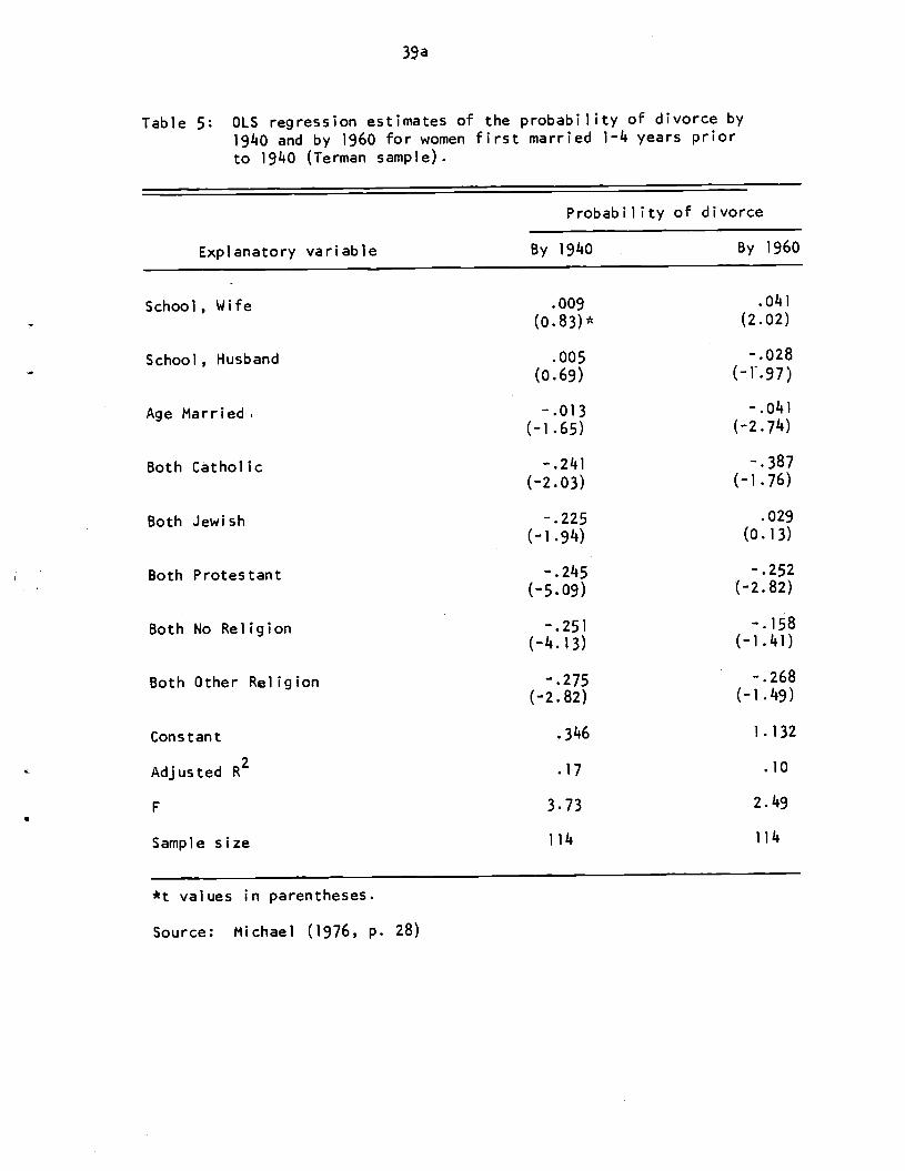
39 a

Table 5: OLS regression estimates of the probability of divorce by19140 and by 1960 for women first married 1-k years prior

to 1940 (Terman sample).

Explanatory variable

School, Wife

School , Husband

Age Married

Both Catholic

Both Jewish

Both Protestant

Both No Religion

Both Other Religion

Constant

Adjusted R2

F

Sample size

*t values in parentheses.

Source: Michael (1976, p. 28)

Probability of divorce

By 19140 By 1960

.009 .041

(o.83) (2.02)

.005 -.028

(0.69) (-1.97)

-.013 -.041

(-1.65) (-2.74)

-.2141 -.387

(-2.03) (—1.76)

-.225 .029

(—.94) (0.13)

-.245 -.252(-5.09) (-2.82)

-.251 -.158

(—4.13) (—1.41)

-.275 -.268

(-2.82) (-1.49)

.346 1.132

.17 .10

3.73 2.49

114 114

differences and the related results mentioned above are all consistent with

this impiication.6

Additional evidence also suggests that persons who intermarry tend to

have higher search costs, and do not simply have different tastes or less luck

in their search. A study of Jews in Indiana showed that the fraction inter-

marrying has been much greater in communities with relatively few Jews (where

the cost of finding a satisfactory Jewish mate is greater) than in communities

with relatively many Jews.66 There is also evidence that persons who marry

relatively young are more likely to intermarry than are persons who marry at

average ages. Our theoretical analysis implies that persons marrying at

young ages have less information about themselves and the marriage market

(see Section 1.3). Hence their high dissolution and intermarriage rates are

related: both are reflections of their limited information.68 This evidence

on intermarriage supports our interpretation of the relation between dissolu-

tion and age at marriage.6

Perhaps the most telling evidence comes from second and later marriages.

If the propensity to intermarry is partly the result of higher search costs,

and if these higher costs persist in the remarriage market, divorced persons

who intermarried in the first marriage should tend to intermarry in subsequent

marriages, and should have relatively high dissolution rates in their later

marriages. The religion—intermarriage rates of Terman subjects in their first

three marriages are presented in Table 6. More than one-half of the Terman women

and one—third of the Terman men who remarried after dissolving a first marriage

with someone from a different religion, again married outside of their own

religion. This is not only much higher than the fraction of religion-inter—

marriages in all first marriages, but is also considerably higher than the

fraction of persons who intermarried after dissolving a marriage with someone

Table 6:

The fraction of Terman Subjects

marriage and previous behavior; who married someone outside of their religion, by order of

information from l95Omarital histories.

0 Q)

Current

Marriage:

First Marriage

Second Marriage

Third Marriage

Married Within Married Outside

Same Religion

Own Religion

On 1st Marriage

On 1st Marriage

Married Within

Same Religion

On 2nd Marriage

Married Outside

Own Religion

On 2nd Marriage

Married someone of

same religion

.88

WOMEN

.50

.81

.44

.40

Married someone of

different religion

.12

.19

.56

.60

.50

Number of Observations

486

26

9

5

It

Married someone of

same religion

.86

MEN

.67

.82

.67

1.00

Married someone of

different religion

.14

.18

.33

0

.33

'

Number of Observations

689

38

18

Li

3

141

from the same religion. Since our theory implies that persons who divorce

tend to have higher search costs, they should have a relatively high rate of

intermarriage in later marriages. The data in Table 6 are consistent with

this implication.

There is evidence that previously divorced Jews intermarry more frequently

than Jews marrying for the first time.7° Moreover, the Rosenthal (1970) study

suggests that the relatively high intermarriage rate on remarriages of divorced

persons is not a necessary consequence of remarriage, for Jewish widows do not

have a high intermarriage rate on their remarriages; indeed, it is even lower

than that of persons marrying for the first time!

We argued earlier that intermarriage is higher among Jews living in

communities with relatively few Jews because they have higher costs of finding

suitable Jewish mates. Put differently, being Jewish in these communities

is a rare trait that raises the cost of search, and as a result, raises the

discordance in traits between mates, and raises the dissolution rate (see

Section 1.3). The Terman sample was selected on the basis of a rare trait,

a high IQ: far less than one percent of the population has an IQ exceeding

the average of this sample (1148). The expectation from our theory is, there-

fore, that Terman subjects would both marry out of their IQ class (they would

"intermarry" with respect to IQ) and divorce at relatively high rates, unless

they were much more efficient searchers in the marriage market.

Unfortunately, information on the IQ's of the Terman subject's spouses

is quite limited, but available evidence is consistent with our expectation.

The average score on a "concept mastery" test of spouses was about one standard

deviation lower than the average score for Terman subjects, even when schooling

level was held constant (see Terman, 1959, pp. 57-60). A regression of the

42

spouse's score on the subject's score has a standard error exceeding 1/3 of

the score of the spouses.7' It is not surprising to find, therefore, that

Terman subjects have had high divorce rates: 27 percent of Terman women had

been divorced from their first husbands by 1972.72

Since the wage rates of mates are negatively correlated in the "optimal"

sorting (see Becker, 19714), and since women typically earn less than men, a

discrepancy between mates in this trait would generally take the form of an

increase in the relative wage rate of the wife. Our theory implies that the

dissolution rake would be higher when her relative wage rate is higher,73 an

implication supported by considerable evidence. For example, Ross and Sawhill

(1975, p. 56) find that each $1,000 increase in the earnings of wives, holding

constant the earnings of their husbands and other variables, increases the

probability of divorce in the subsequent five years by about 1 percentage

point. The evidence on Terman subjects' divorces by 1960 in Table 5 is also

relevant, for the schooling coefficient of Terman women is significantly posi-

tive, and that of their husbands significantly negative, and schooling and

wage rates (not included in the regression) are positively correlated.14

Interesting additional evidence comes from the effects of welfare payments

on dissolutions.75 Welfare conditioned on the household's income is the poor

woman's alimony, and like a higher wage rate for women, reduces the gain from

marriage by increasing the expected income while unmarried. Consequently

welfare would reduce the gain from remaining married, and indeed, Honig (19714)

finds that the fraction of both white and black households headed by females

in different SMSA's is strongly related to the size of welfare payments.

(More generally, any system of transfers in which payments mainly depend on

a household's total income —- be it welfare, negative income tax, or aid

L3

to families with dependent children —— encourages marital dissolutions because

it compensates for the reduction in resources available to the spouses as a

consequence of dissolution.)6

11.3 Fertiliti and the Probability of Divorce

In Table li we reported a strong relation between the probability of

divorce and the number and ages of children, and we presumed that the causation

ran from children to marital stability. However, an exogenous increase in the

expected probability of divorce would reduce the demand for children, and for

other marital-specific capital as well (see Section I.'4 and implication (5)

in 1.6). So this argument implies that a negative correlation between number

of children and the probability of dissolution might reflect, instead, causation

from a higher probability to fewer children.

Usually, the relative importance of different directions of causation

is determined by estimating a simultaneous equation model that includes coef-

ficients reflecting each direction. Such a model could be constructed to

identify the causation between children and dissolution, but we decided

against this strategy since the SEO survey contains no information on the

first spouses of persons who dissolved their first marriages, while the

Terman survey contains only limited relevant information, and neither survey

contains information on any other kind of marital-specific capital. Instead,

we have attempted to study the causation from the probability of dissolution

to the demand for children by constructing a situation (by sample selection)

which largely excludes the reverse causation.

Couples with higher probabilities of dissolution tend to have less

invested in marital-specific capital not only in the early years of marriage

when dissolutions are more frequent, but in later years as well both because

dissolution rates differ then also, and because they would not fully compensate

44

later for reduced investment earlier. Building on this argument, we relate

the number of children of intact couples to several determinants of their

probability of dissolution, and to (other) determinants of their demand for

children. We have restricted the analysis to couples who have essentially

completed their child-bearing in order to circumvent the sizeable random and

other transitory determinants of the timing of births.

From the SEO sample, white women age 40-55 with first marriage intact

were selected. The number of children ever born was regressed on a set pf

independent variables which includes several generally used in fertility

equations and three variables intended to reflect the probability of divorce --

discrepancies between spouses in race, education level and age. Race is

defined as a dummy variable equal to zero if the spouses are not of the same

race and one if they are. The education and the age variables are defined

as the cross-product of the education levels and of the ages of the spouses

respectively; the discrepancy is greater the smaller these cross-products.77

The race and cross-product variables are expected to have positive coefficients

on fertility because smaller discrepancies in traits result in a lower probability

of dissolution and thus a higher demand for children. This regression is

reported in Table 7. The education cross-product does have a powerful positive

coefficient. Racealsohasa significant positive effect: racially mixed

couples tend to have one child fewer than other couples with the same other

measured characteristics. The coefficient for the age cross-product is

counter to our prediction, but its statistical significance s s1ight

Other studies have also found that the interaction between the education

of mates or sometimes the interaction between husband's income and wife's

education has a positive effect on fertility.79 The interaction between IQ's

1+Lia

Table 7: Regression on number of children of women with intactfirst marriages: SEQ white women, ages 140-55.

CoefficientVariable:

(t—value)

Age Husband 0.055(0.98)

Age of Wife 0.0714

(1.23)

Education of Husband -0.200

(_7jL)

Education of Wife -0.19(-7.014)

Wage of Husband -0.006

(-1.05)

Age Married, Wife -0.100

(-2.38)

(Age Married, Wife)2 -0.0001

(-0.15)

Race (= 0 if different) 1.00

(1.90)

Age Cross-Product 0.0016

(—1.33)

Education Cross—Product 0.016

(6.96)

Constant 14.81

0.10

F 36.76

N 3262

45

also appears to affect fertility (see Garrison-Anderson-Reed [1968]) "...pre-

sumably for the same reasons [that explain the similar results of education]

whatever they may be." (p. 124). We have supplied a reason: couples whose IQ's

or educations or other traits differ from what they would be in the optimal

sorting have fewer children because they have a greater probability of dissolution.

Willis (1974) and Ben-Porath (1974) argue that the interaction between education

levels has a positive effect on fertility because the value of the wife's time

is inversely related to the degree of interaction. This may well contribute

to the explanation of the findings on education and IQ but, unlike our argument,

is not relevant to the related finding that discrepancies in race (discussed

above) and religion (discussed below) also reduce fertility.

Additional evidence is available from a regression of the number of

children ever born to Terman women (who first married prior to 1940 and whose

marriage was still intact in 1960) on several variables including a dummy

variable defined as one if the spouses were of the same religion. That religion

variable has a sizeable effect: the number of children is reduced by about .7

if spouses have different religions, which is more than one third of the

average number of chi ldren in this sample (the coefficient's t—value = 1.83).

We showed in the previous section that Terman women are much more likely to

divorce when they marry someone outside of their religion, so these data also

indicate that the demand for children is lower among couples with a relatively

high probability of dissolution.

This section has adduced strong evidence of causation running from the

probability of dissolution to the demand for children: a higher probabil ity

reduces the demand. There is a little evidence also that the demand for other

kinds of marital-specific capital is reduced as well.8° Direct quantitative

evidence, as opposed to the indirect evidence in Table 4, of causation running

from children to the probability of dissolution is available in the evidence

below on remarrieges and dissolution of second marriages.

11.1+ Remarriage

Divorced persons in the United States can remarry again if they choose to,

and the overwhelming majority eventually do. The SEO sample is typical; more than

75 percent of divorced men and more than 70 percent of divorced women remarried

within 15 years of their divorce. The word "eventually" needs to be emphasized,

however, because remarriage is far from immediate. Only 30 percent of the SEO

men and 23 percent of the women remarried within two years of their divorce, and

only 8 and 3 percent, respectively, remarried within five years.81

Our theoretical analysis impl les that the probability of remarriage is

greater when the expected gain from marriage is greater as a result either of

lower search costs or greater gains in the "optimal" sorting (see implication

(8) in Section 1.6). As a test of this implication, the probability ofremar

riage of divorced men and women in the SEO survey was related to several

measures of the expected gain. The calculations in Table 8 were derived from

OLS regressions in which the dependent variable is a dummy equal to one if

the person had remarried by the nth year after the termination of their first

marriage (n = 2, 5, 10, and 15 in the four regressions used in Table 8).82

Higher earnings for men significantly increase the probability of

remarriage at all four durations.8 This is further evidence that the expected

gain from marriage is increased by an increase in men's earnings (see implica-

tion (1) in Section 1.6), evidence that is consistent with the findings that

an increase in earnings reduces both the probability of divorce (Table 1)

and the age at marriage (Keeley, 1971,).

Persons divorced from marriages with relatively large expected gains

would tend to have been married longer than other divorced persons because

46a

Table 8. Implied effects on the cumulative probability of remarriage in specifiedintervals; SEO white men and women aged 50-65 (estimated from OLS regressions''.

A: MALES

2 years 5 years 10 years 15 years

aThe regression is:

Pd = a +b1(AD)

÷ b2(AD)2 +b3S

+b4E

+b5Dur

+b6A

+b7W

+ U.

Indicates the coefficient's t-statistic exceeded 2.0.

0.3-1.5—3.3

3.2

1 .8?

—5.1

4.0

6. 4

6.3?-6.8-7.2

-1.8

8.14"

-12.9-16.9

-3.2

8.4"

L.7

-1.2-9.8

3.80

216

Age at divorce:age 35 instead of 30:age 40 instead of 35:age 45 instead of 40:

Schooling: four additional years:

Earnings: $4000 additional:

Duration of first marriage:lasted five years longer:

,5.1

.,-

5.6 14.14

Age: 10 years younger in 1967 2.8 0.8 -1.6

Widowed in first marriage —8.2 3.3 -7.8

Regression F 3.02 2.39 2.78

Sample size 354 310 261

Means and standar.d deviations of variables used in the regressions:

Age divorced (AD) 40.0

(10.7)37.9(9.6)

35.3(8.0)

33.3(7.0)

Schooling (s) 9.9(3.4)

9.9(3.4)

9.9(3.3)

9.9

(3.2)

Duration of first marriage (Our) 15.4(10.5)

13.5(9.3)

11.3

(7•4)

9.8(6.5)

Age (A) 57.9(14.7)

57.9(4.7)

57.8(4.6)

58.0

(14.7)

Earnings (E) 5762.(4,478)

5,827.(4,584)

5,821.(4,697)

5,732.(4,410)

Widowed (dumy 1 if widowed) (W) 0.38(0.49)

0.34(0.48)

0.28

(0.45)

0.25(0.43)

Remarried (dummy = 1

if remarried) (Pd)0.29(0.45)

0.47(0.50)

0.64

(0.48)

0.76(0.43)

Table 8 (concluded)

14 6b

B: FEMALES

2 years 5 years 10 years 15 years

aPd = a +

b1AD+

b2AD2+

b3S+

b4C+

b5Dur+

b6A+

b7NC

"Indicates the coefficient's t-statistic exceeded 2.0

+ b8W + U.

Age at divorce:-7.3 -7.fl

age 35 instead of 30: -1.5 -5.0?-11.2* —11.0*

age 40 instead of 35: -6.14*—114.4

age 145 instead of 40: —3.2 -7.9 -15.0*

Schooling: four additional years: -1.4 -1.0 —0.7 -3.2

Children:One child -9.0* 33.7 35.3 -26.9

—0.5Each additional child: —l.I4; -1.3

Duration of first marriage5.6*lasted five years longer: 2L,* 3.7*

Age: 10 years younger in 1967: 6.8* 2.8 0.8 9.5

Widowed in first marriage -12.0* -9.3 -10.0* -114.0*

Regression F 11.21 114.71 13.13 9.71

Sample size 991 861 684 536

Means and standard deviations of variables used in the regressions:

Age divorced (AD)

School ing (s) 9.9(3.3)

Children from first marriage (C) 1.9

(1.9)

Duration of first marriage (Dur)

Age (A)

No children (dummy = 1 if

no children) (NC)

Widowed (dummy - 1 if widowed) (w)

Remarried (dummy = 1 if remarried) (Pd)

1+0 . 5(11.7)

38.3(10.8)

9.9(3.2)

1.8

(1 .9)

17.3(10.14)

57.9(4.6)

35.0(9.3)

9.8(3.3)

1.8

(1.8)

14.6

(9.1)

57.8(14.6)

19.4

(11.14)

57.9(14.6)

32.0(8.0)

9.8(3.2)

1.7(1 .8)

12.0

(7.6)

57.8(14.6)

.046 .053(0.28)(0.21) (0.23)

.632 .592 .525 .466

(0.50)(o.48) (0.49)

.124 .294 .474 .621

(0.49)

17

more time is required to accumulate a sufficient amount of adverse information

to offset larger expected gains (see Sections 1.3 and implication (8) In 1.6).

Hence the length of the first marriage can be used as a proxy for the expected

gain,81+ and should be positively related to the probability of marriage. Table

8 strongly confirms this: the probability of remarriage is raised by about five

percentage points for men and somewhat less for women when the first marriage

lasts five years longer.

Education has a small positive, but statistically insignificant effect

on the probability of iemarriage for men, and an even weaker negative effect

on that for women.8 These results are consistent with the weak effect of

education on the probability of divorce (see Tables 1 and 1+), and with the

implication that an increase in education has offsetting effects on the

expected gain from marriage (see implication (3) in Section 1.6).

An increase in age at divorce reduces the probability of remarriage for

both men and women with this distinction: the coefficients are all negative

in the regressions for women, and many are sizeable and statistically signifi-

cant, while none of the coefficients formen are statistically significant,

and some are positive. The more pronounced negative effect for women is

presumably partly related to the closer connection for women between age and

child-bearing capacity, and partly to the steep decline with age in the

ratio of unmarried men to women.86

The probability of remarriage appears to be higher for divorced

persons than for widows: the widow dummy variable has a large negative

effect on the probability of remarriage that is statistically significant

for women. This would not be consistent with our analysis if, as seems 1 ikely,

widows gain more from marriage than divorced persons; after all, persons do

not usually become widowed principally because their marriage was not

successful

48

Thedummy variabledistinguishingwidows fromdivorcees implicitly

assumes that they have been in the "remarriage market" equally long when the

elapsed times from legal termination of their first marriages have been equal.

Yet many divorced persons begin looking for another mate as soon as they

separate, and some separate only after they have found another mate.88 At

least part of the separated time of divorcees should be included, therefore,

when calculating their length of stay in the remarriage market. Since the

SEO survey did not ask for the date of separation, we have reestimated the

regressions underlying Table 8 after simply subtracting two years from the

date of divorce, although the separated time of most divorced persons may

well exceed two years.8 The probability of remarriage in these revised

regressions (not shown here) is no longer smaller for widows; indeed, the

coefficient of the widow variable is usually positive, although never statisti-

cally significant.9°

An explicit estimate of the effect of separation can be derived from

the Terman survey as it includes information about the length of separation

during the first marriage. The time interval between the legal termination

of the first marriage and the comencement of the second marriage, for the

small number of Terman subjects in their second marriage in 1950, was regressed

on the length of separation, a dummy indicating how the first marriage ended

(widowed = 1), and other variables used in the analysis of the SEQ data. The

results in Table 9 indcate that widows do remarry more quickly than divorced

persons -- the coefficient for men is statistically significant91 -- when the

length of separation and other variables are held constant. Moreover, as we

expected, persons do appear to use their time while separated to search for

another mate: both men and women remarried more quickly when they were separated

longer.

49

Children from the first marriage significantly reduce the probability

that women remarry during any given period of time since legal termination

of their first marriage (Panel B of Table 8), and increase the time it takes

to remarry for those who do (Table 9) . The evidence in Table 8 suggests that

the number of children is less important than the presence of any children.

Our theory does imply that chi idren reduce the gain from remarriage because

they are specific to the first marriage, and they raise the cost of searching

for another mate because they raise the shadow price of the mother's time (see

Section 1.5 and implication (5) in Section 1.6) . We say "mother's time" because

the children of divorced parents usually live with their mothers. Consequently

children from their first marriage should not have much effect on the propen-

sity to remarry for divorced men; Table 9 indeed shows that whereas children

significantly raise the duration of time to remarriage of Terman women, they

have no such effect on the Terman men.93

One immediate implication of this evidence on the effects of children

is that divorced men are more likely to remarry partly, perhaps even mostiy,1+

because divorced women usually retain custody of the children. We have crudely

estimated the effect of custody by comparing the probability of remarriage of

SEO men in different remarriage intervals with a probability predicted for

women with no children.95 The results are quite instructive. The actual

frequencies of remarriage two years after the end of the first marriage are

31 percent for SEO men and 22 percent for SEO women. The predicted frequency

for women with no children is 1+2 percent, considerably above the actual prob-

96ability for men!

The causation in the observed negative relation between children and

remarriage rates rather clearly runs from additional children in the first

marriage to a lower probability of remarrying. This supplements the evidence

in Section 11.3 that there is causation running from a lower probability of

Table 9.

Regressions on the time interva' (years) between termination of first

marriage and date of remarriage; for Terman subjects married more

than once by 1950 and with spouse present, by sex.

(t values in parenthesis)

Variable

Women

Men

Age at termination of first marriage

-0.21

(-1.17)

-0.03 (-0.38)

Number of children, first marriage

1.02

(2.13)

-0.19 (-0.70)

Duration of first marriage (yrs.)

0.10

(0.1+5)

-0.+3 (—2.61+)

Length of separation in first marriage

-0.45

(

1.10

) -0.20 (l.1+7)

(in six month intervals)

Widowed

-1.33 (-0.69)

-2.90 (-2.29)

Constant

8.13

6.07

0.13

0.17

F

1.96

3.58

Sample size

72

50

of dissolution to additional children. It also reinforces our contention in

Section 11.1 that the observed negative relationship between children and the

probability of dissolution has an important component that runs from additional

children to a higher probability of remaining married.

11.5 StabIlity of Second and Higher-Order Marriages

We have pointed out that more than three—quarters of persons whose first

marriage ends in divorce in the United States eventually remarry; many also

divore a second time. Some remarry a third time, etcetera. Using divorce

and marriage records from the state of Iowa, Monahan (1958, 1959) finds that

the probability of divorce increases sharply with the order of marriage for

persons previously divorced97 but not for persons previously widowed.

Since these data and most others used in studying second and third

marriages are not standardized for age at marriage, age, or even duration

married, the higher probability of divorce in higher-order marriages might

be easily explained primarily by the increase in age at marriage or the

decline in the average duration married as the order of the marriage increased.8

A major advantage of the SEO data is that different order marriages can be

compared after standardization for age, age at marriage, duration married, and

other variables. However, few persons divorced more than once even in the

large SEO survey, so the evidence on second and third marriage divorces is

based on quite small samples.

Regressions on the probability of divorce are run with the SEO data,

including higher order as well as first marriages. These regressions duplicate

those shown in Table 1 for men and Table 4 for women, except that we have

pooled experiences on second marriages with those on first marriages for the

women and have pooled experiences on second and third marriages with those on

51

first marriages for the men.99 In these pooled regressions two dummy variables

were added. The first indicates a previous marriage (defined as one if the

observation pertains to a second or third marriage) and the other indicates

a previous widowing (defined as one if the first marriage ended in widowhood).

Table 10 gives the coefficients on these two dummy variables only, taken from

the full multiple regression equation.0°

The main findings of Monahan and others apparently continue to hold

even after the standardizations introduced in these regressions. For women,

second marriages are much more unstable than first marriages, especially during

the first five years of marriage: the probability of divorce is about 114 per-

centage points higher on the second than on the first marriage. Moreover,

aside from the first five-year interval, the probability of divorce for widows

is no greater than for women in their first marriage.

The behavior of the Terman women is also tons istent with these results.

By 1972, when they were about 60 years old, 27 percent had been divorced from

their first husbands. More than 55 percent of the women who divorced the

first time and remarried had divorced again -- about twice the divorce rate

from first marriages -- compared to 38 percent of the (just 8) women who were

widowed the first time and had remarried. Only 12 women were married a

third time. Forty percent (14) of those (10) who had been divorced from both

previous marriages were divorced again, whereas neither of the two previously

widowed women were divorced from their marriage.

The results for men in Table 10 are similar: second and third marriages

of divorced men are more unstable than first marriages of men, again especially

during the initial years. Widowers are less likely to divorce after remarriage

than are men previously divorced. Indeed, aside from the initial interval,

Table 10.

Regression coefficients on dummy variables indicating if previously married and previously

widowed, from OLS regressions on the probability of divorce, by specific intervals, by sex

(SEO white men and women, age 15-65).

Explanatory

variable

Women

Marriage

Men

Marriage interval (in years)

15-20

interval

(in years)

0-5

5-10

10-15

0-5

5-10

10-15

15-20

Dummy =

1 if

seco

nd or third

.138

.012

-.002

.026

.036

.013

.016

.017

marriage

(lS.9i)*

(1.36)

(.18)

(2.60)

(1+.13)

(1.68)

(1.78)

(1.60)

Dummy =

1 if widowed in

.002

-.018

-.027

-.022

-.009

-.009

-.016

-.027

first marriage

(.13)

(1.19)

(1.55)

(1.18)

(.L7)

(.51)

(.77)

(1.25)

R2 (entire regression)

.037

.010

.009

.005

.011

.001

.001+

.003

F

(entire regression)

56.82

12.23

7.56

3.15

12.08

0.80

2.71

1.60

N

11960

9627

7683

5736

8688

69'+8

5500

'+026

a,

t values in parenthesis

second or third marriage for men; second marriage for women

Other variables included in the regressions are:

age, education, age at current marriage, for men

their 1966 earnings, and for women the number of children from their current marriage measured at

the beginning of each interval.

52

the probability of divorce is no greater for widowers than for men in their

102first marriage.

Our theory implies that previously divorced persons gain, on average,

less than others from subsequent marriages (See Section 1.5 and implication

tion (9) in Section 1.6). Since the selection of widows is more independent

of their gains from first marriage (see the evidence in the previous section),

we also expect marriages containing previously widowed persons to be more

stable than those containing previously divorced persons.

Consider now the duration to divorce. By extension of the previous

argument, the expected gain from marriage tends to be smaller for persons

previously divorced twice than for those divorced only once, and still smaller

for those divorced three times, and so on. Hence the average duration to

divorce of those terminating their marriage should decline with marriage order

(because less time is required to accumulate sufficient adverse information

when the expected gain is smaller). This can explain Monahan's evidence of

a significant decline with marriage order in the average duration to divorce

for persons previously divorced103 but not previously widowed. It can also

explain the positive relation between the duration of the first marriage

and the probability of remarriage (see Tables 8 and 9), and the evidence in

Table 10 that the probability of divorce on second and third marriages is

especially high during the first few years of marriage.

When the SEO data are not standardized for age and age at marriage

(Monahari's data were not standardized for these variables), they also indicate

that among those who divorce, the length of time from marriage to divorce

declines significantly from first marriage to second marriage. However, when

the data are standardized for age and age at current marriage, the average

53

101+duration is no longer related to marital order. Consequently, when

appropriately standardized, the SEO data do not support our prediction that

duration-to-divorce will decline in'higher-order marriages.

We also ran regressions (not shown) with the SEO data on the propensity

to divorce from second marriages alone, using independent variables similar

to those used for first marriages (see Tables I and 4). Since few persons had

divorced from a second marriage (for example, only 13 men divorced within the

first five years of their second marriage), the statistical significance of

most coefficients is quite low. Yet, the results are generally consistent

with those for first marriages. For example, an increase in the earnings

of men seems to reduce their propensity to divorce on second as well as first

marriages, again except perhaps when earnings are quite high. An increase

in education has weak and inconsistent effects on the propensity to divorce;

as in the results for first marriages, the effect is slightly positive for

women.

An interesting new result for women is shown in Table 11: children from

a prior marriage appear to increase the probability of dissolution from the

current marrage,105 whereas children from the current marriage appear to

decrease this probability in second marriages, just as it does in first

marriages (cf. Table 4). Our explanation of both effects is that children are

marital specific capital: children from the current marriage increase and

children from prior marriages decrease the gain from the current marriage

(see implication (5) in Section 1.6).

The positive effect of children from prior marriages is further evidence

of causation from children to marital stability since an exogenous increase

in the probability that a second marriage will dissolve would hardly raise

the demand for children in the first marriage. There is, however, also further

53a

Table 11. OLS regressions on the probability of divorcefor women in second marriages, by marriageinterval (SEO white women age 15-65).

ExplanatoryMarriage interval (in years)

variables 0-5 5-10 10-15, —

C1 -1.39 -.93 .12

C2• —3.18

P 3.91 ..

(2.11+)"5.01

(2.1+2)

-.70(0.34)

Children from .1+4 .83 .52

1st marriage (.92) (1.62) (.92)

a2 .030 .027 .030

F 3.93 2.30 1.56

N 1032 752 508

t values in parenthesis

* Effects of children are evaluated at the mean numberof children.

Other variables included were age, age at marriage andits square, education, and a dummy variable indicatingwhether the women had been widowed or divorced from theirfirst marriage.

54

evidence of causation from marital stability to children: there are fewer

children in higher order marriages in the SEO survey, even after age at

current marriage and duration of current marriage are held constant.6

Since the probability of dissolution increases with marital order, the

number of children would decline with order if the probability affects the

demand for children.

11.6 The Secular Trend in Divorce

The number of divorces has grown remarkably during the last 125 years

in all Western countries that permit divorce. For example, only two (!)

divorces per year were granted in England between 1800 and 1850 (see Rhein-

stein, 1972, p. 31), whereas in the past year or so there have been approximately

1 million divorces a year in the U.S. Based on 1973 data it is estimated

that about 40 percent of new marriages in the U.S. will end in divorce (see

Preston, 1974). The reported divorce rate in the U.S. (the number of divorces

in the year per 1,000 married women age 15 and over) rose from 4.1 in 1900 to

8.0 by 1920 to 8.8 by 1940 to 9.2 in 1960 with sizable fluctuations around

both World Wars (the historic peak until the last few years had been 19k6

with a divorce rate of 17.9) (see Platens, 1973, p. 24). Since the mid—1960's

the divorce rate increase has accelerated; by 1970 the rate was 14.9 and by

1974, 19.3.107 We believe that the theoretical and empirical analyses in the

previous sections can contribute significantly to an understanding of these

trends and fluctuations, but here we only sketch out the main considerations.108

The number of children per family has been declining since the beginning

of the nineteenth century in the United States, and the decline accelerated

during the last 20 years. Our analysis implies both that a decline in the

55

number of children increases the probability of divorce, and that an increase

in this probability reduces the demand for children (see implication (5) in

Section 1.6); the survey evidence above has confirmed that both directions

of causation are important (see especially Tables 4, 7, 8, 9, and 11). Presum-

ably both directions of causation also are at work in the secular decline in

fertility and secular rise in divorce. Note, however, that the recent accelerated

decline in fertility began in the 1950's, at least five years before the

accelerated increase in divorce.

An increase in the wages of women would reduce the gain from marriage,

even when, the wages of men increased at the same rate, because the sexual

division of labor between market and nonmarket activities would decrease, and

more married women would enter the labor force (see the evidence in Section 11.3).

Therefore, the secular growth in wages, which contributed significantly to the

growth in the labor force participation of women, especially married women,

probably also contributed significantly to the growth in divorce rates. Again

causation probably flows both ways: divorced women (and women who anticipate

divorce) have higher wages because they spend more time in the labor force (see

Section 11.4).

Legal access to divorce became much easier during the last 100 years in

the United States, Great Britain, and most other Western countries. Although

we believe this trend toward easier divorce has been mainly a response to the

increased demand for divorce,109 it may also have been responsible for a small

part of the growth in divorce. Whatever the causation, the ease of obtaining

a divorce and the fraction of women married are positively (not negatively)

correlated across states, even after age and many other variables are held

constant (see Freiden, 1974, and Santos, 1975).

56

A growth in the divorce rate itself encourages additional divorces

because the remarriage market is better when there are more divorced persons

available. There is evidence in Table 8 that the remarriage market did

improve as the divorce rate grew over time, for the probability of remarriage

during the first few years after a divorce also grew over time.H0 Moreover,

the sharp acceleration in divorce rates that began in the 1960's may have been

partly caused by the prior growth in divorce rates, for if the process can be

described by a logistic or related function, the rate of growth would accelerate

for a while after the level became sufficiently high.

Even though an increase in male earnings or age at marriage significantly

reduces the probability of divorce when comparing different households at the

same period in time (see Section 11.1), the relation between the secular

increase in divorce rates and the secular changes in these variables is less

clear. An increase in the earnings of one man relative to the earnings

of other men in the marriage market increases his gain from marriage partly

because he is able to attract a woman with more desirable attributes (See

Section 1.2). On the other hand, when the earnings of all men increase, with

little change in the distribution of the attributes of women, all men cannot

be sorted with more desirable women. Consequently, an increase in the earnings

of any man would have a smaller effect on his gain from marriage and thus on

his probability of dissolution when the earnings of other men also increase.

A similar argument can be made for general increases in education levels, and.

a related argument can be made for a decline in the average age at marriage.

Therefore, the large secular growth in male earnings may not have greatly

reduced, and the secular decline in age at marriage may not have greatly increased,

the propensity to divorce.

57

Tables I and 1 provide some evidence on the trend in probability of

divorce. The estimated trend is measured by the coefficient on age, but its

interpretation across marriage intervals is subject to several qualifications.1

While nearly all the estimated trends are positive, the only significant one

suggests an increase in the probability of divorce of about 1 percent per

decade over the time span covered by the SEO data (1920's to early 1960's).

These estimates of the trend in divorce rates are net of standardizations for

trends in age at marriage, years of schooring, earnings of men and the number

and ages of children born to women. These standardized estimates may be

biased because, as we already mentioned, standardizing with differences across

households in earnings, education, or age at marriage does not correctly

provide for the effect of secular changes in these variables.2 Moreover,

these estimates have not been corrected for the effect of change over time

in the earnings of women, divorce laws, the size of the remarriage market and

other variables that contributed to the observed trend in divorce rates.

Summary and Conclusions

The theory developed in Part I of this paper assumes that each person

maximizes his or her expected utility as he decides whether to marry or to

remain married. The relatively high utility expected when marrying is

reconciled with the relatively low utility expected when divorci.ng by

introducing imperfect information and deviations between real ized and

expected outcomes.

The probability of dissolution is greater when the expected gain from

marrige is smaller and the variance in the distribution of realized outcomes

is larger. Both the expected gain and variance depend on the cost of acquiring

additional infoirination about potential mates in the marriage market. The

58

expected gain will decline as the cost increases because a person facing a

higher cost is induced to accept a less-favorable marriage offer, i.e., a mate

with characteristics that are further away from the optimal characteristics in

the equilibrium—sorting with perfect information. The variance will increase

as tha cost increases because a person facing a higher cost is induced to

accept a mate about which he or she has less information.

The expected gain from marriage also depends systematically on the level

of different characteristics. For example, an increase in the intelligence

or attractiveness of men or women or the earnings of men tends to raise the

gain, whereas an increase in the earnings of women tends to lower the gain.

The accumulation of certain kinds of knowledge and capital such as sexual

compatibility or children, that normally occurs with an increase in the duration

of a marriage, increases the expected gain from remaining married because such

marital-specific capital has less value if the marriage dissolves. Conversely,

a reduction in the expected gain from remaining married discourages the accumula-

tion of marital—specific capital.

The probability and speed of remarriage are positively related to the

expected gain from remarriage, which depends on earnings, age, number of

children from the previous marriage, and other characteristics. Divorced,

but not widowed, persons marrying for a second or third time are more likely

to dissolve their marriages, and tend to dissolve faster, than persons marry-

ing for the first time. The reason that they become divorced is partly

because they tend to gain relatively little from marriage, and partly because

becoming divorced in itself raises the probability of an additional divorce.

-

Many of the more important theoretical implications are listed in Section

1.6. The empirical analysis using the 1967 SEO and 1920-1960 Terman data

strongly supports these implications and is also of considerable interest in its

own right.

59

An increase in the expected earnings of men reduces the probability of

dissolution on first marriages, raises the speed and probability of remarriage

if the first is dissolved, and reduces the probability of dissolution on

second or higher order marriages. An increase in the expected earnings of

women, on the other hand, has the opposite effects: it appears to raise the

probability of dissolution and to reduce the propensity to remarry. This

evidence confi rms theoretical implication (1) in Section 1.6).

An increase in the number of children, especially younger children,

from a first marriage reduces the probability of dissolution of that marriage,

and the speed and probability of remarriage for mothers with custody. Indeed,

if divorced women did not usually receive custody, their propensity to remarry

would not be less than that of divorced men. There is a bit of evidence

that couples often delay their dissolution until their children are grown

(and embody less marital-specific capital). Although children from second

and higher order marriages also lower the probability of dissolution in

these marriages, children from first marriages apparently raise the insta

bilityof subsequent marriages (See implication (5) in Section 1.6).

If a person marries outside of his religion, he is much more likely to

dissolve his marriage, to marry out of his religion if he does remarry, and

then to divorce again. Moreover, even if a divorced (but not a widowed)

person married in his religion the first time, he is rather likely to marry

outside his religion the second time. The propensity to marry outside of

one's religion, and then to dissolve the marriage, also appears to be

directly related to the relative number of potential mates of the same religion

that are available. This and considerable other evidence on intermarriage is

implied by our theoretical analysis (see implication (6) in Section 1.6).

60

An increase in the probability of dissolution, as measured empirically

by the propensity to marry outside of one's religion, race, or education

class, reduces the demand for children (see Table 7) and for other marital-

specific capital, such as skills highly specialized to the nonmarket sector

(see implication (5), Section 1.6). Therefore, the observed negative

relation between the propensity to dissolve and children (and some other

kinds of marital specific capital) involves causation running in both directions.

Persons who marry relatively young are far more likely to dissolve their

marriages than are those who marry at "normal" ages. This has been well known,

but less well known is our finding that persons who marry for the first time

relatively late -— for example, in their early thirties -- also have relatively

high probabilities of dissolution (see implication (4) in Section 1.6).

The propensity to remarry is positively related to male earnings, the

absence of young children, the length of time separated before legal termina-

tion of the first marriage, and the duration of the prior marriage, a variable

that serves as a proxy for unmeasured determinants of the expected gain from

marriage. Widowed men or women are more likely to remarry than are divorced

women or men, after allowance is made for age at legal termination of the

prior marriage, the length of time separated before legal termination, and

some other variables (see implication (8) in Section 1.6).

The probability of dissolution is much higher on second marriages, and

still higher on third marriages, for persons previously divorced but not for

persons previously widowed (see implication (9) in Section 1.6). Although

our theory also predicts that the duration to divorce declines with marital

order for persons previously divorced, the empirical evidence is rather

ambiguous.

61

Most of our empirical evidence involved different households at a moment

in time. Yet our limited examination of evidence on trends in divorce rates

suggests that our theory can also contribute significantly to understanding

and explaining the secular growth in divorce, including the acceleration

since the early 1960's. The most important variables appear to be the

decline over time in number of children, the growth in labor force participa-

tion and earning power of women, the growth in the breadth of the remarriage

market as more persons become divorced, and perhaps also the growth in legal

access to divorce and the growth in public transfer payments.

In many ways, marriage and divorce is a special case of a "contract'

of indefinite duration between two or more partners, such as business partners

or employees and their employer, that can be terminated under specific condi-

tions. A theoretical and empirical analysis of divorce is important not

only because the decision to divorce has significant effects on subsequent

behavior and well-being, but also indirectly because the evidence on

divorce is far more extensive and detailed than the evidence on the

termination of jobs, business partnerships, or other contracts.

We believe that our analysis of divorce further reveals the power of

"the economic approach" to clarify and illuminate demographic behavior. It

is, therefore, an additional contribution to the development of what has

recently been called "sociological economics": the application of economic

concepts and analysis to behavior at least partly outside the monetary sector.

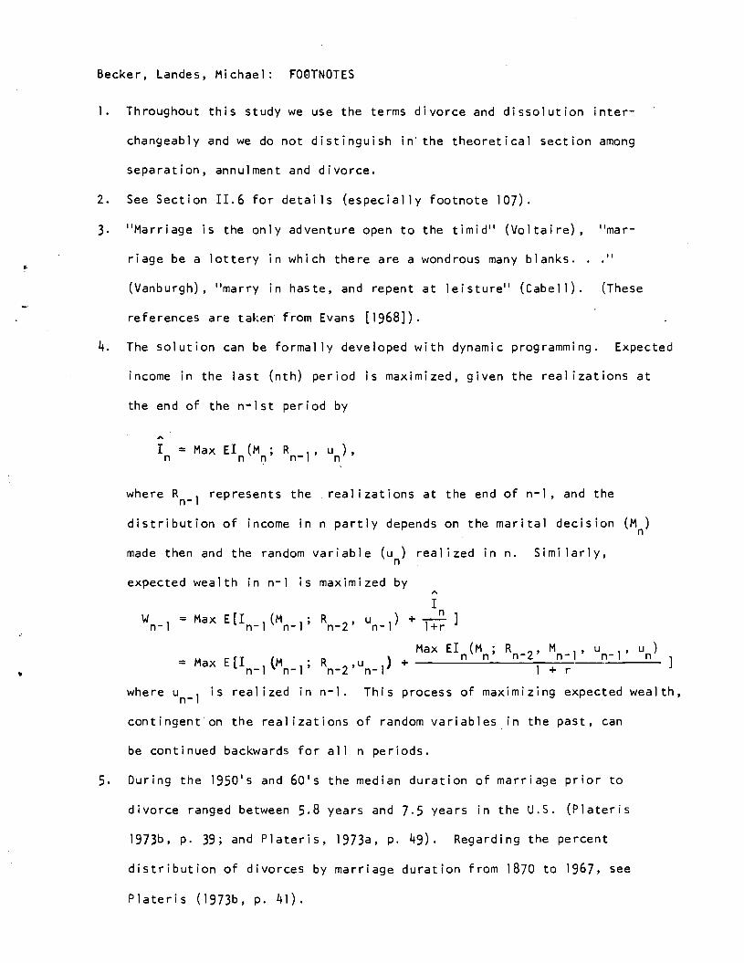
Becker, Landes, Michael: FOOTNOTES

1. Throughout this study we use the terms divorce and dissolution inter-

changeably and we do not distinguish in the theoretical section among

separation, annulment and divorce.

2. See Section 11.6 for details (especially footnote 107).

3. "Marriage is the only adventure open to the timid" (Voltaire), "mar-

riage be a lottery in which there are a wondrous many blanks. .

(Vanburgh), "marry in haste, and repent at ieisture" (Cabeii). (These

references are taken from Evans [1968]).

4. The solution can be formally developed with dynamic programming. Expected

income in the last (nth) period is maximized, given the realizations at

the end of the n-lst period by

I MaxEI(M;R ,u),n n n n—l n

where Rn_i represents the realizations at the end of n-i, and the

distribution of income in n partly depends on the marital decision (Mn)

made then and the random variable (u) realized in n. Similarly,

expected wealth in n-i is maximized by

I

W = Max E[I (M ; R , u ) + ]n—i n-i n—i n—2 n—i i+r

MaxEI(M;R ,M ,u ,u)n n n—2 n—i n-i n= Max E[Ii (Mi; R2,u1) + 1 + r

where Un_i is reaiized in n-i. This process of maximizing expected weaith,

coritingenton the realizations of random variabies in the past, can

be continued backwards for au n periods.

5. During the 1950's and 60's the median duration of marriage prior to

divorce ranged between 5.8 years and 7.5 years in the U.S. (Platens

1973b, p. 39; and Platens, 1973a, p. 49). Regarding the percent

distribution of divorces by marriage duration from 1870 to 1967, see

Platens (1973b, p. 1+1).

F2

6. See Platens (1973b, p. 19). Of course, a divorce might not be sought

if strong opposition were expected.

7. These implications are supported by evidence in Bartel (1975). Hashimoto

(1975) applies a model of combined maximization to the Seattle labor

market, with some empirical confirmation.

8. Accordingly, it is not surprising that the sex differential in age

at first marriage has greatly decined during the last 20 years; the

investments of women have become much less specialized to married life

as they reduced their childbearing and increasingly entered the labor

force (see Platens l973b, p. 55).

9. We say 'relatively" high earnings because we are considering only a

change in the earnings of some men relative to those of other men.

A change in the earnings of all men would have a weaker effect on the

gain from marriage than an equal change in relative earnings if charac-

teristics of women did not change much. We consider these differences

more systematically in our discussion of changes in marital dissolutions

over time (see Section 11.6).

10. Search theory was first applied to the marriage market by Keeley (l97L).

11. For more extensive discussion of this framework, see Wessels (1976).

12. Take a point A. to the right of A where

I > cG' + I - c =

Then by substituting for I from the equation in the text, we have

2.. iiI >1 + (ctG -aG).

Clearly, II must exceed I, for if II were less than I, then cL'Gt would exceed

ctGt from a basic property of the distribution of offers, and the in-

equality could not hold.

F3

13. If Am. were not the upper bound of

2.. 2..

II > V1 (1')m.2.. m.2..I I I

2..

where I is the income to a woman with the trait A from a match withm.2.. 2..

I II

A . Since A is the lower bound of A , thenm. 2.. m.

I I

< (2')

where 2.-L. refers to a woman with a trait slightly lower than A2.

Continuity of the income and value of search functions implies that

inequality (2') could not hold for traits arbitrarily close to A2. , the

lower bound of Am , if inequality (1') held. Hence Am has to be the

upper bound of A2.

14. Jovanovic (1976) develops a model of intensive search along these lines

in the context of matching employees and firms, and derives these and

other implications.

15. Markets are sometimes organized in ways that facilitate marital search.

Examples include dances for tall persons, social activities centered around

a church, residential segregation of minorities, and co-educational univer-

sities that require considerable intelligence for admission.

16. Wessels (1976) shows that the region of acceptable offers is wider and the

probability of a "mismatch" greater when the distribution is less dense.

17. The effect of differences in search efficiency are less clearcut. Although

less efficient searchers make fewer searches, they spend less total time on

search only if the elasticity of the number of searches with respect to

change in efficiency is sufficiently great.

18. If offers were uniformly distributed, the expected income gain from marriage

would equal

1mx÷jaH

2-

10,

where 10 is single income, 1a is the minimum acceptable, and 1mx is the

maximum possible income offer. Since it can be shown that dla < dl, an

increase in single income, with the distribution of offers held constant,

would reduce the expected gain, for

= -1 < 0 as long as dia < 2d1.

If offers were not uniformly distributed, the magnitude of dH/d10 would

change, but it would still tend to be negative.

19. Let the probabil ity of dissolution be determined by

p = f(K, y), (1')

wi th

- < 0, and > 0,

where K is the stock of specific capital, and y are the other

variables that affect dissolution. Also let the stock of specific

capital be determined by

K = h(p, x), (2')

with

— < 0, and— > 0,ap ax

where x are other variables that affect this capital. Then if y changes

with x held constant,

dy ay DK ap dy

F5

or

dy f h (3')

Therefore,

..2. f . ah> — since — and — <.0.dy ay aK

Similarly, it can be shown that

dx ax

20. Calculated from 1967 SEO data.

21. See, for example, the study by Kogut (1972) of the incidence and

stability of consensual unions in Brazil.

22. A shift to the right in the distribution of offers raises the expected

gain from marriage compared both to the minimum acceptable offer -- which

also shifts to the right —- and to the "offer" from being single.

23. We distinguish between these effects in the empirical section.

24. Perhaps more persuasive evidence is that a significant fraction of persons

remarry shortly after their first marriage dissolves (see the empirical

evidence in Table 8).

25. Most widowed persons are considerably older and form a somewhat distinct

market.

26. We present some results in Section 11.4 on the effects of children on

remarri age.

27. Our earlier analysis shows that persons with lower expected gains from

marriage, such as men with low earnings and women with high earnings, or

persons who married out of their race or religion, have lower minimum

F6

acceptable offers. Moreover, there is evidence that they are in fact

less likely to marry (see Section 11.4).

28. An analysis that rules out remarriage is much less applicable when the

minimum acceptable offer in the remarriage market greatly exceeds non-

married wealth. Our predictions about the relation between dissolution

rates and variables like search costs then become more ambiguous.

29. This difference in the average expected gain on first and second marriages

is reduced but not eliminated by the negative relation between the

propensity to remarry and the expected gain from remarriage (see footnote

27).

30. There is little reason to expect persons who were widowed the first

time to have a relatively high dissolution rate on their second marriage;

see the empirical evidence in Section 11.5.

31. In the same way, positive specific capital in one firm could lower

the productivity of a worker moving to another firm because he has

become "accustomed" to the first firm's methods and organization, and

has lost some of his "flexibility."

32. In the same way, separation from one job per se increases the turnover on

all subsequent jobs, which can contribute to the explanation of differences

in turnover rates between so-called "movers" and "stayers." Usually

differences in behavior between "stayers" and "movers" have been simply

taken as given and described (see, for example, Heckman—Willis 1975).

Our analysis probes into the underlying causes, and explains such

differences in behavior in marital and other markets by differences in

more basic characteristics, such as search costs, specific capital, proper-

ties of optimal sortings, and even luck.

F7

33. Gi ick and Norton (1971, p. 308) discuss the strengths and weaknesses of

the SEQ data for the study of marital behavior. The weaknesses mentioned

include the discrepancy between SEO and CPS figures -- the SEO shows a

higher proportion of adults currently divorced and a lower proportion

married. They suggest that the larger number of divorced in the SEQ

"may be closer to the true numbers than those in the CPS." Even so,

according to Glick and Norton, the divorces reported for 1960-66 fall

10 to 20 percent below the numbers reported to vital statistics. The

accuracy of the marital histories presented by the SEO data is, of course,

also subject to some reservation, but the inaccuracies may not be

systematically related to the variables analyzed here.

31k. All persons whose marriage ended by death of a spouse were excluded.

35. For wonn with more than four children ever born, the birth dates for

children other than the first •two and last two were interpolated at

equal intervals between the second and next-to—last child.

36. We have also used the maximum likelihood logit approach, and the

coefficients estimated are quite similar to the OLS estimates, even though

the mean of the dichotomous dependent marital variable is near zero.

Since the OLS and logit estimates are so similar, only OLS results are

reported.

37. The OLS regressions are shown in the Appendix. Since the number of

observations at later marital durations declines even more rapidly

when younger men are included in the study primarily because younger men

have not been exposed to longer durations, we have restricted most of

the analysis to persons in the 35—55 age group. Even here, the number of

observations declines about 25 percent from the first to the third interval

F8

an much more rapidly after that. To test whether the decline in sample

size significantly affects the results, we have also run regressions for

men 45-55 years old, and the results are generally quite similar to those

reported in Table 1, except that the coefficients of earnings and earnings

squared have less statistical significance. The significance is lower

partly because actual earnings at ages 1+5-54 are a poorer measure of

lifetime earnings than are actual earnings at ages 35-1+4.

38. These differences also imply that the average date of marriage was

earlier at later durations: the implied average date of marriage was

1946 [ = 1967 - (1+4.7 - 23.9) 1, 1945, 1944, 1941, and 1938 in the

first through fifth intervals respectively.

39. The age at marriage with the minimum probability of divorce implied by

the regression coefficients ranged from 27.1 to 31.7 in the first

four intervals. The fifth interval has no implied minimum.

40. See, e.g., U.S. Census (l972a) , or Carter and Gi ick (1970) , especially

pp. 234-35. Ross and Sawhill (1975, p. 56) and Bumpass and Sweet (1972)

also find statistically and qualitatively significant effects of age

at marriage. Ross and Sawhill's linear coefficient implies that a

delay in age at marriage, cet. par., reduces the probability of

divorce over a four-year period by two percentage points (the average

probability in the sample is 7.6°.).

41. The upturn at older ages is in evidence for all marriage cohorts since

1920. See U.S. Census (1973) Table 4. The upturn is also evident for

1960 data in Carter and Glick (1970, p. 234).

42. In an often. cited study of 1960 Census data, Cutright (1971, p. 293)

also finds no appreciable effect of male's education on the stability of

first marriages when male's earnings are held constant.

F9

43. The OLS regression estimates imply a positive effect of earnings on the

probability of divorce above earnings of about $33,300, $52,500, $25,000,

$48,400, and $46,300 in each of the five duration intervals respectively.

414. It should also encourage earlier marriages, and this implication is

strongly confirmed with the SEO survey (see Keeley, 1974).

145. The log of earning of each man in the SEO survey was regressed on his

years of schooling, experience (defined as age minus years of schooling

minus 6)., experience squared, and other variables (See the next two

paragraphs). Earnings expected at age 45 when marrying for the first

time are assumed to equal the earnings predicted from this regression

for age 145, with no adjustment for the secular growth in earnings

across cohorts (see the discussion in Section 11.6). "Unexpected

earnings" simply equals the absolute value of the difference between

actual and predicted earnings at the current age.

Married men tend to have higher earnings than separated or divorced

men (l6 higher in the 1967 SEO). If causality runs from earnings to

marital status, as emphasized in this paper, expected earnings should

be computed at actual marital status, and this is, in fact, how the

expected and unexpected earnings variables in Table 2 are computed. How-

ever, expected earnings should be computed net of the effect of marital

status if the causation runs from marital status to earnings (although

unexpected earnings should still be computed at actual marital status.)

Since there is evidence that the causation runs both ways (see Keley

19714) we have estimated E and IE - El both ways. The results with the

measure of expected earnings net of the effect of marital status are

qualitatively similar to those presented in Table 2 for E1 and IE -E1 I

although somewhat weaker.

HO

Similarly, regressions have been run with measures of expected

earnings both gross and net of the effect of weeks worked. Again, the

results presented in Table 2 for E2 and IE - E2 are for the earnings

measure which includes the effect of weeks worked on earnings; again

the results using the measure of expected earnings net of weeks worked

were qualitatively similar, but somewhat weaker.

The third measure of expected earnings, E3, incorporates neither

the effect of marital status nor the effect of weeks worked on earnings.

However, the effects of these variables are present in unexpected

earn i ng s.

We do not have to emphasize that our estimates of expected and

unexpected earnings are extremely crude. They are used partly because

direct evidence on earnings expectations are unavailable, and partly

because the earnings generating function cannot be greatly expanded

since the SEO survey does not contain information on ability, actual

job experience, or other relevant variables.

L+6. For example, the regressions summarized by Table 2 were rerun replacing

the variable IE — E by the two variables X1 = (E E1) if (E E1) > 0

and X1 = 0 otherwise, and X2 = -(E -

E1)if (E -

E1)< 0 and X2 = 0 other-

wise. The coefficients on these two variables were as follows: X1 = 0.099

(t = 1.22), 0.032 (0.46), 0.16 (2.35), 0.053 (0.67), and 0.039 (0.41) in

the five time duration intervals respectively, and X2 = 0.58 (t 3.29)

0.23 (1.49), 0.25 (1.56), 0.73 (0.42), and 0.27 (1.06) respectively. So

in each interval both positive and negative deviations tend to raise the

probability of dissolution.

Eli

47. In one recent nationwide data set, 88 percent of currenft married

women with no child deaths were married only once, compared to less

than 80 percent of those with one or more deaths. Similarly, 88 percent

of ever-married women with no fetal loss were married only once,

compared to 82 percent with one or more losses. Standardizing for

the age of women does not affect this basic picture. These calcula-

tions, based on the 1970 National Fertility Survey, were kindly supplied

by Anne D. Williams.

48. Michael Grossman kindly supplied the following table based on the

NBER-TH data:

Married Divorced

I. Current health = past health

98.1 1.9n 2518 48

2. Current health < past health

97.4 2.6n 1322 35

3. Current health > past health

97.8 2.2n 181 4

A Chi—squared test of the proportions in rows 1 and 2 yields

a test statistic that is significant only at a .85 level of confidence;

the test statistic for rows 1 and 3 is not at all significant. Infor-

mation on health status comes from two questions asked in a 1971 survey:

"What is the state of your general health at present (excellent, good,

fair, poor)?" and "During the years you were attending high school

what was the state of your general health (excellent, good, fair,

poor, don't recall)?" Grossman (1976) analyzed these and other health

data.

Fl2

1+9. The very low explanatory power of these independent variables is partly

explained by the low dissolution rates -- not more than 3.5 percent in each

duration interval. The independent variables in the Terman Sample

discussed later are not radically different from those used here,

but the divorce rates are much higher, 14 to 16 percent, the sample

sizes much smaller, and the coefficients of determination are much

larger (at least .10).

50. Selective attrition or sample censoring as a cohort moves through

time may bias the estimated effects from interval to interval.

51. The pooled regression is shown in the Appendix. The dependent

variable is defined as zero if the man remained married in the par-

ticular five—year interval being considered, and as one if he divorced

in that or any preceding five-year interval. The duration dummy

variables are defined as zero for all subsequent intervals and as

one for the particular and all preceding intervals. (E.g., the

values of the four dumies for an observation on the 15-20 year of

marriage are: = 1; D2 = 1; = 1; = 0.)

The statistical significance of the coefficients in column (7)

of Table I appears to be very high, but should not be taken seriously

because the number of degrees of freedom is greatly overstated. The

stastistical model can be written as

yi — + ciwhere y. equals 1 if a dissolution occurred at duration i or in any

interval prior to i, X is a vector of independent variables that do

not depend on the duration interval , is a vector of coefficients

that may depend on duration, and c. is the error term. Since y. measures

the cumulative incidence of dissolutions, an increase in . not only

increases but also y1÷2, etc. Therefore, the presumption is

F13

that c is serially correlated. Hence the standard errors used to

compute the t values in column (7) may greatly understate the true

standard errors because no allowance was made for the serial correla-

tion in the error term. We have not attempted to make such an allowance.

52. Estimated at the mean values of the other explanatory variables, the

duration dummy variables imply that the probability of divorce in the first

four five year intervals declines from 3.89 to 2.12 to 2.03 to l.84

respectively.

53. Assume that the error term defined in footnote 51 has two components,

= e + u., where u. is serially uncorrelated, and e. has a first

order serial correlation

e. = de.I i—I

ThenV. - dY.1 = (. — d.1)X ÷u.

Since d is probably rather close to 1, this generalized first difference

equation can be simplified to

I

= "I- il AiX + u1 = + u.

This simple difference equation can be viewed as a series of estimating

equations, one for each duration interval, in which the dependent

variable measures the incidence of divorce in that interval. This

equation provides the statistical rationale for the OLS regressions

summarized in columns 1-5 of Table 1. (Whereas y is a derivative of

the unconditional probability in interval i, the estimated equations

are conditioned on there having been no divorce in any prior period.)

We are indebted to James Heckman for a helpful discussion on this

formulation.

FlL

5L1. The probability of divorce P during the first 25 years equals

5P = 1

— II (1 —p1)

i—l

where p. is the probability of divorce during the th five-year interval;

hence the effect of any variable X on P would be

= —. (•11,(1 -

I JI

55. For the first marriage-interval, C1 was defined as .of the 15th month

into the interval instead of at the beginning of the interval. Further-

more the analysis was restricted to women whose first child was not more

than one year old at the date of first marriage. Hence C2 was omitted

from the first interval, and C3 was omitted from the first four intervals.

56. The full OLS regression results are shown in the Appendix.

57. The turning points for women range from ages 23.7 to 32.5 across the

five Tntervals. For men, see footnote 39.

58. The probability would also be increased if the children conceived prior

to marriage were fathered by someone other than the current husband.

This explanation is pursued in Section 11.5 in the analysis of divorces

from second and later marriages.

Our results on the effect of premarital pregnancy are consistent

with many other studies. For example Grabill (1976, Table 9) shows with

1970 census data that the instability of marriage by 1970 is considerably

higher among women with a premaritafly conceived first child: e.g., among

women first married in 1965—69 the percent stably married with husband

present in 1970 was 85.5 percent for women without a premaritally con-

ceived first child, 81.6 percent for women whose first birth was within

six-months of marriage and 70.9 percent for women whose first birth

occurred before first marriage.

F15

59. There is evidence that parents spend more time with younger children

than with older children [see Gronau (1976), Leibowitz (1971+), Walker

(1976), and for an international comparison, Stone(1972)], suggesting

that the care of younger children is more marital-specific. Since

divorce tends to reduce the time spent by both parents with their child-

ren, which presumably reduces the value of children to parents, the effect

of divorce on the value of children is likely to be greater for the

younger children (who absorb more time).

60. See Levinger (1965, p. 24), but also see Monahan (1955, pp 446-56).

61. See Carter and Glick (1970, p. 36), Platens (1973b); andJacobson (1959).

62. Ross and Sawhill (1975) use less detailed and linear measures of the

effects of children; perhaps this explains why they apparently "do not

find that. ..the presence of children has any significant effect on

[marital] stability." (p. 57).

63. See Levinger's survey (1965, p. 24) for references to studies of the

impace of differences in age and education.

64. The subjects were non-randomly selected from California elementary schools

in 1921, and had an IQ exceeding 135; thus they are in the top l of the

IQdistribution. (Formore intensive discussions of the sample, see

Terman (1929—59), Leibowitz (1974), or Michael (1976).)

65. If persons who marry someone of another religion are simply less comit-

ted to their religion, why should their dissolution rates be higher

than those of persons who marry someone in their religion?

66. Rosenthal (1970, Table 2). For example, among Indiana couples previously

single, 32 percent intermarried if they lived in Communities with many

Jews compared to 60 percent in communities with few Jews.

F16

67. For example, in several small samples, Catholic girls who marry before

age 19 intermarried about twice as frequently as Catholic girls marrying

between 19 and 22; Protestant and Jewish girls and boys of all three

religions also had much higher rates of intermarriage when they married

early (see Burchinal and Chancellor (1962) and Rosenthal (1963).

68. There is some evidence that premarital pregnancies are also more common

when spouses differ in religion (see Christensen and Barber (1967))

which suggests that persons marry out of their religion partly because

of a premarital pregnancy.

69. Further support is provided by the relatively high rates of intermarriage

of persons marrying (for the first time) over age 30 for we have argued

that they also have relatively high dissolution rates because they gain

less from marriage (see Burchinal and Chancellor (1963).

70. See Rosenthal (1970) for evidence on Jewish marriages in Iowa during

1953—63 and in Indiana during 196063.

71. The standard error is relevant evidence on discordance because an

increase in search costs also increases the variability between the

traits of mates (see Section 1.3). Wessels (1976) provides additional

evidence that variability is greater at the tails of a distribution of

traits. Using a two-stage method that gives consistent estimates, the

variance of actual to "predicted" levels of spouse's education (or age

at marriage) is greatest at both tails of the education (or age at

marriage) distribution for the U.S. population. He also shows that

the average education of the spouse is less than that of the subject

at the upper tail (consistent with the evidence on concept mastery from

the Terman sample), and is greater than that of the subject at the lower

tail of the distribution.

Fl7

72. Comparison of this rate with comparable groups from the population at

large is hampered by the fact that most Census information pertains to

current marital status not marital history and we expect a relatively

high rate of remarriage among Terman women (see implication 8 in

Section 1.6).

73. Even in the optimal sorting, the expected gain from marriage would be

lower, and hence the probability of dissolution greater, when the

wage rate of the wife relative to that of her husband was greater (see

Section 1.2).

7+. Further evidence that an increase in the wife's wage rate has a desta-

bilizing effect on marriage is found in a study of the early experience

of the income maintenance experiments in Denver and Seattle (see Hannan,

Tuma and Groeneveld, 1976, pp. 60—61).

75. Other evidence comes from the analysis of aggregate data. Freiden (197k)

finds that the fraction of women married in different states, counties

of SMSA's is generally lower, even with age and several other variables

held constant, when their wage rates are higher relative to those of

men; Santos' findings (Santos, 1975) are similar.

76. In their report on the first 18 months of the Denver and Seattle income

maintenance experiments, Hannan, Tuma and Groeneveld (1976) conclude

"The overall impact of income maintenance is to increase the rate of

marital dissolution" (p. 116). By contrast, Sawhill, et al (1975) con-

clude from their study with the Michigan Panel data that "There is no

evidence.. .that higher welfare benefits increase separation rates among

low-income families" (p. 97), but ADFC recipiency (not level of payments)

"inhibits the marriage and remarriage rates of women who head families"

(p. 98).

F18

77. Let the true demand function for children be

C=Z+aOXh+alX+a2{Xh - (d0+d1X)}2 )

where Xh and X, are the education (or age) levels of the husband and

wife respectively, and Z is other variables. The term d0 +d1X gives

the value of Xh that is combined with X in the optimal sorting; hence

d1 > 0 if the optimal sorting has positive assortative mating. The

term Xh - (d0+ d1X)}2 is a measure of the discrepancy between the

optimal and the actual value of Xh. Its coefficient a2 would be less

than zero because the probability of dissolutionwill be higher and

the demand for children smaller when the discrepancy is greater.

By expanding this measure, one gets

C = Z +(a0

-2a2d0)Xh

+(a1

+2a2d0d1)X

+ a2X +a2dX2

-2a2dlXhX+ 2

Since a < 0 and d > 0, the coefficient of X X is o -2a d > 0, and2 1 hw 21

the coefficients of X2 and are a < 0 and a d2 < 0. If d 0, theh w 2 21

coefficients of the linear term are unaffected by any discrepancy.

2 2 . . .. 2 2Since X , X , and X X are highly colinear, we eliminated X and Xh w hw h w

from the regression; this biases the coefficient of XhXW downward ——

i.e., against our hypothesis —— because the omitted variables are both

positively correlated with XhX.

78. As indicated in the previous footnote, this coefficient is probably

biased downward.

79. Kiser (1968) used tabulations from the 1960 Census, and found evidence,

especially at the extreme levels of education, that couples with similar

educational levels had more children. He estimated that assortative

mating "increased the fertility by about 7 for white wives age 35—k4

and ll for white wives age 145-54" (p. 112). Garrison, Anderson

F19

and Reed (1968) state that couples with more similar education have

more children primarily because they are less likely to be childless.

Also see Willis (l971) and Ben-Porath (1974).

80. Participation in the labor force by married women is a (negative) proxy

for marital-specific capital because women who participate are generally

less speciaflzed in nonmarket activities. Participation by wives should

be greater, therefore, when the discrepancy between their traits and

those of their husbands is greater. A regression was rurc for the same

sample of SEO women and the same independent variables as in the

regression in Table 7 but with the dependent variable equal to one if

she participated in the labor force in 1966 and to zero otherwise. The

negative and statistically significant coefficients for both the age

and education interaction terms do sUggest that wives invest more in

market-oriented human capital when the discrepancy in traits is greater

(the race variable has essentially no effect (a t-value of 0.17)).

81. Since considerable time usually elapses between separation and divorce,

the time between dissolution and remarriage is much longer.

82. OLS regressions are shown in the Appendix. Note that whereas the

divorce probabilities analyzed in Section 11.1 are conditional or marginal

probabilities for each successive five-year interval, the probabilities

of remarriage in Table 8 are cumulated over the total n years from the

end of the first marriage. Hence the coefficients in Table 8 give the

effect of each variable during the entire time span specified.

83. It would be better to measure the earnings potential of men over age

50 by their wage rate rather than annual earnings because annual weeks

worked have a considerable htransitoryu variation at these ages, and

because remarriage itself might induce an increase in weeks worked and

thus in annual earnings. We have rerun these regressions replacing

F20

annual earnings by weekly earnings, and these regressions also

exhibit a significant positive effect of earnings on the remarriage rate.

Similar evidence is found in other studies. For example, Sawhill,

Peabody, Jones and Caldwell (1976) find that an increase in family

income in a specified year (1967) raises the probability that divorced

or widowed women remarry during the next five years (see p. 85). Hannan,

Tuma and Groeneveld (1976) report generally positive but insignificant

effects of norma1" earnings on remarriage rates for whites and for

Chicanos during the first 18 months of the Denver/Seattle income main-

tenance experiment, but generally negative, insignificant effects for

Blacks (see p. 87).

8k. It is not surprising, therefore, that expected earnings of divorced men,

a direct measure of the expected gain from marriage, and the duration

of marriage are positively related (e.g., a regression coefficient,

significant at a = .05, implies a 0.6 month increase in duration per

$1000 of expected earnings, holding other variables constant).

85. Hannan etal. (1976) also find an insignificant negative effect for

women; Sawhill etal. (1976) report that they dropped an education variable

from their analysis because of insignificance.

86. For example, in the 1960 Census the number of unmarried men declined

continuously with age, while the number of unmarried women declined to

age 30-3k and rose thereafter. The number of unmarried women per un-

married man, five years older, fell until the men were age 30-3k and rose

thereafter (see accompanying table).

Age Men Women

25-29 11th 111

30-34 100 100

35-39 84 111

1+0-44 73 121

45-49 74 142

Ratio of eligible women

to eligible men

Women five

years younger

1 . 39

0.90

0.96

1.23

1.33

Source: Census (1966).

87. The selection of widows may not be completely independent of the

success of their marriage because "unhappy" persons probably die

more readily than "happy" ones. Since, however, the death rate of

widows is significantly lower than that of divorcees, widows do

appear to be "happier" than divorcees (see Fuchs, 197kb, p. 51Y

88. Evidence from the labor market indicates that many, if not most, persons

find a new job before they quit or are laid-off from their old one:

almost all quits and about 75 percent of layoffs were re-employed with

negligible unemployment in data from the Coleman-Rossi survey (Bartel

1975, p. 39).

89. According to a recent government publication (Platens, 1973b, pp. 15-16)

"before 1967, statistics on separation were collected only once, in 1907,

and published for the entire 20-year period of 1887—1906 for the United

States and every State". The median length of separation in that period

in the United States was 2.8 years and the median in different states

ranged from 1.8 to 5.7 years. For 16 states in the divorce registration

area in 1969 the median duration of time from separation to divorce

F2 I

Index of number of unmarried men

and women (age 30-34 = 100).

F22

ranged from 0.5 years in Kansas to 2.3 years in New York, and on

average over 8 percent of the divorces occurred more than five years

after separation (Platens, 1973a, Tables 21 and 22).

90. The fraction remarrying is much higher for divorced than for widowed

women and slightly higher for divorced than for widowed men when age

at termination of the first marriage is not held constant. For example,

five years after termination of the marriage, L8 of divorced men and 45

of widowed men in the SEO survey had remarried compared to of

divorced women and only 2l of widowed women. The explanation is

that widowed persons are generally older and many more women are

widowed than men. Since divorces occur much earlier and equal number

of men and women become divorced, the remarriage market is much better

for the younger still—fecund divorced woman than for the older widowed

woman.

This interpretation is borne out by figures from the U.S. Census Bureau

for June, 1971:

White men White womenFirst marriageended by: Number remarried Number remarried

(000) (000)

Age 52-56 in 1971

Divorcing 658 83.7 725 79.2lidowing 176 68.8 719 35.3

Age 147-51 in 1971

Divorcing 786 84.1 889 76.8Widowing 145 67.6 1494 146.2

Age 27—31 in 1971

Divorcing 53)4 74.7 821 70.14Widowing 15 73.3 69 50.7

Source: Census (1972b), Table I

F2 3

Our results suggest that these differences between widows and divorced

persons would be elimnated and probably reversed if age at termination

of the first marriage, and duration of exposure were held constant.

91. The coefficients are generally less statistically significant for women

partly because many fewer Terman women had remarried by 1950 (42 compared

to 72 Terman men).

92. The regression results for men are also consistent with those from the

SEC survey in two other regards: the probability of remarriage is

greater for men married longer the first time, and is not affected

by the age at which the men divorced. These Terman results for women,

however, are not consistent with those from the SEO survey, although

as noted in the previous footnote, the sample size is quite small

for women.

93. The SEO survey does not provide information on the children of divorced

(or widied) men.

9. Part of the explanation may be that men earn more than women since Table

8 clearly shows that higher earnings encourage remarriage. However,

the greater nonmarket productivity of women and their greater investment

in marital-specific capital presumably work in the other direction.

Moreover, the earnings of divorced women would probably be higher if

fathers had custody of children.

95. These predictions are estimated from regressions similar to those

reported in Table 4 but estimated for divorced women alone.

96. Differences between the remarriage rates of widowed men and women

are even larger than are those of divorced persons partly because

widows are older (see footnote 90) and perhaps partly because widowed

men try to remarry quickly in order to provide their children with a

parent who has or will acquire child-rearing--specific skills.

F2LI

97. n 1953-55, there were 17 divorces per 100 first marriages, 35 per

100 marriages with both spouses previously divorced once, and a whop-

ping 79 per 100 marriages with both previously divorced at least

twice (Monahan, 1958, Table 5)

98. Note, however, that widows also remarry at older ages, and yet

apparently do not have higher probabilities of divorce.

99. For persons in their third marriage, the SEO survey did not ask how

or when their second marriage terminated. We were able to include

men in their third marriage by assuming that all were divorced (rather

than widowed) from their second marriage, and that their second marriage

terminated during its first five years if ten years elapsed from termi-

nation of the first marriage to commencement of the third, during the

the second five years if 15 years had elapsed, and so on. Women in

their third marriage were excluded because a significant fraction of

them were presumably widowed from their second marriage.

100. The other independent variables include age at current marriage, age,

education, earnings (in the men's regressions only) , and number of

children from the current marriage (in the women's regressions only).

Earnings probably should be omitted since it partly measures the

expected gain from marriage, and therefore, picks up some of the explana-

tory power that should be attributed to the dummy variable measuring

marriage order.

101. As constructed, the first dummy variable's coefficient shows the effect

on the probability of dissolution of being previously divorced compared

to being in the first marriage, and the sum of the two dummy variables'

coefficients shows the effect on the probability of dissolution of being

previously widowed compared to being in the first marriage.

F2 5

102. The standardizations for age at current marriage, age and especially

duration of current marriage were decisive in these findings for men

and women. If the dummy variable distinguishing second and third from

first marriages, and widows from divorced persons were the only indepen-

dent variables, both men and women in later marriages would appear to

have a smaller propensity to divorce than persons in first marriages.

The explanation is mainly that persons in first marriages were generally

married longer, and thus had more opportunity to divorce sometime during

their marriage.

103. In 1953, the median duration to divorce was 6.5 years on first marriages,

3.5 years if both spouses were previously divorced once, and only 1.7

years if both were previously divorced twice (Monahan, 1959, Table III).

104. We are not dealing with completed duration of marriage for all those who

ever divorce, but rather with completed duration for those who had divorced

as of 1966. Hence, as of 1966, second marriages will not have been exposed

as long to the risk of divorce, on average, as first marriages. Standardizing

for age and age at marriage, therefore, holds constant length of time at risk.

The regressions alluded to are not shown.

105. The positive effect of children from prior marriages could even be

underestimated because some of the effect may be picked up by the

premarital conception variable, which has a significant, positive coef-

ficient in he first two marriage duration intervals. A premarital

conception is defined here as any birth subsequent to the legal

termination of the first marriage and prior to the seventh month of

the second marriage, so it might capture the effect of children from

"prior marriages" if some of these births were conceived during the first

F26

marriage or conceived by someone other than the second husband during

the time interval between marriages. The positive effect of the pre-

marital conception variable in the first marriage regressions (see

(Table 4) may also be partly measuring the destabilizing effect of

children from "prior" unions.

106. For example, after 10 years of marriage by women currently married who

married between ages 23—26, 18 and 33 percent were childless, and the

average number of children born to women with children was 1.87 and

1.53, in first and higher order marriages, respectively. Note, how-

ever, that children from prior marriages are excluded from these

comparisons, and they may partly satisfy the demand for children even

though they contribute to dissolution.

107. It was suggested at the outset of this paper that in the first fifteen

years of marriage the probability of divorcing is perhaps ten-times as

high as the probability of widowing. Using actual experience in the

interval 1960—1966 reported in Census (1971), the probabilities of

divorcing and widowing for men are 14.3 and 2.0 percent respectively

and for women 15.7 and 3.4 percent respectively, e.g., about 7fold

for men and 5-fold for women. As the national divorce rate has more

than doubled since 1960 (from 9.2 to 19.3 in 1974) the probability

of divorcing in the first 15 years of marriage based on today's rates

is probably twice as high.

108. Michael has begun a systematic analysis of the trend during the last

two decades.

109. Although we have no direct evidence, there is indirect evidence from

other laws; for example, minimum schooling laws have been mainly a

response to increased enrollments in school (see Landes, Solmon (1972)).

F27

110. According to Table 8, the probability of remarriage is higher for

younger persons primarily during the first two years after a divorce.

Ill. The impact of a 10-year difference in age in Tables 1 and 1 is most

strongly positive in the first two duration intervals. However, the

comparison across intervals is somewhat misleading as a 10-year span

in the first interval represents only 1.7 standard deviations in the

independent variable while by the fifth interval, a 10-year span repre-

sents 3.3 standard deviations in the much—reduced dispersion in the

independent variable, age.

Furthermore, the period of calendar time represented by these five

marriage—duration intervals differs markedly, and divorce rates were

considerably higher in the mid—l940's than at any other time period

covered. The five marriage-duration intervals represented in the

first five columns of Table I commenced on the average in the years

1946, 1951, 1954, 1956, 1958 respectively, so in higher—order intervals

older men are more likely to have been observed during the time interval

(1945-1947) in which divorce rates were especially high. That factor

would tend to impose a negative coefficient on the age variable. The

same qualification applies to Table 14.

112. The appropriate way to standardize for differences in earnings also

partly depends on the life cycle in earnings. If, for example, a 35

and a 145 year old person had the same earnings in 1966, the younger person

would generally have the higher earnings profile because earnings tend to

increase between ages 35 and 45.

Table A-i. Propensity toAged 35—55 in

Dissolve First Marriage by Duration Married. White Men,1967. OLS Estimates. (t—vaiues in parentheses).

Duration Married

0-5y_ears

-2.09(4.47)

5—10 years 10—15 years 15-20 years 20-25 years

- .83(1.84)

- .81i(1.44)

- .57(.68)

.47(.29)

AM2 .37E-01(4.24)

.15E—0l

(1.77)

.13E—01(1.13)

.97E—02(.55)

—. 16E-O1

(.44)

- . 72E-01(.76)

.16

(1.93)

- .92E-01(1.07)

.23

(2.39)

- . 4E-02(.03)

-.11

(2.31)

-.28E-01

(.65)

.99E-01

(1.90)

-.25E-01(.33)

.39E-O1

(.25)

—.32(3.02)

—.21

(2.35)

—.21

(2.32)

—.30(2.96)

—.25(1.91)

Li6E—02

(2.24). 20E—02

(1.15). 42E-02

(2.47). 31 E-02

(1.75). 27E-02

(1.35)

Constant 39.43 14.09 11.92 10.18 -1.00

r2 .011 .003 .007 .006 .008

F 8.18 1.90 3.96 2.11 1.45

N 4413 4045 3337 2156 1089

Coefficients are percentage point effects.

4

Table A-2. Propensity to Dissolve First Marriage by Duration Married. White Women,Aged 35—55 in 1967. OLS Estimates. (t—values in parentheses).

Duration Married

0—5 years 5—10 years 10-15 years 15-20 years 20-25 years

AM -2.18 -1.L7 -2.11 -2.06 -1.84(5.80) (3.28) (3.79) (3.27) (1.85)

AM2 .38E-01 .23E-0l .140E-0l .140E-0l .39E-0l(4.91) (2.37) (3.23) (2.72) (1.59)

S -.11 .25E-Ol .76E-0l -.L+4E-0l .52E-0l(1.11) (.25) (.73) (.43) (.1+3)

A -.41+E-Q1 -.62E—0l -.13E-01 .4E-02 .11

(.9L) (1.28) (.25) (.07) (1.08)

P 1.21+ 3.1+4 1.03 .92 -1.98(1.02) (2.91 (.84) (.78) (1.36)

C —1.lli —2.57 -3.08 -2.02 1.04(1.98) (3.80) (4.92) (3.29) (.83)

C2 —1.79 -1.23 —.39(3.00) (2.61) (.61)

C .38

(.71+)

C + C + C )2.46 .1+3 .18 .33E-01

1 2 3 (2.33) (4.03) (2.1+5 (.1+7)

Constant 36.01 28.80 31.60 29.146 16.03

r2 .0114 .013 .012 .013 .009

F 12.63 10.09 6.85 5.23 1.83

N 5509 5184 1+588 3235 1871

Coefficients are percentage point effects.

Table A—3. Cumulative Propensity to Dissolve First Marriage by DurationMarried, with Dummy Variables for Duration. White Men,Aged 35-55 in 1967. OLS Estimates. (t—values in parentheses).

AM -2.88(8.68)

AM2 .50E-0l(7.82)

S .15

(2.33)

A -.96E-0l(2.k6)

E -.65(9.15)

E2 .90E-02(6.65)

D1 ( = 1 if dependent variable refers 2 12to duration of 5 or more yearssince date of first marriage)

D2 (= 1 if dependent variable refers 2 03to duration of 10 or more years (355)since date of first marriage)

D. ( = 1 if dependent variable refers 1 8k' to duration of 15 or more years (274)since date of first marriage)

Dk (= 1 if dependent variable refers 1 k6to duration of 20 or more years

(

since date of first marriage)

Constant 149.77

r2 .0214

F 41.988

N 168214

Coefficients are percentage point effects

Table A-4. Cumulative Propensity to Remarry by Duration Since FirstMarriage Ended. OLS Estimates. Ct-values in parentheses).

- -A. White Men, Aged 50-65 in 1967

Duration Since First Marriage Ended:2 years 5 years 10 years 15 years

AD 2.38 1.75 -.66 3.38(1.43) (.78) (.22) (.97)

AD2 —.36E—01 -. 33E—01 -.92E-02 -.80E-0l

(1.71) (1.11) (.22) (1.53).

S .81 1.01+ -.1+6 -.79

(1.06) (1.12) (.1+7) (.78)

Dur 1.02 1.13 .88 .94

(2.49) (2.20) (1.56) (1.51+)

A -.28 -.83E—01 .16 1.18

(.49) (.12) (.23) (1.66)

E 1.23 1.58 2.12 2.10

(2.06) (2.30) (3.02) (2.78)

W -8.22 -3.26 -7.83 -9.85(1.51) (.50) (1.17) (1.48)

Constant —16.90 2.04 74.L7 -24.11+

r2 .058 .052 .071 .113

F 3.02 2.39 2.78 3.80

N 35i 310 261 216

Coefficients are percentage point effects

2 iears ________

.83(1.30)

—. 17E-01(2.11+)

-.36(1.08)

.1+8

(2.40)

- . 68(2.77)

-1 . 39(2.24)

7.57(1.41)

—12.26

(5.07)

52.36

.084

11.21

991

Coefficients are percentage point effects

AD

AD2

S

A

Table A-li continued

B. White Women, Aged 50-65

Duration Since First

________ 5 years

88

(.88)

- . 29E-01(2.23)

- .25(.50)

Dur .73

(2.49)

- .28(.77)

-1.25(.05)

32.50(4.45)

-9.32(2.73)

53.34

.121

14.71

861

Kids

No kids

in 1967

Marriage Ended:

10 years

3.64

(2.57)

- . 77E—01

(3.82)

—.17(.28)

1.13(2.84)

-.78E-0l(.18)

-2.92(2. 43)

32.58(4.06)

-10.23(2.56)

19.54

.135

13.13

681+

w

15 years

2.78(1.1+8)

- .66E-01(2.25)

- . 79(1.17)

89(1.72)

- .95(1 .91+)

- . 50(.36)

26.36(3.28)

-13.98(3.22)

102.01+

.128

9.71

536

Cons tant

2r

F

N

S

BIBLIOGRAPHY

Bartel, Ann P. "Job Mobility and Earnings Growth,' Working Paper no. 117,

Nat. Bur. Econ. Res., November, 1975.

Becker, Gary S. "A Theory of Marriage," in T. W. Schultz (ed.) , Economics

of the Famijy, Chicago: University of Chicago Press, 1974.

Bell, H. M. "Youth Tell Their Story," Washington, D.C.: American Council

on Education, 1938.

Ben—Porath, Yoram. "Economic Analysis of Fertility in Israel ," in 1. W.

Sch.ultz (ed.), Economics of the Family, Chicago: University of Chicago

Press, 19714.

Burchinal, Lee G. and Chancellor, Loren E. "Age at Marriage, Occupations of

Grooms and Interrel igious Marriage Rates," Social Forces, 140 (May 1962):

3148—3514.

Bumpass, Larry and Sweet, James. "Differentials in Marital Instability: 1970,"

American Sociological Review , 37 (December 1972) : 751+766.

Carter, Hugh and Glick, Paul C. Marriage_and Divorce: A Social and Economic

Study, Vital and Health Statistics Monographs, American Public Health

Association, Cambridge, MA: Harvard University Press, 1970.

Christensen, Harold T. and Barber, Kenneth E. "Interfaith versus Intrafaith

Marriage in Indiana," Journal of Marriage and the Family, 29 (August

1967): 461-469.

Cutright, Phillips. "Income and Family Events: Marital Instability,'' Journai

of Marriage and the Family, 33, no 2 (May 1971): 291-306.

Evans, Bergen. Dictionary of Quotations, New York: Delacorte Press, 1968

Frieden, Alan. "The United States' Marriage Market," In Economics of the

Family, edited by T. W. Schultz. Chicago: University of Chicago Press,

19714.

B2

Fuchs, Victor R. "Some Economic Aspects of Mortality in Developed Countries,"

The Economics of Health and Medical Care, edited by Mark Penman. London

MacMHlan, l974.(a)

Fuchs, Victor R. Who Shall Live?, New York: Basic Books, Inc., 1974.(b)

Garrison, Robert J.; Anderson, V. Elving; and Sheldon C. Reed. "Assortative

Marriage," ygenics Quarterly 15, no. 2 (June 1968): 113-127.

Glick, Paul C. and Norton, Arthur J. "Frequency, Duration, and Probability

of Marriage and Divorce," Journal of Marriage and the Family 33, no. 2

(May, 1971): 307-317.

Grabi 11, Wilson H. Premarital Fertility, Bureau of the Census, Current Popula-

tion Reports, Special Studies Series P—23, No 63 (August 1976).

Gronau, Reuben. "The Allocation of Time of Israeli Women," J.P.E. 84, no. 4,

pt. 2 (August 1976): S20l-20.

Grossman, Michael. "The Correlation between Health and Schooling," In

hold Production and Consumption, edited by N. E. Terleckyj. New York:

N.B.E.R., 1976.

Hannan, Michael; Tuma, Nancy; and Groeneveld, Lyle P. "The Impact of Income

Maintenance on the Making and Breaking of Marital Unions: Interim Report,"

Center for the Study of Welfare Policy, Stanford Research Institute,

Research Memorandum 28, June 1976.

Hashimoto, M. "Wage Reduction, Unemployment and Specific Human Capital,"

Economic Inquiry. 1.3, no. 4 (December 1975): 485-509.

Heckman, James J. and Willis, Robert J. "A Beta-Logistic Model for the Analysis

of Sequential Labor Force Participation by Married Women," Working Paper

no 112, Nat. Bur. Econ. Res., 1975

B3

Hicks, Mary W. and Platt, Marilyn. "Marital Happiness and Stability: A Review

of the Research in the Sixties," Journal of Marriage and the Family 32,

no. 1 (November 1970).

Honig, Marjorie. "AFDC Income, Recipient Rates, and Family Dissolution,''

Journal of Human Resources 9, no. 3 (Summer 1971i) : 303-22.

Jacobson, Paul H. American Marriage and Divorce. New York: Rinehart and Co., 1959

Jovanovic, Boyan. "An Equilibrium Model of Labor Turnover and Unemployment,"

University of Chicago Mimeo, May 1976.

Keeley, Michael. "A Model of Marital Formation: The Determinants of the Optima]

Age at First Marriage and Differences in Age at Marriage,'' Ph.D. disser-

tation, University of Chicago, l97Lf.

Kiser, Clyde V. "Assortative Mating by Educational Attainment in Relation

to Fertility,'' Eugenics Quarterly 15, no. 2 (June, 1968): 98—112.

Kogut, E. L. "An Economic Analysis of Demographic Phenomena: A Case Study

of Brazil," Ph.D. dissertation, University of Chicago, 1972.

Landes, William and Solmon, Lewis. "Compulsory School ing Legislation: An

Economic Analysis of Law and Social Change in the Nineteenth Century,''

Journal of Economic History, March, 1972.

Landis, Judson T. "Marriages of Mixed and Non—mixed Religious Faith,'1

American Sociological Review 1k, no. 3 (June, 19k9): kOl-06.

Leibowitz, Arleen. "Home Investments in Chi Idren," In Economics of the Family,

edited by 1. W. Schultz. Chicago: Univ. Chicago Press, 197k.

Levinger, George. "Marital Cohesiveness and Dissolution: An Integrative Review,'

Journal of Marriage and the Family 27 (February 1965) :19-28.

Michael, Robert T. "Factors Affecting Divorce: A Study of the Terman Sample,"

Working Paper no. 1k7, Nat. Bur. Ecori. Res. , 1976.

BLI

Monahan, Thomas P. ''Is Childlessness Related to Family Stability?'' American

Sociological Review 20, no. 14 (August 1955): 446-56.

• "The Changing Nature and Instability of Remarriages,'' in Eugenics

teriy, (June 1958) : 73-85.

• "The Duration of Marriage to Divorce: Second Marriages and Migratory

Types," Marriage and Family Livipg (May 1959): 134-38.

Platens, Alexander A. Divorces: Analysis of Changes, Vital and Health

Statistics, Series 21, No. 22, National Center for Health Statistics,

Washington, D.C.: Government Printing Office, 1973. (a)

______• 100 Years of Marriage and Divorce Statistics: 18671967, Vital and

Health Statistics, Series 21, no. 24, National Center for Health Statis

tics, Washington D.C.: Government Printing Office, 1973.(b)

Preston, Samuel H. "Estimating the Proportion of American Marriages That End

in Divorce," mimeo, University of Washington. 1974.

Rheinstein, Max. Marriage Stability, Divorce, and The Law. Chicago: Univ.

of Chicago Press, 1972.

Rosenthal, Erich. ''Studies of Jewish Intermarriage in the United States,''

American Jewish Yearbook 64 (1963): 353•

''Divorce and Religious Intermarriage: The Effect of Previous Marital

Status Upon Subsequent Marital Behavior," Journal of Marriage and the

Family 32 (August 1970) :435-440.

Ross, Heather L. and Sawhill, Isabel V. Time of Transition, The Growth of

Families Headed by Women, Washington, D.C.: The Urban Institute, 1975.

Santos, Fredricka P. ''The Economics of Marital Status," In Sex, Discrimination

and the Division of Labor, edited by Cynthia B. Lloyd. New York: Columbia

Univ. Press, 1975.

B5

Sawhi 11, Isabel; Peabody, Gerald E. ; Jones, Carol A.; and Caldwell , Steven B.,

Income Transfers in Family Structure. Washington, D.C.: The Urban Insti-

tute, 1975.

Stone, Philip J. "Child Care in Twelve Countries,'' In The Use of Time, edited

by A. Szalai. Paris: Mouton, 1972.

Terman, Lewis M. Genetic Studies of Genius, Volumes I-V. stanford: Stanford

Univ. Press, 1925, 1926, 1930, 1947, and 1959 respectively.

U.S. Bureau of the Census. U.S. Census of the Population: 1960, Subject Report,

Marital Status, PC(2) — 4E, Washington D.C.: Government Printing Office,

1966.

_____• Social and Economic Variations in Marriage, Divorce and Remarriage: 1967,

Current Population Reports, Series P—20, No. 223, 1971.

______ U.S. Census of the Population: 1970, Subject Report, Marital Status,

PC(2) - L+C, Washington D.C.: Government Printing Office, 1972.(a)

______• Marriage, Divorce and Remarriage by Year of Birth: June, 1971, Current

Population Reports, Series P—20, No. 239, 1972.(b)

______ U.S. Census of the Population: 1970, Subject Report, Age at First

Marriage, PC(2) — 4D, Washington, D.C. : Government Printing Office, 1973.

Walker, Kathryn E. and Woods, Margaret E. fljae Use: A Measure of Household

Production of Family Goods and Services. Washington, D.C.: American

Home Econ. Assoc., 1976.

Wessels, Walter J. "The Theory of Search in Heterogeneous Markets: The Case of

Marital Search," Ph.D. dissertation, Univ. of Chicago, 1976.

Will is, Robert J. "Economic Theory of Fertility Behavior," In Economics of-

the Family, edited by T. W. Schultz. Chicago: Univ. Chicago Press, l97L.