CE E DP 21 ing and Retaining T s in th e UK: An Analysis ...cee.lse.ac.uk/ceedps/CEEDP21.pdf · In the Zabalza et al (1979) model of the labour market, the demand for teachers is

Recruit

Gradu

ting an

uate Oc

d Reta

ccupati

CE

ining T

ion Cho

Arna

Pe

Steve

Nove

EE DP 2

Teacher

oice fro

ud Chev

ter Dolt

en McIn

ember 2

21

rs in th

om the

valier

ton

ntosh

2002

e UK: A

1960s

An Ana

to the

ISSN 2045

alysis of

1990s

5-6557

f

Published by Centre for the Economics of Education London School of Economics and Political Science Houghton Street London WC2A 2AE Arnaud Chevalier, Peter Dolton and Steven McIntosh, submitted January 2002 ISBN 0 7530 1528 5 Individual copy price: £5 The Centre for the Economics of Education is an independent research centre funded by the Department for Education and Skills. The views expressed in this work are those of the authors and do not necessarily reflect the views of the DfES. All errors and omissions remain the authors.

Executive Summary

A matter of considerable current policy debate is the shortage of teachers that exists in the

UK. Using numbers on the current supply of teachers and an estimate of the demand for

teachers based on the number of children of school age and the government’s desired pupil-

teacher ratio, we estimate that in 2000 there was an excess demand for some 34,000 teachers.

Clearly, if the government wishes to reach its targets on educational standards, then an

appropriate number of teachers would appear to be crucial. The government has very little

means of reducing the demand for teachers, since the school age population is out of its

control and it is has promised to reduce, not increase, the pupil-teacher ratio, and so the best

means of eliminating the excess demand for teachers would appear to be increasing their

supply. This paper therefore focuses on the factors that influence the decision to become a

teacher.

To undertake this analysis, we make use of various surveys that have been undertaken

of cohorts of graduates. In particular, samples of graduates from 1960, 1970, 1980, 1985 and

1990 were surveyed at the time of graduation and also 6/7 years into their working lives (with

the exception of the 1985 cohort who were surveyed 11 years after graduation). The use of

such data allows us to consider variation in both the characteristics of individuals at a certain

point in time, and variation in labour market conditions over time. The key labour market

condition that we consider is the relative wage that individuals could expect to earn in

teaching, relative to other graduate jobs.

The results reveal that relative wages in teaching are indeed important, and suggest

that a 10% increase in the wage paid to teachers, relative to that received in other graduate

professions, would increase the probability of the ‘average graduate’ teaching 6/7 years into

their careers by 5.4 percentage points. However, this ‘wage effect’ differs across the various

cohorts. It is largest for the 1980 and 1990 cohorts, for whom a 10% increase in teachers’

relative wages leads to a 10 percentage point increase in the probability of teaching six years

after graduation (from 14% to 24% in both cases). In 1986, teachers’ wages were at a lower

point relative to average non-manual earnings than those facing any other cohort considered.

In 1996, relative wages were not quite as low as a decade earlier, but had been falling

consistently for five years. It therefore appears that an increase in wages would have the

largest impact on the supply of teachers when the current value of wages is viewed

disfavourably, relative to other graduate earnings.

Other key results in the paper reveal that, other things equal, graduates in certain

subjects or in certain geographical areas are less likely to teach. In particular, graduates in

science, engineering and the social sciences are less likely to be teaching than graduates in

arts subjects, as well as those with education degrees, while graduates living in London and

the South-East are less likely to teach than those in other areas. These results are presumably

due to the alternative careers open to such graduates, even after we control for relative wages.

The results also indicate that there may be some quality issues connected to the

decision to teach, with those students graduating with a first-class or upper second-class

degree less likely to be teachers. There are some problems with making such a comparison

over time however as an increasing proportion of each cohort has obtained such high degree

results, reducing its use as a constant indicator of quality. There are no significant

differences in the A-level points scores of those who become teachers and those who do not.

Finally, the results show that men are less likely to teach than women, and that

graduates coming from a professionally-headed household, or who attended a private school,

are also less likely to teach.

Recruiting and Retaining Teachers in the UK:

An Analysis of Graduate Occupation Choice

From the 1960s to the 1990s

Arnaud Chevalier, Peter Dolton and Steven McIntosh

1. Introduction 1

2. The Labour Market for Teachers 5

3. The Literature on the Supply of Teachers 6

4. Data 9

5. Empirical Methodology 14

6. The Factors Affecting the Decision to Work as a Teacher 15

7. Cohort Effects and Simulations 18

8. Conclusion 24

Appendix 26

References 38

The Centre for the Economics of Education is an independent research centre funded by the Department for Education and Skills. The views expressed in this work are those of the authors and do not necessarily reflect the views of the DfES. All errors and omissions remain the authors.

Acknowledgements

Arnaud Chevalier is a Research Fellow at the Institute for the Study of Social Change and

University College Dublin and an associate at the Centre for the Economics of Education,

London School of Economics. Peter Dolton is a Professor of Economics at LSE, CEE, the

Institute of Education and the University of Newcastle. Steven McIntosh is a Research

Officer at the Centre for the Economics of Education and the Centre for Economic

Performance.

1

1. Introduction

A matter of continuing concern for public policy in the UK is a shortage of schoolteachers in

general, and in certain subjects and geographical areas in particular. The Department for

Education and Skills’ own figures suggest a shortfall in the supply of teachers of some

34,000, divided approximately equally between primary and secondary teachers1. Particular

subjects, such as maths and the sciences, and particular areas, such as London and the South-

East, have suffered severe shortages of teachers in recent years.

In the Zabalza et al (1979) model of the labour market, the demand for teachers is

formulated in terms of the number of children of school age, and the government’s own

desired pupil-teacher ratio. Clearly, if the government was willing to accept higher class

sizes then it could cut the demand for teachers immediately by increasing its desired pupil-

teacher ratio. In the current political climate, with numerous pressures on the government to

cut class sizes and improve key stage examination performance, this option is unlikely to be

adopted. The other factor determining the level of demand for teachers, the number of

children who require teaching, is outside government control. It would therefore appear that

the most feasible route for reducing the excess demand for teachers is via an increase in their

supply. It is thus upon the supply of teachers that this paper focuses.

The supply of teachers can be regarded as all those currently in teaching, plus those

currently not teaching, but who are qualified to teach, and would consider teaching if the

conditions were right. The supply issues at stake are therefore ones of recruitment and

retention, as well as inducing the return of individuals who have left the profession. There

are many factors that are likely to influence the supply of teachers, such as the relative

earnings on offer in teaching and other careers, other labour market opportunities, and

varying relative non-pecuniary conditions of work. To a certain extent, some of these factors

can be controlled by the government, for example, the earnings that teachers receive, and so

public policy can have an influence on supply. The aim of this article is to evaluate some of

the factors that influence the supply decisions of teachers, so that policy initiatives to increase

the supply can be formulated. We do this using a series of data sets that provide information

on five cohorts of individuals, who graduated from higher education in 1960, 1970, 1980,

1985, and 1990. The use of such data allows us to consider both characteristics of individuals

that vary across any cross-sectional group of respondents, and factors that are common to all

2

individuals in a particular cohort, but which have varied over time, such as the state of the

graduate labour market.

Much of the analysis that follows focuses on the earnings that individuals can earn as

teachers, relative to what they could earn in alternative occupations, as one of the key

determinants of the decision to become a teacher. It is likely that non-pecuniary factors such

as workload, job stress, physical surroundings and related factors also play an important role

in the decision to enter teaching. Indeed, evidence would suggest that such conditions are

adversely perceived by current and potential teachers, which can have a real effect on

reducing the supply of labour to teaching. Unfortunately, our data sets do not contain

measures of such working conditions, and so our focus is on more quantifiable determinants

such as levels of remuneration2.

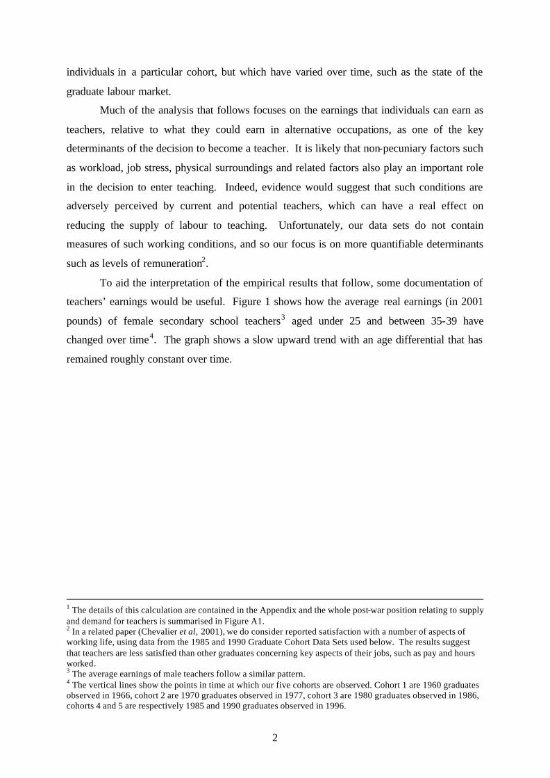
To aid the interpretation of the empirical results that follow, some documentation of

teachers’ earnings would be useful. Figure 1 shows how the average real earnings (in 2001

pounds) of female secondary school teachers3 aged under 25 and between 35-39 have

changed over time4. The graph shows a slow upward trend with an age differential that has

remained roughly constant over time.

1 The details of this calculation are contained in the Appendix and the whole post-war position relating to supply and demand for teachers is summarised in Figure A1. 2 In a related paper (Chevalier et al, 2001), we do consider reported satisfaction with a number of aspects of working life, using data from the 1985 and 1990 Graduate Cohort Data Sets used below. The results suggest that teachers are less satisfied than other graduates concerning key aspects of their jobs, such as pay and hours worked. 3 The average earnings of male teachers follow a similar pattern. 4 The vertical lines show the points in time at which our five cohorts are observed. Cohort 1 are 1960 graduates observed in 1966, cohort 2 are 1970 graduates observed in 1977, cohort 3 are 1980 graduates observed in 1986, cohorts 4 and 5 are respectively 1985 and 1990 graduates observed in 1996.

3

Figure 1: Female Secondary Teachers' Real Wages (2001 £) by Age Group

8000

10000

12000

14000

16000

18000

20000

22000

24000

26000

28000

year

1967

1969

1972

1974

1976

1978

1980

1982

1984

1986

1988

1990

1992

1994

1996

1998

<2535-39

cohort 1 cohort 2 cohort 3 cohorts 4&5

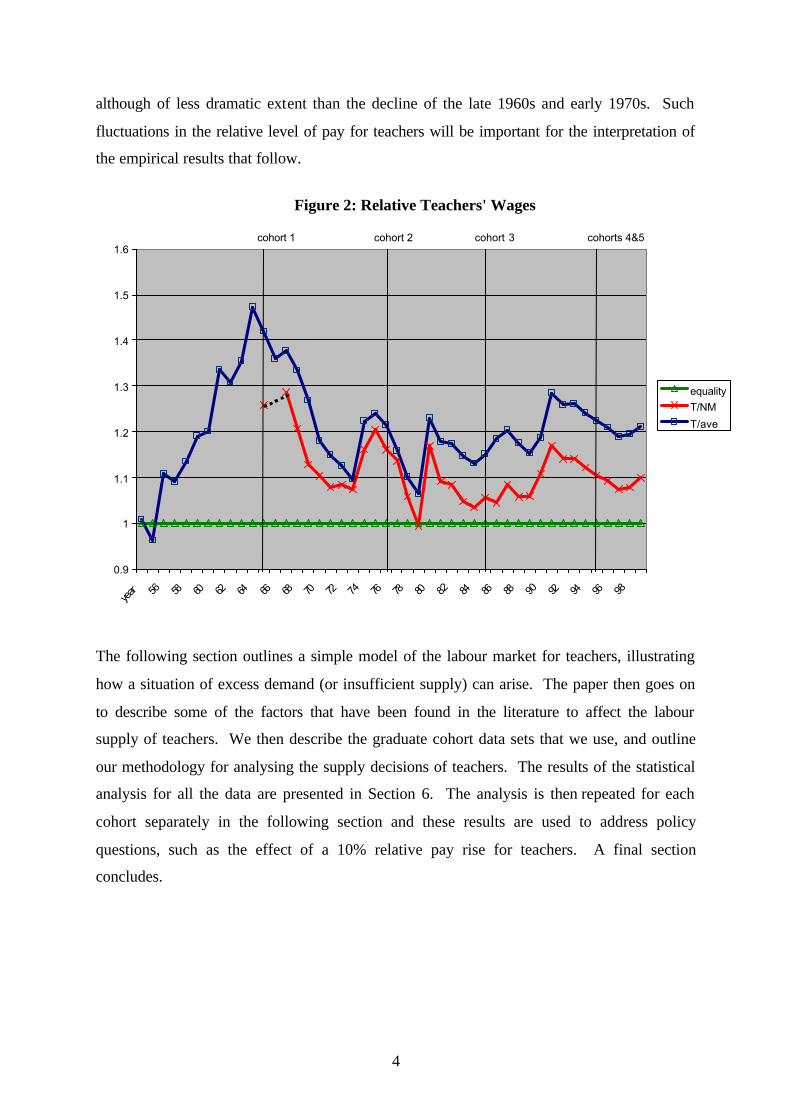
Of prime importance, however, is teachers’ pay relative to other graduate occupations, since

we wish to consider how graduates make choices between becoming a teacher and taking up

another occupation. Figure 2 graphs the relative earnings of teachers compared to average

non-manual earnings and national average earnings5. The highest relative wages were paid to

teachers in the mid-1960s, followed by a considerable deterioration in the period up to 1973.

There followed a series of dramatic adjustments after the Houghton Report (1974) and the

Clegg Commission (1980) recommended that teachers’ pay had been allowed to decline too

far. More recently, the 1990s have seen a continuous decline in the relative wage of teachers,

5 Data on earnings are available from two sources, the October survey of earnings and, since 1968, the New Earnings Survey (NES). With respect to average earnings of all employees, the two surveys give similar estimates over the period that they are both in existence, and so the reported average earnings is a simple average of the two estimates. For specifically non-manual earnings, the DfES’s Labour Market Trends (formerly the Employment Gazette) reports an index based upon the October Survey until 1970, and from then onwards, the NES. However, the resulting estimate is considerably above the estimate of non-manual earnings supplied by the NES, and so in Figure 3, we only display teachers’ earnings relative to the non-manual average from 1968 onwards using the NES. We estimate the position relative to non-manual earnings for 1966 (to gauge the situation for our first cohort), by adding the average difference between the October Survey and NES estimates of teachers’ earnings relative to non-manual earnings (approximately 20 percentage points), to the October Survey estimate of the relative position for that year.

4

although of less dramatic extent than the decline of the late 1960s and early 1970s. Such

fluctuations in the relative level of pay for teachers will be important for the interpretation of

the empirical results that follow.

Figure 2: Relative Teachers' Wages

0.9

1

1.1

1.2

1.3

1.4

1.5

1.6

year 56 58 60 62 64 66 68 70 72 74 76 78 80 82 84 86 88 90 92 94 96 98

equalityT/NMT/ave

cohort 1 cohort 2 cohort 3 cohorts 4&5

The following section outlines a simple model of the labour market for teachers, illustrating

how a situation of excess demand (or insufficient supply) can arise. The paper then goes on

to describe some of the factors that have been found in the literature to affect the labour

supply of teachers. We then describe the graduate cohort data sets that we use, and outline

our methodology for analysing the supply decisions of teachers. The results of the statistical

analysis for all the data are presented in Section 6. The analysis is then repeated for each

cohort separately in the following section and these results are used to address policy

questions, such as the effect of a 10% relative pay rise for teachers. A final section

concludes.

5

2. The Labour Market for Teachers

Following Zabalza et al (1979), the labour market for teachers can be thought of within a

traditional supply and demand framework, with the additional factor to be taken into account

that total spending budgets for education is set by the government, so that, although schools

can decide how they allocate their funds to teacher salaries and other costs, they are still

limited by the overall budget that they have. Although there is a private education sector in

the UK, this accounts for no more than 5-7% of all teachers hired.

Demand for teachers is determined by the number of children in the country of school

age, and the government’s desired pupil-teacher ratio. For a given such ratio, the demand for

teachers is therefore a constant, denoted by Q* in Figure A2. Under the reasonable

assumption that the supply of teachers is a positive function of average teacher earnings, an

upward-sloping labour supply schedule can be drawn as S. In a perfectly competitive market,

a wage of Wa* would therefore clear this labour market. However, the teachers’ labour

market is of course not competitive, and the government, in its role as (almost) exclusive

purchaser of teaching labour, has other considerations, prime amongst which is the level of

expenditure on teachers’ salaries in total. For a given level of such expenditure, an inverse

relationship can be plotted between teachers’ earnings and the number of teachers hired,

labelled E1 in Figure A2; if the government wants to raise the salaries of teachers, it can

afford to hire fewer of them, given a fixed budget. The number of teachers hired is therefore

Qg at average earnings of Wga, and the excess demand for teachers is Q* - Qg. This can only

be eradicated by a relaxing of the budget constraint leading to higher earnings, or other

factors changing to make teaching more attractive, so that more potential teachers supply

their labour at any given wage. This paper examines the supply responses to changes in

wages, and other factors.

Of course, the above analysis is simplistic in that it treats all teachers as being the

same. In reality, there may be teacher shortages in particular regions or in particular subjects,

with an over-supply elsewhere. In addition, the real market position is very different for

primary and secondary school teachers. We can amend Figure A2 to allow for such

possibilities by creating a simple distinction of different kinds of teachers. A simple analysis

would suggest that the possibility of differential wages by subject, in different regions or

between primary and secondary sectors could be adopted to solve the problems of short

supply in particular areas. Whether this solution is actually viable, given the demands of

6

teachers’ unions and the political process in general, is another question. In the empirical

analysis that follows, we allow for the possibility that supply responses differ by subject of

study amongst potential teachers. First though, we review some of the evidence that has been

collated on the supply decisions of teachers.

3. The Literature on the Supply of Teachers

A limited literature exists on the factors affecting the supply decisions of teachers, most of it

originating in the US. This literature can be divided into studies that examine the influences

on the decision to enter teaching, and the influences on the decision to exit from teaching. A

few studies also consider quality aspects of teachers.

Considering first the entry decision, British work on this topic is limited. Dolton

(1990) uses data from the 1980 Graduate Cohort, which follows a sample of graduates for up

to seven years after they have graduated. In this, and most other work in this area, wages are

shown to be an important factor in the decision to become a teacher. Specifically, relative

starting wages in teaching (compared to estimated potential earnings elsewhere) are

positively related to the probability of becoming a teacher. In addition, individuals are more

likely to become teachers the greater is the growth over time in teachers’ earnings, and the

lower is the growth in earnings of non-teachers.

A much earlier study, based only on time series data at the aggregate level in the UK

for the years 1963-1971 by Zabalza et al (1979), estimates the elasticity of the supply of

labour into teaching, with respect to relative teacher earnings. The estimated elasticities

range from 2.4-3.9 for men, and from 0.3-1.8 for women, depending on the definition of

alternative wages used. When teaching wages are split into starting wages and wage growth,

the authors find that the effect of the relative level of starting wages in teaching is similar for

both sexes, while the effect of teacher wage growth over time is much greater for men. This

suggests that the wage effects are greater for men primarily because of their consideration of

career prospects. Court et al (1995) update this analysis for the years 1986-1992, and find

different results. In these years, men and women seem to have similar supply elasticities into

teaching with respect to relative starting wages, of around 4. Relative salary progression and

7

the graduate unemployment rate, however, do not seem to significantly affect the supply of

labour into teaching 6.

There are a similarly small number of US studies to have considered the entry

decision into the teaching profession. An example is Manski (1987), who uses data from the

National Longitudinal Survey of the High School Class of 1972. The results of his probit

equation on occupational choice (teacher/non-teacher) suggest a 10% increase in weekly

teaching earnings will raise the supply of teachers from 19% to 24% of the graduate cohort.

Manski also considers the quality aspect, and calculates that a 10% increase in weekly

teaching earnings, coupled with a minimum requirement for entrance to the profession of an

800 SAT score, would maintain the supply of teachers at 19% of the cohort, while raising the

average academic ability amongst that group to the national ave rage for college graduates.

There are more studies examining the decision to continue in or exit from teaching.

Most of the British work in this area has been undertaken using information on various

cohorts of university graduates, for example Dolton (1990), Dolton and van der Klaauw

(1995a; 1995b; 1999) and Dolton and Mavromaras (1994). With the exception of the last of

these studies, all use data from the 1980 Graduate Cohort. The Dolton (1990) study estimates

a probit equation on whether an individual is in a teaching job seven years after graduating

(conditional on choosing a teaching job as the first job upon graduation). The results suggest

that the factors affecting the decision to continue teaching are very similar to those that affect

the decision to become a teacher in the first place. The three papers by Dolton and van der

Klaauw all adopt a hazard approach to model the length of time spent in the first job after

graduation amongst teachers. The results show that the elasticity of leaving a teaching job

with respect to relative wages is about –1.5, suggesting a large reduction in quit behaviour

amongst teachers, following a rise in earnings. The importance of the outside labour market

and alternative opportunities is also clearly demonstrated by the significance of other

variables in the estimated equation. In particular, teachers are more likely to leave their jobs,

if their local unemployment rate is low, if they have a professional qualification and if they

hold a non-education first degree. When Dolton and van der Klaauw (1995b; 1999) extend

earlier (1995a) work by adopting a ‘competing risks’ approach to their hazard rate, allowing

the explanatory variables to have a differential impact on the likelihood of leaving for non-

teaching work, and the likelihood of leaving the labour force altogether, they find that a

higher teaching wage reduces the probability of teachers leaving the labour force altogether,

6 A more detailed description of these two studies can be found in the appendix.

8

while a higher predicted wage in the non-teaching sector is related to an increased likelihood

of moving into a non-teaching job.

The final paper to use the UK graduate cohort data sets is that of Dolton and

Mavromaras (1994), which, using data from both the 1970 and the 1980 cohorts, is the only

one to provide, as we do here, comparisons over time. The authors decompose the cause of

the fall in the likelihood of becoming a teacher between these two dates into changes in the

characteristics of the individuals themselves, and changes in the characteristics of the job

market that they face. The results reveal that the fall is due almost entirely to deteriorating

market conditions for teachers.

As with the entry into teaching decision, Zabalza et al (1979) also undertake a time

series analysis of the exit decision, considering the years 1963-1972. As with the Dolton and

Mavromaras (1994) study above, they find that males are much more likely to be influenced

by wages than females, the elasticity of the trained graduate separation rate with respect to

relative wages being –2.4 to –3.0 for men, and –0.6 to –0.7 for women. Unlike their analysis

of the entry decision, Zabalza et al find that this gender differential in wage effects exists for

both starting wages and the growth in wages.

Turning to the US literature on the continuation or exit decision, the evidence closest

in spirit to the UK studies using the graduate cohort data sets is provided in two papers by

Stinebrickner (1998; 2001), using data from the National Longitudinal Study of the High

School Class of 1972. The paper actually analyses the 450 respondents to the survey who

became certified to teach sometime between 1975 and 1985. The focus of the analysis is the

length of time between the certification date and 1986 that the respondent spends in teaching.

This therefore has a maximum value of 11 years. As was found with the UK studies,

Stinebrickner (1998) suggests that teachers are more likely to stay in their job, the higher are

the wages that they receive. Stinebrickner (2001) simulates the effects of changing teacher

wages. Two policies are considered, the first being a 25% pay increase for all teachers, and

the second being a 25% pay increase on average, the actual amount depending linearly on

teachers’ SAT scores. The results of the simulation show that the proportion of the eleven

years under consideration that the initial teachers spend in teaching, rises from 0.48 to 0.72

under both of these policies, with wage increases being particularly likely to reduce the

amount of time spent in non-teaching employment, rather than time spent out of the labour

force altogether. The second policy, whereby wages are increased in proportion with teacher

quality, leads to a change in the mix of teachers towards a greater proportion of those of high

quality. A limited number of other papers have also considered this quality aspect. For

9

example, Ballou and Podgursky (1995) suggest that wage rises must be implemented together

with an attempt to target those of higher ability, or, more cost effectively, making the pay rise

conditional on having a certain minimum SAT score, if quality is to increase. In a similar

vein, Hanushek et al (1999), using data for the years 1993-1996 from the UTD Texas Schools

Project database, show that a 10% increase in starting wages is associated with a 2% fall in

the probability of leaving for probationary teachers, and a 1% fall for those with 3-5 years of

experience. The estimated wage elasticity in this case is therefore quite small.

Finally, summarising the remaining US papers to have studied the exit decisions of

teachers, many have used state level data on all teachers registered within particular states,

including Brewer (1996), Rees (1991), Mont and Rees (1996) (all studying New York);

Murnane and Olsen (1989) (Michigan); Murnane and Olsen (1990) (North Carolina),

Theobald (1990) and Theobald and Gritz (1996) (both Washington). All agree that the salary

paid to teachers is negatively related to their propensity to leave, or positively related to the

duration spent in first teaching jobs. Where studies allow for gender differences, a common

finding is that these wage effects are larger for men than for women. In addition, the results

generally show that teachers with higher level qualifications, or who live in areas with higher

average non-teaching wages, and are more likely to leave their teaching jobs.

4. Data

We turn now to our own analysis of the decisions to enter and continue teaching. The data

used in this analysis come from five cross-sections of UK university graduates covering the

period 1960 to 1996. Each cohort was surveyed approximately six years after graduation

apart from the 1985 cohort, for whom eleven years passed between graduation and the date of

survey. Each cohort are surveyed only once, but asked retrospective questions about the first

job after graduation, and in the case of the 1985 cohort surveyed in 1996, they are also asked

about an intermediate year. The following table shows the years about which the labour force

status of each cohort is questioned, with the survey itself taking place, in each case, in the last

year mentioned.

10

Table 1: Graduate Cohort Observation Dates

Cohort Graduation Date

Data Size

Dates of Labour Market Information Interval

1960 1966 1970 1977 1980 1986 1991 1996 1960 6339 √ √ 1970 5421 √ √ 1980 5388 √ √ 1985 3311 √ √ √ 1990 5187 √ √

The 1960, 1970 and 1980 cohorts have been used extensively. These surveys are

nationally representative of the graduate population sampled from all universities. The 1985

and 1990 cohorts are also representative, but are based on a different design. Individuals

were contacted through their institution of origin, and a representative selection of institutions

was used to conduct these surveys. Comparisons across surveys are also complicated by the

modifications to the Higher Education sector in the UK. From the mid-sixties until the early

nineties, two main types of Higher Education institutions co-existed, namely universities and

polytechnics. Higher education colleges were also an increasing source of HE provision

during this period. This distinction was abolished in 1992. Concomitant to this institutional

change, the proportion of a cohort attending Higher Education has also increased drastically

over the period, from about 6% in the 1960s to around 30% in 1995.

The surveys provide data on a range of variables that are likely to influence the

decision whether to teach or not. Key amongst these is the wages received in different

occupations. A measure of relative earnings in teaching is derived, as explained in the

following methodology section. We also control for the local labour market by including a

dummy variable for whether the individual lives in London or the South-East or not, because

of the vastly different labour market in that area, as well as the perception of poor working

conditions in London’s schools 7. Qualifications may also have an impact on the teaching

decision, independently of their effect through the alternative wage that could be earned in

the labour market. Thus, we control for A-level scores, subject and class of degree, type of

institution attended and any higher qualifications obtained. It is expected that those

individuals who do not study for an education degree are less likely to go into teaching.

7 A finer regional split is not possible for the 1960 cohort. In addition, the regional coding is not compatible between 1970/80 surveys and the 1985/90 surveys. Therefore, across all cohorts, the most consistent thing to do was to simply define a London/south-east dummy variable, which could be consistently defined.

11

Particular subjects, such as engineering and science may be particularly unlikely to lead to a

teaching career, because of the availability of other options for holders of such degrees8.

Similarly, postgraduate and professional qualifications should also open up new possibilities

in the labour market, reducing the likelihood of an individual teaching. It has also been

identified in the past that the most academically able graduates do not choose to become

teachers. Data on A-level and degree results, and type of institution attended, allow us to

explore this possibility. However, it should be noted that it is difficult to use these variables

to track changing teacher quality over time. This is because, with respect to degree results for

example, the numbers achieving the best results have increased over the period considered.

For example, whereas 28% of graduates obtained a First Class or Upper Second Class in

1960, this figure had increased to 48% by 1990 (see Table A1).

The remaining variables included in the analysis control for various demographic

factors, which may or may not influence the decision to become a teacher. In particular, we

include variables for gender, whether the respondents were mature students, marital status,

type of school attended, and the socio-economic background of the individuals’ families.

Finally, we add dummy variables to indicate the cohort to which each individual belongs, to

determine whether there is any trend in the decision to become a teacher, irrespective of the

trends in the other variables listed here.

Table A1 provides descriptive statistics for each of these variables, separately by

cohort. Differences in the background of the cohorts can be noted. In the earlier cohorts, the

majority of the graduates are male, but by 1990 the cohort is split evenly between men and

women. The proportion of mature students, defined as older than 25 upon graduation, has

also increased from 7% to 16%. Both of these facts could be associated with an increase in

the teacher supply as ceteris paribus female and mature graduates are more likely to choose a

teaching occupation. Despite the increase in the proportion of a cohort reaching Higher

Education, universities are still largely dominated by students from the most favoured

backgrounds (as measured by paternal social class and the overrepresentation of those

individuals who attended private school). Finally, a higher proportion of recent cohorts have

graduated from a (former) polytechnic institution.

Current earnings do not appear to have varied a great deal over time for graduates,

which is in contradiction with evidence that returns to higher education have increased over

8 It would have been useful to separately classify biological and physical sciences, since the respective labour markets are probably quite different. However, this was not possible to do consistently across all cohorts with the data available to us.

12

the period (Chevalier and Walker, 2001). This may be partly due to differences in the

collection of the data. While the 1960, 1970 and 1980 cohorts reported their earnings, for the

last two cohorts earnings were reported as a banded variable, thus reducing the accuracy with

which earnings are measured. For example, the 1996 survey of the 1990 graduate cohort asks

respondents to say in which of the following bands their annual earnings fall (all in £);

<3999, 4000-5999, 6000-7999, 8000-9999, 10000-11999, 12000-14999, 15000-17999,

18000-19999, 20000-22999, 23000-25999, 26000-28999, 29000-31999, 32000-34999,

35000-39999, 40000-49999, 50000 +.

Also note that the earnings variable used is a real measure of earnings (1970 £’s),

deflated by the index of non-manual earnings, which have grown more rapidly than the usual

‘all earnings’ or retail price index (RPI) deflators.

Finally, since we are interested in the dependent variable of becoming a teacher, then

we are interested in the proportion that do so in each cohort. These figures appear in Table

A1, revealing that although close to 30% of the 1960 cohort worked as teachers six years

after graduation, this proportion fell to 11-15% in later cohorts. Of course, this is likely to be

in large part due to the rapid increase in the number of graduates, which has far outstripped

the growth in the demand for teachers, implying that we should expect a lower proportion of

a graduate cohort to enter teaching now compared to earlier times.

Before continuing to the results section, some limitations of using the graduate cohort

data sets for a study of this type should be pointed out. First, and probably foremost, is that

the cohort data sets are cross-sectional, and comprise respondents the vast majority of whom

are of a similar age (around 21 years old since they are all graduates of a specific year).

Thus, the analysis of wage effects on the probability of teaching are restricted to an analysis

of the effect of current relative wages on the current decision whether to be in teaching or not.

We have no data at multiple points in time with which to calculate a wage progression

profile, in order to estimate the effect of such a profile on teaching likelihoods. It would be

wrong to use the national pay scales to estimate future pay progression, since promotion can

be a key determinant of earnings in the teaching profession, and so without a model with

which to predict future promotions, it is impossible to predict future earnings with any

reliability, given the data at our disposal. This may be an important omission, as the

aggregate time series analysis of Zabalza et al (1979) for the years 1963-1971 (reviewed

above) finds an important impact of such a variable, at least for males, although Court et al

(1995) studying the later period of 1986-1992 can find no evidence of such a relationship. If

salary progression is relevant, however, and under the assumption that it is positively

13

correlated with the current level of earnings, then the omission of this variable may result in

the current earnings effect appearing to be larger than it actually is. Note that the fact that

most of the respondents to the survey are of a similar age also precludes the possibility of

obtaining an approximate estimate of lifetime earnings.

Closely related to the fact that we do not observe the lifetime earnings of individuals

is the fact that we do not know their total job history, in the past and in the future. This

means that we cannot determine the length of time individuals in our cohort samples spend in

teaching, and so we cannot determine the total labour supply change, in terms of teacher

years, that will result from a change in relative earnings. For example, if there is a ‘seven

year itch’ in teaching, so that there is a sudden increase in the number of teachers leaving the

profession at this point in their careers, then this would not be picked up by most of our

cohort data sets, which usually survey individuals six years after graduation. We would

therefore over-estimate the likely effects of changes in wages on the number of individuals

working as teachers in the future. Equally of course, the structure of the cohort surveys may

mean that we do not observe some individuals working as teachers, for example those whose

first job is not in teaching, who then become a teacher, before deciding to leave the

profession before they are questioned by our surveys six or seven years into their careers.

All of this means that we cannot usefully calculate an elasticity of labour supply to

teaching with respect to relative earnings, in the manner that the aggregate time series studies

of Zabalza et al (1979) and Court et al (1995) calculated their elasticities, as reviewed above.

We will therefore refrain from describing any results that we obtain in terms of elasticities, to

avoid any confusion with standard constructs of such a concept. All that is estimated in the

results section below is the change in the likelihood of the particular graduates observed in

our surveys teaching at the time of our survey. Although we do covert these probabilities

into numbers of teachers, based on the total number of graduates in the years concerned, we

make it clear that this only represents the change in the number of teachers from the specific

graduate cohorts that we consider, and at the specific points in time considered, and does not

represent the total change in the labour supply to teaching.

A final limitation of the graduate cohort data sets is their lack of other variables that

may be related to the decision to become a teacher. In particular, working conditions, both

physical in terms of schools’ buildings and surroundings, and aspects of the job, such as

workload and stress, are likely to impact on the likelihood of graduates choosing to be

teachers, but cannot be included in our analysis because no such information is available in

our data sets.

14

5. Empirical Methodology

We turn now to the methodology used to estimate our equations, which is similar to that in

Dolton (1990), and a full description can be found there. The key equation that we want to

estimate is a probit equation for whether graduates are currently in teaching or not, usually

six years after graduation. Algebraically, the equation can be represented as:

131210 )ln(ln uXTWWT at

Ttt +++−+= ββββ (1)

Tt is a dummy variable, taking the value of 1 if the individual is a teacher at time t, the time

of the survey, and 0 otherwise. The key explanatory variable is the relative wage that the

individual can expect to earn at time t, expressed as the difference between the wages that

could be earned as a teacher, WtT , and the wages that could be earned in an alternative job as

a non-teacher, Wta. The variable T1 takes the value of 1 if the individual’s first job following

graduation was as a teacher, and 0 otherwise, and thus controls for possible inertia effects,

such that an individual is more likely to be a teacher now if they originally chose to be a

teacher. This is due to unobserved characteristics, for example a ‘taste’ for teaching, which

makes respondents more likely to teach at both points in time, as well as more usual inertia

effects such as the cost of changing jobs. Finally, the X vector includes all of the other

variables discussed above.

The variable indicating those who chose to teach in their first job is clearly

endogenous, and hence a reduced form probit equation for choice of first job is estimated,

and the predicted values used in the estimation of the structural equation given above.

Likewise, to obtain the wage variables, we estimate two wage equations, one for all current

teachers and one for all non-teachers in the sample, and take the predicted values of these as

the wages that individuals could earn at time t in the teaching and non-teaching state. Of

course, we only observe teachers’ wages for those who chose to be teachers, and we only

observe non-teachers’ wages for those who chose not to teach. Given that this occupational

choice is not random, and that certain factors (some of them unobserved) systematically

explain this allocation, then the two groups, teachers and non-teachers, will differ in these

characteristics, and so the wages that non-teachers receive may not be a good predictor of the

wages that teachers would receive if they were not teaching. It is thus necessary to allow for

this selectivity. We therefore estimate a reduced form version of equation 1, omitting the

15

wage and first job choice variables, and then place the inverse Mills ratio from this equation

into the estimated wage equations:

210 'ln uXW TTTTTt +++= λρσδδ (2)

210 'ln uXW aaaaat +++= λρσδδ (3)

where ? is the inverse Mills ratio, and X’ is a subset of the vector of variables in the

occupation choice equation. In order for the identification process to work, this necessarily

has to be a subset, such that some variables included in the occupationa l choice equation are

excluded from the wage equations. The success of the procedure relies on the

appropriateness of these exclusion restrictions. Thus, the marital status, type of school and

socio-economic background variables are omitted from the wage equations, in order to

provide the identifying restrictions for the selection equation. The choice of these

instruments is determined principally by the available variables in the graduate cohort

datasets, and it should be acknowledged that they are far from perfect. Nevertheless, the

results in the next section show these variables to have a significant effect upon occupational

choice, while there is no theoretical reason for including them in the wage equations. Finally,

X’ also includes some variables not in the occupation equations, but which are frequently

found in wage equations, namely work experience and its square, and part-time status. Since

the wage differential variable, as well as the probability of teaching in the first job, is an

estimated variable, standard errors calculated in the usual way would be biased. We therefore

bootstrap the estimates (500 times), in order to get unbiased standard errors.

6. The Factors Affecting the Decision to Work as a Teacher

This section describes the results of the empirical analysis described above. The first stage is

to estimate the reduced form equation for the occupation choice (teaching or non-teaching) in

the first job. The results are contained in Table A2. The table displays both the estimated

coefficients in the probit equation, and the marginal effects. However, since the determinants

16

of the first job choice are similar to those of the current job choice, to be discussed below, the

first job choice coefficients will not be discussed here9.

Table A3 contains the results for the wage equations. In column 2 the results of the

selection equation on choice of current job are displayed. The inverse Mills ratio from this

equation is then included in the wage equations for teachers and non-teachers, in columns 3

and 4 respectively (denoted ‘lambda’). The significance of the coefficient on this variable in

both wage equations reveals the importance of allowing for selectivity into the teacher or

non-teacher states. The remaining coefficients in the wage equations are as we would expect,

and display the same sign, even if they do differ in magnitude, for both teachers and non-

teachers. Thus we observe higher wages for males, those with a better class of degree and

higher A-level scores, those with postgraduate and professional qualifications, those who live

in London or the South-East, those with more work experience and those who work full-time.

The degree subject coefficients do vary by occupation, with the results suggesting, somewhat

surprisingly, that all subjects attract a significantly positive wage differential with respect to

the omitted category of education degrees in teaching jobs, while in non-teaching jobs, there

are fewer statistically significant differences, with only those holding a language or arts

degree earning less than those with an education degree.

Our main results relate to the choice of current occupation, as displayed in Table A4.

We consider first the wage variable. For each individual, we include the predicted wage

differential (the predicted wage in teaching minus the predicted wage in non-teaching) 10 as a

determinant of occupation choice. The marginal effect in the final column shows that a 10%

rise in teacher earnings, relative to non-teacher graduate earnings, at the time of the survey

will increase the probability of an individual being a teacher at the time of the survey by 5.4

percentage points. Given that the teaching probability ranges from approximately 10-15%

(with the exception of the 1960 cohort), this is a very sizeable effect. Increasing wages

would clearly be an effective method of persuading more graduates to become, and remain,

teachers.

The subject specialisation variables also reveal some interesting determinants of the

decision to teach. As expected, the subject coefficients show that graduates who studied for

an education degree are more likely than those of all other subjects to enter teaching. The

9 It is perhaps surprising how similar first job and current job equations are. In both equations, the same variables attract statistically significant coefficients of almost exactly the same magnitude. Perhaps six years into one’s career is not sufficiently far to differentiate current occupation choice decisions from initial such decisions.

17

difference is greatest for engineering graduates, who have pursued a profession-orientated

subject themselves that offers good prospects in terms of job opportunities, because of a lack

of suitably trained graduates in this field. Outside options are also responsible for the

coefficients on the professional qualifications, PhD and MSc variables, all of which show that

individuals with such qualifications are less likely to work as teachers. Presumably, such

individuals had other careers in mind when they embarked on such studies, since none are

required to enter the teaching profession. We should not be surprised, therefore, that on the

whole they have followed these career paths. In addition, graduates with a first class or upper

second class degree are less likely to teach than those with lower degree classes, holding the

other factors in the equation constant, which, recall, includes alternative wages. Although the

marginal effect is quite small (a 1.6 percentage points lower probability of teaching), this

difference is statistically significant. Thus, holding constant the relative wages on offer in

teaching and non-teaching occupations, there appears to be some non-pecuniary cost to

teaching for those with a good class of degree. Perhaps such graduates believe that their

high- level skills are better suited to alternative employment. The other variables included in

the equation to try to capture quality effects, namely the A-level scores of the respondents

and whether they attended a university or polytechnic, do not attract statistically significant

effects11.

Turning to the cohort effects, there is a clearly observable pattern, the coefficients

declining monotonically with each successive cohort (with the exception of the 1985 cohort).

All cohorts are significantly less likely to teach than the 1960 cohort. Thus, holding all other

factors in the equation constant, individuals in each cohort are less likely than those in the

cohort before to go into teaching, apart from a small rise in the probability between the 1980

and the 1985 cohorts. Given that the early 1980s saw a very deep recession in the UK, the

high levels of unemployment and subsequent lack of alternative employment may have

persuaded graduates at this time to look for a job in a relatively recession-free profession

such as teaching. The largest change in the probability of teaching seems to have occurred

between the 1960 and 1970 cohorts, with a 6.2 percentage point fall in the probability of

becoming a teacher, holding other things constant, between these dates. There was also a 4.0

percentage point fall in this probability between the 1985 and 1990 cohorts. Thus there

10 This is expressed in exponential terms, so that this difference approximates to the proportionate difference between teaching and non-teaching wages. 11 Although of course these variables are likely to be collinear with one another, and so their individual effects may be obscured. For example, college and polytechnic students are likely to have lower A level grades than university students.

18

appears to be an increasing trend away from teaching as a profession, even if other factors

had not changed12. The fact that relative wages in teaching have, on the whole, fallen over

this period, merely re-enforces this trend away from teaching.

The remaining statistically significant effects in Table A4 suggest that men are 4

percentage points less likely to teach than women and that married graduates are 1 percentage

point more likely to teach than single graduates13. There is some evidence that social class

influences the decision to go into teaching, since those individuals who attended a private

school for their education, and those who came from a family with a professional head of

household, are both less likely to choose teaching than state-educated and non-professional

family graduates. The dummy variable indicating graduates who live in London and the

South-East attracts a statistically significant coefficient, which reveals that, holding other

things constant, individuals in this area are over 6 percentage points less likely to teach than

individuals in other areas. This is most probably as a result of the wide range of alternative

professional occupations available in London, compared to other areas, although it is also a

possibility that working conditions in London’s schools are perceived to be worse than in

more provincial areas. Finally, the coefficient on the first job variable shows that,

unsurprisingly, those individuals who initially chose teaching as a career immediately after

graduation are more likely to still be teaching in their current job than those who chose an

alternative first job, the difference in the probabilities being over 9 percentage points. This is

due to inertia in the teaching profession, as in many other occupations, so that the non-

pecuniary benefits or individual characteristic traits that originally attracted graduates to

teaching continue to have an effect six years later.

7. Cohort Effects and Simulations

In the previous section we reported the combined regression results for all the cohorts of

graduates for which data are available. In this section we confirm that these general results

12 An alternative interpretation is that, given the number of graduates has increased much faster than the number of teaching positions since the 1960s, we would naturally expect a fall in the probability of any particular graduate becoming a teacher. Note, however, that the continuing excess demand for teachers does not suggest that graduates are increasingly choosing an occupation other than teaching because of a lack of available teaching positions. 13 It could be the case amongst the young respondents to the graduate cohort surveys that expectations about the possibility of future marriage have more effect on the current occupation choice than current marital status. Unfortunately we do not have any data for the former concept.

19

hold for each of the cohorts separately and use the results of the estimations to perform some

simulations of possible policy changes.

Looking at Table A5, which relates to the probit estimations for each of the cohorts

separately, we see that many of the factors that operate in the aggregate equations are also at

work in separate cohorts. A useful way to summarise the influences on the decision to teach,

and how these have varied in the different cohorts, is to calculate the probability of becoming

a teacher for a person of fixed characteristics, and then to see how this probability has

changed over time, and also how it changes as we vary certain characteristics. Thus, we

define a base individual (Individual 1) as a man, with an A-level score of 10, graduating in an

Arts subject at a university with a 2/1 or above and not living in London. The other

characteristics of this individual will be held constant across all of our stylised individuals

(see the note at the bottom of Figure 3). We then define another 4 individuals, each of whom

has one characteristic that is different to individual 1: Individual 2 has lower ability (A-level

score =6) and graduated with a 2/2 or below, Individual 3 graduated from Science, Individual

4 lives in London and Individual 5 is a woman. The predicted probabilities of being a teacher

over time for these various individuals are reproduced in Figure 314.

For all types, the probability of currently being a teacher has declined through time.

For Individual 1 for example, this probability was 43% in 1966 (cohort 60), but down to 8%

in 1996 (cohort 90). This is an obvious consequence of the smaller proportion of graduates

becoming teachers, which is partly because the number of graduates has expanded

dramatically over the years. Hence what is of most concern to us in this figure is the

difference between our ‘stylised individuals’ rather than the declining probability over time.

Individuals with lower academic results (as measured by A level scores and, with particular

effect, degree classification) and women are more likely to be teachers than our base

individual, while for individuals with a science degree or living in London the probability of

being a teacher is lower, although all differences have been reduced over time15.

14 For these calculations, we do not want to use the conditional estimated coefficients presented in Table A5, where the probability of teaching is conditioned on the predicted relative wage and the probability of teaching in the first job, since the characteristics considered are likely to effect relative wages and first job choice. Hence, to obtain the full effect of changes in the various characteristics on the probability of teaching, we use the estimated coefficients from an unconditional probit, full details of which are available from the authors. 15 For the 1990 cohort, the observed characteristics do not appear to explain much of the variation in the probability of teaching, since all the points, with the exception of the one for which gender is varied, are bunched together.

20

Figure 3: Predicted Probability of Being a Teacher for Different Type of Graduates

0

0.1

0.2

0.3

0.4

0.5

0.6

0.7

Cohort 60 Cohort 70 Cohort 80 Cohort 85 Cohort 90

Observed ind1 A-level 6 Science London Woman

Note: Characteristics held constants for all individuals: University graduate, married, father in interim occupation, no other qualification, state funded school Ind1: Man, Arts graduate, A-level score=10, 2/1 or above, not in London Ind2: Man, Arts graduate, A-level score=6, 2/2 or below, not in London Ind3: Man, Science graduate, A-level score=10, 2/1 or above, not in London Ind4: Man, Arts graduate, A-level score=10, 2/1 or above, live in London Ind5: Woman, Arts graduate, A-level score=10, 2/1 or above, not in London

The remainder of this section will focus on the effect of relative earnings on the decision to

teach. We begin by examining the extent to which teacher wages have lagged non-teacher

wages over time, using the matching methods pioneered by Rosenbaum and Rubin (1983). In

effect, what this method does is to find, for each teacher in our sample, the non-teacher who

looks most similar on the basis of observable characteristics, and examine the difference in

earnings. We then investigate whether earnings differ by occupation amongst graduates who

look the same. Specifically, we estimate a probit equation for the probability of becoming a

teacher and use this to predict the ‘propensity score’ for a graduate to become a teacher.

Using different matching methods (nearest neighbour or Kernel methods) gives us the results

in Table 2. The table presents the mean current pay differential between teachers and their

matched contemporaries. A negative estimate shows the percentage by which teachers earn

less than a comparable group of non-teachers.

21

Table 2: Matched Estimates: Current Pay Differentials between Teachers and Similar Non Teachers.

Cohort 60 Cohort 70 Cohort 80 Cohort 85 Cohort 90

Year Sampled 1966 1977 1986 1996 1996

Years in Teaching 6 7 6 11 6

Relative Wage 1.41 1.21 1.15 1.22 1.22

* One to one match

Bandwidth=0.001 -0.003

(0.003)

0.011

(0.028)

-0.085**

(0.029)

-0.178**

(0.079)

-0.040

(0.047)

Bandwidth=0.0001 -0.001

(0.003)

0.008

(0.029)

-0.115**

(0.030)

-0.240**

(0.076)

-0.026

(0.043)

* Kernel match

Bandwidth=0.001 -0.012 (0.027)

0.010 (0.027)

-0.080 (0.020)

-0.085 (0.088)

-0.019 (0.038)

Bandwidth=0.0001 -0.005 (0.026)

0.016 (0.029)

-0.090 (0.023)

-0.165 (0.089)

-0.030 (0.038)

Non matched (.001) 14 31 38 50 61

Non matched (.0001) 35 108 124 76 112

The results reveal that the teachers most likely to be underpaid relative to observationally

equivalent non-teachers are in the 1980 and 1985 cohorts, observed in 1985 and 1996

respectively. The cohort of teachers who began their careers in 1980 are likely to be

underpaid relative to comparable non-teachers by 8-12% in 1986. This is most likely due to

the five years (according to Figure 2) of declining relative wages that they have endured,

giving them the lowest relative teacher wages of all of the cohorts. The position for the 1985

cohort is interesting, given that they are observed at the same time (1996) as a later cohort of

graduates from 1990. Although the latter group, with only six years experience, are not

underpaid compared to similar non-teachers, the teachers in mid-career who have been

teaching for 11 years are being underpaid, compared to their matched counterparts, by 9-

24%. This comparison thus highlights a further important dimension to the issue of relative

pay, that such comparisons are different at different points in the career life cycle.

Given that there has been such variation in the relative level of teachers’ earnings over

time, it would be interesting to examine how this variation has affected the numbers entering

the profession at each point in time. Some authors researching the teachers’ labour market

have performed simulations using their data to answer questions concerning the potential

22

effect of a pay rise on the supply of teachers. Nearly all of these studies have performed such

simulations at a given point in time. By using a series of cohorts we are in the fortunate

position of being able to carry out such simulations across time.

Table 3 below performs the simulations. For each cohort, the observed probability is

the probability of being a teacher. The predicted probability is calculated for each individual

from the probit estimates including the estimated wage differential between teacher and non-

teacher status and the probability of being a teacher in the first job. We then increase

teachers’ relative earnings by 10%, and recalculate this predicted probability of teaching.

The change in the probability following this pay rise is shown in the fourth row.

Table 3: Probability of Teaching Before and After a Rise in Teachers’ Relative Pay Cohort 60 Cohort 70 Cohort 80 Cohort 85 Cohort 90

Observed 0.279 0.153 0.139 0.112 0.138 Predicted 0.278 0.152 0.138 0.114 0.137 Teacher pay +10% 0.295 0.186 0.235 0.132 0.238 Diff 0.017 0.034 0.097 0.018 0.101 Implied Extra Teachers16

378 1,717 8,420 1,827 11,360

The figures in the table suggest that, in cohorts 3 and 5, a 10% rise in teachers’ relative

earnings would increase the probability of a graduate being in a teaching job six years after

graduating by 10 percentage points (that is, in 1996 for example, 24% of the cohort are

predicted to be teaching if the pay rise is implemented, compared to 14% of the cohort

teaching if it is not, which is equivalent to more than a 70% increase in the actual number of

teachers from this cohort of graduates). In the other years the effects of such a pay rise are

much smaller. Our suggestion is that these findings are consistent with the national

underlying trend in relative teacher wages. The reason for the large potential effect in 1986 is

that the relative wage of teachers was at an historically low value of 1.15 against average

earnings. Our suggestion for the 1996 effect is that it is less to do with a low relative wage

(1.22 against average earnings) but more to do with five uninterrupted years of declining

relative wages. In this context teachers were leaving the profession in large numbers and a

large pay rise would have had a more marked effect. Note, however, that the 1996 effect is

much smaller for the 1985 cohort than for the 1990 cohort. This is perhaps surprising,

23

particularly as Table 2 revealed that the earnings of the 1985 cohort lag those of their non-

teaching counterparts by the greatest amount of all the cohorts. If we are arguing that wage

increases have the largest effect on the decisions to teach when teachers’ relative earnings are

low, why then do we not observe a large effect of earnings on the decisions of the 1985

cohort to teach? We can hypothesise that this is due to the amount of time spent in the labour

market at the point of observation by the 1985 cohort, eleven years as opposed to six/seven

years for all other cohorts, resulting in the graduates of this cohort differing in some

unobservable ways from the graduates of the other cohorts. For example, it may be that those

individuals who are still teaching in 1996 eleven years after graduating, at a time when

teachers’ relative earnings have declined for a number of consecutive years and at a point in

their careers at which teachers’ earnings are falling further behind those of other graduates

with similar job tenure, are those individuals who have a particular desire to teach, or are

particularly suited to teaching and have poor outside options. Varying wages may have little

impact on the decisions to enter, remain or quit teaching amongst such individuals. Thus we

can argue that the effect of a wage increase will be most pronounced on the occupation

decisions of recent graduates.

It would be interesting to calculate not just how the probability of remaining in

teaching changes as the wage rises, but also how many extra graduates in total would be in

teaching if the wage increase was adopted. Unfortunately, this is very difficult to answer,

given that we have only modeled the teaching decisions of a small number of all the past

graduates who could potentially still become teachers, and that we have not modeled wastage

of teachers over their career life cycle, but merely the teacher/non-teacher decision at given

points in time. All we can approximately calculate is, if relative wages for teachers are 10%

higher, how many more teachers there will be in, for example 1996, amongst those who

graduated in 1990. We do this by simply applying the probabilities of individuals teaching to

the known number of graduates in each of the years. Thus, for example, if relative teacher

wages were 10% higher, an additional 11,360 1990 graduates would be teaching in 1996, as

revealed in the final row of Table 3. This might give us some idea of how the current cohort

of graduates would react if relative wages were to rise now, although even this prediction

must be treated with caution, based as it is on the behaviour of a cohort who graduated over

ten years ago. How older cohorts of graduates, who have already chosen alternative careers,

16 The implied number of extra teachers is calculated using the number of graduates leaving university (and polytechnics) in 1960, 1970, 1980, 1985, 1990, which are 22,223; 50,494; 86,800; 101,515 and 112,475 respectively.

24

would react to an increase in wages now is impossible to predict based on the above analysis,

although we can assume that the increased numbers choosing to switch into teaching would

be smaller than the increased supply of new graduates from the current cohort into teaching,

since inertia effects reduce the likelihood of career switches amongst those already in work.

The results suggest that the effect of a pay rise now will be increasingly smaller, the older the

cohort of graduates that we consider. Overall, however, it is not possible, based on the above

analysis, to give a precise answer to the question of by how much would teachers’ pay have

to rise to generate the 34,000 extra teachers that would eliminate the excess demand for

teachers.

8. Conclusion

There currently exists a large excess demand for teachers in the UK, of approximately 34,000

individuals. Given the limited control that the Government has over the demand for teachers,

controlled mostly as it is by the number of pupils, the best hope for narrowing this gap

between demand and supply is to increase supply. Yet the results show that, with the

exception of the recession years of the early 1980s, each cohort in our study has been

successively less likely to choose teaching than the cohort before, holding other things

constant. The Government clearly needs to turn around this trend away from teaching. The

simplest way to do this, if funds allow, would be to relax expenditure limits, and pay higher

wages to teachers, since the results show that the supply of teachers is highly responsive to

the relative wages paid to them. The results suggest that, had teachers’ relative pay been 10%

higher in the 1990s, then over 11,000 more graduates of 1990 would have been teachers in

1996. What we cannot tell from our analysis, however, is the impact of a pay rise now on the

current graduate cohort, as well as the effect on earlier graduates who have chosen alternative

careers, or indeed on the quit behaviour of those who chose to be teachers. As a minimum,

our results do suggest that the extent to which a pay rise for teachers will solve the problems

of shortage will depend on the state of the labour market at the time. More specifically, if

relative teacher earnings are low (as in 1986) or teachers have experienced several successive

years of decline (as in 1996) then the potential for shifting a shortage by raising teacher pay is

greatly increased.

25

The other key results from this study relate to possible supply deficits in particular

subjects and geographical areas. The results reveal that graduates in engineering, sciences

and social sciences are particularly unlikely to choose teaching as a career. Even if earnings

were the same, the alternative professional occupations available for such graduates are likely

to tempt them away from teaching, if working conditions in teaching are not well regarded.

The fact that wages will probably be higher in these alternative professions simply acts to

reinforce this trend. The trend manifests itself in the well-publicised lack of maths and

science teachers. Similarly, graduates in London are also less likely than those in other

regions to be teachers, again presumably because of the large number of alternative

professions open to them in the nation’s capital. The theoretical model above described how

it could be possible to equate demand and supply of teachers in each of the different subjects

or regions, if the Government is willing to pay different wages to different teachers, and can

persuade the teaching unions to accept such a system. Again, however the empirical results

above cannot predict exactly what the wage differences between subjects would have to be to

eliminate specific shortages, since our analysis dealt with aggregates, rather than specific sub-

groups, due to small sample sizes in the various data cells that define these groups.

17 Although note that it is expected that the majority of teachers will receive the higher payments.

26

Appendix

The Excess Demand for Teachers

In the text, it was claimed that there was, in the year 2000, an excess demand for 34,000

teachers. This figure, and similar figures for earlier years as depicted in Figure A1 below,

were calculated according to DfES released figures. The demand for teachers is determined

by the number of pupils, and the Government’s published desired pupil teacher ratio. For

example, in 2000, there were 4,278,123 primary school children (full-time equivalents. The

Government desired that there would be 21.2 primary school children for every primary

school teacher, implying that 210,798 primary school teachers are demanded. In actual fact,

there were 183,762 primary school teachers in 2000, implying an excess demand for primary

school teachers of 18,036. A similar analysis for secondary school teachers reveals that there

was an excess demand of 15,952 teachers, giving the overall excess demand figure of

approximately 34,000, as quoted above. Figure 1 reveals the situation for all years since

1946. The graph shows that there has been an excess demand for teachers almost

continuously throughout this period. This has principally been for secondary school teachers,

although the difference in the excess demand for primary and secondary school teachers

disappeared towards the end of the 1990s.

F i g u r e A 1 E x c e s s D e m a n d f o r T e a c h e r s

- 3 0 0 0 0

- 2 0 0 0 0

- 1 0 0 0 0

0

1 0 0 0 0

2 0 0 0 0

3 0 0 0 0

4 0 0 0 0

5 0 0 0 0

6 0 0 0 0

7 0 0 0 0

1946

1948

1950

1952

1954

1956

1958

1960

1962

1964

1966

1968

1970

1972

1974

1976

1978

1980

1982

1984

1986

1988

1990

1992

1994

1996

1998

2000

Y e a r

Exc

ess

Dem

and

fo

r T

each

ers

Num

ber

s

S e c o n d a r yT o t a lP r i m a r y

27

Figure A2: The Labour Market for Teachers

Wa D

S W a∗ Wg

a E1

Qg Q∗ Q

28

Previous Estimates of the Labour Supply Elasticities to Teaching

Although the nature of the cohort data used in this paper meant that elasticities of labour

supply could not be estimated in the usual way (since the dependent variable in our analysis

is the individual likelihood of being a teacher amongst respondents to a limited number of

surveys covering graduate cohorts from only certain specific years), it is still of use to

summarise here the results of two studies that have estimated formal supply elasticities to

teaching. The first example is Zabalza et al (1979), who estimate time series models for the

entry and leaving decision into and from teaching. They use data from 1963-1971, split into

five subject groups18, thus giving 45 observations.

The first model estimated is the entry decision. The dependent variable is therefore

the proportion of the graduate output from two years previous (thus allowing for time spent in

teacher training) to be in a teaching job in the year in question (estimated using a 5% sample

of graduates). This proportion is explained in terms of relative wages in teaching and

graduate unemployment. Three different specifications of relative wages are adopted. These

differ in terms of the alternative wage used, the average teacher salary being measured in

each case us ing the 5% graduate sample for current teacher wages and official sources for

starting teacher wages19. The three specifications use: (i) a subject specific measure of

alternative wages in the construction of the relative average teacher wage, (ii) the simple

average earnings of all non-manual workers in the construction of the relative average teacher

wage, and (iii), a measure of average starting wages in teaching compared to average starting

wages for all graduates based upon the Annual Reports of the Leeds University Careers and

Appointments Service, together with a measure of wage growth in teaching compared to

alternative occupations. The latter variable assumes a linear lifetime earnings growth

function, and takes the starting wages and the average wages as two points on this line, to

estimate its slope. The relative unemployment variable is simply the proportion of graduates

in each year-subject cell seeking employment on the 31st December of the year of graduation.

Since unemployment amongst teachers is virtually zero in this period, the average graduate

unemployment rate is also the relative unemployment rate.

18 These groups are; group 1 – maths, physics, chemistry and engineering; group 2 – biology, geology and biochemistry; group 3 – French, German and Spanish; group 4- English, history and classics; group 5 – geography, education and social sciences. 19 Attempts were not made to obtain subject-specific teacher wages, since earnings differentials between subject groups in teaching are very small.

29

Separate equations are estimated by the authors for males and females. An Almon lag

structure is estimated, although only the long-run elasticities, allowing for the full effect of

changes in the explanatory variables to work their way through, are reported. These results

suggest that the long run elasticity of the supply of new entrants to the teaching profession

with respect to relative teachers’ wages is 2.4-3.9 for men and 0.3-1.8 for women (the

difference being due to the specification of alternative wages being considered). In the third

specification, which includes both relative starting wages and relative wage growth, the effect

of starting wages is similar for both men and women (with elasticities of 3.4 and 2.8

respectively). However the elasticity of new entrant labour supply to teaching with respect to

the relative growth in teachers’ earnings is 1.6 for men but only 0.4 for women. The authors

argue that this result is due to women having a shorter working time horizon, although it is

not clear why women at the start of their careers, particularly graduate women, do not

consider the future growth of their earnings to this extent.

A similar analysis is undertaken by Court et al (1995), using more recent data for

1986-1992. For each year, the authors have data on five degree subject group (sciences,

social sciences, languages, education and other), which are treated as different observations,

thus providing a sample of 35 observations. The dependent variable for each observation is

the (natural log) of the ratio of graduates entering teaching (taken from Database of Teacher

Records) to the total number of graduates in that subject in that year (obtained from the

Universities’ Statistical Record’s First Destination of University Graduates survey and the

Statistical Sub-Committee of the Association of Graduate Careers Advisory Service – First

Destination of Polytechnic Students survey).

As in Zabalza et al (1979), the explanatory variables in Court et al’s analysis include

the relative starting salary in teaching, the relative salary progression and the unemployment

rate. For teachers’ starting salaries, the average starting salary for new entrants into teaching

was obtained from the Database of Teacher Records. This was compared to the median

starting salaries of graduate non-teachers, obtained from the Association of Graduate

Recruiters, to give relative starting salaries in teaching. Note that this was the same for each

of the degree subjects in a particular year, since subject-specific earnings were available for

neither teachers nor other graduates. It was therefore implicitly assumed that starting salaries

do not vary significantly by degree subject (which is unlikely actually to be true).

For the salary progression variable, the same assumption of linearity as used by

Zabalza et al (1979) is adopted, so that given the relative starting salaries calculated above,

all that is required to calculate relative salary progression is one other point on the salary

30

scale for teachers and other graduates. For teachers, data on average wages for males and

females in the 35-39 age bracket were taken from the annual ‘Statistics of Education:

Teachers in Service, England and Wales’ publications. For non-teaching graduates, average

salaries amongst those in the top three occupational categories (managerial, professional and

associate professional) were used. Again, data were not available on a subject-by-subject

basis, and so the relative salary progression variable is constant across subjects in any one

year.

The unemployment variable is defined as the proportion of graduates from each

subject who are unemployed on 31st December of the year of graduation. This is expressed

as a proportion of those graduates whose destination is known, as recorded in the University

Grants Committee First Destination of University Graduates and First Destination of

Polytechnic Students publications. This variable therefore does vary by subject group.

The key differences between the analyses of Zabalza et al (1979) and Court et al

(1995) is that the latter includes dummy variables for each of the subjects (interpreted as

fixed effects of important non-pecuniary factors that influence the decision to teach), and that

the latter also tests whether a pooled equation across genders is more appropriate than

separate male and female equations. The results show that the effects of the salary and

unemployment variables are very similar for men and women, while the fixed effects differ.

Court et al’s preferred specification (on the basis of a likelihood ratio test) is therefore a

pooled equation with gender specific fixed effects. Presumably, if Zabalza et al (1979) had

performed this test, they would have preferred the separate male and female equations, given

the very different salary effects for the two genders.

The results in Court et al’s (1995) preferred specification reveal that the elasticity of

relative teacher supply with respect to relative teacher salaries is 4.2, which is clearly a

substantial effect, larger than the effect Zabalza et al (1979) obtained for men 20 years

earlier. Unlike Zabalza et al (1979), however, Court et al (1995) find no role for salary

progression and graduate unemployment in influencing the supply of labour to the teaching

profession, both attracting coefficients that are highly statistically insignificant. They argue

that there may be some misspecifications causing these results, however. In terms of the

salary progression variable, it may be that this was mismeasured as a linear scale between

two data points. With respect to unemployment, the authors reveal that this variable is

positively correlated with the proportion of graduates entering PGCE courses, if not with the

proportion entering teaching. Finally, Court et al (1995) suggest that unmeasured structural

effects, as picked up by the fixed effects, are at least as important as the salary and

31

unemployment variables, particularly for women, who seem to be more likely to respond

positively to certain aspects of teaching as a career.

Zabalza et al (1979) also empirically investigate the determinants of the decision to

leave teaching in a similar way to the analyses of entering teaching above. Time series data

from 1963 to 1972 is used, with observations on eight age groups per year, giving a sample of

80 observations. The dependent variable in the analysis is the leaving rate from teaching for

each age group in each year. This is defined as the number of teachers in the ith age group

leaving the teaching profession in year t, expressed as a proportion of the total number of

teachers in that age group at the start of that year. Only those fully leaving the profession are

counted as leavers, as opposed to those transferring to other educational sectors.

Three measures of relative teacher wages are again, as in the entry model, employed,

based on three different measures of alternative wages: (i) an age specific measure of relative

salaries. An age specific measure of alternative (non-teaching) earnings was not available for

the whole period, and so measures were taken from the Department of Education and

Science’s 1966-67 Survey of Earnings of Qualified Manpower, and extrapolated forward

over the whole period of study on the basis of movements in average salaries for all non-

manual workers (ii) the simple average earnings of all non-manual workers, as used in the

analysis of new entrants above, and (iii) the two variables indicating relative starting wages

and relative earnings growth rate, again as used in the analysis of new entrants. Also

included in the estimated equations is an indicator of alternative job opportunities, as

measured by the general rate of unemployment, as well as dummy variables indicating to

which age group the observation belongs. The analysis excludes the group aged over 60, in

order to concentrate on voluntary quits, rather than retirements.

As with the analysis of new entrants, an Almon lag structure is included, to allow

reactions to relative wage changes to work themselves out over a period of time. However,

unlike the earlier work for new entrants, leaving decisions seem to be made instantaneously

(i.e. in the same year) when relative wages change, so that only the current values of the

relative wage variables are included. Finally, the paper notes that the unemployment variable

appears to have no effect on the leaving decisions of male teachers, and so this variable is

excluded from the male equations.

The results suggest that relative wages have an important impact on the decisions of

male trained graduates to leave teaching. The elasticity of the leaving rate with respect to

relative earnings for trained graduate male teachers lies between -2.4 and –3.0, depending on

the measure of alternative wages used. When the relative growth rate of earnings in teaching

32

is added to the specification, the elasticity on the starting wage is also in the same range (-

2.6), while the effect of growth variable is also statistically significant, with an elasticity of –

1.2.

For female graduate trained teachers, the impact of relative earnings on their leaving

behaviour is much smaller, although it remains statistically significant. Specifically, the

elasticity of the female graduate trained teacher leaving rate with respect to relative wages

varies between –0.6 and –0.7, depending on the definition of alternative wages used. When

the relative wage growth variable is added to the specification, its elasticity is –0.1 (still

statistically significant) while the elasticity on starting wages is –0.7. It should also be noted

that females are influenced by the level of unemployment, the elasticity of the leaving rate

with respect to unemployment being –0.2.

33

Table A1: Summary Statistics

1960 1970 1980 1985 1990

Ln current wage 8.235

(0.516)

8.253

(0.394)

8.094

(0.408)

8.526

(0.523)

8.256

(0.407)

Teacher 0.279 0.153 0.139 0.112 0.138

Male 0.700 0.809 0.634 0.592 0.502

First and 2/1 degree class 0.284 0.309 0.358 0.399 0.476

Alevel score 9.635

(2.919)

8.287

(4.164)

7.718

(4.088)

9.113

(4.337)

7.412

(4.497)

Alevel score missing 0.014 0.094 0.071 0.093 0.148

Professional qualification 0.136 0.195 0.221 0.299 0.220

Phd 0.096 0.073 0.053 0.019 0.008

Msc 0.049 0.065 0.068 0.131 0.098

Mature student 0.071 0.055 0.070 0.100 0.161

London and South-East 0.130 0.241 0.260 0.220 0.214

Attended a university 1.000 0.704 0.668 0.828 0.454

Science 0.132 0.229 0.148 0.166 0.162

Social science

0.291 0.347 0.269 0.310 0.249

Language 0.172 0.252 0.269 0.263 0.304

Arts

Others

0.112

0.163

0.098

0.050

0.081

0.105

0.105

0.080

0.074

0.092

Married 0.681 0.695 0.547 0.628 0.377

Private school 0.211 0.273 0.113 0.206 0.153

Dad: Semi skilled 0.087 0.045 0.033 0.050 0.043

Dad: Skilled manual 0.187 0.228 0.091 0.136 0.157

Dad: Skilled non-manual 0.265 0.142 0.267 0.079 0.084

Dad: Interim occupation 0.216 0.397 0.422 0.301 0.293

Dad: Professional 0.192 0.178 0.181 0.351 0.328

Observations 4877 4492 4782 1529 2312

Note: standard deviations in parentheses for the continuous variables.

34

Table A2: First Job Teaching Status Coef Marginal effects Male -0.498 -0.093 (17.75)** (17.75)** First and 2/1 class degree -0.092 -0.015 (3.08)** (3.08)** A-level score -0.004 -0.001 (0.85) (0.85) A-level score missing 0.010 0.002 (0.15) (0.15) Professsional qualification -1.029 -0.116 (20.38)** (20.38)** Phd -0.867 -0.086 (10.95)** (10.95)** Msc -0.217 -0.032 (3.73)** (3.73)** Mature student 0.322 0.064 (6.88)** (6.88)** London and South-East -0.499 -0.068 (11.64)** (11.64)** Attended a university -0.032 -0.005 (0.84) (0.84) Cohort70 -0.038 -0.006 (1.00) (1.00) Cohort 80 -0.625 -0.086 (15.56)** (15.56)** Cohort 85 -0.790 -0.084 (13.41)** (13.41)** Cohort 90 -0.890 -0.096 (17.47)** (17.47)** Engineer -2.176 -0.168 (26.84)** (26.84)** Science -0.974 -0.128 (23.04)** (23.04)** Social science -1.077 -0.128 (24.19)** (24.19)** Language -0.540 -0.067 (11.08)** (11.08)** Arts -0.447 -0.059 (9.47)** (9.47)** Private school -0.317 -0.046 (8.32)** (8.32)** Dad: Semi-skilled 0.123 0.022 (1.53) (1.53) Dad: Skilled manual 0.025 0.004 (0.35) (0.35) Dad: Skilled non manual -0.048 -0.008 (0.68) (0.68) Dad: Interim occupation -0.152 -0.025 (2.24)* (2.24)* Dad: Professional -0.196 -0.030 (2.78)** (2.78)** Constant 0.963 (11.13)** Observations 17992 17992 All standard error are corrected for heteroskedasticity. *, ** indicate significance at the 10% and 5% level respectively.

35

Table A3: The Determinants of Current Wages Selection Teachers Non-teacher Male -0.511 0.107 0.162 (18.39)** (6.63)** (17.44)** First and 2/1 class degree -0.105 0.053 0.055 (3.55)** (4.99)** (7.65)** A-level score -0.009 0.002 0.007 (1.94)* (1.05) (5.87)** A-level score missing -0.117 0.037 0.058 (1.74)* (1.56) (3.66)** Professional qualification -1.132 0.037 0.055 (22.51)** (0.91) (5.12)** Phd -0.891 0.174 0.172 (11.60)** (3.67)** (10.20)** Msc -0.317 0.063 0.077 (5.41)** (2.50)** (6.12)** Mature student 0.176 0.064 0.006 (3.63)** (3.71)** (0.46) London and South-East -0.524 0.114 0.133 (14.52)** (5.47)** (15.17)** Attended a university 0.000 0.021 0.027 (0.01) (1.49) (3.03)** Experience 0.005 0.001 (3.49)** (1.70)* Experience2 0.000 0.000 (0.38) (6.62)** Part-time -0.847 -0.977 (47.18)** (49.97)** Cohort70 -0.034 0.001 -0.141 (0.94) (0.07) (14.45)** Cohort 80 -0.488 -0.170 -0.241 (12.78)** (8.87)** (23.03)** Cohort 85 -0.509 -0..070 -0.383 (9.02)** (1.40) (10.19)** Cohort 90 -0.538 0.126 -0.060 (10.44)** (5.16)** (4.44)** Engineer -1.810 0.114 0.018 (27.84)** (1.84)* (0.82) Science -0.851 0.077 0.002 (20.57)** (3.00)** (0.11) Social science -0.967 0.087 0.015 (21.85)** (2.86)** (0.82) Language -0.393 0.048 -0.066 (8.18)** (2.71)** (3.65)** Arts -0.331 0.037 -0.089 (7.06)** (2.20)** (5.03)** Married 0.074 (2.73)** Private school -0.239 (6.58)** Dad: Semi-skilled 0.172 (2.13)** Dad: Skilled manual 0.052 (0.74) Dad: Skilled non manual 0.001 (0.01) Dad: Interim occupation -0.133 (1.95)* Dad: Professional -0.205 (2.91)** Lambda -0.104 -0.164 (2.75)** (-5.32)** Constant 0.771 7.747 7.855 (8.84)** (157.38)** (185.30)** Observations 17992 3201/17992 14791/17992 All standard error are corrected for heteroskedasticity. *, ** significance at the 10% and 5% level respectively.

36

Table A4: The Determinants of Current Teaching Status:

Coefficient Marginal effect Male -0.215 -0.040 (4.54)** (4.54)** First and 2/1 class degree -0.089 -0.016 (2.98)** (2.98)** A-level score 0.006 0.001 (1.20) (1.20) A-level score missing -0.049 -0.009 (0.73) (0.73) Professional qualification -0.973 -0.121 (14.00)** (14.00)** Phd -0.895 -0.095 (9.53)** (9.53)** Msc -0.291 -0.044 (4.82)** (4.82)** Mature student -0.028 -0.005 (0.51) (0.51) London and South-East -0.431 -0.066 (10.77)** (10.77)** Attended a university 0.015 0.003 (0.41) (0.41) Cohort70 -0.390 -0.062 (6.97)** (6.97)** Cohort 80 -0.580 -0.088 (9.64)** (9.64)** Cohort 85 -0.511 -0.069 (6.73)** (6.73)** Cohort 90 -0.953 -0.109 (10.43)** (10.43)** Engineer -1.840 -0.167 (14.05)** (14.05)** Science -0.926 -0.133 (11.43)** (11.43)** Social science -1.034 -0.135 (12.07)** (12.07)** Language -0.675 -0.085 (9.12)** (9.12)** Arts -0.664 -0.084 (9.20)** (9.20)** Married 0.059 0.010 (2.16)* (2.16)* Private school -0.203 -0.034 (4.93)** (4.93)** Dad: Semi-skilled 0.145 0.028 (1.81)* (1.81)* Dad: Skilled manual 0.054 0.010 (0.78) (0.78) Dad: Skilled non manual 0.004 0.001 (0.05) (0.05) Dad: Interim occupation -0.116 -0.020 (1.70)* (1.70)* Dad: Professional -0.188 -0.031 (2.64)** (2.64)** Prob. Teacher in first job 0.509 0.091 (2.37)** (2.37)** Exp(W(T=1)-W(T=0)) 3.006 0.539 (9.53)** (9.53)** Constant 0.597 (3.20)** Observations 17992 17992 Note: Exp(W(T=1)-W(T=0)) is the expected wage differential for the individual between teaching and non-teaching occupation. All standard errors are obtained by bootstrapping (500 replications). *, ** indicate significance at the 10% and 5% level respectively.

37

Table A5: The Determinant of Current Teaching Status, by Cohort (Marginal Effects) Cohort 60 Cohort 70 Cohort 80 Cohort 85 Cohort 90 Male -0.011 0.006 0.024 -0.045 0.007 (0.33) (0.32) (2.25)** (2.88)** (0.50) First or 2/1 -0.042 -0.011 -0.002 -0.003 0.061 (2.50)** (0.93) (0.32) (0.18) (4.45)** A-levels score -0.001 0.002 -0.000 0.003 0.010 (0.44) (1.04) (0.19) (1.09) (3.59)** A-level missing -0.127 -0.003 -0.033 0.049 0.104 (2.48)** (0.12) (2.77)** (1.18) (3.05)** Professional qual. -0.194 -0.069 -0.052 -0.015 -0.052 (4.21)** (2.63)** (4.27)** (0.89) (4.04)** Ph.D. -0.163 -0.049 -0.066 (3.61)** (2.74)** (5.11)** Master -0.115 -0.017 -0.034 -0.005 0.185 (3.95)** (0.85) (2.63)** (0.31) (4.96)** Mature student -0.031 -0.029 -0.050 -0.015 -0.014 (1.27) (1.45) (5.72)** (0.68) (0.68) London -0.162 -0.035 0.013 -0.058 0.081 (9.63)** (3.00)** (1.12) (4.20)** (3.56)** University 0.019 0.004 -0.000 -0.005 (1.50) (0.42) (0.03) (0.42) Engineering -0.180 -0.082 -0.077 -0.071 -0.095 (3.30)** (2.84)** (5.18)** (2.22)** (2.81)** Science -0.055 0.008 -0.061 -0.086 -0.103 (1.92)* (0.30) (4.47)** (1.85)* (2.49)** Social science -0.040 -0.011 -0.069 -0.089 -0.132 (1.26) (0.39) (4.65)** (2.08)** (2.80)** Language 0.033 -0.018 -0.068 -0.043 -0.082 (1.35) (0.62) (7.67)** (1.25) (4.57)** Arts 0.018 -0.021 -0.030 -0.047 -0.087 (0.80) (0.72) (2.64)** (1.41) (4.37)** Married -0.037 0.012 0.026 0.024 0.002 (2.66)** (1.24) (3.83)** (2.08)** (0.15) Private school -0.038 -0.004 -0.017 0.001 -0.024 (1.41) (0.35) (1.47) (0.07) (1.60) Dad: semi-skilled 0.120 -0.026 0.040 -0.026 -0.007 (2.99)** (0.67) (0.65) (1.02) (0.26) Dad: skilled manual 0.058 -0.016 0.049 -0.010 -0.028 (1.86)* (0.42) (0.82) (0.45) (1.83)* Dad: skilled non manual 0.042 -0.026 0.044 0.054 -0.041 (1.42) (0.70) (0.82) (1.58) (2.48)** Dad: Interim occupation 0.032 -0.044 0.016 0.002 -0.032 (1.04) (1.17) (0.32) (0.12) (2.02)** Dad: Professional 0.011 -0.052 0.011 -0.004 -0.032 (0.32) (1.50) (0.22) (0.17) (2.04)** Prob. Teacher in first job 0.397 0.334 0.129 0.135 0.119 (2.45)** (4.46)** (2.58)** (1.45) (1.12) Exp(W(T=1)-W(T=0)) 0.195 0.303 0.670 0.141 0.757 (3.58)** (4.56)** (12.47)** (1.75)* (6.73)** Observations 4877 4492 4782 1502 2296 Note: Exp(W(T=1)-W(T=0)) is the expected wage differential for the individual between teaching and non-teaching occupation. All standard error are obtained by bootstrapping (500 replications). *, ** indicate significance at the 10% and 5% level respectively.

38

References

Ballou, D. and Podgursky, M. (1995), ‘Recruiting Smarter Teachers,’ Journal of Human Resources, 30, pp. 326-338.

Brewer, D. J. (1996), ‘Career Paths and Quit Decisions: Evidence from Teaching’, Journal of

Labor Economics, 14, pp. 313-339. Chevalier, A. and Walker, I. (2001), ‘Further Results On the Returns to education in the UK,’

in C. Harmon, I. Walker and N. Westergard-Nielsen (Eds.), Education and Earnings in Europe: A Cross Country Analysis of Returns to Education, Edward-Elgar.

Chevalier, A., Dolton, P. and McIntosh, S. (2001), ‘The Job Satisfaction of UK Teachers,’

mimeo. Court, G., Morris, S., Reilly, B. and Williams, M. (1995) ‘Teachers: Recruitment and the

Labour Market,’ Institute for Employment Studies Report 292, University of Sussex. Dolton, P. (1990), ‘The Economics of UK Teacher Supply: the Graduate’s Decision,’

Economic Journal, 100, conference papers, pp. 91-104. Dolton, P. and Mavromaras, K. (1994), ‘Intergenerational Occupational Choice Comparisons:

the Case of Teachers in the UK,’ Economic Journal, 104, pp. 841-863. Dolton, P. and van der Klaauw, W. (1995a), ‘Leaving Teaching in the UK: a Duration

Analysis,’ Economic Journal, 105, pp. 431-444. Dolton, P. and van der Klaauw, W. (1995b), ‘Teaching Salaries and Teacher Retention,’ in

W. Baumol and W. Becker (Eds.), Assessing Educational Practices: the Contribution of Economics, MIT Press: Cambridge MA.

Dolton, P. and van der Klaauw, W. (1999), ‘The Turnover of Teachers: a Competing Risks

Explanation’, Review of Economics and Statistics, 81, pp. 543-552. Flyer, F. and Rosen, S. (1997), ‘The New Economics of Teachers and Education’, Journal of

Labor Economics, 15, pp. S104-S139. Hanushek, E. A., Kain, J. F. and Rivkin, S. G. (1999), ‘Do Higher Salaries Buy Better

Teachers?’, National Bureau of Economic Research, Working Paper No. 7082. Manski, C. F. (1987), ‘Academic Ability, Earnings, and the Decision to Become a Teacher:

Evidence from the National Longitudinal Study of the High School Class of 1972,’ in D. Wise (Ed.), Public Sector Payrolls, University of Chicago Press: Chicago IL.

Mont, D. and Rees, D. I. (1996), ‘The Influence of Classroom Characteristics on High School

Teacher Turnover’, Economic Inquiry, 34, pp. 152-167.

39

Murnane, R. J. and Olsen, R. J. (1989), ‘The Effects of Salaries and Opportunity Costs on Duration in Teaching: Evidence from Michigan’, Review of Economics and Statistics, 71, pp. 347-352.

Murnane, R. J. and Olsen, R. J. (1990), ‘The Effects of Salaries and Opportunity Costs on

Length of Stay in Teaching: Evidence from North Carolina’, Journal of Human Resources, 25, pp. 106-124.

Rees, D. I. (1991), ‘Grievance Procedure Strength and Teacher Quits’, Industrial and Labor

Relations Review, 45, pp. 31-43. Rosenbaum, P. and Rubin, D. (1983), ‘The Central Role of the Propensity Score in

Observational Studies for Causal Effects’, Biometrika, 70, 1, pp. 41-55. Stinebrickner, T. R. (1998), ‘An Empirical Investigation of Teacher Attrition’, Economics of

Education Review, 17, pp. 127-136. Stinebrickner, T. R. (2001), ‘A Dynamic Model of Teacher Labor Supply’, Journal of Labor

Economics, 19, pp. 196-230. Theobald, N. D (1990), ‘An Examination of the Influence of Personal, Professional, and

School District Characteristics on Public School Teacher Retention’, Economics of Education Review, 9, pp. 241-250.

Theobald, N. D. and Gritz, R. M. (1996), ‘The Effects of School District Spending Priorities

on the Exit Paths of Beginning Teachers Leaving the District’, Economics of Education Review, 15, pp. 11-22.

Zabalza, A., Turnbull, P. and Williams, G. (1979), The Economics of Teacher Supply,

Cambridge University Press: Cambridge.

CENTRE FOR THE ECONOMICS OF EDUCATION Recent Discussion Papers

20 G. Conlon The Determinants of Undertaking Academic and Vocational Qualifications in the UK

19 A. Jenkins A. Vignoles A. Wolf F. Galindo-Rueda

The Determinants and Effects of Lifelong Learning

18 S. Gibbons Neighbourhood Effects on Educational Achievement

17 S. Gibbons Paying for Good Neighbours? Neighbourhood Deprivation and the Community Benefits of Education

16 R. Blundell L. Dearden B. Sianesi

Estimating the Returns to Education: Models, Methods and Results

15 S. Gibbons S. Machin

Valuing Primary Schools

14 C. Megir M. Palme

The Effect of a Social Experiment in Education

13 G. Conlon One in Three? The Incidence and Outcomes of LifelongLearners in the United Kingdom

12 A. Jenkins Companies Use of Psychometric Testing and the Changing Demand for Skills: A Review of the Literature

11 G. Conlon The Differential in Earnings Premia Between Academically and Vocationally Trained Males in the United Kingdom

10 P. Dolton O. D. Marcenaro L. Navarro

The Effective Use of Student Time: A Stochastic Frontier Production Function Case Study

9 P. Dolton M. Silles

Over-Education in the Graduate Labour Market: Some Evidence

8 A. Chevalier G. Lanot

The Relative Effect of Family and Financial Characteristics on Educational Achievement

7 A. Chevalier Graduate Over-Education in the UK

6 B. Sianesi J. Van Reenen

The Returns to Education: A Review of the Macro-Economic Literature

5 C. Harmon H. Osterbeek I. Walker

The Returns to Education: A Review of Evidence, Issues and Deficiencies in the Literature

4 L. Dearden S. McIntosh M. Myck A. Vignoles

The Returns to Academic and Vocational Qualifications in Britain

3 S. McIntosh A. Vignoles

Measuring and Assessing the Impact of Basic Skills on Labour Market Outcomes

2 A. Vignoles R. Levacic J. Walker S. Machin D. Reynolds

The Relationship Between Resource Allocation and Pupil Attainment: A Review

1 A. Vignoles T. Desai E. Montado

An Audit of the Data Needs of the DfEE Centres on the Economics of Education and the Wider Benefits of Learning

To order a discussion paper, please contact the Publications Unit Tel 020 7955 7673 Fax 020 7955 7595