深層学習技術と 信号処理・通信系アルゴリズム 概観と展望 名古屋工業大学 和田山 正

Welcome message from author
This document is posted to help you gain knowledge. Please leave a comment to let me know what you think about it! Share it to your friends and learn new things together.
Transcript

深層学習技術と信号処理・通信系アルゴリズム
概観と展望
名古屋工業大学 和田山 正

深層学習技術の進展•画像認識 •音声認識 •自然言語処理 •機械翻訳
ImageNet Classification
Figure 4: (Left) Eight ILSVRC-2010 test images and the five labels considered most probable by our model.The correct label is written under each image, and the probability assigned to the correct label is also shownwith a red bar (if it happens to be in the top 5). (Right) Five ILSVRC-2010 test images in the first column. Theremaining columns show the six training images that produce feature vectors in the last hidden layer with thesmallest Euclidean distance from the feature vector for the test image.
In the left panel of Figure 4 we qualitatively assess what the network has learned by computing itstop-5 predictions on eight test images. Notice that even off-center objects, such as the mite in thetop-left, can be recognized by the net. Most of the top-5 labels appear reasonable. For example,only other types of cat are considered plausible labels for the leopard. In some cases (grille, cherry)there is genuine ambiguity about the intended focus of the photograph.
Another way to probe the network’s visual knowledge is to consider the feature activations inducedby an image at the last, 4096-dimensional hidden layer. If two images produce feature activationvectors with a small Euclidean separation, we can say that the higher levels of the neural networkconsider them to be similar. Figure 4 shows five images from the test set and the six images fromthe training set that are most similar to each of them according to this measure. Notice that at thepixel level, the retrieved training images are generally not close in L2 to the query images in the firstcolumn. For example, the retrieved dogs and elephants appear in a variety of poses. We present theresults for many more test images in the supplementary material.
Computing similarity by using Euclidean distance between two 4096-dimensional, real-valued vec-tors is inefficient, but it could be made efficient by training an auto-encoder to compress these vectorsto short binary codes. This should produce a much better image retrieval method than applying auto-encoders to the raw pixels [14], which does not make use of image labels and hence has a tendencyto retrieve images with similar patterns of edges, whether or not they are semantically similar.
7 Discussion
Our results show that a large, deep convolutional neural network is capable of achieving record-breaking results on a highly challenging dataset using purely supervised learning. It is notablethat our network’s performance degrades if a single convolutional layer is removed. For example,removing any of the middle layers results in a loss of about 2% for the top-1 performance of thenetwork. So the depth really is important for achieving our results.
To simplify our experiments, we did not use any unsupervised pre-training even though we expectthat it will help, especially if we obtain enough computational power to significantly increase thesize of the network without obtaining a corresponding increase in the amount of labeled data. Thusfar, our results have improved as we have made our network larger and trained it longer but we stillhave many orders of magnitude to go in order to match the infero-temporal pathway of the humanvisual system. Ultimately we would like to use very large and deep convolutional nets on videosequences where the temporal structure provides very helpful information that is missing or far lessobvious in static images.
8
cited from: ``ImageNet Classification with Deep Convolutional Neural Networks’’, Alex Krizhevsky et al.
https://www.nvidia.cn/content/tesla/pdf/machine-learning/imagenet-classification-with-deep-convolutional-nn.pdf
深層学習技術は、これらの分野において 特に圧倒的な強みを見せている
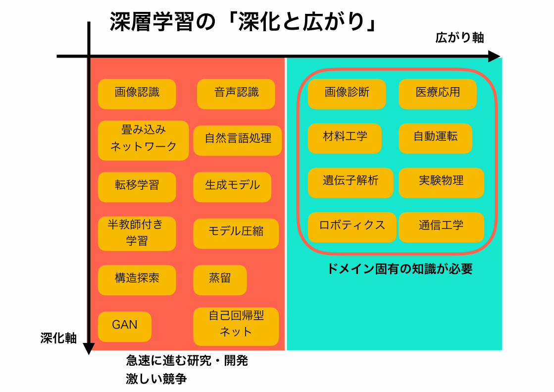
広がり軸
深化軸
画像診断
材料工学
遺伝子解析
構造探索 蒸留
GAN自己回帰型ネット
モデル圧縮
転移学習 実験物理
通信工学
自動運転
医療応用
ドメイン固有の知識が必要
深層学習の「深化と広がり」
画像認識 音声認識
自然言語処理畳み込みネットワーク
半教師付き学習
生成モデル
ロボティクス
急速に進む研究・開発 激しい競争
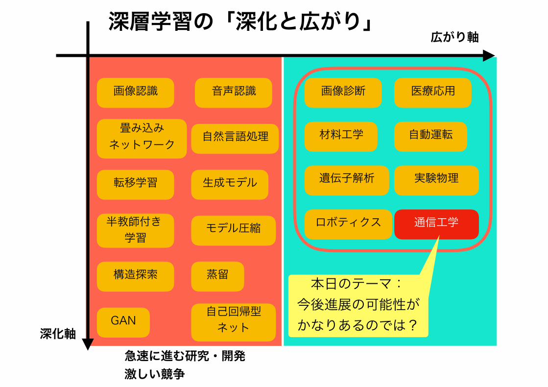
広がり軸
深化軸
画像診断
材料工学
遺伝子解析
構造探索 蒸留
GAN自己回帰型ネット
モデル圧縮
転移学習 実験物理
通信工学
自動運転
医療応用
深層学習の「深化と広がり」
画像認識 音声認識
自然言語処理畳み込みネットワーク
半教師付き学習
生成モデル
ロボティクス
急速に進む研究・開発 激しい競争
本日のテーマ:今後進展の可能性が かなりあるのでは?

cited from: http://icc2018.ieee-icc.org/workshop/promises-and-challenges-machine-learning-communication-networks-ml4com

cited from: https://www.itsoc.org/2019-ieee-international-symposium-on-information-theory

本日のテーマ:データ駆動型アルゴリズム設計
深層学習技術 ≠ 人工知能実現のための技術
通信系アルゴリズムとの自然な結びつき

本日のテーマ:データ駆動型アルゴリズム設計
深層学習技術 ≠ 人工知能実現のための技術
通信系アルゴリズムとの自然な結びつき
学習可能な確率モデル
多段関数の非凸最適化
データ駆動型アルゴリズム設計
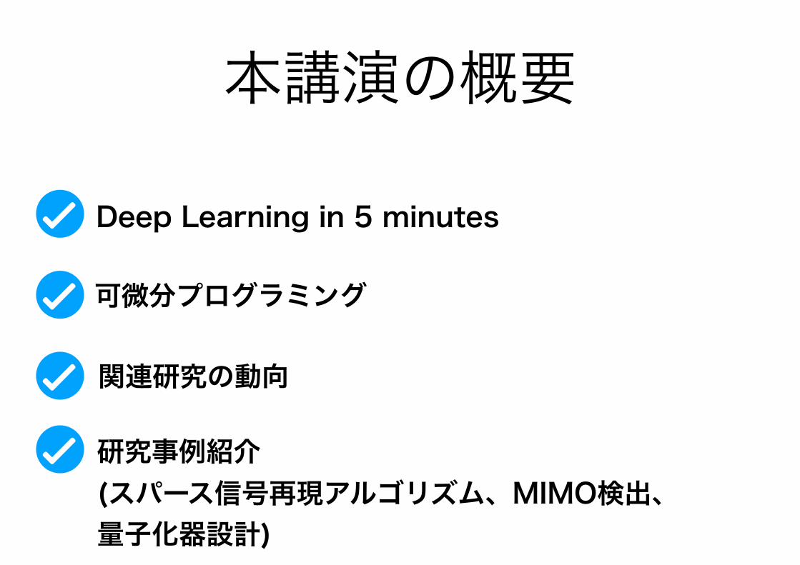
本講演の概要
Deep Learning in 5 minutes
可微分プログラミング
関連研究の動向
研究事例紹介 (スパース信号再現アルゴリズム、MIMO検出、 量子化器設計)

本講演の概要
Deep Learning in 5 minutes
可微分プログラミング
関連研究の動向
研究事例紹介 (スパース信号再現アルゴリズム、MIMO検出、 量子化器設計)

こんな関数を作りたい!
f : ℝn → ℝ 0: 猫
f : ℝn → ℝ 1: 犬
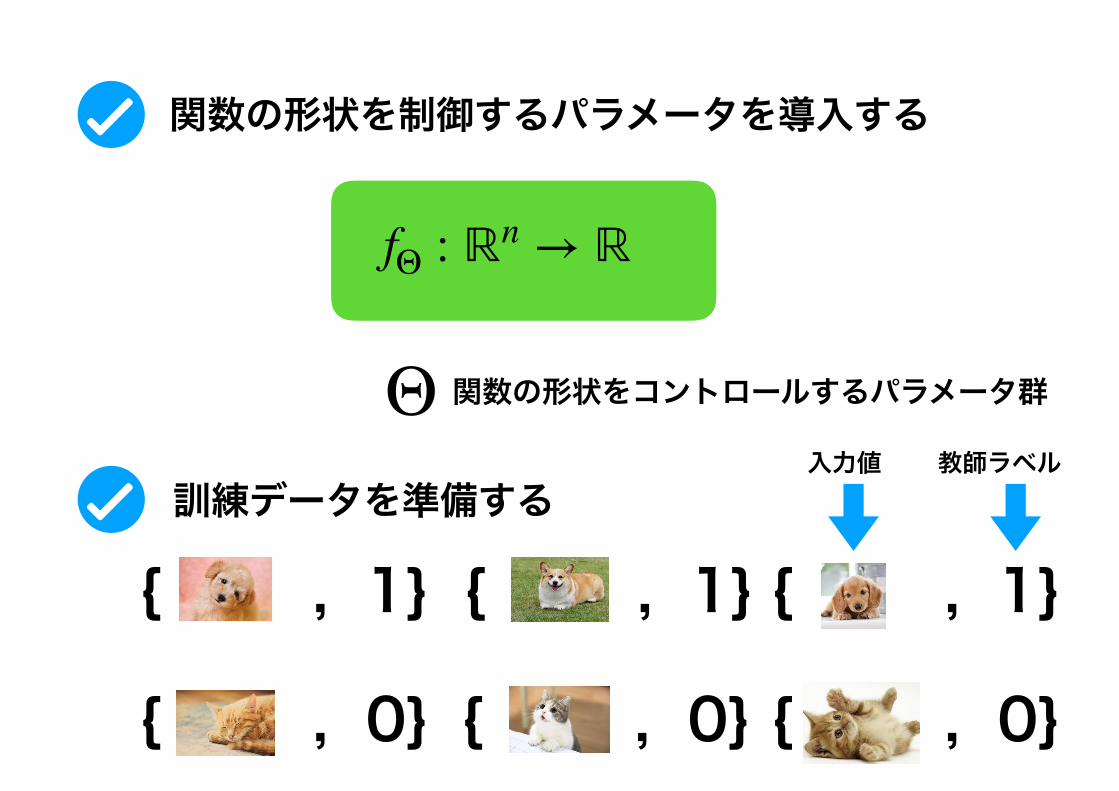
{ , 1}
fΘ : ℝn → ℝ
Θ 関数の形状をコントロールするパラメータ群
関数の形状を制御するパラメータを導入する
訓練データを準備する
{ , 1} { , 1}
{ , 0} { , 0} { , 0}
入力値 教師ラベル

パラメータを更新する(訓練・学習)
fΘ : ℝn → ℝ
{ , 1}{ , 1}{ , 0}
出力と教師ラベルとの間の食い違いがなるべく小さくなるように パラメータを更新する
大量の訓練データを利用
近い値?
y y

深層ネットワークモデル
Wh + b
線形層 活性化関数
g
fΘ : ℝn → ℝm
入力 出力
W h +=
h
bバイアス係数行列
h′�
h′�
Θ = {W1, b1, W2, b2, …}
活性化関数

W h += bh′�
人工ニューラル素子 (ふたたび)人工ニューロン素子は次の構造を持つ:
y = f
!n!
i=1
wixi + b
"(4)
関数 f は活性化関数であり、さまざまな種類の関数が利用されている:
アフィン変換
活性化関数

深層ネットワークの訓練Θ = {W1, b1, W2, b2, …} y = fΘ(x)
{ , 1}
損失関数
xloss(y, y)
y
訓練・学習過程では、損失関数値を最小化するようにパラメータを変更する
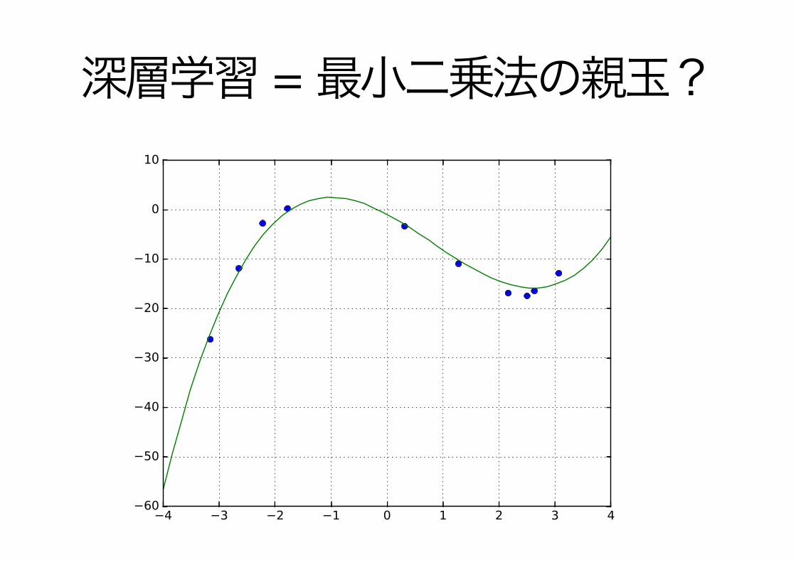
深層学習 = 最小二乗法の親玉?
パラメータ付き関数 f (x|w) の選択 (1)
多項式モデルx ∈ R
f (x |w) = w0 + w1x + w2x2 + · · ·+ wMxM
M をこの多項式モデルの次数と呼ぶ。
3次関数モデルによるフィッティング

最適化技法として確率的勾配法を利用
パラメータの勾配ベクトルの効率的な計算には 誤差逆伝播法(back prop)を利用
補足
よい汎化性能を得るためには、大量の訓練データが必要
一般には、非凸最適化となる

D = {(x1, y1), (x2, y2), …, (xT, yT)}訓練データ
確率的勾配法(SGD)
ミニバッチ B = {(xb1, yb1), (xb2, yb2), …, (xbK, ybK)}
目的関数 GB(Θ) =1K
K
∑k=1
loss(ybk − fΘ(xbk))
り、学習可能パラメータ Θの値を更新する(注4)。Step 1 (初期点設定) Θ := Θ0
Step 2 (ミニバッチ取得) B をランダムに生成(注5)
Step 3 (勾配ベクトルの計算) g := ∇GB(Θ)
Step 4 (探索点更新) Θ := Θ− αg
Step 5 (反復) Step 2に戻るミニバッチ B は確率変数であるため、確率的勾配法は、目的
関数 GB(Θ)の期待値を最小化している手順と見なすことができる。ニューラルネットワーク学習などの学習問題に確率的勾配法を適用することにより汎化能力の高いパラメータが見出されることが経験的に知られている [10]。確率的勾配法の振る舞いやミニバッチサイズ・学習率と汎化誤差との関係に関して、現在の深層学習分野において実験的・理論的研究が活発に進められている [16] [14]。上で述べた確率的勾配法は最も単純なものであり、多くのバ
リエーションや関連した収束加速手法が知られている [10]。例えば、RMSprop, Adam [17]などの手法は、広く深層学習の研究に利用されている。適切な確率的勾配法の選択、学習率の設定とそのスケジュー
リング、ミニバッチサイズなどは、ミニバッチ学習において最も重要なハイパーパラメータ群であり、学習結果の良否はこれらの設定の良し悪しに強く影響される。良いハイパーパラメータ設定を見つけるためには、多少の(場合によってはかなりの)試行錯誤的プロセスが必要となることもある。2. 2 誤差逆伝播法確率的勾配法の実行のためには、学習可能パラメータ Θの導
関数値 (勾配値) を計算する必要がある。誤差逆伝播法は、微分の連鎖則を利用することにより層構造 (または疎な計算グラフ構造)を持つ関数に対して効率の良い導関数値の計算を実現する。誤差逆伝播法は、前向き計算フェーズと後ろ向き計算フェー
ズの2つ計算フェーズを持つ。前向き計算フェーズでは、深層ニューラルネットワークにおいては入力層から順に出力層に向かって信号ベクトル値の評価が行われる。信号流グラフにおいても同様であり、各層での処理を多変数入力・ベクトル値関数φ1,φ2, . . .で表現すると y = φk(· · ·φ2(φ1(x))) として関数値を順に計算していく。なお、後ろ向き計算フェーズのために計算の途中結果は捨ててしまわずに残しておく必要がある。後ろ向き計算フェーズでは、まず、損失関数値を初期値とし
て、出力端から入力端に向かって、微分の連鎖律に従い計算が進行する。具体的な計算としては、φi に関するヤコビ行列と逆伝播ベクトルの積の計算が順次行われる。深層ニューラルネットワークの学習プロセスにおいては、大
量のデータを含む訓練データ集合が利用される。各層での前向き計算では、yk = g(Wkxk + bk)という計算を行う必要がある。
(注4):確率的勾配法はもともとミニバッチサイズが 1 の場合を想定して提案された。本稿では、ミニバッチ型の確率勾配法と陽に区別はしていない。(注5):実際には、全訓練データをミニバッチに分割し、そのミニバッチを順次利用するという手段が取られることが多い。すべての訓練データを使い果たすと(1 エポック)、改めて再度ミニバッチに分割し手続きを繰り返す。
ここで、W は係数行列であり、bk はバイアスベクトルである。すなわち、逆誤差伝播法の実行過程においては大量の行列・ベクトル積 (正確にはテンソル積)の計算を行う必要があり、この計算量が学習時間において支配的となる。2. 3 フレームワークフレームワークは、深層学習の要素技術の主たるものをライブラリの形でまとめたものであり、深層学習技術を利用した研究を進める上で欠かせないプログラム開発のプラットフォームである。代表的なフレームワークとして、TensorFlow、Keras,
PyTorch、Chainerなどがあり、ライブラリ仕様の拡張や機能拡充などを含めて、現在も活発な開発が継続中である。フレームワークを利用する最も大きな利点は、フレームワーク利用者 (プログラム開発者) が誤差逆伝播法の後ろ向き計算を自分で書かなくても良い点にある。すでに述べたように後ろ向き計算フェーズにおいては、微分の連鎖律に従い、行列・ベクトル積の計算と非線形関数の適用を反復して計算を行うことになる。前向き計算と異なり後ろ向き計算は記述をミスしやすく、その計算自体を陽にプログラムとして記述することは、プログラム開発者の著しい負担となる。すべてのフレームワークにおいて誤差逆伝播法の後ろ向き計算は自動化されており、フレームワーク利用者はその恩恵を受けることができる。各フレームワークの内部では計算グラフが構築され、その計算グラフに基づき、後ろ向き計算が実行される。計算グラフの構築においては、前向き計算時に動的に計算グラフが構成される環境 (define by run; PyTorch, Chainer) と事前に計算グラフを明示的にユーザ側で構築しておく環境 (define and run;
TensorFlow) がある。後者にない前者の大きな特徴は訓練データに依存した計算グラフの構築が可能であることが挙げられる。すなわち、前向き計算部 (計算グラフ構築部)において、ループや条件式の利用が可能である。すでに述べたように深層学習において、最も計算時間がかかるのが訓練プロセス実行時 (学習時)に実行される行列・ベクトル積 (正確には、ひとつのミニバッチが一気に計算されるためにテンソル積計算となる)の計算に必要とされる計算時間である。特に画像認識のように扱うべきテンソルのサイズが大きい場合には、GPUに基づく並列計算の利用が必須である。すべてのフレームワークは GPU 計算に対応しており、GPU プログラミングに精通していない開発者も容易に GPUをフル活用した計算を行うことができる。深層学習関連の研究を開始する際には、まずどのフレームワークを利用するかを決めなければならない。個人的な印象としては、アルゴリズム設計・評価研究においては、現時点では、TensorFlow(TensorFlow上で動作するKerasも含めて)とPyTorchの二択の状況に思える。フレームワークの利用者数の点では、世界的に TensorFlow が圧倒的に優位に立っており、それに伴い膨大な関連の情報をネット上で見つけることができる。また、最新の深層学習の論文に掲載されているアルゴリズムの実装をGithubにおいて公開することが広く行われており、TensorFlowによる実装が公開されているケースが非常に多い。一方 PyTorchは、TensorFlowと異なる計算グラフ構成の方
— 4 —
確率的勾配法に基づく最小化バリエーション
Momentum AdaDelta RMSprop Adam

誤差逆伝播法(backprop)
注:ただし途中の計算結果を残す前向き計算フェーズ(単なる値の評価)
損失関数
loss(y, y)
・パラメータの勾配ベクトルを効率良く求めることが目的 ・微分の連鎖律の利用(BCJRアルゴリズムにとても良く似ている)
後ろ向き計算フェーズヤコビ行列とベクトルの積を順次計算

本講演の概要
Deep Learning in 5 minutes
可微分プログラミング
関連研究の動向
研究事例紹介 (スパース信号再現アルゴリズム、MIMO検出、 量子化器設計)
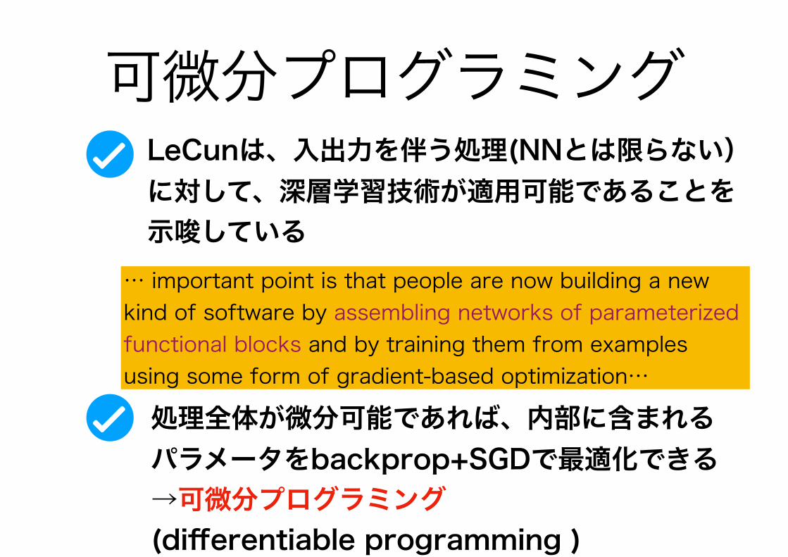
LeCunは、入出力を伴う処理(NNとは限らない)に対して、深層学習技術が適用可能であることを示唆している
処理全体が微分可能であれば、内部に含まれるパラメータをbackprop+SGDで最適化できる→可微分プログラミング(differentiable programming )
可微分プログラミング
… important point is that people are now building a new kind of software by assembling networks of parameterized functional blocks and by training them from examples using some form of gradient-based optimization…

•ビリーフプロパゲーション •ガウス・ザイデル法 •共役勾配法 •反復収縮法(IST) •AMP •ADMM…
反復型アルゴリズムの信号フロー
プロセスA
プロセスB
プロセスC
入力
出力
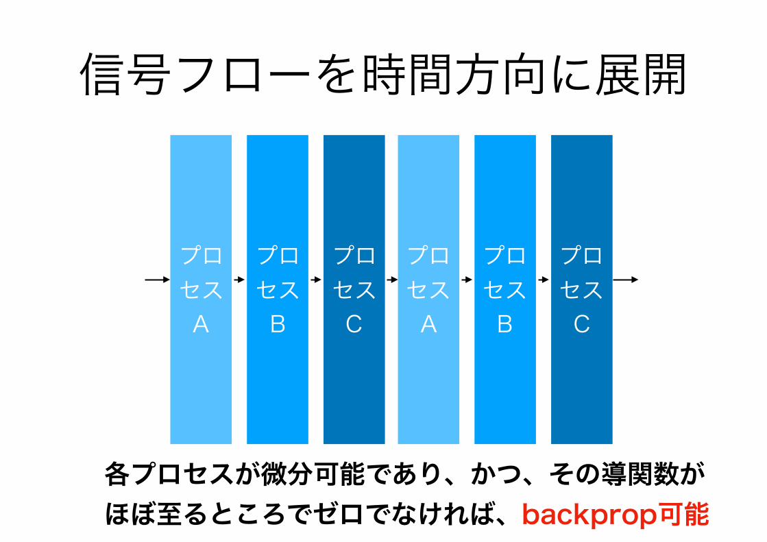
信号フローを時間方向に展開
プロセスA
プロセスB
プロセスC
プロセスA
プロセスB
プロセスC
各プロセスが微分可能であり、かつ、その導関数が ほぼ至るところでゼロでなければ、backprop可能
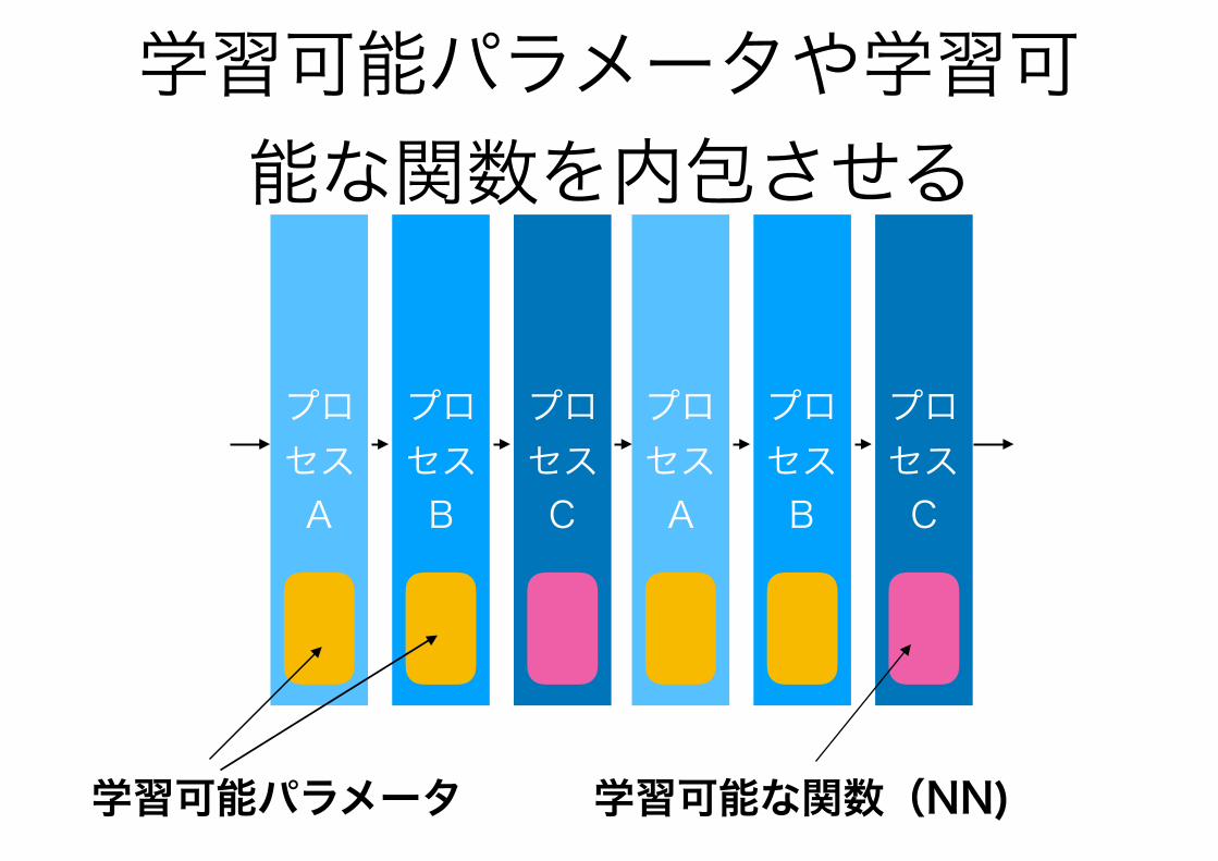
学習可能パラメータや学習可能な関数を内包させる
プロセスA
プロセスB
プロセスC
プロセスA
プロセスB
プロセスC
学習可能パラメータ 学習可能な関数(NN)

プロセスA
プロセスB
プロセスC
プロセスA
プロセスB
プロセスC
損失関数
{観測信号, 元信号}
推定アルゴリズムにおける学習フェーズ

End-to-End アプローチ
プロセスA
プロセスB
プロセスC
入力
出力
深層ニューラルネットワーク
入力
出力
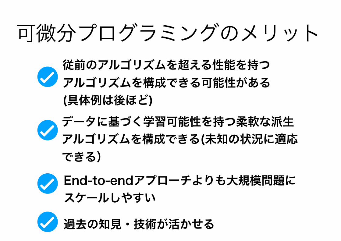
従前のアルゴリズムを超える性能を持つアルゴリズムを構成できる可能性がある(具体例は後ほど)
可微分プログラミングのメリット
データに基づく学習可能性を持つ柔軟な派生アルゴリズムを構成できる(未知の状況に適応できる)
End-to-endアプローチよりも大規模問題にスケールしやすい
過去の知見・技術が活かせる
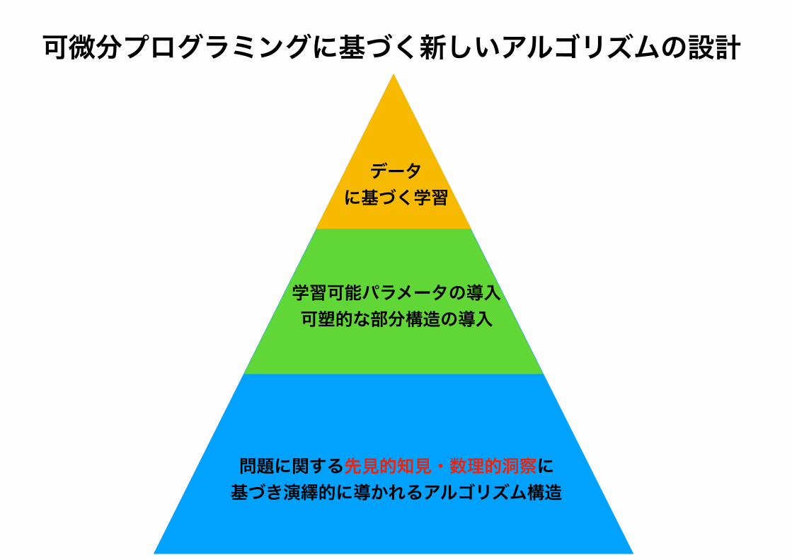
問題に関する先見的知見・数理的洞察に基づき演繹的に導かれるアルゴリズム構造
データに基づく学習
学習可能パラメータの導入 可塑的な部分構造の導入
可微分プログラミングに基づく新しいアルゴリズムの設計

どのパラメータを学習可能パラメータとするか、 は重要な問題(最終的な性能や学習の速度・安定性に大きく影響)
可微分プログラミングにおける 考えどころ
オンライン学習の設定なのか、オフライン学習の 設定なのか

本講演の概要
Deep Learning in 5 minutes
可微分プログラミング
関連研究の動向
研究事例紹介 (スパース信号再現アルゴリズム、MIMO検出、 量子化器設計)
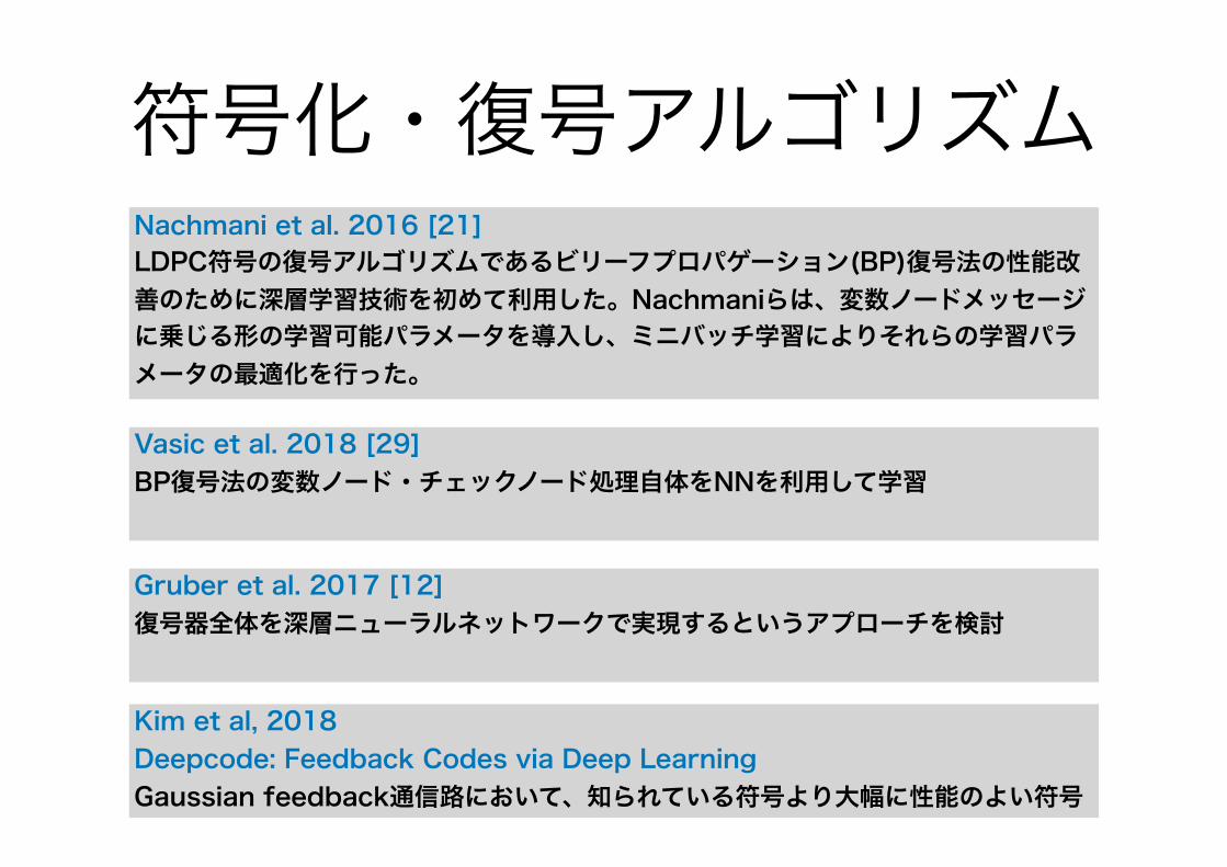
符号化・復号アルゴリズムNachmani et al. 2016 [21] LDPC符号の復号アルゴリズムであるビリーフプロパゲーション(BP)復号法の性能改善のために深層学習技術を初めて利用した。Nachmaniらは、変数ノードメッセージ に乗じる形の学習可能パラメータを導入し、ミニバッチ学習によりそれらの学習パラメータの最適化を行った。
Vasic et al. 2018 [29] BP復号法の変数ノード・チェックノード処理自体をNNを利用して学習
Gruber et al. 2017 [12] 復号器全体を深層ニューラルネットワークで実現するというアプローチを検討
Kim et al, 2018Deepcode: Feedback Codes via Deep Learning Gaussian feedback通信路において、知られている符号より大幅に性能のよい符号

変数ノード処理
ビリーフプロパゲーションに基づくLDPC符号の復号
βj→i = λj + ∑k∈B( j)\i
αk→j
β α β α
αi→j = 2 tanh−1 ∏k∈A(i)\j
tanh ( 12
βk→i)チェックノード処理
λ
すべての処理が微分可能!
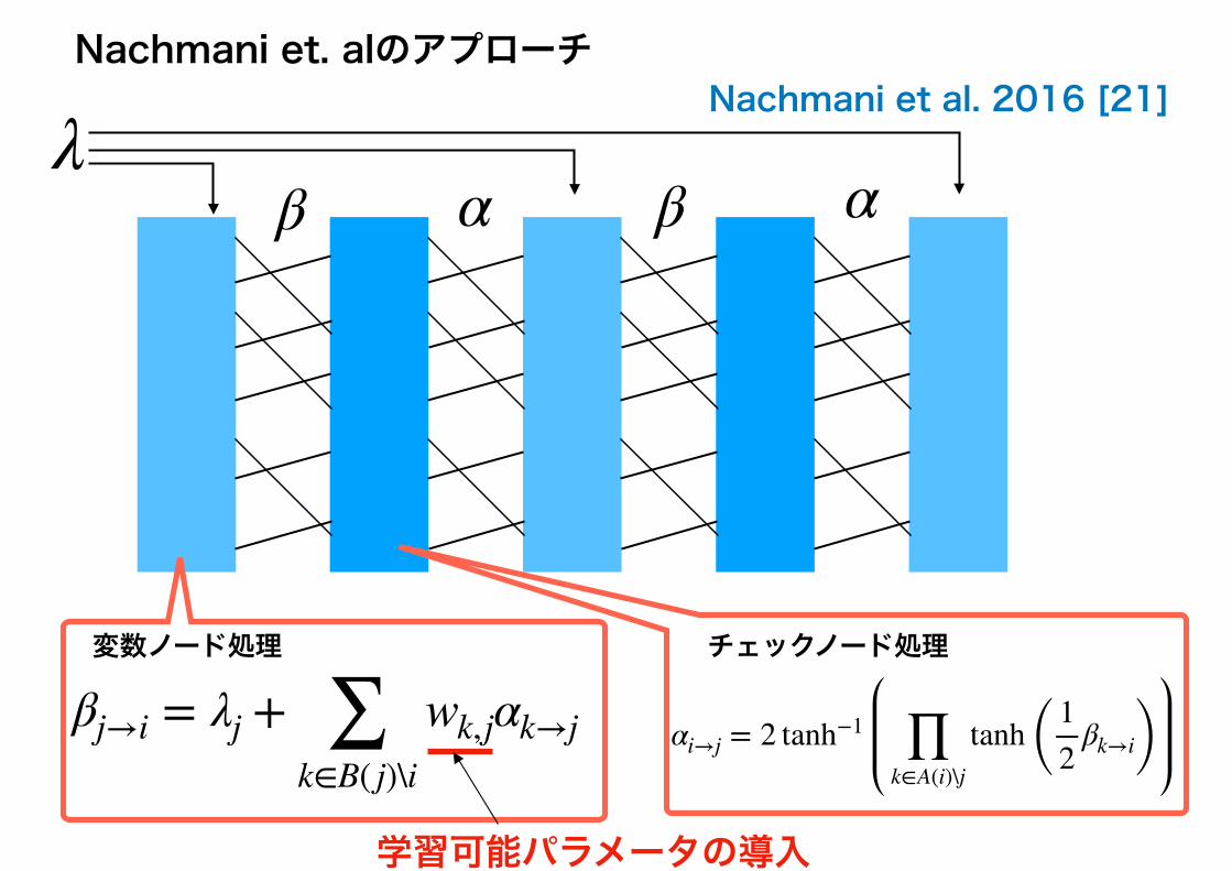
変数ノード処理
Nachmani et. alのアプローチ
βj→i = λj + ∑k∈B( j)\i
wk,jαk→j
β α β α
αi→j = 2 tanh−1 ∏k∈A(i)\j
tanh ( 12
βk→i)チェックノード処理
λ
学習可能パラメータの導入
Nachmani et al. 2016 [21]

本講演の概要
Deep Learning in 5 minutes
可微分プログラミング
関連研究の動向
研究事例紹介 (スパース信号再現アルゴリズム、MIMO検出、 量子化器設計)

研究事例紹介スパース信号再現アルゴリズム
過負荷MIMO 検出
LDPC符号に適した量子化器設計
本研究室の研究を紹介します
Ito, Takabe, W, “Trainable ISTA for Sparse Signal Recovery’’, IEEE ICC Workshop, May, 2018
Imanishi, Takabe, W, “Deep Learning-Aided Iterative Detector for Massive Overloaded MIMO Channels’’, submitted to IEEE GlobalSIP, 2018
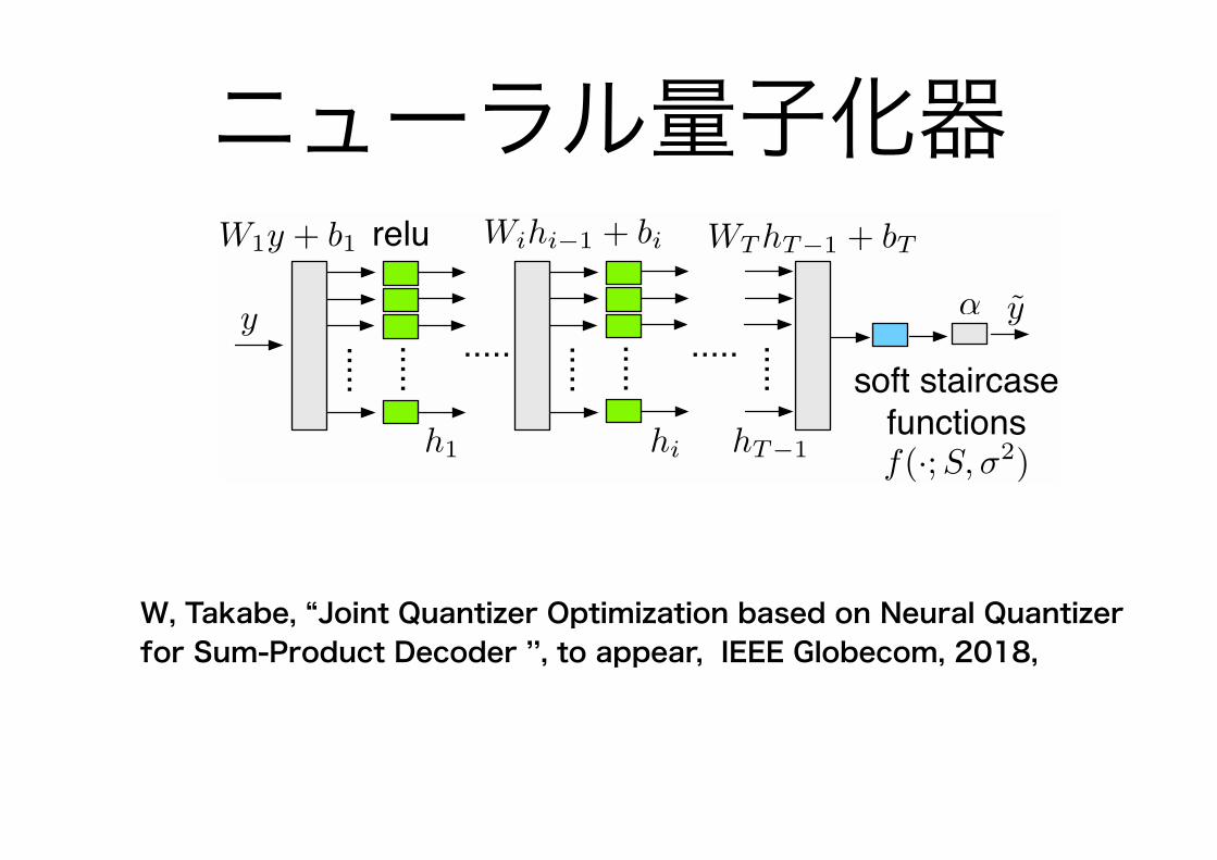
W, Takabe, “Joint Quantizer Optimization based on Neural Quantizer for Sum-Product Decoder ’’, to appear, IEEE Globecom, 2018

圧縮センシングの問題設定
+ =
観測行列 疎ベクトル ノイズ 観測ベクトル
観測ベクトルを見て、疎ベクトルを可能な限り正確に推定したい
「未知変数の数 > 方程式の本数」となる劣決定系問題
Ax
w y
N
M

II. SPARSE RECOVERY BY NEURAL NETWORKS
A. Binary compressed sensing
The main problem for binary compressed sensing is toreconstruct an unknown sparse signal vector x ∈ Rn from theobservation signal vector u ∈ {+1,−1}m under the conditionthat these signals satisfy the relationship:
u = sign(Ax). (1)
The sign function sign(·) is defined by
sign(a) =
!−1 (a ≤ 0),+1 (a > 0).
(2)
The matrix A ∈ Rm×n is called a sensing matrix. We assumethat the length of the observation signal vector u is smallerthan the length of the sparse signal vector x, i.e., m < n. Thisproblem setup is similar to that of the original compressedsensing. The notable difference between them is that theobservation signal u is binarized in a sensing process of binarycompressed sensing. A receiver obtains the observation signalu and then it tries to recover the corresponding hidden signal x.We here make two assumptions for the signal x and the sensingmatrix A. The first assumption is sparsity of the hidden signalx. The original binary signal x ∈ {0, 1}n contains only k non-zero elements, where k is a positive integer much smaller thann, i.e., Hamming weight of x should be k. We call the set ofbinary vectors with Hamming weight k is k-sparse signals.The second assumption is that the receiver completely knowsthe sensing matrix A.
B. Network architecture
When we need an extremely high speed signal processingor an energy-efficient sparse signal processing method forbattery powered sensor, it would be reasonable to develop asparse signal recovery algorithm suitable for the situation. Inthe sparse signal recovery method based on neural networksto be described in this section requires only several matrix-vector products to obtain an output signal, which is an estimatesignal of the sparse vector x. Thus, the proposed methodneeds smaller computational costs than those required byconventional iterative methods.
Our sparse recovery method is based on a 3-layer feedfor-ward neural network illustrated in Fig.??. This architecture isfairly common one; it consists of the input, hidden and outputlayers. Adjacent layers are connected by weighted edges andeach layer includes neural units that can keep real values. Asan activation function, we employed the sigmoid function todetermine the values of the hidden and output layers. In ourproblem setting, the observation signal u is fed into the inputlayer from the left in Fig.??. The signal propagates from leftto right and the output signal y eventually comes out from theoutput layer. The network should be trained so that the outputsignal y is an accurate estimation of the original sparse signalx. The precise description of the network in Fig.?? is givenby the following equations:
h = σ(Whu+ bh), (3)y = σ(Woh+ bo), (4)
x = round(y). (5)
Inputlayer
Hiddenlayer
Outputlayer
・・・
・・・・・
・・・
・・・
round
Fig. 1. Architecture of feedforward neural networks for sparse signalrecovery. An observation signal u comes from the left and is fed to the inputlayer. A sparse estimation vector comes out from the output layer. The sigmoidfunction is used as an activation function.
The function σ(·) is the sigmoid function defined by f(a) =1/(1 + e−a). In this paper, we will follow a simple con-vention that f(a) represents (f(a1), f(a2), . . . , f(an)) wherea = (a1, . . . , an). The round function round(a)(a ∈ R) givesthe nearest integer from a. The equation (??) defines thesignal transformation from the input layer to the hidden layer.An affine transformation is firstly applied to the input signalu ∈ {+1,−1}n and then the sigmoid function is applied. Theweight matrix Wh ∈ Rm×α and the bias vector bh ∈ Rα
defines the affine transformation. The resulting signal h ∈ Rα
is kept in the units in the hidden layer, which are calledhidden units. The parameter α thus means the number ofhidden units. From the hidden layer to the output layer, theequation (??) governs the second signal transformation. Thesecond transformation to yield the signal y consists of theaffine transformation, based on the weight matrix Wo ∈ Rα×n
and the bias vector bo ∈ Rn, and the nonlinear mapping basedon the sigmoid function. The vector y ∈ Rn emitted fromthe output layer is finally rounded to a nearest integer vectorbecause we assumed that non-zero elements in the originalsparse signal x takes the value one. Since the range of thesigmoid function lies in the open interval (0, 1), an element inthe estimate vector x should take the value zero or one.
C. Training
The network in Fig.?? can be seen as a parametrizedestimator x = round(Φθ(u)) where θ is the set of the trainableparameters θ = {Wh,Wo, bh, bo}. It is expected that thetrainable parameter θ should be adjusted in the training phaseso as to minimize the error probability Prob[x = x]. However,it may be computationally intractable to minimize the errorprobability directly. Instated of direct minimization of the errorprobability itself, we will minimize a loss function includinga cross entropy-like loss function and an L1-regularizationterm. In this subsection, the details of the training process isdescribed.
In the training phase of the network, the parameter θshould be updated in order to minimize the values of the givenloss function. Let D = {(u1, x1), . . . , (uL, xL)} be the setof the training data used in the training phase. The signalsui and xi relate as ui = sign(Axi), i = 1, 2, . . . , L. In the
ニューラルネットに 基づくスパース信号再現
Ito, W, SITA2016
0 50 100 150 200 2500.0
0.2
0.4
0.6
0.8
1.0
Index of signal component0 50 100 150 200 250
0.0
0.2
0.4
0.6
0.8
1.0
Fig. 2. Sparse signal recovery for a 6-sparse vector. (top: the original sparsesignal x, bottom: the output y = Φθ∗ (x) from the trained neural network.n = 256,m = 120)
0
0.1
0.2
0.3
0.4
0.5
0.6
0.7
0.8
1 2 3 4 5 6 7 8 9
Reco
very
rate
Learning steps
(x104)
Fig. 3. Learning steps and recovery rate. (n = 256,m = 140, k = 6)
the progress contains fluctuations. The recovery rate appears tobe saturated around 5.0×10⁴ steps. In following experiments,the number of learning steps is thus set to 5 × 10⁴ based onthis observation.
C. Sparse recovery by integer programming
We introduce integer programming (IP)-based sparse sig-nal recovery as a performance benchmark in the subsequentsubsections because it provides the optimal recovery rate. TheIP formulation shown here is based on the linear programmingformulation in [?]. Although IP-based sparse signal recoveryrequires huge computer resources, it is applicable to moderatesize problems if we employ a recent advanced IP solver. Weused IBM CPLEX Optimizer for solving the IP problem shownbelow. The problem needed to solve is to find a feasible binaryvector z = (z1, . . . , zn) ∈ {0, 1}n satisfying the following
0
0.2
0.4
0.6
0.8
1
0 50 100 150 200 250
Rec
over
y ra
te
Length of observation vector m
NN : k=4NN : k=6IP : k=4IP : k=6
Fig. 4. Recovery rates of the proposed scheme (denoted by NN). (n =256, k = 4, 6) As benchmarks, recovery rates of IP-based scheme is alsoincluded (denoted by IP).
conditions:n!
i=1
zi = k, (7)
∀i ∈ [1,m],n!
j=1
Ai,jzj > 0, if ui = +1, (8)
∀i ∈ [1,m],n!
j=1
Ai,jzj ≤ 0, if ui = −1, (9)
where Ai,j is the (i, j) element of the sensing matrix Aand ui is the i-th element of the observation signal u. If afeasible solution z∗ satisfying all the above conditions exists,it becomes an estimate x = z∗. It is clear that these conditionsare consistent with our setting of binary compressed sensing.
D. Experimental results
Fig.?? presents the recovery rates of the proposed schemeunder the condition where n = 256, k = 4, 6. The neuralnetwork shown in Fig.?? was used. In Fig.??, it is seen thatthe recovery rate tend to increase as m increases for all k. Therecovery rate is beyond 90% at m = 140 when the originalsignal is 4-sparse. It can be also observed that the recovery ratestrongly depends on the sparseness parameter k. For example,the recovery rate of k = 6 comes around 70% at m = 140.The IP-based sparse recovery provides the recovery rate 99%at m ≥ 60 when the original signal is 6-sparse vector. Onthe other hand, our neural network yields the recovery ratemore than 90% at m ≥ 240 when the original signal is 6-sparse. Although computation costs of the neural network inthe recovery phase are much smaller than those required forIP-based sparse recovery, the performance gap appears ratherhuge and the neural-based reconstruction should be furtherimproved.
IV. MAJORITY VOTING NEURAL NETWORKS
In the previous section, we saw that neural-based sparsesignal recovery is successful under some parameter setting
End-to-Endアプローチ どうも大きなシステムにうまくスケールしない→方向転換

既存手法: ISTAISITAはよく知られている反復型信号再現アルゴリズム
Brief review of ISTA
ISTA is a well-known sparse recovery algorithm defined by thefollowing simple recursion:
rt = st + βAT (y − Ast) (1)
st+1 = η(rt ; τ), (2)
where β represents a step size and η is the soft thresholdingfunction.
! The initial value is assumed to be s0 = 0.
! Lasso formulation is given by
1
2||y − Ax ||22 + λ||x ||1. (3)
Since the proximal operator of L1-regularization term ||x ||1 isthe soft thresholding function, ISTA can be seen as a proximalgradient descent algorithm
ηはソフトしきい値関数
Brief review of ISTA
ISTA is a well-known sparse recovery algorithm defined by thefollowing simple recursion:
rt = st + βAT (y − Ast) (1)
st+1 = η(rt ; τ), (2)
where β represents a step size and η is the soft thresholdingfunction.
! The initial value is assumed to be s0 = 0.
! Lasso formulation is given by
1
2||y − Ax ||22 + λ||x ||1. (3)
Since the proximal operator of L1-regularization term ||x ||1 isthe soft thresholding function, ISTA can be seen as a proximalgradient descent algorithm
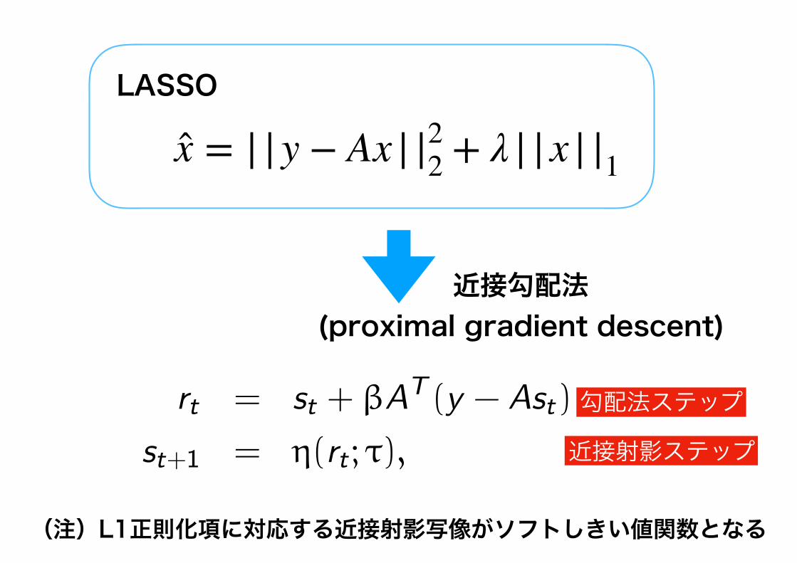
x = | |y − Ax | |22 + λ | |x | |1
LASSO
近接勾配法(proximal gradient descent)
勾配法ステップ
近接射影ステップ
(注)L1正則化項に対応する近接射影写像がソフトしきい値関数となる

LISTAK. Gregor, and Y. LeCun, ``Learning fast approximations of sparse coding,'' Proc. 27th Int. Conf. Machine Learning}, pp. 399--406, 2010.
2.2. スパース信号復元に関する関連研究 9
定義 2.1 関数 η : R !−→ RがE[η′(R)] = 0 (2.23)
を満たす時,ηをダイバージェンスフリー関数と呼ぶ.
ダイバージェンスフリー関数は任意の関数 ηを用いて
ηDF(r) = C · (η(r)− ER[η′(R)] · r) (2.24)
と構成することができる.ここで,パラメータCは任意の係数である.例として,関数 ηを軟判定閾値関数
η(r) = sign(r)max{|r|− τ, 0} (2.25)
としたとき,ダイバージェンスフリー関数は
ηDF(r) = C ·!η(r)−
!1
N
N"
i=1
I(|ri| > τ)
#· r#
(2.26)
となる.ここで,関数 I(|ri| > τ)は指示関数
I(|ri| > τ) =
$1 (if |ri| > τ)
0 (if |ri| ≤ τ)(2.27)
である.誤差分散 v2t , τ
2t の推定式は SEより導出される [18].推定式の導出については次章に
て詳細を述べる.Maらは IIDガウシアン行列やユニタリ不変行列が観測行列の場合について,線形推定誤差と非線形推定誤差が統計的に直交することを用いてこの SEが信頼できることを示した [18].
2.2.4 LISTA
前述した ISTA,AMP,OAMPと異なるアプローチとして,ISTAの構造を持つニューラルネットワークを用いたスパース信号復元法が提案された [27].この手法はLearned
ISTAと呼ばれている.LISTAでは漸化式
rt = Bst + Sy (2.28)
st+1 = η(rt; τt) (2.29)
を T 回反復計算することにより推定信号 x = sT を求める.参考として,LISTAの第 t
層の概要図を図 2.2に示す.
10 第 2章 基礎的事項
図 2.2: LAMPの t反復目の概要.学習可能パラメータはB, S, τt.st, yを受け取り st+1
を出力する.
LISTAは学習可能パラメータΘ = {S,B, {τt}T−1t=0 }を持つ.学習可能パラメータの初期
値は ISTAの設定に基づき,S = βAT , B = I−SAと設定する.Gregorらは,ISTAにおける閾値 τ を層依存の閾値 τtにして,訓練データ {(y, x)}に基づき loss(Θ) = ||x− x||を最小化するように学習可能パラメータ S,B, τtを調整することを提案した.学習可能パラメータの調整には,深層学習において用いられている学習法を用いている.これにより,LISTAは ISTAと比べて非常に高速な推定を可能とした.LISTAでは前述した全ての層で学習をした行列 S,B を共有するモデルの他に,全ての層で独立に行列 St, Bt の学習を行うモデルを考えることができる.全層で行列の共有を行う場合,B ∈ RN×N , S ∈ RN×M より,学習可能パラメータサイズは |Θ| = N2 +NM + T となる.これに対して,全層で独立に行列の学習を行う場合には,前者より復元性能が少し上昇するものの,学習可能パラメータサイズが |Θ| = T (N2 +NM + 1)となり,大幅に総数が増加することになる.ニューラルネットワークの学習可能パラメータは,学習後の振る舞いについての解析が一般的には困難である.しかしながら,LISTAは ISTAの構造を基にニューラルネットワークを構成しているため,それぞれの学習可能パラメータの振る舞いを ISTA
を基に考察することができると考えられている.学習可能パラメータ τtに着目すると,ISTAにおいて τ は軟判定閾値関数に対する閾値として用いられており,τ は rt − xの標準偏差を用いることが良いとされている.このことから,LISTAでは大量の訓練サンプルをもとに,統計的に rt − xの標準偏差の推定を行っていると考えることができる.また,ISTAでは τ の値は全ての反復で同じ値を用いているが,LISTAでは層ごとに異なる τtを用いることで,推定信号 rtに合わせた τtを使用して収縮推定を行うことができる.以上の特徴より,LISTAでは ISTAと比べて非常に高速な収束を可能としている.上述の手法以外にも,ISTAの構造を基にしたニューラルネットワークの構成について様々な研究がされている.例えば,ISTAのパラメータ調整についてではなく,ISTA
における軟判定閾値関数をMSE最適な関数に置き換える手法が提案されている [31].この手法では,MSE最適な関数を近似した関数を収縮関数として使用することを考え
学習可能パラメータ(行列)
可微分アプローチの先駆け

提案手法: TISTA
Ito, Takabe, W, “Trainable ISTA for Sparse Signal Recovery’’, IEEE ICC Workshop, May, 2018
Definition of TISTA
TISTA
The recursive formula of TISTA are summarized as follows:
rt = st + γtW (y − Ast), (4)
st+1 = ηMMSE (rt ; τ2t ), (5)
v2t = max
!||y − Ast ||22 −Mσ2
trace(ATA), ϵ
", (6)
τ2t =v2tN
(N + (γ2t − 2γt)M) +
γ2tσ
2
Ntrace(WW T ), (7)
! γt : trainable variable (trained by mini-batch training)
WはAの疑似逆行列

提案手法: TISTADefinition of TISTA
TISTA
The recursive formula of TISTA are summarized as follows:
rt = st + γtW (y − Ast), (4)
st+1 = ηMMSE (rt ; τ2t ), (5)
v2t = max
!||y − Ast ||22 −Mσ2
trace(ATA), ϵ
", (6)
τ2t =v2tN
(N + (γ2t − 2γt)M) +
γ2tσ
2
Ntrace(WW T ), (7)
! γt : trainable variable (trained by mini-batch training)
学習可能パラメータ(スカラー)
誤差分散の推定式
MMSE Shrinkage functionPlots of ηMMSE as a function of a received signal yα2 = 1, σ2 = 0.2, 0.8.
-3
-2
-1
0
1
2
3
-3 -2 -1 0 1 2 3
outp
ut of M
MS
E e
stim
ato
r
received signal
こんな感じの関数→
近接勾配ライクな処理

Block diagram of TISTAThe t-th iteration of the TISTA with learnable variable γt .
Process A
Process B
Process C
Signal flow
(a) Flow diagram of an iterative algorithm
Process A B C B CA
(b) Signal-flow network and deep learning process
Stochastic gradient descent
Loss function
Parameterupdates
Training data
TISTAの1ラウンド分のブロック図
損失関数
y x
学習可能パラメータ(スカラー)

は、ガウス雑音ベクトルである。圧縮センシングでは、与えられた観測ベクトル yから原信号 xを可能な限り高い精度で再現することを目標とする。圧縮センシングは、最近では広い工学分野においてその応用研究が進められている。例えば、医療画像処理分野 (特にMRI)では、サンプリング回数削減を実現するための画像再現原理として注目されている。また無線通信分野においてもランダムアクセスプロトコル、スペクトルセンシング、通信路推定などの分野で応用研究が発表されている。スパース信号再現アルゴリズムとして様々なアルゴリズムが
知られているが、ここではその一部について紹介するに留める。ISTA [4] [5]は、古くから知られる反復型アルゴリズムであり、次の再帰式に基づく計算を行う。
rt = st + βAT (y −Ast) (2)
st+1 = η(rt; τ). (3)
式 (2)は原信号に対する線形推定式であり、式 (3)は、軟しきい値関数 (soft thresholding function)η(rt; τ)に基づく非線形推定を表す関数である。以上の反復式は、元問題を Lasso形式x = argminx
12 ||y−Ax||22 + λ||x||1 に表現し、それを近接演算
子 (proximal operator)を利用した勾配法 (proximal gradient
descent)を書き下すと ISTAの反復式 (2)(3)が自然に導かれる。ISTAは単純な反復計算に基づくアルゴリズムであり、その
計算量も少ない (1ラウンドの計算につき、O(N2)の計算量で十分である)ため、大規模なスパース信号再現問題に対しても適用が可能である。しかし、解への収束は一般に遅く、数百回から数千回の反復が必要になることもある。また、ハイパーパラメータ β の設定も、かなりシビアであることが知られている。観測行列がある種の条件を満たすときに、ISTAと比べて圧
倒的に高速な収束を見せるスパース信号再現アルゴリズムとして、近年では、AMP [6]がよく知られている。AMPは、ISTA
に似た反復型の構造を持っている。また、最近では、OAMPなど AMPを改良したアルゴリズムもいくつか提案されている。4. 2 TISTAの詳細ここでは、文献 [15] に基づき、TISTAの詳細について述べ
る。TISTAの反復処理は、次の通りまとめられる。
rt = st + γtW (y −Ast), (4)
st+1 = ηMMSE(rt; τ2t ), (5)
v2t = max
!||y −Ast||22 −Mσ2
trace(ATA), ϵ
", (6)
τ2t =
v2tN
(N + (γ2t − 2γt)M) +
γ2t σ
2
Ntrace(WWT ). (7)
行列W はセンシング行列 Aの疑似逆行列である。式 (4)と式(5)は、ほぼ ISTAの線形推定式・非線形推定式と同様である。ただし、TISTA では、収縮関数として軟しきい値関数の代わりにMMSE収縮関数 ηMMSE(y;σ
2)が利用されている。ここで、注目すべき点として、式 (4)に登場する変数 γt が TISTA
における学習可能パラメータである。このパラメータは、学習プロセスにおいて適切な値に調整されることになる。式 (4)を一種の勾配法の過程としてみるとき、γt はステップサイズを定
めるパラメータと見ることもできる。ここで収縮関数である ηMMSE(y;σ
2)は
ηMMSE(y;σ2) =
#yα2
ξ
$pF (y; ξ)
(1− p)F (y;σ2) + pF (y; ξ),
(8)
と定義される。ここで、 ξ = α2 + σ2 であり、F は F (z; v) =1√2πv
exp%
−z2
2v
&と定義される。この MMSE 収縮関数は元信
号の事前確率分布 (この場合、ベルヌーイ・ガウシアン事前分布)により定まる。図 2に ηMMSE(y;σ
2)の概形を示す。この図から見て取れるようにパラメータ σ2 の値により、収縮関数の概形が制御されることになる。TISTA の反復過程において、この σ2 は推定誤差分散 τ2
t と等しく置かれており、推定誤差分散により適切な値が自動的に設定される。TISTA は ISTA をベースとして構成されたアルゴリズムであるが、学習パラメータの導入の仕方に大きな自由度があることを指摘しておきたい。TISTAの場合は γt として、スカラーの学習可能パラメータを各反復処理ごとに導入している。一方、既存の学習型スパース信号再生アルゴリズムである LISTA [11]
や LAMP [2]では、線形推定式に現れる行列そのものを学習可能パラメータとして置いている。このように深層学習に基づいて派生アルゴリズムを作り出す際には、高い構造上の自由度がある。どのような形で学習可能パラメータを導入するか、または可塑性のあるニューラルネットワーク関数近似をどの部分に導入するか、などの慎重な吟味・検討が性能の良い派生アルゴリズム構成のためには重要となる。
-3
-2
-1
0
1
2
3
-3 -2 -1 0 1 2 3
ou
tpu
t o
f M
MS
E e
stim
ato
r
received signal
図 2 TISTA で利用される MMSE 収縮関数
表 1 学習可能パラメータ数の比較 (T ラウンドの処理を仮定)
TISTA LISTA LAMP
# of params T T (N2 +MN + 1) T (NM + 2)
既存のアルゴリズムをベースとして、学習可能なアルゴリズムを構成する際には、どの部分を学習可能にするかの選択によって最終的なアルゴリズム全体の性能、学習プロセスの難易度・速度は変わってくる。表 1 に TISTA, LISTA, LAMP において利用される学習可能パラメータ数の比較を示す。TISTA
は従前のアルゴリズムと比べて圧倒的に学習可能パラメータ数
— 6 —
学習パラメータ数の比較
から、サポートベクトルマシン [1]のように学習における大域最適性の保証が可能な凸最適化に基づくアルゴリズムへの機械学習研究者の興味の移り変わりがあったように見える。今はニューラルネットワーク研究の第 3次ブームがやってきている状況であるが、それは、非凸最適化の復権、そして発展の時代を意味しているのかもしれない。世間的には、深層学習に対して、現状の技術水準を超えた期
待がちらほら出始めている気もするが、技術者・研究者としては、冷静に、その技術的な核は何かを見定めながら、深層学習技術とつきあっていくとともに、その可能性を関連研究分野において探るのが生産的である。
謝 辞本稿の研究の一部は科研費 基盤 (B)16H02878に基づく。名
古屋工業大学 高邉賢史氏からは、本稿の内容を改善するために有益なコメントを頂戴した。感謝の意を表する。
文 献[1] C. M. Bishop, “Pattern recognition and machine learning,
” Springer, 2006.
[2] M. Borgerding and P. Schniter, “Onsager-corrected deep
learning for sparse linear inverse problems,” 2016 IEEE
Global Conf. Signal and Inf. Proc. (GlobalSIP), Washing-
ton, DC, Dec. 2016, pp. 227-231.
[3] A. Caciularu, D. Burshtein “Blind channel equalization us-
ing variational autoencoders, ” arXiv:1803.01526, 2018.
[4] A. Chambolle, R. A. DeVore, N. Lee, and B. J. Lucier,
“Nonlinear wavelet image processing: variational problems,
compression, and noise removal through wavelet shrinkage,”
IEEE Trans. Image Process., vol. 7, no. 3, pp. 319–335, Mar,
1998.
[5] I. Daubechies, M. Defrise, and C. De Mol, “An iterative
thresholding algorithm for linear inverse problems with a
sparsity constraint,” Comm. Pure and Appl. Math., col. 57,
no. 11, pp. 1413-1457, Nov. 2004.
[6] D. L. Donoho, A. Maleki, and A. Montanari, “Message-
passing algorithms for compressed sensing,” Proceedings of
the National Academy of Sciences, vol. 106, no. 45, pp.
18914–18919, Nov. 2009.
[7] N. Farsad, and A. Goldsmith, “Neural network detec-
tion of data sequences in communication systems, ”
arXiv:1802.02046, 2018.
[8] K. Fukushima, “Neocognitron: A self-organizing neural net-
work model for a mechanism of pattern recognition unaf-
fected by shift in position,” Bio. Cybern., vol. 36, no. 4, pp.
193-202, 1980.
[9] I. Goodfellow, J. Pouget-Abadie, M. Mirza, B. Xu, D.
Warde-Farley, S. Ozair, A. Courville, and Y. Bengio,“Gen-
erative adversarial nets,”in Advances in neural information
processing systems, pp. 26722680, 2014.
[10] I. Goodfellow, Y. Bengio, A. Courville “Deep learning, ”
The MIT Press, 2016.
[11] K. Gregor, and Y. LeCun, “Learning fast approximations
of sparse coding,” Proc. 27th Int. Conf. Machine Learning,
pp. 399–406, 2010.
[12] T. Gruber, S. Cammerer, J. Hoydis, and S. ten Brink, “On
deep learning-based channel decoding, ” arXiv:1701.07738,
2017.
[13] G. Hinton, L. Deng, D. Yu, G. Dahl, A. Mohamed, N.
Jaitly, A. Senior, V. Vanhoucke, P. Nguyen, T. Sainath, and
B. Kingsbury, “Deep neural networks for acoustic modeling
in speech recognition: The Shared Views of Four Research
Groups,” IEEE Signal Processing Magazine, vol. 29, no. 6,
pp. 82-97, Nov. 2012.
[14] E. Hoffer, I. Hubara, D. Soudry, “Train longer, generalize
better: closing the generalization gap in large batch training
of neural networks,” arXiv:1705.08741, 2017.
[15] D. Ito, S. Takabe, T. Wadayama, “Trainable ISTA for sparse
signal recovery, ” IEEE International Conference on Com-
munications (ICC) workshop, Promises and Challenges of
Machine Learning in Communication, Kansas City, 2018.
(arXiv:1801.01978)
[16] N. S. Keskar, D. Mudigere, J. Nocedal, M. Smelyanskiy, P.
T. P. Tang, “On large-batch training for deep learning: gen-
eralization gap and sharp minima, ” in Proceedings of ICLR
2017.
[17] D. P. Kingma and J. L. Ba, “Adam: A method for stochas-
tic optimization,” arXiv:1412.6980, 2014.
[18] D. P. Kingma, M. Welling, “Auto-encoding variational
Bayes, ” arXiv:1312.6114v10, 2013.
[19] A. Krizhevsky, I. Sutskever, G. E. Hinton, “Imagenet classi-
fication with deep convolutional neural networks.” Advances
in Neural Inf. Proc. Sys. 2012, pp. 1097-1105, 2012.
[20] Y. A. LeCun, L. Bottou, G. B. Orr, and K. R. Muller, “Ef-
ficient backprop,” in Neural Networks: Tricks of the Trade,
G. B. Orr and K. R. Muller, Eds. Springer-Verlag, London,
UK, 1998, pp. 9-50.
[21] E. Nachmani, Y. Beery and D. Burshtein, “Learning to de-
code linear codes using deep learning,” 2016 54th Annual
Allerton Conf. Comm., Control, and Computing, 2016, pp.
341-346.
[22] E. Nachmani, E. Marciano, D. Burshtein and Y. Be’ery,
“RNN decoding of linear block codes, ” arXiv:1702.07560,
2017.
[23] A. van den Oord, S. Dieleman, H. Zen, K. Simonyan,
O. Vinyals, A. Graves, N. Kalchbrenner, A. Senior, K.
Kavukcuoglu, “WaveNet: a generative model for raw au-
dio,” arXiv:1609.03499v2, 2016.
[24] T. O’Shea and J. Hoydis, “An introduction to deep learn-
ing for the physical layer,” IEEE Transactions on Cognitive
Communications and Networking, vol. PP, no. 99, pp. 1-1.
[25] J. G. Proakis, “Digital communications (2nd ed.),”
McGraw-Hill Book, 1989.
[26] T. Richardson and R. Urbanke, “Modern coding theory,”
Cambridge University Press, 2008.
[27] D. E. Rumelhart, G. E. Hinton, and R. J. Williams, “Learn-
ing representations by back-propagating errors,” Nature,
vol. 323, no. 6088, pp. 533?536, 1986.
[28] R. Tibshirani, “Regression shrinkage and selection via the
lasso,” J. Royal Stat. Society, Series B, vol. 58, pp. 267–288,
1996.
[29] B. Vasic, X. Xiao and S. Lin, “Learning to decode LDPC
codes with finite-alphabet message passing, ” http://ita.
ucsd.edu/workshop/18/files/paper/paper_273.pdf
[30] T. Wadayama and S. Takabe, “Joint quantizer optimiza-
tion based on neural quantizer for sum-product decoder, ”
arXiv:1804.06002, 2018.
[31] W. Xu, Z. Wu, Y. L. Ueng, X. You, and C. Zhang, “Im-
proved polar decoder based on deep learning,”in IEEE In-
ternational Workshop on Signal Processing Systems (SiPS),
Oct 2017, pp. 16, 2017.
[32] 岡谷 貴之, “深層学習, ” 講談社, 2015.
[33] 斎藤 康毅, “ゼロから作る Deep Learning ―Python で学ぶディープラーニングの理論と実装, ” オライリー・ジャパン
[34] フランシス・ショレ (著), 巣籠 悠輔 (訳), “Pythonと Kerasによるディープラーニング,” 株式会社クイープ, 2018.
[35] “ディープラーニングに入門するためのリソース集と学習法(2018 年版),” https://qiita.com/keitakurita/items/
df3a07135c9cfad810c7, Qiita, 2018
— 8 —

Comparisons in NMSENMSE of TISTA, LISTA and AMP;Ai ,j ∼ N (0, 1/M),N = 500,M = 250, SNR = 40dB.The condition Ai ,j ∼ N (0, 1/M) is required for AMP to converge.
-45
-40
-35
-30
-25
-20
-15
-10
-5
0
2 4 6 8 10 12 14 16
NM
SE [d
B]
iteration
TISTALISTAAMP
Comparisons in NMSENMSE of TISTA, LISTA and AMP;Ai ,j ∼ N (0, 1/M),N = 500,M = 250, SNR = 40dB.The condition Ai ,j ∼ N (0, 1/M) is required for AMP to converge.
-45
-40
-35
-30
-25
-20
-15
-10
-5
0
2 4 6 8 10 12 14 16
NM
SE [d
B]
iteration
TISTALISTAAMP
TISTAの復元性能 (10%が非ゼロ元となる状況)
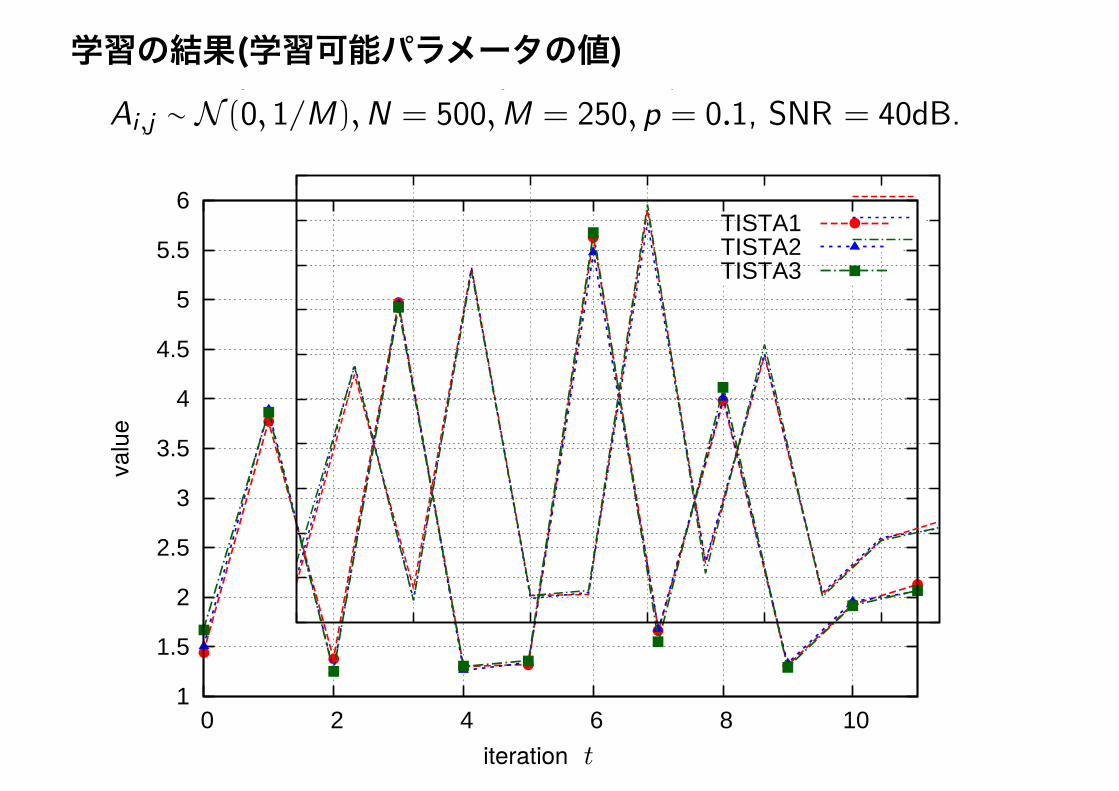
Values of γt
Three sequences of learned parameters γt ;Ai ,j ∼ N (0, 1/M),N = 500,M = 250, p = 0.1, SNR = 40dB.
1
1.5
2
2.5
3
3.5
4
4.5
5
5.5
6
0 2 4 6 8 10
valu
e
iteration
TISTA1TISTA2TISTA3
学習の結果(学習可能パラメータの値)Values of γt
Three sequences of learned parameters γt ;Ai ,j ∼ N (0, 1/M),N = 500,M = 250, p = 0.1, SNR = 40dB.
1
1.5
2
2.5
3
3.5
4
4.5
5
5.5
6
0 2 4 6 8 10
valu
e
iteration
TISTA1TISTA2TISTA3
なぜこの形が有利なのか(収束が速くなるのか)
謎。。。

Binary sensing matrix: TISTA,LISTAN = 500,M = 250, p = 0.1,Ai,j ∈ {−1, 1},SNR = 40 dB
-45
-40
-35
-30
-25
-20
-15
-10
-5
2 4 6 8 10 12 14 16
NM
SE [d
B]
iteration
TISTALISTA
観測行列が2値(+1, -1)の場合Binary sensing matrix: TISTA,LISTAN = 500,M = 250, p = 0.1,Ai,j ∈ {−1, 1},SNR = 40 dB
-45
-40
-35
-30
-25
-20
-15
-10
-5
2 4 6 8 10 12 14 16
NM
SE [d
B]
iteration
TISTALISTA
CDMA検出の状況に近い

過負荷MIMO検出問題送信アンテナ数 > 受信アンテナ数
基地局側は多くのアンテナを持つ余裕があるが、 端末側はコスト・消費電力などの点で、そんなに多くの アンテナを持てない
mmWave MIMOなどでは、アンテナの小型化・ 高集積化が進む
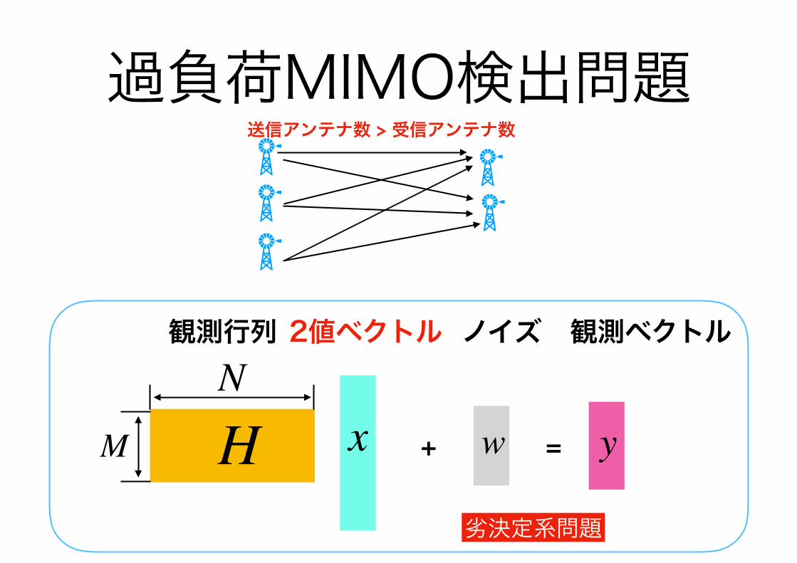
過負荷MIMO検出問題
+ =
観測行列 2値ベクトル ノイズ 観測ベクトル
H x w y
N
M
送信アンテナ数 > 受信アンテナ数
劣決定系問題

recovery problems. Recently, the authors proposed the train-able ISTA (TISTA) [18], which shows significantly faster con-vergence than those of known algorithms such as AMP.
The goal of this paper is to propose a novel trainable iter-ative detection algorithm for massive overloaded MIMO sys-tems, which is called the Trainable Iterative-Detector (TI-detector). Although deep learning architectures for massiveMIMO systems were recently proposed as deep MIMO de-tectors (DMDs) in [19, 20], no deep learning-aided iterativedetectors for massive overloaded MIMO channels have beenproposed as far as the authors are aware of. The architectureof the proposed algorithm is essentially based on TISTA [18]because the success of TISTA would imply that the TISTA ap-proach appears promising not only for sparse signal recoverybut also for various types of detection problems and inverseproblems for underdetermined systems.
2. PROBLEM SETTING
The section describes the channel model and introduces sev-eral definitions and notation. The number of transmit and re-ceive antennas is denoted by n and m, respectively. We onlyconsider the overloaded MIMO scenario in this paper wherem < n holds. It is also assumed that the transmitter doesnot use precoding and that the receiver perfectly knows thechannel state information, i.e., the channel matrix.
Let x ! [x1, x2, . . . , xn]T ∈ Sn be a vector which con-sists of a transmitted symbol xj (j = 1, . . . , n) from the jthantenna. The symbol S ⊂ C represents a symbol alphabet,i.e., a signal constellation. Similarly, y ! [y1, y2, . . . , ym]T ∈Cm denotes a vector composed of a received symbol yi (i =1, . . . ,m) by the ith antenna. A flat Rayleigh fading chan-nel is assumed here and the received symbols y then readsy = Hx + w, where w ∈ Cm consists of complex Gaussianrandom variables with zero mean and covariance σ2
wI . Thematrix H ∈ Cm×n is a channel matrix whose (i, j) entry hi,j
represents a path gain from the jth transmit antenna to the ithreceive antenna. Each entry of H independently follows thecomplex Gaussian distribution with zero mean and unit vari-ance. For the following discussion, it is convenient to derivean equivalent channel model defined over R, i.e., y = Hx+w,where
y !!Re(y)Im(y)
"∈ RM , H !
!Re(H) −Im(H)Im(H) Re(H)
",
x !!Re(x)Im(x)
"∈ SN , w !
!Re(w)Im(w)
"∈ RM ,
and (N,M) ! (2n, 2m). The signal set S is the real counterpart of S. The matrix H ∈ RM×N is converted from H .Similarly, the noise vector w consists of i.i.d. random vari-ables following the Gaussian distribution with zero mean andvariance σ2
w/2. Signal-to-noise ratio (SNR) per receive an-tenna is then represented by SNR ! Es/N0 = N/σ2
w, where
Es ! E[||Hx||22]/m stands for the signal power per receiveantenna and N0 ! σ2
w stands for the noise power per receiveantenna. Throughout the paper, we assume the QPSK modu-lation format, i.e., S ! {1 + j,−1 + j,−1− j, 1− j}, whichis equivalent to the BPSK modulation S ! {−1, 1}.
3. TRAINABLE ITERATIVE-DETECTOR
3.1. Brief review of ISTA
The iterative soft thresholding algorithm (ISTA) is the ori-gin of our proposed algorithm described later. ISTA [17] isknown as a powerful iterative algorithm for sparse signal re-covery from linear observations. The underlying model is de-scribed as u = Av+z where u and v are the linear observationand the sparse signal, respectively. The matrix A is called asensing matrix. ISTA is an iterative algorithm defined by thefollowing recursion:
rt = st + βAT (u−Ast) (1)st+1 = ξ(rt; τ). (2)
Eq.(1) represents a linear estimator and Eq.(2) represents anonlinear estimator based on the soft thresholding functionξ(rt; τ). The soft thresholding function matches to the Lapla-cian prior for the source sparse signal.
3.2. Details of TI-detector
Our proposal, TI-detector, is described by the following re-cursive formulas that are based on those of ISTA:
rt = st + γtW (y −Hst), (3)
st+1 = tanh
#rt|θt|
$, (4)
where tanh(·) is an element-wise function operator. The in-dex variable t represents the index of an iterative step (orlayer) and we set s1 = 0 as the initial value. This algorithmestimates a transmitted signal x from the received signal y andoutputs the estimate x = sT+1 after T iterative steps. Thematrix W in the linear estimator (3) is the Moore-Penrosepseudo inverse matrix of H , i.e., W ! HT (HHT )−1. Weuse the nonlinear estimator (4) based on the hyperbolic tan-gent function derived from the BPSK prior of the transmittedsignals. Note that this type of nonlinear estimator has beencommonly used in several iterative multiuser detection algo-rithms such as the soft parallel interference canceller [21].
The trainable parameters of TI-detector are 2T real scalarvariables {γt}Tt=1 and {θt}Tt=1 in (3) and (4), respectively.Note that the number of trainable parameters of TI-detectoris constant to N and M though a DMD contains O(N2T )parameters in T layers [19]. The trainable parameters areoptimized in a training process described later. The pa-rameters {γt}Tt=1, which control the strength of the lin-ear estimator, are introduced according to the structure of
提案手法:Trainable Iterative Detector
Fig. 1. The t-th layer of the TI-detector. The trainable param-eters are γt and θt.
TISTA [18], i.e., TISTA uses the same linear estimator in(3). The parameters {θt}Tt=1 control the nonlinear estimatorto perform appropriately. For simplicity, we use the nota-tion Θt ! {{γ1, θ1}, {γ2, θ2} . . . , {γt, θt}} as a set of theparameters up to the tth layer.
The computational complexity of TI-detector per itera-tion is O(MN) because one needs to calculate vector-matrixproducts Hst and W (y −Hst) that take O(MN) computa-tional steps. We need to calculate the pseudo inverse matrixW taking O(M3) computational steps only when H changes.
3.3. Training process of TI-detector
In order to retrieve reasonable detection performance fromTI-detector, it is critical to optimize the trainable parametersΘT . We here describe how to train the trainable parametersbased on standard deep learning techniques.
A training data di ! (xi, yi) is stochastically generatedas follows. A transmitted signal xi ∈ {+1,−1}N is gener-ated uniformly at random and the corresponding received sig-nal yi is then generated according to the probabilistic channelmodel yi = Hxi + w with a given H and a fixed varianceσ2w corresponding to a given SNR. A mini-batch consists of
D training data D ! {d1, d2, . . . , dD} and it is fed into theTI-detector. In the training process, we use an incrementaltraining as TISTA [18], i.e., the parameters are sequentiallytrained from the initial layer (t = 1) to the last layer (t = T )in an incremental manner. In the tth round of the incrementaltraining, we optimize the trainable parameters Θt to minimizethe squared loss function
L(Θt) !1
D
!
di∈D
∥xi − x(yi)∥22.
Note that x(yi) represents the output of TI-detector after tthlayer with the input yi, i.e., x(yi) ! st+1. Since the loss func-tion L(Θt) is a differentiable function, we can exploit backpropagation to compute the gradient of Θt efficiently and thegradient can be used in a stochastic gradient optimizer. Foreach round of the incremental training, K mini-batches areprocessed.
As described in Sec. 2, we assume a practical situation inwhich a channel matrix H is a random variable. The problemsetting is called a varying channel (VC) scenario in [19, 20].
Following the VC scenario, a matrix H is randomly generatedfor each mini-batch in a training process of TI-detector.
4. NUMERICAL RESULTS
In this section, we show several numerical results of TI-detector and compare them to those of the IW-SOAV, whichis known as an efficient iterative algorithm for massive over-loaded MIMO systems.
4.1. Experimental setup
We evaluate the detection performance of TI-detector undersituations with (N,M) = (200, 128) and (300, 192), wherethe ratio M/N = 0.64 is fixed. A transmitted signal is gener-ated as i.i.d. random variables with a distribution p(x = 1) =p(x = −1) = 1/2. The BER is then evaluated for a givenSNR. Following the VC scenario, we use randomly generatedchannel matrices for BER estimation, where a channel matrixis kept constant for consecutive D trials.
TI-detector was implemented by PyTorch 0.4.0 [22]. Thefollowing numerical experiments were carried out on a PCwith GPU NVIDIA GerForce GTX 1080 and Intel Core i7-6700K CPU 4.0GHz × 8. In this paper, a training process isexecuted with T = 50 rounds using the Adam optimizer [23]with learning rate ϵ. A training process takes within 25minutes under our environment. The hyperparameters of TI-detector are (D,K, ϵ) = (1250, 2000, 0.025) for (N,M) =(200, 128) and (1000, 1500, 0.025) for (300, 192). To cal-culate the BER of TI-detector, a sign function sgn(z) whichtakes −1 if z ≤ 0 and 1 otherwise is applied to the finalestimate sT+1.
As the baselines of detection performance, we use the IW-SOAV [8] and the standard MMSE detector. The IW-SOAVis a double loop algorithm whose inner loop is the W-SOAVoptimization recovering a signal using a proximal operator.Each round of the W-SOAV takes O(MN) computationalsteps, which is comparable to that of TI-detector. After finish-ing an execution of the inner loop with Kitr iterations, severalparameters are then updated in a re-weighting process basedon a tentative recovered signal. This procedure is repeated Ltimes in the outer loop. The total number of steps of the IW-SOAV is thus KitrL. In the following, we use the simulationresults in [8] with Kitr = 50.
4.2. Main results
We first present the BER performance of each detector as afunction of SNR for (N,M) = (200, 128) in Fig. 2. The re-sults show that the MMSE detector fails to detect transmittedsignals reliably (BER ≃ 10−1) because the system is under-determined. TI-detector exhibits the BER performance supe-rior to that of the IW-SOAV (L = 1), i.e., TI-detector achievesapproximately 5 dB gain at BER = 10−4 over the IW-SOAV
Imanishi, Takabe, W, “Deep Learning-Aided Iterative Detector for Massive Overloaded MIMO Channels’’, submitted to IEEE GlobalSIP, 2018
学習可能パラメータ(スカラー)
学習可能パラメータ(スカラー)

10-6
10-5
10-4
10-3
10-2
10-1
100
0 5 10 15 20 25 30
BE
R
SNR per receive antenna(dB)
TI-detector(T=50)MMSE
IW-SOAV(L=1,Kitr=50)IW-SOAV(L=2,Kitr=50)IW-SOAV(L=5,Kitr=50)
Fig. 2. BER performance for (N,M) = (200, 128).
(L = 1). Note that the computational cost for executing TI-detector with T = 50 is almost comparable to that of the IW-SOAV (L = 1). More interestingly, the BER performanceof TI-detector is fairly close to that of IW-SOAV (L ≥ 2).For example, with SNR = 20 dB, the BER estimate of TI-detector is 4.3× 10⁻⁵ whereas that of the IW-SOAV (L = 2)is 6.8 × 10⁻⁵. It should be noted that the total number itera-tions of the IW-SOAV (L = 2) is 100.
Figure 3 shows the BER performance for (N,M) =(300, 196). TI-detector successfully recovers transmitted sig-nals with lower BER than that of the IW-SOAV(L = 1). Itagain achieves about 5 dB gain against the IW-SOAV(L = 1)at BER = 10−5. Although the IW-SOAV (L ≥ 2) showsconsiderable performance improvements in this case, the gapsbetween the curves of TI-detector and the IW-SOAV (L ≥ 2)are within 2 dB at BER = 10−5.
Figure 4 displays the learned parameters {γt, |θt|} of TI-detector after a training process as a function of a layer indext(= 1, . . . , T ). We find that they exhibit a zigzag shape withdamping amplitude similar to that observed in TISTA [18].The parameter γt, the step size of a linear estimator, is ex-pected to accelerate the convergence of the signal recovery.Theoretical treatments for providing reasonable interpretationon these characteristic shapes of the learned parameters areinteresting open problems.
5. CONCLUDING REMARKS
In this paper, we proposed TI-detector, a deep learning-aidediterative decoder for massive overloaded MIMO channels. TI-detector contains two trainable parameters for each layer: γtcontrolling a step size of the linear estimator and θt dominat-ing strength of the nonlinear estimator. The total number ofthe trainable parameters in T layers is thus 2T , which is sig-nificantly smaller than that used in the previous studies suchas [19, 20]. This fact promotes fast and stable training pro-cesses for TI-detector. The numerical simulations show that
10-6
10-5
10-4
10-3
10-2
10-1
100
0 5 10 15 20 25
BE
R
SNR per receive antenna(dB)
TI-detector(T=50)MMSE
IW-SOAV(L=1,Kitr=50)IW-SOAV(L=2,Kitr=50)IW-SOAV(L=5,Kitr=50)
Fig. 3. BER performance for (N,M) = (300, 192).
0 1 2 3 4 5 6 7 8 9
5 10 15 20 25 30 35 40 45 50
valu
e
index t
γt
0
1
2
3
5 10 15 20 25 30 35 40 45 50
valu
e
index t
|θt|
Fig. 4. Sequences of learned parameters γt (upper) and |θt|(lower); (N,M) = (300, 192), SNR = 20[dB], 1 ≤ t ≤T = 50.
TI-detector outperforms the state-of-the-art IW-SOAV (L =1) by a large margin and achieves a comparable detection per-formance to the IW-SOAV (L ≥ 2). TI-detector thereforecan be seen as a promising iterative detector for overloadedMIMO channels providing an excellent balance between alow computational cost and a reasonable detection perfor-mance. There are several open problems regarding this study.Fast, adding a re-weighting process similar to the one usedin the IW-SOAV (L ≥ 2) to TI-detector seems an interestingdirection to improve the detection performance. Secondly, en-hancing TI-detector toward a large constellation such as QAMis a practically important problem.
AcknowledgementThe authors are very grateful to Mr. Ryo Hayakawa andProf. Kazunori Hayashi for providing their numerical resultsand simulation programs [8].
復号性能の比較 (N, M) = (300, 192)
6. REFERENCES
[1] S. Yang and L. Hanzo, “Fifty years of MIMO detection:the road to large-scale MIMOs,” IEEE Comm. Surveysand Tutorials, vol. 17, no. 4, pp. 1941-1988, Fourthquar-ter 2015.
[2] D. A. Shnidman, “A generalized Nyquist criterion andan optimum linear receiver for a pulse modulation sys-tem,” The Bell System Technical Journal, vol. 46, no. 9,pp. 2163-2177, Nov. 1967.
[3] W. van Etten, “An optimum linear receiver for multi-ple channel digital transmission systems,” IEEE Trans.Comm., vol. 23, no. 8, pp. 828-834, Aug. 1975
[4] K. K. Wong, A. Paulraj, and R. D. Murch, “Efficienthigh-performance decoding for overloaded MIMO an-tenna systems,” IEEE Trans. Wireless Commun., vol. 6,no. 5, pp. 1833-1843, May 2007.
[5] T. Datta, N. Srinidhi, A. Chockalingam, and B. S. Rajan,“Low-complexity near-optimal signal detection in un-derdetermined large-MIMO systems,” in Proc. NationalConf. Comm., Feb. 2012, pp. 1-5.
[6] Y. Fadlallah, A. Assa-El-Bey, K. Amis, D. Pastor, and R.Pyndiah, “New decoding strategy for underdeterminedMIMO transmission using sparse decomposition,” inProc. in Proc. 2013 21st Eur. Signal Proc. Conf., Sep.2013, pp. 1-5.
[7] Y. Fadlallah, A. Assa-El-Bey, K. Amis, D. Pastor, and R.Pyndiah, “New iterative detector of MIMO transmissionusing sparse decomposition,” IEEE Trans. Veh. Tech-nol., vol. 64, no. 8, pp. 3458-3464, Aug. 2015.
[8] R. Hayakawa and K. Hayashi, “Convex optimization-based signal detection for massive overloaded MIMOsystems,” in IEEE Trans. Wireless Comm., vol. 16, no.11, pp. 7080-7091, Nov. 2017.
[9] R. Hayakawa, K. Hayashi, H. Sasahara, and M. Naga-hara, “Massive overloaded MIMO signal detection viaconvex optimization with proximal splitting,” in Proc.2016 24th Eur. Signal Proc. Conf., Aug./Sep. 2016, pp.1383-1387.
[10] M. Nagahara, “Discrete signal reconstruction by sum ofabsolute values”ʡIEEE Signal Process. Lett., vol. 22,no. 10, pp. 15751579, Oct. 2015.
[11] G. E. Hinton and R. R. Salakhutdinov, “Reducing thedimensionality of data with neural networks,” Science,vol. 313, no. 5786, pp. 504-507, Jun. 2006:
[12] A. Krizhevsky, I. Sutskever, and G. E. Hinton, “Ima-genet classification with deep convolutional neural net-works.” in Proc. Advances in Neural Inf. Proc. Sys.2012, pp. 1097-1105, 2012.
[13] G. Hinton et al., “Deep neural networks for acousticmodeling in speech recognition: the shared views offour research groups,” IEEE Signal Processing Maga-zine, vol. 29, no. 6, pp. 82-97, Nov. 2012.
[14] B. Aazhang, B. P. Paris, and G. C. Orsak, “Neural net-works for multiuser detection in code-division multiple-access communications,” IEEE Trans. Comm., vol. 40,no. 7, pp. 1212-1222, Jul. 1992.
[15] E. Nachmani, Y. Beery, and D. Burshtein, “Learning todecode linear codes using deep learning,” 2016 54th An-nual Allerton Conf. Comm., Control, and Computing,2016, pp. 341-346.
[16] K. Gregor and Y. LeCun, “Learning fast approxima-tions of sparse coding,” in Proc. 27th Int. Conf. MachineLearning, pp. 399–406, 2010.
[17] I. Daubechies, M. Defrise, and C. De Mol, “An iterativethresholding algorithm for linear inverse problems witha sparsity constraint,” Comm. Pure and Appl. Math., vol.57, no. 11, pp. 1413-1457, Aug. 2004.
[18] D. Ito, S. Takabe, and T. Wadayama, “Trainable ISTAfor sparse signal recovery,” IEEE Int. Conf. Comm.,Workshop on Promises and Challenges of MachineLearning in Communication Networks, Kansas city,May. 2018. (arXiv:1801.01978)
[19] N. Samuel, T. Diskin and A. Wiesel, “Deep MIMO de-tection,” 2017 IEEE 18th Int. Workshop Signal Process-ing Advances in Wireless Comm., Jul. 2017, pp. 1-5.
[20] N. Samuel, T. Diskin and A. Wiesel, “Learning to de-tect,” arXiv: 1805.07631, 2018.
[21] D. Divsalar, M. K. Simon, and D. Raphaeli, “Improvedparallel interference cancellation for CDMA”, IEEETrans. Commun., vol. 46, no. 2, pp. 258-268, Feb. 1998.
[22] PyTorch, https://pytorch.org
[23] D. P. Kingma and J. L. Ba, “Adam: A method forstochastic optimization,” arXiv:1412.6980, 2014.
IW-SOAV:
5dBゲイン

10-6
10-5
10-4
10-3
10-2
10-1
100
0 5 10 15 20 25 30
BE
R
SNR per receive antenna(dB)
TI-detector(T=50)MMSE
IW-SOAV(L=1,Kitr=50)IW-SOAV(L=2,Kitr=50)IW-SOAV(L=5,Kitr=50)
Fig. 2. BER performance for (N,M) = (200, 128).
(L = 1). Note that the computational cost for executing TI-detector with T = 50 is almost comparable to that of the IW-SOAV (L = 1). More interestingly, the BER performanceof TI-detector is fairly close to that of IW-SOAV (L ≥ 2).For example, with SNR = 20 dB, the BER estimate of TI-detector is 4.3× 10⁻⁵ whereas that of the IW-SOAV (L = 2)is 6.8 × 10⁻⁵. It should be noted that the total number itera-tions of the IW-SOAV (L = 2) is 100.
Figure 3 shows the BER performance for (N,M) =(300, 196). TI-detector successfully recovers transmitted sig-nals with lower BER than that of the IW-SOAV(L = 1). Itagain achieves about 5 dB gain against the IW-SOAV(L = 1)at BER = 10−5. Although the IW-SOAV (L ≥ 2) showsconsiderable performance improvements in this case, the gapsbetween the curves of TI-detector and the IW-SOAV (L ≥ 2)are within 2 dB at BER = 10−5.
Figure 4 displays the learned parameters {γt, |θt|} of TI-detector after a training process as a function of a layer indext(= 1, . . . , T ). We find that they exhibit a zigzag shape withdamping amplitude similar to that observed in TISTA [18].The parameter γt, the step size of a linear estimator, is ex-pected to accelerate the convergence of the signal recovery.Theoretical treatments for providing reasonable interpretationon these characteristic shapes of the learned parameters areinteresting open problems.
5. CONCLUDING REMARKS
In this paper, we proposed TI-detector, a deep learning-aidediterative decoder for massive overloaded MIMO channels. TI-detector contains two trainable parameters for each layer: γtcontrolling a step size of the linear estimator and θt dominat-ing strength of the nonlinear estimator. The total number ofthe trainable parameters in T layers is thus 2T , which is sig-nificantly smaller than that used in the previous studies suchas [19, 20]. This fact promotes fast and stable training pro-cesses for TI-detector. The numerical simulations show that
10-6
10-5
10-4
10-3
10-2
10-1
100
0 5 10 15 20 25
BE
R
SNR per receive antenna(dB)
TI-detector(T=50)MMSE
IW-SOAV(L=1,Kitr=50)IW-SOAV(L=2,Kitr=50)IW-SOAV(L=5,Kitr=50)
Fig. 3. BER performance for (N,M) = (300, 192).
0 1 2 3 4 5 6 7 8 9
5 10 15 20 25 30 35 40 45 50
valu
e
index t
γt
0
1
2
3
5 10 15 20 25 30 35 40 45 50
valu
e
index t
|θt|
Fig. 4. Sequences of learned parameters γt (upper) and |θt|(lower); (N,M) = (300, 192), SNR = 20[dB], 1 ≤ t ≤T = 50.
TI-detector outperforms the state-of-the-art IW-SOAV (L =1) by a large margin and achieves a comparable detection per-formance to the IW-SOAV (L ≥ 2). TI-detector thereforecan be seen as a promising iterative detector for overloadedMIMO channels providing an excellent balance between alow computational cost and a reasonable detection perfor-mance. There are several open problems regarding this study.Fast, adding a re-weighting process similar to the one usedin the IW-SOAV (L ≥ 2) to TI-detector seems an interestingdirection to improve the detection performance. Secondly, en-hancing TI-detector toward a large constellation such as QAMis a practically important problem.
AcknowledgementThe authors are very grateful to Mr. Ryo Hayakawa andProf. Kazunori Hayashi for providing their numerical resultsand simulation programs [8].
学習の結果(学習可能パラメータの値)
謎のジグザグがふたたび出現
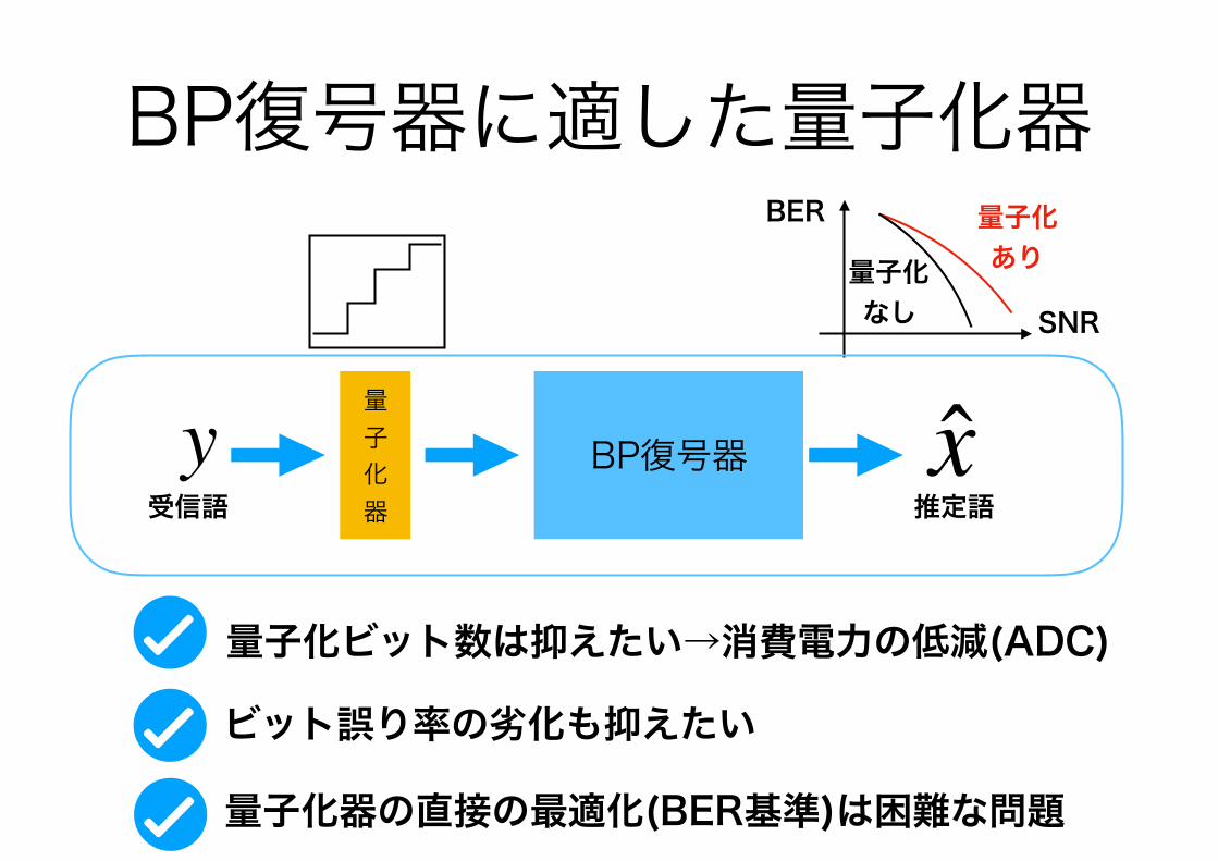
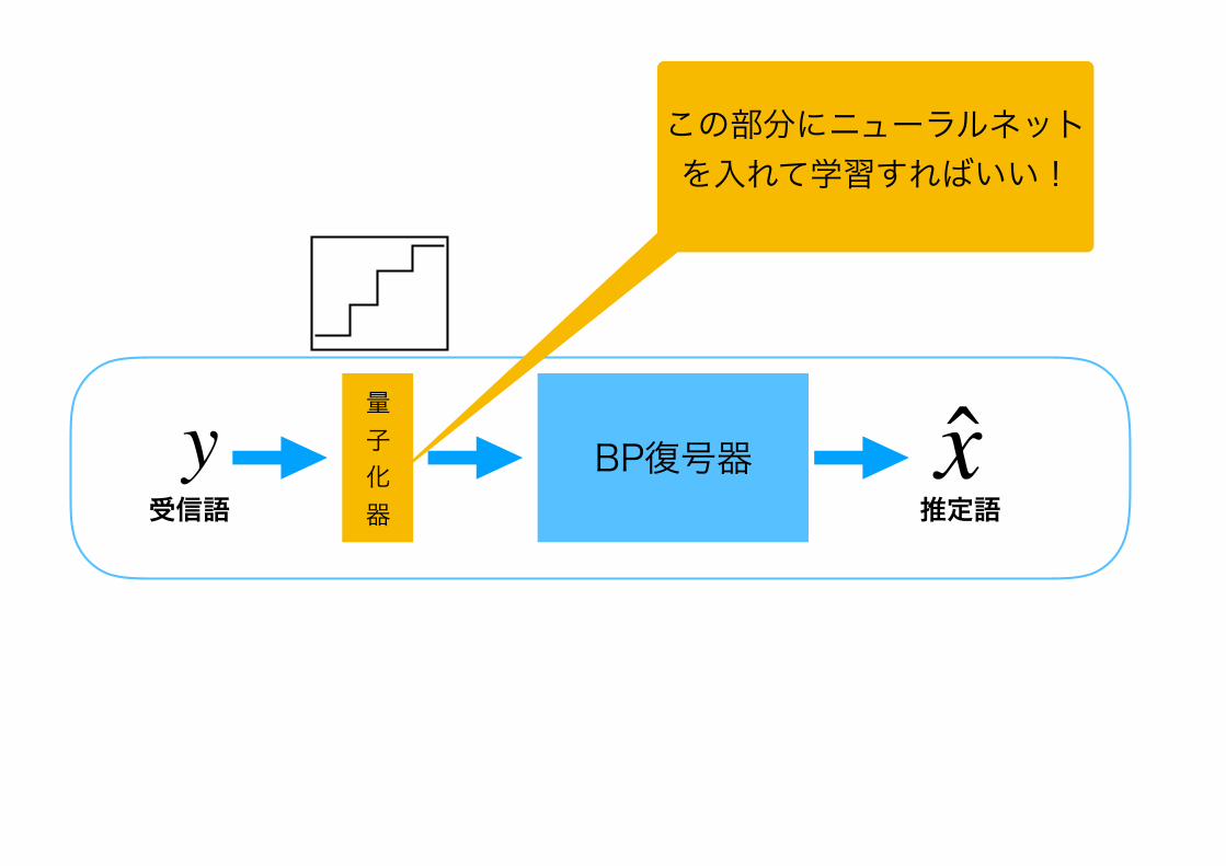
BP復号器に適した量子化器
BP復号器量 子 化 器
y受信語
x推定語
BER
SNR量子化 なし
量子化 あり
量子化ビット数は抑えたい→消費電力の低減(ADC)
ビット誤り率の劣化も抑えたい
量子化器の直接の最適化(BER基準)は困難な問題

Information Bottleneck method
• B. M. Kurkoski and H. Yagi, ``Quantization of binary-input discrete memoryless channels, ''IEEE Trans. Inf. Theory, vol. 60, no. 8, pp. 4544--4552, 2014.
• J. Lewandowsky and G. Bauch,``Information-optimum LDPC decoders based on the information bottleneck method, ‘' IEEE Access, vol. 6, pp. 4054--4071, Jan. 2018.
BP復号器量 子 化 器
y受信語
x推定語
この部分にニューラルネットを入れて学習すればいい!
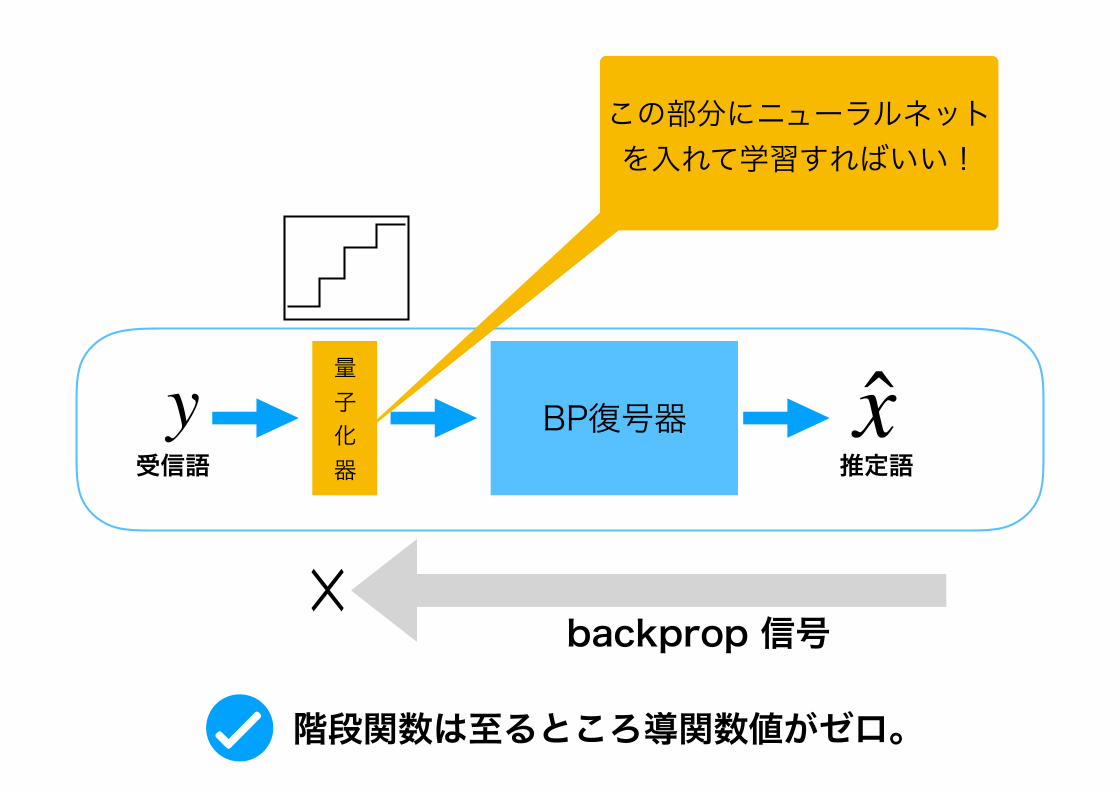
BP復号器量 子 化 器
y受信語
x推定語
この部分にニューラルネットを入れて学習すればいい!
階段関数は至るところ導関数値がゼロ。
☓backprop 信号
ニューラル量子化器
W, Takabe, “Joint Quantizer Optimization based on Neural Quantizer for Sum-Product Decoder ’’, to appear, IEEE Globecom, 2018,
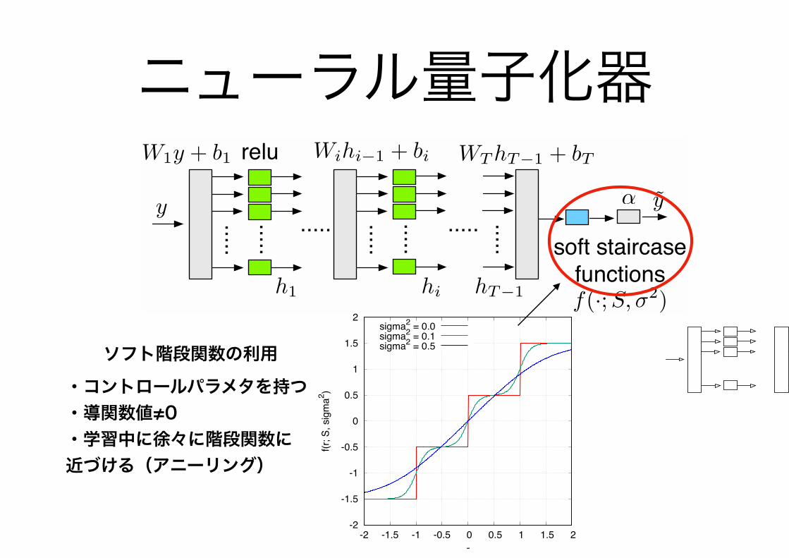
-2
-1.5
-1
-0.5
0
0.5
1
1.5
2
-2 -1.5 -1 -0.5 0 0.5 1 1.5 2
f(r; S
, sig
ma2 )
r
sigma2 = 0.0sigma2 = 0.1sigma2 = 0.5
Fig. 1. Plot of soft staircase functions f(r;S,σ2) for σ2 = 0, 0.1, 0.5, S ={−1.5,−0.5, 0.5, 1.5}.
Using these quantities, the MMSE estimator E[x|y] is givenby
E[x|y] =
! ∞
−∞xp(x|y)dx =
! ∞
−∞
xp(x, y)
p(y)dx (4)
=
"
s∈S s exp#
− (y−s)2
2σ2
$
"
s∈S exp#
− (y−s)2
2σ2
$ = f(r;S,σ2). (5)
III. NEURAL QUANTIZER
A. Architecture
The neural quantizer is a feed-forward neural networkdefined by
h1 = relu(W1y + b1) (6)
hi = relu(Wihi−1 + bi), i ∈ [2, T − 1] (7)
y = αf(WThT−1 + bT ;S,σ2), (8)
where y ∈ R is the input value and y ∈ R is the outputvalue. The function relu is the ReLU function defined by
relu(x)△= max{0, x}(x ∈ R) and we follow the convention
relu(x)△= (relu(x1), . . . , relu(xn)) for x = (x1, . . . , xn) ∈
Rn. From some preliminary experiments, we found that theReLU function is well behaved as an activation function inthe neural quantizer. The vectors hi ∈ Ru(i ∈ [1, T − 1]) arethe hidden state vectors representing the internal states of theneural quantizer. The length of the hidden state vectors u iscalled the hidden state dimension.
The trainable variables are W1 ∈ Ru×1, b1 ∈ Ru, Wi ∈Ru×u, bi ∈ Ru i ∈ [2, T − 1], WT ∈ R1×u, bT ∈ R andα ∈ R. The set of trainable variables is compactly denoted by
Θ△= {W1, . . . ,WT , b1, . . . , bT ,α} for simplicity. The level set
S△= {s0, s1, . . . , sL−1} is defined by si
△= i−L/2+ 1/2(i ∈
[0, L− 1]) for a given positive even integer L, which can beregarded as the number of quantization levels.
W1y + b1
y
soft staircasefunctions
..........
h1.....
hT−1
WThT−1 + bTrelu
α y
..........
hi
Wihi−1 + bi
..... .....f(·;S,σ2)
Fig. 2. Block diagram of the neural quantizer y = qNQ(y; σ2, L).
The entire input and output relationship of the neuralquantizer is denoted by qNQ(·;σ2, L) : R → R, namely,y = qNQ(y;σ2, L). The parameters u, T , σ2, and L arethe hyper parameters required to specify the structure of aneural quantizer. Figure 2 shows a block diagram of the neuralquantizer defined above.
A quantization function q : R → R is usually used inparallel, i.e., y = q(y) for y ∈ Rn. In the present case,the symbol-wise quantization by the neural quantizer canbe described by y = qNQ(y;σ2, L) for y ∈ Rn. Thisparallel quantization process can be carried out using n-neuralquantizers. Throughout the paper, we assume that the entire setof n-neural quantizers shares the trainable variables Θ. Thismeans that the n-neural quantizers are identical.
B. Supervised training with annealing
In the following discussion, we focus on the squared L2
distortion function as the distortion measure, i.e., µ(a, b)△=
||a − b||22. Our pragmatic approach to the quantizer designproblem is to recast the optimization problem as a minimiza-tion of the expected loss
E
%
K&
i=1
||x(i) − D(qNQ(y(i);σ2, L))||22
'
, (9)
where x(i), y(i)(i ∈ [1,K]) are randomly generated samplesof the random variables X and Y . The trainable variables inΘ of the neural quantizer are adjusted to lower the expectedloss by using a stochastic descent type algorithm such asSGD, Momentum, RMSprop, or Adam. If a detector algorithmor a decoding algorithm D is a differentiable function withrespect to its input variable, we can use backpropagation tocompute the gradients on the trainable variables in Θ. Thetemperature parameter σ2 should be appropriately decreasedin a supervised training process.
The supervised training process for the neural quantizer issummarized as follows.
(1) Set t = 1.(2) Sample a mini-batch
B△= {(x1, y1), (x2, y2), . . . , (xK , yK)}
according to the channel model (PX , PY |X), where
x(i), y(i)(i ∈ [1,K]) are realization vectors of ran-dom variables X and Y .
ニューラル量子化器
-2
-1.5
-1
-0.5
0
0.5
1
1.5
2
-2 -1.5 -1 -0.5 0 0.5 1 1.5 2
f(r; S
, sig
ma2 )
r
sigma2 = 0.0sigma2 = 0.1sigma2 = 0.5
Fig. 1. Plot of soft staircase functions f(r;S,σ2) for σ2 = 0, 0.1, 0.5, S ={−1.5,−0.5, 0.5, 1.5}.
Using these quantities, the MMSE estimator E[x|y] is givenby
E[x|y] =
! ∞
−∞xp(x|y)dx =
! ∞
−∞
xp(x, y)
p(y)dx (4)
=
"
s∈S s exp#
− (y−s)2
2σ2
$
"
s∈S exp#
− (y−s)2
2σ2
$ = f(r;S,σ2). (5)
III. NEURAL QUANTIZER
A. Architecture
The neural quantizer is a feed-forward neural networkdefined by
h1 = relu(W1y + b1) (6)
hi = relu(Wihi−1 + bi), i ∈ [2, T − 1] (7)
y = αf(WThT−1 + bT ;S,σ2), (8)
where y ∈ R is the input value and y ∈ R is the outputvalue. The function relu is the ReLU function defined by
relu(x)△= max{0, x}(x ∈ R) and we follow the convention
relu(x)△= (relu(x1), . . . , relu(xn)) for x = (x1, . . . , xn) ∈
Rn. From some preliminary experiments, we found that theReLU function is well behaved as an activation function inthe neural quantizer. The vectors hi ∈ Ru(i ∈ [1, T − 1]) arethe hidden state vectors representing the internal states of theneural quantizer. The length of the hidden state vectors u iscalled the hidden state dimension.
The trainable variables are W1 ∈ Ru×1, b1 ∈ Ru, Wi ∈Ru×u, bi ∈ Ru i ∈ [2, T − 1], WT ∈ R1×u, bT ∈ R andα ∈ R. The set of trainable variables is compactly denoted by
Θ△= {W1, . . . ,WT , b1, . . . , bT ,α} for simplicity. The level set
S△= {s0, s1, . . . , sL−1} is defined by si
△= i−L/2+ 1/2(i ∈
[0, L− 1]) for a given positive even integer L, which can beregarded as the number of quantization levels.
W1y + b1
y
soft staircasefunctions
..........
h1.....
hT−1
WThT−1 + bTrelu
α y
..........
hi
Wihi−1 + bi
..... .....f(·;S,σ2)
Fig. 2. Block diagram of the neural quantizer y = qNQ(y; σ2, L).
The entire input and output relationship of the neuralquantizer is denoted by qNQ(·;σ2, L) : R → R, namely,y = qNQ(y;σ2, L). The parameters u, T , σ2, and L arethe hyper parameters required to specify the structure of aneural quantizer. Figure 2 shows a block diagram of the neuralquantizer defined above.
A quantization function q : R → R is usually used inparallel, i.e., y = q(y) for y ∈ Rn. In the present case,the symbol-wise quantization by the neural quantizer canbe described by y = qNQ(y;σ2, L) for y ∈ Rn. Thisparallel quantization process can be carried out using n-neuralquantizers. Throughout the paper, we assume that the entire setof n-neural quantizers shares the trainable variables Θ. Thismeans that the n-neural quantizers are identical.
B. Supervised training with annealing
In the following discussion, we focus on the squared L2
distortion function as the distortion measure, i.e., µ(a, b)△=
||a − b||22. Our pragmatic approach to the quantizer designproblem is to recast the optimization problem as a minimiza-tion of the expected loss
E
%
K&
i=1
||x(i) − D(qNQ(y(i);σ2, L))||22
'
, (9)
where x(i), y(i)(i ∈ [1,K]) are randomly generated samplesof the random variables X and Y . The trainable variables inΘ of the neural quantizer are adjusted to lower the expectedloss by using a stochastic descent type algorithm such asSGD, Momentum, RMSprop, or Adam. If a detector algorithmor a decoding algorithm D is a differentiable function withrespect to its input variable, we can use backpropagation tocompute the gradients on the trainable variables in Θ. Thetemperature parameter σ2 should be appropriately decreasedin a supervised training process.
The supervised training process for the neural quantizer issummarized as follows.
(1) Set t = 1.(2) Sample a mini-batch
B△= {(x1, y1), (x2, y2), . . . , (xK , yK)}
according to the channel model (PX , PY |X), where
x(i), y(i)(i ∈ [1,K]) are realization vectors of ran-dom variables X and Y .
-2
-1.5
-1
-0.5
0
0.5
1
1.5
2
-2 -1.5 -1 -0.5 0 0.5 1 1.5 2
f(r; S
, sig
ma2 )
r
sigma2 = 0.0sigma2 = 0.1sigma2 = 0.5
Fig. 1. Plot of soft staircase functions f(r;S,σ2) for σ2 = 0, 0.1, 0.5, S ={−1.5,−0.5, 0.5, 1.5}.
Using these quantities, the MMSE estimator E[x|y] is givenby
E[x|y] =
! ∞
−∞xp(x|y)dx =
! ∞
−∞
xp(x, y)
p(y)dx (4)
=
"
s∈S s exp#
− (y−s)2
2σ2
$
"
s∈S exp#
− (y−s)2
2σ2
$ = f(r;S,σ2). (5)
III. NEURAL QUANTIZER
A. Architecture
The neural quantizer is a feed-forward neural networkdefined by
h1 = relu(W1y + b1) (6)
hi = relu(Wihi−1 + bi), i ∈ [2, T − 1] (7)
y = αf(WThT−1 + bT ;S,σ2), (8)
where y ∈ R is the input value and y ∈ R is the outputvalue. The function relu is the ReLU function defined by
relu(x)△= max{0, x}(x ∈ R) and we follow the convention
relu(x)△= (relu(x1), . . . , relu(xn)) for x = (x1, . . . , xn) ∈
Rn. From some preliminary experiments, we found that theReLU function is well behaved as an activation function inthe neural quantizer. The vectors hi ∈ Ru(i ∈ [1, T − 1]) arethe hidden state vectors representing the internal states of theneural quantizer. The length of the hidden state vectors u iscalled the hidden state dimension.
The trainable variables are W1 ∈ Ru×1, b1 ∈ Ru, Wi ∈Ru×u, bi ∈ Ru i ∈ [2, T − 1], WT ∈ R1×u, bT ∈ R andα ∈ R. The set of trainable variables is compactly denoted by
Θ△= {W1, . . . ,WT , b1, . . . , bT ,α} for simplicity. The level set
S△= {s0, s1, . . . , sL−1} is defined by si
△= i−L/2+ 1/2(i ∈
[0, L− 1]) for a given positive even integer L, which can beregarded as the number of quantization levels.
W1y + b1
y
soft staircasefunctions
..........
h1
.....
hT−1
WThT−1 + bTrelu
α y
..........
hi
Wihi−1 + bi
..... .....
f(·;S,σ2)
Fig. 2. Block diagram of the neural quantizer y = qNQ(y; σ2, L).
The entire input and output relationship of the neuralquantizer is denoted by qNQ(·;σ2, L) : R → R, namely,y = qNQ(y;σ2, L). The parameters u, T , σ2, and L arethe hyper parameters required to specify the structure of aneural quantizer. Figure 2 shows a block diagram of the neuralquantizer defined above.
A quantization function q : R → R is usually used inparallel, i.e., y = q(y) for y ∈ Rn. In the present case,the symbol-wise quantization by the neural quantizer canbe described by y = qNQ(y;σ2, L) for y ∈ Rn. Thisparallel quantization process can be carried out using n-neuralquantizers. Throughout the paper, we assume that the entire setof n-neural quantizers shares the trainable variables Θ. Thismeans that the n-neural quantizers are identical.
B. Supervised training with annealing
In the following discussion, we focus on the squared L2
distortion function as the distortion measure, i.e., µ(a, b)△=
||a − b||22. Our pragmatic approach to the quantizer designproblem is to recast the optimization problem as a minimiza-tion of the expected loss
E
%
K&
i=1
||x(i) − D(qNQ(y(i);σ2, L))||22
'
, (9)
where x(i), y(i)(i ∈ [1,K]) are randomly generated samplesof the random variables X and Y . The trainable variables inΘ of the neural quantizer are adjusted to lower the expectedloss by using a stochastic descent type algorithm such asSGD, Momentum, RMSprop, or Adam. If a detector algorithmor a decoding algorithm D is a differentiable function withrespect to its input variable, we can use backpropagation tocompute the gradients on the trainable variables in Θ. Thetemperature parameter σ2 should be appropriately decreasedin a supervised training process.
The supervised training process for the neural quantizer issummarized as follows.
(1) Set t = 1.(2) Sample a mini-batch
B△= {(x1, y1), (x2, y2), . . . , (xK , yK)}
according to the channel model (PX , PY |X), where
x(i), y(i)(i ∈ [1,K]) are realization vectors of ran-dom variables X and Y .
ソフト階段関数の利用・コントロールパラメタを持つ ・導関数値≠0 ・学習中に徐々に階段関数に近づける(アニーリング)

ニューラル量子化器
-2
-1.5
-1
-0.5
0
0.5
1
1.5
2
-2 -1.5 -1 -0.5 0 0.5 1 1.5 2
f(r; S
, sig
ma2 )
r
sigma2 = 0.0sigma2 = 0.1sigma2 = 0.5
Fig. 1. Plot of soft staircase functions f(r;S,σ2) for σ2 = 0, 0.1, 0.5, S ={−1.5,−0.5, 0.5, 1.5}.
Using these quantities, the MMSE estimator E[x|y] is givenby
E[x|y] =
! ∞
−∞xp(x|y)dx =
! ∞
−∞
xp(x, y)
p(y)dx (4)
=
"
s∈S s exp#
− (y−s)2
2σ2
$
"
s∈S exp#
− (y−s)2
2σ2
$ = f(r;S,σ2). (5)
III. NEURAL QUANTIZER
A. Architecture
The neural quantizer is a feed-forward neural networkdefined by
h1 = relu(W1y + b1) (6)
hi = relu(Wihi−1 + bi), i ∈ [2, T − 1] (7)
y = αf(WThT−1 + bT ;S,σ2), (8)
where y ∈ R is the input value and y ∈ R is the outputvalue. The function relu is the ReLU function defined by
relu(x)△= max{0, x}(x ∈ R) and we follow the convention
relu(x)△= (relu(x1), . . . , relu(xn)) for x = (x1, . . . , xn) ∈
Rn. From some preliminary experiments, we found that theReLU function is well behaved as an activation function inthe neural quantizer. The vectors hi ∈ Ru(i ∈ [1, T − 1]) arethe hidden state vectors representing the internal states of theneural quantizer. The length of the hidden state vectors u iscalled the hidden state dimension.
The trainable variables are W1 ∈ Ru×1, b1 ∈ Ru, Wi ∈Ru×u, bi ∈ Ru i ∈ [2, T − 1], WT ∈ R1×u, bT ∈ R andα ∈ R. The set of trainable variables is compactly denoted by
Θ△= {W1, . . . ,WT , b1, . . . , bT ,α} for simplicity. The level set
S△= {s0, s1, . . . , sL−1} is defined by si
△= i−L/2+ 1/2(i ∈
[0, L− 1]) for a given positive even integer L, which can beregarded as the number of quantization levels.
W1y + b1
y
soft staircasefunctions
..........
h1.....
hT−1
WThT−1 + bTrelu
α y
..........
hi
Wihi−1 + bi
..... .....f(·;S,σ2)
Fig. 2. Block diagram of the neural quantizer y = qNQ(y; σ2, L).
The entire input and output relationship of the neuralquantizer is denoted by qNQ(·;σ2, L) : R → R, namely,y = qNQ(y;σ2, L). The parameters u, T , σ2, and L arethe hyper parameters required to specify the structure of aneural quantizer. Figure 2 shows a block diagram of the neuralquantizer defined above.
A quantization function q : R → R is usually used inparallel, i.e., y = q(y) for y ∈ Rn. In the present case,the symbol-wise quantization by the neural quantizer canbe described by y = qNQ(y;σ2, L) for y ∈ Rn. Thisparallel quantization process can be carried out using n-neuralquantizers. Throughout the paper, we assume that the entire setof n-neural quantizers shares the trainable variables Θ. Thismeans that the n-neural quantizers are identical.
B. Supervised training with annealing
In the following discussion, we focus on the squared L2
distortion function as the distortion measure, i.e., µ(a, b)△=
||a − b||22. Our pragmatic approach to the quantizer designproblem is to recast the optimization problem as a minimiza-tion of the expected loss
E
%
K&
i=1
||x(i) − D(qNQ(y(i);σ2, L))||22
'
, (9)
where x(i), y(i)(i ∈ [1,K]) are randomly generated samplesof the random variables X and Y . The trainable variables inΘ of the neural quantizer are adjusted to lower the expectedloss by using a stochastic descent type algorithm such asSGD, Momentum, RMSprop, or Adam. If a detector algorithmor a decoding algorithm D is a differentiable function withrespect to its input variable, we can use backpropagation tocompute the gradients on the trainable variables in Θ. Thetemperature parameter σ2 should be appropriately decreasedin a supervised training process.
The supervised training process for the neural quantizer issummarized as follows.
(1) Set t = 1.(2) Sample a mini-batch
B△= {(x1, y1), (x2, y2), . . . , (xK , yK)}
according to the channel model (PX , PY |X), where
x(i), y(i)(i ∈ [1,K]) are realization vectors of ran-dom variables X and Y .
ニューラルネットによる 非線形座標変換
y

BP復号器量 子 化 器
x推定語
backprop 信号
-2
-1.5
-1
-0.5
0
0.5
1
1.5
2
-2 -1.5 -1 -0.5 0 0.5 1 1.5 2
f(r; S
, sig
ma2 )
r
sigma2 = 0.0sigma2 = 0.1sigma2 = 0.5
Fig. 1. Plot of soft staircase functions f(r;S,σ2) for σ2 = 0, 0.1, 0.5, S ={−1.5,−0.5, 0.5, 1.5}.
Using these quantities, the MMSE estimator E[x|y] is givenby
E[x|y] =
! ∞
−∞xp(x|y)dx =
! ∞
−∞
xp(x, y)
p(y)dx (4)
=
"
s∈S s exp#
− (y−s)2
2σ2
$
"
s∈S exp#
− (y−s)2
2σ2
$ = f(r;S,σ2). (5)
III. NEURAL QUANTIZER
A. Architecture
The neural quantizer is a feed-forward neural networkdefined by
h1 = relu(W1y + b1) (6)
hi = relu(Wihi−1 + bi), i ∈ [2, T − 1] (7)
y = αf(WThT−1 + bT ;S,σ2), (8)
where y ∈ R is the input value and y ∈ R is the outputvalue. The function relu is the ReLU function defined by
relu(x)△= max{0, x}(x ∈ R) and we follow the convention
relu(x)△= (relu(x1), . . . , relu(xn)) for x = (x1, . . . , xn) ∈
Rn. From some preliminary experiments, we found that theReLU function is well behaved as an activation function inthe neural quantizer. The vectors hi ∈ Ru(i ∈ [1, T − 1]) arethe hidden state vectors representing the internal states of theneural quantizer. The length of the hidden state vectors u iscalled the hidden state dimension.
The trainable variables are W1 ∈ Ru×1, b1 ∈ Ru, Wi ∈Ru×u, bi ∈ Ru i ∈ [2, T − 1], WT ∈ R1×u, bT ∈ R andα ∈ R. The set of trainable variables is compactly denoted by
Θ△= {W1, . . . ,WT , b1, . . . , bT ,α} for simplicity. The level set
S△= {s0, s1, . . . , sL−1} is defined by si
△= i−L/2+ 1/2(i ∈
[0, L− 1]) for a given positive even integer L, which can beregarded as the number of quantization levels.
W1y + b1
y
soft staircasefunctions
..........
h1
.....
hT−1
WThT−1 + bTrelu
α y
..........
hi
Wihi−1 + bi
..... .....
f(·;S,σ2)
Fig. 2. Block diagram of the neural quantizer y = qNQ(y; σ2, L).
The entire input and output relationship of the neuralquantizer is denoted by qNQ(·;σ2, L) : R → R, namely,y = qNQ(y;σ2, L). The parameters u, T , σ2, and L arethe hyper parameters required to specify the structure of aneural quantizer. Figure 2 shows a block diagram of the neuralquantizer defined above.
A quantization function q : R → R is usually used inparallel, i.e., y = q(y) for y ∈ Rn. In the present case,the symbol-wise quantization by the neural quantizer canbe described by y = qNQ(y;σ2, L) for y ∈ Rn. Thisparallel quantization process can be carried out using n-neuralquantizers. Throughout the paper, we assume that the entire setof n-neural quantizers shares the trainable variables Θ. Thismeans that the n-neural quantizers are identical.
B. Supervised training with annealing
In the following discussion, we focus on the squared L2
distortion function as the distortion measure, i.e., µ(a, b)△=
||a − b||22. Our pragmatic approach to the quantizer designproblem is to recast the optimization problem as a minimiza-tion of the expected loss
E
%
K&
i=1
||x(i) − D(qNQ(y(i);σ2, L))||22
'
, (9)
where x(i), y(i)(i ∈ [1,K]) are randomly generated samplesof the random variables X and Y . The trainable variables inΘ of the neural quantizer are adjusted to lower the expectedloss by using a stochastic descent type algorithm such asSGD, Momentum, RMSprop, or Adam. If a detector algorithmor a decoding algorithm D is a differentiable function withrespect to its input variable, we can use backpropagation tocompute the gradients on the trainable variables in Θ. Thetemperature parameter σ2 should be appropriately decreasedin a supervised training process.
The supervised training process for the neural quantizer issummarized as follows.
(1) Set t = 1.(2) Sample a mini-batch
B△= {(x1, y1), (x2, y2), . . . , (xK , yK)}
according to the channel model (PX , PY |X), where
x(i), y(i)(i ∈ [1,K]) are realization vectors of ran-dom variables X and Y .
損失関数
y x

10-6
10-5
10-4
10-3
10-2
10-1
100
1 1.2 1.4 1.6 1.8 2 2.2 2.4 2.6 2.8
Bit e
rror r
ate
SNR (dB)
Max steps=25Max steps=100Max steps=500No quantization
Fig. 6. BER curves of sum-product decoder with an 8-level trained neuralquantizer (L = 8, u = 8, T = 2). LDPC code: PEGReg504x1008 (n =1008, m = 504).
of tmax = 25 is very poor because the quantized values werenot appropriately learned. In the experiments, the BER perfor-mance rapidly improves when tmax > 50. The improvementis saturated around tmax = 500. The difference between thebaseline BER curve and the BER curve of tmax = 500 isapproximately 0.1 dB over the entire range of SNR. This resultindicates that the joint optimization method is able to providea quantizer with reasonable BER performance.
Figure 7 plots the trained quantizer functions. The experi-ment setting is the same as in the previous experiments dealingwith PEGReg504x1008. For the purpose of comparison, weincluded the result of a trained quantizer for a regular LDPCcode PEGReg252x504 [16] with n = 504 and m = 252.Figure 7 shows that an 8-level non-uniform quantizer func-tion is learned in the training phase. Moreover, the trainedquantizer automatically learned appropriate LLR conversion.Interestingly, the optimized quantizer for n = 504 is not thesame as the one for n = 1008. This may imply that the optimalquantizer is dependent on the choice of codes.
VI. CONCLUDING SUMMARY
In the present paper, a joint quantizer optimization methodfor constructing a quantizer matched to the sum-productalgorithms was presented. The neural quantizer allows us toexploit standard supervised learning techniques for DNNs tooptimize the quantizer. We limited our focus to the sum-product decoders, but the joint quantizer optimization methodproposed herein is expected to be universal, i.e., the proposedmethod can be applied to another decoding algorithm or adetection algorithm if the algorithm can be described as adifferentiable function.
ACKNOWLEDGMENT
The present study was supported in part by a JSPS Grant-in-Aid for Scientific Research (A) (Grant Number 17H01280),
-5
-4
-3
-2
-1
0
1
2
3
4
5
-2 -1.5 -1 -0.5 0 0.5 1 1.5 2
y
x
PEGReg252x504PEGReg504x1008
Fig. 7. Trained neural quantizers y = qNQ(x) (L = 8, u = 8, T = 2),LDPC codes: PEGReg504x1008 and PEGReg252x504.
and a JSPS Grant-in-Aid for Scientific Research (B) (GrantNumber 16H02878).
REFERENCES
[1] R. G. Gallager, Low-Density Parity-Check Codes, MIT Press, 1963.[2] D. J. C. MacKay, “Good error correcting codes based on very sparse
matrices, ” IEEE Trans. Inf. Theory, vol. 45, no. 2, pp. 399-431, Mar.1999.
[3] T. Richardson and R. Urbanke, Modern Coding Theory, CambridgeUniversity Press, 2008.
[4] N. Tishby, F. C. Pereira, and W. Bialek, “The information bottleneckmethod, ” in Proc. 37th Allerton Conference on Communication andComputation, Monticello, USA, 1999.
[5] J. Lewandowsky and G. Bauch, “Information-optimum LDPC decodersbased on the information bottleneck method, ” IEEE Access, vol. 6, pp.4054–4071, Jan. 2018.
[6] G. Zeitler, R. Koetter, G. Bauch, and J. Widmer, “On quantizer designfor soft values in the multiple-access relay channel, ” in Proc. IEEEICC, Dresden, Germany, 2009, pp. 1-5.
[7] G. Zeitler, “Low-precision analog-to-digital conversion and mutual in-formation in channels with memory, ” in Proc. 48th Annual AllertonConference on Communication, Control and Computing, Monticello,USA, 2010, pp. 745-752.
[8] B. M. Kurkoski and H. Yagi, “Quantization of binary-input discretememoryless channels, ” IEEE Trans. Inf. Theory, vol. 60, no. 8, pp.4544–4552, 2014.
[9] R. H. Walden, “Analog-to-digital converter survey and analysis,” IEEETrans. Commun., vol. 17, no. 4, pp. 539550, Apr. 1999.
[10] J. Singh, O. Dabeer, and U. Madhow, “On the limits of communicationwith low-precision analog-to-digital conversion at the receiver, ” IEEETrans. Commun., vol. 57, no. 12, pp. 36293639, Dec. 2009.
[11] A. Mezghani, M.-S. Khou and J. A. Nossek, “A Modied MMSE Receiverfor Quantized MIMO Systems,” in Proc. IEEE Workshop on SmartAntennas (WSA), 2007.
[12] F.Wang, J. Fang, H. Li, and S. Li, “Quantization design and chan-nel estimation for massive MIMO systems with one-bit ADCs,”ArXiv:1704.04709v1, 2017.
[13] E. Nachmani, Y. Beery and D. Burshtein, “Learning to decode linearcodes using deep learning,” 2016 54th Annual Allerton Conf. Comm.,Control, and Computing, 2016, pp. 341-346.
[14] T. O’Shea and J. Hoydis, “An Introduction to Deep Learning for thePhysical Layer,” IEEE Transactions on Cognitive Communications andNetworking, vol. PP, no. 99, pp. 1-1.
[15] S. P. Lloyd, “Least squares quantization in PCM, ” IEEE Transactionson Information Theory, vol.28,, pp. 129137, 1982.
[16] D. J. C. MacKay Encyclopedia of sparse graph codes, online:http://www.inference.phy.cam.ac.uk/mackay/codes/data.html
8-level trained neural quantizer. LDPC code: PEGReg504x1008 (n = 1008, m = 504).
ビット誤り率の比較 最終的に得られた量子化器

まとめ
通信工学においても、深層学習技術は使える →アルゴリズム設計の可能性が広がる実環境に柔軟に適応する通信系アルゴリズム
可微分プログラミングの考え方
ドメイン固有の知識が鍵

付録
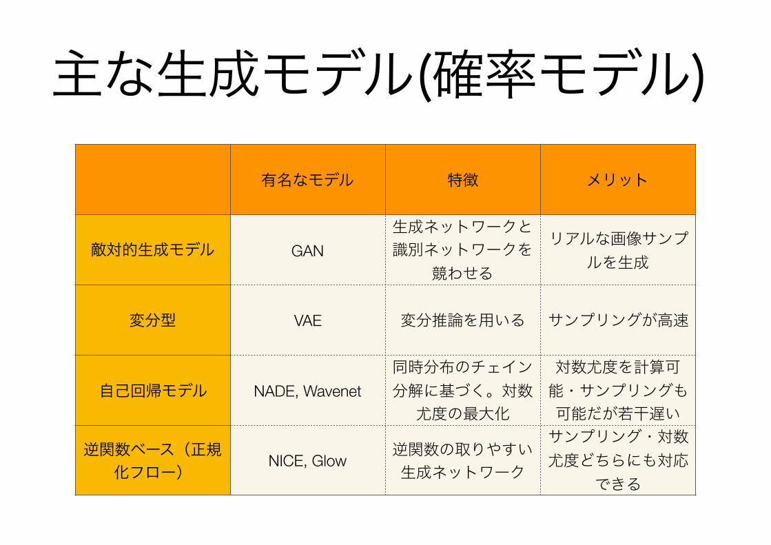
主な生成モデル(確率モデル)有名なモデル 特徴 メリット
敵対的生成モデル GAN生成ネットワークと識別ネットワークを
競わせる
リアルな画像サンプルを生成
変分型 VAE 変分推論を用いる サンプリングが高速
自己回帰モデル NADE, Wavenet同時分布のチェイン分解に基づく。対数尤度の最大化
対数尤度を計算可能・サンプリングも可能だが若干遅い
逆関数ベース(正規化フロー) NICE, Glow 逆関数の取りやすい
生成ネットワーク
サンプリング・対数尤度どちらにも対応
できる

DL計算環境についてコスト メリット デメリット
Google Colabratory
無料 環境構築不要 12時間以上の連続計算ができない
AWS, GCPなどクラウドを借りる 有料 環境構築ボタンひと
つ・メンテ不要
GPU付きインスタンスを借りるとそこそこのお値段
GPUつきマシンを買う 初期投資が必要
手元に実行環境があるのは色々快適
GPUの稼働率はそれほど高くない。。。
CPU 手元のCPUを利用すればタダ
気軽に試せる 遅い(相対的に)

汎化誤差誤差
反復回数
訓練誤差
テスト誤差
過学習 領域
訓練データに含まれない初見のデータに対して適切な出力を与えることが望ましい
最適化技術が大事 正則化技術が大事
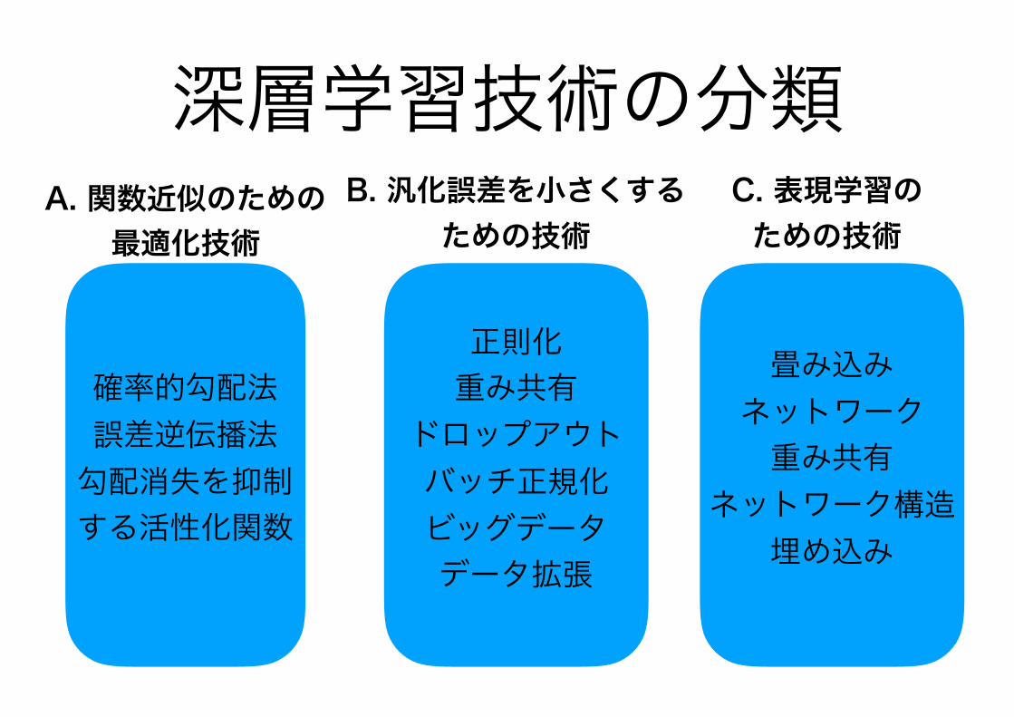
深層学習技術の分類
確率的勾配法 誤差逆伝播法 勾配消失を抑制する活性化関数
A. 関数近似のための 最適化技術
正則化 重み共有
ドロップアウト バッチ正規化 ビッグデータ データ拡張
B. 汎化誤差を小さくする ための技術
畳み込み ネットワーク 重み共有
ネットワーク構造埋め込み
C. 表現学習の ための技術

class Net(nn.Module): def __init__(self): super(Net, self).__init__() self.fc1 = nn.Linear(2, 2) self.fc2 = nn.Linear(2, 2) def forward(self, x): x = F.sigmoid(self.fc1(x)) x = F.sigmoid(self.fc2(x)) return x
model = Net() loss_func = nn.MSELoss() optimizer = optim.Adam(model.parameters(), lr=0.1)
DLフレームワーク・PyTorchによるプログラム例
ネットワークの定義部 順方向計算のみを記述すればよい。 誤差逆伝播法の後ろ向き計算フェーズは 明示的にユーザが書く必要ない
ネットワークのインスタンス化損失関数の指定
オプティマイザの指定
GPUの利用も非常に簡単。深層学習以外の分野でも有用!
深層学習向けのハードウェア推論フェーズ (前向き計算)、逆伝播フェーズ(後ろ向き計算)のいずれにも大量の行列ベクトル積計算が必要とされる。汎用 CPU以上に効率の良い計算が可能な GPU、または、専用のハードウェアへの注目が集まっている。
http://www.nvidia.co.jp/object/tesla-servers-jp.html出典
NVIDIA TESLA GPU Google Tensor Processing Unit (TPU)
http://itpro.nikkeibp.co.jp/atcl/ncd/14/457163/052001464/出典
GPU/ASIC
Related Documents