CDS 301 Fall, 2008 Scalar Visualization Chap. 5 September 23, 2008 Jie Zhang Copyright ©

CDS 301Fall, 2008

Scalar VisualizationChap. 5

September 23, 2008

Jie ZhangCopyright ©

Outline

5.1. Color Mapping5.2. Designing Effective Colormaps5.3. Contouring5.4. Height Plots

Scalar Function

Opacity) Slicing, ,Isosurface e.g., D,-(3

:

)contouring mapping,color plot,-height e.g., D,-(2

:

trivial)D,-(1

:

3

2

RR

RR

RR

f

f

f

Color Mapping

•Associate a specific color with every scalar value•The geometry of Dv is the same as D•color look-up table

:

:functionsfer color tran scalar to

DvD c

)N

if(N-i)fc(c

}{cC

i

,...N,ii

maxmin

21

Where

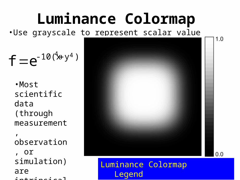
Luminance Colormap•Use grayscale to represent scalar value

Luminance Colormap Legend

)y-10(x 44

ef •Most scientific data (through measurement, observation, or simulation) are intrinsically grayscale, not color

(continued)

Scalar VisualizationChap. 5

September 25, 2008

Rainbow Colormap•Red: high value; Blue: low value•A commonly used colormap

Luminance Colormap Rainbow Colormap

Rainbow Colormap

http://atmoz.org/img/weatherchannel_national_temps.png

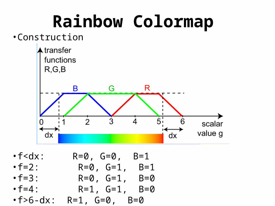
Rainbow Colormap•Construction

•f<dx: R=0, G=0, B=1•f=2: R=0, G=1, B=1•f=3: R=0, G=1, B=0•f=4: R=1, G=1, B=0•f>6-dx: R=1, G=0, B=0

Rainbow ColormapImplementation

void c(float f, float & R, float & G, float &B){

const float dx=0.8f=(f<0) ? 0: (f>1)? 1 : f //clamp f in [0,1]g=(6-2*dx)*f+dx //scale f to [dx, 6-dx]R=max(0, (3-fabs(g-4)-fabs(g-5))/2);G=max(0,(4-fabs(g-2)-fabs(g-4))/2);B=max(0,(3-fabs(g-1)-fabs(g-2))/2);

}

3RR :c

DvD:c

Colormap: Designing Issues

•Choose right color map for correct perception•Grayscale: good in most cases•Rainbow: e.g., temperature map•Rainbow + white: e.g., landscape

•Blue: sea, lowest•Green: fields•Brown: mountains•White: mountain peaks, highest

•Choose appropriate number of colors•Avoid color banding effect (not enough color)

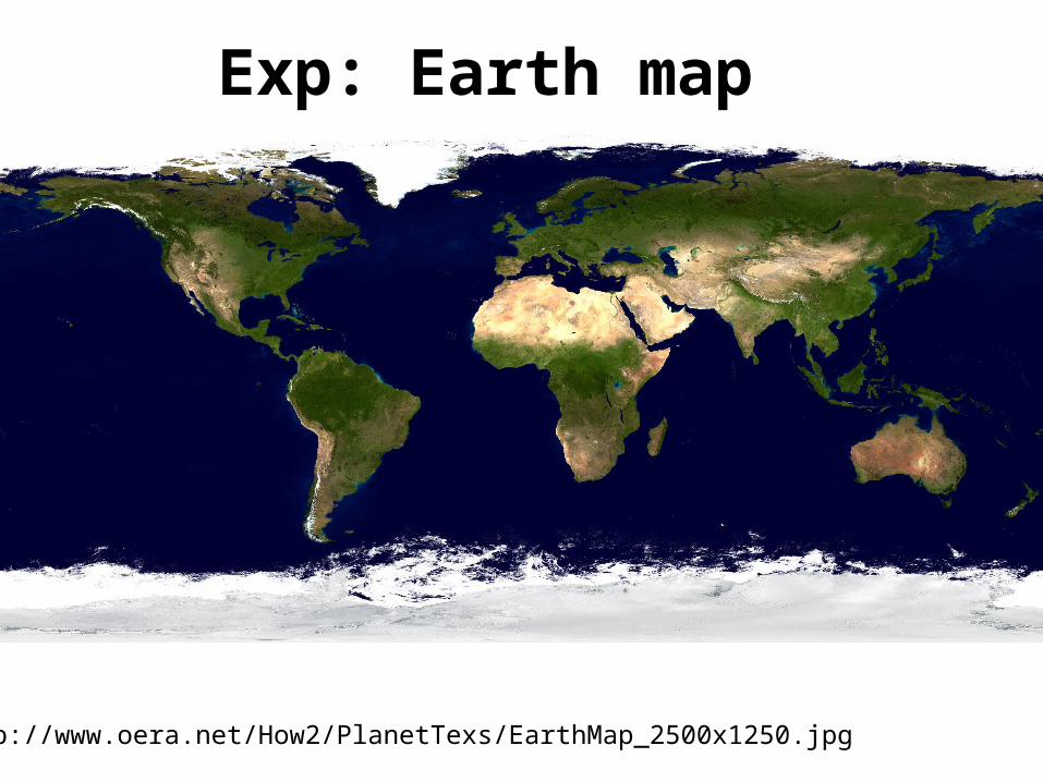
Exp: Earth map

http://www.oera.net/How2/PlanetTexs/EarthMap_2500x1250.jpg

Color Banding Effect

Exp: Sun in green-white colormap

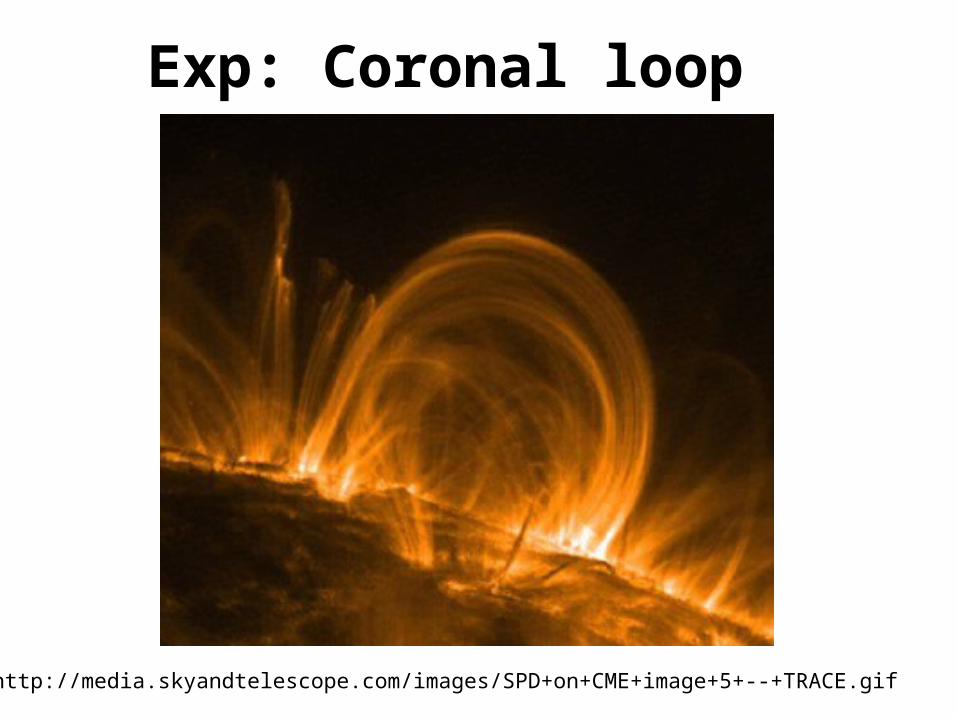
Exp: Coronal loop

http://media.skyandtelescope.com/images/SPD+on+CME+image+5+--+TRACE.gif

Exp: Galaxy M64

http://www.fas.org/irp/imint/docs/rst/Sect20/galaxyM64.jpg

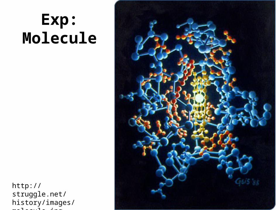
Exp:Molecule

http://struggle.net/history/images/molecule.jpg

ContouringOne contour at s=0.11

S > 0.11 S < 0.11

Contouring

7 contour lines

Contouring•A contour line C is defined as all points p in a dataset D that have the same scalar value, or isovalue s(p)=x

})(|{)( xpsDpxC

•A contour line is also called an isoline

•In 3-D dataset, a contour is a 2-D surface, called isosurface

Contouring

Cartograph

Properties of Contours•Indicating specific values of interest•In the height-plot, a contour line corresponds with the interaction of the graph with a horizontal plane of s value

Properties of Contours•The tangent to a contour line is the direction of the function’s minimal (zero) variation•The perpendicular to a contour line is the direction of the function’s maximum variation: the gradient

Contour lines

Gradient vector

Constructing Contours•For each cell, and then for each edge, test whether the isoline value v is between the attribute values of the two edge end points (vi, vj)•If yes, the isoline intersects the edge at a point q, which uses linear interpolation

ij

ijji

vv

vvpvvpq

)()(

•For each cell, at least two points, and at most as many points as cell edges•Use line segments to connect these edge-intersection points within a cell •A contour line is a polyline.

Constructing Contours

V=0.48

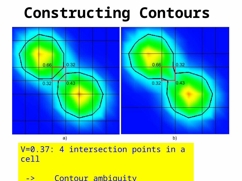
Constructing Contours

V=0.37: 4 intersection points in a cell -> Contour ambiguity

(continued)

Scalar VisualizationChap. 5

September 30, 2008

Implementation: Marching Squares•Determining the topological state of the current cell with respect to the isovalue v

•Inside state (1): vertex attribute value is less than isovalue•Outside state (0): vertex attribute value is larger than isovalue•A quad cell: (S3S2S1S0), 24=16 possible states

•(0001): first vertex inside, other vertices outside•Use optimized code for the topological state to construct independent line segments for each cell•Merge the coincident end points of line segments originating from neighboring grid cells that share an edge

Topological State of a Quad Cell

Implementation: Marching Squares

Topological State of a hex Cell

Implementation: Marching Cube

Marching cube generates a set of polygons for each contoured cell: triangle, quad, pentagon, and hexagon

Contours in 3-D•In 3-D scalar dataset, a contour at a value is an isosurface

Isosurface for a value corresponding to the skin tissue of an MRI scan 1283 voxels

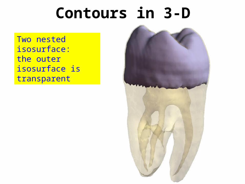
Contours in 3-D

Two nested isosurface: the outer isosurface is transparent

Height Plots•The height plot operation is to “warp” the data domain surface along the surface normal, with a factor proportional to the scalar value

s

hs

Dx

xnxsxm

DDm

),()()(

,:

Height Plots

Height plot over a planar 2-D surface

Height Plots

Height plot over a nonplanar 2-D surface

Demo

IDL: “gaussian_2d.pro”

•Using interactive “isurface” procedure•Choose different color map

Endof Chap. 5

Note: