C:\Documents and Settings\cop...c83.default\Cache\01200B9Bd01

$Page 1: C:\Documents and Settings\cop...c83.default\Cache\01200B9Bd01$
Comparison of explicit atom, united atom, and coarse-grained simulationsof poly„methyl methacrylate…

Chunxia Chen, Praveen Depa, and Janna K. Maranasa�

Department of Chemical Engineering, The Pennsylvania State University, University Park,Pennsylvania 16802, USA

Victoria Garcia SakaiNIST Center for Neutron Research, National Institute of Standards and Technology, Gaithersburg,Maryland 20899-8562, USA

�Received 12 June 2007; accepted 17 December 2007; published online 28 March 2008�

We evaluate explicit atom, united atom, and coarse-grained force fields for molecular dynamicssimulation of poly�methyl methacrylate� �PMMA� by comparison to structural and dynamic neutronscattering data. The coarse-grained force field is assigned based on output of the united atomsimulation, for which we use an existing force field. The atomic structure of PMMA requires the useof two types of coarse-grained beads, one representing the backbone part of the repeat unit and theother representing the side group. The explicit atom description more closely resembles dynamicexperimental data than the united atom description, although the latter provides a reasonableapproximation. The coarse-grained description provides structural and dynamic properties inagreement with the united atom description on which it is based, while allowing extension of thetime trajectory of the simulation. © 2008 American Institute of Physics. �DOI: 10.1063/1.2833545�

I. INTRODUCTION

Molecular dynamics �MD� simulation is extensivelyused for studying chemical and physical properties of a va-riety of materials, including polymer melts. Simulations us-ing atomistic force fields include a high level of chemicaldetail, but computational resources limit the length of timetrajectories. As a result, significant effort has been devoted todeveloping techniques that reduce computational require-ments, extending both system size and trajectory length. Onesuch technique is coarse graining �CG�, which reduces com-putation time by removing detail: CG beads group a fewatoms, monomers, or even the whole chain to a single forcesite. CG force fields can be generic, such as the bead-springmodel1,2 or the bond fluctuation model,3–5 or based on anunderlying atomistic description.6–11 In the latter case,bonded and nonbonded CG potentials are derived from map-ping to appropriate distribution functions from simulationswith an atomistic force field. This method accurately repro-duces structural properties, but since the CG force field isparameterized based only on structural information, dynamicproperties evolve at an accelerated rate compared to the un-derlying atomistic representation.8 For large CG force sites,static properties are matched in a similar way, and the systemevolved using Langevin’s equations of motion where thefriction frequency can be adjusted to obtain correct dynamicproperties.12–14 Our group has parametrized CG force fieldsand investigated the accelerated dynamics of the resultingCG simulations for polyethylene15 �PE� and poly�ethyleneoxide� �PEO�,16 demonstrating that the origin of this “indi-rect speedup” is a reduced attraction to neighboring chains inthe CG description. Because nonbonded interactions are less

attractive, the time spent in such an interaction is reduced,and thus the system evolves at an accelerated rate. The re-duced attraction occurs because the nonbonded potentialwhich provides correct intermolecular packing has a shal-lower potential well than that used in underlying united atom�UA� simulations. This difference is larger in the case ofPEO, resulting in a larger indirect speed up.

In this contribution, we extend our approach to polymerswhich require a CG side group by examining poly�methylmethacrylate� �PMMA�, a well studied polymer with mul-tiple applications due to its high transparency in visible light.Although it has been demonstrated that a CG side group isnot required,17,18 we choose to model PMMA with two typesof coarse-grained beads. This allows for easier replacementof the missing atoms when going from the CG to UA repre-sentations; this is required for comparison to neutron scatter-ing measurements, and for multiscale simulations, whichcombine two or more levels of modeling within the samesimulation box. Our objectives are to provide a CG forcefield for PMMA and examine the impact of reduced chemicaldetail on both static and dynamic properties by comparingresults of simulations using explicit atom �EA�, UA, and CGforce fields. We evaluate the performance of each level ofmodeling based on agreement with neutron scattering mea-surements of both structural and dynamic observables.

We present the remainder of the paper in five sections:Sec. II gives the details of the EA, UA, and CG force fieldsand the simulation methodology, Sec. III discusses experi-mental details, Sec. IV compares structural properties to neu-tron diffraction experiments, Sec. V compares dynamic prop-erties to quasielastic neutron scattering experiments, and Sec.VI closes the manuscript with concluding remarks.a�Electronic mail: [email protected].

THE JOURNAL OF CHEMICAL PHYSICS 128, 124906 �2008�

0021-9606/2008/128�12�/124906/12/$23.00 © 2008 American Institute of Physics128, 124906-1

Downloaded 09 Jun 2008 to 129.6.121.169. Redistribution subject to AIP license or copyright; see http://jcp.aip.org/jcp/copyright.jsp

II. SIMULATION DETAILS

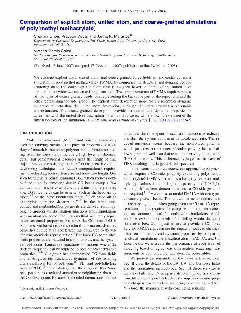
The repeat unit of PMMA in the EA, UA, and CG rep-resentations is presented in Fig. 1. For explicit atom simula-tions, we use the optimized potentials for liquid simulation�OPLS� force field.19,20 For united atom simulations, inwhich CH, CH2, and CH3 groups are treated as single forcesites, we use the force field described in Ref. 21. For coarse-grained simulations, we developed a force field following theprocedure used by our group15 and others6–8 where bondedpotentials result from matching the requisite distributions ob-tained from UA simulations, and nonbonded potentials re-quire coincidence of the intermolecular pair distributionfunction. In CG representation of PMMA, we choose to usetwo types of coarse grained beads, as illustrated in Fig. 1�c�.The main chain atoms and the �-methyl group form coarse-grained bead A and the ester side group forms coarse-grained

bead B. These coarse-grained beads are centered at C1 andO1 �bold in Fig. 1�. This choice of grouping results in elec-trically neutral CG beads, and thus no electrostatic potentialis used. The presence of two types of CG beads increases thenumber of CG potentials that must be assigned: two bondlength �AA and AB� and two bending angle �AAB and AAA�potentials are required. In addition, because the CG bead A isplaced at every second backbone atom, CG torsional distri-butions are not featureless and must also be assigned for thethree types of torsional angles �AAAA, AAAB, and BAAB�.The combination of these torsional potentials prevents theside group from spinning freely about the backbone. We ob-tain potentials from the appropriate united atom distributionsby Boltzmann inversion.22 The distributions used for non-bonded AA, AB, and AB potentials are the C1C1, C1O1, andO1O1 intermolecular pair distribution functions. For ex-ample, the coarse-grained, nonbonded AB potential is setbased on the distribution of intermolecular C1O1 distances ascalculated from a united atom simulation. The distributionsused for bonded potentials describe the variation observed inCG bond lengths, bending angles, and torsional angles usingunited atom simulations. For example, the distribution func-tion required to set the AA stretching potential is the distri-bution of C1–C1 distances as determined from UA coordi-nate snapshots. The CG potential parameters and the UAdistributions used to set them are listed in Table I. Stretchingand bending potentials are represented with analytical func-tions, but torsion and intermolecular potentials are stored intabular format. When the CG force field as obtained above is

[

C2

O1

]C4 C1

C3

C O2

HH H

HH

H

H

H

[

C2

O1

]C4 C1

C3

C O2

HH H

HH

H

H

H

C4[ C

1]

C3

C

O1

C2

O2

C4[ C

1]

C3

C

O1

C2

O2

B

[ A ]

B

[ A ]

(a) (b) (c)

FIG. 1. The PMMA repeat unit as represented in various levels of modeling:�a� the explicit atom model, �b� the united atom model, and �c� the coarse-grained model.

TABLE I. Bonded and nonbonded coarse-grained potential parameters.

ubond�Lij�=−kT ln�A exp�−k1�Lij−L01�2��

BondsUA distribution k1 �Å−2� L01 �Å� A

AAC1C1 distance

142.80 2.81 6.20

ABC1O1 distance

111.11 2.39 5.60

BendsUA distribution

ubend�Qij�=−kT ln�A exp�−k1�Qij−Q01�2�+B exp�−k1�Qij−Q01�2��

k1 �rad−2� k2 �rad−2� Q01 �rad� Q02 �rad� A B

AAAC1C1C1 angle

32.82 82.07 2.10 2.69 0.028 0.043

AAB/BAAC1C1O1 /O1C1C1 angles

35.88 10.34 1.67 1.92 0.030 0.014

TorsionsUA distribution

NonbondedUA distribution

AAAAC1C1C1C1 dihedral

AAC1C1 intermolecular pairdistribution function

AAABC1C1C1O1 dihedral

ABC1O1 intermolecular pairdistribution function

BAABO1C1C1O1 dihedral

BBO1O1 intermolecular pairdistribution function

Potentials are used in tabular form

124906-2 Chen et al. J. Chem. Phys. 128, 124906 �2008�


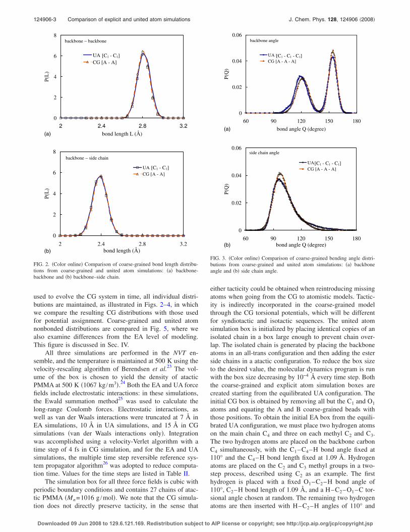
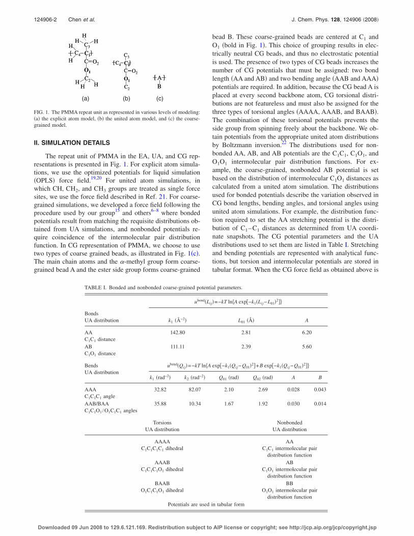
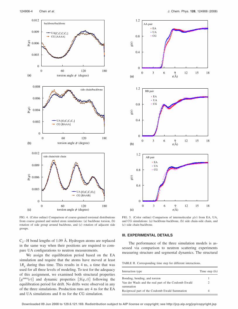
used to evolve the CG system in time, all individual distri-butions are maintained, as illustrated in Figs. 2–4, in whichwe compare the resulting CG distributions with those usedfor potential assignment. Coarse-grained and united atomnonbonded distributions are compared in Fig. 5, where wealso examine differences from the EA level of modeling.This figure is discussed in Sec. IV.

All three simulations are performed in the NVT en-semble, and the temperature is maintained at 500 K using thevelocity-rescaling algorithm of Berendsen et al.23 The vol-ume of the box is chosen to yield the density of atacticPMMA at 500 K �1067 kg /m3�.24 Both the EA and UA forcefields include electrostatic interactions: in these simulations,the Ewald summation method25 was used to calculate thelong-range Coulomb forces. Electrostatic interactions, aswell as van der Waals interactions were truncated at 7 Å inEA simulations, 10 Å in UA simulations, and 15 Å in CGsimulations �van der Waals interactions only�. Integrationwas accomplished using a velocity-Verlet algorithm with atime step of 4 fs in CG simulation, and for the EA and UAsimulations, the multiple time step reversible reference sys-tem propagator algorithm26 was adopted to reduce computa-tion time. Values for the time steps are listed in Table II.

The simulation box for all three force fields is cubic withperiodic boundary conditions and contains 27 chains of atac-tic PMMA �Mn=1016 g /mol�. We note that the CG simula-tion does not directly preserve tacticity, in the sense that

either tacticity could be obtained when reintroducing missingatoms when going from the CG to atomistic models. Tactic-ity is indirectly incorporated in the coarse-grained modelthrough the CG torsional potentials, which will be differentfor syndiotactic and isotactic sequences. The united atomsimulation box is initialized by placing identical copies of anisolated chain in a box large enough to prevent chain over-lap. The isolated chain is generated by placing the backboneatoms in an all-trans configuration and then adding the esterside chains in a atactic configuration. To reduce the box sizeto the desired value, the molecular dynamics program is runwith the box size decreasing by 10−4 Å every time step. Boththe coarse-grained and explicit atom simulation boxes arecreated starting from the equilibrated UA configuration. Theinitial CG box is obtained by removing all but the C1 and O1atoms and equating the A and B coarse-grained beads withthose positions. To obtain the initial EA box from the equili-brated UA configuration, we must place two hydrogen atomson the main chain C4 and three on each methyl C2 and C3.The two hydrogen atoms are placed on the backbone carbonC4 simultaneously, with the C1–C4–H bond angle fixed at110° and the C4–H bond length fixed at 1.09 Å. Hydrogenatoms are placed on the C2 and C3 methyl groups in a two-step process, described using C2 as an example. The firsthydrogen is placed with a fixed O1–C2–H bond angle of110°, C2–H bond length of 1.09 Å, and a H–C2–O1–C tor-sional angle chosen at random. The remaining two hydrogenatoms are then inserted with H–C2–H angles of 110° and

0

2

4

6

8

2 2.4 2.8 3.2

bond length L (Å)

P(L)

UA [C1 - C1]CG [A - A]

backbone − backbone

[C1 - C1]

0

2

4

6

8

2 2.4 2.8 3.2bond length (Å)

P(L)

UA [C1 - C1]CG [A - A]

backbone − side chain

[C1 - C1]

(a)

(b)

FIG. 2. �Color online� Comparison of coarse-grained bond length distribu-tions from coarse-grained and united atom simulations: �a� backbone-backbone and �b� backbone–side chain.

0

0.02

0.04

0.06

60 90 120 150 180

bond angle Q (degree)

P(Q

)

UA [C1 - C1 - C1]

CG [A - A - A]

backbone angle

[C1 - C1 - C1]

(a)

(b)

0

0.02

0.04

0.06

60 90 120 150 180bond angle Q (degree)

P(Q

)

UA [C1 - C1 - C1]

CG [A - A - A]

side chain angle

[C1 - C1 - C1]

FIG. 3. �Color online� Comparison of coarse-grained bending angle distri-butions from coarse-grained and united atom simulations: �a� backboneangle and �b� side chain angle.

124906-3 Comparison of explicit and united atom simulations J. Chem. Phys. 128, 124906 �2008�


C2–H bond lengths of 1.09 Å. Hydrogen atoms are replacedin the same way when their positions are required to com-pare UA configurations to neutron measurements.

We assign the equilibration period based on the EAsimulation and require that the atoms have moved at least1Rg during thus time. This results in 4 ns, a time that wasused for all three levels of modeling. To test for the adequacyof this assignment, we examined both structural properties�ginter�r�� and dynamic properties �S�q , t�� following theequilibration period for drift. No drifts were observed in anyof the three simulations. Production runs are 4 ns for the EAand UA simulations and 8 ns for the CG simulation.

III. EXPERIMENTAL DETAILS

The performance of the three simulation models is as-sessed via comparison to neutron scattering experimentsmeasuring structure and segmental dynamics. The structural

0

0.002

0.004

0.006

0.008

0 60 120 180

torsion angle φ (degree)

P( φ

)

UA [O1C1C1C1]

CG [BAAA]

side chain/backbone

[O1C1C1C1]

0

0.003

0.006

0.009

0.012

0 60 120 180

torsion angle φ (degree)

P( φ

)

UA [C1C1C1C1]

CG [AAAA]

backbone/backbone

[C1C1C1C1]

0

0.003

0.006

0.009

0.012

0 60 120 180torsion angle φ (degree)

P( φ

)

UA [O1C1C1O1]

CG [BAAB]

side chain/side chain

[O1C1C1O1]

(a)

(b)

(c)

FIG. 4. �Color online� Comparison of coarse-grained torsional distributionsfrom coarse-grained and united atom simulations: �a� backbone torsion, �b�rotation of side group around backbone, and �c� rotation of adjacent sidegroups.

0

0.4

0.8

1.2

0 3 6 9 12 15 18r(Å)

g(r)

EAUACG

AA pair

0

0.4

0.8

1.2

0 3 6 9 12 15 18r(Å)

g(r)

EAUACG

BB pair

0

0.4

0.8

1.2

0 3 6 9 12 15 18r(Å)

g(r)

EAUACG

AB pair

(a)

(c)

(b)

FIG. 5. �Color online� Comparison of intermolecular g�r� from EA, UA,and CG simulations: �a� backbone-backbone, �b� side chain-side chain, and�c� side chain-backbone.

TABLE II. Corresponding time step for different interactions.

Interaction type Time step �fs�

Bonding, bending, and torsion 1Van der Waals and the real part of the Coulomb Ewaldsummation

2

Reciprocal part of the Coulomb Ewald Summation 4



measurements provide the static structure factor S�q� and aredescribed in Ref. 27. The segmental relaxation times are ob-tained from fitting decay curves covering a time range fromless than 1 ps �the exact value depends on the spatial scale�to 4 ns and obtained from two neutron spectrometers. Mea-surements on these two instruments, the high flux back-scattering spectrometer �HFBS� and the disk chopper time offlight spectrometer �DCS�, both located at the National Insti-tute of Standards and Technology Center for Neutron Re-search, are described below.

A. High-flux backscattering spectrometer „HFBS…In this spectrometer, neutrons of incident wavelength

6.271 Å �E0=2.08 meV� are Doppler shifted to achieve arange of incident energies ��20 �eV� about this nominalvalue.28 The neutrons are scattered by the sample, afterwhich only those neutrons with a final energy of 2.08 meVare detected. The dynamic range �energy transfer� of�20 �eV sets the shortest time available to the instrument.The instrumental resolution �full width at half maximum�,which sets the longest time, is dependent on the size of theDoppler shift and equal to 0.87 �eV for �20 �eV. For datareduction purposes, this resolution was measured with a va-nadium sample at 295 K. The pressed polymer sample washeld in a cylindrical aluminum can mounted on a closed-cycle refrigerator unit. The thickness of the sample wasaround 0.1 mm, chosen to achieve 90% neutron transmissionand minimize multiple scattering. The PMMAwas purchasedfrom Polymer Standards Service and has a molecular weightof 463 000 g /mol and 76% syndiotactic sequences.

B. Disk chopper time-of-flight spectrometer „DCS…The disk chopper spectrometer uses a fixed incident

wavelength, and energies of scattered neutrons are resolvedby their flight times.29 The spectrometer was operated at anincident wavelength of 4.2 Å and at a resolution of 80 �eV.The instrumental resolution was measured using a vanadiumsample at 295 K with the same instrument configuration. Aswith HFBS, the sample was annular in shape and held in athin-walled aluminum can mounted onto a closed-cycle re-frigerator and of thickness of 0.1 mm to minimize multiplescattering. The measured quasielastic neutron scattering�QENS� spectra collected over 6 h periods were correctedfor detector efficiencies using software developed at NIST�data analysis and visualization environment �DAVE��.30 Thescattering from the empty aluminum can and from the back-ground were subtracted and the data were binned into qgroups in the range of 0.60–2.60 Å−1. Two hydrogenatedPMMA samples were used: the one described for HFBS�463 000 g /mol and 76% syndiotactic� and one closer to thesimulated molecular weight �3500 g /mol�, with the samepercentage of syndiotactic sequences. The glass transitiontemperatures measured by DSC are 397 and 373 K, respec-tively.

IV. STRUCTURE AND CHAIN CONFORMATION

In this section we present results on the structure andconformational properties of PMMA melts investigated by

explicit atom, united atom, and coarse-grained simulations.Experiments to measure structure using neutrons reflect thepositions of all the atoms in PMMA on a roughly equalbasis.27 It is thus necessary to reintroduce the missing atomsfrom united atom and coarse-grained simulations beforecomparing to this data. Because for the CG simulation, thenumber of missing atoms is large compared to the number ofatoms that are advanced during the simulation, we compareonly the EA and UA models to experimental data. The struc-tural properties of the CG model are then assessed by com-paring between all three levels of modeling.

A. Comparison to neutron diffraction

To determine the scattering intensity from simulation co-ordinates, we assume the sample is isotropic, in which case31

I�q� =n

�b2�i�

j

cicjbibj�0

�

�gij�r� − 1�sin qr

qr4�r2dr ,

�1�

where

�b2 =�j

cjbi2. �2�

Here i and j represent different atomic species, the coherentscattering length bi describes the interaction between neutronand nucleus, the momentum transfer q defines the spatialscale, ci is the atomic species concentration, and the totalpair distribution function gij�r� reflects the local packing be-tween all atoms of types i and j.

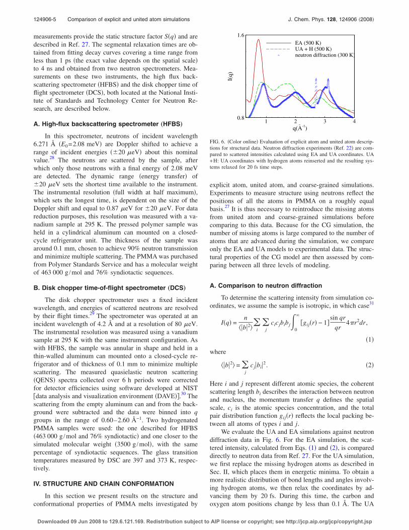
We evaluate the UA and EA simulations against neutrondiffraction data in Fig. 6. For the EA simulation, the scat-tered intensity, calculated from Eqs. �1� and �2�, is compareddirectly to neutron data from Ref. 27. For the UA simulation,we first replace the missing hydrogen atoms as described inSec. II, which places them in energetic minima. To obtain amore realistic distribution of bond lengths and angles involv-ing hydrogen atoms, we then relax the coordinates by ad-vancing them by 20 fs. During this time, the carbon andoxygen atom positions change by less than 0.1 Å. The UA

q(A-1)

I(q)

1 2 3 40.8

1.6

EA (500 K)UA + H (500 K)neutron diffraction (300 K)

FIG. 6. �Color online� Evaluation of explicit atom and united atom descrip-tions for structural data. Neutron diffraction experiments �Ref. 22� are com-pared to scattered intensities calculated using EA and UA coordinates. UA+H: UA coordinates with hydrogen atoms reinserted and the resulting sys-tems relaxed for 20 fs time steps.



scattered intensity shown in Fig. 6 is thus calculated follow-ing reinsertion of hydrogen atoms and relaxation of theirpositions. The experimental scattered intensity is not in ab-solute units, and the relative placement of the experimentalcurve on the y axis is adjusted to provide a reasonable match.The sharp peaks at q=2.7 Å−1 and q=3.1 Å−1 in the experi-mental data are due to the diffraction of the aluminumsample holder. None of the curves show evidence of crystal-linity.

We addressed the difference between EA simulationsand diffraction data in a previous publication;32 differencesin temperature between experiment and simulation causevariation in the first peak position and intensity, and differ-ences in tacticity between simulated and experimentalsamples cause variation in the second and third peaks. Herewe focus on differences between the UA and EA levels ofdescription, which are evident throughout the spatial rangeinvestigated. To determine the origin of these differences, weturn to the real space analog of S�q�, the pair distributionfunction g�r�

g�r� =��r��r� + r�

��r��2. �3�

In the above, ��r�� and ��r�+r� are the instantaneousdensities of atoms at the locations r� and r�+r. Various spe-cific distributions can be obtained by limiting the atoms in-cluded in the calculation. For example, we calculate the in-termolecular g�r� by requiring that atoms in r and r� belong

to different molecules. The angular brackets indicate aver-ages over all atom locations in the simulation box, with��r�� equal to the macroscopic density.

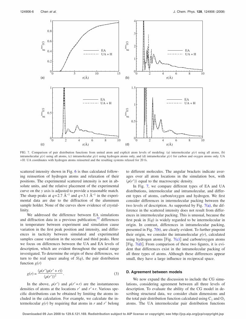
In Fig. 7, we compare different types of EA and UAdistributions, intermolecular and intramolecular, and differ-ent types of atoms, carbon/oxygen and hydrogen. We firstconsider differences in intermolecular packing between thetwo levels of description. As supported by Fig. 7�a�, the dif-ference in the scattered intensity does not result from differ-ences in intermolecular packing. This is unusual, because thefirst peak in S�q� is widely regarded to be intermolecular inorigin. In contrast, differences in intramolecular packing,presented in Fig. 7�b�, are clearly evident. To further pinpointtheir origin, we consider the intramolecular g�r�, calculatedusing hydrogen atoms �Fig. 7�c�� and carbon/oxygen atoms�Fig. 7�d��. From comparison of these two figures, it is evi-dent that differences exist in the intramolecular packing ofall three types of atoms. Although these differences appearsmall, they have a large influence in reciprocal space.

D. Agreement between models

We now expand the discussion to include the CG simu-lations, considering agreement between all three levels ofdescription. To evaluate the ability of the CG model in de-scribing structural data, we consider chain dimensions andthe total pair distribution function calculated using C1 and O1atoms. The UA intermolecular pair distribution functions

r(A)

gin

ter (r

)

0 5 10 150

0.2

0.4

0.6

0.8

1

EAUA + H

r(A)

gin

tra (r

)

0 2 4 6 8 100

1

2

3

4

EAUA + H

r(A)

gin

tra (r

)

0 2 4 6 8 100

0.5

1

EAUA + H

r(A)

gin

tra (r

)

0 2 4 6 8 100

0.5

1

1.5

EAUA + H

(a)

(c)

(b)

(d)

FIG. 7. Comparison of pair distribution functions from united atom and explicit atom levels of modeling: �a� intermolecular g�r� using all atoms, �b�intramolecular g�r� using all atoms, �c� intramolecular g�r� using hydrogen atoms only, and �d� intramolecular g�r� for carbon and oxygen atoms only. UA+H: UA coordinates with hydrogen atoms reinserted and the resulting systems relaxed for 20 fs.



were an input to the CG model, and a comparison betweenthe two was presented in Fig. 5. This comparison also in-cluded results from the EA model, which are in good agree-ment with both UA and CG data.

We assess molecular size and chain conformation by theradius of gyration �Rg� and end-to-end distance �Re�. Theradius of gyration

Rg= ��

im

i�r

i− r

CM�2

M � �4�

represents the average size of the chains, where M is the totalchain mass and mi is the mass of bead i. The position of beadi is indicated by ri and the center of mass rCM of each chainis rCM= ��imiri� /M. In calculating Rg, the summation istaken over all the beads in a chain, which for the EA descrip-tion are all carbon, oxygen, and hydrogen atoms, for the UAdescription are all carbon and oxygen atoms, and for the CGdescription are C1 and O1 atoms. The brackets indicated thatan average is taken over many coordinate snapshots. Theend-to-end distance

Re = �r1 − rn �5�

represents the average span of the chains, where rl and rn arethe positions of the first and last carbon atoms on each chainfor the UA and EA descriptions, and the first and last CGbeads for the CG description. This calculation is also aver-aged over many coordinate snapshots. Table III illustratesthat, within error, all three models provide the same chaindimensions. Thus, the different details of intramolecularpacking in the EA and UA descriptions lead to differences inthe structure factor, but do not influence chain dimensions.

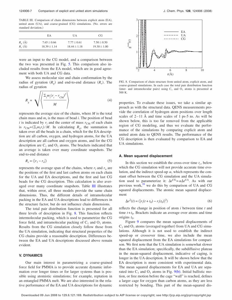
The total pair distribution function is presented for allthree levels of description in Fig. 8. This function reflectsintermolecular packing, which is used to parametrize the CGforce field, and intramolecular packing of C1 and O1 atoms.Results from the CG simulation closely follow those fromthe UA simulation, indicating that structural properties of theCG chains provide a reasonable description. Differences be-tween the EA and UA descriptions discussed above remainevident.

V. DYNAMICS

Our main interest in parametrizing a coarse-grainedforce field for PMMA is to provide accurate dynamic infor-mation over longer times or for larger systems than is pos-sible using atomistic simulations; for example, reptation inan entangled PMMA melt. We are also interested in the rela-tive performance of the EA and UA descriptions for dynamic

properties. To evaluate these issues, we take a similar ap-proach as with the structural data. QENS measurements pro-vide the correlation of hydrogen atom positions over lengthscales of 2–11 Å and time scales of 1 ps-5 ns. As will beshown below, this is too far removed from the applicableregion of CG modeling, and thus we evaluate the perfor-mance of the simulations by comparing explicit atom andunited atom data to QENS results. The performance of theCG description is then evaluated by comparison to EA andUA simulations.

A. Mean squared displacement

In this section we establish the cross-over time tc, belowwhich the CG simulation will not provide accurate time evo-lution, and the indirect speed-up �, which represents the con-stant offset between the CG simulation and the UA simula-tion used to parameterize it: �tCG=��tUA. As with ourprevious work,16 we do this by comparison of UA and CGsquared displacements. The atomic mean squared displace-ment

�r2�t� = �ri�t + t0� − ri�t0�2 �6�

reflects the change in position of atom i between time t andtime t+ t0. Brackets indicate an average over atoms and timeorigins t0.

Figure 9 compares the mean squared displacements ofC1 and O1 atoms �averaged together� from UA and CG simu-lations. Although it is not used to establish the indirectspeed-up or crossover time, we also include the meansquared displacement from the EA simulations for compari-son. We first note that the UA simulation is somewhat slowerthan the EA simulation; specifically, the subdiffusive plateauin the mean-squared displacement, indicative of caging, islonger in the UA description. It will be shown below that theEA description is more consistent with experimental data.The mean squared displacements for EA and UA are sepa-rated into C1 and O1 atoms in Fig. 9�b�. Initial ballistic mo-tion, or free motion before the cage “wall” is reached, definesa larger cage for oxygen than carbon atoms, as they are lessrestricted by bonding. This part of the mean-squared dis-

TABLE III. Comparison of chain dimensions between explicit atom �EA�,united atom �UA�, and coarse-grained �CG� simulations. �No. errors arestandard deviation.�

EA UA CG

Rg �Å� 7.65�0.66 7.77�0.61 7.50�0.50Re �Å� 18.39�1.14 18.44�1.18 19.30�1.00

r(A)

gto

tal (r

)

2 4 6 8 100

1

2

3

EAUACG

FIG. 8. Comparison of chain structure from united atom, explicit atom, andcoarse-grained simulations. In each case the total pair distribution function�inter- and intramolecular pairs� using C1 and O1 atoms is presented at500 K.



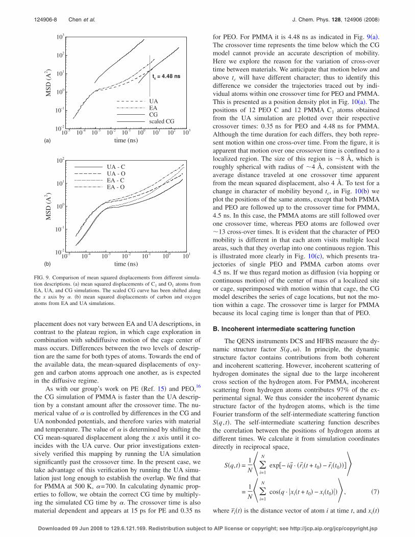
placement does not vary between EA and UA descriptions, incontrast to the plateau region, in which cage exploration incombination with subdiffusive motion of the cage center ofmass occurs. Differences between the two levels of descrip-tion are the same for both types of atoms. Towards the end ofthe available data, the mean-squared displacements of oxy-gen and carbon atoms approach one another, as is expectedin the diffusive regime.

As with our group’s work on PE �Ref. 15� and PEO,16

the CG simulation of PMMA is faster than the UA descrip-tion by a constant amount after the crossover time. The nu-merical value of � is controlled by differences in the CG andUA nonbonded potentials, and therefore varies with materialand temperature. The value of � is determined by shifting theCG mean-squared displacement along the x axis until it co-incides with the UA curve. Our prior investigations exten-sively verified this mapping by running the UA simulationsignificantly past the crossover time. In the present case, wetake advantage of this verification by running the UA simu-lation just long enough to establish the overlap. We find thatfor PMMA at 500 K, �=700. In calculating dynamic prop-erties to follow, we obtain the correct CG time by multiply-ing the simulated CG time by �. The crossover time is alsomaterial dependent and appears at 15 ps for PE and 0.35 ns

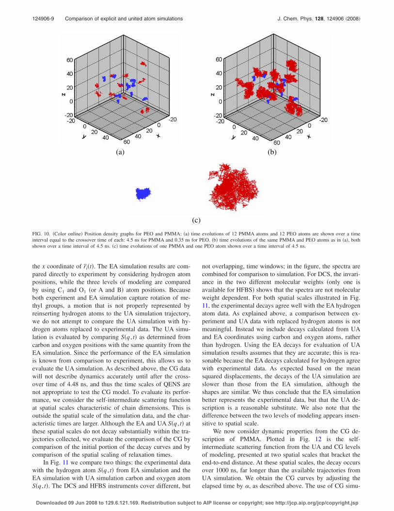
for PEO. For PMMA it is 4.48 ns as indicated in Fig. 9�a�.The crossover time represents the time below which the CGmodel cannot provide an accurate description of mobility.Here we explore the reason for the variation of cross-overtime between materials. We anticipate that motion below andabove tc will have different character; thus to identify thisdifference we consider the trajectories traced out by indi-vidual atoms within one crossover time for PEO and PMMA.This is presented as a position density plot in Fig. 10�a�. Thepositions of 12 PEO C and 12 PMMA C1 atoms obtainedfrom the UA simulation are plotted over their respectivecrossover times: 0.35 ns for PEO and 4.48 ns for PMMA.Although the time duration for each differs, they both repre-sent motion within one cross-over time. From the figure, it isapparent that motion over one crossover time is confined to alocalized region. The size of this region is �8 Å, which isroughly spherical with radius of �4 Å, consistent with theaverage distance traveled at one crossover time apparentfrom the mean squared displacement, also 4 Å. To test for achange in character of mobility beyond tc, in Fig. 10�b� weplot the positions of the same atoms, except that both PMMAand PEO are followed up to the crossover time for PMMA,4.5 ns. In this case, the PMMA atoms are still followed overone crossover time, whereas PEO atoms are followed over�13 cross-over times. It is evident that the character of PEOmobility is different in that each atom visits multiple localareas, such that they overlap into one continuous region. Thisis illustrated more clearly in Fig. 10�c�, which presents tra-jectories of single PEO and PMMA carbon atoms over4.5 ns. If we thus regard motion as diffusion �via hopping orcontinuous motion� of the center of mass of a localized siteor cage, superimposed with motion within that cage, the CGmodel describes the series of cage locations, but not the mo-tion within a cage. The crossover time is larger for PMMAbecause its local caging time is longer than that of PEO.

B. Incoherent intermediate scattering function

The QENS instruments DCS and HFBS measure the dy-namic structure factor S�q ,�. In principle, the dynamicstructure factor contains contributions from both coherentand incoherent scattering. However, incoherent scattering ofhydrogen dominates the signal due to the large incoherentcross section of the hydrogen atom. For PMMA, incoherentscattering from hydrogen atoms contributes 97% of the ex-perimental signal. We thus consider the incoherent dynamicstructure factor of the hydrogen atoms, which is the timeFourier transform of the self-intermediate scattering functionS�q , t�. The self-intermediate scattering function describesthe correlation between the positions of hydrogen atoms atdifferent times. We calculate it from simulation coordinatesdirectly in reciprocal space,

S�q,t� =1

N��i=1

N

exp�− iq� · �r�i�t + t0� − r�i�t0��=1

N��i=1

N

cos�q · xi�t + t0� − xi�t0�� , �7�

where r̄i�t� is the distance vector of atom i at time t, and xi�t�

time (ns)

MS

D(A

2)

10-5

10-4

10-3

10-2

10-1

100

101

102

10310

-2

10-1

100

101

102

103

UA

EA

CG

scaled CG

tc

= 4.48 ns

time (ns)

MS

D(A

2)

10-5

10-4

10-3

10-2

10-1

100

10110

-2

10-1

100

101

102

UA - C

UA - O

EA - C

EA - O

(a)

(b)

FIG. 9. Comparison of mean squared displacements from different simula-tion descriptions. �a� mean squared displacements of C1 and O1 atoms fromEA, UA, and CG simulations. The scaled CG curve has been shifted alongthe x axis by �. �b� mean squared displacements of carbon and oxygenatoms from EA and UA simulations.



the x coordinate of r̄i�t�. The EA simulation results are com-pared directly to experiment by considering hydrogen atompositions, while the three levels of modeling are comparedby using C1 and O1 �or A and B� atom positions. Becauseboth experiment and EA simulation capture rotation of me-thyl groups, a motion that is not properly represented byreinserting hydrogen atoms to the UA simulation trajectory,we do not attempt to compare the UA simulation with hy-drogen atoms replaced to experimental data. The UA simu-lation is evaluated by comparing S�q , t� as determined fromcarbon and oxygen positions with the same quantity from theEA simulation. Since the performance of the EA simulationis known from comparison to experiment, this allows us toevaluate the UA simulation. As described above, the CG datawill not describe dynamics accurately until after the cross-over time of 4.48 ns, and thus the time scales of QENS arenot appropriate to test the CG model. To evaluate its perfor-mance, we consider the self-intermediate scattering functionat spatial scales characteristic of chain dimensions. This isoutside the spatial scale of the simulation data, and the char-acteristic times are larger. Although the EA and UA S�q , t� atthese spatial scales do not decay substantially within the tra-jectories collected, we evaluate the comparison of the CG bycomparison of the initial portion of the decay curves and bycomparison of the spatial scaling of relaxation times.

In Fig. 11 we compare two things: the experimental datawith the hydrogen atom S�q , t� from EA simulation and theEA simulation with UA simulation carbon and oxygen atomS�q , t�. The DCS and HFBS instruments cover different, but

not overlapping, time windows; in the figure, the spectra arecombined for comparison to simulation. For DCS, the invari-ance in the two different molecular weights �only one isavailable for HFBS� shows that the spectra are not molecularweight dependent. For both spatial scales illustrated in Fig.11, the experimental decays agree well with the EA hydrogenatom data. As explained above, a comparison between ex-periment and UA data with replaced hydrogen atoms is notmeaningful. Instead we include decays calculated from UAand EA coordinates using carbon and oxygen atoms, ratherthan hydrogen. Using the EA decays for evaluation of UAsimulation results assumes that they are accurate; this is rea-sonable because the EA decays calculated for hydrogen agreewith experimental data. As expected based on the meansquared displacements, the decays of the UA simulation areslower than those from the EA simulation, although theshapes are similar. We thus conclude that the EA simulationbetter represents the experimental data, but that the UA de-scription is a reasonable substitute. We also note that thedifference between the two levels of modeling appears insen-sitive to spatial scale.

We now consider dynamic properties from the CG de-scription of PMMA. Plotted in Fig. 12 is the self-intermediate scattering function from the UA and CG levelsof modeling, presented at two spatial scales that bracket theend-to-end distance. At these spatial scales, the decay occursover 1000 ns, far longer than the available trajectories fromUA simulation. We obtain the CG curves by adjusting theelapsed time by �, as described above. The use of CG simu-

(a) (b)

(c)

FIG. 10. �Color online� Position density graphs for PEO and PMMA: �a� time evolutions of 12 PMMA atoms and 12 PEO atoms are shown over a timeinterval equal to the crossover time of each: 4.5 ns for PMMA and 0.35 ns for PEO. �b� time evolutions of the same PMMA and PEO atoms as in �a�, bothshown over a time interval of 4.5 ns. �c� time evolutions of one PMMA and one PEO atom shown over a time interval of 4.5 ns.



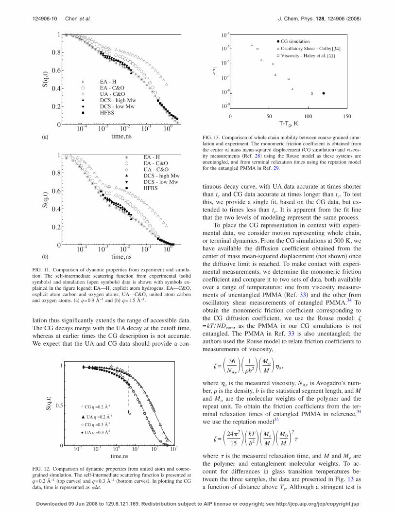
lation thus significantly extends the range of accessible data.The CG decays merge with the UA decay at the cutoff time,whereas at earlier times the CG description is not accurate.We expect that the UA and CG data should provide a con-

tinuous decay curve, with UA data accurate at times shorterthan tc and CG data accurate at times longer than tc. To testthis, we provide a single fit, based on the CG data, but ex-tended to times less than tc. It is apparent from the fit linethat the two levels of modeling represent the same process.

To place the CG representation in context with experi-mental data, we consider motion representing whole chain,or terminal dynamics. From the CG simulations at 500 K, wehave available the diffusion coefficient obtained from thecenter of mass mean-squared displacement �not shown� oncethe diffusive limit is reached. To make contact with experi-mental measurements, we determine the monomeric frictioncoefficient and compare it to two sets of data, both availableover a range of temperatures: one from viscosity measure-ments of unentangled PMMA �Ref. 33� and the other fromoscillatory shear measurements of entangled PMMA.34 Toobtain the monomeric friction coefficient corresponding tothe CG diffusion coefficient, we use the Rouse model: =kT /NDcom, as the PMMA in our CG simulations is notentangled. The PMMA in Ref. 33 is also unentangled; theauthors used the Rouse model to relate friction coefficients tomeasurements of viscosity,

= � 36NAv

�� 1�b2

��Mo

M��o,

where �o is the measured viscosity, NAv is Avogadro’s num-ber, � is the density, b is the statistical segment length, and Mand Mo are the molecular weights of the polymer and therepeat unit. To obtain the friction coefficients from the ter-minal relaxation times of entangled PMMA in reference,34

we use the reptation model35

= �24�215

�� kT

b2��Me

M��M0

M�2�

where � is the measured relaxation time, and M and Me arethe polymer and entanglement molecular weights. To ac-count for differences in glass transition temperatures be-tween the three samples, the data are presented in Fig. 13 asa function of distance above Tg. Although a stringent test is

time,ns

S(q

,t)

10-4

10-3

10-2

10-1

1000

0.2

0.4

0.6

0.8

1

EA - HEA - C&OUA - C&ODCS - high MwDCS - low MwHFBS

time,ns

S(q

,t)

10-4

10-3

10-2

10-1

1000

0.2

0.4

0.6

0.8

1 EA - HEA - C&OUA - C&ODCS - high MwDCS - low MwHFBS

(a)

(b)

FIG. 11. Comparison of dynamic properties from experiment and simula-tion. The self-intermediate scattering function from experimental �solidsymbols� and simulation �open symbols� data is shown with symbols ex-plained in the figure legend: EA—H, explicit atom hydrogens; EA—C&O,explicit atom carbon and oxygen atoms; UA—C&O, united atom carbonand oxygen atoms. �a� q=0.9 Å−1 and �b� q=1.5 Å−1.

time,ns

S(q

,t)

10-2 10-1 100 101 102 1030

0.5

1

tc

CG q =0.2 Å-1

� UA q =0.2 Å-1

� CG q =0.3 Å-1

� UA q =0.3 Å-1

FIG. 12. Comparison of dynamic properties from united atom and coarse-grained simulation. The self-intermediate scattering function is presented atq=0.2 Å−1 �top curves� and q=0.3 Å−1 �bottom curves�. In plotting the CGdata, time is represented as ��t.

1.0E-09

1.0E-08

1.0E-07

1.0E-06

1.0E-05

1.0E-04

0 50 100 150

T-Tg, K

ζ

CG simulation

Oscillatory Shear - Colby [32]

Viscosity - Haley et al. [31]

10-8

10-7

10-9

10-6

10-5

10-4

[33]

[34]

FIG. 13. Comparison of whole chain mobility between coarse-grained simu-lation and experiment. The monomeric friction coefficient is obtained fromthe center of mass mean-squared displacement �CG simulation� and viscos-ity measurements �Ref. 28� using the Rouse model as these systems areunentangled, and from terminal relaxation times using the reptation modelfor the entangled PMMA in Ref. 29.



not possible from simulations at a single temperature, the CGdata point is in reasonable agreement with the temperaturedependence of both sets of experimental data.

An additional test of the performance of the CG modelmay be obtained by comparing the spatial dependence ofcharacteristic times obtained from fitting the decay curves toa model function. For this purpose, we choose the Kolraush-Williams-Watts KWW function

S�q,t� = A exp�− � t

�KWW� � . �8�

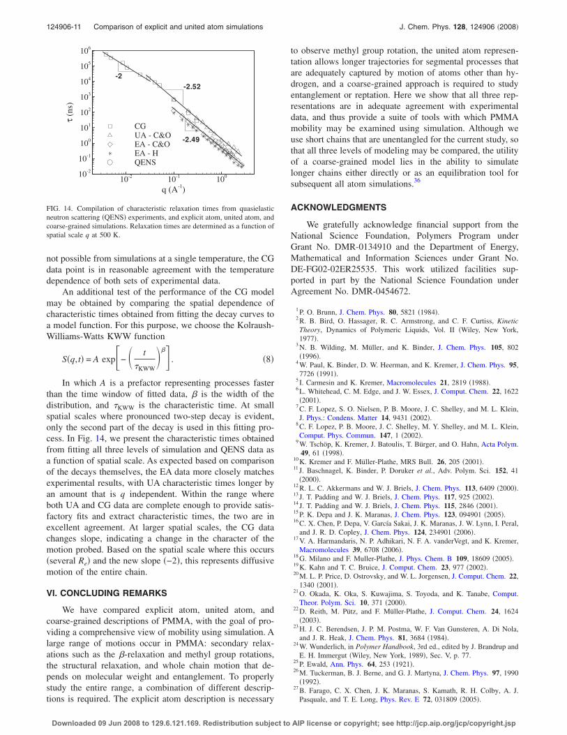
In which A is a prefactor representing processes fasterthan the time window of fitted data, is the width of thedistribution, and �KWW is the characteristic time. At smallspatial scales where pronounced two-step decay is evident,only the second part of the decay is used in this fitting pro-cess. In Fig. 14, we present the characteristic times obtainedfrom fitting all three levels of simulation and QENS data asa function of spatial scale. As expected based on comparisonof the decays themselves, the EA data more closely matchesexperimental results, with UA characteristic times longer byan amount that is q independent. Within the range whereboth UA and CG data are complete enough to provide satis-factory fits and extract characteristic times, the two are inexcellent agreement. At larger spatial scales, the CG datachanges slope, indicating a change in the character of themotion probed. Based on the spatial scale where this occurs�several Re� and the new slope �−2�, this represents diffusivemotion of the entire chain.

VI. CONCLUDING REMARKS

We have compared explicit atom, united atom, andcoarse-grained descriptions of PMMA, with the goal of pro-viding a comprehensive view of mobility using simulation. Alarge range of motions occur in PMMA: secondary relax-ations such as the -relaxation and methyl group rotations,the structural relaxation, and whole chain motion that de-pends on molecular weight and entanglement. To properlystudy the entire range, a combination of different descrip-tions is required. The explicit atom description is necessary

to observe methyl group rotation, the united atom represen-tation allows longer trajectories for segmental processes thatare adequately captured by motion of atoms other than hy-drogen, and a coarse-grained approach is required to studyentanglement or reptation. Here we show that all three rep-resentations are in adequate agreement with experimentaldata, and thus provide a suite of tools with which PMMAmobility may be examined using simulation. Although weuse short chains that are unentangled for the current study, sothat all three levels of modeling may be compared, the utilityof a coarse-grained model lies in the ability to simulatelonger chains either directly or as an equilibration tool forsubsequent all atom simulations.36

ACKNOWLEDGMENTS

We gratefully acknowledge financial support from theNational Science Foundation, Polymers Program underGrant No. DMR-0134910 and the Department of Energy,Mathematical and Information Sciences under Grant No.DE-FG02-02ER25535. This work utilized facilities sup-ported in part by the National Science Foundation underAgreement No. DMR-0454672.

1P. O. Brunn, J. Chem. Phys. 80, 5821 �1984�.2R. B. Bird, O. Hassager, R. C. Armstrong, and C. F. Curtiss, KineticTheory, Dynamics of Polymeric Liquids, Vol. II �Wiley, New York,1977�.3N. B. Wilding, M. Müller, and K. Binder, J. Chem. Phys. 105, 802�1996�.4W. Paul, K. Binder, D. W. Heerman, and K. Kremer, J. Chem. Phys. 95,7726 �1991�.5 I. Carmesin and K. Kremer, Macromolecules 21, 2819 �1988�.6L. Whitehead, C. M. Edge, and J. W. Essex, J. Comput. Chem. 22, 1622�2001�.7C. F. Lopez, S. O. Nielsen, P. B. Moore, J. C. Shelley, and M. L. Klein,J. Phys.: Condens. Matter 14, 9431 �2002�.8C. F. Lopez, P. B. Moore, J. C. Shelley, M. Y. Shelley, and M. L. Klein,Comput. Phys. Commun. 147, 1 �2002�.9W. Tschöp, K. Kremer, J. Batoulis, T. Bürger, and O. Hahn, Acta Polym.

49, 61 �1998�.10K. Kremer and F. Müller-Plathe, MRS Bull. 26, 205 �2001�.11 J. Baschnagel, K. Binder, P. Doruker et al., Adv. Polym. Sci. 152, 41

�2000�.12R. L. C. Akkermans and W. J. Briels, J. Chem. Phys. 113, 6409 �2000�.13 J. T. Padding and W. J. Briels, J. Chem. Phys. 117, 925 �2002�.14 J. T. Padding and W. J. Briels, J. Chem. Phys. 115, 2846 �2001�.15P. K. Depa and J. K. Maranas, J. Chem. Phys. 123, 094901 �2005�.16C. X. Chen, P. Depa, V. García Sakai, J. K. Maranas, J. W. Lynn, I. Peral,and J. R. D. Copley, J. Chem. Phys. 124, 234901 �2006�.

17V. A. Harmandaris, N. P. Adhikari, N. F. A. vanderVegt, and K. Kremer,Macromolecules 39, 6708 �2006�.

18G. Milano and F. Muller-Plathe, J. Phys. Chem. B 109, 18609 �2005�.19K. Kahn and T. C. Bruice, J. Comput. Chem. 23, 977 �2002�.20M. L. P. Price, D. Ostrovsky, and W. L. Jorgensen, J. Comput. Chem. 22,1340 �2001�.

21O. Okada, K. Oka, S. Kuwajima, S. Toyoda, and K. Tanabe, Comput.Theor. Polym. Sci. 10, 371 �2000�.

22D. Reith, M. Pütz, and F. Müller-Plathe, J. Comput. Chem. 24, 1624�2003�.

23H. J. C. Berendsen, J. P. M. Postma, W. F. Van Gunsteren, A. Di Nola,and J. R. Heak, J. Chem. Phys. 81, 3684 �1984�.

24W. Wunderlich, in Polymer Handbook, 3rd ed., edited by J. Brandrup andE. H. Immergut �Wiley, New York, 1989�, Sec. V, p. 77.

25P. Ewald, Ann. Phys. 64, 253 �1921�.26M. Tuckerman, B. J. Berne, and G. J. Martyna, J. Chem. Phys. 97, 1990

�1992�.27B. Farago, C. X. Chen, J. K. Maranas, S. Kamath, R. H. Colby, A. J.Pasquale, and T. E. Long, Phys. Rev. E 72, 031809 �2005�.

q (A-1)

τ(n

s)

10-2

10-1

10010

-2

10-1

100

101

102

103

104

105

106

CGUA - C&OEA - C&OEA - HQENS

-2.52

-2

-2.49

FIG. 14. Compilation of characteristic relaxation times from quasielasticneutron scattering �QENS� experiments, and explicit atom, united atom, andcoarse-grained simulations. Relaxation times are determined as a function ofspatial scale q at 500 K.



28A. Meyer, R. D. Dimeo, P. M. Gehring, and D. A. Neumann, Rev. Sci.Instrum. 74, 2762 �2003�.

29R. D. Copley and J. C. Cook, Chem. Phys. 292, 477 �2003�.30The IDL-based program can be found at http://www.ncnr.nist.gov/dave31O. Borodin, R. J. Douglas, G. D. Smith, F. Trouw, and S. Petrucci, J.Phys. Chem. B 107, 6813 �2003�.

32C. X. Chen, J. K. Maranas, and V. García Sakai, Macromolecules 39,

9630 �2006�.33 J. C. Haley and T. P. Lodge, J. Chem. Phys. 122, 234914 �2005�.34R. H. Colby, Polymer 30, 1275 �1989�.35 J. C. Haley, T. P. Lodge, Y. He, M. D. Ediger, E. D. von Meerwall, andJ. Mijovic, Macromolecules 36, 6142 �2003�.

36B. Hess, S. León, N. van der Vegt, and K. Kremer, Soft Matter 2, 409�2006�.

