CDMTCS Research Report Series Pre-proceedings of the ...

CDMTCSResearchReportSeries

Pre-proceedings of the Workshop“Physics and Computation” 2008

C. S. Calude1, J. F. Costa2 (eds.)1University of Auckland, NZ,2University of Wales Swansea, UK

CDMTCS-327July 2008

Centre for Discrete Mathematics andTheoretical Computer Science

Cristian S. Calude and Jose Felix Costa (eds.)

PHYSICS AND COMPUTATION

(Renaissance) International Worshop

Vienna, Austria, August 25–28, 2008

Pre-proceedings

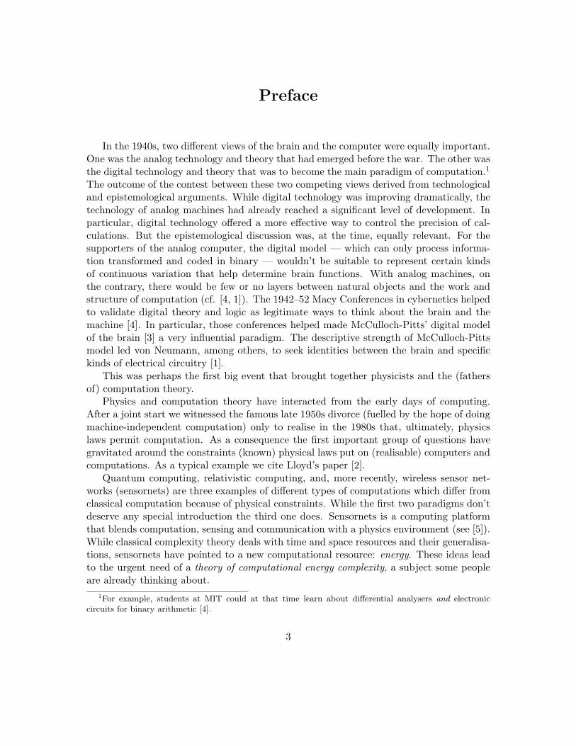
Preface

In the 1940s, two different views of the brain and the computer were equally important.One was the analog technology and theory that had emerged before the war. The other wasthe digital technology and theory that was to become the main paradigm of computation.1

The outcome of the contest between these two competing views derived from technologicaland epistemological arguments. While digital technology was improving dramatically, thetechnology of analog machines had already reached a significant level of development. Inparticular, digital technology offered a more effective way to control the precision of cal-culations. But the epistemological discussion was, at the time, equally relevant. For thesupporters of the analog computer, the digital model — which can only process informa-tion transformed and coded in binary — wouldn’t be suitable to represent certain kindsof continuous variation that help determine brain functions. With analog machines, onthe contrary, there would be few or no layers between natural objects and the work andstructure of computation (cf. [4, 1]). The 1942–52 Macy Conferences in cybernetics helpedto validate digital theory and logic as legitimate ways to think about the brain and themachine [4]. In particular, those conferences helped made McCulloch-Pitts’ digital modelof the brain [3] a very influential paradigm. The descriptive strength of McCulloch-Pittsmodel led von Neumann, among others, to seek identities between the brain and specifickinds of electrical circuitry [1].

This was perhaps the first big event that brought together physicists and the (fathersof) computation theory.

Physics and computation theory have interacted from the early days of computing.After a joint start we witnessed the famous late 1950s divorce (fuelled by the hope of doingmachine-independent computation) only to realise in the 1980s that, ultimately, physicslaws permit computation. As a consequence the first important group of questions havegravitated around the constraints (known) physical laws put on (realisable) computers andcomputations. As a typical example we cite Lloyd’s paper [2].

Quantum computing, relativistic computing, and, more recently, wireless sensor net-works (sensornets) are three examples of different types of computations which differ fromclassical computation because of physical constraints. While the first two paradigms don’tdeserve any special introduction the third one does. Sensornets is a computing platformthat blends computation, sensing and communication with a physics environment (see [5]).While classical complexity theory deals with time and space resources and their generalisa-tions, sensornets have pointed to a new computational resource: energy. These ideas leadto the urgent need of a theory of computational energy complexity, a subject some peopleare already thinking about.

1For example, students at MIT could at that time learn about differential analysers and electroniccircuits for binary arithmetic [4].

3

Secondly, but not less important, is the flow of ideas coming from computability the-ory to physics. Looking at physics with a guided computation/information eye we canask: What, if anything, do the theories of computation and information can say aboutphysics, what physical laws can be deduced using Wheeler’s dictum “it from bit”? Com-putational physics has emerged, along with experiment and theory, as the third, new andcomplementary, approach to discovery in physics.

There is a long tradition of workshops on “Physics and Computation” inaugurated bythe famous 1982 meeting whose proceedings have been published in a special issue of theInt. J. Theor. Phys. Volume 21, Numbers 3–4, April (1982) which starts with Toffoli’sprogramatic article “Physics and computation” (pp. 165–175).

In a first organisational act of re-inaugurating the series of workshops on “Physics andComputation”, we decided to invite twenty eight reputable researchers from the border-lines between computation theory and physics, but also from those sciences that interactstrongly with physics, such like chemistry (reaction-diffusion model of computation), biol-ogy (physical-chemical driven organisms), and economic theory (macro-economic models),covering as much as possible all active fields on the subject. Nineteen researchers answeryes to our call and the pre-proceedings of this workshop is the product of their work. Oursecond act will be to organise next year a second workshop with invited lectures and con-tributed talks, now moving towards a more standard workshop or even a small conference.

The main fields covered by this event are (a) analog computation, (b) experimentalcomputation, (c) Church-Turing thesis, (d) general dynamical systems computation, (e)general relativistic computation, (f) optical computation, (g) physarum computation, (h)quantum computation, (i) reaction-diffusion computation, (j) undecidability results forphysics and economic theory.

∇

The organisers of this event are grateful for the highly appreciated work done bythe reviewers of the papers submitted to the workshop. These experts were: SamsonAbramsky, Andrew Adamatzki, Edwin Beggs, Udi Boker, Olivier Bournez, Caslav Brukner,Manuel Lameiras Campagnolo, S. Barry Cooper, Ben De Lacy Costello, Jean-Charles Del-venne, Francisco Doria, Fernando Ferreira, Jerome Durand-Lose, Luıs M. Gomes, JerzyGorecki, Daniel Graca, Emmanuel Hainry, Andrew Hodges, Mark Hogarth, Bruno Loff,Aono Masashi, Cris Moore, Jerzy Mycka, Istvan Nemeti, James M. Nyce, Kerry Ojakian,Oron Shagrir, Andrea Sorbi, Mike Stannett, Karl Svozil, Cristof Teuscher, John V. Tucker,Kumaraswamy Velupillai, Philip Welch, Damien Woods, Martin Ziegler, Jeffery Zucker.

We extend our thanks to all members of the local Conference Committee of the Confer-ence UC’2008, particularly to Aneta Binder, Rudolf Freund (Chair of UC’2008), FranziskaGusel, and Marion Oswald of the Vienna University of Technology for their invaluableorganisational work.

4

The venue for the conference was the Parkhotel Schonbrunn in immediate vicinity ofSchonbrunn Palace, which, together with its ancillary buildings and extensive park, is byvirtue of its long and colourful history one of the most important cultural monuments inAustria. Vienna, located in the heart of central Europe, is an old city whose historicalrole as the capital of a great empire and the residence of the Habsburgs is reflected inits architectural monuments, its famous art collections and its rich cultural life, in whichmusic has always played an important part.

The workshop was partially supported by the Institute of Computer Languages of theVienna University of Technology, the Centre for Discrete Mathematics and TheoreticalComputer Science of the University of Auckland, the Kurt Godel Society, and the OCG(Austrian Computer Society); we extend to all our gratitude.

C. S. Calude, J. F. Costa

Auckland, NZ, Swansea, UK

References

[1] S. J. Heims. John von Neumann and Norbert Wiener: From Mathematics to the Tech-nologies of Life and Death, MIT Press, 1980.

[2] S. Lloyd. Ultimate physical limits of computation, Nature, 406:1047–1054, 2000.

[3] W. S. McCulloch and W. Pitts. A logical calculus of the ideas immanent in nervousactivity, Bulletin of Mathematical Biophysics, 5:115–133, 1943.

[4] J. M. Nyce. Nature’s machine: mimesis, the analog computer and the rhetoric of tech-nology. In R. Paton (ed), Computing with Biological Metaphors, 414-423, Chapman &Hall, 1994.

[5] F. Zhao. The technical perspective, Comm. ACM, 51, 7 : 98, July (2008).

5

Contents

1 Introduction . . . . . . . . . . . . . . . . . . . . . . . . . . . . . . . . . . . . 32 Andrew Adamatzki. From reaction-diffusion to Physarum computing . . . . 93 Edwin Beggs, John V. Tucker. Computations via Newtonian and relativistic

kinematic systems . . . . . . . . . . . . . . . . . . . . . . . . . . . . . . . . 314 Udi Boker, Nachum Dershowitz. The influence of the domain interpretation

on computational models . . . . . . . . . . . . . . . . . . . . . . . . . . . . 495 Olivier Bournez, Philippe Chassaing, Johanne Cohen, Lucas Gerin, Xavier

Koegler. On the convergence of a population protocol when population goesto infinity . . . . . . . . . . . . . . . . . . . . . . . . . . . . . . . . . . . . . 69

6 Caslav Brukner. Quantum experiments can test mathematical undecidabil-ity (Paper included in the Proceedings of UC 2008, Lecture Notes in Com-puter Science 5204.) . . . . . . . . . . . . . . . . . . . . . . . . . . . . . . . 83

7 S. Barry Cooper. Emergence as a computability–theoretic phenomenon . . 838 Newton C. A. da Costa, Francisco Antonio Doria. How to build a hyper-

computer . . . . . . . . . . . . . . . . . . . . . . . . . . . . . . . . . . . . . 1069 Jean-Charles Delvenne. What is a universal computing machine? . . . . . . 12110 Jerome Durand-Lose. Black hole computation: implementation with signal

machines . . . . . . . . . . . . . . . . . . . . . . . . . . . . . . . . . . . . . 13611 Jerzy Gorecki, J. N. Gorecka, Y. Igarashi. Information processing with

structured excitable medium . . . . . . . . . . . . . . . . . . . . . . . . . . 15912 Daniel Graca, Jorge Buescu, Manuel Lameiras Campagnolo. Computational

bounds on polynomial differential equations . . . . . . . . . . . . . . . . . . 18313 Mark Hogarth. A new problem for rule following . . . . . . . . . . . . . . . 20414 Istvan Nemeti, Hajnal Andreka, Peter Nemeti. General relativistic hyper-

computing and foundation of mathematics . . . . . . . . . . . . . . . . . . . 21015 Mike Stannett. The Computational Status of Physics: A Computable For-

mulation of Quantum Theory . . . . . . . . . . . . . . . . . . . . . . . . . . 23016 Karl Svozil, Josef Tkadlec. On the solution of trivalent decision problems

by quantum state identification . . . . . . . . . . . . . . . . . . . . . . . . . 25117 B. C. Thompson, John V. Tucker, Jeffery Zucker. Unifying computers and

dynamical systems using the theory of synchronous concurrent algorithms . 25718 K. Vela Velupillai. Uncomputability and undecidability in economic theory 28119 Damien Woods, Thomas J. Naughton. Optical computing . . . . . . . . . . 30720 Martin Ziegler. Physically-relativized church-turing hypotheses: Physical

foundations of computing and complexity theory of computational physics . 331

7

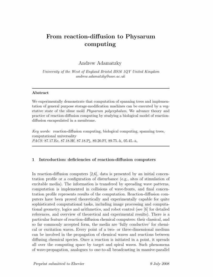
From reaction-diffusion to Physarum

computing

Andrew Adamatzky

University of the West of England Bristol BS16 1QY United [email protected]

Abstract

We experimentally demonstrate that computation of spanning trees and implemen-tation of general purpose storage-modification machines can be executed by a veg-etative state of the slime mold Physarum polycephalum. We advance theory andpractice of reaction-diffusion computing by studying a biological model of reaction-diffusion encapsulated in a membrane.

Key words: reaction-diffusion computing, biological computing, spanning trees,computational universalityPACS: 87.17.Ee, 87.18.Hf, 87.18.Pj, 89.20.Ff, 89.75.-k, 05.45.-a,

1 Introduction: deficiencies of reaction-diffusion computers

In reaction-diffusion computers [2,6], data is presented by an initial concen-tration profile or a configuration of disturbance (e.g., sites of stimulation ofexcitable media). The information is transfered by spreading wave patterns,computation is implemented in collisions of wave-fronts, and final concen-tration profile represents results of the computation. Reaction-diffusion com-puters have been proved theoretically and experimentally capable for quitesophisticated computational tasks, including image processing and computa-tional geometry, logics and arithmetics, and robot control (see [6] for detailedreferences, and overview of theoretical and experimental results). There is aparticular feature of reaction-diffusion chemical computers: their classical, andso far commonly accepted form, the media are ‘fully conductive’ for chemi-cal or excitation waves. Every point of a two- or three-dimensional mediumcan be involved in the propagation of chemical waves and reactions betweendiffusing chemical species. Once a reaction is initiated in a point, it spreadsall over the computing space by target and spiral waves. Such phenomenaof wave-propagation, analogues to one-to-all broadcasting in massive-parallel

Preprint submitted to Elsevier 9 July 2008

systems, are employed to solve problems ranging from the Voronoi diagramconstruction to robot navigation [2,6]. We could not, however, quantize infor-mation (e.g., assign logical values to certain waves) or implement one-to-onetransmission in fully reactive media.

The field of reaction-diffusion computing was started by Kuhnert, Agladzeand Krinsky [40,41], who, over twenty years ago, published their pioneering re-sults on memory implementation and basic image processing in light-sensitiveexcitable chemical systems. Their ideas were further developed by Rambidiand colleagues [57,58]; and in Showalter and Yoshikawa’s laboratories, whodesigned a range of chemical logical gates [71,42]. The computation of theshortest path, one of the classical optimization problems, has also been im-plemented in these laboratories using Belousov-Zhabotinsky media [66,12,6].Untill quite recently, the only way to direct and quantize information in achemical medium was to geometrically constrain the medium. Thus, only re-active or excitable channels are made, along which waves can travel. The wavescollide with other waves at the junctions between the channels and implementcertain logical gates in result of the collision (see an overview in Chapter 1of [6]). Designs based on the geometrical constraining of the reaction-diffusionmedia are somewhat restricted by the conventionality of their architectures.This is because they simply re-enact standard computing architectures in non-standard ‘conductive’ materials.

Using sub-excitable media may be a successful way to quantize information.In sub-excitable media a local disturbance leads to the generation of mobile lo-calization, where wave-fragments travel for a reasonably long distance withoutchanging its shape [61]. The presence of a wave-fragment in a given domainof space signifies logical truth, the absence of the fragment logical falsity [5].Despite being really promising candidates for collision-based computers [5],sub-excitable media are highly sensitive to experimental conditions and com-pact traveling wave-fragments are unstable and difficult to control.

In terms of well-established computing architectures, the following character-istics can be attributed to reaction-diffusion computers:

• massive-parallelism: there are thousands of elementary processing units, ormicrovolumes, in a standard Petri dish [6];

• local connections: microvolumes of a non-stirred chemical medium changetheir states (due to diffusion and reaction) depending on states of (concen-tration of reactants in) their closest neighbours;

• parallel input and output: in chemical reactions with indicators concen-tration profiles of the reagents, one can allow for parallel optical output.There is also a range of light-sensitive chemical reactions where data can beinputted via local disturbances of illumination [6].

• fault-tolerance: being in liquid phase, chemical reaction-diffusion computers

10

do restore their architecture even after substantial part of the medium isremoved, however, the topology and the dynamics of diffusive and, particu-larly, phase waves (e.g., excitation waves in Belousov-Zhabotinsky system)may be affected.

Reaction-diffusion computers — when implemented in chemical medium — aremuch slower than silicon-based massively-parallel processors. When nano-scalematerials are employed, e.g., networks of single-electron circuits [6], reaction-diffusion computers can however outperform even the most advanced siliconanalogues.

There still remains a range of problems where chemical reaction-diffusion pro-cessors could not cope with without the external support from conventionalsilicon-based computing devices. The shortest path computation is one of suchproblems.

One can use excitable media to outline a set of all collision-free paths in a spacewith obstacles [4], but to select and visualize the shortest path amongst allpossible paths, one needs to use an external cellular-automaton processor, orconceptually supply the excitable chemical media with some kind of field of thelocal pointers [4]. Experimental setups [66,12], which claim to directly computea shortest path in chemical media, are indeed employing external computingresources to store time-lapsed snapshots of propagating wave-fronts and toanylise the dynamics of the wave-front propagation. Such usage of externalresources dramatically reduces the fundamental values of the computing withpropagating patterns.

Graph-theoretical computations pose even more difficulties for spatially-extendednon-linear computers. For example, one can compute the Voronoi diagram ofa planar set, but can not invert this diagram [6]. Let us consider a spanningtree, most graph famous of classical proximity graphs. Given a set of planarpoints one wants to connect the points with edges, such that the resultantgraph has no cycles and there is a path between any two points of the set.So far, no algorithms of spanning tree construction were experimentally im-plemented in spatially extended non-linear systems. This is caused mainly byuniformity of spreading wave-fronts, their inability to sharply select directionstoward locations of data points, and also because excitable systems usually donot form stationary structures.

Essentially, to compute a spanning tree over a given planar set, a systemmust first explore the date space, then cover the data points and physicallyrepresenting edges of the tree by the system’s structure. This is not possiblein excitable chemical systems because they are essentially memoryless, and nostationary structure can be formed. Precipitating reaction-diffusion systemsare also uncapable of constructing the trees because not only they operate

11

with uniformly expanding diffusive fronts, but the systems are incapable ofaltering concentration profile of the precipitate once precipitation occurred.

To overcome these difficulties, we should allow reaction-diffusion computersto be geometrically self-constrained while still capable to operate in geometri-cally unconstrained (architectureless or ‘free’) space. Encapsulating reaction-diffusion processes in membranes would a possible solution. The idea is ex-plored in the present paper. Based on our previous results [7–9], we speculatethat vegetative state, or plasmodium, of Physarum polycephalum is a reaction-diffusion system constrained by a membrane that capable for solving graph-theoretical problems (not solvable by ‘classical’ reaction-diffusion computers)and which is also computationally universal.

A brief introduction to computing with Physarum polycephalum is presentedin Sect. 2. Section 3 introduces our experimental findings on constructingspanning trees of finite planar sets by plasmodium of Physarum polycephalum.In Sect. 4 we demonstrate that plasmodium of Physarum polycephalum isan ideal biological substrate for the implementation of Kolmogorov-Uspenskymachines [9]. Directions of further studies are outlined in Sect. 5.

2 Physarum computing

There is a real-world system which strongly resembles encapsulated reaction-diffusion system. Physarum polycephalum is a single cell with many nucleiwhich behave like amoeba. In its vegetative phase, called plasmodium, slimemold actively searches for nutrients. When another source of food is located,plasmodium forms a vein of protoplasm between previous and current food-sources.

Why the plasmodium of Physarum is an analog of an excitable reaction-diffusion system enclosed in a membrane? Growing and feeding plasmodiumexhibits characteristic rhytmic contractions with articulated sources. The con-traction waves are associated with waves of potential change, and the wavesobserved in plasmodium [43,44,77] are similar to the waves found in excitablechemical systems, like Belousov-Zhabotinsky medium. The following wavephenomena were discovered experimentally [77]: undisturbed propagation ofcontraction wave inside the cell body, collision and annihilation of contractionwaves, splitting of the waves by inhomogeneity, and the formation of spiralwaves of contraction (see Fig. 6c–f in [77]). These are closely matching dynam-ics of pattern propagation in excitable reaction-diffusion chemical systems.

Yamada and colleagues [77] indicate a possibility for interaction between thecontraction force generating system with oscillating chemical reactions of cal-

12

cium, ATP and associated pH [56,51,53]. Chemical oscillations can be seen asprimary oscillations — contraction waves are guided by chemical oscillationwaves — because chemical oscillations can be recorded in absence of contrac-tions [46,52,54].

Nakagaki, Aono, Tsuda [15,16,73,49,50,74] and others have been exploring apower of Physarum computing from 2000 [48]. They proved experimentallythat the plasmodium is a unique fruitful object to design various schemesof non-classical computation [15,16,73], including Voronoi diagram [63] andshortest path [49,50,63], and even design of robot controllers [74]. In presentwe paper we focus on one specialized instance of Physarum computing —approximation of spanning trees, and also implementation of a general purposestorage-modification machine.

The scoping experiments were designed as follows. We either covered con-tainer’s bottom with a piece of wet filter paper and placed a piece of livingplasmodium 1 on it, or we just planted plasmodium on a bottom of a bare con-tainer and fixed wet paper on the container’s cover to keep the humidity high.Oat flakes were distributed in the container to supply nutrients and representset of nodes to be spanned by a tree (Sect. 3) or to represent data-nodes ofPhysarum machine (Sect. 4). The containers were stored in the dark exceptduring periods of observation. To color oat flakes, where required, we usedSuperCook Food Colorings: 2 blue (colors E133, E122), yellow (E102, E110,E124), red (E110, E122), and green (E102, E142). The flakes were saturatedwith the colorings, then dried.

3 Approximation of spanning trees

The spanning tree of a finite planar set is a connected, undirected, acyclicplanar graph, which vertices are points of the planar set; every point of thegiven planar set is connected to the tree (but no cycles or loops are formed).The tree is a minimal spanning tree where the sum of edges’ lengths is minimal.Original algorithms for computing minimum spanning trees are described in[39,55,26]. Hundreds if not thousands of papers were published in last 50 years,mostly improving the original algorithms, or adapting them to multi-processorcomputing systems [28,13,32].

Non-classical and nature-inspired computing models brought their own solu-tions to the spanning tree problem. Spanning tree can be approximated byrandom walks, electrical fields, and even social insects [72,23,2,3]. However

1 Thanks to Dr. Soichiro Tsuda for providing me with P. polycephalum culture.2 www.supercook.co.uk

13

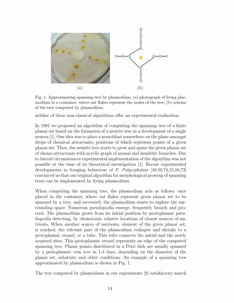
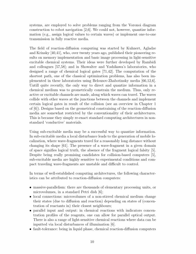
(a) (b)

Fig. 1. Approximating spanning tree by plasmodium: (a) photograph of living plas-modium in a container, where oat flakes represent the nodes of the tree, (b) schemeof the tree computed by plasmodium.

neither of these non-classical algorithms offer an experimental realization.

In 1991 we proposed an algorithm of computing the spanning tree of a finiteplanar set based on the formation of a neurite tree in a development of a singleneuron [1]. Our idea was to place a neuroblast somewhere on the plane amongstdrops of chemical attractants, positions of which represent points of a givenplanar set. Then, the neurite tree starts to grow and spans the given planar setof chemo-attractants with acyclic graph of axonal and dendritic branches. Dueto lateral circumstances experimental implementation of the algorithm was notpossible at the time of its theoretical investigation [1]. Recent experimentaldevelopments in foraging behaviour of P. Polycephalum [49,50,74,15,16,73]convinced us that our original algorithm for morphological growing of spanningtrees can be implemented by living plasmodium.

When computing the spanning tree, the plasmodium acts as follows: onceplaced in the container, where oat flakes represent given planar set to bespanned by a tree, and recovered, the plasmodium starts to explore the sur-rounding space. Numerous pseudopodia emerge, frequently branch and pro-ceed. The plasmodium grows from its initial position by protoplasmic pseu-dopodia detecting, by chemotaxis, relative locations of closest sources of nu-trients. When another source of nutrients, element of the given planar set,is reached, the relevant part of the plasmodium reshapes and shrinks to aprotoplasmic strand, or a tube. This tube connects the initial and the newlyacquired sites. This protoplasmic strand represents an edge of the computedspanning tree. Planar points distributed in a Petri dish are usually spannedby a protoplasmic vein tree in 1-3 days, depending on the diameter of theplanar set, substrate and other conditions. An example of a spanning treeapproximated by plasmodium is shown in Fig. 1.

The tree computed by plasmodium in our experiments [8] satisfactory match

14

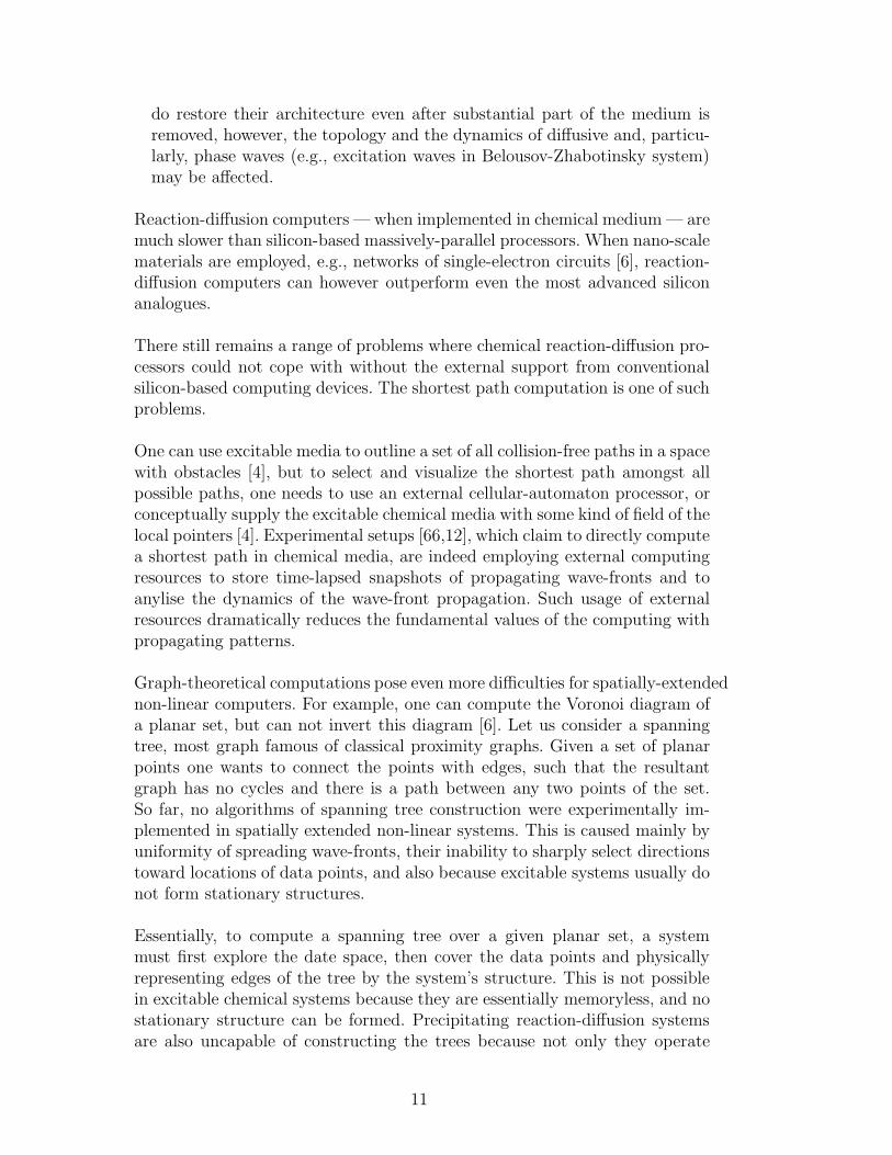
(a)

(b)

(c)

(d)

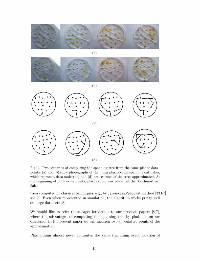
Fig. 2. Two scenarios of computing the spanning tree from the same planar data–points: (a) and (b) show photographs of the living plasmodium spanning oat flakes,which represent data nodes; (c) and (d) are schemes of the trees approximated. Atthe beginning of both experiments, plasmodium was placed at the Southmost oatflake.

trees computed by classical techniques, e.g., by Jaromczyk-Supowit method [33,67],see [8]. Even when represented in simulation, the algorithm works pretty wellon large data sets [8].

We would like to refer those eager for details to our previous papers [8,7],where the advantages of computing the spanning tree by pladmodium arediscussed. In the present paper we will mention two speculative points of theapproximation.

Plasmodium almost never computes the same (including exact location of

15

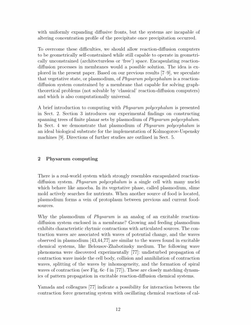
(a)

(b)

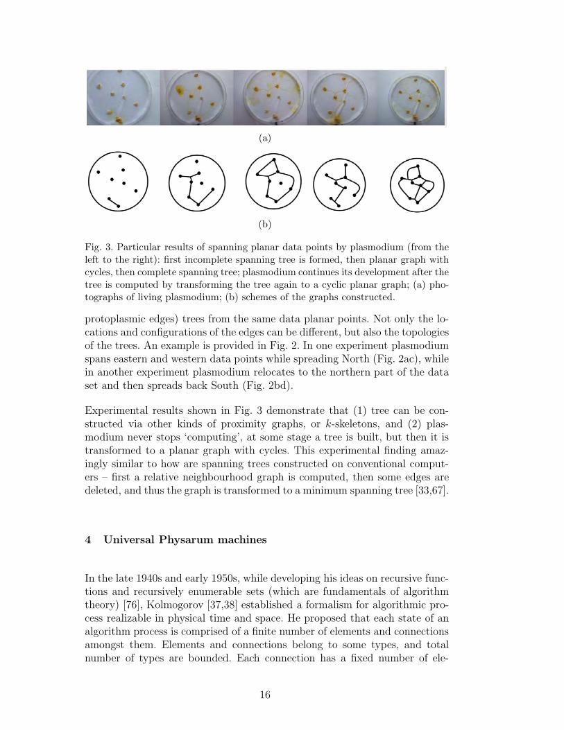
Fig. 3. Particular results of spanning planar data points by plasmodium (from theleft to the right): first incomplete spanning tree is formed, then planar graph withcycles, then complete spanning tree; plasmodium continues its development after thetree is computed by transforming the tree again to a cyclic planar graph; (a) pho-tographs of living plasmodium; (b) schemes of the graphs constructed.

protoplasmic edges) trees from the same data planar points. Not only the lo-cations and configurations of the edges can be different, but also the topologiesof the trees. An example is provided in Fig. 2. In one experiment plasmodiumspans eastern and western data points while spreading North (Fig. 2ac), whilein another experiment plasmodium relocates to the northern part of the dataset and then spreads back South (Fig. 2bd).

Experimental results shown in Fig. 3 demonstrate that (1) tree can be con-structed via other kinds of proximity graphs, or k-skeletons, and (2) plas-modium never stops ‘computing’, at some stage a tree is built, but then it istransformed to a planar graph with cycles. This experimental finding amaz-ingly similar to how are spanning trees constructed on conventional comput-ers – first a relative neighbourhood graph is computed, then some edges aredeleted, and thus the graph is transformed to a minimum spanning tree [33,67].

4 Universal Physarum machines

In the late 1940s and early 1950s, while developing his ideas on recursive func-tions and recursively enumerable sets (which are fundamentals of algorithmtheory) [76], Kolmogorov [37,38] established a formalism for algorithmic pro-cess realizable in physical time and space. He proposed that each state of analgorithm process is comprised of a finite number of elements and connectionsamongst them. Elements and connections belong to some types, and totalnumber of types are bounded. Each connection has a fixed number of ele-

16

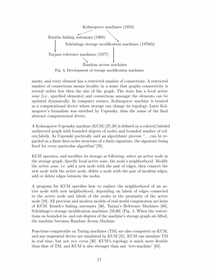
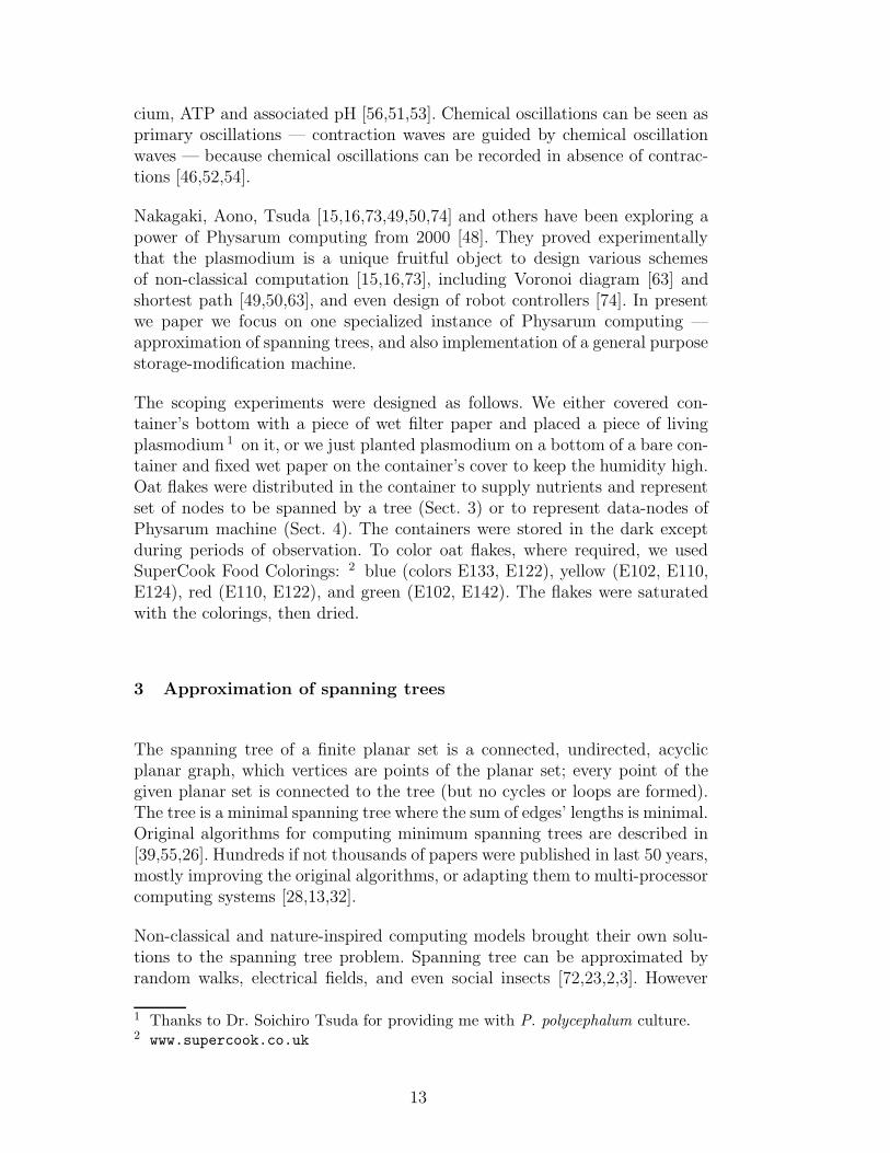
Kolmogorov machines (1953)

Knuths linking automata (1968)

Schonhage storage modification machines (1970th)

Tarjans reference machines (1977)

Random access machines

Fig. 4. Development of storage modification machines.

ments, and every element has a restricted number of connections. A restrictednumber of connections means locality in a sense that graphs connectivity isseveral orders less then the size of the graph. The state has a local activezone (i.e., specified elements) and connections amongst the elements can beupdated dynamically. In computer science, Kolmogorov machine is treatedas a computational device whose storage can change its topology. Later Kol-mogorov’s formalism was enriched by Uspensky, thus the name of the finalabstract computational device.

A Kolmogorov-Uspensky machine (KUM) [37,38] is defined on a colored/labeledundirected graph with bounded degrees of nodes and bounded number of col-ors/labels. As Uspenski poetically said an algorithmic process “. . . can be re-garded as a finite first-order structure of a finite signature, the signature beingfixed for every particular algorithm”[76].

KUM operates, and modifies its storage as following: select an active node inthe storage graph. Specify local active zone, the node’s neighborhood. Modifythe active zone, i.e. add a new node with the pair of edges, then connect thenew node with the active node; delete a node with the pair of incident edges;add or delete edges between the nodes.

A program for KUM specifies how to replace the neighborhood of an ac-tive node with new neighborhood, depending on labels of edges connectedto the active node and labels of the nodes in the proximity of the activenode [19]. All previous and modern models of real-world computation are heirsof KUM: Knuth’s linking automata [36], Tarjan’s Reference Machines [68],Schonhage’s storage modification machines [59,60] (Fig. 4. When the restric-tions on bounded in- and out-degrees of the machine’s storage graph are lifted,the machine becomes Random Access Machine.

Functions computable on Turing machines (TM) are also computed on KUM,and any sequential device are simulated by KUM [31]. KUM can simulate TMin real time, but not vice versa [30]. KUM’s topology is much more flexiblethan that of TM, and KUM is also stronger than any ‘tree-machine’ [65].

17

In 1988 Gurevich [31], suggested that an edge of KUM is not only an in-formational but also a physical entity and reflects the physical proximity ofthe nodes (thus e.g. even in three-dimensional space number of neighbors ofeach node is polynomially bounded). A TM formalizes computation as per-formed by humans[75], whereas KUM formalizes computation as performedby physical process [19].

What would be the best natural implementation of KUM? A potential can-didate should be capable for growing, unfolding, graph-like storage structure,dynamically manipulating nodes and edges, and should have a wide range offunctioning parameters. Vegetative stage, i.e., plasmodium, of a true slimemold Physarum polycephalum satisfies all these requirements.

Physarum machine has two types of nodes: stationary nodes, presented bysources of nutrients (oat flakes), and dynamic nodes, sites where two or moreprotoplasmic veins originate. At the beginning of the computation, the sta-tionary nodes are distributed in the computational space, and the plasmodiumis placed at one point of the space. Starting in the initial conditions, the plas-modium exhibits foraging behavior, and occupies stationary nodes.

An edge of Physarum machine is a strand, or vein, of a protoplasm connectingstationary and/or dynamic nodes. KUM machine is an undirected graph, i.e.,if nodes x and y are connected, then they are connected by two edges (xy)and (yx). In Physarum machine this is implemented by a single edge but withperiodically reversing flow of protoplasm [34,47].

Program and data are represented by a spatial configuration of stationarynodes. Result of the computation over stationary data-node is presented by aconfiguration of dynamical nodes and edges. The initial state of a Physarummachine, includes part of input string (the part which represents position ofplasmodium relatively to stationary nodes), an empty output string, a currentinstruction in the program, and a storage structure consists of one isolatednode. That is, the whole graph structure developed by plasmodium is the resultof its computation, “if S is a terminal state, then the connected component ofthe initial vertex is considered to be the ‘solution”’ [38]. Physarum machinehalts when all data-nodes are utilized.

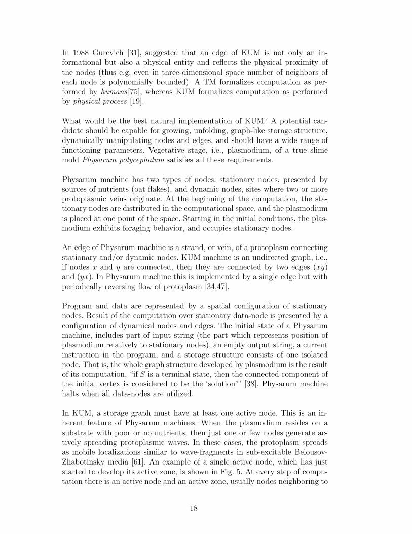
In KUM, a storage graph must have at least one active node. This is an in-herent feature of Physarum machines. When the plasmodium resides on asubstrate with poor or no nutrients, then just one or few nodes generate ac-tively spreading protoplasmic waves. In these cases, the protoplasm spreadsas mobile localizations similar to wave-fragments in sub-excitable Belousov-Zhabotinsky media [61]. An example of a single active node, which has juststarted to develop its active zone, is shown in Fig. 5. At every step of compu-tation there is an active node and an active zone, usually nodes neighboring to

18

(a) (b)

(c) (d)

Fig. 5. Basic operations of Physarum machine: (a) a single active node generatesan active zone at the beginning of computation, (b) addressing of a green-coloureddata-node, (c) and (d) implementation of add node (nodes 3), add edge (edge(5, 4)), remove edge (edge (route, 4)) operations.

active node. The active zone has limited complexity, in a sense that all elementsof the zone are connected by some chain of edges to the initial node. In general,the size of an active zone may vary depending on the computational task. InPhysarum machine an active node is a trigger of contraction/excitation waves,which spread all over the plasmodium tree and cause pseudopodia to propa-gate, change their shape, and even protoplasmic veins to annihilate. An activezone is comprised of stationary or dynamic nodes connected to an active nodewith veins of protoplasm.

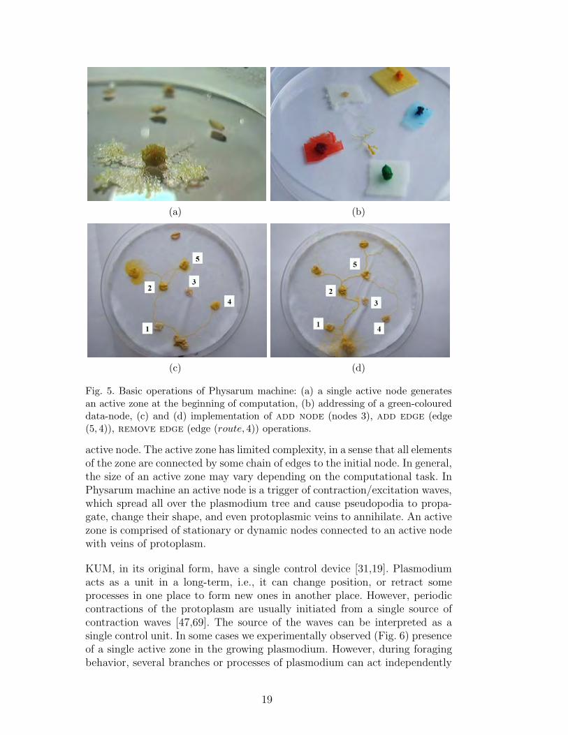
KUM, in its original form, have a single control device [31,19]. Plasmodiumacts as a unit in a long-term, i.e., it can change position, or retract someprocesses in one place to form new ones in another place. However, periodiccontractions of the protoplasm are usually initiated from a single source ofcontraction waves [47,69]. The source of the waves can be interpreted as asingle control unit. In some cases we experimentally observed (Fig. 6) presenceof a single active zone in the growing plasmodium. However, during foragingbehavior, several branches or processes of plasmodium can act independently

19

(a)

(b)

Fig. 6. Serial approximation of spanning tree by plasmodium: (a) snapshots of theliving plasmodium, from the left to the right, made with 6 hours intervals; (b) schemeof the graph. The active zone at each step of computation is encircled.

and almost autonomously.

In contrast to Schonhage machine, KUM has bounded in- and out-degree ofthe storage graph. Graphs developed by Physarum are predominantly planargraphs. Moreover, if we put a piece of vein of protoplasm on top of another veinof protoplasm, the veins fuse [62]. Usually, not more than three protoplasmicstrands join each other in one given point of space. Therefore we can assumethat the average degree of the storage graph in Physarum machines is slightlyhigher then the degree of a spanning tree (average degree of 1.9 as reportedin [22]) but smaller than the average degree of a random planar graph (degree4 [14]).

Every node of KUM must be uniquely addressable and nodes and edgesmust be labeled [38]. There is no direct implementation of such addressingin Physarum machine. With stationary nodes this can be implemented, forexample, by coloring the oat flakes. An example of such experimental imple-mentation of a unique node addressing is shown in Fig. 5b.

A possible set of instructions for Physarum machine could be as follows: com-mon instructions would include input, output, go, halt, and internal in-structions: new, set, if [25]. At the present state of the experimental im-plementation, we assume that input is done via distribution of sources ofnutrients, while output is recorded optically. The instruction set causespointers redirection, and can be realized by a placing a fresh source of nutri-ents in the experimental container, preferably on top of one of the old sources

20

of nutrients. When a new node is created, all pointers can be redirected fromthe old node to the new node. Let us look at the experimental implementationof the core instructions.

To add a stationary node b to node a’s neighborhood, the plasmodium mustpropagate from a to b, and form a protoplasmic vein representing the edge (ab).To form a dynamic node, propagating the pseudopodia must branch into twoor more pseudopodia, and the site of branching will represent the newly formednode. We have also obtained experimental evidence that dynamic nodes can beformed when a tip of growing pseudopodia collides with existing protoplasmicstrande. In some cases merging of protoplasmic veins occur.

To remove the stationary node from Physarum machine, the plasmodiumleaves the node. Annihilating protoplasmic strands, which form a dynamicnode at their intersection, remove the dynamic node from the storage struc-ture of Physarum machine.

To add an edge to a neighborhood, an active node generates propagatingprocesses, which establish a protoplasm vein with one or more neighboringnodes.

When a protoplasmic vein annihilates, e.g., depending on the global stateor when source of nutrients exhausted, the edge represented by the vein isremoved from Physarum machine (Fig. 5cd). The following sequence of opera-tions is demonstrated in Fig. 5cd: node 3 is added to the structure by removingedge (12) and forming two new edges (13) and (23).

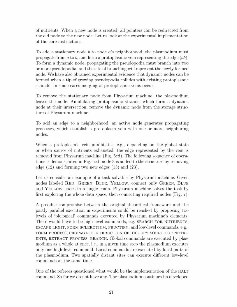
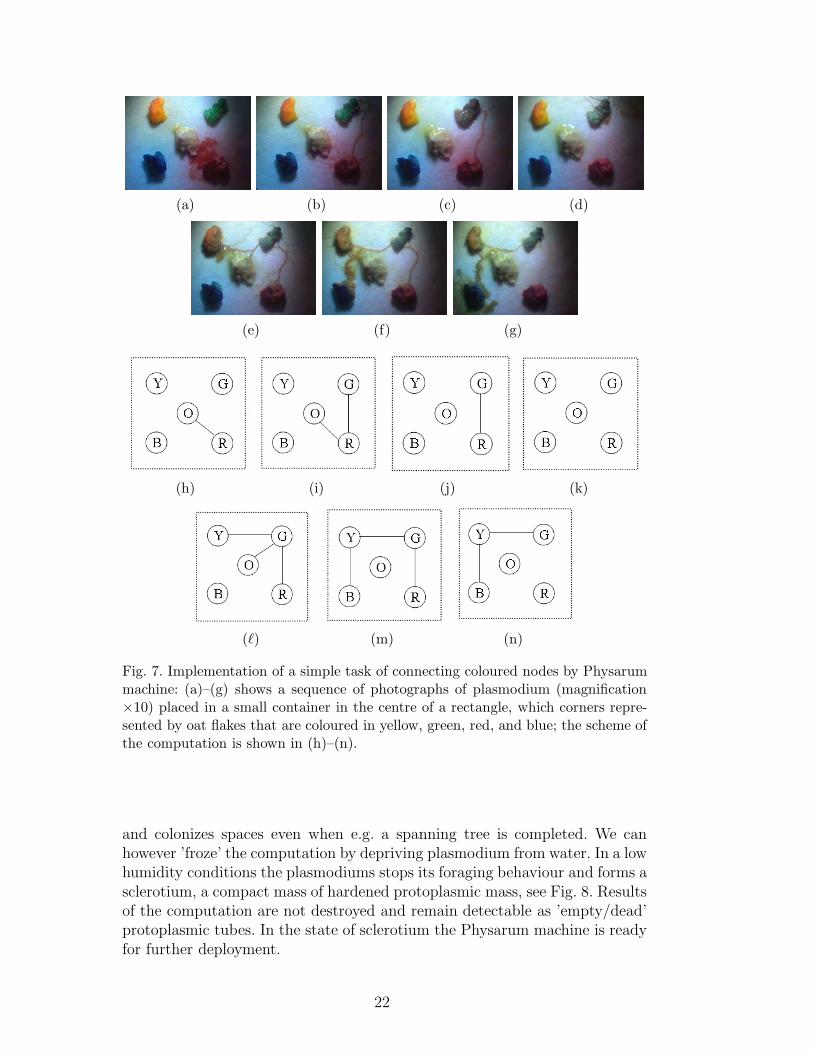
Let us consider an example of a task solvable by Physarum machine. Givennodes labeled Red, Green, Blue, Yellow, connect only Green, Blueand Yellow nodes in a single chain. Physarum machine solves the task byfirst exploring the whole data space, then connecting required nodes (Fig. 7).

A possible compromise between the original theoretical framework and thepartly parallel execution in experiments could be reached by proposing twolevels of ‘biological’ commands executed by Physarum machine’s elements.There would have to be high-level commands, e.g. search for nutrients,escape light, form sclerotium, fructify, and low-level commands, e.g.,form process, propagate in direction of, occupy source of nutri-ents, retract process, branch. Global commands are executed by plas-modium as a whole at once, i.e., in a given time step the plasmodium executesonly one high-level command. Local commands are executed by local parts ofthe plasmodium. Two spatially distant sites can execute different low-levelcommands at the same time.

One of the referees questioned what would be the implementation of the haltcommand. So far we do not have any. The plasmodium continues its developed

21

(a) (b) (c) (d)

(e) (f) (g)

(h) (i) (j) (k)

() (m) (n)

Fig. 7. Implementation of a simple task of connecting coloured nodes by Physarummachine: (a)–(g) shows a sequence of photographs of plasmodium (magnification×10) placed in a small container in the centre of a rectangle, which corners repre-sented by oat flakes that are coloured in yellow, green, red, and blue; the scheme ofthe computation is shown in (h)–(n).

and colonizes spaces even when e.g. a spanning tree is completed. We canhowever ’froze’ the computation by depriving plasmodium from water. In a lowhumidity conditions the plasmodiums stops its foraging behaviour and forms asclerotium, a compact mass of hardened protoplasmic mass, see Fig. 8. Resultsof the computation are not destroyed and remain detectable as ’empty/dead’protoplasmic tubes. In the state of sclerotium the Physarum machine is readyfor further deployment.

22

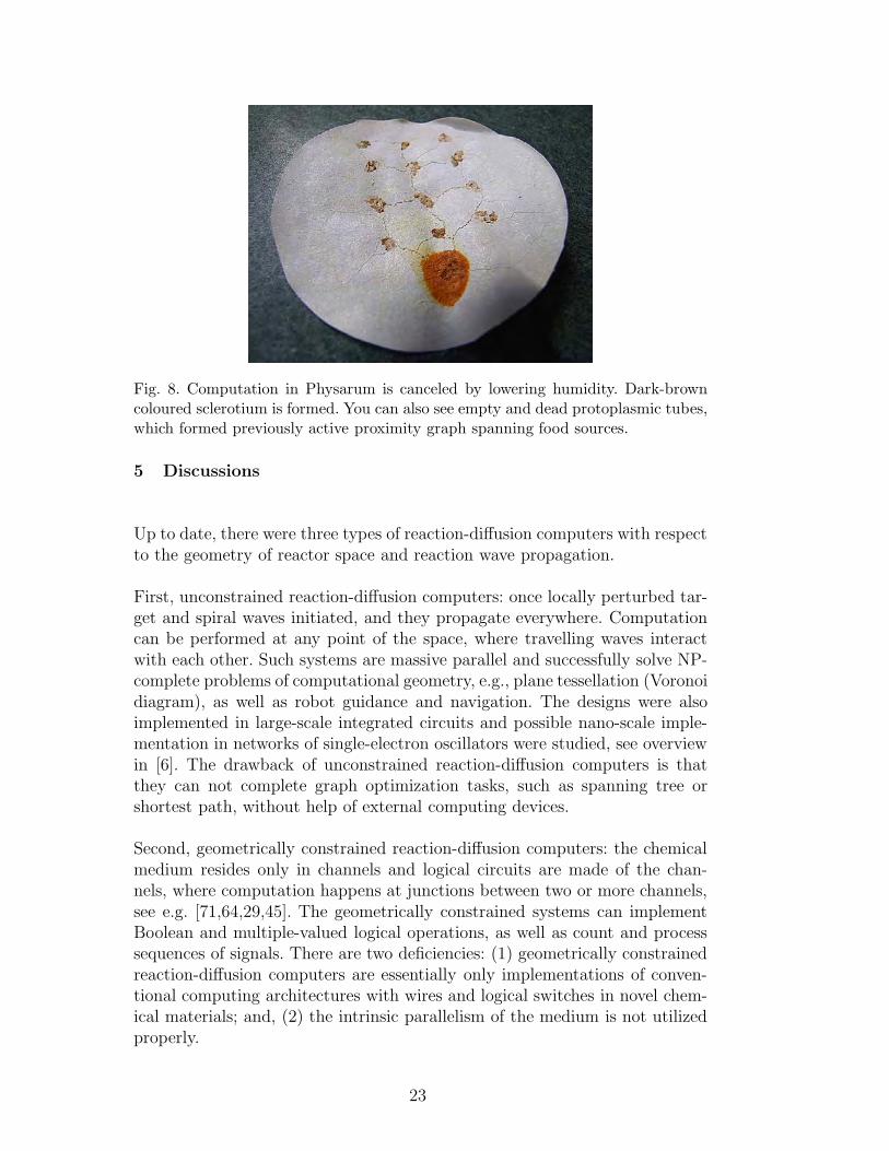
Fig. 8. Computation in Physarum is canceled by lowering humidity. Dark-browncoloured sclerotium is formed. You can also see empty and dead protoplasmic tubes,which formed previously active proximity graph spanning food sources.

5 Discussions

Up to date, there were three types of reaction-diffusion computers with respectto the geometry of reactor space and reaction wave propagation.

First, unconstrained reaction-diffusion computers: once locally perturbed tar-get and spiral waves initiated, and they propagate everywhere. Computationcan be performed at any point of the space, where travelling waves interactwith each other. Such systems are massive parallel and successfully solve NP-complete problems of computational geometry, e.g., plane tessellation (Voronoidiagram), as well as robot guidance and navigation. The designs were alsoimplemented in large-scale integrated circuits and possible nano-scale imple-mentation in networks of single-electron oscillators were studied, see overviewin [6]. The drawback of unconstrained reaction-diffusion computers is thatthey can not complete graph optimization tasks, such as spanning tree orshortest path, without help of external computing devices.

Second, geometrically constrained reaction-diffusion computers: the chemicalmedium resides only in channels and logical circuits are made of the chan-nels, where computation happens at junctions between two or more channels,see e.g. [71,64,29,45]. The geometrically constrained systems can implementBoolean and multiple-valued logical operations, as well as count and processsequences of signals. There are two deficiencies: (1) geometrically constrainedreaction-diffusion computers are essentially only implementations of conven-tional computing architectures with wires and logical switches in novel chem-ical materials; and, (2) the intrinsic parallelism of the medium is not utilizedproperly.

23

Third, reaction constrained reaction-diffusion computers: travelling waves canbe initiated and then propagate anywhere in the reaction space. However dueto low reactivity of the system, no classical (e.g., target) waves are formed. Thisis typical for sub-excitable Belousov-Zhabotinsky systems. Local perturbationleads to formation of compact wave-fragments which can travel for reasonabledistance preserving its shape, see e.g. [61]. The system is an ideal implemen-tation of collision-based computing schemes [5]. The deficiency of the systemis that travelling compact wave-fragment are very sensitive to conditions ofthe medium, and therefore are cumbersome to control.

To overcome all these deficiencies of reaction-diffusion computers, we sug-gested to encapsulate the reaction-diffusion systems in a membrane becausethis seems to be a good combination of unconstrained physical space andmembrane-constrained geometry of propagating patterns 3 . Also, a systemencapsulated in an elastic or contractable membrane would be capable ofreversible shape changing, a feature unavailable in reaction-diffusion chemi-cal systems. We demonstrated that the vegetative state, the plasmodium, ofslime mold Physarum polycephalum, is an ideal biological medium for sug-gested implementation. We have provided first experimental evidences thatplasmodium can compute spanning trees of finite planar sets and implementKolmogorov-Uspensky machines. Thus, Physarum computers can solve graph-theoretic problems and are capable for universal computation.

Physarum computers will be particularly efficient in solving large-scale graphand network (including telecommunication and road traffic networks) opti-mization tasks, and can also be used as embedded controllers for non-silicon(e.g., gel-based) reconfigurable robots and manipulators. They are reasonablyrobust (they live on almost any non-aggressive substrate including plastic,glass and metal foil, in a wide range of temperatures, they do not requirespecial substrates or sophisticated equipment for maintenance) and are pro-grammable (plasmodium exhibits negative phototaxis, and can follow gradi-ents of humidity and some chemo-attractants) spatially extended and, dis-tributed, computing devices.

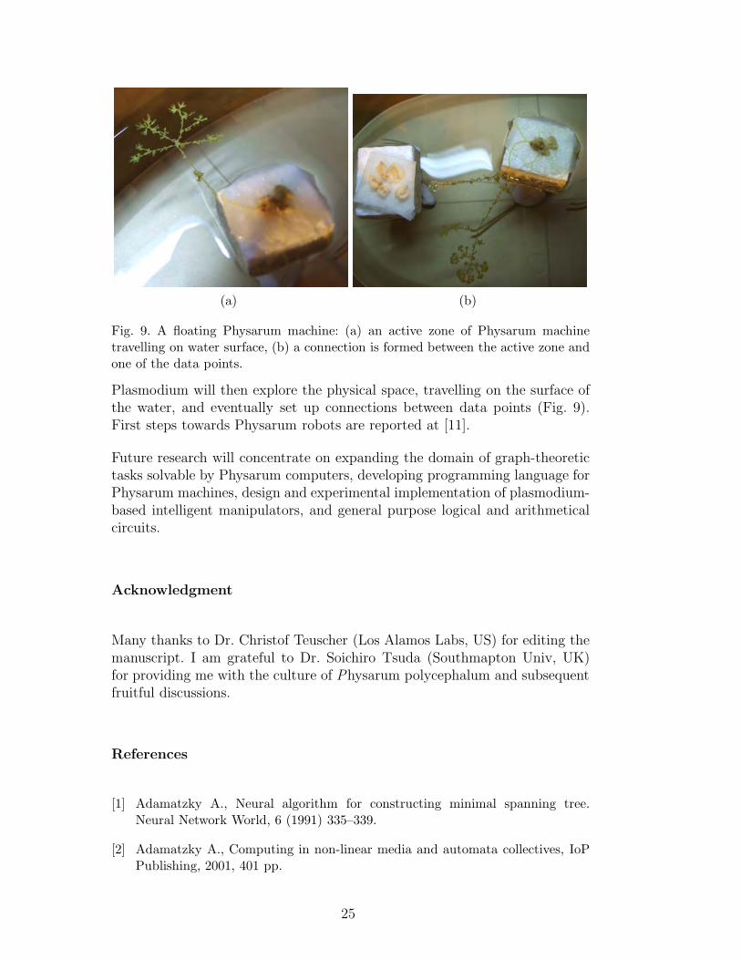
In contrast to ‘classical’ chemical reaction-diffusion computers [6], Physarymmachines can function on virtually any biologically non-agressive substrate,include metal and glass. Moreover, the substrate does not have to be static.For example, to implement Physarum machines with mobile data nodes, onecan use a container with water, place the plasmodium of Physarum on onefloating object, and the oat flakes (data) on several other floating objects.

3 Recently we have demonstrated in chemical and biological laboratory experi-ments that plasmodoium of Physarun polycephalum behaves almost exactly thesame, apart of leaving a ’trace’, as excitation patterns in sub-excitable Belousov-Zhabotinsky medium, see details in [10]. Thus plasmodium is also proved to becapable for collision-based universal computation [5].

24

(a) (b)

Fig. 9. A floating Physarum machine: (a) an active zone of Physarum machinetravelling on water surface, (b) a connection is formed between the active zone andone of the data points.

Plasmodium will then explore the physical space, travelling on the surface ofthe water, and eventually set up connections between data points (Fig. 9).First steps towards Physarum robots are reported at [11].

Future research will concentrate on expanding the domain of graph-theoretictasks solvable by Physarum computers, developing programming language forPhysarum machines, design and experimental implementation of plasmodium-based intelligent manipulators, and general purpose logical and arithmeticalcircuits.

Acknowledgment

Many thanks to Dr. Christof Teuscher (Los Alamos Labs, US) for editing themanuscript. I am grateful to Dr. Soichiro Tsuda (Southmapton Univ, UK)for providing me with the culture of Physarum polycephalum and subsequentfruitful discussions.

References

[1] Adamatzky A., Neural algorithm for constructing minimal spanning tree.Neural Network World, 6 (1991) 335–339.

[2] Adamatzky A., Computing in non-linear media and automata collectives, IoPPublishing, 2001, 401 pp.

25

[3] Adamatzky A. and Holland O. Reaction-diffusion and ant-based load balancingof communication networks. Kybernetes 31 (2002) 667–681.

[4] Adamatzky A. and De Lacy Costello B.P.J., Collision-free path planningin the Belousov-Zhabotinsky medium assisted by a cellular automaton.Naturwissenschaften 89 (2002) 474–478.

[5] Adamatzky A. (Ed.) Collision-Based Computing, Springer, London, 2003.

[6] Adamatzky A., De Lacy Costello B., Asai T. Reaction-Diffusion Computers,Elsevier, Amsterdam, 2005.

[7] Adamatzky A. Physarum machines: encapsulating reaction-diffusion tocompute spanning tree. Naturwisseschaften 94 (2007) 975–980.

[8] Adamatzky A. Growing spanning trees in plasmodium machines, Kybernetes:The International Journal of Systems & Cybernetics 37 (2008) 258–264.

[9] Adamatzky A. Physarum machine: implementation of a Kolmogorov-Uspenskymachine on a biological substrate. Parallel Processing Letters 17 (2007) 455-467.

[10] Adamatzky A., De Lacy Costello B., Shirakawa T. Universal computationwith limited resources: Belousov-Zhabotinsky and Physarum computers. Int.J. Bifurcation & Chaos (2008), in press.

[11] Adamatzky A., Towards Physarum robots: computing and manipulating onwater surface. arXiv:0804.2036v1 [cs.RO]

[12] Agladze K., Magome N., Aliev R., Yamaguchi T. and Yoshikawa K. Findingthe optimal path with the aid of chemical wave. Physica D 106 (1997) 247–254.

[13] Ahuja M. and Zhu Y. A distributed algorithm for minimum weight spanningtree based on echo algorithms In: Proc. Int. Conf. Distr. Computing Syst., 1989,2–8.

[14] Alber J., Dorn F., Niedermeier R., Experiments on Optimally Solving NP-complete Problems on Planar Graphs, Manuscript (2001), http://www.ii.uib.no/~frederic/ADN01.ps

[15] Aono, M., and Gunji, Y.-P., Resolution of infinite-loop in hyperincursive andnonlocal cellular automata: Introduction to slime mold computing. ComputingAnticiaptory Systems, AIP Conference Proceedings, 718 (2001) 177–187.

[16] Aono, M., and Gunji, Y.-P., Material implementation of hyper-incursive fieldon slime mold computer. Computing Anticipatory Systems, AIP ConferenceProceedings, 718 (2004) 188–203.

[17] Bardzin’s J. M. On universality problems in theory of growing automata,Doklady Akademii Nauk SSSR 157 (1964) 542–545.

[18] Barzdin’ J.M. and Kalnins J. A universal automaton with variable structure,Automatic Control and Computing Sciences 8 (1974) 6–12.

26

[19] Blass A. and Gurevich Y. Algorithms: a quest for absolute definitions, Bull.Europ. Assoc. TCS 81 (2003) 195–225.

[20] van Emde Boas, P. Space measures for storage modification machines.Information Process. Lett. 30 (1989) 103–110.

[21] Calude C.S., Dinneen M.J., Paun G., Rozenberg G., Stepney S. UnconventionalComputation: 5th International Conference, Springer, 2006.

[22] Cartigny J., Ingelrest F., Simplot-Ryl D., Stojmenovic I., Localized LMST andRNG based minimum-energy broadcast protocols in ad hoc networks. Ad HocNetworks 3 (2005) 1-16.

[23] Chong F. Analog techniques for adaptive routing on interconnection networksM.I.T. Transit Note No. 14, 1993.

[24] Cloteaux B. and Rajan D. Some separation results between classes of pointeralgorithms, In DCFS ’06: Proceedings of the Eighth Workshop on DescriptionalComplexity of Formal Systems. 2006, 232–240.

[25] Dexter S., Doyle P. and Gurevich Yu. Gurevich abstract state machines andSchonhage storage modification machines, J Universal Computer Science 3(1997) 279–303.

[26] Dijkstra E.A. A note on two problems in connection with graphs Numer. Math.1 (1959) 269–271.

[27] Gacs P. and Leving L. A. Casual nets or what is a deterministic computation,STAN-CS-80-768, 1980.

[28] Gallager R.G., Humblet P.A. and Spira P.M. A distributed algorithm forminimum–weight spanning tree ACM Tranbs. Programming Languages andSystems 5 (1983) 66–77.

[29] Gorecki J., Yoshikawa K. and Igarashi Y., On chemical reactors that can count,J. Phys. Chem., A 107 (2003) 1664–1669.

[30] Grigoriev D. Kolmogorov algorithms are stronger than Turing machines. Notesof Scientific Seminars of LOMI 60 (1976) 29–37, in Russian. English translationin J. Soviet Math. 14 (1980) 1445–1450.

[31] Gurevich Y., On Kolmogorov machines and related issues, in Bull. EATCS 35(1988) 71–82.

[32] Huang S.–T. A fully pipelined minimum spanning tree constructor. J. Parall.Distr. Computing 9 (1990) 55–62.

[33] Jaromczyk J.W. and Kowaluk M. A note on relative neighborhood graphs Proc.3rd Ann. Symp. Computational Geometry, 1987, 233–241.

[34] Kamiya N. The protoplasmic flow in the myxomycete plasmodium as revealedby a volumetric analysis, Protoplasma 39 (1950) 3.

27

[35] Kirkpatrick D.G. and Radke J.D. A framework for computational morphology.In: Toussaint G. T., Ed., Computational Geometry (North-Holland, 1985) 217-248.

[36] Knuth D. E. The Art of Computer Programming, Vol. 1: FundamentalAlgorithms, Addison-Wesley, Reading, Mass. 1968.

[37] Kolmogorov A. N., On the concept of algorithm, Uspekhi Mat. Nauk 8 (1953)175–176.

[38] Kolmogorov A. N., Uspensky V. A. On the definition of an algorithm. UspekhiMat. Nauk, 13 (1958) 3–28, in Russian. English translation: ASM Translations21 (1963) 217–245.

[39] Kruskal J.B. On the shortest subtree of a graph and the traveling problem.Proc. Amer. Math. Sec. 7 (1956) 48–50.

[40] Kuhnert L. A new photochemical memory device in a light sensitive activemedium. Nature 319 (1986) 393.

[41] Kuhnert L., Agladze K. L., Krinsky V. I. Image processing using light-sensitivechemical waves. Nature 337 (1989) 244–247.

[42] Kusumi T., Yamaguchi T., Aliev R., Amemiya T., Ohmori T., Hashimoto H.Yoshikawa K. Numerical study on time delay for chemical wave transmissionvia an inactive gap. Chem. Phys. Lett. 271 (1997) 355–360.

[43] Matsumoto K., Ueda T., and Kobatake Y. Propagation of phase wave in relationto tactic responses by the plasmodium of Physarum polycephalum. J. of Theor.Biology 122 (1986) 339–345.

[44] Matsumoto K., Ueda T. and Kobatake Y. Reversal of thermotaxis withoscillatory stimulation in the plasmodium of Physarum polycephalum, J. Theor.Biology 131 (1988) 175–182.

[45] Motoike I., Adamatzky A. Three-valued logic gates in reaction-diffusionexcitable media. Chaos, Solitons & Fractals 24 (2005) 107–114.

[46] Nakagaki T., Yamada H., Ito M., Reaction-diffusion advection model for patternformation of rhythmic contraction in a giant amoeboid cell of the Physarumplasmodium. J. Theor. Biol. 197 (1999) 497–506.

[47] Nakagakia T., Yamada H., Ueda T. Interaction between cell shape andcontraction pattern in the Physarum plasmodium, Biophysical Chemistry 84(2000) 195–204.

[48] Nakagaki T., Yamada H., and Toth A., Maze-solving by an amoeboid organism.Nature 407 (2000) 470-470.

[49] Nakagaki T., Smart behavior of true slime mold in a labyrinth. Research inMicrobiology 152 (2001) 767-770.

[50] Nakagaki T., Yamada H., and Toth A., Path finding by tube morphogenesis inan amoeboid organism. Biophysical Chemistry 92 (2001) 47-52.

28

[51] Nakamura S., Yoshimoto Y., Kamiya N. Oscillation in surface pH of thePhysarum plasmodium. Proc. Jpn. Acad. 58 (1982) 270–273.

[52] Nakamura S. and Kamiya N. Regional difference in oscillatory characteristics ofPhysarum plasmodium as revealed by surface pH. Cell Struct. Funct. 10 (1985)173–176.

[53] Ogihara S. Calcium and ATP regulation of the oscillatory torsional movementin a triton model of Physarum plasmodial strands. Exp. Cell Res. 138 (1982)377–384.

[54] Oster G. F. and Odel G. M. Mechanics of cytogels I: oscillations in Physarum.Cell Motil. 4 (1984) 469–503.

[55] Prim R.C. Shortest connection networks and some generalizations Bell Syst.Tech. J. 36 (1957) 1389–1401.

[56] Ridgway E. B., Durham A.C.H. Oscillations of calcium ion concentration inPhysarum plasmodia, Protoplasma 100 (1976) 167–177.

[57] Rambidi N. G. Neural network devices based on reaction-duffusion media: anapproach to artificial retina. Supramolecular Science 5 (1998) 765–767.

[58] Rambidi N.G., Shamayaev K. R., Peshkov G. Yu. Image processing using light-sensitive chemical waves. Phys. Lett. A 298 (2002) 375–382.

[59] Schonhage A. Real-time simulation of multi-dimensional Turing machines bystorage modification machines, Project MAC Technical Memorandum 37, MIT(1973).

[60] Schonhage, A. Storage modification machines. SIAM J. Comp. 9 (1980) 490–508.

[61] Sedina-Nadal I, Mihaliuk E, Wang J, Perez-Munuzuri V, Showalter K. Wavepropagation in subexcitable media with periodically modulated excitability.Phys Rev Lett 86 (2001) 1646-9.

[62] Shirakawa T. Private communication, Feb 2007.

[63] Shirakawa T. And Gunji Y. -P. Computation of Voronoi diagram andcollision-free path using the Plasmodium of Physarum polycephalum. Int. J.Unconventional Computing (2008), in press.

[64] Sielewiesiuk J. and Gorecki J., Logical Functions of a Cross Junction ofExcitable Chemical Media, J. Phys. Chem., A105, 8189 (2001).

[65] Shvachko K.V. Different modifications of pointer machines and theircomputational power. In: Proc. Symp. Mathematical Foundations of ComputerScience MFCS. Lect. Notec Comput. Sci. 520 (1991) 426–435.

[66] Steinbock O., Toth A., Showalter K. Navigating complex labyrinths: optimalpaths from chemical waves. Science 267 (1995) 868–871.

29

[67] Supowit K.J. The relative neighbourhood graph, with application to minimumspanning tree. J. ACM 3 (1988) 428–448.

[68] Tarjan R. E. Reference machines require non-linear time to maintain disjointsets, STAN-CS-77-603, March 1977.

[69] Tero A., Kobayashi R., Nakagaki T. A coupled-oscillator model with aconservation law for the rhythmic amoeboid movements of plasmodial slimemolds. Physica D 205 (2005) 125-135.

[70] Tirosh R., Oplatka A., Chet I. Motility in a “cell sap” of the slime moldPhysarum Polycephalum, FEBS Letters 34 (1973) 40–42.

[71] Toth A., Showalter K. Logic gates in excitable media. J. Chem. Phys. 103 (1995)2058-2066.

[72] Lyons R. and Peres Y. Probability on Trees and Networks, 1997. http://mypage.iu.edu/~rdlyons/prbtree/prbtree.html

[73] Tsuda, S., Aono, M., and Gunji, Y.-P., Robust and emergent Physarum-computing. BioSystems 73 (2004) 45–55.

[74] Tsuda, S., Zauner, K. P. and Gunji, Y. P., Robot control: From silicon circuitryto cells, In: Ijspeert, A. J., Masuzawa, T. and Kusumoto, S., Eds. BiologicallyInspired Approaches to Advanced Information Technology, Springer, 2006, 20–32.

[75] Turing A., On computable numbers, with an application to theEntscheidungsproblem, Proc. London Mathematical Society, 42 (1936) 230–265.

[76] Uspensky V.A. Kolmogorov and mathematical logic, The Journal of SymbolicLogic 57 (1992) 385–412.

[77] Yamada H., Nakagaki T., Baker R.E., Maini P.K. Dispersion relation inoscillatory reaction-diffusion systems with self-consistent flow in true slimemold. J. Math. Biol. 54 (2007) 745–760.

30

Computations via Newtonian and relativistickinematic systems

E.J. Beggs1 and J.V. Tucker2

Swansea University,Singleton Park,

Swansea, SA2 8PP,United Kingdom

Abstract

We are developing a rigorous methodology to analyse experimental computation,by which we mean the idea of computing a set or function by experimenting withsome physical equipment. Here we consider experimental computation by kinematicsystems under both Newtonian and relativisitic kinematics. An experimental pro-cedure, expressed in a language similar to imperative programming languages, isapplied to equipment having a common form, that of a bagatelle, and is interpretedusing the two theories. We prove that for any set A of natural numbers there ex-ists a 2-dimensional kinematic system BA with a single particle P whose observablebehaviour decides n ∈ A for all n ∈ N. The procedure can operate under (a) Newto-nian mechanics or (b) relativistic mechanics. The proofs show how any information(coded by some A) can be embedded in the structure of a simple kinematic systemand retrieved by simple observations of its behaviour. We reflect on the methodol-ogy, which seeks a formal theory for performing experiments that can put physicalrestrictions on the construction of systems. We conclude with some open problems.

Keywords: foundations of computation; computable functions and sets;Newtonian kinematic systems; Relativistic kinematic systems; foundations ofmechanics; theory of Gedanken experiments; non-computable physical systems.

1 Introduction

Consider the idea of computing functions by means of physical systems. Suppose eachcomputation by a physical system is based on running an experiment with three stages:

(i) input data x are used to determine initial conditions of the physical system;(ii) the system operates or evolves for a finite or infinite time; and(iii) output data y are obtained by measuring the observable behaviour of a system.

The function f computed by a series of such experiments is simply the relation y =f(x). The function may be partial or multivalued, and the data may be continuous or

1Department of Mathematics. Email: [email protected] of Computer Science. Email: [email protected]

31

discrete. We call the idea of using experiments with physical systems to define functionsexperimental computation. This concept of experimental computation is both old andgeneral. It can be found in ideas about (a) technologies for making calculating instrumentsand machines and (b) modelling physical and biological systems. The concept is alsocomplicated and in need of systematic theoretical investigation.

In contrast, the concept of algorithmic computation is well understood. Computabilitytheory, founded by Church, Turing and Kleene in 1936, is a deep theory for the functionscomputable by algorithms on discrete and continuous data. The obvious questions arise:

What are the functions computable by experiments with a class of physical systems?How do they compare with the functions computable by algorithms?

Related questions arise, about novel technologies for computing and about the computabil-ity of physical systems.

There is no shortage of results, discussion and debate on particular types of experi-mental computation. Many examples of non-computable systems are difficult to interpretphysically [26, 27, 28, 18, 38]. Some are technically incomplete, and, strictly speaking,have the status of conjectures (e.g., [20]). Some theorems encode non-computability ingeneral classes of mathematical systems (e.g., ODEs in [25]) rather than models of specificphysical systems (e.g., wave machines, bagatelles, pendula). Different approaches haveled to a diverse literature but the questions are, we believe, open for essentially all classesof system.

We are developing a methodology that aims to answer such basic questions in a defini-tive way [3, 4, 6]. Based on five general principles (summarised later in Section 2), aparticular feature of our methodology is the detailed analysis of particular examples,in which we seek the precise physical concepts and laws that permit or prevent non-computable functions and behaviours. To do this we choose a precisely defined fragmentT of a physical theory to specify, rather formally, the experimental procedure, equipmentand reason about its behaviour.

We have illustrated and refined our methodology largely by analysing examples ofexperimental computations with idealised kinematic systems. Here we will show thatthere exist simple kinematic procedures and equipment, whose computational behaviour,according to both Newtonian and Relativistic mechanics, can decide the membership ofany subset A of the set N = 0, 1, 2, . . . of natural numbers. The systems are infinitebagatelles that are based on simple energy and momentum conservation principles. Theyeach require unbounded space, time and energy to decide n ∈ N for all n. The Newtoniancase is simple. The relativistic case might be considered to be more realistic and it also hasa useful theoretical property, a maximum propagation speed for objects or information, thespeed of light c. Instead of unbounded velocity in the Newtonian case, in the relativisticcase we exploit the fact that the mass of a particle is unbounded as its speed approachesc.

Theorem 1.1. Let A ⊆ N. There exists a 2-dimensional kinematic system with a singleparticle P whose observable behaviour decides A. More specifically, the system is aninfinite bagatelle for which the following are equivalent: given any n ∈ N

(i) n ∈ A.(ii) In an experiment, given initial velocity Vn the particle P leaves and returns to the

origin within a known time Tn.

32

The system can be set up to operate under a class of kinematic theories, including(a) Newtonian kinematics or(b) Relativistic kinematics.

The velocity Vn and the time Tn are calculated from n and so by simply projectingthe particle and watching the clock while waiting for its return, we can decide A. Thefact that any conceivable discrete information can be represented in the discrete observ-able behaviour of a ball rolling along a line suggests that these elementary theories ofkinematics are undesirably strong. What should be done with these examples?

The bagatelle uncovers an interesting uniformity or generality. The experimental pro-cedure is essentially the same for any bagatelle and is physically sound. The observationand operation of the bagatelles require rather general assumptions that hold of severalkinematic theories. However, it is through the specification or description of the systemthat the computation of any A is possible. If the analysis of the experiment concerned notjust the observation of an existing system but the process of assembly or construction ofthe bagatelle then further conditions on the system would be needed that would restrictthe subsets of N. Thus, the bagatelles also reveal that something is missing: they showthat a formal account of experimentation must include the specification and constructionof mechanical equipment to answer the questions above. A critique of the examples is thesubject of Section 6.

In the case of the bagatelle there are certain natural assumptions on experiments thatwould allow them to compute only the semicomputable and computable subsets of N.Indeed, by choosing A ⊆ N to be a complete semicomputable set then the constructionyields a new universal computer:

Corollary 1.2. There exists a 2-dimensional kinematic system with a single particle Pthat is a universal machine for the computable partial functions on N, i.e. the bagatellecomputes by experiment all and only the computable partial functions on N.

The structure of the paper is this. In Section 2 we summarise our methodology. InSection 3 we describe the construction of a general type of infinite bagatelle. In Section 4we apply the description to make a bagatelle that decides the membership relation for Aunder Newtonian mechanics, and in Section 5 we apply it to make a bagatelle to decidethe membership relation for A under Relativistic mechanics. In Section 6 we reflect onthe examples and argue for formal theory of experimentation to answer the questions.Finally, in Section 7 some open problems are discussed.

The reader should be familiar with theory for the functions computable by algo-rithms on discrete data (Rogers [29], Odifreddi [22], Griffor [16], Stoltenberg-Hansen andTucker [32]) and continuous data (Pour-El and Richards [28], Tucker and Zucker [35, 36],Weihrauch [37]).

2 Methodological principles

With the idea of experimental computation, we can unify a disparate set of physical modelsof computation and seek properties they have in common. In particular, we can attemptto analyse physical models of computation independently of the theory of algorithms.

33

Physical theories play a fundamental role in understanding experimental computation;this we have discussed at length elsewhere [3, 4]. To seek conceptual clarity, and math-ematical precision and detail, we have proposed, in [3, 4, 6], the following five principlesfor an investigation of any class of experimental computations:

Principle 1. Defining a physical subtheory: Define precisely a subtheory T ofa physical theory and examine experimental computation by the systems that are validmodels of the subtheory T .

Principle 2. Classifying computers in a physical theory: Find systems that aremodels of T that can through experimental computation implement specific algorithms,calculators, computers, universal computers and hyper-computers.

Principle 3. Mapping the border between computer and hyper-computer inphysical theory: Analyse what properties of the subtheory T are the source of computableand non-computable behaviour and seek necessary and sufficient conditions for the systemsto implement precisely the algorithmically computable functions.

Principle 4. Reviewing and refining the physical theory: Determine the physicalrelevance of the systems of interest by reviewing the truth or valid scope of the subtheory.Criticism of the system might require strengthening the subtheory T in different ways,leading to a portfolio of theories and examples.

Principle 5. Combining experiments and algorithms: Use a physical system asan oracle in a model of algorithmic computation, such as Turing machines. Determinewhether the subtheory T , the experimental computation, and the protocol extends the powerand efficiency of the algorithmic model.

Principles 1-4 were introduced in [3] and Principle 5 was introduced in [6].To study experimental computation and seek answers to basic questions, the key idea

is to lay bare all the concepts and technicalities of examples by putting them under amathematical microscope using the theory T and, furthermore, to look at the computa-tional behaviour of classes of systems that obey the laws of T . Our methodology requiresa careful formulation of a physical theory T , which can best be done by axiomatisationsa fragment of the physical theory.

3 Experiments with an infinite bagatelle

We describe the structure of our bagatelle, and the steps involved in using the bagatelleto compute. An important point is that the structural form of the bagatelle, and theexperimental procedure to operate it, is common to both the Newtonian and relativisticmachines.

34

3.1 Experiment procedure for the bagatelle

We consider a bagatelle game. A ball is fired into the bagatelle machine with a specifiedvelocity, and the ball may or may not return in a given time period. Nothing else aboutthe bagatelle is externally observable.

Each bagatelle machine is designed to define a subset A of the natural numbers N asfollows:

“Given some number n ∈ N the operator of BA chooses a point particle P , positionsit at an origin 0 and projects the particle with a velocity Vn. Then the operator waitsfor a time Tn and if the particle returns before this time then declares that n ∈ A andotherwise that n /∈ A.”

We can express the experimental procedure in the following experimental pseudocode:

exp-pseudocode Bagatelle;place particle P mass ? radius 0 at point 0;start clock t;project particle at 0 with velocity Vn;wait Tn units and do nothing;if particle in tray at 0 then return “n ∈ A” else return “n /∈ A”end Bagatelle.

In the pseudocode, the particle P is a point particle, with radius 0, but may be of anymass.

Procedures of this kind are an example of “design pattern” called project and wait.They can be applied to a number of kinematic systems, since the equipment is not speci-fied; see the bagatelle machines, marble runs, etc. in Beggs and Tucker [2, 3, 4, 5].

To analyse such a procedure further, we can(a) express the experimental procedure precisely, turning the pseudocode into code;(b) calculate parameters for the mass and size of particles, and velocities and times;(c) determine the accuracy of measurements.

Methods for performing (a) are given in [8], where project and wait programs can befound.

The instructions for operating the bagatelle are independent of the mass and size of theparticles but are base upon velocities and times. We must calculate a table of velocities

V1, V2, V3, . . .

and a table of times

T1, T2, T3, . . .

We will see that these tables of numbers are precisely the same for all the Newtonianbagatelle machines BA. Similarly, the lists of velocities and times are the same for allrelativistic machines.

The gap between Tn and Tn + 1 ensures that we only have to ensure measurement oftime to a certain accuracy.

35

To prove that the experimental procedure works we have to show that each machinecan define a subset A of the natural numbers N as follows: Given n ∈ N, if a ball is firedinto the machine at initial velocity Vn, and the ball returns in a time Return(Vn). Then

n ∈ A if and only if Return(Vn) ≤ Tn ,n /∈ A if and only if Return(Vn) ≥ Tn + 1 . (1)

Note that the result can be determined in a finite time Tn +1, even though the ball mightnever return.

We will do this in a rather generic way that enables us to prove theorems for a classof kinematic theories. Later we apply our analysis to calculating the lists of numbers forthe Newtonian and relativistic models.

3.2 Equipment

Structure of the bagatelle If we were to lift the lid on the bagatelle, we would seesomething like this:

-initial velocity v0

u-

x0

@

#0

-2

-x1

AA

#1

-2

-x2

BBBB

#2

-2

-x3

CCCC

#3

-2

-x4

DDDDDD

#4

-2

6

?

height 56

?

height 46

?

height 3

Fig. 1

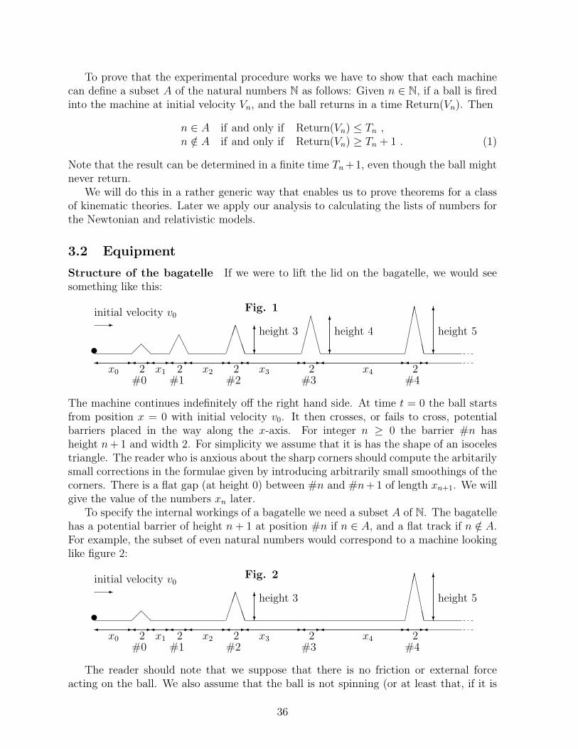
The machine continues indefinitely off the right hand side. At time t = 0 the ball startsfrom position x = 0 with initial velocity v0. It then crosses, or fails to cross, potentialbarriers placed in the way along the x-axis. For integer n ≥ 0 the barrier #n hasheight n+ 1 and width 2. For simplicity we assume that it is has the shape of an isocelestriangle. The reader who is anxious about the sharp corners should compute the arbitarilysmall corrections in the formulae given by introducing arbitrarily small smoothings of thecorners. There is a flat gap (at height 0) between #n and #n+ 1 of length xn+1. We willgive the value of the numbers xn later.

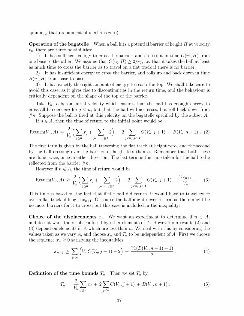
To specify the internal workings of a bagatelle we need a subset A of N. The bagatellehas a potential barrier of height n+ 1 at position #n if n ∈ A, and a flat track if n /∈ A.For example, the subset of even natural numbers would correspond to a machine lookinglike figure 2:

-initial velocity v0

u-

x0

@

#0

-2

-x1

#1

-2

-x2

BBBB

#2

-2

-x3

#3

-2

-x4

DDDDDD

#4

-2

6

?

height 56

?

height 3

Fig. 2

The reader should note that we suppose that there is no friction or external forceacting on the ball. We also assume that the ball is not spinning (or at least that, if it is

36

spinning, that its moment of inertia is zero).

Operation of the bagatelle When a ball hits a potential barrier of height H at velocityv0, there are three possibilities:

1) It has sufficient energy to cross the barrier, and crosses it in time C(v0, H) fromone base to the other. We assume that C(v0, H) ≥ 2/v0, i.e. that it takes the ball at leastas much time to cross the barrier as to travel on a flat track if there is no barrier.

2) It has insufficient energy to cross the barrier, and rolls up and back down in timeB(v0, H) from base to base.

3) It has exactly the right amount of energy to reach the top. We shall take care toavoid this case, as it gives rise to discontinuities in the return time, and the behaviour iscritically dependent on the shape of the top of the barrier.

Take Vn to be an initial velocity which ensures that the ball has enough energy tocross all barriers #j for j < n, but that the ball will not cross, but roll back down from#n. Suppose the ball is fired at this velocity on the bagatelle specified by the subset A.

If n ∈ A, then the time of return to the initial point would be

Return(Vn, A) =2

Vn

(∑j≤n

xj +∑

j<n, j /∈A

2)

+ 2∑

j<n, j∈A

C(Vn, j + 1) + B(Vn, n+ 1) . (2)

The first term is given by the ball traversing the flat track at height zero, and the secondby the ball crossing over the barriers of height less than n. Remember that both theseare done twice, once in either direction. The last term is the time taken for the ball to bereflected from the barrier #n.

However if n /∈ A, the time of return would be

Return(Vn, A) ≥ 2

Vn

(∑j≤n

xj +∑

j<n, j /∈A

2)

+ 2∑

j<n, j∈A

C(Vn, j + 1) +2xn+1

Vn

. (3)

This time is based on the fact that if the ball did return, it would have to travel twiceover a flat track of length xn+1. Of course the ball might never return, as there might beno more barriers for it to cross, but this case is included in the inequality.

Choice of the displacements xn We want an experiment to determine if n ∈ A,and do not want the result confused by other elements of A. However our results (2) and(3) depend on elements in A which are less than n. We deal with this by considering thevalues taken as we vary A, and choose xn and Tn to be independent of A: First we choosethe sequence xn ≥ 0 satisfying the inequalities

xn+1 ≥∑j<n

(VnC(Vn, j + 1)− 2

)+Vn(B(Vn, n+ 1) + 1)

2. (4)

Definition of the time bounds Tn Then we set Tn by

Tn =2

Vn

∑j≤n

xj + 2∑j<n

C(Vn, j + 1) + B(Vn, n+ 1) . (5)

37

If n ∈ A, remembering that C(v0, H) ≥ 2/v0 we have from (2):

Return(Vn, A) ≤ 2

Vn

∑j≤n

xj + 2∑j<n

C(Vn, j + 1) + B(Vn, n+ 1) = Tn. (6)

Correspondingly for n /∈ A, from (3) we have

Return(Vn, A) ≥ 2

Vn

(∑j≤n

xj +∑j<n

2)

+2xn+1

Vn

≥ Tn + 1 . (7)

Let us summarise these general calculations.

Theorem 3.1. For any set A of numbers, let BA be a bagatelle machine specified above.Let P the experimental procedure for its operation. Let T be a kinematic theory in which

1. particles follow deterministic paths, traversing, or else being reflected by, the barriersof the bagatelle;

2. conservation of energy ensures the velocity before and after meeting each barrier isthe same;

3. formulae can be given for the time of crossing and rolling back barriers, and forinitial velocities

C(v0, H) ≥ 2/v0, B(v0, H) and Vn.

Then one can prove in the kinematic theory T that the procedure P decides membershipof the set A.

Condition 1 is not true of quantum kinematics where particles may tunnel throughthe barrier. the effects of friction are forbidden by Condition 2; the calculations wouldneed to be altered to allow for friction.

It remains to find formulae for C, B and Vn in the Newtonian and relativistic theories,which satisfy the conditions.

3.3 Corollaries

Corollary 3.2. Any function f : N→ N can be computed by a Newtonian or Relativisticbagatelle

Proof. Let Gf be the graph of f . Choose an injective function c : N2 → N such as(x, y) 7→ 2x.3y and code the graph Gf as the set c(Gf ). A bagatelle BA based on A = c(Gf )would enable f to be computed experimentally by the mechanical system.

Corollary 3.3. There exist Newtonian and Relativistic bagatelles that are universal ma-chines for the computable partial functions on N, i.e. the bagatelles compute by experimentall and only the computable partial functions on N.

Proof. Choose a bagatelle BA based on A = c(GU), the coded graph of a universal par-tial recursive function U . This would enable U to be computed experimentally by themechanical system.

38

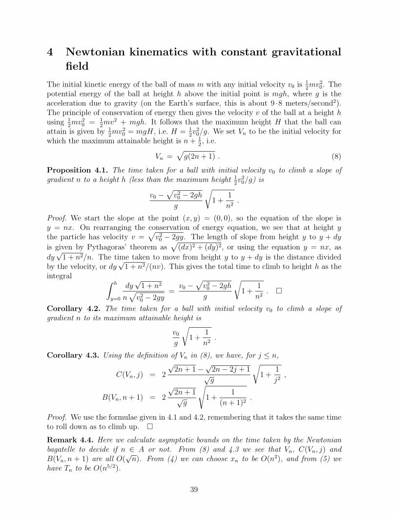
4 Newtonian kinematics with constant gravitational

field

The initial kinetic energy of the ball of mass m with any initial velocity v0 is 12mv2

0. Thepotential energy of the ball at height h above the initial point is mgh, where g is theacceleration due to gravity (on the Earth’s surface, this is about 9 ·8 meters/second2).The principle of conservation of energy then gives the velocity v of the ball at a height husing 1

2mv2

0 = 12mv2 + mgh. It follows that the maximum height H that the ball can

attain is given by 12mv2

0 = mgH, i.e. H = 12v2

0/g. We set Vn to be the initial velocity forwhich the maximum attainable height is n+ 1

2, i.e.

Vn =√g(2n+ 1) . (8)

Proposition 4.1. The time taken for a ball with initial velocity v0 to climb a slope ofgradient n to a height h (less than the maximum height 1

2v2

0/g) is

v0 −√v2

0 − 2gh

g

√1 +

1

n2.

Proof. We start the slope at the point (x, y) = (0, 0), so the equation of the slope isy = nx. On rearranging the conservation of energy equation, we see that at height ythe particle has velocity v =

√v2

0 − 2gy. The length of slope from height y to y + dy

is given by Pythagoras’ theorem as√

(dx)2 + (dy)2, or using the equation y = nx, as

dy√

1 + n2/n. The time taken to move from height y to y + dy is the distance dividedby the velocity, or dy

√1 + n2/(nv). This gives the total time to climb to height h as the

integral ∫ h

y=0

dy√

1 + n2

n√v2

0 − 2gy=

v0 −√v2

0 − 2gh

g

√1 +

1

n2.

Corollary 4.2. The time taken for a ball with initial velocity v0 to climb a slope ofgradient n to its maximum attainable height is

v0

g

√1 +

1

n2.

Corollary 4.3. Using the definition of Vn in (8), we have, for j ≤ n,

C(Vn, j) = 2

√2n+ 1−

√2n− 2j + 1

√g

√1 +

1

j2,

B(Vn, n+ 1) = 2

√2n+ 1√g

√1 +

1

(n+ 1)2.

Proof. We use the formulae given in 4.1 and 4.2, remembering that it takes the same timeto roll down as to climb up.

Remark 4.4. Here we calculate asymptotic bounds on the time taken by the Newtonianbagatelle to decide if n ∈ A or not. From (8) and 4.3 we see that Vn, C(Vn, j) andB(Vn, n + 1) are all O(

√n). From (4) we can choose xn to be O(n2), and from (5) we

have Tn to be O(n5/2).

39

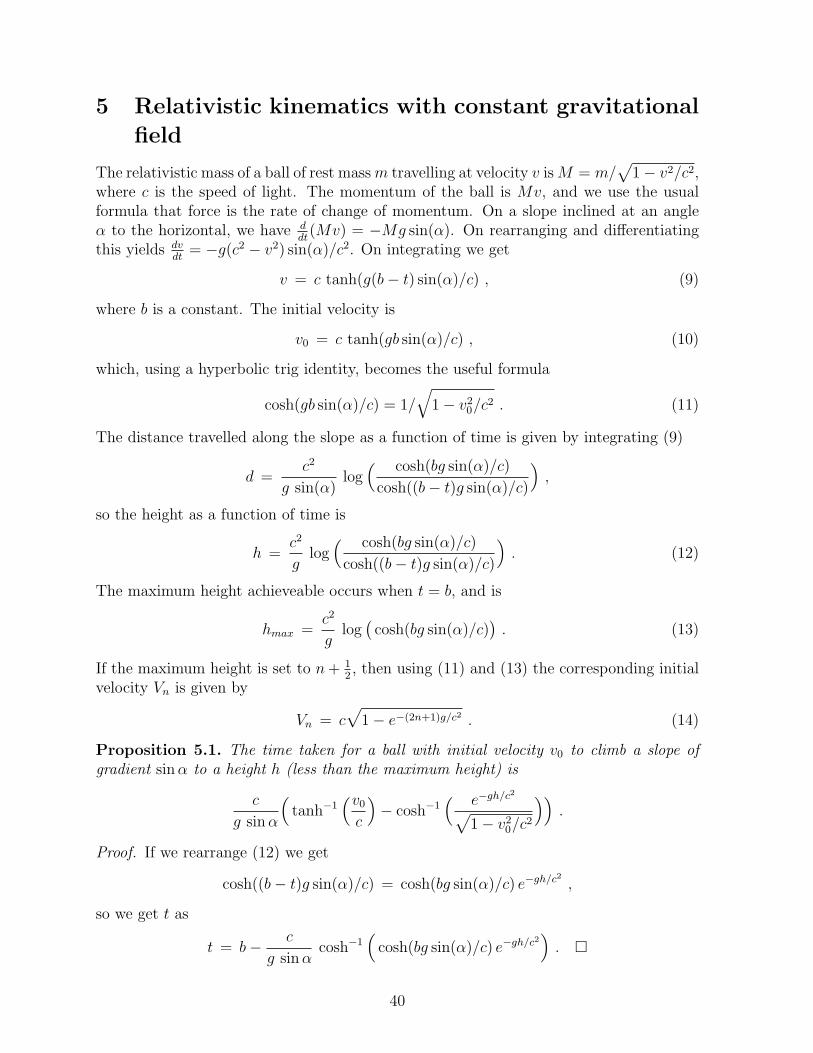
5 Relativistic kinematics with constant gravitational

field

The relativistic mass of a ball of rest massm travelling at velocity v isM = m/√

1− v2/c2,where c is the speed of light. The momentum of the ball is Mv, and we use the usualformula that force is the rate of change of momentum. On a slope inclined at an angleα to the horizontal, we have d

dt(Mv) = −Mg sin(α). On rearranging and differentiating

this yields dvdt

= −g(c2 − v2) sin(α)/c2. On integrating we get

v = c tanh(g(b− t) sin(α)/c) , (9)

where b is a constant. The initial velocity is

v0 = c tanh(gb sin(α)/c) , (10)

which, using a hyperbolic trig identity, becomes the useful formula

cosh(gb sin(α)/c) = 1/√

1− v20/c

2 . (11)

The distance travelled along the slope as a function of time is given by integrating (9)

d =c2

g sin(α)log( cosh(bg sin(α)/c)

cosh((b− t)g sin(α)/c)

),

so the height as a function of time is

h =c2

glog( cosh(bg sin(α)/c)

cosh((b− t)g sin(α)/c)

). (12)

The maximum height achieveable occurs when t = b, and is

hmax =c2

glog(

cosh(bg sin(α)/c)). (13)

If the maximum height is set to n+ 12, then using (11) and (13) the corresponding initial

velocity Vn is given by

Vn = c√

1− e−(2n+1)g/c2 . (14)

Proposition 5.1. The time taken for a ball with initial velocity v0 to climb a slope ofgradient sinα to a height h (less than the maximum height) is

c

g sinα

(tanh−1

(v0

c

)− cosh−1

( e−gh/c2√1− v2

0/c2

)).

Proof. If we rearrange (12) we get

cosh((b− t)g sin(α)/c) = cosh(bg sin(α)/c) e−gh/c2 ,

so we get t as

t = b− c

g sinαcosh−1

(cosh(bg sin(α)/c) e−gh/c2

).

40

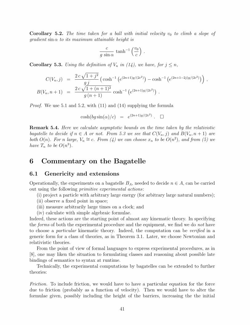
Corollary 5.2. The time taken for a ball with initial velocity v0 to climb a slope ofgradient sinα to its maximum attainable height is

c

g sinαtanh−1

(v0

c

).

Corollary 5.3. Using the definition of Vn in (14), we have, for j ≤ n,

C(Vn, j) =2 c√

1 + j2

g j

(cosh−1

(e(2n+1)g/(2c2)

)− cosh−1

(e(2n+1−2j)g/(2c2)

)),

B(Vn, n+ 1) =2 c√

1 + (n+ 1)2

g (n+ 1)cosh−1

(e(2n+1)g/(2c2)

).

Proof. We use 5.1 and 5.2, with (11) and (14) supplying the formula

cosh(bg sin(α)/c) = e(2n+1)g/(2c2) .

Remark 5.4. Here we calculate asymptotic bounds on the time taken by the relativisticbagatelle to decide if n ∈ A or not. From 5.3 we see that C(Vn, j) and B(Vn, n + 1) areboth O(n). For n large, Vn

∼= c. From (4) we can choose xn to be O(n2), and from (5) wehave Tn to be O(n3).

6 Commentary on the Bagatelle

6.1 Genericity and extensions

Operationally, the experiments on a bagatelle BA, needed to decide n ∈ A, can be carriedout using the following primitive experimental actions :

(i) project a particle with arbitrary large energy (for arbitrary large natural numbers);(ii) observe a fixed point in space;(iii) measure arbitrarily large times on a clock; and(iv) calculate with simple algebraic formulae.

Indeed, these actions are the starting point of almost any kinematic theory. In specifyingthe forms of both the experimental procedure and the equipment, we find we do not haveto choose a particular kinematic theory. Indeed, the computation can be verified in ageneric form for a class of theories, as in Theorem 3.1. Later, we choose Newtonian andrelativistic theories.

From the point of view of formal languages to express experimental procedures, as in[8], one may liken the situation to formulating classes and reasoning about possible latebindings of semantics to syntax at runtime.

Technically, the experimental computations by bagatelles can be extended to furthertheories:

Friction. To include friction, we would have to have a particular equation for the forcedue to friction (probably as a function of velocity). Then we would have to alter theformulae given, possibly including the height of the barriers, increasing the the initial

41

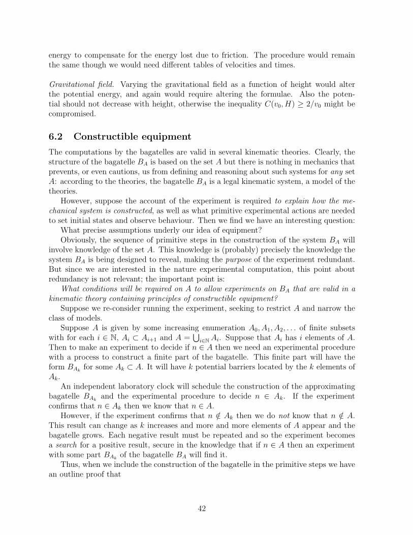
energy to compensate for the energy lost due to friction. The procedure would remainthe same though we would need different tables of velocities and times.

Gravitational field. Varying the gravitational field as a function of height would alterthe potential energy, and again would require altering the formulae. Also the poten-tial should not decrease with height, otherwise the inequality C(v0, H) ≥ 2/v0 might becompromised.

6.2 Constructible equipment

The computations by the bagatelles are valid in several kinematic theories. Clearly, thestructure of the bagatelle BA is based on the set A but there is nothing in mechanics thatprevents, or even cautions, us from defining and reasoning about such systems for any setA: according to the theories, the bagatelle BA is a legal kinematic system, a model of thetheories.

However, suppose the account of the experiment is required to explain how the me-chanical system is constructed, as well as what primitive experimental actions are neededto set initial states and observe behaviour. Then we find we have an interesting question:

What precise assumptions underly our idea of equipment?Obviously, the sequence of primitive steps in the construction of the system BA will

involve knowledge of the set A. This knowledge is (probably) precisely the knowledge thesystem BA is being designed to reveal, making the purpose of the experiment redundant.But since we are interested in the nature experimental computation, this point aboutredundancy is not relevant; the important point is:

What conditions will be required on A to allow experiments on BA that are valid in akinematic theory containing principles of constructible equipment?

Suppose we re-consider running the experiment, seeking to restrict A and narrow theclass of models.

Suppose A is given by some increasing enumeration A0, A1, A2, . . . of finite subsetswith for each i ∈ N, Ai ⊂ Ai+1 and A =

⋃i∈NAi. Suppose that Ai has i elements of A.

Then to make an experiment to decide if n ∈ A then we need an experimental procedurewith a process to construct a finite part of the bagatelle. This finite part will have theform BAk

for some Ak ⊂ A. It will have k potential barriers located by the k elements ofAk.

An independent laboratory clock will schedule the construction of the approximatingbagatelle BAk

and the experimental procedure to decide n ∈ Ak. If the experimentconfirms that n ∈ Ak then we know that n ∈ A.

However, if the experiment confirms that n /∈ Ak then we do not know that n /∈ A.This result can change as k increases and more and more elements of A appear and thebagatelle grows. Each negative result must be repeated and so the experiment becomesa search for a positive result, secure in the knowledge that if n ∈ A then an experimentwith some part BAk

of the bagatelle BA will find it.Thus, when we include the construction of the bagatelle in the primitive steps we have

an outline proof that

42

A is decidable by experiment with constructible equipment if, and only if, the finite subsetsof the enumeration of A can be generated by experiment.

How close are we to a proof that A is decidable by experiment with constructible equip-ment if, and only if, A is recursively enumerable subset of N?

Allowing computability theory to be added to the physical theory would resolvethe matter. Experimental computation by the bagatelles in kinetic theories with con-structible equipment, where the equipment is specified by algorithms, does not lead tonon-computable sets and functions.

6.3 General principles

The bagatelle, and several of our earlier examples [3, 4], show that the notion of equipmentneeds to be analysed. We have proposed

Experimental computation = Experimental procedure + Equipment.

A formal theory is needed that constrains the architecture and construction of mechan-ical systems and formally defines notions of constructible equipment. We have outlinedin [4] the problems of designing formal languages for the specification of constructibleequipment, and of combining them with languages for experimental procedures to makecomplete languages for experimental computation. In [8], we have proposed a set ofconstructs for a programming language for experimental procedures for Newtonian kine-matics. The bagatelle adds gives us further insight into this approach using languages.

First, consider the role of languages in digital computation. We need the equation:

Digital computation language = Programming language + Hardware descriptionlanguage.

This is unfamiliar in programming language theory because the primary aim of pro-gramming is to formulate algorithms that are independent of machines and devices. Bothlanguages have a syntax and a semantics. Theories of syntax are very general, and arewidely understood and used. Semantic methods for programming languages are also welldeveloped, though the semantics of hardware description languages is less so. This viewof digital computation is complemented by this equation:

Experimental computation language = Experimental procedure language + Equipmentdescription language.

Consider the distinction between syntax and semantics for experimental computation.The syntax of the languages can be handled by general methods. The bagatelle exampleshows how semantics is more complicated. Somewhat abstractly, we have a Gedankenexperiment, in which we imagine an operator following the procedure in working withthe equipment. What happens and, in particular, what is computed? To answer this wemake some meta-assumptions and only later choose a theory - Newton’s or Einstein’s.The physical theories are used to define the semantics of the experimental procedure andequipment in order to reason about, predict etc., the behaviour of the system for the

43

benefit of the operator. The bagatelle shows that various semantics are possible for theclass of experimental procedures. Indeed, one is reminded of late binding and runtimes.

The importance of the theory cannot be underestimated. If the theories used forsemantics can be axiomatically specified then we have sounder and sharper reasoning.We also have the phenomenon of unexpected models. It is just as important that we canreason about the bagatelle as we can satisfy ourselves that we can plausibly implementit. Clearly, both kinematic theories apply to experimental computations that we suspectare impossible. It is a problem to prove they are impossible.

One thinks of the first order theory of Peano arithmetic. It is a truly fundamentaland useful theory for reasoning about natural numbers. It has infinitely many different(=non-isomorphic) models but only those isomorhic to the standard model (N|0, n+1, n+m,n.m,=) are algorithmically computable (Tennenbaum’s Theorem).

We expect that research on languages for experimental computation will lead to newideas and techniques in programming language theory.

7 Concluding remarks on kinematic systems

Experimental computation is not well understood and many basic questions are open.There is a paucity of examples that can be formulated and studied in complete detail,though plenty of informal ideas and speculations have been aired. The purpose of ourmethodology is explore experimental computation systematically and precisely. We are inno rush to make physically plausible pronouncements or critiques, rather we propose tostudy examples in forensic detail. Examples based on kinematics, possibly the simplestphysical theory, offer insights into experimental computation, and pose interesting anddifficult theoretical problems.

Our bagatelles are systems that each require unbounded space, time and energy todecide n ∈ A for all n ∈ N. Consider energy. In each of our Newtonian bagatelles massis bounded (indeed, it can be an arbitrary constant) and velocity is unbounded. In eachof our relativistic bagatelles velocity is bounded and mass is unbounded. One can ask ifthere are examples of kinematic systems that are bounded in space, time and energy?

In Newtonian mechanics we are allowed to shrink space and accelerate time. Forexample, the natural numbers n = 0, 1, 2, . . . that mark points in space or steps in timecan be embedded into the interval [0, 1] by n 7→ 1/2n. Shrinking space leads to mechanicalsystems that use arbitrarily small components. Of course, a mechanical system thatexploits the infinite divisibility of space, with no lower bounds on units of space andtime, violates any form of atomic theory. But such examples can be precision tools toinvestigate the theoretical foundations of computability and mechanics. For instance, itis possible to prove that for each set A ⊂ N there exists a valid Newtonian kinematicsystem SA, which is embedded within a bounded 3-dimensional box, operates entirelywithin a fixed finite time interval using a fixed finite amount of energy, and can decidethe membership of the subset A ([4]). The fact that any subset of the natural numberscan be recognised by a simple kinematic system raises an alarm because the theory of thesubsets of natural numbers is so vastly complicated it depends on the foundations of settheory for its exploration.

44

An open problem is this:

Problem 7.1. For all reasonable kinematic theories T , and all T -valid kinematic systemsthat possess both lower and upper bounds on space, time, mass, velocity and energy, arethe sets and functions computable by experiment also computable by algorithms?

We conjecture that the answer is “Yes”. To attempt to prove this, one needs formaldescriptions of equipment as mentioned in Section 6. Our bagatelle examples show thatthe notion of mechanical system - i.e., what qualifies as a valid or legal system in theoreticalmechanics - must be sharpened. To the standard parameters of mass, velocity, distance,time we need to add formal theory that constrains the structure and construction of theequipment and explains how experiments are performed.

Theoretical intuitions about making experiments turn out to be strikingly similar tointuitions about algorithms and computers, although the primitive actions are differentand are implicit in the physical theory. Indeed, we conjecture that a theory of Gedankenexperiments for mechanics, if formalised, could be capable of underpinning the theory ofthe computable as follows:

Problem 7.2. Extend theoretical kinematics by a mathematical theory of construction andthe operation of mechanical equipment, and show that the sets and functions computableby experiment are precisely those computable by algorithms.

This is a difficult problem which we have discussed in detail in [4]. More recent work,in [5], shows that a kinematic device called a scatter machine can compute any realnumber. The construction of the device is bounded in all respects however the theoremdemonstrates that the existence of sharp corners in objects is fatal to computablity!One goal of this direction of research, from physical theory to computablity, is, roughlyspeaking, To derive forms of Church-Turing Thesis as physical laws. However, we canstill ask the question:

Problem 7.3. Does experimental computation in theories with constructible equipment,where the equipment is specified algorithmically, lead to algorithmically computable setsand functions?

We conjecture yes. Finally, we should raise the special case of efficient computationby mechanical systems. New theory is needed to pose and answer a question such as:

Problem 7.4. Are there sets that can be decided in polynomially bounded space and timeby experimental computation with kinematic systems but cannot be decided by algorithmsin polynomial space and time?

We thank Brendan Larvor, David Miller, and J I Zucker for discussions on some ofthe areas mentioned in this paper.

References

[1] J Alper and M Bridger, Newtonian supertasks: A critical review, Synthese 114(1998), 355 – 369.

45

[2] E J Beggs and J V Tucker, Computations via experiments with kinematicsystems, Research Report 4.04, Department of Mathematics, University of WalesSwansea, March 2004 or Technical Report 5-2004, Department of Computer Science,University of Wales Swansea, March 2004.

[3] E J Beggs and J V Tucker, Embedding infinitely parallel computation in New-tonian kinematics, Applied Mathematics and Computation, 178 (2006) 25–43.

[4] E J Beggs and J V Tucker, Can Newtonian systems, bounded in space, time,mass and energy compute all functions?, Theoretical Computer Science, 371 (2007)4–19.

[5] E J Beggs and J V Tucker, Experimental computation of real numbers byNewtonian machines, Proceedings Royal Society Series A, 463 (2007) 1541–1561.

[6] E J Beggs, J F Costa, B Loff and J V Tucker, Computational complexitywith experiments as oracles, in preparation, 2008.

[7] E J Beggs, J F Costa, B Loff, and J V Tucker, The complexity of mea-surement in classical physics, in Theory and Applications of Models of Computation,Lecture Notes in Computer Science, Vol 4978, Springer, 2008, in press.

[8] E J Beggs and J V Tucker, Programming experimental procedures for Newto-nian kinematic machines, A Beckmann et al (eds), —emphComputability in Europe,Athens, 2008, Springer Lecture Notes in Computer Science, 2008, in press.

[9] E J Beggs, J F Costa and J V Tucker, Oracles and advice as measurements,in preparation.

[10] V Bush, The differential analyser. A new machine for solving differential equations,Journal of Franklin Institute 212 (1931), 447-488.

[11] M Davis, The myth of hypercomputation, in Turing Festschrift, Springer, in prepa-ration.

[12] R Geroch and J B Hartle, Computability and physical theories, Foundationsof Physics 16 (1986), 533-550.

[13] D S Graca and J F Costa, Analog computers and recursive functions over thereals, 2003, submitted.

[14] D R Hartree, Calculating Instruments and Machines, Cambridge University Press,1950.

[15] A V Holden, J V Tucker, H Zhang and M Poole, Coupled map lattices ascomputational systems, American Institute of Physics - Chaos 2 (1992), 367-376.

[16] E Griffor, (ed) Handbook of Computability Theory, Elsevier, 1999.

[17] G Kreisel, A notion of mechanistic theory, Synthese 29 (1974), 9-24.

46

[18] G Kreisel, Review of Pour El and Richards, Journal of Symbolic Logic 47 (1974),900-902.

[19] L Lipshitz and L A Rubel, A differentially algebraic replacement theorem, Pro-ceedings of the American Mathematical Society 99(2) (1987), 367 – 372.

[20] C Moore, Unpredictability and undecidability in dynamical systems, Physical Re-view Letters 64 (1990), 2354 – 2357.

[21] C Moore, Recursion theory on the reals and continuous time computation, Theo-retical Computer Science 162 (1996), 23 – 44.

[22] P Odifreddi, Classical Recursion Theory, Studies in Logic and the Foundations ofmathematics, Vol 129, North-Holland, Amsterdam, 1989.

[23] J Perez Laraudogoitia, A beautiful supertask, Mind 105 (1996), 81 – 83.

[24] J Perez Laraudogoitia, Infinity machines and creation ex nihilo, Synthese 114(1998), 259 – 265.

[25] M B Pour-El and J. I. Richards, A computable ordinary differential equationwhich possesses no computable solution, Annals of Mathematical Logic 17 (1979), 61– 90.

[26] M B Pour-El and J. I. Richards, The wave equation with computable initialdata such that its unique solution is not computable, Advances in Mathematics 39(1981), 215 – 239.

[27] M B Pour-El and J. I. Richards, Computability and noncomputability in clas-sical analysis, Transactions of the American Mathematical Society 275 (1983), 539 –560.

[28] M B Pour-El and J. I. Richards, Computability in Analysis and Physics, Per-spectives in Mathematical Logic, Springer-Verlag, Berlin, 1989.

[29] H Rogers, Theory of recursive Functions and Effective Computability, McGraw-Hill, New York, 1967.

[30] C Shannon, Mathematical theory of the differential analyser, Journal of Mathe-matics and Physics 20 (1941), 337-354.

[31] H T Siegelmann, Neural networks and analog computation: Beyond the Turinglimit, Birkhauser, Boston, 1999.

[32] V Stoltenberg-Hansen and J V Tucker, Effective algebras, in S Abramsky,D Gabbay and T Maibaum (eds.) Handbook of Logic in Computer Science. VolumeIV: Semantic Modelling, Oxford University Press, 1995, pp.357-526.

[33] V Stoltenberg-Hansen and J V Tucker, Computable rings and fields, in E.R. Griffor (ed.), Handbook of Computability Theory, Elsevier, 1999, 363 – 447.

47

[34] V Stoltenberg-Hansen and J V Tucker, Computable and continuous partialhomomorphisms on metric partial algebras, Bulletin for Symbolic Logic 9 (2003), 299– 334.

[35] J V Tucker and J I Zucker, Computable functions and semicomputable sets onmany sorted algebras, in S. Abramsky, D. Gabbay and T Maibaum (eds.), Handbookof Logic for Computer Science volume V, Oxford University Press, 2000, 317 – 523.

[36] J V Tucker and J I Zucker, Abstract versus concrete computation on metricpartial algebras, ACM Transactions on Computational Logic, 5 (2004) 611–668.

[37] K Weihrauch, Computable Analysis, An introduction, Springer-Verlag, Heidelberg,2000.

[38] K Weihrauch and N Zhong, Is wave propogation computable or can wave com-puters beat the Turing machine?, Proceedings of London Mathematical Society 85(2002), 312-332.

48

The Influence of Domain Interpretationson Computational Models

Udi Boker and Nachum DershowitzSchool of Computer Science, Tel Aviv University

Ramat Aviv, Tel Aviv 69978, Israel

Abstract

Computational models are usually defined over specific domains. For example, Turing machines are defined overstrings, and the recursive functions over the natural numbers. Nevertheless, one often uses one computational modelto compute functions over another domain, in which case, one is obliged to employ a representation, mapping elementsof one domain into the other. For instance, Turing machines (or modern computers) are understood as computingnumerical functions, by interpreting strings as numbers, via a binary or decimal representation, say.

We ask: Is the choice of the domain interpretation important? Clearly, complexity is influenced, but does therepresentation also affect computability? Can it be that the same model computes strictly more functions via onerepresentation than another? We show that the answer is “yes”, and further analyze the influence of domain inter-pretation on the extensionality of computational models (that is, on the set of functions computed by the model).

We introduce the notion of interpretation-completeness for computational models that are basically unaffected bythe choice of domain interpretation, and prove that Turing machines and the recursive functions are interpretation-complete, while two-counter machines are incomplete. We continue by examining issues based on model extensionalitythat are influenced by the domain interpretation. We suggest a notion for comparing computational power of modelsoperating over arbitrary domains, as well as an interpretation of the Church-Turing Thesis over arbitrary domains.

Key words: domain interpretation, domain representation, hypercomputation, Turing machine, computability, computationalpower, computational models, computational comparison

1. Introduction

We explore the problem of the sensitivity of models to domain interpretation, and the way we propose tohandle it. This introductory section parallels the structure of the paper, as illustrated in Figure 1.

Sensitivity to domain interpretation. A computational model is defined over a specific domain. However,we may often use it to compute functions over a different domain. For example, using Turing machines (ormodern computers) to compute functions over natural numbers requires a string representation by numbers.Another example becomes apparent when comparing the computational power of two models that operate

This work was carried out in partial fulfillment of the requirements for the Ph.D. degree of the first author. Research wassupported in part by the Israel Science Foundation under grant no. 250/05.

Email address: udiboker,[email protected] (Udi Boker and Nachum Dershowitz).

Preprint submitted to Elsevier 9 July 2008

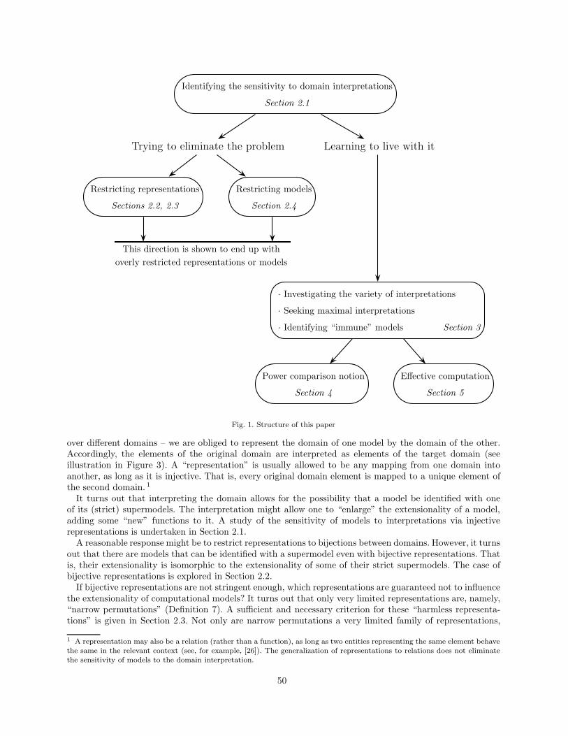
Identifying the sensitivity to domain interpretations

Section 2.1

Trying to eliminate the problem Learning to live with it

Restricting representations

Sections 2.2, 2.3

Restricting models

Section 2.4

This direction is shown to end up withoverly restricted representations or models

· Investigating the variety of interpretations

· Seeking maximal interpretations

· Identifying “immune” models Section 3

Power comparison notion

Section 4

Effective computation

Section 5

Fig. 1. Structure of this paper

over different domains – we are obliged to represent the domain of one model by the domain of the other.Accordingly, the elements of the original domain are interpreted as elements of the target domain (seeillustration in Figure 3). A “representation” is usually allowed to be any mapping from one domain intoanother, as long as it is injective. That is, every original domain element is mapped to a unique element ofthe second domain. 1

It turns out that interpreting the domain allows for the possibility that a model be identified with oneof its (strict) supermodels. The interpretation might allow one to “enlarge” the extensionality of a model,adding some “new” functions to it. A study of the sensitivity of models to interpretations via injectiverepresentations is undertaken in Section 2.1.

A reasonable response might be to restrict representations to bijections between domains. However, it turnsout that there are models that can be identified with a supermodel even with bijective representations. Thatis, their extensionality is isomorphic to the extensionality of some of their strict supermodels. The case ofbijective representations is explored in Section 2.2.

If bijective representations are not stringent enough, which representations are guaranteed not to influencethe extensionality of computational models? It turns out that only very limited representations are, namely,“narrow permutations” (Definition 7). A sufficient and necessary criterion for these “harmless representa-tions” is given in Section 2.3. Not only are narrow permutations a very limited family of representations,

1 A representation may also be a relation (rather than a function), as long as two entities representing the same element behavethe same in the relevant context (see, for example, [26]). The generalization of representations to relations does not eliminatethe sensitivity of models to the domain interpretation.

50

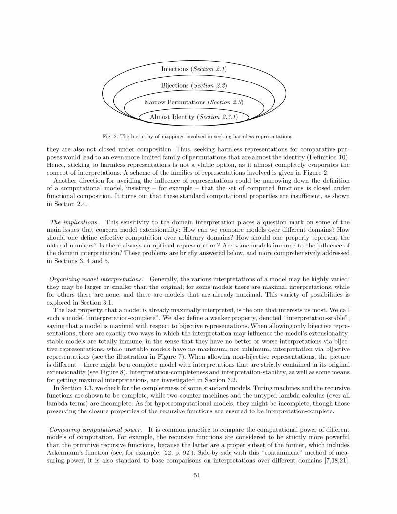
Almost Identity (Section 2.3.1)

Narrow Permutations (Section 2.3)

Bijections (Section 2.2)

Injections (Section 2.1)

Fig. 2. The hierarchy of mappings involved in seeking harmless representations.

they are also not closed under composition. Thus, seeking harmless representations for comparative pur-poses would lead to an even more limited family of permutations that are almost the identity (Definition 10).Hence, sticking to harmless representations is not a viable option, as it almost completely evaporates theconcept of interpretations. A scheme of the families of representations involved is given in Figure 2.

Another direction for avoiding the influence of representations could be narrowing down the definitionof a computational model, insisting – for example – that the set of computed functions is closed underfunctional composition. It turns out that these standard computational properties are insufficient, as shownin Section 2.4.

The implications. This sensitivity to the domain interpretation places a question mark on some of themain issues that concern model extensionality: How can we compare models over different domains? Howshould one define effective computation over arbitrary domains? How should one properly represent thenatural numbers? Is there always an optimal representation? Are some models immune to the influence ofthe domain interpretation? These problems are briefly answered below, and more comprehensively addressedin Sections 3, 4 and 5.

Organizing model interpretations. Generally, the various interpretations of a model may be highly varied:they may be larger or smaller than the original; for some models there are maximal interpretations, whilefor others there are none; and there are models that are already maximal. This variety of possibilities isexplored in Section 3.1.

The last property, that a model is already maximally interpreted, is the one that interests us most. We callsuch a model “interpretation-complete”. We also define a weaker property, denoted “interpretation-stable”,saying that a model is maximal with respect to bijective representations. When allowing only bijective repre-sentations, there are exactly two ways in which the interpretation may influence the model’s extensionality:stable models are totally immune, in the sense that they have no better or worse interpretations via bijec-tive representations, while unstable models have no maximum, nor minimum, interpretation via bijectiverepresentations (see the illustration in Figure 7). When allowing non-bijective representations, the pictureis different – there might be a complete model with interpretations that are strictly contained in its originalextensionality (see Figure 8). Interpretation-completeness and interpretation-stability, as well as some meansfor getting maximal interpretations, are investigated in Section 3.2.

In Section 3.3, we check for the completeness of some standard models. Turing machines and the recursivefunctions are shown to be complete, while two-counter machines and the untyped lambda calculus (over alllambda terms) are incomplete. As for hypercomputational models, they might be incomplete, though thosepreserving the closure properties of the recursive functions are ensured to be interpretation-complete.

Comparing computational power. It is common practice to compare the computational power of differentmodels of computation. For example, the recursive functions are considered to be strictly more powerfulthan the primitive recursive functions, because the latter are a proper subset of the former, which includesAckermann’s function (see, for example, [22, p. 92]). Side-by-side with this “containment” method of mea-suring power, it is also standard to base comparisons on interpretations over different domains [7,18,21].

51

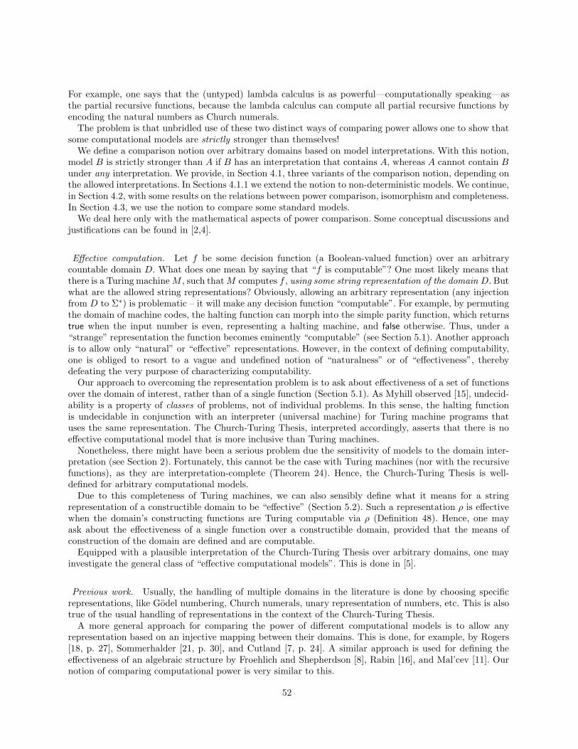
For example, one says that the (untyped) lambda calculus is as powerful—computationally speaking—asthe partial recursive functions, because the lambda calculus can compute all partial recursive functions byencoding the natural numbers as Church numerals.

The problem is that unbridled use of these two distinct ways of comparing power allows one to show thatsome computational models are strictly stronger than themselves!

We define a comparison notion over arbitrary domains based on model interpretations. With this notion,model B is strictly stronger than A if B has an interpretation that contains A, whereas A cannot contain Bunder any interpretation. We provide, in Section 4.1, three variants of the comparison notion, depending onthe allowed interpretations. In Sections 4.1.1 we extend the notion to non-deterministic models. We continue,in Section 4.2, with some results on the relations between power comparison, isomorphism and completeness.In Section 4.3, we use the notion to compare some standard models.

We deal here only with the mathematical aspects of power comparison. Some conceptual discussions andjustifications can be found in [2,4].

Effective computation. Let f be some decision function (a Boolean-valued function) over an arbitrarycountable domain D. What does one mean by saying that “f is computable”? One most likely means thatthere is a Turing machineM , such thatM computes f , using some string representation of the domain D. Butwhat are the allowed string representations? Obviously, allowing an arbitrary representation (any injectionfrom D to Σ∗) is problematic – it will make any decision function “computable”. For example, by permutingthe domain of machine codes, the halting function can morph into the simple parity function, which returnstrue when the input number is even, representing a halting machine, and false otherwise. Thus, under a“strange” representation the function becomes eminently “computable” (see Section 5.1). Another approachis to allow only “natural” or “effective” representations. However, in the context of defining computability,one is obliged to resort to a vague and undefined notion of “naturalness” or of “effectiveness”, therebydefeating the very purpose of characterizing computability.

Our approach to overcoming the representation problem is to ask about effectiveness of a set of functionsover the domain of interest, rather than of a single function (Section 5.1). As Myhill observed [15], undecid-ability is a property of classes of problems, not of individual problems. In this sense, the halting functionis undecidable in conjunction with an interpreter (universal machine) for Turing machine programs thatuses the same representation. The Church-Turing Thesis, interpreted accordingly, asserts that there is noeffective computational model that is more inclusive than Turing machines.

Nonetheless, there might have been a serious problem due the sensitivity of models to the domain inter-pretation (see Section 2). Fortunately, this cannot be the case with Turing machines (nor with the recursivefunctions), as they are interpretation-complete (Theorem 24). Hence, the Church-Turing Thesis is well-defined for arbitrary computational models.

Due to this completeness of Turing machines, we can also sensibly define what it means for a stringrepresentation of a constructible domain to be “effective” (Section 5.2). Such a representation ρ is effectivewhen the domain’s constructing functions are Turing computable via ρ (Definition 48). Hence, one mayask about the effectiveness of a single function over a constructible domain, provided that the means ofconstruction of the domain are defined and are computable.

Equipped with a plausible interpretation of the Church-Turing Thesis over arbitrary domains, one mayinvestigate the general class of “effective computational models”. This is done in [5].

Previous work. Usually, the handling of multiple domains in the literature is done by choosing specificrepresentations, like Godel numbering, Church numerals, unary representation of numbers, etc. This is alsotrue of the usual handling of representations in the context of the Church-Turing Thesis.

A more general approach for comparing the power of different computational models is to allow anyrepresentation based on an injective mapping between their domains. This is done, for example, by Rogers[18, p. 27], Sommerhalder [21, p. 30], and Cutland [7, p. 24]. A similar approach is used for defining theeffectiveness of an algebraic structure by Froehlich and Shepherdson [8], Rabin [16], and Mal’cev [11]. Ournotion of comparing computational power is very similar to this.

52

Richard Montague [13] raises the problem of representation when applying Turing’s notion of computabil-ity to other domains, as well as the circularity in choosing a “computable representation”.

Stewart Shapiro [20] raises the very same problem of representation when applying computability tonumber-theoretic functions. He suggests a definition of an “acceptable notation” (string representation ofnatural numbers), based on some intuitive concepts. We discuss his notion in Section 5.1 and 5.2.

Klaus Weihrauch [25,26] deals heavily with the representation of arbitrary domains by numbers and strings.He defines computability with respect to a representation, and provides justifications for the effectiveness ofthe standard representations. We elaborate on his justifications in Section 5.2.

Our definition of an “effective representation” resembles Shapiro’s notion of “acceptable notation” andgoes along the lines of Weihrauch’s justifications for the effectiveness of the standard representations.

To the best of our knowledge, our work in [2–4] was the first to point out and handle the possible influenceof the representation on the extensionality of computational models. Sections 2, 3, and 4 organize the mainresults of these papers, while adding some new ones, particularly Proposition 14, Proposition 17, Theorem 21,Theorem 25, Theorem 27, and Theorem 46. Section 5 summarizes the first part of our paper [5].

Terminology. We refer to the natural numbers, denoted N, as including zero, and denote by N+ thenatural numbers excluding zero. When we speak of the recursive functions, denoted REC, we mean thepartial recursive functions. Similarly, the set of Turing machines, denoted TM, includes both halting andnon-halting machines. We use the term “domain” of a computational model and of a (partial) function todenote the set of elements over which it operates, not only those for which it is defined. By “image”, wemean the values that a function actually takes: Im f := f(x) | x ∈ dom f.

Proofs are omitted for conciseness reasons.

2. The Sensitivity of Models to the Domain Interpretation

Computational models. Our research concerns computational models. Obviously, a computational modelshould perform some computation; however demarcating a clear border between what is a computationalmodel and what is not is problematic. Accordingly, for achieving maximum generality, we do not want tolimit computational models to any specific mechanism; hence, we allow a model to be any object, as longas it is associated with a set of functions that it computes.

As models may have non-terminating computations, we deal with sets of partial functions. For convenience,we assume that the domain and range (co-domain) of functions are identical. For simplicity, we mainly dealwith deterministic computational models. Most of our definitions and theorems can be directly extended tonon-determinism, while the more involved ones are handled in Section 4.1.1.Definition 1 (Computational Model)– A domain D is any set of atomic elements.– A computational model A over domain D is any object associated with a set of partial functions f : Di →D, i ∈ N+. This set of functions is called the extensionality of the computational model, denoted [[A]].

– We write dom A for the domain over which model A operates.In what follows, we often speak of a “submodel” or a “supermodel” of a model, referring to the containment

relation between their extensionalities. That is, model A is a submodel of B, and B is a supermodel of A, if[[A]] ⊆ [[B]]. By a “strict submodel” we mean that the containment is proper.

In the following subsections, we explore the sensitivity of models to domain interpretations, ending upwith a sufficient and necessary condition for a “harmless representation” (see Figure 2).

2.1. Injective representations

Injective representations are the most frequently used ones. The standard decimal and binary notationsof the natural numbers are injective (they are not bijective since leading zeros are ignored). Comparisonsbetween computational models are usually done by injective encodings; for example: Church numerals andGodel numbering are used for comparing the recursive functions and λ-calculus.

53

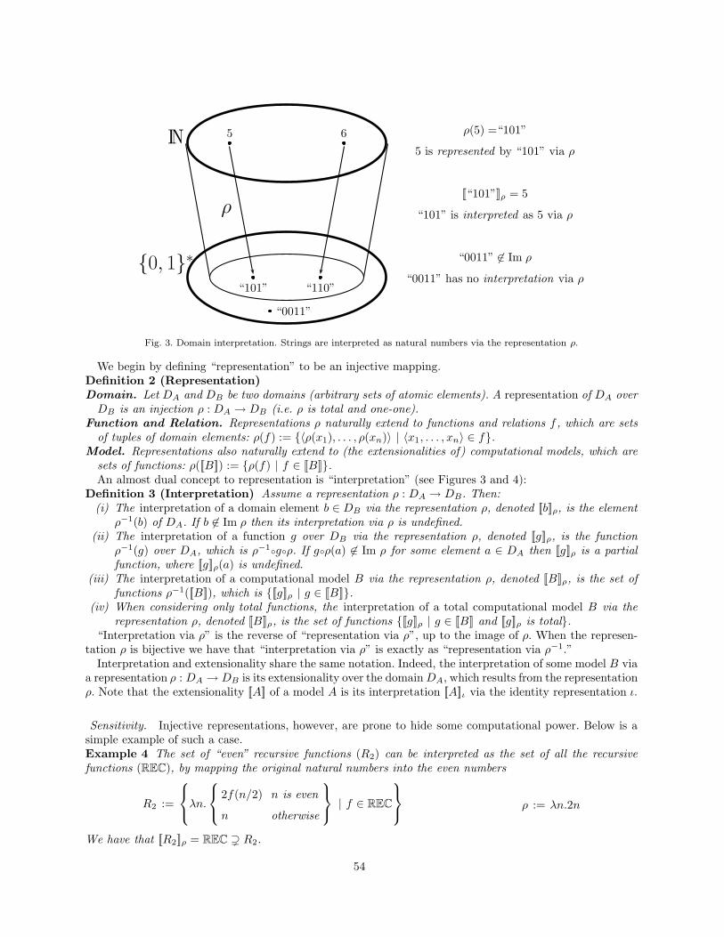
ρ(5) =“101”

5 is represented by “101” via ρ

[[“101”]]ρ = 5

“101” is interpreted as 5 via ρ

“0011” ∈ Im ρ

“0011” has no interpretation via ρ

N

0, 1∗

5 6

“101” “110”

ρ

“0011”

Fig. 3. Domain interpretation. Strings are interpreted as natural numbers via the representation ρ.

We begin by defining “representation” to be an injective mapping.Definition 2 (Representation)Domain. Let DA and DB be two domains (arbitrary sets of atomic elements). A representation of DA overDB is an injection ρ : DA → DB (i.e. ρ is total and one-one).

Function and Relation. Representations ρ naturally extend to functions and relations f , which are setsof tuples of domain elements: ρ(f) := 〈ρ(x1), . . . , ρ(xn)〉 | 〈x1, . . . , xn〉 ∈ f.

Model. Representations also naturally extend to (the extensionalities of) computational models, which aresets of functions: ρ([[B]]) := ρ(f) | f ∈ [[B]].An almost dual concept to representation is “interpretation” (see Figures 3 and 4):

Definition 3 (Interpretation) Assume a representation ρ : DA → DB. Then:(i) The interpretation of a domain element b ∈ DB via the representation ρ, denoted [[b]]ρ, is the element

ρ−1(b) of DA. If b ∈ Im ρ then its interpretation via ρ is undefined.(ii) The interpretation of a function g over DB via the representation ρ, denoted [[g]]ρ, is the function

ρ−1(g) over DA, which is ρ−1gρ. If gρ(a) ∈ Im ρ for some element a ∈ DA then [[g]]ρ is a partialfunction, where [[g]]ρ(a) is undefined.

(iii) The interpretation of a computational model B via the representation ρ, denoted [[B]]ρ, is the set offunctions ρ−1([[B]]), which is [[g]]ρ | g ∈ [[B]].

(iv) When considering only total functions, the interpretation of a total computational model B via therepresentation ρ, denoted [[B]]ρ, is the set of functions [[g]]ρ | g ∈ [[B]] and [[g]]ρ is total.

“Interpretation via ρ” is the reverse of “representation via ρ”, up to the image of ρ. When the represen-tation ρ is bijective we have that “interpretation via ρ” is exactly as “representation via ρ−1.”

Interpretation and extensionality share the same notation. Indeed, the interpretation of some model B viaa representation ρ : DA → DB is its extensionality over the domainDA, which results from the representationρ. Note that the extensionality [[A]] of a model A is its interpretation [[A]]ι via the identity representation ι.

Sensitivity. Injective representations, however, are prone to hide some computational power. Below is asimple example of such a case.Example 4 The set of “even” recursive functions (R2) can be interpreted as the set of all the recursivefunctions (REC), by mapping the original natural numbers into the even numbers

R2 :=

λn.

2f(n/2) n is even

n otherwise

| f ∈ REC

ρ := λn.2n

We have that [[R2]]ρ = REC R2.

54

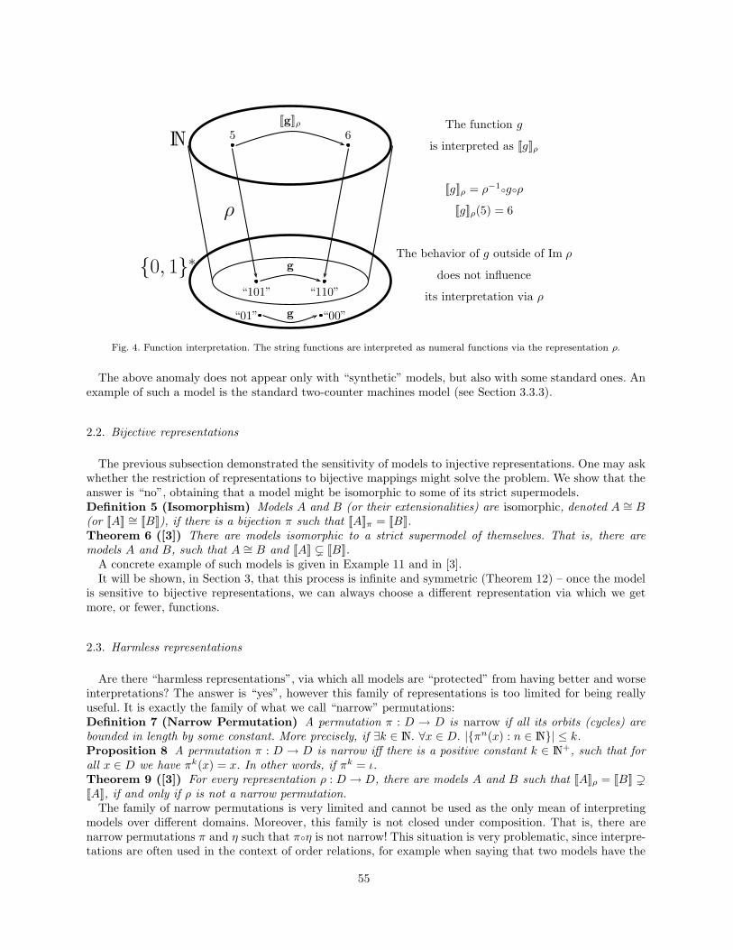
The function g

is interpreted as [[g]]ρ

[[g]]ρ = ρ−1gρ

[[g]]ρ(5) = 6

The behavior of g outside of Im ρ

does not influence

its interpretation via ρ

N

0, 1∗

5 6

“101” “110”

ρ

“01” “00”

[[g]]ρ

g

g

Fig. 4. Function interpretation. The string functions are interpreted as numeral functions via the representation ρ.

The above anomaly does not appear only with “synthetic” models, but also with some standard ones. Anexample of such a model is the standard two-counter machines model (see Section 3.3.3).

2.2. Bijective representations

The previous subsection demonstrated the sensitivity of models to injective representations. One may askwhether the restriction of representations to bijective mappings might solve the problem. We show that theanswer is “no”, obtaining that a model might be isomorphic to some of its strict supermodels.Definition 5 (Isomorphism) Models A and B (or their extensionalities) are isomorphic, denoted A ∼= B(or [[A]] ∼= [[B]]), if there is a bijection π such that [[A]]π = [[B]].Theorem 6 ([3]) There are models isomorphic to a strict supermodel of themselves. That is, there aremodels A and B, such that A ∼= B and [[A]] [[B]].

A concrete example of such models is given in Example 11 and in [3].It will be shown, in Section 3, that this process is infinite and symmetric (Theorem 12) – once the model

is sensitive to bijective representations, we can always choose a different representation via which we getmore, or fewer, functions.

2.3. Harmless representations

Are there “harmless representations”, via which all models are “protected” from having better and worseinterpretations? The answer is “yes”, however this family of representations is too limited for being reallyuseful. It is exactly the family of what we call “narrow” permutations:Definition 7 (Narrow Permutation) A permutation π : D → D is narrow if all its orbits (cycles) arebounded in length by some constant. More precisely, if ∃k ∈ N. ∀x ∈ D. |πn(x) : n ∈ N| ≤ k.Proposition 8 A permutation π : D → D is narrow iff there is a positive constant k ∈ N+, such that forall x ∈ D we have πk(x) = x. In other words, if πk = ι.Theorem 9 ([3]) For every representation ρ : D → D, there are models A and B such that [[A]]ρ = [[B]] [[A]], if and only if ρ is not a narrow permutation.

The family of narrow permutations is very limited and cannot be used as the only mean of interpretingmodels over different domains. Moreover, this family is not closed under composition. That is, there arenarrow permutations π and η such that πη is not narrow! This situation is very problematic, since interpre-tations are often used in the context of order relations, for example when saying that two models have the

55

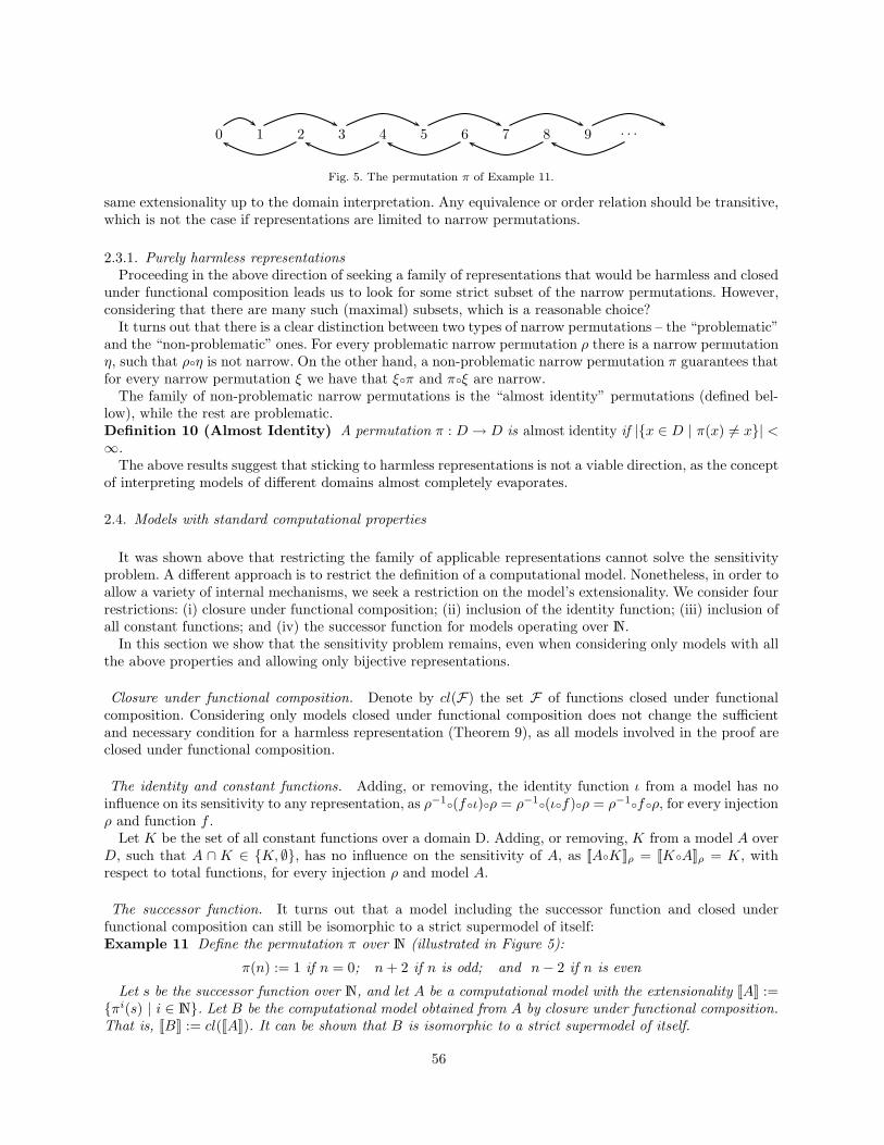
0 1 2 3 4 5 6 7 8 9 . . .

Fig. 5. The permutation π of Example 11.

same extensionality up to the domain interpretation. Any equivalence or order relation should be transitive,which is not the case if representations are limited to narrow permutations.

2.3.1. Purely harmless representationsProceeding in the above direction of seeking a family of representations that would be harmless and closed

under functional composition leads us to look for some strict subset of the narrow permutations. However,considering that there are many such (maximal) subsets, which is a reasonable choice?

It turns out that there is a clear distinction between two types of narrow permutations – the “problematic”and the “non-problematic” ones. For every problematic narrow permutation ρ there is a narrow permutationη, such that ρη is not narrow. On the other hand, a non-problematic narrow permutation π guarantees thatfor every narrow permutation ξ we have that ξπ and πξ are narrow.

The family of non-problematic narrow permutations is the “almost identity” permutations (defined bel-low), while the rest are problematic.Definition 10 (Almost Identity) A permutation π : D → D is almost identity if |x ∈ D | π(x) = x| <∞.

The above results suggest that sticking to harmless representations is not a viable direction, as the conceptof interpreting models of different domains almost completely evaporates.

2.4. Models with standard computational properties

It was shown above that restricting the family of applicable representations cannot solve the sensitivityproblem. A different approach is to restrict the definition of a computational model. Nonetheless, in order toallow a variety of internal mechanisms, we seek a restriction on the model’s extensionality. We consider fourrestrictions: (i) closure under functional composition; (ii) inclusion of the identity function; (iii) inclusion ofall constant functions; and (iv) the successor function for models operating over N.

In this section we show that the sensitivity problem remains, even when considering only models with allthe above properties and allowing only bijective representations.

Closure under functional composition. Denote by cl(F) the set F of functions closed under functionalcomposition. Considering only models closed under functional composition does not change the sufficientand necessary condition for a harmless representation (Theorem 9), as all models involved in the proof areclosed under functional composition.

The identity and constant functions. Adding, or removing, the identity function ι from a model has noinfluence on its sensitivity to any representation, as ρ−1(fι)ρ = ρ−1(ιf)ρ = ρ−1fρ, for every injectionρ and function f .

Let K be the set of all constant functions over a domain D. Adding, or removing, K from a model A overD, such that A ∩ K ∈ K, ∅, has no influence on the sensitivity of A, as [[AK]]ρ = [[KA]]ρ = K, withrespect to total functions, for every injection ρ and model A.

The successor function. It turns out that a model including the successor function and closed underfunctional composition can still be isomorphic to a strict supermodel of itself:Example 11 Define the permutation π over N (illustrated in Figure 5):

π(n) := 1 if n = 0; n+ 2 if n is odd; and n− 2 if n is even

Let s be the successor function over N, and let A be a computational model with the extensionality [[A]] :=πi(s) | i ∈ N. Let B be the computational model obtained from A by closure under functional composition.That is, [[B]] := cl([[A]]). It can be shown that B is isomorphic to a strict supermodel of itself.

56

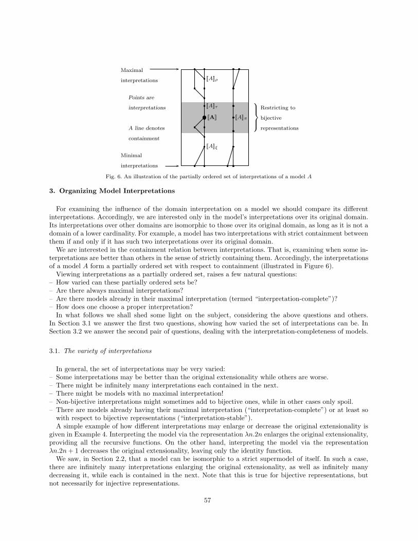
Restricting to

bijective

representations

[[A]]

[[A]]τ

[[A]]ρ

[[A]]ξ

[[A]]π

Maximal

interpretations

Minimal

interpretations

Points are

interpretations

A line denotes

containment

Fig. 6. An illustration of the partially ordered set of interpretations of a model A

3. Organizing Model Interpretations

For examining the influence of the domain interpretation on a model we should compare its differentinterpretations. Accordingly, we are interested only in the model’s interpretations over its original domain.Its interpretations over other domains are isomorphic to those over its original domain, as long as it is not adomain of a lower cardinality. For example, a model has two interpretations with strict containment betweenthem if and only if it has such two interpretations over its original domain.

We are interested in the containment relation between interpretations. That is, examining when some in-terpretations are better than others in the sense of strictly containing them. Accordingly, the interpretationsof a model A form a partially ordered set with respect to containment (illustrated in Figure 6).

Viewing interpretations as a partially ordered set, raises a few natural questions:– How varied can these partially ordered sets be?– Are there always maximal interpretations?– Are there models already in their maximal interpretation (termed “interpretation-complete”)?– How does one choose a proper interpretation?

In what follows we shall shed some light on the subject, considering the above questions and others.In Section 3.1 we answer the first two questions, showing how varied the set of interpretations can be. InSection 3.2 we answer the second pair of questions, dealing with the interpretation-completeness of models.

3.1. The variety of interpretations

In general, the set of interpretations may be very varied:– Some interpretations may be better than the original extensionality while others are worse.– There might be infinitely many interpretations each contained in the next.– There might be models with no maximal interpretation!– Non-bijective interpretations might sometimes add to bijective ones, while in other cases only spoil.– There are models already having their maximal interpretation (“interpretation-complete”) or at least so

with respect to bijective representations (“interpretation-stable”).A simple example of how different interpretations may enlarge or decrease the original extensionality is

given in Example 4. Interpreting the model via the representation λn.2n enlarges the original extensionality,providing all the recursive functions. On the other hand, interpreting the model via the representationλn.2n+ 1 decreases the original extensionality, leaving only the identity function.

We saw, in Section 2.2, that a model can be isomorphic to a strict supermodel of itself. In such a case,there are infinitely many interpretations enlarging the original extensionality, as well as infinitely manydecreasing it, while each is contained in the next. Note that this is true for bijective representations, butnot necessarily for injective representations.

57

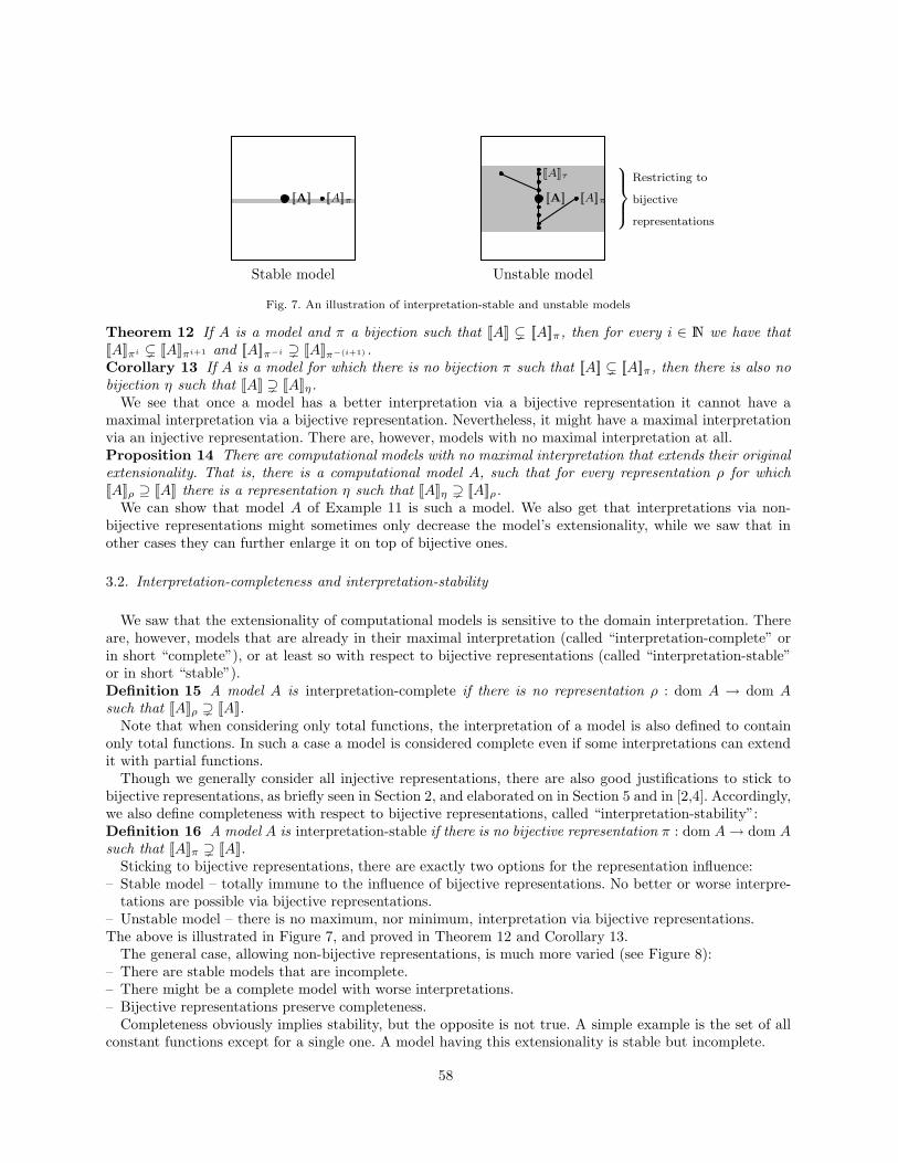
Unstable model

Restricting to

bijective

representations

[[A]]

[[A]]τ

[[A]]π

Stable model

[[A]] [[A]]π

Fig. 7. An illustration of interpretation-stable and unstable models

Theorem 12 If A is a model and π a bijection such that [[A]] [[A]]π, then for every i ∈ N we have that[[A]]πi [[A]]πi+1 and [[A]]π−i [[A]]π−(i+1) .Corollary 13 If A is a model for which there is no bijection π such that [[A]] [[A]]π, then there is also nobijection η such that [[A]] [[A]]η.

We see that once a model has a better interpretation via a bijective representation it cannot have amaximal interpretation via a bijective representation. Nevertheless, it might have a maximal interpretationvia an injective representation. There are, however, models with no maximal interpretation at all.Proposition 14 There are computational models with no maximal interpretation that extends their originalextensionality. That is, there is a computational model A, such that for every representation ρ for which[[A]]ρ ⊇ [[A]] there is a representation η such that [[A]]η [[A]]ρ.

We can show that model A of Example 11 is such a model. We also get that interpretations via non-bijective representations might sometimes only decrease the model’s extensionality, while we saw that inother cases they can further enlarge it on top of bijective ones.

3.2. Interpretation-completeness and interpretation-stability

We saw that the extensionality of computational models is sensitive to the domain interpretation. Thereare, however, models that are already in their maximal interpretation (called “interpretation-complete” orin short “complete”), or at least so with respect to bijective representations (called “interpretation-stable”or in short “stable”).Definition 15 A model A is interpretation-complete if there is no representation ρ : dom A → dom Asuch that [[A]]ρ [[A]].

Note that when considering only total functions, the interpretation of a model is also defined to containonly total functions. In such a case a model is considered complete even if some interpretations can extendit with partial functions.

Though we generally consider all injective representations, there are also good justifications to stick tobijective representations, as briefly seen in Section 2, and elaborated on in Section 5 and in [2,4]. Accordingly,we also define completeness with respect to bijective representations, called “interpretation-stability”:Definition 16 A model A is interpretation-stable if there is no bijective representation π : dom A→ dom Asuch that [[A]]π [[A]].

Sticking to bijective representations, there are exactly two options for the representation influence:– Stable model – totally immune to the influence of bijective representations. No better or worse interpre-

tations are possible via bijective representations.– Unstable model – there is no maximum, nor minimum, interpretation via bijective representations.The above is illustrated in Figure 7, and proved in Theorem 12 and Corollary 13.

The general case, allowing non-bijective representations, is much more varied (see Figure 8):– There are stable models that are incomplete.– There might be a complete model with worse interpretations.– Bijective representations preserve completeness.

Completeness obviously implies stability, but the opposite is not true. A simple example is the set of allconstant functions except for a single one. A model having this extensionality is stable but incomplete.

58

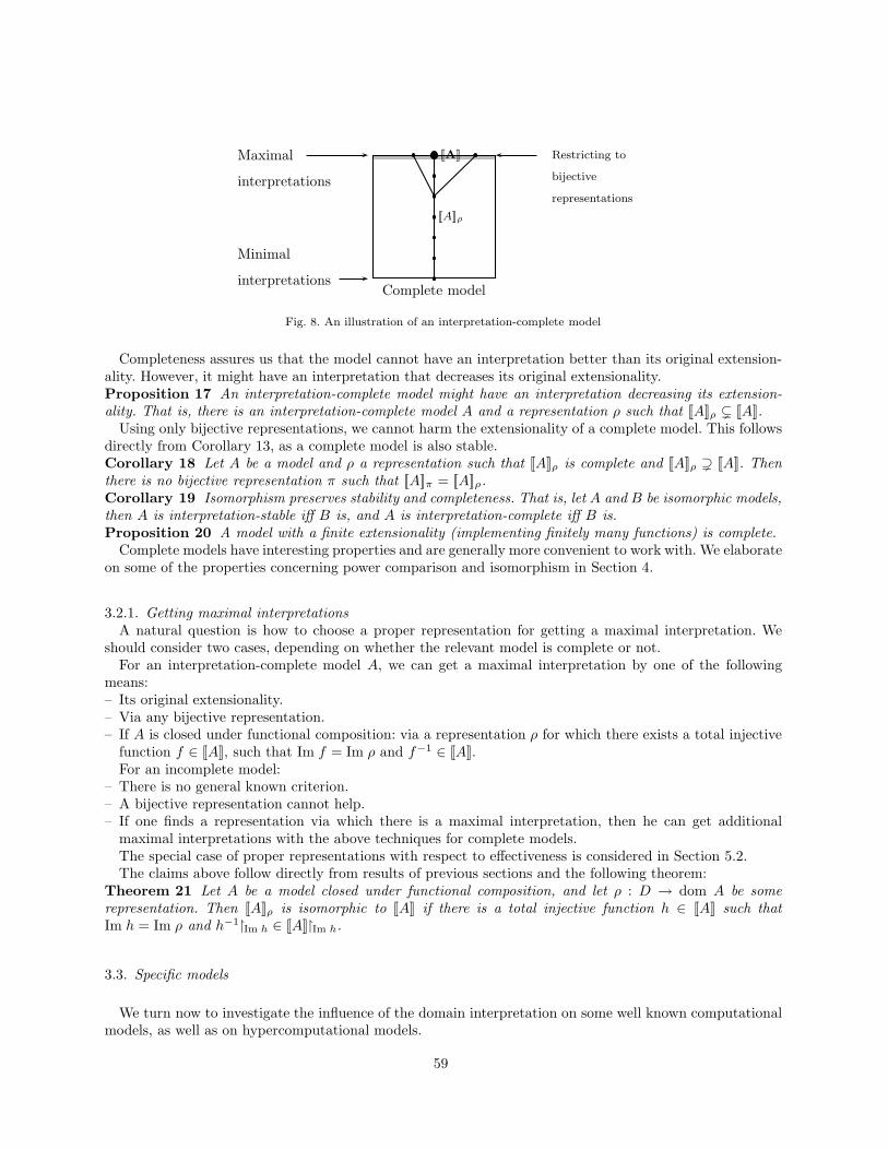
Complete model

[[A]]

[[A]]ρ

Maximal

interpretations

Minimal

interpretations

Restricting to

bijective

representations

Fig. 8. An illustration of an interpretation-complete model

Completeness assures us that the model cannot have an interpretation better than its original extension-ality. However, it might have an interpretation that decreases its original extensionality.Proposition 17 An interpretation-complete model might have an interpretation decreasing its extension-ality. That is, there is an interpretation-complete model A and a representation ρ such that [[A]]ρ [[A]].

Using only bijective representations, we cannot harm the extensionality of a complete model. This followsdirectly from Corollary 13, as a complete model is also stable.Corollary 18 Let A be a model and ρ a representation such that [[A]]ρ is complete and [[A]]ρ [[A]]. Thenthere is no bijective representation π such that [[A]]π = [[A]]ρ.Corollary 19 Isomorphism preserves stability and completeness. That is, let A and B be isomorphic models,then A is interpretation-stable iff B is, and A is interpretation-complete iff B is.Proposition 20 A model with a finite extensionality (implementing finitely many functions) is complete.

Complete models have interesting properties and are generally more convenient to work with. We elaborateon some of the properties concerning power comparison and isomorphism in Section 4.

3.2.1. Getting maximal interpretationsA natural question is how to choose a proper representation for getting a maximal interpretation. We

should consider two cases, depending on whether the relevant model is complete or not.For an interpretation-complete model A, we can get a maximal interpretation by one of the following

means:– Its original extensionality.– Via any bijective representation.– If A is closed under functional composition: via a representation ρ for which there exists a total injective

function f ∈ [[A]], such that Im f = Im ρ and f−1 ∈ [[A]].For an incomplete model:

– There is no general known criterion.– A bijective representation cannot help.– If one finds a representation via which there is a maximal interpretation, then he can get additional

maximal interpretations with the above techniques for complete models.The special case of proper representations with respect to effectiveness is considered in Section 5.2.The claims above follow directly from results of previous sections and the following theorem:

Theorem 21 Let A be a model closed under functional composition, and let ρ : D → dom A be somerepresentation. Then [[A]]ρ is isomorphic to [[A]] if there is a total injective function h ∈ [[A]] such thatIm h = Im ρ and h−1Im h ∈ [[A]]Im h.

3.3. Specific models

We turn now to investigate the influence of the domain interpretation on some well known computationalmodels, as well as on hypercomputational models.

59

3.3.1. The recursive functionsThe recursive functions (both total and partial) are interpretation-complete! Their completeness is of

special importance due to their role in the notion of effectiveness. This is elaborated on in Section 5. Thecompleteness is of both the unary recursive functions and of the functions of any arity.

In Section 3.3.2, it will be shown that the recursive functions are isomorphic to the functions computedby Turing machines. They are also isomorphic to 3-counter machines, while being a maximal interpretationof the incomplete 2-counter machines model.Theorem 22 ([3]) The unary recursive functions are interpretation-complete.Theorem 23 The partial recursive functions and the total recursive functions are interpretation-complete.

3.3.2. Turing machinesTuring machines are interpretation-complete. As with the recursive functions, this completeness is of

special importance due to the role of Turing machines in the notion of effectiveness (see Section 5).Theorem 24 ([3]) Turing machines are interpretation-complete.

When seeking a maximal interpretation for Turing machines or for the recursive functions, the criteria ofSection 3.2.1 may be extended:Theorem 25 An interpretation [[TM]]ρ of Turing machines via some injection ρ is maximal if |Im ρ| isinfinite and there is a function h ∈ [[TM]] such that Im h = Im ρ.Note that the function h above needs not be total nor injective.

3.3.3. Counter machinesThe model of two counter machines is very interesting. It was shown independently by Janis Barzdins

[1], Rich Schroeppel [19], and Frances Yao that two-counter machines cannot compute the function λx.2x.On the other hand, since two-counter machines can compute all the recursive functions via an injectiverepresentation (viz. n → 2n; see, for example, [12]), it follows that two-counter machines are interpretation-incomplete.

It turns out that the models of one-counter machines as well as of three-or-more counter machines areinterpretation-complete.

3.3.4. Hypercomputational modelsA computational model is generally said to be “hypercomputational” if it computes more than Turing

machines or more than the recursive functions (see Definition 47 in Section 5). Due to the completeness ofTuring machines and the recursive functions, such a model may indeed be regarded as more powerful. Powercomparison is treated in detail in Section 4, and the issue of effective computation over arbitrary domainsis treated in detail in Section 5.

Can we conclude from the interpretation-completeness of the recursive functions that every hypercomputa-tional model is interpretation-complete? The answer is, in general, “no”. However, if the hypercomputationalmodel preserves the basic closure properties of the recursive functions, then the answer is “yes”.

The following example is an incomplete hypercomputational model:Example 26 Let h be the (incomputable) halting function. Define:

hi := λn.

2ih(n/2i) 2i divides n

0 otherwiseρ := λn.2n

Let A be a computational model with the extensionality [[A]] := REC∪hi | i ∈ N+. That is, [[A]] includesall the recursive functions and all functions hi for i ≥ 1. We have that [[A]]ρ = REC ∪ hi | i ∈ N [[A]].

Yet, the completeness proof of the recursive functions (Theorem 23) may be extended to hypercompu-tational models, as long as they have the relevant closure properties. It also means that their domain isdenumerable, as with higher cardinalities there is no meaning to primitive recursion or minimalization:Theorem 27 Let A be a computational model over N computing all the recursive function and closed underfunctional composition, primitive recursion and minimalization. Then A is interpretation-complete.

60

A special case of such an interpretation-complete hypercomputational model is an oracle Turing machine.Corollary 28 An oracle Turing machine is interpretation-complete.

4. Comparing Computational Power

It is standard in the literature to compare the power of computational models. However, neglecting thepossibility of interpretation-incomplete models, it is common to say that model B is strictly stronger thanmodel A when it computes strictly more functions. This might allow one to show that some computationalmodels are strictly stronger than themselves (see Section 2).

We define a comparison notion over arbitrary domains based on model interpretations. With this notion,model B is strictly stronger than A if B has an interpretation that contains A, whereas A cannot containB under any interpretation.

We start, in Section 4.1, by providing the mathematical definition of the comparison notion. We give abasic definition, allowing all interpretations, and two additional definitions with some restrictions on theallowed interpretations. In Section 4.1.1 we extend the notion no non-deterministic models.

In Section 4.2 we provide several results with respect to power comparison, isomorphism and completeness.In Section 4.3, we compare between some standard models, as Turing machines, stack machines, etc..

4.1. The comparison notions

Since we are only interested here in the extensional quality of a computational model (the set of functionsor relations that it computes), not complexity-based comparison or step-by-step simulation, we use modelinterpretations as the basis for comparison.

We generally say that model B is at least as powerful as model A if it can compute whatever A can. Whenboth models operate over the same domain it simply means containment: B is at least as powerful as A if[[B]] ⊇ [[A]]. However, when the models operate over different domains we ought to interpret one model overthe domain of the other. Hence, the general comparison notion would say that B is at least as powerful asA if it has an interpretation that contains A.

As one textbook states [21, p. 30]:Computability relative to a coding is the basic concept in comparing the power of computation models.. . .The computational power of the model is represented by the extension of the set of all functions computableaccording to the model. Thus, we can compare the power of computation models using the concept‘incorporation relative to some suitable coding’.We provide three notions of comparison, depending on the allowed representations. The basic, most per-

missive, comparison notion allows any injection, while the firmest notion allows only bijections. In between,we define a notion that allows injections for which the “as-powerful” model can fix their image.Definition 29 (Power Comparison)– Model B is at least as powerful as model A, denoted B A, if it has an interpretation that contains the

extensionality of A. That is, B A iff exists an injection ρ : dom A→ dom B, such that [[B]]ρ ⊇ [[A]].– Model B is decently at least as powerful as model A, denoted B A, if it has an interpretation that

contains the extensionality of A via a representation for which it can fix its image. That is, B A iffexists an injection ρ : dom A → dom B, such that [[B]]ρ ⊇ [[A]] and there is a total function g ∈ [[B]] forwhich Im g = Im ρ and such that for every y ∈ Im ρ we have that g(y) = y.

– Model B is bijectively at least as powerful as model A, denoted B A, if it has a bijective interpretationthat contains the extensionality of A. That is, B A iff exists a bijection π : dom A→ dom B, such that[[B]]π ⊇ [[A]].

Proposition 30 The computational power relations ,, are quasi-orders.Obviously, the two latter comparison notions imply the former one. For the third notion to imply the

second one, it is sufficient that the as-powerful model has some surjective function, even the identity function.Additionally, when assuming a little more about the representation and the model, the second notion alsoimplies the third one (see Theorem 21).

61

Note 31 When comparing the computational power of models, it should be noted that one function cannotbe “better” than another; only a model can be better than another. There is only an equivalence relationbetween functions, where two partial functions, f and g, over the same domain D are deemed equal, denotedf = g, if they are defined for exactly the same elements of the domain and have the same value wheneverthey are defined. For example, a total function f is not better than nor equal to a partial function g that hasthe same values as f when it converges. This is clearly demonstrated by taking g to be a ‘halting function’,which returns 1 when the input encodes a halting machine and diverges otherwise.

Our comparison notions go along with some standard approaches, for instance in [7, p. 24], [18, p. 27] and[21, p. 30]. Our decent-comparison notion follows Rabin’s definition of a computable group [16, p. 343]:“DEFINITION 3. An indexing of a set S is a one to one mapping i : S → I such that i(S) is a recursivesubset of I.”Example 32 Turing machines are at least as powerful as the recursive functions via a unary representationof the natural numbers. See, for example, [9, p. 147]. Indeed, it is so by all three notions (see Theorem 45).

One may wonder why we do not require the representation to be Turing-computable. A detailed answerto that is given in Section 5. The main points are:– When comparing models in the scope of defining effectiveness, the requirement of a Turing-computable

representation leads to a circular definition.– One may wish to compare sub-recursive models or hypercomputational models, for which Turing-

computability is not necessarily the proper constraint.

Power equivalence. The power equivalence relation between models follows directly from the power com-parison notion. Models A and B are of equivalent power if A B and B A.Definition 33 (Power Equivalence)– Models A and B are power equivalent, denoted A ∼ B, if A B and B A.– Models A and B are decently power equivalent, denoted A B, if A B and B A.– Models A and B are bijectively power equivalent, denoted A ≈ B, if A B and B A.Example 34 The (untyped) λ-calculus is power equivalent to the recursive functions, via Church numer-als, on the one hand, and via Godelization, on the other. However, it is not interpretation-complete, as itcannot even compute the identity function over an arbitrary lambda-term. Hence, it is not bijectively-powerequivalent to the recursive functions (otherwise contradicting the completeness of the recursive functions).

Strictly stronger. We generally think of model B as stronger than model A if it can compute more.However, because of the sensitivity to the domain interpretation (Section 2), proper containment does notimply more computational power. That is, [[B]] [[A]] ⇒ B A. This is so for all three comparison notions.

The proper definition of model B being strictly stronger than model A is that B A while A B.Definition 35 (Stronger)– Model B is stronger than model A, denoted B A, if B A while A B.– Model B is decently stronger than model A, denoted B A, if B A while A B.– Model B is bijectively stronger than model A, denoted B A, if B A while A B.

Note that for model B to be stronger than model A there should be no injection ρ via which A ρ B.In contradistinction to the “as powerful” case, some model B may be bijectively stronger than a model A,but not stronger than A. However, if A is interpretation-complete, we do have that B A implies B A(Theorem 42).Example 36 Real recursive functions [14], operating over R2, are decently stronger than Turing machines.The comparison is done via an injective representation ψ : 0, 1∗ → R2, defined by [[x]]ψ := (0, [[x]]ρ), where[[x]]ρ is the standard binary interpretation over the natural numbers [14, p. 849]. Since the model computesthe floor function (λx. x) [14, p. 843], it follows that it also has a function which fixes the representationimage. On the other hand, the real recursive functions are obviously not bijectively stronger than the recursivefunctions, as their domain is of a higher cardinality.

62

Universal machines. Computation is often performed via universal machines, also referred to as “inter-preters”. That is, a single machine (or computer program) gets as input both the machine to interpret andthe latter’s input. One may wonder how to compare the computational power of universal machines. Fromour point of view, computational power is extensionality, meaning the set of computed functions. Hence,when comparing universal machines we compare the sets of functions that they interpret. Accordingly, it isexactly like comparing computational models.

4.1.1. Non-deterministic modelsThe extension of most of the definitions and theorems given so far (in this section and the previous ones)

to non-deterministic models is quite straightforward. There are, however, some specific issues concerning thepower comparison of non-deterministic models, which will be discussed below.

We begin by defining what we mean by a non-deterministic computational model and its extensionality:Definition 37 (Non-deterministic Computational Model) A non-deterministic computationalmodel A over domain D is any object associated with a set of (non-unary) relations over D ∪ ⊥. This setof relations is called the extensionality of the non-deterministic computational model, denoted [[A]].

Note that we use the special symbol ⊥ in the above definition for denoting a non-halting computation,while we did not need it in the definition of a deterministic model (Definition 1). The reason is that anon-deterministic computation might sometimes diverge on a domain element e and sometimes converge tosome value v. In such a case, the value of the computation will be both ⊥ and v, denoted by 〈e,⊥〉, 〈e, v〉 inthe (multivalued) function’s description. On the other hand, the divergence of a deterministic function on adomain element e, may be simply denoted by not having a tuple with e in the function’s description.

As a result of using ⊥ to denote divergence, we may assume that all functions have at least one value forevery domain element.

When investigating the influence of the domain interpretation, we are concerned with the containmentrelation between the different interpretations of a computational model. Hence, the definitions given in thissection and the previous ones apply to both deterministic and non-deterministic models, as in both types ofmodels the interpretations are sets of relations.

When we compare the power of computational models, two functions are considered equal if and onlyif they are described by the same relation, while a model is as powerful as another if it contains all thefunctions of the former (see Note 31). This is also the case when we compare between non-deterministicmodels. There might be cases in which a different approach is required, assuming a different equality notionbetween functions. For example, two non-deterministic functions might be considered equal if they mayalways produce the same value. That is, a function that sometimes diverges and sometimes converges withthe value v is considered equal to a function that always converges with the value v. In such cases, thecomparison notions should be adjusted to take into account the special equality notion between functions.

By this comparison approach, a non-deterministic model B may be as powerful as a deterministic modelA (if it deterministically computes all the functions of A, in addition to its non-deterministic computations),while the opposite is impossible (when B actually has some non-deterministic computations).

4.2. Power comparison, isomorphism, and interpretation-completeness

The general approach for showing that model B is stronger than model A is tedious – we should negatethe possibility that A ρ B for all injections ρ. The situation is much simpler with interpretation-completemodels, for which proper containment does imply more power:Theorem 38 ([3]) For an interpretation-complete model A and some model B, we have that B A iffthere exists an injection ρ such that [[B]]ρ [[A]].

Isomorphism and bijective power equivalence are very similar notions, though not the same. However,when sticking to interpretation-stable models they do coincide:Theorem 39

(i) Isomorphism implies bijective power equivalence.(ii) Bijective power equivalence does not imply isomorphism.

63

(iii) For stable models, bijective power equivalence implies isomorphism. That is, if model A is stable, thenfor every model B, B is isomorphic to A if and only if it is bijectively power equivalent to A.

Isomorphism preserves stability and completeness (Corollary 19). This is also the case, by the abovetheorem, with bijective power equivalence.Corollary 40 Bijective power equivalence preserves stability and completeness. That is, let A and B bebijectively power equivalent models, then A is stable iff B is, and A is complete iff B is.

The formulation of the previous theorem can be strengthened for complete models:Lemma 41 ([3]) If model A is complete and A B A for some model B, then A and B are isomorphic.

Interpretation-completeness also helps with showing that some model is stronger than another.Theorem 42 If model A is complete, then B A implies B ATheorem 43 ([3]) If model A is complete, A ≈ B and [[B]] [[C]], for models B and C, then C A.

4.3. Comparison of some Standard Models

As discussed in the beginning of this section, the proper containment between the recursive functionsand the primitive recursive functions does not imply that the former are strictly more powerful than thelatter. Nonetheless, the recursive functions are indeed strictly more powerful, even by the general comparisonnotion, allowing all possible interpretations of the primitive recursive functions.Theorem 44 ([3]) The primitive recursive functions are strictly weaker than the recursive functions.

We do not know if the primitive recursive functions are interpretation-complete, Theorem 44 notwith-standing.

It is common to show that Turing machines and the recursive functions are of equivalent computationalpower. Actually, they are isomorphic. We base the proof on known results, given in [10].Theorem 45 ([3]) Turing machines, over a binary alphabet, and the recursive functions are isomorphic.

From [10,3] we also have that random access machines and counter machines with unlimited number ofcounters have exactly the same extensionality as the recursive functions.

This is not the case with two-counter machines. They are of equivalent power to the recursive functions,however not isomorphic to them. Indeed, they are bijectively-weaker than them (otherwise contradicting thestability of the recursive functions).

By known results, two-stack machines have the same extensionality as Turing machines.Due to the closure properties of Turing machines and the recursive functions, they are bijectively at least

as powerful as some model A if and only if they are decently at least as powerful as A.Theorem 46 Let A be a computational model operating over a denumerable domain. Then Turing machinesand the recursive functions are decently at least as powerful as A if and only if they are bijectively at leastas powerful as A. That is, TM A iff TM A iff REC A iff REC A.

5. Effective Computation

In 1936, Alonzo Church and Alan Turing each formulated a claim that a particular model of computa-tion completely captures the conceptual notion of “effective” computability. Church [6, p. 356] proposedthat effective computability of numeric functions be identified with Godel and Herbrand’s general recursivefunctions, or – equivalently, as it turned out [6] – with Church and Kleene’s lambda-definable functions ofpositive integers.

Turing, on the other hand, explicitly extends the notion of “effective” beyond the natural numbers [23,fn. p. 166] (emphasis added):

We shall use the expression “computable function” to mean a function calculable by a machine, and welet “effectively calculable” refer to the intuitive idea without particular identification with one of thesedefinitions. We do not restrict the values taken by a computable function to be natural numbers ; we mayfor instance have computable propositional functions.Our purpose, in Section 5.1, is to formalize and analyze the Church-Turing Thesis, referring to functions

over arbitrary domains.

64

Equipped with this definition, and due to the interpretation-completeness of Turing machines, we define,in Section 5.2, effective representations of constructible domains.

5.1. The Church-Turing Thesis over arbitrary domains

Simply put, the Church-Turing Thesis is not well defined for arbitrary domains: the choice of domaininterpretation might have a significant influence on the outcome. We explore below the importance of thedomain interpretation and suggest how to overcome this problem.

Computational model versus single function. A single function over an arbitrary domain cannot be clas-sified as computable or not. Its computability depends on the representation of the domain. 2 For example,the (uncomputable) halting function over the natural numbers (sans the standard order) is isomorphic tothe simple parity function, under a permutation of the natural numbers that maps the usual codes of haltingTuring machines to strings ending in “0”, and the rest of the numbers to strings ending with “1”. The resultis a computable standalone “halting” function.

An analysis of the classes of number-theoretic functions that are computable relative to different notations(representations) is provided by Shapiro [20, p. 15]:

It is shown, in particular, that the class of number-theoretic functions which are computable relativeto every notation is too narrow, containing only rather trivial functions, and that the class of number-theoretic functions which are computable relative to some notation is too broad containing, for example,every characteristic function.An intuitive approach is to restrict the representation only to “natural” mappings between the domains.

However, when doing so in the scope of defining “effectiveness”, one must use a vague and undefined notion.This problem was already pointed out by Richard Montague on 1960 [13, pp. 430–431]:Now Turing’s notion of computability applies directly only to functions on and to the set of naturalnumbers. Even its extension to functions defined on (and with values in) another denumerable set Scannot be accomplished in a completely unobjectionable way. One would be inclined to choose a one-to-one correspondence between S and the set of natural numbers, and to call a function f on S computable ifthe function of natural numbers induced by f under this correspondence is computable in Turing’s sense.But the notion so obtained depends on what correspondence between S and the set of natural numbersis chosen; the sets of computable functions on S correlated with two such correspondences will in generaldiffer. The natural procedure is to restrict consideration to those correspondences which are in some sense‘effective’, and hence to characterize a computable function on S as a function f such that, for someeffective correspondence between S and the set of natural numbers, the function induced by f under thiscorrespondence is computable in Turing’s sense. But the notion of effectiveness remains to be analyzed,and would indeed seem to coincide with computability.Stewart Shapiro suggests a definition of “acceptable notation”, based on intuitive concepts [20, p. 18]:This suggests two informal criteria on notations employed by algorithms:(1) The computist should be able to write numbers in the notation. If he has a particular number in

mind, he should (in principle) be able to write and identify tokens for the corresponding numeral.(2) The computist should be able to read the notation. If he is given a token for a numeral, he should

(in principle) be able to determine what number it denotes.It is admitted that these conditions are, at best, vague and perhaps obscure.Michael Rescorla argues that the circularity is inherent in the Church-Turing Thesis [17].A possible solution is to allow any representation (injection between domains), while checking for the

effectiveness of an entire computational model. That is, to check for the computability of a function togetherwith the other functions that are computable by that computational model. The purpose lying behindthis idea is to view the domain elements as arbitrary objects, deriving all their meaning from the model’s

2 There are functions that are inherently uncomputable, via all domain representations. For example, a permutation of somecountable domain, in which the lengths of the orbits are exactly the standard encodings of the non-halting Turing machines.

65

functions. For example, it is obvious that the halting function has a meaning only if one knows the order ofthe elements of its domain. In that case, the successor function provides the meaning for the elements.

Two variants of this solution, corresponding to the variants of our comparison notion (Definition 29),are to either allow only bijective representations, or else allow injections provided that their images arecomputable.

Adopting the above approach of checking for computability of an entire computational model, we interpretthe Church-Turing Thesis as follows:

Thesis A. All “effective” computational models are of equivalent power to, or weaker than, Turing ma-chines.

By “effective”, in quotes, we mean effective in its intuitive sense.By a “computational model” we refer to any object that is associated with a set of partial functions

(Definition 1). By “equivalent to, or weaker than” we refer to the comparison notions of Definition 29.A strict supermodel of the recursive functions (or Turing machines) is a “hypercomputational” model.

Definition 47 (Hypercomputational Model) A computational model H is hypercomputational if it isstronger than Turing machines. That is, if H TM. (The corresponding variations, using bijective powercomparison or decent power comparison, are H TM or H TM.)

Our interpretation of the Church-Turing Thesis (Thesis A) agrees with Rabin’s definition of a computablegroup [16, p. 343], as well as with its generalization, by Lambert [24, p. 594], to any algebraic structure.Similar notions were also presented by Froehlich and Shepherdson [8] and Mal’cev [11].

Influence of representations. The Church-Turing Thesis, as stated above (Thesis A), matches the intuitiveunderstanding only due to the interpretation-completeness of Turing machines (Theorem 24). Were the thesisdefined in terms of two-counter machines (2CM), for example, it would make no sense: a computational modelis not necessarily stronger than 2CM even if it computes strictly more functions.

5.2. Effective representations

What is an effective representation? We argued above that a “natural representation” must be a vaguenotion when used in the context of defining effectiveness. We avoided the need of restricting the representationby checking the effectiveness of entire computational models. But what if we adopt the Church-Turing Thesis;can we then define what is an effective string representation?

Simply put, there is a problem here. Turing machines operate only over strings. Thus a string represen-tation, which is an injection from some domain D to Σ∗, is not itself computable by a Turing machine. Allthe same, when we consider, for example, string representations of natural numbers, we can obviously sayregarding some of them that they are effective. How is that possible? The point is that we look at the nat-ural numbers as having some structure, usually assuming their standard order. A function over the naturalnumbers without their order is not really well-defined. As we saw, the halting function and the simple parityfunction are exactly the same (isomorphic) function when numbers are unordered.

Hence, even when adopting the Church-Turing Thesis, a domain without any structure cannot have aneffective representation. It is just a set of arbitrary elements. However, if the domain comes with a generatingmechanism (as the natural numbers come with the successor) we can consider effective representations.

Due to the interpretation-completeness of the recursive functions and Turing machines, we can definewhat is an effective string representation of the natural numbers (with their standard structure). A similardefinition can be given for other domains, provided that they come with some finite means of generatingthem all, akin to successor for the naturals.Definition 48 An effective representation of the natural numbers by strings is an injection ρ : N → Σ∗,such that ρ(s) is Turing-computable (ρ(s) ∈ [[TM]]), where s is the successor function over N.That is, a representation of the natural numbers is effective if the successor function is Turing-computablevia this representation.

66

Note 49 One may also require that the image of the representation ρ is Turing computable, along the decentpower comparison notion. In such a case, there would also be a corresponding bijective representation (seeTheorem 21 and 25).

We justify the above definition of an effective representation by showing that: (a) every recursive func-tion is Turing-computable via any effective representation; (b) every non-recursive function is not Turing-computable via any effective representation; and (c) for every non-effective representation there is a recursivefunction that is not Turing-computable via it.Theorem 50 ([5])(a) Let f be a recursive function and ρ : N → Σ∗ an effective representation. Then ρ(f) ∈ [[TM]].(b) Let g be a non-recursive function and ρ : N → Σ∗ an effective representation. Then ρ(g) /∈ [[TM]].(c) Let η : N → Σ∗ be a non-effective representation. Then there is a recursive function f , such that

η(f) /∈ [[TM]].To see the importance of the interpretation-completeness for the definition of an effective representation,

one can check that an analogous definition cannot be provided with two-counter machines as the yardstick.Our definition of an effective representation resembles Shapiro’s notion of an “acceptable notation” [20,

p. 19] and goes along with Weihrauch’s justifications for the effectiveness of the “standard numberings”(representations by natural numbers) [25, p. 80–81]. A description of the correlation between our notion andShapiro’s and Weihrauch’s notions can be found in [5].

6. Discussion

Key points. In this paper, we have explored various aspects of the influence of domain interpretations onthe extensionality of computational models, and suggested how we believe they should be handled. Some ofthe key points are:– The extensionality of computational models is a very interesting set (of functions) – it varies from “fluid”

sets for which containment does not mean more power, as with ordinary sets, to explicit, complete, setsfor which nothing can be added without additional power.

– Get to know your model: Is it interpretation-stable or interpretation-complete?– Compare computational power properly.– Turing machines and the recursive functions are shown to be robust, this time from the representa-

tion/interpretation point of view.– Effectiveness does not apply to a single function; it is a set of functions, or a function together with its

domain constructors, that may be deemed effective.

Domain Representation. One might think that our study is a part of the “domain representation” researcharea. This is not the case. Indeed, the basic concept of “representation” is the same: one set of elements isrepresented by a subset of another set. Nevertheless, the issues studied are very different. Domain repre-sentation concerns mapping of some (possibly topological/metric) sets into domains (partially ordered setswith some properties), and studies the (topological/metric) properties preserved via the mappings.

Further research. A central issue, yet to be understood, is the relation between the internal mechanismof a computational model and its extensional properties of interpretation-completeness and interpretation-stability. With the recursive functions, this relation is apparent, shown in the proof of their interpretation-completeness. However, we do not know how to relate, in general, the completeness or stability of a compu-tational model to its internal mechanism. A more specific open question is whether there is some standard,well known, computational model that is unstable.

References

[1] J. Barzdins. About one class of Turing machines (Minsky machines). Algebra and Logic (seminar), 1(6):42–51, 1962.

67

[2] U. Boker and N. Dershowitz. How to compare the power of computational models. In Computability in Europe 2005: NewComputational Paradigms (Amsterdam), S. Barry Cooper, Benedikt Lowe, Leen Torenvliet, eds., volume 3526 of LectureNotes in Computer Science, pages 54–64, Berlin, Germany, 2005. Springer-Verlag.

[3] U. Boker and N. Dershowitz. Comparing computational power. Logic Journal of the IGPL, 14(5):633–648, 2006.[4] U. Boker and N. Dershowitz. A hypercomputational alien. Applied Mathematics and Computation, 178(1):44–57, 2006.[5] U. Boker and N. Dershowitz. The Church-Turing thesis over arbitrary domains. In A. Avron, N. Dershowitz, and

A. Rabinovich, editors, Pillars of Computer Science, volume 4800 of Lecture Notes in Computer Science, pages 199–229. Springer, 2008.

[6] A. Church. An unsolvable problem of elementary number theory. American Journal of Mathematics, 58:345–363, 1936.[7] N. Cutland. Computability: An Introduction to Recursive Function Theory. Cambridge University Press, Cambridge, 1980.[8] A. Froehlich and J. Shepherdson. Effective procedures in field theory. Philosophical Transactions of the Royal Society of

London, 248:14–20, 1956.[9] F. Hennie. Introduction to Computability. Addison-Wesley, Reading, MA, 1977.[10] N. D. Jones. Computability and Complexity from a Programming Perspective. The MIT Press, Cambridge, Massachusetts,

1997.[11] A. Mal’cev. Constructive algebras I. Russian Mathematical Surveys, 16:77–129, 1961.[12] M. L. Minsky. Computation: Finite and Infinite Machines. Prentice-Hall, Englewood Cliffs, N.J., 1967.[13] R. Montague. Towards a general theory of computability. Synthese, 12(4):429–438, 1960.[14] J. Mycka and J. F. Costa. Real recursive functions and their hierarchy. Journal of Complexity, 20(6):835–857, 2004.[15] J. Myhill. Some philosophical implications of mathematical logic. Three classes of ideas. The Review of Metaphysics,

6(2):165–198, 1952.[16] M. O. Rabin. Computable algebra, general theory and theory of computable fields. Transactions of the American

Mathematical Society, 95(2):341–360, 1960.[17] M. Rescorla. Church’s thesis and the conceptual analysis of computability. Notre Dame Journal of Formal Logic, 48(2):253–

280, 2007.[18] H. Rogers, Jr. Theory of Recursive Functions and Effective Computability. McGraw-Hill, New York, 1966.[19] R. Schroeppel. A two counter machine cannot calculate 2N . Technical report, Massachusetts Institute of Technology,

Artificial Intelligence Laboratory, 1972. available at: ftp://publications.ai.mit.edu/ai-publications/pdf/AIM-257.pdf.[20] S. Shapiro. Acceptable notation. Notre Dame Journal of Formal Logic, 23(1):14–20, 1982.[21] R. Sommerhalder and S. C. van Westrhenen. The Theory of Computability: Programs, Machines, Effectiveness and

Feasibility. Addison-Wesley, Workingham, England, 1988.[22] G. J. Tourlakis. Computability. Reston Publishing Company, Reston, VA, 1984.[23] A. M. Turing. Systems of logic based on ordinals. Proceedings of the London Mathematical Society, 45:161–228, 1939.[24] J. W. M. Lambert. A notion of effectiveness in arbitrary structures. The Journal of Symbolic Logic, 33(4):577–602, 1968.[25] K. Weihrauch. Computability, volume 9 of EATCS Monographs on Theoretical Computer Science. Springer-Verlag, Berlin,

1987.[26] K. Weihrauch. Computable Analysis — An introduction. Springer-Verlag, Berlin, 2000.

68

On the Convergence of a Population Protocol

When Population Goes to Infinity

Olivier Bournez a Philippe Chassaing b Johanne Cohen a

Lucas Gerin b Xavier Koegler c

aLORIA/INRIA-CNRS, 615 Rue du Jardin Botanique, 54602Villers-Les-Nancy, FRANCE

bIECN/UHP, BP 239, 54506 Vandoeuvre-Les-Nancy Cedex, FRANCEc Ecole Normale Superieure, 45, rue d’Ulm, 75230 Paris cedex 05, FRANCE

Abstract

Population protocols have been introduced as a model of sensor networks consistingof very limited mobile agents with no control over their own movement. A popu-lation protocol corresponds to a collection of anonymous agents, modeled by finiteautomata, that interact with one another to carry out computations, by updatingtheir states, using some rules.

Their computational power has been investigated under several hypotheses butalways when restricted to finite size populations. In particular, predicates stablycomputable in the original model have been characterized as those definable inPresburger arithmetic.

In this paper, we study mathematically a particular population protocol that weshow to compute in some natural sense some algebraic irrational number, wheneverthe population goes to infinity. Hence we show that these protocols seem to have arather different computational power when considered as computing functions, andwhen a huge population hypothesis is considered.

1 Motivation

The computational power of networks of finitely many anonymous resource-limited mobile agents has been investigated in several recent papers. In partic-

Email addresses: [email protected] (Olivier Bournez),[email protected] (Philippe Chassaing), [email protected] (JohanneCohen), [email protected] (Lucas Gerin),[email protected] (Xavier Koegler).

Preprint submitted to Elsevier 9 July 2008

ular, the population protocol model, introduced in [1], consists of a populationof finite-state agents that interact in pairs, where each interaction updates thestate of both participants according to a transition based on the previousstates of the participants. When all agents converge after some finite time toa common value, this value represents the result of the computation.

Several variants of the original model have been considered but with com-mon features. Following survey [3]: anonymous finite-state agents (the systemconsists of a large population of indistinguishable finite-state agents), compu-tation by direct interaction (an interaction between two agents updates theirstates according to a joint transition table), unpredictable interaction patterns(the choice of interactions is made by an adversary, possibly limited to pairingonly agents in an interaction graph), distributed input and outputs (the inputto a population protocol is distributed across the initial state of the entire pop-ulation, similarly the output is distributed to all agents), convergence ratherthan termination (the agents’ output are required to converge after some timeto a common correct value).

Typically, in the spirit of [1] and following papers (see again [3] for a survey),population protocols are assumed to (stably) compute predicates: a populationprotocols stably computes a predicate φ, if for any possible input x of φ,whenever φ(x) is true all agents of the population eventually stabilize to a statecorresponding to 1, and whenever φ(x) is false, all agents of the populationeventually stabilize to a state corresponding to 0.

Predicates stably computable by population protocols in this sense have beencharacterized as being precisely the semi-linear predicates, that is to say thosepredicates on counts of input agents definable in first-order Presburger arith-metic [9]. Semilinearity was shown to be sufficient in [1] and necessary in [2].

In this paper, we want to study a new variant: we assume a population closeto infinity (we call this a huge population hypothesis), and we don’t want tofocus on protocols as predicate recognizers, but as computing functions. Weassume outputs to correspond to proportions, which are clearly the analog ofcounts whenever the population is infinite or close to infinity.

Indeed, we consider a particular population protocol, that we prove to con-verge, whatever its initial state is, to a fraction of

√2

2agents in a given state.

We hence show that some algebraic irrational values can be computed in thissense. We also give an asymptotic development of the convergence.

Our motivation is to show that protocols, considered with these two hypothe-ses (huge population, computing functions and not only predicates), have arather different power.

We consider this paper as a first step towards understanding which numbers

70

can be computed by such protocols. Whereas we prove in this paper that√

22

can be computed, and whereas this is easy to see that computable numbersin this sense must be algebraic numbers of [0, 1], we didn’t succeed yet tocharacterize precisely computable numbers.

In this more long term objective, the aim of this current paper is first todiscuss in which sense one can say that these protocols compute an irrationalalgebraic value such as

√2

2, and second to study mathematically formally the

convergence.

Our discussion is organized as follows. In Section 2, we present classical finite-size population protocols and related work. In Section 3, we present the con-sidered system. In Section 4, as a preliminary discussion, we discuss whatcan be said when population is assumed to be finite. The rest of the paperis devoted to consider the case of an infinite population. To do so, we firstdo some mathematical computations in Section 5, in order to use a generaltheorem presented in Section 6 from [10] about approximation of diffusions.This theorem yields the proof of convergence in Section 7. We prove in Sec-tion 8 that this is even possible to use the same theorem to go further andget an asymptotic development of the convergence. Section 9 is devoted to aconclusion and a discussion.

2 Related Work

Population protocols have been introduced in [1]. In the paper, the authorsproved that all semi-linear predicates can be computed but left open the ques-tion of their exact power. This was solved in [2], where it has been proved thatno-more predicates can be computed.

The population protocol model was inspired in part by the work by Diamadiand Fischer on trust propagation in social networks [5]. The model proposedin [1] was motivated by the study of sensor networks in which passive agentswere carried along by other entities. The canonical example given in this latterpaper was sensors attached to a flock of birds.

Much of the work so far on population protocols has concentrated on charac-terizing what predicates on the input configurations can be stably computedin different variants of the models and under various assumptions, such asbounded-degree interaction graphs and random scheduling [3].

Variants considered includes restriction to one-way communications, restric-tion to particular interaction graphs, random interactions, self-stabilizing so-lutions through population protocols to classical problems in distributed algo-

71

rithmic, the taking into account of various kind of failures of agents, etc. Seesurvey [3]. As far as we know, a huge population hypothesis in the sense ofthis paper, has not been considered yet.

Notice that we assume that interactions happen in probabilistic way, accordingto some uniform law. In the original population protocol model, only specificfairness hypotheses were assumed on possible adversaries [1]. Somehow our no-tion of adversary is stronger: for finite state systems, this satisfies the fairnesshypotheses of the original model, but for infinite state systems, we think thatthis becomes more natural to expect such a notion, since fairness hypothesesin the sense [1] become problematic to generalize. Notice that this notion ofadversary has already be considered for finite state systems [3], in order tostudy speed of convergence of specific algorithms.

The result proved in this paper can be considered as a macroscopic abstractionof a system given by microscopic rules of evolutions. See survey [7] for generaldiscussions about extraction of macroscopic dynamics.

Whereas the ordinary differential equation (9) can be immediately abstractedin a physicist approach from the dynamic (1), the formal mathematical equiv-alence of the two is not so immediate, and is somehow a strong motivation ofthis paper.

Actually, these problems seem to arise in many macroscopic justification ofmodels from their microscopic description in experimental science: See forexample the very instructive discussion in [8] about assumptions required forthe justification of the Lotka-Volterra (predator-prey) model of populationdynamics. In particular, observe that the fact that microscopic correlationsmust be neglected (i.e. E[XY ] = E[X]E[Y ] is needed, where E is expectation).With a rather similar hypothesis (here assuming E[p2] = E[p]2), dynamic (9)is clear from rules (1). Somehow, we prove here that this hypothesis is notnecessary for our system.

The techniques used in this paper are based on weak convergence techniques,introduced in [10], relating a stochastic differential equation (whose solutionsare called diffusions) to approximations by a family of Markov processes. Referalso to [6] for an introduction to these techniques. The theorem used here isactually based on the presentation of [4] of a theorem from [10].

3 The Considered System

We now present our system, in a self-contained manner, to avoid to rede-fine formally population protocols. However, the reader can check that this is

72

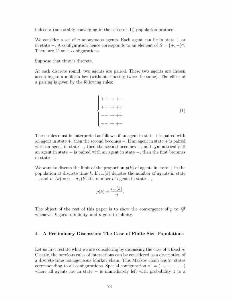
indeed a (non-stably-converging in the sense of [1]) population protocol.

We consider a set of n anonymous agents. Each agent can be in state + orin state −. A configuration hence corresponds to an element of S = +,−n.There are 2n such configurations.

Suppose that time is discrete.

At each discrete round, two agents are paired. These two agents are chosenaccording to a uniform law (without choosing twice the same). The effect ofa pairing is given by the following rules:

++ → +−

+− → ++

−+ → ++

−− → +−

(1)

These rules must be interpreted as follows: if an agent in state + is paired withan agent in state +, then the second becomes −. If an agent in state + is pairedwith an agent in state −, then the second becomes +, and symmetrically. Ifan agent in state − is paired with an agent in state −, then the first becomesin state +.

We want to discuss the limit of the proportion p(k) of agents in state + in thepopulation at discrete time k. If n+(k) denotes the number of agents in state+, and n−(k) = n− n+(k) the number of agents in state −,

p(k) =n+(k)

n.

The object of the rest of this paper is to show the convergence of p to√

22

whenever k goes to infinity, and n goes to infinity.

4 A Preliminary Discussion: The Case of Finite Size Populations

Let us first restate what we are considering by discussing the case of a fixed n.Clearly, the previous rules of interactions can be considered as a description ofa discrete time homogeneous Markov chain. This Markov chain has 2n statescorresponding to all configurations. Special configuration s− = (−,−, · · · ,−)where all agents are in state − is immediately left with probability 1 to a

73

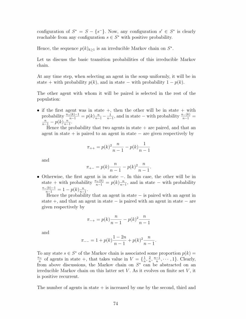
configuration of S∗ = S − s−. Now, any configuration s′ ∈ S∗ is clearlyreachable from any configuration s ∈ S∗ with positive probability.

Hence, the sequence p(k)k≥1 is an irreducible Markov chain on S∗.

Let us discuss the basic transition probabilities of this irreducible Markovchain.

At any time step, when selecting an agent in the soup uniformly, it will be instate + with probability p(k), and in state − with probability 1− p(k).

The other agent with whom it will be paired is selected in the rest of thepopulation:

• if the first agent was in state +, then the other will be in state + withprobability n+(k)−1

n−1= p(k) n

n−1− 1

n−1, and in state − with probability n−(k)

n−1=

nn−1− p(k) n

n−1.

Hence the probability that two agents in state + are paired, and that anagent in state + is paired to an agent in state − are given respectively by

π++ = p(k)2 n

n− 1− p(k)

1

n− 1

and

π+− = p(k)n

n− 1− p(k)2 n

n− 1.

• Otherwise, the first agent is in state −. In this case, the other will be instate + with probability n+(k)

n−1= p(k) n

n−1, and in state − with probability

n−(k)−1n−1

= 1− p(k) nn−1

.Hence the probability that an agent in state − is paired with an agent in

state +, and that an agent in state − is paired with an agent in state − aregiven respectively by

π−+ = p(k)n

n− 1− p(k)2 n

n− 1

and

π−− = 1 + p(k)1− 2n

n− 1+ p(k)2 n

n− 1.

To any state s ∈ S∗ of the Markov chain is associated some proportion p(k) =n+

nof agents in state +, that takes value in V = 1

n, 2n, n−1

n, · · · , 1. Clearly,

from above discussions, the Markov chain on S∗ can be abstracted on anirreducible Markov chain on this latter set V . As it evolves on finite set V , itis positive recurrent.

The number of agents in state + is increased by one by the second, third and

74

fourth rule, hence with probability

π+1 = π+− + π−+ + π−− = 1− π++,

and is decreased by one by the first rule, hence with probability

π−1 = π++.

By ergodic theorem whatever the initial distribution of probability on statesis, the sequence p(k) will ultimately converge in law to the unique stationarydistribution π of the Markov chain on V . Distribution π is given by the uniquesolution with

∑ni=1 π( i

n) = 1 to the global balance equations

π(i

n) = π(

i− 1

n)π+1 + π(

i+ 1

n)π−1,

for i = 1, 2, · · · , n (interpreting π(0) and π(n+1n

) as 0).

As the unique solution to a rational system of equations is rational, the prob-abilities π( i

n) are rational, and hence expectation E[p] on the stationary dis-

tribution, that can be computed from this stationary distribution by

E[p] =n∑i=1

i

nπ(i

n)

is rational.

Hence, when the population is finite, this is clear that the proportion of agentsin state + converges in law to some rational value, that can be computed asabove.

The purpose of the rest of the discussion, is to see that when n goes to infinity,the mean value of p(k) converges to some irrational algebraic value, i.e. to

√2

2.

Notice also that it follows from the fact that the chain restricted to S∗ isirreducible that all configurations of S∗ are visited with some positive proba-bility. Hence, in the classical model of [1] this protocol cannot stably computeany non-trivial predicate. Our notion of convergence is different, and basedon convergence towards limit distributions on proportions, which is a naturalnotion when considering huge populations.

5 Computing Expectation and Variance of Increments

As all rules increase or decrease by 1 the number of agents in state +, givenn+(k), one knows that the increment ∆n = n+(k + 1)− n+(k) takes its value

75

in −1, 1.

From previous discussions, we have:

π+1 = 1− p(k)2 n

n− 1+ p(k)

1

n− 1

and

π−1 = p(k)2 n

n− 1− p(k)

1

n− 1.

We get

E[∆n|n+(k)] = 1× π+1 − 1× π−1,

from which we get the fundamental equation at the source of the followingdiscussion:

E[n+(k + 1)− n+(k)|n+(k)] = 1− 2p(k)2 n

n− 1+ p(k)

2

n− 1(2)

Remark 1 When n goes to infinity, this converges to 1− 2p(k)2.

Assuming that limit commutes, and that the limit p∗ of p(k) when k goes toinfinity exists, it must cancel this quantity. Indeed, the system must convergeto configuration(s) when one doesn’t create nor destroy + in mean.

We get clearly that the limit can only be p∗ =√

22

.

The remaining problem is hence to justify and discuss mathematically the con-vergence.

We will first compute

E[∆2n|n+(k)] = 1× π+1 + 1× π−1

= 1.(3)

It follows, from Equations (2) and (3), that we have

E[p(k + 1)− p(k)|p(k)] =1

n(1− 2p(k)2 n

n− 1+ p(k)

2

n− 1), (4)

which yields the equivalent

nE[p(k + 1)− p(k)|p(k)] ≈ 1− 2p(k)2 (5)

when n goes to infinity, and

E[(p(k + 1)− p(k))2|p(k)] =1

n2, (6)

76

which yields the equivalent

nE[(p(k + 1)− p(k))2|p(k)] ≈ 1

n, (7)

when n goes to infinity.

6 A General Theorem about Approximation of Diffusions

We will use the following theorem from [10]. We use here the formulation ofit in [4] (Theorem 5.8 page 96).

Suppose that we have for all integer n ≥ 1, an homogeneous Markov chain(Y

(n)k ) in Rd of transition π(n)(x, dy), that is to say so that the law of Y

(n)k+1 con-

ditioned by Y(n)0 , · · · , Y (n)

k depends only on Y(n)k and is given, for all Borelian

B, by

P (Y(n)k+1 ∈ B|Y

(n)k ) = π(n)(Y

(n)k , B).

almost surely.

Define for x ∈ Rd,

b(n)(x) = n∫

(y − x)π(n)(x, dy),

a(n)(x) = n∫

(y − x)(y − x)∗π(n)(x, dy),

K(n)(x) = n∫

(y − x)3π(n)(x, dy),

∆(n)ε (x) = nπ(n)(x,B(x, ε)c),

where B(x, ε)c is the complement of the ball centered in x of radius ε.

Define

X(n)(t) = Y(n)bntc + (nt− bntc)(Y (n)

bnt+1c − Y(n)bntc).

The coefficients b(n) and a(n) can be interpreted as the instantaneous drift andvariance (or matrix of covariance) of X(n).

Theorem 1 (Theorem 5.8, page 96 of [4]) Suppose that there exist somecontinuous functions a, b, such that for all R < +∞,

limn→∞

sup|x|≤R|a(n)(x)− a(x)| = 0

limn→∞

sup|x|≤R|b(n)(x)− b(x)| = 0

limn→∞

sup|x|≤R∆(n)ε = 0,∀ε > 0

77

sup|x|≤R

K(n)(x) <∞.

With σ a matrix such that σ(x)σ∗(x) = a(x), x ∈ Rd, we suppose that thestochastic differential equation

dX(t) = b(X(t))dt+ σ(X(t))dB(t), X(0) = x, (8)

has a unique weak solution for all x. This is in particular the case, if it admitsa unique strong solution.

Then for all sequence of initial conditions Y(n)0 → x, the sequence of random

processes X(n) converges in law to the diffusion given by (8).

In other words, for all function F : C(R+,R) → R bounded and continuous,one has

limn→∞

E[F (X(n))] = E[F (X)].

7 Proving Convergence

Consider Y(n)i as the homogeneous Markov chain corresponding to p(k), when

n is fixed. From previous discussions, π(n)(x, .) is a weighted sum of two Diracthat weight x− 1

nand x+ 1

n, with respective probabilities π−1 and π+1, whenever

x is of type in

for some i.

Set a(x) = 1 − 2x2, and b(x) = 0. From the equivalent (5) and (7), we haveclearly

limn→∞

sup|x|≤R|a(n)(x)− a(x)| = 0

limn→∞

sup|x|≤R|b(n)(x)− b(x)| = 0

for all R < +∞.

Since the jumps of Y (n) are bounded in absolute value by 1n, ∆(n)

ε is null, assoon as 1

nis smaller than ε, and so

limn→∞

sup|x|≤R∆(n)ε = 0, ∀ε > 0

sup|x|≤R

K(n)(x) <∞

is easy to establish.

Now, (ordinary and deterministic) differential equation

dX(t) = (1− 2X2)dt (9)

78

has an unique solution for any initial condition.

It follows from above theorem that the sequence of random processes X(n)

defined byX(n)(t) = Y

(n)bntc + (nt− bntc)(Y (n)

bnt+1c − Y(n)bntc)

converges in law to the unique solution of differential equation (9).

Clearly, all solutions of ordinary differential equation (9) converge to√

22

. Doing

the change of variable Z(t) = X(t)−√

22

, we get

dZ(t) = (−2Z2 + 2√

2Z)dt, (10)

that converges to 0.

Coming back to p(k) using definition of X(n)(t), we hence get

Theorem 2 We have for all t,

p(bntc) =

√2

2+ Zn(t),

where Zn(t) converges in law when n goes to infinity to the (deterministic)solution of ordinary differential (10). Solutions of this ordinary differentialequation go to 0 at infinity.

This implies that p(k) must converge to√

22

when k and n go to infinity.

8 An Asymptotic Development of the Dynamic

This is actually possible to go further and prove the equivalent of a central limittheorem, or if one prefers, to do an asymptotic development of the convergence,in terms of stochastic processes.

As p(k) is expected to converge to√

22

, consider the following change of variable:

Y (n)(k) =√n(p(k)−

√2

2).

The subtraction of√

22

is here to get something centered, and the√n factor is

here in analogy with classical central limit theorem.

Clearly, Y (n)(.), that we will also note Y (.) in what follows when n is fixed, isstill an homogeneous Markov Chain.

79

We have

E[Y (k + 1)− Y (k)|Y (k)] =√n(E[p(k + 1)− p(k)|p(k)]),

hence, from (4),

E[Y (k + 1)− Y (k)|Y (k)] =1√n

(1− 2p(k)2 n

n− 1+ p(k)

2

n− 1).

Using p(k) =√

22

+ Y (k)√n

, we get

E[Y (k + 1)− Y (k)|Y (k)] =√

2−1√n(n−1)

+ Y (k)(− 2√

2n−1

+ 2n(n−1)

) + Y (k)2(− 2√n(n−1)

)

which yields the equivalent

nE[Y (k + 1)− Y (k)|Y (k)] ≈ −2√

2Y (k)

when n goes to infinity.

We have

E[(Y (k + 1)− Y (k))2|Y (k)] = n(E[(p(k + 1)− p(k))2|p(k)]),

hence, from equation (6),

nE[(Y (k + 1)− Y (k))2|Y (k)] = 1.

Set a(x) = −2√

2x, b(x) = 1.

From the above calculations we have clearly

limn→∞

sup|x|≤R|a(n)(x)− a(x)| = 0

limn→∞

sup|x|≤R|b(n)(x)− b(x)| = 0

for all R < +∞.

Since the jumps of Y (n) are bounded in absolute value by 1√n, ∆(n)

ε is null, as

soon as 1√n

is smaller than ε, and so

limn→∞

sup|x|≤R∆(n)ε = 0, ∀ε > 0

sup|x|≤R

K(n)(x) <∞

80

is still easy to establish.

Now stochastic differential equation

dX(t) = −2√

2X(t)dt+ dB(t) (11)

is of a well-known type. This is an Orstein-Uhlenbeck process, i.e. a stochasticdifferential equation of type

dX(t) = −bX(t)dt+ σdB(t).

Such an equation is known to have a unique solution for all initial conditionX(0) = x. This solution is given by (see e.g. [4])

X(t) = e−btX(0) +∫ t

0e−b(t−s)σdB(s).

It is known for these processes, that for all initial condition X(0), X(t) con-verges in law when t goes to infinity to the Gaussian N (0, σ

2

2b). This latter

Gaussian is invariant. See for e.g. [4].

We have all the ingredients to apply Theorem 1 again, and get:

Theorem 3 We have for all t,

p(bntc) =

√2

2+

1√nAn(t),

where An(t) converges in law to the unique solution of stochastic differential

equation (11), and hence to the Gaussian N (0,√

28

) when t goes to infinity.

9 Conclusion

In this paper we considered a particular system of rules. This system describesa particular population protocol. These protocols have been introduced in [1]as a sensor network model. Whereas for original definitions of the latter paperit is not considered as (stably) convergent, we proved that it actually computesin some natural sense some irrational algebraic value: indeed, the proportionof agents in state + converges to

√2

2, whatever the initial state of the system

is.

One aim of this paper was to formalize the proof of convergence. We did itusing a diffusion approximation technique, using a theorem due to [10]. Wedetailed fully the proof in order to convince our reader that our reasoning can

81

be easily generalized to other kinds of rules of the same type. In particular,this is easy to derive from the protocol considered here another protocol that

would compute

√√12, by working with an alphabet made of pairs of states.

Clearly, the arguments here would prove its convergence.

We consider this paper as a first step towards understanding which numberscan be computed by such protocols. Whereas we prove in this paper that

√2

2

can be computed, and whereas this is easy to see that computable numbersin this sense must be algebraic numbers of [0, 1], we didn’t succeed yet tocharacterize precisely computable numbers.

References

[1] Dana Angluin, James Aspnes, Zoe Diamadi, Michael J. Fischer, and RenePeralta. Computation in networks of passively mobile finite-state sensors. InTwenty-Third ACM Symposium on Principles of Distributed Computing, pages290–299. ACM Press, July 2004.

[2] Dana Angluin, James Aspnes, and David Eisenstat. Stably computablepredicates are semilinear. In PODC ’06: Proceedings of the twenty-fifth annualACM symposium on Principles of distributed computing, pages 292–299, NewYork, NY, USA, 2006. ACM Press.

[3] James Aspnes and Eric Ruppert. An introduction to population protocols. InBulletin of the EATCS, volume 93, pages 106–125, 2007.

[4] F. Comets and T. Meyre. Calcul stochastique et modeles de diffusions. DunodParis, 2006.

[5] Z. Diamadi and M.J. Fischer. A simple game for the study of trust in distributedsystems. Wuhan University Journal of Natural Sciences, 6(1-2):72–82, 2001.

[6] R. Durrett. Stochastic Calculus: A Practical Introduction. CRC Press, 1996.

[7] D. Givon, R. Kupferman, and A. Stuart. Extracting macroscopic dynamics:model problems and algorithms. Nonlinearity, 17(6):R55–R127, 2004.

[8] Annick Lesne. Discrete vs continuous controversy in physics. MathematicalStructures in Computer Science, 2006. In print.

[9] M. Presburger. Uber die Vollstandig-keit eines gewissen systems der Arithmetikganzer Zahlen, in welchemdie Addition als einzige Operation hervortritt.Comptes-rendus du I Congres des Mathematicians des Pays Slaves, pages 92–101, 1929.

[10] D.W. Stroock and SRS Varadhan. Multidimensional Diffusion Processes.Springer, 1979.

82

Emergence as a Computability-Theoretic

Phenomenon

S. Barry Cooper

Department of Pure MathematicsUniversity of Leeds, Leeds LS2 9JT, U.K.

Abstract

In dealing with emergent phenomena, a common task is to identify useful descrip-tions of them in terms of the underlying atomic processes, and to extract enoughcomputational content from these descriptions to enable predictions to be made.Generally, the underlying atomic processes are quite well understood, and (withimportant exceptions) captured by mathematics from which it is relatively easy toextract algorithmic content.

A widespread view is that the difficulty in describing transitions from algorithmicactivity to the emergence associated with chaotic situations is a simple case of com-plexity outstripping computational resources and human ingenuity. Or, on the otherhand, that phenomena transcending the standard Turing model of computation, ifthey exist, must necessarily lie outside the domain of classical computability theory.

In this article we suggest that much of the current confusion arises from con-ceptual gaps and the lack of a suitably fundamental model within which to situateemergence. We examine the potential for placing emergent relations in a familiarcontext based on Turing’s 1939 model for interactive computation over structuresdescribed in terms of reals. The explanatory power of this model is explored, for-malising informal descriptions in terms of mathematical definability and invariance,and relating a range of basic scientific puzzles to results and intractable problemsin computability theory.

Key words: Computability, emergence, definability, Turing invariance.

1 Computability and Emergence

Since the time of Turing, computability as a concept has hardened, becomehedged around by its impressive technical development and its history, untilits role from almost any viewpoint has become tangential to the very realmysteries of how one models the real universe. This turn of events has had

Preprint submitted to Elsevier 9 July 2008

an air of inevitability, in that even Turing, with his remarkable ability forclarifying concepts and basic questions, was unable to fully import his concernsabout the nature of computability into the burgeoning formal framework ofrecursion theory. And many of those who took up the technical developmentof the subject not only lacked Turing’s vision, but became diverted by thepure excitement and mathematical beauty of the new academic field. ThomasKuhn’s ‘normal science’ contains its own excitements and its minor paradigmshifts, as well as delivering safe research careers.

From the point of view of the logician, recursion theory concerns on theone hand a computable universe whose theory derives its significance fromcomputer-scientific concerns, with a technical content owing only a very basicand vestigial debt to its logical origins. And on the other hand, exhibits anarcane preoccupation with the development of a theory of incomputability, forwhich its practitioners have no explanation or evidence for its existence inthe material world. One may be uneasy about the public criticisms by Mar-tin Davis, Stephen Simpson, and others (see [12]), but their views are widelyrespected.

This leaves many, with eyes wide enough open to see the accumulated evidenceof real-world misbehaviour, looking elsewhere for models. Presented with phe-nomena with seemingly no hope of ever being reduced to a simple classi-cal computational model, the natural alternative has been to develop modelswith direct links to quite particular instances of apparent incomputability ina physical setting. Much of this work, giving rise to a wide range of so-called‘new computational paradigms’, has taken on a distinctly ad hoc aspect. Eventhough the theoretical underpinnings of this newness are absent — even thestandard model of quantum computation is not free from continued scrutiny —the delivery of computational outcomes sufficiently separated from the model’sreal-world template is taken as a pointer to useful applications.

One can highlight three key challenges to a reductionist view of the compu-tational content of the universe, and to the explanational potentialities of thecomputability framework. All three are familiar to the informed non-specialist,are strikingly hard for the specialist to deal with, and are associated with con-troversies, speculations, and a missing clarity which suggests a correspondingmissing conceptual ingredient. Quantum phenomena, and the human brain,present the two most unavoidable challenges to the reductionist agenda. Thereare other relatively specific examples, such as the puzzle of the origins of life.But these are less dramatic, and less in the public domain. The third challenge— emergence — is at first sight less obviously disturbing, but is more preva-lent, more protean in its manifestations, more theoretically deconstructable,and — ultimately — more likely to give rise to a basic theoretical model ofwide application. And potentially of wide enough relevance to throw light onthe two first and more immediate challenges to our understanding of the world.

84

Emergence lies at the core of a number of controversies in science, often usedin a descriptive and speculative way to challenge more mechanistic and re-ductive attempts to interpret the universe. Out of this dichotomy arises aless-than-illuminating polarisation into a relative faithfulness to the simplerLaplacian constructs of the scientific age, and a contemporary counter-cultureinsistent on the essential mystery and predominance of emergent phenomena.The purpose of this article is to point to some sort of reconciliation, mediatedby classical computability concepts going back to Turing — the unifying per-sonality both in his overall concerns with computability, and in his breadth ofinterests, taking in his seminal work on emergence, in the form of his work onmorphogenesis, and specifically phyllotaxis.

2 What is Emergence?

The term emergence is increasingly used in all sorts of contexts, often todescribe any situation in which there appears to be a breakdown in reductionistexplanation, or where there appears to be a global rather than purely localcausal dynamic at work. This is how Stuart Kauffman [26] argues in his recentbook on Reinventing the Sacred: A New View of Science, Reason and Religion(p.281):

We are beyond reductionism: life, agency, meaning, value, and even con-sciousness and morality almost certainly arose naturally, and the evolutionof the biosphere, economy, and human culture are stunningly creative oftenin ways that cannot be foretold, indeed in ways that appear to be partiallylawless. The latter challenge to current science is radical. It runs starklycounter to almost four hundred years of belief that natural laws will besufficient to explain what is real anywhere in the universe, a view I havecalled the Galilean spell. The new view of emergence and ceaseless creativ-ity partially beyond natural law is a truly new scientific worldview in whichscience itself has limits. [My emphasis.]

If one is going to give emergence such a key role in restructuring the Laplacianmodel of science, and to come up with a suitably basic explanatory model,one needs to be more clear about what are the defining characteristics ofemergent phenomena. Ronald, Sipper and Capcarrere [37] draw a parallel withthe development of the Turing Test for intelligent machines, and use Turing’sobserver-based approach to formulate an emergence test. They comment that“overly facile use of the term emergence has made it controversial”, and quoteArkin [2, p.105]:

Emergence is often invoked in an almost mystical sense regarding the ca-pabilities of behavior-based systems. Emergent behavior implies a holistic

85

capability where the sum is considerably greater than its parts. It is truethat what occurs in a behavior-based system is often a surprise to the sys-tem’s designer, but does the surprise come because of a shortcoming of theanalysis of the constituent behavioral building blocks and their coordina-tion, or because of something else?

Ronald, Sipper and Capcarrere’s emergence test “centers on an observer’savowed incapacity (amazement) to reconcile his perception of an experimentin terms of a global world view with his awareness of the atomic nature of theelementary interactions”. As well as an observer, there is a ‘designer’ in thepicture, whose existence is used to assist the description of certain qualifyingfeatures of the atomic interactions of the system to be tested. The test iscomprised of three criteria:

(1) Design: The system has been constructed by the designer, by describinglocal elementary interactions between components (e.g., artificial crea-tures and elements of the environment) in a language L1.

(2) Observation: The observer is fully aware of the design, but describes globalbehaviors and properties of the running system, over a period of time,using a language L2.

(3) Surprise: The language of design L1 and the language of observationL2 are distinct, and the causal link between the elementary interactionsprogrammed in L1 and the behaviors observed in L2 is non-obvious to theobserver — who therefore experiences surprise. In other words, there is acognitive dissonance between the observer’s mental image of the system’sdesign stated in L1 and his contemporaneous observation of the system’sbehavior stated in L2.

Ronald, Sipper and Capcarrere elaborate on this third condition to eliminateevanescent instances of surprise. Notice that one can apply versions of thesecriteria to a wide range of situations in which one is effectively capable of‘looking over the shoulder’ of a putative designer — say one in which the localscience is handed down to us by Nature, and is though to be well-understood,e.g., self-contained systems implementing Newtonian laws. The early historyof chaos theory is replete with examples exhibiting the right quality of sur-prisingness, nicely communicated by the term ‘strange attractor’ coined [38]by David Ruelle and Floris Takens in 1971.

Of course, there is now quite a long history (see for example [1]) aimed atdescribing and improving our understanding of emergence, and as time goeson the observer ‘surprise’ criterion may not be as robust as the correspondingelement of the Turing test. Turing himself played an innovative role in develop-ing demystifying mathematics related to morphogenesis, and more particularlyphyllotaxis, both in his seminal published paper [44] on the mathematical the-ory of biological pattern formation, and in his more opaque and incomplete

86

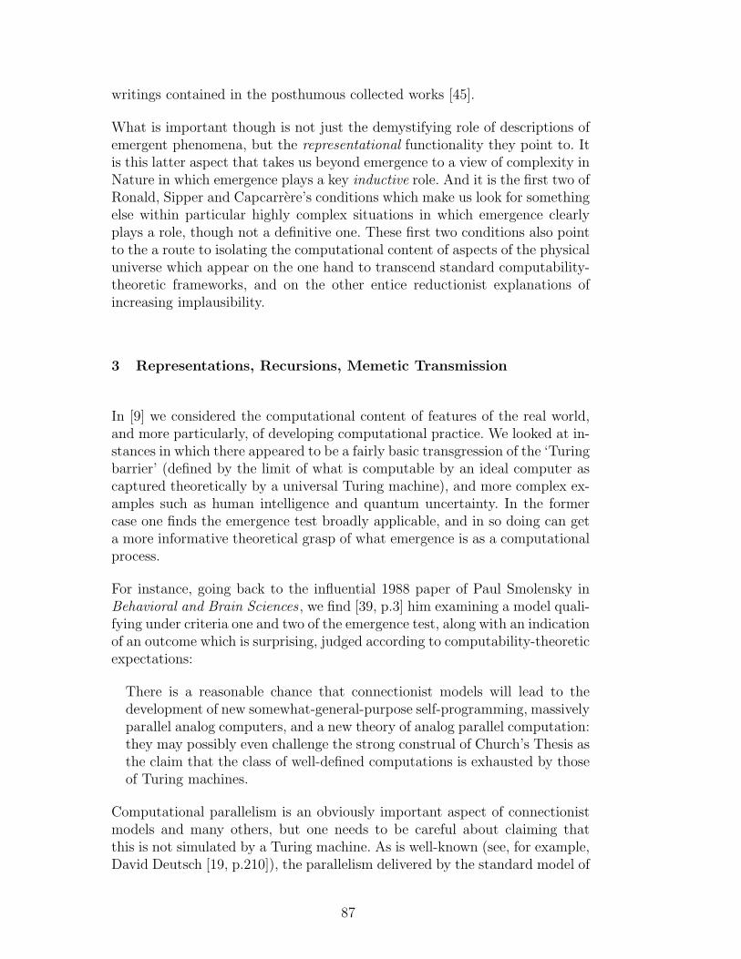
writings contained in the posthumous collected works [45].

What is important though is not just the demystifying role of descriptions ofemergent phenomena, but the representational functionality they point to. Itis this latter aspect that takes us beyond emergence to a view of complexity inNature in which emergence plays a key inductive role. And it is the first two ofRonald, Sipper and Capcarrere’s conditions which make us look for somethingelse within particular highly complex situations in which emergence clearlyplays a role, though not a definitive one. These first two conditions also pointto the a route to isolating the computational content of aspects of the physicaluniverse which appear on the one hand to transcend standard computability-theoretic frameworks, and on the other entice reductionist explanations ofincreasing implausibility.

3 Representations, Recursions, Memetic Transmission

In [9] we considered the computational content of features of the real world,and more particularly, of developing computational practice. We looked at in-stances in which there appeared to be a fairly basic transgression of the ‘Turingbarrier’ (defined by the limit of what is computable by an ideal computer ascaptured theoretically by a universal Turing machine), and more complex ex-amples such as human intelligence and quantum uncertainty. In the formercase one finds the emergence test broadly applicable, and in so doing can geta more informative theoretical grasp of what emergence is as a computationalprocess.

For instance, going back to the influential 1988 paper of Paul Smolensky inBehavioral and Brain Sciences , we find [39, p.3] him examining a model quali-fying under criteria one and two of the emergence test, along with an indicationof an outcome which is surprising, judged according to computability-theoreticexpectations:

There is a reasonable chance that connectionist models will lead to thedevelopment of new somewhat-general-purpose self-programming, massivelyparallel analog computers, and a new theory of analog parallel computation:they may possibly even challenge the strong construal of Church’s Thesis asthe claim that the class of well-defined computations is exhausted by thoseof Turing machines.

Computational parallelism is an obviously important aspect of connectionistmodels and many others, but one needs to be careful about claiming thatthis is not simulated by a Turing machine. As is well-known (see, for example,David Deutsch [19, p.210]), the parallelism delivered by the standard model of

87

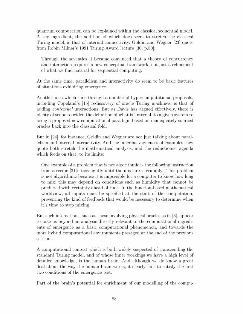
quantum computation can be explained within the classical sequential model.A key ingredient, the addition of which does seem to stretch the classicalTuring model, is that of internal connectivity. Goldin and Wegner [23] quotefrom Robin Milner’s 1991 Turing Award lecture [30, p.80]:

Through the seventies, I became convinced that a theory of concurrencyand interaction requires a new conceptual framework, not just a refinementof what we find natural for sequential computing.

At the same time, parallelism and interactivity do seem to be basic featuresof situations exhibiting emergence.

Another idea which runs through a number of hypercomputational proposals,including Copeland’s [15] rediscovery of oracle Turing machines, is that ofadding contextual interactions. But as Davis has argued effectively, there isplenty of scope to widen the definition of what is ‘internal’ to a given system tobring a proposed new computational paradigm based on inadequately sourcedoracles back into the classical fold.

But in [24], for instance, Goldin and Wegner are not just talking about paral-lelism and internal interactivity. And the inherent vagueness of examples theyquote both stretch the mathematical analysis, and the reductionist agendawhich feeds on that, to its limits:

One example of a problem that is not algorithmic is the following instructionfrom a recipe [31]: ‘toss lightly until the mixture is crumbly.’ This problemis not algorithmic because it is impossible for a computer to know how longto mix: this may depend on conditions such as humidity that cannot bepredicted with certainty ahead of time. In the function-based mathematicalworldview, all inputs must be specified at the start of the computation,preventing the kind of feedback that would be necessary to determine whenit’s time to stop mixing.

But such interactions, such as those involving physical oracles as in [3], appearto take us beyond an analysis directly relevant to the computational ingredi-ents of emergence as a basic computational phenomenon, and towards themore hybrid computational environments presaged at the end of the previoussection.

A computational context which is both widely suspected of transcending thestandard Turing model, and of whose inner workings we have a high level ofdetailed knowledge, is the human brain. And although we do know a greatdeal about the way the human brain works, it clearly fails to satisfy the firsttwo conditions of the emergence test.

Part of the brain’s potential for enrichment of our modelling of the compu-

88

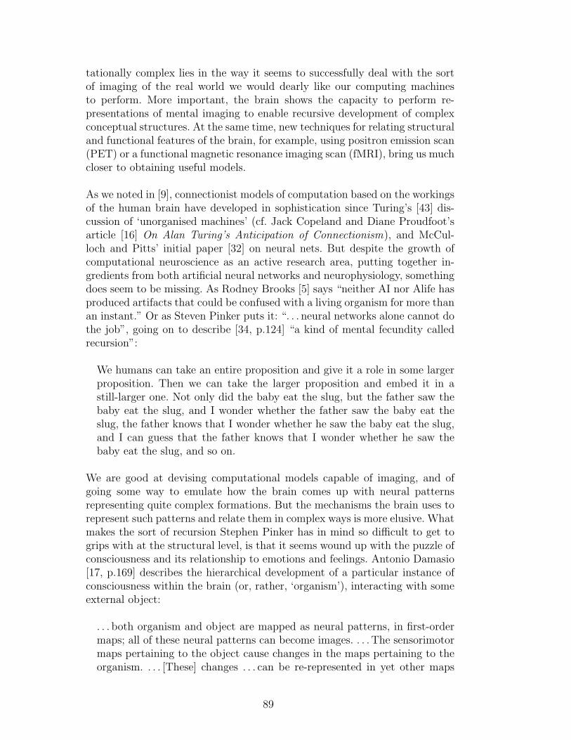
tationally complex lies in the way it seems to successfully deal with the sortof imaging of the real world we would dearly like our computing machinesto perform. More important, the brain shows the capacity to perform re-presentations of mental imaging to enable recursive development of complexconceptual structures. At the same time, new techniques for relating structuraland functional features of the brain, for example, using positron emission scan(PET) or a functional magnetic resonance imaging scan (fMRI), bring us muchcloser to obtaining useful models.

As we noted in [9], connectionist models of computation based on the workingsof the human brain have developed in sophistication since Turing’s [43] dis-cussion of ‘unorganised machines’ (cf. Jack Copeland and Diane Proudfoot’sarticle [16] On Alan Turing’s Anticipation of Connectionism), and McCul-loch and Pitts’ initial paper [32] on neural nets. But despite the growth ofcomputational neuroscience as an active research area, putting together in-gredients from both artificial neural networks and neurophysiology, somethingdoes seem to be missing. As Rodney Brooks [5] says “neither AI nor Alife hasproduced artifacts that could be confused with a living organism for more thanan instant.” Or as Steven Pinker puts it: “. . . neural networks alone cannot dothe job”, going on to describe [34, p.124] “a kind of mental fecundity calledrecursion”:

We humans can take an entire proposition and give it a role in some largerproposition. Then we can take the larger proposition and embed it in astill-larger one. Not only did the baby eat the slug, but the father saw thebaby eat the slug, and I wonder whether the father saw the baby eat theslug, the father knows that I wonder whether he saw the baby eat the slug,and I can guess that the father knows that I wonder whether he saw thebaby eat the slug, and so on.

We are good at devising computational models capable of imaging, and ofgoing some way to emulate how the brain comes up with neural patternsrepresenting quite complex formations. But the mechanisms the brain uses torepresent such patterns and relate them in complex ways is more elusive. Whatmakes the sort of recursion Stephen Pinker has in mind so difficult to get togrips with at the structural level, is that it seems wound up with the puzzle ofconsciousness and its relationship to emotions and feelings. Antonio Damasio[17, p.169] describes the hierarchical development of a particular instance ofconsciousness within the brain (or, rather, ‘organism’), interacting with someexternal object:

. . . both organism and object are mapped as neural patterns, in first-ordermaps; all of these neural patterns can become images. . . . The sensorimotormaps pertaining to the object cause changes in the maps pertaining to theorganism. . . . [These] changes . . . can be re-represented in yet other maps

89

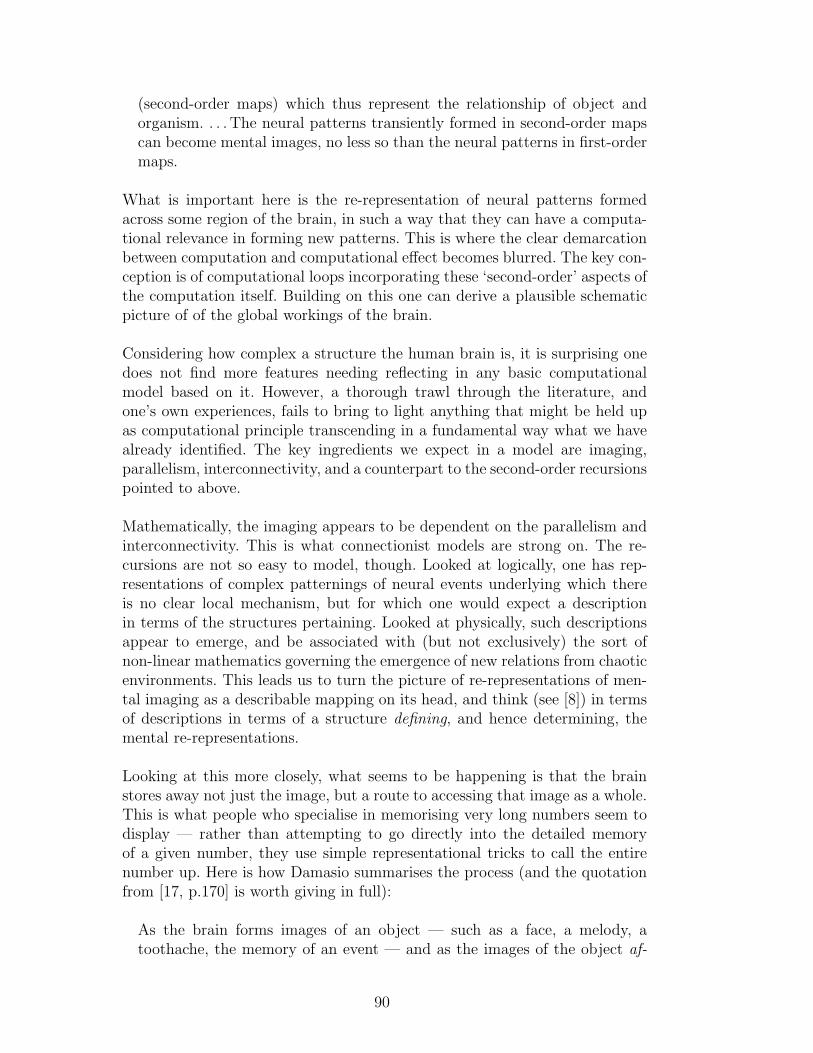
(second-order maps) which thus represent the relationship of object andorganism. . . . The neural patterns transiently formed in second-order mapscan become mental images, no less so than the neural patterns in first-ordermaps.

What is important here is the re-representation of neural patterns formedacross some region of the brain, in such a way that they can have a computa-tional relevance in forming new patterns. This is where the clear demarcationbetween computation and computational effect becomes blurred. The key con-ception is of computational loops incorporating these ‘second-order’ aspects ofthe computation itself. Building on this one can derive a plausible schematicpicture of of the global workings of the brain.

Considering how complex a structure the human brain is, it is surprising onedoes not find more features needing reflecting in any basic computationalmodel based on it. However, a thorough trawl through the literature, andone’s own experiences, fails to bring to light anything that might be held upas computational principle transcending in a fundamental way what we havealready identified. The key ingredients we expect in a model are imaging,parallelism, interconnectivity, and a counterpart to the second-order recursionspointed to above.

Mathematically, the imaging appears to be dependent on the parallelism andinterconnectivity. This is what connectionist models are strong on. The re-cursions are not so easy to model, though. Looked at logically, one has rep-resentations of complex patternings of neural events underlying which thereis no clear local mechanism, but for which one would expect a descriptionin terms of the structures pertaining. Looked at physically, such descriptionsappear to emerge, and be associated with (but not exclusively) the sort ofnon-linear mathematics governing the emergence of new relations from chaoticenvironments. This leads us to turn the picture of re-representations of men-tal imaging as a describable mapping on its head, and think (see [8]) in termsof descriptions in terms of a structure defining, and hence determining, themental re-representations.

Looking at this more closely, what seems to be happening is that the brainstores away not just the image, but a route to accessing that image as a whole.This is what people who specialise in memorising very long numbers seem todisplay — rather than attempting to go directly into the detailed memoryof a given number, they use simple representational tricks to call the entirenumber up. Here is how Damasio summarises the process (and the quotationfrom [17, p.170] is worth giving in full):

As the brain forms images of an object — such as a face, a melody, atoothache, the memory of an event — and as the images of the object af-

90

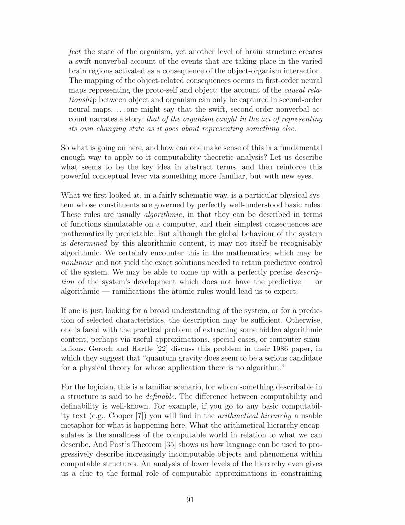
fect the state of the organism, yet another level of brain structure createsa swift nonverbal account of the events that are taking place in the variedbrain regions activated as a consequence of the object-organism interaction.The mapping of the object-related consequences occurs in first-order neuralmaps representing the proto-self and object; the account of the causal rela-tionship between object and organism can only be captured in second-orderneural maps. . . . one might say that the swift, second-order nonverbal ac-count narrates a story: that of the organism caught in the act of representingits own changing state as it goes about representing something else.

So what is going on here, and how can one make sense of this in a fundamentalenough way to apply to it computability-theoretic analysis? Let us describewhat seems to be the key idea in abstract terms, and then reinforce thispowerful conceptual lever via something more familiar, but with new eyes.

What we first looked at, in a fairly schematic way, is a particular physical sys-tem whose constituents are governed by perfectly well-understood basic rules.These rules are usually algorithmic, in that they can be described in termsof functions simulatable on a computer, and their simplest consequences aremathematically predictable. But although the global behaviour of the systemis determined by this algorithmic content, it may not itself be recognisablyalgorithmic. We certainly encounter this in the mathematics, which may benonlinear and not yield the exact solutions needed to retain predictive controlof the system. We may be able to come up with a perfectly precise descrip-tion of the system’s development which does not have the predictive — oralgorithmic — ramifications the atomic rules would lead us to expect.

If one is just looking for a broad understanding of the system, or for a predic-tion of selected characteristics, the description may be sufficient. Otherwise,one is faced with the practical problem of extracting some hidden algorithmiccontent, perhaps via useful approximations, special cases, or computer simu-lations. Geroch and Hartle [22] discuss this problem in their 1986 paper, inwhich they suggest that “quantum gravity does seem to be a serious candidatefor a physical theory for whose application there is no algorithm.”

For the logician, this is a familiar scenario, for whom something describable ina structure is said to be definable. The difference between computability anddefinability is well-known. For example, if you go to any basic computabil-ity text (e.g., Cooper [7]) you will find in the arithmetical hierarchy a usablemetaphor for what is happening here. What the arithmetical hierarchy encap-sulates is the smallness of the computable world in relation to what we candescribe. And Post’s Theorem [35] shows us how language can be used to pro-gressively describe increasingly incomputable objects and phenomena withincomputable structures. An analysis of lower levels of the hierarchy even givesus a clue to the formal role of computable approximations in constraining

91

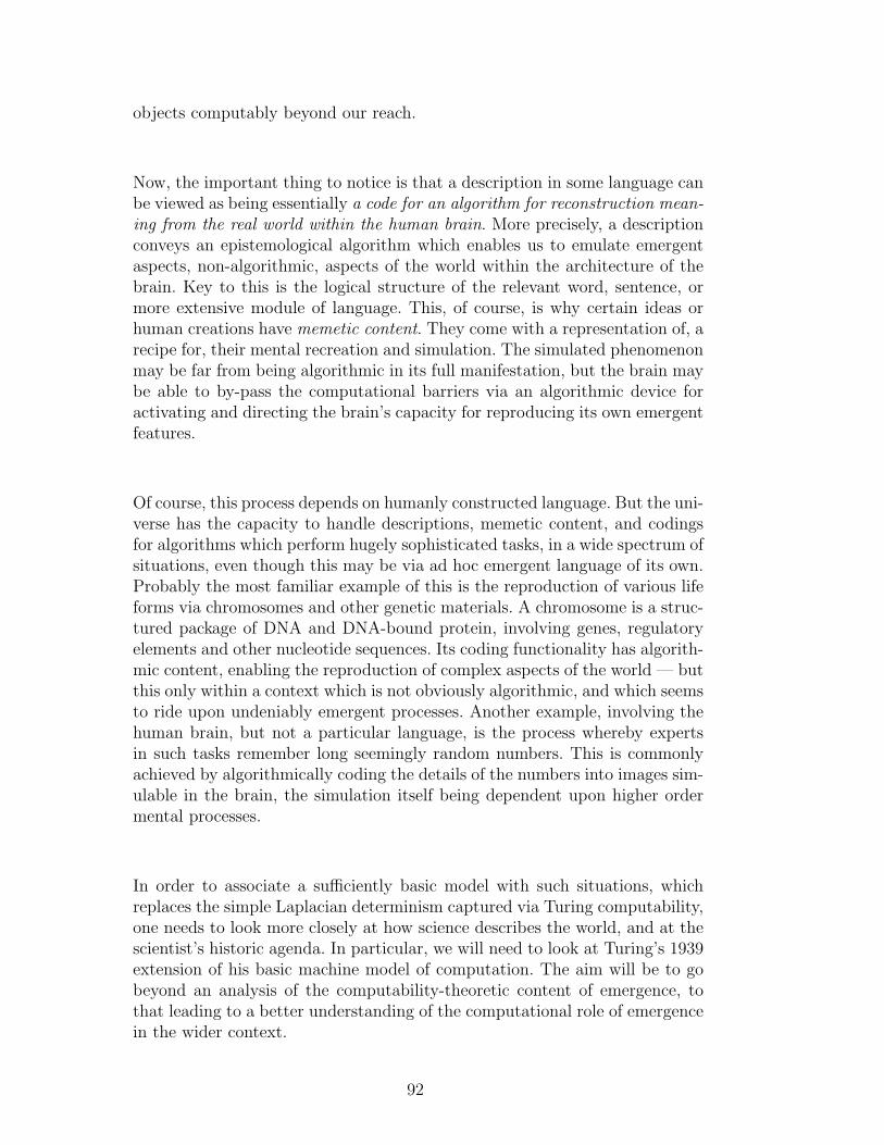
objects computably beyond our reach.

Now, the important thing to notice is that a description in some language canbe viewed as being essentially a code for an algorithm for reconstruction mean-ing from the real world within the human brain. More precisely, a descriptionconveys an epistemological algorithm which enables us to emulate emergentaspects, non-algorithmic, aspects of the world within the architecture of thebrain. Key to this is the logical structure of the relevant word, sentence, ormore extensive module of language. This, of course, is why certain ideas orhuman creations have memetic content. They come with a representation of, arecipe for, their mental recreation and simulation. The simulated phenomenonmay be far from being algorithmic in its full manifestation, but the brain maybe able to by-pass the computational barriers via an algorithmic device foractivating and directing the brain’s capacity for reproducing its own emergentfeatures.

Of course, this process depends on humanly constructed language. But the uni-verse has the capacity to handle descriptions, memetic content, and codingsfor algorithms which perform hugely sophisticated tasks, in a wide spectrum ofsituations, even though this may be via ad hoc emergent language of its own.Probably the most familiar example of this is the reproduction of various lifeforms via chromosomes and other genetic materials. A chromosome is a struc-tured package of DNA and DNA-bound protein, involving genes, regulatoryelements and other nucleotide sequences. Its coding functionality has algorith-mic content, enabling the reproduction of complex aspects of the world — butthis only within a context which is not obviously algorithmic, and which seemsto ride upon undeniably emergent processes. Another example, involving thehuman brain, but not a particular language, is the process whereby expertsin such tasks remember long seemingly random numbers. This is commonlyachieved by algorithmically coding the details of the numbers into images sim-ulable in the brain, the simulation itself being dependent upon higher ordermental processes.

In order to associate a sufficiently basic model with such situations, whichreplaces the simple Laplacian determinism captured via Turing computability,one needs to look more closely at how science describes the world, and at thescientist’s historic agenda. In particular, we will need to look at Turing’s 1939extension of his basic machine model of computation. The aim will be to gobeyond an analysis of the computability-theoretic content of emergence, tothat leading to a better understanding of the computational role of emergencein the wider context.

92

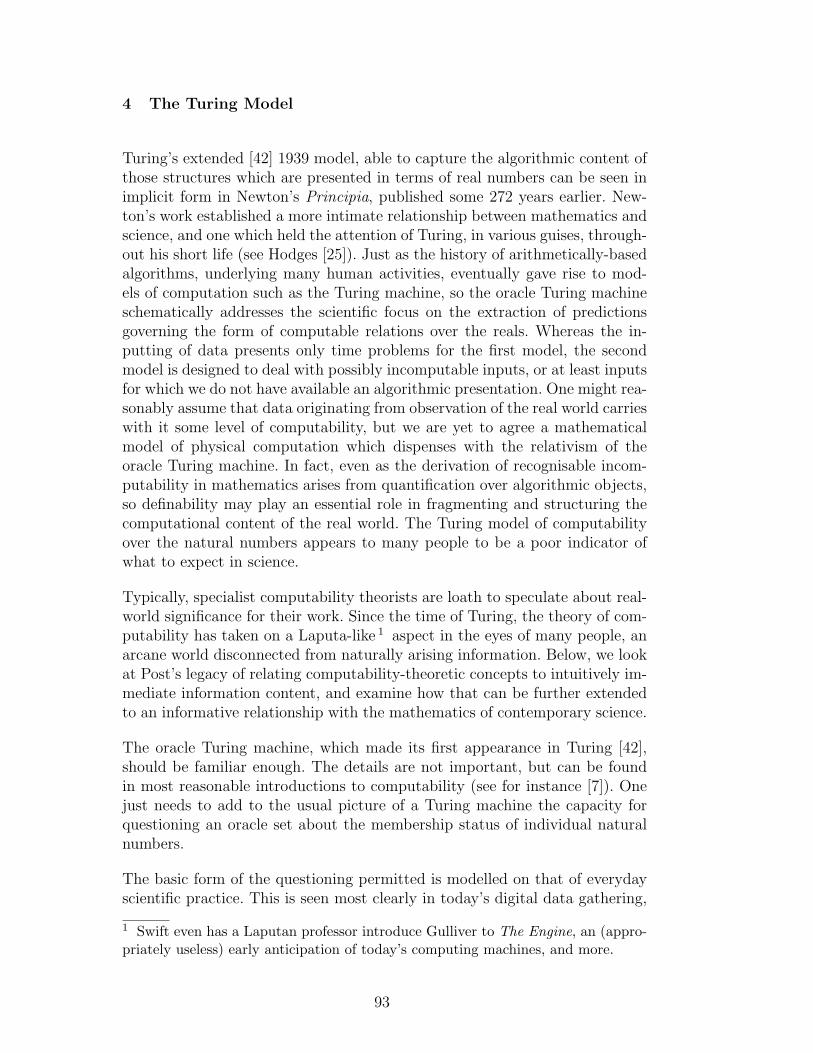
4 The Turing Model

Turing’s extended [42] 1939 model, able to capture the algorithmic content ofthose structures which are presented in terms of real numbers can be seen inimplicit form in Newton’s Principia, published some 272 years earlier. New-ton’s work established a more intimate relationship between mathematics andscience, and one which held the attention of Turing, in various guises, through-out his short life (see Hodges [25]). Just as the history of arithmetically-basedalgorithms, underlying many human activities, eventually gave rise to mod-els of computation such as the Turing machine, so the oracle Turing machineschematically addresses the scientific focus on the extraction of predictionsgoverning the form of computable relations over the reals. Whereas the in-putting of data presents only time problems for the first model, the secondmodel is designed to deal with possibly incomputable inputs, or at least inputsfor which we do not have available an algorithmic presentation. One might rea-sonably assume that data originating from observation of the real world carrieswith it some level of computability, but we are yet to agree a mathematicalmodel of physical computation which dispenses with the relativism of theoracle Turing machine. In fact, even as the derivation of recognisable incom-putability in mathematics arises from quantification over algorithmic objects,so definability may play an essential role in fragmenting and structuring thecomputational content of the real world. The Turing model of computabilityover the natural numbers appears to many people to be a poor indicator ofwhat to expect in science.

Typically, specialist computability theorists are loath to speculate about real-world significance for their work. Since the time of Turing, the theory of com-putability has taken on a Laputa-like 1 aspect in the eyes of many people, anarcane world disconnected from naturally arising information. Below, we lookat Post’s legacy of relating computability-theoretic concepts to intuitively im-mediate information content, and examine how that can be further extendedto an informative relationship with the mathematics of contemporary science.

The oracle Turing machine, which made its first appearance in Turing [42],should be familiar enough. The details are not important, but can be foundin most reasonable introductions to computability (see for instance [7]). Onejust needs to add to the usual picture of a Turing machine the capacity forquestioning an oracle set about the membership status of individual naturalnumbers.

The basic form of the questioning permitted is modelled on that of everydayscientific practice. This is seen most clearly in today’s digital data gathering,

1 Swift even has a Laputan professor introduce Gulliver to The Engine, an (appro-priately useless) early anticipation of today’s computing machines, and more.

93

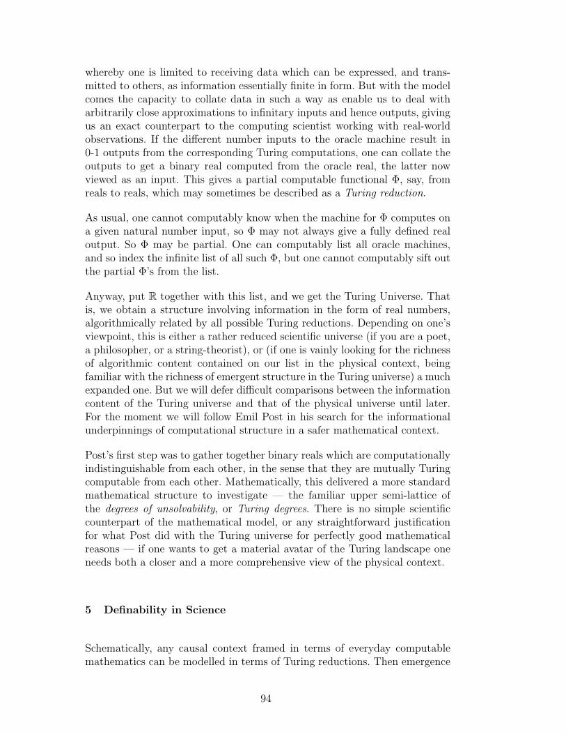
whereby one is limited to receiving data which can be expressed, and trans-mitted to others, as information essentially finite in form. But with the modelcomes the capacity to collate data in such a way as enable us to deal witharbitrarily close approximations to infinitary inputs and hence outputs, givingus an exact counterpart to the computing scientist working with real-worldobservations. If the different number inputs to the oracle machine result in0-1 outputs from the corresponding Turing computations, one can collate theoutputs to get a binary real computed from the oracle real, the latter nowviewed as an input. This gives a partial computable functional Φ, say, fromreals to reals, which may sometimes be described as a Turing reduction.

As usual, one cannot computably know when the machine for Φ computes ona given natural number input, so Φ may not always give a fully defined realoutput. So Φ may be partial. One can computably list all oracle machines,and so index the infinite list of all such Φ, but one cannot computably sift outthe partial Φ’s from the list.

Anyway, put R together with this list, and we get the Turing Universe. Thatis, we obtain a structure involving information in the form of real numbers,algorithmically related by all possible Turing reductions. Depending on one’sviewpoint, this is either a rather reduced scientific universe (if you are a poet,a philosopher, or a string-theorist), or (if one is vainly looking for the richnessof algorithmic content contained on our list in the physical context, beingfamiliar with the richness of emergent structure in the Turing universe) a muchexpanded one. But we will defer difficult comparisons between the informationcontent of the Turing universe and that of the physical universe until later.For the moment we will follow Emil Post in his search for the informationalunderpinnings of computational structure in a safer mathematical context.

Post’s first step was to gather together binary reals which are computationallyindistinguishable from each other, in the sense that they are mutually Turingcomputable from each other. Mathematically, this delivered a more standardmathematical structure to investigate — the familiar upper semi-lattice ofthe degrees of unsolvability, or Turing degrees. There is no simple scientificcounterpart of the mathematical model, or any straightforward justificationfor what Post did with the Turing universe for perfectly good mathematicalreasons — if one wants to get a material avatar of the Turing landscape oneneeds both a closer and a more comprehensive view of the physical context.

5 Definability in Science

Schematically, any causal context framed in terms of everyday computablemathematics can be modelled in terms of Turing reductions. Then emergence

94

can be formalised as definability over the appropriate substructure of the Tur-ing universe; or more generally, as invariance under automorphisms of theTuring universe. Simple and fundamental as the notion of definability is, andbasic as it is to everyday thought and discourse, as a concept it is not wellunderstood outside of logic. This is seen most strikingly in the physicists’apparent lack of awareness of the concept in interpreting the collapse of thewave function. Quantum decoherence and the many-worlds hypothesis com-prise a far more outlandish interpretive option than does speculating thatmeasurements, in enriching an environment, merely lead to an assertion ofdefinability. It appears a sign of desperation to protect consistent histories byinventing new universes, when the mathematics of our observable universesalready contains a straightforward explanation. We have argued (see for in-stance [13]) that many scientific puzzles can be explained in terms of failuresof definability in different contexts, and that the key task is to identify usefultheoretical models within which to investigate the nature of definability morefully. One of the most relevant of these models has to be that of Turing, basedas it is on a careful analysis of the characteristics of algorithmic computation.

This brings us to a well-known and challenging research programme, initiatedby Hartley Rogers in his 1967 paper [36], in which he drew attention to thefundamental problem of characterising the Turing invariant relations. Again,the intuition is that these are key to pinning down how basic laws and entitiesemerge as mathematical constraints on causal structure. It is important tonotice how the richness of Turing structure discovered so far becomes the rawmaterial for a multitude of non-trivially definable relations, matching in itscomplexity what we attempt to model.

Unfortunately, the current state of Rogers’ programme is not good. For anumber of years research in this area was dominated by a proposal originatingwith the Berkeley mathematician Leo Harrington, which can be (very) roughlystated:

Bi-interpretability Conjecture: The Turing definable relations are exactlythose with information content describable in second-order arithmetic.

Most importantly, bi-interpretability is not consistent with the existence ofnon-trivial Turing automorphisms. Despite decades of work by a number ofleaders in the field, the exact status of the conjecture is still a matter ofcontroversy.

For those of us who have grown up with Thomas Kuhn’s 1962 book [29] on thestructure of scientific revolutions, such difficulties and disagreements are notseen as primarily professional failures, or triggers to collective shame (althoughthey may be that too), but rather signs that something scientifically impor-tant is at stake. A far more public controversy currently shapes developments

95

around important issues affecting theoretical physics — see, for example therecent books of Lee Smolin [40] and Peter Woit [47].

This turns out to be very relevant to our theme of the importance of funda-mental notions, such as that of mathematical definability, to the formation ofbasic scientific theories. In this context, the specific focus on string theory ofthe above-mentioned books of Smolin and Woit is important, given that stringtheory was initially intended to remedy a number of inadequacies in currentscientific thinking, without really getting to grips with fundamental issues.Our argument is that string theory does very validly point towards a substitu-tion of abstract mathematics for inaccessible observational data. And that ithas produced some very beautiful and useful mathematics, and widened ourconceptual horizons in relation to models of the universe. But — that it hasfailed to enlist notions of global definability to pin down important elementsof the real world.

As Peter Woit [47, p.1] describes, according to purely pragmatic criteria par-ticle physics has produced a standard model which is remarkably successful,and has great predictive power:

By 1973, physicists had in place what was to become a fantastically suc-cessful theory of fundamental particles and their interactions, a theory thatwas soon to acquire the name of the standard model. Since that time, theoverwhelming triumph of the standard model has been matched by a sim-ilarly overwhelming failure to find any way to make further progress onfundamental questions.

The reasons why people are dissatisfied echo misgivings going back to Einsteinhimself [20, p.63]:

. . . I would like to state a theorem which at present can not be based uponanything more than upon a faith in the simplicity, i.e. intelligibility, of nature. . . nature is so constituted that it is possible logically to lay down suchstrongly determined laws that within these laws only rationally completelydetermined constants occur (not constants, therefore, whose numerical valuecould be changed without destroying the theory) . . .

If one really does have a satisfying description of how the universe is, it shouldnot contain arbitrary elements with no plausible explanation. In particular, atheory containing arbitrary constants, which one adjusts to fit the intendedinterpretation of the theory, is not complete. And as Woit observes:

One way of thinking about what is unsatisfactory about the standard modelis that it leaves seventeen non-trivial numbers still to be explained, . . .

At one time, it had been hoped that string theory would supply a sufficiently

96

fundamental framework to provide a much more coherent and comprehensivedescription, in which such arbitrary ingredients were properly pinned down.But despite its mathematical attractions, there are growing misgivings aboutits claimed status as “the only game in town” as a unifying explanatory theory.Here is how one time string theorist Daniel Friedan [21] combatively puts it:

The longstanding crisis of string theory is its complete failure to explain orpredict any large distance physics. . . . String theory is incapable of deter-mining the dimension, geometry, particle spectrum and coupling constantsof macroscopic spacetime. . . . The reliability of string theory cannot be eval-uated, much less established. String theory has no credibility as a candidatetheory of physics.

Smolin starts his book [40]:

From the beginning of physics, there have been those who imagined theywould be the last generation to face the unknown. Physics has always seemedto its practitioners to be almost complete. This complacency is shatteredonly during revolutions, when honest people are forced to admit that theydon’t know the basics.

He goes on to list what he calls the “five great [unsolved] problems in theo-retical physics”. Gathering these together, and slightly editing, they are [40,pp.5-16]:

1. Combine general relativity and quantum theory into a single theory thatcan claim to be the complete theory of nature.

2. Resolve the problems in the foundations of quantum mechanics.3. The unification of particles and forces problem: Determine whether or not

the various particles and forces can be unified in a theory that explainsthem all as manifestations of a single, fundamental entity.

4. Explain how the values of the free constants in the standard model ofphysics are chosen in nature.

5. Explain dark matter and dark energy. Or, if they do not exist, determinehow and why gravity is modified on large scales.

That each of these questions can be framed in terms of definability is notso surprising, since that is exactly how, essentially, they are approached byresearchers. The question is the extent to which progress is impeded by a lackof consciousness of this fact, and an imperfect grip of what is fundamental.Quoting Einstein again (from a letter to Robert Thornton, dated 7 December1944, Einstein Archive 61-754), this time on the relevance of a philosophicalapproach to physics:

So many people today – and even professional scientists – seem to me likesomeone has seen thousands of trees but has never seen a forest. A knowl-

97

edge of the historical and philosophical background gives that kind of in-dependence from prejudices of his generation from which most scientistsare suffering. This independence created by philosophical insight is – in myopinion – the mark of distinction between a mere artisan or specialist anda real seeker after truth.

Smolin’s comment [40, p.263] is in the same direction, though more specificallydirected at the string theorists:

The style of the string theory community . . . is a continuation of the cultureof elementary-particle theory. This has always been a more brash, aggres-sive, and competitive atmosphere, in which theorists vie to respond quicklyto new developments . . . and are distrustful of philosophical issues. Thisstyle supplanted the more reflective, philosophical style that characterizedEinstein and the inventors of quantum theory, and it triumphed as the cen-ter of science moved to America and the intellectual focus moved from theexploration of fundamental new theories to their application.

So what is it that is fundamental that is being missed? For Smolin [40, p.241],it is causality :

It is not only the case that the spacetime geometry determines what thecausal relations are. This can be turned around: Causal relations can deter-mine determine the spacetime geometry . . . Its easy to talk about space orspacetime emerging from something more fundamental, but those who havetried to develop the idea have found it difficult to realize in practice. . . . Wenow believe they failed because they ignored the role that causality playsin spacetime. These days, many of us working on quantum gravity believethat causality itself is fundamental – and is thus meaningful even at a levelwhere the notion of space has disappeared.

Citing Penrose as an early champion of the role of causality, he also mentionsRafael Sorkin, Fay Dowker, and Fotini Markopoulou, known in this context fortheir interesting work on causal sets (see [4]), which abstract from causalityrelevant aspects of its underlying ordering relation. Essentially, causal setsare partial orderings which are locally finite, providing a model of spacetimewith built-in discreteness. Despite the apparent simplicity of the mathematicalmodel, it has had striking success in approximating the known characteristicsof spacetime. An early prediction, in tune with observation, concerned thevalue of Einstein’s cosmological constant.

Of course, this preoccupation with causality might suggest to a logician a needto also look at its computational content. Smolin’s comment that “Causal re-lations can determine the spacetime geometry” touches on one of the biggestdisappointments with string theory, which turns out to be a ‘background de-pendant’ theory with a vengeance — one has literally thousands of candidate

98

Calabi-Yau spaces for shaping the extra dimensions of superstring theory. Incurrent superstring models, Calabi-Yau manifolds are those qualifying as pos-sible space formations for the six hidden spatial dimensions, their undetectedstatus explained by the assumption of their being smaller than currently ob-servable lengths.

Ideally, a truly fundamental mathematical model should be background inde-pendent, bringing with it a spacetime geometry arising from within.

6 The Emergence-Definability Symbiosis

There are obvious parallels between the Turing universe and the materialworld. Each of which in isolation, to those working with specific complexities,may seem superficial and unduly schematic. But the lessons of the historyof mathematics and its applications is that the simplest of abstractions canyield unexpectedly far-reaching and deep insights into the nature of the realworld. The main achievement of the Turing model, and its definable content,is to illuminate and structure the role of computability theoretic expressionsof emergence.

At the most basic level, science describes the world in terms of real numbers.This is not always immediately apparent, any more that the computer onones desk is obviously an avatar of a universal Turing machine. Nevertheless,scientific theories consist, in their essentials, of postulated relations upon reals.These reals are abstractions, and do not come necessarily with any recognisablemetric. They are used because they are the most advanced presentationaldevice we can practically work with. There is no faith that reality itself consistsof information presented in terms of reals. In fact, those of us who believe thatmathematics is indivisible, no less in its relevance to the material world, havea due humility about the capacity for our science to capture more than asurface description of reality.

Some scientists would take us in the other direction, and claim that the uni-verse is actually finite, or at least countably discrete. We have argued elsewhere(see for example [14]) that to most of us a universe without algorithmic contentis inconceivable. And that once one has swallowed that bitter pill, infinitaryobjects are not just a mathematical convenience (or inconvenience, dependingon one’s viewpoint), but become part of the mathematical mold on which theworld depends for its shape. As it is, we well know how essential algorithmiccontent is to our understanding of the world. The universe comes with recipesfor doing things. It is these recipes which generate the rich information contentwe observe, and it is reals which are the most capacious receptacles we canhumanly carry our information in, and practically unpack.

99

Globally, there are still many questions concerning the extent to which onecan extend the scientific perspective to a comprehensive presentation of theuniverse in terms of reals — the latter being just what we need to do in orderto model the immanent emergence of constants and natural laws from anentire universe. Of course, there are many examples of presentations entailedby scientific models of particular aspects of the real world. But given thefragmentation of science, is fairly clear that less natural presentations may wellhave an explanatory role, despite their lack of a role in practical computation.

The natural laws we observe are largely based on algorithmic relations be-tween reals. For instance, Newtonian laws of motion will computably predict,under reasonable assumptions, the state of two particles moving under gravityover different moments in time. And the character of the computation involvedcan be represented as a Turing functional over the reals representing differenttime-related two-particle states. One can point to physical transitions whichare not obviously algorithmic, but these will usually be composite processes,in which the underlying physical principles are understood, but the mathe-matics of their workings outstrip available analytical techniques. Over fortyyears ago, Georg Kreisel [27] distinguished between classical systems and co-operative phenomena not known to have Turing computable behaviour, andproposed [28, p.143, Note 2] a collision problem related to the 3-body problem,which might result in “an analog computation of a non-recursive function (byrepeating collision experiments sufficiently often)”. However, there is a qual-itatively different apparent breakdown in computability of natural laws atthe quantum level — the measurement problem challenges us to explain howcertain quantum mechanical probabilities are converted into a well-definedoutcome following a measurement. In the absence of a plausible explanation,one is denied a computable prediction. The physical significance of the Turingmodel depends upon its capacity for explaining what is happening here. If thephenomenon is not composite, it does need to be related in a clear way to aTuring universe designed to model computable causal structure. We will needto talk more about definability and invariance.

For the moment, let us think in terms of what an analysis of the automor-phisms of any sufficiently comprehensive, sufficiently fundamental, mathemat-ical model of the material universe might deliver.

Let us first look at the relationship between automorphisms and many-worlds.When one says “I tossed a coin and it came down heads, maybe that meansthere is a parallel universe where I tossed the coin and it came down tails”,one is actually predicating a large degree of correspondence between the twoparallel universes. The assumption that you exist in the two universes puts ahuge degree of constraint on the possible differences — but nevertheless, somerelatively minor aspect of our universe has been rearranged in the parallel one.There are then different ways of relating this to the mathematical concept of

100

an automorphism. One could say that the two parallel worlds are actuallyisomorphic, but that the structure was not able to define the outcome of thecoin toss. So it and its consequences appear differently in the two worlds. Orone could say that what has happened is that the worlds are not isomorphic,that actually we were able to change quite a lot, without the parallel universelooking very different, and that it was these fundamental but hidden differ-ences which forces the worlds to be separate and not superimposed, quantumfashion. The second view is more consistent with the view of quantum ambi-guity displaying a failure of definability. The suggestion here being that theobserved existence of a particle (or cat!) in two different states at the sametime merely exhibits an automorphism of our universe under which the clas-sical level is rigid (just as the Turing universe displays rigidity above 0′′) butunder which the sparseness of defining structure at the more basic quantumlevel enables the automorphism to re-represent our universe, with everythingat our level intact, but with the particle in simultaneously different statesdown at the quantum level. And since our classical world has no need to de-cohere these different possibilities into parallel universes, we live in a worldwith the automorphic versions superimposed. But when we make an observa-tion, we establish a link between the undefined state of the particle and theclassical level of reality, which destroys the relevance of the automorphism.To believe that we now get parallel universes in which the alternative statesare preserved, one now needs to decide how much else one is going to changeabout our universe to enable the state of the particle destroyed as a possiblityto survive in the parallel universe — and what weird and wonderful thingsone must accommodate in order to make that feasible. It is hard at this pointto discard the benefits brought by a little mathematical sophistication. Quan-tum ambiguity as a failure of definability is a far more palatable alternativethan the invention of new worlds of which we have no evidence or scientificunderstanding.

Another key conceptual element in the drawing together of a global picture ofour universe with a basic mathematical model is the correspondence betweenemergent phenomena and definable relations. This gives us a framework withinwhich to explain the particular forms of the physical constants and naturallaws familiar to us from the standard model science currently provides. Itgoes some way towards substantiating Penrose’s [33, pp106-107] ‘strong de-terminism’, according to which “all the complication, variety and apparentrandomness that we see all about us, as well as the precise physical laws, areall exact and unambiguous consequences of one single coherent mathematicalstructure” — and repairs the serious failure of the standard model pointed toby researchers such as Smolin and Woit. It also provides a hierarchical modelof the fragmentation of the scientific enterprise. This means that despite thecausal connections between say particle physics and the study of living organ-isms, the corresponding disciplines are based on quite different basic entitiesand natural laws, and there is no feasible and informative reduction of one

101

to another. The entities in one field may emerge through phase transitionscharacterised in terms of definable relations in the other, along with their dis-tinct causal structures. In this context, it may be that the answer to Smolin’sfirst ‘great unsolved problem in theoretical physics’ consists of an explanationof why there is no single theory (of the kind that makes useful predictions)combining general relativity and quantum theory.

For further discussion of such issues, see [6], [9], [10], [11], [13] and [14].

References

[1] I. Adler, D. Barab and R. V. Jean, A history of the study of phyllotaxis, Annalsof Botany, 80 (1997), 231–244.

[2] R. C. Arkin, Behaviour-Based Robotics, M.I.T. Press, Cambridge, MA, 1998.

[3] E. J. Beggs and J. V. Tucker, Experimental computation of real numbers byNewtonian machines, to appear in Proceedings of the Royal Society Series A.

[4] L. Bombelli, J. Lee, D. Meyer and R. D. Sorkin, Spacetime as a causal set,Phys. Rev. Lett. 59 (1987), 521–524.

[5] R. Brooks, The relationship between matter and life. Nature 409 (2001), 409–411.

[6] S. B. Cooper, Clockwork or Turing U/universe? - Remarks on causaldeterminism and computability, in Models and Computability (S. B. Cooperand J. K. Truss, eds.), London Mathematical Society Lecture Notes Series 259,Cambridge University Press, Cambridge, New York, Melbourne, 1999, pp.63–116.

[7] S. B. Cooper, Computability Theory, Chapman & Hall/CRC, Boca Raton,London, New York, Washington, D.C., 2004.

[8] S. B. Cooper, Computability and emergence. In Mathematical Problems fromApplied Logic. New Logics for the XXI-st Century II (eds. Gabbay D.,Goncharov S., Zakharyaschev M.) Kluwer/Springer International MathematicalSeries, Vol. 5, 2005.

[9] S. B. Cooper, Definability as hypercomputational effect, Applied Mathematicsand Computation, 178 (2006), 72–82.

[10] S. B. Cooper, How Can Nature Help Us Compute?, in SOFSEM 2006: Theoryand Practice of Computer Science - 32nd Conference on Current Trends inTheory and Practice of Computer Science, Merin, Czech Republic, January2006 (J. Wiedermann, J. Stuller, G. Tel, J. Pokorny, M. Bielikova, eds.),Springer Lecture Notes in Computer Science No. 3831, 2006, pp.1–13.

102

[11] S. B. Cooper, Computability and emergence, in Mathematical Problems fromApplied Logic I. Logics for the XXIst Century (D.M. Gabbay, S.S. Goncharov,M. Zakharyaschev, eds.), Springer International Mathematical Series, Vol. 4,2006, pp. 193–231.

[12] S. B. Cooper, The Incomputable Alan Turing, in the Proceedings ofAlan Mathison Turing 2004: A celebration of his life and achievements,Manchester University, 5 June, 2004 (Janet Delve and Jeff Paris,eds.), electronically published by the British Computer Society (2008):http://www.bcs.org/server.php?show=nav.9917.

[13] S. B. Cooper, Extending and interpreting Post’s Programme, to appear.

[14] S. B. Cooper and P. Odifreddi, Incomputability in Nature, in Computabilityand Models (S.B. Cooper and S.S. Goncharov, eds.), Kluwer Academic/Plenum,New York, Boston, Dordrecht, London, Moscow, 2003, pages 137–160.

[15] J. Copeland, Turing’s O-machines, Penrose, Searle, and the brain. Analysis, 58(1998), 128–38.

[16] J. Copeland and D. Proudfoot, On Alan Turing’s anticipation of connectionism.Synthese, 108 (1996), 361–377. Reprinted in Artificial Intelligence: CriticalConcepts in Cognitive Science (R. Chrisley, ed), Volume 2: Symbolic AI.Routledge, London, 2000.

[17] A. Damasio, The Feeling Of What Happens. Harcourt, Orlando, FL., 1999.

[18] M. Davis (Ed.), Solvability, Provability, Definability: The Collected Works ofEmil L. Post , Birkhauser, Boston, Basel, Berlin, 1994.

[19] Deutsch D. (1997) The Fabric of Reality. Penguin, London, New York.

[20] A. Einstein, Autobiographical Notes, in Albert Einstein: Philosopher-Scientist(P. Schilpp, ed.), Open Court Publishing, 1969.

[21] D. Friedan, A Tentative Theory of Large Distance Physics, J. High EnergyPhys. JHEP10 (2003) 063.

[22] R. Geroch and J. B. Hartle, Computability and physical theories, Foundationsof Physics 16 (1986), 533–550.

[23] D. Goldin and P. Wegner, Computation Beyond Turing Machines: seekingappropriate methods to model computing and human thought. Communicationsof the ACM 46 (2003), 100–102.

[24] D. Goldin and P. Wegner, The Church-Turing Thesis: Breaking the Myth, inCiE 2005: New Computational Paradigms: Papers presented at the conferencein Amsterdam, June 8–12, 2005 (Cooper S. B., Lowe B., Torenvliet L., eds.),Lecture Notes in Computer Science No. 3526, Springer-Verlag, 2005.

[25] A. Hodges, Alan Turing: The Enigma, Vintage, London, Melbourne,Johannesburg, 1992.

103

[26] S. A. Kauffman, Reinventing the Sacred: A New View of Science, Reason andReligion, Basic Books, New York, 2008.

[27] G. Kreisel, Mathematical logic: What has it done for the philosophy ofmathematics?, in Bertrand Russell, Philosopher of the Century (R. Schoenman,ed.), Allen and Unwin, London, 1967, pp. 201–272.

[28] G. Kreisel, Church’s Thesis: a kind of reducibility axiom for constructivemathematics, in Intuitionism and proof theory: Proceedings of the SummerConference at Buffalo N.Y. 1968 (A. Kino, J. Myhill and R.E. Vesley, eds.),North-Holland, Amsterdam, London, 1970, pp. 121–150.

[29] T. S. Kuhn, The Structure of Scientific Revolutions, Third edition 1996,University of Chicago Press, Chicago, London.

[30] R. Milner, Elements of interaction:Turing award lecture. Communications ofthe ACM 36 (1993), 78–89.

[31] D. Knuth, The Art of Computer Programming, Vol. 1: Fundamental Algorithms,Addison-Wesley, 1968.

[32] W. McCulloch and W. Pitts, A logical calculus of the ideas immanent in nervousactivity, Bull. Math. Biophys. 5 (2003), 115–133.

[33] R. Penrose, Quantum physics and conscious thought, in Quantum Implications:Essays in honour of David Bohm (BJ. Hiley and F.D. Peat, eds.), Routledge &Kegan Paul, London, New York, 1987, pp. 105–120.

[34] S. Pinker, How the Mind Works. W. W. Norton, New York, 1997.

[35] E. L. Post, Recursively enumerable sets of positive integers and their decisionproblems, Bulletin of the American Mathematical Society , 50 (1944), 284–316;reprinted in E. L. Post, Solvability, Provability, Definability: The CollectedWorks of Emil L. Post , pages 461–494.

[36] H. Rogers, Jr., Some problems of definability in recursive function theory,in Sets, Models and Recursion Theory (JNCrossley, ed), Proceedings of theSummer School in Mathematical Logic and Tenth Logic Colloquium, Leicester,August–September, 1965, North-Holland, Amsterdam, pp. 183–201.

[37] E. M. A. Ronald, M. Sipper and M. S. Capcarrere, Design, observation, surprise!A test of emergence, Artificial Life, 5 (1999), 225–239.

[38] D. Ruelle and F. Takens, On the nature of turbulence, Communications ofMathematical Physics, 20 (1971), 167–192.

[39] P. Smolensky, On the proper treatment of connectionism, Behavioral and BrainSciences 11 (1988), 1–74.

[40] L. Smolin, The Trouble With Physics: The Rise of String Theory, the Fall ofScience and What Comes Next, Allen Lane/Houghton Mifflin, London, NewYork, 2006.

104

[41] A. Turing, On computable numbers, with an application tothe Entscheidungsproblem, Proceedings of the London Mathematical Society ,Vol. 42, 1936–37, pages 230–265; reprinted in A. M. Turing, Collected Works:Mathematical Logic, pages 18–53.

[42] A. Turing, Systems of logic based on ordinals, Proceedings of the LondonMathematical Society , Vol. 45, 1939, pages 161–228; reprinted in A.M. Turing,Collected Works: Mathematical Logic, pages 81–148.

[43] A. M. Turing, Intelligent machinery. National Physical Laboratory Report,1948. In Machine Intelligence 5 (Meltzer B. and Michie D., eds.), EdinburghUniversity Press, Edinburgh, 1969, pp. 3–23. Reprinted in A. M. Turing,Collected Works: Mechanical Intelligence (Ince D. C., ed.), North-Holland,Amsterdam, New York, Oxford, Tokyo, 1992.

[44] A. M. Turing, The chemical basis of morphogenesis, Philosophical Transactionsof the Royal Society of London, B 237 (1952), 37–72; reprinted in A.M. Turing,Collected Works: Morphogenesis.

[45] A. M. Turing, Collected Works, Vol. 3: Morphogenesis (P. T. Saunders, Editor),Elsevier, Amsterdam, New York, Oxford, Tokyo, 1992.

[46] A. M. Turing, Collected Works: Mathematical Logic (R. O. Gandy and C. E.M. Yates, Editors), Elsevier, Amsterdam, New York, Oxford, Tokyo, 2001.

[47] P. Woit, Not Even Wrong: The Failure of String Theory and the ContinuingChallenge to Unify the Laws of Physics, Jonathan Cape, London, 2006.

105

How to build a hypercomputer

N. C. A. da Costa and F. A. Doria∗

Advanced Studies Research Group and Fuzzy Sets LaboratoryPIT, Production Engineering Program

COPPE, UFRJP.O. Box 68507

21945–972 Rio RJ Brazil.

[email protected]@gmail.com

[email protected]

Version 2.0July 9, 2008

Abstract

We claim that the theoretical hypercomputation problem has alreadybeen solved, and that what remains is an engineering problem. Wereview our construction of the Halting Function (the function thatsettles the Halting Problem) and then sketch possible blueprints foran actual hypercomputer.

1 Prologue

The authors have degrees in engineering. Engineers build things. So, thegoal of this paper is to sketch a series of steps at whose conclusion we wouldhave an actual, working hypercomputer.

Will it work? We leave that question unanswered. But, as we insist, weare cautiously optimistic that its answer may turn out to be a “yes.”

We take our cue from the following remark by Scarpellini [15] :∗The authors are partially funded by CNPq–Brazil, Philosophy Section. They also

acknowledge support from the Brazilian Academy of Philosophy.

106

In this connection one may ask whether it is possible to con-struct an analog–computer which is in a position to generatefunctions f(x) for which the predicate

∫f(x) cos(nx) dx > 0 is

not decidable while the machine itself decides by direct mea-surement whether

∫f(x) cos(nx) dx is greater than zero or not.

Such a machine is naturally only of theoretical interest, sincefaultless measuring is assumed, which requires the (absolute)validity of classical electrodynamics and probably such technicalpossibilities as the existence of innitely thin perfectly conduct-ing wires. All the same, the (theoretical) construction of such amachine would illustrate the possibility of non-recursive naturalprocesses.

(Scarpellini’s paper discusses among other results the decidability of suchpredicates.)

The hypercomputation problem

The hypercomputation problem splits into two questions:

1. The theoretical hypercomputation problem. Can we conceive a hyper-computer, given ideal operating conditions?

2. The practical hypercomputation problem. Given a positive answer tothe preceding question, can we build a concrete, working, hypercom-puter?

We argue here that the answer to the first question is a definite “yes,”if we accept that ideal analog machines fit into the requirements (“idealoperating conditions” — just take a look at Scarpellini’s papers [15, 16]).The second question boils down according to our viewpoint to an engineeringproblem; we may answer it with a “maybe,” or “we have to see.” Or, if wefollow the classical injunction: build a prototype!

Then we will see how it performs; which engineering problems must beovercome in order to have a decently working hypercomputer.

Structure of the paper

The paper is divided into two major sections. The first major section ex-plicitly constructs the Halting Function, that is, the function that settlesTuring’s Halting Problem. Of course that cannot be done within PeanoArithmetic, or with the help of partial recursive functions. But we can do

107

it if we extend the language of arithmetic in adequate ways, for there areinfinitely many explicit expressions for the Halting Function. (No extraor-dinary tools are required.)

The second major section sketches the construction of a hypercomputerin a series of steps. We discuss pros and cons; our conclusion is cautiouslyoptimistic — we believe that the gizmo can be made, and that somethinglike it will eventually be built in the near future.

Motivation

The ideas presented here were originally published in [3]. We were interestedin the decision problem for chaotic systems, which appeared to us as apossible example of an undecidable question with practical implications.

A suggestion by P. Suppes [18] led us to Richardson’s transforms [13],and out of those we obtained an explicit expression for the Halting Function(see the references; see also [4, 6] for a survey). It came as a surprise tous; we had long had the incorrect idea that none of the usual mathematicallanguages could explicitly contain an expression for the Halting Function,as it seemed to be something so deeply fundamental.

Then it was clear from start that we were dealing with a constructionthat had something to do with super–Turing machines [17]. However a moreexplicit presentation of our ideas on the matter of hypercomputation wasonly published in 1996 [5].

Style of the paper

Since most results in the present paper have already been discussed else-where, we have decided to argue in an informal, almost naıve way. We havealso added some redundancy to our presentation.

Informed readers will notice that we avoid a detailed characterization ofanalog computers. (We simply supposed that the functions we use in theconstruction of an expression for the Halting Function are computable.) Weare aware of the main theoretical contributions to the field, from Shannon toPour–El. However our starting point is Scarpellini’s remark quoted above:analog computers are usually seen as poor relatives of digital machines, asthey can only compute — in the sense of analog computation — a relativelysmall family of functions. Yet Scarpellini surprised everybody by showingthat ideal analog computers can decide undecidable predicates (with respectto some theory with a recursively enumerable set of theorems). So, they aredefinitely very powerful in an unique way, even if in an idealized domain.

108

2 Hypercomputation theory

(We stress that this is just an informal sketch.) If we define a hypercomputerto be a machine that can generate, or decide, all arithmetical truths, thenvery little is required to build a theory that fits the requirement, namely,Peano Arithmetic (PA) plus Shoenfield’s version of the ω–rule is enough (fora nice presentation of Shoenfield’s rule see [10]).

PA plus Shoenfield’s rule proves all true arithmetic sentences, that is,those that hold of the standard model. The hypercomputation theory wesketched in [5] does so. The idea is: we start from Turing machine theory.We then add to it an expression for the function that settles the HaltingProblem, and postulate it to be (hyper)computable. The jump [14] allows usto decide arithmetic degrees beyond 0 [4, 5]. Given a solution for the HaltingProblem, and given the jump, we can decide any arithmetical sentence in afinite number of steps.

We have also mentioned that a “geometrical principle” implies hyper-computation [5]:

We can always decide whether two smooth curves in the interiorof a rectangle in the plane intersect.

That “geometrical principle” has an advantage and a disadvantage. Theadvantage: it is easy to understand — actually a stricter version of it isenough, but the general version stated above is more synthetic. The dis-advantage: we must show how to translate that principle, which deals withsmooth, continuous geometrical objects, into the discrete objects that arein the domain of arithmetic. The trick is done through Richardson’s trans-forms, soon to be introduced.

So we take:

Definition 2.1 A hypercomputer is a theoretical device that settles at leastthe Halting Problem.

Follows by our constructions (see the references) that such a device canbe extended to another device that settles all arithmetical truths along thestandard model.

3 From Richardson’s transforms to the HaltingFunction

The present section is based on [1]; for the proofs see [13]. Our presentationsplits into several topics:

109

• Formalized arithmetic and Turing machines.

• Richardson’s maps.

• The Halting Function in formal languages that extend arithmetic.

We refer to [12] for notation and requirements from logic. We use: ¬,“not,” ∨, “or,” ∧, “and,” →, “if... then...,” ↔, “if and only if,” ∃x, “thereis a x,” ∀x, “for every x.” P (x) is a formula with x free; it roughly means“x has property P .” Finally T ` ξ means T proves ξ, or ξ is a theorem ofT . ω is the set of natural numbers, ω = 0, 1, 2, . . ..

Algorithmic functions are given by their programs coded in Godel num-bers e [14]. We will sometimes use Turing machines (noted by sans–serifletters with the Godel number as index Me) or partial recursive functions,noted e.

We start from a very simple theory of arithmetic, noted A1. Its languageincludes variables x, y, . . ., two constants, 0 and 1, the equality sign =, andtwo operation signs, +,×. Basically A1 has axioms for the operations +and ×, the behavior of constants 0 and 1, and the trichotomy axiom, thatis, given two natural numbers x and y, either x < y or x = y or x > y. A1contains no induction axiom.

The standard interpretation for A1 is: the variables x, y, . . . range overthe natural numbers, and 0 and 1 are seen as, respectively, zero and one.The only requirement we impose on A1 is: that theory should be strongenough to formally include all of Turing machine theory. Recall that aTuring machine is given by its Godel number, which recursively codes themachine’s program. Rigorously, for A1, we must have:

Definition 3.1 A Turing machine of Godel number e operating on x withoutput y, e(x) = y is representable in theory A1 if there is a formulaFe(x, y) in the language of A1 so that:

1. A1 ` Fe(x, y) ∧ Fe(x, z)→ [y = z], and

2. For natural numbers a, b, if e(a) = b, then A1 ` Fe(a, b).

Then we have the representation theorem for partial recursive functions inA1:

Proposition 3.2 Every Turing machine is representable in A1. Moreoverthere is an effective procedure that allows us to obtain Fe from the Godelnumber e.

110

We restrict here our interest to theories that are arithmetically sound,that is, which have a model with standard arithmetic for its arithmeticalsegment.

Richardson’s map

We now describe the Richardson transforms [6, 13]. We start from a strength-ening of Proposition 3.2:

Proposition 3.3 If e(a) = b, for natural numbers a, b, then we can al-gorithmically construct a polynomial pe over the natural numbers so that[e(a) = b]↔ [∃x1, x2, . . . , xk ∈ ω pe(a, b, x1, x2, . . . , xk) = 0].

Follows:

Proposition 3.4 a ∈ Re, where Re is a recursively enumerable set, if andonly if there are e and p so that ∃x1, x2, . . . , xk ∈ ω [pe(a, x1, x2, . . . , xk) = 0].

Richardson’s map [6, 13] allows us to obtain in an algorithmic way, givenany such pe(a, . . .), a real–defined and real–valued function fe(a, . . .) that hasroots if and only if pe(a, . . .) has roots as a Diophantine equation.

Richardson’s map: multidimensional version

We can be more specific: let A be the algebra of subelementary functions(polynomials over the reals, sines, cosines; everything closed under +,−,products by real numbers and by the functions that generate the algebra,to which we add function composition). Let R denote the real line.

(We do not require the exponential function in our constructions.)We now state the first of Richardson’s main results: given that A1 ⊂

ZFC, and if P is the set of all finite–lenght polynomials over ω:

Proposition 3.5 (Richardson’s Map, I) There is an injection κP : P →A, where P denotes the algebra of ω–valued polynomials in a finite numberof variables, and A is the algebra of subelementary functions described above,such that:

1. κP is constructive, that is, given the expression for p in A1, there is aneffective procedure so that we can obtain the corresponding expressionfor F = κP(p) in ZFC.

111

2. κP is 1–1.

3. For x = (x1, . . . , xn), ∃x ∈ ωn p(m,x) = 0 if and only if ∃x ∈Rn F (m,x) = 0 if and only if ∃x ∈ Rn F (m,x) ≤ 1, for p ∈ Pand F ∈ A.

4. The injection κP is proper.

The crucial property is given in step 3.: it allows us to translate theexistence of roots for Diophantine equations into roots of the correspondingtransformed real–defined and real–valued function, with some extras.

Next step gives us a 1–dimensional version of Richardson’s map.

Richardson’s map: one–dimensional version

Corollary 3.6 (Richardson’s Map, II) Let A1 be the algebra of subele-mentary functions over a single real variable x. Then there is a map κ′ :P → A1 such that:

1. κ′ is constructive.

2. κ′ is 1–1.

3. The inclusion κ′(P) ⊂ A1 is proper.

4. ∃x ∈ ωn p(m,x) = 0 if and only if ∃x ∈ R L(m,x) = 0 if and onlyif ∃x ∈ R G(m,x) ≤ 1, for adequate L,G, whose expressions can beexplicitly exhibited.

The Halting Function

The main result in Alan Turing’s remarkable 1937 paper, “On computablenumbers, with an application to the Entscheidungsproblem” [19], is a proofof the algorithmic unsolvability of a version of the halting problem: givenan arbitrary Turing machine of Godel number e, for input x, there is no al-gorithm that decides whether e(x) stops and outputs something, or entersan infinite loop.

Remark 3.7 Let Mm(a) ↓ mean: “Turing machine of Godel number mstops over input a and gives some output.” Similarly Mm(a) ↑ means, “Tur-ing machine of Godel number m enters an infinite loop over input a.” Thenwe can define the halting function θ:

112

• θ(m, a) = 1 if and only if Mm(a) ↓.

• θ(m, a) = 0 if and only if Mm(a) ↑.

θ(m, a) is the halting function for Mm over input a.

θ isn’t algorithmic, of course [14, 19], that is, there is no Turing machinethat computes it.

Remark 3.8 As we now show, we can explicitly write an expression for afunction in the language of classical analysis that settles the halting problem.We proceed as follows:

• Given Turing machine Mm(a) = b, for natural numbers a, b, we canalgorithmically obtain a polynomial pm(〈a, b〉, x1, . . . , xk) so that:

Mm(a) = b↔ ∃x1, . . . , x2 ∈ ω [pm(〈a, b〉, x1, . . . , xk) = 0].

• Given Fm, real–defined and real–valued, we have that:

∃x1, . . . , x2 ∈ ω [pm(〈a, b〉, x1, . . . , xk) = 0]↔

↔ ∃x1, . . . , xk ∈ RFm(〈a, b〉, x1, . . . , xk) ≤ 1.

and∀x1, . . . , x2 ∈ ω [pm(〈a, b〉, x1, . . . , xk) 6= 0]↔

↔ ∀x1, . . . , xk ∈ RFm(〈a, b〉, x1, . . . , xk) > 1.

• That is to say: Mm(a) ↓ if and only if Fm(a, . . .) goes below 1, andMm(a) ↑ if and only if Fm(a, . . .) stays above 1.

This is the property we use in order to construct the halting functionθm.

We now need the concept of an universal Diophantine polynomial. MartinDavis [7] describes an algorithmic procedure out of which, given a Turingmachine with input a Mm(a), we obtain a polynomial pm(a, x1, . . .) so thatit has roots if and only if Mm(a) converges (outputs some result). Now, ifU(m, a) is an universal Turing machine [14, 19], we can similarly obtain apolynomial p(〈m, a〉, . . .) which stands for pm(a, . . .).

113

More precisely, if [∃x1, . . . , xk pm(〈a, b〉, x1, . . . , xk) = 0] ↔ [Mm(a) = b],then, for the universal polynomial p(〈m, a, b〉, . . .):

[∃x1, . . . , xr p(〈m, a, b〉, x1, . . . , xr) = 0]↔

↔ [∃x1, . . . , xk pm(〈a, b〉, x1, . . . , xk) = 0].

From the preceding considerations, if σ is the sign function, σ(±x) = ±1and σ(0) = 0:

Proposition 3.9 (The Halting Function.) The Halting Function θ(n, q)is explicitly given by:

θ(n, q) = σ(Gn,q),

Gn,q =∫ +∞

−∞Cn,q(x)e−x

2dx,

Cm,q(x) = |Fm,q(x)− 1| − (Fm,q(x)− 1).

Fn,q(x) = κP pn,q.

Here pn,q is the two–parameter universal Diophantine polynomial

p(〈n, q〉, x1, x2, . . . , xr)

and κP is as in Proposition 3.5.There are infinitely many alternative explicit expressions for the halting

function θ [6].

Remark 3.10 We do not require Richardson’s transform to obtain an ex-pression for the Halting Function. There is also an expression for the HaltingFunction even within a simple extension of A1. Let p(n,x) be a 1–parameteruniversal polynomial; x abbreviates x1, . . . , xp. Then either p2(n,x) ≥ 1,for all x ∈ ωp, or there are x in ωp such that p2(n,x) = 0 sometimes. Asσ(x) when restricted to ω is primitive recursive, we may define a functionψ(n,x) = 1− σp2(n,x) such that:

• Either for all x ∈ ωp, ψ(n,x) = 0;

• Or there are x ∈ ωp so that ψ(n,x) = 1 sometimes.

Thus the halting function can be represented as:

θ(n) = σ[∑τq(x)

ψ(n,x)τ q(x)!

],

where τ q(x) denotes the positive integer given out of x by the pairing func-tion τ : if τ q maps q–tuples of positive integers onto single positive integers,τ q+1 = τ(x, τ q(x)). Recall that the infinite sum can be given by a simpleiterative definition.

114

4 How to build a hypercomputer

There are two ways we can attack the question. The first one is based onthe previous construction of the Halting Function. The second one is basedon an alternative, well established technique.

First notice the following:

The Halting Problem is: given an arbitrary Turing machine eand an arbitrary input n, can we check whether e(n) stops?

Now pick up some e, n and keep it fixed. As it will turn out, there isan algorithmic procedure (sketched below) that allows us to check whethere(n) stops or not. (There is a price to pay; it may be of high complexity,but we can leave that difficulty aside for the moment). Difficulties appearwhen we go from this particular instance to a construction that encompassesall instances, that is, when we add the universal quantifier.

We will now consider two possibilities for a hypercomputer.

Our proposal for a hypercomputer

The present construction is based on the following result by Richardson[2, 13, 15, 16]:

Remark 4.1

• Given Turing machine Mm(a) = b, for natural numbers a, b, we canalgorithmically obtain a polynomial pm(〈a, b〉, x1, . . . , xk) so that:

Mm(a) = b↔ ∃x1, . . . , x2 ∈ ω [pm(〈a, b〉, x1, . . . , xk) = 0].

• Recall that we can construct an expression for a Fm, real–defined andreal–valued, so that:

∃x1, . . . , x2 ∈ ω [pm(〈a, b〉, x1, . . . , xk) = 0]↔

↔ ∃x1, . . . , xk ∈ RFm(〈a, b〉, x1, . . . , xk) ≤ 1.

and∀x1, . . . , x2 ∈ ω [pm(〈a, b〉, x1, . . . , xk) 6= 0]↔

↔ ∀x1, . . . , xk ∈ RFm(〈a, b〉, x1, . . . , xk) > 1.

• In a more figurative way: Mm(a) ↓ (converges) if and only if Fm(a, . . .)dives below 1, and Mm(a) ↑ (diverges, enters an infinite loop) if andonly if Fm(a, . . .) stays above 1.

115

(See Remark 3.8.) So, machine e stops over input n if Richardson’stransform F(e,n) of the corresponding Diophantine polynomial p(〈e, n〉, . . .)dives below 0; otherwise it stays above 1. Of course we can modify thecorresponding Richardson transform in such a way that the “signaling gap”from 0 to 1 is widened to an arbitrary k.

Now consider the following analog machine:

• First compactify F by some simple elementary–function map, over thesemi–open interval [0,K), that is to say, map [0,∞) over [0,K) andcarry F over. We will note F ′ the compactified version of function F .

• Given each pair (e, n), F ′(e,n) is built out of elementary functions plusπ.

• So there is an ideal analog computer that computes it.

• Notice that the values (e, n) can be easily coded as parameters in ouranalog machine.

• So, build it.

By the preceding considerations, it is our belief that the theoretical hy-percomputation problem has already been settled. The realistic hypercom-putation problem is another matter, but is a problem that belongs to therealm of engineering.

We see three main difficulties (there may be others) in the actual con-struction of a hypercomputer if we follow the preceding steps:

• The construction of π. How are we going to insert π as a parameterin our machine? We have considered the possibility that π should bederived out of a geometrical, graphical construction.

• Overshoot problems. This is another difficulty to be considered. Thecompactification procedure may lead to irregular, out–of–control be-havior when one goes to the (compactified) infinite point.

• The size of e and n. For actual computers e and n may be very large,and coding them into an analog computer may be quite difficult.

We do not consider the usual objection that says, the world is ruledby quantum mechanics, and is therefore discrete, so any analog, continuousconstruction will end up by being impossible. We suggest reading on thata brilliant, half–forgotten text, Havemann’s essay of the discrete and thecontinuous [11].

116

Turing–Fefermann hypercomputer

The main reason why the authors have always believed that someday some-one will build a hypercomputer stems from the following fact: given oneinstance, or a finite but arbitrary number of instances of the Halting Prob-lem, we can always algorithmically decide them. Here it goes why it isso.

• Each instance of the Halting Problem (if it fails to stop over an input)is arithmetically equivalent to a Π1 sentence,

∀x1, x2, . . . , p(〈m,n〉x1, x2, . . .) 6= 0.

(Here m is the machine, and n is the input we wish to test.)

• Then we know [9, 10, 20] that there will be some theory Tk in theTuring–Fefermann hierarchy, T0 = PA, T1 = PA + Consis PA, . . . ,that will prove such a Π1 sentence, if it is true. On the other hand, wecan recursively test for its negation, ∃x1, x2, . . . , p(. . .) = 0. Thereforewe can build a recursive procedure in order to decide whether m(n)stops or not.

• We thus generate two listings of results.

• List A: we test p(〈m,n〉, x1, x2, . . .) for each n–tuple x1, x2, . . . in orderto check whether some n–tuple is such that p(〈m,n〉, . . .) = 0.

If it does, the procedure stops, and we learn that m(n) stops.

• List B: we go by dovetailing, and generate all theorems for T0, T1, T2,in the Turing–Fefermann hierarchy.

If ∀x1, . . . p(〈m,n〉, x1, . . .) 6= 0 appears among the theorems in thatlisting, we stop the procedure.

There is a catch: procedure B is extremely costly in computational terms(procedure A may also be very costly). However we may use — we expect— our analog machine to speed it up. Anyway, the point is: finite arbi-trary instances of the Halting Problem are always algorithmically decidable.(Franzen’s objections [10] do not apply precisely because of that: we onlyhave to check a finite number of instances of the Halting Problem, in actualsituations.)

Remark 4.2 An important point: we cannot formally “put together” allsuch procedures that settle particular instances of the Halting Problem and

117

obtain a theory with a recursively enumerable set of theorems that settlesall instances of the Halting Problem, as that theory would then violate theGodel incompleteness theorems. In fact, it can be shown that such a theoryimplies Shoenfield’s ω–rule, and PA plus Shoenfield’s rule is a theory witha nonrecursively enumerable set of theorems.

More precisely: no extension of arithmetic with a recursively enumerableset of theorems can prove that the algorithm sketched above delivers what itpromises.

5 Conclusion

We rest our case. To stress the point:

• We believe that the theoretical hypercomputation problem is solved.We can — ideally — build an analog machine that settles arbitraryinstances of the Halting Problem.

• The actual construction of such a machine isn’t a mathematical prob-lem anymore; it is an engineering problem. One has to build a proto-type and see which problems will eventually come up.

If one settles arbitrary instances of the Halting Problem, we may nowconceive a machine that decides sentences along the arithmetical hierarchy[4, 6]. The implications are obvious, and we will not comment on them.

The proof of the pudding is on the eating: next step is to build a proto-type.

We thus rest our case.

6 Acknowledgments

The authors wish to thank Professors C. Calude and J. F. Costa who kindlyinvited them to present this paper at the Vienna workshop on Unusual Mod-els of Computation, August 2008. They also wish to thank two anonymousreferees for their comments and criticisms.

The ongoing research program that led to this text has been sponsored bythe Advanced Studies Group, Production Engineering Program, COPPE–UFRJ, Rio, Brazil. The authors also wish to thank the Institute for Ad-vanced Studies at the University of Sao Paulo for support of this researchproject; we wish to acknowledge support from the Brazilian Academy ofPhilosophy and its chairman Professor J. R. Moderno. Finally FAD wishes

118

to thank Professors R. Bartholo, C. A. Cosenza and S. Fuchs for their invi-tation to join the Fuzzy Sets Lab at COPPE–UFRJ and the Philosophy ofScience Program at the same institution.

The authors acknowledge partial support from CNPq, Philosophy Sec-tion.

References

[1] R. Bartholo, C. A. Cosenza, F. A. Doria, C. Lessa, “Can economicsystems be seen as computing machines?” J. Economic Behavior andOrganization, to appear (2009).

[2] B. J. Copeland and R. Sylvan, “Beyond the universal Turing machine,”Austral. J. Philosophy 77, 46–67 (1999).

[3] N. C. A. da Costa and F. A. Doria, “Undecidability and incompletenessin classical mechanics,” Int. J. Theor. Phys. 30, 1041–1073 (1991).

[4] N. C. A. da Costa and F. A. Doria, “Suppes predicates and the con-struction of unsolvable Problems in the axiomatized sciences,” in P.Humphreys, ed., Patrick Suppes, Scientific Philosopher, II, 151–191Kluwer (1994).

[5] N. C. A. da Costa and F. A. Doria, “Variations on an original theme,”in J. Casti and A. Karlqvist, Boundaries and Barriers, Addison–Wesley(1996).

[6] N. C. A. da Costa and F. A. Doria, “Computing the future,” in K.Vela Velupillai, ed., Computability, Complexity and Constructivity inEconomic Analysis, Blackwell (2005).

[7] M. Davis, “Hilbert’s Tenth Problem is unsolvable,” Amer. Math.Monthly 80, 233 (1973).

[8] F. A. Doria, “Informal vs. formal mathematics,” Synthese 154, 401–415(2007).

[9] S. Feferman, “Transfinite recursive progressions of axiomatic theories,”J. Symbolic Logic 27, 259 (1962).

[10] T. Franzen, “Transfinite progressions: a second look at completeness,”Bull. Symbolic Logic 10, 367-389 (2004).

119

[11] R. Havemann, Dialektik ohne Dogma ?, Rowohlt (1964).

[12] E. Mendelson, Introduction to Mathematical Logic, 4th ed., Chapman& Hall (1997).

[13] D. Richardson, “Some undecidable problems involving elementary func-tions of a real variable,” J. Symbol. Logic 33, 514 (1968).

[14] H. Rogers Jr., Theory of Recursive Functions and Effective Computabil-ity, John Wiley (1967).

[15] B. Scarpellini, “Two undecidable problems of analysis,” Minds and Ma-chines 13, 49–77 (2003).

[16] B. Scarpellini, “Comments to ‘Two undecidable problems of analysis,”’Minds and Machines 13, 79–85 (2003).

[17] I. Stewart, “Deciding the undecidable,” Nature 352, 664–665 (1991).

[18] P. Suppes, personal communication (1990).

[19] A. M. Turing, “On computable numbers, with an application to theEntscheidungsproblem,” Proc. London Math. Society 50, 230 (1937).

[20] A. M. Turing, “Systems of logic based on ordinals,” Proc. London Math.Society, Ser. 2 45, 161 (1939).

120

What is a universal computing machine?

Jean-Charles Delvenne

Universite Catholique de Louvain,Department of Mathematical Engineering,

Avenue Georges Lemaıtre 4, B-1348 Louvain-la-Neuve, Belgium

Abstract

A computer is classically formalised as a universal Turing machine or a similar de-vice. However over the years a lot of research has focused on the computational prop-erties of dynamical systems other than Turing machines, such cellular automata,artificial neural networks, mirrors systems, etc.

In this paper we propose a unifying formalism derived from a generalisation ofTuring’s arguments. Then we review some of universal systems proposed in the lit-erature and show that are particular case of this formalism. Finally, we review someof the attempts to understand the relation between dynamical and computationalproperties of a system.

Key words: Turing universality, dynamical systems

1 Introduction

We are interested in computing machines, which we informally define as ma-chines able to solve decision problems on integers (or finite objects that can beencoded as integers), such as, for instance, primality. We are especially inter-ested in universal computing machines, i.e., those who have the same poweras a universal Turing machine.

Note that in this article we are only interested in solving decision problemson integers, while computable analysis deals with computable functions anddecision problems on the reals (e.g., checking invertibility of a real-valuedmatrix). See for instance [29,3,25,22] on computable analysis.

Email address: [email protected] (Jean-CharlesDelvenne).

Preprint submitted to Elsevier

Also, we do not consider hypercomputation and systems with super-Turingcapabilities, as can be found for instance in [27,4,9].

Note that here we do not define universality as the ability to ‘simulate anyother system’. See for instance [24] for such a notion of universality in the caseof cellular automata.

We start by a quick review of computing machines, such as Turing machines,counter machines, cellular automata. We then observe, with Davis’s definitionof universality, that a computing machine is always a dynamical system to-gether with an r.e.-complete halting problem. We then ask which problems canbe considered as reasonable halting problems for a given dynamical system.

We then generalise Turing’s famous argument to the case where a dynamicalsystem, instead of pencil and paper, is available to a human operator. Thisleads to a general definition of universal computing machine. Then severaldefinitions of universal systems are reviewed and found to be particular casesof this framework.

We finally review some results about the interaction between the computa-tional and dynamical properties of a computing machine.

2 Turing machines

In the beginning of the twentieth century, the question arose, as a consequenceof the search for foundations for mathematics, of a mechanical procedure tosolve a mathematical problem, or algorithm. Several answers, later provedmathematically equivalent, were provided in the thirties and forties, by Post,Church, Kleene, Turing. For the original papers, see [5].

Among those answers, Turing’s is perhaps the most thoroughly argued as amodel for computation. Here we sketch Turing’s argument to construct hismachine, as it will be a basis to our definition of computing machine.

In this article, we only consider decision problems, which was not the point ofview originally taken by Turing. This is not a loss of generality as computingan integer can reduced to a sequence of decision problems.

The algorithm is performed by a human operator, who applies a series ofinstructions on the initial data. Intermediate results are written on paper.

Turing essentially argues that the mind of the operator can only be in finitelymany states, can distinguish only finitely many symbols on paper, and canwrite only finitely many different symbols. Hence the operator is essentially a

122

finite-state automaton (as far as the execution of the algorithm is concerned).The sheet of paper can be similarly considered as an unlimited linear tapedivided into cells. Every cell contains a symbol out of a finite alphabet. Theoperator can read or write the symbol in a cell, and translate the tape one cellto the left or right. The initial data is written on finitely many cells on thetape, while the rest of the tape filled with the blank symbol. The computationends when the operator enters the state of mind ‘The computation is finished’,which we call the halting state. As a result, a human operator executing analgorithm is modeled by a one-tape Turing machine as we know them. For adecision problem, we can also assume that the halting state of mind containsthe answer to the problem, e.g., ‘The computation is finished and the answeris Yes.’ In this case there are two halting states. Note that a computation ona Turing machine can result in three outcomes: ‘Yes’, ‘No’ or no answer at all(i.e., the machine does not halt).

Turing confirms that his definition is sensible by showing that slightly differentmodels, such as two-tape Turing machines, have the same power as Turing ma-chines. That means that for every two-tape Turing machine one can constructin an effective way a one-tape Turing machine the solves the same problem,and conversely. Here by ‘effective’ we mean ‘intuitively computable’.

He then finds that there exists a universal Turing machine, i.e., a Turingmachine such that every pair (Turing machine, initial data) can be convertedin an effective way into an initial data for the universal machine so as topreserve the outcome ‘Yes’, ‘No’ or ‘Does not halt’.

He then proceeds to show that the halting problem is undecidable, more pre-cisely r.e.-complete, as will be said later. The halting problem is the following:Given an initial data for a fixed universal Turing machine, does the universalTuring machine reach a halting state? Equivalently: Given a Turing machineand an initial data for this Turing machine, does the Turing machine reach ahalting state?

3 Other universal machines

Other kinds of machines were subsequently devised to formalise computation,such as, for instance, counter machines (or register machines, or Minsky ma-chines); see, e.g., [19]. A k-counter machine is made of k cells, each of whichcontains a natural integer. At every step, a finite automaton can test if the con-tent of a counter is zero, increment a counter or decrement a counter. Again,the initial data is encoded in the content of the counters, and the computationis considered as finished when we reach a ‘halting state’.

123

It has been proved that there exists a universal counter machine U .

‘Universal’ can be defined in terms of a reduction from the problem solvedby a universal Turing machine. This means there is an effective way to en-code any initial data for a fixed universal Turing machine into an initial datafor the universal counter machine so as to preserve the outcome of the com-putation (‘Yes’, ‘No’, ‘Does not halt’). Note once again that we avoid heretalking about universality as ‘dynamical simulation’ of other dynamical sys-tems, which avoids the need to introduce definitions of simulation.

Hence the halting problem for a universal counter machine (i.e., determiningif a given initial content of the counters and an initial state of the head willreach a halting state of the head) is r.e.-complete as well.

Other similar machines were defined: Post machines, tag machines (also in-vented by Post) for instance; see [18]. For those again, a way to use it forcomputation is defined, and a universal machine is found.

All the machines above are machines with countably many states: the state ofa Turing machine, for instance, is a finite sequence of symbols plus the stateof the head for a Turing machine. All those machines are dynamical systems.For the moment, we loosely define a dynamical system as an object evolvingin time, and completely characterised at any time by its state.

But most dynamical systems studied in mathematics and physics have an un-countable state space, e.g., cellular automata, differential equations, piecewiselinear maps, etc. Examples of those systems have been proved universal. Theirhalting problem is imitated from the Turing machine in the following way. Wechoose a particular countable family of initial states, and countable family offinal states, or final sets of states. Then the halting problem is given an initialstate and a final state/set of states, whether the trajectory starting from theinitial state will reach the final state/set of states. More specific examples aregiven in Section 7.

In that case, finding the relevant halting problem becomes not obvious atall, since there are many ways to select a countable family of initial statesout of uncountably many. For instance, the cellular automaton of rule 110 isuniversal for the eventually periodic states (i.e., periodic sequences of symbolsup to finitely many) but not for periodic sequences or for finite states (i.e.,where all but finitely many symbols are equal to zero).

As observed in [10], some trivial dynamical systems can be also considereduniversal with an artificial halting problem. For instance, take the full shifton 0, 1, 2N is universal with the family of initial states 1n0ta∞, where t isthe halting time of a universal Turing machine on data n. If the machinedoes not halt on n, then the initial state is 1n0∞. If the machine halts on

124

‘Yes’, then a = 1, if it halts on ‘No’, then a = 2. Note that those statesare computable: we can compute the bit of any rank for any state. Thenthe halting problem whether we reach the state 1∞ from the initial stateencodes the halting problem of the Turing machine. Therefore we are boundto conclude that the full shift is a universal computing machine! But it isonly so with respect to a certain cooked up halting problem. It is also clearthat unreasonable choices of initial conditions (i.e., undecidable) will makeeven simpler systems, such as the identity, even more powerful than Turingmachines and shows that choosing a relevant halting problem requires caution.

As a conclusion, to every universal computing machine, is associated a certainr.e.-complete halting problem.

4 Davis universality

Davis [6], turning things around, proposed an astute definition of universalityfor a counter machine, Turing machine or any similar kind of object. A machineis said to be universal if and only if its halting problem is r.e.-complete. Thisdefinition essentially coincides with the former, but it bypasses the the mentionof a universal Turing machine and the need for an effective encoding. Instead,the coding is implicit in the r.e.-completeness of the halting problem. Indeed,an r.e.-complete problem is one to which the halting problem of a universalTuring machine, and any other r.e. problem, can be reduced.

Hence a particular dynamical system is said to be universal with respect toa certain problem, called the halting problem, when this problem is r.e.-complete. In other terms, a computing machine is composed of a dynamicalsystem together with a halting problem. As seen above, the choice of the natu-ral halting problem for a dynamical system is sometimes obvious, by imitationfrom known examples, and sometimes more delicate.

Davis’s definition makes the quest for universal computing machines a partic-ular case of the quest for undecidable mathematical problems. It happens inmathematics that a problem occurs, that one would like to solve, but turns outto be undecidable. For instance, whether a given polynomial in several vari-ables with integral coefficients has an integral zero is r.e.-complete (Hilbert’stenth problem, solved by Matyasevitch in 1970 [17]); whether a finitely pre-sented group is the trivial group is r.e.-complete as well [26]. Those problemshave been raised for their mathematical interest, not in order to define a newkind of computing machine. It seems difficult indeed to interpret them as thehalting problem of some dynamical system.

As a conclusion, we have to solve the double question:

125

• Given a dynamical system, what is a relevant halting problem for it?• What r.e.-complete problems can be considered as the halting problem of

some computing machine?

5 Turing’s argument revisited

In this section, we propose a recipe to address the two questions just above.We adapt Turing’s argument to get a fine understanding of the interactionbetween dynamics and computation, and select a relevant halting problem.

Like in Turing’s original argument, a human wants to solve decision prob-lem. However, this time she has no paper or pencil, but a physical system.She doesn’t necessarily know about the initial state of the system. During theprocess of computation, she can observe and act on the system. Like Turing,we assume that the human operator’s mind can be in finitely many differ-ent states. Hence, we assume that the human can be modelled by a finiteautomaton, with finitely many actions on the system and finitely many pos-sible observations from the system. This finite automaton acts as a controlleron the system, in a feedback loop. Finite automaton accepting inputs (here,observations) and producing outputs (here, actuation) are also called Mealyautomata, or transducers. See Fig. 1. We use the term ‘state’ for both thedynamical system and the controller, which models the mind. This justified asthe controller is itself a dynamical system. By connecting the controller withthe dynamical system, we get a new closed-loop dynamical system.

Hence a computing machine is defined in the following way.

Metadefinition 1 A computing machine is defined by a dynamical systemalong with a countable family of controllers. Every controller is a finite stateautomaton with initial states and final states.

We define the halting problem as the following. Given a controller, the dynam-ical system is initialised to an arbitrary state and the controller is initialisedto one of the initial states; is there a trajectory of the closed-loop system wherethe controller starts from an initial state and eventually reaches a final state?

Some remarks must be made at this point.

The name ‘halting problem’ does not imply that the dynamical system stopsafter we have reached a final (or ‘halting’) state of the automaton. It juststops to be interesting, since we have answered the instance of the problemwe wanted to solve.

126

Contrarily to most examples of universal systems found in the literature, thereis no explicit reference to an ‘initial state’. This is because a particular initialstate x can be encoded in the set of actions: ‘Set the state to x’. Or it can beencoded in the set of observations, in which case the computation starts withthe following instruction: ‘Observe the state; if it is not x then enter an infiniteloop (i.e., never reach a final state)’, which ensures that only computationsstarting by x will be processed.

We therefore see that the need for specifying an initial state is not as funda-mental as it appears.

Since the controllers are finite state automata, it means that for a given con-troller, finitely many observations can be made on the system, and finitelymany actions can be performed on it. As there are countably many controllers,only countably many possible observations and actions are to be consideredfor the system.

We speak of metadefinition rather than definition, because we still have tospecify what is a dynamical system, what kind of observations and actuationsare allowed on them, and how to interconnect the dynamical system withthe controller. The answer to all these questions depends on our ‘model of theworld’. For instance, if we want to model physics by deterministic discrete-timesystems, we’ll consider a system of this kind. If we believe physical quantitiescannot be observed with infinite precision, then we cannot allow the controllerto observe if the system is a state x. And so on. Let us review some possibilities.

6 Dynamical systems

A dynamical system is intuitively anything that evolves in time. Many classesof dynamical systems exist, some of which we quickly describe in this section.

The most typical class is deterministic, discrete-time systems, given by anevolution map f : X → X, where X is the state space. A state x is transformedinto f(x), then f(f(x)), and so on.

Examples include Turing machines, cellular automata, subshifts, piecewiseaffine maps, piecewise polynomial maps and neural networks.

Open dynamical systems (or input/output dynamical systems) allow for ac-tuation. For instance, x is sent to f(x, u), where u is the input (or actuation).

An observation on a dynamical system is most often a map y = g(x), where x isthe state of the system. As we want finitely many values for y, an observationis a partition of the state space of the system into finitely many sets. In

127

principle, we could also consider a nondeterministic relation between x andy (for instance, to model an uncertain observation), but this seems to beunexplored in the literature of computational universality.

We may also consider a nondeterministic system; for instance the state x issent into a ball of radius ε around f(x). This is used to model perturbationsthat we know are bounded by ε.

Continuous-time systems are usually defined by a differential equation x =f(x) on (a part of) Rn, or x = f(x, u), where u(t) is the input function. Inthat case, the closed-loop system is a hybrid system: a mix of continuous anddiscrete dynamics.

Here we do not consider quantum universal systems; see for instance [8].

7 Reachability problems

Most definitions of universality rely on a reachability problem. The reachabilityproblem for a discrete-time deterministic system f : X → X goes as follows:we are given two points x and y (‘point-to-point reachability’) or a point xand a set Y (‘point-to-set’), and the question is whether there is a t such thatf t(x) = y or f t(x) ∈ Y .

A reachability problem is modelled according to Metadefinition 1 as follows.The controller first stets the inital condition to x; then it lets the systemevolves according to f ; when the state of the system is y or belongs to Y , thecontroller jumps to its final state.

Of course, the halting problem for a universal Turing machine, counter ma-chines and many others is a (point-to-set) reachability problem.

In cellular automata, point-to-point reachability with almost periodic configu-rations (made of a same pattern indefinitely repeated except for finitely manycells) is usually considered. For instance the automaton 110 and the Game ofLife are universal according to this definition. Why almost periodic configura-tions and not a wider, or smaller, countable family of points? This is discussedin [28].

For systems in Rn, points with rational coordinates and sets defined by polyno-mial inequalities with rational coefficients (e.g., polyhedra or euclidian balls)are usually considered. The choice of rational numbers seems to be guided bysimplicity only.

Let us give some examples of universal systems according to this definition.

128

• A piecewise-affine continuous map in dimension 2 [13]. This map is definedby a finite set of affine maps of rational coefficients, on domains delimitedby lines with rational coefficients.

• Artificial neural networks for several kinds of saturation functions [27].• A closed-form analytic map in dimension 1 [14].

We can define in a very similar way universal systems in continuous time.Examples of such systems are:

• A piecewise-constant derivative system in dimension 3 [2]. The state spaceis partitioned on finitely domains delimited by hyperplanes with rationalcoefficients, and the vector field is constant with a rational value on everydomain.

• A ray of light between a set of mirrors [21].• Black hole computation, which is the interaction of signals in space-time

[11].

Despite its popularity and apparent simplicity, we believe that the reachabilityproblems as a basis to define universality suffer from several drawbacks.

First, it is possible to reach unpleasant conclusions, such as the full shift beinguniversal, by choosing artificial initial conditions for the system, as alreadyhighlighted in Section 3.

Second, the possibility offered to the controller to set up or observe a state ofthe system with infinite precision seems unphysical. The least uncertainty onthe initial condition can a priori completely destroy the computation; ensur-ing that a physical system is, e.g., in a rational state is obviously an impossibletask in practice. It has been shown that many reachability problems becomedecidable when perturbation is added to the dynamics, thus killing universal-ity; see for instance [1,16,12].

Lastly, it is difficult to prove find interesting necessary or sufficient conditionsof universality base on the dynamical properties of the system, as emphasizedbelow in Section 10.

In next sections, we see two other halting problems that generalise the haltingproblem of Turing machine, and avoid some of the pitfalls mentioned above.

8 Digital computing machines

Suppose we have an arbitrary symbolic dynamical system. A symbolic dynam-ical system is one whose state is a sequence of symbols from a finite alphabet.In other terms, the state space is AN or AZ, for a finite alphabet A, or a closed

129

subset of it. Remember that such a set can be endowed with the producttopology. The dynamical system is given by a continuous map on the statespace.

Of course, the state space could also be AZd, for instance, which can be recoded

into AN by reading content of the cells in arbitrary order.

Symbolic dynamical systems include Turing machines, cellular automata andsubshifts. No actuation is needed, the same map is applied at every step, thecontroller here is only an observer.

What is the most natural halting problem for such a dynamical systems? Inother words, what is a universal digital computing machine?

A cylinder is a set of AN of the form wAN, for any word w ∈ A∗, or a setof the form NAwAN in AZ. Boolean combinations of cylinders are exactly theclopen (closed open sets) of the space.

We choose clopen sets as observation sets. This is a natural choice because itmeans that finitely many symbols are observed at every steps, and it meansthat a finite precision measurement is required. The only initial set is the fullspace; in other terms, nothing is known about the initial state of the dynamicalsystem. Any deterministic finite automaton can be chosen as controller. Thishalting problem was proposed in [7]. We therefore say that a symbolic system isa universal digital computing machine if this halting problem is r.e.-complete.

It was shown [7] that a universal Turing machine is also universal for this defi-nition, with some mild modifications. It also has the advantage to lead to nontrivial conditions on the dynamical properties of the system for universalityto emerge; see Section 10.

The digital computing machines show some robustness to perturbation, be-cause a small enough perturbation on the initial condition of a successfultrajectory (i.e., leading the controller to a final state) will keep the trajectorysuccessful.

9 Actuation of dynamical systems

Turing machines are interpreted very simply as closed loop systems. Givena finite set A of symbols (including a blank symbol), we consider the setAZ (or its restriction to finite configurations if we want a countable statespace; finite configurations are those that are entirely blank except for finitelymany symbols). On this set we have the following possible actuations: shiftto the left, shift to the right or change the symbol in position zero to another

130

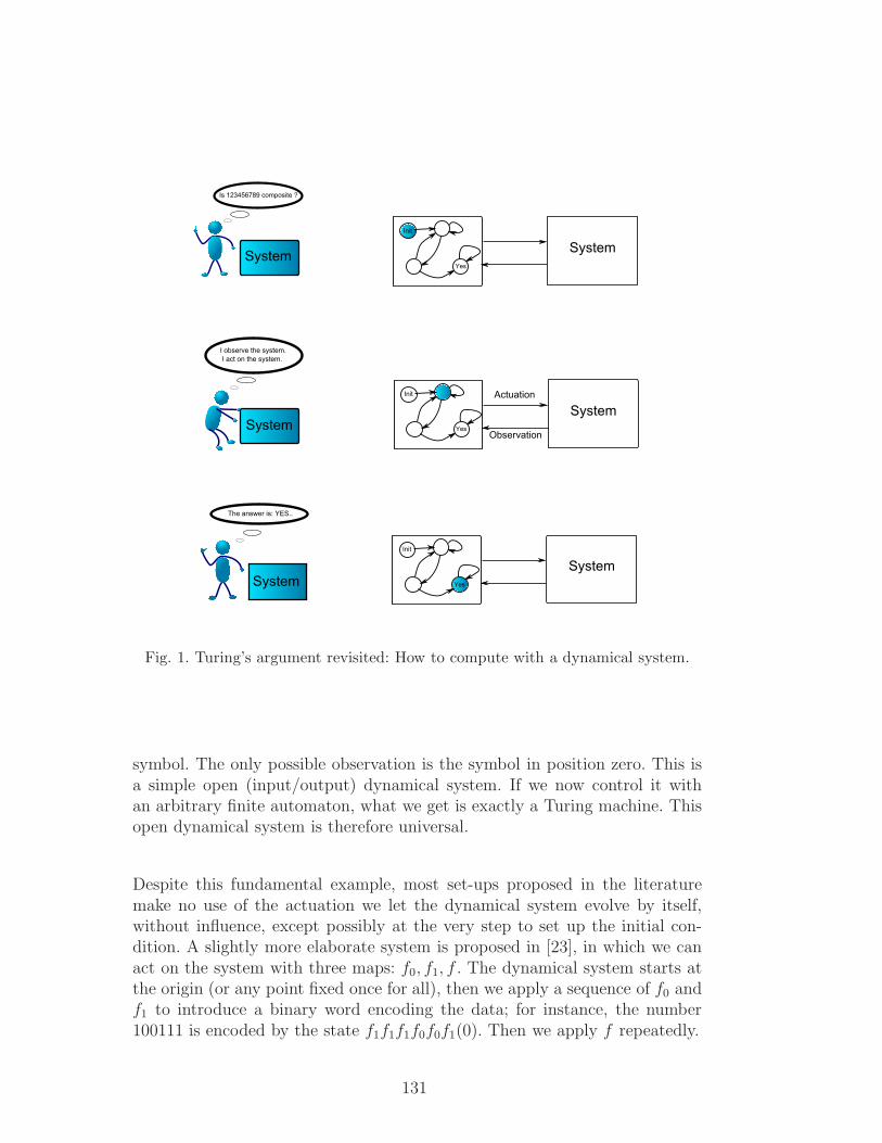
Fig. 1. Turing’s argument revisited: How to compute with a dynamical system.

symbol. The only possible observation is the symbol in position zero. This isa simple open (input/output) dynamical system. If we now control it withan arbitrary finite automaton, what we get is exactly a Turing machine. Thisopen dynamical system is therefore universal.

Despite this fundamental example, most set-ups proposed in the literaturemake no use of the actuation we let the dynamical system evolve by itself,without influence, except possibly at the very step to set up the initial con-dition. A slightly more elaborate system is proposed in [23], in which we canact on the system with three maps: f0, f1, f . The dynamical system starts atthe origin (or any point fixed once for all), then we apply a sequence of f0 andf1 to introduce a binary word encoding the data; for instance, the number100111 is encoded by the state f1f1f1f0f0f1(0). Then we apply f repeatedly.

131

10 Dynamical properties of universal systems

What is the link between the dynamics of a system and its computationalcapabilities?

Wolfram proposed a loose classification of 1-D cellular automata based onthe patterns present in the space-time diagram of the automaton; see [30].He then conjectured that the universal automata are in the so-called ‘fourthclass’, associated to the most complex patterns.

Langton [15] advocated the idea of the ‘edge of chaos’, according to which auniversal cellular automaton is likely to be neither globally stable (all pointsconverging to one single configuration) nor chaotic. See also [20] for a discus-sion. Other authors argue that a universal system may be chaotic; see [27].

However it seems difficult to prove any non-trivial result of this kind with thepoint-to-point or point-to-set reachability definition of universality. Moreovera countable set of points can be ‘hidden’ in a very small part of the state space(nowhere dense, with zero measure for instance), so the link between this setand the global dynamics is unclear in general.

Digital computing machines are analysed in [7], where it is shown that auniversal system according to this definition has at least one proper closedsubsystem, must have a sensitive point and can be Devaney-chaotic.

11 Conclusions

A framework has been proposed to unify many of the definitions of computingmachines found in the literature. A universal computing machine is definedas a dynamical system together with a suitable r.e.-complete problem; thisdefinition is flexible with respect to the kind of dynamical systems we consider.

In particular it appears that reachability problems, despite their mathemat-ical interest, are not the only generalisation of the Turing machine’s haltingproblem, and perhaps not the most natural.

In particular, it appears to us that universality for open dynamical systems isan almost blank field waiting to be explored.

132

12 Acknowledgements

The author is indebted to Jose Felix Costa for pointing some references.

This paper presents research results of the Belgian Programme on Interuniver-sity Attraction Poles, initiated by the Belgian Federal Science Policy Office.It has been also supported by the ARC (Concerted Research Action) “LargeGraphs and Networks”, of the French Community of Belgium. The scientificresponsibility rests with its authors. The author is holding a FNRS fellowship(Belgian Fund for Scientific Research).

References

[1] E. Asarin and A. Bouajjani. Perturbed turing machines and hybrid systems.In Proceedings of the 16th Annual IEEE Symposium on Logic in ComputerScience (LICS-01), pages 269–278, Los Alamitos, CA, June 16–19 2001. IEEEComputer Society.

[2] E. Asarin, O. Maler, and A. Pnueli. Reachability analysis of dynamicalsystems having piecewise-constant derivatives. Theoretical Computer Science,138(1):35–65, 1995.

[3] L. Blum, M. Shub, and S. Smale. On a theory of computation and complexityover the real numbers: NP-completeness, recursive functions and universalmachines. Bulletin of the American Mathematical Society, 21:1–46, 1989.

[4] O. Bournez and M. Cosnard. On the computational power of dynamical systemsand hybrid systems. Theoretical Computer Science, 168:417–459, 1996.

[5] M. Davis, editor. The Undecidable, Basic Papers on Undecidable Propositions,Unsolvable Problems And Computable Functions. Raven Press, 1965.

[6] M. D. Davis. A note on universal Turing machines. In C.E. Shannon andJ. McCarthy, editors, Automata Studies, pages 167–175. Princeton UniversityPress, 1956.

[7] J.-Ch. Delvenne, P. Kurka, and V. D. Blondel. Computational universality insymbolic dynamical systems. Fundamenta Informaticae, 71:1–28, 2006.

[8] D. Deutsch. Quantum theory, the Church-Turing principle and the universalquantum computer. Proceedings of the Royal Society of London Ser. A,A400:97–117, 1985.

[9] Francisco Doria and Jose Felix Costa, editors. Special Issue of AppliedMathematics and Computation on Hypercomputation, volume 178. Elsevier,2006.

133

[10] B. Durand and Z. Roka. The Game of Life: universality revisited. In M. Delormeand J. Mazoyer, editors, Cellular Automata: a Parallel Model, volume 460 ofMathematics and its Applications, pages 51–74. Kluwer Academic Publishers,1999.

[11] Jerome Durand-Lose. Abstract geometrical computation 1: embedding blackhole computations with rational numbers. Fund. Inf., 74(4):491–510, 2006.

[12] Peter Gacs. Reliable cellular automata with self-organization. In 38th AnnualSymposium on Foundations of Computer Science, pages 90–99, Miami Beach,Florida, 20–22 October 1997. IEEE.

[13] P. Koiran, M. Cosnard, and M. Garzon. Computability with low-dimensionaldynamical systems. Theoretical Computer Science, 132(1-2):113–128, 1994.

[14] P. Koiran and C. Moore. Closed-form analytic maps in one and two dimensionscan simulate universal Turing machines. Theoretical Computer Science,210(1):217–223, 1999.

[15] C. G. Langton. Computation at the edge of chaos. Physica D, 42:12–37, 1990.

[16] W. Maass and P. Orponen. On the effect of analog noise in discrete-time analogcomputations. Neural Computation, 10(5):1071–1095, 1998.

[17] Y. V. Matiyasevich. Hilbert’s Tenth Problem. MIT Press, 1993.

[18] M. Minsky. Computation: Finite and Infinite Machines. Prentice-Hall, 1967.

[19] M. L. Minsky. Recursive unsolvability of Post’s problem of “tag” and othertopics in theory of Turing machines. Annals of Mathematics (2), 74:437–455,1961.

[20] M. Mitchell, P. T. Hraber, and J. P. Crutchfield. Dynamic computation,and the “edge of chaos”: A re-examination. In G. Cowan, D. Pines, andD. Melzner, editors, Complexity: Metaphors, Models, and Reality, Santa FeInstitute Proceedings, Volume 19, pages 497–513. Addison-Wesley, 1994. SantaFe Institute Working Paper 93-06-040.

[21] C. Moore. Unpredictability and undecidability in dynamical systems. PhysicalReview Letters, 64(20):2354–2357, 1990.

[22] C. Moore. Recursion theory on the reals and continuous-time computation.Theoretical Computer Science, 162(1):23–44, 1996.

[23] C. Moore. Dynamical recognizers: real-time language recognition by analogcomputers. Theoretical Computer Science, 201:99–136, 1998.

[24] N. Ollinger. The intrinsic universality problem of one-dimensional cellularautomata. In H. Alt and M. Habib, editors, Symposium on Theoretical Aspectsof Computer Science (Berlin, Germany, 2003), volume 2607 of Lecture Notesin Computer Science, pages 632–641. Springer, Berlin, 2003.

134

[25] M. Boykan Pour-El and I. Richards. Computability and noncomputability inclassical analysis. Transactions of the American Mathematical Society, 275:539–560, 1983.

[26] M. O. Rabin. Recursive unsolvability of group theoretic problems. Annals ofMath., 67:172–194, 1958.

[27] H. T. Siegelmann. Neural Networks and Analog Computation: Beyond theTuring Limit. Progress in Theoretical Computer Science. Springer-Verlag, 1999.

[28] K. Sutner. Almost periodic configurations on linear cellular automata.Fundamenta Informaticae, 58(3–4):223–240, 2003.

[29] K. Weihrauch. Computable Analysis. Springer-Verlag, 2000.

[30] S. Wolfram. A new kind of science. Wolfram Media, Inc., Champaign, IL, 2002.

135

Black hole computation: implementations with signalmachines

Jerome Durand-LoseLaboratoire d’Informatique Fondamentale d’Orleans,Universite d’Orleans,B.P. 6759,F-45067 ORLEANS Cedex 2.

1. Introduction

No position is taken on the theoretical and practical feasibility of using anypotentially existing particular black hole for hyper-computing. The readeris referred to other contributions in this issue as well as Etesi and Nemeti(2002); Nemeti and David (2006); Nemeti and Andreka (2006) for clearintroductions and surveys on this topic. All the work presented here in donethe context of so-called “Malament-Hogarth” space-times and not slowlyrotating Kerr black hole. The main differences are that, one, the observerremains out of the black hole and second, nested black holes are considered.

A black hole computation works in the following way. At some location

one observer starts a computing device which he sends on a different world-line such that: at some point, after a finite time on his own world-line theobserver has the whole future of the device infinite world-line in its causalpast and the device can send some limited information to the observer.The device has an infinite time for computing ahead of it and can senda single piece of information to the observer. Not only can the observerperceive this piece of information, but after a finite duration which he isaware of, the observer knows for certain that if he has not received anythingthen the machine never sends anything during its whole, possibly infinite,computation. So that, for example, if the piece of information is sent only

Throughout the article location is to be understood as a position in space and time and position asonly spatial.

136

when the computation stops, at some point, the observer knows for certainwhether the computation ever stops.

From the computer scientist point of view, this allows to have some pieceof information on a whole, potentially infinite, computation. This way theHalting problem or the consistency of many first order logic theory (e.g.Set theory or Arithmetic theory) can be decided. This clearly falls out ofthe classical recursion/computability theory since it allows to decide semi-decidable subsets (Σ0

1 in the arithmetic hierarchy).Malament-Hogarth space-times allow to have nested black holes and so-

called arithmetical sentence deciding (SAD) space-times (Hogarth, 1994,2004). With each infinite level of nested black-holes, the computing powerclimbs up a level of the arithmetic hierarchy (and even the hyper-arithmetichierarchy in second order number theory (Welch, 2006)). The arithmetic hi-erarchy is formed by recursive predicates preceded by alternating quantifierson natural numbers. The level in the hierarchy is defined by the first quan-tifier and the number of alternations.

In computer science, considering and continuing a computation after itspotential infinite span exist in various form. Infinite time Turing machines(Copeland, 2002; Hamkins and Lewis, 2000; Hamkins, 2002, 2007) considerordinal times (and values); the main difference is that the limit of the tapeis available, whilst with black holes only a finite and bounded piece of infor-mation is available. Infinite computations also provide limits, for examplecomputable analysis (Weihrauch, 2000) (type-2 Turing machines) manipu-lates infinite inputs and generates infinite outputs, each one representing areal number. In analog computations, limit operators (as limits of sequencesof real numbers) are also considered (Chadzelek and Hotz, 1999; Kawamura,2005; Mycka, 2003b,a, 2006; Mycka and Costa, 2007; Bournez and Hainry,2007).

The setting in which the black hole effect is simulated here is not the so-lution to any relativity equations. It is rather something that is constructedinside a Newtonian space-time and provide the desired effect whereas blackholes involves non-Euclidean geometry (like the Schwarzschild one). Anyinitially spatially bounded computation can be embedded in a shrinkingstructure resulting in the same computation happening in a spatially andtemporally bounded room, even if it was not the case before. This structureprovide the black hole, outside of it, some information may be received togain some insight on what happen inside.

Abstract geometrical computation (AGC) deals with dimensionless signalswith rectilinear and uniform movement in a (finite dimension) Euclidean

137

space. It is both a continuous and an analog model. The way it is analog isquite unusual because there are finitely many values but continuum manyvariables. Time is evolving equally everywhere. What brings forth the ac-celerating power is that space and time are continuous so that Zeno effectcan happen and indeed, everything heavily relies on it. Throughout the ar-ticle, only dimension 1 spaces are considered, thus space-time diagrams are2 dimensional.

Signals are defined as instances of meta-signals which are of finite num-ber. They move with constant speeds uniquely defined by their meta-signals.When two or more signals meet, a collision happen and they are replacedother signals according to collision rules. A signal machine defines the avail-able meta-signals, their speeds and the collisions rules.

A configuration at a given time is a mapping from R to a finite set (con-taining the meta-signals) defining signals and their positions. Signals aresupposed to be away one from another. The void positions (i.e. position withnothing) are supposed to form an open set. The rest of the configurationcontains only singularities. They are many ways to continue a space-timediagram after an isolated singularity, the ones used here are: let it disappearor turn it into signals.

This model originates in discrete signals in Cellular Automata (Durand-Lose, 2008b). This explains the choice of finitely many meta-signals andconstant speeds. There are other models of computation dealing with Eu-clidean spaces.

Huckenbeck (1989, 1991) developed a model based on finite automataable to draw lines and circles and to compute intersections. Not only arethe primitives different, but also it is sequential and depends on an externaloperator to perform the construction whereas in signals in AGC operate ontheir own.

Jacopini and Sontacchi (1990) developed an approach where a computa-tion results in a polyhedron. They only encompass finite polyhedron (i.e.bounded with finitely many vertices) and allow surfaces and volumes of anydimensions while AGC has only lines.

Another model worth mentioning is the Piecewise Constant Derivative(PCD) system (Bournez, 1999b). There is only one signal, but its speedchanges each time it enters a different polygonal region. Not only is AGCparallel but also there is no such things as boundaries. Nevertheless, PCDare able to hyper-compute and climb up the hyper-arithmetic hierarchy(Bournez, 1999a) while the other two cannot.

In AGC, since signals dwell in a continuous space (R) and time (R+) and

138

there is no absolute scale, it is possible to rescale a configuration. Rescalinga configuration rescales the rest of the space-time. An automatic procedureto freeze the computation, scale it down and unfreeze it, is provided. Whenthis construction is made to restart it-self forever, a singularity is reached.Any AGC-computation starting with only finitely many signals can be em-bedded in this structure so that the corresponding computation is cut incountably many bounded pieces geometrically shrunk and inserted. Thisbrings a general scheme to transform any AGC-computation into one thatcan do the same computation but in a piece of the space-time diagrambounded in both space and time. This is the desired black hole effect. An-other shrinking scheme is presented in Durand-Lose (2006a), but it worksonly for spatially bounded AGC-computations while the one presented heredoes not impose this condition. The construction is detailed since AGC isnot so well-known and it is the cornerstone of the results in the article.

Simulating a Turing machine (TM) is easy using one signal to encode eachcell of the tape and an extra signal for the location of head and the state ofthe finite automaton. Any Turing machine simulation can be embedded inthe shrinking structure making it possible to decide semi-recursive problemsin finite time.

As long as speeds and initial positions are rational and there is no singu-larity, the location of each collision is rational (as the intersection of lineswith rational coefficients). This can be computed in classical discrete com-putability (and have been implemented to generate figures). The model isalso perfectly defined with irrational speeds and positions and can thus bealso considered as an analog model. It has recently been connected to theBlum, Shub and Smale model of computation (which can perform algebraicoperations as well as test the sign on real numbers with exact precision)(Durand-Lose, 2007, 2008a). In the present paper, it is only recalled howreal numbers are encoded and how a singularity is used to provide the mul-tiplication. Our shrinking scheme can be used in this analog context toanswer analog decision problems.

The way a signal machine is transformed to have shrinking capabilitycan be iterated so that singularities/accumulations of any order can begenerated. This allows to decide a formula formed by a total (resp. BSS)recursive predicate preceded by a finite alternation of quantifiers on N (i.e.to climb the corresponding arithmetical hierarchies). For the analog case,this remains a quantification over a countable set .

This is why we do not talk about an analytic hierarchy.

139

In Section 2, the model and the shrinking structure are presented. In Sec-tion 3, the way discrete computation can be done and shrunk is presented.In Section 4, analog computation is considered. Section 5 explains how tohave nested black holes so as to climb the arithmetic hierarchies. Section 6gathers some concluding remarks.

2. Model and Mechanics

The underlying time is R+; there is no such thing as a next configuration.The underlying space is R. A configuration is a mapping from R to a finiteset (yet to be defined). A space-time diagram is a function from R ×R+ tothe same finite set.

What lies on R are signals, collisions between signals or singularities (cre-ated by accumulations). Signals are moving with constant speed dependingonly on their nature. When they meet, an instantaneous collision happensand the signals are replaced by others according to some collision rules.A singularity happens when and where infinitely many collisions, signalsand/or singularities accumulate. Ways to continue a space-time diagrambeyond an isolated singularity are proposed at the end of this section.

2.1. Signal machines and space-time diagrams

Definition 1 A signal machine (SM) is defined by (M, S, R) where M(meta-signals) is a finite set, S (speeds) a function from M to R, and R(collision rules) a partial function from the subsets of M of cardinality atleast two into subsets of M (all these sets are composed of signals of distinctspeeds).

Each signal is an instance of a meta-signal. Its speed is constant and onlydepends on its meta-signal (given by S). When two or more signals meet,R indicates the signals to replace them. Meeting signals must have distinctspeeds otherwise they are parallel and never meet. Signals are not allowedto be superposed, so that all signals emitted by a collision must also havedistinct speeds.

Definition 2 The extended value set, V , is the union of M and R plustwo special values: one for void, , and one for singularity . An (valid)configuration is a total function from R to V such that all the accumulationpoints of its support (the set of non void location, supp(c) = x ∈ R | c(x) =) have the value . A configuration is finite if its support is finite. It issimple if it is finite and is not reached. It is rational if it is simple and

140

its support is included in Q. A SM is rational if all the speeds are rationalnumbers and only rational configurations are used.

As long as there is no singularity, a finite configuration is only followedby finite ones.

To be rational is robust. Signals at rational positions with rational speedscan only meet at rational location. All collisions happen at rational datesand at these dates the positions of signals are all rational. Since rationalnumbers can be encoded and manipulated exactly with any computer, ra-tional SM can be handled inside classical computability theory.

Two results limit the interest and extend of rational SM. First, predictingwhether a singularity ever happens is Σ0

2-complete (in the arithmetical hi-erarchy, which means not even semi-decidable) (Durand-Lose, 2006b) andsecond, a singularity can happen at an irrational position (Durand-Lose,2008a). On the other hand, as long as Turing-computability is involved, ra-tional SM are enough (as shown in Sect. 3). But if analog computations areto be considered, then it is not the case anymore as in Sect. 4.

Let Smin and Smax be the minimal and maximal speeds. The causal past,or backward light-cone, arriving at position x and time t, I−(x, t), is definedby all the positions that might influence the information at (x, t) throughsignals, formally:

I−(x, t) = (x′, t′) | x − Smax(t−t′) ≤ x′ ≤ x − Smin(t−t′) .

Definition 3 The space-time diagram issued from an initial configurationc0 and lasting for T , is a function c from [0, T ] to configurations (i.e. afunction from R × [0, T ] to V ) such that, ∀(x, t) ∈ R × [0, T ] :(i) ∀t∈[0, T ], ct(.) is valid, and c0(.) = c0;(ii) if ct(x)=µ ∈ M then ∃ti, tf∈[0, T ] with ti<t<tf or 0=ti=t<tf or ti<t=tf=T

s.t.:(a) ∀t′ ∈ (ti, tf), ct′(x + S(µ)(t′ − t)) = µ ,(b) ( ti=0 and c0(xi) = µ ) or ( cti(xi) = ρ−→ρ+∈R and µ ∈ ρ+ )

where xi=x + S(µ)(ti − t) ,(c) ( tf=T and ctf (T ) = µ ) or ( ctf (xf ) = ρ−→ρ+∈R and µ ∈ ρ− ) or

ctf (xf )= where xf=x + S(µ)(tf − t) ;(iii) if ct(x)=ρ−→ρ+ ∈ R then ∃ε, 0<ε, ∀t′∈[t−ε, t+ε] ∩ [0, T ], ∀x′∈[x −

ε, x + ε],(a) (x′, t′) = (x, t) ⇒ ct′(x

′) ∈ ρ−∪ρ+ ∪ ,

(b) ∀µ∈M , ct′(x′)=µ ⇔ ∨

µ ∈ ρ− and t′ < t and x′ = x + S(µ)(t′ − t)

µ ∈ ρ+ and t < t′ and x′ = x + S(µ)(t′ − t);

and

141

(iv) if ct(x) = then ∀ε>0, there are infinitely many collisions in I−(x, t)∩R × [t−ε, t) or infinitely many signals in [x − ε, x + ε] × [t−ε, t) .

The definition naturally extends to the case T = +∞. A space-time di-agram is rational if it is correspond to the one of a rational SM. As longas no singularity is reached, the evolution is deterministic; the space-timediagram only depends on c0 and the SM.

2.1.1. Encompassing singularities.When a singularity is reached isolated (i.e. there is nothing round it),

there are various ways to continue the space-time diagram beyond it.

Definition 4 (Schemes to handle isolated singularities) A singular-ity at (x, t) is isolated if there is nothing but void around it in the configu-ration (i.e. ∃ε, ∀x′ ∈ [x − ε, x + ε], x′ = x ⇒ ct(x

′) = ). There are variousschemes to continue a space-time diagram at an isolated singularity.(i) Wall. It remains there forever;(ii) Vanish. It disappears as if it where on another dimension;(iii) Simple trace. It disappears but sends a µs signal; or(iv) Conditional traces. It disappears but sends signals according to which

signals join in (i.e. signals that are not interrupted by any collision –notan infinite succession of signals).

In the two last schemes, µs or the singularity rules have to be added tothe definition of the SM. In such a case, one talks about an extended SM(ESM). Next sections consider ESM and the schemes used are indicated.

The first scheme is not considered here; although it makes sense since sin-gularities generally do not just disappear, in dimension one, it unfortunatelyproduces an unbreakable frontier definitively splitting the configuration intwo. The second one is considered in the section on discrete computationwhile the third is considered in the section on analog computation. Thereason in the analog case is that its position is an important piece of in-formation. The last case is also used to consider the case of a singularityhappening exactly on a higher level structure (as the one presented below)with nested structures in Sect. 5.

The last two schemes impose a modification of the rules of space-timediagrams. One is to allow a signal to start from a singularity to add tob “or ( cti(xi)= ∧ µ = µs )” and to iv something amounting for signalsemitted like the rules for collisions (iii) which is not given since it dependson the scheme and for the last scheme of the singularity rules.

142

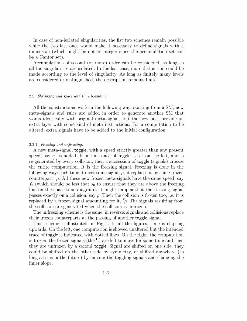
In case of non-isolated singularities, the fist two schemes remain possiblewhile the two last ones would make it necessary to define signals with adimension (which might be not an integer since the accumulation set canbe a Cantor set).

Accumulations of second (or more) order can be considered, as long asall the singularities are isolated. In the last case, more distinction could bemade according to the level of singularity. As long as finitely many levelsare considered or distinguished, the description remains finite.

2.2. Shrinking and space and time bounding

All the constructions work in the following way: starting from a SM, newmeta-signals and rules are added in order to generate another SM thatworks identically with original meta-signals but the new ones provide anextra layer with some kind of meta instructions. For a computation to bealtered, extra signals have to be added to the initial configuration.

2.2.1. Freezing and unfreezing.A new meta-signal, toggle, with a speed strictly greater than any present

speed, say s0 is added. If one instance of toggle is set on the left, and isre-generated by every collision, then a succession of toggle (signals) crossesthe entire computation. It is the freezing signal. Freezing is done in thefollowing way: each time it meet some signal µ, it replaces it by some frozencounterpart Fµ. All these new frozen meta-signals have the same speed, sayf0 (which should be less that s0 to ensure that they are above the freezingline on the space-time diagram). It might happen that the freezing signalpasses exactly on a collision, say ρ. Then the collision is frozen too, i.e. it isreplaced by a frozen signal amounting for it, Fρ. The signals resulting fromthe collision are generated when the collision is unfrozen.

The unfreezing scheme is the same, in reverse: signals and collisions replacetheir frozen counterparts at the passing of another toggle signal.

This scheme is illustrated on Fig. 1. In all the figures, time is elapsingupwards. On the left, one computation is showed unaltered but the intendedtrace of toggle is indicated with dotted lines. On the right, the computationis frozen, the frozen signals (the F.) are left to move for some time and thenthey are unfrozen by a second toggle. Signal are shifted on one side, theycould be shifted on the other side by symmetry, or shifted anywhere (aslong as it is in the future) by moving the toggling signals and changing theinner slope.

143

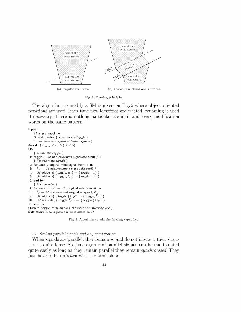
start of thecomputation

rest of thecomputation

(a) Regular evolution.

start of thecomputation

rest of thecomputation

Translat

ion

toggle

toggle

(b) Frozen, translated and unfrozen.

Fig. 1. Freezing principle.

The algorithm to modify a SM is given on Fig. 2 where object orientednotations are used. Each time new identities are created, renaming is usedif necessary. There is nothing particular about it and every modificationworks on the same pattern.

Input:M : signal machineβ: real number speed of the toggle θ: real number speed of frozen signals

Assert: ( Smax < β) ∧ ( θ < β)Do:

Create the toggle 1: toggle ← M .add new meta-signal of speed( β )

For the meta-signals 2: for each µ original meta-signal from M do3: Fµ ← M .add new meta-signal of speed( θ )4: M .add rule( toggle, µ → toggle, Fµ )5: M .add rule( toggle, Fµ → toggle, µ )

6: end for For the rules

7: for each ρ =ρ− → ρ+ original rule from M do8: Fρ ← M .add new meta-signal of speed( θ )9: M .add rule( toggle ∪ ρ− → toggle, Fρ )

10: M .add rule( toggle, Fρ → toggle ∪ ρ+ )11: end forOutput: toggle: meta-signal the freezing/unfreezing one Side effect: New signals and rules added to M

Fig. 2. Algorithm to add the freezing capability.

2.2.2. Scaling parallel signals and any computation.When signals are parallel, they remain so and do not interact, their struc-

ture is quite loose. So that a group of parallel signals can be manipulatedquite easily as long as they remain parallel they remain synchronized. Theyjust have to be unfrozen with the same slope.

144

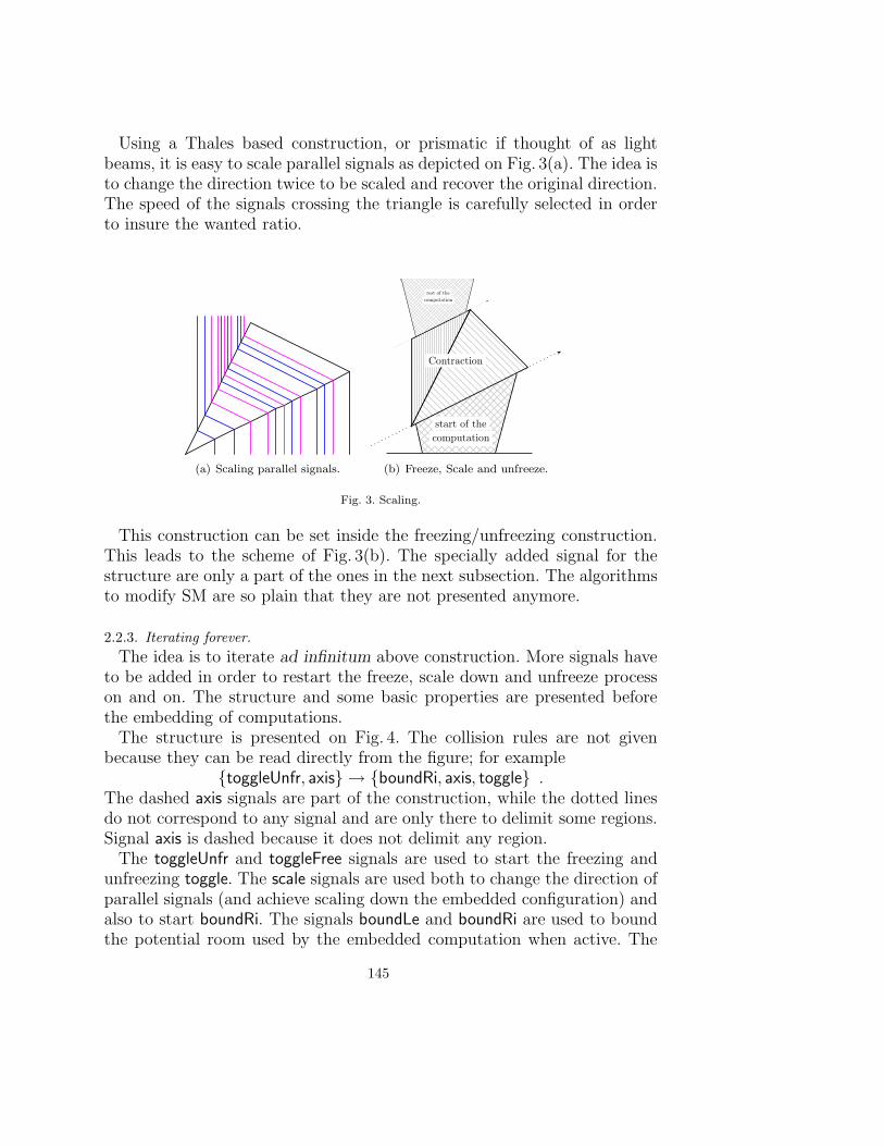
Using a Thales based construction, or prismatic if thought of as lightbeams, it is easy to scale parallel signals as depicted on Fig. 3(a). The idea isto change the direction twice to be scaled and recover the original direction.The speed of the signals crossing the triangle is carefully selected in orderto insure the wanted ratio.

(a) Scaling parallel signals.

start of thecomputation

Contraction

rest of thecomputation

(b) Freeze, Scale and unfreeze.

Fig. 3. Scaling.

This construction can be set inside the freezing/unfreezing construction.This leads to the scheme of Fig. 3(b). The specially added signal for thestructure are only a part of the ones in the next subsection. The algorithmsto modify SM are so plain that they are not presented anymore.

2.2.3. Iterating forever.The idea is to iterate ad infinitum above construction. More signals have

to be added in order to restart the freeze, scale down and unfreeze processon and on. The structure and some basic properties are presented beforethe embedding of computations.

The structure is presented on Fig. 4. The collision rules are not givenbecause they can be read directly from the figure; for example

toggleUnfr, axis → boundRi, axis, toggle .The dashed axis signals are part of the construction, while the dotted linesdo not correspond to any signal and are only there to delimit some regions.Signal axis is dashed because it does not delimit any region.

The toggleUnfr and toggleFree signals are used to start the freezing andunfreezing toggle. The scale signals are used both to change the direction ofparallel signals (and achieve scaling down the embedded configuration) andalso to start boundRi. The signals boundLe and boundRi are used to boundthe potential room used by the embedded computation when active. The

145

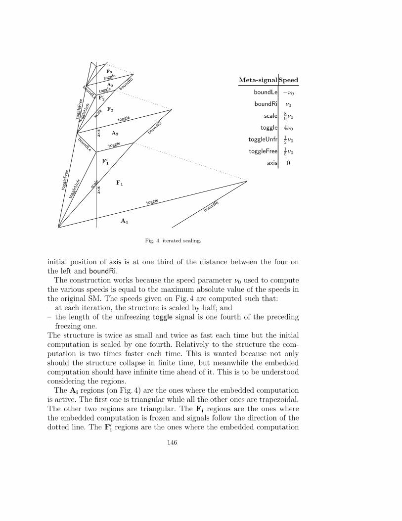
axis

axis

toggle

boun

dRi

togg

leUnf

r

togg

leFre

e

toggle

scale

boundLe

boun

dRi

toggleto

ggleFre

etoggl

e

boundLe

togg

leUnf

rtoggl

escale

boun

dRi

A1

F1

F′1

A2

F2

F′2

A3

F3

Meta-signal Speed

boundLe −ν0boundRi ν0

scale 89ν0

toggle 4ν0

toggleUnfr 12ν0

toggleFree 15ν0

axis 0

Fig. 4. iterated scaling.

initial position of axis is at one third of the distance between the four onthe left and boundRi.

The construction works because the speed parameter ν0 used to computethe various speeds is equal to the maximum absolute value of the speeds inthe original SM. The speeds given on Fig. 4 are computed such that:– at each iteration, the structure is scaled by half; and– the length of the unfreezing toggle signal is one fourth of the preceding

freezing one.The structure is twice as small and twice as fast each time but the initialcomputation is scaled by one fourth. Relatively to the structure the com-putation is two times faster each time. This is wanted because not onlyshould the structure collapse in finite time, but meanwhile the embeddedcomputation should have infinite time ahead of it. This is to be understoodconsidering the regions.

The Ai regions (on Fig. 4) are the ones where the embedded computationis active. The first one is triangular while all the other ones are trapezoidal.The other two regions are triangular. The Fi regions are the ones wherethe embedded computation is frozen and signals follow the direction of thedotted line. The F′

i regions are the ones where the embedded computation

146

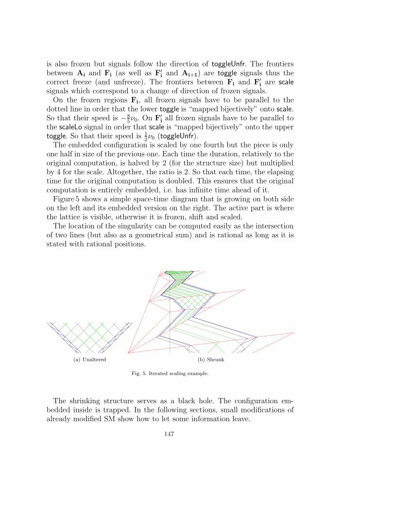
is also frozen but signals follow the direction of toggleUnfr. The frontiersbetween Ai and Fi (as well as F′

i and Ai+1) are toggle signals thus thecorrect freeze (and unfreeze). The frontiers between Fi and F′

i are scalesignals which correspond to a change of direction of frozen signals.

On the frozen regions Fi, all frozen signals have to be parallel to thedotted line in order that the lower toggle is “mapped bijectively” onto scale.So that their speed is −8

5ν0. On F′

i all frozen signals have to be parallel tothe scaleLo signal in order that scale is “mapped bijectively” onto the uppertoggle. So that their speed is 1

2ν0 (toggleUnfr).

The embedded configuration is scaled by one fourth but the piece is onlyone half in size of the previous one. Each time the duration, relatively to theoriginal computation, is halved by 2 (for the structure size) but multipliedby 4 for the scale. Altogether, the ratio is 2. So that each time, the elapsingtime for the original computation is doubled. This ensures that the originalcomputation is entirely embedded, i.e. has infinite time ahead of it.

Figure 5 shows a simple space-time diagram that is growing on both sideon the left and its embedded version on the right. The active part is wherethe lattice is visible, otherwise it is frozen, shift and scaled.

The location of the singularity can be computed easily as the intersectionof two lines (but also as a geometrical sum) and is rational as long as it isstated with rational positions.

(a) Unaltered (b) Shrunk

Fig. 5. Iterated scaling example.

The shrinking structure serves as a black hole. The configuration em-bedded inside is trapped. In the following sections, small modifications ofalready modified SM show how to let some information leave.

147

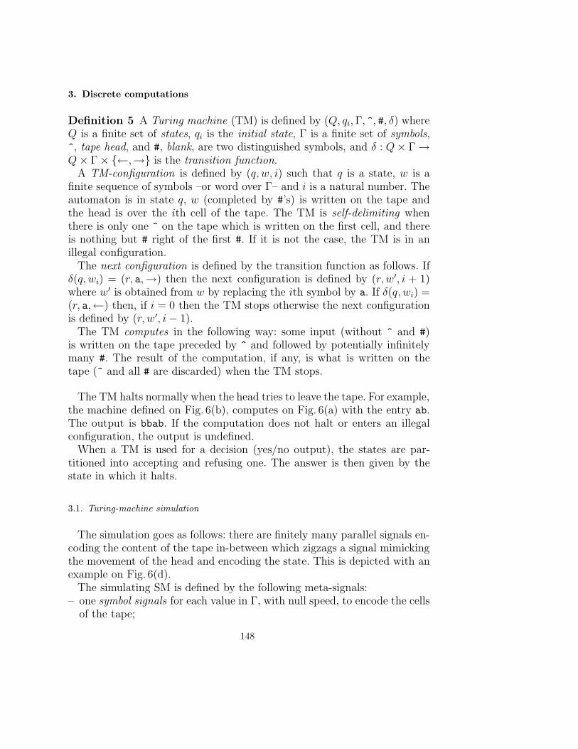
3. Discrete computations

Definition 5 A Turing machine (TM) is defined by (Q, qi, Γ, ^, #, δ) whereQ is a finite set of states, qi is the initial state, Γ is a finite set of symbols,^, tape head, and #, blank, are two distinguished symbols, and δ : Q × Γ →Q × Γ × ←,→ is the transition function.

A TM-configuration is defined by (q, w, i) such that q is a state, w is afinite sequence of symbols –or word over Γ– and i is a natural number. Theautomaton is in state q, w (completed by #’s) is written on the tape andthe head is over the ith cell of the tape. The TM is self-delimiting whenthere is only one ^ on the tape which is written on the first cell, and thereis nothing but # right of the first #. If it is not the case, the TM is in anillegal configuration.

The next configuration is defined by the transition function as follows. Ifδ(q, wi) = (r, a,→) then the next configuration is defined by (r, w′, i + 1)where w′ is obtained from w by replacing the ith symbol by a. If δ(q, wi) =(r, a,←) then, if i = 0 then the TM stops otherwise the next configurationis defined by (r, w′, i − 1).

The TM computes in the following way: some input (without ^ and #)is written on the tape preceded by ^ and followed by potentially infinitelymany #. The result of the computation, if any, is what is written on thetape (^ and all # are discarded) when the TM stops.

The TM halts normally when the head tries to leave the tape. For example,the machine defined on Fig. 6(b), computes on Fig. 6(a) with the entry ab.The output is bbab. If the computation does not halt or enters an illegalconfiguration, the output is undefined.

When a TM is used for a decision (yes/no output), the states are par-titioned into accepting and refusing one. The answer is then given by thestate in which it halts.

3.1. Turing-machine simulation

The simulation goes as follows: there are finitely many parallel signals en-coding the content of the tape in-between which zigzags a signal mimickingthe movement of the head and encoding the state. This is depicted with anexample on Fig. 6(d).

The simulating SM is defined by the following meta-signals:– one symbol signals for each value in Γ, with null speed, to encode the cells

of the tape;

148

^

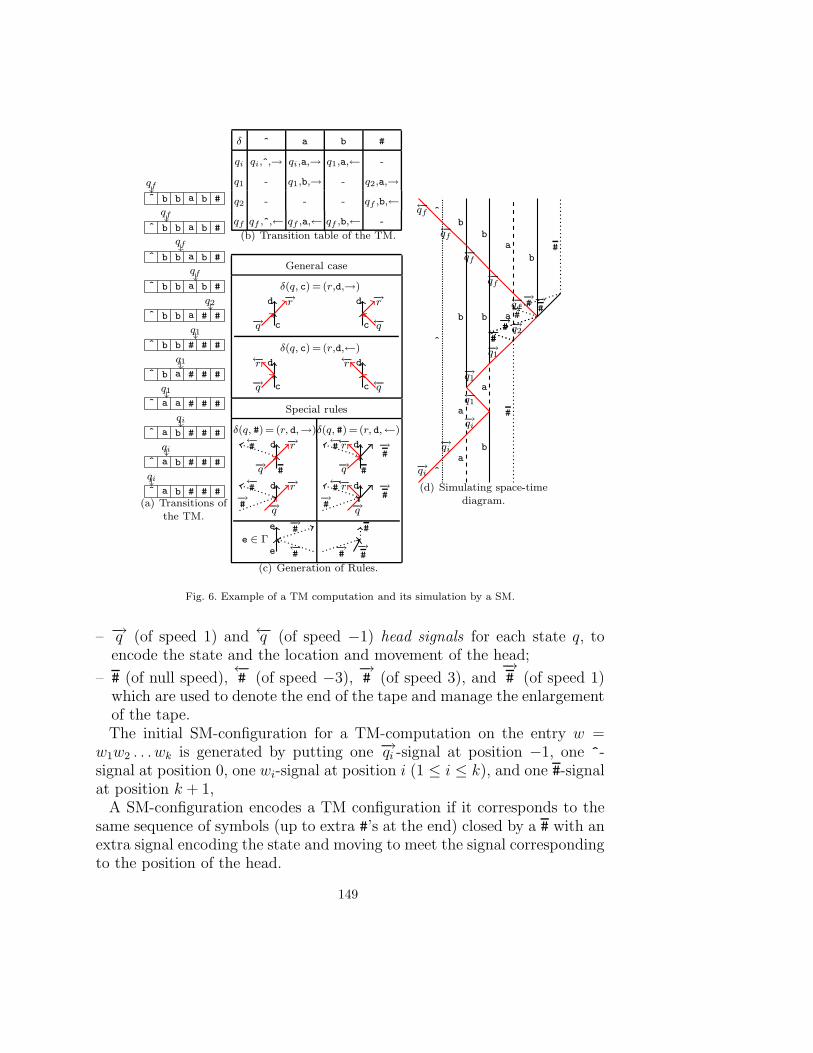
qf

b b a b #

^

qf

b b a b #

^

qf

b b a b #

^

qf

b b a b #

^

q2

b b a # #

^

q1

b b # # #

^

q1

b a # # #

^

q1

a a # # #

^

qi

a b # # #

^

qi

a b # # #

^

qi

a b # # #(a) Transitions of

the TM.

δ ^ a b #

qi qi,^,→ qi,a,→ q1,a,← -

q1 - q1,b,→ - q2,a,→q2 - - - qf ,b,←qf qf ,^,← qf ,a,← qf ,b,← -

(b) Transition table of the TM.

General case

δ(q, c) = (r,d,→)

d

c

−→r−→q

d

c

−→r←−q

δ(q, c) = (r,d,←)

d

c

←−r−→q

d

c

←−r←−q

Special rules

δ(q, #)= (r, d,→)δ(q, #)= (r, d,←)

d

#

−→r−→q

←−# d

#

←−r−→q

←−# −→

#

d−→# −→q

−→r←−# d

−→# −→q

←−r←−# −→

#

e ∈ Γ

e

e

−→#

←−#

#

−→#

−→#

(c) Generation of Rules.

^

^

^

a

a

b

b

b

a

b

b

#

a

a

b

−→qi

−→qi

−→qi

←−q1

−→q1

−→q1

−→q2←−#

−→#

←−qf

←−#

−→#

←−qf

←−#

−→# −→

#

#←−qf

←−qf

←−qf

(d) Simulating space-timediagram.

Fig. 6. Example of a TM computation and its simulation by a SM.

– −→q (of speed 1) and ←−q (of speed −1) head signals for each state q, toencode the state and the location and movement of the head;

– # (of null speed),←−# (of speed −3),

−→# (of speed 3), and

−→# (of speed 1)

which are used to denote the end of the tape and manage the enlargementof the tape.The initial SM-configuration for a TM-computation on the entry w =

w1w2 . . . wk is generated by putting one −→qi -signal at position −1, one ^-signal at position 0, one wi-signal at position i (1 ≤ i ≤ k), and one #-signalat position k + 1,

A SM-configuration encodes a TM configuration if it corresponds to thesame sequence of symbols (up to extra #’s at the end) closed by a # with anextra signal encoding the state and moving to meet the signal correspondingto the position of the head.

149

The collisions rules ensure that the evolution of the SM corresponds tothe computation of the TM. When the head encounters a symbol signal, itperforms the update and move to its next position on the tape. When itmeets the right special signal, the configuration is automatically enlarge.

The generated collision rules are given on Fig. 6(c). When a rule is notdefined, the signal just cross unaffected. From top to bottom, they corre-spond to the following cases. For each TM-transition, two collision rules aregenerated, they correspond to the cases where the head would come fromthe left or from the right. The special rules are made in order to ensure acorrect enlargement of the configuration in the case a head signal meet #,the signal marking the last cell. In such a case, two things have to be done:normally do the TM-transition (as if it were a # signal) and enlarge the con-figuration. The latter means generate one # one position on the right if thehead goes left (left side rules). If the head goes right (right side rules), thenit should be taken care that the head meets something on the right (lowerrow rules). This is illustrated in the middle of Fig. 6(d). In each first case, a←−# is sent on the left. It bounces on the symbol signal on the left (bottom

rule of Fig. 6(c)) and is replaced by−→# , cross whatever signal present to get

where would be the head if it would have gone right. If indeed the headwent right, it is met and the TM-transition is done and the configurationenlargement starts again. If it is not the case (left rules of Fig. 6(c)), then−→# is sent in order to meet

−→# and place the new #. Signals

←−# and

−→# are

three time faster in order to ensure that the meeting happens exactly wherethe next symbol signal should have been.

At the end of the TM-computation simulation, the signal encoding thestate goes out on the left. The process is robust, the positions does nothave to be exact as long as the order of the signals is preserved. It can beimplemented with a rational SM.

3.2. Infinite Turing computation in bounded time

The construction described in Sect. 2 rightfully apply to the above con-struction. It is considered that the singularity vanishes leaving no signal(scheme ii of Def. 4). The infinite acceleration is granted. But the infor-mation leaving the black hole is missing. The ESM has to undergo somemodifications. The first one is to generate the escaping signal, the secondto retrieve it.

The result of a deciding TM is given by the new state whenever it performsa transition on ^ and sends the head on the left. These transitions areclearly identified in the transition table of the TM. So there are also clearly

150

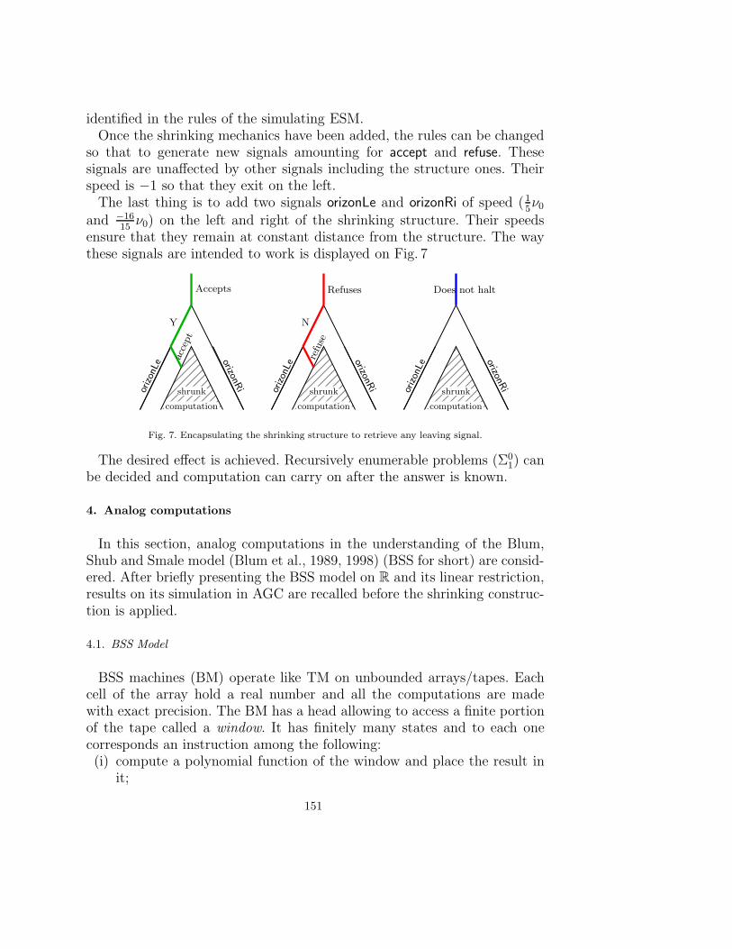
identified in the rules of the simulating ESM.Once the shrinking mechanics have been added, the rules can be changed

so that to generate new signals amounting for accept and refuse. Thesesignals are unaffected by other signals including the structure ones. Theirspeed is −1 so that they exit on the left.

The last thing is to add two signals orizonLe and orizonRi of speed (15ν0

and −1615

ν0) on the left and right of the shrinking structure. Their speedsensure that they remain at constant distance from the structure. The waythese signals are intended to work is displayed on Fig. 7

orizon

Le

orizonRishrunk

computation

Y

Accepts

acce

pt

orizon

Le

orizonRishrunk

computation

N

Refuses

refu

se

orizon

Le

orizonRishrunk

computation

Does not halt

Fig. 7. Encapsulating the shrinking structure to retrieve any leaving signal.

The desired effect is achieved. Recursively enumerable problems (Σ01) can

be decided and computation can carry on after the answer is known.

4. Analog computations

In this section, analog computations in the understanding of the Blum,Shub and Smale model (Blum et al., 1989, 1998) (BSS for short) are consid-ered. After briefly presenting the BSS model on R and its linear restriction,results on its simulation in AGC are recalled before the shrinking construc-tion is applied.

4.1. BSS Model

BSS machines (BM) operate like TM on unbounded arrays/tapes. Eachcell of the array hold a real number and all the computations are madewith exact precision. The BM has a head allowing to access a finite portionof the tape called a window. It has finitely many states and to each onecorresponds an instruction among the following:(i) compute a polynomial function of the window and place the result in

it;

151

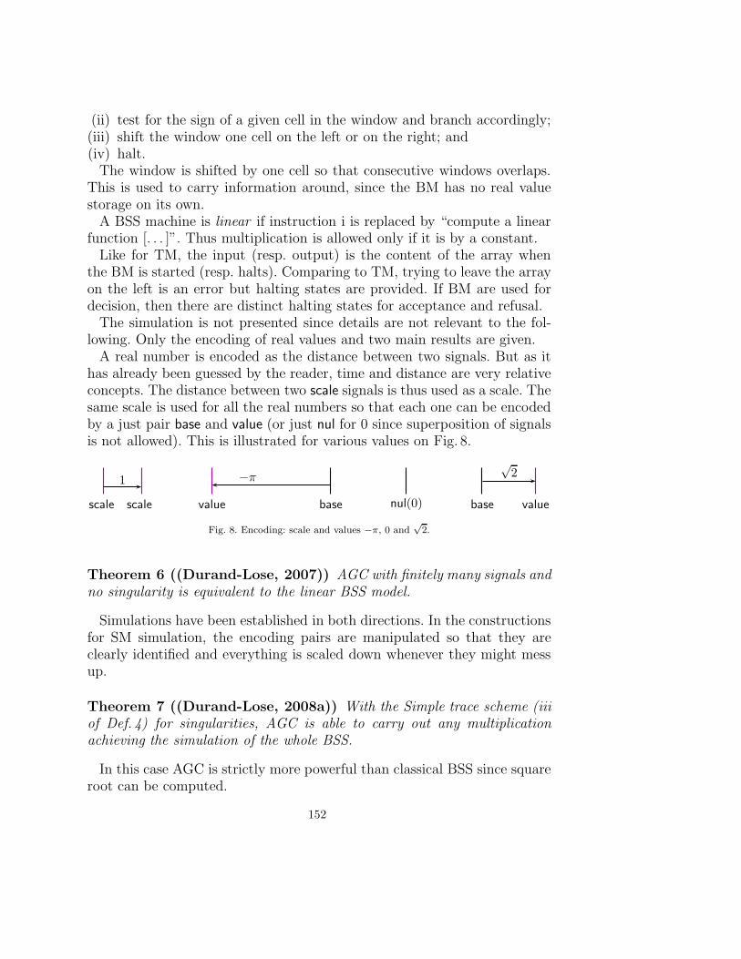
(ii) test for the sign of a given cell in the window and branch accordingly;(iii) shift the window one cell on the left or on the right; and(iv) halt.

The window is shifted by one cell so that consecutive windows overlaps.This is used to carry information around, since the BM has no real valuestorage on its own.

A BSS machine is linear if instruction i is replaced by “compute a linearfunction [. . . ]”. Thus multiplication is allowed only if it is by a constant.

Like for TM, the input (resp. output) is the content of the array whenthe BM is started (resp. halts). Comparing to TM, trying to leave the arrayon the left is an error but halting states are provided. If BM are used fordecision, then there are distinct halting states for acceptance and refusal.

The simulation is not presented since details are not relevant to the fol-lowing. Only the encoding of real values and two main results are given.

A real number is encoded as the distance between two signals. But as ithas already been guessed by the reader, time and distance are very relativeconcepts. The distance between two scale signals is thus used as a scale. Thesame scale is used for all the real numbers so that each one can be encodedby a just pair base and value (or just nul for 0 since superposition of signalsis not allowed). This is illustrated for various values on Fig. 8.

scale scale

1

value base

−πnul(0) base value

√2

Fig. 8. Encoding: scale and values −π, 0 and√

2.

Theorem 6 ((Durand-Lose, 2007)) AGC with finitely many signals andno singularity is equivalent to the linear BSS model.

Simulations have been established in both directions. In the constructionsfor SM simulation, the encoding pairs are manipulated so that they areclearly identified and everything is scaled down whenever they might messup.

Theorem 7 ((Durand-Lose, 2008a)) With the Simple trace scheme (iiiof Def. 4) for singularities, AGC is able to carry out any multiplicationachieving the simulation of the whole BSS.

In this case AGC is strictly more powerful than classical BSS since squareroot can be computed.

152

4.2. Infinite analog computations

The meaning of the shrinking structure on a BM simulation is consideredbefore entering into technical issues.

4.2.1. Interpretation.Assuming that everything works well as expected, the ESM can be made

so that if the computation stops then some information leaves the singular-ity. But what kind of information? Usually it is considered that only finitelymany values can be used , not countably many, not continuum many!Mechanisms as in Subsect. 3.2 can be used to send a few bits, but it is notclear how to send four signals (to encode a real number) ensuring that theyare all at the same scale (i.e. are emitted from the same active region).

With the same construction as previously, using a universal BM, the BSShalting problem, can be decided.Instance HaltBSS

-−→X ,

−→Y : vectors of real numbers

Question

Does the BM represented by−→X stop on entry

−→Y ?

Let us consider another example. BSS machines can simulate any TMand any recursive function. There is a BM with one entry that tries allthe rational numbers sequentially and stops if it is equal to the entry. Sincehalting can be decided, the characteristic function of Q is computable (whichis not usually the case).

The general form of decision problems that can be solved is of the form

∃n ∈ N, φ(n,−→X ) where φ is decision BM that stops for all entries. This

definition is the same as the one for classical recursion except that totalrecursive predicate is replaced by total BSS predicate. The quantification ison N (that can encode Q or many other countable sets) but not on R. Thisdoes not correspond to the first and second level of an analytical hierarchybut an arithmetical one. It corresponds to BCSS-Σ1 in Ziegler (2007). Pleasenote that this is only a lower bound on the computing capability.

If one wants the analog output if the computation stops and just the infor-mation that is does not stop otherwise, it uses a singularity to know whetherthe computation stops and if it is the case, then it starts the computationnormally to get the result in finite time.

For example think about the so-called blue-shift effect and how it might be countered (Nemeti andDavid, 2006, Sub. 5.3.1).

153

If one would like to have the limit of say first cell of the array if any,not only does the shrinking might turn the scale and the distance betweenencoding signals to zero but moreover, if the BM-computation uses biggerand bigger real numbers, its accumulated re-scaling also turns them to zero.So that one would have to find how to generate the value in a way that doesnot lead to zero divided by zero and neither prevents the shrinking.

This has been achieved to get internal multiplication out of linear BSS:three of the four real numbers encoding signals are constant outside of thesingularity and the singularity happens at the correct position for the lastsignal. A general scheme still have to be found.

4.2.2. Technical issues.In each active region, the configuration only undergoes a regular scaling.

Up to scaling, the active regions perfectly assemble. The computation isexact and the real values are preserved even though the encoding can besplit between various active regions (retrieving the value is not obvious).

The difference from the discrete case is that singularities are already usedfor multiplication. These are handled with the simple trace scheme (iii ofDef. 4).

With the structure, both type of singularity should be distinguished par-ticularly because the singularity for multiplication could happen exactly ontoggle so that with the simple trace scheme, the structure would be dam-aged. In this case, one extra frozen meta-signal must exist to encode thesingularity as well as a toggle for the structure. The case iv –which is moregeneral– is used. Since the speed of toggle is greater than the any of theother signal present for the multiplication, it gets straight into the singular-ity without getting involved in any collision and thus distinguishes betweenthe singularities.

If there are infinitely many multiplications, then the singularity is of sec-ond order. This is not a problem for the structure nor the definition ofspace-time diagrams. Rule iv of Def. 3 only asks for infinitely many colli-sions or signals which is also ensured by the accumulating multiplications.

5. Nested singularities

Previous Section ends with a second order singularity. It is possible tobuilt higher order singularities.

Section 2.2 explains how to shrink any space-time diagram that has nosingularity. It is quite easy to set signals to automatically start a singularity(in the spirit of what is done in Durand-Lose (2006b)) and according to the

154

result to start another. There can be finitely or countably many isolatedsingularities (there is a rational location in each open).

The interesting part is when singularities are nested inside another one.In Sect. 4.2.2, it is explained how, with the conditional traces scheme (ivof Def. 4), to handle sub-singularities. The second order structure worksbecause it is built on top of the previous one (after renaming the meta-signals to avoid any conflict). So that the outer one can handle the innerones while the latter proceed on their own.

It is thus natural to reiterate the construction. This can be done safelya finite number of times (more would yield an infinite number of signals).Inside any structure, it is only possible to start a lesser level structure sothat the first one is the topmost and that the number of nested levels insideis bounded by construction of the ESM.

For discrete computations, in the setting presented in Subsect. 3.2, singu-larities are only used to decide and leave no trace (ii of Def. 4). But since asingularity could happen on a toggle of a higher level structure, for the samereason as before, the conditional traces scheme has to be used. For analogcomputations, this scheme is already used. It is thus the natural scheme touse in both cases.

In the discrete case, like for the SAD computers of Hogarth (1994, 2004),each order brings the capability to decide an extra level of the arithmeticalhierarchy by deciding an extra alternating quantifier (on N). As shown, firstorder decides Σ0

1. If nth order singularity allow to decided Σ0n, then it can

be used as oracles inside the top level of a n + 1th order singularity.In the analog case, each level of singularity identically allows to decide an

extra alternation of quantifiers (on N) and to climb the BSS arithmeticalhierarchy. This is not a quantification on R, this is not an algebraic hierarchy.

6. Conclusion

Abstract geometrical computation provides a setting where Black hole-likecomputation can be implemented: a finite portion is infinitely acceleratedwhile a computation can continue outside and get a finite insight on whathappens inside. For SAD computers, the (nested) black holes have to befound while in AGC the computation construct them (signals are the “fab-ric” of space and time) but the maximum level of nesting is limited by theconstruction of the ESM.

In our constructions, there are two levels of space-time: one absolute of theSM and one due to the embedding inside a shrinking structure; singularitiesare created by the fabric of signals. The following have been proved.

155

Theorem 8 With proper handling of accumulation, for any level of thearithmetic hierarchy, a rational ESM can be built to decide it and for anylevel of the BSS arithmetic hierarchy, an ESM can be built to decide it.

These are just decisions, but they can be used as sub-computations in anycomputation.

In the discrete case, the ESM and space-time-diagrams remain rational(irrational coordinate can only be generated as singularity location, but, byconstruction, the singularities built happen only at rational position).

A general construction that would allow all orders with the same ESMis still lacking. One important achievement would be to provide a systemfor transfinite order singularity together with the possibility to nest insiderecursive computations. Considering spaces with more dimensions, couldhelp getting hyper-arithmetic (Bournez, 1999a,b). But our scheme is onlyin one dimension, signals with dimension 1 or more could be used to shrunkin such spaces.

Comparing to infinite time Turing machine (Hamkins and Lewis, 2000;Hamkins, 2002, 2007), the content of the tape is lost since it all accumulatesin one point. So a way to preserve the resulting tape and a limit mechanismstill have to be found to relate to infinite time Turing machines and recur-sive analysis (Weihrauch, 2000). The same problem arise with the analogcounterpart; providing limits would link to the hierarchy of Chadzelek andHotz (1999).

References

Lenore Blum, Michael Shub, and Steve Smale. On a theory of computa-tion and complexity over the real numbers: NP-completeness, recursivefunctions and universal machines. Bull. Amer. Math. Soc., 21(1):1–46,1989.

Lenore Blum, Felipe Cucker, Michael Shub, and Steve Smale. Complexityand real computation. Springer, New York, 1998.

Olivier Bournez. Achilles and the Tortoise climbing up the hyper-arithmetical hierarchy. Theoret. Comp. Sci., 210(1):21–71, 1999a.

Olivier Bournez. Some bounds on the computational power of piecewiseconstant derivative systems. Theory Comput. Syst., 32(1):35–67, 1999b.

Olivier Bournez and Emmanuel Hainry. On the computational capabilitiesof several models. In Jerome Durand-Lose and Maurice Margenstern, ed-itors, Machines, Computations, and Universality, MCU ’07, volume 4664of LNCS, pages 12–23. Springer, 2007.

156

Thomas Chadzelek and Gunter Hotz. Analytic machines. Theoret. Comp.Sci., 219(1-2):151–167, 1999.

B. Jack Copeland. Hypercomputation. Minds & Machines, 12(4):461–502,2002.

Jerome Durand-Lose. Abstract geometrical computation 1: embeddingblack hole computations with rational numbers. Fund. Inf., 74(4):491–510, 2006a.

Jerome Durand-Lose. Forcasting black holes in abstract geometrical compu-tation is highly unpredictable. In J.-Y. Cai, S. B. Cooper, and A. Li, edi-tors, Theory and Appliacations of Models of Computations (TAMC ’06),number 3959 in LNCS, pages 644–653. Springer, 2006b.

Jerome Durand-Lose. Abstract geometrical computation and the linearBlum, Shub and Smale model. In S.B. Cooper, B. Lowe, and A. Sorbi,editors, Computation and Logic in the Real World, 3rd Conf. Computabil-ity in Europe (CiE ’07), number 4497 in LNCS, pages 238–247. Springer,2007.

Jerome Durand-Lose. Abstract geometrical computation with accumula-tions: beyond the Blum, Shub and Smale model. In Arnold Beckmann,Costas Dimitracopoulos, and Benedikt Lowe, editors, Logic adn Theoryof Algorithms, CiE 2008 (abstracts and extended abstracts of unpublishedpapers), pages 107–116. University of Athens, 2008a.

Jerome Durand-Lose. The signal point of view: from cellular au-tomata to signal machines. In Bruno Durand, editor, JourneesAutomates cellulaires (JAC ’08), pages 238–249, 2008b. URLhttp://www.lif.univ-mrs.fr/jac/.

Gabor Etesi and Istvan Nemeti. Non-Turing computations via Malament-Hogarth space-times. Int. J. Theor. Phys., 41(2):341–370, 2002. gr-qc/0104023.

Joel David Hamkins. Infinite time Turing machines: supertask computation.Minds & Machines, 12(4):521–539, 2002. arXiv:math.LO/0212047.

Joel David Hamkins. A survey of infinite time Turing machines. InJ. Durand-Lose and M. Margenstern, editors, Machines, Computationsand Universality (MCA ’07), number 4664 in LNCS, pages 62–71.Springer, 2007.

Joel David Hamkins and Andy Lewis. Infinite time Turing machines. J.Symb. Log., 65(2):567–604, 2000. arXiv:math.LO/9808093.

Mark L. Hogarth. Deciding arithmetic using SAD computers. Brit. J.Philos. Sci., 55:681–691, 2004.

Mark L. Hogarth. Non-Turing computers and non-Turing computability. InBiennial Meeting of the Philosophy of Science Association, pages 126–138,

157

1994.Ulrich Huckenbeck. Euclidian geometry in terms of automata theory. The-

oret. Comp. Sci., 68(1):71–87, 1989.Ulrich Huckenbeck. A result about the power of geometric oracle machines.

Theoret. Comp. Sci., 88(2):231–251, 1991.G. Jacopini and G. Sontacchi. Reversible parallel computation: an evolving

space-model. Theoret. Comp. Sci., 73(1):1–46, 1990.Akitoshi Kawamura. Type-2 computability and Moore’s recursive functions.

Electr. Notes Theor. Comput. Sci., 120:83–95, 2005.Jerzy Mycka. Infinite limits and R-recursive functions. Acta Cybern., 16

(1):83–91, 2003a.Jerzy Mycka. µ-recursion and infinite limits. Theoret. Comp. Sci., 302(1-3):

123–133, 2003b.Jerzy Mycka. Analog computation beyond the Turing limit. Appl. Math.

Comput., 178(1):103–117, 2006.Jerzy Mycka and Jose Felix Costa. A new conceptual framework for analog

computation. Theoret. Comp. Sci., 374(1-3):277–290, 2007.Istvan Nemeti and Hajnal Andreka. Can general relativistic computers

break the Turing barrier? In Arnold Beckmann, Ulrich Berger, BenediktLowe, and John V. Tucker, editors, Logical Approaches to ComputationalBarriers, 2nd Conf. on Computability in Europe, CiE ’06, volume 3988of LNCS, pages 398–412. Springer, 2006.

Istvan Nemeti and Gyula David. Relativistic computers and the Turingbarrier. Appl. Math. Comput., 178(1):118–142, 2006.

Klaus Weihrauch. Introduction to computable analysis. Texts in Theoreticalcomputer science. Springer, Berlin, 2000.

Philip D. Welch. The extentent of computation in malament-hogarth space-time. Brit. J. Philos. Sci., 2006. to appear.

Martin Ziegler. (Short) Survey of real hypercomputation. In S. BarryCooper, Benedikt Lowe, and Andrea Sorbi, editors, Computation andLogic in the Real World, 3rd Conf. Computability in Europe, CiE ’07,volume 4497 of LNCS, pages 809–824. Springer, 2007.

158

Information processing with structuredexcitable medium∗

J. Gorecki1,2, J. N. Gorecka3 and Y. Igarashi 1

1 Institute of Physical Chemistry, Polish Academy of Science,

Kasprzaka 44/52, 01-224 Warsaw, Poland

2 Faculty of Mathematics and Natural Sciences,Cardinal Stefan Wyszynski University,

ul. Dewajtis 5, 01-815 Warsaw, Poland

3 Institute of Physics, Polish Academy of Sciences,Al. Lotnikow 36/42, 02-668 Warsaw, Poland

July 22, 2008

Abstract

There are many ways in which a nonlinear chemical medium canbe used for information processing. Here we are concerned with an ex-citable medium and the straightforward method of information coding:a single excitation pulse represents a bit of information and a groupof excitations forms a message. On the basis of such assumptions in-formation can be coded or in the number of pulses or in the timesbetween subsequent excitations.

The properties of excitable medium provide us with a pleasantenvironment for information processing. Pulses of excitation appearas the result of external stimuli and they propagate in a homogeneousmedium with a constant velocity and a stationary shape. This isachieved by dissipating medium energy.

Our attention is focused on a quite specific type of nonhomoge-neous medium that has an intentionally introduced geometrical struc-ture of regions characterized by different excitability levels. In infor-mation processing applications the geometry plays equally important

∗Paper still under refereeing due to late submission.

159

role as the dynamics of the medium and allows one to construct de-vices that perform complex signal processing operations even for a rel-atively simple kinetics of reactions involved. The ideas of informationprocessing with structured excitable medium are tested in numericalsimulations based on simple reaction-diffusion models and in experi-ments with Bielousov-Zhabotinsky reaction. Considering a chemicalsignal diode as an example we demonstrate a kind of balance betweenthe geometry and the chemical kinetics. A diode action can be ob-served for a wide class of reactions if a complex geometry of excitableand non-excitable areas is fixed. On the other hand, the geometricalconstruction of the diode can be much simplified, but at the cost ofrestricted class of reaction parameters allowed.

We present chemical realizations of simple information processingdevices like logical gates, signal comparers or memory cells and weshow that by combining these devices as building blocks the mediumcan perform complex signal processing operations like for examplecounting of arriving excitations. We also discuss a few ideas for pro-gramming a structured information processing medium with excita-tion pulses.

Keywords: excitability, information processing, Oregonator, BZ-reaaction

1 Introduction

The history of human civilization can be divided into a number of periodswhen a given type of material like stone, bronze or iron played a dominantrole in technology. During such periods a large proportion of tools, weaponsor other goods were manufactured using the dominating material. Nowadays,thanks to the progress in material science and engineering, the materials usedare optimized for the final product application. The authors think that thedomination similar to that mentioned above can be observed today in thefield of information processing. The silicon technology and the conventionalvon Neumann computer architecture [1], based on the clock controlling thesequence of executed instructions and the data flow, has undisputable leader-ship in the field. However, the situation can change in the future, because wediscover more and more examples of unconventional information processingdevices, frequently inspired by biology [2]. These examples play an impor-tant, inspiring role suggesting new solutions, realizations or algorithms [3]going beyond the conventional computer science. It may be expected thatthe new, unconventional strategies of information processing will be very im-portant for the future applications especially in the fields of sensing, visual

160

recognition and orientation in space, high density data storage or artificialintelligence. These applications match well with the common expectationson the development of nanorobotics, where the proper miniaturizations oftracks responsible for sensing the environment and communication are thecrucial factors for potential applications.

Among many branches of unconventional computation one can recognizethe field called reaction-diffusion computing [4]. The name comes after themathematical description of time evolution of the computing medium. Inthe most standard case we consider information processing with a spatiallydistributed chemical reactor. Its state at a given point is defined by localconcentrations of reagents involved. The interactions between reactions pro-ceeding in different places occur via diffusion of molecules, so the evolutionequations include both reaction and diffusive terms. The practical applicabil-ity of a uniform medium resting in its stable state for information processingseems to be null. In order to do something useful we should consider anonequilibrium medium with the right balance between the characteristictime scales for chemical reactions and spatial relaxation. It has been foundthat the medium with Bielousov-Zhabotynsky (BZ) reaction [5] is one of in-teresting candidates for the investigation, because its state is characterizedby color and so it can be easily observed and recorded. The first successfulapplications of reaction-diffusion computing were image processing with anoscillatory chemical reaction [6] and methods of finding the shortest path ina maze using propagating spikes [7]. In both cases a membrane filled withreagents of Bielousov-Zhabotynsky reaction was used a computing medium.

Uniform medium was used for image processing operations and the im-age was introduced as the space dependent phase of chemical oscillations,fixed by the initial illumination level generated by the projected image. Il-lumination level transforms directly into the state of reagents or, from themathematical point of view, into the chemical oscillator phase. The effects ofimage processing can be observed because the phase of BZ- reaction is relatedto the color of the solution. The fact that in BZ reaction rapid changes ofcolor are separated by long periods when colors slowly evolve are especiallyuseful for image processing. Chemical systems can perform such operationsas contour smoothing, contrast enhancement or detail removing as illustratedin Fig. 1. Of course the medium processes an image in a highly parallel way,transforming all points of the image at the same real time [8].

Excitability is a wide spread type of nonequilibrium behavior [5, 9] ob-served in numerous chemical systems including BZ reaction [10], CO oxida-tion on Pt [11], or combustion of gases [12]. The excitable systems sharecommon properties. They have a stable stationary state (the rest state)they remain in when they are not perturbed. The rest state is stable so

161

its small perturbation uniformly decays in time. However, if a perturbationis sufficiently large then system response is strongly nonlinear and it is ac-companied by large changes in variables that characterize the system. Theresponse corresponds to an excitation peak. After an excitation the system isrefractory, which means that it takes a certain recovery time before anotherexcitation can take place. If an excitable medium is spatially distributedthen an excitation can propagate in space in a form of a pulse. Unlike me-chanical waves that dissipate the initial energy and finally decay, travelingpulses use the energy of medium to propagate and finally dissipate it. In atypical homogeneous excitable medium an excitation pulse converges to thisstationary shape after some time and the shape is independent of the initialcondition. The interests in applications of excitable medium for informationprocessing is motivated by similarities with signaling in neural systems basedon excitable biochemical reactions [13]. In particular, spatially distributedexcitable medium if not perturbed resides in its rest state and shows no activ-ity. When activated, pulses of excitation appear, move and interact. Strongerexcitations bring more pulses or generate signals with higher frequencies.

In the following we focus our attention on a quite specific type of nonho-mogeneous excitable medium that has an intentionally introduced geomet-rical structure of regions characterized by different excitability levels. Hereyet again one can see analogy with the structure of nerve system composedof cells linked by nerve channels. Historically, one of the first applicationsof structured chemical medium for information processing was the solutionof the problem of finding the shortest path in a labyrinth [7]. The idea isillustrated in Fig. 2. The labyrinth is build of excitable channels (dark)separated by non-excitable medium (light - illuminated) that does not al-low for interactions between pulses propagating in different channels. Usingan excitable system it is easy to verify if the distance between two selectedpoints (A and B) in a labyrinth is shorter than an assumed value d. In orderto do it one can excite the medium at the point A and observe if excitationappears at the point B before time tAB. The excitation spreads out throughthe labyrinth, separates at the junctions and pulses enter all possible paths.During the time evolution pulses of excitation can collide and annihilate,but the one that propagates along the shortest path has always unexcitedmedium in front. The speed s of a pulse propagating through medium in thestationary state can be regarded as constant if the labyrinth is large enoughand if the influence of corners can be neglected when compared with the timeof propagation in the straight channels. If the length of the shortest pathlinking two points A,B in a labyrinth is shorter than d then the time betweenthe pulse initialization at A and its arrival at B should be shorter than d/s.The algorithm described above is called the ”prairie fire” algorithm and it

162

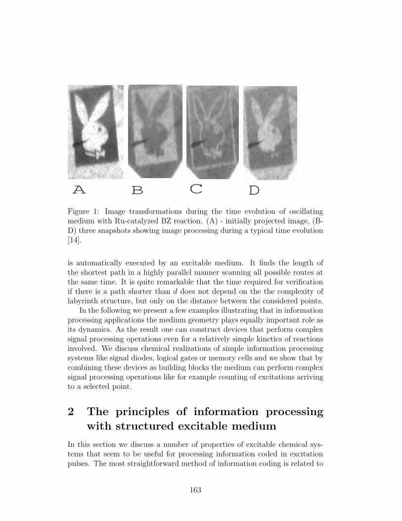
A B C DFigure 1: Image transformations during the time evolution of oscillatingmedium with Ru-catalyzed BZ reaction. (A) - initially projected image, (B-D) three snapshots showing image processing during a typical time evolution[14].

is automatically executed by an excitable medium. It finds the length ofthe shortest path in a highly parallel manner scanning all possible routes atthe same time. It is quite remarkable that the time required for verificationif there is a path shorter than d does not depend on the the complexity oflabyrinth structure, but only on the distance between the considered points.

In the following we present a few examples illustrating that in informationprocessing applications the medium geometry plays equally important role asits dynamics. As the result one can construct devices that perform complexsignal processing operations even for a relatively simple kinetics of reactionsinvolved. We discuss chemical realizations of simple information processingsystems like signal diodes, logical gates or memory cells and we show that bycombining these devices as building blocks the medium can perform complexsignal processing operations like for example counting of excitations arrivingto a selected point.

2 The principles of information processing

with structured excitable medium

In this section we discuss a number of properties of excitable chemical sys-tems that seem to be useful for processing information coded in excitationpulses. The most straightforward method of information coding is related to

163

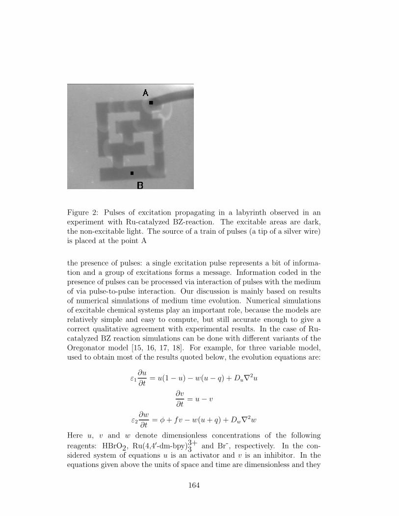
Figure 2: Pulses of excitation propagating in a labyrinth observed in anexperiment with Ru-catalyzed BZ-reaction. The excitable areas are dark,the non-excitable light. The source of a train of pulses (a tip of a silver wire)is placed at the point A

the presence of pulses: a single excitation pulse represents a bit of informa-tion and a group of excitations forms a message. Information coded in thepresence of pulses can be processed via interaction of pulses with the mediumof via pulse-to-pulse interaction. Our discussion is mainly based on resultsof numerical simulations of medium time evolution. Numerical simulationsof excitable chemical systems play an important role, because the models arerelatively simple and easy to compute, but still accurate enough to give acorrect qualitative agreement with experimental results. In the case of Ru-catalyzed BZ reaction simulations can be done with different variants of theOregonator model [15, 16, 17, 18]. For example, for three variable model,used to obtain most of the results quoted below, the evolution equations are:

ε1∂u

∂t= u(1 − u) − w(u − q) + Du∇2u

∂v

∂t= u − v

ε2∂w

∂t= φ + fv − w(u + q) + Dw∇2w

Here u, v and w denote dimensionless concentrations of the following

reagents: HBrO2, Ru(4,4′-dm-bpy)3+3 and Br-, respectively. In the con-

sidered system of equations u is an activator and v is an inhibitor. In theequations given above the units of space and time are dimensionless and they

164

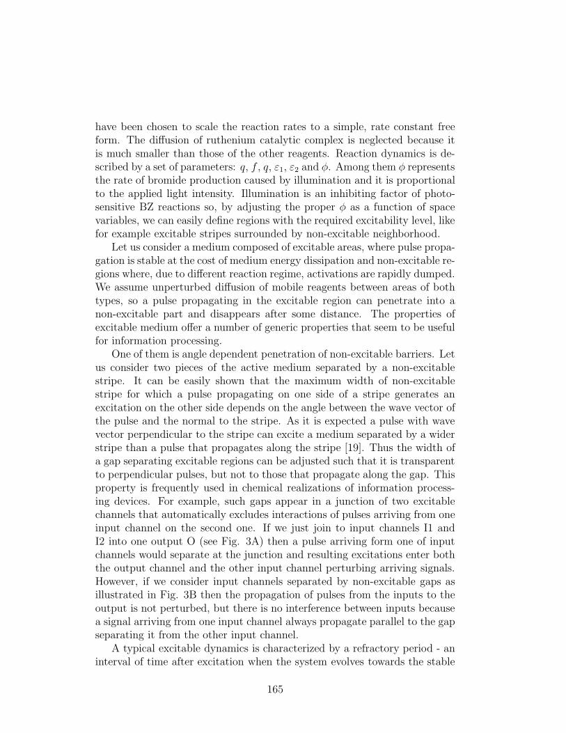
have been chosen to scale the reaction rates to a simple, rate constant freeform. The diffusion of ruthenium catalytic complex is neglected because itis much smaller than those of the other reagents. Reaction dynamics is de-scribed by a set of parameters: q, f , q, ε1, ε2 and φ. Among them φ representsthe rate of bromide production caused by illumination and it is proportionalto the applied light intensity. Illumination is an inhibiting factor of photo-sensitive BZ reactions so, by adjusting the proper φ as a function of spacevariables, we can easily define regions with the required excitability level, likefor example excitable stripes surrounded by non-excitable neighborhood.

Let us consider a medium composed of excitable areas, where pulse propa-gation is stable at the cost of medium energy dissipation and non-excitable re-gions where, due to different reaction regime, activations are rapidly dumped.We assume unperturbed diffusion of mobile reagents between areas of bothtypes, so a pulse propagating in the excitable region can penetrate into anon-excitable part and disappears after some distance. The properties ofexcitable medium offer a number of generic properties that seem to be usefulfor information processing.

One of them is angle dependent penetration of non-excitable barriers. Letus consider two pieces of the active medium separated by a non-excitablestripe. It can be easily shown that the maximum width of non-excitablestripe for which a pulse propagating on one side of a stripe generates anexcitation on the other side depends on the angle between the wave vector ofthe pulse and the normal to the stripe. As it is expected a pulse with wavevector perpendicular to the stripe can excite a medium separated by a widerstripe than a pulse that propagates along the stripe [19]. Thus the width ofa gap separating excitable regions can be adjusted such that it is transparentto perpendicular pulses, but not to those that propagate along the gap. Thisproperty is frequently used in chemical realizations of information process-ing devices. For example, such gaps appear in a junction of two excitablechannels that automatically excludes interactions of pulses arriving from oneinput channel on the second one. If we just join to input channels I1 andI2 into one output O (see Fig. 3A) then a pulse arriving form one of inputchannels would separate at the junction and resulting excitations enter boththe output channel and the other input channel perturbing arriving signals.However, if we consider input channels separated by non-excitable gaps asillustrated in Fig. 3B then the propagation of pulses from the inputs to theoutput is not perturbed, but there is no interference between inputs becausea signal arriving from one input channel always propagate parallel to the gapseparating it from the other input channel.

A typical excitable dynamics is characterized by a refractory period - aninterval of time after excitation when the system evolves towards the stable

165

(A) (B)

Figure 3: The junction of two input channels I1, I2 into a single outputO (a logical OR gate). The black regions are excitable, the white space isnon-excitable. (A) - simple junction, (B) - a junction in which interactionsbetween inputs are excluded.

state and its repeated excitation is difficult due to a large concentration ofinhibitor. For propagating pulses it means that the region behind a pulse isin the refractory regime characterized by a large amplitude of inhibitor andit cannot be re-excited. One of the consequences of a long refractory periodis annihilation of colliding counterpropagating pulses. Another interestingexample of behavior resulting from refractory region behind a pulse can beobserved in a cross-shaped structure build of excitable channels, separatedby gaps penetrable for perpendicular pulses [20, 21] shown in Fig. 4. Theanswer of cross-shaped junction to a pair pulses arriving from two perpendic-ular directions has been studied as a function of the time difference betweenpulses. Of course if the time difference is large pulses propagate indepen-dently along one line. If the time difference is small then the cross-junctionacts like the AND gate and the output excitation appears in one of the cor-ner areas. However, for a certain time difference the first arriving pulse isable to redirect the second and force it to follow. The effect is related withuncompleted relaxation of the central area of the junction at the momentwhen the second pulse arrives. Pulse redirection seems to be an interestingeffect from the point of programming with excitation pulses, but in practiceit requites a high precision in selecting the right time difference.

166

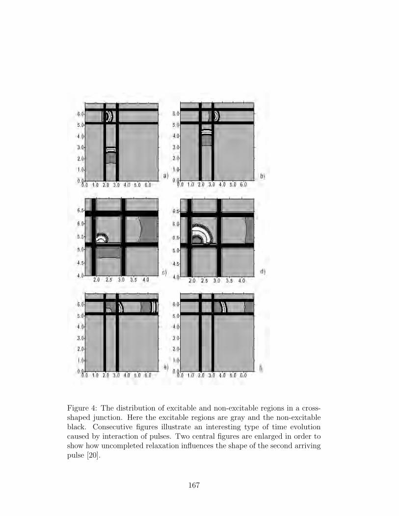
Figure 4: The distribution of excitable and non-excitable regions in a cross-shaped junction. Here the excitable regions are gray and the non-excitableblack. Consecutive figures illustrate an interesting type of time evolutioncaused by interaction of pulses. Two central figures are enlarged in order toshow how uncompleted relaxation influences the shape of the second arrivingpulse [20].

167

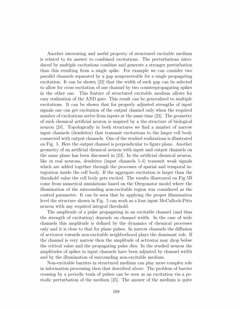
Another interesting and useful property of structured excitable mediumis related to its answer to combined excitations. The perturbations intro-duced by multiple excitations combine and generate a stronger perturbationthan this resulting from a single spike. For example we can consider twoparallel channels separated by a gap nonpenetrable for a single propagatingexcitation. It can be shown [22] that the width of such gap can be selectedto allow for cross excitation of one channel by two counterpropagating spikesin the other one. This feature of structured excitable medium allows foreasy realization of the AND gate. This result can be generalized to multipleexcitations. It can be shown that for properly adjusted strengths of inputsignals one can get excitation of the output channel only when the requirednumber of excitations arrive from inputs at the same time [23]. The geometryof such chemical artificial neuron is inspired by a the structure of biologicalneuron [24]. Topologically in both structures we find a number of narrowinput channels (dendrites) that transmit excitations to the larger cell bodyconnected with output channels. One of the studied realizations is illustratedon Fig. 5. Here the output channel is perpendicular to figure plane. Anothergeometry of an artificial chemical neuron with input and output channels onthe same plane has been discussed in [23]. In the artificial chemical neuron,like in real neurons, dendrites (input channels 1-4) transmit weak signalswhich are added together through the processes of spatial and temporal in-tegration inside the cell body. If the aggregate excitation is larger than thethreshold value the cell body gets excited. The results illustrated on Fig 5Bcome from numerical simulations based on the Oregonator model where theillumination of the surrounding non-excitable region was considered as thecontrol parameter. It can be seen that by applying the proper illuminationlevel the structure shown in Fig. 5 can work as a four input McCulloch-Pittsneuron with any required integral threshold.

The amplitude of a pulse propagating in an excitable channel (and thusthe strength of excitation) depends on channel width. In the case of widechannels this amplitude is defined by the dynamics of chemical processesonly and it is close to that for plane pulses. In narrow channels the diffusionof activator towards non-excitable neighborhood plays the dominant role. Ifthe channel is very narrow then the amplitude of activator may drop belowthe critical value and the propagating pulse dies. In the studied neuron theamplitudes of spikes in input channels have been adjusted by channel widthand by the illumination of surrounding non-excitable medium.

Non-excitable barriers in structured medium can play more complex rolein information processing then that described above. The problem of barriercrossing by a periodic train of pulses can be seen as an excitation via a pe-riodic perturbation of the medium [25]. The answer of the medium is quite

168

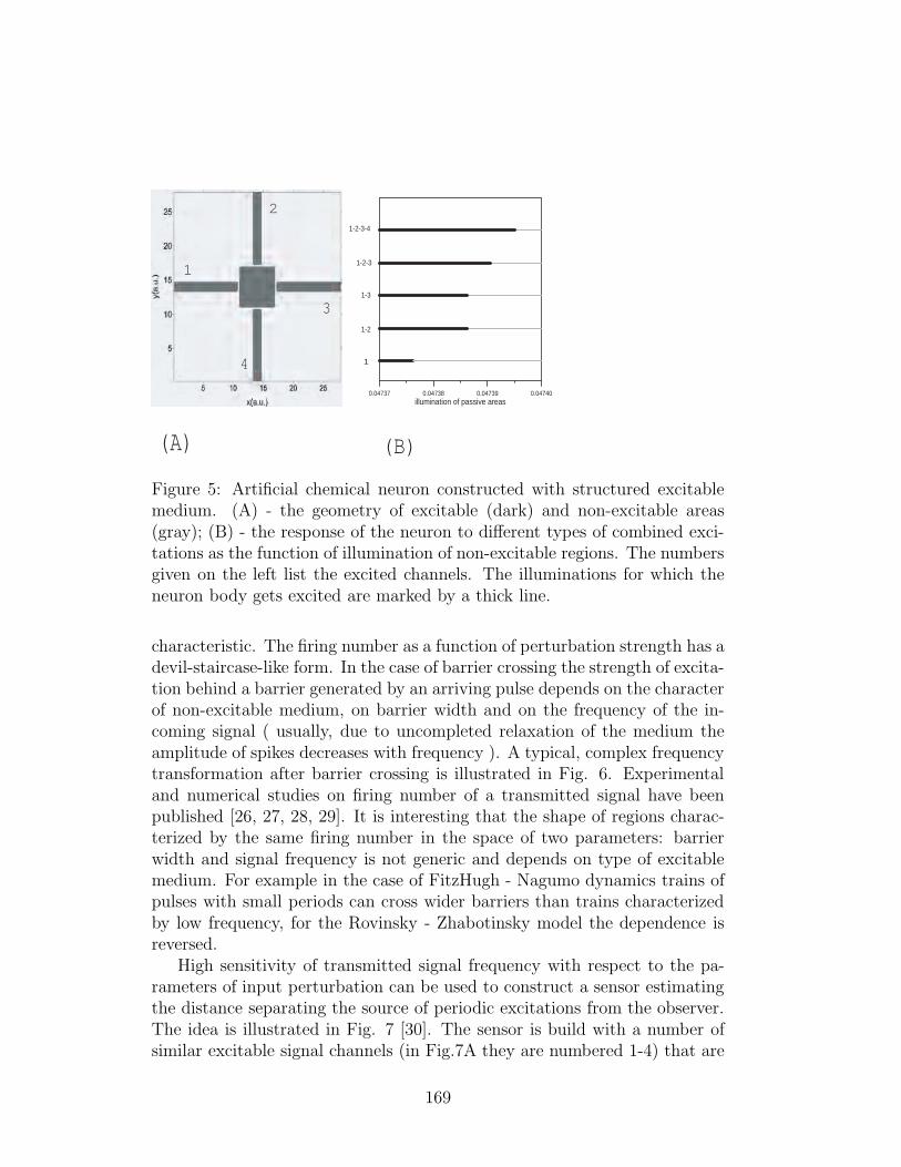
0.04737 0.04738 0.04739 0.04740illumination of passive areas

1

1-2

1-3

1-2-3

1-2-3-4

1

2

3

4

(A) (B)

Figure 5: Artificial chemical neuron constructed with structured excitablemedium. (A) - the geometry of excitable (dark) and non-excitable areas(gray); (B) - the response of the neuron to different types of combined exci-tations as the function of illumination of non-excitable regions. The numbersgiven on the left list the excited channels. The illuminations for which theneuron body gets excited are marked by a thick line.

characteristic. The firing number as a function of perturbation strength has adevil-staircase-like form. In the case of barrier crossing the strength of excita-tion behind a barrier generated by an arriving pulse depends on the characterof non-excitable medium, on barrier width and on the frequency of the in-coming signal ( usually, due to uncompleted relaxation of the medium theamplitude of spikes decreases with frequency ). A typical, complex frequencytransformation after barrier crossing is illustrated in Fig. 6. Experimentaland numerical studies on firing number of a transmitted signal have beenpublished [26, 27, 28, 29]. It is interesting that the shape of regions charac-terized by the same firing number in the space of two parameters: barrierwidth and signal frequency is not generic and depends on type of excitablemedium. For example in the case of FitzHugh - Nagumo dynamics trains ofpulses with small periods can cross wider barriers than trains characterizedby low frequency, for the Rovinsky - Zhabotinsky model the dependence isreversed.

High sensitivity of transmitted signal frequency with respect to the pa-rameters of input perturbation can be used to construct a sensor estimatingthe distance separating the source of periodic excitations from the observer.The idea is illustrated in Fig. 7 [30]. The sensor is build with a number ofsimilar excitable signal channels (in Fig.7A they are numbered 1-4) that are

169

Figure 6: A typical dependence of firing number as a function of frequencyof arriving pulses. The ratio between frequency of output signal (fo) aftercrossing a non-excitable gap separating excitable channel and the input one(fp). Results obtained for the FitzHugh - Nagumo model.

wide enough to ensure a stable propagation of pulses. These sensor chan-nels are separated one from another by parallel non-excitable gaps that donot allow for the interference between pulses propagating in the neighboringchannels. They are also separated from the active medium M by a non ex-citable sensor gap G. The width of this gap is crucial for sensor sensitivity.If the gap is too wide then no excitation of the medium M can generate apulse in the sensor channels. If the gap is narrow then any excitation in frontof a sensor channel can pass G and create a pulse in the channel so signalsin every sensor channel are identical. The width of the gap should be se-lected such that the firing number (defined as the ratio between the numberof pulses that crossed the gap G to the number of pulses of excitation thatwere created in the medium M) depends on the wave vector characterizinga pulse at the gap in front of channel. If the source of periodic excitations Sis close to the array of sensor channels then the wave vectors characterizingexcitations in front of various channels are different. Thus, different frequen-cies of excitations in various channels are expected. On the other hand, ifthe source of excitations is far away from the gap G then the wave vectors infront of different channels should be almost identical and so the frequencies ofexcitations in sensor channels would not differ. Therefore, the system shownin Fig. 7A can sense the distance separating it from the source of excitations.

170

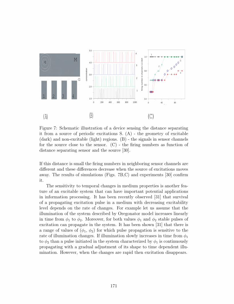
MS

G

1 2 3 4

(A)

0 200 400 600 800 1000ti

1.0

2.0

3.0

4.0

5.0

con

cen

tra

tion

1

2

3

4

0 40 80di t

0.4

0.6

0.8

1.0

firing n

um

ber

in c

hannels

1,2

,3&

4

1

2

3

4

(C)(B)

Figure 7: Schematic illustration of a device sensing the distance separatingit from a source of periodic excitations S. (A) - the geometry of excitable(dark) and non-excitable (light) regions. (B) - the signals in sensor channelsfor the source close to the sensor. (C) - the firing numbers as function ofdistance separating sensor and the source [30].

If this distance is small the firing numbers in neighboring sensor channels aredifferent and these differences decrease when the source of excitations movesaway. The results of simulations (Figs. 7B,C) and experiments [30] confirmit.

The sensitivity to temporal changes in medium properties is another fea-ture of an excitable system that can have important potential applicationsin information processing. It has been recently observed [31] that survivalof a propagating excitation pulse in a medium with decreasing excitabilitylevel depends on the rate of changes. For example let us assume that theillumination of the system described by Oregonator model increases linearlyin time from φ1 to φ2. Moreover, for both values φ1 and φ2 stable pulses ofexcitation can propagate in the system. It has been shown [31] that there isa range of values of (φ1, φ2) for which pulse propagation is sensitive to therate of illumination changes. If illumination slowly increases in time from φ1

to φ2 than a pulse initiated in the system characterized by φ1 is continuouslypropagating with a gradual adjustment of its shape to time dependent illu-mination. However, when the changes are rapid then excitation disappears.

171

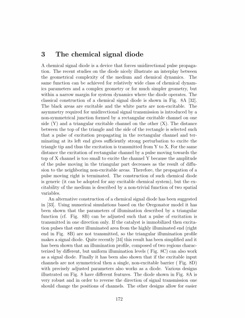
3 The chemical signal diode

A chemical signal diode is a device that forces unidirectional pulse propaga-tion. The recent studies on the diode nicely illustrate an interplay betweenthe geometrical complexity of the medium and chemical dynamics. Thesame function can be achieved for relatively wide class of chemical dynam-ics parameters and a complex geometry or for much simpler geometry, butwithin a narrow margin for system dynamics where the diode operates. Theclassical construction of a chemical signal diode is shown in Fig. 8A [32].The black areas are excitable and the white parts are non-excitable. Theasymmetry required for unidirectional signal transmission is introduced by anon-symmetrical junction formed by a rectangular excitable channel on oneside (Y) and a triangular excitable channel on the other (X). The distancebetween the top of the triangle and the side of the rectangle is selected suchthat a pulse of excitation propagating in the rectangular channel and ter-minating at its left end gives sufficiently strong perturbation to excite thetriangle tip and thus the excitation is transmitted from Y to X. For the samedistance the excitation of rectangular channel by a pulse moving towards thetop of X channel is too small to excite the channel Y because the amplitudeof the pulse moving in the triangular part decreases as the result of diffu-sion to the neighboring non-excitable areas. Therefore, the propagation of apulse moving right is terminated. The construction of such chemical diodeis generic (it can be adopted for any excitable chemical system), but the ex-citability of the medium is described by a non-trivial function of two spatialvariables.

An alternative construction of a chemical signal diode has been suggestedin [33]. Using numerical simulations based on the Oregonator model it hasbeen shown that the parameters of illumination described by a triangularfunction (cf. Fig. 8B) can be adjusted such that a pulse of excitation istransmitted in one direction only. If the catalyst is immobilized then excita-tion pulses that enter illuminated area from the highly illuminated end (rightend in Fig. 8B) are not transmitted, so the triangular illumination profilemakes a signal diode. Quite recently [34] this result has been simplified and ithas been shown that an illumination profile, composed of two regions charac-terized by different, but uniform illumination levels ( Fig. 8C) can also workas a signal diode. Finally it has been also shown that if the excitable inputchannels are not symmetrical then a single, non-excitable barrier ( Fig. 8D)with precisely adjusted parameters also works as a diode. Various designsillustrated on Fig. 8 have different features. The diode shown in Fig. 8A isvery robust and in order to reverse the direction of signal transmission oneshould change the positions of channels. The other designs allow for easier

172

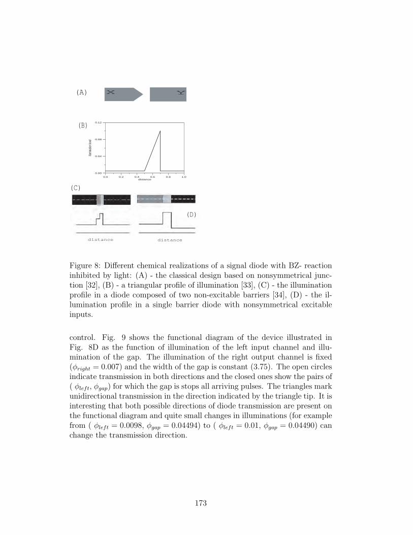
X Y

0.0 0.2 0.4 0.6 0.8 1.0distance

0.00

0.04

0.08

0.12

illumi

natio

n lev

el(A)

(B)

(C)

(D)

distance distance

Figure 8: Different chemical realizations of a signal diode with BZ- reactioninhibited by light: (A) - the classical design based on nonsymmetrical junc-tion [32], (B) - a triangular profile of illumination [33], (C) - the illuminationprofile in a diode composed of two non-excitable barriers [34], (D) - the il-lumination profile in a single barrier diode with nonsymmetrical excitableinputs.

control. Fig. 9 shows the functional diagram of the device illustrated inFig. 8D as the function of illumination of the left input channel and illu-mination of the gap. The illumination of the right output channel is fixed(φright = 0.007) and the width of the gap is constant (3.75). The open circlesindicate transmission in both directions and the closed ones show the pairs of( φleft, φgap) for which the gap is stops all arriving pulses. The triangles markunidirectional transmission in the direction indicated by the triangle tip. It isinteresting that both possible directions of diode transmission are present onthe functional diagram and quite small changes in illuminations (for examplefrom ( φleft = 0.0098, φgap = 0.04494) to ( φleft = 0.01, φgap = 0.04490) canchange the transmission direction.

173

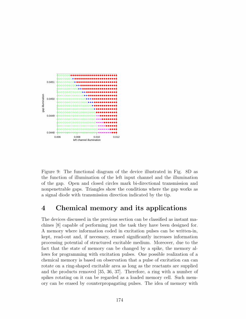
0.006 0.008 0.010 0.012left channel illumination

0.0448

0.0449

0.0450

0.0451

gap

illum

inat

ion

Figure 9: The functional diagram of the device illustrated in Fig. 8D asthe function of illumination of the left input channel and the illuminationof the gap. Open and closed circles mark bi-directional transmission andnonpenetrable gaps. Triangles show the conditions where the gap works asa signal diode with transmission direction indicated by the tip.

4 Chemical memory and its applications

The devices discussed in the previous section can be classified as instant ma-chines [8] capable of performing just the task they have been designed for.A memory where information coded in excitation pulses can be written-in,kept, read-out and, if necessary, erased significantly increases informationprocessing potential of structured excitable medium. Moreover, due to thefact that the state of memory can be changed by a spike, the memory al-lows for programming with excitation pulses. One possible realization of achemical memory is based on observation that a pulse of excitation can canrotate on a ring-shaped excitable area as long as the reactants are suppliedand the products removed [35, 36, 37]. Therefore, a ring with a number ofspikes rotating on it can be regarded as a loaded memory cell. Such mem-ory can be erased by counterpropagating pulses. The idea of memory with

174

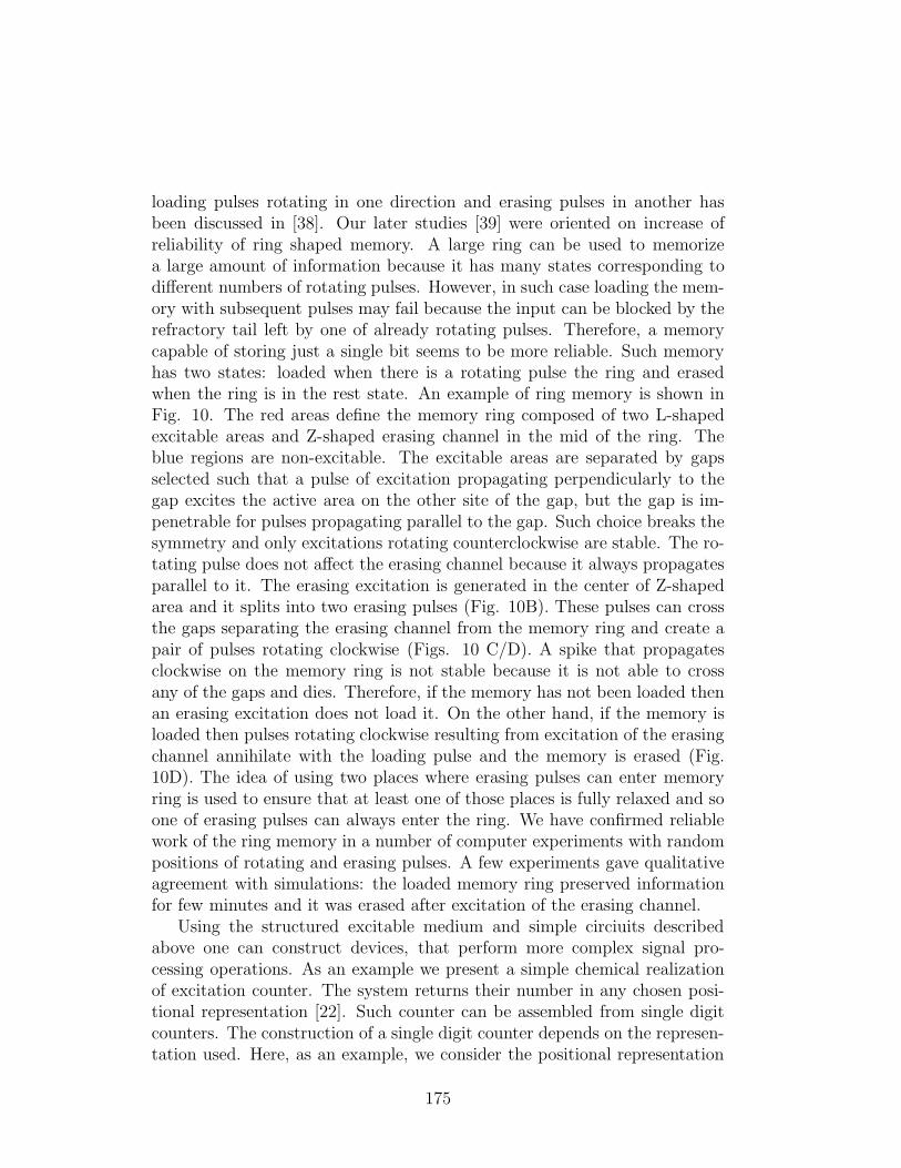
loading pulses rotating in one direction and erasing pulses in another hasbeen discussed in [38]. Our later studies [39] were oriented on increase ofreliability of ring shaped memory. A large ring can be used to memorizea large amount of information because it has many states corresponding todifferent numbers of rotating pulses. However, in such case loading the mem-ory with subsequent pulses may fail because the input can be blocked by therefractory tail left by one of already rotating pulses. Therefore, a memorycapable of storing just a single bit seems to be more reliable. Such memoryhas two states: loaded when there is a rotating pulse the ring and erasedwhen the ring is in the rest state. An example of ring memory is shown inFig. 10. The red areas define the memory ring composed of two L-shapedexcitable areas and Z-shaped erasing channel in the mid of the ring. Theblue regions are non-excitable. The excitable areas are separated by gapsselected such that a pulse of excitation propagating perpendicularly to thegap excites the active area on the other site of the gap, but the gap is im-penetrable for pulses propagating parallel to the gap. Such choice breaks thesymmetry and only excitations rotating counterclockwise are stable. The ro-tating pulse does not affect the erasing channel because it always propagatesparallel to it. The erasing excitation is generated in the center of Z-shapedarea and it splits into two erasing pulses (Fig. 10B). These pulses can crossthe gaps separating the erasing channel from the memory ring and create apair of pulses rotating clockwise (Figs. 10 C/D). A spike that propagatesclockwise on the memory ring is not stable because it is not able to crossany of the gaps and dies. Therefore, if the memory has not been loaded thenan erasing excitation does not load it. On the other hand, if the memory isloaded then pulses rotating clockwise resulting from excitation of the erasingchannel annihilate with the loading pulse and the memory is erased (Fig.10D). The idea of using two places where erasing pulses can enter memoryring is used to ensure that at least one of those places is fully relaxed and soone of erasing pulses can always enter the ring. We have confirmed reliablework of the ring memory in a number of computer experiments with randompositions of rotating and erasing pulses. A few experiments gave qualitativeagreement with simulations: the loaded memory ring preserved informationfor few minutes and it was erased after excitation of the erasing channel.

Using the structured excitable medium and simple circiuits describedabove one can construct devices, that perform more complex signal pro-cessing operations. As an example we present a simple chemical realizationof excitation counter. The system returns their number in any chosen posi-tional representation [22]. Such counter can be assembled from single digitcounters. The construction of a single digit counter depends on the represen-tation used. Here, as an example, we consider the positional representation

175

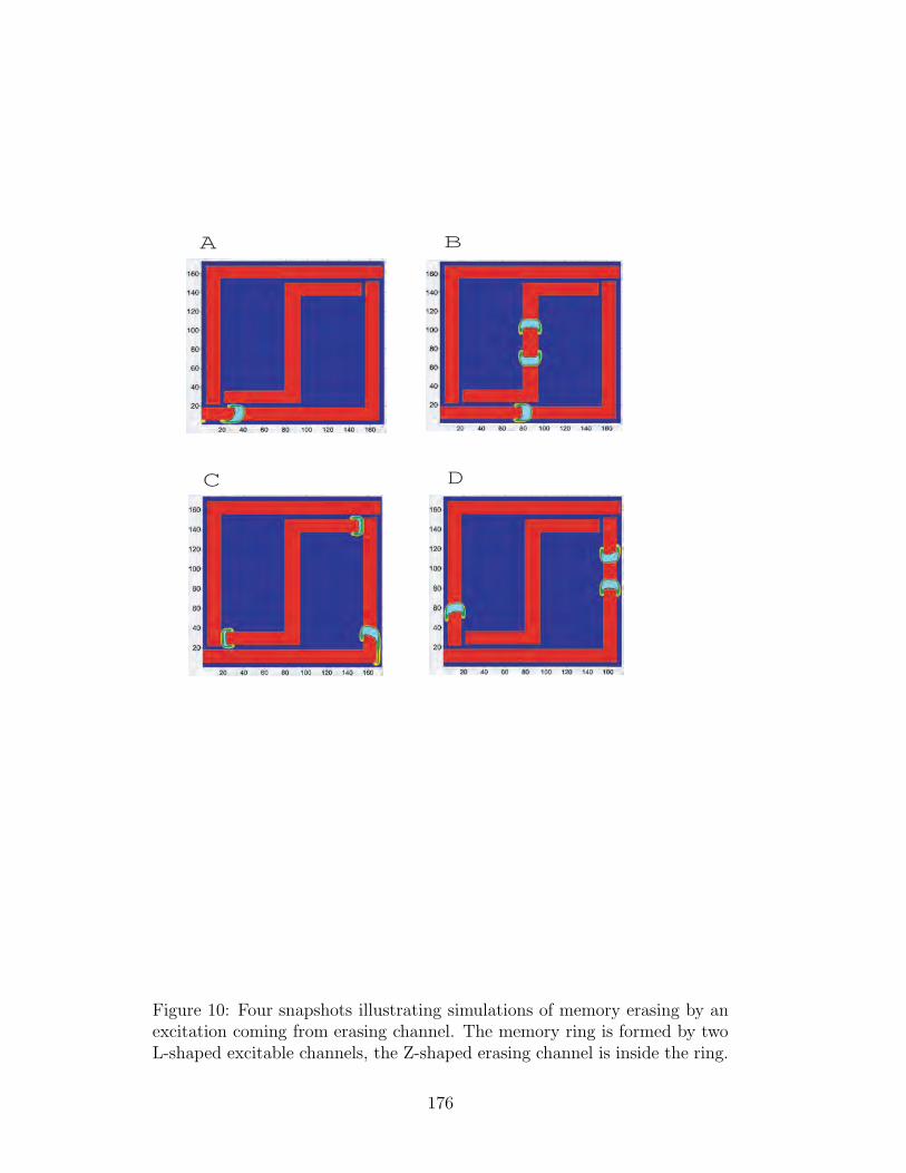
A

C

B

D

Figure 10: Four snapshots illustrating simulations of memory erasing by anexcitation coming from erasing channel. The memory ring is formed by twoL-shaped excitable channels, the Z-shaped erasing channel is inside the ring.

176

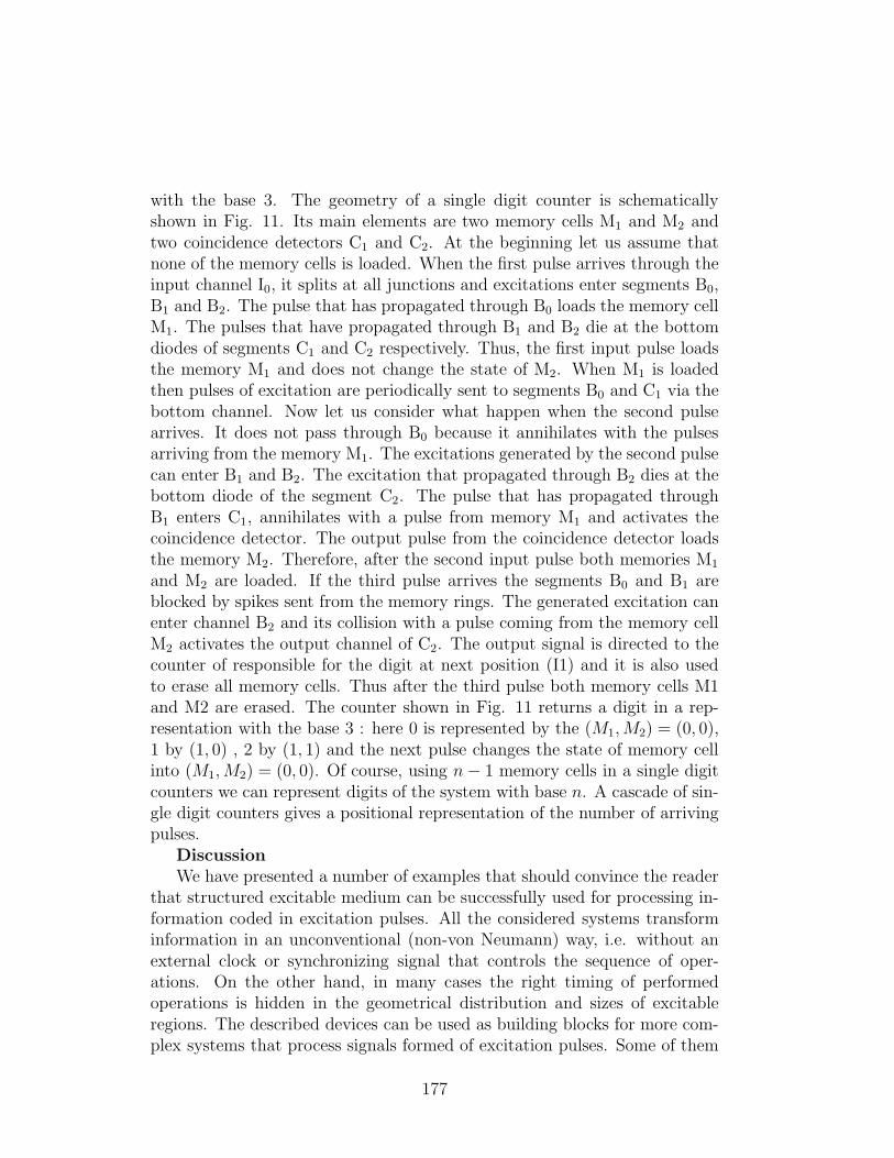
with the base 3. The geometry of a single digit counter is schematicallyshown in Fig. 11. Its main elements are two memory cells M1 and M2 andtwo coincidence detectors C1 and C2. At the beginning let us assume thatnone of the memory cells is loaded. When the first pulse arrives through theinput channel I0, it splits at all junctions and excitations enter segments B0,B1 and B2. The pulse that has propagated through B0 loads the memory cellM1. The pulses that have propagated through B1 and B2 die at the bottomdiodes of segments C1 and C2 respectively. Thus, the first input pulse loadsthe memory M1 and does not change the state of M2. When M1 is loadedthen pulses of excitation are periodically sent to segments B0 and C1 via thebottom channel. Now let us consider what happen when the second pulsearrives. It does not pass through B0 because it annihilates with the pulsesarriving from the memory M1. The excitations generated by the second pulsecan enter B1 and B2. The excitation that propagated through B2 dies at thebottom diode of the segment C2. The pulse that has propagated throughB1 enters C1, annihilates with a pulse from memory M1 and activates thecoincidence detector. The output pulse from the coincidence detector loadsthe memory M2. Therefore, after the second input pulse both memories M1

and M2 are loaded. If the third pulse arrives the segments B0 and B1 areblocked by spikes sent from the memory rings. The generated excitation canenter channel B2 and its collision with a pulse coming from the memory cellM2 activates the output channel of C2. The output signal is directed to thecounter of responsible for the digit at next position (I1) and it is also usedto erase all memory cells. Thus after the third pulse both memory cells M1and M2 are erased. The counter shown in Fig. 11 returns a digit in a rep-resentation with the base 3 : here 0 is represented by the (M1, M2) = (0, 0),1 by (1, 0) , 2 by (1, 1) and the next pulse changes the state of memory cellinto (M1, M2) = (0, 0). Of course, using n − 1 memory cells in a single digitcounters we can represent digits of the system with base n. A cascade of sin-gle digit counters gives a positional representation of the number of arrivingpulses.

DiscussionWe have presented a number of examples that should convince the reader

that structured excitable medium can be successfully used for processing in-formation coded in excitation pulses. All the considered systems transforminformation in an unconventional (non-von Neumann) way, i.e. without anexternal clock or synchronizing signal that controls the sequence of oper-ations. On the other hand, in many cases the right timing of performedoperations is hidden in the geometrical distribution and sizes of excitableregions. The described devices can be used as building blocks for more com-plex systems that process signals formed of excitation pulses. Some of them

177

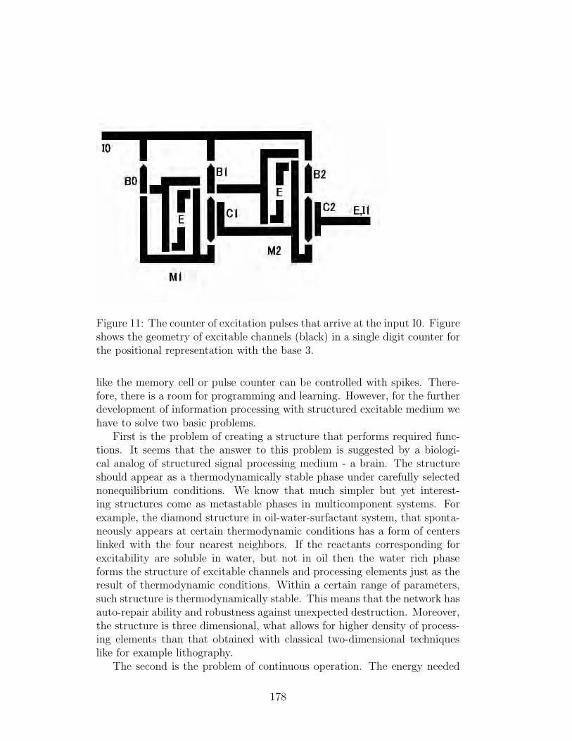
Figure 11: The counter of excitation pulses that arrive at the input I0. Figureshows the geometry of excitable channels (black) in a single digit counter forthe positional representation with the base 3.

like the memory cell or pulse counter can be controlled with spikes. There-fore, there is a room for programming and learning. However, for the furtherdevelopment of information processing with structured excitable medium wehave to solve two basic problems.

First is the problem of creating a structure that performs required func-tions. It seems that the answer to this problem is suggested by a biologi-cal analog of structured signal processing medium - a brain. The structureshould appear as a thermodynamically stable phase under carefully selectednonequilibrium conditions. We know that much simpler but yet interest-ing structures come as metastable phases in multicomponent systems. Forexample, the diamond structure in oil-water-surfactant system, that sponta-neously appears at certain thermodynamic conditions has a form of centerslinked with the four nearest neighbors. If the reactants corresponding forexcitability are soluble in water, but not in oil then the water rich phaseforms the structure of excitable channels and processing elements just as theresult of thermodynamic conditions. Within a certain range of parameters,such structure is thermodynamically stable. This means that the network hasauto-repair ability and robustness against unexpected destruction. Moreover,the structure is three dimensional, what allows for higher density of process-ing elements than that obtained with classical two-dimensional techniqueslike for example lithography.

The second is the problem of continuous operation. The energy needed

178

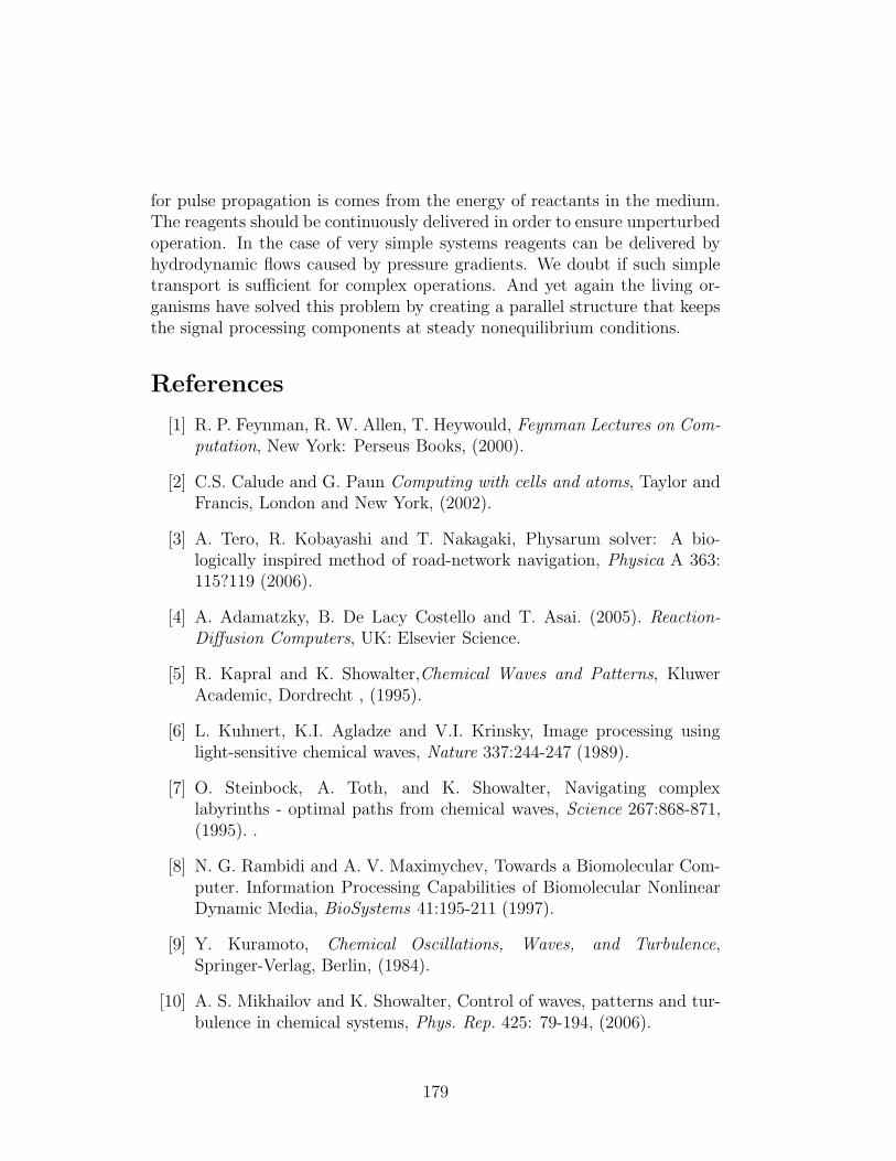
for pulse propagation is comes from the energy of reactants in the medium.The reagents should be continuously delivered in order to ensure unperturbedoperation. In the case of very simple systems reagents can be delivered byhydrodynamic flows caused by pressure gradients. We doubt if such simpletransport is sufficient for complex operations. And yet again the living or-ganisms have solved this problem by creating a parallel structure that keepsthe signal processing components at steady nonequilibrium conditions.

References

[1] R. P. Feynman, R. W. Allen, T. Heywould, Feynman Lectures on Com-putation, New York: Perseus Books, (2000).

[2] C.S. Calude and G. Paun Computing with cells and atoms, Taylor andFrancis, London and New York, (2002).

[3] A. Tero, R. Kobayashi and T. Nakagaki, Physarum solver: A bio-logically inspired method of road-network navigation, Physica A 363:115?119 (2006).

[4] A. Adamatzky, B. De Lacy Costello and T. Asai. (2005). Reaction-Diffusion Computers, UK: Elsevier Science.

[5] R. Kapral and K. Showalter,Chemical Waves and Patterns, KluwerAcademic, Dordrecht , (1995).

[6] L. Kuhnert, K.I. Agladze and V.I. Krinsky, Image processing usinglight-sensitive chemical waves, Nature 337:244-247 (1989).

[7] O. Steinbock, A. Toth, and K. Showalter, Navigating complexlabyrinths - optimal paths from chemical waves, Science 267:868-871,(1995). .

[8] N. G. Rambidi and A. V. Maximychev, Towards a Biomolecular Com-puter. Information Processing Capabilities of Biomolecular NonlinearDynamic Media, BioSystems 41:195-211 (1997).

[9] Y. Kuramoto, Chemical Oscillations, Waves, and Turbulence,Springer-Verlag, Berlin, (1984).

[10] A. S. Mikhailov and K. Showalter, Control of waves, patterns and tur-bulence in chemical systems, Phys. Rep. 425: 79-194, (2006).

179

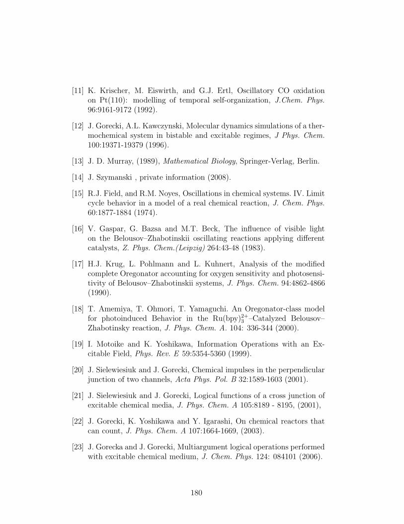
[11] K. Krischer, M. Eiswirth, and G.J. Ertl, Oscillatory CO oxidationon Pt(110): modelling of temporal self-organization, J.Chem. Phys.96:9161-9172 (1992).

[12] J. Gorecki, A.L. Kawczynski, Molecular dynamics simulations of a ther-mochemical system in bistable and excitable regimes, J Phys. Chem.100:19371-19379 (1996).

[13] J. D. Murray, (1989), Mathematical Biology, Springer-Verlag, Berlin.

[14] J. Szymanski , private information (2008).

[15] R.J. Field, and R.M. Noyes, Oscillations in chemical systems. IV. Limitcycle behavior in a model of a real chemical reaction, J. Chem. Phys.60:1877-1884 (1974).

[16] V. Gaspar, G. Bazsa and M.T. Beck, The influence of visible lighton the Belousov–Zhabotinskii oscillating reactions applying differentcatalysts, Z. Phys. Chem.(Leipzig) 264:43-48 (1983).

[17] H.J. Krug, L. Pohlmann and L. Kuhnert, Analysis of the modifiedcomplete Oregonator accounting for oxygen sensitivity and photosensi-tivity of Belousov–Zhabotinskii systems, J. Phys. Chem. 94:4862-4866(1990).

[18] T. Amemiya, T. Ohmori, T. Yamaguchi. An Oregonator-class modelfor photoinduced Behavior in the Ru(bpy)2+

3 –Catalyzed Belousov–Zhabotinsky reaction, J. Phys. Chem. A. 104: 336-344 (2000).

[19] I. Motoike and K. Yoshikawa, Information Operations with an Ex-citable Field, Phys. Rev. E 59:5354-5360 (1999).

[20] J. Sielewiesiuk and J. Gorecki, Chemical impulses in the perpendicularjunction of two channels, Acta Phys. Pol. B 32:1589-1603 (2001).

[21] J. Sielewiesiuk and J. Gorecki, Logical functions of a cross junction ofexcitable chemical media, J. Phys. Chem. A 105:8189 - 8195, (2001),

[22] J. Gorecki, K. Yoshikawa and Y. Igarashi, On chemical reactors thatcan count, J. Phys. Chem. A 107:1664-1669, (2003).

[23] J. Gorecka and J. Gorecki, Multiargument logical operations performedwith excitable chemical medium, J. Chem. Phys. 124: 084101 (2006).

180

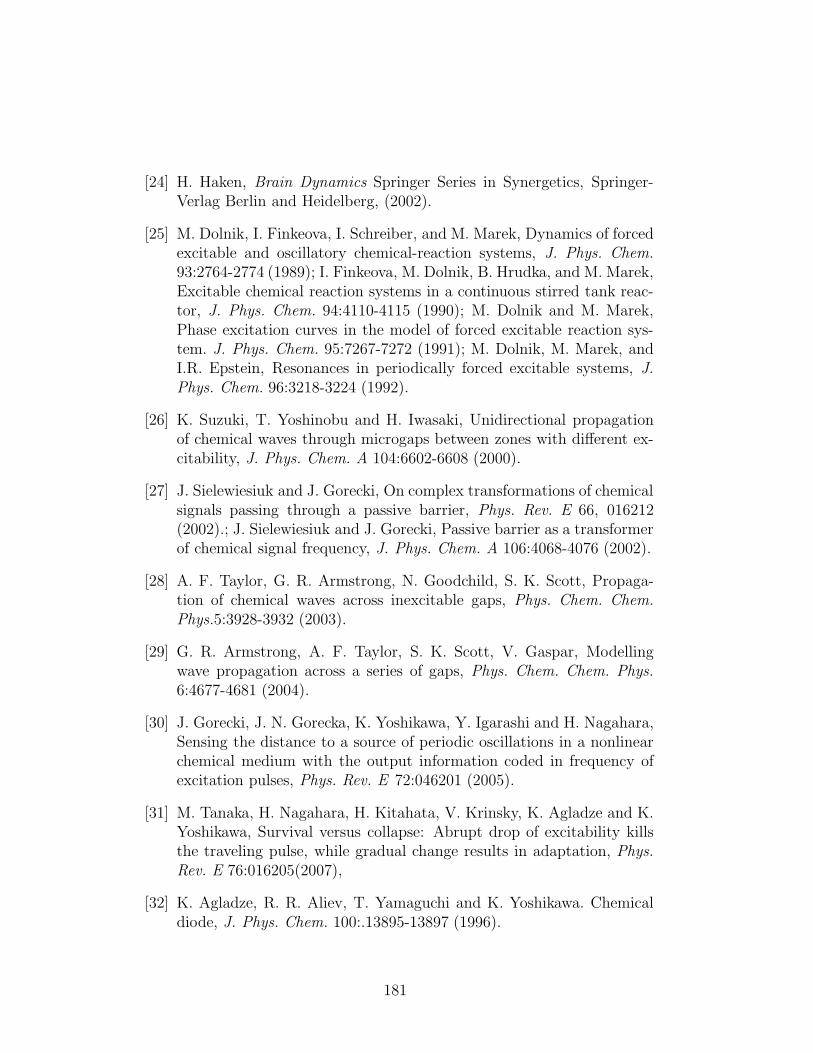
[24] H. Haken, Brain Dynamics Springer Series in Synergetics, Springer-Verlag Berlin and Heidelberg, (2002).

[25] M. Dolnik, I. Finkeova, I. Schreiber, and M. Marek, Dynamics of forcedexcitable and oscillatory chemical-reaction systems, J. Phys. Chem.93:2764-2774 (1989); I. Finkeova, M. Dolnik, B. Hrudka, and M. Marek,Excitable chemical reaction systems in a continuous stirred tank reac-tor, J. Phys. Chem. 94:4110-4115 (1990); M. Dolnik and M. Marek,Phase excitation curves in the model of forced excitable reaction sys-tem. J. Phys. Chem. 95:7267-7272 (1991); M. Dolnik, M. Marek, andI.R. Epstein, Resonances in periodically forced excitable systems, J.Phys. Chem. 96:3218-3224 (1992).

[26] K. Suzuki, T. Yoshinobu and H. Iwasaki, Unidirectional propagationof chemical waves through microgaps between zones with different ex-citability, J. Phys. Chem. A 104:6602-6608 (2000).

[27] J. Sielewiesiuk and J. Gorecki, On complex transformations of chemicalsignals passing through a passive barrier, Phys. Rev. E 66, 016212(2002).; J. Sielewiesiuk and J. Gorecki, Passive barrier as a transformerof chemical signal frequency, J. Phys. Chem. A 106:4068-4076 (2002).

[28] A. F. Taylor, G. R. Armstrong, N. Goodchild, S. K. Scott, Propaga-tion of chemical waves across inexcitable gaps, Phys. Chem. Chem.Phys.5:3928-3932 (2003).

[29] G. R. Armstrong, A. F. Taylor, S. K. Scott, V. Gaspar, Modellingwave propagation across a series of gaps, Phys. Chem. Chem. Phys.6:4677-4681 (2004).

[30] J. Gorecki, J. N. Gorecka, K. Yoshikawa, Y. Igarashi and H. Nagahara,Sensing the distance to a source of periodic oscillations in a nonlinearchemical medium with the output information coded in frequency ofexcitation pulses, Phys. Rev. E 72:046201 (2005).

[31] M. Tanaka, H. Nagahara, H. Kitahata, V. Krinsky, K. Agladze and K.Yoshikawa, Survival versus collapse: Abrupt drop of excitability killsthe traveling pulse, while gradual change results in adaptation, Phys.Rev. E 76:016205(2007),

[32] K. Agladze, R. R. Aliev, T. Yamaguchi and K. Yoshikawa. Chemicaldiode, J. Phys. Chem. 100:.13895-13897 (1996).

181

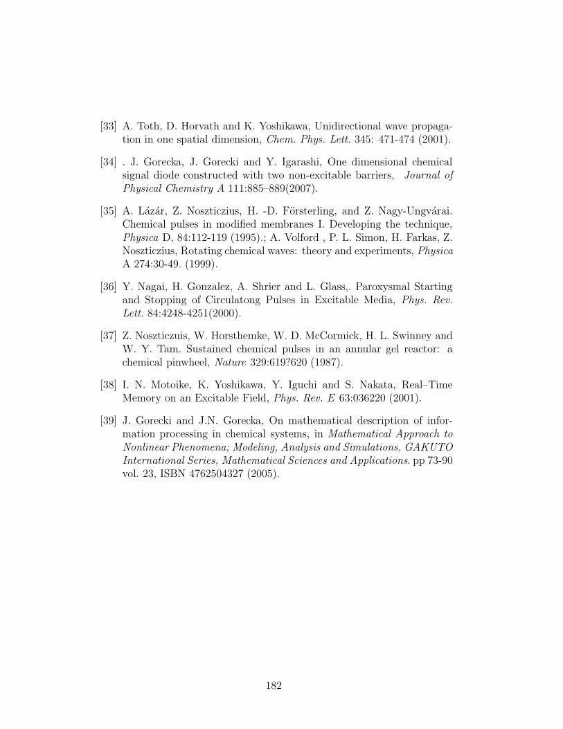
[33] A. Toth, D. Horvath and K. Yoshikawa, Unidirectional wave propaga-tion in one spatial dimension, Chem. Phys. Lett. 345: 471-474 (2001).

[34] . J. Gorecka, J. Gorecki and Y. Igarashi, One dimensional chemicalsignal diode constructed with two non-excitable barriers, Journal ofPhysical Chemistry A 111:885–889(2007).

[35] A. Lazar, Z. Noszticzius, H. -D. Forsterling, and Z. Nagy-Ungvarai.Chemical pulses in modified membranes I. Developing the technique,Physica D, 84:112-119 (1995).; A. Volford , P. L. Simon, H. Farkas, Z.Noszticzius, Rotating chemical waves: theory and experiments, PhysicaA 274:30-49. (1999).

[36] Y. Nagai, H. Gonzalez, A. Shrier and L. Glass,. Paroxysmal Startingand Stopping of Circulatong Pulses in Excitable Media, Phys. Rev.Lett. 84:4248-4251(2000).

[37] Z. Noszticzuis, W. Horsthemke, W. D. McCormick, H. L. Swinney andW. Y. Tam. Sustained chemical pulses in an annular gel reactor: achemical pinwheel, Nature 329:619?620 (1987).

[38] I. N. Motoike, K. Yoshikawa, Y. Iguchi and S. Nakata, Real–TimeMemory on an Excitable Field, Phys. Rev. E 63:036220 (2001).

[39] J. Gorecki and J.N. Gorecka, On mathematical description of infor-mation processing in chemical systems, in Mathematical Approach toNonlinear Phenomena; Modeling, Analysis and Simulations, GAKUTOInternational Series, Mathematical Sciences and Applications. pp 73-90vol. 23, ISBN 4762504327 (2005).

182

Computational bounds on polynomial

differential equations

Daniel S. Graca a,b , Jorge Buescu c,d ,Manuel L. Campagnolo e,b ,

aDM/FCT da Universidade do Algarve, PortugalbSQIG/Instituto de Telecomunicacoes, Lisboa, Portugal

cDM/FCUL, University of Lisbon, PortugaldCMAF, Lisbon, Portugal

eDM/ISA, Technical University of Lisbon, Portugal

Abstract

In this paper we study from a computational perspective some properties of thesolutions of polynomial ordinary differential equations.

We consider elementary (in the sense of Analysis) discrete-time dynamical sys-tems satisfying certain criteria of robustness. We show that those systems can besimulated with elementary and robust continuous-time dynamical systems whichcan be expanded into fully polynomial ordinary differential equations in Q[π]. Thissets a computational lower bound on polynomial ODEs since the former class islarge enough to include the dynamics of arbitrary Turing machines.

We also apply the previous methods to show that the problem of determiningwhether the maximal interval of definition of an initial-value problem defined withpolynomial ODEs is bounded or not is in general undecidable, even if the parametersof the system are computable and comparable and if the degree of the correspondingpolynomial is at most 56.

Combined with earlier results on the computability of solutions of polynomialODEs, one can conclude that there is from a computational point of view a closeconnection between these systems and Turing machines.

Email addresses: [email protected] (Daniel S. Graca), [email protected](Jorge Buescu), [email protected] (Manuel L. Campagnolo).

Preprint submitted to Elsevier 22 July 2008

1 Introduction

Differential equations are a powerful tool to model a diversity of phenomenain fields ranging from basic natural sciences like physics, chemistry or biologyto social sciences or economics. Among these, initial value problems (IVPs)of the form x′ = f(t, x), with x(t0) = x0, where f is a vector field and t isthe independent variable, play a predominant role. In this paper we considerthe large class of polynomial IVPs (PIVPs for short) in which f is a vector ofpolynomials. Many well known models, like the Lorenz equations in meteorol-ogy, the Lotka-Volterra equations for predator-prey systems, or Van der Pol’sequation in electronics [1] fall into this category. In Section 2 we show that infact all the elementary functions of Analysis are solutions of PIVPs. This is astronger version of the well established fact that all elementary functions aredifferentially algebraic [2]. It is also worth noticing that the solutions of PIVPsare precisely the set of functions definable with Shannon’s General PurposeAnalog Computer (GPAC) [3] as proved in [4].

While the qualitative behavior of linear systems (i. e. where f is linear) andplanar systems (where f : R3 → R2) is completely understood [5], it is notknown for all but a few cases how to predict the behavior of the solutionsof general PIVPs from the expression of f , which is the reason why manyfundamental questions about PIVPs (e.g. Hilbert’s 16th problem) are stillopen.

Since most nonlinear differential equations cannot be solved exactly, one hasto resort to numerical methods to obtain approximate solutions. This leads toa range of questions about computational properties of PIVPs. In particular,one can ask if PIVPs have computable approximations, if the domain of thesolution is computable, or even if deciding whether the maximal interval ofexistence is bounded is computable. Such questions have been answered foranalytic IVPs (where f is analytic) in [6]. In Section 2 we point out that theresults in [6] imply that the domain of existence of PIVP functions (i.e. so-lutions of PIVPs) is in general recursively enumerable and that the solutionis computable on its domain. This last result sets an upper bound on thecomputability of PIVP functions since it ensures that as long as f is polyno-mial and computable they can be arbitrarily approximated wherever they aredefined.

To obtain computational lower bounds for PIVPs, one can show that anycomputable function can be approximated by some PIVP function. In [7] itwas proved that under a simple (and unbounded) encoding in N3, the evolutionof Turing machines can be simulated with PIVPs. In this paper, we extendthat result and show that any computable discrete dynamical system on Nm

which admits a robust extension (to be defined) can be simulated with a PIVP.

184

The iteration of maps with IVPs is not new and can be found, for instance, in[8], [9]. However, those constructions are in some sense not satisfactory sincethey involve functions with some degree of discreteness (e.g. functions whichare not analytic or even have discontinuous derivatives) which can be used tobuild “exact clocks” that simulate the discrete steps of the iteration.

In Sections 3 and 4 we state and prove the main result of the paper. We showthat given a map ω on Nm, one can construct a PIVP with coefficients in Q[π]that simulates the iteration of ω as long as ω is extendable to a “robust” map Ωon Rm, in a sense to be defined in Section 3, and Ω is composition of polynomialand PIVP functions with parameters in Q[π] . The simulation is robust, whichis a necessity for our construction, but is also a natural requirement for acontinuous-time physical system described by an IVP. The constructions inSection 4 will also provide the necessary tools to address the issues discussedin the remainder of the paper.

Finally, in Section 5, we review and extend some undecidability results onPIVPs. Our results in [7] imply that reachability for PIVPs is undecidable,i.e., given a PIVP and some open set in phase space, there is no algorithm todecide if the solution of the PIVP crosses the open set. This contrasts with thedecidability of the reachability for linear differential equations [10]. In [11] weshowed that the boundedness of the domain of existence for PVIPs is undecid-able as long as f is polynomial of sufficiently high degree and computable. Atfirst sight, this result might seem trivial, since one can easily construct simplePIVPs which, upon varying one parameter, exhibit a critical value where thesolution is bounded on the left of this parameter value and unbounded on theright. For instance, the PIVP x′ = α(x2−1)t, x(0) = 3 has a maximal intervalwhich is bounded for α > 0 and unbounded if α ≤ 0. Since we cannot compareexactly two arbitrary computable reals [12] the boundedness problem for thePIVP above is undecidable. However, in Section 5 we show that if we con-sider that all input parameters are “comparable”, the boundedness problemremains undecidable. We also prove the claim in [11] that those undecidabilityresults hold for PIVPs where the degree of the polynomial is less or equal to56.

2 The GPAC, Polynomial Differential Equations, and ComputableAnalysis

In this section we introduce some useful definitions and results that will laterbe used in this paper.

Definition 1 Let I ⊆ R be a non-empty open interval and let t0 ∈ I. We saythat g : I → R is a PIVP function on I if it is a component of the solution of

185

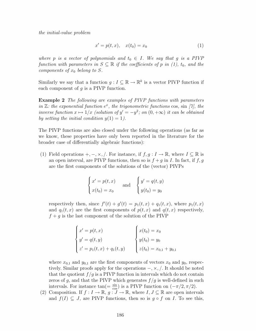
the initial-value problem

x′ = p(t, x), x(t0) = x0 (1)

where p is a vector of polynomials and t0 ∈ I. We say that g is a PIVPfunction with parameters in S ⊆ R if the coefficients of p in (1), t0, and thecomponents of x0 belong to S.

Similarly we say that a function g : I ⊆ R→ Rk is a vector PIVP function ifeach component of g is a PIVP function.

Example 2 The following are examples of PIVP functions with parametersin Z: the exponential function ex, the trigonometric functions cos, sin [7], theinverse function x 7→ 1/x (solution of y′ = −y2; on (0,+∞) it can be obtainedby setting the initial condition y(1) = 1).

The PIVP functions are also closed under the following operations (as far aswe know, these properties have only been reported in the literature for thebroader case of differentially algebraic functions):

(1) Field operations +,−,×, /. For instance, if f, g : I → R, where I ⊆ R isan open interval, are PIVP functions, then so is f + g in I. In fact, if f, gare the first components of the solutions of the (vector) PIVPs

x′ = p(t, x)

x(t0) = x0

and

y′ = q(t, y)

y(t0) = y0

respectively then, since f ′(t) + g′(t) = p1(t, x) + q1(t, x), where p1(t, x)and q1(t, x) are the first components of p(t, x) and q(t, x) respectively,f + g is the last component of the solution of the PIVP

x′ = p(t, x)

y′ = q(t, y)

z′ = p1(t, x) + q1(t, y)

x(t0) = x0

y(t0) = y0

z(t0) = x0,1 + y0,1

where x0,1 and y0,1 are the first components of vectors x0 and y0, respec-tively. Similar proofs apply for the operations −,×, /. It should be notedthat the quotient f/g is a PIVP function in intervals which do not containzeros of g, and that the PIVP which generates f/g is well-defined in suchintervals. For instance tan(= sin

cos) is a PIVP function on (−π/2, π/2).

(2) Composition. If f : I → R, g : J → R, where I, J ⊆ R are open intervalsand f(I) ⊆ J , are PIVP functions, then so is g f on I. To see this,

186

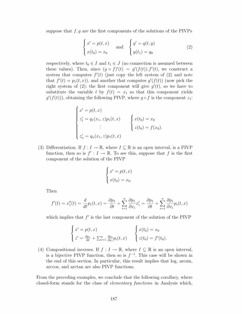
suppose that f, g are the first components of the solutions of the PIVPsx′ = p(t, x)

x(t0) = x0

and

y′ = q(t, y)

y(t1) = y0

(2)

respectively, where t0 ∈ I and t1 ∈ J (no connection is assumed betweenthese values). Then, since (g f)′(t) = g′(f(t)).f ′(t), we construct asystem that computes f ′(t) (just copy the left system of (2) and notethat f ′(t) = p1(t, x)), and another that computes g′(f(t)) (now pick theright system of (2); the first component will give g′(t), so we have tosubstitute the variable t by f(t) = x1 so that this component yieldsg′(f(t))), obtaining the following PIVP, where g f is the component z1:

x′ = p(t, x)

z′1 = q1(x1, z)p1(t, x)...

z′n = qn(x1, z)p1(t, x)

x(t0) = x0

z(t0) = f(x0).

(3) Differentiation. If f : I → R, where I ⊆ R is an open interval, is a PIVPfunction, then so is f ′ : I → R. To see this, suppose that f is the firstcomponent of the solution of the PIVPx

′ = p(t, x)

x(t0) = x0.

Then

f ′(t) = x′′1(t) =d

dtp1(t, x) =

∂p1

∂t+

n∑i=1

∂p1

∂xix′i =

∂p1

∂t+

n∑i=1

∂p1

∂xipi(t, x)

which implies that f ′ is the last component of the solution of the PIVPx′ = p(t, x)

z′ = ∂p1∂t

+∑ni=1

∂p1∂xipi(t, x)

x(t0) = x0

z(t0) = f ′(t0).

(4) Compositional inverses. If f : I → R, where I ⊆ R is an open interval,is a bijective PIVP function, then so is f−1. This case will be shown inthe end of this section. In particular, this result implies that log, arcsin,arccos, and arctan are also PIVP functions.

From the preceding examples, we conclude that the following corollary, whereclosed-form stands for the class of elementary functions in Analysis which,

187

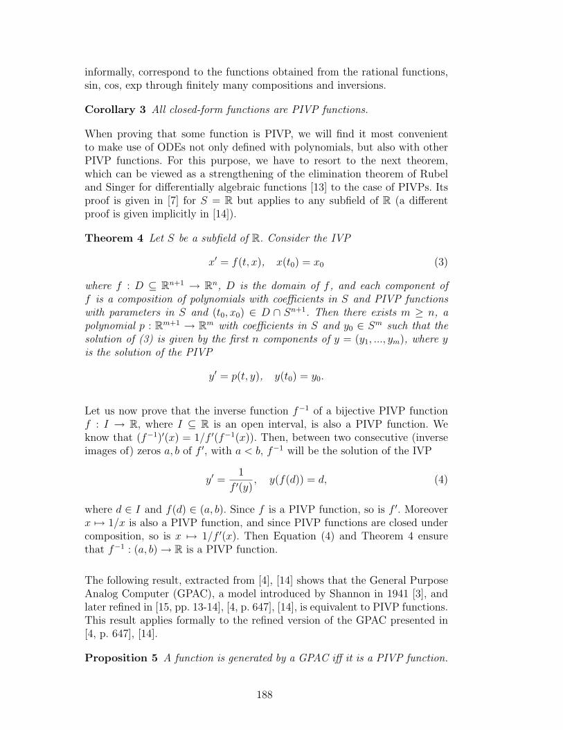
informally, correspond to the functions obtained from the rational functions,sin, cos, exp through finitely many compositions and inversions.

Corollary 3 All closed-form functions are PIVP functions.

When proving that some function is PIVP, we will find it most convenientto make use of ODEs not only defined with polynomials, but also with otherPIVP functions. For this purpose, we have to resort to the next theorem,which can be viewed as a strengthening of the elimination theorem of Rubeland Singer for differentially algebraic functions [13] to the case of PIVPs. Itsproof is given in [7] for S = R but applies to any subfield of R (a differentproof is given implicitly in [14]).

Theorem 4 Let S be a subfield of R. Consider the IVP

x′ = f(t, x), x(t0) = x0 (3)

where f : D ⊆ Rn+1 → Rn, D is the domain of f , and each component off is a composition of polynomials with coefficients in S and PIVP functionswith parameters in S and (t0, x0) ∈ D ∩ Sn+1. Then there exists m ≥ n, apolynomial p : Rm+1 → Rm with coefficients in S and y0 ∈ Sm such that thesolution of (3) is given by the first n components of y = (y1, ..., ym), where yis the solution of the PIVP

y′ = p(t, y), y(t0) = y0.

Let us now prove that the inverse function f−1 of a bijective PIVP functionf : I → R, where I ⊆ R is an open interval, is also a PIVP function. Weknow that (f−1)′(x) = 1/f ′(f−1(x)). Then, between two consecutive (inverseimages of) zeros a, b of f ′, with a < b, f−1 will be the solution of the IVP

y′ =1

f ′(y), y(f(d)) = d, (4)

where d ∈ I and f(d) ∈ (a, b). Since f is a PIVP function, so is f ′. Moreoverx 7→ 1/x is also a PIVP function, and since PIVP functions are closed undercomposition, so is x 7→ 1/f ′(x). Then Equation (4) and Theorem 4 ensurethat f−1 : (a, b)→ R is a PIVP function.

The following result, extracted from [4], [14] shows that the General PurposeAnalog Computer (GPAC), a model introduced by Shannon in 1941 [3], andlater refined in [15, pp. 13-14], [4, p. 647], [14], is equivalent to PIVP functions.This result applies formally to the refined version of the GPAC presented in[4, p. 647], [14].

Proposition 5 A function is generated by a GPAC iff it is a PIVP function.

188

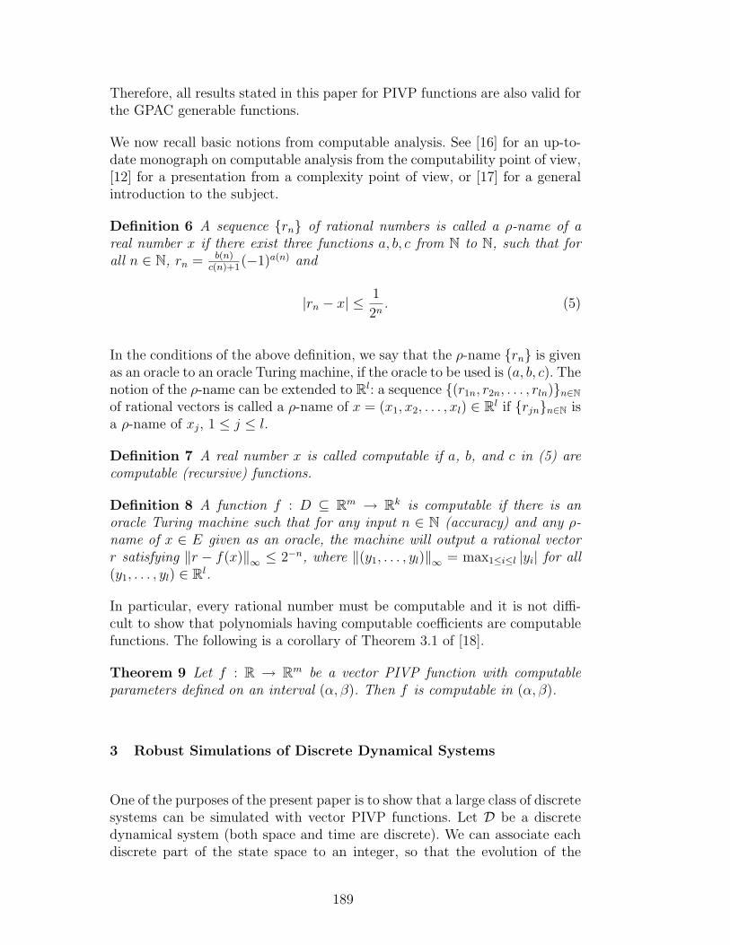
Therefore, all results stated in this paper for PIVP functions are also valid forthe GPAC generable functions.

We now recall basic notions from computable analysis. See [16] for an up-to-date monograph on computable analysis from the computability point of view,[12] for a presentation from a complexity point of view, or [17] for a generalintroduction to the subject.

Definition 6 A sequence rn of rational numbers is called a ρ-name of areal number x if there exist three functions a, b, c from N to N, such that forall n ∈ N, rn = b(n)

c(n)+1(−1)a(n) and

|rn − x| ≤1

2n. (5)

In the conditions of the above definition, we say that the ρ-name rn is givenas an oracle to an oracle Turing machine, if the oracle to be used is (a, b, c). Thenotion of the ρ-name can be extended to Rl: a sequence (r1n, r2n, . . . , rln)n∈Nof rational vectors is called a ρ-name of x = (x1, x2, . . . , xl) ∈ Rl if rjnn∈N isa ρ-name of xj, 1 ≤ j ≤ l.

Definition 7 A real number x is called computable if a, b, and c in (5) arecomputable (recursive) functions.

Definition 8 A function f : D ⊆ Rm → Rk is computable if there is anoracle Turing machine such that for any input n ∈ N (accuracy) and any ρ-name of x ∈ E given as an oracle, the machine will output a rational vectorr satisfying ‖r − f(x)‖∞ ≤ 2−n, where ‖(y1, . . . , yl)‖∞ = max1≤i≤l |yi| for all(y1, . . . , yl) ∈ Rl.

In particular, every rational number must be computable and it is not diffi-cult to show that polynomials having computable coefficients are computablefunctions. The following is a corollary of Theorem 3.1 of [18].

Theorem 9 Let f : R → Rm be a vector PIVP function with computableparameters defined on an interval (α, β). Then f is computable in (α, β).

3 Robust Simulations of Discrete Dynamical Systems

One of the purposes of the present paper is to show that a large class of discretesystems can be simulated with vector PIVP functions. Let D be a discretedynamical system (both space and time are discrete). We can associate eachdiscrete part of the state space to an integer, so that the evolution of the

189

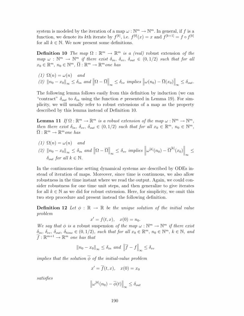
system is modeled by the iteration of a map ω : Nm → Nm. In general, if f is afunction, we denote its kth iterate by f [k], i.e. f [0](x) = x and f [k+1] = f f [k]

for all k ∈ N. We now present some definitions.

Definition 10 The map Ω : Rm → Rm is a (real) robust extension of themap ω : Nm → Nm if there exist δin, δev, δout ∈ (0, 1/2) such that for allx0 ∈ Rm, n0 ∈ Nm, Ω : Rm → Rmone has

(1) Ω(n) = ω(n) and

(2) ‖n0 − x0‖∞ ≤ δin and∥∥∥Ω− Ω

∥∥∥∞≤ δev implies

∥∥∥ω(n0)− Ω(x0)∥∥∥∞≤ δout.

The following lemma follows easily from this definition by induction (we can“contract” δout to δin using the function σ presented in Lemma 19). For sim-plicity, we will usually refer to robust extensions of a map as the propertydescribed by this lemma instead of Definition 10.

Lemma 11 If Ω : Rm → Rm is a robust extension of the map ω : Nm → Nm,then there exist δin, δev, δout ∈ (0, 1/2) such that for all x0 ∈ Rm, n0 ∈ Nm,Ω : Rm → Rmone has

(1) Ω(n) = ω(n) and

(2) ‖n0 − x0‖∞ ≤ δin and∥∥∥Ω− Ω

∥∥∥∞≤ δev implies

∥∥∥∥ω[k](n0)− Ω[k]

(x0)∥∥∥∥∞≤

δout for all k ∈ N.

In the continuous-time setting dynamical systems are described by ODEs in-stead of iteration of maps. Moreover, since time is continuous, we also allowrobustness in the time instant where we read the output. Again, we could con-sider robustness for one time unit steps, and then generalize to give iteratesfor all k ∈ N as we did for robust extension. Here, for simplicity, we omit thistwo step procedure and present instead the following definition.

Definition 12 Let φ : R → R be the unique solution of the initial valueproblem

x′ = f(t, x), x(0) = n0.

We say that φ is a robust suspension of the map ω : Nm → Nm if there existδin, δev, δout, δtime ∈ (0, 1/2), such that for all x0 ∈ Rm, n0 ∈ Nm, k ∈ N, andf : Rm+1 → Rm one has that

‖n0 − x0‖∞ ≤ δin and∥∥∥f − f∥∥∥

∞≤ δev

implies that the solution φ of the initial-value problem

x′ = f(t, x), x(0) = x0

satisfies ∥∥∥ω[k](n0)− φ(t)∥∥∥∞≤ δout

190

for all t ∈ R+0 such that |t− k| ≤ δtime.

These two definitions say that whenever we have a robust extension/suspensionof a map, we can perturb the system by some amount, and still obtain a resultclose to the desired iterate ω[k](n0).

We shall use Q[π], the standard algebraic ring extension of Q by adjoining thetranscendent π, and which is the smallest ring containing Q ∪ π:

Q[π] := anπn + . . .+ a1π + a0 ∈ R|a0, . . . , an ∈ Q.

The following are the main results of this section, to be proved in Section4. The next theorem shows that if the map is a composition of polynomialsand PIVP functions (with parameters in Q[π]), then one can constructivelyobtain a robust suspension of the map which is itself a PIVP function (withparameter in Q[π]).

Theorem 13 If the map ω : Nm → Nm admits a robust extension Ω : Rm →Rm whose components are compositions of polynomials and PIVP functionswith parameters in Q[π], then ω admits a robust suspension φ which is a vectorPIVP function with parameters in Q[π].

The next proposition follows from the proof of Theorem 12 from [7]. Therethe transition of a Turing machine is coded as a map over the integers in thefollowing manner: we code the state as an integer and, using a representationof numbers in some adequate base, we code the right part of the tape as asecond integer, and the left part as a third integer. We denote that encodingby η (see [7, p. 332] for more details).

Proposition 14 Under the encoding η, the transition function ω : N3 → N3

of a Turing machine admits a robust extension Ω : R3 → R3 . Moreover Ωcan be chosen to be a composition of polynomials with coefficients in Q[π] andPIVP functions with parameters in Q[π] (in particular sin, cos and arctan).

Actually in [7] we required algebraic numbers as coefficients for the polynomi-als. But non-rational coefficients are only needed to perform a trigonometricinterpolation, and may be well approximated by rationals for the purpose athand. This approximation will introduce some extra error to the computationof the map, but this is a minor hinderance since the map is robust. FromTheorem 13 and Proposition 14, we obtain the following result.

Corollary 15 With the above encoding, the transition function ω of a givenTuring machine admits a robust suspension φ. Moreover φ is a vector PIVPfunction with parameters in Q[π].

191

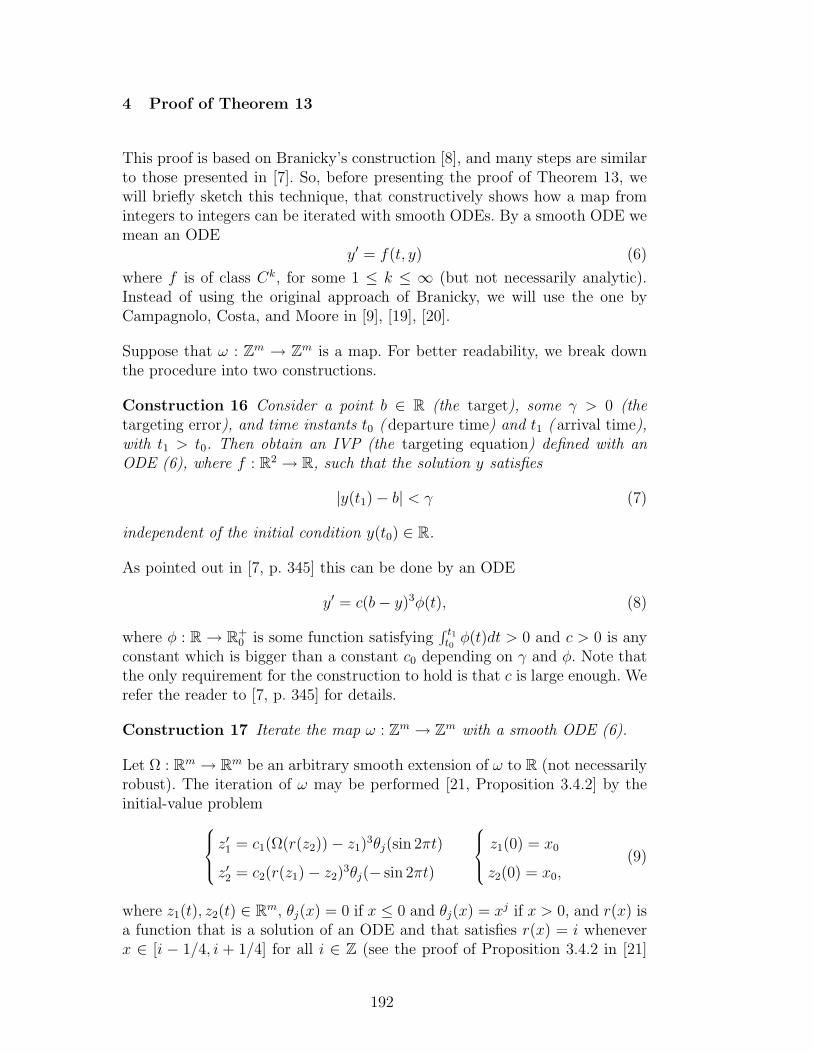
4 Proof of Theorem 13

This proof is based on Branicky’s construction [8], and many steps are similarto those presented in [7]. So, before presenting the proof of Theorem 13, wewill briefly sketch this technique, that constructively shows how a map fromintegers to integers can be iterated with smooth ODEs. By a smooth ODE wemean an ODE

y′ = f(t, y) (6)

where f is of class Ck, for some 1 ≤ k ≤ ∞ (but not necessarily analytic).Instead of using the original approach of Branicky, we will use the one byCampagnolo, Costa, and Moore in [9], [19], [20].

Suppose that ω : Zm → Zm is a map. For better readability, we break downthe procedure into two constructions.

Construction 16 Consider a point b ∈ R (the target), some γ > 0 (thetargeting error), and time instants t0 ( departure time) and t1 ( arrival time),with t1 > t0. Then obtain an IVP (the targeting equation) defined with anODE (6), where f : R2 → R, such that the solution y satisfies

|y(t1)− b| < γ (7)

independent of the initial condition y(t0) ∈ R.

As pointed out in [7, p. 345] this can be done by an ODE

y′ = c(b− y)3φ(t), (8)

where φ : R→ R+0 is some function satisfying

∫ t1t0φ(t)dt > 0 and c > 0 is any

constant which is bigger than a constant c0 depending on γ and φ. Note thatthe only requirement for the construction to hold is that c is large enough. Werefer the reader to [7, p. 345] for details.

Construction 17 Iterate the map ω : Zm → Zm with a smooth ODE (6).

Let Ω : Rm → Rm be an arbitrary smooth extension of ω to R (not necessarilyrobust). The iteration of ω may be performed [21, Proposition 3.4.2] by theinitial-value problem z

′1 = c1(Ω(r(z2))− z1)3θj(sin 2πt)

z′2 = c2(r(z1)− z2)3θj(− sin 2πt)

z1(0) = x0

z2(0) = x0,(9)

where z1(t), z2(t) ∈ Rm, θj(x) = 0 if x ≤ 0 and θj(x) = xj if x > 0, and r(x) isa function that is a solution of an ODE and that satisfies r(x) = i wheneverx ∈ [i − 1/4, i + 1/4] for all i ∈ Z (see the proof of Proposition 3.4.2 in [21]

192

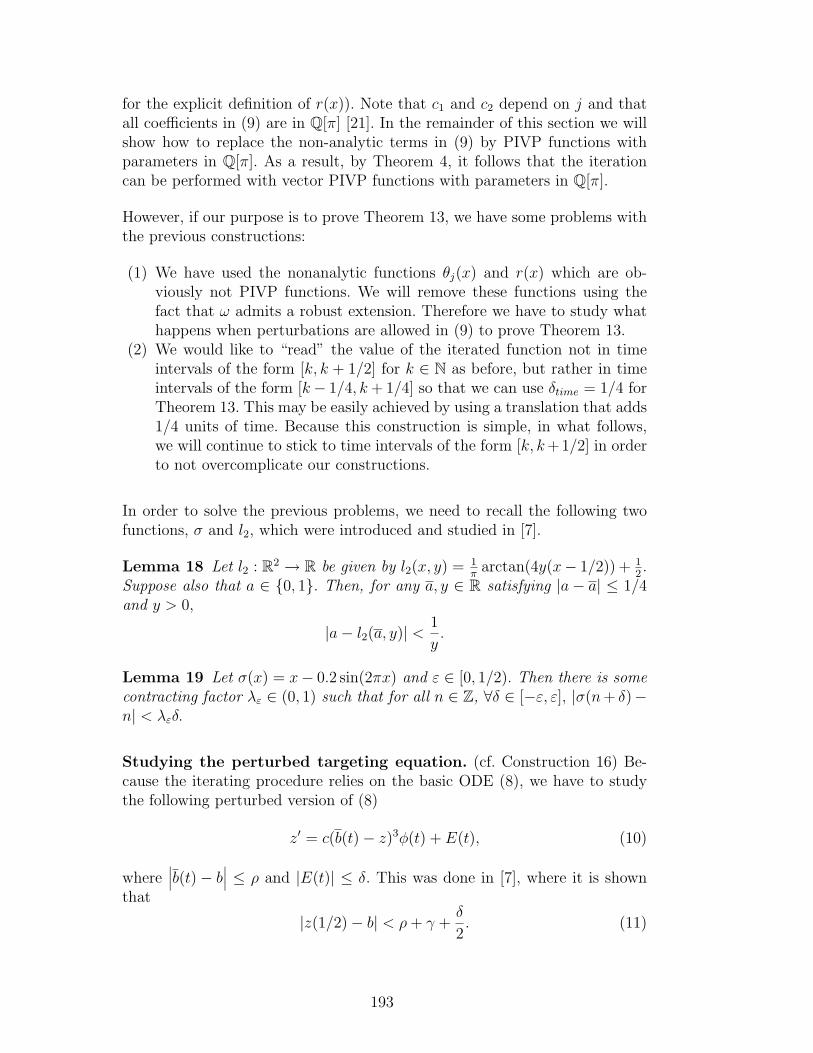
for the explicit definition of r(x)). Note that c1 and c2 depend on j and thatall coefficients in (9) are in Q[π] [21]. In the remainder of this section we willshow how to replace the non-analytic terms in (9) by PIVP functions withparameters in Q[π]. As a result, by Theorem 4, it follows that the iterationcan be performed with vector PIVP functions with parameters in Q[π].

However, if our purpose is to prove Theorem 13, we have some problems withthe previous constructions:

(1) We have used the nonanalytic functions θj(x) and r(x) which are ob-viously not PIVP functions. We will remove these functions using thefact that ω admits a robust extension. Therefore we have to study whathappens when perturbations are allowed in (9) to prove Theorem 13.

(2) We would like to “read” the value of the iterated function not in timeintervals of the form [k, k + 1/2] for k ∈ N as before, but rather in timeintervals of the form [k− 1/4, k+ 1/4] so that we can use δtime = 1/4 forTheorem 13. This may be easily achieved by using a translation that adds1/4 units of time. Because this construction is simple, in what follows,we will continue to stick to time intervals of the form [k, k+ 1/2] in orderto not overcomplicate our constructions.

In order to solve the previous problems, we need to recall the following twofunctions, σ and l2, which were introduced and studied in [7].

Lemma 18 Let l2 : R2 → R be given by l2(x, y) = 1π

arctan(4y(x− 1/2)) + 12.

Suppose also that a ∈ 0, 1. Then, for any a, y ∈ R satisfying |a− a| ≤ 1/4and y > 0,

|a− l2(a, y)| < 1

y.

Lemma 19 Let σ(x) = x− 0.2 sin(2πx) and ε ∈ [0, 1/2). Then there is somecontracting factor λε ∈ (0, 1) such that for all n ∈ Z, ∀δ ∈ [−ε, ε], |σ(n+ δ)−n| < λεδ.

Studying the perturbed targeting equation. (cf. Construction 16) Be-cause the iterating procedure relies on the basic ODE (8), we have to studythe following perturbed version of (8)

z′ = c(b(t)− z)3φ(t) + E(t), (10)

where∣∣∣b(t)− b∣∣∣ ≤ ρ and |E(t)| ≤ δ. This was done in [7], where it is shown

that

|z(1/2)− b| < ρ+ γ +δ

2. (11)

193

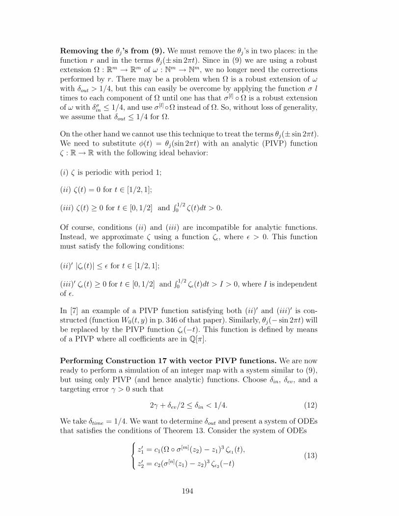
Removing the θj’s from (9). We must remove the θj’s in two places: in thefunction r and in the terms θj(± sin 2πt). Since in (9) we are using a robustextension Ω : Rm → Rm of ω : Nm → Nm, we no longer need the correctionsperformed by r. There may be a problem when Ω is a robust extension of ωwith δout > 1/4, but this can easily be overcome by applying the function σ ltimes to each component of Ω until one has that σ[l] Ω is a robust extensionof ω with δσin ≤ 1/4, and use σ[l]Ω instead of Ω. So, without loss of generality,we assume that δout ≤ 1/4 for Ω.

On the other hand we cannot use this technique to treat the terms θj(± sin 2πt).We need to substitute φ(t) = θj(sin 2πt) with an analytic (PIVP) functionζ : R→ R with the following ideal behavior:

(i) ζ is periodic with period 1;

(ii) ζ(t) = 0 for t ∈ [1/2, 1];

(iii) ζ(t) ≥ 0 for t ∈ [0, 1/2] and∫ 1/2

0 ζ(t)dt > 0.

Of course, conditions (ii) and (iii) are incompatible for analytic functions.Instead, we approximate ζ using a function ζε, where ε > 0. This functionmust satisfy the following conditions:

(ii)′ |ζε(t)| ≤ ε for t ∈ [1/2, 1];

(iii)′ ζε(t) ≥ 0 for t ∈ [0, 1/2] and∫ 1/20 ζε(t)dt > I > 0, where I is independent

of ε.

In [7] an example of a PIVP function satisfying both (ii)′ and (iii)′ is con-structed (function W0(t, y) in p. 346 of that paper). Similarly, θj(− sin 2πt) willbe replaced by the PIVP function ζε(−t). This function is defined by meansof a PIVP where all coefficients are in Q[π].

Performing Construction 17 with vector PIVP functions. We are nowready to perform a simulation of an integer map with a system similar to (9),but using only PIVP (and hence analytic) functions. Choose δin, δev, and atargeting error γ > 0 such that

2γ + δev/2 ≤ δin < 1/4. (12)

We take δtime = 1/4. We want to determine δout and present a system of ODEsthat satisfies the conditions of Theorem 13. Consider the system of ODEs z

′1 = c1(Ω σ[m](z2)− z1)3 ζε1(t),

z′2 = c2(σ[n](z1)− z2)3 ζε2(−t)(13)

194

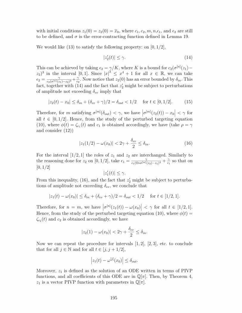
with initial conditions z1(0) = z2(0) = x0, where c1, c2,m, n,ε1, and ε2 are stillto be defined, and σ is the error-contracting function defined in Lemma 19.

We would like (13) to satisfy the following property: on [0, 1/2],

|z′2(t)| ≤ γ. (14)

This can be achieved by taking ε2 = γ/K, where K is a bound for c2(σ[n](z1)−z2)3 in the interval [0, 1]. Since |x|3 ≤ x4 + 1 for all x ∈ R, we can takeε2 = γ

c2(σ[n](z1)−z2)4+ γc2

. Now notice that z2(0) has an error bounded by δin. This

fact, together with (14) and the fact that z′2 might be subject to perturbationsof amplitude not exceeding δev imply that

|z2(t)− x0| ≤ δin + (δev + γ)/2 = δout < 1/2 for t ∈ [0, 1/2]. (15)

Therefore, for m satisfying σ[m](δout) < γ, we have∣∣∣σ[m](z2(t))− x0

∣∣∣ < γ for

all t ∈ [0, 1/2]. Hence, from the study of the perturbed targeting equation(10), where φ(t) = ζε1(t) and c1 is obtained accordingly, we have (take ρ = γand consider (12))

|z1(1/2)− ω(x0)| < 2γ +δev2≤ δin. (16)

For the interval [1/2, 1] the roles of z1 and z2 are interchanged. Similarly tothe reasoning done for z2 on [0, 1/2], take ε1 = γ

c1(Ωσ[m](z2)−z1)4+ γ

c1so that on

[0, 1/2]|z′1(t)| ≤ γ.

From this inequality, (16), and the fact that z′2 might be subject to perturba-tions of amplitude not exceeding δev, we conclude that

|z1(t)− ω(x0)| ≤ δin + (δev + γ)/2 = δout < 1/2 for t ∈ [1/2, 1].

Therefore, for n = m, we have∣∣∣σ[n](z1(t))− ω(x0)

∣∣∣ < γ for all t ∈ [1/2, 1].

Hence, from the study of the perturbed targeting equation (10), where φ(t) =ζε2(t) and c2 is obtained accordingly, we have

|z2(1)− ω(x0)| < 2γ +δev2≤ δin.

Now we can repeat the procedure for intervals [1, 2], [2, 3], etc. to concludethat for all j ∈ N and for all t ∈ [j, j + 1/2],∣∣∣z1(t)− ω[j](x0)

∣∣∣ ≤ δout.

Moreover, z1 is defined as the solution of an ODE written in terms of PIVPfunctions, and all coefficients of this ODE are in Q[π]. Then, by Theorem 4,z1 is a vector PIVP function with parameters in Q[π].

195

5 Application – Undecidability for PIVPs with Comparable Pa-rameters

It is well known from the basic existence-uniqueness theory of ODEs [22], [23]that if f is analytic, then the IVP

x′ = f(t, x), x(t0) = x0 (17)

has a unique solution x(t) defined on a maximal interval of existence I =(α, β) ⊂ R that is analytic on I [24]. The interval is maximal in the sensethat either α = −∞ or x(t) is unbounded as t → α+ with similar conditionsapplying to β (see Proposition 20 for details). Actually, f only needs to becontinuous and locally Lipschitz in the second argument for this maximalinterval to exist.

A question of interest is the following: is it possible to design an automatedmethod that, on input (f, t0, x0), gives as output the maximal interval ofexistence for the solution of (17)? In computability theory, e.g. [25], [26], it iswell known that some problems cannot be answered by the use of an algorithm(more precisely, by the use of a Turing machine). Such problems are labelledundecidable and many examples are known. The most prominent undecidableproblem is the Halting Problem: given a universal Turing machine and someinput to it, decide whether the machine eventually halts or not. To addressthis kind of questions for IVPs, we use the computable analysis approach [17],[12], [16], which we presented in the end of Section 2. Using that approach, itwas shown in [18] that given an analytic IVP (17), defined with computabledata, its corresponding maximal interval may be non-computable.

Non-computability results related to initial-value problems of differential equa-tions are not new. For example, Pour-El and Richards [27] showed that if werelax the condition of analyticity in the IVP (17) defined with computabledata, it can have non-computable solutions. In [28], [29] it is shown that thereis a three-dimensional wave equation, defined with computable data, such thatthe unique solution is nowhere computable. However, in these examples, non-computability is not “genuine” in the sense that the problems under studyare ill-posed: either the solution is not unique or it is unstable [30]. In otherwords, ill-posedness was at the origin of non-computability in those examples.In contrast, an analytic IVP (17) is classically well-posed and, consequently,the non-computability results do not seem to reflect computational and well-posedness deficiencies inherited by the problems.

Motivated by the non-computability result obtained in [18], this latter paperalso addresses the following problem: while it is not possible to compute themaximal interval of (17) is it possible to compute some partial informationabout it? In particular, is it possible to decide if this maximal interval is

196

bounded or not?

This question has interest on its own for the following reason. In many prob-lems, we implicitly assume that t is defined for “all time”. For example, if onewants to compute sinks or limit cycles associated with ODEs, this only makessense if the solution of the ODE is defined for all times t > t0. This is also im-plicitly assumed in problems like reachability [31], [32], [33], [34], [35], etc. Forthis reason, those problems only make sense when associated with ODEs forwhich the maximal interval is unbounded. So, it would be interesting to knowwhich are the “maximal” classes of functions f for which the boundednessproblem is decidable.

In [18], it was shown that for the general class of analytic IVPs, the bound-edness problem of the maximal interval is undecidable. Here we will deepenthis result: we will show that the boundedness problem is still undecidable forPIVPs of degree greater or equal than 56 with parameters in Q[π]. Our resultis slightly different in form from the case of the general class of analytic IVPs.Indeed, the coefficients of the polynomials are coded as finite sequences of in-tegers and not as ρ-name satisfying (5), though from these finite sequences ofintegers one can easily compute ρ-names for the coefficients of the polynomials.

The boundedness problem is decidable for linear differential equations thusimplying that the boundary between decidability/undecidability lies in theclass of polynomials of degree n, for some 2 ≤ n ≤ 56.

This result is shown using methods which differ from those employed in [18].This result was already stated in [11], but we now present its proof.

The following result introduces the notion of maximal interval for ODEs andfollows as an immediate consequence of the fundamental existence-uniquenesstheory for the initial-value problem (17), where the analyticity condition isdropped for f [22], [23], [36].

Proposition 20 Let E be an open subset of Rn+1 and assume that f : E →Rn is continuous on E and locally Lipschitz in the second argument (i.e. inthe last n components). Then for each (t0, x0) ∈ E, the problem (17) has aunique solution x(t) defined on a maximal interval (α, β), on which it is C1.The maximal interval is open and has the property that, if β < +∞ (resp.α > −∞), either (t, x(t)) approaches the boundary of E or x(t) is unboundedas t→ β − (resp. t→ α+).

Note that, as a particular case, when E = Rn+1 and β <∞, x(t) is unboundedas t→ β −. This will be the case under study in this section.

We now introduce a definition that allows us to compare real numbers of

197

some given set, to avoid the trivial undecidability of the boundedness problemsketched in Section 1.

Definition 21 We say that a set D ⊆ R is effectively comparable if D has anaming system γ, if all elements of D are γ-computable, and if given γ-namesof x, y ∈ D, then x = y and x < y are decidable

In the previous definition, “naming system” is either a (finite) notation ora (infinite) representation of the elements of D according to Weihrauch [16,p. 33 and p. 52]. Next we show that Q[π] is effectively comparable. Indeed,given a0, . . . , am ∈ Q (which can easily be coded as a finite sequence using afinite alphabet A), we can take the notation f : A∗ → Q[π]

f(a0, . . . , am) =m∑i=0

aiπi.

Moreover, if α, β ∈ Q[π],

α =m∑i=0

aiπi and β =

n∑i=0

biπi,

where a0, . . . , am, b0, . . . , bn ∈ Q. We can decide if α = β since α = β iffai = bi for all i and ai and bi are rationals. We can also compute arbitrarlyclose approximations of α and β. Therefore, if α 6= β, we can compare thesevalues: we just need to start computing increasing approximations of α andβ until we decide whether α < β or α > β. The following result is similar toTheorem 12 in [11], but here we restrict the parameters of the PIVP to aneffectively comparable set. This prevents the trivial undecidability discussedin Section 1.

Theorem 22 Let D be an effectively comparable set such that Q[π] ⊆ D.The following problem is undecidable: “Given p : Rn+1 → Rn with polynomialcomponents with coefficients in D (these coefficients are given by their names,as described in Definition 21), and (t0, x0) ∈ Q × Qn, decide whether themaximal interval of the IVP (1) is bounded or not”.

Actually, if we are given the description of a universal Turing machine, we canconstructively define a set of polynomial ODEs simulating it that encodes theHalting Problem. If we use the small universal Turing machine presented in[37], having 4 states and 6 symbols, we obtain the following theorem.

Theorem 23 Let D be an effectively comparable set such that Q[π] ⊆ D.There is a vector p : Rn+1 → Rn, with n ≥ 1, defined by polynomials withcoefficients in D (these coefficients are given by their names, as described inDefinition 21), where each component has degree less than or equal to 56, suchthat the following problem is undecidable: “Given (t0, x0) ∈ Q × Qn, decidewhether the maximal interval of the IVP (1) is bounded or not”.

198

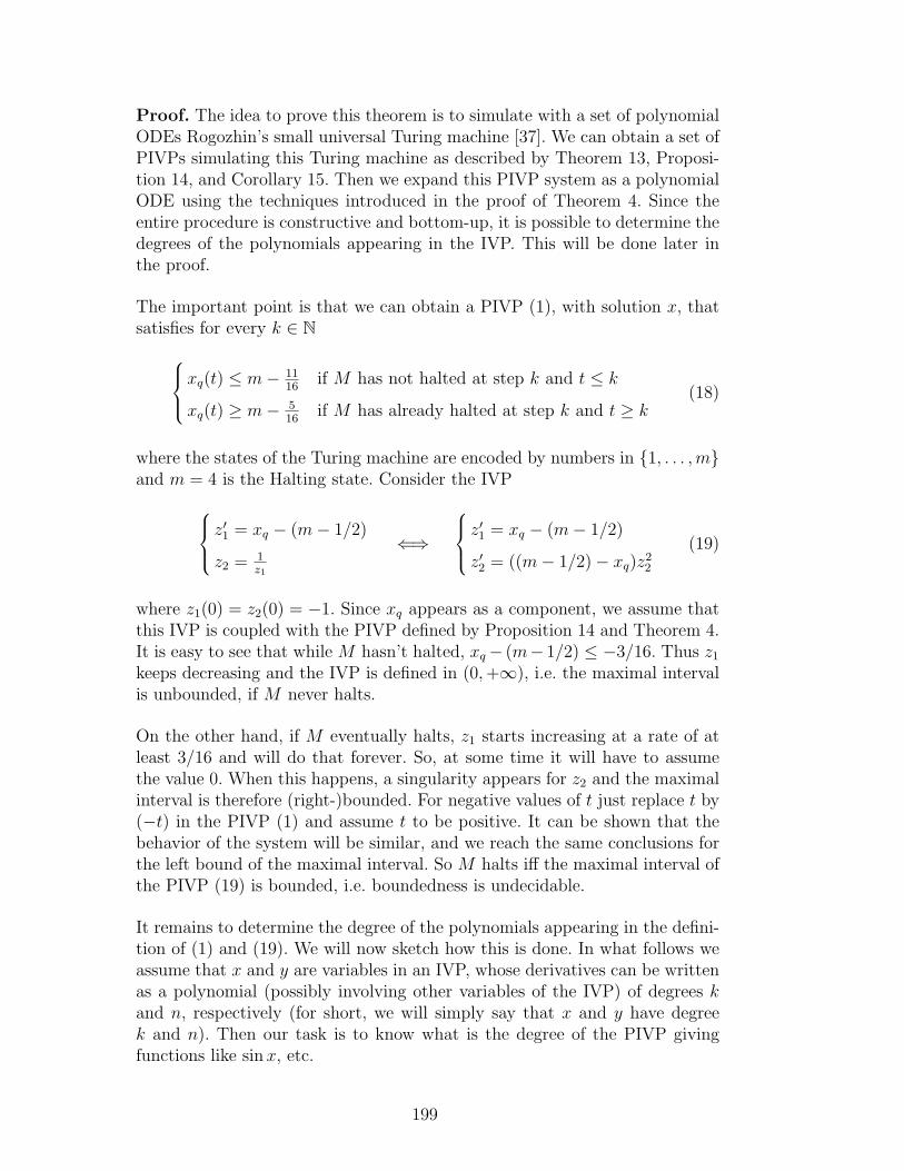
Proof. The idea to prove this theorem is to simulate with a set of polynomialODEs Rogozhin’s small universal Turing machine [37]. We can obtain a set ofPIVPs simulating this Turing machine as described by Theorem 13, Proposi-tion 14, and Corollary 15. Then we expand this PIVP system as a polynomialODE using the techniques introduced in the proof of Theorem 4. Since theentire procedure is constructive and bottom-up, it is possible to determine thedegrees of the polynomials appearing in the IVP. This will be done later inthe proof.

The important point is that we can obtain a PIVP (1), with solution x, thatsatisfies for every k ∈ N

xq(t) ≤ m− 1116

if M has not halted at step k and t ≤ k

xq(t) ≥ m− 516

if M has already halted at step k and t ≥ k(18)

where the states of the Turing machine are encoded by numbers in 1, . . . ,mand m = 4 is the Halting state. Consider the IVP

z′1 = xq − (m− 1/2)

z2 = 1z1

⇐⇒

z′1 = xq − (m− 1/2)

z′2 = ((m− 1/2)− xq)z22

(19)

where z1(0) = z2(0) = −1. Since xq appears as a component, we assume thatthis IVP is coupled with the PIVP defined by Proposition 14 and Theorem 4.It is easy to see that while M hasn’t halted, xq− (m− 1/2) ≤ −3/16. Thus z1

keeps decreasing and the IVP is defined in (0,+∞), i.e. the maximal intervalis unbounded, if M never halts.

On the other hand, if M eventually halts, z1 starts increasing at a rate of atleast 3/16 and will do that forever. So, at some time it will have to assumethe value 0. When this happens, a singularity appears for z2 and the maximalinterval is therefore (right-)bounded. For negative values of t just replace t by(−t) in the PIVP (1) and assume t to be positive. It can be shown that thebehavior of the system will be similar, and we reach the same conclusions forthe left bound of the maximal interval. So M halts iff the maximal interval ofthe PIVP (19) is bounded, i.e. boundedness is undecidable.

It remains to determine the degree of the polynomials appearing in the defini-tion of (1) and (19). We will now sketch how this is done. In what follows weassume that x and y are variables in an IVP, whose derivatives can be writtenas a polynomial (possibly involving other variables of the IVP) of degrees kand n, respectively (for short, we will simply say that x and y have degreek and n). Then our task is to know what is the degree of the PIVP givingfunctions like sin x, etc.

199

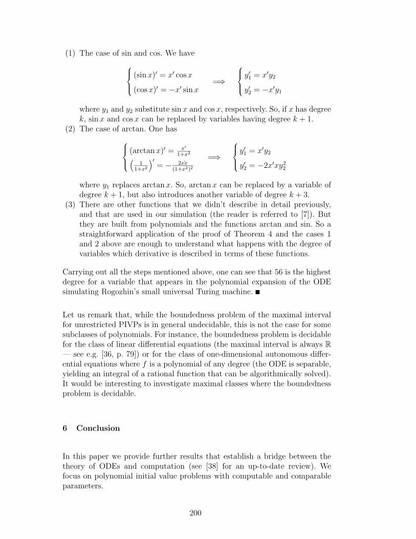
(1) The case of sin and cos. We have (sinx)′ = x′ cosx

(cosx)′ = −x′ sinx=⇒

y′1 = x′y2

y′2 = −x′y1

where y1 and y2 substitute sin x and cos x, respectively. So, if x has degreek, sin x and cos x can be replaced by variables having degree k + 1.

(2) The case of arctan. One has (arctanx)′ = x′

1+x2(1

1+x2

)′= − 2xx

(1+x2)2

=⇒

y′1 = x′y2

y′2 = −2x′xy22

where y1 replaces arctanx. So, arctan x can be replaced by a variable ofdegree k + 1, but also introduces another variable of degree k + 3.

(3) There are other functions that we didn’t describe in detail previously,and that are used in our simulation (the reader is referred to [7]). Butthey are built from polynomials and the functions arctan and sin. So astraightforward application of the proof of Theorem 4 and the cases 1and 2 above are enough to understand what happens with the degree ofvariables which derivative is described in terms of these functions.

Carrying out all the steps mentioned above, one can see that 56 is the highestdegree for a variable that appears in the polynomial expansion of the ODEsimulating Rogozhin’s small universal Turing machine.

Let us remark that, while the boundedness problem of the maximal intervalfor unrestricted PIVPs is in general undecidable, this is not the case for somesubclasses of polynomials. For instance, the boundedness problem is decidablefor the class of linear differential equations (the maximal interval is always R— see e.g. [36, p. 79]) or for the class of one-dimensional autonomous differ-ential equations where f is a polynomial of any degree (the ODE is separable,yielding an integral of a rational function that can be algorithmically solved).It would be interesting to investigate maximal classes where the boundednessproblem is decidable.

6 Conclusion

In this paper we provide further results that establish a bridge between thetheory of ODEs and computation (see [38] for an up-to-date review). Wefocus on polynomial initial value problems with computable and comparableparameters.

200

With respect to computation, our main result is that the boundness of themaximal interval of definition is undecidable even for PIVPs with comparableparameters and degree up to 56. We can view this result as a ODE analog tothe undecidability of the Halting problem for Turing machines.

With respect to polynomial ODEs, we show that they can simulate a largeclass of dynamical systems – including Turing machines – in the presence ofnoise.

Based on the previous results we argue that polynomial ODEs, which are awell known model of physical phenomena, are also a powerful, yet realistic,model of continuous time computation.

Acknowledgments. The authors wish to thank Pieter Collins, Kerry Ojakian,and Ning Zhong, and the anonymous referees for useful remarks and com-ments. DG and MC were partially supported by Fundacao para a Ciencia e aTecnologia and EU FEDER POCTI/POCI via CLC, SQIG - Instituto de Tele-comunicacoes and grant SFRH/BPD/39779/2007 (DG). Additional supportto DG was also provided by the Fundacao Calouste Gulbenkian through thePrograma Gulbenkian de Estımulo a Investigacao. JB was partially supportedby CMAF through FEDER and FCT-Plurianual 2007.

References

[1] M. W. Hirsch, S. Smale, Differential Equations, Dynamical Systems, and LinearAlgebra, Academic Press, 1974.

[2] J. F. Ritt, Integration in Finite Terms. Liouville’s Theory of ElementaryMethods., Columbia Univ. Press, 1948.

[3] C. E. Shannon, Mathematical theory of the differential analyzer, J. Math. Phys.MIT 20 (1941) 337–354.

[4] D. S. Graca, J. F. Costa, Analog computers and recursive functions over thereals, J. Complexity 19 (5) (2003) 644–664.

[5] J. H. Hubbard, B. H. West, Differential Equations: A Dynamical SystemsApproach — Higher-Dimensional Systems, Springer, 1995.

[6] D. S. Graca, N. Zhong, J. Buescu, The ordinary differential equation defined bya computable function whose maximal interval of existence is non-computable,in: G. Hanrot, P. Zimmermann (Eds.), Proceedings of the 7th Conference onReal Numbers and Computers (RNC 7), LORIA/INRIA, 2006, pp. 33–40.

[7] D. S. Graca, M. L. Campagnolo, J. Buescu, Computability with polynomialdifferential equations, Adv. Appl. Math. 40 (3) (2008) 330–349.

201

[8] M. S. Branicky, Universal computation and other capabilities of hybrid andcontinuous dynamical systems, Theoret. Comput. Sci. 138 (1) (1995) 67–100.

[9] M. L. Campagnolo, C. Moore, J. F. Costa, Iteration, inequalities, anddifferentiability in analog computers, J. Complexity 16 (4) (2000) 642–660.

[10] E. Hainry, Reachability in linear dynamical systems, in: A. Beckmann,C. Dimitracopoulos, B. Lowe (Eds.), Computability in Europe 2008 (CiE 2008),Vol. 5028 of LNCS, 2008.

[11] D. S. Graca, J. Buescu, M. L. Campagnolo, Boundedness of the domain ofdefinition is undecidable for polynomial ODEs, in: R. Dillhage, T. Grubba,A. Sorbi, K. Weihrauch, N. Zhong (Eds.), Proceedings of the 4th InternationalConference on Computability and Complexity in Analysis (CCA 2007),FernUniversitat in Hagen, 2007, pp. 127–135.

[12] K.-I. Ko, Computational Complexity of Real Functions, Birkhauser, 1991.

[13] L. A. Rubel, F. Singer, A differentially algebraic elimination theorem withapplication to analog computability in the calculus of variations, Proc. Amer.Math. Soc. 94 (4) (1985) 653–658.

[14] D. S. Graca, Some recent developments on Shannon’s General Purpose AnalogComputer, Math. Log. Quart. 50 (4-5) (2004) 473–485.

[15] M. B. Pour-El, Abstract computability and its relations to the general purposeanalog computer, Trans. Amer. Math. Soc. 199 (1974) 1–28.

[16] K. Weihrauch, Computable Analysis: an Introduction, Springer, 2000.

[17] M. B. Pour-El, J. I. Richards, Computability in Analysis and Physics, Springer,1989.

[18] D. Graca, N. Zhong, J. Buescu, Computability, noncomputability andundecidability of maximal intervals of IVPs, Trans. Amer. Math. Soc.To appear.

[19] M. Campagnolo, C. Moore, Upper and lower bounds on continuous-timecomputation, in: I. Antoniou, C. Calude, M. Dinneen (Eds.), 2nd InternationalConference on Unconventional Models of Computation - UMC’2K, Springer,2001, pp. 135–153.

[20] M. L. Campagnolo, Computational complexity of real valued recursive functionsand analog circuits, Ph.D. thesis, Instituto Superior Tecnico/UniversidadeTecnica de Lisboa (2002).

[21] M. L. Campagnolo, The complexity of real recursive functions, in: C. S.Calude, M. J. Dinneen, F. Peper (Eds.), Unconventional Models of Computation(UMC’02), LNCS 2509, Springer, 2002, pp. 1–14.

[22] E. A. Coddington, N. Levinson, Theory of Ordinary Differential Equations,McGraw-Hill, 1955.

[23] S. Lefshetz, Differential Equations: Geometric Theory, 2nd Edition,Interscience, 1965.

202

[24] V. I. Arnold, Ordinary Differential Equations, MIT Press, 1978.

[25] M. Sipser, Introduction to the Theory of Computation, PWS PublishingCompany, 1997.

[26] J. E. Hopcroft, R. Motwani, J. D. Ullman, Introduction to Automata Theory,Languages, and Computation, 2nd Edition, Addison-Wesley, 2001.

[27] M. B. Pour-El, J. I. Richards, A computable ordinary differential equation whichpossesses no computable solution, Ann. Math. Logic 17 (1979) 61–90.

[28] M. B. Pour-El, J. I. Richards, The wave equation with computable initial datasuch that its unique solution is not computable, Adv. Math. 39 (1981) 215–239.

[29] M. B. Pour-El, N. Zhong, The wave equation with computable initial data whoseunique solution is nowhere computable, Math. Log. Quart. 43 (1997) 499–509.

[30] K. Weihrauch, N. Zhong, Is wave propagation computable or can wavecomputers beat the Turing machine?, Proc. London Math. Soc. 85 (3) (2002)312–332.

[31] R. Alur, D. L. Dill, Automata for modeling real-time systems, in: Automata,Languages and Programming, 17th International Colloquium, LNCS 443,Springer, 1990, pp. 322–335.

[32] E. Asarin, O. Maler, A. Pnueli, Reachability analysis of dynamical systemshaving piecewise-constant derivatives, Theoret. Comput. Sci. 138 (1995) 35–65.

[33] T. A. Henzinger, P. W. Kopke, A. Puri, P. Varaiya, What’s decidable abouthybrid automata?, J. Comput. System Sci. 57 (1) (1998) 94–124.

[34] O. Bournez, Achilles and the Tortoise climbing up the hyper-arithmeticalhierarchy, Theoret. Comput. Sci. 210 (1) (1999) 21–71.

[35] V. D. Blondel, J. N. Tsitsiklis, A survey of computational complexity results insystems and control, Automatica 9 (36) (2000) 1249–1274.

[36] J. K. Hale, Ordinary Differential Equations, 2nd Edition, Robert E. KriegerPub. Co, 1980.

[37] Y. Rogozhin, Small universal Turing machines, Theoret. Comput. Sci. 168 (2)(1996) 215–240.

[38] O. Bournez, M. L. Campagnolo, New Computational Paradigms. ChangingConceptions of What is Computable, Springer-Verlag, New York, 2008, Ch.A Survey on Continuous Time Computations, pp. 383–423.

203

204

A New Problem for Rule Following

Mark Hogarth Girton College, Cambridge

1. Introduction

This is part of an extended argument of mine about the Church-Turing thesis (CTT). In Hogarth 1994 I argued that the thesis is a thoroughly empirical claim. In Hogarth 2004, 2008 I rejected that view, arguing instead that the thesis is really a pseudo-proposition like ‘Australia is below England’, or , better, like ‘Euclidean geometry is the true geometry’. I say ‘better’ because my attitude towards this issue is shaped by an analogy with the concept of geometry. The key idea is that there is no fundamentally privileged computing device (e.g. Turing machine), in just the way that there is no privileged geometry (e.g. Euclidean). From a mathematical viewpoint there are lots of computers, lots of inequivalent ways to execute an algorithm (or procedure or rule). In my previous work I took it that the idea of losing CTT would have important consequences but consequences primarily for computability theory. Here I suggest the consequences extend further and may indeed touch on the nature of pure mathematics itself. Simple counting provides a case study. I also make some remarks about how the analogy with geometry might provide an answer to the stubborn problem of why pure mathematics is applicable to the natural sciences.

2. The liquefaction of computability

This line of enquiry began with the discovery of some non-Turing computers within the theory of general relativity (Hogarth 1992,1994, 2004, 2008; Earman and Norton 1993; Etesi and Nemeti 2001; Nemeti and David 2006). But what I have to say here, and indeed what is important, is not about those computers per se but rather about what their existence reveals about the concept of computability (written Computability). In that sense these non-Turing computers are like the first non-Euclidean geometries: what matters, conceptually speaking, is not the real-world accuracy of the models but their existence.

Let us remind ourselves how the concept of geometry came to change. Writing in 1897, when the status of non-Euclidean geometries was still controversial, Bertrand Russell began his book, An Essay on the Foundations of Geometry, as follows:

‘When a long established system is attacked, it usually happens that the attack begins at a single point, where the weakness of the doctrine is particularly evident. But criticism once invited, is apt to extend much further than the most daring, at first, would have wished.’

‘“First cut the liquefaction, what comes last, But Fichte’s clever cut at God himself?”’

‘So it has been with Geometry.’

The liquefaction of Euclidean geometry began at the end of the 18th century, when Gauss questioned one of the axioms of the Euclidean system, the so-called Axiom of Parallels or Euclid’s Postulate 5 (‘Axioms XI’ in some older manuscripts). Gauss

205

experimented with systems lacking that axiom, but he never published his results for he feared an ‘uproar of the Boeotians’1. The first publications to present a non-Euclidean system were due Lobachevsky in 1829 and Bolyai in 1832; others followed.

There are two strands of argument in Russell’s book. First, that these new geometries represent real possibilities for the geometry of our world and deciding between them is an empirical matter. Secondly, that any possible geometry must possess constant curvature. This idea Russell held for essentially Kantian reasons. With the arrival in 1915 of Einstein’s general theory of relativity this second strand became untenable, a point Russell himself was quick to acknowledge (Torretti, Chapter 7). Space (and spacetime) could possess variable curvature.

The process of liquefaction therefore advanced further than Russell had anticipated in 1897. After Einstein the term ‘geometry’ became broad and vague. ‘Broad’ because it encompassed a myriad of systems suggested by the sciences; ‘vague’ because the lessons of the past were not to attempt to isolate some ‘essential’ features of geometry (like constant curvature); not, in short, to try to cauterize the concept of geometry. We are now not even tempted to ask what makes a system a ‘geometry’. The term, like the term ‘game’, gets applied because of family resemblances with accepted archetypes. We rightly tend to leave it at that.

One way to phrase the conceptual shift taking us from Euclidean geometry to post-Einstein geometry, is to say that the concept of geometry (written Geometry) became two-sided, with physical geometry on one side and pure geometry on the other. Physical geometry is concerned with modeling the geometry of the physical world; it’s part of physics. Pure geometry is concerned with the mathematical structure of each of the many geometrical models now in the offing; it’s part of pure mathematics.

What I argued in Hogarth 2004, 2008 is that Computability now also looks two-sided, exactly because it has come to look so like Geometry.2

In Table 1 I summarize the main points of contact of the two concepts.

The ‘SADs’ referred to above are relativistic computers that can perform some non-Turing computable tasks. In the Appendix I give a representation of the two simplest, the SAD1 and SAD2, alongside representations of a finite Turing machine (FTM) and an ordinary Turing machine (OTM). The reader is encouraged to consult the references for further details, but the key point here is that ‘running’ the same algorithm first on the Turing machine and then on the SAD1 will, in general, produce two different results. Hardware matters.

1 Meaning ‘fools’. The ancient Athenians took a dim view of their neighbours in Boeotia. 2 This is arguably more than just a metaphor / simile. Computers employ space and time = spacetime = spacetime geometry. Thus if Geometry is two-sided, then it is not unreasonable to expect Computability to be two-sided too.

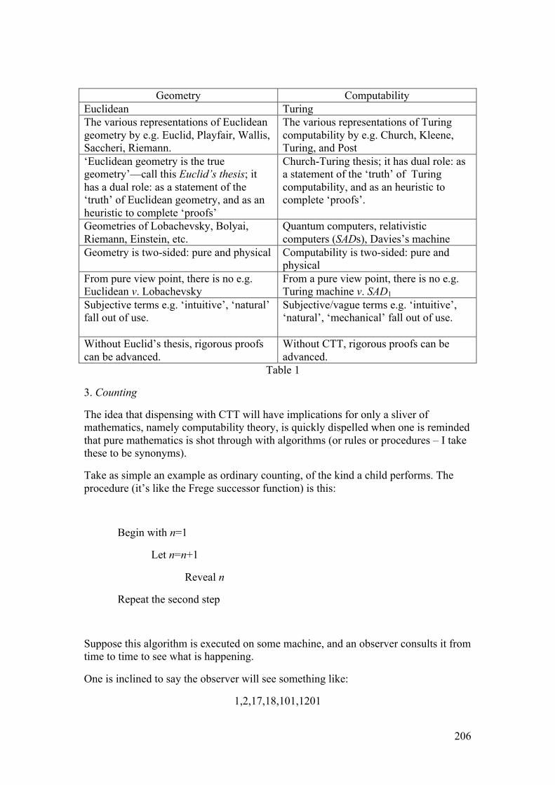
206

Geometry Computability Euclidean Turing The various representations of Euclidean geometry by e.g. Euclid, Playfair, Wallis, Saccheri, Riemann.

The various representations of Turing computability by e.g. Church, Kleene, Turing, and Post

‘Euclidean geometry is the true geometry’—call this Euclid’s thesis; it has a dual role: as a statement of the ‘truth’ of Euclidean geometry, and as an heuristic to complete ‘proofs’

Church-Turing thesis; it has dual role: as a statement of the ‘truth’ of Turing computability, and as an heuristic to complete ‘proofs’.

Geometries of Lobachevsky, Bolyai, Riemann, Einstein, etc.

Quantum computers, relativistic computers (SADs), Davies’s machine

Geometry is two-sided: pure and physical Computability is two-sided: pure and physical

From pure view point, there is no e.g. Euclidean v. Lobachevsky

From a pure view point, there is no e.g. Turing machine v. SAD1

Subjective terms e.g. ‘intuitive’, ‘natural’ fall out of use.

Subjective/vague terms e.g. ‘intuitive’, ‘natural’, ‘mechanical’ fall out of use.

Without Euclid’s thesis, rigorous proofs can be advanced.

Without CTT, rigorous proofs can be advanced.

Table 1

3. Counting

The idea that dispensing with CTT will have implications for only a sliver of mathematics, namely computability theory, is quickly dispelled when one is reminded that pure mathematics is shot through with algorithms (or rules or procedures – I take these to be synonyms).

Take as simple an example as ordinary counting, of the kind a child performs. The procedure (it’s like the Frege successor function) is this:

Begin with n=1

Let n=n+1

Reveal n

Repeat the second step

Suppose this algorithm is executed on some machine, and an observer consults it from time to time to see what is happening.

One is inclined to say the observer will see something like:

1,2,17,18,101,1201

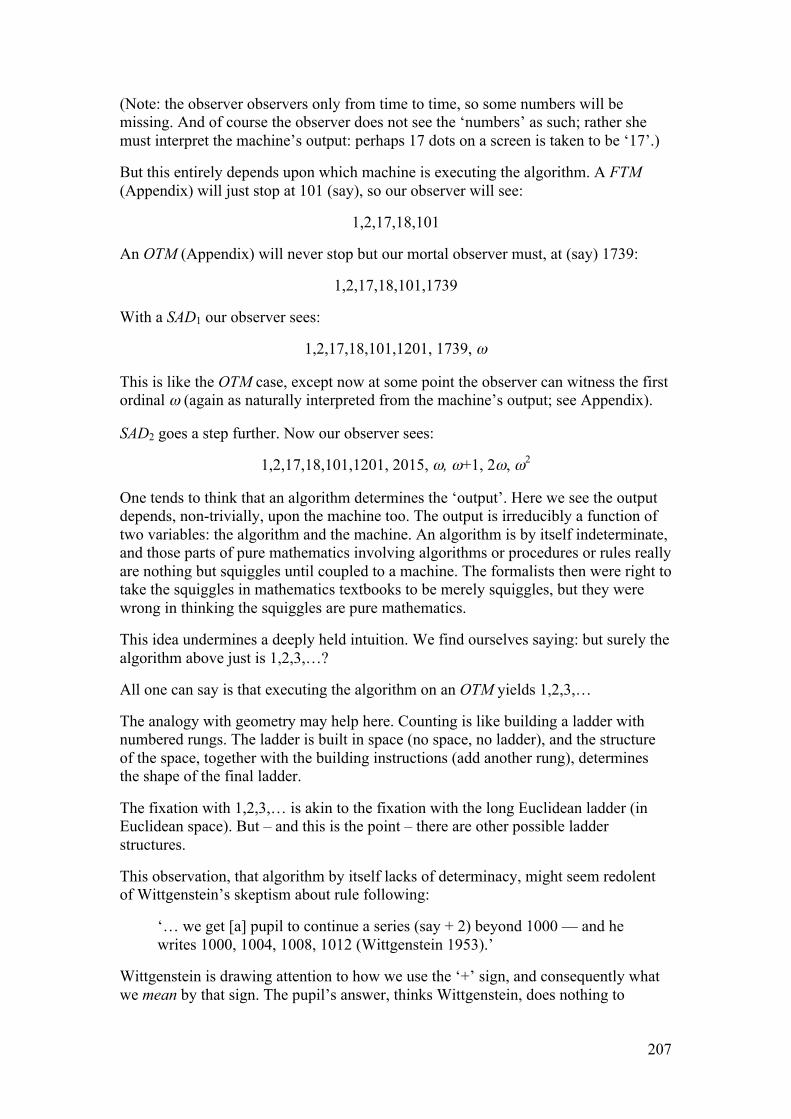
207

(Note: the observer observers only from time to time, so some numbers will be missing. And of course the observer does not see the ‘numbers’ as such; rather she must interpret the machine’s output: perhaps 17 dots on a screen is taken to be ‘17’.)

But this entirely depends upon which machine is executing the algorithm. A FTM (Appendix) will just stop at 101 (say), so our observer will see:

1,2,17,18,101

An OTM (Appendix) will never stop but our mortal observer must, at (say) 1739:

1,2,17,18,101,1739

With a SAD1 our observer sees:

1,2,17,18,101,1201, 1739, ω

This is like the OTM case, except now at some point the observer can witness the first ordinal ω (again as naturally interpreted from the machine’s output; see Appendix).

SAD2 goes a step further. Now our observer sees:

1,2,17,18,101,1201, 2015, ω, ω+1, 2ω, ω2

One tends to think that an algorithm determines the ‘output’. Here we see the output depends, non-trivially, upon the machine too. The output is irreducibly a function of two variables: the algorithm and the machine. An algorithm is by itself indeterminate, and those parts of pure mathematics involving algorithms or procedures or rules really are nothing but squiggles until coupled to a machine. The formalists then were right to take the squiggles in mathematics textbooks to be merely squiggles, but they were wrong in thinking the squiggles are pure mathematics.

This idea undermines a deeply held intuition. We find ourselves saying: but surely the algorithm above just is 1,2,3,…?

All one can say is that executing the algorithm on an OTM yields 1,2,3,…

The analogy with geometry may help here. Counting is like building a ladder with numbered rungs. The ladder is built in space (no space, no ladder), and the structure of the space, together with the building instructions (add another rung), determines the shape of the final ladder.

The fixation with 1,2,3,… is akin to the fixation with the long Euclidean ladder (in Euclidean space). But – and this is the point – there are other possible ladder structures.

This observation, that algorithm by itself lacks of determinacy, might seem redolent of Wittgenstein’s skeptism about rule following:

‘… we get [a] pupil to continue a series (say + 2) beyond 1000 — and he writes 1000, 1004, 1008, 1012 (Wittgenstein 1953).’

Wittgenstein is drawing attention to how we use the ‘+’ sign, and consequently what we mean by that sign. The pupil’s answer, thinks Wittgenstein, does nothing to

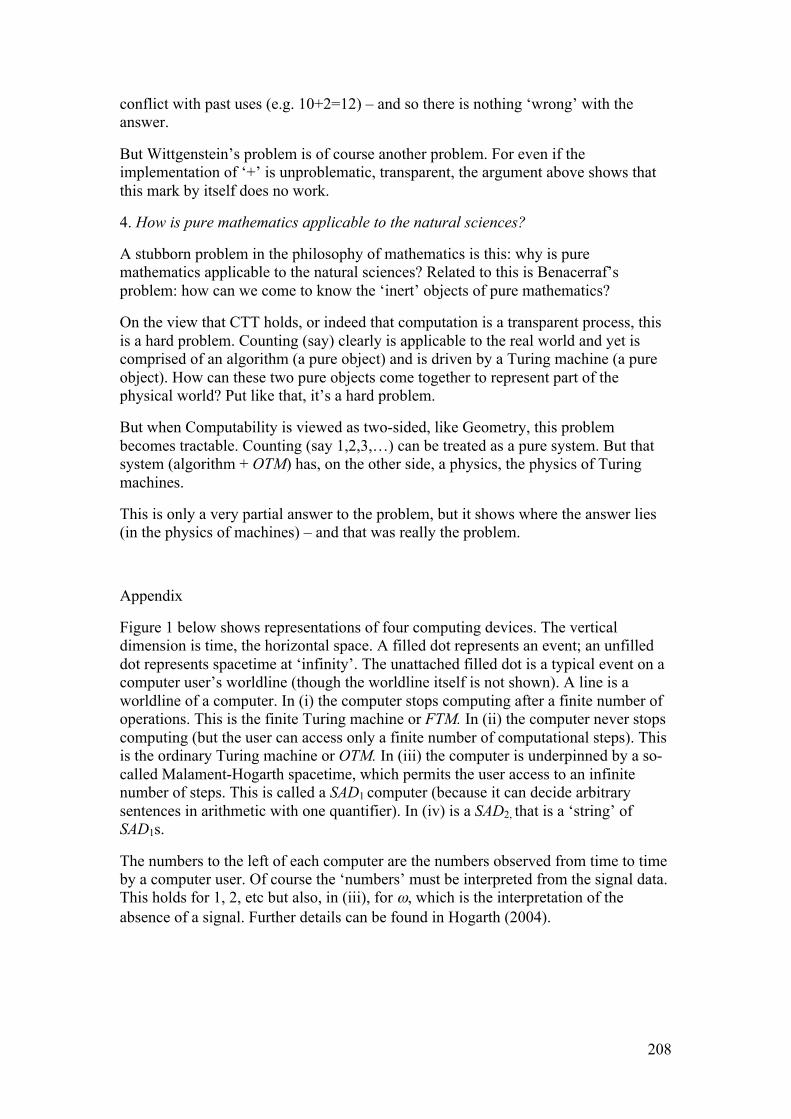
208

conflict with past uses (e.g. 10+2=12) – and so there is nothing ‘wrong’ with the answer.

But Wittgenstein’s problem is of course another problem. For even if the implementation of ‘+’ is unproblematic, transparent, the argument above shows that this mark by itself does no work.

4. How is pure mathematics applicable to the natural sciences?

A stubborn problem in the philosophy of mathematics is this: why is pure mathematics applicable to the natural sciences? Related to this is Benacerraf’s problem: how can we come to know the ‘inert’ objects of pure mathematics?

On the view that CTT holds, or indeed that computation is a transparent process, this is a hard problem. Counting (say) clearly is applicable to the real world and yet is comprised of an algorithm (a pure object) and is driven by a Turing machine (a pure object). How can these two pure objects come together to represent part of the physical world? Put like that, it’s a hard problem.

But when Computability is viewed as two-sided, like Geometry, this problem becomes tractable. Counting (say 1,2,3,…) can be treated as a pure system. But that system (algorithm + OTM) has, on the other side, a physics, the physics of Turing machines.

This is only a very partial answer to the problem, but it shows where the answer lies (in the physics of machines) – and that was really the problem.

Appendix

Figure 1 below shows representations of four computing devices. The vertical dimension is time, the horizontal space. A filled dot represents an event; an unfilled dot represents spacetime at ‘infinity’. The unattached filled dot is a typical event on a computer user’s worldline (though the worldline itself is not shown). A line is a worldline of a computer. In (i) the computer stops computing after a finite number of operations. This is the finite Turing machine or FTM. In (ii) the computer never stops computing (but the user can access only a finite number of computational steps). This is the ordinary Turing machine or OTM. In (iii) the computer is underpinned by a so-called Malament-Hogarth spacetime, which permits the user access to an infinite number of steps. This is called a SAD1 computer (because it can decide arbitrary sentences in arithmetic with one quantifier). In (iv) is a SAD2, that is a ‘string’ of SAD1s.

The numbers to the left of each computer are the numbers observed from time to time by a computer user. Of course the ‘numbers’ must be interpreted from the signal data. This holds for 1, 2, etc but also, in (iii), for ω, which is the interpretation of the absence of a signal. Further details can be found in Hogarth (2004).

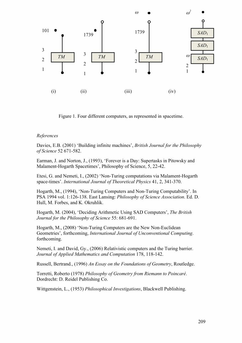
209

(i) (ii) (iii) (iv)

Figure 1. Four different computers, as represented in spacetime.

References

Davies, E.B. (2001) ‘Building infinite machines’, British Journal for the Philosophy of Science 52 671-582.

Earman, J. and Norton, J., (1993), ‘Forever is a Day: Supertasks in Pitowsky and Malament-Hogarth Spacetimes’, Philosophy of Science, 5, 22-42.

Etesi, G. and Nemeti, I., (2002) ‘Non-Turing computations via Malament-Hogarth space-times’. International Journal of Theoretical Physics 41, 2, 341-370.

Hogarth, M., (1994), ‘Non-Turing Computers and Non-Turing Computability’. In PSA 1994 vol. 1:126-138. East Lansing: Philosophy of Science Association. Ed. D. Hull, M. Forbes, and K. Okruhlik.

Hogarth, M. (2004), ‘Deciding Arithmetic Using SAD Computers’, The British Journal for the Philosophy of Science 55: 681-691.

Hogarth, M., (2008) ‘Non-Turing Computers are the New Non-Euclidean Geometries’, forthcoming, International Journal of Unconventional Computing. forthcoming.

Nemeti, I. and David, Gy., (2006) Relativistic computers and the Turing barrier. Journal of Applied Mathematics and Computation 178, 118-142.

Russell, Bertrand., (1996) An Essay on the Foundations of Geometry, Routledge.

Torretti, Roberto (1978) Philosophy of Geometry from Riemann to Poincaré. Dordrecht: D. Reidel Publishing Co.

Wittgenstein, L., (1953) Philosophical Investigations, Blackwell Publishing.

SAD1

SAD1

SAD1

TM TM TM

ω

101

2

1

1739

3

2

1

101

3

2

1

ω2

ω

2 1

ω

1739

3

2

1

General relativistic hypercomputing and

foundation of mathematics

Hajnal Andreka, Istvan Nemeti and Peter Nemeti

Renyi Institute of Mathematics, Budapest P.O.Box 127, H-1364 Hungary,[email protected], [email protected], [email protected]

Abstract. Looking at very recent developments in spacetime theory, wecan wonder whether these results exhibit features of hypercomputationthat traditionally seemed impossible or absurd. Namely, we describe aphysical device in relativistic spacetime which can compute a non-Turingcomputable task, e.g. which can decide the halting problem of Turing ma-chines or decide whether ZF set theory is consistent (more precisely, candecide the theorems of ZF). Starting from this, we will discuss the impactof recent breakthrough results of relativity theory, black hole physics andcosmology to well established foundational issues of computability the-ory as well as to logic. We find that the unexpected, revolutionary resultsin the mentioned branches of science force us to reconsider the status ofthe physical Church Thesis and to consider it as being seriously chal-lenged. We will outline the consequences of all this for the foundation ofmathematics (e.g. to Hilbert’s programme).Observational, empirical evidence will be quoted to show that the state-ments above do not require any assumption of some physical universeoutside of our own one: in our specific physical universe there seem to ex-ist regions of spacetime supporting potential non-Turing computations.Additionally, new “engineering” ideas will be outlined for solving theso-called blue-shift problem of GR-computing. Connections with relatedtalks at the Physics and Computation meeting, e.g. those of JeromeDurand-Lose, Mark Hogarth and Martin Ziegler, will be indicated.

1 Introduction

We discuss here the impact of very recent developments in spacetime theoryand cosmology on well established foundational issues (and interpretations) oflogic and computability theory. The connections between computability theory,logic and spacetime theory (general relativity theory, GR) cut both ways: logicprovides a tangible foundation for GR, cf. [1], while GR and its new developmentsmight profoundly influence our interpretation of basic results of computabilitytheory, as we will see in this paper. The new computability paradigms in turnoffer feedback to the foundation of mathematics and logic.

Because of the interdisciplinary character of this paper, the first two sectionsare somewhat introductory, explaining the basic ideas for the nonspecialist. Wewill start speeding up beginning with section 3.

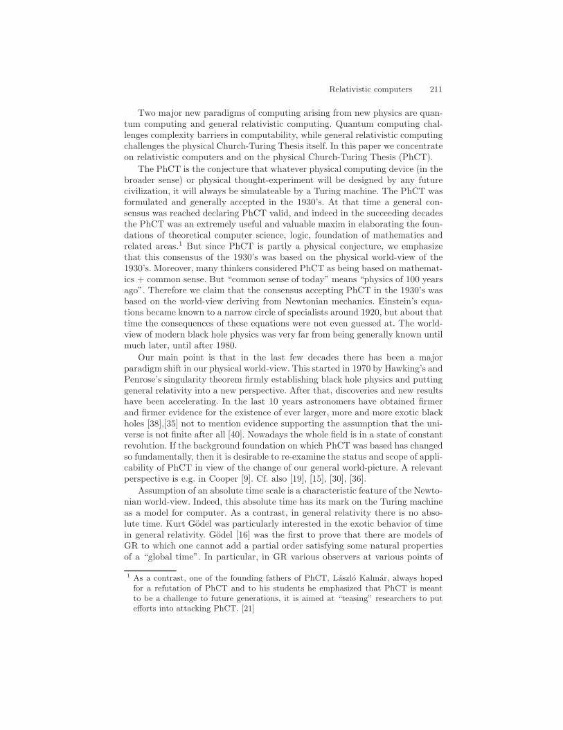
Relativistic computers 211

Two major new paradigms of computing arising from new physics are quan-tum computing and general relativistic computing. Quantum computing chal-lenges complexity barriers in computability, while general relativistic computingchallenges the physical Church-Turing Thesis itself. In this paper we concentrateon relativistic computers and on the physical Church-Turing Thesis (PhCT).

The PhCT is the conjecture that whatever physical computing device (in thebroader sense) or physical thought-experiment will be designed by any futurecivilization, it will always be simulateable by a Turing machine. The PhCT wasformulated and generally accepted in the 1930’s. At that time a general con-sensus was reached declaring PhCT valid, and indeed in the succeeding decadesthe PhCT was an extremely useful and valuable maxim in elaborating the foun-dations of theoretical computer science, logic, foundation of mathematics andrelated areas.1 But since PhCT is partly a physical conjecture, we emphasizethat this consensus of the 1930’s was based on the physical world-view of the1930’s. Moreover, many thinkers considered PhCT as being based on mathemat-ics + common sense. But “common sense of today” means “physics of 100 yearsago”. Therefore we claim that the consensus accepting PhCT in the 1930’s wasbased on the world-view deriving from Newtonian mechanics. Einstein’s equa-tions became known to a narrow circle of specialists around 1920, but about thattime the consequences of these equations were not even guessed at. The world-view of modern black hole physics was very far from being generally known untilmuch later, until after 1980.

Our main point is that in the last few decades there has been a majorparadigm shift in our physical world-view. This started in 1970 by Hawking’s andPenrose’s singularity theorem firmly establishing black hole physics and puttinggeneral relativity into a new perspective. After that, discoveries and new resultshave been accelerating. In the last 10 years astronomers have obtained firmerand firmer evidence for the existence of ever larger, more and more exotic blackholes [38],[35] not to mention evidence supporting the assumption that the uni-verse is not finite after all [40]. Nowadays the whole field is in a state of constantrevolution. If the background foundation on which PhCT was based has changedso fundamentally, then it is desirable to re-examine the status and scope of appli-cability of PhCT in view of the change of our general world-picture. A relevantperspective is e.g. in Cooper [9]. Cf. also [19], [15], [30], [36].

Assumption of an absolute time scale is a characteristic feature of the Newto-nian world-view. Indeed, this absolute time has its mark on the Turing machineas a model for computer. As a contrast, in general relativity there is no abso-lute time. Kurt Godel was particularly interested in the exotic behavior of timein general relativity. Godel [16] was the first to prove that there are models ofGR to which one cannot add a partial order satisfying some natural propertiesof a “global time”. In particular, in GR various observers at various points of

1 As a contrast, one of the founding fathers of PhCT, Laszlo Kalmar, always hopedfor a refutation of PhCT and to his students he emphasized that PhCT is meantto be a challenge to future generations, it is aimed at “teasing” researchers to putefforts into attacking PhCT. [21]

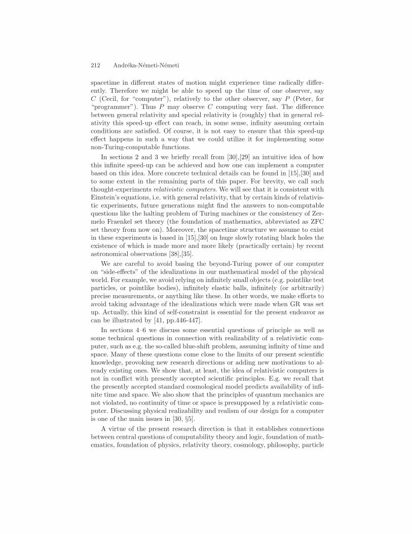
212 Andreka-Nemeti-Nemeti

spacetime in different states of motion might experience time radically differ-ently. Therefore we might be able to speed up the time of one observer, sayC (Cecil, for “computer”), relatively to the other observer, say P (Peter, for“programmer”). Thus P may observe C computing very fast. The differencebetween general relativity and special relativity is (roughly) that in general rel-ativity this speed-up effect can reach, in some sense, infinity assuming certainconditions are satisfied. Of course, it is not easy to ensure that this speed-upeffect happens in such a way that we could utilize it for implementing somenon-Turing-computable functions.

In sections 2 and 3 we briefly recall from [30],[29] an intuitive idea of howthis infinite speed-up can be achieved and how one can implement a computerbased on this idea. More concrete technical details can be found in [15],[30] andto some extent in the remaining parts of this paper. For brevity, we call suchthought-experiments relativistic computers. We will see that it is consistent withEinstein’s equations, i.e. with general relativity, that by certain kinds of relativis-tic experiments, future generations might find the answers to non-computablequestions like the halting problem of Turing machines or the consistency of Zer-melo Fraenkel set theory (the foundation of mathematics, abbreviated as ZFCset theory from now on). Moreover, the spacetime structure we assume to existin these experiments is based in [15],[30] on huge slowly rotating black holes theexistence of which is made more and more likely (practically certain) by recentastronomical observations [38],[35].

We are careful to avoid basing the beyond-Turing power of our computeron “side-effects” of the idealizations in our mathematical model of the physicalworld. For example, we avoid relying on infinitely small objects (e.g. pointlike testparticles, or pointlike bodies), infinitely elastic balls, infinitely (or arbitrarily)precise measurements, or anything like these. In other words, we make efforts toavoid taking advantage of the idealizations which were made when GR was setup. Actually, this kind of self-constraint is essential for the present endeavor ascan be illustrated by [41, pp.446-447].

In sections 4–6 we discuss some essential questions of principle as well assome technical questions in connection with realizability of a relativistic com-puter, such as e.g. the so-called blue-shift problem, assuming infinity of time andspace. Many of these questions come close to the limits of our present scientificknowledge, provoking new research directions or adding new motivations to al-ready existing ones. We show that, at least, the idea of relativistic computers isnot in conflict with presently accepted scientific principles. E.g. we recall thatthe presently accepted standard cosmological model predicts availability of infi-nite time and space. We also show that the principles of quantum mechanics arenot violated, no continuity of time or space is presupposed by a relativistic com-puter. Discussing physical realizability and realism of our design for a computeris one of the main issues in [30, §5].

A virtue of the present research direction is that it establishes connectionsbetween central questions of computability theory and logic, foundation of math-ematics, foundation of physics, relativity theory, cosmology, philosophy, particle

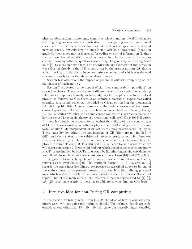
Relativistic computers 213

physics, observational astronomy, computer science and Artificial Intelligence[44]. E.g. it gives new kinds of motivation to investigating central questions ofthese fields like “is the universe finite or infinite (both in space and time) andin what sense”, “exactly how do huge Kerr black holes evaporate” (quantumgravity), “how much matter is needed for coding one bit of information (is theresuch a lower bound at all)”, questions concerning the statuses of the variouscosmic censor hypotheses, questions concerning the geometry of rotating blackholes [5], to mention only a few. The interdisciplinary character of this directionwas reflected already in the 1987 course given by the present authors [28] duringwhich the idea of relativistic hypercomputers emerged and which was devotedto connections between the above mentioned areas.

Section 6 is also about the impact of general relativistic computing on thefoundation of mathematics.

Section 7 is devoted to the impact of the “new computability paradigm” onspacetime theory. There, we discuss a different kind of motivation for studyingrelativistic computers. Namely, such a study may have applications to theoreticalphysics as follows. To GR, there is an infinite hierarchy of hypotheses calledcausality constraints which can be added to GR as outlined in the monograph[11, §6.3, pp.164-167]. Among these occur the various versions of the cosmiccensor hypothesis (CCH) of which the basic reference book of relativity theory[42, p.303] writes “whether the cosmic censor conjecture is correct remains thekey unresolved issue in the theory of gravitational collapse”. On p.305 [42] writes“... there is virtually no evidence for or against the validity of this second versionof CCH”. These causality hypotheses play a role in GR analogous with the roleformulas like GCH independent of ZF set theory play in set theory (or logic).These causality hypotheses are independent of GR (they are not implied byGR), and their status is the subject of intensive study as op. cit. illustratesthis. Now, the study of relativistic computers could, in principle, reveal how thephysical Church Thesis PhCT is situated in this hierarchy, in a sense which wewill discuss in section 7. If we could find out which one of these constraints implyPhCT (or are implied by PhCT), that could be illuminating in why certain issuesare difficult to settle about these constraints, cf. e.g. Etesi [14] and [42, p.303].

Tangible data underlying the above interconnections and also more history,references are available in [30]. The textbook Earman [11, p.119, section 4.9]regards the same interdisciplinary perspective as described above to be one ofthe main virtues of the present research direction. It is the unifying power oflogic which makes it viable to do serious work on such a diverse collection oftopics. One of the main aims of the research direction represented by [1]–[3],[23]–[25] is to make relativity theory accessible for anyone familiar with logic.

2 Intuitive idea for non-Turing GR computing

In this section we briefly recall from [30, 29] the ideas of how relativistic com-puters work, without going into technical details. The technical details are elab-orated, among others, in [15], [19], [30]. To make our narrative more tangible,

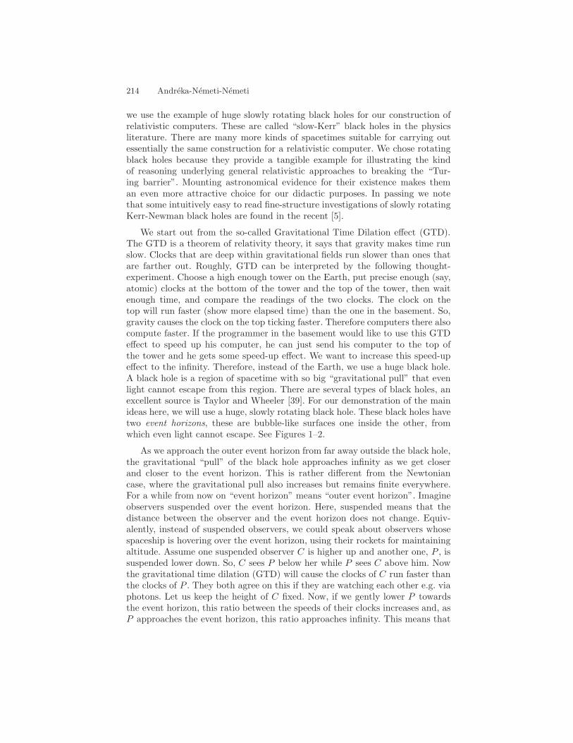
214 Andreka-Nemeti-Nemeti

we use the example of huge slowly rotating black holes for our construction ofrelativistic computers. These are called “slow-Kerr” black holes in the physicsliterature. There are many more kinds of spacetimes suitable for carrying outessentially the same construction for a relativistic computer. We chose rotatingblack holes because they provide a tangible example for illustrating the kindof reasoning underlying general relativistic approaches to breaking the “Tur-ing barrier”. Mounting astronomical evidence for their existence makes theman even more attractive choice for our didactic purposes. In passing we notethat some intuitively easy to read fine-structure investigations of slowly rotatingKerr-Newman black holes are found in the recent [5].

We start out from the so-called Gravitational Time Dilation effect (GTD).The GTD is a theorem of relativity theory, it says that gravity makes time runslow. Clocks that are deep within gravitational fields run slower than ones thatare farther out. Roughly, GTD can be interpreted by the following thought-experiment. Choose a high enough tower on the Earth, put precise enough (say,atomic) clocks at the bottom of the tower and the top of the tower, then waitenough time, and compare the readings of the two clocks. The clock on thetop will run faster (show more elapsed time) than the one in the basement. So,gravity causes the clock on the top ticking faster. Therefore computers there alsocompute faster. If the programmer in the basement would like to use this GTDeffect to speed up his computer, he can just send his computer to the top ofthe tower and he gets some speed-up effect. We want to increase this speed-upeffect to the infinity. Therefore, instead of the Earth, we use a huge black hole.A black hole is a region of spacetime with so big “gravitational pull” that evenlight cannot escape from this region. There are several types of black holes, anexcellent source is Taylor and Wheeler [39]. For our demonstration of the mainideas here, we will use a huge, slowly rotating black hole. These black holes havetwo event horizons, these are bubble-like surfaces one inside the other, fromwhich even light cannot escape. See Figures 1–2.

As we approach the outer event horizon from far away outside the black hole,the gravitational “pull” of the black hole approaches infinity as we get closerand closer to the event horizon. This is rather different from the Newtoniancase, where the gravitational pull also increases but remains finite everywhere.For a while from now on “event horizon” means “outer event horizon”. Imagineobservers suspended over the event horizon. Here, suspended means that thedistance between the observer and the event horizon does not change. Equiv-alently, instead of suspended observers, we could speak about observers whosespaceship is hovering over the event horizon, using their rockets for maintainingaltitude. Assume one suspended observer C is higher up and another one, P , issuspended lower down. So, C sees P below her while P sees C above him. Nowthe gravitational time dilation (GTD) will cause the clocks of C run faster thanthe clocks of P . They both agree on this if they are watching each other e.g. viaphotons. Let us keep the height of C fixed. Now, if we gently lower P towardsthe event horizon, this ratio between the speeds of their clocks increases and, asP approaches the event horizon, this ratio approaches infinity. This means that

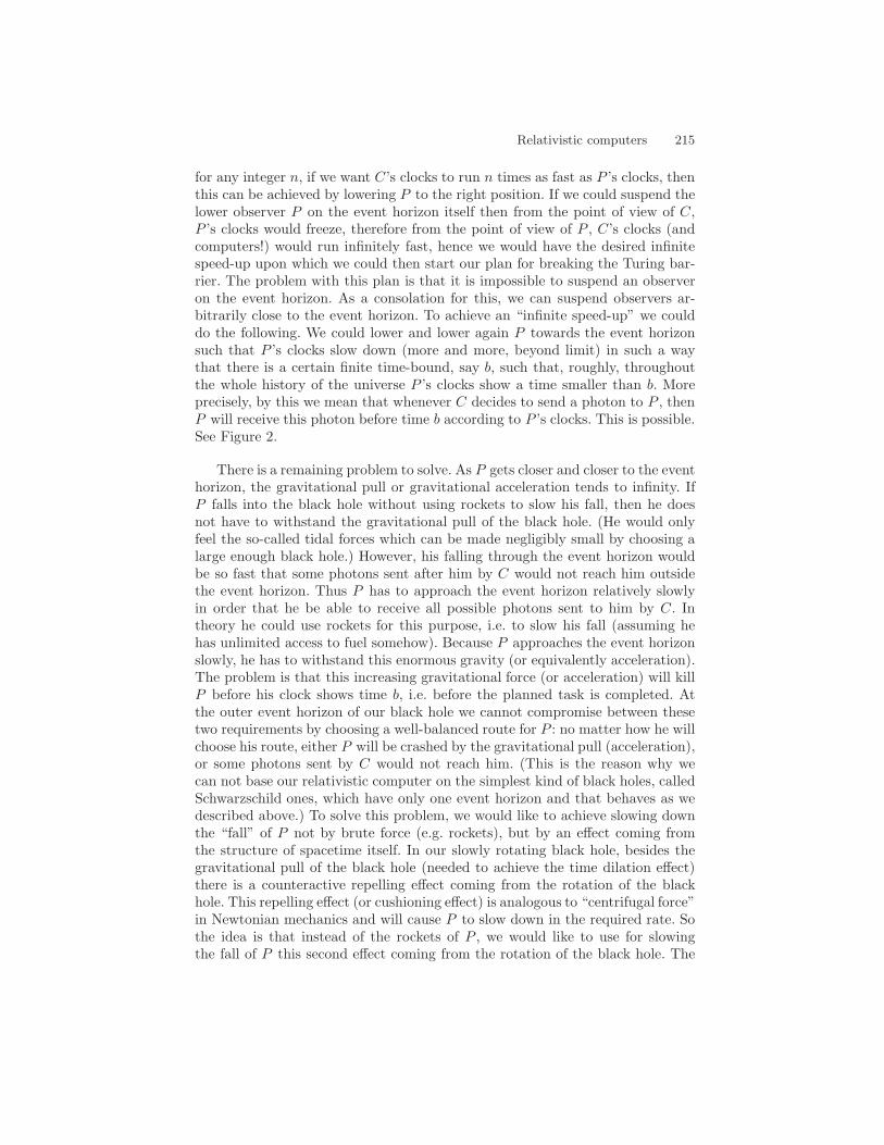
Relativistic computers 215

for any integer n, if we want C’s clocks to run n times as fast as P ’s clocks, thenthis can be achieved by lowering P to the right position. If we could suspend thelower observer P on the event horizon itself then from the point of view of C,P ’s clocks would freeze, therefore from the point of view of P , C’s clocks (andcomputers!) would run infinitely fast, hence we would have the desired infinitespeed-up upon which we could then start our plan for breaking the Turing bar-rier. The problem with this plan is that it is impossible to suspend an observeron the event horizon. As a consolation for this, we can suspend observers ar-bitrarily close to the event horizon. To achieve an “infinite speed-up” we coulddo the following. We could lower and lower again P towards the event horizonsuch that P ’s clocks slow down (more and more, beyond limit) in such a waythat there is a certain finite time-bound, say b, such that, roughly, throughoutthe whole history of the universe P ’s clocks show a time smaller than b. Moreprecisely, by this we mean that whenever C decides to send a photon to P , thenP will receive this photon before time b according to P ’s clocks. This is possible.See Figure 2.

There is a remaining problem to solve. As P gets closer and closer to the eventhorizon, the gravitational pull or gravitational acceleration tends to infinity. IfP falls into the black hole without using rockets to slow his fall, then he doesnot have to withstand the gravitational pull of the black hole. (He would onlyfeel the so-called tidal forces which can be made negligibly small by choosing alarge enough black hole.) However, his falling through the event horizon wouldbe so fast that some photons sent after him by C would not reach him outsidethe event horizon. Thus P has to approach the event horizon relatively slowlyin order that he be able to receive all possible photons sent to him by C. Intheory he could use rockets for this purpose, i.e. to slow his fall (assuming hehas unlimited access to fuel somehow). Because P approaches the event horizonslowly, he has to withstand this enormous gravity (or equivalently acceleration).The problem is that this increasing gravitational force (or acceleration) will killP before his clock shows time b, i.e. before the planned task is completed. Atthe outer event horizon of our black hole we cannot compromise between thesetwo requirements by choosing a well-balanced route for P : no matter how he willchoose his route, either P will be crashed by the gravitational pull (acceleration),or some photons sent by C would not reach him. (This is the reason why wecan not base our relativistic computer on the simplest kind of black holes, calledSchwarzschild ones, which have only one event horizon and that behaves as wedescribed above.) To solve this problem, we would like to achieve slowing downthe “fall” of P not by brute force (e.g. rockets), but by an effect coming fromthe structure of spacetime itself. In our slowly rotating black hole, besides thegravitational pull of the black hole (needed to achieve the time dilation effect)there is a counteractive repelling effect coming from the rotation of the blackhole. This repelling effect (or cushioning effect) is analogous to “centrifugal force”in Newtonian mechanics and will cause P to slow down in the required rate. Sothe idea is that instead of the rockets of P , we would like to use for slowingthe fall of P this second effect coming from the rotation of the black hole. The

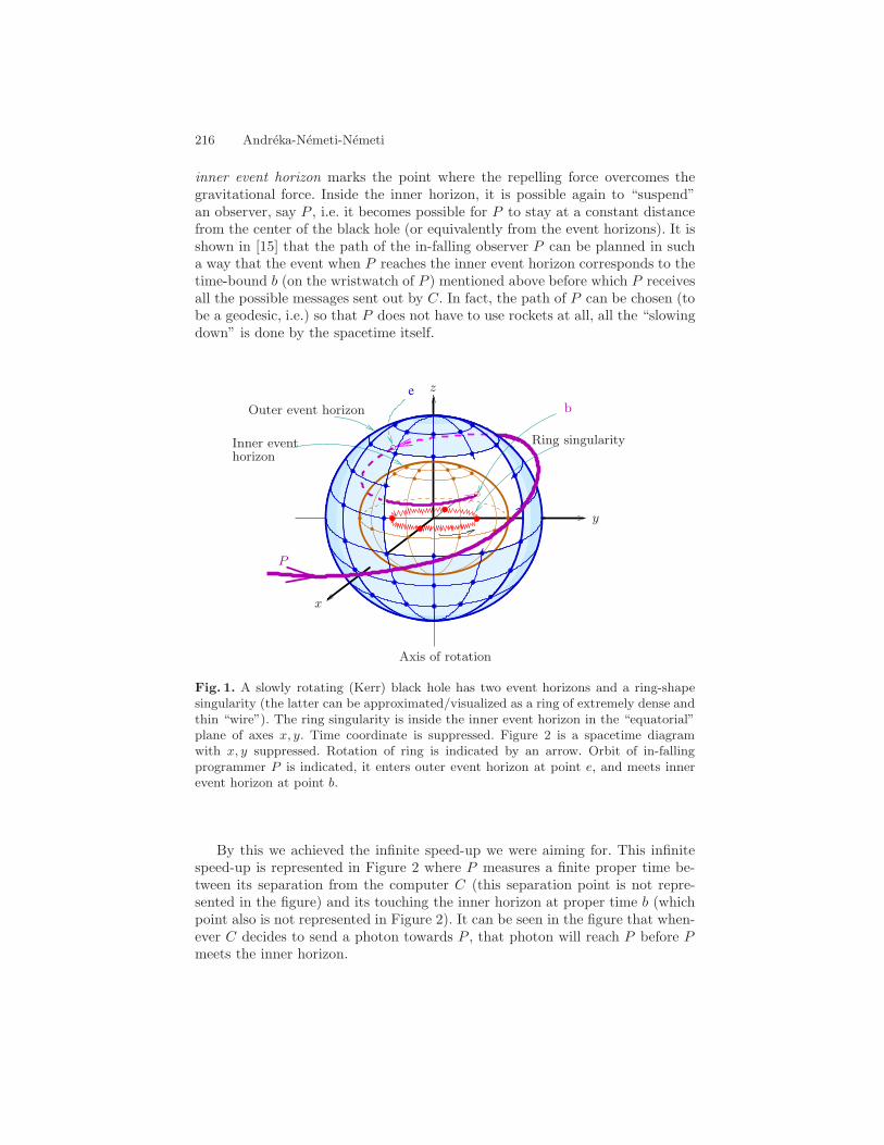
216 Andreka-Nemeti-Nemeti

inner event horizon marks the point where the repelling force overcomes thegravitational force. Inside the inner horizon, it is possible again to “suspend”an observer, say P , i.e. it becomes possible for P to stay at a constant distancefrom the center of the black hole (or equivalently from the event horizons). It isshown in [15] that the path of the in-falling observer P can be planned in sucha way that the event when P reaches the inner event horizon corresponds to thetime-bound b (on the wristwatch of P ) mentioned above before which P receivesall the possible messages sent out by C. In fact, the path of P can be chosen (tobe a geodesic, i.e.) so that P does not have to use rockets at all, all the “slowingdown” is done by the spacetime itself.

e z

x

y

Ring singularity

b

P

Inner eventhorizon

Outer event horizon

Axis of rotation

Fig. 1. A slowly rotating (Kerr) black hole has two event horizons and a ring-shapesingularity (the latter can be approximated/visualized as a ring of extremely dense andthin “wire”). The ring singularity is inside the inner event horizon in the “equatorial”plane of axes x, y. Time coordinate is suppressed. Figure 2 is a spacetime diagramwith x, y suppressed. Rotation of ring is indicated by an arrow. Orbit of in-fallingprogrammer P is indicated, it enters outer event horizon at point e, and meets innerevent horizon at point b.

By this we achieved the infinite speed-up we were aiming for. This infinitespeed-up is represented in Figure 2 where P measures a finite proper time be-tween its separation from the computer C (this separation point is not repre-sented in the figure) and its touching the inner horizon at proper time b (whichpoint also is not represented in Figure 2). It can be seen in the figure that when-ever C decides to send a photon towards P , that photon will reach P before Pmeets the inner horizon.

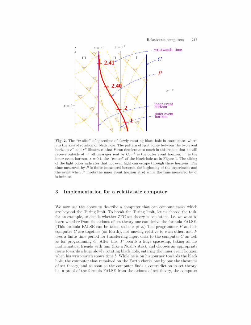
Relativistic computers 217

horizoninner event

outer eventhorizon

wristwatch−time

1

2

2.40

2.41III II I

t z = r− z = r+

z

z = 0

C

P

Fig. 2. The “tz-slice” of spacetime of slowly rotating black hole in coordinates wherez is the axis of rotation of black hole. The pattern of light cones between the two eventhorizons r− and r+ illustrates that P can decelerate so much in this region that he willreceive outside of r− all messages sent by C. r+ is the outer event horizon, r− is theinner event horizon, z = 0 is the “center” of the black hole as in Figure 1. The tiltingof the light cones indicates that not even light can escape through these horizons. Thetime measured by P is finite (measured between the beginning of the experiment andthe event when P meets the inner event horizon at b) while the time measured by Cis infinite.

3 Implementation for a relativistic computer

We now use the above to describe a computer that can compute tasks whichare beyond the Turing limit. To break the Turing limit, let us choose the task,for an example, to decide whether ZFC set theory is consistent. I.e. we want tolearn whether from the axioms of set theory one can derive the formula FALSE.(This formula FALSE can be taken to be x = x.) The programmer P and hiscomputer C are together (on Earth), not moving relative to each other, and Puses a finite time-period for transferring input data to the computer C as wellas for programming C. After this, P boards a huge spaceship, taking all hismathematical friends with him (like a Noah’s Ark), and chooses an appropriateroute towards a huge slowly rotating black hole, entering the inner event horizonwhen his wrist-watch shows time b. While he is on his journey towards the blackhole, the computer that remained on the Earth checks one by one the theoremsof set theory, and as soon as the computer finds a contradiction in set theory,i.e. a proof of the formula FALSE from the axioms of set theory, the computer

218 Andreka-Nemeti-Nemeti

sends a signal to the programmer indicating that set theory is inconsistent. If itdoes not find a proof for FALSE, the computer sends no signal.

The programmer falls into the inner event horizon of the black hole and afterhe has crossed the inner event horizon, he can evaluate the situation. If a lightsignal has arrived from the direction of the computer, of an agreed color andagreed pattern, this means that the computer found an inconsistency in ZFCset theory, therefore the programmer will know that set theory is inconsistent. Ifthe light signal has not arrived, and the programmer is already inside the innerevent horizon, then he will know that the computer did not find an inconsistencyin set theory, did not send the signal, therefore the programmer can concludethat set theory is consistent. So he can build the rest of his mathematics on thesecure knowledge of the consistency of set theory. We will return to the issue ofwhether the programmer has enough space and time and resources for using thejust gained information at the end of section 5.

The above outlined train of thought can be used to show that any recursivelyenumerable set can be decided by a relativistic computer [15]. Actually, morethan that can be done by relativistic computers. Welch [43] shows that the ar-rangement described in section 3 using Kerr black holes can compute exactly ∆2

problems in the arithmetical hierarchy (under some mild extra assumptions).Computability limits connected with such relativistic computers are also ad-dressed in [19], [20], [36], [44].

Relativistic computers are not tied to rotating black holes, there are othergeneral relativistic phenomena on which they can be based. An example is anti-de-Sitter spacetime which attracts more and more attention in explaining recentdiscoveries in cosmology (the present acceleration of the expansion of the uni-verse, cf. [30]). Roughly, in anti-de-Sitter spacetime, time ticks faster and fasterat farther away places in such a way that P can achieve infinite speed-up bysending away the computer C and waiting for a signal from her. This scenario isdescribed and is utilized for computing non-Turing computable functions in [19].This example shows that using black holes (or even singularities) is not inherentin relativistic computers.

Spacetimes suitable for an implementation of relativistic computation likedescribed in this section are called Malament-Hogarth spacetimes in the physicsliterature. A relativistic spacetime is called Malament-Hogarth (MH) if there isan event (called MH-event) in it which contains in its causal past a worldlineof infinite proper length. The spacetime of ordinary Schwarzschild black hole isnot MH, the spacetime of rotating Kerr black hole is MH and any event withinthe inner event horizon is MH, in anti-de-Sitter spacetime every event is an MH-event, the spacetime of an electrically charged BH (called Reissner-Nordstromspacetime) is MH and there are many other examples for MH.

We note that using MH spacetimes does not entail faith in some exotically“benevolent” global property of the whole of our universe. Instead, most of theMH spacetimes, like rotating BH’s, can be built by a future, advanced civiliza-tion inside our usual “standard” universe of high precision cosmology. Namely,such MH spacetimes do not necessarily refer to the whole universe, but instead,

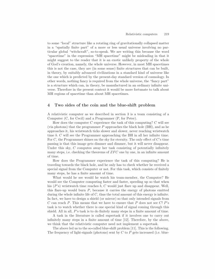
Relativistic computers 219

to some “local” structure like a rotating ring of gravitationally collapsed matterin a “spatially finite part” of a more or less usual universe involving no par-ticular global “witchcraft”, so-to-speak. We are writing this because the word“spacetime” in the expression “MH spacetime” might be misleading in that itmight suggest to the reader that it is an exotic unlikely property of the wholeof God’s creation, namely, the whole universe. However, in most MH spacetimesthis is not the case, they are (in some sense) finite structures that can be built,in theory, by suitably advanced civilizations in a standard kind of universe likethe one which is predicted by the present-day standard version of cosmology. Inother words, nothing fancy is required from the whole universe, the “fancy part”is a structure which can, in theory, be manufactured in an ordinary infinite uni-verse. Therefore in the present context it would be more fortunate to talk aboutMH regions of spacetime than about MH spacetimes.

4 Two sides of the coin and the blue-shift problem

A relativistic computer as we described in section 3 is a team consisting of aComputer (C, for Cecil) and a Programmer (P, for Peter).

How does the computer C experience the task of this computing? C will see(via photons) that the programmer P approaches the black hole (BH), and as heapproaches it, his wristwatch ticks slower and slower, never reaching wristwatchtime b. C will see the Programmer approaching the BH in all her infinite time.For C, the Programmer shines on the sky for eternity. The only effect of C’s timepassing is that this image gets dimmer and dimmer, but it will never disappear.Under this sky, C computes away her task consisting of potentially infinitelymany steps, i.e. checking the theorems of ZFC one by one, in an infinite amountof time.

How does the Programmer experience the task of this computing? He istraveling towards the black hole, and he only has to check whether he received aspecial signal from the Computer or not. For this task, which consists of finitelymany steps, he has a finite amount of time.

What would he see would he watch his team-member, the Computer? Hewould see the Computer computing faster and faster, speeding up so that whenhis (P ’s) wristwatch time reaches b, C would just flare up and disappear. Well,this flare-up would burn P , because it carries the energy of photons emittedduring the whole infinite life of C, thus the total amount of this energy is infinite.In fact, we have to design a shield (or mirror) so that only intended signals fromC can reach P . This means that we have to ensure that P does not see C! P ’stask is to watch whether there is one special kind of signal coming through thisshield. All in all, P ’s task is to do finitely many steps in a finite amount of time.

A task in the literature is called supertask if it involves one to carry outinfinitely many steps in a finite amount of time [12]. Therefore, by the above,we think that the relativistic computer need not implement a supertask.

The above led us to the so-called blue-shift problem [11]. This is the following.The frequency of light-signals (photons) sent by C to P gets increased (i.e. blue-

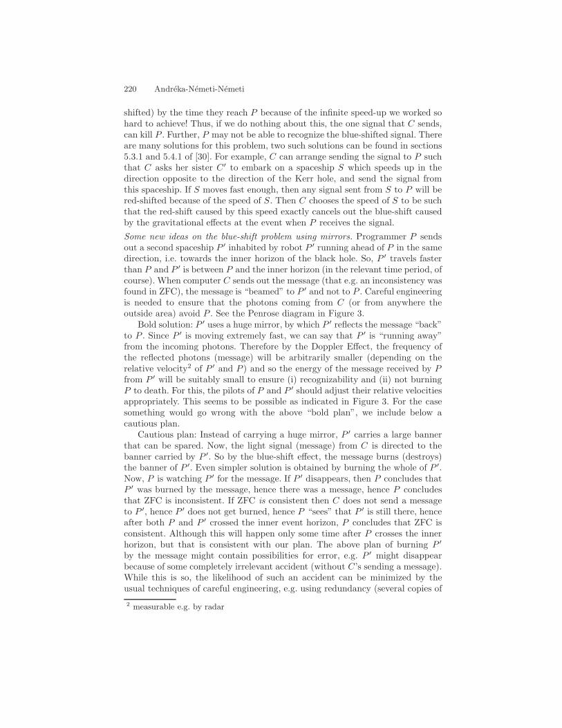
220 Andreka-Nemeti-Nemeti

shifted) by the time they reach P because of the infinite speed-up we worked sohard to achieve! Thus, if we do nothing about this, the one signal that C sends,can kill P . Further, P may not be able to recognize the blue-shifted signal. Thereare many solutions for this problem, two such solutions can be found in sections5.3.1 and 5.4.1 of [30]. For example, C can arrange sending the signal to P suchthat C asks her sister C′ to embark on a spaceship S which speeds up in thedirection opposite to the direction of the Kerr hole, and send the signal fromthis spaceship. If S moves fast enough, then any signal sent from S to P will bered-shifted because of the speed of S. Then C chooses the speed of S to be suchthat the red-shift caused by this speed exactly cancels out the blue-shift causedby the gravitational effects at the event when P receives the signal.Some new ideas on the blue-shift problem using mirrors. Programmer P sendsout a second spaceship P ′ inhabited by robot P ′ running ahead of P in the samedirection, i.e. towards the inner horizon of the black hole. So, P ′ travels fasterthan P and P ′ is between P and the inner horizon (in the relevant time period, ofcourse). When computer C sends out the message (that e.g. an inconsistency wasfound in ZFC), the message is “beamed” to P ′ and not to P . Careful engineeringis needed to ensure that the photons coming from C (or from anywhere theoutside area) avoid P . See the Penrose diagram in Figure 3.

Bold solution: P ′ uses a huge mirror, by which P ′ reflects the message “back”to P . Since P ′ is moving extremely fast, we can say that P ′ is “running away”from the incoming photons. Therefore by the Doppler Effect, the frequency ofthe reflected photons (message) will be arbitrarily smaller (depending on therelative velocity2 of P ′ and P ) and so the energy of the message received by Pfrom P ′ will be suitably small to ensure (i) recognizability and (ii) not burningP to death. For this, the pilots of P and P ′ should adjust their relative velocitiesappropriately. This seems to be possible as indicated in Figure 3. For the casesomething would go wrong with the above “bold plan”, we include below acautious plan.

Cautious plan: Instead of carrying a huge mirror, P ′ carries a large bannerthat can be spared. Now, the light signal (message) from C is directed to thebanner carried by P ′. So by the blue-shift effect, the message burns (destroys)the banner of P ′. Even simpler solution is obtained by burning the whole of P ′.Now, P is watching P ′ for the message. If P ′ disappears, then P concludes thatP ′ was burned by the message, hence there was a message, hence P concludesthat ZFC is inconsistent. If ZFC is consistent then C does not send a messageto P ′, hence P ′ does not get burned, hence P “sees” that P ′ is still there, henceafter both P and P ′ crossed the inner event horizon, P concludes that ZFC isconsistent. Although this will happen only some time after P crosses the innerhorizon, but that is consistent with our plan. The above plan of burning P ′

by the message might contain possibilities for error, e.g. P ′ might disappearbecause of some completely irrelevant accident (without C’s sending a message).While this is so, the likelihood of such an accident can be minimized by theusual techniques of careful engineering, e.g. using redundancy (several copies of

2 measurable e.g. by radar

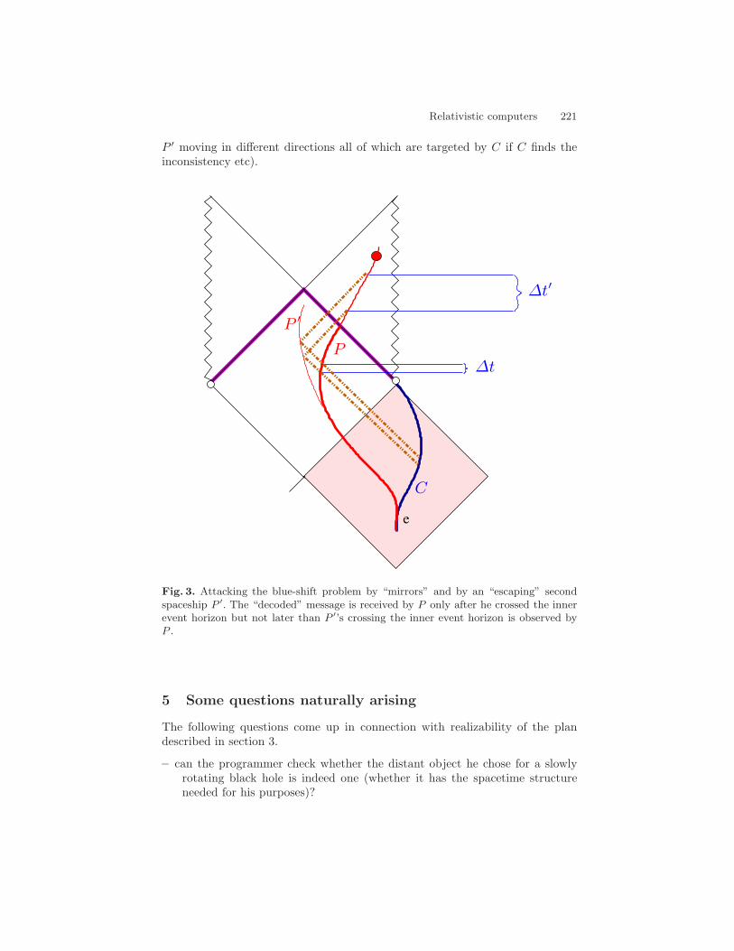
Relativistic computers 221

P ′ moving in different directions all of which are targeted by C if C finds theinconsistency etc).

e

∆t′

∆t

P ′

P

C

Fig. 3. Attacking the blue-shift problem by “mirrors” and by an “escaping” secondspaceship P ′. The “decoded” message is received by P only after he crossed the innerevent horizon but not later than P ′’s crossing the inner event horizon is observed byP .

5 Some questions naturally arising

The following questions come up in connection with realizability of the plandescribed in section 3.

– can the programmer check whether the distant object he chose for a slowlyrotating black hole is indeed one (whether it has the spacetime structureneeded for his purposes)?

222 Andreka-Nemeti-Nemeti

– can he check when he passed the event horizon?– can he survive passing the event horizon?– can he receive and recognize the signal sent by the computer?– how long can he live inside the black hole?– is there a way for the programmer to know that absence of signal from the

computer is not caused by some catastrophe in the life of the computer?– is it possible for a civilization to exist for an infinite amount of time?– can the programmer repeat the computation or is this a once-for-a-lifetime

computation for him?

Here we just assert that the answers to all these questions are in the affirma-tive, or at least do not contradict present scientific knowledge. These questionsare discussed in detail in [30]. Below we address three of these questions.

On the question of traverseability of the event horizon: We chose the blackhole to be large. If the black hole is huge3, the programmer will feel nothingwhen he passes either event horizon of the black hole—one can check that incase of a huge black hole the so-called tidal forces on the event horizons of theblack hole are negligibly small [32], [15].

On the question of how long the programmer can live after crossing the eventhorizon: The question is whether the programmer can use this new information,namely that set theory is consistent, or whatever he wanted to compute, for hispurposes. A pessimist could say that OK they are inside a black hole, so—nowwe are using common sense, we are not using relativity theory—common sensesays that the black hole is a small unfriendly area and the programmer willsooner or later fall into the middle of the black hole where there is a singularityand the singularity will kill the programmer and his friends. The reason why wechose our black hole to be a huge slowly rotating one, say of mass 1010m, is thefollowing. If the programmer falls into a black hole which is as big as this andit rotates slowly, then the programmer will have quite a lot of time inside theblack hole because the center of the black hole is relatively far from the eventhorizon. But this is not the key point. If it rotates, the “matter content”, the so-called singularity, which is the source of the gravitational field of the black holeso-to-speak, is not a point but a ring (see Fig.1). So if the programmer chooseshis route in falling into the black hole in a clever way, say, relatively close to thenorth pole instead of the equatorial plane, then the programmer can comfortablypass through the middle of the ring, never get close to the singularity and happilylive on forever (see Fig.s 1,2). We mean, the rules of relativity will not preventhim from happily living forever. He may have descendants, he can found society,he can use and pass on the so obtained mathematical knowledge.

On the question of whether the computation can be repeated: Let us lookat the extension of slow Kerr spacetime in [31, §3.3, pp.116-140]. Especially,consider the maximal slow Kerr spacetime (MSK) on Fig. 3.16, p.139. By con-sidering this MSK, we can convince ourselves that our GR-computation is re-peatable and with appropriate care it can be made deterministic. Some further

3 this is a technical expression in observational astronomy

Relativistic computers 223

meditation on this repeatability of GR-computing can lead to new perspectiveson the Platonism - formalism debates and views in the philosophical schools ofthe foundations of mathematics. E.g. one of the ages old arguments fades away,namely the argument saying that we cannot have access to any instances ofactual infinity.

6 Can we learn something about infinity? Impact on thefoundation of mathematics.

The relativistic computer as we implemented it in section 3 assumes that an in-finite amount of time is available for C for computing. This seems to be essentialfor breaking the Turing barrier (by our construction). We are in a good positionhere, because of the following. As a result of very recent revolution in cosmology,there is a so-called standard model of cosmology. This standard model is basedon matching members of a family of GR spacetimes against a huge number ofobservational data obtained by three different astronomical projects. This hugenumber of measurements (made and processed by using computers) all pointamazingly to one specific GR spacetime. This spacetime is called the standardcosmological model, and in accordance with the so far highly successful scientificpractice of the last 2500 years, we regard this standard model of the latest formof high-precision cosmology as the model best suited to explain observationsand experience collected so far. According to this standard model, our universeis infinite both in regard of time and space, moreover there is an infinite amountof matter-energy available in it. We will see soon that the latter infinity is notneeded for our construction. For more on this see David [10], [30] and the ref-erences therein. Our point here is not about believing that our universe indeedhas infinite time or not. The point is that assuming availability of an infiniteamount of time for computing is not in contradiction with our present-day sci-entific knowledge.

We would like to say some words on the question of how much matter/energyis needed for storing, say, 10 bits of information. Although this question is notessential for the realizability of the relativistic computer (because of availabilityof infinite energy in the standard model of cosmology), we still find this questioninteresting for purely intellectual/philosophical reasons.

Is information content strongly tied to matter/energy content? Is there alower bound to mass which is needed to store 10 bits of information? This isa question which has nagged one of the authors ever since he wrote his MsCthesis [27] where a separate section was devoted to this issue. The question is:“If I want to write more, do I need more paper to write on?” Right now itseems to us that the answer is in the negative. Matter and information mightbe two independent (orthogonal) “dimensions” of reality. The reason for this isthe following. One might decide to code data by photons. Then the amount ofmatter/energy used is the energy total of these photons. But the energy of aphoton is inversely proportional with its wavelength. So, one might double thewavelength of all photons and then one halved the energy needed to carry the

224 Andreka-Nemeti-Nemeti

same information one coded originally. If this is still too much energy expense,then one can double the wavelength again. Since there is no upper bound tothe wavelengths of photons, there is no lower bound for the energy needed forstoring 10 bits of data.

So, it seems to us that energy and information are not as strongly linkedentities as energy and mass are (via E = mc2). In the above argument when wesaid that there was no upper bound to the wavelength of possible photons, weused that according to the standard cosmological model the Universe is infinitein space. We note that Einstein when inventing photons did not say that thereis a smallest nonzero value for energy. He said this only for light of a fixed color,i.e. fixed wavelength.

We would like to emphasize that we did not use that space is continuous. Weseem to have used that time is continuous, but we can avoid that assumption byrefining the implementation of relativistic computer. Constructions for this arein [30]. Thus, no contradictions with the principles of quantum mechanics seemsto be involved in the idea of relativistic computer.

In the above, we argued that in principle, one can even build a relativisticcomputer sometime in the future. However, a fascinating aspect of relativis-tic computers for us is that they bring up mind-boggling questions about thenature of infinity. These questions would be worth thinking over even if ourpresent-day science would predict a finite universe. We seem to understand andbe familiar with the use of potential infinity in science. However, the abovethought-experiment seems to use the notion of actual infinity. Is infinity a men-tal construction only or does it exist in a more tangible way, too? Can we learnsomething about actual infinity by making physical experiments? This leads toquestions inherent in foundational issues in mathematics and physics. For moreabout this and about connection with Hilbert’s Programme for mathematics werefer to [4].

7 Relativistic Computers and Causality Hypotheses inPhysics

Let us consider the hierarchy of causality hypotheses C0, . . . , C6 summarizedin the monograph Earman [11, §6.3, pp.164-166]. None of these follow from GR(cf. e.g. [42, p.303]), they function as extra possible hypotheses for narrowing thescope of the theory. The strongest of these is the strong cosmic censor hypothesisC6 saying that spacetime is globally hyperbolic. A spacetime is called globallyhyperbolic if it contains a spacelike hypersurface that intersects every causal curvewithout endpoint exactly once. This implies that the “temporal” structure ofspacetime is basically the same as that of the Newtonian world in that it admitsa “global time” associating a real number t(p) to every point p of spacetime.In other words, C6 implies that spacetime admits a “global foliation”, i.e. it isa disjoint union of global time-slices or “global now”-s. This is a quite extremeassumption and its role is more of a logical status, i.e. one investigates questionsof what follows if C6 is assumed rather than assuming that it holds for the

Relativistic computers 225

actual universe. Recall that Wald [42, p.305 lines 7-8] wrote about the cosmiccensor hypothesis that “there is virtually no evidence for or against the validityof this”, as we quoted around the end of section 1. Cf. also [11, pp.97,99] forfurther doubts on C6.

In section 1 we said that the assumption of absolute time has its marks onthe Turing Machine as a model for computer, and now we see that C6 providesa kind of global time. Indeed, the construction of a GR-computer in this paperrelies heavily on failure of C6, because Hogarth proved that no MH-spacetime isglobally hyperbolic [11, Lemma 4.1, p.107]. This motivates the following ques-tion.

Question 1. Does (a carefully formulated variant of) PhCT follow from GR+C6?

On this question: PhCT has not been formalized precisely yet, this is partof why this question is asking for a formulation of PhCT which would followfrom GR+C6. In this question we are asking if there are some natural andconvincing extra conditions on physically realistic computability which wouldyield PhCT from GR+C6. The need for such extra realisticity assumptions isdemonstrated by e.g. Tipler [41, pp.446-447]. Actually, we started collectingsuch conditions for physical realisticity in the middle of sec. 1 (in the paragraphbeginning with “We are careful to avoid ...”). One might conjecture that, undersuitable assumptions on physical realisticity and with a suitable formulation ofPhCT, a kind of positive answer to Question 1 might be plausible4.

Question 1 is about the connection between PhCT and the cosmic censorhypothesis C6. Next we concern ourselves with the connection between PhCTand the Malament-Hogarth property of a spacetime. We note that C6 impliesthat the spacetime is not Malament-Hogarth (NoMH for short), [11, Lemma4.1, p.107] but NoMH does not imply C6 [11, p.110, first 2 sentences of sec.4.5].Hence NoMH is a strictly weaker causality hypothesis than C6. We note that[14] explores the connection between C6 and MH. Again, we have no reason forbelieving in NoMH.

Question 2. Under what natural (extra) conditions is NoMH equivalent withwhat version of PhCT?

On this question: In theory, the MH property implies failure of PhCT (i.e.PhCT ⇒ NoMH), because in any MH-spacetime one can, at least in theory,construct a GR-computer like in this paper, cf. [11, §4], [19]. However, there isa reason why in the works [15], [30], [29] we chose to implement our relativis-tic computer via a huge rotating black hole. Namely, huge-ness of the rotatingBH was used to ensure that the tidal forces at the event horizons do not kill4 Very tentatively: Recently, emerging new kinds of computing devices like the Internet

seem to pose a challenge against the conjecture in Question 1, cf. [44]. However, eventhe Internet (or even the Human Mind) will probably not prove ZFC consistent(assuming C6). So, perhaps we should separate PhCT into two theses, one about“hard” problems like proving the consistency of ZFC, and the other about problemsin general which are not Turing computable.

226 Andreka-Nemeti-Nemeti

the programmer. It is possible to construct a toy-example of a MH spacetimein which our kind of relativistic computer is not realistic physically. By physi-cal realisticity we mean requirements that we do not use infinitely small com-puters (objects), infinitely precise measurements, or the like in designing ournon-Turing computer, cf. [30] for more detail. We note that if we do not insiston physical realisticity, then already in Newtonian Mechanics PhCT would failas demonstrated e.g. in Tipler [41, pp.446-447]. This motivates the question ofwhat natural assumptions would ensure PhCT ⇒ NoMH or equivalently MH ⇒NotPhCT in a physically realistic way. This is one direction of Question 2 above.

The other direction of Question 2 seems to be the harder one: Under whatnatural conditions (if any) does NotPhCT imply MH. I.e. under what conditionsis

() NotPhCT ⇒ MH

true? One way of rephrasing () is to conjecture that if there is a physicallyrealistic non-Turing computer then there must be one which is built up in thestyle of the present paper utilizing MH property of spacetime. (By non-Turingcomputer we mean a physical computer that can compute beyond the Turingbarrier.) This seems to be a daring conjecture. But let us remember that thequestion was: under what conditions is statement () true. In particular, if thephysical non-Turing computer “designed” in the book Pour-El and Richards[34] turns out to be physically realizable, then our conjecture (that under somereasonable conditions () might become true) might get refuted.

We note that the tentative conjecture implicit in Question 2 was arrived atjointly with Gabor Etesi.

8 Logic based conceptual analysis of GR and “reversemathematics” for GR

So far we have been applying general relativity (GR) to logic and to the foun-dation of mathematics (FOM). In the other direction, logic and FOM are beingapplied to a conceptual analysis and logical/mathematical foundation of relativ-ity (including GR). In more detail: FOM has an important branch called reversemathematics. In the latter we ask the question(s) of which axioms of set the-ory are responsible (needed) for which important theorems of mathematics. Ina series of papers, e-books, and book chapters, a team containing the presentauthors has been working on a programme which could be called “exporting thesuccess story of FOM to a foundation of relativity” (set theorist Harvey Fried-man coined this slogan), cf. e.g. [1]–[3], [23]–[25]. Roughly speaking, this groupbuilds up relativity in first-order logic (like FOM is built up as a theory in thesense of mathematical logic), then analyzes the so obtained logical theory fromvarious perspectives and (like in reverse mathematics) attempts to answer theso-called why-type questions asking why a certain prediction of general relativ-ity is being predicted, i.e. which axioms of the theory are responsible for thatparticular prediction.

Relativistic computers 227

Section 7 above can be regarded as a small sample from the above quotedlogical/conceptual analysis of GR and its extensions. A particular example ofthis feedback from logic and FOM to GR is the paper [5].

By the above sketched feedback from logic and FOM to GR, the “circle”GR → Logic → FOM → GR promised in the introduction is completed.

9 History of relativistic computation

The idea of general relativistic computing as described in section 2 was found atdifferent parts of the globe, independently. It was discovered by Nemeti in 1987[28], Pitowsky in 1990 [33], Malament in 1989 [26], and Hogarth in 1992 [18]independently. Nemeti’s idea used large slowly rotating black holes (slow Kerrspacetimes) but the careful study of feasibility and transversability of these wasdone later in Etesi-Nemeti [15]. All this led to a fruitful cooperation betweenthe parties mentioned above, e.g. between Cambridge (Hogarth et al), Budapest(Nemeti et al), Pittsburgh (Earman et al). The first thorough and systematicstudy of relativistic computation was probably Hogarth [19]. Related work onrelativistic computing include [43], [36], [11, §4], [12], [13], [17], [29].

Acknowledgements

Special thanks are due to Gyula David for intensive cooperation and ideas on thissubject. We are grateful for enjoyable discussions to Attila Andai, John Earman,Gabor Etesi, Stefan Gruner, Balazs Gyenis, Mark Hogarth, Judit Madarasz,Victor Pambuccian, Gabor Sagi, Endre Szabo, Laszlo E. Szabo, Renata Tordai,Sandor Valyi, Jirı Wiedermann, Chris Wuthrich. We gratefully acknowledgesupport by the Hungarian National Foundation for scientific research grant No.T73601.

References

1. Andreka, H., Madarasz, J. X. and Nemeti, I., Logic of Spacetime and RelativityTheory. In: Handbook of Spatial Logics, eds: M. Aiello, J. van Benthem, and I.Pratt-Hartman, Springer-Verlag, 2007. pp.607-711.

2. Andreka, H., Madarasz, J. X. and Nemeti, I. with contributions from Andai, A.,Sain, I., Sagi, G., Toke, Cs. and Valyi, S., On the logical structure of relativitytheories. Internet book, Budapest, 2000. http://www.math-inst.hu/pub/algebraic-logic/olsort.html

3. Andreka, H., Madarasz, J. X., Nemeti, I. and Szekely, G., Axiomatizing relativisticdynamics without conservation postulates. Studia Logica 89,2 (2008), 163-186.

4. Andreka, H. and Nemeti, I., Relativistic computers and Hilbert’s Program for math-ematics. Manuscript.

5. Andreka, H., Nemeti, I. and Wuthrich, A twist in the geometry of rotating blackholes: seeking the cause of acausality. General Relativity and Gravitation, to appear.

6. Barrow, J. D., How to do an infinite number of things before breakfast. New Scien-tist, 29 January 2005.

228 Andreka-Nemeti-Nemeti

7. Barrow, J. D. and Tipler, F. J., The anthropic cosmological principle. Oxford Uni-versity Press, 1986.

8. Chown, M., Smash and grab. New Scientist, 2002. April 6, pp.24-28.

9. Cooper, S. B., How can Nature Help Us Compute? In SOFSEM 2006: Theory andPractice of Computer Science - 32nd Conference on Current Trends in Theory andPractice of Computer Science, Merin, Czech Republic, January 2006 (Jiri Wie-dermann, Julius Stuller, Gerard Tel, Jaroslav Pokorny, Maria Bielikova, editors),Springer Lecture Notes in Computer Science No. 3831, 2006, pp. 1-13.

10. David, Gy., Modern cosmology - astronomical, phsical and logical ap-proaches. Abstracts for the conference “Logic in Hungary 2005”, http://atlas-conferences.com/cgi-bin/abstract/caqb-64

11. Earman, J., Bangs, crunches, whimpers, and shrieks. Singularities and acausalitiesin relativistic spacetimes. Oxford university Press, Oxford, 1995.

12. Earman, J. and Norton, J., Forever is a day: supertasks in Pitowsky and Malament-Hogarth spacetimes. Philosophy of Science 60 (1993), 22-42.

13. Earman, J. and Norton, J., Infinite pains: the trouble with supertasks. In: S. Stich(ed.), Paul Benacerraf: the Philosopher and his critics. Blackwell, New York, 1994.

14. Etesi, G., Note on a reformulation of the strong cosmic censor conjecture based oncomputability. Physics Letters B 550 (2002), 1-7. Revised version (2008).

15. Etesi, G. and Nemeti, I., Turing computability and Malament-Hogarth spacetimes.International Journal of Theoretical Physics 41,2 (2002), 342-370.

16. Godel, K., Lecture on rotating universes. In: Kurt Godel Collected Works, Vol.III. Eds.: Feferman, S., Dawson, J. S., Goldfarb, W., Parson, C. and Solovay, R. N.,Oxford University Press, New York Oxford 1995. pp. 261-289.

17. Gyenis, B. and Roberts, B., Supertasks: Godel strikes back. Preprint, Departmentof History and Philosophy of Science, University of Pittsburgh, April 2007.

18. Hogarth, M. L., Non-Turing computers and non-Turing computability. In: D. Hull,M. Forbes, and R. M. Burian (eds), PSA 1994, Vol. 1. East Lansing: Philosophy ofScience Association. pp. 126-138.

19. Hogarth, M. L., Predictability, computability, and spacetime. PhD Disserta-tion, University of Cambridge, UK, 2000. http://ftp.math-inst.hu/pub/algebraic-logic/Hogarththesis.ps.gz

20. Hogarth. M. L., Deciding arithmetic using SAD computers. Brit. J. Phil. Sci. 55(2004), 681-691.

21. Kalmar, L., An Argument Against the Plausibility of Church’s Thesis. In Heyting,A. (ed.) Constructivity in Mathematics. North-Holland, Amsterdam, 1959.

22. van Leeuwen, J. and Wiedermann, J., The Turing Machine paradigm in comtem-porary computing. In B. Enquist & W. Schmid (Eds.), Mathematics Unlimited -2001 and Beyond. Springer-Verlag, Berlin, 2001. pp. 1139-1155.

23. Madarasz, J. X., Nemeti, I. and Szekely, G., Twin Paradox and the logical founda-tion of space-time. Foundation of Physics 36,5 (2006), 681-714. arXiv:gr-qc/0504118.

24. Madarasz, J. X., Nemeti, I. and Szekely, G., First-order logic foundation of relativ-ity theories. In: Mathematical problems from applied logic II, International Mathe-matical Series Vol 5, Springer-Verlag, 2007. pp.217-252.

25. Madarasz, J. X. and Szekely, G., The effects of gravitation on clocks, provedin axiomatic relativity. Abstracts for the conference “Logic in Hungary 2005”,http://atlas-conferences.com/cgi.bin/abstract.caqb-41.

26. Malament, D., Private communication to Earman, J., 1988. Cf. Earman’s book inthe present list of references, p.238.

Relativistic computers 229

27. Nemeti, I., Computing the disturbance of phone lines caused by high-voltage elec-trical power lines. Master Thesis, Dept. Electrodynamics, Technical University Bu-dapest, 1965.

28. Nemeti, I., On logic, relativity, and the limitations of human knowledge. IowaState University, Department of Mathematics, Ph. D. course during the academicyear 1987/88.

29. Nemeti, I. and Andreka, H., Can general relativistic computers break the Turingbarrier? In: Arnold Beckmann, Ulrich Berger, Benedikt Lowe, and John V. Tucker(eds.): Logical Approaches to Computational Barriers, Second Conference on Com-putability in Europe, CiE 2006, Swansea, UK, July 2006, Proceedings, Lecture Notesin Computer Science 3988, Springer-Verlag Berlin Heidelberg 2006. pp.398-412.

30. Nemeti, I. and David, Gy., Relativistic computers and the Turing barrier. Journalof Applied Mathematics and Computation 178 (2006), 118-142.

31. O’Neill, B., The geometry of Kerr black holes. A K Peters, Wellesley, 1995.32. Ori, A., On the traversability of the Cauchy horizon: Herman and Hiscock’s argu-

ment revisited, in: Internal Structures of Black Holes and Spacetime Singularitites(ed. A. Ori, L.M. Ori), Ann. Isra. Phys. Soc. 13, IOP (1997).

33. Pitowsky, I., The physical Church thesis and physical computational complexity.Iyyun A Jerusalem Philosophical Quarterly 39 (1990), 81-99.

34. Pour-El, M. B. and Richards, J. I., Computability in analysis and physics, Springer-Verlag, Berlin (1989).

35. Reynolds, C. C., Brenneman, L. W. and Garofalo, D., Black hole spin in AGN andGBHCs. Oct. 5, 2004. arXiv:astro-ph/0410116. (Evidence for rotating black holes.)

36. Sagi, G. and Etesi, G., Transfinite computations and diameters of spacetimes.Preprint, Hungarian Academy of Sciences, Budapest.

37. Shagrir, O. and Pitowsky, I., Physical hypercomputation and the Church-TuringThesis. Minds and machines 13 (2003), 87-101.

38. Strohmayer, T. E., Discovery of a 450 HZ quasi-periodic oscillation from the mi-croquasar GRO J1655-40 with the Rossi X-Ray timing explorer. The AstrophysicalJournal, 553,1 (2001), pp.L49-L53. (Evidence for rotating black holes.) arXiv:astro-ph/0104487.

39. Taylor, E. F. and Wheeler, J. A., Black Holes. Addison, Wesley, Longman, SanFrancisco, 2000.

40. Tegmark, M., Parallel Universes. Scientific American May 2003, pp.41-51.41. Tipler, F. J., The physics of immortality. Anchor Books, New York, 1994.42. Wald, R. M., General relativity. University of Chicago Press, Chicago 1984.43. Welch, P. D., Turing unbound: on the extent of computation in Malament-Hogarth

spacetimes. The Britisch Journal for the Philosophy of Science, to appear. Schoolof Mathematics, University of Bristol, September 2006. arXiv:gr-qc/0609035v1

44. Wiedermann, J. and van Leeuwen, J., Relativistic computers and non-uniformcomplexity theory. In: Calude et al (eds.) UMC 2002. Lecture Notes in ComputerScience Vol. 2509, Springer-Verlag, Berlin, 2002. pp.287-299.

45. Wischik, L., A formalization of non-finite computation. Dissertationfor the degree of Master of Philosophy, University of Cambridge, 1997.www.wischik.com/lu/philosophy/non-finite-computation.html

The Computational Status of Physics:A Computable Formulation of Quantum Theory I

Mike Stannett

Department of Computer Science, University of SheffieldRegent Court, 211 Portobello Street, Sheffield S1 4DP, United Kingdom

Abstract

According to the Church-Turing Thesis, effective formal behaviours can be simulated byTuring machines; this has naturally led to speculation that physical systems can also besimulated computationally. But is this wider claim true, or do behaviours exist which arestrictly hypercomputational? Several idealised computational models are known whichsuggest the feasibility of physical hypercomputation – some based on cosmology; someon quantum theory; some on Newtonian physics. While the physicality of these modelsis debatable, they nonetheless throw into question the validity of simply extending theChurch-Turing Thesis to include all physical, as well as effective formal, systems.

We propose that the physicality of hypercomputational behaviours be determinedinstead from first principles, and show that quantum theory can be reformulated in away that partially resolves the question, by explaining why all physical behaviours can beregarded as ‘computing something’ in the standard computational state-machine sense.While our approach does not rule out the possibility of hypercomputation completely, itstrongly limits the form such hypercomputation must take.

Key words: Hypercomputation, quantum theory, theory of computation, philosophy ofmathematics, temporal structure, natural computationPACS: 89.20.-a, 03.67.Lx2000 MSC: 68Q05, 81P10, 81P68

1. Introduction

According to the Church-Turing Thesis (CTT), all effective computational behaviourscan be simulated by Turing machines [1]. Although CTT was proposed in the context offormal mathematical systems, it is widely accepted that it can be applied more generally;in particular, given that physical devices are routinely used for computational purposes,it is now widely assumed that all (finitely-resourced, finitely-specified) physical machinebehaviours can be simulated by Turing machines. However, this extended claim (knownin the literature as Thesis M [2, 3]) is not a logical consequence of CTT, since it is not

IThis paper is still under the reviewing process.Email addresses: [email protected] (Mike Stannett)

Preprint submitted to Applied Mathematics and Computation July 9, 2008

clear that every physical machine can meaningfully be said to ‘compute something’ in thesame sense as Turing machines. Proponents of digital physics [4, 5, 6] stretch CTT stillfurther, interpreting it to mean that all physical behaviours (whether machine-generatedor not) are Turing-simulable.

The main aim of this paper is to investigate Thesis M and its extensions in moredetail. Is it actually true that all physical behaviours are necessarily computable, orare there behaviours which go beyond the Turing limit? We will show that quantumtheory can be reformulated in a way that partially resolves this question, by explainingwhy physical behaviours can indeed always be regarded as ‘computing something’ inthe strict state-machine sense. While our approach does not rule out the possibility ofhypercomputation completely, it limits the form such hypercomputation must take.

As we recall in section 2, this question has been debated indirectly over many decades[7]; but it has become prominent recently with the rise of quantum computation and dig-ital physics. As is well known, Shor’s algorithm [8] can factorise integers faster than anyTuring program, and this already suggests that quantum theory has super-Turing poten-tial. However, we need to distinguish carefully what we mean by ‘hypercomputation’ inthis context. Where a computational model – for example, Deutsch’s Universal Quan-tum Computer (UQC) [9] – computes the same class of functions as the Turing machine,albeit potentially faster, we call it a super-Turing model. If it is capable of computingfunctions which no Turing machine can compute, we call it hypercomputational. In par-ticular, then, while the UQC is an apparently super-Turing model, it is well known thatit is not hypercomputational, whence its implementation would not resolve the questionwhether hypercomputation is physically feasible.

1.1. Layout of the paperWe begin in section 2 by considering briefly what is already known concerning the re-

lationship between physics and (hyper)computation. After summarising the information-theoretic approach familiar from It from Bit , we review three known hypercomputationalsystems: non-collision singularities in the Newtonian n-body problem; the Swansea Scat-ter Machine Experiment (also Newtonian); and Hogarth’s cosmologically inspired familyof SAD computers. We then focus on quantum theory, where it is unclear whether anyhypercomputational model has yet been established. The question then arises whethera new approach might be able to resolve the issue. We will show that this is indeedthe case, though only to a limited extent, by deriving a first-principles reformulation ofFeynman’s path-integral model; we review the standard formulation briefly in section 3,and present our new formulation in section 4.

In our version of Feynman’s model, there is no such thing as a continuous trajectory.Instead, whenever a particle moves from one spacetime event to another, it does so byperforming a finite sequence of ‘hops’, where each hop takes the particle directly fromone location to another, with no intervening motion. Although this seems somewhaticonoclastic, we argue that ‘finitary’ motion of this kind is the only form of motionactually supported by observational evidence.

In section 5 we consider the computational significance of the model, insofar as itaddresses the question whether hypercomputation is physically feasible. From a mathe-matical point of view it makes little difference whether we allow ‘hops’ to move a particlebackwards as well as forwards in time, and we consider both models. In each case, the

231

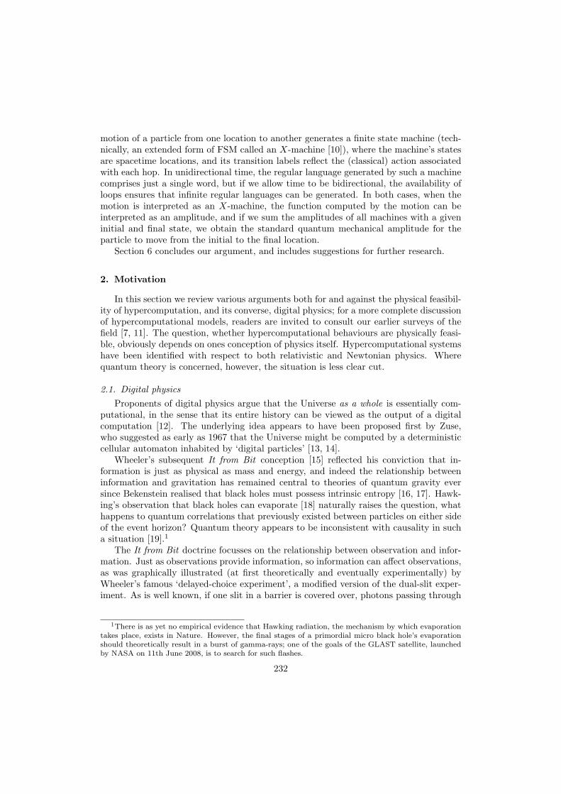
motion of a particle from one location to another generates a finite state machine (tech-nically, an extended form of FSM called an X-machine [10]), where the machine’s statesare spacetime locations, and its transition labels reflect the (classical) action associatedwith each hop. In unidirectional time, the regular language generated by such a machinecomprises just a single word, but if we allow time to be bidirectional, the availability ofloops ensures that infinite regular languages can be generated. In both cases, when themotion is interpreted as an X-machine, the function computed by the motion can beinterpreted as an amplitude, and if we sum the amplitudes of all machines with a giveninitial and final state, we obtain the standard quantum mechanical amplitude for theparticle to move from the initial to the final location.

Section 6 concludes our argument, and includes suggestions for further research.

2. Motivation

In this section we review various arguments both for and against the physical feasibil-ity of hypercomputation, and its converse, digital physics; for a more complete discussionof hypercomputational models, readers are invited to consult our earlier surveys of thefield [7, 11]. The question, whether hypercomputational behaviours are physically feasi-ble, obviously depends on ones conception of physics itself. Hypercomputational systemshave been identified with respect to both relativistic and Newtonian physics. Wherequantum theory is concerned, however, the situation is less clear cut.

2.1. Digital physicsProponents of digital physics argue that the Universe as a whole is essentially com-

putational, in the sense that its entire history can be viewed as the output of a digitalcomputation [12]. The underlying idea appears to have been proposed first by Zuse,who suggested as early as 1967 that the Universe might be computed by a deterministiccellular automaton inhabited by ‘digital particles’ [13, 14].

Wheeler’s subsequent It from Bit conception [15] reflected his conviction that in-formation is just as physical as mass and energy, and indeed the relationship betweeninformation and gravitation has remained central to theories of quantum gravity eversince Bekenstein realised that black holes must possess intrinsic entropy [16, 17]. Hawk-ing’s observation that black holes can evaporate [18] naturally raises the question, whathappens to quantum correlations that previously existed between particles on either sideof the event horizon? Quantum theory appears to be inconsistent with causality in sucha situation [19].1

The It from Bit doctrine focusses on the relationship between observation and infor-mation. Just as observations provide information, so information can affect observations,as was graphically illustrated (at first theoretically and eventually experimentally) byWheeler’s famous ‘delayed-choice experiment’, a modified version of the dual-slit exper-iment. As is well known, if one slit in a barrier is covered over, photons passing through

1There is as yet no empirical evidence that Hawking radiation, the mechanism by which evaporationtakes place, exists in Nature. However, the final stages of a primordial micro black hole’s evaporationshould theoretically result in a burst of gamma-rays; one of the goals of the GLAST satellite, launchedby NASA on 11th June 2008, is to search for such flashes.

232

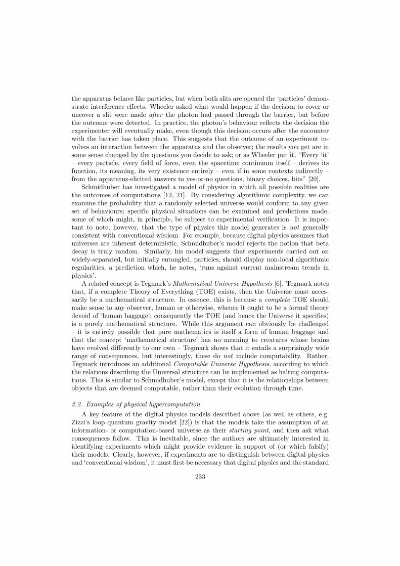
the apparatus behave like particles, but when both slits are opened the ‘particles’ demon-strate interference effects. Wheeler asked what would happen if the decision to cover oruncover a slit were made after the photon had passed through the barrier, but beforethe outcome were detected. In practice, the photon’s behaviour reflects the decision theexperimenter will eventually make, even though this decision occurs after the encounterwith the barrier has taken place. This suggests that the outcome of an experiment in-volves an interaction between the apparatus and the observer; the results you get are insome sense changed by the questions you decide to ask; or as Wheeler put it, “Every ‘it’– every particle, every field of force, even the spacetime continuum itself – derives itsfunction, its meaning, its very existence entirely – even if in some contexts indirectly –from the apparatus-elicited answers to yes-or-no questions, binary choices, bits” [20].

Schmidhuber has investigated a model of physics in which all possible realities arethe outcomes of computations [12, 21]. By considering algorithmic complexity, we canexamine the probability that a randomly selected universe would conform to any givenset of behaviours; specific physical situations can be examined and predictions made,some of which might, in principle, be subject to experimental verification. It is impor-tant to note, however, that the type of physics this model generates is not generallyconsistent with conventional wisdom. For example, because digital physics assumes thatuniverses are inherent deterministic, Schmidhuber’s model rejects the notion that betadecay is truly random. Similarly, his model suggests that experiments carried out onwidely-separated, but initially entangled, particles, should display non-local algorithmicregularities, a prediction which, he notes, ‘runs against current mainstream trends inphysics’.

A related concept is Tegmark’s Mathematical Universe Hypothesis [6]. Tegmark notesthat, if a complete Theory of Everything (TOE) exists, then the Universe must neces-sarily be a mathematical structure. In essence, this is because a complete TOE shouldmake sense to any observer, human or otherwise, whence it ought to be a formal theorydevoid of ‘human baggage’; consequently the TOE (and hence the Universe it specifies)is a purely mathematical structure. While this argument can obviously be challenged– it is entirely possible that pure mathematics is itself a form of human baggage andthat the concept ‘mathematical structure’ has no meaning to creatures whose brainshave evolved differently to our own – Tegmark shows that it entails a surprisingly widerange of consequences, but interestingly, these do not include computability. Rather,Tegmark introduces an additional Computable Universe Hypothesis, according to whichthe relations describing the Universal structure can be implemented as halting computa-tions. This is similar to Schmidhuber’s model, except that it is the relationships betweenobjects that are deemed computable, rather than their evolution through time.

2.2. Examples of physical hypercomputationA key feature of the digital physics models described above (as well as others, e.g.

Zizzi’s loop quantum gravity model [22]) is that the models take the assumption of aninformation- or computation-based universe as their starting point, and then ask whatconsequences follow. This is inevitable, since the authors are ultimately interested inidentifying experiments which might provide evidence in support of (or which falsify)their models. Clearly, however, if experiments are to distinguish between digital physicsand ‘conventional wisdom’, it must first be necessary that digital physics and the standard

233

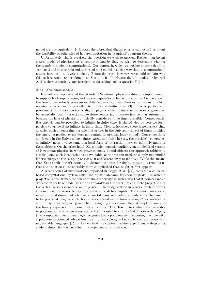
model are not equivalent. It follows, therefore, that digital physics cannot tell us aboutthe feasibility or otherwise of hypercomputation in ‘standard’ quantum theory.

Unfortunately, this is precisely the question we wish to answer. Rather than inventa new model of physics that is computational by fiat, we wish to determine whetherthe standard model is computational. Our approach, which we outline in some detail insections 3 and 4, is to reformulate the existing model in such a way that its computationalnature becomes intuitively obvious. Before doing so, however, we should explain whythis task is worth undertaking – as Zuse put it, “Is Nature digital, analog or hybrid?And is there essentially any justification for asking such a question?” [14]

2.2.1. Newtonian modelsIt is not often appreciated that standard Newtonian physics is already complex enough

to support both super-Turing and hypercomputational behaviours, but as Xia has shown,the Newtonian n-body problem exhibits ‘non-collision singularities’, solutions in whichmassive objects can be propelled to infinity in finite time [23]. This is particularlyproblematic for those models of digital physics which claim the Universe is generatedby essentially local interactions, like those connecting processes in a cellular automaton,because the laws of physics are typically considered to be time-reversible. Consequently,if a particle can be propelled to infinity in finite time, it should also be possible for aparticle to arrive from infinity in finite time. Clearly, however, there is no earliest timeat which such an emerging particle first arrives in the Universe (the set of times at whichthe emerging particle exists does not contain its greatest lower bound). Consequently, ifall objects in the Universe have finite extent and finite history, the particle’s ‘emergenceat infinity’ must involve some non-local form of interaction between infinitely many ofthese objects. On the other hand, Xia’s model depends implicitly on an idealised versionof Newtonian physics, in which gravitationally bound objects can approach arbitrarilyclosely (some such idealisation is unavoidable, as the system needs to supply unboundedkinetic energy to the escaping object as it accelerates away to infinity). While this meansthat Xia’s result doesn’t actually undermine the case for digital physics, it reminds usthat the situation is considerably more complicated than might at first appear.

A recent series of investigations, reported in Beggs et al. [24], concerns a collision-based computational system called the Scatter Machine Experiment (SME), in which aprojectile is fired from a cannon at an inelastic wedge in such a way that it bounces into adetector either to one side (up) of the apparatus or the other (down); if the projectile hitsthe vertex, various scenarios can be posited. The wedge is fixed in position with its vertexat some height x whose binary expansion we wish to compute. The cannon can also bemoved up and down, but whereas x can take any real value, we only allow the cannonto be placed at heights u which can be expressed in the form u = m/2n for suitable mand n. By repeatedly firing and then re-aligning the cannon, they attempt to computethe binary expansion of x, one digit at a time. The class of sets which are decidablein polynomial time, when a certain protocol is used to run the SME, is exactly P/poly(the complexity class of languages recognized by a polynomial-time Turing machine witha polynomial-bounded advice function). Since P/poly is known to contain recursivelyundecidable languages [25], it follows that the scatter machine experiment – despite itsevident simplicity – is behaving in a hypercomputational way.

234

2.2.2. Relativistic modelsThe SADn hierarchy is a family of computational models which exploit the properties

of certain singularities in Malament-Hogarth spacetimes [26]. These are singularities withcomputationally useful properties; in particular, if a test particle falls into the singularity,it experiences infinite proper time during its journey; but an outside observer sees theentire descent occurring in finite time. By exploiting such a singularity, we can easilysolve the Halting Problem. For suppose we want to know whether some program P halts.We set it running on a computer, and then send that computer into the singularity. Fromour vantage point, the entire process lasts just a finite length of time, say T seconds.From the computer’s point of view the descent takes forever, so if P is going to halt, itwill have enough time to do so. We therefore program the computer’s operating systemso that, if P halts, a rocket is launched back out of the singularity (this is possible forthis kind of singularity) so as to arrive at some previously determined place and time(sufficiently later than T seconds from now). We then travel to the rendezvous point. Ifa rocket arrives at the scheduled time, we know that P must have halted. If no rocketarrives, we know that the operating system never had cause to launch it, and we concludethat P ran forever.

Hogarth refers to this hypercomputational system as an SAD1 computer; it uses astandard Turing machine to run the underlying program P , but gains hypercomput-ational power from the geometrical properties of the spacetime in which that Turingmachine finds itself. If we now repeat the construction, but this time using an SAD1

computer in an attempt to decide some question, the resulting (SAD1 + singularity)system is called an SAD2 machine, and so on. Finally, by dovetailing a sequence ofmachines, one from from each level of the hierarchy, and sending the whole lot intoa singularity, we obtain an AD machine. The SADn machines decide precisely thosefirst order statements which occupy the nth of the Arithmetic Hierarchy, while the ADmachine can decide the whole of arithmetic [27].

2.2.3. Quantum theoretical modelsQuantum mechanics is, perhaps, mankind’s most impressive scientific achievement

to date; it enables us to predict various physical outcomes with remarkable accuracyacross a wide range of both everyday and exotic situations. In addition, as It fromBit demonstrates, there are clear parallels between quantum theory and informationtheory; since computation is largely seen as the study of information processing, it is notsurprising that the field has proven fertile ground for researchers in both digital physicsand hypercomputation theory.

One possible hypercomputational model in quantum theory is Kieu’s adiabatic quan-tum algorithm for deciding Hilbert’s Tenth problem, concerning the solution of Diophan-tine equations. Since this problem is known to be recursively undecidable [28], Kieu’salgorithm – essentially a method for searching infinite sets in finite time – must be hyper-computational. Although Kieu’s claims are controversial and his algorithm have beendisputed by various authors, he has sought to address these criticisms in a forthcomingpaper [29]. For the time being, therefore, the jury is out.

235

3. The Standard Path-Integral Formulation

As we explained in section 2.2, we aim to reformulate the standard version of quantumtheory from first principles in such a way that its computational aspects become essen-tially self-evident. We begin by recapitulating Feynman’s (non-relativistic) path-integralformulation presented in [30, §§3–4]. Given initial and final locations qI = (xI , tI) andqF = (xF , tF ) (where tF > tI), the goal of the standard formulation is to determinethe amplitude φ(qF , qI) that a particle P follows a trajectory qI → qF lying entirelywithin some prescribed non-empty open space-time region R. As Feynman shows, thisamplitude can then be used to generate a Schrodinger wave-equation description of thesystem, whence this formulation is equivalent to other standard (non-relativistic) modelsof quantum theory. In Section 4, we will develop a generalised finitary formulation of thesame amplitude, and show that it is equivalent to the standard path-integral formulationpresented below.

For the sake of illustration, we shall assume that space is 1-dimensional, so that spatiallocations can be specified by a single coordinate x — the extension to higher dimensionsis straightforward. Furthermore, we shall assume in this paper that the region R is asimple rectangle of the form R = X × T , where X and T = (tmin, tmax) are non-emptyopen intervals in R; this does not limit our results, because open rectangles form a basefor the standard topology on R2, and all of our formulae are derived via integration.2

Suppose, then, that a particle P is located initially at qI = (xI , tI), and subsequentlyat qF = (xF , tF ), and that its trajectory from qI to qF is some continuous path lyingentirely within the region R = X × T . Choose some positive integer ν, and split theduration δt = tF − tI into ν + 1 equal segments: for n = 0, . . . , ν + 1, we define tn =tI +nδt/(ν+1), so that t0 = tI and tν+1 = tF . We write x0, . . . , xν+1 for the correspondingspatial locations, and define qn = (xn, tn). While each of the values xn can vary from pathto path, the values tn are fixed. To distinguish this situation from the situation below(where tn is allowed to vary), we shall typically write q† = (x, t†) for those locationsqn whose associated tn-value is fixed (the points qI and qF are assumed to be fixedthroughout). We will also sometimes write [ q† ] or [ q†1, . . . , q

†ν ] for the arbitrary path

qI = q†0 → q†1 → · · · → q†ν → q†ν+1 = qF . Apart from the fixed values x0 ≡ xI andxν+1 ≡ xF , each of the xn is constrained only by the requirement that xn ∈ X, whencethe path [ q† ] has ν degrees of freedom.

In classical physics, the action associated with a path p is given by S =∫pL dt,

where the function L = L(x(t), x(t)), the Lagrangian, is a function of position x andvelocity x, only. However, to form this integral we need to specify the motion of theparticle in each subinterval (t†n, t

†n+1), so we assume that P follows some path q†n → q†n+1

that is classically permissible. Each segment q†n → q†n+1 of the path has associated

classical action S(q†n+1, q†n), and probability amplitude

⟨q†n+1

∣∣∣ q†n⟩ defined for all q and(subsequent) q′ by 〈q′ | q〉 = exp iS(q′, q)/~. The action S is determined by the clas-sical Principle of Least Action. This says that the classical path is one which min-imises this action, so that S(q′, q) = min

∫ t′tLdt. The total action associated with the

2Integrating over a union of disjoint rectangles is the same as summing the component integrals:given any integrable function f(x, t) defined on a disjoint union R =

SαRα, we have

RR f =

Pα

RRα

f .

236

path is S[ q†1, . . . , q†ν ] =

∑n S(q†n+1, q

†n) and the associated amplitude is the product⟨

qF∣∣ q†ν⟩ ⟨q†ν ∣∣∣ q†ν−1

⟩. . .⟨q†2

∣∣∣ q†1⟩⟨q†1 ∣∣∣ qI⟩. Summing over all such paths now yields thecomposite amplitude

φν(qF , qI) =1Aν

∫ ⟨qF∣∣ q†ν⟩ dxν ⟨q†ν ∣∣∣ q†ν−1

⟩dxν−1 . . .

⟨q†2

∣∣∣ q†1⟩ dx1

⟨q†1

∣∣∣ qI⟩ (1)

where Aν is a normalisation factor. All that remains is to take the limit as ν → ∞,subject to the assumption that the resulting path x = x(t) is continuous. This gives usthe required amplitude φ(xF , xI) that the particle travels from qI to qF by a trajectorythat lies entirely3 within R:

φ(qF , qI) = limν→∞

1Aν

∫ ⟨qF∣∣ q†ν⟩ dxν ⟨q†ν ∣∣∣ q†ν−1

⟩dxν−1 . . .

⟨q†2

∣∣∣ q†1⟩ dx1

⟨q†1

∣∣∣ qI⟩ .

4. A Finitary Formulation

In section 3 we showed how the amplitude φ(qF , qI), that the particle P travels fromqI to qF along some path lying entirely within the non-empty open spacetime regionR = X × T , is given by φ = limν→∞ φν . If we now write

∆n = φn − φn−1 , (2)

it follows from the identity φν = (φν − φν−1) + · · ·+ (φ1 − φ0) + φ0 that

limν→∞

φν = limν→∞

(φ0 +

ν∑n=1

∆n

)= φ0 +

∞∑n=1

∆n .

This replacing of a limit with a sum is a key feature of our model, since it allows us todescribe a system in terms of a set of mutually distinct finite sets of observations. We canthink of this sum in terms of correction factors. For, suppose you were asked to estimatethe amplitude φ(qF , qI) that some object or particle P will be observed at qF , given thatit had already been observed at qI and was constrained to move within the region R.With no other information to hand, your best bet would be to assume that P followssome action-minimising classical path, and so the estimate you give is the associatedamplitude 〈qF | qI〉. Some time later, you realise that one or more observations mayhave been made on the particle while it was moving from qI to qF , and that this wouldhave perturbed the amplitude. To take account of these possibilities, you add a series ofcorrection factors to your original estimate; first you add ∆1 in case 1 observation hadtaken place, instead of the 0 observations you had originally assumed. Then you add ∆2

in case there were actually 2 observations, and so on. Each ∆n takes into account theextra information acquired by performing n observations instead of n− 1, and since theoverall estimate needs to take all of the corrections into account, we have φ = φ0 +

∑∆n.

The simple truth, however, is that continuous motion cannot be observed, becausemaking an observation takes time. The best we can ever do is to make a series of distinct

3Strictly, only the internal points of the trajectory are required to lie in R. Either (or both) of theendpoints qI and qF can lie outside R, provided they are on its boundary.

237

measurements showing us where an object was at finitely many closely-spaced instantst1, t2, . . . , tν during the relocation from qI to qF . The classical spirit within us then tellsus to extrapolate these discrete points into a continuous curve (namely, that path which‘best’ joins the points). It is as if we draw the individual locations on celluloid, and thenplay a mental film projector to give ourselves the comfortable impression of continuousmovement. But this mental film projector — represented in the standard formulationby the construction of limφν — is no part of physical observation; it represents insteadan assumption about the way the world ‘ought to be’. All we can truthfully say is thatthe object was at such and such a location xn when we observed it at time tn, andwas subsequently at location xn+1 at time tn+1. Regardless of underlying reality (aboutwhich we can say virtually nothing), the observed universe is inherently discrete. We canask ourselves how the motion appears if no observations are made; the composite answer,taking into account all potential observers, is given by some amplitude ψ0. If we ask howit appears if precisely ν observations are made during the relocation from qI to qF , we getanother amplitude ψν . Since these possibilities are all mutually exclusive, and accountfor every possible finitely observed relocation from qI to qF , the overall amplitude thatthe relocation happens is the sum of these amplitudes, namely some function ψ =

∑ψν .

Although they both involve infinite sums, these two descriptions are very different,because ψn tells us the amplitude for a path with a specific number of hops, while ∆n

describes what happens when we change the number of hops. Nonetheless, prompted bythe formal structural similarity of the equations φ = φ0 +

∑φn and ψ = ψ0 +

∑ψn, we

shall equate the two sets of terms, and attempt to find solutions. By requiring ψ0 = φ0

and ψn = ∆n, this will ensure that the description we generate – no matter how unnaturalit might appear at first sight — satisfies φ = ψ, whence it describes exactly the sameversion of physics as the standard formulation.

The surprising feature in what follows is that the description we generate is notunnatural. Quite the opposite. To see why, we need to remember that amplitudes arenormally given in the form φn = exp i(S1 + · · ·+ Sn))/~. In very rough terms, we canthink of the various S values as being essentially equal, so that φn ≈ exp inS/~. Whenwe compute ∆n, we are asking how φn changes when n changes; in other words, we canthink of ∆n in fairly loose terms as a measure of dφn/dn. Again arguing loosely, we cancalculate dφn/dn ≈ iSφn/~, and now it becomes clear why equating the two sets of termsworks, for in essence, ∆n is approximately proportional to φn. Since ψn is structurallysimilar to φn, in the sense that both measure the amplitude associate with a sequenceof jumps, it is not surprising to find a similar relationship holding between ∆n and ψn.Since the equations we form will eventually include integrals with normalisation factors,these factors will effectively absorb any remaining constants of proportionality.

4.1. Paths, Actions and AmplitudesThe standard formulation assumes that each trajectory x(t) is a consistently future-

pointing spacetime path; this is implicit in the continuity of the representation x ≡ x(t),which assigns one location to each t in the interval [tI , tF ]. Since our formulation rejectsthis assumption, we need to provide a different definition for paths.

We shall assume the abstract existence of a clock, represented by the integer variableτ , used to indicate the order in which observations occur. Each time the clock ticks, i.e.for each τ = 0, 1, 2, . . . , the particle is observed to exist at some space-time location qτ =(xτ , tτ). We call each transition qτ → qτ+1 a hop. A finite sequence of consecutive hops

238

q0 → · · · → qν+1 constitutes a path. As before, we take q0 = (xI , tI) and qν+1 = (xF , tF ),and consider the properties of an arbitrary path from qI to qF via ν intermediate points,all of which are required to lie in the prescribed space-time region R = X × T .

We again write [ q1, . . . , qν ] for the path qI → q1 → · · · → qν → qF . However,whereas the intervals tn+1 − tn were formally fixed to have identical duration δt/(ν+1),there is no constraint on the temporal separation tτ+1 − tτ in the finitary formulation;the path q0 → · · · → qν+1 therefore has 2ν degrees of freedom, or twice the number inthe standard formulation. Notice that we now write qn rather than q†n, to show that thevalue tn is no longer fixed.

What is not clear at this stage is whether hops need necessarily always be future-pointing. The standard formulation forces this on us through its assumption that somecontinuous motion t 7→ x(t) is being observed, but this assumption is no longer relevant.We shall therefore describe two finitary formulations, one in which hops are unidirec-tional in time, and one in which space and time are treated symmetrically, in that hopscan move both forwards and backwards in time as well as space. Both models are re-lated to computation theory, but the second is by far the more interesting, both from acomputational, and a physical, point of view. The mathematical distinction between thetwo models is minor. If time is unidirectional into the future, then tτ+1 must lie in therange tτ < tτ+1 ≤ tmax. Otherwise, it can take any value in T .

In the standard formulation, any unobserved motion from one observation to the nextis assumed to be classical, and its amplitude is determined by minimising the classicalaction S. Since we no longer assume that any such motion exists, we shall simply assumethat each hop q → q′ has a hop amplitude, denoted 〈q′ | q〉h, and that this amplitude (whenit is non-zero) is associated with an abstract hop action, denoted sh(q′, q), by the formula〈q′ | q〉h = eish(q′,q)/~. One of our tasks will be to identify the function sh.

The amplitude associated with the path [ q1, . . . qν ] is defined, as usual, to be theproduct 〈qF | qν〉h× · · · × 〈q1 | qI〉h. The amplitude computed by summing over all pathsof this length will be denoted ψn, so that the overall finitary amplitude that the particlemoves from qI to qF along a sequence of hops lying entirely within R is just ψ(qF , qI) =∑∞n=0 ψn.

4.2. The Finitary EquationsConsider again the formulae giving the amplitude that a particle P follows a path

from qI to qF that lies entirely within the region R, subject to the assumption that qFoccurs later than qI — the standard formulation isn’t defined when this isn’t the case.We can write these in the form

φ = φ0 +∞∑n=1

∆n (3)

ψ = ψ0 +∞∑n=1

ψn (4)

whence it is clear that one particular solution can be obtained by solving the infinitefamily of equations

ψ0 = φ0 (5)ψn = φn − φn−1 (i.e. ψn = ∆n) for n > 0 (6)

239

to find the hop-action sh. Since the terms φn and An are those of the standard formula-tion, we shall henceforth assume that S, φn, ∆n and An are all known functions in whatfollows.

4.3. Solving the EquationsAs usual, we shall assume that qF occurs later than qI (so that φn = φn(qF , qI) is

defined for each n). We shall be careful to distinguish locations q† = (x, t†) for which thetime of observation is fixed in the standard formulation, from those of the form q = (x, t)used in the finitary version, for which the value of t is variable. Note first that (1) canbe rewritten to give us a recursive definition of φn, viz.

φν(qF , qI) =1Aν

∫ ⟨qF∣∣ q†ν⟩ dxν ⟨q†ν ∣∣∣ q†ν−1

⟩dxν−1 . . .

⟨q†2

∣∣∣ q†1⟩ dx1

⟨q†1

∣∣∣ qI⟩=Aν−1

Aν

∫ ⟨qF∣∣ q†ν⟩ dxν 1

Aν−1

∫ ⟨q†ν

∣∣∣ q†ν−1

⟩dxν−1 . . .

⟨q†2

∣∣∣ q†1⟩ dx1

⟨q†1

∣∣∣ qI⟩=Aν−1

Aν

∫ ⟨qF∣∣ q†ν⟩φν−1(q†ν , qI) dxν

(7)and an identical derivation gives ψν in the form

ψν(qF , qI) =Bν−1

Bν

∫X

∫T ′〈qF | qν〉h ψν−1(qν , qI) dtν dxν (8)

where the Bn are normalisation factors, and the integration range T ′ depends on whetherwe allow hops to jump backwards in time, or insist instead that they move only forwards(we consider the two cases separately, below).

Using (7) to substitute for φν in the definition (2) of ∆n gives

∆ν(qF , qI) = φν(qF , qI)− φν−1(qF , qI)

=[Aν−1

Aν

∫ ⟨qF∣∣ q†ν⟩φν−1(q†ν , qI) dxν

]− φν−1(qF , qI) .

The case ν = 0 is worth noting in detail. The amplitudes φ0(qF , qI) and ψ0(qF , qI)describe the situation in which P moves from qF to qI without being observed. In thestandard formulation, it is assumed in such circumstances that P follows some classicalpath for which the action S is minimal, while in the finitary formulation we assume thatthe particle hops directly from qI to qF . The amplitudes for these behaviours are 〈qF | qI〉and 〈qF | qI〉h, respectively. However, we need to remember that φ0 and ψ0 are defined interms of their contribution to the overall amplitudes φ and ψ; it is important, therefore,to include the relevant normalisation factors. We therefore define, in accordance with(1), (3), (4) and (8),

φ0(qF , qI) =1A0〈qF | qI〉 and ψ0(qF , qI) =

1B0〈qF | qI〉h ,

so that, whenever qF occurs later than qI ,

〈qF | qI〉h = σ 〈qF | qI〉 (9)240

whereσ = B0/A0 .

Taking principal logarithms on both sides of (9) now gives

sh(qF , qI) = S(qF , qI)− i~ log σ

and if we assume that sh should be real-valued (the classical action S is always real-valued), then log σ must be a real multiple of i, say σ = eiρ where ρ ∈ R, whence|σ|2 = 1. Consequently, |〈qF | qI〉h|

2 = |〈qF | qI〉h|2, and the two formulations assign the

same standard and finitary probabilities to the relocation qI → qF , whenever this isunobserved and future-directed. Moreover, since

sh(qF , qI) = S(qF , qI) + ρ~

we see that our earlier intuition is essentially confirmed: the hop-action sh (the bestestimate of the path-amplitude, given that no observations will be made) is just theclassical action S, though possibly re-scaled by the addition of a constant action of sizeρ~ (which we can think of as a kind of ‘zero-point’ action). For the purposes of thispaper, the values of ρ and σ = eiρ are essentially arbitrary; we shall leave ρ (and henceσ) an undetermined parameter of the model, in terms of which

B0 = σA0 (10)

andsh(qF , qI) = S(qF , qI) + ρ~ if qF occurs after qI . (11)

The physical significance of ρ is discussed briefly in Section 4.5, in relation to null-hops.

4.4. The Unidirectional ModelIf we wish to allow only future-pointing hops — we shall call this the unidirectional

model — there is little left to do. We know from (5) and (6) that each function ψn isdefined in terms of the known functions φ0 and ∆n. It only remains to identify the hopamplitude sh and the normalisation factors Bn. As explained above, our solutions willbe given in terms of the undetermined phase parameter σ.

Since the side-condition on (11) is satisfied, the hop amplitude is given in terms ofthe classical action by the formula 〈q′ | q〉h = σ 〈q′ | q〉 = σ expiS(q′, q)/~, whenever q′

follows q.To find the normalisation factors, we note first that (10) gives us the value B0 = σA0

directly. Next, when ν > 0, we observe that, since tν must come after tν−1, the range T ′

in (8) is the interval (tν−1, tF ). Consequently,

ψν(qF , qI) =Bν−1

Bν

∫X

∫ tF

tν−1

〈qF | qν〉h ψν−1(qν , qI) dtν dxν

=σBν−1

Bν

∫X

∫ tF

tν−1

〈qF | qν〉ψν−1(qν , qI) dtν dxν .

(12)

241

When ν = 1, (12) can be rewritten

ψ1(qF , qI) =σB0

B1

∫X

∫ tF

tI

〈qF | q1〉ψ0(q1, qI) dt1 dx1

=σB0

B1

∫X

∫ tF

tI

〈qF | q1〉1B0〈q1 | qI〉h dt1 dx1

=σ2

B1

∫X

∫ tF

tI

〈qF | q1〉 〈q1 | qI〉 dt1 dx1

and, since ψ1 = ∆1, this gives us

B1 =

(∫X

∫ tFtI〈qF | q1〉 〈q1 | qI〉 dt1 dx1

∆1(qF , qI)

)σ2 .

Finally, for ν > 1, (12) becomes

∆ν(qF , qI) = ψν(qF , qI)

=σBν−1

Bν

∫X

∫ tF

tν−1

〈qF | qν〉ψν−1(qν , qI) dtν dxν

=σBν−1

Bν

∫X

∫ tF

tν−1

〈qF | qν〉∆ν−1(qν , qI) dtν dxν

and hence Bν can be defined recursively, as

Bν =σBν−1

∆ν(qF , qI)

∫X

∫ tF

tν−1

〈qF | qν〉∆ν−1(qν , qI) dtν dxν .

4.5. The Bidirectional ModelFar more interesting is the case where hops are allowed to jump backwards as well as

forwards in time. It is important to note that the derivation of Bν given above for theunidirectional model no longer works, because it relies on using (9) to replace 〈qF | qν〉hwith σ 〈qF | qν〉, and on (6) to replace ψn+1(qν , qI) with ∆n+1(qν , qI). But our use of(9) assumes that qF occurs after qν , and that of (6) that qν comes after qI , and neitherassumption is generally valid in the bidirectional model. Consequently, before we canmake progress, we need to decide how 〈q′ | q〉h should be defined when the hop q → q′

moves backwards in time.To address this problem, we recall the standard interpretation of anti-matter as ‘mat-

ter moving backwards in time’. For example, the Feynman diagram in Figure 1 showshow the annihilation of e.g. an electron and a positron (its antiparticle) to form twophotons can be interpreted instead as showing an electron that moves forward in time,interacts with the photons, and then returns into the past.

Accordingly, whenever we are presented with a backwards hop by the particle P , were-interpret it as a forwards hop by the appropriate anti-particle, P . Writing S for theclassical action associated with the antiparticle P , we therefore define

sh(qF , qI) =

ρ~ + S(qF , qI) if qI is earlier than qF , andρ~ + S(qI , qF ) if qI is later than qF .

(13)

242

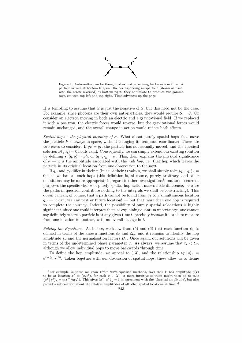
Figure 1: Anti-matter can be thought of as matter moving backwards in time. Aparticle arrives at bottom left, and the corresponding antiparticle (shown as usualwith the arrow reversed) at bottom right; they annihilate to produce two gammarays, emitted top left and top right. Time advances up the page.

It is tempting to assume that S is just the negative of S, but this need not be the case.For example, since photons are their own anti-particles, they would require S = S. Orconsider an electron moving in both an electric and a gravitational field. If we replacedit with a positron, the electric forces would reverse, but the gravitational forces wouldremain unchanged, and the overall change in action would reflect both effects.

Spatial hops - the physical meaning of σ. What about purely spatial hops that movethe particle P sideways in space, without changing its temporal coordinate? There aretwo cases to consider. If qF = qI , the particle has not actually moved, and the classicalsolution S(q, q) = 0 holds valid. Consequently, we can simply extend our existing solutionby defining sh(q, q) = ρ~, or 〈q | q〉h = σ. This, then, explains the physical significanceof σ — it is the amplitude associated with the null hop, i.e. that hop which leaves theparticle in its original location from one observation to the next.

If qF and qI differ in their x (but not their t) values, we shall simply take 〈qF | qI〉h =0; i.e. we ban all such hops (this definition is, of course, purely arbitrary, and otherdefinitions may be more appropriate in regard to other investigations4; but for our currentpurposes the specific choice of purely spatial hop action makes little difference, becausethe paths in question contribute nothing to the integrals we shall be constructing). Thisdoesn’t mean, of course, that a path cannot be found from qI to a simultaneous locationqF — it can, via any past or future location! — but that more than one hop is requiredto complete the journey. Indeed, the possibility of purely spatial relocations is highlysignificant, since one could interpret them as explaining quantum uncertainty: one cannotsay definitely where a particle is at any given time t, precisely because it is able to relocatefrom one location to another, with no overall change in t.

Solving the Equations. As before, we know from (5) and (6) that each function ψn isdefined in terms of the known functions φ0 and ∆n, and it remains to identify the hopamplitude sh and the normalisation factors Bn. Once again, our solutions will be givenin terms of the undetermined phase parameter σ. As always, we assume that tI < tF ,although we allow individual hops to move backwards through time.

To define the hop amplitude, we appeal to (13), and the relationship 〈q′ | q〉h =eish(q′,q)/~. Taken together with our discussion of spatial hops, these allow us to define

4For example, suppose we know (from wave-equation methods, say) that P has amplitude η(x)to be at location x† = (x, t†), for each x ∈ X. A more intuitive solution might then be to take˙x†˛y†¸h

= η(x†)/η(y†). This gives˙x†˛x†¸h

= 1 in agreement with the ‘classical amplitude’, but also

provides information about the relative amplitudes of all other spatial locations at time t†.

243

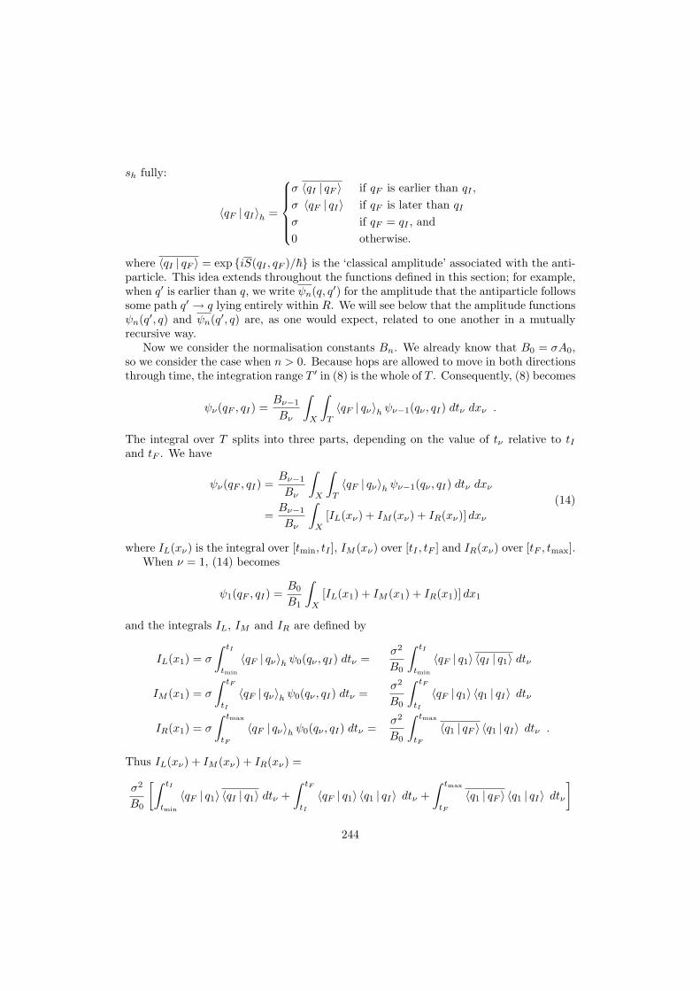
sh fully:

〈qF | qI〉h =

σ 〈qI | qF 〉 if qF is earlier than qI ,σ 〈qF | qI〉 if qF is later than qI

σ if qF = qI , and0 otherwise.

where 〈qI | qF 〉 = exp iS(qI , qF )/~ is the ‘classical amplitude’ associated with the anti-particle. This idea extends throughout the functions defined in this section; for example,when q′ is earlier than q, we write ψn(q, q′) for the amplitude that the antiparticle followssome path q′ → q lying entirely within R. We will see below that the amplitude functionsψn(q′, q) and ψn(q′, q) are, as one would expect, related to one another in a mutuallyrecursive way.

Now we consider the normalisation constants Bn. We already know that B0 = σA0,so we consider the case when n > 0. Because hops are allowed to move in both directionsthrough time, the integration range T ′ in (8) is the whole of T . Consequently, (8) becomes

ψν(qF , qI) =Bν−1

Bν

∫X

∫T

〈qF | qν〉h ψν−1(qν , qI) dtν dxν .

The integral over T splits into three parts, depending on the value of tν relative to tIand tF . We have

ψν(qF , qI) =Bν−1

Bν

∫X

∫T

〈qF | qν〉h ψν−1(qν , qI) dtν dxν

=Bν−1

Bν

∫X

[IL(xν) + IM (xν) + IR(xν)] dxν(14)

where IL(xν) is the integral over [tmin, tI ], IM (xν) over [tI , tF ] and IR(xν) over [tF , tmax].When ν = 1, (14) becomes

ψ1(qF , qI) =B0

B1

∫X

[IL(x1) + IM (x1) + IR(x1)] dx1

and the integrals IL, IM and IR are defined by

IL(x1) = σ

∫ tI

tmin

〈qF | qν〉h ψ0(qν , qI) dtν =σ2

B0

∫ tI

tmin

〈qF | q1〉 〈qI | q1〉 dtν

IM (x1) = σ

∫ tF

tI

〈qF | qν〉h ψ0(qν , qI) dtν =σ2

B0

∫ tF

tI

〈qF | q1〉 〈q1 | qI〉 dtν

IR(x1) = σ

∫ tmax

tF

〈qF | qν〉h ψ0(qν , qI) dtν =σ2

B0

∫ tmax

tF

〈q1 | qF 〉 〈q1 | qI〉 dtν .

Thus IL(xν) + IM (xν) + IR(xν) =

σ2

B0

[∫ tI

tmin

〈qF | q1〉 〈qI | q1〉 dtν +∫ tF

tI

〈qF | q1〉 〈q1 | qI〉 dtν +∫ tmax

tF

〈q1 | qF 〉 〈q1 | qI〉 dtν]

244

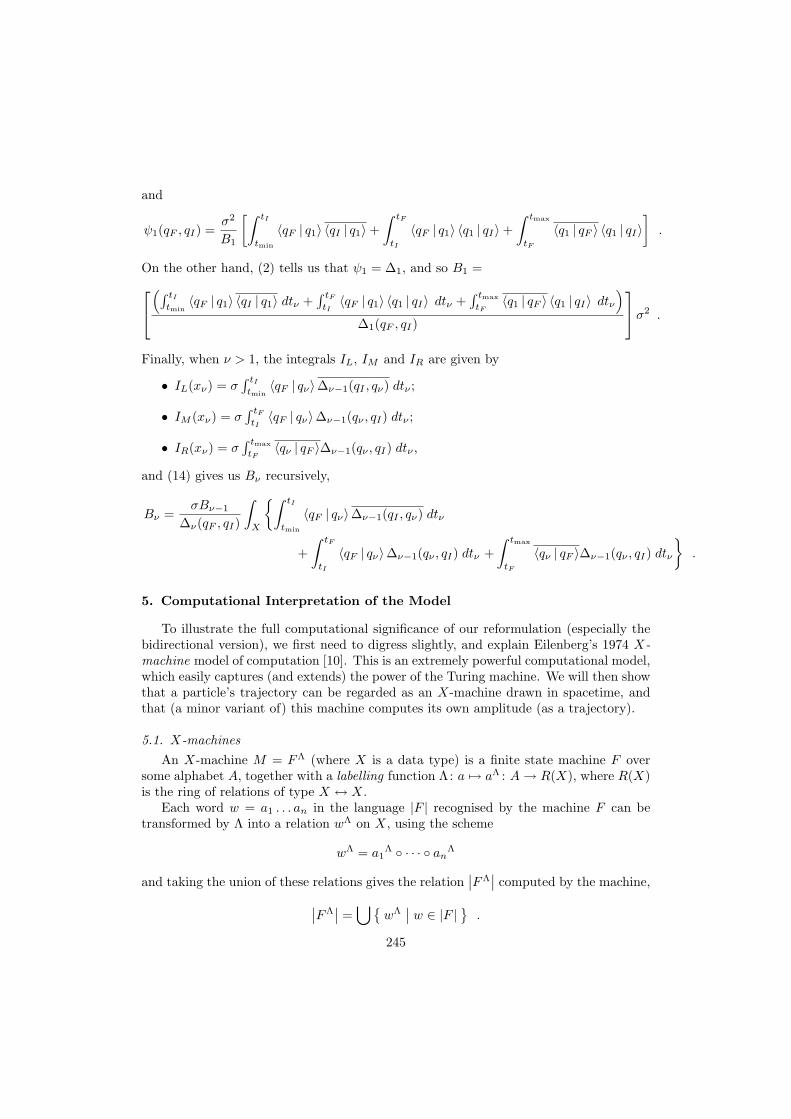
and

ψ1(qF , qI) =σ2

B1

[∫ tI

tmin

〈qF | q1〉 〈qI | q1〉+∫ tF

tI

〈qF | q1〉 〈q1 | qI〉+∫ tmax

tF

〈q1 | qF 〉 〈q1 | qI〉].

On the other hand, (2) tells us that ψ1 = ∆1, and so B1 =(∫ tI

tmin〈qF | q1〉 〈qI | q1〉 dtν +

∫ tFtI〈qF | q1〉 〈q1 | qI〉 dtν +

∫ tmax

tF〈q1 | qF 〉 〈q1 | qI〉 dtν

)∆1(qF , qI)

σ2 .

Finally, when ν > 1, the integrals IL, IM and IR are given by

• IL(xν) = σ∫ tItmin〈qF | qν〉∆ν−1(qI , qν) dtν ;

• IM (xν) = σ∫ tFtI〈qF | qν〉∆ν−1(qν , qI) dtν ;

• IR(xν) = σ∫ tmax

tF〈qν | qF 〉∆ν−1(qν , qI) dtν ,

and (14) gives us Bν recursively,

Bν =σBν−1

∆ν(qF , qI)

∫X

∫ tI

tmin

〈qF | qν〉∆ν−1(qI , qν) dtν

+∫ tF

tI

〈qF | qν〉∆ν−1(qν , qI) dtν +∫ tmax

tF

〈qν | qF 〉∆ν−1(qν , qI) dtν

.

5. Computational Interpretation of the Model

To illustrate the full computational significance of our reformulation (especially thebidirectional version), we first need to digress slightly, and explain Eilenberg’s 1974 X-machine model of computation [10]. This is an extremely powerful computational model,which easily captures (and extends) the power of the Turing machine. We will then showthat a particle’s trajectory can be regarded as an X-machine drawn in spacetime, andthat (a minor variant of) this machine computes its own amplitude (as a trajectory).

5.1. X-machinesAn X-machine M = FΛ (where X is a data type) is a finite state machine F over

some alphabet A, together with a labelling function Λ: a 7→ aΛ : A→ R(X), where R(X)is the ring of relations of type X ↔ X.

Each word w = a1 . . . an in the language |F | recognised by the machine F can betransformed by Λ into a relation wΛ on X, using the scheme

wΛ = a1Λ · · · anΛ

and taking the union of these relations gives the relation∣∣FΛ

∣∣ computed by the machine,∣∣FΛ∣∣ =

⋃wΛ

∣∣ w ∈ |F | .

245

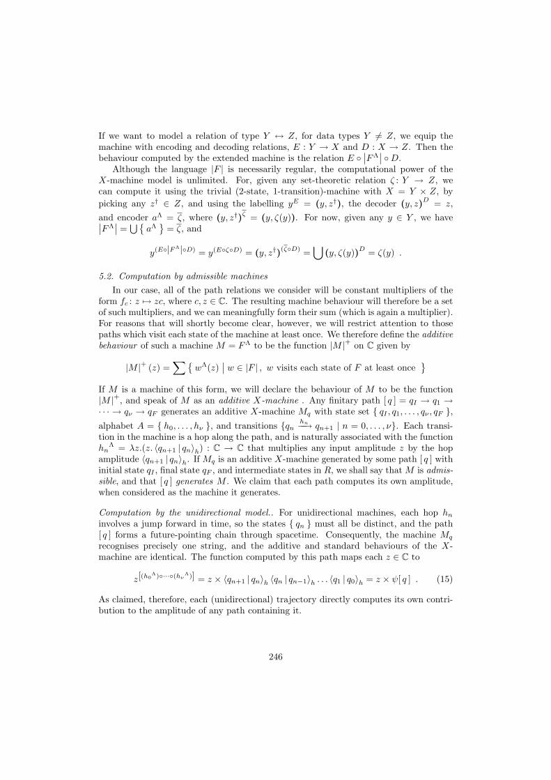
If we want to model a relation of type Y ↔ Z, for data types Y 6= Z, we equip themachine with encoding and decoding relations, E : Y → X and D : X → Z. Then thebehaviour computed by the extended machine is the relation E

∣∣FΛ∣∣ D.

Although the language |F | is necessarily regular, the computational power of theX-machine model is unlimited. For, given any set-theoretic relation ζ : Y → Z, wecan compute it using the trivial (2-state, 1-transition)-machine with X = Y × Z, bypicking any z† ∈ Z, and using the labelling yE = (y, z†), the decoder (y, z)D = z,and encoder aΛ = ζ, where (y, z†)ζ = (y, ζ(y)). For now, given any y ∈ Y , we have∣∣FΛ

∣∣ =⋃

aΛ

= ζ, and

y(E|FΛ|D) = y(EζD) = (y, z†)(ζD) =⋃

(y, ζ(y))D = ζ(y) .

5.2. Computation by admissible machinesIn our case, all of the path relations we consider will be constant multipliers of the

form fc : z 7→ zc, where c, z ∈ C. The resulting machine behaviour will therefore be a setof such multipliers, and we can meaningfully form their sum (which is again a multiplier).For reasons that will shortly become clear, however, we will restrict attention to thosepaths which visit each state of the machine at least once. We therefore define the additivebehaviour of such a machine M = FΛ to be the function |M |+ on C given by

|M |+ (z) =∑

wΛ(z)∣∣ w ∈ |F | , w visits each state of F at least once

If M is a machine of this form, we will declare the behaviour of M to be the function|M |+, and speak of M as an additive X-machine . Any finitary path [ q ] = qI → q1 →· · · → qν → qF generates an additive X-machine Mq with state set qI , q1, . . . , qν , qF ,alphabet A = h0, . . . , hν , and transitions qn

hn−−→ qn+1 | n = 0, . . . , ν. Each transi-tion in the machine is a hop along the path, and is naturally associated with the functionhn

Λ = λz.(z. 〈qn+1 | qn〉h) : C → C that multiplies any input amplitude z by the hopamplitude 〈qn+1 | qn〉h. If Mq is an additive X-machine generated by some path [ q ] withinitial state qI , final state qF , and intermediate states in R, we shall say that M is admis-sible, and that [ q ] generates M . We claim that each path computes its own amplitude,when considered as the machine it generates.

Computation by the unidirectional model.. For unidirectional machines, each hop hninvolves a jump forward in time, so the states qn must all be distinct, and the path[ q ] forms a future-pointing chain through spacetime. Consequently, the machine Mq

recognises precisely one string, and the additive and standard behaviours of the X-machine are identical. The function computed by this path maps each z ∈ C to

z[(h0Λ)···(hνΛ)] = z × 〈qn+1 | qn〉h 〈qn | qn−1〉h . . . 〈q1 | q0〉h = z × ψ[ q ] . (15)

As claimed, therefore, each (unidirectional) trajectory directly computes its own contri-bution to the amplitude of any path containing it.

246

Computation by the bidirectional model.. Equation (15) holds also for unidirectionalpaths in bidirectional machines, but the general physical interpretation is more com-plicated, because of the possibility of loops. Essentially, we need to distinguish carefullybetween two related questions, viz.

• what is the amplitude that the path [ q ] is traversed?

• what is the amplitude that the path [ q ] is observed to have been traversed?

To see why, let us suppose that the path [ q ] contains only one loop, and that mis minimal such that qm+1 = qn+1 for some n satisfying m < n; write the associatedsequence of hops as a concatenation of three segments, viz. h0 . . . hν = u.v.w, whereu = h0 . . . hm, v = hm+1 . . . hn and w = hn+1 . . . hν . Since v represents a spacetimeloop from qm+1 back to qn+1 = qm+1, there is no observable difference between anyof the paths u.vj .w, for j ≥ 1. Consequently, while the amplitude for the path [ q ] isjust ψ[ q ], the amplitude that this path is observed is instead the amplitude ψ∗[ q ] =∑∞j=1 ψ[u ]× (ψ[ v ])j × ψ[w ].More generally, given the machine F generated by any bidirectional trajectory [ q ],

and any two strings α, β which are recognised by F , and which visit each state at leastonce, there will be no observable difference between α and β. Consequently, if we define

F+ =wΛ

∣∣ w ∈ |F | , w visits each state at least once

then the amplitude ψ+ that [ q ] is observed to have been the path traversed will satisfy,for z ∈ C,

z.ψ+ =∑

wΛ(z)∣∣ w ∈ F+

=∣∣FΛ

∣∣+ (z)

and once again, if we think of [ q ] as an additive X-machine, it computes its own contri-bution to the amplitude of any path containing it.

6. Concluding Arguments

Recall that an additive X-machine M is admissible provided there is some finitarybidirectional path [ q ] that generates it. Say that two paths [ q ]1 and [ q ]2 are equiv-alent, provided they generate precisely the same admissible machine M . Clearly, thisis an equivalence relation, and given any path [ q ], there will some equivalence class qcontaining it. Moreover, the amplitude |M |+ is given by summing the amplitudes of thevarious paths in q. Consequently, summing over all paths is the same as summing overall admissible machines, so that (regarding ψ(qF , qI) as a multiplier),

ψ(qF , qI) =∑

|M |+∣∣∣ M is admissible

,

and ψ(qF , qI) can be regarded as integrating all of the admissible machine amplitudes. Inthe bidirectional formulation, then, the nature of motion in quantum theory reveals itselfto be inherently computational. It is not that trajectories can be computed; rather, theyare computations. As a particle hops through spacetime, it simultaneously constructs andexecutes a computational state machine, and the amplitude computed by this machineis precisely the amplitude of the trajectory that constructed it.

247

In section 2.1, we noted how digital physics assumes the existence of a computationthat computes each universe’s history, which suggests that the ‘computer’ which executesthe computation is somehow external to the universes being constructed. In contrast, thebidirectional model is telling us that each universe is a process, in which each trajectoryis a sub-process which computes its own amplitude. Moreover, all of these sub-processesinteract with one another non-locally, because hop amplitudes are based on the classicalaction, and this in turn depends on the ever-changing spacetime distribution of the otherparticles. In other words, as we have argued elsewhere, quantum theory is best thoughtof, not in terms of computation, but in terms of interactive formal processes [31].

Clearly, this idea has echoes of It from Bit , and indeed the bidirectional model helpsexplain Wheeler’s delayed-choice experiment. The apparent paradox relies on two as-sumptions concerning the experimental set-up. First, the photon must pass through thebarrier in order to be observed on the other side; and second, we can reliably identify atime by which the photon has travelled beyond the barrier (we need to make our delayedchoice after this time). Both of our reformulations refute the first assumption (the discon-tinuous nature of hop-based motion means that the Intermediate Value Theorem cannotbe invoked to prove that the trajectory necessarily passes through the barrier), while thebidirectional model also refutes the second assumption, since there is no reliable sensein which the decision can be said to have been made ‘after’ the trajectory intersects thebarrier. Thus the delayed-choice experiment contains no paradox, and there is nothingto explain.

We should also be clear as to what our reformulation does not say. Throughoutthis discussion we have focussed on the computational nature of trajectories, but itshould be stressed that there is an important distinction to be be drawn between whata process does, and how that process is structured. This is the same distinction asthat highlighted in section 2.1 between Schmidhuber’s and Tegmark’s versions of thecomputational universe hypothesis: whereas Schmidhuber considers process evolutionsto be computable, Tegmark requires instead that their descriptions be computable. Inour case, while we know that each trajectory computes its amplitude, we cannot say thatthe amplitude itself is necessarily ‘computable’ in the Turing sense, because we cannot asyet identify the extent to which the two forms of computation are related. As a process,each trajectory is computational, but the values it manipulates need not be.

6.1. Open questions1. Clearly, we need to determine the relationship between trajectory computations andTuring computations. There must certainly be some such relationship, because the un-derlying X-machine model is closely related to the Finite State Machine, which alsounderpins the basic structure of the Turing machine.

2. Although we have exchanged continuous motion for motion based on discrete hops, wehave not as yet done away with continuous spaces in their entirety, because many of theexpressions given in this paper make use of integration. As we argued above, continuity isnot directly observable, so we would prefer a purely discrete model. We should thereforeinvestigate the extent to which the formulation presented here can be re-expressed inpurely formal terms, for example using the π-calculus (a standard theoretical vehicle formodelling mobile distributed process-based systems).

248

3. Suppose we impose the condition that whenever a particle hops inside some arbitraryregion (which we can think of as the interior of an event horizon), it cannot hop backout again. This will have a global influence upon trajectory amplitudes, because everyjourney would otherwise have the option to include hops that pass through the excludedregion. In particular, the observed positions of geodesics (which can be modelled interms of trajectories) can be expected to change position, whence the presence of theexcluded region will generate a perceived ‘warping’ of spacetime geometry. Does thiswarping agree with the warping predicted by General Relativity? Can the bidirectionalmodel be extended to give a model of quantum gravity?

References

[1] S. C. Kleene. Introduction to Metamathematics. North Holland, 1952.[2] R. Gandy. Church’s Thesis and Principles for Mechanisms. In J. Barwise, H.J. Keisler, and

K. Kunen, editors, The Kleene Symposium, pages 123–148. North-Holland, Amsterdam, 1980.[3] B. Jack Copeland. The Church-Turing Thesis. In Edward N. Zalta, editor, The Stanford Encyclo-

pedia of Philosophy. Stanford University, Fall 2002. Online publication, retrieved 4 July 2008 fromhttp://plato.stanford.edu/archives/fall2002/entries/church-turing/.

[4] S. Wolfram. A New Kind of Science. Wolfram Media, 2002. ISBN 1-57955-008-8.[5] S. Lloyd. A theory of quantum gravity based on quantum computation. Preprint, retrieved 4 July

2008 from arXiv:quant-ph/0501135, 26 Apr 2006.[6] M. Tegmark. The Mathematical Universe. Foundations of Physics, 38(2):101–150, 2008. Preprint

available online, retrieved 4 July 2008 from arXiv:0704.0646[gr-qc].[7] M. Stannett. The case for hypercomputation. Applied Mathematics and Computation, 178:8–24,

2006.[8] P. Shor. Polynomial-time algorithms for prime factorization and discrete logarithms on a quantum

computer. In S. Goldwasser, editor, Proc. 35th Annual Symp. on Foundations of Computer Science,page 124. IEEE Computer Society Press, Los Alamitos, CA, 1994. Revised version (1995) availableonline, retrieved 4 July 2008 from arXiv:quant-ph/9508027v2. Subsequently published as SIAM J.Sci. Statist. Comput., 26:1484, 1997.

[9] D. Deutsch. Quantum Theory, the Church-Turing Principle and the Universal Quantum Computer.Proc. Royal Society, Series A, 400:97–117, 1985.

[10] S. Eilenberg. Automata, Languages, and Machines, Vol. A. Academic Press, London, 1974.[11] M. Stannett. Computation and Hypercomputation. Minds and Machines, 13(1):115–153, 2003.[12] J. Schmidhuber. A Computer Scientist’s View of Life, the Universe, and Everything. In C. Freksa,

editor, Foundations of Computer Science: Potential – Theory – Cognition, volume 1337 of LectureNotes in Computer Science, pages 201–208. Springer, 1997.

[13] K. Zuse. Rechnender Raum. Elektronische Datenverarbeitung, 8:336–344, 1967. Available online, re-trieved 4 July 2008 from ftp://ftp.idsia.ch/pub/juergen/zuse67scan.pdf. This is a preliminarysummary of [14].

[14] K. Zuse. Rechnender Raum. Schriften zur Datenverarbeitung, Band 1. Friedrich Vieweg & Sohn,Braunschweig, 1969. English translation: Calculating Space, MIT Technical Translation AZT-70-164-GEMIT, MIT (Proj. MAC), Cambridge, Mass. 02139, Feb. 1970. Available online, retrieved 4July 2008 from ftp://ftp.idsia.ch/pub/juergen/zuserechnenderraum.pdf. A German-languagesummary appeared in 1967 as [13].

[15] J. Wheeler. Recent Thinking about the Nature of the Physical World. It from Bit. In Rosalind B.Mendell and Allen I. Mincer, editors, Frontiers in Cosmic Physics; Symposium in memory of SergeAlexander Korff, held on September 13, 1990, in New York, NY, volume 655 of Annals of the NewYork Academy of Sciences, page 349. Academy of Sciences, New York, NY, 1990.

[16] J. D. Bekenstein. Black Holes and the Second Law. Lettere al Nuovo Cimento, 4:737, 1972.[17] J. D. Bekenstein. Black Holes and Entropy. Physical Reviews, D7:2333–2346, 1973.[18] S. W. Hawking. Black hole explosions? Nature, 248:30–31, 1 March, 1974.[19] L. Susskind and J. Lindesay. An Introduction to Black Holes, Information and the String Theory

Revolution – The Holographic Universe. World Scientific, 2005.[20] J. Horgan. Profile: Physicist John A. Wheeler, Questioning the “It from Bit”. Scientific American,

pages 36–37, June 1991.

249

[21] J. Schmidhuber. Algorithmic Theories of Everything. Technical Report IDSIA–20–00, IDSIA,Galleria 2, 6928 Manno (Lugano), Switzerland, December 2000. Available online, retrieved 4 July2008 from arXiv:quant-ph/0011122.

[22] P. Zizzi. Spacetime at the Planck Scale: The Quantum Computer View. In C. Garola, A. Rossi, andS. Sozzo, editors, The Foundations of Quantum Mechanics: Historical Analysis and Open Questions– Cesena 2004, pages 345–358. World Scientific, 2004. Preprint available online, retrieved 4 July2008 from arXiv:gr-qc/0304032.

[23] Z. Xia. The existence of non-collision singularities in the n-body problem. Annals of Mathematics,135(3):411–468, 1992.

[24] E. Beggs, J. F. Costa, B. Loff, and J. V. Tucker. Computational complexity with experiments asoracles. Proceedings of the Royal Society A, To appear, 2008. Published online, 24 June 2008.

[25] O. Goldreich. Computational Complexity: A Conceptual Perspective. Cambridge University Press,2008.

[26] M. Hogarth. Does General Relativity Allow an Observer to View an Eternity in a Finite Time?Foundations of Physics Letters, 5:173–181, 1992.

[27] M. Hogarth. Deciding Arithmetic Using SAD Computers. The British Journal for the Philosophyof Science, 55(4):681–691, 2004.

[28] Y. Matiyasevich. Hilbert’s Tenth Problem. MIT Press, Cambridge, MA, 1993.[29] T. Kieu. Hypercomputability of Quantum Adiabatic Processes. International Journal of Uncon-

ventional Computing (Special Issue on Hypercomputation), 4, In press, 2008.[30] R. P. Feynman. Space-Time Approach to Non-Relativistic Quantum Mechanics. Reviews of Modern

Physics, 20(2):367–387, April 1948.[31] M. Stannett. Physical Hypercomputation. In A. Adamatzky, L. Bull, B. De Lacy Costello, S. Step-

ney, and C. Teuscher, editors, Unconventional Computing 2007, pages 265–288. Luniver Press,2007.

250

On the solution of trivalent decision problems by quantum state identification

Karl Svozil∗

Institute for Theoretical Physics, Vienna University of Technology, Wiedner Hauptstraße 8-10/136, A-1040 Vienna,Austria

Josef Tkadlec†

Department of Mathematics, Faculty of Electrical Engineering, Czech Technical University, 166 27 Praha,Czech Republic

The trivalent functions of a trit can be grouped into equipartitions of three elements. We discussthe separation of the corresponding functional classes by quantum state identifications.

PACS numbers: 03.67.Lx,03.65.UdKeywords: Trits, trivalent decision problems, quantum state identification

I. QUANTUM COMPUTATION BY STATE IDENTIFICATION

One of the advantages of quantum computation (Beals et al., 2001; Bennett et al., 1997; Cleve, 2000; Fortnow,2003; Gruska, 1999; Mermin, 2007; Nielsen and Chuang, 2000; Ozhigov, 1998) over classical algorithms (Odifreddi,1989; Rogers, Jr., 1967) is due to the fact that during a quantum computation some classically useful informationcan be coded in or “spread among” multi-partite coherent states in such a way that certain decision problems can besolved by identifying a quantum state which “globally” contains that solution (Mermin, 2003; Svozil, 2006). Thereby,information about single cases contributing to the solution of the decision problem are not useful for (and even makesimpossible) the quantum computation.

In comparison, the retreival of information, such as the result of a decision problem, is analogous to the preparationand characterization of states with the properties corresponding to such a decision problem. In particular, unlikeclassical physical states, quantum states can also be characterized with respect to propositions and properties notencoded into a single quantum, but “spread among” quanta in an entangled multi-partite state (Brukner and Zeilinger,1999a,b, 2003; Donath and Svozil, 2002; Svozil, 2002, 2004; Zeilinger, 1999). Stated differently (Brukner et al., 2002),the essence of entanglement can be identified by two observations: the finiteness of the amount of information perparticipating quantum, and the possibility that “the information in a composite system resides more in the correlationsthan in properties of individuals.” This is also evident from the fact that entangled states cannot be represented asthe product of individual states of the participating quanta (cf. Ref. (Mermin, 2007), Sect. 1.5).

The potentiality to quantum mechanically solve decision problems by considering an appropriate multipartite stateis not only present in binary decision problems of the usual type, such as Deutsch’s algorithm (Cleve et al., 1998;Deutsch, 1985; Deutsch and Jozsa, 1992; Mermin, 2007; Nielsen and Chuang, 2000). It can be extended to d-arydecision problems on dits. (For the related state determination problem, see Ref. (Zeilinger, 1999), footnote 6, andRef. (Svozil, 2002).)

In what follows we shall consider as the simplest of such problems the trivalent functions of one trit. We shall groupthem in three functional classes corresponding to an equipartition of the set of functions into three elements. We theninvestigate the possibility to separate each of these classes by quantum state identifications (Donath and Svozil, 2002;Svozil, 2002).

A strategy to identify an observable associated with the solution of a decision problem can be implemented via themethod of general state identification (Donath and Svozil, 2002; Svozil, 2002, 2004) as follows (Svozil, 2006):

1. Re-encode the behaviour of the algorithm or function involved in the decision problem into an orthogonal setof states, such that every distinct function results in a single distinct state orthogonal to all the other ones.Suppose that this is impossible because the number of functions exceeds the number of orthogonal states, then

∗Electronic address: [email protected]; URL: http://tph.tuwien.ac.at/~svozil†Electronic address: [email protected]; URL: http://math.feld.cvut.cz/tkadlec/

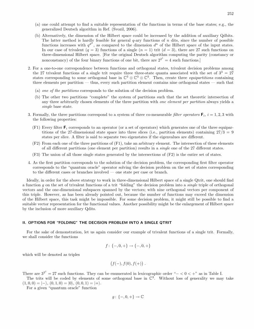
252

(a) one could attempt to find a suitable representation of the functions in terms of the base states; e.g., thegeneralized Deutsch algorithm in Ref. (Svozil, 2006).

(b) Alternatively, the dimension of the Hilbert space could be increased by the addition of auxiliary Qdbits.The latter method is hardly feasible for general q-ary functions of n dits, since the number of possiblefunctions increases with qd

n

, as compared to the dimension dn of the Hilbert space of the input states.In our case of trivalent (q = 3) functions of a single (n = 1) trit (d = 3), there are 27 such functions onthree-dimensional Hilbert space. [For the original Deutsch algorithm computing the parity (constancy ornonconstancy) of the four binary functions of one bit, there are 221

= 4 such functions.]

2. For a one-to-one correspondence between functions and orthogonal states, trivalent decision problems amongthe 27 trivalent functions of a single trit require three three-state quanta associated with the set of 33 = 27states corresponding to some orthogonal base in C3 ⊗ C3 ⊗ C3. Then, create three equipartitions containingthree elements per partition — thus, every such partition element contains nine orthogonal states — such that

(a) one of the partitions corresponds to the solution of the decision problem.

(b) The other two partitions “complete” the system of partitions such that the set theoretic intersection ofany three arbitrarily chosen elements of the three partition with one element per partition always yields asingle base state.

3. Formally, the three partitions correspond to a system of three co-measurable filter operators Fi, i = 1, 2, 3 withthe following properties:

(F1) Every filter Fi corresponds to an operator (or a set of operators) which generates one of the three equipar-titions of the 27-dimensional state space into three slices (i.e., partition elements) containing 27/3 = 9states per slice. A filter is said to separate two eigenstates if the eigenvalues are different.

(F2) From each one of the three partitions of (F1), take an arbitrary element. The intersection of these elementsof all different partitions (one element per partition) results in a single one of the 27 different states.

(F3) The union of all those single states generated by the intersections of (F2) is the entire set of states.

4. As the first partition corresponds to the solution of the decision problem, the corresponding first filter operatorcorresponds to the “quantum oracle” operator solving the decision problem on the set of states correspondingto the different cases or branches involved — one state per case or branch.

Ideally, in order for the above strategy to work in three-dimensional Hilbert space of a single Qtrit, one should finda function g on the set of trivalent functions of a trit “folding” the decision problem into a single triple of orthogonalvectors and the one-dimensional subspaces spanned by the vectors; with nine orthogonal vectors per component ofthis triple. However, as has been already pointed out, because the number of functions may exceed the dimensionof the Hilbert space, this task might be impossible. For some decision problem, it might still be possible to find asuitable vector representation for the functional values. Another possibility might be the enlargement of Hilbert spaceby the inclusion of more auxiliary Qdits.

II. OPTIONS FOR “FOLDING” THE DECISION PROBLEM INTO A SINGLE QTRIT

For the sake of demonstration, let us again consider our example of trivalent functions of a single trit. Formally,we shall consider the functions

f : −, 0,+ → −, 0,+

which will be denoted as triples (f(−), f(0), f(+)

).

There are 331= 27 such functions. They can be enumerated in lexicographic order “− < 0 < +” as in Table I.

The trits will be coded by elements of some orthogonal base in C3. Without loss of generality we may take(1, 0, 0) = |−〉, (0, 1, 0) = |0〉, (0, 0, 1) = |+〉.

For a given “quantum oracle” function

g : −, 0,+ → C

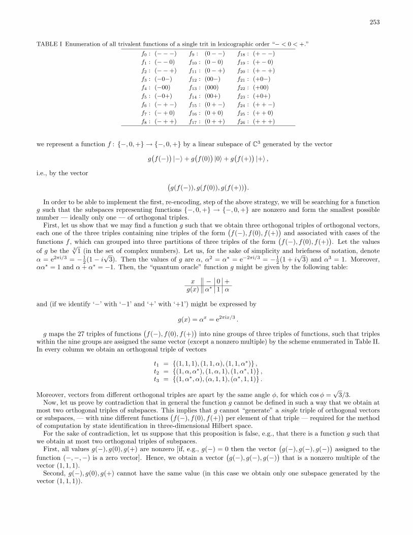
253

TABLE I Enumeration of all trivalent functions of a single trit in lexicographic order “− < 0 < +.”

f0 : (−−−)

f1 : (−− 0)

f2 : (−−+)

f3 : (−0−)

f4 : (−00)

f5 : (−0+)

f6 : (−+−)

f7 : (−+ 0)

f8 : (−+ +)

f9 : (0−−)

f10 : (0− 0)

f11 : (0−+)

f12 : (00−)

f13 : (000)

f14 : (00+)

f15 : (0 +−)

f16 : (0 + 0)

f17 : (0 + +)

f18 : (+−−)

f19 : (+− 0)

f20 : (+−+)

f21 : (+0−)

f22 : (+00)

f23 : (+0+)

f24 : (+ +−)

f25 : (+ + 0)

f26 : (+ + +)

we represent a function f : −, 0,+ → −, 0,+ by a linear subspace of C3 generated by the vector

g(f(−)

)|−〉+ g

(f(0)

)|0〉+ g

(f(+)

)|+〉 ,

i.e., by the vector (g(f(−)), g(f(0)), g(f(+))

).

In order to be able to implement the first, re-encoding, step of the above strategy, we will be searching for a functiong such that the subspaces representing functions −, 0,+ → −, 0,+ are nonzero and form the smallest possiblenumber — ideally only one — of orthogonal triples.

First, let us show that we may find a function g such that we obtain three orthogonal triples of orthogonal vectors,each one of the three triples containing nine triples of the form

(f(−), f(0), f(+)

)and associated with cases of the

functions f , which can grouped into three partitions of three triples of the form(f(−), f(0), f(+)

). Let the values

of g be the 3√

1 (in the set of complex numbers). Let us, for the sake of simplicity and briefness of notation, denoteα = e2πi/3 = − 1

2 (1 − i√

3). Then the values of g are α, α2 = α∗ = e−2πi/3 = − 12 (1 + i

√3) and α3 = 1. Moreover,

αα∗ = 1 and α+ α∗ = −1. Then, the “quantum oracle” function g might be given by the following table:

x − 0 +g(x) α∗ 1 α

and (if we identify ‘−’ with ‘−1’ and ‘+’ with ‘+1’) might be expressed by

g(x) = αx = e2πix/3 .

g maps the 27 triples of functions(f(−), f(0), f(+)

)into nine groups of three triples of functions, such that triples

within the nine groups are assigned the same vector (except a nonzero multiple) by the scheme enumerated in Table II.In every column we obtain an orthogonal triple of vectors

t1 = (1, 1, 1), (1, 1, α), (1, 1, α∗) ,t2 = (1, α, α∗), (1, α, 1), (1, α∗, 1) ,t3 = (1, α∗, α), (α, 1, 1), (α∗, 1, 1) .

Moreover, vectors from different orthogonal triples are apart by the same angle φ, for which cosφ =√

3/3.Now, let us prove by contradiction that in general the function g cannot be defined in such a way that we obtain at

most two orthogonal triples of subspaces. This implies that g cannot “generate” a single triple of orthogonal vectorsor subspaces, — with nine different functions

(f(−), f(0), f(+)

)per element of that triple — required for the method

of computation by state identification in three-dimensional Hilbert space.For the sake of contradiction, let us suppose that this proposition is false, e.g., that there is a function g such that

we obtain at most two orthogonal triples of subspaces.First, all values g(−), g(0), g(+) are nonzero [if, e.g., g(−) = 0 then the vector

(g(−), g(−), g(−)

)assigned to the

function (−,−,−) is a zero vector]. Hence, we obtain a vector(g(−), g(−), g(−)

)that is a nonzero multiple of the

vector (1, 1, 1).Second, g(−), g(0), g(+) cannot have the same value (in this case we obtain only one subspace generated by the

vector (1, 1, 1)).

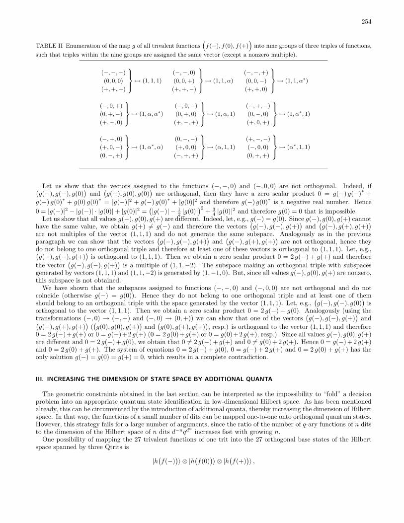
254

TABLE II Enumeration of the map g of all trivalent functions“f(−), f(0), f(+)

”into nine groups of three triples of functions,

such that triples within the nine groups are assigned the same vector (except a nonzero multiple).

(−,−,−)

(0, 0, 0)

(+,+,+)

9>=>; 7→ (1, 1, 1)

(−,−, 0)

(0, 0,+)

(+,+,−)

9>=>; 7→ (1, 1, α)

(−,−,+)

(0, 0,−)

(+,+, 0)

9>=>; 7→ (1, 1, α∗)

(−, 0,+)

(0,+,−)

(+,−, 0)

9>=>; 7→ (1, α, α∗)

(−, 0,−)

(0,+, 0)

(+,−,+)

9>=>; 7→ (1, α, 1)

(−,+,−)

(0,−, 0)

(+, 0,+)

9>=>; 7→ (1, α∗, 1)

(−,+, 0)

(+, 0,−)

(0,−,+)

9>=>; 7→ (1, α∗, α)

(0,−,−)

(+, 0, 0)

(−,+,+)

9>=>; 7→ (α, 1, 1)

(+,−,−)

(−, 0, 0)

(0,+,+)

9>=>; 7→ (α∗, 1, 1)

Let us show that the vectors assigned to the functions (−,−, 0) and (−, 0, 0) are not orthogonal. Indeed, if(g(−), g(−), g(0)

)and

(g(−), g(0), g(0)

)are orthogonal, then they have a zero scalar product 0 = g(−) g(−)∗ +

g(−) g(0)∗ + g(0) g(0)∗ = |g(−)|2 + g(−) g(0)∗ + |g(0)|2 and therefore g(−) g(0)∗ is a negative real number. Hence0 = |g(−)|2 − |g(−)| · |g(0)|+ |g(0)|2 =

(|g(−)| − 1

2 |g(0)|)2 + 3

4 |g(0)|2 and therefore g(0) = 0 that is impossible.Let us show that all values g(−), g(0), g(+) are different. Indeed, let, e.g., g(−) = g(0). Since g(−), g(0), g(+) cannot

have the same value, we obtain g(+) 6= g(−) and therefore the vectors(g(−), g(−), g(+)

)and

(g(−), g(+), g(+)

)are not multiples of the vector (1, 1, 1) and do not generate the same subspace. Analogously as in the previousparagraph we can show that the vectors

(g(−), g(−), g(+)

)and

(g(−), g(+), g(+)

)are not orthogonal, hence they

do not belong to one orthogonal triple and therefore at least one of these vectors is orthogonal to (1, 1, 1). Let, e.g.,(g(−), g(−), g(+)

)is orthogonal to (1, 1, 1). Then we obtain a zero scalar product 0 = 2 g(−) + g(+) and therefore

the vector(g(−), g(−), g(+)

)is a multiple of (1, 1,−2). The subspace making an orthogonal triple with subspaces

generated by vectors (1, 1, 1) and (1, 1,−2) is generated by (1,−1, 0). But, since all values g(−), g(0), g(+) are nonzero,this subspace is not obtained.

We have shown that the subspaces assigned to functions (−,−, 0) and (−, 0, 0) are not orthogonal and do notcoincide (otherwise g(−) = g(0)). Hence they do not belong to one orthogonal triple and at least one of themshould belong to an orthogonal triple with the space generated by the vector (1, 1, 1). Let, e.g.,

(g(−), g(−), g(0)

)is

orthogonal to the vector (1, 1, 1). Then we obtain a zero scalar product 0 = 2 g(−) + g(0). Analogously (using thetransformations (−, 0) → (−,+) and (−, 0) → (0,+)) we can show that one of the vectors

(g(−), g(−), g(+)

)and(

g(−), g(+), g(+))

((g(0), g(0), g(+)

)and

(g(0), g(+), g(+)

), resp.) is orthogonal to the vector (1, 1, 1) and therefore

0 = 2 g(−)+g(+) or 0 = g(−)+2 g(+) (0 = 2 g(0)+g(+) or 0 = g(0)+2 g(+), resp.). Since all values g(−), g(0), g(+)are different and 0 = 2 g(−) + g(0), we obtain that 0 6= 2 g(−) + g(+) and 0 6= g(0) + 2 g(+). Hence 0 = g(−) + 2 g(+)and 0 = 2 g(0) + g(+). The system of equations 0 = 2 g(−) + g(0), 0 = g(−) + 2 g(+) and 0 = 2 g(0) + g(+) has theonly solution g(−) = g(0) = g(+) = 0, which results in a complete contradiction.

III. INCREASING THE DIMENSION OF STATE SPACE BY ADDITIONAL QUANTA

The geometric constraints obtained in the last section can be interpreted as the impossibility to “fold” a decisionproblem into an appropriate quantum state identification in low-dimensional Hilbert space. As has been mentionedalready, this can be circumvented by the introduction of additional quanta, thereby increasing the dimension of Hilbertspace. In that way, the functions of a small number of dits can be mapped one-to-one onto orthogonal quantum states.However, this strategy fails for a large number of arguments, since the ratio of the number of q-ary functions of n ditsto the dimension of the Hilbert space of n dits d−nqd

n

increases fast with growing n.One possibility of mapping the 27 trivalent functions of one trit into the 27 orthogonal base states of the Hilbert

space spanned by three Qtrits is

|h(f(−)

)〉 ⊗ |h

(f(0)

)〉 ⊗ |h

(f(+)

)〉 ,

255

with h = id being the identity function. A reversible implementation of this function can be given by

h :∏x∈−,0,+ |x〉|0〉 →

→∏x∈−,0,+ |x〉|0⊕ h(f(x))〉 =∏

x∈−,0,+ |x〉|h(f(x))〉 ,

where “⊕” stands for modulo-two addition.For the sake of demonstration, consider the following trivalent decision problem associated with the three triples of

vectors t1, t2, and t3 as follows:

Given some trivalent function of a single trit fi(x), i ∈ 0, . . . , 26, x ∈ −, 0,+. Find the triple ofvectors t among the three triples t1, t2 and t3, such that g(fi) ∈ t.

IV. SUMMARY

In summary we find that, in three-dimensional Hilbert space, we cannot solve the type of trivalent decision problemsdiscussed above by a single query. Such a behaviour has already been observed for the problem to find the parity ofan unknown binary function f : 0, 1k → 0, 1 of k bits, which turned out to be quantum computationally hard(Beals et al., 2001; Farhi et al., 1998; Miao, 2001; Orus et al., 2004; Stadelhofer et al., 2005). We conjecture that thishardness increases with the number d of possible states of a single dit.

We have also explicitly discussed a trivalent decision problem which can be interpreted as the solution of a quantumstate identification problem.

Acknowledgements

The work was supported by the research plan of the Ministry of Education of the Czech Republic no. 6840770010and by the grant of the Grant Agency of the Czech republic no. 201/07/1051 and by the exchange agreement of bothof our universities.

References

Beals R, Buhrman H, Cleve R, Mosca M and de Wolf R (2001) Quantum lower bounds by polynomials. Journal of the ACM,48:778–797.

Bennett C H, Bernstein E, Brassard G and Vazirani U (1997) Strengths and weaknesses of quantum computing. SIAM Journalon Computing, 26:1510–1523.

Brukner C and Zeilinger A (1999a) Malus’ law and quantum information. Acta Physica Slovaca, 49(4):647–652.Brukner C and Zeilinger A (1999b) Operationally invariant information in quantum mechanics. Physical Review Letters,

83(17):3354–3357.Brukner C and Zeilinger A (2003) Information and fundamental elements of the structure of quantum theory. In Castell, L.

and Ischebek, O., editors, Time, Quantum and Information, pages 323–355. Springer, Berlin.Brukner C, Zukowski M and Zeilinger A (2002) The essence of entanglement. Translated to Chinese by Qiang Zhang and

Yond-de Zhang, New Advances in Physics (Journal of the Chinese Physical Society)Cleve R (2000) An introduction to quantum complexity theory. In Macchiavello, C., Palma, G. and Zeilinger, A., editors,

Collected Papers on Quantum Computation and Quantum Information Theory, pages 103–127, Singapore. World Scientific.Cleve R, Ekert A, Macchiavello C and Mosca M (1998) Rapid solution of problems by quantum computation. Proceedings of

the Royal Society A: Mathematical, Physical and Engineering Sciences, 454(1969):339–354.Deutsch D (1985) Quantum theory, the Church-Turing principle and the universal quantum computer. Proceedings of the

Royal Society of London. Series A, Mathematical and Physical Sciences (1934-1990), 400(1818):97–117.Deutsch D and Jozsa R (1992) Rapid solution of problems by quantum computation. Proceedings of the Royal Society:

Mathematical and Physical Sciences (1990-1995), 439(1907):553–558.Donath N and Svozil K (2002) Finding a state among a complete set of orthogonal ones. Physical Review A (Atomic, Molecular

and Optical Physics), 65:044302.Farhi E, Goldstone J, Gutmann S and Sipser M (1998) Limit on the speed of quantum computation in determining parity.

Physical Review Letters, 81:5442–5444.Fortnow L (2003) One complexity theorist’s view of quantum computing. Theoretical Computer Science, 292:597–610.Gruska J (1999) Quantum Computing. McGraw-Hill, London.Mermin N D (2003) From Cbits to Qbits: Teaching computer scientists quantum mechanics. American Journal of Physics,

71:23–30.

256

Mermin N D (2007) Quantum Computer Science. Cambridge University Press, Cambridge.Miao X (2001) A polynomial-time solution to the parity problem on an NMR quantum computer.Nielsen M A and Chuang I L (2000) Quantum Computation and Quantum Information. Cambridge University Press, Cam-

bridge.Odifreddi P (1989) Classical Recursion Theory, Vol. 1. North-Holland, Amsterdam.Orus R, Latorre J I and Martin-Delgado M A (2004) Systematic analysis of majorization in quantum algorithms. European

Physical Journal D, 29:119–132.Ozhigov Y (1998) Quantum computer can not speed up iterated applications of a black box. Lecture Notes In Computer

Science, 1509:152–159.Rogers Jr H (1967) Theory of Recursive Functions and Effective Computability. MacGraw-Hill, New York.Stadelhofer R, Suterand D and Banzhaf W (2005) Quantum and classical parallelism in parity algorithms for ensemble quantum

computers. Physical Review A (Atomic, Molecular and Optical Physics), 71:032345.Svozil K (2002) Quantum information in base n defined by state partitions. Physical Review A (Atomic, Molecular and Optical

Physics), 66:044306.Svozil K (2004) Quantum information via state partitions and the context translation principle. Journal of Modern Optics,

51:811–819.Svozil K (2006) Characterization of quantum computable decision problems by state discrimination. In Adenier, G., Khrennikov,

A. and Nieuwenhuizen, T. M., editors, Quantum Theory: Reconsideration of Foundations - 3, volume 810, pages 271–279.American Institute of Physics.

Zeilinger A (1999) A foundational principle for quantum mechanics. Foundations of Physics, 29(4):631–643.

257

Unifying computers and dynamical systems usingthe theory of synchronous concurrent algorithms1

B.C. ThompsonDepartment of Computer Science,

Swansea University, Swansea SA2 8PP, Wales

J.V. TuckerDepartment of Computer Science,

Swansea University, Swansea SA2 8PP, [email protected]

J.I. ZuckerDepartment of Computing and Software,

McMaster University, Hamilton, Ont. L8S 4T1, [email protected]

Abstract

A synchronous concurrent algorithm (SCA) is a parallel deterministic algorithm

based on a network of modules and channels, computing and communicating data in

parallel, and synchronised by a set of clocks. Many types of algorithms, computer

architectures, and mathematical models of spatially extensive physical and biological

systems are examples of SCAs. For example, conventional digital hardware is made

from components that are SCAs and many computational models possess the essential

features of SCAs, including systolic arrays, neural networks, cellular automata and

coupled map lattices.

In this paper we formalise the general concept of an SCA equipped with a global

clock in order to analyse precisely (i) specifications of their spatio-temporal behaviour;

and (ii) the senses in which the algorithms are correct. We start the mathematical

study of SCA computation, specification and correctness using methods based on

computation on many-sorted topological algebras and equational logic. We show that

specifications can be given equationally and, hence, that the correctness of SCAs can

be reduced to the validity of equations in certain computable algebras. Since the

idea of an SCA is general, our methods and results apply to each of the classes of

algorithms and dynamical systems above.

Key words and phrases: synchronous concurrent algorithm; dynamical systems;

many sorted algebras; equational specifications; streams; computability on topological

algebras; computable physical systems.

1This paper is still under review due to late submission

258

1 Introduction

1.1 The Concept

A synchronous concurrent algorithm (SCA) is an algorithm based on a network of modulesand channels, computing and communicating data in parallel, and synchronised by a set ofclocks. The etymology of ‘synchronous’ is Greek: “at the same time”. SCAs can processinfinite streams of input data and return infinite streams of output data. Most importantly,a SCA is a parallel deterministic algorithm. The deterministic nature of these algorithmsis established by a single, global clock.

Many types of algorithms, computer architectures, and mathematical models of spa-tially extensive physical and biological systems are examples of SCAs. First and foremost,conventional digital hardware, including all forms of serial and parallel computers anddigital controllers, is made from components that are SCAs. In many cases, completespecifications of computers at different levels of abstraction are SCAs. Interestingly, thestructure of Charles Babbage’s Analytical Engine (developed from 1833 onwards) is thatof an SCA.

Further, many specialised models of computation possess the essential features of SCAs,including systolic arrays, neural networks, cellular automata and coupled map lattices.

The parallel algorithms, architectures and dynamical systems that comprise the classof SCAs have many applications, ranging from their use in special purpose devices (forcommunication and signal processing, graphics, and process control instrumentation) tocomputational models of biological and physical phenomena.

From the point of view of computing, an SCA can be considered to be a type of de-terministic data flow network, in which time is explicit and enjoys a primary role. SCAsrequire a new specialised mathematical theory with applications of its own.

From the point of view of mathematical physics and biology, an SCA can be consideredto be a type of spatially extensive discrete space, discrete time, deterministic dynamicalsystem that is studied independently or as an approximation to continuous space, contin-uous time dynamical systems.

In most cases, SCAs are complicated and require extensive simulation and mathematicalanalysis to understand their operation, behaviour and verification. In fact, in the indepen-dent literatures on the above types of SCAs it is often difficult to formulate precisely

(i) specific SCAs and their operation in time;

(ii) specifications of their spatio-temporal behaviour; and

(iii) the senses in which the algorithms are correct.

In the case of neural networks, correctness is further complicated by the difficulty of writ-ing problem specifications, the existence of a learning phase, and notions of approximatecorrectness. In the case of non-linear dynamical systems, correctness is concerned withproperties such as chaotic, stable, and coherent behaviour over time. Thus, SCAs consti-titute a wide ranging class of useful algorithms for which many basic questions concerningtheir structure and design remain unanswered.

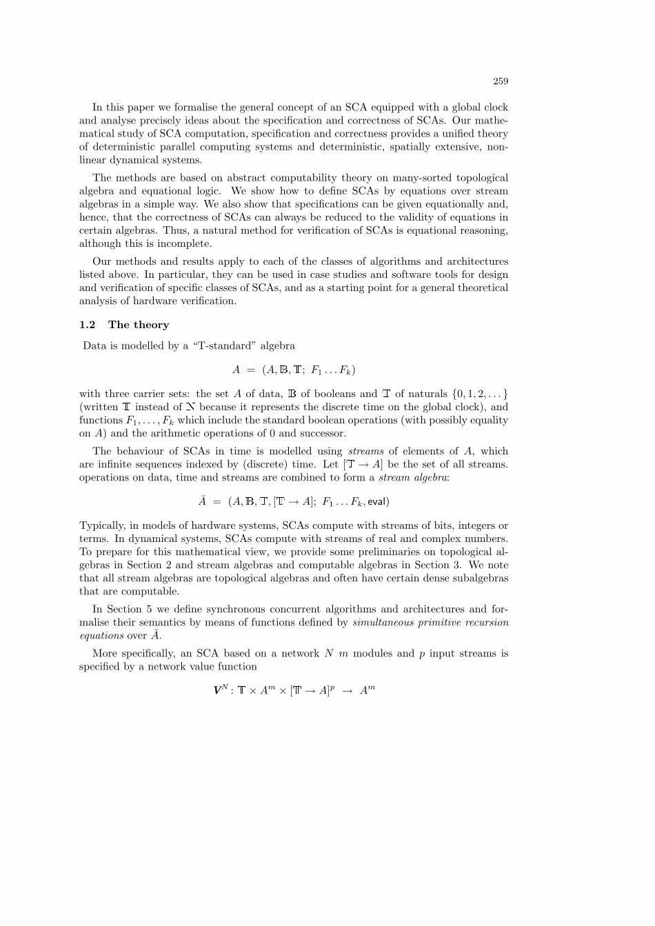
259

In this paper we formalise the general concept of an SCA equipped with a global clockand analyse precisely ideas about the specification and correctness of SCAs. Our mathe-matical study of SCA computation, specification and correctness provides a unified theoryof deterministic parallel computing systems and deterministic, spatially extensive, non-linear dynamical systems.

The methods are based on abstract computability theory on many-sorted topologicalalgebra and equational logic. We show how to define SCAs by equations over streamalgebras in a simple way. We also show that specifications can be given equationally and,hence, that the correctness of SCAs can always be reduced to the validity of equations incertain algebras. Thus, a natural method for verification of SCAs is equational reasoning,although this is incomplete.

Our methods and results apply to each of the classes of algorithms and architectureslisted above. In particular, they can be used in case studies and software tools for designand verification of specific classes of SCAs, and as a starting point for a general theoreticalanalysis of hardware verification.

1.2 The theory

Data is modelled by a “T-standard” algebra

A = (A,B,T; F1 . . . Fk)

with three carrier sets: the set A of data, B of booleans and T of naturals 0, 1, 2, . . . (written T instead of N because it represents the discrete time on the global clock), andfunctions F1, . . . , Fk which include the standard boolean operations (with possibly equalityon A) and the arithmetic operations of 0 and successor.

The behaviour of SCAs in time is modelled using streams of elements of A, whichare infinite sequences indexed by (discrete) time. Let [T→ A] be the set of all streams.operations on data, time and streams are combined to form a stream algebra:

A = (A,B,T, [T→ A]; F1 . . . Fk, eval)

Typically, in models of hardware systems, SCAs compute with streams of bits, integers orterms. In dynamical systems, SCAs compute with streams of real and complex numbers.To prepare for this mathematical view, we provide some preliminaries on topological al-gebras in Section 2 and stream algebras and computable algebras in Section 3. We notethat all stream algebras are topological algebras and often have certain dense subalgebrasthat are computable.

In Section 5 we define synchronous concurrent algorithms and architectures and for-malise their semantics by means of functions defined by simultaneous primitive recursionequations over A.

More specifically, an SCA based on a network N m modules and p input streams isspecified by a network value function

VN : T×Am × [T→ A]p → Am

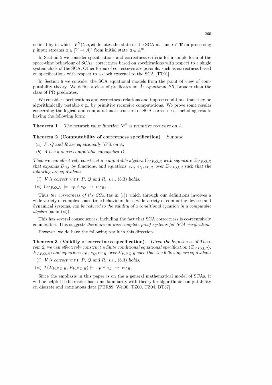
260

defined by in which VN (t,a,x) denotes the state of the SCA at time t ∈ T on processingp input streams x ∈ [T→ A]p from initial state a ∈ Am.

In Section 5 we consider specifications and correctness criteria for a simple form of thespace-time behaviour of SCAs: correctness based on specifications with respect to a singlesystem clock of the SCA. Other forms of correctness are possible, such as correctness basedon specifications with respect to a clock external to the SCA [TT91].

In Section 6 we consider the SCA equational models from the point of view of com-putability theory. We define a class of predicates on A: equational PR, broader than theclass of PR predicates.

We consider specifications and correctness relations and impose conditions that they bealgorithmically testable e.g., by primitive recursive computations. We prove some resultsconcerning the logical and computational structure of SCA correctness, including resultshaving the following form:

Theorem 1. The network value function VN is primitive recursive on A.

Theorem 2 (Computability of correctness specification). Suppose

(a) P , Q and R are equationally λPR on A,

(b) A has a dense computable subalgebra D.

Then we can effectively construct a computable algebra CV,P,Q,R with signature ΣV,P,Q,R

that expands Dreg by functions, and equations eP , eQ, eV,R over ΣV,P,Q,R such that thefollowing are equivalent:

(i) V is correct w.r.t. P , Q and R, i.e., (6.3) holds;

(ii) CV,P,Q,R |= eP ∧ eQ → eV,R.

Thus the correctness of the SCA (as in (i)) which through our definitions involves awide variety of complex space-time behaviours for a wide variety of computing devices anddynamical systems, can be reduced to the validity of a conditional equation in a computablealgebra (as in (ii)).

This has several consequences, including the fact that SCA correctness is co-recursivelyenumerable. This suggests there are no nice complete proof systems for SCA verification.

However, we do have the following result in this direction.

Theorem 3 (Validity of correctness specification). Given the hypotheses of Theo-rem 2, we can effectively construct a finite conditional equational specification (ΣV,P,Q,R),EV,P,Q,R) and equations eP , eQ, eV,R over ΣV,P,Q,R such that the following are equivalent:

(i) V is correct w.r.t. P , Q and R, i.e., (6.3) holds;

(ii) T (ΣV,P,Q,R, EV,P,Q,R) |= eP ∧ eQ → eV,R.

Since the emphasis in this paper is on the a general mathematical model of SCAs, itwill be helpful if the reader has some familiarity with theory for algorithmic computabilityon discrete and continuous data [PER89, Wei00, TZ00, TZ04, BT87].

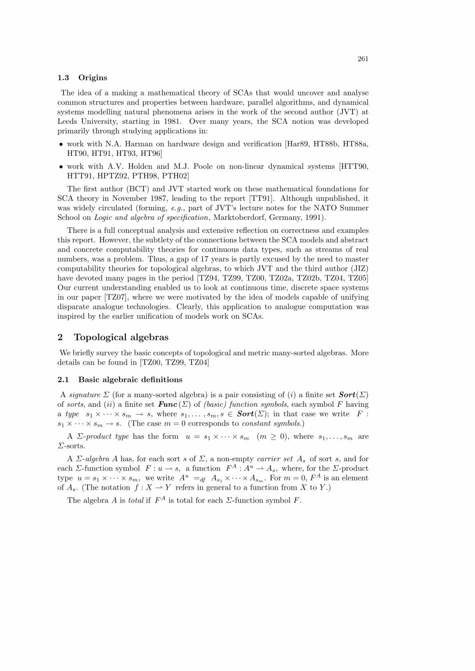
261

1.3 Origins

The idea of a making a mathematical theory of SCAs that would uncover and analysecommon structures and properties between hardware, parallel algorithms, and dynamicalsystems modelling natural phenomena arises in the work of the second author (JVT) atLeeds University, starting in 1981. Over many years, the SCA notion was developedprimarily through studying applications in:

• work with N.A. Harman on hardware design and verification [Har89, HT88b, HT88a,HT90, HT91, HT93, HT96]

• work with A.V. Holden and M.J. Poole on non-linear dynamical systems [HTT90,HTT91, HPTZ92, PTH98, PTH02]

The first author (BCT) and JVT started work on these mathematical foundations forSCA theory in November 1987, leading to the report [TT91]. Although unpublished, itwas widely circulated (forming, e.g., part of JVT’s lecture notes for the NATO SummerSchool on Logic and algebra of specification, Marktoberdorf, Germany, 1991).

There is a full conceptual analysis and extensive reflection on correctness and examplesthis report. However, the subtlety of the connections between the SCA models and abstractand concrete computability theories for continuous data types, such as streams of realnumbers, was a problem. Thus, a gap of 17 years is partly excused by the need to mastercomputability theories for topological algebras, to which JVT and the third author (JIZ)have devoted many pages in the period [TZ94, TZ99, TZ00, TZ02a, TZ02b, TZ04, TZ05]Our current understanding enabled us to look at continuous time, discrete space systemsin our paper [TZ07], where we were motivated by the idea of models capable of unifyingdisparate analogue technologies. Clearly, this application to analogue computation wasinspired by the earlier unification of models work on SCAs.

2 Topological algebras

We briefly survey the basic concepts of topological and metric many-sorted algebras. Moredetails can be found in [TZ00, TZ99, TZ04]

2.1 Basic algebraic definitions

A signature Σ (for a many-sorted algebra) is a pair consisting of (i) a finite set Sort(Σ)of sorts, and (ii) a finite set Func (Σ) of (basic) function symbols, each symbol F havinga type s1 × · · · × sm → s, where s1, . . . , sm, s ∈ Sort(Σ); in that case we write F :s1 × · · · × sm → s. (The case m = 0 corresponds to constant symbols.)

A Σ-product type has the form u = s1 × · · · × sm (m ≥ 0), where s1, . . . , sm areΣ-sorts.

A Σ-algebra A has, for each sort s of Σ, a non-empty carrier set As of sort s, and foreach Σ-function symbol F : u→ s, a function FA : Au As, where, for the Σ-producttype u = s1 × · · · × sm, we write Au =df As1 ×· · ·×Asm . For m = 0, FA is an elementof As. (The notation f : X Y refers in general to a function from X to Y .)

The algebra A is total if FA is total for each Σ-function symbol F .

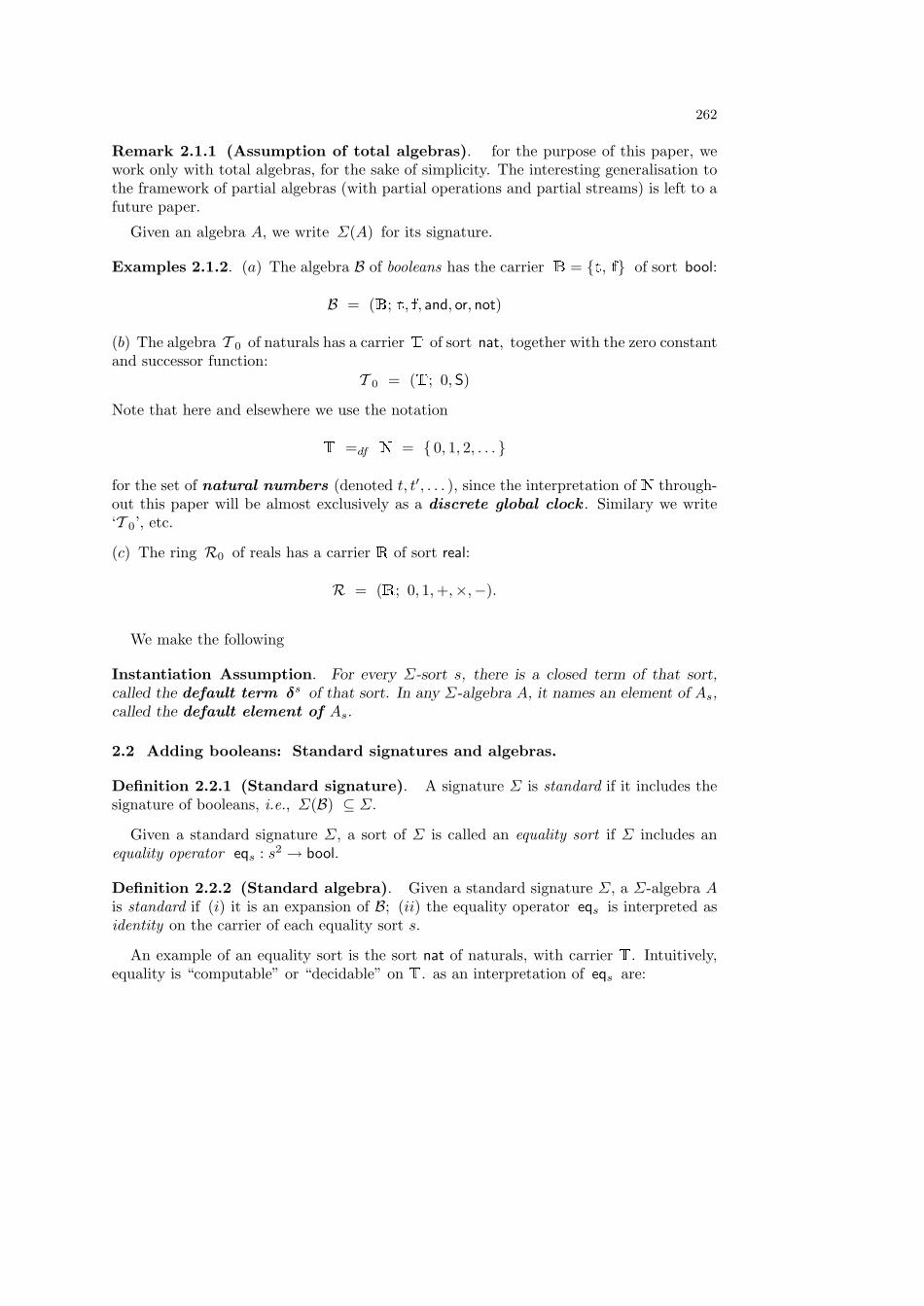
262

Remark 2.1.1 (Assumption of total algebras). for the purpose of this paper, wework only with total algebras, for the sake of simplicity. The interesting generalisation tothe framework of partial algebras (with partial operations and partial streams) is left to afuture paper.

Given an algebra A, we write Σ(A) for its signature.

Examples 2.1.2. (a) The algebra B of booleans has the carrier B = t, f of sort bool:

B = (B; t, f, and, or, not)

(b) The algebra T 0 of naturals has a carrier T of sort nat, together with the zero constantand successor function:

T 0 = (T; 0,S)

Note that here and elsewhere we use the notation

T =df N = 0, 1, 2, . . .

for the set of natural numbers (denoted t, t′, . . . ), since the interpretation of N through-out this paper will be almost exclusively as a discrete global clock . Similary we write‘T 0’, etc.

(c) The ring R0 of reals has a carrier R of sort real:

R = (R; 0, 1,+,×,−).

We make the following

Instantiation Assumption. For every Σ-sort s, there is a closed term of that sort,called the default term δs of that sort. In any Σ-algebra A, it names an element of As,called the default element of As.

2.2 Adding booleans: Standard signatures and algebras.

Definition 2.2.1 (Standard signature). A signature Σ is standard if it includes thesignature of booleans, i.e., Σ(B) ⊆ Σ.

Given a standard signature Σ, a sort of Σ is called an equality sort if Σ includes anequality operator eqs : s2 → bool.

Definition 2.2.2 (Standard algebra). Given a standard signature Σ, a Σ-algebra Ais standard if (i) it is an expansion of B; (ii) the equality operator eqs is interpreted asidentity on the carrier of each equality sort s.

An example of an equality sort is the sort nat of naturals, with carrier T. Intuitively,equality is “computable” or “decidable” on T. as an interpretation of eqs are:

263

A non-equality sort is the sort real of reals. Intuitively, equality is (“co-semi-decidable”,but) not (totally) decidable on R.

Any many-sorted signature Σ can be standardised to a signature ΣB by adjoiningthe sort bool together with the standard boolean operations; and, correspondingly, anyalgebra A can be standardised to an algebra AB by adjoining the algebra B, together withequality at the equality sorts.

Examples 2.2.4.

(a) A standard algebra of naturals T is formed by standardising the algebra T 0

(Example 2.1.2(b)), with (total) equality and order operations on T:

T = (T 0,B; eqnat, lessnat)

(b) The standardised ring of reals (cf. Example 2.1.2(c)):

R = (R0,B)

Note that there is no (total) equality on R, as discused above.

2.3 Adding the naturals: T-standard signatures and algebras.

Definition 2.3.1 (T-standard signature). A signature Σ is T-standard if (i) it isstandard, and (ii) it contains the standard signature of naturals, i.e., Σ(T ) ⊆ Σ.

Definition 2.3.2 (T-standard algebra). Given an T-standard signature Σ, a corre-sponding Σ-algebra A is T-standard if it is an expansion of T .

Any standard signature Σ can be T-standardised to a signature ΣT by adjoining the sortnat and the operations 0, S, eqnat and lessnat. Correspondingly, any standard Σ-algebraA can be T-standardised to an algebra AT by adjoining the carrier T together with thecorresponding standard functions.

Throughout this paper, we will assume:

T-standardness Assumption. The signature Σ, and the Σ-algebra A, are T-standard.

2.4 Topological algebras.

Definition 2.4.1. (a) A topological Σ-algebra is a Σ-algebra with topologies on thecarriers such that each of the basic Σ-functions is continuous.

(b) A (T-)standard topological algebra is a topological algebra which is also an (T-)standardalgebra, such that the carriers B (and T) have the discrete topology.

Examples 2.4.2. (a) Discrete algebras: The standard algebras B and T of booleansand naturals respectively (§§2.1, 2.2) are topological (total) algebras under the discretetopology. All functions on them are trivially continuous, since the carriers are discrete.

264

(b) The T-standard topological total real algebra RT is defined by

RT = (R, T ; divnat)

where R is the standardised ring of reals (2.2.4(b)), T is the standard algebra of naturals(2.2.4(a)), and divnat : R×T→ R) is the total (continuous!) function defined by

divnat(x, t) =x/t if t 6= 00 if t = 0

Note that RT does not contain (total) boolean-valued functions ‘<’ or ‘=’ on the reals,since they are not continuous; nor does it contain division of reals by reals, since thatcannot be total and continuous. See [TZ99, TZ04, TZ05] for discussions of these issues.

2.5 Metric algebra

A particular type of topological algebra is a metric algebra. This is a many-sorted standardalgebra A with an associated metric:

A = (A1, . . . , Ar,R; FA1 , . . . , FAk , d

A1 , . . . , d

Ar )

where R is the standardised ring of reals (Example 2.2.4(b)), the carriers Ai are metricspaces with metrics dAi : A2

i → R, (i = 1, . . . , r), F1, . . . , Fk are the Σ-function symbolsother than d1, . . . , dk, and the functions FAi are all continuous with respect to thesemetrics. The carriers B and T (included among the Ai) are given the discrete metric,which induces the discrete topology.

Clearly, metric algebras can be viewed as special cases of topological algebras.

Example 2.5.1. The real algebraRT (Example 2.4.3(b)) can be recast as a metric algebrain an obvious way.

3 Stream algebras; Computable algebras

3.1 Adding streams to algebras: Algebras A of signature Σ

LetΣ be a T-standard signature, and A a T-standard Σ-algebra. We define an extensionof Σ and a corresponding expansion of A.

We choose a set S ⊆ Sort(Σ) of pre-stream sorts, and then extend ΣN to a stream

signature ΣS relative to S, as follows. With each s ∈ S, associate a new stream sorts, also written nat→ s. Then

(a) Sort(ΣS) = Sort(Σ) ∪ s | s ∈ S;

(b) Func(ΣS) consists of Func (Σ), together with the evaluation function

evals : (nat→ s)× nat→ s,

265

for each s ∈ S.

Now we can expand AT to a (ΣS)-stream algebra AS by adding for each s ∈ S:

(i) the carrier for s, which is the set

As = As = [T→ As]

of all streams on As i.e., functions u : T→ As;

(ii) the interpretation of evals on A as the function evalAs : [T→ As]×T→ As whichevaluates a stream at a time instant: evalAs (u, t) = u(t).

The algebra AS is the (full) stream algebra over A with respect to S. (We will

usually omit explicit reference to the set S.)

Note that the Instantiation Assumption does not hold (in general) for the signature ofa stream algebra.

3.2 Expanding topological algebras to stream algebras

The algebraic expansion of an algebra A to a stream algebra A induces a correspondingtopological expansion.

(a) The topological T-standardisation AT , of signature ΣT , is constructed from A by givingthe new carrier T the discrete topology.

(b) Next, a topology on AT can be extended to one on A by giving the stream carriers[T→ As] the product topology based on As, where the basic open sets have the form

U = u ∈ As | u(ti) ∈ Ui for i = 1, . . . , n (2.1)

for some n > 0, t1, . . . , tn ∈ T and U1, . . . , Un open subsets of As.

With this topology, the operator evalAs is continuous.

Remarks 3.2.1.

(1) This topology is the same as the inverse limit topology on [T→ As] [TZ08, §2.1].

(2) If As is metrisable by the metric ds, then so is [T→ As] [TZ08, §3.1], by the metric

ds(u, v) =df

∞∑t=0

min(ds(u(t), v(t)), 2−t

)

266

3.3 Regular streams

Let B be a Σ-subalgebra of A. Then the stream algebra B over B is a Σ-subalgebraof the stream algebra A. Further, for any stream sort s, if we replace [T → Bs] by anynonempty subset of it in the definition ofB, then we again obtain a “stream subalgebra”of A. All subalgebras of A are obtained in this way.

Of special interest is the following subset of the set As of all streams in A of sort s.Define the set of regular streams of A of sort s by

(As)reg = [T→ As]reg = u ∈ [T→ As] | ∃t0 ∀t ≥ t0 (u(t) = δs)

where δs is the default element of As (2.1).

Further, for each T-standard Σ-algebra A we define Areg, the regular stream algebra

over A, to be the Σ-subalgeba of the stream algebra A obtained by restricting , at eachstream sort s, As to the set (As)reg of regular streams of sort s.

Lemma 3.3.1. If B is a Σ-subalgebra of A then the regular stream algebra (B)reg over

B is a Σ-subalgebra of the stream algebras B, Areg, and A.

3.4 Dense regular subalgebras

We need the following general topological result.

Lemma 3.4.1. If X is a topological space and Y a Hausdorff space, and f : X → Yand g : X → Y are both continuous, with f D = g D for some dense subset D of X,then f = g.

Let A be a Σ-algebra.

Definition 3.4.2 (Dense subset). A Sort(Σ)-indexed subset D is dense in A if forall Σ-sorts s, Ds is dense in As.

Lemma 3.4.3. Let A be a T-standard topological Σ-algebra. Then

(i) if A is Hausdorff then so is A;

(ii) if D is a dense Σ-subalgebra of A then D and Dreg are dense Σ-subalgebras of A.

Proof: We prove the second part of (ii). Note first that Dbool = Abool = B and Dnat =Anat = N. Now, for any stream sort s, by assumption Ds is dense in As. It remains toshow that (Ds)reg is dense in As = [T→ As]. Choose any basic open set U in [T→ As],as in (2.1). Since Ds is dense in As, we can find di ∈ Ui ∩Ds for i = 1, . . . , n. Now definea stream u by

ui(t) =

di if t = ti for i = 1, . . . , n

δs otherwise.

Then u ∈ U ∩ (Ds)reg.

267

From now on, we will assume that all our topological algebras satisfy

Hausdorff Assumption. A is a Hausdorff topological algebra.

3.5 Computable algebras; Computable stream algebras

In order to investigate effective aspects of correctness specification of SCAs (Section 8),we need the concept of a computable algebra [BT87].

Definition 3.5.1 (Recursive number algebra). A recursive number Σ-algebra Ω is aΣ-algebra in which for each Σ-sort s, Ωs is a recursive subset of N and for each Σ-functionsymbol F : u→ s,

FΩ : Ωu → Ωs

is a total recursive function.

Let A be a T-standard Σ-algebra.

Definition 3.5.2 (Effectively presented algebra). An effective presentation (α,Ω)for A consists of a recursive number Σ-algebra Ω and a Σ-epimorphism α : Ω → A.We assume that Ωnat = N and αnat = idN.A is said to be effectively presented by (α,Ω).

Next we define the Sort(Σ)-sorted congruence relation

≡α = 〈≡α,s| s ∈ Sort(Σ)〉

induced by α on Ω:x ≡α,s y ⇐⇒ αs(x) = αs(y)

for all x, y ∈ Ωs. Note also that A ∼= Ω/≡α.

Definition 3.5.3 (Computable algebra). A is computable if it has an effectivepresentation (α,Ω) in which ≡α is decidable on Ω; that is, for each s ∈ S, ≡α,s is decidable.

Note, next, that the stream algebra A has uncountable carrier sets As and so it cannotbe effectively presented. We therefore work with a regular subalgebra of A.

Lemma 3.5.4. Let D be a computable dense Σ-subalgebra of A. Then Dreg is acomputable dense Σ-subalgebra of A.

Proof: It is easy to extend an effective presentation for A with decidable equality to onefor A. The denseness of Dreg in A follows from Lemma 3.4.3.

Remark 3.5.5. An example of a computable dense subalgebra of an algebra, satisfyingthe assumptions of Lemma 3.5.4, is in the real algebra RT (Example 2.4.3(b)), in whichthe rationals Q form a dense subset of R.

268

4 Synchronous Concurrent Algorithms

4.1 Introduction to SCAs

An SCA is an algorithm given by a network N of modules, channels, sources andsinks. The modules compute and communicate in parallel; computation and data flowbetween modules is synchronised by a single global clock measuring discrete time, withvalues in T.

For simplicity, assume that our T-standard Σ-algebra A contains only one carrier (apartfrom B and T), also called A, of sort data. The data flowing between modules are takenfrom this set.

The SCA processes streams or infinite sequences u(0), u(1), u(2), . . . of data from A,clocked by T. Such a stream is represented as a function u : T→ A. Let [T→ A] be theset of all streams over A.

The network N is made from a set M1, . . . ,Mm of modules, a set Iin of p sources and aset Iout of q sinks. For simplicity we represent the modules, sources and sinks as naturalnumbers: I = 1, . . . ,m, Iin = 1, . . . , p and Iout = 1, . . . , q.

Communication between modules occurs by means of the channels. These have unitbandwidth and are unidirectional; that is, they can transmit only a single datum a ∈ Aat any one time in one direction. Channels may branch with the intention that the datumtransmitted along the channel is “copied” and transmitted along each branch. However,channels may not merge.

A module is an atomic computing device capable of some specific internal processing.If module Mi has ki(> 0) input channels and one output channel then we assume theprocessing of Mi to be specified by a total function Fi : Aki → A with the intention that ifa1, . . . , aki

∈ A arrive on the module’s ki input channels (one datum per channel) at timet then Mi computes Fi(a1, . . . , aki), and transmits it at time t+ 1.

A source has no input and one output channel (which may branch). A network withp sources will process p input streams u1, . . . , up ∈ [T→ A], or, equivalently, a vector-valued input stream u ∈ [T→ A]p with u(t) = (u1(t), . . . , up(t)).

The sinks each have one input and no output channel. These will transmit the q outputstreams.

An SCA’s architecture is given by three wiring functions

α : I×N → Iin ∪ I

β : I×N → S,Mout : Iout → I.

The map out is such that for each sink i, out(i) is the module that supplies i.

The maps α and β are partial functions that enumerate the inputs to a given module inthe following way. Given a module i ∈ I with ki input channels, for j = 1, . . . , ki the jthinput channel is the output channel of module α(i, j) if β(i, j) = M, or the output channelof source α(i, j) if β(i, j) = S. If j 6∈ 1, . . . , ki then α(i, j) and β(i, j) are undefined.

269

Note that feedback is characterised by a module i with input j, where α(i, j) = i andβ(i, j) = M.

The initial state of the network is specified by a vector a = (a1, . . . , am) ∈ Am, whereai denotes the value output by module i at time t = 0.

4.2 Informal Explanation of Operation

Initially, at time t = 0, each module i has some initial value ai ∈ A on its output channel.Each source j of N is yet to supply its first input datum uj(0) to the network. Thus, att = 0 there is a single datum on every channel in the network.

Each module i now computes by first reading ite input data and then evaluating Fi onthese data. The result of this evaluation is stored on the module’s output channel.

Unit Delay Assumption. For each module in N , the element on its output channel attime t+ 1 is uniquely determined by the data on its input channels at time t.

So we assume that it takes at most one time cycle for every module to read, evaluateand store in some order, and that any module taking less than one time unit is forced towait until any slower modules have finished.

Hence, as the clock beats t = 0, 1, 2, . . . , the modules concurrently pass data and com-pute with each module performing its t-th read/evaluate/store sequence starting at timet and ending by time t+ 1.

4.3 Algebraic Formalisation

We start with a T-standard signature ΣT and Σ-algebra AT (§2.3). As stated above, weassume for convenience that there are only three carriers: A of data, B of booleans and Tof naturals (i.e., discrete time instants). Apart from the standard boolean and arithmeticoperations, there may be other functions, including (perhaps) equality on A.

Now we form the module algebra AN by adding the module functions to AT :

AN = (AT ; F1, . . . ,Fm)

Next, we extend this to the algebra AN of streams over AN (§3.1), which we call the

module stream algebra :

AN = (AN , [T→ A]; eval).

Recall that the input to N is a stream tuple u = (u1, . . . , up) ∈ [T → A]p and theinitial values are a = (a1, . . . , am) ∈ Am.

Termination Assumption. At each time t ∈ T there is a value output from eachmodule, which can be determined uniquely from t, u and a.

We return to the Unit Delay and Termination Assumptions in Section 4.6.

270

For each module i ∈ I we define its module value function

Vi : T×Am × [T→ A]p → A

where Vi(t,u,a) is the value output by the module i at time t when the network isexecuted on input u and initial data a. Note that these functions are total by AssumptionT.

Thus the state of the network N is given by combining the module value functionsV1, . . . ,Vm into the single network value function

VN : T×Am × [T→ A]p → Am (4.1a)

defined byVN (t,a,x) = (V1(t,a,x) . . . ,Vm(t,a,x)). (4.1b)

This defines the state of N at each time cycle. (We will sometimes drop the “networksuperscript” ‘N’.)

The concurrent execution of the modules of N is modelled by the parallel evaluation ofV1, . . . ,Vm. We now develop general formulae for the computation of V1, . . . ,Vm andhence of VN .

4.4 Recursive network equations

We define V1(t,a,x), . . . ,Vm(t,a,x) for a = (a1, . . . , am) ∈ Am, x = (x1, . . . , xp) ∈[T→ A]p, and t = 0, 1, 2, . . . , by simultaneous recursion on t.

Base case: Initialisation. For i = 1, . . . ,m:

Vi(0,a,x) = ai (4.2)

Recursion step: State transition. Each module i has a functional specificationFi : Aki → A, where, if b1, . . . , bki

arrive on i’s input channels at time t then the valueoutput by the module at time t + 1 is Fi(b1, . . . , bki

). Let the SCA have wiring functionsα and β as described in §4.1. Then for i = 1, . . . ,m and all t ≥ 0

Vi(t+ 1,a,x) = Fi(bi1, . . . , biki) (4.3a)

where for j = 1, . . . , ki

bij =

Vα(i,j)(t,a,x) if β(i, j) = M

xα(i,j)(t) if β(i, j) = S.(4.3b)

Remark 4.4.1. The equations (4.2) and (4.3) together form a definition by simulta-neous primitive recursion .

271

Remark 4.4.2 (Stream transformation). We can rewrite the network value functionV (4.1) as a stream transformation by “abstraction” or “currying”; i.e., define

V : Am × [T→ A]p → [T→ A]m (4.4a)

whereV(a,x)(t) = V(t,a,x). (4.4b)

We return to a consideration of these two forms, from a computational point of view, in§6.2.

4.5 Output specification

Note that the network value function VN gives the values output by every module inthe network. In many cases we are interested only in the values sent to the network’ssinks. When the network has q > 0 sinks with Iout = 1, . . . , q we use the functionout : Iout → I (§4.1). Now define the network output function

Vout : T×Am × [T→ A]p → Aq (4.5a)

byVout(t,a,x) = (Vout(1)(t,a,x), . . . ,Vout(q)(t,a,x)), (4.5b)

so that Vout(t,a,x) is the vector of q values at the sinks of N at time t.

Note (cf. Remark 4.4.2) that we can also reformulate Vout as a stream transformationby abstraction:

Vout : Am × [T→ A]p → [T→ A]q

whereVout(a,x)(t) = Vout(t,a,x).

4.6 Generalisation of the model: Partial algebra of data

There are many fruitful generalisations of our mathematical model. We wish to mentionone, where we drop the assumption that the data algebra A is total. This is of greatpractical importance, in the case, for example, that A is an algebra of reals, that includesthe operation of real division, and the boolean operations of equality and order . In orderthat these operations be continuous, we must make them partial , as explained in [TZ04].

In such a framework, the module functions will also be partial. as will the network valuefunction. We will also have to work with partial streams.

If we maintain our assumption that the channels have unit bandwidth (§4.1), we willhave to drop both the Unit Delay and Termination Assumptions (§§4.2,4.3). We will alsohave to replace our global clock model with a system of local clocks. We conjecture thatthis will be equivalent to the global clock model, with the Termination and Unit DelayAssumptions, in the special case that the algebra A, and the function modules, are total.

Details will be given in a forthcoming publication.

272

5 Specifications and Correctness

5.1 Indexed sets and operations

Let S be a finite non-empty set. An S-indexed set A is a family A = 〈As | s ∈ S〉.Given two S-indexed sets A = 〈As | s ∈ S〉 and B = 〈Bs | s ∈ S〉, an S-indexed map-

ping from A to B is a family f = 〈fs | s ∈ S〉 where fs : As → Bs for each s ∈ S. Insymbols we write f : A→ B.

5.2 Syntax: Variables, terms and equations

(a) Var(Σ) is a Sort(Σ)-indexed set, the set of Σ-variables (x, x1, x′, . . . ). Vars(Σ) isthe set of Σ-variables of sort s, denoted xs, . . . .

(b) T(Σ) is the Sort(Σ)-indexed set of Σ-terms (denoted t, . . . ), where the set Tms(Σ)of such terms of sort s (denoted t : s) is defined (simultaneously over S) by

ts ::= xs | c | F (ts11 , . . . , tsmm )

where c is a constant symbol of type s, and F is a Σ-function symbol of type s1, . . . , sm → s(m > 0). We also use the notation b, . . . for boolean terms, i.e., terms of sort bool.

Let var(E) be the set of variables contained in any syntactic object E.

(c) Eq(Σ) is the set of Σ-equations (ts1 = ts2) between Σ-terms of the same Σ-sort. Wealso write equations as e, e′, . . . .

5.3 Semantics: Assignments and term evaluations; Satisfaction

Let A be a Σ-algebra. A (Σ-)assignment on A is an S-indexed map θ : Var(Σ) → A.

Definition 5.3.1 (Term evaluation). Given an assignment θ : Var(Σ) → A, weextend it to an S-indexed map [[ · ]]A,θ : T(Σ) → A, defined by structural induction onT(Σ):

(i) If t ≡ x then [[t]]A,θ = θ(x).

(ii) If t ≡ c then [[t]]A,θ = cA.

(iii) If t ≡ F (t1, . . . , tm) then [[t]]A,θ = FA([[t1]]A,θ, . . . , [[tm]]A,θ).

Note that for a closed term t, [[t]]A,θ does not depend on θ. We therefore write it as tA.

Definition 5.3.2 (Equational specification). A (Σ)-equational specification is a pair(Σ,E) where E ⊆ Eq(Σ).

Definition 5.3.3 (Equational satisfaction). Let A be a Σ-algebra.

(a) A satisfies the Σ-equation (t1 = t2), written A |= t1 = t2, if for all Σ-assignmentsθ on A, [[t1]]A,θ = [[t2]]A,θ.

(b) A satisfies the equational specification (Σ,E), written A |= E, if A |= e for alle ∈ E.

273

5.4 Correctness of an SCA

We develop the concept of specification of an algebra introduced above, and apply itparticularly to stream algebras and SCAs. Hence we introduce the notion of correctnessof an SCA. We will concentrate on relational correctness.

Suppose that a computational task or behaviour is specified by a relation of the form

R ⊆ T×Am × [T→ A]p ×Aq (5.1)

such that for each t ∈ T, a ∈ Am, x ∈ [T→ A]p, and y ∈ Aq,

R(t,a,x,y)

means that y is acceptable as an output at time t for and initial state a and input streamx. We call R the specification relation .

There are various ways of formulating correctness w.r.t. a specification relation R, de-pending on how we treat initialisations and inputs: We can consider a particularinitialisation , or all initialisations from some subset of Am (possibly all of Am).Similarly, we can consider a particular input stream , or all inputs from some subsetof [T→ A]p (possibly all of [T→ A]p). To take a typical (and useful) case:

Definition 5.4.1 (Correctness for initialisations and inputs from some set).For any sets P ⊆ Am of initialisations and Q ⊆ [T→ A]p of inputs, the SCA is correctw.r.t. P , Q and R if

(∀t ∈ T) (∀a ∈ P ) (∀x ∈ Q) R(t,a,x,Vout(t,a,x)). (5.2)

Here the output value function Vout : T × Am × [T→ A]p → Aq (3.9) is a selectionfunction for the relation R, relative to P and Q.

We will investigate the computational significance of such correctness assertions in thenext section.

6 Primitive recursive computability on stream algebras

6.1 Primitive recursion on abstract algebras

In [TZ88] we developed a theory of abstract computability on standard abstractmany-sorted algebras. We formulated a generalised Church-Turing thesis, whichidentifies a certain class of functions (namely, ‘µPR’ computable or ‘While’ computable)with functions algorithmically computable on such structures.

We also developed a theory of generalised primitive recursion over T-standardalgebras A. These generalise Kleene’s primitive recursion functions on N [Kle52]. andform a proper subclass of the class µPR.

Briefly, we define a class PR(A) of PR (primitive recursive) functions on A, generated byschemes for (i) the initial functions and constants, i.e., the interpretations on A of the Σ-functions, (ii) projections, (iii) definition by cases, (iv) composition, and (v) simultaneousprimitive recursion.

274

Note that the class µPR(A) is formed from PR(A) by adding a scheme for the (con-structive) least number operator.

Lemma 6.1.1 (PR computability and continuity). Let A be a topological algebra.Then all functions in PR(A) are continuous.

This is proved, in fact for all µPR functions, in [TZ88].

We now consider a class of relations on algebras broader than primitive recursiveness.

Definition 6.1.2 (Equationally PR definable relations). A relation R ⊆ Au onan algebra A is equationally PR definable on A (EqPR(A)) if there are PR(A) functionsfR, gR : u→ s for some Σ-sorts u, s such that for all a ∈ Au

a ∈ R ⇐⇒ fR(a) = gR(a). (6.1)

We call the rhs of (6.1) a PR defining equation for R, and the pair (fR, gR) PR definingfunctions for R.

Remark 6.1.3 (Comparison of PR and EqPR computability). Note that EqPR(A)is a broader concept than PR(A). For on the one hand, any PR(A) relation R is alsoEqPR(A), since (if χR is the characteristic function of R)

a ∈ R ⇐⇒ χR(a) = true

(a special case of (6.1)). But on the other hand, the range sort s (in Definition 6.1.2) neednot be an equality sort (cf. §2.2), i.e., equality at sort s is not necessarily PR.

6.2 Primitive recursion on stream algebras

Assume for simplicity (as stated in Section 4) that our T-standard Σ-algebra A contains(apart from B and T) only one carrier A of data.

Consider now PR stream valued functions or stream transformers on A:

f : [T→ A]m ×An → [T→ A]. (6.2)

It has been shown [TZ94] that all PR stream transformers f of type as in (6.2) have theform

f(u1, . . . , um, a1, . . . , an) = uf0(u1,...,um,a1,...,an)

for some PR functionf0 : [T→ A]m ×An → T.

In other words, PR stream transformers are not “interesting”; they only return one of theinput streams (the choice of which one depending primitive recursively on the inputs).

We therefore consider a broader, more interesting class of stream transformers, namelythe class λPR(A) formed from PR(A) by adding a scheme for stream (λ)-abstraction. Notethat a function f as in (6.2) will be in λPR(A) if its “cartesian” or “uncurried” form

f : [T→ A]m ×An ×T → A

275

is in PR(A), wheref(u,a, t) = f(u,a)(t).

Note also that we can define the class EqλPR(A) of equational λPR definable relations onA, analogously to EqPR(A) (Definition 6.1.2).

Now assume A, and hence A, are topological algebras.

Lemma 6.2.1. For f as in (6.2), f is continuous iff f is continuous.

Hence, from Lemma 6.1.1:

Lemma 6.2.2. All functions in λPR(A) are continuous.

Corollary 6.2.3. Let A be Hausdorff T-standard Σ-algebra, and D a dense subalgebraof A. Let f and g be λPR functions on A. Then the following are equivalent:

(i) f = g on A

(ii) f = g on D

(iii) f = g on Areg

(iv) f = g on Dreg.

Proof: From Lemmas 3.4.1, 3.4.3 and 6.2.2.

6.3 Primitive recursiveness of SCA state function

Recall the module, network and output value functions (§§4.3, 4.5).

Theorem 1. For any SCA over A with network N and module functions F1, . . . ,Fm:

(a) The module value functions V1, . . . ,Vm, network value function VN and networkvalue function Vout are in PR(A).

(b) The abstracted forms V and Vout are in λPR(A).

Proof: The main step in (a) is to show that VN is definable (uniquely) by simultaneousprimitive recursion (equations 4.8) from the module functions V1, . . . ,Vm. This can beseen by a simple inductive argument, parallelling the PR definition.

Remark 6.3.1 (Fixed point theory for network functions). In [TZ08] the questionof the existence of a solution to network equations is investigated in a more general context,which includes, as special cases, (i) a discrete global clock , characteristic of SCAs, and(ii) a continuous global clock , characteristic of analog systems [TZ07]. This involvesa fixed point argument as follows. Define, for all a ∈ Am and x ∈ [T→ A]p, the streamtransformation

Φa,x : [T→ A]m → [T→ A]m

by Φa,x(u) = v, where (cf. equations (4.2) and (4.3)) for i = 1, . . . ,m

vi(0) = ai

276

and for all t ≥ 0vi(t+ 1) = Fi(bi1, . . . , biki

)

where for j = 1, . . . , ki

bij =

uα(i,j)(t) if β(i, j) = M

xα(i,j)(t) if β(i, j) = S.

Then Φa,x is contracting , in the sense that for all t ∈ T and all u1,u2 ∈ [T→ A]m:

u1 t = u2 t =⇒ Φa,x(u1)t+1 = Φa,x(u2)t+1

(where ‘u t’ means the restriction of u to the initial segment 0, 1, . . . , t of T.) Fromthis we can derive the existence of a unique fixed point u of Φa,x, satisfying u = V(a,x).

6.4 Computability of relational correctness specification

Recall the definition (5.4.1) of correctness for a specification relation R with initialisationsand input streams from sets P ⊆ Am and Q ⊆ [T→ A]p respectively (repeating (5.2)):

(∀t ∈ T) (∀a ∈ P ) (∀x ∈ Q) R(t,a,x,Vout(t,a,x)). (6.3)

Theorem 2 (Computability of correctness specification). Suppose

(a) P , Q and R are EqλPR on A,

(b) A has a dense computable subalgebra D.

Then we can effectively construct a computable algebra CV,P,Q,R with signature ΣV,P,Q,R

that expands Dreg by functions, and equations eP , eQ, eV,R over ΣV,P,Q,R such that thefollowing are equivalent:

(i) V is correct w.r.t. P , Q and R, i.e., (6.3) holds;

(ii) CV,P,Q,R |= eP ∧ eQ → eV,R.

In consequence, correctness in the sense of (i) can be effectively reduced to the validity ofconditional equations in a computable algebra and is co-recursively enumerable.

Proof: We prove (i)⇒(ii). Consider the statement

a ∈ P ∧ x ∈ Q −→ R(t,a,x,Vout(t,a,x)). (6.4)

Let (fP , gP ), (fQ, gQ) and (fR, gR) be λPR defining functions for the sets P , Q and Rrespectively. By assumption and Theorem 1, these functions, as well as V, are all λPRon Dreg. By assumption (i), (6.4) holds on A, and therefore, by Corollary 6.2.3, on Dreg.Since D is a computable algebra, so is Dreg, by Lemma 3.5.4, with effective presentation(α,Ω) say (recall §3.5). Now expand Dreg to the algebra

CV,P,Q,R =df (Dreg; V, fP , gP , fQ, gQ, fR, gR) (6.5)

277

with signature ΣV,P,Q,R. Since the seven functions shown in (6.5) are all λPR over Dreg,they are “α-computable” on Dreg. (This follows from the soundness theorem for abstractcomputability [TZ04]). Hence CV,P,Q,R is also a computable algebra. Moreover (6.4) hasthe form of a conditional equation eP ∧ eQ → eV,R over CV,P,Q,R. Hence (ii) follows.

That the correctness problem is co-r.e. follows from the α-computability of the functionsnoted above, together with the decidability of ≡α.

Example 6.4.1. Let A be the T-standard topological agebra RT (Example 2.4.3(b)).A has a dense computable subalgebra D = QT consisting of the rationals Q with thesame signature as A. As a (very simple) example of an equationally λPR (in fact, PR)specification relation, we could take

R(t, a, x1, x2, y) ⇐⇒ x1(t)2 + x2(t)2 = y2.

A more interesting example would be something like

R′(t, a, x1, x2, y) ⇐⇒ (0 < x1(t)) ∧ (0 < x2(t)) ∧ (x1(t)2 + x2(t)2 < y2),

i.e., a boolean combination of equalities and inequalities between λPR terms.

The problem here is that equality and order, as total operations on R, are not com-putable [TZ99, TZ04, TZ05]. In this paper we have solved this problem for equality byusing the computable subalgebra QT of RT , together with the concept of equational PRdefinability (Definition 6.1.2).

To handle ‘<’, however, would seem to require a major extension of the theory, so as toincorporate partial algebras. This is planned for a future publication.

We could ask if condition (ii) in Theorem 2 could be replaced by a statement that theconditional equation is a valid consequence of a certain set of axioms, i.e., a completenessresult. However the correctness problem for conditional equations in stream algebras iscomplete Π0

1 [BT87] and so completeness fails. In this direction, however, we can prove thefollowing, using results of Bergstra and Tucker on initial algebra semantics [BT80, BT82,BT87, BT92].

Theorem 3 (Validity of correctness specification). Given the hypotheses of Theo-rem 2, we can effectively construct a finite conditional equational specification (ΣV,P,Q,R),EV,P,Q,R) and equations eP , eQ, eV,R over ΣV,P,Q,R such that the following are equivalent:

(i) V is correct w.r.t. P , Q and R, i.e., (6.3) holds;

(ii) T (ΣV,P,Q,R, EV,P,Q,R) |= eP ∧ eQ → eV,R,

where T (ΣV,P,Q,R, EV,P,Q,R) is the ΣV,P,Q,R-term model generated by EV,P,Q,R.

In particular (ΣV,P,Q,R, EV,P,Q,R) can be chosen to be either (a) a complete orthogonalterm rewriting system; or (b) a small specification: if A has n+ 2 sorts then ΣV,P,Q,R has6(n+ 2) hidden operations and EV,P,Q,R has 4(n+ 2) equations.

278

7 Concluding remarks

Since the idea of a SCA is general, our methods and results apply to the various classesof algorithms, architectures and physical models mentioned in the Introduction, as well asto several others.

Consider abstract hardware, for example. Our mathematical notions can be used toclarify and improve methods developed in case studies and software tools for design, simu-lation and verification work on specific classes of SCAs; and to make comparisons and helptransfer specific methods between different classes. A fundamental problem in computingis that of hierarchy and the relationship between levels of abstraction in specifications andprograms. A theory of SCAs could be used as a starting point for a very general theory ofhardware.

As another example, consider physical modelling. Our notions can be used to clarify andimprove methods developed in case studies and software tools for modelling, simulationand analysis work on specific classes of SCAs; and to make comparisons and help transferspecific methods between different classes. Again, hierarchy and the relationship betweenlevels of abstractions in physical models is a fundamental problem. As one example ofthis, in [PTH02] we discuss how ideas from hardware design can be applied to non-lineardynamical systems in the case of whole-heart modelling.

There are, however, many more mathematical questions to answer. For example, wewant to investigate the theory of SCAs based on partial data algebras, with partial streams.

Acknowledgments. We thank the following colleagues for many useful and stimulatingdiscussions on the subject: J.A. Bergstra, B.R.J. McConnell, M.J. Poole, R. Stephens,W.B. Yates, S.M. Eker, K. Hobley, A.R. Martin, and A.V. Holden. The research of thesecond and third authors was supported in part by a grant from EPSRC (Engineering andPhysical Sciences Research Council, UK). The research of the third author was supportedin part by a grant from NSERC (Natural Sciences and Engineering Research Council,Canada).

References

References

[BT80] J.A. Bergstra and J.V. Tucker. A characterisation of computable data types by means of afinite equational specification method. In J.W. de Bakker and J. van Leeuwen, editors, 7thInternational Colloquium on Automata, Languages and Programming, Noordwijkerhout,The Netherlands, July 1980, volume 85 of Lecture Notes in Computer Science, pages76–90. Springer-Verlag, 1980.

[BT82] J.A. Bergstra and J.V. Tucker. The completeness of the algebraic specification methodsfor data types. Information and Control, 54:186–200, 1982.

[BT87] J.A. Bergstra and J.V. Tucker. Algebraic specifications of computable and semicom-putable data types. Theoretical Computer Science, 50:137–181, 1987.

279

[BT92] J.A. Bergstra and J.V. Tucker. Equational specifications, complete term rewriting systemsand computable and semicomputable algebras. Technical Report CS-20-92, Departmentof Computer Science, Swansea University, Swansea, Wales, 1992.

[Har89] N.A. Harman. Formal specifications for digital systems. PhD Thesis, School of ComputerStudies, University of Leeds, 1989.

[HPTZ92] A.V. Holden, M. Poole, J.V. Tucker, and H. Zhang. Coupled map lattices as computa-tional systems. Chaos, 2:367–376, 1992.

[HT88a] N.A. Harman and J.V. Tucker. Clocks, retimings, and the formal specification of a uart.In G. Milne, editor, The Fusion of Hardware Design and Verification (Proceedings of IFIPWorking Group 10.2 Working Conference), pages 375–396. North Holland, 1988.

[HT88b] N.A. Harman and J.V. Tucker. Formal specifications and the design of verifiable comput-ers. In Proceedings of 1988 UK IT Conference, held under the auspices of the InformationEngineering Directorate of the Department of Trade and Industry, pages 500–503. Insti-tute of Electrical Engineers, 1988.

[HT90] N.A. Harman and J.V. Tucker. The formal specification of a digital correlator i: userspecification process. In K. McEvoy and J.V. Tucker, editors, Theoretical Foundations ofVLSI Design, pages 161–262. Cambridge University Press, 1990.

[HT91] N.A. Harman and J.V. Tucker. Consistent refinements of specifications for digital systems.In P. Prinetto, editor, Correct hardware design methodologies (Proceedings ESPRIT BRA3216 Workshop), pages 281–304. Elsevier, 1991.

[HT93] N.A. Harman and J.V. Tucker. Algebraic methods and the correctness of microprocessors.In G.J. Milne and L. Pierre, editors, Correct Hardware Design and Verification Methods,volume 683 of Lecture Notes in Computer Science, pages 92–108. Springer-Verlag, 1993.

[HT96] N.A. Harman and J.V. Tucker. Algebraic models of microprocessors: architecture andorganisation. Acta Informatica, 33:421–456, 1996.

[HTT90] A.V. Holden, B.C. Thompson, and J.V. Tucker. The computational structure of neuralsystems. In A.V. Holden and V.I. Kryukov, editors, Neurocomputers and Attention I:Neurobiology, Synchronisation and Chaos, pages 223–240. Manchester University Press,1990.

[HTT91] A.V. Holden, B.C. Thompson, and J.V. Tucker. Can excitable media be considered ascomputational systems? Physica D, 49:240–246, 1991.

[Kle52] S.C. Kleene. Introduction to Metamathematics. North Holland, 1952.

[PER89] M.B. Pour-El and J.I. Richards. Computability in Analysis and Physics. Springer-Verlag,1989.

[PTH98] M.J. Poole, J.V. Tucker, and A.V. Holden. Hierarchies of spatially extended systems andsynchronous concurrent algorithms. In B. Moller and J.V. Tucker, editors, Prospects forhardware foundations, volume 1546 of Lecture Notes in Computer Science, pages 184–235.Springer-Verlag, 1998.

280

[PTH02] M.J. Poole, J.V. Tucker, and A.V. Holden. Hierarchical reconstructions of cardiac tissue.Chaos, Solitons and Fractals, 13:1581–1612, 2002.

[TT91] B.C. Thompson and J.V. Tucker. Algebraic specification of synchronous concurrent al-gorithms and architectures (Revised). Research Report 9-91, Department of ComputerScience, Swansea University, Swansea, Wales, 1991.

[TZ88] J.V. Tucker and J.I. Zucker. Program Correctness over Abstract Data Types, with Error-State Semantics, volume 6 of CWI Monographs. North Holland, 1988.

[TZ94] J.V. Tucker and J.I. Zucker. Computable functions on stream algebras. In H. Schwicht-enberg, editor, Proof and Computation: NATO Advanced Study Institute InternationalSummer School at Marktoberdorf, 1993, pages 341–382. Springer-Verlag, 1994.

[TZ99] J.V. Tucker and J.I. Zucker. Computation by ‘while’ programs on topological partialalgebras. Theoretical Computer Science, 219:379–420, 1999.

[TZ00] J.V. Tucker and J.I. Zucker. Computable functions and semicomputable sets on many-sorted algebras. In S. Abramsky, D. Gabbay, and T. Maibaum, editors, Handbook of Logicin Computer Science, volume 5, pages 317–523. Oxford University Press, 2000.

[TZ02a] J.V. Tucker and J.I. Zucker. Abstract computability and algebraic specification. ACMTransactions on Computational Logic, 3:279–333, 2002.

[TZ02b] J.V. Tucker and J.I. Zucker. Infinitary initial algebra specifications for stream algebras.In W. Sieg, R. Sommer, and C. Talcott, editors, Reflections on the Foundations of Math-ematics: Essays in honor of Solomon Feferman, volume 15 of Lecture Notes in Logic,pages 234–256. Association for Symbolic Logic, 2002.

[TZ04] J.V. Tucker and J.I. Zucker. Abstract versus concrete computation on metric partialalgebras. ACM Transactions on Computational Logic, 5:611–668, 2004.

[TZ05] J.V. Tucker and J.I. Zucker. Computable total functions, algebraic specifications anddynamical systems. Journal of Logic and Algebraic Programming, 62:71–108, 2005.

[TZ07] J.V. Tucker and J.I. Zucker. Computability of analog networks. Theoretical ComputerScience, 371:115–146, 2007.

[TZ08] J.V. Tucker and J.I. Zucker. Computation on algebras of continuous functions. In prepa-ration, 2008.

[Wei00] K. Weihrauch. Computable Analysis: An Introduction. Springer-Verlag, 2000.

UncomputabilityI and Undecidability in EconomicTheory

K. Vela Velupillaia,∗

aDepartment of Economics, University of Trento, Via Inama 5, 381 00 Trento, Italy

Abstract

Economic theory, game theory and mathematical statistics have all increasinglybecome algorithmic sciences. Computable Economics, Algorithmic Game The-ory ([28]) and Algorithmic Statistics ([13]) are frontier research subjects. All ofthem, each in its own way, are underpinned by (classical) recursion theory – andits applied branches, say computational complexity theory or algorithmic infor-mation theory – and, occasionally, proof theory. These research paradigms haveposed new mathematical and metamathematical questions and, inadvertently,undermined the traditional mathematical foundations of economic theory. Aconcise, but partial, pathway into these new frontiers is the subject matter ofthis paper. Interpreting the core of mathematical economic theory to be definedby General Equilibrium Theory and Game Theory, a general – but concise –analysis of the computable and decidable content of the implications of thesetwo areas are discussed. Issues at the frontiers of macroeconomics, now domi-nated by Recursive Macroeconomic Theory1, are also tackled, albeit ultra briefly.

IBy ‘uncomputability’ I mean both that arising from (classical) recursion theoretic con-siderations, and from those due to formal non-constructivities (in any sense of constructivemathematics).

∗Quite serendipitously, I am in the happy position of being able to pay long overdueacknowledgements to four of my “fellow-invitees” at this meeting: Ann Condon, Barry Cooper,Chico Doria and Karl Svozil - although they are, almost certainly, unaware of the kind ofways in which I have benefitted from their wisdom and scholarship, over the years (cf. inparticular, [7], [8] and [46], respectively). Indeed, in the case of Barry Cooper, I am also deeplyindebted to his own distinguished teacher, R.L. Goodstein, whose works have had a lastinginfluence in the way I think about the kind of mathematics that is suitable for mathematizingeconomics. In particular, it was from his outstanding calculus text ([14]) that I learned thefelicitous phrase ’undecidable disjunction’, which was instrumental in my understanding ofthe pernicious influence of the Bolzano-Weierstrass theorem in algorithmic mathematics and,a fortiori, in algorithmic economics.But, as always these days, it is to Chico Doria and StefanoZambelli that I owe most - without the slightest implications for the remaining infelicities inthe paper.

Email addresses: [email protected] (K. Vela Velupillai)1The qualification ‘recursive’ here has nothing to do with ‘recursion theory’. Instead, this

is a reference to the mathematical formalizations of the rational economic agent’s intertem-poral optimization problems, in terms of Markov Decision Processes, (Kalman) Filtering andDynamic Programming, where a kind of ‘recursion’ is invoked in the solution methods. Themetaphor of the rational economic agent as a ‘signal processor’ underpins the recursive macroe-

Preprint submitted to Elsevier July 10, 2008

The point of view adopted is that of classical recursion theory and varieties ofconstructive mathematics.

Key words: General Equilibrium Theory, Game Theory, RecursiveMacroeconomics, (Un)computability, (Un)decidability, Constructivity

1. A Mathematical and Metamathematical Preamble2

Distinguished pure mathematicians, applied mathematicians, philosophersand physicists have, with the innocence of integrity and the objectivity of theirrespective disciplines, observing the mathematical practice and analytical as-sumptions of economists, have emulated the ‘little child’ in Hans ChristianAndersen’s evocative tale to exclaim similar obvious verities, from the pointof view of algorithmic mathematics. I have in mind the ‘innocent’, but obvi-ously potent, observations made by Michael Rabin ([35]), Hilary Putnam ([34])Maury Osborne ([29]), Jacob Schwartz ([41]), Steve Smale ([42]), Glenn Shafer& Vladimir Vovk ([39]) and David Ruelle ([36])3, each tackling an importantcore issue in mathematical economics and finding it less than adequate from aserious mathematical and computable point of view – in addition to being con-trived, even from the point of view of common sense economics4. Decidability ingames, uncomputability in rational choice, inappropriateness of real analysis inthe modelling of financial market dynamics, the gratuitous assumption of (topo-logical) fix point formalizations in equilibrium economic theory, the question ofthe algorithmic solvability of supply-demand (diophantine) equation systems,finance theory without probability (but with an algorithmically underpinnedtheory of martingagles), are some of the issues these ‘innocent’ pioneers raised,against the naked economic theoretic emperor.

I hasten to add that there were pioneers even within the ‘citadel’ of economictheory. Their contributions have been discussed and documented in various ofmy writings over the past 20 years or so and, therefore, I shall not rehash that

conomic paradigm.2I am deeply indebted to two anonymous referees for clarifying many obscure issues in

an earlier version of this paper. They also contributed with deep and penetrating questionsand suggestions that contributed considerably to improving the paper. Alas, they are notresponsible for the remaining obscurities.

3In addition to the themes Ruelle broached in this ‘Gibbs Lecture’, the first four, chapter 9and the last four chapters of his elegant new book ([37]) are also relevant for the philosophicalunderpinnings of this paper. Although the two Ruelle references are not directly related tothe subject matter of this paper, I include them because the mathematical themes of theseworks are deeply relevant to my approach here.

4Discerning scholars would notice that I have not included the absolutely pioneering workof Louis Bachelier in this list (cf. [9] or [12] for easily accessible English versions of Bachelier’sTheorie de la Speculation). This is only because he did not raise issues of computability,decidability and constructivity, that he could not possibly have done at the time he wrote,even though Hilbert’s famous ‘Paris Lecture’ was only five months away from when Bachelierdefended his remarkable doctoral dissertation – also in Paris.

282

part of the story here5. Suffice it to mention just the more obvious pioneerswho emerged from within the ‘citadel’: Peter Albin, Kenneth Arrow, DouglasBridges6, Alain Lewis, Herbert Scarf and Herbert Simon. Albin, Arrow, Lewis,Scarf and Simon considered seriously, to a greater and lesser extent, the issueof modelling economic behaviour, both in the case of individually rational andin cases of strategically rational interactions, the place of formal computabilityconsiderations and their implications. Bridges and Scarf were early contributorsto what may be called ‘constructive economics’, complementing the ‘computableeconomics’ of the former contributors. Scarf, of course, straddled both divides,without – surprisingly – providing a unifying underpinning in what I have cometo call ’algorithmic economics’7.

Economic theory, at every level and at almost all frontiers - be it microe-conomics or macroeconomics, game theory or IO - is now almost irreversiblydominated by computational, numerical8 and experimental considerations. Cu-riously, though, none of the frontier emphasis from any one of these three pointsof view - computational, numerical or experimental - is underpinned by the nat-ural algorithmic mathematics of either computability theory or constructiveanalysis9. In particular, the much vaunted field of Computable General Equi-librium theory, with explicit claims that it is based on constructive and com-putable foundations is neither the one, nor the other10. Similarly, NewclassicalEconomics, the dominant strand in Macroeconomics, has as its formal core so-called Recursive Macroeconomic Theory. The dominance of computational andnumerical analysis, powerfully underpinned by serious approximation theory, istotally devoid of computable or constructive foundations.

5The absence of any detailed discussion of honest priorities from within the ‘citadel’ in thispaper is also for reasons of space constraints.

6Douglas Bridges is, of course, a distinguished mathematician who has made fundamentalcontributions - both at the research frontiers and at the level of cultured pedagogy - to con-structive analysis, computability theory and their interdependence, too. However, I considerhis contributions to ‘constructive economics’ to be at least as pioneering as Alain Lewis’s to‘computable economics’. Alas, neither the one nor the other seems to have made the slightestdifference to the orthodox, routine, practice of the mathematical economist.

7In this paper I shall not discuss the place of computational complexity theory in economics,which has an almost equally distinguished ancestry. I provide a fairly full discussion of therole of computational complexity theory, from the point of view of algorithmic economics in[54]

8By this I aim to refer to classical numerical analysis, which has only in recent yearsshown tendencies of merging with computability theory - for example through the work ofSteve Smale and his many collaborators (cf. for example [2]). To the best of my knowledgethe foundational work in computable analysis and constructive analysis was never properlyintegrated with classical numerical analysis.

9With the notable exception of the writings of the above mentioned pioneers, none ofwhom work - or worked - in any of these three areas, as conceived and understood these days.For excellent expositions of numerical and computational methods in economics, particularlymacroeconomics, see [4], [18] and [23].

10A complete and detailed analysis of the false claims – from the point of view of com-putability and constructivity – of the proponents and practitioners of CGE modelling is givenin my recent paper devoted explicitly to the topic (cf. [52]).

283

The reasons for this paradoxical lack of interest in computability or construc-tivity considerations, even while almost the whole of economic theory is almostcompletely dominated by numerical, computational and experimental consid-erations, are quite easy to discern: the reliance of every kind of mathematicaleconomics on real analysis for formalization. I shall not go into too many detailsof this ‘conjecture’ in this paper, but once again the interested reader is referredto [51] and [53] for more comprehensive discussions and formal analysis (but seealso § 3, below).

Against this ‘potted’ background of pioneering innocence and core issues,the rest of this paper is structured as follows. Some of the key results on un-computability and undecidability, mostly derived by this author are summarisedin a fairly merciless telegraphic form (with adequate and detailed references tosources) in the next section. In section 3 some remarks on the mathematicalunderpinnings of these ‘negative’ results are discussed and, again, stated in theusual telegraphic form. The concluding section suggests a framework for in-voking my ‘version’ of unconventional computation models for mathematicalmodels of the economy.

Two distinguished pioneers of economic theory and, appropriately, nationalincome accounting, Kenneth Arrow and Richard Stone (in collaboration withAlan Brown) – who also happened to be Nobel Laureates – almost delineatedthe subject matter of what I have come to call Computable Economics. Theformer conjectured, more than two decades ago, as a frontier research strategyfor the mathematical economic theorist, that:

“The next step in analysis, I would conjecture, is a more con-sistent assumption of computability in the formulation of economichypothesis. This is likely to have its own difficulties because, ofcourse, not everything is computable, and there will be in this sensean inherently unpredictable element in rational behavior.” [1]

Richard Stone (together with Alan Brown), speaking as an appliedeconomist, grappling with the conundrums of adapting an economic theory for-mulated in terms of a mathematics alien to the digital computer and to thenature of the data11, confessed his own credo in characteristically perceptive

11Maury Osborne, with the clarity that can only come from a rank outsider to the internalparadoxes of the dissonance between economic theory and applied economics, noted pungently:

“There are numerous other paradoxical beliefs of this society [of economists], con-sequent to the difference between discrete numbers. . . in which data is recorded,whereas the theoreticians of this society tend to think in terms of real numbers....No matter how hard I looked, I never could see any actual real [economic]data that showed that [these solid, smooth, lines of economic theory] ... actuallycould be observed in nature. . . . At this point a beady eyed Chicken Little might. . . say, ‘Look here, you can’t have solid lines on that picture because there isalways a smallest unit of money . . . and in addition there is always a unit ofsomething that you buy. . . . [I]n any event we should have just whole numbersof some sort on [the supply-demand] diagram on both axes. The lines should be

284

terms 12

“Our approach is quantitative because economic life is largelyconcerned with quantities. We use [digital] computers because theyare the best means that exist for answering the questions we ask. Itis our responsibility to formulate the questions and get together thedata which the computer needs to answer them.” [3], p.viii

Economic analysis, as practised by the mathematical economist – whether asa microeconomist or a macroeconomist, or even as a game theorist or an IO theo-rist – continues, with princely unconcern for these conjectures and conundrums,to be mired in, and underpinned by, conventional real analysis. Therefore, it isa ‘cheap’ exercise to extract, discover and display varieties of uncomputabilities,undecidabilities and non-constructivities in the citadel of economic theory. Any-one with a modicum of expertise in recursion theory, constructive analysis oreven nonstandard analysis in its constructive modes, would find, in any readingfrom these more algorithmically oriented perspectives, the citadel of economictheory, game theory and IO replete with uncomputabilities, undecidabilities andnon-constructivities – even elements of incompleteness.

Against this ‘potted’ background of pioneering innocence and core issues, therest of this paper is structured as follows. Some of the key results on uncom-putability and undecidability, mostly derived by this author, are summarizedin a fairly merciless telegraphic form (with adequate and detailed referencesto sources) in the next section. In section 3 some remarks on the mathemati-cal underpinnings of these ‘negative’ results are discussed and, again, stated inthe usual telegraphic form. The concluding section suggests a framework forinvoking my ‘version’ of unconventional computation models for mathematicalmodels of the economy13.

dotted.. . . Then our mathematician Zero will have an objection on the groundsthat if we are going to have dotted lines instead of solid lines on the curve thenthere does not exist any such thing as a slope, or a derivative, or a logarithmicderivative either.. . . .

“If you think in terms of solid lines while the practice is in terms of dots andlittle steps up and down, this misbelief on your part is worth, I would sayconservatively, to the governors of the exchange, at least eighty million dollarsper year.” [29], pp.16-34.

12Prefaced, elegantly and appositely, with a typically telling observation by Samuel Johnson:”Nothing amuses more harmlessly than computation, and nothing is oftener applicable to realbusiness or speculative enquiries. A thousand stories which the ignorant tell, and believe, dieaway at once when the computist takes them in his grip”

ibid, p.viiSurely, this is simply a more literary expression of that famous credo of Leibniz:“..[W]hen a controversy arises, disputation will no more be needed between two philosophers

than between two computers. It will suffice that, pen in hand, they sit down ... and say toeach other: Let us calculate.” [19]

13An acute observation by one of the referees requires at least a nodding mention. Thereferee wondered why the paper did not consider the famous ‘Socialist Calculation Debate’,

285

2. Uncomputability and Undecidability in Economic Theory

Although many of the results described in this section may appear to havebeen obtained ’cheaply’ – in the sense mentioned above – my own reasons forhaving worked with the aim of locating uncomputabilities, non-constructivitiesand undecidabilities in core areas of economic theory have always been a com-bination of intellectual curiosity – along the lines conjectured by Arrow, above–and the desire to make the subject meaningfully quantitative – in the sensesuggested by Brown and Stone (op.cit). In the process an explicit research strat-egy has also emerged, on the strategy of making economic theory consistentlyalgorithmic. The most convincing and admirably transparent example of thisresearch strategy is the one adopted by Michael Rabin to transform the cele-brated Gale-Stewart Game to an Algorithmic Game and, then, to characteriseits effective content. A full discussion of this particular episode in the develop-ment of Computable Economics is given in [48] and [50], chapter 7. However,the various subsections below simply report some of the results I have obtained,on uncomputability, non-constructivity and undecidability in economic theory,without, in each case, describing the background motivation, the precise re-search and proof strategy that was developed to obtain the result and the fullextent of the implications for Computable Economics.

2.1. Undecidability (and Uncomputability) of Maximizing ChoiceAll of mathematical economics and every kind of orthodox game theory rely

on some form of formalized notion of individually ‘rational behaviour’ Two keyresults that I derived more than two decades ago, are the following, stated astheorems14:

Theorem 1. Rational economic agents in the sense of economic theory areequivalent to suitably indexed Turing Machines; i.e, decision processes imple-mented by rational economic agents - viz., choice behaviour - is equivalent tothe computing behaviour of a suitably indexed Turing Machine.

emerging, initially, from careless remarks by Pareto about the computing capabilities of adecentralised market. This issue later – in the 1920s and 1930s, revisited by one of theprotagonists as late as 1967 – became a full-blooded debated about the feasibility of a de-centralised planning system, an oxymoron if ever there was one. However, the reason I amnot considering the debate in this paper is twin-pronged: firstly, it was, essentially, aboutanalog computing (although Oskar Lange muddied the issue in his revisit to the problem in1967 in the Dobb Festschrift); secondly, it is less about computability than computationalcomplexity. For reasons of space, I have had to refrain from any serious consideration of anykind of complexity issue - whether of the computational or algorithmic variety.

14A perceptive referee wondered ‘why rational choice can be interpreted as an equivalentof the whole class of Turing machines, maybe we should consider in this context only somesubclass of Turing machines (e.g. polynomial-time Turing machines)’. This is an obviouslyimportant point, which I have addressed in other writings, in the spirit of Herbert Simon’sresearch program on boundedly rational choice and satisficing decision problems by economicagents. However, the question of restricting the class of Turing machines to a ‘relevant’subclass becomes pertinent when one begins to focus attention on the ‘complexity of choice’,implemented in empirically relevant contexts. Unfortunately, to go into details of this aspectwill require me to expand this paper beyond the allocated constraints and its limited scope.

286

Put another way, this theorem states that the process of rational choice by aneconomic agent is equivalent to the computing activity of a suitably programmedTuring Machine.Proof. Essentially by construction from first principles (no non-constructiveassumptions are invoked). See [49].

An essential, but mathematically trivial, implication of this Theorem is thefollowing result:

Theorem 2. Rational choice, understood as maximizing choice, is undecidable.

Proof. The procedure is to show, again by construction, that preference order-ing is effectively undecidable. See [50], §3.3 for the details.

Remark 3. These kinds of results are the reasons for the introduction of for-malized concepts of bounded rationality and satisficing by Herbert Simon. Cur-rent practice, particularly in varieties of experimental game theory, to identifyboundedly rational choice with the computing activities of a Finite Automatonare completely contrary to the theoretical constructs and cognitive underpinningsof Herbert Simon’s framework. The key mistake in current practice is to divorcethe definition of bounded rationality from that of satisficing. Simon’s frameworkdoes not refer to the orthodox maximizing paradigm; it refers to the recursiontheorist’ s and the combinatorial optimizer’s framework of decision procedures.

2.2. Computable and Decidable Paradoxes of Excess Demand Function2.2.1. Algorithmic Undecidability of a Computable General Equilibrium

The excess demand function plays a crucial role in all aspects of computablegeneral equilibrium theory and, indeed, in the foundation of microeconomics.Its significance in computable general equilibrium theory is due to the crucialrole it plays in what has come to be called Uzawa’s Equivalence Theorem (cf.[44], §11.4) – the equivalence between a Walrasian Equilibrium Existence The-orem (WEET) and the Brouwer Fixed Point Theorem. The finesse in one halfof the equivalence theorem, i.e., that WEET implies the Brouwer fix point the-orem, is to show the feasibility of devising a continuous excess demand function,X(p), satisfying Walras’ Law,(and homogeneity), from an arbitrary continuousfunction, say f(.) : S → S, where S is the unit simplex in RN , such that theequilibrium price vector, p∗, implied by X(p) is also the fix point for f(.), fromwhich it is ‘constructed’. For the benefit of those whose memories may wellrequire some rejuvenations,a simple, succinct, version of Walras’ Law can bestated as follows:

∀p, p ·X (p) =N∑i=1

pi ·Xi (p) = 0. (1)

I am concerned, firstly, with the recursion theoretic status of X(p). Is thisfunction computable for arbitrary p ∈ S? Obviously, if it is, then there isno need to use the alleged constructive procedure to determine the Brouwer fixpoint (or any of the other usual topological fix points that are invoked in general

287

equilibrium theory and CGE Modelling) to locate the economic equilibriumimplied by WEET.

The key step in proceeding from a given, arbitrary, f(.) : S → S to an excessdemand function X(p) is the definition of an appropriate scalar:

µ(p) =

∑ni=1 pifi(

pλ(p) )∑n

i=1 p2i

=p.f(p)‖p‖2

(2)

Where:

λ(p) =n∑i=1

pi (3)

From (1) and (2), the following excess demand function, X(p), is defined:

xi(p) = fi(p

λ(p))− piµ(p) (4)

i.e.,X(p) = f(p)− µ(p)p (5)

I claim that the procedure that leads to the definition of (3) [or, equivalently,(4)] to determine p∗is provably undecidable. In other words, the crucial scalarin (1) cannot be defined recursion theoretically (and, a fortiori, constructively)to effectivize a sequence of projections that would ensure convergence to theequilibrium price vector.

Clearly, given any p ∈ S, all the elements on the r.h.s of (1) and (2) seem tobe well defined. However, f(p) is not necessarily computable (nor meaningfullyconstructive) for arbitrary p ∈ S. Restricting the choice of f(.) to the partialrecursive functions may most obviously violate the assumption of Walras’ Law.Therefore, I shall show that it is impossible to devise an algorithm to define (3)[or (4)] for an arbitrary f(p), such that the equilibrium p∗ for the defined excessdemand function is also the fix point of f(.). If it were possible, then the famousHalting Problem for Turing Machines can be solved, which is an impossibility.

Theorem 4. X(p∗), as defined in (3) [or (4)] above is undecidable; i.e., cannotbe determined algorithmically.Proof. Suppose, contrariwise, there is an algorithm which, given an arbitraryf(.) : S → S, determines X(p∗). This means, therefore, that the given algo-rithm determines the equilibrium p∗ implied by WEET. In other words, giventhe arbitrary initial conditions p ∈ S and f(.) : S → S, the assumption of theexistence of an algorithm to determine X(p∗) implies that its halting configura-tions are decidable. But this violates the undecidability of the Halting Problemfor Turing Machines. Hence, the assumption that there exists an algorithm todetermine - i.e., to construct - X(p∗) is untenable.

Remark 5. The algorithmically important content of the proof is the follow-ing. Starting with an arbitrary continuous function mapping the simplex intoitself and an arbitrary price vector, the existence of an algorithm to determine

288

X(p∗) entails the feasibility of a procedure to choose price sequences in somedetermined way to check for p∗ and to halt when such a price vector is found.Now, the two scalars, µ and λ are determined once f(.) and p are given. Butan arbitrary initial price vector p, except for flukes, will not be the equilibriumprice vector p∗. Therefore the existence of an algorithm would imply that thereis a systematic procedure to choose price vectors, determine the values of f(.), µand λ and the associated excess demand vector X(p;µ, λ). At each determina-tion of such an excess demand vector, a projection of the given, arbitrary, f(p),on the current X(p), for the current p, will have to be tried. This proceduremust continue till the projection for a price vector results in excess demandsthat vanish for some price. Unless severe recursive constraints are imposed onprice sequences - constraints that will make very little economic sense - such atest is algorithmically infeasible. In other words, given an arbitrary, continuous,f(.), there is no procedure - algorithm (constructive or recursion theoretic) - bywhich a sequence of price vectors, p ∈ S, can be systematically tested to find p∗.

Corollary 6. The Recursive Competitive Equilibrium (RCE)of New ClassicalMacroeconomics – Recursive Macroeconomic Theory – is uncomputable.

Remark 7. See [55] (definition 2, p. 16) for a detailed definition of RCE andhints on proving this Corollary.

Remark 8. The proof procedure is almost exactly analogous to the one usedabove to show the recursive undecidability of a computable general equilibrium –with one significant difference. Instead of using the unsolvability of the Haltingproblem for Turing Machines to derive the contradiction, I use a version ofRice’s Theorem.

Remark 9. The more empirically relevant question would be to consider thequestion of the feasibility of approximating X (p∗). This, like the issue of con-sidering a subclass of Turing machines to formalize empirically relevant rationalchoice procedures, falls under a burgeoning research program on the complexityof computing varieties of economic and game theoretic equilibria. Since I havehad to limit the scope of my considerations in this paper to questions of com-putability and decidability in principle, I must - albeit reluctantly - refrain fromgoing further into these issues. An excellent reference on the problem, via adiscussion of the complexity of computing Nash equilibria, can be found in [30].

2.2.2. Recursive Undecidability of the Excess Demand FunctionThe nature of economic data and the parameters underpinning the mecha-

nisms generating the data – as noted by Stone and Osborne, if any substantia-tion of the obvious must be invoked via the wisdom of eminence – should implythat the excess demand function is a Diophantine relation. Suppose we takeeconomic reality, Stone, Osborne and Smale seriously assume that all variablesand parameters defining the excess demand functions are, in fact, integer orrational valued (with the former, in addition, being non-negative, as well).

289

Indeed, Smale has brilliantly articulated the perplexity of the Arrow-Debreu‘subversion’ of the classic problem of supply-demand equilibrium as a system ofequations to be solved for non-negative valued, rational-number variables, intoa system of inequalities whose consistency is proved by blind appeals to non-constructive fix point theorems and, thereby, an existence of a set of equilibriumprices is asserted:

“We return to the subject of equilibrium theory. The existencetheory of the static approach is deeply rooted to the use of the mathe-matics of fixed point theory. Thus one step in the liberation from thestatic point of view would be to use a mathematics of a differentkind. Furthermore, proofs of fixed point theorems traditionally usedifficult ideas of algebraic topology, and this has obscured the eco-nomic phenomena underlying the existence of equilibria. Also theeconomic equilibrium problem presents itself most directly and withthe most tradition not as a fixed point problem, but as an equation,supply equals demand. Mathematical economists have trans-lated the problem of solving this equation into a fixed pointproblem.

I think it is fair to say that for the main existence problems in thetheory of economic equilibrium, one can now bypass the fixedpoint approach and attack the equations directly to giveexistence of solutions, with a simpler kind of mathematicsand even mathematics with dynamic and algorithmic overtones.”

[42], p.290; bold emphasis added.

To ‘attack the equations directly,’ taking into account the obvious constraintson variables and parameters in economics - i.e., that the variables have to benon-negative, rational numbers and the parameters at least the latter (and ifthey are not the former, then there are feasible transformations to make themso, cf. [24], chapter 1) – is actually a very simple matter. I shall only indicatethe skeleton of such an approach here. Full details are available in the author’sother writings.

Now, dividing the vector of parameters and variables characterizing the ex-cess demand function X into two parts, a vector a of parameters and the vectorof prices, p, we can write a relation of the form (in supply-demand equilibrium)

X (a1, a2, ....., an, x1, x2, ..., xm) = 0

where:

Definition 10. X is a polynomial15 with integer (or rational number) co-efficients with respect to the parameters a1, a2, ....., an and variables

15I am restricting the excess demand functions to be polynomials simply to be consistentwith the traditional definition. The more mathematically satisfying approach may have beento consider, in the general case, arbitrary functions from N to N. I am indebted to a referee’sobservation regarding the need to clarify this point.

290

x1, x2, ..., xm (which are also non-negative) and is called a parametric Dio-phantine equation.

Definition 11. X in Definition 8 defines a set z of the parameters for whichthere are values of the unknowns such that:

〈a1, a2, ..., an〉 ∈ ⇐⇒ ∃x1, x2, ..., xm [X (a1, a2, ..., an, x1, x2, ..., xm) = 0] (6)

Loosely speaking, the relations denoted in the above two definitions can becalled Diophantine representations. Then sets, such as z, having a Diophantinerepresentation, are called simply Diophantine. With this much terminology athand, it is possible to state the fundamental problem of a Diophantine systemof excess demand equations as follows:

Problem 12. A set, say 〈a1, a2, ....., an〉 ∈ G, is given. Determine if this set isDiophantine. If it is, find a Diophantine representation for it.

Of course, the set z may be so structured as to possess equivalence classes ofproperties, P and relations, R.Then it is possible also to talk, analogously, abouta Diophantine representation of a Property P or a Diophantine representationof a Relation R. For example, in the latter case we have:

R (a1, a2, ....., an)⇐⇒ ∃x1, x2, ..., xm [X (a1, a2, ....., an, x1, x2, ..., xm) = 0]

Next, how can we talk about the solvability of a Diophantine representa-tion of the excess demand relation? This is where undecidability (and uncom-putability) will enter – through a remarkable connection with recursion theory,summarized in the next Proposition:

Proposition 13. Given any parametric Diophantine equation, X, it is possibleto construct a Turing Machine, M , such that M will eventually Halt, beginningwith a representation of the parametric n-tuple, 〈a1, a2, ....., an〉, iff X in Defi-nition 9 is solvable for the unknowns, x1, x2, ..., xm.

But, then, given the famous result on the Unsolvability of the Halting prob-lem for Turing Machines, we are forced to come to terms with the algorithmicunsolvability of the excess demand function as a Diophantine equations.

2.3. Nonconstructivity of Welfare TheoremsLet me conclude this section by showing, in a very general way, the role

played by the Hahn-Banach Theorem in proving the crucial ‘Second WelfareTheorem’ in economics. I shall refer to the way it is presented, proved anddiscussed in [22] (although I could equally well have chosen the slightly simplerand clearer exposition in [44]). The Second Welfare Theorem establishes the

291

proposition that any Pareto optimum can, for suitably chosen prices, be sup-ported as a competitive equilibrium. The role of the Hahn-Banach theorem inthis proposition is in establishing the suitable price system.

Lucas and Stokey state ‘their’ version of the Hahn-Banach Theorem in thefollowing way16:

Theorem 14. Geometric form of the Hahn-Banch Theorem.Let S be a normed vector space; let A,B ⊂ S be convex sets. Assume:(a). Either B has an interior point and A ∩ B = ∅,

(B : closure of B

);

(b). Or, S is finite dimensional and A ∩B = ∅;Then: ∃ a continuous linear functional φ, not identically zero on S, and a

constant c s.t:φ(y) ≤ c ≤ φ(x), ∀x ∈ A and ∀y ∈ B.

Next, I state the economic part of the problem in merciless telegraphic formas follows:

There areI consumers, indexed i = 1, ...., I;S is a vector space with the usual norm;Consumer i chooses from commodity set Xi ⊆ S, evaluated according to the

utility function ui : Xi → <;There are J firms, indexed j = 1, ...., J ;Choice by firm j is from the technology possibility set, Yj ⊆ S; (evaluated

along profit maximizing lines);The mathematical structure is represented by the following absolutely stan-

dard assumptions:

1. ∀i,Xi is convex ;2. ∀i, if x, x′ ∈ Ci, ui(x) > ui(x′), and if θ ∈ (0, 1) , then ui [θx+ (1− θ)x′] >ui(x′);

3. ∀i, ui : Xi → < is continuous;4. The set Y =

∑j Yj is convex ;

5. Either the set Y =∑j Yj has an interior point, or S is finite dimensional ;

Then, the Second Fundamental Theorem of Welfare Economics is:

Theorem 15. Let assumptions 1 − 5 be satisfied; let[(x0i

),(y0j

)]be a Pareto

Optimal allocation; assume, for some h ∈

1, .....I,∃xh ∈ Xh with uh(xh) >

16Essentially, the ‘classical’ mathematician’s Hahn-Banach theorem guarantees the exten-sion of a bounded linear functional, say ρ, from a linear subset Y of a separable normed linearspace, X, to a functional, η, on the whole space X, with exact preservation of norm; i.e.,|ρ| = |η|. The constructive Hahn-Banach theorem, on the other hand, cannot deliver thispseudo-exactness and preserves the extension as: |ρ| ≤ |η|+ε, ∀ε > 0. The role of the positiveε in the constructive version of the Hahn-Banach theorem is elegantly discussed by Nerode,Metakides and Constable in their beautiful piece in the Bishop Memorial Volume ([27], pp.85-91). Again, compare the difference between the ‘classical’ IVT and the constructive IVTto get a feel for the role of ε.

292

uh(x0h). Then ∃ a continuous linear functional φ : S → <, not identically zero

on S, s.t:(a). ∀i, x ∈ Xi and ui(x) ≥ ui(x0) =⇒ φ(x) ≥ φ(x0

i );(b). ∀j, y ∈ Yj =⇒ φ(j) ≤ φ(y0

i );

Anyone can see, as anyone would have seen and has seen for the last 70years, that an economic problem has been ‘mangled’ into a mathematical formto conform to the structure and form of a mathematical theorem. This was thecase with the way Nash formulated his problems; the way the Arrow-Debreuformulation of the general equilibrium problem was made famous; and legionsof others.

It is a pure mechanical procedure to verify that the assumptions of theeconomic problem satisfy the conditions of the Hahn-Banach Theorem and,therefore, the powerful Second Fundamental Theorem of Welfare Economics is‘proved’17.

The Hahn-Banach theorem does have a constructive version, but only onsubspaces of separable normed spaces. The standard, ‘classical’ version, validon nonseparable normed spaces depends on Zorn’s Lemma which is, of course,equivalent to the axiom of choice, and is therefore, non-constructive18.

Schechter’s perceptive comment on the constructive Hahn-Banach theorem isthe precept I wish economists with a numerical, computational or experimentalbent should keep in mind (ibid, p. 135; italics in original; emphasis added).:

“[O]ne of the fundamental theorems of classical functional analysisis the Hahn-Banach Theorem; ... some versions assert the existenceof a certain type of linear functional on a normed space X. Thetheorem is inherently nonconstructive, but a constructive proof canbe given for a variant involving normed spaces X that are separable– i.e., normed spaces that have a countable dense subset. Little islost in restricting one’s attention to separable spaces19, for in appliedmath most or all normed spaces of interest are separable. The con-structive version of the Hahn-Banach Theorem is more complicated,but it has the advantage that it actually finds the linear functionalin question.”

So, one may be excused for wondering, why economists rely on the ‘classical’

17To the best of my knowledge an equivalence between the two, analogous to that betweenthe Brouwer fix point theorem and the Walrasian equilibrium existence theorem, proved byUzawa ([47]), has not been shown.

18This is not a strictly accurate statement, although this is the way many advanced bookson functional analysis tend to present the Hahn-Banach theorem. For a reasonably accessiblediscussion of the precise dependency of the Hahn-Banach theorem on the kind of axiom ofchoice (i.e., whether countable axiom of choice or the axiom of dependent choice), see [26].For an even better and fuller discussion of the Hahn-Banach theorem, both from ‘classical’and a constructive points of view, Schechter’s encyclopedic treatise is unbeatable ([38]).

19However, it must be remembered that Ishihara, [17], has shown the constructive validityof the Hahn-Banach theorem also for uniformly convex spaces.

293

versions of these theorems? They are devoid of numerical meaning and compu-tational content. Why go through the rigmarole of first formalizing in terms ofnumerically meaningless and computationally invalid concepts to then seek im-possible and intractable approximations to determine uncomputable equilibria,undecidably efficient allocations, and so on?

Thus my question is: why should an economist force the economic domainto be a normed vector space? Why not a separable normed vector space? Isn’tthis because of pure ignorance of constructive mathematics and a carelessnessabout the nature and scope of fundamental economic entities and the domainover which they should be defined?

2.4. Noneffectivity of GamesThe most celebrated exercise in Computable Economics or what has recently

come to be called Algorithmic Game Theory is Michael Rabin’s famous result:

Theorem 16. (Rabin, 1957) There are games in which the player who intheory can always win cannot do so in practice because it is impossible tosupply him with effective instructions regarding how he should play in orderto win.

Rabin’s strategy to obtain this result is the paradigmatic example of whatI conceive to be the typical research program of a Computable Economist. Es-sentially, the idea is to consider any formal, orthodox, game theoretic exampleand strip it away of all non-effective considerations and, then, ask whether theremaining scaffolding is capable of being algorithmically decidable in an em-pirically meaningful sense. A complete description and explanation of Rabin’sstrategy is fully discussed in [48].

But at the time I first studied Rabin’s example – about twenty years ago –and extracted his implicit research strategy as a paradigmatic example for thework of a Computable Economist, I missed an important aspect: its place in aparticular tradition of game theory. It was only in very recent times that I havebeen able to place it in the original tradition of game theory – the traditionthat began with Zermelo, before it was ‘subverted’ by the von Neumann-Nashsubjective approach which dominates all current frontiers of research in gametheory, at least in the citadel of economic theory (including its computationaland experimental branches). My starting point for the tradition that cameto a transitory completion, therefore, would be Zermelo’s celebrated lecture of1912 ([58]) and his pioneering formulation of an adversarial situation into analternating game and its subsequent formulation and solution as a mini-maxproblem by Jan Mycielski in terms of alternating the existential and universalquantifiers.

The Zermelo game has no subjective component of any sort. It is an entirelyobjective game of perfect information, although it is often considered part ofthe orthodox game theoretic tradition. Let me describe the gist of the kind ofgame considered by Zermelo, first. In a 2-player game of perfect information,alternative moves are made by the two players, say A and B. The game, say

294

as in Chess, is played by each of the players ‘moving’ one of a finite number ofcounters available to him or her, according to specified rules, along a ‘tree’ - inthe case of Chess, of course, on a board of fixed dimension, etc. Player A, say,makes the first move (perhaps determined by a chance mechanism) and placesone of the counters, say a0 ∈ A0, on the designated ‘tree’ at some allowableposition (again, for evocative purposes, say as in Chess or any other similarboard game); player B, then, observes the move made by A - i.e., observes, withperfect recall, the placement of the counter a1 - and makes the second move byplacing, say b1 ∈ B1, on an allowable position on the ‘board’; and so on. Let ussuppose these alternating choices terminate after Player B’s n − th move; i.e.,when bn ∈ Bn has been placed in an appropriate place on the ‘board’.

Definition 17. A play of such a game consists of a sequence of such alternativemoves by the two players

Suppose we label the alternating individual moves by the two players withthe natural numbers in such a way that:

1. The even numbers, say, a(0), a(2), ....., a(n−1) enumerate player A’s moves;2. The odd numbers, say, b(1), b(3), ......., b(n) enumerate player B’s moves;

• Then, each (finite) play can be expressed as a sequence, say γ, ofnatural numbers.

Suppose we define the set α as the set of plays which are wins for player A;and, similarly, the set β as the set of plays which are wins for player B.

Definition 18. A strategy is a function from any (finite) string of natural num-bers as input generates a single natural number, say σ, as an output.

Definition 19. A game is determined if one of the players has a winningstrategy; i.e., if either σ ∈ α or σ ∈ β.

Theorem 20. Zermelo’s Theorem: ∃ a winning strategy for player A, whateveris the play chosen by B; and vice versa for B20

Remark 21. This is Zermelo’s version of a minimax theorem in a perfect re-call, perfect information, game.

It is in connection with this result and the minimax form of it that Steinhausobserved, with considerable perplexity:

20One referee found this way of stating the celebrated ‘Zermelo Theorem’ somewhat ’un-clear’. The best I can do, to respond to the referee’s gentle – albeit indirect – admonition tostate it more intuitively is to refer to the excellent pedagogical discussion, and a particularlylucid version, of the Zermelo Theorem in [45].

295

“[My] inability [to prove the minimax theorem] was a consequenceof the ignorance of Zermelo’s paper ([58]) in spite of its having beenpublished in 1913. .... J von Neumann was aware of the impor-tance of the minimax principle (cf. [57]); it is, however, difficultto understand the absence of a quotation of Zermelo’s lecture in hispublications.”

Steinhaus ([45], p. 460; italics added)

Why didn’t von Neumann refer, in 1928, to the Zermelo-tradition of alter-nating games? The tentative answer to such a question is a whole researchprogram in itself and I will simply have to place it on an agenda and passon. I have no doubts whatsoever that any serious study to answer this almostrhetorical question will reap a rich harvest of further cons perpetrated by themathematical economists, perhaps inadvertently. The point I wish to make issomething else and has to do with the axiom of choice and its place in economicconning. So, let me return to this theme.

Mycielski (cf., [45], pp. 460-1) formulated the Zermelo minimax theorem interms of alternating logical quantifiers as follows21:

∼∪

a0∈A0∩

b1∈B1......... ∪

an∈An−1∩

bn∈Bn

(a0b1a2b3.....an−1bn)∈ α

=⇒∩

a0∈A0∪

b1∈B1......... ∩

an∈An−1∪

bn∈Bn

(a0b1a2b3.....an−1bn)/∈ β

Now, summarizing the structure of the game and taking into account My-cielski’s formulation in terms of alternating we can state as follows:

1. The sequential moves by the players can be modelled by alternating exis-tential and universal quantifiers.

2. The existential quantifier moves first; if the total number of moves is odd,then an existential quantifier determines the last chosen integer; if not, theuniversal quantifier determines the final integer to be chosen.

3. One of the players tries to make a logical expression, preceded by thesealternating quantifiers true; the other tries to make it false.

4. Thus, inside the braces the win condition in any play is stated as a propo-sition to be satisfied by generating a number belonging to a given set.

5. If, therefore, we can extract an arithmetical form - since we are dealingwith sequences of natural numbers - for the win condition it will be possibleto discuss recursive solvability, decidability and computability of winningstrategies.

The above definitions, descriptions and structures define, therefore, an Arith-metical Game of length n (cf. [50], pp. 125-6 for a formal definition). Statingthe Zermelo theorem in a more formal and general form, we have:

21Discerning and knowledgeable readers will recognize, in this formulation, the way Godelderived undecidable sentences.

296

Theorem 22. Arithmetical Games of finite length are determined.

Remark 23. However, the qualifications required by Harrop’s Theorem (seebelow) have to be added as ‘constructive’ caveats to this result22.

The more general theorem, for games of arbitrary (non-finite) length, canbe proved by standard diagonalization arguments and is23:

Theorem 24. Arithmetical Games on any countable set or on any set whichhas a countable complement is determined.

Now, enter the axiom of choice! Suppose we allow any unrestricted sets α andβ. Then, for example if they are imperfect sets24, the game is not determined. Ifwe work within ZFC, then such sets are routinely acceptable and lead to gamesthat cannot be determined - even if we assume perfect information and perfectrecall. Surely, this is counter-intuitive? For this reason, this tradition in gametheory chose to renounce the axiom of choice and work with an alternative axiomthat restricts the class of sets within which arithmetical games are played. Thealternative axiom is the axiom of determinacy, introduced by Steinhaus:

Axiom 25. The Axiom of Determinacy: Arithmetical Games on every sub-set of the Baire line25 is determined.

The motivation given by Steinhaus ([45], pp. 464-5) is a salutary lessonfor mathematically minded economists or economists who choose to accept theaxiom of choice on ‘democratic’ principles or economists who are too lazy tostudy carefully the economic meaning of accepting a mathematical axiom:

“It is known that [the Axiom of Choice] produces such conse-quences as the decomposition of a ball into five parts which can beput together to build up a new ball of twice the volume of the oldone [the Banach-Tarski paradox], a result considered as paradoxicalby many scientists. There is another objection: how are we to speakof perfect information for [players] A and B if it is impossible toverify whether both of them think of the same set when they speakof [α]? This impossibility is inherent in every set having only [theAxiom of Choice] as its certificate of birth. In such circumstances itis doubtful whether human beings will ever play really [an infinitegame].

All these considerations impelled me to place the blame on theAxiom of Choice. Sixty years of the theory of sets have elapsed since

22I am indebted to a referee for making me think about this important point.23The real time paradox of implementing an infinite play is easily resolved (cf., [45], pp.

465; [50], chapter 7).24A set G is a perfect set if it is a closed set in which every point is a limit point.25A Baire line is an irrational line which, in turn, is a line obtainable from a continuum by

removing a countable dense subset.

297

this Axiom was proclaimed, and some ideas have .... convinced methat a purely negative attitude against [the Axiom of Choice] wouldbe dangerous to propose. Thus I have chosen the idea of replacing[the Axiom of Choice] by the [above Axiom of Determinacy].

italics added.

There is a whole tradition of game theory, beginning at the beginning, so tospeak, with Zermelo, linking up, via Rabin’s modification of the Gale-Stewartinfinite game, to recursion theoretic formulations of arithmetical games under-pinned by the axiom of determinacy and completely independent of the axiomof choice and eschewing all subjective considerations. In this traditionnotions of effective playability, solvability and decidability questions take onfully meaningful computational and computable form where one can investi-gate whether it is feasible to instruct a player, who is known to have a winningstrategy, to actually select a sequence to achieve the win.

3. Towards Unconventional Computational Models in Economic The-ory

My personal view – indeed, vision – has been evolving, very gradually, to-wards a mathematical economics that is formalized exclusively in terms of strictBrouwerian Constructive Mathematics. To make this case, from methodologicaland epistemological points of view would require more space than I have at mydisposal and, moreover, would necessitate a widening of the scope of the paper.Therefore, I shall only make a few salient observations that may indicate thereasons for this vision.

Even more than a justification from an algorithmic point of view, for whichit is possible to make almost equally strong cases for either a classical com-putability or Bishop-style constructivist approaches towards a consistent quan-titative formalization of economic theory, there is the epistemological question ofthe meaning of proving economic propositions using classical, non-constructive,logic. To the best of my knowledge, there is only one serious, fundamental,work in economic theory that is consistently constructive in the way the eco-nomic propositions in it are proved: Piero Sraffa’s magnum opus, [43]. I havedissected the methods of proof in this elegant, terse, text and made my casefor a constructive epistemology in the formalization of economic theory (see[56]). However, from a strictly methodological point of view, I remain indiffer-ent between formalizing economic entities and processes recursion theoreticallyor constructively, either of them in any of the many variants in which they arebeing developed these days.

Whether methodologically or epistemologically, a formalization of economictheory via classical recursion theory or any variant of constructive mathematics,will have to lead to fairly drastic rethinking of fundamental issues in economicsfrom policy and empirical points of view. This is primarily because the welfaretheorems and computable properties of equilibria lose their quantitative under-pinnings and become almost mystically sustained. The issues I have chosen to

298

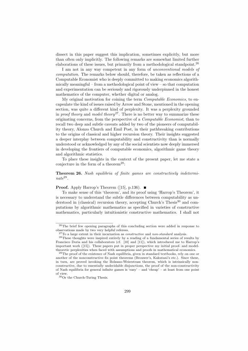
dissect in this paper suggest this implication, sometimes explicitly, but morethan often only implicitly. The following remarks are somewhat limited furtherelaborations of these issues, but primarily from a methodological standpoint.26

I am not in any way competent in any form of unconventional models ofcomputation. The remarks below should, therefore, be taken as reflections of aComputable Economist who is deeply committed to making economics algorith-mically meaningful – from a methodological point of view – so that computationand experimentation can be seriously and rigorously underpinned in the honestmathematics of the computer, whether digital or analog.

My original motivation for coining the term Computable Economics, to en-capsulate the kind of issues raised by Arrow and Stone, mentioned in the openingsection, was quite a different kind of perplexity. It was a perplexity groundedin proof theory and model theory27. There is no better way to summarize theseoriginating concerns, from the perspective of a Computable Economist, than torecall two deep and subtle caveats added by two of the pioneers of computabil-ity theory, Alonzo Church and Emil Post, in their pathbreaking contributionsto the origins of classical and higher recursion theory. Their insights suggesteda deeper interplay between computability and constructivity than is normallyunderstood or acknowledged by any of the social scientists now deeply immersedin developing the frontiers of computable economics, algorithmic game theoryand algorithmic statistics.

To place these insights in the context of the present paper, let me state aconjecture in the form of a theorem28:

Theorem 26. Nash equilibria of finite games are constructively indetermi-nate29.

Proof. Apply Harrop’s Theorem ([15], p.136).To make sense of this ‘theorem’, and its proof using ‘Harrop’s Theorem’, it

is necessary to understand the subtle differences between computability as un-derstood in (classical) recursion theory, accepting Church’s Thesis30 and com-putations by algorithmic mathematics as specified in varieties of constructivemathematics, particularly intuitionistic constructive mathematics. I shall not

26The brief few opening paragraphs of this concluding section were added in response toobservations made by two very helpful referees.

27To a large extent in their incarnation as constructive and non-standard analysis.28These thoughts were inspired entirely by a reading of a fundamental series of results by

Francisco Doria and his collaborators (cf. [10] and [11]), which introduced me to Harrop’simportant work ([15]). These papers put in proper perspective my initial proof- and model-theoretic perplexities when faced with assumptions and proofs in mathematical economics.

29The proof of the existence of Nash equilibria, given in standard textbooks, rely on one oranother of the nonconstructive fix point theorems (Brouwer’s, Kakutani’s etc.). Since these,in turn, are proved invoking the Bolzano-Weierstrass theorem, which is intrinsically non-constructive, due to essentially undecidable disjunctions, the proof of the non-constructivityof Nash equilibria for general infinite games is ‘easy’ – and ‘cheap’ – at least from one pointof view.

30Or the Church-Turing Thesis.

299

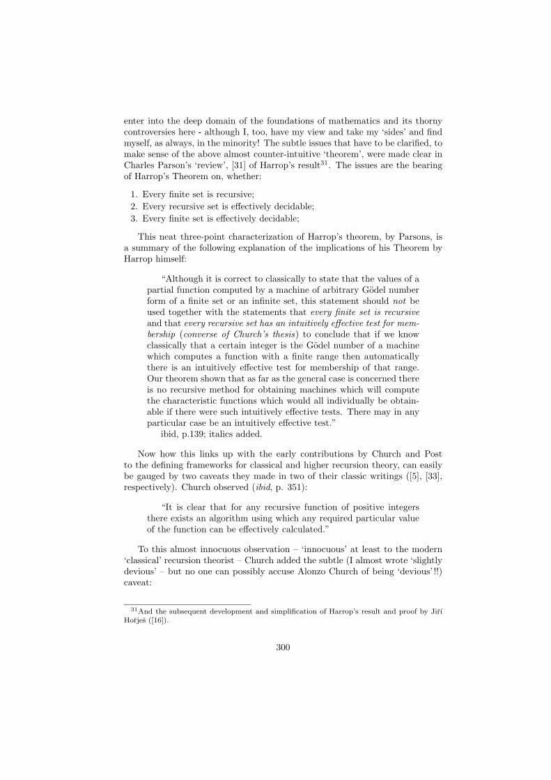
enter into the deep domain of the foundations of mathematics and its thornycontroversies here - although I, too, have my view and take my ‘sides’ and findmyself, as always, in the minority! The subtle issues that have to be clarified, tomake sense of the above almost counter-intuitive ‘theorem’, were made clear inCharles Parson’s ‘review’, [31] of Harrop’s result31. The issues are the bearingof Harrop’s Theorem on, whether:

1. Every finite set is recursive;2. Every recursive set is effectively decidable;3. Every finite set is effectively decidable;

This neat three-point characterization of Harrop’s theorem, by Parsons, isa summary of the following explanation of the implications of his Theorem byHarrop himself:

“Although it is correct to classically to state that the values of apartial function computed by a machine of arbitrary Godel numberform of a finite set or an infinite set, this statement should not beused together with the statements that every finite set is recursiveand that every recursive set has an intuitively effective test for mem-bership (converse of Church’s thesis) to conclude that if we knowclassically that a certain integer is the Godel number of a machinewhich computes a function with a finite range then automaticallythere is an intuitively effective test for membership of that range.Our theorem shown that as far as the general case is concerned thereis no recursive method for obtaining machines which will computethe characteristic functions which would all individually be obtain-able if there were such intuitively effective tests. There may in anyparticular case be an intuitively effective test.”

ibid, p.139; italics added.

Now how this links up with the early contributions by Church and Postto the defining frameworks for classical and higher recursion theory, can easilybe gauged by two caveats they made in two of their classic writings ([5], [33],respectively). Church observed (ibid, p. 351):

“It is clear that for any recursive function of positive integersthere exists an algorithm using which any required particular valueof the function can be effectively calculated.”

To this almost innocuous observation – ‘innocuous’ at least to the modern‘classical’ recursion theorist – Church added the subtle (I almost wrote ‘slightlydevious’ – but no one can possibly accuse Alonzo Church of being ‘devious’ !!)caveat:

31And the subsequent development and simplification of Harrop’s result and proof by JirıHorjes ([16]).

300

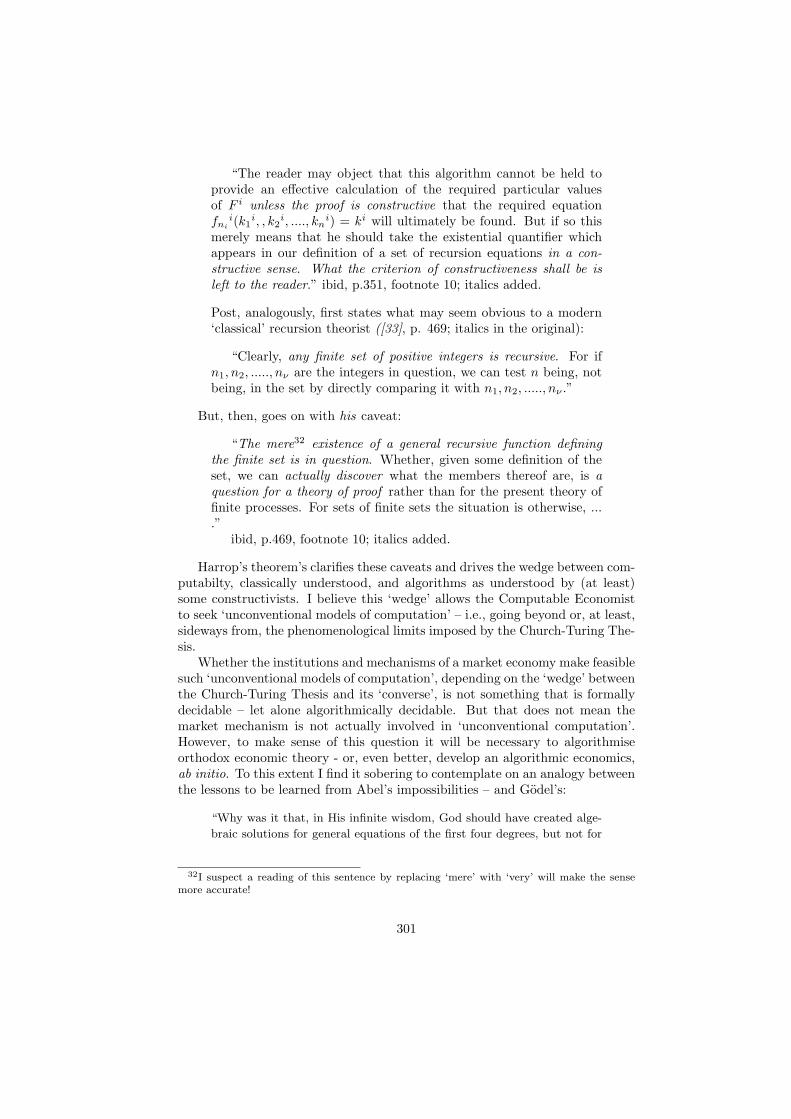
“The reader may object that this algorithm cannot be held toprovide an effective calculation of the required particular valuesof F i unless the proof is constructive that the required equationfni

i(k1i, , k2

i, ...., kni) = ki will ultimately be found. But if so this

merely means that he should take the existential quantifier whichappears in our definition of a set of recursion equations in a con-structive sense. What the criterion of constructiveness shall be isleft to the reader.” ibid, p.351, footnote 10; italics added.

Post, analogously, first states what may seem obvious to a modern‘classical’ recursion theorist ([33], p. 469; italics in the original):

“Clearly, any finite set of positive integers is recursive. For ifn1, n2, ....., nν are the integers in question, we can test n being, notbeing, in the set by directly comparing it with n1, n2, ....., nν .”

But, then, goes on with his caveat:

“The mere32 existence of a general recursive function definingthe finite set is in question. Whether, given some definition of theset, we can actually discover what the members thereof are, is aquestion for a theory of proof rather than for the present theory offinite processes. For sets of finite sets the situation is otherwise, ....”

ibid, p.469, footnote 10; italics added.

Harrop’s theorem’s clarifies these caveats and drives the wedge between com-putabilty, classically understood, and algorithms as understood by (at least)some constructivists. I believe this ‘wedge’ allows the Computable Economistto seek ‘unconventional models of computation’ – i.e., going beyond or, at least,sideways from, the phenomenological limits imposed by the Church-Turing The-sis.

Whether the institutions and mechanisms of a market economy make feasiblesuch ‘unconventional models of computation’, depending on the ‘wedge’ betweenthe Church-Turing Thesis and its ‘converse’, is not something that is formallydecidable – let alone algorithmically decidable. But that does not mean themarket mechanism is not actually involved in ‘unconventional computation’.However, to make sense of this question it will be necessary to algorithmiseorthodox economic theory - or, even better, develop an algorithmic economics,ab initio. To this extent I find it sobering to contemplate on an analogy betweenthe lessons to be learned from Abel’s impossibilities – and Godel’s:

“Why was it that, in His infinite wisdom, God should have created alge-

braic solutions for general equations of the first four degrees, but not for

32I suspect a reading of this sentence by replacing ‘mere’ with ‘very’ will make the sensemore accurate!

301

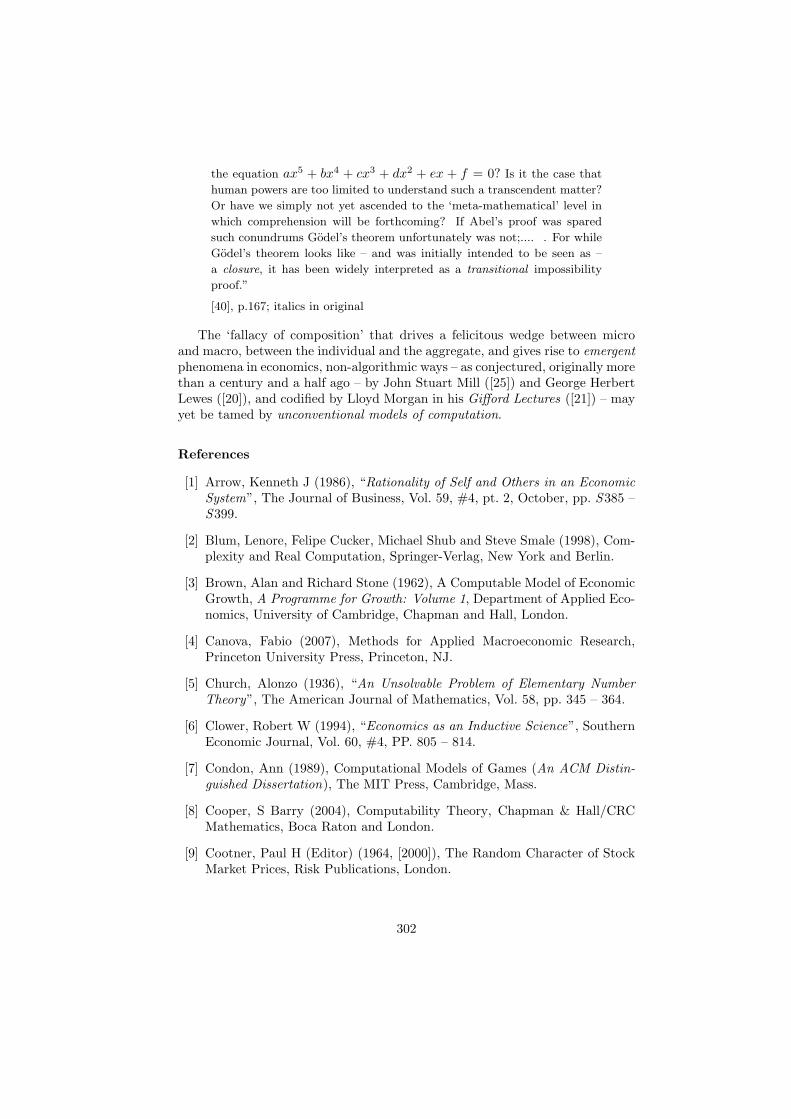
the equation ax5 + bx4 + cx3 + dx2 + ex + f = 0? Is it the case that

human powers are too limited to understand such a transcendent matter?

Or have we simply not yet ascended to the ‘meta-mathematical’ level in

which comprehension will be forthcoming? If Abel’s proof was spared

such conundrums Godel’s theorem unfortunately was not;.... . For while

Godel’s theorem looks like – and was initially intended to be seen as –

a closure, it has been widely interpreted as a transitional impossibility

proof.”

[40], p.167; italics in original

The ‘fallacy of composition’ that drives a felicitous wedge between microand macro, between the individual and the aggregate, and gives rise to emergentphenomena in economics, non-algorithmic ways – as conjectured, originally morethan a century and a half ago – by John Stuart Mill ([25]) and George HerbertLewes ([20]), and codified by Lloyd Morgan in his Gifford Lectures ([21]) – mayyet be tamed by unconventional models of computation.

References

[1] Arrow, Kenneth J (1986), “Rationality of Self and Others in an EconomicSystem”, The Journal of Business, Vol. 59, #4, pt. 2, October, pp. S385 –S399.

[2] Blum, Lenore, Felipe Cucker, Michael Shub and Steve Smale (1998), Com-plexity and Real Computation, Springer-Verlag, New York and Berlin.

[3] Brown, Alan and Richard Stone (1962), A Computable Model of EconomicGrowth, A Programme for Growth: Volume 1, Department of Applied Eco-nomics, University of Cambridge, Chapman and Hall, London.

[4] Canova, Fabio (2007), Methods for Applied Macroeconomic Research,Princeton University Press, Princeton, NJ.

[5] Church, Alonzo (1936), “An Unsolvable Problem of Elementary NumberTheory”, The American Journal of Mathematics, Vol. 58, pp. 345 – 364.

[6] Clower, Robert W (1994), “Economics as an Inductive Science”, SouthernEconomic Journal, Vol. 60, #4, PP. 805 – 814.

[7] Condon, Ann (1989), Computational Models of Games (An ACM Distin-guished Dissertation), The MIT Press, Cambridge, Mass.

[8] Cooper, S Barry (2004), Computability Theory, Chapman & Hall/CRCMathematics, Boca Raton and London.

[9] Cootner, Paul H (Editor) (1964, [2000]), The Random Character of StockMarket Prices, Risk Publications, London.

302

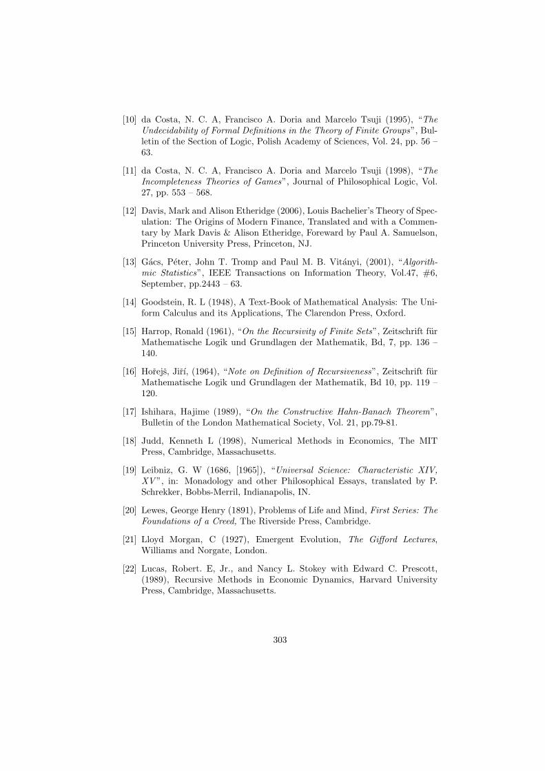
[10] da Costa, N. C. A, Francisco A. Doria and Marcelo Tsuji (1995), “TheUndecidability of Formal Definitions in the Theory of Finite Groups”, Bul-letin of the Section of Logic, Polish Academy of Sciences, Vol. 24, pp. 56 –63.

[11] da Costa, N. C. A, Francisco A. Doria and Marcelo Tsuji (1998), “TheIncompleteness Theories of Games”, Journal of Philosophical Logic, Vol.27, pp. 553 – 568.

[12] Davis, Mark and Alison Etheridge (2006), Louis Bachelier’s Theory of Spec-ulation: The Origins of Modern Finance, Translated and with a Commen-tary by Mark Davis & Alison Etheridge, Foreward by Paul A. Samuelson,Princeton University Press, Princeton, NJ.

[13] Gacs, Peter, John T. Tromp and Paul M. B. Vitanyi, (2001), “Algorith-mic Statistics”, IEEE Transactions on Information Theory, Vol.47, #6,September, pp.2443 – 63.

[14] Goodstein, R. L (1948), A Text-Book of Mathematical Analysis: The Uni-form Calculus and its Applications, The Clarendon Press, Oxford.

[15] Harrop, Ronald (1961), “On the Recursivity of Finite Sets”, Zeitschrift furMathematische Logik und Grundlagen der Mathematik, Bd, 7, pp. 136 –140.

[16] Horejs, Jirı, (1964), “Note on Definition of Recursiveness”, Zeitschrift furMathematische Logik und Grundlagen der Mathematik, Bd 10, pp. 119 –120.

[17] Ishihara, Hajime (1989), “On the Constructive Hahn-Banach Theorem”,Bulletin of the London Mathematical Society, Vol. 21, pp.79-81.

[18] Judd, Kenneth L (1998), Numerical Methods in Economics, The MITPress, Cambridge, Massachusetts.

[19] Leibniz, G. W (1686, [1965]), “Universal Science: Characteristic XIV,XV ”, in: Monadology and other Philosophical Essays, translated by P.Schrekker, Bobbs-Merril, Indianapolis, IN.

[20] Lewes, George Henry (1891), Problems of Life and Mind, First Series: TheFoundations of a Creed, The Riverside Press, Cambridge.

[21] Lloyd Morgan, C (1927), Emergent Evolution, The Gifford Lectures,Williams and Norgate, London.

[22] Lucas, Robert. E, Jr., and Nancy L. Stokey with Edward C. Prescott,(1989), Recursive Methods in Economic Dynamics, Harvard UniversityPress, Cambridge, Massachusetts.

303

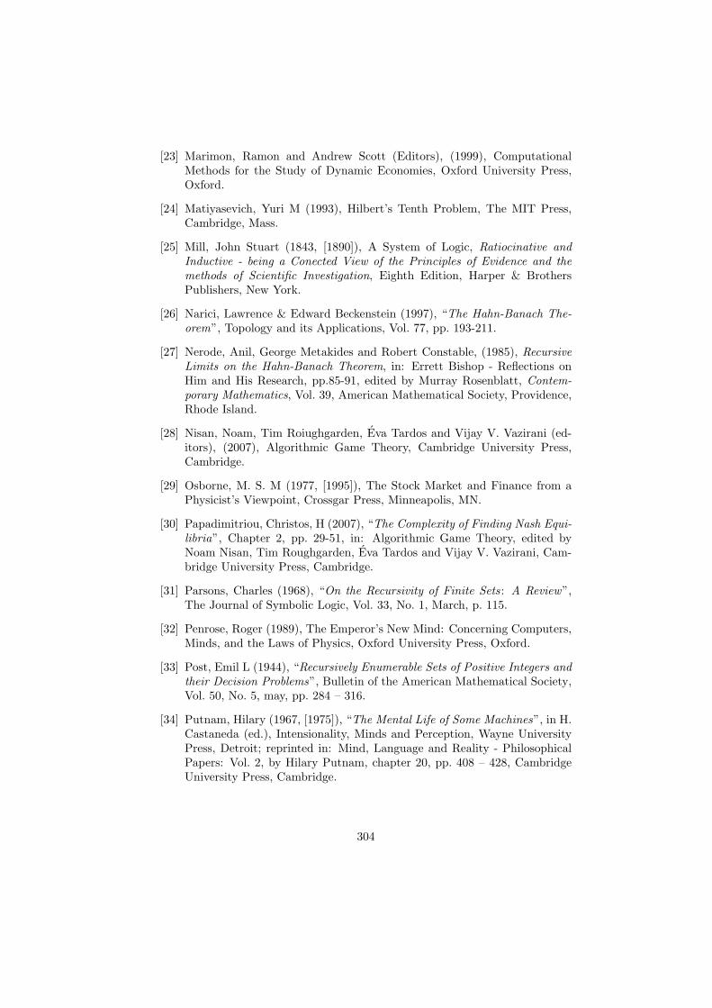
[23] Marimon, Ramon and Andrew Scott (Editors), (1999), ComputationalMethods for the Study of Dynamic Economies, Oxford University Press,Oxford.

[24] Matiyasevich, Yuri M (1993), Hilbert’s Tenth Problem, The MIT Press,Cambridge, Mass.

[25] Mill, John Stuart (1843, [1890]), A System of Logic, Ratiocinative andInductive - being a Conected View of the Principles of Evidence and themethods of Scientific Investigation, Eighth Edition, Harper & BrothersPublishers, New York.

[26] Narici, Lawrence & Edward Beckenstein (1997), “The Hahn-Banach The-orem”, Topology and its Applications, Vol. 77, pp. 193-211.

[27] Nerode, Anil, George Metakides and Robert Constable, (1985), RecursiveLimits on the Hahn-Banach Theorem, in: Errett Bishop - Reflections onHim and His Research, pp.85-91, edited by Murray Rosenblatt, Contem-porary Mathematics, Vol. 39, American Mathematical Society, Providence,Rhode Island.

[28] Nisan, Noam, Tim Roiughgarden, Eva Tardos and Vijay V. Vazirani (ed-itors), (2007), Algorithmic Game Theory, Cambridge University Press,Cambridge.

[29] Osborne, M. S. M (1977, [1995]), The Stock Market and Finance from aPhysicist’s Viewpoint, Crossgar Press, Minneapolis, MN.

[30] Papadimitriou, Christos, H (2007), “The Complexity of Finding Nash Equi-libria”, Chapter 2, pp. 29-51, in: Algorithmic Game Theory, edited byNoam Nisan, Tim Roughgarden, Eva Tardos and Vijay V. Vazirani, Cam-bridge University Press, Cambridge.

[31] Parsons, Charles (1968), “On the Recursivity of Finite Sets: A Review”,The Journal of Symbolic Logic, Vol. 33, No. 1, March, p. 115.

[32] Penrose, Roger (1989), The Emperor’s New Mind: Concerning Computers,Minds, and the Laws of Physics, Oxford University Press, Oxford.

[33] Post, Emil L (1944), “Recursively Enumerable Sets of Positive Integers andtheir Decision Problems”, Bulletin of the American Mathematical Society,Vol. 50, No. 5, may, pp. 284 – 316.

[34] Putnam, Hilary (1967, [1975]), “The Mental Life of Some Machines”, in H.Castaneda (ed.), Intensionality, Minds and Perception, Wayne UniversityPress, Detroit; reprinted in: Mind, Language and Reality - PhilosophicalPapers: Vol. 2, by Hilary Putnam, chapter 20, pp. 408 – 428, CambridgeUniversity Press, Cambridge.

304

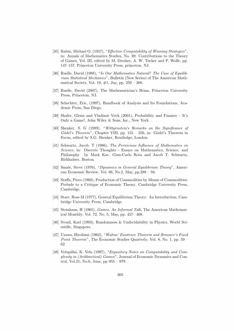
[35] Rabin, Michael O, (1957), “Effective Computability of Winning Strategies”,in: Annals of Mathematics Studies, No. 39: Contributions to the Theoryof Games, Vol. III, edited by M. Dresher, A. W. Tucker and P. Wolfe, pp.147–157, Princeton University Press, princeton, NJ.

[36] Ruelle, David (1988), “Is Our Mathematics Natural? The Case of Equilib-rium Statistical Mechanics”, Bulletin (New Series) of The American Math-emtical Society, Vol. 19, #1, Juy, pp. 259 – 268.

[37] Ruelle, David (2007), The Mathematician’s Brian, Princeton UniversityPress, Princeton, NJ.

[38] Schechter, Eric, (1997), Handbook of Analysis and Its Foundations, Aca-demic Press, San Diego.

[39] Shafer, Glenn and Vladimir Vovk (2001), Probability and Finance – It’sOnly a Game!, John Wiley & Sons, Inc., New York.

[40] Shenker, S. G (1989), “Wittgenstein’s Remarks on the Significance ofGodel’s Theorem”, Chapter VIII, pp. 155 – 256, in: Godel’s Theorem inFocus, edited by S.G. Shenker, Routledge, London.

[41] Schwartz, Jacob. T (1986), The Pernicious Influence of Mathematics onScience, in: Discrete Thoughts - Essays on Mathematics, Science, andPhilosophy by Mark Kac, Gian-Carlo Rota and Jacob T. Schwartz,Birkhauser, Boston.

[42] Smale, Steve (1976), “Dynamics in General Equilibrium Theory”, Ameri-can Economic Review, Vol. 66, No.2, May, pp.288 – 94.

[43] Sraffa, Piero (1960), Production of Commodities by Means of Commodities:Prelude to a Critique of Economic Theory, Cambridge University Press,Cambridge.

[44] Starr, Ross M (1977), General Equilibrium Theory: An Introduction, Cam-bridge University Press, Cambridge.

[45] Steinhaus, H (1965), Games, An Informal Talk, The American Mathemat-ical Monthly, Vol. 72, No. 5, May, pp. 457– 468.

[46] Svozil, Karl (1993), Randomness & Undecidability in Physics, World Sci-entific, Singapore.

[47] Uzawa, Hirofumi (1962), “Walras’ Existence Theorem and Brouwer’s FixedPoint Theorem”, The Economic Studies Quarterly, Vol. 8, No. 1, pp. 59 –62.

[48] Velupillai, K. Vela (1997), “Expository Notes on Computability and Com-plexity in (Arithmetical) Games”, Journal of Economic Dynamics and Con-trol, Vol.21, No.6, June, pp 955 – 979.

305

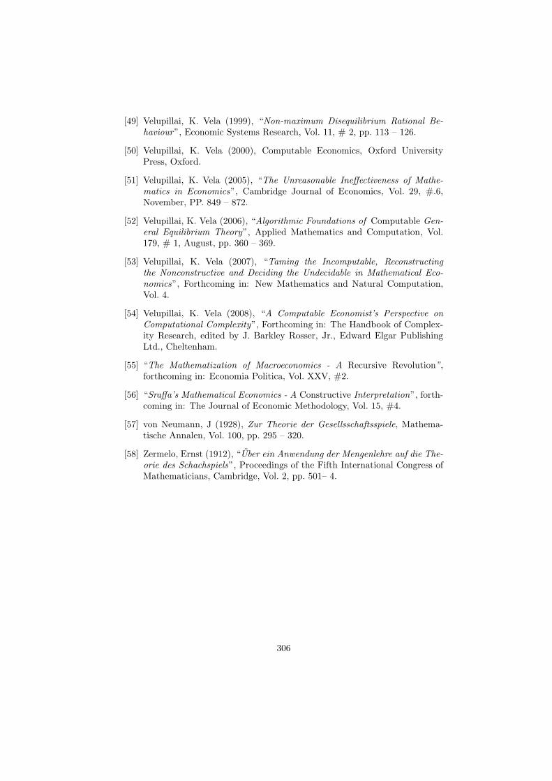
[49] Velupillai, K. Vela (1999), “Non-maximum Disequilibrium Rational Be-haviour”, Economic Systems Research, Vol. 11, # 2, pp. 113 – 126.

[50] Velupillai, K. Vela (2000), Computable Economics, Oxford UniversityPress, Oxford.

[51] Velupillai, K. Vela (2005), “The Unreasonable Ineffectiveness of Mathe-matics in Economics”, Cambridge Journal of Economics, Vol. 29, #.6,November, PP. 849 – 872.

[52] Velupillai, K. Vela (2006), “Algorithmic Foundations of Computable Gen-eral Equilibrium Theory”, Applied Mathematics and Computation, Vol.179, # 1, August, pp. 360 – 369.

[53] Velupillai, K. Vela (2007), “Taming the Incomputable, Reconstructingthe Nonconstructive and Deciding the Undecidable in Mathematical Eco-nomics”, Forthcoming in: New Mathematics and Natural Computation,Vol. 4.

[54] Velupillai, K. Vela (2008), “A Computable Economist’s Perspective onComputational Complexity”, Forthcoming in: The Handbook of Complex-ity Research, edited by J. Barkley Rosser, Jr., Edward Elgar PublishingLtd., Cheltenham.

[55] “The Mathematization of Macroeconomics - A Recursive Revolution”,forthcoming in: Economia Politica, Vol. XXV, #2.

[56] “Sraffa’s Mathematical Economics - A Constructive Interpretation”, forth-coming in: The Journal of Economic Methodology, Vol. 15, #4.

[57] von Neumann, J (1928), Zur Theorie der Gesellsschaftsspiele, Mathema-tische Annalen, Vol. 100, pp. 295 – 320.

[58] Zermelo, Ernst (1912), “Uber ein Anwendung der Mengenlehre auf die The-orie des Schachspiels”, Proceedings of the Fifth International Congress ofMathematicians, Cambridge, Vol. 2, pp. 501– 4.

306

Optical computing

Damien Woods a

aDepartment of Computer Science and Artificial IntelligenceUniversity of Seville, Spain

Thomas J. Naughton b,c

bDepartment of Computer ScienceNational University of Ireland, Maynooth, County Kildare, Ireland

cUniversity of Oulu, RFMedia Laboratory, Oulu Southern Institute, Vierimaantie 5, 84100 Ylivieska,Finland

Abstract

We consider optical computers that encode data using images and compute by transforming suchimages. We give an overview of a number of such optical computing architectures, includingdescriptions of the type of hardware commonly used in optical computing, as well as someof the computational efficiencies of optical devices. We go on to discuss optical computingfrom the point of view of computational complexity theory, with the aim of putting some old,and some very recent, results in context. Finally, we focus on a particular optical model ofcomputation called the continuous space machine. We describe some results for this modelincluding characterisations in terms of well-known complexity classes.

Key words:PACS:

1. Introduction

In this survey we consider optical computers that encode data using images and com-pute by transforming such images. We try to bring together, and thus give context to, alarge range of architectures and algorithms that come under the term optical computing.

DW acknowledges support from Junta de Andalucıa grant TIC-581. TN acknowledges support fromthe European Commission Framework Programme 6 through a Marie Curie Intra-European Fellowship.

Email addresses: [email protected] (Damien Woods), [email protected] (Thomas J. Naughton).URLs: http://www.cs.ucc.ie/∼dw5 (Damien Woods), http://www.cs.nuim.ie/∼tnaughton/

(Thomas J. Naughton).

Preprint submitted to Elsevier 10 July 2008

In Section 2 we begin by stating what we mean by the term optical computing, and wediscuss some common optical computing architectures. Unlike a number of other areas ofnature inspired computing, optical computers have existed (mostly in laboratories) formany years, and so in Section 3 we describe hardware components that are found in manyoptical computing systems. In Section 4 we describe some of the physical principles thatunderlie the parallel abilities and efficiencies found in optical computing. These includehigh fan-in, high interconnection densities, and low energy consumption.

In order to understand the abilities of optics as a computing medium we would arguethat computational complexity theory is an indispensable tool. So in Section 5 we collecta number of existing algorithmic results for optical computers. In particular we focuson algorithms and models for matrix-vector multipliers, and some other architectures.We also offer suggestions for future work directions for optical algorithm designers. InSection 6, we take a detailed look at a particular model of optical computing (the contin-uous space machine, or CSM) that encompasses most of the functionality that coherentoptical information processing has to offer. We begin by defining the CSM and a total ofseven complexity measures that are inspired by real-world (optical) resources. We go onto discuss how the CSM’s operations could be carried out physically. Section 7 containssome example datastructures and algorithms for the CSM. In Section 8 we motivate andintroduce an important restriction of the model called the C2-CSM, and in Section 9we briefly describe a number of C2-CSM computational complexity results, and theirimplications.

2. Brief overview of optical computing architectures

Traditionally, in optical information processing a distinction was made between sig-nal/image processing through optics and numerical processing through optics, with onlythe latter (and often only the digital version of the latter) being called optical comput-ing [57,48,29,101]. However, it was always difficult to clearly delineate between the two,since it was largely a question of the interpretation the programmer attached to theoutput optical signals. The most important argument for referring to the latter only asoptical computing had to do with the fact that the perceived limits (or at least, ambi-tions) of the former was simply for special-purpose signal/image processing devices whilethe ambitions for the latter was general-purpose computation. Given recent results onthe computational power of optical image processing architectures [63,98,93], it is notthe case that such architectures are limited to special-purpose tasks.

Furthermore, as the field become increasingly multidisciplinary, and in particular ascomputer scientists play a more prominent role, it is necessary to bring the definitionof optical computing in line with the broad definition of computing. In particular, thisfacilitates analysis from the theoretical computer science point of view. The distinctionbetween analog optical computing and digital optical computing is similarly blurred giventhe prevalence of digital multiplication schemes effected through analog convolution [48].Our broad interpretation of the term optical computing has been espoused before [19].

308

2.1. Optical pattern recognition

Arguably, optical computing began with the design and implementation of opticalsystems to arbitrarily modify the complex valued spatial frequencies of an image. Thisconcept, spatial filtering [67,86,89], is at the root of optics’ ability to perform efficientconvolution and correlation operations. In a basic pattern recognition application, spatialfiltering is called matched filtering, where a filter is chosen that matches (i.e. conjugates)the spectrum of the sought object. Employing this operation for advanced pattern recog-nition [12,18,43,47], effort focused on achieving systems invariant to scaling, rotation,out-of-plane rotation, deformation, and signal dependent noise, while retaining the exist-ing invariance to translating, adding noise to, and obscuring parts of the input. Effort alsowent into injecting nonlinearities into these inherently linear systems to achieve widerfunctionality [46]. Improvements were made to the fundamental limitations of the basicmatched filter design, most notably the joint transform correlator architecture [92].

Optical correlators that use incoherent sources of illumination (both spatially and tem-porally) rather than lasers are also possible [11,71]. The simplest incoherent correlatorwould have the same basic spatial filtering architecture as that used for matched fil-tering. While coherent systems in principle are more capable than incoherent systems(principally because the former naturally represents complex functions while the latternaturally represents real functions), incoherent systems require less precise positioningwhen it comes to system construction and are less susceptible to noise.

Trade-offs between space and time were proposed and demonstrated. These includedtime integrating correlators [90] (architecturally simpler linear time variants of the con-stant time space integrating matched filter mentioned already) and systolic architec-tures [21]. In addition to pattern recognition, a common application for these classes ofarchitectures was numerical calculation.

2.2. Analog optical numerical computation

An important strand of image-based optical computation involved numerical calcula-tions: analog computation as well as multi-level discrete computation. Matrix-vector andmatrix-matrix multiplication systems were proposed and demonstrated [42,57,90,48,4,29,51].The capability to expand a beam of light and to focus many beams of light to a commonpoint directly corresponded to high fan-out and fan-in capabilities, respectively. The limi-tations of encoding a number simply as an intensity value (finite dynamic range and finiteintensity resolution in the modulators and detectors) could be overcome by representingthe numbers in some base. Significant effort went into dealing with carry operations sothat in additions, subtractions, and multiplications each digit could be processed in par-allel. Algorithms based on convolution to multiply numbers in this representation weredemonstrated [48], with a single post-processing step to combine the sub-calculationsand deal with the carry operations.

An application that benefited greatly from the tightly-coupled parallelism afforded byoptics was the solving of sets of simultaneous equations and matrix inversion [17,1]. Anapplication that, further, was tolerant to the inherent inaccuracies and noise of analogoptics was optical neural networks [28,20] including online neural learning in the presenceof noise [62].

309

2.3. Digital optical computing

The next major advances came in the form of optical equivalents of digital comput-ers [44]. The flexibility of digital systems over analog systems in general was a majorfactor behind the interest in this form of optical computation [78]. Specific drawbacks ofthe analog computing paradigm in optics that this new paradigm addressed included noperceived ability to perform general purpose computation, accumulation of noise fromone computation step to another, and systematic errors introduced by imperfect analogcomponents. The aim was to design digital optical computers that followed the sameprinciples as conventional electronic processors but which could perform many binaryoperations in parallel. These systems were designed from logic gates using nonlinear op-tical elements: semitransparent materials whose transmitted intensity has a nonlineardependence on the input intensity.

Digital optical computing was also proposed as an application of architectures designedoriginally for image-based processing, for example logic effected through symbolic substi-tution [10]. At the confluence of computing and communication, optical techniques wereproposed for the routing of signals in long-haul networks [29,101].

3. Optical computing hardware

The three most basic hardware components of an optical information processing systemare a source, a modulator, and a detector. A source generates the light, a modulatormultiplies the light by a (usually, spatially varying) function, and a detector senses theresulting light. These and others are introduced in this section.

3.1. Sources

Lasers are a common source of illumination because at some levels they are math-ematically simpler to understand, but incoherent sources such as light-emitting diodesare also used frequently for increased tolerance to noise and when nonnegative functionsare sufficient for the computation. Usually, the source is monochromatic to avoid theproblem of colour dispersion as the light passes through refracting optical components,unless this dispersion is itself the basis for the computation.

3.2. Spatial light modulators (SLMs)

It is possible to encode a spatial function (a 2D image) in an optical wavefront. A pageof text when illuminated with sunlight, for example, does this job perfectly. This wouldbe called an amplitude-modulating reflective SLM. Modulation is a multiplicative effect,so an image encoded in the incoming wavefront will be pointwise multiplied by the imageon the SLM. Modulators can also act on phase and polarisation, and can be transmissiverather than reflective. They include photographic film, and electro-optic, magneto-optic,and acousto-optic devices [57,4,48,29,35]. One class of note are the optically-addressedSLMs, in which, typically, a 2D light pattern falling on a photosensitive layer on one sideof the SLM spatially varies (with an identical pattern) the reflective properties of the

310

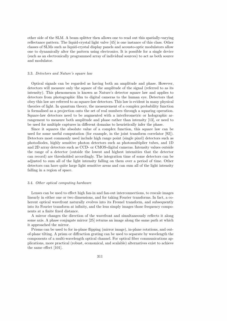
other side of the SLM. A beam splitter then allows one to read out this spatially-varyingreflectance pattern. The liquid-crystal light valve [45] is one instance of this class. Otherclasses of SLMs such as liquid-crystal display panels and acousto-optic modulators allowone to dynamically alter the pattern using electronics. It is possible for a single device(such as an electronically programmed array of individual sources) to act as both sourceand modulator.

3.3. Detectors and Nature’s square law

Optical signals can be regarded as having both an amplitude and phase. However,detectors will measure only the square of the amplitude of the signal (referred to as itsintensity). This phenomenon is known as Nature’s detector square law and applies todetectors from photographic film to digital cameras to the human eye. Detectors thatobey this law are referred to as square-law detectors. This law is evident in many physicaltheories of light. In quantum theory, the measurement of a complex probability functionis formalised as a projection onto the set of real numbers through a squaring operation.Square-law detectors need to be augmented with a interferometric or holographic ar-rangement to measure both amplitude and phase rather than intensity [13], or need tobe used for multiple captures in different domains to heuristically infer the phase.

Since it squares the absolute value of a complex function, this square law can beused for some useful computation (for example, in the joint transform correlator [92]).Detectors most commonly used include high range point (single pixel) detectors such asphotodiodes, highly sensitive photon detectors such as photomultiplier tubes, and 1Dand 2D array detectors such as CCD- or CMOS-digital cameras. Intensity values outsidethe range of a detector (outside the lowest and highest intensities that the detectorcan record) are thresholded accordingly. The integration time of some detectors can beadjusted to sum all of the light intensity falling on them over a period of time. Otherdetectors can have quite large light sensitive areas and can sum all of the light intensityfalling in a region of space.

3.4. Other optical computing hardware

Lenses can be used to effect high fan-in and fan-out interconnections, to rescale imageslinearly in either one or two dimensions, and for taking Fourier transforms. In fact, a co-herent optical wavefront naturally evolves into its Fresnel transform, and subsequentlyinto its Fourier transform at infinity, and the lens simply images those frequency compo-nents at a finite fixed distance.

A mirror changes the direction of the wavefront and simultaneously reflects it alongsome axis. A phase conjugate mirror [25] returns an image along the same path at whichit approached the mirror.

Prisms can be used to for in-plane flipping (mirror image), in-plane rotations, and out-of-plane tilting. A prism or diffraction grating can be used to separate by wavelength thecomponents of a multi-wavelength optical channel. For optical fiber communications ap-plications, more practical (robust, economical, and scalable) alternatives exist to achievethe same effect [101].

311

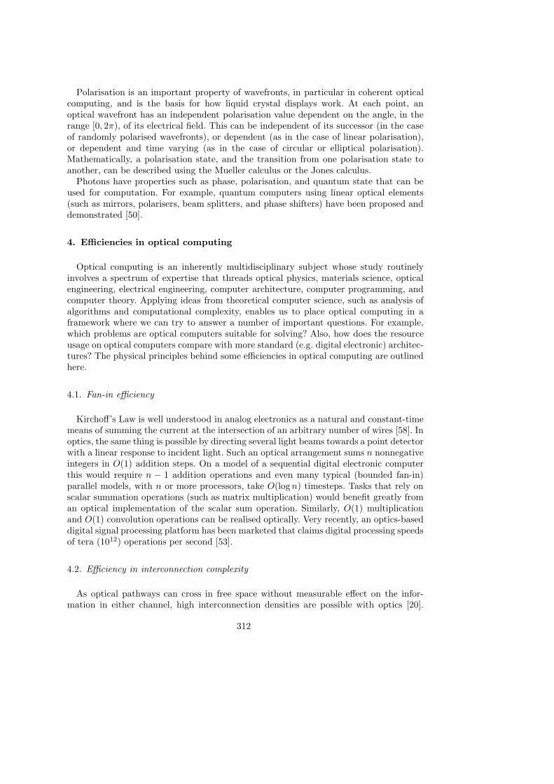
Polarisation is an important property of wavefronts, in particular in coherent opticalcomputing, and is the basis for how liquid crystal displays work. At each point, anoptical wavefront has an independent polarisation value dependent on the angle, in therange [0, 2π), of its electrical field. This can be independent of its successor (in the caseof randomly polarised wavefronts), or dependent (as in the case of linear polarisation),or dependent and time varying (as in the case of circular or elliptical polarisation).Mathematically, a polarisation state, and the transition from one polarisation state toanother, can be described using the Mueller calculus or the Jones calculus.

Photons have properties such as phase, polarisation, and quantum state that can beused for computation. For example, quantum computers using linear optical elements(such as mirrors, polarisers, beam splitters, and phase shifters) have been proposed anddemonstrated [50].

4. Efficiencies in optical computing

Optical computing is an inherently multidisciplinary subject whose study routinelyinvolves a spectrum of expertise that threads optical physics, materials science, opticalengineering, electrical engineering, computer architecture, computer programming, andcomputer theory. Applying ideas from theoretical computer science, such as analysis ofalgorithms and computational complexity, enables us to place optical computing in aframework where we can try to answer a number of important questions. For example,which problems are optical computers suitable for solving? Also, how does the resourceusage on optical computers compare with more standard (e.g. digital electronic) architec-tures? The physical principles behind some efficiencies in optical computing are outlinedhere.

4.1. Fan-in efficiency

Kirchoff’s Law is well understood in analog electronics as a natural and constant-timemeans of summing the current at the intersection of an arbitrary number of wires [58]. Inoptics, the same thing is possible by directing several light beams towards a point detectorwith a linear response to incident light. Such an optical arrangement sums n nonnegativeintegers in O(1) addition steps. On a model of a sequential digital electronic computerthis would require n − 1 addition operations and even many typical (bounded fan-in)parallel models, with n or more processors, take O(log n) timesteps. Tasks that rely onscalar summation operations (such as matrix multiplication) would benefit greatly froman optical implementation of the scalar sum operation. Similarly, O(1) multiplicationand O(1) convolution operations can be realised optically. Very recently, an optics-baseddigital signal processing platform has been marketed that claims digital processing speedsof tera (1012) operations per second [53].

4.2. Efficiency in interconnection complexity

As optical pathways can cross in free space without measurable effect on the infor-mation in either channel, high interconnection densities are possible with optics [20].

312

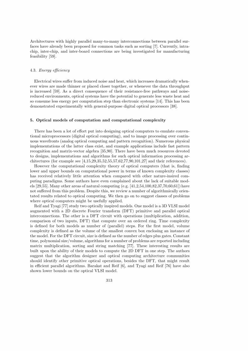
Architectures with highly parallel many-to-many interconnections between parallel sur-faces have already been proposed for common tasks such as sorting [7]. Currently, intra-chip, inter-chip, and inter-board connections are being investigated for manufacturingfeasibility [59].

4.3. Energy efficiency

Electrical wires suffer from induced noise and heat, which increases dramatically when-ever wires are made thinner or placed closer together, or whenever the data throughputis increased [59]. As a direct consequence of their resistance-free pathways and noise-reduced environments, optical systems have the potential to generate less waste heat andso consume less energy per computation step than electronic systems [14]. This has beendemonstrated experimentally with general-purpose digital optical processors [38].

5. Optical models of computation and computational complexity

There has been a lot of effort put into designing optical computers to emulate conven-tional microprocessors (digital optical computing), and to image processing over contin-uous wavefronts (analog optical computing and pattern recognition). Numerous physicalimplementations of the latter class exist, and example applications include fast patternrecognition and matrix-vector algebra [35,90]. There have been much resources devotedto designs, implementations and algorithms for such optical information processing ar-chitectures (for example see [4,15,29,35,52,55,57,62,77,90,101,27] and their references).

However the computational complexity theory of optical computers (that is, findinglower and upper bounds on computational power in terms of known complexity classes)has received relatively little attention when compared with other nature-insired com-puting paradigms. Some authors have even complained about the lack of suitable mod-els [29,55]. Many other areas of natural computing (e.g. [41,2,54,100,82,37,70,60,61]) havenot suffered from this problem. Despite this, we review a number of algorithmically orien-tated results related to optical computing. We then go on to suggest classes of problemswhere optical computers might be usefully applied.

Reif and Tyagi [77] study two optically inspired models. One model is a 3D VLSI modelaugmented with a 2D discrete Fourier transform (DFT) primitive and parallel opticalinterconnections. The other is a DFT circuit with operations (multiplication, addition,comparison of two inputs, DFT) that compute over an ordered ring. Time complexityis defined for both models as number of (parallel) steps. For the first model, volumecomplexity is defined as the volume of the smallest convex box enclosing an instance ofthe model. For the DFT circuit, size is defined as the number of edges plus gates. Constanttime, polynomial size/volume, algorithms for a number of problems are reported includingmatrix multiplication, sorting and string matching [77]. These interesting results arebuilt upon the ability of their models to compute the 2D DFT in one step. The authorssuggest that the algorithm designer and optical computing architecture communitiesshould identify other primitive optical operations, besides the DFT, that might resultin efficient parallel algorithms. Barakat and Reif [6], and Tyagi and Reif [76] have alsoshown lower bounds on the optical VLSI model.

313

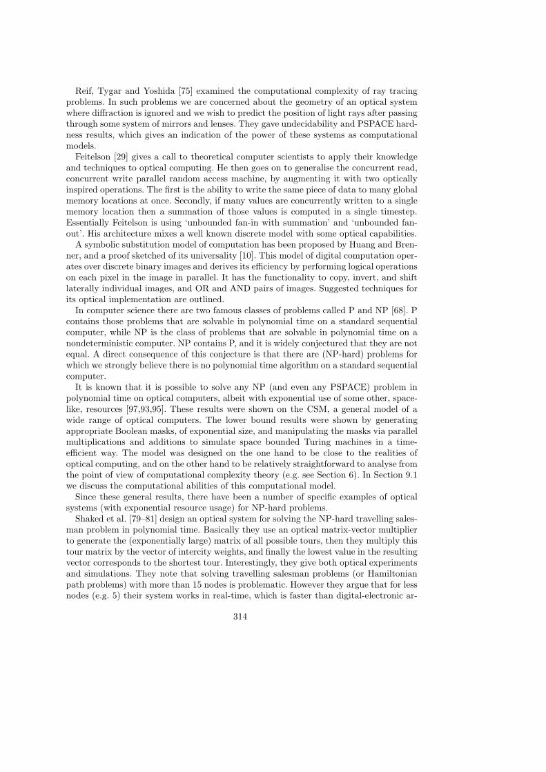
Reif, Tygar and Yoshida [75] examined the computational complexity of ray tracingproblems. In such problems we are concerned about the geometry of an optical systemwhere diffraction is ignored and we wish to predict the position of light rays after passingthrough some system of mirrors and lenses. They gave undecidability and PSPACE hard-ness results, which gives an indication of the power of these systems as computationalmodels.

Feitelson [29] gives a call to theoretical computer scientists to apply their knowledgeand techniques to optical computing. He then goes on to generalise the concurrent read,concurrent write parallel random access machine, by augmenting it with two opticallyinspired operations. The first is the ability to write the same piece of data to many globalmemory locations at once. Secondly, if many values are concurrently written to a singlememory location then a summation of those values is computed in a single timestep.Essentially Feitelson is using ‘unbounded fan-in with summation’ and ‘unbounded fan-out’. His architecture mixes a well known discrete model with some optical capabilities.

A symbolic substitution model of computation has been proposed by Huang and Bren-ner, and a proof sketched of its universality [10]. This model of digital computation oper-ates over discrete binary images and derives its efficiency by performing logical operationson each pixel in the image in parallel. It has the functionality to copy, invert, and shiftlaterally individual images, and OR and AND pairs of images. Suggested techniques forits optical implementation are outlined.

In computer science there are two famous classes of problems called P and NP [68]. Pcontains those problems that are solvable in polynomial time on a standard sequentialcomputer, while NP is the class of problems that are solvable in polynomial time on anondeterministic computer. NP contains P, and it is widely conjectured that they are notequal. A direct consequence of this conjecture is that there are (NP-hard) problems forwhich we strongly believe there is no polynomial time algorithm on a standard sequentialcomputer.

It is known that it is possible to solve any NP (and even any PSPACE) problem inpolynomial time on optical computers, albeit with exponential use of some other, space-like, resources [97,93,95]. These results were shown on the CSM, a general model of awide range of optical computers. The lower bound results were shown by generatingappropriate Boolean masks, of exponential size, and manipulating the masks via parallelmultiplications and additions to simulate space bounded Turing machines in a time-efficient way. The model was designed on the one hand to be close to the realities ofoptical computing, and on the other hand to be relatively straightforward to analyse fromthe point of view of computational complexity theory (e.g. see Section 6). In Section 9.1we discuss the computational abilities of this computational model.

Since these general results, there have been a number of specific examples of opticalsystems (with exponential resource usage) for NP-hard problems.

Shaked et al. [79–81] design an optical system for solving the NP-hard travelling sales-man problem in polynomial time. Basically they use an optical matrix-vector multiplierto generate the (exponentially large) matrix of all possible tours, then they multiply thistour matrix by the vector of intercity weights, and finally the lowest value in the resultingvector corresponds to the shortest tour. Interestingly, they give both optical experimentsand simulations. They note that solving travelling salesman problems (or Hamiltonianpath problems) with more than 15 nodes is problematic. However they argue that for lessnodes (e.g. 5) their system works in real-time, which is faster than digital-electronic ar-

314

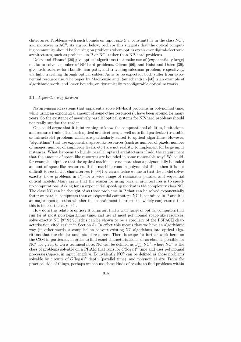
chitectures. Problems with such bounds on input size (i.e. constant) lie in the class NC1,and moreover in AC0. As argued below, perhaps this suggests that the optical comput-ing community should be focusing on problems where optics excels over digital-electronicarchitectures, such as problems in P or NC, rather than NP-hard problems.

Dolev and Fitoussi [26] give optical algorithms that make use of (exponentially large)masks to solve a number of NP-hard problems. Oltean [66], and Haist and Osten [39],give architectures for Hamiltonian path, and travelling salesman problem, respectively,via light travelling through optical cables. As is to be expected, both suffer from expo-nential resource use. The paper by MacKenzie and Ramachandran [56] is an example ofalgorithmic work, and lower bounds, on dynamically reconfigurable optical networks.

5.1. A possible way forward

Nature-inspired systems that apparently solve NP-hard problems in polynomial time,while using an exponential amount of some other resource(s), have been around for manyyears. So the existence of massively parallel optical systems for NP-hard problems shouldnot really suprise the reader.

One could argue that it is interesting to know the computational abilities, limitations,and resource trade-offs of such optical architectures, as well as to find particular (tractableor intractable) problems which are particularly suited to optical algorithms. However,“algorithms” that use exponential space-like resources (such as number of pixels, numberof images, number of amplitude levels, etc.) are not realistic to implement for large inputinstances. What happens to highly parallel optical architectures if add the requirementthat the amount of space-like resources are bounded in some reasonable way? We could,for example, stipulate that the optical machine use no more than a polynomially boundedamount of space-like resources. If the machine runs in polynomial time, then it is notdifficult to see that it characterises P [99] (by characterise we mean that the model solvesexactly those problems in P), for a wide range of reasonable parallel and sequentialoptical models. Many argue that the reason for using parallel architectures is to speed-up computations. Asking for an exponential speed-up motivates the complexity class NC.The class NC can be thought of as those problems in P that can be solved exponentiallyfaster on parallel computers than on sequential computers. NC is contained in P and it isan major open question whether this containment is strict: it is widely conjectured thatthis is indeed the case [36].

How does this relate to optics? It turns out that a wide range of optical computers thatrun for at most polylogarithmic time, and use at most polynomial space-like resources,solve exactly NC [97,93,95] (this can be shown to be a corollary of the PSPACE char-acterisation cited earlier in Section 5). In effect this means that we have an algorithmicway (in other words, a compiler) to convert existing NC algorithms into optical algo-rithms that use similar amounts of resources. There is scope for further work here, onthe CSM in particular, in order to find exact characterisations, or as close as possible forNCk for given k. On a technical note, NC can be defined as ∪∞

k=0NCk, where NCk is theclass of problems solvable on a PRAM that runs for O(log n)k time and uses polynomialprocessors/space, in input length n. Equivalently NCk can be defined as those problemssolvable by circuits of O(log n)k depth (parallel time), and polynomial size. From thepractical side of things, perhaps we can use these kinds of results to find problems within

315

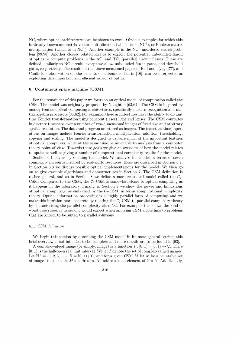
NC, where optical architectures can be shown to excel. Obvious examples for which thisis already known are matrix-vector multiplication (which lies in NC2), or Boolean matrixmultiplication (which is in NC1). Another example is the NC1 unordered search prob-lem [99,98]. Another closely related idea is to exploit the potential unbounded fan-inof optics to compute problems in the AC, and TC, (parallel) circuit classes. These aredefined similarly to NC circuits except we allow unbounded fan-in gates, and thresholdgates, respectively. The results in the above mentioned paper of Reif and Tyagi [77], andCaulfield’s observation on the benefits of unbounded fan-in [16], can be interpreted asexploiting this important and efficient aspect of optics.

6. Continuous space machine (CSM)

For the remainder of this paper we focus on an optical model of computation called theCSM. The model was originally proposed by Naughton [63,64]. The CSM is inspired byanalog Fourier optical computing architectures, specifically pattern recognition and ma-trix algebra processors [35,62]. For example, these architectures have the ability to do unittime Fourier transformation using coherent (laser) light and lenses. The CSM computesin discrete timesteps over a number of two-dimensional images of fixed size and arbitraryspatial resolution. The data and program are stored as images. The (constant time) oper-ations on images include Fourier transformation, multiplication, addition, thresholding,copying and scaling. The model is designed to capture much of the important featuresof optical computers, while at the same time be amenable to analysis from a computertheory point of view. Towards these goals we give an overview of how the model relatesto optics as well as giving a number of computational complexity results for the model.

Section 6.1 begins by defining the model. We analyse the model in terms of sevencomplexity measures inspired by real-world resources, these are described in Section 6.2.In Section 6.3 we discuss possible optical implementations for the model. We then goon to give example algorithms and datastructures in Section 7. The CSM definition israther general, and so in Section 8 we define a more restricted model called the C2-CSM. Compared to the CSM, the C2-CSM is somewhat closer to optical computing asit happens in the laboratory. Finally, in Section 9 we show the power and limitationsof optical computing, as embodied by the C2-CSM, in terms computational complexitytheory. Optical information processing is a highly parallel form of computing and wemake this intuition more concrete by relating the C2-CSM to parallel complexity theoryby characterising the parallel complexity class NC. For example, this shows the kind ofworst case resource usage one would expect when applying CSM algorithms to problemsthat are known to be suited to parallel solutions.

6.1. CSM definition

We begin this section by describing the CSM model in its most general setting, thisbrief overview is not intended to be complete and more details are to be found in [93].

A complex-valued image (or simply, image) is a function f : [0, 1)× [0, 1) → C, where[0, 1) is the half-open real unit interval. We let I denote the set of complex-valued images.Let N+ = 1, 2, 3, . . ., N = N+ ∪ 0, and for a given CSM M let N be a countable setof images that encode M ’s addresses. An address is an element of N × N. Additionally,

316

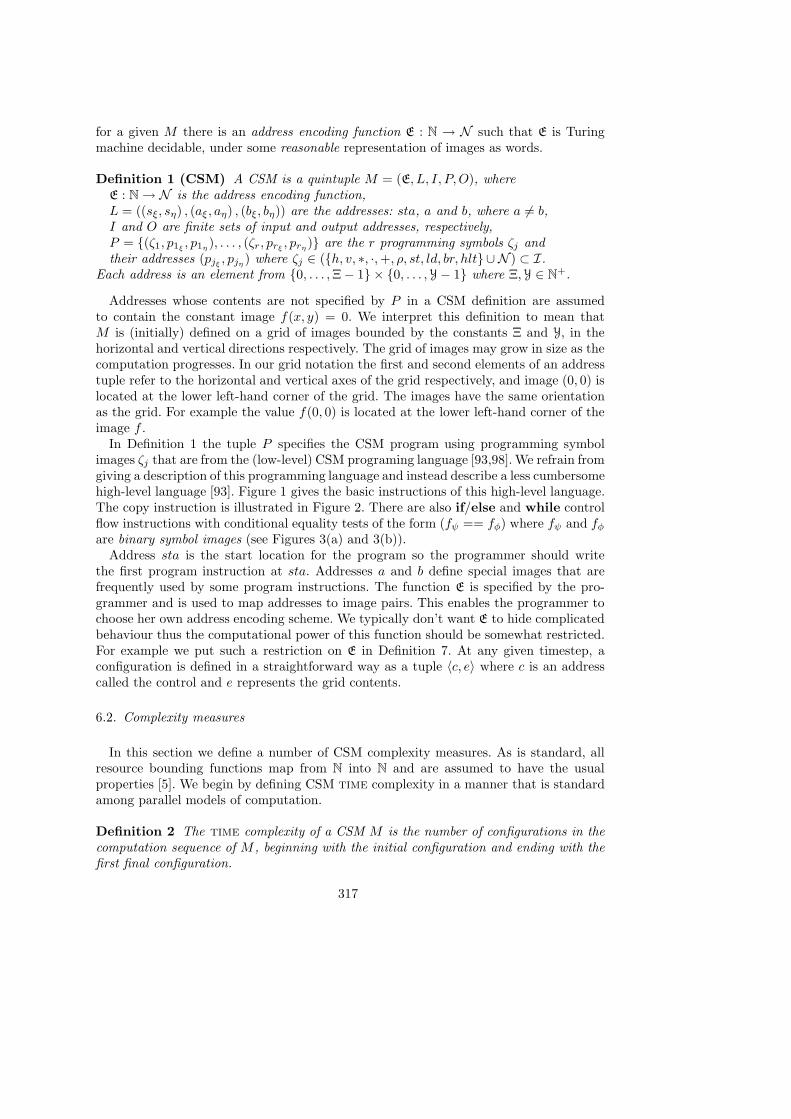
for a given M there is an address encoding function E : N → N such that E is Turingmachine decidable, under some reasonable representation of images as words.

Definition 1 (CSM) A CSM is a quintuple M = (E, L, I, P,O), whereE : N → N is the address encoding function,L = ((sξ, sη) , (aξ, aη) , (bξ, bη)) are the addresses: sta, a and b, where a = b,I and O are finite sets of input and output addresses, respectively,P = (ζ1, p1ξ

, p1η ), . . . , (ζr, prξ, prη) are the r programming symbols ζj and

their addresses (pjξ , pjη ) where ζj ∈ (h, v, ∗, ·,+, ρ, st, ld, br, hlt∪ N ) ⊂ I.Each address is an element from 0, . . . ,Ξ − 1 × 0, . . . ,Y − 1 where Ξ,Y ∈ N+.

Addresses whose contents are not specified by P in a CSM definition are assumedto contain the constant image f(x, y) = 0. We interpret this definition to mean thatM is (initially) defined on a grid of images bounded by the constants Ξ and Y, in thehorizontal and vertical directions respectively. The grid of images may grow in size as thecomputation progresses. In our grid notation the first and second elements of an addresstuple refer to the horizontal and vertical axes of the grid respectively, and image (0, 0) islocated at the lower left-hand corner of the grid. The images have the same orientationas the grid. For example the value f(0, 0) is located at the lower left-hand corner of theimage f .

In Definition 1 the tuple P specifies the CSM program using programming symbolimages ζj that are from the (low-level) CSM programing language [93,98]. We refrain fromgiving a description of this programming language and instead describe a less cumbersomehigh-level language [93]. Figure 1 gives the basic instructions of this high-level language.The copy instruction is illustrated in Figure 2. There are also if/else and while controlflow instructions with conditional equality tests of the form (fψ == fφ) where fψ and fφare binary symbol images (see Figures 3(a) and 3(b)).

Address sta is the start location for the program so the programmer should writethe first program instruction at sta. Addresses a and b define special images that arefrequently used by some program instructions. The function E is specified by the pro-grammer and is used to map addresses to image pairs. This enables the programmer tochoose her own address encoding scheme. We typically don’t want E to hide complicatedbehaviour thus the computational power of this function should be somewhat restricted.For example we put such a restriction on E in Definition 7. At any given timestep, aconfiguration is defined in a straightforward way as a tuple 〈c, e〉 where c is an addresscalled the control and e represents the grid contents.

6.2. Complexity measures

In this section we define a number of CSM complexity measures. As is standard, allresource bounding functions map from N into N and are assumed to have the usualproperties [5]. We begin by defining CSM time complexity in a manner that is standardamong parallel models of computation.

Definition 2 The time complexity of a CSM M is the number of configurations in thecomputation sequence of M , beginning with the initial configuration and ending with thefirst final configuration.

317

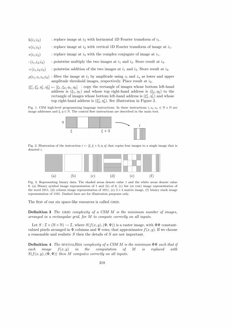
h(i1;i2) : replace image at i2 with horizontal 1D Fourier transform of i1.

v(i1;i2) : replace image at i2 with vertical 1D Fourier transform of image at i1.

∗(i1;i2) : replace image at i2 with the complex conjugate of image at i1.

··· (i1,i2;i3) : pointwise multiply the two images at i1 and i2. Store result at i3.

+(i1,i2;i3) : pointwise addition of the two images at i1 and i2. Store result at i3.

ρ(i1,zl,zu;i2) : filter the image at i1 by amplitude using zl and zu as lower and upperamplitude threshold images, respectively. Place result at i2.

[ξ′1, ξ′2, η

′1, η

′2] ← [ξ1, ξ2, η1, η2] : copy the rectangle of images whose bottom left-hand

address is (ξ1, η1) and whose top right-hand address is (ξ2, η2) to therectangle of images whose bottom left-hand address is (ξ′1, η

′1) and whose

top right-hand address is (ξ′2, η′2). See illustration in Figure 2.

Fig. 1. CSM high-level programming language instructions. In these instructions i, zl, zu ∈ N × N areimage addresses and ξ, η ∈ N. The control flow instructions are described in the main text.

ξ ξ + 3

ηi

Fig. 2. Illustration of the instruction i ← [ξ, ξ + 3, η, η] that copies four images to a single image that isdenoted i.

(a) (b) (c) (d) (e) (f)

Fig. 3. Representing binary data. The shaded areas denote value 1 and the white areas denote value0. (a) Binary symbol image representation of 1 and (b) of 0, (c) list (or row) image representation ofthe word 1011, (d) column image representation of 1011, (e) 3 × 4 matrix image, (f) binary stack imagerepresentation of 1101. Dashed lines are for illustration purposes only.

The first of our six space-like resources is called grid.

Definition 3 The grid complexity of a CSM M is the minimum number of images,arranged in a rectangular grid, for M to compute correctly on all inputs.

Let S : I × (N×N) → I, where S(f(x, y), (Φ,Ψ)) is a raster image, with ΦΨ constant-valued pixels arranged in Φ columns and Ψ rows, that approximates f(x, y). If we choosea reasonable and realistic S then the details of S are not important.

Definition 4 The spatialRes complexity of a CSM M is the minimum ΦΨ such that ifeach image f(x, y) in the computation of M is replaced withS(f(x, y), (Φ,Ψ)) then M computes correctly on all inputs.

318

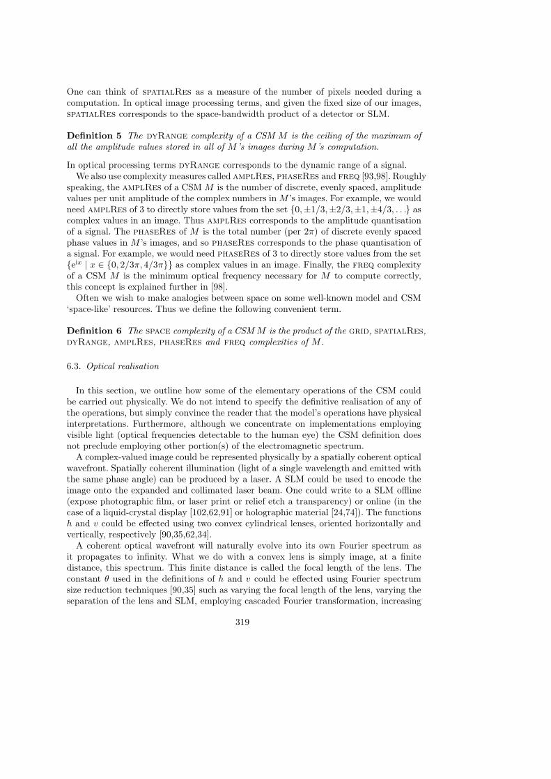
One can think of spatialRes as a measure of the number of pixels needed during acomputation. In optical image processing terms, and given the fixed size of our images,spatialRes corresponds to the space-bandwidth product of a detector or SLM.

Definition 5 The dyRange complexity of a CSM M is the ceiling of the maximum ofall the amplitude values stored in all of M ’s images during M ’s computation.

In optical processing terms dyRange corresponds to the dynamic range of a signal.We also use complexity measures called amplRes, phaseRes and freq [93,98]. Roughly

speaking, the amplRes of a CSM M is the number of discrete, evenly spaced, amplitudevalues per unit amplitude of the complex numbers in M ’s images. For example, we wouldneed amplRes of 3 to directly store values from the set 0,±1/3,±2/3,±1,±4/3, . . . ascomplex values in an image. Thus amplRes corresponds to the amplitude quantisationof a signal. The phaseRes of M is the total number (per 2π) of discrete evenly spacedphase values in M ’s images, and so phaseRes corresponds to the phase quantisation ofa signal. For example, we would need phaseRes of 3 to directly store values from the seteix | x ∈ 0, 2/3π, 4/3π as complex values in an image. Finally, the freq complexityof a CSM M is the minimum optical frequency necessary for M to compute correctly,this concept is explained further in [98].

Often we wish to make analogies between space on some well-known model and CSM‘space-like’ resources. Thus we define the following convenient term.

Definition 6 The space complexity of a CSM M is the product of the grid, spatialRes,dyRange, amplRes, phaseRes and freq complexities of M .

6.3. Optical realisation

In this section, we outline how some of the elementary operations of the CSM couldbe carried out physically. We do not intend to specify the definitive realisation of any ofthe operations, but simply convince the reader that the model’s operations have physicalinterpretations. Furthermore, although we concentrate on implementations employingvisible light (optical frequencies detectable to the human eye) the CSM definition doesnot preclude employing other portion(s) of the electromagnetic spectrum.

A complex-valued image could be represented physically by a spatially coherent opticalwavefront. Spatially coherent illumination (light of a single wavelength and emitted withthe same phase angle) can be produced by a laser. A SLM could be used to encode theimage onto the expanded and collimated laser beam. One could write to a SLM offline(expose photographic film, or laser print or relief etch a transparency) or online (in thecase of a liquid-crystal display [102,62,91] or holographic material [24,74]). The functionsh and v could be effected using two convex cylindrical lenses, oriented horizontally andvertically, respectively [90,35,62,34].

A coherent optical wavefront will naturally evolve into its own Fourier spectrum asit propagates to infinity. What we do with a convex lens is simply image, at a finitedistance, this spectrum. This finite distance is called the focal length of the lens. Theconstant θ used in the definitions of h and v could be effected using Fourier spectrumsize reduction techniques [90,35] such as varying the focal length of the lens, varying theseparation of the lens and SLM, employing cascaded Fourier transformation, increasing

319

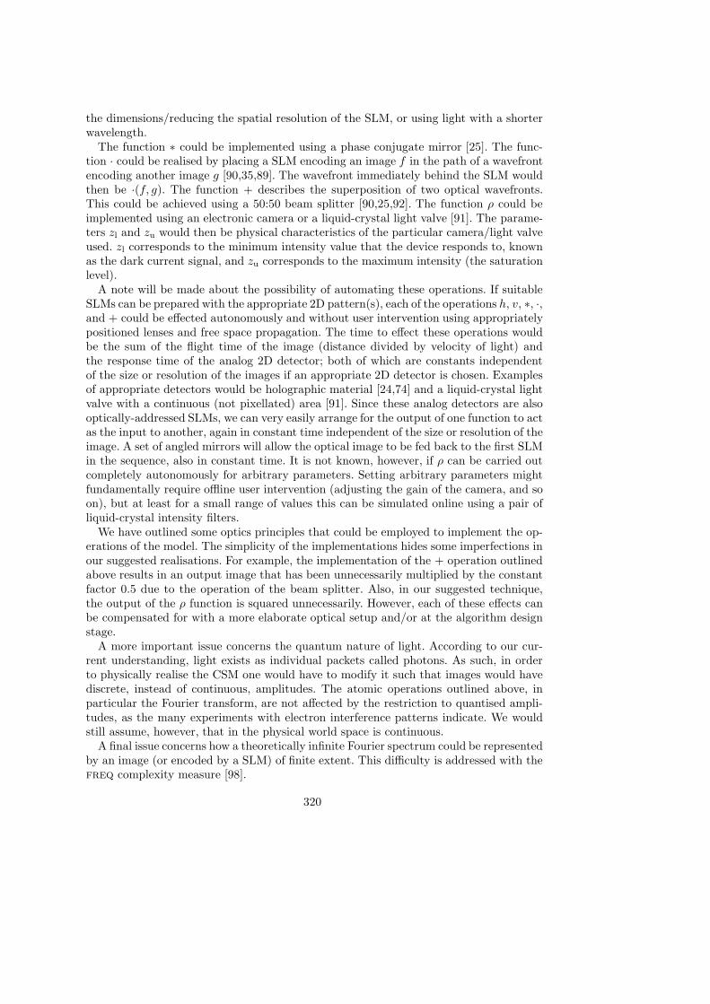
the dimensions/reducing the spatial resolution of the SLM, or using light with a shorterwavelength.

The function ∗ could be implemented using a phase conjugate mirror [25]. The func-tion · could be realised by placing a SLM encoding an image f in the path of a wavefrontencoding another image g [90,35,89]. The wavefront immediately behind the SLM wouldthen be ·(f, g). The function + describes the superposition of two optical wavefronts.This could be achieved using a 50:50 beam splitter [90,25,92]. The function ρ could beimplemented using an electronic camera or a liquid-crystal light valve [91]. The parame-ters zl and zu would then be physical characteristics of the particular camera/light valveused. zl corresponds to the minimum intensity value that the device responds to, knownas the dark current signal, and zu corresponds to the maximum intensity (the saturationlevel).

A note will be made about the possibility of automating these operations. If suitableSLMs can be prepared with the appropriate 2D pattern(s), each of the operations h, v, ∗, ·,and + could be effected autonomously and without user intervention using appropriatelypositioned lenses and free space propagation. The time to effect these operations wouldbe the sum of the flight time of the image (distance divided by velocity of light) andthe response time of the analog 2D detector; both of which are constants independentof the size or resolution of the images if an appropriate 2D detector is chosen. Examplesof appropriate detectors would be holographic material [24,74] and a liquid-crystal lightvalve with a continuous (not pixellated) area [91]. Since these analog detectors are alsooptically-addressed SLMs, we can very easily arrange for the output of one function to actas the input to another, again in constant time independent of the size or resolution of theimage. A set of angled mirrors will allow the optical image to be fed back to the first SLMin the sequence, also in constant time. It is not known, however, if ρ can be carried outcompletely autonomously for arbitrary parameters. Setting arbitrary parameters mightfundamentally require offline user intervention (adjusting the gain of the camera, and soon), but at least for a small range of values this can be simulated online using a pair ofliquid-crystal intensity filters.

We have outlined some optics principles that could be employed to implement the op-erations of the model. The simplicity of the implementations hides some imperfections inour suggested realisations. For example, the implementation of the + operation outlinedabove results in an output image that has been unnecessarily multiplied by the constantfactor 0.5 due to the operation of the beam splitter. Also, in our suggested technique,the output of the ρ function is squared unnecessarily. However, each of these effects canbe compensated for with a more elaborate optical setup and/or at the algorithm designstage.

A more important issue concerns the quantum nature of light. According to our cur-rent understanding, light exists as individual packets called photons. As such, in orderto physically realise the CSM one would have to modify it such that images would havediscrete, instead of continuous, amplitudes. The atomic operations outlined above, inparticular the Fourier transform, are not affected by the restriction to quantised ampli-tudes, as the many experiments with electron interference patterns indicate. We wouldstill assume, however, that in the physical world space is continuous.

A final issue concerns how a theoretically infinite Fourier spectrum could be representedby an image (or encoded by a SLM) of finite extent. This difficulty is addressed with thefreq complexity measure [98].

320

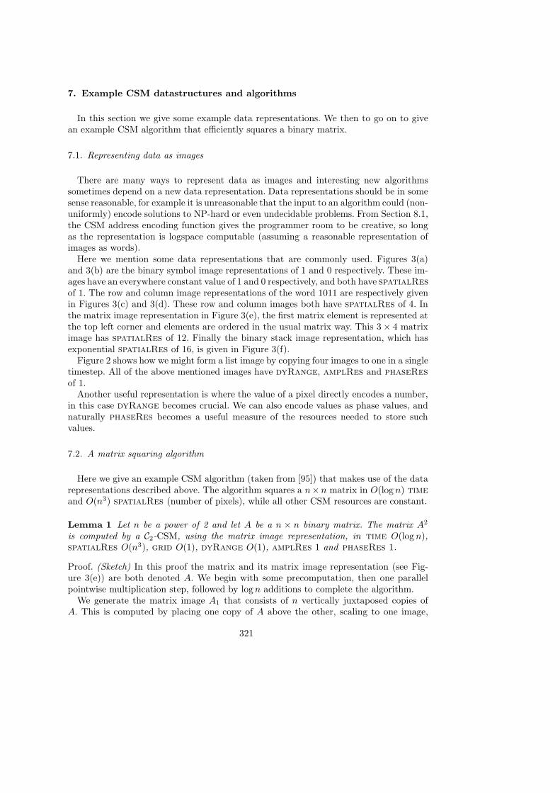
7. Example CSM datastructures and algorithms

In this section we give some example data representations. We then to go on to givean example CSM algorithm that efficiently squares a binary matrix.

7.1. Representing data as images

There are many ways to represent data as images and interesting new algorithmssometimes depend on a new data representation. Data representations should be in somesense reasonable, for example it is unreasonable that the input to an algorithm could (non-uniformly) encode solutions to NP-hard or even undecidable problems. From Section 8.1,the CSM address encoding function gives the programmer room to be creative, so longas the representation is logspace computable (assuming a reasonable representation ofimages as words).

Here we mention some data representations that are commonly used. Figures 3(a)and 3(b) are the binary symbol image representations of 1 and 0 respectively. These im-ages have an everywhere constant value of 1 and 0 respectively, and both have spatialResof 1. The row and column image representations of the word 1011 are respectively givenin Figures 3(c) and 3(d). These row and column images both have spatialRes of 4. Inthe matrix image representation in Figure 3(e), the first matrix element is represented atthe top left corner and elements are ordered in the usual matrix way. This 3 × 4 matriximage has spatialRes of 12. Finally the binary stack image representation, which hasexponential spatialRes of 16, is given in Figure 3(f).

Figure 2 shows how we might form a list image by copying four images to one in a singletimestep. All of the above mentioned images have dyRange, amplRes and phaseResof 1.

Another useful representation is where the value of a pixel directly encodes a number,in this case dyRange becomes crucial. We can also encode values as phase values, andnaturally phaseRes becomes a useful measure of the resources needed to store suchvalues.

7.2. A matrix squaring algorithm

Here we give an example CSM algorithm (taken from [95]) that makes use of the datarepresentations described above. The algorithm squares a n×n matrix in O(log n) timeand O(n3) spatialRes (number of pixels), while all other CSM resources are constant.

Lemma 1 Let n be a power of 2 and let A be a n × n binary matrix. The matrix A2

is computed by a C2-CSM, using the matrix image representation, in time O(log n),spatialRes O(n3), grid O(1), dyRange O(1), amplRes 1 and phaseRes 1.

Proof. (Sketch) In this proof the matrix and its matrix image representation (see Fig-ure 3(e)) are both denoted A. We begin with some precomputation, then one parallelpointwise multiplication step, followed by logn additions to complete the algorithm.

We generate the matrix image A1 that consists of n vertically juxtaposed copies ofA. This is computed by placing one copy of A above the other, scaling to one image,

321

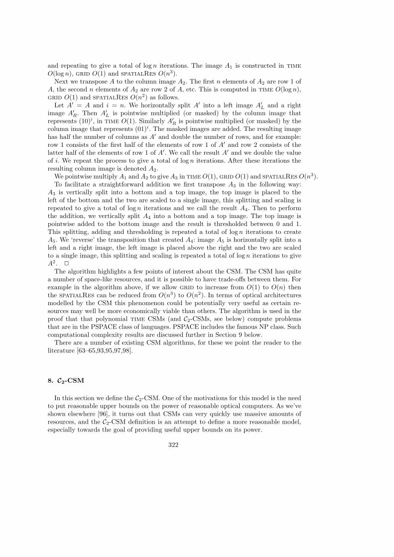
and repeating to give a total of log n iterations. The image A1 is constructed in timeO(log n), grid O(1) and spatialRes O(n3).

Next we transpose A to the column image A2. The first n elements of A2 are row 1 ofA, the second n elements of A2 are row 2 of A, etc. This is computed in time O(log n),grid O(1) and spatialRes O(n2) as follows.

Let A′ = A and i = n. We horizontally split A′ into a left image A′L and a right

image A′R. Then A′

L is pointwise multiplied (or masked) by the column image thatrepresents (10)i, in time O(1). Similarly A′

R is pointwise multiplied (or masked) by thecolumn image that represents (01)i. The masked images are added. The resulting imagehas half the number of columns as A′ and double the number of rows, and for example:row 1 consists of the first half of the elements of row 1 of A′ and row 2 consists of thelatter half of the elements of row 1 of A′. We call the result A′ and we double the valueof i. We repeat the process to give a total of logn iterations. After these iterations theresulting column image is denoted A2.

We pointwise multiply A1 andA2 to giveA3 in timeO(1), grid O(1) and spatialRes O(n3).To facilitate a straightforward addition we first transpose A3 in the following way:

A3 is vertically split into a bottom and a top image, the top image is placed to theleft of the bottom and the two are scaled to a single image, this splitting and scaling isrepeated to give a total of logn iterations and we call the result A4. Then to performthe addition, we vertically split A4 into a bottom and a top image. The top image ispointwise added to the bottom image and the result is thresholded between 0 and 1.This splitting, adding and thresholding is repeated a total of logn iterations to createA5. We ‘reverse’ the transposition that created A4: image A5 is horizontally split into aleft and a right image, the left image is placed above the right and the two are scaledto a single image, this splitting and scaling is repeated a total of logn iterations to giveA2.

The algorithm highlights a few points of interest about the CSM. The CSM has quitea number of space-like resources, and it is possible to have trade-offs between them. Forexample in the algorithm above, if we allow grid to increase from O(1) to O(n) thenthe spatialRes can be reduced from O(n3) to O(n2). In terms of optical architecturesmodelled by the CSM this phenomenon could be potentially very useful as certain re-sources may well be more economically viable than others. The algorithm is used in theproof that that polynomial time CSMs (and C2-CSMs, see below) compute problemsthat are in the PSPACE class of languages. PSPACE includes the famous NP class. Suchcomputational complexity results are discussed further in Section 9 below.

There are a number of existing CSM algorithms, for these we point the reader to theliterature [63–65,93,95,97,98].

8. C2-CSM

In this section we define the C2-CSM. One of the motivations for this model is the needto put reasonable upper bounds on the power of reasonable optical computers. As we’veshown elsewhere [96], it turns out that CSMs can very quickly use massive amounts ofresources, and the C2-CSM definition is an attempt to define a more reasonable model,especially towards the goal of providing useful upper bounds on its power.

322

8.1. C2-CSM

Motivated by a desire to apply standard complexity theory tools to the model, wedefined [93,96] the C2-CSM, a restricted and more realistic class of CSM.

Definition 7 (C2-CSM) A C2-CSM is a CSM whose computation time is defined fort ∈ 1, 2, . . . , T (n) and has the following restrictions:– For all time t both amplRes and phaseRes have constant value of 2.– For all time t each of grid, spatialRes and dyRange is 2O(t) and space is rede-

fined to be the product of all complexity measures except time and freq.– Operations h and v compute the discrete Fourier transform in the horizontal and ver-

tical directions respectively.– Given some reasonable binary word representation of the set of addresses N , the ad-

dress encoding function E : N → N is decidable by a logspace Turing machine.

Let us discuss these restrictions. The restrictions on amplRes and phaseRes implythat C2-CSM images are of the form f : [0, 1) × [0, 1) → 0,± 1

2 ,±1,± 32 , . . .. We have

replaced the Fourier transform with the discrete Fourier transform [9], this essentiallymeans that freq is now solely dependent on spatialRes; hence freq is not an interest-ing complexity measure for C2-CSMs and we do not analyse C2-CSMs in terms of freqcomplexity [93,96]. Restricting the growth of space is not unique to our model, suchrestrictions are to be found elsewhere [33,69,73].

In Section 6.1 we stated that the address encoding function E should be Turing ma-chine decidable, here we strengthen this condition. At first glance sequential logspacecomputability may perhaps seem like a strong restriction, but in fact it is quite weak.From an optical implementation point of view it should be the case that E is not compli-cated, otherwise we cannot assume fast addressing. Other (sequential/parallel) modelsusually have a very restricted ‘addressing function’: in most cases it is simply the identityfunction on N. Without an explicit or implicit restriction on the computational complex-ity of E, finding non-trivial upper bounds on the power of C2-CSMs is impossible as Ecould encode an arbitrarily complex Turing machine. As a weaker restriction we couldgive a specific E. However, this restricts the generality of the model and prohibits theprogrammer from developing novel, reasonable, addressing schemes.

9. Optical computing and computational complexity

As we saw in Section 5, there are number of optical algorithms that use the inherentparallelism of optics to provide fast solutions to certain problems. An alternative approachis to ask the following question: How does a given optical model relate to standard se-quential and parallel models? Establishing a relationship with computational complexitytheory, by describing both upper and lower bounds on the model, gives immediate accessto a large collection of useful algorithms and proof techniques.

The parallel computation thesis [31,23,49,87,69] states that parallel time (polynomi-ally) corresponds to sequential space, for reasonable parallel and sequential models. Anexample would be the fact that the class of problems solvable in polynomial space on anumber of parallel models is equivalent to PSPACE, the class of problems solvable onTuring machines that use at most polynomial space [40,8,30,32,22,33,88,85,83,3,84].

323

Of course the thesis can never be proved, it relates the intuitive notion of reasonableparallelism to the precise notion of a Turing machine. When results of this type werefirst shown researchers were suitably impressed; their parallel models truly had greatpower. For example if model M verifies the thesis then M decides PSPACE (includ-ing NP) languages in polynomial time. However there is another side to this coin. It isstraightforward to verify that given our current best algorithms, M will use at least asuperpolynomial amount of some other resource (like space or number of processors) todecide a PSPACE-complete or NP-complete language. Since the composition of polyno-mials is itself a polynomial, it follows that if we restrict the parallel computer to use atmost polynomial time and polynomial other resources, then it can at most solve problemsin P.

Nevertheless, asking if M verifies the thesis is an important question. Certain problems,such as those in the class NC, are efficiently parallelisable. NC can be defined as the classof problems that are solvable in polylogarithmic time on a parallel computer that uses apolynomial amount of hardware. So one can think of NC as those problems in P whichare solved exponentially faster on parallel computation thesis models than on sequentialmodels. If M verifies the thesis then it may be useful to apply M to these problems. Wealso know that if M verifies the thesis then there are (P-complete) problems for whichit is widely believed that we will not find exponential speed-up using M .

9.1. C2-CSM and parallel complexity theory

Here we summarise some characterisations of the computing power of optical comput-ers. Such characterisations enable the algorithm designer to know what kinds of problemsare solvable with resource bounded optical algorithms.

Theorem 2 below gives lower bounds on the computational power of the C2-CSM byshowing that it is at least as powerful as models that verify the parallel computationthesis.

Theorem 2 ([95,97]) NSPACE(S(n)) ⊆ C2-CSM–TIME(O(S2(n)))

In particular, polynomial time C2-CSMs accept the PSPACE languages. PSPACE isthe class of problems solvable by Turing machines that use polynomial space, whichincludes the famous class NP, and so NP-complete problems can be solved by C2-CSMsin polynomial time. However, any C2-CSM algorithm that we could presently write tosolve PSPACE or NP problems would require exponential space.

Theorem 2 is established by giving a C2-CSM algorithm that efficiently generates, andsquares, the transition matrix of a S(n) = Ω(log n) space bounded Turing machine.This transition matrix represents all possible computations of the Turing machine andis of size O(2S) × O(2S). The matrix squaring part was already given as an example(Lemma 1), and the remainder of the algorithm is given in [95]. The algorithm usesspace that is cubic in one of the matrix dimensions. In particular the algorithm usescubic spatialRes, O(23S), and all other space-like resources are constant. This theoremimproves upon the time overhead of a previous similar result [93,97] that was establishedvia C2-CSM simulation of the vector machines [72,73] of Pratt, Rabin, and Stockmeyer.

From the resource usage point of view, it is interesting to see that the older of these twoalgorithms uses grid, dyRange, and spatialRes that are each O(2S), while the newer

324

algorithm shows that if we allow more spatialRes we can in fact use only constant gridand dyRange. It would be interesting to find other such resource trade-offs within themodel.

Since NP is contained in PSPACE, Theorem 2, and the corresponding earlier resultsin [93,97], show that this optical model solves NP-complete problems in polynomial time.As described in Section 5, this has also been shown experimentally, for example Shakedet al. [80] have recently given a polynomial time, exponential space, optical algorithmto solve the NP-complete travelling salesperson problem. Their optical setup can beimplemented on the CSM.

The other of the two inclusions that are necessary in order to verify the parallel com-putation thesis have also been shown: C2-CSMs computing in time T (n) are no morepowerful than TO(1)(n) space bounded deterministic Turing machines. More precisely,we have:

Theorem 3 ([93,94]) C2-CSM-TIME(T (n)) ⊆ DSPACE(O(T 2(n)))

This result gives an upper bound on the power of C2-CSMs and was established via C2-CSM simulation by logspace uniform circuits of size and depth polynomial in space andtime respectively [94].

These computational complexity results for the C2-CSM have shown that the model iscapable of parallel processing in much the same way as models that verify the parallelcomputation thesis (and models that are known to characterise the parallel class NC).These results strongly depend on their use of non-constant spatialRes. The algorithmsexploit the ability of optical computers, and the CSM in particular, to operate on largenumbers of pixels in parallel. But what happens when we do not have arbitrary numbersof pixels? If allow images to have only a constant number of pixels then we need tofind new CSM algorithms. It turns out that such machines also characterise PSPACE inpolynomial time.

Theorem 4 ([99]) PSPACE is characterised by C2-CSMs that are restricted to use poly-nomial time T = O(nk), spatialRes O(1), grid O(1), and generalised to use amplRes

O(22T

), dyRange O(22T

).

So by treating images as registers and generating exponentially large, and exponentiallysmall, values we can solve seemingly intractable problems. Of course this kind of CSM isquite unrealistic from the point of view of optical implementations. In particular, accuratemultiplication of such values is difficult to implement in optics [99].

To restrict the model we could replace arbitrary multiplication, by multiplication byconstants, which can be easily simulated by a constant number of additions. If we disallowmultiplication in this way, we characterise P.

Theorem 5 ([99]) C2-CSMs without multiplication, that compute in polynomial time,polynomial grid O(nk), and spatialRes O(1), characterise P.

We can swap the roles of grid and spatialRes, and still obtain a P characterisation:

Theorem 6 ([99]) CSMs without multiplication, that compute in polynomial time,polynomial spatialRes O(nk), and grid O(1), characterise P.

325

Theorems 5 and 6 give conditions under which our optical model essentially looses itsparallel abilities and acts like a standard sequential Turing machine.

Via the proofs of Theorems 2 and 3 we can show that C2-CSMs that simultaneouslyuse polynomial space and polylogarithmic time solve exactly those problems in theclass NC.

Corollary 7 C2-CSM-SPACE,TIME(nO(1), logO(1) n) = NC

Problems in NC highlight the power of parallelism, as these problems can be solvedexponentially faster on a polynomial amount of parallel resources than on polynomialtime sequential machines. As further work in this area one could try to find alternatecharacterisations of NC in terms of the C2-CSM. In particular, one could try to findfurther interesting trade-offs between the various space-like resources of the model. Inthe real world this would correspond to computing over various different optical resources.As discussed in Section 5 it would be interesting for optical algorithm designers to try todesign (implementable) optical algorithms for NC problems in an effort to find problemsthat are well-suited to optical solutions.

References

[1] M. A. G. Abushagur and H. J. Caulfield. Speed and convergence of bimodal optical computers.Optical Engineering, 26(1):22–27, Jan. 1987.

[2] L. M. Adleman. Molecular computation of solutions to combinatorial problems. Science, 266:1021–1024, Nov. 1994.

[3] A. Alhazov and M. de Jesus Perez-Jimenez. Uniform solution to QSAT using polarizationlessactive membranes. In J. Durand-Lose and M. Margenstern, editors, Machines, Computations andUniversality (MCU), volume 4664 of LNCS, pages 122–133, Orleans, France, Sept. 2007. Springer.

[4] H. H. Arsenault and Y. Sheng. An Introduction to Optics in Computers, volume TT8 of TutorialTexts in Optical Engineering. SPIE Press, Bellingham, Washington, 1992.

[5] J. L. Balcazar, J. Dıaz, and J. Gabarro. Structural complexity, vols I and II. EATCS Monographson Theoretical Computer Science. Springer, Berlin, 1988.

[6] R. Barakat and J. H. Reif. Lower bounds on the computational efficiency of optical computingsystems. Applied Optics, 26(6):1015–1018, Mar. 1987.

[7] F. R. Beyette Jr., P. A. Mitkas, S. A. Feld, and C. W. Wilmsen. Bitonic sorting using anoptoelectronic recirculating architecture. Applied Optics, 33(35):8164–8172, Dec. 1994.

[8] A. Borodin. On relating time and space to size and depth. SIAM Journal on Computing, 6(4):733–744, Dec. 1977.

[9] R. N. Bracewell. The Fourier transform and its applications. Electrical and electronic engineeringseries. McGraw-Hill, second edition, 1978.

[10] K.-H. Brenner, A. Huang, and N. Streibl. Digital optical computing with symbolic substitution.Applied Optics, 25(18):3054–3060, Sept. 1986.

[11] D. P. Casasent and G. P. House. Comparison of coherent and noncoherent optical correlators. InOptical Pattern Recognition V, Proceedings of SPIE vol. 2237, pages 170–178, Apr. 1994.

[12] D. P. Casasent and D. Psaltis. Position, rotation, and scale invariant optical correlation. AppliedOptics, 15(7):1795–1799, 1976.

[13] H. J. Caulfield, editor. Handbook of Optical Holography. Academic Press, New York, 1979.[14] H. J. Caulfield. The energetic advantage of analog over digital computing. In OSA Optical

Computing Technical Digest Series, volume 9, pages 180–183, 1989.[15] H. J. Caulfield. Space-time complexity in optical computing. In B. Javidi, editor, Optical

information-processing systems and architectures II, volume 1347, pages 566–572. SPIE, July 1990.[16] H. J. Caulfield. Space-time complexity in optical computing. Multidimensional Systems and Signal

Processing, 2(4):373–378, Nov. 1991. Special issue on optical signal processing.

326

[17] H. J. Caulfield and M. A. G. Abushagur. Hybrid analog-digital algebra processors. In Optical andHybrid Computing II, Proceedings of SPIE vol. 634, pages 86–95, Orlando, Florida, Apr. 1986.

[18] H. J. Caulfield and R. Haimes. Generalized matched filtering. Applied Optics, 19(2):181–183, Jan.1980.

[19] H. J. Caulfield, S. Horvitz, and W. A. V. Winkle. Introduction to the special issue on opticalcomputing. Proceedings of the IEEE, 65(1):4–5, Jan. 1977.

[20] H. J. Caulfield, J. M. Kinser, and S. K. Rogers. Optical neural networks. Proceedings of the IEEE,77:1573–1582, 1989.

[21] H. J. Caulfield, W. T. Rhodes, M. J. Foster, and S. Horvitz. Optical implementation of systolicarray processing. Optics Communications, 40:86–90, 1981.

[22] A. K. Chandra, D. C. Kozen, and L. J. Stockmeyer. Alternation. Journal of the ACM, 28(1):114–133, Jan. 1981.

[23] A. K. Chandra and L. J. Stockmeyer. Alternation. In 17th annual symposium on Foundations ofComputer Science, pages 98–108, Houston, Texas, Oct. 1976. IEEE. (Preliminary Version).

[24] F. S. Chen, J. T. LaMacchia, and D. B. Fraser. Holographic storage in lithium niobate. AppliedPhysics Letters, 13(7):223–225, oct 1968.

[25] A. E. Chiou. Photorefractive phase-conjugate optics for image processing, trapping, andmanipulation of microscopic objects. Proceedings of the IEEE, 87(12):2074–2085, Dec. 1999.

[26] S. Dolev and H. Fitoussi. The traveling beam: optical solution for bounded NP-complete problems.In P. Crescenzi, G. Prencipe, and G. Pucci, editors, The fourth international conference on funwith algorithms (FUN), pages 120–134, 2007.

[27] J. Durand-Lose. Reversible conservative rational abstract geometrical computation is Turing-universal. In Logical Approaches to Computational Barriers, Second Conference on Computabilityin Europe, (CiE), volume 3988 of Lecture Notes in Computer Science, pages 163–172, Swansea,UK, 2006. Springer.

[28] N. H. Farhat and D. Psaltis. New approach to optical information processing based on the Hopfieldmodel. Journal of the Optical Society of America A, 1:1296, 1984.

[29] D. G. Feitelson. Optical Computing: A survey for computer scientists. MIT Press, Cambridge,Massachusetts, 1988.

[30] S. Fortune and J. Wyllie. Parallelism in random access machines. In Proc. 10th Annual ACMSymposium on Theory of Computing, pages 114–118, 1978.

[31] L. M. Goldschlager. Synchronous parallel computation. PhD thesis, University of Toronto,Computer Science Department, Dec. 1977.

[32] L. M. Goldschlager. A unified approach to models of synchronous parallel machines. In Proc. 10thAnnual ACM Symposium on Theory of Computing, pages 89–94, 1978.

[33] L. M. Goldschlager. A universal interconnection pattern for parallel computers. Journal of theACM, 29(4):1073–1086, Oct. 1982.

[34] J. W. Goodman. Operations achievable with coherent optical information processing systems.Proceedings of the IEEE, 65(1):29–38, Jan. 1977.

[35] J. W. Goodman. Introduction to Fourier Optics. Roberts & Company, Englewood, Colorado, thirdedition, 2005.

[36] R. Greenlaw, H. J. Hoover, and W. L. Ruzzo. Limits to parallel computation: P-completenesstheory. Oxford university Press, Oxford, 1995.

[37] L. K. Grover. A fast quantum mechanical algorithm for database search. In Proc. 28th AnnualACM Symposium on Theory of Computing, pages 212–219, May 1996.

[38] P. S. Guilfoyle, J. M. Hessenbruch, and R. V. Stone. Free-space interconnects for high-performanceoptoelectronic switching. IEEE Computer, 31(2):69–75, Feb. 1998.

[39] T. Haist and W. Osten. An optical solution for the travelling salesman problem. Optics Express,15(16):10473–10482, Aug. 2007. Erratum: Vol. 15(10), pp 12627. Aug. 2007.

[40] J. Hartmanis and J. Simon. On the power of multiplication in random access machines. InProceedings of the 15th annual symposium on switching and automata theory, pages 13–23, TheUniversity of New Orleans, Oct. 1974. IEEE.

[41] T. Head. Formal language theory and DNA: an analysis of the generative capacity of specificrecombinant behaviors. Bulletin of Mathematical Biology, 49(6):737–759, 1987.

[42] J. L. Horner, editor. Optical Signal Processing. Academic Press, San Diego, 1987.[43] Y.-N. Hsu and H. H. Arsenault. Optical pattern recognition using circular harmonic expansion.

Applied Optics, 21(22):4016–4019, Nov. 1982.

327

[44] A. Huang. Architectural considerations involved in the design of an optical digital computer.Proceedings of the IEEE, 72(7):780–786, July 1984.

[45] A. D. Jacobson, T. D. Beard, W. P. Bleha, J. D. Morgerum, and S. Y. Wong. The liquid crystal lightvalue, an optical-to-optical interface device. In Proceedings of the Conference on Parallel ImageProcessing, Goddard Space Flight Center, pages 288–299, Mar. 1972. Document X-711-72-308.

[46] B. Javidi. Nonlinear joint power spectrum based optical correlation. Applied Optics, 28(12):2358–2367, June 1989.

[47] B. Javidi and J. Wang. Optimum distortion-invariant filter for detecting a noisy distorted target innonoverlapping background noise. Journal of the Optical Society of America A, 12(12):2604–2614,Dec. 1995.

[48] M. A. Karim and A. A. S. Awwal. Optical Computing: An Introduction. Wiley, New York, 1992.

[49] R. M. Karp and V. Ramachandran. Parallel algorithms for shared memory machines. In J. vanLeeuwen, editor, Handbook of Theoretical Computer Science, volume A, chapter 17. Elsevier,Amsterdam, 1990.

[50] E. Knill, R. LaFlamme, and G. J. Milburn. A scheme for efficient quantum computation withlinear optics. Nature, 409:46–52, 2001.

[51] J. N. Lee, editor. Design Issues in Optical Processing. Cambridge Studies in Modern Optics.Cambridge University Press, Cambridge, Great Britain, 1995.

[52] J. N. Lee, editor. Design issues in optical processing. Cambridge studies in modern optics.Cambridge University Press, 1995.

[53] Lenslet Labs. Enlight256. white paper report, Lenslet Ltd., 6 Galgalei Haplada St, Herzelia Pituach,46733 Israel, Nov. 2003.

[54] R. J. Lipton. Using DNA to solve NP-complete problems. Science, 268:542–545, Apr. 1995.

[55] A. Louri and A. Post. Complexity analysis of optical-computing paradigms. Applied Optics,31(26):5568–5583, Sept. 1992.

[56] P. D. MacKenzie and V. Ramachandran. Ercw prams and optical communication. TheoreticalComputer Science, 196:153–180, 1998.

[57] A. D. McAulay. Optical Computer Architectures: The Application of Optical Concepts to NextGeneration Computers. Wiley, New York, 1991.

[58] C. Mead. Analog VLSI and Neural Systems. Addison-Wesley, Reading, Massachusetts, 1989.

[59] D. A. Miller. Rationale and challenges for optical interconnects to electronic chips. Proceedings ofthe IEEE, 88(6):728–749, June 2000.

[60] C. Moore. Generalized shifts: undecidability and unpredictability in dynamical systems.Nonlinearity, 4:199–230, 1991.

[61] C. Moore. Majority-vote cellular automata, Ising dynamics and P-completeness. Journal ofStatistical Physics, 88(3/4):795–805, 1997.

[62] T. Naughton, Z. Javadpour, J. Keating, M. Klıma, and J. Rott. General-purpose acousto-opticconnectionist processor. Optical Engineering, 38(7):1170–1177, July 1999.

[63] T. J. Naughton. Continuous-space model of computation is Turing universal. In S. Bains andL. J. Irakliotis, editors, Critical Technologies for the Future of Computing, Proceedings of SPIEvol. 4109, pages 121–128, San Diego, California, Aug. 2000.

[64] T. J. Naughton. A model of computation for Fourier optical processors. In R. A. Lessard andT. Galstian, editors, Optics in Computing 2000, Proc. SPIE vol. 4089, pages 24–34, Quebec,Canada, June 2000.

[65] T. J. Naughton and D. Woods. On the computational power of a continuous-space optical modelof computation. In M. Margenstern and Y. Rogozhin, editors, Machines, Computations andUniversality: Third International Conference (MCU’01), volume 2055 of LNCS, pages 288–299,Chisinau, Moldova, May 2001. Springer.

[66] M. Oltean. A light-based device for solving the Hamiltonian path problem. In Fifth InternationalConference on Unconventional Computation (UC’06), volume 4135 of LNCS, pages 217–227, York,

UK, 2006. Springer.[67] E. L. O’Neill. Spatial filtering in optics. IRE Transactions on Information Theory, 2:56–65, June

1956.

[68] C. H. Papadimitriou. Computational complexity. Addison-Wesley, 1995.

[69] I. Parberry. Parallel complexity theory. Wiley, 1987.[70] G. Paun. Membrane computing: an introduction. Springer, 2002.

328

[71] A. Pe’er, D. Wang, A. W. Lohmann, and A. A. Friesem. Optical correlation with totally incoherentlight. Optics Letters, 24(21):1469–1471, Nov. 1999.

[72] V. R. Pratt, M. O. Rabin, and L. J. Stockmeyer. A characterisation of the power of vector machines.In Proc. 6th annual ACM symposium on theory of computing, pages 122–134. ACM press, 1974.

[73] V. R. Pratt and L. J. Stockmeyer. A characterisation of the power of vector machines. Journal ofComputer and Systems Sciences, 12:198–221, 1976.

[74] A. Pu, R. F. Denkewalter, and D. Psaltis. Real-time vehicle navigation using a holographic memory.

Optical Engineering, 36(10):2737–2746, Oct. 1997.[75] J. Reif, D. Tygar, and A. Yoshida. The computability and complexity of optical beam tracing. In

31st Annual IEEE Symposium on Foundations of Computer Science (FOCS), pages 106–114, St.Louis, MO, Oct. 1990. IEEE.

[76] J. H. Reif and A. Tyagi. Energy complexity of optical computations. In 2nd IEEE Symposium onParallel and Distributed Processing, pages 14–21, Dallas, TX, Dec. 1990.

[77] J. H. Reif and A. Tyagi. Efficient parallel algorithms for optical computing with the discrete Fouriertransform (DFT) primitive. Applied Optics, 36(29):7327–7340, Oct. 1997.

[78] A. A. Sawchuk and T. C. Strand. Digital optical computing. Proceedings of the IEEE, 72(7):758–779, July 1984.

[79] N. T. Shaked, S. Messika, S. Dolev, and J. Rosen. Optical solution for bounded NP-completeproblems. Applied Optics, 46(5):711–724, Feb. 2007.

[80] N. T. Shaked, G. Simon, T. Tabib, S. Mesika, S. Dolev, and J. Rosen. Optical processor for solvingthe traveling salesman problem (TSP). In B. Javidi, D. Psaltis, and H. J. Caulfield, editors, Proc.of SPIE, Optical Information Systems IV, volume 63110G, Aug. 2006.

[81] N. T. Shaked, T. Tabib, G. Simon, S. Messika, S. Dolev, and J. Rosen. Optical binary-

matrix synthesis for solving bounded NP-complete combinatorical problems. Optical Engineering,46(10):108201–1–108201–11, Oct. 2007.

[82] P. Shor. Algorithms for quantum computation: Discrete logarithms and factoring. In Proceedings35th Annual Symposium on Foundations Computer Science, pages 124–134, 1994.

[83] P. Sosık. The computational power of cell division in P systems: Beating down parallel computers?Natural Computing, 2(3):287–298, 2003.

[84] P. Sosık and A. Rodrıguez-Paton. Membrane computing and complexity theory: A characterizationof PSPACE. Journal of Computer and System Sciences, 73(1):137–152, 2007.

[85] J. Tromp and P. van Emde Boas. Associative storage modification machines. In K. Ambos-Spies,S. Homer, and U. Schoning, editors, Complexity theory: current research, pages 291–313. CambridgeUniversity Press, 1993.

[86] G. L. Turin. An introduction to matched filters. IRE Transactions on Information Theory,6(3):311–329, June 1960.

[87] P. van Emde Boas. Machine models and simulations. In J. van Leeuwen, editor, Handbook ofTheoretical Computer Science, volume A, chapter 1. Elsevier, Amsterdam, 1990.

[88] J. van Leeuwen and J. Wiedermann. Array processing machines. BIT, 27:25–43, 1987.

[89] A. VanderLugt. Signal detection by complex spatial filtering. IEEE Transactions on InformationTheory, 10(2):139–145, Apr. 1964.

[90] A. VanderLugt. Optical Signal Processing. Wiley, New York, 1992.

[91] P.-Y. Wang and M. Saffman. Selecting optical patterns with spatial phase modulation. OpticsLetters, 24(16):1118–1120, Aug. 1999.

[92] C. S. Weaver and J. W. Goodman. A technique for optically convolving two functions. AppliedOptics, 5(7):1248–1249, July 1966.

[93] D. Woods. Computational complexity of an optical model of computation. PhD thesis, NationalUniversity of Ireland, Maynooth, 2005.

[94] D. Woods. Upper bounds on the computational power of an optical model of computation. InX. Deng and D. Du, editors, 16th International Symposium on Algorithms and Computation(ISAAC 2005), volume 3827 of LNCS, pages 777–788, Sanya, China, Dec. 2005. Springer.

[95] D. Woods. Optical computing and computational complexity. In Fifth International Conferenceon Unconventional Computation (UC’06), volume 4135 of LNCS, pages 27–40, York, UK, 2006.Springer. Invited.

[96] D. Woods and J. P. Gibson. Complexity of continuous space machine operations. In S. B.Cooper, B. Loewe, and L. Torenvliet, editors, New Computational Paradigms, First Conference

329

on Computability in Europe (CiE 2005), volume 3526 of LNCS, pages 540–551, Amsterdam, June2005. Springer.

[97] D. Woods and J. P. Gibson. Lower bounds on the computational power of an optical model ofcomputation. In C. S. Calude, M. J. Dinneen, G. Paun, M. J. Perez-Jimenez, and G. Rozenberg,editors, Fourth International Conference on Unconventional Computation (UC’05), volume 3699of LNCS, pages 237–250, Sevilla, Oct. 2005. Springer.

[98] D. Woods and T. J. Naughton. An optical model of computation. Theoretical Computer Science,334(1-3):227–258, Apr. 2005.

[99] D. Woods and T. J. Naughton. Sequential and parallel optical computing. In InternationalWorkshop on Optical SuperComputing, 2008. To appear.

[100] T. Yokomori. Molecular computing paradigm – toward freedom from Turing’s charm. Naturalcomputing, 1(4):333–390, 2002.

[101] F. T. S. Yu, S. Jutamulia, and S. Yin, editors. Introduction to information optics. Academic Press,San Diego, 2001.

[102] F. T. S. Yu, T. Lu, X. Yang, and D. A. Gregory. Optical neural network with pocket-sized liquid-crystal televisions. Optics Letters, 15(15):863–865, Aug. 1990.

330

Physically-Relativized Church-Turing Hypotheses:Physical Foundations of Computing and

Complexity Theory of Computational Physics

Martin Ziegler?

University of Paderborn, GERMANY

Abstract. We turn the physical Church-Turing Hypothesis from an ambiguous source of sensationalspeculations into a (collection of) sound and well-defined scientific problem(s):Examining recent controversies and causes for misunderstanding concerning the state of the Church-Turing Hypothesis (CTH), it is suggested to study the CTH ‘sharpened’ relative to an arbitrary butspecific physical theory—rather than vaguely referring to “nature” in general. For this purpose wecombine physical structuralism with computational complexity theory. The benefits of this approachare illustrated by some exemplary results on computability and complexity in computational physics.

1 Introduction . . . . . . . . . . . . . . . . . . . . . . . . . . . . . . . . . . . . . . . . . . . . . . . . . . . . . . . . . . . . . . . . . . . 3311.1 Turing Universality in Computer Science and Mathematics . . . . . . . . . . . . . . . . . . . . . . . 3311.2 Turing Universality in Physics . . . . . . . . . . . . . . . . . . . . . . . . . . . . . . . . . . . . . . . . . . . . . . . 3311.3 Summary . . . . . . . . . . . . . . . . . . . . . . . . . . . . . . . . . . . . . . . . . . . . . . . . . . . . . . . . . . . . . . . . 332

2 Physical Computing . . . . . . . . . . . . . . . . . . . . . . . . . . . . . . . . . . . . . . . . . . . . . . . . . . . . . . . . . . . . 3333 Physical Theories . . . . . . . . . . . . . . . . . . . . . . . . . . . . . . . . . . . . . . . . . . . . . . . . . . . . . . . . . . . . . . 334

3.1 Structuralism in Physics . . . . . . . . . . . . . . . . . . . . . . . . . . . . . . . . . . . . . . . . . . . . . . . . . . . . 3343.2 On the Reality of Physical Theories . . . . . . . . . . . . . . . . . . . . . . . . . . . . . . . . . . . . . . . . . . 335

4 Hypercomputation in Classical Mechanics? . . . . . . . . . . . . . . . . . . . . . . . . . . . . . . . . . . . . . . . . 3364.1 Existence in Physics . . . . . . . . . . . . . . . . . . . . . . . . . . . . . . . . . . . . . . . . . . . . . . . . . . . . . . . 3364.2 Constructivism into Physical Theories! . . . . . . . . . . . . . . . . . . . . . . . . . . . . . . . . . . . . . . . 337

4.2.1 Constructing Physical Objects . . . . . . . . . . . . . . . . . . . . . . . . . . . . . . . . . . . . . . . . . 3374.2.2 Pre-Theories: Ancestry among Physical Theories . . . . . . . . . . . . . . . . . . . . . . . . . 338

5 Computational Physics . . . . . . . . . . . . . . . . . . . . . . . . . . . . . . . . . . . . . . . . . . . . . . . . . . . . . . . . . . 3395.1 Complexity in Computational Physics↔ Physically-Relativized CTH . . . . . . . . . . . . . 3395.2 Real Number Computation . . . . . . . . . . . . . . . . . . . . . . . . . . . . . . . . . . . . . . . . . . . . . . . . . . 340

6 Vision of a Research Programme . . . . . . . . . . . . . . . . . . . . . . . . . . . . . . . . . . . . . . . . . . . . . . . . . 3406.1 Celestial Mechanics . . . . . . . . . . . . . . . . . . . . . . . . . . . . . . . . . . . . . . . . . . . . . . . . . . . . . . . 341

6.1.1 Newton . . . . . . . . . . . . . . . . . . . . . . . . . . . . . . . . . . . . . . . . . . . . . . . . . . . . . . . . . . . . 3416.1.2 Planar Eudoxus/Aristotle . . . . . . . . . . . . . . . . . . . . . . . . . . . . . . . . . . . . . . . . . . . . . 3416.1.3 Proofs . . . . . . . . . . . . . . . . . . . . . . . . . . . . . . . . . . . . . . . . . . . . . . . . . . . . . . . . . . . . . 3426.1.4 General Eudoxus/Aristotle; Ptolemy, Copernicus, and Kepler . . . . . . . . . . . . . . . 344

6.2 Opticks . . . . . . . . . . . . . . . . . . . . . . . . . . . . . . . . . . . . . . . . . . . . . . . . . . . . . . . . . . . . . . . . . . 3446.2.1 Geometric Optics . . . . . . . . . . . . . . . . . . . . . . . . . . . . . . . . . . . . . . . . . . . . . . . . . . . . 3446.2.2 Electrodynamics . . . . . . . . . . . . . . . . . . . . . . . . . . . . . . . . . . . . . . . . . . . . . . . . . . . . . 344

6.3 Quantum Mechanics . . . . . . . . . . . . . . . . . . . . . . . . . . . . . . . . . . . . . . . . . . . . . . . . . . . . . . . 3456.3.1 Quantum Logic . . . . . . . . . . . . . . . . . . . . . . . . . . . . . . . . . . . . . . . . . . . . . . . . . . . . . 345

7 Conclusion . . . . . . . . . . . . . . . . . . . . . . . . . . . . . . . . . . . . . . . . . . . . . . . . . . . . . . . . . . . . . . . . . . . . 346References . . . . . . . . . . . . . . . . . . . . . . . . . . . . . . . . . . . . . . . . . . . . . . . . . . . . . . . . . . . . . . . . . . . . . . . 347? Supported by DFG project Zi1009-1/2. The author would also like to use this opportunity to express his gratitude

to JOHN V. TUCKER from Swansea University for putting him on the present (scientific and career) track. BRUNO

LOFF and ANDREA REICHENBERGER have kindly provided constructive remarks that helped improving this work.

332 Martin Ziegler

1 Introduction

In 1937 Alan Turing investigated the capabilities and fundamental limitations of a mathematical abstractionand idealization of a computer. Nowadays, this Turing machine (TM) is considered the most appropriatemodel of actual digital computers reflecting what a common PC can do or cannot do, and capturing itsfundamental capabilities in computability and complexity classes: any computation problem that can be(efficiently) solved in practice by a PC belongs to ∆1 (to P ); and vice versa. In this sense, the TM is widelybelieved to be universal; and problems P 6∈ P , or the Halting problem H 6∈ ∆1, have to be faced up asprincipally unsolvable.

1.1 Turing Universality in Computer Science and Mathematics

There are some good reasons for this belief:

• There exists a so-called universal Turing machine (UTM), capable of simulating (with at most poly-nomial slowdown) any other given TM.• Several other reasonable models of computation have turned out as equivalent to the TM: WHILE-

programs, λ–calculus etc. Notice that these models correspond to real-world programming languageslike Lisp.

We qualify those good reasons as computer scientific—in contrast to the following evidence based on apurely mathematical notion:

• An integer function f is TM-computable iff it is µ-recursive;that is, f belongs to the least class of functions

– containing the constant function 0,– the successor function x 7→ x+1,– the projections (x1, . . . ,xn) 7→ xi,– and being closed under composition,– under primitive recursion,– and under so-called µ-recursion.

1.2 Turing Universality in Physics

The? Church-Turing Hypothesis (CTH) claims that every function which would naturally be regarded ascomputable is computable under his [i.e. Turing’s] definition, i.e. by one of his machines [Klee52, p.376].Its strong version claims that efficient natural computability corresponds to polynomial-time Turing com-putability. Put differently, CTH predicts a negative answer to the following

Question 1. Does nature admit the existence of a system whose computational power strictly exceeds thatof a TM?

Notice that the CTH exceeds the realm of computer science; it involves physics as the general analysis ofnature. Hence, in addition to the computer scientific and mathematical dimensions of Turing universality, athird dimension would arise if the answer to Question 1 turned out to be negative (cmp. [Benn95,Svoz05]):

• The class of (efficiently) physically computable functions coincides with the class of (polynomial-time)Turing computable ones.

Insofar a TM can be built at least in principle?? it constitutes a physical system. Conversely, a negativeanswer to Question 1 means that every physical ‘computer’ can be simulated (maybe even in polynomialtime) by a TM. Such an answer is supported by long experience in two ways:

? To be fair, this is just one out of a variety of refined interpretations of a claim which neither ALONZO CHURCH norALAN TURING have ever put forth; see, e.g. [Hodg06], [Ord02, SECTION 2.2], [Cope02], or [LoCo08]. In fact Irefer to what in in literature is more specifically called the physical Church-Turing Hypothesis, but for reasons ofconciseness shall in the sequel omit this adjective.

?? it is for instance realized (in good approximation) by any standard PC

Physically-Relativized Church-Turing Hypotheses 333

– the constant failure to physically solve the Halting problem and– the success of simulating a plethora of physical systems on a TM,

namely in Computational Physics.

So far all attempts have failed to prove the CTH, i.e. have given at best bounds on the speed of cal-culations but not on the general capabilities of computation, based e.g. on the laws of thermodynamics[BeLa85,Fran02] or on the speed of light (special relativity) [Lloy02]. In fact it has been suggested [Loff07,p.39] that the Church-Turing Hypothesis be included into physics as an axiom (called the Church-Turingcriterion): just like the impossibility to extract energy from nothing (or from thermal energy alone) startedas a recurring experience and was then postulated as the First (Second) Law of Thermodynamics—andonly later ‘justified’ using Statistical Mechanics. Either way, whether axiomatizing or trying to prove theChurch-Turing Thesis, first of all one needs a formalization of Question 1.

Such attempts are, of course, not new. For instance, Gandy Machines have been proposed [Gand80,Sieg00]a model of computation based on some specific physical principles. Our approach on the other hand is basedon arbitrary physical theories, providing a more thorough and accurate formal coverage of ‘nature’.

1.3 Summary

The CTH is the subject of a plethora of publications and of many disputes and speculations. The presentwork aims to put some reason into the ongoing [Galt06] and often sensational [Kie03b,Lloy06] discussion.We are convinced that formalizing Question 1 will come useful. However, it seems unlikely that one singleformalization can reach consensus. We notice that most, if not all, disputes about the state of the Church-Turing Hypothesis arise from disagreeing and/or implicit conceptions of how to formalize it [Smi99b].The best we can hope for is a class of formalizations, namely one for each physical theory [BeTu07,SECTION 2(b)]. Let me fortify this:

Manifesto 2. a) Describing the scientific laws of nature is the purpose and virtue of physics. It does soby means of various physical theories Φ, each of which ‘covers’ some part of reality (but may deviateon other parts).

b) Consequently, instead of vaguely referring to ‘nature’ (recall Section 1.2) any claim concerning (thestate of) the CTH should explicitly mention the specific physical theory Φ it considers;

c) and criticism against such a claim as ‘based on unrealistic presumptions’ should be regarded as di-rected towards the underlying physical theory (and stipulate re-investigation subject to another Φ,rather than dismissing the claim itself); cmp. [BeTu07, PRINCIPLE 2.4].

d) Also the input/output encoding better be specified explicitly when referring to some “CTHΦ”: How isthe argument ~x, of natural or real numbers, fed into the system; i.e. how does its preparation (e.g. inQuantum Mechanics) proceed operationally; and how is the ‘result’ to be read off (e.g. what ‘question’is the system to answer)? [Ship93, SECTION I]

Particularly Item b) is central to the present work and explains for its title!The suggestion to consider physically-relativized Church-Turing Hypotheses “CTHΦ” (cmp. also [BeTu07,

PRINCIPLE 2.1]) bears the spirit of the related treatment of the famous “P versus N P ” Question in[BGS75]; there it has been shown that, relative to some oracle, both complexity classes coincide whereasrelative to another one they do not.

Section 3 below expands on the concept of a physical theory Φ and its analogy to a model of com-putation in computer science. We turn Manifesto 2b) into a research programme (Section 6) and illustrateits benefit for computational physics. Before, Section 2 reports on previous attempts to disprove the CTHby examples of hypercomputers purportedly capable of solving the Halting problem, and the respectivephysical theories they exploit. Subsequently, we simplify one such example in order to inspect its sourceof computational power. Based on this insight, we are in Section 4.2 led to extend the above Manifesto:

Manifesto 2 (continued).

e) The concept of “existence” of a hypercomputational physical system (recall Question 1) must be inter-preted from a constructivistic point of view.

334 Martin Ziegler

2 Physical Computing

Common (necessarily informal) arguments in favor of the Church-Turing Hypothesis usually proceed alongthe following line: A physical system is mathematically described by an ordinary or partial differentialequation which can be solved numerically using time-stepping—as long as the solution remains regular:whereas a singular solution is unphysical or too unstable (or both) in order to be harnessed for physicalcomputing.

On the other hand, in literature there are a variety of suggestions for physical systems of computationalpower exceeding that of a TM, e.g.

Example 3 i) General Relativity might admit for space-times such that the clock of a TM M followingone world-line seems to reach infinity within finite time according to the clock of an observer O startingat the same event but following another world-line; thus O can decide whether M terminates or not[EtNe02].However it is unknown whether such space-times actually exist in our universe; and if they exist,how to locate them and how far from earth they might be in order to be used for solving the Haltingproblem. (Notice that the closest known Black Hole, namely next to star V4641, takes at least 1600years to travel to). Finally, it has been criticized that the TM in question had to run indefinitely—anduse corresponding amounts of storage tape and energy.

ii) While ‘standard’ quantum computers using a finite number of qubits can be simulated on a TM (al-though possibly at exponential slowdown), Quantum Mechanics (QM) supports operators on infinitesuperpositions which could be exploited to solve the Halting problem [CDS00,Kie03a,ACP04,Zieg05].On the other hand there are already considerable doubts that finite??? quantum parallelism is in con-siderable is practical due to issues of decoherence, i.e. susceptibility to external, classical noise (akind of instability if you like); hence how much more unrealistic be infinite one!

iii) Already in their mathematical formulation, certain theories of Quantum Gravitation involve combi-natorial conditions which are known undecidable to a TM [GeHa86].These, however, are still mere (and preliminary) theories. . .

iv) A light ray passing through a finite system of mirrors corresponds to the computation of a Turingmachine; and by detecting whether it finally arrives at a certain position, one can solve the Haltingproblem [RTY94].The catch is that the ray must adhere to Geometric Optics, i.e. have infinitely small diameter, bedevoid of dispersion, and propagate instantaneously; also the mirrors have to be perfect.

v) The above claim that singular solutions can be ruled out is put into question by the discovery of non-collision singularities in Newtonian many-body systems [Yao03,Smi06a,Svoz07].On the other hand, the construction of these singularities heavily relies on the moving particles beingideal points obeying Newton’s Law (with the singularity at 0) up to arbitrary small distances.

vi) Even Classical Mechanics has been suggested to allow for physical objects which can be probedin finite time to answer queries “n ∈ X” for any fixed set X ⊆ N (and in particular for the Haltingproblem) [BeTu04].However creating this classical device seems to require solving X in the first place.

vii) Already 1D heat conduction has been shown [PERi81] capable of evolving a computable initial con-dition x 7→ u(0,x) into an uncomputable one x 7→ u(1,x). Here the caveat is that, while the initialcondition is computable and continuously differentiable, its derivative is not, and hence again implic-itly contains the superrecursive power as input [WeZh02].

Notice that each approach is based on and exploits sometimes beyond recognition some (more or lessspecific) physical theory. Also, the indicated reproaches against each approach to hypercomputation aim atthe physical theory it is based on.

??? The present world-record seems to provide calculations on only 28 qubits; and even that is rather questionable[Pont07]

Physically-Relativized Church-Turing Hypotheses 335

3 Physical Theories

have been devised as the scientific means for objectively describing and predicting the behavior of naturefor thousands of years. Nowadays, we may feel inclined to patronize e.g. ARISTOTLE’s eight books, buthis concept of Elements (air, fire, earth, water) constitutes an important first step towards putting somestructure into the many phenomena experienced†

Since Aristotle, a plethora of physical theories of space-time has evolved (cf. e.g. [Duhe85]), associatedwith famous names like GALILEO GALILEI, PTOLEMY, NICOLAUS COPERNICUS, JOHANNES KEPLER,SIR ISAAC NEWTON, HENDRIK LORENTZ, and ALBERT EINSTEIN. Moreover, theories of electricity andmagnetism have sprung and later became unified (JAMES CLERK MAXWELL) with GAUSSian Optics. Andthere are various‡ quantum mechanical and field theories. The unification process continued: Electricityand Magnetism, been merged into Electrodynamics, were joined by Quantum Mechanics to make upQuantumelectrodynamics (QED), and then with Weak Interaction formed Electroweak Interaction;moreover Gravitation and Special Relativity became General Relativity.

Remark 4 (Analogy between a Physical Theory and a Model of Computation). Each such theory hasarisen, or rather been devised in order to describe some part of nature with sufficient accuracy—while nec-essarily neglecting others. (Quantum Mechanics for instance is aimed at describing elementary particlesmoving considerably slower than light; whereas Relativity Theory focuses on very fast yet macroscopic ob-jects.) We point out the analogy of a physical theory to a model of computation in computer science: Here,the aim is to reflect some aspects of actual computing devises as well, possibly at the expense of otheraspects. (A Turing machine has unbounded working tape; hence it can decide whether a 4GB-memorybounded PC algorithm terminates. Whereas the canonical model for computing devises with finite mem-ory, a DFA is unable to decide the correct placement of brackets.)

But what exactly is a physical theory? In addition to a means for clearing up misunderstandings as indicatedin Footnote‡, agreement on this issue is a crucial prerequisite for treating important further questions like:

Are Newton’s Laws an extension of Kepler’s? [Duhe54]Does Quantum Mechanics imply Classical Mechanics—and if so, in what sense exactly?

To us, such intertheory relations [Batt07,Stoe95] are in turn relevant in view of the above Manifesto 2 withquestions as the following one:

Do the computational capabilities of Quantum Mechanics include those of Classical Mechanics?

3.1 Structuralism in Physics

Just like a physical theory is regularly obtained by trying to infer a simple description of a family of em-pirical data points obtained from experimental measurements, a meta-theory of physics takes the variety ofexisting physical theories as empirical data points and tries to identify their common underlying structure.The philosophy of science knows several meta-theories of physics, i.e., conceptions of what a physicaltheory is [Schm08]:

• SNEED focuses on their mathematical aspects [Snee71]; STEGMÜLLER suggests to formalize physicaltheories in analogy to the Bourbaki Programme in mathematics [Steg79,Steg86].

• C.F. V. WEIZSÄCKER envisions the success of unifying previously distinct theories (recall above) tocontinue and ultimately lead into a “Theory of Everything” [Weiz85,Sch97b]. From this point of viewany other physical theory (like e.g. Newton Mechanics) is merely a tentative draft [Wein94].

† Even more, closer observation reveals that an argument like “A rock flung up will fall down, because it is a rock’snature to rest on earth.” is no less circular than the following two more contemporary ones: “A rock flung up willfall down, because there is a force pulling it towards the earth.” and Electrons in an atom occupy different orbits,because they are Fermions.

‡ Remember how scientists regularly get into a fight when starting to talk about (their conception of) Quantum Me-chanics

336 Martin Ziegler

• MITTELSTAEDT emphasizes pluralism in physical theories, i.e., various theories equally appropriate todescribe the same range of phenomena [Mitt72, SECTION 4]. Also [Hage82] points out (among manyother things) that any physical theory or model is a mere approximation and idealization of reality.• For our purpose, LUDWIG [Ludw90] and, building thereon, SCHRÖTER [Schr96] propose the most

appropriate and elaborated formalization, based on the following (meta-)

Definition 5 (Sketch). A physical theory Φ consists of

– a description of a part of nature it applies to (WB)– a mathematical theory as the language to describe it (MT)– and mapping between physical and mathematical objects (AP).

In this setting, each physical theory has a specific and limited range of applicability (WB): a quite pragmaticapproach, compared to the almost eschatological hope of von Weizsäcker and Weinberg for a ToE. Fromthe point of view of Ludwig and Schröter on the other hand, each new theory adds to and extends with itsWB (=images of MT under AP) that part of nature ‘covered’ by physics: just like a mathematical manifoldbeing covered and described by the images of Euclidean subsets under charts [Miln97]; see also [Svoz06].

Remark 6. Some major physical theories have already been formalized in the sense of Definition 5; wemention for instance two‡ Quantum Mechanics [Ludw85,Haet96] and space-time theories[Meis90,Schr88,ScSc92,Sche92,Sch97a]. Fortunately, our approach suffices with a rather low level of de-tail compared to the depth of formalization of each of the three components (WB,MT,AP) provided by theexhaustive [Schr96].

3.2 On the Reality of Physical Theories

The purpose of a physical theory Φ is to describe a part of nature. Hence, when some better descriptionΦ′ is found, a ‘revolution’ may occur and Φ gets disposed of [Kuhn62]. However a full rejection of Φ

has never happened (and is one source of criticism against Kuhn): more commonly, the new theory Φ′ isapplied to those parts of nature which the old one would not describe (sufficiently well) while keeping Φ

for applications where it long has turned as appropriate.

Example 7 a) Classical/Continuum Mechanics (CM) for instance is often heard of as ‘wrong’—becausematter is in fact composed from atoms circled by electrons on stable orbits—yet it still constitutes thetheory which most mechanical engineering is based on.

b) Similarly, audio systems are successfully designed using Ohm’s Law for (complex) electrical resis-tance: in spite of Maxwell’s Equations being a more accurate description of alternating currents, notto mention QED.

Ludwig in [Ludw85] has proven that QM, often considered as ‘better’ (in the sense of more fundamentaland realistic) a theory than CM, does not include or imply CM; see also [Boku08]. (Nevertheless suchclaims regularly re-emerge especially in popular science.) Moreover, even QM itself is merely§ an approx-imation to parts of nature, unrealistic e.g. at high velocities or in the presence of large masses.

These observations urge us to enhance Manifesto 2a+c) with an ontological commitment to scientificrealism:

Manifesto 8. A physical theory Φ (like, e.g. CM) constitutes an element of reality: It exists¶ no less than“points” or “atoms” do. In particular, it is advisable to investigate the computational power of, and withinsuch a Φ: Dismissing a theory for being ‘unrealistic’ in one extend or another would in consequencedeprive us of all of them!

§ In particular we disagree with the, seemingly prevalent, opinion that Quantum Theory is somehow salient or evenuniversal in some sense [HaHa83,Holl96]

¶ Note that this refers to existence on the meta-level of physical theories, as opposed to the existence of a physicalobject within a physical theory according to Manifesto 2e). Our distinction between these two levels is analogousto GÖDEL’s (meta-)proof of the existence (!), for any [. . . ] mathematical theory, of an arithmetical statement whichcannot, within this theory, be proven nor refuted.

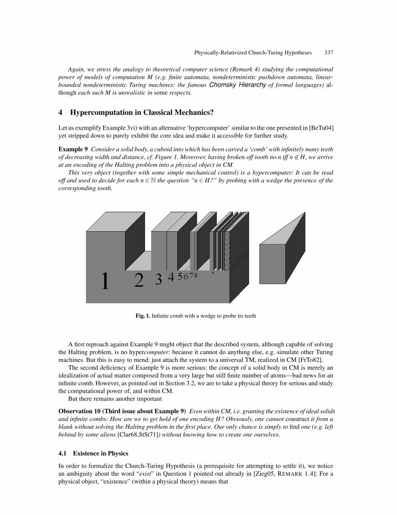
Physically-Relativized Church-Turing Hypotheses 337

Again, we stress the analogy to theoretical computer science (Remark 4) studying the computationalpower of models of computation M (e.g. finite automata, nondeterministic pushdown automata, linear-bounded nondeterministic Turing machines: the famous Chomsky Hierarchy of formal languages) al-though each such M is unrealistic in some respects.

4 Hypercomputation in Classical Mechanics?

Let us exemplify Example 3vi) with an alternative ‘hypercomputer’ similar to the one presented in [BeTu04]yet stripped down to purely exhibit the core idea and make it accessible for further study.

Example 9 Consider a solid body, a cuboid into which has been carved a ‘comb’ with infinitely many teethof decreasing width and distance, cf. Figure 1. Moreover, having broken off tooth no.n iff n 6∈ H, we arriveat an encoding of the Halting problem into a physical object in CM.

This very object (together with some simple mechanical control) is a hypercomputer: It can be readoff and used to decide for each n ∈ N the question “n ∈ H?” by probing with a wedge the presence of thecorresponding tooth.

Fig. 1. Infinite comb with a wedge to probe its teeth

A first reproach against Example 9 might object that the described system, although capable of solvingthe Halting problem, is no hypercomputer: because it cannot do anything else, e.g. simulate other Turingmachines. But this is easy to mend: just attach the system to a universal TM, realized in CM [FrTo82].

The second deficiency of Example 9 is more serious: the concept of a solid body in CM is merely anidealization of actual matter composed from a very large but still finite number of atoms—bad news for aninfinite comb. However, as pointed out in Section 3.2, we are to take a physical theory for serious and studythe computational power of, and within CM.

But there remains another important

Observation 10 (Third issue about Example 9) Even within CM, i.e. granting the existence of ideal solidsand infinite combs: How are we to get hold of one encoding H? Obviously, one cannot construct it from ablank without solving the Halting problem in the first place. Our only chance is simply to find one (e.g. leftbehind by some aliens [Clar68,StSt71]) without knowing how to create one ourselves.

4.1 Existence in Physics

In order to formalize the Church-Turing Hypothesis (a prerequisite for attempting to settle it), we noticean ambiguity about the word “exist” in Question 1 pointed out already in [Zieg05, REMARK 1.4]: For aphysical object, “existence” (within a physical theory) means that

338 Martin Ziegler

A) one has to actually construct it?B) its non-existence leads to a contradiction?C) or that its existence does not lead to a contradiction (i.e. is consistent)?

These three opinions correspond in mathematics to the points of view taken by a constructivist, a classicalmathematician (working e.g. in the Zermelo-Fraenkel framework) and one ‘believing’ in the Axiom ofChoice, respectively. The last standpoint (C) is well known to lead to counter-intuitive consequences whentaken in the physical realm of CM:

Example 11 (Banach-Tarski Paradoxon) For a solid ball (say of gold) of unit size in 3-space, there existsa partition into finitely many (although necessarily not Lebesgue-measurable) pieces that, if put togetherappropriately (i.e. after applying certain Euclidean isometries), then form two solid balls of unit size.

This example (see also [Svoz97]) is in no danger of causing inflation: first, because actual material gold isnot infinitely divisible (cmp. the second deficiency of Example 9); secondly, even within CM, because thepartition of the ball ‘exists’ merely in the above Sense C).

Hence, in order to avoid both ‘obviously’ unnatural (counter-) Examples 9 and 11, Manifesto 8 leadsus to transfer and adapt the constructivist standpoint from mathematics to physics and for physics as well.

4.2 Constructivism into Physical Theories!

As explained above, the “existence” of some physical object within a theory Φ has to be interpreted con-structively; cmp. e.g. PROBLEMS 6.2 and 6.3 in [BeTu04]. To this end and as in [CDCG95], let us distin-guish two ways of introducing constructivism into a physical theory Φ = (MT,AP,WB):

α) By interpreting the mathematical theory MT constructively; compare [BiBr85,Kush84,BrSv00,Flet02]and [DSKS95, SECTION III].

β) By imposing constructivism onto the side of physical objects WB.

It seems that Method α), although meritable of its own, does not quite meet our goal of making a physicaltheory constructive:

Example 12 Consider the condition for a function f : X → Y between normed spaces to be open; or evensimpler: that of the image f [B(0,1)]⊆ Y of the unit ball in X to be an open subset of Y .

∀u ∈ f [B(0,1)] ∃ε > 0 ∀y ∈ B(u,ε) ∃x ∈ B(0,1) : f (x) = y . (1)

A constructivist would insist that both existential quantifiers have to be interpreted constructively; whereasin a setting of computation on real numbers by rational approximation, applications suffice that only ε iscomputable from u, while the existence of x depending on y need not: compare [Zieg06].

4.2.1 Constructing Physical ObjectsUnderlying β) is the conception that every object in nature (or more precisely: that part of nature describedby WB) be

• either a primitive one (e.g. a tree, modeled in Φ as a homogeneous cylinder of density ρ = 0.7g/cm3;or some ore, modeled as CuFeS2)

• or the result of some technological process applied to such primitive objects.

The latter may, e.g., include crafting a tree into a wheel or even a wooden gear; or smelting ore to producebronze.

Notice how such a process—the sequence of operations from cutting the tree, cleaning, sawing, carving;or of melting, reducing, and alloying copper—constitutes an algorithm (and crucial cultural knowledgepassed on from carpenters or redsmiths‖ to their apprentices). More modern and advanced science, too,

‖ An attentative referee has pointed out the inconsequence to admit human interaction for creating a hypercom-puter, but not during the computation itself. Permitting the latter leads to notions considered, e.g., in [Mins68]or [GoWe08].

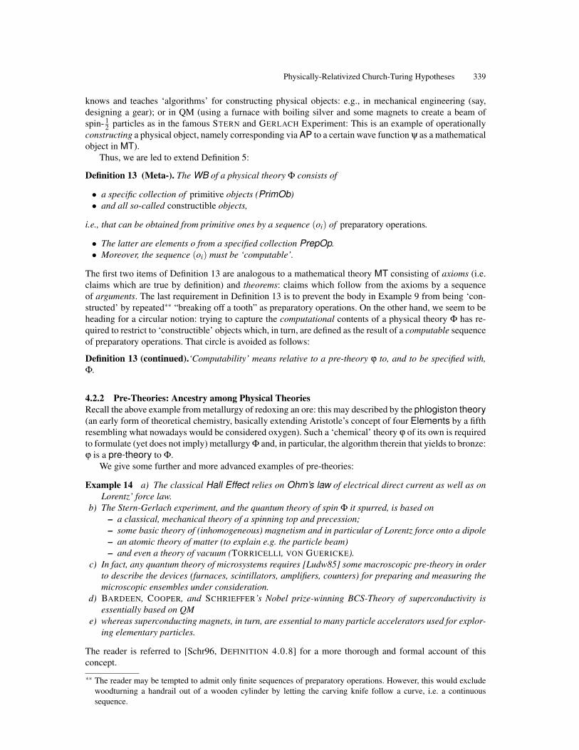
Physically-Relativized Church-Turing Hypotheses 339

knows and teaches ‘algorithms’ for constructing physical objects: e.g., in mechanical engineering (say,designing a gear); or in QM (using a furnace with boiling silver and some magnets to create a beam ofspin- 1

2 particles as in the famous STERN and GERLACH Experiment: This is an example of operationallyconstructing a physical object, namely corresponding via AP to a certain wave function ψ as a mathematicalobject in MT).

Thus, we are led to extend Definition 5:

Definition 13 (Meta-). The WB of a physical theory Φ consists of

• a specific collection of primitive objects (PrimOb)• and all so-called constructible objects,

i.e., that can be obtained from primitive ones by a sequence (oi) of preparatory operations.

• The latter are elements o from a specified collection PrepOp.• Moreover, the sequence (oi) must be ‘computable’.

The first two items of Definition 13 are analogous to a mathematical theory MT consisting of axioms (i.e.claims which are true by definition) and theorems: claims which follow from the axioms by a sequenceof arguments. The last requirement in Definition 13 is to prevent the body in Example 9 from being ‘con-structed’ by repeated∗∗ “breaking off a tooth” as preparatory operations. On the other hand, we seem to beheading for a circular notion: trying to capture the computational contents of a physical theory Φ has re-quired to restrict to ‘constructible’ objects which, in turn, are defined as the result of a computable sequenceof preparatory operations. That circle is avoided as follows:

Definition 13 (continued).‘Computability’ means relative to a pre-theory ϕ to, and to be specified with,Φ.

4.2.2 Pre-Theories: Ancestry among Physical TheoriesRecall the above example from metallurgy of redoxing an ore: this may described by the phlogiston theory(an early form of theoretical chemistry, basically extending Aristotle’s concept of four Elements by a fifthresembling what nowadays would be considered oxygen). Such a ‘chemical’ theory ϕ of its own is requiredto formulate (yet does not imply) metallurgy Φ and, in particular, the algorithm therein that yields to bronze:ϕ is a pre-theory to Φ.

We give some further and more advanced examples of pre-theories:

Example 14 a) The classical Hall Effect relies on Ohm’s law of electrical direct current as well as onLorentz’ force law.

b) The Stern-Gerlach experiment, and the quantum theory of spin Φ it spurred, is based on– a classical, mechanical theory of a spinning top and precession;– some basic theory of (inhomogeneous) magnetism and in particular of Lorentz force onto a dipole– an atomic theory of matter (to explain e.g. the particle beam)– and even a theory of vacuum (TORRICELLI, VON GUERICKE).

c) In fact, any quantum theory of microsystems requires [Ludw85] some macroscopic pre-theory in orderto describe the devices (furnaces, scintillators, amplifiers, counters) for preparing and measuring themicroscopic ensembles under consideration.

d) BARDEEN, COOPER, and SCHRIEFFER’s Nobel prize-winning BCS-Theory of superconductivity isessentially based on QM

e) whereas superconducting magnets, in turn, are essential to many particle accelerators used for explor-ing elementary particles.

The reader is referred to [Schr96, DEFINITION 4.0.8] for a more thorough and formal account of thisconcept.

∗∗ The reader may be tempted to admit only finite sequences of preparatory operations. However, this would excludewoodturning a handrail out of a wooden cylinder by letting the carving knife follow a curve, i.e. a continuoussequence.

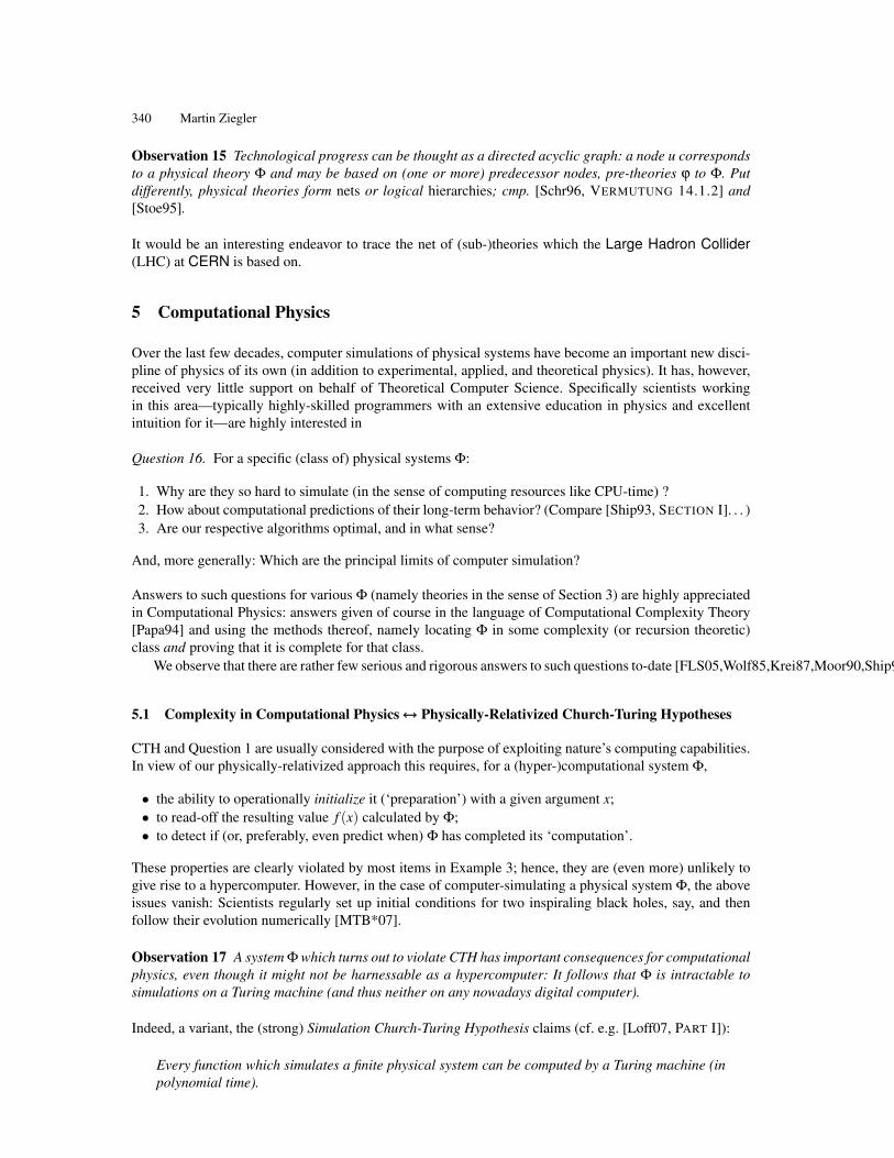
340 Martin Ziegler

Observation 15 Technological progress can be thought as a directed acyclic graph: a node u correspondsto a physical theory Φ and may be based on (one or more) predecessor nodes, pre-theories ϕ to Φ. Putdifferently, physical theories form nets or logical hierarchies; cmp. [Schr96, VERMUTUNG 14.1.2] and[Stoe95].

It would be an interesting endeavor to trace the net of (sub-)theories which the Large Hadron Collider(LHC) at CERN is based on.

5 Computational Physics

Over the last few decades, computer simulations of physical systems have become an important new disci-pline of physics of its own (in addition to experimental, applied, and theoretical physics). It has, however,received very little support on behalf of Theoretical Computer Science. Specifically scientists workingin this area—typically highly-skilled programmers with an extensive education in physics and excellentintuition for it—are highly interested in

Question 16. For a specific (class of) physical systems Φ:

1. Why are they so hard to simulate (in the sense of computing resources like CPU-time) ?2. How about computational predictions of their long-term behavior? (Compare [Ship93, SECTION I]. . . )3. Are our respective algorithms optimal, and in what sense?

And, more generally: Which are the principal limits of computer simulation?

Answers to such questions for various Φ (namely theories in the sense of Section 3) are highly appreciatedin Computational Physics: answers given of course in the language of Computational Complexity Theory[Papa94] and using the methods thereof, namely locating Φ in some complexity (or recursion theoretic)class and proving that it is complete for that class.

We observe that there are rather few serious and rigorous answers to such questions to-date [FLS05,Wolf85,Krei87,Moor90,Ship93,Svoz93,ReTa93,RTY94,PIM06,Loff07].

5.1 Complexity in Computational Physics↔↔↔ Physically-Relativized Church-Turing Hypotheses

CTH and Question 1 are usually considered with the purpose of exploiting nature’s computing capabilities.In view of our physically-relativized approach this requires, for a (hyper-)computational system Φ,

• the ability to operationally initialize it (‘preparation’) with a given argument x;• to read-off the resulting value f (x) calculated by Φ;• to detect if (or, preferably, even predict when) Φ has completed its ‘computation’.

These properties are clearly violated by most items in Example 3; hence, they are (even more) unlikely togive rise to a hypercomputer. However, in the case of computer-simulating a physical system Φ, the aboveissues vanish: Scientists regularly set up initial conditions for two inspiraling black holes, say, and thenfollow their evolution numerically [MTB*07].

Observation 17 A system Φ which turns out to violate CTH has important consequences for computationalphysics, even though it might not be harnessable as a hypercomputer: It follows that Φ is intractable tosimulations on a Turing machine (and thus neither on any nowadays digital computer).

Indeed, a variant, the (strong) Simulation Church-Turing Hypothesis claims (cf. e.g. [Loff07, PART I]):

Every function which simulates a finite physical system can be computed by a Turing machine (inpolynomial time).

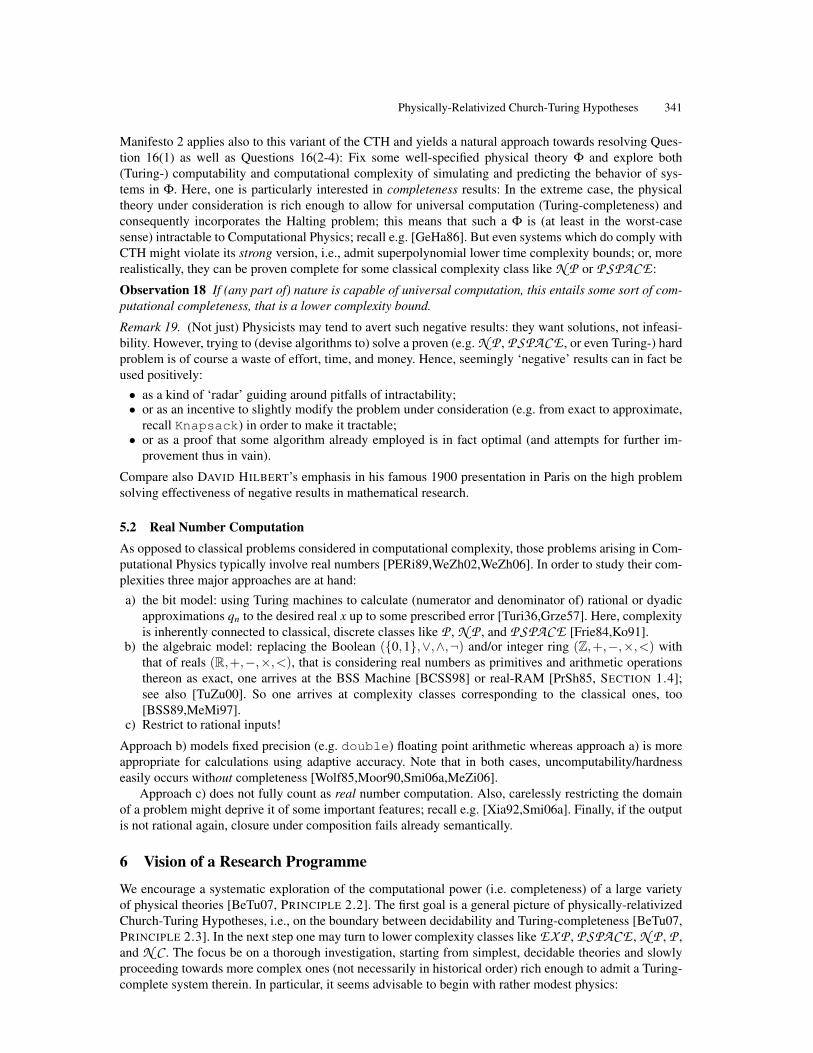
Physically-Relativized Church-Turing Hypotheses 341

Manifesto 2 applies also to this variant of the CTH and yields a natural approach towards resolving Ques-tion 16(1) as well as Questions 16(2-4): Fix some well-specified physical theory Φ and explore both(Turing-) computability and computational complexity of simulating and predicting the behavior of sys-tems in Φ. Here, one is particularly interested in completeness results: In the extreme case, the physicaltheory under consideration is rich enough to allow for universal computation (Turing-completeness) andconsequently incorporates the Halting problem; this means that such a Φ is (at least in the worst-casesense) intractable to Computational Physics; recall e.g. [GeHa86]. But even systems which do comply withCTH might violate its strong version, i.e., admit superpolynomial lower time complexity bounds; or, morerealistically, they can be proven complete for some classical complexity class like N P or P SPACE :

Observation 18 If (any part of) nature is capable of universal computation, this entails some sort of com-putational completeness, that is a lower complexity bound.

Remark 19. (Not just) Physicists may tend to avert such negative results: they want solutions, not infeasi-bility. However, trying to (devise algorithms to) solve a proven (e.g. N P , P SPACE , or even Turing-) hardproblem is of course a waste of effort, time, and money. Hence, seemingly ‘negative’ results can in fact beused positively:• as a kind of ‘radar’ guiding around pitfalls of intractability;• or as an incentive to slightly modify the problem under consideration (e.g. from exact to approximate,

recall Knapsack) in order to make it tractable;• or as a proof that some algorithm already employed is in fact optimal (and attempts for further im-

provement thus in vain).

Compare also DAVID HILBERT’s emphasis in his famous 1900 presentation in Paris on the high problemsolving effectiveness of negative results in mathematical research.

5.2 Real Number ComputationAs opposed to classical problems considered in computational complexity, those problems arising in Com-putational Physics typically involve real numbers [PERi89,WeZh02,WeZh06]. In order to study their com-plexities three major approaches are at hand:a) the bit model: using Turing machines to calculate (numerator and denominator of) rational or dyadic

approximations qn to the desired real x up to some prescribed error [Turi36,Grze57]. Here, complexityis inherently connected to classical, discrete classes like P , N P , and P SPACE [Frie84,Ko91].

b) the algebraic model: replacing the Boolean (0,1,∨,∧,¬) and/or integer ring (Z,+,−,×,<) withthat of reals (R,+,−,×,<), that is considering real numbers as primitives and arithmetic operationsthereon as exact, one arrives at the BSS Machine [BCSS98] or real-RAM [PrSh85, SECTION 1.4];see also [TuZu00]. So one arrives at complexity classes corresponding to the classical ones, too[BSS89,MeMi97].

c) Restrict to rational inputs!

Approach b) models fixed precision (e.g. double) floating point arithmetic whereas approach a) is moreappropriate for calculations using adaptive accuracy. Note that in both cases, uncomputability/hardnesseasily occurs without completeness [Wolf85,Moor90,Smi06a,MeZi06].

Approach c) does not fully count as real number computation. Also, carelessly restricting the domainof a problem might deprive it of some important features; recall e.g. [Xia92,Smi06a]. Finally, if the outputis not rational again, closure under composition fails already semantically.

6 Vision of a Research Programme

We encourage a systematic exploration of the computational power (i.e. completeness) of a large varietyof physical theories [BeTu07, PRINCIPLE 2.2]. The first goal is a general picture of physically-relativizedChurch-Turing Hypotheses, i.e., on the boundary between decidability and Turing-completeness [BeTu07,PRINCIPLE 2.3]. In the next step one may turn to lower complexity classes like EX P , P SPACE , N P , P ,and N C . The focus be on a thorough investigation, starting from simplest, decidable theories and slowlyproceeding towards more complex ones (not necessarily in historical order) rich enough to admit a Turing-complete system therein. In particular, it seems advisable to begin with rather modest physics:

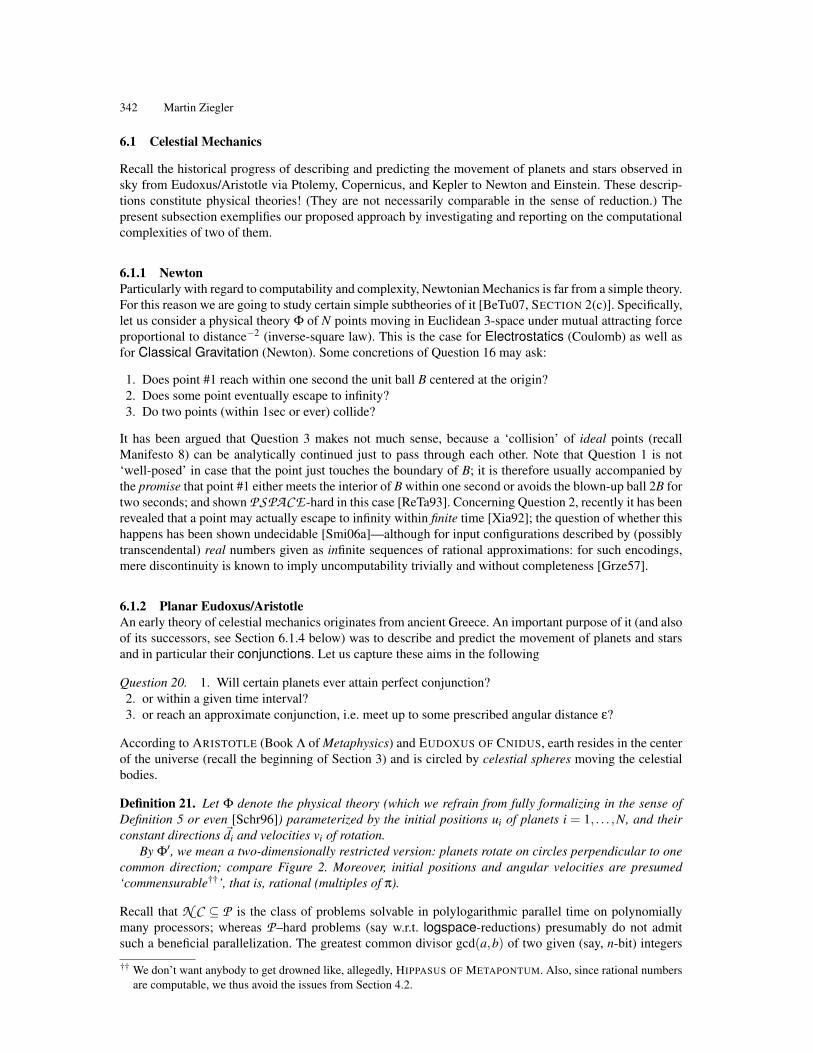
342 Martin Ziegler

6.1 Celestial Mechanics

Recall the historical progress of describing and predicting the movement of planets and stars observed insky from Eudoxus/Aristotle via Ptolemy, Copernicus, and Kepler to Newton and Einstein. These descrip-tions constitute physical theories! (They are not necessarily comparable in the sense of reduction.) Thepresent subsection exemplifies our proposed approach by investigating and reporting on the computationalcomplexities of two of them.

6.1.1 NewtonParticularly with regard to computability and complexity, Newtonian Mechanics is far from a simple theory.For this reason we are going to study certain simple subtheories of it [BeTu07, SECTION 2(c)]. Specifically,let us consider a physical theory Φ of N points moving in Euclidean 3-space under mutual attracting forceproportional to distance−2 (inverse-square law). This is the case for Electrostatics (Coulomb) as well asfor Classical Gravitation (Newton). Some concretions of Question 16 may ask:

1. Does point #1 reach within one second the unit ball B centered at the origin?2. Does some point eventually escape to infinity?3. Do two points (within 1sec or ever) collide?

It has been argued that Question 3 makes not much sense, because a ‘collision’ of ideal points (recallManifesto 8) can be analytically continued just to pass through each other. Note that Question 1 is not‘well-posed’ in case that the point just touches the boundary of B; it is therefore usually accompanied bythe promise that point #1 either meets the interior of B within one second or avoids the blown-up ball 2B fortwo seconds; and shown P SPACE-hard in this case [ReTa93]. Concerning Question 2, recently it has beenrevealed that a point may actually escape to infinity within finite time [Xia92]; the question of whether thishappens has been shown undecidable [Smi06a]—although for input configurations described by (possiblytranscendental) real numbers given as infinite sequences of rational approximations: for such encodings,mere discontinuity is known to imply uncomputability trivially and without completeness [Grze57].

6.1.2 Planar Eudoxus/AristotleAn early theory of celestial mechanics originates from ancient Greece. An important purpose of it (and alsoof its successors, see Section 6.1.4 below) was to describe and predict the movement of planets and starsand in particular their conjunctions. Let us capture these aims in the following

Question 20. 1. Will certain planets ever attain perfect conjunction?2. or within a given time interval?3. or reach an approximate conjunction, i.e. meet up to some prescribed angular distance ε?

According to ARISTOTLE (Book Λ of Metaphysics) and EUDOXUS OF CNIDUS, earth resides in the centerof the universe (recall the beginning of Section 3) and is circled by celestial spheres moving the celestialbodies.

Definition 21. Let Φ denote the physical theory (which we refrain from fully formalizing in the sense ofDefinition 5 or even [Schr96]) parameterized by the initial positions ui of planets i = 1, . . . ,N, and theirconstant directions ~di and velocities vi of rotation.

By Φ′, we mean a two-dimensionally restricted version: planets rotate on circles perpendicular to onecommon direction; compare Figure 2. Moreover, initial positions and angular velocities are presumed‘commensurable††’, that is, rational (multiples of π).

Recall that N C ⊆ P is the class of problems solvable in polylogarithmic parallel time on polynomiallymany processors; whereas P –hard problems (say w.r.t. logspace-reductions) presumably do not admitsuch a beneficial parallelization. The greatest common divisor gcd(a,b) of two given (say, n-bit) integers

†† We don’t want anybody to get drowned like, allegedly, HIPPASUS OF METAPONTUM. Also, since rational numbersare computable, we thus avoid the issues from Section 4.2.

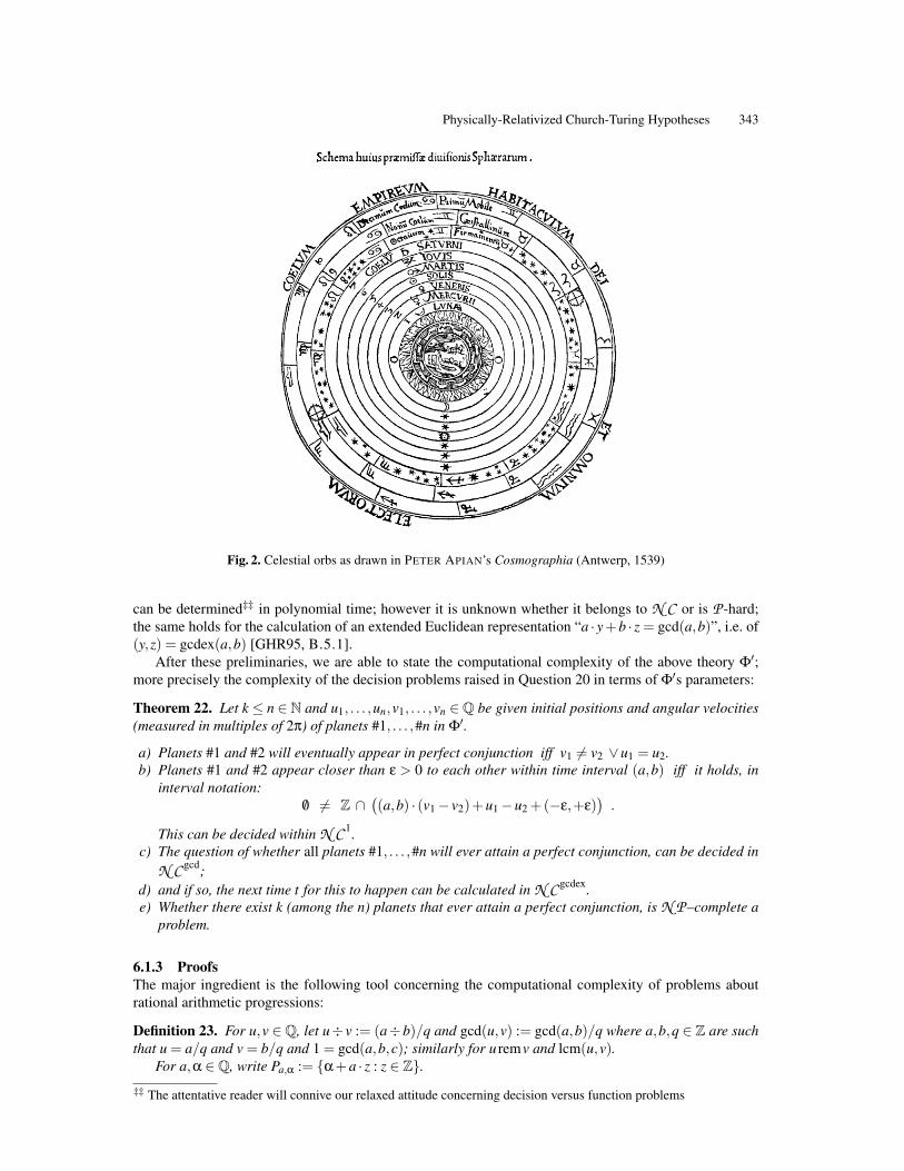
Physically-Relativized Church-Turing Hypotheses 343

Fig. 2. Celestial orbs as drawn in PETER APIAN’s Cosmographia (Antwerp, 1539)

can be determined‡‡ in polynomial time; however it is unknown whether it belongs to N C or is P -hard;the same holds for the calculation of an extended Euclidean representation “a · y+b · z = gcd(a,b)”, i.e. of(y,z) = gcdex(a,b) [GHR95, B.5.1].

After these preliminaries, we are able to state the computational complexity of the above theory Φ′;more precisely the complexity of the decision problems raised in Question 20 in terms of Φ′s parameters:

Theorem 22. Let k ≤ n ∈ N and u1, . . . ,un,v1, . . . ,vn ∈Q be given initial positions and angular velocities(measured in multiples of 2π) of planets #1, . . . ,#n in Φ′.

a) Planets #1 and #2 will eventually appear in perfect conjunction iff v1 6= v2 ∨u1 = u2.b) Planets #1 and #2 appear closer than ε > 0 to each other within time interval (a,b) iff it holds, in

interval notation:/0 6= Z ∩

((a,b) · (v1− v2)+u1−u2 +(−ε,+ε)

).

This can be decided within N C 1.c) The question of whether all planets #1, . . . ,#n will ever attain a perfect conjunction, can be decided in

N C gcd;d) and if so, the next time t for this to happen can be calculated in N C gcdex.e) Whether there exist k (among the n) planets that ever attain a perfect conjunction, is N P –complete a

problem.

6.1.3 ProofsThe major ingredient is the following tool concerning the computational complexity of problems aboutrational arithmetic progressions:

Definition 23. For u,v ∈Q, let u÷ v := (a÷b)/q and gcd(u,v) := gcd(a,b)/q where a,b,q ∈ Z are suchthat u = a/q and v = b/q and 1 = gcd(a,b,c); similarly for u remv and lcm(u,v).

For a,α ∈Q, write Pa,α := α+a · z : z ∈ Z.‡‡ The attentative reader will connive our relaxed attitude concerning decision versus function problems

344 Martin Ziegler

Lemma 24. a) Given a,α∈Q, the unique 0≤ α′ < a with Pa,α = Pa,α′ can be calculated as α′ := α remawithin complexity class N C 1.

b) Given a,α and b,β, the question whether Pa,α∩Pb,β = /0 can be decided in N C gcd

c) and, if so, (c,γ) with Pa,α∩Pb,β = Pc,γ can be calculated in N C gcdex.d) Items b) and c) extend from the intersection of two given arithmetic progressions to that of k.e) Given n,k and a1,α1, . . . ,an,αn, deciding whether some k among the arithmetic progressions P(i1) :=

Pai1 ,αi1, . . . ,P(ik) := Paik ,αik

have a non-empty common intersection, is N P –complete.

A result similar to the last item has been obtained in [MaHa94]. . .

Proof. a) Notice that Pa,α = Pa,α′⇔α−α′ ∈ Pa,0. Hence there exists exactly one such α′ in [0,a), namelyα′ = α rema. Moreover, integer division belongs to N C [BCH86,CDL01].

b) Observe that Pa,α∩Pb,β 6= /0 holds iff gcd(a,b) divides α−β. Indeed, the extended Euclidean algorithmthen yields z′1,z

′2 ∈Z with gcd(a,b)=−a ·z′1 +b ·z′2; then α−β =−a ·z1 +b ·z2 yields Pa,α 3α+a ·z1 =

β+b · z2 ∈ Pb,β. Conversely α+a · z1 = β+b · z2 ∈ Pa,α∩Pb,β implies that α−β =−a · z1 +b · z2 is amultiple of any (and in particular the greatest) common divisor of a and b.

c) Notice that c = lcm(a,b) = a ·b/gcd(a,b); according to the proof of b), γ := α+a · z1 will do, wherez1,z2 ∈ Z with α−β =−a · z1 +b · z2 result from the extended Euclidean algorithm applied to (a,b).

d) Notice thatx ∈ Pa1,α1 ∩·· ·∩Pak,αk ⇔ x≡ αi (mod ai), i = 1, . . . ,k . (2)

According to the Chinese Remainder Theorem, the latter system of congruences in turn admits sucha solution x iff gcd(ai,a j) divides αi−α j for all pairs (i, j).In order to calculate such an x, notice that a straight-forward iterative Pa1..k−1,α1..k−1 ∩Pak,αk fails as itdoes not parallelize well, and also the numbers calculated according to c) may double in length in eachof the k steps. Instead, combine the Pai,αi in a binary way first two tuples Pa2 j,2 j+1,α2 j,2 j+1 of adjacentones, then on to quadruples and so on. At logarithmic depth (=parallel time), this yields the desiredresult x =: α0 and a0 := lcm(a1, . . . ,ak) satisfying Pa0,α0 =

Tki=1 Pai,αi .

e) It is easy to guess i1, . . . , ik and, based on d), verify in polynomial time that P(i1)∩ . . .∩P(ik) 6= /0.We establish N P –hardness by reduction from Clique [GaJo79]: Given a graph G = ([n],E), choosen · (n−1)/2 pairwise coprime integers qi,` = q`,i ≥ 2, 1≤ i < `≤ n; for instance qi,` := pi+n·(`−1) willdo, where pm denotes the m-th prime number, found in time polynomial in n ≤ |〈G〉| (though not in|〈pm〉| ≈ logm+ loglogm) by simple exhaustive search. Then calculate ai := ∏ 6=i qi,` and observe thatgcd(ai,a j) = qi, j for i 6= j. Now start with α1 := 0 and iteratively for ` = 2,3, . . . ,n determine α` bysolving the following system of simultaneous congruences:

α` ≡

αi (mod qi,`) for (i, `) ∈ E1+αi (mod qi,`) for (i, `) 6∈ E , 1≤ i < ` (3)

Indeed, as the qi,` are pairwise coprime, the Chinese Remainder Theorem asserts the existence of asolution—computable in time polynomial in n, regarding that α` can be bounded by ∏i, j qi, j having apolynomial number of bits). The thus constructed vector (αi)i satisfies:

αi ≡ α j (mod gcd(ai,a j)︸ ︷︷ ︸=qi, j

) ⇔ (i, j) ∈ E

because, for (i, j) 6∈ E, Equation (3) implies αi ≡ α j+1 (mod qi, j).We claim that this mapping G 7→ (ai,αi : 1≤ i≤ n) constitutes the desired reduction: Indeed, accordingto Equation (2), any sub-collection P(i1), . . . ,P(ik) has non-empty intersection (i.e. a common elementx) iff αi` ≡ αi j (mod gcd(ai` ,ai j)), i.e., by our construction, iff (i`, i j) ∈ E; hence, cliques of G arein one-to-one correspondence with subcollections of intersecting arithmetic progressions. ut

Proof (Theorem 22). At time t, planet #i appears at angular position ui + t · vi mod 1; and an exact con-junction between #i and # j occurs whenever ui + t · vi = u j + t · v j + z for some z ∈ Z, that is iff

t ∈u j−ui

vi− v j+ z · 1

vi− v j

= P(i, j) := Pai, j ,αi, j where ai, j :=

1vi− v j

,αi, j :=u j−ui

vi− v j. (4)

Physically-Relativized Church-Turing Hypotheses 345

Therefore, planets #1, . . . ,#n attain a conjunction at some time t iff t ∈Tn

i=1 P(1,i). The existence of such tthus amounts to the non-emptiness of the joint intersection of arithmetic progressions and can be decided inthe claimed complexity according to Lemma 24b+d). Moreover, Lemma 24a+c+d) shows how to calculatethe smallest t.

Concerning N P –hardness claimed in Item f), we reduce from Lemma 24e): Given n arithmetic pro-gressions P(i) = Pai,αi , let ui := −αi ·ai, vi := 1/ai, and u0 := 0 =: v0. Then conjunctions between #0 and#i occur exactly at times t ∈ P(i); and P(i1), . . . ,P(ik) meet iff (and when/where) #0,#i1, . . . ,#ik do.

Approximate conjunction up to ε in time interval (u,v) means:

∃t ∈ (u,v) ∃z ∈ Z : (v2− v1)t +u2−u1 + z ∈ (−ε,+ε)

which is equivalent to Claim b). The boundaries of the interval (a,b) · (v1− v2)+ u1− u2 +(−ε,+ε) canbe calculated in N C 1. ut

6.1.4 General Eudoxus/Aristotle; Ptolemy, Copernicus, and KeplerProceeding from the restricted 2D theory Φ′ to Eudoxus/Aristotle’s full Φ obviously complicates the com-putational complexity of the above predictions; and it seems desirable to make that precise, e.g. with thehelp of [ACG93,GaOv95,BrKi98,CPPY06]. Moreover also Φ in turn had been refined: PTOLEMY intro-duced additional so-called epicycles and deferents located and rotating on the originally earth-centeredspheres. That extension (and its additional free parameters) allowed him to describe the observed planetarymotions more accurately. Copernicus relocated the spheres (and sub-spheres thereon) to be centered aroundthe sun rather than earth. And Kepler replaced them with ellipses in space. Again, the respective increasein complexity is worth-while investigating:

From an observer’s perspective located on earth, the planets’ 3D movements project down to curves.So, we are led to study the complexity of deciding whether and when such given curves, parameterizedby time, intersect. A first step is to decide (mathematically) whether these curves are of an algebraic ortranscendental nature, in order to choose the appropriate model of computation (Section 5.2). We pointout that even for problems which naturally involve transcendental numbers restricting the input to rationals(and handling them in the original Turing model), may turn out to admit surprising algorithmic treatment;see, e.g., [CCK*04] or [Zieg06, PROPOSITION 30]!

6.2 Opticks

There is an abundance of (physical theories giving) explanations for optical phenomena; cmp. e.g. TheBook of Optics by IBN AL-HAYTHAM (1021) or NEWTON’s book providing the title of this section. We arespecifically interested in the progression from geometric via Gaussian optics (taking into account disper-sion) over HUYGENS and FOURIER (i.e. diffractive, wave) optics to Maxwell’s theory of electromagnetismand even to quantum and quantum field theories (describing e.g. Raman/Rayleigh and other kinds of scat-tering). Note that this sequence of optical theories Φi reflects their historical succession, but not a logicalone in the sense that Φi+1 ‘implies’ (and hence is computationally at least as hard as) Φi.

Our purpose is to explore more thoroughly the computational complexities of these theories. Their com-putational relations may happen to be similar, unrelated, or just opposite to their historical ones! Considerfor example geometric optics versus Electrodynamics:

6.2.1 Geometric Optics considers light rays as ideal geometric objects, i.e., of infinitesimal sectionproceeding instantaneously and straightly until hitting a, say, mirror. Now depending on the kind of mirrors(straight or curved, with rational or algebraic parameters) and the availability of further optical devices(lenses, beam splitters), [RTY94] has developed a fairly exhaustive (although not entirely sound) taxonomyof the induced computational complexities of ray tracing ranging from P SPACE to undecidable!

6.2.2 Electrodynamics on the other hand treats light as a vector-valued wave obeying a system of linearpartial differential equations named after JAMES CLERK MAXWELL. From given initial conditions, theirsolution is computable even over real numbers [WeZh99]!

346 Martin Ziegler

6.3 Quantum Mechanics

The advent of Quantum Computing is based on the hope to surpass the strong CTH, i.e. to build computersnot polynomial-time equivalent to a Turing machine. It originates back to RICHARD P. FEYNMAN’s famousLectures on Computation [FLS05] and has, in connection with the work of PETER SHOR’s, become afashionable yet speculative [Kie03a] research topic lacking a general picture[Myrv95,Smi99a,Breu02,Zieg05,WeZh06,Smi06b].

Speaking in complexity theoretic terms, the (as usual highly ambiguous) question raised by the strongCTH (recall Section 1.2) asks to locate the computational power of QM somewhere among or betweenP , P IntegerFactorization, N P , and ∆2. Further, it is worth-while to explore how the answer depends on theunderlying Hamiltonians being un-/bounded as indicated in [PERi89, CHAPTER 3]?

For a sound and more definite investigation, our approach suggests to start exploring well-specifiedsub- and pre-theories of QM. These may, e.g., be the BOHR-SOMMERFELD theory of classical electronorbits with integral action-angle conditions.

Another promising direction considers computational capabilities and complexity of Quantum Logic:

6.3.1 Quantum Logic arises as an abstraction of the purely algebraic structure exhibited by the collec-tion of effect operators (i.e. projections onto closed subspaces) introduced by G. LUDWIG on a Hilbertspace, that are certain quantum mechanical observables; cf. e.g. [Birk67,Svoz98]. This discipline has flour-ished from the comparison with (i.e. systematic and thorough investigation of similarities and differencesto) Boolean logic:

For a finite-dimensional Hilbert space H ∈ RN ,CN, variables a,b,c denote any linear subspace ofH , including 0 := 0 and 1 := H itself; moreover let a∧ b := a∩ b, ¬a := a⊥, a ≤ b :⇔ a ⊆ b, anda∨b := linspan(a∪b). These operations indeed extend the classical Boolean connectives in that the latterare recovered by restricting to 0 and 1, i.e. to N = 1. The collection of linear subspaces of H , equippedwith (∨,∧,¬,≤), forms a lattice; which however violates distributivity: Formula

(a ∨ b) ∧ (a∨b⊥) ∧ (a⊥∨b) ∧ (a⊥∨b⊥) = 1 (5)

is not classically satisfiable but does, for N ≥ 2 admit satisfying assignment a := linspan(1

0

)and b :=

linspan(1

1

). Nevertheless it has recently been proved that the satisfiability problem for such quantum logic

formula is decidable [DHMW05, SECTION 3] and raised the question on the algorithmic complexity ofthis problem. We make the following

Proposition 25. For N ∈ N, let

QLN :=〈ϕ〉 : formula ϕ in m variables

admits subspaces a1, . . . ,am ⊆ CN such that ϕ(a1, . . . ,am) 6= 0

. (6)

a) QL1 is N P –complete,b) For each N ≤M, QLN 4 QLM . In particular, QLM is N P –hard.c) For fixed N (or with N given unary), QLN ∈N P C.

That is, QLN can be decided by a nondeterministic BSS machine in time polynomial in N and m; recallSection 5.2 (and cmp. also [CuGr97] for BSS computation on binary inputs).

Proof. Item a) is of course the famous Cook-Levin Theorem. Item b) follows from QLN ⊆QLM [DHMW05,LEMMA 5]. Concerning Item c), a BSS machine may first ‘guess’ dimensions 0 ≤ d1, . . . ,dm ≤ N of, andorthogonal bases for, subspaces a1, . . . ,am; then use linear algebra to obtain an orthogonal basis for thevalue ϕ(a1, . . . ,am). ut

More generally, we envision a theory of computational complexity similar to that of Boolean circuits[Papa94, SECTIONS 4.3 and 11.4] with classical gates replaced by such quantum logic ones (cmp. [Ying05]for quantum logic finite automata). Note that this is different from (well-studied) ‘standard’ quantum com-plexity theory and the quantum circuit model it is based on:

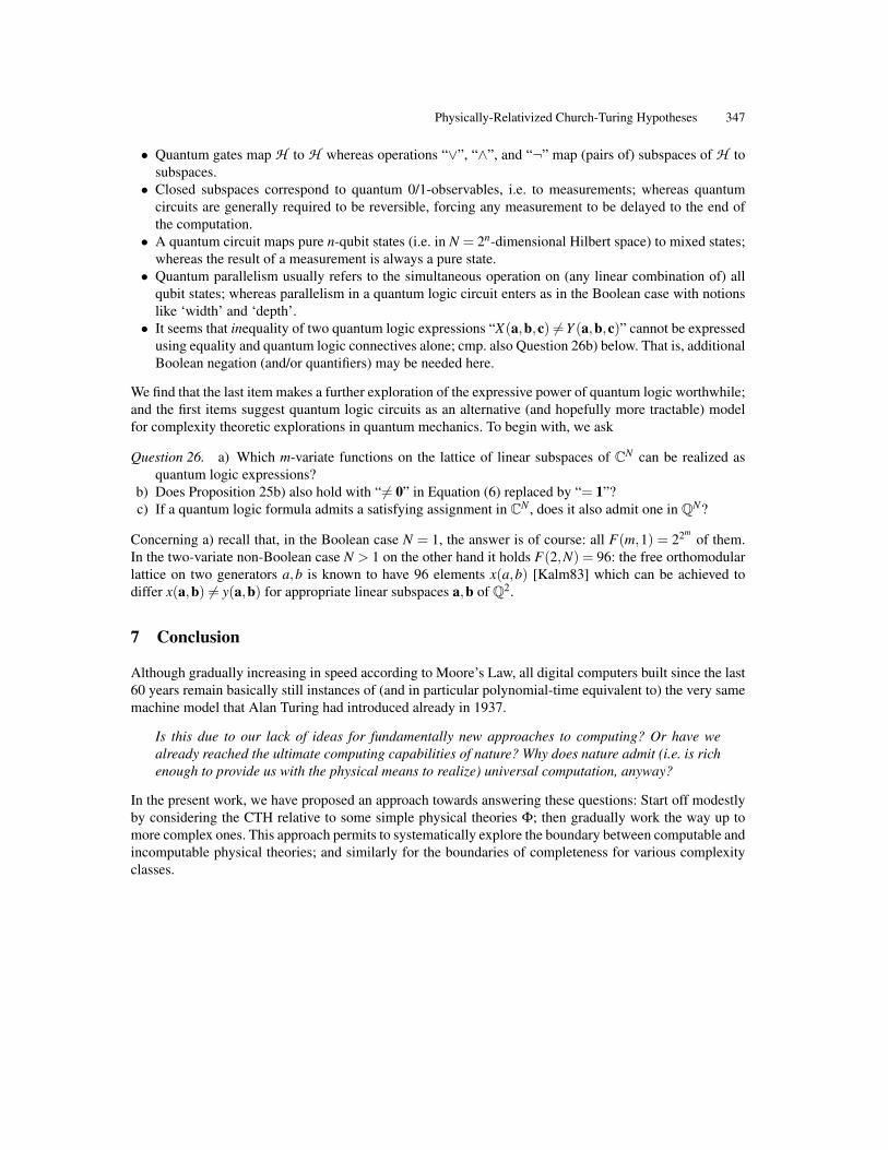
Physically-Relativized Church-Turing Hypotheses 347

• Quantum gates map H to H whereas operations “∨”, “∧”, and “¬” map (pairs of) subspaces of H tosubspaces.

• Closed subspaces correspond to quantum 0/1-observables, i.e. to measurements; whereas quantumcircuits are generally required to be reversible, forcing any measurement to be delayed to the end ofthe computation.

• A quantum circuit maps pure n-qubit states (i.e. in N = 2n-dimensional Hilbert space) to mixed states;whereas the result of a measurement is always a pure state.

• Quantum parallelism usually refers to the simultaneous operation on (any linear combination of) allqubit states; whereas parallelism in a quantum logic circuit enters as in the Boolean case with notionslike ‘width’ and ‘depth’.

• It seems that inequality of two quantum logic expressions “X(a,b,c) 6= Y (a,b,c)” cannot be expressedusing equality and quantum logic connectives alone; cmp. also Question 26b) below. That is, additionalBoolean negation (and/or quantifiers) may be needed here.

We find that the last item makes a further exploration of the expressive power of quantum logic worthwhile;and the first items suggest quantum logic circuits as an alternative (and hopefully more tractable) modelfor complexity theoretic explorations in quantum mechanics. To begin with, we ask

Question 26. a) Which m-variate functions on the lattice of linear subspaces of CN can be realized asquantum logic expressions?

b) Does Proposition 25b) also hold with “6= 0” in Equation (6) replaced by “= 1”?c) If a quantum logic formula admits a satisfying assignment in CN , does it also admit one in QN?

Concerning a) recall that, in the Boolean case N = 1, the answer is of course: all F(m,1) = 22mof them.

In the two-variate non-Boolean case N > 1 on the other hand it holds F(2,N) = 96: the free orthomodularlattice on two generators a,b is known to have 96 elements x(a,b) [Kalm83] which can be achieved todiffer x(a,b) 6= y(a,b) for appropriate linear subspaces a,b of Q2.

7 Conclusion

Although gradually increasing in speed according to Moore’s Law, all digital computers built since the last60 years remain basically still instances of (and in particular polynomial-time equivalent to) the very samemachine model that Alan Turing had introduced already in 1937.

Is this due to our lack of ideas for fundamentally new approaches to computing? Or have wealready reached the ultimate computing capabilities of nature? Why does nature admit (i.e. is richenough to provide us with the physical means to realize) universal computation, anyway?

In the present work, we have proposed an approach towards answering these questions: Start off modestlyby considering the CTH relative to some simple physical theories Φ; then gradually work the way up tomore complex ones. This approach permits to systematically explore the boundary between computable andincomputable physical theories; and similarly for the boundaries of completeness for various complexityclasses.

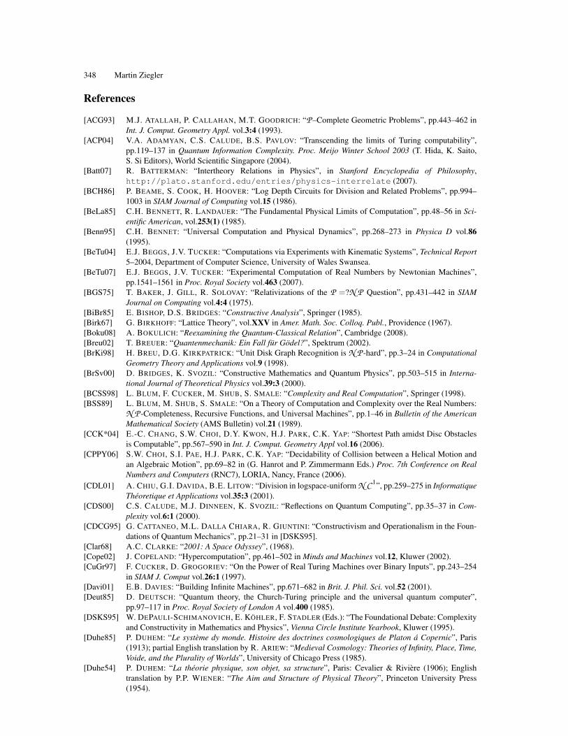
348 Martin Ziegler

References

[ACG93] M.J. ATALLAH, P. CALLAHAN, M.T. GOODRICH: “P –Complete Geometric Problems”, pp.443–462 inInt. J. Comput. Geometry Appl. vol.3:4 (1993).

[ACP04] V.A. ADAMYAN, C.S. CALUDE, B.S. PAVLOV: “Transcending the limits of Turing computability”,pp.119–137 in Quantum Information Complexity. Proc. Meijo Winter School 2003 (T. Hida, K. Saito,S. Si Editors), World Scientific Singapore (2004).

[Batt07] R. BATTERMAN: “Intertheory Relations in Physics”, in Stanford Encyclopedia of Philosophy,http://plato.stanford.edu/entries/physics-interrelate (2007).

[BCH86] P. BEAME, S. COOK, H. HOOVER: “Log Depth Circuits for Division and Related Problems”, pp.994–1003 in SIAM Journal of Computing vol.15 (1986).

[BeLa85] C.H. BENNETT, R. LANDAUER: “The Fundamental Physical Limits of Computation”, pp.48–56 in Sci-entific American, vol.253(1) (1985).

[Benn95] C.H. BENNET: “Universal Computation and Physical Dynamics”, pp.268–273 in Physica D vol.86(1995).

[BeTu04] E.J. BEGGS, J.V. TUCKER: “Computations via Experiments with Kinematic Systems”, Technical Report5–2004, Department of Computer Science, University of Wales Swansea.

[BeTu07] E.J. BEGGS, J.V. TUCKER: “Experimental Computation of Real Numbers by Newtonian Machines”,pp.1541–1561 in Proc. Royal Society vol.463 (2007).

[BGS75] T. BAKER, J. GILL, R. SOLOVAY: “Relativizations of the P =?N P Question”, pp.431–442 in SIAMJournal on Computing vol.4:4 (1975).

[BiBr85] E. BISHOP, D.S. BRIDGES: “Constructive Analysis”, Springer (1985).[Birk67] G. BIRKHOFF: “Lattice Theory”, vol.XXV in Amer. Math. Soc. Colloq. Publ., Providence (1967).[Boku08] A. BOKULICH: “Reexamining the Quantum-Classical Relation”, Cambridge (2008).[Breu02] T. BREUER: “Quantenmechanik: Ein Fall für Gödel?”, Spektrum (2002).[BrKi98] H. BREU, D.G. KIRKPATRICK: “Unit Disk Graph Recognition is N P -hard”, pp.3–24 in Computational

Geometry Theory and Applications vol.9 (1998).[BrSv00] D. BRIDGES, K. SVOZIL: “Constructive Mathematics and Quantum Physics”, pp.503–515 in Interna-

tional Journal of Theoretical Physics vol.39:3 (2000).[BCSS98] L. BLUM, F. CUCKER, M. SHUB, S. SMALE: “Complexity and Real Computation”, Springer (1998).[BSS89] L. BLUM, M. SHUB, S. SMALE: “On a Theory of Computation and Complexity over the Real Numbers:

N P -Completeness, Recursive Functions, and Universal Machines”, pp.1–46 in Bulletin of the AmericanMathematical Society (AMS Bulletin) vol.21 (1989).

[CCK*04] E.-C. CHANG, S.W. CHOI, D.Y. KWON, H.J. PARK, C.K. YAP: “Shortest Path amidst Disc Obstaclesis Computable”, pp.567–590 in Int. J. Comput. Geometry Appl vol.16 (2006).

[CPPY06] S.W. CHOI, S.I. PAE, H.J. PARK, C.K. YAP: “Decidability of Collision between a Helical Motion andan Algebraic Motion”, pp.69–82 in (G. Hanrot and P. Zimmermann Eds.) Proc. 7th Conference on RealNumbers and Computers (RNC7), LORIA, Nancy, France (2006).

[CDL01] A. CHIU, G.I. DAVIDA, B.E. LITOW: “Division in logspace-uniform N C 1”, pp.259–275 in InformatiqueThéoretique et Applications vol.35:3 (2001).

[CDS00] C.S. CALUDE, M.J. DINNEEN, K. SVOZIL: “Reflections on Quantum Computing”, pp.35–37 in Com-plexity vol.6:1 (2000).

[CDCG95] G. CATTANEO, M.L. DALLA CHIARA, R. GIUNTINI: “Constructivism and Operationalism in the Foun-dations of Quantum Mechanics”, pp.21–31 in [DSKS95].

[Clar68] A.C. CLARKE: “2001: A Space Odyssey”, (1968).[Cope02] J. COPELAND: “Hypercomputation”, pp.461–502 in Minds and Machines vol.12, Kluwer (2002).[CuGr97] F. CUCKER, D. GROGORIEV: “On the Power of Real Turing Machines over Binary Inputs”, pp.243–254

in SIAM J. Comput vol.26:1 (1997).[Davi01] E.B. DAVIES: “Building Infinite Machines”, pp.671–682 in Brit. J. Phil. Sci. vol.52 (2001).[Deut85] D. DEUTSCH: “Quantum theory, the Church-Turing principle and the universal quantum computer”,

pp.97–117 in Proc. Royal Society of London A vol.400 (1985).[DSKS95] W. DEPAULI-SCHIMANOVICH, E. KÖHLER, F. STADLER (Eds.): “The Foundational Debate: Complexity

and Constructivity in Mathematics and Physics”, Vienna Circle Institute Yearbook, Kluwer (1995).[Duhe85] P. DUHEM: “Le système dy monde. Histoire des doctrines cosmologiques de Platon á Copernic”, Paris

(1913); partial English translation by R. ARIEW: “Medieval Cosmology: Theories of Infinity, Place, Time,Voide, and the Plurality of Worlds”, University of Chicago Press (1985).

[Duhe54] P. DUHEM: “La théorie physique, son objet, sa structure”, Paris: Cevalier & Rivière (1906); Englishtranslation by P.P. WIENER: “The Aim and Structure of Physical Theory”, Princeton University Press(1954).

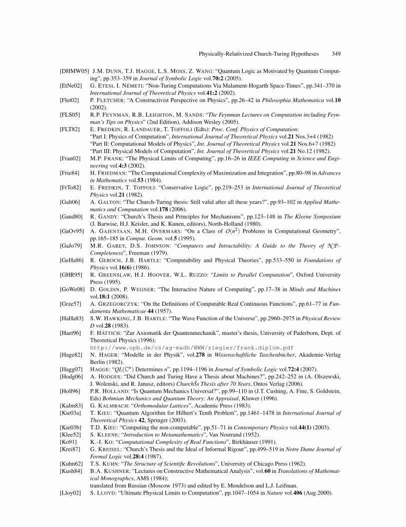
Physically-Relativized Church-Turing Hypotheses 349

[DHMW05] J.M. DUNN, T.J. HAGGE, L.S. MOSS, Z. WANG: “Quantum Logic as Motivated by Quantum Comput-ing”, pp.353–359 in Journal of Symbolic Logic vol.70:2 (2005).

[EtNe02] G. ETESI, I. NÉMETI: “Non-Turing Computations Via Malament-Hogarth Space-Times”, pp.341–370 inInternational Journal of Theoretical Physics vol.41:2 (2002).

[Flet02] P. FLETCHER: “A Constructivist Perspective on Physics”, pp.26–42 in Philosophia Mathematica vol.10(2002).

[FLS05] R.P. FEYNMAN, R.B. LEIGHTON, M. SANDS: “The Feynman Lectures on Computation including Feyn-man’s Tips on Physics” (2nd Edition), Addison Wesley (2005).

[FLT82] E. FREDKIN, R. LANDAUER, T. TOFFOLI (Edts): Proc. Conf. Physics of Computation:“Part I: Physics of Computation”, International Journal of Theoretical Physics vol.21 Nos.3+4 (1982)“Part II: Computational Models of Physics”, Int. Journal of Theoretical Physics vol.21 Nos.6+7 (1982)“Part III: Physical Models of Computation”, Int. Journal of Theoretical Physics vol.21 No.12 (1982).

[Fran02] M.P. FRANK: “The Physical Limits of Computing”, pp.16–26 in IEEE Computing in Science and Engi-neering vol.4:3 (2002).

[Frie84] H. FRIEDMAN: “The Computational Complexity of Maximization and Integration”, pp.80–98 in Advancesin Mathematics vol.53 (1984).

[FrTo82] E. FREDKIN, T. TOFFOLI: “Conservative Logic”, pp.219–253 in International Journal of TheoreticalPhysics vol.21 (1982).

[Galt06] A. GALTON: “The Church-Turing thesis: Still valid after all these years?”, pp.93–102 in Applied Mathe-matics and Computation vol.178 (2006).

[Gand80] R. GANDY: “Church’s Thesis and Principles for Mechanisms”, pp.123–148 in The Kleene Symposium(J. Barwise, H.J. Keisler, and K. Kunen, editors), North-Holland (1980).

[GaOv95] A. GAJENTAAN, M.H. OVERMARS: “On a Class of O(n2) Problems in Computational Geometry”,pp.165–185 in Comput. Geom. vol.5 (1995).

[GaJo79] M.R. GAREY, D.S. JOHNSON: “Computers and Intractability: A Guide to the Theory of N P –Completeness”, Freeman (1979).

[GeHa86] R. GEROCH, J.B. HARTLE: “Computability and Physical Theories”, pp.533–550 in Foundations ofPhysics vol.16(6) (1986).

[GHR95] R. GREENSLAW, H.J. HOOVER, W.L. RUZZO: “Limits to Parallel Computation”, Oxford UniversityPress (1995).

[GoWe08] D. GOLDIN, P. WEGNER: “The Interactive Nature of Computing”, pp.17–38 in Minds and Machinesvol.18:1 (2008).

[Grze57] A. GRZEGORCZYK: “On the Definitions of Computable Real Continuous Functions”, pp.61–77 in Fun-damenta Mathematicae 44 (1957).

[HaHa83] S.W. HAWKING, J.B. HARTLE: “The Wave Function of the Universe”, pp.2960–2975 in Physical ReviewD vol.28 (1983).

[Haet96] F. HÄTTICH: “Zur Axiomatik der Quantenmechanik”, master’s thesis, University of Paderborn, Dept. ofTheoretical Physics (1996);http://www.upb.de/cs/ag-madh/WWW/ziegler/frank.diplom.pdf

[Hage82] N. HAGER: “Modelle in der Physik”, vol.278 in Wissenschaftliche Taschenbücher, Akademie-VerlagBerlin (1982).

[Hagg07] HAGGE: “QL(Cn) Determines n”, pp.1194–1196 in Journal of Symbolic Logic vol.72:4 (2007).[Hodg06] A. HODGES: “Did Church and Turing Have a Thesis about Machines?”, pp.242–252 in (A. Olszewski,

J. Wolenski, and R. Janusz, editors) ChurchŠs Thesis after 70 Years, Ontos Verlag (2006).[Holl96] P.R. HOLLAND: “Is Quantum Mechanics Universal?”, pp.99–110 in (J.T. Cushing, A. Fine, S. Goldstein,

Eds) Bohmian Mechanics and Quantum Theory: An Appraisal, Kluwer (1996).[Kalm83] G. KALMBACH: “Orthomodular Lattices”, Academic Press (1983).[Kie03a] T. KIEU: “Quantum Algorithm for Hilbert’s Tenth Problem”, pp.1461–1478 in International Journal of

Theoretical Physics 42, Springer (2003).[Kie03b] T.D. KIEU: “Computing the non-computable”, pp.51–71 in Contemporary Physics vol.44(1) (2003).[Klee52] S. KLEENE: “Introduction to Metamathematics”, Van Nostrand (1952).[Ko91] K.-I. KO: “Computational Complexity of Real Functions”, Birkhäuser (1991).[Krei87] G. KREISEL: “Church’s Thesis and the Ideal of Informal Rigour”, pp.499–519 in Notre Dame Journal of

Formal Logic vol.28:4 (1987).[Kuhn62] T.S. KUHN: “The Structure of Scientific Revolutions”, University of Chicago Press (1962).[Kush84] B.A. KUSHNER: “Lectures on Constructive Mathematical Analysis”, vol.60 in Translations of Mathemat-

ical Monographcs, AMS (1984);translated from Russian (Moscow 1973) and edited by E. Mendelson and L.J. Leifman.

[Lloy02] S. LLOYD: “Ultimate Physical Limits to Computation”, pp.1047–1054 in Nature vol.406 (Aug.2000).

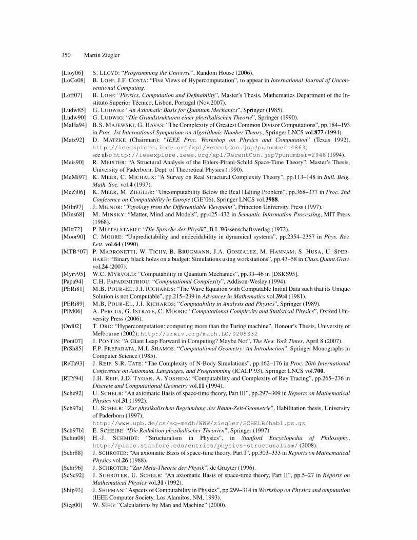
350 Martin Ziegler

[Lloy06] S. LLOYD: “Programming the Universe”, Random House (2006).[LoCo08] B. LOFF, J.F. COSTA: “Five Views of Hypercomputation”, to appear in International Journal of Uncon-

ventional Computing.[Loff07] B. LOFF: “Physics, Computation and Definability”, Master’s Thesis, Mathematics Department of the In-

stituto Superior Técnico, Lisbon, Portugal (Nov.2007).[Ludw85] G. LUDWIG: “An Axiomatic Basis for Quantum Mechanics”, Springer (1985).[Ludw90] G. LUDWIG: “Die Grundstrukturen einer physikalischen Theorie”, Springer (1990).[MaHa94] B.S. MAJEWSKI, G. HAVAS: “The Complexity of Greatest Common Divisor Computations”, pp.184–193

in Proc. 1st International Symposium on Algorithmic Number Theory, Springer LNCS vol.877 (1994).[Matz92] D. MATZKE (Chairman): “IEEE Proc. Workshop on Physics and Computation” (Texas 1992),

http://ieeexplore.ieee.org/xpl/RecentCon.jsp?punumber=4863;see also http://ieeexplore.ieee.org/xpl/RecentCon.jsp?punumber=2948 (1994).

[Meis90] R. MEISTER: “A Structural Analysis of the Ehlers-Pirani-Schild Space-Time Theory”, Master’s Thesis,University of Paderborn, Dept. of Theoretical Physics (1990).

[MeMi97] K. MEER, C. MICHAUX: “A Survey on Real Structural Complexity Theory”, pp.113–148 in Bull. Belg.Math. Soc. vol.4 (1997).

[MeZi06] K. MEER, M. ZIEGLER: “Uncomputability Below the Real Halting Problem”, pp.368–377 in Proc. 2ndConference on Computability in Europe (CiE’06), Springer LNCS vol.3988.

[Miln97] J. MILNOR: “Topology from the Differentiable Viewpoint”, Princeton University Press (1997).[Mins68] M. MINSKY: “Matter, Mind and Models”, pp.425–432 in Semantic Information Processing, MIT Press

(1968).[Mitt72] P. MITTELSTAEDT: “Die Sprache der Physik”, B.I. Wissenschaftsverlag (1972).[Moor90] C. MOORE: “Unpredictability and undecidability in dynamical systems”, pp.2354–2357 in Phys. Rev.

Lett. vol.64 (1990).[MTB*07] P. MARRONETTI, W. TICHY, B. BRÜGMANN, J.A. GONZALEZ, M. HANNAM, S. HUSA, U. SPER-

HAKE: “Binary black holes on a budget: Simulations using workstations”, pp.43–58 in Class.Quant.Grav.vol.24 (2007).

[Myrv95] W.C. MYRVOLD: “Computability in Quantum Mechanics”, pp.33–46 in [DSKS95].[Papa94] C.H. PAPADIMITRIOU: “Computational Complexity”, Addison-Wesley (1994).[PERi81] M.B. POUR-EL, J.I. RICHARDS: “The Wave Equation with Computable Initial Data such that its Unique

Solution is not Computable”, pp.215–239 in Advances in Mathematics vol.39:4 (1981).[PERi89] M.B. POUR-EL, J.I. RICHARDS: “Computability in Analysis and Physics”, Springer (1989).[PIM06] A. PERCUS, G. ISTRATE, C. MOORE: “Computational Complexity and Statistical Physics”, Oxford Uni-

versity Press (2006).[Ord02] T. ORD: “Hypercomputation: computing more than the Turing machine”, Honour’s Thesis, University of

Melbourne (2002); http://arxiv.org/math.LO/0209332[Pont07] J. PONTIN: “A Giant Leap Forward in Computing? Maybe Not”, The New York Times, April 8 (2007).[PrSh85] F.P. PREPARATA, M.I. SHAMOS: “Computational Geometry: An Introduction”, Springer Monographs in

Computer Science (1985).[ReTa93] J. REIF, S.R. TATE: “The Complexity of N-Body Simulations”, pp.162–176 in Proc. 20th International

Conference on Automata, Languages, and Programming (ICALP’93), Springer LNCS vol.700.[RTY94] J.H. REIF, J.D. TYGAR, A. YOSHIDA: “Computability and Complexity of Ray Tracing”, pp.265–276 in

Discrete and Computational Geometry vol.11 (1994).[Sche92] U. SCHELB: “An axiomatic Basis of space-time theory, Part III”, pp.297–309 in Reports on Mathematical

Physics vol.31 (1992).[Sch97a] U. SCHELB: “Zur physikalischen Begründung der Raum-Zeit-Geometrie”, Habilitation thesis, University

of Paderborn (1997);http://www.upb.de/cs/ag-madh/WWW/ziegler/SCHELB/hab1.ps.gz

[Sch97b] E. SCHEIBE: “Die Reduktion physikalischer Theorien”, Springer (1997).[Schm08] H.-J. SCHMIDT: “Structuralism in Physics”, in Stanford Encyclopedia of Philosophy,

http://plato.stanford.edu/entries/physics-structuralism/ (2008).[Schr88] J. SCHRÖTER: “An axiomatic Basis of space-time theory, Part I”, pp.303–333 in Reports on Mathematical

Physics vol.26 (1988).[Schr96] J. SCHRÖTER: “Zur Meta-Theorie der Physik”, de Gruyter (1996).[ScSc92] J. SCHRÖTER, U. SCHELB: “An axiomatic Basis of space-time theory, Part II”, pp.5–27 in Reports on

Mathematical Physics vol.31 (1992).[Ship93] J. SHIPMAN: “Aspects of Computability in Physics”, pp.299–314 in Workshop on Physics and omputation

(IEEE Computer Society, Los Alamitos, NM, 1993).[Sieg00] W. SIEG: “Calculations by Man and Machine” (2000).

Physically-Relativized Church-Turing Hypotheses 351

[Smi99a] W.D. SMITH: “Church’s Thesis meets Quantum Mechanics”, pre-print (1999);http://www.math.temple.edu/ wds/homepage/churchq.ps

[Smi99b] W.D. SMITH: “History of «Church’s Theses» and a Manifesto on Converting Physics into a RigorousAlgorithmic Discipline”, pre-print (1999);http://www.math.temple.edu/ wds/homepage/churchhist.ps

[Smi06a] W.D. SMITH: “Church’s Thesis meets the N-Body Problem”, pp.154–183 in Applied Mathematics andComputation vol.178 (2006).

[Smi06b] W.D. SMITH: “Three counterexamples refuting Kieu’s plan for «quantum adiabatic hypercomputation»and some uncomputable quantum mechanical tasks”, pp.184–193 in J. Applied Mathematics and Compu-tation vol.178 (2006).

[Snee71] J.D. SNEED: “The Logical Structure of Mathematical Physics”, Reidel Dordrecht (1971).[Steg79] W. STEGMÜLLER: “The Structuralist View of Theories”, Springer (1979).[Steg86] W. STEGMÜLLER: “Theorie und Erfahrung”, vol.II part.F in Probleme und Resultate der Wissenschafts-

theorie und Analytischen Philosophie, Springer Studienausgabe (1986).[Stoe95] M. STÖLZNER: “Levels of Physical Theories”, pp.47–64 in [DSKS95].[StSt71] A. STRUGATSKY, B. STRUGATSKY: “Roadside Picnic” (1971).[Svoz93] K. SVOZIL: “Randomness and Undecidability in Physics”, World Scientific (1993).[Svoz95] K. SVOZIL: “A Constructivist Manifesto for the Physical Sciences – Constructive Re-Interpretation of

Physical Undecidability”, pp.65–88 in [DSKS95].[Svoz97] K. SVOZIL: “Linear Chaos Via Paradoxical Set Decompositions”, pp.785–793 in Chaos, Solitons, and

Fractals vol.7:5 (1996).[Svoz98] K. SVOZIL: “Quantum Logic”, Springer (1998).[Svoz05] K. SVOZIL: “Computational universes”, pp.845–859 in Chaos, Solitons and Fractals vol.25:4 (2005).[Svoz06] K. SVOZIL: “Physics and metaphysics look at computation”, pp.491–517 in Church’s Thesis after 70

Years (A. Olszewski, J. Wolenski, R. Janusz Edts.), Ontos (2006).[Svoz07] K. SVOZIL: “Omega and the Time Evolution of the n-Body Problem”, pp.231–236 in Randomness and

Complexity, from Leibniz to Chaitin (C.S. Calude Edt.), World Scientific (2007).[Turi36] A.M. TURING: “On Computable Numbers, with an Application to the Entscheidungsproblem”, pp.230–

265 in Proc. London Math. Soc. vol.42(2) (1936).[TuZu00] J.V. TUCKER, J.I. ZUCKER: “Computable functions and semicomputable sets on many-sorted algebras”,

pp.317–523 in Handbook of Logic in Computer Science vol.5 (S. Abramsky, D.M. Gabbay, T.S.E. May-baum Edts), Oxford Science Publications (2000).

[Yao03] A.C.-C. YAO: “Classical Physics and the Church-Turing Thesis”, pp.100–105 in Journal of the Associa-tion for Computing Machinery vol.50(1) (2003).

[Wein94] S. WEINBERG: “Dreams of a Final Theory: The Scientist’s Search for the Ultimate Laws of Nature”,Vintage (1994).

[Weiz85] C.F. VON WEIZSÄCKER: “Das Gefüge der Theorien”, Kapitel 6 in Aufbau der Physik, Carl Hanser (1985).[WeZh99] K. WEIHRAUCH, N. ZHONG: “The Wave Propagator Is Turing Computable”, pp.697–707 in Proc. 26th

International Colloquium on Automata, Languages and Programming (ICALP 1999), Springer LNCSvol.1644.

[WeZh02] K. WEIHRAUCH, N. ZHONG: “Is wave propagation computable or can wave computers beat the turingmachine?”, pp.312–332 in Proc. London Mathematical Society vol.85:2 (2002).

[WeZh06] K. WEIHRAUCH, N. ZHONG: “Computing Schrödinger propagators on Type-2 Turing machines”,pp.918–935 in Journal of Complexity vol.22:6 (2006).

[Wolf85] S. WOLFRAM: “Undecidability and Intractability in Theoretical Physics”, pp.735–738 in Physical ReviewLetters vol.54:8 (1985).

[Xia92] Z. XIA: “The Existence of Noncollision Singularities in the N-Body Problem”, pp.411–468 in Ann. Math.vol.135:3 (1992).

[Ying05] M. YING: “A Theory of Computation Based on Quantum Logic (I)”, pp.134–207 in Theoretical ComputerScience vol.344 (2005).

[Zieg05] M. ZIEGLER: “Computational Power of Infinite Quantum Parallelism”, pp.2057–2071 in InternationalJournal of Theoretical Physics vol.44:11 (2005).

[Zieg06] M. ZIEGLER: “Effectively Open Real Functions”, pp.827–849 in Journal of Complexity vol.22 (2006).[Zieg08] M. ZIEGLER: “(A Meta-Theory of) Physics and Computation”, p.145 in Verhandlungen der Deutschen

Physikalischen Gesellschaft (DPG), Feb.2008.[Zuse06] “Is the Universe a Computer? From Konrad Zuse’s Invention of the Computer to

his «Calculating Space» to Quantum Computing”, Symposium under the patronageof Dr. Annette Schavan, Federal Minister of Education and Research (Nov. 2006).http://www.gi-ev.de/regionalgruppen/berlin/download/veranstaltungen/ist_das_universum_flyer.pdf

Author Index

Adamatzki, AndrewAndreka, HajnalBeggs, EdwinBoker, UdiBournez, OlivierBrukner, CaslavBuescu, JorgeCampagnolo, Manuel LameirasChassaing, PhilippeCohen, JohanneCooper, S. Barryda Costa, Newton C. A.Delvenne, Jean-CharlesDershowitz, NachumDoria, Francisco AntonioDurand-Lose, JeromeGerin, LucasGorecka, J. N.

Gorecki, JerzyGraca, DanielHogarth, MarkIgarashi, Y.Koegler, XavierNaughton, Thomas J.Nemeti, IstvanNemeti, PeterStannett, MikeSvozil, KarlTkadlec, JosefThompson, B. C.Tucker, John V.Velupillai, K. VelaWoods, DamienZiegler, MartinZucker, Jeffery

352