CBN tool flank wear modelling using Hybrid Neural Network

Int. J. Mechatronics and Manufacturing Systems, Vol. 1, No. 1, 2008 83

Copyright © 2008 Inderscience Enterprises Ltd.

CBN tool flank wear modelling using Hybrid Neural Network

Xiaoyu Wang and Yong Huang* Department of Mechanical Engineering, Clemson University, Clemson, SC 29634-0921, USA E-mail: [email protected] E-mail: [email protected] *Corresponding author

Nhan Nguyen and Kalmanje Krishnakumar Intelligent Systems Division, NASA Ames Research Center, Moffett Field, CA 94035, USA E-mail: [email protected] E-mail: [email protected]

Abstract: Accurate tool wear modelling is indispensable for successful hard turning technology implementation. In this study, a Hybrid Neural Network-based modelling approach, which integrates an analytical tool wear model and an artificial neural network, is proposed to predict Cubic Boron Nitride (CBN) tool flank wear in turning hardened 52100 bearing steel. Extended Kalman Filter algorithm is used to train the proposed neural network, and the network connectivity is further optimised to achieve an improved and robust modelling performance. Results show that the proposed Hybrid Neural Network excels the analytical tool wear model approach and the general neural network-based modelling approach.

Keywords: tool wear; hard turning; Hybrid Neural Network; HNN; Extended Kalman Filter; EKF; connectivity optimisation.

Reference to this paper should be made as follows: Wang, X., Huang, Y., Nguyen, N. and Krishnakumar, K. (2008) ‘CBN tool flank wear modelling using Hybrid Neural Network’, Int. J. Mechatronics and Manufacturing Systems, Vol. 1, No. 1, pp.83–102.

Biographical notes: Xiaoyu Wang is a PhD candidate in Mechanical Engineering at Clemson University, South Carolina. He earned his MS in Mechanical Engineering from the Florida International University, Miami, Florida. His research interests encompass wireless sensor networks for energy management, artificial intelligence, and nonlinear control.

Yong Huang received his BS Degree in Mechatronics Engineering from Xidian University, China in 1993, his MS Degree in Mechanical Engineering from Zhejiang University, China and the University of Alabama, in 1996 and 1999 respectively, and his MS in Electrical and Computer Engineering and PhD in Mechanical Engineering from the Georgia Institute of Technology, Georgia in 2002. As Professor of Mechanical Engineering at Clemson University,

84 X. Wang et al.

South Carolina since 2003, his research is about manufacturing process development, modelling, and monitoring. His current research interests are biomanufacturing, material property modelling in manufacturing, and manufacturing process monitoring.

Nhan Nguyen is a research scientist with the Intelligent Systems Division at NASA Ames Research Center. He currently serves as the Project Scientist for the Integrated Resilient Aircraft Control project for NASA Aeronautics Research Mission Directorate. His current research interests include adaptive control, neural net intelligent flight control, and optimal control of distributed-parameter systems.

Kalmanje Krishnakumar is a scientist and the group lead of the Adaptive Control and Evolvable Systems group of the Intelligent Systems Division at the NASA Ames Research Center, California. His research and development interests include intelligent systems and their applications to control of aerospace systems and vehicles. Before joining NASA in 2001, he was an Associate Professor of Aerospace Engineering and the Director of the Intelligent Control Laboratory at the University of Alabama, Tuscaloosa. He is a past Associate Editor of the AIAA Journal of Guidance, Control, and Dynamics; past member of the AIAA Journal of Aircraft; and past chairman of the AIAA technical committee on Intelligent Systems. He is an Associate Fellow of AIAA.

1 Introduction and background

Hard turning usually refers to the single point turning of materials which have hardness values higher than 50HRc. Hard turning has many attractive advantages such as less equipment cost, shorter setup time, greater part geometry flexibility, and no need to use cutting fluid over grinding (König et al., 1984). Cubic Boron Nitride (CBN) tools have been generally used in hard turning operations due to CBN tools’ excellent performance in wear resistance, hardness, and strength. However, CBN tool wear, especially flank wear, is still a major hurdle for hard turning to be widely implemented. Both low quality of workpiece surface finish and tool change down time due to severe CBN tool wear affect the performance of CBN hard turning. Besides continuous efforts in tool material development and tool geometry design, cutting condition optimisation is of great importance to improve tool life in hard turning. In order to optimise the cutting conditions in hard turning, accurate tool wear modelling is of great importance.

Generally speaking, tool wear modelling has been intensively researched by numerous researchers. The documented approaches can be mainly classified into the following four categories:

• analytical model-based approach, which studies the tool wear rate as a function of cutting conditions, cutting geometry, and material property of tool and/or workpiece (Usui et al., 1978; Kramer, 1986; Huang, 2002)

• computational method-based approach, which uses the Finite Element Method (FEM) in modelling the tool wear progression (Yen et al., 2004; Xie et al., 2005)

CBN tool flank wear modelling using Hybrid Neural Network 85

• Artificial Intelligence (AI)-based approach, among which are Artificial Neural Network (ANN or NN) (Wang and Dornfeld, 1992), fuzzy logic (Kuo and Cohenb, 1998), and support vector machine (Sun et al., 2004)

• parametric model-based approach, among which are the Taylor tool life model (Poulachon et al., 2001) and the regression model (Ozel and Karpat, 2005).

With respect to CBN tool wear modelling in hard turning, the main endeavors include analytical model-based approach (Huang and Liang, 2004), AI-based approach (Ozel and Nadgir, 2002; Ozel and Karpat, 2005; Wang et al., 2006, 2008), and Taylor’s tool life equation-based approach (Poulachon et al., 2001; Dawson, 2002), to name a few.

The above approaches have their own advantages and weaknesses for different applications. Analytical approach can provide underlying physical insights of the tool wear progression; however, it is usually developed by ignoring some unknown effects or assuming some ideal situations (Scheffer et al., 2003; Huang and Liang, 2004). As a result, analytical model-based modelling accuracy is often undermined. Although the FEM approach can give a lot of useful information of the tool wear process while having a good accuracy, the involved computational time is of concern for online applications. Parametric model-based approach is relatively easy to develop, but modelling accuracy is not satisfactory with limited physical information. Although the issues of speed and accuracy are not big hurdles for the AI-based approach, the AI-based predictive models are developed in a black-box manner and cannot offer many physical insights into the underlying mechanism of the tool wear process.

By examining the pros and cons of the available tool wear modelling approaches, this study aims to combine the advantages of the developed analytical tool wear models and the ANN-based AI approach as a hybrid approach to tool wear modelling challenges. While analytical models can offer information revealing the physical mechanism of the studied process, ANN has shown to be an effective and reliable choice for tool wear modelling (Chryssoluouris and Guillot, 1990; Das et al., 1996; Dimla and Lister, 2000; Haber and Alique, 2003) due to the ANN capacity in modelling non-linear system with little a priori knowledge about the process. A Hybrid Neural Network (HNN) approach, which integrates an analytical approach (Huang and Liang, 2004) and an ANN (Wang et al., 2008), is proposed as a promising alternative to model CBN tool wear in hard turning. The ANN estimates the intermediate process information such as average normal stress and average temperature along the tool-workpiece interface, and the tool wear rate is further predicted using the analytical tool wear model based on the estimated temperature and stress information. There are three main advantages of the proposed HNN approach over other existing ANN-based approaches in this study:

• The structure of the proposed ANN (Wang et al., 2008) is much more generalised. For the proposed Fully Forward Connected Neural Network, only the number of hidden neurons is to be predetermined instead of the number of hidden layers and the neuron number for each hidden layer, which makes it a much more generalised modelling approach.

86 X. Wang et al.

• The hybrid approach can provide more process information (stress and temperature in this study) than that provided by a general network-based modelling approach. Furthermore, only part of process needs to be modelled while using the HNN approach, therefore fewer training data are required to train the NN (Ng and Hussain, 2004).

• A previous study found that even if the tool wear length can be accurately predicted using HNN, the intermediate variables, average normal stress and average temperature of the network outputs, can be varied (Wang et al., 2006). This problem is due to the nonlinear relationship in the analytical tool wear model (Huang and Liang, 2004). This non-unique solution problem is alleviated in this study by confining the two variables (temperature and stress) through modifying the network output neuron activation function.

The rest of the paper is organised as follows. First, theoretical background on the analytical model and the neural network implementation are introduced. Network training algorithm and network optimisation technique are emphasised in the following sections. Second, the proposed HNN approach is compared with the other available modelling approaches using the experimental data (Huang and Liang, 2004). Finally, the conclusions are made regarding the proposed HNN.

2 Theoretical background

2.1 Introduction of Hybrid Neural Network (HNN)

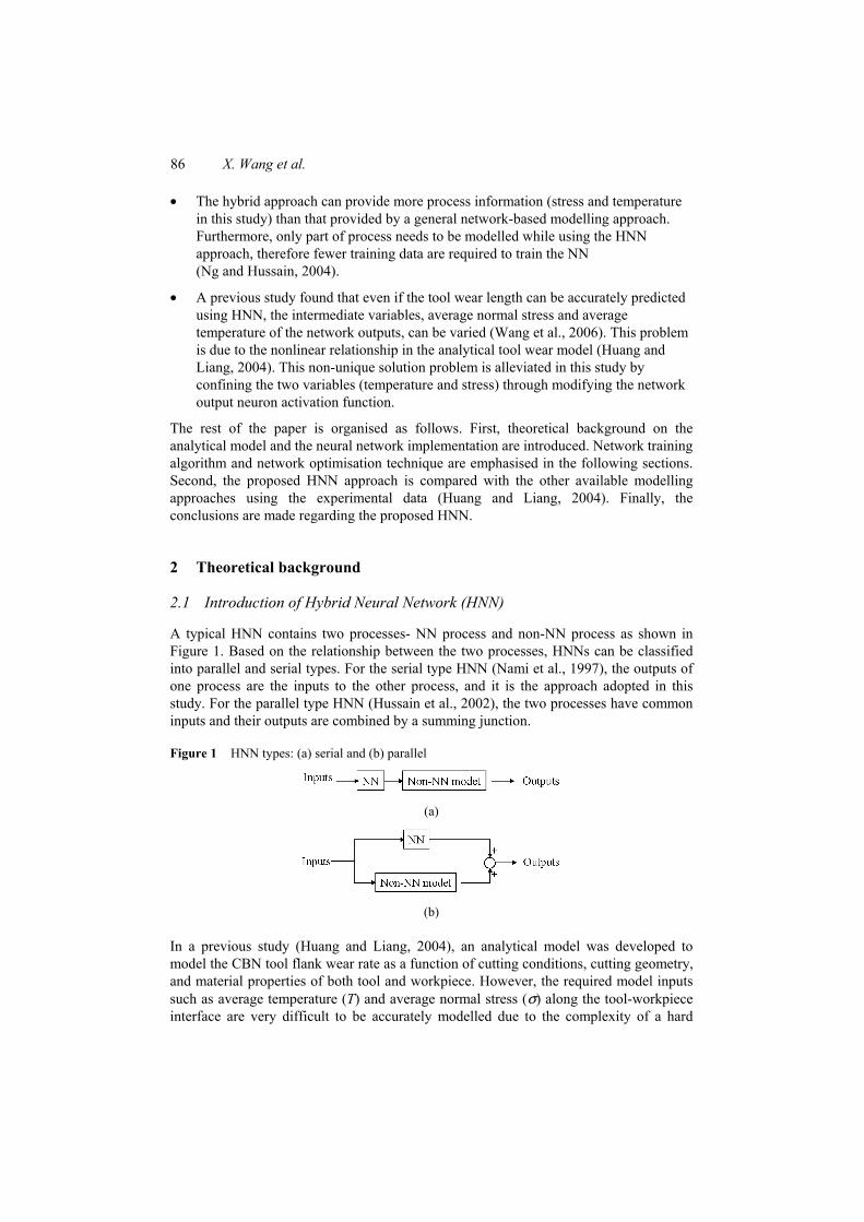
A typical HNN contains two processes- NN process and non-NN process as shown in Figure 1. Based on the relationship between the two processes, HNNs can be classified into parallel and serial types. For the serial type HNN (Nami et al., 1997), the outputs of one process are the inputs to the other process, and it is the approach adopted in this study. For the parallel type HNN (Hussain et al., 2002), the two processes have common inputs and their outputs are combined by a summing junction.

Figure 1 HNN types: (a) serial and (b) parallel

(a)

(b)

In a previous study (Huang and Liang, 2004), an analytical model was developed to model the CBN tool flank wear rate as a function of cutting conditions, cutting geometry, and material properties of both tool and workpiece. However, the required model inputs such as average temperature (T) and average normal stress (σ) along the tool-workpiece interface are very difficult to be accurately modelled due to the complexity of a hard


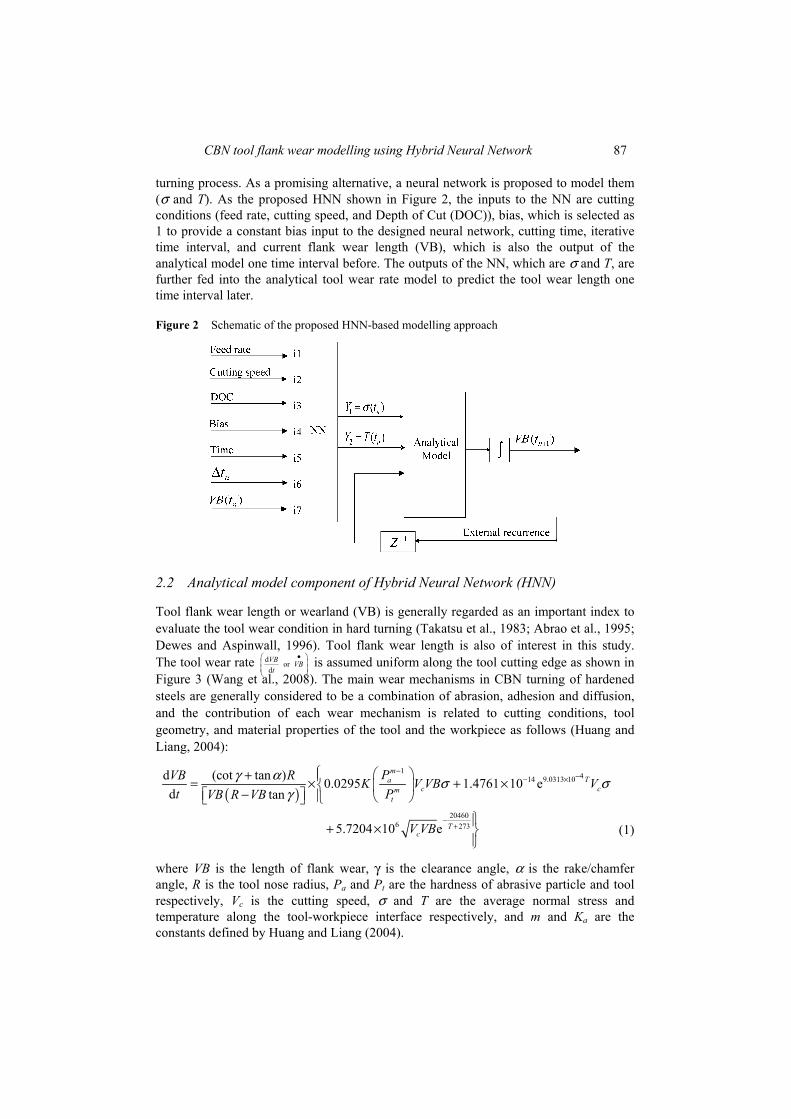
turning process. As a promising alternative, a neural network is proposed to model them (σ and T). As the proposed HNN shown in Figure 2, the inputs to the NN are cutting conditions (feed rate, cutting speed, and Depth of Cut (DOC)), bias, which is selected as 1 to provide a constant bias input to the designed neural network, cutting time, iterative time interval, and current flank wear length (VB), which is also the output of the analytical model one time interval before. The outputs of the NN, which are σ and T, are further fed into the analytical tool wear rate model to predict the tool wear length one time interval later.

Figure 2 Schematic of the proposed HNN-based modelling approach

2.2 Analytical model component of Hybrid Neural Network (HNN)

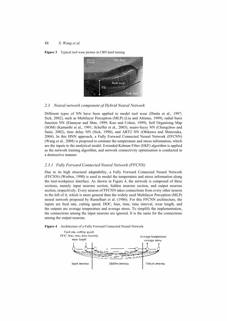
Tool flank wear length or wearland (VB) is generally regarded as an important index to evaluate the tool wear condition in hard turning (Takatsu et al., 1983; Abrao et al., 1995; Dewes and Aspinwall, 1996). Tool flank wear length is also of interest in this study. The tool wear rate d or

dVB VBt

•

is assumed uniform along the tool cutting edge as shown in Figure 3 (Wang et al., 2008). The main wear mechanisms in CBN turning of hardened steels are generally considered to be a combination of abrasion, adhesion and diffusion, and the contribution of each wear mechanism is related to cutting conditions, tool geometry, and material properties of the tool and the workpiece as follows (Huang and Liang, 2004):

( )1

414 9.0313 10

204606 273

d (cot tan ) 0.0295 1.4761 10 ed tan

5.7204 10 e

mTa

c cmt

Tc

PVB R K V VB Vt PVB R VB

V VB

γ α σ σγ

−−− ×

−+

+ = × + × − + ×

(1)

where VB is the length of flank wear, γ is the clearance angle, α is the rake/chamfer angle, R is the tool nose radius, Pa and Pt are the hardness of abrasive particle and tool respectively, Vc is the cutting speed, σ and T are the average normal stress and temperature along the tool-workpiece interface respectively, and m and Ka are the constants defined by Huang and Liang (2004).

88 X. Wang et al.

Figure 3 Typical tool wear picture in CBN hard turning

2.3 Neural network component of Hybrid Neural Network

Different types of NN have been applied to model tool wear (Dimla et al., 1997; Sick, 2002), such as Multilayer Perceptron (MLP) (Liu and Altintas, 1999), radial basis function NN (Elanayar and Shin, 1999; Kuo and Cohen, 1999), Self Organising Map (SOM) (Kamarthi et al., 1991; Scheffer et al., 2003), neuro-fuzzy NN (Chungchoo and Saini, 2002), time delay NN (Sick, 1998), and ART2 NN (Obikawa and Shinozuka, 2004). In this HNN approach, a Fully Forward Connected Neural Network (FFCNN) (Wang et al., 2008) is proposed to estimate the temperature and stress information, which are the inputs to the analytical model. Extended Kalman Filter (EKF) algorithm is applied as the network training algorithm, and network connectivity optimisation is conducted in a destructive manner.

2.3.1 Fully Forward Connected Neural Network (FFCNN)

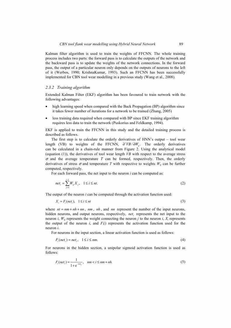
Due to its high structural adaptability, a Fully Forward Connected Neural Network (FFCNN) (Werbos, 1990) is used to model the temperature and stress information along the tool-workpiece interface. As shown in Figure 4, the network is composed of three sections, namely input neurons section, hidden neurons section, and output neurons section, respectively. Every neuron of FFCNN takes connections from every other neuron to the left of it, which is more general than the widely used Multilayer Perception (MLP) neural network proposed by Rumelhart et al. (1986). For this FFCNN architecture, the inputs are feed rate, cutting speed, DOC, bias, time, time interval, wear length, and the outputs are average temperature and average stress. To simplify the implementation, the connections among the input neurons are ignored. It is the same for the connections among the output neurons.

Figure 4 Architecture of a Fully Forward Connected Neural Network


Kalman filter algorithm is used to train the weights of FFCNN. The whole training process includes two parts: the forward pass is to calculate the outputs of the network and the backward pass is to update the weights of the network connections. In the forward pass, the output of a particular neuron only depends on the outputs of neurons to the left of it (Werbos, 1990; KrishnaKumar, 1993). Such an FFCNN has been successfully implemented for CBN tool wear modelling in a previous study (Wang et al., 2008).

2.3.2 Training algorithm

Extended Kalman Filter (EKF) algorithm has been favoured to train network with the following advantages:

• high learning speed when compared with the Back Propagation (BP) algorithm since it takes fewer number of iterations for a network to be trained (Zhang, 2005)

• less training data required when compared with BP since EKF training algorithm requires less data to train the network (Puskorius and Feldkamp, 1994).

EKF is applied to train the FFCNN in this study and the detailed training process is described as follows.

The first step is to calculate the orderly derivatives of HNN’s output – tool wear length (VB) to weights of the FFCNN, / .ijVB W+∂ ∂ The orderly derivatives can be calculated in a chain-rule manner from Figure 2. Using the analytical model (equation (1)), the derivatives of tool wear length VB with respect to the average stress σ and the average temperature T can be formed, respectively. Then, the orderly derivatives of stress σ and temperature T with respective to weights Wij can be further computed, respectively.

For each forward pass, the net input to the neuron i can be computed as: 1

1, 1 .

i

i ij jj

net W X i nt−

=

= ≤ ≤∑ (2)

The output of the neuron i can be computed through the activation function used:

( ), 1i i iX F net i nt= ≤ ≤ (3)

where nt nm nh nn= + + , nm , nh , and nn represent the number of the input neurons, hidden neurons, and output neurons, respectively, inet represents the net input to the neuron i, Wij represents the weight connecting the neuron j to the neuron i, Xi represents the output of the neuron i, and Fi() represents the activation function used for the neuron i.

For neurons in the input section, a linear activation function is used as follows:

( ) , 1 .i i iF net net i nm= ≤ ≤ (4)

For neurons in the hidden section, a unipolar sigmoid activation function is used as follows:

1( ) , .1 e

i i netiF net nm i nm nh−= < ≤ +

+ (5)

90 X. Wang et al.

For neurons in the output section, a modified sigmoid function is implemented as follows:

e( ) (1 ) 2 , 11 e

neti nm nh

i i nm nh i nm nh i i i neti nm nhY F net i nnγ τ τ

− + +

+ + + + − + +

= = − + ≤ ≤

+ (6)

where Yi represents the output of the output neuron i of FFCNN and the number of outputs nn is 2 in this study, Y1 is the average stress, Y2 is the average temperature, γi is the corresponding values for Yi estimated using the analytical stress and temperature models as stated in Huang and Liang (2004), ( < 1)i iτ τ is the constraint coefficient for Yi, which is to confine Yi within a physically feasible range of [1 – τi, 1 + τi]γi. Such an approach has been adopted to successfully implement physical constraints in ANN training as an effective mathematical fix (Cao et al., 2004). If such a range is not imposed in network training, the non-unique solution problem exists for this study (Wang et al., 2006), which means that there are multiple combinations of Yi satisfying the training criterion of error minimisation.

To calculate tool wear length VB(t) at any time t based on a known tool wear rate at an early time t1 (t > t1), 1d / d ( )VB t t which is denoted as 1( )VB t

• for simplicity, should be

first estimated using equation (1), then VB(t) can be predicted using a first-order approximation as follows:

1 1 1( ) ( ) ( )( ).VB t VB t VB t t t•

= + − (7)

Through equation (7), the tool wear length VB at time t is extrapolated from VB at time t1, and the time elapse (t – t1) is defined as the time interval between the measurement moments of VB(t) and VB(t1).

Then the orderly derivative of VB respective to Wij at time t can be calculated by:

1 1( ) ( ) ( )ij ij

VB VBt t t tW W

•+∂ ∂= −

∂ ∂ (8)

From Figure 2, the right side of equation (8) can be further simplified by the chain rule as follows:

1

nnL

Lij L ij

YVB VBW Y W

• •+

=

∂∂ ∂=∂ ∂ ∂∑ (9)

/ LVB Y•

∂ ∂ (L = 1 and 2 in this study) can be computed by differentiating equation (1) as follows:

( )

•414 9.0313 10

1

1(cot tan ) 0.0295 1.4761 10

tanT

c c

mPVB R aK V VB e VmY VB R VB Pt

γ αγ

−− ×

− ∂ + = × + × ∂ −

(10)


( ) {•

44 14 9.0313 10

2

204606 273

2

(cot tan ) 9.0313 10 1.4761 10 etan

20460 5.7204 10 e( 273)

Tc

Tc

VB R VY VB R VB

V VBT

γ α σγ

−− − ×

−+

∂ += × × × ×∂ −

+ × × + (11)

/L ijY W+∂ ∂ in equation (9) can be calculated as follows:

iL Lj

ij i i

XY Y XW X net

+ + ∂∂ ∂=∂ ∂ ∂

(12)

1.

nm nhjL L

jij ii j j

XY Y WX X net

+ ++

= +

∂∂ ∂=∂ ∂ ∂∑ (13)

For the above discussion, zero initial conditions are generally assumed as follows: •

(0) 0 and (0) 0ij

VBVBW

∂= =∂

(14)

The second step is to update the network weights using the EKF algorithm. The FFCNN’s trainable weights Wij are first arranged into an M dimensional vector W, and the elements of / ijVB W+∂ ∂ are arranged into an M × nn matrix Hm (Haykin, 1999), where M is the number of trainable weights. The trainable weights vector W is updated using an EKF algorithm (Huang and KrishnaKumar, 2004). The algorithm is illustrated as follows:

1( ) [ ( ) ( ) ( ) ( )]Tk k k k kA n R n H n P n H n −= + (15)

( ) ( ) ( ) ( )k k k kK n P n H n A n= (16)

( 1) ( ) ( ) ( )k k k kW n W n K n nξ+ = + (17)

( 1) ( ) ( ) ( ) ( ) ( )Tk k k k k kP n P n K n H n P n Q n+ = − + (18)

where nk is the filter iteration step, P(nk) is the approximate error covariance matrix at step nk, R(nk) is the covariance matrix of measurement noise, and Q(nk) is the covariance matrix of process noise. The presence of R(nk) and Q(nk) helps to avoid numerical divergence of the algorithm and poor local minima. W(0) and P(0) are initial values of the weight vector and the error covariance matrix, which are normally taken as a small random vector and a matrix with large diagonal elements, respectively. The EKF algorithm requires, in addition to the estimate of the network’s weight vector, the storing and updating of an approximate error covariance matrix P(nk), which is used as a measure of the estimation accuracy of the weight estimate. The matrix A(nk) and the Kalman gain matrix K(nk) are computed at each time step, and they are used to update the weigh vector W(nk + 1) and the error covariance matrix P(nk + 1).

92 X. Wang et al.

2.3.3 Network connectivity optimisation

ANN-based tool wear modelling approach has some common issues such as under-training problem, convergence problem, overfitting problem, and topology optimisation problem (Danaher et al., 2004). While the first two can be easily mitigated by carefully selecting stopping criteria, the latter two are of interest here through an optimisation approach, which optimises the network topology as well as reduces the risk of overfitting.

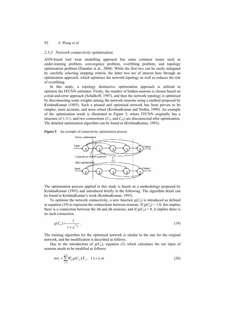
In this study, a topology destructive optimisation approach is utilised to optimise the FFCNN estimator. Firstly, the number of hidden neurons is chosen based on a-trial-and-error approach (Schalkoff, 1997), and then the network topology is optimised by disconnecting some weights among the network neurons using a method proposed by KrishnaKumar (1993). Such a pruned and optimised network has been proven to be simpler, more accurate, and more robust (KrishnaKumar and Nishta, 1999). An example of the optimisation result is illustrated in Figure 5, where FFCNN originally has a structure of 1-3-1, and two connections (C31 and C42) are disconnected after optimisation. The detailed optimisation algorithm can be found in (KrishnaKumar, 1993).

Figure 5 An example of connectivity optimisation process

The optimisation process applied in this study is based on a methodology proposed by KrishnaKumar (1993) and introduced briefly in the following. The algorithm detail can be found in KrishnaKumar’s work (KrishnaKumar, 1993).

To optimise the network connectivity, a new function g(Cij) is introduced as defined in equation (19) to represent the connections between neurons. If g(Cij) = 1.0, this implies there is a connection between the ith and jth neurons; and if g(Cij) = 0, it implies there is no such connection.

1( ) .1 e

ij Cijg C −=

+ (19)

The training algorithm for the optimised network is similar to the one for the original network, and the modification is described as follows.

Due to the introduction of g(Cij), equation (2) which calculates the net input of neurons needs to be modified as follows:

1

1

( ) , 1i

i ij ij jj

net W g C X i nt−

=

= ≤ ≤∑ (20)


where Cij is the connection coefficient from the neuron j to the neuron i. Also, equation (12) should be modified as follows:

( )iL Lij j

ij i i

XY Y g C XW X net

+ + ∂∂ ∂=∂ ∂ ∂

(21)

/L ijY C+∂ ∂ is calculated as follows:

( ).ijiL L

ij jij i i ij

g CXY Y W XC X net C

+ + ∂∂∂ ∂=∂ ∂ ∂ ∂

(22)

The optimisation process has two phases. At the first phase, the network architecture is determined in a destructive manner. Both the weights and connection coefficients are updated using the EKF algorithm as discussed in Section 2.3.2. At the beginning of optimisation, each Cij is set as 0. During the training process, both Wij and Cij are updated. When enough number of iterations is reached, connections with Cij < 0 is disconnected by setting g(Cij)= 0 and the others is left connected by setting g(Cij)= 1. Then the network architecture is determined. At the second phase, weights Wij are further refined using the same training data. The HNN after the network connectivity optimisation is called as the Optimised HNN (OHNN) in this study.

3 Experimental validation

3.1 Experiment setup

To better appreciate the validity in applying the proposed HNN and OHNN estimators for CBN tool wear modelling, hardened AISI 52100 bearing steel with a hardness 62 HRc was machined on a horizontal Hardinge lathe using a low CBN content tool insert (Kennametal KD050) with a –20° and 0.1 mm wide edge chamfer and a 0.8 mm nose radius. The ISO DCLNR-164D tool holder was used, which introduced a negative 5° rake angle. No cutting fluid was applied. Flank wear length was measured using an optical microscope (Zygo NewView 200). The experiment was stopped when sudden force jump was observed signalling a chipping or broken tool condition.

Machining test was performed based on a standard central composite design test matrix with an alpha value of 1.414. The centre point (0, 0) was determined based on the tool manufacturer’s recommendation (Huang and Liang, 2004). A typical depth of cut was suggested as 0.203 mm, which was used in the test matrix. To further investigate the effect of depth of cut on tool wear, experiments with various depths of cut were also studied. Ten different cutting conditions (Huang and Liang, 2004), namely conditions 1–5, 8–10, a, and b are listed in Table 1. Conditions 7 and 11 are not utilised here since they are the same as condition 4, and condition 6 (cutting speed = 3.36 m/s) is also not used since the break-in period accounted for a large portion of tool flank wear and microchipping was a dominant factor of tool life under such an aggressive cutting speed. Uncertainty characterisation is not offered here due to the size of the experimental data set.

94 X. Wang et al.

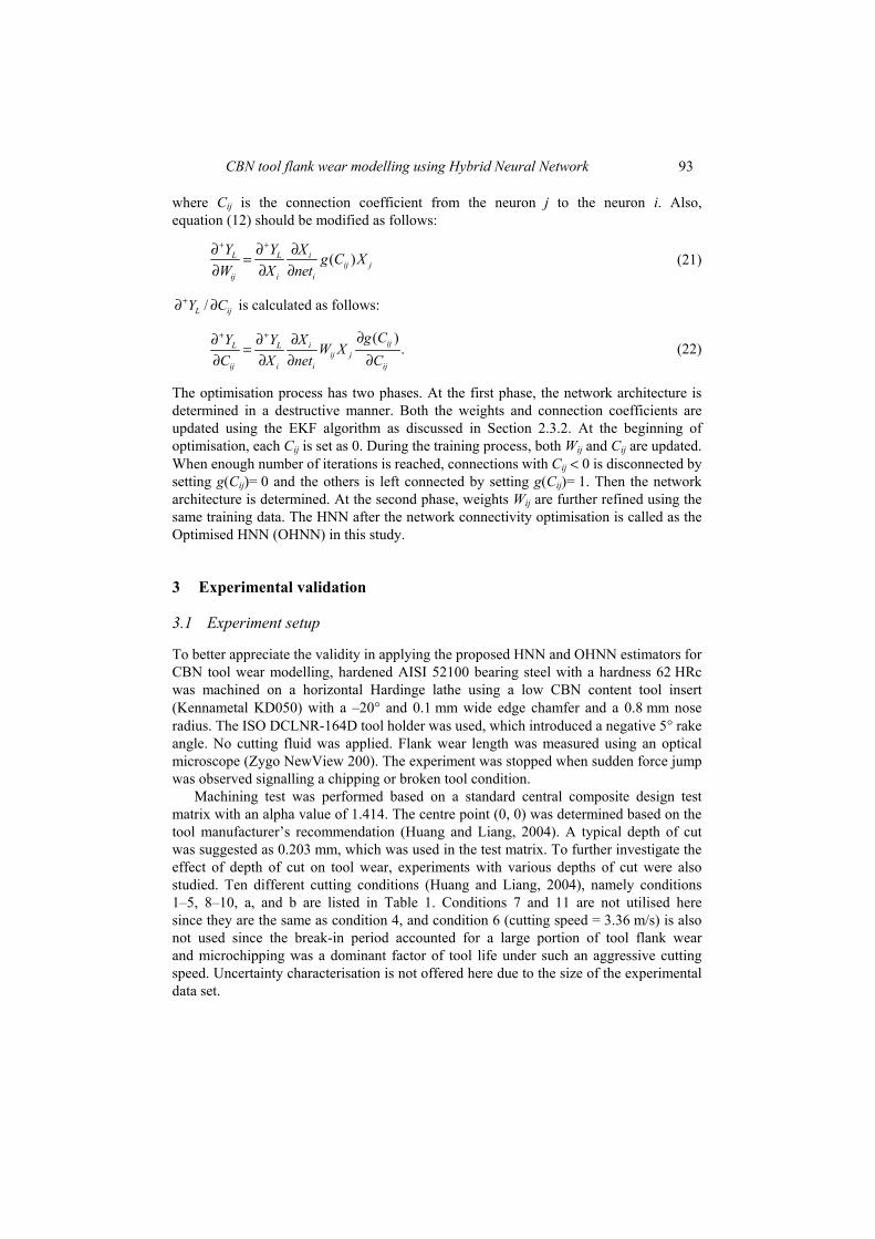
Table 1 Cutting conditions of the experiments

Condition index Speed (m/s) Feed (mm/rev) Depth of cut (mm) 1 3.05 0.152 0.203 2 1.52 0.152 0.203 3 3.05 0.076 0.203 4 2.29 0.114 0.203 5 1.52 0.076 0.203 8 2.29 0.061 0.203 9 2.29 0.168 0.203 10 1.21 0.114 0.203 a 1.52 0.076 0.102 b 1.52 0.076 0.152

3.2 Networks implementation

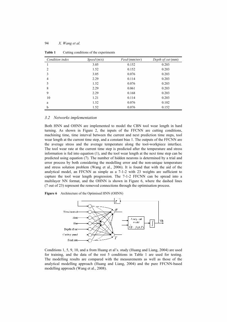
Both HNN and OHNN are implemented to model the CBN tool wear length in hard turning. As shown in Figure 2, the inputs of the FFCNN are cutting conditions, machining time, time interval between the current and next prediction time steps, tool wear length at the current time step, and a constant bias 1. The outputs of the FFCNN are the average stress and the average temperature along the tool-workpiece interface. The tool wear rate at the current time step is predicted after the temperature and stress information is fed into equation (1), and the tool wear length at the next time step can be predicted using equation (7). The number of hidden neurons is determined by a trial and error process by both considering the modelling error and the non-unique temperature and stress solution problem (Wang et al., 2006). It is found that with the aid of the analytical model, an FFCNN as simple as a 7-1-2 with 23 weights are sufficient to capture the tool wear length progression. The 7-1-2 FFCNN can be spread into a multilayer NN format, and the OHNN is shown in Figure 6, where the dashed lines (7 out of 23) represent the removed connections through the optimisation process.

Figure 6 Architecture of the Optimised HNN (OHNN)

Conditions 1, 5, 9, 10, and a from Huang et al’s. study (Huang and Liang, 2004) are used for training, and the data of the rest 5 conditions in Table 1 are used for testing. The modelling results are compared with the measurements as well as those of the analytical modelling approach (Huang and Liang, 2004) and the pure FFCNN-based modelling approach (Wang et al., 2008).


The EKF algorithm is applied to train the network weights. The diagonal elements of the process noise covariance matrix Q is initialised as 0.01 and this value descends linearly within 10,000 training cycles until Q reaches the minimum limit 0.000001. The diagonal elements of the measurement noise covariance matrix R, are initialised as 100 and they further descend linearly until R reaches the minimum boundary 2. Both R and Q help the training process overcome the trap of local minimum.

In order to avoid the saturation problem, all inputs of FFCNN except the tool wear length (VB) feedback are first normalised before they are fed into the network. The normalisation is performed using a linear mapping function as follows:

max minmin min

max min

( ) N NN N

X XX X X X

X X−

= − +−

(23)

where XN is the normalised inputs, X is the original value of inputs, XNmax and XNmin are the maximum and minimum values of the normalised inputs, and Xmax and Xmin are the maximum and minimum values of the inputs before normalisation. VB (unit as mm during computation) is treated by multiplying with a constant value, which is 30 in this study.

3.3 Simulation results

Learning speed comparison between HNN and OHNN has been performed, and both the networks are trained by EKF. The comparison shows that the learning convergence speed of OHNN is faster than that of HNN, which confirms the observation from a previous study (Wang et al., 2008). Note that for this comparison, some connections of optimised FFCNN have been removed already and the convergence study is based on the network refining phase as discussed in Section 2.3.3.

3.3.1 Generalisation capability

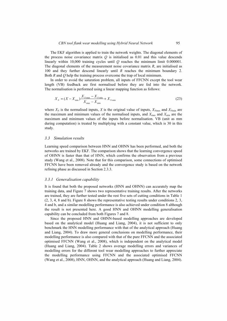
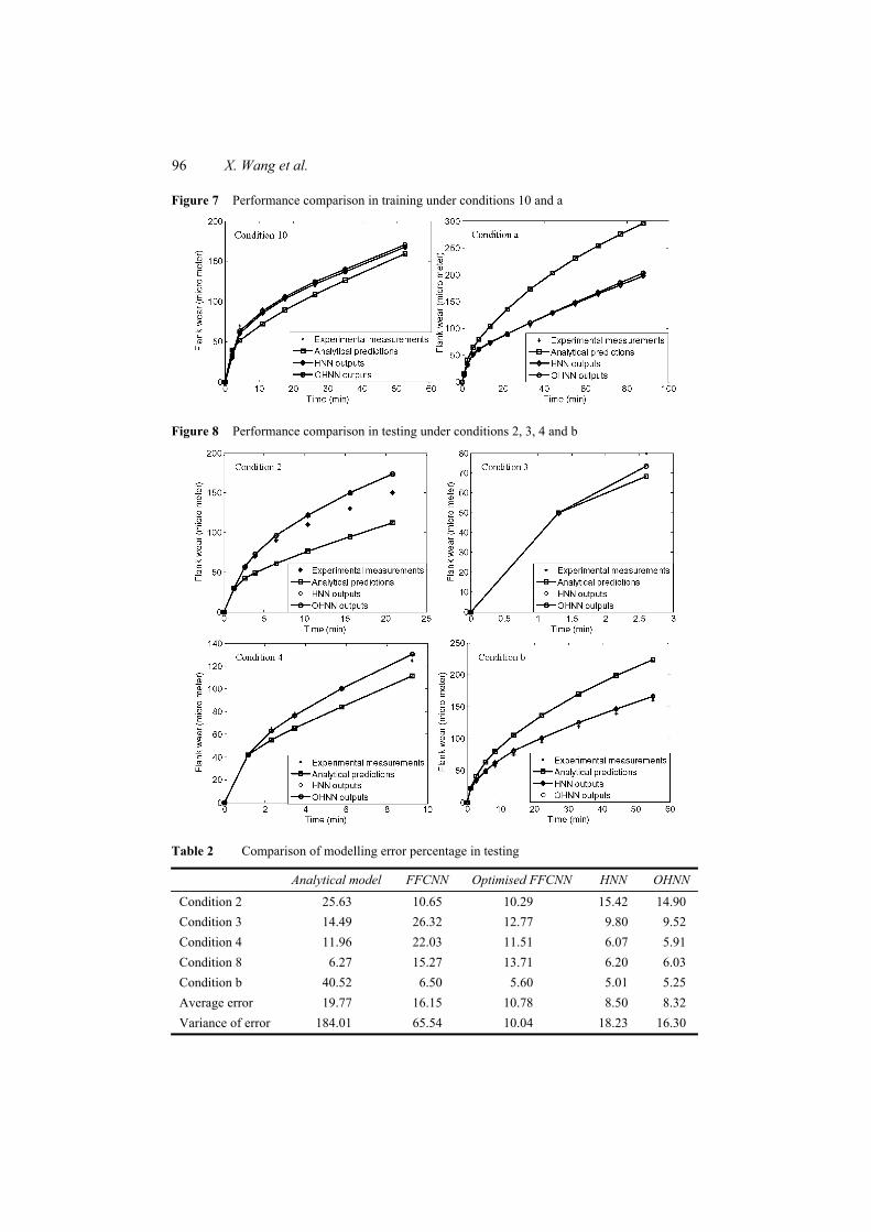
It is found that both the proposed networks (HNN and OHNN) can accurately map the training data, and Figure 7 shows two representative training results. After the networks are trained, they are further tested under the rest five sets of cutting conditions in Table 1 (2, 3, 4, 8 and b). Figure 8 shows the representative testing results under conditions 2, 3, 4 and b, and a similar modelling performance is also achieved under condition 8 although the result is not presented here. A good HNN and OHNN modelling generalisation capability can be concluded from both Figures 7 and 8.

Since the proposed HNN and OHNN-based modelling approaches are developed based on the analytical model (Huang and Liang, 2004), it is not sufficient to only benchmark the HNN modelling performance with that of the analytical approach (Huang and Liang, 2004). To draw more general conclusions on modelling performance, their modelling performance is also compared with that of the pure FFCNN and the associated optimised FFCNN (Wang et al., 2008), which is independent on the analytical model (Huang and Liang, 2004). Table 2 shows average modelling errors and variances of modelling errors for the different tool wear modelling approaches to further appreciate the modelling performance using FFCNN and the associated optimised FFCNN (Wang et al., 2008), HNN, OHNN, and the analytical approach (Huang and Liang, 2004).

96 X. Wang et al.

Figure 7 Performance comparison in training under conditions 10 and a

Figure 8 Performance comparison in testing under conditions 2, 3, 4 and b

Table 2 Comparison of modelling error percentage in testing

Analytical model FFCNN Optimised FFCNN HNN OHNN

Condition 2 25.63 10.65 10.29 15.42 14.90 Condition 3 14.49 26.32 12.77 9.80 9.52 Condition 4 11.96 22.03 11.51 6.07 5.91 Condition 8 6.27 15.27 13.71 6.20 6.03 Condition b 40.52 6.50 5.60 5.01 5.25 Average error 19.77 16.15 10.78 8.50 8.32 Variance of error 184.01 65.54 10.04 18.23 16.30


By examining the modelling performance data in Table 2, it can be seen:

• comparing the performance of HNN/OHNN with that of the analytical model, HNN and OHNN excel in all the five testing conditions, which proves that the additional FFCNN improve the modelling performance of the original analytical approach

• comparing the performance of OHNN with that of HNN, OHNN further improves the modelling capability as OHNN improves the modelling accuracy under four out of the five conditions (except condition b)

• comparing the performance of OHNN and the optimised FFCNN, though the structure of the OHNN (with one hidden neuron) is much simpler than that of the latter (with five hidden neurons), it can be seen the modelling accuracy of OHNN is still generally better (except condition 2).

Generally speaking, OHNN has the smallest average modelling error among the five investigated approaches although the optimised FFCNN has a relatively smaller error variance than that of OHNN, which indicates that the generalisation capability of OHNN is one of the excellent among the investigated approaches. In addition, the HNN and OHNN-based approaches offer the temperature and stress information of the hard turning process, which cannot be provided using any other pure FFCNN-based black-box approaches.

It should be pointed out that the modelling accuracy of HNN and OHNN is also depends on the accuracy of the analytical model (Huang and Liang, 2004) since the analytical model is also a critical component of the HNN and OHNN-based approaches. It is found that the modelling performance correlation between HNN/OHNN and the analytical model is higher than 90% in training and 79% in testing, respectively. An improved analytical model is expected to further improve the modelling accuracy of the HNN and OHNN-based approaches.

3.3.2 Stress and temperature information along the interface

To solve the non-unique temperature and stress solution problem (Wang et al., 2006), the constraint coefficients τi in equation (6), which are used to confine the output ranges of stress σ and temperature T, need to be carefully selected. The value of τi is determined in the training process by a trial and error approach. Small values τi (0.05) for estimation of stress and temperature are first selected. Since the training error is found to have a relative high value (> 0.05) and both the stress and temperature results reach the specified lower and upper boundaries ((1 – τi)γi and (1 + τi)γi as specified by the output neuron activation functions), the values of coefficients τi are further increased until the network training error is less than 4 × 10–3 and the estimated stress and temperature results are within the boundaries. In this study, τ1 is finally selected as 0.25 for the stress output neuron and τ2 0.2 for the temperature output neuron.

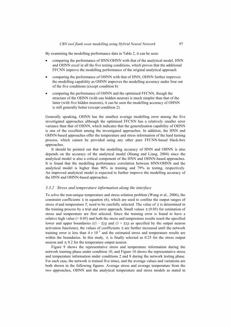
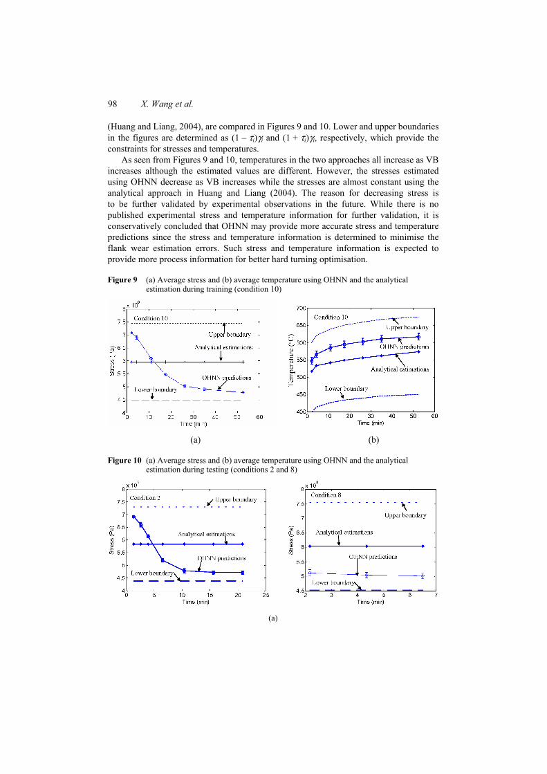
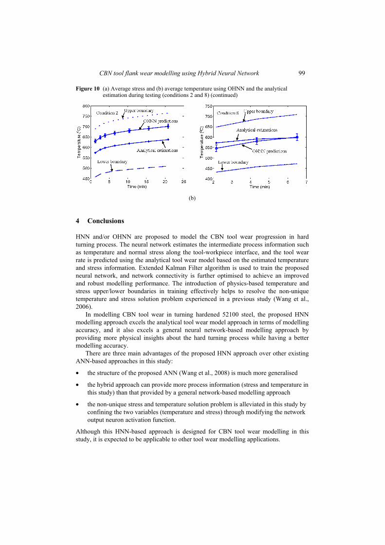
Figure 9 shows the representative stress and temperature information during the network training phase under condition 10, and Figure 10 shows the representative stress and temperature information under conditions 2 and 8 during the network testing phase. For each case, the network is trained five times, and the average values and variations are both shown in the following figures. Average stress and average temperature from the two approaches, OHNN and the analytical temperature and stress models as stated in

98 X. Wang et al.

(Huang and Liang, 2004), are compared in Figures 9 and 10. Lower and upper boundaries in the figures are determined as (1 – τi)γi and (1 + τi)γi, respectively, which provide the constraints for stresses and temperatures.

As seen from Figures 9 and 10, temperatures in the two approaches all increase as VB increases although the estimated values are different. However, the stresses estimated using OHNN decrease as VB increases while the stresses are almost constant using the analytical approach in Huang and Liang (2004). The reason for decreasing stress is to be further validated by experimental observations in the future. While there is no published experimental stress and temperature information for further validation, it is conservatively concluded that OHNN may provide more accurate stress and temperature predictions since the stress and temperature information is determined to minimise the flank wear estimation errors. Such stress and temperature information is expected to provide more process information for better hard turning optimisation.

Figure 9 (a) Average stress and (b) average temperature using OHNN and the analytical estimation during training (condition 10)

(a) (b)

Figure 10 (a) Average stress and (b) average temperature using OHNN and the analytical estimation during testing (conditions 2 and 8)

(a)


Figure 10 (a) Average stress and (b) average temperature using OHNN and the analytical estimation during testing (conditions 2 and 8) (continued)

(b)

4 Conclusions

HNN and/or OHNN are proposed to model the CBN tool wear progression in hard turning process. The neural network estimates the intermediate process information such as temperature and normal stress along the tool-workpiece interface, and the tool wear rate is predicted using the analytical tool wear model based on the estimated temperature and stress information. Extended Kalman Filter algorithm is used to train the proposed neural network, and network connectivity is further optimised to achieve an improved and robust modelling performance. The introduction of physics-based temperature and stress upper/lower boundaries in training effectively helps to resolve the non-unique temperature and stress solution problem experienced in a previous study (Wang et al., 2006).

In modelling CBN tool wear in turning hardened 52100 steel, the proposed HNN modelling approach excels the analytical tool wear model approach in terms of modelling accuracy, and it also excels a general neural network-based modelling approach by providing more physical insights about the hard turning process while having a better modelling accuracy.

There are three main advantages of the proposed HNN approach over other existing ANN-based approaches in this study:

• the structure of the proposed ANN (Wang et al., 2008) is much more generalised

• the hybrid approach can provide more process information (stress and temperature in this study) than that provided by a general network-based modelling approach

• the non-unique stress and temperature solution problem is alleviated in this study by confining the two variables (temperature and stress) through modifying the network output neuron activation function.

Although this HNN-based approach is designed for CBN tool wear modelling in this study, it is expected to be applicable to other tool wear modelling applications.

100 X. Wang et al.

Acknowledgements

The authors would like to acknowledge the financial support from the South Carolina Space Grant Consortium and the NASA Ames Research Center.

References Abrao, A.M., Wise, M.L.H. and Aspinwall, D.K. (1995) ‘Tool life and workpiece surface integrity

evaluations when machining hardened AISI 52100 steels with conventional ceramic and PCBN tool materials’, SME Technical Paper, MR95-159, pp.1–9.

Cao, M., Wang, K.W., Fujii, Y. and Tobler, W.E. (2004) ‘A hybrid neural network approach for the development of friction component dynamic model’, Journal of Dynamic Systems, Measurement and Control, Vol. 126, No. 1, pp.144–153.

Chryssoluouris, G. and Guillot, M. (1990) ‘A comparison of statistical and AI approaches to the selection of process parameters in intelligent machining’, ASME, Journal of Engineering for Industry, Vol. 112, pp.122–131.

Chungchoo, C. and Saini, D. (2002) ‘On-line tool wear estimation in CNC turning operations using Fuzzy neural network model’, International Journal of Machine Tools and Manufacture, Vol. 42, pp.29–40.

Danaher, S., Datta, S., Waddle, I. and Hackney, P. (2004) ‘Erosion modeling using Bayesian regulated artificial neural networks’, Wear, Vol. 256, pp.879–888.

Das, S., Chattopadhyay, A.B. and Murthy, A.S.R. (1996) ‘Force parameters for on-line tool wear estimation: a neural network approach’, Neural Networks, Vol. 9, pp.1639–1645.

Dawson, T. (2002) Machining Hardened Steel with Polycrystalline Cubic Boron Nitride Cutting Tools, PhD Thesis, Georgia Institute of Technology, GA.

Dewes, R.C. and Aspinwall, D.K. (1996) ‘The use of high speed machining for the manufacture of hardened steel dies’, Trans. NAMRI, Vol. 24, pp.21–26.

Dimla Sr., D.E., Lister, P.M. and Leighton, N.J. (1997) ‘Neural network solutions to the tool condition monitoring problem in metal cutting – a critical review of methods’, International Journal of Machine Tools and Manufacture, Vol. 37, pp.1219–1241.

Dimla Sr., D.E. and Lister, P.M. (2000) ‘On-line metal cutting tool condition monitoring. II tool-state classification using multi-layer perceptron neural networks’, International Journal of Machine Tools and Manufacture, Vol. 40, pp.769–781.

Elanayar, S.V.T. and Shin, Y.C. (1999) ‘Robust tool wear monitoring using radial basis function neural network’, ASME Journal of Dynamic Systems, Measurement and Control, Vol. 117, pp.459–467.

Haber, R.E. and Alique, A. (2003) ‘Intelligent process supervision for predicting tool wear in machining processes’, Mechatronics, Vol. 13, pp.825–849.

Haykin, S. (1999) Neural Networks: A Comprehensive Foundation, 2nd ed., Prentice-Hall, Upper Saddle River, NJ.

Huang, Y. (2002) Predictive Modeling of Tool Wear Rate with Application to CBN Hard Turning, PhD Thesis, Georgia Institute of Technology, GA.

Huang, Y. and KrishnaKumar, K. (2004) ‘Estimating engine quality parameters using a novel fully connected recurrent neural network’, Proc. 2004 Japan – USA Symposium on Flexible Automation, Denver, CO, UL_033, 19–21 July, pp.1–6.

Huang, Y. and Liang, S.Y. (2004) ‘Modeling of CBN tool flank wear progression in finish hard turning’, ASME J. Manufacturing Science and Engineering, Vol. 126, pp.98–106.

Hussain, M.A., Rahman, M.S. and Ng, C.W. (2002) ‘Prediction of pores formation (porosity) in foods during drying: generic models by the use of hybrid neural network’, Journal of Food Engineering, Vol. 51, pp.239–248.


Kamarthi, S.V., Sankar, G.S., Cohen, P.H. and Kumara, S.R.T. (1991) ‘On-line tool wear monitoring using a Kohonen’s feature map’, Intelligent Engineering Systems through Artificial Neural Networks, Proceeding of the First Artificial Neural Networks in Engineering Conference, St. Louis, Vol. 1, pp.639–644.

König, W., Hochschule, T., Komanduri, R., Schenectady, D. and Tonshoff, H.K. (1984) ‘Machining of hard materials’, Annals of CIRP, Vol. 33, No. 2, pp.417–427.

Kramer, B.M. (1986) ‘Predicted wear resistances of binary carbide coatings’, J. Vac. Sci. Technol. A, Vol. A4, No. 6, pp.2870–2873.

KrishnaKumar, K. (1993) ‘Optimization of the neural net connectivity pattern using a backpropagation algorithm’, Neurocomputing, Vol. 5, pp.273–286.

KrishnaKumar, K. and Nishta, K. (1999) ‘Robustness analysis of Nueral networks with an application to system identification’, Journal of Guidance, Control and Dynamics, Vol. 22, pp.695–701.

Kuo, R.J. and Cohenb, P.H. (1998) ‘Intelligent tool wear estimation system through artificial neural networks and fuzzy modeling’, Artificial Intelligence in Engineering, Vol. 12, pp.229–242.

Kuo, R.J. and Cohen, P.H. (1999) ‘Multi-sensor integration for on-line tool wear estimation through radial basis function networks and Fuzzy neural network’, Neural Networks, Vol. 12, pp.355–370.

Liu, Q. and Altintas, Y. (1999) ‘On-line monitoring of flank wear in turning with multilayered feed-forward neural network’, International Journal of Machine Tools and Manufacture, Vol. 39, pp.1945–1959.

Nami, Z., Misman, O., Erbil, A. and May, G.S. (1997) ‘Semi-empirical neural network modeling of metal-organic chemical vapor deposition’, IEEE Transactions on Semiconductor Manufacturing, Vol. 10, No. 2, pp.288–294.

Ng, C.W. and Hussain, M.A. (2004) ‘Hybrid neural network – prior knowledge model in temperature control of a semi – batch polymerization process’, Chemical Engineering and Processing, Vol. 34, No. 4, pp.559–570.

Obikawa, T. and Shinozuka, J. (2004) ‘Monitoring of flank wear of coated tools in high speed machining with a neural network ART2’, International Journal of Machine Tools and Manufacture, Vol. 44, pp.1311–1318.

Ozel, T. and Nadgir, A. (2002) ‘Prediction of flank wear by using back propagation neural network modeling when cutting hardened H-13 steel with Chamfered and Honed tools’, International Journal of Machine Tools and Manufacture, Vol. 42, pp.287–297.

Ozel, T. and Karpat, Y. (2005) ‘Predictive modeling of surface roughness and tool wear in hard turning using regression and neural networks’, International Journal of Machine Tools and Manufacture, Vol. 45, pp.467–479.

Poulachon, G., Moisan, A. and Jawahir, I.S. (2001) ‘Tool-wear mechanisms in hard turning with polycrystalline cubic boron nitride tools’, Wear, Vol. 250, pp.576–586.

Puskorius, G.V. and Feldkamp, L.A. (1994) ‘Neurocontrol of nonlinear dynamical systems with kalman filter trained recurrent networks’, IEEE Trans. on Neural Networks, Vol. 5, pp.279–297.

Rumelhart, D.E., McClelland, J.L. and The PDP Research Group (1986) Parallel Distributed Processing: Explorations in the Microstructure of Cognition, Foundations, MIT Press Cambridge, MA, Vol. 1.

Schalkoff, R.J. (1997) Artificial Neural Networks, McGraw-Hill Inc., New York. Scheffer, C., Kratz, H., Heyns, P.S. and Klocke, F. (2003) ‘Development of a tool wear-monitoring

system for hard turning’, International Journal of Machine Tools and Manufacture, Vol. 43, pp.973–985.

Sick, B. (1998) ‘On-line tool wear classification in turning with time-delay neural networks and process-specific pre-processing’, International Joint Conference on Neural Networks, Anchorage, pp.84–89.

102 X. Wang et al.

Sick, B. (2002) ‘On-line and indirect tool wear monitoring in turning with artificial neural networks: a review of more than a decade of research’, Mechanical Systems and Signal Processing, Vol. 16, pp.487–546.

Sun, J., Rahman, M., Wong, Y.S. and Hong, G.S. (2004) ‘Multiclassification of tool wear with support vector machine by manufacturing loss consideration’, International Journal of Machine Tools and Manufacture, Vol. 44, pp.1179–1187.

Takatsu, S., Shimoda, H. and Otani, K. (1983) ‘Effect of CBN content on the cutting performance of polycrystalline CBN tools’, Int. J. Refract. Hard Mat., Vol. 2, No. 4, pp.175–178.

Usui, E., Shirakashi, T. and Kitagawa, T. (1978) ‘Analytical prediction of three dimensional cutting process, Part 3, cutting temperature and crater wear of carbide tool’, Journal of Engineering for Industry, Vol. 100, pp.236–243.

Wang, X., Huang, Y., Nguyen, N. and Krishnakumar, K. (2006) ‘CBN tool flank wear modeling using a hybrid neural network’, Proc. 2006 International Symposium on Flexible Automation, Osaka, Japan, Vol. 0231-b(L), pp.67–74.

Wang, X., Wang, W., Huang, Y., Nguyen, N. and Krishnakumar, K. (2008) ‘Design of neural network-based estimator for tool wear modeling in hard turning’, Journal of Intelligent Manufacturing, in print, DOI 10.1007/s10845-008-0090-8.

Wang, Z. and Dornfeld, D.A. (1992) ‘In-process monitoring using neural networks’, Proceedings of the 1992 Japan – USA Symposium on Flexible Automation Part 1 (of 2), San Francisco, CA, USA, 13–15 July, pp.263–270.

Werbos, P.J. (1990) ‘Back propagation through time: what is does and how to do it’, Proc. IEEE, Vol. 78, No. 10, pp.1550–1560.

Xie, L.J., Schmidt, J., Schmidt, C. and Biesinger, F. (2005) ‘2D FEM estimate of tool wear in turning operation’, Wear, Vol. 258, pp.1479–1490.

Yen, Y.C., Söhner, J., Lilly, B. and Altan, T. (2004) ‘Estimation of tool wear in orthogonal cutting using the finite element analysis’, Journal of Materials Processing Technology, Vol. 146, pp.82–91.

Zhang, L. (2005) ‘Neural network-based market clearing price prediction and confidence interval estimation with an improved Extended Kalman Filter method’, IEEE Transactions on Power Systems, Vol. 20, No. 1, pp.59–66.

CBN tool flank wear modelling using Hybrid Neural Network

Documents