HAL Id: tel-02511334 https://tel.archives-ouvertes.fr/tel-02511334 Submitted on 18 Mar 2020 HAL is a multi-disciplinary open access archive for the deposit and dissemination of sci- entific research documents, whether they are pub- lished or not. The documents may come from teaching and research institutions in France or abroad, or from public or private research centers. L’archive ouverte pluridisciplinaire HAL, est destinée au dépôt et à la diffusion de documents scientifiques de niveau recherche, publiés ou non, émanant des établissements d’enseignement et de recherche français ou étrangers, des laboratoires publics ou privés. Cavitation & supercavitation : obtenir un projectile profilé stable Thibault Guillet To cite this version: Thibault Guillet. Cavitation & supercavitation : obtenir un projectile profilé stable. Mechanics of the fluids [physics.class-ph]. Institut Polytechnique de Paris, 2019. English. NNT: 2019IPPAX007. tel-02511334

Welcome message from author
This document is posted to help you gain knowledge. Please leave a comment to let me know what you think about it! Share it to your friends and learn new things together.
Transcript
HAL Id: tel-02511334https://tel.archives-ouvertes.fr/tel-02511334
Submitted on 18 Mar 2020
HAL is a multi-disciplinary open accessarchive for the deposit and dissemination of sci-entific research documents, whether they are pub-lished or not. The documents may come fromteaching and research institutions in France orabroad, or from public or private research centers.
L’archive ouverte pluridisciplinaire HAL, estdestinée au dépôt et à la diffusion de documentsscientifiques de niveau recherche, publiés ou non,émanant des établissements d’enseignement et derecherche français ou étrangers, des laboratoirespublics ou privés.
Cavitation & supercavitation : obtenir un projectileprofilé stableThibault Guillet
To cite this version:Thibault Guillet. Cavitation & supercavitation : obtenir un projectile profilé stable. Mechanics ofthe fluids [physics.class-ph]. Institut Polytechnique de Paris, 2019. English. NNT : 2019IPPAX007.tel-02511334
626
NN
T:2
019I
PPA
X00
7
Cavitation & Supercavitation :From a bluff to a stable streamlined
projectileThese de doctorat de l’Institut Polytechnique de Paris
preparee a l’Ecole polytechnique
Ecole doctorale n626 Ecole Doctorale de l’Institut Polytechnique de Paris (ED IPParis)
Specialite de doctorat : Ingenierie Mecanique et Energetique
These presentee et soutenue a Palaiseau, le 19 decembre 2019, par
THIBAULT GUILLET
Composition du Jury :
Detlef LohseProfesseur, University of Twente President
Irmgard BischofbergerProfesseure assistante, Massachussett Institute of Technology Rapporteure
Olivier CadotProfesseur, University of Liverpool Rapporteur
Sunghwang JungProfesseur associe, Cornell University Examinateur
Christophe ClanetDirecteur de Recherche, Ecole polytechnique Directeur de these
Caroline CohenProfesseure Assitante, Ecole polytechnique Co-directrice de these
David QuereDirecteur de Recherche, ESPCI Co-encadrant
Remerciements
Firstly, I would like to thank all the jury members to have made it to the campus duringthe worst times of the French public transportations strike. Thanks to Irmgard Bishofbergerand Olivier Cadot for carefully reading the manuscript and for their remarks. I would like tothank Detlef Lohse for his questions and remarks which will really impact the continuationof this work. I acknowledge Sunny Jung for his comments and for accepting to follow thedefense through skype.
Je souhaiterais remercier David de m’avoir communique sa passion pour la science, larecherche et les matieres molles : sans sa contribution, je ne me serais jamais lance dansl’aventure de la these. Merci de m’avoir envoye chez Sid Nagel a Chicago en stage detroisieme annee : tu m’as donne l’opportunite de faire mes premiers pas dans la recherchedans une equipe formidable. Pendant la these, malgre ton emploi du temps extremementcharge, tu as toujours repondu present (tout du moins apres un nombre d’appels suffisant).Tu as la fantastique capacite de sublimer le travail de tes thesards et thesardes ; j’espereavoir appris ne serait-ce qu’une infime partie de tes talents de redaction.
Merci beaucoup a Christophe. Je ne sais pas trop comment tu resumerais cette these ...J’hesite entre ”on a pas beaucoup avance, mais on a bien rigole !” ou ”c’etait super maison a rien compris”. Plus serieusement, un grand merci pour toutes les fois ou tu m’as sortide galeres : theoriques, numeriques ou experimentales. Je ressortais toujours de ton bureauavec plein de nouvelles idees - pas toujours bonnes - mais surtout en ayant fait le pleinde motivation. Merci aussi d’avoir desamorce les situations administratives compliquees,comme lorsqu’au mois de juin, trois de tes thesardes et thesards n’etaient toujours pasinscrits a l’ecole doctorale.
Un grand merci a Caroline : je ne sais pas trop comment je pourrais resumer tout ce quetu m’as apporte pendant ces trois ans. Merci pour tous les moments que nous avons passea discuter des projets de these : simulations, modeles et surtout experiences. Et on n’a pasfait qu’en discuter : depuis les experiences faites a RedBull a Los Angeles, jusqu’aux tests ouil fallait frapper le plus fort possible contre les murs du prefa (pas toujours avec les poings),en passant par le voyage en Autriche ! Tu fais partie de ces chercheurs et chercheuses quis’emerveillent devant toutes les experiences : cela est tres motivant ! Particularite speciale: plus le dispositif est a l’arrache, plus il te plait !
Un immense merci a Juliette : tu as fait enormement pour cette these. Grace a toi, ledispositif experimental final est impressionnant : il t’aura fallu moins d’une semaine pourdemontrer que le dispositif initial de ton stage, prepare pendant plusieurs semaine avecCaroline, etait inoperant ... Sans ton apport, cette these ne serait pas grand chose. Merciaussi de m’avoir aide sur les autres projets, en particulier a monter le canal pendant plusieursjours (semaines ?). Ce fut un plaisir de travailler avec toi et je te souhaite le meilleur pourla suite de ta these : je serai ravi de suivre tes avancees.
2
Merci a Kevin : ton implication dans ma these ne transparait que tres peu et pourtantje sais qu’elle a ete determinante. Tu as toujours pris de ton temps libre pour essayer derepondre a mes questions, qu’elles soient stupides ou extremement complexes. Tu es tresgenereux : tu fais des problemes des autres tes problemes. J’aurais aime pouvoir t’aiderautant que tu m’a aide ... Je te souhaite beaucoup de courage pour l’annee difficile qui sepresente.
Un grand merci a Romain : sans toi aucun de mes dispositifs experimentaux n’auraientleur forme actuelle. C’etait toujours agreable de faire des tours au centre de tri afin derecuperer des materiaux pour les experiences. Et bien entendu, a chaque passage, nousrecuperions au moins : un ecran de PC, une bobine avec un coeur en fonte de 10 kg etun appareil electronique qui encombrerait le prefa pendant 3 mois avant de retourner a ladecharge ... Je te souhaite plein de reussite pour Phyling !
Merci a Martin de m’avoir permis de rentrer doucement dans la these avec un projet qu’ilavait deja debute. Merci pour l’aide que tu m’a apporte pour la realisations des experienceset pour l’ecriture de l’article.
Merci beaucoup a Pierre et Ambre : ce fut un plaisir de partager ces trois annees avecvous. Des meilleurs moments (aperos, soirees pizzas...) aux plus affreux (une journee avecles pieds mouilles passee proche de Saporo).
Merci a tous les membres du prefa : Tim pour nos echanges sur les arcanes du web et pourton aide dans le combat permanent pour le reglage du thermostat, JiPhi pour toute l’aideque tu m’a apporte et pour tes scuds, Tom pour les bons moments passes en deplacements,Bcube pour tes lecons de beatbox. Ainsi qu’aux nouveaux occupants, Charlie et Antoine,j’espere que vous perpetuerez les bonnes traditions du prefa. Un grand merci aux membresde la compagnie des interfaces que j’aurais aime pouvoir cotoyer plus souvent : Joachim,Pierre, Saurabh et Aditya...
Je souhaiterais remercier particulierement les ITA du LadhyX qui ont toujours ete presentslorsque j’ai eu besoin d’eux. Un grand merci a Sandrine, Magali et Delphine : parti-culierement lorsqu’il a fallu gerer la commande BMP. Un grand merci a Caroline pourtoute l’aide qu’elle m’a apportee dans la conception des differente pieces des dispositifsexperimentaux, a Dani et Toai pour leur soutien IT, a Avin et Antoine qui ont du s’arracherles cheveux avec la securite du prefa.
Merci a Guilhem qui m’a fait confiance pour encadrer l’equipe representant l’X a l’IPTpendant trois ans aux cotes de Daniel et Fabian. Cette experience a ete extremementenrichissante ! Un grand merci aux eleves, j’espere que vous aurez autant appris que moiet que vous garderez un bon souvenir de vos apres-midis au prefa. Pour la premiere annee: Corentin, Lucien, Pierre, Felix, Deborah et Alexis ; pour la deuxieme annee : Quentin,Fang, Clement, Julie, Angel, Anthony et Amaury pour la deuxieme annee ; pour la derniereannee : Mathieu, Tristan, Kyrylo, Han Yu et Alexandre.
Merci aux anciens de l’equipe : Jacopo, Raphaelle et Guillaume. Vous avez tout de suiterepondu present pour discuter de vos parcours et vous m’avez beaucoup aide a faire monchoix.
3
Un grand merci a tous mes coequipiers du Vincennes Volley Club qui m’ont aide a mevider la tete pendant ces trois annees de these. Je souhaite remercier particulierement Ericqui m’a beaucoup aide au moment de rejoindre SGR.
Merci beaucoup a tous mes amis pour tous les moments que j’ai pu passer avec euxpendant ces trois annees et pour le soutien qu’ils m’ont apporte. Merci a Pierre-Philippepour les weekends de l’intelligence et pour tout le reste. Merci a Louis pour les soireesraclettes, bonnes bouffes et jeux. Merci aussi a Paul et Agathe pour les soirees jeux (j’esperequ’on finira par eradiquer toutes ces maladies), Eric et Lea pour les moments de souffrancepartages en montagne, Marco, Caro, Leo, Nicolas, Guillaume et Martina meme si on ne vousvoit plus, Come et toute sa famille remoise, Louis, Samuel et toutes les autres personnes quicomptent pour moi.
Enfin, merci a ma famille. En particulier a mes parents, qui, meme s’ils n’ont pas toujourscompris ce que je faisais, ont toujours ete la pour me soutenir, specialement quand j’etais al’etranger. J’espere avoir herite d’une petite partie de l’optimisme et du dynamisme de monpere ainsi que la rigueur et l’organisation de ma mere. Merci a vous, ainsi qu’aux parentsde Lucie, d’avoir participe a l’organisation du pot.
Merci a mes grands-parents, je sais que vous auriez tous aime etre present pour voir unde vos petit-fils devenir docteur. Merci pour tous ce que vous avez fait pour moi quandj’etais petit : vacances a Royan, lectures dans le lit, apres-midis a aller voir passer les trains... J’ai beaucoup appris de vous. Je vous souhaite plein de bonheur.
Merci a Philippe de m’avoir introduit a l’escalade, au surf, au longboard ... Je souhaiteaussi remercier tout le reste de ma famille, qui sera toujours la pour me soutenir.
Merci a mes deux freres qui m’ont toujours pousse a me depasser. Depuis mon plus jeuneage quand Nicolas me faisait croire qu’il me poussait en velo alors qu’en fait il venait dem’apprendre a en faire. Jusqu’a quelques mois en arriere, lorsque Henri a su trouver lesmots, et peut etre les medicaments aussi, pour me faire arriver au sommet du Mont-Blanc,alors que ce n’etait pas gagne vu mon etat en entrant dans le refuge Vallot.
Merci a Chameau de s’assurer que je suis bien reveille tout les matins. Saches seulementque le matin peut commencer plus tard que 5h30, surtout le weekend.
Merci a Lucie de partager ma vie et de faire en sorte que chaque jour soit meilleur que leprecedent : tu es la meilleure des equipieres.
4
Resume substantiel
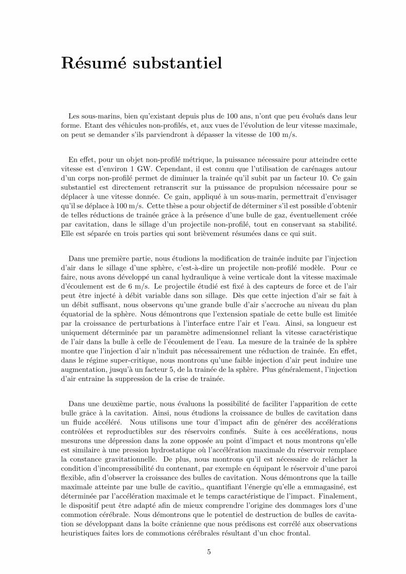
Les sous-marins, bien qu’existant depuis plus de 100 ans, n’ont que peu evolues dans leurforme. Etant des vehicules non-profiles, et, aux vues de l’evolution de leur vitesse maximale,on peut se demander s’ils parviendront a depasser la vitesse de 100 m/s.
En effet, pour un objet non-profile metrique, la puissance necessaire pour atteindre cettevitesse est d’environ 1 GW. Cependant, il est connu que l’utilisation de carenages autourd’un corps non-profile permet de diminuer la trainee qu’il subit par un facteur 10. Ce gainsubstantiel est directement retranscrit sur la puissance de propulsion necessaire pour sedeplacer a une vitesse donnee. Ce gain, applique a un sous-marin, permettrait d’envisagerqu’il se deplace a 100 m/s. Cette these a pour objectif de determiner s’il est possible d’obtenirde telles reductions de trainee grace a la presence d’une bulle de gaz, eventuellement creeepar cavitation, dans le sillage d’un projectile non-profile, tout en conservant sa stabilite.Elle est separee en trois parties qui sont brievement resumees dans ce qui suit.
Dans une premiere partie, nous etudions la modification de trainee induite par l’injectiond’air dans le sillage d’une sphere, c’est-a-dire un projectile non-profile modele. Pour cefaire, nous avons developpe un canal hydraulique a veine verticale dont la vitesse maximaled’ecoulement est de 6 m/s. Le projectile etudie est fixe a des capteurs de force et de l’airpeut etre injecte a debit variable dans son sillage. Des que cette injection d’air se fait aun debit suffisant, nous observons qu’une grande bulle d’air s’accroche au niveau du planequatorial de la sphere. Nous demontrons que l’extension spatiale de cette bulle est limiteepar la croissance de perturbations a l’interface entre l’air et l’eau. Ainsi, sa longueur estuniquement determinee par un parametre adimensionnel reliant la vitesse caracteristiquede l’air dans la bulle a celle de l’ecoulement de l’eau. La mesure de la trainee de la spheremontre que l’injection d’air n’induit pas necessairement une reduction de trainee. En effet,dans le regime super-critique, nous montrons qu’une faible injection d’air peut induire uneaugmentation, jusqu’a un facteur 5, de la trainee de la sphere. Plus generalement, l’injectiond’air entraine la suppression de la crise de trainee.
Dans une deuxieme partie, nous evaluons la possibilite de faciliter l’apparition de cettebulle grace a la cavitation. Ainsi, nous etudions la croissance de bulles de cavitation dansun fluide accelere. Nous utilisons une tour d’impact afin de generer des accelerationscontrolees et reproductibles sur des reservoirs confines. Suite a ces accelerations, nousmesurons une depression dans la zone opposee au point d’impact et nous montrons qu’elleest similaire a une pression hydrostatique ou l’acceleration maximale du reservoir remplacela constance gravitationnelle. De plus, nous montrons qu’il est necessaire de relacher lacondition d’incompressibilite du contenant, par exemple en equipant le reservoir d’une paroiflexible, afin d’observer la croissance des bulles de cavitation. Nous demontrons que la taillemaximale atteinte par une bulle de cavitio,, quantifiant l’energie qu’elle a emmagasine, estdeterminee par l’acceleration maximale et le temps caracteristique de l’impact. Finalement,le dispositif peut etre adapte afin de mieux comprendre l’origine des dommages lors d’unecommotion cerebrale. Nous demontrons que le potentiel de destruction de bulles de cavita-tion se developpant dans la boıte cranienne que nous predisons est correle aux observationsheuristiques faites lors de commotions cerebrales resultant d’un choc frontal.
5

Enfin, dans une troisieme partie, nous nous interessons a la stabilite de la trajectoire desprojectiles resultant de la croissance d’une bulle de gaz dans le sillage d’un objet non-profile.Nous les modelisons par des projectiles profiles avec une repartition de masse inhomogene.Apres l’impact de tels projectiles a la surface d’un bain d’eau, nous observons que leurtrajectoire n’est pas necessairement rectiligne. En effet, en fonction de la vitesse d’impactdu projectile et de la position de son centre de gravite, trois types de trajectoire peuventetre observees. L’apparition de trajectoires courbes resulte d’un equilibre entre la force deportance (destabilisatrice) et la poussee d’Archimede (stabilisatrice). Apres avoir caracteriseles projectiles utilises en soufflerie, nous demontrons que leur trajectoire peut etre prediteen resolvant les equations quasi-statiques du mouvement.
6
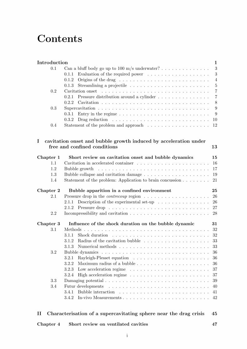
Contents
Introduction 10.1 Can a bluff body go up to 100 m/s underwater? . . . . . . . . . . . . . . 3
0.1.1 Evaluation of the required power . . . . . . . . . . . . . . . . . . 3
0.1.2 Origins of the drag . . . . . . . . . . . . . . . . . . . . . . . . . . 4
0.1.3 Streamlining a projectile . . . . . . . . . . . . . . . . . . . . . . . 5
0.2 Cavitation onset . . . . . . . . . . . . . . . . . . . . . . . . . . . . . . . 7
0.2.1 Pressure distribution around a cylinder . . . . . . . . . . . . . . . 7
0.2.2 Cavitation . . . . . . . . . . . . . . . . . . . . . . . . . . . . . . . 8
0.3 Supercavitation . . . . . . . . . . . . . . . . . . . . . . . . . . . . . . . . 9
0.3.1 Entry in the regime . . . . . . . . . . . . . . . . . . . . . . . . . . 9
0.3.2 Drag reduction . . . . . . . . . . . . . . . . . . . . . . . . . . . . 10
0.4 Statement of the problem and approach . . . . . . . . . . . . . . . . . . 12
I cavitation onset and bubble growth induced by acceleration underfree and confined conditions 13
Chapter 1 Short review on cavitation onset and bubble dynamics 15
1.1 Cavitation in accelerated container . . . . . . . . . . . . . . . . . . . . . 16
1.2 Bubble growth . . . . . . . . . . . . . . . . . . . . . . . . . . . . . . . . 17
1.3 Bubble collapse and cavitation damage . . . . . . . . . . . . . . . . . . . 19
1.4 Statement of the problem: Application to brain concussion . . . . . . . . 21
Chapter 2 Bubble apparition in a confined environment 25
2.1 Pressure drop in the contrecoup region . . . . . . . . . . . . . . . . . . . 26
2.1.1 Description of the experimental set-up . . . . . . . . . . . . . . . 26
2.1.2 Pressure drop . . . . . . . . . . . . . . . . . . . . . . . . . . . . . 27
2.2 Incompressibility and cavitation . . . . . . . . . . . . . . . . . . . . . . . 28
Chapter 3 Influence of the shock duration on the bubble dynamic 31
3.1 Methods . . . . . . . . . . . . . . . . . . . . . . . . . . . . . . . . . . . . 32
3.1.1 Shock duration . . . . . . . . . . . . . . . . . . . . . . . . . . . . 32
3.1.2 Radius of the cavitation bubble . . . . . . . . . . . . . . . . . . . 33
3.1.3 Numerical methods . . . . . . . . . . . . . . . . . . . . . . . . . . 33
3.2 Bubble dynamics . . . . . . . . . . . . . . . . . . . . . . . . . . . . . . . 36
3.2.1 Rayleigh-Plesset equation . . . . . . . . . . . . . . . . . . . . . . 36
3.2.2 Maximum radius of a bubble . . . . . . . . . . . . . . . . . . . . . 36
3.2.3 Low acceleration regime . . . . . . . . . . . . . . . . . . . . . . . 37
3.2.4 High acceleration regime . . . . . . . . . . . . . . . . . . . . . . . 37
3.3 Damaging potential . . . . . . . . . . . . . . . . . . . . . . . . . . . . . . 39
3.4 Futur developments . . . . . . . . . . . . . . . . . . . . . . . . . . . . . 40
3.4.1 Bubble interaction . . . . . . . . . . . . . . . . . . . . . . . . . . 41
3.4.2 In-vivo Measurements . . . . . . . . . . . . . . . . . . . . . . . . . 42
II Characterisation of a supercavitating sphere near the drag crisis 45
Chapter 4 Short review on ventilated cavities 47
i
4.1 Generalities on ventilated cavities . . . . . . . . . . . . . . . . . . . . . . 48
4.2 Ventilated cavities in the wake of projectiles . . . . . . . . . . . . . . . . 49
4.2.1 Dimensional analysis . . . . . . . . . . . . . . . . . . . . . . . . . 49
4.2.2 Length of the cavity and shedding process . . . . . . . . . . . . . 49
4.2.3 Influence of the blockage ratio . . . . . . . . . . . . . . . . . . . . 51
4.2.4 Drag reduction: application to spheres . . . . . . . . . . . . . . . 51
4.3 Statement of the problem . . . . . . . . . . . . . . . . . . . . . . . . . . 53
Chapter 5 Experimental set-up 55
5.1 Hydraulic tunnel construction . . . . . . . . . . . . . . . . . . . . . . . . 56
5.2 Flow in the empty test-section . . . . . . . . . . . . . . . . . . . . . . . . 56
5.3 Drag measurements . . . . . . . . . . . . . . . . . . . . . . . . . . . . . . 57
5.3.1 Validation of the measurement set-up . . . . . . . . . . . . . . . . 57
5.3.2 Drag coefficient of a sphere . . . . . . . . . . . . . . . . . . . . . . 58
Chapter 6 In-crisis drag modification 61
6.1 Morphology of the bubbles . . . . . . . . . . . . . . . . . . . . . . . . . . 62
6.2 Bubble length . . . . . . . . . . . . . . . . . . . . . . . . . . . . . . . . . 63
6.2.1 Bubble length measurements . . . . . . . . . . . . . . . . . . . . . 63
6.2.2 Surface instability properties . . . . . . . . . . . . . . . . . . . . . 65
6.3 In-crisis force measurements . . . . . . . . . . . . . . . . . . . . . . . . . 67
6.3.1 Drag of a sphere with air injection at its back . . . . . . . . . . . 69
6.3.2 Drag modification . . . . . . . . . . . . . . . . . . . . . . . . . . . 69
6.3.3 Application to supercavitation . . . . . . . . . . . . . . . . . . . . 70
III Stability of the trajectory of the streamlined projectile 73
Chapter 7 Short review on water entry and path instabilities 75
7.1 Water entry . . . . . . . . . . . . . . . . . . . . . . . . . . . . . . . . . . 76
7.1.1 Cavity formation . . . . . . . . . . . . . . . . . . . . . . . . . . . 76
7.1.2 Slender bodies . . . . . . . . . . . . . . . . . . . . . . . . . . . . . 77
7.2 Path instabilities . . . . . . . . . . . . . . . . . . . . . . . . . . . . . . . 78
7.3 Statement of the problem . . . . . . . . . . . . . . . . . . . . . . . . . . 79
7.4 Experimental details . . . . . . . . . . . . . . . . . . . . . . . . . . . . . 79
7.4.1 Trajectory reconstruction . . . . . . . . . . . . . . . . . . . . . . . 79
7.4.2 Projectiles . . . . . . . . . . . . . . . . . . . . . . . . . . . . . . . 80
7.4.3 Releasing method . . . . . . . . . . . . . . . . . . . . . . . . . . . 80
Chapter 8 Path instabilities of streamlined bodies 83
8.1 Experimental Results . . . . . . . . . . . . . . . . . . . . . . . . . . . . . 84
8.1.1 Nature of the trajectory . . . . . . . . . . . . . . . . . . . . . . . 84
8.1.2 Quasi-planar trajectories . . . . . . . . . . . . . . . . . . . . . . . 86
8.2 Equations of motion and closing parameters . . . . . . . . . . . . . . . . 87
8.2.1 Presentation of the model . . . . . . . . . . . . . . . . . . . . . . 87
8.2.2 Lift and Drag . . . . . . . . . . . . . . . . . . . . . . . . . . . . . 88
8.2.3 Position of the aerodynamic center . . . . . . . . . . . . . . . . . 89
8.2.4 Dissipative torque . . . . . . . . . . . . . . . . . . . . . . . . . . . 90
8.3 Results and discussion . . . . . . . . . . . . . . . . . . . . . . . . . . . . 91
8.3.1 Solution of the equation of motion . . . . . . . . . . . . . . . . . . 91
8.3.2 Critical velocity and growth time . . . . . . . . . . . . . . . . . . 92
8.3.3 Quantitative comparison and dive depth . . . . . . . . . . . . . . 94
ii

8.4 Controlling the instability . . . . . . . . . . . . . . . . . . . . . . . . . . 96
Conclusion 99
Appendices 105
Appendix A List of publication 107
Appendix B International Physicists’ Tournament 109
Bibliography 119
iii

iv

INTRODUCTION
1


0.1. Can a bluff body go up to 100 m/s underwater?
Intro
Figure 1: Drawing of the front page of Red Rackham’s Treasure, by Herge 1944.
The publication of Red Rackham’s Treasure in 1944 followed the early development of sub-marines in the navy, such that, at this time, the invention of Professor Cuthbert Calculuswas still uncanny to most of the readers. Since then, even though submarines have com-pletely changed (size, shape, propulsion technique...), their maximum speed is still below100 m/s. Which leaves the following question open: Can a bluff body go up to 100 m/sunderwater?
0.1 Can a bluff body go up to 100 m/s underwater?
0.1.1 Evaluation of the required power
When a body travels underwater at a velocity U , it experiences a drag force D resisting toits motion. This force is generally expressed as follows [1]:
D =1
2ρSCDU
2 (1)
where ρ denotes the density of water, S the cross-stream surface of the body and CD thedrag coefficient. The drag coefficient depends on both the geometry of the object consideredand the Reynolds number Re = UL/ν, which compares the inertial effects to the viscouseffects in the flow [1]. In this expression, L is the characteristic size of the body and ν thekinematic viscosity of the fluid.
3
Intro
100 10510-2
100
102
104
−1
−1/2 0.5
UL
1 2 3 4 5
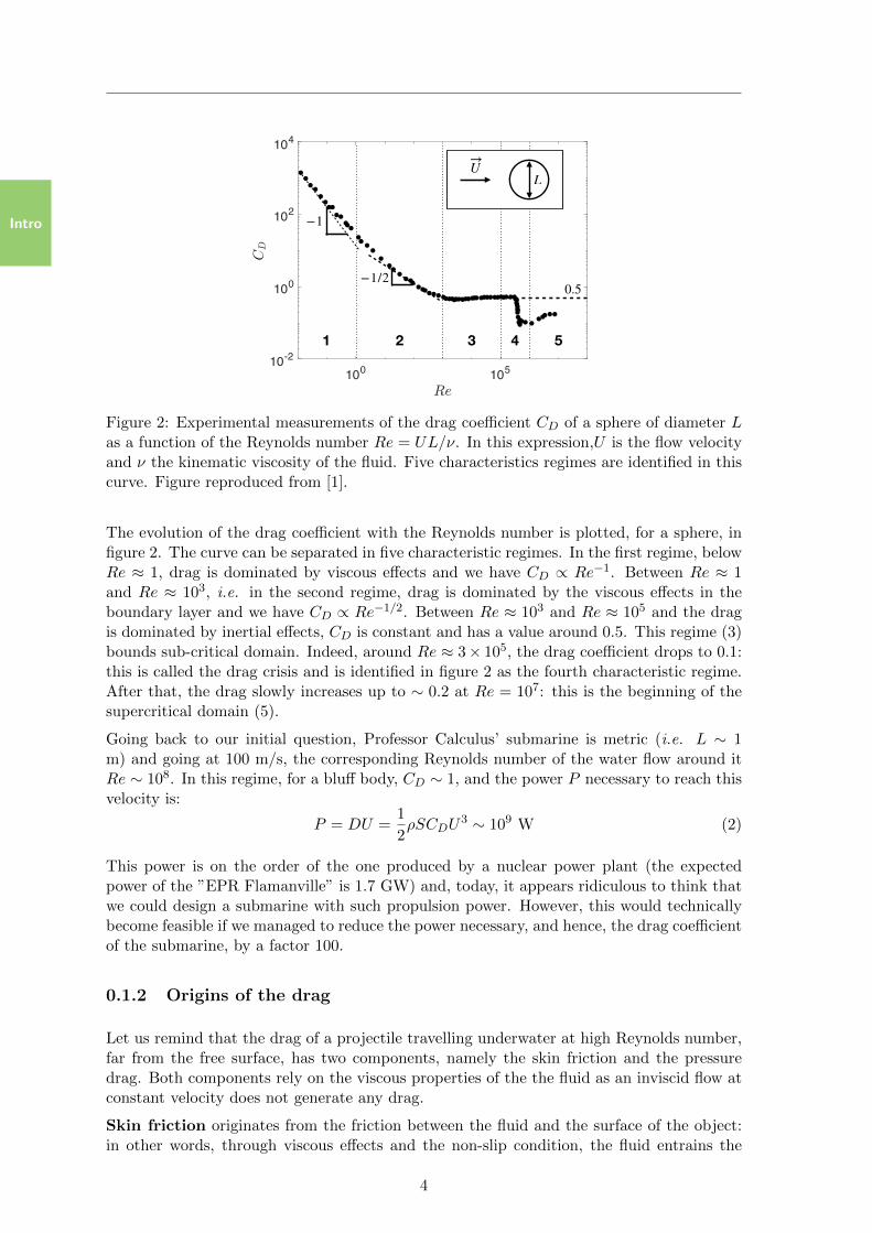
Figure 2: Experimental measurements of the drag coefficient CD of a sphere of diameter Las a function of the Reynolds number Re = UL/ν. In this expression,U is the flow velocityand ν the kinematic viscosity of the fluid. Five characteristics regimes are identified in thiscurve. Figure reproduced from [1].
The evolution of the drag coefficient with the Reynolds number is plotted, for a sphere, infigure 2. The curve can be separated in five characteristic regimes. In the first regime, belowRe ≈ 1, drag is dominated by viscous effects and we have CD ∝ Re−1. Between Re ≈ 1and Re ≈ 103, i.e. in the second regime, drag is dominated by the viscous effects in theboundary layer and we have CD ∝ Re−1/2. Between Re ≈ 103 and Re ≈ 105 and the dragis dominated by inertial effects, CD is constant and has a value around 0.5. This regime (3)bounds sub-critical domain. Indeed, around Re ≈ 3× 10⁵, the drag coefficient drops to 0.1:this is called the drag crisis and is identified in figure 2 as the fourth characteristic regime.After that, the drag slowly increases up to ∼ 0.2 at Re = 107: this is the beginning of thesupercritical domain (5).
Going back to our initial question, Professor Calculus’ submarine is metric (i.e. L ∼ 1m) and going at 100 m/s, the corresponding Reynolds number of the water flow around itRe ∼ 108. In this regime, for a bluff body, CD ∼ 1, and the power P necessary to reach thisvelocity is:
P = DU =1
2ρSCDU
3 ∼ 109 W (2)
This power is on the order of the one produced by a nuclear power plant (the expectedpower of the ”EPR Flamanville” is 1.7 GW) and, today, it appears ridiculous to think thatwe could design a submarine with such propulsion power. However, this would technicallybecome feasible if we managed to reduce the power necessary, and hence, the drag coefficientof the submarine, by a factor 100.
0.1.2 Origins of the drag
Let us remind that the drag of a projectile travelling underwater at high Reynolds number,far from the free surface, has two components, namely the skin friction and the pressuredrag. Both components rely on the viscous properties of the the fluid as an inviscid flow atconstant velocity does not generate any drag.
Skin friction originates from the friction between the fluid and the surface of the object:in other words, through viscous effects and the non-slip condition, the fluid entrains the
4
0.1. Can a bluff body go up to 100 m/s underwater?
Intro
object. As a consequence, the skin friction mainly depends on the flow in the boundarylayers, i.e. the regions near the surface of the object, where viscosity dominates. Locally,the contribution of the skin friction to a unit surface δS is δDF = ηδS ∂u∂y , where u is thetangential component of flow velocity, ∂u/∂y its gradient normal to the surface and η thedynamical viscosity of the fluid. From this expression, we deduce that this component ofthe drag depends on the total wetted area of the projectile.
Pressure drag arises from the pressure difference between the upstream and downstreamfaces of the projectile. As a consequence, it is strongly correlated to the streamwise asym-metry of the flow: for instance to the development of structures in the wake of the projectile.This component of the drag depends on the frontal area of the projectile.
104 105 106 107
100
Thom (1929)Achenbach (1968)
1 %
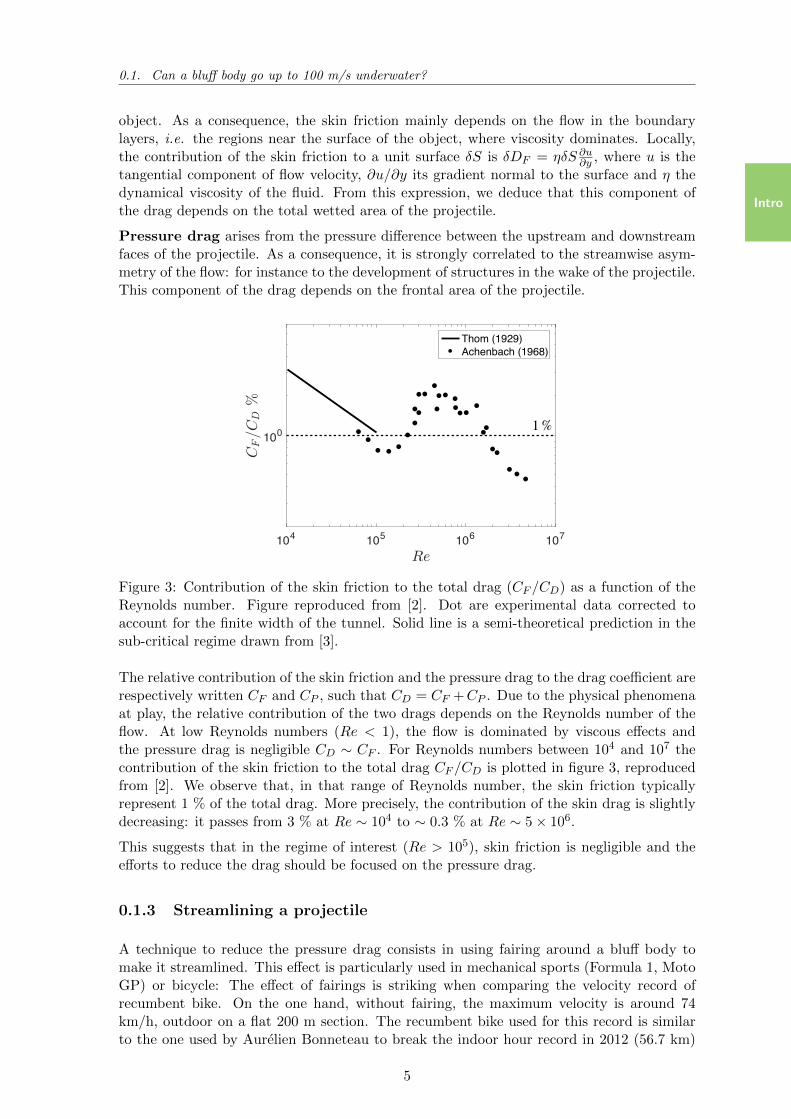
Figure 3: Contribution of the skin friction to the total drag (CF /CD) as a function of theReynolds number. Figure reproduced from [2]. Dot are experimental data corrected toaccount for the finite width of the tunnel. Solid line is a semi-theoretical prediction in thesub-critical regime drawn from [3].
The relative contribution of the skin friction and the pressure drag to the drag coefficient arerespectively written CF and CP , such that CD = CF +CP . Due to the physical phenomenaat play, the relative contribution of the two drags depends on the Reynolds number of theflow. At low Reynolds numbers (Re < 1), the flow is dominated by viscous effects andthe pressure drag is negligible CD ∼ CF . For Reynolds numbers between 104 and 107 thecontribution of the skin friction to the total drag CF /CD is plotted in figure 3, reproducedfrom [2]. We observe that, in that range of Reynolds number, the skin friction typicallyrepresent 1 % of the total drag. More precisely, the contribution of the skin drag is slightlydecreasing: it passes from 3 % at Re ∼ 104 to ∼ 0.3 % at Re ∼ 5× 10⁶.
This suggests that in the regime of interest (Re > 105), skin friction is negligible and theefforts to reduce the drag should be focused on the pressure drag.
0.1.3 Streamlining a projectile
A technique to reduce the pressure drag consists in using fairing around a bluff body tomake it streamlined. This effect is particularly used in mechanical sports (Formula 1, MotoGP) or bicycle: The effect of fairings is striking when comparing the velocity record ofrecumbent bike. On the one hand, without fairing, the maximum velocity is around 74km/h, outdoor on a flat 200 m section. The recumbent bike used for this record is similarto the one used by Aurelien Bonneteau to break the indoor hour record in 2012 (56.7 km)
5
Intro
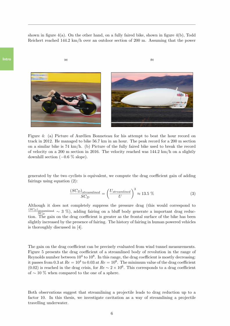
shown in figure 4(a). On the other hand, on a fully faired bike, shown in figure 4(b), ToddReichert reached 144.2 km/h over an outdoor section of 200 m. Assuming that the power
(a) (b)
Figure 4: (a) Picture of Aurelien Bonneteau for his attempt to beat the hour record ontrack in 2012. He managed to bike 56.7 km in an hour. The peak record for a 200 m sectionon a similar bike is 74 km/h. (b) Picture of the fully faired bike used to break the recordof velocity on a 200 m section in 2016. The velocity reached was 144.2 km/h on a slightlydownhill section (−0.6 % slope).
generated by the two cyclists is equivalent, we compute the drag coefficient gain of addingfairings using equation (2):
(SCD)streamlinedSCD
=
(Ustreamlined
U
)3
≈ 13.5 % (3)
Although it does not completely suppress the pressure drag (this would correspond to(SCD)streamlined
SCD∼ 3 %), adding fairing on a bluff body generate a important drag reduc-
tion. The gain on the drag coefficient is greater as the frontal surface of the bike has beenslightly increased by the presence of fairing. The history of fairing in human powered vehiclesis thoroughly discussed in [4].
The gain on the drag coefficient can be precisely evaluated from wind tunnel measurements.Figure 5 presents the drag coefficient of a streamlined body of revolution in the range ofReynolds number between 104 to 108. In this range, the drag coefficient is mostly decreasing:it passes from 0.3 atRe = 104 to 0.03 atRe = 108. The minimum value of the drag coefficient(0.02) is reached in the drag crisis, for Re ∼ 2× 10⁶. This corresponds to a drag coefficientof ∼ 10 % when compared to the one of a sphere.
Both observations suggest that streamlining a projectile leads to drag reduction up to afactor 10. In this thesis, we investigate cavitation as a way of streamlining a projectiletravelling underwater.
6

0.2. Cavitation onset
Intro
104 105 106 107 10810-2
10-1
100
U
LaminarTurbulent
L
Figure 5: Drag coefficient CD of a streamlined body of revolution as a function of theReynolds number Re = UL/ν. Figure reproduced from [1]. Solid lines indicate the trendsfor sub and super critical regimes. Dots are experimental data. The profile of the projectileused is the one of the R101 airship and is sketched in the inset. Drag coefficient is based onfrontal area.
0.2 Cavitation onset
0.2.1 Pressure distribution around a cylinder
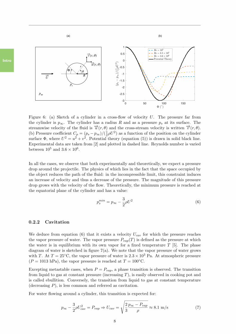
When a projectile travels underwater, the pressure distribution in the fluid is modified. Athigh Reynolds number, the pressure field around a two-dimensional projectile can easily beevaluated assuming that the flow is potential.
Let us consider a cylinder of radius R in a cross flow of velocity−→U , far from the projectile.
This situation is sketched in figure 6(a). For a potential flow, writing −→u (r, θ) the streamwisevelocity and −→v (r, θ) the cross-stream velocity, we have:
u(r, θ) = U
(1− cos(2θ)
(R
r
)2)
v(r, θ) = − U sin(2θ)
(R
r
)2(4)
Using Bernoulli, we express the pressure at the boundary of the cylinder:
ps = p∞ +1
2ρU2
(1− 4 sin2 θ
)(5)
This relation is plotted in figure 6(b) and compared with measurements taken from [2]for Reynolds numbers ranging from 105 to 3.6 × 10⁶. Potential theory matches well theexperimental data up to Φ = 50. Beyond this value, for all Reynolds the pressure isfound to reach a plateau, such that Cp = (ps − p∞)/(12ρU
2) lies between -1.25 and -0.4.The discrepancies between potential theory and experiments comes from the fact that theboundary layer is neglected, in particular the flow separation it induces and the wake itcreates.
7
Intro
0 50 100 150-3
-2.5
-2
-1.5
-1
-0.5
0
0.5
1
p∞
ps
U
Φ
(a) (b)
R
u (r, θ)
v (r, θ)
rθ
Figure 6: (a) Sketch of a cylinder in a cross-flow of velocity U . The pressure far fromthe cylinder is p∞. The cylinder has a radius R and as a pressure ps at its surface. Thestreamwise velocity of the fluid is −→u (r, θ) and the cross-stream velocity is written −→v (r, θ).(b) Pressure coefficient Cp = (ps− p∞)/(12ρU
2) as a function of the position on the cylindersurface Φ, where U2 = u2 + v2. Potential theory (equation (5)) is drawn in solid black line.Experimental data are taken from [2] and plotted in dashed line. Reynolds number is variedbetween 105 and 3.6× 10⁶.
In all the cases, we observe that both experimentally and theoretically, we expect a pressuredrop around the projectile. The physics of which lies in the fact that the space occupied bythe object reduces the path of the fluid: in the incompressible limit, this constraint inducesan increase of velocity and thus a decrease of the pressure. The magnitude of this pressuredrop grows with the velocity of the flow. Theoretically, the minimum pressure is reached atthe equatorial plane of the cylinder and has a value:
pmins = p∞ −3
2ρU2 (6)
0.2.2 Cavitation
We deduce from equation (6) that it exists a velocity Ucav for which the pressure reachesthe vapor pressure of water. The vapor pressure Pvap(T ) is defined as the pressure at whichthe water is in equilibrium with its own vapor for a fixed temperature T [5]. The phasediagram of water is sketched in figure 7(a). We note that the vapor pressure of water growswith T . At T = 25C, the vapor pressure of water is 2.3× 10³ Pa. At atmospheric pressure(P = 1013 hPa), the vapor pressure is reached at T = 100C.
Excepting metastable cases, when P = Pvap, a phase transition is observed. The transitionfrom liquid to gas at constant pressure (increasing T ), is easily observed in cooking pot andis called ebullition. Conversely, the transition from liquid to gas at constant temperature(decreasing P ), is less common and referred as cavitation.
For water flowing around a cylinder, this transition is expected for:
p∞ −3
2ρU2
cav = Pvap ⇒ Ucav =
√2
3
p∞ − Pvapρ
≈ 8.1 m/s (7)
8

0.3. Supercavitation
IntroSolid Liquid
Gas
0 100
1.013
105
0.023
25
(a) (b)
T (C)
P(P
a)
Pvap(25)
Pvap(100)
Figure 7: (a) Phase diagram of water as a function of its temperature T and its pressureP . The vapor pressure of water is written Pvap. (b) Picture of the cavitation trail observedbehind a ship propeller at the Cavitation Research Laboratory of the Australian MaritimeCollege (http://www.amc.edu.au/facilities/cavitation).
Cavitation is thus expected roughly above 10 m/s. This velocity is typically reached atthe tip of the blades of ship propellers where it is known that cavitation is observed asillustrated by the picture of figure 7(b), taken from the Cavitation Research Laboratoryof the Australian Maritime College website. In this picture, we observe that bubbles arecreated on the low pressure side of the boat propeller blades. An helicoidal wake of bubblesis then created by the advection of bubbles in the wake of the blades.
According to the results obtained for a cylinder in a potential flow (equation (5)), thedimensionless parameter that governs the pressure at the boundary of an object travellingunderwater, and hence the creation of vapor bubbles in a flow [6, 7], called the cavitationnumber σ, writes:
σ =p∞ − Pvap
12ρU
2(8)
0.3 Supercavitation
0.3.1 Entry in the regime
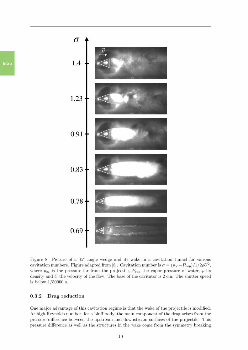
From the definition of the cavitation number (8), we expect cavitation bubble to nucleate ina flow wherever σ ∼ 1. For a two dimensional wedge, the influence of the cavitation numberon the phase transition is shown in figure 8 adapted from [8]. For σ = 1.4, we indeed observea trail of bubbles created in the near wake of the cavitator. These bubbles then display acharacteristic wake pattern.
As the cavitation number is decreased, the bubbles invade a larger region of the wake ofthe wedge. For σ below 1.23, a large bubble starts pinning at the rim of the wedge. Thecharacteristic streamwise size of this bubble grows when σ is reduced. Above σ = 0.78 theinterface of the bubble is largely turbulent and unstationnary. However, for σ = 0.69 theinstabilities at the interface of the large bubble have almost disappeared. This regime, inwhich a large cavitation bubble is pinned on the cavitator is called supercavitation.
9
Intro
128 Inter J Nav Archit Oc Engng (2012) 4:123~131
σ = 1.40
σ = 1.40
σ = 1.23
σ = 1.23
σ = 0.91
σ = 0.91
σ = 0.83
σ = 0.83
σ = 0.78
σ = 0.78
σ = 0.69
σ = 0.69
(a) General video camera (30 fps) strips. (b) High-speed camera (50,000 fps) strips.
Fig. 10 Sequence of events of the supercavity in the wake of a 45° cavitator (flow speed V = 9.4 m/s).
Brought to you by | Ecole PolytechniqueAuthenticated
Download Date | 8/26/19 2:18 PM
σ
1.4
1.23
0.91
0.83
0.78
0.69
U
Figure 8: Picture of a 45 angle wedge and its wake in a cavitation tunnel for variouscavitation numbers. Figure adapted from [8]. Cavitation number is σ = (p∞−Pvap)/1/2ρU2,where p∞ is the pressure far from the projectile, Pvap the vapor pressure of water, ρ itsdensity and U the velocity of the flow. The base of the cavitator is 2 cm. The shutter speedis below 1/50000 s.
0.3.2 Drag reduction
One major advantage of this cavitation regime is that the wake of the projectile is modified.At high Reynolds number, for a bluff body, the main component of the drag arises from thepressure difference between the upstream and downstream surfaces of the projectile. Thispressure difference as well as the structures in the wake come from the symmetry breaking
10
0.3. Supercavitation
Intro
due to the boundary layer separation [1].
Since the cavitation bubble tends to ”streamline” the solid that moves through water, themain consequence of the modification of the wake of the projectile in the supercavitationregime is a reduction of its drag. Numerous studies have focused on the determination ofthe drag reduction via the computation of the stationnary shape of the bubble. All thosestudies are thoroughly reviewed in [6, 7]. However, it is interesting to note that all theoreticalstudies assume a potential flow, a constant pressure in the gas and they neglect evaporation.The closure condition of the cavity is widely discussed and the different models includes:releasing the free-surface dynamical conditions at a fixed point (open wake model) [9], theuse of an ”image object” onto which the clavity closes (Riabouchinsky model) [10], havinga jet flowing back into the cavity (re-entrant jet model) [11].
0 0.2 0.4 0.6 0.8 1 1.2 1.4 1.60.2
0.4
0.6
0.8
1
1.2
1.4
(o) (i)U d
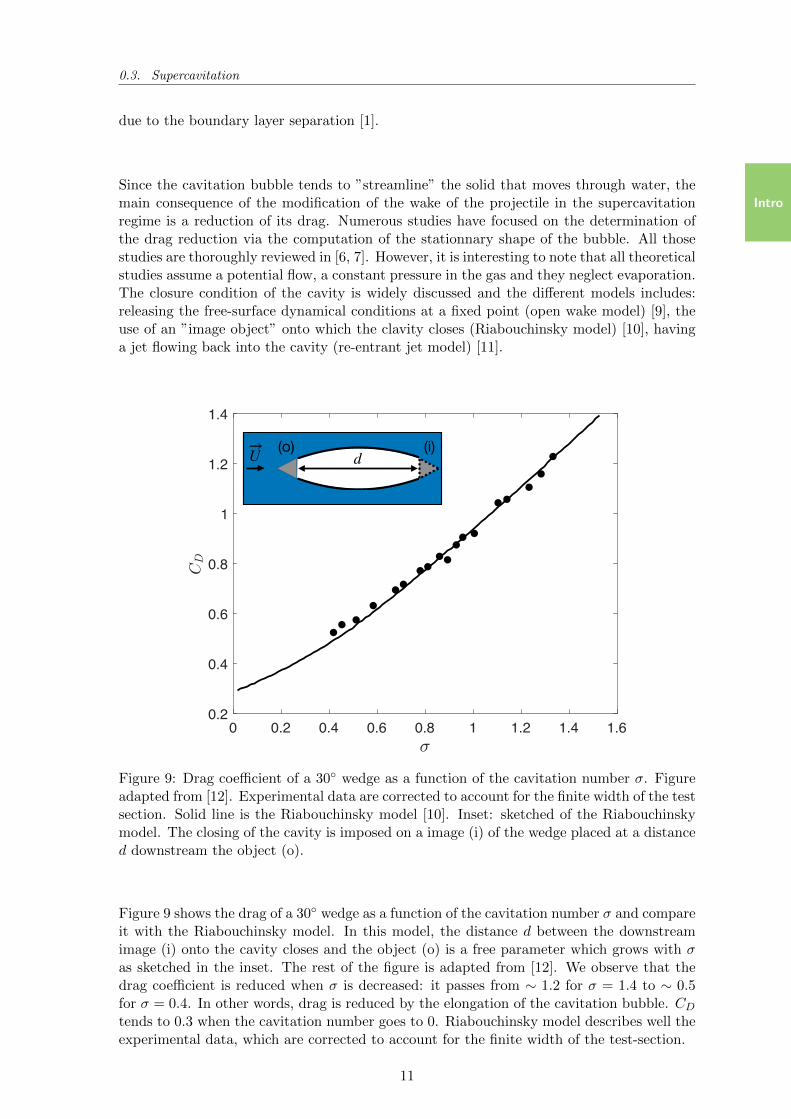
Figure 9: Drag coefficient of a 30 wedge as a function of the cavitation number σ. Figureadapted from [12]. Experimental data are corrected to account for the finite width of the testsection. Solid line is the Riabouchinsky model [10]. Inset: sketched of the Riabouchinskymodel. The closing of the cavity is imposed on a image (i) of the wedge placed at a distanced downstream the object (o).
Figure 9 shows the drag of a 30 wedge as a function of the cavitation number σ and compareit with the Riabouchinsky model. In this model, the distance d between the downstreamimage (i) onto the cavity closes and the object (o) is a free parameter which grows with σas sketched in the inset. The rest of the figure is adapted from [12]. We observe that thedrag coefficient is reduced when σ is decreased: it passes from ∼ 1.2 for σ = 1.4 to ∼ 0.5for σ = 0.4. In other words, drag is reduced by the elongation of the cavitation bubble. CDtends to 0.3 when the cavitation number goes to 0. Riabouchinsky model describes well theexperimental data, which are corrected to account for the finite width of the test-section.
11

Intro
0.4 Statement of the problem and approach
This thesis is dedicated to the experimental and theorical study of cavitation and supercav-itation. It is decomposed in three different parts:
• In Part I, we focus on the cavitation onset and the early growth of a cavitation bubble.To that end, cavitation is triggered by an hydrostatic-like pressure drop following theacceleration of a closed container. We will study both the influence of the confinementon the vapor production and the dependence of the bubble dynamic on the timeevolution of the acceleration. This unsteady induction of cavitation can be used tofacilitate the entry in the supercavitation regime, model the early stages of the launchof torpedoes or missiles or to better understand the implication of cavitation in brainconcussion. This last application is the main point of interest of Part I.
• In Part II, we present the experimental set-up developed to determine the hydro-dynamic properties of a supercavitating sphere. We create a system analogous tosupercavitation by replacing the phase transition of water by a controlled air injectionin the wake of the sphere. We concentrate on the influence of the bubble on the dragcrisis of the sphere.
• In Part III, we consider that a supercavitating is analogous to a streamlined projectilewith inhomogeneous mass distribution. We focus on determining the condition underwhich, such projectiles, follow straight trajectories following their impact on water.This work can be apply to predict the trajectory stability of projectile such has missilesor torpedoes as well as to understand the way birds like gannet dive.
12

PART I
CAVITATION ONSET ANDBUBBLE GROWTH INDUCEDBY ACCELERATION UNDER
FREE AND CONFINEDCONDITIONS
13
I
Decreasing the pressure of a liquid below its vapor pressure can trigger a phase transitionthrough the nucleation of gas bubbles. This phenomenon is called cavitation. We wish tocharacterise the early stage of the growth of cavitation bubbles developing near a projectiletravelling underwater. However, in such a system, the velocities required to reach a pressuredrop high enough to observe cavitation are challenging to obtain in a simple experimental set-up. In this part, we study the dynamic of a bubble growing in a low pressure region of a fluidcreated through the acceleration of its container. In a first chapter, we quickly review thestate of the art of cavitation in accelerated container. We then present our experimental set-up and show how the confinement of cavitation bubble change their threshold of apparition.Finally, the third chapter focus on the study on bubble dynamics in accelerated container.Through this part, we show that this framework allows us to investigate whether cavitationcan be the cause of the damages observed in the brain following a shock on the head, theso-called brain concussion.
14
1Short review on cavitation onset
and bubble dynamics
Fluid container accelerated when hit by a hammer: Cavitation bubbles grow in the regionopposite of the point of impact and shatter the reservoir.
Contents
1.1 Cavitation in accelerated container . . . . . . . . . . . . . . 16
1.2 Bubble growth . . . . . . . . . . . . . . . . . . . . . . . . . 17
1.3 Bubble collapse and cavitation damage . . . . . . . . . . . . 19
1.4 Statement of the problem: Application to brain concussion . 21
15
Chapter 1. Short review on cavitation onset and bubble dynamics
I
1.1 Cavitation in accelerated container
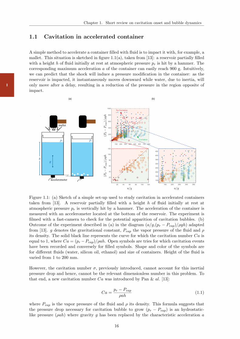
A simple method to accelerate a container filled with fluid is to impact it with, for example, amallet. This situation is sketched in figure 1.1(a), taken from [13]: a reservoir partially filledwith a height h of fluid initially at rest at atmospheric pressure pr is hit by a hammer. Thecorresponding maximum acceleration a of the container can easily reach 900 g. Intuitively,we can predict that the shock will induce a pressure modification in the container: as thereservoir is impacted, it instantaneously moves downward while water, due to inertia, willonly move after a delay, resulting in a reduction of the pressure in the region opposite ofimpact.
mallet
h
pr
g
accelerometer
pb
pr
pb rigid floor
pr
pb
hg
pr
pb
t=t0 t=t1 t=t0 t=t1
A B
Fig. 2. Free body diagram of the fluid column: mean liquid column height (h), reference pressure (pr ), pressure at the bottom of the container (pb), andgravitational acceleration (g). Experiment done at USU/BYU facilities (A), where the impact is imparted by a rubber mallet. The TUAT experiment uses a glasstest tube with a rounded bottom, where the impact is imparted by collision with the ground (B). The small difference traveled between t0 and t1 is shownas dashed lines to emphasize the relative acceleration (experimental evidence shown in Fig. S2 and Movie S4).
Experimental Setup
More details about the experiments can be found in Materials and
Methods. Two separate groups independently conducted the fol-lowing experiments with different setups and measurement tech-niques to validate Eq. 4 or 5.
pr = 101.3 kPa, D = 8.0 mm, Silicone oil, TUATpr = 101.3 kPa, D = 14.2 mm, Silicone oil, TUATpr = 101.3 kPa, D = 27.2 mm, Silicone oil, TUAT
pr = 86.9 kPa, D = 55.0 mm, Water, USU/BYU
pr = 19.0 kPa, D = 55.0 mm, Water, USU/BYUpr = 85.7 kPa, D = 55.0 mm, Water, USU/BYU
pr = 101.3 kPa, D = 14.2 mm, Ethanol, TUAT
Ca =1No Cavitation
Cavitation
A
B C
Fig. 3. Phase diagram for the cavitation onset by acceleration in the (pr pv )/gh, a/g plane (A) for various fluid types, container diameters (D),pressures (pr ), and fluid depths (h) as marked in the legend. Open markers denote cavitation detection and filled markers denote absence of cavitationdetection. Lines represent theoretical separation between cavity formation (shaded in red) and none (shaded in green) based on Ca = 1 in Eq. 5. Changingthe stiffness of the container and a nonfluid medium was also investigated as shown in Figs. S3 and S4 and Table S2. Close-up view (B) of concentrated datapoints in the region where the reference pressure was varied (red-squared region in A). Close-up view (C) of collapsed data points in the region where thefluid type was varied (blue-squared region in A).
The group from Utah State University and Brigham YoungUniversity (USU/BYU) used a cylindrical cavitation tube builtfrom transparent acrylic (1, 20). The cavitation tube was fittedwith a pressure tap to control internal pressure and an accelero-meter with a maximum measurable acceleration of 1,000 g
8472 | www.pnas.org/cgi/doi/10.1073/pnas.1702502114 Pan et al.
(a) (b)
EN
GIN
EER
IN
G
mallet
h
pr
g
accelerometer
pb
pr
pb rigid floor
pr
pb
hg
pr
pb
t=t0 t=t1 t=t0 t=t1
A B
Fig. 2. Free body diagram of the fluid column: mean liquid column height (h), reference pressure (pr ), pressure at the bottom of the container (pb), andgravitational acceleration (g). Experiment done at USU/BYU facilities (A), where the impact is imparted by a rubber mallet. The TUAT experiment uses a glasstest tube with a rounded bottom, where the impact is imparted by collision with the ground (B). The small difference traveled between t0 and t1 is shownas dashed lines to emphasize the relative acceleration (experimental evidence shown in Fig. S2 and Movie S4).
Experimental Setup
More details about the experiments can be found in Materials and
Methods. Two separate groups independently conducted the fol-lowing experiments with different setups and measurement tech-niques to validate Eq. 4 or 5.
Fig. 3. Phase diagram for the cavitation onset by acceleration in the (pr pv )/gh, a/g plane (A) for various fluid types, container diameters (D),pressures (pr ), and fluid depths (h) as marked in the legend. Open markers denote cavitation detection and filled markers denote absence of cavitationdetection. Lines represent theoretical separation between cavity formation (shaded in red) and none (shaded in green) based on Ca = 1 in Eq. 5. Changingthe stiffness of the container and a nonfluid medium was also investigated as shown in Figs. S3 and S4 and Table S2. Close-up view (B) of concentrated datapoints in the region where the reference pressure was varied (red-squared region in A). Close-up view (C) of collapsed data points in the region where thefluid type was varied (blue-squared region in A).
The group from Utah State University and Brigham YoungUniversity (USU/BYU) used a cylindrical cavitation tube builtfrom transparent acrylic (1, 20). The cavitation tube was fittedwith a pressure tap to control internal pressure and an accelero-meter with a maximum measurable acceleration of 1,000 g
Pan et al. PNAS Early Edition | 3 of 5
(P0
Pvap)/gh
(P0
Pvap)/gh
a/g a/g
Figure 1.1: (a) Sketch of a simple set-up used to study cavitation in accelerated containerstaken from [13]. A reservoir partially filled with a height h of fluid initially at rest atatmospheric pressure pr is vertically hit by a hammer. The acceleration of the container ismeasured with an accelerometer located at the bottom of the reservoir. The experiment isfilmed with a fast-camera to check for the potential apparition of cavitation bubbles. (b)Outcome of the experiment described in (a) in the diagram (a/g,(pr − Pvap)/ρgh) adaptedfrom [13]. g denotes the gravitational constant, Pvap the vapor pressure of the fluid and ρits density. The solid black line represents the curve for which the cavitation number Ca isequal to 1, where Ca = (pr−Pvap)/ρah. Open symbols are tries for which cavitation eventshave been recorded and conversely for filled symbols. Shape and color of the symbols arefor different fluids (water, silicon oil, ethanol) and size of containers. Height of the fluid isvaried from 1 to 200 mm.
However, the cavitation number σ, previously introduced, cannot account for this inertialpressure drop and hence, cannot be the relevant dimensionless number in this problem. Tothat end, a new cavitation number Ca was introduced by Pan & al. [13]:
Ca =pr − Pvapρah
(1.1)
where Pvap is the vapor pressure of the fluid and ρ its density. This formula suggests thatthe pressure drop necessary for cavitation bubble to grow (pr − Pvap) is an hydrostatic-like pressure (ρah) where gravity g has been replaced by the characteristic acceleration a
16
1.2. Bubble growth
I
of the shock. The experiment described before can then be performed while measuringthe acceleration a and filming the container to check for cavitation bubbles. The figure1.1(b), reproduced from [13], displays the results in the diagram (a/g, (pr−Pvap)/ρgh). Thedimensionless acceleration of the shock a/g is extensively varied from 20 to 800 (changing theintensity of the hit) and the parameter (pr−Pvap)/ρgh is varied from ∼ 10 to 1000 (changingthe fluid and its height h). Over the whole range of parameters, most of the experimentsin which cavitation events have been recorded (open symbols) lies below the curve Ca andreciprocally for tries where no cavitation bubbles were detected (filled symbols).
This cavitation number and the experimental results suggest that the pressure drop in anaccelerated column of fluid scales as ρah. However, this does not tell us how this relation ismodified when the container does not have a free surface and is fully filled. Additionally, thestudy of the dynamic of the cavitation bubble in such a set-up is left open. These questionsare the main interests of our work, and before addressing them, let us briefly review theliterature on bubble dynamic.
1.2 Bubble growth
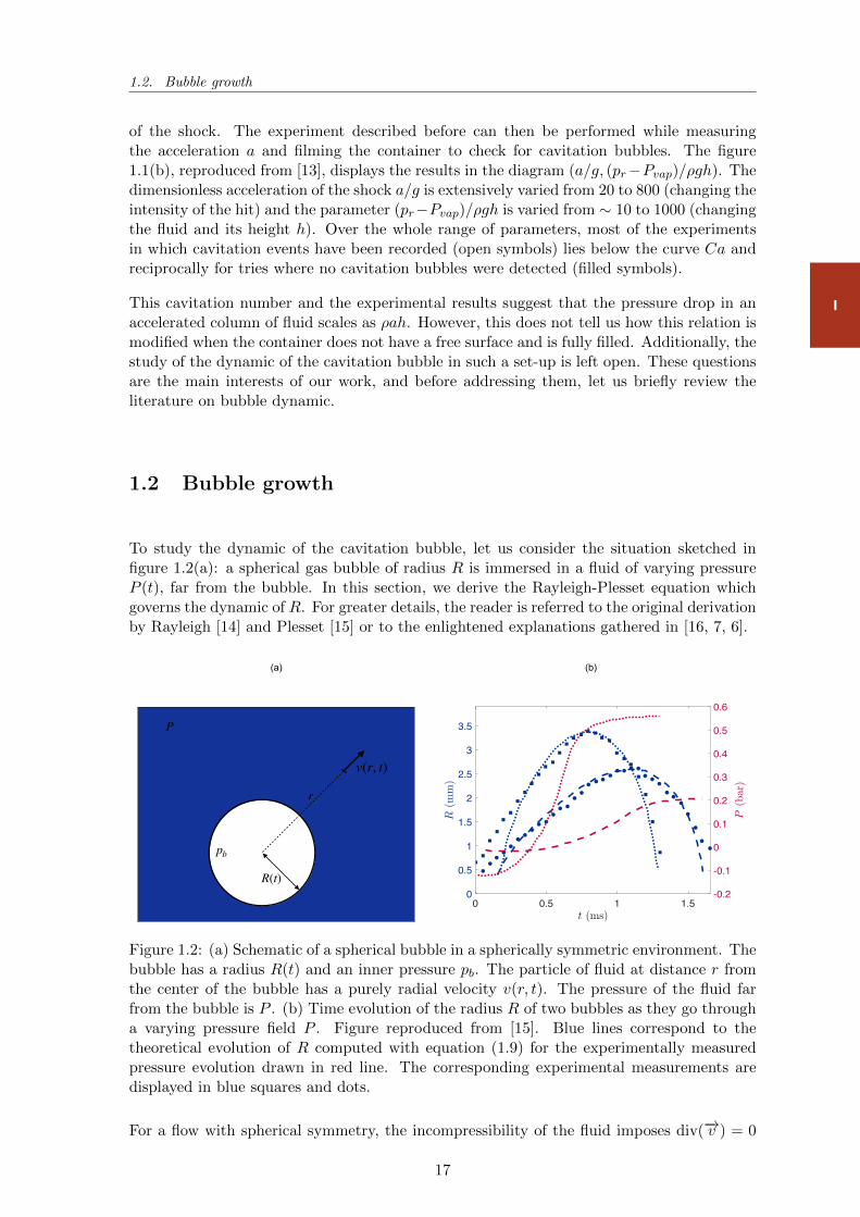
To study the dynamic of the cavitation bubble, let us consider the situation sketched infigure 1.2(a): a spherical gas bubble of radius R is immersed in a fluid of varying pressureP (t), far from the bubble. In this section, we derive the Rayleigh-Plesset equation whichgoverns the dynamic of R. For greater details, the reader is referred to the original derivationby Rayleigh [14] and Plesset [15] or to the enlightened explanations gathered in [16, 7, 6].
0 0.5 1 1.50
0.5
1
1.5
2
2.5
3
3.5
-0.2
-0.1
0
0.1
0.2
0.3
0.4
0.5
0.6
R(t)
r
v(r, t)
P
pb
(a) (b)
Figure 1.2: (a) Schematic of a spherical bubble in a spherically symmetric environment. Thebubble has a radius R(t) and an inner pressure pb. The particle of fluid at distance r fromthe center of the bubble has a purely radial velocity v(r, t). The pressure of the fluid farfrom the bubble is P . (b) Time evolution of the radius R of two bubbles as they go througha varying pressure field P . Figure reproduced from [15]. Blue lines correspond to thetheoretical evolution of R computed with equation (1.9) for the experimentally measuredpressure evolution drawn in red line. The corresponding experimental measurements aredisplayed in blue squares and dots.
For a flow with spherical symmetry, the incompressibility of the fluid imposes div(−→v ) = 0
17
Chapter 1. Short review on cavitation onset and bubble dynamics
I
which yields, assuming that there is no mass transport through the bubble interface:
v =R2R
r2(1.2)
The fluid flow is governed by the Navier-Stokes equation which, when projected along theradial direction, reads as follows:
ρ∂v
∂t+ ρv
∂v
∂r= −∂p
∂r+ η
(1
r
∂2(rv)
∂r2− 2v
r2
)(1.3)
Where η denotes the dynamic viscosity of the outer fluid and p(r, t) its pressure at a distancer from the center of the bubble. Substituting v with its expression (1.2), we find that theviscous term is strictly null and we obtain:
ρR2R+ 2RR2
r2− ρ2R4R2
r5= −∂p
∂r(1.4)
Integrating between r = R(t) and r =∞ where p(∞) = P (t) we obtain:
ρR2R+ 2RR2
r− ρR
4R2
2r4= p(R)− P (t) (1.5)
The pressure in the outer fluid at the interface of the bubble p(R) can further be evaluatedthrough the continuity of the radial stress across the bubble interface:
p(R) = pb −4ηR
R− 2γ
R(1.6)
where pb(R) is the pressure of the gaz inside the bubble and γ the surface tension between theliquid and the gas. Substituting this expression in equation (1.5) yields the Rayleigh-Plessetequation:
RR+3
2R2 +
4νR
R+
2γ
ρR=pb − P∞
ρ(1.7)
pb(R) can itself be expressed assuming that the gas transformation in the bubble is isother-mal and that the bubble is initially at rest with the surrounding liquid of pressure P0:
pb(R) =
(P0 +
2γ
R0
)(R0
R
)3
(1.8)
with R0 being the initial radius of the bubble and Pvap the vapor pressure of water. Injectingthis relation in the Rayleigh-Plesset equation gives:
RR+3
2R2 +
4νR
R+
2γ
ρR=Pvap + (P0 + 2γ
R0)(R0R
)3 − P (t)
ρ(1.9)
This equation was first confronted to experimental data by Plesset in 1949 [15]. The cavita-tion bubble was created in a cavitation tunnel and then travelled through a spatially varyingpressure field, resulting in a time evolution of its radius. This evolution could be followedusing a fast-camera. Figure 1.2(b), reproduces two of the time evolution of the radius ofthe bubble from [15]. This suggests that as the pressure difference is negative, the bubblegrows. When the outer pressure exceeds the inner pressure, the bubble keeps growing withinertia, but then rapidly collapses.
18
1.3. Bubble collapse and cavitation damage
I
1.3 Bubble collapse and cavitation damage
Cavitation has been thoroughly studied for boat propeller applications. Indeed, a propelleror the rotor of a hydraulic pump is composed of streamlined blades with a concave anda convex side. When rotating towards the concave side, the blades produce a pressuredifference between their two sides. In particular, a low pressure zone will appear on theconvex side, called the suction side. As shown before, when the rotor velocity is highenough, the pressure on the suction side can go below the vapor pressure of water, andhence, trigger the nucleation of cavitation bubble. This phenomenon has been shown to havetwo consequences on the propeller operation. First, it reduces its efficiency and changes theoptimal shape of a propeller [17]. Second, it erodes the blades and dramatically shortens itslife expectancy [18, 19, 20].
M. Dular et al. / Wear 257 (2004) 1176–1184 1179
Fig. 6. Sequence of top view images for ALE25 hydrofoil. The flow is fromleft to the right. Significant dynamic cavitation behaviour can be seen nearthe front wall, while the cavitation at the rear wall remains nearly steady.
(fluctuations of cavitation region with separation of the cav-itation cloud) while cavitation at the rear wall (where thehydrofoil length is the greatest) remains nearly steady (withno cloud separation).
4. Cavitation erosion tests
Due to the problems with reproducibility of the galvaniccopper coating method, only a small part of the surface wasinvestigated for the cavitation erosion in previous investiga-tions. This was done using pure copper specimens insertedinto the hydrofoil [10]. To get the information about the ero-sion on the whole surface of the hydrofoil, a polished copperfoil, 0.2-mm thick, was fixed to its surface using adhesivefilm. The hardness of the copper coating was approximately40HV. A sufficient number of pits was obtained after 1 h ex-posure to the cavitating flow (the exposure time was constantfor all operating conditions).Pits have a diameter of magnitude order 10−5 m, and can
be distinguished only by sufficient magnification. Images ofthe pitted surface were acquired using an Olympus BX-40microscope and a CCD camera (Fig. 7).The enlargement scale was 50:1 leading to the resolution
of 1.95!m per pixel. 925 images (one image embraces anarea of 1.2mm× 1.5mmbig) of the pitted surfacewere takenfor each operating point (the part of the surface evaluated byimages represents approximately 48% of the copper coatedhydrofoil surface).
Fig. 7. Camera, microscope, light source and hydrofoil arrangement forsurface image acquisition. About 925 images of the pitted surface weretaken for each experiment.
Fig. 8. Image of the surface prior (left) and after (right) the exposure to thecavitating flow. While we see no damage on the left image, almost 5% ofthe surface on the right image is covered with pits.
Fig. 8 shows an image of the surface before the exposureto cavitating flow (left) (0% damaged surface) and after 1 hof exposure (right) (4.98% damaged surface).
5. Image post-processing
Image post-processing is based on the fact that image nwith ij pixels can be presented as a matrix with ij elements. 8bit resolution gives 256 levels of grey level A(i, j, n), whichthe matrix element can occupy (0 for black pixel and 255 forwhite pixel):
A(i, j, n)∈ 0, 1, . . . , 255. (2)
(a) (b)
0.5 mm
B
A
Impact Max cavity growth erutcarFtesnonoitativaC
accelerometer
bubbleformation
bubblegrowth
50 mm
10 mm
0 ms 0.28 0.33 3.20 5.33
0 ms 0.10 1.46 3.20 7.47
Fig. 1. Two cases of cavitation onset introduced by large accelerations in low-speed flows. A bottle filled with water accelerated by the impact of amallet on the top (A). A test tube filled with silicone oil accelerated by an impact with the ground (B). Both image sets correspond to the impact (firstframe), tiny bubble appearance (second frame), bubble expansion (third frame), bubble collapse and cracking (fourth frame), and crack propagation/failure(fifth frame). Although the time between each event is different, the overall behavior is very similar (Movies S1–S4). Relative timing of bubble collapseand fracture incidence suggests that implosion-induced waves are likely responsible for fracture initiation, although further investigation into fracturemechanisms in the case studies presented here would be necessary to confirm this observation (Fig. S1). Relationships between cavitation and structuraldamage are well-documented elsewhere in biological and man-made systems (27–31).
@v
@t= 1
rp. [2]
Integrating Eq. 2 along the centerline of the liquid from the freesurface to the bottom of the column (assuming the depth of theliquid is h), denoting the magnitude of the vertical component of@v/@t as a , and solving for the pressure difference in the liquidcolumn yields
pr pb = ah, [3]
where pr is the reference pressure at the free surface and pb isthe pressure at the bottom of the column. Cavitation is likely tooccur when pb < pv . Thus, we can establish
Ca =pr pv
ah[4]
as an indicator of cavitation onset when the flow undergoes aviolent acceleration. We refer to this expression as the quiescentcavitation number.
To gain physical insight into the interpretation of the quiescentcavitation number, gravitational acceleration can be introducedand Eq. 4 can be reformulated as
Ca =(pr pv )/gh
a/g. [5]
Gravitational acceleration is not an essential term in the cav-itation number. However, it is included here to enable a for-mulation with explicit physical meaning. The numerator is themaximum nondimensionalized force that the pressure differ-ence can provide (similar to Eq. 1) and the denominator isthe nondimensionalized inertial force the liquid experiencesunder acceleration (in contrast to the fluid momentum of Eq. 1).Thus, once the inertial forces exceed the maximum pressuredifference (i.e., Ca < 1), cavitation is likely. However, whenCa > 1 the pressure is large enough to balance the vacuum intro-duced by acceleration. Hence, cavitation is not likely.
2 of 5 | www.pnas.org/cgi/doi/10.1073/pnas.1702502114 Pan et al.
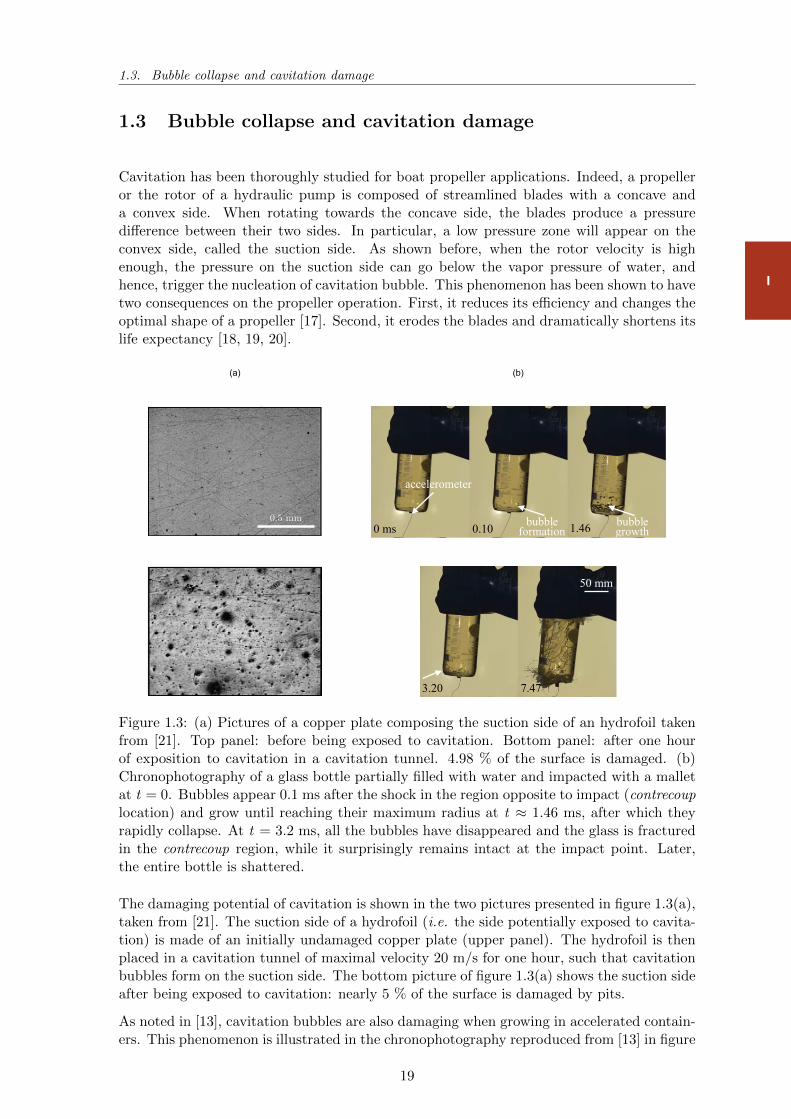
Figure 1.3: (a) Pictures of a copper plate composing the suction side of an hydrofoil takenfrom [21]. Top panel: before being exposed to cavitation. Bottom panel: after one hourof exposition to cavitation in a cavitation tunnel. 4.98 % of the surface is damaged. (b)Chronophotography of a glass bottle partially filled with water and impacted with a malletat t = 0. Bubbles appear 0.1 ms after the shock in the region opposite to impact (contrecouplocation) and grow until reaching their maximum radius at t ≈ 1.46 ms, after which theyrapidly collapse. At t = 3.2 ms, all the bubbles have disappeared and the glass is fracturedin the contrecoup region, while it surprisingly remains intact at the impact point. Later,the entire bottle is shattered.
The damaging potential of cavitation is shown in the two pictures presented in figure 1.3(a),taken from [21]. The suction side of a hydrofoil (i.e. the side potentially exposed to cavita-tion) is made of an initially undamaged copper plate (upper panel). The hydrofoil is thenplaced in a cavitation tunnel of maximal velocity 20 m/s for one hour, such that cavitationbubbles form on the suction side. The bottom picture of figure 1.3(a) shows the suction sideafter being exposed to cavitation: nearly 5 % of the surface is damaged by pits.
As noted in [13], cavitation bubbles are also damaging when growing in accelerated contain-ers. This phenomenon is illustrated in the chronophotography reproduced from [13] in figure
19
Chapter 1. Short review on cavitation onset and bubble dynamics
I
1.3(b) where the effect of the impact of a hammer on a glass reservoir partially filled withwater is followed. Time origin is fixed at impact, and cavitation bubbles quickly appear inthe contrecoup area (at t ≈ 0.1 ms), that is, the region with size comparable to that of thehammer and located opposite to it. Bubbles then grow and reach their maximum size (a fewmillimeters) at t ≈ 1.46 ms, after which they collapse in less than 2 ms, which fractures theglass at t ≈ 3.2 ms. Remarkably, the glass is fractured at the point of collapse of cavitationbubbles while it remains intact at the point of impact of the hammer, suggesting that thecollapse of cavitation bubbles is responsible for the damages. At later times, the wholecontainer is shattered.
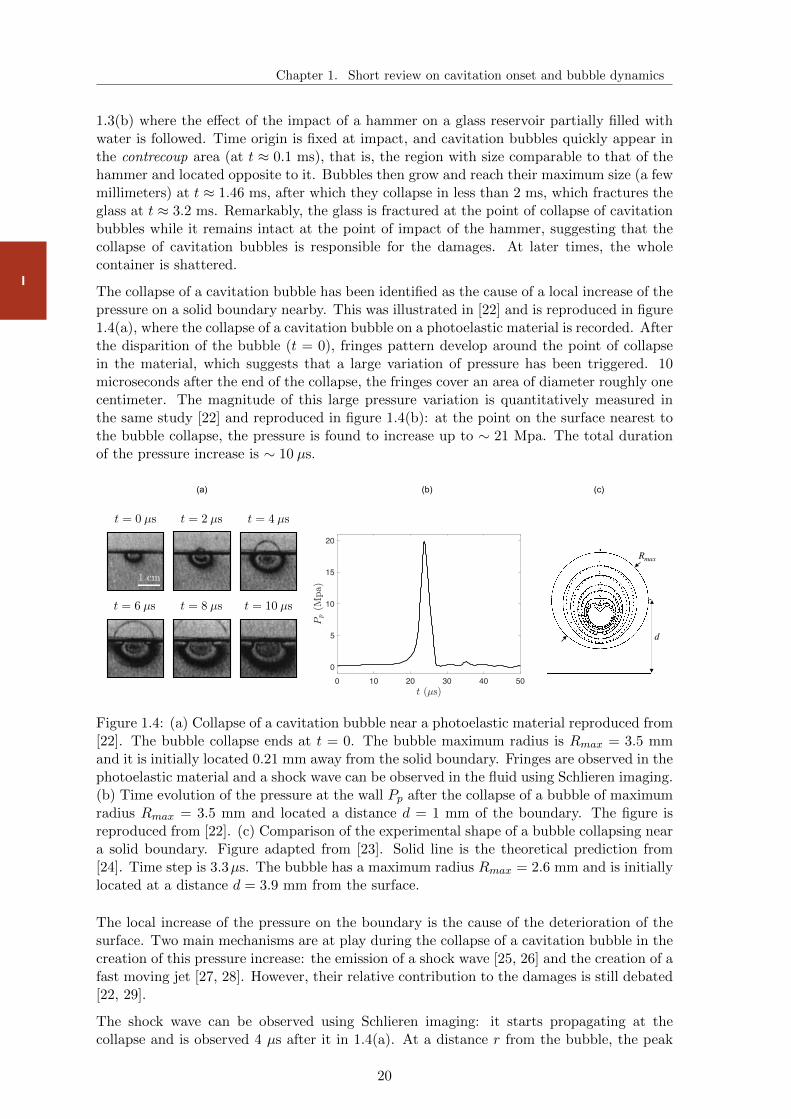
The collapse of a cavitation bubble has been identified as the cause of a local increase of thepressure on a solid boundary nearby. This was illustrated in [22] and is reproduced in figure1.4(a), where the collapse of a cavitation bubble on a photoelastic material is recorded. Afterthe disparition of the bubble (t = 0), fringes pattern develop around the point of collapsein the material, which suggests that a large variation of pressure has been triggered. 10microseconds after the end of the collapse, the fringes cover an area of diameter roughly onecentimeter. The magnitude of this large pressure variation is quantitatively measured inthe same study [22] and reproduced in figure 1.4(b): at the point on the surface nearest tothe bubble collapse, the pressure is found to increase up to ∼ 21 Mpa. The total durationof the pressure increase is ∼ 10 µs.
0 10 20 30 40 50
0
5
10
15
20
(c)(a) (b)
396 W . Lauterborn and H . Bolle n
7 ////////// /Solid . . ' ' boundary . ' . ' ' .-//////////////////////////////Il//////% FIGURE 6. Comparison of experimentally determined bubble shapes (open circles) on collapse of a spherical bubble near a plane solid wall with theoretical curves taken from Plesset & Chapman (1971) (solid curves). The framing rate is 300000 framesls, the mexi- mum bubble radius R, = 2.6 mm, the distance of the bubble centre from the wall 6 = 3.9 mm and b/Rmx = 1.5. Curve 0 1 2 3 4 5 6 7 Time, R-(po/Ap)4 0 0.725 0.825 0.961 0.991 1.016 1.028 1.036 (p,, is the density of the liquid and Ap is the constant difference between the ambient liquid pressure and the pressure in the cavity.)
compared backwards in time. The result is shown in figure 6. The open circles represent experimental data while the solid lines are taken from the calculations of Plesset & Chapman. The initial (experimental) bubble shape is not exactly spherical. But nevertheless the behaviour of the bubble (involution of the top and jet formation towards the boundary) fits the theory almost quantitatively.
6. Discussion The dynamics of laser-induced cavitationbubblesin water near solid boundaries
have been investigated by high-speed photography. Jetting effects could be studied in considerable detail. I n the example reported here a maximum jet velocity (or, rather, tip velocity) of 120 m/s was measured at a framing rate of 250000 framesls and a value of b/RmBx = 3-08 (figure 4). The measured tip velocities depend on the framing rate used. They are higher the higher the
9DD
C5
: 8
1
.25
57
9DD
C 4
23
:58
8
4 /
40
D49
:AE
,E8
2DCE
34D
DD9
23
:58
DC
7EC
22:
232D
9DD
C 4
23
:58
8
4D
C
Rmax
d
550 Y . Tomita and A . S h i m
- 5mm FIGURE 16. Initiation of stress fringe caused by liquid-jet impact; R,,, = 5.1 mm,
LIR,,, = 0.68, a = 5.2 mm/kg.
___c H 10-
FIQURE 17. Isochromatic fringe patterns in epoxy resins due to impulsive pressure generated at the first collapse of a bubble; (a ) LIR,,, = 0.059 (R,,, = 3.5 mm); ( b ) LIR,,, = 0.43 (R,,, = 5.1 mm); frame interval 2 p, exposure 0.4 p.
of the gth-order fringe. Since the shape of the w1.5 versus LIR,,, curve is very similar to that of theplmsx versus LIR,,, curve, i t can be conjectured that the pressure-time histories measured by the transducer represent the shock-wave pressures. In this connection, an important piece of experimental evidence is the generation of multiple shock waves prior to a main shock wave. It is interesting that the maximum value of wo.5 occurs at LIR,,, z 0.9, which corresponds exactly to the tendency of plot of the pulse width of pressure wave versus L/R,,, (Shima et al. 1983, 1984).
Figure 17 shows the isochromatic fringe patterns. I n particular, an interesting phenomenon can be seen in figure 17 ( b ) : two longitudinal waves are generated from different points on the model surface. This suggests the generation of local impulsive forces acting on the surface. On the other hand, as shown in figure 8, the solid boundary is probably hit by impulsive pressures at not only the first but also a t the second collapse of a bubble near a boundary. Figure 18 shows the fringe patterns for LIR,,, = 1.05 and 0.35. At the second collapse of a bubble, weak stress fringes appear in figure 18(a)(2), whereas impulsive stress fringes can be clearly seen in figure 18(b)(2). I n particular, in the fourth and fifth frames of figure 18(b)(2) two fringes can be seen to develop from different portions of the epoxy surface and combine into a single fringe with the passage of time. The new fringe is quite similar to the one a t the first collapse shown in figure 18(a)(l) . In general, a bubble vortex ring composed of a number of tiny bubbles seems to be formed in the torus-like bubble interior after the first collapse of the original bubble. At the second collapse, a part of the ring collapses rapidly and results in the radiation of a shock wave. Lauterborn ( 1982) observed shock waves emitted from individial tiny bubbles. The pressures caused by the collapse of these bubbles certainly contribute to the fringe initiation in figure 18 (b ) (2).
9DD
C5
: 8
1
.25
657
9DD
C 4
2:5
86
84
6 /4
60
D649
:AE6
,E8
2DCE
64DD
D96
2:5
866
D6C
7EC6
22:
26
2D9D
DC
42
:586
8
46
D6C
t = 0 µs t = 2 µs t = 4 µs
t = 6 µs t = 8 µs t = 10 µs
1 cm
Figure 1.4: (a) Collapse of a cavitation bubble near a photoelastic material reproduced from[22]. The bubble collapse ends at t = 0. The bubble maximum radius is Rmax = 3.5 mmand it is initially located 0.21 mm away from the solid boundary. Fringes are observed in thephotoelastic material and a shock wave can be observed in the fluid using Schlieren imaging.(b) Time evolution of the pressure at the wall Pp after the collapse of a bubble of maximumradius Rmax = 3.5 mm and located a distance d = 1 mm of the boundary. The figure isreproduced from [22]. (c) Comparison of the experimental shape of a bubble collapsing neara solid boundary. Figure adapted from [23]. Solid line is the theoretical prediction from[24]. Time step is 3.3µs. The bubble has a maximum radius Rmax = 2.6 mm and is initiallylocated at a distance d = 3.9 mm from the surface.
The local increase of the pressure on the boundary is the cause of the deterioration of thesurface. Two main mechanisms are at play during the collapse of a cavitation bubble in thecreation of this pressure increase: the emission of a shock wave [25, 26] and the creation of afast moving jet [27, 28]. However, their relative contribution to the damages is still debated[22, 29].
The shock wave can be observed using Schlieren imaging: it starts propagating at thecollapse and is observed 4 µs after it in 1.4(a). At a distance r from the bubble, the peak
20
1.4. Statement of the problem: Application to brain concussion
I
pressure of the shock wave Pp was shown to scale as [30, 6]:
Pp ≈ 100P∞Rmaxr
(1.10)
where Rmax denotes the maximum radius of the bubble.
When a cavitation bubble collapses near a solid boundary, a jet is created. The jet is foundto be directed towards the boundary. The formation of the jet can be intuitively understoodassuming potential flow: a collapsing bubble behaves as a sink and its mirror image withrespect to the wall needs to be considered to respect the impermeability boundary condition.As a consequence, the bubble collapses in a pressure gradient perpendicular to the wall whichresults in the deformation of its interface and the creation of the re-entrant jet. The earlydevelopment of the jet was observed experimentally in [23] and compared with theoreticalprediction from [24]. The results, from [23] are presented in figure 1.4(c). The bubble, beforethe collapse, has a maximum radius Rmax = 2.6 mm and is located at a distance d = 3.9mm from the boundary. Roughly 16 µs after the beginning of the collapse, the interfaceat the point opposite to the solid boundary starts to curve in, resulting in the creation ofthe jet. At later times, beyond the scope of the theoretical study presented here, the jet isfound to impact the boundary at a velocity up to 200 m/s. This impact could be the causeof the local increase of the pressure in the material.
1.4 Statement of the problem: Application to brain concus-sion
The study of cavitation in an accelerated and confined environment is relevant for defensesapplications: the launch of missiles and torpedoes from submarines or the accelerationphases of propellers. Additionally, the damages caused by the collapse of cavitation bubblesare often listed as a possible cause of the brain concussion following a violent impact onthe head. In such applications, avoiding or at least reducing the damages induced by thecollapse of cavitation bubbles is crucial.
The application of cavitation to the understanding of mild Traumatic Brain Injuries (mTBI)particularly caught our attention: the experiment of a mallet impacting a fluid containersketched in figure 1.1(a) seems to be a direct model of a shock on the head. Indeed,the container represents the cranial vault while brain tissues and physiological fluids aremodelled by the water (they have a relative density close to 1 and are mainly composed ofwater).
So far, mTBI are known to be a common consequence of linear shocks on the head, inmotorized vehicle accidents or sports [31, 32] . Their detection and prevention is a majormedical concern not only because they can be lethal, but also because they are often involvedin the early development of neuronal diseases [33, 34, 35]. One of these disease is the ChronicTraumatic Encephalopathy (CTE), which results from repetitive brain trauma [36], and wasdiagnosed on an important rate of U.S. football players. Figure 1.5(a), taken from [36],presents coronal sections of a normal brain (top) and of a brain displaying a CTE (bottom):the pathological brain shows dilatation of the ventricles, atrophy and shrinkage of cerebralstructures.
The severity of the damages following a linear impacts on the head are commonly classifiedby the so-called Wayne State University (WSTC) curve [37, 38]. Characterizing shocksby their peak acceleration a and timespan τ , the WSTC, drawn in figure 1.5(b), has a
21
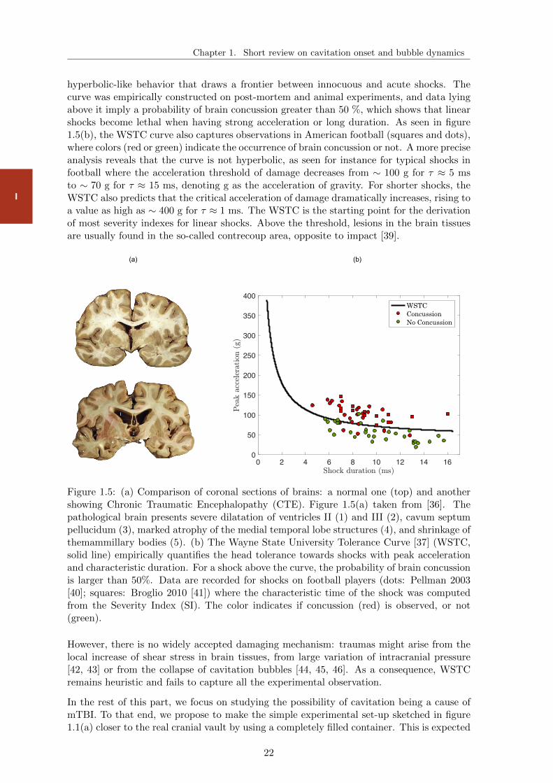
Chapter 1. Short review on cavitation onset and bubble dynamics
I
hyperbolic-like behavior that draws a frontier between innocuous and acute shocks. Thecurve was empirically constructed on post-mortem and animal experiments, and data lyingabove it imply a probability of brain concussion greater than 50 %, which shows that linearshocks become lethal when having strong acceleration or long duration. As seen in figure1.5(b), the WSTC curve also captures observations in American football (squares and dots),where colors (red or green) indicate the occurrence of brain concussion or not. A more preciseanalysis reveals that the curve is not hyperbolic, as seen for instance for typical shocks infootball where the acceleration threshold of damage decreases from ∼ 100 g for τ ≈ 5 msto ∼ 70 g for τ ≈ 15 ms, denoting g as the acceleration of gravity. For shorter shocks, theWSTC also predicts that the critical acceleration of damage dramatically increases, rising toa value as high as ∼ 400 g for τ ≈ 1 ms. The WSTC is the starting point for the derivationof most severity indexes for linear shocks. Above the threshold, lesions in the brain tissuesare usually found in the so-called contrecoup area, opposite to impact [39].
0 2 4 6 8 10 12 14 160
50
100
150
200
250
300
350
400
ConcussionNo Concussion
WSTCWSTC
(a) (b)
Figure 1.5: (a) Comparison of coronal sections of brains: a normal one (top) and anothershowing Chronic Traumatic Encephalopathy (CTE). Figure 1.5(a) taken from [36]. Thepathological brain presents severe dilatation of ventricles II (1) and III (2), cavum septumpellucidum (3), marked atrophy of the medial temporal lobe structures (4), and shrinkage ofthemammillary bodies (5). (b) The Wayne State University Tolerance Curve [37] (WSTC,solid line) empirically quantifies the head tolerance towards shocks with peak accelerationand characteristic duration. For a shock above the curve, the probability of brain concussionis larger than 50%. Data are recorded for shocks on football players (dots: Pellman 2003[40]; squares: Broglio 2010 [41]) where the characteristic time of the shock was computedfrom the Severity Index (SI). The color indicates if concussion (red) is observed, or not(green).
However, there is no widely accepted damaging mechanism: traumas might arise from thelocal increase of shear stress in brain tissues, from large variation of intracranial pressure[42, 43] or from the collapse of cavitation bubbles [44, 45, 46]. As a consequence, WSTCremains heuristic and fails to capture all the experimental observation.
In the rest of this part, we focus on studying the possibility of cavitation being a cause ofmTBI. To that end, we propose to make the simple experimental set-up sketched in figure1.1(a) closer to the real cranial vault by using a completely filled container. This is expected
22
1.4. Statement of the problem: Application to brain concussion
I
to change the onset of cavitation as the pressure at the bottom of the tank was determinedby both the acceleration of the shock and the ambient air pressure in the container.
As for defenses applications, evaluating the damaging potential of the cavitation bubbles isalso crucial. To that end, equation (1.10) suggests that the maximum radius of a cavitationbubble is a good proxy for assessing its damaging potential. To determine its maximumradius, we wish to study the dynamic of the growth of a cavitation bubble in an acceleratedfluid container. In particular, we would like to determine if it is governed by Rayleigh-Plessetequation.
Finally, the heuristic observations gathered in the WSTC state that the severity of thedamages following a shock is uniquely determined by both its maximum acceleration and itscharacteristic timespan. This raises two questions regarding a scenario of mTBI based oncavitation: Does the damaging potential of a cavitation bubble in an accelerated containerdepends on these two parameters? If so, can it be analytically evaluated?
In chapter 2, we present an experimental set-up, analogous to the cranial vault, which allowsus to monitor the growth of the confined cavitation bubbles and measures both the pressureand the acceleration of the container.
In chapter 3, we focus on determining the damaging potential of a cavitation bubble in suchan experimental set-up. To that end, we study, both experimentally and theoretically thedynamic of the cavitation bubbles.
23

Chapter 1. Short review on cavitation onset and bubble dynamics
I
24

2Bubble apparition in a confined
environment
The large majority of the work presented in the two following chapters was realized in collab-oration with Juliette Amauger, at that time, intern in the group. This work would not havebeen nearly as good without her implication and determination to overcome the (numerous)difficulties.
Illustration of the growth and the collapse of a bubble recorded using the experimental set-updescribed in this chapter.
Contents
2.1 Pressure drop in the contrecoup region . . . . . . . . . . . . 26
2.2 Incompressibility and cavitation . . . . . . . . . . . . . . . . 28
25
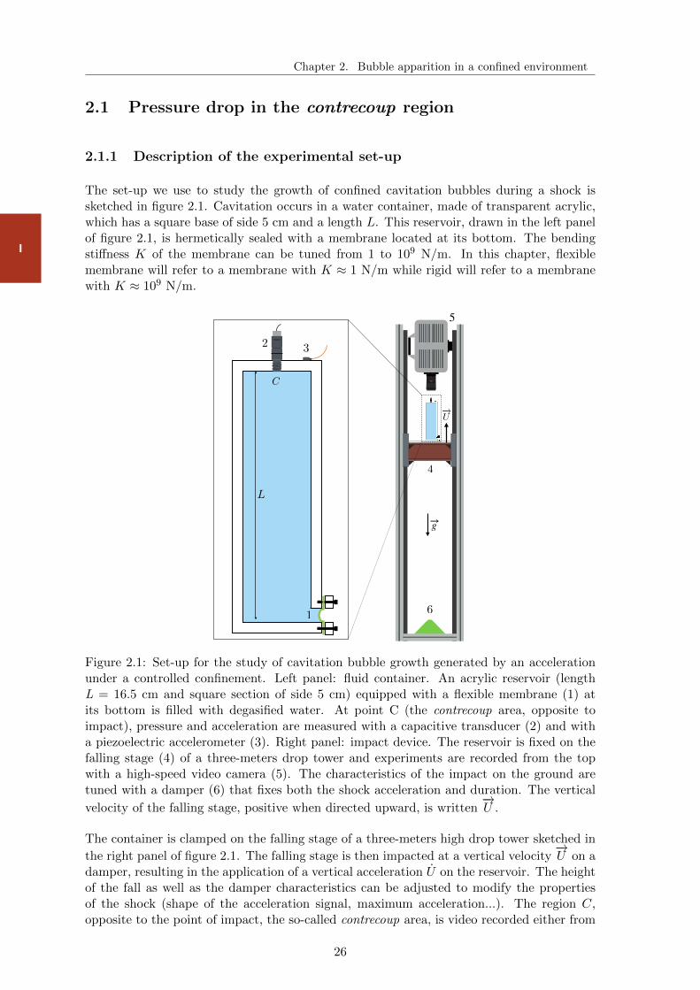
Chapter 2. Bubble apparition in a confined environment
I
2.1 Pressure drop in the contrecoup region
2.1.1 Description of the experimental set-up
The set-up we use to study the growth of confined cavitation bubbles during a shock issketched in figure 2.1. Cavitation occurs in a water container, made of transparent acrylic,which has a square base of side 5 cm and a length L. This reservoir, drawn in the left panelof figure 2.1, is hermetically sealed with a membrane located at its bottom. The bendingstiffness K of the membrane can be tuned from 1 to 109 N/m. In this chapter, flexiblemembrane will refer to a membrane with K ≈ 1 N/m while rigid will refer to a membranewith K ≈ 109 N/m.
4
6
L
C
2 3
1
5
!U
g
Figure 2.1: Set-up for the study of cavitation bubble growth generated by an accelerationunder a controlled confinement. Left panel: fluid container. An acrylic reservoir (lengthL = 16.5 cm and square section of side 5 cm) equipped with a flexible membrane (1) atits bottom is filled with degasified water. At point C (the contrecoup area, opposite toimpact), pressure and acceleration are measured with a capacitive transducer (2) and witha piezoelectric accelerometer (3). Right panel: impact device. The reservoir is fixed on thefalling stage (4) of a three-meters drop tower and experiments are recorded from the topwith a high-speed video camera (5). The characteristics of the impact on the ground aretuned with a damper (6) that fixes both the shock acceleration and duration. The vertical
velocity of the falling stage, positive when directed upward, is written−→U .
The container is clamped on the falling stage of a three-meters high drop tower sketched in
the right panel of figure 2.1. The falling stage is then impacted at a vertical velocity−→U on a
damper, resulting in the application of a vertical acceleration U on the reservoir. The heightof the fall as well as the damper characteristics can be adjusted to modify the propertiesof the shock (shape of the acceleration signal, maximum acceleration...). The region C,opposite to the point of impact, the so-called contrecoup area, is video recorded either from
26
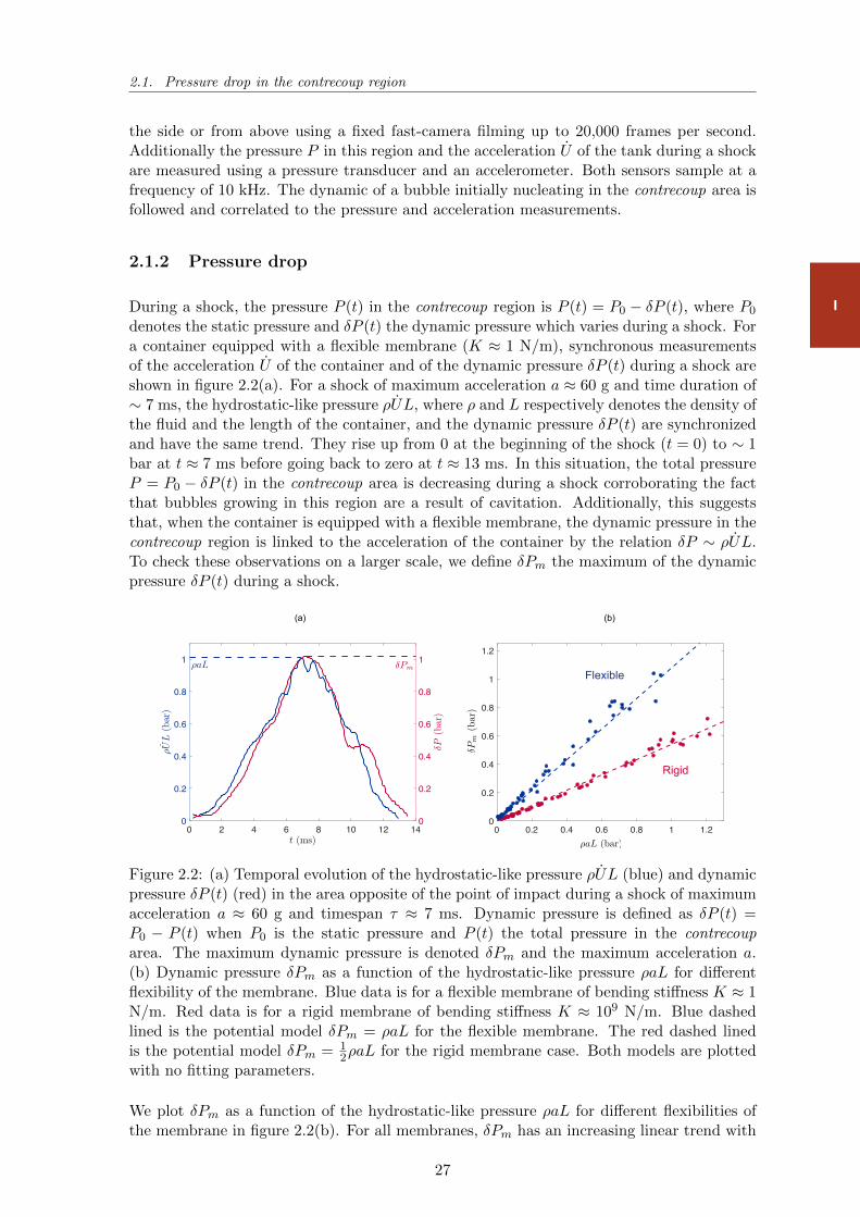
2.1. Pressure drop in the contrecoup region
I
the side or from above using a fixed fast-camera filming up to 20,000 frames per second.Additionally the pressure P in this region and the acceleration U of the tank during a shockare measured using a pressure transducer and an accelerometer. Both sensors sample at afrequency of 10 kHz. The dynamic of a bubble initially nucleating in the contrecoup area isfollowed and correlated to the pressure and acceleration measurements.
2.1.2 Pressure drop
During a shock, the pressure P (t) in the contrecoup region is P (t) = P0 − δP (t), where P0
denotes the static pressure and δP (t) the dynamic pressure which varies during a shock. Fora container equipped with a flexible membrane (K ≈ 1 N/m), synchronous measurementsof the acceleration U of the container and of the dynamic pressure δP (t) during a shock areshown in figure 2.2(a). For a shock of maximum acceleration a ≈ 60 g and time duration of∼ 7 ms, the hydrostatic-like pressure ρUL, where ρ and L respectively denotes the density ofthe fluid and the length of the container, and the dynamic pressure δP (t) are synchronizedand have the same trend. They rise up from 0 at the beginning of the shock (t = 0) to ∼ 1bar at t ≈ 7 ms before going back to zero at t ≈ 13 ms. In this situation, the total pressureP = P0 − δP (t) in the contrecoup area is decreasing during a shock corroborating the factthat bubbles growing in this region are a result of cavitation. Additionally, this suggeststhat, when the container is equipped with a flexible membrane, the dynamic pressure in thecontrecoup region is linked to the acceleration of the container by the relation δP ∼ ρUL.To check these observations on a larger scale, we define δPm the maximum of the dynamicpressure δP (t) during a shock.
0 2 4 6 8 10 12 140
0.2
0.4
0.6
0.8
1
0
0.2
0.4
0.6
0.8
1
0 0.2 0.4 0.6 0.8 1 1.20
0.2
0.4
0.6
0.8
1
1.2
aL (bar)
Flexible
Rigid
(b)(a)
aL Pm
Pm
(bar
)
Figure 2.2: (a) Temporal evolution of the hydrostatic-like pressure ρUL (blue) and dynamicpressure δP (t) (red) in the area opposite of the point of impact during a shock of maximumacceleration a ≈ 60 g and timespan τ ≈ 7 ms. Dynamic pressure is defined as δP (t) =P0 − P (t) when P0 is the static pressure and P (t) the total pressure in the contrecouparea. The maximum dynamic pressure is denoted δPm and the maximum acceleration a.(b) Dynamic pressure δPm as a function of the hydrostatic-like pressure ρaL for differentflexibility of the membrane. Blue data is for a flexible membrane of bending stiffness K ≈ 1N/m. Red data is for a rigid membrane of bending stiffness K ≈ 109 N/m. Blue dashedlined is the potential model δPm = ρaL for the flexible membrane. The red dashed linedis the potential model δPm = 1
2ρaL for the rigid membrane case. Both models are plottedwith no fitting parameters.
We plot δPm as a function of the hydrostatic-like pressure ρaL for different flexibilities ofthe membrane in figure 2.2(b). For all membranes, δPm has an increasing linear trend with
27

Chapter 2. Bubble apparition in a confined environment
I
ρaL. This confirms that, no matter what are the properties of the container used, there isalways a pressure drop in the contrecoup region. For a flexible membrane (K ≈ 1 N/m, bluedata), we recover the previous relation δPm = 1.03ρaL ± 0.08ρaL for the maximum valueof the pressure drop. However, when using a rigid membrane (K ≈ 109 N/m, red data), wefind δPm = 0.49ρaL± 0.05ρaL.
These behaviours can be recovered theoretically in the following way: as the characteristicvelocity of the reservoir filled with water when it impacts the damper is 1 − 3 m/s, theReynolds number of the flow in the reservoir is greater than 105 which allow us to assumethe flow to be potential. Writing U the velocity of the reservoir, aligned with the verticalaxis z directed upward, the only solution for the potential Φ is Φ(z, t) = U(t)z and theunstationary Bernoulli equation writes:
ρzdU
dt+
1
2ρU2 + P + ρgz = constant (2.1)
The pressure at the bottom of the tank is PB(t) = P statB − δPB(t) and at the top P (t) =P0−δP (t). For the rigid membrane case, the problem is fully anti-symmetric with respect tothe middle of the reservoir. Hence, δPB(t) = −δP (t). Using Bernoulli equation between thetop and bottom points yields δP (t) = 1
2ρUL. This relation is plotted in red dashed line infigure 2.2(b) and describes well the data for the container equipped with a rigid membrane.For the flexible membrane regime, a pressure is initially imposed near the membrane. Hence,expressing Bernoulli equation between the extremities of the reservoir, we get δP (t) = ρUL.It is plotted in blue dashed line in figure 2.2(b) and is in good agreement with the data forthe flexible membrane regime.
As a consequence, the apparition of cavitation bubbles in a confined environment dependson the properties of the container. For a flexible container, we recover that the pressure inthe contrecoup reaches the vapor pressure of water Pvap for Ca =
P0−Pvap
ρaL = 1 as previouslyobserved in [13]. However, using a rigid container will result in a delayed apparition ofcavitation bubbles: the vapor pressure of water is reached in the contrecoup region for cav-itation number as low as 1/2. In other words, using a rigid reservoir inhibits the nucleationof cavitation bubbles.
Additionally, it is interesting to note that, in either situation, the pressure variation in thetank alone cannot be the cause of traumatic brain injuries reported in American football orboxing: head accelerations rarely overcome 150 g [47, 48] and the pressure drop below 600g in the contrecoup region is negligible compared to the typical yield stress of tissues [49].Hence, an energy focusing mechanism needs to be involved in the brain damaging process.
2.2 Incompressibility and cavitation
For a shock of maximal acceleration a ≈ 150 g, the maximal pressure drop is δPm ∼ 2.5bar in the flexible membrane case and δPm ∼ 1.3 bar in the rigid membrane case. Theminimum absolute pressure in the contrecoup region Pm = P0 − δPm is far below the vaporpressure of water (Pvap ≈ 1.3 × 10⁻² bar) in both cases, i.e. the cavitation number is farbelow 1/2. As a consequence, we expect cavitation bubbles to nucleate in this region inboth situations. To check for their growth, we observe the container from the side during ashock of maximum acceleration a ≈ 150 g and time duration of ∼ 7 ms. Figure 2.3 presentsthe two chronophotographies obtained for different rigidities of the membrane used.
For a flexible membrane (K ≈ 1 N/m), we observe that, during the shock, the initiallybubbles present on the wall grow until they reach their maximum size around t = 9.6 ms.
28
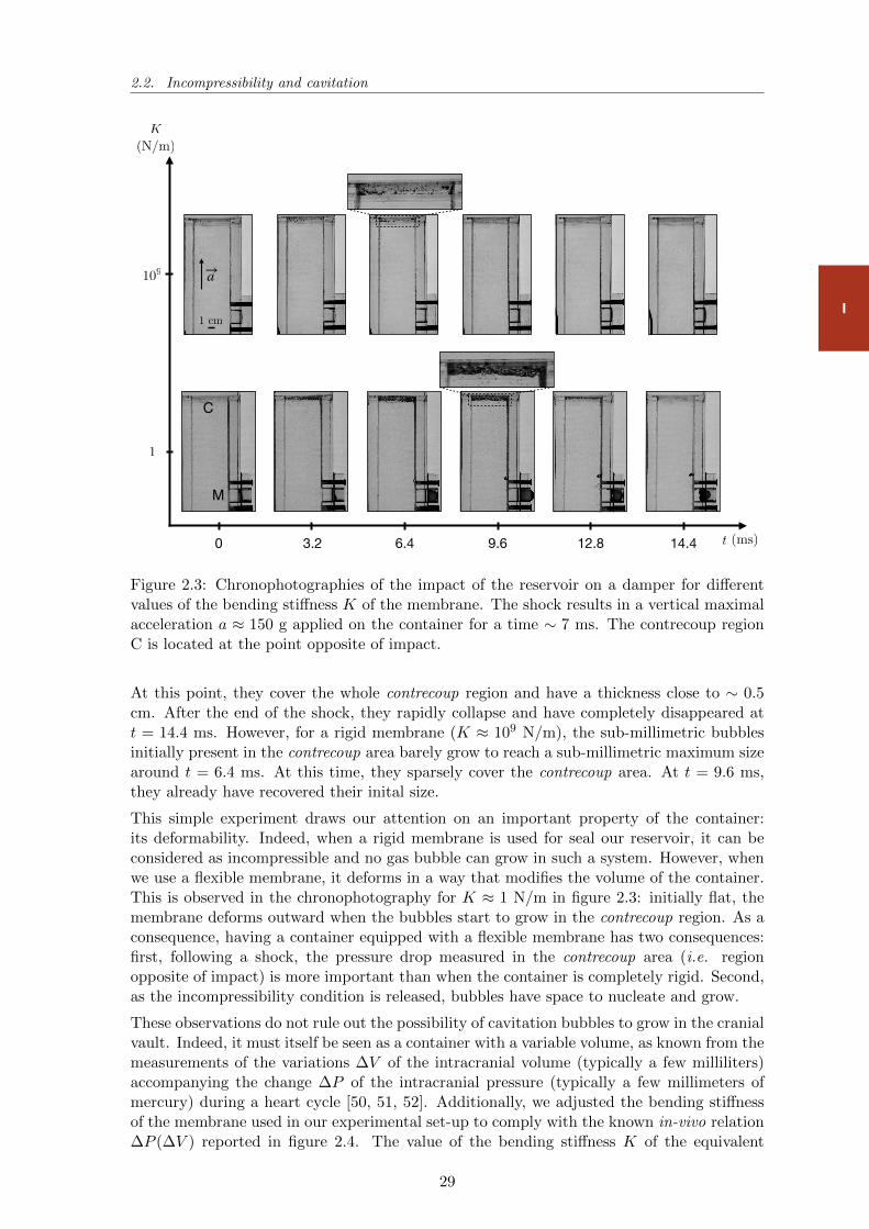
2.2. Incompressibility and cavitation
I
K(N/m)
t (ms)0 3.2 6.4 9.6 12.8 14.4
109
1
C
M
a
1 cm
Figure 2.3: Chronophotographies of the impact of the reservoir on a damper for differentvalues of the bending stiffness K of the membrane. The shock results in a vertical maximalacceleration a ≈ 150 g applied on the container for a time ∼ 7 ms. The contrecoup regionC is located at the point opposite of impact.
At this point, they cover the whole contrecoup region and have a thickness close to ∼ 0.5cm. After the end of the shock, they rapidly collapse and have completely disappeared att = 14.4 ms. However, for a rigid membrane (K ≈ 109 N/m), the sub-millimetric bubblesinitially present in the contrecoup area barely grow to reach a sub-millimetric maximum sizearound t = 6.4 ms. At this time, they sparsely cover the contrecoup area. At t = 9.6 ms,they already have recovered their inital size.
This simple experiment draws our attention on an important property of the container:its deformability. Indeed, when a rigid membrane is used for seal our reservoir, it can beconsidered as incompressible and no gas bubble can grow in such a system. However, whenwe use a flexible membrane, it deforms in a way that modifies the volume of the container.This is observed in the chronophotography for K ≈ 1 N/m in figure 2.3: initially flat, themembrane deforms outward when the bubbles start to grow in the contrecoup region. As aconsequence, having a container equipped with a flexible membrane has two consequences:first, following a shock, the pressure drop measured in the contrecoup area (i.e. regionopposite of impact) is more important than when the container is completely rigid. Second,as the incompressibility condition is released, bubbles have space to nucleate and grow.
These observations do not rule out the possibility of cavitation bubbles to grow in the cranialvault. Indeed, it must itself be seen as a container with a variable volume, as known from themeasurements of the variations ∆V of the intracranial volume (typically a few milliliters)accompanying the change ∆P of the intracranial pressure (typically a few millimeters ofmercury) during a heart cycle [50, 51, 52]. Additionally, we adjusted the bending stiffnessof the membrane used in our experimental set-up to comply with the known in-vivo relation∆P (∆V ) reported in figure 2.4. The value of the bending stiffness K of the equivalent
29
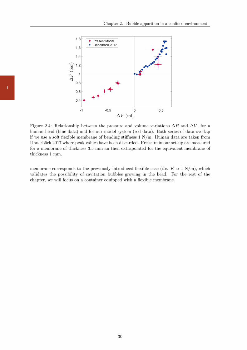
Chapter 2. Bubble apparition in a confined environment
I
-1 -0.5 0 0.5
0.4
0.6
0.8
1
1.2
1.4
1.6
1.8 Present ModelUnnerbäck 2017
P
(bar)
V (ml)
Figure 2.4: Relationship between the pressure and volume variations ∆P and ∆V , for ahuman head (blue data) and for our model system (red data). Both series of data overlapif we use a soft flexible membrane of bending stiffness 1 N/m. Human data are taken fromUnnerback 2017 where peak values have been discarded. Pressure in our set-up are measuredfor a membrane of thickness 3.5 mm an then extrapolated for the equivalent membrane ofthickness 1 mm.
membrane corresponds to the previously introduced flexible case (i.e. K ≈ 1 N/m), whichvalidates the possibility of cavitation bubbles growing in the head. For the rest of thechapter, we will focus on a container equipped with a flexible membrane.
30

3Influence of the shock duration
on the bubble dynamic
Chronophotography of the shattering of a rounded bottom flask induced by the collapse ofcavitation bubbles in the region opposite to the point of impact. Yellow is for t = 0 (i.e.impact of the hammer), green is for t = 1.2 ms and blue for t = 6.65 ms.
Contents
3.1 Methods . . . . . . . . . . . . . . . . . . . . . . . . . . . . . 32
3.2 Bubble dynamics . . . . . . . . . . . . . . . . . . . . . . . . 36
3.3 Damaging potential . . . . . . . . . . . . . . . . . . . . . . 39
3.4 Futur developments . . . . . . . . . . . . . . . . . . . . . . 40
31
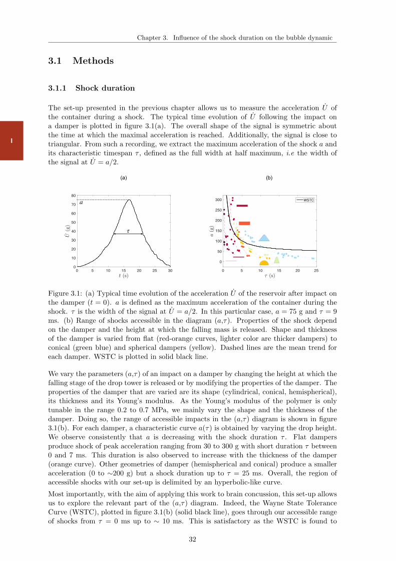
Chapter 3. Influence of the shock duration on the bubble dynamic
I
3.1 Methods
3.1.1 Shock duration
The set-up presented in the previous chapter allows us to measure the acceleration U ofthe container during a shock. The typical time evolution of U following the impact ona damper is plotted in figure 3.1(a). The overall shape of the signal is symmetric aboutthe time at which the maximal acceleration is reached. Additionally, the signal is close totriangular. From such a recording, we extract the maximum acceleration of the shock a andits characteristic timespan τ , defined as the full width at half maximum, i.e the width ofthe signal at U = a/2.
0 5 10 15 20 25
0
50
100
150
200
250
300 WSTC
(a) (b)
0 5 10 15 20 25 300
10
20
30
40
50
60
70
80
a
τ
Figure 3.1: (a) Typical time evolution of the acceleration U of the reservoir after impact onthe damper (t = 0). a is defined as the maximum acceleration of the container during theshock. τ is the width of the signal at U = a/2. In this particular case, a = 75 g and τ = 9ms. (b) Range of shocks accessible in the diagram (a,τ). Properties of the shock dependon the damper and the height at which the falling mass is released. Shape and thicknessof the damper is varied from flat (red-orange curves, lighter color are thicker dampers) toconical (green blue) and spherical dampers (yellow). Dashed lines are the mean trend foreach damper. WSTC is plotted in solid black line.
We vary the parameters (a,τ) of an impact on a damper by changing the height at which thefalling stage of the drop tower is released or by modifying the properties of the damper. Theproperties of the damper that are varied are its shape (cylindrical, conical, hemispherical),its thickness and its Young’s modulus. As the Young’s modulus of the polymer is onlytunable in the range 0.2 to 0.7 MPa, we mainly vary the shape and the thickness of thedamper. Doing so, the range of accessible impacts in the (a,τ) diagram is shown in figure3.1(b). For each damper, a characteristic curve a(τ) is obtained by varying the drop height.We observe consistently that a is decreasing with the shock duration τ . Flat dampersproduce shock of peak acceleration ranging from 30 to 300 g with short duration τ between0 and 7 ms. This duration is also observed to increase with the thickness of the damper(orange curve). Other geometries of damper (hemispherical and conical) produce a smalleracceleration (0 to ∼200 g) but a shock duration up to τ = 25 ms. Overall, the region ofaccessible shocks with our set-up is delimited by an hyperbolic-like curve.
Most importantly, with the aim of applying this work to brain concussion, this set-up allowsus to explore the relevant part of the (a,τ) diagram. Indeed, the Wayne State ToleranceCurve (WSTC), plotted in figure 3.1(b) (solid black line), goes through our accessible rangeof shocks from τ = 0 ms up to ∼ 10 ms. This is satisfactory as the WSTC is found to
32
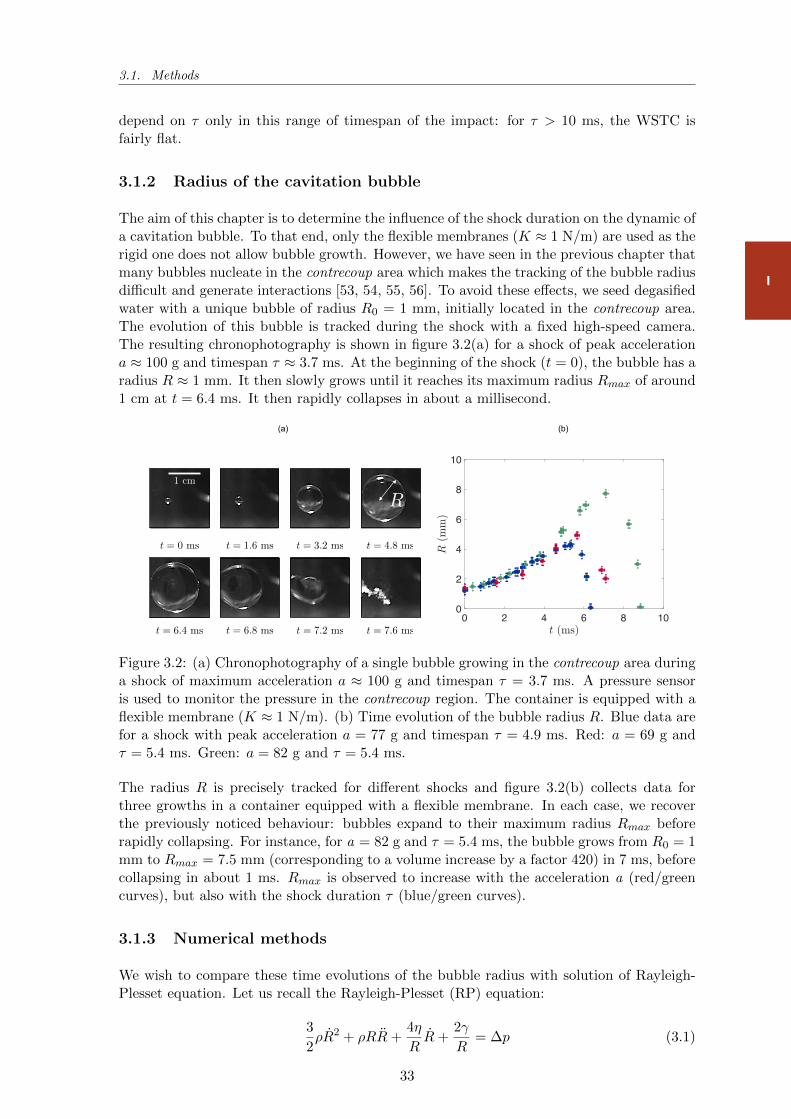
3.1. Methods
I
depend on τ only in this range of timespan of the impact: for τ > 10 ms, the WSTC isfairly flat.
3.1.2 Radius of the cavitation bubble
The aim of this chapter is to determine the influence of the shock duration on the dynamic ofa cavitation bubble. To that end, only the flexible membranes (K ≈ 1 N/m) are used as therigid one does not allow bubble growth. However, we have seen in the previous chapter thatmany bubbles nucleate in the contrecoup area which makes the tracking of the bubble radiusdifficult and generate interactions [53, 54, 55, 56]. To avoid these effects, we seed degasifiedwater with a unique bubble of radius R0 = 1 mm, initially located in the contrecoup area.The evolution of this bubble is tracked during the shock with a fixed high-speed camera.The resulting chronophotography is shown in figure 3.2(a) for a shock of peak accelerationa ≈ 100 g and timespan τ ≈ 3.7 ms. At the beginning of the shock (t = 0), the bubble has aradius R ≈ 1 mm. It then slowly grows until it reaches its maximum radius Rmax of around1 cm at t = 6.4 ms. It then rapidly collapses in about a millisecond.
0 2 4 6 8 100
2
4
6
8
10
1 cm
t = 0 ms t = 1.6 ms t = 3.2 ms t = 4.8 ms
t = 6.4 ms t = 6.8 ms t = 7.2 ms t = 7.6 ms
R
(a) (b)
Figure 3.2: (a) Chronophotography of a single bubble growing in the contrecoup area duringa shock of maximum acceleration a ≈ 100 g and timespan τ = 3.7 ms. A pressure sensoris used to monitor the pressure in the contrecoup region. The container is equipped with aflexible membrane (K ≈ 1 N/m). (b) Time evolution of the bubble radius R. Blue data arefor a shock with peak acceleration a = 77 g and timespan τ = 4.9 ms. Red: a = 69 g andτ = 5.4 ms. Green: a = 82 g and τ = 5.4 ms.
The radius R is precisely tracked for different shocks and figure 3.2(b) collects data forthree growths in a container equipped with a flexible membrane. In each case, we recoverthe previously noticed behaviour: bubbles expand to their maximum radius Rmax beforerapidly collapsing. For instance, for a = 82 g and τ = 5.4 ms, the bubble grows from R0 = 1mm to Rmax = 7.5 mm (corresponding to a volume increase by a factor 420) in 7 ms, beforecollapsing in about 1 ms. Rmax is observed to increase with the acceleration a (red/greencurves), but also with the shock duration τ (blue/green curves).
3.1.3 Numerical methods
We wish to compare these time evolutions of the bubble radius with solution of Rayleigh-Plesset equation. Let us recall the Rayleigh-Plesset (RP) equation:
3
2ρR2 + ρRR+
4η
RR+
2γ
R= ∆p (3.1)
33
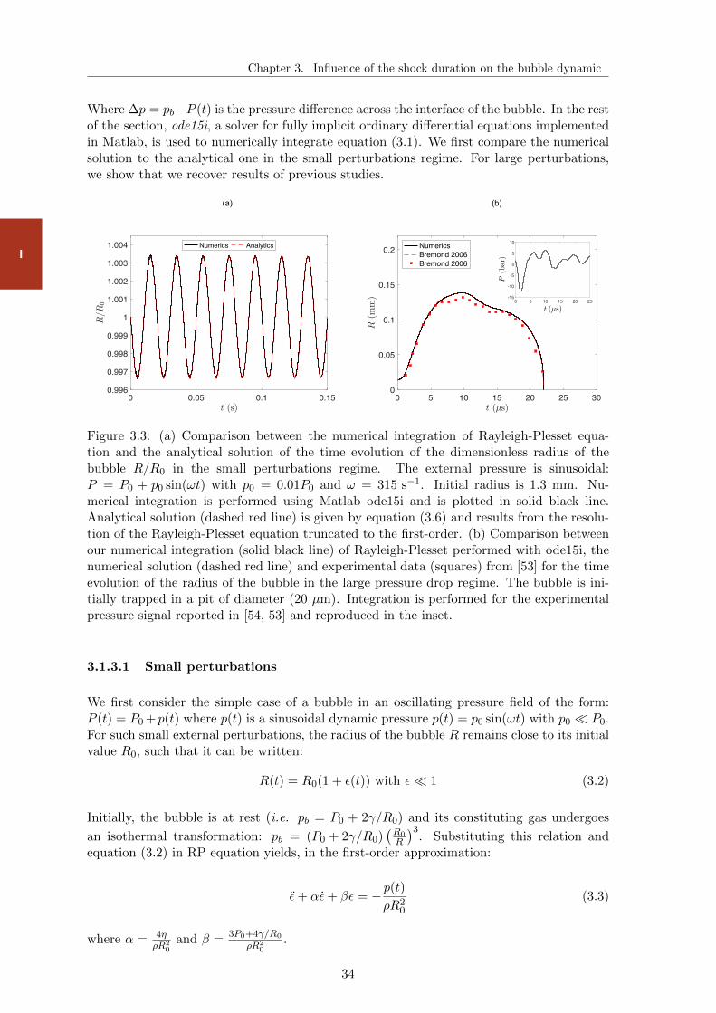
Chapter 3. Influence of the shock duration on the bubble dynamic
I
Where ∆p = pb−P (t) is the pressure difference across the interface of the bubble. In the restof the section, ode15i, a solver for fully implicit ordinary differential equations implementedin Matlab, is used to numerically integrate equation (3.1). We first compare the numericalsolution to the analytical one in the small perturbations regime. For large perturbations,we show that we recover results of previous studies.
0 5 10 15 20 25 300
0.05
0.1
0.15
0.2 NumericsBremond 2006Bremond 2006
0 0.05 0.1 0.150.996
0.997
0.998
0.999
1
1.001
1.002
1.003
1.004 Numerics Analytics
(a) (b)
0 5 10 15 20 25-15
-10
-5
0
5
10
P(b
ar)
t (µs)
Figure 3.3: (a) Comparison between the numerical integration of Rayleigh-Plesset equa-tion and the analytical solution of the time evolution of the dimensionless radius of thebubble R/R0 in the small perturbations regime. The external pressure is sinusoidal:P = P0 + p0 sin(ωt) with p0 = 0.01P0 and ω = 315 s−1. Initial radius is 1.3 mm. Nu-merical integration is performed using Matlab ode15i and is plotted in solid black line.Analytical solution (dashed red line) is given by equation (3.6) and results from the resolu-tion of the Rayleigh-Plesset equation truncated to the first-order. (b) Comparison betweenour numerical integration (solid black line) of Rayleigh-Plesset performed with ode15i, thenumerical solution (dashed red line) and experimental data (squares) from [53] for the timeevolution of the radius of the bubble in the large pressure drop regime. The bubble is ini-tially trapped in a pit of diameter (20 µm). Integration is performed for the experimentalpressure signal reported in [54, 53] and reproduced in the inset.
3.1.3.1 Small perturbations
We first consider the simple case of a bubble in an oscillating pressure field of the form:P (t) = P0 +p(t) where p(t) is a sinusoidal dynamic pressure p(t) = p0 sin(ωt) with p0 P0.For such small external perturbations, the radius of the bubble R remains close to its initialvalue R0, such that it can be written:
R(t) = R0(1 + ε(t)) with ε 1 (3.2)
Initially, the bubble is at rest (i.e. pb = P0 + 2γ/R0) and its constituting gas undergoes
an isothermal transformation: pb = (P0 + 2γ/R0)(R0R
)3. Substituting this relation and
equation (3.2) in RP equation yields, in the first-order approximation:
ε+ αε+ βε = −p(t)ρR2
0
(3.3)
where α = 4ηρR2
0and β = 3P0+4γ/R0
ρR20
.
34
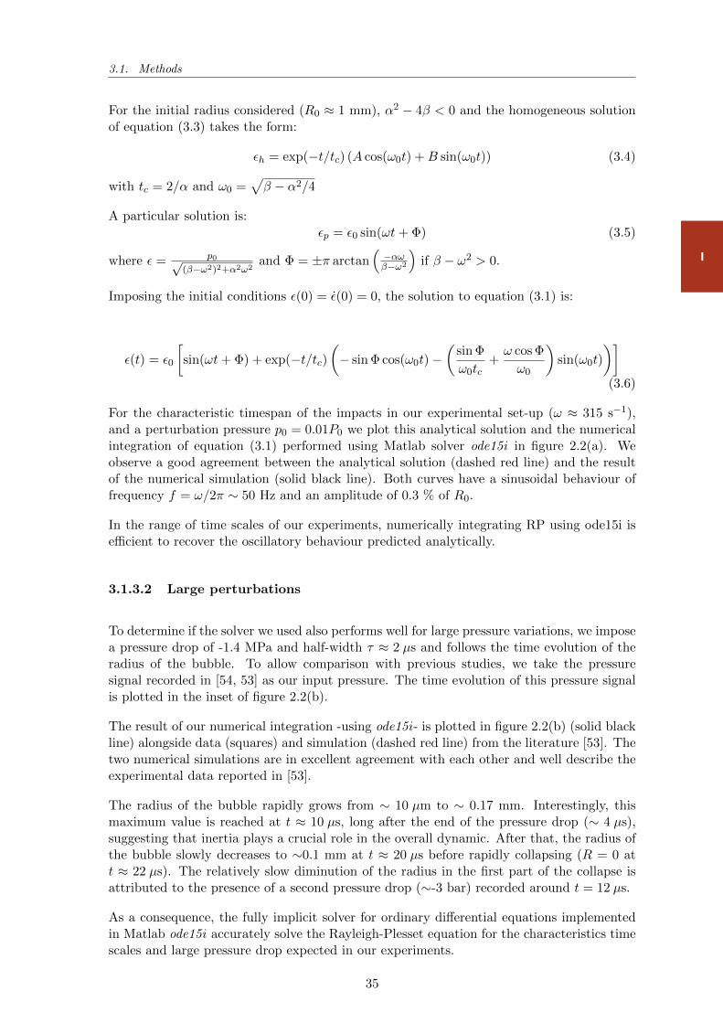
3.1. Methods
I
For the initial radius considered (R0 ≈ 1 mm), α2 − 4β < 0 and the homogeneous solutionof equation (3.3) takes the form:
εh = exp(−t/tc) (A cos(ω0t) +B sin(ω0t)) (3.4)
with tc = 2/α and ω0 =√β − α2/4
A particular solution is:εp = ε0 sin(ωt+ Φ) (3.5)
where ε = p0√(β−ω2)2+α2ω2
and Φ = ±π arctan(−αωβ−ω2
)if β − ω2 > 0.
Imposing the initial conditions ε(0) = ε(0) = 0, the solution to equation (3.1) is:
ε(t) = ε0
[sin(ωt+ Φ) + exp(−t/tc)
(− sin Φ cos(ω0t)−
(sin Φ
ω0tc+ω cos Φ
ω0
)sin(ω0t)
)]
(3.6)
For the characteristic timespan of the impacts in our experimental set-up (ω ≈ 315 s−1),and a perturbation pressure p0 = 0.01P0 we plot this analytical solution and the numericalintegration of equation (3.1) performed using Matlab solver ode15i in figure 2.2(a). Weobserve a good agreement between the analytical solution (dashed red line) and the resultof the numerical simulation (solid black line). Both curves have a sinusoidal behaviour offrequency f = ω/2π ∼ 50 Hz and an amplitude of 0.3 % of R0.
In the range of time scales of our experiments, numerically integrating RP using ode15i isefficient to recover the oscillatory behaviour predicted analytically.
3.1.3.2 Large perturbations
To determine if the solver we used also performs well for large pressure variations, we imposea pressure drop of -1.4 MPa and half-width τ ≈ 2 µs and follows the time evolution of theradius of the bubble. To allow comparison with previous studies, we take the pressuresignal recorded in [54, 53] as our input pressure. The time evolution of this pressure signalis plotted in the inset of figure 2.2(b).
The result of our numerical integration -using ode15i - is plotted in figure 2.2(b) (solid blackline) alongside data (squares) and simulation (dashed red line) from the literature [53]. Thetwo numerical simulations are in excellent agreement with each other and well describe theexperimental data reported in [53].
The radius of the bubble rapidly grows from ∼ 10 µm to ∼ 0.17 mm. Interestingly, thismaximum value is reached at t ≈ 10 µs, long after the end of the pressure drop (∼ 4 µs),suggesting that inertia plays a crucial role in the overall dynamic. After that, the radius ofthe bubble slowly decreases to ∼0.1 mm at t ≈ 20 µs before rapidly collapsing (R = 0 att ≈ 22 µs). The relatively slow diminution of the radius in the first part of the collapse isattributed to the presence of a second pressure drop (∼-3 bar) recorded around t = 12 µs.
As a consequence, the fully implicit solver for ordinary differential equations implementedin Matlab ode15i accurately solve the Rayleigh-Plesset equation for the characteristics timescales and large pressure drop expected in our experiments.
35
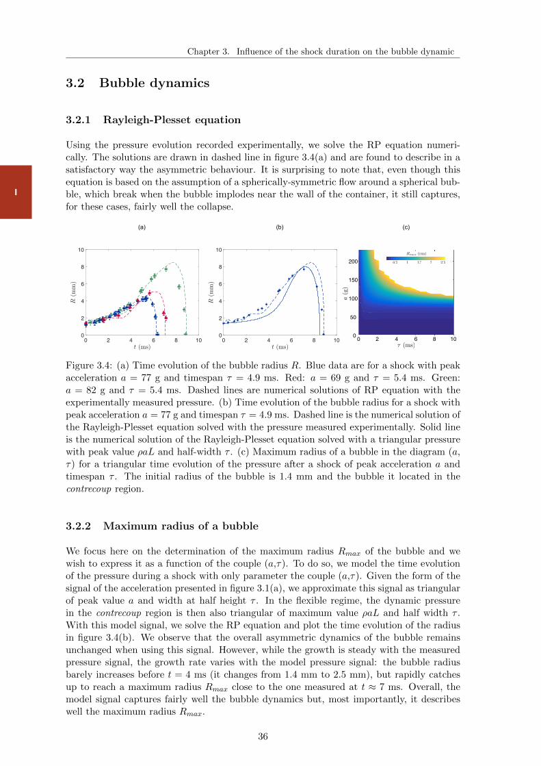
Chapter 3. Influence of the shock duration on the bubble dynamic
I
3.2 Bubble dynamics
3.2.1 Rayleigh-Plesset equation
Using the pressure evolution recorded experimentally, we solve the RP equation numeri-cally. The solutions are drawn in dashed line in figure 3.4(a) and are found to describe in asatisfactory way the asymmetric behaviour. It is surprising to note that, even though thisequation is based on the assumption of a spherically-symmetric flow around a spherical bub-ble, which break when the bubble implodes near the wall of the container, it still captures,for these cases, fairly well the collapse.
0 2 4 6 8 100
2
4
6
8
10
0 2 4 6 8 100
2
4
6
8
10
(a) (b)
0.5 1 1.5 2 2.5
0 2 4 6 8 100
50
100
150
200Rmax (cm)
(ms)a
(g)
(c)
Figure 3.4: (a) Time evolution of the bubble radius R. Blue data are for a shock with peakacceleration a = 77 g and timespan τ = 4.9 ms. Red: a = 69 g and τ = 5.4 ms. Green:a = 82 g and τ = 5.4 ms. Dashed lines are numerical solutions of RP equation with theexperimentally measured pressure. (b) Time evolution of the bubble radius for a shock withpeak acceleration a = 77 g and timespan τ = 4.9 ms. Dashed line is the numerical solution ofthe Rayleigh-Plesset equation solved with the pressure measured experimentally. Solid lineis the numerical solution of the Rayleigh-Plesset equation solved with a triangular pressurewith peak value ρaL and half-width τ . (c) Maximum radius of a bubble in the diagram (a,τ) for a triangular time evolution of the pressure after a shock of peak acceleration a andtimespan τ . The initial radius of the bubble is 1.4 mm and the bubble it located in thecontrecoup region.
3.2.2 Maximum radius of a bubble
We focus here on the determination of the maximum radius Rmax of the bubble and wewish to express it as a function of the couple (a,τ). To do so, we model the time evolutionof the pressure during a shock with only parameter the couple (a,τ). Given the form of thesignal of the acceleration presented in figure 3.1(a), we approximate this signal as triangularof peak value a and width at half height τ . In the flexible regime, the dynamic pressurein the contrecoup region is then also triangular of maximum value ρaL and half width τ .With this model signal, we solve the RP equation and plot the time evolution of the radiusin figure 3.4(b). We observe that the overall asymmetric dynamics of the bubble remainsunchanged when using this signal. However, while the growth is steady with the measuredpressure signal, the growth rate varies with the model pressure signal: the bubble radiusbarely increases before t = 4 ms (it changes from 1.4 mm to 2.5 mm), but rapidly catchesup to reach a maximum radius Rmax close to the one measured at t ≈ 7 ms. Overall, themodel signal captures fairly well the bubble dynamics but, most importantly, it describeswell the maximum radius Rmax.
36
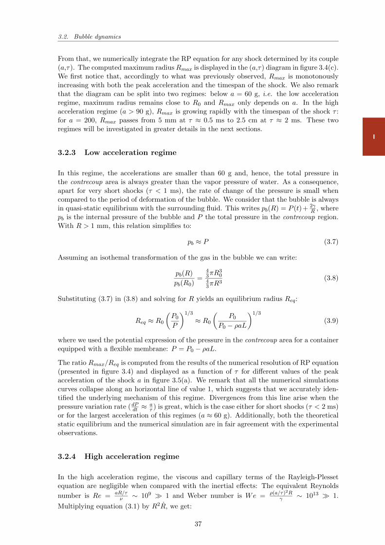
3.2. Bubble dynamics
I
From that, we numerically integrate the RP equation for any shock determined by its couple(a,τ). The computed maximum radiusRmax is displayed in the (a,τ) diagram in figure 3.4(c).We first notice that, accordingly to what was previously observed, Rmax is monotonouslyincreasing with both the peak acceleration and the timespan of the shock. We also remarkthat the diagram can be split into two regimes: below a = 60 g, i.e. the low accelerationregime, maximum radius remains close to R0 and Rmax only depends on a. In the highacceleration regime (a > 90 g), Rmax is growing rapidly with the timespan of the shock τ :for a = 200, Rmax passes from 5 mm at τ ≈ 0.5 ms to 2.5 cm at τ ≈ 2 ms. These tworegimes will be investigated in greater details in the next sections.
3.2.3 Low acceleration regime
In this regime, the accelerations are smaller than 60 g and, hence, the total pressure inthe contrecoup area is always greater than the vapor pressure of water. As a consequence,apart for very short shocks (τ < 1 ms), the rate of change of the pressure is small whencompared to the period of deformation of the bubble. We consider that the bubble is alwaysin quasi-static equilibrium with the surrounding fluid. This writes pb(R) = P (t)+ 2γ
R , wherepb is the internal pressure of the bubble and P the total pressure in the contrecoup region.With R > 1 mm, this relation simplifies to:
pb ≈ P (3.7)
Assuming an isothemal transformation of the gas in the bubble we can write:
pb(R)
pb(R0)=
43πR
30
43πR
3(3.8)
Substituting (3.7) in (3.8) and solving for R yields an equilibrium radius Req:
Req ≈ R0
(P0
P
)1/3
≈ R0
(P0
P0 − ρaL
)1/3
(3.9)
where we used the potential expression of the pressure in the contrecoup area for a containerequipped with a flexible membrane: P = P0 − ρaL.
The ratio Rmax/Req is computed from the results of the numerical resolution of RP equation(presented in figure 3.4) and displayed as a function of τ for different values of the peakacceleration of the shock a in figure 3.5(a). We remark that all the numerical simulationscurves collapse along an horizontal line of value 1, which suggests that we accurately iden-tified the underlying mechanism of this regime. Divergences from this line arise when thepressure variation rate (dPdt ≈ a
τ ) is great, which is the case either for short shocks (τ < 2 ms)or for the largest acceleration of this regimes (a ≈ 60 g). Additionally, both the theoreticalstatic equilibrium and the numerical simulation are in fair agreement with the experimentalobservations.
3.2.4 High acceleration regime
In the high acceleration regime, the viscous and capillary terms of the Rayleigh-Plessetequation are negligible when compared with the inertial effects: The equivalent Reynolds
number is Re = aR/τν ∼ 109 1 and Weber number is We = ρ(a/τ)2R
γ ∼ 1013 1.
Multiplying equation (3.1) by R2R, we get:
37
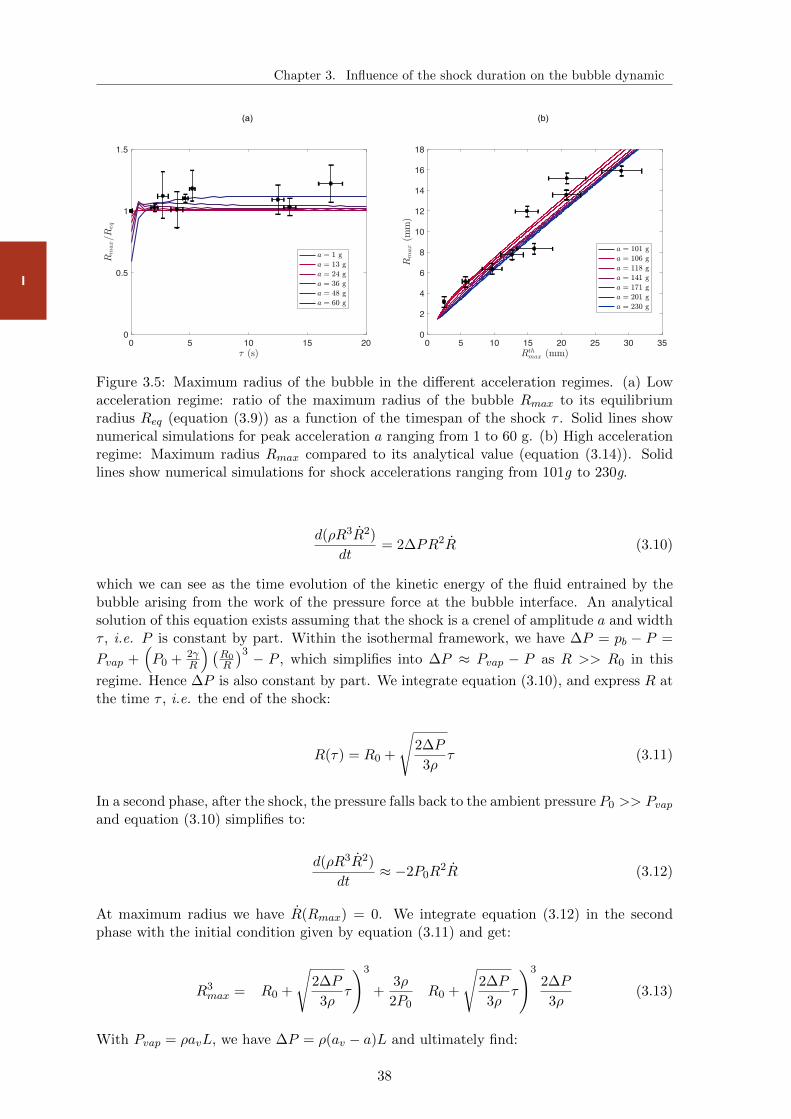
Chapter 3. Influence of the shock duration on the bubble dynamic
I35
0 5 10 15 20 25 30 350
2
4
6
8
10
12
14
16
18
(a) (b)
0 5 10 15 200
0.5
1
1.5
Figure 3.5: Maximum radius of the bubble in the different acceleration regimes. (a) Lowacceleration regime: ratio of the maximum radius of the bubble Rmax to its equilibriumradius Req (equation (3.9)) as a function of the timespan of the shock τ . Solid lines shownumerical simulations for peak acceleration a ranging from 1 to 60 g. (b) High accelerationregime: Maximum radius Rmax compared to its analytical value (equation (3.14)). Solidlines show numerical simulations for shock accelerations ranging from 101g to 230g.
d(ρR3R2)
dt= 2∆PR2R (3.10)
which we can see as the time evolution of the kinetic energy of the fluid entrained by thebubble arising from the work of the pressure force at the bubble interface. An analyticalsolution of this equation exists assuming that the shock is a crenel of amplitude a and widthτ , i.e. P is constant by part. Within the isothermal framework, we have ∆P = pb − P =
Pvap +(P0 + 2γ
R
) (R0R
)3 − P , which simplifies into ∆P ≈ Pvap − P as R >> R0 in this
regime. Hence ∆P is also constant by part. We integrate equation (3.10), and express R atthe time τ , i.e. the end of the shock:
R(τ) = R0 +
√2∆P
3ρτ (3.11)
In a second phase, after the shock, the pressure falls back to the ambient pressure P0 >> Pvapand equation (3.10) simplifies to:
d(ρR3R2)
dt≈ −2P0R
2R (3.12)
At maximum radius we have R(Rmax) = 0. We integrate equation (3.12) in the secondphase with the initial condition given by equation (3.11) and get:
R3max =
(R0 +
√2∆P
3ρτ
)3
+3ρ
2P0
(R0 +
√2∆P
3ρτ
)32∆P
3ρ(3.13)
With Pvap = ρavL, we have ∆P = ρ(av − a)L and ultimately find:
38
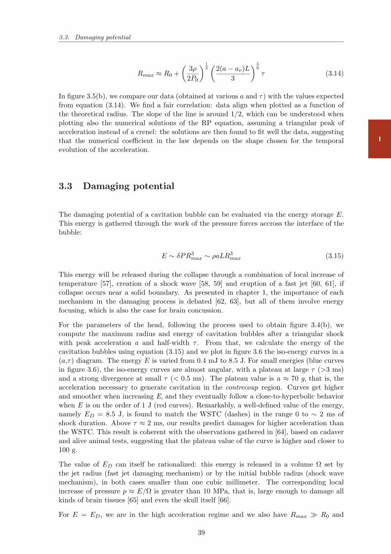
3.3. Damaging potential
I
Rmax ≈ R0 +
(3ρ
2P0
) 13(
2(a− av)L3
) 56
τ (3.14)
In figure 3.5(b), we compare our data (obtained at various a and τ) with the values expectedfrom equation (3.14). We find a fair correlation: data align when plotted as a function ofthe theoretical radius. The slope of the line is around 1/2, which can be understood whenplotting also the numerical solutions of the RP equation, assuming a triangular peak ofacceleration instead of a crenel: the solutions are then found to fit well the data, suggestingthat the numerical coefficient in the law depends on the shape chosen for the temporalevolution of the acceleration.
3.3 Damaging potential
The damaging potential of a cavitation bubble can be evaluated via the energy storage E.This energy is gathered through the work of the pressure forces accross the interface of thebubble:
E ∼ δPR3max ∼ ρaLR3
max (3.15)
This energy will be released during the collapse through a combination of local increase oftemperature [57], creation of a shock wave [58, 59] and eruption of a fast jet [60, 61], ifcollapse occurs near a solid boundary. As presented in chapter 1, the importance of eachmechanism in the damaging process is debated [62, 63], but all of them involve energyfocusing, which is also the case for brain concussion.
For the parameters of the head, following the process used to obtain figure 3.4(b), wecompute the maximum radius and energy of cavitation bubbles after a triangular shockwith peak acceleration a and half-width τ . From that, we calculate the energy of thecavitation bubbles using equation (3.15) and we plot in figure 3.6 the iso-energy curves in a(a,τ) diagram. The energy E is varied from 0.4 mJ to 8.5 J. For small energies (blue curvesin figure 3.6), the iso-energy curves are almost angular, with a plateau at large τ (>3 ms)and a strong divergence at small τ (< 0.5 ms). The plateau value is a ≈ 70 g, that is, theacceleration necessary to generate cavitation in the contrecoup region. Curves get higherand smoother when increasing E, and they eventually follow a close-to-hyperbolic behaviorwhen E is on the order of 1 J (red curves). Remarkably, a well-defined value of the energy,namely ED = 8.5 J, is found to match the WSTC (dashes) in the range 0 to ∼ 2 ms ofshock duration. Above τ ≈ 2 ms, our results predict damages for higher acceleration thanthe WSTC. This result is coherent with the observations gathered in [64], based on cadaverand alive animal tests, suggesting that the plateau value of the curve is higher and closer to100 g.
The value of ED can itself be rationalized: this energy is released in a volume Ω set bythe jet radius (fast jet damaging mechanism) or by the initial bubble radius (shock wavemechanism), in both cases smaller than one cubic millimeter. The corresponding localincrease of pressure p ≈ E/Ω is greater than 10 MPa, that is, large enough to damage allkinds of brain tissues [65] and even the skull itself [66].
For E = ED, we are in the high acceleration regime and we also have Rmax R0 and
39
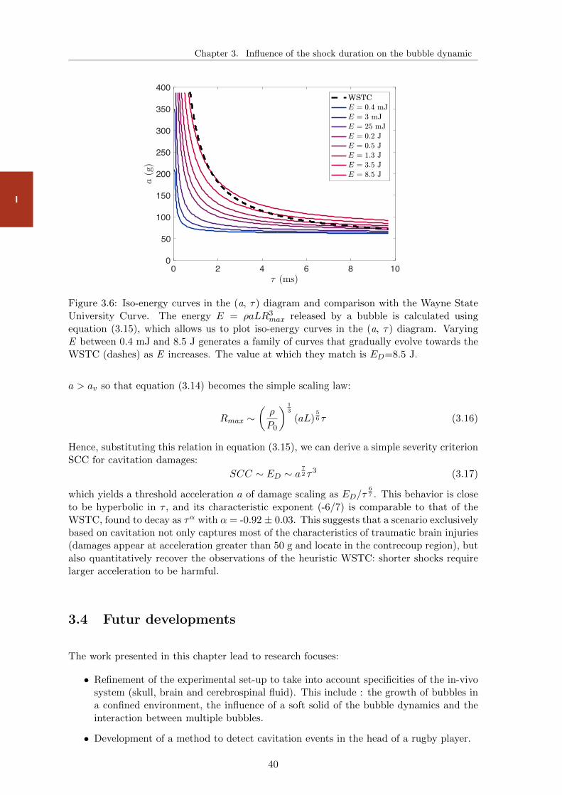
Chapter 3. Influence of the shock duration on the bubble dynamic
I
0 2 4 6 8 100
50
100
150
200
250
300
350
400WSTC
Figure 3.6: Iso-energy curves in the (a, τ) diagram and comparison with the Wayne StateUniversity Curve. The energy E = ρaLR3
max released by a bubble is calculated usingequation (3.15), which allows us to plot iso-energy curves in the (a, τ) diagram. VaryingE between 0.4 mJ and 8.5 J generates a family of curves that gradually evolve towards theWSTC (dashes) as E increases. The value at which they match is ED=8.5 J.
a > av so that equation (3.14) becomes the simple scaling law:
Rmax ∼(ρ
P0
) 13
(aL)56 τ (3.16)
Hence, substituting this relation in equation (3.15), we can derive a simple severity criterionSCC for cavitation damages:
SCC ∼ ED ∼ a72 τ3 (3.17)
which yields a threshold acceleration a of damage scaling as ED/τ67 . This behavior is close
to be hyperbolic in τ , and its characteristic exponent (-6/7) is comparable to that of theWSTC, found to decay as τα with α = -0.92 ± 0.03. This suggests that a scenario exclusivelybased on cavitation not only captures most of the characteristics of traumatic brain injuries(damages appear at acceleration greater than 50 g and locate in the contrecoup region), butalso quantitatively recover the observations of the heuristic WSTC: shorter shocks requirelarger acceleration to be harmful.
3.4 Futur developments
The work presented in this chapter lead to research focuses:
• Refinement of the experimental set-up to take into account specificities of the in-vivosystem (skull, brain and cerebrospinal fluid). This include : the growth of bubbles ina confined environment, the influence of a soft solid of the bubble dynamics and theinteraction between multiple bubbles.
• Development of a method to detect cavitation events in the head of a rugby player.
40
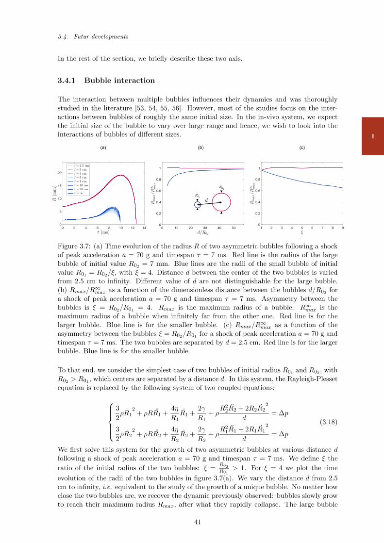
3.4. Futur developments
I
In the rest of the section, we briefly describe these two axis.
3.4.1 Bubble interaction
The interaction between multiple bubbles influences their dynamics and was thoroughlystudied in the literature [53, 54, 55, 56]. However, most of the studies focus on the inter-actions between bubbles of roughly the same initial size. In the in-vivo system, we expectthe initial size of the bubble to vary over large range and hence, we wish to look into theinteractions of bubbles of different sizes.
0 2 4 6 8 10 12 140
5
10
15
20
0 10 20 30 40 500
0.2
0.4
0.6
0.8
1
dR01
R02
(a) (b) (c)
1 2 3 4 5 6 7 8 90
0.2
0.4
0.6
0.8
1
Figure 3.7: (a) Time evolution of the radius R of two asymmetric bubbles following a shockof peak acceleration a = 70 g and timespan τ = 7 ms. Red line is the radius of the largebubble of initial value R02 = 7 mm. Blue lines are the radii of the small bubble of initialvalue R01 = R02/ξ, with ξ = 4. Distance d between the center of the two bubbles is variedfrom 2.5 cm to infinity. Different value of d are not distinguishable for the large bubble.(b) Rmax/R
∞max as a function of the dimensionless distance between the bubbles d/R02 for
a shock of peak acceleration a = 70 g and timespan τ = 7 ms. Asymmetry between thebubbles is ξ = R02/R01 = 4. Rmax is the maximum radius of a bubble. R∞max is themaximum radius of a bubble when infinitely far from the other one. Red line is for thelarger bubble. Blue line is for the smaller bubble. (c) Rmax/R
∞max as a function of the
asymmetry between the bubbles ξ = R02/R01 for a shock of peak acceleration a = 70 g andtimespan τ = 7 ms. The two bubbles are separated by d = 2.5 cm. Red line is for the largerbubble. Blue line is for the smaller bubble.
To that end, we consider the simplest case of two bubbles of initial radius R01 and R02 , withR02 > R01 , which centers are separated by a distance d. In this system, the Rayleigh-Plessetequation is replaced by the following system of two coupled equations:
3
2ρR1
2+ ρRR1 +
4η
R1R1 +
2γ
R1+ ρ
R22R2 + 2R2R2
2
d= ∆p
3
2ρR2
2+ ρRR2 +
4η
R2R2 +
2γ
R2+ ρ
R21R1 + 2R1R1
2
d= ∆p
(3.18)
We first solve this system for the growth of two asymmetric bubbles at various distance dfollowing a shock of peak acceleration a = 70 g and timespan τ = 7 ms. We define ξ the
ratio of the initial radius of the two bubbles: ξ =R02R01
> 1. For ξ = 4 we plot the time
evolution of the radii of the two bubbles in figure 3.7(a). We vary the distance d from 2.5cm to infinity, i.e. equivalent to the study of the growth of a unique bubble. No matter howclose the two bubbles are, we recover the dynamic previously observed: bubbles slowly growto reach their maximum radius Rmax, after what they rapidly collapse. The large bubble
41
Chapter 3. Influence of the shock duration on the bubble dynamic
I
(red curve), is barely affected by the presence of a small bubble in its vicinity: curves fordifferent distances cannot be distinguished in figure 3.7(a). However, the dynamic of thesmall bubble (blue curve) is largely modified by the presence of the large bubble. Thecurve of the time evolution of the radius R1 flattens and becomes more symmetric as thetwo bubbles are brought closer: when alone (d =∞) the small bubble reaches a maximumradius of ∼ 7 mm while it barely reaches ∼ 5 mm when the two bubbles are 2.5 cm apart.
We then concentrate on the maximum radius of the bubble Rmax, which we prove to bea quantification of the stored energy, and compare it with the maximum radius that thebubble would reach if it was alone R∞max. We plot in figure 3.7(b) the ratio Rmax/R
∞max as
a function of the dimensionless distance d/R02 between the bubbles for ξ = 4. Looking atthe maximum radius of the larger bubble (red curve, R2), we retrieve the fact that it is notaffected by the smaller bubble (Rmax2/R
∞max2 = 1). Nonetheless, the maximum radius of
the smaller bubble is reduced by the presence of the larger one. This influence is reducedwhen the two bubbles are spread apart: Rmax1/R
∞max1 onsets at ∼0.7 when d/R02 ≈ 3.5
and then tends to 1 when d/R02 goes to infinity (Rmax1/R∞max1 ≈ 0.98 for d/R02 ≈ 50).
Finally, we investigate the dependence of the maximum radii on the asymmetry of the two
bubble ξ =R02R01
as displayed in figure 3.7(c), where Rmax/R∞max is plotted against ξ for
d/R02 = 3.6. When the two bubbles are identical (ξ = 1), their maximum radius is slightlyreduced when compared to the case of an unique bubble (Rmax/R
∞max ≈ 0.95). However,
as soon as the asymmetry is increased, the larger bubble reaches its plateau value for itsmaximum radius (Rmax2/R
∞max2 = 1 for ξ ≈ 2) while the smaller bubble has its growth
inhibited (Rmax1/R∞max1 decreases and reach ∼0.6 for ξ ≈ 9).
Although this dependencies should be investigated experimentally, we can already say thatinteraction between bubbles should not influence the maximum damaging potential of cav-itation bubbles created after a shock on the head. Indeed, it can be evaluated taking thelargest nucleus which will grow to the largest bubble being only slightly influenced by others.
3.4.2 In-vivo Measurements
We wish to detect cavitation events in the head of sports players (especially in rugby orboxing) to facilitate the diagnostic of brain concussion during a game. As we mentionedbefore, it is currently based on an on-field clinical test which leaves more than 30 % of theconcussions undetected before the end of the game. As a consequence, players face greateraftermaths and longer recovery times.
To that end, we wish to use the characteristic noise generated at the collapse of a cavitationbubble, already thoroughly studied in diverse situations [67, 68, 69]. Here we present thein-vitro illustration of the set-up we wish to develop for sports players. The experimentalset-up is sketched in figure 3.8(a). Apart from the fact that two accelerometers are used, it isidentical to the one previously described: it consists of a reservoir, equipped with a flexiblemembrane, accelerated vertically upon a shock on a damper. The first accelerometer (A1) islocated on the outer wall of the contrecoup region while the other (A2) is on the falling stageof the impact tower. For a shock of peak acceleration a = 135 g and timespan τ ≈ 2 ms,the time evolution of the acceleration measured by the two accelerometers is shown in figure3.8(b). The acceleration measured by the second accelerometer (blue curve) only consistsof a typical shock of peak acceleration ∼ 120 g and half-width ∼ 2 ms. However, the firstaccelerometer not only measures roughly the same shock, but also captures a high intensity(∼ 200 g) and frequency signal 8 milliseconds after the beginning of the impact. Figure3.8(c) displays a choronophotography of the contrecoup region during the shock. Initially,no bubbles are present in the container. 1.5 ms after the shock, a cloud of millimetric bubbles
42
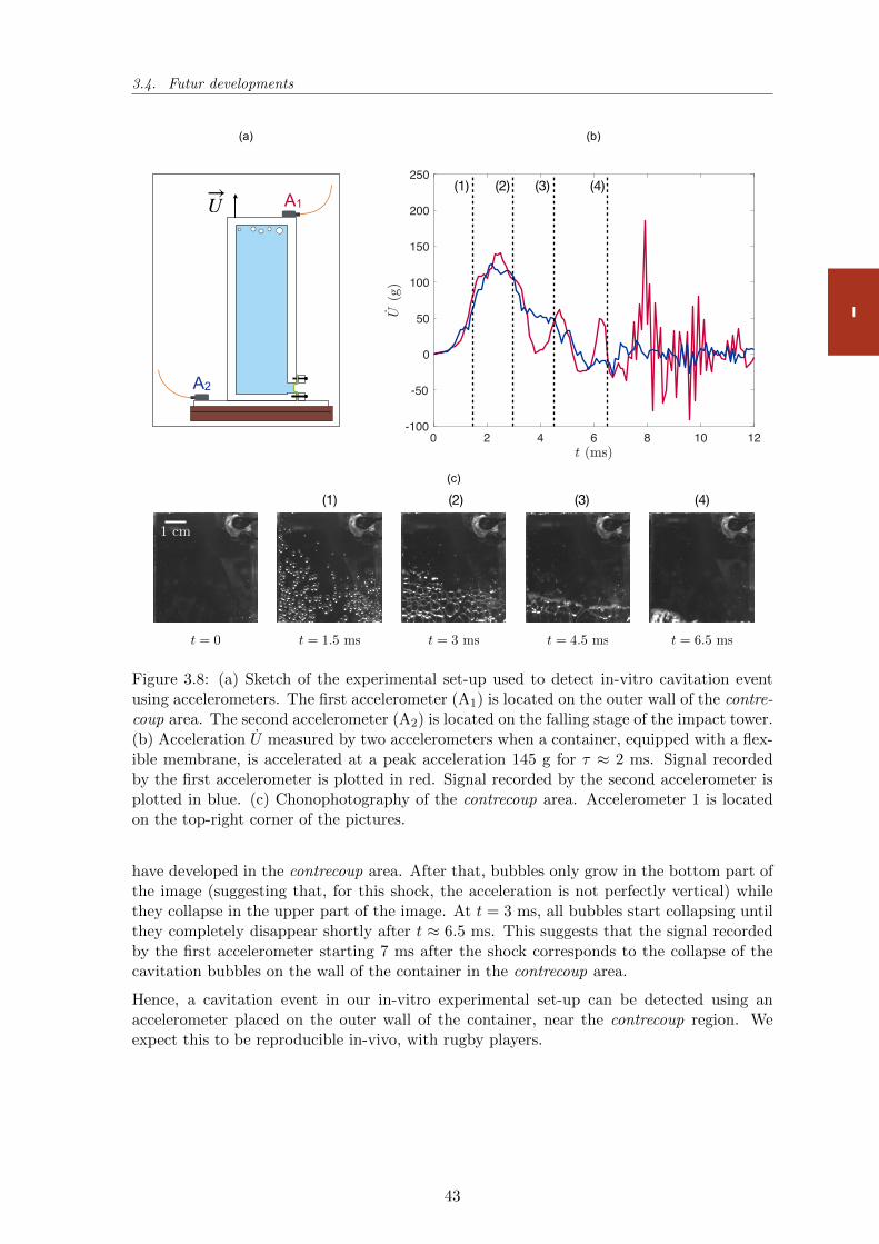
3.4. Futur developments
I
1 cm
(c)
0 2 4 6 8 10 12-100
-50
0
50
100
150
200
250
U A1
A2
(a) (b)
t = 6.5 mst = 4.5 mst = 3 mst = 1.5 mst = 0
(1) (2) (3) (4)
(1) (2) (3) (4)
Figure 3.8: (a) Sketch of the experimental set-up used to detect in-vitro cavitation eventusing accelerometers. The first accelerometer (A1) is located on the outer wall of the contre-coup area. The second accelerometer (A2) is located on the falling stage of the impact tower.(b) Acceleration U measured by two accelerometers when a container, equipped with a flex-ible membrane, is accelerated at a peak acceleration 145 g for τ ≈ 2 ms. Signal recordedby the first accelerometer is plotted in red. Signal recorded by the second accelerometer isplotted in blue. (c) Chonophotography of the contrecoup area. Accelerometer 1 is locatedon the top-right corner of the pictures.
have developed in the contrecoup area. After that, bubbles only grow in the bottom part ofthe image (suggesting that, for this shock, the acceleration is not perfectly vertical) whilethey collapse in the upper part of the image. At t = 3 ms, all bubbles start collapsing untilthey completely disappear shortly after t ≈ 6.5 ms. This suggests that the signal recordedby the first accelerometer starting 7 ms after the shock corresponds to the collapse of thecavitation bubbles on the wall of the container in the contrecoup area.
Hence, a cavitation event in our in-vitro experimental set-up can be detected using anaccelerometer placed on the outer wall of the container, near the contrecoup region. Weexpect this to be reproducible in-vivo, with rugby players.
43

Chapter 3. Influence of the shock duration on the bubble dynamic
I
Take home message of Part I
1. A pressure drop is measured in the region opposite of impact (contrecouparea) when a container of length L filled with water is accelerated by a shock of peakacceleration a and characteristic timespan τ . For a container equipped with a flexiblemembrane, the pressure drop has a magnitude δP = ρaL while it is δP = 1
2ρaLwhen the container is completely rigid.
2. Cavitation onset in a confined environment is determined by the cavitationnumber Ca introduced in [13]. For a deformable container, cavitation occurs forCa ≈ 1. However, for non-deformable container, the incompressibility conditionprevent bubbles from nucleating.
3. Growth of the bubble during a shock is accurately predicted by Rayleigh-Plesset equation. The maximum radius of the bubble Rmax can be analytically
predicted for a crenel shock. We find: Rmax ≈ R0 +(
3ρ2P0
) 13(2(a−av)L
3
) 56τ . In
particular, this shows that the characteristic time of the shock is a crucialparameter and that considering only the peak acceleration of the shock is not suf-ficient to fully capture the behaviour of cavitation bubbles in an accelerated container.
4. Maximum radius of the bubble quantify the energy E it stores. E is foundto scale as δPR3
max ∼ ρaLR3max. This is also the damaging potential of a bubble.
5. Damages caused by cavitation in a brain concussion scenario can accountfor the overall observations gathered in the Wayne State University Tolerance Curve(WSTC).
6. This work is expected to lead to improvement of the detection of brain concus-sions in sports (using the characteristic noise produced at the collapse of cavitationbubbles) as well as to lead to the development of new safety gears (such as self-rigidifying necklaces that would limit cavitation bubbles).
44
PART II
CHARACTERISATION OF ASUPERCAVITATING SPHERE
NEAR THE DRAG CRISIS
45
II
We have seen in the previous part that a pressure drop can trigger the growth of cavitationbubbles. As a consequence, if an underwater projectile travels fast enough, i.e. at a smallenough cavitation number, it enters the supercavitation regime. In this regime, the pressurearound the projectile is far below the vapor pressure of the liquid, such that a large cavitationbubble develops around the projectile. We wish to quantify the drag modification inducedby the presence of such a bubble. As we stated before, this regime is experimentally difficultto reproduce. However, the natural bubble created through cavitation can be mimicked viaartificial gas injection. This system is called ventilated cavities and is going to be the mainfocus of this part. First, we briefly review earlier works on the subject. We then presentour experimental set-up designed to study ventilated cavities behind spheres near the dragcrisis. Finally, we focus on the main results of our study, which address how the morphologyof the ventilated cavity affect the drag of the projectile.
46

4Short review on ventilated
cavities
Ventilated cavities behind a disk (top picture) and a fence (bottom picture).
Contents
4.1 Generalities on ventilated cavities . . . . . . . . . . . . . . . 48
4.2 Ventilated cavities in the wake of projectiles . . . . . . . . . 49
4.3 Statement of the problem . . . . . . . . . . . . . . . . . . . 53
47
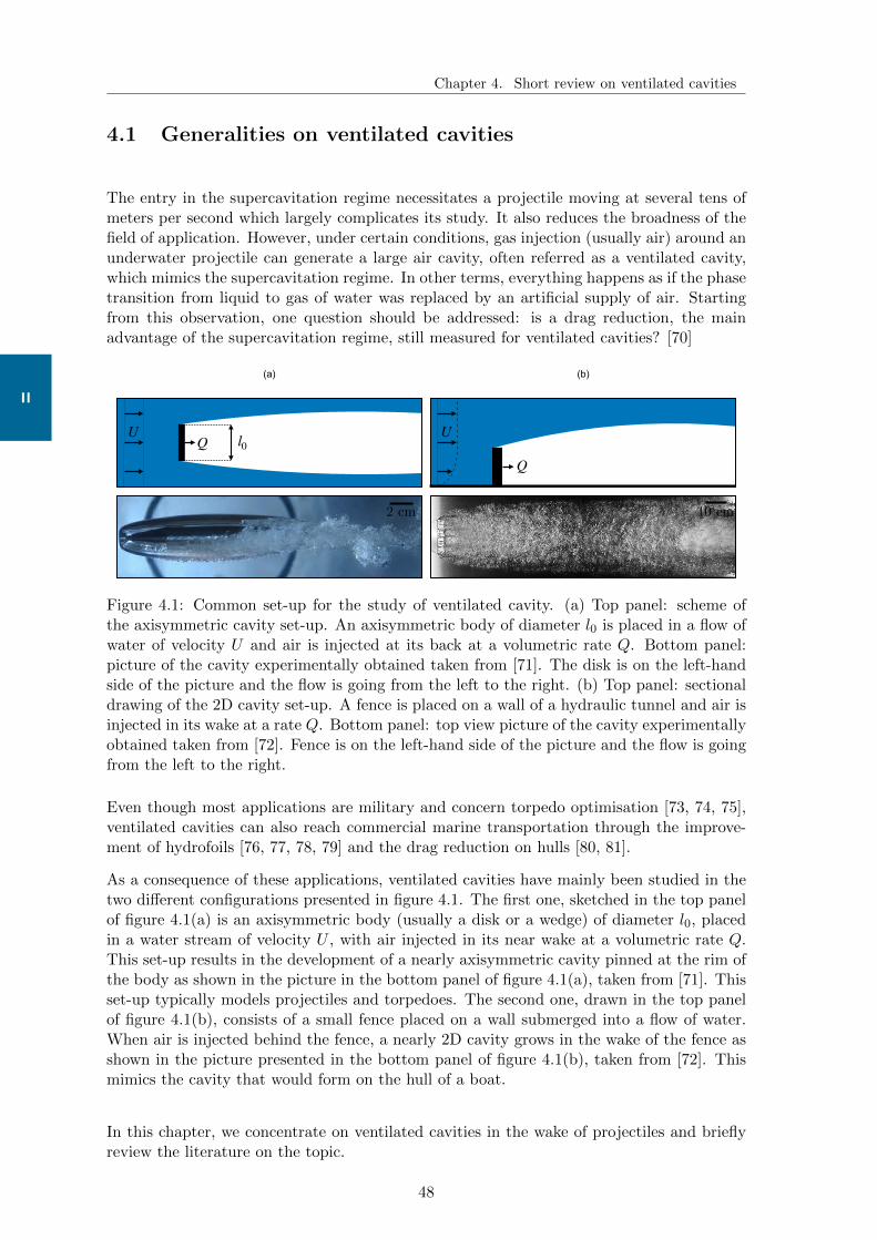
Chapter 4. Short review on ventilated cavities
II
4.1 Generalities on ventilated cavities
The entry in the supercavitation regime necessitates a projectile moving at several tens ofmeters per second which largely complicates its study. It also reduces the broadness of thefield of application. However, under certain conditions, gas injection (usually air) around anunderwater projectile can generate a large air cavity, often referred as a ventilated cavity,which mimics the supercavitation regime. In other terms, everything happens as if the phasetransition from liquid to gas of water was replaced by an artificial supply of air. Startingfrom this observation, one question should be addressed: is a drag reduction, the mainadvantage of the supercavitation regime, still measured for ventilated cavities? [70]
(a) (b)
l0U
U
2 cm 10 cm
Figure 4.1: Common set-up for the study of ventilated cavity. (a) Top panel: scheme ofthe axisymmetric cavity set-up. An axisymmetric body of diameter l0 is placed in a flow ofwater of velocity U and air is injected at its back at a volumetric rate Q. Bottom panel:picture of the cavity experimentally obtained taken from [71]. The disk is on the left-handside of the picture and the flow is going from the left to the right. (b) Top panel: sectionaldrawing of the 2D cavity set-up. A fence is placed on a wall of a hydraulic tunnel and air isinjected in its wake at a rate Q. Bottom panel: top view picture of the cavity experimentallyobtained taken from [72]. Fence is on the left-hand side of the picture and the flow is goingfrom the left to the right.
Even though most applications are military and concern torpedo optimisation [73, 74, 75],ventilated cavities can also reach commercial marine transportation through the improve-ment of hydrofoils [76, 77, 78, 79] and the drag reduction on hulls [80, 81].
As a consequence of these applications, ventilated cavities have mainly been studied in thetwo different configurations presented in figure 4.1. The first one, sketched in the top panelof figure 4.1(a) is an axisymmetric body (usually a disk or a wedge) of diameter l0, placedin a water stream of velocity U , with air injected in its near wake at a volumetric rate Q.This set-up results in the development of a nearly axisymmetric cavity pinned at the rim ofthe body as shown in the picture in the bottom panel of figure 4.1(a), taken from [71]. Thisset-up typically models projectiles and torpedoes. The second one, drawn in the top panelof figure 4.1(b), consists of a small fence placed on a wall submerged into a flow of water.When air is injected behind the fence, a nearly 2D cavity grows in the wake of the fence asshown in the picture presented in the bottom panel of figure 4.1(b), taken from [72]. Thismimics the cavity that would form on the hull of a boat.
In this chapter, we concentrate on ventilated cavities in the wake of projectiles and brieflyreview the literature on the topic.
48
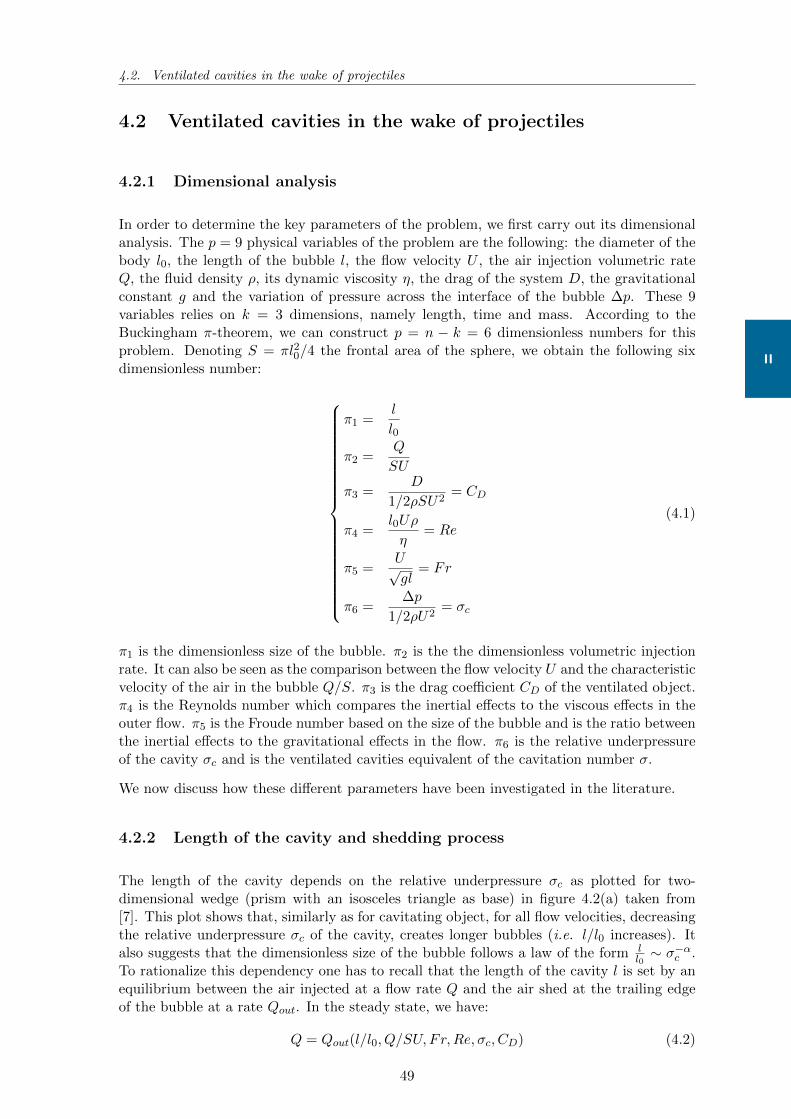
4.2. Ventilated cavities in the wake of projectiles
II
4.2 Ventilated cavities in the wake of projectiles
4.2.1 Dimensional analysis
In order to determine the key parameters of the problem, we first carry out its dimensionalanalysis. The p = 9 physical variables of the problem are the following: the diameter of thebody l0, the length of the bubble l, the flow velocity U , the air injection volumetric rateQ, the fluid density ρ, its dynamic viscosity η, the drag of the system D, the gravitationalconstant g and the variation of pressure across the interface of the bubble ∆p. These 9variables relies on k = 3 dimensions, namely length, time and mass. According to theBuckingham π-theorem, we can construct p = n − k = 6 dimensionless numbers for thisproblem. Denoting S = πl20/4 the frontal area of the sphere, we obtain the following sixdimensionless number:
π1 =l
l0
π2 =Q
SU
π3 =D
1/2ρSU2= CD
π4 =l0Uρ
η= Re
π5 =U√gl
= Fr
π6 =∆p
1/2ρU2= σc
(4.1)
π1 is the dimensionless size of the bubble. π2 is the the dimensionless volumetric injectionrate. It can also be seen as the comparison between the flow velocity U and the characteristicvelocity of the air in the bubble Q/S. π3 is the drag coefficient CD of the ventilated object.π4 is the Reynolds number which compares the inertial effects to the viscous effects in theouter flow. π5 is the Froude number based on the size of the bubble and is the ratio betweenthe inertial effects to the gravitational effects in the flow. π6 is the relative underpressureof the cavity σc and is the ventilated cavities equivalent of the cavitation number σ.
We now discuss how these different parameters have been investigated in the literature.
4.2.2 Length of the cavity and shedding process
The length of the cavity depends on the relative underpressure σc as plotted for two-dimensional wedge (prism with an isosceles triangle as base) in figure 4.2(a) taken from[7]. This plot shows that, similarly as for cavitating object, for all flow velocities, decreasingthe relative underpressure σc of the cavity, creates longer bubbles (i.e. l/l0 increases). Italso suggests that the dimensionless size of the bubble follows a law of the form l
l0∼ σ−αc .
To rationalize this dependency one has to recall that the length of the cavity l is set by anequilibrium between the air injected at a flow rate Q and the air shed at the trailing edgeof the bubble at a rate Qout. In the steady state, we have:
Q = Qout(l/l0, Q/SU, Fr,Re, σc, CD) (4.2)
49
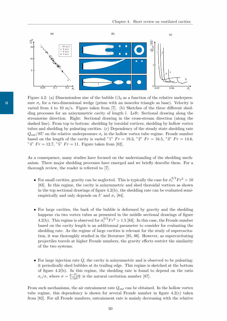
Chapter 4. Short review on ventilated cavities
II
(b) (c)(a)
σc
l/l 0
20
10
5
0.05 0.1 0.2
8 m/s10 m/s
6 m/s4 m/s
lσc
Qou
t/SU
0
1
0.02 0.06
Figure 4.2: (a) Dimensionless size of the bubble l/l0 as a function of the relative underpres-sure σc for a two-dimensional wedge (prism with an isosceles triangle as base). Velocity isvaried from 4 to 10 m/s. Figure taken from [7]. (b) Sketches of the three different shed-ding processes for an axisymmetric cavity of length l. Left: Sectional drawing along thestreamwise direction. Right: Sectional drawing in the cross-stream direction (along thedashed line). From top to bottom: shedding by toroidal vortices, shedding by hollow vortextubes and shedding by pulsating cavities. (c) Dependency of the steady state shedding rateQout/SU on the relative underpressure σc in the hollow vortex tube regime. Froude numberbased on the length of the cavity is varied ”1” Fr = 19.3, ”2” Fr = 16.5, ”3” Fr = 14.6,”4” Fr = 12.7, ”5” Fr = 11. Figure taken from [82].
As a consequence, many studies have focused on the understanding of the shedding mech-anism. Three major shedding processes have emerged and we briefly describe them. For athorough review, the reader is referred to [7].
• For small cavities, gravity can be neglected. This is typically the case for σ3/2c Fr2 > 10
[83]. In this regime, the cavity is axisymmetric and shed thoroidal vortices as shownin the top sectional drawings of figure 4.2(b), the shedding rate can be evaluated semi-empirically and only depends on U and σc [84].
• For large cavities, the back of the bubble is deformed by gravity and the sheddinghappens via two vortex tubes as presented in the middle sectional drawings of figure
4.2(b). This regime is observed for σ3/2c Fr2 > 1.5 [83]. In this case, the Froude number
based on the cavity length is an additionnal parameter to consider for evaluating theshedding rate. As the regime of large cavities is relevant for the study of supercavita-tion, it was thoroughly studied in the literature [85, 86]. However, as supercavitatingprojectiles travels at higher Froude numbers, the gravity effects restrict the similarityof the two systems.
• For large injection rate Q, the cavity is axisymmetric and is observed to be pulsating:it periodically shed bubbles at its trailing edge. This regime is sketched at the bottomof figure 4.2(b). In this regime, the shedding rate is found to depend on the ratio
σc/σ, where σ =p−Pvap
1/2ρU2 is the natural cavitation number [87].
From such mechanisms, the air entrainment rate Qout can be obtained. In the hollow vortextube regime, this dependency is shown for several Froude number in figure 4.2(c) takenfrom [82]. For all Froude numbers, entrainment rate is mainly decreasing with the relative
50
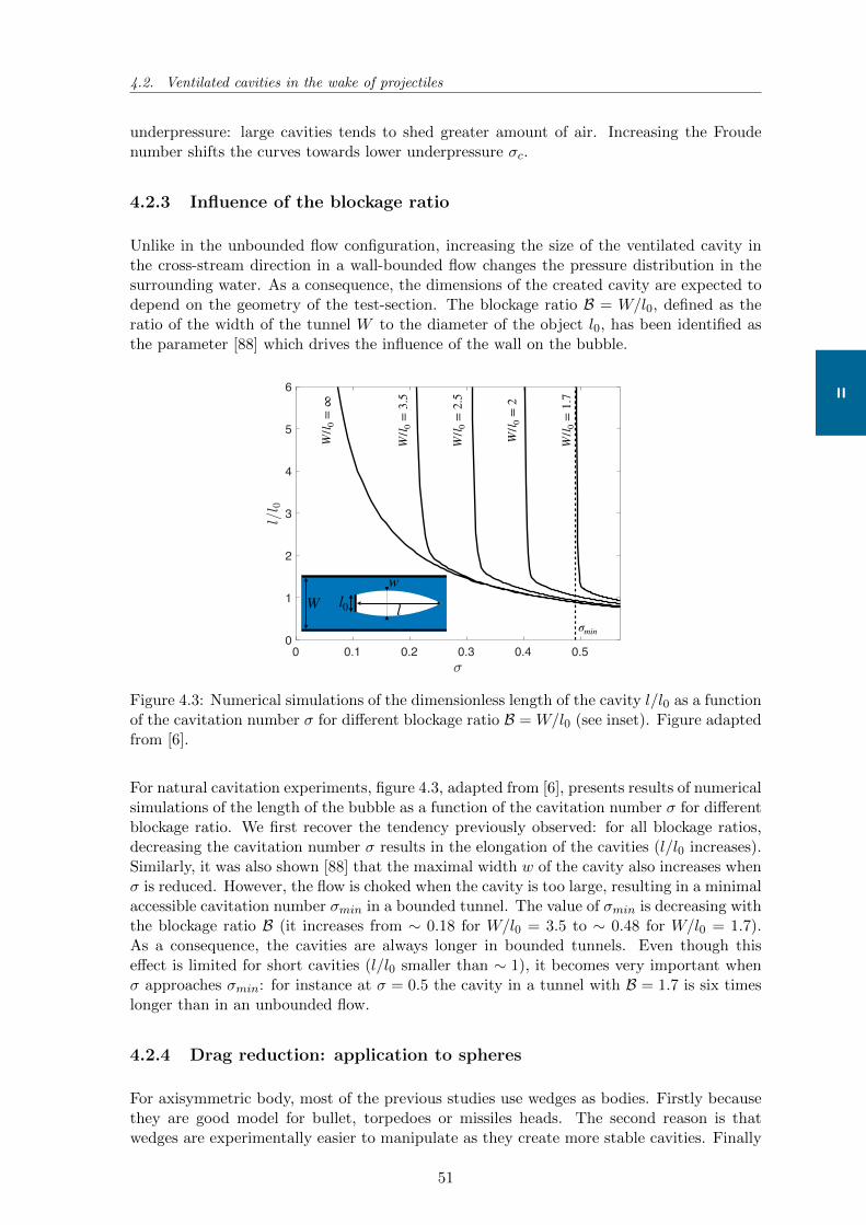
4.2. Ventilated cavities in the wake of projectiles
II
underpressure: large cavities tends to shed greater amount of air. Increasing the Froudenumber shifts the curves towards lower underpressure σc.
4.2.3 Influence of the blockage ratio
Unlike in the unbounded flow configuration, increasing the size of the ventilated cavity inthe cross-stream direction in a wall-bounded flow changes the pressure distribution in thesurrounding water. As a consequence, the dimensions of the created cavity are expected todepend on the geometry of the test-section. The blockage ratio B = W/l0, defined as theratio of the width of the tunnel W to the diameter of the object l0, has been identified asthe parameter [88] which drives the influence of the wall on the bubble.
0 0.1 0.2 0.3 0.4 0.50
1
2
3
4
5
6
W/l 0
=1.7
W/l 0
=2
W/l 0
=2.5
W/l 0
=3.5
W/l 0
=∞
W l0 l
w
σmin
Figure 4.3: Numerical simulations of the dimensionless length of the cavity l/l0 as a functionof the cavitation number σ for different blockage ratio B = W/l0 (see inset). Figure adaptedfrom [6].
For natural cavitation experiments, figure 4.3, adapted from [6], presents results of numericalsimulations of the length of the bubble as a function of the cavitation number σ for differentblockage ratio. We first recover the tendency previously observed: for all blockage ratios,decreasing the cavitation number σ results in the elongation of the cavities (l/l0 increases).Similarly, it was also shown [88] that the maximal width w of the cavity also increases whenσ is reduced. However, the flow is choked when the cavity is too large, resulting in a minimalaccessible cavitation number σmin in a bounded tunnel. The value of σmin is decreasing withthe blockage ratio B (it increases from ∼ 0.18 for W/l0 = 3.5 to ∼ 0.48 for W/l0 = 1.7).As a consequence, the cavities are always longer in bounded tunnels. Even though thiseffect is limited for short cavities (l/l0 smaller than ∼ 1), it becomes very important whenσ approaches σmin: for instance at σ = 0.5 the cavity in a tunnel with B = 1.7 is six timeslonger than in an unbounded flow.
4.2.4 Drag reduction: application to spheres
For axisymmetric body, most of the previous studies use wedges as bodies. Firstly becausethey are good model for bullet, torpedoes or missiles heads. The second reason is thatwedges are experimentally easier to manipulate as they create more stable cavities. Finally
51
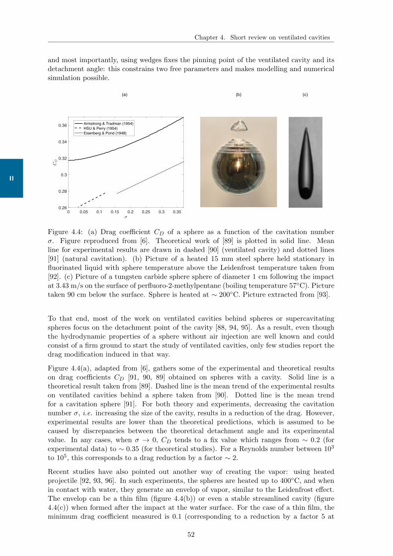
Chapter 4. Short review on ventilated cavities
II
and most importantly, using wedges fixes the pinning point of the ventilated cavity and itsdetachment angle: this constrains two free parameters and makes modelling and numericalsimulation possible.
(a) (b)
0 0.05 0.1 0.15 0.2 0.25 0.3 0.350.26
0.28
0.3
0.32
0.34
0.36 Armstrong & Tradman (1954)HSU & Perry (1954)Eisenberg & Pond (1948)
If the solid-liquid interface of the sphere is replaced byan ideal nondeformable spherical gas-liquid interfacewhere it is assumed to have zero tangential stress, thedrag coefficient has the form CD ¼ 16=Re at lowReynolds number that follows from the Hardamard-Rubczynski formula: FD ¼ 4!"RU, for Re ! 0; andhas the theoretical limiting form CD ¼ 48=Re, forRe ! 1 as obtained by Levich [18]. However, deforma-tion of the gas-liquid interface has a significant effect onthe drag coefficient at large Re [19] so the Levich result isnot observed in practice [20]. The present experimentaltechnique offers an alternative methodology to probe thedrag on a nondeformable ‘‘bubble’’ at larger Re.
We produce an inverted Leidenfrost effect by immersinga metallic sphere, heated to an initial temperature TS, in aliquid with a low vaporization heat capacity. The perflu-orinated liquid we used, FC-72 (3MTM FluorinertTM
Electronic Liquid, mostly composed of perfluorohexane,C6F14) has a boiling point of 56
"C and a vaporization heatcapacity that is approximately 30 times lower than that ofwater. Figure 1 shows snapshots of the states of fluidmotion associated with the cooling of a stationary steelsphere (initial temperature TS ¼ 250 "C) suspended mag-netically in the FC-72 liquid. When first immersed inthe liquid, a continuous thin vapor layer forms around thesphere, evident by the rippling waves moving along thesphere surface accompanied by periodic release of bubblesfrom the upper pole of the sphere [Fig. 1(a)]. The vaporlayer thickness estimated by high magnification imaging atthe sphere surface was found to be in the range of 100 to200 "m (see supplemental materials Fig. 3S [21]). Afterthe sphere temperature cools below the Leidenfrost tem-perature, TL, of about 130
"C, in about 25 sec. in this case,the continuous vapor layer surrounding the sphere can no
longer be maintained and the fluid comes into direct con-tact with the hot sphere surface. This point is marked by avery dramatic and explosive release of bubbles [Fig. 1(b)].The entire sphere cooling process can be seen in thesupplemental video 1 [21].In our moving sphere experiments, a sphere is heated in
a temperature-controlled furnace and then released to fallfreely under gravity in a cylindrical tank with height of 2 mand diameter of 80 mm filled with the perfluorinated liquid.The subsequent motion is captured with a high-speedcamera to determine the terminal velocity, U. The dragcoefficient of the sphere can then be calculated from thebalance between gravity, buoyancy and drag forces as:CD ¼ ð8g½#s % #&RÞ=ð3#U2Þ, where g is the gravitationalacceleration, #s is the sphere density and # is the liquiddensity (See supplemental material for experimental de-tails and notes on the drag coefficient derivation account-ing for the cylinder wall effects [21]).In Fig. 2 we show the dependence of the terminal
velocity of a 20 mm diameter steel sphere with spheretemperatures in the range: 25 "C< TS < 280 "C. Thedata clearly demonstrate the dramatic effect due to theonset of the Leidenfrost regime. An initial increase insphere temperature from 25 "C to 110 "C results in amoderate increase in the terminal velocity of about 20%in the range 1:3 m=s to 1:6 m=s. Such variations could bedue to a confluence of the heat-induced viscosity change ofthe surrounding fluid and the partial coverage of the spherewith bubbles when the sphere temperature is above theboiling point of the fluid. However, when the spheretemperature exceeds the Leidenfrost temperature,TL ¼ 130 "C, we observe an increase in the terminal ve-locity by a factor of 2.6 to a nearly constant value of about
FIG. 1 (color online). (a) Digital camera snapshot of a heated15 mm steel sphere held stationary in fluorinated liquid withsphere temperature TS above the Leidenfrost temperature TL. Athin vapor layer streaming around the sphere can be observed bythe ripples moving along the sphere surface. (b) Snapshot at theinstant when the sphere has cooled to the Leidenfrost tempera-ture that is marked by an explosive release of bubbles. (Seesupplemental video 1 [21]).
FIG. 2 (color online). Variation of the terminal velocity withthe sphere temperature measured for a 20 mm steel spherefalling through the liquid (FC-72). Open square data points(blue) are for temperature below the Leidenfrost temperature(TL ¼ 130 "C) and solid square (red) for temperature above TL
(see supplemental video 2 [21]).
PRL 106, 214501 (2011) P HY S I CA L R EV I EW LE T T E R Sweek ending27 MAY 2011
214501-2
Stable–streamlined and helical cavity formation 729
60.7 cm 66.8 cm 73.5 cm 73.3 cm
95.9 cm 95.8 cm 99.6 cm 109 cm
(a)
(b)
FIGURE 5. Stable–streamlined cavities obtained using D0 = 10 mm (a) steel (% = 4.54,Ut = 1 m s1) and (b) tungsten carbide spheres (% = 8.70, Ut = 1.6 m s1) for increasingimpact velocities of U0 = 3.43, 3.70, 3.96, 4.20 and 4.43 m s1 (corresponding to releaseheights of hr = 60, 70, 80, 90 and 100 cm respectively). The depth zs (cm) indicatesthe distance from the free surface where the stable cavity state is first achieved in eachcase. Here, Dc and Lc are the cavity diameter and length measurements respectively; Fr =240–400.
which finds its roots in the dual-cavity structure reported previously by Marston et al.(2012). This structure, which is shown forming in figure 7(a) with close-up views in(c), results in a distinct cavity pinch-off of its own (t = 30 ms) and is described ashaving sensitive dependence on the sphere temperature and impact speed. Marstonet al. (2012) ascribed the origin of the dual-cavity structure to the vapour layer notbeing able to fully form within the time scale of one radius penetration, i.e tU0/R0 = 1.The presence of a physical contact line observed around the sphere equator initiatednucleate boiling and was shed backwards by the advancing vapour layer until thesphere was encapsulated entirely. However, since the presence of a vapour layeraround the entire bottom hemisphere was indicated with marked uncertainty in theimages recorded, the origin of the dual-cavity structure could not be fully understoodin their study. For hot spheres impacting the liquid medium at comparatively highervelocities (U0 = 6.25 m s1), the formation of asymmetric cavities comprising threeor four columns of liquid converging towards the cavity centre was also shown usingtop-down views. The liquid columns were attributed to the contact of the cavity wallwith the hot sphere, but the origin of the instability resulting in their formation couldnot be explained.
In the parameter space of experiments conducted at constant Ts in this study,the series of events occurring before a dual-structure cavity forms (i.e t 6 10 ms infigure 7a) are observed to occur indefinitely (as shown in figure 7b) above a thresholdimpact Reynolds number (see figure 12). The cavity is noted to develop evident ridgesor streaks (see the close-ups in figure 7d) which stem from the sphere surface andfollow random trajectories about its equator as it descends into the tank. Columnsof liquid very similar to those observed by Marston et al. (2012) are noted tooriginate from each of these ridges, which break up while moving radially inwards toinduce a fine and continuous spray of droplets within the cavity. The cavity collapses
,E
:03
35
7E
EE
20
136
6
2
2:
.:
27C
/0
C19
27
01
365C
0D0
:01:
07
EE
E 2
01
36
62
73
6
95
(c)
Figure 4.4: (a) Drag coefficient CD of a sphere as a function of the cavitation numberσ. Figure reproduced from [6]. Theoretical work of [89] is plotted in solid line. Meanline for experimental results are drawn in dashed [90] (ventilated cavity) and dotted lines[91] (natural cavitation). (b) Picture of a heated 15 mm steel sphere held stationary influorinated liquid with sphere temperature above the Leidenfrost temperature taken from[92]. (c) Picture of a tungsten carbide sphere sphere of diameter 1 cm following the impactat 3.43 m/s on the surface of perfluoro-2-methylpentane (boiling temperature 57C). Picturetaken 90 cm below the surface. Sphere is heated at ∼ 200C. Picture extracted from [93].
To that end, most of the work on ventilated cavities behind spheres or supercavitatingspheres focus on the detachment point of the cavity [88, 94, 95]. As a result, even thoughthe hydrodynamic properties of a sphere without air injection are well known and couldconsist of a firm ground to start the study of ventilated cavities, only few studies report thedrag modification induced in that way.
Figure 4.4(a), adapted from [6], gathers some of the experimental and theoretical resultson drag coefficients CD [91, 90, 89] obtained on spheres with a cavity. Solid line is atheoretical result taken from [89]. Dashed line is the mean trend of the experimental resultson ventilated cavities behind a sphere taken from [90]. Dotted line is the mean trendfor a cavitation sphere [91]. For both theory and experiments, decreasing the cavitationnumber σ, i.e. increasing the size of the cavity, results in a reduction of the drag. However,experimental results are lower than the theoretical predictions, which is assumed to becaused by discrepancies between the theoretical detachment angle and its experimentalvalue. In any cases, when σ → 0, CD tends to a fix value which ranges from ∼ 0.2 (forexperimental data) to ∼ 0.35 (for theoretical studies). For a Reynolds number between 103
to 105, this corresponds to a drag reduction by a factor ∼ 2.
Recent studies have also pointed out another way of creating the vapor: using heatedprojectile [92, 93, 96]. In such experiments, the spheres are heated up to 400C, and whenin contact with water, they generate an envelop of vapor, similar to the Leidenfrost effect.The envelop can be a thin film (figure 4.4(b)) or even a stable streamlined cavity (figure4.4(c)) when formed after the impact at the water surface. For the case of a thin film, theminimum drag coefficient measured is 0.1 (corresponding to a reduction by a factor 5 at
52
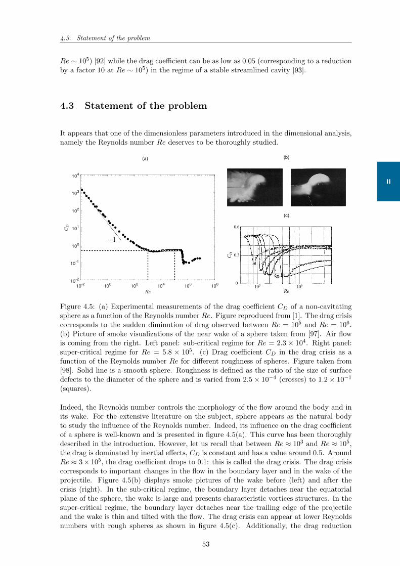
4.3. Statement of the problem
II
Re ∼ 105) [92] while the drag coefficient can be as low as 0.05 (corresponding to a reductionby a factor 10 at Re ∼ 105) in the regime of a stable streamlined cavity [93].
4.3 Statement of the problem
It appears that one of the dimensionless parameters introduced in the dimensional analysis,namely the Reynolds number Re deserves to be thoroughly studied.
10-2 100 102 104 106 10810-2
10-1
100
101
102
103
104
(a)
(b)
(c)
−1
Re
C D
0
0.6
0.3
105 106
(b)
Figure 4.5: (a) Experimental measurements of the drag coefficient CD of a non-cavitatingsphere as a function of the Reynolds number Re. Figure reproduced from [1]. The drag crisiscorresponds to the sudden diminution of drag observed between Re = 105 and Re = 106.(b) Picture of smoke visualizations of the near wake of a sphere taken from [97]. Air flowis coming from the right. Left panel: sub-critical regime for Re = 2.3 × 10⁴. Right panel:super-critical regime for Re = 5.8 × 10⁵. (c) Drag coefficient CD in the drag crisis as afunction of the Reynolds number Re for different roughness of spheres. Figure taken from[98]. Solid line is a smooth sphere. Roughness is defined as the ratio of the size of surfacedefects to the diameter of the sphere and is varied from 2.5 × 10⁻⁴ (crosses) to 1.2 × 10⁻¹
(squares).
Indeed, the Reynolds number controls the morphology of the flow around the body and inits wake. For the extensive literature on the subject, sphere appears as the natural bodyto study the influence of the Reynolds number. Indeed, its influence on the drag coefficientof a sphere is well-known and is presented in figure 4.5(a). This curve has been thoroughlydescribed in the introduction. However, let us recall that between Re ≈ 103 and Re ≈ 105,the drag is dominated by inertial effects, CD is constant and has a value around 0.5. AroundRe ≈ 3× 10⁵, the drag coefficient drops to 0.1: this is called the drag crisis. The drag crisiscorresponds to important changes in the flow in the boundary layer and in the wake of theprojectile. Figure 4.5(b) displays smoke pictures of the wake before (left) and after thecrisis (right). In the sub-critical regime, the boundary layer detaches near the equatorialplane of the sphere, the wake is large and presents characteristic vortices structures. In thesuper-critical regime, the boundary layer detaches near the trailing edge of the projectileand the wake is thin and tilted with the flow. The drag crisis can appear at lower Reynoldsnumbers with rough spheres as shown in figure 4.5(c). Additionally, the drag reduction
53
Chapter 4. Short review on ventilated cavities
II
previously reported for Leidenfrost spheres enveloped with a thin layer of vapor [92, 96] hasbeen attributed to an early trigger of the drag crisis.
Most applications of ventilated cavities are underwater fast moving object (typically tor-pedoes). They are in a regime for which gravity is negligible and the flow super-critical.However, ventilated cavities have only been studied for Reynolds numbers between 103
and 105. Given the differences in the flow and in the origin of the drag depending theReynolds number, it appears crucial to investigate ventilated cavity flow in a broader rangeof Reynolds number.
As a consequence, the rest of the study will concentrate on ventilated cavities behind spheresin the range of Reynolds number of the drag crisis. The study will be carried out in a regimefor which the gravity is negligible. The ventilation will be controlled via the dimensionlessvolumetric injection rate Q/SU .
54
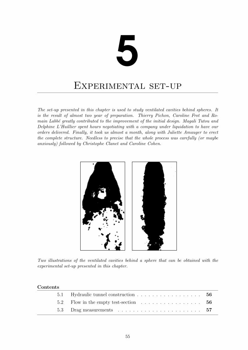
5Experimental set-up
The set-up presented in this chapter is used to study ventilated cavities behind spheres. Itis the result of almost two year of preparation. Thierry Pichon, Caroline Frot and Ro-main Labbe greatly contributed to the improvement of the initial design. Magali Tutou andDelphine L’Huillier spent hours negotiating with a company under liquidation to have ourorders delivered. Finally, it took us almost a month, along with Juliette Amauger to erectthe complete structure. Needless to precise that the whole process was carefully (or maybeanxiously) followed by Christophe Clanet and Caroline Cohen.
Two illustrations of the ventilated cavities behind a sphere that can be obtained with theexperimental set-up presented in this chapter.
Contents
5.1 Hydraulic tunnel construction . . . . . . . . . . . . . . . . . 56
5.2 Flow in the empty test-section . . . . . . . . . . . . . . . . 56
5.3 Drag measurements . . . . . . . . . . . . . . . . . . . . . . 57
55
Chapter 5. Experimental set-up
II
5.1 Hydraulic tunnel construction
The experimental set-up used to study ventilated cavities is an hydraulic tunnel with a ver-tical test section sketched in figure 5.1. The flow of water is driven by a pump (Grundfos,(1)) with tunable flow rate from 50 to 270 cubic meters per hour. Pumped water passesthrough a valve (2) and is poured via a vertical outlet pipe (3) into a three-meters long tran-quilization tank (4). At the other end of the tank, the water passes though an honeycomb(with centrimetric holes) and a vertical converging nozzle (5), which reduction ratio is 4 to 1,before entering the test-section (6). The test-section is vertical and has inner dimensions of11 by 11 by 70 cm. It is made of three centimeters thick transparent acrylic and is equippedwith two side windows to change the object tested. An air-injection system (7) allows us toinject, at a control flow rate, air in the test section. Finally, water is fed back into the pumpthrough a return pipe (8). In this study, objects tested are spheres of diameter l0 varyingfrom 2 to 3 cm. To obtain smooth spheres, half spheres are 3D-printed in AcrylonitrileButadiene Styrene (ABS), attached together and then smoothed above an acetone bath at70C during two minutes. W = 11 cm being the width of the tunnel test-section, we definethe blockage ratio B = W/l0 which ranges from 3.5 to 5.5. As presented in figure 4.3, thesevalues should be sufficient to reach equivalent cavitation numbers as low as 0.15.
To measure the drag of tested projectiles (i), they are attached onto two submersible forcesensors (iii) with a 3D-printed streamlined holder (ii) as shown in figure 5.1(b). Air isinjected at the trailing edge of the projectile (i) through the holder (ii) as drawn in figure5.1(c). The flow rate is measured using mechanical flow meter (Key Instruments, (7) infigure 5.1) with an accuracy below 5% and can be varied from 0.4 to 20 liters per minute(lpm).
5.2 Flow in the empty test-section
The resulting flow in the test-section can be visualized via Particle Image Velocimetry(PIV). We use the sub-millimetric bubbles entrained in the tunnel as PIV particles. Theintantaneous velocity field can decomposed in a streamwise (vertical) component −u(t) eyand an horizontal component v(t)ex. The typical streamwise velocity u all across the tunnelis plotted in figure 5.2(a) for the pump running at 75 Hz. We note that, apart from the0.5 cm close to the tunnel walls, the streamwise velocity is fairly homogeneous. Indeed, inthe ten central centimeters of the test-section, the velocity only varies between 4.4 and 4.6m/s, which corresponds to a variation below 5 %. From such measurements, we computethe average velocity in the streamwise direction U in the central part of test section. Figure5.2(b) displays the typical intantaneous non-dimensional cross-stream velocity v/U . Inmost of the tunnel, its value is below 1.5 % and it never exceeds 4%. The maximum value isonly reached in the right part of the tunnel, which create an asymmetric in the test-section.Although this is satisfactory for our applications, this effect was further reduced by ensuringthat the swirling motion induced by the suction in the tranquilization tank is axisymmetric.
With such measurements, we can average the velocity u over the streamwise direction (y-axis) to obtain the mean profile across the tunnel. Doing so for different running frequenciesof the pump, we obtain the profiles plotted in figure 5.3(a). All the profiles share the sameshape: the velocity u is fairly constant in the central part of the tunnel and rapidly decaysin the centimeter near the walls. The maximum velocity of the profile increase with therunning frequency of the pump. From this profile, we compute U , the average of u in the
56
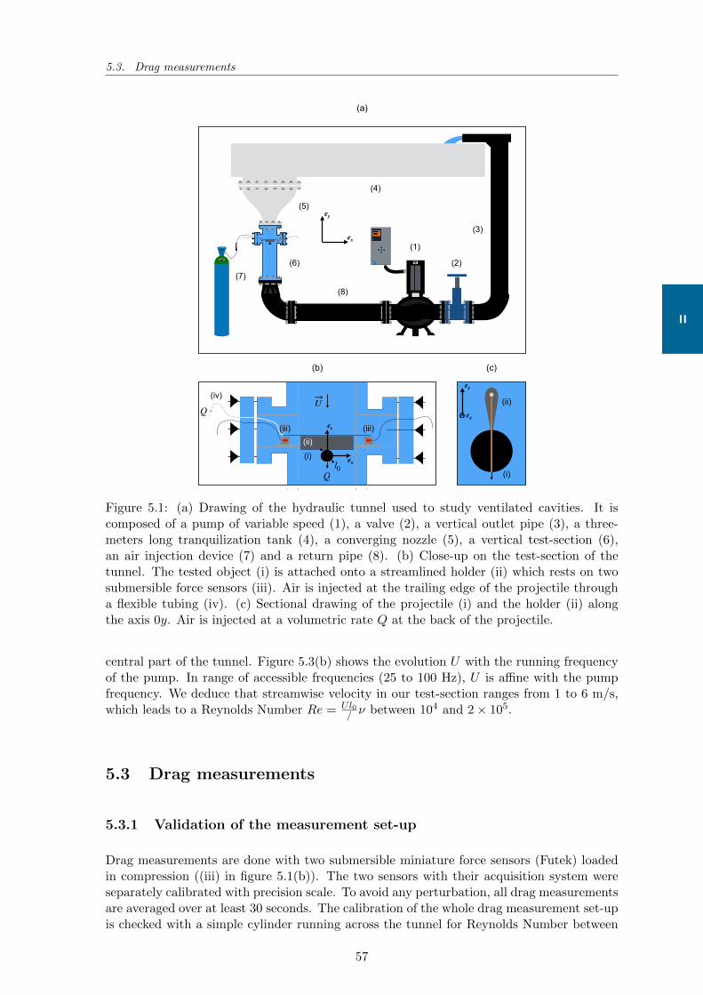
5.3. Drag measurements
II
UQ
Ql0
Q
ex
ey
(4)
(5)
(6)(7)
(1)
(3)
(2)
(8)
ex
ey
ex
ey
(a)
(b) (c)
(iii) (iii)
(i)
(ii)
(iv)
(i)
(ii)
Figure 5.1: (a) Drawing of the hydraulic tunnel used to study ventilated cavities. It iscomposed of a pump of variable speed (1), a valve (2), a vertical outlet pipe (3), a three-meters long tranquilization tank (4), a converging nozzle (5), a vertical test-section (6),an air injection device (7) and a return pipe (8). (b) Close-up on the test-section of thetunnel. The tested object (i) is attached onto a streamlined holder (ii) which rests on twosubmersible force sensors (iii). Air is injected at the trailing edge of the projectile througha flexible tubing (iv). (c) Sectional drawing of the projectile (i) and the holder (ii) alongthe axis 0y. Air is injected at a volumetric rate Q at the back of the projectile.
central part of the tunnel. Figure 5.3(b) shows the evolution U with the running frequencyof the pump. In range of accessible frequencies (25 to 100 Hz), U is affine with the pumpfrequency. We deduce that streamwise velocity in our test-section ranges from 1 to 6 m/s,which leads to a Reynolds Number Re = Ul0
/ ν between 104 and 2× 10⁵.
5.3 Drag measurements
5.3.1 Validation of the measurement set-up
Drag measurements are done with two submersible miniature force sensors (Futek) loadedin compression ((iii) in figure 5.1(b)). The two sensors with their acquisition system wereseparately calibrated with precision scale. To avoid any perturbation, all drag measurementsare averaged over at least 30 seconds. The calibration of the whole drag measurement set-upis checked with a simple cylinder running across the tunnel for Reynolds Number between
57
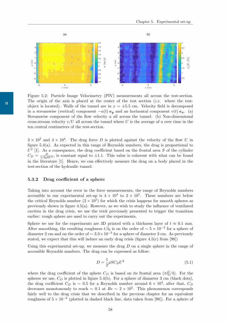
Chapter 5. Experimental set-up
II
-5 0 5
-3
-2
-1
0
1
2
3
0.5
1
1.5
2
2.5
3
3.5
4
-5 0 5
-3
-2
-1
0
1
2
3
3.6
3.7
3.8
3.9
4
4.1
4.2
4.3
4.4
4.5
4.6
u(m
/s)
|v|/
U(%
)
(a) (b)
Figure 5.2: Particle Image Velocimetry (PIV) measurements all across the test-section.The origin of the axis is placed at the center of the test section (i.e. where the test-object is located). Walls of the tunnel are in x = ±5.5 cm. Velocity field is decomposedin a streamwise (vertical) component −u(t) ey and an horizontal component v(t) ex. (a)Streamwise component of the flow velocity u all across the tunnel. (b) Non-dimensionalcross-stream velocity v/U all across the tunnel where U is the average of u over time in theten central centimeters of the test-section.
3 × 10³ and 4 × 10⁴. The drag force D is plotted against the velocity of the flow U infigure 5.4(a). As expected in this range of Reynolds numbers, the drag is proportional toU2 [1]. As a consequence, the drag coefficient based on the frontal area S of the cylinderCD = D
1/2ρSU2 , is constant equal to ±1.1. This value is coherent with what can be found
in the literature [1]. Hence, we can effectively measure the drag on a body placed in thetest-section of the hydraulic tunnel.
5.3.2 Drag coefficient of a sphere
Taking into account the error in the force measurements, the range of Reynolds numbersaccessible in our experimental set-up is 4 × 10⁴ to 2 × 10⁵. These numbers are belowthe critical Reynolds number (3 × 10⁵) for which the crisis happens for smooth spheres aspreviously shown in figure 4.5(a). However, as we wish to study the influence of ventilatedcavities in the drag crisis, we use the trick previously presented to trigger the transitionearlier: rough sphere are used to carry out the experiments.
Sphere we use for the experiments are 3D printed with a thickness layer of t ≈ 0.1 mm.After smoothing, the resulting roughness t/l0 is on the order of ∼ 5× 10⁻³ for a sphere ofdiameter 2 cm and on the order of ∼ 3.3×10⁻³ for a sphere of diameter 3 cm. As previouslystated, we expect that this will induce an early drag crisis (figure 4.5(c) from [98])
Using this experimental set-up, we measure the drag D on a single sphere in the range ofaccessible Reynolds numbers. The drag can be expressed as follow:
D =1
2ρSCDU
2 (5.1)
where the drag coefficient of the sphere CD is based on its frontal area (πl20/4). For thespheres we use, CD is plotted in figure 5.4(b). For a sphere of diameter 3 cm (black dots),the drag coefficient CD is ∼ 0.5 for a Reynolds number around 6 × 10⁴, after that, CDdecreases monotonously to reach ∼ 0.1 at Re ∼ 2 × 10⁵. This phenomenon correspondsfairly well to the drag crisis that we described in the previous chapter for an equivalentroughness of 5× 10⁻³ (plotted in dashed black line, data taken from [98]). For a sphere of
58
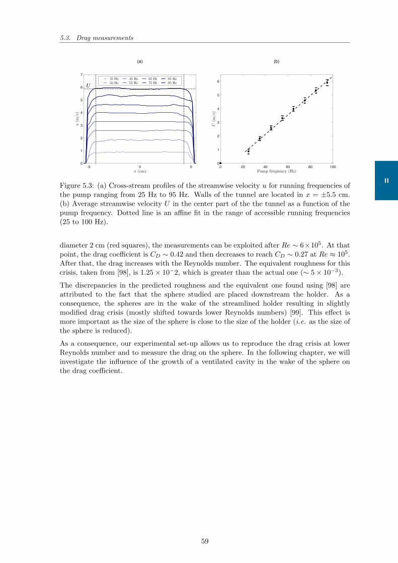
5.3. Drag measurements
II
0 20 40 60 80 1000
1
2
3
4
5
6
-5 0 50
1
2
3
4
5
6
7
(a) (b)
25 Hz35 Hz
45 Hz55 Hz
65 Hz75 Hz
85 Hz95 HzU
Figure 5.3: (a) Cross-stream profiles of the streamwise velocity u for running frequencies ofthe pump ranging from 25 Hz to 95 Hz. Walls of the tunnel are located in x = ±5.5 cm.(b) Average streamwise velocity U in the center part of the the tunnel as a function of thepump frequency. Dotted line is an affine fit in the range of accessible running frequencies(25 to 100 Hz).
diameter 2 cm (red squares), the measurements can be exploited after Re ∼ 6×10⁵. At thatpoint, the drag coefficient is CD ∼ 0.42 and then decreases to reach CD ∼ 0.27 at Re ≈ 105.After that, the drag increases with the Reynolds number. The equivalent roughness for thiscrisis, taken from [98], is 1.25× 10⁻², which is greater than the actual one (∼ 5× 10⁻³).
The discrepancies in the predicted roughness and the equivalent one found using [98] areattributed to the fact that the sphere studied are placed downstream the holder. As aconsequence, the spheres are in the wake of the streamlined holder resulting in slightlymodified drag crisis (mostly shifted towards lower Reynolds numbers) [99]. This effect ismore important as the size of the sphere is close to the size of the holder (i.e. as the size ofthe sphere is reduced).
As a consequence, our experimental set-up allows us to reproduce the drag crisis at lowerReynolds number and to measure the drag on the sphere. In the following chapter, we willinvestigate the influence of the growth of a ventilated cavity in the wake of the sphere onthe drag coefficient.
59
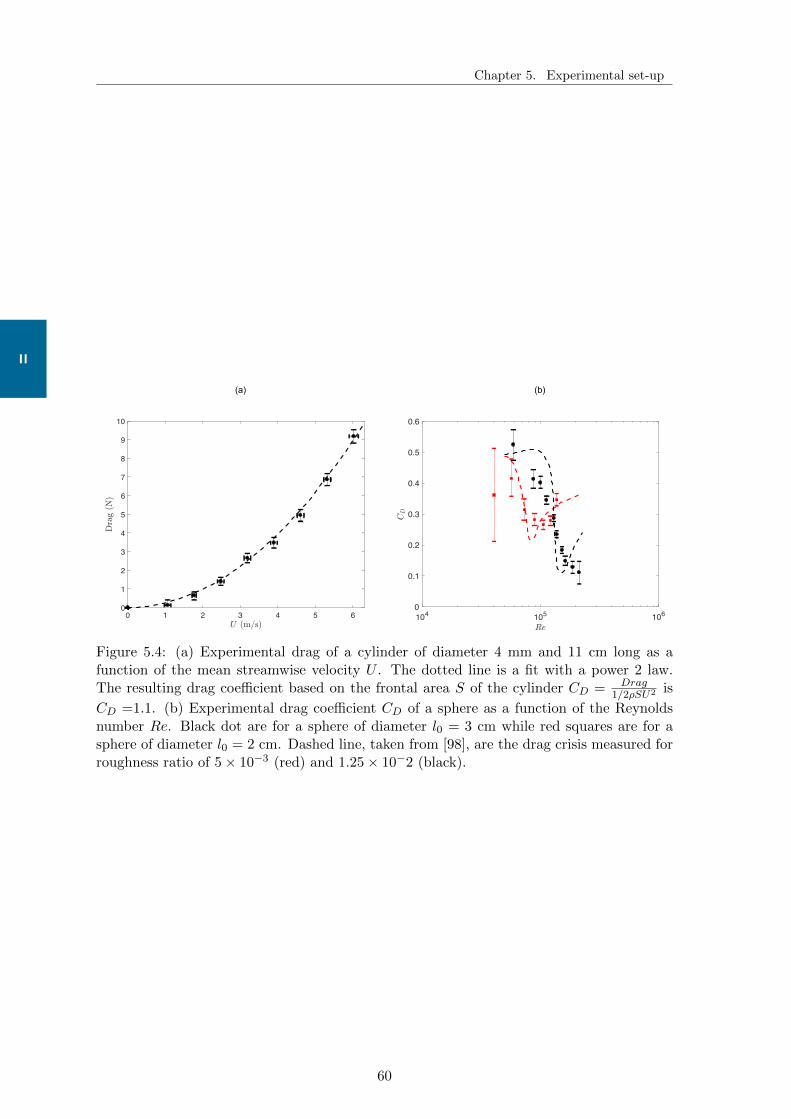
Chapter 5. Experimental set-up
II
104 105 1060
0.1
0.2
0.3
0.4
0.5
0.6
0 1 2 3 4 5 60
1
2
3
4
5
6
7
8
9
10
(a) (b)
Figure 5.4: (a) Experimental drag of a cylinder of diameter 4 mm and 11 cm long as afunction of the mean streamwise velocity U . The dotted line is a fit with a power 2 law.The resulting drag coefficient based on the frontal area S of the cylinder CD = Drag
1/2ρSU2 is
CD =1.1. (b) Experimental drag coefficient CD of a sphere as a function of the Reynoldsnumber Re. Black dot are for a sphere of diameter l0 = 3 cm while red squares are for asphere of diameter l0 = 2 cm. Dashed line, taken from [98], are the drag crisis measured forroughness ratio of 5× 10⁻³ (red) and 1.25× 10⁻² (black).
60
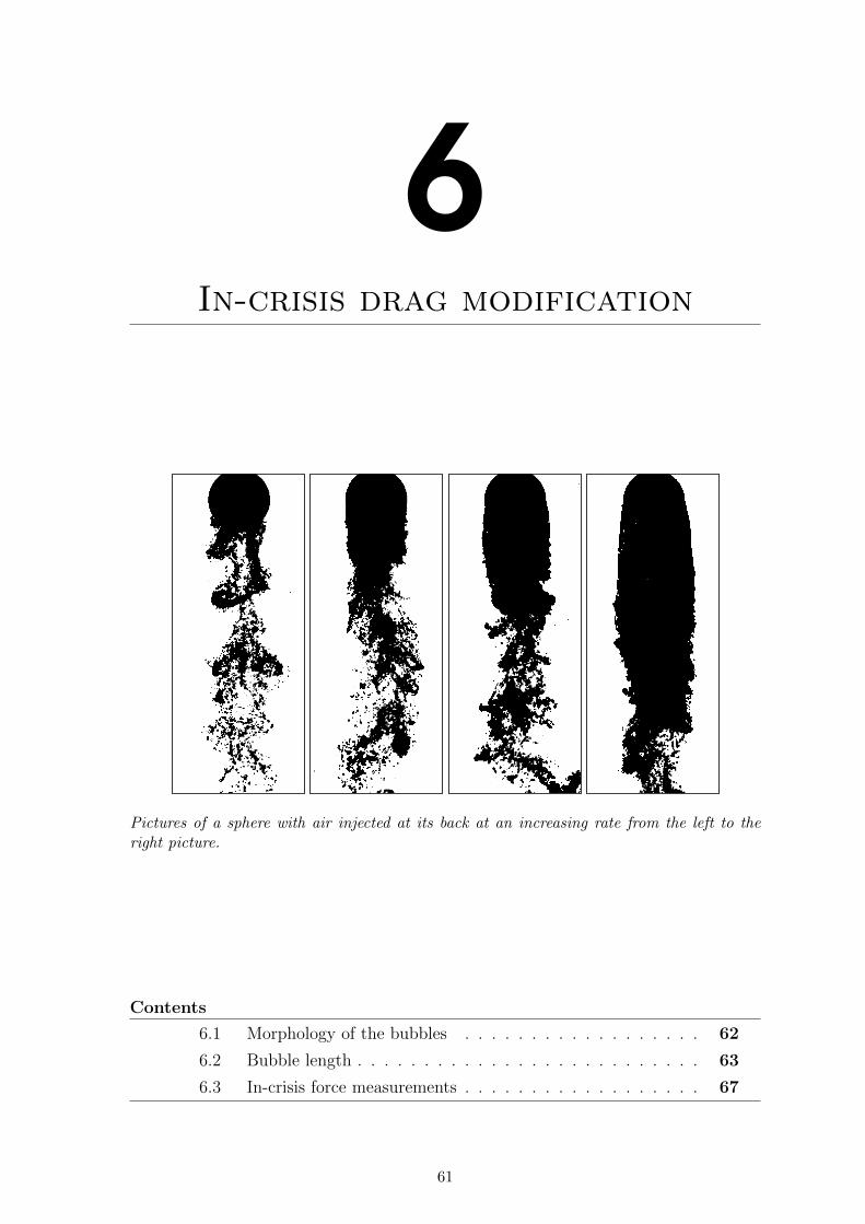
6In-crisis drag modification
Pictures of a sphere with air injected at its back at an increasing rate from the left to theright picture.
Contents
6.1 Morphology of the bubbles . . . . . . . . . . . . . . . . . . 62
6.2 Bubble length . . . . . . . . . . . . . . . . . . . . . . . . . . 63
6.3 In-crisis force measurements . . . . . . . . . . . . . . . . . . 67
61
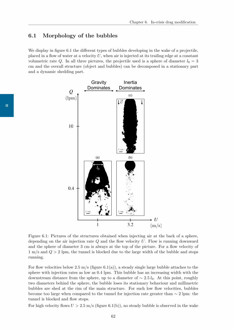
Chapter 6. In-crisis drag modification
II
6.1 Morphology of the bubbles
We display in figure 6.1 the different types of bubbles developing in the wake of a projectile,placed in a flow of water at a velocity U , when air is injected at its trailing edge at a constantvolumetric rate Q. In all three pictures, the projectile used is a sphere of diameter l0 = 3cm and the overall structure (object and bubbles) can be decomposed in a stationary partand a dynamic shedding part.
U
Q(lpm)
(m/s)
0.4
10
1 3.2
(b)
(c)
(a)
1 cm
1 cm1 cm
Gravity Dominates
Inertia Dominates
l0
U
Figure 6.1: Pictures of the structures obtained when injecting air at the back of a sphere,depending on the air injection rate Q and the flow velocity U . Flow is running downwardand the sphere of diameter 3 cm is always at the top of the picture. For a flow velocity of1 m/s and Q > 2 lpm, the tunnel is blocked due to the large width of the bubble and stopsrunning.
For flow velocities below 2.5 m/s (figure 6.1(a)), a steady single large bubble attaches to thesphere with injection rates as low as 0.4 lpm. This bubble has an increasing width with thedownstream distance from the sphere, up to a diameter of ∼ 2.5 l0. At this point, roughlytwo diameters behind the sphere, the bubble loses its stationary behaviour and millimetricbubbles are shed at the rim of the main structure. For such low flow velocities, bubblesbecome too large when compared to the tunnel for injection rate greater than ∼ 2 lpm: thetunnel is blocked and flow stops.
For high velocity flows U > 2.5 m/s (figure 6.1(b)), no steady bubble is observed in the wake
62
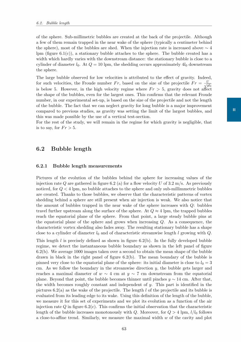
6.2. Bubble length
II
of the sphere. Sub-millimetric bubbles are created at the back of the projectile. Althougha few of them remain trapped in the near wake of the sphere (typically a centimeter behindthe sphere), most of the bubbles are shed. When the injection rate is increased above ∼ 4lpm (figure 6.1(c)), a stationary bubble attaches to the sphere. The bubble created has awidth which hardly varies with the downstream distance: the stationary bubble is close to acylinder of diameter l0. At Q = 10 lpm, the shedding occurs approximately 4l0 downstreamthe sphere.
The large bubble observed for low velocities is attributed to the effect of gravity. Indeed,for such velocities, the Froude number Fr, based on the size of the projectile Fr = U√
gl0is below 5. However, in the high velocity regime where Fr > 5, gravity does not affectthe shape of the bubbles, even for the largest ones. This confirms that the relevant Froudenumber, in our experimental set-up, is based on the size of the projectile and not the lengthof the bubble. The fact that we can neglect gravity for long bubble is a major improvementcompared to previous studies, as gravity was setting the limit of the largest bubbles, andthis was made possible by the use of a vertical test-section.For the rest of the study, we will remain in the regime for which gravity is negligible, thatis to say, for Fr > 5.
6.2 Bubble length
6.2.1 Bubble length measurements
Pictures of the evolution of the bubbles behind the sphere for increasing values of theinjection rate Q are gathered in figure 6.2 (a) for a flow velocity U of 3.2 m/s. As previouslynoticed, for Q < 4 lpm, no bubble attaches to the sphere and only sub-millimmetric bubblesare created. Thanks to those bubbles, we observe that the characteristic patterns of vortexshedding behind a sphere are still present when air injection is weak. We also notice thatthe amount of bubbles trapped in the near wake of the sphere increases with Q: bubblestravel further upstream along the surface of the sphere. At Q ≈ 4 lpm, the trapped bubblesreach the equatorial plane of the sphere. From that point, a large steady bubble pins atthe equatorial plane of the sphere and grows when increasing Q. As a consequence, thecharacteristic vortex shedding also fades away. The resulting stationary bubble has a shapeclose to a cylinder of diameter l0 and of characteristic streamwise length l growing with Q.
This length l is precisely defined as shown in figure 6.2(b). In the fully developed bubbleregime, we detect the instantaneous bubble boundary as shown in the left panel of figure6.2(b). We average 1000 images taken over a second to obtain the mean shape of the bubbledrawn in black in the right panel of figure 6.2(b). The mean boundary of the bubble ispinned very close to the equatorial plane of the sphere: its initial diameter is close to l0 = 3cm. As we follow the boundary in the streamwise direction y, the bubble gets larger andreaches a maximal diameter of w ∼ 4 cm at y ∼ 7 cm downstream from the equatorialplane. Beyond that point, the bubble becomes thinner until pinches y ∼ 14 cm. After that,the width becomes roughly constant and independent of y. This part is identified in thepictures 6.2(a) as the wake of the projectile. The length l of the projectile and its bubble isevaluated from its leading edge to its wake. Using this definition of the length of the bubble,we measure it for this set of experiments and we plot its evolution as a function of the airinjection rate Q in figure 6.2(c). This confirms the initial observation that the characteristiclength of the bubble increases monotonously with Q. Moreover, for Q > 4 lpm, l/l0 followsa close-to-affine trend. Similarly, we measure the maximal width w of the cavity and plot
63
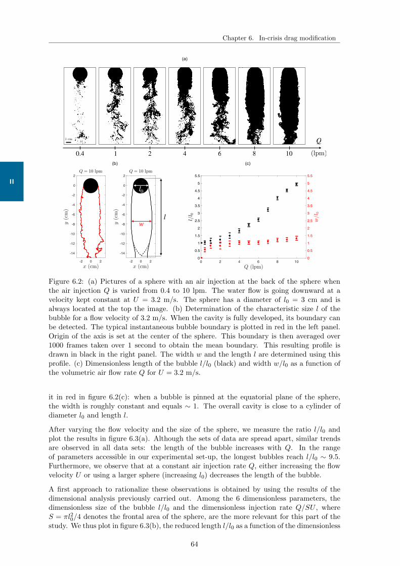
Chapter 6. In-crisis drag modification
II
0 2 4 6 8 100
0.5
1
1.5
2
2.5
3
3.5
4
4.5
5
5.5
0
0.5
1
1.5
2
2.5
3
3.5
4
4.5
5
5.5
-2 0 2
-14
-12
-10
-8
-6
-4
-2
0
2
-2 0 2
-14
-12
-10
-8
-6
-4
-2
0
2
Q
(lpm)0.4 101 2 4 6 8
(a)
1 cm
(b) (c)
l
l0
Q = 10 lpm Q = 10 lpm
w
Figure 6.2: (a) Pictures of a sphere with an air injection at the back of the sphere whenthe air injection Q is varied from 0.4 to 10 lpm. The water flow is going downward at avelocity kept constant at U = 3.2 m/s. The sphere has a diameter of l0 = 3 cm and isalways located at the top the image. (b) Determination of the characteristic size l of thebubble for a flow velocity of 3.2 m/s. When the cavity is fully developed, its boundary canbe detected. The typical instantaneous bubble boundary is plotted in red in the left panel.Origin of the axis is set at the center of the sphere. This boundary is then averaged over1000 frames taken over 1 second to obtain the mean boundary. This resulting profile isdrawn in black in the right panel. The width w and the length l are determined using thisprofile. (c) Dimensionless length of the bubble l/l0 (black) and width w/l0 as a function ofthe volumetric air flow rate Q for U = 3.2 m/s.
it in red in figure 6.2(c): when a bubble is pinned at the equatorial plane of the sphere,the width is roughly constant and equals ∼ 1. The overall cavity is close to a cylinder ofdiameter l0 and length l.
After varying the flow velocity and the size of the sphere, we measure the ratio l/l0 andplot the results in figure 6.3(a). Although the sets of data are spread apart, similar trendsare observed in all data sets: the length of the bubble increases with Q. In the rangeof parameters accessible in our experimental set-up, the longest bubbles reach l/l0 ∼ 9.5.Furthermore, we observe that at a constant air injection rate Q, either increasing the flowvelocity U or using a larger sphere (increasing l0) decreases the length of the bubble.
A first approach to rationalize these observations is obtained by using the results of thedimensional analysis previously carried out. Among the 6 dimensionless parameters, thedimensionless size of the bubble l/l0 and the dimensionless injection rate Q/SU , whereS = πl20/4 denotes the frontal area of the sphere, are the more relevant for this part of thestudy. We thus plot in figure 6.3(b), the reduced length l/l0 as a function of the dimensionless
64
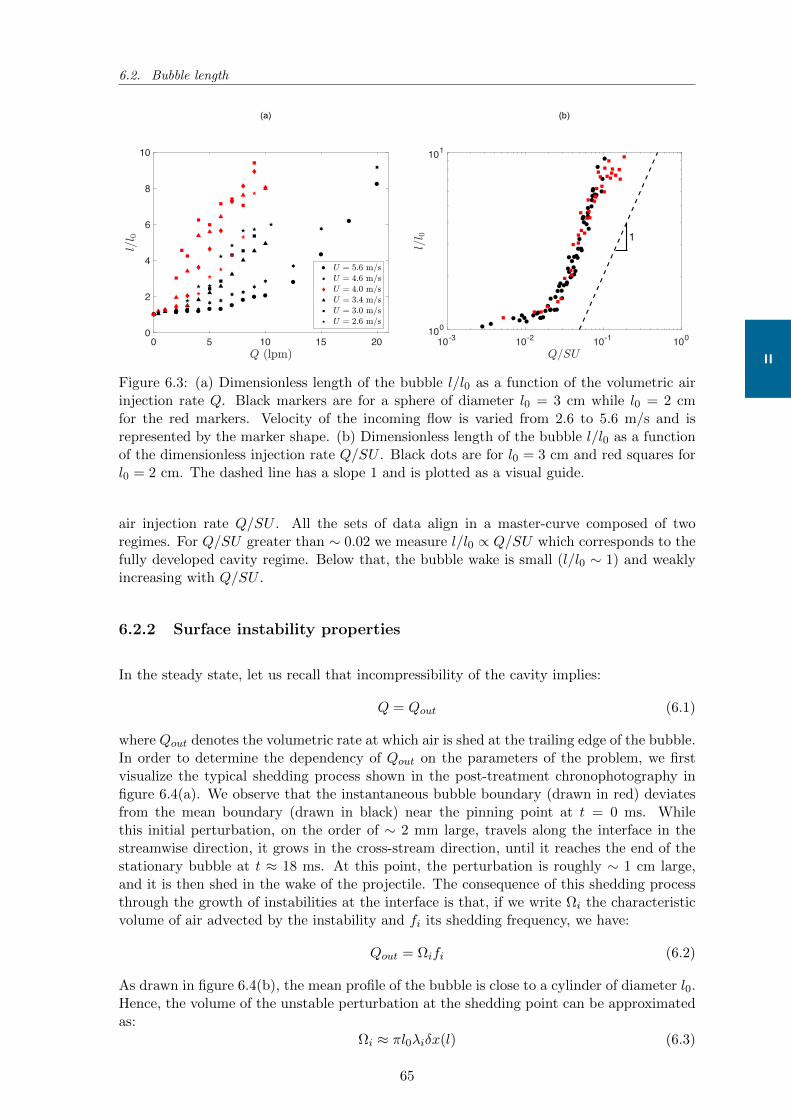
6.2. Bubble length
II
0 5 10 15 200
2
4
6
8
10
10-3 10-2 10-1 100100
101
(a) (b)
1
Figure 6.3: (a) Dimensionless length of the bubble l/l0 as a function of the volumetric airinjection rate Q. Black markers are for a sphere of diameter l0 = 3 cm while l0 = 2 cmfor the red markers. Velocity of the incoming flow is varied from 2.6 to 5.6 m/s and isrepresented by the marker shape. (b) Dimensionless length of the bubble l/l0 as a functionof the dimensionless injection rate Q/SU . Black dots are for l0 = 3 cm and red squares forl0 = 2 cm. The dashed line has a slope 1 and is plotted as a visual guide.
air injection rate Q/SU . All the sets of data align in a master-curve composed of tworegimes. For Q/SU greater than ∼ 0.02 we measure l/l0 ∝ Q/SU which corresponds to thefully developed cavity regime. Below that, the bubble wake is small (l/l0 ∼ 1) and weaklyincreasing with Q/SU .
6.2.2 Surface instability properties
In the steady state, let us recall that incompressibility of the cavity implies:
Q = Qout (6.1)
where Qout denotes the volumetric rate at which air is shed at the trailing edge of the bubble.In order to determine the dependency of Qout on the parameters of the problem, we firstvisualize the typical shedding process shown in the post-treatment chronophotography infigure 6.4(a). We observe that the instantaneous bubble boundary (drawn in red) deviatesfrom the mean boundary (drawn in black) near the pinning point at t = 0 ms. Whilethis initial perturbation, on the order of ∼ 2 mm large, travels along the interface in thestreamwise direction, it grows in the cross-stream direction, until it reaches the end of thestationary bubble at t ≈ 18 ms. At this point, the perturbation is roughly ∼ 1 cm large,and it is then shed in the wake of the projectile. The consequence of this shedding processthrough the growth of instabilities at the interface is that, if we write Ωi the characteristicvolume of air advected by the instability and fi its shedding frequency, we have:
Qout = Ωifi (6.2)
As drawn in figure 6.4(b), the mean profile of the bubble is close to a cylinder of diameter l0.Hence, the volume of the unstable perturbation at the shedding point can be approximatedas:
Ωi ≈ πl0λiδx(l) (6.3)
65
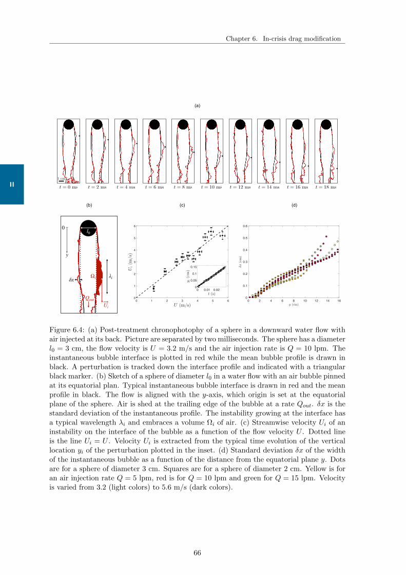
Chapter 6. In-crisis drag modification
II
0 2 4 6 8 10 12 14 160
0.1
0.2
0.3
0.4
0.5
0.6
0 1 2 3 4 5 60
1
2
3
4
5
6
(a)
t = 0 ms t = 2 ms t = 4 ms t = 6 ms t = 8 ms t = 10 ms t = 12 ms t = 14 ms t = 16 ms t = 18 ms
1 cm
l
-2 0 2
-12
-10
-8
-6
-4
-2
0
Qout
λiδx
U
Ωi
l0
(b) (c)
y
0 2 4 6 8 10 12 14 160
0.1
0.2
0.3
0.4
0.5
0.6
(d)
0 0.01 0.020
0.05
0.1
0.15
0
Ui
Figure 6.4: (a) Post-treatment chronophotophy of a sphere in a downward water flow withair injected at its back. Picture are separated by two milliseconds. The sphere has a diameterl0 = 3 cm, the flow velocity is U = 3.2 m/s and the air injection rate is Q = 10 lpm. Theinstantaneous bubble interface is plotted in red while the mean bubble profile is drawn inblack. A perturbation is tracked down the interface profile and indicated with a triangularblack marker. (b) Sketch of a sphere of diameter l0 in a water flow with an air bubble pinnedat its equatorial plan. Typical instantaneous bubble interface is drawn in red and the meanprofile in black. The flow is aligned with the y-axis, which origin is set at the equatorialplane of the sphere. Air is shed at the trailing edge of the bubble at a rate Qout. δx is thestandard deviation of the instantaneous profile. The instability growing at the interface hasa typical wavelength λi and embraces a volume Ωi of air. (c) Streamwise velocity Ui of aninstability on the interface of the bubble as a function of the flow velocity U . Dotted lineis the line Ui = U . Velocity Ui is extracted from the typical time evolution of the verticallocation yi of the perturbation plotted in the inset. (d) Standard deviation δx of the widthof the instantaneous bubble as a function of the distance from the equatorial plane y. Dotsare for a sphere of diameter 3 cm. Squares are for a sphere of diameter 2 cm. Yellow is foran air injection rate Q = 5 lpm, red is for Q = 10 lpm and green for Q = 15 lpm. Velocityis varied from 3.2 (light colors) to 5.6 m/s (dark colors).
66
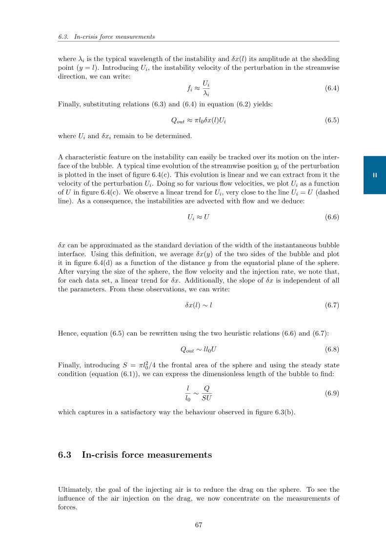
6.3. In-crisis force measurements
II
where λi is the typical wavelength of the instability and δx(l) its amplitude at the sheddingpoint (y = l). Introducing Ui, the instability velocity of the perturbation in the streamwisedirection, we can write:
fi ≈Uiλi
(6.4)
Finally, substituting relations (6.3) and (6.4) in equation (6.2) yields:
Qout ≈ πl0δx(l)Ui (6.5)
where Ui and δxi remain to be determined.
A characteristic feature on the instability can easily be tracked over its motion on the inter-face of the bubble. A typical time evolution of the streamwise position yi of the perturbationis plotted in the inset of figure 6.4(c). This evolution is linear and we can extract from it thevelocity of the perturbation Ui. Doing so for various flow velocities, we plot Ui as a functionof U in figure 6.4(c). We observe a linear trend for Ui, very close to the line Ui = U (dashedline). As a consequence, the instabilities are advected with flow and we deduce:
Ui ≈ U (6.6)
δx can be approximated as the standard deviation of the width of the instantaneous bubbleinterface. Using this definition, we average δx(y) of the two sides of the bubble and plotit in figure 6.4(d) as a function of the distance y from the equatorial plane of the sphere.After varying the size of the sphere, the flow velocity and the injection rate, we note that,for each data set, a linear trend for δx. Additionally, the slope of δx is independent of allthe parameters. From these observations, we can write:
δx(l) ∼ l (6.7)
Hence, equation (6.5) can be rewritten using the two heuristic relations (6.6) and (6.7):
Qout ∼ ll0U (6.8)
Finally, introducing S = πl20/4 the frontal area of the sphere and using the steady statecondition (equation (6.1)), we can express the dimensionless length of the bubble to find:
l
l0∼ Q
SU(6.9)
which captures in a satisfactory way the behaviour observed in figure 6.3(b).
6.3 In-crisis force measurements
Ultimately, the goal of the injecting air is to reduce the drag on the sphere. To see theinfluence of the air injection on the drag, we now concentrate on the measurements offorces.
67
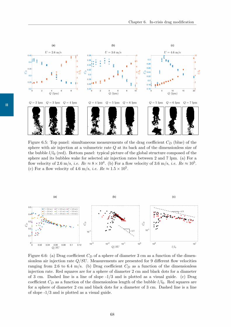
Chapter 6. In-crisis drag modification
IIQ = 2 lpm Q = 3 lpm Q = 4 lpm Q = 4 lpm Q = 5 lpm Q = 5 lpm Q = 6 lpmQ = 6 lpm Q = 7 lpm
0 2 4 6 8 100.24
0.26
0.28
0.3
0.32
0.34
0.36
0.38
0
1
2
3
4
5
6
(b)
U = 3.6 m/s
0 2 4 6 80.2
0.25
0.3
0.35
0.4
0.45
0
1
2
3
4
5
6
(a)
U = 2.6 m/s
0 5 10 15 200.16
0.18
0.2
0.22
0.24
0.26
0.28
0.3
0
2
4
6
8
10
(c)
U = 4.6 m/s
Figure 6.5: Top panel: simultaneous measurements of the drag coefficient CD (blue) of thesphere with air injection at a volumetric rate Q at its back and of the dimensionless size ofthe bubble l/l0 (red). Bottom panel: typical picture of the global structure composed of thesphere and its bubbles wake for selected air injection rates between 2 and 7 lpm. (a) For aflow velocity of 2.6 m/s, i.e. Re ≈ 8×10⁴. (b) For a flow velocity of 3.6 m/s, i.e. Re ≈ 105.(c) For a flow velocity of 4.6 m/s, i.e. Re ≈ 1.5× 10⁵.
0 0.02 0.04 0.06 0.08 0.1 0.120
0.1
0.2
0.3
0.4
0.5
(a) (b) (c)
U = 3.4 m/s
U = 3.0 m/s
U = 2.6 m/s U = 3.9 m/s
U = 4.1 m/s
U = 4.6 m/s
U = 4.9 m/s
U = 5.6 m/s
U = 6.4 m/s
10-3 10-2 10-1 100
10-1 −1/3
100 101
10-1
−1/3
Figure 6.6: (a) Drag coefficient CD of a sphere of diameter 3 cm as a function of the dimen-sionless air injection rate Q/SU . Measurements are presented for 9 different flow velocitiesranging from 2.6 to 6.4 m/s. (b) Drag coefficient CD as a function of the dimensionlessinjection rate. Red squares are for a sphere of diameter 2 cm and black dots for a diameterof 3 cm. Dashed line is a line of slope -1/3 and is plotted as a visual guide. (c) Dragcoefficient CD as a function of the dimensionless length of the bubble l/l0. Red squares arefor a sphere of diameter 2 cm and black dots for a diameter of 3 cm. Dashed line is a lineof slope -1/3 and is plotted as a visual guide.
68
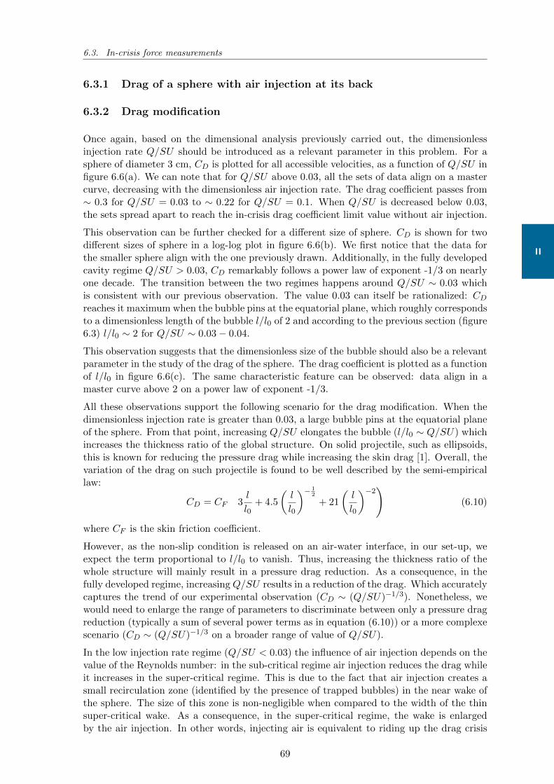
6.3. In-crisis force measurements
II
6.3.1 Drag of a sphere with air injection at its back
6.3.2 Drag modification
Once again, based on the dimensional analysis previously carried out, the dimensionlessinjection rate Q/SU should be introduced as a relevant parameter in this problem. For asphere of diameter 3 cm, CD is plotted for all accessible velocities, as a function of Q/SU infigure 6.6(a). We can note that for Q/SU above 0.03, all the sets of data align on a mastercurve, decreasing with the dimensionless air injection rate. The drag coefficient passes from∼ 0.3 for Q/SU = 0.03 to ∼ 0.22 for Q/SU = 0.1. When Q/SU is decreased below 0.03,the sets spread apart to reach the in-crisis drag coefficient limit value without air injection.
This observation can be further checked for a different size of sphere. CD is shown for twodifferent sizes of sphere in a log-log plot in figure 6.6(b). We first notice that the data forthe smaller sphere align with the one previously drawn. Additionally, in the fully developedcavity regime Q/SU > 0.03, CD remarkably follows a power law of exponent -1/3 on nearlyone decade. The transition between the two regimes happens around Q/SU ∼ 0.03 whichis consistent with our previous observation. The value 0.03 can itself be rationalized: CDreaches it maximum when the bubble pins at the equatorial plane, which roughly correspondsto a dimensionless length of the bubble l/l0 of 2 and according to the previous section (figure6.3) l/l0 ∼ 2 for Q/SU ∼ 0.03− 0.04.
This observation suggests that the dimensionless size of the bubble should also be a relevantparameter in the study of the drag of the sphere. The drag coefficient is plotted as a functionof l/l0 in figure 6.6(c). The same characteristic feature can be observed: data align in amaster curve above 2 on a power law of exponent -1/3.
All these observations support the following scenario for the drag modification. When thedimensionless injection rate is greater than 0.03, a large bubble pins at the equatorial planeof the sphere. From that point, increasing Q/SU elongates the bubble (l/l0 ∼ Q/SU) whichincreases the thickness ratio of the global structure. On solid projectile, such as ellipsoids,this is known for reducing the pressure drag while increasing the skin drag [1]. Overall, thevariation of the drag on such projectile is found to be well described by the semi-empiricallaw:
CD = CF
(3l
l0+ 4.5
(l
l0
)− 12
+ 21
(l
l0
)−2)(6.10)
where CF is the skin friction coefficient.
However, as the non-slip condition is released on an air-water interface, in our set-up, weexpect the term proportional to l/l0 to vanish. Thus, increasing the thickness ratio of thewhole structure will mainly result in a pressure drag reduction. As a consequence, in thefully developed regime, increasing Q/SU results in a reduction of the drag. Which accuratelycaptures the trend of our experimental observation (CD ∼ (Q/SU)−1/3). Nonetheless, wewould need to enlarge the range of parameters to discriminate between only a pressure dragreduction (typically a sum of several power terms as in equation (6.10)) or a more complexescenario (CD ∼ (Q/SU)−1/3 on a broader range of value of Q/SU).
In the low injection rate regime (Q/SU < 0.03) the influence of air injection depends on thevalue of the Reynolds number: in the sub-critical regime air injection reduces the drag whileit increases in the super-critical regime. This is due to the fact that air injection creates asmall recirculation zone (identified by the presence of trapped bubbles) in the near wake ofthe sphere. The size of this zone is non-negligible when compared to the width of the thinsuper-critical wake. As a consequence, in the super-critical regime, the wake is enlargedby the air injection. In other words, injecting air is equivalent to riding up the drag crisis
69
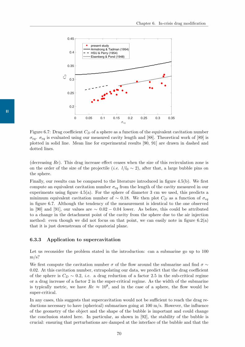
Chapter 6. In-crisis drag modification
II
0 0.05 0.1 0.15 0.2 0.25 0.3 0.35
0.2
0.25
0.3
0.35
0.4
0.45
present studyArmstrong & Tadman (1954)HSU & Perry (1954)Eisenberg & Pond (1948)
Figure 6.7: Drag coefficient CD of a sphere as a function of the equivalent cavitation numberσeq. σeq is evaluated using our measured cavity length and [88]. Theoretical work of [89] isplotted in solid line. Mean line for experimental results [90, 91] are drawn in dashed anddotted lines.
(decreasing Re). This drag increase effect ceases when the size of this recirculation zone ison the order of the size of the projectile (i.e. l/l0 ∼ 2), after that, a large bubble pins onthe sphere.
Finally, our results can be compared to the literature introduced in figure 4.5(b). We firstcompute an equivalent cavitation number σeq from the length of the cavity measured in ourexperiments using figure 4.5(a). For the sphere of diameter 3 cm we used, this predicts aminimum equivalent cavitation number of ∼ 0.18. We then plot CD as a function of σeqin figure 6.7. Although the tendency of the measurement is identical to the one observedin [90] and [91], our values are ∼ 0.02 − 0.04 lower. As before, this could be attributedto a change in the detachment point of the cavity from the sphere due to the air injectionmethod: even though we did not focus on that point, we can easily note in figure 6.2(a)that it is just downstream of the equatorial plane.
6.3.3 Application to supercavitation
Let us reconsider the problem stated in the introduction: can a submarine go up to 100m/s?
We first compute the cavitation number σ of the flow around the submarine and find σ ∼0.02. At this cavitation number, extrapolating our data, we predict that the drag coefficientof the sphere is CD ∼ 0.2, i.e. a drag reduction of a factor 2.5 in the sub-critical regimeor a drag increase of a factor 2 in the super-critical regime. As the width of the submarineis typically metric, we have Re ≈ 108, and in the case of a sphere, the flow would besuper-critical.
In any cases, this suggests that supercavitation would not be sufficient to reach the drag re-ductions necessary to have (spherical) submarines going at 100 m/s. However, the influenceof the geometry of the object and the shape of the bubble is important and could changethe conclusion stated here. In particular, as shown in [92], the stability of the bubble iscrucial: ensuring that perturbations are damped at the interface of the bubble and that the
70

6.3. In-crisis force measurements
II
bubble pinches off in a stationary point as presented in figure 4.4(c), the drag coefficientcan be reduced as low as 0.05. This value of the drag coefficient is still too high to make asubmarine going at 100 m/s technically feasible. However, it shows that an important dragreduction (by a factor 10) can be achieved using supercavitation, as low as the one that aremeasured when streamlining a projectile using fairing and presented in the introduction.
71
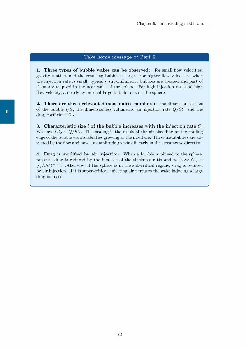
Chapter 6. In-crisis drag modification
II
Take home message of Part 6
1. Three types of bubble wakes can be observed: for small flow velocities,gravity matters and the resulting bubble is large. For higher flow velocities, whenthe injection rate is small, typically sub-millimetric bubbles are created and part ofthem are trapped in the near wake of the sphere. For high injection rate and highflow velocity, a nearly cylindrical large bubble pins on the sphere.
2. There are three relevant dimensionless numbers: the dimensionless sizeof the bubble l/l0, the dimensionless volumetric air injection rate Q/SU and thedrag coefficient CD.
3. Characteristic size l of the bubble increases with the injection rate Q.We have l/l0 ∼ Q/SU . This scaling is the result of the air shedding at the trailingedge of the bubble via instabilities growing at the interface. These instabilities are ad-vected by the flow and have an amplitude growing linearly in the streamwise direction.
4. Drag is modified by air injection. When a bubble is pinned to the sphere,pressure drag is reduced by the increase of the thickness ratio and we have CD ∼(Q/SU)−1/3. Otherwise, if the sphere is in the sub-critical regime, drag is reducedby air injection. If it is super-critical, injecting air perturbs the wake inducing a largedrag increase.
72

PART III
STABILITY OF THETRAJECTORY OF THE
STREAMLINED PROJECTILE
73
III
We have seen in part I that a projectile going fast enough underwater generates a gas bubblearound it. We then showed that such a bubble reduces its drag, making the whole systemanalogous to an inhomogeneous streamlined projectile. In the present part, we characterisethe trajectory of a streamlined projectile following its impact on water. In particular, wedetermine whether the projectile will have a straight trajectory and will reach its target. Inchapter 7, we review the literature and present our experimental set-up. We then presentour main results in chapter 8: the conditions under which a streamlined projectile follows astraight trajectory.
74
7Short review on water entry and
path instabilities
Picture of a gannet about to enter water. Photo credits: Steve Ward Nature Photography(www.stevewardneature.co.uk).
Contents
7.1 Water entry . . . . . . . . . . . . . . . . . . . . . . . . . . . 76
7.2 Path instabilities . . . . . . . . . . . . . . . . . . . . . . . . 78
7.3 Statement of the problem . . . . . . . . . . . . . . . . . . . 79
7.4 Experimental details . . . . . . . . . . . . . . . . . . . . . . 79
75
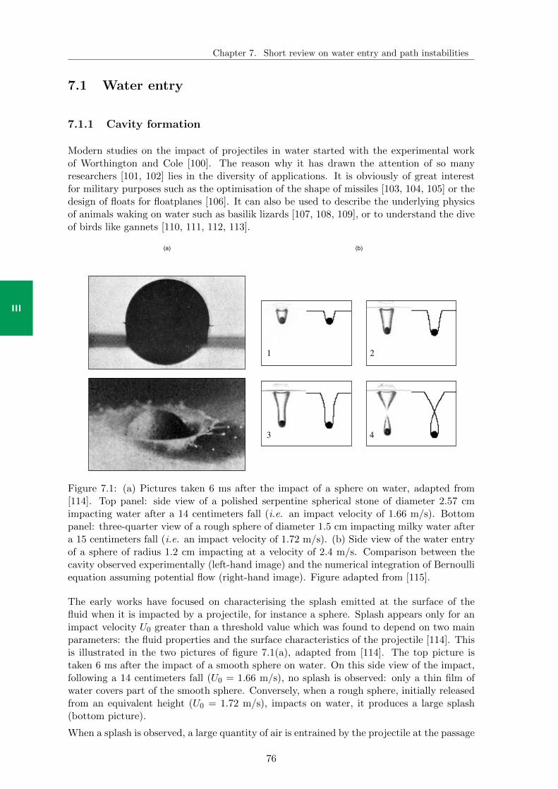
Chapter 7. Short review on water entry and path instabilities
III
7.1 Water entry
7.1.1 Cavity formation
Modern studies on the impact of projectiles in water started with the experimental workof Worthington and Cole [100]. The reason why it has drawn the attention of so manyresearchers [101, 102] lies in the diversity of applications. It is obviously of great interestfor military purposes such as the optimisation of the shape of missiles [103, 104, 105] or thedesign of floats for floatplanes [106]. It can also be used to describe the underlying physicsof animals waking on water such as basilik lizards [107, 108, 109], or to understand the diveof birds like gannets [110, 111, 112, 113].
(b)
Dynamics of transient cavities 13
1 2 3 4
5 6 7 8
Figure 13. Comparison between the cavity observed experimentally with a solid sphereof radius R = 11.5 mm and Froude number Fr =52 (left-hand image) and the numericalintegration of equation (4.18) (right-hand image).
R0 must be chosen large compared to the capillary length a ≡√
σ/(ρg). The presentstudy is conducted in this limit R0/a ≫ 1.
With these assumptions, the challenge now is to make an appropriate choice forthe potential φ: a direct extension of the method used to solve the Besant–Rayleighproblem consists of assuming a purely radial motion ru = RR, which leads to
φ = RR ln(r/R∞), R < r < R∞ (4.15)
= 0, r > R∞. (4.16)
In this expression for the velocity potential, R∞ is a function of time which canbe evaluated through an assumption on the total kinetic energy: At a depth z, weconsider a layer of liquid of thickness dz. The total kinetic energy in this layer isT ≡ 1
2
! R∞R
ρ 2πr dr dz u2. Using the above evaluation of the velocity we can integratethis expression and find T = πρ dz R2R2 ln(R∞/R). Since all the motion is radial, thiskinetic energy comes from the motion of the liquid layer πR2 dz. Assuming thatT ≈ πR2 dz R2, this suggests that ln(R∞/R) ≈ 1, which states that the motion in theliquid extends over a region of the order of the local size of the hole R (R∞ ≈ 2.7 R).
Using this expression for the potential, we can simplify the momentumequation (4.14) and get the equation for the cavity:
RR + 32 R
2 = −gz. (4.17)
The only difference with the equation (4.5) obtained for the Besant–Rayleigh problemis that the pressure is not constant but depends linearly on z. At a given z, this equ-ation for the cylindrical cavity can be integrated once:
R2 = αU 2
"R0
R
#3
+2
3gz
$"R0
R
#3
− 1
%(4.18)
where we have used the limit condition R2 (R = R0) = αU 2 with α a constant smallerthan 1. Since H = Ut is the depth of the cavity at time t , we integrate equation (4.18)numerically from z = 0 to z = H and for each z location from t = 0 to (H − z)/U ,using the initial condition R(t = 0) = R0. The results obtained are compared to theexperimental observations in figure 13, where the solid sphere (R = 11.5 mm) impactswith a Froude number Fr = 52. The numerical integration is done with α = 0.1. Thecomparison reveals that the general features observed experimentally are captured
CC4
9 A7
0
1454
ACC
31
2A94
75
A73
A5 .
35
/C5
39
D5D7
1CD2
:53C
CC
5,1
2A94
75,
A5C5
AD
51E
1912
51C
CC 3
12A
9475
A7
3A5
C5A
(a)
1 2
3 4
Figure 7.1: (a) Pictures taken 6 ms after the impact of a sphere on water, adapted from[114]. Top panel: side view of a polished serpentine spherical stone of diameter 2.57 cmimpacting water after a 14 centimeters fall (i.e. an impact velocity of 1.66 m/s). Bottompanel: three-quarter view of a rough sphere of diameter 1.5 cm impacting milky water aftera 15 centimeters fall (i.e. an impact velocity of 1.72 m/s). (b) Side view of the water entryof a sphere of radius 1.2 cm impacting at a velocity of 2.4 m/s. Comparison between thecavity observed experimentally (left-hand image) and the numerical integration of Bernoulliequation assuming potential flow (right-hand image). Figure adapted from [115].
The early works have focused on characterising the splash emitted at the surface of thefluid when it is impacted by a projectile, for instance a sphere. Splash appears only for animpact velocity U0 greater than a threshold value which was found to depend on two mainparameters: the fluid properties and the surface characteristics of the projectile [114]. Thisis illustrated in the two pictures of figure 7.1(a), adapted from [114]. The top picture istaken 6 ms after the impact of a smooth sphere on water. On this side view of the impact,following a 14 centimeters fall (U0 = 1.66 m/s), no splash is observed: only a thin film ofwater covers part of the smooth sphere. Conversely, when a rough sphere, initially releasedfrom an equivalent height (U0 = 1.72 m/s), impacts on water, it produces a large splash(bottom picture).
When a splash is observed, a large quantity of air is entrained by the projectile at the passage
76
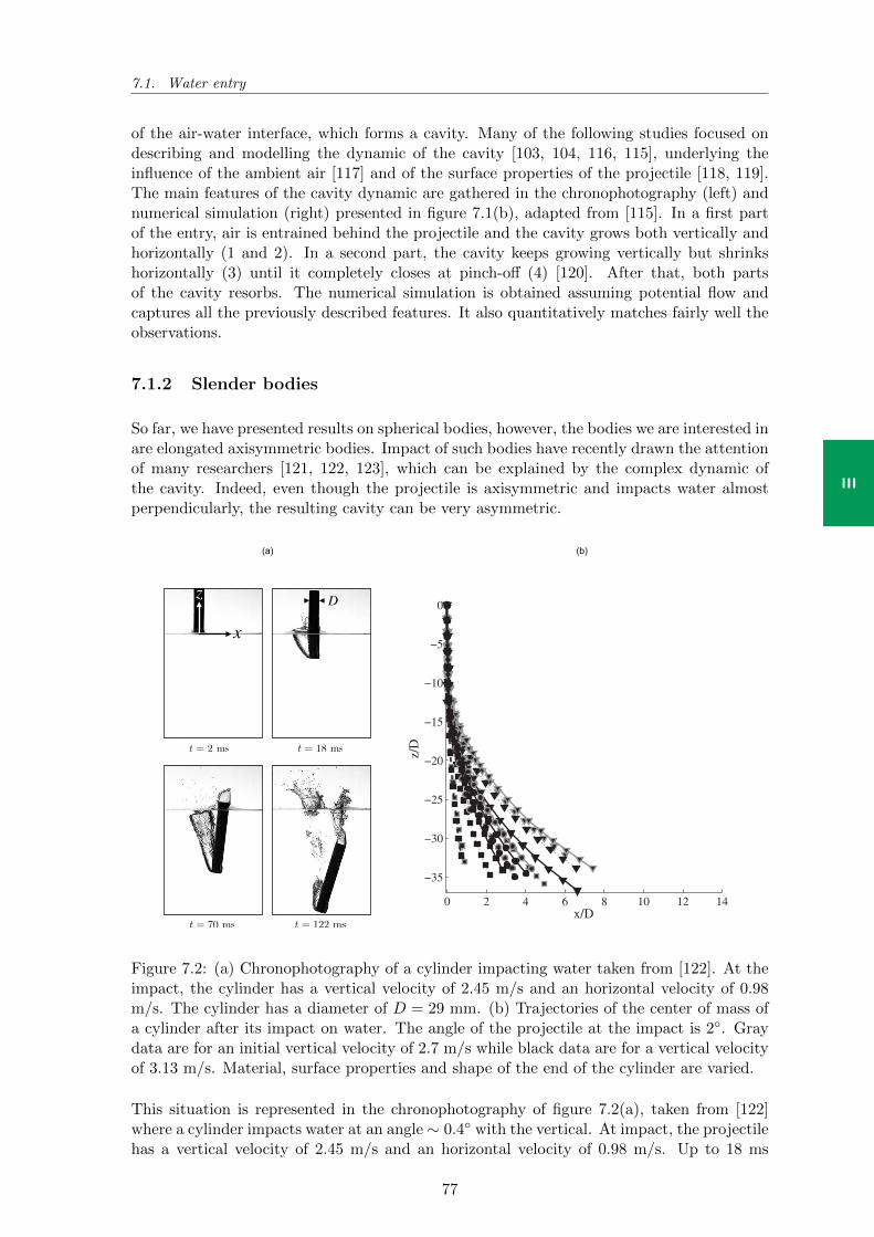
7.1. Water entry
III
of the air-water interface, which forms a cavity. Many of the following studies focused ondescribing and modelling the dynamic of the cavity [103, 104, 116, 115], underlying theinfluence of the ambient air [117] and of the surface properties of the projectile [118, 119].The main features of the cavity dynamic are gathered in the chronophotography (left) andnumerical simulation (right) presented in figure 7.1(b), adapted from [115]. In a first partof the entry, air is entrained behind the projectile and the cavity grows both vertically andhorizontally (1 and 2). In a second part, the cavity keeps growing vertically but shrinkshorizontally (3) until it completely closes at pinch-off (4) [120]. After that, both partsof the cavity resorbs. The numerical simulation is obtained assuming potential flow andcaptures all the previously described features. It also quantitatively matches fairly well theobservations.
7.1.2 Slender bodies
So far, we have presented results on spherical bodies, however, the bodies we are interested inare elongated axisymmetric bodies. Impact of such bodies have recently drawn the attentionof many researchers [121, 122, 123], which can be explained by the complex dynamic ofthe cavity. Indeed, even though the projectile is axisymmetric and impacts water almostperpendicularly, the resulting cavity can be very asymmetric.
44 W. Xia, C. Wang and Y. Wei et al. / International Journal of Multiphase Flow 118 (2019) 37–49
Fig. 8. Impact cavities by a cylinder with decreasing inclined angles. The inclined angles from a to d are α0 = 89.6 º, 79.7 º, 68.7 º, 61.5 º, and the corresponding initial horizontal and vertical velocities are u 0 = 0.98 ± 0.05 m/s and v 0 = −2.45 ± 0.06 m/s, respectively. cylinder side, the pinch-off time is treated as the break time. Fig. 9 shows the break time and pinch-off time normalized by the time of D / v 0 as the function of inclined angle. The non-dimensional time of cavity break increases as the inclined angle increases.
A side cavity is generated as the cavity breaks in Fig. 8 b,c and d . In addition, the side cavity also can be found with increasing
Fig. 9. Time characteristics of the impact cavities of the inclined cylinders with hor- izontal velocity shown in Fig. 6 c and Fig. 8 . The times for cavity break ( !) and pinch off ( " ) are normalized by the time D/v 0 .
the horizontal velocity under same inclined angle ( Fig. 6 d ). By comparison, the angle of attack ϕ0 for the case where the side cavity occurs is larger than that for those cases without. The reason is that a greater moment, caused by the inertial force and impact force, acts on the gravity centre of the cylinder and drives it to rotate rapidly. Consequently, the rotational speed of the cylinder is a trigger for creating the side cavity in the current investigation. Furthermore, a break jet generated by cavity break penetrates into the cavity, forming a water wedge ( Fig. 8 b,c and d ). The flow behaviour of the water wedge is shown in Fig. 10 . The
Fig. 10. Sketches of the behaviours of the water wedge. This cross section was cut from Fig. 8 d by a horizontal plane.
t = 2 ms t = 18 ms
t = 70 ms t = 122 ms
(b)(a)
072108-10 Bodily, Carlson, and Truscott Phys. Fluids 26, 072108 (2014)
FIG. 8. (a) Hydrophilic and hydrophobic vertical (0) entry cases show less than 0.6 diameters of lateral displacement. (b)The half-and-half case resulted in maximum lateral displacement of 2.1 diameters. (c) A 2 impact angle results in a maximumlateral displacement of 7.8 diameters. (d) A maximum lateral displacement of 13.1 diameters is seen for the hydrophobic 5
entry case. The legend in (a) is used for all four plots. The gray lines represent Uo = 2.7 m/s and the black lines representUo = 3.13 m/s. The coordinate frame in (b) is the same for all subsequent trajectory plots. D is the diameter of the projectile(2.54 cm). The markers indicate a time step of 15.63 ms. See Table I for wetting angles.
Truscott et al.30 showed that from impact to pinch-off hydrophobic spheres had increasedvelocity compared to hydrophilic ones due to the diminished formation of vortices behind thecavity-forming hydrophobic spheres. Here it appears that the slender bodies have relatively the samespeeds up to pinch-off whether hydrophilic or hydrophobic. However, the flat nose hydrophobic casedoes seem to have a significantly slower speed at depth. This difference between spheres and slenderaxisymmetric bodies could be due to the long body inhibiting vortex shedding in both hydrophilicand hydrophobic cases near the surface coupled with the increased hydrodynamic drag for thehydrophobic case. Further study of the slender axisymmetric bodies using PIV would be beneficialto understand the exact causes of the velocity differences.
Dz
x
Figure 7.2: (a) Chronophotography of a cylinder impacting water taken from [122]. At theimpact, the cylinder has a vertical velocity of 2.45 m/s and an horizontal velocity of 0.98m/s. The cylinder has a diameter of D = 29 mm. (b) Trajectories of the center of mass ofa cylinder after its impact on water. The angle of the projectile at the impact is 2. Graydata are for an initial vertical velocity of 2.7 m/s while black data are for a vertical velocityof 3.13 m/s. Material, surface properties and shape of the end of the cylinder are varied.
This situation is represented in the chronophotography of figure 7.2(a), taken from [122]where a cylinder impacts water at an angle ∼ 0.4 with the vertical. At impact, the projectilehas a vertical velocity of 2.45 m/s and an horizontal velocity of 0.98 m/s. Up to 18 ms
77
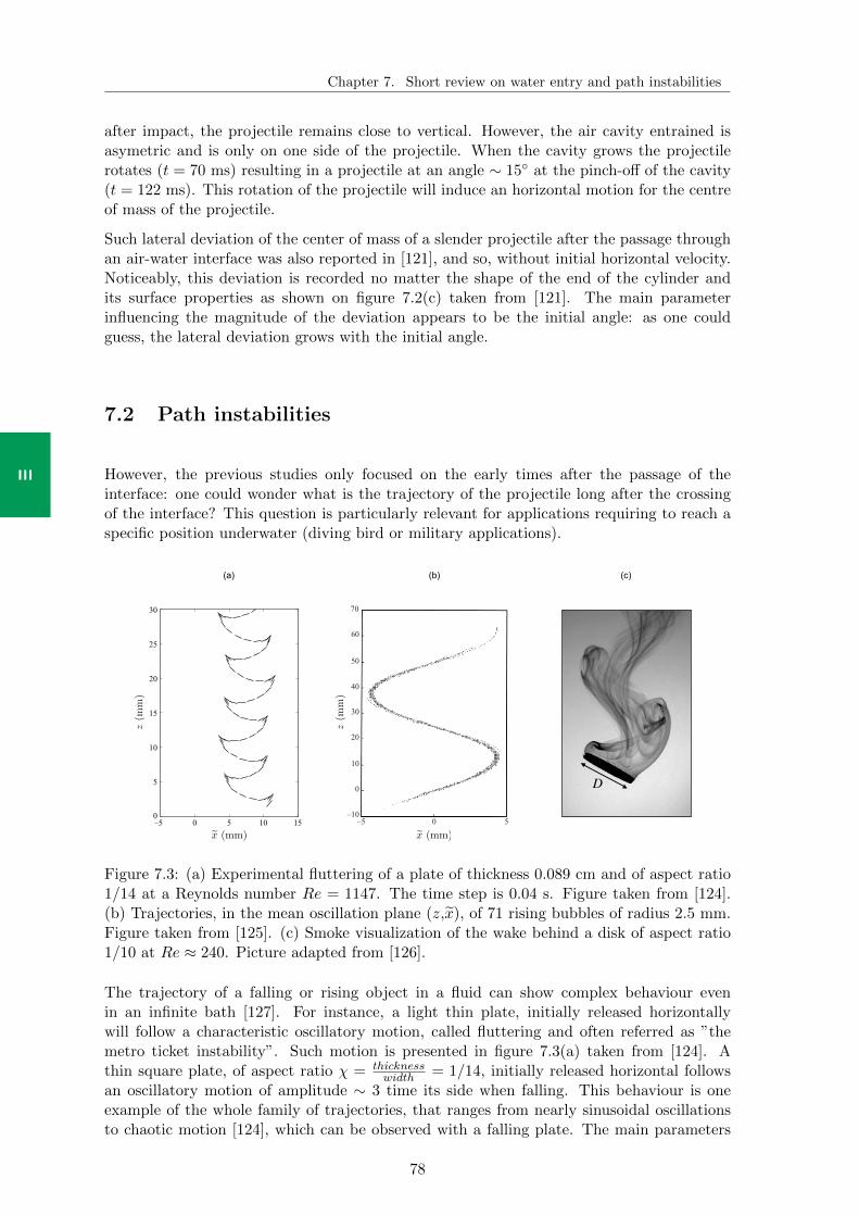
Chapter 7. Short review on water entry and path instabilities
III
after impact, the projectile remains close to vertical. However, the air cavity entrained isasymetric and is only on one side of the projectile. When the cavity grows the projectilerotates (t = 70 ms) resulting in a projectile at an angle ∼ 15 at the pinch-off of the cavity(t = 122 ms). This rotation of the projectile will induce an horizontal motion for the centreof mass of the projectile.
Such lateral deviation of the center of mass of a slender projectile after the passage throughan air-water interface was also reported in [121], and so, without initial horizontal velocity.Noticeably, this deviation is recorded no matter the shape of the end of the cylinder andits surface properties as shown on figure 7.2(c) taken from [121]. The main parameterinfluencing the magnitude of the deviation appears to be the initial angle: as one couldguess, the lateral deviation grows with the initial angle.
7.2 Path instabilities
However, the previous studies only focused on the early times after the passage of theinterface: one could wonder what is the trajectory of the projectile long after the crossingof the interface? This question is particularly relevant for applications requiring to reach aspecific position underwater (diving bird or military applications).
Unsteady aerodynamics of fluttering and tumbling plates 71
5 10 15 20 25 30
10
15
20
x (cm)
y (c
m)
(c)
β = 1/5
Re = 737
I* = 0.48
10 15 20 25 300
5
10
15
20
25
30
35
x (cm)
(1) (2)
(b)
β = 1/6
Re = 1770
I* = 0.39
–5 0 5 10 150
5
10
15
20
25
30
x (cm)
y (c
m)
(a)
β = 1/14
Re = 1147
I* = 0.16
Figure 2. Measured plate trajectories: (a) the fluttering plate with h = 0.081 cm and β = 1/14,(b) two apparently chaotic trajectories for the h = 0.162 cm and β = 1/6 plate, and (c) thetumbling plate with h =0.162 cm and β =1/5. For clarity the two trajectories in (b) aredisplaced from each other 0.5 cm horizontally and 1.5 cm vertically. The thick line segmentsshow the plate cross-sections with time intervals of 0.04 s in (a) and 0.025 s in (b) and (c).
where Ω, V1, V2, and V3 are constants. The constant Ω is the angular frequency ofthe periodic motion, V2 is the average descent speed, and V1 and V3 describe theamplitudes of the oscillations in vx and vy , respectively. Figure 4 shows the curve(4.1) and (4.2) with the parameters Ω = 9.8 rad s−1, V1 = 32.6 cm s−1, V2 = 9.1 cm s−1,and V3 = 14.5 cm s−1 obtained from the fits shown by the two dotted lines in figure 3.
9DD
C5
:
01
2565
79D
DC
42
:56
46
.46
/D6
49:A
E6E
2DCE
64DD
D96
,2:5
6,
6D6
C7E
C62
2:2
62D
9DD
C 4
2:5
6 4
6D6
C
potentialflowtheoryisperformedasawaytoemphasizeindirectlytheroleofthewake.
Wecarriedoutanexperimentalstudyonthefreeriseofflatcylinders.Thephysicalparametersgoverningtheproblemarethegravityg,thefluiddensity!fandkine-maticviscosity",thebodydensity!b,thediameterd,andthicknessh.Theproblemisthenentirelycharacterizedbythreedimensionlessparameters,namelytheaspectratiod/h,thebody-to-fluiddensityratio!b/!f,andtheArchimedesnumber,whichmaybethoughtofasaReynoldsnumberbasedonagravitationalvelocityscale,Ar=d/"!3/16"#!f−!b$/!f%gh.Notethatforbodieswithnegligiblethickness#d/h→#$thenondimensionalparam-eterI*proportionalto!b/!fh/discommonlyused.Itisclearlyimportanttointroduceanondimensionalparameterinvolvingthedensitydifferenceandanotheroneinvolvingthedensityratio,butweknownophysicalargumenttopre-ferI*to!b/!f.Forpracticalreasonsthedensityratio!b/!fisfixedclosetounityinthepresentexperiments,andwefocusontheroleoftheaspectratioandArchimedesnumber.Theaspectratiod/hisvariedfrom1.5to10inordertoinvesti-gatethemajorkinematicdifferencesoccurringwhenthebodyanisotropyissignificantlychanged.Thecylindersaremadeofanylonofdensitycloseto1.02g/cm3andtheirdiametersrangefrom1to1.8cm.Theyarereleasedatthebottomofatank1.70mhigh,havingasquaresectionof40cmsidewidth,filledupwithsaltwater.Weusedverysmallbody-to-fluiddensitydifferences,!f−!b/!f&10−2,resultinginmoderateArchimedesnumbers,70$Ar$120,forwhichharmonicoscillationsofthebodiesareobserved.Forthispurposethedensitiesofboththebodiesandthefluidweredeterminedwithanaccuracyof5%10−4g/cm3.Thehomo-geneityofthesolutionwithinthetankwasalsocheckedtomakesurethatnostratificationoccurred.Thecylinderswerereleasedatthebottomofthetankusinganoriginalshutterconsistingoftwohorizontalplatesthatslideinoppositedi-rections.Wecheckedthattheinitialconditionsofrelease#inclinationandvelocityperturbation$hadnoinfluenceontheperiodicmotion.Nevertheless,thecylinderswerere-leasedgentlyandface-up#withaninclinationlessthan10°$.Theriseofthecylinderswasthenfollowedbytwoperpen-diculartravellingcameraswhosepositionwasrecordedbyahigh-accuracymagneticencoder.Imageprocessingallowedthedeterminationofthebodytranslationandorientationviacontourdetectionwithanaccuracyof±0.15mm.
IntherangeofArconsideredhere,aftertheinitialtran-sient,theperiodictrajectoryofthebodylieswithinanearlyverticalplane:thehorizontaldriftislessthan2°andtheangularvelocityofthepossiblerotationofthezigzagplaneismorethan50timessmallerthantheprincipaloscillationfrequency.Figure1showstwoinstantaneouspicturesofabodyanditswakeduringthefinalperiodicmotionforaspectratiosof2and10,respectively,andArabout85.Inthisfigure,thebodieshavebeencoveredwithdyeinordertovisualizetheunsteadinessofthewake.Sincetheuseofdyedoesnotallowustomaintaintherequiredaccuracyonthedensitydifference,thequantitativeresultsonthebodymo-tiondiscussedbelowwereobtainedwithoutdye.
WithinthechosenrangeofArchimedesnumber,thever-
ticalmeanvelocity#Vz$variesbetween10and35mm/s,andthecorrespondingReynoldsnumber,Re=Vzd/",variesbe-tween200and320.TheevolutionofRewithArisgiveninFig.2fordifferentvaluesoftheaspectratio.TheReynoldsnumberisseentobelinearlydependentontheArchimedesnumberandtodependonlyweaklyontheaspectratio.ThisallowsustocharacterizetheflowaroundbothfixedandfreelymovingbodiesthroughRe,insteadofusingArforthelatter.
Thetwo-dimensionaloscillatorymotionofthebodymaybecharacterizedbyatwo-componentvelocityvectorandaone-componentrotationrate.Inallcases,thehorizontalve-locitycomponentandtherotationratearefoundtoexperi-enceharmonicoscillationsatthesamefrequency#Fig.3$.Theamplitudeofthehorizontalvelocitycomponentliesbe-tween1and10mm/s,whichcorrespondstodisplacementsofthebodycenterrangingfrom1.5to6mm.Theamplitudeoftheverticalvelocityoscillationisconsiderablysmaller.Asalreadyreportedforrisingbubbles
7,12andfallingthin
strips,13
theverticalvelocityoscillateswithafrequencythat
FIG.1.Visualizationofthewakebehindtwofreelyrisingcylinders,Ar=85#Re&240$.Left:d/h=2;right:d/h=10.
FIG.2.ReynoldsnumberasafunctionoftheArchimedesnumberforvari-ousaspectratios.
098107-2Fernandesetal.Phys.Fluids17,098107!2005"
246 K. Ellingsen and F. Risso
z
x
y
Principal plane of oscillations Á
Ê
x0
z0
y0
Ó
Figure 7. Definition of the principal frame of oscillations (, , ).
70
60
50
40
30
20
10
0
–10–5 0 5
Ó (mm)
Ê (m
m)
70
60
50
40
30
20
10
0
–10–5 0 5
Á (mm)
Figure 8. Superimposition of 71 bubble trajectories in the principal frame of oscillation.
is determined while that of the secondary one depends on the experimental runs.The vertical motion shows weak oscillations at twice the frequency of the horizontalmotion. Their amplitude, their phase and the mean rise velocity are determined.
At this point, we propose the following interpretation. The rectilinear trajectory is
144
6ACC
31
2A94
7
A73
A .
3/
C3
9D
D71C
D2:
3CC
C,1
2A94
7,
AC
A6D
1E19
121C
CC 3
12A
947
A7
3A
CA
CC
49
A7
0
ex (mm)ex (mm)
z(m
m)
z(m
m)
(b)(a) (c)
Re = 1147
= 1/14
D
Figure 7.3: (a) Experimental fluttering of a plate of thickness 0.089 cm and of aspect ratio1/14 at a Reynolds number Re = 1147. The time step is 0.04 s. Figure taken from [124].(b) Trajectories, in the mean oscillation plane (z,x), of 71 rising bubbles of radius 2.5 mm.Figure taken from [125]. (c) Smoke visualization of the wake behind a disk of aspect ratio1/10 at Re ≈ 240. Picture adapted from [126].
The trajectory of a falling or rising object in a fluid can show complex behaviour evenin an infinite bath [127]. For instance, a light thin plate, initially released horizontallywill follow a characteristic oscillatory motion, called fluttering and often referred as ”themetro ticket instability”. Such motion is presented in figure 7.3(a) taken from [124]. Athin square plate, of aspect ratio χ = thickness
width = 1/14, initially released horizontal followsan oscillatory motion of amplitude ∼ 3 time its side when falling. This behaviour is oneexample of the whole family of trajectories, that ranges from nearly sinusoidal oscillationsto chaotic motion [124], which can be observed with a falling plate. The main parameters
78
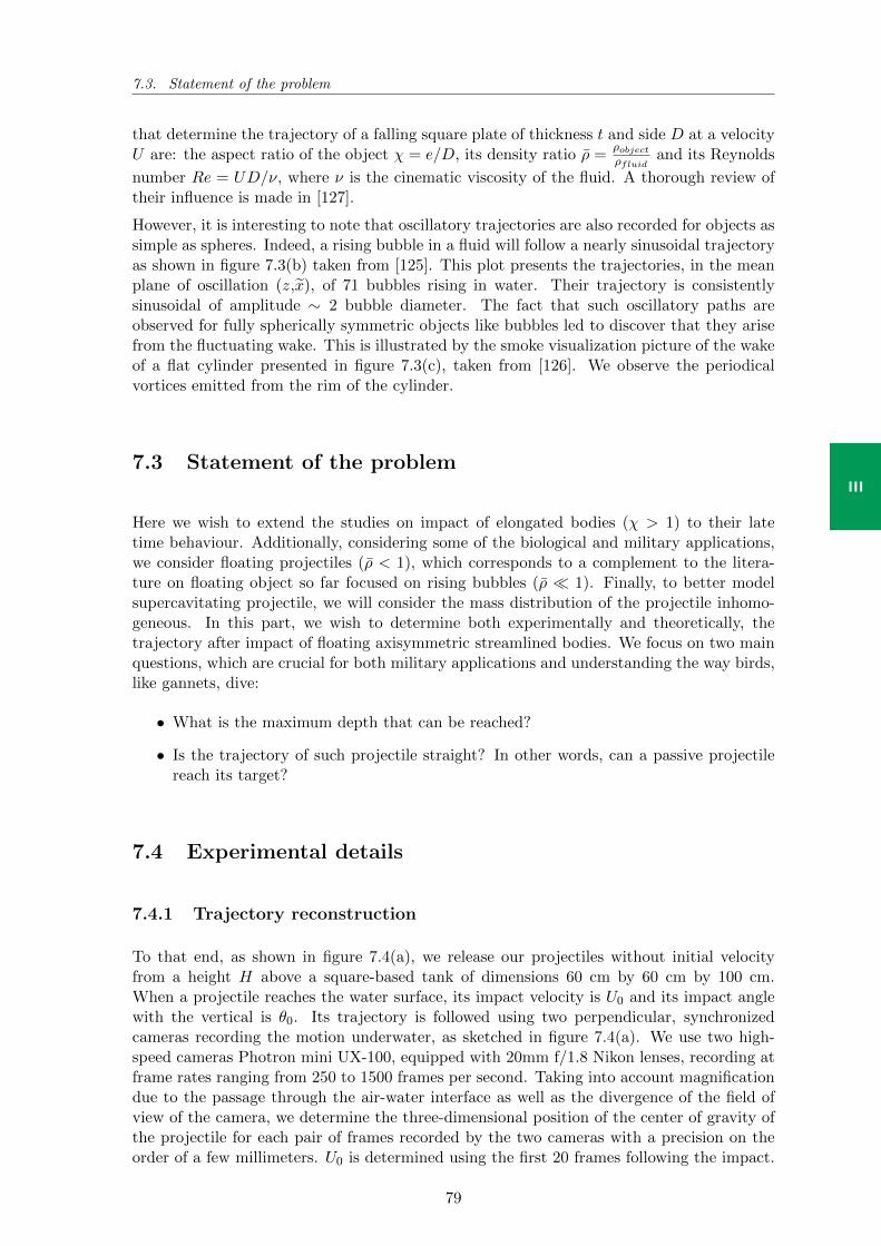
7.3. Statement of the problem
III
that determine the trajectory of a falling square plate of thickness t and side D at a velocityU are: the aspect ratio of the object χ = e/D, its density ratio ρ =
ρobjectρfluid
and its Reynolds
number Re = UD/ν, where ν is the cinematic viscosity of the fluid. A thorough review oftheir influence is made in [127].
However, it is interesting to note that oscillatory trajectories are also recorded for objects assimple as spheres. Indeed, a rising bubble in a fluid will follow a nearly sinusoidal trajectoryas shown in figure 7.3(b) taken from [125]. This plot presents the trajectories, in the meanplane of oscillation (z,x), of 71 bubbles rising in water. Their trajectory is consistentlysinusoidal of amplitude ∼ 2 bubble diameter. The fact that such oscillatory paths areobserved for fully spherically symmetric objects like bubbles led to discover that they arisefrom the fluctuating wake. This is illustrated by the smoke visualization picture of the wakeof a flat cylinder presented in figure 7.3(c), taken from [126]. We observe the periodicalvortices emitted from the rim of the cylinder.
7.3 Statement of the problem
Here we wish to extend the studies on impact of elongated bodies (χ > 1) to their latetime behaviour. Additionally, considering some of the biological and military applications,we consider floating projectiles (ρ < 1), which corresponds to a complement to the litera-ture on floating object so far focused on rising bubbles (ρ 1). Finally, to better modelsupercavitating projectile, we will consider the mass distribution of the projectile inhomo-geneous. In this part, we wish to determine both experimentally and theoretically, thetrajectory after impact of floating axisymmetric streamlined bodies. We focus on two mainquestions, which are crucial for both military applications and understanding the way birds,like gannets, dive:
• What is the maximum depth that can be reached?
• Is the trajectory of such projectile straight? In other words, can a passive projectilereach its target?
7.4 Experimental details
7.4.1 Trajectory reconstruction
To that end, as shown in figure 7.4(a), we release our projectiles without initial velocityfrom a height H above a square-based tank of dimensions 60 cm by 60 cm by 100 cm.When a projectile reaches the water surface, its impact velocity is U0 and its impact anglewith the vertical is θ0. Its trajectory is followed using two perpendicular, synchronizedcameras recording the motion underwater, as sketched in figure 7.4(a). We use two high-speed cameras Photron mini UX-100, equipped with 20mm f/1.8 Nikon lenses, recording atframe rates ranging from 250 to 1500 frames per second. Taking into account magnificationdue to the passage through the air-water interface as well as the divergence of the field ofview of the camera, we determine the three-dimensional position of the center of gravity ofthe projectile for each pair of frames recorded by the two cameras with a precision on theorder of a few millimeters. U0 is determined using the first 20 frames following the impact.
79
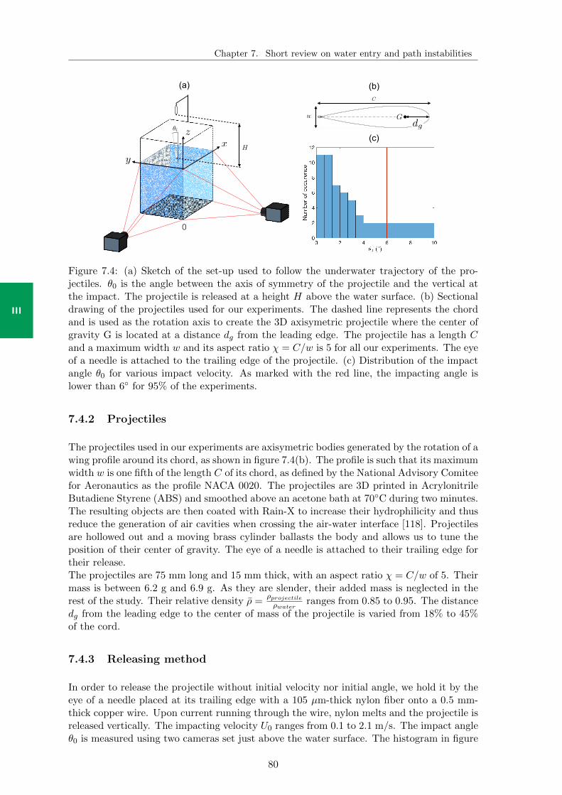
Chapter 7. Short review on water entry and path instabilities
III
(b)
(c)
(a)
0
dgG
C
0
H
w
x
y
z
Figure 7.4: (a) Sketch of the set-up used to follow the underwater trajectory of the pro-jectiles. θ0 is the angle between the axis of symmetry of the projectile and the vertical atthe impact. The projectile is released at a height H above the water surface. (b) Sectionaldrawing of the projectiles used for our experiments. The dashed line represents the chordand is used as the rotation axis to create the 3D axisymetric projectile where the center ofgravity G is located at a distance dg from the leading edge. The projectile has a length Cand a maximum width w and its aspect ratio χ = C/w is 5 for all our experiments. The eyeof a needle is attached to the trailing edge of the projectile. (c) Distribution of the impactangle θ0 for various impact velocity. As marked with the red line, the impacting angle islower than 6 for 95% of the experiments.
7.4.2 Projectiles
The projectiles used in our experiments are axisymetric bodies generated by the rotation of awing profile around its chord, as shown in figure 7.4(b). The profile is such that its maximumwidth w is one fifth of the length C of its chord, as defined by the National Advisory Comiteefor Aeronautics as the profile NACA 0020. The projectiles are 3D printed in AcrylonitrileButadiene Styrene (ABS) and smoothed above an acetone bath at 70C during two minutes.The resulting objects are then coated with Rain-X to increase their hydrophilicity and thusreduce the generation of air cavities when crossing the air-water interface [118]. Projectilesare hollowed out and a moving brass cylinder ballasts the body and allows us to tune theposition of their center of gravity. The eye of a needle is attached to their trailing edge fortheir release.The projectiles are 75 mm long and 15 mm thick, with an aspect ratio χ = C/w of 5. Theirmass is between 6.2 g and 6.9 g. As they are slender, their added mass is neglected in therest of the study. Their relative density ρ =
ρprojectileρwater
ranges from 0.85 to 0.95. The distancedg from the leading edge to the center of mass of the projectile is varied from 18% to 45%of the cord.
7.4.3 Releasing method
In order to release the projectile without initial velocity nor initial angle, we hold it by theeye of a needle placed at its trailing edge with a 105 µm-thick nylon fiber onto a 0.5 mm-thick copper wire. Upon current running through the wire, nylon melts and the projectile isreleased vertically. The impacting velocity U0 ranges from 0.1 to 2.1 m/s. The impact angleθ0 is measured using two cameras set just above the water surface. The histogram in figure
80

7.4. Experimental details
III
7.4(c) shows that our method ensures an impact angle below 6 in 95% of the experiments.
81
Chapter 7. Short review on water entry and path instabilities
III
82
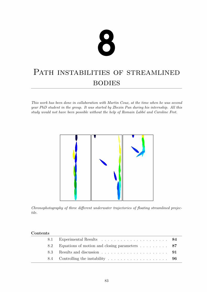
8Path instabilities of streamlined
bodies
This work has been done in collaboration with Martin Coux, at the time when he was secondyear PhD student in the group. It was started by Zhexin Pan during his internship. All thisstudy would not have been possible without the help of Romain Labbe and Caroline Frot.
Chronophotography of three different underwater trajectories of floating streamlined projec-tile.
Contents
8.1 Experimental Results . . . . . . . . . . . . . . . . . . . . . 84
8.2 Equations of motion and closing parameters . . . . . . . . . 87
8.3 Results and discussion . . . . . . . . . . . . . . . . . . . . . 91
8.4 Controlling the instability . . . . . . . . . . . . . . . . . . . 96
83
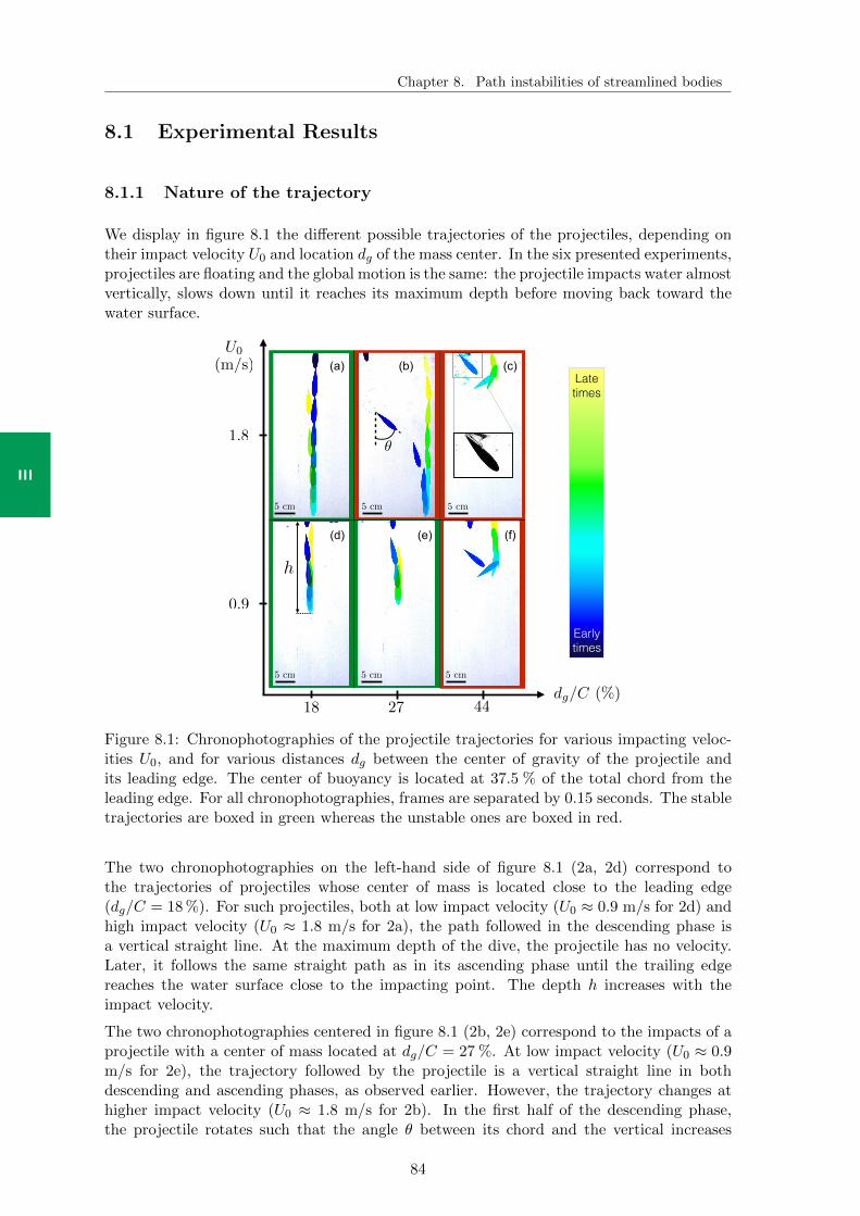
Chapter 8. Path instabilities of streamlined bodies
III
8.1 Experimental Results
8.1.1 Nature of the trajectory
We display in figure 8.1 the different possible trajectories of the projectiles, depending ontheir impact velocity U0 and location dg of the mass center. In the six presented experiments,projectiles are floating and the global motion is the same: the projectile impacts water almostvertically, slows down until it reaches its maximum depth before moving back toward thewater surface.
Early times
Late times
(a) (b) (c)
(d) (e) (f)
h
U0
(m/s)
dg/C (%)
1.8
0.9
18 27 44
5 cm 5 cm 5 cm
5 cm 5 cm 5 cm
Figure 8.1: Chronophotographies of the projectile trajectories for various impacting veloc-ities U0, and for various distances dg between the center of gravity of the projectile andits leading edge. The center of buoyancy is located at 37.5 % of the total chord from theleading edge. For all chronophotographies, frames are separated by 0.15 seconds. The stabletrajectories are boxed in green whereas the unstable ones are boxed in red.
The two chronophotographies on the left-hand side of figure 8.1 (2a, 2d) correspond tothe trajectories of projectiles whose center of mass is located close to the leading edge(dg/C = 18 %). For such projectiles, both at low impact velocity (U0 ≈ 0.9 m/s for 2d) andhigh impact velocity (U0 ≈ 1.8 m/s for 2a), the path followed in the descending phase isa vertical straight line. At the maximum depth of the dive, the projectile has no velocity.Later, it follows the same straight path as in its ascending phase until the trailing edgereaches the water surface close to the impacting point. The depth h increases with theimpact velocity.
The two chronophotographies centered in figure 8.1 (2b, 2e) correspond to the impacts of aprojectile with a center of mass located at dg/C = 27 %. At low impact velocity (U0 ≈ 0.9m/s for 2e), the trajectory followed by the projectile is a vertical straight line in bothdescending and ascending phases, as observed earlier. However, the trajectory changes athigher impact velocity (U0 ≈ 1.8 m/s for 2b). In the first half of the descending phase,the projectile rotates such that the angle θ between its chord and the vertical increases
84
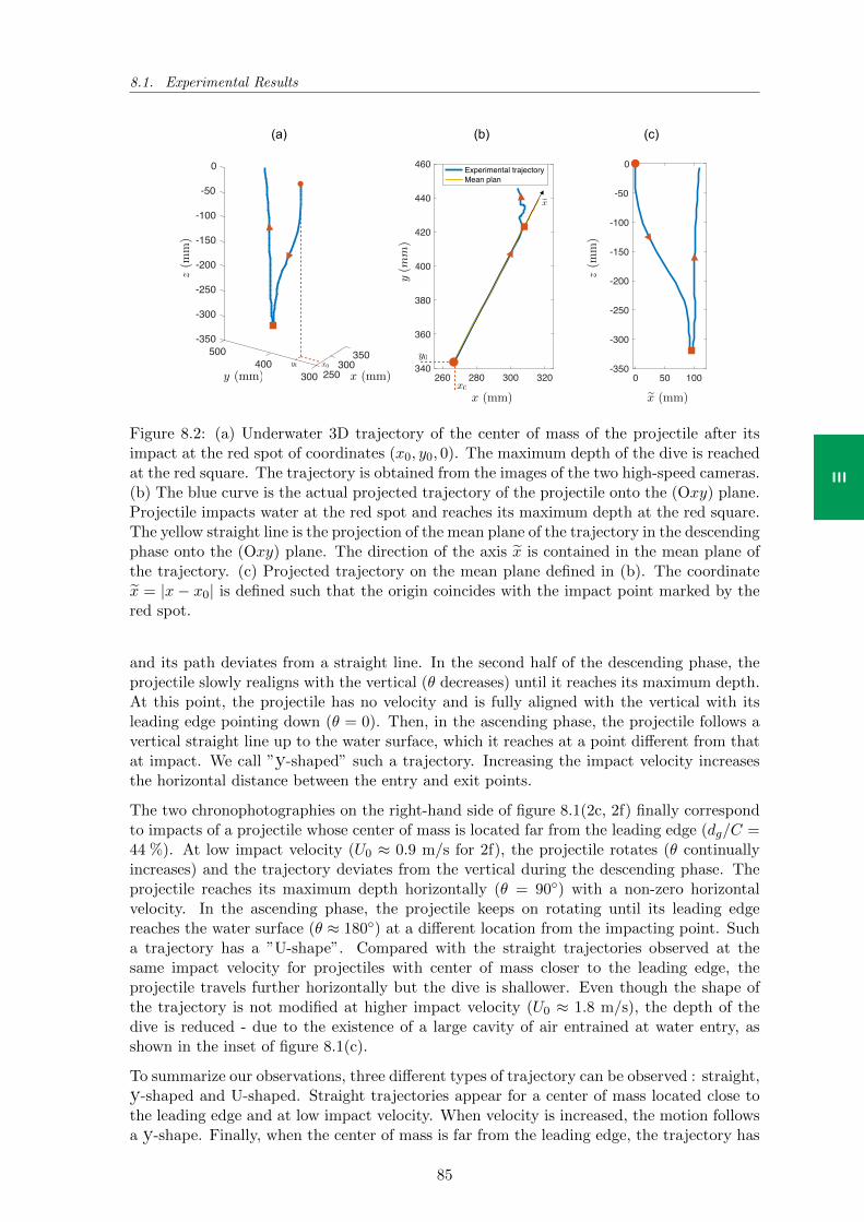
8.1. Experimental Results
III
260 280 300 320x (mm)
340
360
380
400
420
440
460
y (m
m)
Experimental trajectoryMean plan
0 50 100-350
-300
-250
-200
-150
-100
-50
0
(a) (b) (c)
x0
y0
-350
-300
500 350
-250
y (mm)
-200
x (mm)
400 300
z (m
m) -150
-100
250300
-50
0
x0y0
ex
y(m
m)
z(m
m)
z(m
m)
z(m
m)
ex (mm)x (mm)
x (mm)y (mm)
Figure 8.2: (a) Underwater 3D trajectory of the center of mass of the projectile after itsimpact at the red spot of coordinates (x0, y0, 0). The maximum depth of the dive is reachedat the red square. The trajectory is obtained from the images of the two high-speed cameras.(b) The blue curve is the actual projected trajectory of the projectile onto the (Oxy) plane.Projectile impacts water at the red spot and reaches its maximum depth at the red square.The yellow straight line is the projection of the mean plane of the trajectory in the descendingphase onto the (Oxy) plane. The direction of the axis x is contained in the mean plane ofthe trajectory. (c) Projected trajectory on the mean plane defined in (b). The coordinatex = |x− x0| is defined such that the origin coincides with the impact point marked by thered spot.
and its path deviates from a straight line. In the second half of the descending phase, theprojectile slowly realigns with the vertical (θ decreases) until it reaches its maximum depth.At this point, the projectile has no velocity and is fully aligned with the vertical with itsleading edge pointing down (θ = 0). Then, in the ascending phase, the projectile follows avertical straight line up to the water surface, which it reaches at a point different from thatat impact. We call ”y-shaped” such a trajectory. Increasing the impact velocity increasesthe horizontal distance between the entry and exit points.
The two chronophotographies on the right-hand side of figure 8.1(2c, 2f) finally correspondto impacts of a projectile whose center of mass is located far from the leading edge (dg/C =44 %). At low impact velocity (U0 ≈ 0.9 m/s for 2f), the projectile rotates (θ continuallyincreases) and the trajectory deviates from the vertical during the descending phase. Theprojectile reaches its maximum depth horizontally (θ = 90) with a non-zero horizontalvelocity. In the ascending phase, the projectile keeps on rotating until its leading edgereaches the water surface (θ ≈ 180) at a different location from the impacting point. Sucha trajectory has a ”U-shape”. Compared with the straight trajectories observed at thesame impact velocity for projectiles with center of mass closer to the leading edge, theprojectile travels further horizontally but the dive is shallower. Even though the shape ofthe trajectory is not modified at higher impact velocity (U0 ≈ 1.8 m/s), the depth of thedive is reduced - due to the existence of a large cavity of air entrained at water entry, asshown in the inset of figure 8.1(c).
To summarize our observations, three different types of trajectory can be observed : straight,y-shaped and U-shaped. Straight trajectories appear for a center of mass located close tothe leading edge and at low impact velocity. When velocity is increased, the motion followsa y-shape. Finally, when the center of mass is far from the leading edge, the trajectory has
85
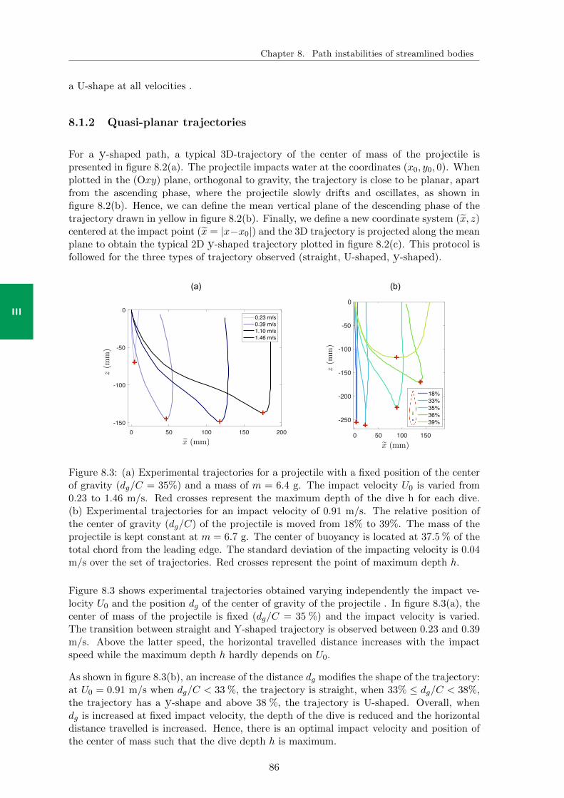
Chapter 8. Path instabilities of streamlined bodies
III
a U-shape at all velocities .
8.1.2 Quasi-planar trajectories
For a y-shaped path, a typical 3D-trajectory of the center of mass of the projectile ispresented in figure 8.2(a). The projectile impacts water at the coordinates (x0, y0, 0). Whenplotted in the (Oxy) plane, orthogonal to gravity, the trajectory is close to be planar, apartfrom the ascending phase, where the projectile slowly drifts and oscillates, as shown infigure 8.2(b). Hence, we can define the mean vertical plane of the descending phase of thetrajectory drawn in yellow in figure 8.2(b). Finally, we define a new coordinate system (x, z)centered at the impact point (x = |x−x0|) and the 3D trajectory is projected along the meanplane to obtain the typical 2D y-shaped trajectory plotted in figure 8.2(c). This protocol isfollowed for the three types of trajectory observed (straight, U-shaped, y-shaped).
0 50 100 150
-250
-200
-150
-100
-50
0
18%33%35%36%39%
0 50 100 150 200-150
-100
-50
00.23 m/s0.39 m/s1.10 m/s1.46 m/s
(a) (b)
ex (mm)ex (mm)
z(m
m)
z(m
m)
ex (mm)
z(m
m)
ex (mm)
Figure 8.3: (a) Experimental trajectories for a projectile with a fixed position of the centerof gravity (dg/C = 35%) and a mass of m = 6.4 g. The impact velocity U0 is varied from0.23 to 1.46 m/s. Red crosses represent the maximum depth of the dive h for each dive.(b) Experimental trajectories for an impact velocity of 0.91 m/s. The relative position ofthe center of gravity (dg/C) of the projectile is moved from 18% to 39%. The mass of theprojectile is kept constant at m = 6.7 g. The center of buoyancy is located at 37.5 % of thetotal chord from the leading edge. The standard deviation of the impacting velocity is 0.04m/s over the set of trajectories. Red crosses represent the point of maximum depth h.
Figure 8.3 shows experimental trajectories obtained varying independently the impact ve-locity U0 and the position dg of the center of gravity of the projectile . In figure 8.3(a), thecenter of mass of the projectile is fixed (dg/C = 35 %) and the impact velocity is varied.The transition between straight and Y-shaped trajectory is observed between 0.23 and 0.39m/s. Above the latter speed, the horizontal travelled distance increases with the impactspeed while the maximum depth h hardly depends on U0.
As shown in figure 8.3(b), an increase of the distance dg modifies the shape of the trajectory:at U0 = 0.91 m/s when dg/C < 33 %, the trajectory is straight, when 33% ≤ dg/C < 38%,the trajectory has a y-shape and above 38 %, the trajectory is U-shaped. Overall, whendg is increased at fixed impact velocity, the depth of the dive is reduced and the horizontaldistance travelled is increased. Hence, there is an optimal impact velocity and position ofthe center of mass such that the dive depth h is maximum.
86
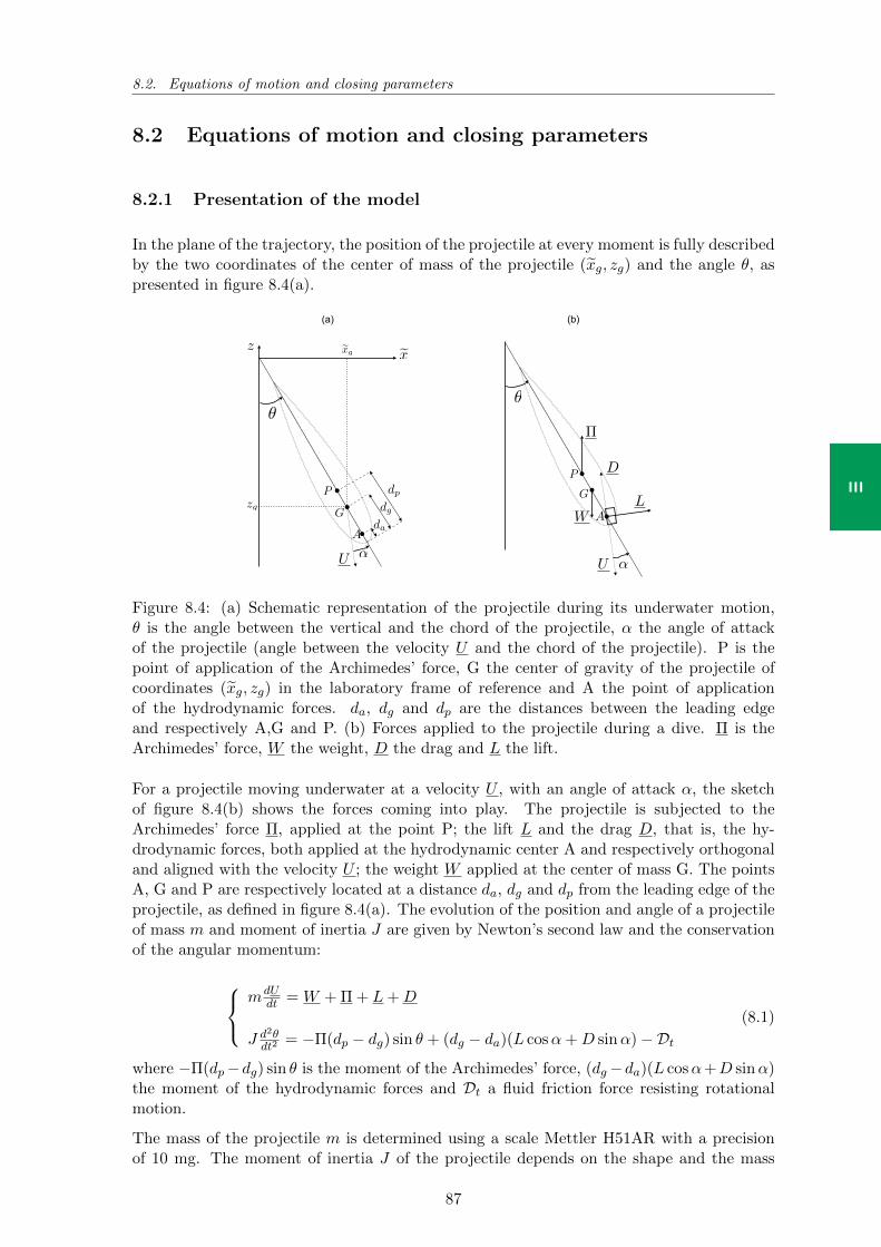
8.2. Equations of motion and closing parameters
III
8.2 Equations of motion and closing parameters
8.2.1 Presentation of the model
In the plane of the trajectory, the position of the projectile at every moment is fully describedby the two coordinates of the center of mass of the projectile (xg, zg) and the angle θ, aspresented in figure 8.4(a).
↵
P
G
A
dp
da
dg
(a) (b)
U
WL
D
U ↵
z exexg
zg
P
G
A
Figure 8.4: (a) Schematic representation of the projectile during its underwater motion,θ is the angle between the vertical and the chord of the projectile, α the angle of attackof the projectile (angle between the velocity U and the chord of the projectile). P is thepoint of application of the Archimedes’ force, G the center of gravity of the projectile ofcoordinates (xg, zg) in the laboratory frame of reference and A the point of applicationof the hydrodynamic forces. da, dg and dp are the distances between the leading edgeand respectively A,G and P. (b) Forces applied to the projectile during a dive. Π is theArchimedes’ force, W the weight, D the drag and L the lift.
For a projectile moving underwater at a velocity U , with an angle of attack α, the sketchof figure 8.4(b) shows the forces coming into play. The projectile is subjected to theArchimedes’ force Π, applied at the point P; the lift L and the drag D, that is, the hy-drodynamic forces, both applied at the hydrodynamic center A and respectively orthogonaland aligned with the velocity U ; the weight W applied at the center of mass G. The pointsA, G and P are respectively located at a distance da, dg and dp from the leading edge of theprojectile, as defined in figure 8.4(a). The evolution of the position and angle of a projectileof mass m and moment of inertia J are given by Newton’s second law and the conservationof the angular momentum:
mdUdt = W + Π + L+D
J d2θdt2
= −Π(dp − dg) sin θ + (dg − da)(L cosα+D sinα)−Dt(8.1)
where −Π(dp−dg) sin θ is the moment of the Archimedes’ force, (dg−da)(L cosα+D sinα)the moment of the hydrodynamic forces and Dt a fluid friction force resisting rotationalmotion.
The mass of the projectile m is determined using a scale Mettler H51AR with a precisionof 10 mg. The moment of inertia J of the projectile depends on the shape and the mass
87
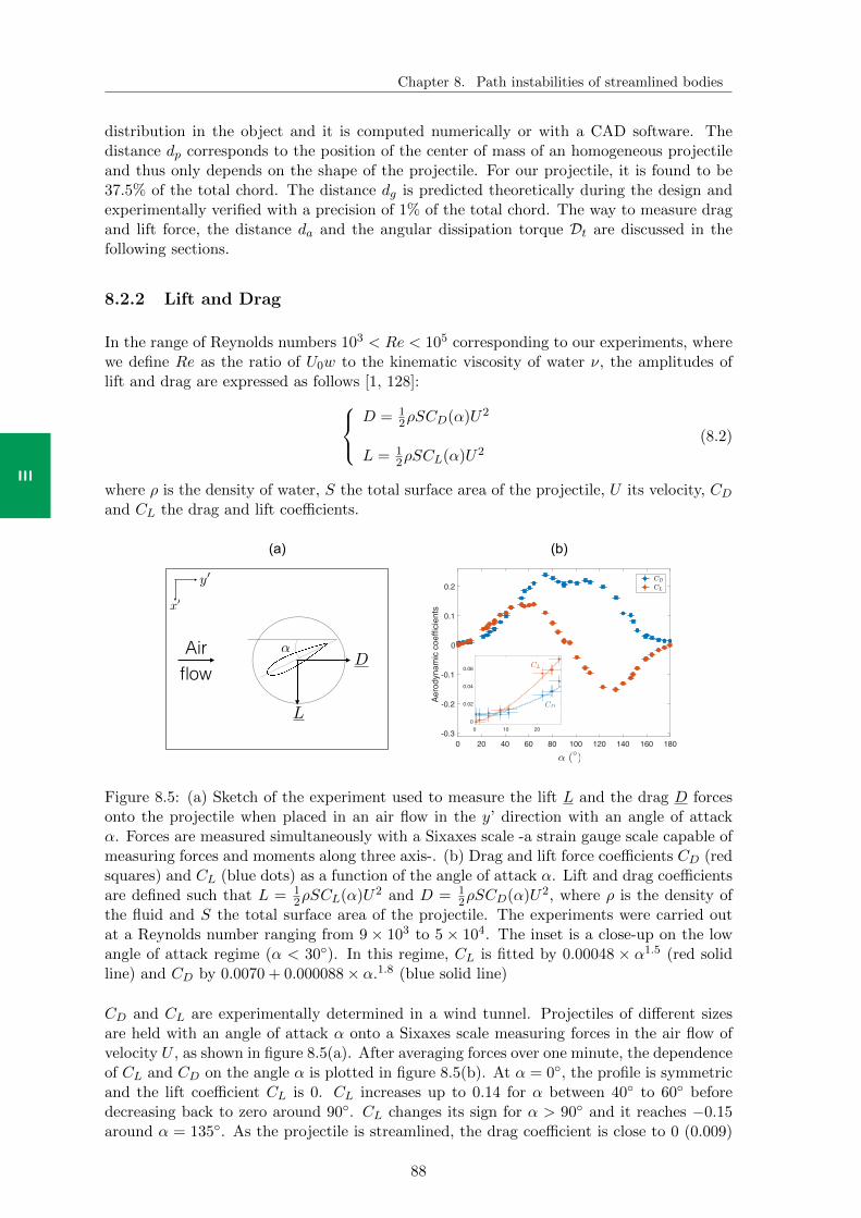
Chapter 8. Path instabilities of streamlined bodies
III
distribution in the object and it is computed numerically or with a CAD software. Thedistance dp corresponds to the position of the center of mass of an homogeneous projectileand thus only depends on the shape of the projectile. For our projectile, it is found to be37.5% of the total chord. The distance dg is predicted theoretically during the design andexperimentally verified with a precision of 1% of the total chord. The way to measure dragand lift force, the distance da and the angular dissipation torque Dt are discussed in thefollowing sections.
8.2.2 Lift and Drag
In the range of Reynolds numbers 103 < Re < 105 corresponding to our experiments, wherewe define Re as the ratio of U0w to the kinematic viscosity of water ν, the amplitudes oflift and drag are expressed as follows [1, 128]:
D = 12ρSCD(α)U2
L = 12ρSCL(α)U2
(8.2)
where ρ is the density of water, S the total surface area of the projectile, U its velocity, CDand CL the drag and lift coefficients.
0 20 40 60 80 100 120 140 160 180 (°)
-0.3
-0.2
-0.1
0
0.1
0.2
Aero
dyna
mic
coe
ffici
ents
↵
(a) (b)
L
DAir
flow
y0
x0
0 10 200
0.02
0.04
0.06
CD
CL
↵ ()
Figure 8.5: (a) Sketch of the experiment used to measure the lift L and the drag D forcesonto the projectile when placed in an air flow in the y’ direction with an angle of attackα. Forces are measured simultaneously with a Sixaxes scale -a strain gauge scale capable ofmeasuring forces and moments along three axis-. (b) Drag and lift force coefficients CD (redsquares) and CL (blue dots) as a function of the angle of attack α. Lift and drag coefficientsare defined such that L = 1
2ρSCL(α)U2 and D = 12ρSCD(α)U2, where ρ is the density of
the fluid and S the total surface area of the projectile. The experiments were carried outat a Reynolds number ranging from 9 × 10³ to 5 × 10⁴. The inset is a close-up on the lowangle of attack regime (α < 30). In this regime, CL is fitted by 0.00048 × α1.5 (red solidline) and CD by 0.0070 + 0.000088× α.1.8 (blue solid line)
CD and CL are experimentally determined in a wind tunnel. Projectiles of different sizesare held with an angle of attack α onto a Sixaxes scale measuring forces in the air flow ofvelocity U , as shown in figure 8.5(a). After averaging forces over one minute, the dependenceof CL and CD on the angle α is plotted in figure 8.5(b). At α = 0, the profile is symmetricand the lift coefficient CL is 0. CL increases up to 0.14 for α between 40 to 60 beforedecreasing back to zero around 90. CL changes its sign for α > 90 and it reaches −0.15around α = 135. As the projectile is streamlined, the drag coefficient is close to 0 (0.009)
88
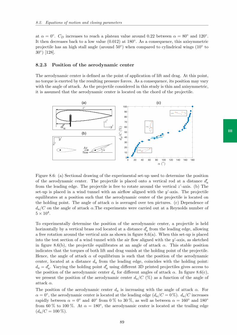
8.2. Equations of motion and closing parameters
III
at α = 0. CD increases to reach a plateau value around 0.22 between α = 80 and 120.It then decreases back to a low value (0.012) at 180. As a consequence, this axisymmetricprojectile has an high stall angle (around 50) when compared to cylindrical wings (10 to30) [128].
8.2.3 Position of the aerodynamic center
The aerodynamic center is defined as the point of application of lift and drag. At this point,no torque is exerted by the resulting pressure forces. As a consequence, its position may varywith the angle of attack. As the projectile considered in this study is thin and axisymmetric,it is assumed that the aerodynamic center is located on the chord of the projectile.
0 20 40 60 80 100 120 140 160 180 (°)
0
10
20
30
40
50
60
70
80
90
100
↵
(a)
(b)
(c)
d0a
Air flow
C
y0
x0
y0z0
dg/C
(%)
↵ ()
Figure 8.6: (a) Sectional drawing of the experimental set-up used to determine the positionof the aerodynamic center. The projectile is placed onto a vertical rod at a distance d′afrom the leading edge. The projectile is free to rotate around the vertical z’-axis. (b) Theset-up is placed in a wind tunnel with an airflow aligned with the y’-axis. The projectileequilibrates at a position such that the aerodynamic center of the projectile is located onthe holding point. The angle of attack α is averaged over ten pictures. (c) Dependence ofda/C on the angle of attack α.The experiments were carried out at a Reynolds number of5× 104.
To experimentally determine the position of the aerodynamic center, a projectile is heldhorizontally by a vertical brass rod located at a distance d′a from the leading edge, allowinga free rotation around the vertical axis as shown in figure 8.6(a). When this set-up is placedinto the test section of a wind tunnel with the air flow aligned with the y’-axis, as sketchedin figure 8.6(b), the projectile equilibrates at an angle of attack α. This stable positionindicates that the torques of both lift and drag vanish at the holding point of the projectile.Hence, the angle of attack α of equilibrium is such that the position of the aerodynamiccenter, located at a distance da from the leading edge, coincides with the holding point:da = d′a. Varying the holding point d′a using different 3D printed projectiles gives access tothe position of the aerodynamic center da for different angles of attack α. In figure 8.6(c),we present the position of the aerodynamic center da/C (%) as a function of the angle ofattack α.
The position of the aerodynamic center da is increasing with the angle of attack α. Forα = 0, the aerodynamic center is located at the leading edge (da/C = 0%). da/C increasesrapidly between α = 0 and 40 from 0 % to 30 %, as well as between α = 160 and 180
from 60 % to 100 %. At α = 180, the aerodynamic center is located at the trailing edge(da/C = 100 %).
89
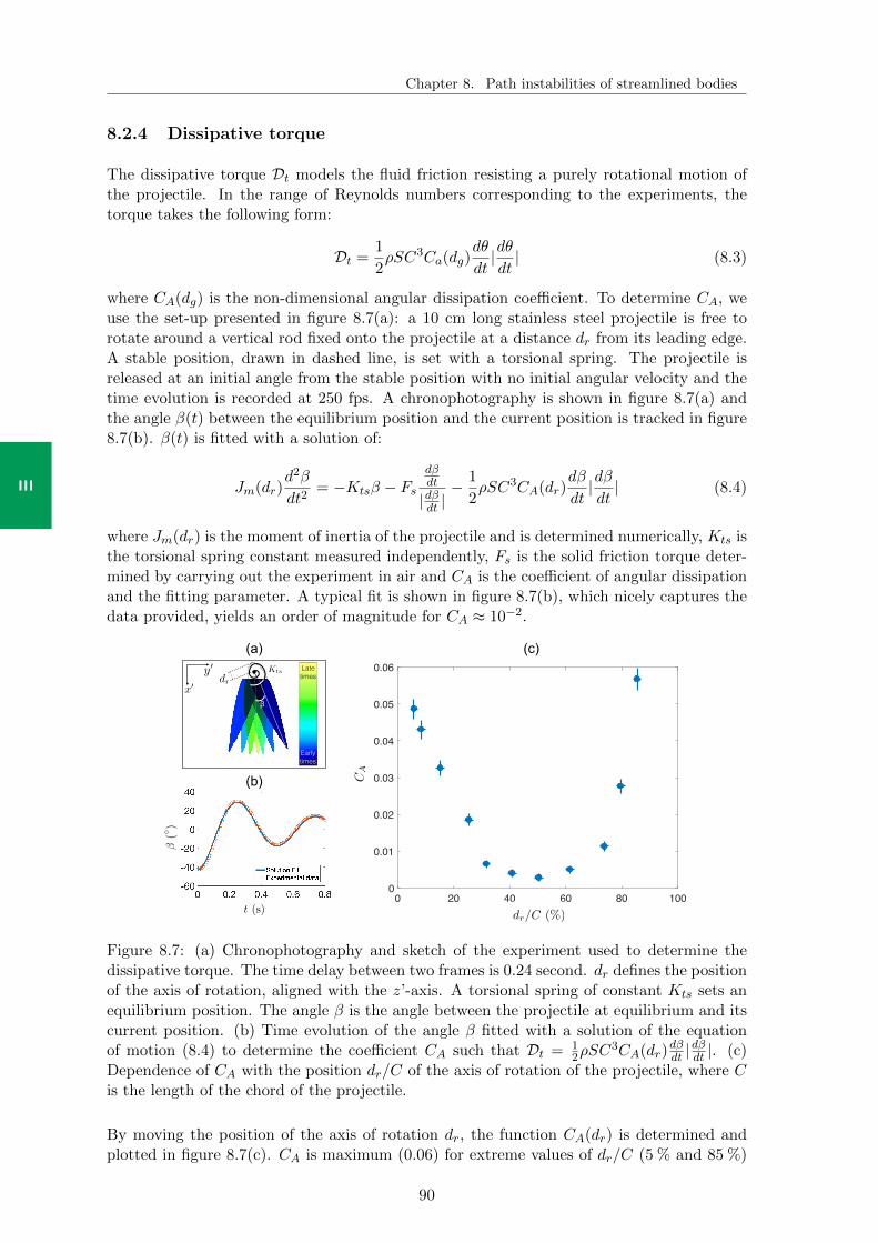
Chapter 8. Path instabilities of streamlined bodies
III
8.2.4 Dissipative torque
The dissipative torque Dt models the fluid friction resisting a purely rotational motion ofthe projectile. In the range of Reynolds numbers corresponding to the experiments, thetorque takes the following form:
Dt =1
2ρSC3Ca(dg)
dθ
dt|dθdt| (8.3)
where CA(dg) is the non-dimensional angular dissipation coefficient. To determine CA, weuse the set-up presented in figure 8.7(a): a 10 cm long stainless steel projectile is free torotate around a vertical rod fixed onto the projectile at a distance dr from its leading edge.A stable position, drawn in dashed line, is set with a torsional spring. The projectile isreleased at an initial angle from the stable position with no initial angular velocity and thetime evolution is recorded at 250 fps. A chronophotography is shown in figure 8.7(a) andthe angle β(t) between the equilibrium position and the current position is tracked in figure8.7(b). β(t) is fitted with a solution of:
Jm(dr)d2β
dt2= −Ktsβ − Fs
dβdt
|dβdt |− 1
2ρSC3CA(dr)
dβ
dt|dβdt| (8.4)
where Jm(dr) is the moment of inertia of the projectile and is determined numerically, Kts isthe torsional spring constant measured independently, Fs is the solid friction torque deter-mined by carrying out the experiment in air and CA is the coefficient of angular dissipationand the fitting parameter. A typical fit is shown in figure 8.7(b), which nicely captures thedata provided, yields an order of magnitude for CA ≈ 10−2.
0 20 40 60 80 1000
0.01
0.02
0.03
0.04
0.05
0.06
(a) (c)
β
dr
(b)
Early times
Late times
Ktsy0
x0
dr/C (%)
CA
t (s)
(
)
Figure 8.7: (a) Chronophotography and sketch of the experiment used to determine thedissipative torque. The time delay between two frames is 0.24 second. dr defines the positionof the axis of rotation, aligned with the z’-axis. A torsional spring of constant Kts sets anequilibrium position. The angle β is the angle between the projectile at equilibrium and itscurrent position. (b) Time evolution of the angle β fitted with a solution of the equationof motion (8.4) to determine the coefficient CA such that Dt = 1
2ρSC3CA(dr)
dβdt |
dβdt |. (c)
Dependence of CA with the position dr/C of the axis of rotation of the projectile, where Cis the length of the chord of the projectile.
By moving the position of the axis of rotation dr, the function CA(dr) is determined andplotted in figure 8.7(c). CA is maximum (0.06) for extreme values of dr/C (5 % and 85 %)
90
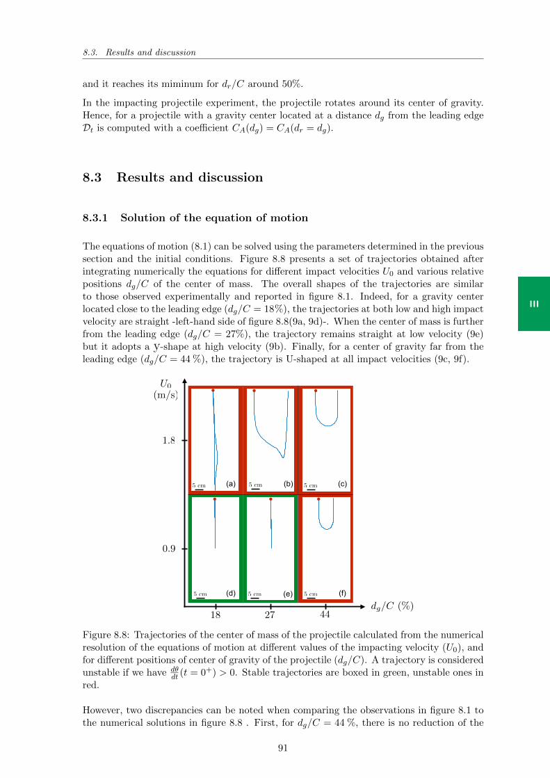
8.3. Results and discussion
III
and it reaches its miminum for dr/C around 50%.
In the impacting projectile experiment, the projectile rotates around its center of gravity.Hence, for a projectile with a gravity center located at a distance dg from the leading edgeDt is computed with a coefficient CA(dg) = CA(dr = dg).
8.3 Results and discussion
8.3.1 Solution of the equation of motion
The equations of motion (8.1) can be solved using the parameters determined in the previoussection and the initial conditions. Figure 8.8 presents a set of trajectories obtained afterintegrating numerically the equations for different impact velocities U0 and various relativepositions dg/C of the center of mass. The overall shapes of the trajectories are similarto those observed experimentally and reported in figure 8.1. Indeed, for a gravity centerlocated close to the leading edge (dg/C = 18%), the trajectories at both low and high impactvelocity are straight -left-hand side of figure 8.8(9a, 9d)-. When the center of mass is furtherfrom the leading edge (dg/C = 27%), the trajectory remains straight at low velocity (9e)but it adopts a y-shape at high velocity (9b). Finally, for a center of gravity far from theleading edge (dg/C = 44 %), the trajectory is U-shaped at all impact velocities (9c, 9f).
(a) (b) (c)
(d) (e) (f)
U0
(m/s)
dg/C (%)
1.8
0.9
18 27 44
5 cm 5 cm 5 cm
5 cm 5 cm 5 cm
Figure 8.8: Trajectories of the center of mass of the projectile calculated from the numericalresolution of the equations of motion at different values of the impacting velocity (U0), andfor different positions of center of gravity of the projectile (dg/C). A trajectory is consideredunstable if we have dθ
dt (t = 0+) > 0. Stable trajectories are boxed in green, unstable ones inred.
However, two discrepancies can be noted when comparing the observations in figure 8.1 tothe numerical solutions in figure 8.8 . First, for dg/C = 44 %, there is no reduction of the
91
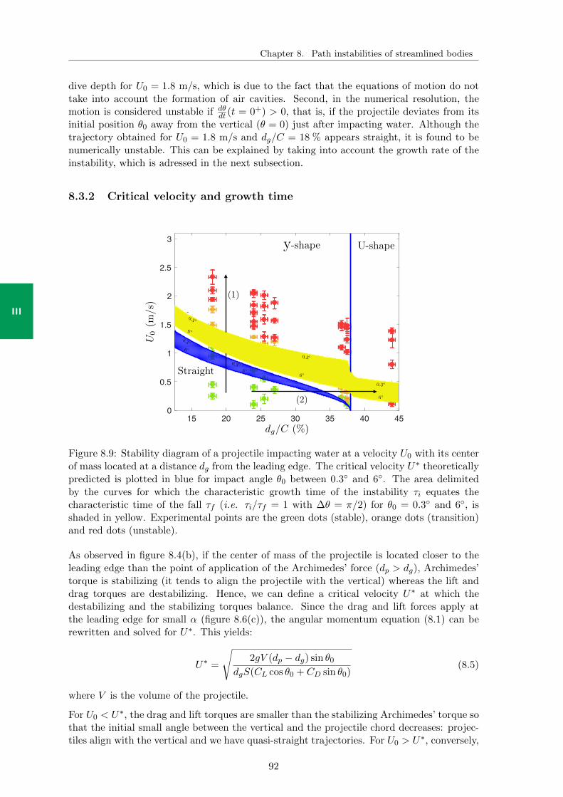
Chapter 8. Path instabilities of streamlined bodies
III
dive depth for U0 = 1.8 m/s, which is due to the fact that the equations of motion do nottake into account the formation of air cavities. Second, in the numerical resolution, themotion is considered unstable if dθ
dt (t = 0+) > 0, that is, if the projectile deviates from itsinitial position θ0 away from the vertical (θ = 0) just after impacting water. Although thetrajectory obtained for U0 = 1.8 m/s and dg/C = 18 % appears straight, it is found to benumerically unstable. This can be explained by taking into account the growth rate of theinstability, which is adressed in the next subsection.
8.3.2 Critical velocity and growth time
15 20 25 30 35 40 450
0.5
1
1.5
2
2.5
3
1
1
1
1
1
1
1
1
0.3
0.3
6
6
0.3
0.3
6
6
6
0.3
U0
(m/s
)
dg/C (%)
y-shape U-shape
Straight
(1)
(2)
Figure 8.9: Stability diagram of a projectile impacting water at a velocity U0 with its centerof mass located at a distance dg from the leading edge. The critical velocity U∗ theoreticallypredicted is plotted in blue for impact angle θ0 between 0.3 and 6. The area delimitedby the curves for which the characteristic growth time of the instability τi equates thecharacteristic time of the fall τf (i.e. τi/τf = 1 with ∆θ = π/2) for θ0 = 0.3 and 6, isshaded in yellow. Experimental points are the green dots (stable), orange dots (transition)and red dots (unstable).
As observed in figure 8.4(b), if the center of mass of the projectile is located closer to theleading edge than the point of application of the Archimedes’ force (dp > dg), Archimedes’torque is stabilizing (it tends to align the projectile with the vertical) whereas the lift anddrag torques are destabilizing. Hence, we can define a critical velocity U∗ at which thedestabilizing and the stabilizing torques balance. Since the drag and lift forces apply atthe leading edge for small α (figure 8.6(c)), the angular momentum equation (8.1) can berewritten and solved for U∗. This yields:
U∗ =
√2gV (dp − dg) sin θ0
dgS(CL cos θ0 + CD sin θ0)(8.5)
where V is the volume of the projectile.
For U0 < U∗, the drag and lift torques are smaller than the stabilizing Archimedes’ torque sothat the initial small angle between the vertical and the projectile chord decreases: projec-tiles align with the vertical and we have quasi-straight trajectories. For U0 > U∗, conversely,
92
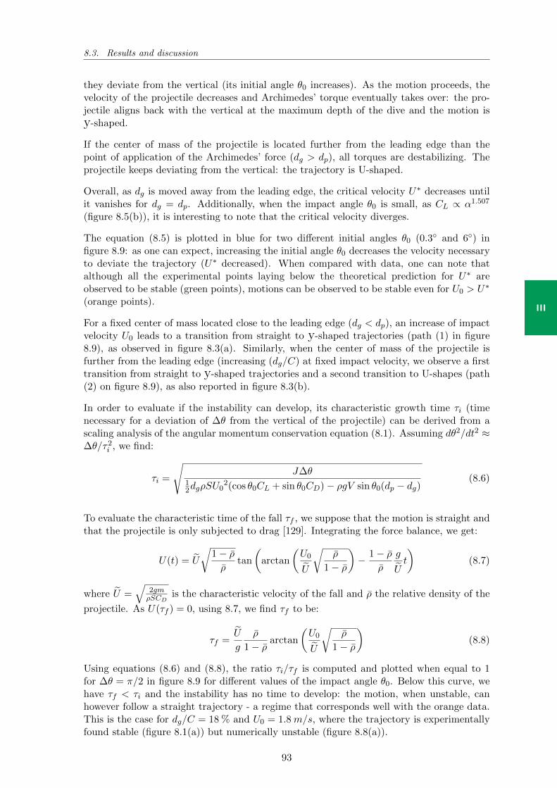
8.3. Results and discussion
III
they deviate from the vertical (its initial angle θ0 increases). As the motion proceeds, thevelocity of the projectile decreases and Archimedes’ torque eventually takes over: the pro-jectile aligns back with the vertical at the maximum depth of the dive and the motion isy-shaped.
If the center of mass of the projectile is located further from the leading edge than thepoint of application of the Archimedes’ force (dg > dp), all torques are destabilizing. Theprojectile keeps deviating from the vertical: the trajectory is U-shaped.
Overall, as dg is moved away from the leading edge, the critical velocity U∗ decreases untilit vanishes for dg = dp. Additionally, when the impact angle θ0 is small, as CL ∝ α1.507
(figure 8.5(b)), it is interesting to note that the critical velocity diverges.
The equation (8.5) is plotted in blue for two different initial angles θ0 (0.3 and 6) infigure 8.9: as one can expect, increasing the initial angle θ0 decreases the velocity necessaryto deviate the trajectory (U∗ decreased). When compared with data, one can note thatalthough all the experimental points laying below the theoretical prediction for U∗ areobserved to be stable (green points), motions can be observed to be stable even for U0 > U∗
(orange points).
For a fixed center of mass located close to the leading edge (dg < dp), an increase of impactvelocity U0 leads to a transition from straight to y-shaped trajectories (path (1) in figure8.9), as observed in figure 8.3(a). Similarly, when the center of mass of the projectile isfurther from the leading edge (increasing (dg/C) at fixed impact velocity, we observe a firsttransition from straight to y-shaped trajectories and a second transition to U-shapes (path(2) on figure 8.9), as also reported in figure 8.3(b).
In order to evaluate if the instability can develop, its characteristic growth time τi (timenecessary for a deviation of ∆θ from the vertical of the projectile) can be derived from ascaling analysis of the angular momentum conservation equation (8.1). Assuming dθ2/dt2 ≈∆θ/τ2i , we find:
τi =
√J∆θ
12dgρSU0
2(cos θ0CL + sin θ0CD)− ρgV sin θ0(dp − dg)(8.6)
To evaluate the characteristic time of the fall τf , we suppose that the motion is straight andthat the projectile is only subjected to drag [129]. Integrating the force balance, we get:
U(t) = U
√1− ρρ
tan
(arctan
(U0
U
√ρ
1− ρ
)− 1− ρ
ρ
g
Ut
)(8.7)
where U =√
2gmρSCD
is the characteristic velocity of the fall and ρ the relative density of the
projectile. As U(τf ) = 0, using 8.7, we find τf to be:
τf =U
g
ρ
1− ρ arctan
(U0
U
√ρ
1− ρ
)(8.8)
Using equations (8.6) and (8.8), the ratio τi/τf is computed and plotted when equal to 1for ∆θ = π/2 in figure 8.9 for different values of the impact angle θ0. Below this curve, wehave τf < τi and the instability has no time to develop: the motion, when unstable, canhowever follow a straight trajectory - a regime that corresponds well with the orange data.This is the case for dg/C = 18 % and U0 = 1.8m/s, where the trajectory is experimentallyfound stable (figure 8.1(a)) but numerically unstable (figure 8.8(a)).
93
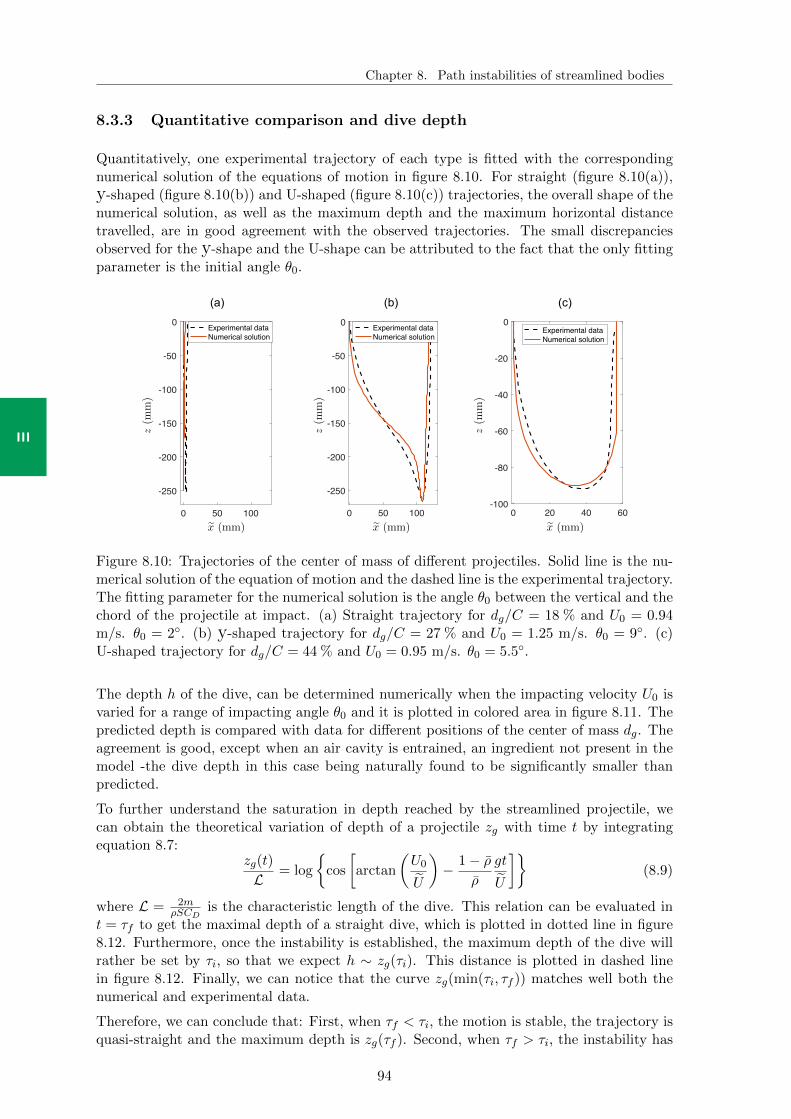
Chapter 8. Path instabilities of streamlined bodies
III
8.3.3 Quantitative comparison and dive depth
Quantitatively, one experimental trajectory of each type is fitted with the correspondingnumerical solution of the equations of motion in figure 8.10. For straight (figure 8.10(a)),y-shaped (figure 8.10(b)) and U-shaped (figure 8.10(c)) trajectories, the overall shape of thenumerical solution, as well as the maximum depth and the maximum horizontal distancetravelled, are in good agreement with the observed trajectories. The small discrepanciesobserved for the y-shape and the U-shape can be attributed to the fact that the only fittingparameter is the initial angle θ0.
0 20 40 60-100
-80
-60
-40
-20
0Experimental dataNumerical solution
0 50 100
-250
-200
-150
-100
-50
0 Experimental dataNumerical solution
(a) (b) (c)
0 50 100
-250
-200
-150
-100
-50
0 Experimental dataNumerical solution
z(m
m)
z(m
m)
z(m
m)
ex (mm) ex (mm) ex (mm)
Figure 8.10: Trajectories of the center of mass of different projectiles. Solid line is the nu-merical solution of the equation of motion and the dashed line is the experimental trajectory.The fitting parameter for the numerical solution is the angle θ0 between the vertical and thechord of the projectile at impact. (a) Straight trajectory for dg/C = 18 % and U0 = 0.94m/s. θ0 = 2. (b) y-shaped trajectory for dg/C = 27 % and U0 = 1.25 m/s. θ0 = 9. (c)U-shaped trajectory for dg/C = 44 % and U0 = 0.95 m/s. θ0 = 5.5.
The depth h of the dive, can be determined numerically when the impacting velocity U0 isvaried for a range of impacting angle θ0 and it is plotted in colored area in figure 8.11. Thepredicted depth is compared with data for different positions of the center of mass dg. Theagreement is good, except when an air cavity is entrained, an ingredient not present in themodel -the dive depth in this case being naturally found to be significantly smaller thanpredicted.
To further understand the saturation in depth reached by the streamlined projectile, wecan obtain the theoretical variation of depth of a projectile zg with time t by integratingequation 8.7:
zg(t)
L = log
cos
[arctan
(U0
U
)− 1− ρ
ρ
gt
U
](8.9)
where L = 2mρSCD
is the characteristic length of the dive. This relation can be evaluated int = τf to get the maximal depth of a straight dive, which is plotted in dotted line in figure8.12. Furthermore, once the instability is established, the maximum depth of the dive willrather be set by τi, so that we expect h ∼ zg(τi). This distance is plotted in dashed linein figure 8.12. Finally, we can notice that the curve zg(min(τi, τf )) matches well both thenumerical and experimental data.
Therefore, we can conclude that: First, when τf < τi, the motion is stable, the trajectory isquasi-straight and the maximum depth is zg(τf ). Second, when τf > τi, the instability has
94
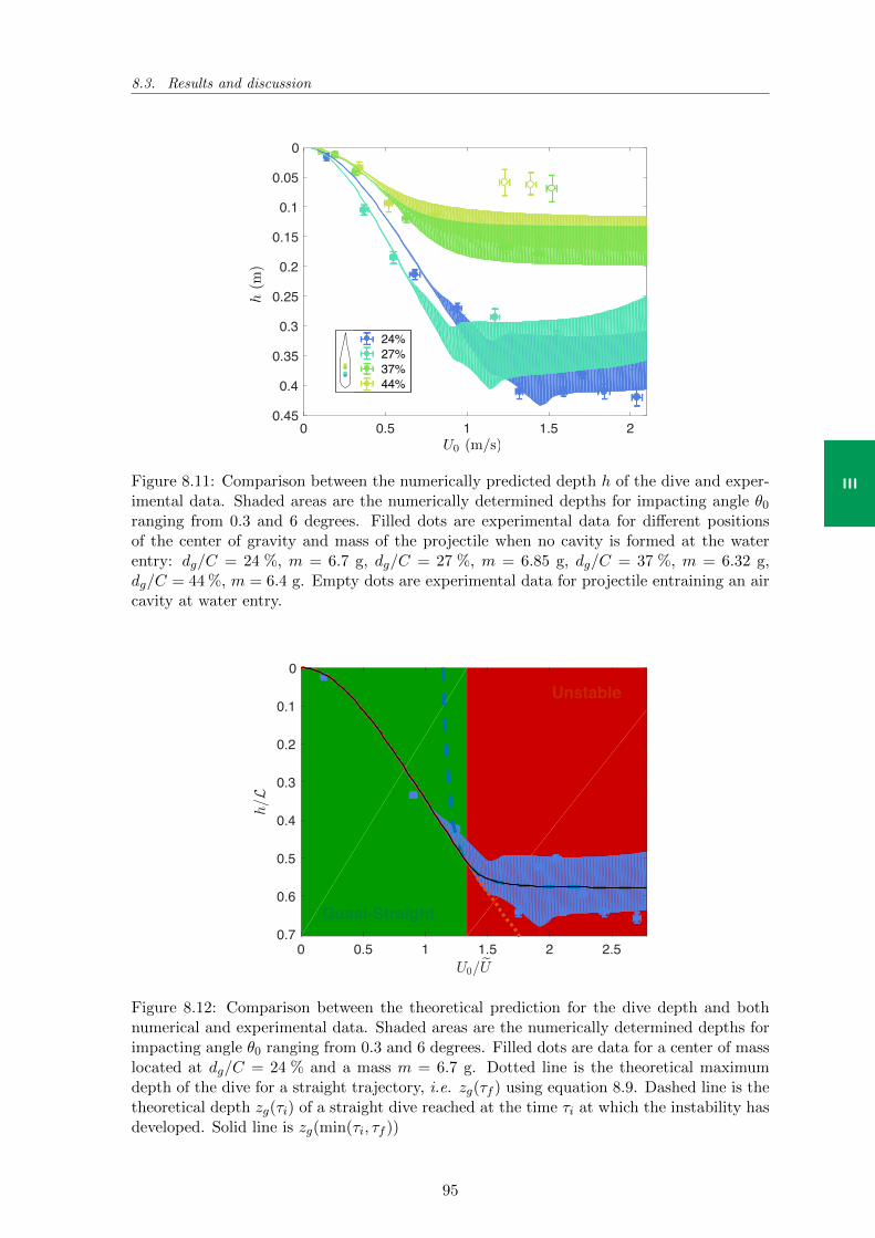
8.3. Results and discussion
III
0 0.5 1 1.5 2-0.45
-0.4
-0.35
-0.3
-0.25
-0.2
-0.15
-0.1
-0.05
0
24%27%37%44%
U0 (m/s)
h(m
)
Figure 8.11: Comparison between the numerically predicted depth h of the dive and exper-imental data. Shaded areas are the numerically determined depths for impacting angle θ0ranging from 0.3 and 6 degrees. Filled dots are experimental data for different positionsof the center of gravity and mass of the projectile when no cavity is formed at the waterentry: dg/C = 24 %, m = 6.7 g, dg/C = 27 %, m = 6.85 g, dg/C = 37 %, m = 6.32 g,dg/C = 44 %, m = 6.4 g. Empty dots are experimental data for projectile entraining an aircavity at water entry.
0 0.5 1 1.5 2 2.5-0.7
-0.6
-0.5
-0.4
-0.3
-0.2
-0.1
0
Quasi-Straight
Unstable
Figure 8.12: Comparison between the theoretical prediction for the dive depth and bothnumerical and experimental data. Shaded areas are the numerically determined depths forimpacting angle θ0 ranging from 0.3 and 6 degrees. Filled dots are data for a center of masslocated at dg/C = 24 % and a mass m = 6.7 g. Dotted line is the theoretical maximumdepth of the dive for a straight trajectory, i.e. zg(τf ) using equation 8.9. Dashed line is thetheoretical depth zg(τi) of a straight dive reached at the time τi at which the instability hasdeveloped. Solid line is zg(min(τi, τf ))
95
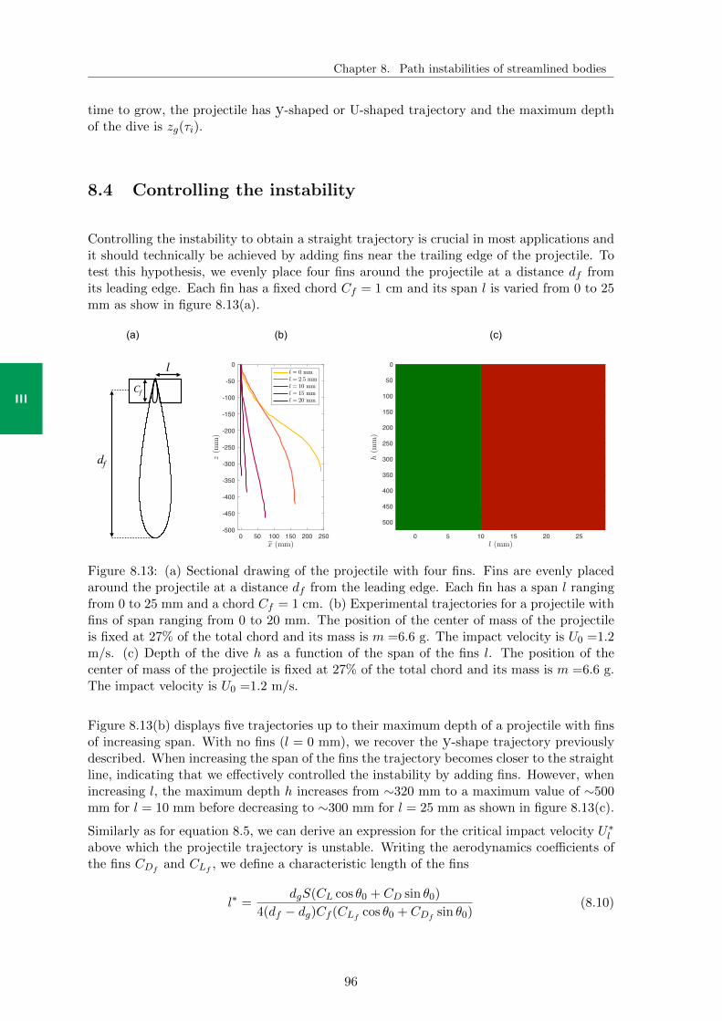
Chapter 8. Path instabilities of streamlined bodies
III
time to grow, the projectile has y-shaped or U-shaped trajectory and the maximum depthof the dive is zg(τi).
8.4 Controlling the instability
Controlling the instability to obtain a straight trajectory is crucial in most applications andit should technically be achieved by adding fins near the trailing edge of the projectile. Totest this hypothesis, we evenly place four fins around the projectile at a distance df fromits leading edge. Each fin has a fixed chord Cf = 1 cm and its span l is varied from 0 to 25mm as show in figure 8.13(a).
0 50 100 150 200 250-500
-450
-400
-350
-300
-250
-200
-150
-100
-50
0
(a) (b)
0 5 10 15 20 25
-500
-450
-400
-350
-300
-250
-200
-150
-100
-50
0
(c)
Stabilization Drag Increase
lCf
df
Figure 8.13: (a) Sectional drawing of the projectile with four fins. Fins are evenly placedaround the projectile at a distance df from the leading edge. Each fin has a span l rangingfrom 0 to 25 mm and a chord Cf = 1 cm. (b) Experimental trajectories for a projectile withfins of span ranging from 0 to 20 mm. The position of the center of mass of the projectileis fixed at 27% of the total chord and its mass is m =6.6 g. The impact velocity is U0 =1.2m/s. (c) Depth of the dive h as a function of the span of the fins l. The position of thecenter of mass of the projectile is fixed at 27% of the total chord and its mass is m =6.6 g.The impact velocity is U0 =1.2 m/s.
Figure 8.13(b) displays five trajectories up to their maximum depth of a projectile with finsof increasing span. With no fins (l = 0 mm), we recover the y-shape trajectory previouslydescribed. When increasing the span of the fins the trajectory becomes closer to the straightline, indicating that we effectively controlled the instability by adding fins. However, whenincreasing l, the maximum depth h increases from ∼320 mm to a maximum value of ∼500mm for l = 10 mm before decreasing to ∼300 mm for l = 25 mm as shown in figure 8.13(c).
Similarly as for equation 8.5, we can derive an expression for the critical impact velocity U∗labove which the projectile trajectory is unstable. Writing the aerodynamics coefficients ofthe fins CDf
and CLf, we define a characteristic length of the fins
l∗ =dgS(CL cos θ0 + CD sin θ0)
4(df − dg)Cf (CLfcos θ0 + CDf
sin θ0)(8.10)
96
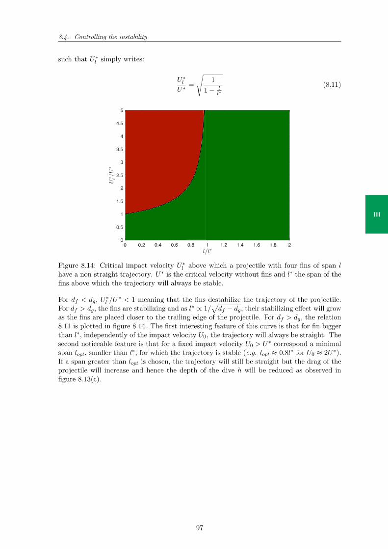
8.4. Controlling the instability
III
such that U∗l simply writes:
U∗lU∗
=
√1
1− ll∗
(8.11)
0 0.2 0.4 0.6 0.8 1 1.2 1.4 1.6 1.8 20
0.5
1
1.5
2
2.5
3
3.5
4
4.5
5
StableUnstable
Figure 8.14: Critical impact velocity U∗l above which a projectile with four fins of span lhave a non-straight trajectory. U∗ is the critical velocity without fins and l∗ the span of thefins above which the trajectory will always be stable.
For df < dg, U∗l /U
∗ < 1 meaning that the fins destabilize the trajectory of the projectile.For df > dg, the fins are stabilizing and as l∗ ∝ 1/
√df − dg, their stabilizing effect will grow
as the fins are placed closer to the trailing edge of the projectile. For df > dg, the relation8.11 is plotted in figure 8.14. The first interesting feature of this curve is that for fin biggerthan l∗, independently of the impact velocity U0, the trajectory will always be straight. Thesecond noticeable feature is that for a fixed impact velocity U0 > U∗ correspond a minimalspan lopt, smaller than l∗, for which the trajectory is stable (e.g. lopt ≈ 0.8l∗ for U0 ≈ 2U∗).If a span greater than lopt is chosen, the trajectory will still be straight but the drag of theprojectile will increase and hence the depth of the dive h will be reduced as observed infigure 8.13(c).
97
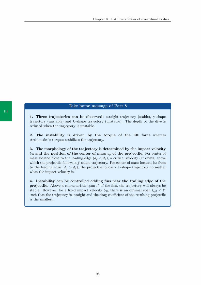
Chapter 8. Path instabilities of streamlined bodies
III
Take home message of Part 8
1. Three trajectories can be observed: straight trajectory (stable), y-shapetrajectory (unstable) and U-shape trajectory (unstable). The depth of the dive isreduced when the trajectory is unstable.
2. The instability is driven by the torque of the lift force whereasArchimedes’s torques stabilizes the trajectory.
3. The morphology of the trajectory is determined by the impact velocityU0 and the position of the center of mass dg of the projectile. For center ofmass located close to the leading edge (dg < dp), a critical velocity U∗ exists, abovewhich the projectile follows a y-shape trajectory. For center of mass located far fromto the leading edge (dg > dp), the projectile follow a U-shape trajectory no matterwhat the impact velocity is.
4. Instability can be controlled adding fins near the trailing edge of theprojectile. Above a characteristic span l∗ of the fins, the trajectory will always bestable. However, for a fixed impact velocity U0, there is an optimal span lopt < l∗
such that the trajectory is straight and the drag coefficient of the resulting projectileis the smallest.
98

CONCLUSION
99

Con
In this thesis we address the question of how cavitation can turn a bluff body into a stablestreamlined projectile. In particular, we wish to determine if cavitation alone could makea submarine travelling at 100 m/s possible. A body moving underwater is surrounded by aregion of low pressure in its wake. If the projectile is travelling fast enough, the pressure dropcan trigger cavitation, that is, the phase change of the liquid to gas. A further increase ofthe projectile velocity eventually leads to the formation of a large gas bubble: the so-calledsupercavitation regime. This bubble induces a modification of the drag of the projectilewhich, under certain circumstances, makes it analogous to a streamlined projectile. Toinvestigate this phenomenon, we first report, in Part I, the study of the initial growth of acavitation bubble. We then concentrate, in Part II, on measuring the drag reduction thatcan be achieved with supercavitation and we finally derive, in Part III, the conditions for astreamlined projectile to have a straight trajectory.
Cavitation bubble dynamics is an experimentally difficult problem to address if thepressure drop is only generated by a steady velocity: this is due to the fact that velocitiesneeded for cavitation bubbles nucleation are typically larger than 20 m/s at atmosphericpressure. However, cavitation of a fluid can easily be observed when the fluid is accelerated.Simply impacting a container filled with water with a hammer can trigger pressure dropof several bars. In Part I, we used this phenomenon to study the growth of a cavitationbubble in a transient pressure field. A short review of previous work on this topic is madein Chapter 1. To address this question, we built a drop-tower, described in Chapter 2,which allowed us to have reproducible impacts of high acceleration on a water container.We showed theoretically and experimentally that a pressure drop is indeed generated inthe area opposite to the point of impact and that its magnitude is proportional to boththe size of the container and the acceleration of the tank. This pressure drop eventuallytriggers the phase transition of the liquid water into gas. In Chapter 3, we showed that theradius of the cavitation bubble created has a dynamical evolution which follows the classicalRayleigh-Plesset equation. As the pressure drop is transient, the bubble rapidly collapses:we observed bubbles which typically had a life expectancy of a few tens of milliseconds andreached centimetric maximum radius. The collapse of the bubbles is a fast process whichhas been shown to be responsible for damages on nearby surfaces: for instance, it is knownto be the main mechanism involved in boat propellers aging. The energy released throughthis process can be directly linked to the maximum radius of the bubble. We analyticallyderived an expression for the the value of the maximum radius of a bubble in a transientpressure drop. The whole study can be used to improve the understanding of material aginginduced by cavitation but also to investigate the causes of traumatic brain injuries, alsoknown as brain concussion in sports. Indeed, the container filled of water is analogous ofa cranial vault and the shock we imposed is similar to the impact that could be receivedduring boxing. We showed in Chapter 3 that we can predict the damaging potential of acavitation bubble in the head and that it is in a good agreement with the heuristic medicalobservations. These results prove that cavitation is a relevant mechanism to consider forbrain concussion and they are encouraging as they could lead to an improved detection andprevention of the brain concussion. However, a lot of questions are still open and needto be tackled to prove the implication of cavitation in the damaging process of the brain.Experimentally, it would be interesting to evaluate the damaging potential of a bubble ona material similar to the brain. For instance, this material could be a cell layer, a brainslice or a polymer of the same mechanical properties. Theoretically, the influence of theconfinement of the bubble on its dynamic is yet to be determined: as an incompressible flowin a planar geometry does not vanish at infinity, the time evolution of the bubble radiuscannot be derived from Rayleigh-Plesset equation. Finally, in-situ recording of cavitationbubbles would definitely prove that the phenomenon should be taken into account in thebrain damage process. To do so, one could identify the noise generated by the collapse
101
Con
of a cavitation bubble following a shock on the head of a boxer or rugby player. Thesame process was recently used to identify cavitation as the mechanism of knuckle cracking[69]. Finally, this work on cavitation under acceleration in confined environments opens theperspective of a new way to generate the phase transition, which could facilitate the entryin the supercavitation regime. This work could directly be applied to model the launchof fast travelling objects underwater, for instance torpedoes, which begin their trajectoriesaccelerating in a confined environment.
Drag modification in the supercavitation regime can be evaluated in a standardhydrodynamic tunnel replacing the vapor production due to cavitation by an artificial airinjection. The cavity created is referred as a ventilated cavity. In Part II, we investigate themodification of the drag induced by a ventilated cavity behind a sphere near its drag crisis.In chapter 4, we briefly reviewed the literature on this subject. To tackle this problem, wedeveloped a hydrodynamic tunnel, presented in Chapter 5, that allows us to measure thedrag on a sphere while injecting air at a constant rate in its wake. Additionally, we usedspheres of different roughness to study the influence of the ventilated cavity on the dragcrisis. We showed in Chapter 6 that the dimensions of the bubble created are uniquelydetermined by the dimensionless air injection rate. This number compare the volumetric airinjection rate to the volumetric water flow rate based on the frontal area of the projectile.In particular, for high dimensionless air injection rate (> 0.04), a unique bubble was foundto pin at the equatorial plane of the sphere. This bubble is nearly cylindrical and its lengthwas measured to be proportional to the dimensionless air injection rate. This behaviourwas shown to be caused by the growth of perturbation at the interface of the bubble. Wealso measured the drag of the resulting system: in the high dimensionless air injection rateregime (> 0.04), we found that the drag was proportional to the dimensionless injection rateto the power (−1/3). As a consequence, we could measure drag reductions up to a factor50% in our experimental configuration for the largest bubbles. This result also suggeststhat we could reach even higher drag reductions by increasing the air injection. However,we also showed that the air injection in the vicinity of the projectile does not always lead toa drag reduction. In particular, when the water flow around the sphere is supercritical (atReynolds number above 106 for a smooth sphere), the wake of the sphere is thin and theboundary layer detaches near the back of the sphere. Injecting air at the back of the spherein this regime results in a perturbation of the supercritical wake leading to a drag increase(up to a factor 5). While the results presented in Chapter 6 suggest that a submarine, evenin the supercavitation regime, could not reach 100 m/s, several open questions should beaddressed before ruling out this possibility. Theoretically, most previous work to predict thedrag of supercavitating bodies are based on the potential flow theory and cannot account forthe complexity of the drag crisis. The complexity of the interactions of the injected air withthe wake could be approached using numerical models. Experimentally, it was shown, in adifferent system, that drag coefficient of a sphere with a gas bubble in its wake could be aslow as 0.05 [92]. To achieve this ground breaking value, our experimental set-up should beimproved to limit the growth of perturbations at the interface of the bubble. The resultingbubble pinch off at a stable point. Among all the possible improvements, we identified themost important as: the reduction of the turbulence of the water flow, the limitation of theinfluence of the holder on the flow around the sphere and the use of smooth spheres to avoidconstraining the pinning point of the bubble.
Stability of the trajectory of a streamlined body is crucial to predict the final des-tination of the projectile. We showed, using air injection, that a supercavitating projectilecan reach drag coefficients as low as the one measured for streamlined bodies. To study thetrajectories of such projectiles, we simplified this system, in Part III to a floating streamlinedprojectile with an inhomogeneous mass distribution. We focused on the trajectory of suchprojectiles following an impact on water. To do so, in chapter 7, we briefly reviewed the
102
Con
available literature and presented the experimental set-up we developed to impact projectilesat variable and nearly vertical velocity on water. We demonstrated both theoretically andexperimentally in Chapter 8 that three families of underwater trajectories could be observed:straight, U-shaped, y-shaped. Although only the first type of trajectory was considered sta-ble, all families share the same overall behaviour: the projectile slows down after its impact,reaches a maximum depth and then moves back to the surface. The instability which re-sults in the U-shaped and y-shaped trajectory is driven by the torque of the lift force on theprojectile while Archimedes’s torque stabilizes the trajectory. As a consequence, for a givenshape of the projectile, the transition between the stable and the unstable regime dependson the position of the center of mass of the projectile and its impact velocity. Hence, for acenter of mass located near the leading edge, the projectile is stable for an impact velocitybelow a critical velocity. Above this velocity, the trajectory was observed to be y-shaped.For a center of mass located far from the leading edge, the trajectory will always be unstableand U-shaped. After measuring in separated experimental set-up the different aerodynamicproperties of the projectile (aerodynamic coefficients, position of the aerodynamic center),we were able to analytically predict the shape of the trajectory and the maximum depth ofthe dive, which was found to be reduced when the trajectory is unstable. Further takinginto account the growth time of the instability, we were able to capture the experimental ob-servations of the transition between the different families of trajectories. Finally, we showedthat the stability of the trajectory can be ensured by adding fins near the trailing edge ofthe projectile. Such fins can be design to unsure stability either up to a certain velocity orfor all impact velocity. In the latter case, large fins are used which results in a increase ofthe drag and a reduction of the depth of the dive. Even though we propose, in Part III,several techniques to unsure stability, it does not provide any explanation on how gannets,or other diving birds, control this instability and can reach their target. Our hypothesis, isthat gannets dive with a horizontal component of the velocity. In this manner, they imposethe plane of instability and they can prevent the instability from growing only with theirfeet, which act as unidirectional fins. This hypothesis should be tested with projectile im-pacting water with an initial horizontal velocity equipped with unidirectional fins. Finally,we could get back to the initial system of a bubble pinned to a projectile, which raise twoquestions: What is the dynamic of the bubble when it is not aligned with the flow? Can thebubble exert a torque on the projectile? These questions remain open and would necessitaterethinking both experimental set-up presented in Part II and III to be tackled.
103

Apx
104

APPENDICES
105


AList of publication
The Path Instabilities of Streamlined Bodies, T. Guillet, M. Coux, D. Quere and C. Clanet,Journal of Fluid Mechanics 864 (2019): 286-302.
Analytical criterion for traumatic brain injuries, T. Guillet, J. Amauger, P. Decq, D. Quere,C. Cohen and C. Clanet (submitted).
Drag modification induced by a ventilated cavity near the drag crisis of a sphere, T. Guillet,D. Quere, C. Cohen and C. Clanet (in preparation).
Critical density for the stability of a 2D magnet array, C. Reiss, F. Bastit, D. Sulem, A.Bacot, L. Cousin, P. Goux and T. Guillet, Emergent Scientist 2 (2018).
From the microstructure of steels to the explosion of sparks, A. Guillen, F. Goh, J. Andre,A. Barral, C. Brochet, Q. Louis and T. Guillet, Emergent Scientist 3 (2019).
Motion of rain drops on a car side window, J. Andre, C. Brochet, Q. Louis, A. Barral,A. Guillen, F. Goh, A. Prieto and T. Guillet, Emergent Scientist 3 (2019).
Sound of a nut rolling inside an elastic rubber balloon, A. Barral, Q. Louis, C. Brochet,J. Andre, A. Guillen, F. Goh, A. Prieto and T. Guillet, Emergent Scientist 3 (2019).
107

Appendix A. List of publication
Apx
108
BInternational Physicists’
Tournament
I had the chance to be Team Leader for the team representing Ecole polytechnique at theInternational Physicists’ Tournament. To prepare for the tournament, a team of 6 studentshave to work on 13 to 17 physics research problems for 8 months. The problems cover awide range of different topics from fluid mechanics to electromagnetism and always havean experimental component. During the tournament, the students have to present theirsolution and debate on how it could be improved with other teams. I followed three groupsover my PhD and they ended up at the third position in 2017, the second position in 2018and first in 2019: one could say that it is moment to retire!
After the tournament, we also encouraged students to have their first experience on peer-reviewed publishing: some of their work has been published in Emergent Scientist. Thisappendix present an example of such article entitled ”Sound of a nut rolling inside an elasticrubber balloon”.
109
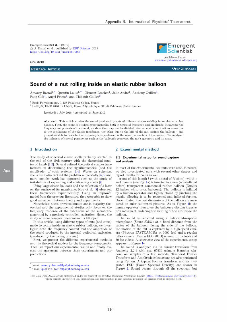
Emergent Scientist 3, 6 (2019)c© A. Barral et al., published by EDP Sciences, 2019https://doi.org/10.1051/emsci/2019005
Available online at:www.emergent-scientist.edp-open.orgIPT 2018
RESEARCH ARTICLE
Sound of a nut rolling inside an elastic rubber balloonAmaury Barral1,*, Quentin Louis1,**, Clement Brochet1, Julie Andre1, Anthony Guillen1,Fang Goh1, Angel Prieto1, and Thibault Guillet2
1 Ecole Polytechnique, 91128 Palaiseau Cedex, France2 LadHyX, UMR 7646 du CNRS, Ecole Polytechnique, 91128 Palaiseau Cedex, France
Received: 4 July 2018 / Accepted: 14 June 2019
Abstract. This article studies the sound produced by nuts of different shapes swirling in an elastic rubberballoon. First, the sound is studied experimentally, both in terms of frequency and amplitude. Regarding thefrequency components of the sound, we show that they can be divided into two main contributions – one dueto the oscillations of the elastic membrane, the other due to the hits of the nut against the balloon – andpresent models to describe the frequency’s dependence on the main parameters of the system. We analysedthe influence of several parameters such as the balloon’s geometry, the nut’s geometry and its mass.
1 Introduction
The study of spherical elastic shells probably started atthe end of the 19th century with the theoretical stud-ies of Lamb [1,2]. Several refined theoretical studies havefocused on determining the eigenfrequencies (and theamplitude) of such systems [3,4]. Works on sphericalshells have also tackled the problem numerically [5,6] andmore complex work has appeared such as the study ofinstabilities of expanding and contracting shells [7].Using large elastic balloons and the reflection of a laser
on the surface of its membrane, Kuo et al. [8] observedthese frequencies experimentally. Using an improvedmodel from the previous literature, they were able to showgood agreement between theory and experiments.Nonetheless these previous studies are in majority the-
oretical and the experimental studies only focus on thefrequency response of the vibrations of the membranegenerated by a precisely controlled excitation. Hence, thestudy of more complex phenomenon is left open.In this article, using different types of nuts (and coins)
made to rotate inside an elastic rubber balloon, we inves-tigate both the frequency content and the amplitude ofthe sound produced by the internal periodical excitation(produced by the rolling of a nut).First, we present the different experimental methods
and the theoretical models for the frequency components.Then, we report our experimental results and finally dis-cuss the agreement between those experiments and ourpredictions.
* e-mail: [email protected]** e-mail: [email protected]
2 Experimental method
2.1 Experimental setup for sound captureand analysis
In most of the experiments, hex nuts were used. However,we also investigated nuts with several other shapes andreport results for coins as well.A nut of side length l (with a total of N sides), width e
and massm (see Fig. 1a) is inserted in a new (non-inflatedbefore) transparent commercial rubber balloon (Nuolux12 inches white latex balloons). The balloon is inflatedby a human operator and tightly closed by pinching thenozzle, allowing it to be reopened and inflated further.Once inflated, the new dimensions of the balloon are mea-sured on ruler-calibrated pictures. As in Figure 1b thehuman operator then gives the balloon a circular transla-tion movement, inducing the swirling of the nut inside theballoon.The sound is recorded using a calibrated-response
microphone (Shure SM57) at a fixed distance from thecenter of the balloon, facing the side of the balloon,the motion of the nut is captured by a high-speed cam-era (Photron FASTCAM SA at 3000 fps) and a regularreflex camera (Canon EOS 700D) is used for pictures and30 fps videos. A schematic view of the experimental setupappears in Figure 1c.The sound is analysed via its Fourier transform from
Audacity 2.2.1 with size 65536 using a Hanning win-dow, on samples of a few seconds. Temporal FourierTransform and Amplitude calculations are also performedusing Python. A typical Fourier transform and its inte-grated PSD (Power Spectral Density) are shown inFigure 2. Sound occurs through all the spectrum but
This is an Open Access article distributed under the terms of the Creative Commons Attribution License (http://creativecommons.org/licenses/by/4.0),which permits unrestricted use, distribution, and reproduction in any medium, provided the original work is properly cited.
Appendix B. International Physicists’ Tournament
Apx
110
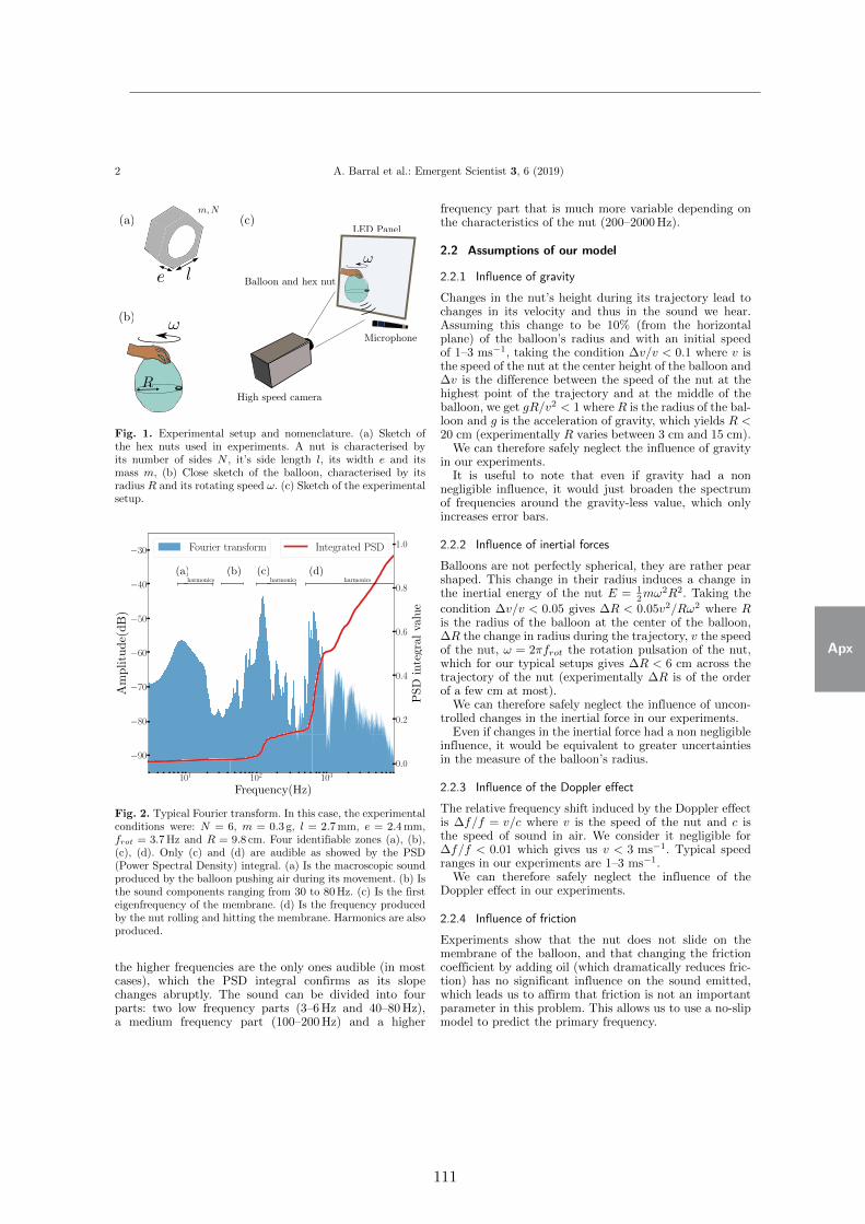
2 A. Barral et al.: Emergent Scientist 3, 6 (2019)
Fig. 1. Experimental setup and nomenclature. (a) Sketch ofthe hex nuts used in experiments. A nut is characterised byits number of sides N , it’s side length l, its width e and itsmass m, (b) Close sketch of the balloon, characterised by itsradius R and its rotating speed ω. (c) Sketch of the experimentalsetup.
Fig. 2. Typical Fourier transform. In this case, the experimentalconditions were: N = 6, m = 0.3 g, l = 2.7mm, e = 2.4mm,frot = 3.7Hz and R = 9.8 cm. Four identifiable zones (a), (b),(c), (d). Only (c) and (d) are audible as showed by the PSD(Power Spectral Density) integral. (a) Is the macroscopic soundproduced by the balloon pushing air during its movement. (b) Isthe sound components ranging from 30 to 80Hz. (c) Is the firsteigenfrequency of the membrane. (d) Is the frequency producedby the nut rolling and hitting the membrane. Harmonics are alsoproduced.
the higher frequencies are the only ones audible (in mostcases), which the PSD integral confirms as its slopechanges abruptly. The sound can be divided into fourparts: two low frequency parts (3–6Hz and 40–80Hz),a medium frequency part (100–200Hz) and a higher
frequency part that is much more variable depending onthe characteristics of the nut (200–2000Hz).
2.2 Assumptions of our model
2.2.1 Influence of gravity
Changes in the nut’s height during its trajectory lead tochanges in its velocity and thus in the sound we hear.Assuming this change to be 10% (from the horizontalplane) of the balloon’s radius and with an initial speedof 1–3 ms−1, taking the condition ∆v/v < 0.1 where v isthe speed of the nut at the center height of the balloon and∆v is the difference between the speed of the nut at thehighest point of the trajectory and at the middle of theballoon, we get gR/v2 < 1 where R is the radius of the bal-loon and g is the acceleration of gravity, which yields R <20 cm (experimentally R varies between 3 cm and 15 cm).We can therefore safely neglect the influence of gravity
in our experiments.It is useful to note that even if gravity had a non
negligible influence, it would just broaden the spectrumof frequencies around the gravity-less value, which onlyincreases error bars.
2.2.2 Influence of inertial forces
Balloons are not perfectly spherical, they are rather pearshaped. This change in their radius induces a change inthe inertial energy of the nut E = 1
2mω2R2. Taking the
condition ∆v/v < 0.05 gives ∆R < 0.05v2/Rω2 where Ris the radius of the balloon at the center of the balloon,∆R the change in radius during the trajectory, v the speedof the nut, ω = 2πfrot the rotation pulsation of the nut,which for our typical setups gives ∆R < 6 cm across thetrajectory of the nut (experimentally ∆R is of the orderof a few cm at most).We can therefore safely neglect the influence of uncon-
trolled changes in the inertial force in our experiments.Even if changes in the inertial force had a non negligible
influence, it would be equivalent to greater uncertaintiesin the measure of the balloon’s radius.
2.2.3 Influence of the Doppler effect
The relative frequency shift induced by the Doppler effectis ∆f/f = v/c where v is the speed of the nut and c isthe speed of sound in air. We consider it negligible for∆f/f < 0.01 which gives us v < 3 ms−1. Typical speedranges in our experiments are 1–3 ms−1.We can therefore safely neglect the influence of the
Doppler effect in our experiments.
2.2.4 Influence of friction
Experiments show that the nut does not slide on themembrane of the balloon, and that changing the frictioncoefficient by adding oil (which dramatically reduces fric-tion) has no significant influence on the sound emitted,which leads us to affirm that friction is not an importantparameter in this problem. This allows us to use a no-slipmodel to predict the primary frequency.
Apx
111
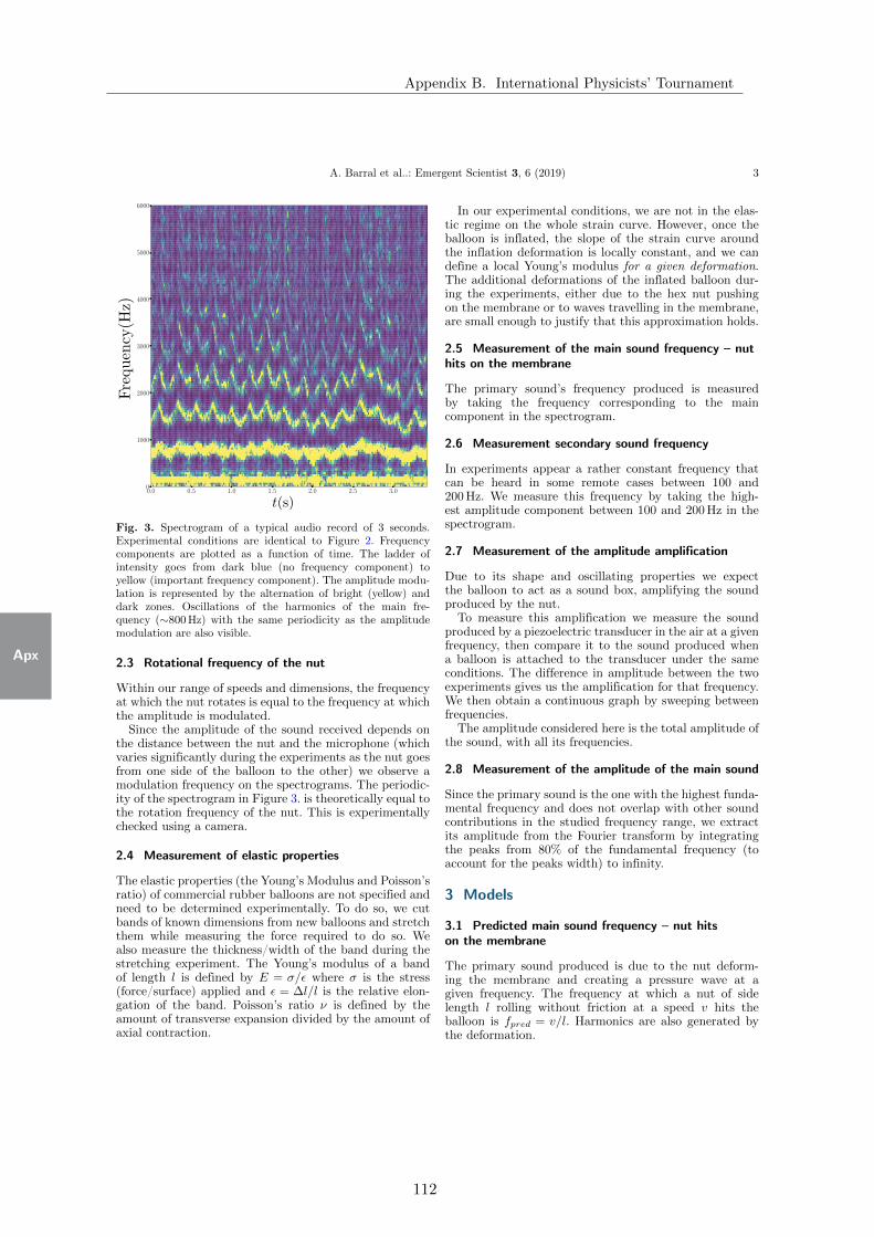
A. Barral et al..: Emergent Scientist 3, 6 (2019) 3
Fig. 3. Spectrogram of a typical audio record of 3 seconds.Experimental conditions are identical to Figure 2. Frequencycomponents are plotted as a function of time. The ladder ofintensity goes from dark blue (no frequency component) toyellow (important frequency component). The amplitude modu-lation is represented by the alternation of bright (yellow) anddark zones. Oscillations of the harmonics of the main fre-quency (∼800Hz) with the same periodicity as the amplitudemodulation are also visible.
2.3 Rotational frequency of the nut
Within our range of speeds and dimensions, the frequencyat which the nut rotates is equal to the frequency at whichthe amplitude is modulated.Since the amplitude of the sound received depends on
the distance between the nut and the microphone (whichvaries significantly during the experiments as the nut goesfrom one side of the balloon to the other) we observe amodulation frequency on the spectrograms. The periodic-ity of the spectrogram in Figure 3. is theoretically equal tothe rotation frequency of the nut. This is experimentallychecked using a camera.
2.4 Measurement of elastic properties
The elastic properties (the Young’s Modulus and Poisson’sratio) of commercial rubber balloons are not specified andneed to be determined experimentally. To do so, we cutbands of known dimensions from new balloons and stretchthem while measuring the force required to do so. Wealso measure the thickness/width of the band during thestretching experiment. The Young’s modulus of a bandof length l is defined by E = σ/ε where σ is the stress(force/surface) applied and ε = ∆l/l is the relative elon-gation of the band. Poisson’s ratio ν is defined by theamount of transverse expansion divided by the amount ofaxial contraction.
In our experimental conditions, we are not in the elas-tic regime on the whole strain curve. However, once theballoon is inflated, the slope of the strain curve aroundthe inflation deformation is locally constant, and we candefine a local Young’s modulus for a given deformation.The additional deformations of the inflated balloon dur-ing the experiments, either due to the hex nut pushingon the membrane or to waves travelling in the membrane,are small enough to justify that this approximation holds.
2.5 Measurement of the main sound frequency – nuthits on the membrane
The primary sound’s frequency produced is measuredby taking the frequency corresponding to the maincomponent in the spectrogram.
2.6 Measurement secondary sound frequency
In experiments appear a rather constant frequency thatcan be heard in some remote cases between 100 and200Hz. We measure this frequency by taking the high-est amplitude component between 100 and 200Hz in thespectrogram.
2.7 Measurement of the amplitude amplification
Due to its shape and oscillating properties we expectthe balloon to act as a sound box, amplifying the soundproduced by the nut.To measure this amplification we measure the sound
produced by a piezoelectric transducer in the air at a givenfrequency, then compare it to the sound produced whena balloon is attached to the transducer under the sameconditions. The difference in amplitude between the twoexperiments gives us the amplification for that frequency.We then obtain a continuous graph by sweeping betweenfrequencies.The amplitude considered here is the total amplitude of
the sound, with all its frequencies.
2.8 Measurement of the amplitude of the main sound
Since the primary sound is the one with the highest funda-mental frequency and does not overlap with other soundcontributions in the studied frequency range, we extractits amplitude from the Fourier transform by integratingthe peaks from 80% of the fundamental frequency (toaccount for the peaks width) to infinity.
3 Models
3.1 Predicted main sound frequency – nut hitson the membrane
The primary sound produced is due to the nut deform-ing the membrane and creating a pressure wave at agiven frequency. The frequency at which a nut of sidelength l rolling without friction at a speed v hits theballoon is fpred = v/l. Harmonics are also generated bythe deformation.
Appendix B. International Physicists’ Tournament
Apx
112
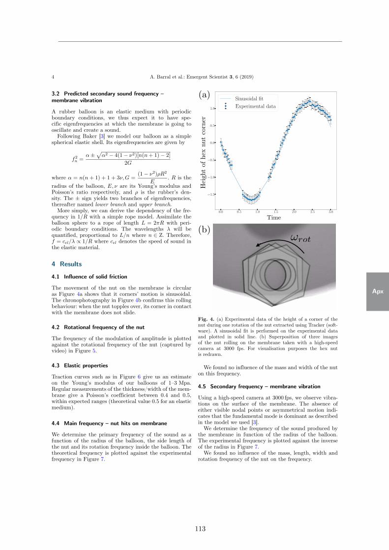
4 A. Barral et al.: Emergent Scientist 3, 6 (2019)
3.2 Predicted secondary sound frequency –membrane vibration
A rubber balloon is an elastic medium with periodicboundary conditions, we thus expect it to have spe-cific eigenfrequencies at which the membrane is going tooscillate and create a sound.Following Baker [3] we model our balloon as a simple
spherical elastic shell. Its eigenfrequencies are given by
f2n =α±
√α2 − 4(1− ν2)[n(n+ 1)− 2]
2G
where α = n(n + 1) + 1 + 3ν,G =(1− ν2)ρR2
E. R is the
radius of the balloon, E, ν are its Young’s modulus andPoisson’s ratio respectively, and ρ is the rubber’s den-sity. The ± sign yields two branches of eigenfrequencies,thereafter named lower branch and upper branch.More simply, we can derive the dependency of the fre-
quency in 1/R with a simple rope model. Assimilate theballoon sphere to a rope of length L = 2πR with peri-odic boundary conditions. The wavelengths λ will bequantified, proportional to L/n where n ∈ Z. Therefore,f = cel/λ ∝ 1/R where cel denotes the speed of sound inthe elastic material.
4 Results
4.1 Influence of solid friction
The movement of the nut on the membrane is circularas Figure 4a shows that it corners’ motion is sinusoidal.The chronophotography in Figure 4b confirms this rollingbehaviour: when the nut topples over, its corner in contactwith the membrane does not slide.
4.2 Rotational frequency of the nut
The frequency of the modulation of amplitude is plottedagainst the rotational frequency of the nut (captured byvideo) in Figure 5.
4.3 Elastic properties
Traction curves such as in Figure 6 give us an estimateon the Young’s modulus of our balloons of 1–3 Mpa.Regular measurements of the thickness/width of the mem-brane give a Poisson’s coefficient between 0.4 and 0.5,within expected ranges (theoretical value 0.5 for an elasticmedium).
4.4 Main frequency – nut hits on membrane
We determine the primary frequency of the sound as afunction of the radius of the balloon, the side length ofthe nut and its rotation frequency inside the balloon. Thetheoretical frequency is plotted against the experimentalfrequency in Figure 7.
Fig. 4. (a) Experimental data of the height of a corner of thenut during one rotation of the nut extracted using Tracker (soft-ware). A sinusoidal fit is performed on the experimental dataand plotted in solid line. (b) Superposition of three imagesof the nut rolling on the membrane taken with a high-speedcamera at 3000 fps. For visualisation purposes the hex nutis redrawn.
We found no influence of the mass and width of the nuton this frequency.
4.5 Secondary frequency – membrane vibration
Using a high-speed camera at 3000 fps, we observe vibra-tions on the surface of the membrane. The absence ofeither visible nodal points or asymmetrical motion indi-cates that the fundamental mode is dominant as describedin the model we used [3].We determine the frequency of the sound produced by
the membrane in function of the radius of the balloon.The experimental frequency is plotted against the inverseof the radius in Figure 7.We found no influence of the mass, length, width and
rotation frequency of the nut on the frequency.
Apx
113
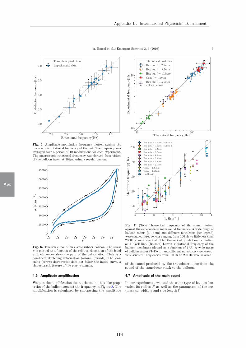
A. Barral et al..: Emergent Scientist 3, 6 (2019) 5
Fig. 5. Amplitude modulation frequency plotted against themacroscopic rotational frequency of the nut. The frequency wasaveraged over a period of 10 modulations for each experiment.The macroscopic rotational frequency was derived from videosof the balloon taken at 30 fps, using a regular camera.
Fig. 6. Traction curve of an elastic rubber balloon. The stressσ is plotted as a function of the relative elongation of the bandε. Black arrows show the path of the deformation. Their is anon-linear stretching deformation (arrows upwards). The loos-ening (arrows downwards) does not follow the initial curve, acharacteristic feature of the plastic domain.
4.6 Amplitude amplification
We plot the amplification due to the sound-box-like prop-erties of the balloon against the frequency in Figure 8. Theamplification is calculated by subtracting the amplitude
Fig. 7. (Top) Theoretical frequency of the sound plottedagainst the experimental main sound frequency. A wide range ofballoon radius (3–15 cm) and different nuts/coins (see legend)were studied. Frequencies ranging from 100Hz to little less than2000Hz were reached. The theoretical prediction is plottedas a black line. (Bottom) Lowest vibrational frequency of theballoon membrane plotted as a function of 1/R. A wide rangeof balloon radius (3–15 cm) and different nuts/coins (see legend)were studied. Frequencies from 100Hz to 200Hz were reached.
of the sound produced by the transducer alone from thesound of the transducer stuck to the balloon.
4.7 Amplitude of the main sound
In our experiments, we used the same type of balloon butvaried its radius R as well as the parameters of the nut(mass m, width e and side length l).
Appendix B. International Physicists’ Tournament
Apx
114
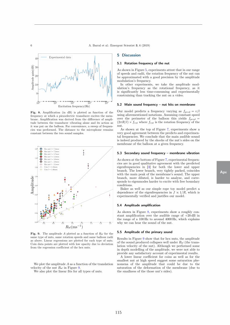
6 A. Barral et al.: Emergent Scientist 3, 6 (2019)
Fig. 8. Amplification (in dB) is plotted as function of thefrequency at which a piezoelectric transducer excites the mem-brane. Amplification was derived from the difference of ampli-tude between the transducer vibrating alone and its action asit was put on the balloon. For convenience, a sweep of frequen-cies was performed. The distance to the microphone remainsconstant between the two sound samples.
Fig. 9. The amplitude A plotted as a function of Rω for thesame type of nuts, same rotation speeds and same balloon radiias above. Linear regressions are plotted for each type of nuts.Coin data points are plotted with low opacity due to deviationfrom the regression coefficient of the hex nuts.
We plot the amplitude A as a function of the translationvelocity of the nut Rω in Figure 9.We also plot the linear fits for all types of nuts.
5 Discussion
5.1 Rotation frequency of the nut
As shown in Figure 5, experiments attest that in our rangeof speeds and radii, the rotation frequency of the nut canbe approximated with a good precision by the amplitudemodulation’s frequency.In other experiments, we take the amplitude mod-
ulation’s frequency as the rotational frequency, as itis significantly less time-consuming and experimentallyconstraining than tracking the nut on a video.
5.2 Main sound frequency – nut hits on membrane
Our model predicts a frequency varying as fpred = v/lusing aforementioned notations. Assuming constant speedover the perimeter of the balloon this yields fpred =(2πR/l)× frot where frot is the rotation frequency of thenut.As shown at the top of Figure 7, experiments show a
very good agreement between the predicts and experimen-tal frequencies. We conclude that the main audible soundis indeed produced by the shocks of the nut’s sides on themembrane of the balloon at a given frequency.
5.3 Secondary sound frequency – membrane vibration
As shown at the bottom of Figure 7, experimental frequen-cies are in good qualitative agreement with the predictedeigenfrequencies in [3] for both the lower and upperbranch. The lower branch, very tightly packed, coincideswith the main peak of the membrane’s sound. The upperbranch, more diluted, is harder to analyze, and corre-sponds to eigenmodes harder to excite with free boundaryconditions.Baker as well as our simple rope toy model predict a
dependence of the eigenfrequencies in f ∝ 1/R, which isexperimentally verified and justifies our model.
5.4 Amplitude amplification
As shown in Figure 8, experiments show a roughly con-stant amplification over the audible range of +20 dB inthe range of a 100Hz to around 4000Hz, which explainswhy we can hear the sound of the nut.
5.5 Amplitude of the primary sound
Results in Figure 9 show that for hex nuts, the amplitudeof the sound produced collapses well under Rω (the trans-lation velocity of the nut). Although we performed somein depth modelling of the amplitude, we were not able toprovide any satisfactory account of experimental results.A lower linear coefficient for coins as well as for the
smallest nut at high speed suggest some saturation phe-nomena of the amplitude that could be due to thesaturation of the deformation of the membrane (due tothe smallness of the those nut’s sides).
Apx
115
A. Barral et al..: Emergent Scientist 3, 6 (2019) 7
6 Dead ends and possible improvements
6.1 Higher order eigenfrequencies
Measuring higher order eigenfrequencies proves a very dif-ficult task using Fourier transforms. Due to their smalleramplitudes they tend to overlap with other less significantsignals or with one another, especially in the lower branch.A setup based on laser measurements as done by Kuo [8]would be more suited for such experiments.
6.2 Mechanical setup
Doing the experiments by hand induces non negligibleincertitudes. We also used a mechanized setup via a labshaker but did not present any such results here. Indeed,that setup has two major drawbacks: first of all it cre-ates a nontrivial background noise, which can not easilybe removed by simple algorithms, and masks most mem-brane frequencies. The other issue is that while using amechanized setup we encountered a new phenomena offrequency modulation due to the forced excitations, whichhinders our experiments. We believe this phenomena tooccur the following way: to a given excitation frequencyis associated a stable orbit in the balloon. If the nut isnot initially on this orbit, it will move towards it dueto the normal reaction on the balloon’s surface. Due toinertia, it will however not stop at the stable orbit butovershoot it. This induces an up/down motion of the rota-tion plane, and thus a modulation of the sound. This isbacked up by experimental data but we do not discuss itfurther here.
6.3 Influence of gas
Our model does not take into account the inner andouter gas. This has been studied by Kuo [8] but requiresexperimental data we do not have (such as the pressuredifference across the membrane). We expect the gas tohave no significant influence on the main sound’s fre-quency, save for the heavy gases which could leads tonon negligible dampening of the oscillations and thus achange in the harmonics’ amplitude and frequency. We doexpect a dependency of the membrane’s eigenfrequencieswith the gas’s density.
6.4 Unexplained frequencies
During most experiments we consistently observe between30 and 80Hz a block of inaudible frequencies that seemsrelatively unaffected by experimental parameters. A quickanalysis did not permit to determine whether this was onlydue to noise. We believe this block might be due to finedetails on the nut’s geometry but do not discuss it furtherhere.
6.5 Theoretical model for the amplitude
Although results show an interesting collapse of the dataof amplitude with Rω dependency and despite a thorough
research to provide a theoretical explanation of this depen-dency, we did not manage to provide any convincingproof. The issue residing in the large range of mod-elling hypotheses one can make which would require moreexperimental data with a wider range of different nuts tobe tested.
7 Conclusion
In this article we have investigated the sound producedby a nut when it is made to roll inside a balloon, bothexperimentally and theoretically. After discussing thebehavior of the nut on the membrane and explaining theamplitude modulation that one can hear when listeningto the sound emitted we have studied the two maincomponents of the sound emitted: membrane vibrationsand the impact of the nut on the membrane. Regardingthe membrane oscillations we showed experimentally thatthe frequency of the lower branch varies as the inverse ofthe radius of the balloon. Regarding the impact of the nutwe derived the theoretical frequency of the sound thatcorrelates very well with the main frequency componentmeasured in the experiments. On the amplitude of thesound, we studied the effect of the balloon acting as asound box and experimentally showed that in the rangeof frequencies at which the nut rolls the amplification ofthe sound is around 20 dB. For nuts, we experimentallyshowed a linear dependency of the amplitude of the soundemitted on the speed of nut.
This work is based on a problem proposed in the 2018 edition ofthe International Physicists’ Tournament (IPT). We are gratefulto Christophe Clanet, from the LadHyX, Guilhem Gallot fromthe LOB and Fabian Cadiz from the PMC at Ecole polytech-nique for their fruitful suggestions and corrections brought tothe core of this article. We also thank the teams from ParisSudat the French Physicists’ Tournament (FPT) and the teams ofSwitzerland and Brazil at the IPT for the intense discussions wehad in order to solve this problem.
Author contribution statement
Amaury Barral and Quentin Louis have contributedequally to this work.
References
1. H. Lamb, On the vibrations of an elastic sphere, Proc. Lond.Math. Soc. 1, 189–212 (1881)
2. H. Lamb, On the vibrations of a spherical shell, Pro. Lond.Math. Soc. 1, 50–56 (1882)
3. W.E. Baker, Axisymmetric modes of vibration of thinspherical shell, J. Acoust. Soc. Am. 33, 1749–1758(1961)
4. A. Silbiger, Nonaxisymmetric modes of vibration of thinspherical shells, J. Acoust. Soc. Am. 34, 862 (1962)
5. A.R. Robinson, M.S. Zarghamee, A numerical method foranalysis of free vibration of spherical shells, AIAA J. 5,1256–1261 (1967)
Appendix B. International Physicists’ Tournament
Apx
116

8 A. Barral et al.: Emergent Scientist 3, 6 (2019)
6. S.K. Panda, B.N. Singh, Nonlinear free vibration of sphericalshell panel using higher order shear deformation theory–afinite element approach, Int. J. Pres. Vessels Pip. 86, 373–383(2009)
7. A. Goriely, M.B. Amar, Differential growth and instability inelastic shells, Phys. Rev. Lett. 94, 198103 (2005)
8. K.A. Kuo et al., Small oscillations of a pressurized, elastic,spherical shell: model and experiments, J. Sound Vib. 359,168–178 (2015)
Cite this article as: Amaury Barral, Quentin Louis, Clement Brochet, Julie Andre, Anthony Guillen, Fang Goh, Angel Prieto,Thibault Guillet. Sound of a nut rolling inside an elastic rubber balloon, Emergent Scientist 3, 6 (2019)
Apx
117

Appendix B. International Physicists’ Tournament
Apx
118
Bibliography
bib
Bibliography
[1] S. F. Hoerner. Fluid-dynamic drag: practical information on aerodynamic drag andhydrodynamic resistance. Hoerner Fluid Dynamics, 1965.
[2] E. Achenbach. Distribution of local pressure and skin friction around a circular cylin-der in cross-flow up to re = 5 × 10⁶. Journal of Fluid Mechanics, 34(4):625–639,1968.
[3] A. Thom. An investigation of fluid flow in two dimensions. HM Stationery Office,1929.
[4] Albert C Gross, Chester R Kyle, and Douglas J Malewicki. The aerodynamics ofhuman-powered land vehicles. Scientific American, 249(6):142–152, 1983.
[5] Yakovich Ilich Frenkel. Kinetic theory of liquids. 1955.
[6] C. E. Brennen. Cavitation and bubble dynamics. Cambridge University Press, 2014.
[7] J. P. Franc and J. M. Michel. Fundamentals of cavitation, volume 76. Springer science& Business media, 2006.
[8] B. K. Ahn, T. K. Lee, H. T. Kim, and C. S. Lee. Experimental investigation of super-cavitating flows. International Journal of Naval Architecture and Ocean Engineering,4(2):123–131, 2012.
[9] N. E. Joukowsky. I. a modification of kirchhoff’s method of determining a two-dimensional motion of a fluid given a constant velocity along an unknown streamline.ii. determination of the motion of a fluid for any condition given on a streamline. Rec.Math, 25:121–278, 1890.
[10] D. Riabouchinsky. On steady fluid motions with free surfaces. Proceedings of theLondon Mathematical Society, 2(1):206–215, 1921.
[11] D. A. Efros. Hydrodynamic theory of two-dimensional flow with cavitation. In Dokl.Akad. Nauk SSSR, volume 51, pages 267–270, 1946.
[12] T. Y. T. Wu, A. K. Whitney, and C. E. Brennen. Cavity-flow wall effects and correctionrules. Journal of Fluid Mechanics, 49(2):223–256, 1971.
[13] Z. Pan, A. Kiyama, Y. Tagawa, D. J. Daily, S. L. Thomson, R. Hurd, and T. T. Tr-uscott. Cavitation onset caused by acceleration. Proceedings of the National Academyof Sciences, 114(32):8470–8474, 2017.
[14] Lord Rayleigh. VIII. On the pressure developed in a liquid during the collapse ofa spherical cavity. The London, Edinburgh, and Dublin Philosophical Magazine andJournal of Science, 34(200):94–98, 1917.
[15] M. S. Plesset. The dynamics of cavitation bubbles. Journal of applied mechanics,16:277–282, 1949.
[16] M. S. Plesset and A. Prosperetti. Bubble Dynamics and Cavitation. Annual ReviewFluid Mechanics, 9:145, 1977.
[17] S. Gaggero, G. Tani, D. Villa, M. Viviani, P. Ausonio, P. Travi, G. Bizzarri, andF. Serra. Efficient and multi-objective cavitating propeller optimization: An applica-tion to a high-speed craft. Applied Ocean Research, 64:31–57, 2017.
119
Bibliography
bib
[18] R. E. A. Arndt. Recent advances in cavitation research. In Advances in Hydroscience,volume 12, pages 1–78. Elsevier, 1981.
[19] J. R. Blake and D. C. Gibson. Cavitation bubbles near boundaries. Annual review offluid mechanics, 19(1):99–123, 1987.
[20] R. E. A. Arndt, R. L. Voigt Jr, J. P. Sinclair, P. Rodrique, and A. Ferreira. Cavitationerosion in hydroturbines. Journal of Hydraulic Engineering, 115(10):1297–1315, 1989.
[21] M. Dular, B. Bachert, B. Stoffel, and B. Sirok. Relationship between cavitation struc-tures and cavitation damage. Wear, 257(11):1176–1184, 2004.
[22] Y. Tomita and A. Shima. Mechanisms of impulsive pressure generation and damagepit formation by bubble collapse. Journal of Fluid Mechanics, 169:535–564, 1986.
[23] W. Lauterborn and H. Bolle. Experimental investigations of cavitation-bubble collapsein the neighbourhood of a solid boundary. Journal of Fluid Mechanics, 72(2):391–399,1975.
[24] M. S. Plesset and R. B. Chapman. Collapse of an initially spherical vapour cavity inthe neighbourhood of a solid boundary. Journal of Fluid Mechanics, 47(2):283–290,1971.
[25] R. Pecha and B. Gompf. Microimplosions: cavitation collapse and shock wave emissionon a nanosecond time scale. Physical review letters, 84(6):1328, 2000.
[26] G. E. Reisman, Y. C. Wang, and C. E. Brennen. Observations of shock waves in cloudcavitation. Journal of Fluid Mechanics, 355:255–283, 1998.
[27] C. F. Naude and A. T. Ellis. On the mechanism of cavitation damage by nonhemispher-ical cavities collapsing in contact with a solid boundary. Journal of Basic Engineering,83(4):648–656, 1961.
[28] T. B. Benjamin and A. T. Ellis. The collapse of cavitation bubbles and the pressuresthereby produced against solid boundaries. Philosophical Transactions for the RoyalSociety of London. Series A, Mathematical and Physical Sciences, pages 221–240,1966.
[29] A. Philipp and W. Lauterborn. Cavitation erosion by single laser-produced bubbles.Journal of Fluid Mechanics, 361:75–116, 1998.
[30] R. Hickling and M. S. Plesset. Collapse and rebound of a spherical bubble in water.The Physics of Fluids, 7(1):7–14, 1964.
[31] T. Covassin, R. Moran, and R. J. Elbin. Sex differences in reported concussion injuryrates and time loss from participation: an update of the national collegiate athleticassociation injury surveillance program from 2004–2005 through 2008–2009. Journalof athletic training, 51(3):189–194, 2016.
[32] G. W. Roberts, D. Allsop, and C. Bruton. The occult aftermath of boxing. Journalof Neurology, Neurosurgery & Psychiatry, 53(5):373–378, 1990.
[33] J. Mez, D. H. Daneshvar, P. T. Kiernan, B. Abdolmohammadi, V. E. Alvarez, B. R.Huber, M. L. Alosco, T. M. Solomon, C. J. Nowinski, L. McHale, et al. Clinicopatho-logical evaluation of chronic traumatic encephalopathy in players of american football.Jama, 318(4):360–370, 2017.
120
Bibliography
bib
[34] M. A. Kiraly and S. J. Kiraly. Traumatic brain injury and delayed sequelae: a review-traumatic brain injury and mild traumatic brain injury (concussion) are precursorsto later-onset brain disorders, including early-onset dementia. The Scientific WorldJournal, 7:1768–1776, 2007.
[35] B. E. Gavett, R. A. Stern, R. C. Cantu, C. J. Nowinski, and A. C. McKee. Mildtraumatic brain injury: a risk factor for neurodegeneration. Alzheimer’s research &therapy, 2(3):18, 2010.
[36] R. A. Stern, D. O. Riley, D. H. Daneshvar, C. J. Nowinski, R. C. Cantu, and A. C.McKee. Long-term consequences of repetitive brain trauma: chronic traumatic en-cephalopathy. Pm&r, 3(10):S460–S467, 2011.
[37] E. S. Gurdjian, Verne L Roberts, and L M Thomas. Tolerance curves of accelera-tion and intracranial pressure and protective index in experimental head injury. TheJournal of Trauma, 6:600–604, 1966.
[38] H. R. Lissner, M. Lebow, and F. G. Evans. Experimental studies on the relationbetween acceleration and intracranial pressure changes in man. Surgery, gynecology& obstetrics, 111:329, 1960.
[39] A. K. Ommaya, R. L. Grubb, and R. A. Naumann. Coup and contre-coup injury:observations on the mechanics of visible brain injuries in the rhesus monkey. Journalof Neurosurgery, 35(5):503–516, 1971.
[40] E. J. Pellman, D. C. Viano, A. M. Tucker, I. R. Casson, and J. F. Waekerle. Concussionin Professional Football: Reconstruction of Game Impacts and Injuries. Neurosurgery,53(4):799–814, 2003.
[41] S. P. Broglio, B. Schnebal, J. J. Sosnoff, S. Shin, X. Feng, X. He, and J. Zimmerman.The Biomechanical Properties of Concussions in High School Football. Med. Sci.Sports Exerc., 42(11):2064–2071, 2010.
[42] W. N. Hardy, T. B. Khalil, and A. I. King. Literature review of head injury biome-chanics. International Journal of Impact Engineering, 15(4):561–586, 1994.
[43] T. El Sayed, A. Mota, F. Fraternali, and M. Ortiz. Biomechanics of traumatic braininjury. Comput. Methods Appl. Mech. Engrg., 197:4692–4701, 2008.
[44] B. K. Sreedhar, S. K. Albert, and A. B. Pandit. Cavitation damage: Theory andmeasurements - A review. Wear, 372-373:177–196, 2017.
[45] Y. T. Wu and A. Adnan. Effect of Shock-Induced Cavitation Bubble Collapse on thedamage in the Simulated Perineuronal Net of the Brain. Scientific Reports, 7(1):38–42,2017.
[46] P. Lubock and W. Goldsmith. Experimental Cavitation studies in a model head-necksystem. J. Biomechanics, 13:1041–1052, 1980.
[47] S. Rowson, G. Brolinson, M. Goforth, D. Dietter, and S. Duma. Linear and AngularHead Acceleration Measurements in Collegiate Football. Journal of BiomechanicalEngineering, 131(6):061016, 2009.
[48] S. M. Duma, S. J. Manoogian, W. R. Bussone, P. G. Brolinson, M. W. Goforth, J. J.Donnenwerth, R. M. Greenwald, J. J. Chu, and J. J. Crisco. Analysis of real-timehead accelerations in collegiate football players. Clinical Journal of Sport Medicine,15(1):3–8, 2005.
121

Bibliography
bib
[49] A. K. Ommaya. Mechanical properties of tissues of the nervous system. Journal ofBiomechanics, 1(2):127–138, 2004.
[50] M. Unnerback, J. T. Ottesen, and P. Reinstrup. ICP curve morphology and intracra-nial flow-volume changes: a simultaneous ICP and cine phase contrast MRI study inhumans. Acta Neurochirurgica, 160(2):219–224, 2018.
[51] C. J. J. Avezaat, J. H. M. Van Eijndhoven, and D. J. Wyper. Cerebrospinal fluidpulse pressure and intracranial volume-pressure relationships. Journal of Neurology,Neurosurgery and Psychiatry, 42(8):687–700, 1979.
[52] M. Czosnyka and J. D. Pickard. Monitoring and interpretation of intracranial pressure.Journal of Neurology, Neurosurgery and Psychiatry, 75(6):813–821, 2004.
[53] N. Bremond, M. Arora, S. M. Dammer, and D. Lohse. Interaction of cavitation bubbleson a wall. Physics of Fluids, 18(12), 2006.
[54] N. Bremond, M. Arora, C. D. Ohl, and D. Lohse. Controlled multibubble surfacecavitation. Physical Review Letters, 96(22):1–4, 2006.
[55] N. A. Pelekasis, A. Gaki, A. Doinikov, and J. A. Tsamopoulos. Secondary Bjerknesforces between two bubbles and the phenomenon of acoustic streamers, volume 500.2004.
[56] R. Mettin, I. Akhatov, U. Parlitz, C. D. Ohl, and W. Lauterborn. Bjerknes forcesbetween small cavitation bubbles in a strong acoustic field. Physical Review E -Statistical Physics, Plasmas, Fluids, and Related Interdisciplinary Topics, 56(3):2924–2931, 1997.
[57] E. A. Neppiras and B. E. Noltingk. Cavitation produced by Ultrasonics. Proceedingsof the Physical Society. Section B, 63(9):674–685, 1950.
[58] G. E. Reisman, Y. C. Wang, and C. E. Brennen. Observations of shock waves in cloudcavitation. Journal of Fluid Mechanics, 355:255–283, 1998.
[59] R. Pecha and B. Gompf. Microimplosions: Cavitation collapse and shock wave emis-sion on a nanosecond time scale. Physical Review Letters, 84(6):1328–1330, 2000.
[60] C. F. Naude and A. T. Ellis. On the Mechanism of Cavitation Damage by Nonhemi-spherical Cavities Collapsing in Contact With a Solid Boundary. Journal of BasicEngineering, 83(4):648–656, 1961.
[61] T. B. Benjamin and A. T. Ellis. The Collapse of Cavitation Bubbles and the Pressuresthereby Produced against Solid Boundaries. Philosophical Transactions of the RoyalSociety A: Mathematical, Physical and Engineering Sciences, 260(1110):221–240, 1966.
[62] A. Shima and Y. Tomita. Mechanism of Impulsive Pressure Generation and DamagePit Formation by Cavitation Bubble Collapse. Journal of the Society of MechanicalEngineers, 90(819):164–169, 1985.
[63] W. Lauterborn and A. Philipp. Cavitation erosion by single laser-produced bubbles.Journal of Fluid Mechanics, 361:75–116, 1998.
[64] K. Ono, A. Kikuchi, M. Nakamura, H. Kobayashi, and N. Nakamura. Human headtolerance to sagittal impact-reliable estimation deduced from experimental head injuryusing subhuman primates and human cadaver skulls. SAE Transactions, pages 3837–3866, 1980.
122
Bibliography
bib
[65] Atsuhiro Nakagawa, Kazuyoshi Takayama, Miki Fujimura, Kaoruko Kato, TomohiroOhki, Atsushi Saito, and Teiji Tominaga. Pressure-dependent effect of shock waves onrat brain: induction of neuronal apoptosis mediated by a caspase-dependent pathway.Journal of Neurosurgery, 106:667–676, 2008.
[66] C. Van Lierde, B. Depreitere, J. V. Sloten, R. Van Audekercke, G. Van Der Perre, andJ. Goffin. Skull biomechanics - The energy absorbability of the human skull frontalbone during fracture under quasi-static loading. Journal of Applied Biomaterials &Biomechanics, 1:194–199, 2003.
[67] M. Harrison. An experimental study of single bubble cavitation noise. The Journalof the Acoustical Society of America, 24(6):776–782, 1952.
[68] E. Cramer and W. Lauterborn. Acoustic cavitation noise spectra. In Mechanics andPhysics of Bubbles in Liquids, pages 209–214. Springer, 1982.
[69] V. C. Suja and A. I. Barakat. A mathematical model for the sounds produced byknuckle cracking. Scientific reports, 8(1):4600, 2018.
[70] S. L. Ceccio. Friction drag reduction of external flows with bubble and gas injection.Annual Review of Fluid Mechanics, 42:183–203, 2010.
[71] E. Kawakami and R. E. A. Arndt. Investigation of the behavior of ventilated super-cavities. Journal of Fluids Engineering, 133(9):091305, 2011.
[72] L. Barbaca, B. Pearce, and P. Brandner. Experimental investigation of ventilatedcavity flow over a 3d wall mounted fence. 2016.
[73] E. Alyanak, V. Venkayya, R. Grandhi, and R. Penmetsa. Structural response andoptimization of a supercavitating torpedo. Finite Elements in Analysis and Design,41(6):563–582, 2005.
[74] J. H. Choi, R. C. Penmetsa, and R. V. Grandhi. Shape optimization of the cavitator fora supercavitating torpedo. Structural and Multidisciplinary Optimization, 29(2):159–167, 2005.
[75] E. Alyanak, R. Grandhi, and R. Penmetsa. Optimum design of a supercavitatingtorpedo considering overall size, shape, and structural configuration. InternationalJournal of Solids and Structures, 43(3-4):642–657, 2006.
[76] T. G. Lang and D. A. Daybell. Water tunnel tests of three vented hydrofoils intwo-dimensional flow. Journal of Ship Research, 5(3):1–15, 1961.
[77] Thomas G Lang. Base ventilated hydrofoil, February 12 1963. US Patent 3,077,173.
[78] A. J. Acosta. Hydrofoils and hydrofoil craft. Annual Review of Fluid Mechanics,5(1):161–184, 1973.
[79] A. Rowe and J. M. Michel. Two-dimensional base-vented hydrofoils near a free surface:influence of the ventilation number. Journal of Fluids Engineering, 97(4):465–473,1975.
[80] R. Latorre. Ship hull drag reduction using bottom air injection. Ocean engineering,24(2):161–175, 1997.
[81] K. I. Matveev, T. J. Burnett, and A. E. Ockfen. Study of air-ventilated cavity undermodel hull on water surface. Ocean Engineering, 36(12-13):930–940, 2009.
123
Bibliography
bib
[82] V. N. Semenenko. Artificial supercavitation. physics and calculation. Technical report,Ukrainian Academy of Sciences Kiev Inst. of Hydromechanics, 2001.
[83] V. N. Buyvol. Slender cavities in flows with perturbations. Kiev: Naukova Dumka,1980.
[84] G. V. Logvinovich. Hydrodynamics of flows with free boundaries, 1969.
[85] R. N. Cox and W. A. Clayden. Air entrainment at the rear of a steady cavity. InProceedings of the Symposium on Cavitation in Hydrodynamics, 1955.
[86] L. A. Ephstein. Characteristics of ventilated cavities and some scale effects. In Symp.IUTAM, pages 173–185, 1981.
[87] J. M. Michel. Some features of water flows with ventilated cavities. ASME J. FluidsEng, 106(3):319–326, 1984.
[88] C. E. Brennen. A numerical solution of axisymmetric cavity flows. Journal of FluidMechanics, 37(4):671–688, 1969.
[89] A. H. Armstrong and K. G. Tadman. Axisymmetric cavity flow about ellipsoids. InProc. Joint Admiralty-US Navy Meeting on Hydroballistics, 1954.
[90] E. Y. Hsu and B. Perry. Water tunnel experiments on spheres in cavity flow. 1954.
[91] P. Eisenberg and H. L. Pond. Water tunnel investigations of steady state cavities.Technical report, David Taylor Model Basin Washington DC, 1948.
[92] I. U. Vakarelski, J. O. Marston, D. Y. C. Chan, and S. T. Thoroddsen. Drag reductionby leidenfrost vapor layers. Physical review letters, 106(21):214501, 2011.
[93] M. M. Mansoor, I. U. Vakarelski, J. O. Marston, T. T. Truscott, and S. T. Thoroddsen.Stable–streamlined and helical cavities following the impact of leidenfrost spheres.Journal of Fluid Mechanics, 823:716–754, 2017.
[94] R. C. Ackerberg. The effects of capillarity on free-streamline separation. Journal ofFluid Mechanics, 70(2):333–352, 1975.
[95] V. H. Arakeri. Viscous effects on the position of cavitation separation from smoothbodies. Journal of Fluid Mechanics, 68(4):779–799, 1975.
[96] I. U. Vakarelski, Derek Y. C. Chan, and S. T. Thoroddsen. Leidenfrost vapour layermoderation of the drag crisis and trajectories of superhydrophobic and hydrophilicspheres falling in water. Soft Matter, 10(31):5662–5668, 2014.
[97] Sadatoshi Taneda. Visual observations of the flow past a sphere at reynolds numbersbetween 10 4 and 10 6. Journal of Fluid Mechanics, 85(1):187–192, 1978.
[98] E. Achenbach. The effects of surface roughness and tunnel blockage on the flow pastspheres. Journal of fluid mechanics, 65(1):113–125, 1974.
[99] L. B. Torobin and W. H. Gauvin. The drag coefficients of single spheres moving insteady and accelerated motion in a turbulent fluid. AIChE Journal, 7(4):615–619,1961.
[100] A. M. Worthington and R. S. Cole. Impact with a liquid surface studied by the aid ofinstantaneous photography. paper ii. Philosophical Transactions of the Royal Societyof London. Series A, Containing Papers of a Mathematical or Physical Character,194:175–199, 1900.
124
Bibliography
bib
[101] G. Birkhoff and E.H. Zarantonello. Jets, wakes, and cavities. Academic, New York,1957.
[102] T. T. Truscott, B. P. Epps, and J. Belden. Water entry of projectiles. Annual Reviewof Fluid Mechanics, 46:355–378, 2014.
[103] A. May. Vertical entry of missiles into water. Journal of Applied Physics, 23:1362–1372, 1952.
[104] A. May. Water entry and the cavity-running behavior of missiles. Technical report,NAVSEA Hydroballistics Advisory Committee Silver Spring MD, 1975.
[105] M. Lee, R.G. Longoria, and D.E. Wilson. Cavity dynamics in high-speed water entry.Physics of Fluids, 9(3):540–550, 1997.
[106] T. Von Karman. The impact on seaplane floats during landing. 1929.
[107] J.W. Glasheen and T.A. McMahon. Vertical water entry of disks at low froude num-bers. Physics of Fluids, 8(8):2078–2083, 1996.
[108] J.W. Glasheen and T.A. McMahon. A hydrodynamic model of locomotion in thebasilisk lizard. Nature, 380(6572):340, 1996.
[109] R. Bergmann, D. Van Der Meer, S. Gekle, A. Van Der Bos, and D. Lohse. Controlledimpact of a disk on a water surface: cavity dynamics. Journal of Fluid Mechanics,633:381–409, 2009.
[110] N. J. Adams and C. B. Walter. Maximum diving depths of cape gannets. The Condor,95:734–736, 1993.
[111] P. A. Prince, N. Huin, and H. Weimerskirch. Diving depths of albatrosses. AntarcticScience, 6:353–354, 1994.
[112] A. S. Brierley and P. G. Fernandes. Diving depths of northern gannets: acoustic obser-vations of sula bassana from an autonomous underwater vehicle. The Auk, 118(2):529–534, 2001.
[113] B. Chang, M. Croson, L. Straker, S. Gart, C. Dove, J. Gerwin, and S. Jung. Howseabirds plunge-dive without injuries. Proceedings of the National Academy of Sci-ences, 113(43):12006–12011, 2016.
[114] A. M. Worthington. A study of splashes. Longmans, Green, and Company, 1908.
[115] V. Duclaux, F. Caille, C. Duez, C. Ybert, L. Bocquet, and C. Clanet. Dynamics oftransient cavities. Journal of Fluid Mechanics, 591:1–19, 2007.
[116] S. Gaudet. Numerical simulation of circular disks entering the free surface of a fluid.Physics of Fluids, 10:2489–2499, 1998.
[117] D. Gilbarg and R. A. Anderson. Influence of atmospheric pressure on the phenomenaaccompanying the entry of spheres into water. Journal of Applied Physics, 19:127–139,1948.
[118] C. Duez, C. Ybert, C. Clanet, and L. Bocquet. Making a splash with water repellency.Nature Physics, 3:180–183, 2007.
[119] J. M. Aristoff and J. W. M. Bush. Water entry of small hydrophobic spheres. Journalof Fluid Mechanics, 619:45–78, 2009.
125
Bibliography
bib
[120] S. Gekle and J. M. Gordillo. Generation and breakup of worthington jets after cavitycollapse. part 1. jet formation. Journal of Fluid Mechanics, 663:293–330, 2010.
[121] K. G. Bodily, S. J. Carlson, and T. T. Truscott. The water entry of slender axisym-metric bodies. Physics of Fluids, 26(7):072108, 2014.
[122] W. Xia, C. Wang, Y. Wei, and J. Li. Experimental study on water entry of inclinedcircular cylinders with horizontal velocities. International Journal of Multiphase Flow,2019.
[123] N. Kim and H. Park. Water entry of rounded cylindrical bodies with different aspectratios and surface conditions. Journal of Fluid Mechanics, 863:757–788, 2019.
[124] A. Andersen, U. Pesavento, and Z. J. Wang. Unsteady aerodynamics of fluttering andtumbling plates. Journal of Fluid Mechanics, 541:65–90, 2005.
[125] K. Ellingsen and F. Risso. On the rise of an ellipsoidal bubble in water: oscillatorypaths and liquid-induced velocity. Journal of Fluid Mechanics, 440:235–268, 2001.
[126] P. C. Fernandes, P. Ern, F. Risso, and J. Magnaudet. On the zigzag dynamics offreely moving axisymmetric bodies. Physics of Fluids, 17(9):098107, 2005.
[127] P. Ern, F. Risso, D. Fabre, and J. Magnaudet. Wake-induced oscillatory paths ofbodies freely rising or falling in fluids. Annual Review of Fluid Mechanics, 44:97–121,2012.
[128] S. F. Hoerner and H. V. Borst. Fluid-dynamic lift: practical information on aerody-namic and hydrodynamic lift. LA Hoerner, 1985.
[129] C. Cohen, B. Darbois-Texier, G. Dupeux, E. Brunel, D. Quere, and C. Clanet. Theaerodynamic wall. Proc. R. Soc. A, 470:20130497, 2014.
126

Bibliography
bib
127

Bibliography
bib
128
Titre : Cavitation & Supercavitation : Obtenir un projectile profile stable
Mots cles : cavitation, supercavitation, dynmique de bulles, cavite ventilee, reduction de trainee, entree dansl’eau, instabilite
Resume : La supercavitation utilise le changement dephase du liquide-vapeur au mouvement rapide d’unprojectile pour le profiler et ainsi reduire sa trainee.Dans cette these, nous abordons la supercavitationsous differents aspects : la cavitation induite paracceleration en environnement confine, la reductionde trainee engendree par la cavite d’air et la sta-bilite des trajectoires des objets ainsi profiles. Plusprecisement, nous nous interessons dans un premiertemps, a la fois experimentalement et theoriquement,a la croissance des bulles de cavitation. Apres avoirmontre que cette croissance n’est possible que dansune enceinte deformable, nous prouvons, dans le casparticulier ou la depression a l’origine de l’appari-tion de ces bulles est transitoire, que leur dynamiquesuit l’equation de Rayleigh-Plesset et que leur rayonmaximal peut etre predit analytiquement. Si la vitessedu projectile est assez grande, les bulles de cavita-tion grossissent et coalescent pour former une unique
bulle, accrochee a la surface du projectile et situeedans son sillage: c’est le regime dit de supercavita-tion. Nous montrons que ce regime peut etre repro-duit dans un canal hydraulique ”classique”, a faiblevitesse, en injectant de l’air a la surface du projectile.Avec ce dispositif experimental, nous demontrons quela taille relative de la bulle est uniquement determineepar un parametre adimensionnel. Dans le cas d’unesphere, nous mesurons la modification de traineeainsi engendree. Enfin, le systeme global sphere +bulle peut etre considere comme un projectile profilede densite inhomogene. Nous montons que de telsprojectiles profiles, suivent des trajectoires courbesapres leur impact dans l’eau. Nous demontrons, ala fois experimentalement et theoriquement, que laforme de leur trajectoire est determinee par leur vi-tesse d’impact, leur forme et la position de leur centrede gravite.
Title : Cavitation & Supercavitation: From a bluff to a stable streamlined projectile
Keywords : cavitation, supercavitation, bubble dynamics, ventilated cavity, drag reduction, water entry, insta-bility
Abstract : Supercavitation uses the phase transitionliquid-gaseous, triggered by the fast motion of a pro-jectile, to streamline its shape and reduce its drag. Inthis thesis, we address several aspects of supercavi-tation: cavitation triggered by acceleration in a confi-ned geometry, drag reduction induced by the air ca-vity and the stability of the trajectory of such stream-lined projectiles. More precisely, we first study bothexperimentally and theoretically the growth of cavita-tion bubbles. After showing that their growth is uni-quely possible in a deformable container, we prove, inthe case of a transient pressure drop, that the dyna-mic of the bubbles follows the Rayleigh-Plesset equa-tion and that their maximum radius can analytically bepredicted. If the velocity of the projectile is high en-ough, the bubbles grow and coalesce to form a largebubble pinned at the surface of the projectile and lo-
cated in its wake: this is the so-called supercavitationregime. We show that this regime can be mimicked in”regular”, low velocity, hydrodynamic tunnel via air in-jection at the surface of the projectile. In this set-up,we demonstrate that the relative size of the bubble isgoverned by an unique dimensionless parameter. Inthe case of a sphere, we measure the drag modifica-tion induced by the presence of the bubble. Finally, theoverall system sphere + bubble is analogous to ainhomogeneous streamlined projectile. We show thatsuch streamlined projectiles can follows curved paths,following their impact on water. We demonstrate, bothexperimentally and theoretically, that the morphologyof their trajectory is governed by the impact velocity,their shape and the position of the center of mass ofthe projectile.
Institut Polytechnique de Paris91120 Palaiseau, France
Related Documents