Categories of Physical Processes - arXiv

Categories of Physical Processes

Stanis law SzawielInstitute of Mathematics, University of Warsaw

ul. Banacha 2, 00-913 Warsaw, Poland

November 4, 2021

Abstract

We study the mathematical foundations of physics. We reconstructtextbook quantum theory from a single symmetric monoidal functor

GNS : Phys −→ ∗Mod,

based on the Gelfand-Naimark-Segal construction and the notion of repre-sentability.

We derive the probabilistic interpretation of quantum mechanics, includ-ing the Born rule, the Schrodinger and Heisenberg pictures, the relationbetween symmetries and group representations, and a theory of quantumMarkov processes, including wave function collapse. Inclusion of the classicallimit and deformation quantization is briefly sketched.

Gauge symmetry and extended locality cannot currently be accommo-dated, due to conceptual difficulties discussed in an appendix.

Contents

Introduction 30.1 A Simple Idea . . . . . . . . . . . . . . . . . . . . . . . . . . . . . . 30.2 Functorial Physics . . . . . . . . . . . . . . . . . . . . . . . . . . . 80.3 Current Limitations and Perplexities . . . . . . . . . . . . . . . . . 160.4 Motivation . . . . . . . . . . . . . . . . . . . . . . . . . . . . . . . . 190.5 Detailed Organization . . . . . . . . . . . . . . . . . . . . . . . . . 20

1

arX

iv:1

709.

0909

6v2

[m

ath-

ph]

27

Sep

2017

1 Algebraic Preliminaries 221.1 ∗-Algebras . . . . . . . . . . . . . . . . . . . . . . . . . . . . . . . . 221.2 Bilinear Forms . . . . . . . . . . . . . . . . . . . . . . . . . . . . . 231.3 ∗-Modules . . . . . . . . . . . . . . . . . . . . . . . . . . . . . . . . 261.4 The Fibration of ∗-Modules . . . . . . . . . . . . . . . . . . . . . . 271.5 Tensor Products . . . . . . . . . . . . . . . . . . . . . . . . . . . . . 28

1.5.1 Tensor Products of ∗-Algebras . . . . . . . . . . . . . . . . . 281.5.2 Tensor Products of ∗-Modules . . . . . . . . . . . . . . . . . 29

1.6 Cyclic Modules . . . . . . . . . . . . . . . . . . . . . . . . . . . . . 30

2 Construction of the GNS Representation Functor 312.1 Representable States . . . . . . . . . . . . . . . . . . . . . . . . . . 312.2 Positivity . . . . . . . . . . . . . . . . . . . . . . . . . . . . . . . . 35

2.2.1 Complete Positivity . . . . . . . . . . . . . . . . . . . . . . . 372.3 Categories of Physical Processes . . . . . . . . . . . . . . . . . . . . 382.4 Representations of Physical Processes . . . . . . . . . . . . . . . . . 39

2.4.1 Construction for Positive States . . . . . . . . . . . . . . . . 392.4.2 Construction in General . . . . . . . . . . . . . . . . . . . . 402.4.3 The Covariant Representation . . . . . . . . . . . . . . . . . 42

3 Computations and Examples 433.1 Dinaturality . . . . . . . . . . . . . . . . . . . . . . . . . . . . . . . 433.2 Antiunitary Processes . . . . . . . . . . . . . . . . . . . . . . . . . . 443.3 Normalization . . . . . . . . . . . . . . . . . . . . . . . . . . . . . . 473.4 Examples . . . . . . . . . . . . . . . . . . . . . . . . . . . . . . . . 48

4 Recovering Traditional Physics, part I 494.1 Lifting the Schrodinger Picture . . . . . . . . . . . . . . . . . . . . 494.2 Probability, Wave Functions, and Eigenvalues . . . . . . . . . . . . 51

4.2.1 Eigenvalue-Eigenvector Link . . . . . . . . . . . . . . . . . . 534.2.2 Generalized Eigenvalue-Eigenvector Link . . . . . . . . . . . 55

4.3 Symmetries and Group Representations . . . . . . . . . . . . . . . . 584.3.1 Time Reversal . . . . . . . . . . . . . . . . . . . . . . . . . . 594.3.2 Inhomogeneous Time . . . . . . . . . . . . . . . . . . . . . . 60

4.4 Composite Systems . . . . . . . . . . . . . . . . . . . . . . . . . . . 61

5 Statistical Physics and Non-Unitary Processes 635.1 Non-unitary GNS . . . . . . . . . . . . . . . . . . . . . . . . . . . . 635.2 The Covariant Representation . . . . . . . . . . . . . . . . . . . . . 665.3 Gelfand Duals of Markov Processes . . . . . . . . . . . . . . . . . . 675.4 Quantum Markov Processes . . . . . . . . . . . . . . . . . . . . . . 69

2

5.5 Conditioning . . . . . . . . . . . . . . . . . . . . . . . . . . . . . . 715.5.1 State Vector Collapse . . . . . . . . . . . . . . . . . . . . . . 715.5.2 Scattering . . . . . . . . . . . . . . . . . . . . . . . . . . . . 725.5.3 Corollary: The “Penrose Problem” . . . . . . . . . . . . . . 73

5.6 Remarks on Measurement and Interpretation . . . . . . . . . . . . . 74

6 Sins of Omission 776.1 Internalizing GNS . . . . . . . . . . . . . . . . . . . . . . . . . . . 776.2 Infinitesimal Symmetries . . . . . . . . . . . . . . . . . . . . . . . . 806.3 The Classical Limit . . . . . . . . . . . . . . . . . . . . . . . . . . . 816.4 Compatibility . . . . . . . . . . . . . . . . . . . . . . . . . . . . . . 82

References 82

A On The Notion of Gauge Theory 86A.1 The Problem . . . . . . . . . . . . . . . . . . . . . . . . . . . . . . 86A.2 In Pursuit of Proper Language . . . . . . . . . . . . . . . . . . . . . 90A.3 Dependent Fields . . . . . . . . . . . . . . . . . . . . . . . . . . . . 92A.4 The Pathology of Dependent Symmetry . . . . . . . . . . . . . . . . 93A.5 The Problem of Dynamics . . . . . . . . . . . . . . . . . . . . . . . 94A.6 What’s an Observable? . . . . . . . . . . . . . . . . . . . . . . . . . 94A.7 Quantization . . . . . . . . . . . . . . . . . . . . . . . . . . . . . . 95

B Chasing The Moduli Theory of Vacua 97B.1 The Stack of Vacua . . . . . . . . . . . . . . . . . . . . . . . . . . . 97B.2 Speculation on the Nature of the Path Integral . . . . . . . . . . . . 100

Introduction

0.1 A Simple Idea

Let us attempt to do physics synthetically, and postulate a category of physicalprocesses, Phys. It’s objects are to be states, denoted ϕ, ψ, . . ., and it’s morphismsare to be physical processes, such as time evolution U(t) : ϕ→ ψ, or maybe evenasymptotic scattering, such as pair production γ + γ → e− + e+. Which categoryare we in?

Every state ϕ should determine its observable quantities, O(ϕ), which, owingto the nature of numbers, are to form an algebra. We will use real and complexnumbers, but the enterprising reader can attempt to follow along our discussionreplacing C/R with Z[i]/Z, leading to a sort of “arithmetical physics”. This istechnically challenging, and I have been unable to do so.

3

For the purposes of this introduction we will assume that O(ϕ) is a unitalC∗-algebra, but this is not necessary, and is in fact deeply insufficient. State spacesof gauge theories determine Hopf algebroids (with exotic morphisms) instead ofalgebras, at least classically. In such theories the characteristic algebraic structureand the notion of observable part ways (we discuss this in depth in appendix A).For these, and other reasons I will not commit to deep technical considerations infunctional analysis.

Every physical process should be accompanied by a description of what happensto any observable quantity. Thus we postulate that O is a functor

O : Phys −→ C∗Algop.

Note the variance. We are effectively treating algebras as noncommutative spaces.It’s well known that the world is not deterministic1, so we do not expect

observables to have specific values in a given state, but we do require an average,or expectation value

〈−〉ϕ : O(ϕ) −→ C,

a linear functional, or a measure on the noncommutative phase space. Again, thisis not strictly true. Even in ordinary probability theory there are random variableswithout an expectation value, and the massless 2d quantum scalar field appearsto be a noncommutative object of this type (cf. [Wi99b, §1.5]), defining a stateanalogous to the Lebesgue measure – with no probabilistic interpretation. I do notyet know how to capture such phenomena.

Digression (The “L1 digression”). This is also related to the problem multiplyinglocal operators in quantum field theory [Wi99a, Lecture 3]. If we tentatively writeO(ϕ) = L1(ϕ) – a noncommutative L1 space – then the problem becomes clear:L1 functions do not form an algebra under pointwise multiplication. If O(ϕ) is tobe an algebra, then it must be either a lot bigger or a lot smaller than “all theobservables with an expectation value”. Our choice above means the latter, butone can lead a happy mathematical life with the former choice [Ta12, §2.5].

This suggests that demanding expectation values from all entities in QFT isunfounded. In particular I expect all products of all operators to be definablewithout trickery. They will be singular objects (beyond distributions) which merelyhappen to have no expectation value.

The absence of free-form constructions in noncommutative geometry preventsprogress in this direction. In set theory L1(µ) is a discovery, a structure unknownto µ itself. In the noncommutative setting it’s an intrinsic feature of µ, to be givenbefore µ has a chance to exist.

1At least not in any sense that is operationalizable in contemporary experiments. Ideas suchas superdeterminism cannot really be tested, only pushed back.

4

When no confusion can arise we will write ϕ for 〈−〉ϕ.For a process f : ϕ→ ψ we can now construct a diagram

O(ϕ)O(ψ)

C

O(f)

ϕψ

Since we imagine that O(f) completely explains what happens to the observablequantities – including their expectation values – we require this diagram to commute:

O(f)∗ϕ = ψ.

States are not meant to be complete descriptions of the world, even if allconcrete constructions (mechanics, field theory, etc.) treat them as such. Physicsstudies subsystems of the world, and so we need a method to build bigger systemsout of smaller ones. We must investigate the idea of physically composing systemsand their states. Any cosmological considerations will require further conceptualrefinements, in particular making sense of the notion of self-measurement (cf. section5.6).

Unlike abstract logical objects, like terms and propositions, physical entitiescannot be duplicated or deleted without effort. They appear to form a linear typesystem [BSt09]. Consequently we postulate that Phys is a symmetric monoidalcategory, and that the O functor is such as well2. We interpret ϕ ⊗ ψ as thenoninteracting composite of ϕ and ψ. The states are put in two parallel worlds,which are identical except for the distinctiveness provided by ϕ and ψ. Thisstructure is an idealization of carefully putting things side by side, while screeningall interactions.

Digression. Systematically treating Phys as a type system leads to extremelyinteresting philosophical considerations, allowing definitions such as “causality isnecessary linear implication” and “matter sources are infinitesimally close possibleworlds”. Counterfactual conditionals can be given natural meanings, based inphysical laws. A mathematical analysis of (in)commensurability is possible. Suchideas will be pursued elsewhere.

Since ϕ and ψ are independent in ϕ⊗ ψ, we postulate a weak noncommutativeindependence condition

〈−〉ϕ⊗ψ = 〈−〉ϕ ⊗ 〈−〉ψ.We have already postulated plenty, but for reasons mysterious to me physicists

require more. The following definition is fundamental.

2Which monoidal structure on C∗-algebras? It suffices for it to functorially extend to completelypositive maps. In particular the maximal and minimal structures are both fine.

5

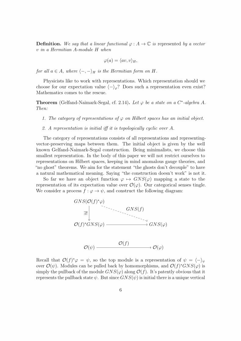
Definition. We say that a linear functional ϕ : A→ C is represented by a vectorv in a Hermitian A-module H when

ϕ(a) = 〈av, v〉H ,

for all a ∈ A, where 〈−,−〉H is the Hermitian form on H.

Physicists like to work with representations. Which representation should wechoose for our expectation value 〈−〉ϕ? Does such a representation even exist?Mathematics comes to the rescue.

Theorem (Gelfand-Naimark-Segal, cf. 2.14). Let ϕ be a state on a C∗-algebra A.Then:

1. The category of representations of ϕ on Hilbert spaces has an initial object.

2. A representation is initial iff it is topologically cyclic over A.

The category of representations consists of all representations and representing-vector-preserving maps between them. The initial object is given by the wellknown Gelfand-Naimark-Segal construction. Being minimalists, we choose thissmallest representation. In the body of this paper we will not restrict ourselves torepresentations on Hilbert spaces, keeping in mind anomalous gauge theories, and“no ghost” theorems. We aim for the statement “the ghosts don’t decouple” to havea natural mathematical meaning. Saying “the construction doesn’t work” is not it.

So far we have an object function ϕ 7→ GNS(ϕ) mapping a state to therepresentation of its expectation value over O(ϕ). Our categorical senses tingle.We consider a process f : ϕ→ ψ, and construct the following diagram:

GNS(ϕ)

GNS(O(f)∗ϕ)

O(f)∗GNS(ϕ)

O(ϕ)O(ψ)

∃!GNS(f)

O(f)

Recall that O(f)∗ϕ = ψ, so the top module is a representation of ψ = 〈−〉ψover O(ψ). Modules can be pulled back by homomorphisms, and O(f)∗GNS(ϕ) issimply the pullback of the module GNS(ϕ) along O(f). It’s patently obvious that itrepresents the pullback state ψ. But sinceGNS(ψ) is initial there is a unique vertical

6

map displayed above. The canonical homomorphism O(f)∗GNS(ϕ)→ GNS(ϕ) isa homomorphism of modules over O(f). We declare GNS(f) to be the composite,so that the diagram commutes. The following theorem follows exclusively from thefurther application of universal properties.

Theorem (cf. 2.30). The construction above gives a symmetric monoidal functor

GNS : Physop −→ ∗Mod,

fibered over C∗Alg.

The codomain is the category of ∗-modules. These are representations of C∗-algebras with isometric module homomorphisms along algebra homomorphisms.The theorem above includes the well known fact that

GNS(ϕ⊗ ψ) = GNS(ϕ)⊗GNS(ψ),

but it should be emphasized that the entire value of the this construction is thatit defines a functor. Every single statement and application below is completelydependent on it, just to make sense. Without functoriality this whole enterprisewould be worthless.

The contravariance of GNS may be concerning – don’t we want a covariantrepresentation? Not really – it is this functor that has all the crucial properties thatwe need in our formalization of physics. But the physically natural direction is easyto recover. We just compose with taking an adjoint (leaving objects untouched):

Phys ∗Modop ∗ModadjGNSop adjoint

GNSc

The codomain category is the category of ∗-modules and adjoint homomorphisms –whose definition is an exercise for the reader (cheaters can skip to definition 1.17).GNSc is called the covariant representation, and is symmetric monoidal just likeGNS.

At this point we abandon our synthetic pretense. For now, we have all theinformation we need, and Phys can be defined as the comma category

Phys = 1 ↓ S,

where S is the state functor on C∗-algebras

S : C∗Algop −→ Set.

7

This means that the objects of Phys are pairs (A,ϕ), with ϕ a state on A, andthe morphisms (A,ϕ)→ (B,ψ) are C∗-algebra homomorphisms f : B → A suchthat f ∗ϕ = ψ. The functor O forgets the state, and

(A,ϕ)⊗ (B,ψ) = (A⊗B,ϕ⊗ ψ).

It is important to not forget the synthetic pretense – the main contribution ofthis paper is the construction scheme for Phys, and not any specific construction.While this version of Phys covers quite a lot, it’s not close to being the final thing.The gauge theory problem and “L1 digression” lose none of their confoundingpower.

Despite these shortcomings, Phys captures physics in a stunningly beautifulway. We now turn to demonstrate this.

0.2 Functorial Physics

Symmetries

Why would a G-symmetric state define a unitary representation of G? Textbookspresent a rather torturous derivation of this fact. I propose using composition:

G Phys ∗ModadjGNSc

Pretty easy! Here we treat G as a one object groupoid, and a G-equivariantobject is just a functor out of G. In fact G can be an arbitrary groupoid, suchas inhomogeneous time (various other categories of time are discussed in section4.3.2).

The picture above describes the following situation. The single object of Gmaps to a state ϕ in Phys. Every morphism g ∈ G maps to a process

g : ϕ −→ ϕ,

compatibly with identities and composition. This in turn gives homomorphisms ofobservables and unitary maps of representations:

O(g) : O(ϕ) −→ O(ϕ)

GNSc(g) : GNS(ϕ) −→ GNS(ϕ).

The former preserve the expectation value 〈−〉ϕ, and the latter preserve the vectorrepresenting this expectation Ω ∈ GNS(ϕ). These two maps are compatible in thesense that we have the following identity of inner products in GNS(ϕ):

〈(g · a)v, w〉 = 〈agv, gw〉,

8

where on the left g acts only on the observable a, and on the right g acts only onthe vectors v and w. This means that the mapping a 7→ g · a on observables isunitarily implemented by conjugation g∗(−)g in GNS(ϕ), as it should be.

The more fundamental compatibility, from which the former follows is

GNSc(g)(av) = O(g−1)(a)GNSc(g)(v),

for all observables a ∈ O(ϕ) and vectors v ∈ GNS(ϕ). This is just what it meansto be a morphism in ∗Modadj over an isomorphism of algebras.

All this is fully compatible with composite systems. If ϕ is G-equivariant and ψis G′-equivariant, then ϕ⊗ ψ is naturally (G×G′)-equivariant, again just becauseof composition.

By the wonders of category theory (Cat being cartesian closed) passing to theequivariant GNS construction is as trivial as adorning all formulas with a G in theexponent. It’s all just composition. We obtain the following symmetric monoidalfunctors,

PhysG ∗ModGadjGNSGc

Rep(G)U

where U is the forgetful functor from equivariant modules to unitary representations.A major step in the construction of physical theories is investigating the fibers ofU .

Digression. In gauge theories the distinction between “internal” and “external”symmetries – actual symmetries and gauge equivalences, appears to be unsustain-able. Since gauge equivalences do not alter physical states, none of the precedingdiscussion seems to apply. We refer again to appendix A, where tentative ideas onhow to proceed are presented.

Probability Theory

Many a tome has been written on the supposed mysteries of quantum mechanics.Here we will merely present certain mathematical devices, in the hope that theysubtract from, rather than add to the mystery.

Let Prob be the category of compact probability spaces (with Radon measures)and probability preserving continuous maps (measurable maps require W ∗-algebras).For such a space X we may perform two constructions. First we can construct thealgebra C(X), of continuous complex-valued functions on X. There is a naturalstate on C(X), given by the expectation value

E : C(X) −→ C

E(f) =

∫X

f dP.

9

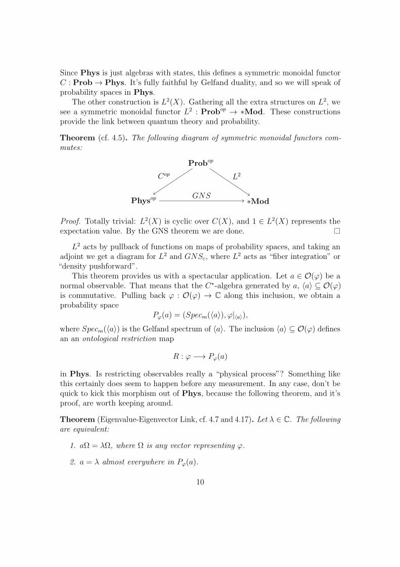
Since Phys is just algebras with states, this defines a symmetric monoidal functorC : Prob→ Phys. It’s fully faithful by Gelfand duality, and so we will speak ofprobability spaces in Phys.

The other construction is L2(X). Gathering all the extra structures on L2, wesee a symmetric monoidal functor L2 : Probop → ∗Mod. These constructionsprovide the link between quantum theory and probability.

Theorem (cf. 4.5). The following diagram of symmetric monoidal functors com-mutes:

Probop

Physop ∗Mod

Cop L2

GNS

Proof. Totally trivial: L2(X) is cyclic over C(X), and 1 ∈ L2(X) represents theexpectation value. By the GNS theorem we are done.

L2 acts by pullback of functions on maps of probability spaces, and taking anadjoint we get a diagram for L2 and GNSc, where L2 acts as “fiber integration” or“density pushforward”.

This theorem provides us with a spectacular application. Let a ∈ O(ϕ) be anormal observable. That means that the C∗-algebra generated by a, 〈a〉 ⊆ O(ϕ)is commutative. Pulling back ϕ : O(ϕ) → C along this inclusion, we obtain aprobability space

Pϕ(a) = (Specm(〈a〉), ϕ|〈a〉),

where Specm(〈a〉) is the Gelfand spectrum of 〈a〉. The inclusion 〈a〉 ⊆ O(ϕ) definesan an ontological restriction map

R : ϕ −→ Pϕ(a)

in Phys. Is restricting observables really a “physical process”? Something likethis certainly does seem to happen before any measurement. In any case, don’t bequick to kick this morphism out of Phys, because the following theorem, and it’sproof, are worth keeping around.

Theorem (Eigenvalue-Eigenvector Link, cf. 4.7 and 4.17). Let λ ∈ C. The followingare equivalent:

1. aΩ = λΩ, where Ω is any vector representing ϕ.

2. a = λ almost everywhere in Pϕ(a).

10

Proof. Just compute GNS(R) using the previous theorem:

GNS(R) : L2(ϕ|〈a〉) −→ GNS(ϕ).

This is a morphism of representations of ϕ over the inclusion map 〈a〉 ⊆ O(ϕ). So

aΩ = λΩ iff a · 1 = λ · 1 in L2 iff a = λ a.e.

Beyond this argument, Pϕ(a) simply is a probability space, with 〈−〉ϕ identifiedas the expectation value on that space. By Gelfand duality a defines a randomvariable Pϕ(a) → C. As a mathematical structure, the Born rule emerges auto-matically from our formalism. One mystery is reduced to another – the otherbeing the phenomenological connection between probability theory and reality.This connection is a much more fundamental, and unduly neglected mystery. Still,philosophers have taken note and spilled plenty of ink over it [Ha12].

Quantum Markov Processes

Is pair production really a process in Phys? Not exactly, but it can easily beaccommodated3. First we recall classical Markov processes.

Let X be a compact Hausdorff space. Then the Radon probability measures onX, M(X) also form a compact Hausdorff space. A Markov process from X to Y isjust a continuous map

X −→M(Y ).

The points of X don’t map to specific points in Y , but rather to probabilitymeasures on Y giving distributions of “where they could have gone”.

Probability measures can be pushed forward, multiplied, and their familiesintegrated against other measures. All this structure amounts to saying that M isa lax monoidal monad

M : CptHaus −→ CptHaus.

The category of Markov processes is the Kleisli category of this monad CptHausM ,which is monoidal for obvious, and formal category-theoretic reasons [Za12].

Recently, computer scientists (!) have discovered the following amazing theorem.

Theorem (Generalized Gelfand Duality, theorem 5.1 in [FJ15]). Gelfand dualityextends to a contravariant monoidal equivalence between CptHausM and thecategory of completely positive unital maps between commutative C∗-algebras.

3As long as you believe that QED has an actual scattering matrix.

11

This extension is easy to explain using ordinary Gelfand duality. To a completelypositive unital map Φ : C(Y )→ C(X) we assign the Markov process

x 7→ Φ∗δx,

where δx is the Dirac delta at x ∈ X, and Φ∗δx ∈ M(Y ) is its pullback, with δxconsidered as a linear functional on C(X).

This allows us to generalize the entire construction to Markov processes – simplyconstruct Phys using completely positive maps instead of algebra homomorphisms.Call the result PhysM . The previously introduced category Prob can be definedas 1 ↓M – the elements of M , and probability spaces with Markov maps betweenthem can be defined as

ProbM = 1/CptHausM .

The entire construction extends and complete probabilistic compatibility ismaintained.

Theorem (Non-Unitary GNS Representation, cf. 5.6). There is a commuting prismof symmetric monoidal functors:

Probop

Physop ∗Mod

ProbopM

PhysopM Hilb

Cop L2

GNS

Cop L2U

GNSM

On top we see the usual GNS representation, and its relation to probabilityspaces. The unlabeled vertical arrows are inclusions, and U is the forgetful functorto Hilbert spaces. On the bottom we see the stochastic extension of GNS, GNSM .Its values are no longer homomorphisms of ∗-modules, but merely bounded linearmaps. The L2 functor also extends in a natural manner.

As before, we define the covariant representation, GNSM,c as the adjoint ofGNSM :

GNSM,c = GNS∗M .

The construction of GNSM is no longer completely trivial. A version formeasurable maps between probability spaces would require extending generalizedGelfand duality to von Neumann algebras, and more importantly their morphisms.Rather than focus on the details, let’s look at two examples, covered in detail insection 5.5.

12

State Vector Collapse. Let ϕ : A → C be a state, P ∈ A a self-adjointprojection, and let

Φ : A −→ A

a 7→ PaP.

This completely positive map is a noncommutative version of probabilistic condi-tioning (imagine that P is the indicator function of some event in a probabilityspace). Its GNSM representation can be computed as follows.

Proposition (State Vector Collapse).

1. If ϕ is represented by Ω then Φ∗ϕ is represented by PΩ.

2. GNSM(Φ) is the composite

GNS(Φ∗ϕ) GNS(ϕ) GNS(ϕ)inclusion P

3. Consequently, GNSM,c(Φ) is cyclic (maps Ω to PΩ), and is the composite

GNS(Φ∗ϕ)GNS(ϕ) GNS(ϕ)orthogonal projectionP

If A = End(H) and Ω ∈ H, then the inclusions and projections are identities(unless PΩ = 0), and we are left with just the action of P on H.

Scattering Theory. Let S : F(H)→ F(H) be a unitary scattering operator onthe Fock space of some Hilbert space H. Let Hα, Hβ ⊆ F(H) be subspaces of statesof particles of type α and β, respectively. We can decompose this scattering matrixin to its “matrix elements” Sαβ : α→ β, which are quantum Markov processes.

Proposition (Matrix Element Decomposition). There is a process Sαβ : α −→ βin PhysM such that GNSM,c(Sαβ) is the composite

Hα F(H) F(H) HβS projectioninclusion

This proposition allows giving the informal expression γ + γ → e+ + e− itsintended mathematical meaning. I view the accurate reproduction of physicaldiscourse as a critical indicator of success.

13

Classical Physics and Differential Geometry

We must unfortunately shift gears and redo everything in a topos. This is brieflyoutlined in section 6, and will be fully fleshed out in a forthcoming paper. Thereader is issued a stack warning at this point – proficiency with stacks is assumedpast this point.

Let E be a ringed topos, with ring R. Examples to keep in mind are models ofsynthetic differential geometry [MR91], especially the Cahiers topos, which containsthe convenient vector spaces [KR86]. It is unfortunately not obvious whether theyoccur in valid examples.

Let E be the stack of objects over E (i.e. the codomain fibration), and let Elcbe the substack generated by the global sections. It’s the stack of “locally constant”objects of E, which are obtainable by gluing a cocycle of trivial families. In contrast,E contains all families, with fibers glued “completely arbitrarily”. The differencebetween E and Elc is like the difference between all bundles and the locally trivialones. The inclusion Elc ⊆ E is fully faithful. The construction of Phys, ∗Mod asa stacks, and GNS as a stack morphism uses Elc as a “universe of sets” to ensureexpected behavior (physics can go wild without the “lc” in Elc cf. remark 6.3).

The easiest way to perform the construction is to invoke stack semantics [Sh10]on an appropriate formula defining GNS, substituting Elc whenever the categoryof sets is mentioned. The result is that GNS becomes a morphism of monoidalstacks over E.

Infinitesimal Symmetries. Assume the Kock-Lawvere axiom, and let D be thefirst order infinitesimals (defined internally as x ∈ R : x2 = 0). Next let G be agroup object in E, considered as a one object groupoid (more generally, we allow aprestack of groupoids over E). The G-equivariant states are prestack morphisms

G −→ Phys,

analogously to before4. Differentiating this amounts to the evaluation of thisprestack morphism at D. By the Kock-Lawvere axiom this results in an antihomo-morphism of Lie algebras

Lie(G) −→ ∗Der(O(ϕ)),

from the Lie algebra of G to the ∗-derivations on the observables of ϕ. If thesederivations have generators, then we can ask about their compatibility with theGNS representation.

4The stackification of G is the stack of G-torsors [BH11], so it’s convenient to keep prestacksaround.

14

Theorem. Let X ∈ Lie(G) act as the inner derivation [Q,−] on O(ϕ), for someQ ∈ O(ϕ). Then GNS(X) acts on GNS(ϕ), and

GNS(X) = Q iff QΩ = 0

Thus infinitesimal generators coincide in the Heisenberg and Schrodinger picturesonly if the representing vector is invariant under the chosen generator. Thisinvariance can always be sabotaged, since the center, Z(A), always includes thescalars. Recall that the center is just Hochschild cohomology HH0(A). The theoremabove suggests that keeping around choices for generators is a good idea, which inturn suggests lifting the entire formalism to higher (e.g. derived) categories.

The Classical Limit. How do Poisson brackets appear in this setting? Rdefines the affine line A1 in E, and ~-dependent families of states are simply mapsA1 → Phys, with A1 seen as categorically discrete. The classical limit is just therestriction to infinitesimal ~.

D is is an amazingly tiny object in the sense of Lawvere [MR91, Appendix 4],and so, restricting such a ~-family to the first order infinitesimals one studies theconstruction of Phys on the trivial families in E/D. The Kock-Lawvere axiomshows that these are just the first order deformations of linear functionals on analgebra equipped with a ∗-Hochschild cocycle. The antisymmetric part of this cocyledetermines a Poisson structure, and the symmetric part controls the deformationsof any singularities (principal connections with isotropy groups and spacetimeswith nontrivial isometries are examples of singular points in their respective stacks).The ∗-part of the cocycle is traditionally taken to be trivial. Working with Elcprotects us from considering any nontrivial families in E/D, which are plentiful.

The monoidal structure on Phys restricts to a product operation on ∗-Hochschildcocycles, which generalizes the usual product of Poisson structures. In this sense,classical and quantum composition are fully compatible.

In particular we obtain “classical Hilbert spaces of states”, which for pure statesx on a Poisson manifold X amount to the “walking L2 spaces”

GNS(x) = L2(δx),

considered as modules over C∞(X). Any nontrivial dynamical flow on X completelychanges the entire spaces (outside of fixed points), making them relatively useless.Being one-dimensional is also a drawback. However, there is a “classical Schrodingerequation” – it’s just a deformation of L2(δx) as a C∞(X)-module, in some tangentdirection in TxX. Flow-invariant probability measures µ support a “Schrodingerequation” on L2(µ), with the Poisson bracket interpreted as a differential operator.

This discussion shows, contrary to certain claims in the literature, that thedegrees of linearity or non-linearity of quantum and classical theories are exactlythe same. The only difference is that classical states don’t like sharing their sectors.

15

0.3 Current Limitations and Perplexities

Classical Thermodynamics

We have traded classical thermodynamics, in which entropy is a postulated ob-servable, for statistical mechanics, where there is a formula for entropy. Thelatter is included in our formalism, under the guise of Markov processes, and theformer excluded, as a matter of form. The derivation of thermodynamics fromthe more modern, probability-based statistical mechanics requires making sense ofthe “coarse-graining” operation, even in a classical setting. This, in turn, requiresmeasure theory in potentially infinite dimensions. This problem in mathematicalanalysis will have to patiently wait for a proper solution. Physicists should alsoconsider solving problem of actually specifying the measures on the ignored degreesof freedom. This is a serious issue – no decisive discussion of the thermodynamicsof computation can take place before this (for a rare point of clarity on this see[GLPS]). Classical thermodynamics is not essential to the program outlined below.The other omissions are more serious, and will be the focus of future work.

Gauge Symmetry, Gravity, and Extended Locality

Gauge theories are, by my own standards, not included in this formalism. Mycurrent understanding of this problem is presented in appendix A. The moral ofthat story is that higher categories are essential for the proper treatment of theorieswith gauge equivalences, and that the conceptual structures underpinning gaugetheories are not clear at all. The notion of symmetry may have to be revised.

Next in line is the general notion of locality. I have specifically taken careto avoid saying “spacetime” in any part of this work. String theory looms large,and the door to emergent spacetime must be kept open, even if nothing passesthrough. But, independently of ideology, locality – especially extended locality– is conceptually confusing. General Relativity is a theory of spacetime, not inspacetime. The idea of locality in gravitationally coupled theories is extremelyunclear, and will be investigated in forthcoming work [Sz].

The common ground between extended locality and this work is inaccessibledue to the following perplexing questions:

1. Does λϕ4 define an extended field theory?

2. Does Yang-Mills theory define an extended field theory?

How far do these theories extend? In which dimensions? Why would Dp-braneexcitations define a p-category, and not the usual Hilbert space (0-category!) foundin textbooks? Are defects with prescribed support inherently perturbative, non-dynamical objects? After all, D-brane modes can induce physical motion. Does

16

this imply that defect cobordisms describe off-shell processes? None of these issuesare clear to me.

There is one hint available: the λϕ4 lagrangian does not appear to define anextended lagrangian (cf. [Fr94, Appendix]), and the scalar field does not have anyinteresting boundary conditions in higher codimensions. This suggests that scalarfield theory does not extend, and that there is a hierarchy of n-extendible theories,with n ∈ N. Structures like Phys would then describe its bottom floor.

The last and greatest omission is string theory. The standard perturbativeformalism does define an object in SymMonCat/Phys, the 2-category of “gen-eralized physical theories”, but this construction does not properly capture anydualities. The central idea of string theory still seems to be missing. At a moretechnical level, string theory contains higher gauge fields, leading us back to theproblem of integrating gauge symmetry with the construction of Phys.

Conceptual Limitations of C∗-algebras

Despite the disavowal of C∗-algebras in the introduction, some concept of com-pleteness providing a supply of modules isomorphic to their duals seems necessaryto give the internal constructions of section 6 realistic examples.

Nevertheless, there is a long list of reasons, beyond the “L1 digression” in theintroduction, for abandoning C∗-algebras, particularly the “C” part of C∗, andtheir topological kin, as the nexus of formalization of quantum theory:

1. Let F be the space of classical fields of some field theory. As is evidentin [DF99], any serious development of classical field theory requires theconsideration of the de Rham bicomplex Ω∗(F × M) = Ω∗(F) ⊗ Ω∗(M),where M is spacetime. The algebra C∞(F) is simply not enough, as it doesnot determine the required bicomplex.

2. The incorporation of fermions requires working with superalgebras, even clas-sically. Otherwise deformation quantization can never yield anticommutationrelations. This is no problem on its own, but:

3. Fermionic fields are odd points of superfunction spaces. To preserve themone must work with ringed sites over these function spaces.

For example, the space of sections of a superbundle E → X, Γ(E), definednaturally as a subobject of the sheaf exponential EX , gives rise to thesite Y ↓ Γ(E), where Y : Sm → Sh(Sm) is the Yoneda embedding ofsupermanifolds into the category of sheaves over itself. The natural algebraof observables to consider in this case is the sheaf of superalgebras

(U −→ Γ(E)) 7−→ C∞(U).

17

The global sections 1→ Γ(E) consist of purely even fields, and so consideringonly them is insufficient. Doing so would result in a complete absence offermionic observables, and consequently no possibility of anticommutationrelations in quantum field theory.

4. The incorporation of gauge invariance complicates the picture even more.We refer again to appendix A. Even a naive incorporation of the BV-BRSTformalism would require complexes of objects.

Naively adding these points together, we are faced with sheaves of differentialgraded super-C∗-algebras, as the bare minimum for expressing the standard model.Always true to form, gravity demands much more:

5. General Relativity is properly thought of as a dynamical theory of spacetime,rather than a theory of the gravitational field in spacetime. This means thatgravity is prior to other fields, and requires the consideration of the “spaceof all spacetimes”, i.e. the stack of Lorentzian manifolds. This stack will beanalyzed in detail in forthcoming work [Sz]. The unfortunate result of thisanalysis is that we must internalize everything into the category of sheaveson that stack.

So a minimal incorporation of fermions, gauge fields, and gravity necessitates aconsideration of internal sheaves of differential graded super-C∗-algebras.

We cannot simply ignore these foundational structural issues. The rift betweenformal mathematics and physics cannot be allowed to grow any larger than it isright now. And despite the advent of “physical mathematics” [Mo14], of perhapsbecause of it, the rift has been growing.

The Problem of Wilsonian Ice Cubes

If the project of section 6 can be successfully populated with interesting examples,then the Wilsonian picture of renormalization, and in particular of critical phenom-ena, will become available. The very essence of considering families of theories isturning the GNS functor into a morphism of stacks.

However localized phase transitions will still be a mystery. Consider the processof making ice cubes. Since the thermodynamical temperature is an externalparameter, and not a localizable dynamical quantity, the act of making our cubesdestroys the stars and makes the intergalactic medium boil. I would like to thinkthat the production of ice cubes does not require traversing a family of parallelrealities, each with its own distinct physics.

Despite the tongue-in-cheek narration, the problem is serious. It’s not just thatmixed phases must be far from equilibrium. It’s what mixed phases actually are,

18

as a mathematical structure. What does it mean to have ice here and not there?The crucial point is that the Wilsonian picture is metatheoretical – we deal withthe space of all theories. These theories describe only parts of the world, but theythink otherwise. The “logical signature” of an effective field theory looks just likeany other QFT. As a matter of formal structure they no different from fundamentaltheories.

There must be a dynamical theory of localized phase transitions. How aredistinct effective descriptions patched together in spacetime? The statisticalensembles cannot form a sheaf on spacetime (or any similar structure), since the“rest of the world” is almost never a reservoir of the appropriate type. Despite this,thermometers work even when there is no well-defined temperature. What is themeaning of the numbers they produce?

The problem of reconciling effective theories with their spatiotemporal domainsof validity is a critical conceptual component of mathematical physics. Doubly sowhen we realize that our experiments are localized in spacetime.

0.4 Motivation

My aim is to take the language of the physicists at face value – path integrals and all,to the greatest possible extent allowed by the law. Give it mathematical semantics,and ultimately express (much less prove) conjectures like “Witten’s theorem” –that spaces of vacua in certain Yang-Mills theories have trivial dependence on~ (cf. conjecture B.2). Without being castrated by premature mathematicalformalization, this language has proven to give its practitioners powerful vision,and insight into the mathematical world, not to mention a basket of Nobel prizesand a Fields medal. Edward Witten, in particular, has sight where mathematiciansare blind. But we cannot allow mediators or middlemen to guide us to the truth.Nature is a good approximation to mathematics, but it’s not the real thing.

We must abandon the fear of not making it back to the mathematical mainland– that we can never get the stories right the way they’re told, take an intellectualswim, and listen to what physicists actually have to say. Doing this, one seesthat the arguments used by Witten [Wi99b] are compelling, in the sense that theycan be expressed in a fully typed formal language, whose expected semantics takevalues in the complete mathematical theory of quantum fields5. Language and itsmeaning – these two objects are separable, and the former dictates the form of thelatter. This is a severe restriction, and invaluable tool that we have the bad habitof discarding, mangling the types of objects physicists discuss beyond recognition.The content of this work is uniquely determined just by trying not to do it.

Most mathematicians and physicists confuse an understanding of this language

5A similar statement about string theory would be false, at least today.

19

– and its source, “physical intuition” – with the construction of mathematicalapproximations to the expected full semantics. This makes listening difficult, sinceit requires disentangling the intended statements from their faulty mathematicalcloak. Fortunately there are physicists who speak clearly. Weinberg, after explicitlydistancing himself from “rigor”, managed to convey QFT with conceptual claritythat is unmatched by other texts [We05]. Among these texts I include the entireliterature on constructive quantum field theory.

Another effect of this confusion is that an eminently reasonable question, suchas

Is a D-brane actually a tachyonic condensate [Oh01], or actually aboundary condition [Po05, 8.7]?

can be ineffectually answered by

Actually, a D-brane is, by definition, a certain KK-class [BMRS].

By definition! None of these D-brane notions can coincide – that would be atype error6. The best we can hope for is that a single object of a different kinddetermines, in appropriate circumstances, the members of these three diversecategories. Giving a premature definition makes this not only formally impossible,but also steers thinking away from these crucial foundational issues. Type errorscannot be corrected by cleverness or computation, since types reflect intent. Theonly way to deal with them is to change one’s mind.

As stated, my interest in physics is the construction of this language, and itssemantics. The purpose is to allow the import of physical intuition, developedover the past century, into mathematics. Since this intuition greatly exceeds ourmathematical understanding (e.g. [Wi08]), this should allow great progress, notjust in stating theorems (as has been happening in the past decades), but in thetechnique of proof. Rather than receive toys from physicists, I scheme to steal thetoy factory. A grand heist.

The present work is the first step in this program. Here I begin outlining theform of a mathematical structure in which the entirety of physics has a commonmeeting ground. The language developed here has a chance to faithfully express thestories that physicists tell. It is incomplete in its current form, but more complete,by far, than anything I have found in the literature.

0.5 Detailed Organization

In section 1 we establish definitions, conventions, and recall elementary algebraicresults in their most useful forms (for our purposes, at least). This section was

6as in programming and computer science

20

written with topoi in mind, so we work in considerable generality, in excess of whatis actually needed outside of section 6. We work with arbitrary ∗-algebras andnondegenerate Hermitian ∗-modules over them.

As seen in the introduction, the lack of topology is not a technical limitation.The reader can effortlessly redo the entire paper for C∗-algebras, and likely (withsome effort) even for von Neumann algebras7. We will not do any of this, forreasons stated previously.

Section 2 introduces the basic construction scheme. We begin by studyingthe notion of representability of a state, without any normalization or positivityconditions. We characterize representability in theorem 2.4, and provide the propergeneralization of the GNS construction for such objects. We show that representablestates are convex in all linear functionals, and establish that the state functor issymmetric lax monoidal.

Next we study positivity. No topology is required. In theorem 2.14 we showthat the GNS representation of a positive state is initial among all pre-Hilbertrepresentations, and proceed to link our variant of the GNS construction to thetraditional one. We define complete positivity for ∗-algebra maps and derive avariant of the Stinespring factorization theorem – theorem 2.19. It is used in section5.1 to show that quantum Markov processes have GNS representations.

Next we work to define all the variants of the category of physical processes.They include taking everything, just the positive states, or just the admissiblemorphisms. Admissibility is required for turning the GNS construction into afunctor, which is then automatically strong symmetric monoidal. All processesbetween positive states are admissible. Finally we give two versions of the covariantrepresentation, depending on how much topology is allowed.

Section 3 is devoted to sample computations and examples. We compute theaction of the GNS functor in relation to the functor of pulling back states. We showhow to incorporate antilinear processes into Phys, with theorem 3.5 protectingus from boundless confusion. We tackle the problem of non-normalized states,providing a functorial normalization procedure. Finally we discuss the classicexamples of the GNS construction, the L2 space and pre-Hilbert spaces over theirendomorphism algebras.

In section 4 we begin the formal reconstruction of textbook physics from ourformalism. Theorem 4.1 and corollary 4.2 serve as an example factory, showinghow to lift Schrodinger picture unitary operators to maps in Phys while preservingtheir intended representations.

Next we tackle the probabilistic interpretation of quantum mechanics, startingwith the fundamental relation between the GNS functor and the L2 functor, givenby theorem 4.5. This allows us to derive a canonical random variable from any

7All the work is in the morphisms, since W ∗-algebras “are” C∗-algebras.

21

normal observable, giving the eigenvalue-eigenvector link and the Born rule. Thelink persists in much greater generality, and we rederive it in such in theorem 4.17.Since our algebras include the C∗- and W ∗-categories, and we deny ourselves theuse of spectral theory, the presentation is not as elegant as in the introduction.

Next we discuss symmetries and group representations. The functorial natureof GNS makes this essentially trivial. We show how to deal with time reversal andinhomogeneous, irreversible time evolution.

Finally we characterize the monoidal structure on Phys for normalized statesin terms of axioms describing system composition.

In section 5 we generalize our constructions to noncommutative Markov pro-cesses. We extend the notion of admissibility to ∗-linear maps which are notnecessarily homomorphisms, and show that all completely positive maps are admis-sible for positive states. We extend the GNS functor to admissible ∗-linear mapsand show that this extension is maintains complete probabilistic compatibility, asgiven by theorem 4.5, in theorem 5.12. To state that theorem we extend Gelfandduality, following [FJ15], to Markov processes between compact Hausdorff spaces.To illustrate this extension we show how arbitrary orthogonal projections can beseen as representations of noncommutative conditioning maps.

In the final subsections we propose investigating the relation of the non-unitaryGNS representation to bordism representations, information theory.

Section 6 is provided for interested readers, and sketches the internalization of theGNS representation into models of synthetic differential geometry. The formalismsof infinitesimal symmetries, the classical limit and deformation quantization canall be seen to have a place there. The intended application of this construction isdiscussed in appendix B.

1 Algebraic Preliminaries

Conventions

We assume that algebras have units, and that homomorphisms preserve them. Wedo not assume commutativity. By “module” we mean left module, likewise forideals. Unlabeled tensor products are taken over C, except in section 1.6, wherethey are over Z.

1.1 ∗-Algebras

Definition 1.1. A ∗-algebra is a C-algebra A, together with a conjugate-linear,involutive anti-homomorphism ∗ : A→ A.

22

A map of ∗-algebras is a C-algebra homomorphism which preserves the ∗operation. In this way ∗-algebras organize into a category, which we will denote by∗Alg.

In the commutative case, the role of the ∗ operation can be understood com-pletely through Galois descent.

Lemma 1.2. Let A be a commutative C-algebra. Then ∗ operations on A corre-spond to semilinear Gal(C/R)-actions on A.

Proof. This is immediate from the definition of a semilinear action, and the factthat Gal(C/R) is generated by conjugation.

By Galois descent we obtain the following corollary.

Corollary 1.3. The category of commutative ∗-algebras is equivalent to the categoryof C-algebras with chosen real form.

The equivalence maps A to its R-subalgebra of self-adjoint elements, traditionallydenoted by Asa.

In the noncommutative case, the ∗-operation is not a semilinear Galois action,and its physical significance remains mysterious to me.

1.2 Bilinear Forms

We must recall some facts about bilinear forms and their radicals. Let R be acommutative ring.

Definition 1.4. Let M be an R module. If M is equipped with and R-bilinearform

〈−,−〉M : M ⊗RM −→ R,

we will call it a bilinear module over R. The bilinear form determines its left andright radicals:

M⊥ = m ∈M : 〈m,−〉M = 0⊥M = m ∈M : 〈−,m〉M = 0.

Elements of these radicals are called left (right) degenerate, respectively, and moduleswith vanishing left (right) radicals are called left (right) nondegenerate.

For symmetric and Hermitian forms both radicals obviously coincide, and thereis a unique notion of nondegeneracy.

Remark 1.5. We will call all maps preserving given bilinear forms isometries,even if the forms have no geometric significance.

23

Definition 1.6. Let M and N be bilinear modules. An morphism f : M → N iscalled right adjointable, if there exists a map f ∗ : N →M such that

〈f(m), n〉N = 〈m, f ∗(n)〉M ,

for all m ∈ M and n ∈ N . We will call this map a right adjoint to f . Leftadjointable maps are defined analogously.

If M is right nondegenerate, then f ∗ is unique, and adjointness implies thelinearity of f ∗ (which we require anyway, but is not always necessary). Withoutadditional assumptions adjoints may fail to exist. For symmetric and Hermitianforms there is a unique notion of adjoint.

The following lemma is extremely useful in the various constructions we willundertake. It controls the behavior of degenerate vectors under adjointable maps.

Lemma 1.7. Let M and N be bilinear modules. If f : M → N has a left adjointf ∗, then

f(M⊥) ⊆ N⊥

f ∗(⊥N) ⊆ ⊥M.

Proof. 〈f(m), n〉N = 0 iff 〈m, f ∗(n)〉M = 0. So f(m) is left-degenerate if m is, andf ∗(n) is right-degenerate if n is.

In other words, left adjoint maps preserve left radicals and right adjoint mapspreserve right radicals. The non-uniqueness of the adjoint is irrelevant, and thelinearity of f and f ∗ is not required above.

Bilinear modules can be added and multiplied. The orthogonal direct sumM ⊕N has carries the bilinear form

〈(m,n), (m′, n′)〉M⊕N = 〈m,m′〉M + 〈n, n′〉N .

The radicals of a direct sum are easily computed.

Proposition 1.8. Let M,N be bilinear modules, with M ⊕ N their orthogonaldirect sum. Then their left radicals satisfy

(M ⊕N)⊥ = M⊥ ⊕N⊥,

with an analogous formula for right radicals.

Proof. Clearly we have M⊥ ⊕ N⊥ ⊆ (M ⊕ N)⊥. To show the other inclusionsuppose that 〈(m,n),−〉M⊕N = 0. Evaluating this on (m′, 0) we see that m ∈M⊥.Evaluating on (0, n′) we see that n ∈ N⊥.

24

The tensor product of bilinear modules M ⊗R N is also bilinear, through theformula

〈m⊗ n,m′ ⊗ n′〉M⊗N = 〈m,m′〉M〈n, n′〉N .Without additional assumptions the radicals can misbehave under tensor prod-

ucts. Any bilinear module M determines an exact sequence

0 −→M⊥ −→M −→ HomR(M,R), (1)

with the last arrow being m 7→ 〈m,−〉M . Tensoring such sequences results in anynumber of homological situations. Here we will simply assume that nothing can gowrong.

Lemma 1.9. Let M and N be bilinear vector spaces over a field k. Then their leftradicals satisfy

(M ⊗k N)⊥ = M⊥ ⊗k N +M ⊗k N⊥,and analogously for the right radicals. In particular, if M and N are nondegenerate,then so is M ⊗k N .

Proof. The radical (M ⊗k N)⊥ is clearly the kernel of the map

M ⊗k N −→ (M ⊗k N)∗,

where m⊗ n maps to 〈m,−〉M〈n,−〉N . This map is arises as the composite

M ⊗k N −→M∗ ⊗k N∗ −→ (M ⊗k N)∗,

where the last arrow is the natural one (arising from ⊗k begin a functor), and thefirst is

m⊗ n 7→ 〈m,−〉M ⊗ 〈n,−〉N .Since the natural map M∗ ⊗k N∗ → (M ⊗k N)∗ is injective, the result follows bytaking the tensor product of the sequences (1) for M and N .

Remark 1.10.

• This lemma is useless in topoi, effectively limiting the supply of examples insection 6.

• The discussion here is a first indicator that derived categories are warrantedin a more complete development of Phys. A bilinear module M should bereplaced by the complex M given by

0 −→M⊥ −→M,

with the nondegenerate form recovered as the cohomology H0(M).

25

• The real property required of bilinear modules M in our constructions is thatthe functor M ⊗R (−) preserves nondegenerate bilinear forms.

The final lemma will serve to define the tensor product of ∗-modules, once theyhave been defined.

Lemma 1.11. Let f : M → N and g : S → T be right adjointable maps of bilinearR-modules. Then f ⊗R g : M ⊗R S → N ⊗R T is also right adjointable.

Proof. The adjoint is obviously f ∗ ⊗ g∗, for any two right adjoints f ∗, g∗ of f andg, respectively, since

〈f ⊗ g(m⊗ s), n⊗ t〉 = 〈f(m), n〉〈g(s), t〉 =

〈m, f ∗(n)〉〈s, g∗(t)〉 = 〈m⊗ s, f ∗ ⊗ g∗(n⊗ t)〉.

One can then extend by multilinearity to all tensors, or interpret the aboveas a diagrammatic computation. Either way, the possible degeneracy poses noproblems.

1.3 ∗-Modules

Let M be a nondegenerate Hermitian complex vector space. By End(M) we denotethe space of adjointable endomorphisms of V . We record the obvious fact that it isa ∗-algebra.

Proposition 1.12. End(M) is a ∗-algebra, with ∗ mapping each endomorphismf to its associated f ∗.

Remark 1.13. Adjointable maps between Hilbert spaces are exactly the boundedones. This follows from the uniform boundedness principle.

Definition 1.14. Let A be a ∗-algebra. A ∗-module over A is a nondegenerateHermitian vector space M , together with a map of ∗-algebras A→ End(M).

Remark 1.15. The intersection of nondegenerate subspaces of a quadratic spacemay be degenerate, and hence the “∗-submodule generated by X” need not existwithout additional assumptions, such as positivity of the Hermitian form. One mustbe extremely careful to prove that any expected submodules actually exist.

Because of this, in the sequel ∗-modules will always be named such, and will bestrictly distinguished from ordinary modules, which will appear in the course ofour constructions.

We will need a notion of homomorphism between ∗-modules over differentalgebras. Let f : A→ B be a map of ∗-algebras, and let M be a ∗-module over A,and N be a ∗-module over B.

26

Definition 1.16. A map of ∗-modules h : M → N over f is an isometric C-linearmap (cf. remark 1.5), such that h(am) = f(a)h(m) for all a ∈ A and m ∈M .

An ordinary map is simply a map over the identity of the underlying algebra.Our work will also require a slightly more exotic notion of homomorphism.

Definition 1.17. A linear map h : N → M of ∗-modules is an adjoint homo-morphism over f if it is a coisometry (adjoint of an isometry) of the underlyingHermitian forms and ah(n) = h(f(a)n) for all a ∈ A and n ∈ N .

Note the direction. The name comes from the following obvious proposition.

Proposition 1.18.

1. Let h : M → N have an adjoint h∗ : N → M . Then h is a homomorphismover f iff h∗ is an adjoint homomorphism over f .

2. Adjoint homomorphisms over an invertible map f are exactly the homomor-phisms over f−1.

1.4 The Fibration of ∗-Modules

Definition 1.19.

• The category ∗Mod, of ∗-modules and their homomorphisms, has as objectspairs (A,M), where A is an ∗-algebra, and M is a ∗-module over A.

The morphisms are pairs (f, h) : (A,M) → (B,N), where f : A → B is amorphism of ∗-algebras, and h : M → N is a morphism of ∗-modules over f .

• The category ∗Modadj is defined analogously, but with maps (f, h) : (A,M)→(B,N), where f : B → A is a map of ∗-algebras, and h is an adjointhomomorphism over f .

There is an obvious projection functor π : ∗Mod → ∗Alg, which forgets themodules. This map is a fibration (in the sense of Grothendieck, cf. [St08] or [Vi08]).

Theorem 1.20. π is a Grothendieck fibration.

Proof. Let f : A → B be a morphism of ∗-algebras, and let N be a ∗-moduleover B. The cartesian (sometimes called prone) lifting of f can be constructed asfollows.

The domain f ∗N is just N as a Hermitian vector space, with module structuregiven by the composite

Af−→ B −→ End(N),

27

where the last arrow is the ∗-module structure of N .The homomorphism f ∗N → N is just the identity, as a function of sets.Clearly, such maps are closed under composition, and the morphisms M → N

over f factor uniquely through the lift f ∗N → N to module morphisms over A(i.e. over the identity on A).

1.5 Tensor Products

1.5.1 Tensor Products of ∗-Algebras

Recall the universal property of the tensor product of rings.

Theorem 1.21 (Universal Property of the Tensor Product). Let R, S be uni-tal rings. Their tensor product R ⊗Z S is initial among the rings T with ringhomomorphisms

f : R −→ T

g : S −→ T,

such that the images of f and g commute in T .

Proof. The tensor product certainly is such a ring, with f and g given by

r 7−→ r ⊗ 1

s 7−→ 1⊗ s.

Now consider T and arbitrary maps f and g, as in the statement of the theorem.The map

R× S −→ T

(r, s) 7−→ f(r)g(s)

is clearly bilinear, and hence factors through R⊗Z S. Since the images of f and gcommute, it’s a homomorphism of rings. Finally, the composites

R→ R× S −→ T

r 7→ (r, 1) 7→ f(r)g(1)

S → R× S −→ T

s 7→ (1, s) 7→ f(1)g(s),

are f and g, respectively, showing that the factorization through R⊗Z S recoversf and g, and that the factorization is unique.

28

Remark 1.22. Let R ∗ S be the coproduct of R and S in the category of rings.Then there is an obvious map

R ∗ S −→ R⊗Z S,

which is easily seen to be surjective, by the fact that the images of R and S generateboth rings. This gives a different construction of R⊗ZS, and shows that the identityis a symmetric monoidal functor

(Rng,⊗Z) −→ (Rng, ∗).

Taking opposite categories, we see that this relates the “naive” product of noncom-mutative spaces to their traditional “product”.

Now let A and B be ∗-algebras. Then A⊗B is an ∗-algebra, with ∗ given by

(a⊗ b)∗ = a∗ ⊗ b∗.

This is well-defined, since A and B commute in A⊗B. The universal property ofthe preceding theorem persists.

Theorem 1.23. A⊗B is initial among the ∗-algebras C with ∗-homomorphismsfrom A and B whose images commute.

Proof. The same proof as before applies to the homomorphism part. It’s obviousthat the ∗-structure is respected.

1.5.2 Tensor Products of ∗-Modules

Recall that if M is an R-module and N is an S-module, then M ⊗Z N is andR⊗Z S-module, with r ⊗ s acting as

m⊗ n 7−→ rm⊗ sn.

The same thing happens with ∗-modules, but we must be careful about nondegen-eracy and adjointability.

Lemma 1.24. If M is a ∗-module over A and N is a ∗-module over B, thenM ⊗N is naturally a ∗-module over A⊗B.

Proof. The module structure on M ⊗N is not in question. The bilinear form onM ⊗N is nondegenerate by lemma 1.9. To see that the ∗-structure is preserved,note that by lemma 1.11 the structure map

A⊗B −→ End(M)⊗ End(N) −→ End(M ⊗N)

actually lands in the adjointable maps End(M ⊗N) ⊆ End(M ⊗N).

29

This allows us to prove the following important theorem.

Theorem 1.25. The fibration of ∗-modules π : ∗Mod → ∗Alg is a strong sym-metric monoidal functor.

Proof. Properly speaking, this is obvious once we know the domain is symmetricmonoidal. But this is obvious: the usual structure on modules extends to ∗-modules,since the structure maps

M ⊗ (N ⊗O)α−→ (M ⊗N)⊗O

I ⊗M λ−→M

M ⊗ I ρ−→M

M ⊗N σ−→ N ⊗N

are clearly isometric.

1.6 Cyclic Modules

Let R be a ring.

Definition 1.26. A cyclic R-module is an R-module M together with an elementm ∈ M such that Rm = M . The distinguished element m is called the cyclicvector.

We will introduce cyclic modules as pairs (M,m). If no confusion can arise, thecyclic vector will subsequently be omitted.

Definition 1.27. Let (M,m) and (N, n) be cyclic modules. A cyclic morphismM → N is a module morphism M → N which maps m to n.

The resulting category of cyclic modules over R will be denoted by Cyc(R).Let Ideals(R) be the partial order of ideals (submodules) of R, considered as a

category. The following theorem follows immediately from the lattice isomorphismtheorem for modules.

Theorem 1.28. The functors Ideals(R) Cyc(R) given by

I ⊂ R 7→ (R/I, [1])

(M,m) 7→ AnnR(m)

constitute an equivalence of categories.

Here AnnR stands for the annihilator ideal over the ring R, and [1] ∈ R/I isthe class of the unit.

30

Corollary 1.29. Let f : R → S be a homomorphism of rings, and let (M,m) ∈Cyc(R) and (N, n) be an S-module with chosen element n ∈ N . Then there is atmost one homomorphism M → N over f which maps m to n.

Proof. The maps M → N over f correspond to R-module maps M → f ∗N . Theelement n ∈ f ∗N is part of a cyclic submodule Rn. Since the canonical map overf , f ∗N → N is (as a function of sets) the identity, the claim follows from theorem1.28.

The (external) tensor product of modules restricts to the category of cyclicmodules.

Proposition 1.30. Let (M,m) be a cyclic R-module, and (N, n) be cyclic S-module.Then M ⊗N is cyclic over R⊗ S with cyclic vector m⊗ n.

Proof. R⊗ S(m⊗ n) ⊆M ⊗N is a submodule containing all the simple tensors.Hence it is equal to M ⊗N .

Here is a plentiful source of cyclic modules.

Proposition 1.31. Let V be a pre-Hilbert space. Then V is a cyclic module forEnd(V ), and any nonzero vector is a cyclic vector.

Proof. Let v, w ∈ V be nonzero. We will show an adjointable map V → V mappingv to w. Let W = Span(v, w) ⊆ V be the subspace spanned by v and w, and letW⊥ be its orthogonal complement (which exists, since W is finite dimensional).Then W is a finite dimensional Hilbert space, and hence cyclic for End(W ). Letf ∈ End(W ) map v to w. The map we are looking for is f ⊕ 1W⊥ . Its adjoint isf ∗ ⊕ 1W⊥ .

2 Construction of the GNS Representation Func-

tor

2.1 Representable States

Let A be a ∗-algebra.

Definition 2.1. A linear map ϕ : A→ C is called a representable state if thereexists a ∗-module M over A, with an element m ∈M such that

ϕ(a) = 〈am,m〉,

for all a ∈ A.

31

We will say that M (or m) represents ϕ, or that ϕ is a representable state onA. We require neither ϕ nor m to be normalized.

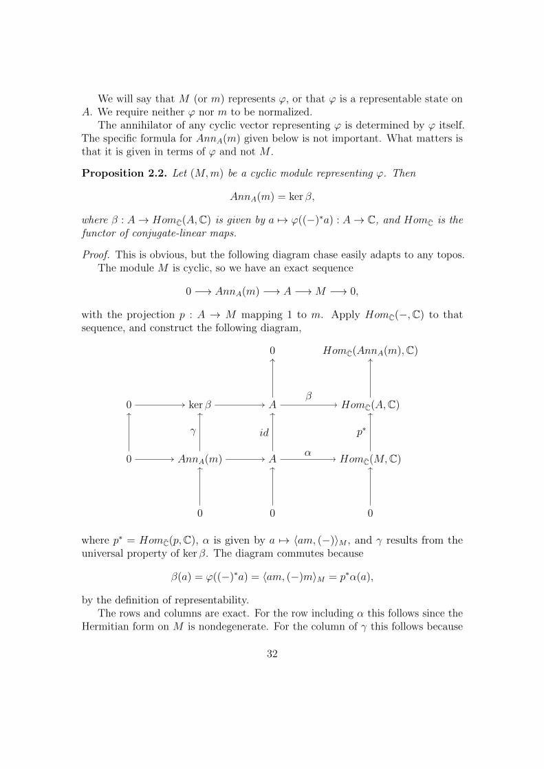
The annihilator of any cyclic vector representing ϕ is determined by ϕ itself.The specific formula for AnnA(m) given below is not important. What matters isthat it is given in terms of ϕ and not M .

Proposition 2.2. Let (M,m) be a cyclic module representing ϕ. Then

AnnA(m) = ker β,

where β : A→ HomC(A,C) is given by a 7→ ϕ((−)∗a) : A→ C, and HomC is thefunctor of conjugate-linear maps.

Proof. This is obvious, but the following diagram chase easily adapts to any topos.The module M is cyclic, so we have an exact sequence

0 −→ AnnA(m) −→ A −→M −→ 0,

with the projection p : A → M mapping 1 to m. Apply HomC(−,C) to thatsequence, and construct the following diagram,

0 HomC(AnnA(m),C)

0 ker β A HomC(A,C)

0 AnnA(m) A HomC(M,C)

0 0 0

β

α

p∗idγ

where p∗ = HomC(p,C), α is given by a 7→ 〈am, (−)〉M , and γ results from theuniversal property of ker β. The diagram commutes because

β(a) = ϕ((−)∗a) = 〈am, (−)m〉M = p∗α(a),

by the definition of representability.The rows and columns are exact. For the row including α this follows since the

Hermitian form on M is nondegenerate. For the column of γ this follows because

32

its composite with the inclusion ker β → A is a monomorphism. The other casesare obvious.

By the four lemma of homological algebra, applied to the two middle rows, γ isan isomorphism.

Remark 2.3. Note that the above proposition does not apply to non-cyclic modules.In fact if (M,m) represents ϕ then the cyclic module generated by m may not be a∗-module, because the Hermitian form on Am inherited from M may be degenerate.

Representability has several useful characterizations.

Theorem 2.4. Let ϕ : A→ C be a linear map. The following are equivalent:

1. There exists a cyclic ∗-module over A which represents ϕ. This module isunique up to a unique cyclic isometry.

2. ϕ is a representable state.

3. ϕ is ∗-linear: ϕ(a∗) = ϕ(a).

Proof. Clearly 1 =⇒ 2 =⇒ 3. We prove 3 =⇒ 1.Uniqueness follows from proposition 2.2 and theorem 1.28: any two representing

modules are uniquely isomorphic. These isomorphisms are unitary by cyclicity. Inthe diagram,

A

M M ′

displaying the canonical cyclic isomorphism between two cyclic representations,the maps from A (mapping 1 to the cyclic vectors) are epimorphisms, and inducethe same Hermitian form on A, namely

〈a, b〉ϕ = ϕ(b∗a), (2)

showing the horizontal map M →M ′ must be isometric.Existence follows from a variant of the GNS construction. Reconsider the

bilinear form on the A-module A given by equation 2. It is Hermitian by 3, butmay be degenerate. To obtain nondegeneracy we divide A by A⊥, the radical ofthe Hermitian form 〈−,−〉ϕ.

Left multiplication by a on A is adjointable with respect to 〈−,−〉ϕ, with theadjoint being left multiplication by a∗. By lemma 1.7 A⊥ is a submodule of A.

33

Thus A/A⊥ is an A-module. By construction, the Hermitian form 〈−,−〉ϕfactors through A/A⊥:

〈−,−〉ϕ : A/A⊥ × A/A⊥ −→ C,

and is nondegenerate on A/A⊥. Thus it gives A/A⊥ the structure of a ∗-module,which clearly represents ϕ through the cyclic vector [1].

Remark 2.5. Note that the norm of the cyclic vector satisfies ‖m‖2 = ϕ(1), soϕ must be defined, or at least uniquely definable, on a unital algebra, if we are tohave any hope for uniqueness.

Definition 2.6. The unique cyclic module representing ϕ is called the GNS spaceassociated to ϕ, and will be denoted by GNS(ϕ). The cyclic vector representingϕ in GNS(ϕ) will be denoted by Ω, or Ωϕ, if several different states are underconsideration.

The behavior of representable states under tensor products is predictable.

Proposition 2.7. Let ϕ be a representable state on A and ψ a representable stateon B. Then ϕ⊗ψ : A⊗B → C is representable, and represented by (M⊗N,m⊗n),for any representations (M,m) and (N, n) of ϕ and ψ, respectively.

Proof. This follows immediately from the definition of the Hermitian form onM ⊗N , and the definition of representability.

Corollary 2.8.GNS(ϕ⊗ ψ) = GNS(ϕ)⊗GNS(ψ)

Proof. Immediate by propositions 1.30 and 2.7.

We denote the set of representable states on A by Sr(A). The following theoremestablishes the functorial properties of Sr, and the notion of pure and mixed statesin our setting. By ConvC we denote the category of convex subsets of complexvector spaces and C-affine maps between them.

Theorem 2.9. The construction A 7→ Sr(A) is part of a functor Sr : ∗Algop →ConvC.

Proof. The dual space construction A 7→ A∗ is a functor of the type we are lookingfor, and Sr(A) ⊆ A∗, so we will construct our functor as a subfunctor of (−)∗.

We must check if this is well-defined, that is, if ϕ ∈ Sr(A), and f : B → A is a∗-algebra map, then f ∗ϕ ∈ Sr(B). But this is easy: if (M,m) represents ϕ, then(f ∗M,m) represents f ∗ϕ. Alternatively, it is trivial to check that f ∗ϕ is ∗-linear ifϕ is.

34

What remains is to see that Sr(A) is a convex subset of A∗. So let ϕ, ψ ∈ Sr(A)be represented by (M,m) and (N, n) respectively. The state tϕ + (1 − t)ψ, fort ∈ [0; 1], is represented by

(M ⊕N,√tm+

√1− tn),

where M ⊕N is the orthogonal direct sum of M and N (which is nondegenerateby proposition 1.8).

The category ConvC has finite products, and is therefore symmetric monoidal.We have also seen that ∗Alg is monoidal under the usual tensor product. Thefollowing natural transformations give Sr the structure of a lax monoidal functor∗Algop → ConvC.

Sr(A)× Sr(B) −→ Sr(A⊗B)

(ϕ, ψ) 7−→ ϕ⊗ ψ

1 −→ Sr(C)

∗ 7−→ id : C −→ C.

Note that this structure is inherited from the natural structure on the dual spacefunctor (−)∗. The verification of the following theorem is thus routine, and isomitted.

Theorem 2.10. The above definitions make Sr into a symmetric lax monoidalfunctor.

2.2 Positivity

Let A be a ∗-algebra.

Definition 2.11.

• An element b ∈ A is called positive if it is of the form b = a∗a for somea ∈ A.

• A linear map A → B of ∗-algebras is called positive if it maps positiveelements to positive elements.

• A linear map A→ C is called a positive state if it is positive and representable.

Positive maps compose, and thus result in a category. Clearly ∗-homomorphismsare positive. Further examples will be given below.

35

Proposition 2.12. A state ϕ is positive iff its GNS space is a pre-Hilbert space.

Proof.〈a, a〉 ≥ 0 ⇐⇒ ϕ(a∗a) ≥ 0,

since the left hand sides are equal. The result follows since the module underconsideration is cyclic.

Corollary 2.13. If ϕ and ψ are positive, then so is ϕ⊗ ψ.

Proof. By lemma 1.9 the tensor product of pre-Hilbert spaces is a pre-Hilbertspace.

Theorem 2.14 (Universality of the GNS Construction). Let ϕ be a positive state.Then GNS(ϕ) is initial among the pre-Hilbert ∗-modules representing ϕ.

Proof. Let (M,m) be a representation of ϕ. Then Am ⊂ M also represents ϕ,since it is obviously a ∗-submodule of M (unlike in the indefinite case, cf. remark1.15), and is cyclic. Thus by theorem 1.28 and proposition 2.2 there is a uniquemap

GNS(ϕ) −→ Am →M

mapping Ω to m.

In light of this theorem the classical GNS result can be restated as “positivelinear functionals on a C∗-algebra are representable”.

Let Sp(A) be the set of positive states on A.

Theorem 2.15. Sp ⊆ Sr is a symmetric monoidal subfunctor.

Proof. The pullback of a positive state is positive, since maps of ∗-algebras arepositive. The set Sp(A) is also obviously convex, since R≥0 ⊆ R is convex. Bycorollary 2.13, and the obvious fact that id : C→ C is a positive state, the monoidalstructure can be inherited from Sr.

The following lemma connects us to the more traditional versions of the GNSconstruction, and is needed for representing maps of positive states.

Lemma 2.16. Let ϕ : A→ C be a positive state. Then for the induced Hermitianform on A, we have A⊥ = a ∈ A : 〈a, a〉 = 0.

Proof. Clearly A⊥ ⊆ a ∈ A : 〈a, a〉 = 0. To see the other inclusion recall thegeneral Cauchy-Schwartz inequality (or its proof), which is still valid in our setting:|〈a, b〉|2 ≤ 〈a, a〉〈b, b〉, for any a, b ∈ A. Thus if 〈a, a〉 = 0, then 〈a, b〉 = 0 for anyb ∈ A.

36

2.2.1 Complete Positivity

In this section we recover a variant of the Stinespring factorization theorem.

Definition 2.17. Mn(−) = (−)⊗Mn(C) : ∗Alg→ ∗Alg.

Definition 2.18. A linear map Φ : A→ B between ∗-algebras is completely positiveif it is ∗-linear and Mn(Φ) is positive for all n ∈ N.

In the setting of C∗-algebras ∗-linearity is a consequence of ordinary positivity.In our case we list it as a separate requirement. Clearly, completely positive mapsform a category which includes the ∗-homomorphisms.

Now let Φ : A → B be completely positive, and let ϕ : B → C be a positivestate on B. Set H = A⊗B, and let

V : B −→ H be given byb 7−→ 1A ⊗ bV ∗ : H −→ B be given bya⊗ b 7−→ Φ(a)b

π(a) : H −→ H be given bya′ ⊗ b 7−→ aa′ ⊗ b.

Declare π(a)∗ = π(a∗), and finally define a bilinear form on H by

〈a1 ⊗ b1, a2 ⊗ b2〉H = 〈Φ(a∗2a1)b1, b2〉ϕ.

By inspection, π(a) and π(a)∗ are adjoint with respect to the Hermitian form onH (which may be degenerate), and π defines an A-module structure on H. Bythe ∗-linearity of Φ, V and V ∗ are also adjoint, with B endowed with the form〈a, b〉ϕ = ϕ(b∗a). By construction we have

Φ(a) = V ∗π(a)V (1B).

The form 〈−,−〉H is positive semi-definite by the complete positivity of Φ and thepositivity of ϕ. Indeed, for any a1, . . . an ∈ A we have [a∗i aj] ∈Mn(A), a positiveelement, equal to X∗X, where X ∈Mn(A) is the matrix with first row (ai), andthe rest 0. This means that Mn(Φ)([a∗i aj]) is positive, hence – by our definition ofpositivity – of the form L∗L, for some L ∈Mn(B), and so

〈∑j

aj ⊗ xj,∑i

ai ⊗ xi〉H = 〈Mn(Φ)([a∗i aj])x, x〉Bn = 〈Lx, Lx〉Bn ≥ 0,

where x = (x1, . . . , xn) ∈ Bn, and Bn is the n-fold orthogonal sum of (B, 〈−,−〉ϕ).We are now ready to state the factorization theorem. Let Φ : A → B be

completely positive, and let ϕ : B → C be a positive state, and let i : B →End(GNS(ϕ)) be its GNS representation.

37

Theorem 2.19 (Stinespring Factorization Theorem). There exists a pre-Hilbert A-module H and an adjointable linear map V : GNS(ϕ)→ H such that V ∗πV = iΦ,where π is the representation of A on H.

Proof. Factor out all the degeneracy in the above formulas. Lemma 1.7 ensureseverything remains well-defined.

Remark 2.20. Conversely, one can easily compute that all maps of the formV ∗πV , where V is any adjointable map between pre-Hilbert spaces, are completelypositive according to our definition.

One can replace B with an arbitrary pre-Hilbert ∗-module L over B, but noreal generality is gained.

Corollary 2.21. Let L be a pre-Hilbert ∗-module over B, and let Φ : A → Bbe completely positive. Then there exists a pre-Hilbert ∗-module H over A, andan adjointable linear map V : L → H such that V ∗πV = iΦ, where π is therepresentation of A on H, and i is the representation of B on L.

Proof. Apply the previous theorem to the composite iΦ, and note that by propo-sition 1.31 and theorem 2.4 we have L = GNS(ϕ), for ϕ : End(L)→ C given byϕ(f) = 〈f(v), v〉L, for any choice of nonzero v ∈ L.

2.3 Categories of Physical Processes

Let 1 be the terminal category, and 1→ ConvC the functor which picks out theaffine point.

Definition 2.22.

• The unrestricted category of physical processes is the comma category 1 ↓ Sr.It will be denoted by Physr.

• The category of positive physical processes is 1 ↓ Sp. It will be called Physp.

• The category of physical processes (just so), Phys, will be constructed belowin definition 2.29, after the introduction of admissible morphisms.

Physr is strong symmetric monoidal by theorem 2.10, and purely formalproperties of forming comma categories. The others are monoidal subcategories,with Physp being such by theorem 2.15. For convenience, we will spell out thedetails of Physr.

The objects of Physr are pairs (A,ϕ), with A a ∗-algebra, and ϕ : A → C arepresentable state on A. A morphism

(A,ϕ) −→ (B,ψ)

38

in Physr is a ∗-algebra homomorphism f : B → A such that ψ = f ∗ϕ = ϕ f .As in the introduction, we will write f : ϕ → ψ for morphisms in Physr,

omitting the algebras. They can be recovered by applying the observables functor

O : Physr −→ ∗Algop,

which is simply forgetting the state: (A,ϕ) 7→ A.The monoidal structure is defined by

(A,ϕ)⊗ (B,ψ) = (A⊗B,ϕ⊗ ψ),

with the obvious formula for morphisms.Examples of physical processes abound. A vast supply of objects and morphisms

will be constructed in theorem 4.1, where it is shown how to lift Schrodinger pictureoperators, observables, and states to Physp. Using that theorem all W ∗- orC∗-dynamical systems (with invertible dynamics) can be lifted into our formalism.

2.4 Representations of Physical Processes

2.4.1 Construction for Positive States

We will now construct a symmetric monoidal functor

Physopp −→ ∗Mod,

whose object function is given by ϕ 7→ GNS(ϕ). It will serve as a foundation forour formalization of physics.

The construction, outlined in the introduction, follows immediately from theo-rem 2.14. Let f : ϕ→ ψ be a morphism in Physp. Then O(f)∗GNS(ϕ) representsψ and so we have a map

GNS(ψ) −→ O(f)∗GNS(ϕ).

We define GNS(f) to be the composite of this map with the cartesian lift of O(f):

GNS(ψ) −→ O(f)∗GNS(ϕ) −→ GNS(ϕ).

Note that GNS(f) lies over f , making GNS fibered over ∗Alg.The fact that this construction defines a functor, which is furthermore strong

symmetric monoidal in a natural way, follows from theorem 2.14 and corollary1.29, applied repeatedly to every condition we have to check. The structures wemust exhibit are uniquely specified by appeals to theorem 2.14, and any coherencelaws are satisfied by corollary 1.29. Since we will perform the construction in moregenerality, we leave the details to the reader.

Without positivity we have no analog of universality, O(f)∗GNS(ϕ) does notneed to contain a cyclic module representing ψ, and so we must restrict the mapswe can represent. This leads to the notion of admissibility.

39

2.4.2 Construction in General

Now we consider a map f : ϕ→ ψ in Physr, with ϕ not necessarily positive. Toease notation, write O(f) = f : A→ B, with A = O(ψ) and B = O(ϕ). We alsoabbreviate f ∗ = O(f)∗.

Recall that GNS(ϕ) = B/B⊥ and GNS(ψ) = A/A⊥, with (−)⊥ denotingthe radical of the induced Hermitian form. We wish to define a map GNS(f) :GNS(ψ)→ GNS(ϕ), but so far we only have the following diagram.

A/f−1(B⊥) GNS(ψ)

GNS(ϕ)

π

[f ]?

The map [f ] is a morphism of cyclic modules over f , and is given by [x] 7→ [f(x)].The horizontal map π is a quotient projection (since we clearly have f−1(B⊥) ⊆ A⊥,by the definition of ψ). To fill in the dashed map, we simply assume that π is anisomorphism, leading to the following definition.

Definition 2.23. The map f : A→ B is called admissible for ϕ if A⊥ ⊆ f−1(B⊥).

Proposition 2.24. The following are equivalent:

1. f is admissible for ϕ

2. π is an isomorphism

3. The Hermitian form defined by ψ on A/f−1(B⊥) is nondegenerate

4. A/f−1(B⊥) represents ψ

5. f ∗GNS(ϕ) contains a cyclic module representing ψ.

Proof. The implications 1 =⇒ 2 =⇒ 3 =⇒ 4 are trivial. We have 4 =⇒ 5since the image of [f ] in f ∗GNS(ϕ) is the sought after module.

Finally, we show 5 =⇒ 1 as follows. By 5 and theorem 2.4(1), there is a cyclicmap GNS(ψ)→ f ∗GNS(ϕ), and hence a cyclic map GNS(ψ)→ GNS(ϕ) over f .But, by the construction of GNS spaces, this must be a cyclic map A/A⊥ → B/B⊥

over f . Thus, by cyclicity, x ∈ A⊥ implies f(x) ∈ B⊥, which is 1.

40

Remark 2.25. Note that any cyclic map completing the triangle above will make itcommute (by proposition 1.29). This is implicit in the proof of the last implicationabove. Consequently, the content of proposition 2.24 is that there is only onereasonable formula for GNS(f), i.e. [f ], and it gives a well-defined map iff f isadmissible.

Definition 2.26. Let f : ϕ → ψ be a morphism in Physr, such that O(f) isadmissible for ϕ. Then the GNS representation of f is defined to be

GNS(f) : GNS(ψ) −→ GNS(ϕ)

GNS(f)([x]) = [f(x)].

Admissible homomorphisms have all the categorical properties we require.

Proposition 2.27.

1. Composites of admissible maps are admissible

2. The tensor product of admissible maps is admissible

3. All maps between positive states are admissible

Proof. 1. is obvious by direct computation. 3. is obvious by proposition 2.16.To see 2. note that, since all modules over C are flat (being free), the tensor

product of nondegenerate forms is nondegenerate. Consider a tensor of admissiblemaps f ⊗ f ′ : ϕ ⊗ ϕ′ → ψ ⊗ ψ′, over homomorphisms f, f ′ of ∗-algebras, andcompute (f ⊗ f ′)∗GNS(ϕ⊗ ϕ′) = f ∗GNS(ϕ)⊗ (f ′)∗GNS(ϕ′), using proposition2.8. Both factors of the product contain cyclic modules representing ψ and ψ′,respectively, by proposition 2.24(5). Therefore their tensor product – a cyclicsubmodule of (f ⊗ f ′)∗GNS(ϕ⊗ ϕ′) represents ψ ⊗ ψ′. So f ⊗ f ′ is admissible byproposition 2.24(5).

Remark 2.28. If f : ϕ → ψ is a map in Physr, and ϕ is positive, then ψ is aswell. This makes proposition 2.27(3) easier to apply.

Definition 2.29. We denote by Phys = Physa the symmetric monoidal subcate-gory of Physr spanned by the admissible morphisms.

Phys is well-defined by proposition 2.27. Note that Physp ⊆ Phys by propo-sition 2.27(3).

Theorem 2.30. The constructions

ϕ 7−→ GNS(ϕ)

f 7−→ GNS(f),

41

for objects ϕ ∈ Phys, and morphisms f : ϕ → ψ in Phys, are part of a strongsymmetric monoidal functor

GNS : Phys −→ ∗Mod,

fibered over ∗Alg.

Proof. GNS(f) is always cyclic, and hence preserves composition by corollary 1.29.It is strong symmetric monoidal by corollary 2.8. All coherence diagrams commuteby corollary 1.29, since all the morphisms involved in these diagrams are obviouslycyclic.

GNS(f) is fibered over ∗Alg by its explicit construction.

2.4.3 The Covariant Representation

Let ∗Modp denote the category pre-Hilbert ∗-modules, and ∗Modadj the categoryof Hilbert ∗-modules, with algebras acting by closable maps.

Definition 2.31. The covariant GNS construction is the composite

Physp ∗Modopp ∗ModadjGNSop completion + adjoint

It will be denoted by GNSc.

Thus GNSc(f) acts as the adjoint of GNS(f) on the completion of the appro-priate pre-Hilbert spaces. The existence of adjoints requires completeness, so we useit out of necessity. Topology does not internalize well, so this construction cannotreasonably be repeated in a topos (unlike its contravariant cousin, see section 6).Despite this, it is the “correct” version for physical applications, as is evident intheorems 3.1, 4.1, 4.19 and section 5.5.

Theorem 2.32. GNSc is a symmetric monoidal functor Physp → ∗Modadj

Proof. By definition, GNSc is a composite of such.

There is a more topological variant of this definition, the details of which weleave to the reader. Define a monoidal subfunctor Sb ⊆ Sp consisting of thosestates ϕ ∈ Sp(A), for which A acts by bounded operators on GNS(ϕ). This canbe expressed using only ϕ. Then the covariant representation can be defined onPhysb = 1 ↓ Sb, with codomain the ordinary Hilbert modules – with algebrasacting by bounded, not just closable maps. Note that, since GNS(f) is alwaysisometric, GNSc(f) will always be coisometric, and hence bounded.

42

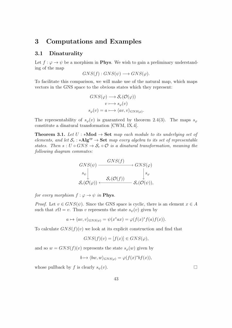
3 Computations and Examples

3.1 Dinaturality

Let f : ϕ→ ψ be a morphism in Phys. We wish to gain a preliminary understand-ing of the map

GNS(f) : GNS(ψ) −→ GNS(ϕ).

To facilitate this comparison, we will make use of the natural map, which mapsvectors in the GNS space to the obvious states which they represent:

GNS(ϕ) −→ Sr(O(ϕ))

v 7−→ sϕ(v)

sϕ(v) = a 7−→ 〈av, v〉GNS(ϕ).

The representability of sϕ(v) is guaranteed by theorem 2.4(3). The maps sϕconstitute a dinatural transformation [CWM, IX.4].

Theorem 3.1. Let U : ∗Mod → Set map each module to its underlying set ofelements, and let Sr : ∗Algop → Set map every algebra to its set of representablestates. Then s : U GNS → Sr O is a dinatural transformation, meaning thefollowing diagram commutes:

GNS(ψ) GNS(ϕ)

Sr(O(ϕ)) Sr(O(ψ)),

GNS(f)

sψSr(O(f))

sϕ

for every morphism f : ϕ→ ψ in Phys.

Proof. Let v ∈ GNS(ψ). Since the GNS space is cyclic, there is an element x ∈ Asuch that xΩ = v. Thus v represents the state sψ(v) given by

a 7→ 〈av, v〉GNS(ψ) = ψ(x∗ax) = ϕ(f(x)∗f(a)f(x)).

To calculate GNS(f)(v) we look at its explicit construction and find that

GNS(f)(v) = [f(x)] ∈ GNS(ϕ),

and so w = GNS(f)(v) represents the state sϕ(w) given by

b 7→ 〈bw,w〉GNS(ϕ) = ϕ(f(x)∗bf(x)),

whose pullback by f is clearly sψ(v).

43

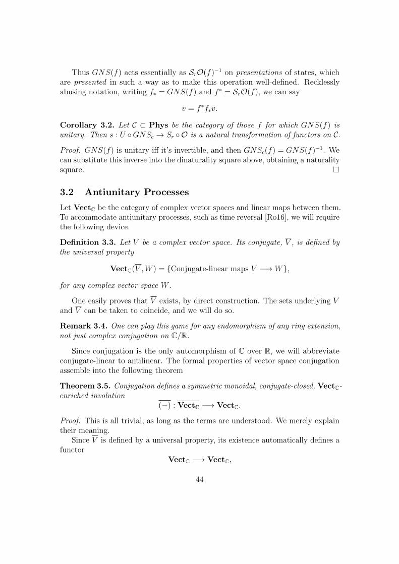
Thus GNS(f) acts essentially as SrO(f)−1 on presentations of states, whichare presented in such a way as to make this operation well-defined. Recklesslyabusing notation, writing f∗ = GNS(f) and f ∗ = SrO(f), we can say

v = f ∗f∗v.

Corollary 3.2. Let C ⊂ Phys be the category of those f for which GNS(f) isunitary. Then s : U GNSc → Sr O is a natural transformation of functors on C.

Proof. GNS(f) is unitary iff it’s invertible, and then GNSc(f) = GNS(f)−1. Wecan substitute this inverse into the dinaturality square above, obtaining a naturalitysquare.

3.2 Antiunitary Processes

Let VectC be the category of complex vector spaces and linear maps between them.To accommodate antiunitary processes, such as time reversal [Ro16], we will requirethe following device.

Definition 3.3. Let V be a complex vector space. Its conjugate, V , is defined bythe universal property

VectC(V ,W ) = Conjugate-linear maps V −→ W,

for any complex vector space W .

One easily proves that V exists, by direct construction. The sets underlying Vand V can be taken to coincide, and we will do so.

Remark 3.4. One can play this game for any endomorphism of any ring extension,not just complex conjugation on C/R.

Since conjugation is the only automorphism of C over R, we will abbreviateconjugate-linear to antilinear. The formal properties of vector space conjugationassemble into the following theorem

Theorem 3.5. Conjugation defines a symmetric monoidal, conjugate-closed, VectC-enriched involution

(−) : VectC −→ VectC.

Proof. This is all trivial, as long as the terms are understood. We merely explaintheir meaning.

Since V is defined by a universal property, its existence automatically defines afunctor

VectC −→ VectC,

44

with object function V 7→ V .R-bilinear forms can be antilinear (in both variables), and such forms are clearly

represented by both V ⊗W and V ⊗W . Thus we have V ⊗W = V ⊗W , makingconjugation into a strong symmetric monoidal functor.

Since VectC is monoidal closed, we can ask if conjugation is a closed functor.It’s not, but the natural maps

VectC(V,W ) −→ VectC(V ,W )

f 7−→ f

are antilinear, thus defining isomorphisms

VectC(V,W )→ VectC(V ,W ).

This is the meaning of conjugate-closed.Since VectC is symmetric monoidal closed, it is self-enriched, and since conju-

gation is symmetric monoidal we can extend the action of conjugation to VectC-enriched categories, such as VectC itself, resulting in VectC. Then conjugation isan enriched functor, as displayed in the statement of the theorem.

Such functors are rightfully called conjugate-enriched, and can be composed,just like contravariant functors. Conjugation thus understood is involutive (up tocoherent natural isomorphism), since

V = V,

which follows from the fact that an anti-antilinear map is just linear, since conjuga-tion (on C) is an involution.

Remark 3.6. The last step of the proof shows the usefulness of the general perspec-tive of remark 3.4, utilizing the composition of σ- and ρ-linearity to (σ ρ)-linearity.

Remark 3.7. Due to the involutivity, V also represents antilinear maps into V .

Theorem 3.5 allows us to conjugate essentially anything, in particular ∗-algebrasand their modules. Extreme care must be taken, however, to distinguish conjugationof vector spaces and their maps and the function of complex conjugation on C.Failure to do so will result in catastrophic error – object types will stop matching.

As an example, let us conjugate a Hermitian form. The conjugate of

H ⊗H −→ C

isH ⊗H −→ C,

45

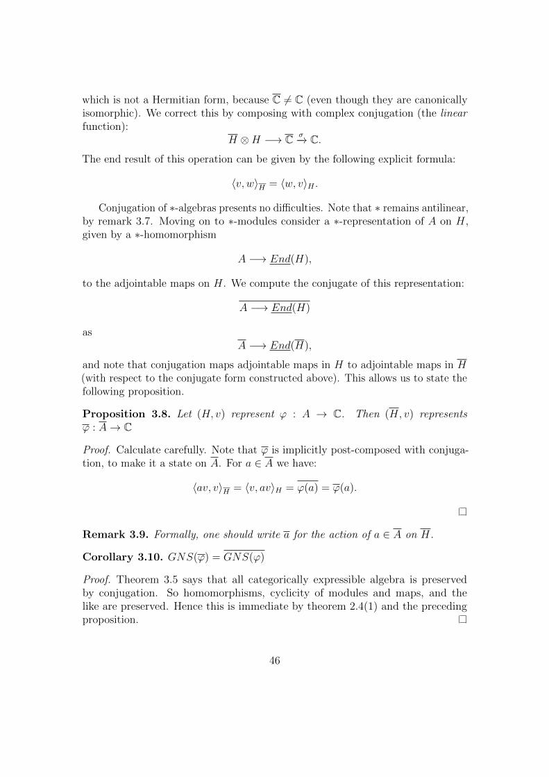
which is not a Hermitian form, because C 6= C (even though they are canonicallyisomorphic). We correct this by composing with complex conjugation (the linearfunction):

H ⊗H −→ C σ−→ C.

The end result of this operation can be given by the following explicit formula:

〈v, w〉H = 〈w, v〉H .

Conjugation of ∗-algebras presents no difficulties. Note that ∗ remains antilinear,by remark 3.7. Moving on to ∗-modules consider a ∗-representation of A on H,given by a ∗-homomorphism

A −→ End(H),

to the adjointable maps on H. We compute the conjugate of this representation:

A −→ End(H)

asA −→ End(H),

and note that conjugation maps adjointable maps in H to adjointable maps in H(with respect to the conjugate form constructed above). This allows us to state thefollowing proposition.

Proposition 3.8. Let (H, v) represent ϕ : A → C. Then (H, v) representsϕ : A→ C

Proof. Calculate carefully. Note that ϕ is implicitly post-composed with conjuga-tion, to make it a state on A. For a ∈ A we have:

〈av, v〉H = 〈v, av〉H = ϕ(a) = ϕ(a).

Remark 3.9. Formally, one should write a for the action of a ∈ A on H.

Corollary 3.10. GNS(ϕ) = GNS(ϕ)

Proof. Theorem 3.5 says that all categorically expressible algebra is preservedby conjugation. So homomorphisms, cyclicity of modules and maps, and thelike are preserved. Hence this is immediate by theorem 2.4(1) and the precedingproposition.

46

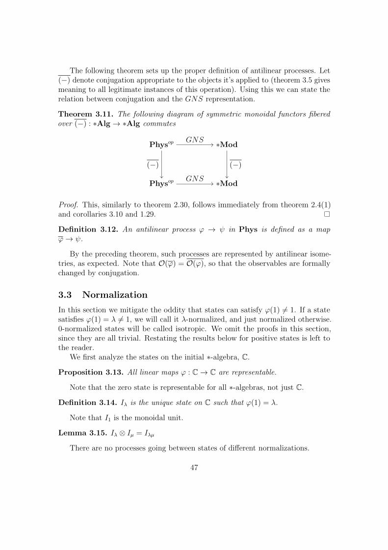
The following theorem sets up the proper definition of antilinear processes. Let(−) denote conjugation appropriate to the objects it’s applied to (theorem 3.5 givesmeaning to all legitimate instances of this operation). Using this we can state therelation between conjugation and the GNS representation.

Theorem 3.11. The following diagram of symmetric monoidal functors fiberedover (−) : ∗Alg→ ∗Alg commutes

Physop ∗Mod

Physop ∗Mod

GNS

(−)

GNS

(−)

Proof. This, similarly to theorem 2.30, follows immediately from theorem 2.4(1)and corollaries 3.10 and 1.29.

Definition 3.12. An antilinear process ϕ → ψ in Phys is defined as a mapϕ→ ψ.

By the preceding theorem, such processes are represented by antilinear isome-tries, as expected. Note that O(ϕ) = O(ϕ), so that the observables are formallychanged by conjugation.

3.3 Normalization

In this section we mitigate the oddity that states can satisfy ϕ(1) 6= 1. If a statesatisfies ϕ(1) = λ 6= 1, we will call it λ-normalized, and just normalized otherwise.0-normalized states will be called isotropic. We omit the proofs in this section,since they are all trivial. Restating the results below for positive states is left tothe reader.

We first analyze the states on the initial ∗-algebra, C.

Proposition 3.13. All linear maps ϕ : C→ C are representable.

Note that the zero state is representable for all ∗-algebras, not just C.

Definition 3.14. Iλ is the unique state on C such that ϕ(1) = λ.

Note that I1 is the monoidal unit.

Lemma 3.15. Iλ ⊗ Iµ = Iλµ

There are no processes going between states of different normalizations.

47

Lemma 3.16. If f : ϕ→ ψ is a morphism in Phys, then ϕ(1) = ψ(1).

We can now understand the various roles played by non-normalized states. LetPhysλ be the full subcategory of Phys containing the λ-normalized states.

Theorem 3.17.

1. Phys is the disjoint union of the Physλ:

Phys =∐λ∈C

Physλ

2. The monoidal structure on Phys restricts to

⊗ : Physλ ×Physµ −→ Physλµ.

3. For λ 6= 0, Iλ ⊗ (−) : Physµ → Physλµ is an equivalence.

4. Iλ is terminal in Physλ.

5. I0 ⊗ (−) maps every state to a zero state.

Let C be the multiplicative monoid of complex numbers, considered as a discretemonoidal category.

Corollary 3.18. The functor Phys → C given by ϕ 7→ ϕ(1) is a symmetricmonoidal fibration, trivial over C∗ ⊆ C.

Thus Phys is monoidally equivalent to Phys0 + C∗ ×Phys1, where C∗ is thediscrete monoidal category of nonzero complex numbers. The equivalence is givenby the inclusion of Phys0 on the first term, and by (λ, ϕ) 7→ Iλ ⊗ ϕ on the second.

We are left with only two interesting subcategories of Phys: the monoidalsubcategory Phys1, of normalized states, and the mysterious monoidal ideal Phys0,of isotropic states.

3.4 Examples

Commutative C∗-algebras and Positive States

By the Riesz-Markov theorem any state ϕ : C(X)→ C is a Radon measure µ onX, with the identification being given by ϕ(f) =

∫Xf(x) dµ(x). The Hermitian

form 〈−,−〉ϕ is then given by

〈f, g〉ϕ =

∫X

f(x)g(x) dµ(x),

48

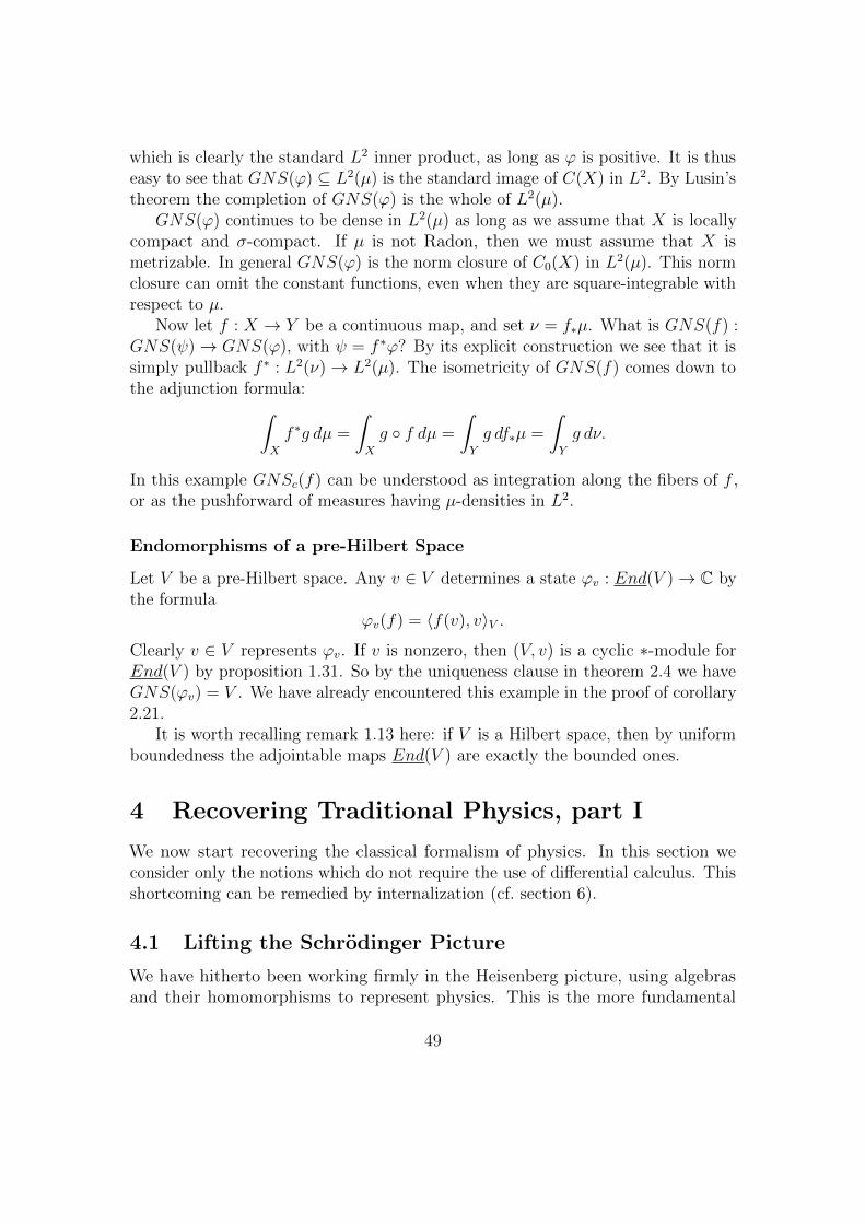
which is clearly the standard L2 inner product, as long as ϕ is positive. It is thuseasy to see that GNS(ϕ) ⊆ L2(µ) is the standard image of C(X) in L2. By Lusin’stheorem the completion of GNS(ϕ) is the whole of L2(µ).

GNS(ϕ) continues to be dense in L2(µ) as long as we assume that X is locallycompact and σ-compact. If µ is not Radon, then we must assume that X ismetrizable. In general GNS(ϕ) is the norm closure of C0(X) in L2(µ). This normclosure can omit the constant functions, even when they are square-integrable withrespect to µ.

Now let f : X → Y be a continuous map, and set ν = f∗µ. What is GNS(f) :GNS(ψ)→ GNS(ϕ), with ψ = f ∗ϕ? By its explicit construction we see that it issimply pullback f ∗ : L2(ν)→ L2(µ). The isometricity of GNS(f) comes down tothe adjunction formula:∫

X

f ∗g dµ =

∫X

g f dµ =

∫Y

g df∗µ =

∫Y

g dν.

In this example GNSc(f) can be understood as integration along the fibers of f ,or as the pushforward of measures having µ-densities in L2.

Endomorphisms of a pre-Hilbert Space

Let V be a pre-Hilbert space. Any v ∈ V determines a state ϕv : End(V )→ C bythe formula

ϕv(f) = 〈f(v), v〉V .

Clearly v ∈ V represents ϕv. If v is nonzero, then (V, v) is a cyclic ∗-module forEnd(V ) by proposition 1.31. So by the uniqueness clause in theorem 2.4 we haveGNS(ϕv) = V . We have already encountered this example in the proof of corollary2.21.

It is worth recalling remark 1.13 here: if V is a Hilbert space, then by uniformboundedness the adjointable maps End(V ) are exactly the bounded ones.

4 Recovering Traditional Physics, part I

We now start recovering the classical formalism of physics. In this section weconsider only the notions which do not require the use of differential calculus. Thisshortcoming can be remedied by internalization (cf. section 6).

4.1 Lifting the Schrodinger Picture

We have hitherto been working firmly in the Heisenberg picture, using algebrasand their homomorphisms to represent physics. This is the more fundamental

49

picture, due to classical mechanics. Here take the first steps toward recoveringthe Schrodinger picture. We can already attach morphisms of Hilbert spaces tohomomorphisms of algebras, through the GNS functor. We now investigate howmuch of this can be reversed.

Let H be a faithful pre-Hilbert ∗-module over A, and let U : H → H ′ be anadjointable isometric linear map to some other pre-Hilbert space. Set B = UAU∗ ⊆End(H ′). Then the map f : A→ B given by

f(a) = UaU∗,

is a homomorphism of ∗-algebras. The map f is well-defined by the faithfulnessof H. Note that B is a ∗-algebra, but not a subalgebra of End(H ′) unless U isunitary.

Recall that every vector ψ ∈ H defines a state s(ψ) ∈ Sr(A) by the formula

s(ψ)(a) = 〈aψ, ψ〉H .

In the following theorem we abuse notation, and write ψ for both the vector andthe state it represents. This will not cause confusion, since one can recover theproper meaning by analyzing the types of our expressions.

Theorem 4.1 (Lifting of the Schrodinger Picture). In the situation above, for anystate ψ ∈ H we have f : Uψ → ψ in Phys, and GNS(f) = U |GNS(ψ), i.e. thefollowing diagram commutes:

GNS(ψ) GNS(Uψ)

H H ′

GNS(f)

U

Proof. By the pre-Hilbert condition and theorem 2.14, GNS(ψ) = Aψ ⊆ H, withψ seen as a state on A, and GNS(Uψ) = UAU∗Uψ = UAψ, with Uψ seen as astate on B. Finally, by the construction of f , U restricts to a cyclic morphismGNS(ψ) → GNS(Uψ) over f . So if GNS(f) maps ψ to Uψ, we will be done,invoking corollary 1.29. But this is obvious, since by the isometricity of U we have

f ∗(Uψ)(a) = 〈f(a)Uψ,Uψ〉H′ = 〈UaU∗Uψ,Uψ〉H′ = 〈aψ, ψ〉H = ψ(a).

GNS(f) must then map ψ to Uψ, by its construction for positive states in section2.4.1.

Perhaps the following is the more natural statement.

50

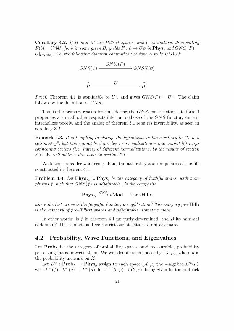
Corollary 4.2. If H and H ′ are Hilbert spaces, and U is unitary, then settingF (b) = U∗bU , for b in some given B, yields F : ψ → Uψ in Phys, and GNSc(F ) =U |GNS(ψ), i.e. the following diagram commutes (we take A to be U∗BU):

GNS(ψ) GNS(Uψ)

H H ′

GNSc(F )

U

Proof. Theorem 4.1 is applicable to U∗, and gives GNS(F ) = U∗. The claimfollows by the definition of GNSc.

This is the primary reason for considering the GNSc construction. Its formalproperties are in all other respects inferior to those of the GNS functor, since itinternalizes poorly, and the analog of theorem 3.1 requires invertibility, as seen incorollary 3.2.

Remark 4.3. It is tempting to change the hypothesis in the corollary to “U is acoisometry”, but this cannot be done due to normalization – one cannot lift mapsconnecting vectors (i.e. states) of different normalizations, by the results of section3.3. We will address this issue in section 5.1.

We leave the reader wondering about the naturality and uniqueness of the liftconstructed in theorem 4.1.

Problem 4.4. Let Physfa ⊆ Physp be the category of faithful states, with mor-phisms f such that GNS(f) is adjointable. Is the composite

PhysfaGNS−−−→ ∗Mod −→ pre-Hilb,

where the last arrow is the forgetful functor, an opfibration? The category pre-Hilbis the category of pre-Hilbert spaces and adjointable isometric maps.

In other words: is f in theorem 4.1 uniquely determined, and B its minimalcodomain? This is obvious if we restrict our attention to unitary maps.

4.2 Probability, Wave Functions, and Eigenvalues

Let ProbL be the category of probability spaces, and measurable, probabilitypreserving maps between them. We will denote such spaces by (X,µ), where µ isthe probability measure on X.

Let L∞ : ProbL → Physp assign to each space (X,µ) the ∗-algebra L∞(µ),with L∞(f) : L∞(ν)→ L∞(µ), for f : (X,µ)→ (Y, ν), being given by the pullback

51

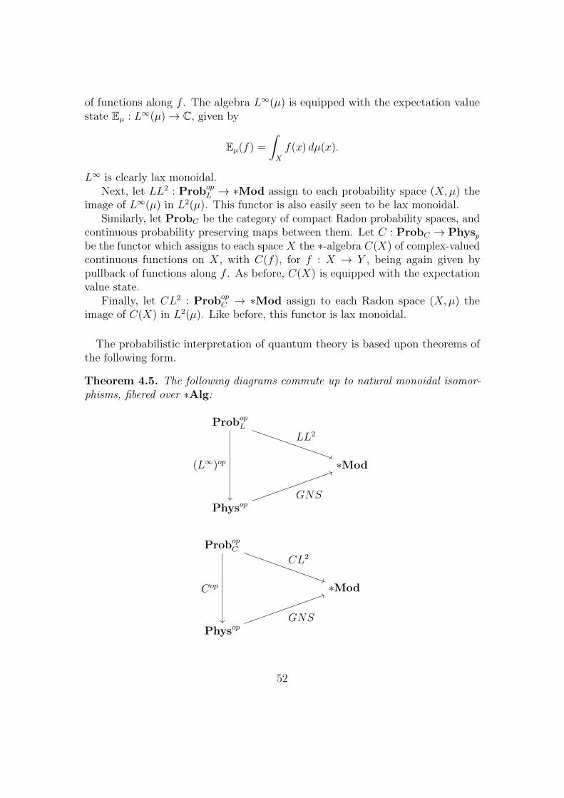
of functions along f . The algebra L∞(µ) is equipped with the expectation valuestate Eµ : L∞(µ)→ C, given by

Eµ(f) =

∫X

f(x) dµ(x).

L∞ is clearly lax monoidal.Next, let LL2 : ProbopL → ∗Mod assign to each probability space (X,µ) the

image of L∞(µ) in L2(µ). This functor is also easily seen to be lax monoidal.Similarly, let ProbC be the category of compact Radon probability spaces, and

continuous probability preserving maps between them. Let C : ProbC → Physpbe the functor which assigns to each space X the ∗-algebra C(X) of complex-valuedcontinuous functions on X, with C(f), for f : X → Y , being again given bypullback of functions along f . As before, C(X) is equipped with the expectationvalue state.

Finally, let CL2 : ProbopC → ∗Mod assign to each Radon space (X,µ) theimage of C(X) in L2(µ). Like before, this functor is lax monoidal.

The probabilistic interpretation of quantum theory is based upon theorems ofthe following form.

Theorem 4.5. The following diagrams commute up to natural monoidal isomor-phisms, fibered over ∗Alg:

ProbopL

∗Mod

Physop

LL2

(L∞)op

GNS

ProbopC

∗Mod

Physop

CL2

Cop

GNS

52

Proof. The LL2 and CL2 functors take values in cyclic modules and cyclic maps.In both cases the constant function 1 represents the expectation value:

〈f1, 1〉L2 =

∫X

f(x) dµ(x) = Eµ(f).

Thus, by theorem 2.4 and corollary 1.29, LL2 and CL2 coincide with GNS up tounique isomorphism, which then must be natural by cyclicity.

Remark 4.6.

• The monoidal structures on LL2 and CL2 can also be constructed as part ofthe proof of the above theorem.

• We can also use the algebras L =⋂p≥1 L

p to represent probability measures.This is usually bigger than L∞ due to, for example, Gaussian random variables,and is not a Banach space in general. The resulting GNS space is not the L2

space of the probability measure, and, for general reasons, L cannot act on inby bounded operators.

• The theorem remains true if we replace probability measures by finite signedmeasures. Complex measures, on the other hand, cannot be accommodated.One would need to replace Hilbert spaces by quadratic complex spaces.

It is important to understand that the above theorem is only one of a hugefamily of theorems. The category of probability spaces can be replaced by anynumber of similar categories, and we have only given diagrams for the two mostimportant cases. The proof always come down to the same simple argument: theL2 space contains an obvious representation of the state in question.

This diversity is the result of our liberal approach. Physp contains, inadvertentlyin some sense, various categories of structured ∗-algebras, such as C∗-algebras, vonNeumann algebras, and ∗-algebras of purely algebraic origin. The reader wishingto distinguish them must merely consider a variant of the construction of Phys,suiting the specific application.

4.2.1 Eigenvalue-Eigenvector Link

Here is a prototypical application of theorems of this sort. Let a ∈ O(ϕ) be anormal observable of some positive state ϕ. Normality means that [a, a∗] = 0or, equivalently, that the ∗-algebra generated by a in O(ϕ) is commutative. Oneimagines this algebra, denoted by 〈a〉, to be the algebra of functions on someprobability space, with the probability measure given by the restriction of ϕ to 〈a〉.This gives an object Pϕ(a) in Physp.

Typically Pϕ(a) can be completed into some algebra in the image of L∞ or C.One then has the following theorem.

53

Theorem 4.7 (Eigenvalue-Eigenvector Link). Suppose that the canonical mapϕ→ Pϕ(a), induced by the inclusion 〈a〉 ⊆ O(ϕ), admits a factorization

ϕR−→ (C(X),Eµ) −→ Pϕ(a),

orϕ

R−→ (L∞(X,µ),Eµ) −→ Pϕ(a),

with the second arrow being over an inclusion 〈a〉 ⊆ C(X) or 〈a〉 ⊆ L∞(X,µ).Then a is canonically a random variable on X and the following are equivalent

for any λ ∈ C:

1. aΩϕ = λΩϕ

2. a = λ almost everywhere on X

3. P(a = λ) = 1

Proof. The equivalence 2⇔ 3 is obvious. To see the equivalence 1⇔ 2 computeGNS(R):

CL2(X,µ) −→ GNS(ϕ)

orLL2(X,µ) −→ GNS(ϕ).

These are morphisms of cyclic modules representing ϕ for a. Thus aΩϕ = λΩϕ isequivalent to a · 1 = λ · 1 in CL2 or LL2, where 1 is the constant function on X.But this last condition is equivalent to a = λ a.e. by basic measure theory.

Remark 4.8. The statement of this theorem is slightly awkward, again, due toour liberal inclusion of any kind of ∗-algebra in our categories. In the setting ofpure C∗-algebras on can give a much sharper statement, using the full L2 space andnot requiring a given factorization (since it can always be constructed by spectraltheory).

Digression: GNSp and the massless 2d quantum scalar field

Theorem 4.5 suggests that the GNS construction is the noncommutative analogue ofthe L2 space. It is well known that the massless quantum scalar field in 2 dimensionscannot be defined in the same manner as in higher dimensions [Wi99b, §1.5]. Onewonders whether the field “really does not exist” or, as Witten’s constructionssuggest, is merely located outside the “L2-realm”. This leads to the followingproblem.

54

Problem 4.9. Define the p-analog of the GNS construction, such that for Radonmeasures on compact Hausdorff spaces we have GNSp(µ) = Lp(µ). Define themassless 2d quantum scalar field in some GNS0 space.

The theory of noncommutative Lp spaces for von Neumann algebras is wellestablished [PX03] (somewhat less so for p = 0), and may be relevant here. Butthe assumption of traciality is problematic.

4.2.2 Generalized Eigenvalue-Eigenvector Link

The eigenvalue-eigenvector link can be derived in considerably greater generality,by substituting for Gelfand duality the duality between algebras and affine schemes.No real measure theory is needed – we will only need to deal with analogues ofDirac delta measures.

Let ϕ be a state with algebra of observables A = O(ϕ). Let a ∈ A be a normalelement. Theorems 4.5 and 4.7 say that the number ϕ(a) is to be interpreted asthe expectation value, in the sense of probability theory, of a in the state ϕ.

The ∗-algebra generated by a, B = C[a, a∗] is commutative. We will denote itsinclusion in A by i : B → A.

Passing to the geometric picture, we obtain an affine scheme X = Spec(B)over C, with chosen real form XR. By the adjunction Γ a Spec, between globalsections and the spectrum functor, the global sections of the structure sheaf OXcorrespond to complex scheme maps X → A1

C. In addition, for X = Spec(B), wehave OX(X) = B. Thus a ∈ A is a complex-valued function on X, and we maytalk about its values at the points of X.

Since we are in the algebraic category, we will have to deal with the fact thatthe type of value a has depends on the point it is evaluated on: the value of a atx ∈ X is an element of the residue field OX,x/mx, which is an extension of C. Forthis reason, we restrict our attention to the C-points of X, for which this extensionis trivial.

We can now formalize the statement that self-adjoint observables are real-valued.

Proposition 4.10. Self adjoint elements x ∈ B determine maps XR → A1R.

Proof. This is just an algebraic geometry consequence of corollary 1.3.

This means, in addition, that self-adjoint observables are determined by theirvalues on the real part of X, i.e. XR. Their “analytic continuation” to X isautomatic.

The state ϕ restricts from A to B, giving us a measure-like structure on X:

OX(X) = Bi∗ϕ−−→ C.

55

We will abuse terminology, and call linear maps OX(X)→ C measures on X. Weare interested in measures supported by single points on X – the “Dirac deltameasures”.

Definition 4.11. Let X be a scheme over C, and x ∈ X a C-point. The Dirac deltaat x, denoted δx, is the localization (i.e. evaluation) map OX(X)→ OX,x/mx = C.

Regular functions separate points on affine X, and so we have the followinglemma.

Lemma 4.12. If δx = δy on an affine scheme X over C, then x = y.

Proof. The Dirac delta measures are ring homomorphisms, so when they are equal,they determine the same maximal ideal in OX(X), and hence the same C-point ofX.

The lemma fails for projective varieties, since then OX(X) = C.Measures naturally push forward under maps of spaces, and the same is true in

our setting.

Definition 4.13. Let ϕ be a measure on X, and f : X → Y a map of schemesover C. Then f∗ϕ defined by

OY (Y )f∗−→ OX(X)

ϕ−→ C,

is a measure on Y .

Since X = Spec(B) is the “space of possible values”, or “possible (pure) states”of a ∈ B = C[a, a∗], the following principle is an algebraic reformulation of thecondition P(a = λ) = 1.

Principle 4.14 (Definition of “having a definite value”). The observable a ∈ Ahas value λ ∈ C in the state ϕ : A→ C if

i∗ϕ = δx,

for some C-point x ∈ X satisfying a(x) = λ, where a : X → A1C is the map

constructed above, and λ ∈ A1C is the C-point corresponding to λ ∈ C.

Remark 4.15. In the setting of probability spaces, the above definition is easilyseen to be equivalent to 4.7(2-3).

We can make the definition more concrete by pushing forward to A1C:

Proposition 4.16. The observable a has value λ in ϕ iff a∗i∗ϕ = δλ.

56

Proof. If a(x) = λ then a∗i∗ϕ = a∗δx = δa(x) = δλ. Conversely, if a∗i

∗ϕ = δλ, theni∗ϕ : B → C is a ring homomorphism, by explicit inspection on all elements of B(recall that ϕ is ∗-linear), and so represents a C-point x ∈ X = Spec(B). Theni∗ϕ = δx by our definition of the Dirac delta. Finally a(x) = λ by lemma 4.12.

We can now generalize the eigenvalue-eigenvector link to our entire setting.

Theorem 4.17 (Generalized Eigenvalue-Eigenvector Link).

a) If any (hence every) cyclic vector representing ϕ is a λ-eigenvector of a, thenthe observable a has value λ in ϕ.

b) If i is admissible for ϕ, and the observable a has value λ in ϕ, then any(hence every) cyclic vector representing ϕ is a λ-eigenvector of a.

Proof. Any cyclic vector Ω representing ϕ is part of the unique cyclic modulerepresenting ϕ, so we may use whichever representation we like.

If Ω is an λ-eigenvector of Ω, then the unique cyclic ∗-module representingi∗ϕ is one-dimensional, and one again finds that i∗ϕ is a ring homomorphism, byexplicit computation, giving i∗ϕ = δx, for some C-point x ∈ X. And again, λ isthe only possible value of a(x), by lemma 4.12.

If i∗ϕ = δx, then GNS(i∗ϕ) = L2(δx) = C, with B acting by evaluation(localization). In particular a acts as multiplication by a(x) = λ, by assumption.By admissibility we have the map of ∗-modules over i:

GNS(i∗ϕ)GNS(i)−−−−→ GNS(ϕ).

Denoting by Ω and Ω′ the cyclic vectors of GNS(ϕ) and GNS(i∗ϕ), respectively,we have

aΩ = aGNS(i)(Ω′) = GNS(i)(aΩ′) = GNS(i)(λΩ′) = λGNS(i)(Ω′) = λΩ.

Corollary 4.18. Let ϕ be a positive state. Then a has value λ in ϕ iff any vectorin a pre-Hilbert module representing ϕ is a λ-eigenvector of a.

Proof. This follows from theorem 2.14, proposition 2.24, and the preceding theorem.

57

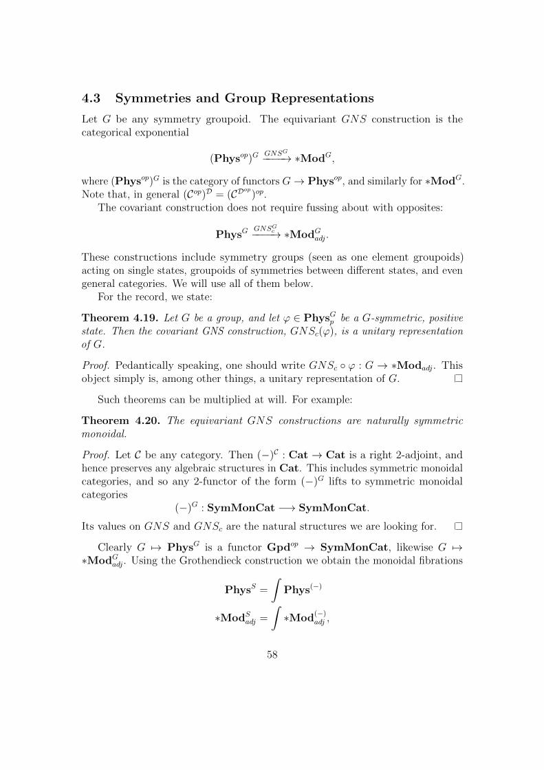
4.3 Symmetries and Group Representations

Let G be any symmetry groupoid. The equivariant GNS construction is thecategorical exponential

(Physop)GGNSG−−−−→ ∗ModG,

where (Physop)G is the category of functors G→ Physop, and similarly for ∗ModG.Note that, in general (Cop)D = (CDop)op.

The covariant construction does not require fussing about with opposites:

PhysGGNSGc−−−−→ ∗ModGadj.

These constructions include symmetry groups (seen as one element groupoids)acting on single states, groupoids of symmetries between different states, and evengeneral categories. We will use all of them below.

For the record, we state:

Theorem 4.19. Let G be a group, and let ϕ ∈ PhysGp be a G-symmetric, positivestate. Then the covariant GNS construction, GNSc(ϕ), is a unitary representationof G.

Proof. Pedantically speaking, one should write GNSc ϕ : G → ∗Modadj. Thisobject simply is, among other things, a unitary representation of G.

Such theorems can be multiplied at will. For example:

Theorem 4.20. The equivariant GNS constructions are naturally symmetricmonoidal.

Proof. Let C be any category. Then (−)C : Cat → Cat is a right 2-adjoint, andhence preserves any algebraic structures in Cat. This includes symmetric monoidalcategories, and so any 2-functor of the form (−)G lifts to symmetric monoidalcategories

(−)G : SymMonCat −→ SymMonCat.

Its values on GNS and GNSc are the natural structures we are looking for.

Clearly G 7→ PhysG is a functor Gpdop → SymMonCat, likewise G 7→∗ModGadj. Using the Grothendieck construction we obtain the monoidal fibrations

PhysS =

∫Phys(−)

∗ModSadj =

∫∗Mod

(−)adj ,

58

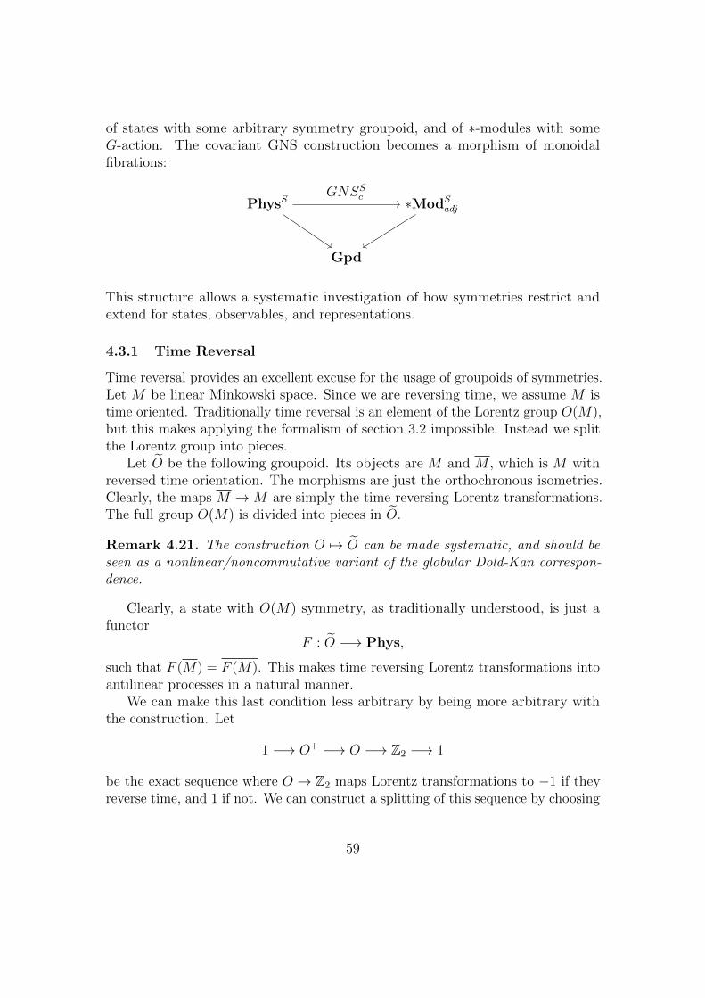
of states with some arbitrary symmetry groupoid, and of ∗-modules with someG-action. The covariant GNS construction becomes a morphism of monoidalfibrations:

PhysS ∗ModSadj

Gpd

GNSSc

This structure allows a systematic investigation of how symmetries restrict andextend for states, observables, and representations.

4.3.1 Time Reversal

Time reversal provides an excellent excuse for the usage of groupoids of symmetries.Let M be linear Minkowski space. Since we are reversing time, we assume M istime oriented. Traditionally time reversal is an element of the Lorentz group O(M),but this makes applying the formalism of section 3.2 impossible. Instead we splitthe Lorentz group into pieces.

Let O be the following groupoid. Its objects are M and M , which is M withreversed time orientation. The morphisms are just the orthochronous isometries.Clearly, the maps M →M are simply the time reversing Lorentz transformations.The full group O(M) is divided into pieces in O.

Remark 4.21. The construction O 7→ O can be made systematic, and should beseen as a nonlinear/noncommutative variant of the globular Dold-Kan correspon-dence.

Clearly, a state with O(M) symmetry, as traditionally understood, is just afunctor

F : O −→ Phys,

such that F (M) = F (M). This makes time reversing Lorentz transformations intoantilinear processes in a natural manner.

We can make this last condition less arbitrary by being more arbitrary withthe construction. Let

1 −→ O+ −→ O −→ Z2 −→ 1

be the exact sequence where O → Z2 maps Lorentz transformations to −1 if theyreverse time, and 1 if not. We can construct a splitting of this sequence by choosing

59

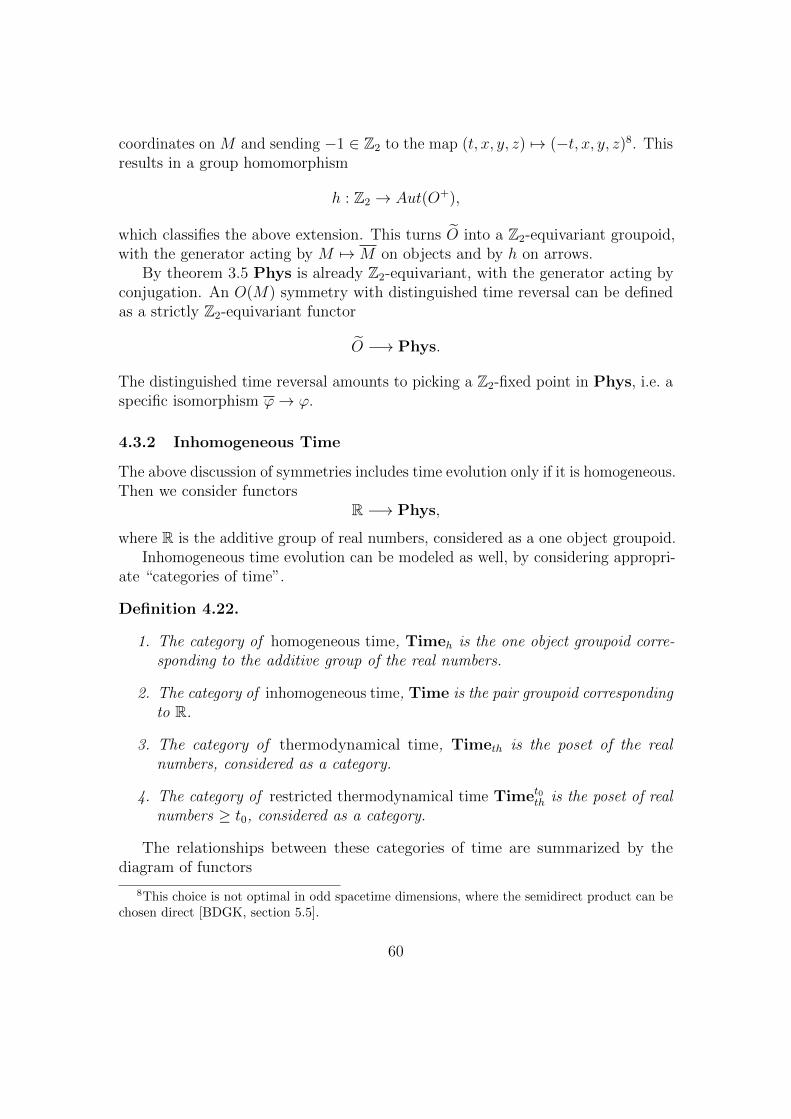
coordinates on M and sending −1 ∈ Z2 to the map (t, x, y, z) 7→ (−t, x, y, z)8. Thisresults in a group homomorphism

h : Z2 → Aut(O+),

which classifies the above extension. This turns O into a Z2-equivariant groupoid,with the generator acting by M 7→M on objects and by h on arrows.

By theorem 3.5 Phys is already Z2-equivariant, with the generator acting byconjugation. An O(M) symmetry with distinguished time reversal can be definedas a strictly Z2-equivariant functor

O −→ Phys.

The distinguished time reversal amounts to picking a Z2-fixed point in Phys, i.e. aspecific isomorphism ϕ→ ϕ.

4.3.2 Inhomogeneous Time

The above discussion of symmetries includes time evolution only if it is homogeneous.Then we consider functors

R −→ Phys,

where R is the additive group of real numbers, considered as a one object groupoid.Inhomogeneous time evolution can be modeled as well, by considering appropri-

ate “categories of time”.

Definition 4.22.

1. The category of homogeneous time, Timeh is the one object groupoid corre-sponding to the additive group of the real numbers.

2. The category of inhomogeneous time, Time is the pair groupoid correspondingto R.

3. The category of thermodynamical time, Timeth is the poset of the realnumbers, considered as a category.

4. The category of restricted thermodynamical time Timet0th is the poset of realnumbers ≥ t0, considered as a category.

The relationships between these categories of time are summarized by thediagram of functors

8This choice is not optimal in odd spacetime dimensions, where the semidirect product can bechosen direct [BDGK, section 5.5].

60

Timet0th ⊆ Timeth Time Timeh,i p

where i is the obvious inclusion, and is actually a localization of Timeth, invertingall arrows. The functor p collapses the distinct time objects into one, and mapsthe unique morphism t→ t′ to t′ − t.

The categories of states equipped with various notions of time evolution corre-spond to the exponentials

PhysTime,

with Time carrying an appropriate subscript.Homogeneous time determines a single state ϕ and an additive group of auto-

morphisms U(t) : ϕ→ ϕ, t ∈ R.Inhomogeneous time determines a state ϕ(t) for every time t ∈ R, and invertible

maps U(t, t′) : ϕ(t)→ ϕ(t′) subject to U(t, t) = id and

U(t′, t′′)U(t, t′) = U(t, t′′).

Thermodynamical time is similar to inhomogeneous time, but U(t, t′) is only givenfor t ≤ t′, and need not be invertible. Restricted time simply restricts t to t ≥ t0for objects and morphisms.

In section 5.1 we will construct a statistical version of Phys, called PhysM . Inthat category thermodynamical time can truly come into its own, with

PhysTime

t0th

M

generalizing the notion of a quantum dynamical semigroup (cf. [Ho01]).

4.4 Composite Systems

In this section we assume states are normalized, working exclusively with Phys1.The monoidal structure on normalized states can be characterized as the mostgeneral notion of composite satisfying the following axioms.

Axioms 4.23 (Axioms for Composite Systems). A state ϕ ψ will be called acomposite of ϕ and ψ if we are given the following structure and properties:

1. Composition: there are morphisms

pϕ : ϕ ψ −→ ϕ

pψ : ϕ ψ −→ ψ,

in Phys1, meaning that ϕ ψ contains a copy of both ϕ and ψ.

61

2. Noninteraction: these copies do not affect each other, meaning:

ϕ ψ(pϕ(a)pψ(b)) = ϕ(a)ψ(b),

for all a ∈ O(ϕ) and b ∈ O(ψ).

3. Probabilistic Independence: these copies are independent, in the sense ofnoncommutative probability theory. For any a ∈ O(ϕ) and b ∈ O(ψ) we have

[pϕ(a), pψ(b)] = 0,

in O(ϕ ψ). Here [x, y] denotes the commutator of x and y.

Remark 4.24.

• These axioms are not completely independent. Composition implies all in-stances of noninteraction in which a = 1 or b = 1.

• Without the normalization assumption the composition axiom can’t be satisfied.By theorem 3.17(1-2) if either ϕ or ψ is not normalized then one of pϕ or pψcannot exist. If neither is normalized then neither can exist.

Theorem 4.25. ϕ⊗ ψ is initial among the composites of ϕ and ψ.

Proof. ϕ ⊗ ψ clearly satisfies requirements 1-3. That it is initial follows fromtheorem 1.23: by probabilistic independence the maps O(pϕ) and O(pψ) factoruniquely through O(ϕ)⊗O(ψ), and by noninteraction the pullback of ϕ ψ alongthis factorization must be ϕ ⊗ ψ. This gives a unique structure preserving mapϕ⊗ ψ → ϕ ψ in Phys1.

Corollary 4.26. The initial composite satisfies the following additional axioms:

4. Process Covariance: ⊗ is a functor:

⊗ : Phys1 ×Phys1 −→ Phys1.

This means that processes can be composed, in addition to states.

5. Naturality of Composition: the components pϕ and pψ form natural transfor-mations ⊗ → πi, where πi is the projection

πi : Phys1 ×Phys1 −→ Phys1.

This means that the initial composite is uniform, and not dependent on thedetails of any states.

6. No Further Relations: ⊗ is initial in the category of functors with the struc-tures and properties above.

Proof. These are obvious, with point 6 being a weakening of theorem 4.25.

Theorem 4.25 and corollary 3.18 characterize the monoidal product on Physfor all non-isotropic states. The composites of isotropic states remain mysterious.

62

5 Statistical Physics and Non-Unitary Processes

5.1 Non-unitary GNS

To define noncommutative Markov processes, we must extend the notion of admis-sibility.

Definition 5.1. A ∗-linear map Φ : A→ B between ∗-algebras is admissible for astate ϕ ∈ Sr(B) if A⊥ ⊆ Φ−1(B⊥).

Here A⊥ is computed for the Hermitian form induced by ψ = Φ∗ϕ. Note thatψ is representable by theorem 2.4(3). Unlike before, the inclusion Φ−1(B⊥) ⊆ A⊥

is no longer trivial, since Φ is not multiplicative.Just like in section 2.4.2 we define the linear map

GNSM(Φ) : GNS(ψ) = A/A⊥ → B/B⊥ = GNS(ϕ)

by the formula [x] 7→ [Φ(x)]. No analogue of proposition 2.24 is available, and theformula looks like an arbitrary choice.

GNSM (Φ) is no longer isometric or cyclic, but it can be computed in interestingcases, due to the following proposition.

Proposition 5.2. GNSM(Φ) : GNS(ψ)→ GNS(ϕ) satisfies the following iden-tity:

GNSM(Φ)(aΩψ) = Φ(a)Ωϕ,

for all a ∈ A.

Proof. GNSM(Φ)(aΩψ) = GNSM(Φ)([a]) = [Φ(a)] = Φ(a)Ωϕ.

Note that this property looks like “being a linear map over Φ”, but it applies onlyto the cyclic vector. We do not, in general, haveGNSM (Φ)(av) = Φ(a)GNSM (Φ)(v)for arbitrary v ∈ GNS(ψ) and a ∈ A. Note also that this proposition applies toa = 1, showing that GNSM(Φ) is cyclic iff it’s unital.

An analogue of proposition 2.27 is available.

Proposition 5.3.

1. The composite of admissible maps is admissible

2. The tensor product of admissible maps is admissible

3. Completely positive maps between positive states are admissible

Proof. We deal with the complications of not being a homomorphism on a case-by-case basis.

63

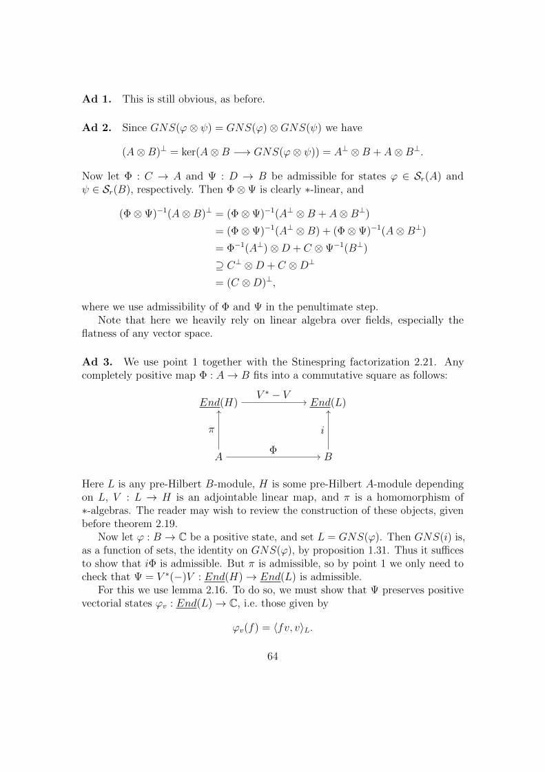
Ad 1. This is still obvious, as before.

Ad 2. Since GNS(ϕ⊗ ψ) = GNS(ϕ)⊗GNS(ψ) we have

(A⊗B)⊥ = ker(A⊗B −→ GNS(ϕ⊗ ψ)) = A⊥ ⊗B + A⊗B⊥.

Now let Φ : C → A and Ψ : D → B be admissible for states ϕ ∈ Sr(A) andψ ∈ Sr(B), respectively. Then Φ⊗Ψ is clearly ∗-linear, and

(Φ⊗Ψ)−1(A⊗B)⊥ = (Φ⊗Ψ)−1(A⊥ ⊗B + A⊗B⊥)

= (Φ⊗Ψ)−1(A⊥ ⊗B) + (Φ⊗Ψ)−1(A⊗B⊥)

= Φ−1(A⊥)⊗D + C ⊗Ψ−1(B⊥)

⊇ C⊥ ⊗D + C ⊗D⊥

= (C ⊗D)⊥,

where we use admissibility of Φ and Ψ in the penultimate step.Note that here we heavily rely on linear algebra over fields, especially the

flatness of any vector space.

Ad 3. We use point 1 together with the Stinespring factorization 2.21. Anycompletely positive map Φ : A→ B fits into a commutative square as follows:

End(H) End(L)

A B

π

Φ

V ∗ − V

i

Here L is any pre-Hilbert B-module, H is some pre-Hilbert A-module dependingon L, V : L → H is an adjointable linear map, and π is a homomorphism of∗-algebras. The reader may wish to review the construction of these objects, givenbefore theorem 2.19.

Now let ϕ : B → C be a positive state, and set L = GNS(ϕ). Then GNS(i) is,as a function of sets, the identity on GNS(ϕ), by proposition 1.31. Thus it sufficesto show that iΦ is admissible. But π is admissible, so by point 1 we only need tocheck that Ψ = V ∗(−)V : End(H)→ End(L) is admissible.

For this we use lemma 2.16. To do so, we must show that Ψ preserves positivevectorial states ϕv : End(L)→ C, i.e. those given by

ϕv(f) = 〈fv, v〉L.

64

We computeΨ∗ϕv(f) = 〈V ∗fV v, v〉L = 〈fV v, V v〉H ,

which is non-negative, since H is a pre-Hilbert space.Next we set v = Ωϕ ∈ L, and check the admissibility of Ψ for ϕv using lemma

2.16. We see thatEnd(H)⊥ = f : Ψ∗ϕv(f

∗f) = 0,

which is exactly those f ∈ End(H) for which fV v = 0. On the other hand

End(L)⊥ = g : ϕv(g∗g) = 0,

which is those g ∈ End(L) for which gv = 0. Thus if f ∈ End(H)⊥ thenΨ(f) = V ∗fV ∈ End(L)⊥, which means Ψ is admissible for ϕv.

Now let ∗AlgM be the category of ∗-linear maps between ∗-algebras, and let

SM : ∗AlgopM −→ Set

be the functor assigning to every algebra its set of representable states. This iswell-defined by theorem 2.4(3).

Definition 5.4. PhysM is the subcategory of 1 ↓ SM spanned by the admissiblemorphisms.

This is well-defined by proposition 5.3, which also implies the next theorem.

Theorem 5.5. PhysM is a symmetric monoidal category.

Before stating that GNSM is symmetric monoidal, we must determine itscodomain. For now, we declare it to be Herm, the category of nondegenerateHermitian vector spaces and all linear maps between them. This category issymmetric monoidal by lemma 1.9.

This choice neglects a lot of structure, such as the module structure on GNS(ϕ),and the property described in proposition 5.2. Because of this we cannot say thatGNSM is fibered over ∗AlgM .

Theorem 5.6. The constructions

ϕ 7−→ GNS(ϕ)

Φ 7−→ GNSM(Φ),

for objects ϕ ∈ PhysM and morphisms Φ : ϕ→ ψ in PhysM , are part of a strongsymmetric monoidal functor

GNSM : PhysM −→ Herm.

65

Proof. For any state ϕ the module GNS(ϕ) is cyclic, and so we can use proposition5.2 for computations. That GNSM is a functor is then obvious.

Note that PhysM has the same objects as Phys (literally). It just has moremorphisms. Thus the monoidal structure is already there, and we merely have tocheck that our transformation

GNSM(ϕ)⊗GNSM(ψ) −→ GNSM(ϕ⊗ ψ) (3)

remains natural. The coherence conditions don’t involve maps outside of Phys,and so are still automatically satisfied.

The isomorphism (3), constructed abstractly in theorem 2.30, is easily computedby cyclicity. It’s the map

aΩϕ ⊗ bΩψ 7−→ a⊗ bΩϕ⊗ψ,

where a ∈ O(ϕ) and b ∈ O(ψ) are acting on the appropriate cyclic vectors.Now consider Φ : ϕ′ → ϕ and Ψ : ψ′ → ψ in PhysM and compute:

GNSM(Φ⊗Ψ)(a⊗ bΩϕ⊗ψ) = Φ⊗Ψ(a⊗ b)Ωϕ′⊗ψ′

= Φ(a)⊗Ψ(b)Ωϕ′⊗ψ′

7→ Φ(a)Ωϕ′ ⊗Ψ(b)Ωψ′

= GNSM(Φ)(aΩϕ′)⊗GNSM(bΩψ′)

= GNSM(Φ)⊗GNSM(Ψ)(aΩϕ′ ⊗ bΩψ′),

where we first use proposition 5.2, and check naturality for the inverse of (3).

5.2 The Covariant Representation

A new problem arises when trying to take the adjoint of GNSM . The mapsGNSM(Φ) are not isometric, and so are not guaranteed to have an adjoints uponpassing to Hilbert completions. We deal with this in a manner similar to what wesuggested after theorem 2.32.

Let preHilb ⊆ Herm be the monoidal subcategory of pre-Hilbert spaces andbounded maps between them. Define

PhysM,pb = GNS−1M (preHilb),

giving a monoidal subcategory of PhysM spanned by the positive states andprocesses with bounded GNS representations between them. This category containsPhysp, and is therefore already quite rich. We will see in section 5.5 that it is aproper extension of Physp.

66

Definition 5.7. The covariant GNSM construction, GNSM,c is defined as thecomposite

PhysM,pb preHilbop HilbGNSopM completion + adjoint

By the definition of the tensor product of Hilbert spaces, we have the followingtheorem.

Theorem 5.8. GNSM,c : PhysM,pb −→ Hilb is a symmetric monoidal functor.

5.3 Gelfand Duals of Markov Processes

In this section we extend Gelfand duality to Markov processes and completelypositive maps. We follow [FJ15], albeit with more pedestrian notation.

The Gelfand dual of a completely positive unital map is a Markov process inRadon measures. To see this consider a (completely) positive map

Φ : C(Y ) −→ C(X),

and compute

Φ(f)(x) =

∫X

Φ(f) dδx =

∫Y

f dΦ∗(δx),

where δx is the Dirac delta measure at x (i.e. evaluation at x). This shows that Φis the dual of the Markov process given by

X −→M(Y )

x 7−→ Φ∗(δx),

where M(Y ) is the space of Radon probability measures on Y .Conversely, given a Markov process F : X → M(Y ) we obtain a completely

positive map

C(Y ) −→ C(X)

f 7−→ (x 7→∫Y

f dF (δx)).

These identifications clearly generalize Gelfand duality, and are compatible withcomposition. To see the second claim, recall that multiplication in M is given incomponents mX : M(M(X))→M(X) by∫

X

f d(mX(λ)) =

∫M(X)

∫X

f(x) dν(x) dλ(ν).

67

The composition of two Markov processes F : X →M(Y ), G : Y →M(Z) is givenby

XF−→M(Y )

M(G)−−−→M(M(Z))mZ−−→M(Z).

Now consider two positive maps Ψ : C(Z)→ C(Y ),Φ : C(Y )→ C(X), with dualsG,F respectively. The dual of their composite is

x 7→ Ψ∗(Φ∗(δx)) = Ψ∗(F (x)) = mZG∗(F (x)) = G(F (x)).

To see the penultimate equality consider any Radon measure µ in place of F (x),and compute:∫

Z

f d(mZG∗µ) =

∫M(Z)

∫Z

f(z) dν(z) d(G∗µ)(ν) =

∫Y

∫Z

f(z) dG(y)(z) dµ(y),

demonstrating that Ψ∗(µ) = mZ(G∗µ). The last equality uses the well knownadjunction formula:

∫g∗f dµ =

∫f g dµ =

∫f dg∗µ.

The Radon measure monad is lax monoidal, with the monoidal structure givenby

M(X)×M(Y ) −→M(X × Y )

(µ, ν) 7−→ µ⊗ ν1 −→M(1)

∗ 7−→ δ1

One easily verifies that the composition and unit on M are monoidal transforma-tions. Because of this, for completely formal reasons [Za12], the Kleisli categoryCptHausM for M is monoidal, with the monoidal product given by

(XF−→M(Z))⊗ (Y

G−→M(T )) = X × Y F×G−−−→M(Z)×M(T ) −→M(Z × T ),

where the last arrow is the monoidal product on M .The identification of completely positive maps with Markov processes is monoidal.

Given Φ : C(T ) → C(Y ),Ψ : C(Z) → C(X), with duals F,G respectively,the dual of Φ ⊗ Ψ : C(Z) ⊗ C(T ) → C(X) ⊗ C(Y ) is, under the identificationC(X)⊗ C(Y ) ' C(X × Y ), F ⊗G. To see this note that under the isomorphismC(X)⊗ C(Y ) ' C(X × Y ) the measure δ(x,y), for (x, y) ∈ X × Y , corresponds tothe functional δx ⊗ δy on C(X)⊗ C(Y ), and compute

(Φ⊗Ψ)∗(δ(x,y)) ' (Φ⊗Ψ)∗(δx⊗δy) = Φ∗(δx)⊗Ψ∗(δy) = F (x)⊗G(y) = F⊗G(x, y),

demonstrating that the dual of Φ⊗Ψ is F ⊗G.These computations demonstrate the following theorem.

68

Theorem 5.9 (Theorem 5.1 in [FJ15] ). Gelfand duality extends to a monoidalequivalence

CptHausM = commutative C∗-algebras with positive unital mapsop,

where CptHausM is the Kleisli category of the Radon probability measure monad,i.e. the category of Markov processes in CptHaus.

Equivalently CptHausM is the category of Markov processes with Radonmeasure kernels between compact Hausdorff spaces.

Remark 5.10. We have restricted ourselves to probability measures, since onlythen is M(X) a compact Hausdorff space. Finite measures give a locally compactHausdorff space, and require working with locally compact spaces from the beginning.Since we are focusing on unital algebras, we will not pursue this generalization here.

Corollary 5.11. The category of compact Radon probability spaces and Markovprocesses between them is monoidally equivalent to the category of states on com-mutative C∗-algebras and positive unital maps between them.

Proof. The first category is the coslice 1/CptHausM and the second is the sliceC∗-algebras and positive maps between them/C. They are clearly dual to eachother, through the above monoidal equivalence.

5.4 Quantum Markov Processes

The discussion above allows us to generalize the relationship between the GNSconstruction and probability theory (theorem 4.5) to the case of Markov processes.We begin by extending the functor CL2 to our new setting.

Let F : X → Y be a Markov process between probability spaces. Then bycorollary 5.11 we obtain a completely positive unital map

C(F ) : C(Y ) −→ C(X),

which furthermore preserves the expectation values on C(X) and C(Y ).We define

CL2(F ) : L2(Y ) −→ L2(X)

by the formula

CL2(F )(f)(x) =

∫Y

f dF (δx), (4)

with the right hand side seen as an element of L2(X). One easily sees that this iswell defined, and monoidal. Indeed, the formula (4) is just the composite of pullingback by the Gelfand dual of C(F ) with the projection to the GNS space. Assuch it is immediately obvious that CL2(F ) is given by the same formula definingGNSM , leading us to the following theorem.

69

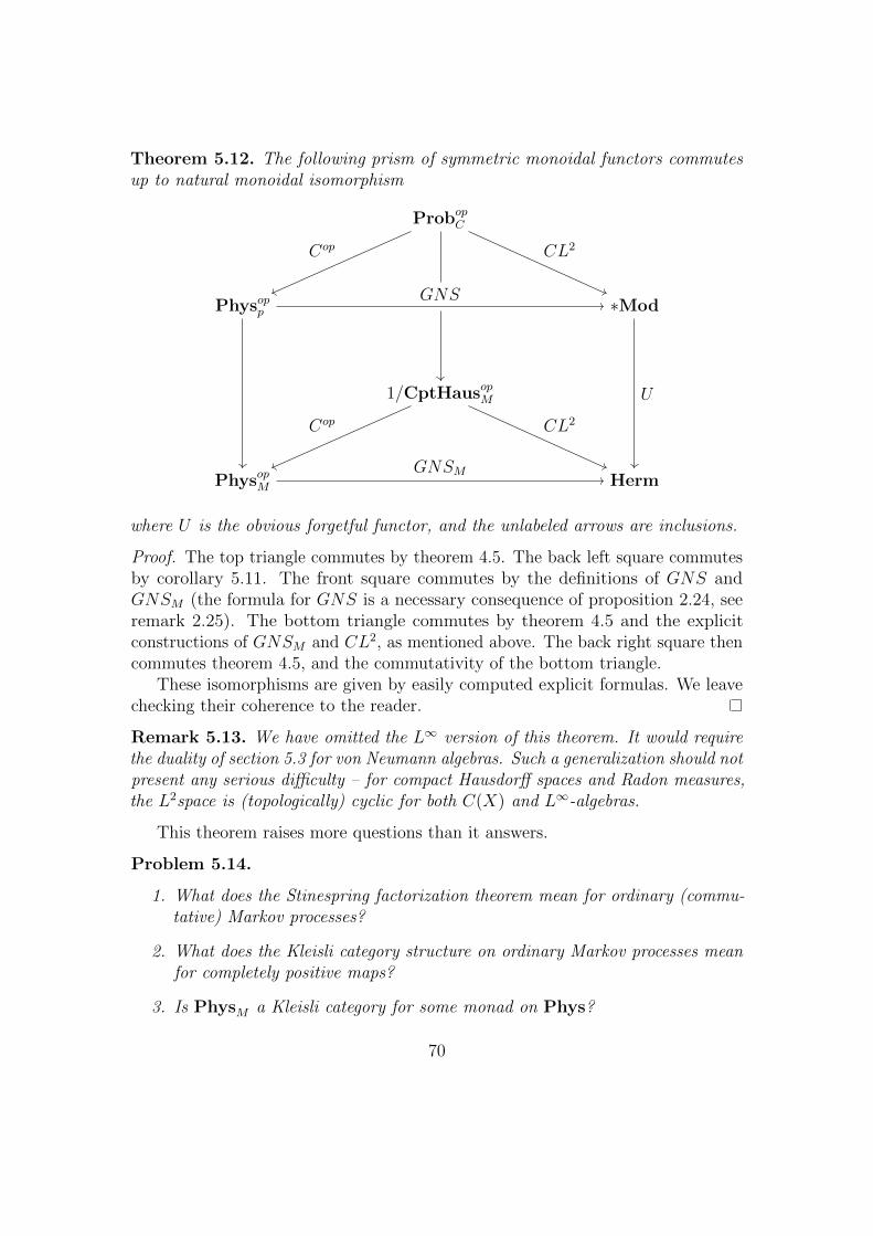
Theorem 5.12. The following prism of symmetric monoidal functors commutesup to natural monoidal isomorphism

ProbopC

Physopp ∗Mod

1/CptHausopM

PhysopM Herm

U

GNSM

CL2

GNS

Cop

CL2Cop

where U is the obvious forgetful functor, and the unlabeled arrows are inclusions.

Proof. The top triangle commutes by theorem 4.5. The back left square commutesby corollary 5.11. The front square commutes by the definitions of GNS andGNSM (the formula for GNS is a necessary consequence of proposition 2.24, seeremark 2.25). The bottom triangle commutes by theorem 4.5 and the explicitconstructions of GNSM and CL2, as mentioned above. The back right square thencommutes theorem 4.5, and the commutativity of the bottom triangle.

These isomorphisms are given by easily computed explicit formulas. We leavechecking their coherence to the reader.

Remark 5.13. We have omitted the L∞ version of this theorem. It would requirethe duality of section 5.3 for von Neumann algebras. Such a generalization should notpresent any serious difficulty – for compact Hausdorff spaces and Radon measures,the L2space is (topologically) cyclic for both C(X) and L∞-algebras.

This theorem raises more questions than it answers.

Problem 5.14.

1. What does the Stinespring factorization theorem mean for ordinary (commu-tative) Markov processes?

2. What does the Kleisli category structure on ordinary Markov processes meanfor completely positive maps?

3. Is PhysM a Kleisli category for some monad on Phys?

70

Example. Let Time = R≥0 be the the order of the nonnegative real numbers,considered as a category. The functor category

PhysTimeM ,

represents a vast generalization of the category of quantum dynamical semigroups(cf. [Ho01]). The preceding theorem shows that this notion completely subsumesthe notion of a Markov semigroup, defined as semigroups of maps in 1/CptHausM .

5.5 Conditioning

Since GNS maps for admissible morphisms are not usually cyclic, the properreformulation of theorem 4.1 is not obvious. Corollary 2.21 makes this superfluousto a certain extent, giving a definite form to the most interesting maps underinvestigation – the completely positive ones. Here we will simply note some obviousexamples, which exhibit enough cyclicity for computation. The reader should thinkof these computations as extending corollary 4.2 to coisometries.

5.5.1 State Vector Collapse

Consider an inclusion i : H → H ′ of Hilbert spaces. Its adjoint i∗ is the orthogonalprojection H ′ → H. Both Φ = i∗(−)i and Ψ = i(−)i∗ are completely positive mapsbetween End(H) and End(H ′), with Φ Ψ = 1End(H), and Ψ Φ = ii∗(−)ii∗ beinga conditioning operator by the self-adjoint projection P = ii∗. By proposition 1.31both H and H ′ are cyclic for their endomorphism algebras, and any nonzero vectoris cyclic. By remark 1.13 End(H) is just the usual algebra of all bounded operatorson H, and H is algebraically cyclic over it – no closure required.

Now let v ∈ H, and ϕv : End(H)→ C be the state given by ϕv(a) = 〈av, v〉H .By the above GNS(ϕv) = H, with cyclic vector Ωϕv = v. Next let ψ = Φ∗ϕv, andcompute

Φ∗ϕv(a) = ϕv(Φ(a)) = 〈i∗aiv, v〉H = 〈aiv, iv〉H′ ,

to see that ψ = ϕiv. Thus GNSM(Φ) : H → H ′. By proposition 5.2, it acts as

aiv 7−→ Φ(a)v = i∗aiv,

for a ∈ End(H ′), and v kept fixed, and so GNSM (Φ) = i∗. Similarly, Ψ∗ϕw = ϕi∗w,for w ∈ H ′, and GNSM(Ψ) = i, acting as

ai∗w 7−→ Ψ(a)i∗w = iai∗ii∗w = iai∗w,

for a ∈ End(H).

71

This gives GNSM(Ψ) GNSM(Φ) = GNSM(Φ Ψ) = ii∗ = P , the orthogonalprojection onto H. Note that, since GNSM is contravariant, the morphism “ΦΨ”,as an arrow of PhysM , corresponds to the algebra homomorphism Ψ Φ. Thecovariant GNSM functor yields GNSM,c(Φ) = i, and GNSM,c(Ψ) = i∗. This givesthe expected identity GNSM,c(Φ Ψ) = P . This is another indication of thephysical naturality of the GNSc construction.

We can also compute the effect of conditioning on an arbitrary ∗-algebra A. LetP ∈ A be a self-adjoint projection, let ϕ be a positive state on A, let Φ : A→ Abe Φ(a) = PaP , and set ψ = Φ∗ϕ. Clearly, Φ is completely positive. Note that

ψ(a) = ϕ(Φ(a)) = ϕ(PaP ) = 〈aPΩϕ, PΩϕ〉GNS(ϕ),

and hence ψ is represented by PΩϕ ∈ GNS(ϕ). Thus, by theorem 2.14, GNS(ψ) =APΩϕ ⊆ GNS(ϕ),

As above, GNSM(Φ) : GNS(ψ)→ GNS(ϕ) acts as

aPΩϕ = aΩψ 7−→ PaPΩϕ = PaΩψ,

which means it is the composite

GNS(ψ) → GNS(ϕ)P−→ GNS(ϕ).

Note that GNS(ψ) is not, in general, contained in the image of P , so this is anontrivial map. If A = End(H), and ϕ = ϕv for some v ∈ H, we would haveGNS(ψ) = H = GNS(ϕ), as long as ψ is nonzero. For general A, GNS(ψ) maybe a proper subspace of GNS(ϕ). Returning to the current situation, GNSM,c(Φ)is given by the action of P ∗ = P followed by the orthogonal projection onto (theHilbert completion of) GNS(ψ).

I submit to the reader that these computations provide a reasonable mathe-matical interpretation of the notion of “state vector collapse”, with P given by asuitable spectral projection. What we have shown is that it is an unnormalizedconditioning operation. The lack of normalization is not a problem – rescaling is aMarkov process in our setting.

5.5.2 Scattering

We can define scattering processes, such as annihilation e+ + e− → γ + γ, directlyas Markov processes, for any well-defined scattering matrix.

Let α and β denote two types of particles (possibly composite). The scatteringprocess α→ β is given by the composite

Hαiα−→ F(H)

S−→ F(H)pβ−→ Hβ,

72

where Hα, Hβ ⊆ F(H) are the Hilbert spaces of states of the α and β particles,F is the Fock space functor, H is an arbitrary Hilbert space (usually a uniformmixture of elementary particles), S is a unitary operator (called the scatteringmatrix), and the i and p maps are inclusions and projections, respectively. Sinceall these maps are inclusions, projections, or are unitary, this composite defines anarrow Sαβ : α→ β in PhysM over the completely positive map (pβSi)

∗(−)pβSi :End(Hβ)→ End(Hα), such that GNSM,c(Sαβ) is the composite displayed above.

Note that in decomposing S into its matrix elements we lose the full algebra ofobservables on Fock space, and must restrict to the observables preserving the αand β particles.

5.5.3 Corollary: The “Penrose Problem”

We finish this section by indulging in wild quantum gravity speculation. Belowwe unapologetically ignore the specific content of Penrose’s ideas [Pe95], andgratuitously appropriate his name nonetheless.

The critical point I wish to communicate here is that the basic idea of gravitycollapsing the state of a system could be right. What’s more, we are in a positionto look for its mathematical realization. We formulate the search as follows.

Problem 5.15 (“Penrose Problem”). Which bordisms can be monoidally repre-sented by conditioning maps?

More formally let Bord be some category of structured bordisms, such astimelike Lorentzian bordisms. Are there any symmetric monoidal functors

Bord −→ PhysM ,

which map a bordism to a conditioning process? Clearly, such bordisms cannot beinvertible. But, with the extra structure afforded by a metric, there are plenty ofsuch morphisms, even for topologically trivial bordisms. Expanding and collapsingspacetimes are both obvious examples. Dualizing the the TQFT wisdom that

(. . . ) the absence of topology change implies unitary time evolution.

John Baez, [Ba06] (emphasis original)

we can say that

The presence of a dynamical metric allows non-unitary time evolution.

We even know that this allowance is utilized by quantum field theory in curvedspacetime [Wa94].

73

At the physical level of rigor, we can formulate our question as follows: dynamicalspacetime appears to represent a flux of information. Can this information be usedto condition states evolving in that spacetime? Can there be a gravity-inducedoutflux beyond what is required by the canonical commutation relations?

The answer to the second question appears to be yes – consider Hawkingradiation. I consider it to be an exact result in an approximate theory, henceworthy of mathematical consideration. By hand-waving CPT arguments [Ha14] weexpect influxes to be possible as well.

It would be interesting to investigate this obviously information theoretic aspectof bordism representations to Verlinde’s ideas on entropic gravity [Ve17].

5.6 Remarks on Measurement and Interpretation

Having constructed state vector collapse as a legitimate dynamical object, it is onlynatural to return to the problem of interpreting quantum theory. In this section wereturn to the axiomatic postulates of the introduction, treating states and processessynthetically. This determines abstract categories called Phys and PhysM , whichshould not be confused with their specific models constructed earlier. We proceedthrough a series of remarks.

1. There is no recognized measurement problem in classical mechanics. This isonly possible due to assigning probability a purely epistemic role, claiming itto be a quantification of our ignorance (and exclusively ignorance).

2. This makes mixed states completely fictitious. If there is a classical systemwhose (mixed) states do not obey Choquet theory, then this claim would beinvalidated. Mixed states would need to be treated as independently existingentities. As far as ontology is concerned, the probabilistic combination12ϕ+ 1

2ψ is just as problematic as any complex superposition.

3. Quantum theory makes such epistemic dodging impossible. Due to the com-mutation relations, [p, q] = i~, the states required by epistemic interpretationsdo not exist. There is no probability space on which p and q are both scalarvariables.

4. Hidden variable theories push back on the epistemic front, postulating anunobservable (even in principle [DGZ04, 2.5-2.6]) exact state. This alters themathematical formalism, and will not be discussed here.

5. No two interpretations can disagree on the statistics of measurement, sincethat would lead to empirical differences. What role is left? It seems that it isexclusively the probabilistic aspect of quantum theory that is problematic. To

74

challenge this claim one would need to produce a non-epistemic interpretationof statistical mechanics which does not extend to quantum theory.

6. If the observable functor, O, is not faithful, then measurement statistics canfail to distinguish two distinct processes. From a realist perspective, this givesrise to essentially non-quantitative “laws” of physics, and deeply muddies theproblem of measurement. We give three examples of increasing sophistication.

Failure of Gelfand Duality. Consider a non-Hausdorff space X, seenas a space of states of some system. Then the observables X → R factorthrough the Hausdorffization, which collapses certain states in X. Sincecontinuous maps X → Y serve (by analogy) as physical processes, we seethat observables can miss differences among them.

Random Processes in PhysM . The category PhysM can be constructedinside the topos of presheaves on probability spaces (cf. section 6). Thenthere are stochastic (i.e. internal) functors

(· −→ ·)→ PhysM ,

which are empirically indistinguishable. In particular, one cannot tell ifcollapse actually occurs during measurement or not.

To get an approximate idea of how stochastic functors work, consider randomvariables taking values in the arrows of PhysM , without fixed domains andcodomains. This approximation is unfortunately not technically viable, sincethere is no natural σ-algebra on the arrows of PhysM , or even on the hom-sets.

Gauge Theories. If our discussion in appendix A is on the right track,then Phys for gauge theories should look something like the 2-category Gpd,of all groupoids. Then O is simply Gpd(−,R), with R discrete. This functoris obviously not faithful.

This unfaithfulness seems to have the effect of necessitating the considerationof ghosts, despite the fact that they “have no physical significance”.

7. These examples suggest that there is plenty of purely mathematical ambi-guity to go around, even before any serious interpretation is required. Inparticular, the notion of measurement, classical or quantum, is sorely lackingin conceptual development and mathematical structure.

75

8. The standard form of a measurement, given by a process

System⊗ Apparatus −→ System⊗ Apparatus,

is inadequate in two ways:

(a) If the system is either the universe, or the apparatus, then the formabove is simply wrong. There is nothing outside the universe, andself-measurement does not involve two copies of oneself. Yet we measurethe universe and ourselves regularly. What happens? Why wouldmeasurement be a distinguished type of physical process? If it’s notdistinguished from mere time evolution, how would we distinguish it?Such a distinction would be a prima facie formal object, with directimpact on our empirical pronouncements – a truly miraculous entity.

(b) As we have seen in section 4.4, ⊗ is the noninteracting composite. Spatialcompositions in laboratories are not of this kind. In particular, thecomposites have significantly fewer possible states: two bricks and brick⊗brick differ because of fermionic statistics. The ultimate significance ofthis is unclear to me.

9. It would be interesting to consider complete interpretations as fully formalstructures, taking the form of phenomenological reduction functors

PhysM −→ Pheno,

taking values in phenomenological categories, constructed out of phenomena –the direct objects of experience, which do not require any additional interpre-tation. Every person does seem to have such a metacategory (cf. [CWM, I.1])at hand. Can it be made a mathematical object? Is there a mathematicaltheory of subjectivity?

10. If probability is ontologically traumatic, then it’s exit could be even moreso. The imaginary Planck constant i~ is a parameter controlling degree ofnoncommutativity among observables. To similarly introduce a parameter a,controlling associativity, would wipe out our access to probabilistic structures.Observables would have expectation values, but not distributions! Frequen-tism would somehow necessarily fail (magic!), and the existence of conservedquantities could depend on the choice of observables.

11. The preceding is a general phenomenon. Whenever we have a functor ofcategories of spaces F : C → D, which is not a morphism of sites, thegeometries of X and F (X) can differ greatly. This applies in particular tononcommutative and nonassociative geometries. For a riveting discussion ofhow the geometry of the affine line depends on commutativity see [Mad].

76

6 Sins of Omission

Two items are conspicuously missing from the preceding work. They are differentialgeometry and classical mechanics. Their inclusion, via internalization in sometopos E, will now be briefly sketched. The full details will appear in forthcomingwork. What follows is an outline which may interest experts. Before that, someremarks on the difficulties still to be addressed.

Internal topology and integration/measure theory seem to require approachesradically differing from classical mathematics. Because of this the covariant rep-resentation, GNSc, is missing. Without completeness, or something like it, theadjoints required by GNSc are not guaranteed to exist. The Markov representa-tion GNSM should not pose difficulties, but the whole probabilistic framework ismissing, because of the lack of integration theory.

The primary difficulty of (locally) internalizing the GNS functor is an amplesupply of nondegenerate Hermitian forms, closed under the tensor product. Thesewould be supplied by lemma 1.9, if not for the fact that fields are a useless conceptin a topos. Over general rings, tensor products of bilinear forms seem to invokeessentially all possible homological complications. Even in the Cahiers topos, onewould need to verify the flatness of Hilbert spaces (what a concept!) to prove theexistence of interesting infinite dimensional examples. General convenient vectorspaces are not bornologically flat, so there is no reason to expect flatness afterembedding in the Cahiers topos.

The way forward seems to require developing the homological algebra of C∞-rings, or at least the C∞-analogues of relative affine schemes, coherence (for rings),and maps locally of finite type. Then the C∞-finitely generated examples wouldbe interesting. In well adapted models of synthetic differential geometry the C∞-structure on the ring object R is visible internally, since C∞(R) = E(R,R). TheC∞-rings in E are then the models of an internal algebraic theory, a notion whichis well understood [J02, D5.3].

The intended application of these constructions is setting the stage for the con-struction of the moduli space of vacua. The constructions below can be understoodas endowing Phys with a smooth structure, giving rise to a “space of all theories”.Naive attempts to construct a “subspace of vacua” within that space are met withstiff technical resistance. For a discussion of these issues we refer to appendix B.

6.1 Internalizing GNS

Let E be a model of synthetic differential geometry [MR91], with ring R. Choosea quadratic extension R→ C, to be treated as an analogue of the usual extensionC/R. In particular, we demand an involution (−) of C, such that xx lies in R forall x ∈ C, and is positive if R happens to be ordered (we worked specifically to be

77

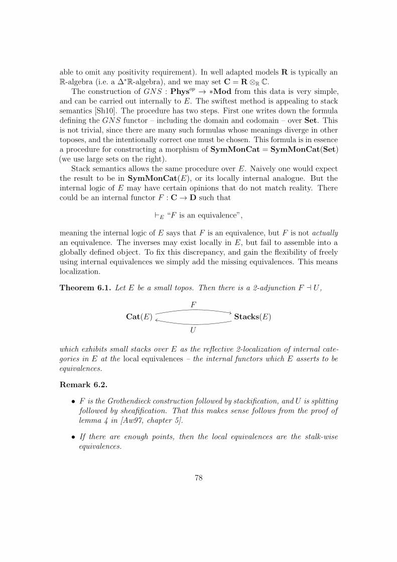
able to omit any positivity requirement). In well adapted models R is typically anR-algebra (i.e. a ∆∗R-algebra), and we may set C = R⊗R C.

The construction of GNS : Physop → ∗Mod from this data is very simple,and can be carried out internally to E. The swiftest method is appealing to stacksemantics [Sh10]. The procedure has two steps. First one writes down the formuladefining the GNS functor – including the domain and codomain – over Set. Thisis not trivial, since there are many such formulas whose meanings diverge in othertoposes, and the intentionally correct one must be chosen. This formula is in essencea procedure for constructing a morphism of SymMonCat = SymMonCat(Set)(we use large sets on the right).

Stack semantics allows the same procedure over E. Naively one would expectthe result to be in SymMonCat(E), or its locally internal analogue. But theinternal logic of E may have certain opinions that do not match reality. Therecould be an internal functor F : C→ D such that

`E “F is an equivalence”,

meaning the internal logic of E says that F is an equivalence, but F is not actuallyan equivalence. The inverses may exist locally in E, but fail to assemble into aglobally defined object. To fix this discrepancy, and gain the flexibility of freelyusing internal equivalences we simply add the missing equivalences. This meanslocalization.

Theorem 6.1. Let E be a small topos. Then there is a 2-adjunction F a U ,

Stacks(E)Cat(E)

F

U

which exhibits small stacks over E as the reflective 2-localization of internal cate-gories in E at the local equivalences – the internal functors which E asserts to beequivalences.

Remark 6.2.

• F is the Grothendieck construction followed by stackification, and U is splittingfollowed by sheafification. That this makes sense follows from the proof oflemma 4 in [Aw97, chapter 5].

• If there are enough points, then the local equivalences are the stalk-wiseequivalences.

78

• This theorem extends to any κ-ary superextensive site, linking stacks over Cand internal categories in Sh(C). One wonders whether superextensivity isrequired.

Following this philosophy we take the defining formula for the GNS functor,and replace any instance of Set with “the stack of objects of E”, better known asthe codomain fibration E·→· −→ E (call it E). To our horror, we realize that theresult is not quite right.

What should replace the category of sets is what I will call Elc – the “stack oflocally constant objects” of E. It’s the full substack of E generated by the globalsections. One way to construct it is as the stackification of a presheaf of categoreson E whose objects are always the objects of E, and whose morphisms at stage Xbetween A and B are given by E/X(π∗A, π∗B), where π : X → 1.

This has the effect of working with families of objects which are locally trivial.Elc(X) consists of those families in E/X = E(X) which become trivial over somecovering of X. They are glued from product families via a cocycle. The inclusionElc ⊆ E is fully faithful, so we do not lose any of the morphisms.

Remark 6.3. If we use the full stack of objects then physical oddities can occur.In particular the existence of constants of nature can depend on the value of otherconstants of nature! Think of the residue fields in the base of a non-trivial familyof schemes. Classical physics also becomes “richer” (or “infested with junk”),encompassing exotic structures other than Poisson algebras.

Ultimately, the result is a morphism of monoidal stacks over E. For aestheticreasons we may wish to push the entire setting into internal categories in somecolossal topos. “Internal categories of physical processes” sounds much more elegantthan “stacks of processes”.

Over well-adapted models the result includes at least the finite dimensionalC∗-algebras, and their full moduli theory. The Cahiers topos includes all theconvenient vector spaces [KR86] as R-modules, and so one hopes for a lot more,but they cannot be used to construct examples until we prove them to be R-flat. Ido not expect all convenient vector spaces to be flat, and if Hilbert spaces are notflat, then very few interesting examples will exist.

In this manner have arrived in a paradisal world, where everything is smooth.Both functors and families of objects and morphisms can be differentiated, and thesetwo modes of differentiation lead to the traditional differential equations of quantumtheory (Heisenberg and Schrodinger) and to classical mechanics, respectively. Wegive only examples.

79

6.2 Infinitesimal Symmetries

Consider a G-equivariant ∗-algebra, i.e. a functor A : G→ ∗Alg. We treat G as aone object groupoid, and hence, by the Grothendieck construction, as a prestackover E (its stackification consists of G-torsors [BH11], so we keep prestacks aroundfor simplicity). In this picture, A is a morphism of prestacks, and, unwinding thedefinitions, we see that A amounts to a traditionally defined equivariant object ina fibration (cf. [Vi08]). Below we write A for both the functor and the image in∗Alg of the single object of G, a particular ∗-algebra in E.

Let D = x ∈ R : x2 = 0 ⊆ R be the first order infinitesimals. In the syntheticsetting differentiation is reduced to composing with D. Since we are working withprestacks, this amounts to evaluation, by the “Yoneda lemma for fibrations” [St08].Evaluating A(D), we find the following: G(D) = TG is just the tangent bundle ofG, and the rest of the structure amounts to a homomorphism

TG −→ End(A)(D) = EndD(A×D),

where the codomain is the endomorphisms of A over D, that is commuting diagrams

A×D A×D

D

f

π π

where f is a ∗-algebra homomorphism, and the π are projections to D. The Kock-Lawvere axiom shows that this data amounts to a ∗-derivation A→ A, recoveringthe usual the notion of infinitesimal symmetry. In particular we obtain a morphismof Lie algebras

Lie(G) −→ ∗Der(A).

Since all we are really doing is composition, we can compose everything with theGNS functor.

Theorem 6.4. Let X ∈ Lie(G) act as the inner derivation [Q,−] on A, for someQ ∈ A, and let ϕ be a G-equivariant state over A. Then GNS(X) acts on GNS(ϕ),and

GNS(X) = Q iff QΩ = 0

Thus infinitesimal generators coincide in the Heisenberg and Schrodinger picturesonly if the representing vector is invariant under the chosen generator. Thisinvariance can always be sabotaged, since Z(A) always includes C. Choices matter,

80

and in this case are classified by Hochschild cohomology HH0(A) = Z(A). This isthe second indication – after lemma 1.9 (see remark 1.10) – that we should pass toa derived (i.e. higher categorical) formalism.

Remark 6.5. Morally speaking, theorem 6.4 shows that GNSc would, had weenough modules isomorphic to their duals at our disposal, map the Heisenbergequation to the Schrodinger equation. This infinitesimal result would complete theequivalence of these pictures, as it is traditionally understood.

This discussion can be extended to groupoids. For simplicity, let’s consider thepair groupoid for the affine line A1, which is just the base ring R as an object. Theobjects are A1 itself, and there is a unique morphism t → t′ for any two points,which we will identify with translation by t′ − t. We will call this groupoid P (A1).

Differentiating, we see that P (A1)(D) has as objects tangent vectors to theobjects of P (A1). This means tangent vectors to A1, which are naturally justvectors in A1. The specific object (point) to which these vectors are attached isdetermined by restriction 1 → D → A1. The morphisms of these “infinitesimalfamilies of objects” are again tangent vectors, with the unique morphism v → widentified with the translation by w − v.

All this data maps to ∗Alg(D), determining infinitesimal families of ∗-algebrasAv, for v ∈ A1, and isomorphisms (w − v) : Av → Aw of ∗-algebras over D.Since everything is R-linear, this is determined completely by any nontrivial mapv : A0 → Av, which is a derivation along a deformation of A. If the deformation istrivial, i.e. time acts on observables but not their algebra, we get a time-dependentfamily of derivations of A, just as expected.

The possibility of deformation arises since we allowed infinitesimal movementof the algebra itself, not just of its elements. The very notion of multiplicationmoved, along with a movement of the elements. This leads to a discussion of theclassical limit.

6.3 The Classical Limit

Consider the affine line A1 as a discrete category in E. It again defines a stack overE, and we define ~-families of ∗-algebras to be functors A1 → ∗Alg. The classicallimit of such a family is its restriction to infinitesimal ~. Thus we are led to studymaps

D −→ ∗Alg.

Because Elc is full, maps X → ∗Alg are those ∗-algebras in E/X which becometrivial – as objects, but not algebras! – over some covering of X. Maps retainarbitrary dependence on the fibers. In well adapted models this construction

81

includes vector bundles over manifolds equipped with not-locally-trivial ∗-algebrastructures.

Since D is amazingly tiny in the sense of Lawvere [MR91, appendix 4], mapsD → ∗Alg are simply ∗-algebra structures on π : A × D → D in E/D, whichextend the given structure on A (thought of as sitting in the fiber over 0 ∈ D). TheKock-Lawvere axiom shows that these are exactly the ∗-Hochschild cocycles on A.

The monoidal structure on ∗Alg restricts to a product of Hochschild cocycles,which includes the traditional product of Poisson structures. Classical and quantumcomposite systems are thus fully compatible.

In this way we include a very general version of deformation quantization. Inparticular the quantization of singular phase spaces can utilize symmetric Hochschildcocycles, in addition to the antisymmetric ones (which correspond to Poissonbrackets). This may have bearing on the quantization of principal connections withisotropy and spacetimes with isometries (cf. remark A.4 in appendix A).

6.4 Compatibility

All of these considerations are functorial. In particular, the inhomogeneous Heisen-berg, Schrodinger, and Hamilton equations, as well as a “classical Schrodingerequation” all derive from a single object in

PhysA1×P (A1),

where the first factor controls the value of ~ and the second is the pair groupoid ofA1, representing inhomogeneous time evolution.

References

[Aw97] S. Awodey, Logic in Topoi: Functorial Semantics for Higher-Order Logic,Ph.D. dissertation, University of Chicago, 1997. Available at:

https://www.andrew.cmu.edu/user/awodey/thesis/thesis.ps.gz

[Ba06] J. C. Baez, Quantum Quandaries: A Category-Theoretic Perspec-tive, in Structural Foundations of Quantum Gravity, D. P. Rickles,S. R. D. French and J. Saatsi (eds), Oxford University Press, 2006.Available as arXiv:quant-ph/0404040.

[BSh06] J. C. Baez, M. Shulman, Lectures on n-Categories and Cohomology,available as arXiv:math/0608420 [math.CT].

82

[BSt09] J. C. Baez, M. Stay, Physics, Topology, Logic and Computation: ARosetta Stone, in New Structures for Physics, Bob Coecke ed., LectureNotes in Physics 813, Springer, Berlin, 2011, pp. 95-174. Available asarXiv:0903.0340 [quant-ph].

[BShSh] M. Benini, A. Schenkel, U. Schreiber, The stack of Yang-Mills fields onLorentzian manifolds, available as arXiv:1704.01378 [math-ph].

[BShSz] M. Benini, A. Schenkel, , Homotopy Colimits and Global Observables inAbelian Gauge Theory, Letters in Mathematical Physics 105(9), 2015,pp. 1193–1222. Available as arXiv:1503.08839 [math-ph].

[BDGK] M. Berg, C. DeWitt-Morette, S. Gwo, E. Kramer, The Pin Group inPhysics: C, P and T, Rev. Math. Phys. 13, 2001, 953. Available asarXiv:math-ph/0012006.

[Be99] J. Bernstein, Notes on Supersymmetry, in Quantum Fields and Strings:A Course for Mathematicians, P. Deligne et. al. (eds), AMS, ProvidenceRI, 1999.

[BMRS] J. Brodzki, V. Mathai, J. Rosenberg, R. J. Szabo, D-branes, RR-fieldsand Duality on Noncommutative Manifolds, Commun. Math. Phys. (277),2008, pp. 643-706.

[BH11] M. Bunge, C. Hermida, Pseudomonadicity and 2-Stack Completions,CRM Proc. Lecture Notes 53, AMS, Providence RI, 2011, pp. 29–54.

[DF99] P. Deligne, D. S. Freed, Classical Field Theory, in Quantum Fields andStrings: A Course for Mathematicians, P. Deligne et. al. (eds), AMS,Providence RI, 1999.

[DGZ04] D. Durr, S. Goldstein, N. Zanghi, Quantum Equilibrium and theRole of Operators as Observables in Quantum Theory, Journalof Statistical Physics 116(1–4), 2004, pp. 959–1055. Available ashttps://arxiv.org/abs/quant-ph/0308038.

[Fr94] D. S. Freed, Higher Algebraic Structues and Quantization, Commun.Math. Phys. 159 (1994), 343-398, available as arXiv:hep-th/9212115.

[FSS94] J. Fuchs, M. G. Schmidt, C. Schweigert On the configuration space ofgauge theories, Nuclear Physics B 426(1), 1994, pp. 107-128.

[FJ15] R. Furber, B. Jacobs, From Kleisli Categories to Commutative C∗-algebras: Probabilistic Gelfand Duality, Logical Methods in ComputerScience 11(1:5) (2015), pp. 1-28.

83

[GLPS] B. Groisman, J. Ladyman, S. Presnell, A. J. Short, The connectionbetween logical and thermodynamic irreversibility, Studies in Historyand Philosophy of Science Part B: Studies in History and Philosophy ofModern Physics 38(1), 2007, pp. 58-79.

[Gr03] G. Grubl, The quantum measurement problem enhanced, Physics LettersA 316(3-4), 2003, pp. 153–158. Available as arXiv:quant-ph/0202101.

[Ha12] A. Hajek, Interpretations of Probability, The Stanford Encyclopedia ofPhilosophy (Winter 2012 Edition), Edward N. Zalta (ed.). Available at:

https://plato.stanford.edu/archives/win2012/entries/probability-interpret/

[Ha14] S. W. Hawking, Information Preservation and Weather Forecasting forBlack Holes, preprint. Available as arXiv:1401.5761 [hep-th].

[Ho01] S. Holevo, Statistical Structure of Quantum Theory, Lecture Notes inPhysics Monographs 67, Springer-Verlag, Berlin, 2001.

[J02] P. T. Johnstone, Sketches of an Elephant: A Topos Theory Compendium,Oxford Logic Guides 43 & 44, Clarendon Press, Oxford University Press2002.

[KR86] A. Kock, G. E. Reyes, Corrigendum and addenda to: Convenient vectorspaces embed into the Cahiers topos, Cahiers de Topologie et GeometrieDifferentielle Categoriques 27(1), 1986, pp. 3-17.

[K03] M. Kontsevich, Deformation Quantization of Poisson Manifolds, Lettersin Mathematical Physics 66(3), 2003, pp. 157–216. Available as arXiv:q-alg/9709040.

[Mad] D. Madore, A Few Reflections on Noncommutative Algebraic Geome-try/The Quest for the Holy Scheme, versions 7 and 9. Available at:

http://www.madore.org/∼david/math/.

[CWM] S. Mac Lane, Categories for the Working Mathematician, GraduateTexts in Mathematics 5, Springer-Verlag, New York, 1998.

[MR91] I. Moerdijk, G. E. Reyes, Models for Smooth Infinitesimal Analysis,Springer-Verlag, New York, 1991.

[Mo14] G. W. Moore, Physical Mathematics and the Future, talk at Strings 2014.Notes available at

http://www.physics.rutgers.edu/∼gmoore/PhysicalMathematicsAndFuture.pdf

84

[Se15] N. Seiberg, Symmetries Then and Now, presentation at the 40th An-niversary Conference – Laboratoire de Physique Theorique, 2015.

Slides: https://www.lpt.ens.fr/IMG/pdf/seiberg.pdf

[Sh10] M. Shulman, Stack semantics and the comparison of material and struc-tural set theories. Available as arXiv:1004.3802 [math.CT].

[StPr] Authors of the Stacks Project, Stacks Project, 2017.

Website: http://stacks.math.columbia.edu.

[Oh01] K. Ohmori, A Review on Tachyon Condensation in Open String FieldTheories. Available as arXiv:hep-th/0102085.

[Pe95] R. Penrose, On Gravity’s Role in Quantum State Reduction, GeneralRelativity and Gravitation 28(5), 1996, pp. 581–600.

[Po05] J. Polchinski, String Theory, Cambridge Monographs on MathematicalPhysics, Cambridge University Press, New York, 2005.

[PX03] G. Pisier, Q. Xu, Noncommutative Lp-Spaces, in Handbook of the Geom-etry of Banach Spaces, W. B. Johnson, J. Lindenstrauss (eds), Elsevier,Amsterdam, 2003.

[Ro16] B. W. Roberts, Three Myths About Time Reversal in Quantum Theory,available as arXiv:1607.07388 [physics.hist-ph].

[SS14] U. Schreiber, M. Shulman, Quantum Gauge Field Theory in CohesiveHomotopy Type Theory, EPTCS 158, 2014, pp. 109-126. Available asarXiv:1408.0054 [math-ph]

[St08] T. Streicher, Fibered Categories a la Jean Benabou. Available athttp://www.mathematik.tu-darmstadt.de/∼streicher/FIBR/FibLec.pdf.

[Sz] S. Szawiel, Categorical General Relativity, manuscript in preparation.

[Ta12] T. Tao, Topics in Random Matrix Theory, Graduate Studies in Mathe-matics 132, AMS, Providence RI, 2012.

[HoTT] The Univalent Foundations Program, Homotopy Type Theory: UnivalentFoundations of Mathematics, Intitute for Advanced Study, 2013.

Website: https://homotopytypetheory.org/book

[Ve17] E. P. Verlinde, Emergent Gravity and the Dark Universe, SciPost Phys.2(3), 2017.

85

[Vi08] A. Vistoli, Notes on Grothendieck topologies, fibered categories anddescent theory. Available at http://homepage.sns.it/vistoli/descent.pdf

[Wa94] R. M. Wald, Quantum Field Theory in Curved Spacetime and BlackHole Thermodynamics, Chicago Lectures in Physics, Chicago UniversityPress, Chicago, 1994.

[We05] S. Weinberg, The Quantum Theory of Fields, volumes 1-3, CambridgeUniversity Press, Cambridge, 2005.

[Wi99b] E. Witten, Dynamics of Quantum Field Theory, in Quantum Fields andStrings: A Course for Mathematicians, P. Deligne et. al., (eds), AMS,Providence RI, 1999.

[Wi99a] E. Witten, Perturbative Quantum Field Theory, in Quantum Fields andStrings: A Course for Mathematicians, P. Deligne et. al. (eds), AMS,Providence RI, 1999.

[Wi08] E. Witten, Gauge Theory and Wild Ramification, Analysis and Applica-tions 6(4), 2008, pp. 429-501. Available as arXiv:0710.0631 [hep-th].

[Xu01] P. Xu, Quantum Groupoids, Communications in Mathematical Physics216(3), 2001, pp. 539–581. Available as arXiv:math/9905192 [math.QA].

[Za12] M. Zawadowski, The formal theory of monoidal monads, JPAA 216(8-9),2012, pp. 1932-1942. Available as arXiv:1012.0547 [math.CT].

A On The Notion of Gauge Theory

The ideas presented here are not really new, but deserve being intensely stressed,for they deeply challenge any claim to understanding the general notion of gaugetheory, especially quantum gauge theory.

These ideas are present implicitly or explicitly in the thinking of several authors,including Freed and Deligne [DF99, §4.2], Schreiber and Schulman [SS14] (amongmany), as well as Benini, Schenkel and Szabo [BShSh, BShSz], and very likelymany others.

A.1 The Problem

Consider a classical theory with space of states X, carrying an action of a groupG. Is G a group of gauge equivalences, or an ordinary symmetry group? In thephysicists’ practice the distinction is always clear. However, there does not seem to

86

be a mathematical criterion for establishing such a distinction. Yang-Mills theory,for example, together with the claim that the connection field is an empiricallymeasurable observable, appears to be a perfectly fine mathematical structure. It issimply not a gauge theory, and does not have a well posed first order initial valueproblem.

In general, phase space-based approaches to gauge invariance are doomed.Despite appearances, gauge theories are not a special class of constrained systems.Gauge symmetry is not a property inconveniencing the construction of phase space,but a structure, and attempts to infer it from anything else cannot succeed.

Locality is also not a very promising candidate, since it requires saying “space-time” and “Cauchy surface”. Whatever string theory turns out to be, it willprobably be out of luck with this kind of definition. And we definitely want it tomake the list! Thus we seek a more conceptual understanding of gauge symmetry.

That is a rather tall order, since we are faced with the following dumbfoundingclaims:

• Diffeomorphisms in General Relativity are gauge equivalences.

• But: isometries are actual symmetries, not just gauge equivalences (think ofthe Poincare group, and Killing vector fields in general).

• The automorphisms of a principal bundle are gauge equivalences.

• But: the fiberwise constant automorphisms of a trivial principal bundle areactual symmetries (how else would electric charge be conserved?).

As the reader can see, there’s a lot of backtracking going on. It gets worse. Considera nontrivial principal G-bundle P over a spacetime M . Then we have an exactsequence

1 −→ GP −→ Aut(P ) −→ Diff(M),

where GP is the group of M -automorphisms of P , and Aut(P ) consists of all theG-automorphisms of P . The last map is typically not onto, and does not split overits image (which consists of the maps f such that f ∗P ' P ).

Considering the above, one would like to say things such as “gauge theory isisometry invariant”. For example, it is said that “Yang-Mills theory is Lorentzinvariant”. But this is problematic in two respects. First, the relevant symmetrygroup is Aut(P ), not Diff(M), so isometries are not even in a position to act onour fields. This can be fixed by considering all principal bundles instead of just P ,or just the trivial ones.

The second problem is deeper: let φ ∈ Aut(P ) map to an isometry of M in thesequence above. Then, since our sequence does not split, we have an automorphismacting on our fields, which has a “symmetry part”, but does not have a “gauge

87

part”. And it certainly could have a “gauge part”, since GP is included in Aut(P ).It appears that gauge equivalences and actual symmetries cannot, in general, beneatly separated. This is especially true if indiscriminate symmetry gauging isallowed (cf. [DF99, §2.8]).

It is therefore difficult to accept the claim, commonly made in the community[Se15], that gauge equivalences are “redundancies in the description” or “do-nothingtransformations”, and that they have no physical significance. In the presenceof gauge equivalences, without further constraints, one cannot simply pass to areduced phase space. The Aharonov-Bohm effect and Dijkgraaf-Witten theorycannot be understood, indeed cannot exist, if we simply divide out the gaugeequivalences. It is also clear that gauge transformations are not plain symmetries.Pushing a metric around by diffeomorphisms certainly does not alter the state of asystem in any physically relevant way.

What are we to make of this situation? I tentatively propose the followingdefinition, which includes all Yang-Mills theories, General Relativity, as well as amultitude of (limits of) string theories among “theories with gauge equivalences”.

Definition A.1. A classical theory with gauge equivalences is a theory whose spaceof states has an additional structure9 of a k-groupoid.

The case k = 0 is trivial, requiring no additional structure, and so one shouldreally speak of k-gauge theories, including non-examples as the degenerate case.For k > 1 we allow weak groupoids. In the examples below we have k = 1, but sincethe Kalb-Ramond field in string theory is a connection on a principal 2-bundle,one expects stringy examples with k > 1.

Example 1: General Relativity

The state space of general relativity is the groupoid of all Lorentzian manifolds andtheir isometries. We use the notion of “state space” loosely. We want to preservethe ability to couple the theory to other fields, and so we disregard the equationsof motion. Of course, Einstein spacetimes form a subgroupoid.

Example 2: Yang-Mills Theory

The state space of Yang-Mills theory, with structure group G on a spacetime M , isthe groupoid of G-principal bundles with G-connection and connection-preservingisomorphisms between them. This example is slightly ambiguous, since it is notclear whether to include all bundle morphisms or just the equivariant ones. This

9This excludes the natural structure of ω-groupoid that the space of states possesses in virtueof being a space.

88

choice affects, for example, color charge conservation on topologically nontrivialspacetimes (as we see below).

Example 3: In General?

Let A be an algebra of observables with a group G of symmetries acting on it.Then the groupoid of states is the action groupoid S(A)//G (also known as theweak quotient), where S(A) is the space of states, with the action of G given bythe fact that S is a functor. Unlike the previous examples S(A) includes mixedstates, causing further complications.

Remark A.2 (The Problem of Emergence). There are multiple contexts in whichgauge symmetry is emergent. Definition A.1 would then dictate the discontinuouschange in dimX, the categorical dimension of X, classifying any perturbationremoving emergent gauge symmetry as a singular perturbation.

Digression on The Geometry of Groupoids

To really work with definition A.1, one must define the notion of a smooth mapinto X, which should be understood as a smooth family of objects and morphismsof X. This leads immediately to the notion of a stack, since stacks are a higherlocalization of internal categories (including groupoids). We will not make thisprecise here, but will merely assert that a groupoid with a localizable notion ofmorphism into it (from a space) automatically defines a stack, with the originalgroupoid being the global sections of that stack. An idea of how this works can beextracted from theorem 6.1 and remark 6.2.

This allows us to speak of the geometry of X, in particular the sheaves onX, Sh(X). This topos naturally contains all the geometric invariants of X whichcan be defined as sheaves on the site of spaces. This means that objects like thedifferential forms, Ω∗X , are canonically defined. If infinitesimals are available, thenother constructions, such as tangent vectors and vector fields can be defined. Thesecan’t be pulled back from the site of spaces. In such cases one can prove the usualrelation Ω1(X) = Γ(T ∗X), which is not usually taken as a definition for stacks.

Most importantly gauge invariance is inherently baked in to the formalism. Inexamples 1 and 2 there are smooth action functionals

S : X −→ R,

whose differentials dS ∈ Ω1(X) are legitimate 1-forms. The stacks of solutions arethe substacks x ∈ X : dS(x) = 0 ⊆ X. For the bare Einstein-Hilbert action theglobal sections of the solution stack are simply the groupoid of Einstein manifoldsand their isometries.

89

This notion of solution is automatically gauge invariant since it is really a2-pullback in a 2-category. The mystery of why “imposing gauge invariance” – acolimit construction – commutes with imposing the equations of motion – a limitconstruction – is resolved. Gauge invariance is encoded in the 2-cells of a 2-category,and the equations of motion are a 2-categorical construction.

This kind of stacky geometry, including measure theory, will be explored indepth in upcoming work [Sz]. The treatment of noncompact spacetimes requiresdelicate analysis.

A.2 In Pursuit of Proper Language

As I have already stressed, the ideas behind definition A.1 are not new. I wouldlike to build on the idea of that definition, and give gauge theories a distinguishedstructural place among all theories, and clarifying the notion of “theory” in general.I begin with the following distinction:

Definition A.3. Let x ∈ X be a state in a classical theory with gauge equivalences.Then:

• The symmetries of x are by definition the groupoid

AutX(x) = X(x, x)

of self-equivalences of x.

• The gauge equivalences are maps x→ y in X.

Example 1: General Relativity

Diffeomorphisms f : M →M ′ are exhibited among Lorentzian manifolds by mapsof the form (M, g)→ (M ′, f∗g). The automorphisms of (M, g) are therefore exactlythe isometries.

Example 2: Yang-Mills Theory

Analogously to gravity, the gauge transformations act by pushforward, and arecounted as gauge equivalences iff they change the connection. The isotropy groupof a connection is not counted among the equivalences! It consists of genuinesymmetries according to our definition.

This leads to our first real problem: one must decide if the bundle morphismsin this example are to be equivariant. The decision may be obvious, but considerthe following question: do we want QCD to enjoy color charge conservation ontopologically nontrivial manifolds? If so, then the equivariant maps are too little –

90

one must also include the right G-action as a symmetry, since this seems to be theonly way to include “constant gauge transformations” as symmetries on generalspacetimes. Without this global symmetry, features such as the Higgs mechanismwould fail.

Example 3: In General?

Here we come to the crux of the matter. We must confront the effects of definitionA.3 on the notion of symmetry in ordinary theories (those with k = 0). They arequite curious: for non-gauge theories the definition dictates that time-invariantstates, such as vacua, would have time translation symmetry, but that same“symmetry” would act as a mere gauge transformation on non-ivariant (e.g. excited)states.

The symmetries of a lagrangian field theory [DF99, §2.6] would likewise beclassified as gauge, except at their fixed points. In this respect, either definition A.3or the construction of this example is problematic. Perhaps this is just a linguisticdeficiency, or a historical lack of appreciation for groupoids, as opposed to groups.

Remark A.4. This discussion suggests that perturbative quantization should takethe automorphism group into account. From a geometric perspective states withautomorphisms are singular points in the space of states, in the sense that G-fixedpoints in some G-space X are usually singular points in the quotient space X/G.

Since working with definition A.1 amounts to replacing X/G with the actiongroupoid (weak quotient), or more properly its stackification, the quotient stack[X/G], this suggests that all points with nontrivial automorphisms should be con-sidered singular in any groupoid.

The opportunity for special treatment of these states is clearly visible in thegeneral formalism of deformation quantization – singularities allow the appearanceof nontrivial symmetric Hochschild cocycles. All isotropic (reducible) connectionsare such singularities, and the space of connections is full of them [FSS94].

The Necessity of Higher Categories

At this point, the reader would be right to protest in confusion. What preventsus from setting x = y in definition A.3, and completely confusing the supposeddistinction? Insisting that x 6= y in the second case is tenable, but goes against thephilosophy of category theory. It seems that a decisive discussion of these mattersrequires the systematic use of higher-categorical formalism. Such a formalism iscurrently only available in the form of homotopy type theory [HoTT]. There wefind the general notion of an identity type, and a distinction between definitionalequality and propositional equality. The Atiyah-Singer index theorem is an exampleof a propositional equality – two differently constructed numbers are proven to be

91

equal. By contrast renaming variables is an example of a definitional equality –such equalities have no mathematical content, and their use in deductive reasoningis limited to bookkeeping. In this perspective gauge equivalences arise frompropositional equalities, and symmetries from propositional equalities betweendefinitionally equal states.

A.3 Dependent Fields

In constructing a field theory, the specification of spacetime and any additionalstructure on it (like orientation, spin-structure, etc.) is prior to the introduction ofany other fields. This is so because the spacetime determines what fields can beintroduced. Fields are dependent on spacetime. There can be multiple levels ofdependency: spinor fields depend on the metric field and the orientation, which inturn depend on spacetime. In gauge theory this dependence is subtler: the sectionsof a bundle Γ(P [V ]), associated to a principal bundle P , are the equivariant mapsP → V . These depend on P for the specification of their domain.

So it seems that we must introduce a general notion of a dependent field – afield definable only in the presence of other fields, and parametrically dependentupon them. Again, one can frame this using type-theoretic language: if fieldsare understood as types, then dependent fields are dependent types. The prime“field” would be spacetime. After that one can introduce general tensorial fields,such as the metric. After the introduction of a metric, and an orientation, spinorfields become available (giving a possibly empty space of fields, if there is no spinstructure on spacetime). Dependently on spacetime, one can introduce principalbundle “fields” (thought of as maps to the classifying stack BG), then, dependentlyon those, connection fields and fields associated to representations of the structuregroup. This leads to the following definition.

Definition A.5. Let X the the groupoid of states of a classical theory with gaugeequivalences. A dependent field for this theory is a functor F : Φ→ X.

Note the strange direction! It is critical to what follows.

Example 1: Scalar Fields

Let X be the groupoid of spacetimes and isometries. Then C∞ : Xop → Set, whichassigns to each spacetime M its ring of smooth functions C∞(M,R) determines adependent field through the Grothendieck construction,

Φ =

∫C∞,

92

which means that Φ is the category of pairs (M,φ), with φ a scalar field on M ,with the obvious projection to X. F : Φ→ X is simply forgets φ.

A similar construction encompasses all ordinary natural fields, such as tensorfields.

Example 2: Bundles

Extraordinary fields include bundles. Let G be a group, with BG its classifyingstack, the dependent field

X ↓ BG,

is simply the category of principal G-bundles over spacetimes. The comma categoryis constructed from the forgetful functor X → Spc into spaces and the singleobject inclusion BG → Spc. Here F is again the projection X ↓ BG→ X.

Bundles with additional structure, such as a connection, can easily be includedhere. This allows us to add spin structures to manifolds as “fields” and dependentlyon that, spinor fields, extending example 1.

A.4 The Pathology of Dependent Symmetry

In this picture symmetries also become dependent. The sequence

1 −→ GP −→ Aut(P ) −→ Diff(M),

displays the nontrivial dependence of gauge symmetries on diffeomorphisms. Thefibers Autf (P ), for f ∈ Diff(M), can be empty or not, and are glued together ina nontrivial manner, owing to the non-splitness of the sequence.

The fact that the sequence is not exact at Diff(M) is precisely the statementthat the dependent field F : Spc ↓ BG→ Spc mapping bundles to their underlyingspaces is not full on automorphisms.

The lack of fullness has real consequences, and is typically considered patho-logical. The treatment of the energy-momentum tensor in [DF99, §2.9] is plaguedby it. The definition of “weak diffeomorphism invariance” given there looks veryawkward, but is natural in our setting: it is exactly fullness of F on the D-points,where D is the object of first order infinitesimals. Such points are also calledSpec(R[ε])-points, a traditional paraphrase of the notion in algebraic geometry.

Flat connections are then the first order functorial splittings of dependentfields, and since they are not guaranteed to exist, arbitrary connections, which are“functors not preserving composition” are recommended in ibid. instead. Regardlessof this effort, the application of Noether’s theorem is frustrated [DF99, 2.183-2.190].

Noninfinitesimal splittings correspond to strictly equivariant groupoids, by thenonlinear Dold-Kan correspondence, or the “layer-cake philosophy” [BSh06]. An

93

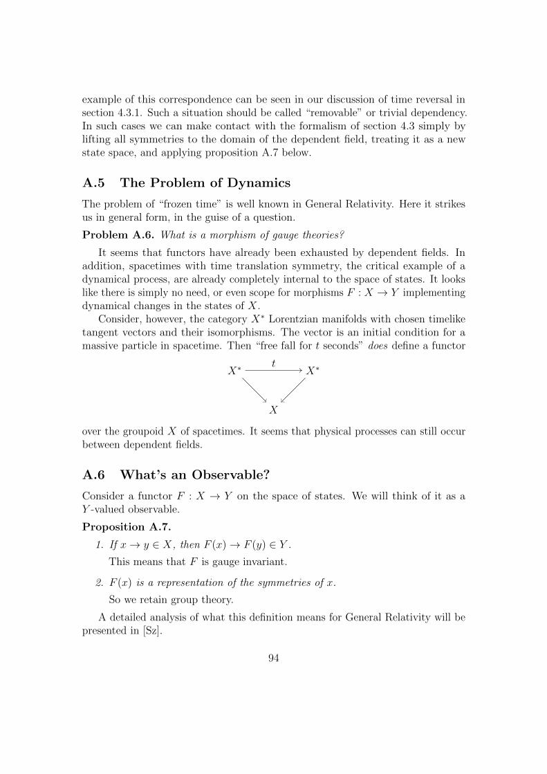
example of this correspondence can be seen in our discussion of time reversal insection 4.3.1. Such a situation should be called “removable” or trivial dependency.In such cases we can make contact with the formalism of section 4.3 simply bylifting all symmetries to the domain of the dependent field, treating it as a newstate space, and applying proposition A.7 below.

A.5 The Problem of Dynamics

The problem of “frozen time” is well known in General Relativity. Here it strikesus in general form, in the guise of a question.

Problem A.6. What is a morphism of gauge theories?

It seems that functors have already been exhausted by dependent fields. Inaddition, spacetimes with time translation symmetry, the critical example of adynamical process, are already completely internal to the space of states. It lookslike there is simply no need, or even scope for morphisms F : X → Y implementingdynamical changes in the states of X.

Consider, however, the category X∗ Lorentzian manifolds with chosen timeliketangent vectors and their isomorphisms. The vector is an initial condition for amassive particle in spacetime. Then “free fall for t seconds” does define a functor

X∗X∗

X

t

over the groupoid X of spacetimes. It seems that physical processes can still occurbetween dependent fields.

A.6 What’s an Observable?

Consider a functor F : X → Y on the space of states. We will think of it as aY -valued observable.

Proposition A.7.

1. If x→ y ∈ X, then F (x)→ F (y) ∈ Y .

This means that F is gauge invariant.

2. F (x) is a representation of the symmetries of x.

So we retain group theory.

A detailed analysis of what this definition means for General Relativity will bepresented in [Sz].

94

Relation with the Traditional Treatment

The contemporary treatment of observables for gauge theories deviates slightlyfrom this idea of observable, with the observables on X being given by the groupoidcohomology H∗(X,E), where E is a representation of X. Such an object is asmooth sheaf of vector spaces on X, which is just a morphism X → Vect, to thestack of vector spaces (traditionally called the classifying stack of vector bundles).

In Yang-Mills theory one usually takes X to be the stack of families of principalG-bundles (which is not the classifying stack BG [BShSh]), and E = R, the trivialrepresentation (i.e. the representation induced from the constant sheaf R over thetrivial groupoid).

The first group, H0(X,E), is the invariant sections of E over X. Therefore thegroup H0(X,R) does consist of functors X → R, with R considered discrete. Avariant of our idea is included in contemporary thinking. In any case, these areexactly R-valued functions on the isomorphism classes of X, and so exactly whatwe would expect a scalar observable to be in both Yang-Mills theory and GeneralRelativity.

The higher groups are more mysterious, encoding ghost fields (which are globalin this perspective [BShSz]). Their physical significance has been questioned, butat the very least they control possible gauge invariant couplings of the theory toother fields. If one imagines a “space of all theories”, then the ghost fields wouldbe crucial in determining the theory’s ultimate location in that space.

In the functorial perspective ghosts become invisible, as they should be. Theirrole in the notion of observable amounts to describing maps X → BnE, where Bis the delooping functor. Applying the Yoneda lemma, we see that such maps arepart of the “observable functor” Hom(X,−), necessary in reconstructing X fromthe structure of its observables.

The physical significance of delooping, while obscure, can be illuminated some-what. The ghost observables H2(X,E) control the extensions of X by E, andhence, in our terminology, (some class of) dependent fields. Thus, our precedingremarks were correct – the role of ghost fields, at least in part, is to control thepossible couplings between the base theory and its dependent fields10.

A.7 Quantization

Let F a U be an adjoint equivalence of categories

10A similar understanding of ghost fields was also communicated to me by Alexander Schenkel.

95

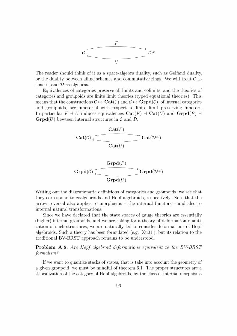
DopC

F

U

The reader should think of it as a space-algebra duality, such as Gelfand duality,or the duality between affine schemes and commutative rings. We will treat C asspaces, and D as algebras.

Equivalences of categories preserve all limits and colimits, and the theories ofcategories and groupoids are finite limit theories (typed equational theories). Thismeans that the constructions C 7→ Cat(C) and C 7→ Grpd(C), of internal categoriesand groupoids, are functorial with respect to finite limit preserving functors.In particular F a U induces equivalences Cat(F ) a Cat(U) and Grpd(F ) aGrpd(U) bewteen internal structures in C and D.

Cat(Dop)Cat(C)

Grpd(Dop)Grpd(C)

Cat(F )

Cat(U)

Grpd(F )

Grpd(U)

Writing out the diagrammatic definitions of categories and groupoids, we see thatthey correspond to coalgebroids and Hopf algebroids, respectively. Note that thearrow reversal also applies to morphisms – the internal functors – and also tointernal natural transformations.

Since we have declared that the state spaces of gauge theories are essentially(higher) internal groupoids, and we are asking for a theory of deformation quanti-zation of such structures, we are naturally led to consider deformations of Hopfalgebroids. Such a theory has been formulated (e.g. [Xu01]), but its relation to thetraditional BV-BRST approach remains to be understood.

Problem A.8. Are Hopf algebroid deformations equivalent to the BV-BRSTformalism?

If we want to quantize stacks of states, that is take into account the geometry ofa given groupoid, we must be mindful of theorem 6.1. The proper structures are a2-localization of the category of Hopf algebroids, by the class of internal morphisms

96

dual to the local equivalences. Localization can have drastic effects on how thingslook: a group G, seen as a one object groupoid is the category of G-torsors whenseen as a stack [BH11].

Problem A.9. What’s a noncommutative stack?

In other words we are interested in computing the localization of Hopf alge-broids by morphisms dual to the local equivalences in purely algebraic terms, andsubsequently allowing everything to be noncommutative.

B Chasing The Moduli Theory of Vacua

In this appendix we work abstractly, over some base topos E of “spaces”, with anordered ring R. GNS is then a stack morphism over E, as sketched in section 6. Wewrite OX for the pullback of R along the geometric morphism E/X → E/1 = Einduced by the unique map X → 1 in E.

B.1 The Stack of Vacua

It appears that most, if not all “path integral arguments” and “duality theorems”are at their cores simply isomorphisms of vacuum states of certain theories. Thuswe wish to study the notion of a vacuum. For this reason one of the central, longterm aims of the studying the category Phys, is the construction of the stack ofvacua

Vac −→ PhysTime.

Here Time is the groupoid of homogeneous time. Vacua are to be understood as“minimal energy states”. This is deliberately ambiguous, due to the problems below.

The wording assumes that every time evolution has a Hamiltonian, to be able todefine “energy”. More importantly, the notion of vacuum state is predicatedupon the notion of time evolution. In theories of emergent spacetime theconcept of vacuum seems ambiguous. Mere stability – as in the string landscape –seems insufficient, as there are theories with time-invariant states which are notvacua, and yet there is no global generator of time evolution whose expectationvalue we could wish to minimize. Clearly, there is conceptual work to be done here.

The category Vac should be thought of as “the space of all vacua”, with theprojection

π : Vac −→ (∗Algop)Time −→ ∗Algop

giving us the observables (at any time, every time, or some specific time – thisusually doesn’t matter) to which a given vacuum belongs. This structure does not,at least “morally”, contain the string landscape, as explained in the introduction.

97

Remark B.1. We have not formally required the purity of our states. This hasthe effect that Vac will include classical mixed states of minimal energy, which arenot usually considered vacua. For an illuminating discussion see [Wi99b, §1.1].The technical problems discussed below make this objection temporarily moot.

The study of Vac is the study of how quantum vacua behave in families. Thefollowing issues stand out as extremely interesting.

Is Vac a Stack?

This might seem obvious. But there are caveats, which I believe should influence theform of the definition. First, we assumed the existence of a Hamiltonian pointwise,that is for states over the point in the category of spaces. As every time evolutionis a homology class of Hamiltonians, the existence of a Hamiltonian for an entirefamily is a homological problem. We may – and will – simply demand specifying asolution in the definition.

The other problem is more concerning. The notion of state we have been usinguntil now appears to be too generous for Vac to form a stack. It arises – again– from the nonuniqueness of the Hamiltonian. The following situation may arise:there could be a family of candidate vacua ϕ : X → PhysTime, and a centralobservable f ∈ π(ϕ), whose expectation value 〈f〉 ∈ OX changes sign, as a functionon X (f is a section of OX which is just a map X → R in E).

In this situation the very notion of “vacuum” does not make sense. Sincewe can add f to any Hamiltonian for this family, the possible values of energy〈H + af〉 = 〈H〉+ a〈f〉, for a ≥ 0, are not linearly ordered in OX , and minimalitydoes not make sense. Consequently, defining Vac by demanding minimal energyfor every generalized element, or “generalized vacuum”, ϕ does not seem to makesense.

More abstractly, we can explain this by noting that OX will in general be onlypartially ordered, even if R is linearly ordered. Energy will always carry a freeOX-action, since OX sits in the center of every ∗-algebra over X, and energy isalways a torsor over the center of the algebra. Such torsors are also partiallyordered, but, unlike for linearly ordered R, minimality in partially ordered torsorscan always be ruined by the phenomenon described above.

There are several ways to proceed. One would be to demand something similarto “¬¬minimality” internally to E, in the sense of asserting that it’s not truethat there are lower energy states than the one under consideration. Anotherwould be pointwise (or maybe even stalkwise) minimality. One imagines sections ofPhys which are vacuum states pointwise. For the time being, we leave this issueunresolved.

98

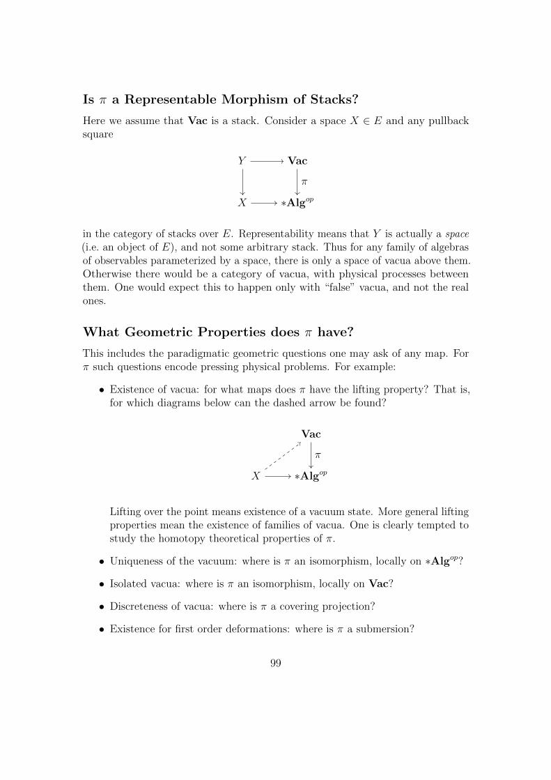
Is π a Representable Morphism of Stacks?

Here we assume that Vac is a stack. Consider a space X ∈ E and any pullbacksquare

Y Vac

X ∗Algop

π

in the category of stacks over E. Representability means that Y is actually a space(i.e. an object of E), and not some arbitrary stack. Thus for any family of algebrasof observables parameterized by a space, there is only a space of vacua above them.Otherwise there would be a category of vacua, with physical processes betweenthem. One would expect this to happen only with “false” vacua, and not the realones.

What Geometric Properties does π have?

This includes the paradigmatic geometric questions one may ask of any map. Forπ such questions encode pressing physical problems. For example:

• Existence of vacua: for what maps does π have the lifting property? That is,for which diagrams below can the dashed arrow be found?

Vac

X ∗Algop

π

Lifting over the point means existence of a vacuum state. More general liftingproperties mean the existence of families of vacua. One is clearly tempted tostudy the homotopy theoretical properties of π.

• Uniqueness of the vacuum: where is π an isomorphism, locally on ∗Algop?

• Isolated vacua: where is π an isomorphism, locally on Vac?

• Discreteness of vacua: where is π a covering projection?

• Existence for first order deformations: where is π a submersion?

99

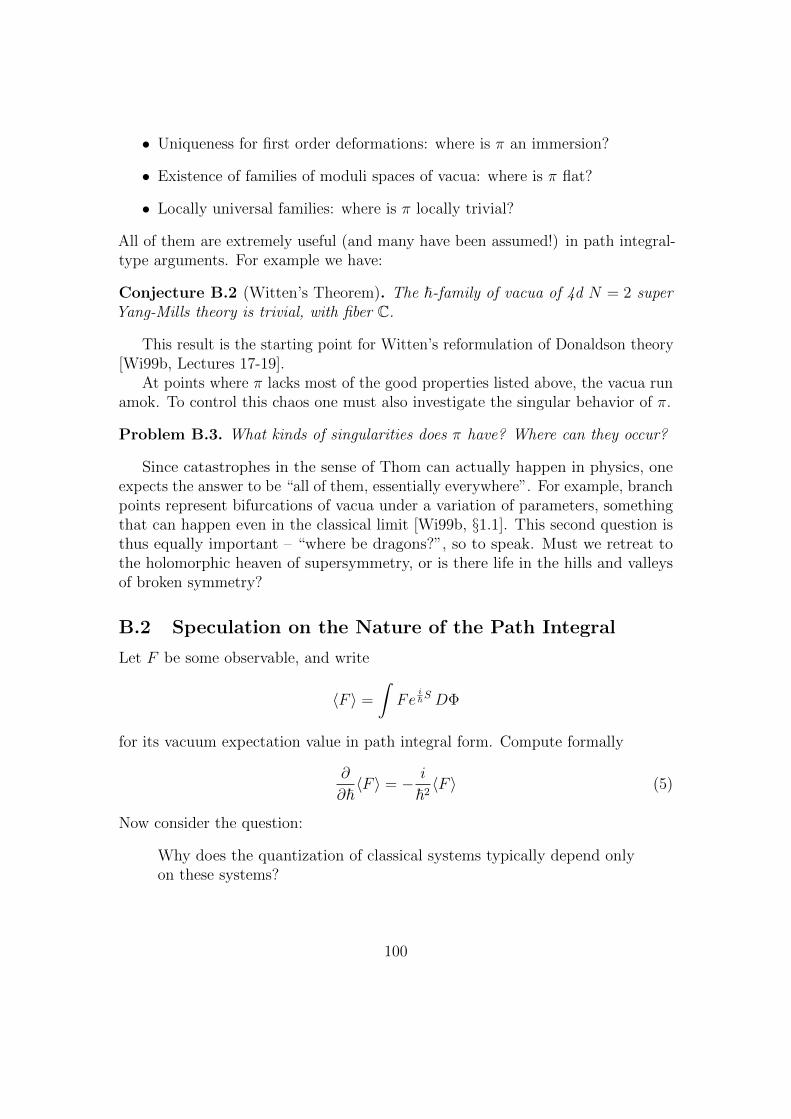
• Uniqueness for first order deformations: where is π an immersion?

• Existence of families of moduli spaces of vacua: where is π flat?

• Locally universal families: where is π locally trivial?

All of them are extremely useful (and many have been assumed!) in path integral-type arguments. For example we have:

Conjecture B.2 (Witten’s Theorem). The ~-family of vacua of 4d N = 2 superYang-Mills theory is trivial, with fiber C.

This result is the starting point for Witten’s reformulation of Donaldson theory[Wi99b, Lectures 17-19].

At points where π lacks most of the good properties listed above, the vacua runamok. To control this chaos one must also investigate the singular behavior of π.

Problem B.3. What kinds of singularities does π have? Where can they occur?

Since catastrophes in the sense of Thom can actually happen in physics, oneexpects the answer to be “all of them, essentially everywhere”. For example, branchpoints represent bifurcations of vacua under a variation of parameters, somethingthat can happen even in the classical limit [Wi99b, §1.1]. This second question isthus equally important – “where be dragons?”, so to speak. Must we retreat tothe holomorphic heaven of supersymmetry, or is there life in the hills and valleysof broken symmetry?

B.2 Speculation on the Nature of the Path Integral

Let F be some observable, and write

〈F 〉 =

∫Fe

i~S DΦ

for its vacuum expectation value in path integral form. Compute formally

∂

∂~〈F 〉 = − i

~2〈F 〉 (5)

Now consider the question:

Why does the quantization of classical systems typically depend onlyon these systems?

100

You may think that the implicit claim is outrageous, and patently false, but I don’tobserve physicists in the wild arguing about quantization ambiguities. In our besttheorem on deformation quantization [K03] the result is also essentially unique.

Why is the Poisson structure – a tangent vector in the space of algebras ofobservables – sufficient to determine the observables for ~ ≈ 10−34? That’s a smallnumber, but not infinitesimal. Why are there no “~-phase transitions” in whichthe observables radically change their nature?

Naively, one would have to expect a “quantization vector field”, which controlschanges in ~ at positive values, in addition to the Poisson structure, which controlsthings at ~ = 0. This is what equation 5 provides.

Conjecture B.4. The path integral is a connection, in the sense of differentialgeometry, on a ~-family of vacua. Its content for states in the vacuum sector issummarized by equation 5.

What about the observables? We know a priori how to differentiate those, andthe results should coincide.

Conjecture B.5. The ~-derivative of the operator product expansion defines anassociative deformation of the OPE algebra.

At face value, this would contradict the common expectation of extended fieldtheory, that the path integral is essentially tied to locality and gluing conditions.If spacetime is emergent in any capacity, then either this is not true, or emergentspacetime exceeds the expressive capacity of quantum theory11. Looking at stringtheory, I find my self leaning toward the latter.

Regardless of that, in the perspective developed here the 1-dimensional gluinglaw should only be expected in cases with specified time evolution. Pursuing thisanalogy to higher dimensions leads to considering functors

M −→ Vac,

where M is a bordism, playing the role of spacetime, generalizing time evolution

R −→ Vac.

More broadly we can consider functors into Phys.To make this analogy precise, and to make contact with the formalism of

extended local field theory, we would need to investigate functors

nBord(M) −→ nPhys,

11I do not grant claims of emergence unless a significant portion of General Relativity emergesas well, dynamically, with a range of geometries, time included. This is because GR is part of ourconcept of spacetime.

101

from bordisms in a spacetime M to some n-categorical version of Phys. Ourdiscussion of gauge theories in appendix A certainly suggests that Phys shouldbe a higher category. An n-categorical GNS construction would then providea link from such functors to ordinary extended local field theories, defined asrepresentations of structured bordism categories on “n-Hilbert spaces”, whateverthey turn out to be.

The higher category typically expected to take center stage is

SymMonCat(nBord, nPhys),

which I would interpret as the category of all “universal”, spacetime independentextended local theories. This seems to be the only way of explaining the otherwisebizarre constructions of [Fr94]. More confusingly, one may attempt to make senseof theories over the point.

This discussion also resonates with the idea of “generalized physical theories”defined as objects of the slice 2-category SymMonCat/Phys. There is a muchlarger and conceptually sensible framework to be discovered here. In particular,the distinction between what we call a state in this paper and the notion of a wholetheory is not clear.

102