Casimir effect in quadratic theories of gravity

Eur. Phys. J. C (2019) 79:41 https://doi.org/10.1140/epjc/s10052-019-6574-1

Regular Article - Theoretical Physics

Casimir effect in quadratic theories of gravity

Luca Buoninfante1,2,3,a , Gaetano Lambiase1,2,b, Luciano Petruzziello1,2,c, Antonio Stabile1,2,d

1 Dipartimento di Fisica “E.R. Caianiello”, Università di Salerno, 84084 Fisciano, SA, Italy2 INFN-Gruppo Collegato di Salerno, Fisciano, Italy3 Van Swinderen Institute, University of Groningen, 9747 AG Groningen, The Netherlands

Received: 4 December 2018 / Accepted: 7 January 2019© The Author(s) 2019

Abstract In this paper, we study the Casimir effect in acurved spacetime described by gravitational actions quadraticin the curvature. In particular, we consider the dynamics ofa massless scalar field confined between two nearby platesand compute the corresponding mean vacuum energy den-sity and pressure in the framework of quadratic theories ofgravity. Since we are interested in the weak-field limit, as faras the gravitational sector is concerned we work in the linearregime. Remarkably, corrections to the flat spacetime resultdue to extended models of gravity (although very small) mayappear at the first-order of our perturbative analysis, whereasgeneral relativity contributions start appearing at the secondorder. Future experiments on the Casimir effect might repre-sent a useful tool to test and constrain extended theories ofgravity.

1 Introduction

Einstein’s general relativity (GR) has undergone many chal-lenges in the last century, but it always proved its worththanks to high precision experiments which have confirmeda plethora of its predictions [1]. Despite its extraordinaryachievements, there are still open questions which need tofind an answer, that is nowhere to be found in GR. Forinstance, in the short-distance (ultraviolet) regime, from aclassical point of view Einstein’s theory turns out to beincomplete due to the presence of black holes and cosmo-logical singularities, whereas from a quantum perspective itfails to be a renormalizable theory. On the other hand, at largescales GR is not capable of coming up with an explanationfor dark matter and dark energy, even though their presence

a e-mail: [email protected] e-mail: [email protected] e-mail: [email protected] e-mail: [email protected]

is strongly supported by observational data already availablefor a long time.

In the past years, all these fundamental issues stimulateda vivid investigation revolving around a plausible extensionof Einstein’s GR domain. Among all the theories that poppedout with the above intent, one of the straightforward approachconsists of generalizing the Einstein-Hilbert action by includ-ing terms which are quadratic in the curvature, for exampleR2, RμνRμν and RμνρσRμνρσ . First interesting results inthe context of quadratic gravity can be attributed to Stelle[2,3], who showed that a gravitational theory described by theEinstein-Hilbert action with the addition ofR2 andRμνRμν

turns out to be power-counting renormalizable. However, thisapparatus lacks of predictability due to the presence of a mas-sive spin-2 ghost degree of freedom which breaks unitarity atthe quantum level, when the standard quantization prescrip-tion is adopted 1. Despite the presence of the ghost field, sucha theory can still be considered predictive as an effective fieldtheory whose validity is accurate at energy scales lower thanthe cut-off represented by the mass of the ghost. Anotherimportant improvement of quadratic gravity can be found inthe Starobinski-model of inflation [9–11], which is able tosuitably explain the current data; differently from the modelof Stelle, here only the term R2 shows up in the quadraticpart of the action. It is also worthwhile to highlight that grav-itational actions with quadratic curvature corrections weretaken into account in several different frameworks (see forexample Refs. [12–23]).

The models so far discussed have been developed employ-ing local quadratic theories of gravity, which means thatthe corresponding Lagrangian depends polynomially onthe fields and their derivatives. In recent years, also non-local quadratic theories have aroused a significant interest,

1 See Refs. [4–8] for recent investigations where the theory is madeunitary using an alternative quantization prescription where the massivespin-2 is not a ghost but becomes a fake degree of freedom (fakeon)which preserves the optical theorem.

0123456789().: V,-vol 123

41 Page 2 of 10 Eur. Phys. J. C (2019) 79:41

since the presence of non-local form-factors in the gravi-tational action may be useful both to solve the problem ofghosts and to considerably improve the ultraviolet behav-ior of the quantum theory (see Refs. [24–31] for moredetails).

On the other hand, all the models introduced up to nowcan be argument of further theoretical treatment. Indeed, asalready anticipated, they can be included in countless appli-cations of the most disparate physical frameworks. For whatconcerns our work, we are mainly focused on the analy-sis of the Casimir effect when the spacetime backgroundis described by quadratic theories of gravity. The Casimireffect is a concrete manifestation of quantum field theory(QFT), which occurs whenever a quantum field is boundedin a finite region of space. Since it was firstly introduced to thescientific community [32,33], it has risen a constant interestand investigative efforts, due to the possibility of extrapo-lating substantial pieces of information from experiments.Such a statement holds true not only for the case in whichthe Casimir effect is analyzed in flat spacetime [34–44], butalso when the confinement of the quantum field occurs in acurved background [45–62], and even when Lorentz sym-metry is violated [63–67] or mixed fields are considered[68].

In this article, we study the Casimir effect in a curvedspacetime emerging from a pure gravitational actionquadratic in the curvature invariants. For this purpose, weclosely follow the approach introduced in Ref. [69], inwhich the authors analyze a scalar-tensor fourth order actionstemmed from a non-commutative geometric theory. In con-trast, we analyze the dynamics of a massless scalar fieldbetween two nearby plates in a curved background describedby quadratic theories of gravity and in the weak-field limit.

The paper is organized as follows: in Sect. 2, we brieflyreview the most important features of gravitational theorieswhose action is quadratic in the curvature invariants, with apeculiar attention to the linearized solutions. In Sect. 3, westudy the dynamics of the massless scalar field in the con-text of the Casimir effect with a curved background. Sec-tion 4 is devoted to the calculation of the main physicalquantities of the Casimir effect, namely the mean vacuumenergy density and the pressure, for several quadratic theo-ries of gravity. Section 5 contains discussions and conclu-sion.

Throughout the whole paper, the adopted metric signatureis diag (−,+,+,+) and natural units c = h̄ = 1 are used.

2 Quadratic theories of gravity

Let us consider the most general gravitational action whichis quadratic in the curvature, parity-invariant and torsion-free[20,26–30]

S= 1

2κ2

∫d4x

√−g

{R+1

2RF1(�)R+RμνF2(�)Rμν

+RμνρσF3(�)Rμνρσ},

(1)

where κ := √8πG, � = gμν∇μ∇ν is the d’Alembert oper-

ator in curved spacetime and the form-factors Fi (�) aregeneric operators of � that can be either local or non-local

Fi (�) =N∑

n=0

fi,n�n, i = 1, 2, 3. (2)

In what follows, we deal with both positive and negativepowers of the d’Alembertian, which means we consider bothultraviolet and infrared modifications of Einstein’s generalrelativity. Note that, if n > 0 and N is finite (namely, N <

∞), we have a local theory of gravity of order 2N + 2 inderivatives, whereas if N = ∞ and/or n < 0 we have anon-local theory of gravity whose form-factors Fi (�) arenot polynomials of �.

Our primary aim is to study the Casimir effect between twoplates in a slightly curved background described by the actionin Eq. (1). Thus, we can apply a weak-field approximationin order to derive the linearized regime of Eq. (1) around theMinkowski background ημν

gμν = ημν + κhμν , (3)

where hμν is the linearized metric perturbation.At the linearized level, the relevant contribution coming

from the action is of the order O(h2); in such a regime, theterm RμνρσF3(�)Rμνρσ in Eq. (1) can be safely neglected.Indeed, if we do not exceed the aforementioned order ofexpansion, it is always possible to rewrite the Riemannsquared contribution in terms of Ricci scalar and Ricci tensorsquared by virtue of the following identity:

Rμνρσ �nRμνρσ = 4Rμν�nRμν −R�nR+O(R3)+div,

(4)

where div stands for total derivatives and O(R3) only con-tributes at order O(h3). Hence, in the linearized regime wecan set F3(�) = 0 without loss of generality.

2.1 Linearized metric solutions: point-like source in aweak-field limit

We now want to linearize the action Eq. (1) and analyze thecorresponding linearized field equations. By expanding thespacetime metric around the Minkowski background as inEq. (3), the quadratic gravitational action up to the orderO(h2) reads [27]

123

Eur. Phys. J. C (2019) 79:41 Page 3 of 10 41

S = 1

2

∫d4x

{1

2hμνa(�)�hμν − hσ

μa(�)∂σ ∂νhμν

+hc(�)∂μ∂νhμν − 1

2hc(�)�h

+1

2hλσ a(�) − c(�)

� ∂λ∂σ ∂μ∂νhμν

},

(5)

where h ≡ ημνhμν and

a(�) = 1 + 1

2F2(�)� ,

c(�) = 1 − 2F1(�)� − 1

2F2(�)� .

(6)

The related linearized field equations are represented by

a(�)(�hμν − ∂σ ∂νh

σμ − ∂σ ∂μh

σν

) + c(�)(ημν∂ρ∂σ h

ρσ

+ ∂μ∂νh − ημν�h) + a(�)−c(�)

� ∂μ∂ν∂ρ∂σ hρσ

= −2κ2Tμν,

(7)

where

Tμν = 2√−g

δSmδgμν

, (8)

is the stress-energy tensor generating the gravitational field,with Sm being the matter action.

We are interested in finding the expression for the lin-earized metric generated by a static point-like source2:

ds2 = −(1 + 2Φ)dt2 + (1 − 2Ψ )(dr2 + r2dΩ2), (9)

where Φ and Ψ are the metric potentials generated by

Tμν = mδ0μδ0

νδ(3)(r). (10)

By using κh00 = −2Φ, κhi j = −2Ψ δi j , κh = 2(Φ − 3Ψ )

and assuming the source to be static, that is � � ∇2, T =ηρσ T ρσ � −T00 = −ρ , the field equations for the twometric potentials read3

a(a − 3c)

a − 2c∇2Φ(r) = 8πGρ(r),

a(a − 3c)

c∇2Ψ (r) = −8πGρ(r),

(11)

where a ≡ a(∇2), c ≡ c(∇2) and ρ(r) = mδ(3)(r).

2 Note that the linearized metric in Eq. (9) is expressed in isotropiccoordinates, where dr2 + r2dΩ2 = dx2 + dy2 + dz2.

3 In order to obtain the differential equations in Eq. (11), we have con-sidered and combined the trace and (00)-component of the field equa-tions in Eq. (7).

We can solve the two differential equations in Eq. (11)by employing Fourier transform and then anti-transform tocoordinate space. Thus, we obtain

Φ(r) = −8πGm∫

d3k

(2π)3

1

k2

a − 2c

a(a − 3c)eik·r

= −4Gm

πr

∫ ∞

0dk

a − 2c

a(a − 3c)

sin(kr)

k,

Ψ (r) = 8πGm∫

d3k

(2π)3

1

k2

c

a(a − 3c)eik·r

= 4Gm

πr

∫ ∞

0dk

c

a(a − 3c)

sin(kr)

k,

(12)

where a ≡ a(k2) and c ≡ c(k2).It is immediate to observe that, if a = c, the two metric

potentials coincide, Φ = Ψ . Therefore, as a special case werecover general relativity

a = c = 1 �⇒ Φ(r) = Ψ (r) = −Gm

r, (13)

as expected.

3 Massless scalar field in a curved background and theCasimir effect

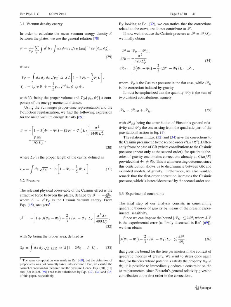
We now want to study the behavior of a massless scalar fieldψ(t, r) confined between two plates and embedded in a grav-itational field (see Fig. 1); to this aim, we basically followthe procedure presented in Ref. [69].

In the configuration of Fig. 1, ψ(t, r) obeys the followingfield equation [70]:

(� + ξ R)ψ(t, r) = 1√−g∂α

[√−g gαβ ∂βψ(t, r)]

+ξ R ψ(t, r) = 0 ,

(14)

where ξ is the coupling parameter between geometry andmatter.4 For simplicity, we consider the massless scalar fieldψ(t, r) confined between two parallel plates separated by adistance L and with extension S, placed at a distance R fromthe gravitational non-rotating source (R L ,

√S).

We select a reference frame with the origin in the point-like source of gravity and the z-axis along the radial direction,perpendicular to the surface of the plates. We can then expandthe metric tensor components and R(r) around the distance

4 It is worth noting that higher-order couplings in the curvature betweenmatter and geometry can in principle be inserted in the analysis, butsince we are dealing with the linearized regime only the contributionR ψ survives in the field equations, which means that in the action weonly consider the non-minimal coupling R ψ2.

123

41 Page 4 of 10 Eur. Phys. J. C (2019) 79:41

Fig. 1 In this picture, the configuration of the Casimir-like system ina gravitational field is represented

R along the z direction by using the gravitational potentialsΦ(r) and Ψ (r) given in Eq. (12)

g00(r) � −1 − 2 Φ0 − 2 Φ1 z ,

gi j (r) � 1 − 2 Ψ0 − 2 Ψ1 z ,

R(r) � R0 + R1 z ,

(15)

where

Φ0 = Φ(R), Φ1 = dΦ(r)

dr

∣∣∣r=R

,

Ψ0 = Ψ (R), Ψ1 = dΨ (r)

dr

∣∣∣r=R

,

R0 = R(R), R1 = dR(r)

dr

∣∣∣r=R

, (16)

and the variable z is free to range in the interval [0, L].Adopting the metric Eq. (15), the field equation for the

scalar field ψ(t, r) of Eq. (14) becomes

ψ̈(t, r) −[

1 + 4η + 4γ z

]∇2ψ(t, r)

+ξ

[R0 + R1z

]ψ(t, r) = 0 , (17)

where the dot indicates a derivative with respect to t , and

η ≡ Φ0 + Ψ0 ,

γ ≡ Φ1 + Ψ1 .

(18)

In order to solve Eq. (17) we perform the ansatz

ψ(t, r) = N Υ (z) ei (ωt−k⊥·r⊥) , (19)

where k⊥ ≡ (kx , ky), r⊥ ≡ (x, y) and N is a normalizationconstant. The field equation in Eq. (17) thus becomes

(∂2χ + χ)Υ (χ) = 0 , (20)

where

χ ≡ χ(z) = a − b z ≡ α β−2/3 − β1/3 z ,

α = (1 − 4 η

)ω2 − k2⊥ − ξ R0 ,

β = 4 ω2 γ + ξ R1 .

(21)

The solution of Eq. (20) can be expressed in terms of Besselfunctions

Υ (χ) = √χ

[C1 J1/3

(2

3χ3/2

)+ C2 J−1/3

(2

3χ3/2

)],

(22)

where C1 and C2 are constants. We note that χ 1 sinceβ � α. For this reason, we can rewrite Eq. (22) as [71]

Υ (χ) �√

3

π√

χsin

[2

3χ3/2 + τ

]. (23)

If we assume that the field ψ satisfies Dirichlet boundaryconditions on the plates, that is

ψ(z = 0) = ψ(z = L) = 0 , (24)

after some algebra, we find the relation

2

3

[χ3/2(0

) − χ3/2(L)] = n π, (25)

with n being an integer number.From Eq. (25), we compute the energy spectrum, which

turns out to be

ω2n = (

1+4η+2γ L)[k2⊥+

(nπ

L

)2]+ξ

[R0 + 1

2R1 L

].

(26)

Finally, we derive the normalization constant

N 2n = a b

3 S ωn n(1 − Φ0

) , (27)

by means of the scalar product of QFT in curved spacetimes[70]

(ψn, ψm

)= −i∫V

√gΣ nμ dx dy dz

×[(

∂μ ψn)ψ∗m − ψn

(∂μ ψm

)∗]

.

(28)

Note that gΣ is the induced metric on a spacelike Cauchyhypersurface Σ .

123

Eur. Phys. J. C (2019) 79:41 Page 5 of 10 41

3.1 Vacuum density energy

In order to calculate the mean vacuum energy density Ebetween the plates, we use the general relation [70]

E = 1

VP

∑n

∫d2 k⊥

∫dx dy dz

√gΣ

(g00

)−1T00

(ψn, ψ

∗n

),

(29)

where

VP =∫

dx dy dz√gΣ � S L

[1 − 3Ψ0 − 3

2Ψ1L

],

Tμν = ∂μ ψ ∂ν ψ − 1

2gμνg

αβ∂α ψ ∂β ψ ,

with VP being the proper volume and T00(ψn, ψ

∗n

)a com-

ponent of the energy-momentum tensor.Using the Schwinger proper-time representation and the

ζ -function regularization, we find the following expressionfor the mean vacuum energy density [69]:

E = −[

1 + 3(Φ0 − Ψ0

) − (2Ψ1 − Φ1

)LP

]π2

1440 L4P

+ ξ R1

192 LP,

(30)

where LP is the proper length of the cavity, defined as

LP =∫

dz√g33 � L

[1 − Ψ0 − 1

2Ψ1 L

]. (31)

3.2 Pressure

The relevant physical observable of the Casimir effect is theattractive force between the plates, defined by F = − ∂E

∂LP,

where E = E VP is the Casimir vacuum energy. FromEqs. (15), one gets5

F = −[

1 + 3(Φ0 − Ψ0

) − 2

3(2Ψ1 − Φ1) LP

]π2 SP

480 L4P

,

(32)

with SP being the proper area, defined as

SP =∫

dx dy√g11g22 � S [1 − 2Ψ0 − Ψ1 L] . (33)

5 The same computation was made in Ref. [69], but the definition ofproper area was not correctly taken into account. Here, we exhibit thecorrect expression for the force and the pressure. Hence, Eqs. (30), (31)

and (32) in Ref. [69] need to be substituted by Eqs. (32), (34) and (36)of this paper, respectively.

By looking at Eq. (32), we can notice that the correctionsrelated to the curvature do not contribute to F .

If now we introduce the Casimir pressure as P = F/Sp,we finally obtain

P = P0 + PG ,

P0 = − π2

480 L4P

,

PG =[

3(Φ0 − Ψ0

) − 2

3(2Ψ1 − Φ1) LP

]P0 ,

(34)

where P0 is the Casimir pressure in the flat case, while PG

is the correction induced by gravity.It must be emphasized that the quantity PG is the sum of

two distinct contributions, namely

PG = PGR + PQ , (35)

with PGR being the contribution of Einstein’s general rela-tivity and PQ the one arising from the quadratic part of thegravitational action in Eq. (1).

The relations in Eqs. (32) and (34) give the corrections tothe Casimir pressure up to the second orderO(m/R2). Differ-ently from the case of GR (where contributions to the Casimirpressure appear only at the second order), for quadratic the-ories of gravity one obtains corrections already at O(m/R)

provided that Φ0 = Ψ0. This is an interesting outcome, sincethis contribution allows us to discriminate between GR andextended models of gravity. Furthermore, we also want toremark that the first-order correction increases the Casimirpressure, which is instead decreased by the second-order one.

3.3 Experimental constraints

The final step of our analysis consists in constrainingquadratic theories of gravity by means of the present exper-imental sensitivity.

Since we can impose the bound |PG | � δP , where δPis the experimental error (as firstly discussed in Ref. [69]),we then obtain

∣∣∣∣3(Φ0 − Ψ0

) − 2

3(2Ψ1 − Φ1) LP

∣∣∣∣ � δP

P0, (36)

that gives the bound for the free parameters in the context ofquadratic theories of gravity. We want to stress once againthat, for theories whose potentials satisfy the property Φ0 =Ψ0, it is possible to immediately deduce a constraint on theextra parameters, since Einstein’s general relativity gives nocontribution at the first order in the corrections.

123

41 Page 6 of 10 Eur. Phys. J. C (2019) 79:41

4 Application to several quadratic theories of gravity

Let us now apply the above formalism of the Casimir effectto several quadratic theories of gravity. We consider bothlocal and non-local models and compute the correspondingmetric potentials and the linearized Ricci scalar. Their knowl-edge is indispensable to study the dynamics of a scalar fieldbetween two plates in a slightly curved background, and thusto constrain the parameters of new physics appearing in suchextended theories. The Ricci scalar does not appear in theformula for the pressure (see Eq. (32)), but we compute it forthe sake of completeness.

Note that the second term in the l.h.s. of Eq. (36) is of orderO

(m/R2

)for every analyzed theory, whereas the first one

goes like O (m/R). Since we assume R to be large, whenΦ = Ψ, we can safely neglect the second-order contribu-tions6 that stem from Ψ1 and Φ1.

We also want to stress that, in the case of Einstein’s GR,Φ = Ψ = −Gm/r, and thus we recover the results for theCasimir energy and the Casimir pressure obtained in Ref.[45].

4.1 f (R)-gravity

We first address the easiest extension of the Einstein-Hilbertaction by including a Ricci squared contribution with a con-stant form-factor

F1 = α , F2 = 0 �⇒ a = 1 , c = 1 − 2 α � . (37)

This choice belongs to the class of f (R) theories, where theLagrangian is truncated up to the order O(R2)

f (R) � R + αR2, (38)

and where the cosmological constant is set to zero.For the above selection of the form-factors, the two metric

potentials in Eq. (12) become

Φ(r) = −Gm

r

(1 + 1

3e−m0r

),

Ψ (r) = −Gm

r

(1 − 1

3e−m0r

),

(39)

wherem0 = 1/√

3 α is the mass of the spin-0 massive degreeof freedom coming from the Ricci scalar squared contribu-tion.

The linearized Ricci scalar is given by

R = 2 G m

re−m0r m2

0 . (40)

6 These factors are also multiplied by LP , which makes our assumptioneven stronger, given that the proper length of the cavity is small.

Plugging the above expressions in Eq. (36), we have

e−m0R � δP

P0

R

2Gm. (41)

4.2 Stelle’s fourth order gravity

Let us now consider Stelle’s fourth order gravity [2,3], whichis achieved with the following form-factors:

F1 =α , F2 =β �⇒ a=1+1

2β �, c = 1−2α �− 1

2β � .

(42)

Differently from the previous case, the Ricci tensor squaredcontribution in the action is clearly recognizable through aconstant, non-vanishing form-factor. It is possible to checkthat the gravitational action related to this model turns out tobe renormalizable [2,3].

For the above choice of the form-factors, the two metricpotentials in Eq. (12) now read

Φ(r) = −Gm

r

(1 + 1

3e−m0r − 4

3e−m2r

),

Ψ (r) = −Gm

r

(1 − 1

3e−m0r − 2

3e−m2r

),

(43)

where m0 = 2/√

12 α + β and m2 = √2/(−β) correspond

to the masses of the spin-0 and of the spin-2 massive mode,respectively.

In order to avoid tachyonic solutions, we need to requireβ < 0. In addition to that, the spin-2 mode is a ghost-likedegree of freedom. Such an outcome is not surprising, sinceit is known that, for any local higher derivative theory ofgravity, ghost-like degrees of freedom always appear [20].

The linearized Ricci scalar generated by a point-likesource and derived from the metric with potentials given byEq. (43) is the same as the one of Eq. (40)

R = 2 G m

re−m0r m2

0 . (44)

It is opportune to explain why the linearized Ricci scalarfor Stelle’s theory has the same form of the linearized Ricciscalar in Eq. (40). Given the following two metric potentials:

Φ(r) = −Gm

r

(1 + a e−m0r + b e−m2r

),

Ψ (r) = −Gm

r

(1 + c e−m0r + d e−m2r

),

(45)

the related linearized Ricci scalar is

123

Eur. Phys. J. C (2019) 79:41 Page 7 of 10 41

R = 2Gm

r

((a − 2c) e−m0r m2

0 + (b − 2d) e−m2r m22

).

(46)

We can now understand that, in the case of Stelle’s theory, thelinearized Ricci scalar is given by Eq. (44), because b−2 d =−4/3−2 (−2/3) = 0. Thus, only the term depending on m0

survives. We also want to stress that the curvature invariantin Stelle’s theory is still singular at r = 0.

The correction to the Casimir pressure P given by thismodel is

∣∣∣e−m0R − e−m2R∣∣∣ � δP

P0

R

2Gm. (47)

As expected, for m2 → ∞ (β → 0) we immediately obtainthe same expression of Eq. (41).

4.3 Sixth order gravity

Here, we deal with a sixth order gravity model, which is anexample of super-renormalizable theory [20,72]

F1 = α � , F2 = β ��⇒ a = 1 + 1

2β �2, c = 1 − 2α�2 − 1

2β�2 .

(48)

The form-factors of the two metric potentials in Eq. (12)assume the following expression:

Φ(r) = −Gm

r

(1 + 1

3e−m0r cos(m0r) − 4

3e−m2r cos(m2r)

),

Ψ (r) = −Gm

r

(1 − 1

3e−m0r cos(m0r) − 2

3e−m2r cos(m2r)

),

(49)

where the masses of the spin-0 and spin-2 degrees of freedomare now given by m0 = 2−1/2(−3 α − β)−1/4 and m2 =(2 β)−1/4, respectively.

This time, tachyonic solutions are avoided for −3 α− β >

0, which can be satisfied by the requirement α < 0 and−3 α > β, with β > 0. The current higher derivative theoryof gravity has no real ghost-modes around the Minkowskibackground but a pair of complex conjugate poles with equalreal and imaginary parts [73,74], and corresponds to the socalled Lee-Wick gravity [75,76]. It is worthwhile noting thatin this higher derivative theory the unitarity condition is notviolated, indeed the optical theorem still holds [4,77,78].

The linearized Ricci scalar for this model turns out to be

R = 2 G m

rsin(m0r) e

−m0r m20 . (50)

We remark that, in the linearized Ricci scalar, there is no m2

dependence for the same reason explained before. However,

the crucial difference here is that the curvature is regular atr = 0.

In this case, the bound on the pressure in Eq. (36) becomes

∣∣∣e−m0Rcos (m0R) − e−m2Rcos (m2R)

∣∣∣ � δP

P0

R

2Gm. (51)

This expression resembles the one of Eq. (47), apart fromoscillatory functions of the products m0R and m2R. Further-more, as for the case of Stelle’s theory, in Eq. (51) the limitm2 → ∞ smoothly approaches the outcome of Eq. (41), withthe only difference that now the periodic function cos(m0R)

is in principle not negligible.

4.4 Ghost-free infinite derivative gravity

We now wish to consider an example of ghost-free non-localtheory of gravity [25–31,79–86]. For the sake of clarity, wedecide to adopt the simplest ghost-free choice for the non-local form-factors [27]

F1 = −1

2F2 = 1 − e−�/M2

s

2 � �⇒ a = c = e−�/M2s ,

(52)

where Ms is the scale at which the non-locality of the grav-itational interaction should become manifest. Note that, forthe special ghost-free choice in Eq. (52), no extra degrees offreedom other than the massless transverse spin-2 gravitonpropagate around the Minkowski background.

Since we have chosen a = c, the metric potentials ofEq. (12) coincide

Φ(r) = Ψ (r) = −Gm

rErf

(Ms r

2

), (53)

The corresponding linearized Ricci scalar is given by

R = G m M3s e

− M2s r

2

4√π

, (54)

which shows a Gaussian behavior induced by the presenceof non-local gravitational interaction, whose role is to smearout the point-like source at the origin.

Since the two metric potentials coincide, we get no con-tribution at the first order, but we can constrain such a theorystarting from the second-order correction. If this is the case,then the equation for the constraint reads

∣∣∣∣∣∣e− M2

s R2

4 Ms√π

− 1

RErf

(Ms R

2

)∣∣∣∣∣∣ � δP

LPP0

3R

2 Gm. (55)

123

41 Page 8 of 10 Eur. Phys. J. C (2019) 79:41

It is worth emphasizing that it would be very difficult toconstrain this kind of non-local theory with Solar system’sexperiments, since the non-locality of the gravitational inter-action described by the metric with the potential in Eq. (53)is expected to become relevant only at scales comparable tothe Schwarzschild radius [31,81,82].

4.5 Non-local gravity with non-analytic form-factors

For the last case, we consider two models of non-localinfrared extension of Einstein’s general relativity, whereform-factors are non-analytic functions of �. These theoriesare inspired by quantum corrections to the effective action ofquantum gravity [87–93].

1. The first model is described by the following choice ofthe form-factors:

F1 = α

� , F2 = 0 �⇒ a = 1 , c = 1 − 2α . (56)

The two metric potentials are infrared modifications ofthe Newtonian one

Φ(r) = −Gm

r

(4α − 1

3α − 1

),

Ψ (r) = −Gm

r

(2α − 1

3α − 1

).

(57)

Such a spacetime metric has a vanishing linearized Ricciscalar,

R = 0 , (58)

but it is not Ricci-flat, since some components of Rμν

are non-vanishing.The expression for the Casimir pressure correction givenby such a quadratic theory of gravity leads to the bound

∣∣∣∣ α

3α − 1

∣∣∣∣ � δP

P0

R

6Gm. (59)

In the last Equation, if we treat α as a small parameter,we obtain the constraint

|α| � δP

P0

R

6Gm. (60)

Hence, differently from the other results, by performingsuch an expansion it is possible to have a direct access tothe free parameter of the theoretical model, thus imme-diately obtaining a constraint on it.

2. The non-local form factors for the second model are

F1 = β

�2 , F2 = 0 �⇒ a = 1 , c = 1 − 2β

� .

(61)

In this framework, the infrared modification is not aconstant, but the metric potentials show a Yukawa-likebehavior

Φ(r) = −Gm

r

4

3

(1 − 1

4e−√

3βr)

,

Ψ (r) = −Gm

r

2

3

(1 + 1

2e−√

3βr)

.

(62)

The corresponding linearized Ricci scalar isnon-vanishing and negative

R = −6G m

re−√

3βr β . (63)

For this second example of non-local gravity with non-analytic form-factors, we obtain the bound

∣∣∣1 − e−√3βR

∣∣∣ � δP

P0

R

2Gm. (64)

5 Discussions and conclusions

In this paper, we have discussed the Casimir effect in the con-text of quadratic theories of gravity. In particular, we havefocused our attention on the corrections to the Casimir pres-sure which come from the gravitational sector that makesthese models different from GR. We have also described thepossibility to infer several constraints on the free parametersof the above theories in a completely transparent way, byrelating them to the current experimental errors. In all theanalyzed contexts, we have worked in the weak field regime,in which computations related to the metric potentials and tothe Casimir effect are easy to carry out. This has proved tobe convenient in order to immediately separate the Casimirpressure in all of its relevant contributions, as seen in Eq. (34).

A feature which is omnipresent in the outcomes ofEqs. (41), (51), (55), (60) and (64) is that they all dependon the quantity (δP/P0)(R/Gm). If we consider the caseof the Earth, and thus R ≡ R⊕, m ≡ M⊕, we get

δP

P0

R⊕GM⊕

� 106 , (65)

if we assume the value δP/P0 � 10−3, stemming from thecurrent experimental precision [94].

In order to enhance the attained bounds, there is the neces-sity either to implement the experiment of the Casimir effectnear another astrophysical object (which is not the Earth) or

123

Eur. Phys. J. C (2019) 79:41 Page 9 of 10 41

to significantly improve the sensitivity of the experimentalinstruments. For what concerns the former, however, there isalso the problem to adapt the solution of the Klein-Gordonequation to the nature of the spacetime that is under consider-ation. For instance, in the case of blackholes the ratio R/Gmis substantially lowered, but our formalism based on a linearregime is no longer valid.

As a final observation, we want to focus the attention onemore time on the fact that the first-order corrections to thepressure P in Eq. (34) cannot be attributable to GR, sincein Einstein’s theory Φ0 = Ψ0 . Hence, any gravitational con-tribution to the Casimir pressure arising at this order is inti-mately connected to an extended theory of gravity for whicha = c (see Eq. (12)). From an experimental point of view,such a consideration would also imply a more stringent boundon the free parameters of these models. In this perspective,future experiments of the Casimir effect in curved back-ground might represent a powerful tool to test and constrainextended theories of gravity.

Acknowledgements The authors are thankful to Anupam Mazumdar.LB would like to thank Breno Giacchini and Shubham Maheshwari fordiscussions.

Data Availability Statement This manuscript has no associated dataor the data will not be deposited. [Authors’ comment: Data sharingnot applicable to this article as no datasets were generated or analysedduring the current study.]

Open Access This article is distributed under the terms of the CreativeCommons Attribution 4.0 International License (http://creativecommons.org/licenses/by/4.0/), which permits unrestricted use, distribution,and reproduction in any medium, provided you give appropriate creditto the original author(s) and the source, provide a link to the CreativeCommons license, and indicate if changes were made.Funded by SCOAP3.

References

1. C.M. Will, Living Rev. Rel. 17, 4 (2014)2. K.S. Stelle, Phys. Rev. D 16, 953 (1977)3. K.S. Stelle, Gen. Rel. Grav. 9, 353–371 (1978)4. D. Anselmi, JHEP 1706, 086 (2017)5. D. Anselmi, JHEP 1802, 141 (2018)6. D. Anselmi, M. Piva, JHEP 1805, 027 (2018)7. D. Anselmi, M. Piva, JHEP 1811, 021 (2018)8. D. Anselmi. arXiv:1809.05037 [hep-th]9. A.A. Starobinski, Phys. Lett. B 91, 99–102 (1980)

10. A.A. Starobinski, Proceedings of the Second Seminar “QuantumTheory of Gravity”, Moscow, 13–15 October 1981, INR Press,Moscow, pp. 58–72 (1982)

11. A.A. Starobinsky, Sov. Astron. Lett. 9, 302 (1983)12. S. Capozziello, G. Lambiase, M. Sakellariadou, An Stabile, Phys.

Rev. D 91, 044012 (2015)13. G. Lambiase, M. Sakellariadou, A. Stabile, An Stabile, JCAP 1507,

003 (2015)14. G. Lambiase, M. Sakellariadou, A. Stabile, JCAP 1312, 020 (2013)15. N. Radicella, G. Lambiase, L. Parisi, G. Vilasi, JCAP 1412, 014

(2014)

16. S. Capozziello, G. Lambiase, Int. J. Mod. Phys. D 12, 843–852(2003)

17. S. Calchi Novati, S. Capozziello, G. Lambiase, Grav. Cosmol. 6,173–180 (2000)

18. S. Capozziello, G. Lambiase, H.J. Schmidt, Ann. Phys. 9, 39–48(2000)

19. S. Capozziello, G. Lambiase, G. Papini, G. Scarpetta, Phys. Lett.A 254, 11–17 (1999)

20. M. Asorey, J.L. Lopez, I.L. Shapiro, Int. J. Mod. Phys. A 12, 5711(1997)

21. A. Stabile, An Stabile, S. Capozziello, Phys. Rev. D 88(9), 124011(2013)

22. A. Stabile, An Stabile, Phys. Rev. D 85, 044014 (2012)23. G. Lambiase, S. Mohanty, An Stabile, Eur. Phys. J. C 78, 350 (2018)24. E.T. Tomboulis. arXiv:hep-th/970214625. T. Biswas, A. Mazumdar, W. Siegel, JCAP 0603, 009 (2006)26. L. Modesto, Phys. Rev. D 86, 044005 (2012)27. T. Biswas, E. Gerwick, T. Koivisto, A. Mazumdar, Phys. Rev. Lett.

108, 031101 (2012)28. T. Biswas, A. Conroy, A.S. Koshelev, A. Mazumdar, Class. Quant.

Grav. 31, 015022 (2014). (Erratum: Class. Quant. Grav. 31, 159501(2014))

29. T. Biswas, A.S. Koshelev, A. Mazumdar, Fundam. Theor. Phys.183, 97 (2016)

30. T. Biswas, A.S. Koshelev, A. Mazumdar, Phys. Rev. D 95, 043533(2017)

31. A.S. Koshelev, A. Mazumdar, Phys. Rev. D 96(8), 084069 (2017)32. H. Casimir, Proc. K. Ned. Akad. Wet. 51, 793 (1948)33. H. Casimir, D. Polder, Phys. Rev. 73, 360 (1948)34. K.A. Milton, The Casimir effect: Physical Manifestations of Zero-

Point Energy (World Scientific, River edge, 2001)35. V.V. Nesterenko, G. Lambiase, G. Scarpetta, Riv. Nuovo Cim.

27(6), 1–74 (2004)36. V.V. Nesterenko, G. Lambiase, G. Scarpetta, Ann. Phys. 298, 403

(2002)37. V.V. Nesterenko, G. Lambiase, G. Scarpetta, Int. J. Mod. Phys. A

17, 790 (2002)38. V.V. Nesterenko, G. Lambiase, G. Scarpetta, Phys. Rev. D 64,

025013 (2001)39. V.V. Nesterenko, G. Lambiase, G. Scarpetta, J. Math. Phys. 42,

1974 (2001)40. G. Lambiase, G. Scarpetta, V.V. Nesterenko, Mod. Phys. Lett. A

16, 1983 (2001)41. G. Lambiase, V.V. Nesterenko, M. Bordag, J. Math. Phys. 40, 6254

(1999)42. M. Bordag, U. Mohideen, V.M. Mostepanenko, Phys. Rep. 353, 1

(2001)43. C. Genet, A. Lambrecht, S. Reynaud, On the nature of dark energy.

In: P. Brax, J. Martin, J. P. Uzan (Fronter Group) (eds.) 18th IAPColl. on the Nature of Dark Energy: Observations and TheoreticalResults in the Accelerating Universe, Paris, France, 1–5 July 2002,pp. 121–30

44. G. Bressi, G. Carugno, R. Onofrio, G. Ruoso, Phys. Rev. Lett. 88,041804 (2002)

45. F. Sorge, Class. Quant. Grav. 22, 5109 (2005)46. V.G. Bagrov, I.L. Buchbinder, S.D. Odintsov, Phys. Lett. B 184,

202 (1987)47. V.G. Bagrov, I.L. Buchbinder, S.D. Odintsov, Yad. Fiz. 45, 1192

(1987)48. I.L. Buchbinder, P.M. Lavrov, S.D. Odintsov, Nucl. Phys. B 308,

191 (1988)49. S.D. Odintsov, Sov. Phys. J. 32, 458 (1989)50. M.R. Setare, Class. Quant. Grav. 18, 2097 (2001)51. E. Calloni, L. di Fiore, G. Esposito, L. Milano, L. Rosa, Int. J. Mod.

Phys. A 17, 804 (2002)

123

41 Page 10 of 10 Eur. Phys. J. C (2019) 79:41

52. G. Esposito, G.M. Napolitano, L. Rosa, Phys. Rev. D 77, 105011(2008)

53. G. Bimonte, G. Esposito, L. Rosa, Phys. Rev. D 78, 024010 (2008)54. E. Calloni, M. De Laurentis, R. De Rosa, F. Garufi, L. Rosa, L. Di

Fiore, G. Esposito, C. Rovelli, P. Ruggi, F. Tafuri, Phys. Rev. D 90,022002 (2014)

55. B. Nazari, Eur. Phys. J. C 75, 501 (2015)56. P. Bueno, P.A. Cano, V.S. Min, M.R. Visser, Phys. Rev. D 95,

044010 (2017)57. M.R. Tanhayi, R. Pirmoradian, R. Int, J. Theor. Phys.55, 766 (2016)58. S.A. Fulling, K.A. Milton, P. Parashar, A. Romeo, K.V. Shajesh, J.

Wagner, Phys. Rev. D 76, 025004 (2007)59. K.A. Milton, P. Parashar, K.V. Shajesh, J. Wagner, J. Phys. A 40,

10935 (2007)60. K.V. Shajesh, K.A. Milton, P. Parashar, J.A. Wagner, J. Phys. A 41,

164058 (2008)61. K.A. Milton, K.V. Shajesh, S.A. Fulling, P. Parashar, Phys. Rev. D

89, 064027 (2014)62. K.A. Milton, S.A. Fulling, P. Parashar, A. Romeo, K.V. Shajesh,

J.A. Wagner, J. Phys. A 41, 164052 (2008)63. M. Blasone, G. Lambiase, L. Petruzziello, A. Stabile, Eur. Phys. J.

C 78(11), 976 (2018)64. M.B. Cruz, E.R. Bezerra de Mello, A.Y. Petrov, Phys. Rev. D 96(4),

045019 (2017)65. M.B. Cruz, E.R. Bezerra De Mello, A.Y. Petrov, Mod. Phys. Lett.

A 33, 1850115 (2018)66. M. Frank, I. Turan, Phys. Rev. D 74, 033016 (2006)67. A. Martin-Ruiz, C.A. Escobar, Phys. Rev. D 94, 076010 (2016)68. M. Blasone, G.G. Luciano, L. Petruzziello, L. Smaldone, Phys.

Lett. B 786, 278 (2018)69. G. Lambiase, A. Stabile, An Stabile, Phys. Rev. D 95, 084019

(2017)70. N.D. Birrell, P.C.W. Davies, Quantum Fields in Curved Space

(Cambridge University Press, Cambridge, 1982)71. I.S. Gradshteyn, I.M. Ryzhik, Table of Integrals, Series and Prod-

ucts (Academic, New York, 1980)72. B.L. Giacchini, T. de Paula Netto. arXiv:1806.05664 [gr-qc]

73. A. Accioly, B.L. Giacchini, I.L. Shapiro, Phys. Rev. D 96(10),104004 (2017)

74. B.L. Giacchini, Phys. Lett. B 766, 306 (2017)75. L. Modesto, I.L. Shapiro, Phys. Lett. B 755, 279 (2016)76. L. Modesto, Nucl. Phys. B 909, 584 (2016)77. D. Anselmi, M. Piva, JHEP 1706, 066 (2017)78. D. Anselmi, M. Piva, Phys. Rev. D 96(4), 045009 (2017)79. J. Edholm, A.S. Koshelev, A. Mazumdar, Phys. Rev. D 94(10),

104033 (2016)80. L. Buoninfante, Master’s Thesis (2016). arXiv:1610.08744v4 [gr-

qc]81. L. Buoninfante, A.S. Koshelev, G. Lambiase, A. Mazumdar, JCAP

1809(09), 034 (2018)82. L. Buoninfante, A.S. Koshelev, G. Lambiase, J. Marto, A. Mazum-

dar, JCAP 1806(06), 014 (2018)83. L. Buoninfante, G. Harmsen, S. Maheshwari, A. Mazumdar, Phys.

Rev. D 98(8), 084009 (2018)84. L. Buoninfante, G. Lambiase, A. Mazumdar. arXiv:1805.03559

[hep-th]85. L. Buoninfante, A.S. Cornell, G. Harmsen, A.S. Koshelev, G. Lam-

biase, J. Marto, A. Mazumdar, Phys. Rev. D 98(8), 084041 (2018)86. A. Mazumdar, G. Stettinger. arXiv:1811.00885 [hep-th]87. A.O. Barvinsky, G.A. Vilkovisky, Phys. Rept. 119, 1–74 (1985)88. S. Deser, R.P. Woodard, Phys. Rev. Lett. 99, 111301 (2007)89. E. Belgacem, Y. Dirian, S. Foffa, M. Maggiore, JCAP 1803(03),

002 (2018)90. L. Tan, R.P. Woodard, JCAP 1805(05), 037 (2018)91. S. Deser, R.P. Woodard, JCAP 1311, 036 (2013)92. A. Conroy, T. Koivisto, A. Mazumdar, A. Teimouri, Class. Quant.

Grav. 32(1), 015024 (2015)93. R.P. Woodard, Universe 4(8), 88 (2018)94. V.M. Mostepanenko, J. Phys. Conf. Ser. 161, 012003 (2009)

123