CasePacket2013_v4

1

6TH ANNUAL INTERCOLLEGIATE TRADING COMPETITION 2013

Traders@MIT welcomes you to our 6th Annual Intercollegiate Trading Competition! We are excited to be holding the competition again this year and are confident that it will provide a rich and challenging learning experience. This single-day event will consist of both open-outcry and electronic trading. Teams will be ranked overall based on their total weighted rankings from each of the five cases. Note: We will be posting various updates regarding the competition and the case packet on our website: http://traders.mit.edu/competition/. Please check it often.

SPONSORS We want to thank our sponsors for helping to make this competition possible: DRW Trading, JP Morgan, FLOW Trading, Bank of America Merrill Lynch, Goldman Sachs, D.E. Shaw, IMC Financial Markets, Chopper Trading, Spot Trading, Belvedere Trading, Wolverine Trading, SIG, Knight Capital Group, Citadel, and Element Capital. You will be able to have lunch with and speak with company representatives throughout the day. We also would like to thank Rotman Interactive Trader for allowing us to use their software.

PRIZES The first-place team is offered admission to the Rotman International Trading Competition at the Rotman School of Management, University of Toronto. The top 5 overall teams will split over $1000 in prizes. The winners of each individual case will also receive a small prize. In addition, DRW Trading Group will be taking the winner teams to dinner after the competition. Bank of America Merrill Lynch will also offer an exclusive firm visit to the winners. The remainder of this packet contains the competition schedule, descriptions of the cases that will be presented, logistical notes, and other preparatory information. We recommend that you read it thoroughly and build the necessary Excel models before the day of the competition. Each competitor must bring a Windows compatible laptop. Please contact [email protected] if you have any questions regarding the competition.

Intercollegiate Trading Competition 2013

Platinum Sponsors

Gold Sponsors

Silver Sponsors

2

ABOUT TRADERS@MIT The purpose of Traders@MIT is to prepare its members for a career in the financial markets by teaching the fundamentals of financial products and exploring differences in various trading desks. Our Executive Board consists of 16 dedicated individuals who work to put together this competition, the largest trading competition in the country. In addition to the Fall Competition, we organize regular company educational sessions and teach a for-credit Intro to Trading seminar.

Schedule of Events

Friday, November 15th:

9:30PM – 12:00AM: Competitor Networking Event – Champions Sports Bar (see page 4)

Saturday, November 16th:

The competition will be held at the MIT Tang Center (see page 5)

9:00AM – 10:00AM: Registration & Check-In, Breakfast

10:00AM – 11:00AM: Electronic Simulation: Sales & Trader

11:15AM – 12:00PM: Electronic Simulation: Volatility Arbitrage

12:15PM – 1:45PM: Lunch with sponsors – Picower Institute for Learning and Memory (p. 6)

2:00PM – 3:00PM: Quant Open Outcry: Index Futures; Sponsored by Flow Traders

3:00PM – 3:45PM: Electronic Simulation: Price Discovery

3:45PM – 4:00PM: Break

4:00PM – 4:45PM: Electronic Simulation: Commodities

5:00PM – 7:00PM: Networking Reception & Awards Ceremony -- Marriott Cambridge Hotel

3

Requirements Software – Rotman Interactive Trader (RIT) We will be using Rotman Interactive Trader (RIT) for the electronic trading portions of the competition. You are able to download RIT at: http://rit.rotman.utoronto.ca/software.asp. This is a Windows-only application. Both team members are allowed to run RIT, although only one individual is allowed to place trades. Here are two tutorials: http://rit.rotman.utoronto.ca/cases/RIT%20-%20User%20Guide%20-%20Client%20Software%20Feature%20Guide.pdf http://rit.rotman.utoronto.ca/cases/Microstructure%202%20-%20Tutorial.pdf To receive real-time data in Excel, please be sure to install the Excel RTD Links from the same website. Practice Sessions We recommend contestants familiarize themselves with the trading platform using the practice case listed on RIT’s web page: http://rit.rotman.utoronto.ca/demo.asp In addition, we will be hosting mandatory practice sessions in the coming weeks. You must attend one, although there is no limit on how many you can attend. The practice session allows you to familiarize yourself with both RIT and the competition cases. The times for these sessions are: Tuesday-Thursday, November 5-7 @ 9pm Tuesday-Thursday, November 12-14 @ 9pm The specifics for the practice sessions can be found here: https://www.dropbox.com/s/uurn4gcfxli1tvv/Practice%20Session%20Cases.pdf Attire Business formal or business casual attire is strongly recommended.

4

Locations Friday Evening Networking Session The Friday night networking session will be held at Champions Sports Grill, starting at 9:30pm on Friday. There will be plenty of food and drinks – come meet and hang out with your fellow competitors and Traders@MIT Executive Board members. Everyone is invited! Champions is located at: 50 Broadway Dr. Cambridge, MA 02139 From Google Maps

5

Competition Room The competition will be held at the Massachusetts Institute of Technology (MIT) at the Sloan Tang Center (Building 51) in Room 345. The Tang Center is located at: 70 Memorial Dr. Cambridge, MA 02139

6

Networking Lunch Lunch will be held at the Picower Institute for Learning and Memory (Building 46) in the third floor atrium. The Picower Institute for Learning and Memory is located at: MIT Building 46 43 Vassar St. Cambridge, MA 02139 Walking directions from competition room

7

Paper Trading: Quant Open Outcry Sponsored by Flow Traders This case will be worth 20% of each team’s final score. Overview

During the Quant Open Outcry case, teams of two will trade FLOW Index futures. Each team consists of a trader, who will trade on the floor of the trading room, and an analyst, who will be located in the gallery seating of the room. Teams will construct pricing models based on historical index levels and the indicators explained below. Analysts can view the current indicators at traders.mit.edu/competition/quant-outcry/ or get this data programmatically, as described below. These inputs should be used to construct pricing models. You should construct your pricing model before the day of the competition. Using their models, analysts will convey trading instructions to traders using hand signals – no verbal communication is allowed between traders and analysts. It is recommended that you develop a system of hand signals prior to the case. The case will last for 40 minutes, divided into two 15-minute heats and one 10-minute “blitz” heat. Accurately forecasting the index level and rapidly relaying trading instructions will result in higher profits. The FLOW Index will begin trading at a value of 1000, and the final value for each heat will depend on the economic indicators. Note that the index returns are noisy – you should not expect to predict them perfectly from the indicator values. After heat one ends, analysts and traders must switch places and period two of the case will be run. Either teammate may be the analyst or trader in the third round. Correlations between the FLOW Index and indicators may or may not stay fixed throughout the entire event, so it is suggested that analysts keep track of the accuracy of the model and consider re-running analyses when necessary. Case Information

There are various indicators that affect the FLOW Index, mostly types of economic data. There will be one release per week. For the first two heats, a reading for each of the indicators will be released every 30 seconds to the analysts. For the final blitz heat, readings will be released every 10 seconds. Note that this data will not be available to pit traders. Indicator releases can be considered accurate and free of errors. Although pit traders cannot see indicator releases, both traders and analysts will be able to see the spot market in real time on the projector screen.

8

Appendix 3 includes 50,000 data points of historical data for the level of the FLOW Index and the economic indicators. You may use these data to estimate a model to predict the FLOW Index. Appendix 3 has been provided with this case packet. Constructing a Useful Pricing Model

Each team is advised to develop a model (using, for example, Excel or Python) to determine the relationship between economic indicators and the FLOW Index. New indicator values should be entered into the Excel model when they are released, in order to predict the next-period index value. Historical data from Appendix 3 should be considered accurate for modeling the future position of the FLOW Index. The following indicators will be available:

1. Gross Domestic Product (GDP) 2. Employment Cost Index (ECI) 3. Business Productivity and Costs (BPC) 4. Housing Starts (HS) 5. Consumer Price Index (CPI) 6. Capacity Utilization (CAP) 7. Unemployment Rate (U) 8. World Equity Indices (WEI) 9. Dollar/Money Supply (DMS) 10. Gold Price (Gold)

Each indicator has a different effect on the FLOW Index; this effect might not be linear. Further, some indicators might require differentiating in order to be useful in prediction (i.e. you might want to use the change in a given indicator’s value since last period, rather than the value itself, as an input to your predictive model). In addition, the World Equity Index encompasses emerging markets only. Here are a few suggestions for building a good model:

• Some indicators may have no effect on the FLOW index • Use ordinary least-squares regression to estimate your model. You can do this in Excel. • For the dependent variable in your regression, use 𝛥 log𝐹𝑙𝑜𝑤 rather than just 𝐹𝑙𝑜𝑤. That is,

try to predict the proportional change in the index value between the current and next period, rather than trying to predict the index value itself. Then transform this output into the predicted index value using formulas in Excel and display the prediction to the analyst.

• Some regressors make more sense in terms of proportional change. For such an indicator 𝐼𝑁𝐷, 𝛥 log 𝐼𝑁𝐷 is a good choice for an independent variable. Use judgment – this does not make sense for all of them. Sometimes the absolute change is a better indicator, and sometimes the indicator value itself (not transformed) makes the most sense.

• Consider including the last-period log FLOW return as a regressor. • Consider including values from previous periods for leading indicators. • Avoid including terms with no statistically significant relationship to prevent over-fitting.

9

• Coefficients of certain terms in your regression will not necessarily be constant. They could, for instance, depend on the deviation of IND from the mean and have the form 𝑎 + 𝑏𝑧, or 𝑐! + 𝑐!𝑧!! , where 𝑧 and 𝑧_𝑖 are z-scores of certain indicators and 𝑎, 𝑏, 𝑐! are constants.

• When in doubt, looking at plots of the data can be helpful. • Make it easy for the analyst to type in the next values of the indicators as they become

available. Use Excel formulas to automatically perform any necessary transformations of the input indicator values required by the model.

• To predict FLOW at time t, you can use indicators released at time 0, 1, …, t. Keep in mind that older indicator releases may no longer be relevant.

Trading Profits

Each team’s outstanding positions at the end of the trading session will be settled in the same manner as in the Social Outcry case. The quality of analysts’ models will not factor into your final score; however, accurate estimates of the Index will greatly assist you in achieving higher profits. Teams will be scored based on their total P&L over the two heats. Indicator API

We have an API that analysts can query programmatically for the indicators. This will be especially valuable for the blitz round. To get the current value of the indicators, make a GET request to https://traders.scripts.mit.edu/competition/quant-outcry/api/ with your username and password in the form of

{“username”: “T@MIT”, “password”: “hunter2”}

You will receive a JSON object back with the following keys: “indicators”, “tick”, and “time_to_next”. If the case is not running, these values will be null. Otherwise, they will have the following values. indicators points to a JSON object of the indicators. An example of this object is {"GDP": 18.92, "CPI": 239.04, "BPC": 110.54, "Gold": 1318.74, "HS": 605.4, "WEI": 608.38, "CAP": 70.55, "ECI": 42357.14, "DMS": 10817.28, "U": 12.14, "FLOW": 993.38}. Note that the order of the items in the object is not deterministic. tick will indicate which release the data is relevant to. time_to_next is the time in seconds until the next data release. indicators[“FLOW”] is the value of the indicator at the previous release. If at any time, you wish to get all the data up to that point, make a GET request to https://traders.scripts.mit.edu/competition/quant-outcry/api/all/ with your credentials as indicated above. You will receive back a JSON object with “indicators” as the only key. This will point to an array of indicator JSON objects, as defined above.

10

https://traders.scripts.mit.edu/competition/quant-outcry/api/dummy/ and https://traders.scripts.mit.edu/competition/quant-outcry/api/all/dummy/ are set up for you to test your infrastructure. These two endpoints return random data. Teams that deliberately send excessive queries will be penalized.

Rules

During the trading period, feel free to shout out your position (e.g. “Selling at 1200”). When you are asked for a position, you must provide both a bid and ask. For example, you can say: “500 at 1200”, meaning that you are willing to buy at 500 and sell at 1200. Remember, you cannot retract an offer. Say you want to take up someone’s offer to sell at 550. You say “sold at 550”, and if you are the first person to buy, then the transaction is complete. Fill out the order form provided and hand it to a Traders@MIT exec board member. A representative from both teams must be present for your transaction to be validated.

11

RIT - Electronic Trading: Volatility Arbitrage This case will be worth 15% of each team’s final score. Overview

In this case you will use news releases on fundamental and market conditions to trade options on the T@MIT index, an equity index. Your ability to earn profits will depend on:

1. your ability to predict changes in implied volatility across different option strike prices, 2. your ability to identify and enter appropriate positions to profit from them, and 3. your ability to hedge your positions, primarily through delta- and vega-hedging.

This case is relatively complex. We strongly recommend investing time in understanding the relevant concepts and building a useful model before the day of the competition. Options Basics

A European option is a financial derivative that confers the right but not the obligation to either buy (for a "call" option) or sell (for a "put" option) a given product (the "underlying") at a fixed price (the "strike price") on but not before a given date (the "expiration date"). The value of an option depends on the volatility of the underlying, which is the standard deviation of the (usually annualized) logarithmic return distribution of the underlying. Intuitively, volatility quantifies how much the price might fluctuate in percentage terms. Volatility is not directly observable; it must be estimated from data. It comes in two forms:

1. Realized volatility is the volatility of a product over some past time period. The simplest estimate is the sample standard deviation of the annualized log returns during the period.

2. Implied volatility is the volatility that a product must have in the future in order for the price of some particular option on it to be theoretically fair. I.e., it is the future volatility implied by the price of the option in question. See below for estimation.

Options Pricing Model

Given underlying price ("spot price") S, strike price K, risk-free interest rate r, volatility σ, current time t, and expiration time T, the Black-Scholes formula for the value C of a European call option on a non-dividend-paying asset subject to certain assumptions is:

𝐶 = 𝑁 𝑑! 𝑆 − 𝑁 𝑑! 𝐾𝑒!! !!! 𝑑! = [ln(𝑆/𝐾)+ (𝑟 + 𝜎!/2)(𝑇 − 𝑡)]/(𝜎 𝑇 − 𝑡)

12

𝑑! = 𝑑! − 𝜎 𝑇 − 𝑡 N(x) is the standard normal cumulative distribution function and ln(x) is the natural logarithm. Extending this model for continuous dividend yield q produces the Garman-Kohlhagen formula:

𝐶 = 𝑁 𝑑! 𝑆𝑒!!(!!!) − 𝑁 𝑑! 𝐾𝑒!! !!! 𝑑! = [ln(𝑆/𝐾)+ (𝑟 − 𝑞 + 𝜎!/2)(𝑇 − 𝑡)]/(𝜎 𝑇 − 𝑡)

𝑑! = 𝑑! − 𝜎 𝑇 − 𝑡 The value P for a corresponding put option can be obtained from put-call parity, which for European options with continuous dividend rate q is as follows:

𝐶 + 𝐾𝑒!!(!!!) = 𝑃 + 𝑆𝑒!!(!!!) Volatility Smile and Skew

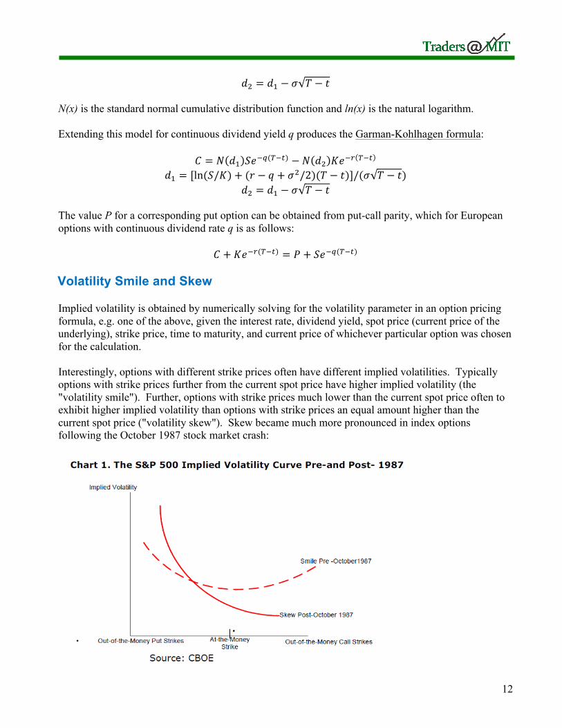
Implied volatility is obtained by numerically solving for the volatility parameter in an option pricing formula, e.g. one of the above, given the interest rate, dividend yield, spot price (current price of the underlying), strike price, time to maturity, and current price of whichever particular option was chosen for the calculation. Interestingly, options with different strike prices often have different implied volatilities. Typically options with strike prices further from the current spot price have higher implied volatility (the "volatility smile"). Further, options with strike prices much lower than the current spot price often to exhibit higher implied volatility than options with strike prices an equal amount higher than the current spot price ("volatility skew"). Skew became much more pronounced in index options following the October 1987 stock market crash:

13

This can be viewed as a consequence of the fact that the Black-Scholes formula and related extensions assume the spot price follows a geometric Brownian motion, which is equivalent to claiming that incremental logarithmic returns are normally-distributed and have a constant standard deviation. In reality, returns are not typically normally-distributed. They tend to have a higher probability of extreme events than would be the case under a normal distribution ("fat tails"), particularly for extreme negative events. Further, volatility itself can vary. As depicted above, an increase in the perceived likelihood of extreme negative events can increase volatility skew. Likewise, a belief that both extreme positive and negative events have become more likely while leaving the size of more typical events unchanged can make the volatility smile more pronounced. This must be distinguished from a belief that price movements will simply be larger on average than they have been in the recent past, which instead produces a parallel shift upward in the implied volatilities of options at all strike prices. Note that it is possible for both to occur simultaneously. Here are two examples. The left is from just prior to an earnings release for a stock. Note the pronounced curvature and asymmetry in the front-month options (red). Also note that the overall level of volatility for the front-month options is higher than for longer-dated options, indicating that most of the variability in price is expected to occur in the near-term:

In contrast, the chart on the right comes from a company that engages in numerous patent lawsuits. A particular one is expected to reach a decision soon, and the decision will be either very good or very bad for the future of the company. The front-month options again exhibit a substantial volatility smile, but it is more symmetrical this time. Also, subsequent volatility remains high in this example given the risks of other ongoing litigation and R&D. However, these later risks are expected to be less binary than the impending decision: market participants predict the later return distribution will have thinner tails, so the IV surface is flatter. Hedging and the Greeks

Options have various risk factors, commonly called the "Greeks". The Greeks describe the effects of changes in various parameters on the price of the option, and are typically expressed as partial derivatives in the context of the Black-Scholes option pricing model and related extensions. The simplest and most important Greeks are:

14

• Delta -- the partial derivative of the option price with respect to the spot price (always positive for calls; always negative for puts). Delta tells you how many shares of the underlying you must sell to hedge a call or buy to hedge a put.

• Gamma -- the partial derivative of delta with respect to the spot price (always positive). Gamma determines how quickly you must adjust a delta hedge when price changes.

• "Vega" -- the partial derivative of the option price with respect to the volatility of the underlying (always positive). Positive vega can only be hedged by selling other options.

• Theta -- the partial derivative of the option price with respect to time (always negative). Note that options lose value fastest when they are close to expiring.

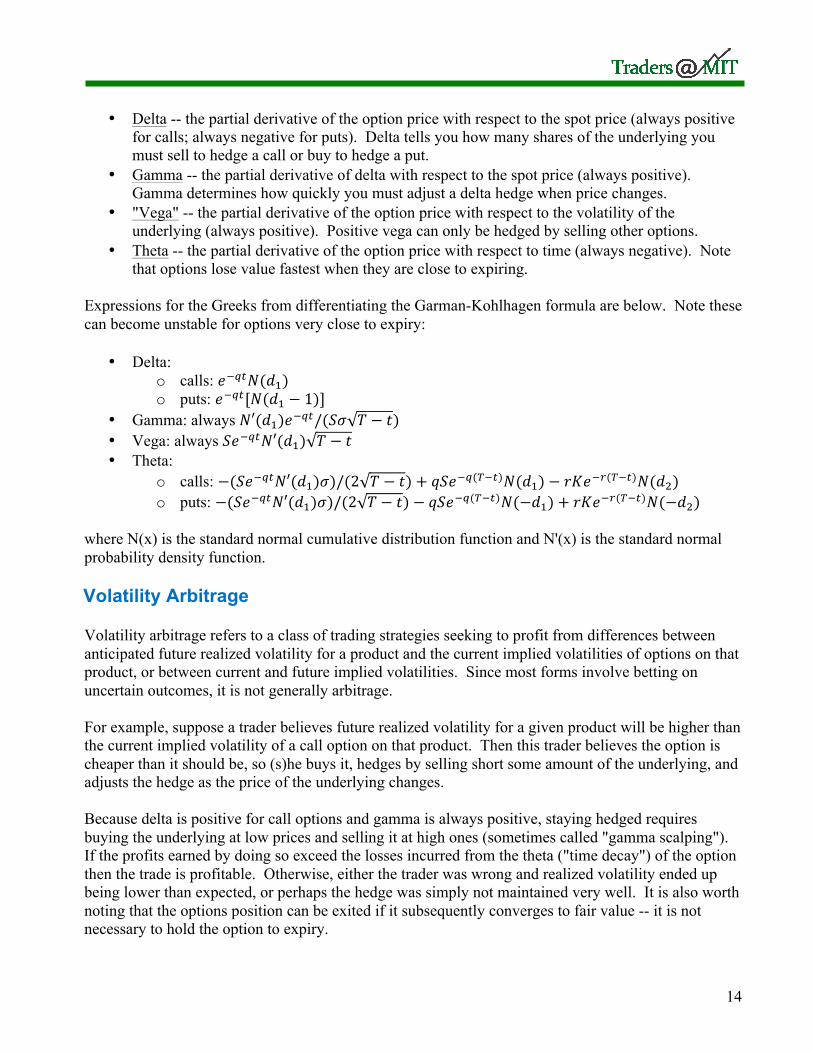
Expressions for the Greeks from differentiating the Garman-Kohlhagen formula are below. Note these can become unstable for options very close to expiry:

• Delta: o calls: 𝑒!!"𝑁(𝑑!) o puts: 𝑒!!"[𝑁(𝑑! − 1)]

• Gamma: always 𝑁′(𝑑!)𝑒!!"/(𝑆𝜎 𝑇 − 𝑡) • Vega: always 𝑆𝑒!!"𝑁′(𝑑!) 𝑇 − 𝑡 • Theta:

o calls: −(𝑆𝑒!!"𝑁′(𝑑!)𝜎)/(2 𝑇 − 𝑡)+ 𝑞𝑆𝑒!!(!!!)𝑁(𝑑!)− 𝑟𝐾𝑒!!(!!!)𝑁(𝑑!) o puts: −(𝑆𝑒!!"𝑁′(𝑑!)𝜎)/(2 𝑇 − 𝑡)− 𝑞𝑆𝑒!!(!!!)𝑁(−𝑑!)+ 𝑟𝐾𝑒!!(!!!)𝑁(−𝑑!)

where N(x) is the standard normal cumulative distribution function and N'(x) is the standard normal probability density function. Volatility Arbitrage

Volatility arbitrage refers to a class of trading strategies seeking to profit from differences between anticipated future realized volatility for a product and the current implied volatilities of options on that product, or between current and future implied volatilities. Since most forms involve betting on uncertain outcomes, it is not generally arbitrage. For example, suppose a trader believes future realized volatility for a given product will be higher than the current implied volatility of a call option on that product. Then this trader believes the option is cheaper than it should be, so (s)he buys it, hedges by selling short some amount of the underlying, and adjusts the hedge as the price of the underlying changes. Because delta is positive for call options and gamma is always positive, staying hedged requires buying the underlying at low prices and selling it at high ones (sometimes called "gamma scalping"). If the profits earned by doing so exceed the losses incurred from the theta ("time decay") of the option then the trade is profitable. Otherwise, either the trader was wrong and realized volatility ended up being lower than expected, or perhaps the hedge was simply not maintained very well. It is also worth noting that the options position can be exited if it subsequently converges to fair value -- it is not necessary to hold the option to expiry.

15

One of the most common types of volatility arbitrage is called volatility surface relative value trading, which is what you will be doing in this case. It involves attempting to earn profits by predicting changes in the shape of the volatility smile. For example, suppose based on fundamental news or excess demand/supply by market participants that you expect an increase in the curvature of the volatility smile. Then you could buy options far out on the curve, perhaps hedge some vega exposure by shorting options with strike prices closer to the current spot price ("at-the-money" options) if you have no view on the future overall level of volatility, and then hedge your delta exposure by holding a position in the underlying equal and opposite to the remaining delta of your options portfolio. This leaves you exposed only to changes in the curvature of the smile. Trading on anticipated changes in skew or broad shifts in volatility across the entire option chain are just special cases of this approach. Again: an upward shift along the entire volatility smile implies that realized volatility is expected to increase overall; i.e. the return distribution became wider. In contrast, a symmetrical increase in the curvature of the smile means that regardless of the average-case magnitude of returns there is now a higher anticipated probability of very negative and very positive events than previously; i.e. the tails became fatter. Pay careful attention to the implications of news releases. Case Information

The tradable instruments are options and futures on the T@MIT index, the latter solely for hedging. Both are cash-settled. Note the options underlier is the index, not the futures contract. There are four options in each round of the case: two puts and two calls. Options expire at the end of each round and their tickers are subsequently re-used. All tickers are as follows:

Strike Price Put Option Ticker

Call Option Ticker

$900 T900P $1000 T1000P T1000C $1100 T1100C

The ticker for the T@MIT index itself is "TMX". The index is viewable but not tradable. To successfully trade this case, you should make a pricing model to show the current volatility smile, your current portfolio Greeks, and any refinements or derived metrics that help you trade faster and better. This will allow you to quickly pursue opportunities in response to news releases and hedge your positions. For hedging, note the relationship between the price S of a dividend-paying asset and the price F for a forward or futures contract on that asset is given by:

𝐹 = 𝑆𝑒(!!!)(!!!)

Futures Tickers

Expires (end of):

TMM Each Period

16

There will be four 7.5-minute periods. Each period represents one month of trading. One team member will trade while the other monitors a pricing model and advises the trader. Team members will switch roles after each period. Trading activity by both partners during any given round is grounds for disqualification. Unlike the SEC, we have granular audit logs -- please don't make us use them. All tradable instruments expire at the end of each round. Each round begins with the T@MIT index at 1000. The continuously-compounded risk-free interest rate is 5% annualized. Trading Periods 4 Period Time 7.5 minutes (equivalent to 1 month) Compounding Interval 30 seconds (rate adjusted to equal the force of interest above) Trading Limits and Costs

The contract multiplier for options on the T@MIT index is 10. Options have a trading fee of $0.50 per contract per transaction. There is a gross trading limit of 1400 options contracts, and a net limit of 700 options contracts. Options that expire in-the-money pay out their intrinsic values. The contract multiplier for futures on the T@MIT index is 20. Futures have a trading fee of $1.00 per contract per transaction. There is a gross trading limit of 600 futures contracts, and a net limit of 300 futures contracts. All future contracts are cash-settled upon expiry. Trading Profits

All outstanding positions at the end of each period will be closed out by RIT. Winners will be determined by ranked P&L across the four rounds.

17

RIT - Electronic Trading: Equities Sales & Trader This case will be worth 25% of each team’s final score. Overview

During the Equities Sales and Trader case, teams will trade on four different stocks. Unlike the other cases, traders in this case may act as both proprietary traders and agency traders for institutional clients. The goal of an agency trader is to be a source of liquidity to clients. A successful agency trader must be cautious about which and how many orders to accept. Clients such as pension funds, mutual funds, and hedge funds may request to buy or sell a certain amount of a certain stock at a certain price at various times during the case. For example, you might get a request that says, “The Oregon Teachers Retirement fund wants to sell 10,000 shares of BRB to you at $30.10. Accept/Decline?” As an agency trader, you can earn money both from the spread between the price paid by the client and that at which you are able to execute, and a commission proportional to the dollar size of the order. At no point during the case do you have to accept an order from any client – you may always choose to prop trade. You will have 30 seconds to decide whether or not to accept an order. At the end of the 30 seconds, if you have not acted, the order will be declined by default. Should you wish to hold on to your positions from clients, you will be subject to market risk. If you wish to minimize this risk and profit purely from market making, you can offload your positions onto the market. However, most client orders will be sufficiently large that immediate execution would result in adverse market impact. You can reduce risk while offloading the position by hedging your exposure according to market and industry correlations. Each stock has a historical beta coefficient against the T@MIT Index, and an extremely liquid market in T@MIT Index futures is available against which positions obtained through institutional orders may be hedged. Stocks also have correlations across industry groups, which can be exploited depending upon liquidity. There will be four seven and half-minute periods. Each period represents three months of trading. One team member will trade while the other performs analysis. Team members will switch roles after each period. Case Information

During each period, your goal will be to maximize your P&L. Stocks may be positively or negatively correlated with each other, and the strength of these correlations varies. Additionally, in each of the four rounds, you will have an initial endowment of some number of shares. If those shares are tradable, you may sell them at any point during the 7.5-minute period. If your initial endowment is not tradable, you may either hedge your position with a long or short position in the T@MIT Index futures or a correlated stock, or accept the risk of holding on to the position without a hedge. There is a

18

maximum order size of 10,000 shares when submitting a single order. See the tables below for more information. During periods of high volatility, you may find it difficult to quickly hedge or offload positions you take on from institutional clients, so it may be more profitable to prop trade. During periods of lower volatility, it may be easier and more profitable to take on institutional orders. There will not be any market news in this case. Available Equities: Company name Industry Ticker Beta Finest School in the Country

Consumer/Retail MIT 0.3

League of Legends Consumer/Retail LOL 1 Bee-Rescue Brigade Media & TV BRB -0.7 Wind & Tomato Fund Energy/Commodities WTF 1.5

Period 1: Period 2: Ticker Initial Endowment

(shares) Tradable Ticker Endowment Tradable

MIT 500 Yes MIT None Yes LOL None Yes LOL None Yes BRB 500 Yes BRB 500 No WTF None No WTF None Yes

Period 3: Period 4: Ticker Initial Endowment

(shares) Tradable Ticker Endowment Tradable

MIT 1500 No MIT None No LOL None Yes LOL 500 Yes BRB None Yes BRB 500 No WTF 1000 Yes WTF None Yes

Starting Endowment $1,000,000 Trading Periods 4 Period Time 7.5 minutes (equivalent to 3 months) Risk-Free Rate 5% per year Compounding Interval 30 seconds

19

Margin Requirements and Trading Costs

A trading fee of $0.02 per share is charged on every stock transaction. All stocks are marginable. A margin loan of 50% of an equity’s value is given for long positions, and margin collateral of 150% of an equity’s value is required for short positions. The index value will start between $300 and $400, and the futures contract multiplier is 20. A trading fee of $2 per contract will be charged for every futures transaction. Initial margin of $5000 per contract is required to open a long or short position in the futures. The maximum order size is 50 contracts. There is no maintenance margin, so margin calls will not be issued, but negative cash balances will be treated as loans and will accrue interest at the risk-free rate. As always, margin balances are deducted from your buying power, and you must have sufficient buying power to enter into any margined position. Trading Profits

All outstanding positions at the end of each period will be closed out by RIT at a randomly chosen price, which occurred in the last 60 seconds. We suggest that you close out all positions prior to the end of the round in order to avoid liquidation at a loss. You will be ranked according to overall P&L.

20

RIT - Electronic Trading: Price Discovery Case This case will be worth 25% of each team’s final score. Introduction

Traffic Emulsifiers (TRA), Dynamic Extraterrestrial Response (DER), Synchronous Alchemy (SA), Timber Machinations (TM), and International Turbines (IT) have just issued earnings reports for the most recent quarter. According to various analysts, the target price of TRA for the next quarter is between $20 and $40 per share, the target price for DER is between $10 and $20 per share, the target price for SA is between $60 and $90 per share, the target price for TM is between $30 and $70 per share, and the target price for IT is between $50 and $80 per share. The true price of each stock is randomly drawn from a uniform distribution but will not be revealed until the end of the period. The period will begin with the stock prices equal to their expected values. There are four 10-minute periods. One team member will trade while the other performs analysis. Team members will switch roles after each period. When a number of traders hold potentially different information or views on a particular security, the markets provide a mechanism for price discovery. In this case, traders can take price estimates they receive from research analysts and prices quoted by other traders in the open market to deduce the true value of each stock. Tradable Securities, Endowments, and Interest Rates

There are 6 securities in this case: Traffic Emulsifiers (TRA), Dynamic Extraterrestrial Response (DER), Synchronous Alchemy (SA), Timber Machinations (TM) and International Turbines (IT), and the Dubious Industrial Average Exchange Traded Fund (DIA). The true value of DIA should be the sum of the prices of TRA, DER, SA, TM, and IT. Traders begin the case with an endowment of $1,000,000 dollars and can buy (“go long”) and short-sell (“go short”) all securities. There is a maximum order size of 10,000 shares when submitting a single order. Each period represents one quarter of the year. The risk free rate is 0%, so there is no interest paid on cash balances. Information

During each period, each trader will receive 6 private news items for each stock (each news item will consist of a price estimate of each stock, and all three stock estimates will be given at the same time). These news items will provide him or her with an estimate of the final price of the stock. Each estimate is a sample  𝐸! from a multivariate normal distribution with mean 𝑃! and standard deviation  𝜎! 𝑡 =   !""!!

!" (t is the number of seconds that have elapsed since the beginning of the

21

trading period, 𝑃! is the final price of the stock at close). The correlation coefficients for the multivariate normal are

𝜌!"#,!"# -0.54585 𝜌!"#,!" -0.22928 𝜌!"#,!" +0.40733 𝜌!"#,!" -0.14563 𝜌!"#,!" +0.22727 𝜌!"#,!" -0.74261 𝜌!"#,!" -0.06071 𝜌!",!" +0.01909 𝜌!",!" -0.08560 𝜌!",!" +0.04993

It is important to note that each sample comes from a multivariate normal distribution. Because 𝑡 is constantly increasing, the standard deviation of each distribution decreases as the end of the period nears. In other words, the expected accuracy of the estimates improves and traders’ uncertainty decreases as time goes on. Notice that it is possible for the estimate to be outside of the target range. Margin Requirements and Trading Costs

A trading fee of 2 cents per stock and ETF is charged on every buy and sell transaction. All securities are marginable. A margin loan of 50% of a security’s value is given for long positions, and margin collateral of 150% of a security’s value is required for short positions. Position Close-Out Any non-zero position in a security will be closed-out at the end of trading using the actual price.

22

RIT - Electronic Trading: Commodities Case The Commodities case will be worth 15% of each team’s final score. Introduction You are a commodities trader in Cambridge, MA, specializing in crude oil futures – namely the West Massachusetts Intermediate (WMI). In this case, you will analyze news releases affecting the supply & demand of crude oil. In response, you will buy and sell futures contracts for different delivery months of crude oil. You earn profits by correctly forecasting the future values. Crack Spread Crude oil is a raw material. When refined, it yields two main products: gasoline and heating oil. This oil-refining process is known as “cracking.” For simplicity, we will classify the two by-products as gas and oil. Crude oil will be referred to as crude. While not directly tradable, you are able to see the spot prices of gas and oil. In this case, we will assume the 3-2-1 spread: three barrels of crude produce two barrels of gasoline and one barrel of oil. Therefore, we should expect the price relationship to be:

3PCrude = 2PGas + POil . Of course, there are various dynamics in the market that result in slight deviations in the prices of the three products. Some factors include: presence of contango or backwardation, relative supply and demand of the by-products, and refining costs. The term crack spread refers to the absolute difference in price between the left and right sides of the above equation. As a simple example, if crude oil future is trading at $4/barrel, gas at $4/barrel, and oil at $5/barrel, then the crack spread is $1/barrel. Case Details Tradable Securities, Endowments and Interest Rates There are 3 tradable futures contracts in this case. Each futures contract represents 1,000 barrels of crude oil settled/delivered at the end of December, January, or February. All contracts will be marked to market every 30 seconds based on the last traded price. Contracts will settle at the end of their respective months based on the calculated market price (explained in the Market Dynamics section). There is a maximum order size of 25 futures contracts in a single order.

Trading  Periods   3  Period  Time   600  Seconds  (10  minutes)  

Calendar  Time  Per  Period   1  Month  Compounding  Interval   1  Day  (30  seconds)  

23

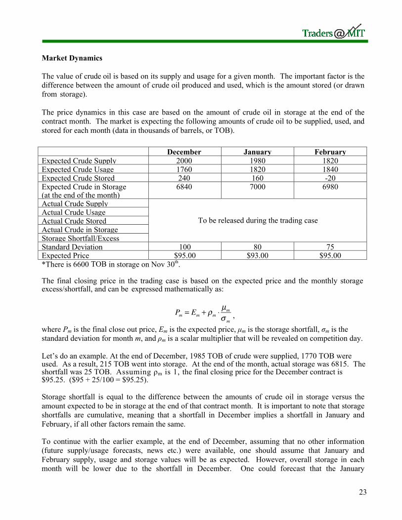
Market Dynamics The value of crude oil is based on its supply and usage for a given month. The important factor is the difference between the amount of crude oil produced and used, which is the amount stored (or drawn from storage). The price dynamics in this case are based on the amount of crude oil in storage at the end of the contract month. The market is expecting the following amounts of crude oil to be supplied, used, and stored for each month (data in thousands of barrels, or TOB). December January February Expected Crude Supply 2000 1980 1820 Expected Crude Usage 1760 1820 1840 Expected Crude Stored 240 160 -20 Expected Crude in Storage (at the end of the month)

6840 7000 6980

Actual Crude Supply

To be released during the trading case Actual Crude Usage Actual Crude Stored Actual Crude in Storage Storage Shortfall/Excess Standard Deviation 100 80 75 Expected Price $95.00 $93.00 $95.00 *There is 6600 TOB in storage on Nov 30th. The final closing price in the trading case is based on the expected price and the monthly storage excess/shortfall, and can be expressed mathematically as:

Pm = Em + ρm ⋅µm

σ m,

where Pm is the final close out price, Em is the expected price, µm is the storage shortfall, σm is the standard deviation for month m, and ρm is a scalar multiplier that will be revealed on competition day. Let’s do an example. At the end of December, 1985 TOB of crude were supplied, 1770 TOB were used. As a result, 215 TOB went into storage. At the end of the month, actual storage was 6815. The shortfall was 25 TOB. Assuming ρm is 1, the final closing price for the December contract is $95.25. ($95 + 25/100 = $95.25). Storage shortfall is equal to the difference between the amounts of crude oil in storage versus the amount expected to be in storage at the end of that contract month. It is important to note that storage shortfalls are cumulative, meaning that a shortfall in December implies a shortfall in January and February, if all other factors remain the same. To continue with the earlier example, at the end of December, assuming that no other information (future supply/usage forecasts, news etc.) were available, one should assume that January and February supply, usage and storage values will be as expected. However, overall storage in each month will be lower due to the shortfall in December. One could forecast that the January

24

contract’s closing price will be $93.31 ($93.00 + 25/80), and February’s closing price will be $95.33 ($95.00 + 25/75). Trading the Crack Spread Throughout the period, you will also have access to the spot prices of the two by-products of crude: gasoline and heating oil. You can assume that the relation equation defined in the introduction holds, and that the crack spread remains constant unless there are external factors driving the spread. Traders will be periodically given information which allows them to model future crude oil data so that they can forecast future prices. Information Release Schedule There are two types of periodic information releases provided to traders: weekly US Energy Information Administration (EIA) data, and news events. The news events give insights into the price of gas, price of oil and the crack spread to help traders tune their model. Each month the news is released according to the following schedule:

Sample Releases: Weekly EIA Report Wk #1 December Energy Information Administration Weekly Supply Data : 500 TOB Energy Information Administration Weekly Usage Data : 444 TOB News A small gasoline pipeline exploded today, injuring two workers. Officials have not released an estimate as to when the pipeline will be back up. Gasoline prices rise relative to heating oil, and the crack spread remains unchanged.

Release Release Time (Seconds)

Elapsed) 1st Week EIA Data 120 2nd Week EIA Data 270 3rd Week EIA Data 420 4th Week EIA Data 570 Random News Events Random

25

Liquidity Traders Orders are constantly submitted to the market by computerized agents. These orders are displayed in the limit order book under the name ANON. Liquidity traders submit both market and limit orders and represent both noise (uninformed) flow, and informed flow. At times liquidity trades will drive the market towards its true value while other times it will drive it away from its true value. Margin Requirements and Position Limits A trading fee of $5 dollars per futures contract is charged for every transaction. Your maximum position is limited to 500 net, or 1000 gross. Settlement and Position Close-Out Futures positions that remain open at the end of the period will be marked-to-market at the last traded price. If the end of the period is also the expiration of the contract, the contract will be marked to market at the final fair value (calculated based on the crude storage shortfall/excess). Case Notes and Clarification

- There is no intra-month seasonality, that is, if the month’s expected supply is 2000 TOB, you can assume that means that 500 TOB is supplied per week, in expectation.

- Assume that the spot market for gas and oil react faster that the futures market for crude. - Although not explicitly given, keep in mind the interest rates and cost of carry, as they might

help with your pricing models