CASE STUDY: Global Warming – the forest from the trees APPENDIX 8: Thiessen polygons An imposing name, but the method of Thiessen polygons is a straightforward, objective, replicable procedure to “determine the area of influence of a point in a set of points”. If you have a set of irregularly distributed points within a bounded region, using this procedure you can divide up the region into a set of polygons each containing just one of the points such that “the area contained in each polygon is closer to the point on which the polygon is based than to any other point in the dataset” (BBC, 2009). The Thiessen polygon procedure has a wide variety of applications but here we will use it to show how the average temperature anomaly of a bounded region can be estimated from the temperature anomalies at any number of irregularly distributed weather stations within it. Though the procedure here is done by hand and subject to rounding-off errors, there are computer programs available that can do the calculations with precision. The procedure set out below describes how to determine the average annual temperature anomalies for the States of Victoria, NSW and Queensland based on the data sets from 12 rural meteorological stations. It demonstrates that the method of Thiessen Polygons produces a robust time series of annual temperature anomalies for the three states. 1. Plot the labelled position of each Met Station on a scale map of the region(s) for which you wish to calculate the temperatu re average. 2. Connect each Met Station to its nearest neighbour by drawing straight lines between the stations to produce a so-called triangulat ed irregular network (TIN).

Welcome message from author
This document is posted to help you gain knowledge. Please leave a comment to let me know what you think about it! Share it to your friends and learn new things together.
Transcript
CASE STUDY: Global Warming – the forest from the trees
APPENDIX 8: Thiessen polygons
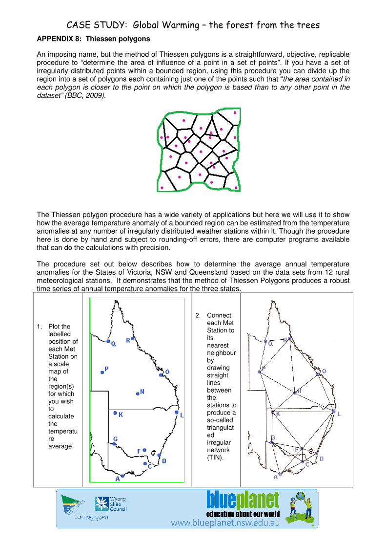
An imposing name, but the method of Thiessen polygons is a straightforward, objective, replicable procedure to “determine the area of influence of a point in a set of points”. If you have a set of irregularly distributed points within a bounded region, using this procedure you can divide up the region into a set of polygons each containing just one of the points such that “the area contained in each polygon is closer to the point on which the polygon is based than to any other point in the dataset” (BBC, 2009).
The Thiessen polygon procedure has a wide variety of applications but here we will use it to show how the average temperature anomaly of a bounded region can be estimated from the temperature anomalies at any number of irregularly distributed weather stations within it. Though the procedure here is done by hand and subject to rounding-off errors, there are computer programs available that can do the calculations with precision. The procedure set out below describes how to determine the average annual temperature anomalies for the States of Victoria, NSW and Queensland based on the data sets from 12 rural meteorological stations. It demonstrates that the method of Thiessen Polygons produces a robust time series of annual temperature anomalies for the three states.
1. Plot the labelled position of each Met Station on a scale map of the region(s) for which you wish to calculate the temperature average.
2. Connect each Met Station to its nearest neighbour by drawing straight lines between the stations to produce a so-called triangulated irregular network (TIN).

CASE STUDY: Global Warming – the forest from the trees
3. Bisect
each connecting line with a perpendicular. One way to do this is with a compass set to produce arcs centred on a station and with radii equal to the distances to the nearest neighbouring stations. The points of intersection of pairs of arcs define the perpendicular bisectors.
4. These perpendicular bisectors meet to form a set of closed polygons (the set of ‘Thiessen Polygons’) each containing only one Met Station; this Met Station is the closest station to any particular point within that polygon.
5. Calculate the relative areas of the polygons. There are a variety of techniques to do this, but a simple one is to print the map with its polygons onto fine grid paper and then to count the number of grid squares within each polygon (making sure to include an estimate of
6. Calculate the fraction of area that each Met Station’s polygon contributes to the area of the State. This fraction is the weighting factor that will be used to determine the contribution that each Met Station’s
STATE Met Station
Relative Land Area
Fraction of the State
A 48 0.353 C 47 0.346 F 2 0.015 G 39 0.287
VIC
TOTAL 136 1.000 C 5 0.011 D 46 0.102 F 134 0.296 G 71 0.157 K 79 0.174 L 88 0.194 N 30 0.066
NSW
TOTAL 453 1.000
K 43 0.053 L 36 0.045 N 182 0.226 O 122 0.152 P 178 0.221 Q 124 0.154 R 120 0.149
QLD
TOTAL 805 1.000

CASE STUDY: Global Warming – the forest from the trees
the number of squares that equate to the portions of fractured grids within the polygon boundaries) .
recorded temperature anomaly will make to the average temperature anomaly for each state.
7. Now, for any particular year of interest (e.g. 2008), multiply the annual temperature anomaly for each Met Station by its appropriate weighting factor. (The same weighting factor can be used for every year so long as the position of each Met Station remains unchanged over those years.)
We illustrate this here for the particular case of the calculation of the mean temperature anomaly for the State of Queensland in the year 2008.
Met Station
Weight (i.e. fraction of the State included in the Station’s Polygon)
Annual Mean
Temperature Anomaly at
the Met Station in
2008 (
0C )
Weight X
Anomaly (
0C)
K. 0.053 0.8 0.04
L 0.045 0.2 0.01
N 0.226 -0.4 -0.09 O 0.152 0.2 0.03
P 0.221 1.1 0.24
Q. 0.154 0.2 0.03
R 0.149 0.6 0.09
TOTAL 1.000 --- 0.35
8. The sum of these calculations represents the average temperature anomaly for the state of Queensland in 2008
Our estimated temperature anomaly for Queensland in 2008 is +0.35
0C, a
fairly unimpressive number, considering it represents thousands of hours of daily meteorological measurements and data processing from 7 met station across North Eastern Australia. Incidentally ,the Bureau of Meteorological ,using their gridded weighting methodology applied to at least 28 stations’ records, estimated this anomaly to be +0.17
0C (exactly
half our estimate) which when added to the Mean Temperature for 1961-1990 represents an average temperature for Queensland in 2008 of 22.40
0C.
Related Documents


