Case Studies V 2 on Women's Employment and Pay in Latin America EDITED BY .GEORGE PSACHAROPOULOS AND ZAFIRIS TZANNATOS Re :,'S EMPLUB) AL Public Disclosure Authorized Public Disclosure Authorized Public Disclosure Authorized Public Disclosure Authorized

Welcome message from author
This document is posted to help you gain knowledge. Please leave a comment to let me know what you think about it! Share it to your friends and learn new things together.
Transcript
Case Studies V 2
on Women's
Employment and
Pay in Latin America
EDITED BY
.GEORGE
PSACHAROPOULOS
AND
ZAFIRIS
TZANNATOS Re :,'S EMPLUB)
AL
Pub
lic D
iscl
osur
e A
utho
rized
Pub
lic D
iscl
osur
e A
utho
rized
Pub
lic D
iscl
osur
e A
utho
rized
Pub
lic D
iscl
osur
e A
utho
rized

Case Studies
on Women's
Employment and
Pay in Latin America

Case Studies
on Women's
Employment and
Pay in Latin America
EDITED BY
GEORGE PSACHAROPOULOS
AND
ZAFIRIS TZANNATOS
The World BankWaskington, D.C.
O 1992 The International Bank for Reconstructionand Development / The World Bank1818 H Street, N.W., Washington, D.C. 20433
All rights reservedManufactured in the United States of AmericaFirst printing November 1992
This volume is a companion to the World Bank Regional and Sectoral Study Women's Empley mt and Payin Latin Ametica: Overview and Metbodolojy. The World Bank Regional and Sectoral Studies series providesan outlet for work that is relatively limited in its subject matter or geographical coverage but that contributesto the intellectual foundations of development operations and policy formulation. These studies have notnecessarily been edited with the same rigor as Bank publications that carry the imprint of a university press.
The findings, interpretations, and condusions expressed in this publication are those of the authors and shouldnot be attributed in any manner to the World Bank, to its affiliated organizations, or to the members of itsBoard of Executive Directors or the countries they represent.
The material in this publication is copyrighted. Requests for permission to reproduce portions of it shouldbe sent to the Office of the Publisher at the address shown in the copyright notice above. The World Bankencourages dissemination of its work and will normally give permission promptly and, when the reproductionis for noncommercial purposes, without asking a fee. Permission to copy portions for classroom use is grantedthrough the Copyright Clearance Center, 27 Congress Street, Salem, Massachusetts 01970, U.S A.
The complete backdist of publications from the World Bank is shown in the annual Index of Publications,which contains an alphabetical tide list and indexes of subjects, authors, and countries and regions. The latestedition is available free of charge from Distribution Unit, Office of the Publisher, The World Bank, 1818 HStreet, N.W., Washington, D.C. 20433, U.S.A., or from Publications, The World Bank, 66, avenue d'Iena,75116 Paris, France.
George Psacharopoulos is the senior human resources adviser to the World Bank's Latin America andCaribbean Technical Department. He previously taught at the London School of Economics. Zafiris Tzannatosis a labor economist with the Population and Human Resources Department at the World Bank. He is anhonorary rcesarch fellow at the Universities of Nottingham and St. Andrews in the United Kingdom.
Cover desagn by Sam Ferro
Library of Co ngws Catakgis - in-Publication Data
Case studies on women's employment and pay in Latin America / editedby George Psacharopoulos and Zafiris Tzannatos.
p. cm.Includes bibliographical references.ISBN 0-8213-2308-31. Women-Employment-Latin America-Case studies. 2. Wages-
Latin America-Case studies. 3. Discrimination in employment-Latin America-Case studies. 4. Sex discrimination against women-Latin America-Case studies. I. Psacharopoulos, George.II. Tzannatos, Zafiris, 1953.HD6100.5.C37 19923311.4'098-dc2O 92-40880
CIP
Contents
Acknowledgments viiForeword ix
1 Female Labor Force Participation andGender Earnings Differentials in Argentina 1
by Y. C. Ng
2 Women in the Labor Force In Bolivia:Participation and Earnings 21
by K. Scott
3 Labor Force Behavior and Earnings of BrazilianWomen and Men, 1980 39
by M. Stelener, J. B. Smith, J. A. Breslawand G. Monette
4 Female Labor Force Participation and WageDetermination in Brazil, 1989 89
by J. Tiefenthaler
5 Is There Sex Discrimination in Chile?Evidence from the CASEN Survey 119
by I. Gill
6 Labor Markets, the Wage Gap and GenderDiscrimination: The Case of Colombia 149
by J. Tenjo
7 Female Labor Market Participation andWages in Colombia 169
by T. Magnac
8 Women's Labor Force Participation andEarnings in Colombia 197
by E. Velez and C. Winter
v
n Women's Employment and Pay in Latin America
9 Female Labor Force Participation and EarningsDifferentials in Costa Rica 209
by H. Yang
10 Why Women Earn Less Than Men in Costa Ricaby T. H. Gindling 223
11 The Effect of Education on Female Labor ForceParticipation and Earnings in Ecuador 255
by G. Jakubson and G. Psacharopoulos
12 Female Labor Force Participation and Earnings in Guatemala 273by M. Arends
13 Women's Labor Force Participation and Earnings inHonduras 299
by C. Winter and T. H. Gindling
14 Female Labor Force Participation and Earnings:The Case of Jamaica 323
by K. Scott
15 Women's Participation Decisions and Earnings in Mexico 339by D. Steele
16 Female Labor Force Participation and Wages:A Case Study of Panama 349
by M. Arends
17 Women's Labor Market Participation and Male-FemaleWage Differences in Peru 373
by S. Khandker
18 Is There Sex Discrimination in Peru? Evidence from the1990 Lima Living Standards Survey 397
by I. Gill
19 Women's Labor Force Participation and Earnings:The Case of Uruguay 431
by M. Arends
20 Female Participation and Earnings, Venezuela 1987 451by D. Cox and G. Psacharopoulos
21 Female Earnings, Labor Force Participation andDiscrimination in Venezuela, 1989 463
by C. Winter
Appendix A: Contents of Companion Volume 477Appendix B: Authors of Country Case Studies 479
Acknowledgments
We have benefited from comments and encouragement from many people who read earlierversions of this study and participated in seminars given at the World Bank, the University of St.Andrews, and conferences organized by the Comparative and International Education Society,the International Union for the Scientific Study of Population, and the European Society forPopulation Economics. In particular we would like to thank Ana-Marfa Arriagada, AlessandroCigno, Deborah DeGraff, Barbara Herz, David Huggart, Emmanuel Jimenez, Philip Musgrove,and Michelle Riboud for their helpful comments, Professor William Greene for providing purposebuilt routines for LIMDEP which facilitated the estimation procedures used in the country studies;Diane Steele and Carolyn Winter for their reviews of the book; Hongyu Yang for preparing thegraphics; and Donna Hannah for typing and preparing the earlier versions of this book and MartaOspina for taking these tasks over and eventually putting the book into its present form. Thecompletion of the present study would have not been possible without the generous support ofthe Norwegian Trust Fund.
vii

Foreword
Women's role in economic development can be examined from many different perspectives,including the feminist, anthropological, sociological, economic and legislative. This studyemploys an economic perspective and focuses on how women behave and are treated in the workforce in a number of Latin American economies. It specifically considers the determinants ofwomen's labor force participation and male-to-female earnings differentials. Understanding thereasons for "low" labor market participation rates among women, or "high" wage discriminationagainst women, can lead to policies that will improve the efficiency and equity with which humanresources are utilized in a particular country.
The study is in two volumes. The companion volume presents aggregate data on the evolutionof female labor force participation in Latin America over time, showing that in some countriestwice as many women (of comparable age groups) work in the market relative to twenty yearsago. This volume uses household survey data to analyze labor force participation rates and wagesearned by men and women in similar positions, paying special attention to the role of educationas a factor influencing women's decision to work. The results show that, overall, the more yearsof schooling a woman has, the more likely she is to participate in the labor force. In addition,more educated women earn significantly more than less educated women. The book also attemptsanalyses of the common factors which determine salaries paid to men and women in an effort toidentify what part of the male/female earnings differential can be attributed to different humancapital endowments between the sexes, and what part is due to unexplained factors such asdiscrimination. Differences in human capital endowments explain only a small proportion of thewage differential in most of the country studies. The remaining proportion thus represents theupper bound to discrimination.
It is our hope that this work will be followed up by a more careful look at labor legislation andthe role it plays in preventing women from reaching their full productive potential.
S. Shahid HusainVice President
Latin America and the Caribbean RegionThe World Bank
ix

Female Labor Force Participation andGender Earnings Differentials in Argentina
Ying Chu Ng
1. Introduction
In this study we estimate earnings functions for Argentinian males and females using the 1985Buenos Aires Household Survey data. Our purpose is two-fold. First, we seek to investigate theincome differentials between male and female workers. Second, we examine the existence ofearnings discrimination by gender. In the following section we provide a brief overview of theArgentine economy and the operation of the labor market. In the third section we discuss thedata base used in the analysis and present the main characteristics of male and female labor forceparticipants. Female labor force participation and the factors influencing women's decision toparticipate are discussed in Section 4. In Section 5 we present the results from earnings functionsestimates for male and female workers, and Section 6 provides an analysis and discussion of theextent to which male/female earnings differentials can be attributed to differences in humancapital endowments and to discriminatory practices by employers in the labor market. The paperconcludes with a discussion of these findings in Section 7.
2. The Argentine Economy and Labor Market
Since the 1940s political events in Argentina have had a considerable impact on the functioningof the economy, the structure of the labor market, and the earnings structure of workers.Government policies favoring import-substitution and the introduction of a wage settingmechanism meant that the growth of relative wages from the 1940s to the 1980s was highest innon-tradable activities. This, plus the fact that wage determination was increasingly influencedby collective bargaining, has led to a concentration of resources, including human resources, inurban areas. More than 30 percent (in 1987) of the total population was concentrated in thecapital, Buenos Aires.
In general, labor force participation rates in the urban markets in Argentina are above 40 percentof the resident population (Sanchez, 1987). However, the Argentine labor market is characterizedby cyclical periods in which labor is either scarce or relatively abundant. Two factors explainthis. First, there are substantial fluctuations in terms of domestic and foreign migration. Second,the fact that unemployment and underemployment rates remain relatively low regardless ofwhether there is an excess or scarcity of labor suggests that there may be a strong "addedworker" effect operating. Riveros and Sanchez (1990) provide evidence that this is the case.They report that the "added worker' effect resulted in substantial increases in female labor force
I
2 Women's Employment and Pay in Latin America
participation rates, particularly among women aged 35 to 49 years, during the economic crisisof the early 1980s.
In Argentina there is not only a higher labor force participation rate relative to other LatinAmerican countries, but workers also tend to work longer hours. Dieguez (n.d.) reported thatamong 3.9 million employed individuals in May 1985, 37.6 percent worked between 35 and 45hours weekly, and 31.4 percent worked over 45 hours per week, while only 17.5 percent workedless than 35 hours per week.
Female workers. Among female workers de Lattes (1983) found that in both 1960 and 1970there was a higher participation rate among single and divorced women aged between 25 and 59years than among married women of the same age. Wainerman (1979) and de Lattes (1983) foundsimilar results: The probability of single female participation in the work force was at least threetimes that of married females. Education is an important variable determining femaleparticipation rates. Wainerman (1979) found that more educated women were more likely toparticipate in the labor force. Data collected from the Instituto Nacional de Estadistica y Censos(n.d.) showed that in Buenos Aires in 1970 the proportion of working females with less thanprimary education was substantially lower than women with higher educational attainment.Women with secondary or university education made up the largest portion of the female workforce (de Lattes, 1983).
Female migrants constitute an important proportion of the female labor force in urban areas(Marshall, 1977; de Lattes, 1983) and especially in Buenos Aires.
Female workers are concentrated in non-agricultural activities. More than 65 percent of workersin the non-tradable sector were females in the 1960s, and this figure increased to 79 percent ofworkers in 1980.
3. Data Characteristics
The data used in this study are drawn from the 1985 Buenos Aires Household Survey which wasundertaken by the National Institute of Statistics (NDEC) and surveyed 15,580 individuals.Though the survey covers only Buenos Aires, it represents more than 30 percent of the totalpopulation of the country. In the present study, we extract females (working and non-working)and working males aged 15 to 65, resulting in a sample of 7,097 individuals.
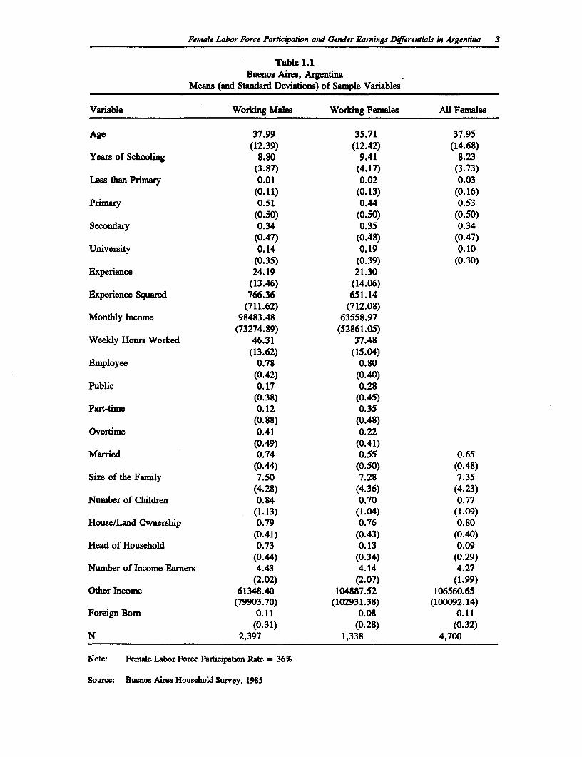
The descriptive statistics and the definitions of the main variables are presented in Table 1.1.The female participation rate is 36 percent. The average education level of the sample is nearly9 years of schooling for both sexes. Working females average over 9 years of schooling but haveless work experience than males. The overall sample characteristics are very similar for bothmales and females. A very large portion of the working population is employed in the dependentemployment sector - 80 percent of females and 78 percent of males. Females work fewer hoursthan males on average and the number of part-time female workers is about twice that of part-time males. The average earnings of females is about 64.5 percent that of males, and otherincome (defined as the difference between family income and the respondent's labor income) is1.75 times as much for females as it is for males.
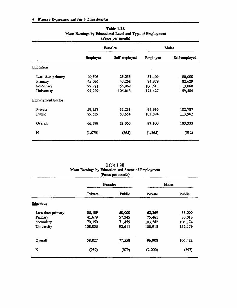
In order to have a closer look at the earning differentials, information on earnings amongdifferent employment sectors and employment types by educational level is presented in Tables1.2A and 1.2B. Regardless of the differences in sector and employment type, the higher the
Femake Labor Force Participation and Gender Earnings Differentials in Argentina 3
Table 1.1Buenos Aires, Argentina
Means (and Standard Deviations) of Sample Variables
Variable Working Males Working Females All Females
Age 37.99 35.71 37.95(12.39) (12.42) (14.68)
Years of Schooling 8.80 9.41 8.23(3.87) (4.17) (3.73)
Less than Primary 0.01 0.02 0.03(0.11) (0.13) (0.16)
Primary 0.51 0.44 0.53(0.50) (0.50) (0.50)
Secondary 0.34 0.35 0.34(0.47) (0.48) (0.47)
University 0.14 0.19 0.10(0.35) (0.39) (0.30)
Experience 24.19 21.30(13.46) (14.06)
Experience Squared 766.36 651.14(711.62) (712.08)
Monthly Income 98483.48 63558.97(73274.89) (52861.05)
Weekly Hours Worked 46.31 37.48(13.62) (15.04)
Employee 0.78 0.80(0.42) (0.40)
Public 0.17 0.28(0.38) (0.45)
Part-time 0.12 0.35(0.88) (0.48)
Overtime 0.41 0.22(0.49) (0.41)
Married 0.74 0.55 0.65(0.44) (0.50) (0.48)
Size of the Family 7.50 7.28 7.35(4.28) (4.36) (4.23)
Number of Children 0.84 0.70 0.77(1.13) (1.04) (1.09)
House/Land Ownership 0.79 0.76 0.80(0.41) (0.43) (0.40)
Head of Household 0.73 0.13 0.09(0.44) (0.34) (0.29)
Number of Income Earners 4.43 4.14 4.27(2.02) (2.07) (1.99)
Other Income 61348.40 104887.52 106560.65(79903.70) (102931.38) (100092.14)
Foreign Bom 0.11 0.08 0.11(0.31) (0.28) (0.32)
N 2,397 1,338 4,700
Note: Female Labor Force Participation Rate = 36%
Source: Buenos Aires Household Survey, 1985
4 Women's Employment and Pay in Latin America
Table 1.2AMean Earnings by Educational Level and Type of Employment
(Pesos per month)
Females Males
Employee Self-employed Employee Self-employed
Education
Less than primary 40,506 25,233 51,409 80,000Primary 45,026 40,268 74,379 82,629Secondary 72,721 56,969 100,513 113,068University 97,229 106,813 174,427 159,484
Emplovment Sector
Private 59,957 52,231 94,916 102,787Public 79,539 50,654 105,894 113,962
Overall 66,399 52,060 97,100 103,333
N (1,073) (265) (1,865) (532)
Table 1.2BMean Earnings by Education and Sector of Employment
(Peso per month)
Females Males
Private Public Private Public
Education
Less than primary 36,109 50,000 62,269 38,000Primary 41,679 57,345 75,461 80,018Secondary 70,150 71,459 103,282 106,174University 108,056 92,611 180,918 152,179
Overall 58,027 77,558 96,908 106,422
N (959) (379) (2,000) (397)
Female Labor Force Parnicwpaion and Gender Earnings D&fferenials in Argenina 5
education level the more the individual earns. Males earn about 50 percent more than femaleswith the same education, except where employees have less than primary education or where theyare self-employed with less than primary education.
Within employment type, different patterns are seen for males and females. Self-employed malesearn more than wage employees at all levels except males with university education. The exactopposite pattern is seen for females: Employees earn more than the self-employed at all levelsexcept females with university education. There is no clear pattern for male earnings by publicand private sector. However, female workers in the public sector earn more than those in theprivate sector for all education levels except for university education.
From the sample statistics, there is obviously a wage gap between males and females. Ineconomic theory, wage differentials come from two broad sources: (1) differences in "skill'(attributes) and (2) differences in 'treatment' (wage structure), i.e., from discrimination byemployers. The upper bound of this discrimination can be computed by using the Oaxaca (1973)decomposition technique. This requires estimating earnings functions for females and males.
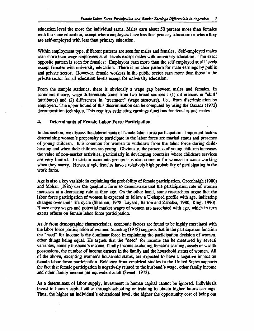
4. Determinants of Female Labor Force Participation
In this section, we discuss the determinants of female labor force participation. Important factorsdetermining women's propensity to participate in the labor force are marital status and presenceof young children. It is common for women to withdraw from the labor force during child-bearing and when their children are young. Obviously, the presence of young children increasesthe value of non-market activities, particularly in developing countries where childcare servicesare very limited. In certain economic groups it is also common for women to cease workingwhen they marry. Hence, single females have a relatively high probability of participating in thework force.
Age is also a key variable in explaining the probability of female participation. Greenhalgh (1980)and Mohan (1985) use the quadratic form to demonstrate that the participation rate of womenincreases at a decreasing rate as they age. On the other hand, some researchers argue that thelabor force participation of women is expected to follow a U-shaped profile with age, indicatingchanges over their life cycle (Sheehan, 1978; Layard, Barton and Zabalza, 1980; King, 1990).Hence entry wages and potential market wages of women are associated with age, which in turnexerts effects on female labor force participation.
Aside from demographic characteristics, economic factors are found to be highly correlated withthe labor force participation of women. Standing (1978) suggests that in the participation functionthe "need" for income is the dominant force in explaining the participation decision of women,other things being equal. He argues that the "need" for income can be measured by severalvariables, namely husband's income, family income excluding female's earning, assets or wealthpossessions, the number of income earners in the family and the household status of women. Allof the above, excepting women's household status, are expected to have a negative impact onfemale labor force participation. Evidence from empirical studies in the United States supportsthe fact that female participation is negatively related to the husband's wage, other family incomeand other family income per equivalent adult (Sweet, 1973).
As a determinant of labor supply, investment in human capital cannot be ignored. Individualsinvest in human capital either through schooling or training to obtain higher future earnings.Thus, the higher an individual's educational level, the higher the opportunity cost of being out
6 Women's Employment and Pay in Latin America
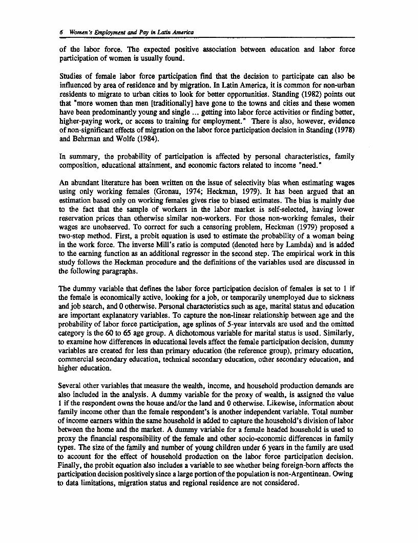
of the labor force. The expected positive association between education and labor forceparticipation of women is usually found.
Studies of female labor force participation find that the decision to participate can also beinfluenced by area of residence and by migration. In Latin America, it is common for non-urbanresidents to migrate to urban cities to look for better opportunities. Standing (1982) points outthat "more women than men [traditionally] have gone to the towns and cities and these womenhave been predominantly young and single ... getting into labor force activities or finding better,higher-paying work, or access to training for employment." There is also, however, evidenceof non-significant effects of migration on the labor force participation decision in Standing (1978)and Behrman and Wolfe (1984).
In summary, the probability of participation is affected by personal characteristics, familycomposition, educational attainment, and economic factors related to income "need."
An abundant literature has been written on the issue of selectivity bias when estimating wagesusing only working females (Gronau, 1974; Heckman, 1979). It has been argued that anestimation based only on working females gives rise to biased estimates. The bias is mainly dueto the fact that the sample of workers in the labor market is self-selected, having lowerreservation prices than otherwise similar non-workers. For those non-working females, theirwages are unobserved. To correct for such a censoring problem, Heckman (1979) proposed atwo-step method. First, a probit equation is used to estimate the probability of a woman beingin the work force. The inverse Mill's ratio is computed (denoted here by Lambda) and is addedto the earning function as an additional regressor in the second step. The empirical work in thisstudy follows the Heckman procedure and the definitions of the variables used are discussed inthe following paragraphs.
The dummy variable that defines the labor force participation decision of females is set to 1 ifthe female is economically active, looking for a job, or temporarily unemployed due to sicknessand job search, and 0 otherwise. Personal characteristics such as age, marital status and educationare important explanatory variables. To capture the non-linear relationship between age and theprobability of labor force participation, age splines of 5-year intervals are used and the omittedcategory is the 60 to 65 age group. A dichotomous variable for marital status is used. Similarly,to examine how differences in educational levels affect the female participation decision, dummyvariables are created for less than primary education (the reference group), primary education,commercial secondary education, technical secondary education, other secondary education, andhigher education.
Several other variables that measure the wealth, income, and household production demands arealso included in the analysis. A dummy variable for the proxy of wealth, is assigned the value1 if the respondent owns the house and/or the land and 0 otherwise. Likewise, information aboutfamily income other than the female respondent's is another independent variable. Total numberof income earners within the same household is added to capture the household's division of laborbetween the home and the market. A dummy variable for a female headed household is used toproxy the financial responsibility of the female and other socio-economic differences in familytypes. The size of the family and number of young children under 6 years in the family are usedto account for the effect of household production on the labor force participation decision.Finally, the probit equation also includes a variable to see whether being foreign-born affects theparticipation decision positively since a large portion of the population is non-Argentinean. Owingto data limitations, migration status and regional residence are not considered.
Femal Labor Fore Pafficipawon and Gender Earnings Diferentail in Argenina 7
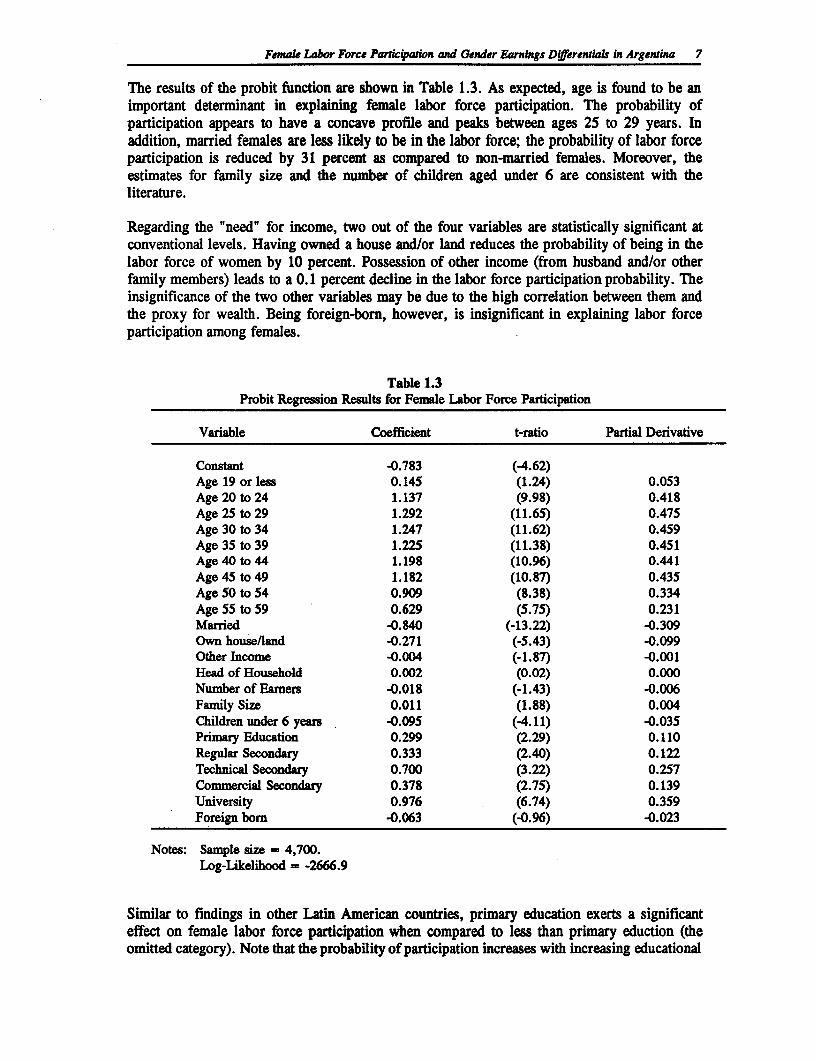
The results of the probit function are shown in Table 1.3. As expected, age is found to be animportant determinant in explaining female labor force participation. The probability ofparticipation appears to have a concave profile and peaks between ages 25 to 29 years. Inaddition, married females are less likely to be in the labor force; the probability of labor forceparticipation is reduced by 31 percent as compared to non-married females. Moreover, theestimates for family size and the number of children aged under 6 are consistent with theliterature.
Regarding the "need" for income, two out of the four variables are statistically significant atconventional levels. Having owned a house and/or land reduces the probability of being in thelabor force of women by 10 percent. Possession of other income (from husband and/or otherfamily members) leads to a 0.1 percent decline in the labor force participation probability. Theinsignificance of the two other variables may be due to the high correlation between them andthe proxy for wealth. Being foreign-born, however, is insignificant in explaining labor forceparticipation among females.
Table 1.3Probit Regression Results for Female Labor Force Participation
Variable Coefficient t-ratio Partial Derivative
Constant -0.783 (-4.62)Age 19 or less 0.145 (1.24) 0.053Age 20 to 24 1.137 (9.98) 0.418Age 25 to 29 1.292 (11.65) 0.475Age 30 to 34 1.247 (11.62) 0.459Age 35 to 39 1.225 (11.38) 0.451Age 40 to 44 1.198 (10.96) 0.441Age 45 to 49 1.182 (10.87) 0.435Age 50 to 54 0.909 (8.38) 0.334Age 55 to 59 0.629 (5.75) 0.231Married -0.840 (-13.22) -0.309Own house/land -0.271 (-5.43) -0.099Other Income -0.004 (-1.87) -0.001Head of Household 0.002 (0.02) 0.000Number of Earners -0.018 (-1.43) -0.006Family Size 0.011 (1.88) 0.004Children under 6 years -0.095 (-4.11) -0.035Primary Education 0.299 (2.29) 0.110Regular Secondary 0.333 (2.40) 0.122Technical Secondary 0.700 (3.22) 0.257Commercial Secondary 0.378 (2.75) 0.139University 0.976 (6.74) 0.359Foreign born -0.063 (-0.96) -0.023
Notes: Sample size = 4,700.Log-Likelihood = -2666.9
Similar to findings in other Latin American countries, primary education exerts a significanteffect on female labor force participation when compared to less than primary eduction (theomitted category). Note that the probability of participation increases with increasing educational
8 Women's Employment and Pay in Latin America
attainment. The highest probability of participation is found for those with completed highereducation (36 percent). The participation probability varies by type of secondary education.According to our estimates, of the three types of secondary education, having technical secondaryeducation gives the highest probability of participating (26 percent) while commercial secondaryeducation only increases the participation probability by 14 percent.
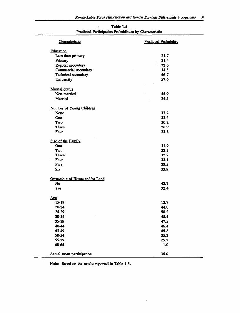
Using the above probit results, we examine the effect of changes in certain characteristics onfemale labor force participation by simulation. Given that other sample characteristics remainunchanged, we predict the probability of labor force participation for different educational levels,marital status, the number of young children, the size of the family, the ownership of houseand/or land, and age groups. The predicted probabilities are found in Table 1.4. As one mightexpect, increases in educational levels lead to an increase in participation probability. It is alsointeresting to find that the predicted probabilities for primary education and academic (regular)secondary education differ by only 1 percent. This interesting finding may reflect the impact ofcompulsory primary education which reduces the reward differences between primary andsecondary education (as shown in Table 1.1 over 50 percent of females in the sample haveprimary education). Commercial secondary education, on the other hand, does not increase theparticipation probability as much as technical secondary education does with respect to academicsecondary education.
The probability of participation for non-married women is twice that for married women. Thenumber of young children is another constraint on the participation decision. In Table 1.4,predicted probability drops from 37 percent to 23 percent when the number of young childrenincreases from none to 4, other things being equal. Consequently, household responsibilities ofwomen are important factors affecting the participation decision. In contrast, the size of thefamily increases the probability of participation with a flat rate of 0.4 percentage point. Thisinteresting result may demonstrate the fact that as the size of the family increases, the timeneeded for childcare and home production from the women is overcome by the 'need' for incometo support the family. Owning a house and/or the land causes the probability of participation todecline from 42 percent to 32 percent. Finally, predicted probabilities from the age splinesdemonstrate an inverted U-shaped profile with the highest probability for women aged 25 to 29years.
5. Earnings Functions
Mincer's basic model for estimating earnings functions regresses hourly earnings (wage rates)on schooling, experience and experience squared. The standard way of incorporating educationis to use a continuous variable to measure the years of schooling so estimates of private rates ofreturn to additional year of schooling can be obtained. According to economic theory, theearnings profile appears to be increasing at a decreasing rate with years of market attachment.Labor market experience and its square are used to test for this. In most cases, significantquadratic effects with eventual diminishing marginal returns to experience have been found(Shields, 1980; Behrman and Wolfe, 1984). In the absence of actual experience information,potential experience was calculated as age minus years of schooling minus six.
We estimate a Mincer-type earnings function in which years of schooling, experience, experiencesquared and the natural logarithm of hours worked are included as regressors. A separateearnings function is estimated for females and males to account for any wage differences due tosectoral and industrial differences.
Female Labor Force Participation and Gender Earnings Dfferentiab in Argentina 9
Table 1.4Predicted Participation Probabilities by Chamcteristic
Characteristic Predicted Probability
EducationLess than primary 21.7Primary 31.4Regular secondary 32.6Commercial secondary 34.3Technical secondary 46.7University 57.6
Marital StatusNon-married 55.9Married 24.5
Number of Young ChildrenNone 37.2One 33.6Two 30.2Three 26.9Four 23.8
Size of the FamilyOne 31.9Two 32.3Three 32.7Four 33.1Five 33.5six 33.9
Ownershig of House and/or LandNo 42.7Yes 32.4
Age15-19 12.720-24 44.025-29 50.230-34 48.435-39 47.540-44 46.445-49 45.850-54 35.255-59 25.560-65 1.0
Actual mean participation 36.0
Note: Based on the results reported in Table 1.3.
10 Women's Fmployment and Pay in Latin America
For both males and females, the standard Mincer-type regression function includes independentvariables measuring the years of schooling (S), potential labor market experience (defined asAGE-S-6)1 and its square and the natural logarithm of weekly hours work. The dependentvariable of the earnings functions is the natural logarithm of monthly earnings.
In order to account for any structural difference in the labor market that affects the "treatment"component of wage differentials, separate earnings functions for males and females are estimated.With the exception of a change in the schooling variable (which is replaced by categoricaleducational levels as described in the probit equation), several independent variables that measuresectoral employment and types of employment are included. In addition to potential experience,several dichotomous variables indicating whether individuals have received on-the-job trainingare added to capture the impact of specific training.2
Similarly, dummy variables for being employed in the public sector or not, working in thedependent employment sector or not, and whether weekly hours of work is less than 35 or over453 are included.
Earnings differences due to any intra-industrial differentials are taken into account by variousindustrial sector dummy variables. Finally, being married and/or being a foreign-born individual(FOREIGN) may affect earnings as well. In the case of females, earning functions are estimatedby ordinary least squares (OLS) and are presented for the purpose of comparison with respect tothe equation with selectivity adjustment.
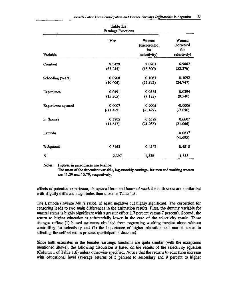
Table 1.5 shows the results for earnings functions of males and females that are consistent withthe theory. The inverse Mill's ratio (Lambda) in the female earnings function in column 3 ofTable 1.5 is marginally significant and negative. Consequently, it is not surprising to find thatresults of the Heckman procedure are little different from those in the regular OLS. For bothtypes of estimation, an additional year of schooling increases earnings by about 11 percent.Likewise, potential labor market experience and its square reveal a non-linear earnings profilefor females, increasing at an decreasing rate.
For males, the earnings elasticity with respect to hours of work is 0.3905 and for females is0.6589 (uncorrected for selectivity) or 0.6607 (corrected for selectivity). Moreover, the returnsto education for males is lower than for females, 9 percent compared to 11 percent. The rewardof potential market experience among males is higher than that of females.
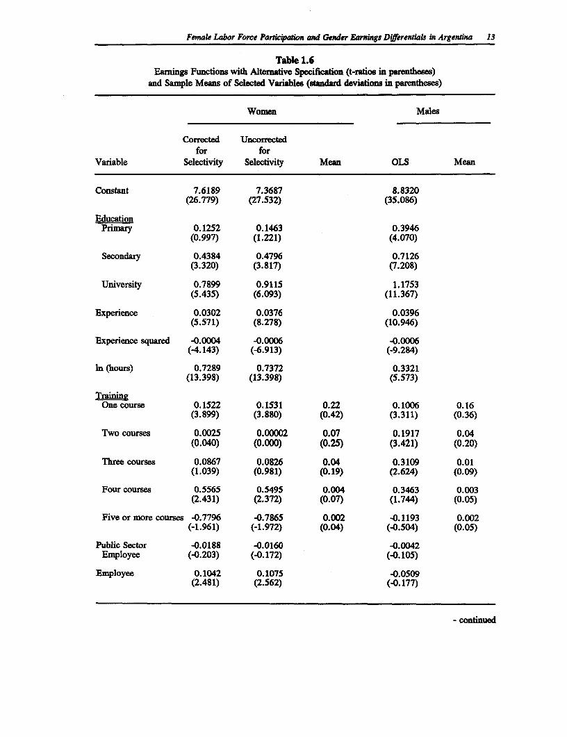
A different specification of the earnings function, which includes information associated withlabor market structure and training produces slightly different results for each earnings function.Table 1.6 presents earnings functions for both males and females, with female earnings functionsestimated using regular OLS and OLS with selectivity adjustment. As shown in the table, the
Though the definition has been criticized by various scholars, a more accurate measure isunavailable from this data set. As a result, the reader should be cautious in the interpretation of theestimates.
2 See Kugler and Psacharopoulos (1989).
3 The purpose of the hours of work variable is to account for any effect of working overtime andmoonlighting since there is a large proportion of respondents working more than 45 hours per week.
Femak Labor Force Participation and Gender Earnings Differentials in Argentina 11
Table 1.5Earnings Functions
Men Women Women(uncorrected (corrected
for forVariable selectivity) selectivity)
Constant 8.3429 7.0701 6.9662(63.245) (48.300) (52.276)
Schooling (years) 0.0908 0.1067 0.1092(30.006) (22.875) (24.747)
Experience 0.0491 0.0384 0.0394(15.505) (9.185) (9.540)
Experience squared -0.0007 -0.0005 -0.0006(-11.482) (-6.472) (-7.050)
In (hours) 0.3905 0.6589 0.6607(11.647) (21.055) (21.066)
Lambda -0.0837(-1.695)
R-Squared 0.3463 0.4527 0.4515
N 2,397 1,338 1,338
Notes: Figures in parentheses are t-ratios.The mean of the dependent variable, log-monthly earings, for men and worling womenare 11.29 and 10.79, respectively.
effects of potential experience, its squared term and hours of work for both sexes are similar butwith slightly different magnitudes than those in Table 1.5.
The Lambda (inverse Mill's ratio), is again negative but highly significant. The correction forcensoring leads to two main differences in the estimation results. First, the dummy variable formarital status is highly significant with a greater effect (17 percent versus 7 percent). Second, thereturn to higher education is substantially lower in the case of the selectivity result. Thesechanges reflect (1) biased estimates obtained from regressing working females alone withoutcontrolling for selectivity and (2) the importance of higher education and marital status inaffecting the self-selection process (participation decision).
Since both estimates in the females earnings functions are quite similar (with the exceptionsmentioned above), the following discussion is based on the results of the selectivity equation(Column 1 of Table 1.6) unless otherwise specified. Notice that the returns to education increasewith educational level (average returns of 5 percent to secondary and 9 percent to higher
12 Women's Employment and Pay in Latin America
education) except for primary education.4 The insignificant effect of primary education onfemale's earnings might indicate the 'deflation value" effect which results from compulsoryprimary education.
The experience profile appears to be concave, peaking at 34.33 years calculated at the mean valueof the working female sample. A one percent increase in weekly hours worked leads to a 0.73percent increase in earnings.
The consequence of having any work-related training has an interesting impact on earnings. Inthe case of females, having one training course enhances female earnings by 15 percent whilehaving two or three training courses makes no difference to earnings compared to those havingno training at all. Earnings increase by 56 percent if a female has four training courses, whilehaving five or more training courses has a negative impact on earnings, compared to thereference group (no training). This result is puzzling but also likely to be imprecise - less thanone percent of the females in the sample fell into the latter two groups.
For females, earnings do not differ between the public and private sectors, other things equal.On the other hand, if they are an employee (dependent employment) they will earn 10 percentmore than the self-employed, holding other factors constant. This is not surprising given the wagedetermination system in Argentina.
Earmings of part-timers are not statistically different from those of full-time workers. Those whowork more than 45 hours weekly, however, earn about 22 percent less than full-time workers,holding hours of work constant.
In the female labor market, ethnicity does not affect earnings. A working married female earns17 percent more than a non-married woman, though the probability of participation is negativelyassociated with marital status. Those who work after marriage tend to have a higher educationalattainment or more investment in human capital.
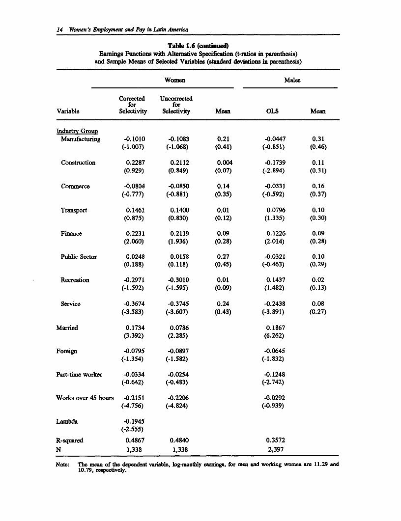
Across different types of industry, only finance and services industries exert effects on femaleearnings. Working in the finance industry allows females to earn 22 percent more while servicefemale workers are paid 37 percent less than other types of industry (the omitted group). Thelatter result is as expected since the relative overcrowding and the low skill requirement in thatsector lowers average earnings.
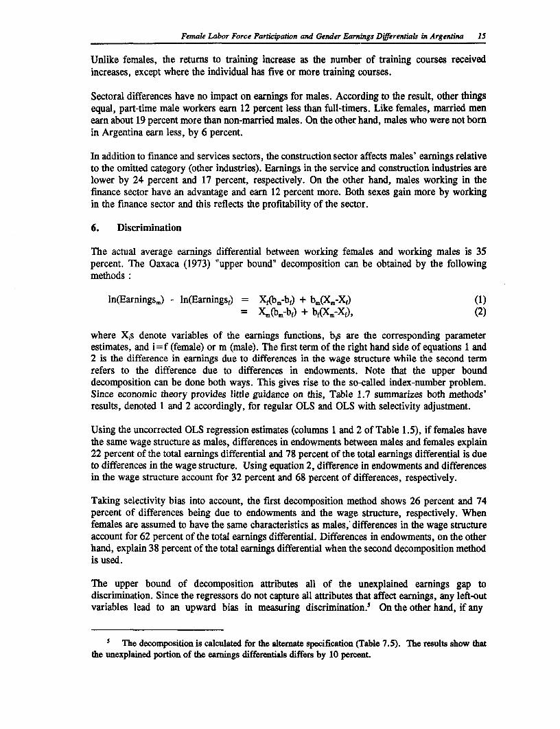
For males, the alternate specification shows a different picture. The rate of return to differentlevels of education increases with each successive level of education, with the exception ofsecondary education (an average of 6.6 percent return to primary education, 5.3 percent tosecondary education and 11.6 percent to university level).
The experience profile is concave in shape and has a lower decreasing rate than that of women.Males' earnings are less sensitive with respect to the number of hours worked per week (elasticityof 0.332).
4 The average retums to each educational level is calculated by dividing the change in coefficientsof the compared educational levels by the difference in years of schooling between the comparededucational levels.
Femalk Labor Force Partcipation and Gender Earnings Differentials in Argenhna 13
Table 1.6Eamings Functions with Alternative Specification (t-ratios in parentheses)
and Sample Means of Selected Variables (standard deviations in parentheses)
Women Males
Corrected Uncorrectedfor for
Variable Selectivity Selectivity Mean OLS Mean
Constant 7.6189 7.3687 8.8320(26.779) (27.532) (35.086)
EducationPrimary 0.1252 0.1463 0.3946
(0.997) (1.221) (4.070)
Secondary 0.4384 0.4796 0.7126(3.320) (3.817) (7.208)
University 0.7899 0.9115 1.1753(5.435) (6.093) (11.367)
Experience 0.0302 0.0376 0.0396(5.571) (8.278) (10.946)
Experience squared -0.0004 -0.0006 -0.0006(-4.143) (-6.913) (-9.284)
In (hours) 0.7289 0.7372 0.3321(13.398) (13.398) (5.573)
TrainingOne course 0.1522 0.1531 0.22 0.1006 0.16
(3.899) (3.880) (0.42) (3.311) (0.36)
Two courses 0.0025 0.00002 0.07 0.1917 0.04(0.040) (0.000) (0.25) (3.421) (0.20)
Three courses 0.0867 0.0826 0.04 0.3109 0.01(1.039) (0.981) (0.19) (2.624) (0.09)
Four courses 0.5565 0.5495 0.004 0.3463 0.003(2.431) (2.372) (0.07) (1.744) (0.05)
Five or more courses -0.7796 -0.7865 0.002 -0.1193 0.002(-1.961) (-1.972) (0.04) (-0.504) (0.05)
Public Sector -0.0188 -0.0160 -0.0042Employee (-0.203) (-0.172) (-0.105)
Employee 0.1042 0.1075 -0.0509(2.481) (2.562) (-0.177)
- continued
14 Women's Employment and Pay in Latin Amtrica
Table 1.6 (continued)Earnings Functions with Alternative Specification (t-ratios in parenthesis)
and Sample Means of Selected Variables (sandard deviations in parenthesis)
Women Males
Corrected Uncorrectedfor for
Variable Selectivity Selectivity Mean OLS Mean
Industry GroupManufacturing -0.1010 -0.1083 0.21 -0.0447 0.31
(-1.007) (-1.068) (0.41) (-0.851) (0.46)
Construction 0.2287 0.2112 0.004 -0.1739 0.11(0.929) (0.849) (0.07) (-2.894) (0.31)
Commerce -0.0804 -0.0850 0.14 -0.0331 0.16(-0.777) (-0.881) (0.35) (-0.592) (0.37)
Transport 0.1461 0.1400 0.01 0.0796 0.10(0.875) (0.830) (0.12) (1.335) (0.30)
Finance 0.2231 0.2119 0.09 0.1226 0.09(2.060) (1.936) (0.28) (2.014) (0.28)
Public Sector 0.0248 0.0158 0.27 -0.0321 0.10(0.188) (0.118) (0.4) (-0.463) (0.29)
Recreation -0.2971 -0.3010 0.01 0.1437 0.02(-1.592) (-1.595) (0.09) (1.482) (0.13)
Service -0.3674 -0.3745 0.24 -0.2438 0.08(-3.583) (-3.607) (0.43) (-3.891) (0.27)
Married 0.1734 0.0786 0.1867(3.392) (2.285) (6.262)
Foreign -0.0795 -0.0897 -0.0645(-1.354) (-1.582) (-1.832)
Part-time worker -0.0334 -0.0254 -0.1248(-0.642) (-0.483) (-2.742)
Works over 45 hours -0.2151 -0.2206 -0.0292(-4.756) (-4.824) (-0.939)
Lambda -0.1945(-2.555)
R-squared 0.4867 0.4840 0.3572
N 1,338 1,338 2,397
Note: The mean of the dependent variable, log-monthly eaningx, for men and workdng women are 11.29 and10.79, reqpectively.
Female Labor Force Participation and Gender Earnings Differentials in Argentina 15
Unlike females, the returns to training increase as the number of training courses receivedincreases, except where the individual has five or more training courses.
Sectoral differences have no impact on earnings for males. According to the result, other thingsequal, part-time male workers earn 12 percent less than full-timers. Like females, married menearn about 19 percent more than non-married males. On the other hand, males who were not bornin Argentina earn less, by 6 percent.
In addition to finance and services sectors, the construction sector affects males' earnings relativeto the omitted category (other industries). Earnings in the service and construction industries arelower by 24 percent and 17 percent, respectively. On the other hand, males working in thefinance sector have an advantage and earn 12 percent more. Both sexes gain more by workingin the finance sector and this reflects the profitability of the sector.
6. Discrimination
The actual average earnings differential between working females and working males is 35percent. The Oaxaca (1973) "upper bound" decomposition can be obtained by the followingmethods:
ln(Earningsm) - ln(Earningsf) = Xf(bm-bf) + bm(Xm-Xf) (1)= Xm(b=-bf) + bf(Xm-Xf), (2)
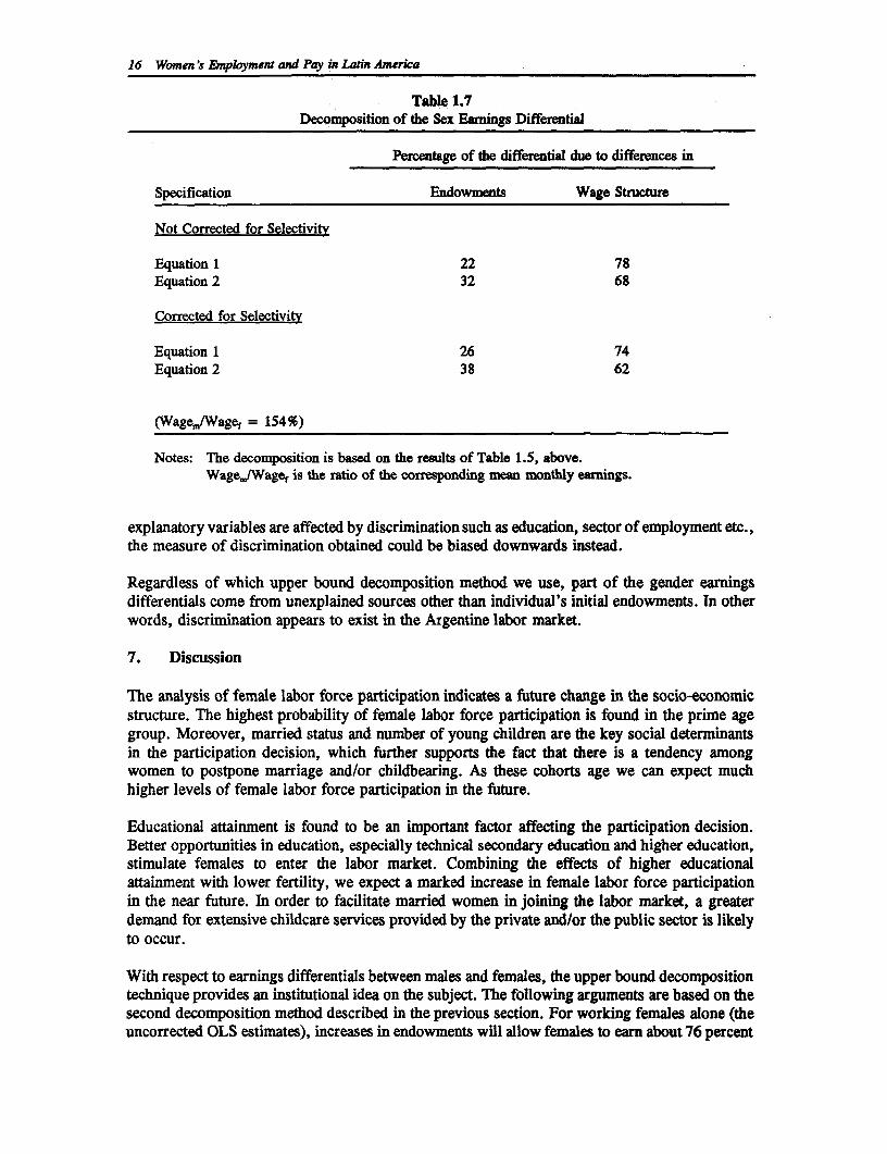
where Xis denote variables of the earnings functions, bis are the corresponding parameterestimates, and i=f (female) or m (male). The first term of the right hand side of equations 1 and2 is the difference in earnings due to differences in the wage structure while the second termrefers to the difference due to differences in endowments. Note that the upper bounddecomposition can be done both ways. This gives rise to the so-called index-number problem.Since economic theory provides little guidance on this, Table 1.7 summarizes both methods'results, denoted 1 and 2 accordingly, for regular OLS and OLS with selectivity adjustment.
Using the uncorrected OLS regression estimates (columns 1 and 2 of Table 1.5), if females havethe same wage structure as males, differences in endowments between males and females explain22 percent of the total earnings differential and 78 percent of the total earnings differential is dueto differences in the wage structure. Using equation 2, difference in endowments and differencesin the wage structure account for 32 percent and 68 percent of differences, respectively.
Taking selectivity bias into account, the first decomposition method shows 26 percent and 74percent of differences being due to endowments and the wage structure, respectively. Whenfemales are assumed to have the same characteristics as males,' differences in the wage structureaccount for 62 percent of the total earnings differential. Differences in endowments, on the otherhand, explain 38 percent of the total earnings differential when the second decomposition methodis used.
The upper bound of decomposition attributes all of the unexplained earnings gap todiscrimination. Since the regressors do not capture all attributes that affect earnings, any left-outvariables lead to an upward bias in measuring discrimination.5 On the other hand, if any
5 The decomposition is calculated for the alternate specification (Table 7.5). The results show thatthe unexplained portion of the earnings differentials differs by 10 percent.
16 Women's Employment and Pay in Latin America
Table 1.7Decomposition of the Sex Earnings Differential
Percentage of the differential due to differences in
Specification Endowments Wage Structure
Not Corrected for Selectivitv
Equation 1 22 78Equation 2 32 68
Corrected for Selectivitv
Equation 1 26 74Equation 2 38 62
(Wagem/Wagef = 154%)
Notes: The decomposition is based on the results of Table 1.5, above.WagejIWagef is the ratio of the corresponding mean monthly earnings.
explanatory variables are affected by discrimination such as education, sector of employment etc.,the measure of discrimination obtained could be biased downwards instead.
Regardless of which upper bound decomposition method we use, part of the gender earningsdifferentials come from unexplained sources other than individual's initial endowments. In otherwords, discrimination appears to exist in the Argentine labor market.
7. Discussion
The analysis of female labor force participation indicates a future change in the socio-economicstructure. The highest probability of female labor force participation is found in the prime agegroup. Moreover, married status and number of young children are the key social determinantsin the participation decision, which further supports the fact that there is a tendency amongwomen to postpone marriage and/or childbearing. As these cohorts age we can expect muchhigher levels of female labor force participation in the future.
Educational attainment is found to be an important factor affecting the participation decision.Better opportunities in education, especially technical secondary education and higher education,stimulate females to enter the labor market. Combining the effects of higher educationalattainment with lower fertility, we expect a marked increase in female labor force participationin the near future. In order to facilitate married women in joining the labor market, a greaterdemand for extensive childcare services provided by the private and/or the public sector is likelyto occur.
With respect to earnings differentials between males and females, the upper bound decompositiontechnique provides an institutional idea on the subject. The following arguments are based on thesecond decomposition method described in the previous section. For working females alone (theuncorrected OLS estimates), increases in endowments will allow females to earn about 76 percent

Femal Labor Force Partpioxn and Gender Earnigs Dierentiak un Argentina 17
of male earnings. On the other hand, if females are treated as males, the earnings differentialdrops to 10 percent. Hence, to bring about greater equality between working miles and workingfemales, more emphasis should be placed on the treatment of females in the labor market,occupations and job mobility.
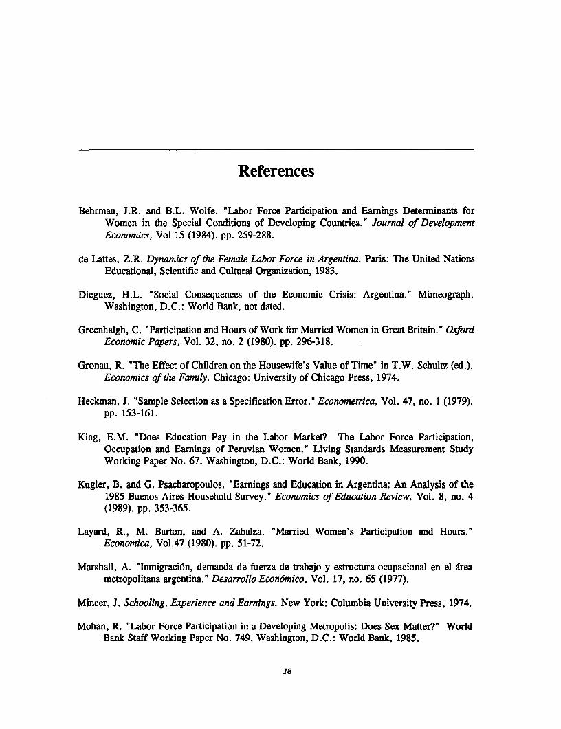
References
Behrman, J.R. and B.L. Wolfe. "Labor Force Participation and Earnings Determinants forWomen in the Special Conditions of Developing Countries." Journal of DevelopmentEconomics, Vol 15 (1984). pp. 259-288.
de Lattes, Z.R. Dynamics of the Female Labor Force in Argentina. Paris: The United NationsEducational, Scientific and Cultural Organization, 1983.
Dieguez, H.L. "Social Consequences of the Economic Crisis: Argentina." Mimeograph.Washington, D.C.: World Bank, not dated.
Greenhalgh, C. "Participation and Hours of Work for Married Women in Great Britain." OxfordEconomic Papers, Vol. 32, no. 2 (1980). pp. 296-318.
Gronau, R. "The Effect of Children on the Housewife's Value of Time" in T.W. Schultz (ed.).Economics of the Family. Chicago: University of Chicago Press, 1974.
Heckman, J. "Sample Selection as a Specification Error." Econometrica, Vol. 47, no. 1 (1979).pp. 153-161.
King, E.M. "Does Education Pay in the Labor Market? The Labor Force Participation,Occupation and Earnings of Peruvian Women." Living Standards Measurement StudyWorking Paper No. 67. Washington, D.C.: World Bank, 1990.
Kugler, B. and G. Psacharopoulos. "Earnings and Education in Argentina: An Analysis of the1985 Buenos Aires Household Survey." Economics of Education Review, Vol. 8, no. 4(1989). pp. 353-365.
Layard, R., M. Barton, and A. Zabalza. "Married Women's Participation and Hours."Economica, Vol.47 (1980). pp. 51-72.
Marshall, A. "Inmigraci6n, demanda de fuerza de trabajo y estructura ocupacional en el areametropolitana argentina." Desarrollo Econ6mico, Vol. 17, no. 65 (1977).
Mincer, J. Schooling, Experience and Earnings. New York: Columbia University Press, 1974.
Mohan, R. "Labor Force Participation in a Developing Metropolis: Does Sex Matter?" WorldBank Staff Working Paper No. 749. Washington, D.C.: World Bank, 1985.
18
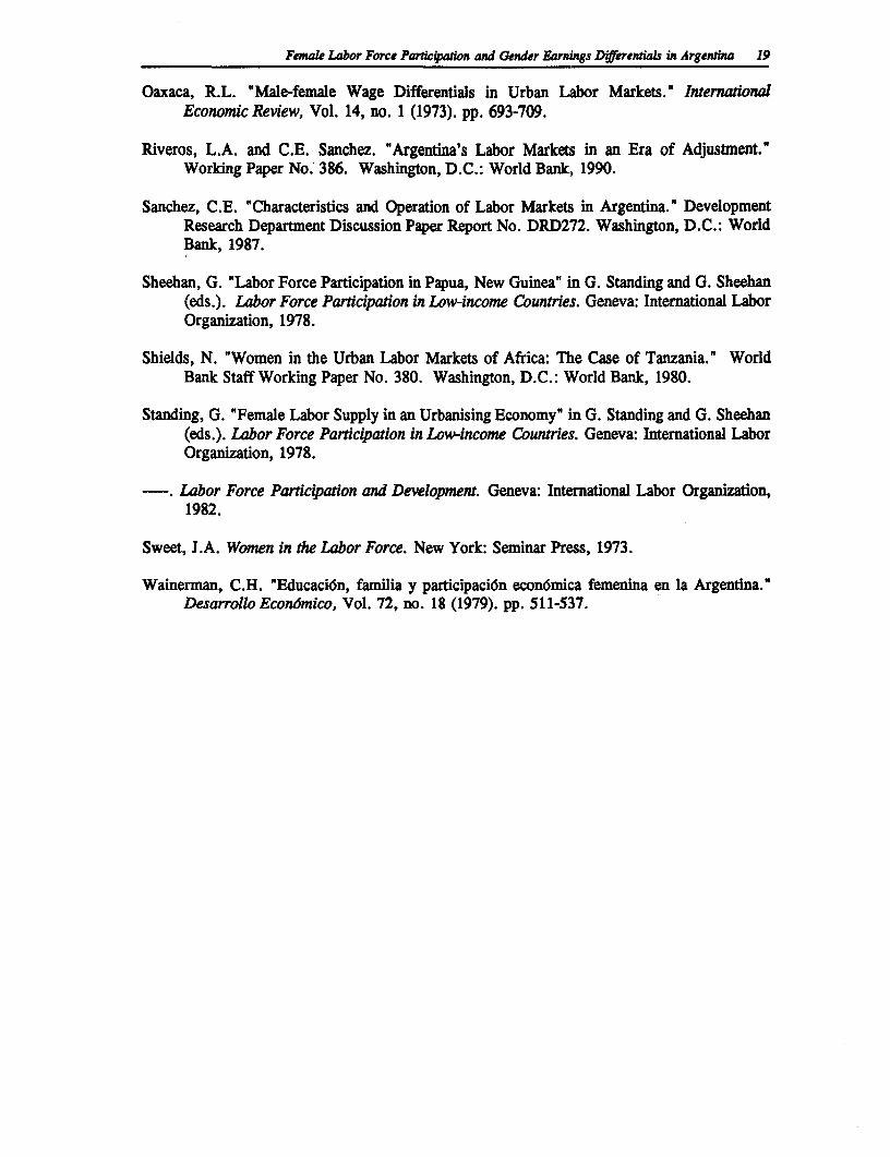
Female Labor Force ParticWpation and Gender Earnings Differentias in Argentina 19
Oaxaca, R.L. "Male-female Wage Differentials in Urban Labor Markets." InernationalEconomic Revew, Vol. 14, no. 1 (1973). pp. 693-709.
Riveros, L.A. and C.E. Sanchez. "Argentina's Labor Markets in an Era of Adjustment."Working Paper No. 386. Washington, D.C.: World Bank, 1990.
Sanchez, C.E. "Characteristics and Operation of Labor Markets in Argentina." DevelopmentResearch Department Discussion Paper Report No. DRD272. Washington, D.C.: WorldBank, 1987.
Sheehan, G. "Labor Force Participation in Papua, New Guinea" in G. Standing and G. Sheehan(eds.). Labor Force Participation in Low-income Countries. Geneva: International LaborOrganization, 1978.
Shields, N. "Women in the Urban Labor Markets of Africa: The Case of Tanzania." WorldBank Staff Working Paper No. 380. Washington, D.C.: World Bank, 1980.
Standing, G. "Female Labor Supply in an Urbanising Economy" in G. Standing and G. Sheehan(eds.). Labor Force Participation in Low-income Countries. Geneva: International LaborOrganization, 1978.
Labor Force Participation and Development. Geneva: International Labor Organization,1982.
Sweet, J.A. Women in the Labor Force. New York: Seminar Press, 1973.
Wainerman, C.H. "Educacidn, familia y participaci6n econ6mica femenina en la Argentina."Desarrollo Econ6mico, Vol. 72, no. 18 (1979). pp. 511-537.

2
Women in the Labor Force in Bolivia:Participation and Earnings
Katherine MacKinnon Scott
1. Introduction
In 1989, ten years after the United Nations approved the Agreement on the Elimination of allForms of Discrimination against Women, the Honorable National Congress of Bolivia ratified theagreement, joining close to one hundred other countries in pledging to analyze existing laws andlegislation to determine where changes needed to be made to bring the legal codes into alignmentwith the United Nations' Agreement.
In the same year that the Agreement was ratified, weeldy earnings for women in Bolivia were,on average, only 63 percent of male earnings, female-headed households were more likely to bebelow the poverty line than male-headed households and the female illiteracy rate was twice themale rate. It is not at all clear that existing labor law is responsible for the gender-baseddifferential in earnings and living standards observed in Bolivia, especially when there is someagreement that existing laws are not always enforced. It appears that there are other factorswhich affect the earnings of men and women in Bolivia. This study focuses on the determinantsof earnings and those factors which explain the observed wage differential between genders inBolivia. By decomposing the earnings functions of the two groups it will be possible to identifythat part of earnings which is explained by different endowment levels and that part which is dueto different market values being placed on male and female labor. A better understanding oflabor markets in Bolivia will assist in the formulation of policies which can complement thelegislative changes being envisioned and serve to include women in the economic activities of thecountry on a more equal footing.
The following section of the study presents background information on Bolivia, its economy, andlabor force characteristics. Information on the data used in the study is provided in Section 3.Several limitations on the degree to which the data can be used to extrapolate to the country asa whole are discussed in that section. The fourth section contains the labor force participationfunction for women. This participation function provides the means by which the female earningsfunction can be corrected for selectivity. Section 5 contains the description and results of themale and female earnings functions and the decomposition of these is carried out in Section 6.In the final section the overall results of the analysis are discussed and recommendations forimproving the situation of working women in Bolivia are presented.
21
22 Women's Employment and Pay in Latin America
2. The Bolivian Economy and the Labor Market
Bolivia is a landlocked country with three distinct geographic regions (highlands, valleys andtropical plains), several ethnic groups speaking different languages (Aymara, Quechua, Guarani,Spanish) and an economy heavily dependent on the export of primary products. The country ispoor, especially compared to the other countries in the Latin American region. Per capita GrossNational Product was US$570 in 1988 (World Bank, 1990b). Various social indicators alsoreveal the degree of poverty in the country. In 1988, adult illiteracy was 25 percent (WorldBank, 1990b). Rural illiteracy rates were much higher than urban ones (31.3 percent versus 7.7percent) and, of the illiterate population, 65 percent were women (World Bank, 1990a). Lifeexpectancy at birth, in 1988, was 53 years, infant mortality was 108 per 1000 live births, andthe maternal mortality rate (per 100,000 live births) was 480 in 1980 (World Bank, 1990b). Thepeople most likely to live in poverty in Bolivia are those who live in rural areas, own little land,are female, are of Indian origin, are from the central Andean Region, and work in agricultureor household industries.
The physical characteristics of Bolivia (low population density, distinct geographical regions)which have hindered the integration of the economy (Horton, 1989), and the dependence of theeconomy on primary products has made Bolivia very vulnerable to external shocks. During theeconomic crisis, which began in the late 1970s and continued through the first half of the 1980s,inflation reached 24,000 percent, GDP fell by 15 percent between 1976 and 1985 and per capitaGDP fell by 30 percent in the same period (Arteaga, 1987).
In 1976 (the year of the last national census), 80 percent of the population was considered to bepoor and 20 percent was considered to be extremely poor'. Concentrations of poverty werefound in the rural areas, especially in the Altiplano. GDP per capita has fallen steadilythroughout the 1980s and, in 1988, stood at only 72.7 percent of its 1980 level (World Bank,1990c). Recent data collected from a variety of sources2 lead to the conclusion that the state ofpoverty in the country has not improved and, in fact, may be worse in rural areas (World Bank,1990a).
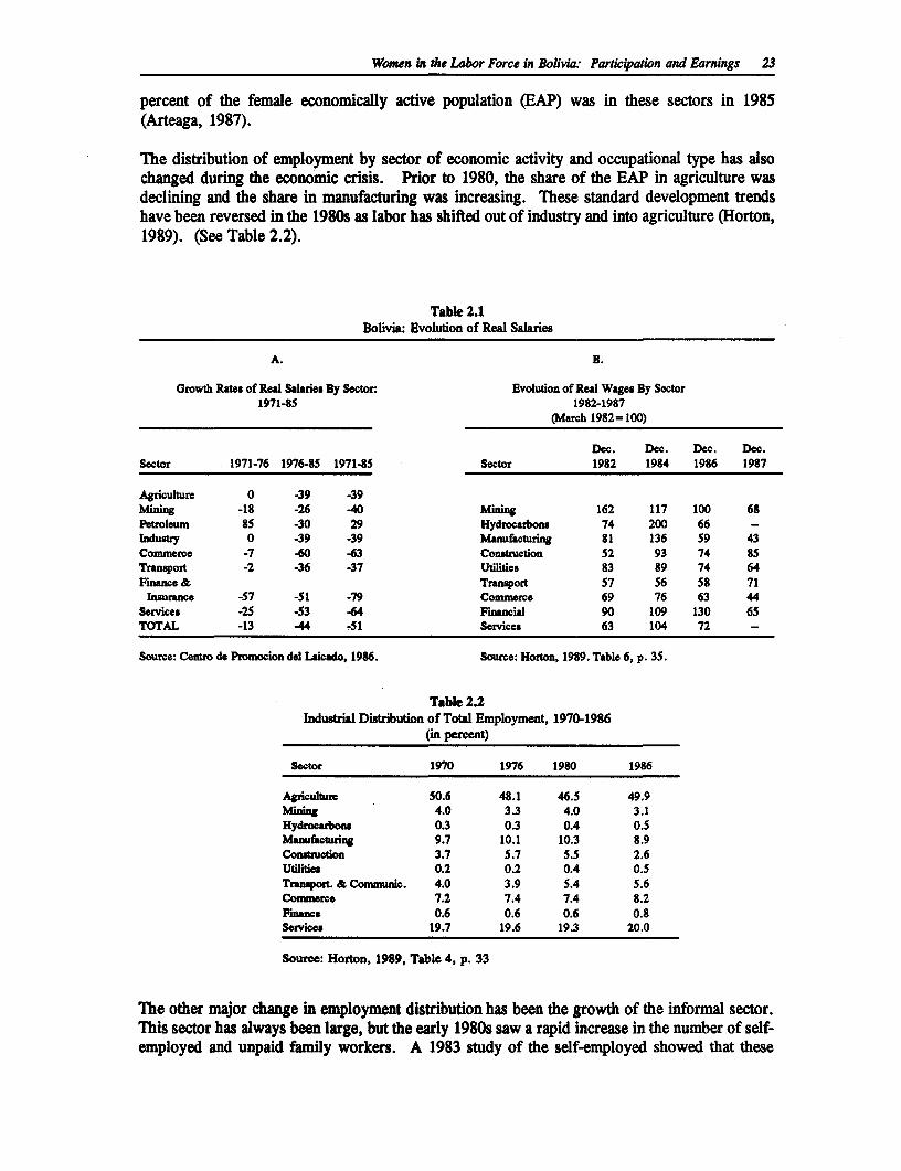
The labor force. The economic crisis has led to a substantial decline in real wages and salariesin Bolivia. (See Table 2.1 for estimates of the fall in real earnings.) While there is somediscrepancy in the data, both sources used in Table 2.1 show wages in commerce to have beenparticularly hard hit by the economic crisis. Wages in the service and manufacturing sectorswere also among those which lost more of their real value. Wages in the financial sector alsofell although there is some discrepancy in the data about the extent of the decline. Of specificinterest to the present study is the fact that the commercial and service sectors, where the realvalue of wages eroded most, are the two sectors where female employment is concentrated: 81
1 A household was considered to be poor if its income covered 70 percent or less of the basic needsbasket developed by PREALC. It was extremely poor if its income covered only 30 percent or less of thebasic needs basket.
2 The National listitute of Statistics of Bolivia has carried out, in the 1980s, a series of surveys,some of the most important of which are, Encuesta Permanente de Establecimientos Economicos (1983 andother years), Encuesta Nacional de Poblacion y Vivienda (1988), Encuesta Permanente de Hogares (annualsince 1980), and the Encuesta Integrada de Hogares (EIH which combines the old labor force survey withparts of a Living Standards Measurement Survey. The EIH was started in 1989.
Women in the Labor Force in BoIivia ParticTation and Earnings 23
percent of the female economically active population (EAP) was in these sectors in 1985(Arteaga, 1987).
The distribution of employment by sector of economic activity and occupational type has alsochanged during the economic crisis. Prior to 1980, the share of the EAP in agriculture wasdeclining and the share in manufacturing was increasing. These standard development trendshave been reversed in the 1980s as labor has shifted out of industry and into agriculture (Horton,1989). (See Table 2.2).
Table 2.1Bolivia: Evolution of Real Salaries
A. B.
Growth Rates of Real Salaries By Sector: Evolution of Real Wages By Sector1971-85 1982-1987
(March 1982=100)
Dec. Dec. Dec. Dec.Sector 1971-76 1976-85 1971-85 Sector 1982 1984 1986 1987
Agriculture 0 -39 -39Mining -18 -26 -40 Mining 162 117 100 68Petroleum 85 -30 29 Hydrocarbons 74 200 66 -Industry 0 -39 -39 Manufacturing 81 136 59 43Commerce -7 -60 -63 Constuction 52 93 74 85Transport -2 -36 -37 Utilities 83 89 74 64Finance & Transport 57 56 58 71
Insurance -57 -51 -79 Commerce 69 76 63 44Services -25 -53 -64 Financial 90 109 130 65TOTAL -13 -44 -51 Services 63 104 72 -
Source: Centro de Promocion del laicado, 1986. Source: Horton, 1989. Table 6, p. 35.
Table 2.2Industrial Distribution of Total Employment, 1970-1986
(in percent)
Sector 1970 1976 1980 1986
Agriculture 50.6 48.1 46.5 49.9Mining 4.0 3.3 4.0 3.1Hydrocarbosu 0.3 0.3 0.4 0.5Manufiring 9.7 10.1 10.3 8.9Contuction 3.7 5.7 5.5 2.6Utilities 0.2 0.2 0.4 0.5Tranport. & Communic. 4.0 3.9 5.4 5.6Commerce 7.2 7.4 7.4 8.2Finee 0.6 0.6 0.6 0.8Services 19.7 19.6 19.3 20.0
Source: Horton, 1989, Table 4, p. 33
The other major change in employment distribution has been the growth of the informal sector.This sector has always been large, but the early 1980s saw a rapid increase in the number of self-employed and unpaid family workers. A 1983 study of the self-employed showed that these
24 Women's Employment and Pay in Latin America
workers as a percent of the urban labor force had increased from 29 percent in 1976 to 34percent in 1983. The annual rate of growth of employment in the self-employed sector averaged5.95 percent and that of unpaid family workers grew by 7.66 percent. In contrast, the salariedlabor force grew only 2.25 percent annually during the same period. (Casanovas, 1984). Arecent World Bank report (1990a) indicates that another cause of the fall in income has been themovement of large segments of the working force out of the formal sector and into the informalone.
Unemployment rose in the 1980s, with the highest rates found in areas where mining had beena significant industry (Potosi and Oruro). While figures provided by various sources differ, thereis consensus that the increase was quite high; the lowest estimate is an increase of 26 percentbetween 1980 and 1987 (Horton, 1989). It is argued however, that unemployment rates reallyreflect the fall in formal sector employment and those that appear as unemployed are actuallyworking in the informal sector (Horton, 1989; and World Bank, 1990a).
Women in the laborforce. Female participation in the labor force in 1988 was estimated atalmost 29 percent (i.e., 29 percent of all women aged 10 and up participated in the labor force).In the eje central3 , women's labor force participation was estimated at 35 percent in 1987, upfrom the 1976 level of 20 percent (World Bank, 1989; and Horton, 1989). The rate ofparticipation of women has not, however, changed significantly since 1980. Femaleunemployment rates have been lower than male rates in the 1980s although femaleunderemployment is higher.4 As has been noted above, women have lower levels of educationthan men, are more heavily concentrated in the unpaid and family businesses, and are foundprimarily in commerce and service industries and the informal sector (World Bank, 1990a; andHorton, 1989).
Legally, there are still various statutes in Bolivia limiting women's full participation in the laborforce. First, with some exceptions (nurses, domestic servants) women are not permitted to workat night. Second, the 1942 legal code limits the work week of women to only 40 hours, incontrast to men's legal work week of 48 hours. Third, except in cases where "the work requiresa higher proportion,' women are only allowed to make up 45 percent of the wage and/or salaryearners in any given establishment (United States Bureau of Labor Statistics, 1962). Moreover,the labor code bars women from carrying out jobs considered to be dangerous, unhealthy or hard-labor.5
The significance of these laws is not clear since it appears that they are not enforced (WorldBank, 1989). Since the National Congress of Bolivia ratified the United Nations' "Convencionsobre la eliminacion de todas formas de discriminacion contra la mujer" in 1988, severalcommissions have been formed to review the existing legislation and recommend changes in thosestatutes which discriminate against women.
3 Includes the cities of La Paz, Santa Cruz, Cochabamba and Oruro.
4 Underemployment is defined as worling less than 12 hours in the reference week (Horton, 1989).
5 See: World Bank, 1989; and Romero de Aliaga, 1975.
Women in the Labor Force in Bolivia: Participation and Earnings 25
3. The Data
The data for the analysis come from the second round of the 1989 Integrated Household Survey(EIH), a bi-annual survey carried out by the National Statistical Institute of Bolivia (INE). Thesurvey is essentially a living standards measurement survey. Unlike the 1988 survey, The EIHonly covers the capital cities of eight departments of the country (Cobija, the capital of Pando wasnot included), the city of El Alto, and all other cities with populations greater than 10,000. Littleor no information on the rural population of the country is contained in the data. It should beremembered that the results of the analysis contained in the present study are applicable only tothe urban labor force. The way in which labor markets function on a national level and in ruralareas may be quite different.
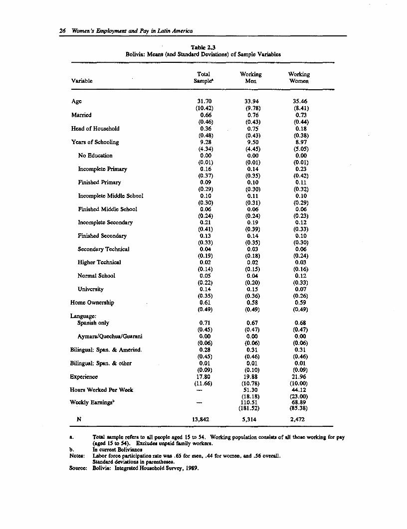
The EIH data used here were collected in November of 1989. Included in the survey are 7,267households with data on 36,126 individuals. Of these, a total of 13,842 cases were used. Thissample included all people of prime working age range (15 to 54) for whom relevant data wereavailable.6 Table 2.3 shows some of the characteristics of the total sample used as well as thecharacteristics of the working population. Working men and women are defined as all thosepeople who worked for more than one hour in the reference week for pay. This definitionexcludes unpaid family workers but includes the self-employed.' Excluding unpaid familyworkers from the definition of the employed will underestimate both male and femaleparticipation rates. Female participation rates will be underestimated more than male rates asmore women are unpaid family workers than men. Excluding domestic servants will also lowerparticipation rates of women more than men.
Of the total of 13,842 individuals included in the sample, 7,786 people, or 56 percent, areclassified as working, i.e., receive pay. Participation rates for women (44 percent) aresignificantly lower than for men (65 percent).
The average age of the sample is almost 32 years. Working women and men are more likely tobe married than the sample as a whole. Eighteen percent of working women are heads ofhouseholds as compared to 75 percent of working men.
Working women have, on average, one-half year less schooling than their male counterparts.While this overall gap in education is not large, the distribution of men and women by highestlevel of education completed shows some sharp differences. Only one quarter of working menended their schooling at the primary school level compared to more than one-third of workingwomen. The largest gap in educational achievement occurs at the university level; only 7 percentof working women have a university degree compared to 15 percent of the men. Proportionallymore women than men have attended a teacher training or normal school and greater percentagesof women have attended some form of technical school, especially at secondary level.
6 While the prime working age is usually considered to be between ages 20 and 60, the limits usedhere reflect more accurately the reality of Bolivia. The survey itself collects labor data for ages 10 andup. School attendance rates, however, are still fairly high until age 15. After age 15, attendance is lowand the percentage of working individuals increases. Thus the lower bound of the working age populationhas been set at 15 in this study.
7 Domestic servants have been elimiated from the analysis due, in part, to the difficulties ofdetermining actual income and also because of the limited data in this survey on such workers.
26 Women's Enployment and Pay in Lati America
Table 2.3Bolivia: Means (and Standard Deviations) of Sample Variables
Total Working WorkingVariable Sample' Men Women
Age 31.70 33.94 35.46(10.42) (9.78) (8.41)
Married 0.66 0.76 0.73(0.46) (0.43) (0.44)
Head of Household 0.36 0.75 0.18(0.48) (0.43) (0.38)
Years of Schooling 9.28 9.50 8.97(4.34) (4.45) (5.05)
No Education 0.00 0.00 0.00(0.01) (0.01) (0.01)
Incomplete Primary 0.16 0.14 0.23(0.37) (0.35) (0.42)
Finished Primary 0.09 0.10 0.11(0.29) (0.30) (0.32)
Incomplete Middle School 0.10 0.11 0.10(0.30) (0.31) (0.29)
Finished Middle School 0.06 0.06 0.06(0.24) (0.24) (0.23)
Incomplete Secondary 0.21 0.19 0.12(0.41) (0.39) (0.33)
Finished Secondary 0.13 0.14 0.10(0.33) (0.35) (0.30)
Secondary Technical 0.04 0.03 0.06(0.19) (0.18) (0.24)
Higher Technical 0.02 0.02 0.03(0.14) (0.15) (0.16)
Normal School 0.05 0.04 0.12(0.22) (0.20) (0.33)
University 0.14 0.15 0.07(0.35) (0.36) (0.26)
Home Ownership 0.61 0.58 0.59(0.49) (0.49) (0.49)
Language:Spanish only 0.71 0.67 0.68
(0.45) (0.47) (0.47)AymaralQuechua/Guarani 0.00 0.00 0.00
(0.06) (0.06) (0.06)Bilingual: Span. & Amerind. 0.28 0.31 0.31
(0.45) (0.46) (0.46)Bilingual: Span. & other 0.01 0.01 0.01
(0.09) (0.10) (0.09)Experience 17.80 19.88 21.96
(11.66) (10.78) (10.00)Hours Worked Per Week - 51.30 44.12
(18.18) (23.00)Weeldy Earnings6 - 110.51 68.89
(181.52) (85.38)
N 13,842 5,314 2,472
a. Total sample refers to all people aged 15 to 54. Working population consists of all those working for pay(aged 15 to 54). Excludes unpaid family workers.
b. In current BolivianosNotes: Labor force participation rate was .65 for men, .44 for women, and .56 overall.
Standard deviations in parentheses.Source: Bolivia: Integrated Household Survey, 1989.
Women in the Labor Force in Bolivia: Participation and Earnings 27
Only two people in the sample (both males) have no education of any sort. This is somewhatsurprising given the levels of illiteracy found in Bolivia. Urban illiteracy was calculated by INEin 1988 to be almost 11 percent with 13.8 percent of the population having no formal schooling.Given the exclusion of people over 55 from the sample, one would expect illiteracy rates to belower in the sample than the population. This cannot be the full explanation, however, as 11percent of those aged 20-55 years have had no formal schooling (Instituto Nacional de Estadistica,1989). It is not clear why people with no formal schooling are so underrepresented in thissample. The underrepresentation of people with no formal schooling biases the level of femaleeducational achievement more than men as a greater proportion of women are illiterate.
Slightly more than 70 percent of the sample speak only Spanish while 28 percent speak bothSpanish and an Amerindian language (Aymara, Quechua or Guarani). One percent speaksSpanish and another non-indigenous language.
The most striking difference in the sample is the large gap between the earnings of working menand women. Average weekly earnings for men are Bs.110.5 and Bs.68.9 for females. Thesefigures are consistent with previous estimates.8 On average, women earn slightly more than 60percent of men's earnings on a weekly basis. Women also work fewer hours, on average 7 hoursa week less than men. If women worked the same number of hours per week as their malecounterparts they would earn 80.1 bolivianos, less than average male earnings.
4. The Determinants of Female Labor Force Participation
Whether women participate or not depends on their reservation wage -- i.e., the value of theirlabor in the home. When this reservation wage is below the market wage women will participatein the labor force. If a woman's reservation wage is higher than that found in the market, shewill not participate.
This unobserved reservation wage means that female earnings functions estimates using ordinaryleast squares (OLS) will be biased. Only the market wage is observed and thus the OLS earningsfunction will suffer from the problems inherent in using censored samples. HEeckman (1979)provides an estimation technique to correct for this selectivity bias. First, a labor forceparticipation function for women is estimated. The inverse Mill's ratio (Lambda) from thisequation is then entered on the right-hand side of the earnings function equation. This correctsfor selectivity. Thus, the first step in estimating female earnings function is to specify a modelof female labor force participation.
Labor force participation among women in Bolivia is low. Only 44 percent of the present sampleof women work for pay. As noted above, the definition of working women may underestimatethe real female work force as unpaid family workers are excluded from the definition. Alsoexcluded from this definition are the unemployed. This is not a significant number of people(Instituto Nacional de Estadistica in 1988, calculated urban unemployment rates for women to be
I Horton (1989) provides estimates of male and female labor eamnings as a percent of the averageearnings for all workers. In 1982, male eanings were 102.6 percent of the average and female eaningswere 95 percent. The equivalent percentages in 1987 were 120.2 and 68.6 percent for men and womenrespectively. Similar calculations based on the data used here show men earning 118.4 percent of averageearnings and women 70.5 percent.
28 Women's Employment and Pay in Latin America
less than 2 percent of the labor force). The advantage of excluding the unemployed is that thereare definitional problems involved in the measurement of this group.'
The dependent variable in the participation function is a dichotomous variable which takes thevalue of one if the woman is working for pay and zero otherwise. A probit function is used toestimate participation rates. The regressors measure personal characteristics of the individualwoman, her family and socio-economic characteristics, and area of residence.
Personal characteristics include educational level, age, health and fertility patterns. Schoolingis entered as a series of dummy variables for each level of schooling. Note that for secondarytechnical, post-secondary technical, teacher's college, and university, no data were available forthe number of years of the level completed by individuals who are still students. Hence thedummy variable for these four education categories takes on the value of one if a person hascompleted the level or is presently a student in that level of education. The education coefficientsare expected to be positive as it has been shown that, while increased schooling increases boththe asking and the offered wage, the latter increases more (Heckman, 1979) .
Age is entered in the participation function as a series of dummy variables (in five year ranges)to take into account any non-linearity in the relationship of age to participation. It is not a cleara priori what the signs of the coefficients of these age variables will be. Some evidence existsshowing that younger women are more likely to be unemployed (Instituto Nacional de Estadistica,1988) which would decrease the probability of this group's participation. Where enrollment inhigher education is high, labor force participation will also be lower. Given the extremely lowrate of higher education enrollment among women this will have little effect.
Ethnic origin may be an important variable since different cultures have different attitudestowards paid employment for women and have different opportunities in the society.'° A proxyvariable for ethnicity, language(s) spoken, is used here. Four dummy variables are used forlanguage indicating whether the person speaks; (1) only Spanish; (2) only Amerindian languages;(3) both Spanish and one or more Amerindian languages and; (4) Spanish and another language.It is expected that those who do not speak Spanish will have a lower probability of participation.
Health will affect a woman's decision to participate in the labor market (Behrman and Wolfe,1984). The proxy for health status used here is number of days (out of the previous month) thata person has been incapacitated, i.e., physically unable to carry out her regular activities.Fertility is especially important in the Bolivian context. Given the high infant mortality rate inBolivia, the number of pregnancies a women has had will not be strictly correlated with thenumber of children she is raising. Hence, fertility is measured by two variables, the number ofchildren that the woman has given birth to, and whether the woman has been pregnant in the lastyear (measured by a dummy variable). It is expected that women who are, or have been,pregnant recently will be less likely to be in the labor force. It is argued that women tend toleave the labor force in order to have children, returning when their children are grown or atleast able to take care of themselves. Thus, the number of children under age 6 (preschool age)
9 For example: One measurement of the unemployed counts as unemployed only those activelysearching for work (McFarlane, 1988; and ILO, 1982), while another includes as unemployed all thosewho say they want to work. Obviously, the definition used will affect one's results.
10 A recent World Bank study (1990a) argues that there is evidence of ethnically based discriminationin Bolivia.
Women in the Labor Force in Bovia: Particyation and Earnings 29
is expected to lower a woman's probability of participating. This especially true where there areinadequate childcare facilities, as is the case in Bolivia (World Bank, 1989). Also included inthe equation is a variable measuring number of children between the ages of 6 and 14 a womanhas who are living in her household. Given the lack of universal participation in primary schoolin Bolivia (net primary enrollment in 1988 was only 83 percent (World Bank, 1990b)) the numberof children a woman has to care for in this group is also expected to lower her probability ofparticipating. Total family size has also been included in the equation. The sign of thecoefficient on this variable may be either positive or negative. On the one hand, a largerhousehold may have a positive impact on participation because of greater demands for incomeor the presence of non-working adults who can provide childcare. On the other hand, the sizeof the household may raise the value of the woman's household production activities and reducethe probability that she will participate in the labor force.
A woman who heads a household is more likely to work for pay. Married women will beexpected to have a lower probability of participation than unmarried women. The income of amarried woman's spouse is also included in the equation. It is expected to have a negative impacton participation. The final regressors in the equation are those having to do with geographiclocation and socio-economic status. It is expected that different areas of the country (highlands,valleys and tropical plains) are associated with different probabilities of participation. Thetropical plains area of the country is experiencing the greatest growth in population thoughimmigration and participation rates will be higher in this region.
To capture the effect of socio-economic status, variables measuring home ownership (a proxy forfamily wealth), total family income and access to public water and sewage disposal are included.(lhe latter two are, to some extent, proxies for the value of the home.) The effect of wealth onparticipation can be either positive or negative. There is less need to earn income if one's familyhas a certain level of wealth. But, also, it has been shown in other countries that relatively better-off women are more likely to work outside the home than lower-income women.
The results of the participation function are presented in Table 2.4. The age category omittedfrom the equation is from 15 to 19 years. As can be seen in the table, all other age groups aremore likely to participate than this youngest group. All of the age variables are significant. Ascan be seen from the simulations presented in Table 2.5, the participation rate for women peaksin the 35 to 39 age range. The 40 to 44 age group has similar participation rates but theprobability of participation declines for older women, possibly because retirement for womencovered by social security is age 50.
Other personal characteristics are also significant. Married women are less likely to work thannon-married women and those who are heads of households are more likely to work.Interestingly, the number of children under six that a woman has does not have a significantimpact on labor force participation. This may be because women in the informal sector are ableto either arrange their work schedule to fit childcare needs or are able to take their children withas them they work.
A woman's health status does have a significant negative impact on the probability ofparticipation. The effect, however, is quite small.
As expected, women who are presentiy students are less likely to participate in the labor forcethan non-students. Unexpectedly, however, educational attainment at the primary, middle andsecondary school levels does not have a significant impact on participation. There are two
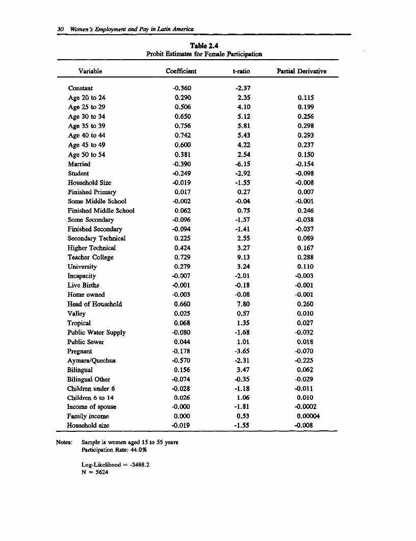
30 Women's Employment and Pay in Latin America
Table 2.4Probit Estimates for Female Participation
Variable Coefficient t-ratio Partial Derivative
Constant -0.360 -2.37Age 20 to 24 0.290 2.35 0.115Age 25 to 29 0.506 4.10 0.199Age 30 to 34 0.650 5.12 0.256Age 35 to 39 0.756 5.81 0.298Age 40 to 44 0.742 5.43 0.293Age 45 to 49 0.600 4.22 0.237Age 50 to 54 0.381 2.54 0.150Married -0.390 -6.15 -0.154Student -0.249 -2.92 -0.098Household Size -0.019 -1.55 -0.008Finished Primary 0.017 0.27 0.007Some Middle School -0.002 -0.04 -0.001Finished Middle School 0.062 0.75 0.246Some Secondary -0.096 -1.57 -0.038Finished Secondary -0.094 -1.41 -0.037Secondary Technical 0.225 2.55 0.089Higher Technical 0.424 3.27 0.167Teacher College 0.729 9.13 0.288University 0.279 3.24 0.110Incapacity -0.007 -2.01 -0.003Live Births -0.001 -0.18 -0.001Home owned -0.003 -0.08 -0.001Head of Household 0.660 7.80 0.260Valley 0.025 0.57 0.010Tropical 0.068 1.35 0.027Public Water Supply -0.080 -1.68 -0.032Public Sewer 0.044 1.01 0.018Pregnant -0.178 -3.65 -0.070Aymara/Quechua -0.570 -2.31 -0.225Bilingual 0.156 3.47 0.062Bilingual Other -0.074 -0.35 -0.029Children under 6 -0.028 -1.18 -0.011Children 6 to 14 0.026 1.06 0.010Income of spouse -0.000 -1.81 -0.0002Family income 0.000 0.53 0.00004Household size -0.019 -1.55 -0.008
Notes: Sample is women aged 15 to 55 yearsParticipation Rate: 44.0%
Log-Likelihood = -3488.2N = 5624
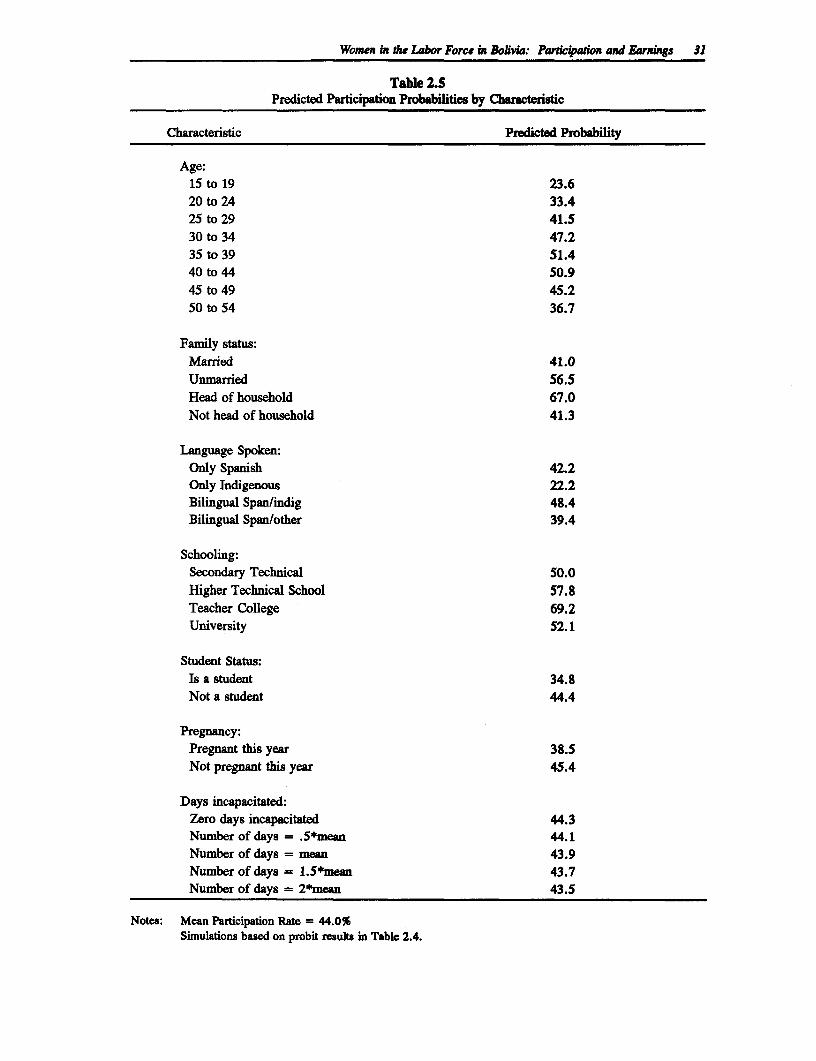
Women in die Labor Force in Bolivia: Pa_hco#wn and Earnings 31
Table 2.5Predicted Participation Probabilities by Charactenstic
Characteristic Predicted Probability
Age:15 to 19 23.620 to 24 33.425 to 29 41.530 to 34 47.235 to 39 51.440 to 44 50.945 to 49 45.250 to 54 36.7
Family status:Married 41.0Unmarried 56.5Head of household 67.0Not head of household 41.3
Language Spoken:Only Spanish 42.2Only Indigenous 22.2Bilingual Span/indig 48.4Bilingual Span/other 39.4
Schooling:Secondary Technical 50.0Higher Technical School 57.8Teacher College 69.2University 52.1
Student Status:Is a student 34.8Not a student 44.4
Pregnancy:Pregnant this year 38.5Not pregnant this year 45.4
Days incapacitated:Zero days incapacitated 44.3Number of days = .5*mean 44.1Number of days = mean 43.9Number of days = 1.5*mean 43.7Number of days = 2*mean 43.5
Notes: Mean Participation Rate = 44.0%Simulations based on probit result in Tabk 2.4.
32 Women's Employment and Pay in Latin America
possible explanations for this. First, women are concentrated in the informal sector where thevalue of education credentials are limited. Second, and perhaps more importantly, Boliviamaintains two separate school systems, one rural and one urban. The curriculum and the qualityof the two systems are very different (World Bank, 1989b). Hence, women who have beeneducated in rural areas will have received very different training. It is not possible to determinethe type of schooling a person received and the education variables for these levels may reflectdifferences in quality which confound the analysis.
In contrast, attendance in, or completion of, technical school (either secondary or post-secondary), teachers' colleges, or university has a highly significant, positive effect on probabilityof participation. The type of schooling with the greatest impact is that of teacher training. Ascan be seen in Table 2.5, all else being equal, a woman who attends a teachers' college has aprobability of participating close to 70 percent, over 25 percentage points higher than that for awoman with the average level of education. Interestingly, technical education at the post-secondary level has a greater impact on participation than does a university education (57.8percent probability versus 52.1 percent, respectively).
Pregnancy has the expected negative impact on participation. Women who were pregnant in thegiven year had a probability of participation of 38.5 percent. Women who had not been pregnantin the preceding twelve months had a probability of participating of 45.4 percent. The numberof children a woman has given birth to has an insignificant impact on participation rates.
Ethnicity also proves to have a significant impact on labor force participation with those womenwho speak no Spanish having the lowest participation rates (22.2 percent, all else held constant).Bilingual women participate at a higher rate than women who speak only Spanish. It should benoted that ethnicity and income levels are highly correlated in Bolivia (World Bank, 1990a) andthe effects of ethnic origin are probably partly reflecting economic status.
T1he variables measuring family wealth and socio-economic status (own home, public water andpublic sewage) have insignificant effects on the probability of labor force participation. On theone hand, this may reflect the contradictory effects of wealth on participation indicated above.On the other hand, home ownership may not be a good proxy for wealth in Bolivia and accessto public water and sewage may be more a function of urban living than socio-economic status.Neither the total family income nor the spouse's income have a significant impact onparticipation.
Contrary to expectations, the regional variables are not significant. Like the variables for sourceof water and sewage disposal, the fact that the sample is urban may account for this lack ofimpact of geography on labor force participation.
In summary, the most important effects on female labor force participation in Bolivia areschooling, student status, age, language spoken, marital status, pregnancy, and number ofchildren between ages 6 and 14. Women between the ages of 35 and 39, those who areunmarried, and/or bilingual, and/or highly educated are the most likely to participate in the labormarket.
5. Earnings Functions
The standard earnings function is the Mincerian (1974) formulation of schooling, experience andexperience squared regressed on the natural log of earnings:
Women in t Labor Force in Bolivia: Partcipon and Earnings 33
LnY = bo + bjS + b2EX + b3 EX2 (1)
Where:
LnY = the natural log of weekly earningsS = years of schoolingEX = experienceEX2 = experience squared
To standardize for hours worked, the natural log of hours (LNH) was entered on the right handside of the equation. It should be kept in mind that the experience variable used here is actuallypotential experience (i.e., age - years of schooling - 5). Potential experience will closelyapproximate real experience for any person who has worked steadily since s/he left school.However, as women are more likely to move in and out of the labor force, the potentialexperience variable may overestimate women's actual experience.
For female earnings, can the model answer the questions about the effect of human capital onearnings for women in the labor force? The sample used in the earnings functions includes theentire male and female working population (i.e., those working for pay). Three separatespecifications were used: One for males, one for females not correcting for selectivity and onefor females correcting for the selectivity bias. The results of the three earnings functions areshown in Table 2.6.
All of the variables have a significant effect on earnings for both men and women. The impactof schooling is less for women than men although the difference is not great. Experience andexperience squared have much less of an impact on earnings for women than men. The numberof hours worked, however, has a greater impact on women's earnings than on men's.
Te returns to schooling are significant, but not as high as those found in other Latin Americancountries"1. To some extent this reflects the size of the informal sector in the economy whereeducation has less of an impact than in the private formal and/or public sector. Returns toexperience and experience squared are also low, perhaps for the same reason. Only hours hasa high return (relative to men) impact. The inverse Mill's ratio is not significant.
6. Discrimination
As the sample characteristics presented in Table 2.3 demonstrate, there is a substantial gender-based difference in average weekly earnings. By subtracting the two earnings equations (the maleand female (uncorrected) equations) it is possible to determine what percent of this difference isdue to the different endowment levels of the two groups and what is due to the way in which eachgroups' endowments are valued in the market place (Oaxaca, 1973).
The initial difference between the earnings of men and women can be expressed as:
LnYm - LnYf = X.bm - Xfbf (2)
Algebraic manipulations give the following equation:
LnYm - LnYf = bm(XQ-X) + Xf(b7bt) (2a)
See other chapters in this volume.
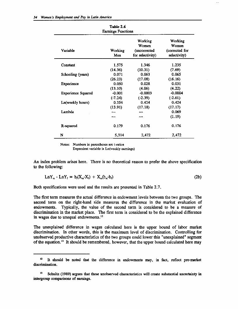
34 Women's Employment and Pay in Latin America
Table 2.6Earnings Functions
Working WorkingWomen Women
Variable Working (uncorrected (corrected forMen for selectivity) selectivity)
Constant 1.575 1.346 1.235(14.36) (10.31) (7.69)
Schooling (years) 0.071 0.063 0.065(26.23) (17.08) (16.16)
Experience 0.050 0.028 0.031(13.10) (4.06) (4.22)
Experience Squared -0.001 -0.0003 -0.0004(-7.24) (-2.39) (-2.61)
Ln(weekly hours) 0.354 0.424 0.424(13.91) (17.18) (17.17)
Lambda --- --- 0.069(1. 19)
R-squared 0.179 0.176 0.176
N 5,314 2,472 2,472
Notes: Numbers in parentheses are t-ratiosDependent variable is Ln(weekly earnings)
An index problem arises here. There is no theoretical reason to prefer the above specificationto the following:
LnYm - LnYf = bf(X.,-Xf) + Xm(bm-bf) (2b)
Both specifications were used and the results are presented in Table 2.7.
The first term measures the actual difference in endowment levels between the two groups. Thesecond term on the right-hand side measures the difference in the market evaluation ofendowments. Typically, the value of the second term is considered to be a measure ofdiscrimination in the market place. The first term is considered to be the explained differencein wages due to unequal endowments."2
The unexplained difference in wages calculated here is the upper bound of labor marketdiscrimination. In other words, this is the maximum level of discrimination. Controlling forunobserved productive characteristics of the two groups could lower this "unexplained" segmentof the equation.13 It should lbe remembered, however, that the upper bound calculated here may
12 It should be noted that the difference in endowments may, in fact, reflect pre-marketdiscrimination.
13 Schultz (1989) argues that these unobserved characteristics will create substantial uncertainty inintergroup comparisons of eamings.
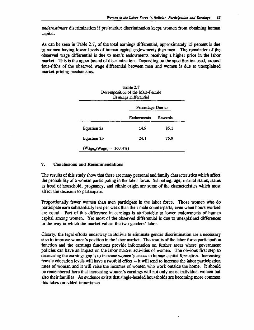
Women in the Labor Force in Bolivia: Participadon and Earnings 35
underestimate discrimination if pre-market discrimination keeps women from obtaining humancapital.
As can be seen in Table 2.7, of the total earnings differential, approximately 15 percent is dueto women having lower levels of human capital endowments than men. The remainder of theobserved wage differential is due to men's endowments receiving a higher price in the labormarket. This is the upper bound of discrimination. Depending on the specification used, aroundfour-fifths of the observed wage differential between men and women is due to unexplainedmarket pricing mechanisms.
Table 2.7Decomposition of the Male-Female
Earnings Differential
Percentage Due to
Endowments Rewards
Equation 2a 14.9 85.1
Equation 2b 24.1 75.9
(Wagej/Wagef = 160.4%)
7. Conclusions and Recommendations
The results of this study show that there are many personal and family characteristics which affectthe probability of a woman participating in the labor force. Schooling, age, marital status, statusas head of household, pregnancy, and ethnic origin are some of the characteristics which mostaffect the decision to participate.
Proportionally fewer women than men participate in the labor force. Those women who doparticipate earn substantially less per week than their male counterparts, even when hours workedare equal. Part of this difference in earnings is attributable to lower endowments of humancapital among women. Yet most of the observed differential is due to unexplained differencesin the way in which the market values the two genders' labor.
Clearly, the legal efforts underway in Bolivia to eliminate gender discrimination are a necessarystep to improve women's position in the labor market. The results of the labor force participationfunction and the earnings functions provide information on further areas where governmentpolicies can have an impact on the labor market activities of women. The obvious first step todecreasing the earnings gap is to increase women's access to human capital formation. Increasingfemale education levels will have a twofold effect - it will tend to increase the labor participationrates of woman and it will raise the incomes of women who work outside the home. It shouldbe remembered here that increasing women's earnings will not only assist individual women butalso their families. As evidence exists that single-headed households are becoming more commonthis takes on added importance.
36 Women's F.mployment and Pay in Latin America
Further increases in female earnings could come about from policies designed to increaseproductivity in the informal sector. This sector typically has access to very little capital and isconstrained by the low levels of technology used. Programs designed to increase creditavailability for small businesses in the informal sector and provide technical assistance wouldbenefit the economy as a whole. In the process, the specific benefits to women could be largesince a sizeable percentage of women working in urban areas are in this sector.
Without further information about the reasons why male labor is valued so much more highlythan female labor it will be difficult to affect the remainder of the observed wage differential inBolivia. But policies aimed at improving the legal enviromnent in which women work, increasingtheir access to education, and assisting the informal sector can all have a significant impact onwomen's participation rates and earnings.
References
Arteaga, V. "La Crisis Econ6mica y sus efectos sobre la mujer en Bolivia." Paper presented atthe United Nations' Childrens' Fund Simposio Nacional sobre Mujer y NecesidadesBasicas. Bolivia, June 1987.
Behrman, J. R. and B. Wolfe. "Labor Force participation and Earnings Determinants forWomen in the Special Conditions of Developing Countries", Journal of DevelopmentEconomics, Vol 46 (1984). pp. 259-288.
Casanovas, R. "Los Trabajadores pro Cuenta Propia en el mercado de Trabajo: El Caso de laciudad de La Paz, Boliva." Paper presented at the International Seminar "El SectorInformal Urbano en America Latina y el Ecuador". Quito: ILDIS/CEPESIU, 1984.
Heckman, J. "Sample Selection Bias as a Specification Error." Econometrica, Vol.47, no. 1(1979). pp. 153-161.
Horton, S. "Labour Markets in an era of Adjustment: Bolivia." (Incomplete draft). Universityof Toronto, 1989.
Mincer, J. Schooling, Experience, and Earnings. New York: Columbia University Press, 1974.
Oaxaca, R.L. "Male-female Wage Differentials in Urban Labor Markets." InternationalEconomic Review, Vol. 14, no. 1 (1973). pp. 693-709.
Romero de Aliaga, N. "The Legal Situation of the Bolivian Woman." Fletcher School of Lawand Diplomacy, La Paz, Bolivia: International Advisory Committee on Population andLaw, 1975.
United States' Bureau of Labor Statistics, "Labor Law and Practice in Bolivia." 1962. ReportNo. 218. Washington, D.C.: United States Department of Labor, 1962.
World Bank. "Bolivia: Poverty Report." Report No. 8643-BO. Latin America and CaribbeanRegion, Country Operations Division I. Washington, D.C.: World Bank, 1990a.
World Bank. World Development Report, 1990. Washington, D.C.: World Bank, 1990b.
World Bank. "Social Spending in Latin America: The Story of the 1980s." World Bank:Discussion Paper Series No. 88. Washington D.C.: World Bank, 1990c.
37

38 Wonen's nEployment and Pay in Latn America
World Bank. "Country Assessment of Women's Role in Development: Proposed Bank Approachand Plan of Action." R.N. 8064-BO. Latin America and Caribbean Region, CountryOperations Division 1. Washington, D.C.: The World Bank, 1989.
3
Labor Force Behavior and Earnings of BrazilianWomen and Men, 1980
Morton Stelcner, J. Barny Smith, Jon A. Breslaw and Georges Monette'
1. Introduction
Interest in the role of women in the development process of Third World countries increasedduring the last decade. A major concern is the status of women in what Behrman and Wolfe(1984) term the "special conditions" of labor markets in developing countries.2 Increasingattention is being given to analyzing the labor force behavior of women and to their returns tohuman capital, especially education. However, the volume of research on these women isconsiderably less than that for men in developing countries and for women in industrializedcountries. This study reduces this gap by examining labor force patterns among married andsingle women, and compares these with their male counterparts.
We present an analysis of the labor force behavior of Brazilian women and men using a sampleof 53,000 drawn from the 1980 Census. The specific concerns of the study are the determinantsof labor force status (employee, self-employed, or no market work) and earnings of workers.We pay particular attention to the impact of education on labor market outcomes. Fourpopulation groups are considered: wives and husbands, single (never married) women and men.
2. Brazil: Economic Background
An analysis of the labor force behavior of Brazilian men and women is important because it isrepresentative of a developing country experiencing severe economic problems. As for most ofits neighbors, the 1980s for Brazil, the largest and most populous country in Latin America, werea "lost decade" in terms of the severity and duration of the economic progress in the 1970s whenper capita GDP grew on average by 1.4 percent per year in 1970-1973 and by 7.1 percent in1974-1980. Brazil started the 1980s with much economic compromise and many successes, but
I The authors thank Ana-Maria Arriagada for her invaluable help in providing the data base andclarifying its contents, and Linda Bonin for her editorial advice. Brenda Butler, a computer science studentat Concordia University, provided competent programming assistance. We also thank Daniel M. Shapiro,Department of Economics, Concordia University, for providing helpful comments and criticisms thatshaped the final version of the paper.
2 As Behrman and Wolfe (1984, p. 260) aptly state, the special conditions include 'regional andsectoral pluralism, the relevance of human capital investments in health and nutrition, and distinctivedeterminants of opportunity costs for labor force participation."
39
40 Women's Employment and Pay in Latin America
early in the decade its economic performance began to deteriorate rapidly and dramatically, andhas not yet ended. In 1981 per capita GDP fell by 4.3 percent, while for the rest of the decadethe average annual (erratic) growth rate was about 1 percent. The economic prospects for the1990s are not encouraging: in 1990 gross domestic product shrank by 4.3 percent, reflecting adecline of 8 percent in industrial production.
A question that has been receiving increasing attention is: How have the worsening economicconditions, on top of persistent poverty, affected peoples' welfare in Latin America? Sincemarket work is the most important income source, an analysis of the labor force behavior ofBrazilian men and women, just prior to the onset of the economic difficulties, should shed lighton how the economic crisis will affect structural changes in the labor markets and provideinsights about the role of factors such as education in this process. This chapter examines thesituation in 1980, while the next chapter considers the conditions in 1989.
The vastness and diversity of Brazil and its well-documented substantial regional economicdisparities led us to perform the analysis for six distinct economic regions as well as the entirecountry. We thus reexamine the issue of "geographical aggregation bias' or "regional pluralism"in assessing returns to human capital, and how they differ by types of employment and bygender.3
A novelty of this study is that it examines the determinants of wages' by explicitly incorporatingthe selection (self or otherwise) of persons into three types of labor force status. As cogentlyargued by Schultz (1988), it is important to assess whether work-status effects bias the parameterestimates of wage functions. Few studies of labor markets in developing countries analyze theimpact of sample selectivity and adjustments in earnings regressions, especially when three typesof labor force status are involved.
The structure of the paper is as follows. Section 3 discusses the data used in the study. Sections4 and 5 summarize the model of labor force status and wage determinants, and includediscussions of the theoretical characterizations and econometric specifications. Section 6 reportsthe empirical findings and their interpretation. The final section contains the conclusions.
3. Data and Stylized Facts
The models used in this study are applied to data originally taken from a public use sample tape(PUST) of the 1980 Brazilian Census. The tape, which represents a 3 percent sample, contains3,526,000 individuals and about 800,000 households. The PUST was used to extract a subsampleof 200,000 individuals and about 40,000 households. From these data, we culled samples of
3 The issue of regional pluralism is examined for Brazil by Birdsall and Behrman (1984) with 1970Census data, for Nicaragua by Behrman and Birdsall (1984), and for Panama by Heckman and Hotz(1986). Unfortunately, there are very few studies that examine male-female differences in labor mairetoutcomes for developing countries, especially in the context of regional pluralism.
4 We use the terms 'wages' and 'earnings' interchangeably throughout the paper. Also, "hourlyearnings," "wage' or 'wage rate" are considered to be synonymous, as are "employee" and "wage earner. "
Labor Force Behavior and Earnings of Brazilian Women and Men, 1980 41
individuals who were generally between the ages of 15 and 65 years.5 This resulted in a sampleof 28,926 wives and husbands, 11,225 single (never married) women, and 12,974 single men.6
Although the Census data provides much useful information, it has a principal disadvantage:Incomplete information on the number of hours worked.7 Data are provided on monthlyearnings, but not on monthly hours worked, nor hourly earnings. Instead, we are given data onweekly hours of work in intervals: 0 hours (non-workers), 1-14 hours, 15-29 hours, 30-39 hours,40-48 hours and 49 or more hours. An index of continuous hours worked is desirable beforeapplying standard statistical techniques in estimating the wage function.
The study uses hourly earnings as the principal measure of remuneration because, as discussedin detail by Behrman (1990), Blinder (1976), and Schultz (1988), it is inappropriate (especiallyfor women and the self-employed) to use monthly earnings (monthly hours times hourly earnings)as the dependent variable. To do so may confound wage rate effects and labor supply effectswhich, in turn, may bias the parameter estimates of the returns to wage-determiningcharacteristics. The direction of the bias depends on whether the labor supply curve is normalor backward-bending. Moreover, as stated by Blinder (1976), the expedient of adding the logof hours as a regressor leads to "strained interpretations" of the parameter estimates of theearnings function.
The hourly earnings measure we use, however, is marred by incomplete information on hoursworked. The data provided no direct measure of hourly earnings, but we could calculate thehourly rate from monthly earnings and hours worked during the week of enumeration. Asmentioned above, there was, however, a problem - information on weekly hours worked wasavailable in intervals only, and no information was provided on the number of weeks per monththat a person worked. In earlier studies of Brazilian labor markets, Birdsall and Fox (1985) andDabos and Psacharopoulos (1991) used the 1970 and 1980 census data, respectively, to constructa continuous hours variable by assigning values (usually mid-point) to each work interval.8 Thisprocedure is likely to create a measurement error and the problem can be thought of as an errorsin variables problem in which parameter estimates are likely to be inconsistent and biased. Thedirection of this bias is not known. Nevertheless, we use their mid-point values, but note thecaveat in interpreting the results below.9
5 An exception is made for married men. There were 1,441 married men over the age of 65; about40 percent of them worked, usually over 30 hours per week.
6 The single (never married) men and women in the sample are relatively young. The average ageof single men and women is 25 years and 21 years, respectively. About 35 percent of single men areunder 20 years, and 40 percent are between 20 and 35 years of age; the corresponding proportions forwomen are 58 percent and 30 percent. Also, 38 percent of women reported that they were still attendingschool on a part- or full-time basis, as did 28 percent of the men.
7 Unfortunately, the data base also omitted information on migration for married and single men.In addition, for single men it failed to include information on household characteristics, non-labor income,and whether the person worked in the public sector.
I Birdsall and Behrman (1984), who also used the 1970 Census data in their study of Brazilian men,make no mention of this issue. They do not indicate whether they use hourly or monthly earnings.
9 As pointed out by Ham and Hsiao (1984), labor economists and econometricians have giveninsufficient attention this important question.
42 Women's Employment and Pay in Latin America
Important Characteistics of the Data
To provide a background for the study, we present detailed descriptive statistics in AppendixTables 3A.1 to 3A.6. There are substantial regional disparities, gender and work-statusdifferences, and differences between married and single people in the summary information.These features, as well as results from other studies of Brazil, strongly indicated that the studyshould treat each of the economic regions separately: the Northwest (North plus Central-West),Northeast, South, the Southeast (the states of Rio de Janeiro and Guanabara, Sao Paulo), andOther Southeast states (Minas Gerias and Espirito Santo).'0 For each region, we estimate themodels of labor force status and wage determination for four demographic groups, marriedwomen, married men, single women and single men. This approach allows one not only to detectregional differences, but also to draw comparisons among the demographic groups.
While a complete discussion of the information in the Appendix tables would be too lengthy topresent here, we do examine the more important stylized (i.e., abstracted for the purpose of theanalysis) facts about Brazilian labor markets. These stylized facts provide a useful backgroundfor the empirical analysis.
Regional dispariies.11 There are acute economic disparities in Brazil which had a populationof about 121.3 million in 1980. There are sharp differences among the highly industrialized andmodern southern regions (Rio de Janeiro, Sao Paulo, Other Southeast, and the South), theNorthwest (where the capital city is located), and the Northeast, which is heavily dependent onagricultural activities. The southern regions have about 60 percent of the population, and 17percent of the land mass; the Northeast accounts for 30 percent of the population and 19 percentof total area, while the vast Northwest has about 10 percent of the population. Although thereare pockets of poverty in the southern regions (in Rio de Janeiro, Minas Gerias, Espirito Santo,and Santa Catarina), they are the relatively prosperous parts of Brazil, while the Northeast is thepoorest area, whatever indicators one wishes to use.
Looking at Appendix Tables 3A.1 and 3A.2 (data for married people), we obtain a goodindication of the intensity of these regional disparities. All monetary units are in 1980cruzeiros."2 Total monthly employment earnings of husbands in the Northeast is $8,020compared to $12,790 in the Northwest, $11,730 in Other Southeast, $18,970 in Rio, $20,170 inSao Paulo, and $13,020 in the South. The pattern for monthly asset and transfer income issimilar -- $2,650 in the Northeast, $3,620 in the Northwest, $4,440 in Other Southeast, $8,900
10 The states in each region are:North: Rondonia, Acre, Amazonas, Roraima, Para, AmapaCentral-West: Mato Grosso, Goias, Distrito FederalNortheast: Maranhao, Piaui, Ceara, Rio Grande do Norte, Paraiba, Pemambuco, Alagoas,
Sergipe and BahiaSouth: Parana, Rio Grande do Sul, Santa CatarinaSoutheast: Rio de Janeiro and Guanabara, Sao Paulo, Minas Gerais and Espirito Santo
" We caution the reader that we did not take spatial price variations into account when makingregional comparison because we were unable to obtain geographical price indices. For further discussionof this issue see Birdsall and Behrman (1984) and Thomas (1980).
12 In 1980 the official exchange rate was about 40 cruzeiros = $ 1 (US). The monetary units usedare cruzeiros expressed with the symbol S.
Labor Force Behavior and Earnings of Brazilian Women and Men, 1980 43
in Rio, $8,760 in Sao Paulo, $4,280 in the South. In brief, family income is much lower in theNortheast than in the rest of Brazil.
A similar pattern is revealed when education is examined. In the Northeast, the average years ofschooling for husbands and wives are 2.2 and 2.3 years, respectively. The corresponding valuesfor the other regions are: Northwest: 3.5 and 3.4 years; Other Southeast: 3.4 and 3.4; Rio: 6.1and 5.4 years; Sao Paulo: 5.0 and 4.5 years; and South: 4.1 and 3.9 years.
There are also some noteworthy regional differences in labor force participation patterns. In theNortheast, Northwest, and Other Southeast, wives' labor force participation rates are in the 82-85percent range, while in the remaining regions they are in the 76-78 percent range. As regardsmarket work activities, in the Northeast just over one-half of working wives are self-employed.In the Northwest, the fraction is one-third, and it is about 37 percent in the Other Southeast andthe South. In the urbanized regions of Rio and Sao Paulo, only 20 percent of working wives areself-employed. This pattern is similar for husbands. Over 60 percent of working husbands in theNortheast are self-employed. The proportion drops to 53 percent in the Northwest, to 45 percentin the Other Southeast and in the South, to 29 percent in Sao Paulo, and to 23 percent in Rio.
The above regional configuration for earnings, education and labor force participation alsoprevails among singles. For example, consider the data on single women (Appendix 3A.4). Inthe Northeast, the average monthly earnings of employees and the (paid) self-employed are about$4,900 and $2,000, respectively. The corresponding values for the other regions: Northwest:$5,200 and $4,400; Other Southeast: $4,600 and $4,100; Rio: $8,300 and $12,200; Sao Paulo$7,800 and $11,100; and South: $9,200 and $4,500. As regards education, the average yearsof schooling among single women is 4.1 years in the Northeast; 5.2 years in the Northwest; 5.4years in the Other Southeast; 7.4 years in Rio; 7.1 years in Sao Paulo; and 5.9 years in theSouth. Finally, we note regional differences in labor force participation. In the Northeast, only30 percent of single women are in the labor force. This compares with 33 percent in theNorthwest, 37 percent in the Other Southeast, 41 percent in Rio, 59 percent in Sao Paulo, and44 percent in the South. The types of market work performed by single women also differsamong regions. In the Northeast, 63 percent of working women are employees. This proportionrises considerably in the other regions - 87 percent in the Northwest, 90 percent in the OtherSoutheast, 93 percent in Rio and in Sao Paulo, and 77 percent in the South. Much the same storycan be told about single men (Appendix Table 3A.5).
Gender and martal status differences. It should come as no surprise to find that there arenotable gender and marital status differences in labor force activities and outcomes. First, asnoted above, the labor force participation rate of men is much higher than that of women. Theparticipation rate of single women exceeds that of married women. There are also interestingdifferences in the types of jobs, and, among workers, in earnings, hours of work, and wage-determining characteristics (education, experience). Bearing in mind regional differences, themain features are as follows.
Job composition. The job composition of men and women differs. The proportion of womenworkers who are employees generally exceeds that of men. Nationally, about 65 percent ofworking wives and 83 percent of single women are employees compared to 43 percent ofhusbands and 75 percent of single men. A regional breakdown shows that this pattern is largelysustained. In the Northeast, 39 percent of working husbands and 44 percent of single men areemployees compared to 48 percent of working wives and 63 percent of single women. Theproportions for the Northwest are: husbands, 47 percent; single men, 66 percent; wives, 67
44 Women's Employment and Pay in Latin America
percent; and single women, 87 percent. The male-female differences are somewhat smaller inthe remaining regions. In the Other Southeast, 64 percent of working wives and 90 percent ofsingle women are employees, while 56 percent of husbands and 77 of single men are employees.In Rio, the proportions for wives and husbands are about the same, about 80 percent, while forsingle men and women, the proportions are 86 percent and 93 percent, respectively. In SaoPaulo, about 80 percent of wives and 70 percent of husbands are employees, as are 93 percentof single women and 87 percent of single men. In the South, 63 percent of working wives and54 percent of husbands are wage earners, while the proportions for single men and women areabout the same at 75 percent.
Earnings. Looking at Appendix Table 3A.3 (for married people) and Appendix Table 3A.6 (forsingles), we see that women, on average, earn less than men, and also work fewer hours.Nationally, the average monthly wage of husbands who are employees is $15,100 and $9,200 forwives; the values for single men and women are $7,800 and $6,400, respectively. Thus, thewife-husband earnings ratio is 0.61, while the single female-male ratio is 0.82. Among the (paid)self-employed, monthly earnings of husbands and wives are $14,600 and $7,900, respectively,yielding a ratio of 0.54. Single self-employed men earn $7,500, while their female counterpartsearn $4,500, for a ratio of 0.60.
These indicators of female-male earnings disparities must be treated with caution because womentend to work fewer hours than men. Accordingly, it would be useful to take labor supplydifferences into account by examining differences in hourly earnings between men and women.This changes the story somewhat. The average hourly wage for employee husbands and wivesis $84 and $63, respectively, yielding a ratio of 0.75. The corresponding values for self-employed workers is $84 for husbands and $55 for wives, for a ratio of 0.65. The hourly wagefor single male and female employees is almost the same, $45 for men and $40 for women, sothat the ratio is 0.89. Paid self-employed women earn about two-thirds the hourly earnings ofself-employed men ($43).
These summary statistics on the male-female hourly earnings gap suggest that working wives(employees or self-employed) are, on average, worse off than their husbands. However, the gapbetween single men and women employees is much smaller, but the earnings differential amongthe self-employed remains large. We also note that the observed wage may differ from the wageoffer, which takes into account labor force status decisions. In the econometric analysis weconcentrate on male-female differences in wage offers.
One should also note the regional differences in the male-female hourly earnings gap. Foremployees, the wife-husband wage ratio ranges from a low of 0.65 in Sao Paulo to a high of 0.92in the Other Southeast. The ratio is 0.72 in the Northeast, 0.76 in the South, 0.80 in Rio, and0.85 in the Northwest. Regional differences in the female-male earnings ratio of roughly 0.60among self-employed spouses are much less pronounced.
As shown in Appendix Table 3A.6 for singles, the average hourly wage of women employeesis about equal to that of men. In most regions, the female-male wage ratio is similar to thenational average (0.89). In the Other Southeast, the ratio is 0.77, while in Sao Paulo and theNorthwest, it is 0.81 and 0.85, respectively. In the Northeast and Rio, the average wage of singlewomen exceeds that of single men. Worst off are single self-employed women whose hourlyearnings are about 70 percent those of men.
Labor Force Behavior and Earnings of Brazilian Women and Men, 1980 45
Education. We now turn to a brief summary of the differences in the principal variables that arelikely to affect labor force status and wages. Nationally, as well as within specific regions andlabor force status, education levels of working women are generally higher than those of men.For Brazil as a whole, the mean years of schooling for wives who are employees is 7.0, whilefor husbands it is 4.9 years. Single women employees have 7.4 years, while single men have5.7 years. Similarly, self-employed wives have 3.4 years of schooling and their husbandcounterparts 2.9 years. The means for self-employed single women and men are 3.3 years and3.1 years, respectively. In each region, with few exceptions, the education levels of womenemployees exceed those of men employees by 2 to 3 years of school. Among the self-employed,women have an education advantage of less than a year.
The relationship between education and labor force status is as expected. Generally, theeducational attainment of employees is higher than that of the self-employed, and the latter havemore years of schooling than those not working. For example, the average years of school ofnon-working wives is 3.2 years compared to 3.4 years for self-employed wives and 7.0 years foremployees. With minor variations this pattern prevails for men and single women in all regions.
Age. As regards age, regional differences are relatively small. However, in all regions, wivesand married and single men who are employees tend to be younger than their self-employedcounterparts. For example, the average age of a married male employee is 38 years, and thatof the self-employed man, 42 years. The corresponding values for wives are 36 years and 38years, while for single men they are 24 years and 28 years. The pattern for single women differs.Nationally, the average ages of employees and the self-employed are about the same, 23 yearsand 22 years, respectively. However, in some regions (Northwest, Sao Paulo) self-employedsingle women are older (25 years) than employees (22 years). In the Northeast, the OtherSoutheast, and Rio, the average ages are the same (22-23 years), while in the South self-employed single women are younger than employees (19 years and 21 years). It should also benoted that single women and men are much younger than married women and men.
Fertility and child composition. We next consider past fertility and the child composition of thehousehold, which are particularly relevant to the analysis of married women. First we note thatwell over 80 percent of the married households in the sample are comprised of nuclear familiesthat consist only of a father, a mother, and children. The proportions are slightly lower foremployee wives than for non-working or self-employed wives. The two exceptions are in theNortheast and the Northwest, where the proportion of nuclear families is about 70 percent.
A Brazilian wife in our sample, on average, gave birth to about 4 Oive or dead) children. Theaverage is lowest among employee wives (3.0) and, surprisingly, highest among self-employedwives (4.7); for non-working wives it is 4.2 births. As expected, these numbers mask importantregional differences. Fertility is highest in the Northeast and lowest in the three southern regions.In the Northeast, the averages for non-working, self-employed, and employee wives are 5.2, 6.1,and 3.9, respectively. The corresponding values for the Northwest are 4.2, 4.6, and 3.3, whilefor the Other Southeast they are 4.4, 4.9, and 3.3. Fertility in the southern regions is lower. InRio and Sao Paulo, the averages are almost the same: 3.4 for non-working wives, 3.2 for self-employed wives, and 2.5 for employees. The values in the South are 3.9 for non-working andself-employed wives, and 2.8 for wives who are employees.
Now, we comment on child composition. The average number of each type of child - babies,toddlers, and school-age children - in the household is highest in the Northwest and Northeast.In these regions the average number of babies is about 0.56, which is much higher than that in
46 Women's Employment and Pay in Latin America
the other regions0.33 in Rio, 0.38 in Sao Paulo and the South, and 0.46 in Other Southeast.This pattern generally repeats itself for each child type and labor force status. It is noteworthythat the average number of babies among non-working wives is much higher than amongworkers. For each type of working wife the average number of babies is roughly the same inmost regions.
The average number of toddlers in the household (0.40) is about the same for non-working andself-employed wives, but lower for employees (0.30). Of course, there are regional differences.For example, in the Northeast and Northwest, the average number of toddlers is 0.50, while inthe remaining regions it is about 0.34.
The profile of school-age children is different. The national average of self-employed wives(1.30) exceeds that of employees (0.93) and non-workers (1.04). As expected, there are regionaldifferences. In Rio, Sao Paulo, and the South, the average for self-employed wives is 0.84, 1.10,and 1.19, respectively; for employees, 0.68, 0.88, and 0.88, respectively, and for non-workingwives, 0.79, 0.85, and 0.96. The corresponding averages for the remaining three regions are:Northeast, 1.24, 1.52, and 1.14; Northwest, 1.16, 1.59, 1.11; and the Other Southeast, 1.14,1.21, and 1.00.
In contrast to married women, Appendix Table 3A.4 shows that the child composition for singlewomen is different. Single women may live alone and may have children, or live in householdswith children. However, in our sample of relatively young women, over 90 percent aredaughters or daughters-in-law of a male household head. The average number of babies is aboutone-half that for married women (0.20). With a few exceptions (Northwest, Other Southeast,and Rio), there is little discernible difference in this magnitude between non-working and self-employed workers. However, the value for employees tends to be smaller than that for self-employed, especially in the Northeast, the Other Southeast, and Rio. As regards toddlers, thenational average is 0.24, and the mean is lower for employees (0.19) than for non-working (0.25)or self-employed (0.32) women. However, in the Northeast, Rio, Sao Paulo, and the South, theaverage is higher for self-employed women than that for non-working women, while in theremaining regions, the average is the same. The average number of school-age children presentin the household is lower for married women (1.04) than for single women (1.35). There arefewer such children among women who are employees (1.17) than among non-working (1.43)or self-employed women (1.17). As expected, these values are higher in the Northeast, theNorthwest, and the Other Southeast than in the remaining three regions. Also, with the exceptionof the Northeast, the average for self-employed women are 1.02 and 1.15, respectively; in theSouth, the corresponding values are 1.23 and 1.69.
Overall, the salient features presented above and the details provided in the tables indicate thatthere are important regional, labor force status, gender and marital status differences in the data.This suggests a stratification of the sample by region, work status, gender and marital status.Such an approach provides the opportunity to explore the extent to which the descriptive profilesare reflected in the empirical analysis of labor market outcomes.
Labor Force Behavior and Earrings of Brazilian Women and Men, 1980 47
4. Female Labor Force Partidpation
Before proceeding with the models, it should be noted that only 20 percent of married womenand 41 percent of single women performed market work (i.e. reported positive hours of work)."3
Of the working women a negligible fraction (1.5 percent) were employers, and about 8 percentof married and 10 percent of single women workers reported that they did not receiveremuneration for their market work (unpaid family workers). Among working wives, 65 percentwere employees and 35 percent were self-employed; the corresponding figures for single womenwere 83 percent and 17 percent. As regards men, 90 percent of married men were employed,and of this group, 4 percent were employers, 40 percent were self-employed, and 56 percentwere employees. All single men in our sample were in the labor force; 75 percent wereemployees and 25 percent were self-employed. A negligible fraction of men were unpaid familyworkers.
This information on Brazil, discussed more fully later, indicates that the labor force status choicemodel should be characterized by a three-way choice (employee, self-employment, and non-work)for women and married men, while a two-way choice (wage work and self-employment) shouldsuffice for single men. This is the approach we adopt.
The econometric specifications of the models were carefully considered given the data at ourdisposal. Table 3.1 below displays the definitions and measurement of the variables used in theanalysis. In specifying the models we tried to maintain uniformity as much as possible acrossregions, gender, marital and labor force status.14 However, because of small cell counts orinsufficient information (especially for single men) it was necessary to be flexible.
While we analyze the data for single (never married) women and men, most of our attention isgiven to the labor force behavior of married women. Wives are usually secondary workers whoalso bear the responsibility for household maintenance and child raising. We note that, foranalysis and policy purposes, the labor force behavior of wives is of considerable current interest.
The explanatory variables in the labor force status model are straightforward and standard in theliterature. For single and married women, these are age, age squared (divided by 100), yearsof education, child composition (the number of babies, toddlers, and school-age children),"5
household size, asset and transfer income of the household, home ownership, number of rooms
13 The low participation rates of Brazilian women should not be surprising. We note that at the turnof the century women comprised 45 percent of the reported labor force, mainly in agriculture, home-basedtextiles, and domestic-servant activities. Two decades later the proportion fell to 20 percent, and has sinceremained in the 20-25 percent range. A possible reason for the relatively low participation rate is themaner in which statistical information on women's activities is collected. Most census and surveypractices in developing countries typically exclude unpaid family and intermittent workers (especially inhome-based market activities) from the labor force. For further discussion, see Boulding (1983).
14 Considerable effort and resources were devoted to ensuring that data inconsistencies were removedand to experimenting with alternative specifications. Generally, the estimates were not sensitive toalternative specifications.
15 Since over 80 percent of married households are nuclear families, the children variables generallyreflect the fertility of the wife. This is certainly the case for the sample of relatively young single women,90 percent of whom are daughters or daughters-in-law of a male household head.
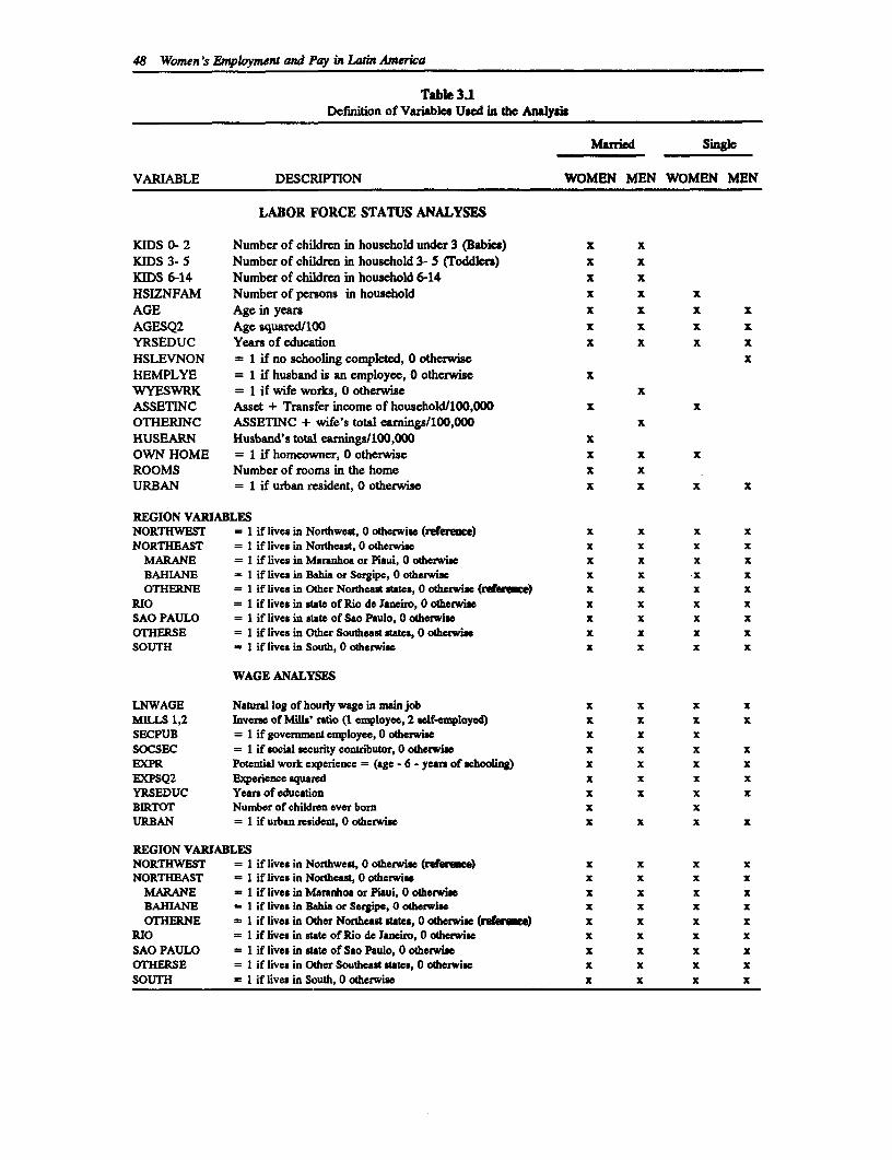
48 Women's Employment and Pay an Latin America
Table 3.1Definition of Variabla Used in the Analysis
Married Single
VARIABLE DESCRWIPION WOMEN MEN WOMEN MEN
LABOR FORCE STATUS ANALYSES
KIDS 0- 2 Number of children in household under 3 (Babies) x xKIDS 3- 5 Number of children in household 3- 5 (Toddlers) x xKIDS 6-14 Number of children in household 6-14 x xHSIZNFAM Number of persons in household x x xAGE Age in years x x x xAGESQ2 Age squared/100 x x x xYRSEDUC Years of education x x x xHSLEVNON = 1 if no schooling completed, 0 otherwise xHEMPLYE = 1 if husband is an employee, 0 otherwise xWYESWRK = 1 if wife works, 0 otherwise xASSETINC Asset + Transfer income of householdtlOO,000 x xOTHERINC ASSETINC + wife's total earnings/100,000 xHUSEARN Husband's total earnings/100,000 xOWN HOME = 1 if homeowner, O otherwise x x xROOMS Number of rooms in the home x xURBAN = 1 if urban resident, 0 otherwise x x x x
REGION VARIABLESNORTHWEST = 1 if lives in Northwest, 0 otherwise (referesce) x x x xNORTHEAST = I if lives in Northeast, 0 otherwise x x x x
MARANE = I if lives in Maranhoa or Piaui, O otherwise x x x xBAHIANE = 1 if lives in Bahia or Sergipe, O otherwiwc x x x xOTHERNE = 1 if lives in Other Northeast states, 0 otherwise (refer'ce) x x x x
RIO = I if lives in state of Rio de Janeiro, O otherwine x x x xSAO PAULO = I if lives in ste of Sao Paulo, O otherwie x x x xOTHERSE = I if lives in Other Southeast states, O otherwixe x x x xSOUTH = I if lives in South, O otherwise x x x x
WAGE ANALYSES
LNWAGE Natural log of hourly wage in main job x x x xMILLS 1,2 Invere of Mills' ratio (I employee, 2 elf-employed) x x x xSECPUB = 1 if govermnent employee, 0 otherwise x x xSOCSEC = 1 if social security contributor, 0 otherwise x x x xEXPR Potential work experience = (age - 6 - years of schooling) x x x xEXPSQ2 Experiencc quared x x x xYRSEDUC Years of education x x x xBIRTOT Number of children ever born x xURBAN = I if urban resident, 0 otherwise x x x x
REGION VARIABLESNORTHWEST = I if lives in Northwest, 0 otherwise (reference) x x x xNORTHEAST = 1 if lives in Northeast, 0 otherwise x x x x
MARANE = I if lives in Maranhoa or Piaui, O otherwise x x x xBAHIANE = 1 if lives in Bahia or Sergipe, O otherwise x x x xOTHERNE = I if lives in Other Northeast states, 0 otherwise (refareace) x x x x
RIO = I if lives in sate of Rio de Janeiro, O otherwise x x x xSAO PAULO = l if lives in state of Sao Paulo, odherwise x x x xOTHERSE = I if lives in Other Southeast stes, O otherwise x x x xSOUTH = I if lives in South, 0 otherwise x x x x
Labor Force Behavior and Earnings of Brazilian Women and Men, 1980 49
in the house, and urban residence. In the analysis of wives, we also include the husband'smonthly earnings, and a dummy variable if he is a wage and salary worker.
For married men, the variables are age and its square, years of education, home ownership, assetand transfer income plus the wife's earnings, whether the wife worked, and urban residence. Forsingle men, the data base did not provide information on household characteristics, and thefollowing variables were used: age and its square, years of education, urban residence, and adummy variable indicating whether the person completed any schooling.
For the entire Brazil sample we also estimated the model with and without regional dummyvariables (the excluded category is Northwest). This was also done for the Northeast, for whichthe state dummy variables are Bahia/Sergipe and Maranhao/Piaui (the excluded category is OtherNortheast states).'6 The results did not change in any significant way.
Labor Force Status Choice Model
Our analysis uses the standard one-period static labor supply framework in which preferences aredefined by a utility function whose arguments are the Hicksian composite of all goods, non-market time, and a vector of exogenous variables that affect labor force decisions.'7 Rationaldecision making is reflected in the maximization of the utility function subject to time and budgetconstraints."s One of an individual's decisions is to select amongst three mutually exclusivealternatives: employee, self-employment, and no work.19 These choices are indexed by 1, 2,and 3, and choices 1 and 2 have reported hours of work. The alternative chosen is the one thatyields the highest utility. In other words, the individual compares the pecuniary andnonpecuniary costs and benefits of each labor force status and chooses the one that yields thelargest gain.
More formally, let Vj be the maximum utility attainable for an individual if alternative j = 1, 2,3 is chosen. Assuming that this indirect utility function is linear for estimation purposes: Vj =x,yj + e*, where x is a (row) vector of observed explanatory variables (the non-stochasticcomponent or measured individual characteristics), yj is a vector of unknown parameters, and fjis a random disturbance corresponding to unobserved individual differences in tastes.
Thus, the probability that alternative j is chosen is just the probability that the individualcharacteristics (x) 'pay off" more in the jth alternative than in any other choice:
16 We also estimated the model with state dummy varables for the remaining regions, and found thatthe results did not change in any significant way. The results are available from the authors.
17 In keeping with the standard assumptions, the labor force behavior of other household membersis assumed to be exogenous. For instance, wives make labor supply decisions without reference to thoseof the husband, and likewise husbands. A future research topic is the issue of joint decision-making andhousehold labor supply.
is For fuller discussions of the model see Greene (1990), Hill (1988) and Trost and Lee (1984).
19 This assumption, of course, precludes concurrent multiplejob holdings, but this is of little concernin this study. Almost no women in the sample reported that they held a second job. About 5 percent of themen reported second jobs.
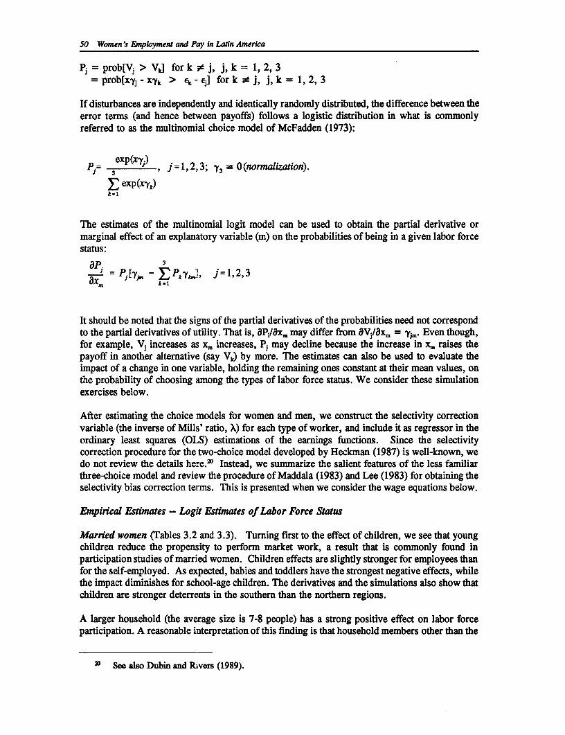
50 Women's Employment and Pay in Latin America
Pj = prob[Vj > Vd for k • j, j, k = 1, 2, 3= prob[xyj - xyk > ek - Ej] for k X j, j, k = 1, 2, 3
If disturbances are independently and identically randomly distributed, the difference between theerror terms (and hence between payoffs) follows a logistic distribution in what is commonlyreferred to as the multinomial choice model of McFadden (1973):
p= exp(xy) , j=1,2,3; 7 3 a 0 (normalization).
E exp(xy,)k-I
The estimates of the multinomial logit model can be used to obtain the partial derivative ormarginal effect of an explanatory variable (m) on the probabilities of being in a given labor forcestatus:
P.M P['Y SPtyb,,, j =1, 2, 3ax. ' J k-1
It should be noted that the signs of the partial derivatives of the probabilities need not correspondto the partial derivatives of utility. That is, aPi/axm may differ from aVj/axm = -yj. Even though,for example, Vj increases as xm increases, Pj may decline because the increase in x. raises thepayoff in another alternative (say Vk) by more. The estimates can also be used to evaluate theimpact of a change in one variable, holding the remaining ones constant at their mean values, onthe probability of choosing among the types of labor force status. We consider these simulationexercises below.
After estimating the choice models for women and men, we construct the selectivity correctionvariable (the inverse of Mills' ratio, X) for each type of worker, and include it as regressor in theordinary least squares (OLS) estimations of the earnings functions. Since the selectivitycorrection procedure for the two-choice model developed by Heckman (1987) is well-known, wedo not review the details here.' Instead, we summarize the salient features of the less familiarthree-choice model and review the procedure of Maddala (1983) and Lee (1983) for obtaining theselectivity bias correction terms. This is presented when we consider the wage equations below.
Empirical Estinates - Logit Estinates of Labor Force Status
Married women (rables 3.2 and 3.3). Turning first to the effect of children, we see that youngchildren reduce the propensity to perform market work, a result that is commonly found inparticipation studies of married women. Children effects are slightly stronger for employees thanfor the self-employed. As expected, babies and toddlers have the strongest negative effects, whilethe impact diminishes for school-age children. The derivatives and the simulations also show thatchildren are stronger deterrents in the southern than the northern regions.
A larger household (the average size is 7-8 people) has a strong positive effect on labor forceparticipation. A reasonable interpretation of this finding is that household members other than the
20 See also Dubin and Rivers (1989).
Labor Force Behavior and Earnings of Brazilian Women and Men, 1980 51
wife serve as childcare alternatives and share house-keeping chores, thereby releasing the wife'stime for labor market activities. Household size effects appear to be stronger in Rio, Sao Pauloand the South than in the remaining regions.
As regards the housing characteristics variables, in most instances home ownership (a proxy forwealth) does not have a statistically significant impact on labor force status. In only two casesis the coefficient significant and negative - for employees in Rio and Sao Paulo. The coefficientis unexpectedly positive and significant for self-employed wives in the Northeast. This maysimply reflect the poor quality of housing in the region. The number of rooms, which proxiesthe burden of housework, has the expected negative impact in all regions, except Rio, where thecoefficient is not statistically significant.2"
If the husband is an employee, this increases the probability that the wife will work as anemployee, but reduces the probability that she will be self-employed. This may reflect selectivemating in which relatively better educated men marry more highly educated women. We notethat wives who are employees tend to have husbands who are wage earners, and that employeeshave more schooling than the self-employed. Income effects are captured by two variables:husband's earnings and asset plus transfer income. In most cases, the higher the husband'searnings the lower the probability that a wife will work as an employee, but this variable has littleeffect on the self-employment choice. Overall, husband's earnings has a small significantnegative effect. The other variable used to approximate income effects (asset plus transferincome, but not husband's earnings) also has the expected negative effect on the propensity towork, particularly on the probability of working as an employee. However, with the exceptionof Rio and Sao Paulo, it generally has a small impact.
The dummy variable for urbanization presumably reflects a mix of demand-side and taste effects,which are likely to work in the same direction. An urban area may provide more plentiful jobopportunities and a more congenial environment for a wife to perform market work, and thusencourage greater participation than in rural areas.' We see that living in an urban area hasa positive effect on labor force participation, especially as an employee. In most regions,however, the urban variable has no significant impact on self-employment. In the Northeast andSouth, the urban variable has a negative effect on being self-employed, while in the OtherSoutheast and Rio (which also encompasses rural areas) the impact is positive.
The age of the wife is significantly related to labor force status, but in a non-linear fashion. Thisis readily seen by glancing at the coefficients, the marginal effects, and the predictedprobabilities. Younger wives (under 25 years) and older wives (over 40 years) are less likely toparticipate than wives in the 25-40 years age range, yielding an inversely U-shaped ageconditional profile, which accords with prior expectations and other empirical results fordeveloping countries.' This pattern is generally repeated for both employees and the self-employed.
21 The number of rooms in a house may also be a surrogate for wealth, depending on the quality ofthe dwelling, which is not known. As regards the finding for Rio, one hypothesis, though not testable withthese data, is that there is better access to domestics in Rio than in the other regions.
22 The same reasoning can be used in interpreting the effects of regional dummy variables.
23 See, for instance, Psacharopoulos and Tzmnnatos (1989), Mohan (1988), and Standing and Sheehan(1978).
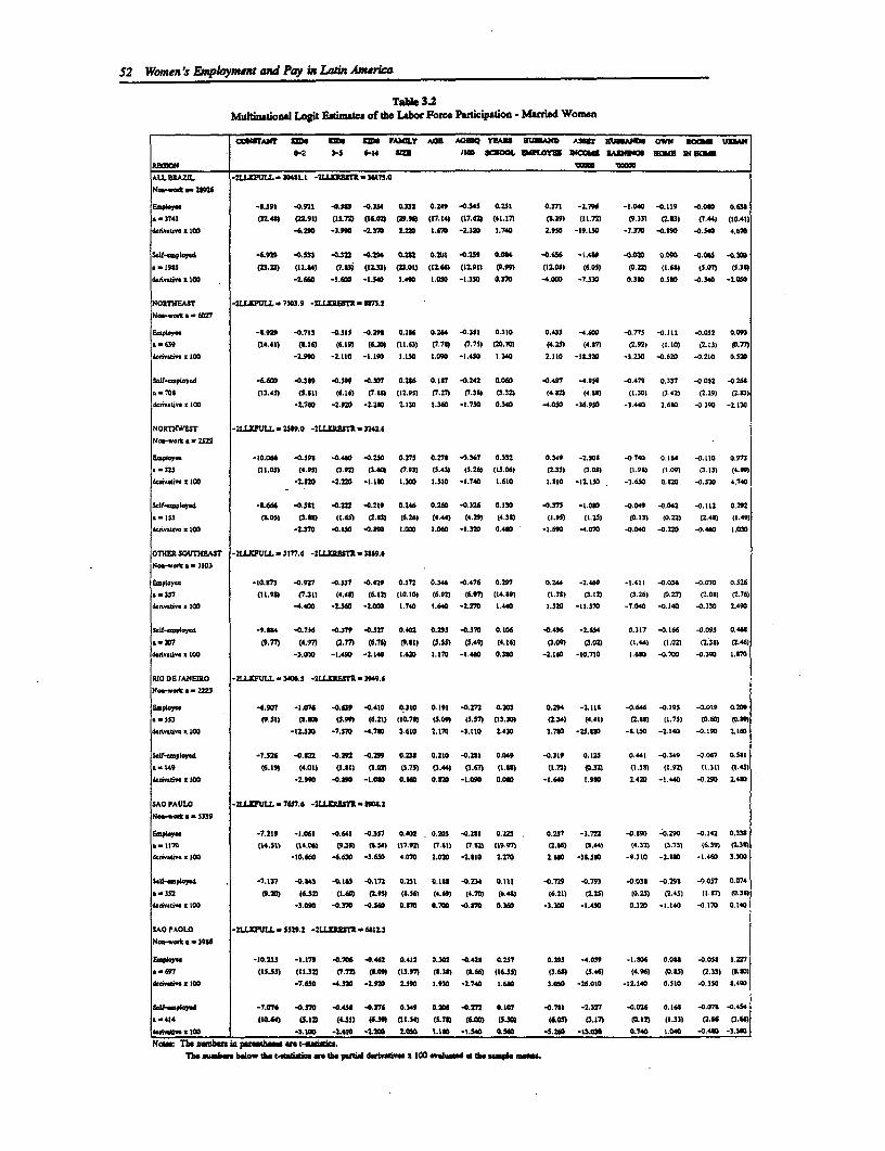
52 Women's Employmnt and Pay h Latin America
Taib 31Mul=nationl Logit FainMes of tbo IAbor Force Participation - Musfied Women
coUrAq gm UN ZNAI&M.Y AME AOUQ YEA= EUSAND .uin ZU,A,ffI OW, aOCMu uw0-2 3-5 -14 8ct /to SIOOL LOI YU &I3 B E1OS NOW 20 MM
ALBL AZL -23LDULL 304Jt.1 -2LLXRE8.- 3t17.0Nowe-M.t 2*924
E#oy. -. 93 -0.0921 -0450 0.354 0.332 0.249 4.34S 0.2S1 0.371 -2.796 -1.040 -0.119 -0.080 0.638a.3741 (2.48) (22.91) (1 .72) (1G.0) (9.9) (17.14) (17.42 (41.1) (8.39) (11.m7 (9.33) 2.31 (7.44) (10.41)dad.aiw x 100 -4290 -3.990 -2.370 L22 1.673 -2.320 1.740 2.950 -19.150 -7.370 -0.00 -0.340 4.670
SO1-Mpb7sd -4929 4.533 4-.M2 4.294 0.282 0.201 -0.259 0.064 -0.46 -L.49 -0.010 0.0 -0.04S 4.303
.- ISU 23.22 (1.84) (7.0-i (2.3) (2301) (12.6) (2.9t (9.99) (12.0t) (4.05) (0.22) (I.") (5.07) (5.35)
diowa. 100 -2.440 -1.4C -1.30 1.490 1.050 -1.350 0.370 -4.O0 -7.330 0.300 0.580 4.340 -L050
NORTHEASr -2LLKfL - 7503.9 -2L T - U513.2
Noeok a . 6027
Employ- u4.m920 -0.713 -0.515 -0.291 0.28U 0.264 -0.351 0.310 0.433 -4.640 -0.775 -0.111 -0.052 0.093
a -39 (14.4) (.16) (619) (6.203 (13.3) C7.71) (7.75) (20.70) (4.25) (4.81 (292) (t.10) (2.3U (.77)4ana.i0 I 100 -2.990 -2.110 -1.190 1.150 1.090 -1.450 1.340 2.110 -12.320 -3.230 4.620 -0.210 0.520
5cflfo..ptayd -6.60 -0.389 4.399 -0.307 0.206 0.157 -0.242 0.060 0.497 -4.959 -0.479 0.337 -0.052 -0.261-.703 (13.45) (5.91) (6.16) (7.0) (12.95) (7.217) 1.39) (3.32) (4.02) (4.11) (1.301 (3.421 (2.29) 12.23)
4.nto..i, x 100 -2.760 -2.920 -2.2xO 2.130 1.360 -1.750 0.340 -4.050 -36.950 -3.440 2.690 -0.390 -2.130
NORTHWEST -2U IMULL - 2589.0 -2LLLRESTR .3242.6
Noo-o* a . 2522
Emplye -10.04 -0.595 -0.40 -0.250 0.275 0.278 -. 367 0.332 0.349 -2.50 -0740 0.164 -0.130 0.973-323 (1l.01 (4.95) (3.92) (.06) (7.93) (3.43) (5.26) (13.06) (2.35) 13.08) (1.93 (1.09 (3.1 4.
4vawaiv s 1103 -2.130 -2.220 -1.33 120I I.31o -1.740 1.610 1.310 -12.150 -3.430 o.120 -0.520 4.740
sa3r-ompl.1 -3.644 -0.311 -0.222 4.219 0.246 0.260 4.324 0.130 -o.37 -3.080 4.049 -0.042 -0.112 0.292
a-3155 (.os) (2.3 (1.65) (2.) 16.26) (I44) (429) (438) (.9) (1.25) (0.13) (0.2) (241) (1.4914 ia.ug" x 100 -2.370 -0.30 -0.89 1.020 1.060 -1.320 0.480 -1.690 -4.070 -0.040 o -. 0o -0.460 1.030
OTHER SOUTHEASr -2LLJFULL - 3177.4 -2U MRESTI -. 3n9.N-oe a .3103
Elmoya -30.81 4.9n -0.531 4.429 0.3n 0.346 -0.46 0.297 0.244 -2.469 -1.411 -0036 4-0070 0.526a-37 (11.983) (7JI) (4.48) (6.12) (10.30) (6.923 (6.97) (14.89 (1.79) (3.12) (3.26) (0.27) (2.031 (2.761d4vind. a 100 -4.400 -2.540 -2000 1.740 1.640 -2.270 1.440 1.320 -3.5710 -1.040 -0.140 -0.330 2.40
S.U-.m;Io77d -9.384 4.736 4.379 4.327 0.402 0.295 4.310 0.106 -0.496 -2.44 0.317 -0.66 -0.095 0.44s
a-207 (9-77) (4.97) C2.77) (6.71 (9.3 (1.55) (5.49) (4.16) (3.09) .02) 1.44) (1.02) (2.39 (2.4)do4nni. 100 -3.000 -1.490 -2.140 1.620 1.170 -1.460 0.330 -2.160 -10.710 3.630 -0.700 -0.390 L.0
R10 IDgANEIRO -2LLXFULL- 3406.5 -2LuLETER-3949.6
Na.-wa - 2223
Employ" -6.907 -1.074 -04-639 4-410 0310 0.91 -. 27 0.33 0.294 -2.11S -0.46 -0.195 -0.019 0.20
1-053 (9.53) (3-.0 (5-99) (6-21) (10.76) (S.9 (5.37) (13.30) (2.34) (4.41) a238 (1.75) (0803 (1393daoia.Uo x 100 -12.520 -7.30 -4.70s 3.1W 2.1t7 -3110 2.430 1740 -2u.230 -1.1u0 -2.140 -0.10 2.140
seaf-empl3rd -7.328 4.122 4.292 -0.299 0.238 0.210 -0.281 0.049 -0.319 0.325 0.643 4.349 -0.047 0.581
. t49 (6.19 (4.0t) .-11 (2.31 (5.7S) O.4 (3.67) (n.8) (L.7) (0.321 (.3 (.92) (.3 (.daiatioa L00 -2.990 -03s -. 080 o.o 0.520 -3.090 0.03 -1.640 3.980 2.420 -1.440 -0.290 2.430
SAO PAULO -2LLULL - 747.6 -2LU nth * 9901.2N-sw*k e 35339
Employe -7.219 -3.043 -0.641 4.3S7 0.402 0.203 0.2s3 0.o23 . 0.237 -3.722 04.9 -0.290 -o.42 0.33811_ 0 (14.51) (14.0) CO.3) (5.54) (11.9 (17.61) (7.32) (19.7) (IA) (0.4) u4.321) t.751 (6.39 M.M
da,ntia6a 0300 -10.660 -6.630 -3.650 4.070 2.0O0 -2.SI 2.270 2.360 -3.08. -9.310 -.2.O -1.460 3.seo
uI pwy.o, . -1.137 -0.h3 -0.165 -0.172 0.23) o.11 -0.234 .311 -o.729 -0.793 -0.035 -0.295 -0.057 0.074
u-332 (9.20) (.32) (.60) .93) (LS.61 (4.69) (4.70) (6.4) (6.21) (2.25) (0.25) 12.4S) (3.5 (0.35)4nvdiaX s100 -3.090 4.370 4*.34 0.370 0.700 -431 0.360 -3.no -1.430 0.3230 3.40 4.137 0.140
SAO PAOLO -2LLFULL - 5529.2 -2LLREItR -812.3Noeo* aot . 3956
Emp3oy- -10.215 -1.179 -0706 -0.462 0.412 0.302 0.424 0.237 0.325 -4.039 -1.806 0.03u -0.050 I.237.- 649 (15.5) (11.32) (7173 (209) (13.97) (1.38) 3S.66) (16.53.) (3a6 O.46) (4.96) (0.15) (2.33) (LIM
denia.ax 030 -7.650 -4.20 -2.920 2.590 1.930 -2740 1.600 3.050 -26.010 -12.140 0.510 -0.350 S.490
s u-m1aymi -7.074 -0.30 -00.41 -4.m7 0.349 0.206 -0.m7 0.107 -0.781 -2.337 -0.026 0.18 -0.078 -0.454
5-414 (1064) (5.12) (4.1 (6o,) (11.54) (50.m (600) (5.30) (4.5) (3.37) (0.32) (1.33) (2.46 (2.64u alos 100 -2.100 -2No -2.20 2.051.10 -1.340 0.540 -s.260 -12.40 0.740 1.040 -0.440 -3.540
Now: The awobes in pueob_e jS t1_g&83ieTE subjse be&ow dhe t9-di4 am the po e dwW m d 100 etluma a (h s,e e
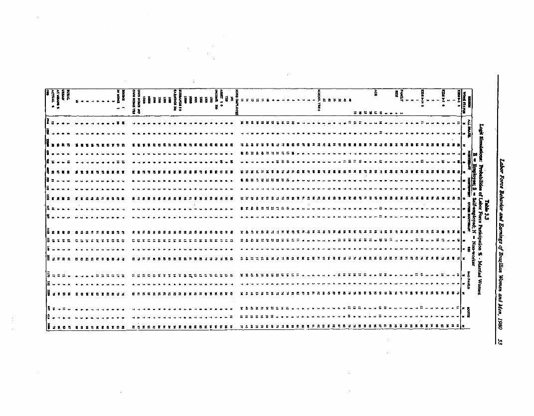
S ~~~~ . a~~ .-. . . .. . . .-
U aam a aa aa ;a a a aa aa aa a a aa a % a a a a a a a C !3 a a t ai a .a aa% -- aa a a ! t a a a a a s a a a a a :a a C a a a a a as a
. . . . . . . . . . . . . . . . . . . . .. . . . . . . . . . . . . 3. . . . . . . . . . . . . . . . . . . . . . . . . . . . .~~~~~~~~~~~~~~~~~I
. .. .. .. .. .. .. .- -. - - ...... . ..... .:a. .a.;a.-.-.- .-. .
~ ~:aa a u~ amna* a: an nna an: n an an : a a a :a~ anaaaa as a: a ~a A ICa338a aa I au a IIax
... . .. .. . .. .. .. .. . .. .. . .. . .. .. . .. . . .. .. . .. .. . ..
.. . .. . ... .. .
40 oooe .o ..oo .. .. .. .J . . .
I~~aaa naaaaaa:nn aaaaaaa:aIaCa a a a:: T 3
54 Women's Employment and Pay in Latin America
The role of education as a determinant of labor force status is of special interest. The effect ofeducation reflects both non-pecuniary factors ("tastes" for market work versus work at home) andpecuniary ones (potential market earnings). It is expected that education would not only bepositively related to labor force participation, but would also play an important role in "sorting"working wives between wage work and self-employment. The estimates show that this is indeedthe case. In all regions, increasing educational attainment monotonically increases the probabilityof working and, especially, of working as an employee.
It is important to draw attention to the difference in the effect of schooling on the probabilitiesof working as an employee and on self-employment. The effect of education is considerablystronger on the former than the latter. Although the education effect is significant in all regions,there are regional variations, particularly on the probability of working as an employee. Forexample, in Rio and Sao Paulo, the marginal effects of the education variable for employees are0.024 and 0.020, respectively, suggesting that an additional year of schooling increases theprobability of being an employee by about 2 percent. For the self-employed, an additional yearof schooling increases the probability by 0.8 and 0.4 percent in Rio and Sao Paulo, respectively.In the other regions, the partial derivatives of education for employees range from 0.013 to .016,while those for the self-employed (0.003 to 0.005) are similar to Sao Paulo.
A better picture of the prominent role of education in determining labor market status can beobtained by looking at the predicted probabilities in Table 3.3. A cursory examination shows thatan additional year of schooling (especially in excess of 5 years) not only increases the probabilityof participation, but more importantly, the probability of working as an employee. For example,nationally, an increase in schooling from 5 to 6 years increases the participation probability by3 percentage points, but only as an employee. Similarly, an increase from 10 to 11 years raisesthe probability by 5 percentage points, again as an employee. In sum, the principal effect ofeducation is to increase the propensity of wives to work as employees. The schooling effects onself-employment are very small. Of course, the force of schooling effects on labor market statusis linked to the role of education in determining the market wage, which is a major incentive fora woman to enter the labor force.
Married men (Tables 3.4 and 3.5). The estimated parameters of the logit function for marriedmen look reasonable and most variables are significant determinants of labor force status.
In most instances (Rio is the exception), having a working wife does not have a statisticallysignificant effect on the work-status of the husband. We also see that household size affects thehusband's work-status in selected regions - the Northeast, Other Southeast, Sao Paulo and theSouth. The larger the household the more likely it is that a married man will be an employee.The effects of living in an urban area on work status are significant in most cases. Generally,a husband who lives in an urban area is more likely to be an employee, and less likely to be self-employed. This may reflect the more plentiful wage work opportunities in urban areas. Thestrength of the effects of the urban variable, however, is not uniform across regions. Asexpected, home ownership and his non-labor income have retarding effects on working either asan employee or a self-employed worker.
Age generally has the expected effect in most cases. Exceptions are in Rio, where the coefficientof age is not statistically significant for both types of workers, in the Other Southeast, where itis not significant for employees, and in Sao Paulo where it is not significant for the self-employed.
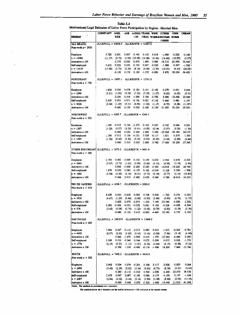
Labor Force Behavior and Earnings of Brazilian Women and Men, 1980 55
Table 3.4Multinational Logit Estimates of Labor Force Participation by Region - Married Men
CONSTANT AMIL AGE AGESQ YEARS WIFE OTHER OWN URBANRBGION SIZE /100 CHOO WORKSINCOME HOME
/100000ALL BRAZIL -2LLKFULL = 43838.9 -2LLKRESTR = 54587.5
Non-work a = 2920
Employee 3.720 0.031 0.027 -0.143 0.110 0.019 -1.989 -0.535 -0.160
a = 14596 (11.17) (3.72) (1.96) (10.09) (14.38) (0.30) (14.42) (10.07) (2.57)derivative x 100 0.270 -0.020 -0.870 1.690 0.900 -18.710 -20.990 30.440
Self-employed 3.612 0.022 0.032 -0.122 0.047 -0.020 -1.399 0.347 -1.560a = 11410 (11.0S) (2.75) (2.36) (9.16) (6.08) (0.30) (10.54) (6.43) (26.05)
derivativex 100 40.130 0.170 0.190 -1.270 -0.890 9.870 20.250 -34.420
NORTHEAST -2LLKFULL = 10897.1 -2LLKRESTR = 13741.8
Non-work n = 758
Employee 1.824 0.030 0.078 -0.182 0.141 -0.162 -3.279 4.431 0.034
n = 2590 (3.21) (1.92) (3.20) (7.22) (7.33) (1.27) (6.62) (4.02) (0.31)derivative x 100 0.230 0.310 -1.000 2.740 -0.750 0.590 -19.430 25.040
Self-employed 2.429 0.021 0.071 -0.152 0.021 -0.142 -3.660 0.481 -1.197
n = 4026 (4.54) (1.45) (3.21) (6.94) (1.05) (1.17) (6.70) (4.59) (11.87)derivativex 100 40.090 0.130 0.020 -2.360 40.150 -21.650 20.320 -29.520
NORTHWEST -2LLKFULL = 4283.7 -2LLKRESTR = 5349.7
Non-work n = 202
Employec 1.359 -0.015 0.156 -0.273 0.145 0.037 -2.742 -0.654 -0.291a = 1307 (1.28) (0.57) (3.25) (5.41) (4.59) (0.14) (5.07) (3.30) (1.36)derivativex 100 40.090 0.230 -0.940 2.890 3.590 -25.540 -29.190 24.270
Sclf-employed 1.398 -0.012 0.156 40.251 0.029 -0.117 -1.821 0.570 -1.365a = 1493 (1.36) (0.49) (3.42) (5.35) (0.93) (0.45) (3.65) (2.88) (6.66)derivative x 100 0.040 0.310 0.020 -2.600 -3.760 17.690 29.250 -27.340
OTHER SOUTHEAST -2LLKFULL = 5670.6 -2LLKRESTR = 6891.4
Non-work n = 362
Employee 2.795 0.092 0.049 -0.152 0.159 -0.032 -3.464 -0.478 -0.525
n = 1863 (3.07) (3.73) (1.26) (3.90) (5.66) (0.16) (6.36) (3.18) (2.96)derivaivex 100 0.850 -0.600 -0.280 0.350 4.360 -16.910 -19.220 28.760
Self-employed 1.S79 0.065 0.082 -0.159 0.162 -0.019 -3.128 0.330 -1.888n = 1442 (2.08) (2.65) (2.16) (4.21) (5.75) (0.10) (5.77) (2.15) (10.87)derivaive x 100 43.460 0.910 -0.480 0.430 0.240 0.760 18.610 -34.230
RIO DE JANEIRO -2LLKFULL = 4298.7 -2LLKRESTR = 5096.0
Non-work a = 416
Employee 4.659 0.030 -0.026 -0.085 0.108 0.450 -1.762 -0.374 -0.325n = 1933 (4.67) (1.29) (0.64) (2.08) (6.52) (2.69) (5.93) (2.70) (1.37)derivative x 100 0.650 -0.070 -0.970 1.320 7.190 -33.360 -6.950 2.320Self-employed 3.552 -0.002 -0.031 -0.052 0.061 0.145 -0.229 -0.058 -0.594a = 576 (3.43) (0.08) (0.74) (1.25) (3.45) (0.79) (0.92) (0.38) (2.36)
derivative x 100 -0.490 -0.130 0.410 -0.620 -4.440 23.190 4.770 -5.150
SAO PAULO -2LLKFULL = 10019.9 -2LLKPESTR = I 184.0
Non-work n = 680
Employee 7.982 0.047 -0.112 -0.015 0.085 0.012 -1.672 -0.343 -0.781a = 4405 (8.97) (2.62) (3.20) (0.43) (6.16) (0.09) (7.96) (3.18) (4.06)derivative x 100 0.840 -1.670 0.890 0.410 1.370 -23.340 -8.660 9.280Self-employed 5.569 0.010 -0.040 -0.064 0.075 -0.059 -0.673 0.065 -1.374
n = 1776 (6.19) (0.53) (1.12) (1.81) (5.35) (0.44) (4.15) (0.58) (7.12)denvativex 100 -0.700 1.330 -0.990 -0.110 -1.400 18.320 7.840 -12.740
SOUTH -2LLKFULL = 7402.2 -2LLKRESTR = 9614.9
Non-work n = 502
Employee 2.945 0.054 0.074 -0.201 0.106 0.117 -3.928 -0.820 0.064
n = 2498 (3.42) (2.29) (2.02) (5.34) (5.03) (0.73) (8.39) (5.61) (0.43)
derivativex 100 0.280 -0.110 -0.910 0.740 -1.030 4.240 -23.570 38.530
Self-employed 2.475 0.047 0.087 -0.182 0.0S4 0.175 4.150 0.137 -1.634
n = 2097 (2.94) (2.02) (2.46) (5.14) (3.96) (1.09) (8.46) (0.92) (11.55)derivative x 100 -0.060 0.460 0.070 -0.320 1.660 -13.440 21.910 41.690Nate: Tha ambenm ia pamate ean t-atiastiti...
Tkc esbam bclow the t-uitisties arm the partial denertiev. x 100 evaluated at the sample mean.
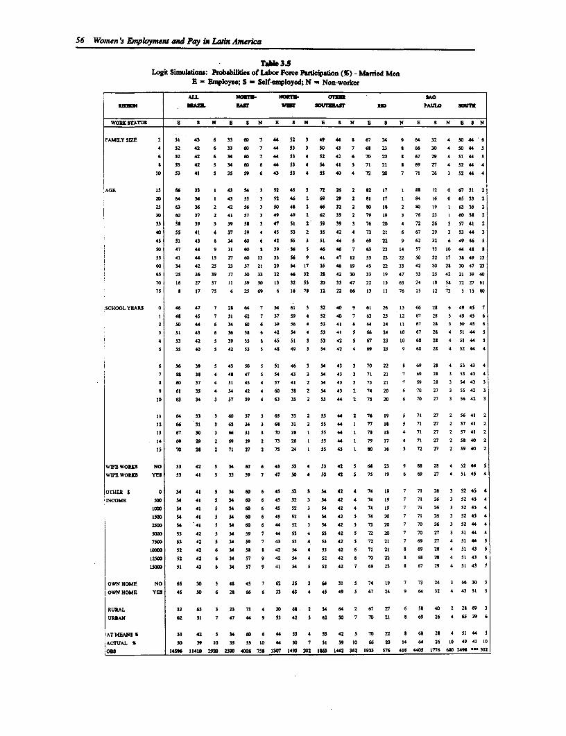
56 Women's Employment and Pay in Latn America
TabIe 35Logit Simulations: Probabilities of Labor Force Participation (%) - Married Men
E - Employec; S - Self-employed; N - Non-worker
ALm NOETZ- NOaTl- arm MO
lBamm BRlAE BAN Wm SoUTwAir RI PAULO SOUKs
WORK IrATUS B S N a S N B S N B S N E S N E S N B S N
FAMILY SIE 2 Sl 43 6 33 60 7 44 32 3 49 44 S 67 24 9 64 32 4 50 44 6
4 52 42 6 33 60 7 44 33 3 50 43 7 6S 23 a 66 30 4 50 44 5
6 52 42 6 34 60 7 44 33 4 52 42 6 70 22 9 67 29 4 51 44 5
S 53 42 5 34 60 6 44 53 4 54 41 5 71 21 8 69 2 4 52 44 4
10 53 41 5 3S 59 6 43 53 4 55 40 4 72 20 7 71 26 3 52 44 4
AGE 15 66 33 1 43 54 3 52 45 3 72 26 2 92 17 1 So 12 0 67 31 2
20 64 34 1 43 55 3 52 46 2 69 29 2 Sl 17 1 S4 16 0 65 33 2
25 63 36 2 42 56 3 50 4S 2 66 32 2 80 is 2 S0 19 1 63 35 2
30 60 37 2 41 37 3 49 49 2 62 35 2 79 19 3 76 23 1 60 392
35 55 39 3 39 SS 3 47 51 2 59 39 3 76 20 4 72 26 2 57 41 2
40 55 41 4 37 59 4 45 53 2 55 42 4 73 21 6 67 29 3 53 44 3
45 51 43 6 34 60 6 42 55 3 SI 44 5 69 22 9 62 32 6 494 5
50 47 44 9 31 60 9 39 56 5 46 46 7 63 23 14 57 33 10 44 489
55 41 44 is 27 60 13 35 56 9 41 47 12 55 23 22 50 32 17 31 49 13
60 34 42 25 23 5 21 29 54 17 35 46 19 45 22 33 42 30 29 30 47 23
63 25 36 39 17 50 33 22 46 32 2S 42 30 33 19 47 33 25 42 21 39 40
70 16 2 57 11 39 50 13 32 55 20 33 47 22 15 63 24 1 53 12 27 61
75 a 17 75 6 25 69 6 16 78 12 22 66 13 11 76 i3 12 73 5 15 S0
SCHOOL YEARS 0 46 47 7 29 64 7 34 61 5 52 40 9 61 26 13 66 29 6 49 45 7
1 49 45 7 31 62 7 37 59 4 52 40 7 63 25 12 67 2S 5 49 45 6
2 50 44 6 34 60 6 39 56 4 53 41 6 64 24 11 67 28 5 50 45 6
3 51 43 6 36 5s 6 42 54 4 53 41 5 66 24 10 67 2S 4 51 44 5
4 53 42 5 39 55 6 43 51 3 53 42 5 67 23 10 6S 28 4 31 445
5 55 40 5 42 53 5 48 49 3 54 42 4 69 23 9 61 29 4 52 444
6 36 39 5 45 50 5 51 46 3 54 43 3 70 22 S 69 29 4 33 43 4
7 SS 35 4 48 47 5 54 43 3 54 43 3 71 21 7 69 29 3 53 43 4
S 60 37 4 51 45 4 57 41 2 54 43 3 73 21 7 69 29 3 54 43 3
9 61 35 4 54 42 4 60 39 2 54 43 2 74 20 6 70 27 3 55 42 3
10 63 34 3 57 39 4 63 35 2 55 44 2 75 20 6 70 27 3 56 42 3
II 64 33 3 60 37 3 65 33 2 55 44 2 76 19 5 71 27 2 56 41 2
12 66 31 3 63 34 3 61 31 2 55 44 1 77 IS 5 71 n7 2 57 41 2
13 67 30 3 66 31 3 70 29 1 55 44 1 71 19 4 71 2 2 57 41 2
14 69 29 2 69 29 2 73 26 1 55 44 1 79 17 4 71 27 2 59 40 2
Is 70 26 2 71 27 2 75 24 1 55 45 1 s0 16 3 72 27 2 59 40 2
WIFEWORXS NO 53 42 5 34 60 6 43 53 4 53 42 5 6S 23 9 68 28 4 5244 5
WIPE WORKS YES 53 41 5 33 59 7 47 50 4 53 42 5 75 19 6 69 27 4 51 45 4
OTHER S 0 54 41 3 34 60 6 45 52 3 54 42 4 74 19 7 71 26 3 52 45 4
INCOME 500 54 41 5 34 60 6 45 52 3 54 42 4 74 19 7 71 26 3 52 45 4
1000 54 41 5 34 60 6 45 52 3 54 42 4 74 19 7 71 26 3 52 45 4
1500 54 41 5 34 60 6 45 52 3 54 42 5 74 20 7 71 26 3 52 45 4
2500 54 41 5 34 60 6 44 52 3 54 42 s 73 20 7 70 26 3 52 444
5000 53 42 5 34 59 7 44 53 4 53 42 5 72 20 7 70 27 3 444
7500 53 42 S 34 59 7 43 53 4 53 42 S 72 21 7 69 27 4 51 443
1000 52 42 6 34 S5 S 42 54 4 53 42 6 71 21 8 69 29 4 S3 433
12500 52 42 6 34 57 9 42 54 4 52 42 6 70 22 8 68 21 4 51 43 6
15000 51 .93 6 34 57 9 41 54 5 52 42 7 69 23 a 67 29 4 3l 43 7
OWN HOME NO 65 30 5 4S 45 7 62 35 3 64 31 5 74 19 7 73 24 3 66 30 3
OWN HOU4E YES 45 50 6 29 66 6 33 63 4 45 49 5 67 24 9 64 32 4 43 51 5
RURAL 32 65 3 23 73 4 30 63 2 34 64 2 67 27 6 59 40 2 29 69 3
URSAN 62 31 7 47 44 9 53 42 5 62 30 7 70 21 9 69 26 4 65 29 6
AT MEANS % 53 42 5 34 60 6 44 53 4 53 42 5 70 22 9 69 29 4 51 44 5
ACTUAL S 50 39 10 35 5S 10 44 50 7 51 39 10 66 20 14 64 26 10 49 41 10
0N 1459 11410 2920 259D 4026 758 1307 1493 202 1963 1442 362 1933 576 416 4405 1776 6S0 24 91 502
Labor Force Behavior and Earnings of Brazilian Womnen and Men, 1980 57
As was the case for wives, the estimates show that schooling proves to be an effectiveexplanatory variable in sorting husbands between wage work and self-employment. Looking atthe predicted probabilities (Table 3.5), we see that additional years of schooling result inconsistent increases in the probability that a working husband is an employee. This is usuallymatched by decreases in the probability that he is self-employed. Of course, the strength of theschooling effects varies from region to region.
Single women' (Table 3.6 and Table 3.7). The logit estimates for single women show that thechildren variables play a minor role in determining labor force status. The coefficient on thebabies variable is statistically significant in only two regions (Northwest and South) and foremployees only. Similarly, the coefficient on the toddlers variable is not significant in mostregions, but it is puzzlingly significant and positive for employees in the Northeast. The presenceof school-age children makes participation more likely as an employee in Rio and as a self-employed worker in Sao Paulo. Household size generally does not have a significant (positive)impact, except in the South and in Sao Paulo for wage work only. Age effects are generallypresent, as expected, for both employees and self-employed women. The coefficients ofasset/transfer income and of home ownership have the predicted negative coefficients, but onlyin determining work as an employee. However, these tend to have a positive effect on theprobability of self-employment. Overall, however, the strength of the effects is small. The proxyfor housework and number of rooms tends to discourage working, especially as an employee.Living in an urban area has a strong positive impact on working as an employee, and a negativeeffect on self-employment.
Finally, we remark on the important role of education in determining labor force status. As wasthe case for married women, increasing school attainment increases the probability of working,but mostly as an employee. Only in the Northeast does education have a positive effect on self-employment. It is interesting to note that regional differences in schooling effects are not asstrong among single women as among married women. For example, in Rio and Sao Paulo, themarginal effects of the education variable for employees are 0.029 and 0.031, respectively,suggesting that an additional year of schooling increases the probability of being an employee byabout 3 percent. In the other regions, the partial derivatives of education for employees rangefrom 0.025 to 0.039. The predicted probabilities in Table 3.7 show that an additional year ofschooling in excess of 5 years increases the probability of working as an employee from 28percent to 32 percent. Similarly, an increase from 10 to 11 years raises the probability from 48percent to 52 percent. In sum, the main effect of education is to increase the propensity of singlewomen to work as employees.
Single men (Tables 3.8 and 3.9). The estimates for single men reflect the choice betweenworking as an employee or being self-employed. Unfortunately, the set of regressors excludeshousehold characteristics and, perhaps more important, migrant status because no information wasprovided in the data set. Nationally, 41 percent of the men did not complete any schooling,especially those who were self-employed - 64 percent versus 33 percent for employees. In theNortheast the respective proportions rise to 84 percent and 53 percent, while in Rio and SaoPaulo they are 37 percent and 25 percent.
24 The reader should note the small number of self-employed single women in the Northwest, theOther Southeast, and Rio. We do not comment on these results for obvious reasons.
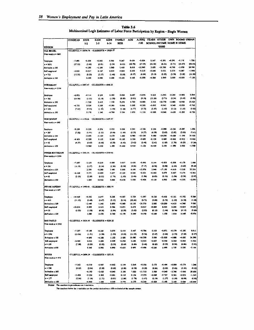
58 Women's Employment and Pay in Latin America
Table 3.6Multinominal Logit Estimates of Labor Force Participation by Region - Single Women
CONSTA-N KIDS KICS KIDS FAMILY AGE ASESQ YEARS OTHER OWN ROOMS URBAN0-2 3-5 6-14 SIZE 1100 SCHOOLINCOME HOME N HOME
REGION '000ALL fRAZIL -2LLKFltLL - 1074.74 -2LIJRlt .19320.57
Noa-t a -.6601
E-bt*- -7.493 -0.199 -0.042 0.0es 0.067 0.424 -0.634 0.167 -0.31 -0.291 -0.117 I.25*
-3871 (27.22) (3.66) 607.S) (2.24) (4.62) (20.70) (11.25) (21.50) (6.21) (5.71) (14.47) (10.41)
""tin x 100 -4.190 -1.190 1.060 1.410 8.610 -12.960 3.620 -11.310 -6.760 -3.630 20.340
S1f-pl.oyd -5.010 -0.017 0.17 0.059 0.002 0.242 -0.313 -0.040 0.031 0.371 -0.067 -1.04s
a - 753 (12.32) (0.20) (2.37) (1.46) (.08) (Mm7) (6.64) (3.19) (0.23) (3.78) (3.29) (11.30)
daintv- . 100 0.230 0.990 0.200 -0.100 0.520 -0.530 -0.500 0.990 2.30D -0.050 -7.130
NORTHEAST -2LUFULL =3987.47 -2LLXRESTR = 4943.33
N--o .a -21356
E,p1oyjc -8.S32 -0.114 0.229 0.102 0.020 0.437 -0.616 0.213 -1.042 -0.2US -0.0OU 0.S49
a-561 (14.06) (1.01) (2.1S) (1.90) (.S9) (9.93) (0.1) (12.26) (3.71) (2.34) (3.19) (5.90)
d. .v.t x 100 -1.300 2.410 1.250 0.270 4.730 -6.690 2.510 -t0.770 -3.300 -0.950 10.420
Sctf-pl.ycd -4.731 0.OD6 0.169 -0.005 0.040 0.202 -0.260 -. 092 -0.941 0.540 -0.039 -0.762
= 328 (7.63) (0.03) (1.46) (1.40) (1.21) (4.77) (3.72) (3.37) (1.45) (3.13) (1.30 (0.02)
d,i,ia,. 100 0.170 1.040 -0.760 0.330 1.070 -1.310 -0.930 -6.040 4.420 -042D -6.720
NORTHWEST -2LLKFULL = 1176.00 -2LLKRESTR-1497.97
Noa-.k a -646
E0.ptlyao -9.239 -0.329 -0.274 0.055 0.06 0.001 -0.760 0.196 -0.900 -0.536 -0.097 L.303
*-2S7 (7.92) (1.91) (1.53) (0.60) (1.f6) (5.35) (4.27) (6.35) (2.6S3 (.02) (2.03) (5.41)
danvativa x 100 -S.PO -5.130 0.670 1.660 S.S60 -13.530 3.6S0 -1S.330 -9.420 -1.590 24.150
Self-aploycd -8.M53 -0.230 0.152 0.540 -0.160 0.516 -0.650 -0.158 0.640 -0.662 -0.015 -0.460
*=42 (4.37) (0.60) (0.46) (3.03) (1.43) (3.42) (A.4) (2.42) (1.63) (3.70) .20). (1.26)
dc.n6,. 100 -0.360 0.530 1.240 4.440 0.950 -1.12D -0.500 2.190 -1.290 0.020 -1.920
alHR SOtJIEAST -2LLKXFULL = 2261.91 -2LLKRESTR - 27079.81
N_oa-k a = 1086
Eap4oyaa -7.687 0.10 -0.019 0.083 0.037 0.430 -0.643 0.144 -0.S35 -0.208 -0.170 1.600
-5=1 (10.19) (1.07) (0.14) (1.34) tO.96) (8.56) (7.17) (6.96 (2.98) (1.56) (0.62) (9.4)
d&,ivwU x 100 2.590 -0.3S0 1.4S2 0.890 S,590 -12.070 2.940 -17.150 -4.610 -3.320 35.270
SaOf-mploya.d -4.410 0.371 -0.009 0.257 -0.153 0.243 -0.331 -0.002 0.079 0.427 -0.174 -0.902
*-65 (3.19) (2.09) tO03) (1.75) (1.63) (2.43) (1.99) t7.03) tO.16) (1.36) (7239) (2.97)
dcxfivnti x 100 1.500 -0.010 0.660 -0.470 0.330 -0.400 -0.120 0930 1.390 -0.350 -3.970
RIO DE JANtERO -2LLKWULL . 1490.41 -2LLKREsTR = 13.-19
N- a - 697
EaPac . -10.629 -0.092 O.077 0.266 -0.007 0.729 -1.097 0.126 4.432 -0.11 -0.192 0.329
-453 (11.12) (0.48) (0.47) (3.12) (0.14) (10.34) (0.75) (5.09) (1.72) (I.09 (4.58) (1.010
dcdv.t.1xIOD -2.440 1.540 5.690 -o0.090 6.130 -24.370 2.040 -10.230 -4.410 -4.340 9.0f0
5.1-*oaoya -10.014 0.393 0.213 0.306 -0.071 0.472 4.617 .0009 0.453 0.334 4.014 4.243
-32 (3.03) (1.00) (0.56) (3.94) 3-5)3 (3.62) (2.9S) 3)033 (1.46) .)76) (0.15) (0.36)
d&.va O. 00 I'.0S 0.470 0.740 -0.170 0.540 -0.570 -. 140 1.550 1,010 0.140 -0.970
SAO PAULO -2LLWPULL . 3614.49 -2LLXRESTR -4224.22
Nc-ot* a - 1043
Eaaocy -7.237 -0.1S6 -0.153 0.070 0.153 0.467 0.706 0.123 4.971 4.179 0.192 0.911
a = 1391 (13.05) (1.30) (1.30) (1.32) (5.03) (11.33) (9.36) (7.67) (5.04) (1.78) (7.29) (3.57)
dcrniv. x.100 -4.690 -4.180 1.130 3.350 I0.530 -16.210 3.090 -23.t20 -4.30 -4.630 24.390
0-mLpo-Y'd -B.303 0.055 0.209 0.309 -0.034 0.480 -0.615 -0.027 -0.056 0.242 -0.044 -1.014
a -109 a 7.0 t0.2DU)P2 a59) (0.49) (S.0S0 (5.40) (0.ttS (0.23) (0.99) (0.84) (3.91)
danv.ia .400 0.540 0.90 0.090 -0.410 0.690 -0.690 -0.330 1.690 1.150 0.223 -5.130
SOUTH -2LLKFULL -2604.34 -2LLKRESTR =3233.61
Na-ok a - 973
E.playa. -7.262 -0.310 -0.087 -0.002 0.139 0.360 -0.550 0.175 -0.414 -0.099 -0.174 1.246
_ -99S (9.6S) (2.04) (0.59) (0.03) (3.90) (6.5S) (5.28) (0.24) (2.63) (0.65) (3.54) (0.62)
deoooiv x ID00 -6.190 -2.42D -0.040 3.190 7.620 -11.310 3.923 -9.040 -2.540 -3.630 29.630
Self-mployed -3.408 -0,250 0.305 -0.001 0.119 0.136 -0.75 0.0t9 0.737 0.361 4.053 -1.545
a- 177 (3.04) (1.16) (1.71) (0.01) (0.94) (1.79) (.67) 2.0 19) (0.37) (1.59) (0.99) (090)
drivtiw. . 10 0.323 1.330 O 0.370 0.170 -0.510 -0.s20 -3.190 2.160 0-030 -10 840
Notes: 7hc oataban in p xa 0a. -no.a
Th. a-bmtc t0 tMs t-timk ..s l tt c p.Iti.1 d-i.fti-e x 100 -vh4tV4 a th.c .w
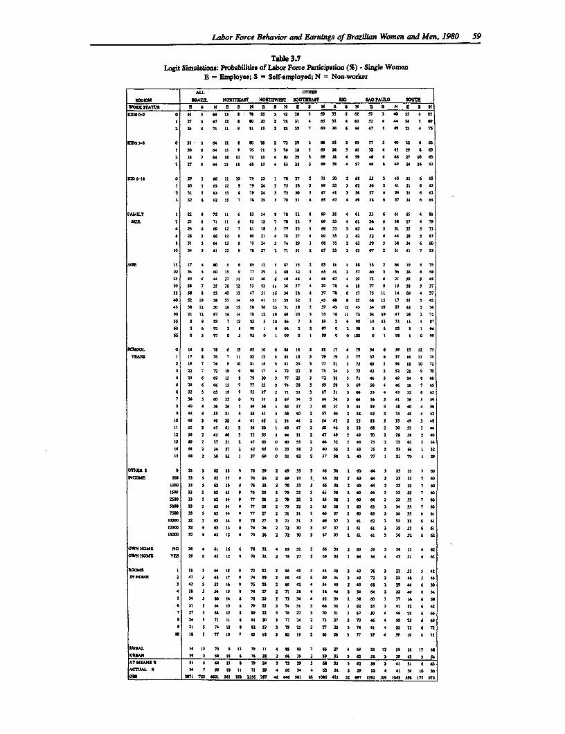
Labor Force Behavior and Earnings of Brazilian Women and Men, 1980 59
TaIe 3.7Logit Simulations: Probabilities of Labor Force Participation (%) - Single Women
B = Employee; S = Self-employed; N = Non-worker
AM OT.
304 0RAWL NoonEAsT NORTUWr S0UIT 1B3 AAO PAULo SOUTHWORXSTATlS E 2 N E S N B S N B 3 N a S N B S N e S N
1MS0-2 0 31 S 6413 2 7n 26 3 7 28 69 33 2 62 37 3 40 32 6 62
3 27 s 67 12 6 o2 20 2 71 31 4 65 32 4 62 32 4 44 26 3 69
2 24 6 71 1i 9 31 is 2 23 33 7 60 30 6 64 47 3 4 21 4 75
103-S5 0 32 S 6412 U * 26 2 72 29 3 6333 M 63 37 3 40 2 6 6
2 30 6 64 LS 9 76 21 3 76 22 3 69 46 3 61 52 4 43 29 * 63
2 26 7 64 22 10 72 16 4 ID 22 3 69 38 4 59 4* 6 44 27 30 63
3 2 9 64 22 I2 49 13 4 33 23 2 29 39 4 57 44 * 49 24 24 62
lD6-14 0 29 2 66 11 10 79 23 1 76 27 2 72 30 2 6a 33 3 43 31 6 63
1 30 5 62 22 9 79 24 2 75 23 3 69 33 3 62 56 3 42 31 6 63
2 3L 5 63 13 2 79 24 3 73 30 3 67 41 3 56 37 4 39 31 6 63
3 32 6 62 23 7 73 25 5 70 31 4 65 47 4 49 St 6 37 31 6 63
PAMIILY 1 32 6 72 1l 6 23 14 S 78 22 2 69 35 4 62 33 6 62 15 4 21
sZe 2 23 6 71 12 6 82 25 7 76 23 7 69 33 4 62 36 6 53 17 4 79
4 26 6 69 12 7 21 1t 5 77 25 5 69 3M 3 62 44 s Sl 22 5 73
6 29 5 66 12 S 30 21 4 76 27 4 69 3M 3 62 52 4 44 23 5 67
9 31 $ 64 13 2 79 24 3 74 29 3 6a 35 2 63 59 3 33 34 6 60
10 34 5 St 13 9 72 27 2 71 31 2 07 33 2 63 67 2 31 41 7 53
AOl 1s 17 4 60 6 6 29 12 1 37 25 2 83 12 1 U 3S 2 64 29 6 73
20 34 5 60 25 9 77 29 3 6a 32 3 63 42 3 17 60 3 36 36 6 S2
25 50 6 44 27 St 63 44 6 46 46 4 42 67 4 29 73 6 21 53 5 45
30 53 7 35 36 12 52 53 12 36 57 4 39 72 4 12 77 a 25 532 3 7
33 s3 a 33 40 13 67 St 16 34 53 4 27 79 6 17 75 12 14 60 4 37
40 52 13 22 37 24 49 41 22 31 52 2 43 62 2 23 63 l5 17 3S 2 42
45 32 12 s0 29 is St 26 23 S1 33 5 37 4S 22 43 34 29 27 43 3 54
50 22 12 67 16 24 70 22 19 69 20 5 75 26 1 73 34 19 47 26 2 71
55 a 9 23 7 12 U2 3 10 26 7 3 39 2 6 92 '2 23 73 1 1 37
40 2 6 92 2 2 90 1 4 96 2 2 97 o 2 94 s 5 92 3 1 96
62 o 3 97 0 5 9 0 1299 0 1 99 0 02 71 0 1 92 1 o 99
slooL a 24 t 76 6 15 22 23 4 64 26 3 St 2 4 79 34 6 36 23 12 75
YEA"S I 27 a 76 121 02 12 5 23 1t 3 79 19 3 77 37 6 57 16 21 74
2 19 7 74 9 20 It 24 5 31 20 3 77 22 3 73 40 5 54 It 20 72
3 22 7 72 20 9 60 27 4 79 22 3 73 24 3 73 43 5 52 22 9 70
4 25 6 69 23 * 79 20 3 77 25 3 72 26 3 71 46 3 49 24 a 63
5 23 4 66 13 7 77 23 3 74 23 3 69 28 3 69 50 4 46 23 7 63
6 n 5 22 29 7 73 27 2 71 31 3 67 32 3 66 53 4 43 32 6 62
7 36 5 60 22 6 72 32 2 67 34 3 64 34 3 64 56 3 41 36 5 39
2 40 4 56 26 3 69 36 1 63 37 3 60 37 3 61 59 3 33 40 4 56
9 44 4 33 31 4 65 41 1 St 40 2 57 40 2 3t 62 3 35 43 4 32
20 46 3 49 35 4 6 45 1 54 0 4 2 s 43 2 SS 653 3 49 3 48
22 52 3 45 42 3 56 so 6 49 47 2 s0 46 2 32 a3 2 30 33 3 44
22 56 2 4 4 46 2 32 SS 1 44 3S 2 47 49 2 49 70 2 23 33 2 40
13 60 2 37 31 2 67 60 0 40 53 2 44 32 2 46 73 2 23 62 2 36
14 64 2 34 27 2 42 63 0 3M 53 2 40 5S 2 42 73 2 23 66 1 32
13 64 2 36 62 1 37 69 0 22 62 2 37 53 2 40 77 1 21 70 1 29
OTH S 0 33 5 22 IS 9 76 29 2 69 33 3 65 32 2 60 66 3 33 33 7 40
"IWOIE soo 33 5 62 5 9 76 23 2 6633 3. 65 3 2 60 64 3 332 3 7 60
2ow 33 5 62 l5 9 76 2 2 70 33 3 65 32 2 60 64 3 33 33 7 60
2360 33 5 6 15 9 76 2* 2 70 32 3 65 32 2 40 64 3 53 33 7 60
2360 33 5 62 14 9 77 20 2 70 S2 3 65 3S 2 60 64 3 33 33 7 60
soo 33 5 62 14 9 77 23 2 70 32 3 65 32 2 60 62 3 34 33 7 60
7500 33 3 62 14 9 77 27 2 72 32 3 66 37 2 60 63 3 34 32 6 61
IC= 32 5 6 24 9 72 27 2 72 31 3 66 27 2 42 62 3 05 33 6 42
12500 32 5 63 22 2 72 26 2 7n 30 3 67 37 2 62 61 2 35 32 6 61
13000 n 3 63 13 3 79 26 2 72 30 3 67 37 2 62 61 3 36 32 6 62
OWINHOMi NO 36 4 61 16 6 72 32 6 n2 2 66 43 2 60 59 3 32 3 4 62
OWN KO3R4f YES 29 6 6S 3 2 9 7 22 2 76 n 3 69 33 364 a 4 4 42 22 6 63
RO2S I 51 S 44 IS 9 72 32 2 66 49 s 46 3s 2 40 76 2 22 32 s 42
IN HOME 2 47 3 42 27 9 74 30 2 63 4 5 30 34 2 45 7 3 23 4 5 46
3 42 5 52 26 9 73 22 2 69 42 4 34 49 2 49 63 2 29 44 6 30
4 32 5 56 25 9 76 27 2 71 23 4 St 44 2 34 64 3 33 40 6 34
5 34 5 66 14 * 72 23 2 73 34 4 42 39 2 52 40 2 n7 36 6 53
4 S3 5 24 12 * 79 23 3 74 32 2 66 23 2 62 23 3 42 22 6 42
7 27 3 6 12 & 60 22 2 76 27 3 70 2 3 6?7 60 4 44 29 6 66
2 24 s 72 12 S 22 20 2 77 24 2 73 27 2 70 46 4 s0 22 * 69
9 22 s 74 10 * 32 19 3 79 21 2 77 23 3 74 42 4 35 22 6 7n
2o Is s 77 10 7 3 It 3 60 29 2 6 20 3 77 37 4 S3 19 4 71
RUIRAL 24 23 73 n 23 79 1 4 62 20 7 a3 27 4 69 2 122 33 16 17 6a
URIA 39 3 22 Is 6 76 32 2 66 39 2 51 35 3 62 St 3 39 43 3 54
ATMEANS 32 * 6423 2 7924 27322 3 633 242 36 3 4231 452
ACrUAL S 34 7 S9 Is 22 72 29 4 66 34 4 6 36 3 39 50 4 41 34 2036
ot 2S72 723 662l 362 32S 2136 227 42 646 322 63 2026 433 n 697 2392 271 2063 s99 277 973
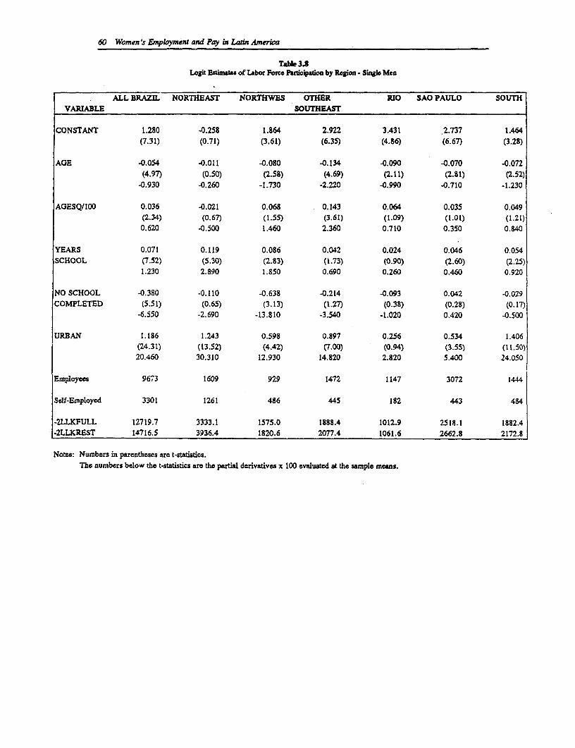
60 Women's Ernployment and Pay n Latin Arica
Ta 3.8Logit Esimate. of LAbor Force Paticipation by Region - Sngle. Men
ALL BRAZIL NORTHEAST NORTHWES OTHER RIO SAO PAULO SOUTHVARIABLE SOUTHEAST
CONSTANT 1.280 -0.258 1.864 2.922 3.431 2.737 1.464(7.31) (0.71) (3.61) (6.35) (4.86) (6.67) (3.28)
AGE -0.054 -0.011 -0.080 -0.134 -0.090 -0.070 -0.072(4.97) (0.50) (2.58) (4.69) (2.11) (2.81) (2.52)
-0.930 -0.260 -1.730 -2.220 -0.990 -0.710 -1.230
AGESQ/100 0.036 -0.021 0.068 0.143 0.064 0.035 0.049(2.34) (0.67) (1.55) (3.61) (1.09) (1.01) (1.21)0.620 -0.500 1.460 2.360 0.710 0.350 0.840
YEARS 0.071 0.119 0.086 0.042 0.024 0.046 0.054SCHOOL (7.52) (5.30) (2.83) (1.73) (0.90) (2.60) (2.25)
1.230 2.890 1.850 0.690 0.260 0.460 0.920
NO SCHOOL -0.380 -0.110 -0.638 -0.214 -0.093 0.042 -0.029COMPLETED (5.51) (0.65) (3.13) (1.27) (0.38) (0.28) (0.17)
-6.550 -2.690 -13.810 -3.540 -1.020 0.420 -0.500
URBAN 1.186 1.243 0.598 0.897 0.256 0.534 1.406(24.31) (13.52) (4.42) (7.00) (0.94) (3.55) (11.50)20.460 30.310 12.930 14.820 2.820 5.400 24.050
Employees 9673 1609 929 1472 1147 3072 1444
Self-Employed 3301 1261 486 445 182 443 484
-2LLKFULL 12719.7 3333.1 1575.0 1888.4 1012.9 2518.1 1882.4-2LLKREST 14716.5 3936.4 1820.6 2077.4 1061.6 2662.8 2172.8
Notes: Numbers in parentheses are t-statistics.The numbers below the t-statistics are the partial derivatives x 100 evaluated at the sample means.
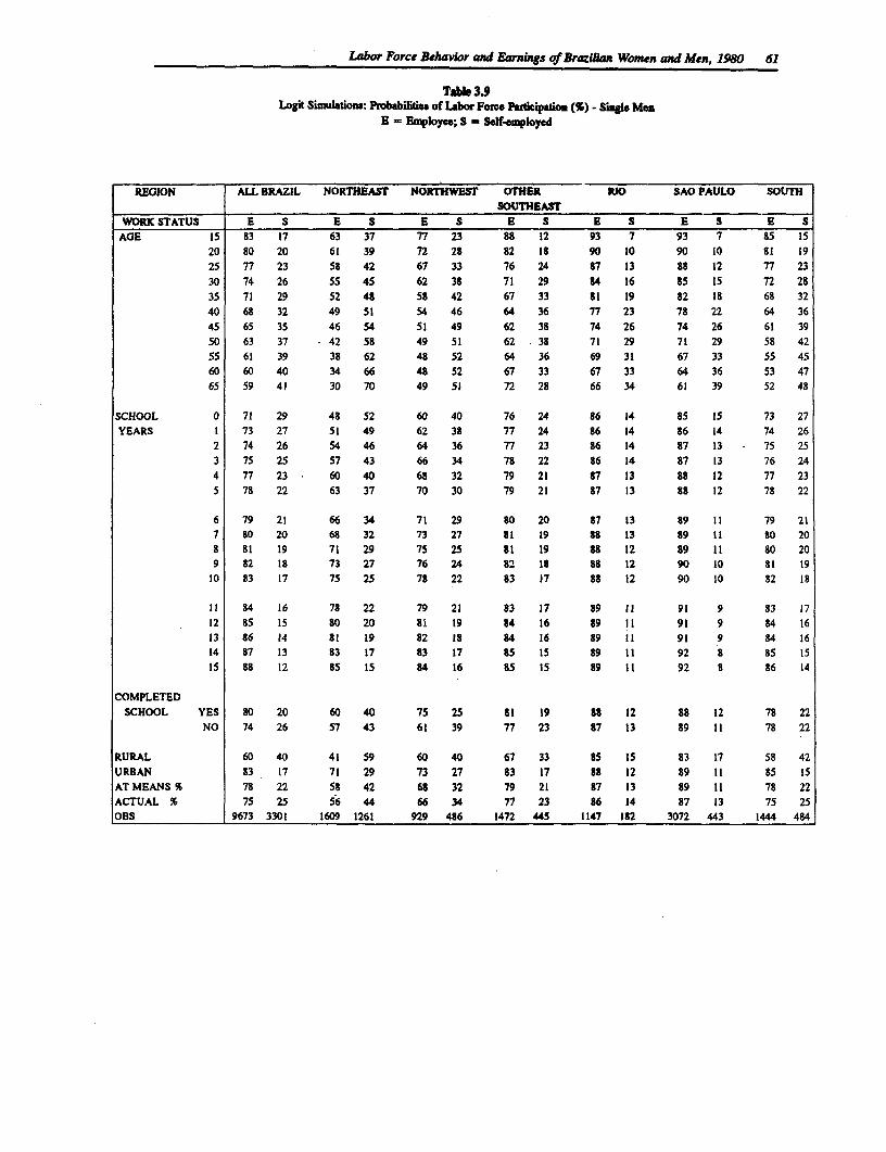
Labor Force Behavior and Eanings of Brazilian Women and Men, 1980 61
Tabl 3.9Logit Simulations: Probabilitie, of Labor Formc Paticipatio () - Single Men
E Employee; S - Self-employed
REGION ALL BRAZIL NORTHEAST NORTHWEST OTHER RIO SAO PAULO SOUTHSOUTHEAST
WORK STATUS E S E S E S E S E S E S B SAGE 15 83 17 63 37 77 23 88 12 93 7 93 7 85 15
20 80 20 61 39 72 28 82 IS 90 10 90 10 81 1925 77 23 58 42 67 33 76 24 87 13 88 12 77 2330 74 26 55 45 62 38 71 29 84 16 85 is 72 2835 71 29 52 48 58 42 67 33 81 19 82 IS 68 3240 68 32 49 51 54 46 64 36 77 23 78 22 64 3645 65 35 46 54 51 49 62 38 74 26 74 26 61 3950 63 37 42 58 49 51 62 .38 71 29 71 29 58 4255 61 39 38 62 48 52 64 36 69 31 67 33 55 4560 60 40 34 66 48 52 67 33 67 33 64 36 53 4765 59 41 30 70 49 51 72 28 66 34 61 39 52 48
SCHOOL 0 71 29 48 52 60 40 76 24 86 14 85 15 73 27YEARS 1 73 27 51 49 62 38 77 24 86 14 86 14 74 26
2 74 26 54 46 64 36 77 23 86 14 87 13 - 75 253 75 25 57 43 66 34 78 22 86 14 87 13 76 244 77 23 60 40 68 32 79 21 87 13 S8 12 77 235 78 22 63 37 70 30 79 21 87 13 88 12 78 22
6 79 21 66 34 71 29 80 20 87 13 89 11 79 217 80 20 68 32 73 27 81 19 88 13 89 11 80 208 S 19 71 29 75 25 at 19 88 12 89 11 80 209 82 18 73 27 76 24 82 18 88 12 90 10 81 19
10 83 17 75 25 78 22 83 17 88 12 90 10 82 18
11 84 16 78 22 79 21 83 17 89 11 91 9 83 1712 85 15 80 20 81 19 84 16 89 11 91 9 84 1613 86 14 81 19 82 18 84 16 89 11 91 9 84 1614 87 13 83 17 83 17 85 15 89 11 92 8 85 1515 88 12 85 15 84 16 85 Is 89 11 92 8 86 14
COMPLETEDSCHOOL YES S0 20 60 40 75 25 81 19 88 12 88 12 78 22
NO 74 26 57 43 61 39 77 23 87 13 89 11 78 22
RURAL 60 40 41 59 60 40 67 33 85 15 83 17 58 42URBAN 83 17 71 29 73 27 83 17 88 12 89 11 85 1IAT MEANS % 78 22 58 42 68 32 79 21 87 13 89 it 78 22ACTUAL % 75 25 56 44 66 34 77 23 86 14 87 13 75 25OBS 9673 3301 1609 1261 929 486 1472 445 1147 182 3072 443 1444 484
62 Women's Employment and Pay in Latin America
The results show that the probability of holding a wage job decreases with age, but the coefficienton age squared is generally not significant. In all regions, living in an urban area stronglyincreases the probability of being an employee. The urban effect is especially strong in theNortheast and the South.
Once again, the education effects are interesting. In most instances, (the Northwest is theexception), uncompleted schooling is not an important factor in determining the type of job.'The amount of schooling, however, does play a role in the Northwest, the Northeast, and theOther Southeast. In the remaining regions, the coefficient of the schooling is not significant. Thesimulations generally reflect the pattern found for single women. For example, an extra year ofschooling raises the probability of being an employee by about 3 percentage points.
5. Wage Determinants
The analysis of wage determinants is based on the human capital framework developed by Becker(1964) and Mincer (1974). This provides the theoretical base for the study of wages as a functionof productivity-enhancing variables. We estimate a wage function where the dependent variableis the natural log of the hourly earnings (including cash in-kind payments) which is obtained bydividing monthly earnings by weekly hours times 4.33. In doing so, we assumed that theindividual worked for the entire month.
The regressors are the inverse of the Mills' ratio, potential work experience (age - 6 - years ofschooling), experience squared (divided by 100), years of education, dummy variables indicatingpublic sector employment, contributions to social security, urban and state residence. Since dataon actual work experience are not reported, the set of regressors in the female wage equationsalso include the number of babies ever born, which is used to reflect interruptions in potentialwork experience.
Wage Functions - The Issue of Selectivity Bias
Now, we consider the specification of the wage function:
Let: C1 = 1, if the person is an employee (1), 0 otherwise;C2 = 1, if the person is self-employed (2), 0 otherwise;C3 = 1, if the person does not work (3), 0 otherwise;
The wage function in the jth work-status is given by:
lnW1 ={ zaj + ,j if C, = 1, j = 1,2O otherwise
where lnWj is natural log of the wage, z is a (row) vector of wage-determining characteristics,which has some elements in common with x, Ca is a vector of estimated parameters and Oj is theerror term. If the individual does not work a = 3), then no market wage function is observed.
Traditional OLS estimation of the wage function may produce biased and inconsistent parameterestimates owing to selectivity bias because the observations on earnings by job alternative are not
2 The data showed that the proportion of single men who did not complete any schooling was muchhigher than that of single women.
Labor Force Behavior and Earnings of Brazilian Women and Men, 1980 63
randomly distributed. The selectivity bias correction term (A) for the multinomial logit choicecase is derived using the transformation of Maddala (1983, p.275). That is, ^ = O[Jy(xy)] /F(x,y), where 0 is the standard normal distribution function, F is the logistic distributionfunction, and the transformation J = 0-F. Thus, for each work-status wage regression a = 1,2) X can be included as a regressor.
ln Wi = z + , icA+ s
In sum, because decisions about labor force status as well as wage offers influence the observedwage structure, corrections for selectivity bias are needed to obtain consistent parameter estimatesof the wage determinants.
Empirical Estmates
Married women. Table 3.10 shows that the effect of the selectivity correcting variable amongwives varies across regions and work status. At the national level, both the employee and self-employment wage regressions are subject to selectivity bias. However, a region by regioncomparison seems to tell a different story. In three regions, the Northeast, the Northwest, andthe Other Southeast, the coefficient of Lambda is not statistically significant in either of the wageregressions. Both wage regressions for Rio are subject to sample selection bias - the coefficienton Lambda is positive and significant in the wage function of employees, and negative andsignificant in that of the self-employed. In Sao Paulo and the South, the coefficient of Lambdais negative and significant only in the wage regression for employees.
The coefficients of the best available work experience variables in the data are generally asexpected, but there are regional variations. Experience effects do not appear to be present in thetwo wage regressions for the Northwest, and in that of the self-employed in all regions, exceptthe Northeast where the coefficients on all experience variables are statistically significant. Inthe national wage regressions, all experience coefficients are statistically significant, suggestingthat there may be geographical aggregation bias" in assessing returns to work experience.Moreover, there are also some regional differences in the magnitudes of the coefficients of theexperience variables (especially experience squared) of employees.
Because the measure of work experience for wives is imperfect we also included the number ofchildren ever-born in an attempt to capture interruptions in potential work experience.Nationally, the coefficient on this variable is statistically significant and negative (-0.033 foremployees and -0.036 for self-employed). However, this proxy for discontinuity in workexperience met with limited success in the region-specific regressions. The parameter estimatesare significant only in wage regression of employees the Northeast (-0.025) and in Sao Paulo(-0.021).
In most regions the coefficient estimates of the effects of having a job in the public sector are notsignificant and, in one case (the Northeast) it is unexpectedly significantly negative (4.286).Only in Rio does public sector employment have a positive effect of about 16 percent on wages.
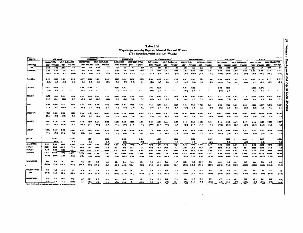
Talie 3.10Wage Regmessions by Region - Marred Men and Womien
fThe dependent variable is: LN WAGE)
a~~~uoe~~~~~ ALL BAsZIL 8b0M1102T 04007H(0507 0)r*0 4mOH Zr 100 DE JA4E20O RAN PAULO 8017175*1lOY M.-E06wIYU Em[POFER IML-MGWlo fl 04913Y0 502I'.P-8*0 YED 064?WY0 OBu-09wy0 EMPLOYOO SEP-02PLOYMI BIPLOyF0 89ELP-EM4007ED 0IWLYI 3EL-EMPOWYED
00145W 3741 11410 Isis 2500 050 4026 347 1307 323 1493 117 1*63 337 1442 175 1933 553 576 143 4403 1179 1776 311 2408 697 5W97 2COO4STA24T ~~2.390 1.752 2.133 LI22 2,334 1.31 2.142 1.527 2.2*5 2.094 2.646 3.11* 2.429 2.659 2.051 18*14 3.255 2233* 2.2*2 3.014 3*70G 2.293 2.560 2039 2.60) I70 2354 2.343
154.3 (25.3) 434.51 (12.4) (14.4) (LI1) (19.4) (6.1) (19*3) (0.3) (16.2) ISM2 (39.2) (9.7) (14.5) 43.7) (14.3) (12.)) (80.9) 47.3) (25.4) (2.5) (59.2) (5.1) (26.9) 484.43 (16.5) (4.4)
OD601A -0.95 -4.397 0.247 0.3)3 40.117 -0.222 0.21t 0.166 0.027 -0.122 0.002 -0.0)2 -0.2.04 0.0262 0.324 0.714 -0.622 -0).203 1.271 3.440 -0.184 -0.430 1.779 0,832 -0.203 -0.226 0.27) -0279(6.0 (6.3) (4.5) (2.8) 42.5) (1.6) (2.24 (0.41 05.4) (0.7) (2.05 01.1) (2.6) (1.7) (20) (1.2) (4.03 (2.2 (3.01 (2.64 (10.3) (7.1) (6.A) (1.04 (4.7) (2.83 (1.34 05.4)
SECPU* -0.070 -0).207 - - -0.094 -0.2506 0.150 -0.025 0.022 0.1209 - -0.056 0.135 - -0.078 0.049 ---. 022 0.07* 8(4.7) (4.0) - - (2.S) 44.2) - (.1) 05.3) - 0.3) (1.7) - -(2.5) (2.4) - -(50) (1.1) ODA05) (1.4) --
SOC3IC 0.272 0.334 0.465 0,600 0.203 0.441 0.467 0.743 0.061 0.206 0.303 0.602 0.349 0.304 0.421 0.622 0.08 0.1*2 0.317 0.258 0.521 0.318 0.373 0.529 0.228 0.415 0.415 0.521(12*3) (22.2) 422.3) (9.0) (0.4) (53.5 (22.6) (5.0) (1.4) (2.6) (3.22 45.2) (0.6) 44.51 (7.2) (3.0) (1.8) (2.3) (7.34 (1.7) (10.6) (7.7) (8.7) (4*8) (6.3) (6.5) (8.45 (039
EXPS 0.062 0.05 0.032 0.027 0.032 0.081 0.029 0.061 0.009 0.003 0.031 -0.013 0.030 0.032 0.056 0.012 0.041 0.034 0.012 -0.044 0.029 0.032 0.002 0.036 0.036 0.039 0.032 0.027422.05 (9.9) (10.3) (2.3) (6.7) (2.3) (2.8) (2.2) (8.2) 05.3) (3.7) 20.3) (6.7) (7.7) (4.1) 05.3) (7.8) 453-) (1.2) 42.7) 48.3) (6.2) 40.23 (2.7) (8.03 44.42 (0.1) (13)
E0Ps3/1018 -0.065 -0.040 -0,03* -0.023 -0.044 -0.042 -0.023 -0.062 -0.069 0.016 -0.041 0.0(3 -0.032 -0.041 -0.042 0.002 -0.077 -0I.04 -0,0i1 0.082 -0.072 -0.044 -0.007 40.065 -0.061 -0.0.55 -0.027 -0.057122.6) 46.2) (8.03 (2.0) (6.22 (2.2) CI.2) (241) (7.3) 0-5.5 (3.53 05.2) (7.0) (2.7) (3.7) (05.0 05.5) (2.4) 0D.75 42.0) (25.51 (4.03 05.6) (1.3) 0573 (3.0) (3,5) (2.31
Y820ESUC 0.147 0.156 0.230 0.125 0.240 0.170 0.1.2 0.195 0.132 0.152 0.13D 0.13) 0.134 0.154 0.136 0.152 0.154 0,166 0.126 0.131 0.22* 0.152 0.095 0.227 0.130 0.129 0.12 0.897(04.2) (39.2) (47.0) (24.)) (20.7) (23.2) (26.4) (5.9) CZ.24 (9.5) 413.8) (4.5) (27.3) (10.7) 414.0) (4.0) (42.0) (10.0) (23.01 (6.4) 00.3) (2.9) (23.2) (7.5) 021.4) (14.43 (16.4) (4*8)
URBAN 0.326 0.547 0.437 0.467 0.145 0.214 0.449 0.321 0.150 0.M90 0.520 -. 315 0.314 0.170 0.392 0.370 0.207 0,016 0.34) 0.026 0.426 0.215* 0.400 0.367 0.341 0.187 0.322 0.270(27.5) (2.2) (12.2) (7.4) 43.0) (2.61 48.0) 0.21) (2.8) (2.6) (5.3) (1.4) (4.0) (1.7) (3.83 (2.6) (.3.) 05.1 (2.84 05.2) (13.2) (3.4) (4.8) (1.0) (8.1) (2.7) (0. 1) 42.7)
050701 - ~~~~~~-0.033 - 40.036 - -0.025 - 40.024 - -0.8* - 4.022 - -0.005 - -0.042 - -0.016 - -0.037 - -. 021 - 4.023 - -0.023 - 4.014- (7.2) - (4.7) - (L.S) - (2.5) - 05.5) 05.7) - 0-5.3 - (I.01 - 42.3) - 25) -(32 (2.3) - (1.3) -(2.3)
RFQIA*D 0.551 0.364 0.414 0.449 0.515 8.539 0.300 0.29 0.494 0.541 0.292 0.330 0.045 0.644 0.309 0.421 0.576 0.634 0.460 0.510 0.50 0.663 0.373 0.436 0.502 0.563 0.778 0.3490-TT 2555.1 421.3 2541.4 871.6 54.2 20.9 207.3 51.0 2*1.1 46.5 M0.] 1.8 317.6 78.5 140.0 27.1 573.4 139.53 20.0 39.0 067.81 261.4 173.2 33.4 350.2 120.0 156.5 24.8
ERR60 6.309 0.633 0*28a 0.2 0.0-55 I 0.79 ol .2 8.625 0.622 0.761 0.807 0.542 0.5115 G.W 030) 0606 0.605 0.722 0.78* 8.542 0.322 0.7021 05541 0.336 0.513 0.850 0.2411.4WAGE 3,0553 5.6679 3.6764 3 3.20 5.0581 3.1646 .1369 2.055 3.233 3.0096 5,739 5.2339 3.607 3.559 3.7239 3.250 42422 3.9705 4.3106 3.7513 4.261 3.0315 4.424 3.0644 3.23 35.030 3.200 3.4243
(0-29 (05965 (1.07) (12.3) 0591) (1"8 (0.06) (21.083 405.6) 14.8 05.80) (1.005 05.20) 05.n7 (1.010 (114) (0.43) (1.02) 05.48) (1.18 (0.24) 05.as) (G.48 (8.081 05.76) 0.71) (2.01) O5."8
WAGEJIHOUR 63.9 63.1 69.2 34.7 00.2 43.2 43.3 26.6 72.4 61.4 72.4 46.2 39.0 33.2 78.8 52.7 113.4 92.0 12603 93.3 106.4 69.4 134.3 60.0 40.6 32.1 04.0 35.5(211.6) (79.0) (294.5) (220.2) (239.0) (62.83 414.2) (62.3) (99.4) 269.4) (253.5) (28.9) (78.4) (54.04 (260.9) (*3.0) 4135.6) (1239.8) (2614.1) (102.6) (129.7) 456.2) (1323.) (248.3) (106.0) (62.0) (1*2.2) (91.34
WAGE2(504N1H 23.2 9.2 24.6 7.0 20.4 6.3 7.5 3.6 15.2 907 23.4 6.8 20.0 7.6 24.6 7.6 39.0 25.0 25.0 23.2 19.3 20.3 27.8 23.5 12.4 7.0 25.7 8.2VW (393) (21.0) 433.6) (28.2) (26.0) 49.7) (21.5) (9.4) (27.3) (11.6) (31.3) (12.4) (13.6) (9.34 (30.7) (15.34 (27.4) 426.0) (33.6) (30.0) (23.2) (20.1) (31.9) (24.83 (16.4) (7.61 (32.3) (26.53
I4OULSAVEEK 47.0 39.6 46.9 37.6 43.9 37.3 44.7 36.5 47.2 40.0 46.0 275 47.4 37.5 48.0 37.4 46.4 39.7 47.3 37.9 47.3 41.2 43.5 39.0 47.) 38.0 48.0 39.2______ 4.7) (228 (780(2 (7 (7.) 1(2.24 (7.2) (21.6) (7.23 (10.4) (7.5) (12.4) (6.5) (12.6) (7.7) (1354) (7.2) 422.14 (9.7) (14.5) (6.0) (20.21) (7.7) 42332) 46.7) (22.2) (7.9) (14.2)
II4 N-b- 04 .04. p4149k.. _.20426.- 46,6...44
Labor Force Behavior and Earnings of Brazoian Women and Men, 1980 65
We note, however, that the national wage regression displays a disadvantage of 11 percent, whichobscures regional differences.'
Access to social security (SOCSEC) has a strong effect on hourly earnings of both types ofworkers in all regions. This dummy variable, as discussed in Dabos and Psacharopoulos (1991),reflects unmeasurable job quality characteristics and conditions of employment, including healthcare, pensions, and other fringe benefits. Nationally, about 80 percent of employees and 30percent of the self-employed in the sample reported that they contribute to social security. Ofcourse, there are regional variations in these magnitudes and in the parameter estimates.27 Theestimated positive effects of SOCSEC on hourly earnings among the'self-employed are usuallyin excess of 50 percent, and range from 75 percent in the Northeast to 53 percent in the South.Only in Rio is the impact relatively small and statistically weak. In the employee wage regression,the estimated wage gain from contributing to social security is smaller. It varies from 18 percentin Rio, 27 percent in the Northwest, and 38 percent in Sao Paulo, to over 40 percent in theremaining regions. Nationally, the estimate is 33 percent.
Urban residence is generally associated with higher hourly earnings especially for employees, butless so for the self-employed. The coefficient of the urban variable for self-employed wives isstatistically significant and positive only in the Northeast and Sao Paulo, while in the nationalwage regression it is strongly significant.
The relationship between education and hourly earnings is indeed interesting. The parameterestimates and the low standard errors show that schooling proves to be the most consistentlyeffective variable determining hourly earnings. Table 3.10 shows that the wage gains fromschooling among both employees and the self-employed are striking. Self-employed wives havesomewhat lower estimated (private) returns to schooling than employees. The national wageregressions imply a return to schooling of 16 percent for employees and 13 percent for the self-employed. These magnitudes, however, are undoubtedly affected by regional heterogeneity.'
Consider first the region-specific wage regressions of employees. The estimates indicate that thereare regional differences. In Rio and the Northeast, the estimated return to education is about 17percent; in the Northwest and Other Southeast it is 15 percent, while in Sao Paulo and the South,the returns are 14 percent and 13 percent, respectively. There is also regional variation in theestimated returns among self-employed wives. In the Northeast and the South the return is about10 percent, about 14 percent in the Northwest, and about 13 percent in the remaining areas. Insum, our estimates of returns to schooling in Brazil are much in line with those obtained in recentstudies of women's earnings in other Latin American countries.9
2 A high proportion of employee wives work in the public sector - over one-half in the Northeast,Northwest, and Other Southeast; just over one-third in Rio and the South, and about one-quarter in SaoPaulo. We recognize that public versus private sector employment is subject to a selection process. Thisis a topic for future research.
27 Since enrollment in a social security scheme is voluntary, this variable also may be subject to aselection process, especially among the self-employed.
28 The inclusion of regional dummy variables in the national wage function slightly altered the pointestimates: 0.15 for employees and 0.12 for the self-employed.
I See Arriagada (1990) on Peru; Bebrman and Wolfe (1984) on Nicaragua; Khandker (1990) andKing (1990) on Peru; and Terrell (1989) on Guatemala.
66 Women's Employment and Pay in Latin America
Marred men. The estimated wage functions for husbands in Table 3.10 show that there isevidence of selectivity bias. In most instances the coefficient of Lambda is significantly negativefor employees and significantly positive for the self-employed. In the Northwest, however, wecan detect no evidence of selectivity bias for either type of worker, while in the South, thecoefficient of Lambda is significant only in the employee regression and in the Northeast, onlyin the wage function of the self-employed.
The effects of experience on hourly earnings are generally as expected, though there arevariations across regions and work status. All coefficients are statistically significant in theemployee regressions, as are most coefficients in the self-employed regressions (the exceptionsare Rio and Sao Paulo). The effect of public sector employment in most regions is either negative(Northeast and Sao Paulo) or not statistically significant. Only in the Northwest is there asignificant positive impact of 15 percent. In all regions, working in an urban area generally hasa strong positive effect on hourly earnings, especially of employees, in all regions. Contributingto social security generally has a significantly strong positive effect on hourly earnings for bothemployees and the self-employed. The exceptions are among employees in Rio and the Northwestwhere the coefficient on this variable is not statistically significant.
As in the regressions for wives, the coefficients of the education variable stand out, and in allinstances there are statistically significant returns to schooling. Nationally, the returns foremployees and the self-employed are similar: 15 percent and 14 percent, respectively. A regionalcomparison shows the following pattern. Among employees, the returns are highest in Rio andthe Northeast (about 15 percent), followed by the Northwest (14 percent), the Other Southeastand the South (about 13 percent), and Sao Paulo (12 percent). The regional pattern among self-employed workers is: Other Southeast, 14 percent; the Northeast, 13 percent; the Northwest andRio, about 12 percent; and Sao Paulo and the South, just under 10 percent. Finally, we note thatmarried women tend to have higher returns to schooling (and more schooling) than theirhusbands. This seems to be the case for both wage and self-employed workers.
Single men and women (Table 3.11). Looking only at the regressions for which there is asufficient sample size (ie. ignoring those for self-employed women in the Northwest, the OtherSoutheast, Rio, and the South), we see that selectivity effects are found in both the male andfemale employee equations. In all regions, the Lambda correction terms are significantly negativefor female employees, but not for the self-employed. The male regressions tell a somewhatdifferent story. For employees, the coefficient of Lambda is significantly negative in theNortheast, and significantly positive in Sao Paulo and the South, while in the remaining regionsit is not. For self-employed men, there is evidence of selectivity bias only in Rio, where thecoefficient of Lambda is negative.
The results for the remaining regressors are generally consistent with a priori expectations. Livingin an urban area makes a smaller contribution to expected earnings of employees among singlesthan among married people. (The urban coefficient is not statistically significant for the self-employed.) Moreover, urban residence has a positive impact among female wage earners onlyin the Other Southeast and in Sao Paulo, and for males only in the Northeast. Unexpectedly, inthe state of Sao Paulo urban residence has a negative effect on earnings for male employees, 10percent of whom worked in rural areas. Access to social security strongly enhances earnings ofmen and women in both work activities; the effects tend to be stronger for women than men. Thepublic sector employment variable (which is relevant only for women because of missinginformation for men) shows a positive and significant effect on earnings only in the southernregions (Other Southeast, Rio, Sao Paulo, and the South).
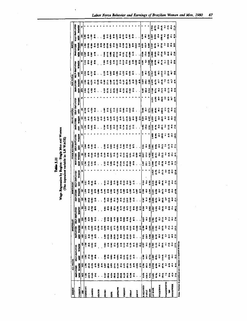
Labor Force Behavior and Earnings of Brazilian Women and Men, 1980 67
I P. ~~~~~~~~~~~~~~ | |~~ 0 0 - ;gos°St*ERSi|i
?
I ~~~~~~~~~~2e|~~~~~~~~- P- 6 P;^,Rd$dt60 nXt
. . . . .t . .. . . . . . . ... . . . .
43 Cs d* c
}^ .... . . ........ . . s . ."g .. ea 8,I- °
Ca
z
X |; D ~. . . . . . . . . . . . . . . . . . . . . R ea,t;
"~~ ~~~ 15 | w!uRcEs|ZOt SNS0
a * s a .66 R a P,
l -d s c s d Z d d 2 re 1 c 2
I~~~~~~~~~~~~~~~~~~~~~~~~I
II SI~~. s 3F
y
d d~~~~~0 i 3 , vgRSFRR O2OA@ t z E eO!NgT g Rag i ROSO tzj* 0
|~~~~~~~~ ~~~~ ,.* @t oto so $ ox 0 tWc1
_ _ ~~~~~~~~~~~~~~~~~~~~~~~~~~~~~~~~~~~~.1
11|~~~~~~ ~~~ I -:t 1|2|! 0 2
68 Women's Employment and Pay in Latin America
The results for the experience variables are in line with the concave earnings-experience profiles.The coefficients for experience and experience squared are significant in all the employeeregressions, but less so for the self-employed. The coefficient of the fertility variable in thefemale regressions is significantly negative (-0.06) only in Rio for employees.
Education makes a large positive contribution to expected hourly earnings; the estimatedschooling coefficients are consistently strong. Table 3.11 shows that women employees havehigher returns to education than men, while among the self-employed they are about the same.Nationally, the returns to schooling among male and female employees are 13 percent and 15percent, respectively. The corresponding values for the self-employed are 12 percent and 11percent.
As might be expected, there are important regional differences. In the Northeast, the return forfemale employees is 18 percent, but only 14 percent for men. In the Northwest, the return is 21percent for women, and 13 percent for men, while in Rio the values are 18 percent and 13percent. In the Other Southeast the female advantage is 2 percentage points (15 percent versus13 percent), and in the South the advantage is 4 percentage points (14 percent and 10 percent).In Sao Paulo, the schooling returns are the same for male and female employees (14 percent).As regards the self-employed, the estimated returns to education for women is higher than thatfor men in the Northeast (10 percent versus 7 percent), but slightly lower in Sao Paulo (13percent versus 12 percent).
6. Accounting For Male-Female Earnings Differentials
The usual strategy in analyzing male-female wage differentials is to partition the observed wagegap between an "endowments" component and a "coefficients" component. The latter is derivedas an unexplained residual and is called "discrimination." We use the popular "decompositionapproach," first developed by Oaxaca (1973), and extend its implementation to incorporateselectivity bias (Reimers, 1985) and the approach of Cotton (1988) that addresses the "indexnumber" problem.
The decomposition analysis is based on observed mean characteristics (eg. education, workexperience) and the parameter estimates of the selectivity-bias corrected wage equations. Theseregressions yield estimated wage structures of men and women in each work status. That is, theregression coefficients indicate the way in which the labor market rewards the backgroundattributes. The basic question addressed by the decomposition method is: How much would themale-female wage gap change if men and women were paid according to a common wagestructure, but their work-related attributes remained as they are? We now summarize themethod.'
The decomposition analysis typically involves a logarithmic scale which can be transformed intomonetary units. For each group of workers, the difference in the observed geometric mean wagesbetween males (m) females (f) can be written as:
30 The limitations of the technique in measuring discrimination are discussed by Cain (1986),Shapiro and Stelcner (1987), and Gunderson (1989).
Labor Force Behavior and Earnings of Brazilan Women and Men, 1980 69
TnW,i - TnW1 = (ZmIn -z + (Xa,A, -
where the Zs are the average background characteristics, and the As and the Rs are theestimated parameters.
As discussed by Reimers (1985), the observed wage differential has two components -differences in mean wage offers (based on selectivity-corrected estimates) and differences inaverage selectivity bias between men and women. Depending on the magnitudes and directionof selectivity bias, the differences in observed mean wages may under- or over-state thedifference in mean wage offers. Hence, the decomposition of the male-female wage differentialshould be based on wage offers, and not on observed wages.
The difference in average wage offers is given by:
NWN - 1W)= (=&Z -Z A)
where:
iWf = ThiWf - XK
The decomposition method is straightforward and focuses on the issue of "unequal pay for equalproductivity-generating characteristics," or wage discrimination. The decomposition of the gapin wage offers centers on differences in mean characteristics and differences in the estimatedreturns to these characteristics. In other words, if the estimated returns to the characteristics arethe same for men and women, the wage offer gap would be solely attributable to differences inproductivity-generating traits.
There is an index number problem in applying the technique: Which common wage structure(estimated coefficients) should be used as the non-discriminating norm? Since there is no clearcut solution to this problem we perform the analysis with three norms: (1) the male coefficients,(2) the female coefficients, and (3) a weighted average of the male and female coefficients basedon the proportions of men and women in the sample.
The difference in average wage offers can now be decomposed into two components: A portionthat is attributable to differences in regression coefficients, and a part that can be attributed todifferences in endowments. There are at least three ways to compute these magnitudes.
1. If the male wage function is used as the non-discriminatory norm:
nnW,= - -W =f 4(I = - + A(Z, - )
The term on the right is the endowments component and that on the left the coefficients orresidual component.
2. If the female wage function is used as the non-discriminatory norm:
70 Women's Employment and Pay in Latin America
Tj - m = Wf- +. Z -Z'
Again, the term on the right is the endowments component and that on the left the coefficientscomponent.
3. A third alternative suggested by Cotton (1988) is to define the non-discriminatory normas the weighted average of the male and female coefficients where the weights are proportionsof men (Pm) and women (Pf).
Let P = +Pmf +
mW7 _ mW" = ZX -As) + Z( - + Zz - Z
As before, the third term represents the portion attributable to differing endowments. The firstand second terms divide the "unexplained" residual into two parts: A "premium" or higher thanexpected returns for men (the first term) and a "penalty" or lower than expected returns forwomen (the second term).
In the decomposition analysis we analyze wage differentials first between married men andwomen, and then between single men and women. This is done separately for employees andthe self-employed.
Estinates of Discrmination
It should be noted that the decomposition analysis is carried out using a logarithmic scale whichcan then be transformed into monetary units - cruzeiros.31 Since we are flexible regarding thechoice of a non-discriminatory norm we present three estimates: using male coefficient weights,female coefficient weights, and a weighted average of the two. The endowments and coefficientscomponents are reported in terms of logarithms, cruzeiros, and percentage of the gap in wageoffers (expressed in logarithms). Before proceeding with the findings, we emphasize that thereare some important limitations of the method, which include missing variables and errors inmeasurement problems. These shortcomings of the technique should be borne in mind.
Married employees3 2 (Table 3.12). Looking at Table 3.12 we see that the national observedwage gap (row 3) is 29 percent, but the magnitude varies across regions. It is highest in SaoPaulo (41 percent), followed by the Northeast (39 percent), Rio and the South (about 25 percent).The lowest value is in the Northwest (15 percent). After removing selectivity bias effects, thereis quite a dramatic change in the gap in average wage offers when compared to the observeddifferential. At the national level the gap in wage offers rises to 33 percent (row 13). However,in Sao Paulo and Rio the gap in wage offers increases to 122 and 88 percent, respectively; in theNorthwest it falls to only 5 percent, and in the Northeast it remains unchanged at 38 percent. Inthe South the mean wage offer of husbands is about 40 percent higher than that of wives, whilein the Other Southeast it is 22 percent higher. This suggests that in most cases the observed wage
31 In 1980 the official exchange rate was about 40 cruzeiros = $ 1 Us.
I See Zabalza and Arfufat (1985) for a similar comparison of hourly eamings for British marriedmen and women.
Labor Force Behavior and Earnings of Brazilian Women and Men, 1980 71
differential understates the disparity in wage offers due, of course, to differences in selectivitybias effects in the wage equations of husbands and wives.
The decomposition of the gap in wage offers shows that the "endowments" component favorswives, but this is far outweighed by the "coefficients" component, which penalizes wives in favorof husbands. Using the proportional weights (rows 18-21), we see that, for the entire country,the endowments portion favors wives by 70 percent of the wage offer gap, but husbands havecoefficient advantages of 170 percent. In monetary terms, the endowment component translatesinto $15/hour while the "discrimination" component reflects $33/hour. This pattern -
endowments favoring wives and coefficients favoring husbands - is similar in the other regionswhere the wage offer gap is large, and it seems not to make much of a difference which weightsare chosen as the non-discriminating norm. In each case, the coefficients component, as anestimate of discrimination, is in excess of 100 percent of the wage offer differential.
There are several possible reasons for this large unexplained residual, and the attempt to measure"discrimination" is fraught with well-known difficulties and limitations. First, the presence ofmissing variables and errors-in-measurement bias may have unpredictable effects on thedecomposition. Unobserved factors originating outside the labor market (e.g., householdresponsibilities, quality of education, ability, motivation, and aspirations) and imperfectlymeasured observed productivity traits (e.g. work experience) have, no doubt, influenced ourestimate of "discrimination." Second, we note that the decomposition of the wage gap is basedon the "average" man and woman, so that the entire weight is placed on mean observedcharacteristics which have a large dispersion. Recent work by Kuhn (1987) suggests that animprovement could be made by examining individual-specific measures of the "unexplained"component. This implies that it may be desirable to examine the distribution properties of theresidual portion among individual women and men. Third, there is some evidence that the OLSestimator used by conventional analyses such as ours may result in upwardly-biased estimates ofthe unexplained male-female wage gap.' Finally, in examining the regression coefficients andmean characteristics we see that the intercept differences account for the largest part of theunexplained wage gap.3' We caution the reader, however, that no importance should be givento this. For, as Jones (1983) has shown, a further division of the unexplained gap betweenintercept and slope effects is not independent of the arbitrary measurement of the explanatoryvariables, so that it is impossible to uniquely disentangle the portion of the wage gap betweencoefficient and intercept differences.
With the above qualifications, our decomposition of the wage gap between husbands and wivessuggests an interesting conclusion: If married women and men wage earners were paid accordingto a common wage structure, the wages of wives would be at least as high as that of husbands(compare rows 11 and 12).
The married self-employed (Table 3.13). The decomposition analysis of the earnings gap for theself-employed is shown in Table 3.13. Two versions are presented. We present the analysis of
33 Evidence on this point is given in Ohsfeldt and Culler (1986) who show that a nonparametric'smearing' estimator yields a lower measure of the unexplained portion than does traditional OLS.
3' When we examined the contribution of each variable to the 'discrimination' component (notreported here), we found that, in most cases, the returns to background characteristics tended to favorwomen rather than men, and thus contributed to narrowing the wage gap. The difference in the male-femaleintercepts far outweighed the coefficient differences of the explanatory variables.
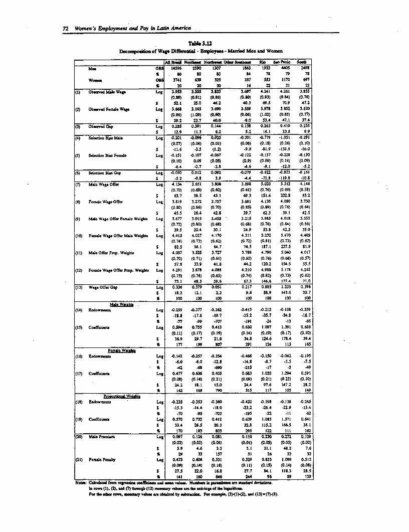
72 Women's Employment and Pay in Lain America
Ta 3.12DecoPoaition of War Diffmaeil - Enyloy. - Maffd Men and Women
All Bre NOat Notlrat Otbr Sahng Rio So Paulo Southmmn 0B 14596 2590 1307 1863 1933 4405 2498
S S0 S0 80 84 78 79 78W rom 0B 3741 639 325 357 553 1170 697
S 20 20 20 16 22 21 22(1) Obsred Mael Wage Log 3.953 3.555 3.S33 3.691 4.241 4.261 3.855
(0.89) (0-91) (0.86 (0.80) (0.93) (0.84) (0.76)S 52.1 35.0 46.2 40.3 69.5 70.9 47.2
(2) Oberved Femle War Log 3.668 3.165 3.690 3.559 3.978 3.852 3.620(0.96 (1.09) (0.90) (0.06) (1.02) (0.85) (0.77)
S 39.2 23.7 40.0 -9.0 53.4 47.1 37.4(3) Obacved Gap Los 0.2S5 0.391 0.144 0.138 0.263 0.410 0.235
S 12.9 11.3 6.2 5.2 16.1 23.8 9.9(4) Sleedion Bi Male Log 40.201 4.096 0.025 40.201 40.779 *1.051 .0.291
(0.07) (0.04) (0.01) (0.06) (0.18) (0.26) (0.10)
S -11.6 -3.5 (1.2) .9.0 41.9 -131.9 -16.0(5) Slecton Bia Femole Log 40.151 .0.107 .0.067 40.122 .0.157 40.22S 40.130
(0.10) 0.09 (0.05) (0.9) (0.09) (0.14) (0.09)S 46.4 -2.7 -2.3 -4.6 .9.1 -12.0 -5.2
(6) SelectionBias Gp Log .0.050 0.012 0.092 -0.079 .0.622 .0.823 40.161S -5.2 40.8 3.9 -4.4 -72.8 -119.8 -10.8
(7) MaleWage Offer Log 4.154 3.651 3.808 3.898 5.020 5.312 4.146(0.70) (0.69) (0.60) (0.61) (0.76) (0.69) (0.58)
S 63.7 38.5 45.1 49.3 151.4 202.8 63.2(a) Female Wage Offer Log 3.819 3.272 3.757 3.681 4.135 4.0S0 3.750
(0.80) (0.86) (0.70) (0.85) (0.89) (0.76) (0.64)S 45.5 26.4 42.8 39.7 62.5 59.1 42.5
(9) Male WageOffwrFemaeWeights Log 3.677 3.015 3.403 3.215 3.985 4.018 3.555(0.72) (0.80) (0.68) (0.6S) (0.76) (0.64) (0.56)
S 39.5 20.4 30.i 24.9 53.8 42.5 35.0(10) FDmaIe Wage Offer MWle Weights Log 4.413 4.027 4.170 4.311 5.232 5.470 4.405
(0.74) (0.73) (0.62) (0.72) (0.82) (0.73) (0.62)S 82.5 56.1 64.7 74.5 187.1 237.5 81.9
(11) Male Offer Prop. Weights Log 4.057 3.525 3.727 3.788 4.790 5.040 4.017(0.70) (0.71) (0.61) (0.62) (0.76) (0.68) (0.57)
S 57.8 33.9 41.6 44.2 120.2 154.5 55.5(12) Female Wage Offer Prop. Weights Log 4.291 3.878 4.0S8 4.210 4.98J 5.178 4.262
(0.75) (0.76) (0.63) (0.74) (0.82) (0.73) (0.62)S 73.1 48.3 59.6 67.3 146.6 177.4 71.0
(13) Wage Offer Gap Log 0.336 0.379 0.051 0.217 0.8J5 1.233 0.396S 18.2 12.1 2.3 9.6 88.9 143.6 20.7% 100 100 200 100 100 100 100
Male Wetabr(14) Endowrmeu Log .0.259 40.377 .0.362 40.413 .0.212 .0.158 .0.259
S -18.8 -17.6 -19.7 -25.2 -35.7 -34.8 -18.759 -77 -99 -707 -191 -24 -13 .65
(15) Coeffircina Log 0.594 0.755 0.413 0.630 1.097 1.391 0.655(0.11) (0.17) (0.19) (0.14) (0.19) (0.17) (0.10)
S 36.9 29.7 21.9 34.8 124.6 178.4 39.4% 177 199 807 291 124 113 165
Fmale Wsigb(16) End boM Log 4.142 40.257 4.354 4.466 4.150 4.062 4.195
S 46.0 46.0 -12.8 -14.t 48.7 *3.5 -7.5% -42 4S .690 -215 .17 -5 -49
(17) Coeficinb Log 0.477 0.636 0.405 0.683 1.035 1.294 0.591(0.08) (0.14) (0.21) (0.09) (0.21) (0.23) (0.20)
S 24.2 28.1 15.0 24.4 97.6 147.2 28.25 142 168 790 315 117 l05 149
Provrtonel Wdeihts(28) Endowments Log 4.235 4.353 4.360 4.422 4.198 4.13S 0.245
S -15.3 -24.4 -IS.0 -23.2 -26.4 -22.9 -15.4I .70 -93 .703 -195 -22 -11 -62
(19) Coeficeiata Los 0.570 0.732 0.412 0.639 1.083 1.371 0.641S 33.4 26.5 20.3 32.8 15.2 166.5 36.1S 170 193 803 295 122 211 162
(20) Mae Premium Log 0.097 0.126 0.0S1 0.110 0.230 0.272 0.129
(0.02) (0.03) (0.04) (0.01) (0.05) (0.05) (0.02)S 5.9 4.6 3.5 5.1 31.1 48.2 7.6% 29 33 157 51 26 22 33
(21) Fmale PenAlty Log 0.473 0.606 0.331 0.529 0.SS3 1.099 0.512
(0-09) (0.14) (0.16) (O.12) (0.15) (0.14) (0.08)S 27.5 22.0 16.8 27.7 84.1 128.3 2S.55 141 160 646 244 96 89 129
Nola: Calculatd from rgraioe ceficia ad ma vel s Nu in parenthese are danderd devliona.1n iowa tl), 2) aN (7) *bm (12) Moeamy vale us tbe ait-lop of dh lop ijbma.For the otbet rmw, matay valui ar obtaind by sFbtaor epm=pia, (3)X1).(2). and (13)-(7)-(8).
Labor Force Behavwor and Earnings of Brazilian Women and Men, 1980 73
the husband-wife wage gap for paid self-employed workers. Then, since some wives (and a smallnumber of husbands) are unpaid self-employed workers, we impute a fitted wage for them anddecompose the wage offer differential between all self-employed wives and husbands. The twoversions yield a similar set of results.
The observed hourly earnings gap for Brazil between paid self-employed husbands and wives is48 percent (row 3, right panel). It is lowest in the South (39 percent), and highest in theNortheast, Rio and Sao Paulo (56-59 percent). The values for the Northwest and the OtherSoutheast are 53 percent and 47 percent respectively. We also see that the wage offer differential(row 13) tends to be smaller than the observed gap. Nationally, the wage offer gap falls to 37percent. Similarly, in the Northeast and Northwest it drops to about 42 percent; in the OtherSoutheast to 36 percent, and to only 17 and 18 percent in Sao Paulo and the South, respectively.Only in Rio does the wage offer gap (59 percent) exceed slightly the observed differential (57percent).
The decomposition of the wage offer gap yields results similar to that obtained for employees.The differential attributable to coefficient differences (the "discrimination" component) is stronglyin favor of husbands, and this portion outweighs the "endowment" component, which usuallyfavors wives. With the exception of Rio, the coefficients component is in excess of 100 percentof the gap in offers of hourly earnings. Unlike employees, an examination of the contribution ofthe explanatory variables to the earnings differential showed that the coefficient differences of thework experience variables was a consistent major contributor to widening the gap.
The conclusion we reach for self-employed wives and husbands is the same as that for employees:If productivity-generating traits of self-employed wives were rewarded on the same basis as thoseof self-employed husbands, the hourly earnings of wives would be at least equal to that of theirhusbands (compare row 11 and 12).
Single employees (Table 3.14). With a few exceptions, the observed male-female pay differentialis smaller for single than for married people. Nationally, the gap is 18 percent, but the magnitudevaries across regions, from 6 percent in Rio to 34 percent in the Other Southeast. However,looking at the gap in wage offers, we see that in three regions (the Northeast, the Northwest,and Rio) single women fare better than do men, while in the remaining regions the average wagesoffered to men exceed those offered to women.35
First consider the differential in the three regions where male wage offers exceed those offemales. Looking at row 18 (proportional weights), we see that the men are strongly favored interms of the coefficients component, implying that women tend to be paid less than men who areotherwise comparable in terms of background characteristics. The male advantage translates intoa cruzeiro gain of $9/hour in the Other Southeast, $11/hour in the South, and $60/hour in SaoPaulo.
The story is different in the Northeast, the Northwest and Rio, where female wage offers exceedthose of men. In the Northeast women have average wage offers that are 77 percent higher, whilein the Northwest and Rio the female advantage is about 40 percent (row 13). The decompositionof the wage differentials shows that in each region women are favored in terms of the
I We also performed the decomposition for employees based on the regressions that excluded thepublic sector dummy variable in the female equation. The results did not change in any significant way.
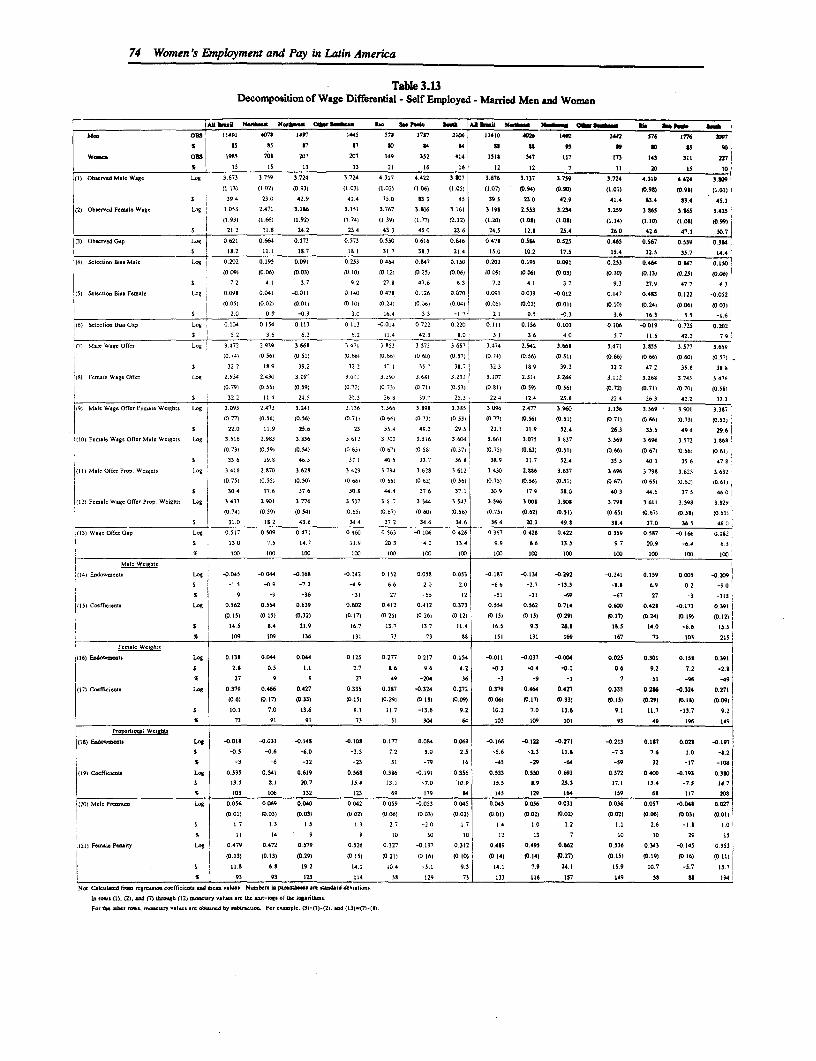
74 Women 's Employment and Pay in Latin America
Tabl 3.13Decomposition of Wage Differential - Self Employed - Married Men and Women
~~AM S....) ~~~~~ 14
o, od A8Mil 11.1 S.. P.W. -&.. I Al U.a Nwilo Ndb- 0 l. m im W so ? . 5.4
66.. OiSA 11491 4073 1497 1445 578 178 2106 1r 10 40 14 2 1442 57 1776 2807
S as5 *5 a7 s so 84 84U90 to 37 *9 t5 90
W-e, oa0 19B15 703 207 207 149 352 414 Isis 847 117 173 143 311 227
S 15 15 13 13 21 16 16 12 12 7 11 20 Is 10
(l) Ob-cnc3 M8.. Wag, Log 3 673 3.759 3.724 3.724 4.317 4.422 3.S07 3.676 3.137 3.759 I.724 4319 4.424 3.809
(I 13) (1.02) (5.93) (1.03) (1.02) (1.06) (1.05) (1.07) (5.94) (0.90) (1.01) 10.991 10.98) (1.01)
S 39 4 3 0 42.9 41 4 75.0 83.3 45 39.5 23.0 42.4 41.4 83.4 83.4 45.1
(2) Ob-c. Fcm1.)l Wag. Log 3.053 2.471 3.106 3.151 3.767 3.806 3.161 3.19S 2.533 3.234 3.259 3 S65 3865 3.425
(l.93l (1.66) (1.92) (1,74) (1.39) (1.771 f2.12) (l.20) (1.021 (10.00 (1.14) (1.10) (1 09) f0.99)
S 1 21.2 1.8 24.2 23.4 43.3 45 0 23 6 24.5 12.1 23.4 26.0 42.6 47.1 30.7
(3) Ob-9n0d G.p Lg| 0.621 0.664 0.573 0.573 0.550 0.616 0.646 0.478 0.5U4 0.S2S 0.465 0.367 0.559 0.3114
$ 18.2 11.1 18.7 18.1 31.7 38.3 21.4 13.0 10.2 17.5 1i.4 32.3 35.7 14
14) SaI5.1io ., .Ml), Log 0.202 0.195 0.091 0.253 0.464 0.047 0.150 0.202 0.195 0.091 0.253 0.464 0.147 0.150(
(0.09) J0.06) (0.03) (0.10) (0.12) (235) (0.06) (5.091) (006) (0031 (0.101 (0.13) (5.25) (5.06)
S 7.2 41 3.7 92 270 47.6 6.3 7.2 41 3.7 9.3 27.9 47.7 63
(5) Bi1cc .. 0g.. Fcle L7g 0.091 0.041 -0.011 0N14O 0.478 0.126 .0.070 0.091 0 039 -0.012 0.147 0.483 0.122 -0.052
(0.05) (0.02) (0.0)) 10 IC) (0.24) (0 06) (0.04) (0.05) (f.021) (.01) (0 10) (0524) (0.061 (0.031)
S I 2.0 0. -0.3 3Q. 164 53 -17 2.1 0.5 -0.3 3.6 16.3 5 -1.6
1 S6) Slii- o.S--.- Gp Lg| 0.104 0 154 0.113 01)3 -0.0)4 0.722 0.220 0.156 0.103 0.106 -0.019 0.725 0.202
S_________________________________ L 5.2 36 0.2 6.2 114 423 00 53 .6 4.0 5.7 11.6 42.2 79
(7) Ma), Wag. ON(c Lg| 3 472 2 939 3 661 3.43 3 853 3 573 3 637 3 474 2.942 3.668 3.471 3 S55 3.577 3.659
(0.7)) 0o 56) (0 51) 10. (O 66) (0 60) (0 (7) (D 74) 10.56) (.3 1) (5 66) (0661 (0.601 (0.371
S 32 2 189 39.2 32.7 42 35 7 38.7 32.3 8 9 39.2 32.2 47.2 35.1 38 8
,) F-.), Wa.R Off.r Log 2.934 2.437 3.197 3.011 3.20) 3.6S1 3.21 3.107 2.314 3.246 3.112 3260 3.743 3476
10.75) 10.35) 10.39) 10 72) (0 73, (0.7)) 10.33, 10.6)S) f0.59) 10.36) (5.72) (5.71) (5.70) (0.58)
S 32.2 I 1 4 24.5 20.3 26 8 397 23 3 22 4 12.4 25.6 22 4 26 3 4.Z2 32.3
19) M.). Wig. Offcr F-aa. W.igbt, Lo0 3.093 2.473 3.241 3 136 3.566 35.98 3 385 3.096 2.477 3.960 3.136 3.569 3.901 3 357
(2.71) (0.50) (0.561 (0.71, (056) (073) (0.53) (0.771 (57.56) 60.511 f(0.71) 10.69) 10.73) (5.5311
S 22.0 119 25.6 23 35.4 49.3 29.5 22.1 119 52.4 26.3 350 494 29.6
(10) F-ala wag, Ofler Ma), W6g6ht, Log 3.516 2.983 3.836 3.6)2 3 702 3.516 36014 3.661 3 075 3 637 3.569 3 696 3.572 3.868
10.73, (0.39, (0.64) 10.63) 10.67) 10.56, 10.57) 10.73) (5.63) (0.3)) (5.66) (0.671 (0 391 (0 61i
5 336 19.8 463 37) 4035 3.7 368 36.9 217 52.4 3595 403 3556 476.
I1 ) M.]. offcr, Pp. Wa,ga l.og 3A416 2.670 3.628 3.429 3 794 3.20 3.612 | 3430 2.816 3.637 3.696 3 796 3 625 3.632
i [~~~~~~~~~~~0.73) (0.33) (0.30) (069) (0 33) 1062) (0.301 (0.73) (05.3) (0.31) (0.67i (5.65) (0.62, 0.61,
4 176 37.6 30.0 4.9 37 37.1 30.9 179 3.0 40.3 446 373 460
i (12) F-=c W.g Off., P-p Wcighl- Log 3 433 2.901 3.776 3.537 3 617 3 44 3.643 3.596 3.009 3.908 3.798 3.6)) 359S 3.829
(074) (0.59) (0 54) (0.63, (5067) (5 60) (0.56) (0.73) (0.62) (5.51) (0.65) 50 67) o 5.8 10 61)
iS 31.0 1.2 43.6 344 372 34.6 34.6 364 20.3 49.8 38.4 37.0 36.5 460
(3) W.gz off., Gap Log 0517 0.509 0.471 0 460 0.563 -0.106 0.426 0.367 0.420 0.422 0 359 0.537 -0 166 0 112
S 130 7.5 14.7 119 203 -4.0 134 9.9 6. 13.3 9.7 20.9 -6.4 6.3
9 100 100 1l0 100 100 t100 10 10 1 100 100 100 1D0
6-.). L °-0.045 -0 044 -0.160 -0.142 0.152 0 053 0.053 -0187 -04134 -0.292 -0.241 0.159 0.905 -0209
S -1.5 -0.9 -7 2 -4 9 6.6 2.0 2.0 -6.6 -2.7 -13.3 -8.s 69 0.2 -90
0 -9 -9 -36 -31 27 -55 12 -51 -31 -69 -67 27 -3 -115I
[(13) Co.ic=li.a Log 0.562 0.o54 0.639 0.602 0.412 0.412 0.373 0.554 0.S62 0.714 0.60D 0.428 -0.171 0.391
(5.15) (0.15) (0.32) (0.17) (0.26) (0.26) (0.12) (0.15) (0.15) (0.29) (6017) (0.241 10.195 (0.12)
S 14.3 8.4 21.9 167 1 13 7 137 11.4 16.5 9.3 26.9 18.5 14.0 -6.6 13.5
0 109 109 136 131 73 73 U 151 131 169 167 73 103 215
Fasal, Wighl,
(16)1 E t.a Log 0.138 0.094 0.044 0.125 0.277 0.217 0.154 -0.011 -0.037 -0.004 0.025 0.301 0.151 0.391
S 2.0 0.5 1.1 2.7 8 6 9.6 4.2 0.3 *0.4 -0.1 0.6 9.2 7.2 -2.8
5i 27 9 8 27 49 -204 30 -3 -9 -1 7 51 -96 -49
(17) Co.fl0,.a L 0.379 0.466 0.427 0.335 0.287 -0.324 0.272 0.379 0.464 0.427 0.335 0.2U6 -0.324 0.271
(0.6) (5.17) (0.33) (0.15) (0.29) (OI.9) (0.09) 10.06) 10.17) 10.33) (0.15) (0.29) (5.10) (0.09)
S 10.1 7.0 13.6 9.1 11.7 -13.6 9.2 10.2 7.0 13.6 9.1 11.7 -13.7 9.2
S 73 91 91 73 51 304 64 103 109 101 93 49 196 149
Froroni00l Wai,ibla.
a) Ed4a au Log -0.0)8 -0.031 -0.145 -0.108 0.177 0.04 0.069 -0.166 -0.122 -0.271 -0.213 0.167 0.02S -0.197
S -0. -0.6 -6.0 -3.5 7.2 3 0 2.5 -5.6 -2.3 11.8 -7.3 7.6 1.0 -S.2
ti; -3 -6 -32 -23 31 -79 16 -45 -29 -64 -59 32 -17 -18
(191 Cocffic)ro3 L-o 0.535 0.541 0.619 0.568 0.3S6 -0.191 0.336 0.533 0.50 0.693 0.572 0.400 -0.193 0.390
S 13.3 S.) 20.7 13.4 13. -7.0 10.9 1.5 8.9 25.3 17.1 13.4 -7.5 4.7
S103 106 132 123 69 179 U4 145 129 164 159 6i 117 200S
120) M8.) FPcmi,a Log 0.056 0.069 0.044 0.042 0 059 -0.053 0 045 0.045 0.0S6 0.031 0.036 0.057 -0.048 0.027
(o001) (0o3) (0.03) (0.02) (006) (003) (0.02) (5.0)) (0.02) (0.02) (0.02) (1 061 (005 ) (0.0II
S 1.7 1.3 1.5 1.3 2.7 -2.0 17 1.4 1.0 1.2 1.1 2.6 -1.8 I10
7i II 14 9 9 (0 S0 10 12 13 7 10 10 29 15i
j(21) Fc.m.P-l aa(ly Lo| 0.479 0.472 0.579 0.526 0.327 -0.137 0.312 0.489 0.493 0.662 0.536 0.343 -0145 0.353
(0.13) (0.13) (0.291 (0.15) (0.21) (0.10) (0. 0lt (0.14) (0.14 (0.27) (0.15) (O.19) (0.16) (O 11)
S 11.0 6.8 19.2 14.1 104 -5.1 9.3 14.1 79 24.1 15.9 10.7 -5.7 13.7I ________________________________________________________ 93 93 123 114 53 129 73 133 116 157 149 59 U 194
Nat Ck4.iitd f(59 -igmSaioO -a.21,(14t5said - a.. a.),.M.P1.4.6.5 paI .a.a M4adr.a d.ala).ao
ia i- (1). (2). .c.i C7) ts6.agh (12) a.a4lay aaI c t1c aao- of Lb6 ICgia11,.-
Fr. aSh., _90., -.4.01y87 a-)., -b icd by b.aacl,aa. For c--pI. f31-(IN-(2). .44 (13)-(7(-(S)
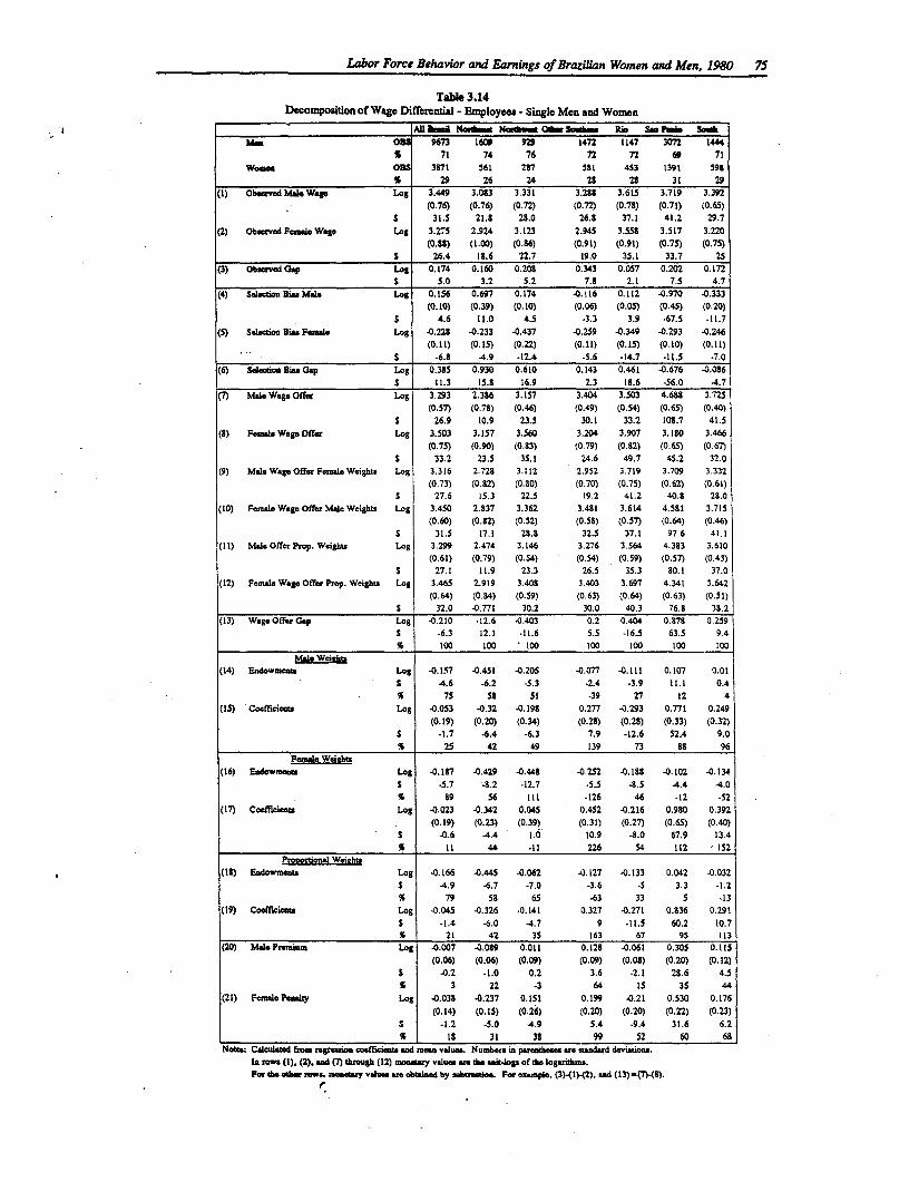
Labor Force Behavior and Earnings of Brazilian Women and Men, 1980 75
Tabe 3.14Decomposition of Wage Differenti - Employecs - Single Men and Women
.____________ All i H .da i Nnwet Ot Soi- _ R Sia Po Soo
iM_ Oi# 9673 1t0 929 1472 1147 3072 1444S 71 74 76 72 72 6 71
Womr OS 3871 561 2t7 5t1 453 1391 598S 29 26 24 28 28 31 29
(1) Observed Mae Way Log 3.449 3.083 3.331 3.288 3.615 3.719 3.392(0.76) (0.76) (0.72) (0.72) (0.78) (0.71) (0.65)
S 31.5 21.8 2S.0 26.S 37.1 41.2 29.7(2) Observed Feale Wage Log 3.X5 2.924 3.123 2.945 3.558 3.517 3.220
(0.88) (1.00) (0.86) (0.91) (0.91) (0.75) (0.75)$ 26.4 18.6 22.7 19.0 35.1 33.7 25
(3) Obswved Gap Log 0.174 0.160 0.208 0.343 0.057 0.202 0.172S 5.0 3.2 5.2 7.8 2.1 7.5 4.7
(4) Saeedee Bias Maie Log 0.156 0.697 0.174 40.116 0.112 40.970 -0.333
(0. 10) (0.39) (0.10) (0.06) (0.05) (0.45) (0.20)S 4.6 11.0 4.5 -3.3 3.9 -67.5 -11.7
(5) Selection Bis Femue Log .0.228 40.233 40.437 40.259 -0.349 40.293 .0.246
(0.11) (0-.5 (0.22) (0.11) (0.15) (0.10) (0.11)
S -6.S -4.9 -12.4 -5.6 -14.7 -11.5 -7.0(6) Selectioo Bias Gap Log 0.3S5 0.930 0.610 0.143 0.461 .0.676 .0.086
s 11.3 15.8 16.9 2.3 18.6 -56.0 -4.7
(7) Mae Wage Offer Log 3.293 2.386 3.157 3.404 3.503 4.6S8 3.725(0.57) (0.78) (0.46) (0.49) (0.54) (0.65) (0.40)
S 26.9 10.9 23.5 30.1 33.2 108.7 41.5
(8) Female WageOffer Log 3.503 3.157 3.560 3.204 3.907 3.180 3.466
(0.75) (0.90) (0.83) (0.79) (0.S2) (0.65) (0.67)
S 33.2 23.5 35.1 24.6 49.7 45.2 32.0
(9) Male Wage Offer Female Weights Log 3.316 2.728 3.112 2.952 3.719 3.709 3.332
(0.73) (0.12) (0.80) (0.70) (0.75) (0.62) (0.61)S 27.6 15.3 22.5 19.2 41.2 40.8 28.0
(10) FemraeWageOfferMoleWeights Log 3.450 2.837 3.362 3.481 3.614 4.581 3.715
(0.60) (0.82) (0.52) (0.51) (0.57) (0.64) (0.46)
S 31.5 17.1 28.8 32.5 37.1 97.6 41.1(11) Male Offer Prop. Weights Log 3.299 2.474 3.146 3.276 3.564 4.383 3.610
(0.61) (0.79) (0.54) (0.54) (0.59) (0.57) (0.43)S 27.1 11.9 23.3 26.5 35.3 10.1 37.0
(12) Female Wage Offer Prop. Weights Log 3.465 2.919 3.408 3.403 3.697 4.341 3.642
(0.64) (0.94) (0.59) (0.63) (0.64) (0.63) (0.51)S 32.0 40.771 30.2 30.0 40.3 76.8 38.2
(13) Wag Offer Gap Log .0.210 -12.6 -0.403 0.2 .0.404 0.S78 0.259
S -6.3 12.1 -11.6 5.5 -16.5 63.5 9.4% 100 100 ' tOO 100 100 100 100
M i Wwei b(14) Endowments Log -0.1.57 40.451 40.205 -0.077 -. 111 0.107 0.01
S 4.6 -6.2 -5.3 -2.4 -3.9 11.1 0.4.% 75 SS 51 -39 27 12 4
(15) Coefficiae Log -0.053 -0.32 40.198 0.277 -0.293 0.771 0.249(0.19) (0.20) (0.34) (0.28) (0.28) (0.33) (0.32)
S -1.7 46.4 -6.3 7.9 -12.6 52.4 9.0
sC 25 42 49 139 73 aS 96
Fermb Weighs(16) Endowmnr Log 40.1S7 40.429 -0.448 -0.252 -0.188 -. 102 -0.134
S -5.7 -8.2 -12.7 -5.5 -S.5 4.4 4.0% . 5 S9 56 111 -126 46 -12 -52
(17) Coefficirnu Log o 0.023 -0.342 0.045 0.452 -0.216 0.9S0 0.392
(0.19) (0.23) (0.39) (0.31) (0.27) (0.65) (0.40)
S -0.6 4.4 1.0 10.9 -8.0 67.9 13.4
% 11 44 -11 226 54 112 152Prooortiunal Wejehb
(1) Endowments Log .0.166 -. 445 -0.062 -0.127 -0.133 0.042 -0.032
S 4.9 -6.7 -7.0 -3.6 -5 3.3 -1.2
% 79 5S 65 -63 33 5 -13(19) Coeffieieors Log .0.045 -0.326 -0.141 0.327 -0.27t 0,136 0.291
S -1.4 -6.0 -4.7 9 .11.5 60.2 10.7% 21 42 35 163 67 95 113
(20) Male Premiu Log .0.007 -0.089 0.011 0.128 -0.061 0.305 0.115
(0.06) (0.06) (0.09) (0.09) (0.08) (0.20) (0.12)
S -0.2 -1.0 0.2 3.6 -2.1 28.6 4.5
% 3 22 -3 64 15 35 44(21) Female Penalty Log -0.038 -0.237 0.151 0.199 -0.21 0.530 0.176
(0.14) (0.15) (0.26) (0.20) (0.20) (0.22) (0.23)
S -1.2 -5.0 4.9 5.4 -9.4 31.6 6.2
% Is 31 38 99 52 60 68Notes: Caleulaed from regrui coefficits ad mesn values. Number, in Parentheaesae standard deviations.
i ro (1) (, ad M(7) through (12) monstry valuwea the asi-lop of the logarthms.For th othe rows, moesay values ae obtained by aubtratice. For exampoe. (3)-(l).{2). and(13)().
. ~~~~~~~~~~~~~~~~~~~~~~~~..
76 Women's Employment and Pay in Latin America
endowments and coefficients components. In the Northwest, the residual component is 35 percentof the wage offer gap; it is 42 percent in the Northeast, and 67 percent in Rio.
The single self-employed (Table 3.15). Finally, we come to the results for the self-employedshown in Table 3.15. The analysis of the hourly earnings gap that shows the observed earningsdifferential (row 3, right panel) differs from the gap in offered wages (row 13). For example,nationally and in the Northeast the observed hourly wage is about one-half that of men. However,the offered wages of women are only 23 percent less than those offered to men for the entirecountry, and in the Northeast women have an earnings advantage of 28 percent. Thedecomposition results show that nationally men are strongly favored in terms of coefficientdifferences, while in the Northeast the reverse is the case - the coefficients component stronglypenalizes men. The pattern is similar when the analysis is performed for all (paid and unpaid)self-employed workers (see left panel).
In sum, the decomposition analysis for single men and women yields a much lower measure of"discrimination" than that for wives and husbands. This suggests that factors outside the labormarket (household responsibilities, fertility, and work interruptions) probably play an importantrole in the earnings disadvantage of married women.
7. Discussion
In this study we have used data from the 1980 Census of Brazil to investigate determinants oflabor force status and earnings in samples of married and single men and women. Unlike moststudies on labor markets in developing countries, we analyzed labor force status in terms of athree-choice model (employee, self-employed, no work). Moreover, our analysis of earningsdeterminants among employees and the self-employed explicitly incorporates the selection ofindividuals among the three types of labor force status. National and region-specific selectivitycorrected wage regressions were then used to examine the effects of human capital and otherwage-determining characteristics, and to explore the issue of male-female wage differentialsamong wage and self-employed workers.
Main Findings
1. The regional diversity of Brazil is clearly reflected in the estimated models of labor forcestatus and earnings. This pluralism leads us to concur with Birdsall and Behrman (1984)that much care must be taken in reaching conclusions from estimates for Brazil "as awhole. " Nation-wide estimates of policy-relevant considerations such as returns to humancapital and gender disparities may be misleading.
2. It is important to analyze the labor force status, especially of single and married women,in terms of a three-choice context. For example, although education plays an important rolein determining overall labor market participation, the principal effect is to increase thepropensity to perform wage work; the schooling effects on self-employment are generallysmall. Our empirical results suggest that modeling labor force behavior in developingcountries in terms of only a "work or no-work" choice is likely to mask important aspectsof the underlying determining factors. This point is especially relevant for women, and,during periods of prolonged recession, for men as well.
3. Our results reflect the well-documented findings that the presence of young children in thehome and more advanced age discourages married women's labor market participation.
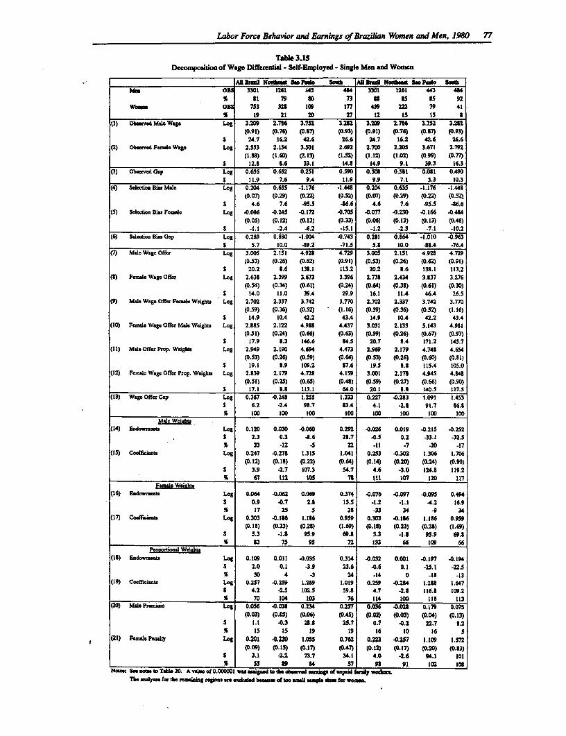
Labor Force Behavior and Earnings of Brazilian Women and Men, 1980 77
Tabi 3.1SDecomWosition of Wage Diffeintiail - Self-Employed - Single Men and Women
A_- 3ih1 NMIg gee South Al basE adeeg Se PwAo SoiutMole OBE 3301 1261 443 4t4 3301 1261 443 4t4
% &8 79 80 73 8 85 85 92Wor. O! 753 328 10 177 439 222 79 41
1 19 21 20 27 12 15 Is 8(1) Obsrvd MaleWage Log 3.209 2.7t6 3.751 3.2J2 3.209 2.7t6 3.752 3.282
(0.91) (0.76) (0.S7) (0.93) (0.91) (0.76) (0.87) (0.93)S 24.7 16.2 42.6 26.6 24.7 16.2 42.6 26.6
(2) Observed FealWe Wage Los 2.553 2.154 3.501 2.692 2.70D 2.205 3.671 2.792(1.88) (1.60) (2.13) (1-52) (1.12) (1.01) (0.99) (0.77)
S 12.8 8.6 33.1 14.8 14.9 9.1 39.3 16.3(3) Obved Gap Log 0.656 0.632 .251 0.590 0.50t 0.581 0.081 0.490
S 11.9 7.6 9.4 11.9 9.9 7.1 3.3 10.3(4) Selection Bias Male Log 0.204 0.635 -1.176 *1.448 0.204 0.635 -1.176 -1.448
(0.07) (0.29) (0.22) (0-52) (0.07) (0.29) (0.22) (0.52).S 4.6 7.6 -95.5 -86.6 4.6 7.6 -95.5 -86.6
(5) Selection Bias Femle Log 4.086 40.245 -0.172 4.705 4.077 4.230 4.166 4.484(0.05) (0.12) (0.13) (0.33) (0.06) (0.13) (0.13) (0.48)
S -1.1 -2.4 .6.2 -15.1 -1.2 -2.3 -7.1 -10.2(6) Seldetion Ba Gap Los 0.289 0.S0 -1.004 4.743 0.281 0.864 -1.010 4.963
S 5.7 10.0 -89.2 -71.5 5.8 10.0 -8.4 -76.4(7) Male Wage Offor Los 3.005 2.151 4.928 4.729 3.005 2.151 4.928 4.729
(0.53) (0.26) (0.62) (0.91) (0.53) (0.26) (0.62) (0.91)S 20.2 8.6 138.1 113.2 20.2 8.6 138.1 113.2
(8) Femaltc Wage Offer Log 2.638 2.399 3.673 3.396 2.778 2.434 3.837 3.276(0.54) (0.34) (0.61) (0.24) (0.64) (0.38) (0.61) (0.30)
S 14.0 11.0 39.4 29.9 16.1 21.4 46.4 26.5(9) Male Wap Offer Female Wcights Log 2.702 2.337 3.742 3.770 2.702 2.337 3.742 3.770
(0.59) (0.36) (0.52) (1.26) (0.59) (0.36) (0.52) (1.16)S 14.9 10.4 42.2 43.4 14.9 10.4 42.2 43.4
(10) Female Wage Offer Male Weighu Log 2.885 2.122 4.988 4.437 3.031 2.133 5.143 4.981(0.51) (0.24) (0.66) (0.63) (0.59) (0.26) (0.67) (0.97)
S 17.9 8.3 146.6 84.5 20.7 8.4 171.2 145.7(11) Male Offer Prop. Weights Los 2.949 2.190 4.694 4.473 2.969 2.179 4.748 4.654
(0.53) (0.26) (0.59) (0.64) (0.53) (0.26) (0.60) (0.81)S 19.1 8.9 209.2 87.6 19.5 8.8 115.4 105.0
(12) Female Wage Offer Prop. Weights Log 2.839 2.179 4.728 4.159 3.001 2.178 4.945 4.S48(0.51) (0.25) (0.65) (0.48) (0.59) (0.27) (0.66) (0.90)
S 17.1 8.8 113.1 64.0 20.1 8.8 140.5 127.5(13) Wage Offer Glap Log 0.367 4.248 1.255 1.333 0.227 4.283 1.091 1.453
S 6.2 -2.4 98.7 83.4 4.1 -2.8 91.7 86.8% 100 100 100 100 100 100 100 100
Male Wei"au(14) Endowmaeta Log 0.120 0.030 4.060 0.292 4.026 0.019 4.215 4.252
S 2.3 0.3 4.6 28.7 4.5 0.2 -33.1 -32.5% 33 -12 -5 22 -11 -7 -20 -17
(15) Coeftict Log 0.247 4.27S 1.315 1.041 0.253 4.302 1.306 1.706(0.12) (0.18) (0.22) (0.64) (0.14) (0.20) (0.24) (0.90)
$ 3.9 -2.7 107.3 54.7 4.6 -3.0 124.8 119.2.% 67 112 106 78 111 107 120 117
Female Weih"(16) Badowmeet Log 0.064 4.062 0.069 0.374 4.076 4.097 4.095 0.494
S 0.9 4.7 2.8 13.5 -2.2 -1.1 .4.2 16.9% 17 25 5 28 -33 34 -9 34
(17) Coeffleiente Log 0.303 4.186 1.186 0.959 0.303 4.186 1.186 0.959(0.28) (0.23) (0.28) (1.69) (0.18) (0.23) (0.28) (1.69)
S 5.3 -1.8 95.9 69.8 5.3 -1.8 95.9 69.8% 83 75 95 72 133 66 209 66
Prooorl Wei"ht_(18) Eadowmeau Log 0.109 0.011 4.035 0.314 4.032 0.001 4.197 4.194
S 2.0 0.1 -3.9 23.6 4.6 0.1 -25.1 -22.5% 30 4 -3 24 -14 0 -I8 -13
(19) Codecieanu Log 0.2S7 4.259 1.2t9 1.019 0.259 4.2t4 1.288 1.647S 4.2 -2.5 12.5 59.8 4.7 -2.8 116.8 100.2% 70 104 103 76 114 200 12 113
(20) Male Premium Log 0.056 4.038 0.234 0.257 0.036 4.028 0.179 0.075(0.03) (0.05) (0.06) (0.45) (0.02) (0.03) (0.04) (0.13)
S 1.1 4.3 28.8 25.7 0.7 4.2 22.7 8.2% 15 15 19 19 16 10 16 5
Female Penalty Log 0.201 4.220 i.055 0.762 0.223 4.257 I.IG9 1.572
(0.09) (0.15) (0.17) (0.47) (0.12) (0.17) (0.20) (0.83)S 3.1 -2.2 73.7 34.1 4.0 -2.6 94.1 101% 55 89 84 57 9 91 102 108
No- See eat.. to Tae 20. A value of 0.000001 wa &=good to the abewee eanga f depi hmiy woemThe asaalYre for the remaig rions are xeluded b_as of to saa m for wonme.
78 Women's Employment and Pay in Latin America
Brazil does not differ in these respects from other countries. To some extent, a largerhousehold and having a spouse who is an employee mitigates these deterrent effects.
4. Urban residence is conducive for both men and women to work as employees and alsoenhances their earnings. The effects, however, on being self-employed and on earnings aregenerally weak.
5. Our estimates show that education is an important, perhaps the most important, determinantof labor force status and earnings. We found that education not only enhances earnings,but plays an important role in "sorting" individuals among the alternative labor forceactivities. These indirect "sorting effects" of schooling strongly suggest the importance ofincorporating them in an analysis of earnings determinants. Schooling effects remain strongin the selectivity-corrected wage regressions for males and females, especially foremployees, but less so among the self-employed. We also note that our estimated returnsto schooling are generally bracketed by those obtained for other Latin American countries.
6. Finally, we comment about male-female earnings differentials. The decomposition analysesrevealed that the gap in wage offers between husbands and wives could not be accountedfor by differences in earnings-determining traits. This residual could be attributed, withcaution, to labor market "discrimination." Our results show that if the given wage-determining characteristics of wives were rewarded on the same basis as those of husbands,the (hypothetical) average hourly earnings of married women would be at least equal tothose of their spouses. What makes us uneasy about calling this result "discrimination" ismainly that it is basecl on data and estimation methods that are subject to well-knownlimitations, including husband-wife Oife-cycle) productivity differences that are not easilymeasurable or observable. An indication that this is likely to be the case is revealed by thefindings for the samples of the relatively young men and women. The "unexplained" wagegap was generally not an issue; in fact, the decomposition analysis showed that the labormarket tended to "favor" single women. An important question, however, is will the"premium" persist after they marry?
Policy Implications
A decade has passed since the 1980 Census of Brazil and it might be asked how the findings ofthe study are relevant today? As stated in the introduction, after a period of relatively highgrowth in the 1970s, the ]1980s were a "lost decade" for Brazil. The prospects are notencouraging. The statistics for 1990 show that Brazil experienced its sharpest recession in adecade. Gross domestic product declined by 4.3 percent (US$12 billion), the monthly inflationrate was 20 percent, industrial production shrank by 8 percent, and over 250,000 workers losttheir jobs in the state of Sao Paulo alone. Moreover, little progress has been made in reducingthe massive debt of $125 billion.
The reduced household incomnes and prospects for wage employment will dramatically alter thestructure of labor markets. More single and married women as well as children, who previouslydid not perform market work, will continue to join the labor force, probably as self-employedworkers. Men who held wage jobs will either become unemployed or self-employed. Largegroups of young people are unlikely to complete their schooling and those who do will find itincreasingly difficult to find wage jobs corresponding to their qualification. Both groups, nodoubt, will resort to self-employment. At the same time, the sharp reductions in federal and statesocial expenditures on health and education in the 1980s is likely to continue.
Labor Force Behavior and Earnings of Brazilian Women and Men, 1980 79
While our study provides several vital insights into how policy, such as extended support foreducation resulting in a more highly-skilled labor force, may be expected to influence work statusand earnings, any conclusions and policy implications are made based on our cross-sectional(static) data. It is quite reasonable to expect that the magnitudes of the responses we haveestimated may differ between 1980 and the present due to the business cycle. However, it isunlikely that the direction of the results would change. This is confirmed in the next chapter.Nonetheless, it is important to study with some care the dynamic (including stability) dimensionsof work status and earnings determinants. One, and perhaps the only, way now available to dothis would be to redo the analysis using a more recent data set. Adopting our approach for the1990 Census or other recent data would be particularly useful given that 1990 stands in starkcontrast to 1980 in Brazil. Knowledge of the determinants of work status and earnings in bothexpansionary and recessionary periods suggests that policy can be conditioned on current andexpected aggregate economic activity.
The overall effects on the development process of the structural changes in the labor market andthe budgetary squeezes on education are not yet well understood. This study provides abenchmark by which the consequences of the Brazilian economic crisis may be compared. Thenext chapter examines the relevant issues using data for 1989.
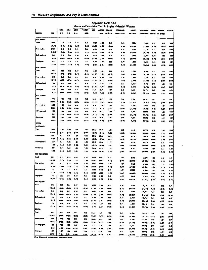
80 Women's Employment and Pay in Latin America
Appeni Table 3A.1Means and Variables Used il Logits - Mamed Women
822Ta T ID3 S FaAWLY AO AOQ YUA WU3AND ANN DMmn OM RawII 1 UM
RO0M OHS 0-2 3-5 6-14 3= 4 SaCOOL ODLOVM ascIan eAas H013 19100
AMWTO 2t26 0.45 0.40 3.04 7.33 36.19 145 S.6" 0.531 5,350 13, 0.61 3.11 O."
104.01 (0.67) (065) (1.39) (2.813 (12.048 (956) (.60 00 (1335 47.010 03.49A) (32) (47
Nam-otm 2020 0.48 0.42 1.04 7.22 36.34 14.00 3.11 0.49 30 3 13,150 0.61 SAY 6.0
o001 (0.68 (0.66) (1.39) (L73) (52.303 (9.933 0.35) (0303 (1S.28 MM6 AI I0.46 t9 0A.
S3f-V.8Y*d 1915 0.34 0.40 1.30 8.36 30.0 IS.64 3.38 0.33 SAO W3.740 0.64 5.21 .0
4.9% p0.63) (0.53 (1.34) (.0o) 5.0o0 4.D00 (2.43 (0.473 0.610) (24.35 kV7 tL4(2.41 04"
~E3ayeaa 3741 0.31 o.3 0.63 7.45 33.97 12.43 6.96 0.70 4,430 36,400 0.55 5.3s 0.01
9129 (0-35) (0573 (.32) (2.9 (9O.51) 7.1 (s504) (0463 (11.460 0 (OD 5A (263 (".13
NORRATeul 7374 0.56 0.50 1.26 7.72 36.45 14.41 2.30 0.35 2.650 .020 0.67 5.60 0.30
100.0% (0.75) (0.73) (1.50) (.11) (52.35) (982) (3.39) (0.44) (844 (19.221 (0.473 (217) 03.S5
N? -* m 6027 0.58 0.52 1.24 7.63 36.53 14.94 3.91 0.34 2.640 7.550 0.67 4.94 04
11.7% (0.75) (0.74) (1.57) (t.01) (12.70) (10.13 (LI"9 (0.40) (8.4130 (17,9130 (0.47) CLIO) 0330
Sd.aplay 701 0.53 0.46 1.52 8.74 37.85 15.39 1.77 0.22 2.30 6.090 0.77 4.91 0.4
9.6% (0.74) (D72) (1.641 (3.25) (13.26) (8.9t3 (293) 0.42) (6.3903 (IO.3 (0,42) M.M73 3A49
EfO3 639 0.39 0.34 1.14 7.60 34.33 12.71 6.59 0.60 2.600 14.770 0.60 5.64 0.74
3.7% (0.64) (0.63) (1.56) (3.62) (9.63) (7.20) (4.94) (0.493 (6,420) 2.70) (0.49) (2.73) 0.423
NOXTIEWEST
Tc,l 3072 0.56 0.48 1.34 7.60 34.05 12.97 3.35 0.44 3.6)0 12.790 0.62 4.61 0.63
304.0% (0.74) (0.69) (1.51) (1.10) (11.74) 19.01) (-.60) (0.05) (3.610) (25.703 04A) (2.3) (0.49)
N4a.-.a,ka,. 2522 0.59 0.49 1.16 7.50 34.04 13.06 2.81 0.42 3,450 12.030 0.62 4.53 0.37
84.0% (0.76) (0.70) (3.40) (2.95) (12.12) (0.32) (3.07) (0.49) (11.590 (25,550) D44) (2.25) 0.5)
31i_-m 3 15s 0.4a 0.44 1.59 .90 3.4 14.47 1.51 0.34 1.30 11.24 0.45 4.62 0.46
5.2% (0.60) (0.64) (1.763 (5.4) (10.113 (7.99) (.64) 03.44) (153703) (26.3703 (0.48) (2.633 03.473
ENa94Ya 325 0.42 0.35 1.13 7.76 32.14 13.60 7.43 0.65 4.204 5s.570 0.40 5.39 0.09
10.85 (0.6) (.03 (1.5) (3.77) (0.9 (6.503 (4.60 (0.43) 49.531) 02.U00 IDA4 (2.443 0.311
OTNEF
SOUTHEASr
TWe 367 0.46 0.40 3.13 7.40 35.25 14.57 3.43 0.51 4,440 311730 0.54 5.53 0.66
304.0% (0.66) (0.0) (1.43) (2.O) (33.97) (9.46) (.62) (0.50) (33.500) (2.910) (0.49) (243) 0.473
N? r.-k 3103 0.49 0.41 1.14 7.30 36.26 34.64 2.9 0.50 4.250 0,.60 0.3 5.50 0.62
34.6% (0.67) (0.64) (1.45) (2.74) (12.32) (9.76) (3.12) 0.54) (13.410) (20.140) (0-49) (2.39) (0.40)
Sclr-FwWe4 207 0.31 0.36 1.21 8.54 39.13 16.36 3.77 0.43 6.12D 17,040 0.63 5.37 0.77
5.65 (0.0) (0-62) (1.32) (91) (t.72n (.24) (3.92) (0.46) (I3.604 (42.960) (0.4) (2.45) (0.42)
154a00eaa 357 0.32 0.n2 1.00 7.53 34.54 12.77 7.14 0.64 4.740 16,230 0.59 6.31 0.64
9.75 (0.55) (0.35) (3.33) (3.03) (0.23) (6.74) (5.073 (0.40) (12,1103 (27,500 (0.49) (2.60) 00.32)
RW DE ANEO
TOWl 2923 0.32 * 0.33 0.77 6.87 37.56 35.50 5.44 0.66 .910 38.970 0.55 5.30 0.93
1003S (0.57) (0.39) (3.12) (2.36) (11.30) t(950 4.31) (0.47) (21,200) (29.240 (0.50) (2.30) (0.29)
N4m- eakm 2223 0.37 0.35 0.79 6.79 37.92 15.09 4.79 0.65 9.130 17.20 o.n 5.22 0.90
76.0% (0-.0) (0.6) (1.14) (2.60 (32.24) (0.96) (3.75) (0.40) (19a0 (26.26 to -3.3) (2.1) (0.503
SaIf-aepIqad 149 0.21 0.31 0.54 7.52 345.6 15.92 S.0 0.39 12.93 23,904 0.32 5.40 O.955.13 (0.43) (0.5) (1.36) (2.ss) (30.20) (0.24) (4.50 0.49) (44.60 (46.150 (0s (L24) (0.213
EEO a 555 0.22 0.24 0.64 7.05 35.31 13.83 8.00 0.76 6.600 24,470 0.33 5.56 0.
I1.S (0.47) 0.50 (.02 -.4 (0.) (5-s. (1.M) (0.41) (16.700 (52,010) (G.Sd (3.42) 0.21)
SAO PAULO
T.3 6461 0.34 0.34 0.57 7.09 36.24 14.54 4.53 0.64 8,760 20.170 0.53 5.02 0.89
3oo0s (0.4 4.59) (1.23) (2.54) (11.4) (0.36 (4.6 (.AS) (22.22% (54.3" (0.50) a (.3
N..-aa.tm 5359 0.40 0.55 0.A 6.ff 36.71 34.91 4.05 0.64 9.230 19.090 0.54 5.04 0.67
77.8% (0.62) 3.40 (1.21) (246) (32.263 (9.79) (3.s (0.44) 2.0103 O4.353 (0.50 (2.54) 0P.34)
.- FI-ad 352 0.22 0.54 1.10 7.85 38.49 1S.8 4.93 0.47 13.630 22.900 0.54 5.40 0.0
5.3% O0.49) (0.4) (.40) (2.10) (10.33) (444) (4.41) (0.503 (2.40) o0.053) (0.5 (2 a.75) (0.33)
Emplo4y 3370 0.29 0.21 0.14 7.S1 33.42 12.10 6.63 0.74 5,s 20.510 0.45 4.03 0.94
17.1% (0.53n (.4) (.26) (2.64) (.66) (7.193 (5.26) (0-44) (32,023) (35,470 (0.S0 (A.45S) S0.24
JlXnHTOWl 5097 0.39 0.35 0.97 7.3 36.13 3.53S 3.90 0.49 4,240 13,029 0.66 5.33 0.63
100.0% (.56) (0.9) (3.30) (2.3) (12.3M (9.73n (3.513 0 4 t0° (25,210) (0.47 23) PA.
N _a.-aaokag, 396 0.42 0.36 0.96 6.96 36.4 14.935 3.42 0.44 4.530 12.850 0.63 5.24 0.54
73.23 (0.61) (0.40) (1.20) (.44) (12.13 (1o.169) C2.94 0.50) (30104o3 0.510 (.44) (a2.) 6.S1-a.pIywd 414 0.33 0.33 1.39 3.14 37.79 S.50 3.73 0.27 4.310 33.8M 0.74 S.42 0.43
1% 3 (055) (.5 0..31) (2. (11.06) (1.70) (.37 (0.44) 311.4003 (4.503 .44) (40
E"40y.aa 697 0.27 0.29 0.33 7.34 32.31 33.96 6.70 0.70 5.940 14.30 0.65 S.66 0.3
13.7% (0.50) s0.n (3.23) (264) (0.31) (6.31) (4.833 (0.44) . .74 (37,0 ) (0.4) (2.63 (0.32)Na6 l4mNp54c f3 laa dlIi
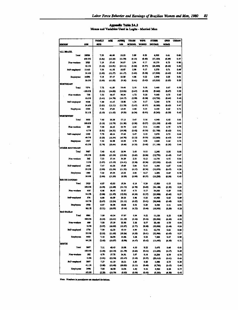
Labor Force Behavior and Earnings of Brazlian Women and Men, 1980 81
AppuUx Tabe 3A.2Mean ta Vaiabic Uoed in LAita - Mauied Men
FIAMLY AM AOQ YAM WEE OnT am URUARom Om8 am 113 8HOOL woR 1mm Buo
Total 28926 7.33 40.98 11.53 3.69 0.20 6.950 0.61 0.65
100.01 (2.8) (3.24) (11.9) (4.15) (0.40) (37,100) (0.49) 0.47NOm-Wogka 2920 7.19 57.45 34.67 2.94 0.17 IC.70 0.73 0.30
10.1% (3.16) (12.91) (34.11) (3.36) 37 (25.400) (0.43) 0.40
S3 F-amq'ed 11410 7.53 41.56 1L. 2.90 0.17 3,370 0.71 0.49
39.4% (292) (12.7 (1-17) (.62) (0.36) (17,990) (0.43) 0.30
EnpIoyo 14596 7.19 37.17 15.03 4.56 0.22 5.940 0.30 0.81
303% (2-63) (11.0 (9.10) (4.41) (0.42) (13,010) (0.0) 0.39
NOm28AxrTOal 734 7.72 M1.5 19.41 2.t9 0.11 3,460 0.67 0.30
-100.0% (3.11) (14. (13.02) (3.47) (0.39) (9,640 (0.47) 0.50
Nos-wookou 758 7.32 58.47 36.34 3.72 O.S 9,640 0.73 0.63
10.3% (3.41) (14.70) (16.17) (2.9" (0.38) (13,750) (0.44) 0.4U
SelF-cmp1ac'od 4026 7.3 41.43 18.3 1.34 0.17 2,240 0.76 0.33
54.6% p3.05) (13.11) (11.79) (247) (0.37) (6,330 (0.43) 0.47
Employ 239 7.54 37.64 13.41 3.S6 0.21 3,340 0.S3 0.71
35.1% (3-10) (11.43) (9.50) (4.34) (0.41) (9,240 (0.50) 0.45
NORIZIWE
TOWl 3002 7.60 39.38 17.15 3.47 0.16 4,940 0.62 0.61
100.0% (3.10) (32.79) (11.30) O.90) (0.37) (13,19 (0.46) 0.49
Nan-woiku 202 7.99 36.33 33.79 2.45 0.14 13,490 0.72 0.71
6.7% (3.81) (14.31) (14.94 (3.42) (0.35) (21,70) (0.4S) 0.41
Solf-mployod 1493 7.73 40.14 17.83 2.47 0.13 3,370 0.73 0.46
49.71 (3.23) (3L34) (10.70) 0.12) (0.33) (12,38) (0.4) 0.50
Employe" 1307 7.35 35.90 14.02 4.78 0.20 4.840 0.46 0.74
43.53 (271) (30.64) (8.66) (4.3) (0.40) (11,130) (0.50) 0.44oTilli SOU73lRAX
Totdl 3667 7.40 41.45 1."4 3.43 0.15 5.540 0.56 0.66
300.01 (2.80) (13.24) (2.04) (.63) (0.36) (12,770) (0.49) 0.47
Nosn-Wook 362 7.33 37.14 34.39 2.33 0.15 15,770 0.72 0.11
9.91 (3.07) (13.39) (34.41) (2s8 (0.38) (22.950) (0.4) 0.40
3eif9mp4oyd 1442 7.47 42.36 19.69 3.04 0.14 4,39 0.67 0.45
39.31 (2.9 (32.34) (11.32) (3.37) (0.34) (3o.8 (0.47) 0.50
Employao I a 7.35 37.34 15.35 3.9 0.17 4.20D 0.49 0.76
50.n1 (266) (11.20 (P.29) (.90) (0.37) (10,230 0.50) 0.43
310 DE LANEM
Totll 2925 6.7 42.05 19.34 6.34 0.24 12,000 0.55 0.91
100.01 (2.59) (12.39) (11.73) (4.70) (0.43) (24,180) (0.50 0.29
N eo-wodwas 416 6.86 s643 33.27 4.75 0.17 24,050 0.0 0.92
14.21 (6 (11.92) (12.9) (4.34) (0.37) (25.9) (0.46) 0.7
SfIOId 376 6." 43.2 20.23 3.36 0.22 14.980 0.62 0.89
19.71 (267) (12.24) (11.31) (4.67) (0A41) 6.90 (0.49) 0.32
noplapoos 3933 6.37 36.58 36.08 6.52 0.26 8,320 0.51 0.92
66.11 ( 1) (10.95 (9.14) (4.73) (0.44) (16.950) (0.3 0.26SAO0 PAULO
Total G6a 7.09 4034 17.87 5.04 0.22 13,130 0.53 0.86
100.01 (2.34) (12.41) (11.19) (4.46) (.42) (23,.90) (0.50) 0.32
No-weon 480 7.03 57.19 33.90 3.56 0.17 28,130 0.70 0.94
9.9s (2.97) (1.9) (32.07) 0.77) (0.38) (32,020) (0.46) 0.24
3ef-3 1776 7.09 42.29 19.39 4.99 0.21 12,770 0.61 O.S4
25.91 (2.5) (11.63 (10.26) (4.50 (3.A) (32,9) (0.49) 0.37
Employo 4405 7.10 36.98 34.6 5.21 0.23 7,80 0.47 o.89
64.21 (245) (3o. (8.99) (4.47) (0.42) (15,490) (0,50) 0.31
Total 5097 7.11 40.43 11.OS 4.10 0.22 5,670 0.66 0.61
300.01 (252) (13.13) (11.79) (3.62) (0.41) (1.690) (0.47) 0.49
Nos-wodon 502 6.79 S7.75 34.91 3.07 0.16 16,200 0.79 0.73
9.ss (291) 02.38) (13.47) (3-19) (0.3n (20,410) (0.41) 0.43
s- d 2097 7.27 41.19 IL8I 3.50 0.20 4,010 0.7S 0.39
41.11 (269) (12.40) (10.5) (3.11) (0.40) (9,720) (0.45) 0.49
Emnploy..a 2491 7.05 36.30 14.34 4.52 0.24 4,900 0.56 0.77
49.01 (L22) (0.79h (3.32 (.96) (0.43) (9,S30) (0.50) 0.42
Note: N _,ba in pmuudwu an ido davaniam.
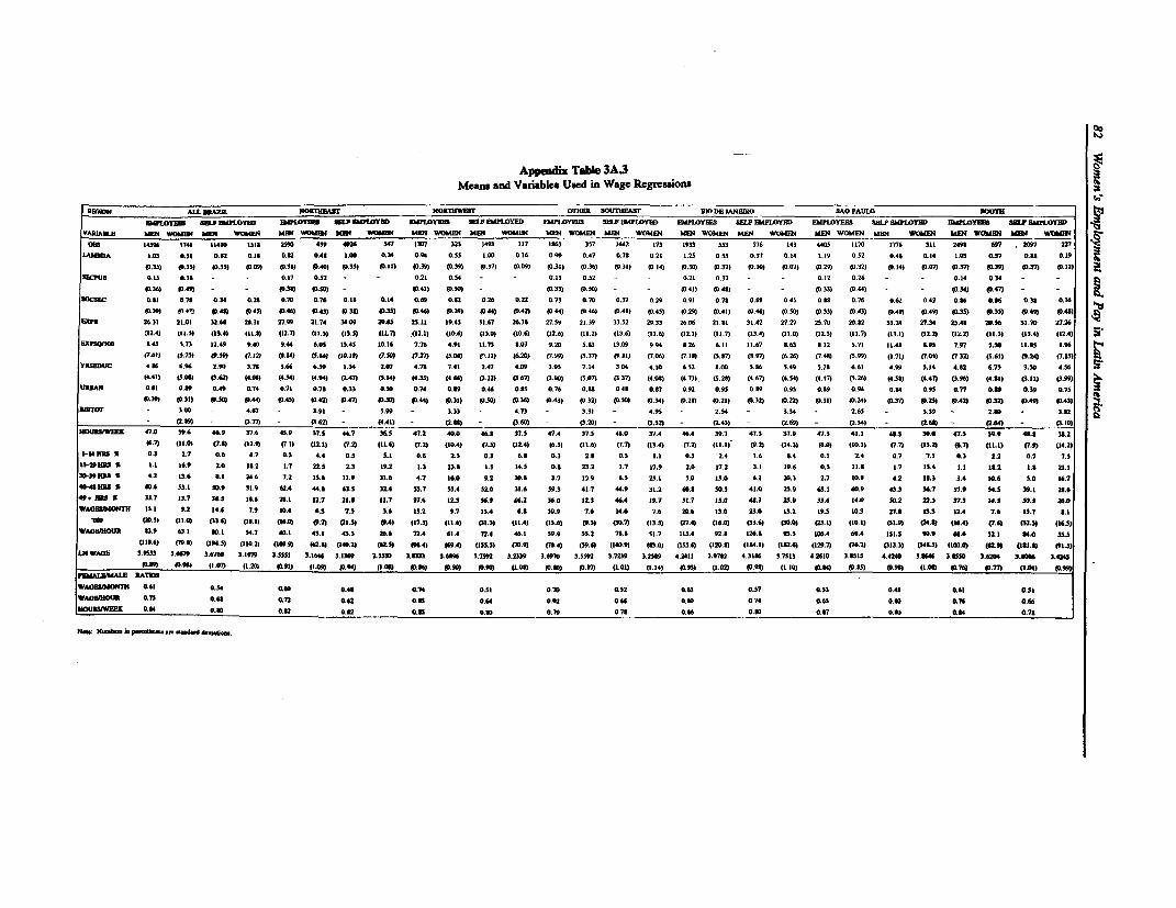
Appendix Table 3A.3Means and Variables Used in Wage Regressions
om~~~~~~~~ ~~AU. sRzn. NORT2s6Xr NOahl(36M CYrlil 303(UFI0ABr RiD JANEn SAG PAULO sm..13
MP.Yn am- EmpLyNI BIFLOYBE o"mmP 1fmY0 UdPWYRE LPImbeDo EPlWYaM 362. EOMPLY3 E6LOYE03 5E1 34WLY02D EMPLOYEES 061JMPLOYED EMiLOYsM 05? EMAOYED
buIAE mE WIO&M mmO womN MEN W601630 363 wo6 mmE WObME mEN WoOMEN ME WOMEN MEN WOMEN MEN WOuME mEN WOMP3 MEN WOMEN MEN WMN MNWMN~ 6hE
00 1436 34 140 125 20 59 45 4 1307 323 1493 III 1063 337 14U2 173 I933 333 3176 143 4405 1170O 176 311 26066 967 22LAIiSDA 1.03 0.11 0.02 0.15 0.02 0.43~~~~~~~~~GA 106 03.0 0.90 0.53 LOD 0.16 0099 0-47 0.72 .21 1.25 053 0.37 0.14 1.29 0.2 0.45 0.14 103 0357 OU 0.19
93331 93.33) 93.33) 9309) 9330) 93401 9333) 9312) 93303 93~~~~~~(039) 93-37) M100) 90331) (036) 90332) 9314 9D.301 9.32) 93.26) 9307) 9329) 93.32) 93.14) 90.07) 90333) 9339) )3) 90322)
~~23B 923 030 - - 017 032 - - 021 0.34 - - 6.13 032 - - 0.21 0.37 - - 0.22 0.26 - - 014 034 -0.2 0.2 0.3 0.1 0.2 0.1 0.3
93.36) t3.493 - - 930) 9330) - - 0941) 93.03 - - 93-33) 93.30) - D9.411 90.40) - - 9333) 93.44) - - 934) 93.47) -
U1csoW 002 0359 0.34 0.20 0.5 070 0 23 01 014 069 0.42 0.26 0.22 0.73 0.70 0.37 0.29 0.91 0.78 0.69 0.45 0.03 0.76 0.62 0.42 030 36 0 306 036
930 94) 934) 33 94) 33 93) 33 9346) 93.34) (D44) 9342) 93.44) 9346) 93.49) (0.45) 93.201 90.41) 93.44) 9336I) 9033)) 90.43) P049) (D-49) )333) 9D333) 9349 93.44)03(95 2632 21.01 32.61 21.32 27.49 2274 3409 5962 33 II 29.43 32.07 26.35 27.34 2914 39 33526.3 29.33 21.326306222.01 320642127.27133.702726.07032.26 3 27.347.34 4255436M% S31570 27752
,12.4) (112.3) (13.4) (11.9) (12.7) (22.3) (23.0) (11.7) (12.1) (0.-6) (13.0) (0.-6) (12.0) (12.2) (23.6) 202.61 (22.1) (22.7) (13.4) (21.01 (12.3) 721.7) (13.2) (12.2) (22.2) (11.3) (13.4) (22.4)3110Q1220 0.43 3.73 22.49 9.41) 9.44 6.65 13.42 20.26 7.76 4.91 12.73 3.07 9.59 3.03 13.09 9.96 0.26 6.11 11.67 8.63 0.12 3.71 11.40 0.95 7.97 3.30 HA.0 0.06
(7.62) (3.73) P9.M9 (7.122 (1)4) (53.6) (20."9) (7.30) (7.27) (S.043 t¶'i1) (6.20) (7.99) (3.37) 49.01) p7.06 (7.13) (3.07 (0.97 10.20) (7.49) (5.00) (0.71) (7.06) (7.33) (3.61) (9.26 (7.13
YRSEDUC 4.30 6.96 2.90 3.70 3.66 6.59 1.34 2.07 4.70 7.41 2.47 4.09 3.93 7.14 3.04 4.10 6.32 00 3.00 5 36 .49 3.20 6.621 .9 31 .3 .3 31 3
246) (3.00) (3.42 (4.06) (4.34) (4.94) (2.47) (2.14) 64.33) (4.60 P3.1) 03.673 (3.90) (3.07) (3.37) (4.05) (4.7)) (3.20) (4.67) (4.34) (4.47) (3.26) (4.33) (4.47) (3.96) (4.021) (3.11) (3993
UR5AO 0.02 0.09 0.40 0.74 0.71 0.70 0.33 9.30 0.74 0.30 0.46 0.03 0.76 0.m 0.40 0.07 0.92 0.93 0.59 0.95 0.09 0.94 0.04 0.93 0.77 0089 0.39 0~75
93.399 93.31) 93."9 93.44) 93.452 .4R2) 93.47) P-.3M 93.44) 93.31) 93.30) 93.36) 90.43) 93.32) 93.10) 93.34) 93.25) 93.22) 93.32) 932) 9.2 32) 9.7 333 34) 9.2 34) 9.3
DIRTOT - 330 - ~~~~~ ~ ~ ~~~~~4.67 - .91 - .09 3.33 4 .73 - 3.32 4.93 .3 3.34 - 2.65 3.39 2.001 - 3.03
- (2089) - (3.77) - (3.62) - (4.41) - (2.30) (3.46) - (3.20) - (3.32) - (Z.43) - (2.69) - (2.34) - 2.Z -(.64) - (3.20)
130U09WEEK 43.0 306 46.9 37.0 45.9 13.3 44.7 3. -47.2 40.0 46.8 27.S 47.4 37.5 45.0 37.4 46.4 39.7 47.3 37.9 47.3 41.1 49.5 39.0 47.3 "9.9 40.8 26.2
(6.7) (12.9) (7.0) (22.9) (7.2) (12.2) (7.9) (11.93 (7.3) (10.4) (7.0) (32.4) (6.3) (21.6) (7.7) (23.4) (7.3) (22.21_ (93.) (14.3) (6.0) (20.22) (3.7) (13.2) 96.7) (11.1) (7.9) (24.3)
2-240 1a 0.3 2.7 0.6 6.7 0.3 4.4 0.3 3.1 0.6 2.3 0.3 6.0 0.3 2.01 0.3 3.1 0.) 2.4 2.6 5.4 0.1 2.4 0.7 ?.I 0.) 2.2 0.7 7.3
IS23-9HI 5 1.1 26.9 2.0 20.2 2.7 33.5 2.3 29.2 1.7 13.3 1.3 14.3 0.5 33.2 1.7 17.9 2.0 27.2 3.2 19.6 6.3 12.2 1.7 13.4 2.1 23.2 1.0 21.2
W30.39353 4.7 13.6 0.1 59.6 7.3 13.6 11.9 31.6 4.7 16.0 9.2 30.5 2,7 17.9 6.3 27.2 3.0 13.6 6.2 3D.3 2.7 16.0 4.2 2I.3 3.4 10.6 3.0 26.7
40.433HRS 5 460.6 33.2 30.9 32.9 62.4 46.0 63.0 32.4 55.7 33.4 02.0 31.6 39.3 42.7 44.9 31.2 460. 30.3 42.6 23.9 63.1 460.9 43.3 36.7 37.9 34.3 29,2 26.6
49. IllS 33.7 23.7 36.3 10.6 20.1 12.7 21.5 21.7 37.0 22.1 36.9 4.16. 36.0 12.3 46.4 29.7 31.7 23.0 44.0 25.9 33.4 14.0 30.2 23.3 37.3 24.3 33.3 59.0
WAOUIJI00NTH0 23.2 9.2 24.6 7.9 60.4 6.2 7.3 16 213.3 9.7 23.4 6.0 10.9 7.6 14.6 7.6 30.6 23.0 33.0 23.3 29.3 20.3 27. 13.3 12.4 7.6 2.5.7 0.2
mm (23D.3) (22.03 (33.6) (20.12 (2690) (9.7) (11.2) (9.43 (17.3) (21.0) (32.3) (11.4) (23.0) (9.31 (30.7) (23.3) (07.4 (26.01 (33.6) (20.0) (03.12 (20.21) (21.9) (24.9) (36.4) (7.6) (32.2) (16.5)
WAOR04OUR 03.9 6521 30.2 34.7 46.2 43.2 43.3 59.6 72.4 62.4 32.4 46.2 39.9 33.2 70.0 92.7 123.4 92.8 226.3 93.3 10.4 69.4 1)1.7 90.9 64.6 32.2 64.0 33.3
(I1296) (79$) (294.)) (220.3) (209.9) (62.9) (146.2) (62.4) (96.4) (69.4) (233.)) (30.9) ((0.4) (39.9) (1460.9) (03.0) (155.4) (139.9) (230.2) (120.9) (126.7) (76.2) 3323.3) (240.5) (104.0) 932.0) (232.63 (92.3)
1.2 WAGE 39)33 3.6679 3.6746 3.29M 3.5331 3.0646 3.1369 2.2330 3.033 3.606 3.7S92 332339 3.6930 3.5359 3.7239 3.239 4.5221 3.970 4.3106 3.7513 4.2620 3.0315 4.4240 3.3046 3.333 3.63M4 3.6116 3.436
(109) 93.96) (2.073 (2.363 0923 (1.09) 93.963 ~~~~~(3.0 93.36) PM0) VIM9 (1.093 93.33 ID.97 (1.013 (1.143 0393) (1.62) 9.0 12) 9.6 30) 9,0 25) 9.6 37) (O) 9.9
WAG(BM0003 9.62 0.34 0.609 0.49 0.70 0)2I 0.70 6.52 0.62 0.07 0.33 0.40 0.6 0.33
WA(06200(R 0.7) O.46 0.72 0.62 0.33 0."4 0.02 0."6 0.30 0.74 0.65 0.30 0.76 0.06
Ho2J5OMRRK 0.30 0.30 0.02 0.02 0.5) 0.09 0.79 0.70 0.30 0.30 0.17 0.3000 00.70
MM:M N(-644 k2 2P 02222624344300-
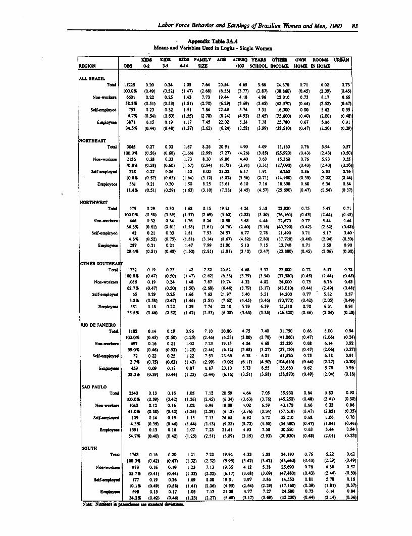
Labor Force Behavior and Earnings of BraziRan Women and Men, 1980 83
Appadi Table 3A.4Means and Variables Used in Logibs - Single Women
ID tUD5 KtS FAMLY AGB AaESQ YEARS OTHER OWN ROOMS URBANREGION O0S 0-2 3-5 6-14 SIZE /100 SCHOOL INCOME HOME IN HOME
ALL BRAZILTobl 11225 0.20 0.24 1.35 7.64 20.54 4.65 5.68 24,870 0.71 6.02 0.73
100.0% (0.49) (0.52) (1.47) (2.6S) (6.55) (3.77) (3.87) (38,860) (0.45) (2.39) (0.45)Non-worbn 6601 0.22 0.25 1.43 7.73 19.44 4.18 4.96 25,310 0.73 6.17 0.66
58.8% (0.51) (0.53) (1.51) (2.70) (6.29) (3.69) (3.45) (42,370) (0.44) (2.52) (0.47)Self4employed 753 0.23 0.32 1.51 7.84 22.49 5.74 3.31 16,300 0.80 5.62 0.35
6.7% (0.54) (0.60) (1.55) (2.78) (8.24) (4.93) (3.45) (35,600) (0.40) (2.00) (0.48)Employea 3871 0.15 0.19 1.17 7.45 22.02 5.24 7.38 25,780 0.67 5.86 0.91
34.5% (0.44) (0.48) (1.37) (2.62) (6.24) (3.52) (3.99) (32,510) (0.47) (2.20) (0.29)
NORTHEASTTotl 3045 0.27 0.33 1.67 8.26 20.91 4.90 4.09 15,160 0.76 5.94 0.57
100.0% (0.56) (0.60) (1.66) (2.99) (7.27) (4.26) (3.85) (25,920) (0.43) (2.43) (0.50)Non-wortl 2156 0.28 0.33 1.73 8.30 19.86 4.40 3.63 15,360 0.76 5.93 0.55
70.8% (0.58) (0.60) (1.67) (2.94) (6.72) (3.91) (3.31) (27,090) (0.43) (2.43) (0.50)Selfemployed 328 0.27 0.36 1.50 8.00 23.22 6.17 1.91 8,260 0.86 5.34 0.26
10.8% (0.57) (0.65) (1.64) (3.12) (8.82) (5.36) (2.71) (14,930) (0.35) (2.02) (0.44)Employe 561 0.21 0.30 1.50 8.25 23.61 6.10 7.16 18,390 0.68 6.34 0.84
18.4% (0.51) (0.59) (1.63) (3.10) (7.28) (4.45) (4.57) (25,690) (0.47) (2.54) (0.37)
NORTHWESTTotal 975 0.29 0.30 1.68 S.15 19.81 4.24 5.18 22,930 0.75 5.47 0.71
100.0% (0.58) (0.59) (1.57) (2.69) (5.60) (2.88) (3.50) (36,160) (0.43) (2.44) (0.45)Non-worsa 646 0.32 0.34 1.76 8.24 18.58 3.68 4.46 22.670 0.77 5.44 0.64
66.3% (0.61) (0.61) (1.58) (2.61) (4.76) (2.40) (3.16) (40,390) (0.42) (2.62) (0.48)Sdf-emtpcyeod 42 0.21 0.33 1.81 7.93 24.57 6.77 2.76 21,490 0.71 5.17 0.40
4.3% (0.52) (0.75) (1.81) (3.14) (8.67) (4.82) (2.80) (37,720) (0.46) (2.04) (0.50)Employees 287 0.21 0.21 1.47 7.99 21.90 5.13 7.15 23.740 0.71 5.59 0.90
29.4% (0.51) (0.48) (1.50) (2.81) (5.81) (3.10) (3.47) (23,880) (0.45) (2.06) (0.30)
OTHER SOUTHEAsrTotWl 1732 0.19 0.23 1.42 7.82 20.62 4.68 5.37 22.800 0.72 6.57 0.72
100.0% (0.47) (0.50) (1.47) (2.62) (6.58) (3.79) (3.54) (37,580) (0.45) (2.44) (0.45)Non-workHrs 1086 0.19 0.24 1.48 7.87 19.74 4.32 4.82 24,000 0.73 6.76 0.63
62.7% (0.47) (0.50) (1.50) (2.68) (6.46) (3.79) (3.17) (43,010) (0.44) (2.49) (0.4t)Self-employed 65 0.29 0.25 1.66 7.63 21.97 5.40 3.51 14,200 0.77 5.82 0.37
3.8% (0.58) (0.47) (1.46) (2.51) (7.62) (4.45) (3.46) (20,770) (0.42) (2.05) (0.49)Employee 581 0.18 0.22 1.29 7.74 22.10 5.29 6.59 21,510 0.70 6.31 0.91
33.5% (0.46) (0.52) (1.42) (2.53) (6.38) (3.63) (3.85) (26,320) (0.46) (2.34) (0.22)
RIO DE JANEIROTol 1182 0.14 0.19 0.96 7.10 20.80 4.75 7.40 31,750 0.66 6.00 0.94
100.0% (0.45) (0.50) (1.25) (2.46) (6.53) (3.80) (3.70) (41,060) (0.47) (2.06) (0.24)Non-woekam 697 0.16 0.21 1.02 7.23 19.15 4.04 6.68 33,330 0.68 6.14 0.92
59.0% (0.46) (0.S2) (1.25) (2.44) (6.12) (3.68) (3.27) (37,130) (0.47) (2.06) (0.27)Self-employed 32 0.22 0.25 1.22 7.53 23.66 6.38 6.81 41,520 0.75 6.38 0.91
2.7% (0.75) (0.62) (1.43) (2.99) (9.02) (6.11) (4.50) (104,610) (0.44) (2.27) (0.30)Em toyee 453 0.09 0.17 0.87 6.87 23.13 5.73 8.55 28,630 0.62 5.76 0.96
38.3% (0.39) (0.44) (1.23) (2.44) (6.16) (3.51) (3.98) (38,870) (0.49) (2.04) (0.18)
SAO PAULOToal 2543 0.13 0.16 1.05 7.12 20.59 4.64 7.05 35.930 0.64 5.83 0.90
100.0% (0.39) (0.42) (1.26) (2.45) (6.34) (3.63) (3.76) (45,250) (0.48) (2.41) (0.30)Non-wotrkrs 1043 0.12 0.16 1.02 6.96 19.08 4.02 6.59 43,170 0.66 6.32 0.86
41.0% (0.38) (0.42) (1.24) (2.39) (6.18) (3.76) (3.34) (57,610) (0.47) (2.82) (0.35)Self-employed 109 0.14 0.19 1.15 7.15 24.65 6.92 5.72 35,210 0.6a 6.06 0.70
4.3% (0.35) (0.46) (1.44) (2.13) (9.23) (5.72) (4.50) (54,480) (0.47) (1.94) (0.46)Employe 1391 0.13 0.16 1.07 7.23 21.41 4.93 7.50 30,550 0.63 S.44 0.94
54.7% (0.40) (0.42) (1.25) (2.51) (5.89) (3.19) (3.93) (30,930) (0.4t) (2.01) (0.23)
SOUTHToWl 1748 0.16 0.20 1.21 7.22 19.94 4.33 5.88 24,180 0.76 6.22 0.f'
100.0% (0.42) (0.47) (1.32) (2.32) (5.95) (3.42) (3.42) (43,640) (0.43) (2.29) (0.49)Noa-woken 973 0.16 0.19 1.23 7.13 19.35 4.12 5.38 25,690 0.76 6.36 0.57
55.7% (0.41) (0.44) (1.33) (2.32) (6.17) (3.68) (3.09) (47,480) (0.43) (2.44) (0.50)Self-employed 177 0.19 0.36 1.69 8.08 19.31 3.97 3.86 14,550 0.81 5.78 0.16
10.1% (0.49) (0.58) (1.41) (2.36) (4.95) (2.54) (2.29) (17.160) (0.39) (1.81) (0.37)Em tOye 598 0.15 0.17 1.05 7.13 21.08 4.77 7.27 24,580 0.73 6.14 0.U4
134.2% (0.42) (0.46) (1.23) (2.27) (5.68) (3.17) (3.69) (42.230) (0.44) (2.14) (0.36)Ndow Numb. n psrhes ia _isd ds mbom.
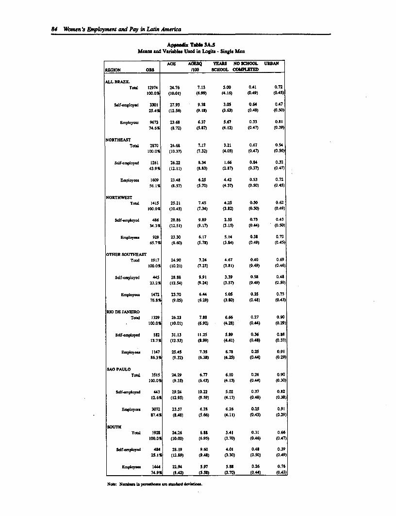
84 WOmen 's Fpnqloyme and Pay i Latin America
Appedix Tabb 3A5Means and Variabls Used in Logits - Single Men
AGE AGESQ YEARS NO SCHOOL URBANREGION 0O3 II00 SCHOOL COM1PLEED
ALL BRAZILTotal 12974 24.76 7.13 5.00 0.41 0.72
100.0% (20.01) (6.99) (4.16) (0.49) (0.45)
Self-employed 3301 27.93 9.38 3.05 0.64 0.4725.4 (12.56) (9.18) (3.63) (0.4S) (0.50)
Employe 9673 23.68 6.37 5.67 0.33 0.8174.6% (8.72) (5.87) (4.12) (0.47) (0.39)
NORTHEASTTOWl 2S70 24.68 7.17 3.21 0.67 0.54
100.0% (10.37) (7.32) (4.03) (0.47) (0.50)
SAf-employcd 1261 26.22 8.34 1.66 0.84 0.3243.9% (12.11) (8.83) (2.87) (0.37) (0.47)
Employees 1609 23.48 6.25 4.42 0.53 0.7256.1% (8.57) (5.70) (4.37) (0.50) (0.45)
NORTHWESTTotal 1415 25.21 7.45 4.25 0.50 0.62
100.0% (20.45) (7.34) (3.82) (0.50) (0.49)
Self-employed 486 28.86 9.89 2.55 0.73 0.4334.3% (12.51) (9.17) (3.15) (0.44) (0.50)
Employee 929 23.30 6.17 5.14 0.38 0.7265.7% (8.60) (5.78) (3.84) (0.49) (0.45)
OTHER SOUTHEASTTotal 1917 24.90 7.24 4.67 0.40 0.69
100.0% (10.21) (7.23) (3.81) (0.49) (0.46)
Self-employed 445 28.U8 9.91 3.39 0.58 0.4823.2% (12.54) (9.24) (3.57) (0.49) (0.50)
Employ... 1472 23.70 6.44 5.05 0.35 0.7576.8% (9.05) (6.29) (3.80) (0.48) (0.43)
RIO DE IANEIMOTotal 1329 26.23 7.S8 6.66 0.27 0.90
100.0% (10.01) (6.92) (4.28) (0.44) (0.29)
Sdf.employed 182 31.13 11.25 5.89 0.36 0.8813.7% (12.53) (S.99) (4.41) (0.48) (0.33)
E npUoles 1147 25.45 7.35 6.78 0.25 0.9186.3% (9.32) (6.38) (4.2) (0.44) (0.29)
SAO PAULOTotal 3515 24.29 6.77 6.10 0.26 0.90
100.0% (9.35) (6.43) (4.13) (0.44) (0.30)
Self-employed 443 29.24 10.22 5.02 0.37 0.8212.6% (12.9S) (9.59) (4.13) (0.48) (0.38)
Employes 3072 23.57 6.28 6.26 0.25 0.9187.4% (8.48) (5.66) (4.11) (0.43) (0.29)
SOUTHTotbl 1928 24.26 6.88 5.41 0.31 0.66
100.0% (20.00) (6.95) (3.70) (0.46) (0.47)
Self-employed 484 28.19 9.60 4.01 0.48 0.3925.1% (12.89) (9.48) (3.30) (0.50) (0.49)
Employae 1444 22.94 5.97 5.8U 0.26 0.7674.9% (8.42) (5.5S) (3.70) (0.44) (0.43
Note: Numb..I in patheur an adud dwistos.
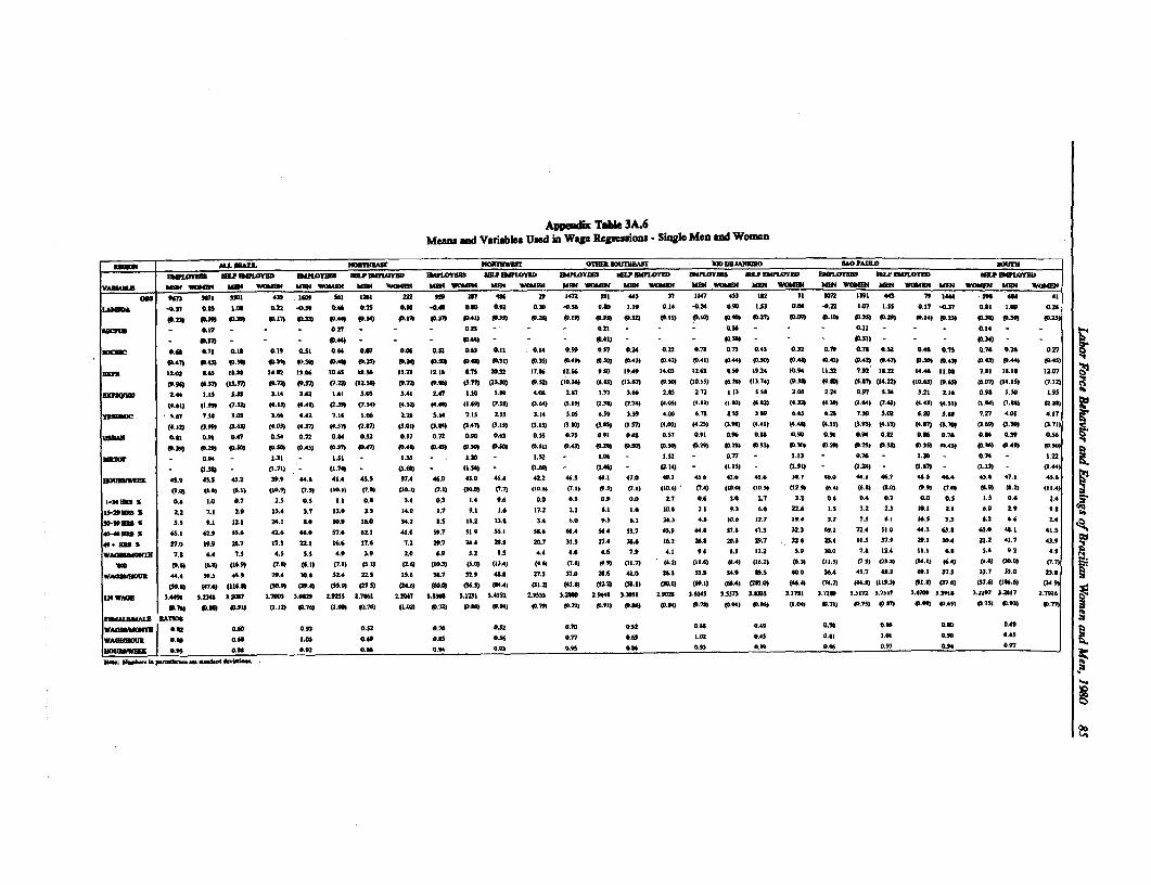
Apsueix Tabk 3A.6Mean and Variables Used in Wage Regressions -Snl e n oe
54 Mi 096252. ~~~~~~~~~~~~~~~~~~~~NORT08617 monOE1wT (STfE.305T5563 %MD1364A035 SAO PAULO moo.m
068 9472 3075 2291 429 1484 361 5261 332 939~~~~~~~~~~~~~g 2N7 454 29 5433 531 4 37 1147 433 132 St Sam3 5392 441 79 244 .9 484 41
LANMA -45.37 0.02 1.06 0323 -4239 04" 0.73 030 -044 0.39 093 0.30 4036 5534 5.59 0.54 40.24 0.93 1JI 0550 -0232 5.02 1.35 0.37 -0.37 0.81 1.09 0,24
P.23) P-95 P33 95175 33 93405 p.34) 50.515 P.1) 50.41 P3." 9P254 op595 9333) 9L2) 40.5(5 13) 9.48 P.37 P010 0) P1 33) 0P29 9514) P.23) P293 P2) 10-23)
mo5n3 - 0.57 - - 027 0 .22 . 0.21 0.56 - -- 0.53 - - 014 --
403P. - - - 9.445- - A 44 - - 41) - D (024 - - P0352 - - P214) -
046wO. 075 0.56 0.19 0.35 0.64 0.07 0.04 0.15 0.43 0.5 0.54 0.59 0.37 0.24 0.22 0.75 0.73 0.43 0.32 0.79 0.70 0.23 0.48 0.13, 0.70 0.26 0.11
WEM 52.01 IL" 50.99 14.32 13.06 W0.4 58.36 150.73 52.56 8.752D3.22 17.54 12.46 .5 59.49 14.03 52.41 639 59.34 50.94 25.32 792 IS2M 5446 55.99 7.21 50.1 12.07 61
p9650 5457) (5237)4 072) (P."7 (7.232 (12.39 .732 59.94) (5.77) (13.30 952) 550.36) (6.83) (13.67 (9505 (50.333 (6.265 (13.745 (9.385 (9.35 (2.32) (14.22) (50.63) (91.43) 36.07 (14.135 (7.122
3098023 2.44 3.53 3.33 3.14 2.62 1.45 3.0 3.41 2.47 5.10 2.89 4.06 2.67 5.37 5.46 7.03 272 153 2.28 2.02 2.24 0.97 5.34 3.21 2.56 0."9 S3.0 1.93
(44.6) 51.99) (7.332 (4.13) (4.40) (2.20 (7.34) (4.32) (4.49) (5.49) (7.50 (3.44) (2.59) (2.50) (7.745 (4.02) (4.535 51.523 (6.32) (4.325 (429 (5.4) (7.435 (4.435 (4.51 7.5) (I 7 .95) 52.3)
Ymimic 2.67 7.58 3.05 2.66 4.42 7.34 1.06 2.26 5.14 7.15 2.33 3.14 3.33 6.50 3.39 4.OD 6.75 0.23 2.00 6.62 6.26 7.30 2.0 6.24 3.09 7.21 4.05 4.17
(4.132 (2M 509 (.4) (4.02) (4.27) (4.33) (2.82) (2.055 (2.44) (3.47) (.5 0. 52) 0. 50)Mo (2.82) (317) (4.03) (4.25) P2.9M (4.455 4440 (4Al .51) (2.02) (4.53) (4.07 (31.783 (.9 23) (.1
VW"363 0AN 0.2 0.47 0.34 0.72 0.84 0.32 0.31 0.73 0.93 OR)s 0.5 0.75 5.95 0.6 037 09 .9 .9 0.3 001 099.3 .6 0.608 0.29) 0,36 '
- 534 1 L31 1.35 1 .33 - 1.20 - 5.2 1 .04 - .23 - 0.77 1.52 0.16 1 .201) 0.74 - 1332
- (2.39 0 .713 (1.75 (1.462 - (2.34) - (.602 (1.46) - (2.54) - (5.12) - (1.915 (1.245 56) -. (1.13) - (1544)
E0303WE3 41.9 42.3 43.2 39.9 44.8 4154 43.) 37.4 46.0 43.0 43.4 42.2 46.3 44.1 47.0 405.3 4246 41.6 43.6 25.1 46.0 44.3 46.7 43.3 46.4 62.8 07.5 456
(73 0.) ( 6.1) (30.) ( 2.3 15.5 (7.5) LI V, (50.5) (7,1) (10.09 (7.7) (10.6) (7.5 50.25 (2.1) (50.6), (74) (50.0) (50.5) (12.9) (0.4) (6.83 (10.0 (9.9) (7553 .9) (2.23 (5i 4)
5-545101 5 OR 5.0 0.7 2.) 0.3 5.5 0.5 3.4 0.2 1.4 0.4 0.0 0.3 0.9 2.0 2.7 0.6 %A 2.7 3.2 0.4 0.4 0.7 0.0 0.2 5.3 0.4 2.4
16-29rM a 2.2 7.1 2.9 52.4 2.7 12.9 3.5 54.0 1.7 9.1 5.4 17.5 2.1 $.5 1.6 50.0 3.5 9.2 6.4 22.6 1.3 3.2 2.3 50.5 . 6.0 2.9 9.5 t
30-930 8 2.3 9.1 12.1 34.1 5.4 10,9 14.0 34.2 85. 12.2 12.9 3.4 6.0 1.3 L.1 24.3 4.6 0 139 5.7 19.4 3.7 7.2 8.5 16.2 3,2 0.2 6.6 2.4
40-450Mm 436.1 62.9 53.6 42.6 "6. 57.6 03.5 4154 50.7 1.9 22.1 30-6 6014 54.4 53.7 43.9 44.5 57.5 67.3 32.3 44.2 77.4 35.0 44.3 43.8 43.0 48.1 413.34
.m 37.0 19.9 25.7 17.2 33.j 16.6 17.6 7.2 20.7 24.4 23.9 30.7 35.3 27.4 30.4 56.2 20.5 20.3 29.7 2 3.6 23,4 16.5371.90 95 3. 5. 574.
WA0MUOTK 7.0 6.4 7.3 4.3 3.2 4.9 2.9 2.4 4.9 5.2 0.3 4.4 4.6 4.6 7.4 4.1 9.4 5.3 52.2 3.94 10.2 7.67 524 151.5S.$ .2 4.5 3.4 9.2 44,3.1 GS 5.4 .2 4.
40 (956) (6.) (24.9) (78 (6.5) (7.55 (2.55) (2.4 (50.3) (3.9) (13.45 (4.6) (7.83 (4.83 (11.7) 44.33 (5.4) (5.4) (56.23 (6.25 (55.5) (7.3) (22.5) (14,1) (6.4) (4.63 (0.83) (7.1)
WA514WUOOR 44.4 50. 42. 29A 50.0 22.4 23.3 152. 24.7 22.9 44.5 27.5 11.0 24.4 42.0 2. 22.5 34.9 09.2 40.0 56.4 41.7 61.2 0.5 11.3 32.7 53.0 23.5
(59.) 447.6) (154.9) (20.9) (29.4) (33.9) (2.7.) (34.83 OA00 (24.2) (54.4) (25.2) 443.83 (22.3 (3L55 (30.8 (69.5) (01.45 (25.83 (46.45 (74.7) (44.83 (159.3) 591.83 (77.05 (27.83 (5114) (349)
136 WAG 3.4491 3.?14 3.20987 2.7993 3.02 2.933 2.756 2.IM6 2.23t3 .1231 3.4332 2.9523 3.235 2.9440 3."503 2.932 3.6154 3.3273 3.53)5 3.1571 ).710 3.5172 3.7517 3.6399 3.3919 3.2197 .35121 2.7916
P76) P89) 9555TW (552) 92.710 (1509 40L74) (193 p072) 984) P5645 9705 P072) OD991 5086) P8M5 9878) 90915 93.96) (1.04) P.75) P.7$5 45) (D495VA P42 9.755 0033 O77)
WVmD0730 093m 0.40 0.93 0.32 4.7 0.13 0.30 9.32 0.041 Ga 0.10 0.09 0,43 0.49
WAWIDOS 0589 G.05 1.00 0.0 0.53 6.34 0.77 0643 1.03 0.43 0.05 1.05 0.00 8.42
MU11 SW 093 0.95 0. 93 0. 46 0.46,4 0.93 0.04 0.016 0.3 .5 4 0.93 9.94 0.97
References
Arriagada, A-M. "Labor Market Outcomes of Non-formal Training for Male and FemaleWorkers in Peru." Economics of Education Review, Vol. 9, no. 1 (1990). pp. 331-342.
Becker, G.S. Human Capital. New York: Columbia University Press, 1964.
Behrman, J.R. "The Action of Human Resources and Poverty on One Another: What We haveYet to Learn." Living Standards Measurement Study Working Paper No. 74. Washington,D.C.: World Bank, Population and Human Resources Department, 1990.
Behrman, J.R. and B. Wolfe. "Labor Force Participation and Earnings Determinants for Womenin the Special Conditions of Developing Countries." Journal of Development Economics,Vol. 46 (1984). pp. 259-288.
Birdsall, J. and J.R. Behrman. "Does Geographical Aggregation Cause Overestimates of theReturns to Schooling?" Oxford Bulletin of Economics and Statistics, Vol. 46, no. 1 (1984).pp. 55-72.
Birdsall, J. and L.M. Fox. "Why Males Earn More: Location and Training of Brazilian SchoolTeachers." Economic Development and Cultural Change, Vol. 33, no. 3 (1985). pp. 533-556.
Blinder, A.S. "On Dogmatism in Human Capital Theory." Journal of Human Resources, Vol.11, no.1 (1976). pp. 8-22.
Boulding, E. "Measurement of Women's Work in the Third World: Problems and Suggestions"in M. Buvinic, M.A. Lycette and W.P. McGreevey (eds.). Women and Poverty in theThird World. Cambridge, Baltimore: Johns Hopkins University Press, 1983.
Cain, G.G. "The Economic Analysis of Labor Market Discrimination: A Survey" in 0.Ashenfelter and R. Layard (eds.). Handbook of Labor Economics. New York: Elsevier,1986.
Cotton, J. "On the Decomposition of Wage Differentials." Revew of Economics and Statistics,Vol. 70, no. 2 (1988). pp. 236-243.
Dabos, M. and G. Psacharopoulos. "An Analysis of the Sources of Earnings Variation AmongBrazilian Males." Economics of Education Review, 1991 (forthcoming).
86
Labor Force Behavior and Earnings of Brazilian Women and Men, 1980 87
Dubin, J.A. and D. Rivers. "Selection Bias in Linear Regression, Logit and Probit Models."Social Science Working Paper No. 698. Pasadena,California: California Institute ofTechnology, Division of Humanities and Social Sciences, 1989.
Greene, W.H. Econometric Analysis. New York: Macmillan, 1990.
Gunderson, M. "Male-Female Wage Differentials and Policy Responses." Journal of EconomicLiterature, Vol. 27 (1989). pp. 46-72.
Ham, J. and C. Hsiao. "Two-stage Estimation of Structural Labor Supply Parameters UsingInterval Data from the 1971 Canadian Census." Journal of Econometrics, Vol. 24 (1984).pp. 133-158.
Heckman, J.J. "Selection Bias and Self-selection" in J. Eatwell, M. Milgate and P. Newman(eds.). Ihe New Palgrave: A Dictionary of Economics. New York: Stockton Press, 1987.
Heckman, J.J. and V.J. Hotz. "An Investigation of the Labor Market Earnings of PanamanianMales." Journal of Human Resources, Vol. 21, no. 4 (1986). pp. 507-542.
Hill, M.A. "Female Labor Supply in Japan: Implications of the Informal Sector for Labor ForceParticipation and Hours of Work." Journal of Human Resources, Vol. 24, no. 1 (1988).pp. 459-468.
Jones, F.L. "On Decomposing the Wage Gap: A Critical Comment on Blinder's Method."Journal of Human Resources, Vol. 18 (1983). pp. 126-130.
King, E.M. "Does Education Pay in the Labor Market? The Labor Force Participation,Occupation and Earnings of Peruvian Women." Living Standards Measurement StudyWorking Paper No. 67. Washington, D.C.: World Bank, Population and HumanResources Department, 1990.
Khandker, S.R. "Labor Market Participation, Returns to Education, and Male-female WageDifferences in Peru." PRE Working Paper Series No. 461. Washington, D.C.: WorldBank, Population and Human Resources Department, 1990.
Kuhn, P. "Sex Discrimination in Labor Markets: The Role of Statistical Evidence." AmericanEconomic Review, Vol. 77 (1987). pp. 567-583.
Lee, F.L. "Generalized Econometric Models with Selectivity." Econometrica, Vol. 51, no. 2(1983). pp. 126-130.
Maddala, G.S. Limited-dependent and Qualitative Variables in Econometrics. Cambridge:Cambridge University Press, 1983.
McFadden, D. "Conditional Logit Analysis of Qualitative Choice Behavior" in P. Zarembka(ed.). Frontiers in Econometrics. New York: Academic Press, 1973.
Mincer, J. Schooling, Experience and Earnings. New York: Columbia University Press, 1974.
88 Women's Employment and Pay in Latn America
Mohan, R. Work, Wage, and Welfare in a Developing Metropolis: Consequences of Growth inBogota, Colombia. New York: Oxford University Press, 1988.
Oaxaca, R. "Male-female Wage Differentials in Urban Labor Markets." International EconomicReview, Vol. 14 (1973). pp. 693-709.
Ohsfeldt, R.L. and S.D. Culler. "Differences in Income Between Male and Female Physicians."Journal of Health Economics, Vol. 5 (1986). pp. 335-346.
Psacharopoulos, G. and Z. Tzannatos. "Female Labor Force Participation: An InternationalPerspective." The World Bank Research Observer, Vol. 4, no. 2 (1989). pp. 187-201.
Reimers, C.W. "A Comparative Analysis of the Wages of Hispanics, Blacks and Non-HispanicWhites" in G.J. Borjas and M. Tienda (eds.). Hispanics in the U.S.Economy. New York:Academic Press, 1985.
Schultz, T.P. "Education Investments and Returns" in H. Chenery and T.N. Srinivasan (eds.).Handbook of Development Economics. Amsterdam: Elsevier Science Publishers, 1988.
Shapiro, D.M. and M. Stelcner. "The Persistence of the Male-female Earnings Gap in Canada,1970-1980: The Impact of Equal Pay Laws and Language Policies." Canadian PublicPolicy/Analyse de Politique, Vol. 13, no. 4 (1987). pp. 462476.
Standing, G. and G. Sheenhan (eds.). Labour Force Participation in Low-Income Countries.Geneva: International Labor Office, 1978.
Terrell, T. "An Analysis of the Wage Structure in Guatemala City." Journal of DevelopingAreas, Vol.23 (1989). pp. 405-424.
Thomas, V. "Spatial Differences in the Cost of Living." Journal of Urban Economics, Vol. 8(1980).
Trost, R. and L.F. Lee. "Technical Training and Earnings: A Polychotomous Choice Model withSelectivity." Review of Economics and Statistcs, Vol. 66 (1984). pp. 151-156.
Zabalza, A. and J.L. Arrufat. "The Extent of Sex Discrimination in Great Britain" in A. Zabalzaand Z. Tzannatos. Women and Equal Pay: 7he Effects of Legislation on FemaleEmployment and Wages in Britain. Cambridge: Cambridge University Press, 1985.
4
Female Labor Force Participationand Wage Determination in Brazil, 1989
JiU liefenthaler
1. Introduction
Over the past two decades, many countries have experienced drastic increases in female laborforce participation. However, participation rates, in general, are still lower for women than menand women's wages are significantly lower than men's in most countries. These differentialshave spurred an interest in the determinants of both women's participation decisions and women'swages.
While studies on women's work in developed countries are generally based on a single sectormodel, there has been a growing interest among development economists in the effects of morecomplex labor markets in developing countries on modeling and estimating women's decisionsto work and women's earnings functions. The importance of accounting for the large informalsector in many developing countries was recognized over 30 years ago by Jaffe and Azumi(1960). They observed that women engaged in informal or "cottage-industry' work had higherfertility rates than women who worked in the formal sector. Results from several more recentstudies, using more rigorous empirical analysis, have supported Jaffe and Azumi's suppositionthat women's costs of participation are not equivalent across sectors.'
In this study, a multi-sector model of female labor force participation and wage determination inBrazil is estimated. In analyzing the Brazilian labor market it is important to distinguish betweenthe formal sector and the large informal sector. However, it is also important to account for thedistinction between the unregistered workers and the self-employed within the informal sector.The characteristic that distinguishes formal sector wage-earners from informal sectorwage-earners is that formal sector employees carry a work booklet. Under Brazilian labor law,employers are obligated to sign the employee's work booklet when contracting a worker.Unregistered employment is illegal with the exception of self-employment.
In Section 2, the distinctions between these three identified sectors are more rigorously explored,the data are discussed, and some sample characteristics are presented and discussed. Section 3briefly outlines the theoretical polychotomous choice model that underlies the empirical analysis.In Section 4, the empirical model is specified. The results from estimating the multi-sector
See, for example, Hili (1980, 1983, 1988), Smith (1981), Blau (1984), and Tiefenthaler (1991).
89
90 Women's Employment and Pay in Latin America
briefly outlines the theoretical polychotomous choice model that underlies the empirical analysis.In Section 4, the empirical model is specified. The results from estimating the multi-sectorparticipation equations for both single women and married women are presented in Section 5, andSection 6 contains the results from estimating the sectoral wage equations. The potential existenceof sex differentials in the earnings functions is discussed in Section 7. The conclusions of thisresearch are outlined in Section 8.
2. Data and Sample Characteristics
Sector definitions and characteristics. Most studies of labor markets in developing (anddeveloped) countries prior to 1980 regarded the labor market as one sector and the labor forceparticipation decision as simply a decision to work or not to work. However, several more recentstudies have attempted to construct more accurate multi-sector models of the participation decisionin more complex labor markets. The common sectoral decomposition is to increase theparticipation decision from two choices (work or don't work) to three choices - non-participation,work in the formal sector or work in the informal sector. In these models, non-participants areconsidered to be those who do not work for pay. The formal sector is defined as comprising allindividuals who work for a wage while the informal sector is made up of the self-employed.
In this study, following Alderman and Kozel's (1989) study of multi-sector participation and wagedetermination in Pakistan, the sectoral decomposition is taken a step further. As Alderman andKozel found in urban Pakistan, in Brazil a formal sector exists parallel to an informalwage-earning sector as well as a self-employment sector. Therefore, the participation decisionpresents four distinct labor market alternatives: non-participation (N), working for a wage in theformal sector (F), working for a wage in the informal sector (1), and self-employment (S). Whilenon-participation and self-employment continue to be defined as they are in the precedingparagraph, there is an important distinction between formal and informal sector employees.
The informal sector employees are easily distinguished from their formal sector counterpartsbecause informal workers do not carry booklets required by Brazilian labor law and, therefore,are not registered with the government. Employers must sign all employees' work booklets andthen register the employees. Unregistered work is illegal with the exception of self-employment.When an employer signs an individual's booklet, the employer gets access to all information onthat individual's former employment because the booklet, by law, is a record of the employee'swork history including wages.
There are both pros and cons to being officially registered as a worker in Brazil. The benefitsinclude eligibility for unemployment compensation, social security (27 percent of the total 37percent is paid by the employer), protection of labor law including minimum wage legislation,benefits of labor negotiations and union membership. However, unregistered workers do nothave to pay payroll taxes and their wages are not regulated by official wage indexations. Inaddition, people who are collecting various government transfers can continue to collect themwhile working in the informal sector.
The employer faces many added costs when registering employees including the 27 percent socialsecurity payment and other payroll taxes, the possibility of dismissal fines, union bargaining, andthe regulation of Brazilian labor law. Employers must weigh these costs against the probabilityof being caught and fined for employing unregistered workers (see Table 4.1 for the sectoraldecomposition of the work force for the Brazilian sample).
Female Labor Force Participation and Wage Detennination in Brazil, 1989 91
Data. The data for this study were collected from 70,777 Brazilian households (301,088individuals) in the fourth quarter of 1989 by the National Statistical Service. Data collection wasorganized according to four distinct regions: Rio de Janeiro and Sao Paulo, the rest of the South(Parana, Santa Catarina, Rio Grande do Sul, Minas Gerais, and Espirito Santo), the Northeast(Maranhao, Piaui, Ceara, Rio Grande do Norte, Paraiba, Pernambuco, Alagoas, Sergipe, andBahia), and the Northwest/Central (Distrito Federal, Rondonia, Acre, Amazonas, Roraima, Para,Amapa, Mato Grosso do Sul, Mato Grosso, and Goias). These four regions comprise the strataused in a modified stratified random sampling scheme based on the 1980 demographic census.Information was collected on household demographics, individual characteristics of all householdmembers, educational histories of all school-aged (5 years and older) household members, andlabor and income details of all household members over age nine.
The final sample, used for both data and regression analyses, includes 9,973 single women,50,452 married women, and 58,000 men. The male subsample includes all married men whosespouse is under age 65 and all single male heads of households.2 The 50,452 married womenare comprised of all married women under age 65 and the subsample of single women includesall female single heads of households.
Sample charaderistics. Brazil experienced rapid rises in employment and productivity in the1960s and the 1970s. However, during the 1980s, the world recession and debt problemscontributed to a resurgence in unemployment rates and an average annual growth rate of only onepercent. Although recovery was under way by 1989, when the data employed in this study werecollected, the backdrop of this study is an economy worn by a decade of recession andadjustment.
In this section, statistics describing Brazilian women's labor market opportunities in 1989 arediscussed. Women's participation rates, earnings, and wages are presented and compared withmen's. It is often suggested that women bear a disproportionate share of the burden ofadjustment. By comparing the data from this study with those from a study by Stelcner et al.(1991) which uses Brazilian data from 1980, this hypothesis is evaluated. In addition, regionaldisparities in participation rates and wages will also be discussed.
Sex differentials. As outlined in the introduction, although women are increasingly entering thelabor force, men's participation rates are still higher and men earn higher wages than women.In this sample, 86.4 percent of men participate in the paid labor force compared with only 57.4percent of women. Single women are more likely to participate in the labor force than marriedwomen. Sixty-two percent of single women categorized themselves as paid laborers while only34 percent of married women worked for pay. Men who work make more than their femalecounterparts. Male workers' average earnings are 1430.36 cruzados (C) per month while singlewomen and married women make, on average, 811.54C and 762.53C per month, respectively.One source of the deviation in total earnings is the number of hours worked. The average manspends approximately 46 hours in a primary job per week while women, on average, workaround 37 hours in a primary job. The six percent of men who hold two jobs work, on average,20 hours per week in their second jobs while the average woman who holds two jobs (5.5percent) spends approximately 18 hours at her second job.
2 Some men over retirement age, 65, had to be included in the male subsample in order thathusbands' wages could be predicted for all females under 65.
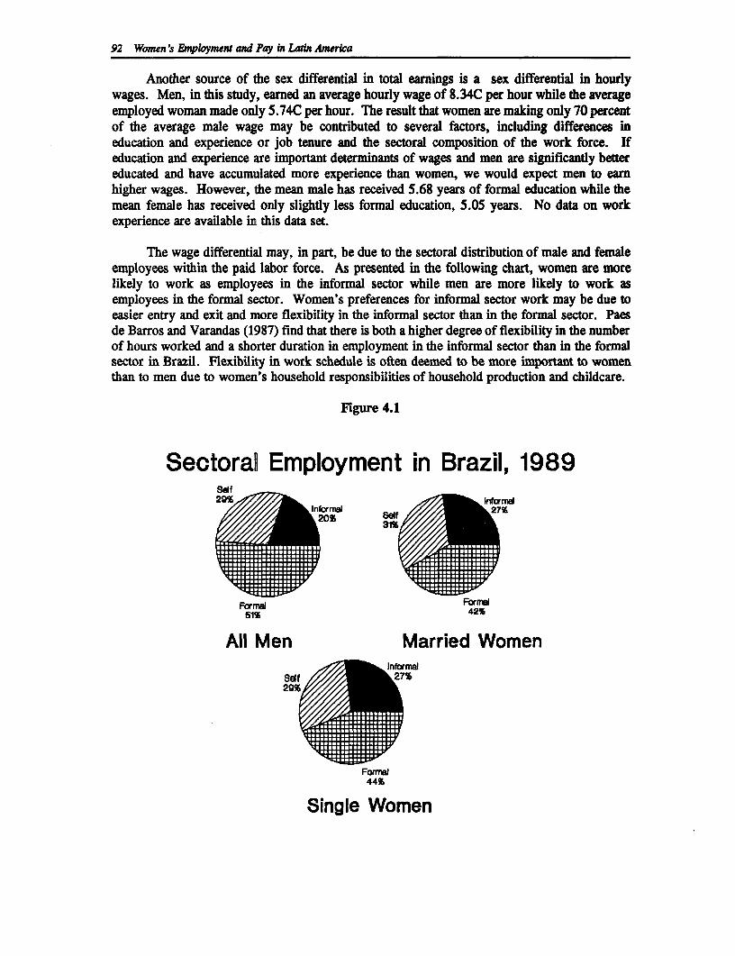
92 Women's Employment and Pay in Latin America
Another source of the sex differential in total earnings is a sex differential in hourlywages. Men, in this study, earned an average hourly wage of 8.34C per hour while the averageemployed woman made only 5.74C per hour. The result that women are making only 70 percentof the average male wage may be contributed to several factors, including differences ineducation and experience or job tenure and the sectoral composition of the work force. Ifeducation and experience are important determinants of wages and men are significantly bettereducated and have accumulated more experience than women, we would expect men to earnhigher wages. However, the mean male has received 5.68 years of formal education while themean female has received only slightly less formal education, 5.05 years. No data on workexperience are available in this data set.
The wage differential may, in part, be due to the sectoral distribution of male and femaleemployees within the paid labor force. As presented in the following chart, women are morelikely to work as employees in the informal sector while men are more likely to work asemployees in the formal sector. Women's preferences for informal sector work may be due toeasier entry and exit and more flexibility in the informal sector than in the formal sector. Paesde Barros and Varandas (1987) find that there is both a higher degree of flexibility in the numberof hours worked and a shorter duration in employment in the informal sector than in the formalsector in Brazil. Flexibility in work schedule is often deemed to be more important to womenthan to men due to women's household responsibilities of household production and childcare.
Figure 4.1
Sectoral Employment in Brazil, 1989Self
2ForMal
5j% 42%
All Men Married Women
Formal44%
Single Women
Femake Labor Force Partipation and Wage Determinaion in Brazil, 1989 93
An alternative explanation for the disproportionate number of women working as informalemployees is a shortage of jobs in the formal sector. If such a shortage exists, formal sectoremployers may discriminate against women who are then forced to work in the informal sector.However, Sedlacek, Paes de Barros, and Varandas (1989) conclude that no such mobility barriersbetween formal and informal sector employment exist.
As shown in the table below, wages are, on average, higher for both men and women in theformal sector than in the informal sectors. However, it is also important to note that the sexdifferential is greater among formal employees (women earn 70.3 percent of men's wages) andthe self-employed (70.5 percent) than in the informal sector (85.2 percent).
Table 4.1Sectoral Wages by Sex Group in Brazil (Cmzados/hour), 1989.
Men Married Women Single Women
Formal Employees 10.93 7.68 7.46Informal Employees 5.28 4.51 4.46Self-Employed 5.96 4.17 4.37
By reviewing the information in the chart and the table, the interpretation is that a contributingfactor to relatively low wages for women is that women are disproportionately represented asemployees in the lower wage sector. These data suggest that if the proportion of women workingin the formal sector increases, the sex differential in wages would be expected to decrease.
Changes in women's economic opportunitiks - 1980 to 1989. It is often suggested thatdisadvantaged groups - the rural poor, women, children, minorities - bear a disproportionalamount of the burden of economic adjustment programs (see, for example, Cornia et al. (1987)).The 1980s was a decade of adjustment for Brazil as she recovered from the world recession andbegan to deal with the problems of a bulging foreign debt. Although there are many measuresof welfare, comparing women's economic opportunities in 1980 with those in 1989 will providesome insight into the effects of the adjustment programs on the well-being of Brazilian women.
Participation rates of both single women and married women increased from 1980 to 1989.According to Stelcner et al. (1991), 20 percent of the married women and 41 percent of the singlewomen in their sample reported to be working for pay. In the sample taken in 1989, used in thisstudy, over 34 percent of married women and 62 percent of single women were wage earners.This comparison is consistent with Edwards' (1991) study of economy-wide trends in theBrazilian labor market in the 1980s as she finds that 'labor force participation has continued toincrease significantly during the decade of the 1980s."
Although participation has increased among both married and single women, the increases havenot been proportionally distributed across sectors. In 1980, from the Stelcner et al. sample, 65percent of working married women were employees (either with or without an employmentbooklet) while the remaining 35 percent were self-employed. In 1989, slightly more marriedwomen classified themselves as employees at 69 percent while the percentage of self-employedfell to 31. The opposite transition occurred among single working women. In the 1980 sample,83 percent said they were employees and only 17 percent were self-employed. In 1989, thenumber of employees fell to 71 percent of working single women while more women classifiedthemselves as self-employed, 29 percent.
94 Women's Employment and Pay in Latin America
Although earnings are not directly comparable across years, the female/male earnings ratio iscomparable and provides evidence of women's relative position in the economy. In the Stelcneret al. 1980 sample, the female/male earnings ratio was 59 percent (61 percent for married womenand 54 percent for single women). This number fell slightly to 56 percent in the 1989 sample(55 percent for married women and 57 percent for single women). Single women made a relativegain in total earnings throughout the decade while married women lost ground to men.
The female/male ratio of hourly wages is a better measure for comparing women's relativeeconomic strength across time. In the 1980 sample, the female/male wage ratio was 75 percentfor employees while self-employed women were making only 68 percent of their malecounterparts' wages. There was little change in this statistic over the decade. In the 1989sample, employed women were making 76 percent of employed men's wages while self-employedwomen were making 69 percent of self-employed men's wages. Women gained little in theireconomic power relative to men in the 1980s as the sex ratio of wages improved by only onepercent in both sectors over the decade.
Regional differentials. Brazil is a large and diverse country. Studies which have accounted forits size and diversity by treating distinct regions separately and including regional dummyvariables have found that regional differences should not be ignored. Stelcner et al. (1991), usingdata from 1980, extensively analyze regional differences in labor market conditions in Brazil.They note important differences between the highly industrialized and modem regions in theSouth (Rio de Janeiro, Sao Paulo, Other Southeast, and the South) and the Northeast which isheavily dependent on agricultural activities. Their data analysis, most notably, points to muchlower incomes, wages, and education in the Northeast region than in the rest of Brazil. Theconclusion is that significant barriers to migration exist which prevent the equalization of wagesacross regions.
Table 4.2Regional Wages in Brazil, 1989.
Male Female Female/Male'(Cruzados/hour) (percent)
Rio de Janeiro 10.89 8.47 77.8Sao Paulo 11.18 8.23 73.6South 9.00 6.68 74.2Other Southeast 7.87 5.15 65.4Northeast 5.61 3.56 63.5Northwest/Central 9.19 6.43 70.0
a. The ratio of the average woman's wage to the average man's wage.
These regional wage differentials continue to persist in 1989. As the following table shows,mean wages are not equal across regions. (It is important to note, however, that these wageshave not been adjusted to reflect any cost of living discrepancies which may exist across regions.)Wages are notably lowest in the Northeast for both men and women. The ratio of female/malewages is also lowest in the Northeast while this ratio is highest in Rio de Janeiro. A relationshipappears to exist between high wages and more favorable female/male wage ratios.
Female Labor Force Participatfon and Wage Determination in Brazil, 1989 95
There are few noteworthy regional differences in the labor force participation patterns of women,as shown in Table 4.3. Participation of married women varies by less than four percent acrossthe seven regions while the participation of single women jumps over seven percent from a lowof 59.1 percent in the Northeast to over 66 percent in the Northwest/Central. Participation ratesare the lowest in the Northeast for both married women and single women followed closely bySao Paulo. One striking figure in male participation rates is the relatively low participation ofmen in Rio de Janeiro. While this city definitely has the lowest male participation rate, thefemale participation rates for Rio are relatively moderate.
Table 4.3Regional Participation Rates in Brazil, 1989
(percent)
Male Female Ratio"
Rio de Janeiro 81.0 36.8 61.2Sao Paulo 85.2 33.3 59.4South 86.8 35.6 64.3Southeast 86.2 33.3 61.3Northeast 85.5 33.1 59.1Northwest/Central 90.5 35.8 66.7
a. Note that the male participation rates are lower than expected because the male sampleincludes some men over age 65. Men 65 with wives under 65 were included in thesample because wages had to be predicted for these men so the women could beincluded in the female sample.
3. Theoretical Model
Assume that a woman must choose among the four mutually exclusive alternatives discussed inthe previous sections - working in the formal sector (F), working for a wage in the informalsector (I), being self-employed in the informal sector (S), and not working in the labor force (N).The problem that the woman faces is to choose the labor force alternative which maximizeshousehold utility. Assuming that the household observes the offered wages the woman could earnin each sector, the value of her time in household production, and the time and money costs ofparticipation in each sector, the household maximizes the household utility function subject to thehousehold time and budget constraints under each alternative. The household then compares thelevels of indirect utility obtainable from the various choices and chooses the participation statusthat maximizes household indirect utility.
Following Maddala (1983), the indirect utility function is decomposed into a nonstochasticcomponent and a stochastic component where the nonstochastic component is a linear functionof the observable variables in the indirect utility functions and the stochastic component is afunction of unobservables. The probability that individual i will participate in sector k is theprobability that the indirect utility yielded in sector k is greater than that derived from the othersectors. This implies that the probability of individual i participating in sector k is the probabilitythat the difference between the stochastic components is greater than the difference between thenonstochastic components.
96 Women 's Employment and Pay in Latin America
This analysis implies that the offered wage in sector k for individual i is observed if theindividual participates in sector k and the condition for participation in k is that the differencebetween the stochastic components is greater than the difference in the nonstochastic components.Therefore, this is the selection rule for the multi-sector model. Consistent estimates of the threesector wage equations can be obtained by accounting for this selection rule in the estimations.
The form of the participation equation, the method of estimation, and the calculation of theselection correction will depend upon the distributional assumption on the errors. Assume thatthe errors of the linear indirect utility functions are independently and identically distributed withthe type I extreme-value distribution (also called the Weibull distribution). Given this distributionof the errors, the difference between the errors has a logistic distribution (see McFadden (1973)).
Because the difference between the errors is assumed to follow a logistic distribution, theparticipation equation must be estimated with the multinomial logit model. The probabilities ofparticipation in each sector, given that the nonstochastic component of indirect utility is a linearfunction, under the multinomial model are written as:
exp(b,1)Pik = E (6, k=F,I,S j=F,I,S,N. (1)
E exp(bp1 )'
The above expression requires some normalization. Using a commonly used and simplenormalization, that the coefficients of the nonparticipation alternative 5 N = °, together with thethree probability equations uniquely determines the selection probabilities and guarantees that theysum to one for each individual. The multinomial logit model can then be estimated usingmaximum likelihood methods.
As mentioned in the previous section, it is also interesting to estimate the sectoral wageequations. Because of the existence of selection bias (those women from whom wages areobserved all have an offered wage above the reservation wage), a Heckman-type method mustto used to correct for the selectivity. Hay (1980) adapted Heckman's (1979) inverse Mill's ratiocorrection for probit models so that it is applicable to both binary and multinomial logit models.In the multinomial logit model, the correction is:
lik = p NOW_ + (J-1 1 Ii,,lt = J(k I )log(P1 ) i (2)
where J = the total number of alternative choices, in this case J equals four.
The procedure for estimating the three sector wage equations free from selection bias is then tofirst estimate the maximum likelihood participation equation. By using the results to calculatethe probabilities of participation, Hay's inverse Mill's ratio for the multinomial logit participationmodel can be calculated. Then, given the inverse Mill's ratio, the wage equations can beestimated. It is important to note that the derivation of the multinomial logit model ofparticipation did not require any assumption about the distribution of the errors in the wageequations. Consequently, they can be assumed to be normally distributed and the wage equationscan be estimated using ordinary least squares (OLS).
Female Labor Force Participaton and Wage Determimaion in Brazil, 1989 97
4. Empirical Specification
As pointed out in Section 3, three wage equations will be estimated, one for each sector. Theoffered wages in each sector are hypothesized to be a function of a vector of the individual'shuman capital variables and labor market conditions. Consequently, the wage equations are setup as standard Mincer equations (see Mincer (1974)) with formal education, predicted experience,experience-squared, regional dummies, and racial dummies included as regressors. Formaleducation is included to pick up wage increases resulting from human capital investment.Experience is believed to have important positive effects on both productivity and earnings butat a declining rate. The racial dummies are included to account for the possibility ofdiscrimination (white or of European descent is the omitted category) and the regional dummiesare included to reflect differing employment opportunities across regions.
The wage variable for each sector is measured as total income in cruzados per month divided bythe average number of hours worked per month (the number of hours worked in a weekmultiplied by four). The reference period is the September 24 through September 30, 1989.Formal education is measured as six dummy variables - (1) if the woman received any formalschooling, (2) if the woman completed the first four years of primary school', (3) if the womenfinished primary school (eight years), (4) if the woman finished secondary school, (5) if thewoman finished college, and (6) if the woman did any graduate work. The survey question askedwas "highest grade completed" and this variable was converted into the six dummy variablesspecified. The dummy variables are specified such that all six will be equal to one for a womanwho has attained post-graduate work (the first five will be equal to one for a woman whocompleted college and stopped, etc.). Therefore, the coefficients on all six variables have toadded up to get the total premium paid to education for a woman who has achieved highereducation (the first five added up for the total returns to finishing college, etc.).
Labor market experience is measured in years. However, because no data were collected onexperience, this variable was constructed using the standard formula: age - education - 6.Although this formula has worked well as a proxy for male work experience, it has notperformed as well as a predictor of female labor market experience because women are morelikely to take additional time off work due to childbirth and childcare. However, this proxy willbe used for a lack of a better alternative. The regional dummy variables are specified as follow:Rio de Janeiro, Sao Paulo, Other South (Parana, Santa Catarina, Rio Grande do Sul, MinasGerais, and Espirito Santo), Northeast (Maranhao, Piaui, Cerara, Rio Grande do Norte, Paraiba,Pernambuco, Alagoas, Sergipe, and Bahia), and Northwest/Central (Distrito Federal, Rondonia,Acre, Amazonas, Roraima, Para, Amapa, Mato Grosso do Sul, Mato Grosso, and Goias). TheOther South is the omitted category in the regressions.
From the theoretical derivation in Section 3, it is clear that the variables included as regressorsin the participation equation should reflect the offered wages across sectors and the differing costsof employment in the three sectors as well as other factors that influence the reservation wage.Age and the formal education dummy variables are included in the participation equation to proxyfor the offered wages (wages across sectors cannot be included because they are not observed forall women and because of endogeneity) and because they will affect the reservation wage. The
3 A distinction was made between finishing the first four years of prnmary school and compleingprmary school because prior to 1971 grades 14 wero considered compulsory and entrance into the nextlevels (grades 5-8 and grades 9-11) was controlled by examination.
98 Women's Employment and Pay in Latin America
number of children in the household disaggregated into four different groups (children under age2, children 3 to 5, children 6 to 12, daughters over 13, and sons over 13) are included to reflectchildcare costs. The total number of children is disaggregated into these groups because thepresence of some groups may increase childcare costs (children under 2) while others maydecrease these costs (daughters over 13). A dummy for whether or not the husband isself-employed is included in the married women's regression to reflect other opportunity costsof participating in the labor force. The household head being self-employed in an activity inwhich the woman can help is expected to raise the shadow value of the woman's time in non-market activities and reduce the probability that she will be a wage earner.
Monthly unearned income (includes both cash and in-kind unearned income from all sources) andthe husband's hourly wage are hypothesized to increase the reservation wage. Both of thesevariables are measured in current cruzados. Because not all husbands work, the husbands' wagesare predicted from selectivity-corrected wage equations (see Appendix). A dummy for whetheror not the household owns the home in which they are living is included as a measure ofhousehold wealth. Therefore, owning a home is also expected to increase the reservation wage.The racial dummies are included to pick up any variance in ideas about women and work acrossethnic cultures and the regional dummies are included to reflect differing labor marketopportunities and values across regions.
Table 4.4 shows the means and standard deviations (in parenthesis) of all of independent variablesincluded in the participation and wage equations. The means and characteristics of the dependentvariables were discussed in Section 2. Because separate regressions will be undertaken formarried women and single women in the following sections, the means and standard deviationsare presented by these subsamples.
5. The Determinants of Female Labor Force Participation
Single women. Table 4.5 presents the results from estimating the multi-sector participationequation for single women using maximum likelihood multinomial logit methods. Statistical testsof pooling the five regions specified in the previous section were accepted for the subsample ofsingle women as well as for the married women and male subsamples. Consequently, theregional data were pooled and dummies were included to account for intercept regional effects.The partial derivatives are in bold, the logit coefficients follow and the t-ratios are the numbersin parenthesis. The log likelihood from estimation of this equation is -11,191.
Age is included in the participation equation to reflect the effects of human capital investmentson wages which will effect participation. As expected, age has a positive and significant effecton work in all three sectors. An interpretation is that as age increases, the level of human capitalacquired increases and the offered wage goes up. An increasing wage, holding all else constant,will increase the probability of participation. Age-squared is included as a regressor to pick uppossible nonlinearities in this relationship. The significance of the squared terms in all threesectors supports the hypothesis of curvature in the effects of age on the probability ofparticipation.
Education has stronger effects in increasing the participation of single women in the formal sectorthan in the informal and self-employed sectors. In fact, additional education decreases theprobability of participation in the informal and self-employed sectors in many instances.Attaining each of the first three levels of education increases the probability of formal sectorparticipation by between eight to nine percentage points. Finishing secondary school and college
Female Labor Force Particq,ation and Wage Determinaton in Brazil, 1989 99
Table 4.4Means (and Standard Deviations) of Independent Variables
Variables Married Women Single Women
Age 37.09 (11.53) 44.69 (11.89)Age-squared 1508.9 (922.3) 2138.7 (1044.5)Some Primary .820 (.386) .749 (.433)Primary - Level 4 .617 (.486) .551 (.497)Primary - Level 8 .291 (.454) .279 (.448)Secondary .181 (.385) .194 (.395)College .067 (.250) .091 (.87)Graduate Work .002 (.039) .003 (.055)Own Home .667 (.471) .657 (.478)Black .042 (.201) .070 (.255)Mulatto/Indian .395 (.489) .427 (.495)Asian .004 (.066) .003 (.056)Uneamed Income 173.75 (879.34) 280.31 (701.55)Husband's Wage 1.488 (6.338)Husband Self-Employed .263 (.440)
# Children 0-2 .342 (.578) .089 (.317)# Children 3-5 .314 (.555) .134 (.394)# Children 6-12 .831 (1.063) .465 (.830)# Daughters > 13 .504 (.899) .561 (.887)# Sons > 13 .428 (.794) .634 (.966)Experience 23.728 (11.50) 29.487 (12.89)Experience-Squared 695.23 (625.7) 1035.4 (788.3)Sao Paulo .128 (.334) .110 (.313)Rio de Janeiro .072 (.258) .092 (.289)Northwest/Central .208 (.406) .205 (.404)Northeast .287 (.452) .303 (.460)
each increase it an additional 13 percentage points while attaining some higher education increasesthe probability of being a formal sector employee another 22 percentage points. Education isincluded in the participation equation to reflect the effects of wages on the probability ofparticipation. Given the results, it is expected that education has the highest returns in the formalsector because women with more education are more likely to choose to work in this sector.
The dummy variable for owning a home and the continuous variable for unearned income areincluded in the estimated equation to proxy for wealth. These proxies for wealth are expectedto have negative effects on the probability of participation in all three sectors. Owning a homedoes have a negative and significant effect on participation in all three sectors. Unearned incomealso has a negative and strongly significant effect on the probability of participation in all threesectors. Increasing income by 1000 cruzados per month decreases participation by 11 percentagepoints in the formal sector and 6 to 7 percentage points in the other two sectors.
The racial dummy variables are included in the participation equation to reflect different ethnicand cultural values about women and work across races. The reference group is white singlewomen. The results show that black single women are more likely to be employees in both theformal and informal sectors than white single women but less likely to be self-employed. Indianand mulatto women are more likely to participate in all three sectors than white women. Asianwomen are 19 percentage points more likely to participate as self-employed than white women.
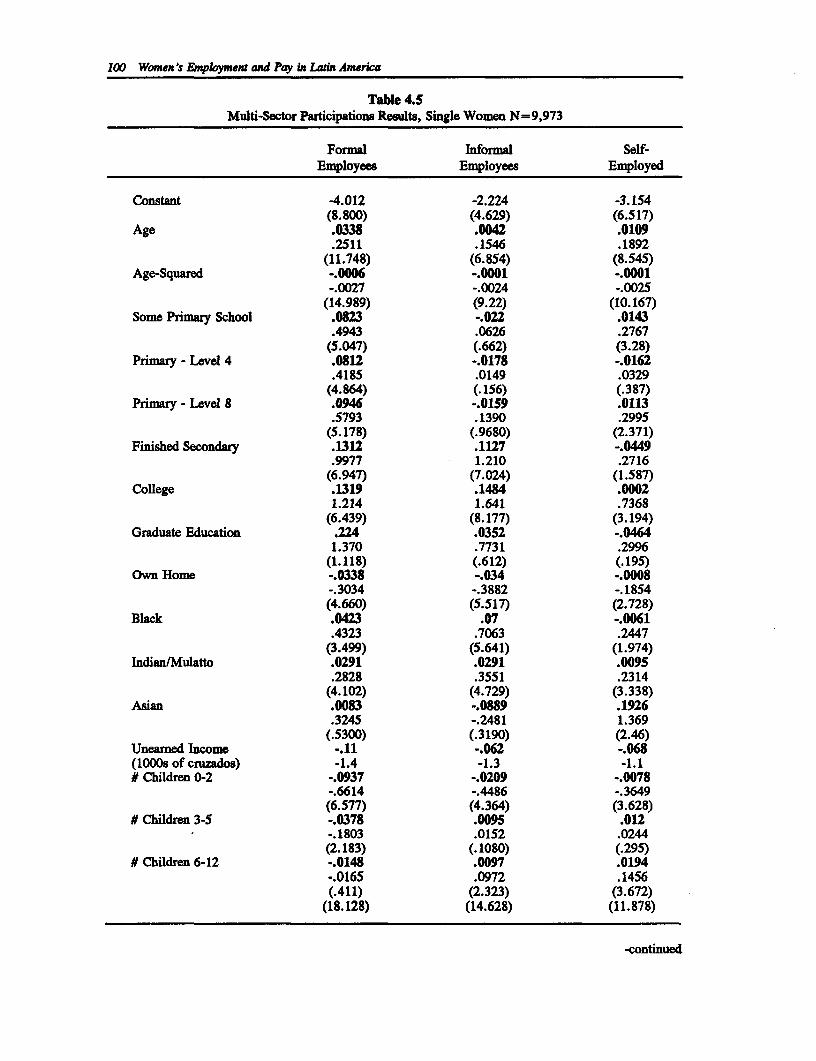
100 Women's lEnpkymen and Pay in Latin America
Table 4.5Multi-Sector Participations Results, Single Women N=9,973
Formal Informal Self-Employees Employees Employed
Constant -4.012 -2.224 -3.154(8.800) (4.629) (6.517)
Age .0338 .0042 .0109.2511 .1546 .1892
(11.748) (6.854) (8.545)Age-Squared -.0006 -.0001 -.0001
-.0027 -.0024 -.0025(14.989) (9.22) (10.167)
Some Primary School .0823 -.022 .0143.4943 .0626 .2767
(5.047) (.662) (3.28)Primary - Level 4 .0812 -.0178 -.0162
.4185 .0149 .0329(4.864) (.156) (.387)
Primary - Level 8 .0946 -.0159 .0113.5793 .1390 .2995
(5.178) (.9680) (2.371)Finished Secondary .1312 .1127 -.0449
.9977 1.210 .2716(6.947) (7.024) (1.587)
College .1319 .1484 .00021.214 1.641 .7368
(6.439) (8.177) (3.194)Graduate Education .224 .0352 -.0464
1.370 .7731 .2996(1.118) (.612) (.195)
Own Home -.0338 -.034 -.0008-.3034 -.3882 -.1854(4.660) (5.517) (2.728)
Black .0423 .07 -.0061.4323 .7063 .2447
(3.499) (5.641) (1.974)Indian/Mulatto .0291 .0291 .0095
.2828 .3551 .2314(4.102) (4.729) (3.338)
Asian .0083 -.0889 .1926.3245 -.2481 1.369
(.5300) (.3190) (2.46)Uneaned Income -.11 -.062 -.068(1000s of cruzados) -1.4 -1.3 -1.1# Children 0-2 -.0937 -.0209 -.0078
-.6614 -.4486 -.3649(6.577) (4.364) (3.628)
# Children 3-5 -.0378 .0095 .012-.1803 .0152 .0244(2.183) (.1080) (.295)
# Children 6-12 -.0148 .0097 .0194-.0165 .0972 .1456(.411) (2.323) (3.672)
(18.128) (14.628) (11.878)
-continued
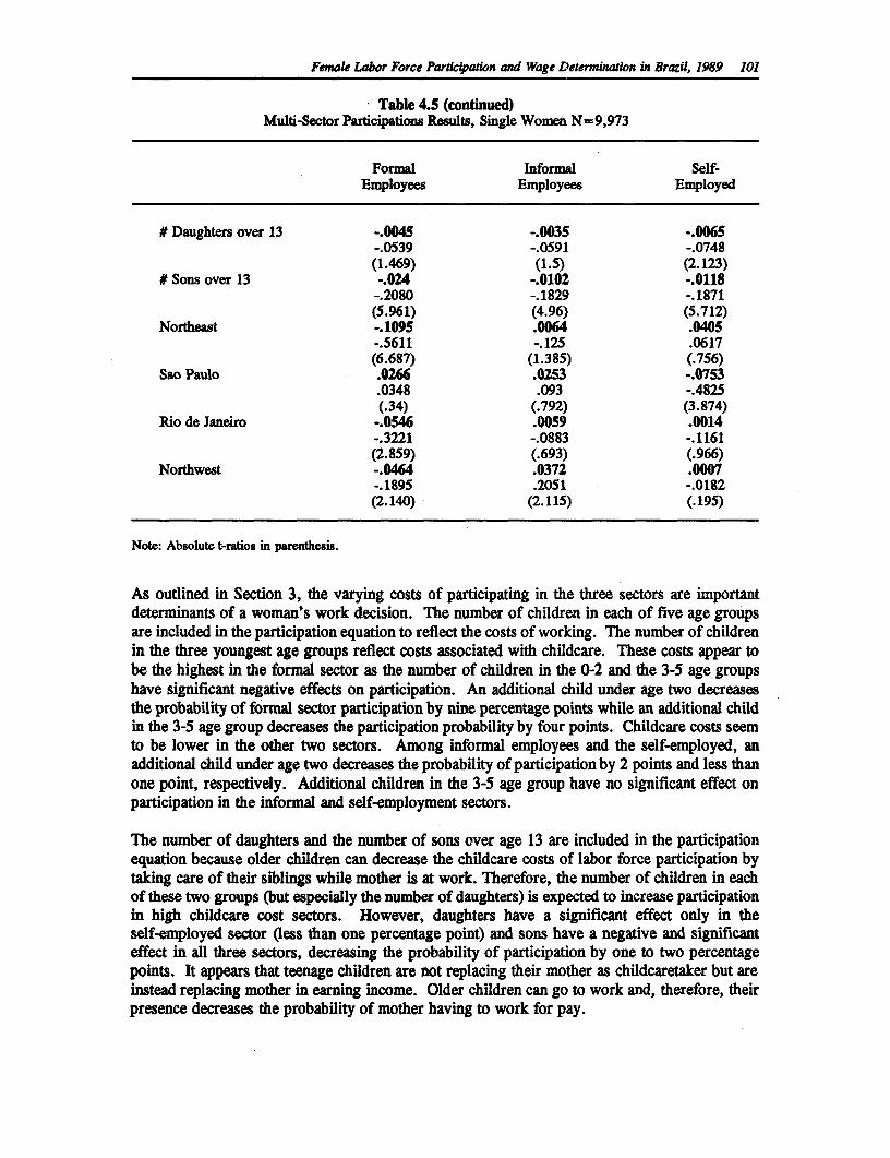
Femalk Labor Force Participatfon and Wage Determination in Brazil, 1989 101
Table 4.5 (continued)Multi-Sector Participations Results, Single Women N=9,973
Formal Informal Self-Employees Employees Employed
# Daughters over 13 -.0045 -.0035 -.0065-.0539 -.0591 -.0748(1.469) (1.5) (2.123)
# Sons over 13 -.024 -.0102 -.0118-.2080 -.1829 -.1871(5.961) (4.96) (5.712)
Northeast -.1095 .0064 .0405-.5611 -. 125 .0617(6.687) (1.385) (.756)
Sao Paulo .0266 .0253 -.0753.0348 .093 -.4825(.34) (.792) (3.874)
Rio de Janeiro -.0546 .0059 .0014-.3221 -.0883 -.1161(2.859) (.693) (.966)
Northwest -.0464 .0372 .0007-.1895 .2051 -.0182(2.140) (2.115) (.195)
Note: Absolute t-ratios in parenthesis.
As outlined in Section 3, the varying costs of participating in the three sectors are importantdeterminants of a woman's work decision. The number of children in each of five age groupsare included in the participation equation to reflect the costs of working. The number of childrenin the three youngest age groups reflect costs associated with childcare. These costs appear tobe the highest in the formal sector as the number of children in the 0-2 and the 3-5 age groupshave significant negative effects on participation. An additional child under age two decreasesthe probability of formal sector participation by nine percentage points while an additional childin the 3-5 age group decreases the participation probability by four points. Childcare costs seemto be lower in the other two sectors. Among informal employees and the self-employed, anadditional child under age two decreases the probability of participation by 2 points and less thanone point, respectively. Additional children in the 3-5 age group have no significant effect onparticipation in the informal and self-employment sectors.
The number of daughters and the number of sons over age 13 are included in the participationequation because older children can decrease the childcare costs of labor force participation bytaking care of their siblings while mother is at work. Therefore, the number of children in eachof these two groups (but especially the number of daughters) is expected to increase participationin high childcare cost sectors. However, daughters have a significant effect only in theself-employed sector (less than one percentage point) and sons have a negative and significanteffect in all three sectors, decreasing the probability of participation by one to two percentagepoints. It appears that teenage children are not replacing their mother as childcaretaker but areinstead replacing mother in earning income. Older children can go to work and, therefore, theirpresence decreases the probability of mother having to work for pay.
102 Women's Employment and Pay in Latin America
The regional dummy variables are included in the equation to pick up differing values andopportunities across regions in Brazil. Since a test of pooling across regions without includingthese dummy variables was rejected, some significance is expected. The relative region is the"other South" (see the previous section). The results confirm that there are differences acrossregions. In Rio de Janeiro, the Northeast, and the Northwest, women are less likely to be formalsector workers than women who live in the more industrial South. The only significancedifference between the South and Sao Paulo is that women in Sao Paulo are approximately eightpercentage points less likely to be self-employed.
Table 4.6 presents logit simulations to help to interpret the participation results. The independentvariables are set equal to their sample means and a single variable is varied for each simulationexercise. The constant term has been adjusted so that the predicted probabilities of participation,evaluated at the means of the independent variables, are equal to the actual means of thedependent variable.
The age simulations are adjusted to reflect both changes in age and age-squared. As the othervariables are held constant at their means, the probability of being a formal employee increasesfrom 20 to 30 years but then decreases after the age of 30. In the other two sectors, theprobability of participation continues to increase with age through age 50. All else held constant,a 20-year-old single woman, a 30-year-old, and a 40-year-old are all most likely to be in theformal sector while a 50-year-old is most likely to be at home.
The next simulation is education. As education increases, the probability of being a non-participant continually falls. A woman with no formal schooling is most likely not to participatewhile the probability of being a non-participant for a woman with a graduate education is lessthan two percent. As schooling increases, the probability of being a formal sector employeeincreases with each level. A woman with a graduate degree has a 72 percent probability of beinga formal employee. The effects of education on participation in the other two sectors are not asstrong. In fact, in the self-employed sector, additional levels of education generally lead todecreases in the participation probability. A woman with a graduate degree is almost as likelyto not participate as she is likely to be self-employed.
Those women who own homes are more likely to be non-participants than those who do not ownhomes and less likely to work as either formal or informal employees. Owning a home has noeffect on the probability of self-employment. The most striking result from the simulations withthe racial dummy variables is the relatively high probability that an Asian woman isself-employed and the relatively low probability than she is an informal employee.
The most interesting results from the child variable simulations is for the youngest age groups.The probability of being a non-participant increases with each additional child 0-2. A woman withno young children has a 37 percent probability of staying home while the probability for a womanwith two small children increases to over 62 percent. The probability of being in all three sectorsdecreases with each additional child but the greatest decreases are in the formal sector - theprobability decreases approximately nine percentage points for the first child and seven points forthe second child. The number of children aged 3-5 also increases the probability of being a non-participant and decreases the probability of being in the formal sector but at much smallerchanges than with the 0-2 age group.
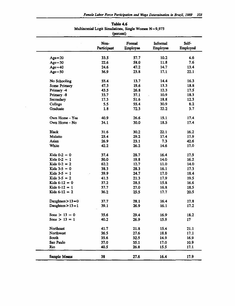
Femak Labor Force Participation and Wage Determination in Brazil, 1989 103
Table 4.6Multinomial Logit Simulations, Single Women N=9,973
(percent)
Non- Formal informal Self-Participant Employee Employee Employed
Age=20 33.5 57.7 10.2 4.6Age=30 22.6 58.0 11.8 7.6Age=40 24.6 47.2 14.7 13.4Age=50 36.9 23.8 17.1 22.1
No Schooling 55.4 13.7 14.4 16.3Some Primary 47.3 19.6 13.3 18.8Primary -4 43.5 26.8 12.3 17.5Primary -8 33.7 37.1 10.9 18.3Secondary 17.3 51.6 18.8 12.3College 5.5 55.4 30.9 8.2Graduate 1.8 72.3 22.2 3.7
Own Home - Yes 40.9 26.6 15.1 17.4Own Home - No 34.1 30.0 18.5 17.4
Black 31.6 30.2 22.1 16.2Mulatto 25.4 29.2 17.4 17.9Asian 26.9 23.1 7.3 42.6White 42.2 26.2 14.6 17.0
Kids 0-2 = 0 37.4 28.7 16.4 17.5Kids 0-2 = 1 50.0 19.8 14.0 16.2Kids 0-2 = 2 62.2 12.7 11.0 14.0Kids 3-5 = 0 38.3 28.3 16.1 17.3Kids 3-5 = 1 39.9 24.7 17.0 18.4Kids 3-5 = 2 41.3 21.3 17.9 19.5Kids 6-12 = 0 37.2 28.5 15.8 16.6Kids 6-12 = 1 37.7 27.0 16.8 18.5Kids 6-12 = 2 36.2 25.5 17.7 20.5
Daughters>13=0 37.7 28.1 16.4 17.8Daughters > 13 = 1 39.1 26.9 16.1 17.2
Sons > 13 = 0 35.6 29.4 16.9 18.2Sons > 13 = 1 40.2 26.9 15.9 17
Northeast 41.7 21.8 15.4 21.1Northwest 36.5 27.6 18.8 17.1South 35.6 32.5 14.9 16.9Sao Paulo 37.0 35.1 17.0 10.9Rio 40.5 26.8 15.5 17.1
Sample Means 38 27.6 16.4 17.9
104 Women's Emplyment and Pay in Latin America
The regional simulations show that, as in the total sample, single women in each region are mostlikely to be non-participants. However, women in the Northeast are the most likely to be non-participants and to be self-employed, women in Sao Paulo are the most likely to be in the formalsector, and women in the Northwest are the most likely to be informal employees.
Married women. The multinomial logit results from estimating the participation equation usingdata on 50,452 married women are presented in Table 4.7. The same maximum likelihoodmethods used to estimate the participation equation for single women are employed here. Thelog likelihood function for this participation equation is 46,165. The results from estimating theparticipation equation for married women are very similar to the results presented previously forsingle women. Age, again, has a positive and significant effect on participation in all threesectors. The education variables continue to have the strongest effects in the formal sector(however, all of these effects are weaker than those for single women). Unearned incomecontinues to have a significantly negative effect on participation in all three sectors. Children inthe 0-2 age group significantly decrease the probability of participation in all sectors and childrenin the 3-5 age group decrease the probability of being a formal sector employee.
The regional results, again, show that women in the Northeast, the Northwest, and Rio are lesslikely to be in the formal sector than women in the South and that women in Sao Paulo are lesslikely to work in formal sector. While most of the racial results found for single women holdtrue for married women, an important difference is that the high increase in the probability ofan Asian single woman being self-employed does not hold for married Asian women. In fact,there is no significant difference between the probability of Asian women and white women beingself-employed (this difference was close to 20 percentage points for single women). This resultlikely reflects that married Asian women are helping their husband's with their businesses (theyare unpaid family workers) rather than being self-employed themselves.
There are two additional variables included in the married women's participation equation - thehusband's wage and the husband's self-employment status. The husband's wage (expected toincrease the reservation wage and decrease the probability of participation) has a stronglysignificant and negative effect on participation in all three sectors. If her husband isself-employed, the probability of a woman being an employee in both the formal and informalsectors falls while the probability of being self-employed increases by two percentage points.
The Table 4.8 presents the results from replicating the simulations for single women using theresults from estimating the married women's participation equation.
The probability of participation increases until age 40 in the formal and informal sectors and thenbegins to fall while in the self-employment sector, the probability continuously increases with agethrough age 50. Formal education, again, has strong negative effects on the probability of beinga non-participant and strong positive effects on the probability of being a formal employee.While a woman with no formal education has a 77 percent probability of being a non-participantand a six percent chance of being a formal employee, a woman with a graduate education has athree percent probability of being a non-participant and a 48 percent change of working in theformal sector. Higher levels of education also have significant effects in increasing informalemployment. However, the effects are relatively negligible in self-employment.
Among married women, mulatto women are the most likely to be non-participants. Black womenhave the highest probability of the four racial groups of working in both the formal and informalsectors while Asian women still have the highest probability of being self-employed (however,
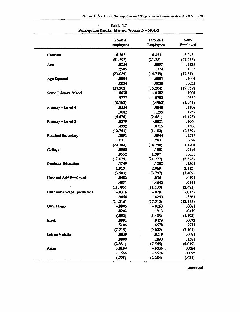
Female Labor Force Participation and Wage Determination in Brazil, 1989 105
Table 4.7Participation Results, Married Women N=50,452
Formal informal Self-Employees Employees Employed
Constant -6.387 -4.853 -5.943(31.297) (21.28) (27.583)
Age .0254 .0097 .0127.2505 .1774 .1933
(23.029) (14.739) (17.81)Age-Squared -.0004 -.0001 -.0001
-.0034 -.0023 -.0023(24.302) (15.204) (17.258)
Some Primary School .0638 -.0102 .0001.5277 -.0280 .0830
(8.163) (.4960) (1.741)Primary - Level 4 .0334 .0048 .0107
.3082 .1255 .1757(6.676) (2.481) (4.175)
Primary - Level 8 .0579 -.0021 .006.4992 .0715 .1506
(10.753) (1.100) (2.889)Finished Secondary .1091 .0944 -.0274
1.031 1.283 .0097(20.744) (18.256) (.140)
College .0908 .1001 .0196.9552 1.397 .5050
(17.075) (21.277) (5.328)Graduate Education .1749 .12B2 .1509
1.913 2.069 2.113(3.583) (3.797) (3.409)
Husband Self-Employed -.0482 -.034 .0191-.4331 -.4640 .0842
(11.795) (11.130) (2.481)Husband's Wage (predicted) -.0316 -.028 -.0225
-.3456 -.4260 -.3365(14.216) (17.515) (13.838)
Own Home -.0005 -.0163 .0061-.0202 -.1913 .0410(.652) (5.433) (1.193)
Black .0502 .0473 .0072.5106 .6678 .2275
(7.215) (9.002) (3.101)IndianlMulatto .0039 .0219 .0091
.0800 .2890 .1388(2.381) (7.565) (4.019)
Asian 0.0104 -.0533 .0084-.1568 -.6574 -.0052(.795) (2.284) (.021)
-continued
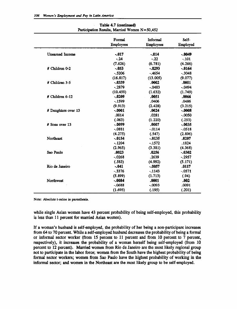
106 Women's Enployment and Pay in Latin America
Table 4.7 (continued)Participation Results, Married Women N=50,452
Formal Informal Self-Employees Employees Employed
Unearned Income -.017 -.014 -.0049-.24 -.22 -.101
(7.626) (6.781) (4.266)# Children 0-2 -.053 -.0293 -.0164
-.5206 -.4654 -.3048(16.817) (13.005) (9.077)
# Children 3-5 -.0339 .0002 .0001-.2879 -.0483 -.0494
(10.459) (1.632) (1.749)# Children 6-12 -.0209 .0051 .0066
-.1599 .0406 .0486(9.913) (2.428) (3.215)
# Daughters over 13 -.0001 .0024 -.0008.0014 .0281 -.0050(.063) (1.220) (.253)
# Sons over 13 -.0099 .0007 -.0035-.0881 -.0114 -.0518(4.275) (.547) (2.896)
Northeast -.0154 -.0135 .0207-.1204 -.1572 .1824(2.965) (3.381) (4.368)
Sao Paulo .0023 .0256 -.0302-.0268 .2639 -.2957(.583) (4.992) (5.171)
Rio de Janeiro -.041 -.0057 .0117-.3376 -.1143 -.0571(5.899) (1.713) (.94)
Northwest -.0084 .0001 .002-.0688 -.0093 .0091(1.695) (.195) (.201)
Note: Absolute t-ratios in parenthesis.
while single Asian women have 43 percent probability of being self-employed, this probabilityis less than 11 percent for married Asian women).
If a woman's husband is self-employed, the probability of her being a non-participant increasesfrom 64 to 70 percent. While a self-employed husband decreases the probability of being a formalor informal sector worker (from 15 percent to 11 percent and from 10 percent to 7 percent,respectively), it increases the probability of a woman herself being self-employed (from 10percent to 12 percent). Married women from Rio de Janeiro are the most likely regional groupnot to participate in the labor force; women from the South have the highest probability of beingformal sector workers; women from Sao Paulo have the highest probability of working in theinformal sector; and women in the Northeast are the most likely group to be self-employed.
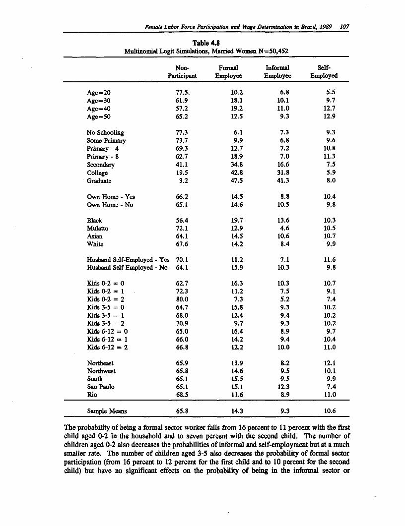
Female Labor Force Partwipation and Wage Determinaton in Brazil, 1989 107
Table 4.8Multinomial Logit Simulations, Married Women N=50,452
Non- Formal Informal Self-Participant Employee Employee Employed
Age=20 77.5. 10.2 6.8 5.5Age=30 61.9 18.3 10.1 9.7Age=40 57.2 19.2 11.0 12.7Age=50 65.2 12.5 9.3 12.9
No Schooling 77.3 6.1 7.3 9.3Some Primary 73.7 9.9 6.8 9.6Primary - 4 69.3 12.7 7.2 10.8Primary - 8 62.7 18.9 7.0 11.3Secondary 41.1 34.8 16.6 7.5College 19.5 42.8 31.8 5.9Graduate 3.2 47.5 41.3 8.0
Own Home - Yes 66.2 14.5 8.8 10.4Own Home - No 65.1 14.6 10.5 9.8
Black 56.4 19.7 13.6 10.3Mulatto 72.1 12.9 4.6 10.5Asian 64.1 14.5 10.6 10.7White 67.6 14.2 8.4 9.9
Husband Self-Employed - Yes 70.1 11.2 7.1 11.6Husband Self-Employed - No 64.1 15.9 10.3 9.8
Kids 0-2 = 0 62.7 16.3 10.3 10.7Kids 0-2 = 1 72.3 11.2 7.5 9.1Kids 0-2 = 2 80.0 7.3 5.2 7.4Kids 3-5 = 0 64.7 15.8 9.3 10.2Kids 3-5 = 1 68.0 12.4 9.4 10.2Kids 3-5 = 2 70.9 9.7 9.3 10.2Kids 6-12 = 0 65.0 16.4 8.9 9.7Kids 6-12 = 1 66.0 14.2 9.4 10.4Kids 6-12 = 2 66.8 12.2 10.0 11.0
Northeast 65.9 13.9 8.2 12.1Northwest 65.8 14.6 9.5 10.1South 65.1 15.5 9.5 9.9Sao Paulo 65.1 15.1 12.3 7.4Rio 68.5 11.6 8.9 11.0
Sample Means 65.8 14.3 9.3 10.6
The probability of being a formal sector worker falls from 16 percent to 11 percent with the firstchild aged 0-2 in the household and to seven percent with the second child. The number ofchildren aged 0-2 also decreases the probabilities of informal and self-employment but at a muchsmaller rate. The number of children aged 3-5 also decreases the probability of formal sectorparticipation (from 16 percent to 12 percent for the first child and to 10 percent for the secondchild) but have no significant effects on the probability of being in the informal sector or
108 Women 's Empkyment and Pay in Latin America
self-employed. While the number of children aged 6-12 had little effect on single women'semployment, their presence again decreases the probability of a married woman working in theformal sector. However, children in this age group also have a positive effect on informal sectorparticipation and self-employment.
6. Earnings Functions
Table 4.9 presents the results from estimating the earnings functions for single women andmarried women. The earnings functions are estimated as Mincer equations with the natural logof wages regressed on levels of the independent variables. The first three columns are resultsfrom estimating the sectoral wage equations for single women and columns four through six arethe results from estimating the sectoral wage equations for married women. These results arecorrected for selectivity using the inverse Mill's ratio for the multinomial logit model presentedin Section 3. The standard errors have been corrected for the use of an estimated inverse Mill'sratio. The OLS results are presented in Appendix Table 4A.3 for comparison. Because theselection term is significant in most of the equations, the selectivity corrected results are used fordiscussion and the calculations of discrimination to follow.
The selection term is strongly significant in the formal and self-employment sectors for singlewomen and in both the formal and informal sectors for married women. Consequently, in thesecases, the selection correction was needed to get consistent estimates of the earnings functions.Predicted experience has a positive and significant effect on wages in all three sectors for bothsingle and married women (except self-employed single women). For single women, the rate ofreturn of a year of experience is approximately three percent in the formal sector, four percentin the informal sector, and one percent in self-employment. Married women enjoy slightly higherreturns to experience at five percent in the formal sector, four percent in the informal, and threepercent in self-employment. The relationship between experience, however, is not linear as thesquared terms are negative and significant in each equation.
The racial variables are also significant in many cases. Among married women, black womenmake 16 percent less than white women in the formal sector, eight percent less in the informalsector, and 15 percent less in self-employment. The results are similar for single black womenas they make 23 percent, three percent, and 16 percent less, respectively, than white singlewomen. These results suggest that there appears to be more discrimination against black womenin the formal and self-employed sectors than in the informal employee sector. Mulatto womenalso make significantly less than white women in all three sectors (21 percent, nine percent, and14 percent less, respectively, for married women and 15 percent, eight percent, and 10 percentless, respectively, for single women). While married Asian women make significantly more thanwhite women in self-employment (56 percent), this results does not hold among single Asianwomen.
There also are regional differences in the earnings functions for both single and married women.In the Northeast, both groups make less in all three sectors than in the South (the referenceregion). In the formal sector, married women in the Northeast make 35 percent less and singlewomen make 27 percent less and in the informal sector, married women make 46 percent lessand single women make 36 percent less. Both groups make 39 percent less in self-employmentin the Northeast than in the South. However, in Sao Paulo, women make more (from 23 to 47percent more) in all three sectors than they would in the "other South." In Rio de Janeiro and inthe Northwest, there are some regional differences but they are not across the board as in the
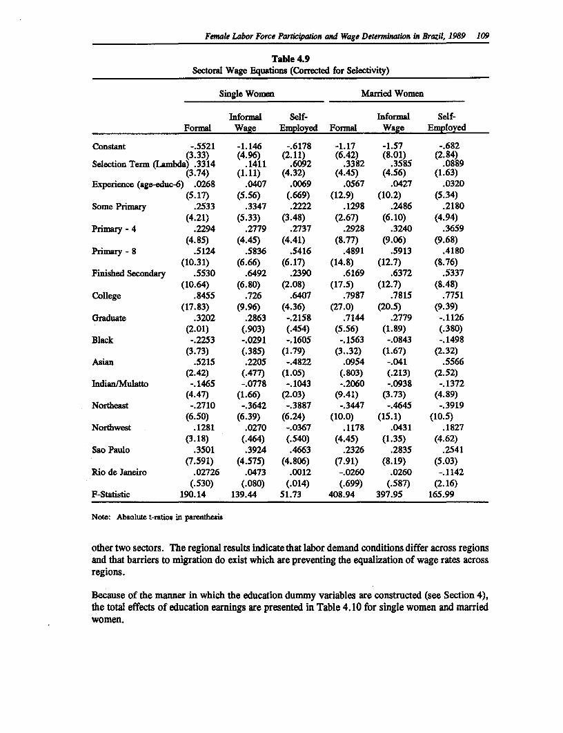
Femak Labor Force Partic4pfion and Wage Determinaion in Brazil, 1989 109
Table 4.9Sectoral Wage Equations (Corrected for Selectivity)
Single Women Married Women
Informal Self- Informal Self-Formal Wage Employed Formal Wage Employed
Constant -.5521 -1.146 -.6178 -1.17 -1.57 -.682(3.33) (4.96) (2.11) (6.42) (8.01) (2.84)
Selection Term (Lambda) .3314 .1411 .6092 .3382 .3585 .0889(3.74) (1.11) (4.32) (4.45) (4.56) (1.63)
Experience (age-educ-6) .0268 .0407 .0069 .0567 .0427 .0320(5.17) (5.56) (.669) (12.9) (10.2) (5.34)
Some Primary .2533 .3347 .2222 .1298 .2486 .2180(4.21) (5.33) (3.48) (2.67) (6-10) (4.94)
Primary - 4 .2294 .2779 .2737 .2928 .3240 .3659(4.85) (4.45) (4.41) (8.77) (9.06) (9.68)
Primary - 8 .5124 .5836 .5416 .4891 .5913 .4180(10.31) (6.66) (6.17) (14.8) (12.7) (8.76)
Finished Secondary .5530 .6492 .2390 .6169 .6372 .5337(10.64) (6.80) (2.08) (17.5) (12.7) (8.48)
College .8455 .726 .6407 .7987 .7815 .7751(17.83) (9.96) (4.36) (27.0) (20.5) (9.39)
Graduate .3202 .2863 -.2158 .7144 .2779 -.1126(2.01) (.903) (.454) (5.56) (1.89) (.380)
Black -.2253 -.0291 -.1605 -.1563 -.0843 -.1498(3.73) (.385) (1.79) (3. 32) (1.67) (2.32)
Asian .5215 .2205 -.4822 .0954 -.041 .5566(2.42) (.477) (1.05) (.803) (.213) (2.52)
Indian/Mulatto -.1465 -.0778 -. 1043 -.2060 -.0938 -.1372(4.47) (1.66) (2.03) (9.41) (3.73) (4.89)
Northeast -.2710 -.3642 -.3887 -.3447 -.4645 -.3919(6.50) (6.39) (6.24) (10.0) (15.1) (10.5)
Northwest .1281 .0270 -.0367 .1178 .0431 .1827(3.18) (.464) (.540) (4.45) (1.35) (4.62)
Sao Paulo .3501 .3924 .4663 .2326 .2835 .2541(7.591) (4.575) (4.806) (7.91) (8.19) (5.03)
Rio de Janeiro .02726 .0473 .0012 -.0260 .0260 -.1142(.530) (.080) (.014) (.699) (.587) (2.16)
F-Statistic 190.14 139.44 51.73 408.94 397.95 165.99
Note: Absolute t-ratios in parenthesis
other two sectors. The regional results indicate that labor demand conditions differ across regionsand that barriers to migration do exist which are preventing the equalization of wage rates acrossregions.
Because of the manner in which the education dummy variables are constructed (see Section 4),the total effects of education earnings are presented in Table 4.10 for single women and marriedwomen.
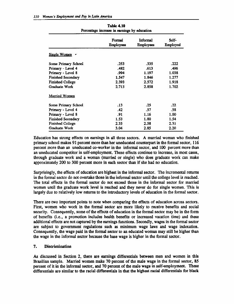
110 Women's Employment and Pay in Latin America
Table 4.10Percentage increase in eamings by education
Formal Informal Self-Employees Employees Employed
Single Women -
Some Primary School .253 .335 .222Primary - Level 4 .482 .613 .496Primary - Level 8 .994 1.197 1.038Finished Secondary 1.547 1.846 1.277Finished College 2.393 2.572 1.918Graduate Work 2.713 2.858 1.702
Married Women
Some Primary School .13 .25 .22Primary - Level 4 .42 .57 .58Primary - Level 8 .91 1.16 1.00Finished Secondary 1.53 1.80 1.54Finished College 2.33 2.58 2.31Graduate Work 3.04 2.85 2.20
Education has strong effects on earnings in all three sectors. A married woman who finishedprimary school makes 91 percent more than her uneducated counterpart in the formal sector, 116percent more than an uneducated co-worker in the informal sector, and 100 percent more thanan uneducated competitor in self-employment. These effects continue to increase, in most cases,through graduate work and a woman (married or single) who does graduate work can makeapproximately 200 to 300 percent more in each sector than if she had no education.
Surprisingly, the effects of education are highest in the informal sector. The incremental returnsin the formal sector do not overtake those in the informal sector until the college level is reached.The total effects in the formal sector do not exceed those in the informal sector for marriedwomen until the graduate work level is reached and they never do for single women. This islargely due to relatively low returns to the introductory levels of education in the formal sector.
There are two important points to note when comparing the effects of education across sectors.First, women who work in the formal sector are more likely to receive benefits and socialsecurity. Consequently, some of the effects of education in the formal sector may be in the formof benefits (i.e., a promotion includes health benefits or increased vacation time) and theseadditional effects are not captured by the earnings functions. Secondly, wages in the formal sectorare subject to government regulations such as minimum wage laws and wage indexation.Consequently, the wage paid in the formal sector to an educated woman may still be higher thanthe wage in the informal sector because the base wage is higher in the formal sector.
7. Discrimination
As discussed in Section 2, there are earnings differentials between men and women in thisBrazilian sample. Married women make 70 percent of the male wage in the formal sector, 85percent of it in the informal sector, and 70 percent of the male wage in self-employment. Thesedifferentials are similar to the racial differentials in that the highest racial differentials for black
Femak Labor Force Paricipation and Wage Deterintion in Brazil, 1989 111
and mulatto women compared with white women were in the formal and self-employment sectors.It would be interesting to explain how much of the sex earnings differential is explained bydifferent endowments and how much is unexplained or due to labor market structures.
The standard Oaxaca (1973) decomposition permits us to estimate these two components of thesex wage differential. The decomposition is written as:
ln(wage.) - ln(wagef) = X/(b. - bf) + b,(X, - X) (3)= X.f- b)+ b/X- X) (4)
where the Xs are the endowments and the bs are the coefficients from the estimated earningsfunctions. The two equations are alternative representations of the decomposition and neither ispreferred over the other. However, because we are dealing with index numbers, the twoequations will not produce equivalent results. The first term in the decompositions is the amountof the differential attributed to the labor market rewards or unexplained factors. This term isoften interpreted as the amount of the differential due to discrimination. The second term is theamount of the differential attributable to differences in endowments.
Table 4.11 presents the decompositions of the sex earnings differentials into the percentage pointsattributable to differences in endowments and the percentage points due to discrimination. Thenumbers in parenthesis are the percentages of the total explained by each component.Discrimination appears to be slighdy higher in the formal and self-employment sectors than inthe informal sector.
Table 4.11Decomposition of the Earnings Differentials
Rewards Endowments
Formal SectorEquation 3 24.3 (81%) 5.7 (19%)Equation 4 26.7 (89%) 3.3 (11%)
Informal SectorEquation 3 10.8 (72%) 4.2 (28%)Equation 4 11.3 (75%) 3.7 (25%)
Self-EmploymentEquation 3 24.8 (83%) 5.2 (17%)Equation 4 35.2 (84%) 4.8 (16%)
(100% of differential)
8. Conclusions
Labor force participation rates of both single and married women have increased since theStelcner et al. (1991) study using 1980 data. In 1989, 34 percent of married women wereworking for pay and 62 percent of single women were wage earners. However, the increasesin participation have not been proportionally distributed across the three identified market sectors.Between 1980 and 1989, the percentage of married women who classified themselves asemployees increased while the percentage who considered themselves to be self-employed fell.
112 Women's Employment and Pay in Latin America
The opposite occurred among single women. The number of single woman employees fell andthe number of self-employed single women increased.
The results from estimating the multi-sector participation equation reinforce many of thehypotheses concerning the determinants of the probability of participation. The theoretical modelshows that the important determinants are those variables which influence the wage, the variableswhich affect the reservation wage and the proxies for the costs of participation across sectors.Age and education, human capital variables expected to increase the offered wages, were foundto have positive effects on participation in all sectors. The effects of education are the strongestin the formal sector. The proxies for wealth - unearned income, owning a home, and thehusband's wage - which increase the reservation wages are found to have, as expected, negativeeffects on participation across sectors. The most important costs of participation, childcare costs,have the strongest negative effects on formal sector participation. This result supports thehypothesis that formal sector work and childcare are less compatible than work inself-employment or the informal sector.
In estimating the sectoral wage equations, it is necessary to correct for sample selectivity. Theselection correction is significant in many cases indicating that OLS results will be biased.Education and predicted experience have significant and positive effects on earnings for men,single women, and married women. Although, it was expected from the participation results,that the highest returns would be paid to education in the formal sector, the highest returns arepaid in the informal sector especially at lower levels of education. Despite the high returns toeducation in the informal sector, women with more education are more likely to participate in theformal sector. It is important to note that although the returns are higher in the informal sector,the overall wage paid to a highly educated woman may still be higher in the formal sectorbecause the returns in the formal sector may be added to a higher starting base wage. The basewage may be higher in the formal sector because of the existence of labor unions, minimum wagelaws, and other government regulations in the formal sector. It is also inportant to note that thisdiscrepancy in returns may be due to non-monetary returns to education in the formal sector suchas increases in benefits and better working conditions.
As discussed in Section 3, the differentials between male and female wages changed little between1980 and 1989. In 1989, the sample indicates that women in the formal and self-employedsectors make 70 percent of their male counterparts. In the informal sector, the differential is lessas women make 85 percent of the male wage. The decompositions of the wage rates in Section7 suggest that discrimination is a more important source of the earnings differentials between menand women than differences in male and female endowments. In the formal and self-employedsectors, between 81 and 89 percent of the wage differential is attributable to discrimination whilein the informal sector 72 to 75 percent of the differential is due to discrimination.
Female Labor Force Particiation and Wage Determunalion in Brazil, 1989 113
Appendix 4A
Male Participation Equation and Earnings Functions
As discussed in the text, a husband's wage is assumed to be a determining factor in a woman'sparticipation decision. However, because not all husbands in the sample work for pay andbecause of endogeneity problems, husbands' wages must be predicted before estimating marriedwomen's participation decisions. Consistently estimating wage equations to be used for predictionrequires several steps:
1. Estimate the multi-sector participation equations for males. The sectoraldefinitions are assumed to be the same for men and women and are outlinedin Section 2.
2. Calculate the inverse Mill's ratios - one for each individual for each sector.See the equation for the inverse Mill's ratio in Section 3.
3. Estimate the wage equations including the appropriate inverse Mill's ratios asregressors.
4. Use the resulting coefficients to predict a wage for each individual in each ofthe three sectors.
5. Use the wage of the sector in which the individual is most likely to participateas that individual's wage or market value of time.
The following tables present the results from estimating a multinomial logit participationequation and the results from estimating the three sectoral wage equations for the male subsample(with and without a selectivity correction) respectively. The log likelihood from estimating theparticipation equation for men is -61,829.
114 Women's Employment and Pay in Latin America
Appendix Table 4A.1Sectoral Participation Equation, Men N=58,000
Formal Informal Self-Employees Employees Employed
Constant 1.458 2.950 1.504(7.599) (14.86) (7.892)
Age .1048 .0412 .0956(13.401) (5.096) (12.573)
Age-Squared -.0020 -.0013 -0.0017(25.567) (15.382) (22.519)
Some Primary School .3652 -.2666 .0968(7.46) (5.159) (2.045)
Primary - Level 4 .1335 -.2605 -.1318(2.957) (5.060) (2.848)
Finished Secondary .4433 .3936 .0121(5.297) (4.161) (.13)
College 1.029 1.249 .8338(9.845) (10.976) (7.219)
Graduate Education 3.396 3.335 2.553(3.817) (3.673) (2.675)
Urban .4657 -1.163 -1.456(9.700) (23.687) (31.675)
Own Home -.2201 -.5645 .3131(5.799) (13.845) (7.812)
Black -.0783 .1442 -.4906(1.129) (1.919) (6.616)
Indian/Mulatto -.0089 .1392 -.0753(.238) (3.398) (1.975)
Asian .3009 -.5276 .6385(1.273) (1.552) (2.638)
Uneamed Income -.0006 -.0006 -.0006(25.337) (17.318) (19.753)
Northeast -.2742 .1616 .2009(6.083) (3.266) (4.414)
Sao Paulo .0297 -.2411 -.2930(.579) (3.896) (5.244)
Rio de Janeiro -.2836 -.1182 -.4737(4.72) (1.684) (7.042)
Northwest .1689 .6624 .4931(3.333) (12.002) (9.517)
Note: Absolute t-rados in parenthesem.
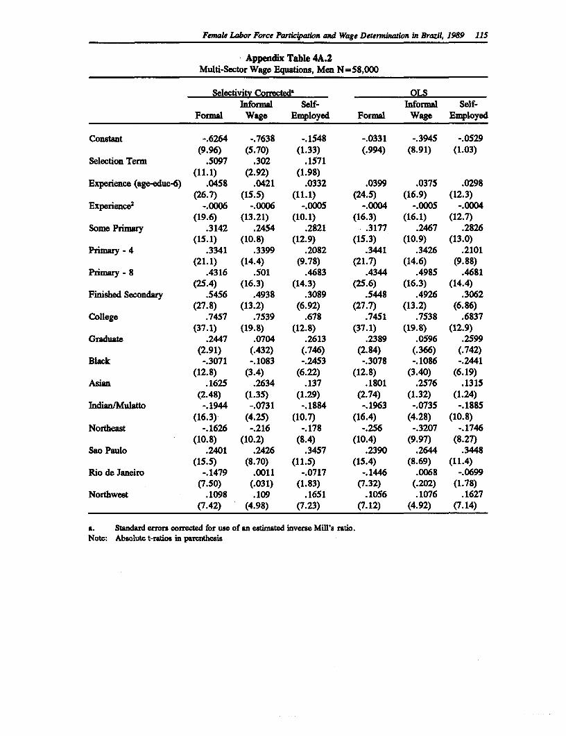
Female Labor Force Partipation and Wage Determination in Brazil, 1989 115
Appendix Table 4A.2Multi-Sector Wage Equations, Men N=58,000
Selectivity Corrected' OLSInformal Self- Informal Self-
Formal Wage Employed Formal Wage Employed
Constant -.6264 -.7638 -.1548 -.0331 -.3945 -.0529(9.96) (5.70) (1.33) (.994) (8.91) (1.03)
Selection Term .5097 .302 .1571(11.1) (2.92) (1.98)
Expenence (age-educ-6) .0458 .0421 .0332 .0399 .0375 .0298(26.7) (15.5) (11.1) (24.5) (16.9) (12.3)
Experience2 -.0006 -.0006 -.0005 -.0004 -.0005 -.0004(19.6) (13.21) (10.1) (16.3) (16.1) (12.7)
Some Primary .3142 .2454 .2821 .3177 .2467 .2826(15.1) (10.8) (12.9) (15.3) (10.9) (13.0)
Primary - 4 .3341 .3399 .2082 .3441 .3426 .2101(21.1) (14.4) (9.78) (21.7) (14.6) (9.88)
Primary - 8 .4316 .501 .4683 .4344 .4985 .4681(25.4) (16.3) (14.3) (25.6) (16.3) (14.4)
Finished Secondary .5456 .4938 .3089 .5448 .4926 .3062(27.8) (13.2) (6.92) (27.7) (13.2) (6.86)
College .7457 .7539 .678 .7451 .7538 .6837(37.1) (19.8) (12.8) (37.1) (19.8) (12.9)
Graduate .2447 .0704 .2613 .2389 .0596 .2599(2.91) (.432) (.746) (2.84) (.366) (.742)
Black -.3071 -.1083 -.2453 -.3078 -.1086 -.2441(12.8) (3.4) (6.22) (12.8) (3.40) (6.19)
Asian .1625 .2634 .137 .1801 .2576 .1315(2.48) (1.35) (1.29) (2.74) (1.32) (1.24)
Indian/Mulatto -.1944 -.0731 -.1884 -.1963 -.0735 -.1885(16.3) (4.25) (10.7) (16.4) (4.28) (10.8)
Northeast -.1626 -.216 -.178 -.256 -.3207 -.1746(10.8) (10.2) (8.4) (10.4) (9.97) (8.27)
Sao Paulo .2401 .2426 .3457 .2390 .2644 .3448(15.5) (8.70) (11.5) (15.4) (8.69) (11.4)
Rio de Janeiro -.1479 .0011 -.0717 -.1446 .0068 -.0699(7.50) (.031) (1.83) (7.32) (.202) (1.78)
Northwest .1098 .109 .1651 .1056 .1076 .1627(7.42) (4.98) (7.23) (7.12) (4.92) (7.14)
a. Standard errors corrected for use of an estimated inverse Mill's ratio.Note: Absolute t-ratios in parenthesis
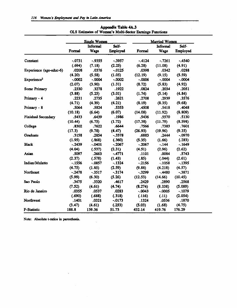
116 Women 's Enploymmnt and Pay in Latin America
Appendix Table 4A.3OLS Estimates of Women's Multi-Sector Earnings Functions
Single Women Married WomenInformal Self- informal Self-
Formal Wage Employed Formal Wage Employed
Constant -.0731 -.9355 -.3957 -.4124 -.7261 -.4540(.694) (7.18) (2.25) (6.28) (11.08) (4.91)
Experience (age-educ-6) .0208 .0376 -.0125 .0398 .0342 .0288(4.20) (5.58) (1.05) (12.19) (9.15) (5.59)
Experience2 -.0002 -.0004 -.0002 -.0006 -.0004 -.0004(2.07) (3.90) (1.31) (8.72) (5.83) (4.92)
Some Primary .2330 .3278 .1922 .0824 .2034 .2051(3.88) (5.25) (3.01) (1.74) (5.14) (4.84)
Primary - 4 .2231 .2735 .2621 .2708 .2939 .3576(4.71) (4.39) (4.21) (8.19) (8.35) (9.68)
Primary - 8 .5064 .5824 .5353 .4508 .5418 .4048(10.18) (6.64) (6.07) (14.08) (11.92) (8.809)
Finished Secondary .5433 .6439 .1986 .5436 .5570 .5130(10.44) (6.75) (1.72) (17.38) (11.79) (8.598)
College .8302 .7622 .6644 .7566 .7383 .7601(17.3) (9.78) (4.47) (26.93) (19.96) (9.35)
Graduate .3158 .2854 -.3378 .6883 .2444 -.0970(1.95) (.868) (.360) (5.35) (1.66) (.283)
Black -.2439 -.0401 -.2067 -.2067 -.144 -.1649(4.04) (.537) (2.31) (4.51) (2.96) (2.62)
Asian .5097 .2663 -.4771 .1101 .0084 .5743(2.37) (.578) (1.43) (.85) (.044) (2.61)
IndianlMulatto -.1556 -.0857 -.1324 -.2156 -.1058 -.1395(4.75) (1.85) (2.59) (9.88) (4.218) (4.57)
Northeast -.2478 -.3517 -.3174 -.3299 -.4480 -.3871(5.99) (6.30) (5.26) (12.53) (14.66) (10.45)
Sao Paulo .3475 .3320 .4617 .2429 .2890 .2568(7.52) (4.61) (4.74) (8.274) (8.338) (5.089)
Rio de Janeiro .0355 .0537 .0283 -.0043 -.0005 -.1079(.690) (.688) (.318) (.116) (.11) (2.054)
Northwest .1401 .0321 -.0173 .1324 .0536 .1870(3.47) (4.61) (.253) (5.03) (1.68) (4.75)
F-Statistic 188.8 139.36 51.73 432.14 419.76 176.29
Note: Absolute t-ratios in parnthesis.
References
Alderman, H. and V. Kozel. "Formal and Informal Sector Wage Determination in UrbanLow-Income Neighborhoods in Pakistan," Living Standards Measurement Study WorkingPaper No. 65, World Bank, 1989.
Blau, D.M. "A Model of Child Nutrition, Fertility, and Women's Time Allocation," Researchin opulation Economics 5:113-135, 1984.
Cornia, G.A., R. Jolly, and F. Stewart. Adjustment with a Human Face. Oxford: ClarendonPress, 1987.
Edwards, A. Cox. "Brazil: The Brazilian Labor Market in the 1980s," World Bank, CountryOperations Division, Country Department 1, Latin America and Caribbean Regional, 1991.Office, mimeo.
Hay, J.W. "Occupational Choice and Occupational Earnings: Selectivity Bias in a SimultaneousLogit-OLS Model," unpublished Ph.D. dissertation, Yale University, 1980.
Heckman, J.J. "Sample Selection Bias as a Specification Error," Econometrica 47,1:153-1611979.
Hill, M.A. "Labor Force Participation of Married Women in Urban Japan," Ph.D. dissertation,Duke University 1980.
Hill, M.A. "Female Labor Force Participation in Developing and Developed Countries -Consideration of the Informal Sector," Review of Economics and Statistics 63,3:459-468,1983.
Hill, M.A. "Female Labor Supply in Japan: Implications of the Informal Sector For Labor ForceParticipation and Hours of Work," The Journal of Human Resources 24:143-161, 1988.
Jaffe, A.J. and K. Azumi. "The Birth Rate and Cottage Industries in Underdeveloped Countries,"Economics Development and Cultural Change 9:52-63, 1960.
Lee, L.F. "Generalized Econometric Models with Selectivity," Econometnica 51:507-512, 1983.
Maddala, G.S. Limited-Dependent and Qualitative Variables in Econometrics. Cambridge:Cambridge University Press, 1983.
117
118 Women's Employment and Pay in Latin America
McCabe, J.L. and M.R. Rosenzweig. "Female Employment Creation and Family Size," in R.Ridker, ed., Population and Development. Ihe Search for Selective Interventions.Baltimore: The Johns Hopkins University Press, 1976.
McFadden, D. "Conditional Logit Analysis of Qualitative Choice Behavior," in P. Zarembka(ed.), Frontiers in Econometrics. New York: Academic Press 1973.
Mincer, J. Schooling, Experience, and Earnings. New York: Columbia University Press, 1974.
Oaxaca, R. "Male-female Wages Differenctians in Urban Labor Markets," InternationalEconomic Review 14:693-709, 1973.
Paes de Barros, R. and S. Varandas. "A Carteira de Trabalho e, as Condicoes de Trabalho eRemuneracao dos Chefes de Familia no Brasil," IPEA, 1987.
Sedlacek, G.L., R. Paes de Barros, and S. Varandas. "Segmentacao Mobilidade No Mercado deTrabalho Brasileiro: Uma Analise Da Regiao Metropolitana De Sao Paulo," in PerspectivasDa Economia Brasileira - 1989 IPEA/INPES, 1989.
Smith, S.K. "Determinants of Female Labor Force Participation and Family Size in MexicoCity," Economic Development and Cultural Change 30,1:129-152, 1981.
Stelcner, M., J.B. Smith, J.A. Brelaw, and G. Monette. "Labor Force Behavior and Earningsof Brazilian Women and Men," in this volume, 1991.
Tiefenthaler, J.M. "A Multi-Sector Model of Female Labor Force Participation and WageDetermination: Empirical Evidence from Cebu Island, Philippines," unpublished Ph.D.dissertation, Duke University, 1991.
Trost, R. and L.F. Lee. "Technical Training and Earnings: A Polychotomous Choice Model withSelectivity," Review of Economics and Statistics 66:151-156, 1984.
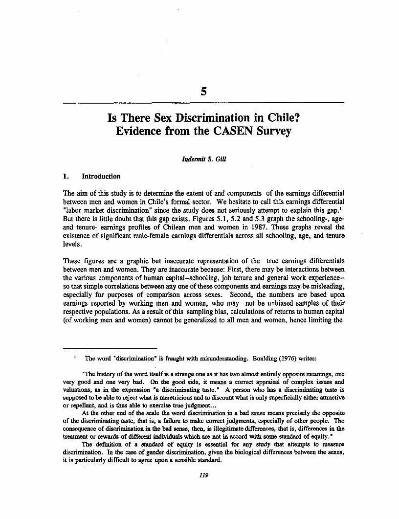
5
Is There Sex Discrimination in Chile?Evidence from the CASEN Survey
Indermit S. Gil
1. Introduction
The aim of this study is to determine the extent of and components of the earnings differentialbetween men and women in Chile's formal sector. We hesitate to call this earnings differential"labor market discrimination" since the study does not seriously attempt to explain this gap.'But there is little doubt that this gap exists. Figures 5.1, 5.2 and 5.3 graph the schooling-, age-and tenure- earnings profiles of Chilean men and women in 1987. These graphs reveal theexistence of significant male-female earnings differentials across all schooling, age, and tenurelevels.
These figures are a graphic but inaccurate representation of the true earnings differentialsbetween men and women. They are inaccurate because: First, there may be interactions betweenthe various components of human capital-schooling, job tenure and general work experience-so that simple correlations between any one of these components and earnings may be misleading,especially for purposes of comparison across sexes. Second, the numbers are based uponearnings reported by working men and women, who may not be unbiased samples of theirrespective populations. As a result of this sampling bias, calculations of returns to human capital(of working men and women) cannot be generalized to all men and women, hence limiting the
The word 'discrimination' is fraught with misunderstanding. Boulding (1976) writes:
'The history of the word itself is a strange one as it has two almost entirely opposite meanings, onevery good and one very bad. On the good side, it means a correct appraisal of complex issues andvaluations, as in the expression 'a discriminating taste." A person who has a discriminating taste issupposed to be able to reject what is meretricious and to discount what is only superficially either attractiveor repellant, and is thus able to exercise true judgment...
At the other end of the scale the word discrimination in a bad sense means precisely the oppositeof the discriminating taste, that is, a failure to make correct judgments, especially of other people. Theconsequence of discrimination in the bad sense, then, is illegitimate differences, that is, differences in thetreatment or rewards of different individuals which are not in accord with some standard of equity."
The definition of a standard of equity is essential for any study that attempts to measurediscrimination. In the case of gender discrimination, given the biological differences between the sexes,it is particularly difficult to agree upon a sensible standard.
119
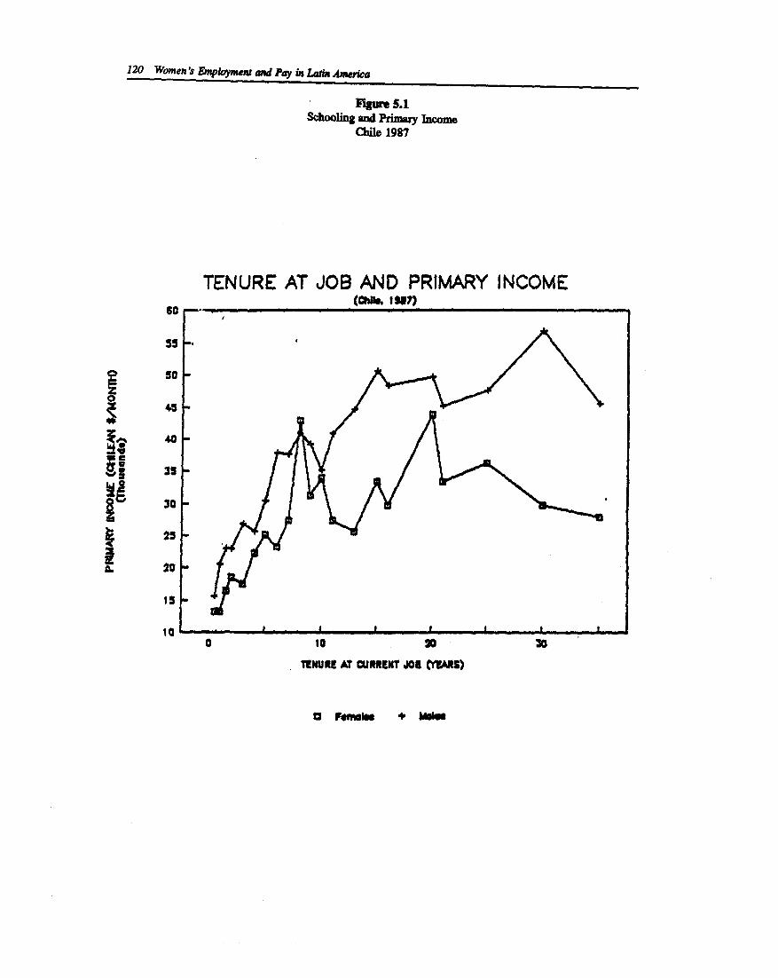
120 Women Is Empolymem and Pay in Latn America
igue 5.1Schooling and Primay Income
Chile 1987
TENURE AT JOB AND PRIMARY INCOME(Chu I
50 _ . -
55
45
~~ 2~5
0.~~3
1520
0 10 20 30
TtlURtE A? CUIRENT JOB ARWS)
Femi" + b
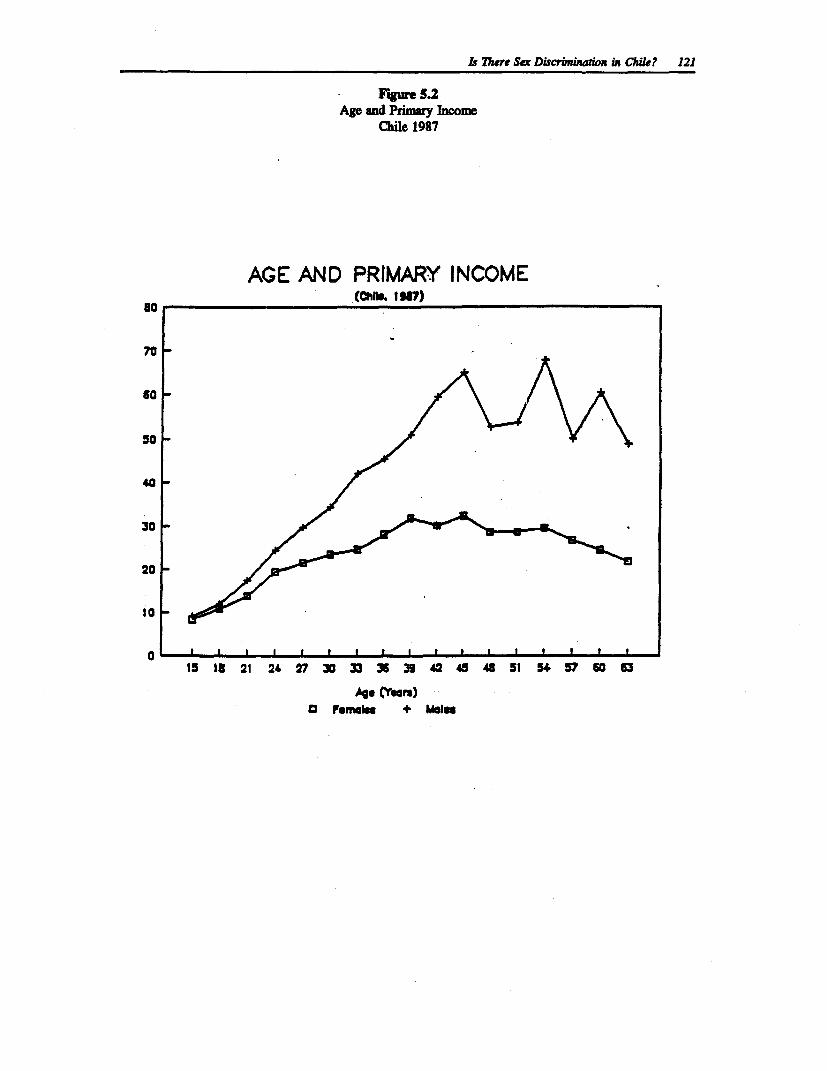
Is There Sex Discrbminaion in Chile? 121
Figue 5.2Age and Primay Income
Chile 1987
AGE AND PRIMARY INCOME(CNn. ,1,?)so
70-
60
40 _
3
20 -
10 _
0 * I I * e l I l e I
15 11 21 24 27 30 33 t 39 42 46 48 51 54 57 60 63
Age (Years)a frnieb + *Mam
122 Women's Enplioyment and Pay in Latin America
Figure 5.3Tenure at Job and Primary Income
Chile, 1987
SCHOOULNG AND PRIMARY INCOME(ChI~. 1937)
140
130
120
110
0 10090
C
A V70
60
40-
30
20
0 2 4 6 a tO 12 14 1 to15schooling + Malt
s There Sex Discrimination in Chile? 123
applicability of studies relying on rates of return calculations to propose subsidization of schoolingor job training.2
Later sections of this chapter correct for both these problems. Human capital earnings functionsusing all three measures of skill are estimated to calculate returns to each of these components(see Mincer 1974). The sample selectivity bias is corrected using a now familiar method proposedby Heckman (1979). The male-female earnings differential is then divided into two components:The segment due to lower endowments of human capital of women, and the segment due to lowerreturns to the human capital of women (See Oaxaca, 1973 for details).
Schooling levels are lower for working men than women, the gender gap in job tenure is small,but working men are older than working women, and hence men have greater (potential) workexperience. Thus composite human capital endowments are roughly the same for men andwomen. Much of the earnings differentials then must be explained by differential returns and/orunobserved ability.
The plan of this chapter is as follows. The next section provides a brief overview of the labormarket in Chile. Section 3 discusses the characteristics of the data used in this study: Informationfrom the National Socioeconomic Survey (Encuesta de Caracterizacion Socioeconomica Nacional,or CASEN) of Chilean households conducted in 1987. Section 4 examines the determinants offemale and male work participation. Section 5 uses the results of work participation regressionsto adjust for sample selectivity in analyzing the determinants of earnings of workers. Section 6uses these earnings regressions to compute the components of the earnings differential betweenmen and women, dividing it into the part due to market structure and the part due to observablehuman capital differences. Section 6 also offers partial explanations for the gender differentialin returns to human capital based on male-female differences in the industrial and occupationaldistribution of employment. Section 7 concludes the paper.
2. The Chilean Labor Market
Chile is a relatively developed labor market in terms of life expectancy, degree of urbanization(usually associated with advanced health and education systems), and literacy rates. Table 5.1shows some key indicators of development for Chile, Latin America and the Caribbean, and theUnited States. Chilean health and schooling levels seems to lie about halfway between LatinAmerican and United States' levels. Paradoxically, this is not reflected in correspondingdifferences in per capita income.3
For the purposes of this study, the interesting comparisons are those of male-female differencesin schooling enrollments and labor force participation. There are almost no gender differencesin schooling investments. However, women constitute only about 28 percent of the labor force,
2 There are other problems with these graphs. Reported earnings do not represent true returns tohuman capital where part or all of output is self-consumed. These skill-earnings profiles can also beinterpreted as approximating unobserved ability-eanings relationships: see Willis & Rosen (1979). Theseproblems are not addressed here.
3 Such discrepancies between human capital and income is the subject of the 'Human DevelopmentReport' (UNDP 1990), which proposes an average of indicators of income, health and education as anindex of development. For some theoretical shortcomings of this index and their resolution, see Gill andBhalla (1990).
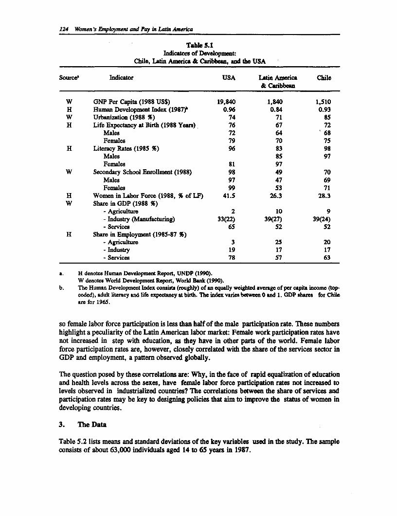
124 Women's Employment and Pay in Latin America
Table S.1Indicators of Development:
Chile, Latin America & Caribbean, and the USA
Source Indicator USA Latin America Chile& Caribbean
W GNP Per Capita (1988 US$) 19,840 1,840 1,510H Human Development Index (1987)b 0.96 0.84 0.93W Urbanization (1988 %) 74 71 85H Life Expectancy at Birth (1988 Years) 76 67 72
Males 72 64 '68Females 79 70 75
H Literacy Rates (1985 %) 96 83 98Males 85 97Females 81 97
W Secondary School Enrollment (1988) 98 49 70Males 97 47 69Females 99 53 71
H Women in Labor Force (1988, % of LF) 41.5 26.3 28.3W Share in GDP (1988 %)
- Agriculture 2 10 9- Industry (Manufacturing) 33(22) 39(27) 39(24)- Services 65 52 52
H Share in Employment (1985-87 %)- Agriculture 3 25 20- Industry 19 17 17- Services 78 57 63
a. H denotes Human Development Report, UNDP (1990).W denotes World Development Report, World Bank (1990).
b. The Human Development Index consists (roughly) of an equally weighted average of per capita income (top-coded), adult literacy and life expectancy at birth. The index vares between 0 and 1. GDP shames for Chileare for 1965.
so female labor force participation is less than half of the male participation rate. These numbershighlight a peculiarity of the Latin American labor market: Female work participation rates havenot increased in step with education, as they have in other parts of the world. Female laborforce participation rates are, however, closely correlated with the share of the services sector inGDP and employment, a pattern observed globally.
The question posed by these correlations are: Why, in the face of rapid equalization of educationand health levels across the sexes, have female labor force participation rates not increased tolevels observed in industrialized countries? The correlations between the share of services andparticipation rates may be key to designing policies that aim to improve the status of women indeveloping countries.
3. The Data
Table 5.2 lists means and standard deviations of the key variables used in the study. The sampleconsists of about 63,000 individuals aged 14 to 65 years in 1987.
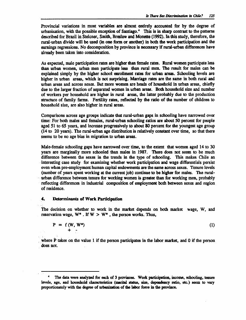
b There Sex Discrinta*ion in Chie? 125
Provincial variations in most variables are almost entirely accounted for by the degree ofurbanization, with the possible exception of Santiago.' This is in sharp contrast to the patternsdescribed for Brazil in Stelcner, Smith, Breslaw and Monette (1992). In this study, therefore, therural-urban divide will be used (in one form or another) in both the work participation and theearnings regressions. No decomposition by province is necessary if rural-urban differences havealready been taken into consideration.
As expected, male participation rates are higher than female rates. Rural women participate lessthan urban women, urban men participate less than rural men. The result for males can beexplained simply by the higher school enrollment rates for urban areas. Schooling levels arehigher in urban areas, which is not surprising. Marriage rates are the same in both rural andurban areas and across sexes. But more women are heads of household in urban areas, chieflydue to the larger fraction of separated women in urban areas. Both household size and numberof workers per household are higher in rural areas, the latter probably due to the productionstructure of family farms. Fertility rates, reflected by the ratio of the number of children tohousehold size, are also higher in rural areas.
Comparisons across age groups indicate that rural-urban gaps in schooling have narrowed overtime: For both males and females, rural-urban schooling ratios are about 50 percent for peopleaged 51 to 65 years, and increase progressively to about 80 percent for the youngest age group(14 to 20 years). The rural-urban age distribution is relatively constant over time, so that thereseems to be no age bias in migration to urban areas.
Male-female schooling gaps have narrowed over time, to the extent that women aged 14 to 30years are marginally more schooled than males in 1987. There does not seem to be muchdifference between the sexes in the trends in the type of schooling. This makes Chile aninteresting case study for examining whether work participation and wage differentials persisteven when pre-employment human capital endowments are the same across sexes. Tenure levels(number of years spent working at the current job) continue to be higher for males. The rural-urban difference between tenure for working women is greater than for working men, probablyreflecting differences in industrial composition of employment both between sexes and regionof residence.
4. Determinants of Work Participation
The decision on whether to work in the market depends on both market wage, W, andreservation wage, W* . If W > W* , the person works. Thus,
P = f(W,W*) (1)
where P takes on the value 1 if the person participates in the labor market, and 0 if the persondoes not.
4 The data were analyzad for each of 3 provinces. Worrk participation, income, schooling, tenurelevels, age, and household characteristics (marital status, size, dependency ratio, etc.) seem to varyproportionately with the degree of urbanization of the labor force in the provice.
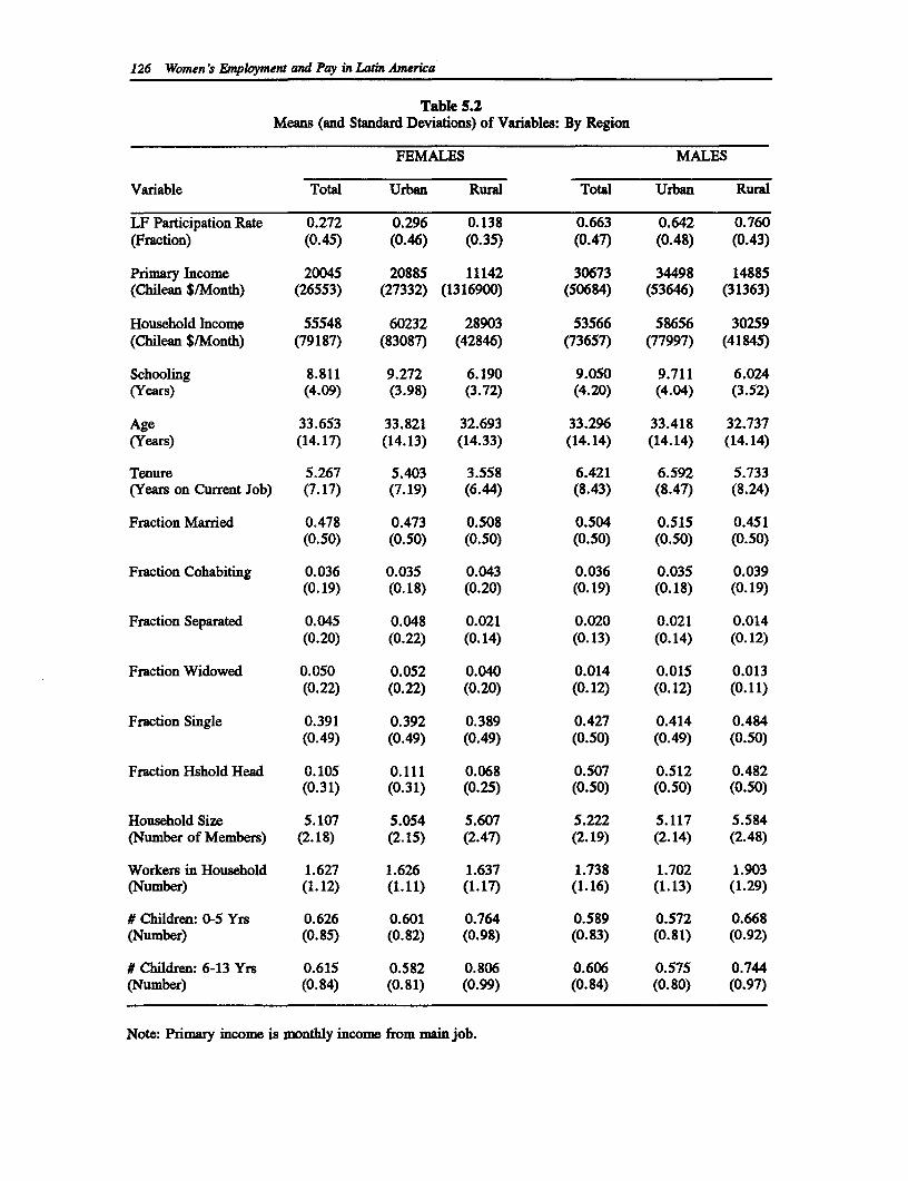
126 Women's Employment and Pay in Lain America
Table 5.2Means (and Standard Deviations) of Variables: By Region
FEMALES MALES
Variable Total Urban Rural Total Urban Rural
LF Participation Rate 0.272 0.296 0.138 0.663 0.642 0.760(Fraction) (0.45) (0.46) (0.35) (0.47) (0.48) (0.43)
Primary Income 20045 20885 11142 30673 34498 14885(Chilean $/Month) (26553) (27332) (1316900) (50684) (53646) (31363)
Household Income 55548 60232 28903 53566 58656 30259(Chilean $/Month) (79187) (83087) (42846) (73657) (77997) (41845)
Schooling 8.811 9.272 6.190 9.050 9.711 6.024(Years) (4.09) (3.98) (3.72) (4.20) (4.04) (3.52)
Age 33.653 33.821 32.693 33.296 33.418 32.737(Years) (14.17) (14.13) (14.33) (14.14) (14.14) (14.14)
Tenure 5.267 5.403 3.558 6.421 6.592 5.733(Years on Current Job) (7.17) (7.19) (6.44) (8.43) (8.47) (8.24)
Fraction Married 0.478 0.473 0.508 0.504 0.515 0.451(0.50) (0.50) (0.50) (0.50) (0.50) (0.50)
Fraction Cohabiting 0.036 0.035 0.043 0.036 0.035 0.039(0.19) (0.18) (0.20) (0.19) (0.18) (0.19)
Fraction Separated 0.045 0.048 0.021 0.020 0.021 0.014(0.20) (0.22) (0.14) (0.13) (0.14) (0.12)
Fraction Widowed 0.050 0.052 0.040 0.014 0.015 0.013(0.22) (0.22) (0.20) (0.12) (0.12) (0.11)
Fraction Single 0.391 0.392 0.389 0.427 0.414 0.484(0.49) (0.49) (0.49) (0.50) (0.49) (0.50)
Fraction Hshold Head 0.105 0.111 0.068 0.507 0.512 0.482(0.31) (0.31) (0.25) (0.50) (0.50) (0.50)
Household Size 5.107 5.054 5.607 5.222 5.117 5.584(Number of Members) (2.18) (2.15) (2.47) (2.19) (2.14) (2.48)
Workers in Household 1.627 1.626 1.637 1.738 1.702 1.903(Number) (1.12) (1.11) (1.17) (1.16) (1.13) (1.29)
# Children: 0-5 Yrs 0.626 0.601 0.764 0.589 0.572 0.668(Number) (0.85) (0.82) (0.98) (0.83) (0.81) (0.92)
# Children: 6-13 Yrs 0.615 0.582 0.806 0.606 0.575 0.744(Number) (0.84) (0.81) (0.99) (0.84) (0.80) (0.97)
Note: Primary income is monthly income from main job.
Is There Sex Dascriadon in Chile? 127
Market wage W depends upon stocks of productive skills - human capital - such as schoolingand job market experience, and the state of the labor market - regional and infrastructural factors- which determines the reward to these skills. Reservation wage W* depends upon theproductivity in activities other than labor market work. For both men and women, it maydepend upon the returns to further investment in human capital, which may require full timeschool attendance. Thus, for example, reservation wage rates will be higher for students whohave begun studies toward a degree but have not yet obtained a diploma. W* also depends uponhousehold characteristics such as the number of (young) children and other dependent relatives,and on household wealth.
Table 5.3 reports the results of probit estimations for the work participation functions (equation1 above) of women and men aged 14 to 65 years.5 Table 5.3 also reports the percentage changein the probability of participation ("%Deriv"), evaluated at the means of the right-hand-sidevariables. The results indicate that:
1. Higher schooling levels are positively associated with the probability ofparticipation, except when the years of schooling indicate incomplete programs ofstudy (8 to 11 years for both females and males, and 13 to 15 years for males).
2. The age profile of participation is inverted U-shaped. The profile for males is morecurved than for females.
3. Married and cohabiting women are less likely to work than those who are single orseparated. Married and cohabiting men are more likely to work than separated orsingle men. This result is consistent with the theory that marriage allows males andfemales to specialize in tasks, and females have a comparative advantage over menin household production.
4. Being a household head is positively correlated with the probability of participationfor both men and women.
5. Higher household income (total income of other members of the household)increases the likelihood of work for women, but decreases it for men. The resultfor women is somewhat puzzling.
6. Holding constant household size and the number of children, increases in the numberof workers increase the probability of participation for both women and men.Holding constant the total number of household workers and children, increases inhousehold decrease the probability of participation for both women and men.
7. The more young children there are in the household, the lower the likelihood ofparticipation of women, but the greater the probability of men working. Older
5 Many functional forms were fitted. The nrsults do not change significantly, so the most easilyinterpretable form is reported.
128 Women's Employment and Pay in Latin America
children have similar but weaker effects on decisions to work.' There is noevidence that older female children are substitutes for adult females in householdtasks.
8. Rural women participate less than urban women; urban men participate less thanrural men.
Using the probit regressions in Table 5.3 and Appendix Table 5A.2, we conducted simulationsof the effects of schooling, age, marital status, and household characteristics on femaleparticipation probabilities. Results of the simulation exercises are reported in Table 5.4 below.
Reasons for not working. Table 5.5 reports the reasons for not working. Naturally, the sampleconsists of those individuals for whom W* > W. A short description of the table is that womenwho do not work cite working at home, in school, and retired (in that order) as the mostimportant reasons, and men who do not work are in school, unemployed, or are retired (in thatorder).
Appendix Table SA. 1 reports the reasons for not working by sex, marital status, and age group.Married, cohabiting and widowed women overwhelmingly cite household work as the reason fornot working in the market (with "Retired" being the only other important reason for about 25percent of non-workers aged more than 50 years). Single and separated women do not workbecause they are in school (when they are young), or because of household work (for all ages).More than 10 percent of single women aged 21 to 40 years also list unemployment as a reasonfor not working.
Prime aged men who are married, cohabiting and widowed and who do not work are generallyunemployed (actively looking for work). Older non-workers are pensioners. Single men who donot work are in school (age groups 14-20 and 21-30 years), or unemployed (age groups 21-30,31-40 and 41-50 years), or physically unable to work (age groups 31-40, 41-50 and 51-65years).
Following Killingsworth and Heckman (1986), the error term in the work participation equationcan be divided into three components: The error term due to differences in tastes (utilityfunction errors), the errors due to unaccounted-for differences in budget constraints, and theerrors due to discrepancies between observed and optimal decisions. This last error is moreimportant for men, since "Unemployed" as a reason for not working is more important for menthan for women. Such differences between the sexes make it inadvisable to attach a uniforminterpretation to the sample selectivity correction terms (inverse of the Mill's ratio) for men andwomen, since these are derived from the error term in their respective participation functions.This problem is discussed further in the next section.
6 To further examine the effects of children on the decision to work, examine the probit esfimatesof men and women by marital status listed in Table A11.2 in the Appendix. For married and cohabitingwomen, increases in the number of children lowers the probability of participation, especially if the numberof children are 0 to 5 years old. For single and separated women, the number of children in the householdincreases the likelihood of working. The number of children has no effect on the participation decisionof men, holding constant household size and number of workers in the household.
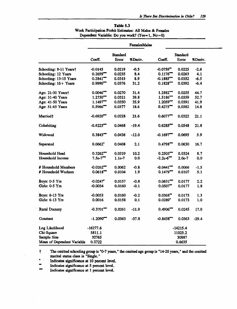
Is There Sax Discrimiration in Chile? 129
Table 5.3Work Participation Probit Estimates: All Males & Females
Dependent Variable: Do you work? (Yes= 1, No=0)
FemalesMales
Standard StandardCoeff. Error %Deriv. Coeff. Error %Deriv.
Schooling: 8-11 Yearst -0.0145 0.0219 -0.5 -0.0759w 0.0225 -2.6Schooling: 12 Years 0.2699 0.0235 8.4 0.1176 0.0263 4.1Schooling: 13-15 Years 0.2841 0.0315 8.9 -0. 1885w 0.0352 -6.5Schooling: 16+ Years 0.9990* 0.0376 31.2 0.1828 0.0392 -6.4
Age: 21-30 Yearst 0.0046 0.0270 31.4 1.2882" 0.0255 44.7Age: 31-40 Years 1.2750w 0.0321 39.8 1.5186- 0.0359 52.7Age: 41-50 Years 1.1497w 0.0350 35.9 1.2059-"" 0.0391 41.9Age: 51-65 Years 0.5966-n 0.0377 18.6 0.4275- 0.0382 14.8
Marriedt -0.6920*" 0.0228 21.6 0.6077M 0.0322 21.1
Cohabiting -0.6223- 0.0468 -19.4 0.6285 0.0548 21.8
Widowed 0.3843- 0.0436 -12.0 -0. 1697* 0.0695 5.9
Separated 0.0662* 0.0408 2.1 0.4798- 0.0630 16.7
Household Head 0.3262-" 0.0319 10.2 0.2503- 0.0324 8.7Household Income 7.5e-7'" 1. le-7 0.0 -2.2e-6~ 2.0e-7 0.0
N Household Members -0.0262'" 0.0062 -0.8 -0.0441w 0.0066 -1.5N Household Workers 0.0618- 0.0104 1.9 0.1479~ 0.0107 5.1
Boys: 0-5 Yrs -0.0247* 0.0157 -0.8 0.0631- 0.0177 2.2Girls: 0-5 Yrs -0.0034 0.0160 -0.1 0.0507" 0.0177 1.8
Boys: 6-13 Yrs -0.0053 0.0160 -0.2 0.0368" 0.0173 1.3Girls: 6-13 Yrs 0.0016 0.0158 0.1 0.0289* 0.0173 1.0
Rural Dummy -0.3701'" 0.0261 -11.9 0.4906- 0.0245 17.0
Constant -1.2090'" 0.0363 -37.8 -0.8458- 0.0363 -29.4
Log Likelihood -16277.6 -14215.4Chi-Square 5811.1 11025.2Sample Size 32765 30887Mean of Dependent Variable 0.2722 0.6635
t The omitted schooling group is "0-7 years," the omitted age group is "14-20 years," and the omittedmarital status class is "Single."
* Indicates significance at 10 percent level.Indicates significance at 5 percent level.Indicates significance at 1 percent level.
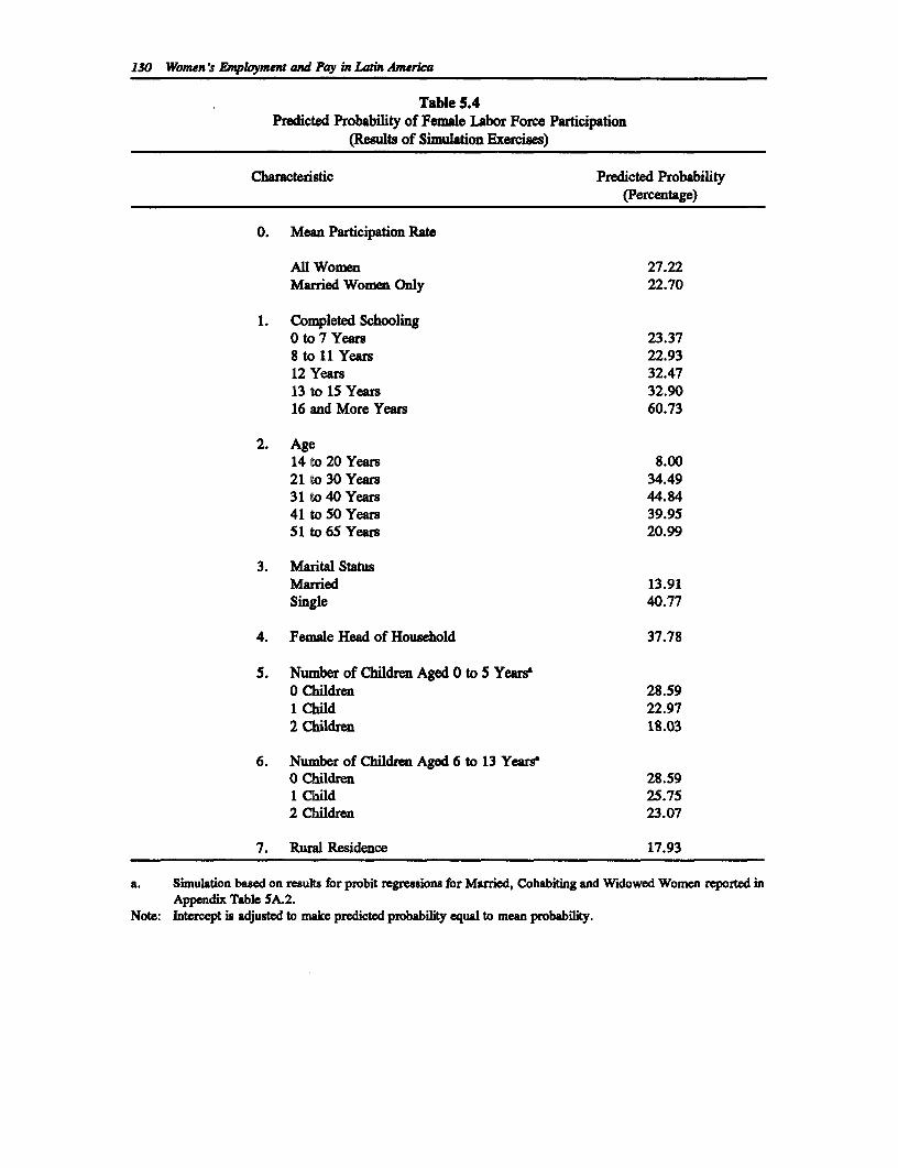
130 Women's Employmmnt and Pay in Latin America
Table S.4Predicted Probability of Female Labor Force Participation
(Results of Simulation Exercises)
Characteristic Predicted Probability(Percentage)
0. Mean Participation Rate
All Women 27.22Married Women Only 22.70
1. Completed SchoolingO to 7 Years 23.378 to 11 Years 22.9312 Years 32.4713 to 15 Years 32.9016 and More Years 60.73
2. Age14 to 20 Years 8.0021 to 30 Years 34.4931 to 40 Years 44.8441 to 50 Years 39.9551 to 65 Years 20.99
3. Marital StatusMarried 13.91Single 40.77
4. Female Head of Household 37.78
5. Number of Children Aged 0 to 5 Yeas0 Children 28.591 Child 22.972 Children 18.03
6. Number of Children Aged 6 to 13 Years0 Children 28.591 Child 25.752 Children 23.07
7. Runal Residence 17.93
a. Simulation based on results for probit regressions for Married, Cohabiting and Widowed Women reported inAppendix Table 5A.2.
Note: Intercept is adjused to make predicted probability equal to mean probability.
Is TJere Sex Discrnination in Chile? 131
Table .5Reasons for not Worldng: By Sex and Marital Status (%)
Married, Cohabiting Separated Total& Widowed & Sinele
Women Men Women Men Women Men
1. Looking for First Job 0.16 0.60 3.91 8.49 1.62 6.362. Unemployed 1.06 30.35 5.17 10.35 2.66 15.753. Household Work 88.38 3.78 35.24 1.57 67.71 2.174. Studying 0.55 2.17 48.35 64.15 19.14 47.405. Retired (Pensions, etc) 7.36 45.00 2.69 2.12 5.55 13.716. Rentier 0.13 0.34 0.09 0.06 0.11 0.137. Unable to Work 1.56 9.78 3.52 6.12 2.32 7.118. Temporarily Inactive 0.60 6.63 0.70 1.60 0.64 2.969. Other Reasons 0.21 1.35 0.33 5.55 0.25 4.41
Total Observations 14,956 2,669 9,516 7,208 24,472 9,877
5. Earnings Functions
The problem of sample selectivity. Earnings data are available only for working women andmen, that is, individuals with W > W*. For people who have the same wage, W, working menand women have smaller W* than those who do not work. For individuals with the samereservation wage, W*, working women have relatively high market wages, W. Because of boththese differences, working men and women are unrepresentative of the male and femalepopulations, and policy inferences derived from regressions for workers may be invalid both fornonworking men and women and for working men and women.
The problem can be interpreted, alternatively, as:
1. sample selectivity bias, or
2. a problem of omitted relevant variables in estimating the human capital earningsfunction (equivalently, of simultaneous equations bias), or
3. a problem of truncated data, since we do not observe (offered) wages for peoplewho do not work.
Following Killingsworth and Heckman (1986), let the work participation decision be:
P =W) +Rp + u (2)
where P = 1 if the individual works, 0 otherwise, W is the market wage, R is a set of variablesthat determine the reservation wage W*, and u is the error term. The human capital earningsfunction, which determines the market wage, is:
W = X, + v (3)
where X is the matrix of observed human capital variables (schooling, tenure, general workexperience, etc), ,@ is the vector of returns to these variables, and v is the error term.
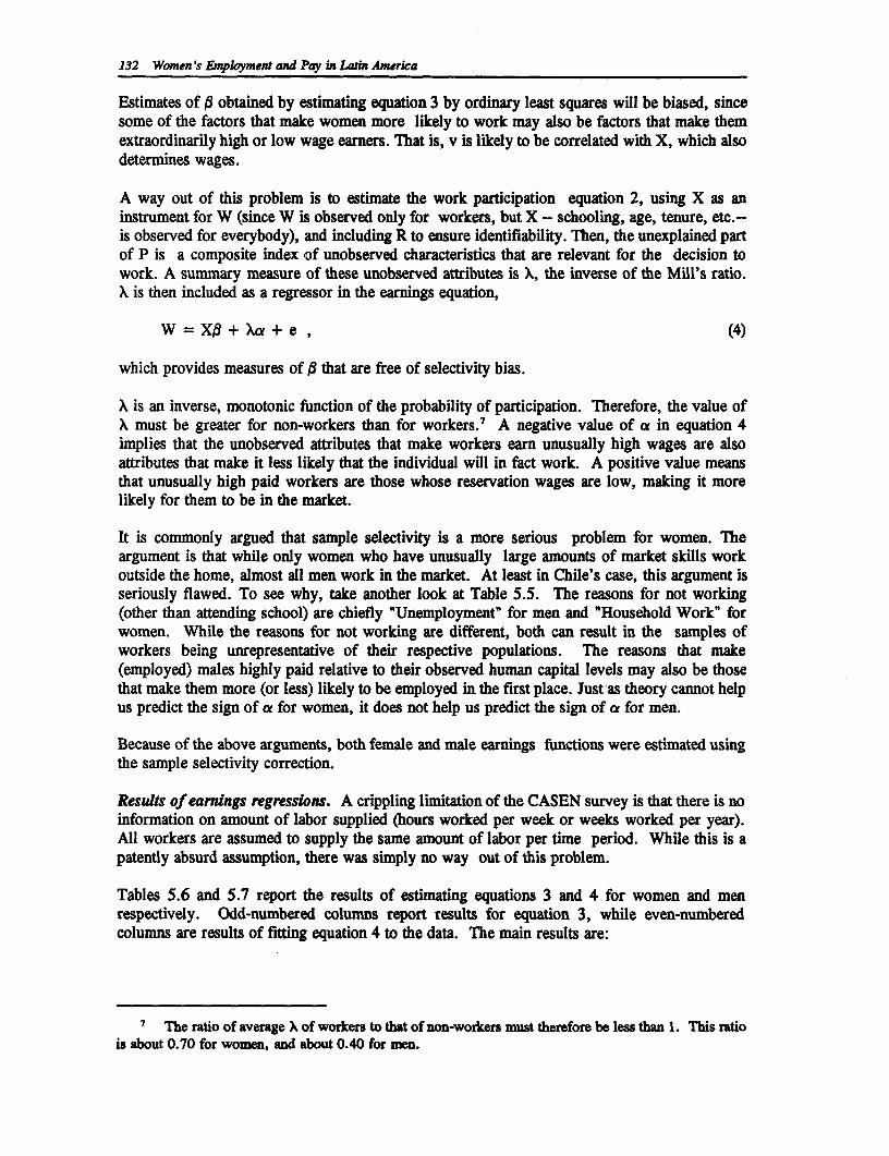
132 Women's Employment and Pay in Latin America
Estimates of , obtained by estimating equation 3 by ordinary least squares will be biased, sincesome of the factors that make women more likely to work may also be factors that make themextraordinarily high or low wage earners. That is, v is likely to be correlated with X, which alsodetermines wages.
A way out of this problem is to estimate the work participation equation 2, using X as aninstrument for W (since W is observed only for workers, but X - schooling, age, tenure, etc.-is observed for everybody), and including R to ensure identifiability. Then, the unexplained partof P is a composite index of unobserved characteristics that are relevant for the decision towork. A summary measure of these unobserved attributes is X, the inverse of the Mill's ratio.X is then included as a regressor in the earnings equation,
W = X,8 + Xa + e , (4)
which provides measures of ,B that are free of selectivity bias.
X is an inverse, monotonic function of the probability of participation. Therefore, the value ofX must be greater for non-workers than for workers.7 A negative value of a in equation 4implies that the unobserved attributes that make workers earn unusually high wages are alsoattributes that make it less likely that the individual will in fact work. A positive value meansthat unusually high paid workers are those whose reservation wages are low, making it morelikely for them to be in the market.
It is commonly argued that sample selectivity is a more serious problem for women. Theargument is that while only women who have unusually large amounts of market skills workoutside the home, almost all men work in the market. At least in Chile's case, this argument isseriously flawed. To see why, take another look at Table 5.5. The reasons for not working(other than attending school) are chiefly "Unemployment' for men and "Household Work" forwomen. While the reasons for not working are different, both can result in the samples ofworkers being unrepresentative of their respective populations. The reasons that make(employed) males highly paid relative to their observed human capital levels may also be thosethat make them more (or less) likely to be employed in the first place. Just as theory cannot helpus predict the sign of a for women, it does not help us predict the sign of a for men.
Because of the above arguments, both female and male earnings functions were estimated usingthe sample selectivity correction.
Results of earnings regressions. A crippling limitation of the CASEN survey is that there is noinformation on amount of labor supplied (hours worked per week or weeks worked per year).All workers are assumed to supply the same amount of labor per time period. While this is apatently absurd assumption, there was simply no way out of this problem.
Tables 5.6 and 5.7 report the results of estimating equations 3 and 4 for women and menrespectively. Odd-numbered columns report results for equation 3, while even-numberedcolumns are results of fitting equation 4 to the data. The main results are:
7 The ratio of average X of workers to that of non-workers must therfore be less than 1. This ratiois about 0.70 for women, and about 0.40 for men.
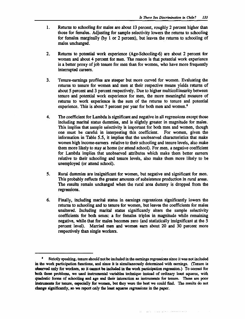
Is There Sex Discrnmination in Chile? 133
1. Returns to schooling for males are about 13 percent, roughly 2 percent higher thanthose for females. Adjusting for sample selectivity lowers the returns to schoolingfor females marginally (by 1 or 2 percent), but leaves the returns to schooling ofmales unchanged.
2. Returns to potential work experience (Age-Schooling-6) are about 2 percent forwomen and about 4 percent for men. The reason is that potential work experienceis a better proxy of job tenure for men than for women, who have more frequentlyinterrupted careers.
3. Tenure-earnings profiles are steeper but more curved for women. Evaluating thereturns to tenure for women and men at their respective means yields returns ofabout 5 percent and 3 percent respectively. Due to higher multicollinearity betweentenure and potential work experience for men, the more meaningful measure ofreturns to work experience is the sum of the returns to tenure and potentialexperience. This is about 7 percent per year for both men and women.'
4. The coefficient for Lambda is significant and negative in all regressions except thoseincluding marital status dummies, and is slightly greater in magnitude for males.This implies that sample selectivity is important for both men and women, thoughone must be careful in interpreting this coefficient. For women, given theinformation in Table 5.5, it implies that the unobserved characteristics that makewomen high income-earners relative to their schooling and tenure levels, also makethem more likely to stay at home (or attend school). For men, a negative coefficientfor Lambda implies that unobserved attributes which make them better earnersrelative to their schooling and tenure levels, also make them more likely to beunemployed (or attend school).
5. Rural dummies are insignificant for women, but negative and significant for men.This probably reflects the greater amounts of subsistence production in rural areas.The results remain unchanged when the rural area dummy is dropped from theregresslions.
6. Finally, including marital status in earnings regressions significantly lowers thereturns to schooling and to tenure for women, but leaves the coefficients for malesunaltered. Including marital status significantly alters the sample selectivitycoefficients for both sexes: a for females triples in magnitude while remainingnegative, while that for males becomes zero (and statistically insignificant at the 5percent level). Married men and women earn about 20 and 30 percent morerespectively than single workers.
Strictly spealing, tenure should not be included in the earnings regressions since it was not includedin the work participation functions, and since it is simultaneously determined with earnings. (Tenure isobserved only for workers, so it cannot be included in the work participation regression.) To correct forboth these problems, we used instrumental variables technique instead of ordinary least squares, withquadratic forms of schooling and age and their interaction as instruments for tenure. These are poorinstruments for tenure, especially for women, but they were the best we could find. The results do notchange significantly, so we report only the least squares regressions in the paper.
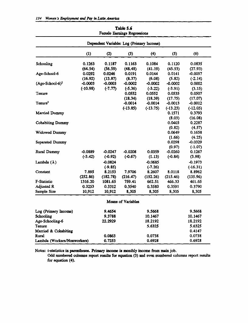
134 Women's Employmen and Pay in Latn America
Table 5.6Female Eanings Regressions
Dependent Variable: Log (Primary Income)
(1) (2) (3) (4) (5) (6)
Schooling 0.1263 0.1187 0.1163 0.1084 0.1120 0.0835(64.54) (56.59) (48.48) (41.19) (45.53) (27.93)
Age-School-6 0.0292 0.0246 0.0191 0.0144 0.0141 -0.0057(16.92) (13.87) (8.37) (6.08) (5.82) (-2.14)
(Age-School-6)2 -0.0003 -0.0003 -0.0002 -0.0002 -0.0002 0.0002(-10.98) (-7.77) (-5.36) (-3.22) (-3.91) (3.15)
Tenure 0.0552 0.0552 0.0535 0.0507(18.34) (18.39) (17.75) (17.07)
Tenure2 -0.0014 -0.0014 -0.0013 -0.0012(-13.85) (-13.75) (-13.23) (-12.05)
Married Dummy 0.1571 0.3793(8.03) (16.08)
Cohabiting Dummy 0.0403 0.2287(0.82) (4.57)
Widowed Dummy 0.0649 0.1658(1.66) (4.25)
Separated Dummy 0.0298 -0.0329(0.97) (-1.07)
Rural Dummy -0.0889 -0.0247 -0.0208 0.0359 -0.0260 0.1267(-3.42) (-0.92) (-0.67) (1.13) (-0.84) (3.98)
Lambda (A) -0.0824 -0.0685 -0.1973(-9.85) (-7.26) (-16.31)
Constant 7.895 8.2153 7.9706 8.2607 8.0118 8.8962(252.86) (182.78) (216.47) (152.26) (215.46) (135.96)
F-Statistic 1316.20 1081.65 759.41 662.51 466.33 461.65Adjusted R 0.3253 0.3312 0.3540 0.3580 0.3591 0.3790Sample Size 10,912 10,912 8,305 8,305 8,305 8,305
Means of Variables
Log (Primary Income) 9.4654 9.5668 9.5668Schooling 9.3788 10.1467 10.1467Age-Schooling-6 22.2929 18.2192 18.2192Tenure 5.6325 5.6325Married & Cohabiting 0.4147Rural 0.0863 0.0738 0.0738Lambda (Workers/Nonworkers) 0.7253 0.6928 0.6928
Notes: t-statistics in parentheses. Primary income is monthly income from main job.Odd numbered columns report results for equation (3) and even numbered columns report resultsfor equation (4).
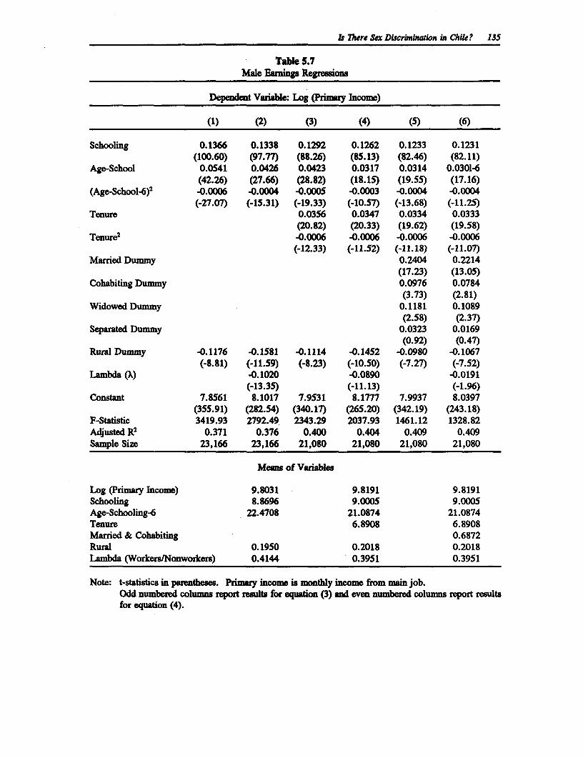
I There Sex Discrmnutdon in Chie? 135
Table 5.7Male Earnings Regressions
Dependent Variable: Log (Primary Income)
(1) (2) (3) (4) (5) (6)
Schooling 0.1366 0.1338 0.1292 0.1262 0.1233 0.1231(100.60) (97.77) (88.26) (85.13) (82.46) (82.11)
Age-School 0.0541 0.0426 0.0423 0.0317 0.0314 0.0301-6(42.26) (27.66) (28.82) (18.15) (19.55) (17.16)
(Age-School-6)2 -0.0006 -0.0004 -0.0005 -0.0003 -0.0004 -0.0004(-27.07) (-15.31) (-19.33) (-10.57) (-13.68) (-11.25)
Tenure 0.0356 0.0347 0.0334 0.0333(20.82) (20.33) (19.62) (19.58)
Tenure2 -0.0006 -0.0006 -0.0006 -0.0006(-12.33) (-11.52) (-11.18) (-11.07)
Married Dummy 0.2404 0.2214(17.23) (13.05)
Cohabiting Dummy 0.0976 0.0784(3.73) (2.81)
Widowed Dummy 0.1181 0.1089(2.58) (2.37)
Separated Dummy 0.0323 0.0169(0.92) (0.47)
Rumal Dummy -0.1176 -0.1581 -0.1114 -0.1452 -0.0980 -0.1067(-8.81) (-11.59) (-8.23) (-10.50) (-7.27) (-7.52)
Lambda (A) -0.1020 -0.0890 -0.0191(-13.35) (-11.13) (-1.96)
Constant 7.8561 8.1017 7.9531 8.1777 7.9937 8.0397(355.91) (282.54) (340.17) (265.20) (342.19) (243.18)
F-Statistic 3419.93 2792.49 2343.29 2037.93 1461.12 1328.82Adjusted R2 0.371 0.376 0.400 0.404 0.409 0.409Sample Size 23,166 23,166 21,080 21,080 21,080 21,080
Means of Variables
Log (Primary Income) 9.8031 9.8191 9.8191Schooling 8.8696 9.0005 9.0005Age-Schooling-6 22.4708 21.0874 21.0874Tenure 6.8908 6.8908Married & Cohabiting 0.6872Rural 0.1950 0.2018 0.2018Lambda (Workers/Nonworkers) 0.4144 0.3951 0.3951
Note: t-statistics in parentheses. Primary income is monthly income from main job.Odd numbered columns report results for equation (3) and even numbered colums report resultsfor equabon (4).
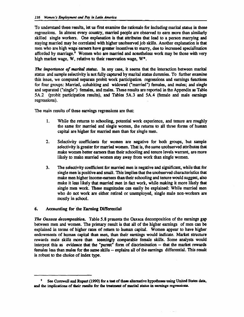
136 Women's EMployment and Pay in Lain America
To understand these results, let us first examine the rationale for including marital status in theseregressions. In almost every country, married people are observed to earn more than similarlyskilled single workers. One explanation is that attributes that lead to a person marrying andstaying married may be correlated with higher unobserved job skills. Another explanation is thatmen who are high wage earners have greater incentives to marry, due to increased specializationafforded by marriage.9 Women who are married and nonetheless work may be those with veryhigh market wage, W, relative to their reservation wage, W*.
The importance of nsaial status. In any case, it seems that the interaction between maritalstatus and sample selectivity is not fully captured by marital status dummies. To further examinethis issue, we computed separate probit work participation regressions and earnings functionsfor four groups: Married, cohabiting and widowed ("married") females, and males; and singleand separated ("single") females, and males. These results are reported in the Appendix as Table5A.2 (probit participation results), and Tables 5A.3 and 5A.4 (female and male earningsregressions).
The main results of these earnings regressions are that:
1. While the returns to schooling, potential work experience, and tenure are roughlythe same for married and single women, the returns to all three forms of humancapital are higher for married men than for single men.
2. Selectivity coefficients for women are negative for both groups, but sampleselectivity is greater for married women. That is, the same unobserved attributes thatmake women better earners than their schooling and tenure levels warrant, are morelikely to make married women stay away from work than single women.
3. The selectivity coefficient for married men is negative and significant, while that forsingle men is positive and small. This implies that the unobserved characteristics thatmake men higher income-earners than their schooling and tenure would suggest, alsomake it less likely that married men in fact work, while making it more likely thatsingle men work. These magnitudes can easily be explained: While married menwho do not work are either retired or unemployed, single male non-workers aremostly in school.
6. Accounting for the Earning Differential
lTe Oaxaca decomposition. Table 5.8 presents the Oaxaca decomposition of the earnings gapbetween men and women. The primary result is that all of the higher earnings of men can beexplained in terms of higher rates of return to human capital. Women appear to have higherendowments of human capital than men, than their earnings would indicate. Market structurerewards male skills more than seemingly comparable female skills. Some analysts wouldinterpret this as evidence that the "purest' form of discrimination - that the market rewardsfemales less than males for the same skills - explains all of the earnings differential. This resultis robust to the choice of index type.
9 See Cornwell and Rupert (1990) for a test of these altenative hypotheses using United States data,and the implications of their resudts for the atment of marita status in eamings regressions.
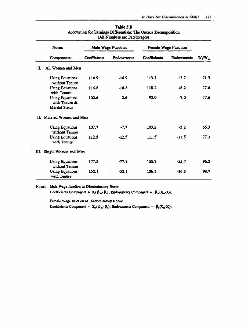
s There Sex Discrinauidon in Chike? 137
Table S.8Accounting for Earnings Differentials: The Oaxaca Decomposition
(All Numbers are Percentages)
Norm: Male Wage Function Female Wage Function
Components: Coefficients Endowments Coefficients Endowments W,/W,
I. All Women and Men
Using Equations 114.9 -14.9 113.7 -13.7 71.3without Tenure
Using Equations 116.8 -16.8 118.2 -18.2 77.6with Tenure
Using Equations 102.6 -2.6 93.0 7.0 77.6with Tenure &
Marital Status
ll. Married Women and Men
Using Equations 107.7 -7.7 103.2 -3.2 65.3without Tenure
Using Equations 112.5 -12.5 111.5 -11.5 77.3with Tenure
Ill. Single Women and Men
Using Equations 177.8 -77.8 155.7 -55.7 96.3without Tenure
Using Equations 152.1 -52.1 136.3 -36.3 98.7with Tenure
Notes: Male Wage function as Disriminatory Norm:Coefficients Component = X1( P- Pf), Endowments Component = ,(X.-X,).
Female Wage function as Discriminatory Norn:Coefficients Component = X.( ,- P), Endowments Component = ,(X,-X.
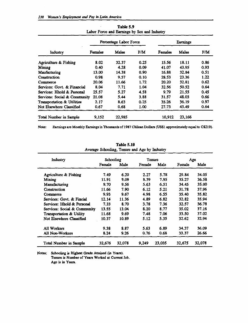
138 Women's Employment and Pay in Latin America
Table 5.9Labor Force and Earnings by Sex and Industry
Percentage Labor Force Earnings
Industry Females Males F/M Females Males F/M
Agriculture & Fishing 8.02 32.37 0.25 15.56 18.11 0.86Mining 0.40 4.28 0.09 41.07 43.95 0.93Maufacturing 13.00 14.38 0.90 16.88 32.84 0.51Construction 0.98 9.57 0.10 28.53 23.36 1.22Commerce 20.06 11.66 1.72 20.20 32.81 0.62Services: Govt. & Financial 8.04 7.71 1.04 32.56 50.52 0.64Services: Hhold & Personal 25.57 5.27 4.58 9.79 21.55 0.45Services: Social & Community 21.08 5.44 3.88 31.57 48.03 0.66Transportation & Utilities 2.17 8.63 0.25 35.26 36.19 0.97Not Elsewhere Classified 0.67 0.68 1.00 27.73 43.49 0.64
Total Number in Sample 9,152 22,985 10,912 23,166
Note: Eramings are Monthly Earnings in Thousands of 1987 Chilean Dollars (US$1 approximately equal to C$219).
Table 5.10Average Schooling, Tenure and Age by Industry
Industry Schooling Tenure AgeFemale Male Female Male Female Male
Agriculture & Fishing 7.49 6.20 2.27 5.78 29.84 34.05Mining 11.91 9.09 8.39 7.95 35.27 36.58Manufacturing 9.70 9.56 5.63 6.51 34.45 35.00Construction 11.66 7.90 6.12 5.21 31.78 37.96Commerce 9.93 9.67 4.98 6.55 35.40 35.82Services: Govt. & Fincial 12.14 11.36 4.89 6.82 32.82 35.94Services: Hhold & Personal 7.33 8.70 3.78 7.36 32.57 36.78Services: Social & Community 13.55 13.04 8.20 8.77 35.02 37.16Transportation & Utility 11.68 9.69 7.48 7.06 33.50 37.02Not Elsewhere Classified 10.37 10.89 5.12 5.35 32.62 32.94
All Workers 9.38 8.87 5.63 6.89 34.37 36.09All Non-Workers 8.24 9.26 0.76 0.68 33.37 26.66
Total Number in Sample 32,676 32,078 9,249 23,035 32,675 32,078
Notes: Schooling is Highest Grade Atained (in Years).Tenure is Number of Years Worked at Current Job.Age is in Years.
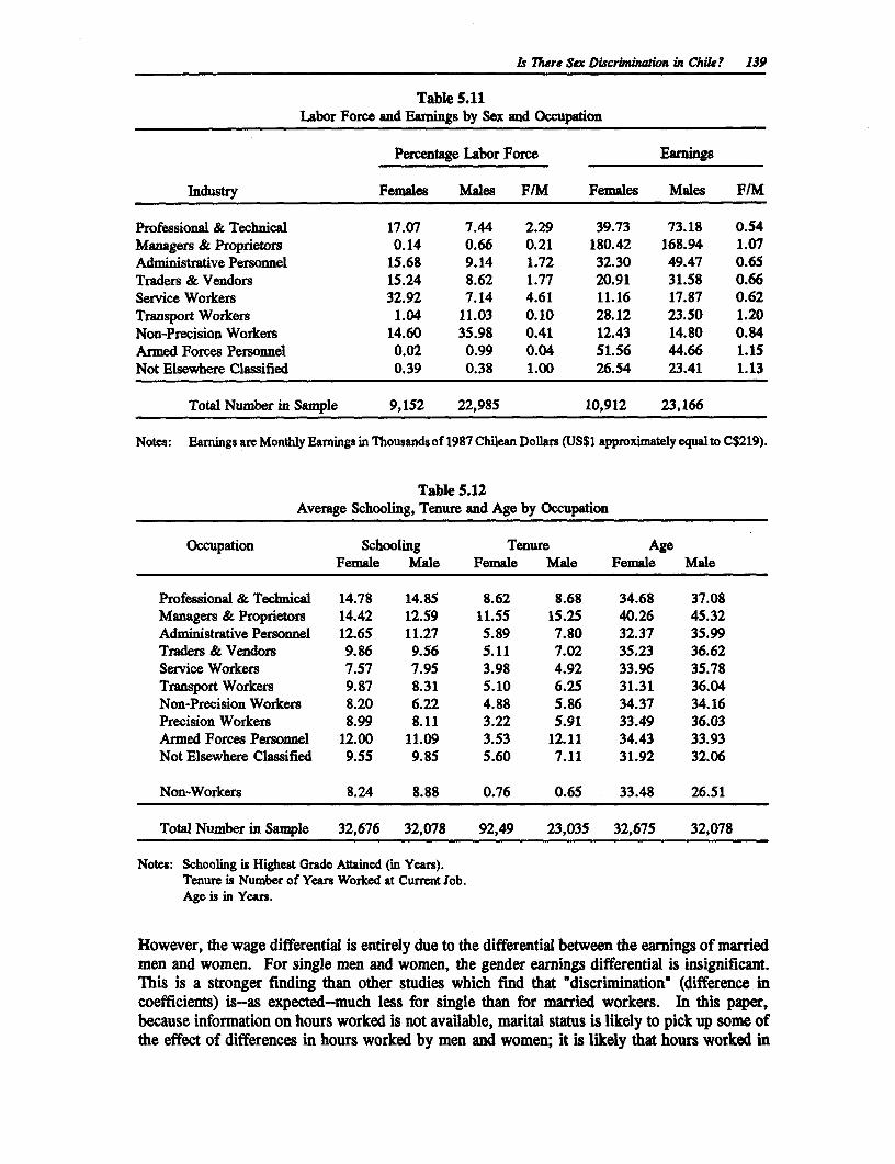
f There Sex Discrinination in Chik? 139
Table 5.11Labor Force and Earnings by Sex and Occupation
Percentage Labor Force Earnings
Industry Females Males F/M Females Males F/M
Professional & Technical 17.07 7.44 2.29 39.73 73.18 0.54Managers & Proprietors 0.14 0.66 0.21 180.42 168.94 1.07Administrative Personnel 15.68 9.14 1.72 32.30 49.47 0.65Traders & Vendors 15.24 8.62 1.77 20.91 31.58 0.66Service Workers 32.92 7.14 4.61 11.16 17.87 0.62Transport Workers 1.04 11.03 0.10 28.12 23.50 1.20Non-Precision Workers 14.60 35.98 0.41 12.43 14.80 0.84Armed Forces Personnel 0.02 0.99 0.04 51.56 44.66 1.15Not Elsewhere Classified 0.39 0.38 1.00 26.54 23.41 1.13
Total Number in Sample 9,152 22,985 10,912 23,166
Notes: Earnings are Monthly Earnings in Thousands of 1987 Chilean Dollars (US$1 approximately equal to C$219).
Table 5.12Average Schooling, Tenure and Age by Occupation
Occupation Schooling Tenure AgeFemale Male Female Male Female Male
Professional & Technical 14.78 14.85 8.62 8.68 34.68 37.08Managers & Proprietors 14.42 12.59 11.55 15.25 40.26 45.32Administrative Personnel 12.65 11.27 5.89 7.80 32.37 35.99Traders & Vendors 9.86 9.56 5.11 7.02 35.23 36.62Service Workers 7.57 7.95 3.98 4.92 33.96 35.78Transport Workers 9.87 8.31 5.10 6.25 31.31 36.04Non-Precision Workers 8.20 6.22 4.88 5.86 34.37 34.16Precision Workers 8.99 8.11 3.22 5.91 33.49 36.03Armed Forces Personnel 12.00 11.09 3.53 12.11 34.43 33.93Not Elsewhere Classified 9.55 9.85 5.60 7.11 31.92 32.06
Non-Workers 8.24 8.88 0.76 0.65 33.48 26.51
Total Number in Sample 32,676 32,078 92,49 23,035 32,675 32,078
Notes: Schooling is Highest Grade Attained (in Years).Tenure is Number of Years Worked at Current Job.Age is in Years.
However, the wage differential is entirely due to the differential between the earnings of marriedmen and women. For single men and women, the gender earnings differential is insignificant.This is a stronger finding than other studies which find that "discrimination" (difference incoefficients) is-as expected-much less for single than for married workers. In this paper,because information on hours worked is not available, marital status is likely to pick up some ofthe effect of differences in hours worked by men and women; it is likely that hours worked in
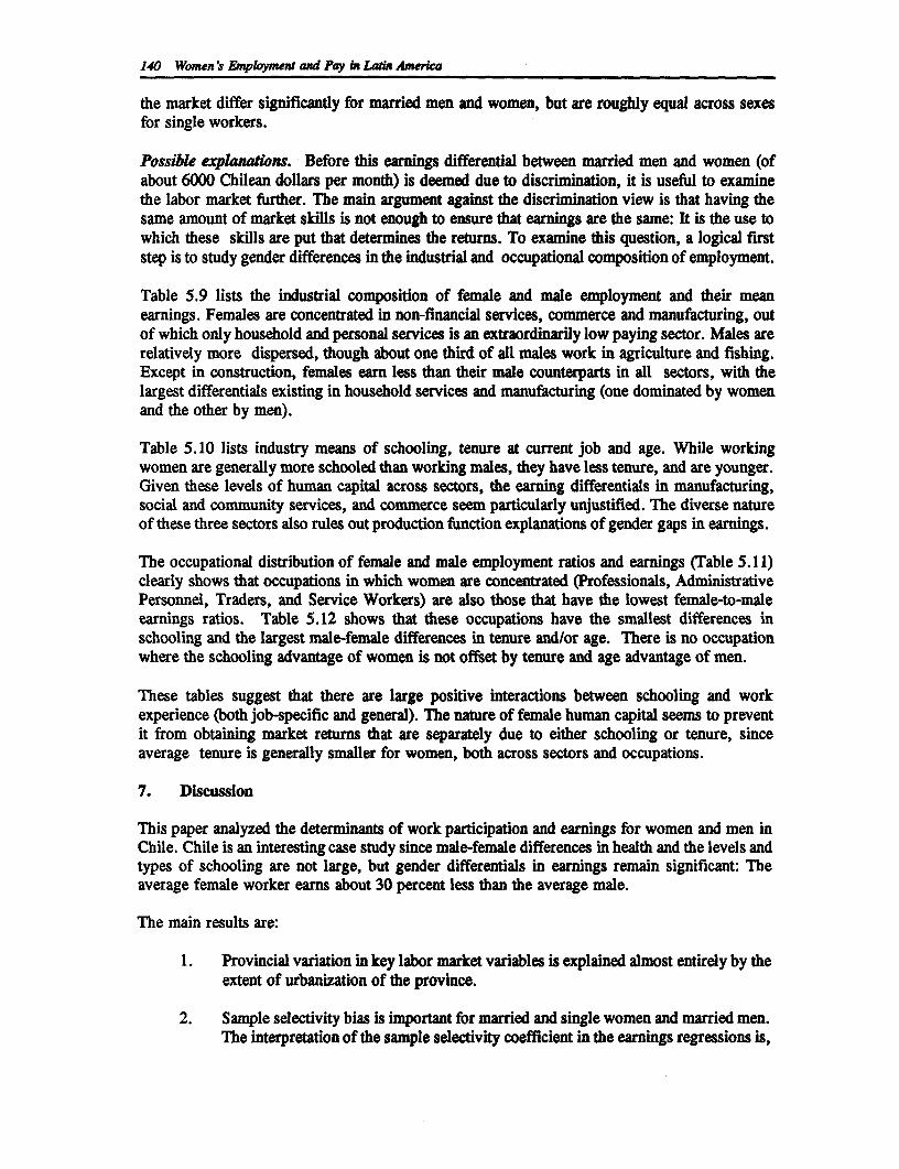
140 Women's Employment ad Pay it Latn America
the market differ significantly for married men and women, but are roughly equal across sexesfor single workers.
Possible explanations. Before this earnings differential between married men and women (ofabout 6000 Chilean dollars per month) is deemed due to discrimination, it is useful to examinethe labor market further. The main argument against the discrimination view is that having thesame amount of market skills is not enough to ensure that earnings are the same: It is the use towhich these skills are put that determines the returns. To examine this question, a logical firststep is to study gender differences in the industrial and occupational composition of employment.
Table 5.9 lists the industrial composition of female and male employment and their meanearnings. Females are concentrated in non-financial services, commerce and manufacturing, outof which only household and personal services is an extraordinarily low paying sector. Males arerelatively more dispersed, though about one third of all males work in agriculture and fishing.Except in construction, females earn less than their male counterparts in all sectors, with thelargest differentials existing in household services and manufacturing (one dominated by womenand the other by men).
Table 5.10 lists industry means of schooling, tenure at current job and age. While workingwomen are generally more schooled than working males, they have less tenure, and are younger.Given these levels of human capital across sectors, the earning differentials in manufacturing,social and community services, and commerce seem particularly unjustified. The diverse natureof these three sectors also rules out production function explanations of gender gaps in earnings.
The occupational distribution of female and male employment ratios and earnings (Table 5.11)clearly shows that occupations in which women are concentrated (Professionals, AdministrativePersonnel, Traders, and Service Workers) are also those that have the lowest female-to-maleearnings ratios. Table 5.12 shows that these occupations have the smallest differences inschooling and the largest male-female differences in tenure and/or age. There is no occupationwhere the schooling advantage of women is not offset by tenure and age advantage of men.
These tables suggest that there are large positive interactions between schooling and workexperience (both job-specific and general). The nature of female human capital seems to preventit from obtaining market returns that are separately due to either schooling or tenure, sinceaverage tenure is generally smaller for women, both across sectors and occupations.
7. Discussion
This paper analyzed the determinants of work participation and earnings for women and men inChile. Chile is an interesting case study since male-female differences in health and the levels andtypes of schooling are not large, but gender differentials in earnings remain significant: Theaverage female worker earns about 30 percent less than the average male.
The main results are:
1. Provincial variation in key labor market variables is explained almost entirely by theextent of urbanization of the province.
2. Sample selectivity bias is important for married and single women and married men.The interpretation of the sample selectivity coefficient in the earnings regressions is,
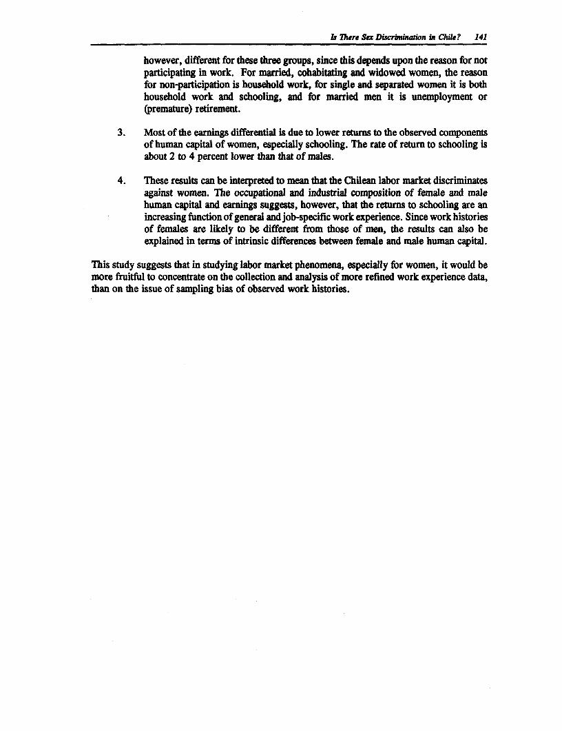
Is There Scx Discrbninahion in Chilk? 141
however, different for these three groups, since this depends upon the reason for notparticipating in work. For married, cohabitating and widowed women, the reasonfor non-participation is household work, for single and separated women it is bothhousehold work and schooling, and for married men it is unemployment or(premature) retirement.
3. Most of the earnings differential is due to lower returns to the observed componentsof human capital of women, especially schooling. The rate of return to schooling isabout 2 to 4 percent lower than that of males.
4. These results can be interpreted to mean that the Chilean labor market discriminatesagainst women. The occupational and industrial composition of female and malehuman capital and earnings suggests, however, that the returns to schooling are anincreasing function of general and job-specific work experience. Since work historiesof females are likely to be different from those of men, the results can also beexplained in terms of intrinsic differences between female and male human capital.
This study suggests that in studying labor market phenomena, especially for women, it would bemore fruitful to concentrate on the collection and analysis of more refined work experience data,than on the issue of sampling bias of observed work histories.
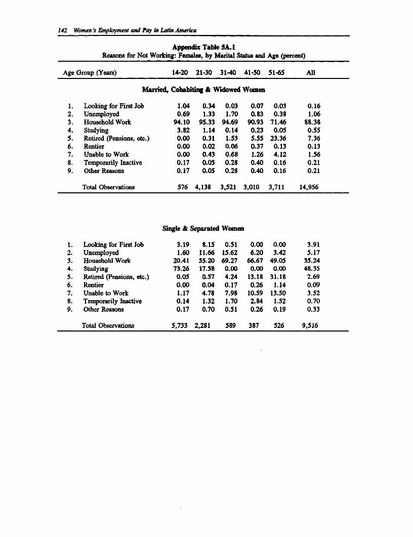
142 Women's Employment and Pay in Latin America
Appendix Table 5A.1Reasons for Not Working: Females, by Marital Status and Age (percent)
Age Group (Years) 14-20 21-30 31-40 41-50 51-65 All
Married, Cohabiting & Widowed Women
1. Looling for First Job 1.04 0.34 0.03 0.07 0.03 0.162. Unemployed 0.69 1.33 1.70 0.83 0.38 1.063. Household Work 94.10 95.33 94.69 90.93 71.46 88.384. Studying 3.82 1.14 0.14 0.23 0.05 0.555. Retired (Pensions, etc.) 0.00 0.31 1.53 5.55 23.36 7.366. Rentier 0.00 0.02 0.06 0.37 0.13 0.137. Unable to Work 0.00 0.43 0.68 1.26 4.12 1.568. Temporarily Inactive 0.17 0.05 0.28 0.40 0.16 0.219. Other Reasons 0.17 0.05 0.28 0.40 0.16 0.21
Total Observations 576 4,138 3,521 3,010 3,711 14,956
Single & Separated Women
1. Looking for First Job 3.19 8.15 0.51 0.00 0.00 3.912. Unemployed 1.60 11.66 15.62 6.20 3.42 5.173. Household Work 20.41 55.20 69.27 66.67 49.05 35.244. Studying 73.26 17.58 0.00 0.00 0.00 48.355. Retired (Pensions, etc.) 0.05 0.57 4.24 13.18 31.18 2.696. Rentier 0.00 0.04 0.17 0.26 1.14 0.097. Unable to Work 1.17 4.78 7.98 10.59 13.50 3.528. Temporarily Inactive 0.14 1.32 1.70 2.84 1.52 0.709. Other Reasons 0.17 0.70 0.51 0.26 0.19 0.33
Total Observations 5,733 2,281 589 387 526 9,516
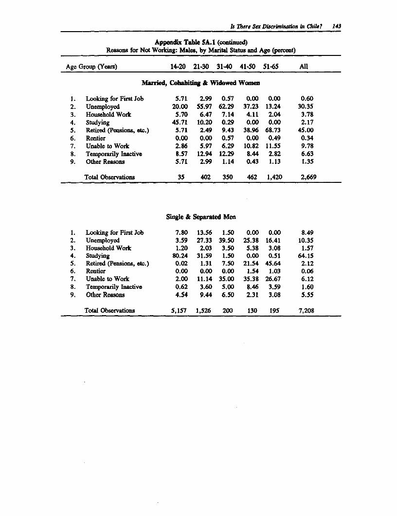
Is There Sgx Discrimination in Chile? 143
Appendix Table SA.1 (continued)Reasons for Not Working: Males, by Marital Status and Age (percent)
Age Group (Years) 14-20 21-30 31-40 41-50 51-65 All
Married, Cohabiti & Widowed Women
1. Looking for First Job 5.71 2.99 0.57 0.00 0.00 0.602. Unemployed 20.00 55.97 62.29 37.23 13.24 30.353. Household Work 5.70 6.47 7.14 4.11 2.04 3.784. Studying 45.71 10.20 0.29 0.00 0.00 2.175. Retired (Pensions, etc.) 5.71 2.49 9.43 38.96 68.73 45.006. Rentier 0.00 0.00 0.57 0.00 0.49 0.347. Unable to Work 2.86 5.97 6.29 10.82 11.55 9.788. Temporarily Inactive 8.57 12.94 12.29 8.44 2.82 6.639. Other Reasons 5.71 2.99 1.14 0.43 1.13 1.35
Total Observations 35 402 350 462 1,420 2,669
Single & Separated Men
1. Looking for First Job 7.80 13.56 1.50 0.00 0.00 8.492. Unemployed 3.59 27.33 39.50 25.38 16.41 10.353. Household Work 1.20 2.03 3.50 5.38 3.08 1.574. Studying 80.24 31.59 1.50 0.00 0.51 64.155. Retired (Pensions, etc.) 0.02 1.31 7.50 21.54 45.64 2.126. Rentier 0.00 0.00 0.00 1.54 1.03 0.067. Unable to Work 2.00 11.14 35.00 35.38 26.67 6.128. Temporarily Inactive 0.62 3.60 5.00 8.46 3.59 1.609. Other Reasons 4.54 9.44 6.50 2.31 3.08 5.55
Total Observations 5,157 1,526 200 130 195 7,208
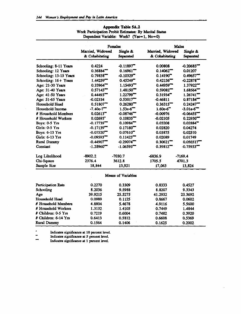
144 Women's Emplyment and Pay in Lahn America
Appendix Table SA.2Work Participation Probit Estimates: By Marital Status
Dependent Variable: Work (Yes=l, No=0)
Females MalesMarried, Widowed Single & Married, Widowed Single &
& Cohabitating Separated & Cohabitating Separated
Schooling: 8-11 Years 0.4224 -0.1189r 0.00808 -0.20683Schooling: 12 Years 0.36884w 0.16961 0.14062- 0.01207Schooling: 13-15 Years 0.79838' -0.10329- 0.14190 0.49657wSchooling: 16 + Years 1.44259w 0.45249 0.42136w -0.22878wAge: 21-30 Years 0.33964- 1. 15493w 0.44959 1.37922"Age: 31-40 Years 0.57143w 1.48150' 0.59082 1.68564*Age: 41-50 Years 0.44493w 1.22799 0.31934i 1.26741wAge: 51-65 Years -0.02334 0.53017 -0.46811 0.87184'Household Head 0.51807- 0.26280 0.36315- 0.24247wHousehold Income -7.40e-7* 1.53e-6 1.60e-6 -3.01e-6~# Household Members 0.02613w -0.08746w -0.00976 -0.06455# Household Workers 0.02693* 0. 10835 -0.02105 0.22930inBoys: 0-5 Yrs -0. 17739w 0.10984w 0.03208 0.02884WGirls: 0-5 Yrs -0. 17139w 0.17180 0.02820 0.04274Boys: 6-13 Yrs -0.07520' 0.07610w 0.03875 0.02510Girls: 6-13 Yrs -0.09593a 0.11423 0.02089 0.01749Rural Dummy -0.44907 -0.29074- 0.30621~ 0.056517-Constant -1.28960" -1.06593 0.39812 -0.75933
Log Likelihood -8902.2 -7030.7 -6836.9 -7169.4Chi-Square 2376.4 3612.8 1705.5 4701.3Sample Size 18,844 13,921 17,063 13,824
Means of Variables
Participation Rate 0.2270 0.3309 0.8333 0.4527Schooling 8.2036 9.5988 8.8207 9.3343Age 39.9215 25.5275 41.2932 23.3692Household Head 0.0989 0.1125 0.8667 0.0602# Household Members 4.8804 5.4678 4.9116 5.5600# Household Workers 1.3132 1.4105 0.7449 1.4844# Children: 0-5 Yrs 0.7219 0.6004 0.7482 0.3920# Children: 6-14 Yrs 0.6413 0.5812 0.6608 0.5369Rural Dummy 0.1564 0.1406 0.1625 0.2002
Indicates significance at 10 percent level.Indicates significance at 5 percent level.Indicates significance at 1 percent level.
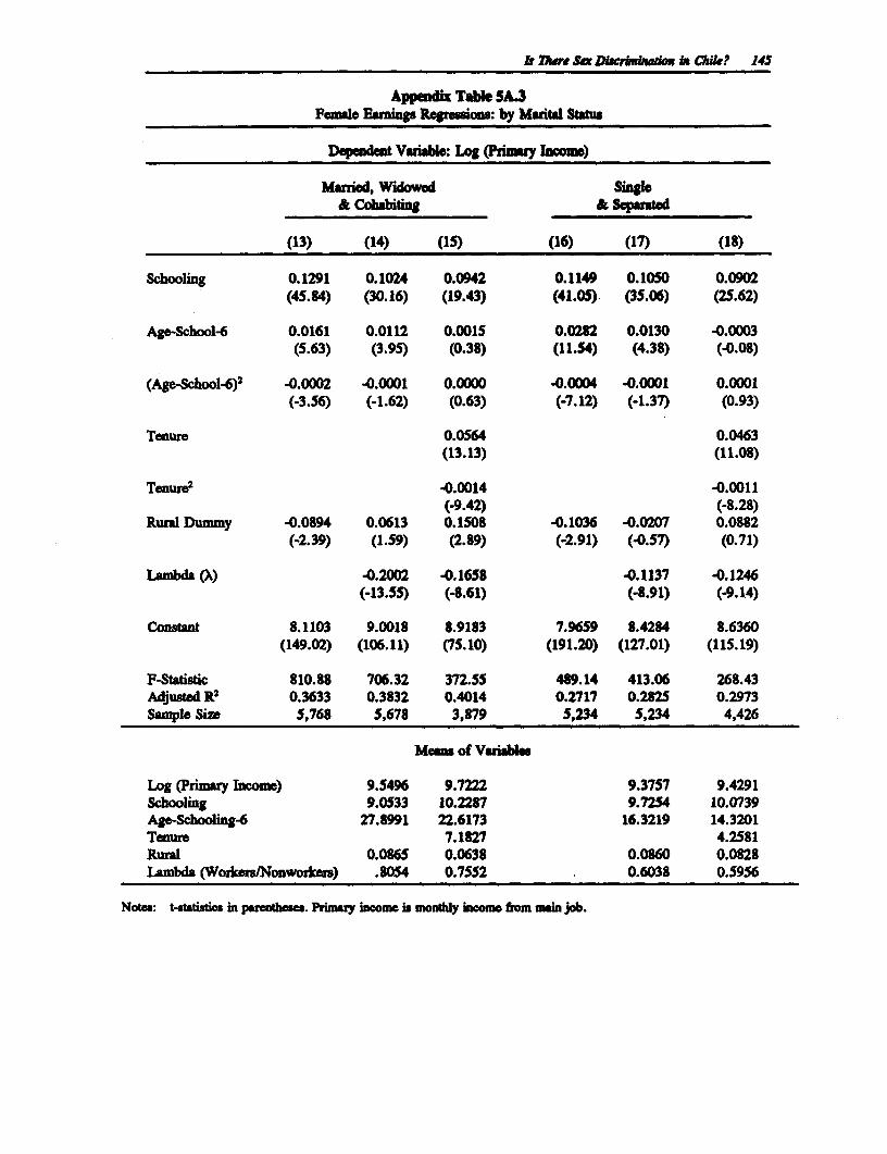
& Thkre Six Dhbc.Lqwdou in Chik? 145
Aperndix Table 5A.3Female Eanings Rogeouons: by Manitl Stain
Deqpedent Variable: LAg (Primy IOncM)
Maried, Wiuowed Single& Coabiting & Septd
(13) (14) (15) (16) (17) (18)
Schooling 0.1291 0.1024 0.0942 0.1149 0.100 0.0902(45.84) (30.16) (19.43) (41.05). (35.06) (25.62)
Age-School-6 0.0161 0.0112 0.0015 0.0282 0.0130 -0.0003(5.63) (3.95) (0.38) (11.54) (4.38) (-0.08)
(Age-S1hool-6r -0.0002 -0.0001 0.0000 -0.0004 -0.0001 0.0001(-3.56) (-1.62) (0.63) (-7.12) (-1.37) (0.93)
Tenure 0.0564 0.0463(13.13) (11.08)
Tenure2 -0.0014 -0.0011(-9.42) (-8.28)
Runrl Dummy -0.0894 0.0613 0.1508 -0.1036 -0.0207 0.0882(-2.39) (1.59) (2.89) (-2.91) (40.57) (0.71)
Lambda (X) -0.2002 -0.1658 -0.1137 -0.1246(-13.55) (-8.61) (-8.91) (-9.14)
Constant 8.1103 9.0018 8.9183 7.9659 8.4284 8.6360(149.02) (106.11) (75.10) (191.20) (127.01) (11S.19)
F-Statistic 810.88 706.32 372.55 489.14 413.06 268.43Adjusted R2 0.3633 0.3832 0.4014 0.2717 0.2825 0.2973Sample Size 5,768 5,678 3,879 5,234 5,234 4,426
Mea of VariaeS
Log (Primy Income) 9.5496 9.7222 9.3757 9.4291Schooling 9.0533 10.2287 9.7254 10.0739Age-Schooling-6 27.8991 22.6173 16.3219 14.3201Tenure 7.1827 4.2581Rural 0.0865 0.0638 0.0860 0.0828Lambda (Workers/Nonworkers) .8054 0.7552 0.6038 0.5956
Notes: t-statistics in puaenthems. Puimuly income is montly income from main job.
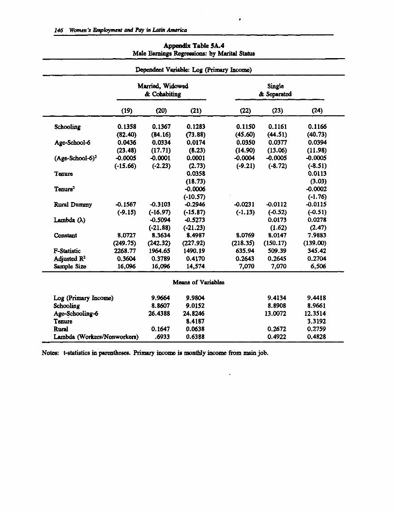
146 Women's EnA1oymw and Pay us Latn America
Appendix Table 5A.4Male Eamings Regressions: by Marital Status
Dependent Variable: Log (Primary Income)
Married, Widowed Single& Cohabiting & Separated
(19) (20) (21) (22) (23) (24)
Schooling 0.1358 0.1367 0.1283 0.1150 0.1161 0.1166(82.40) (84.16) (73.88) (45.60) (44.51) (40.73)
Age-School-6 0.0436 0.0334 0.0174 0.0350 0.0377 0.0394(23.48) (17.71) (8.23) (14.90) (13.06) (11.98)
(Age-School-6)2 -0.0005 -0.0001 0.0001 -0.0004 -0.0005 -0.0005(-15.66) (-2.23) (2.73) (-9.21) (-8.72) (-8.51)
Tenure 0.0358 0.0113(18.73) (3.03)
Tenure2 -0.0006 -0.0002(-10.57) (-1.76)
Rural Dummy -0.1567 -0.3103 -0.2946 -0.0231 -0.0112 -0.0115(-9.15) (-16.97) (-15.87) (-1.13) (-0.52) (-0.51)
Lambda (A) -0.5094 -0.5273 0.0173 0.0278(-21.88) (-21.23) (1.62) (2.47)
Constant 8.0727 8.3634 8.4987 8.0769 8.0147 7.9883(249.75) (242.32) (227.92) (218.35) (150.17) (139.00)
F-Statistic 2268.77 1964.65 1490.19 635.94 509.39 345.42Adjusted R2 0.3604 0.3789 0.4170 0.2643 0.2645 0.2704Sample Size 16,096 16,096 14,574. 7,070 7,070 6,506
Meams of Variables
Log (Primary Income) 9.9664 9.9804 9.4134 9.4418Schooling 8.8607 9.0152 8.8908 8.9661Age-Schooling-6 26.4388 24.8246 13.0072 12.3514Tenure 8.4187 3.3192Rurl 0.1647 0.0638 0.2672 0.2759Lambda (Workers/Nonworkers) .6933 0.6388 0.4922 0.4828
Notes: t-statistics in parentheses. Primary income is monthly income from main job.
References
Boulding, K. "Toward a Theory of Discrimination." in P. Wallace (ed.). Equal EmploymentOpportunity and the AT&T Case. Cambridge, Massachusetts: The MIT Press, 1976.
Cornwell, C. and P. Rupert. "Unobservable Individual Effects, Marriage and the Earnings ofYoung Men." Working Paper. State University of New York at Buffalo, 1990.
Gill, I.S. and S.S. Bhalla. 'Income Growth and Improvement in Living Standards."Mimeograph. Washington, D.C.: World Bank, 1990.
Heckman, J.J. "Sample Selection Bias as a Specification Error." Econometrica, Vol. 47 (1979).pp. 153-161.
Killingsworth, M.R. and J.J. Heckman. "Female Labor Supply: A Survey" in 0. Ashenfelter andR. Layard (eds.). Handbook of Labor Economics. Vol. 1. New York: Elsevier SciencePublishers, 1986.
Mincer, J. Schooling, Experience and Earnings. New York: Columbia University Press, 1974.
Oaxaca, R. "Male-female Wage Differentials in Urban Labor Markets." Internationol EconomicReview. Vol. 14, no. 1 (1973). pp. 693-701.
Stelcner, M.J., B. Smith, J. Breslaw and G. Monette. "Labor Force Behavior and Earnings ofBrazilian Women and Men, 1980." This volume, 1992.
United Nations Development Programme. Human Development Report. New York: OxfordUniversity Press, 1990.
Willis, R.J. and S. Rosen. "Education and Self-selection." Jounal of Political Econonmy(supplement). Vol. 87 (1979). pp. S7-S36.
World Bank. World Development Report. Washington, D.C.: Oxford University Press, 1990.
147

6
Labor Markets, the Wage Gap and GenderDiscrimination:
The Case of Colombia
Jaime Tenjo'
1. Introduction
Earnings differentials between men and women have been documented in a large number ofstudies both for developed and developing countries. However, unlike the case of more advancedcountries2, very little work has been done in developing countries to explain why men aresystematically paid more than women. In many earnings functions, for example, the introductionof a dummy variable for sex has produced statistically significant coefficients that indicate sizabledifferences in pay between men and women3 but very little effort has been made to investigatemore thoroughly the source of this differential4. Rather, researchers have been more concernedwith explanations of differentials between regions (rural-urban), between sectors (modern-tradi-tional or formal-informal) and between industries (agriculture versus manufacture, etc). Asexplained below, gender wage differentials can be associated with a number of factors such asdifferences in productivity, working conditions, discrimination, etc. This paper is an attempt toidentify the degree to which these and other factors contribute to the explanation of the wage gapbetween men and women in Colombia.
The structure of the paper is the following: Section 2 presents a discussion of the reasons for theexistence of wage differentials in the labor market and the meaning of various forms of
The author wishes to acknowledge the useful comments and support received from A. Berry,P. Bowles, I. Newton and the participants in the Development Workshop of the University of Toronto. Theerrors remaining are mine alone.
2 A summary of the work done in developed countries in this area can be found in Gunderson(1989).
3 For a summary of the most important findings of this type of analysis in the case of DevelopingCountries see Fields (1980).
4 Important exceptions are the contribution by Chapman and Harding (1985), by Gannicott (1986),and Schultz (1989).
149
150 Women 's Epnloyment and Pay in Latin America
discrimination. Section 3 introduces a model to measure the earnings gap between men andwomen and its composition. Sections 4 and 5 present the results of the estimation of the modelwith Colombian data. In Section 6 a comparison with other country studies is made. Section 7investigates some aspects of women's access to high paying occupations. Section 8 summarizesand concludes.
2. Wage Differentials and Discrimination
As explained below, two types of discrimination can be identified: market discrimination and non-market discrimination. Both manifest themselves in wage differentials but are generated in verydifferent ways. A brief discussion of these two forms of discrimination and the way in which theyare generated is important at this point.
Competitive markets. It is difficult to explain discrimination in the labor market undercompetitive conditions. In competitive markets wage differences are either temporary or"compensating differentials' that reflect differences in working conditions, workers'characteristics and preferences, or human capital endowments. If women prefer, say, safer jobs,or have lesser amounts of human capital than men, they will, of course, earn lower wages.However, in this case there is no discrimination in the labor market but compensations fordifferences in productivity or working conditions5 .
However, discrimination can exist outside the market and the result of it be reflected by themarket in the form of wage differentials in favor of men. For example, women could come tothe market with smaller human capital endowments than men because they do not have equalaccess to the educational system6. Or it could be that the double role of being home-makers andworkers make women's investment in education less profitable than men's. Women can also bevictims of social practices and prejudices that crowd them into 'feminine' occupations (maids,secretaries, teachers, etc). Wages in these occupations would be lower than if women couldcompete with men in other occupations. Whatever the case, the competitive market reflectsdiscriminatory practices in the society, but is not the source of them. Discrimination takes placeoutside of the market sphere.
Non-competitive markets. When non-competitive elements are recognized, the possibility ofdiscrimination in the market arises. The following are some examples of market generated wagediscrimination:
1. Market segmentation (formal-informal, modern-traditional, etc.) can occur along sexlines. In this case wage differentials between segments of the market coincides withsex differentials.
5 Becker's (1957) theory of discrimination allows for the possibility of discrimination in competitiveconditions by introducing the assumption that producers maximize their utility which is a function of profitsand the sex composition of his labor force. Under this assumption the wage differential against women isthe amount necessary to compensate the employer (or groups of influential workers) for the disutilityproduced by hiring one additional women rather than a man.
6 In most developing countries school enrollment ratios and the levels of educational attnment arelower for women than for men. See for example Najafizadeh and Mennerick (1988).
Labor Markets, the Wage Gap and Gender Discrimination: The Case of Colombia 151
2. Non-competitive firms may pay wages above the market wage rate in order to lowerlabor turnover and have a continuous queue of workers available for work. Therationing of these (well paying) jobs can be done on the basis of sex (favoring menover women).
3. Discrimination can be generated by patriarchal attitudes of non-competitiveemployers who can decide to pay higher wages to male employees because theyadhere to the belief that men have more economic responsibilities than women, orthat women are secondary earners.
4. Information problems may be responsible for discrimination against women. Forexample, job evaluation procedures can be gender biased or rely heavily on thesubjective opinions of male supervisors.
5. Systemic discrimination against women can exist in the form of gender biased jobrequirements (height or physical strength) or access to the necessary networks thatfacilitate the entrance into high paying jobs in the economy.
On the basis of the arguments above, two forms of discrimination can be identified: Market andnon-market discrimination. Market discrimination exists when there is a systematic wagedifferential that cannot be explained in terms of compensating differentials. Non-marketdiscrimination exists when social practices result in women entering the market in conditions ofdisadvantage relative to men. In both cases discrimination manifests itself as wage differentialsbut in the case of non-market discrinination the market only reflects the discriminatory treatmentof women in other areas of the society. In other words, market discrimination produces asituation in which men and women are remunerated according to different rules while non-marketdiscrimination is more likely to manifest itself in the form of different "productivity factors"(endowments) between sexes.
3. A Model to Measure the Size and Composition of the Wage Differentials
The methodology applied here is well established in the literature8. The departure point is theearnings function of the human capital theory. According to this theory the wage rate (W) of aperson i can be expressed in the following way:
ln(Wi) = XiB + Ei (1)
where Xi is a vector of explanatory human capital variables representing relevant characteristicsof individual i, as well as a set of dummy variables that reflect differences in working conditionsand characteristics of occupations; B is a vector of associated parameters and Ei is the error termwhich is assumed to have mean zero and constant variance across the population. The model can
7 In some cases these requirements reflect legitimate needs of the job. However, in the modemtechnological world pure physical attributes have become less important than attributes that can be acquiredthrough training. The retention of these requirements can serve the purpose of limiting the number of jobapplicants in order to reduce the cost of screening and hiring. The problem is that these procedures,intentionally or not, may restrict the access of women to ceruain occupations.
a See Gunderson, op cit.
152 Women's EWloyment and Pay in Latin America
be expanded with the inclusion of other variables (institutions for example) to make it generalenough to test the importance of different theoretical explanations of wage rates.
As is well known, the estimation of equation 1 by ordinary least squares (OLS) is likely toproduce biased parameter estimates due to the fact that the samples are not random9. Thisproblem can be solved by adding to equation 1 the inverse of the Mill's ratio, which is amonotone decreasing function of the probability that an observation is selected into the sample'0.Equation 1 then becomes
Ln(Wi) = XiB + bLi + Ui (2)
where Li is the Mill's ratio and U the error term (assumed to have zero mean and constantvariance).
One way of proceeding is to separate men and women and define different wage equations foreach group. In this case one has:
ln(Wmi) = XmiBm + bmLmi + Umi i = i,...,Nm (3a)
ln(Wfj) = XfjBf + bfLtf + Uft j = 1,...,Nf (3b)
where the subscripts m and f refer to males and females respectively. By doing the necessarytransformations, the "corrected" average wage differential between men and women can beexpressed in the following way:
ln(Wm)-ln(Wf)-(bmLm-bfLf) = (Xm-Xf)Bm + Xf(Bm-Bf) (4)
where ln(WVm) and ln(Wf) are the predicted average wage rates; and Xm, Xf, Lm, and Lf aremean values of the respective variables.
Equation 4 decomposes the wage differential between men and women in two ways: The firstterm on the right measures the differential due to differences in the amount of human capital andother variables (endowments), while the second term measures the differential due to theapplication of different remuneration rules (market discrimination). In a competitive market thelatter term should be equal to zero and the total differential would reflect only differences in theamount of human capital between men and women or compensating differential betweenoccupations. This difference in endowments, however, can be the result of non-market discrimi-nation. For example, women can have smaller human capital endowments because somehow theiraccess to the educational system is restricted. If market discrimination against women exists, thenXf(Bm-Bf) will be positive".
9 See for example Gronau (1974).
to See Heckman (1979).
i The implicit assumption here is that if no market discrimination existed women would be paidaccording to the same mles that apply to men (namely Bm). It is possible to argue that this approachoverestimates the discrimination component because most likely the parameter of a non-discriminatorysituation (call them Be) are between Bm and Bf. In this case the model in the text has to be modifiedslightly but the essence of the analysis remains the same.
Labor Markets, the Wage Gap aad Gender Discrimination: The Case of Colombia 153
4. Wage Equations and Sex Differentials in Colombia
The methodology presented above requires two steps: First the estimation of separate wageequations for men and women, and second, the decomposition of the total differential along thelines of equation 4. This part of the paper deals with the first step while the second step isdiscussed in Section 5.
The data used in the estimation is a household sample for BogotA (Colombia) collected by theColombian Department of Statistics (DANE) in December 1979. The sample includes both laborforce participants and non-participants. For the estimation of the wage equations only the sub-sample of wage earners was used, but the selection bias correction is done on the basis of all thesample.
Table 6.1 presents the sample gross earnings per hour differentials between men and women byoccupations and types of jobs. According to this table men earn on average 32.7 percent (28percent in geometric terms2) more than women for each hour of work. The differential rangesfrom 3.23 percent in favor of women in transportation occupations, to 127.8 percent in favor ofmen among supervisors. In terms of the types of jobs, the highest differential is among whitecollar workers (32.2 percent in favor of men) while the smallest one is among domestic servants(4.9 percent in favor of women). The special case of domestic servants is analyzed in Section 7.This is a very particular group composed almost exclusively of women (only 2 men versus 349women in the sample are classified as domestic servants). Serious problems with the quality ofthe data for this particular group exist.
For the estimation of the model in equations 3a and 3b the following variables were used:
1. Human Capital VariablesEDUCATION = Years of SchoolingEXPERIENCE = Number of consecutive years in the same economic sector. A
quadratic form of this variable was used to allow for the pos-sibility of decreasing returns to experience.
SENIORITY = Number of consecutive years in the same firm.TRAINING = 1 if the worker received training in the firm and 0 otherwise.
2. Occupations: a set of dummy variables equal to 1 if the worker is in the respectiveoccupation and 0 otherwise. The occupations are DIRECTOR, SUPERVISOR,PROFESSIONAL, CLERICAL, SALES PERSONAL, and (personal) SERVICEOCCUPATIONS.
3. Other Variables: Another set of dummy variables that are equal to 1 if the workerhas the characteristic described.UNION = There is a union in the firm.MARRIED = The worker is married or lives in a common law situation.R-MIGR = The worker has lived in BogotA for less than three years.
12 The geometric mean reduces the weight of the extreme positive values, thus producing a lowermean than the arithmetic average. The geometric differential is the difference between the logarithm of thegeometric means and is more comparable with the results of the model in sections 3, 4 and 5 than thearithmetic mean.
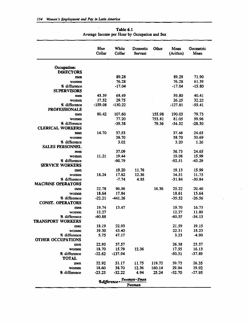
154 Women's Employment and Pay in Latin America
Table 6.1Average Income per Hour by Occupation and Sex
Blue White Domestic Other Mean GeometricCollar Collar Servant (Arithm) Mean
Occupation:DIRECTORS
men 89.28 89.28 71.90women 76.28 76.28 61.39
% difference -17.04 -17.04 -15.80SUPERVISORS
men 45.39 68.49 59.80 40.41women 17.52 29.75 26.25 32.22
% difference -159.08 -130.22 -127.81 -55.41PROFESSIONALS
men 80.42 107.60 155.98 190.03 79.73women 77.20 755.81 81.05 59.96
% difference -39.38 79.36 -34.52 -28.50CLERICAL WORKERS
men 14.70 37.53 37.46 24.65women 38.70 38.70 30.69
% difference 3.02 3.20 1.26SALES PERSONNEL
men 37.09 36.73 24.65women 11.21 19.44 19.08 15.99
% difference -90.79 -92.51 -43.29SERVICE WORKERS
men 19.20 11.76 19.13 15.99women 18.24 17.82 12.36 14.51 11.75
% difference -7.74 4.85 -31.84 -30.84MACHINE OPERATORS
men 22.78 96.56 16.36 25.22 20.40woomen 18.64 17.84 18.61 15.64
% difference -22.21 -441.26 -35.52 -26.56CONST. OPERATORS
men 19.74 13.47 19.70 16.73women 12.27 12.27 11.89
% difference -60.88 -60.55 -34.13TRANSPORT WORKERS
men 18.19 22.93 21.59 19.15women 19.30 43.40 22.31 18.23
% difference 5.75 47.17 3.23 -4.90OTHER OCCUPATIONS
men 22.93 37.57 26.38 23.57women 18.70 15.79 12.36 17.55 16.13
% difference -22.62 -137.94 -50.31 -37.89TOTAL
men 22.92 51.17 11.75 119.72 39.73 26.35women 18.60 38.70 12.36 160.14 29.94 19.92
% difference -23.23 -32.22 4.94 25.24 -32.70 -27.95
%difference Ywomen-YmenYwomcn
Labor Markets, the Wage Gap and Gender Dlscrimintuion: The Case of Colombia 155
4. LAMBDA = The inverse of the Mill's ratio. As indicated above, this variableis introduced to correct the selection bias problem. The detailsof the estimation of this variable are in the Appendix. In thismodel the parameters of the variables in (1) can be interpretedas the returns to various forms of "measured" human capital, theparameters in (2) measure a combination of compensatingdifferentials and the effect of some (possible) barriers to entry insome occupations. Finally the parameters of variables in (3),except Lambda, measure the (percentage) wage differentialattributable to those variables.
Separate equations were estimated for men, women including servants, and women excludingservants"3 and the results are presented in Table 6.2A and Table 6.2B. For comparison purposesthe (selection bias) corrected and uncorrected estimates are included. The statistics are in generalgood: The adjusted R-squared are above 0.5 (high for cross-section analysis), and most of theparameters are significantly different from zero. Even the parameters with low t-values areinteresting because they shed light on important aspects of the functioning of the labor markets.
It is interesting to note that the t-values of Lambda are below the 5 percent significance level formen but not in the case of women, indicating that there is not a serious selection bias problemin the sample of women. As explained in Section 5, the conclusions about the composition of thewage differential between men and women are not very sensitive to this type of correction. Inspite of the low t-values of Lambda in the case of women, the effect of the correction is the ex-pected one: It decreases the values of the coefficients associated with the human capital variablessuch as Education.
The general results of the estimation are consistent with those obtained in a large number of otherstudies in developing countries14. The returns to education are slightly lower than 10 percent,which is the value usually obtained, but this is not unreasonable given the large number ofvariables included in the model, not available in other cases. What is more important for thepurposes of this paper is that there is a clear difference in the estimated coefficients (correctedand uncorrected) of men and women and that the estimates for women are very sensitive to theinclusion or exclusion of domestic servants. The exclusion of domestic servants makes the es-timates for women closer to those for men.
In general men have higher returns to education than women and the quadratic form ofexperience indicates that the returns to additional years of experience decline faster for womenthan for men. Women receive higher returns to seniority and on-the-job training. Someoccupation premiums are higher for men than for women. Such is the case of Directors andprofessional occupations. Unions benefit both men and women but the exclusion of servantsdecreases the contribution of this variable. The premium to variables like recent migration (R-migr) and service occupations are not significantly different from zero.
13 There are two reasons to exclude domestic servants: One is that their measured wage rate is lessreliable than in the case of other workers, because a proportion of this payment is in kind (food andshelter). Two, that domestic servants constitute a very particular group of individuals (young, uneducated,female, immigrants) that are not comparable with the rest of the women in the sample. The case ofdomestic servants will be analyzed in Section 7.
14 Good reviews of these studies can be found in Fields (1980) and Psacharopoulos (1981).
156 Women's Employment and Pay in Latin America
5. Size and Composition of the Wage Gap
The average wage gap and its composition, as expressed in equation 4 can be computed directlyfrom the information given in Table 6.2A. Endowments are measured by the mean values of thevariables in the model and discrimination by the difference in the coefficients. A summary ofthese results is presented in Table 6.3.
The most obvious implication of these results is that a large part of the wage differential betweenmen and women is due to the existence of domestic servants and to the fact that they areparticularly poorly endowed: When domestic servants are excluded, not only does the totaldifferential drop by about 64 percent, but the endowment component also is significandy reduced(by about 90 percent).
Contribution of human capitol variables. It is important to notice that when endowments aremeasured by the mean values of the variables in the model (Table 6.2A), women (excludingservants) are not at a great disadvantage relative to men: On average they have higher levels ofeducation than men but smaller amounts of other human capital variables. On balance this resultsin a small negative contribution of human capital endowments to the gross differential. Thegreatest disadvantage for women in terms of their human capital endowments is their shortamount of experience, a result of the double role that they play as homemakers and workers. Asindicated above, this can be a result of non-market discrimination, a reflection of individual pre-ferences, or an (endogenous) response to the existence of market discrimination. The lack ofbetter data makes it difficult to carry the analysis any further.
The effect of correcting the selection bias is to increase the total wage differential and the marketdiscrimination component, leaving the endowment component almost unchanged.
Certainly a closer look at the factors that produce these results is of great interest. Table 6.4presents the contribution of each variable in the model to the total differential in hourly earningsestimated on the basis of the corrected coefficients"5 . The rest of this section considers only theresults of the estimations excluding domestic servants Oast three columns of Table 6.4). Theparticular case of domestic servants is analyzed below under "Some International Comparisons."
In contrast with the above results, the contribution of human capital variables to thediscrimination component is shockingly large: The fact that the returns to women's educationare lower than those of men is the single largest discriminatory element found in the analysis andhas a magnitude larger than the total wage differential between the two groups (10.36 percentversus 9.85 percent).
It is important to notice, however, that given the kind of data used here (the only ones available),not all the measured discrimination component of education can be attributed to actual marketdiscrimination. It is possible that at least one part of it reflects differences in productivity createdby differences in the quality and type of education that women receive. If this is the case, theactual market discrimination component is overestimated by the results in Table 6.4, and the non-market discrimination element is underestimated.
15 The exercise with the uncorrected coefficients was also done and the results do not changedramatically.
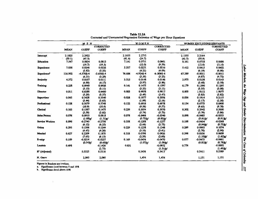
Table 12.2ACorrected and Uncorrected Regression Estimates of Wage per Hour Equations
M E N WOMEN WOMEN EXCLUDING SERVANTSCORRECTED CORRECTED CORRECTED
MEAN COEFF COEFF MEAN COEFF COEFF MEAN COEFF COEFF
Intercept 2.1825 2.2922 2.1675 2.2712 2.1355 2.2164(59.1) (45.0) (41.4) (24.7) (41.5) (30.9)
Education 7.547 0.0834 0.0813 7.141 0.0711 0.0661 8.161 0.0718 0.0686(19.7) (19.3) (12.0) (9.59) (12.0) (11.0)
Experience 7.038 0.0246 0.0226 5.557 0.0221 0.0216 5.412 0.0413 0.0402(5.82) (5.33) (4.21) (4.09) (6.19) (6.00) F
Experience2 116.902 -4.576E-4 -3.656E-4 76.606 -4.924E-4 4-.806E-4 67.389 -0.0011 40.0011(4.21) (3.29) (3.36) (3.25) (4.87) (4.72)
Seniority 4.372 0.0107 0.0111 3.515 0.0148 0.0146 3.975 0.0138 0.0143(4.00) (4.17) (3.97) (3.86) (3.48) (3.58)
Tmining 0.228 0.0940 0.0926 0.141 0.1475 0.1397 0.179 0.1390 0.1295(3.13) (3.11) (3.33) (3.11) (3.35) (3.08)
Ditector 0.011 0.6288 0.6400 0.003 0.9858 0.9817 0.003 1.0112 1.007S (5.29) (5.37) (3.49) (3.47) (3.83) (3.82)
Supervisor 0.045 0.3428 0.3540 0.028 0.1877 0.2056 0.036 0.1914 0.2115(5.44) (5.65) (1-99) (2.16) (2.17) (2.38)
Profeasional 0.128 0.5679 0.5748 0.122 0.6916 0.6978 0.154 0.6773 0.6900(10.9) (10.9) (9.56) (9.57) (9.65) (9.78)
Clerical 0.163 0.1387 0.1475 0.239 0.3054 0.3070 0.302 0.2942 0.3000(3.58) (3.82) (5.74) (S.73) (5.79) (5.86)
Sales Person 0.076 0.0910 0.081S 0.078 -0.0466 40.0540 0.098 40.048S -0.0553 5t
(1.88)ffi/ (1-71)!! ~~~~(0.73)b/ (0.83)_/ (0.81)bl (0.91)_/iiService Workers 0.090 -0.2740 40.2758 0.358 -0.1208 40.1257 0.188 -0.0454 -0.0368
(6.12) (6.25) (2.66) (2.75) (0.94)k/ (0.75)k/Union 0.293 0.1306 0.1244 0.229 0.1238 0.1348 0.289 0.0993 0.1074
(4.45) (4.26) (3.16) (3.41) (2.70) (2.90)Married 0.627 0.2209 0.1875 0.318 0.0798 0.0926 0.398 0.0356 0.0609
(7.65) (6.13) (2.39) (2.60) (1.10)JI (1.62)/.R-miqr 0.109 -0.0214 -0.0237 0.169 -0.0454 -0.0470 0.077 -0.0473 40.0461
(0.54)b/ (0-60)k/ (1.07)_/ (1.09)11/ (0.Sl)hf/ (0.78)k/ LAmbda 0.498 -0.1426 0.831 40.0852 0.776 -0.0892
(2.73) (1.31)b/ (1.49)h/R2 (Adjusted) 0.5325 0.5316 0.5438 0.5417 0.5411 0.5389
N. Oserv 2,060 2,060 1,454 1,454 1,151 1,151
Figures in Brackets are t-values.a. Significance level between S and 10%b. Significance level above 10%
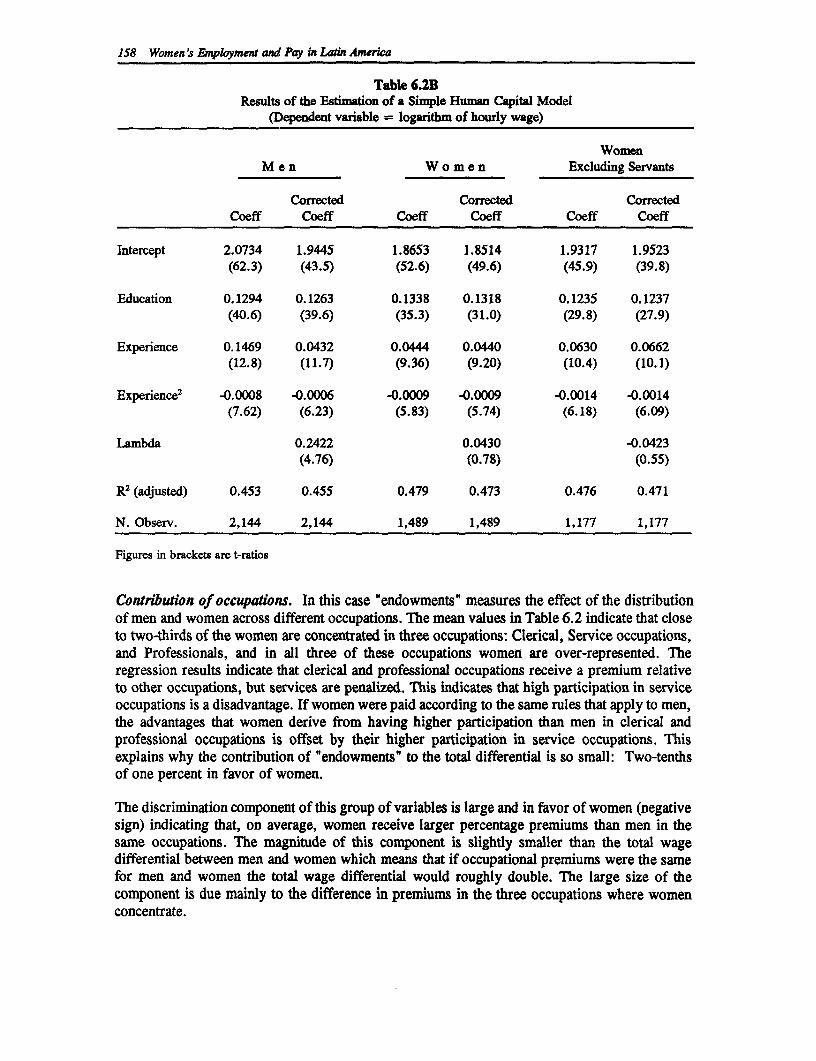
158 Women 's Employment and Pay in Latin America
Table 6.2BResults of the Estimation of a Simple Human Capital Model
(Dependent vaiable = logarithm of hourly wage)
WomenMen Women Excluding Servants
Corrected Corrected CorrectedCoeff Coeff Coeff Coeff Coeff Coeff
Intercept 2.0734 1.9445 1.8653 1.8514 1.9317 1.9523(62.3) (43.5) (52.6) (49.6) (45.9) (39.8)
Education 0.1294 0.1263 0.1338 0.1318 0.1235 0.1237(40.6) (39.6) (35.3) (31.0) (29.8) (27.9)
Experience 0.1469 0.0432 0.0444 0.0440 0.0630 0.0662(12.8) (11.7) (9.36) (9.20) (10.4) (10.1)
Experience2 -0.0008 -0.0006 -0.0009 -0.0009 -0.0014 -0.0014(7.62) (6.23) (5.83) (5.74) (6.18) (6.09)
Lambda 0.2422 0.0430 -0.0423(4.76) (0.78) (0.55)
R2 (adjusted) 0.453 0.455 0.479 0.473 0.476 0.471
N. Observ. 2,144 2,144 1,489 1,489 1,177 1,177
Figures in brackets are t-ratios
Contribution of occupations. In this case "endowments" measures the effect of the distributionof men and women across different occupations. The mean values in Table 6.2 indicate that closeto two-thirds of the women are concentrated in three occupations: Clerical, Service occupations,and Professionals, and in all three of these occupations women are over-represented. Theregression results indicate that clerical and professional occupations receive a premium relativeto other occupations, but services are penalized. This indicates that high participation in serviceoccupations is a disadvantage. If women were paid according to the same rules that apply to men,the advantages that women derive from having higher participation than men in clerical andprofessional occupations is offset by their higher participation in service occupations. Thisexplains why the contribution of "endowments' to the total differential is so small: Two-tenthsof one percent in favor of women.
The discrimination component of this group of variables is large and in favor of women (negativesign) indicating that, on average, women receive larger percentage premiums than men in thesame occupations. The magnitude of this component is slightly smaller than the total wagedifferential between men and women which means that if occupational premiums were the samefor men and women the total wage differential would roughly double. The large size of thecomponent is due mainly to the difference in premiums in the three occupations where womenconcentrate.
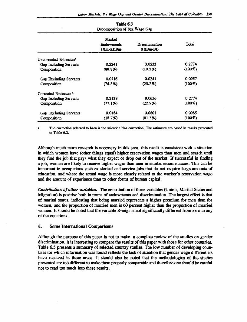
Labor Markets, the Wage Gap and Gender Discrimination: The Case of Colombia 159
Table 6.3Decomposition of Sex Wage Gap
MarketEndowments Discrimination Total(Xm-Xf)Bm Xf(Bm-Bf)
Uncorrected EstimateseGap Including Servants 0.2241 0.0532 0.2774Composition (80.8%) (19.2%) (100%)
Gap Excluding Servants 0.0716 0.0241 0.0957Composition (74.8%) (25.2%) (100%)
Corrected Estimates "Gap Including Servants 0.2138 0.0636 0.2774Composition (77.1%) (22.9%) (100%)
Gap Excluding Servants 0.0184 0.0801 0.0985Composition (18.7%) (81.3%) (100%)
a. The correction referred to here is the selection bias correction. The estimates are based in results presentedin Table 6.2.
Although much more research is necessary in this area, this result is consistent with a situationin which women have (other things equal) higher reservation wages than men and search untilthey find the job that pays what they expect or drop out of the market. If successful in findinga job, women are likely to receive higher wages than men in similar circumstances. This can beim portant in occupations such as clerical and service jobs that do not require large amounts ofeducation, and where the actual wage is more closely related to the worker's reservation wageand the amount of experience than to other forms of human capital.
Contribution of other variables. The contribution of these variables (Union, Marital Status andMigration) is positive both in terms of endowments and discrimination. The largest effect is thatof marital status, indicating that being married represents a higher premium for men than forwomen, and the proportion of married men is 60 percent higher than the proportion of marriedwomen. It should be noted that the variable R-migr is not significantly different from zero in anyof the equations.
6. Some International Comparisons
Although the purpose of this paper is not to make a complete review of the studies on genderdiscrimination, it is interesting to compare the results of this paper with those for other countries.Table 6.5 presents a summary of selected country studies. The low number of developing coun-tries for which information was found reflects the lack of attention that gender wage differentialshave received in these areas. It should also be noted that the methodologies of the studiespresented are too different to make them properly comparable and therefore one should be carefulnot to read too much into these results.
160 Women's Entployment and Pay in Latin America
Table 6.4Contribution of the Variables in the Model
to the Wage Differential
Including Servants Excluding Servants
Endowments Discrimination Total Endowments Discrimination Total
Education 0.0330 0.1085 0.1415 -0.0499 0.1036 0.0537Experience 0.0187 0.0144 0.0331 0.0186 -0.0458 -0.0272Seniority 0.0095 -0.0123 -0.0028 0.0044 -0.0127 -0.0083Training 0.0080 -0.0066 0.0014 0.0045 -0.0066 -0.0021
TOTALHUMAN CAPITAL 0.0693 0.1040 0.1733 -0.0223 0.0386 0.0163
Director 0.0051 -0.0010 0.0041 0.0051 -0.0011 0.0040Supervisor 0.0060 0.0042 0.0102 0.0032 0.0051 0.0083Professionals 0.0034 -0.0150 -0.0116 -0.0149 -0.0177 -0.0327Clerical -0.0112 -0.0381 -0.0493 -0.0205 -0.0461 -0.0666Sales Person -0.0002 0.0106 0.0104 -0.0018 0.0134 0.0116Service 0.0739 -0.0537 0.0202 0.0270 -0.0449 -0.0179
TOTALOCCUPATIONS 0.0771 -0.0931 -0.0160 -0.0019 -0.0913 -0.0932
Union 0.0080 -0.0024 0.0056 0.0005 0.0050 0.0055Married 0.0579 0.0302 0.0881 0.0429 0.0504 0.0933R.migr 0.0014 0.0039 0.0053 -0.0008 0.0017 0.0009
TOTALOTHER VAR 0.0673 0.0317 0.0990 0.0426 0.0571 0.0997
Intercept 0.0210 0.0210 0.0758 0.0758Lambda 0.0475 -0.0477 -0.0002 0.0396 -0.0414 -0.0018
TOTAL 0.2613 0.0159 0.2772 0.0580 0.0387 0.0967
Note: Following equation 4, the 'corrected" wage gap in Table 6.3 can be obtained by subtracting from the total inthis table the values of Lambda.
Source: Table 6.2.
One of the most interesting observations in the table is that even if domestic servants are includedin the comparison, the wage gap estimated for Colombia is one of the smallest by internationalstandards, only the gap in the service industry in the United States is smaller. If servants areexcluded, the gap in this paper is by far the smallest. The gap for Malaysia is also lower thanmost of the differentials for developed countries although slightly higher than the Colombian one.Taiwan presents wage differentials and composition closer to those found in developed countries.
A similar thing happens with the discrimination component. Again developing countries havesmaller levels of discrimination than developed ones, whether in absolute or in relative terms.
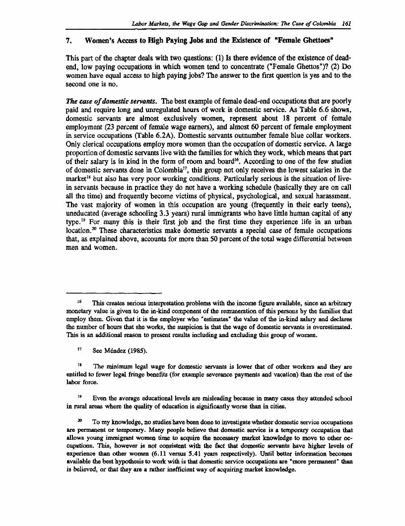
Labor Markets, the Wage Gap and Gender Discrimination: The Case of Colombia 161
7. Women's Access to High Paying Jobs and the Existence of "Female Ghettoes"
This part of the chapter deals with two questions: (1) Is there evidence of the existence of dead-end, low paying occupations in which women tend to concentrate ("Female Ghettos")? (2) Dowomen have equal access to high paying jobs? The answer to the first question is yes and to thesecond one is no.
1The case of domestic servants. The best example of female dead-end occupations that are poorlypaid and require long and unregulated hours of work is domestic service. As Table 6.6 shows,domestic servants are almost exclusively women, represent about 18 percent of femaleemployment (23 percent of female wage earners), and almost 60 percent of female employmentin service occupations (Table 6.2A). Domestic servants outnumber female blue collar workers.Only clerical occupations employ more women than the occupation of domestic service. A largeproportion of domestic servants live with the families for which they work, which means that partof their salary is in kind in the form of room and board'. According to one of the few studiesof domestic servants done in Colombia"7, this group not only receives the lowest salaries in themarket18 but also has very poor working conditions. Particularly serious is the situation of live-in servants because in practice they do not have a working schedule (basically they are on callall the time) and frequently become victims of physical, psychological, and sexual harassment.The vast majority of women in this occupation are young (frequently in their early teens),uneducated (average schooling 3.3 years) rural immigrants who have little human capital of anytype."9 For many this is their first job and the first time they experience life in an urbanlocation.' These characteristics make domestic servants a special case of female occupationsthat, as explained above, accounts for more than 50 percent of the total wage differential betweenmen and women.
16 This creates serious interpretation problems with the income figure available, since an arbitrarymonetary value is given to the in-kind component of the remuneration of this persons by the families thatemploy them. Given that it is the employer who 'estimates' the value of the in-kind salary and declaresthe number of hours that she works, the suspicion is that the wage of domestic servants is overestimated.This is an additional reason to present results including and excluding this group of women.
17 See M6ndez (1985).
is The mninimum legal wage for domestic servants is lower that of other workers and they areentitled to fewer legal fringe benefits (for example severance payments and vacation) than the rest of thelabor force.
19 Even the average educational levels are misleading because in many cases they attended schoolin rural areas where the quality of education is significantly worse than in cities.
X To my knowledge, no studies have been done to investigate whether domestic service occupationsare permanent or temporary. Many people believe that domestic service is a temporary occupation thatallows young immigrant women time to acquire the necessary market knowledge to move to other oc-cupations. This, however is not consistent with the fact that domestic servants have higher levels ofexperience than other women (6.11 versus 5.41 years respectively). Until better information becomesavailable the best hypothesis to work with is that domestic service occupations are 'more permanent' thanis believed, or that they are a rather inefficient way of acquiring market knowledge.
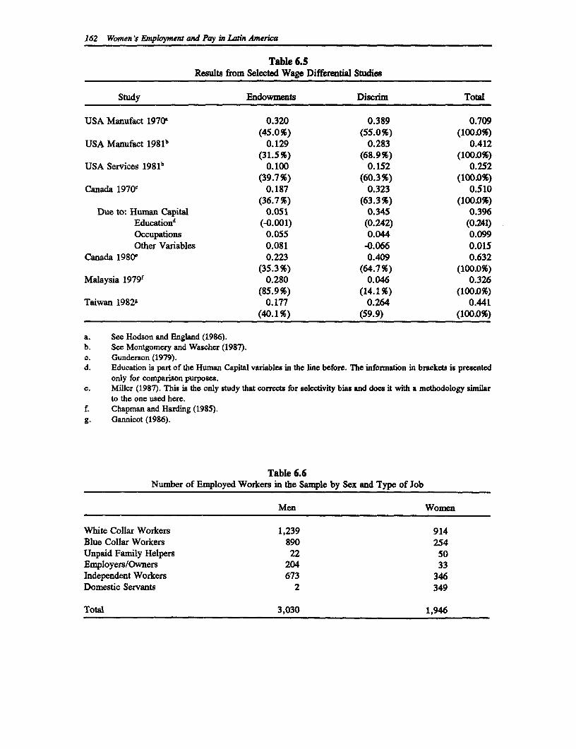
162 Women's Employment and Pay in Latin America
Table 6.5Results from Selected Wage Differential Studies
Study Endowments Discrim Total
USA Manufact 1970' 0.320 0.389 0.709(45.0%) (55.0%) (100.0%)
USA Manufact 1981b 0.129 0.283 0.412(31.5%) (68.9%) (100.0%)
USA Services 1981b 0.100 0.152 0.252(39.7%) (60.3%) (100.0%)
Canada 19700 0.187 0.323 0.510(36.7%) (63.3%) (100.0%)
Due to: Human Capital 0.051 0.345 0.396Educationd (-0.001) (0.242) (0.241)Occupations 0.055 0.044 0.099Other Variables 0.081 -0.066 0.015
Canada 19800 0.223 0.409 0.632(35.3%) (64.7%) (100.0%)
Malaysia 1979' 0.280 0.046 0.326(85.9%) (14.1%) (100.0%)
Taiwan 1982k 0.177 0.264 0.441(40.1%) (59.9) (100.0%)
a. See Hodson and England (1986).b. See Montgomery and Wascher (1987).e. Gunderson (1979).d. Education is part of the Human Capital variables in the line before. The information in brackets is presented
only for comparison purposes.e. Miller (1987). This is the only study that corrects for selectivity bias and does it with a methodology similar
to the one used here.f. Chapman and Harding (1985).g. Gannicot (1986).
Table 6.6Number of Employed Workers in the Sample by Sex and Type of Job
Men Women
White Collar Workers 1,239 914Blue Collar Workers 890 254Unpaid Family Helpers 22 50Employers/Owners 204 33Independent Workers 673 346Domestic Servants 2 349
Total 3,030 1,946
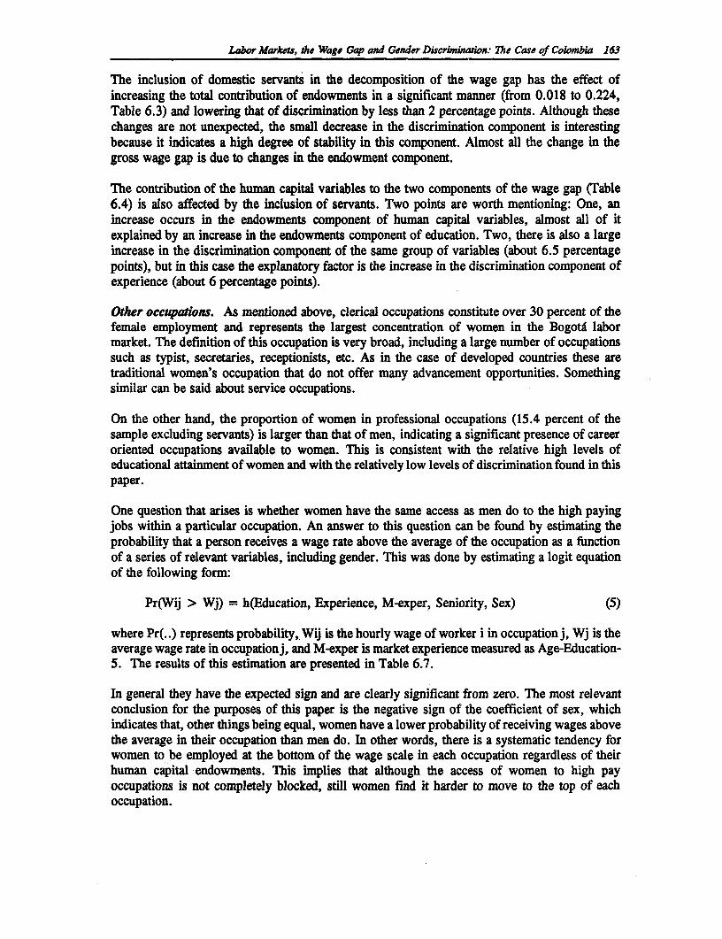
Labor Markut, the Wage Gap and Gender D scrvninadon: The Case of Colombia 163
The inclusion of domestic servants in the decomposition of the wage gap has the effect ofincreasing the total contribution of endowments in a significant manner (from 0.018 to 0.224,Table 6.3) and lowering that of discrimination by less than 2 percentage points. Although thesechanges are not unexpected, the small decrease in the discrimination component is interestingbecause it indicates a high degree of stability in this component. Almost all the change in thegross wage gap is due to changes in the endowment component.
The contribution of the human capital variables to the two components of the wage gap (Table6.4) is also affected by the inclusion of servants. Two points are worth mentioning: One, anincrease occurs in the endowments component of human capital variables, almost all of itexplained by an increase in the endowments component of education. Two, there is also a largeincrease in the discrimination component of the same group of variables (about 6.5 percentagepoints), but in this case the explanatory factor is the increase in the discrimination component ofexperience (about 6 percentage points).
Other occupation. As mentioned above, clerical occupations constitute over 30 percent of thefemale employment and represents the largest concentration of women in the BogotA labormarket. The definition of this occupation is very broad, including a large number of occupationssuch as typist, secretaries, receptionists, etc. As in the case of developed countries these aretraditional women's occupation that do not offer many advancement opportunities. Somethingsimilar can be said about service occupations.
On the other hand, the proportion of women in professional occupations (15.4 percent of thesample excluding servants) is larger than that of men, indicating a significant presence of careeroriented occupations available to women. This is consistent with the relative high levels ofeducational attainment of women and with the relatively low levels of discrimination found in thispaper.
One question that arises is whether women have the same access as men do to the high payingjobs within a particular occupation. An answer to this question can be found by estimating theprobability that a person receives a wage rate above the average of the occupation as a functionof a series of relevant variables, including gender. This was done by estimating a logit equationof the following form:
Pr(Wij > Wj) = h(Education, Experience, M-exper, Seniority, Sex) (5)
where Pr(..) represents probability, Wij is the hourly wage of worker i in occupation j, Wj is theaverage wage rate in occupationj, and M-exper is market experience measured as Age-Education-5. The results of this estimation are presented in Table 6.7.
In general they have the expected sign and are clearly significant from zero. The most relevantconclusion for the purposes of this paper is the negative sign of the coefficient of sex, whichindicates that, other things being equal, women have a lower probability of receiving wages abovethe average in their occupation than men do. In other words, there is a systematic tendency forwomen to be employed at the bottom of the wage scale in each occupation regardless of theirhuman capital endowments. This implies that although the access of women to high payoccupations is not completely blocked, still women find it harder to move to the top of eachoccupation.
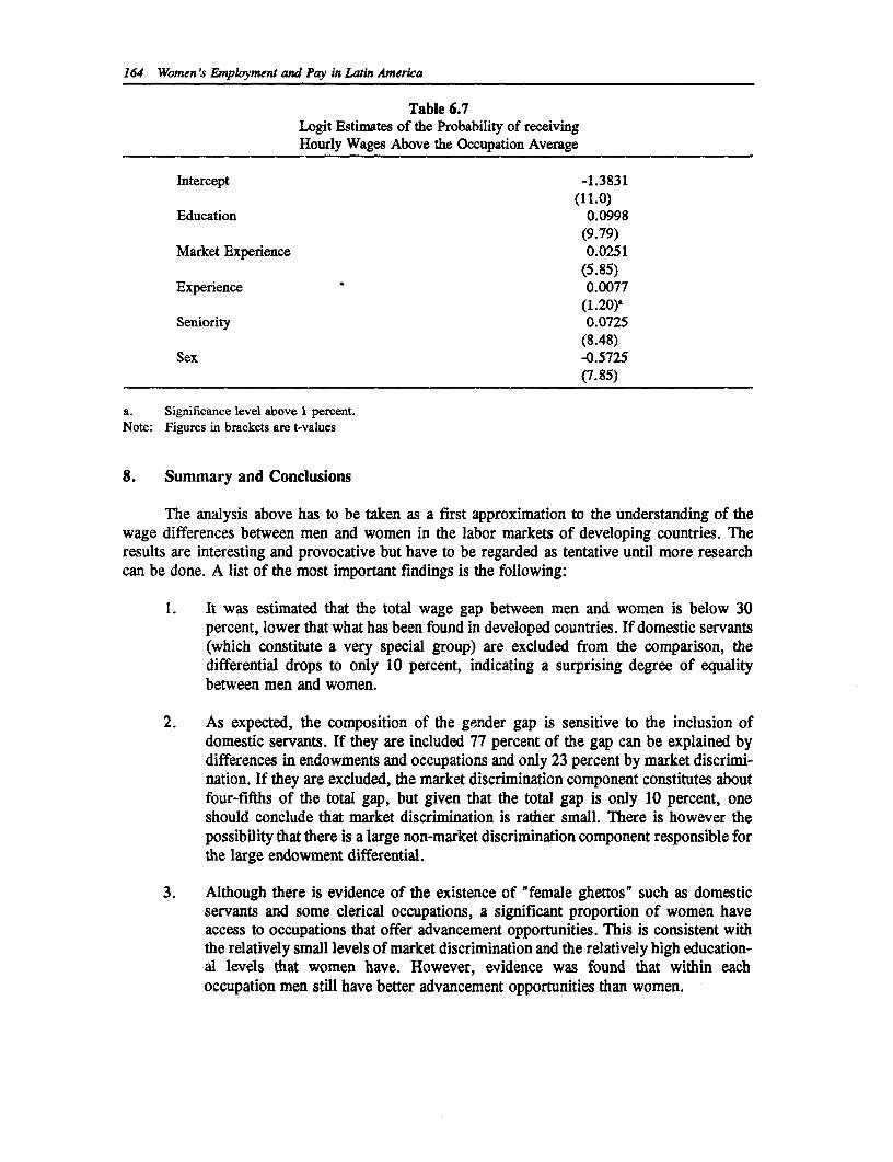
164 Women's Employment and Pay in Latin America
Table 6.7Logit Estimates of the Probability of receivingHourly Wages Above the Occupation Average
Intercept -1.3831(11.0)
Education 0.0998(9.79)
Market Experience 0.0251(5.85)
Experience 0.0077(1.20).
Seniority 0.0725(8.48)
Sex -0.5725(7.85)
a. Significance level above 1 percent.Note: Figures in brackets are t-values
8. Summary and Conclusions
The analysis above has to be taken as a first approximation to the understanding of thewage differences between men and women in the labor markets of developing countries. Theresults are interesting and provocative but have to be regarded as tentative until more researchcan be done. A list of the most important findings is the following:
1. It was estimated that the total wage gap between men and women is below 30percent, lower that what has been found in developed countries. If domestic servants(which constitute a very special group) are excluded from the comparison, thedifferential drops to only 10 percent, indicating a surprising degree of equalitybetween men and women.
2. As expected, the composition of the gender gap is sensitive to the inclusion ofdomestic servants. If they are included 77 percent of the gap can be explained bydifferences in endowments and occupations and only 23 percent by market discrimi-nation. If they are excluded, the market discrimination component constitutes aboutfour-fifths of the total gap, but given that the total gap is only 10 percent, oneshould conclude that market discrimination is rather small. There is however thepossibility that there is a large non-market discrimination component responsible forthe large endowment differential.
3. Although there is evidence of the existence of "female ghettos" such as domesticservants and some clerical occupations, a significant proportion of women haveaccess to occupations that offer advancement opportunities. This is consistent withthe relatively small levels of market discrimination and the relatively high education-al levels that women have. However, evidence was found that within eachoccupation men still have better advancement opportunities than women.
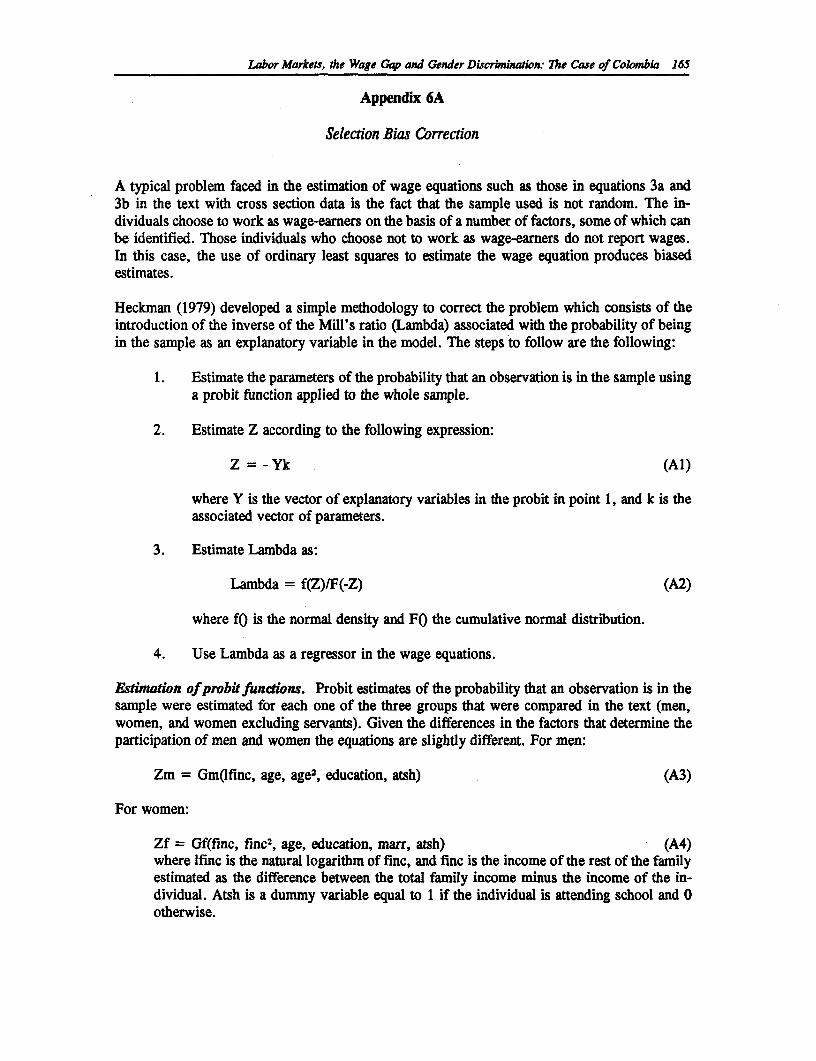
Labor Markets, the Wage Gap and Gender Discrinination: The Case of Colombia 165
Appendix 6A
Selection Bias Correction
A typical problem faced in the estimation of wage equations such as those in equations 3a and3b in the text with cross section data is the fact that the sample used is not random. The in-dividuals choose to work as wage-earners on the basis of a number of factors, some of which canbe identified. Those individuals who choose not to work as wage-earners do not report wages.In this case, the use of ordinary least squares to estimate the wage equation produces biasedestimates.
Heckman (1979) developed a simple methodology to correct the problem which consists of theintroduction of the inverse of the Mill's ratio (Lambda) associated with the probability of beingin the sample as an explanatory variable in the model. The steps to follow are the following:
1. Estimate the parameters of the probability that an observation is in the sample usinga probit function applied to the whole sample.
2. Estimate Z according to the following expression:
Z = -Yk (A1)
where Y is the vector of explanatory variables in the probit in point 1, and k is theassociated vector of parameters.
3. Estimate Lambda as:
Lambda = f(Z)/F(-Z) (A2)
where fO is the normal density and FO the cumulative normal distribution.
4. Use Lambda as a regressor in the wage equations.
Estimation of probit functions. Probit estimates of the probability that an observation is in thesample were estimated for each one of the three groups that were compared in the text (men,women, and women excluding servants). Given the differences in the factors that determine theparticipation of men and women the equations are slightly different. For men:
Zm = GmQfinc, age, age2, education, atsh) (A3)
For women:
Zf = Gf(finc, finc2 , age, education, marr, atsh) (A4)where lfinc is the natural logarithm of finc, and finc is the income of the rest of the familyestimated as the difference between the total family income minus the income of the in-dividual. Atsh is a dummy variable equal to 1 if the individual is attending school and 0otherwise.
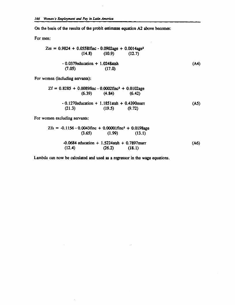
166 Women's EAployment and Pay in Lain America
On the basis of the results of the probit estimates equation A2 above becomes:
For men:
Zm = 0.9824 + 0.05581finc - 0.0902age + 0.0014age2
(14.8) (10.9) (12.7)
- 0.0379education + 1.0248atsh (A4)(7.05) (17.0)
For women (including servants):
Zf = 0.8285 + 0.0089finc - 0.0002finc2 + 0.0102age(6.39) (4.84) (6.42)
- 0.1270education + 1.185latsh + 0.4390marr (AS)(21.3) (19.5) (9.72)
For women excluding servants:
Zfs = -0.1156 - 0.0043finc + 0.OOOOlfinc2 + 0.0198age(3.65) (1.99) (13.1)
-0.0684 education + 1.5224atsh + 0.7897marr (A6)(12.4) (26.2) (18.1)
Lambda can now be calculated and used as a regressor in the wage equations.
References
Becker, G.S. The Economics of Discrimination. Chicago: University of Chicago Press, 1957.
Chapman, B.J. and J.R. Harding. "Sex Differentials in Earnings: An Analysis of MalaysianWage Data." Journal of Development Studies, Vol. 21 (April, 1985). pp. 362-376.
Fields, F. "Education and Income Distribution in Developing Countries: A Review of Literature"in T. King (ed.). Education and Income. Washington D.C.: World Bank Staff Paper No.402, World Bank, 1980.
Gannicot, K. "Women, Wages and Discrimination: Some Evidence from Taiwan." EconomicDevelopment and Cultural Change, Vol. 34, no. 4 (July, 1986). pp. 721-730.
Gronau, R. "Wage Comparisons - A Selectivity Bias." Journal of Political Economy, Vol. 82,no. 6 (1974). pp. 1119-1143.
Gunderson, M. "Male-Female Wage Differential and Policy Responses." Journal of EconomicLiterature, Vol. 27, no. 1 (March, 1989). pp. 46-72.
--- "Decomposition of the Male/Female Earnings Differential: Canada 1970." Canadian Journalof Economics, Vol. 12, no. 3 (August, 1979). pp. 479-485.
Heckman, J. "Sample Selection Bias as a Specification Error." Econometrica, Vol. 47, no. I(January, 1979). pp. 153-161.
Hodson, R. and P. England. "Industrial Structure and Sex Differences in Earnings." IndustrialRelations, Vol. 25, no.1 (Winter, 1986). pp. 16-32.
Mendez, M. and R. Askew. "The Colombian 'Muchacha del Servicio'". Unpublishedmimeograph. Bogota, 1985.
Miller, P.W. "Gender Differences in Observed and Offered Wages in Canada, 1980." CanadianJournal of Economics, Vol. 20, no. 2 (May, 1987). pp. 225-244.
Montgomery, E. and W. Wascher. "Race and Gender Wage Inequality in Services andManufacturing." Industrial Relations, Vol. 26, no. 3 (Fall, 1987). pp. 284-290.
167

168 Women's Enployment and Pay in LaIix America
Psacharopoulos, G. "Returns to Education: An Updated International Comparison." ComparativeEducation, Vol. 17, no. 3 (1981). pp. 321-341.
Najafizadeh, M. and L.A. Mennerick. 'Worldwide Educational Expansion from 1950 to 1980:The Failure of the Expansion of Schooling in Developing Countries." Journal ofDeveloping Areas, Vol. 22 (April, 1988). pp. 333-358.
Schultz, T.P. Returns to Women's Education. Washington D.C.: World Bank, 1989.
7
Female Labor Market Participation and Wages inColombia
Thierry Magnac'
1. Introduction
This paper describes the estimation results of a microeconometric model of female participationin Colombia. The samples used are drawn from urban household surveys between 1980 and1985. The set of exogenous variables includes individual as well as household-relatedcharacteristics. The results are used to assess the power of the modeling strategy in explainingthe dramatic increase in female participation rates. Wage equations are estimated correcting forselectivity biases and compared for males and females.
2. The Colombian Labor Market
The industrialization process in Colombia dates back to the 1930s but a significant increase in theindustrial labor force took place in the late 1940s. Colombia was in those days mainly anagricultural country: The agricultural sector employed 55.6 percent of the whole labor force in1951 (Bourguignon, 1986). GDP growth between 1950 and 1980 had been sizeable despite the"violencia" period in the 1950s and had averaged 5.5 percent in the late 1960s and early 1970s(Sarmiento Palacio, 1984). This period marked the end of the import-substitution policies, theindustrial sector producing 85 percent of consumption goods, 50 percent of intermediate goodsand 20 percent of capital goods, consumed in the country (Sarmiento Palacio, 1984). Export-promoting policies for manufactured goods were then set up but Colombia mostly remained asingle-good exporting country where coffee still accounted for 70 percent of exports in 1980, and50 percent in 1984 (DANE, 1986).
The Colombian economy underwent a crisis in 1974 but quickly recovered because of thebooming coffee prices and exports in 1976-86 ("bonanza cafetera"). Inflation soared to 30percent yearly in 1980. In this disequilibrium context, the international crisis of 1979-80 hitColombia very hard. A severe recession began and lasted at least until 1984 when productiongot back to its 1980 level although the employment level lagged behind.
I I want to thank J. A. Ocampo, Director of Fedesarrollo, Bogota, where I began this work andthank the DANE in Bogota for having given me access to data and computers while I was there. To bealso acknowledged is the help of people in the Laboratoire d'Economie Politique in Paris and especiallyF. Bourguignon who followed and encouraged this work. The usual disclaimer applies.
169
170 Women 's Employment and Pay in Latin America
Nevertheless, the history of last twenty years shows that the Colombian labor market has adjustedvery quickly. In fact, despite catastrophic predictions by the ILO in 1970 (Misi6n de Empleo,ILO, 1970) of unemployment rates in the 1980s, the economy and particularly the modem sectorsucceeded in creating a huge number of jobs in absolute and relative terms. The ILO reportcorrectly predicted the dramatic increase in labor supply but underestimated the labor demandgrowth. Even if labor demand and supply growth are hardly distinguishable using the aggregatedata, some points are worth mentioning. Several factors caused the growth in labor supply.First, the demographic growth rate, though decreasing, was still large because both fecundity andmortality were decreasing. Another factor feeding urban labor supply growth was the continuousflow of migrants from rural to urban areas. Migration only stabilized in the early 1980s when65 percent of the population was living in towns of 20,000 and above (DANE, 1986). Finally,female labor force participation rates had been increasing in the 1970s and 1980s. The ratio offemale to male workers went up from 20 percent in 1964 to 26 percent in 1973 and 31 percentin 1978 (Bourguignon, 1986).
However, the international crisis changed the labor market situation. If the analysis is restrictedto the urban labor market (Coyuntura Econ6mica, 1985), it is clear that global participation ratedecreased during 1981-82 but went up again in 1983. It shows that the unemployment ratedramatically increased (7.5 percent in 1980 to 7.5 percent in 1985). Labor demand was stagnantor decreasing, particularly in the modem sector, and the number of self-employed soared. Themodern sector's wages began to decrease at the end of 1985. High inflation prevailed during thisperiod (20 to 25 percent).
The focus of this study is married women's participation rates, because they seem the mostresponsive to changing economic conditions. The standard participation microeconomic model(Killingsworth, 1983) is estimated using household data for six consecutive years. Exogenousvariables used are individual as well as household-related characteristics. The usual effects arefound. Human capital variables positively affect the probability of participation, while thenumber of children and other household member's incomes act negatively on it. The number ofother women in the household have a sizeable impact and capture the likely substitutions indomestic work in the household. The results show that the coefficients are generally stable overtime.
The predictions of this model can then be used to assess the power of this participation model inexplaining the huge increase in female participation which took place during the period. Evenif it explains only 30 percent of the increase, it relates the increase to changes in education andfecundity over the period which corroborates a finding derived from macroeconomic studies. Theresidual (70 percent) might be attributed either to missing variables determining labor supply orto labor demand factors. Demand and supply are obviously connected to wages. To informallyevaluate the impact of the demand factors, some estimation results related to the wage equationsduring the period are proposed. They are compared to equations for the male household's headsand other members in order to gauge discrimination effects. Some evidence is produced showingthat the difference between male and female wages might be biased if the work experience offemales is not correctly measured, as is the case in these data.
The plan of the paper is as follows. Section 3 presents a descriptive analysis of female laborparticipation during the period, a very brief survey of previous studies and the estimation resultsof the participation models. It concludes by assessing their explanatory power. Section 4discusses and presents the results of the estimations for the wage equations.
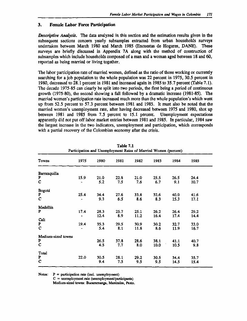
Femak Labor Market Participation and Wages in Colombia 171
3. Female Labor Force Participation
Descnrptive Analysis. The data analyzed in this section and the estimation results given in thesubsequent sections concern yearly subsamples extracted from urban households surveysundertaken between March 1980 and March 1985 (Encuestas de Hogares, DANE). Thesesurveys are briefly discussed in Appendix 7A along with the method of construction ofsubsamples which include households composed of a man and a woman aged between 18 and 60,reported as being married or living together.
The labor participation rate of married women, defined as the ratio of those working or currentlysearching for a job population to the whole population was 22 percent in 1975, 30.5 percent in1980, decreased to 28.1 percent in 1981 and increased again in 1985 to 35.7 percent (Table 7.1).The decade 1975-85 can clearly be split into two periods, the first being a period of continuousgrowth (1975-80), the second showing a fall followed by a dramatic increase (1981-85). Themarried women's participation rate increased much more than the whole population's which wentup from 52.5 percent to 57.3 percent between 1981 and 1985. It must also be noted that themarried women's unemployment rate, after having decreased between 1975 and 1980, shot upbetween 1981 and 1985 from 7.5 percent to 15.1 percent. Unemployment expectationsapparently did not put off labor market entries between 1981 and 1985. In particular, 1984 sawthe largest increase in the two indicators, unemployment and participation, which correspondswith a partial recovery of the Colombian economy after the crisis.
Table 7.1Participation and Unemployment Rates of Married Women (percent)
Towns 1975 1980 1981 1982 1983 1984 1985
BarranquillaP 15.9 21.0 22.8 21.0 25.5 26.5 24.4C - 5.2 7.5 7.6 6.7 9.1 10.7
BogotaP 25.4 34.4 27.6 33.8 32.6 40.0 41.6C - 9.3 6.5 8.6 8.3 15.3 17.1
MedellfnP 17.4 28.3 25.7 25.1 26.2 26.4 29.2
- 12.4 8.9 11.2 16.4 17.4 14.4CaliP 19.4 35.3 29.5 30.9 30.2 32.7 33.0C - 5.4 8.1 11.8 8.6 11.9 16.7
Medium-sized townsP 26.5 37.8 28.6 38.1 41.1 40.7C 4.5 7.7 8.0 10.0 10.5 9.8
TotalP 22.0 30.5 28.1 29.2 30.5 34.4 35.7C 9.4 7.5 9.5 9.5 14.5 15.4
Notes: P = participation rate (incl. unemployment)C = unemployment rate (unemployment/participants)Medium-sized towns: Bucaramanga, Manizales, Pasto.
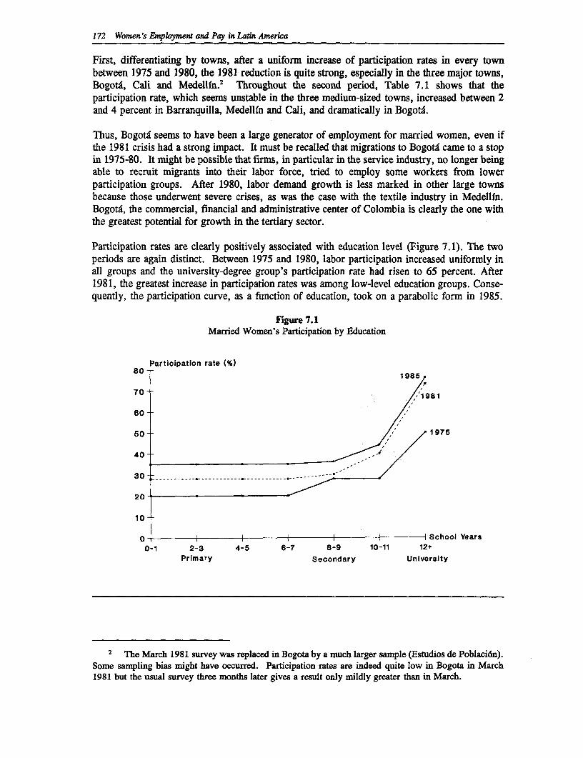
172 Women's Employment and Pay in Latin America
First, differentiating by towns, after a uniform increase of participation rates in every townbetween 1975 and 1980, the 1981 reduction is quite strong, especially in the three major towns,Bogota, Cali and Medellfn.2 Throughout the second period, Table 7.1 shows that theparticipation rate, which seems unstable in the three medium-sized towns, increased between 2and 4 percent in Barranquilla, Medellfn and Cali, and dramatically in Bogota.
Thus, BogotA seems to have been a large generator of employment for married women, even ifthe 1981 crisis had a strong impact. It must be recalled that migrations to Bogota came to a stopin 1975-80. It might be possible that firms, in particular in the service industry, no longer beingable to recruit migrants into their labor force, tried to employ some workers from lowerparticipation groups. After 1980, labor demand growth is less marked in other large townsbecause those underwent severe crises, as was the case with the textile industry in Medellfn.Bogota, the commercial, financial and administrative center of Colombia is clearly the one withthe greatest potential for growth in the tertiary sector.
Participation rates are clearly positively associated with education level (Figure 7.1). The twoperiods are again distinct. Between 1975 and 1980, labor participation increased uniformly inall groups and the university-degree group's participation rate had risen to 65 percent. After1981, the greatest increase in participation rates was among low-level education groups. Conse-quently, the participation curve, as a function of education, took on a parabolic form in 1985.
Figure 7.1Married Women's Participation by Education
Participation rate (%)80 -1985
70 -"1981
60
so / 1975
40
20 -
1 0
0 I I ISchool Years0-1 2-3 4-5 6-7 8-9 10-11 12+
Primary Secondary University
2 The March 1981 survey was replaced in Bogota by a much larger sample (Estudios de Poblaci6n).Some sampling bias might have occurred. Participation rates are indeed quite low in Bogota in March1981 but the usual survey three months later gives a result only mildly greater than in March.
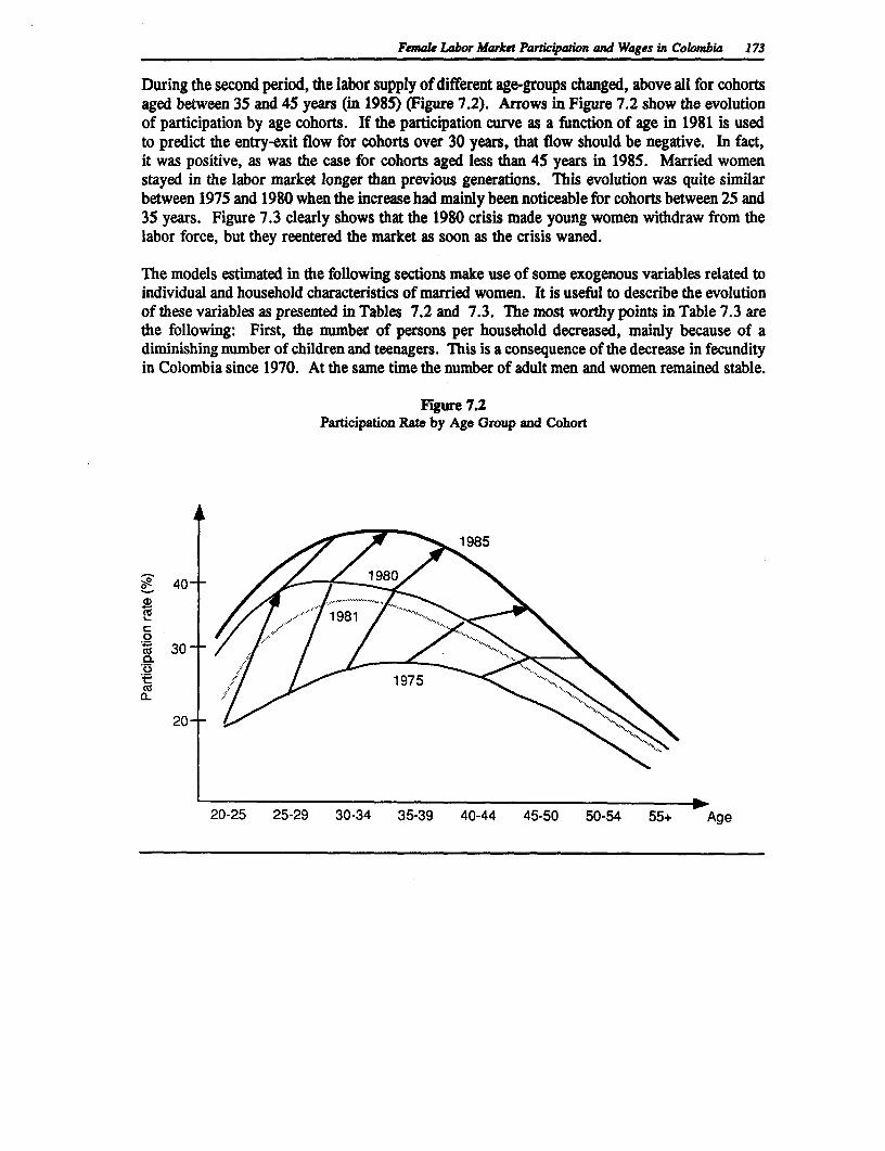
Femal Labor Market Paricipadon and Wages in Colombia 173
During the second period, the labor supply of different age-groups changed, above all for cohortsaged between 35 and 45 years (in 1985) (Figure 7.2). Arrows in Figure 7.2 show the evolutionof participation by age cohorts. If the participation curve as a function of age in 1981 is usedto predict the entry-exit flow for cohorts over 30 years, that flow should be negative. In fact,it was positive, as was the case for cohorts aged less than 45 years in 1985. Married womenstayed in the labor market longer than previous generations. This evolution was quite similarbetween 1975 and 1980 when the increase had mainly been noticeable for cohorts between 25 and35 years. Figure 7.3 clearly shows that the 1980 crisis made young women withdraw from thelabor force, but they reentered the market as soon as the crisis waned.
The models estimated in the following sections make use of some exogenous variables related toindividual and household characteristics of married women. It is useful to describe the evolutionof these variables as presented in Tables 7.2 and 7.3. The most worthy points in Table 7.3 arethe following: First, the number of persons per household decreased, mainly because of adiminishing number of children and teenagers. This is a consequence of the decrease in fecundityin Colombia since 1970. At the same time the number of adult men and women remained stable.
Fgure 7.2Participation Rate by Age Group and Cohort
6401 1981 ~ ~ 98
01 30
CtCu
20
20-25 25-29 30-34 35-39 40-44 45-50 50-54 55+ Age
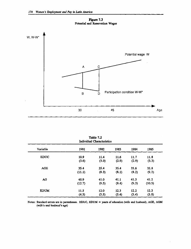
174 Women's Employment and Pay in Latin America
ESgure 7.3Potential and Reservation Wages
W, W-W*
Potential wage W
B D Participation condition W-W*
30 45 Age
Table 7.2Individual Characteristics
Variable 1981 1982 1983 1984 1985
EDUC 10.9 11.4 11.6 11.7 11.8(3.6) (3.0) (2.9) (2.9) (3.3)
AGE 35.4 35.4 35.4 35.6 35.8(11.1) (8.3) (8.1) (8.2) (9.2)
AG 40.9 41.0 41.1 41.3 41.2(12.7) (9.5) (9.4) (9.3) (10.5)
EDUM 11.5 12.0 12.3 12.2 12.3(4.3) (3.5) (3.4) (3.4) (3.8)
Notes: Standard errors are in parentheses. EDUC, EDUM = years of education (wife and husband), AGE, AGM(wife's and husband's age)
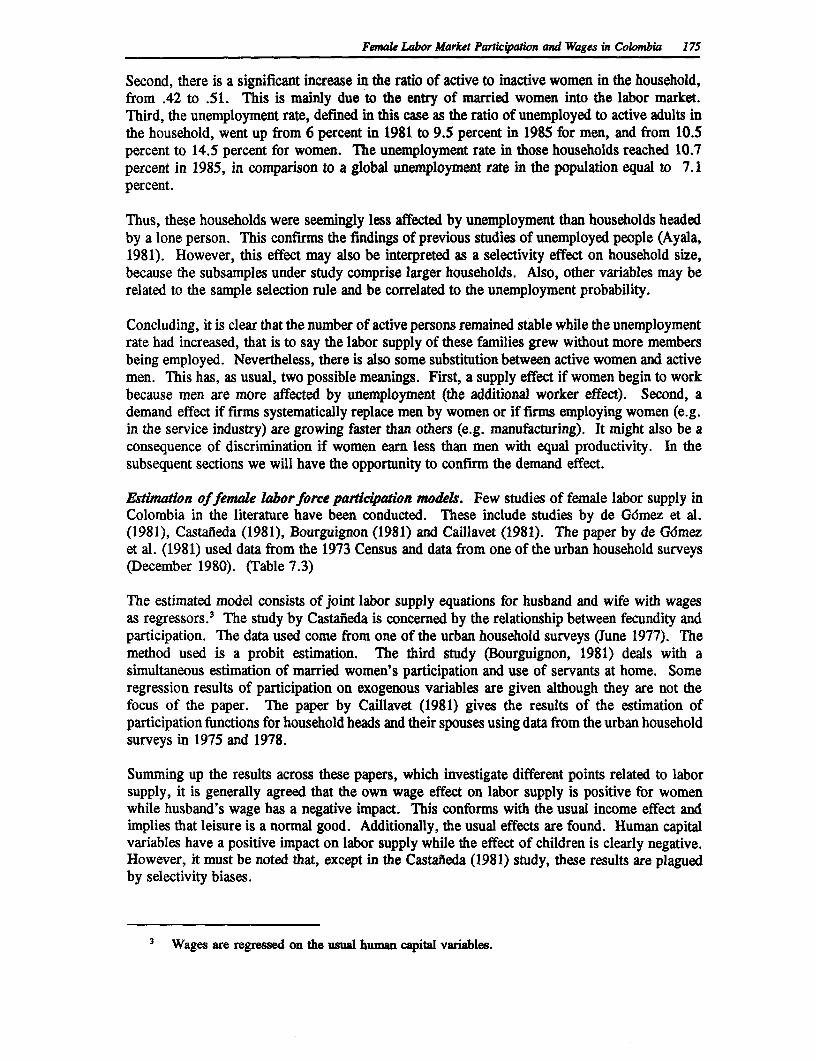
Femakl Labor Market Parficpation and Wages in Colombia 175
Second, there is a significant increase in the ratio of active to inactive women in the household,from .42 to .51. This is mainly due to the entry of married women into the labor market.Third, the unemployment rate, defined in this case as the ratio of unemployed to active adults inthe household, went up from 6 percent in 1981 to 9.5 percent in 1985 for men, and from 10.5percent to 14.5 percent for women. The unemployment rate in those households reached 10.7percent in 1985, in comparison to a global unemployment rate in the population equal to 7.1percent.
Thus, these households were seemingly less affected by unemployment than households headedby a lone person. This confirms the findings of previous studies of unemployed people (Ayala,1981). However, this effect may also be interpreted as a selectivity effect on household size,because the subsamples under study comprise larger households. Also, other variables may berelated to the sample selection rule and be correlated to the unemployment probability.
Concluding, it is clear that the number of active persons remained stable while the unemploymentrate had increased, that is to say the labor supply of these families grew without more membersbeing employed. Nevertheless, there is also some substitution between active women and activemen. This has, as usual, two possible meanings. First, a supply effect if women begin to workbecause men are more affected by unemployment (the additional worker effect). Second, ademand effect if firms systematically replace men by women or if firms employing women (e.g.in the service industry) are growing faster than others (e.g. manufacturing). It might also be aconsequence of discrimination if women earn less than men with equal productivity. In thesubsequent sections we will have the opportunity to confirm the demand effect.
Estimadion offemale labor force paricipaion models. Few studies of female labor supply inColombia in the literature have been conducted. These include studies by de G6mez et al.(1981), Castafieda (1981), Bourguignon (1981) and Caillavet (1981). The paper by de Gomezet al. (1981) used data from the 1973 Census and data from one of the urban household surveys(December 1980). (Table 7.3)
The estimated model consists of joint labor supply equations for husband and wife with wagesas regressors.3 The study by Castafieda is concerned by the relationship between fecundity andparticipation. The data used come from one of the urban household surveys (June 1977). Themethod used is a probit estimation. The third study (Bourguignon, 1981) deals with asimultaneous estimation of married women's participation and use of servants at home. Someregression results of participation on exogenous variables are given although they are not thefocus of the paper. The paper by Caillavet (1981) gives the results of the estimation ofparticipation functions for household heads and their spouses using data from the urban householdsurveys in 1975 and 1978.
Summing up the results across these papers, which investigate different points related to laborsupply, it is generally agreed that the own wage effect on labor supply is positive for womenwhile husband's wage has a negative impact. This conforms with the usual income effect andimplies that leisure is a normal good. Additionally, the usual effects are found. Human capitalvariables have a positive impact on labor supply while the effect of children is clearly negative.However, it must be noted that, except in the Castafneda (1981) study, these results are plaguedby selectivity biases.
3 Wages are regressed on the usual human capital variables.
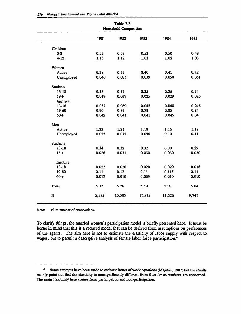
176 Women's Employment and Pay in Latin America
Table 7.3Household Composition
1981 1982 1983 1984 1985
Children0-3 0.55 0.53 0.52 0.50 0.484-12 1.13 1.12 1.03 1.05 1.03
WomenActive 0.38 0.39 0.40 0.41 0.42Unemployed 0.040 0.035 0.039 0.058 0.061
Students13-18 0.38 0.37 0.35 0.36 0.3419+ 0.019 0.027 0.025 0.029 0.026Inactive13-18 0.057 0.060 0.048 0.048 0.04619-60 0.90 0.89 0.88 0.85 0.8460+ 0.042 0.041 0.041 0.045 0.043
MenActive 1.23 1.21 1.18 1.16 1.18Unemployed 0.073 0.077 0.096 0.10 0.11
Students13-18 0.34 0.32 0.32 0.30 0.2918+ 0.026 0.031 0.030 0.030 0.030
Inactive13-18 0.022 0.020 0.020 0.020 0.01819-60 0.11 0.12 0.11 0.115 0.1160+ 0.012 0.010 0.009 0.010 0.010
Total 5.32 5.26 5.10 5.09 5.04
N 5,585 10,505 11,535 11,526 9,741
Note: N = number of observations.
To clarify things, the married women's participation model is briefly presented here. It must beborne in mind that this is a reduced model that can be derived from assumptions on preferencesof the agents. The aim here is not to estimate the elasticity of labor supply with respect towages, but to permit a descriptive analysis of female labor force participation.'
4 Some attempts have been made to estimate hours of work equations (Magnac, 1987) but the resultsmainly point out that the elasticity is nonsignificantly different from 0 as far as workers are concemed.The main flexibility here comes from participation and non-participation.
Female Labor Market Particpation and Wages in Colombia 177
The basic model of labor participation (Killingsworth, 1983) states:
Participation if w - we > 0Non-participation if w - w < 0
where w is the potential or market hourly wage and w* the reservation or asked wage.
Two additional equations are specified:
log(w) = Xn + ulog(w') = ZT + v
The first equation, the wage equation, relates the logarithm of the hourly wage rate to humancapital variables (X). The second equation, the reservation wage equation, is derived from thepreferences of the married women and depends either on personal or household characteristics.5
If u and v, conditional on X and Z, are supposed binormally distributed, the estimation strategyto get consistent estimators is Probit and the reduced form model comprises variables X and Z.
This model was estimated using six subsequent years (1980-85) keeping the same set ofexogenous variables. The households' characteristics retained in the present specification havebeen chosen for their significance among a large number of explicative variables (Appendix 7B).
These exogenous variables are the following:
Hwnan capital variables:6
EDUC completed years of educationEXP work experience which is not reported in the survey and which is approximated hereby age minus educationEXP2 work experience squared
Household's characteristics:7
IMAR husband's income in thousands of pesos (constant 1981)DM dummy variable equal to 1 in case of non-reported husband's incomeIOTR other household members' income in 1,000 pesosD number of other household members' non-reported incomes
5 This set-up is called the male chauvinistic model because it assumes that the married woman is thelast to choose in the family. Or similarly that she had well-defined preferences conditional on all othervariables. The interpretations we are going to propose here assume that household organization anddecisions to work by other members is given and that it is not made simultaneously with the marriedwoman's decision to work. This is a disputable assumption but an instrumental variable procedure tocorrect these biases is out of the scope of the present paper.
6 Influence the potential wage function (X) and possibly preferences as well.
7 Incomes are real incomes computed by deflating nominal incomes by an aggregate consumptionprice index (DANE, 1986).
178 Women's Employment and Pay in Latin America
Household composition.3El number of children between 0 and 1 yearE2 number of children between 1 and 3 yearsHST1 number of male students between 12 and 18HST2 number of male students over 18FST2 number of female students over 18HDE number of unemployed male adultsMJI number of inactive women between 12 and 18MAI number of inactive women between 18 and 60MVI number of inactive women over 60
In the specification, dummy variables for towns were added to this list in order to correct firstfor some sampling effects in different years and, secondly, to take into account the fact thatfemale participation depends on the unique economic development and labor demand determinantsin each town.
All estimation results are given in Table 7.4. The coefficients of the human capital variables(EDUC, EXP, EXP2) are significant and stable across time. Differences are not significantacross years. From these estimates can be deduced that the highest point of the predictedparticipation curve as a function of age is around 30 years although it varies slightly across timein the interval 28 to 33. It is largely before the highest point in the wage equation function. Thisimplies that the reservation wage increases strongly after 30 as represented in Figure 7.3, sinceAB > CD. This can be attributed to changes in the domestic production function when thewoman ages and acquires a larger relative productivity in comparison to the other members.Specialization in domestic work is important at this age. This can also be related to generationor cohort effects if there are systematic differences in the division of domestic work acrossgenerations. Unfortunately, a cross-section analysis does not permit us to distinguish betweenthe two interpretations.
The husband's income effect is significant (except in 1981) and negative as expected. Howeverit is unstable (1981-82) and the differences are significant. Strong interactions with othercomposition variables might be responsible for this instability. Similarly, the other members'income effect has the expected negative sign. Dummy variables for non-reporting errors aresignificant and negative only for other members. This confirms that other members' incomeeffect is much larger than the husband's. As the estimated model is a reduced form, this incomeeffect might take into account substitution effects between the married woman's labor supply andother potential workers in the household. The substitution with the household head is a priorismaller. Nevertheless, variables such as the number of active members in the household haveproved to be nonsignificant (Appendix 7B).
Among the household's composition variables, the effect of children aged between 0 and 3 islargely significant as expected. The opportunity cost of the married woman's time increaseswhen she has young children. Additionally, the influence of the numbers of inactive women onthe participation probability is positive and significant. This is clearly related to substitutions indomestic work within the household between women. If the married woman works outside the
8 The married woman is clearly not included in these comments.
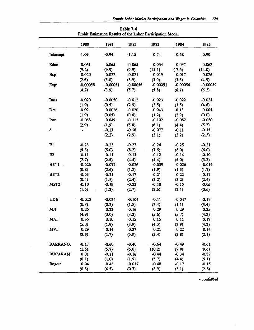
Female Labor Market Participation and Wages in Colombia 179
Table 7.4Probit Estimation Re6ults of the Labor Participation Model
1980 1981 1982 1983 1984 1985
Intercept -1.09 -0.94 -1.15 -0.74 -0.68 -0.90
Educ 0.061 0.065 0.065 0.064 0.057 0.062(9.2) (9.9) (9.9) (15.1) (7.6) (14.0)
Exp 0.020 0.022 0.021 0.019 0.017 0.026(2.5) (3.0) (3.9) (3.9) (3.5) (4.9)
Exp2 -0.00058 -0.00051 -0.00055 -0.00051 -0.00054 -0.00059(4.2) (3.9) (5.7) (5.8) (6.1) (6.2)
Imar -0.020 -0.0050 -0.012 -0.023 -0.022 -0.024(1.9) (0.5) (2.9) (2.5) (3.5) (4.6)
Dm -0.09 0.0026 -0.020 -0.043 -0.13 0.004(1.9) (0.05) (0.6) (1.2) (2.9) (0.0)
Iotr -0.063 -0.049 -0.113 -0.102 -0.082 -0.080(2.9) (1.9) (5.8) (6.1) (4.4) (5.2)
d - -0.13 -0.10 -0.077 -0.11 -0.15(2.2) (2.9) (2.1) (2.2) (2.3)
El -0.23 -0.22 -0.27 -0.24 -0.25 -0.21(5.3) (5.0) (8.2) (7.5) (8.0) (6.0)
E2 -0.11 -0.11 -0.13 -0.12 -0.14 -0.10(2.7) (2.5) (4.4) (4.4) (5.0) (3.3)
HSTI -0.026 -0.077 -0.026 -0.039 -0.026 -0.016(0.8) (2.6) (1.2) (1.9) (1.3) (1.7)
HST2 -0.03 -0.21 -0.17 -0.21 -0.22 -0.17(0.4) (1.8) (2.4) (3.2) (3.2) (2.4)
MST2 -0.10 -0.19 -0.23 -0.18 -0.15 -0.05(1.6) (1.3) (2.7) (2.6) (2.1) (0.6)
HDE -0.020 -0.024 -0.104 -0.11 -0.047 -0.17(0.3) (0.3) (1.8) (2.4) (1.1) (3.4)
MII 0.26 0.22 0.16 0.29 0.29 0.25(4.9) (3.0) (3.3) (5.6) (5.7) (4.3)
MAI 0.36 0.10 0.15 0.15 0.11 0.17(5.0) (1.9) (3.9) (4.3) (2.9) (4.3)
MVI 0.29 0.14 0.37 0.21 0.22 0.14(3.3) (1.7) (5.9) (3.4) (3.8) (2.1)
BARRANQ. -0.17 -0.60 -. 40 -0.64 -0.49 -0.61(1.5) (5.7) (6.0) (10.2) (7.8) (9.6)
BUCARAM. 0.01 -0.11 -0.16 -0.44 -0.34 -0.37(0.1) (1.0) (1.9) (5.7) (4.4) (5.1)
Bogota -0.04 -0.43 -0.037 -0.48 -0.17 -0.15(0.3) (4.5) (0.7) (8.9) (3.1) (2.8)
- continued
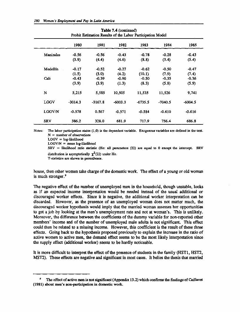
180 Women's Employment and Pay in Latin America
Table 7.4 (continued)Probit Estimation Results of the Labor Participation Model
1980 1981 1982 1983 1984 1985
Manizales -0.56 -0.56 -0.43 -0.78 -0.28 -0.43(3.9) (4.4) (4.6) (8.8) (3.4) (5.4)
Medellin -0.17 -0.52 -0.27 -0.62 -0.50 -0.47(1.5) (5.0) (4.2) (10.1) (7.9) (7.4)
Cali -0.43 -0.39 -0.90 -0.50 -0.35 -0.36(3.9) (3.9) (1.3) (8.3) (5.8) (5.9)
N 5,215 5,585 10,505 11,535 11,526 9,741
LOGV -3014.3 -3167.8 -6003.3 -6735.5 -7040.5 -6004.5
LOGV/N -0.578 0.567 -0.571 -0.584 -0.610 -0.616
SRV 386.2 328.0 681.9 717.9 756.4 686.8
Notes: The labor participation status (1,0) is the dependent variable. Exogenous variables are defined in the text.N = number of observationsLOGV = log-likelihoodLOGV/N = mean log-likelihoodSRV = likelihood ratio statistic (Ho: all parameters (22) are equal to 0 except the intercept. SRV
distribution is asymptotically X2(22) under Ho.T-statistics are shown in parentheses.
house, then other women take charge of the domestic work. The effect of a young or old womanis much stronger.9
The negative effect of the number of unemployed men in the household, though unstable, looksas if an expected income interpretation would be needed instead of the usual additional ordiscouraged worker effects. Since it is negative, the additional worker interpretation can bediscarded. However, as the presence of an unemployed woman does not matter much, thediscouraged worker hypothesis would imply that the married woman assesses her opportunitiesto get a job by looking at the men's unemployment rate and not at woman's. This is unlikely.Moreover, the difference between the coefficients of the dummy variable for non-reported othermembers' income and of the number of unemployed male adults is not significant. This effectcould then be related to a missing income. However, this coefficient is the result of these threeeffects. Going back to the hypothesis proposed previously to explain the increase in the ratio ofactive women to active men, the demand effect seems to be the most likely interpretation sincethe supply effect (additional worker) seems to be hardly noticeable.
It is more difficult to interpret the effect of the presence of students in the family (HST1, HST2,MST2). These effects are negative and significant in most cases. It belies the thesis that married
9 The effect of active men is not significant (Appendix 13.2) which confirms the findings of Caillavet(1981) about men's non-participation in domestic work.
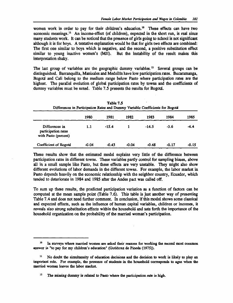
Female Labor Market Particqpaion and Wages in Colombia 181
women work in order to pay for their children's education.'° These effects can have twoeconomic meanings."1 An income-effect (of children), expected in the short run, is real sincemany students work. It can be noticed that the presence of girls going to school is not significantalthough it is for boys. A tentative explanation would be that for girls two effects are combined:The first one similar to boys which is negative, and the second, a positive substitution effectsimilar to young inactive women's (MJI). But the instability of the result makes thisinterpretation shaky.
The last group of variables are the geographic dummy variables."2 Several groups can bedistinguished. Barranquilla, Manizales and Medellfn have low participation rates. Bucaramanga,BogotA and Cali belong to the medium range below Pasto where participation rates are thehighest. The parallel evolution of global participation rates by towns and the coefficients ofdummy variables must be noted. Table 7.5 presents the results for Bogota.
Table 7.5Differences in Participation Rates and Dummy Variable Coefficients for Bogota
1980 1981 1982 1983 1984 1985
Differences in 1.1 -15.4 1 -14.5 -3.6 -4.4participation rates
with Pasto (percent)
Coefficient of Bogota -0.04 -0.43 -0.04 -0.48 -0.17 -0.1S
These results show that the estimated model explains very little of the difference betweenparticipation rates in different towns. These variables partly control for sampling biases, aboveall in a small sample like Pasto, but these effects are very unstable. They might also showdifferent evolutions of labor demands in the different towns. For example, the labor market inPasto depends heavily on the economic relationship with the neighbor country, Ecuador, whichtended to deteriorate in 1984 and 1985 after the Andes pact was called off.
To sum up these results, the predicted participation variation as a function of factors can becomputed at the mean sample point (Table 7.6). This table is just another way of presentingTable 7.4 and does not need further comment. In conclusion, if this model shows some classicaland expected effects, such as the influence of human capital variables, children or incomes, itreveals also strong substitution effects within the household and sets forth the importance of thehousehold organization on the probability of the married woman's participation.
10 In surveys where married women are asked their reasons for working the second most commonanswer is 'to pay for my children's education" (Gutierrez de Pineda (1975)).
11 No doubt the simultaneity of education decisions and the decision to work is likely to play animportant role. For example, the presence of students in the household corresponds to ages when themarried woman leaves the labor market.
12 The missing dummy is related to Pasto where the participation rate is high.
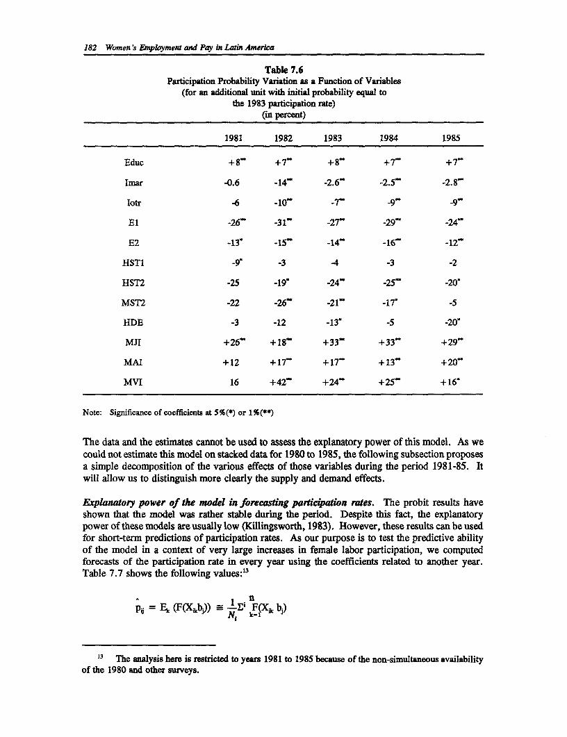
182 Women's Employment and Pay in Latin America
Table 7.6Participation Probability Variation as a Function of Variables
(for an additional unit with initial probability equal tothe 1983 participation rate)
(in percent)
1981 1982 1983 1984 1985
Educ +8- +7" +8" +7" +7-
Imar -0.6 -14" -2.6 -2.5" -2.8"
Iotr -6 -10" -7" -9" -9"
El -26" -31" -27" -29" -24
E2 -13* -15- -14" -16" -12-
HSTI -9* -3 -4 -3 -2
HST2 -25 -19* -24- -25 -20*
MST2 -22 -26" -21" -17' -5
HIDE -3 -12 -13* -5 -20*
MJI +26" +18" +33" +33" +29"
MAI +12 +17" +17" +13- +20"
MVI 16 +42" +24 +25" + 16*
Note: Significance of coefficients at 5%(*) or 1%(**)
The data and the estimates cannot be used to assess the explanatory power of this model. As wecould not estimate this model on stacked data for 1980 to 1985, the following subsection proposesa simple decomposition of the various effects of those variables during the period 1981-85. Itwill allow us to distinguish more clearly the supply and demand effects.
Explanatory power of the model in forecasting paficipation rates. The probit results haveshown that the model was rather stable during the period. Despite this fact, the explanatorypower of these models are usually low (Killingsworth, 1983). However, these results can be usedfor short-term predictions of participation rates. As our purpose is to test the predictive abilityof the model in a context of very large increases in female labor participation, we computedforecasts of the participation rate in every year using the coefficients related to another year.Table 7.7 shows the following values:13
pu=k((-E) .' FQI~b)N1 k-I
13 The analysis here is restricted to yeasr 1981 to 1985 because of the non-simultaneous availabilityof the 1980 and other surveys.
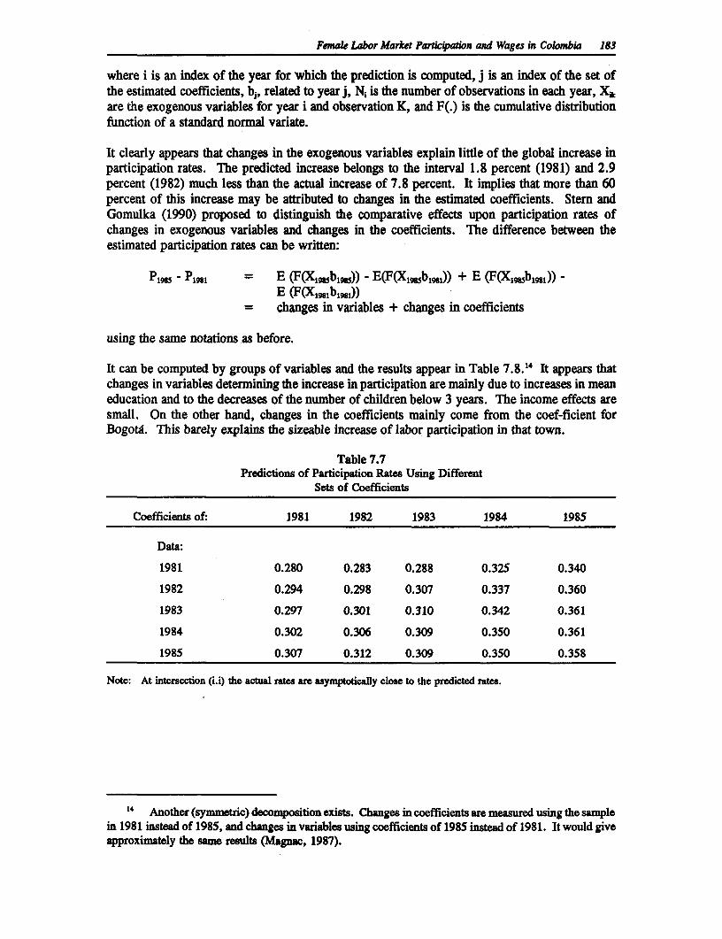
Femak Labor Market Partic4iation and Wages in Colombia 183
where i is an index of the year for which the prediction is computed, j is an index of the set ofthe estimated coefficients, bj, related to year j, N; is the number of observations in each year, X*,are the exogenous variables for year i and observation K, and F(.) is the cumulative distributionfunction of a standard normal variate.
It clearly appears that changes in the exogenous variables explain little of the global increase inparticipation rates. The predicted increase belongs to the interval 1.8 percent (1981) and 2.9percent (1982) much less than the actual increase of 7.8 percent. It implies that more than 60percent of this increase may be attributed to changes in the estimated coefficients. Stem andGomulka (1990) proposed to distinguish the comparative effects upon participation rates ofchanges in exogenous variables and changes in the coefficients. The difference between theestimated participation rates can be written:
P,m - P,gi = E (F(X1n5b1"5)) - E(F(Xjmbj9 1s)) + E (F(Xjmb1sg1)) -E (F(XIgnlblg,,))
= changes in variables + changes in coefficients
using the same notations as before.
It can be computed by groups of variables and the results appear in Table 7.8.14 It appears thatchanges in variables determining the increase in participation are mainly due to increases in meaneducation and to the decreases of the number of children below 3 years. The income effects aresmall. On the other hand, changes in the coefficients mainly come from the coef-ficient forBogotd. This barely explains the sizeable increase of labor participation in that town.
Table 7.7Predictions of Participation Rates Using Different
Sets of Coefficients
Coefficients of: 1981 1982 1983 1984 1985
Data:
1981 0.280 0.283 0.288 0.325 0.340
1982 0.294 0.298 0.307 0.337 0.360
1983 0.297 0.301 0.310 0.342 0.361
1984 0.302 0.306 0.309 0.350 0.361
1985 0.307 0.312 0.309 0.350 0.358
Note: At intersection (i.i) the actual rates are asymptotically close to the predicted rates.
14 Another (symmetric) decomposition exists. Changes in coefficients are measured using the samplein 1981 instead of 1985, and changes in variables using coefficients of 1985 instead of 1981. It would giveapproximately the same results (Magnac, 1987).
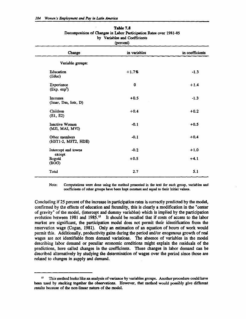
184 Women's Employment and Pay in Latin America
Table 7.8Decomposition of Changes in Labor Participation Rates over 1981-85
by Vanables and Coefficients(percent)
Change in variables in coefficients
Variable groups:
Education +1.7% -1.3(Educ)
Experience 0 +1.4(Exp. exp)
Incomes +0.5 -1.3(Imar, Dm, lotr, D)
Children +0.4 +0.2(El, E2)
Inactive Women -0.1 +0.5(MJI, MAI, MVI)
Other members -0.1 +0.4(HST1-2, MST2, HDE)
Intercept and towns -0.2 +1.0except
BogotA +0.5 +4.1(BOG)
Total 2.7 5.1
Note: Computations were done using the method presented in the text for each group, variables andcoefficients of other groups have been kept constant and equal to their initial values.
Concluding if 25 percent of the increase in participation rates is correctly predicted by the model,confirmed by the effects of education and fecundity, this is clearly a modification in the 'centerof gravity" of the model, (intercept and dummy variables) which is implied by the participationevolution between 1981 and 1985.1' It should be recalled that if costs of access to the labormarket are significant, the participation model does not permit their identification from thereservation wage (Cogan, 1981). Only an estimation of an equation of hours of work wouldpermit this. Additionally, productivity gains during the period and/or exogenous growth of realwages are not identifiable from demand variations. The absence of variables in the modeldescribing labor demand or peculiar economic conditions might explain the residuals of thepredictions, here called changes in the coefficients. These changes in labor demand can bedescribed alternatively by studying the determination of wages over the period since those arerelated to changes in supply and demand.
is This method looks like an analysis of variance by variables groups. Another procedure could havebeen used by stacking together the observations. However, that method would possibly give differentresults because of the non-linear nature of the model.
Female Labor Market Participation and Wages in Colombia 185
4. Wage Functions
Tables 7.9 and 7.10 show the results of such estimates for different groups in the populationdrawn from different survey studies (Mohan, 1981; Carrizosa, 1982). The dependent variablein those regressions is generally the logarithm of total income or labor income.
Results are rather scattered. The education coefficient, that is to say its mean yield, variesbetween .14 and .20. These variations can be explained mainly by different survey coveragesor by the different sets of variables used. These results imply that income doubles for every 5additional years of education which roughly correspond to an entire cycle in a primary orsecondary school. These yields are much higher than in developed countries, as generally thecase is in less developed countries (LDCs) (Psacharopoulos, 1973) but even seem to be quitelarge by LDCs standards.
The usual long-term interpretation of Mincer (1962) would relate these yields to the interest ratesbut they may also be related to high costs of education (Magnac, 1987). Given the limited accessto the financial markets of many households, the second reason may be the most important.However, in the 1970s large increases in average education took place since primary educationbecame compulsory in the 1960s. Education yields should have shown large short-run variations.This indeed shows up in these results. The question of whether these fluctuations are related todemand or supply shocks remains unsolved.
Married women's wage equations. In order to correct for the selectivity bias in the wageequations (Killingsworth, 1983), a Heckman (1979) procedure is used here. The inverse Mill'sratio associated with the participation equations estimated in the previous section is included asa regressor. This method will give consistent estimates of the coefficients but inconsistentestimates of the standard errors.'6
Table 7.11 shows the estimation results for the following equation, with and without selectivitycorrections:
log(w) = Xa + u
where w is the hourly wage rate, defined as the ratio of labor income to normal hours of work.
The R2 is relatively high given the number of observations and the coefficients are largelysignificant, especially for education. The usual positive effect of education and the positive butdecreasing effect of experience is corroborated. Without selectivity corrections, an additionalyear of education increases wages on average by 14 percent and the maximum point for the wageprofile as a function of age is reached for experience equal to 30, that is to say around age 40.
Coefficients have a positive trend between 1981 and 1984 but decrease again to their 1981 levelsin 1985. On the other hand, 1980 coefficients appear to be very large. This decrease can bepartially explained by the evolution of labor participation over the period. In 1983, and aboveall in 1984, there is a large increase in participation rates and women, with low education andlittle experience, enter the labor market. This group, with low earnings, make the wage functionsteeper (Figure 7.4). This phenomenon could be attributed to the modification of the selectionrule across time.
16 These are reported for information purposes. For 1980, a standard complete likelihood methodwas used but the numerical results were not any different from those given here.
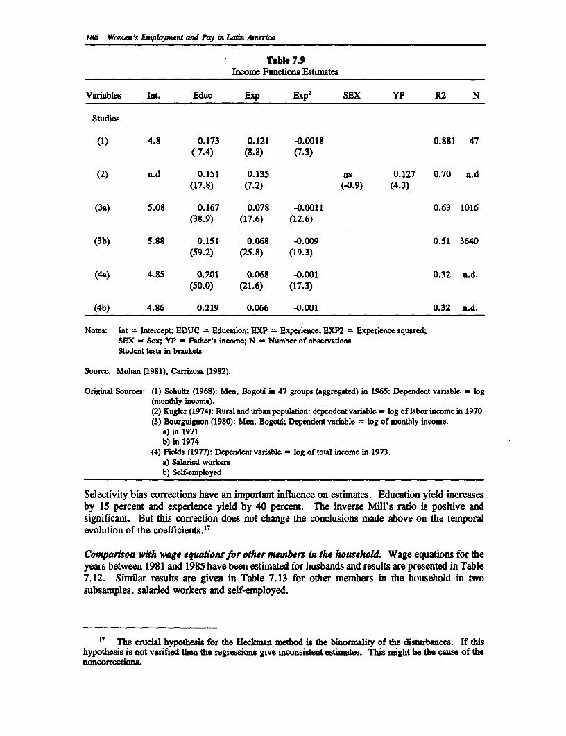
186 Women's Employment and Pay in Latin America
Table 7.9Income Functions Estimates
Variables Int. Educ Exp Exp2 SEX YP R2 N
Studies
(1) 4.8 0.173 0.121 -0.0018 0.881 47(7.4) (8.8) (7.3)
(2) n.d 0.151 0.135 ns 0.127 0.70 n.d(17.8) (7.2) (-0.9) (4.3)
(3a) 5.08 0.167 0.078 -0.0011 0.63 1016(38.9) (17.6) (12.6)
(3b) 5.88 0.151 0.068 -0.009 0.51 3640(59.2) (25.8) (19.3)
(4a) 4.85 0.201 0.068 -0.001 0.32 n.d.(50.0) (21.6) (17.3)
(4b) 4.86 0.219 0.066 -0.001 0.32 n.d.
Notes: Int = Intercept; EDUC = Education; EXP = Experience; EXP2 Experience squared;SEX = Sex; YP = Father's income; N = Number of observationsStudent tests in brackets
Source: Mohan (1981), Carrizosa (1982).
Original Sources: (1) Schukz (1968): Men, Bogota in 47 groups (aggregated) in 1965: Dependent variable = log(monthly income).(2) Kugler (1974): Rural and urban population: dependent variable = log of labor income in 1970.(3) Bourguignon (1980): Men, Bogota; Dependent variable = log of monthly income.
a) in 1971b) in 1974
(4) Fields (1977): Dependent variable = log of total income in 1973.a) Salaried workersb) Self-employed
Selectivity bias corrections have an important influence on estimates. Education yield increasesby 15 percent and experience yield by 40 percent. The inverse Mill's ratio is positive andsignificant. But this correction does not change the conclusions made above on the temporalevolution of the coefficients.'7
Comparson with wage equations for other members in the household. Wage equations for theyears between 1981 and 1985 have been estimated for husbands and results are presented in Table7.12. Similar results are given in Table 7.13 for other members in the household in twosubsamples, salaried workers and self-employed.
17 The crucial hypothesis for the Heckman method is the binormality of the disturbances. If thishypothesis is not verified then the regressions give inconsistent estimates. This might be the cause of thenoncorrections.
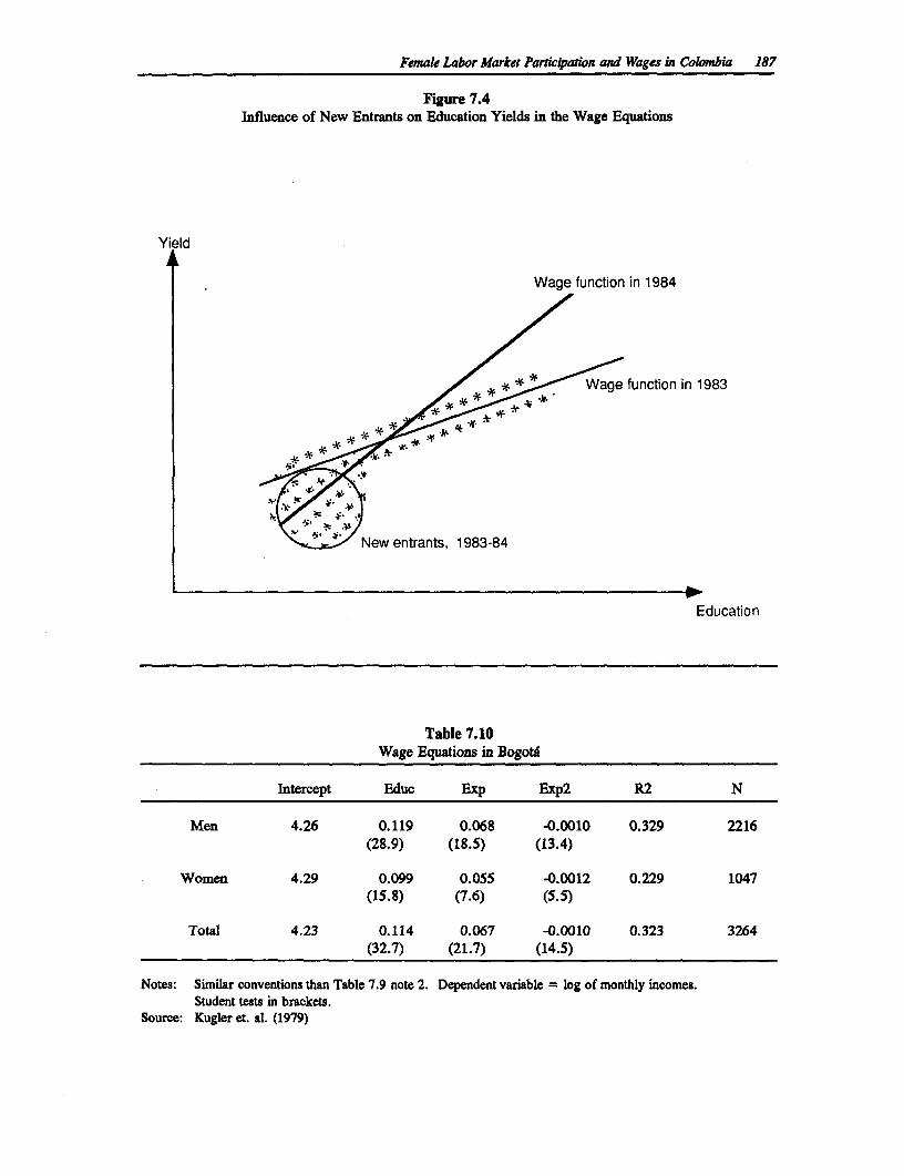
Female Labor Market Particiption and Wages in Colombia 187
Figure 7.4Influence of New Entrants on Education Yields in the Wage Equations
Yield
Wage function in 1984
*s * Wagefunction in 1983
New entrants, 1983-84
Education
Table 7.10Wage Equations in BogotA
Intercept Educ Exp Exp2 R2 N
Men 4.26 0.119 0.068 -0.0010 0.329 2216(28.9) (18.5) (13.4)
Women 4.29 0.099 0.055 -0.0012 0.229 1047(15.8) (7.6) (5.5)
Total 4.23 0.114 0.067 -0.0010 0.323 3264(32.7) (21.7) (14.5)
Notes: Similar conventions than Table 7.9 note 2. Dependent variable = log of monthly incomes.Student tests in brackets.
Source: Kugler et. al. (1979)
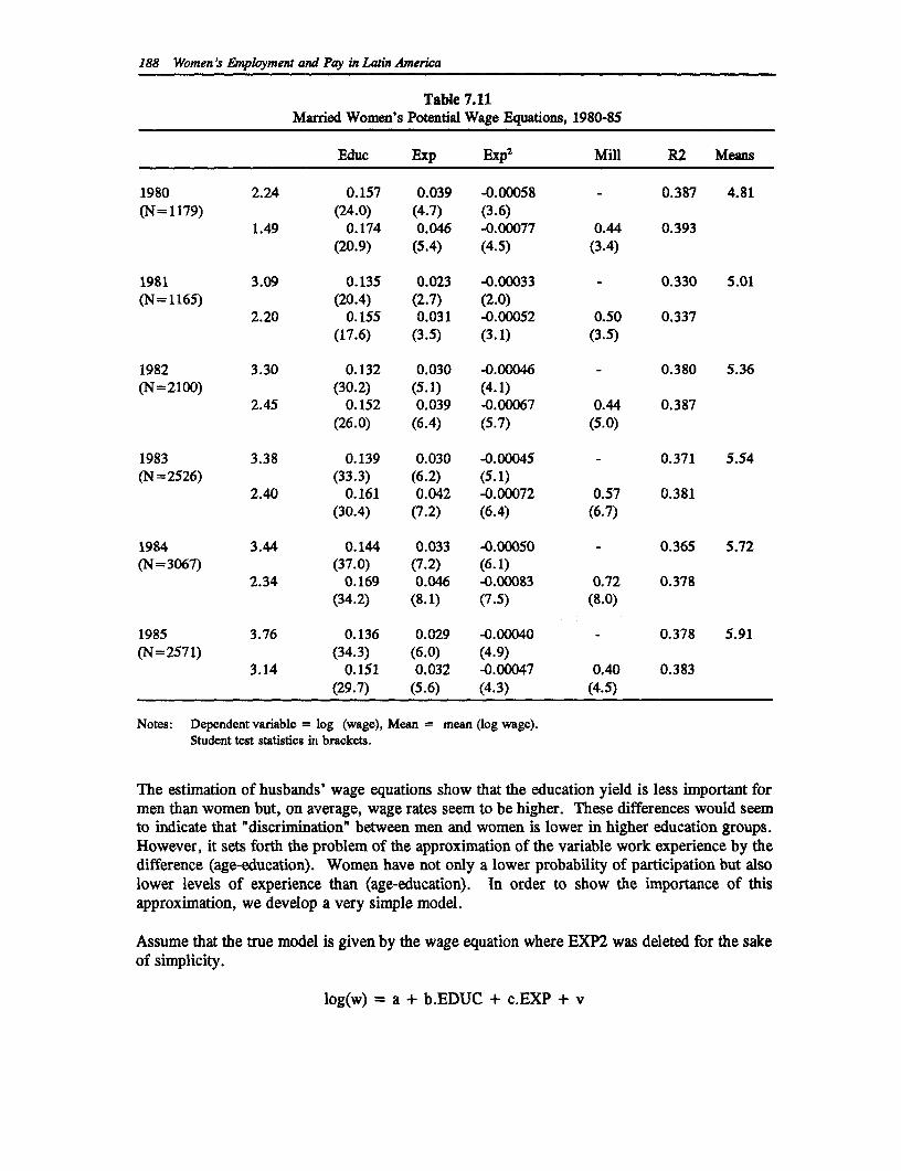
188 Women's Employment and Pay in Latin America
Table 7.11Married Women's Potential Wage Equations, 1980-85
Educ Exp Exp2 Mill R2 Means
1980 2.24 0.157 0.039 -0.00058 - 0.387 4.81(N= 1179) (24.0) (4.7) (3.6)
1.49 0.174 0.046 -0.00077 0.44 0.393(20.9) (5.4) (4.5) (3.4)
1981 3.09 0.135 0.023 -0.00033 - 0.330 5.01(N= 1165) (20.4) (2.7) (2.0)
2.20 0.155 0.031 -0.00052 0.50 0.337(17.6) (3.5) (3.1) (3.5)
1982 3.30 0.132 0.030 -0.00046 - 0.380 5.36(N=2100) (30.2) (5.1) (4.1)
2.45 0.152 0.039 -0.00067 0.44 0.387(26.0) (6.4) (5.7) (5.0)
1983 3.38 0.139 0.030 -0.00045 - 0.371 5.54(N=2526) (33.3) (6.2) (5.1)
2.40 0.161 0.042 -0.00072 0.57 0.381(30.4) (7.2) (6.4) (6.7)
1984 3.44 0.144 0.033 -0.00050 - 0.365 5.72(N=3067) (37.0) (7.2) (6.1)
2.34 0.169 0.046 -0.00083 0.72 0.378(34.2) (8.1) (7.5) (8.0)
1985 3.76 0.136 0.029 -0.00040 - 0.378 5.91(N=2571) (34.3) (6.0) (4.9)
3.14 0.151 0.032 -0.00047 0.40 0.383(29.7) (5.6) (4.3) (4.5)
Notes: Dependent variable = log (wage), Mean = mean (log wage).Student test statistics in brackets.
The estimation of husbands' wage equations show that the education yield is less important formen than women but, on average, wage rates seem to be higher. These differences would seemto indicate that "discrimination' between men and women is lower in higher education groups.However, it sets forth the problem of the approximation of the variable work experience by thedifference (age-education). Women have not only a lower probability of participation but alsolower levels of experience than (age-education). In order to show the importance of thisapproximation, we develop a very simple model.
Assume that the true model is given by the wage equation where EXP2 was deleted for the sakeof simplicity.
log(w) = a + b.EDUC + c.EXP + v
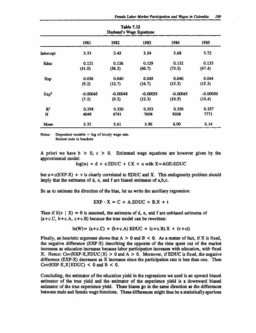
Femaek Labor Market Partic4waion and Wages in Colombia 189
Table 7.12Husband's Wage Equations
1981 1982 1983 1984 1985
Intercept 3.33 3.43 3.54 3.68 3.72
Educ 0.121 0.126 0.129 0.132 0.133(41.0) (56.3) (66.7) (73.5) (67.4)
Exp 0.036 0.040 0.045 0.040 0.044(9.2) (12.7) (16.7) (15.3) (15.3)
Exp2 -0.00045 -0.00048 -0.00055 -0.00045 -0.00050(7.2) (9.2) (12.3) (10.5) (10.4)
R2 0.298 0.320 0.353 0.356 0.357N 4048 6781 7698 9208 7771
Mean 5.32 5.61 5.86 6.00 6.14
Notes: Dependent variable = log of hourly wage rate.Student tests in brackets
A priori we have b > 0, c > 0. Estimated wage equations are however given by theapproximated model:
log(w) = d + e.EDUC + f.X + u with X=AGE-EDUC
but u=c(EXP-X) + v is clearly correlated to EDUC and X. This endogeneity problem shouldimply that the estimates of d, e, and f are biased estimates of a,b,c.
So as to estimate the direction of the bias, let us write the auxiliary regression:
EXP - X = C + A.EDUC + B.X + t
Then if E(v j X) = 0 is assumed, the estimates of d, e, and f are unbiased estimates of(a+c.C, b+c.A, c+c.B) because the true model can be rewritten:
ln(W)= (a+c.C) + (b+c.A) EDUC + (c+c.B).X + (v+ct)
Finally, an heuristic argument shows that A > 0 and B < 0. As a matter of fact, if X is fixed,the negative difference (EXP-X) describing the opposite of the time spent out of the marketincreases as education increases because labor participation increases with education, with fixedX. Hence: Cov(EXP-X,EDUC I X) > 0 and A > 0. Moreover, if EDUC is fixed, the negativedifference (EXP-X) decreases as X increases since the participation rate is less than one. ThenCov(EXP-X,XIEDUC) < 0 and B < 0.
Concluding, the estimator of the education yield in the regressions we used is an upward biasedestimator of the true yield and the estimator of the experience yield is a downward biasedestimator of the true experience yield. These biases go in the same direction as the differencesbetween male and female wage functions. These differences might thus be a statistically spurious
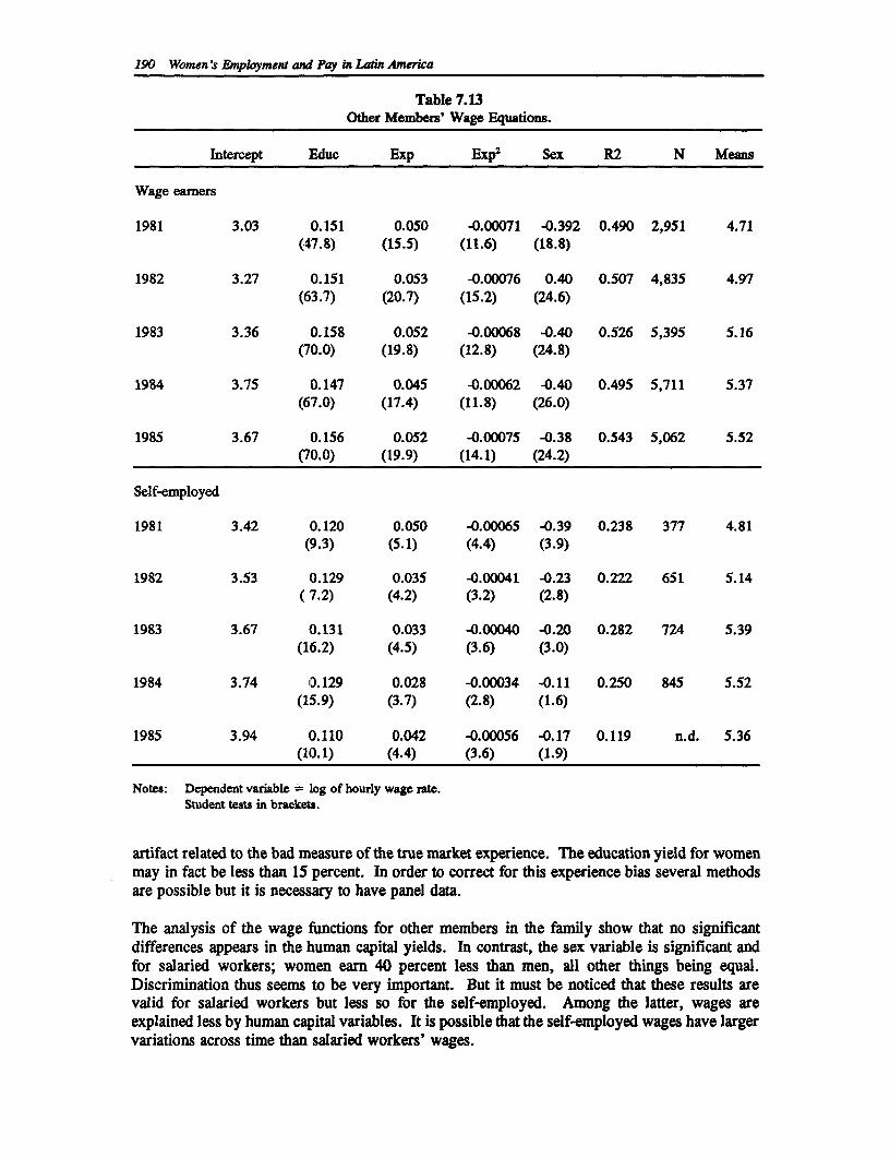
190 Women's Employment and Pay in Latin America
Table 7.13Other Members' Wage Equations.
Intercept Educ Exp Exp2 Sex R2 N Means
Wage earners
1981 3.03 0.151 0.050 -0.00071 -0.392 0.490 2,951 4.71(47.8) (15.5) (11.6) (18.8)
1982 3.27 0.151 0.053 -0.00076 0.40 0.507 4,835 4.97(63.7) (20.7) (15.2) (24.6)
1983 3.36 0.158 0.052 -0.00068 -0.40 0.526 5,395 5.16(70.0) (19.8) (12.8) (24.8)
1984 3.75 0.147 0.045 -0.00062 -0.40 0.495 5,711 5.37(67.0) (17.4) (11.8) (26.0)
1985 3.67 0.156 0.052 -0.00075 -0.38 0.543 5,062 5.52(70.0) (19.9) (14.1) (24-2)
Self-employed
1981 3.42 0.120 0.050 -0.00065 -0.39 0.238 377 4.81(9.3) (5.1) (4.4) (3.9)
1982 3.53 0.129 0.035 -0.00041 -0.23 0.222 651 5.14(7.2) (4.2) (3.2) (2.8)
1983 3.67 0.131 0.033 -0.00040 -0.20 0.282 724 5.39(16.2) (4.5) (3.6) (3.0)
1984 3.74 0.129 0.028 -0.00034 -0.11 0.250 845 5.52(15.9) (3.7) (2.8) (1.6)
1985 3.94 0.110 0.042 -0.00056 -0.17 0.119 n.d. 5.36(10.1) (4.4) (3.6) (1.9)
Notes: Dependent variable = log of hourly wage rate.Student tests in brackets.
artifact related to the bad measure of the true market experience. The education yield for womenmay in fact be less than 15 percent. In order to correct for this experience bias several methodsare possible but it is necessary to have panel data.
The analysis of the wage functions for other members in the family show that no significantdifferences appears in the human capital yields. In contrast, the sex variable is significant andfor salaried workers; women earn 40 percent less than men, all other things being equal.Discrimination thus seems to be very important. But it must be noticed that these results arevalid for salaried workers but less so for the self-employed. Among the latter, wages areexplained less by human capital variables. It is possible that the self-employed wages have largervariations across time than salaried workers' wages.
Female Labor Market Participation and Wages in Colombia 191
5. Conclusions
In this paper, the results lead to some firm conclusions but also pose some questions about thebasic hypothesis of the model. First, the results of the participation model seem robust and stableacross time. The results show the importance of the classical effects of human capital variablesor incomes on the labor participation of married women. They also permit us to measure thesubstitution effects within the household. Nevertheless, even if 25 percent of the increase inparticipation is predicted by supply effects, such as increasing average education of decreasingfecundity, its explanatory power remains quite small in cross-section and rather mild in time-series.
The estimation of wage equations is usual but omits variables related to occupations or to thedemand side of the labor market. The latter seem to be an important determinant of the evolutionof the labor market (Magnac, 1991). In particular, the segmentation hypothesis of the labormarket should be considered. However, in this case the estimation of wage equations by merelyincluding occupational status variables is plagued by major biases since those variables areendogenously determined. Occupational status is chosen at the same time as participation. It isthus necessary to use a more complete model so as to treat it in a more rigorous way.
192 Women's Employment and Pay in Latin America
Appendix 7A
Household Composition Variables Left Out of the Analysis of Female Participation
Number of persons in the family.
Number of children of the household's head aged between 3 and 12.
Number of children of other members.
Number of active adult men and women.
Number of students aged between 12 and 18.
Number of unemployed women.
These variables were left out of the analysis because they were not significant in all samplesexcept the number of persons and the number of active women which were left out because ofa strong colinearity with other members' income (IOTR).
Appendix 7BPresentation of the Data
The data used in the estimations come from the yearly Encuestas de Hogares (EH) from March1980 to 1985 (EH26 to EH46) collected by the DANE in the four major cities of Colombia,Bogota, Medellfn, Barranquilla, Cali, and in the smaller towns Bucaramanga, Manizales andPasto. The DANE in recent years aims to include suburbs in the surveys but it was not the casein 1980 to 1985 surveys. The survey methods are homogeneous in the period under study, withthe exceptions of March 1981 in BogotA where the sample is much larger and of March 1982 forthe three smaller towns for the same reason (Estudios de Poblaci6n).
Generally speaking, the main questionnaire consists of questions related to individualcharacteristics on work, income, etc., but it is easy to construct household variables from thesurvey.
These surveys or similar ones have been studied by Ayala (1981) who compared the results toa survey undertaken by the CEDE (Universidad de les Andes, Empleo y Pobreza, 1978) inBogota. Differences are rather mild, but the Encuestas de Hogares seems to underestimate thenumber of children in the family and domestic services as well. Similarly, it seems that partialwork is underreported, in particular by unemployed people.
Another possible criticism is the sampling strategy based on the 1973 census. The latter is notrenowned for its coverage. However, the DANE reactualises these predictions by cartographicmethods. Nevertheless, as suburbs are left out, no coverage exists for the districts called barriosde invasion setting up very quickly. The poorest families are surely missed.
The sample that we selected retains the following criteria: The family must be composed of amale household head and his wife or companion, the latter being aged between 18 and 60. Thenumber of households varies between 5,000 and 10,000 (Table 7.6). Generally left out are 20to 25 percent of the households present in the whole sample. All household's variables have beenconstructed from individual observations by counting methods.
References
Aguiar, N. "La mujer en la fuerza de trabajo en la America Latina: un resumen introductorio."Desarrollo y Sociedad, Vol. 13, January (1984).
Angulo Novoa, A. and Ldpez de Rodrfguez, C. Trabajo yfecundidad de la mujer colombilana.Fedesarrollo: Bogotd, April 1975.
Ayala, U. Comparaciones intertemporales de estad(sticas sobre fiuerza laboral. Bogota:Universidad de los Andes, CEDE, 1981.
El empleo en las grandes ciudades colombianas. Bogota: Universidad de los Andes, CEDE,1981.
Bayona, A. "El descenso de la fecundidad y su impacto sobre la participacion de la mujer en laactividad en Colombia" in Imiplicaciones socioecon6micas y demogrdficas del descenso delafecundidad en Colombia, Vol. 18, April (1982).
Berry, A. and M. Urrutia, Income Distribution in Colombia. New Haven, London: YaleUniversity Press, 1976.
Bonilla de Ramos, E. La Madre Trabajadora. Document 66. BogotA: Universidad de los Andes,1981.
Bourguignon, F. "Participation, emploi et travail domestiques des femmes mariees."Consommation, Vol. 2 (1981). pp. 75-98.
-. "The Labor Market in Colombia." Washington D.C.: The World Bank, Report No.DRD157, 1986.
Bourguignon, F., IT. Gagey and T. Magnac. "On Estimating Female Labor Supply Behavior inDeveloping Countries." Doc. LEP, Vol. 103, January (1985). pp.4 1 .
Caceres, I. Algune s aspectos de la situaci6n de la mujer trabajadora en Colombia. UnpublishedDissertation. Bogota: Universidad de los Andes, 1977.
Caillavet, F. Allocation du temps des menages a Bogotd, Colombie. Unpublished Dissertation.University of Paris, 1981.
193
194 Women's Employment and Pay in Latin America
Castanieda, IT. "Determinantes del cambio poblacional en Colombia.' Desarrollo y Sociedad,Vol. 4, July (1980).
'La participaci6n de las madres en el mercado urbano en Colombia." Desarrollo ySociedad, (1981).
Departamento Administrativo Nacional de Estadfstica (DANE). Boletines de estadfstica. Bogota.
-. Metodologfa de las encuestas de hogares. BogotA, 1986.
Colombia Estadfstica 86. Bogota, 1986.
Fields, G. and T.P. Schultz. "Income Generating Functions in a Low Income Country:Colombia." Review of Income and Wealth, Vol. 28, no. 1 (1982). pp. 71-87.
G6mez de, M. I., B. Kugler and A. Reyes. Determinantes econ6micos y demogr4ficos de laparticipaci6n laboral en Colombia. Bogota: CCRP, 1981.
Gourieroux, C. Econometrie des variables qualitatives. Paris: Economica, 1984.
Guti6rrez de Pineda, V. Estructura, funci6n y cambio de la familia en Colombia. Bogota:ACFM, 1975.
Heckman, J. "Sample Selection Bias as a Specification Erro9r." Economietrica, Vol. 47, no. 1(1979). pp. 153-161.
Kugler, B., A. Reyes, and M. I. de G6mez. Educaci6n y Mercado de Trabajo Urbano enColombia. BogotA: Monograffas de la CCPR. Vol. 10, 1979.
Killingsworth, M. Labor Supply. New Jersey: Cambridge University Press, 1983.
Kugler, B. "Influencia de la educacion en los ingresos de trabajo: el caso colombiano." Rev. dePlaneaci6n y Desarrollo, (1971).
Le6n de Leal, M. La mujer y el desarrollo en Colombia. Bogota: ACEP, 1977.
Magnac, T. Analyse de l 'offre de travail sur un marche concurrentiel ou segmente. UnpublishedDissertation. Paris: EHESS, 1987.
"Competitive or Segmented Labour Markets?" Econometrica, Vol 59 (1): 165-187, 1991.
Mohan, R. Ihe Determinants of Labor Earnings in Developing Metropolis: Estimates fromBogotd and Cali, Colombia. Washington D.C.: The World Bank, 1981.
Munoz, C. and M. Palacios. El ni/to trabajador. Bogota: Carlos Valencia Editores, 1980.
Ranis, G. "Distribuci6n del ingreso y crecimiento en Colombia." Desarrollo y Sociedad, Vol.1, January (1980).
Rey de Marulanda, N. El trabajo de la mujer. Bogota: Universidad de los Andes, CEDE, 1981.
Female Labor Market Participaton and Wages in Colombia 195
Rey de Marulanda, N., U. Ayala, M.C. Niho and F. Duran. Empleo y pobreza. Bogota:Universidad de los Andes, CEDE, 1978.
Reyna, J. V., H. G. Buendfa and C. C. Argaez. Desarrollo social en la decada del 70. BogotA:UNICEF, 1984.
Stem, N. and J. Gomulka. "The Employment of Married Women in the U.K. 1970-83."Econ6mica, Vol. 571 (1990). pp. 171-200.
Urrutia, M. Winners and Losers in Colombia's Economic Growth of the 70's. London: OxfordUniversity Press, 1984.

Chapter 8
Women's Labor Force Participation and Earnings inColombia
Eduardo Velez and Carolyn Winter
1. Introduction
This chapter contributes to the rather small literature on factors influencing female labor forceparticipation and earnings in Colombia. The movement of women from the home to theworkplace is generally seen to be an indicator of increasing sex equality in society since it impliesimproved access to education by women and reduced fertility rates. While women's labor forceparticipation rates have increased substantially in Colombia (from 19 percent in 1951 to 39percent in 1985)1 relatively little is known about women's work experience, their occupations,or their earnings relative to men. In this chapter we address the following questions: Whatfactors influence a women's decision to participate in the labor market? Are human capitalindicators lower for women than men? and, What accounts for the earnings differential betweenthe sexes?
The following section briefly describes the Colombian labor market. Section 3 describes thecharacteristics of the sample used in this analysis and Section 4 identifies the most importantdeterminants of women's labor force participation. Section 5 presents earnings function estimatesfor male and female workers respectively, allowing us to examine earnings differences whilecontrolling for human capital endowments. In Section 6 we decompose the earnings differentialinto the portion attributable to differences in productivity related variables and the portionattributable to "unexplained" factors (largely differences in the way employers reward male andfemale workers). A discussion of these findings and their implications for policy formulation ispresented in the final section.
2. The Colombian Labor Market
A wealth of resources, extensive industrial diversification, and prudent fiscal management has ledto sustained economic growth, averaging close to 5 percent per annum since the 1960s, and thecontinuing real growth in real incomes.
In the last few decades the country has experienced a rapid social transformation that has affectedthe structure of the labor force and labor-supply behavior. In fact, the urban share of thepopulation increased from 31 percent in 1938 to almost 70 percent in 1985; total fertility rates
ILO (1990).
197
198 Women's Employment and Pay in Latin America
declined by about 45 percent from the early 1960s and are currently estimated at about 3.5percent; maternal mortality that was 254 per 100,000 live births in 1964 was 107 in 1984;primary education enrollment more than doubled, and secondary education enrollment increasedsix-fold since the 1960s; and a substantial modification of the sectoral distribution of the laborforce occurred - the agricultural sector accounted for 57.2 percent of the labor force in 1950 and34.3 percent in 1980, the industrial sector for 17.9 percent in 1950 and 23.5 percent in 1980, andthe service sector for 24.9 percent in 1950 and 42.3 percent in 1980.
A significant change in the Colombian labor market over the last few decades has been theincrease in women's labor force participation from 19 percent in 1950 to 39 percent in 1985.Women continue, however, to be heavily represented in the informal sector and it is estimated(Federico de Alonso, 1990) that 64 percent of working women were in the informal sector in1990.
In terms of educational achievement, gross enrollment ratios at primary and secondary educationare about the same for boys and girls. Even in higher education women show good standingrelative to men; in 1986 the enrollment ratio for higher education as a whole was 13.1, and was12.6 for women. Since the end of the 1970s more women than men have been attending highereducation (DANE, 1985). However, field of study varies significantly by gender, with womenbeing found in educational tracks that lead to low-paying careers. The average education of laborforce participants has increased substantially over the past 30 years; more than 40 percent hadno education in 1951, only 8 percent had gone beyond primary education, and the illiteracy ratewas around 10 percent. The average educational level of the labor force has more than doubledsince the 1960s; an impressive change.
3. Sample Characteristics
The data used in this analysis are from the June 1988 National Household Survey conducted bythe Departamento Administrativo Nacional de Estadfstica (DANE) in the largest Colombiancities.2 The survey covers about 75,000 individuals aged twelve years or older in more than20,000 households and provides detailed data on individual socio-economic and labor status. A10 percent random sample of households was selected for use in this analysis. As we wereprimarily interested in prime-age workers, we retained in our subsample individuals aged 15 to60 years.
Table 8.1 shows the mean characteristics of the sample by gender and, for women, by workstatus. Individuals were classified as working if they were employed in the formal sector,reported positive earnings and worked more than 2 hours a week. Within the sample of workingmales and females, individuals who reported earning less than 10 percent of the mean hourlywage or more than 15 times the mean hourly wage for their sex were excluded. This procedureresulted in our dropping nine cases from the sample in which reported earnings were over threestandard deviations from the mean. The sample used in the analysis was composed of 3,163working males, 1,748 working females and 5,735 non-working females. The female participationrate in the sample was 25 percent.
2 The sample is representative of Colombia's urban population and the socio-economic compositionof each city. The cities and metropolitan areas included in the sample are: BogotA, Medellfn, Cali,Barranquilla, Bucaramanga, Cartagena, Cucuta, Manizales, Pasto, Ibague, Pereira and Villavicencio.
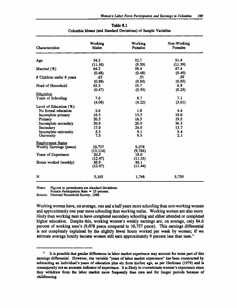
Women 's Labor Force Participation and Earnings in Colombia 199
Table 8.1Colombia Means (and Standard Deviations) of Sample Variables
Working Working Non-WorkingCharacteristics Males Females Females
Age 34.2 32.7 31.4(11.16) (9.59) (11.39)
Married (%) 64.2 38.4 47.4(0.48) (0.48) (0.49)
# Children under 6 years .63 .51 .59(0.88) (0.84) (0.85)
Head of Household 65.3 19.7 6.8(0.47) (0.39) (0.25)
EducationYears of Schooling 7.6 8.7 7.1
(4.08) (4.22) (3.61)Level of Education (%):
No formal education 2.6 1.8 4.4Incomplete primary 16.3 13.3 18.6Primary 20.5 16.5 19.5Incomplete secondary 30.9 26.0 36.3Secondary 17.0 24.0 13.7Incomplete university 5.3 9.1 5.4University 7.5 9.5 2.1
Emplovment StatusWeekly Earnings (pesos) 10,727 9,078
(13,114) (9,766)Years of Experience 20.5 18.0
(12.47) (11.25)Hours worked (weekly) 49.9 46.1
(12.07) (11.44)
N 3,163 1,748 5,735
Notes: Figures in parentheses arc standard deviations.Female Participation Rate = 25 percent.
Source: National Household Survey, 1988.
Working women have, on average, one and a half years more schooling than non-working womenand approximately one year more schooling than working males. Working women are also morelikely than working men to have completed secondary schooling and either attended or completedhigher education. Despite this, working women's weekly earnings are, on average, only 84.6percent of working men's (9,078 pesos compared to 10,727 pesos). This earnings differentialis not completely explained by the slightly fewer hours worked per week by women; if weestimate average hourly income women still earn approximately 9 percent less than men.3
I It is possible that gender differences in labor market experience may account for some part of thisearnings differential. However, our variable 'years of labor market experience' has been constructed bysubtracting an individual's years of education plus six from his/her age, as per Heckman (1979) and isconsequently not an accurate indicator of experience. It is likely to overestimate women's experience sincethey withdraw from the labor market more frequently than men and for longer periods because ofchildbearing.
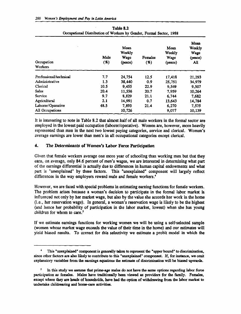
200 Women's Employment and Pay in Latin America
Table 8.2Occupational Distribution of Workers by Gender, Formal Sector, 1988
MeanMean Mean Weeldy
Weeldy Weekly WageMale Wage Females Wage (pesos)
Occupation (%) (pesos) (%) (pesos) AllWorkers
Professional/technical 7.7 24,754 12.5 17,418 21,293Administrative 1.3 38,440 0.9 25,751 34,979Clerical 10.5 9,455 22.9 9,549 9,507Sales 20.4 11,556 20.7 7,959 10,264Service 9.7 8,829 21.1 6,744 7,682Agricultural 2.1 14,991 0.7 13,643 14,784Laborer/Operative 48.5 7,893 21.4 6,270 7,575All Occupations 10,726 9,077 10,139
It is interesting to note in Table 8.2 that almost half of all male workers in the formal sector areemployed in the lowest paid occupation Oaborer/operative). Women are, however, more heavilyrepresented than men in the next two lowest paying categories, service and clerical. Women'saverage earnings are lower than men's in all occupational categories except clerical.
4. The Determinants of Women's Labor Force Participation
Given that female workers average one more year of schooling than working men but that theyearn, on average, only 84.6 percent of men's wages, we are interested in determining what partof the earnings differential is actually due to differences in human capital endowments and whatpart is "unexplained" by these factors. This "unexplained' component will largely reflectdifferences in the way employers reward male and female workers.4
However, we are faced with special problems in estimating earning functions for female workers.The problem arises because a woman's decision to participate in the formal labor market isinfluenced not only by her market wage, but also by the value she accords her work in the home(i.e., her reservation wage). In general, a woman's reservation wage is likely to be the highest(and hence her probability of participation in the labor market, lowest) when she has youngchildren for whom to care.5
If we estimate earnings functions for working women we will be using a self-selected sample(women whose market wage exceeds the value of their time in the home) and our estimates willyield biased results. To correct for this selectivity we estimate a probit model in which the
4 This "unexplained" component is generaUy taken to represent the 'upper bound" to discrimination,since other factors are also likely to contribute to this 'unexplained' component. If, for instance, we omitexplanatory variables from the earnings equations the estimate of discrimination will be biased upwards.
I In this study we assume that prime-age males do not have the same options regarding labor forceparticipation as females. Males have traditionally been viewed as providers for the family. Females,except where they are heads of households, have had the option of withdrawing from the labor market toundertake childrearing and home-care activities.
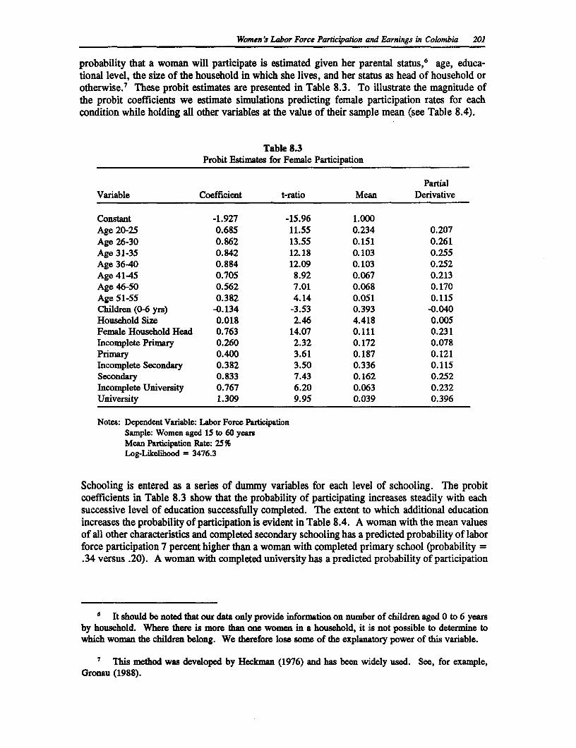
Women 's Labor Force Participaton and Earnings in Colombia 201
probability that a woman will participate is estimated given her parental status,6 age, educa-tional level, the size of the household in which she lives, and her status as head of household orotherwise.' These probit estimates are presented in Table 8.3. To illustrate the magnitude ofthe probit coefficients we estimate simulations predicting female participation rates for eachcondition while holding all other variables at the value of their sample mean (see Table 8.4).
Table 8.3Probit Estimates for Female Participation
PartialVariable Coefficient t-ratio Mean Derivative
Constant -1.927 -15.96 1.000Age 20-25 0.685 11.55 0.234 0.207Age 26-30 0.862 13.55 0.151 0.261Age 31-35 0.842 12.18 0.103 0.255Age 36-40 0.884 12.09 0.103 0.252Age 41-45 0.705 8.92 0.067 0.213Age 46-50 0.562 7.01 0.068 0.170Age 51-55 0.382 4.14 0.051 0.115Children (0-6 yrs) -0.134 -3.53 0.393 -0.040Household Size 0.018 2.46 4.418 0.005Fenmle Household Head 0.763 14.07 0.111 0.231Incomplete Primary 0.260 2.32 0.172 0.078Primary 0.400 3.61 0.187 0.121Incomplete Secondary 0.382 3.50 0.336 0.115Secondary 0.833 7.43 0.162 0.252Incomplete University 0.767 6.20 0.063 0.232University 1.309 9.95 0.039 0.396
Notes: Dependent Variable: Labor Force ParticipationSample: Women aged 15 to 60 yearsMean Participation Rate: 25%Log-Likelihood = 3476.3
Schooling is entered as a series of dummy variables for each level of schooling. The probitcoefficients in Table 8.3 show that the probability of participating increases steadily with eachsuccessive level of education successfully completed. The extent to which additional educationincreases the probability of participation is evident in Table 8.4. A woman with the mean valuesof all other characteristics and completed secondary schooling has a predicted probability of laborforce participation 7 percent higher than a woman with completed primary school (probability =.34 versus .20). A woman with completed university has a predicted probability of participation
I It should be noted that our data only provide information on number of children aged 0 to 6 yearsby household. Where there is more than one women in a household, it is not possible to determine towhich woman the children belong. We therefore lose some of the explanatory power of this variable.
7 This method was developed by Heckman (1976) and has been widely used. See, for example,Gronau (1988).
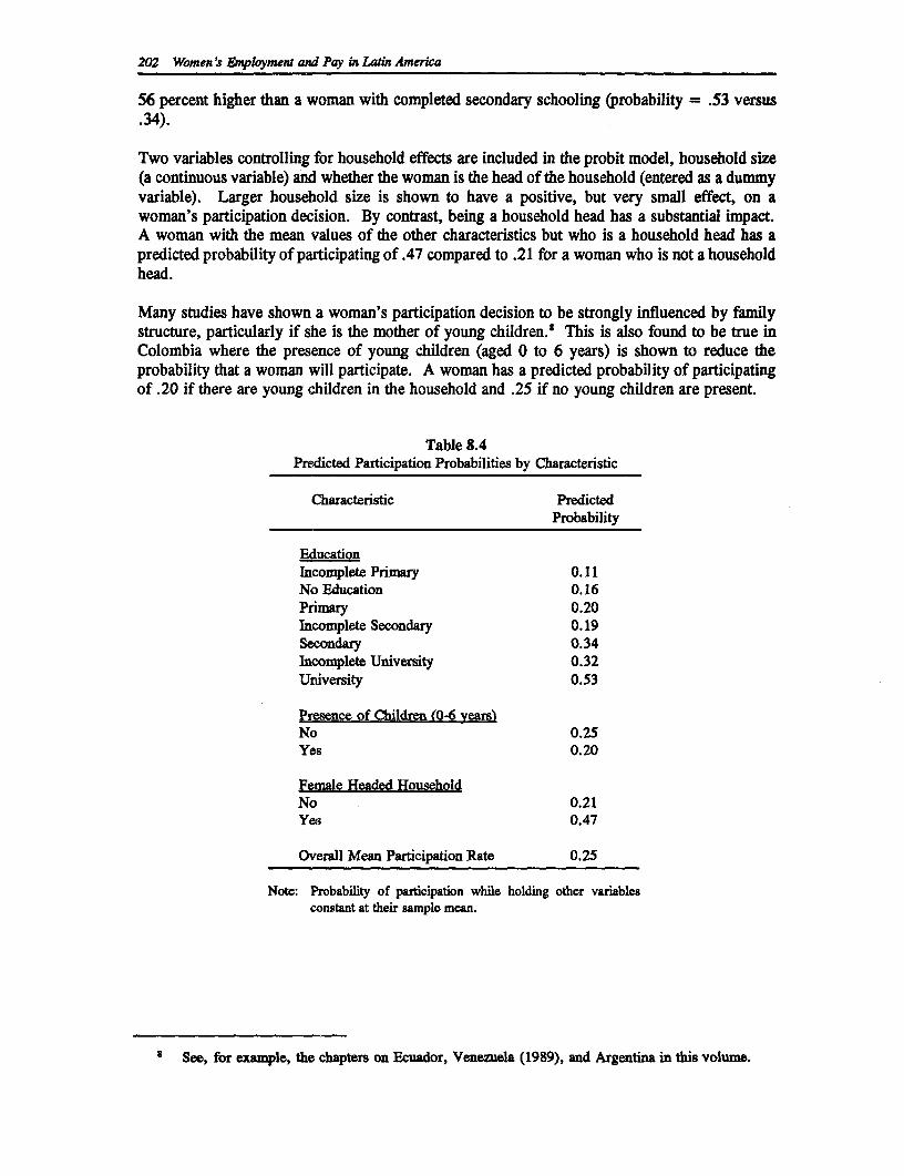
202 Women's Employment and Pay in Latn America
56 percent higher than a woman with completed secondary schooling (probability = .53 versus.34).
Two variables controlling for household effects are included in the probit model, household size(a continuous variable) and whether the woman is the head of the household (entered as a dummyvariable). Larger household size is shown to have a positive, but very small effect, on awoman's participation decision. By contrast, being a household head has a substantial impact.A woman with the mean values of the other characteristics but who is a household head has apredicted probability of participating of .47 compared to .21 for a woman who is not a householdhead.
Many studies have shown a woman's participation decision to be strongly influenced by familystructure, particularly if she is the mother of young children.' This is also found to be true inColombia where the presence of young children (aged 0 to 6 years) is shown to reduce theprobability that a woman will participate. A woman has a predicted probability of participatingof .20 if there are young children in the household and .25 if no young children are present.
Table 8.4Predicted Participation Probabilities by Characteristic
Characteristic PredictedProbability
EducationIncomplete Primary 0.11No Education 0.16Primary 0.20Incomplete Secondary 0.19Secondary 0.34incomplete University 0.32University 0.53
Presence of Children (0-6 years)No 0.25Yes 0.20
Female Headed HouseholdNo 0.21Yes 0.47
Overall Mean Participation Rate 0.25
Note: Probability of participation while holding other variablesconstant at their sample mean.
' See, for example, the chapters on Ecuador, Venezuela (1989), and Argentina in this volume.
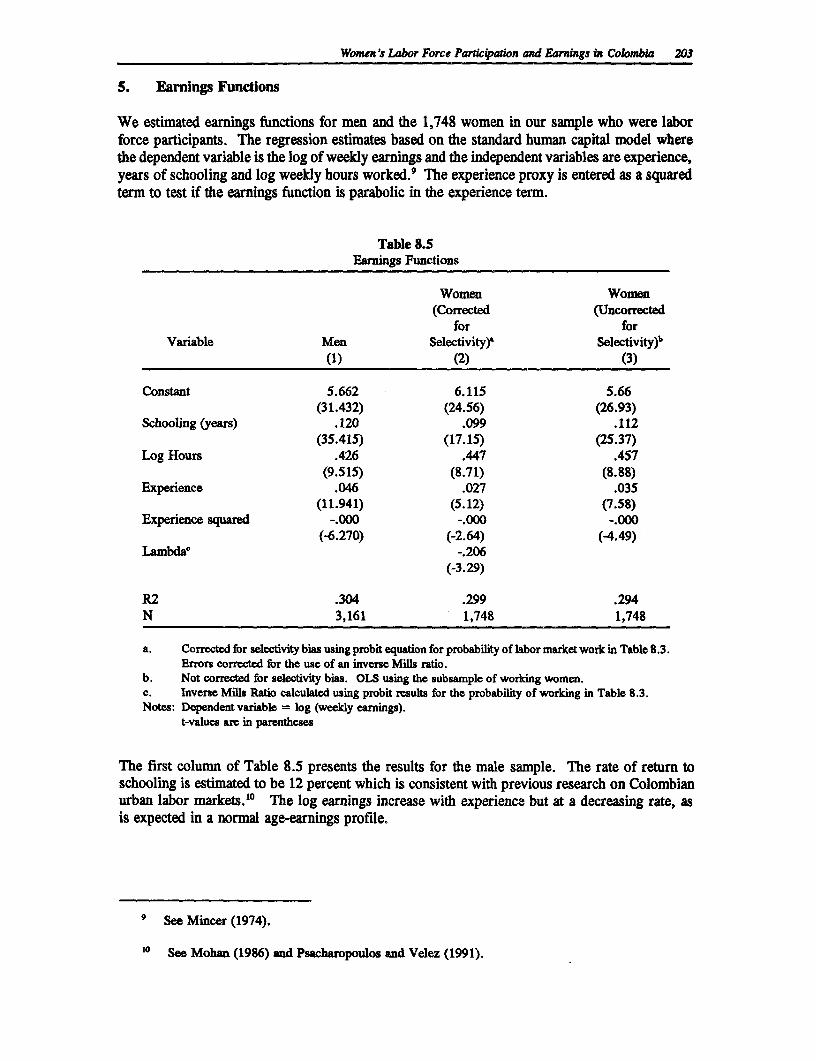
Women's Labor Force Particq,afion and Earnings in Colombia 203
5. Earnings Functions
We estimated earnings functions for men and the 1,748 women in our sample who were laborforce participants. The regression estimates based on the standard human capital model wherethe dependent variable is the log of weekly earnings and the independent variables are experience,years of schooling and log weekly hours worked.9 The experience proxy is entered as a squaredterm to test if the earnings function is parabolic in the experience term.
Table 8.5Earnings Functions
Women Women(Corrected (Uncorrected
for forVariable Men Selectivity)' Selectivity)b
(1) (2) (3)
Constant 5.662 6.115 5.66(31.432) (24.56) (26.93)
Schooling (years) .120 .099 .112(35.415) (17.15) (25.37)
Log Hours .426 .447 .457(9.515) (8.71) (8.88)
Experience .046 .027 .035(11.941) (5.12) (7.58)
Experience squared -.000 -.000 -.000(-6.270) (-2.64) (-4.49)
Lambda' -.206(-3.29)
R2 .304 .299 .294N 3,161 1,748 1,748
a. Corrected for selectivity bias using probit equation for probability of labor market work in Table 8.3.Errors corrected for the use of an inverse Mills ratio.
b. Not corrected for selectivity bias. OLS using the subsample of working women.c. Inverse Mills Ratio calculated using probit rmsults for the probability of working in Table 8.3.Notes: Dependent variable = log (weeldy earnings).
t-values are in parentheses
The first column of Table 8.5 presents the results for the male sample. The rate of return toschooling is estimated to be 12 percent which is consistent with previous research on Colombianurban labor markets.'0 The log earnings increase with experience but at a decreasing rate, asis expected in a normal age-earnings profile.
I See Mincer (1974).
10 See Mohan (1986) and Psacharopoulos and Velez (1991).
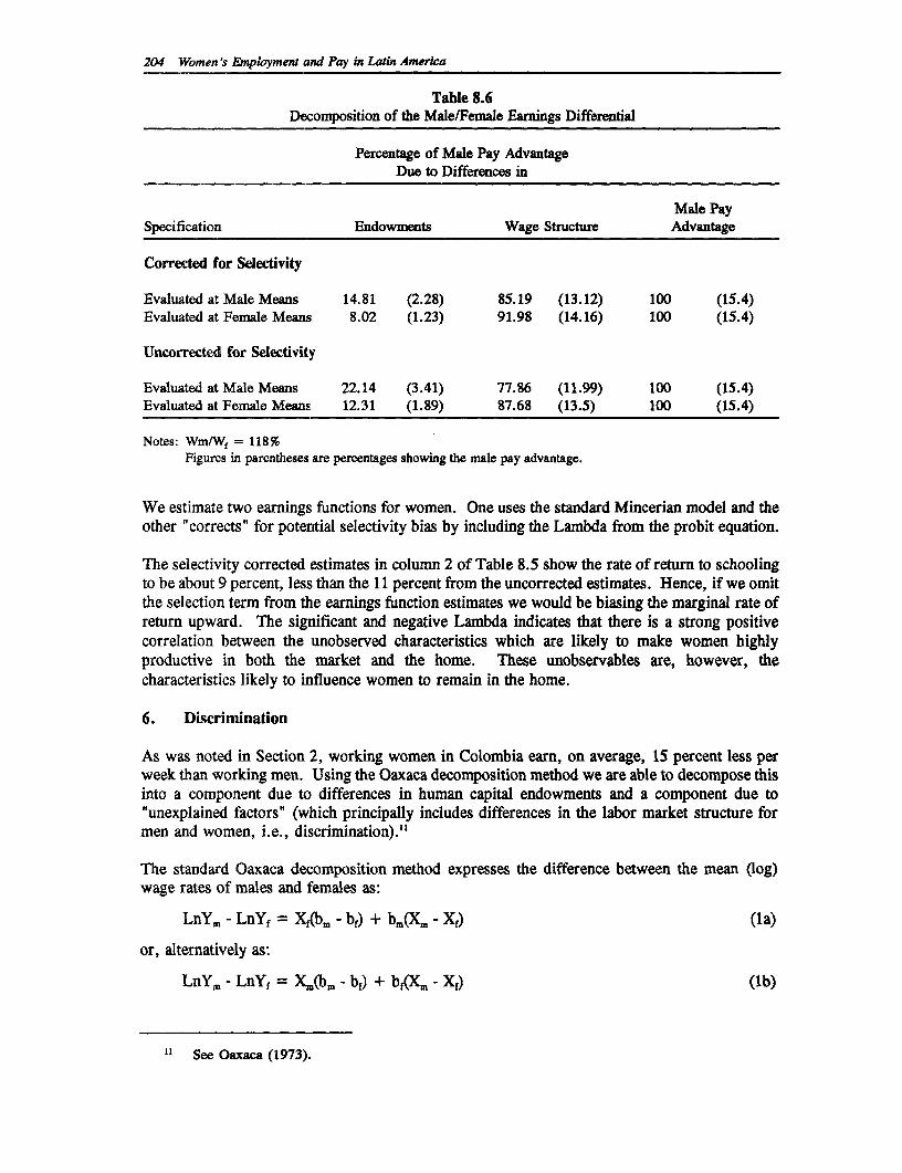
204 Women's Employment and Pay in Latin America
Table 8.6Decomposition of the Male/Female Eamings Differential
Percentage of Male Pay AdvantageDue to Differences in
Male PaySpecification Endowments Wage Structure Advantage
Corrected for Selectivity
Evaluated at Male Means 14.81 (2.28) 85.19 (13.12) 100 (15.4)Evaluated at Female Means 8.02 (1.23) 91.98 (14.16) 100 (15.4)
Uncorrected for Selectivity
Evaluated at Male Means 22.14 (3.41) 77.86 (11.99) 100 (15.4)Evaluated at Female Means 12.31 (1.89) 87.68 (13.5) 100 (15.4)
Notes: Wm[Wf = 118%Figures in parentheses are percentages showing the male pay advantage.
We estimate two earnings functions for women. One uses the standard Mincerian model and theother "corrects" for potential selectivity bias by including the Lambda from the probit equation.
The selectivity corrected estimates in column 2 of Table 8.5 show the rate of return to schoolingto be about 9 percent, less than the 11 percent from the uncorrected estimates. Hence, if we omitthe selection term from the earnings function estimates we would be biasing the marginal rate ofreturn upward. The significant and negative Lambda indicates that there is a strong positivecorrelation between the unobserved characteristics which are likely to make women highlyproductive in both the market and the home. These unobservables are, however, thecharacteristics likely to influence women to remain in the home.
6. Discrimination
As was noted in Section 2, working women in Colombia earn, on average, 15 percent less perweek than working men. Using the Oaxaca decomposition method we are able to decompose thisinto a component due to differences in human capital endowments and a component due to"unexplained factors" (which principally includes differences in the labor market structure formen and women, i.e., discrimination)."
The standard Oaxaca decomposition method expresses the difference between the mean (log)wage rates of males and females as:
LnY. - LnYf = Xf(bm - bf) + bm(Xm - Xf) (la)
or, alternatively as:
LnYm - LnYf = XY.(bm - bf) + bf(Xm - Xf) (lb)
See Oaxaca (1973).
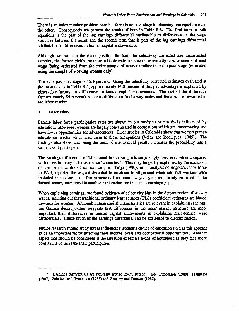
Women 's Labor Force Participation and Earnings in Colombia 205
There is an index number problem here but there is no advantage to choosing one equation overthe other. Consequently we present the results of both in Table 8.6. The first term in bothequations is the part of the log earnings differential attributable to differences in the wagestructure between the sexes and the second term that is part of the log earnings differentialattributable to differences in human capital endowments.
Although we estimate the decomposition for both the selectivity corrected and uncorrectedsamples, the former yields the more reliable estimate since it essentially uses women's offeredwage (being estimated from the entire sample of women) rather than the paid wage (estimatedusing the sample of working women only).
The male pay advantage is 15.4 percent. Using the selectivity corrected estimates evaluated atthe male means in Table 8.5, approximately 14.8 percent of this pay advantage is explained byobservable factors, or differences in human capital endowments. The rest of the difference(approximately 85 percent) is due to differences in the way males and females are rewarded inthe labor market.
7. Discussion
Female labor force participation rates are shown in our study to be positively influenced byeducation. However, women are largely concentrated in occupations which are lower paying andhave fewer opportunities for advancements. Prior studies in Colombia show that women pursueeducational tracks which lead them to these occupations (Velez and Rodriguez, 1989). Thefindings also show that being the head of a household greatly increases the probability that awoman will participate.
The earnings differential of 15.4 found in our sample is surprisingly low, even when comparedwith those in many in industrialized countries.'2 This may be partly explained by the exclusionof non-formal workers from our sample. Tenjo (1990), in an analysis of Bogota's labor forcein 1979, reported the wage differential to be closer to 30 percent when informal workers wereincluded in the sample. The presence of minimum wage legislation, firmly enforced in theformal sector, may provide another explanation for this small earnings gap.
When explaining earnings, we found evidence of selectivity bias in the determination of weeklywages, pointing out that traditional ordinary least squares (OLS) coefficient estimates are biasedupwards for women. Although human capital characteristics are relevant in explaining earnings,the Oaxaca decomposition suggests that differences in the labor market structure are moreimportant than differences in human capital endowments in explaining male-female wagedifferentials. Hence much of the earnings differential can be attributed to discrimination.
Future research should study issues influencing women's choice of education field as this appearsto be an important factor affecting their income levels and occupational opportunities. Anotheraspect that should be considered is the situation of female heads of household as they face moreconstraints to increase their participation.
12 Eamings differentials are typically around 25-30 percent. See Gunderson (1989), Tzannatos(1987), Zabalza and Tzannatos (1985) and Gregory and Duncan (1982).
References
Departamento Administrativo Nacional de Estadfstica (DANE). 50 Aflos de EstadfsticasEducativas. BogotA: Departamento Administrativo Nacional de Estadfstica, 1985.
Gregory, R.G. and R.C. Duncan. "Segmented Labour Market Theories and the AustralianExperience of Equal Pay for Women." Journal of Post-Keynesian Economics, Vol. 3(1982), pp. 403428.
Gronau, R. "Sex-Related Wage Differentials and Women's Interrupted Labor Careers: TheChicken and Egg Question." Journal of Labor Economics, Vol. 6, no. 1 (1988), pp. 277-301.
Gunderson, M. "Male-Female Wage Differentials and Policy Responses." Journal of EconomicLiterature, Vol. 27, no. 1 (1989), pp. 46-117.
Heckman, J. "The Common Structure of Statistical Model Truncation, Sample Selection andLimited Dependent Variables and a Simple Estimator for such Models." Annals ofEconomic and Social Measurement, Vol. 5, no. 4 (1976), pp. 679-694.
Heckman, J. "Sample Selection Bias as a Specification Error." Econometrica, Vol. 47, no. 1(1979), pp. 153-161.
International Labor Office. Yearbook of Labor Statistics: Retrospective Edition, 1950-1990.Geneva: International Labor Office, 1990.
Mincer, J. Schooling, Experience and Earnings. New York: Columbia University Press, 1974.
Mohan, R. Work, Wages, and Welfare in a Developing Metropolis. Consequences of Growthin Bogota, Colombia. New York: Oxford University Press, 1986.
Oaxaca, R. "Male-female Wage Differentials in Urban Labor Markets." International EconomicsReview, Vol. 14, no. 1 (1973), pp. 693-709.
Psacharopoulos, G. and E. Velez. "Schooling, Ability and Earnings in Colombia, 1988."Economic Development and Cultural Change. forthcoming, 1991.
206
Women 's Labor Force Parsicipation and Earnings in Colombia 207
Rico de Alonso, N. 'Caraterfsticas y Condiciones de la Participacidn Laboral Femenina a NivelUrbano en Colombia." Paper presented at the Workshop on Mujer y ParticipacionLaboral. Bogota, April 1990.
Tenjo, J. "Labor Market, Wage Gap and Gender Discrimination: The Case of Colombia."Mimeograph. University of Toronto: Department of Economics, 1990.
Tzannatos, Z. "Equal Pay in Greece and Britain." Industrial Relations Journal, Vol. 18, no. 4(1987), pp. 275-283.
Velez E. and P. Rodriguez, "Mujer y Educaci6n en Colombia." Mimeograph. Instituto SERde Investigaci6n. Bogota, 1989.
Zabalza, A. and Z. Tzannatos, Women and Equal Pay: Ihe Effects of Legislation on FemaleEmployment and Wages in Britain. Cambridge: Cambridge University Press, 1985.

9
Female Labor Force Participation and EarningsDifferentials in Costa Rica
Hongyu Yang
1. Introduction
Over the last decade interest in the treatment of women in the labor markets of developingcountries has increased dramatically, and more attention is being paid to analyzing the labor forcebehavior of women and the returns to human capital, especially education. Do women and menenjoy the same returns to human capital? Is there an earnings differential between working menand women? In the case of Costa Rica, the evidence shows that such a gap exists. Figures 9.1and 9.2 reveal the existence of significant male-female earnings differentials across schooling andage. What factors cause this difference? And how do these factors influence a woman's decisionto participate in the labor force? In this chapter we try to answer these questions. First, wedetermine the earnings differential between male and female workers in Costa Rica. Then weestimate the extent of wage discrimination against females.
In the following section we briefly review the economy and labor market in Costa Rica. InSection 3 we discuss the data used in this study and present the main characteristics of male andfemale labor force participants. In Section 4 we examine labor force participation and the factorsinfluencing women's decision to participate. In Section 5 we analyze the result of the male andfemale earnings functions and the decomposition is carried out in Section 6. In the final sectionwe discuss these findings and their implications.
2. The Costa Rican Economy and the Labor Market
For most of the last twenty-five years economic growth in Costa Rica has generated improvedemployment opportunities for workers. However, during the economic recession in 1981-82,labor market conditions deteriorated countrywide. Fortunately, recession was the exception ratherthan the rule in Costa Rica. Gross domestic product grew by 6.5 percent per annum in the 1960sand by 4.5 percent per annum between 1970 and 1982.
Between 1963 and 1973 the Costa Rican labor force became markedly better educated. Theproportion without education fell from 15 percent to 10 percent, the proportion of illiterates fellby virtually the same percentage, and the proportion with only one to three years of primary-education fell from 37 percent to 26 percent. At the same time the proportion with four to sixyears of primary education increased from 37 percent to 45 percent, the proportion withsecondary education from 9 percent to 16 percent, and the proportion with university educationfrom 2 percent to 4 percent (Fields, 1988). Between 1965 and 1988 the higher education
209
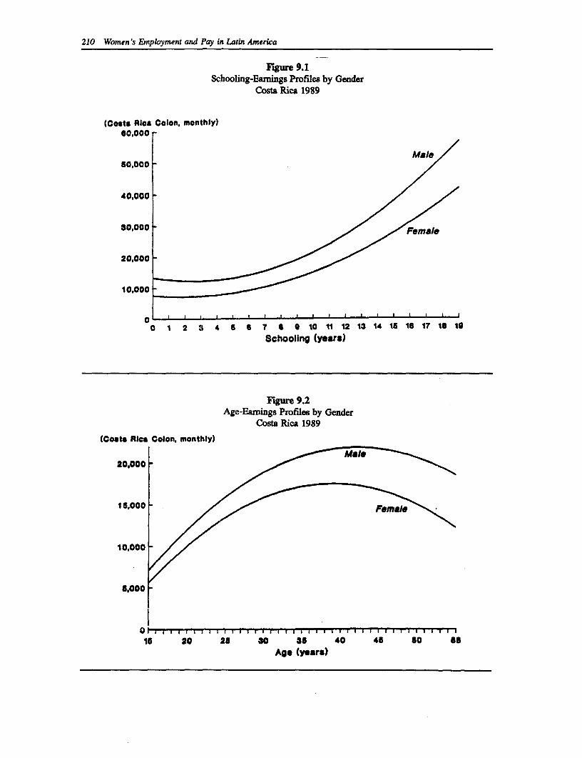
210 Women's Employment and Pay in Latin America
Figure 9.1Schooling-Earnings Profiles by Gender
Costa Rica 1989
(Costs Rica Colon, monthly)eo,ooo -
40,000 -
30,000 -
20,000
10,000
00 1 2 3 4 5 6 7 9 9 10 11 12 13 14 15 16 17 1t 19
Schooling (years)
Fiue 9.2Age-Eamings Profiles by Gender
Costa Rica 1989
(Costa Rloa Colon, monthly)
20,000 -
15,000 /
10,000
6,000
15 20 20 30 35 40 45 50 asAge (years)
Female Labor Force Partdcpaion and Earnings Differentials un Costa Rica 211
enrollment ratio rose from 6 percent to 24 percent and the secondary enrollment ratio increasedfrom 24 percent to 41 percent; primary school enrollment was virtually 100 percent (UNESCO,Statistical Yearbook).
Economic growth has brought more employment opportunities and created enough new jobs tokeep pace with the growth in the labor force. Not only are more people employed, but the mixof jobs has improved in favor of the better-paying categories: Wage-earners in place of unpaidfamily workers; professional, technical, managerial, and office workers rather than manualworkers; manufacturing and other sectors in place of agriculture; public as opposed to privateemployment.
3. Data Characteristics
The data used in this study come from the Encuesta de Hogares de Propositos Multiples (EHPM),a nationwide household survey that is conducted by the Statistics and Census Department of CostaRica. The data were collected in July 1989. The data set contains 34,368 individual observationsfrom 7,637 households. Information is available on personal characteristics of the populationsuch as age, sex, education and area of residence. Employment variables include occupation, jobcategory and hours worked per week. Information exists on labor income, other income andfamily income. From this data set, a total of 15,867 cases were used. This sample included allindividuals in the prime working age range (20 to 60 years) for whom relevant data wereavailable.
Table 9.1 provides descriptive statistics for the main variables in the sample. Working men andworking women are defined as those who worked for more than one hour for pay during thereference week. This definition excludes unpaid family workers. As Table 9.1 shows, thefemale labor force participation rate (27 percent) is significantly lower than that for men (76percent). The marriage rate for working females is lower than for working males, and is muchhigher among non-working females. Working women have less children than non-workingwomen. This suggests that marriage and family have a great influence on female participation.
Table 9.1 also shows great differences in the distribution of men and women by education level.Only 11 percent of working men had completed secondary school compared to 22 percent ofworking women. The largest gap in educational achievement occurs at the university level: Only5 percent of working men have university degrees compared to 11 percent of working women.Overall, the average years of schooling for working females is two years greater than that fortheir male counterparts. This was confirmed elsewhere in a recent study (Gindling, 1991) whichshowed that from 1980 to 1985 the average years of schooling for working women was aboutone and half years more than that of working men. This is typical in Latin America andCaribbean countries.' However, despite the fact that women have more schooling than men,they earn less than males.
Tables 9.2A and 9.2B show the education and earnings differentials by occupation and workingsector in more detail. Women's schooling is higher than men's in all occupational categoriesexcept two: Managers and service workers. Women's average earnings, however, are lower thanmen's in all occupational categories. In the public sector females have an average of
I In Argentina average schooling for working females is 9.4 years, while for working men it is 8.8years; and in Venezuela, average years of schooling are 8.5 and 6.9 for working females and malesrespectively.
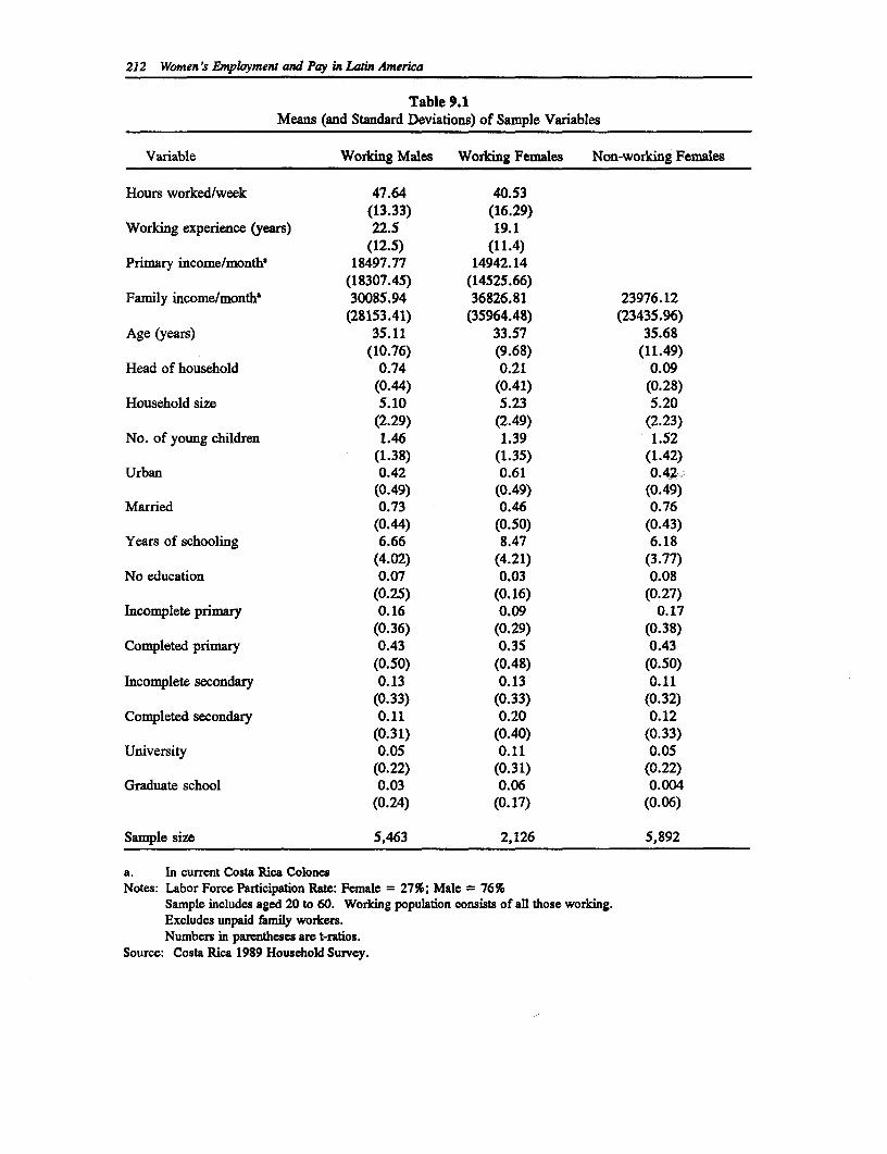
212 Women's Employment and Pay in Latin America
Table 9.1Means (and Standard Deviations) of Sample Variables
Variable Working Males Working Females Non-working Females
Hours worked/week 47.64 40.53(13.33) (16.29)
Working experience (years) 22.5 19.1(12.5) (11.4)
Primary income/month' 18497.77 14942.14(18307.45) (14525.66)
Family income/montha 30085.94 36826.81 23976.12(28153.41) (35964.48) (23435.96)
Age (years) 35.11 33.57 35.68(10.76) (9.68) (11.49)
Head of household 0.74 0.21 0.09(0.44) (0.41) (0.28)
Household size 5.10 5.23 5.20(2.29) (2.49) (2.23)
No. of young children 1.46 1.39 1.52(1.38) (1.35) (1.42)
Urban 0.42 0.61 0.42=.(0.49) (0.49) (0.49)
Married 0.73 0.46 0.76(0.44) (0.50) (0.43)
Years of schooling 6.66 8.47 6.18(4.02) (4.21) (3.77)
No education 0.07 0.03 0.08(0.25) (0.16) (0.27)
Incomplete primary 0.16 0.09 0.17(0.36) (0.29) (0.38)
Completed primary 0.43 0.35 0.43(0.50) (0.48) (0.50)
Incomplete secondary 0.13 0.13 0.11(0.33) (0.33) (0.32)
Completed secondary 0.11 0.20 0.12(0.31) (0.40) (0.33)
University 0.05 0.11 0.05(0.22) (0.31) (0.22)
Graduate school 0.03 0.06 0.004(0.24) (0.17) (0.06)
Sample size 5,463 2,126 5,892
a. In current Costa Rica ColonesNotes: Labor Force Participation Rate: Femnale = 27%; Male = 76%
Sample includes aged 20 to 60. Working population consists of all those working.Excludes unpaid family workers.Numbers in parentheses are t-ratios.
Source: Costa Rica 1989 Household Survey.
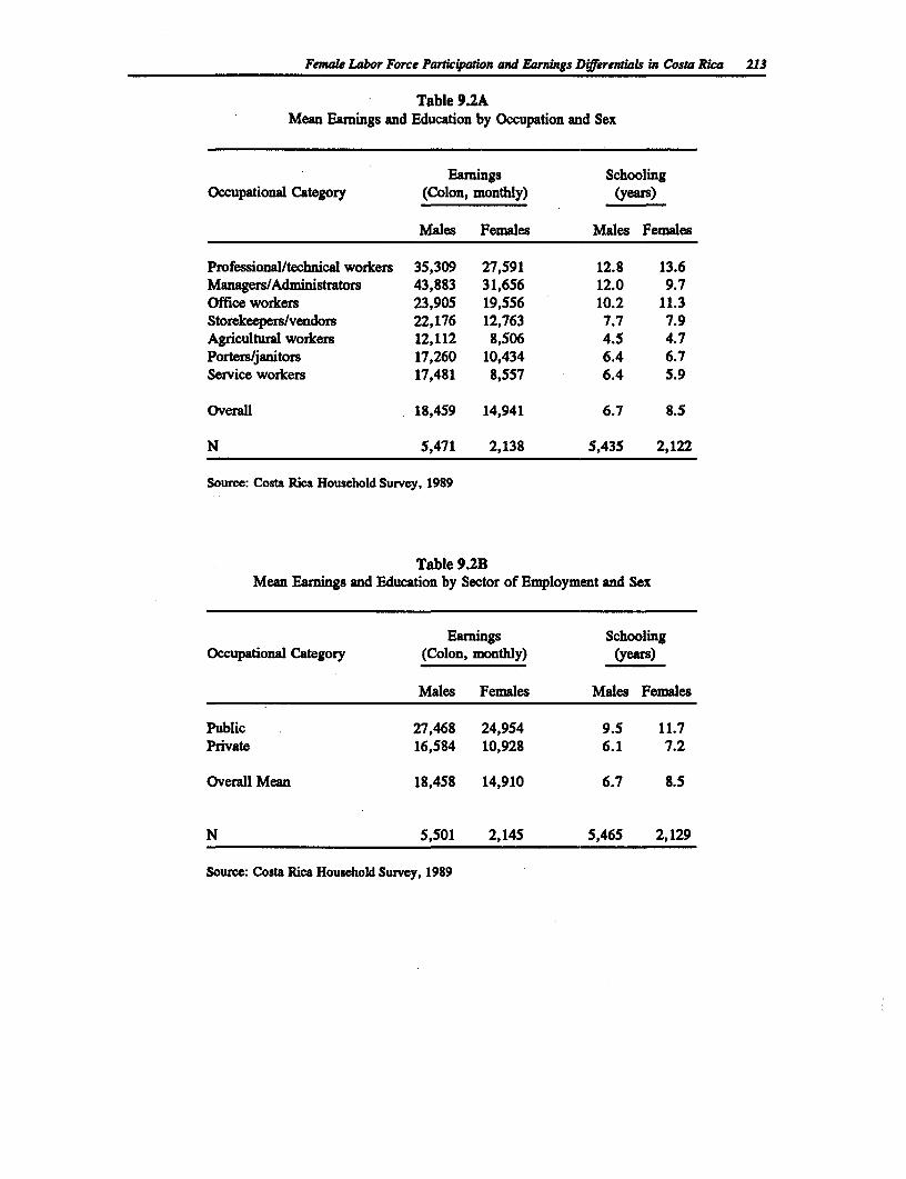
Fenale Labor Force Particiatwon and Earnings Differenials in Costa Rica 213
Table 9.2AMean Earnings and Education by Occupation and Sex
Earnings SchoolingOccupational Category (Colon, monthly) (years)
Males Females Males Females
Professional/technical workers 35,309 27,591 12.8 13.6Managers/Administrators 43,883 31,656 12.0 9.7Office workers 23,905 19,556 10.2 11.3Storekeepers/vendors 22,176 12,763 7.7 7.9Agricultural workers 12,112 8,506 4.5 4.7Porters/janitors 17,260 10,434 6.4 6.7Service workers 17,481 8,557 6.4 5.9
Overall 18,459 14,941 6.7 8.5
N 5,471 2,138 5,435 2,122
Source: Costa Rica Household Survey, 1989
Table 9.2BMean Eanings and Education by Sector of Employment and Sex
Earnings SchoolingOccupational Category (Colon, monthly) (years)
Males Females Males Females
Public 27,468 24,954 9.5 11.7Private 16,584 10,928 6.1 7.2
Overall Mean 18,458 14,910 6.7 8.5
N 5,501 2,145 5,465 2,129
Source: Costa Rica Household Survey, 1989
214 Women's Employment and Pay in Ladin America
two more years of schooling than males, and in private sector one year more. Nevertheless,women make 65.9 percent of men's earnings in the private sector and 90.8 percent in the publicsector.
4. The Determinants of Female Labor Force Participation
As is commonly known, the major factors which influence women's labor market activity areeducational attainment, marital status, fertility, "need" for income (which is measured byhusband's income, family income excluding female's earnings, the number of earners in a familyand the household status of women) and age.
Whether women participate in the labor force or not depends on those factors and theirreservation wage. That is, when a woman searches in the labor market for a job, she will havesome idea of the wage she desires or merits, based on her value at home or her previous wage.She can thus be viewed as setting a minimum standard for jobs she will find acceptable. She willaccept a job that pays above this critical value and reject offers below this value.
This means that our sample of working women are self-selected. Therefore, if we use this non-random sample to estimate the earnings function for female workers, the result will be biased.Non-working women are unobserved. In order to correct for this selectivity bias, we use thewell-known two-step method proposed by Heckman (1979). A probit equation is used to estimatethe probability of a woman being in the work force and the inverse Mill's ratio (Lambda) iscomputed and added to the earnings function as an additional regressor.
In the probit work participation functions, age and schooling are entered as a series of dummyvariables for each age group (in 5 years cohorts) and each level of schooling. This is to take intoaccount any non-linearity in the effect of either age or schooling on participation. Other dummyvariables in this model are marital status, residential area, and being a head of household.Number of young children and household size are continuous variables.
Table 9.3 presents the results of probit estimates for female work participation. Using thoseresults we predict the probability of labor force participation for each characteristic (Table 9.4).As expected, women with incomplete primary education are less likely to participate in the laborforce. At the completed primary level, however, educational attainment does not have asignificant impact on participation. This is explained by the fact that about 50 percent of womenare service workers and 30 percent are blue collar workers. This implies that the value ofeducation credentials in the informal sector is limited. A similar situation exists in Bolivia.
The other education levels show a positive significant impact on participation. Secondary schoolgraduates have an estimated participation probability that is 14 percentage points higher thanincomplete primary school graduates. University graduates have a participation probability 21percentage points higher than the graduates with some primary education. Graduate schoolgraduates have the highest participation probability of all (54.2 percentage).
Married women participate less than unmarried women, 17.7 percent versus 40.4 percent. Thisreflects the fact that married women are likely to withdraw from the labor force if they haveyoung children. The variable Presence of Children shows the difference among number ofchildren. The more children a woman has, the less likely she is to participate in the labor force.Being a household head is also associated with a higher participation probability than that of non-household head.
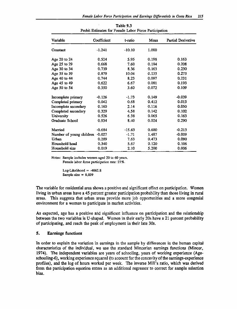
Female Labor Force Participation and Earnings Diferentials in Costa Rica 215
Table 9.3Probit Estimates for Female Labor Force Participation
Variable Coefficient t-ratio Mean Partial Derivative
Constant -1.241 -10.10 1.000
Age 20 to 24 0.524 5.95 0.198 0.163Age 25 to 29 0.668 7.60 0.184 0.208Age 30 to 34 0.739 8.36 0.163 0.230Age 35 to 39 0.879 10.04 0.133 0.273Age 40 to 44 0.744 8.23 0.097 0.231Age 45 to 49 0.622 6.67 0.081 0.193Age 50 to 54 0.350 3.60 0.072 0.109
Incomplete primary -0.126 -1.73 0.149 -0.039Completed primary 0.042 0.68 0.412 0.013Incomplete secondary 0.160 2.14 0.116 0.050Completed secondary 0.329 4.58 0.142 0.102University 0.526 6.38 0.065 0.163Graduate School 0.934 8.40 0.024 0.290
Married -0.684 -15.63 0.680 -0.213Number of young children -0.027 -1.71 1.487 -0.009Urban 0.289 7.63 0.473 0.090Household head 0.340 5.67 0.120 0.106Household size 0.019 2.10 5.200 0.006
Notes: Sample includes women aged 20 to 60 years.Female labor force participation rate: 27%.
Log-Likelihood = 4062.8Sample size = 8,039
Tlhe variable for residential area shows a positive and significant effect on participation. Womenliving in urban areas have a 45 percent greater participation probability than those living in ruralareas. This suggests that urban areas provide more job opportunities and a more congenialenvironment for a woman to participate in market activities.
As expected, age has a positive and significant influence on participation and the relationshipbetween the two variables is U-shaped. Women in their early 20s have a 21 percent probabilityof participating, and reach the peak of employment in their late 30s.
5. Earnings functions
In order to explain the variation in earnings in the sample by differences in the human capitalcharacteristics of the individual, we use the standard Mincerian earnings functions (Mincer,1974). The independent variables are years of schooling, years of working experience (Age-schooling-6), working experience squared (to account for the concavity of the earnings-experienceprofiles), and the log of hours worked per week. The inverse Mill's ratio, which was derivedfrom the participation equation enters as an additional regressor to correct for sample selectionbias.
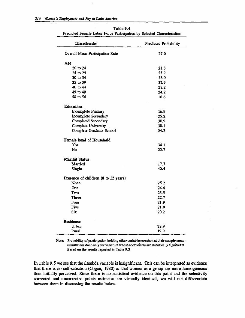
216 Women's Employment and Pay in Latin America
Table 9.4Predicted Female Labor Force Participation by Selected Characteristics
Characteristic Predicted Probability
Overall Mean Participation Rate 27.0
Age20 to 24 21.325 to 29 25.730 to 34 28.035 to 39 32.940 to 44 28.245 to 49 24.250 to 54 16.6
Education.Incomplete Primary 16.9Incomplete Secondary 25.2Completed Secondary 30.9Complete University 38.1Complete Graduate School 54.2
Female head of HouseholdYes 34.1No 22.7
Marital StatusMarried 17.7Single 40.4
Presence of children (0 to 12 years)None 25.2One 24.4Two 23.5Three 22.7Four 21.9Five 21.0Six 20.2
ResidenceUrban 28.9Rural 19.9
Note: Probability of participation holding other variables constant at their sample mean.Simulations done only for variables whose coefficients are statistically significant.Based on the results reported in Table 9.3
In Table 9.5 we see that the Lambda variable is insignificant. This can be interpreted as evidencethat there is no self-selection (Cogan, 1980) or that women as a group are more homogeneousthan initially perceived. Since there is no statistical evidence on this point and the selectivitycorrected and uncorrected points estimates are virtually identical, we will not differentiatebetween them in discussing the results below.
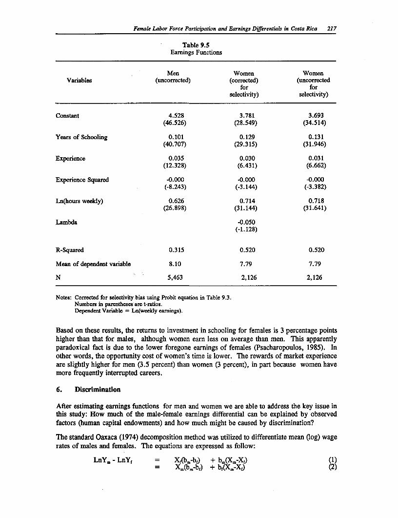
Female Labor Force Participation and Earnings Diffierentials in Costa Rica 217
Table 9.5Earnings Functions
Men Women WomenVariables (uncorrected) (corrected) (uncorrected
for forselectivity) selectivity)
Constant 4.528 3.781 3.693(46.526) (28.549) (34.514)
Years of Schooling 0.101 0.129 0.131(40.707) (29.315) (31.946)
Experience 0.035 0.030 0.031(12.328) (6.431) (6.662)
Experience Squared -0.000 -0.000 -0.000(-8.243) (-3.144) (-3.382)
Ln(hours weekly) 0.626 0.714 0.718(26.898) (31.144) (31.641)
Lambda -0.050(-1.128)
R-Squared 0.315 0.520 0.520
Mean of dependent variable 8.10 7.79 7.79
N 5,463 2,126 2,126
Notes: Corrected for selectivity bias using Probit equation in Table 9.3.Numbers in parentheses are t-ratios.Dependent Variable = Ln(weekly earnings).
Based on these results, the returns to investment in schooling for females is 3 percentage pointshigher than that for males, although women earn less on average than men. This apparentlyparadoxical fact is due to the lower foregone earnings of females (Psacharopoulos, 1985). Inother words, the opportunity cost of women's time is lower. The rewards of market experienceare slightly higher for men (3.5 percent) than women (3 percent), in part because women havemore frequently interrupted careers.
6. Discrimination
After estimating earnings functions for men and women we are able to address the key issue inthis study: How much of the male-female earnings differential can be explained by observedfactors (human capital endowments) and how much might be caused by discrimination?
The standard Oaxaca (1974) decomposition method was utilized to differentiate mean (log) wagerates of males and females. The equations are expressed as follow:
LnYm - LnYf = Xf(bm-bf) + bm(Xm-Xf) (1)= Xm(bm-bf) + bf(Xm-Xf) (2)
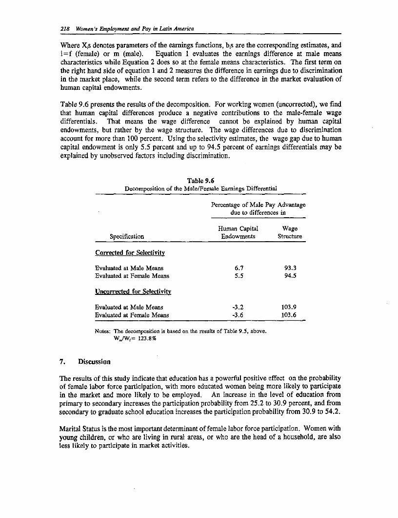
218 Women's Employment and Pay in Latin America
Where X1s denotes parameters of the earnings functions, bis are the corresponding estimates, andi=f (female) or m (male). Equation 1 evaluates the earnings difference at male meanscharacteristics while Equation 2 does so at the female means characteristics. The first term onthe right hand side of equation 1 and 2 measures the difference in earnings due to discriminationin the market place, while the second term refers to the difference in the market evaluation ofhuman capital endowments.
Table 9.6 presents the results of the decomposition. For working women (uncorrected), we findthat human capital differences produce a negative contributions to the male-female wagedifferentials. That means the wage difference cannot be explained by human capitalendowments, but rather by the wage structure. The wage differences due to discriminationaccount for more than 100 percent. Using the selectivity estimates, the wage gap due to humancapital endowment is only 5.5 percent and up to 94.5 percent of earnings differentials may beexplained by unobserved factors including discrimination.
Table 9.6Decomposition of the Male/Female Earnings Differential
Percentage of Male Pay Advantagedue to differences in
Human Capital WageSpecification Endowments Structure
Corrected for Selectivitv
Evaluated at Male Means 6.7 93.3Evaluated at Female Means 5.5 94.5
Uncorrected for Selectivity
Evaluated at Male Means -3.2 103.9Evaluated at Female Means -3.6 103.6
Notes: The decomposition is based on the results of Table 9.5, above.W./W,= 123.8%
7. Discussion
The results of this study indicate that education has a powerful positive effect on the probabilityof female labor force participation, with more educated women being more likely to participatein the market and more likely to be employed. An increase in the level of education fromprimary to secondary increases the participation probability from 25.2 to 30.9 percent, and fromsecondary to graduate school education increases the participation probability from 30.9 to 54.2.
Marital Status is the most important determinant of female labor force participation. Women withyoung children, or who are living in rural areas, or who are the head of a household, are alsoless likely to participate in market activities.
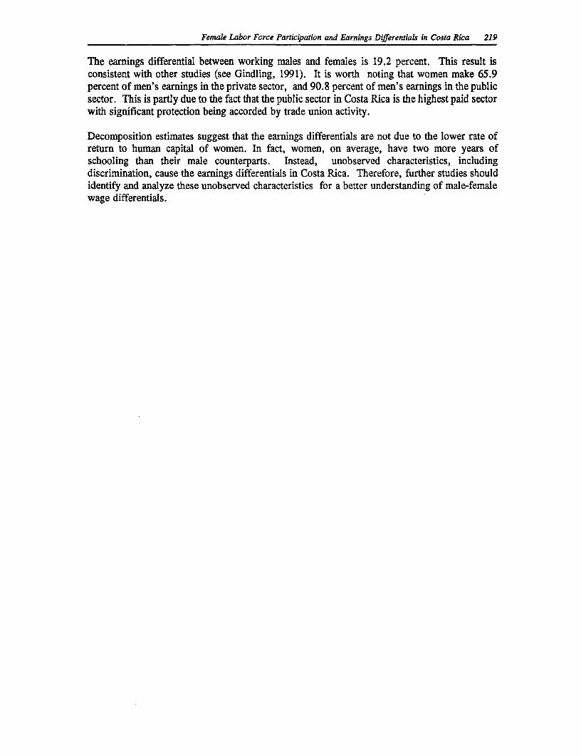
Female Labor Force Participation and Earnings Differentials in Costa Rica 219
The earnings differential between working males and females is 19.2 percent. This result isconsistent with other studies (see Gindling, 1991). It is worth noting that women make 65.9percent of men's earnings in the private sector, and 90.8 percent of men's earnings in the publicsector. This is partly due to the fact that the public sector in Costa Rica is the highest paid sectorwith significant protection being accorded by trade union activity.
Decomposition estimates suggest that the earnings differentials are not due to the lower rate ofreturn to human capital of women. In fact, women, on average, have two more years ofschooling than their male counterparts. Instead, unobserved characteristics, includingdiscrimination, cause the earnings differentials in Costa Rica. Therefore, further studies shouldidentify and analyze these unobserved characteristics for a better understanding of male-femalewage differentials.
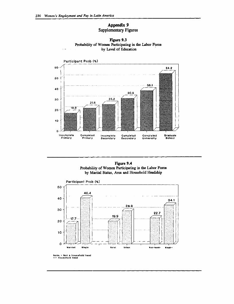
220 Women 's Employment and Pay in Latin Amerca
Appendix 9Supplementary Figures
Figure 9.3Probability of Women Participating in the Labor Force
by Level of Education
Participant Prob (%)
60 - 64.2
60 .
40-
20-
10
0 Incomplete Completed Incomplete Completed Completed Graduate
Primary Primary Secondary Secondary Univeraity School
Figure 9.4Probability of Women Participating in the Labor Force
by Marital Status, Area and Household Headship
Participant Prob (%)
50 -S0- , ~40.4
40 . 34.1
30 -22.7
20 -
10
0 Mautied B ru.lI Urbac No"-hoad. Hood.-
Note: * Not a household headHousehold head
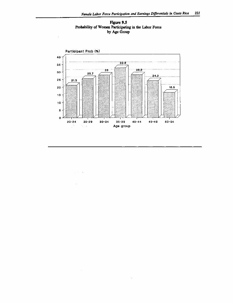
Female Labor Force Participation and Earnings Differentials in Costa Rica 221
Fgu 9.5Probability of Women Participating in the Labor Force
by Age Group
Participant Prob (%)
40
35 - 32.9
30-
25 21.3
20 -16.8
15
10
20-24 25-29 30-34 35-39 40-44 45-49 50-54
Age group
References
Cogan, J. "Married Women's Labor Supply: A Comparison of Alternative Estimates" in J.P.Smith (ed.) Female Labor Supply: Theory and Estimation. Princeton, NJ: PrincetonUniversity Press, 1980.
Gindling, T.H. "Women Wage and Economic Crisis in Costa Rica." 1991 (Forthcoming),University of Maryland: Dept. of Economics.
Fields, G.S. "Employment and Economic Growth in Costa Rica." World Development, Vol. 16,no. 12 (1988). pp 1493-1507.
Hackman, J. "Sample Selection as a Specification Error." Econometrica, Vol. 47, no. 1 (1979).pp 153-161.
Mincer, J. Schooling, Experience and Earnings. New York: Columbia University Press, 1974.
Oaxaca, R.L. "Male-female Wage Differentials in Urban Labor Markets." InternationalEconomic Review, Vol. 14, no. 1 (1974). pp. 693-709.
Psacharopoulos, G. "Returns to Education: A Further International Update and Implications."Journal of Hunan Resources, Vol. 20, no.4 (1985). pp 583-604.
UNESCO, Statistical Yearbook, New York: UNESCO (1976, 1990).
222
10
Why Women Earn Less Than Men in Costa Rica
T. H. Gindling
1. Introduction
In Costa Rica, men earn higher wages than women on average. In 1989, within the CentralValley (the focus of this chapter) men's wages were, on average, 3.5 percent higher thanwomen's.' The difference between the average wages of men and women in Costa Rica is lowerthan that for any other country reported in this volume.
In this chapter we measure the impact of differences in observable human capital endowmentsand different access to higher paying jobs for men and women on the male-female wage gap.These two potential sources of wage differences are not mutually exclusive. For example, mencould have access to higher paying jobs because they have higher levels of education, and higherpaying jobs require more educated workers. Therefore, we will explicitly measure the degreeto which access to higher paying jobs is caused by differences in endowments. In addition, wewill measure that part of the male-female wage differential which is attributable to women beingpaid differently than men with the same endowments in similar jobs. We will also measure thepart of the differences in male and female wages unexplained by differences in observed humancapital endowments. While this difference is often used as a measure of labor marketdiscrimination, we are unable to distinguish discrimination from unmeasured gender differencesin tastes, human capital or ability. Nor can we distinguish differences in wages due todiscrimination from compensating differentials. Similarly, we cannot distinguish which part ofthe differential unexplained by differences in observed endowments is due to pre-labor marketdiscrimination or tastes.2
i These data are from the Household Surveys of Employment and Unemployment for 1989. Forthe country as a whole, an average man earned wages that were also 3.5 percent higher than an averagewoman's. According to the Household Surveys of Employment and Unemployment for 1987 and 1988,in 1988 the male-female wage differential was 4.4 percent for the country as a whole and 9.8 percent forthe Central Valley, and in 1987 the male-female wage differential was 8.6 percent for the country as awhole and 6.5 percent for the Central Valley.
2 This technique for measuring labor market discrimination is sometimes called the 'residualdifference" method. Beginning with Oaxaca (1973) many studies of male-female earings and wagedifferences have used this methodology. In recent literature reviews, Cain (1986) and Gunderson (1989)exhaustively list and discuss the difficulties with using this as a measure of labor market discrimination.Carvajal and Geithman (1983) and Gindling (1990, 1989a) have addressed the issue of male-female wagedifferentials in Costa Rica. The present study extends these analyses. We measure differences betweenmale and female wages due to differences in human capital and differences in access to higher paying jobs.
223
224 Women's Employment and Pay in Latin America
2. The Costa Rican Labor Market and Women
In Costa Rica the economic expansion of the late 1970's gave way, in the early 1980's, to thedeepest recession since the 1930's.3 GNP stagnated between 1979 and 1980 and fell in 1981 and1982. Increased borrowing by the Central Government and Central Bank to finance increasedspending and an overvalued exchange rate caused foreign public debt to more than doublebetween 1978 and 1981. In December of 1980 the colon was devalued. This was followed bya dramatic increase in inflation (from 18.1 percent in 1980 to 90.1 percent in 1982) and a steepdecline in real earnings (35 percent from July 1980 to July 1982). The unemployment rate rosesteadily from 1979 and reached a peak of 9.4 percent in July 1982. Underemployment alsoincreased, from 4.7 percent of the labor force in 1979 to 7.0 percent in 1982.
In mid-1982 the government instituted a package of policies intended to stabilize and reviveconfidence in the economy. By mid-1983 the economy had entered into a period of recovery.Rising terms of trade, increased foreign aid and the stabilization policies combined to bring aboutincreases in the GDP, lower inflation and higher real earnings. By 1986, real earnings hadnearly regained 1980 levels and GDP growth reached 5.5 percent. Between 1986 and 1989, GDPgrowth averaged 4.5 percent and unemployment and inflation rates remained low.
Gindling (1990, 1989a) notes that the male-female wage and earnings differentials increasedbetween 1980 and 1982, but then fell to pre-recession levels by 1986. Results in Gindling (1990,1989a) suggest that the increase in the male-female wage differential during the recession wasprimarily due to secondary family workers entering the labor force to compensate for the fallingearnings of the family's primary worker (the "added worker" effect). These entrants weredisproportionately female and had lower levels of education than women already in the laborforce. After the recession, these secondary family workers left the labor force.
Starting in 1984 Costa Rica began a comprehensive structural adjustment program. The aim wasto increase and diversify exports (Lizano, 1990). In particular, so-called "non-traditional"exports were encouraged through breaks, subsidies and technical assistance. "Non-traditional"exports included any export that was neither coffee, bananas, sugar or beef, and which was notexported to a Central American Common Market country. By 1990, the majority of Costa Rica'sexports (by value) were "non-traditional exports. " Most successful "non-traditional exports" havebeen agricultural goods (for example, flowers, ornamental plants and pineapples). However,some manufacturing products have become important exports, most notably textiles and electronicassembly. It is likely that women are disproportionately represented in this sector, particularlyin the textile and electronic assembly industries. However, no data are available to verify thissupposition.4
Recently, the legislature of Costa Rica passed the Law for the Promotion of the Social Equalityof Women, the most comprehensive law of its kind in Latin America. The first article of thislaw states that "it is the obligation of the state to promote and guarantee the equality of rightsbetween men and women in the political, economic, social and cultural arenas." However, by1989, the year studied in this chapter, the law was not yet implemented.
3 The 1975-78 period was characterized by the rapid growth of Gross Domestic Product andAggregate Demand, financed by a large increase in the price of coffee. In 1978 the terms of trade begandeclining from its 'coffee boom" high. Driven largely by a fall in the price of coffee, terms of tradecontinued to fall until 1982.
4 See Gindling and Berry (1990) and Tardanico (1992) for a more comprehensive discussion of theCosta Rican labor market in the 1980's.
1Wy Women Earn Less Than Men in Costa Rica 225
3. The Methodology
We will assume the mean natural logarithm of wages of men and women (W;) can be representedby the wage equations:
Wi = Bi.Xi'(1)
where i= Male (M) and Female (F), Bi is a vector of parameters to be estimated, and Y. is avector of the average endowments (wage-determining personal characteristics) for men andwomen, including human capital endowments such as years of education, type of education,experience and other variables. The difference in mean natural logarithm of wages of men andwomen can be decomposed as follows:
WM - WF = BM' XM XF) + W-M B)'_F (2)= E + U
where XM is a vector of average endowments for men and & is a vector of the averageendowments for women. E is the part of difference between the average wages of men and theaverage wages of women explained by differences in endowments. U is the part not explainedby differences in endowments; it is the difference between what women earn now and whatwomen would earn if women faced the same wage-determination structure as men. U might beconsidered a rough measure of the difference in wages between men and women due to labormarket discrimination. However, difficulties with interpreting U as the difference due todiscrimination are well documented (for example, see Cain, 1986).5 At this we will alsoexplicitly measure the impact of each endowment on the male-female wage differential.
We also describe a method for measuring the part of the male-female wage differential due todifferences between men and women in access to good jobs. This method was first developed byBrown, Moon and Zoloth (1980). Let the probability that a man or woman (i) is found workingin a given job 0) be represented by Pu. Assume that the mean natural logarithm of wages of menand women in each job can be represented by:
;= B_'X (3)
The difference in average wages between men and women can be decomposed into:
WM - WF -jwFJXM;JXB n_jI)) + EjMj XMJ[PWj-PFjD) (4)
=W + J
where J is the part of the average wage differential due to differences between men and womenin access to jobs that pay higher wages, and W is the part due to differences in the pay that menand women earn within the same jobs.
5 An altemative decomposition would be to measure U as the difference between the wages meneam now and the wages men would eam if men faced the same wage-determining structure as women.In this case equation one would be:
WM -WF ='(M -XF) + LM- Bp)'XM (2a)= E + U
I also estimate this formulation of E and U. I report these in a footnote in Section 5. Cotton (1988) arguesthat to measure discrimination U should measure the difference in wages that would exist between men andwomen in the absence of discrimination. He argues that the best measure of discrimination would be:
WM -WF =B'LM - XF) + [@M - B-)'L + _)' XF] (2b)- E + U
where B.. BPM + BFPF where PM and Pf are the sample proportions of women and men. We do notpresent estimates of these statistics because they become cumbersome when we attempt to measuredifferences due to different access to high paying jobs.
226 Women's Employment and Pay in Latin America
Let P measure the probability that women in the sample would be found in sector j if faced withthe same job-assignment structure as men. PFj is estimated by assuming that:
P^fn= exppffKmZma (5)Ek expv,,'.Z.)
where P,fn is the probability that each man, n, is found in job j, i is a vector of endowmentsfor each man, n, KJ is a vector of parameters to be estimated (for men) and k = all jobs. Xis estimated using the logit technique and then:
p -pE M Z iS calculated for each female worker, n,Ek expC;N ZF.)
and sector, j (where ZFn is a vector of personal characteristics for each woman, n.) The meanof 1Fj in each sector is PFj. Adding and subtracting 'XFj PFj and B hXF PF from equation 3one oltains:
W -WF (6)w;& j[M XFj-%BF9XFj]D + FIj(PFJRwJM5 4 BM 'XFj]) +
S + b[PFJ J]) + ;j +
JU + JE
where WE is the part of the W explained by differences in endowments, WU is the part of Wunexplained by differences in endowments, JE is the part of J explained by differences inendowments, and JU is the part of J unexplained by differences in endowments. WU can beconsidered a rough approximation of wage discrimination against women, while JU can be canbe considered a rough approximation of job discrimination.6
6 Job discrimination is considered to be the situation where qualified women are kept out of higherpaying jobs. Wage discrimination is considered to be the situation where women are paid less than equallyqualified men in the same jobs.
WU is a weighted average of the difference between what women earn now in each job and whatwomen would eam in each job if they were paid according to the same wage structure as men. JU is thewage differential between what women eam now and what they would eam if women faced the same jobassignment structure as men. An alternative measure, analogous to the measure discussed in the lastfootnote, is to construct WU as the difference between the wages men earn now in each job and the wagesmen would earn if they were paid according to the wage determining structure of women, and to constructJU as the wage differential between what men earn now and what men would eam if they faced the samejob assignment structure as women. That is, estimate KFj using the logit technique calculate:
ji = K'Zji for each male worker, i, and
EKFkiZMli
sector, j. The mean of PMji in each sector is P. Then add and subtract BFj'XmjPMj and ^,FJ'X; from:
WM - WF E(PM.5 'Xi-JBFjX) + @F XFjP PF]D (4a)+ JM
to obtain:WM - WF =j (PMjw'Xmj -BFj XMJ]) + Ej(PMj[DXj LIj RFj XFjD + (6a)
(Fj XFj[PMj-PMjI) + Ej(BFj XFJPWj PFJD
=WEU + WE +JU + JE
These estimates are presented in a footnote in Section 5.
Why Women Earn Less Than Men in Costa Rica 227
4. The Data and Specification of the Variables
The data used to estimate the decompositions described in Section 3 are from the HouseholdSurvey of Employment and Unemployment conducted by the Statistics and Census Departnentof the Costa Rican government. The Household Survey is conducted annually and we use themost recent survey available, 1989. The survey provides reliable data on wages, some jobcharacteristics and some personal characteristics of workers. We use data from the CentralValley of Costa Rica to control for labor market conditions which may vary across regions andaffect male-female differentials. The Central Valley includes the two largest cities in the country,San Jose and Alajeula, as well as two of the next four largest cities, Heredia and Cartago. Thecities in the Central Valley are all within commuting distance of one another, and are expectedto comprise a unified labor market. Over 60 percent of the Costa Rican labor force works in theCentral Valley.
The literature on labor market segmentation (for example, Piore, 1971) justifies dividing the labormarket into sectors. In segmented labor markets some workers are in "formal" sector jobs whereworking conditions are better and status and wages are higher than in the "informal" sectors.Access to formal sector jobs is limited and formal sector workers are protected from competitionfrom informal sector workers by unions, labor protection legislation or internal labor markets.Wages in the formal sectors are higher than those in the informal sector for workers withidentical human capital. Gindling (1991) argues that the labor market in the Central Valley ofCosta Rica can be thought of as segmented into at least three distinct sectors. We consider two"formal" sectors where workers are "protected." The public (formal) sector is the highest paidsector, workers being protected by unions (the public sector is the only heavily unionized sectorin Costa Rica) and government wage and hiring policies. Private-formal sector workers areprotected by legislation (primarily minimum wage laws) and may be paid efficiency wages bylarge finrs. On average, they earn lower wages than public sector workers. Workers in theinformal sector are not protected by laws or unions (worker protection legislation is not enforcedin the informal sector), and are paid the lowest wages of any sector.7 (For a discussion of labormarket segmentation in Costa Rica see Gindling, 1991 and 1989b.) Tenjo (1990) notes theimportance of the domestic servant sector of the Colombian labor market in bringing about male-female earnings differentials. In this paper, we consider domestic servants as a separate sector.Unfortunately, we do not have reliable data on the value of payments in-kind to domesticservants. Because payments in-kind (for example, room, board, transportation, etc.) can beexpected to be larger for domestic servants than for other workers, reported wages for domesticservants will probably under-estimate the actual returns to labor of domestic servants relative toother workers.
Work in the United States on discrimination and differential access of women to good jobs hasfocused on higher paying occupations (for example, Brown, Moon and Zoloth, 1980). In thispaper we also measure the difference in wages between men and women due to different accessto higher paying occupations within sectors. We are able to distinguish between four
7 If a worker is employed by the central government or a semi-autonomous (par-statal) enterprisethen he/she is assigned to the public sector. If a worker is not assigned to the public sector, and he/sheeither works in a firm with more than five employees, or has more than high school education, or isclassed as a professional or technical worker, he or she is assigned to the private-formal sector. If aworker is employed in a firm with five or fewer employee and does not have high school education, thatworker is assigned to the informal sector. On average, the highest wages are paid in the public sector andthe lowest in the informal sector.
228 Women's Employment and Pay in Latin America
occupational classes (in order of descending average wages): directors and managers,professionals and technical employees, administrative personnel, and laborers. Theseoccupational differences are useful only for the two formal sectors.!
We thus divide the labor market into ten different sectors and occupations ("jobs") - an informalsector, a domestic servant sector, and four different occupations within the public and private-formal sectors, respectively.
The wage function. The dependent variable in the wage function is the natural logarithm ofhourly wages for the principal employment of the worker. The numbers presented in the resultssection will be the difference between the average logarithm of male and female wages. Thedifference in average wages in the Central Valley of Costa Rica between men and women is 3.5percent of the female wage, while the difference between the average natural logarithms of wagesis .05. There is a one-to-one correspondence between the percentage average difference and thedifference in logarithms.9
The independent variables in the wage function include measures of human capital endowments.These are years of potential experience (age minus years of formal education minus five), EXP,experience squared, EXP2, and two measures of education: years of formal education (primary,secondary or university), ED, and a dummy variable which indicates whether or not a workerhas had non-formal education, EXTRAED.
The independent variables also include an indicator of the location where the worker lives.Birdsall and Fox (1985), in a study of school teachers in Brazil, and Behrman and Wolfe (1984),in a study of women in Nicaragua, concluded that differences in the cost of living in differentregions were important determinants of women's wages and male-female wage differentials. Weinclude a dummy variable that is one if the worker lives in a rural area, RURAL, and anotherdummy variable which is one if a worker lives in an urban area that is not San Jose, URBAN.We expect that cost of living will be higher in San Jose, and higher in urban than rural areasoutside San Jose.
We also control for two data problems. We expect the reported wages of self-employed workerswill be over-estimated relative to salaried workers because they will include returns to capital andentrepreneurial input as well as labor. Therefore, we include a dummy variable which is one if
8 We use the International Occupational Classification (Clasificacion Internacional Uniforme deOcupaciones) to classify workers into different occupations. We divide workers into professional andtechnical workers (one-digit classification 0), directors, and managers (including owners, one-digitclassification 1), administrative personnel (one-digit classification 2), and laborers (one-digit classifications3 through 9).
9 "Wages' are defined as the ratio of earnings to hours worked (data on hourly wages are notavailable). 'Eamnings" are defined as labor earnings from the principal job. The data on earnings and hoursworked are not strictly comparable; reported earnings are 'normal' monthly earnings while reported hoursworked are the hours worked in the week prior to the survey. We estimate hourly wages by dividingmonthly earnings by 4.3 divided by the hours worked per week. The household surveys do not sample allgroups of people in the proportion that they are found in the population. For example, because householdsin rural areas are spaced farther apart than those in urban areas, people in rural areas are under-sampledrelative to those in urban areas. The data contain weighing factors which allow the researcher to estimatepopulation parameters from the sample data. The average wages reported in this paper are unweighted.
lWy Women Earn Less Than Men in Costa Rica 229
the worker is self-employed, SELFEMPL. A second data problem is that we do not have dataon the value of payments in-kind. This problem is especially important for domestic servants.We attempt to address this problem by including a dummy variable which is one if a workerreceives payments in-kind, INKIND.
Job (sector and occupation) assignment functions. The dependent variable is a qualitativevariable that denotes the sector and occupation of the worker (see McFadden, 1984).
In these equations we want to control for any gender differences in human capital endowmentswhich may affect access to higher paying sectors and occupations. Therefore we include, asindependent variables, the same variables that were included in the wage function.'0 We alsowant to control for differences in tastes for different sectors and occupations. For example, aworker may prefer to work in the informal sector because of the more flexible working hours(even though pay is less than in the formal sectors). Included are dummy variables indicatingwhether a worker is married, single or divorced, MARRIED, whether a worker is the head ofa household, JEFE, and the number of children in the household, CHILD.
Table 10.1 presents the means and standard deviations of the variables used in the estimation ofthe wage and job assignment functions for men and women. (Table 10A. 1 in the Appendixpresents the means and standard deviations of the variables used in the estimation of thesefunctions for each sex and each sector and occupation.) Women average more years of formaleducation than men (8.7 versus 7.2 years). Employed women are also more likely to have hadsome non-formal education (30 percent of employed women have had some non-formal educationcompared to 15 percent of men). This may be because more highly educated women select toenter the work force than women with less education. On the other hand, most men may decideto work regardless of their education level. Also, younger workers are more likely to havehigher levels of education in Costa Rica and the female work force is, on average, younger thanthe male work force. On average, potential experience is lower for employed women thanemployed men (18 years compared to 22 years for men). This is perhaps also a reflection of theage distributions of men and women in the work force. Employed women are less likely thanmen to be self-employed or to be heads of households.
Part B of Table 10.1 reports means and standard deviations for the variables used in this studyusing a sample which excludes domestic servants. As noted before, the wages of domesticservants are likely to be underestimated because they do not include the value of payments in-kind. This may artificially drive up the measured male-female wage differential. By excludingdomestic servants from the sample, we can examine the effect of domestic servants on the male-female wage differential. If domestic servants are excluded from the sample, the average womanearns a higher wage than the average man. Also, the proportion of women reporting in-kindpayments falls (from .068 to .018). This indicates that many domestic servants receive paymentsin-kind and that this data problem may be causing part of the observed male-female wagedifferential. However, care must be taken in interpreting this result. Domestic servants arealmost always women. When domestic servants are excluded from the sample, the lowest paid
10 Several variables that were included in the estimation of the wage function are not included inthe estimation of the job assignment functions because they do not exhibit any variation within at least onesector/occupation group. These are URBAN, RURAL, SELFEMPL and INKIND. These variables arealso excluded from the estimates of the wage functions for each sex and sector/occupation. In addition tothese variables, we exclude EXP2 from the estimate of the sector assignment function because the estimateswill otherwise not converge.
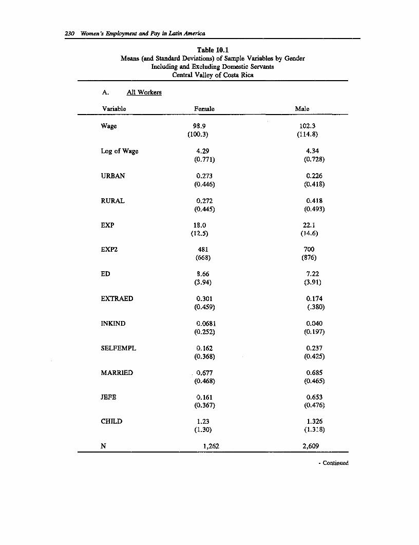
230 Women Is Employment and Pay in Latin America
Table 10.1Means (and Standard Deviations) of Sample Variables by Gender
Including and Excluding Domestic ServantsCentral Valley of Costa Rica
A. All Workers
Variable Female Male
Wage 98.9 102.3(100.3) (114.8)
Log of Wage 4.29 4.34(0.771) (0.728)
URBAN 0.273 0.226(0.446) (0.418)
RURAL 0.272 0.418(0.445) (0.493)
EXP 18.0 22.1(12.5) (14.6)
EXP2 481 700(668) (876)
ED 8.66 7.22(3.94) (3.91)
EXTRAED 0.301 0.174(0.459) (.380)
INKIND 0.0681 0.040(0.252) (0.197)
SELFEMPL 0.162 0.237(0.368) (0.425)
MARRIED 0.677 0.685(0.468) (0.465)
JEFE 0.161 0.653(0.367) (0.476)
CHILD 1.23 1.326(1.30) (1.318)
N 1,262 2,609
- Continued
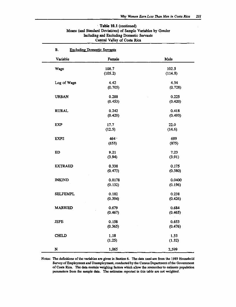
'Why Women Earn Less 7han Men in Costa Rica 231
Table 10.1 (continued)Means (and Standard Deviations) of Sample Variables by Gender
Including and Excluding Domestic ServantsCentral Valley of Costa Rica
B. Excludine Domestic Servants
Variable Female Male
Wage 108.7 102.5(105.2) (114.8)
Log of Wage 4.42 4.34(0.705) (0.728)
URBAN 0.288 0.225(0.453) (0.420)
RURAL 0.242 0.418(0.429) (0.493)
EXP 17.7 22.0(12.5) (14.6)
EXP2 464, 699(653) (875)
ED 9.21 7.23(3.94) (3.91)
EXTRAED 0.338 0.175(0.473) (0.380)
INKIND 0.0178 0.0400(0.132) (0.196)
SELFEMPL 0.182 0.238(0.394) (0.426)
MARRIED 0.679 0.684(0.467) (0.465)
JEFE 0.158 0.653(0.365) (0.476)
CHILD 1.18 1.33(1.25) (1.32)
N 1,065 2,599
Notes: The definitions of the variables are given in Section 6. The data used are from the 1989 HouseholdSurvey of Employment and Unemployment, conducted by the Census Departnent of the Governmentof Costa Rica. The data contain weighing factors which allow the researcher to estimate populationparameters from the sample data. The estimates reported in this table are not weighted.
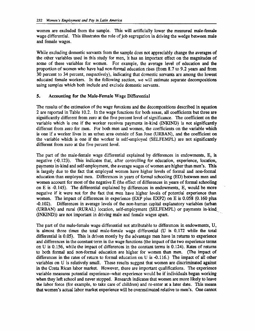
232 Women's Employment and Pay in Latin America
women are excluded from the sample. This will artificially lower the measured male-femalewage differential. This illustrates the role of job segregation in driving the wedge between maleand female wages.
While excluding domestic servants from the sample does not appreciably change the averages ofthe other variables used in this study for men, it has an important effect on the magnitudes ofsome of these variables for women. For example, the average level of education and theproportion of women who have had non-formal education rises (from 8.7 to 9.2 years and from30 percent to 34 percent, respectively), indicating that domestic servants are among the lowesteducated female workers. In the following section, we will estimate separate decompositionsusing samples which both include and exclude domestic servants.
5. Accounting for the Male-Female Wage Differential
The results of the estimation of the wage functions and the decompositions described in equation2 are reported in Table 10.2. In the wage functions for both sexes, all coefficients but three aresignificantly different from zero at the five percent level of significance. The coefficient on thevariable which is one if the worker receives payments in-kind (NKIND) is not significantlydifferent from zero for men. For both men and women, the coefficients on the variable whichis one if a worker lives in an urban area outside of San Jose (URBAN), and the coefficient onthe variable which is one if the worker is self-employed (SELFEMPL) are not significantlydifferent from zero at the five percent level.
The part of the male-female wage differential explained by differences in endowments, E, isnegative (-0.123). This indicates that, after controlling for education, experience, location,payments in-kind and self-employment, the average wages of women are higher than men's. Thisis largely due to the fact that employed women have higher levels of formal and non-formaleducation than employed men. Differences in years of formal schooling (ED) between men andwomen account for most of the negative E (the effect of differences in years of formal schoolingon E is -0.145). The differential explained by differences in endowments, E, would be morenegative if it were not for the fact that men have higher levels of potential experience thanwomen. The impact of differences in experience (EXP plus EXP2) on E is 0.058 (0.160 plus-0.102). Differences in average levels of the non-human capital explanatory variables (urban(URBAN) and rural (RURAL) location, self-employment (SELFEMPL) or payments in-kind-(INKIND)) are not important in driving male and female wages apart.
The part of the male-female wage differential not attributable to differences in endowments, U,is almost three times the total male-female wage differential (U is 0.172 while the totaldifferential is 0.05). This is driven mostly by the advantage men have in returns to experienceand differences in the constant term in the wage functions (the impact of the two experience termson U is 0.156, while the impact of differences in the constant terms is 0.124). Rates of returnsto both formal and non-formal education are higher for women than men. (The impact ofdifferences in the rates of return to formal education on U is -0.116.) The impact of all othervariables on U is relatively small. These results suggest that women are discriminated againstin the Costa Rican labor market. However, there are important qualifications. The experiencevariable measures potential experience--what experience would be if individuals began workingwhen they left school and never stopped. Research indicates that women are more likely to leavethe labor force (for example, to take care of children) and re-enter at a later date. This meansthat women's actual labor market experience will be overestimated relative to men's. One cannot
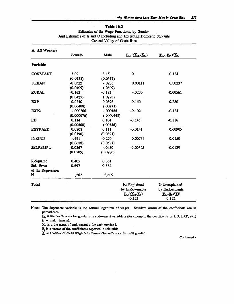
Why Women Earn Less Than Men in Costa Rica 233
Table 10.2Estimates of the Wage Functions, by Gender
And Estimates of E and U Including and Excluding Domestic ServantsCentral Valley of Costa Rica
A. All WorkersFemale Male M.'M--X-F) MA- IF)
Variable
CONSTANT 3.02 3.15 0 0.124(0.0738) (0.0517)
URBAN -0.0322 -.0236 0.00111 0.00237(0.0409) (.0309)
RURAL -0.163 -0.183 -.0270 -0.00561(0.0425) (.0278)
EXP 0.0240 0.0396 0.160 0.280(0.00408) (.00271)
EXP2 -.000206 -.000465 -0.102 -0.124(0.000076) (.0000448)
ED 0.114 0.101 -0.145 -0.116(0.00500) (.00356)
EXTRAED 0.0808 0.111 -0.0141 0.00905(0.0390) (0.0321)
INKIND -.491 -0.270 0.00754 0.0150(0.0688) (0.0587)
SELFEMPL -0.0367 -.0430 -0.00323 -0.0129(0.0505) (0.0286)
R-Squared 0.405 0.364Std. Error 0.597 0.582of the RegressionN 1,262 2,609
Total E: Explained U:Unexplainedby Endowments by Endowments
'(M-X)F)-0.123 0.172
Notes: The dependent variable is the natural logarithm of wages. Standard errors of the coefficients are inparentheses.BL is the coefficients for gender i on endowment variable z (for example, the coefficients on ED, EXP, etc.)(i = male, female).XL is a the mean of endowment z for each gender i.Bi is a vector of the coefficients reported in this table.X is a vector of mean wage determining characteristics for each gender.
Continued -
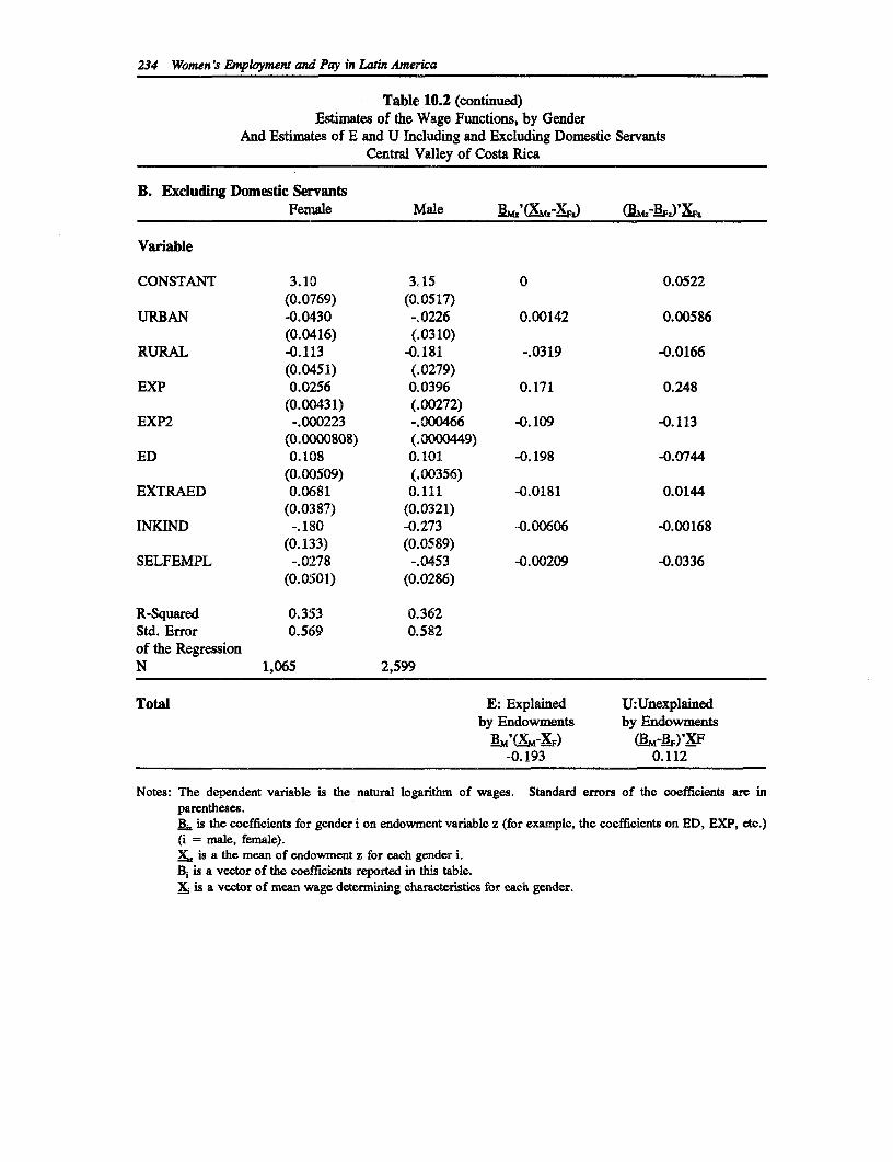
234 Women's rEmployment and Pay in Lain America
Table 10.2 (continued)Estimates of the Wage Functions, by Gender
And Estimates of E and U Including and Excluding Domestic ServantsCentral Valley of Costa Rica
B. Exduding Domestic ServantsFemale Male B'(L-X )
Variable
CONSTANT 3.10 3.15 0 0.0522(0.0769) (0.0517)
URBAN -0.0430 -.0226 0.00142 0.00586(0.0416) (.0310)
RURAL -0.113 -0.181 -.0319 -0.0166(0.0451) (.0279)
EXP 0.0256 0.0396 0.171 0.248(0.00431) (.00272)
EXP2 -.000223 -.000466 -0.109 -0.113(0.0000808) (.0000449)
ED 0.108 0.101 -0.198 -0.0744(0.00509) (.00356)
EXTRAED 0.0681 0.111 -0.0181 0.0144(0.0387) (0.0321)
INKIND -.180 -0.273 -0.00606 -0.00168(0.133) (0.0589)
SELFEMPL -.0278 -.0453 -0.00209 -0.0336(0.0501) (0.0286)
R-Squared 0.353 0.362Std. Error 0.569 0.582of the RegressionN 1,065 2,599
Total E: Explained U:Unexplainedby Endowments by Endowments
]3m'(-XM-X) @-m)X-0.193 0.112
Notes: The dependent variable is the natural logarithm of wages. Standard errors of the coefficients are inparentheses.B is the coefficients for gender i on endowment variable z (for example, the coefficients on ED, EXP, etc.)(i = male, female).X- is a the mean of endowment z for each gender i.Bi is a vector of the coefficients reported in this table.Xj is a vector of mean wage determining characteristics for each gender.
Why Women Earn Less Than Men in Costa Rica 235
be sure if the gender difference in the coefficients on experience is due to differences in the rateof return to experience or to unmeasured differences in labor market experience. The fact thatthe rest of the difference is due to differences in intercept terms indicates that much of thedifference in the wages between men and women is due to factors we cannot identify."1
The importance of domestic servants in driving the wedge between male and female wages hasalready been noted. When domestic servants are excluded from the sample used to estimate thewage equations the conclusions drawn above still hold (see Part B of Table 10.2). E is stillnegative (-..193) and U positive (0.112). The most important variable causing E to be negativeis still education and the most important variable causing U to be positive is potential experience.The biggest difference between parts A and B of Table 10.2 is the impact of the intercept term.The wage differential due to differences in the intercept terms is smaller (from .124 to .0522) inthe estimates of the wage equations without data on domestic servants. This indicates that a partof the unexplained difference found in the first set of numbers is caused by the impact ofdomestic servants. With one exception, all coefficients are similar to those reported for theestimation where the full sample was used. The exception is the coefficient for the variablewhich is one if the worker receives payment in-kind for women; it is not significantly differentfrom zero at the five percent level.
Table 10.3 presents the male-female wage differential for each sector and occupation, theproportion of men and women in each sector and occupation, and estimates of W (the part of thewage differential due to different wages paid to men and women in the same sectors andoccupations) and J (the part of the differential attributable to different access to higher payingsectors and occupations- see equation 4). Women are over-represented in the relatively higherpaying sectors and occupations; specifically among professional and technical workers andadministrative personnel in the public sector (see the last column of Table 10.3-the differencebetween the proportion of men and the proportion of women in these two sector/occupations is-.0.080 and -0.0302, respectively). There is no significant difference in the participation of menand women in the highest paying sector/occupation in the public sector, directors and managers.Women are also over-represented as domestic servants, the lowest paying sector/occupation (thedifference between the proportion of men and the proportion of women in the domestic servantsector is -0.152). Women are under-represented in the other three of the four lowest payingsector/occupations; the informal sector, and among laborers in the public and private-formalsectors (see the last column of Table 10.3, the differences between the proportion of men and theproportion of women in these sectors are positive)."2 Despite women being over-representedin the lowest paying domestic servant sector, J, the part of the male-female wage differenceattributable to different access to higher paying sectors and occupations, is a negative .0.0223,indicating that women are, on average, over-represented in the higher paying sectors andoccupations.
W, the part of the wage differential due to different wages paid to men and women in the samesectors and occupations, is a positive 0.0723. This indicates that, on average, women are paidless than men in the same sectors and occupations. Women are paid more than men in only two
11 Using the decompositions described in equation 2a, the difference attributable to endowments,E, is -0.129, the difference not attributable to endowments, U, is 0.178.
12 On average, women are over-represented in the public sector and under-represented in theinformal and pnvate-formal sectors.
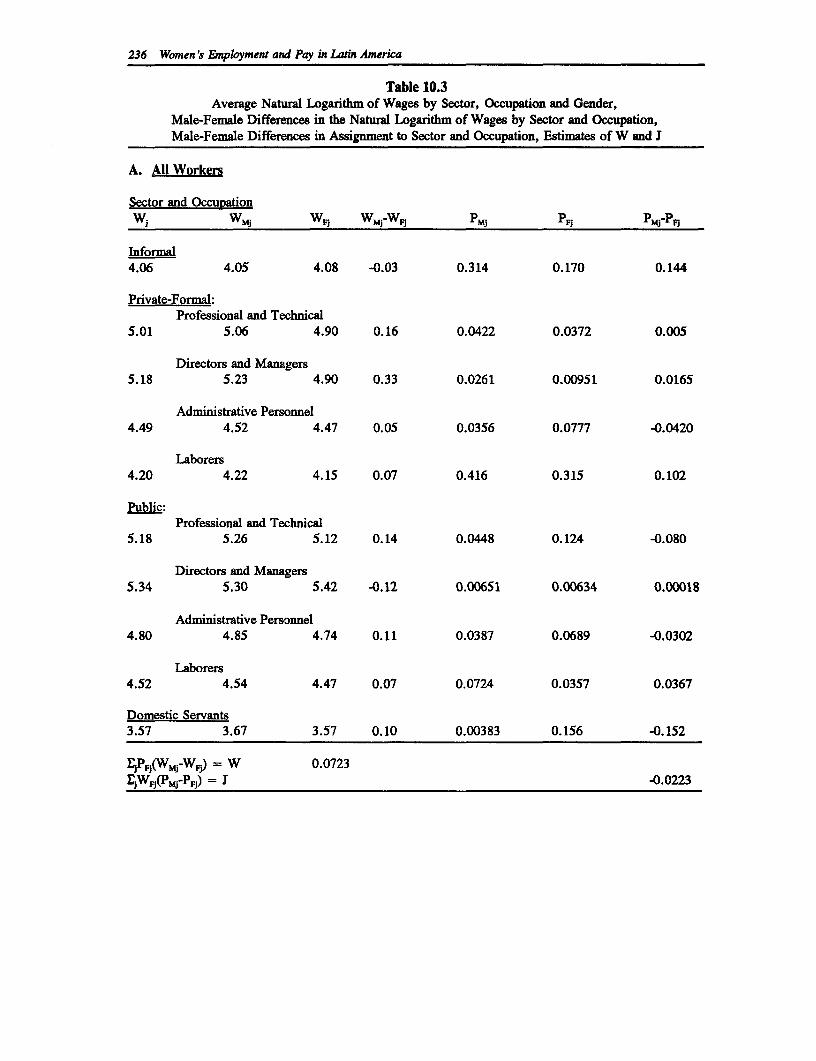
236 Women's Employment and Pay in Latin America
Table 10.3Average Natural Logarithm of Wages by Sector, Occupation and Gender,
Male-Female Differences in the Natual Logarithm of Wages by Sector and Occupation,Male-Female Differences in Assignment to Sector and Occupation, Estimates of W and I
A. All Workers
Sector and QccupationWi WMj WF, WM-WF, PMj PFJ PMj-Pp
Informal4.06 4.05 4.08 -0.03 0.314 0.170 0.144
Private-Formal:Professional and Technical
5.01 5.06 4.90 0.16 0.0422 0.0372 0.005
Directors and Managers5.18 5.23 4.90 0.33 0.0261 0.00951 0.0165
Administrative Personnel4.49 4.52 4.47 0.05 0.0356 0.0777 -0.0420
Laborers4.20 4.22 4.15 0.07 0.416 0.315 0.102
Public:Professional and Technical
5.18 5.26 5.12 0.14 0.0448 0.124 -0.080
Directors and Managers5.34 5.30 5.42 -0.12 0.00651 0.00634 0.00018
Administrative Personnel4.80 4.85 4.74 0.11 0.0387 0.0689 -0.0302
Laborers4.52 4.54 4.47 0.07 0.0724 0.0357 0.0367
Domestic Servants3.57 3.67 3.57 0.10 0.00383 0.156 -0.152
EgP ,(WMj-WF) = W 0.0723EJWF,(PMj-PF,) = J -0.0223
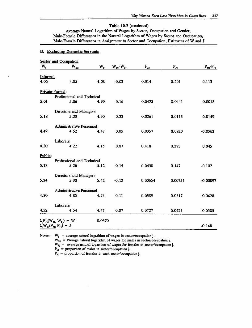
Why Women Earn Less Than Men in Costa Rica 237
Table 10.3 (continued)Average Natural Logarithm of Wages by Sector, Occupation and Gender,
Male-Female Differences in the Natural Logarithm of Wages by Sector and Occupation,Male-Female Differences in Assignment to Sector and Occupation, Estimates of W and J
B. Excluding Domestic Servants
Sector and OccupationWi WMjW M WF WMWF PMj PE PM MPFj
Informal4.06 4.05 4.08 -0.03 0.314 0.201 0.113
Private-Formal:Professional and Technical
5.01 5.06 4.90 0.16 0.0423 0.0441 -0.0018
Directors and Managers5.18 5.23 4.90 0.33 0.0261 0.0113 0.0149
Administrative Personnel4.49 4.52 4.47 0.05 0.0357 0.0920 -0.0562
Laborers4.20 4.22 4.15 0.07 0.418 0.373 0.045
Public:Professional and Technical
5.18 5.26 5.12 0.14 0.0450 0.147 -0.102
Directors and Managers5.34 5.30 5.42 -0.12 0.00654 0.00751 -0.00097
Administrative Personnel4.80 4.85 4.74 0.11 0.0389 0.0817 -0.0428
Laborers4.52 4.54 4.47 0.07 0.0727 0.0423 0.0305
EyPFI(WMj-WFJ) = W 0.0670EJWFj(pMj-PFI) = J -0.148
Notes: W= average natural logarithm of wages in sector/occupation j.WMj = average natural logarithm of wages for males in sector/occupation j.W;= average natural logarithm of wages for females in sector/occupation j.Pmj= proportion of males in sector/occupation j.P,= proportion of females in each sector/occupation j.
238 Women's Employment and Pay in Latin America
sector/occupation groups: directors and managers in the public sector and in the informal sector(see column four in Table 10.3-the difference between the average natural logarithm of wagesfor men and the average natural logarithm of wages for women is -0.12 and -0.03 respectivelyfor these sector/occupations)."3
The second set of estimates in Table 10.3 excludes domestic servants from the sample. Whenthis is done, W does not change appreciably while J falls (from -0.0233 to -0.148). This isexpected because, with the exclusion of the lowest paid women from the sample, women are noweven more over-represented in the higher paying sectors and occupations.14 Estimates of themultinominal logit model by sector/occupation are presented in Table 10.4.
Tables 10.5 and 10.6 present the estimates of the decompositions described in equation 6.15 Inthe last few paragraphs we concluded that women earn less than men with the same endowments,and that women are paid less than men in the same occupations and sectors. This is consistentwith the decompositions presented in Table 10.6.
WU, the difference between the wages of men and women within sectors and occupations thatis not explained by differences in endowments, is the only one of the decompositions reportedin Table 10.6 which is positive (0.114). This indicates that the primary reason why women earnless than men is because women in the same sectors and occupations as (observably) equallyqualified men are paid lower wages. In particular, men are paid more than women with the sameendowments in every sector/occupation except among directors and managers in the public sector(see column 1 in Table 10.6-only among directors and managers in the public sector is thedifference in the average natural logarithm of wages for men and women unexplained bydifferences in endowments negative, specifically it is 4.0610).
WE, the difference between the wages of men and women within sectors and occupations thatis explained by differences in endowments is negative indicating that, on average, within eachsector and occupation women have higher human capital endowments than men. Only amongadministrative personnel in the public sector are men paid more than women because they havehigher levels of human capital endowments (see column 2 in Table 10.6--only amongadministrative personnel is the difference in the natural logarithm of wages between men andwomen due to differences in endowments positive, specifically 0.00313).
13 In the public sector as a whole, and in the informal sector as a whole, women are paid more thanmen.
14 Estimates of W and J using the decompositions described in equation 4a are 0.0521 for W and-0.00211 for J when domestic servants are included in the sample and 0.0519 for W and -0.132 for J whendomestic servants are excluded from the sample.
15 In estimating the wage functions to calculate the decompositions described in equation 6 we usea smaller set of independent variables than was used to estimate the wage functions by gender. This isbecause the excluded variables have no variation in the sample for some jobs. We exclude the non-humancapital variables; dummy variables for location, payments in-kind and self-enployment. We include allhuman capital variables. The variables that we exclude had little impact on the measure of the differencein Table 16.3. We do not report decompositions using a sample which includes domestic servants in Table16.5. This is because there were not enough men in the domestic servant sector to estimate a wagefimction. The results of the estimate of the multinomial logit estimates for men and women are reportedin Table 16.4. The wage equations for each sex, sector and occupation are reported in Table A16.2 in theAppendix.
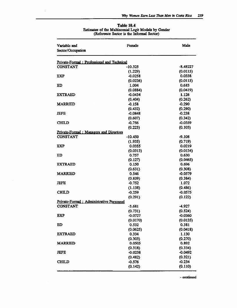
Why Women Earn Less Than Men m Costa Rica 239
Table 10.4Estimates of the Multinomial Logit Models by Gender
(Reference Sector is the Informal Sector)
Variable and Female MaleSector/Occupation
Private-Formal: Professional and TechnicalCONSTANT -10.325 -8.48227
(1.229) (0.0115)EXP -0.0258 0.0338
(0.0226) (0.0115)ED 1.004 0.683
(0.0884) (0.0419)EXTRAED -0.0434 1.126
(0.404) (0.262)MARRIED -0.158 -0.290
(0.432) (0.290)JEFE -0.0848 -0.238
(0.607) (0.342)CHILD -0.756 -0.0359
(0.223) (0.103)Private-Formal: Manaeers and DirectorsCONSTANT -10.450 -9.108
(1.935) (0.719)EXP 0.0355 0.0219
(0.0313) (0.0134)ED 0.757 0.630
(0.127) (0.0465)EXTRAED 0.150 0.696
(0.631) (0.308)MARRIED 0.546 -0.0579
(0.839) (0.384)JEFE -0.752 1.072
(1.138) (0.486)CHILD -0.259 -0.0575
(0.291) (0.122)Private-Formal: Administrative PersonnelCONSTANT -3.681 -4.927
(0.731) (0.524)EXP -0.0727 -0.0360
(0.0170) (0.0135)ED 0.532 0.381
(0.0625) (0.0418)EXTRAED 0.334 1.130
(0.303) (0.270)MARRIED 0.0505 0.892
(0.318) (0.334)JEFE -0.0238 -0.0492
(0.482) (0.321)CHILD -0.576 -0.234
(0.142) (0.110)
- continued
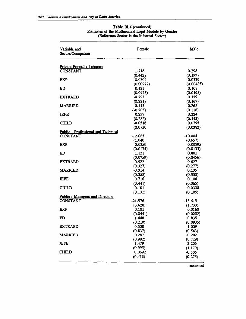
240 Women's Employment and Pay in Latin America
Table 10.4 (continued)Estimates of the Multinomial Logit Models by Gender
(Reference Sector is the Informal Sector)
Variable and Female MaleSector/Occupation
Private-Formal: LaborersCONSTANT 1.716 0.298
(0.442) (0.193)EXP -0.0804 -0.0339
(0.00977) (0.00485)ED 0.123 0.108
(0.0428) (0.0198)EXTRAED -0.793 0.359
(0.221) (0.167)MARRIED -0.113 -0.268
(-0.205) (0.116)JEFE 0.237 0.224
(0.282) (0.143)CHILD -0.0516 0.0795
(0.0730 (0.0382)Public: Professional and TechnicalCONSTANT -12.085 -10.004
(1.040) (0.657)EXP 0.0359 0.00895
(0.0174) (0.0133)ED 1.121 0.801
(0.0759) (0.0456)EXTRAED -0.922 0.627
(0.327) (0.277)MARRIED -0.314 0.135
(0.358) (0.338)JEFE 0.716 0.108
(0.441) (0.365)C-HILD 0.101 0.0330
(0.131) (0.105)Public: Managers and DirectorsCONSTANT -21.976 -13.615
(3.628) (1.733)EXP 0.101 0.0160
(0.0441) (0.0252)ED 1.448 0.835
(0.210) (0.0935)EXTRAED -0.530 1.009
(0.837) (0.543)MARRIED 0.287 -0.202
(0.992) (0.729)JEFE 1.479 2.205
(0.995) (1.179)CHILD 0.0692 -0.505
(0.413) (0.275)
- continued
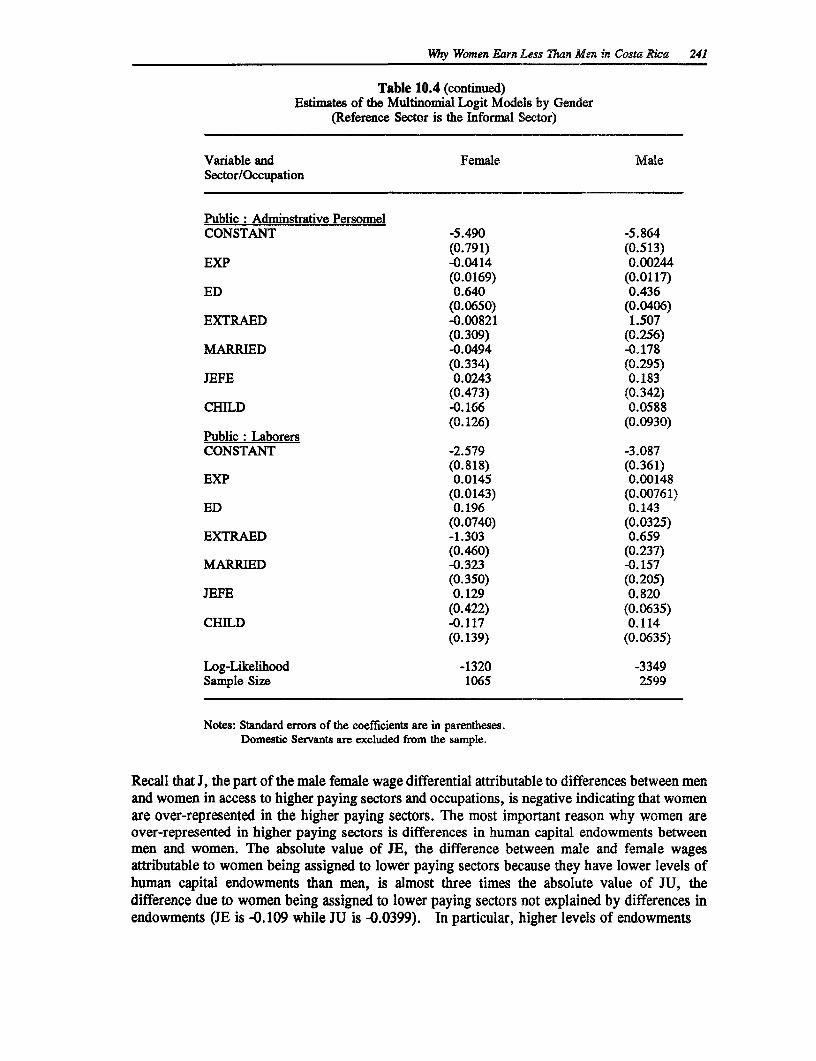
Why Women Earn Less Than Men in Costa Rica 241
Table 10.4 (continued)Estimates of the Multinomial Logit Models by Gender
(Reference Sector is the Informal Sector)
Variable and Female MaleSector/Occupation
Public: Adminstrative PersonnelCONSTANT -5.490 -5.864
(0.791) (0.513)EXP -0.0414 0.00244
(0.0169) (0.0117)ED 0.640 0.436
(0.0650) (0.0406)EXTRAED -0.00821 1.507
(0.309) (0.256)MARRIED -0.0494 -0.178
(0.334) (0.295)JEFE 0.0243 0.183
(0.473) (0.342)CHILD -0.166 0.0588
(0.126) (0.0930)Public: LaborersCONSTANT -2.579 -3.087
(0.818) (0.361)EXP 0.0145 0.00148
(0.0143) (0.00761)ED 0.196 0.143
(0.0740) (0.0325)EXTRAED -1.303 0.659
(0.460) (0.237)MARRIED -0.323 -0.157
(0.350) (0.205)JEFE 0.129 0.820
(0.422) (0.0635)CHILD -0.117 0.114
(0.139) (0.0635)
Log-Likelihood -1320 -3349Sample Size 1065 2599
Notes: Standard errors of the coefficients are in parentheses.Domestic Servants are excluded from the sample.
Recall that J, the part of the male female wage differential attributable to differences between menand women in access to higher paying sectors and occupations, is negative indicating that womenare over-represented in the higher paying sectors. The most important reason why women areover-represented in higher paying sectors is differences in human capital endowments betweenmen and women. The absolute value of JE, the difference between male and female wagesattributable to women being assigned to lower paying sectors because they have lower levels ofhuman capital endowments than men, is almost three times the absolute value of JU, thedifference due to women being assigned to lower paying sectors not explained by differences inendowments (JE is -0.109 while JU is -0.0399). In particular, higher levels of endowments
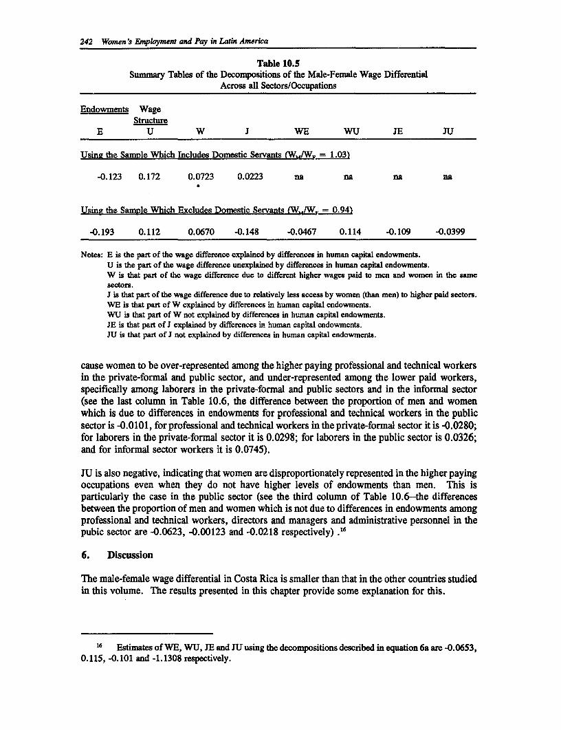
242 Women's Employment and Pay in Latin America
Table 10.5Summary Tables of the Decompositions of the Male-Female Wage Differential
Across all Sectors/Occupations
Endowments WageStructure
E U W i WE WU JE JU
Usine the Sample Which Includes Domestic Servants (W-/W. 1.03)
-0.123 0.172 0.0723 0.0223 na na na na
Usina the Sample Which Excludes Domestic Servants (WW,., = 0.94)
-0.193 0.112 0.0670 -0.148 -0.0467 0.114 -0.109 -0.0399
Notes: E is the part of the wage difference explained by differences in human capital endowments.U is the part of the wage difference unexplained by differences in human capital endowments.w is that part of the wage difference due to different higher wages paid to men and women in the samesectors.i is that part of the wage difference due to relatively less access by women (than men) to higher paid sectors.WE is that part of W explained by differences in human capital endowments.WU is that part of W not explained by differences in human capital endowments.JE is that part of J explained by differences in human capital endowments.JU is that part of J not explained by differences in human capital endowments.
cause women to be over-represented among the higher paying professional and technical workersin the private-formal and public sector, and under-represented among the lower paid workers,specifically among laborers in the private-formal and public sectors and in the informal sector(see the last column in Table 10.6, the difference between the proportion of men and womenwhich is due to differences in endowments for professional and technical workers in the publicsector is -0.0101, for professional and technical workers in the private-formal sector it is -0.0280;for laborers in the private-formal sector it is 0.0298; for laborers in the public sector is 0.0326;and for informal sector workers it is 0.0745).
JU is also negative, indicating that women are disproportionately represented in the higher payingoccupations even when they do not have higher levels of endowments than men. This isparticularly the case in the public sector (see the third column of Table 10.6--the differencesbetween the proportion of men and women which is not due to differences in endowments amongprofessional and technical workers, directors and managers and administrative personnel in thepubic sector are -0.0623, -0.00123 and -0.0218 respectively) .6
6. Discussion
The male-female wage differential in Costa Rica is smaller than that in the other countries studiedin this volume. The results presented in this chapter provide some explanation for this.
16 Estimates of WE, WU, JE and JU using the decompositions described in equation 6a are -0.0653,0.115, -0.101 and -1.1308 respectively.
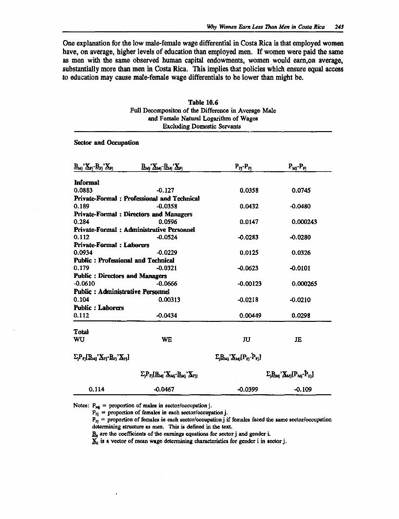
Why Women Earn Less Than Men in Costa Rica 243
One explanation for the low male-female wage differential in Costa Rica is that employed womenhave, on average, higher levels of education than employed men. If women were paid the sameas men with the same observed human capital endowments, women would earn,on average,substantially more than men in Costa Rica. This implies that policies which ensure equal accessto education may cause male-female wage differentials to be lower than might be.
Table 10.6Full Decompositon of the Difference in Average Male
and Female Natural Logarithm of WagesExcluding Domestic Servants
Sector and Occupation
_Mj'XFj--F;'XF3 B3mjXMj _MB XFj PFX PFi PMj PFj
Infonnal0.0883 -0.127 0.0358 0.0745Private-Fonnal: Professional and Technical0.189 -0.0358 0.0432 -0.0480Private-Formal : Directors and Managers0.284 0.0596 0.0147 0.000243Private-Formal: Adminiistrative Personnel0.112 -0.0524 -0.0283 -0.0280Private-Fonnal Laborers0.0934 -0.0229 0.0125 0.0326Public: Professional and Technical0.179 -0.0321 -0.0623 -0.0101Public : Directors and Managers-0.0610 -0.0666 -0.00123 0.000265Public : Administrative Personnel0.104 0.00313 -0.0218 -0.0210Public : Laborers0.112 -0.0434 0.00449 0.0298
TotalWU WE JU JE
F- Fj1Rj _XF3 _F3 XF3 E'-j; LD[PF3 P'F3]
F-,PFjMM _Xmj-_13mj'-XF,j r-iaNjLjXMj-pMj4PF3]
0.114 -0.0467 -0.0399 -0.109
Notes: PMj = proportion of males in sector/occupation j.P= proportion of females in each sector/occupation j.P= proportion of females in each sector/occupationj if females faced the same sector/occupationdetermining structure as men. This is defined in the text.B, are the coefficients of the eamings equations for sector j and gender i.X is a vector of mean wage determining characteristics for gender i in sector j.
244 Women's Employment and Pay in Latin America
Another reason why male-female wage differentials are low in Costa Rica is that women areover-represented in the higher paying sectors and occupations. Specifically, women are over-represented in the highest paying public sector, and in higher paying occupations within thepublic sector. In part, this is because the public sector hires, more than any other sector, highlyeducated workers. In addition, the public sector hires women over men even if they have thesame levels of human capital endowments.
The low male-female wage differential in Costa Rica does not necessarily imply that labor marketdiscrimination against women is less in Costa Rica than in other Latin American countries. Themost important reason that, on average, women are paid less than men in Costa Rica is thatwomen are paid less than men with the same endowments and in the same sectors andoccupations. If women were paid the same as men with the same human capital endowments inthe same sectors and occupations, women would, on average, earn higher wages than men. Thisindicates that labor market discrimination may be an important phenomenon in Costa Rica.
Men are also paid more than women in Costa Rica because women are disproportionatelyrepresented in the lowest paying domestic servant sector. However, it is probable that thereported wages of domestic servants underestimate the actual returns to their labor; part of thepayment to domestic servants is as payment in-kind, which is not reported. This would indicatethat the "true" male-female wage differential in the Central Valley of Costa Rica is lower thanthe 3.5 percent reported at the beginning of this paper.
A final point regarding public policy in Costa Rica and male-female wage differentials: As partof the structural adjustment program currently being carried out in Costa Rica, the governmenthas promised to reduce public sector employment (Lizano, 1990). The public sector plays animportant role in keeping the male-female wage differential low in Costa Rica. If public sectoremployment does fall in Costa Rica, a rise in the male-female wage differential is likely.
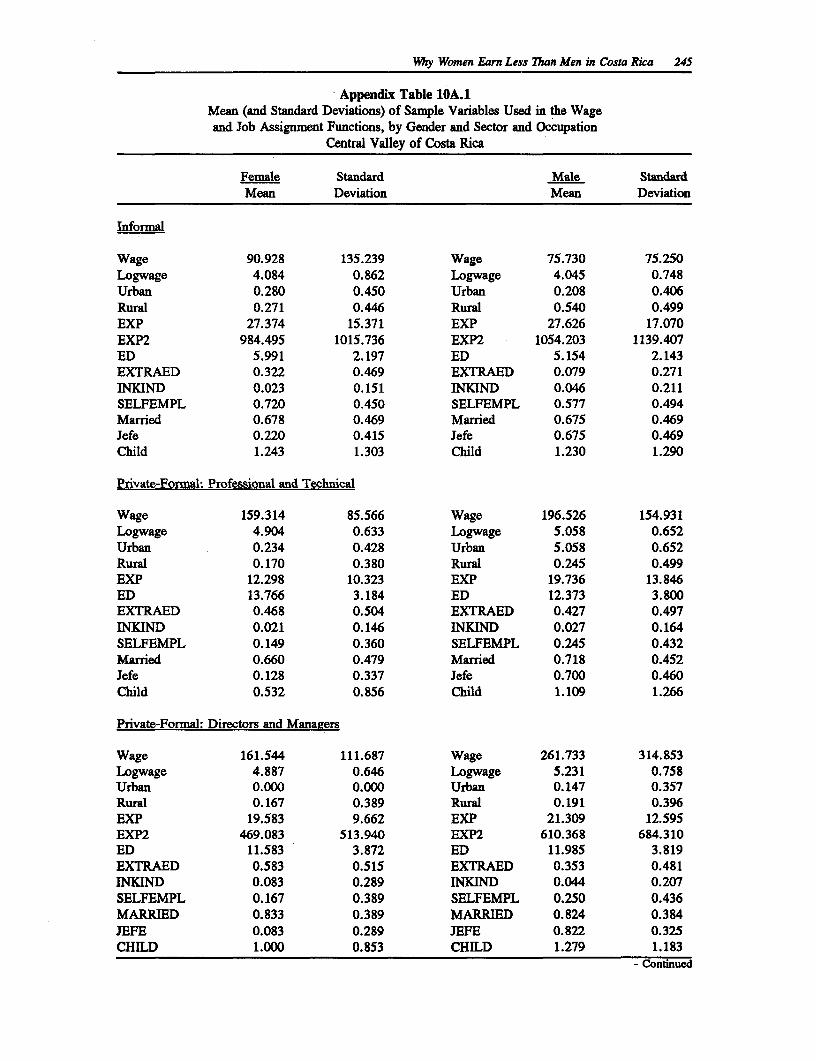
Why Women Earn Less Than Men in Costa Rica 245
Appendix Table 10A.1Mean (and Standard Deviations) of Sample Variables Used in the Wageand Job Assignment Functions, by Gender and Sector and Occupation
Central Valley of Costa Rica
Female Standard Male StandardMean Deviation Mean Deviation
Informal
Wage 90.928 135.239 Wage 75.730 75.250Logwage 4.084 0.862 Logwage 4.045 0.748Urban 0.280 0.450 Urban 0.208 0.406Rural 0.271 0.446 Rural 0.540 0.499EXP 27.374 15.371 EXP 27.626 17.070EXP2 984.495 1015.736 EXP2 1054.203 1139.407ED 5.991 2.197 ED 5.154 2.143EXTRAED 0.322 0.469 EXTRAED 0.079 0.271INKIND 0.023 0.151 INKIND 0.046 0.211SELFEMPL 0.720 0.450 SELFEMPL 0.577 0.494Married 0.678 0.469 Married 0.675 0.469Jefe 0.220 0.415 Jefe 0.675 0.469Child 1.243 1.303 Child 1.230 1.290
Private-Formal: Professional and Technical
Wage 159.314 85.566 Wage 196.526 154.931Logwage 4.904 0.633 Logwage 5.058 0.652Urban 0.234 0.428 Urban 5.058 0.652Rural 0.170 0.380 Rural 0.245 0.499EXP 12.298 10.323 EXP 19.736 13.846ED 13.766 3.184 ED 12.373 3.800EXTRAED 0.468 0.504 EXTRAED 0.427 0.497INKIND 0.021 0.146 INKIND 0.027 0.164SELFEMPL 0.149 0.360 SELFEMPL 0.245 0.432Married 0.660 0.479 Married 0.718 0.452Jefe 0.128 0.337 Jefe 0.700 0.460Child 0.532 0.856 Child 1.109 1.266
Private-Formal: Directors and Mana,aers
Wage 161.544 111.687 Wage 261.733 314.853Logwage 4.887 0.646 Logwage 5.231 0.758Urban 0.000 0.000 Urban 0.147 0.357Rural 0.167 0.389 Rual 0.191 0.396EXP 19.583 9.662 EXP 21.309 12.595EXP2 469.083 513.940 EXP2 610.368 684.310ED 11.583 3.872 ED 11.985 3.819EXTRAED 0.583 0.515 EXTRAED 0.353 0.481INKIND 0.083 0.289 INKIND 0.044 0.207SELFEMPL 0.167 0.389 SELFEMPL 0.250 0.436MARRIED 0.833 0.389 MARRIED 0.824 0.384JEFE 0.083 0.289 JEFE 0.822 0.325CHILD 1.000 0.853 CHILD 1.279 1.183
- Continued
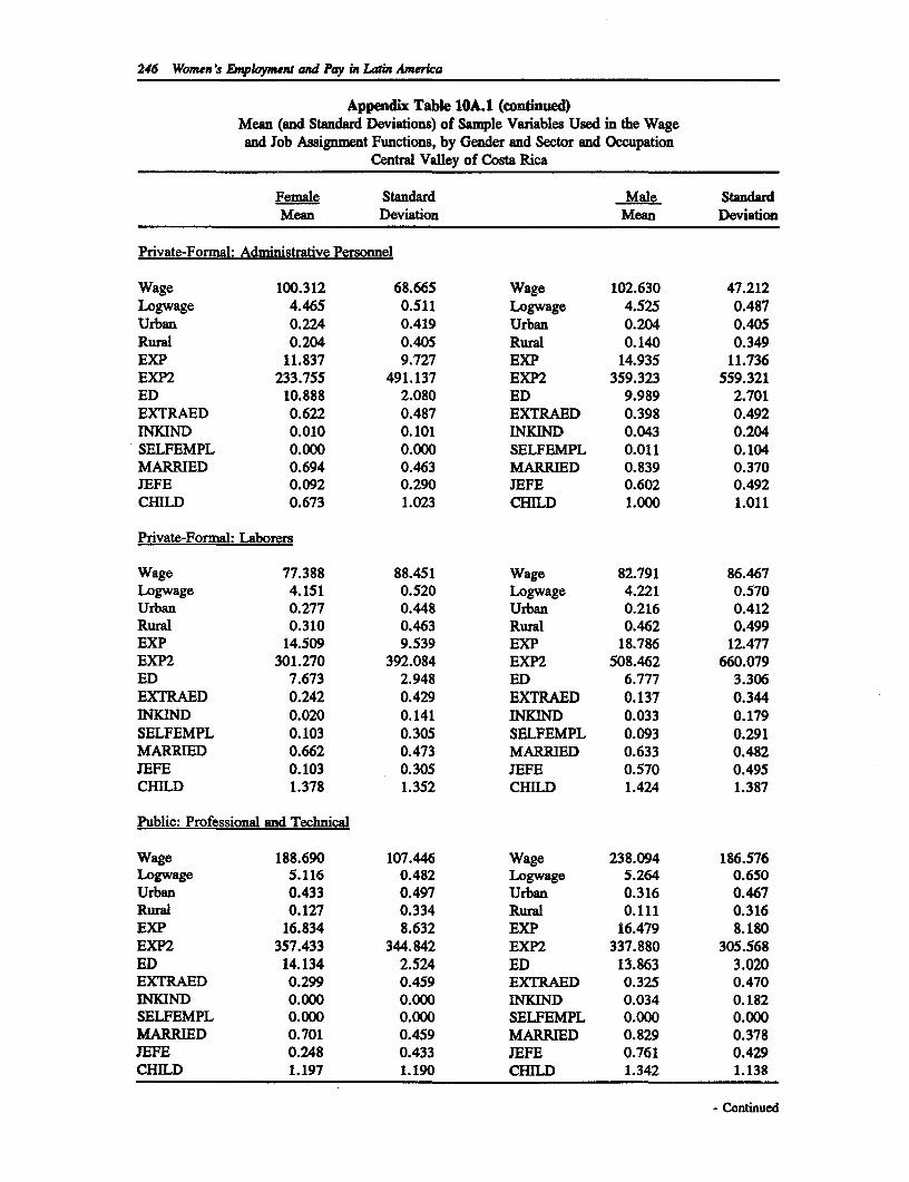
246 Women 's Employment and Pay in Latin America
Appendix Table 10A.1 (continued)Mean (and Standard Deviations) of Sample Variables Used in the Wageand Job Assigment Functions, by Gender and Sector and Occupation
Central Valley of Costa Rica
Female Standard Male StandardMean Deviation Mean Deviation
Private-Formal: Administrative Personnel
Wage 100.312 68.665 Wage 102.630 47.212Logwage 4.465 0.511 Logwage 4.525 0.487Urban 0.224 0.419 Urban 0.204 0.405Rural 0.204 0.405 Rural 0.140 0.349EXP 11.837 9.727 EXP 14.935 11.736EXP2 233.755 491.137 EXP2 359.323 559.321ED 10.888 2.080 ED 9.989 2.701EXTRAED 0.622 0.487 EXTRAED 0.398 0.492INKIND 0.010 0.101 INKIND 0.043 0.204SELFEMPL 0.000 0.000 SELFEMPL 0.011 0.104MARRIED 0.694 0.463 MARRIED 0.839 0.3701EFE 0.092 0.290 JEFE 0.602 0.492CHILD 0.673 1.023 CHILD 1.000 1.011
Private-Formal: Laborers
Wage 77.388 88.451 Wage 82.791 86.467Logwage 4.151 0.520 Logwage 4.221 0.570Urban 0.277 0.448 Urban 0.216 0.412Rural 0.310 0.463 Rural 0.462 0.499EXP 14.509 9.539 EXP 18.786 12.477EXP2 301.270 392.084 EXP2 508.462 660.079ED 7.673 2.948 ED 6.777 3.306EXTRAED 0.242 0.429 EXTRAED 0.137 0.344INKIND 0.020 0.141 INXIND 0.033 0.179SELFEMPL 0.103 0.305 SELFEMPL 0.093 0.291MARRIED 0.662 0.473 MARRIED 0.633 0.482JEFE 0.103 0.305 JEFE 0.570 0.495CHILD 1.378 1.352 CHILD 1.424 1.387
Public: Professional and Technical
Wage 188.690 107.446 Wage 238.094 186.576Logwage 5.116 0.482 Logwage 5.264 0.650Urban 0.433 0.497 Urban 0.316 0.467Rural 0.127 0.334 Rual 0.111 0.316EXP 16.834 8.632 EXP 16.479 8.180EXP2 357.433 344.842 EXP2 337.880 305.568ED 14.134 2.524 ED 13.863 3.020EXTRAED 0.299 0.459 EXTRAED 0.325 0.470INKIND 0.000 0.000 INKIND 0.034 0.182SELFEMPL 0.000 0.000 SELFEMPL 0.000 0.000MARRIED 0.701 0.459 MARRIED 0.829 0.378JEFE 0.248 0.433 JEFE 0.761 0.429CHILD 1.197 1.190 CHILD 1.342 1.138
- Continued
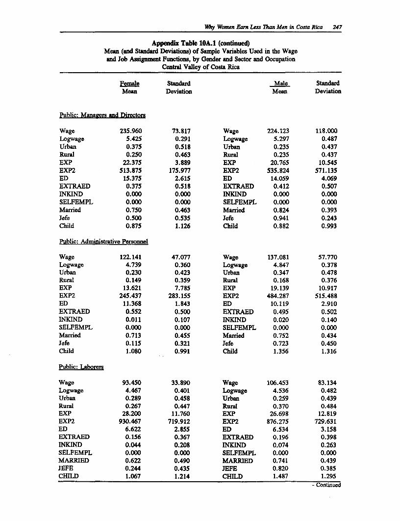
Why Womnen Earn Len Than Men in Costa Rica 247
Appendix Table 10A.1 (continued)Mean (and Standard Deviations) of Sample Variables Used in the Wageand Job Asignment Functions, by Gender and Sector and Occupation
Central VaUley of Costa Rica
Female Standard Male StandardMean Deviation Mean Deviation
Public: Managers and Directors
Wage 235.960 73.817 Wage 224.123 118.000Logwage 5.425 0.291 Logwage 5.297 0.487Urban 0.375 0.518 Urban 0.235 0.437Rural 0.250 0.463 Rural 0.235 0.437EXP 22.375 3.889 EXP 20.765 10.545EXP2 513.875 175.977 EXP2 535.824 571.135ED 15.375 2.615 ED 14.059 4.069EXTRAED 0.375 0.518 EXTRAED 0.412 0.507INKIND 0.000 0.000 INKIND 0.000 0.000SELFEMPL 0.000 0.000 SELFEMPL 0.000 0.000Married 0.750 0.463 Married 0.824 0.393Jefe 0.500 0.535 Jefe 0.941 0.243Child 0.875 1.126 Child 0.882 0.993
Public: Administrative Personnel
Wage 122.141 47.077 Wage 137.081 57.770Logwage 4.739 0.360 Logwage 4.847 0.378Urban 0,230 0.423 Urban 0.347 0.478Rural 0.149 0.359 Rural 0.168 0.376EXP 13.621 7.785 EXP 19.139 10.917EXP2 245.437 283.155 EXP2 484.287 515.488ED 11.368 1.843 ED 10.119 2.910EXTRAED 0.552 0.500 EXTRAED 0.495 0.502INKIND 0.011 0.107 INKIND 0.020 0.140SELFEMPL 0.000 0.000 SELFEMPL 0.000 0.000Married 0.713 0.455 Married 0.752 0.434Jefe 0.115 0.321 Jefe 0.723 0.450Child 1.080 0.991 Child 1.356 1.316
Public: Laborers
Wage 93.450 33.890 Wage 106.453 83.134Logwage 4.467 0.401 Logwage 4.536 0.482Urban 0.289 0.458 Urban 0.259 0.439Rurl 0.267 0.447 Rural 0.370 0.484EXP 28.200 11.760 EXP 26.698 12.819EXP2 930.467 719.912 EXP2 876.275 729.631ED 6.622 2.855 ED 6.534 3.158EXTRAED 0.156 0.367 EXTRAED 0.196 0.398INKIND 0.044 0.208 INKIND 0.074 0.263SELFEMPL 0.000 0.000 SELFEMPL 0.000 0.000MARRIED 0.622 0.490 MARRIED 0.741 0.439JEFE 0.244 0.435 JEFE 0.820 0.385CHILD 1.067 1.214 CHILD 1.487 1.295
- Continued
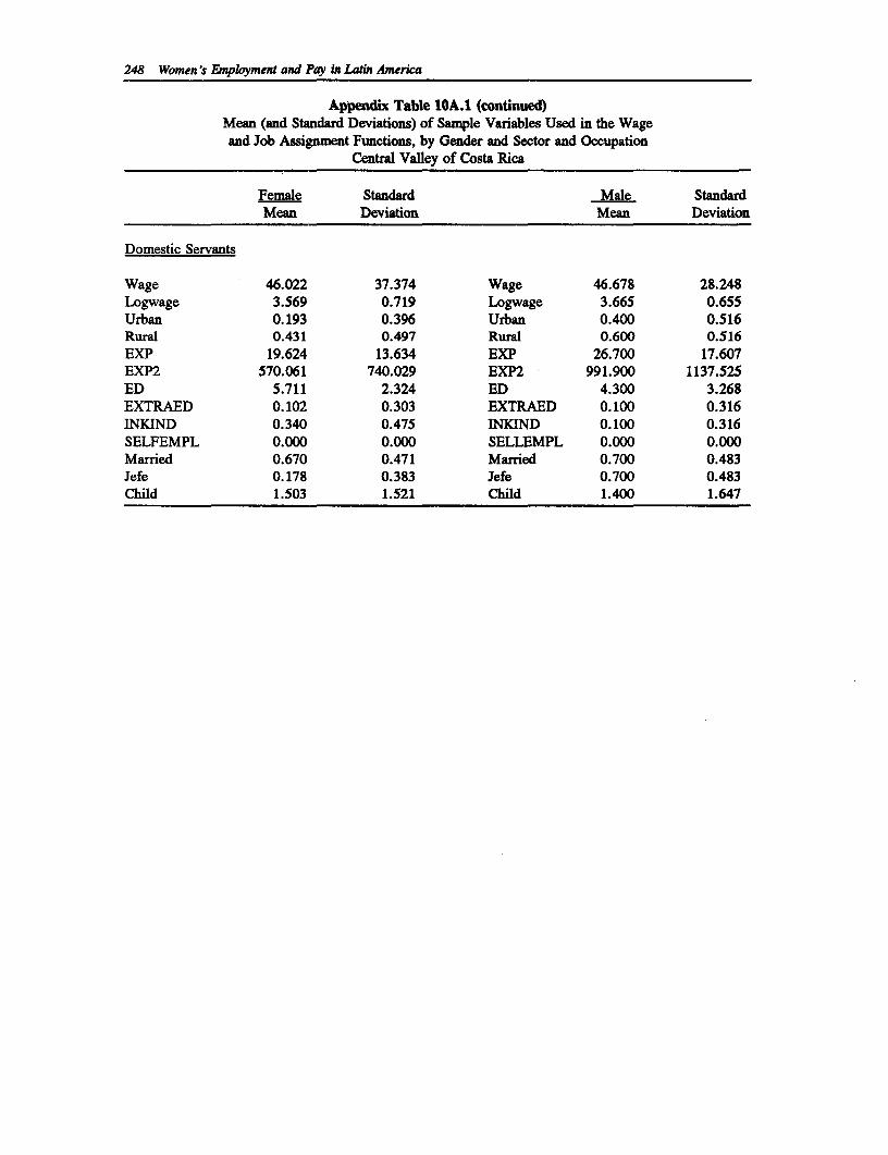
248 Women's Employment and Pay in Latin America
Appendix Table 1OA.1 (continued)Mean (and Standard Deviations) of Sample Variables Used in the Wageand Job Assignment Functions, by Gender and Sector and Occupation
Central Valley of Costa Rica
Female Standard Male StandardMean Deviation Mean Deviation
Domestic Servants
Wage 46.022 37.374 Wage 46.678 28.248Logwage 3.569 0.719 Logwage 3.665 0.655Urban 0.193 0.396 Urban 0.400 0.516Rural 0.431 0.497 Rural 0.600 0.516EXP 19.624 13.634 EXP 26.700 17.607EXP2 570.061 740.029 EXP2 991.900 1137.525ED 5.711 2.324 ED 4.300 3.268EXTRAED 0.102 0.303 EXTRAED 0.100 0.316INKIND 0.340 0.475 INKIND 0.100 0.316SELFEMPL 0.000 0.000 SELLEMPL 0.000 0.000Married 0.670 0.471 Married 0.700 0.483Jefe 0.178 0.383 Jefe 0.700 0.483Child 1.503 1.521 Child 1.400 1.647
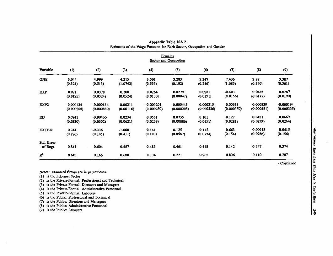
Appendix Table 10A.2Estimates of the Wage Function for Each Sector, Occupation and Gender
FemalesSector and Occupation
Variable (1) (2) (3) (4) (5) (6) (7) (8) (9)
ONE 3.044 4.999 4.215 3.501 3.283 3.247 7.436 3.87 3.387(0.321) (0.513) (1.0742) (0.335) (0.102) (0.246) (1.685) (0.340) (0.361)
EXP 0.021 0.0378 0.100 0.0264 0.0279 0.0281 -0.403 0.0435 0.0287(0.0135) (0.0324) (0.0524) (0.0130) (0.00847) (0.0131) (0.0156) (0.0177) (0.0199)
EXP2 -0.000134 -0.000134 -0.00211 -0.000201 -0.000443 -0.000215 0.00933 -0.000839 -0.000194(0.000205) (0.000880) (0.00116) (0.000250) (0.000205) (0.000336) (0.000350) (0.000481) (0.000335)
ED 0.0841 -0.00436 0.0234 0.0561 0.0735 0.101 0.127 0.0421 0.0669(0.0330) (0.0302) (0.0621) (0.0259) (0.00886) (0.0151) (0.0281) (0.0239) (0.0264)
EXTED 0.244 -0.336 -1.000 0.141 0.125 0.112 0.663 0.00918 0.0415(0.126) (0.185) (0.411) (0.103) (0.0587) (0.0734) (0.154) (0.0786) (0.156)
Std. Errorof Regr. 0.841 0.604 0.457 0.485 0.461 0.418 0.142 0.347 0.374
R2 0.643 0.166 0.680 0.134 0.221 0.262 0.896 0.110 0.207
- Continued
Notes: Standard Errors are in parentheses.(1) is the Informal Sector(2) is the Private-Formal: Professional and Technical(3) is the Private-Formal: Directors and Managers(4) is the Private-Formal: Administrative Personnel(5) is the Private-Formal: Laborers(6) is the Public: Professional and Technical(7) is the Public: Directors and Managers(8) is the Public: Administrative Personnel(9) is the Public: Laborers
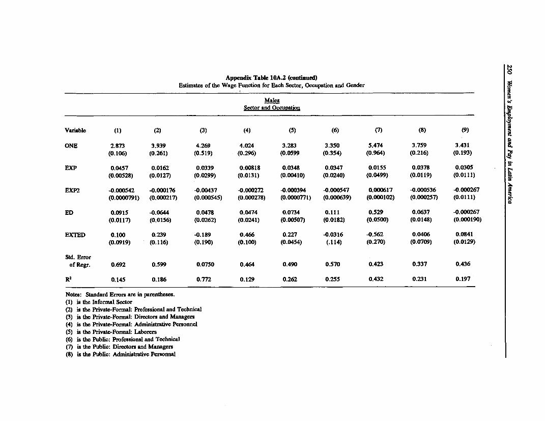
wAppendix Table 1OA.2 (continued)
Estimates of the Wage Function for Each Sector, Occupation and Gender0
MalesSector and Occuvation
Variable (1) (2) (3) (4) (5) (6) (7) (8) (9)
ONE 2.873 3.939 4.269 4.024 3.283 3.350 5.474 3.759 3.431(0.106) (0.261) (0.519) (0.296) (0.0599 (0.354) (0.964) (0.216) (0.193)
EXP 0.0457 0.0162 0.0339 0.00818 0.0348 0.0347 0.0155 0.0378 0.0305(0.00528) (0.0127) (0.0299) (0.0131) (0.00410) (0.0240) (0.0499) (0.0119) (0.0111)
EXP2 -0.000542 -0.000176 -0.00437 -0.000272 -0.000394 -0.000547 0.000617 -0.000536 -0.000267(0.0000791) (0.000217) (0.000545) (0.000278) (0.0000771) (0.000639) (0.000102) (0.000257) (0.0111)
ED 0.0915 -0.0644 0.0478 0.0474 0.0734 0.111 0.529 0.0637 -0.000267(0.0117) (0.0156) (0.0262) (0.0241) (0.00507) (0.0182) (0.0500) (0.0148) (0.000190)
EXTED 0.100 0.239 -0.189 0.466 0.227 -0.0316 -0.562 0.0406 0.0841(0.0919) (0.116) (0.190) (0.100) (0.0454) (.114) (0.270) (0.0709) (0.0129)
Std. Errorof Regr. 0.692 0.599 0.0750 0.464 0.490 0.570 0.423 0.337 0.436
R2 0.145 0.186 0.772 0.129 0.262 0.255 0.432 0.231 0.197
Notes: Standard Errors are in parentheses.(1) is the Informal Sector(2) is the Private-Formal: Professional and Technical(3) is the Private-Formal: Directors and Managers(4) is the Private-Formal: Administrative Personnel(5) is the Private-Formal: Laborers(6) is the Public: Professional and Technical(7) is the Public: Directors and Managers(8) is the Public: Administrative Personnal
Why Women Earn Less Than Men 1n Costa Rica 251
Appendix 1OB
Definitions of the Sectors
If a worker is employed by the central government or semi-autonomous (para-statal) enterprisethey are assigned to the public sector. If a worker is not assigned to the public sector, and heor she either works in a firm with greater than five employees or has an education level abovehigh school, or is classed as a professional or technical worker, he or she is assigned to theprivate-formal sector. If a worker is employed in a firm with five or fewer employees, and doesnot have an education level above high school, that worker is assigned to the informal sector.Highest wages are paid in the public sector, while lowest wages are found in the two informalsectors.
Within the private-formal and public sectors workers are further divided into four differentoccupations. We use the International Occupational Classification (Clasificacion InternacionalUniforme de Ocupaciones). We divide workers into professional and technical, directors, ownersand general administrators, administrative employees, and other workers.
Appendix 10.2
Separating the Impact of Occupations and SectorsOn the Male-Female Wage Difference
To separate the impact on wage differentials of different access to sectors from differences inwages due to different access to occupations within sectors we first estimate:
WM - WF = E(PFjfij'XwB_Fj XFj]) + EB"'[PN-PFj) (34)
-;W + J
and
WM- WF = E(PFjm -B )X + P '-_'X (3-5)
so &gRXWj1Fj PFjD) + EMM'Xhf[PW PFjD)
- Wu + WE +JU + JE
where j indicates only the informal, private-formal and public sectors. We then desegregate theW's (W, WU and WE) further into that part due to differences in wages due to men and womenbeing paid different wages within occupations and sectors and that part due to different accessto occupations within sectors. Specifically, we again estimate 34 and 3-5 using subsets of thedata used to estimate the decompositions described above; first, we estimate these decompositionsusing data that includes workers within the private-formal sector and second, using data onworkers within the public sector (hat is, let j in equations 34 and 3-5 indicate the occupationwithin each sector rather than the sector.)
252 Women's Enmployment and Pay in Latin America
We find that the difference in the wages between men and women due to different access to theinformal, private-formal and public sectors, J in equation 3-5, is negative."7 This reflects thefact that women are over-represented in the higher-paid public sector. Women are over-represented in the public sector both because they have higher levels of education than men andalso because they have disproportionate access to the public sector than men with the sameexperience and education. That is, JU and JE are both negative.
We find that the difference in wages between men and women due to different access tooccupations within the private-formal sector, J, is also negative. In the private-formal sector, thisis because women have higher levels of human capital than men (JE is negative while JU ispositive). However, J is small (relative to the total difference in average wages between men andwomen) within the private-formal sector.
Within the public sector, women are over-represented among the higher paid occupations. J isnegative and in absolute value terms is larger than the J measured taking into account access tosectors. We conclude that the public sector, by hiring women into higher paying occupations,is a factor keeping the wages of women high.
17 The independent variables used in the estimating of the wage equations at this step are the fullset desribed in the text. In estimating the wage equations in the next step, I use the more limited set ofindependent variables.
References
Behrman, J., B. Wolfe and D. Blau. "Human Capital and Earnings Distribution in a DevelopingCountry: The Case of Pre-Revolutionary Nicaragua." Economic Development and CulturalChange, (1985a). pp. 1-29.
-. "Labor Force Participation and Earnings Determinants for Women in the Special Conditionsof Developing Countries. " Journal of Development Economics, Vol.15 (1985b). pp. 259-288.
Birdsall, N. and M. L. Fox. "Why Males Earn More: Location and Training of BrazilianSchoolteachers." Economic Development and Cultural Change, Vol. 33, no. 3 (1985). pp.533-556.
Brown, R., M. Moon and B. Zoloth. "Incorporating Occupational Attainment in Studies of Male-Female Earnings Differentials." Journal of Human Resources, Vol. 15, no. 1 (1980). pp.3-28.
Cain, G. "The Economic Analysis of Labor Market Discrimination: A Survey", in 0.Ashenfelter and R. Leyard (eds.). Handbook of Labor Economics. North Holland, NewYork: North Holland, 1986. pp. 693-785.
Carvajal, M. and D. Geithman. "Human Capital and Sex Discrimination: Some Evidence fromCosta Rica, 1963-1973", Florida International University Latin American and CaribbeanCenter, Discussion Paper No. 15, April, 1983.
Chapman, B. and J. Ross Harding. "Sex Differences in Earnings: An Analysis of MalaysianWage Data." Journal of Development Studies, Vol. 21 (1985).
Cotton, J. "On the Decomposition of Wage Differentials." The Review of Economics andStatistics, (1988). pp. 236-243.
Gindling, T.H. "Labor Market Segmentation and the Determination of Wages in the Public,Private-formal and Informal Sectors in San Jose, Costa Rica." Economic Development andCultural Change, Vol. 39, no. 3, (1991). pp. 585-606.
-. "Ingresos de las Mujeres y Crisis Economica en Costa Rica." University of Costa RicaInstitute for Research in Economic Science Working Paper #138. Costa Rica, 1990.
253
254 Women's Employment and Pay fn Latn rica
"Women's Wages and Economic Crisis in Costa Rica.' Paper presented at the 1989Congress of the Latin American Studies Association. December, Miami, 1989a.
"Crisis economica y segmentacion en el mercado de trabajo urbano en Costa Rica." Revistade Ciencias Economicas, Vol 9 (1989b). pp. 79-94.
Gindling T. H. and Berry, A. "Labor Market and Adjustment in Costa Rica", in S. Horton,R.Kanbur, and D. Mazumdar (eds.). Labor Markets in an Era of Adjustment. WashingtonD.C.: The World Bank, Economic Development Institute, 1990.
Gunderson, M. "Male-Female Wage Differentials and Policy Responses." Journal of EconomicLiterature, Vol 27, March (1989). pp. 46-72.
Koopman, J. Review of Women in the Third World: Work and Daily Life by J. Bisihliat and M.Fieloux, Economic Development and Cultural Change, Vol. 39, no. 2 (1991). pp.437443.
Lizano. Programa de Ajuste Estructural en Costa Rica. Academia de Centroamericana Estudios6, San Jose, Costa Rica.
McFadden, D. "Econometric Analysis of Quantitative Response Models" in Z. Griliches and M.Intriligator (eds.). Handbook of Econometrics, Vol. 2. New York: Elseveir SciencePublishing, 1984. pp.136-145
Oaxaca, R. "Male-female Wage Differentials in Urban Labor Markets." International EconomicReview, Vol. 14, no. 1 (1973). pp. 693-709.
Piore, M. "The Dual Labor Market: Theory and Implications", in D. M. Gordon, (ed.).Problems in Political Economy: An Urban Perspective. Lexington, Mass.: Heath, 1971.
Tardanico, R. 'Economic Crisis and Structural Adjustment: The Labor Market of San Jose,Costa Rica, 1979-1987." Comparative Urban and Community Research, Vol. 4.forthcoming.
Tenjo, J. "Labor Markets, Wage Gap and Gender Discrimination: The Case of Colombia."Mimeograph. Toronto: University of Toronto, Department of Economics, 1990.
11
The Effect of Education on Female Labor ForceParticipation and Earnings in Ecuador
George Jakubson and George Psacharopoulos
1. Introduction
An earlier analysis of women's labor force participation in Ecuador was undertaken by Finn andJusenius (1975) using data for 1966. They found rather low rates of labor force participationamnong urban women, in the order of 25 percent, with participation rates being highest amongwomen who had completed college (89 percent). Single women were more likely to work in thelabor market, but earned substantially less than working wives, who also tended to be older andbetter educated.
Average earnings of employed women were approximately 55 percent of the average earningsof employed men. Controlling for age, education, and region, that differential drops to 20percent. They speculate that the occupational distribution of men and women contributes to theremaining earnings differential.
2. Ecuador's Economy and Labor Market
Rapid development of the petroleum and service sectors during the 1970s meant that Ecuador hadan average growth in GDP of 6.7 percent a year for the period 1970 to 1982. Socialexpenditures during that period produced major improvements in education and health, andliteracy and school enrollment rates increased. The country developed a national network ofhealth care facilities and registered decreases in infant and child mortality and a decline in birthrates. Urban development was also been significant. These improvements have had a positiveeffect on the social status of women in Ecuador; women constituted 16.3 percent of theeconomically active population in 1962 and 20.6 percent in 1982.
However, a decline in public sector revenues and expenditure since 1982, brought about in partby the sharp reduction in world oil prices in 1986 and the disruption of oil production, has causedserious problems for the education, health, housing and other social sectors, as well as forunemployment. Women, and especially poor women, have been affected by these economiccrises.
Labor force participation rates among women have continued to rise, except among females aged12 to 19 years who are remaining in school longer. Increased female labor force participationrates have been particularly high among women between ages 25 and 34 years. Participation
255
256 Women's Employment and Pay in Latin America
rates have increased across all marital status categories and married women increased their laborforce participation between 1974 and 1982 from 16.8 percent to 21.1 percent. It is reported that61 percent of female heads of household were in the labor force in 1987 (World Bank, 1989).
Available evidence from several surveys suggests that female monthly earnings are lower thanmales across all educational levels and occupational categories. Even when adjustments are madefor differences in average hours worked per week, women with similar levels of schooling andyears of experience still earn less than men. This chapter investigates the causes of theseearnings differentials.
3. Data Characteristics
The data used in this chapter come from the 1987 Ecuador Household Survey which wasconducted in the three largest cities, Quito, Cuenca, and Guayaquil. The sample thereforeconsists only of urban households. The reader should bear this in mind when interpreting theempirical findings.
The overall sample contains 21,855 individual observations. The sample used here consists of4,876 households for which there are clean data on labor force participation and, where relevant,hours of work, earnings and other variables. Descriptive statistics appear in Table 11.1.
The sample was restricted to household heads and spouses between ages 12 and 64 at the timeof the survey. There are 3,899 husband/wife pairs and 977 female heads of household.
Labor force participation was determined from responses to questions on recent activity. Thequestionnaire enabled us to distinguish not only those who were currently at work, but those whowere temporarily away from work, on strike, on vacation, actively looking for work, etc., so thatwe could construct a very accurate measure of labor force participation. Forty-six percent ofthe 4,876 women were labor force participants. Of these women, 11 percent were not currentlyin a job at the time of the survey, so 41 percent of the female sample, or 1,975 women, wereworking in the labor market. All 3,899 men in the analysis sample were working in the labormarket at the time of the survey.
The "years of schooling" variable was constructed using information on both the type ofschooling completed (for example, primary) and the number of years in each school type. Weadded the number of grades in each schooling class completed (with the exception of the highest)to the number of years completed in the highest schooling class, so obtaining the number of yearsof schooling. Note that this really only approximates years of schooling. If an individualrepeated a grade of primary school, or if (s)he skipped a grade, that will not be reflected in ourmeasure. Nor does the variable measure number of grades of school completed. If an individualrepeated a grade in the highest class of schooling, that will not be taken into account in ourmeasure. Men averaged 9.7 years of schooling and women 8.54 years. Female workers hadmore years of schooling than women on average, 9.05 years.
Males averaged 39.7 years of age and women 37.7 years. There was little difference, onaverage, between female workers and non-workers, though there is somewhat less variation inage among female workers. Work experience was constructed as age minus years of schoolingminus six.
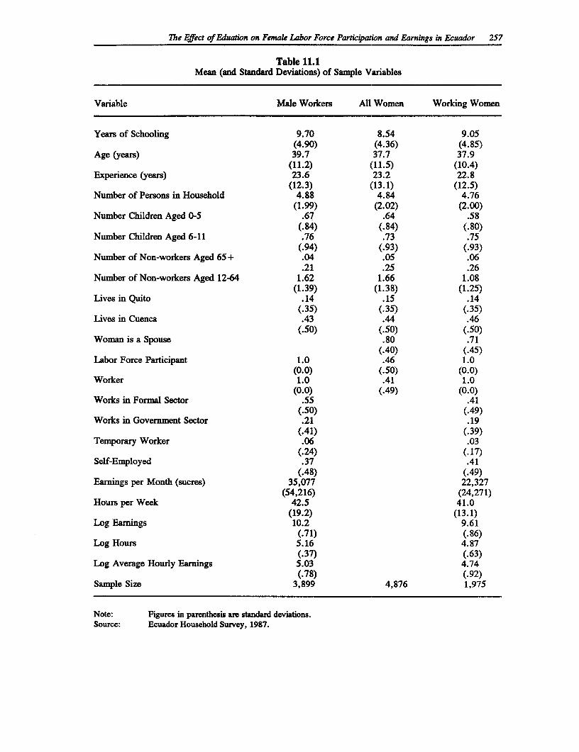
The Effect of Eduation on Female Labor Force Particpoation and Earnings in Ecuador 257
Table 11.1Mean (and Standard Deviations) of Sample Variables
Variable Male Workers All Women Working Women
Years of Schooling 9.70 8.54 9.05(4.90) (4.36) (4.85)
Age (years) 39.7 37.7 37.9(11.2) (11.5) (10.4)
Experience (years) 23.6 23.2 22.8(12.3) (13.1) (12.5)
Number of Persons in Household 4.88 4.84 4.76(1.99) (2.02) (2.00)
Number Children Aged 0-5 .67 .64 .58(.84) (.84) (.80)
Number Children Aged 6-11 .76 .73 .75(.94) (.93) (.93)
Number of Non-workers Aged 65+ .04 .05 .06.21 .25 .26
Number of Non-workers Aged 12-64 1.62 1.66 1.08(1.39) (1.38) (1.25)
Lives in Quito .14 .15 .14(.35) (.35) (.35)
Lives in Cuenca .43 .44 .46(.50) (.50) (.50)
Woman is a Spouse .80 .71(.40) (.45)
Labor Force Participant 1.0 .46 1.0(0.0) (.50) (0.0)
Worker 1.0 .41 1.0(0.0) (.49) (0.0)
Works in Formal Sector .55 .41(.50) (.49)
Works in Government Sector .21 .19(.41) (.39)
Temporary Worker .06 .03(.24) (.17)
Self-Employed .37 .41(.48) (.49)
Earnings per Month (sucres) 35,077 22,327(54,216) (24,271)
Hours per Week 42.5 41.0(19.2) (13.1)
Log Earnings 10.2 9.61(.71) (.86)
Log Hours 5.16 4.87(.37) (.63)
Log Average Hourly Earnings 5.03 4.74(.78) (.92)
Sample Size 3,899 4,876 1,975
Note: Figures in parenthesis are standard deviations.Source: Ecuador Household Survey, 1987.
258 Women's Employment and Pay in Latin America
The survey records number of persons per household and the relationship of each person to thehousehold head. Household servants living in the household are included in this count. Wecould also identify the number of individuals in the household by age and earning status.Households had an average of 1.6 adults between ages 12 and 64 who were neither head norspouse and who were not working in the labor market. On average, the households contained.64 children between ages 0 and 5 and .73 children between ages 6 and 11. Twelve year oldswere treated as "adults" in the analysis since labor force questions were asked of those twelveand older.
The sample was unevenly distributed among the three cities. Fifteen percent lived in Quito, 47percent in Cuenca, and 38 percent in Guayaquil. Eighty percent of the women were eithermarried or cohabiting with a male. The remaining 20 percent were female heads of household.Among married and cohabiting women, 92.5 percent of their male partners worked in the labormarket, although only 66 percent of the husbands of working wives also worked.
Among male workers, 55 percent worked in the formal sector. Participation in this sector wasdetermined on the basis of their coverage by the social security system. Twenty-one percentworked in the government sector, 37 percent were self-employed, and 6 percent were classed astemporary workers. On average, they worked 42.5 hours per week and earned 35,007 sucresper month. Of working women, 41 percent worked in the formal sector, 39 percent worked inthe government sector, 49 percent were self-employed, and 17 percent were classed as temporaryworkers. On average, they worked 41 hours per week and earned 22,327 sucres per month.
Monthly earnings were constructed using information on earnings in the previous pay period.These were adjusted to reflect monthly earnings, assuming that earnings were the same in eachof the pay periods needed to cover one month.'
The wage measure used in the analysis is the natural logarithm of average hourly earnings.Hours of work in the previous week were multiplied by 4 to reflect monthly hours. We thusassume that hours per week were constant. Average hourly earnings is the ratio of monthlyearnings to monthly hours, and its logarithm is used as the wage measure below. On average,working women earned 27 percent less than working men.
We chose to use this wage measure rather than the logarithm of total earnings for the followingreason. The logarithm of average hourly earnings is the difference between the logarithm ofearnings and the logarithm of hours of work:
log avern = log earn - log hours
Hence, in a regression of log earnings on log hours, the log hours variable should have acoefficient of unity:
log avern = log earn - log hours = B'x + ulog earn =B'x + log hours + u
For example, if the pay period was two weeks long, then monthly earnings are twice the eaningsin the previous pay period.
The Effect of Eduation on Female Labor Force Participation and Earnings in Ecuador 259
For both men and working women, the coefficient of log hours in a log earnings regression wasquite far from unity. This is most likely to be the result of measurement error in the hoursvariable.
In a regression equation this error simply becomes part of the disturbance term. While it reducesthe precision with which the coefficients are estimated, it imparts no bias per se to the estimates.Measurement error in an explanatory variable, in contrast, does impart a bias. Using thelogarithm of average hourly earnings as the dependent variable keeps all the measurement erroron the left hand side of the estimating equation.
Experiments estimating hours equations are consistent with this analysis. The coefficient ofaverage hourly earnings in a regression equation for hours of work is biased downwards if hoursare measured with error. Essentially, a positive measurement error in hours induces a negativemeasurement error in average hourly earnings, and a negative measurement error in hoursinduces a positive measurement error in average hourly earnings, leading to a downward bias.For both the male and working female samples, the coefficient on average hourly earnings in anhours equation was either essentially zero or negative. This result is consistent with themeasurement error hypothesis.
4. Determinants of Female Labor Force Participation
We utilize a probit model to analyze the probability of labor force participation and labor marketwork for women in the sample. In the probit model we have:
P(y= I I x) =F('x),
where FO is the standard normal cumulative distribution function (cdf) and the dependent variabley takes on the values 0 or 1. We utilize maximum likelihood methods to estimate the coefficientsB. The inverse of the information matrix, evaluated at the maximum likelihood estimates, is usedfor inference. Standard errors are the square roots of the diagonal elements.
The derivative of the probability that y = 1, evaluated at x = xO, is:
f(B'xO) B
where fO is the standard normal probability density function (pdf). The derivative takes itsmaximum (absolute) value, for any given B, at values of x where B'x = 0, and decreases in(absolute) value as B'x moves away from zero. Since the term fO is always positive, the sign ofthe derivative is the sign of B.
In essence, the effect of a change in an explanatory variable on the probability of labor forceparticipation (or labor market work) depends on that probability. When the probability of labormarket participation is close to one or zero, changes in the explanatory variables have muchsmaller effects than when that probability is .5. Therefore, one must pick a point at which toevaluate the derivative.
We estimate the derivative by replacing the population parameter B by its maximum likelihoodestimate b. Two logical choices for points of evaluation of the derivative are (1) the sample meanvalues of the explanatory variables (xbar), and (2) the sample mean value of the dependentvariable (ybar). In contrast to a linear model, the predicted value of the probability of labor force
260 Women's Employment and Pay in Latin America
participation in a probit model, evaluated at the sample means of the explanatory variables, is notequal to the mean of the dependent variable. The former is:
f(b'xbar) b
while the latter is:
F-1 (ybar) b
where F'O is the inverse of the standard normal cdf.
We use the latter point of evaluation, and evaluate the derivatives at the mean value of thedependent variable. For purposes of the simulation studies below, we adjust the constant termbo so that the predicted probability at the mean values of the explanatory variables is equal to themean value of the dependent variable. The new constant term bo' is constructed as:
bo' = bo + [ F1I(ybar) - F(b'xbar) ] .
In cases in which the mean of the dependent variable is close to .5 the adjustment required isrelatively small. That is the situation with these data. The labor force participation rate for thesewomen is 46 percent and 41 percent. In cases in which the mean of the dependent variable isclose to 0 or 1 the changes in the derivatives due to the adjustment can be more substantial.
Table 11.2 displays the results of probit equations for the probability of labor force participationand labor market work for the women in the sample. (Note that all men in the sample areworking in the labor market.) The left hand panel of the table displays the results for labor forceparticipation and the right hand panel displays the results for labor market work.
At the bottom of Table 11.2 we report the mean of the dependent variable followed by themaximized value of the log likelihood function. We display the chi-square statistic and degreesof freedom for testing the null hypothesis that all the slope coefficients in the model are zero.For both equations there is clear evidence against the hypothesis that the explanatory variableshave no effect.
Years of schooling is a marginally significant determinant of female labor force participation anda significant determinant of labor market work. More highly educated women are more likelyto participate and to work, but the effect is small.
Age is a significant determinant of both labor force participation and labor market work. Wespecified a quadratic in age to account for nonlinearities in the relationship and found clearevidence of curvature. Both probabilities increase with age to a peak at just over 40 years of ageand then decline. Wives are significantly less likely to participate and work than female headsof household, and wives of working husbands are significantly less likely to participate and workthan wives whose husbands do not work in the labor market.
Family structure has an important influence on the work and participation probabilities. Thelabor force participation decision, in theory, is made by comparing the value of market time (thewage) to the value of non-market time. Non-market time should be more valuable for womenwith larger families, other things equal.
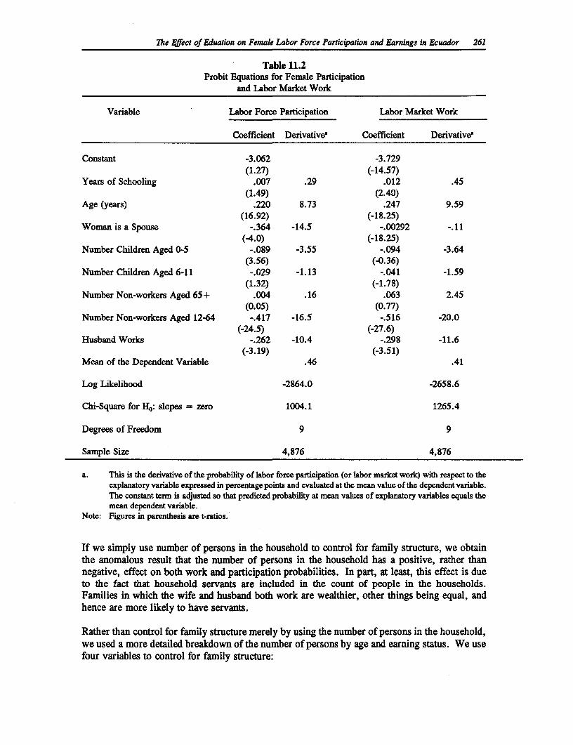
The Effect of Eduation on Femak Labor Force Particiation and Earnings in Ecuador 261
Table 11.2Probit Equations for Female Participation
and Labor Market Work
Variable Labor Force Participation Labor Market Work
Coefficient Derivative' Coefficient Derivative'
Constant -3.062 -3.729(1.27) (-14.57)
Years of Schooling .007 .29 .012 .45(1.49) (2.40)
Age (years) .220 8.73 .247 9.59(16.92) (-18.25)
Woman is a Spouse -.364 -14.5 -.00292 -.11(-4.0) (-18.25)
Number Children Aged 0-5 -.089 -3.55 -.094 -3.64(3.56) (-0.36)
Number Children Aged 6-11 -.029 -1.13 -.041 -1.59(1.32) (-1.78)
Number Non-workers Aged 65+ .004 .16 .063 2.45(0.05) (0.77)
Number Non-workers Aged 12-64 -.417 -16.5 -.516 -20.0(-24.5) (-27.6)
Husband Works -.262 -10.4 -.298 -11.6(-3.19) (-3.51)
Mean of the Dependent Variable .46 .41
Log Likelihood -2864.0 -2658.6
Chi-Square for Ho: slopes = zero 1004.1 1265.4
Degrees of Freedom 9 9
Sample Size 4,876 4,876
a. This is the derivative of the probability of labor force participation (or labor market work) with respect to theexplanatory variable expressed in percentage points and evaluated at the mean value of the dependent variable.The constant term is adjusted so that predicted probability at mean values of explanatory variables equals themean dependent variable.
Note: Figures in parenthesis are t-ratios.
If we simply use number of persons in the household to control for family structure, we obtainthe anomalous result that the number of persons in the household has a positive, rather thannegative, effect on both work and participation probabilities. In part, at least, this effect is dueto the fact that household servants are included in the count of people in the households.Families in which the wife and husband both work are wealthier, other things being equal, andhence are more likely to have servants.
Rather than control for family structure merely by using the number of persons in the household,we used a more detailed breakdown of the number of persons by age and earning status. We usefour variables to control for family structure:
262 Women's Employment and Pay in Latin America
1. The number of children under six years of age. These children are not yet inschool, and hence require substantial allocations of time.
2. The number of children between six and eleven years of age. These children are inschool. They require time for childrearing, but may also be available to care foryounger siblings after school.
3. The number of non-working adults over sixty five years of age. These aged peoplemay require some care, but may also be available for childcare.
4. The number of non-working adults between twelve and sixty four years of age. Itis not clear who these people are. They may be unemployed or disabled membersof the extended family, etc.
There is a striking difference between these results as displayed in Table 11.2 and those in whichwe simply used the number of persons in the household. Children under six years of agesignificantly reduce the probability of labor force participation and market work. In contrast,school age children have no significant effect on labor force participation probability and amarginally significant (t = 1.8 in a sample of 4,876) effect on probability of labor market work.Both point estimates are negative.2
The number of aged non-workers has no effect on either labor force participation or marketwork. In part this is because there are very few households in the sample containing such people.In contrast, the number of non-workers between 12 and 64 years of age has a large significantnegative effect on both labor force participation and market work. This effect is larger than theeffect of young children in both equations.
In order to give a concrete idea of the magnitudes of the probit coefficients we conducted anumber of simulation studies. In each case we set the values of the explanatory variables to theirsample means, and then varied a single dimension (except where noted below). We adjusted theconstant term so that the predicted probability, evaluated at the means of the explanatoryvariables, is equal to the mean of the dependent variable. The results of these simulation studiesappear in Table 11.3.
The first simulation concerns the effect of schooling. A woman with the mean values of the othercharacteristics and 16 years of schooling has a predicted probability of labor force participation11 percent higher than that of a woman with zero years of schooling (probability .49 versus .44)and a predicted probability of labor market work which is 13 percent higher (.44 versus .39).Thus, while schooling has a positive effect on both labor force participation and market work,that effect is small.
The next simulation concerns the effect of age. In performing these simulations, we adjustedboth the value of age and the value of its square. Age effects are substantively much larger thanthe schooling effect. Other things equal (to their mean values), a 20 year old woman has a
2 Note, however, that cross section estimates of the effects of children on female labor forceparticipation are biased upwards (in absolute value) as compared to panel data estimates in United States'data (Jakubson, 1988). Essentially, if there are permanent components of tastes which lead a woman tohave more children and to stay at home, the cross section estimate contains both the effects of children and(part of) the effect of these tastes.
The Effect of Eduation on Female Labor Force Participation and Earnings in Ecuador 263
predicted probability of participation of .18, in contrast to a 40 year old woman whose predictedprobability of participation is .61. Participation probabilities increase with age to about 40 yearsand then decline, though a 50 year old has a higher predicted participation probability than a 30year old. There are similar age effects on the probability of working in the labor market. Atage 20 the predicted probability is .11, at age 30 it is .41, at age 40 it is .58, and at age 50 it is.52.
Female heads of household are much more likely to work and participate in the labor market thanwives. The predicted participation probability for female heads is 50 percent higher than that ofwives, and their predicted probability of working is almost twice that of wives. (In thissimulation the value of the "husband works" variable is also adjusted so that a female head hasno husband working.) Wives of working husbands are approximately 20 percent less likely towork or participate in the labor force than wives whose husbands do not work.
Table 11.3Predicted Participation Probabilities by Characteristic
Predicted ProbabilityCharacteristic Participation Working
Years of Schooling = 0 .44 .39Years of Schooling = 6 .46 .40Years of Schooling = 12 .47 .42Years of Schooling = 16 .49 .44
Age = 20 .18 .11Age = 30 .48 .41Age = 40 .61 .58Age = 50 .54 .52
Wife .43 .38Female Head of Householda .65 .61
Husband Worksb .41 .35Husband Does not Workb .51 .46
Number of Children Aged 0-5 = 0 .49 .43Number of Children Aged 0-5 = 1 .45 .39Number of Children Aged 0-5 = 2 .42 .36
Number Non-workers Aged 12-64 = 0 .73 .73Number Non-workers Aged 12-64 = 1 .57 .54Number Non-workers Aged 12-64 = 2 .41 .34Number Non-workers Aged 12-64 = 3 .26 .18
a. Simulaion also sets 'Husband Wors" equal to 0.b. Simulation also sts Woman is a Spouws equal to 1.
The last two simulation studies concern family structure effects. We first consider changes inthe number of young children (under six years of age). A woman with mean characteristics withno young children has a predicted participation probability of .49. With two young children that
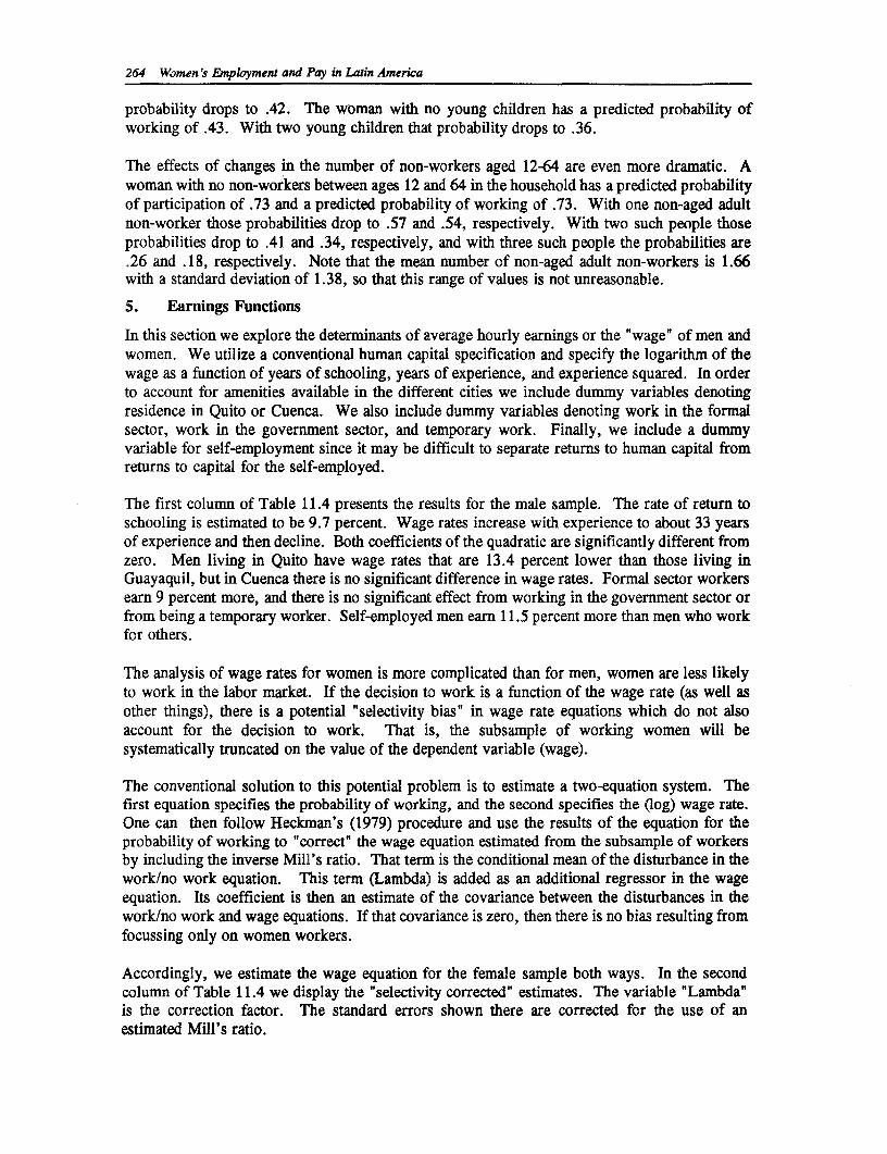
264 Women's Employment and Pay in Latin America
probability drops to .42. The woman with no young children has a predicted probability ofworking of .43. With two young children that probability drops to .36.
The effects of changes in the number of non-workers aged 12-64 are even more dramatic. Awoman with no non-workers between ages 12 and 64 in the household has a predicted probabilityof participation of .73 and a predicted probability of working of .73. With one non-aged adultnon-worker those probabilities drop to .57 and .54, respectively. With two such people thoseprobabilities drop to .41 and .34, respectively, and with three such people the probabilities are.26 and .18, respectively. Note that the mean number of non-aged adult non-workers is 1.66with a standard deviation of 1.38, so that this range of values is not unreasonable.
5. Earnings Functions
In this section we explore the determinants of average hourly earnings or the "wage" of men andwomen. We utilize a conventional human capital specification and specify the logarithm of thewage as a function of years of schooling, years of experience, and experience squared. In orderto account for amenities available in the different cities we include dummy variables denotingresidence in Quito or Cuenca. We also include dummy variables denoting work in the formalsector, work in the government sector, and temporary work. Finally, we include a dummyvariable for self-employment since it may be difficult to separate returns to human capital fromreturns to capital for the self-employed.
The first column of Table 11.4 presents the results for the male sample. The rate of return toschooling is estimated to be 9.7 percent. Wage rates increase with experience to about 33 yearsof experience and then decline. Both coefficients of the quadratic are significantly different fromzero. Men living in Quito have wage rates that are 13.4 percent lower than those living inGuayaquil, but in Cuenca there is no significant difference in wage rates. Formal sector workersearn 9 percent more, and there is no significant effect from working in the government sector orfrom being a temporary worker. Self-employed men earn 11.5 percent more than men who workfor others.
The analysis of wage rates for women is more complicated than for men, women are less likelyto work in the labor market. If the decision to work is a function of the wage rate (as well asother things), there is a potential "selectivity bias" in wage rate equations which do not alsoaccount for the decision to work. That is, the subsample of working women will besystematically truncated on the value of the dependent variable (wage).
The conventional solution to this potential problem is to estimate a two-equation system. Thefirst equation specifies the probability of working, and the second specifies the (log) wage rate.One can then follow Heckman's (1979) procedure and use the results of the equation for theprobability of working to "correct" the wage equation estimated from the subsample of workersby including the inverse Mill's ratio. That term is the conditional mean of the disturbance in thework/no work equation. This term (Lambda) is added as an additional regressor in the wageequation. Its coefficient is then an estimate of the covariance between the disturbances in thework/no work and wage equations. If that covariance is zero, then there is no bias resulting fromfocussing only on women workers.
Accordingly, we estimate the wage equation for the female sample both ways. In the secondcolumn of Table 11.4 we display the "selectivity corrected" estimates. The variable "Lambda"is the correction factor. The standard errors shown there are corrected for the use of anestimated Mill's ratio.
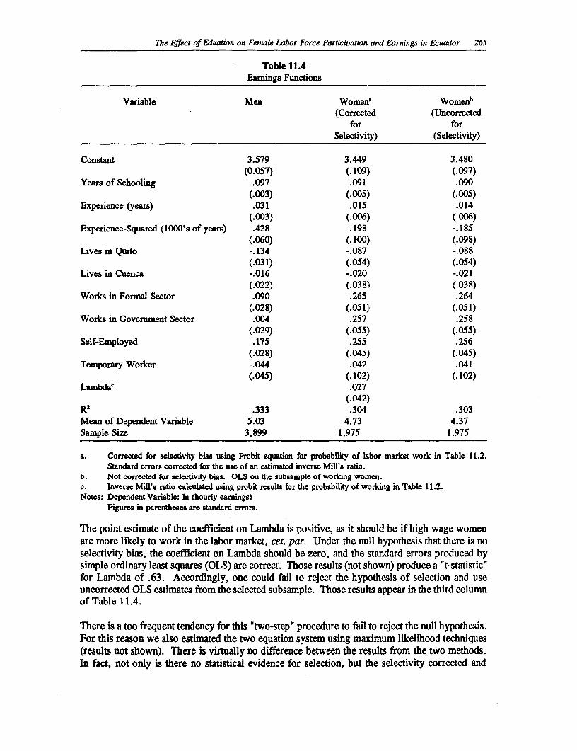
The Effect of Eduation on Female Labor Force Particiation and Earnings in Ecuador 265
Table 11.4Earnings Functions
Variable Men Women' Womenb(Corrected (Uncorrected
for forSelectivity) (Selectivity)
Constant 3.579 3.449 3.480(0.057) (.109) (.097)
Years of Schooling .097 .091 .090(.003) (.005) (.005)
Experience (years) .031 .015 .014(.003) (.006) (.006)
Experience-Squared (1000's of years) -.428 -.198 -.185(.060) (.100) (.098)
Lives in Quito -.134 -.087 -.088(.031) (.054) (.054)
Lives in Cuenca -.016 -.020 -.021(.022) (.038) (.038)
Works in Formal Sector .090 .265 .264(.028) (.051) (.051)
Works in Government Sector .004 .257 .258(.029) (.055) (.055)
Self-Employed .175 .255 .256(.028) (.045) (.045)
Temporary Worker -.044 .042 .041(.045) (.102) (.102)
Lambda0 .027(.042)
R2 .333 .304 .303Mean of Dependent Variable 5.03 4.73 4.37Sample Size 3,899 1,975 1,975
a. Corrected for selectivity bias using Probit equation for probability of labor market work in Table 11.2.Standard errors corrected for the use of an estimated inverse Mill's ratio.
b. Not corrected for selectivity bias. OLS on the subsample of worldng women.c. Inverse Mill's ratio calculated using probit results for the probability of working in Table 11.2.Notes: Dependent Variable: In (hourly earnings)
Figures in parentheses are standard errors.
The point estimate of the coefficient on Lambda is positive, as it should be if high wage womenare more likely to work in the labor market, cet. par. Under the null hypothesis that there is noselectivity bias, the coefficient on Lambda should be zero, and the standard errors produced bysimple ordinary least squares (OLS) are correct. Those results (not shown) produce a "t-statistic"for Lambda of .63. Accordingly, one could fail to reject the hypothesis of selection and useuncorrected OLS estimates from the selected subsample. Those results appear in the third columnof Table 11.4.
There is a too frequent tendency for this 'two-step" procedure to fail to reject the null hypothesis.For this reason we also estimated the two equation system using maximum likelihood techniques(results not shown). There is virtually no difference between the results from the two methods.In fact, not only is there no statistical evidence for selection, but the selectivity corrected and
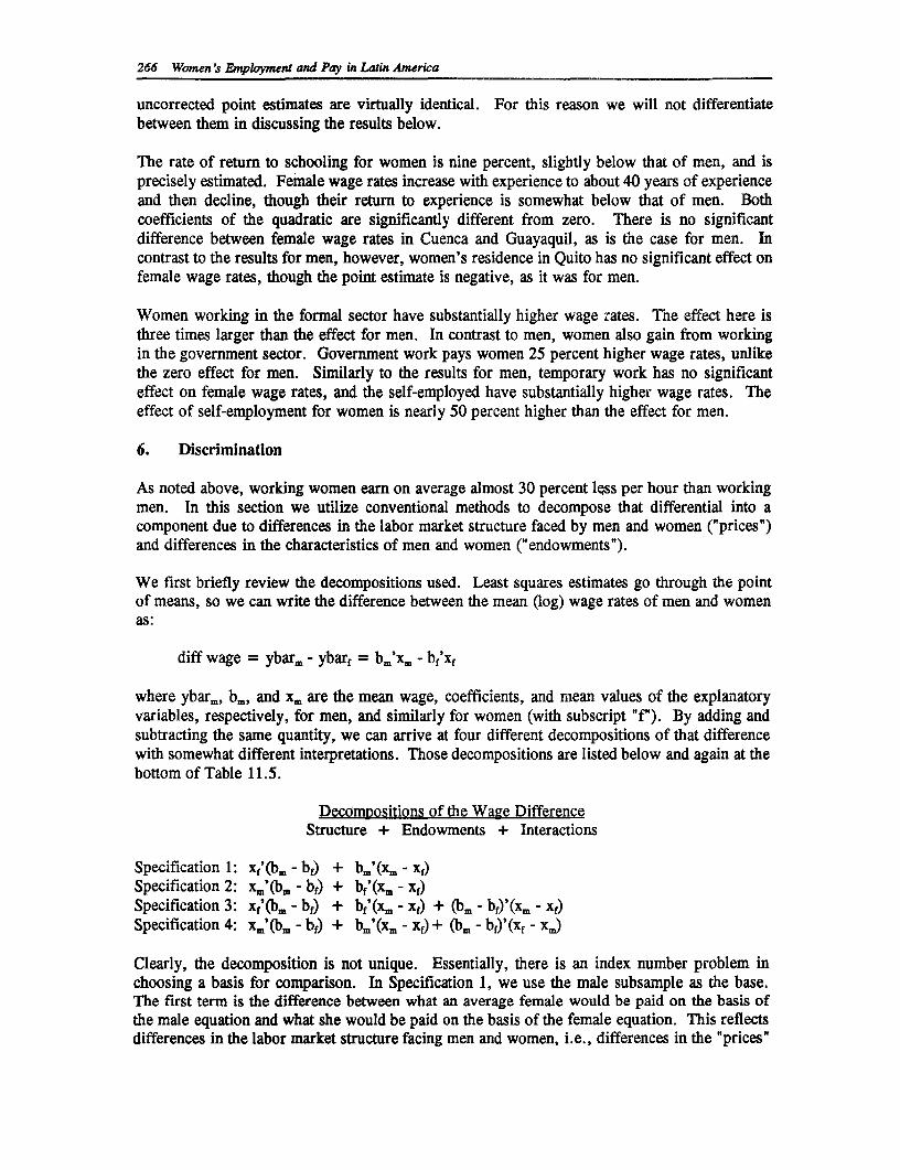
266 Women's Employment and Pay in Latin America
uncorrected point estimates are virtually identical. For this reason we will not differentiatebetween them in discussing the results below.
The rate of return to schooling for women is nine percent, slightly below that of men, and isprecisely estimated. Female wage rates increase with experience to about 40 years of experienceand then decline, though their return to experience is somewhat below that of men. Bothcoefficients of the quadratic are significantly different from zero. There is no significantdifference between female wage rates in Cuenca and Guayaquil, as is the case for men. Incontrast to the results for men, however, women's residence in Quito has no significant effect onfemale wage rates, though the point estimate is negative, as it was for men.
Women working in the formal sector have substantially higher wage rates. The effect here isthree times larger than the effect for men. In contrast to men, women also gain from workingin the government sector. Government work pays women 25 percent higher wage rates, unlikethe zero effect for men. Similarly to the results for men, temporary work has no significanteffect on female wage rates, and the self-employed have substantially higher wage rates. Theeffect of self-employment for women is nearly 50 percent higher than the effect for men.
6. Discrimination
As noted above, working women earn on average almost 30 percent less per hour than workingmen. In this section we utilize conventional methods to decompose that differential into acomponent due to differences in the labor market structure faced by men and women ("prices")and differences in the characteristics of men and women ("endowments").
We first briefly review the decompositions used. Least squares estimates go through the pointof means, so we can write the difference between the mean Oog) wage rates of men and womenas:
diff wage = ybarm - ybarf = bm'xm - bf'xf
where ybar., bi, and xm are the mean wage, coefficients, and mean values of the explanatoryvariables, respectively, for men, and similarly for women (with subscript "f"). By adding andsubtracting the same quantity, we can arrive at four different decompositions of that differencewith somewhat different interpretations. Those decompositions are listed below and again at thebottom of Table 11.5.
Decompositions of the Wage DifferenceStructure + Endowments + Interactions
Specification 1: Xf'(b. - bf) + b.'(x, - Xf)
Specification 2: x.'(b. - bf) + bf'(x. - xf)Specification 3: xf'(b. - bf) + bf'(x. - Xf) + (b. - bf)'(xm - xf)Specification 4: x,'(b. - bf) + bm'(x. - xf) + (bi - bf)'(xf - xj)
Clearly, the decomposition is not unique. Essentially, there is an index number problem inchoosing a basis for comparison. In Specification 1, we use the male subsample as the base.The first term is the difference between what an average female would be paid on the basis ofthe male equation and what she would be paid on the basis of the female equation. This reflectsdifferences in the labor market structure facing men and women, i.e., differences in the "prices"
The Effect of Eduation on Female Labor Force Particpation and Earnings in Ecuador 267
of human capital characteristics. The second term is the difference between the pay to an averagemale and the pay to an average female, based on the male wage equation. This reflectsdifferences in the characteristics (endowments) between men and women. Alternatively, onecould do the same decomposition, but use the female subsample as the base. This is thedecomposition in Specification 2.
Specifications 3 and 4 extend the analysis to allow for interaction effects. Specification 3 is anextension of Specification 1 and Specification 4 is an extension of Specification 2. InSpecification 3, the labor market structure term is the same as in Specification 1, that is, thedifference between the pay of an average female based on the male wage equation and based onthe female equation. The endowment term is now the difference between the pay of an averagemale and an average female, based this time on the female wage equation. The last term consistsof interaction effects between the differences in the wage equations and the differences in averagecharacteristics. Specification 4 is a similar extension of Specification 2.
No specification is theoretically correct in all cases. If we assume that the labor market for menoperates "correctly," then it is sensible to use the male labor market as the basis for the decom-position. Hence we have some preference for Specification 1 as the simplest case andSpecification 3 as a more complicated case. We present the results for all four specifications inTable 11.5.
We must also deal with the question of what to use as the coefficients and characteristics of the"average" female. There are basically two possible choices for each. We could either use thewage equation estimates which have been corrected for selectivity bias or the uncorrected wageequation estimates. Similarly, we could either use the mean characteristics of all women or thoseof working women. The answers depend on the population about which we wish to makeinference.
Suppose for the moment that wage rates could be observed for all women, whether or not theywork in the labor market. One would then use the full sample of women to estimate the wageequation. Of course, we can only observe wage rates for those women who do work. Theuncorrected wage equation, estimated on the subsample of working women, estimates theparameters of the conditional expectation of the Oog) wage, given that the woman works, and(implicitly) given the current rule for deciding whether or not to work in the labor market. Thepurpose of the selectivity "correction' is to obtain estimates comparable to those which we wouldobtain if we could observe wage rates independently of labor force status. Hence the correctedwage equation estimates refer to the entire population, not just the working subsample.
We calculate the decomposition in two ways. In Table 11.5, the decompositions listed under theheading "Total Population" use the first interpretable method. Here we use the corrected femalewage equation and the mean characteristics of all women. From this decomposition one couldforecast the effects of policy changes. The decompositions listed under the heading "WorkersOnly" follow the second interpretable method. Here we use the uncorrected wage equation andthe mean characteristics of working women.
For the population as a whole, women on average earn 50 percent less than men. UsingSpecification 1 where we use the experience of men as the basis for the decomposition, 31percentage points of the wage differential are shown to be due to differences in labor marketstructure and 19 percentage points are due to differences in endowments. Of the difference dueto labor market structure, 13 of the 31 percentage points are due to the differences in the
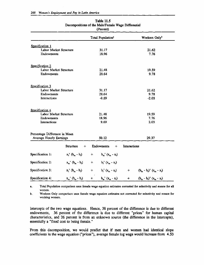
268 Women's Employment and Pay in Latin America
Table 11.5Decompositions of the Male/Female Wage Differential
(Percent)
Total Population! Workers OQlyb
SRecification 1Labor Market Structure 31.17 21.62Endowments 18.96 7.76
Specification 2Labor Market Structure 21.48 19.59Endowments 28.64 9.78
Specification 3Labor Market Structure 31.17 21.62Endowments 28.64 9.78Interactions -9.69 -2.03
Specification 4Labor Market Structure 21.48 19.59Endowments 18.96 7.76Interactions 9.69 2.03
Percentage Difference in MeanAverage Hourly Earnings 50.12 29.37
Structure + Endowments + Interactions
Specification 1: xf' (bm - bf) + bm' (xm - xd
Specification 2: x=' (bm - bf) + b,' (xm -xf)
Specification 3: Xf' (bm - bf) + bf' (x. - Xf) + (bm - bJ)' (x. - xj)
Specification 4: x.' (bm - bf) + bm' (xm - xf) + (bm - bf)' (XY - Xf)
a. Total Population comparison uses female wage equation estimates corrected for selectivity and means for allwomen.
b. Workers Only comparison uses female wage equation estimates not corrected for selectivity and means forworking women.
intercepts of the two wage equations. Hence, 38 percent of the difference is due to differentendowments, 36 percent of the difference is due to different "prices' for human capitalcharacteristics, and 26 percent is from an unknown source (the difference in the intercepts),essentially a "fixed cost to being female."
From this decomposition, we would predict that if men and women had identical slopecoefficients in the wage equation ("prices"), average female log wage would increase from 4.53
The Effect of Eduation on Female Labor Force Particiation and Earnings in Ecuador 269
to 4.71. If, in addition, the mean characteristics were the same the average female log wagewould rise to 4.90. Finally, if the intercepts were the same (no "fixed cost" to being female)there would be no wage differential.
If we use the female sample as the basis for the decomposition (Specification 2) the results aresomewhat different. A much larger proportion of the wage differential (55 percent) is due todifferences in endowments and only 17 percent is due to different returns to human capitalcharacteristics. This is probably not the correct basis for comparison, however.
The expanded specifications (3 and 4) which include interaction terms tell much the same story.There is a difference in the sign of the interaction term. When we use male experience as thebasis for comparison, the interaction effect is negative. That is, the interaction term tends toreduce the size of the predicted wage differential. In contrast, the interaction term is positivewhen we use the female experience as the basis of comparison.
The descriptive decompositions based only on working women are somewhat different. Themean difference in log wage rates is 29 percentage points. Using Specification 1, three-fourthsof the difference is due to differences in labor market structure and only one-fourth is due toendowments. That pattern is maintained throughout all the specifications.
7. Discussion
Female labor force participation and earnings of employed women have increased, relative tomen, since the 1966 survey analyzed by Finn and Jusenius (1975). Our sample shows theparticipation rate to be close to 50 percent, as opposed to 25 percent, and the average workingwoman earns 70 percent of average male earnings, in contrast to 55 percent.
Female labor force participation is positively related to education, with more educated womenbeing more likely to participate in the market and more likely to be employed. At sample meanvalues, an increase in years of schooling from 6 to 12 increases the participation probability from.46 to .47 and increases the employment probability from .40 to .42.
Marital status and household status are the most important social determinants of both labor forceparticipation and employment. Wives with working husbands are much less likely to work andparticipate than female heads of household. Women with young children are also less likely toparticipate and work.
We find no evidence of selectivity bias in the determinants of (log) average hourly earnings forwomen. That is, there is no evidence of systematic selection into the labor market based onunobservable variables which are correlated with the wage predictors. Therefore, wage equationsestimated on the subsample of working women are no different than shadow wage relationshipsfor all women.
Education is an important determinant of earnings for both men and women, and its effect isessentially the same for both groups. The return to labor market experience is higher for men,while sectoral differences are larger for women than men. In particular, women gain more fromself-employment, government work, and formal sector work than do men. In contrast, men losemore in Quito (relative to the other cities) than do women.
270 Women's Enmployment and Pay in Latin America
In general, the decompositions of the wage rate differentials in Table 11.5 suggest that differencesin labor market structure are more important than differences in labor market endowments inexplaining the difference between average earnings of men and women. This is particularly truewhen one considers the subsample of working women. For these women, roughly twentypercentage points of the 30 percent differential can be attributed to differences in labor marketstructure, independent of the decomposition method employed. The most important differenceappears to be the higher return to experience for men.
Differences in labor market endowments are more important when we consider all women. Theyaccount for almost one-half of the difference in average hourly earnings between men andwomen. This result is driven by the labor force participation and employment probabilities,which are functions of both social variables (marital status and household structure) as well aseducation.
Between ten and fifteen percentage points of the male-female earnings differential is due to theconstant terms in the earnings equations. This represents an essentially unknown source ofearnings differences. That effect is ameliorated when women work in the formal sector, thegovernment sector, or are self-employed. These results suggest that women face a more seriouswage disadvantage in the informal sector. Policies to extend formal sector coverage may be mosteffective in reducing the male-female earnings differential, at least for urban women.
References
Finn, M. and C.L. Jusenius. "The Position of Women in the Ecuadorian Labor Force." OhioState University: Center for Human Resource Research, 1975.
Gronau, R. "The Effect of Children on the Housewife's Value of Time" in T.W. Schultz (ed.).Economics of the Family. Chicago: University of Chicago Press, 1974.
Heckman, J.J. "Sample Selection Bias as a Specification Error." Econometrica, Vol. 47, no. 1(1979). pp. 53-161.
Jakubson, G. "The Sensitivity of Labor Supply Parameter Estimates to Unobserved individualEffects: Fixed and Random Effects Estimates in a Nonlinear Model Using Panel Data."Journal of Labor Economics,, 1988.
Mincer, J. Schooling, Experience and Earnings. New York: Columbia University Press, 1974.
Oaxaca, R. "Male-Female Wage Differentials in Urban Labor Markets." International EconomicReview, Vol. 14, no. 1 (1973). pp. 693-709.
World Bank. "Ecuador: Country Assessment of Women's Role in Development." Mimeograph.Washington, D.C.: Latin America and Caribbean Region, World Bank, 1989.
271

12
Female Labor Force Participation and Earnings inGuatemala
Mary Arends
1. Introduction
This chapter examines female labor force participation in Guatemala and attempts to explain theearnings differential between men and women using the human capital model. Guatemala hasunique development problems. Its literacy rate is the lowest in Latin America, and there is alarge schooling gap between men and women. About 40 percent of its population areAmerindians, many of whom do not speak Spanish, and who have little access to social servicesor to formal labor markets. About half the work force is employed in agriculture, much of it atthe subsistence level.
Section 2 presents an overview of the Guatemalan economy, labor market, and schooling system.Section 3 presents the results of probit regressions for both men and women analyzing thecharacteristics which make an individual likely to be observed in the labor market. Building onthe results of Section 3, Section 4 presents the results of earnings regressions for men and womenboth corrected and uncorrected for selectivity. There are separate earnings regressions for menand women who work in the formal sector. Lastly, in Section 5, an upper bound on labor marketdiscrimination is estimated and discussed. Section 6 summarizes the findings and gives policyrecommendations.
2. The Guatemalan Economy and Labor Market
Guatemala had a GNP per capita of $910 in 1989, placing it only above Bolivia, the DominicanRepublic and Honduras among Latin American countries. The annual GNP per capita growthrate from 1965 to 1989 was .9 percent.1 Population growth rates between 1980 and 1989 werehigher than average for Latin America at 2.8 percent per year. 2 Ethnically, Guatemala is a verydiverse country, with 23 different languages spoken, and 40 percent of the populationAmerindian. The Indians are marginalized from Guatemalan Spanish-speaking society, tend tobe concentrated in rural areas, and tend to be subsistence farmers.
From 1980 to 1985, the country's GDP declined by an average of 1.1 percent per year. Arecovery started in 1986, and from 1988 to 1989, GDP grew by 4 percent in real terms.
World Bank Development Report 1991, Table 1.
2 Economist Intelligence Unit, p. 12 (1991).
273
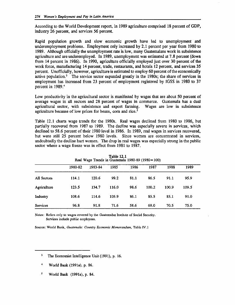
274 Women's Employment and Pay in Latin America
According to the World Development report, in 1989 agriculture comprised 18 percent of GDP,industry 26 percent, and services 56 percent.
Rapid population growth and slow economic growth have led to unemployment andunderemployment problems. Employment only increased by 2.1 percent per year from 1980 to1989. Although officially the unemployment rate is low, many Guatemalans work in subsistenceagriculture and are underemployed. In 1989, unemployment was estimated at 7.8 percent (downfrom 14 percent in 1986). In 1990, agriculture officially employed just over 30 percent of thework force, manufacturing 14 percent, trade, restaurants, and hotels 12 percent, and services 35percent. Unofficially, however, agriculture is estimated to employ 60 percent of the economicallyactive population.3 The service sector expanded greatly in the 1980s; the share of services inemployment has increased from 23 percent of employment registered by IGSS in 1980 to 37percent in 1989.4
Low productivity in the agricultural sector is manifested by wages that are about 50 percent ofaverage wages in all sectors and 28 percent of wages in commerce. Guatemala has a dualagricultural sector, with subsistence and export farming. Wages are low in subsistenceagriculture because of low prices for beans, corn and rice.5
Table 12.1 charts wage trends for the 1980s. Real wages declined from 1980 to 1986, butpartially recovered from 1987 to 1989. The decline was especially severe in services, whichdeclined to 58.6 percent of their 1980 level in 1986. In 1989, real wages in services recovered,but were still 25 percent below 1980 levels. Since women are concentrated in services,undoubtedly the decline hurt women. The drop in real wages was especially strong in the publicsector where a wage freeze was in effect from 1981 to 1987.
Table 12.1Real Wage Trends in Guatemala 1980-89 (1980= 100)
1980-82 1983-84 1985 1986 1987 1988 1989
All Sectors 114.1 120.6 99.2 81.1 86.5 91.1 95.9
Agriculture 123.5 134.7 116.0 98.6 100.2 100.9 109.5
Industry 108.6 114.6 105.9 86.1 85.5 85.1 91.0
Services 96.8 91.8 71.6 58.6 69.0 70.5 75.0
Notes: Refers only to wages covered by the Guatemalan Institute of Social Security.Services include public employees.
Source: World Bank, Guatemala: Country Economic Memorandum, Table IV.1
3 The Economist Intelligence Unit (1991), p. 16.
4 World Bank (199la), p. 86.
5 World Bank (1991a), p. 84.
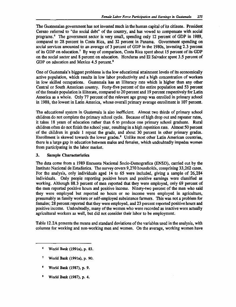
Femak Labor Force Participation and Earnings in Guatemala 275
The Guatemalan government has not invested much in the human capital of its citizens. PresidentCerezo referred to "the social debt" of the country, and has vowed to compensate with socialprograms.6 The government sector is very small, spending only 12 percent of GDP in 1989,compared to 28 percent in Costa Rica, and 32 percent in Panama. Government spending onsocial services amounted to an average of 3 percent of GDP in the 1980s, investing 2.3 percentof its GDP on education.7 By way of comparison, Costa Rica spent about 15 percent of its GDPon the social sector and 8 percent on education. Honduras and El Salvador spent 3.5 percent ofGDP on education and Mexico 4.5 percent.!
One of Guatemala's biggest problems is the low educational attainment levels of its economicallyactive population, which results in low labor productivity and a high concentration of workersin low skilled occupations. Guatemala has an illiteracy rate which is higher than any otherCentral or South American country. Forty-five percent of the entire population and 53 percentof the female population is illiterate, compared to 20 percent and 19 percent respectively for LatinAmerica as a whole. Only 77 percent of the relevant age group was enrolled in primary schoolin 1988, the lowest in Latin America, whose overall primary average enrollment is 107 percent.
The educational system in Guatemala is also inefficient. Almost two thirds of primary schoolchildren do not complete the primary school cycle. Because of high drop out and repeater rates,it takes 18 years of education rather than 6 to produce one primary school graduate. Ruralchildren often do not finish the school year, resulting in a high repetition rate. Almost 50 percentof the children in grade 1 repeat the grade, and about 30 percent in other primary grades.Enrollment is skewed towards the lower grades.9 Unlike most other Latin American countries,there is a large gap in education between males and females, which undoubtedly impedes womenfrom participating in the labor market.
3. Sample Characteristics
The data come from a 1989 Encuesta Nacional Socio-Demografica (ENSD), carried out by theInstituto Nacional de Estadistica. The survey covers 9,270 households, comprising 33,262 cases.For the analysis, only individuals aged 14 to 65 were included, giving a sample of 26,284individuals. Only people reporting positive hours and positive earnings were classified asworking. Although 88.3 percent of men reported that they were employed, only 69 percent ofthe men reported positive hours and positive income. Ninety-two percent of the men who saidthey were employed but reported no hours or no income were employed in agriculture,presumably as family workers or self-employed subsistence farmers. This was not a problem forfemales; 28 percent reported that they were employed, and 23 percent reported positive hours andpositive income. Undoubtedly, many of the women who were recorded as inactive were actuallyagricultural workers as well, but did not consider their labor to be employment.
Table 12.2A presents the means and standard deviations of the variables used in the analysis, withcolumns for working and non-working men and women. On the average, working women have
6 World Bank (199 la), p. 83.
7 World Bank (1991a), p. 90.
s World Bank (1987), p. 9.
9 World Bank (1987), p. 4.
276 Women's Employment and Pay in Latin America
almost a year of schooling more than working men.'0 Working women have higher educationalattainments as well--16 percent have completed secondary education or above, as compared to8 percent of the working men. Non-working women have very low levels of schooling, sooverall women have .84 years of schooling less than men. A higher percentage of non-workingwomen are illiterate than working women, while literacy rates for working and non-working menare about the same.
The survey has no variable for work experience, so a proxy is constructed where potentialexperience equals age minus schooling minus 6. This variable will tend to overstate actualexperience, especially for women, because they are likely to have interrupted their working liveste have children. Working men have 2.83 more years of potential experience than workingwomen.
Both men and women work over forty hours per week, with men working over 48 hours on theaverage. Men worked almost 6 hours a week more than the women.
To compute the hourly wage, monthly earnings are divided by monthly hours, equal to weeklyhours multiplied by 4.3. Women have a very small pay disadvantage, earning on average 97percent of male wages. This is very low for Latin America, and for developed countries aswell. "
The self-employed category includes domestic workers and excludes professionals. Over half ofthe working women are self-employed, compared to 34 percent of working men. Twenty-twopercent of non-working men are classified as self-employed, again because of the missing datafor men who are recorded as employed, but have no hours or no income. Fifty-seven percentof working men work in the private sector, and 9 percent in the public sector. Thirty-sevenpercent of working women work in the private sector and 11 percent in the public sector.
The analysis includes several household variables, including marital status, household size,number of children younger than 10 years old in the household, total household income, and thenumber of workers in the household. Since the survey includes only children aged 10 and over,it is not possible to distinguish between children younger than 6 and older than 6, nor can thechildren be assigned to their actual parents or guardians. For this reason, the child variablerepresents the number of children in the household. Working women come from smaller-sizedhouseholds, are less likely to be married, and have fewer children than non-working women.Working men also come from smaller households, but have more children and are much morelikely to be married than non-working men.
Table 12.2B presents the means and standard deviations of the variables used in the analysis,broken down by self-employed and formal sector. Here, the formal sector is defined to includeboth private and public sector employees. Self-employed males and females are older and haveless education than males and females employed in the formal sector. Women in the formalsector have about 4.5 more years of education than self-employed women, and for men thedifference is 2.3 years. Also, females and males with greater family responsibilities are more
10 In the data, only the years of schooling at the appropriate level was available. It was not possibleto determine whether the respondent was held back or whether the years of schooling indicate the highestgrade actually completed. Given Guatemala's high repeater rate, this is likely to overstate actual education.
it See other chapters in this volume. The pay ratio is 81 percent in Honduras, 75 percent inUruguay, 70 percent in Venezuela, 85 percent in Panama, and 58 percent in Jamaica.
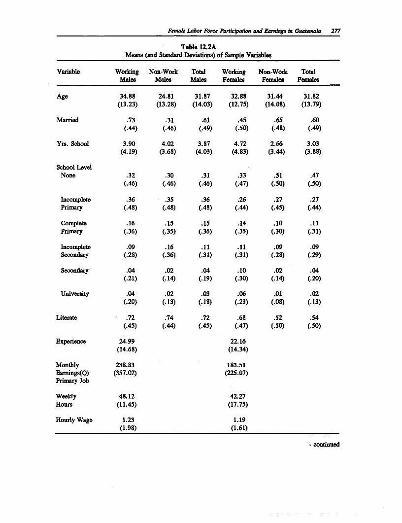
Femal Labor Force Participation and Earngs s Guatemala 277
Table 12.2AMeans (and Standard Deviations) of Sample Variables
Variable Working Non-Work Total Working Non-Work TotalMales Males Males Females Females Females
Age 34.88 24.81 31.87 32.88 31.44 31.82(13.23) (13.28) (14.03) (12.75) (14.08) (13.79)
Married .73 .31 .61 .45 .65 .60(.44) (.46) (.49) (.50) (.48) (.49)
Yrs. School 3.90 4.02 3.87 4.72 2.66 3.03(4.19) (3.68) (4.03) (4.83) (3.44) (3.88)
School LevelNone .32 .30 .31 .33 .51 .47
(.46) (.46) (.46) (.47) (.50) (.50)
Incomplete .36 .35 .36 .26 .27 .27Primary (.48) (.48) (.48) (.44) (.45) (.44)
Complete .16 .15 .15 .14 .10 .11Primary (.36) (.35) (.36) (.35) (.30) (.31)
Incomplete .09 .16 .11 .11 .09 .09Secondary (.28) (.36) (.31) (.31) (.28) (.29)
Secondary .04 .02 .04 .10 .02 .04(.21) (.14) (.19) (.30) (.14) (.20)
University .04 .02 .03 .06 .01 .02(.20) (.13) (.18) (.23) (.08) (.13)
Literate .72 .74 .72 .68 .52 .54(.45) (.44) (.45) (.47) (.50) (.50)
Experience 24.99 22.16(14.68) (14.34)
Monthly 238.83 183.51Earnings(Q) (357.02) (225.07)Primary Job
Weekly 48.12 42.27Hours (11.45) (17.75)
Hourly Wage 1.23 1.19(1.98) (1.61)
- continued
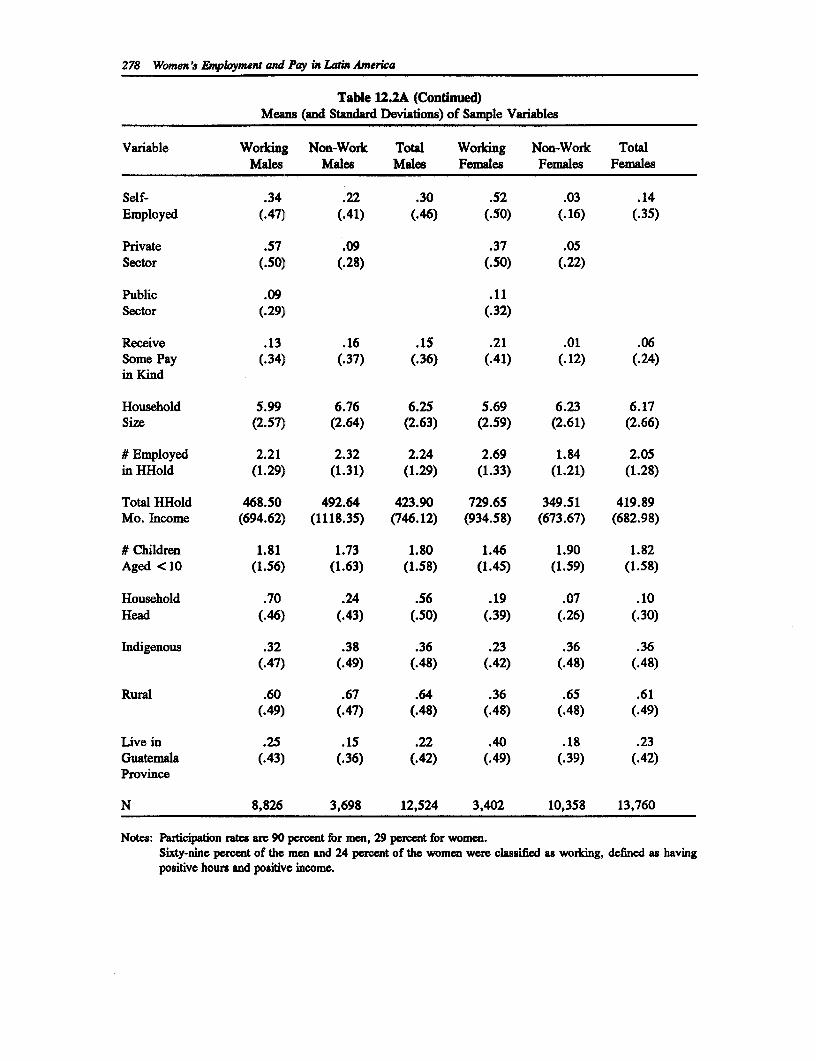
278 Women's Employment and Pay in Latin America
Table 12.2A (Continued)Means (and Standard Deviations) of Sample Variables
Variable Working Non-Work Total Working Non-Work TotalMales Males Males Females Females Females
Self- .34 .22 .30 .52 .03 .14Employed (.47) (.41) (.46) (.50) (.16) (.35)
Private .57 .09 .37 .05Sector (.50) (.28) (.50) (.22)
Public .09 .11Sector (.29) (.32)
Receive .13 .16 .15 .21 .01 .06Some Pay (.34) (.37) (.36) (.41) (.12) (.24)in Kind
Household 5.99 6.76 6.25 5.69 6.23 6.17Size (2.57) (2.64) (2.63) (2.59) (2.61) (2.66)
# Employed 2.21 2.32 2.24 2.69 1.84 2.05in HHold (1.29) (1.31) (1.29) (1.33) (1.21) (1.28)
Total HHold 468.50 492.64 423.90 729.65 349.51 419.89Mo. Income (694.62) (1118.35) (746.12) (934.58) (673.67) (682.98)
# Children 1.81 1.73 1.80 1.46 1.90 1.82Aged <10 (1.56) (1.63) (1.58) (1.45) (1.59) (1.58)
Household .70 .24 .56 .19 .07 .10Head (.46) (.43) (.50) (.39) (.26) (.30)
Indigenous .32 .38 .36 .23 .36 .36(.47) (.49) (.48) (.42) (.48) (.48)
Rural .60 .67 .64 .36 .65 .61(.49) (.47) (.48) (.48) (.48) (.49)
Live in .25 .15 .22 .40 .18 .23Guatemala (.43) (.36) (.42) (.49) (.39) (.42)Province
N 8,826 3,698 12,524 3,402 10,358 13,760
Notes: Participation rates are 90 pecent for men, 29 percent for women.Sixty-nine percent of the men and 24 percent of the women were classified as wording, defined as havingpositive hours and positive income.
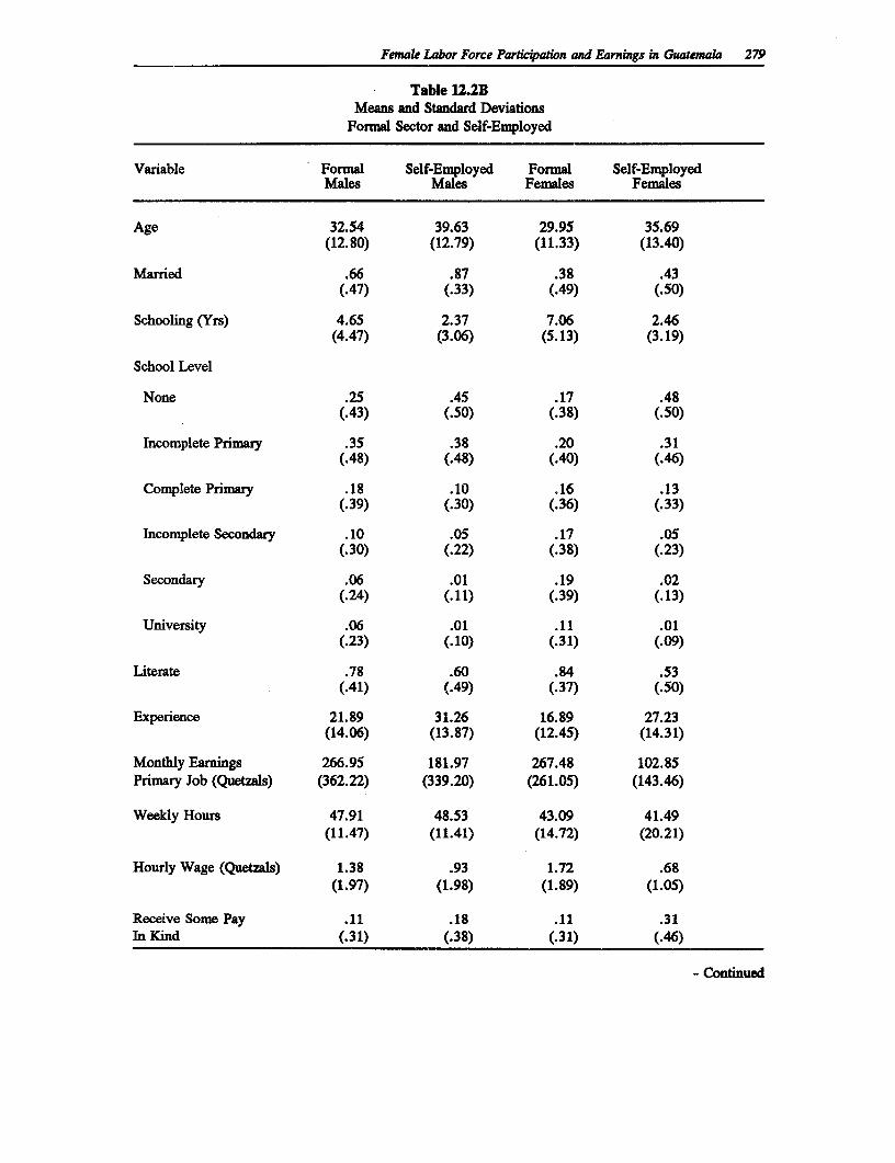
Femal Labor Force Participation and Earnings in Guatemala 279
Table 12.2BMeans and Standard Deviations
Fornal Sector and Self-Employed
Variable Formal Self-Employed Formal Self-EmnployedMales Males Females Fenales
Age 32.54 39.63 29.95 35.69(12.80) (12.79) (11.33) (13.40)
Married .66 .87 .38 .43(.47) (.33) (.49) (.50)
Schooling (Yrs) 4.65 2.37 7.06 2.46(4.47) (3.06) (5.13) (3.19)
School Level
None .25 .45 .17 .48(.43) (.50) (.38) (.50)
Incomplete Primary .35 .38 .20 .31(.48) (.48) (.40) (.46)
Comnplete Primary .18 .10 .16 .13(.39) (.30) (.36) (.33)
Incomplete Secondary .10 .05 .17 .05(.30) (.22) (.38) (.23)
Secondary .06 .01 .19 .02(.24) (.11) (.39) (.13)
University .06 .01 .11 .01(.23) (.10) (.31) (.09)
Literate .78 .60 .84 .53(.41) (.49) (.37) (.50)
Experience 21.89 31.26 16.89 27.23(14.06) (13.87) (12.45) (14.31)
Monthly Eamnings 266.95 181.97 267.48 102.85Primary Job (Quetzals) (362.22) (339.20) (261.05) (143.46)
Weekly Hours 47.91 48.53 43.09 41.49(11.47) (11.41) (14.72) (20.21)
Hourly Wage (Quetzals) 1.38 .93 1.72 .68(1.97) (1.98) (1.89) (1.05)
Receive Some Pay .11 .18 .11 .31In Kind (.31) (.38) (.31) (.46)
- Continued
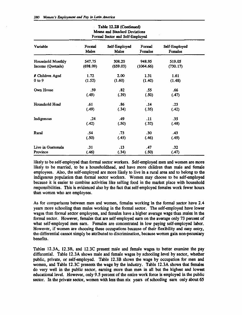
280 Women's Employment and Pay in Latin America
Table 12.2B (Continued)Means and Standard Deviations
Formal Sector and Self-Employed
Variable Formal Self-Employed Formal Self-ErnployedMales Males Females Females
Household Monthly 547.75 308.20 948.95 519.05Income (Quetzals) (698.09) (659.03) (1064.66) (730.17)
# Children Aged 1.72 2.00 1.31 1.61O to 9 (1.52) (1.60) (1.40) (1.48)
Own House .59 .82 .55 .66(.49) (.39) (.50) (.47)
Household Head .61 .86 .14 .23(.49) (.34) (.35) (.42)
Indigenous .24 .49 .11 .35(.42) (.50) (.32) (.48)
Rural .54 .73 .30 .43(.50) (.45) (.46) (.49)
Live in Guatemala .31 .13 .47 .32Province (.46) (.34) (.50) (.47)
likely to be self-employed than formal sector workers. Self-employed men and women are morelikely to be married, to be a householdhead, and have more children than male and femaleemployees. Also, the self-employed are more likely to live in a rural area and to belong to theindigenous population than formal sector workers. Women may choose to be self-employedbecause it is easier to combine activities like selling food in the market place with householdresponsibilities. This is evidenced also by the fact that self-employed females work fewer hoursthan women who are employees.
As for comparisons between men and women, females working in the formal sector have 2.4years more schooling than males working in the formal sector. The self-employed have lowerwages than formal sector employees, and females have a higher average wage than males in theformal sector. However, females that are self-employed earn on the average only 73 percent ofwhat self-employed men earn. Females are concentrated in low paying self-employed labor.However, if women are choosing these occupations because of their flexibility and easy entry,the differential cannot simply be attributed to discrimination, because women gain non-pecuniarybenefits.
Tables 12.3A, 12.3B, and 12.3C present male and female wages to better examine the paydifferential. Table 12.3A shows male and female wages by schooling level by sector, whetherpublic, private, or self-employed. Table 12.3B shows the wage by occupation for men andwomen, and Table 12.3C presents the wage by the industry. Table 12.3A shows that femalesdo very well in the public sector, earning more than men in all but the highest and lowesteducational level. However, only 9.5 percent of the entire work force is employed in the publicsector. In the private sector, women with less than six years of schooling earn only about 65
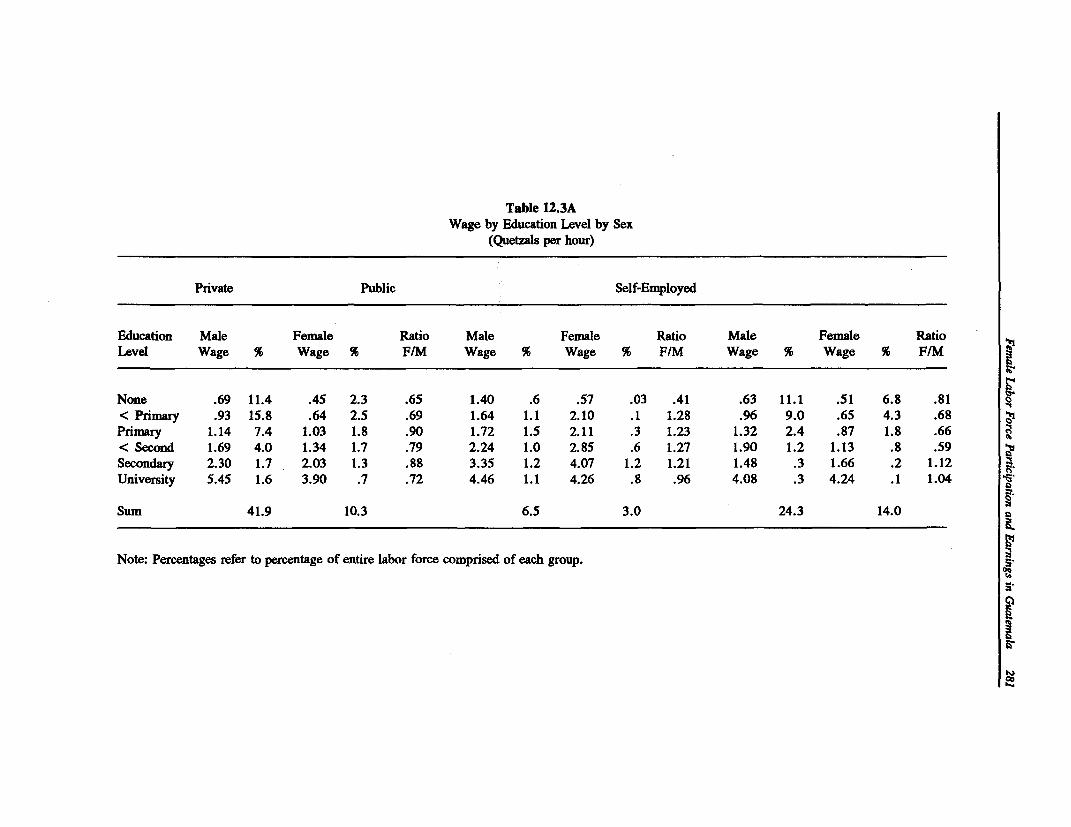
Table 12.3AWage by Education Level by Sex
(Quetzals per hour)
Private Public Self-Employed
Education Male Female Ratio Male Female Ratio Male Female RatioLevel Wage % Wage % F/M Wage % Wage % F/M Wage % Wage % F/M
None .69 11.4 .45 2.3 .65 1.40 .6 .57 .03 .41 .63 11.1 .51 6.8 .81 N
< Primary .93 15.8 .64 2.5 .69 1.64 1.1 2.10 .1 1.28 .96 9.0 .65 4.3 .68Primary 1.14 7.4 1.03 1.8 .90 1.72 1.5 2.11 .3 1.23 1.32 2.4 .87 1.8 .66< Second 1.69 4.0 1.34 1.7 .79 2.24 1.0 2.85 .6 1.27 1.90 1.2 1.13 .8 .59Secondary 2.30 1.7 2.03 1.3 .88 3.35 1.2 4.07 1.2 1.21 1.48 .3 1.66 .2 1.12 NUniversity 5.45 1.6 3.90 .7 .72 4.46 1.1 4.26 .8 .96 4.08 .3 4.24 .1 1.04
Sum 41.9 10.3 6.5 3.0 24.3 14.0
Note: Percentages refer to percentage of entire labor force comprised of each group.
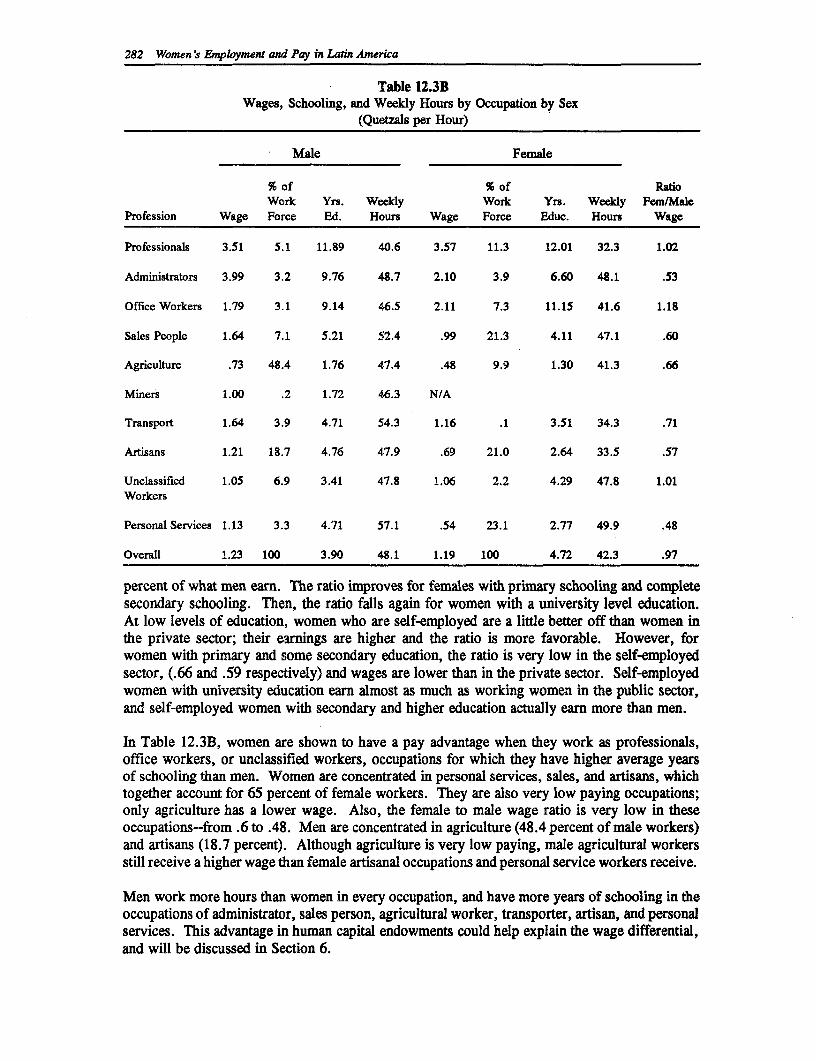
282 Women's Employment and Pay in Latin America
Table 12.3BWages, Schooling, and Weekly Hours by Occupation by Sex
(Quetzals per Hour)
Male Female
% of % of RatioWork Yrs. Weekly Work Yrs. Weekly Fem/Male
Profession Wage Force Ed. Hours Wage Force Educ. Hours Wage
Professionals 3.51 5.1 11.89 40.6 3.57 11.3 12.01 32.3 1.02
Administrators 3.99 3.2 9.76 48.7 2.10 3.9 6.60 48.1 .53
Office Workers 1.79 3.1 9.14 46.5 2.11 7.3 11.15 41.6 1.18
Sales People 1.64 7.1 5.21 52.4 .99 21.3 4.11 47.1 .60
Agriculture .73 48.4 1.76 47.4 .48 9.9 1.30 41.3 .66
Miners 1.00 .2 1.72 46.3 N/A
Transport 1.64 3.9 4.71 54.3 1.16 .1 3.51 34.3 .71
Artisans 1.21 18.7 4.76 47.9 .69 21.0 2.64 33.5 .57
Unclassified 1.05 6.9 3.41 47.8 1.06 2.2 4.29 47.8 1.01Workers
Personal Services 1.13 3.3 4.71 57.1 .54 23.1 2.77 49.9 .48
Overall 1.23 100 3.90 48.1 1.19 100 4.72 42.3 .97
percent of what men earn. The ratio improves for females with primary schooling and completesecondary schooling. Then, the ratio falls again for women with a university level education.At low levels of education, women who are self-employed are a little better off than women inthe private sector; their earnings are higher and the ratio is more favorable. However, forwomen with primary and some secondary education, the ratio is very low in the self-employedsector, (.66 and .59 respectively) and wages are lower than in the private sector. Self-employedwomen with university education earn almost as much as working women in the public sector,and self-employed women with secondary and higher education actually earn more than men.
In Table 12.3B, women are shown to have a pay advantage when they work as professionals,office workers, or unclassified workers, occupations for which they have higher average yearsof schooling than men. Women are concentrated in personal services, sales, and artisans, whichtogether account for 65 percent of female workers. They are also very low paying occupations;only agriculture has a lower wage. Also, the female to male wage ratio is very low in theseoccupations-from .6 to .48. Men are concentrated in agriculture (48.4 percent of male workers)and artisans (18.7 percent). Although agriculture is very low paying, male agricultural workersstill receive a higher wage than female artisanal occupations and personal service workers receive.
Men work more hours than women in every occupation, and have more years of schooling in theoccupations of administrator, sales person, agricultural worker, transporter, artisan, and personalservices. This advantage in human capital endowments could help explain the wage differential,and will be discussed in Section 6.
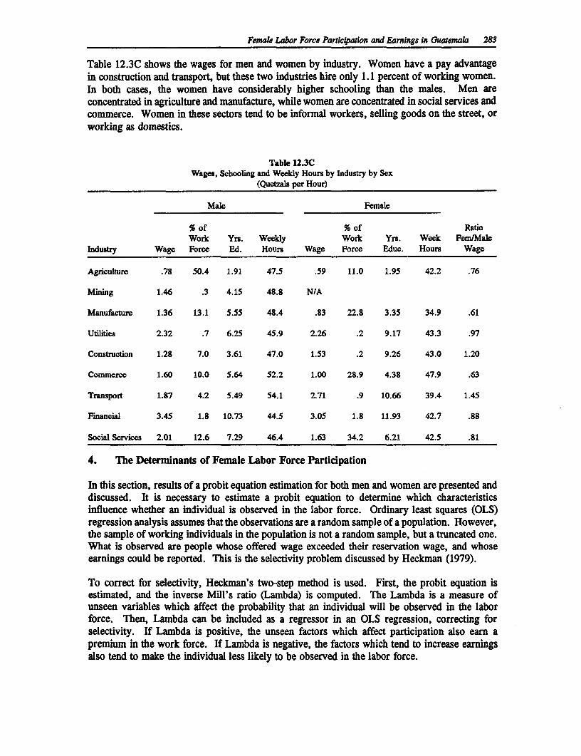
Femak Labor Force Participation and Earnings in Guatemala 283
Table 12.3C shows the wages for men and women by industry. Women have a pay advantagein construction and transport, but these two industries hire only 1.1 percent of working women.In both cases, the women have considerably higher schooling than the males. Men areconcentrated in agriculture and manufacture, while women are concentrated in social services andcommerce. Women in these sectors tend to be informal workers, selling goods on the street, orworking as domestics.
Table 12.3CWages, Schooling and Weekly Hours by Industry by Sex
(Quetzals per Hour)
Male Female
% of % of RatioWork Yrs. Weekly Work Yrs. Week Fem/Male
Industry Wage Force Ed. Hours Wage Force Educ. Hours Wage
Agriculture .78 50.4 1.91 47.5 .59 11.0 1.95 42.2 .76
Mining 1.46 .3 4.15 48.8 N/A
Manufiacture 1.36 13.1 5.55 48.4 .83 22.8 3.35 34.9 .61
utilities 2.32 .7 6.25 45.9 2.26 .2 9.17 43.3 .97
Construction 1.28 7.0 3.61 47.0 1.53 .2 9.26 43.0 1.20
Commerce 1.60 10.0 5.64 52.2 1.00 28.9 4.38 47.9 .63
Transport 1.87 4.2 5.49 54.1 2.71 .9 10.66 39.4 1.45
Financial 3.45 1.8 10.73 44.5 3.05 1.8 11.93 42.7 .88
Social Services 2.01 12.6 7.29 46.4 1.63 34.2 6.21 42.5 .81
4. The Determinants of Female Labor Force Participation
In this section, results of a probit equation estimation for both men and women are presented anddiscussed. It is necessary to estimate a probit equation to determine which characteristicsinfluence whether an individual is observed in the labor force. Ordinary least squares (OLS)regression analysis assumes that the observations are a random sample of a population. However,the sample of working individuals in the population is not a random sample, but a truncated one.What is observed are people whose offered wage exceeded their reservation wage, and whoseearnings could be reported. This is the selectivity problem discussed by Heckman (1979).
To correct for selectivity, Heekman's two-step method is used. First, the probit equation isestimated, and the inverse Mill's ratio (Lambda) is computed. The Lambda is a measure ofunseen variables which affect the probability that an individual will be observed in the laborforce. Then, Lambda can be included as a regressor in an OLS regression, correcting forselectivity. If Lambda is positive, the unseen factors which affect participation also earn apremium in the work force. If Lambda is negative, the factors which tend to increase earningsalso tend to make the individual less likely to be observed in the labor force.
284 Women 's Employment and Pay in Latin America
The probit equations include right hand side variables for educational levels, age splines, locality,marital status, household structure, and the "need for income" (proxied by the number of otheremployed people in the household and total household income excluding the respondent'sincome). Table 12.4A presents the results for men and Table 12.4B the results for women.
Looking at Table 12.4A, only two educational variables (no education and some secondaryeducation) and four age variables are significant at the five percent level for men. Since maleparticipation rates are already high (69 percent) the partial derivatives which represent the slopeof the probit function are small.
The variables representing marital status, household headship, location, ethnic origin, andmonthly household income are all significant. For men, being married increases the probabilityof working. Household headship also has a large positive effect on participation. Thecoefficients of the dummy variables representing ethnic origin and rural location are negative, aswould be expected by the lack of access to formal labor markets. Also, many subsistencefarmers and family workers did not have any earnings or hours reported and so were coded as"not-working." Most of the indigenous and rural population are subsistence farmers; 73 percentof indigenous men are agricultural workers. Also, of the indigenous men, 42 percent were self-employed and 21 percent were family workers.
Table 12.5 presents the results of a simulation to isolate the effect of each variable on theprobability of participation. Other variables are held at the sample mean, while each dummyvariable is set equal to 1. For men, looking at education, the probability of participation variesonly by ten percentage points. Men who have completed secondary school have the highestprobability of participation, while those with incomplete secondary schooling have the lowest.Those with incomplete secondary education could have a very high reservation wage as they tryto complete secondary. Also, the expected participation rate could be low because of raisedexpectations. Those with incomplete secondary schooling perceive themselves as more qualifiedthan those with primary education, so they want a better job, but they are not qualified for jobsrequiring a secondary school degree. Completing secondary school appears to be an importantqualification in the Guatemalan labor market. The secondary school diploma could be asignalling device that employers look for when hiring labor.
The effects of age on participation are notable for the 14 to 19 age group, where participationis at its lowest. Almost 70 percent are actually active, but of those working, about half arefamily workers in agriculture. Twenty-five percent of the men in the youngest age group arestudents. Participation peaks at the ages of 30 to 34 and is level until the ages of 50 and above.For older men, the probability declines steadily. There is not an abrupt falling off inparticipation levels.
In Table 12.4B, which presents the results of the probit estimation for females, it is apparent thatschooling level is an important determinant of participation. It is significant at the 5 percent levelfor all schooling levels except university, and the partial derivatives are large compared to othervariables. The number of children and marital status have the expected negative and significantimpact on participation, indicating that women with more household responsibilities have a higherreservation wage than single or childless women.
All of the age splines are significant, except for age 50 to 54. Participation peaks between theages of 30 and 34. However, in Guatemala, participation dips for women aged 35 to 39 and thenrises again.
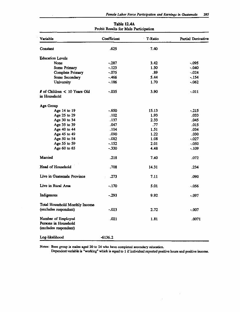
Female Labor Force Parucipahon and Earnings in Guatemala 285
Table 12.4AProbit Results for Male Participation
Variable Coefficient T-Ratio Partial Derivative
Constant .625 7.40
Education LevelsNone -.287 3.42 -.095Some Primary -.123 1.50 -.040Complete Primary -.075 .89 -.024Some Secondary -.466 5.44 -.154University -.186 1.70 -.062
#of Children < 10 Years Old -.035 3.90 -.011in Household
Age GroupAge 14 to 19 -.650 15.13 -.215Age 25 to 29 .102 1.93 .033Age 30 to 34 .137 2.33 .045Age 35 to 39 .047 .77 .015Age 40 to 44 .104 1.51 .034Age 45 to 49 .090 1.22 .030Age 50 to 54 -.082 1.08 -.027Age 55 to 59 -. 152 2.01 -.050Age 60 to 65 -.330 4.48 -. 109
Married .218 7.40 .072
Head of Household .708 14.31 .234
Live in Guatemala Province .273 7.11 .090
Live in Rural Area -.170 5.01 -.056
Indigenous -.293 9.92 -.097
Total Household Monthly Income(excludes respondent) -.023 2.72 -.007
Number of Employed .021 1.81 .0071Persons in Household(excludes respondent)
Log-likelihood -6136.2
Notes: Base group is males aged 20 to 24 who have completed secondary education.Dependent variable is wworking' which is equal to 1 if individual reported positive hours and positive income.
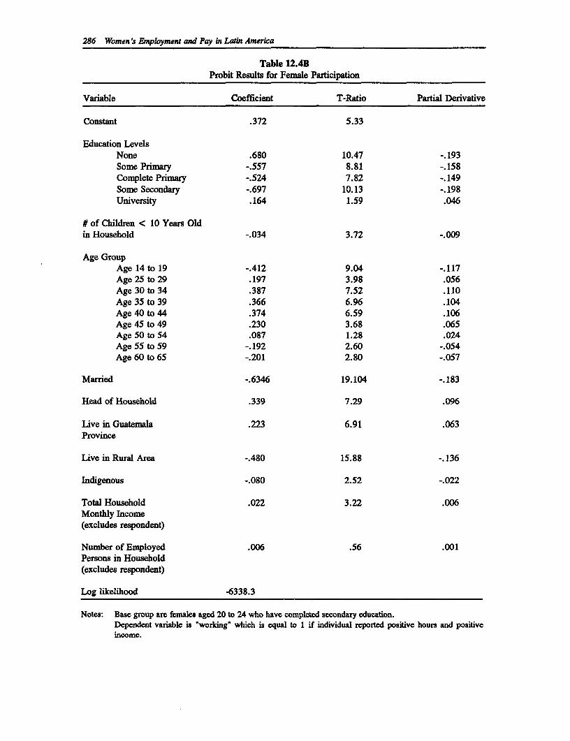
286 Women's Fpwloyment and Pay in Latin America
Table 12.4BProbit Results for Female Participation
Variable Coefficient T-Ratio Partial Derivative
Constant .372 5.33
Education LevelsNone .680 10.47 -.193Some Primary -.557 8.81 -.158Complete Primary -.524 7.82 -.149Some Secondary -.697 10.13 -.198University .164 1.59 .046
# of Children < 10 Years Oldin Household -.034 3.72 -.009
Age GroupAge 14 to 19 -.412 9.04 -.117Age 25 to 29 .197 3.98 .056Age 30 to 34 .387 7.52 .110Age 35 to 39 .366 6.96 .104Age 40 to 44 .374 6.59 .106Age 45 to 49 .230 3.68 .065Age 50 to 54 .087 1.28 .024Age 55 to 59 -.192 2.60 -.054Age 60 to 65 -.201 2.80 -.057
Married -.6346 19.104 -.183
Head of Household .339 7.29 .096
Live in Guatemala .223 6.91 .063Province
Live in Rural Area -.480 15.88 -.136
Indigenous -.080 2.52 -.022
Total Household .022 3.22 .006Monthly Income(excludes respondent)
Number of Employed .006 .56 .001Persons in Household(excludes respondent)
Log likelihood -6338.3
Notes: Base group are females aged 20 to 24 who have completed secondary education.Dependent variable is "workdng" which is equal to 1 if individual reported positive hours and positiveincome.
Femok Labor Force Parnic;don and Earnings in Guatemala 287
Being the head of a household increases the probability of participation, as does living inGuatemala province and living in an urban area. A woman from an indigenous group is lesslikely to participate in the labor market. Household income has a positive effect on participation,which contradicts the "need for income" theory, which posits that women with less income arecompelled to seek remunerated work. The number of other employed people in the householdis not a significant variable.
Examining Table 12.5, it is apparent that education has a strong effect on participation-theprobability increases from .18 for women with no education to .41 for women with completedsecondary education. The lowest probability is for women with some secondary education, whichfurther supports the belief that secondary education has a signalling effect. The probability ofparticipating increases about 25 percent between no education and completed primary school, butthe biggest jump in participation occurs with completed secondary schooling. The probabilityat that level is double what it is for primary school. In Guatemala, the effects of havingcompleted secondary school are very similar to having attended the university level because ofthe very low schooling attainments for the population as a whole and women in particular.
The probability of participation drops by a percentage point, which is 5 percent of theparticipation rate with no children, when a woman has one child and further drops with additionalchildren. That probability drops 13 percent between having no children and having three children.The effect is not as strong as has been presented in the other country case studies"2; perhapsdifferent results would be obtained if the number of children aged 0 to 6 and who in thehousehold is primarily responsible for them could be determined.
Age is an important determinant of participation. The level stays about the same from age 30to 44. Participation begins to drop off at age 45 to 49, and then continues to steadily decline,although for the oldest groups (age 55 to 59 and 60 to 65) it is higher than the youngest group(age 15 to 19). Surprisingly, participation stays relatively high at older ages. This was not thecase in Uruguay and Panama, where participation fell off more abruptly.
An unmarried woman is twice as likely to be in the work force as a married woman. If a womanis a household head, she is about 50 percent more likely to work than a woman who is not ahousehold head. A female household head is likely to be single, divorced, or widowed, andtherefore has a responsibility to earn wage income. Even so, a household head has only a 30percent probability of working, low compared to other countries.
Being of an indigenous group has a surprisingly small effect on participation, given the lack ofaccess to labor market opportunities. The rural and indigenous variables are highly correlated.Thus, the rural coefficient may include the effects of the indigenous variables.
The effects of household headship, location, and ethnic group are similar for men and women,although household headship and location do not have as large an effect in percentage terms. Formen, household headship increases the probability of participation by 24 percentage points.Ethnicity has a larger impact for men; indian men are 13 percent less likely to be observed in thework force than latinos, or Spanish-speaking men. For women, the corresponding decrease inprobability is 10.5 percent.
12 For example, see the chapters on Panama, Uruguay, and Venezuela in this volume.
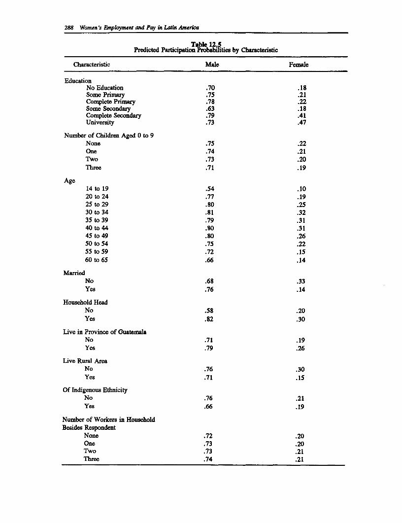
288 Women's Emnployment and Pay in Latin America
Table 12.5Predicted Participation Probabilities by Characteristic
Characteristic Male Female
EducationNo Education .70 .18Some Primary .75 .21Complete Primary .78 .22Some Secondary .63 .18Complete Secondary .79 .41University .73 .47
Number of Children Aged 0 to 9None .75 .22One .74 .21Two .73 .20Three .71 .19
Age14 to 19 .54 .1020 to 24 .77 .1925 to 29 .80 .2530 to 34 .81 .3235 to 39 .79 .3140 to 44 .80 .3145 to 49 .80 .2650 to 54 .75 .2255 to 59 .72 .1560 to 65 .66 .14
MarriedNo .68 .33Yes .76 .14
Household HeadNo .58 .20Yes .82 .30
Live in Province of GuatemalaNo .71 .19Yes .79 .26
Live Rural AreaNo .76 .30Yes .71 .15
Of Indigenous EthnicityNo .76 .21Yes .66 .19
Number of Workers in HouseholdBesides Respondent
None .72 .20One .73 .20Two .73 .21Three .74 .21
Female Labor Force Particiation and Earnings in Guatemala 289
5. Earnings Functions
In this section, the returns to different human capital characteristics are estimated for men andwomen, in order to investigate the earnings gap between men and women. The standardMincerian (1974) earnings function is used, where:
log Yi = a + b, Schoolingi + b2 Experiencei + b3 Experience Squaredi + e,
In the specification, the log of monthly earnings is the dependent variable, and the log of monthlyhours is included as a regressor. To correct for selectivity, the inverse Mill's ratio (Lambda) isalso included as a regressor.
Table 12.6 presents the results of separate earnings regressions for men and women, bothcorrecting for selectivity and using the standard model. Examilning the non-corrected model,females earn a higher return to education (16 percent versus 14 percent) and a slightly lowerreturn to potential experience (.041 versus .045).11 The experience squared term is significantand negative, indicating a concave shape. The elasticity of income to hours worked is higher forwomen; a one percent increase in monthly hours worked leads to a .48 percent increase inearnings. The R-squared is higher for females than males, suggesting that the earnings functionhas a better "fit" when explaining female earnings.
When Lambda is included as a regressor, the returns to schooling fall for both men and women,and the elasticity of earnings to hours falls also. Females have about a 2 percentage point higherreturn to a year of schooling than men. With selectivity, female returns to experience are higherthan the male returns to experience (.034 versus .019). The coefficient of Lambda for both menand women is negative and significant, and is greater in absolute value for males. This indicatesthat unobserved characteristics that earn a premium in the labor market also make the individualless likely to be observed in the labor market. The significance of Lambda indicates that theuncorrected regression coefficients are biased.
In Table 12.7, the results of a regression including only those employed in the formal sector arepresented. The probit estimates used to derive Lambda using formal sector participation as thedependent variable are presented in the Appendix Tables.
When only the formal sector is considered, in the selectivity equations, females have more thana 4 percentage point advantage in returns to schooling. The returns to schooling are lower in theformal sector than when all sectors are considered. For women, the return is only slightly lower.For males, returns to education in the formal sector are 2 percentage points less than for allsectors. The return to potential experience is higher in the formal sector for both men andwomen, but the gains drop more rapidly than for all sectors. The coefficient on Lambda becomesmore negative for men while for women, it becomes less negative when going from Table 12.6to Table 12.7. These findings are the opposite of Terrell's (1989), who found that returns to
13 Other studies have estimated returns to education in Guatemala. Sumner (1981) found a rate ofreturn ranging from 5.9 percent to 10.8 percent. He examined the eamings of male farm workerscompared to employees. Terrell (1989) estimated the rate of return to be only 2.2 percent. However, sheincluded occupational and sectoral dummy variables in the regression. Terrell's study included women andlooked at discrimination between male and female street vendors and shop assistants as representatives ofthe informal and formal sectors.
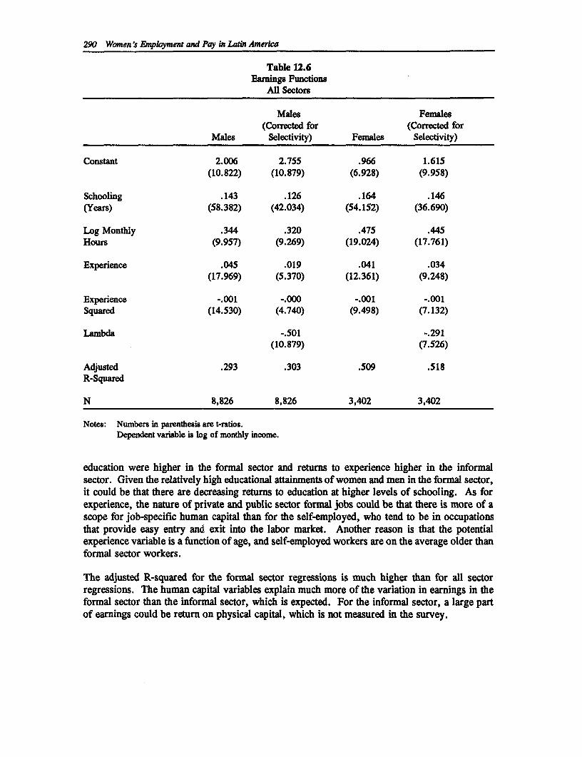
290 Women 's Employment and Pay in Latin Amerca
Table 12.6Earnings Functions
All Sectors
Males Females(Corrected for (Corrected for
Males Selectivity) Females Selectivity)
Constant 2.006 2.755 .966 1.615(10.822) (10.879) (6.928) (9.958)
Schooling .143 .126 .164 .146(Years) (58.382) (42.034) (54.152) (36.690)
Log Monthly .344 .320 .475 .445Hours (9.957) (9.269) (19.024) (17.761)
Experience .045 .019 .041 .034(17.969) (5.370) (12.361) (9.248)
Experience -.001 -.000 -.001 -.001Squared (14.530) (4.740) (9.498) (7.132)
Lambda -.501 -.291(10.879) (7.526)
Adjusted .293 .303 .509 .518R-Squared
N 8,826 8,826 3,402 3,402
Notes: Numbers in parenthesis are t-ratios.Dependent variable is log of monthly income.
education were higher in the formal sector and returns to experience higher in the informalsector. Given the relatively high educational attainments of women and men in the formal sector,it could be that there are decreasing returns to education at higher levels of schooling. As forexperience, the nature of private and public sector formal jobs could be that there is more of ascope for job-specific human capital than for the self-employed, who tend to be in occupationsthat provide easy entry and exit into the labor market. Another reason is that the potentialexperience variable is a function of age, and self-employed workers are on the average older thanformal sector workers.
The adjusted R-squared for the formal sector regressions is much higher than for all sectorregressions. The human capital variables explain much more of the variation in earnings in theformal sector than the informal sector, which is expected. For the informal sector, a large partof earnings could be return on physical capital, which is not measured in the survey.
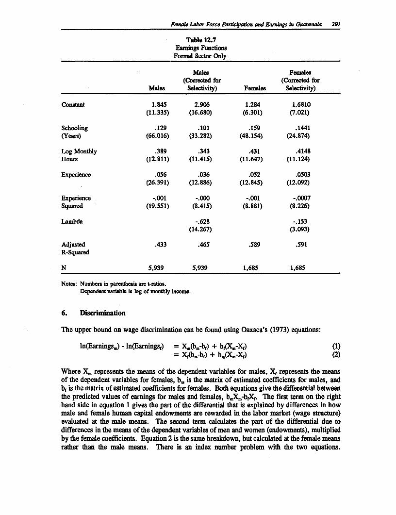
Female Labor Force Particapatson and Earnings in Guatmala 291
Table 12.7Earnings Functions
Formal Sector Only
Males Females(Corrected for (Corrected for
Males Selectivity) Females Selectivity)
Constant 1.845 2.906 1.284 1.6810(11.335) (16.680) (6.301) (7.021)
Schooling .129 .101 .159 .1441(Years) (66.016) (33.282) (48.154) (24.874)
Log Monthly .389 .343 .431 .4148Hours (12.811) (11.415) (11.647) (11.124)
Experience .056 .036 .052 .0503(26.391) (12.886) (12.845) (12.092)
Experience -.001 -.000 -.001 -.0007Squared (19.551) (8.415) (8.881) (8.226)
L.,ambda -.628 -.153(14.267) (3.093)
Adjusted .433 .465 .589 .591R-Squared
N 5,939 5,939 1,685 1,685
Notes: Numbers in parenthesis are t-ratios.Dependent variable is log of monthly income.
6. Discrimination
The upper bound on wage discrimination can be found using Oaxaca's (1973) equations:
ln(Earnings.) - ln(Earningsf) = Xm(bm7bf) + bf(XmjXf) (1)= Xf(bj-bf) + bm(Xm-Xf) (2)
Where X. represents the means of the dependent variables for males, Xf represents the meansof the dependent variables for females, bI is the matrix of estimated coefficients for males, andbf is the matrix of estimated coefficients for females. Both equations give the differential betweenthe predicted values of earnings for males and females, bmX,-bfXf. The first term on the righthand side in equation 1 gives the part of the differential that is explained by differences in howmale and female human capital endowments are rewarded in the labor market (wage structure)evaluated at the male means. The second term calculates the part of the differential due todifferences in the means of the dependent variables of men and women (endowments), multipliedby the female coefficients. Equation 2 is the same breakdown, but calculated at the female meansrather than the male means. There is an index number problem with the two equations.
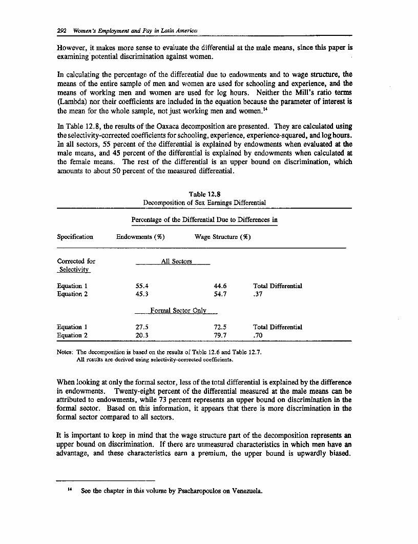
292 Women's Employment and Pay in Latin America
However, it makes more sense to evaluate the differential at the male means, since this paper isexamining potential discrimination against women.
In calculating the percentage of the differential due to endowments and to wage structure, themeans of the entire sample of men and women are used for schooling and experience, and themeans of working men and women are used for log hours. Neither the Mill's ratio terms(Lambda) nor their coefficients are included in the equation because the parameter of interest isthe mean for the whole sample, not just working men and women."4
In Table 12.8, the results of the Oaxaca decomposition are presented. They are calculated usingthe selectivity-corrected coefficients for schooling, experience, experience-squared, and log hours.In all sectors, 55 percent of the differential is explained by endowments when evaluated at themale means, and 45 percent of the differential is explained by endowments when calculated atthe female means. The rest of the differential is an upper bound on discrimination, whichamounts to about 50 percent of the measured differential.
Table 12.8Decomposition of Sex Earnings Differential
Percentage of the Differential Due to Differences in
Specification Endowments (%) Wage Structure (%)
Corrected for All SectorsSelectivity
Equation 1 55.4 44.6 Total DifferentialEquation 2 45.:3 54.7 .37
Formal Sector Oy
Equation 1 27.:5 72.5 Total DifferentialEquation 2 20.3 79.7 .70
Notes: The decomposition is based on the results of Table 12.6 and Table 12.7.All results are derived using selectivity-corrected coefficients.
When looking at only the formal sector, less of the total differential is explained by the differencein endowments. Twenty-eight percent of the differential measured at the male means can beattributed to endowments, while 73 percent represents an upper bound on discrimination in theformal sector. Based on this information, it appears that there is more discrimination in theformal sector compared to all sectors.
It is important to keep in mind that the wage structure part of the decomposition represents anupper bound on discrimination. If there are unmeasured characteristics in which men have anadvantage, and these characteristics earn a premium, the upper bound is upwardly biased.
14 See the chapter in this volume by Psacharopoulos on Venezuela.
Femae Labor Force Parti4paton and Earnings in Guatemala 293
However, if there is discrimination which impedes women from obtaining the schooling theydesire or from entering a lucrative occupation, discrimination will be downwardly biased.
7. Discussion
One of the biggest problems Guatemalan women face is the lack of schooling opportunities.There is a large schooling gap that favors men. Increasing quantity and quality of schooling,especially at the primary and secondary level, would undoubtedly increase women's labor forceparticipation, allow more opportunity to enter into formal labor markets, and increase earnings.
Although the overall difference between male and female wages appears small, it masks importantdistinctions between the formal and informal sector. Most women workers are self-employedworkers. On the average, they make 75 percent of what men earn. Female workers in the publicsector, to contrast, have higher wages than males in the same sector. In the formal sector,females have a higher average wage, although males have an earnings advantage when predictingwages for the entire sample. The high ratio of female to male wages does not rule out labormarket discrimination. The Oaxaca decomposition shows that between 73 and 80 percent of thedifferential between male and female earnings in the formal sector is due to differences in howmale and female human capital characteristics are rewarded in the market. It appears thatdiscrimination is greater in the formal sector than in all sectors.
Occupational choice appears to be an important factor in determining wages. Another questionis whether females are constrained by societal factors from entering many occupations, orwhether women choose to work in certain jobs because of their compatibility with householdwork.
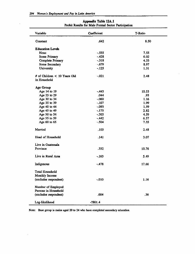
294 Women 's Employment and Pay in Latin America
Appendix Table 12A.1Probit Results for Male Formal Sector Participation
Variable Coefficient T-Ratio
Constant .642 8.50
Education LevelsNone -.555 7.55Some Primary -.428 6.02Complete Primary -.318 4.33Some Secondary -.679 8.97University -.125 1.31
# of Children < 10 Years Old -.021 2.48in Household
Age GroupAge 14 to 19 -.443 10.53Age 25 to 29 .044 .93Age 30 to 34 -.060 1.16Age 35 to 39 -.107 1.99Age 40 to 44 -.093 1.59Age 45 to 49 -.175 2.82Age 50 to 54 -.303 4.59Age 55 to 59 -.442 6.57Age 60 to 65 -.504 7.35
Married .103 2.48
Head of Household .141 3.07
Live in GuatemalaProvince .352 10.76
Live in Rural Area -.163 5.49
Indigenous -.478 17.66
Total HouseholdMonthly Income(excludes respondent) -.010 1.16
Number of EmployedPersons in Household(excludes respondent) .004 .36
Log-likelihood -7801.4
Note: Base group is males aged 20 to 24 who have completed secondary education.
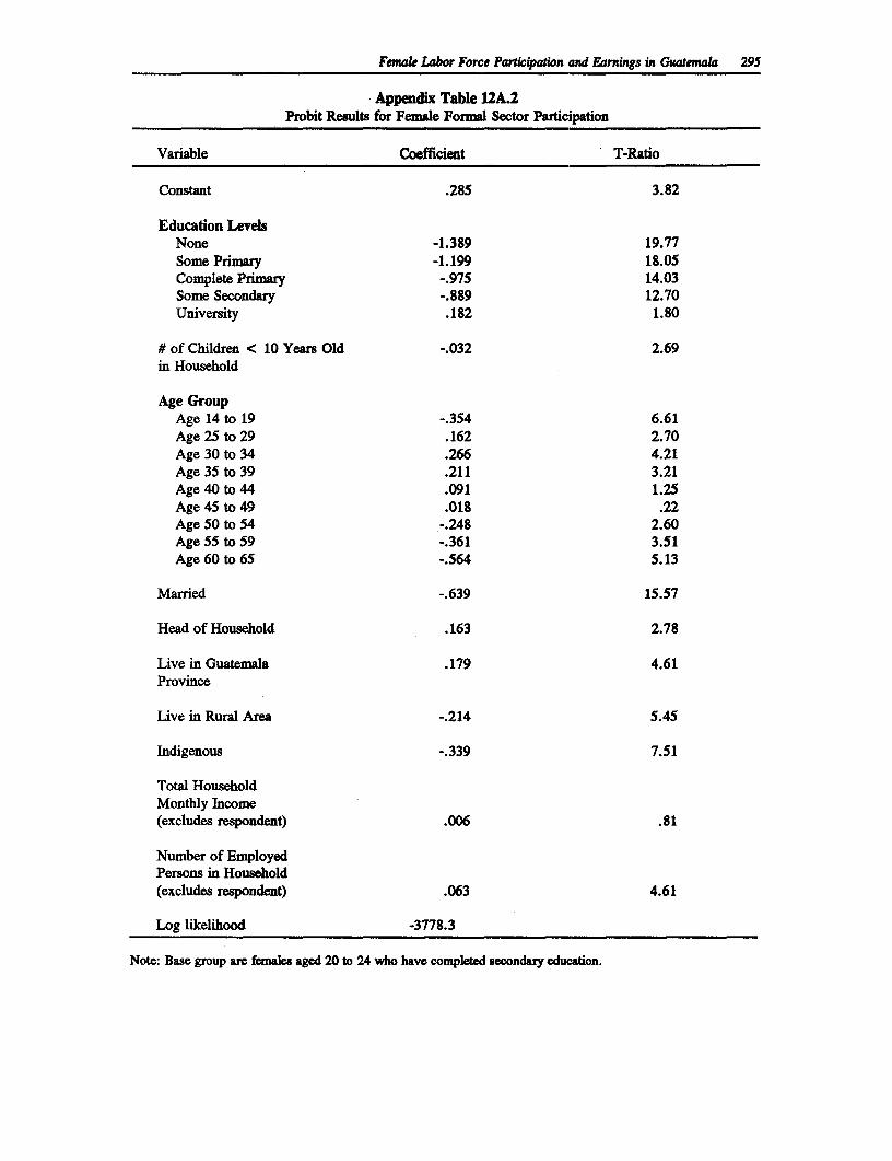
Female Labor Force Participation and Earnings in Guatemala 295
Appendix Table 12A.2Probit Results for Female Formal Sector Participation
Variable Coefficient T-Ratio
Constant .285 3.82
Education LevelsNone -1.389 19.77Some Primary -1.199 18.05Complete Primary -.975 14.03Some Secondary -.889 12.70University .182 1.80
# of Children < 10 Years Old -.032 2.69in Household
Age GroupAge 14 to 19 -.354 6.61Age 25 to 29 .162 2.70Age 30 to 34 .266 4.21Age 35 to 39 .211 3.21Age 40 to 44 .091 1.25Age 45 to 49 .018 .22Age 50 to 54 -.248 2.60Age 55 to 59 -.361 3.51Age 60 to 65 -.564 5.13
Married -.639 15.57
Head of Household .163 2.78
Live in Guatemala .179 4.61Province
Live in Rural Area -.214 5.45
Indigenous -.339 7.51
Total HouseholdMonthly Income(excludes respondent) .006 .81
Number of EmployedPersons in Household(excludes respondent) .063 4.61
Log likelihood -3778.3
Note: Base group are females aged 20 to 24 who have completed secondary education.
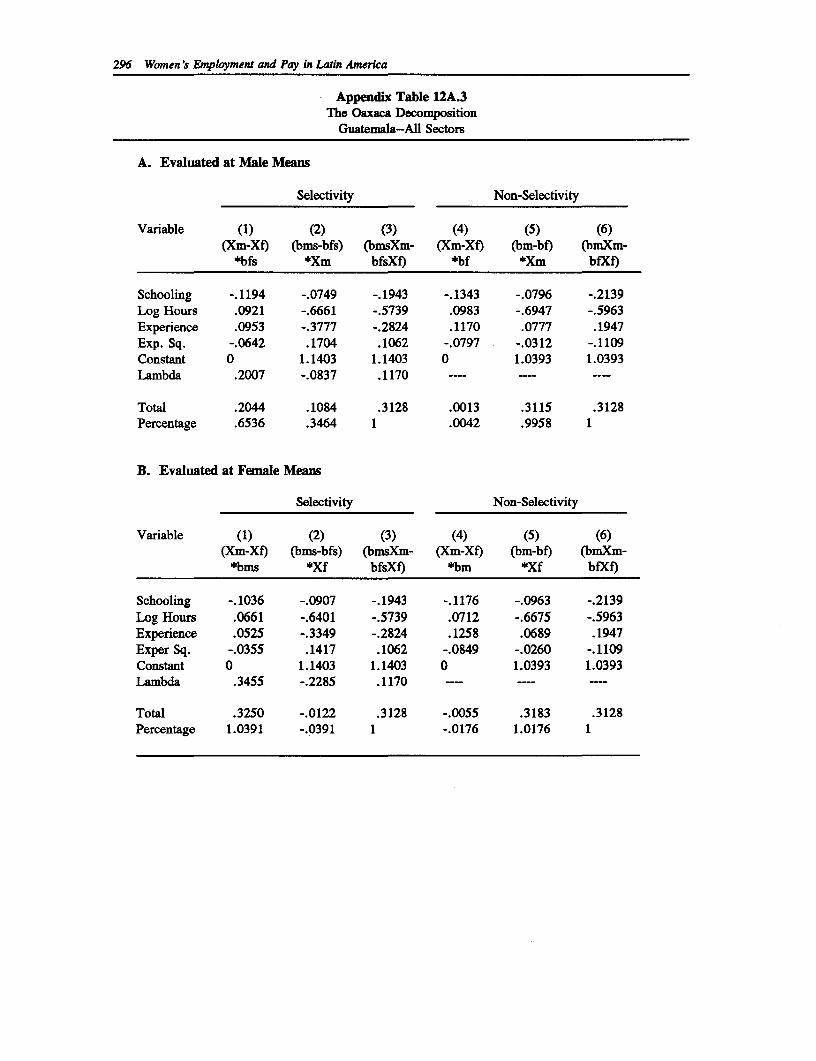
296 Women's Employment and Pay in Latin America
Appendix Table 12A.3The Oaxaca Decomposition
Guatemala-All Sectors
A. Evaluated at Male Means
Selectivity Non-Selectivity
Variable (1) (2) (3) (4) (5) (6)(Xm-Xf) (bms-bfs) (bmsXm- (Xm-Xf) (bm-bf) (bmXm-
*bfs *Xm bfsXf) *bf Xm bfXf)
Schooling -.1194 -.0749 -.1943 -.1343 -.0796 -.2139Log Hours .0921 -.6661 -.5739 .0983 -.6947 -.5963Experience .0953 -.3777 -.2824 .1170 .0777 .1947Exp. Sq. -.0642 .1704 .1062 -.0797 -.0312 -. 1109Constant 0 1.1403 1.1403 0 1.0393 1.0393Lambda .2007 -.0837 .1170 --- -- --
Total .2044 .1084 .3128 .0013 .3115 .3128Percentage .6536 .3464 1 .0042 .9958 1
B. Evaluated at Female Means
Selectivity Non-Selectivity
Variable (1) (2) (3) (4) (5) (6)(Xm-Xf) (bms-bfs) (bmsXm- (Xm-Xf) (bm-bf) (bmXm-
*bms *Xf bfsXf) *bm *Xf bfXf)
Schooling -.1036 -.0907 -.1943 -.1176 -.0963 -.2139Log Hours .0661 -.6401 -.5739 .0712 -.6675 -.5963Experience .0525 -.3349 -.2824 .1258 .0689 .1947Exper Sq. -.0355 .1417 .1062 -.0849 -.0260 -. 1109Constant 0 1.1403 1.1403 0 1.0393 1.0393Lambda .3455 -.2285 .1170 -- ---- -
Total .3250 -.0122 .3128 -.0055 .3183 .3128Percentage 1.0391 -.0391 1 -.0176 1.0176 1
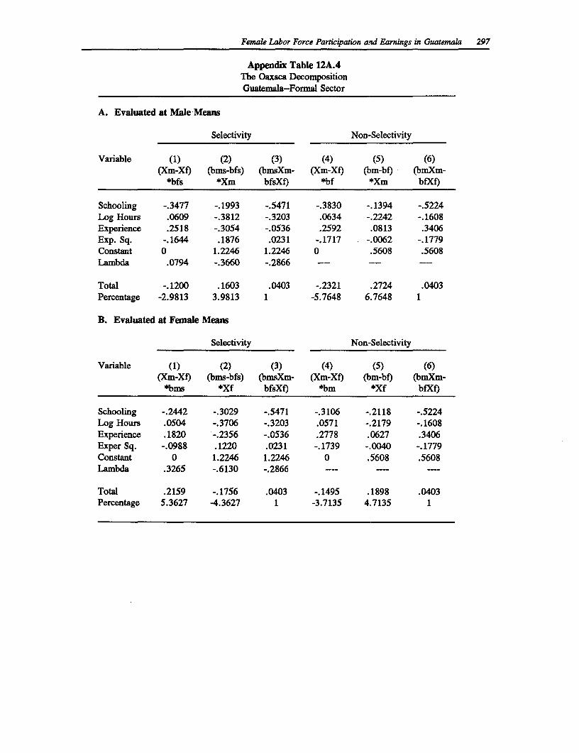
Female Labor Force Participation and Earnings in Guatemala 297
Appendix Table 12A.4The Oaxaca DecompositionGuatemala-Formal Sector
A. Evaluated at Male Means
Selectivity Non-Selectivity
Variable (1) (2) (3) (4) (5) (6)(Xm-Xf) (bms-bfs) (bmsXm- (Xm-X) (bm-bf) (bmXm-
*bfs *Xm bfsXf) *bf *Xm bfXf)
Schooling -.3477 -.1993 -.5471 -.3830 -.1394 -.5224Log Hours .0609 -.3812 -.3203 .0634 -.2242 -.1608Experience .2518 -.3054 -.0536 .2592 .0813 .3406Exp. Sq. -.1644 .1876 .0231 -.1717 -.0062 -.1779Constant 0 1.2246 1.2246 0 .5608 .5608Lambda .0794 -.3660 -.2866 --
Total -.1200 .1603 .0403 -.2321 .2724 .0403Percentage -2.9813 3.9813 1 -5.7648 6.7648 1
B. Evaluated at Female Means
Selectivity Non-Selectivity
Variable (1) (2) (3) (4) (5) (6)(Xm-Xf) (bms-bfs) (bmsXm- (Xm-Xf) (bm-bf) (bmXm-
*bms *Xf bfsXf) *bm *Xf bfXf)
Schooling -.2442 -.3029 -.5471 -.3106 -.2118 -.5224Log Hours .0504 -.3706 -.3203 .0571 -.2179 -. 1608Experience .1820 -.2356 -.0536 .2778 .0627 .3406Exper Sq. -.0988 .1220 .0231 -. 1739 -.0040 -. 1779Constant 0 1.2246 1.2246 0 .5608 .5608Lambda .3265 -.6130 -.2866 --- -- -
Total .2159 -.1756 .0403 -.1495 .1898 .0403Percentage 5.3627 -4.3627 1 -3.7135 4.7135 1
References
Economist Intelligence Unit. Guatemala, El Salvador, Honduras: Country Profile 1991-92. London:Economist Intelligence Unit Limited, 1991.
Heckman, J.J. 'Sample Selection Bias as a Specification Error." Econometrica, Vol. 47, no. 1 (1979). pp.153-161.
Killingsworth, M.R. and J.J. Heckman. 'Female Labor Supply: A Survey' in 0. Ashenfelter and R.Layard (eds.) Handbook of Labor Economics. Amsterdam: North Holland, 1986, pp. 103-204.
Mincer, J. Schooling, Experience, and Earnings. New York: Columbia University Press, 1974.
Oaxaca, R. 'Male-female Wage Differentials in Urban Labor Markets." International Economic Review,Vol. 14, no. 1 (1973). pp. 693-701.
Rodriguez, Aida and Susana Schkolnik. Chile y Guatemala: Factores que afectan la participacionfemininaen la actividad economica. Santiago, Chile: Centro Latinoamericano de Demografia, 1974.
Sumner, Daniel. "Wage Functions and Occupational Selection in a Rural Less Developed Country Setting."Review of Economics and Statistics, Vol. 63, (1981) pp. 513-519.
Terrell, Katherine. "An Analysis of Wage Structure in Guatemala City." The Journal ofDeveloping Areas,Vol. 23 (April 1989) pp. 405-423.
World Bank. Guatemala: Basic Education Sector Memorandum. Projects Department, Latin America andthe Caribbean Regional Office, Report No. 6248-GU, June 6, 1986.
World Bank. Guatemala: Country Economic Memorandum. Country Department II, Latin America and theCaribbean Region, Report No. 9378-GU, June 19, 1991.
World Bank. Second Basic Education Project: Staff Appraisal Report. Country Department II, LatinAmerica and the Caribbean Regional Office, Report No. 7004-GU, November 10, 1987.
World Bank. Social Indicators of Development 1990. Baltimore, MD: Johns Hopkins University Press,1990. p. 124-5.
World Bank. World Development Report 1991. New York: Oxford University Press, 1991.
298
13
Women's Labor Force Participation and Earnings inHonduras
Carolyn Winter and T.H. Gindling
1. Introduction
Honduras, with a per capita GNP of US$598 in 1990, is one of the poorest countries in LatinAmerica. Beset by economic crises, it is in the midst of a structural adjustment program that is,in the short term, increasing unemployment, reducing real wages and imposing additionalhardships on an already poor population. Women's labor force participation rates are relativelylow; in 1989 just over 30 percent of women aged 15 to 65 years were working in the labormarket compared to 72 percent of men in the same age group. The earnings differential betweenmen and women is surprisingly low in Honduras, with women earning just over 81 percent ofmen's weekly average earnings.'
The objectives of this paper are to examine (1) what factors influence a woman's decision toparticipate in the labor market and (2) whether working men and women with similar observablehuman capital endowments are rewarded equally in the labor market. In examining these issues,however, it is important to recognize that labor markets in Honduras are not homogenous. Likemost Latin American countries, the labor market consists of a formal waged and salaried sector,subject to government regulations and trade union activities, and an informal sector composedof self-employed workers and merchants and traders. More than half of all working women areself-employed workers while two thirds of men work in formal sector employment.
Simple univariate models are used to examine the determinants of the decision to work and thedecision to work in either the formal sector or in self-employment. The participation probitequations are of interest in that they explain what factors influence a woman's decision to enterthe labor market and what factors are principally responsible for their concentration in theinformal sector. The results of the probit regressions are used in estimating selectivity-correctedwage equations for female and male workers by economic sector. We determine how much ofthe earnings differential is due to gender differences in human capital endowments using theOaxaca decomposition method.
I This differential is low not only relative to other Latin American countries, but also relative tomany industrialized countries. In Bolivia and Jamaica, for instance, women earn 63 percent and 58 percentof men's earnings, respectively (see the relevant chapters in this volume). In industrialized countries suchas Britain, Australia and the United States, women earn close to three quarters of men's earnings.(Gunderson, 1989).
299
300 Women's Employment and Pay in Latin Amerca
The following section of the paper, Section 2, briefly outlines the economic situation in Hondurasand describes the main features of the labor market. Section 3 presents the mean characteristicsof the working and non-working populations as derived from the Encuesta de Hogares. Section4 describes the methodology used and presents the empirical results of the participation equationsand in Section 5 we present the selectivity corrected earnings functions estimates. Section 6presents the results of the Oaxaca decomposition. The policy implications of these findings arediscussed in Section 7.
2. The Honduran Economy and Labor Market
Honduras' economic progress has been slow over the past two decades. Major structuralimbalances in the economy have compounded problems caused by the extremely limiteddiversification of the productive sectors. Agriculture continues to be the most important sectorof the economy accounting for almost one quarter of GDP in 1990 and generating close to two-thirds of merchandise exports. Agricultural exports are, however, limited to three or four crops(coffee, bananas and sugar), making the economy very vulnerable to drops in commodity prices.Sharp falls in the market prices of these products in the 1980s has slowed economic growth anda real GDP growth of 2.3 percent in 1989 fell to an estimated -1.1 percent in 1990.2
Estimates of unemployment vary widely, but it is clear that the rate of labor market absorptionhas declined markedly with the economic downswing.3 Rapid population growth has also meantthat employment opportunities have not been able to keep pace with the increase in the laborforce.4 Underemployment of workers is also reportedly high in all sectors of employment,affecting as much as 60 percent of the economically active population.5
Male and female workers exhibit very different patterns of employment in Honduras. Table 13.1shows the ratio of male to female earnings by economic sector (public, private and self-employment). Over half of working women are working in the lowest paying economic sector,self-employment, where they earn only 62 percent of men's earnings. While men workpredominantly in the private sector, it is interesting to note that women have a pay advantageover men in this sector. In the public sector the differential is very low, with women earning 95percent of men's wages. Overall, women in the formal sector (private and public sectorscombined) have a pay advantage of almost 6 percent.
Economically active men work predominantly in the agricultural sector as Table 13.2B shows.The majority of these agricultural workers (59 percent) are self-employed. Average weeklyearnings are lowest in this sector and are particularly low among self-employed agriculturalworkers. By contrast, only 2.8 percent of women work in the agricultural sector and arepredominantly in the higher paying private sector (see Table 13.2A).
2 Economist Country Report, (1991).
3 Estimates of unemployment in the late 1980s vary from 12 to 25 percent. See Economist CountryProfile (1990) and World Bank (1987).
4 The World Bank (1990) reports that the total fertility rate was 5.6 children per woman in 1987.A 1987 World Bank report estimated that 10,000 new work positions were being created annually for anestimated 30,000 new labor force entrants.
5 Nyrop (1987).
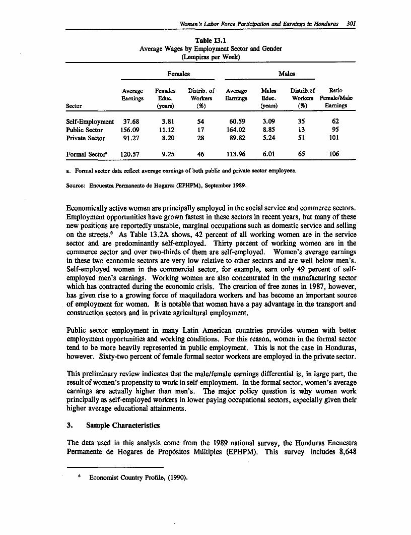
Women 's Labor Force Participation and Earnings in Honduras 301
Table 13.1Average Wages by Employment Sector and Gender
(Lempiras per Week)
Females Males
Average Females Distrib. of Average Males Distrib.of RatioEarnings Educ. Workers Earnings Educ. Workers Female/Male
Sector (years) (%) (years) (%) Earnings
Self-Employment 37.68 3.81 54 60.59 3.09 35 62Public Sector 156.09 11.12 17 164.02 8.85 13 95Private Sector 91.27 8.20 28 89.82 5.24 51 101
Formal Sector& 120.57 9.25 46 113.96 6.01 65 106
a. Formal sector data reflect average earnings of both public and private sector employees.
Source: Encuestra Permanente de Hogares (EPHPM), September 1989.
Economically active women are principally employed in the social service and commerce sectors.Employment opportunities have grown fastest in these sectors in recent years, but many of thesenew positions are reportedly unstable, marginal occupations such as domestic service and sellingon the streets.6 As Table 13.2A shows, 42 percent of all working women are in the servicesector and are predominantly self-employed. Thirty percent of working women are in thecommerce sector and over two-thirds of them are self-employed. Women's average earningsin these two economic sectors are very low relative to other sectors and are well below men's.Self-employed women in the commercial sector, for example, earn only 49 percent of self-employed men's earnings. Working women are also concentrated in the manufacturing sectorwhich has contracted during the economic crisis. The creation of free zones in 1987, however,has given rise to a growing force of maquiladora workers and has become an important sourceof employment for women. It is notable that women have a pay advantage in the transport andconstruction sectors and in private agricultural employment.
Public sector employment in many Latin American countries provides women with betteremployment opportunities and working conditions. For this reason, women in the formal sectortend to be more heavily represented in public employment. This is not the case in Honduras,however. Sixty-two percent of female formal sector workers are employed in the private sector.
This preliminary review indicates that the male/female earnings differential is, in large part, theresult of women's propensity to work in self-employment. In the formal sector, women's averageearnings are actually higher than men's. The major policy question is why women workprincipally as self-employed workers in lower paying occupational sectors, especially given theirhigher average educational attainments.
3. Sample Characteristics
The data used in this analysis come from the 1989 national survey, the Honduras EncuestraPermanente de Hogares de Prop6sitos Multiples (EPHPM). This survey includes 8,648
6 Economist Country Profile, (1990).
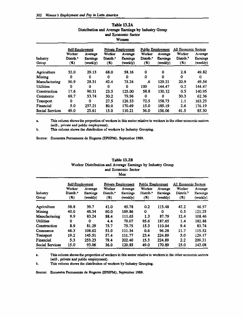
302 Women's Employment and Pay in Latin Amerca
Table 13.2ADistribution and Average Eamings by Industry Group
and Economic SectorWomen
Self-Emploent Private Emvlovment Public Emiolovment All Economic SectorsWorker Average Worker Average Worker Average Worker Average
Industry Distrib.a Earnings Distrib.a Eamings Distrib. Earnings Distrib.b EarningsGroup (%) (weekly) (X) (weekly) (%) (weekly) (%) (weekly)
Agriculture 32.0 29.13 68.0 58.16 0 0 2.8 49.82Mining 0 0 0 0 0 0 0 0Manufacturing 56.9 28.31 42.4 75.24 .6 129.21 20.9 49.54Utilities 0 0 0 0 100 144.47 0.2 144.47Construction 17.6 90.31 23.5 125.00 58.8 130.12 0.5 140.95Commerce 69.7 53.74 30.2 79.96 0 0 30.3 62.36Transport 0 0 27.5 126.53 72.5 158.73 1.1 163.23Financial 5.0 237.21 80.0 170.69 15.0 185.19 2.6 176.19Social Services 49.0 25.61 15.0 110.21 36.0 156.06 41.5 85.30
a. This column shows the proportion of workers in this sector relative to workers in the other economic sectors(self-, private and public employment).
b. This column shows the distribution of workers by Industry Grouping.
Source: Encuestra Permanente do Hogares (EPHPM), September 1989.
Table 13.2BWorker Distribution and Average Earnings by Industry Group
and Economic SectorMen
Self-Employment Private Emolovment Public Emolovment All Economic SectorsWorker Average Worker Average Worker Average Worker Average
Industry Distrib.a Earnings Distrib.' Earnings Distrib.' Earnings Distrib.' EarningsGroup (%) (weekly) (%) (weekly) (%) (weekly) (%) (weekly)
Agriculture 58.8 39.7 41.0 45.78 0.2 113.48 42.2 46.57Mining 40.0 48.34 60.0 169.86 0 0 0.3 121.25Manufacturing 9.9 83.24 88.4 111.65 1.3 87.79 12.4 108.46Utilities 0 0 4.4 79.07 95.6 187.65 1.4 182.88Construction 8.9 81.29 75.7 75.75 15.3 110.04 9.4 83.74Commerce 48.3 108.62 51.0 111.34 0.6 96.28 11.7 115.52Transport 19.2 145.51 57.4 111.77 23.4 224.89 5.0 129.17Financial 5.3 253.23 79.4 202.40 15.3 224.89 2.2 209.21Social Services 15.0 93.06 36.0 120.85 49.0 170.89 15.0 143.08
a. This column shows the proportion of workers in this sector relative to workers in the other economic sectors(self-, private and public employment).
b. This column shows the distribution of workers by Industry Grouping.
Source: Encuestra Permanente de Hogares (EPHPM), September 1989.
Women's Labor Force Participaion and Earnings in Honduras 303
households and 46,672 individuals and has information on labor force participation, earnings,hours worked and employment by occupational sector. It also contains information on individualcharacteristics such as age, years of education, and marital status, and on householdcharacteristics such as number of children in the household, ownership status, number ofhousehold members, and total income of the household.
As the focus of our study is prime-aged workers we restricted our sample to individuals aged 15to 65 years. Our sample thus consisted of 23,388 individuals, which included 12,498 women and10,890 men.
Tables 13.3A and 13.3B show the mean characteristics of the sample by gender and work status.Individuals were considered to be working if they reported positive earnings from public, privateor self-employed work and if they reported working positive hours during the week prior to thesurvey. Individuals seeking employment were hot included in the sample. The femaleparticipation rate in our sample was just over 30 percent, which is low but comparable to theaverage female participation rate for all Latin American countries. The male participation rate,72 percent, is relatively low as would be expected given the existing high levels ofunemployment.
Women work slightly fewer hours per week than men on average and, across all economicsectors, earn approximately 81 percent of men's average earnings. However, as Tables 13.3Aand 13.3B show, the significantly lower earnings of self-employed women account for much ofthis differential; self-employed women earn only 62 percent of self-employed men's earningsalthough they report working the same number of hours per week. The earnings differential isvery small in the public sector where women earn 95 percent of men's earnings and in the privatesector women actually have a pay advantage over men. Women's average earnings in the formalsector are higher than men's.
As the data do not provide information on individuals' years of experience in the labor force, weconstructed this variable in the standard way as age minus years of education minus six. Clearly,this measure will tend to overestimate experience, especially for women who generally withdrawfrom the labor market when they have young children to care for. Estimated years of experienceare considerably higher for self-employed men and women than for workers in the formal sectors.
Although women workers average one and a half years more schooling than men, women'seducational advantage widens if we consider only formal sector workers. Here, women have 3.2years more schooling than men. In the private sector women have almost three more years ofschooling than men and in the public sector they have over two years more schooling. Workingwomen have 1.6 years more schooling than non-working women. Non-working men, however,have 1.2 years more schooling than their working counterparts which may partly reflect thereported high levels of education unemployment among men. (World Bank, 1990b).
Working women have fewer pre-school age children (under 7 years) than non-working women.Among working women, self-employed working women have more young children than womenin the formal sector.
4. The Determinants of Labor Force Participation
In this section we try to identify the major determinants of individuals' labor force participationdecisions. It is assumed that the decision to work is made simultaneously with the decision
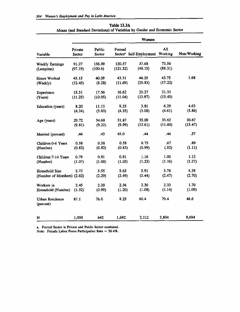
304 Women's Employment and Pay in Latin America
Table L3.3AMeans (and Standard Deviations) of Variables by Gender and Economic Sector
Women
Private Public Formal AllVariable Sector Sector Sectorg Self-Employment Working Non-Working
Weekly Earnings 91.27 156.09 120.57 37.68 73.54(Lempiras) (97.19) (100.6) (121.32) (48.15) (88.31)
Hours Worked 45.15 40.09 43.31 44.25 43.75 1.68(Weekly) (12.45) (8.28) (11.69) (20.83) (17.22)
Experience 15.51 17.56 16.62 25.27 21.33(Years) (11.25) (10.05) (11.04) (13.97) (13.45)
Education (years) 8.20 11.12 9.25 3.81 6.29 4.63(4.24) (3.83) (4.35) (3.08) (4.61) (3.86)
Age (years) 29.72 34.68 31.87 35.09 33.62 30.67(9.81) (9.22) (9.99) (12.61) (11.60) (13.47)
Married (percent) .44 .43 45.0 .44 .44 .57
Children:0-6 Years 0.58 0.58 0.58 0.75 .67 .89(Number) (0.83) (0.83) (0.83) (0.99) (.92) (1.11)
Children:7-14 Years 0.79 0.81 0.81 1.16 1.00 1.12(Number) (1.07) (1.00) (1.05) (1.23) (1.16) (1.27)
Household Size 5.72 5.55 5.65 5.91 5.78 6.38(Number of Members) (2.62) (2.29) (2.49) (2.44) (2.47) (2.70)
Workers in 2.45 2.20 2.36 2.30 2.33 1.70Household (Number) (1.32) (0.99) (1.20) (1.08) (1.14) (1.09)
Urban Residence 87.1 76.0 8.25 60.4 70.4 46.6(percent)
N 1,050 642 1,692 2,112 3,804 8,694
a. Formnal Sector is Private and Public Sector combined.Note: Female Labor Force Participation Rate = 30.4%.
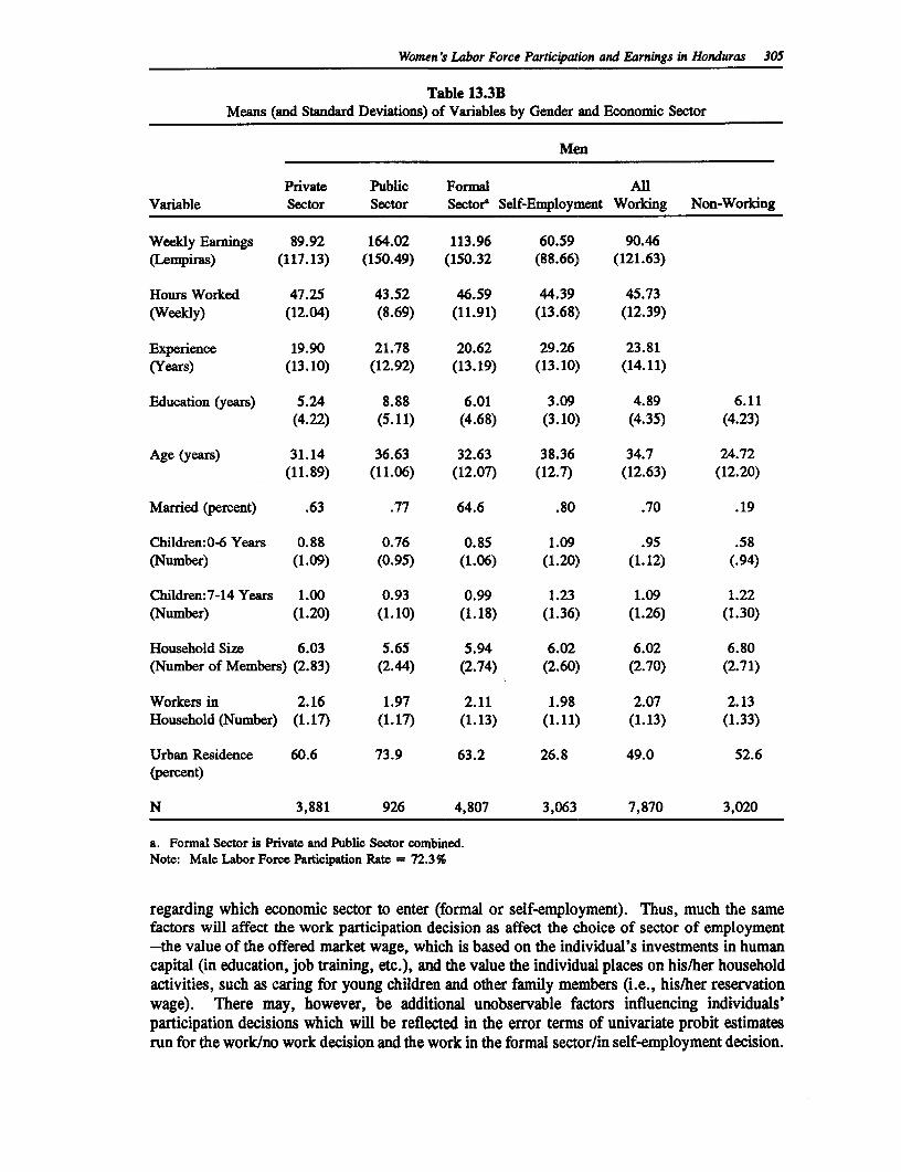
Women's Labor Force Participation and Earnings in Honduras 305
Table 13.3BMeans (and Standard Deviations) of Variables by Gender and Economic Sector
Men
Private Public Formal AllVariable Sector Sector Sector' Self-Employment Working Non-Working
Weeldy Earnings 89.92 164.02 113.96 60.59 90.46(Lempiras) (117.13) (150.49) (150.32 (88.66) (121.63)
Hours Worked 47.25 43.52 46.59 44.39 45.73(Weekly) (12.04) (8.69) (11.91) (13.68) (12.39)
Experience 19.90 21.78 20.62 29.26 23.81(Years) (13.10) (12.92) (13.19) (13.10) (14.11)
Education (years) 5.24 8.88 6.01 3.09 4.89 6.11(4.22) (5.11) (4.68) (3.10) (4.35) (4.23)
Age (years) 31.14 36.63 32.63 38.36 34.7 24.72(11.89) (11.06) (12.07) (12.7) (12.63) (12.20)
Married (percent) .63 .77 64.6 .80 .70 .19
Children:0-6 Years 0.88 0.76 0.85 1.09 .95 .58(Number) (1.09) (0.95) (1.06) (1.20) (1.12) (.94)
Children:7-14 Years 1.00 0.93 0.99 1.23 1.09 1.22(Number) (1.20) (1.10) (1.18) (1.36) (1.26) (1.30)
Household Size 6.03 5.65 5.94 6.02 6.02 6.80(Number of Members) (2.83) (2.44) (2.74) (2.60) (2.70) (2.71)
Workers in 2.16 1.97 2.11 1.98 2.07 2.13Household (Number) (1.17) (1.17) (1.13) (1.11) (1.13) (1.33)
Urban Residence 60.6 73.9 63.2 26.8 49.0 52.6(percent)
N 3,881 926 4,807 3,063 7,870 3,020
a. Formal Sector is Private and Public Sector combined.Note: Male Labor Force Participation Rate = 72.3%
regarding which economic sector to enter (formal or self-employment). Thus, much the samefactors will affect the work participation decision as affect the choice of sector of employment-the value of the offered market wage, which is based on the individual's investments in humancapital (in education, job training, etc.), and the value the individual places on his/her householdactivities, such as caring for young children and other family members (i.e., his/her reservationwage). There may, however, be additional unobservable factors influencing individuals'participation decisions which will be reflected in the error terms of univariate probit estimatesrun for the work/no work decision and the work in the formal sector/in self-employment decision.
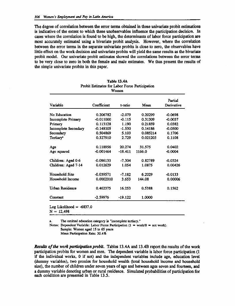
306 Women's Employment and Pay in Latin America
The degree of correlation between the error terms obtained in these univariate probit estimationsis indicative of the extent to which these unobservables influence the participation decision. Incases where the correlation is found to be high, the determinants of labor force participation aremost accurately estimated using a bivariate probit analysis. However, where the correlationbetween the error terms in the separate univariate probits is close to zero, the observables havelittle effect on the work decision and univariate probits will yield the same results as the bivariateprobit model. Our univariate probit estimates showed the correlations between the error termsto be very close to zero in both the female and male estimates. We thus present the results ofthe simple univariate probits in this paper.
Table 13.4AProbit Estimates for Labor Force Participation
Women
PartialVariable Coefficient t-ratio Mean Derivative
No Education 0.206782 -2.079 0.20299 -0.0698Incomplete Primary -0.011000 -0.115 0.31309 -0.0037Primary 0.113128 1.190 0.21859 0.0382Incomplete Secondary -0.148105 -1.530 0.14186 -0.0500Secondary 0.504869 5.103 0.085214 0.1706Tertiary' 0.327910 2.729 0.021203 0.1108
Age 0.118956 20.274 31.575 0.0402Age squared -0.001464 -18.411 1166.0 -0.0004
Children: Aged 0-6 -0.096133 -7.304 0.82789 -0.0324Children: Aged 7-14 0.012629 1.054 1.0875 0.00426
Household Size -0.039571 -7.182 6.2029 -0.0133Household Income 0.0002010 3.653 144.08 0.00006
Urban Residence 0.462375 16.253 0.5388 0.1562
Constant -2.59976 -19.122 1.0000
Log Likelihood = -6837.0N = 12,498
a. The omitted education category is 'incomplete tertiary."Notes: Dependent Variable: Labor Force Participation (1 = work/O = not work).
Sample: Women aged 15 to 65 yearsMean Participation Rate: 30.4%
Results of the work participation probit. Tables 13.4A and 13.4B report the results of the workparticipation probits for women and men. The dependent variable is labor force participation (1if the individual works, 0 if not) and the independent variables include age, education level(dummy variables), two proxies for household wealth (total household income and householdsize), the number of children under seven years of age and between ages seven and fourteen, anda dummy variable denoting urban or rural residence. Simulated probabilities of participation foreach condition are presented in Table 13.5.
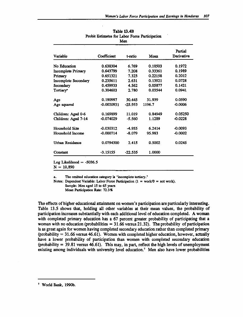
Women's Labor Force Participaion and Earnings in Honduras 307
Table 13.4BProbit Estimates for Labor Force Participation
Men
PartialVariable Coefficient t-ratio Mean Derivative
No Education 0.638304 6.769 0.18503 0.1972Incomplete Primary 0.643799 7.208 0.33361 0.1989Primary 0.651321 7.323 0.22158 0.2012Incomplete Secondary 0.235611 2.631 0.13921 0.0728Secondary 0.459933 4.562 0.05877 0.1421Tertiary3 0.304603 2.780 0.03544 0.0941
Age 0.190997 30.445 31.939 0.0590Age squared -0.0020931 -25.953 1196.7 -0.0006
Children: Aged 0-6 0.169899 11.019 0.84949 0.05250Children: Aged 7-14 -0.074029 -5.560 1.1289 -0.0228
Household Size -0.030312 -4.955 6.2414 -0.0093Household Income -0.000714 -8.079 95.983 -0.0002
Urban Residence 0.0794300 2.415 0.5002 0.0245
Constant -3.15155 -22.535 1.0000
Log Likelihood = -5036.5N = 10,890
a. The omitted education category is "incomplete tertiary."Notes: Dependent Variable: Labor Force Participation (1 = work/O = not work).
Sample: Men aged 15 to 65 yearsMean Participation Rate: 72.3%
The effects of higher educational attainment on women's participation are particularly interesting.Table 13.5 shows that, holding all other variables at their mean values, the probability ofparticipation increases substantially with each additional level of education completed. A womanwith completed primary education has a 67 percent greater probability of participating that awoman with no education (probabilities = 31.66 versus 21.32). The probability of participationis as great again for women having completed secondary education rather than completed primary(probability = 31.66 versus 46.61). Women with completed higher education, however, actuallyhave a lower probability of participation than women with completed secondary education(probability = 39.81 versus 46.61). This may, in part, reflect the high levels of unemploymentexisting among individuals with university level education.7 Men also have lower probabilities
7 World Bank, l990b.
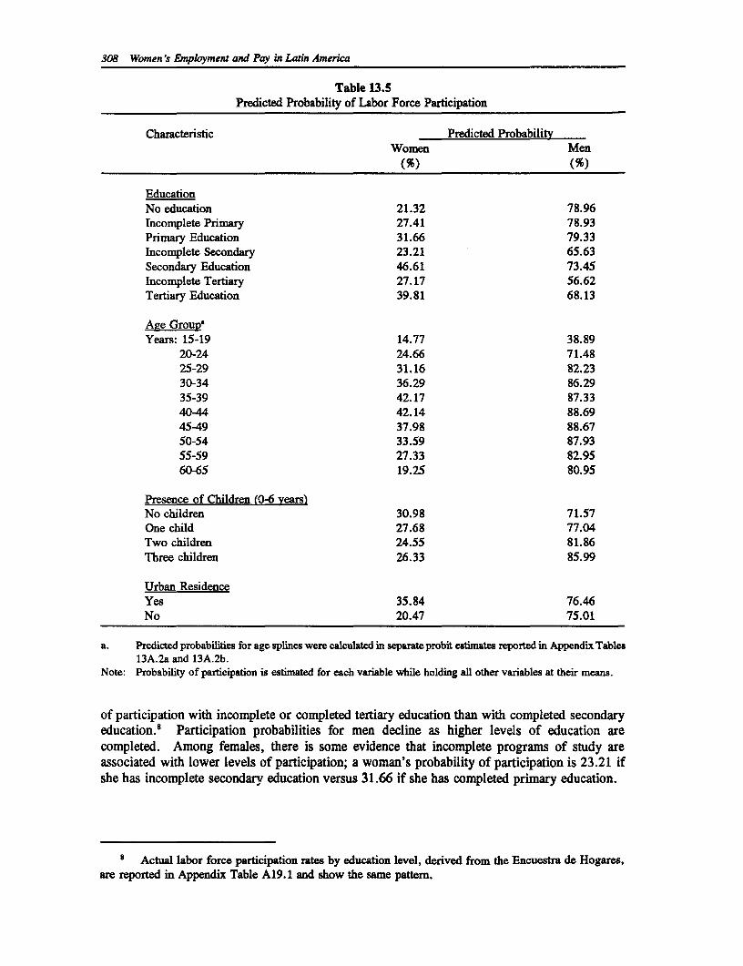
308 Women's Employment and Pay in Latin America
Table 13.5Predicted Probability of Labor Force Participation
Characteristic Predicted ProbabilityWomen Men
(%) (%)
EducationNo education 21.32 78.96Incomplete Primary 27.41 78.93Primary Education 31.66 79.33Incomplete Secondary 23.21 65.63Secondary Education 46.61 73.45Incomplete Tertiary 27.17 56.62Tertiary Education 39.81 68.13
Age GrouR9Years: 15-19 14.77 38.89
20-24 24.66 71.4825-29 31.16 82.2330-34 36.29 86.2935-39 42.17 87.3340-44 42.14 88.6945-49 37.98 88.6750-54 33.59 87.9355-59 27.33 82.9560-65 19.25 80.95
Presence of Children (0-6 vears)No children 30.98 71.57One child 27.68 77.04Two children 24.55 81.86Three children 26.33 85.99
Urban ResidenceYes 35.84 76.46No 20.47 75.01
a. Predicted probabilities for age splines were calculated in separate probit estimates reported in Appendix Tables13A.2a and 13A.2b.
Note: Probability of participation is estimated for each variable while holding all other variables at their means.
of participation with incomplete or completed tertiary education than with completed secondaryeducation. 8 Participation probabilities for men decline as higher levels of education arecompleted. Among females, there is some evidence that incomplete programs of study areassociated with lower levels of participation; a woman's probability of participation is 23.21 ifshe has incomplete secondary education versus 31.66 if she has completed primary education.
8 Actual labor force participation rates by education level, derived from the Encuestra de Hogares,are reported in Appendix Table A19.1 and show the same pattern.
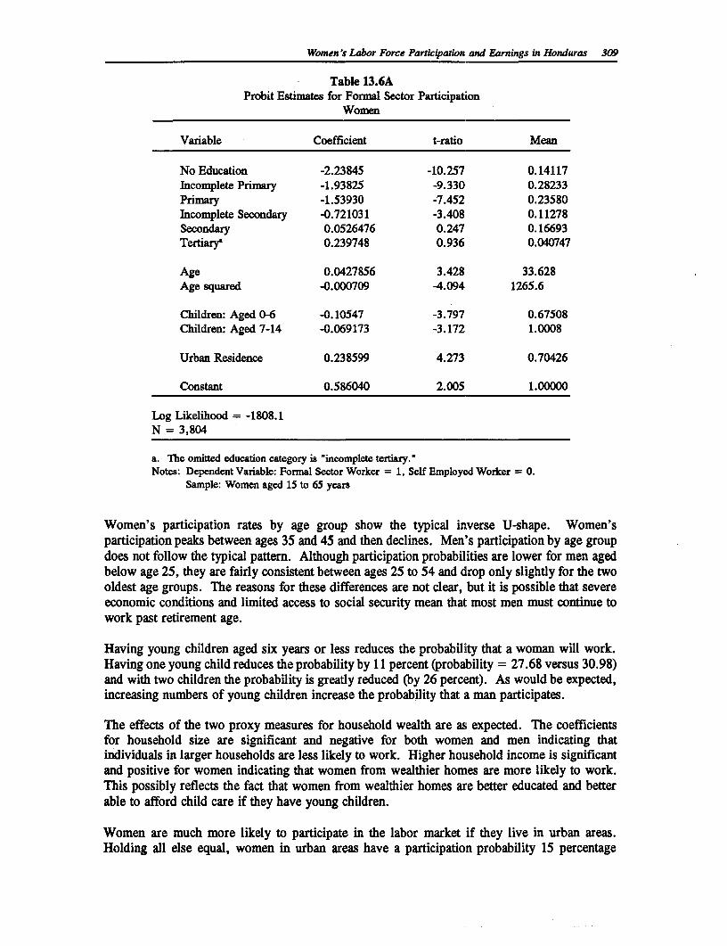
Womnen's Labor Force Partcipation and Earnings in Honduras 309
Table 13.6AProbit Estimates for Formal Sector Participation
Women
Variable Coefficient t-ratio Mean
No Education -2.23845 -10.257 0.14117Incomplete Primary -1.93825 -9.330 0.28233Primary -1.53930 -7.452 0.23580Incomplete Secondary -0.721031 -3.408 0.11278Secondary 0.0526476 0.247 0.16693Tertiarya 0.239748 0.936 0.040747
Age 0.0427856 3.428 33.628Age squared -0.000709 -4.094 1265.6
Children: Aged 0-6 -0.10547 -3.797 0.67508Children: Aged 7-14 -0.069173 -3.172 1.0008
Urban Residence 0.238599 4.273 0.70426
Constant 0.586040 2.005 1.00000
Log Likelihood = -1808.1N = 3,804
a. The omitted education category is "incomplete tertiary."Notes: Dependent Variable: Formal Sector Worker = 1, Self Employed Worker = 0.
Sample: Women aged 15 to 65 years
Women's participation rates by age group show the typical inverse U-shape. Women'sparticipation peaks between ages 35 and 45 and then declines. Men's participation by age groupdoes not follow the typical pattern. Although participation probabilities are lower for men agedbelow age 25, they are fairly consistent between ages 25 to 54 and drop only slightly for the twooldest age groups. The reasons for these differences are not clear, but it is possible that severeeconomic conditions and limited access to social security mean that most men must continue towork past retirement age.
Having young children aged six years or less reduces the probability that a woman will work.Having one young child reduces the probability by 11 percent (probability = 27.68 versus 30.98)and with two children the probability is greatly reduced (by 26 percent). As would be expected,increasing numbers of young children increase the probability that a man participates.
The effects of the two proxy measures for household wealth are as expected. The coefficientsfor household size are significant and negative for both women and men indicating thatindividuals in larger households are less likely to work. Higher household income is significantand positive for women indicating that women from wealthier homes are more likely to work.This possibly reflects the fact that women from wealthier homes are better educated and betterable to afford child care if they have young children.
Women are much more likely to participate in the labor market if they live in urban areas.Holding all else equal, women in urban areas have a participation probability 15 percentage
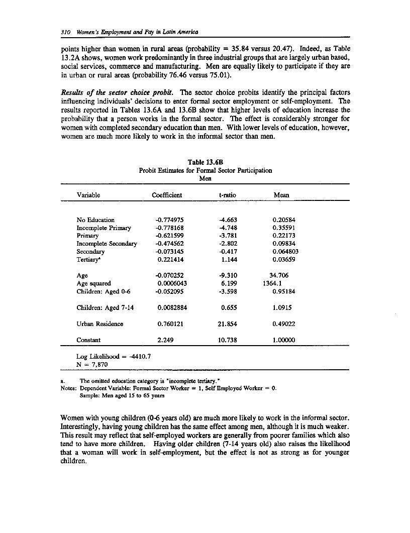
310 Women's Employment and Pay in Latin America
points higher than women in rural areas (probability = 35.84 versus 20.47). Indeed, as Table13 .2A shows, women work predominantly in three industrial groups that are largely urban based,social services, commerce and manufacturing. Men are equally likely to participate if they arein urban or rural areas (probability 76.46 versus 75.01).
Results of the sector choice probit. The sector choice probits identify the principal factorsinfluencing individuals' decisions to enter formal sector employment or self-employment. Theresults reported in Tables 13.6A and 13.6B show that higher levels of education increase theprobability that a person works in the formal sector. The effect is considerably stronger forwomen with completed secondary education than men. With lower levels of education, however,women are much more likely to work in the informal sector than men.
Table 13.6BProbit Estimates for Formal Sector Participation
Men
Variable Coefficient t-ratio Mean
No Education -0.774975 -4.663 0.20584Incomplete Primary -0.778168 -4.748 0.35591Primary -0.621599 -3.781 0.22173Incomplete Secondary -0.474562 -2.802 0.09834Secondary -0.073145 -0.417 0.064803Tertiarys 0.221414 1.144 0.03659
Age -0.070252 -9.310 34.706Age squared 0.0006043 6.199 1364.1Children: Aged 0-6 -0.052095 -3.598 0.95184
Children: Aged 7-14 0.0082884 0.655 1.0915
Urban Residence 0.760121 21.854 0.49022
Constant 2.249 10.738 1.00000
Log Likelihood = -4410.7N = 7,870
a. The omitted education category is "incomplete tertiary."Notes: Dependent Variable: Formal Sector Worker = 1, Self Employed Worker = 0.
Sample: Men aged 15 to 65 years
Women with young children (0-6 years old) are much more likely to work in the informal sector.Interestingly, having young children has the same effect among men, although it is much weaker.This result may reflect that self-employed workers are generally from poorer families which alsotend to have more children. Having older children (7-14 years old) also raises the likelihoodthat a woman will work in self-employment, but the effect is not as strong as for youngerchildren.
Women's Labor Force Participation and Earnings in Honduras 311
The age variable shows that women are more likely to work in the formal sector as they getolder. This may occur because younger women are more likely to have pre-school age childrenand, lacking access to child care facilities, may turn to self-employment where the more flexiblework hours permit them to combine work and childcare activities. The effect is reversed amongmen; older men are more likely to be working in self-employment.
Living in an urban area significantly increases the probability that both women and men willwork in the formal sector. The effect is especially high for men.
5. Earnings Functions
In this section we estimate standard Mincerian earnings functions for men and women workersto explain what factors account for male/female earnings differentials. We estimate the earningsfunctions for all workers and separately for formal sector and self-employed workers.
In proceeding with these estimates, however, we are faced with problems of selectivity bias attwo levels. First, there is a potential selectivity bias problem in examining the causes of theearnings differential between male and female workers. If we use samples consisting only ofworking males and working females we will in effect have a self-selected sample including onlyindividuals whose market wage exceeds their reservation wage. This is generally a more seriousproblem among women since their reservation wage rises when they have young children to carefor. Given the relatively low participation rate among men in Honduras, however, we cannotdiscount the possibility that certain groups of men may have high reservation wages too. Tocorrect for potential selectivity bias in this instance we use Heckman's (1979) procedure andinclude the Lambda (the inverse Mill's Ratio) estimated in the labor force participation probitregressions in the earnings functions as an independent variable. The coefficients of the Lambdasin the earnings functions provide an estimate of the covariance between the disturbances in thework/no work and wage equations.
The second potential selectivity bias problem occurs in the earnings functions estimated for formalsector and self-employed workers. Here again we have self-selected samples of workers. Wethus introduce two selectivity correction Lambdas in this set of earnings functions, one whichcorrects for selectivity in the work/no work decision and one correcting for the formal/self-employment decision.
Earnings functions estimates for al workers. Earnings functions, corrected and uncorrected forselectivity bias, were estimated with the dependent variable being the log of weekly wages.Independent variables included years of education, experience and experience squared and the logof hours worked. The results are shown in Table 13.7.
In the selectivity corrected female earnings functions the Lambda is significant and negative atthe 5 percent level, indicating that the sample of female workers is indeed not a random sample.Thus, we choose to interpret the selectivity corrected estimates although we also report theuncorrected estimates.
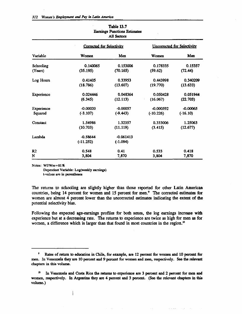
312 Women's Enmployment and Pay in Latin America
Table 13.7Eamings Functions Estimates
All Sectors
Corrected for Selectivity Uncorrected for Selectivity
Variable Women Men Women Men
Schooling 0.140065 0.153006 0.178335 0.15357(Years) (35.195) (70.165) (59.62) (72.44)
Log Hours 0.41405 0.33953 0.443998 0.340209(18.786) (13.607) (19.770) (13.633)
Experience 0.024446 0.048364 0.050428 0.051944(6.345) (12.113) (16.067) (22.703)
Experience -0.00020 -0.00057 -0.000592 -0.00065Squared (-3.107) (-9.443) (-10.226) (-16.10)
Constant 1.54986 1.32357 0.333006 1.25063(10.703) (11.119) (3.415) (12.677)
Lambda -0.58644 -0.061413(-11.252) (-1.094)
R2 0.548 0.41 0.533 0.418N 3,804 7,870 3,804 7,870
Notes: Wf/Wm=81%Dependent Variable: Log(weekly eamnings)t-values are in parentheses
The returns to schooling are slightly higher than those reported for other Latin Americancountries, being 14 percent for women and 15 percent for men.' The corrected estimates forwomen are almost 4 percent lower than the uncorrected estimates indicating the extent of thepotential selectivity bias.
Following the expected age-earnings profiles for both sexes, the log earnings increase withexperience but at a decreasing rate. The returns to experience are twice as high for men as forwomen, a difference which is larger than that found in most countries in the region.'°
9 Rates of return to education in Chile, for example, are 12 percent for women and 10 percent formen. In Venezuela they are 10 percent and 9 percent for women and men, respectively. See the relevantchapters in this volume.
'° In Venezuela and Costa Rica the retuns to experience are 3 percent and 2 percent for men andwomen, respectively. In Argenina they are 4 pet and 3 percent. (See the relevant chapters in thisvolume.)
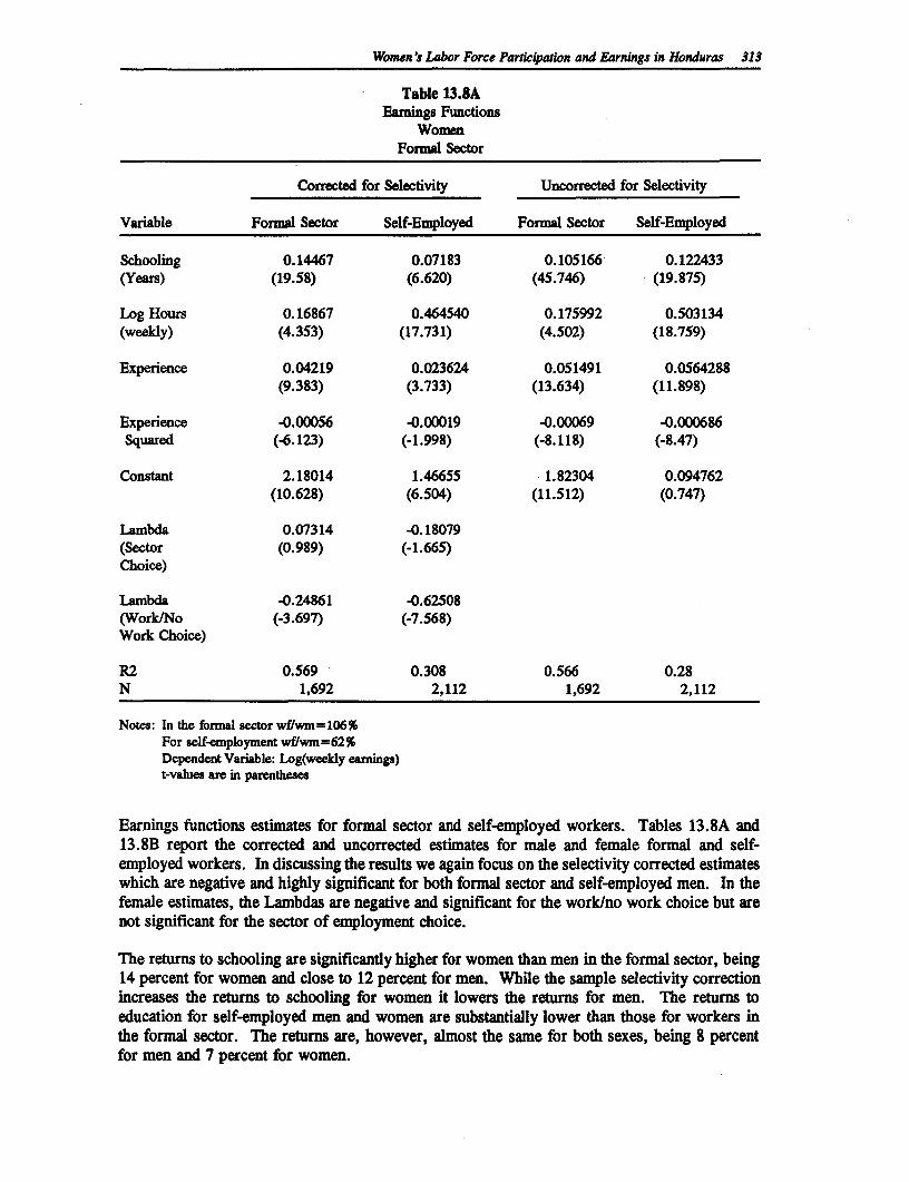
Women's Labor Force Participation and Earnings in Honduras 313
Table 13.8AEarnings Functions
WomenFormal Sector
Corrected for Selectivity Uncorrected for Selectivity
Variable Formal Sector Self-Employed Formal Sector Self-Employed
Schooling 0.14467 0.07183 0.105166 0.122433(Years) (19.58) (6.620) (45.746) (19.875)
Log Hours 0.16867 0.464540 0.175992 0.503134(weekly) (4.353) (17.731) (4.502) (18.759)
Experience 0.04219 0.023624 0.051491 0.0564288(9.383) (3.733) (13.634) (11.898)
Experience -0.00056 -0.00019 -0.00069 -0.000686Squared (-6.123) (-1.998) (-8.118) (-8.47)
Constant 2.18014 1.46655 1.82304 0.094762(10.628) (6.504) (11.512) (0.747)
Lambda 0.07314 -0.18079(Sector (0.989) (-1.665)Choice)
Lambda -0.24861 -0.62508(Work/No (-3.697) (-7.568)Work Choice)
R2 0.569 0.308 0.566 0.28N 1,692 2,112 1,692 2,112
Notes: In the formal sector wf/wm =106%For self-employment wflwm=62%Dependent Variable: Log(weekly earings)t-values are in parentheses
Earnings functions estimates for formal sector and self-employed workers. Tables 13.8A and13.8B report the corrected and uncorrected estimates for male and female formal and self-employed workers. In discussing the results we again focus on the selectivity corrected estimateswhich are negative and highly significant for both formal sector and self-employed men. In thefemale estimates, the Lambdas are negative and significant for the work/no work choice but arenot significant for the sector of employment choice.
The returns to schooling are significantly higher for women than men in the formal sector, being14 percent for women and close to 12 percent for men. While the sample selectivity correctionincreases the returns to schooling for women it lowers the returns for men. The returns toeducation for self-employed men and women are substantially lower than those for workers inthe formal sector. The returns are, however, almost the same for both sexes, being 8 percentfor men and 7 percent for women.
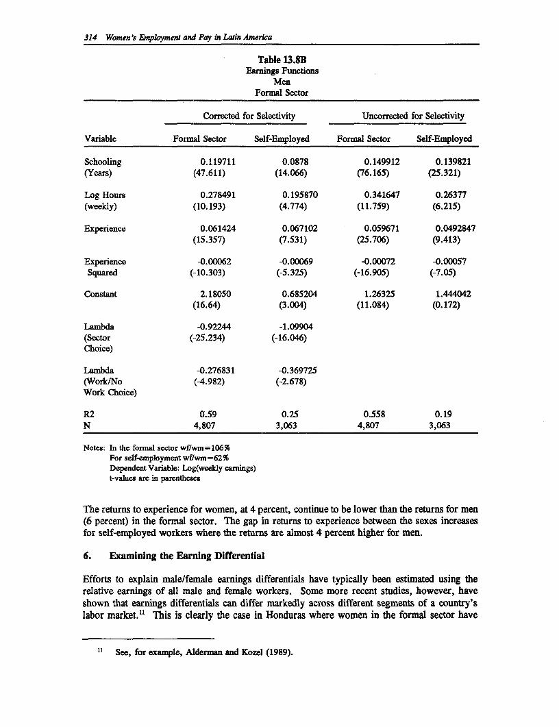
314 Women's Employment and Pay in Latin America
Table 13.8BEarnings Functions
MenFormal Sector
Corrected for Selectivity Uncorrected for Selectivity
Variable Formal Sector Self-Employed Formal Sector Self-Employed
Schooling 0.119711 0.0878 0.149912 0.139821(Years) (47.611) (14.066) (76.165) (25.321)
Log Hours 0.278491 0.195870 0.341647 0.26377(weekly) (10.193) (4.774) (11.759) (6.215)
Experience 0.061424 0.067102 0.059671 0.0492847(15.357) (7.531) (25.706) (9.413)
Experience -0.00062 -0.00069 -0.00072 -0.00057Squared (-10.303) (-5.325) (-16.905) (-7.05)
Constant 2.18050 0.685204 1.26325 1.444042(16.64) (3.004) (11.084) (0.172)
Lambda -0.92244 -1.09904(Sector (-25.234) (-16.046)Choice)
Lambda -0.276831 -0.369725(Work/No (-4.982) (-2.678)Work Choice)
R2 0.59 0.25 0.558 0.19N 4,807 3,063 4,807 3,063
Notes: In the formal sector wf/wm=106%For self-employment wf/wm=62%Dependent Variable: Log(weekly earnings)t-values are in parentheses
The returns to experience for women, at 4 percent, continue to be lower than the returns for men(6 percent) in the formal sector. The gap in returns to experience between the sexes increasesfor self-employed workers where the returns are almost 4 percent higher for men.
6. Examining the Earning Differential
Efforts to explain male/female earnings differentials have typically been estimated using therelative earnings of all male and female workers. Some more recent studies, however, haveshown that earnings differentials can differ markedly across different segments of a country'slabor market.'" This is clearly the case in Honduras where women in the formal sector have
" See, for example, Alderman and Kozel (1989).
Women's Labor Force Particyahon and Earnings in Honduras 315
a pay advantage of 6 percent, but earn only 62 percent of men's earnings in self-employed work.Given these differences we examine the causes of the earnings differentials separately for formaland self-employed workers as well as for all workers.
The Oaxaca (1973) decomposition method enables us to estimate what proportion of the earningsdifferential can be explained by differences in human capital endowments (education andexperience) and what proportion remains 'unexplained" by these endowments. We are unableto determine what factors contribute to this 'unexplained" proportion; it is really a catch-allreflecting differences in the way the labor market structure rewards female and male workers(i.e., discrimination) as well as the effects of omitted variables. However, it is generally takento be representative of the "upper bound" of discrimination and to reflect the way in which thelabor market rewards the attributes of male and female workers.
The Oaxaca decomposition expresses the difference between the mean Oog) wage rates of malesand females as:
BmXm-BfXf = Xm(Bm-Bf) + Bf(Xm-Xf) (1)= Xf(Bm-Bf) + Bm(Xm-Xf) (2)
Where: Bm,Bf are the estimated coefficients of the earnings functions.Xm,Xf are the means of the explanatory variables in the earnings functions.
Equations 1 and 2 estimate the same thing but the weighting of each is different; one is estimatedusing the male means and the other using the female means. There is theoretically no advantageto using one equation over the other, so both estimates are reported. We present thedecompositions using the selectivity corrected estimates.
Table 13.9 presents the Oaxaca estimates for all workers and by economic sector. The estimatesshow that the earnings differential is not explained by women's lower human capital endowments.In fact, the negative sign for the endowments estimates show women to have the advantage interms of endowments. The size of the endowments advantage differs substantially by economicsector, being large in the formal sector and relatively small in among self-employed workers.These estimates reflect actual differences in educational attainment between women and men inthe different sectors as shown in Tables 13.2A and 13.2B. Women average two and a half yearsmore schooling than men in the formal sector and .72 of a year more schooling in self-employment
Working women as a whole average almost one and a half years more schooling than workingmen. Any advantage which women have in terms of endowments, however, is canceled out bythe fact that the wage structure is so favorable to men in all sectors. The large advantage whichfemale formal sector workers have in terms of endowments (-610.66), for instance, is canceledout by the way the wage structure rewards women for these attributes (710.44). These estimatesthus indicate that wage discrimination in Honduras, imposed either informally by employers orformally by labor legislation, greatly reduces women's potential earnings. This is true in botheconomic sectors, but is more severe in the formal sector.
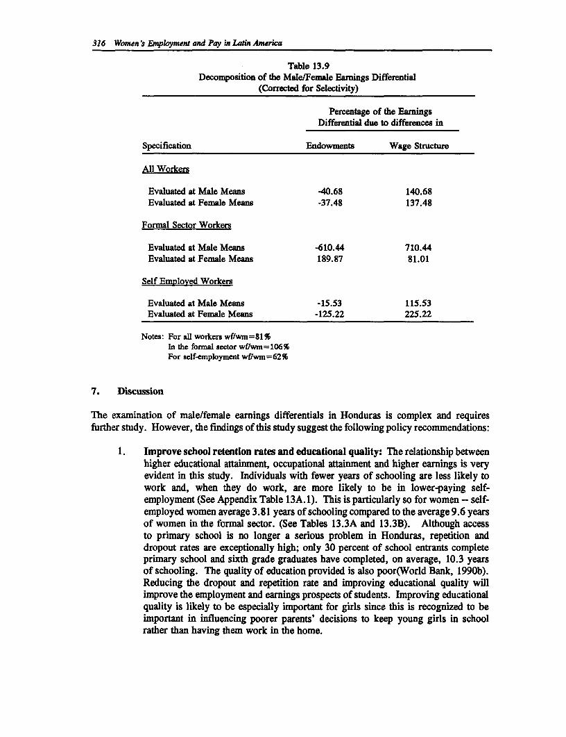
316 Women's mnployment and Pay in Latin America
Table 13.9Decomposition of the Male/Female Eamings Differential
(Corrected for Selectivity)
Percentage of the EarningsDifferential due to differences in
Specification Endowments Wage Structure
All Workers
Evaluated at Male Means -40.68 140.68Evaluated at Female Means -37.48 137.48
Formal Sector Workers
Evaluated at Male Means -610.44 710.44Evaluated at Fenale Means 189.87 81.01
Self E5Ioved Workers
Evaluated at Male Means -15.53 115.53Evaluated at Female Means -125.22 225.22
Notes: For all workers wfwm=81%In the formal sector wf/wm=106%For self-employment wf/wm=62%
7. Discussion
The examination of male/female earnings differentials in Honduras is complex and requiresfurther study. However, the findings of this study suggest the following policy recommendations:
i . Improve school retention rates and educational quality: The relationship betweenhigher educational attainment, occupational attainment and higher earnings is veryevident in this study. Individuals with fewer years of schooling are less likely towork and, when they do work, are more likely to be in lower-paying self-employment (See Appendix Table 13A. 1). This is particularly so for women - self-employed women average 3.81 years of schooling compared to the average 9.6 yearsof women in the formal sector. (See Tables 13.3A and 13.3B). Although accessto primary school is no longer a serious problem in Honduras, repetition anddropout rates are exceptionally high; only 30 percent of school entrants completeprimary school and sixth grade graduates have completed, on average, 10.3 yearsof schooling. The quality of education provided is also poor(World Bank, 1990b).Reducing the dropout and repetition rate and improving educational quality willimprove the employment and earnings prospects of students. Improving educationalquality is likely to be especially important for girls since this is recognized to beimportant in influencing poorer parents' decisions to keep young girls in schoolrather than having them work in the home.
Women's Labor Force Paracipadon and Earnings in Honduras 317
2. Primary and secondary education should be given priority in educationalspending: This study shows that the probability of participation among womenincreases substantially if they have completed primary and secondary education.Both female and male secondary school graduates have higher (predicted and real)participation rates than individuals with incomplete or complete tertiary education(See Appendix Table 13A. 1 and Table 13.5), indicating that public investments willyield higher returns if invested in lower educational levels.
3. Labor and commercial legislation should be reviewed to determine whether thereare laws which prevent women from participating in certain sectors or which limitwomen entrepreneurs' access to credit. This study indicates that women in theformal sector are affected by wage discrimination. The reasons for this are not clearbut in many Latin American countries legislation regulates women's participation invarious industries and occupations, thereby limiting their productivity and earningspotential. A study of existing legislation and its implementation would help toidentify whether this is the case in Honduras. It is also not clear why self-employedwomen earn so much less on average than self-employed men. Limited access byself-employed women to credit could be a contributing factor. Legislation alsoregulates women's access to credit in many Latin American countries, a factor whichcould also be clarified in a review of the country's labor and commercial laws.
4. Review textbooks to remove gender stereotyping and provide incentives for girlsto pursue non-traditional courses of study: Women in Honduras workpredominantly in the lowest paying economic sector (self-employment) and areconcentrated in the lowest paying occupations (social services, commerce andmanufacturing) in both economic sectors (See Tables 13.2A and 13.2B). Thereasons why women choose to enter lower-paying occupations even when they havehigher education is not clear, but these occupations have traditionally beenconsidered "women's work." The removal of gender stereotyping in schooltextbooks may be one way to change these attitudes and to encourage women toenter more productive occupations with higher rewards. Another approach wouldbe to encourage girls to pursue non-traditional courses of study, such as thesciences. However, the way in which these incentives could be provided wouldhave to be given careful consideration.
5. Stimulate private sector provision of childcare: This study shows that theprobability that a woman will participate in the labor force declines sharply whenshe has young children to care for. Having one pre-school aged child reduced theprobability that a woman will work by 11 percent, and having two young childrenreduced the probability by 21 percent (See Table 13.5). Improved access toadequate childcare services would permit more women to work. In cases wherewomen enter self-employment because childcare responsibilities make it difficult forthem to adhere to the set working hours of the formal sector, access to childcarewould permit them to move into the formal sector.
6. Macroeconomic adjustment measures will dearly continue to be important instimulating economic growth and in increasing the capacity of the labor market toabsorb new entrants to the work force.
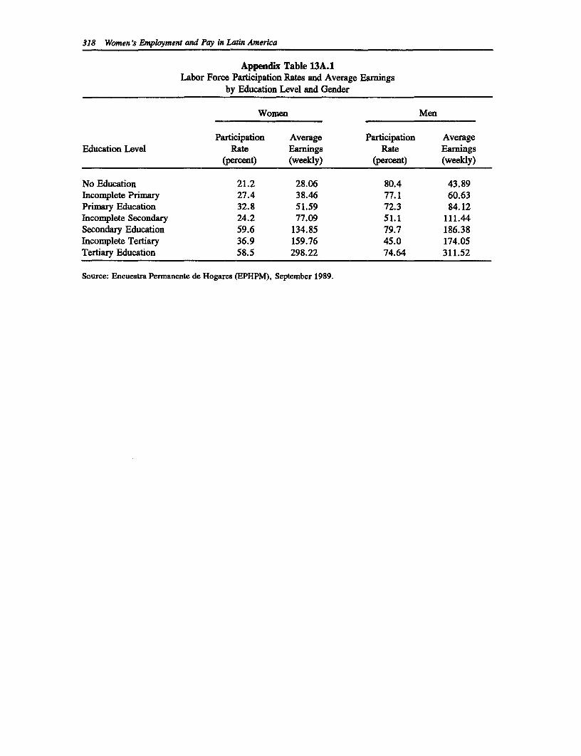
318 Women's Enployment and Pay in Latin America
Appendix Table 13A.1Labor Force Participation Rates and Average Eanings
by Education Level and Gender
Women Men
Participation Average Participation AverageEducation Level Rate Eamings Rate Eamnings
(percent) (weekly) (percent) (weekly)
No Education 21.2 28.06 80.4 43.89Incomplete Primary 27.4 38.46 77.1 60.63Primary Education 32.8 51.59 72.3 84.12Incomplete Secondary 24.2 77.09 51.1 111.44Secondary Education 59.6 134.85 79.7 186.38Incomplete Tertiary 36.9 159.76 45.0 174.05Tertiary Education 58.5 298.22 74.64 311.52
Source: Encuestra Permanente de Hogares (EPHPM), September 1989.
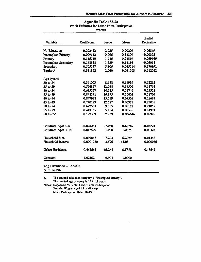
Women 's Labor Force Partic@afion and Earnings in Honduras 319
Appendix Table 13A.2aProbit Estimates for Labor Force Participation
Women
PartialVariable Coefficient t-ratio Mean Derivative
No Education -0.202482 -2.035 0.20299 -0.06849Incomplete Primary -0.009142 -0.096 0.31309 -0.00392Primary 0.115780 1.216 0.21859 0.039166Incomplete Secondary -0.148358 -1.529 0.14186 -0.05018Secondary 0.505177 5.106 0.085214 0.170891Tertiary8 0.331862 2.760 0.021203 0.112262
Age (years)20 to 24 0.361003 8.188 0.16939 0.1221225 to 29 0.554827 12.038 0.14306 0.1876830 to 34 0.695527 14.385 0.11746 0.2352835 to 39 0.848591 16.895 0.10002 0.2870640 to 44 0.847938 15.559 0.07505 0.2868345 to 49 0.740173 12.627 0.06313 0.2503850 to 54 0.622538 9.765 0.05112 0.2105955 to 59 0.443165 5.884 0.03576 0.1499160 to 6 5 b 0.177309 2.239 0.036646 0.05998
Children: Aged 0-6 -0.095233 -7.080 0.82789 -0.03221Children: Aged 7-14 0.012520 1.000 1.0875 0.00423
Household Size -0.039867 -7.203 6.2029 -0.01348Household Income 0.0001980 3.596 144.08 0.000066
Urban Residence 0.462566 16.264 0.5388 0.15647
Constant -1.02162 -9.901 1.0000
Log Likelihood = -6844.6N = 12,498
a. The omited education category is "incomplete tertiary".b. The omitted age category is 15 to 19 years.Notes: Dependent Variable: Labor Force Participation
Sample: Women aged 15 to 65 yearsMean Participation Rate: 30.4%
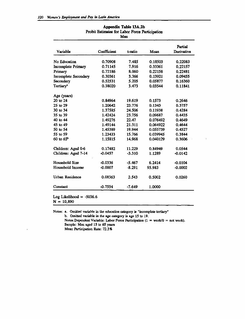
320 Women's Employment and Pay in Latin America
Appendix Table 13A.2bProbit Estimates for Labor Force Participation
Men
PartialVariable Coefficient t-ratio Mean Derivative
No Education 0.70908 7.485 0.18503 0.22083Incomplete Primary 0.71145 7.916 0.33361 0.22157Primary 0.72186 8.060 0.22158 0.22481Incomplete Secondary 0.30361 3.366 0.13921 0.09455Secondary 0.52531 5.205 0.05877 0.16360Tertiary8 0.38020 3.473 0.03544 0.11841
Age (years)20 to 24 0.84964 19.619 0.1573 0.264625 to 29 1.20642 23.776 0.1343 0.375730 to 34 1.37585 24.506 0.11938 0.428435 to 39 1.42424 23.756 0.09687 0.443540 to 44 1.49276 22.47 0.076492 0.464945 to 49 1.49144 21.311 0.064922 0.464450 to 54 1.45389 19.944 0.055739 0.452755 to 59 1.23433 15.766 0.039945 0.384460 to 65" 1.15815 14.968 0.040129 0.3606
Children: Aged 0-6 0.17482 11.229 0.84949 0.0544Children: Aged 7-14 -0.0457 -3.310 1.1289 -0.0142
Household Size -0.0336 -5.467 6.2414 -0.0104Household Income -0.0007 -8.291 95.983 -0.0002
Urban Residence 0.08363 2.543 0.5002 0.0260
constant -0.7554 -7.649 1.0000
Log Likelihood = -5036.6N = 10,890
Notes: a. Omitted variable in the education category is "incomplete terdary"b. Omitted variable in the age category is age 15 to 19.Notes:Dependent Variable: Labor Force Participation (1 = worktO = not work).Sample: Men aged 15 to 65 yearsMean Participation Rate: 72.3%
References
Alderman, H. and V. Kozel. "Formal and Informal Sector Wage Determination in Urban Low-Income Neighborhoods in Pakistan." Living Standards Measurements Working Paper No.65. Washington D.C.: World Bank.
Danes, S.M., M. Winter and M.B. Whiteford. "Informal and Formal Market Participation ofRural Honduran Women." Working Paper No. 82. Michigan State University: Womenin International Development Institute, 1985.
Gronau, R. "Sex-Related Wage Differentials and Women's Interrupted Labor Careers: TheChicken and Egg Question." Journal of Labor Economics, Vol. 6, no. 3 (1988). pp. 277-301.
Gunderson, M. "Male-Female Wage Differentials and Policy Responses." Journal of EconomicLiterature, Vol. 27 (1989). pp. 46-72.
Heckman, J.J. "Sample Selection Bias as a Specification Error." Econometrica, Vol. 47, no. 1(1979). pp. 53-161.
Nyrop, R. (ed.). Honduras: A Country Study. American University: Foreign Areas Studies,1987.
Oaxaca, R.L. "Male-female Wage Differentials in Urban Labor Markets." InternationalEconomic Review, Vol. 14, no. 1 (1973). pp. 693-709.
The Economist Intelligence Unit. Guatemala, El Salvador, Honduras. Country Report. No. 3.New York, 1991.
The Economist Intelligence Unit. Guatemala, El Salvador, Honduras. Country Profile 1989-90.New York, 1991.
Tunali, I. "A General Structure for Models of Double-Selection and an Application to a JointMigration/Earnings Process with Remigration." Research in Labor Economics, Vol. 8, PartB (1986). pp. 235-282.
World Bank. "Social Investmnent in Guatemala, El Salvador and Honduras." Workshop onPoverty Alleviation, Basic Social Services and Social Investment Funds within theConsultative Group Framework. Latin America and Caribbean Regional Office, June,1990a.
321

322 Women's Enployment and Pay in Latin America
World Bank. "Honduras Social Sector Programs." Country Departnent I. Latin America andCaribbean Regional Office, November, 1990b.
World Bank. "Honduras: Country Economic Memorandum." Latin American and CaribbeanRegional Office, April, 1987.
World Bank. "Honduras: A Review of Selected Key Problems of the Agricultural Sector."Projects Department, Latin American and Caribbean Regional Office, October, 1981.
14
Female Labor Force Participation and Earnings:The Case of Jamaica
Katherine MacKinnon Scott
1. Introduction
On average, women's weekly earnings in Jamaica are only 57.7 percent of men's earnings. InJamaica this has serious social ramifications as one-third of all households are headed by women.The observed wage differential helps to explain why female heads of households and theirdependents are more likely to live in poverty than male heads of households and their dependents.From both the viewpoint of equity and social well-being, understanding the causes of this wagedifferential is important. This study is an empirical investigation of gender-based wagedifferentials in Jamaica. The specific issue to be addressed is the extent to which observeddifferences between male and female earnings are a function of different human capitalcharacteristics or the different values placed on male and female labor in the market.
Labor force survey data from October 1989 are used in the analysis. Specifically, earningsfunctions for men and women are compared and the wage differential that exists is decomposedinto two components: The portion due to different endowment levels between men and women(the explained differential) and that due to discrimination in the labor market (or the unexplaineddifferential). The earnings function for women is corrected for selectivity through the use of theinverse Mill's ratio obtained from the relevant labor force participation function.
Section 2 provides background information on Jamaica and its labor market characteristics. Adescription of the data and the sample used is presented in Section 3. Section 4 contains theresults of the participation function for women and Section 5 the results of the earnings functionsfor men and women. The extent of gender-based labor market discrimination is presented in thesixth section and Section 7 discusses the findings and recommendations.
2. The Jamaican Labor Market
Jamaica is a small country with only 2.3 million inhabitants. In 1987, agriculture employed onequarter of the population but contributed just over 6 percent of GDP. In contrast, manufacturingemployed close to 15 percent of the population and comprised over 22 percent of GDP. Theother large employment sectors are services and commerce (representing 26 and 13 percent ofemployment respectively) with the remainder of employment being primarily in construction andtransport (Statistical Institute of Jamaica, 1989). The economy is heavily dependent on bauxiteand alumina exports and the fall in bauxite prices in the 1980s had a serious impact on theeconomic situation of the country. In addition, the primary agricultural crop is sugar, whichfaces a highly stagnant international market.
323
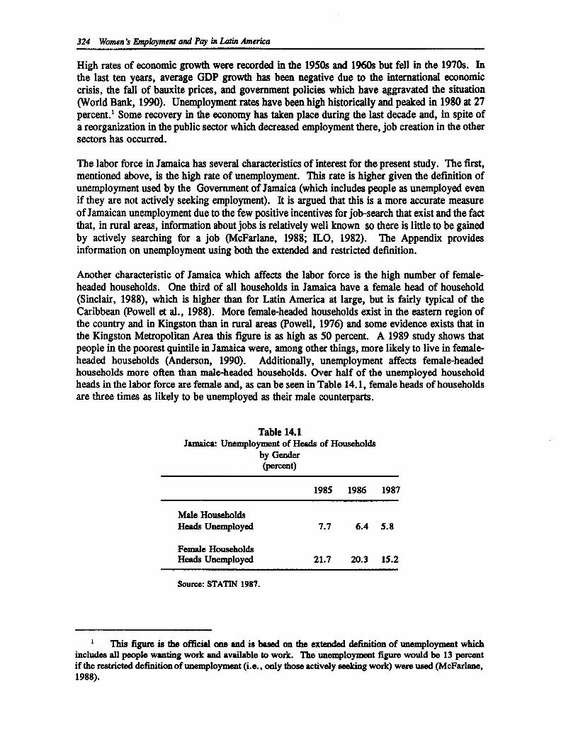
324 Women's Employment and Pay in Latin America
High rates of economic growth were recorded in the 1950s and 1960s but fell in the 1970s. Inthe last ten years, average GDP growth has been negative due to the international economiccrisis, the fall of bauxite prices, and government policies which have aggravated the situation(World Bank, 1990). Unemployment rates have been high historically and peaked in 1980 at 27percent.' Some recovery in the economy has taken place during the last decade and, in spite ofa reorganization in the public sector which decreased employment there, job creation in the othersectors has occurred.
The labor force in Jamaica has several characteristics of interest for the present study. The first,mentioned above, is the high rate of unemployment. This rate is higher given the definition ofunemployment used by the Government of Jamaica (which includes people as unemployed evenif they are not actively seeking employment). It is argued that this is a more accurate measureof Jamaican unemployment due to the few positive incentives for job-search that exist and the factthat, in rural areas, information about jobs is relatively well known so there is little to be gainedby actively searching for a job (McFarlane, 1988; lLO, 1982). The Appendix providesinformation on unemployment using both the extended and restricted definition.
Another characteristic of Jamaica which affects the labor force is the high number of female-headed households. One third of all households in Jamaica have a female head of household(Sinclair, 1988), which is higher than for Latin America at large, but is fairly typical of theCaribbean (Powell et al., 1988). More female-headed households exist in the eastern region ofthe country and in Kingston than in rural areas (Powell, 1976) and some evidence exists that inthe Kingston Metropolitan Area this figure is as high as 50 percent. A 1989 study shows thatpeople in the poorest quintile in Jamaica were, among other things, more likely to live in female-headed households (Anderson, 1990). Additionally, unemployment affects female-headedhouseholds more often than male-headed households. Over half of the unemployed householdheads in the labor force are female and, as can be seen in Table 14.1, female heads of householdsare three times as likely to be unemployed as their male counterparts.
Table 14.1Jamaica: Unemployment of Heads of Households
by Gender(percent)
1985 1986 1987
Male HouseholdsHeads Unemployed 7.7 6.4 5.8
Female HouseholdsHeads Unemployed 21.7 20.3 15.2
Source: STATIN 1987.
This figure is the official one and is based an the extended definition of unemployment whichincludes all people wanting work and available to work. The unemployment figure would be 13 percentif the restricted definition of unemployment (i.e., only those actively seeking work) were used (McFarlane,1988).
Female Labor Force Parfic!pafion and Earnings: The Case of Jamaka 325
A third characteristic of the labor force is the large proportion who are self-employed. Theincrease in self-employment began in the 1970s (Klinov, 1987) and by the early 1980s almostone-half of all male workers and one-third of all female workers were self-employed (Doeringer,1987). It is argued that half of the self-employed are actually in the informal sector (Lisk, 1987),a higher proportion than in Latin America and the Caribbean as a whole (ILO, 1988). The fallin formal sector employment coincided with a rise in employment in the informal sector with asubsequent fall in the informal sector's productivity (Doeringer, 1987). There is evidence thatthe informal sector in Jamaica works to absorb the excess supply of labor (Klinov, 1987;Doeringer, 1987) and may well be a form of disguised unemployment (Villarreal Gonda, 1983).
The final point concerning the labor force that is of interest for this study is the lack of trainingreceived by workers. Ninety percent of the labor force in Jamaica has had no specialized orvocational training (Lisk, 1987). In essence, the only training received by Jamaican workers ison-the-job training. In addition to this lack of training, the quality of the formal educationalsystem is presumed to be low; few companies rely on the schooling system for skill training(Doeringer, 1987) and employers in both public and private sectors have indicated that the basiclevel of knowledge of school leavers, and particularly people with three years of secondaryeducation, is so low that "many of them are almost untrainable" (UNESCO, 1983:119).
The characteristics of the Jamaican labor market outlined above have an impact on both thedecision to participate in the labor force and the productivity of the labor force. First, womenwho are heads of households can be expected to have participation rates similar to those of men.Second, the labor absorption role of the informal sector leads to low productivity which maydecrease the impact of human capital investments on earnings. Finally, the absence of trainingand the lack of articulation between formal education and the needs of the labor market alsoinfluence human capital and earnings.
3. The Data
The data used in this paper are from a random sample of the 1989 Labor Force Survey carriedout by the Statistical Institute of Jamaica. This is a bi-annual survey carried out in April andOctober of each year. In the October 1989 round the survey covered 6,000 households. The dataused in the present analysis is a random sample of this October, 1989 data set and includes 5,219households for a total of 18,657 individuals. Of these individuals, 5,654 are in the prime agefor working (between ages 20 and 59).
Table 14.2 presents some summary information on this prime age group. The workingpopulation is defined as all those with positive earnings and hours worked. This definition omitsunpaid family workers but it does include the self-employed. Almost 62 percent of the samplepopulation is defined as working.
The sample is a fairly young one with the average age of working men and women being 35years, slightly higher than the age of the sample population as a whole. Working women havethe highest education levels, having completed an average of 7.8 years of schooling. Workingmen have, on average, approximately half a year less schooling than their female counterparts.Only at the university level do men have more schooling, although the difference is slight.
Thirty-eight percent of the sample of working women are heads of households compared to 54percent of working males. Working women live in slightly larger households than working men.
326 Women Is Employment and Pay in Latin America
The difference in size is primarily due to the fact that working women live in households withmore children under age 14.
Experience, as used here, is potential experience, not actual experience.2 Potential experienceclosely approximates actual experience for those individuals who have worked steadily sinceleaving school. This potential experience may be a good approximation of real experience formen but for women, who traditionally move in and out of the labor force, the experience variablewill overstate actual experience.3
As is the case in many other Latin American and Caribbean countries (see other chapters in thisvolume), the greatest difference between male and female workers is found in earnings. Thedifference in weekly earnings between men and women in Jamaica is substantial. As can be seenin Table 14.2, working women earn only 57.7 percent of what men earn even though womenwork, in hourly terms, only six percent less per week than men.4 The minimum wage inJamaica in 1988 for a forty hour week was J$80. Thus, if the weekly earnings in Table 14.2 areadjusted to a forty hour week both men and women are, on average, still making less than theminimum wage. Men, however, earn an average of 70 percent of the minimum wage whileworking women, on average, earn only 43 percent. Correcting for the difference in hoursworked shows women earning 61.4 percent of men's earnings.
4. Determinants of Female Labor Force Participation
For women, unlike men, there is assumed to be a reservation wage which will affect a woman'sdecision to participate in the labor force.5 When the reservation wage is higher than marketwages, women will remain outside the labor market. Only when this unobserved reservationwage, or the non-market value of women's labor, is lower than the market wage will womenchoose to participate in the labor market. As the reservation wage is not observed for non-working women, the female earnings function will produce biased results if an ordinary leastsquares earnings estimation technique is used. In order to correct for this selectivity bias it isnecessary to estimate a participation function for women which regresses women's demographicand human capital characteristics on their probability of participating in the labor market(Heckman, 1979). From this equation, the inverse Mill's ratio can be calculated and includedin the earnings function.
2 This is calculated as "age minus number of years of schooling minus 6." This definition followsMincer, 1974.
3 A 1988 study of female-headed households in Jamaica showed that one-third of the women whoworked did so intermittently [Powell, 1988].
4 The eanings variable was constructed from information on annual earnings and number of monthsworked. The earnings variable used here is annual earnings divided by the number of months workeddivided by 4.2. The information on both hours worked per week and months worked per year collectedin the survey is not continuous. Continuous variables were created by taling the midpoint of the rangesprovided for each.
5 There is some evidence in Jamaica that men may also have a reservation wage as male labor forceparticipation rates in Jamaica are lower than those in other countries. For the purposes of the presentstudy, however, the reservation wage for men is considered to be zero.
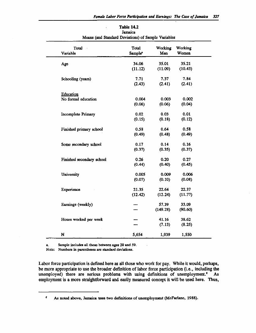
Female Labor Force Parwic,ation and Earnings: The Case of Jamaica 327
Table 14.2Jamaica
Means (and Standard Deviations) of Sample Variables
Total Total Working WorkingVariable Sample Men Women
Age 34.06 35.01 35.21(11.12) (11.09) (10.43)
Schooling (years) 7.71 7.37 7.84(2.43) (2.41) (2.41)
EducationNo formal education 0.004 0.003 0.002
(0.06) (0.06) (0.04)
Incomplete Primary 0.02 0.03 0.01(0.15) (0.18) (0.12)
Finished primary school 0.58 0.64 0.58(0.49) (0.48) (0.49)
Some secondary school 0.17 0.14 0.16(0.37) (0.35) (0.37)
Finished secondary school 0.26 0.20 0.27(0.44) (0.40) (0.45)
University 0.005 0.009 0.006(0.07) (0.10) (0.08)
Experience 21.35 22.64 22.37(12.42) (12.24) (11.77)
Earnings (weekly) - 57.39 33.09_- (149.28) (90.60)
Hours worked per week 41.16 38.62- (7.13) (8.25)
N 5,654 1,939 1,550
a. Sample includes aU those between ages 20 and 59.Note: Numbers in parentheses are standard deviations.
Labor force participation is defined here as all those who work for pay. While it would, perhaps,be more appropriate to use the broader definition of labor force participation (i.e., including theunemployed) there are serious problems with using definitions of unemployment.A Asemployment is a more straightforward and easily measured concept it will be used here. Thus,
6 As noted above, Jamaica uses two definitions of unemployment (McFarlane, 1988).
328 Women's Employment and Pay in Latin America
a woman is considered to participate in the labor force if she reports hours worked and haspositive earnings. Women who are self-employed are considered to be participating althoughunpaid family workers and the unemployed are excluded. Of the 3,212 women between ages 20and 59 included here, 1,550 were working for pay (48.3 percent of all women and 27.4 percentof the sample). Given the dichotomous nature of the dependent variable, a probit model is usedto estimate the probability of participation.
The regressors in the participation function take into account family, geographic location, andpersonal characteristics of the individual women. Family variables include number of childrenand adults in the household. Children in the household are divided into two groups, those undersix and those aged 6 to 14 years. In general, it is predicted that the presence of children underage six will increase the value of a woman's time in the house in terms of household productionand hence lower her probability of participating in the labor force. Heckman (1974) found thatthe effect of having one child under six is to raise the asking price (the wage at which a womanwill work) by 15 percent, which thus lowers the probability of participation.
It should be noted that it is not possible to determine to whom the children in the sample"belong." In other words, in any given household there may be more than one woman withchildren. The way in which the data were collected makes it impossible to determine how manychildren each of these women has. The inability to match children with their mothers may not,however, be a serious problem in the present analysis. Some evidence from Jamaica indicatesthat the responsibilities of childcare fall to all females in the household regardless of who theactual mother is (World Bank, 1985; Powell et al, 1988). If all women in a given householdshare in childcare responsibilities, then the expected sign of the coefficient for the presence ofvery young children will still be negative.
It is expected that the presence of non-earning adults in a woman's household would increase herprobability of participating. On the one hand, if these adults take over childcare responsibilities,as has been shown to be the case in Jamaica (Powell et al., 1988), they will free the children'smother to work outside the home. On the other hand, each adult with zero income representsa drain on family resources that might force females within the household to work. Thus, whilethe sign of the coefficient is expected to be positive, it will not be possible to determine whicheffect has the greater impact. The presence of income earning adults is expected to have theopposite effect, decreasing the need for further income.
Also included in the model is a variable which addresses the status of the individual woman inthe household. A large percentage of women in the sample are heads of households. Thesewomen will be more likely to be primary workers, working full time and having less choice aboutlabor market participation. It is expected that they will be more likely to participate in the laborforce.
The geographic area, and specifically the parish in which a woman lives, is also expected toinfluence her decision to participate. It would be expected that urban dwellers would be morelikely to participate given the (1) more "liberal" attitudes towards women's participation in theurban areas, and (2) the high rates of migration experienced in Jamaica, especially among womanto urban areas (World Bank, 1985).' Kingston and St. Andrews are the two parishes with the
7 The cause of migration is typically to find work (Ankar & Knowles, 1978). To the extent thatwomen who migrate do find work, it is expected that the coefficients on the urban variables will bepositive.
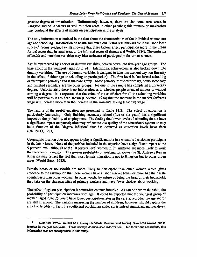
Female Labor Force ParticipaJon and Eantings: The Case of Jamaia 329
greatest degree of urbanization. Unfortunately, however, there are also some rural areas inKingston and St. Andrews as well as urban areas in other parishes; this mixture of rural/urbanmay confound the effects of parish on participation in the analysis.
The only information contained in the data about the characteristics of the individual women areage and schooling. Information on health and nutritional status was unavailable in the labor forcesurvey.8 Some evidence exists showing that these factors affect participation more in the urbanformal sector than in rural areas or the informal sector (Behrman and Wolfe, 1984). The omissionof health and nutrition variables may bias estimates of participation for urban women.
Age is represented by a series of dummy variables, broken down into five-year age groups. Thebase group is the youngest (ages 20 to 24). Educational achievement is also broken down intodummy variables. (The use of dummy variables is designed to take into account any non-linearityin the effect of either age or schooling on participation). The first level is "no formal schoolingor incomplete primary' and is the base group. Some primary, finished primary, some secondaryand finished secondary are the other groups. No one in the sample has completed a universitydegree. Unfortunately there is no information as to whether people attended university withoutearning a degree. It is expected that the value of the coefficient for all the schooling variableswill be positive as it has been shown (Heckman, 1974) that the increase in the market (offered)wage will increase more than the increase in the woman's asking (shadow) wage.
The results of the probit equation are presented in Table 14.3. The effect of education isparticularly interesting. Only finishing secondary school (five or six years) has a significantimpact on the probability of employment. The finding that lower levels of schooling do not havea significant impact on participation may reflect the low quality of the educational system or maybe a function of the "degree inflation" that has occurred as education levels have risen(UNESCO, 1983).
Geographic location does not appear to play a significant role in a woman's decision to participatein the labor force. None of the parishes included in the equation have a significant impact at the5 percent level, although at the 10 percent level women in St. Andrews are more likely to workthan women in Kingston. The greater probability of working for women in St. Andrews than inKingston may reflect the fact that most female migration is not to Kingston but to other urbanareas (World Bank, 1985).
Female heads of households are more likely to participate than other women which givescredence to the assumption that these women have a labor market behavior more like their malecounterparts than other women. In other words, by nature of being the head of their household,they take on the characteristics of primary workers and have fewer choices about working.
The effect of age on participation is somewhat counter-intuitive. As can be seen in the table, theprobability of participation increases with age. It could be expected that the youngest group ofwomen, aged 20 to 25 would have lower participation rates as they are at reproductive age and/orare still in school. The variable measuring the number of children, however, should capture theeffect of fertility (in fact, the coefficient on children under six is indeed significant and negative).
a Note that several rounds of a Living Standards Measurement Survey have been carried out inJamaica in the past two years. These surveys do have such information. Due to various constraints, thisinformation was not incorporated in this study.
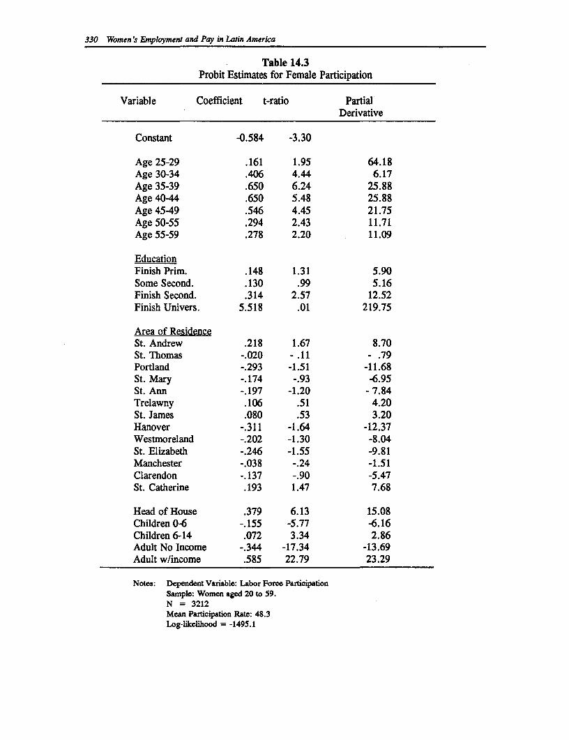
330 Women's Employment and Pay in Latin America
Table 14.3Probit Estimates for Female Participation
Variable Coefficient t-ratio PartialDerivative
Constant -0.584 -3.30
Age 25-29 .161 1.95 64.18Age 30-34 .406 4.44 6.17Age 35-39 .650 6.24 25.88Age 40-44 .650 5.48 25.88Age 45-49 .546 4.45 21.75Age 50-55 .294 2.43 11.71Age 55-59 .278 2.20 11.09
EducationFinish Prim. .148 1.31 5.90Some Second. .130 .99 5.16Finish Second. .314 2.57 12.52Finish Univers. 5.518 .01 219.75
Area of ResidenceSt. Andrew .218 1.67 8.70St. Thomas -.020 - .11 - .79Portland -.293 -1.51 -11.68St. Mary -.174 -.93 -6.95St. Ann -.197 -1.20 - 7.84Trelawny .106 .51 4.20St. James .080 .53 3.20Hanover -.311 -1.64 -12.37Westmoreland -.202 -1.30 -8.04St. Elizabeth -.246 -1.55 -9.81Manchester -.038 -.24 -1.51Clarendon -.137 -.90 -5.47St. Catherine .193 1.47 7.68
Head of House .379 6.13 15.08Children 0-6 -.155 -5.77 -6.16Children 6-14 .072 3.34 2.86Adult No Income -.344 -17.34 -13.69Adult w/income .585 22.79 23.29
Notes: Dependent Variable: Labor Force ParticipationSample: Women aged 20 to 59.N = 3212Mean Participation Rate: 48.3Log-likelihood = -1495.1
Femae Labor Force Parficwdiox and Earnings: The Case of Jamakca 331
Also, fewer than one percent of all Jamaican women have a university degree which indicates thatwomen aged 20 to 24 are not in school.9 Running a probit which has overall participation (i.e.,including the unemployed) as the dependent variable shows that the two youngest groups havethe highest rates of participation. Clearly, the negative coefficients in the present equation areindicative of the extremely high unemployment rates among these age groups.
The composition of the family has a significant impact on female participation. As expected, thenumber of children under age six has a negative impact on the probability of participation. Thenumber of children aged six to fourteen has a positive impact on participation.
The signs of the coefficients on the number of adults, income earners and non-earners in thehousehold are the reverse of the expected ones. A greater number of non-wage earning adultsin the household lowers the probability of participation while the more earning adults there arein the household, the higher the participation. If the non-earning adults are elderly or males whowill not take over household duties, it may well be that the effect of having more of these non-earning adults is to raise the value of the woman's non-market labor. It is not, however, clearwhy an increase in earning adults increases the probability of participation.
Simulations based on the above equation show the impact of various characteristics of women.As can be seen in Table 14.4, the probability of participating in the labor force increases withage up until a woman reaches age 45 when participation starts to decline. Women in age ranges35 to 40 and 40 to 45 have the highest participation rates (61.4 percent). The difference is quitelarge - twenty-five percentage points between a 20 year old and a 40 year old.
A completed secondary degree is the only educational level which significantly affects theprobability of participation. Women who complete secondary school have a three percentagepoint higher probability of working than a woman with the average level of education (ess thaneight years of schooling).
Other simulations show the change in participation based on status in the household and thecomposition of the household. Heads of households are shown to be much more likely toparticipate than woman who are not heads of households (15 percentage points higher). Havingtwo children under age 6 lowers the probability of participation below the average level andhaving two or more children between ages six and fourteen raises the level of participation abovethe average level.
Both the number of adults with income and those without affect the probability of participationto a great extent. Notice that a woman in a household with one non-earning adult has a 48.6percent probability, but that a woman in a household with two non-earning adults has only a 35.3probability of participating. The same type of impact on participation can be seen in the numberof income earning adults.
9 Unless of course large groups of people attend the university without completing degrees. Thedata do not provide information on this.
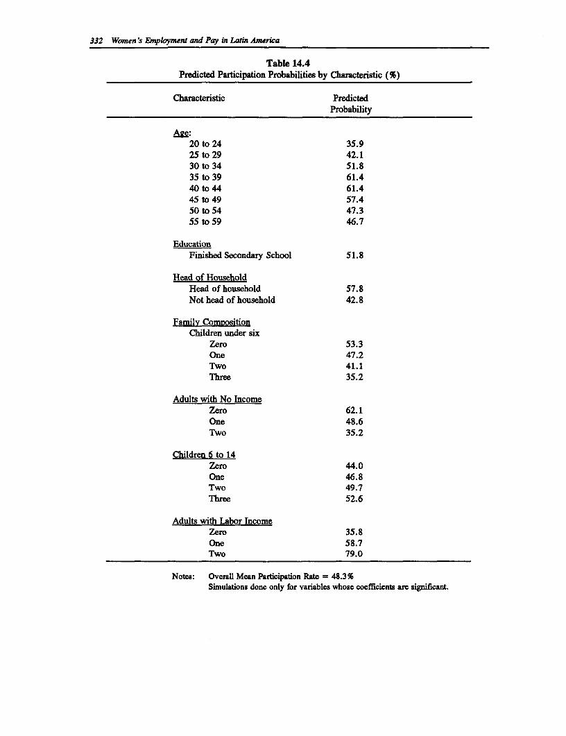
332 Women's Enpltoyment and Pay in Latin America
Table 14.4Predicted Participation Probabilities by Characteristic (%)
Characteristic PredictedProbability
Age:20 to 24 35.925to29 42.130 to 34 51.835 to 39 61.440 to 44 61.445 to 49 57.450 to 54 47.355 to 59 46.7
EducationFinished Secondary School 51.8
Head of HouseholdHead of household 57.8Not head of household 42.8
Family CompositionChildren under six
Zero 53.3One 47.2Two 41.1Three 35.2
Adults with No IncomeZero 62.1One 48.6Two 35.2
Children 6 to 14Zero 44.0One 46.8Two 49.7Three 52.6
Adults with Labor IncomeZero 35.8One 58.7Two 79.0
Notes: Overall Mean Participation Rate = 48.3%Simulations done only for variables whose coefficients are significant.
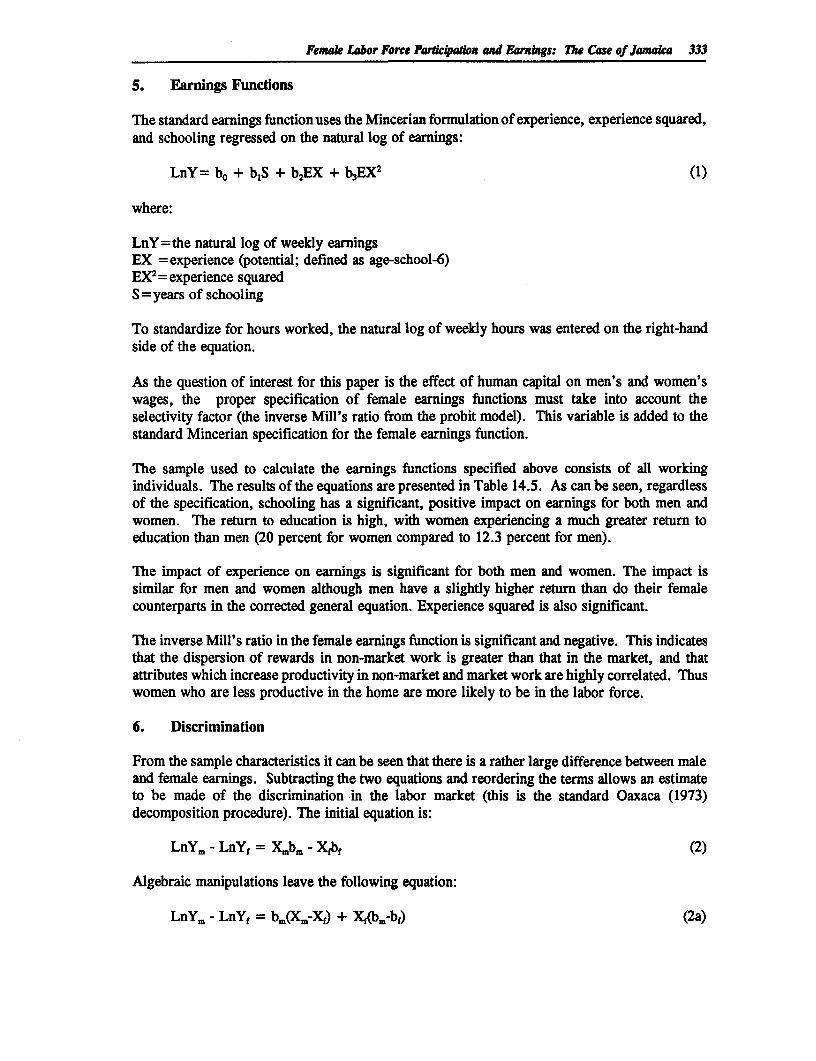
Femae Labor Force Parwc(padon and Earnings: The Case of JamaIca 333
5. Earnings Functions
The standard earnings function uses the Mincerian formulation of experience, experience squared,and schooling regressed on the natural log of earnings:
LnY= bo + b1 S + b2EX + b3EX2 (1)
where:
LnY=the natural log of weekly earningsEX =experience (potential; defined as age-school-6)EX2= experience squaredS =years of schooling
To standardize for hours worked, the natural log of weekly hours was entered on the right-handside of the equation.
As the question of interest for this paper is the effect of human capital on men's and women'swages, the proper specification of female earnings functions must take into account theselectivity factor (the inverse Mill's ratio from the probit model). This variable is added to thestandard Mincerian specification for the female earnings function.
The sample used to calculate the earnings functions specified above consists of all workingindividuals. The results of the equations are presented in Table 14.5. As can be seen, regardlessof the specification, schooling has a significant, positive impact on earnings for both men andwomen. The return to education is high, with women experiencing a much greater return toeducation than men (20 percent for women compared to 12.3 percent for men).
The impact of experience on earnings is significant for both men and women. The impact issimilar for men and women although men have a slightly higher return than do their femalecounterparts in the corrected general equation. Experience squared is also significant.
The inverse Mill's ratio in the female earnings function is significant and negative. This indicatesthat the dispersion of rewards in non-market work is greater than that in the market, and thatattributes which increase productivity in non-market and market work are highly correlated. Thuswomen who are less productive in the home are more likely to be in the labor force.
6. Discrimination
From the sample characteristics it can be seen that there is a rather large difference between maleand female earnings. Subtracting the two equations and reordering the terms allows an estimateto be made of the discrimination in the labor market (this is the standard Oaxaca (1973)decomposition procedure). The initial equation is:
LnY. - LnYf = X.bm - Xfbf (2)
Algebraic manipulations leave the following equation:
LnYm - LnYf = bm(Xm-Xf) + Xf(bj-bf) (2a)
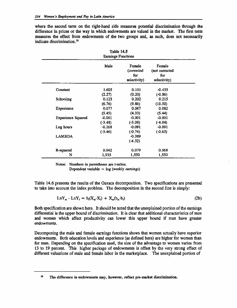
334 Women 's Employment and Pay in Latin America
where the second term on the right-hand side measures potential discrimination through thedifference in prices or the way in which endowments are valued in the market. The first termmeasures the effect from endowments of the two groups and, as such, does not necessarilyindicate discrimination.1 0
Table 14.5Earnings Functions
Male Female Female(corrected (not corrected
for forselectivity) selectivity)
Constant 1.605 0.101 -0.435(2.27) (0.20) (-0.86)
Schooling 0.123 0.202 0.215(6.76) (9.86) (10.50)
Experience 0.077 0.067 0.082(5.4.5) (4.33) (5.44)
Experience Squared -0.001 -0.001 -0.001(-3.48) (-3.08) (4.04)
Log hours -0.268 -0.091 -0.091(-3.46) (-0.74) (-0.63)
LAMBDA -0.389(4.32)
R-squared 0.042 0.079 0.068N 1,935 1,550 1,550
Notes: Numbers in parentheses are t-ratios.Dependent variable = log (weekly earnings)
Table 14.6 presents the results of the Oaxaca decomposition. Two specifications are presentedto take into account the index problem. The decomposition in the second line is simply:
LnYm - LnYf = bf(Xm-Xf) + Xm(bm-bf) (2b)
Both specification are shown here. It should be noted that the unexplained portion of the earningsdifferential is the upper bound of discrimination. It is clear that additional characteristics of menand women which affect productivity can lower this upper bound if men have greaterendowments.
Decomposing the male and female earnings functions shows that women actually have superiorendowments. Both education levels and experience (as defined here) are higher for women thanfor men. Depending on the specification used, the size of the advantage to women varies from13 to 19 percent. This higher package of endowments is offset by the very strong effect ofdifferent valuations of male and female labor in the marketplace. The unexplained portion of
10 The difference in endowments may, however, reflect pre-market discrimination.
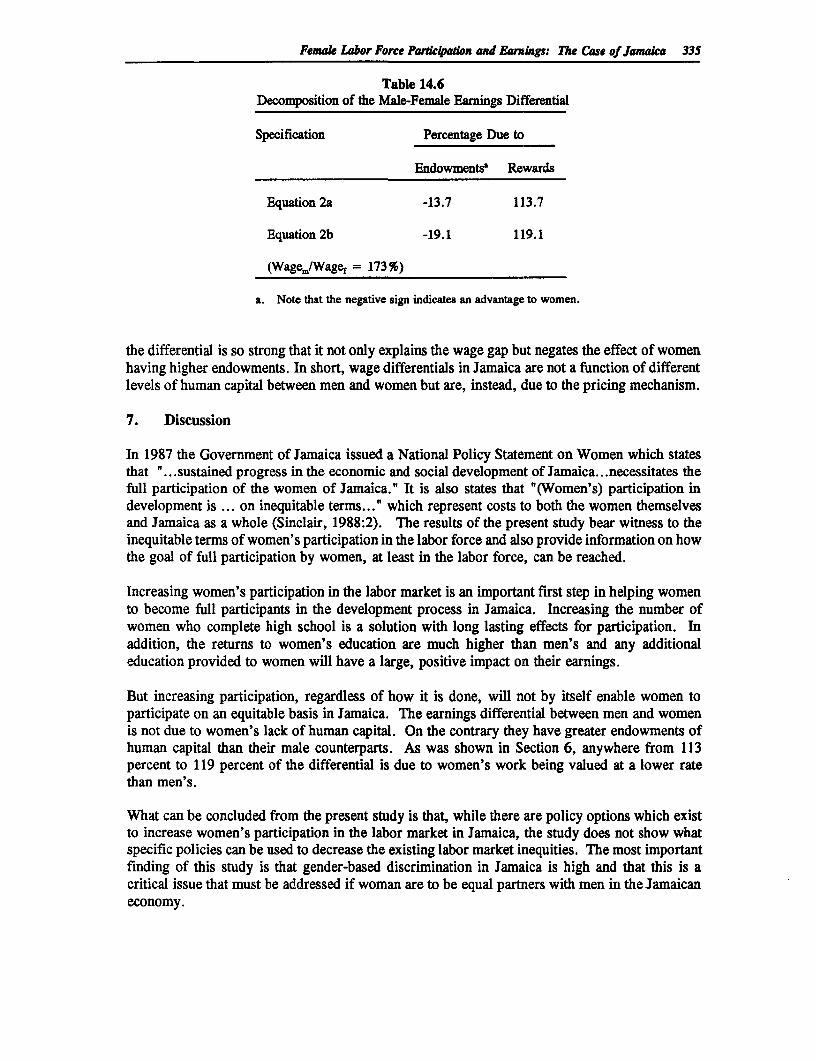
Femalk Labor Force Parci4paon and Earnuigs: The Case of Jamaia 335
Table 14.6Decomposition of the Male-Female Earnings Differential
Specification Percentage Due to
Endowments' Rewards
Equation 2a -13.7 113.7
Equation 2b -19.1 119.1
(Wage./Wagef = 173%)
a. Note that the negative sign indicates an advantage to women.
the differential is so strong that it not only explains the wage gap but negates the effect of womenhaving higher endowments. In short, wage differentials in Jamaica are not a function of differentlevels of human capital between men and women but are, instead, due to the pricing mechanism.
7. Discussion
In 1987 the Government of Jamaica issued a National Policy Statement on Women which statesthat "...sustained progress in the economic and social development of Jamaica...necessitates thefull participation of the women of Jamaica." It is also states that "(Women's) participation indevelopment is ... on inequitable terms..." which represent costs to both the women themselvesand Jamaica as a whole (Sinclair, 1988:2). The results of the present study bear witness to theinequitable terms of women's participation in the labor force and also provide information on howthe goal of full participation by women, at least in the labor force, can be reached.
Increasing women's participation in the labor market is an important first step in helping womento become full participants in the development process in Jamaica. Increasing the number ofwomen who complete high school is a solution with long lasting effects for participation. Inaddition, the returns to women's education are much higher than men's and any additionaleducation provided to women will have a large, positive impact on their earnings.
But increasing participation, regardless of how it is done, will not by itself enable women toparticipate on an equitable basis in Jamaica. The earnings differential between men and womenis not due to women's lack of human capital. On the contrary they have greater endowments ofhuman capital than their male counterparts. As was shown in Section 6, anywhere from 113percent to 119 percent of the differential is due to women's work being valued at a lower ratethan men's.
What can be concluded from the present study is that, while there are policy options which existto increase women's participation in the labor market in Jamaica, the study does not show whatspecific policies can be used to decrease the existing labor market inequities. The most importantfinding of this study is that gender-based discrimination in Jamaica is high and that this is acritical issue that must be addressed if woman are to be equal partners with men in the Jamaicaneconomy.
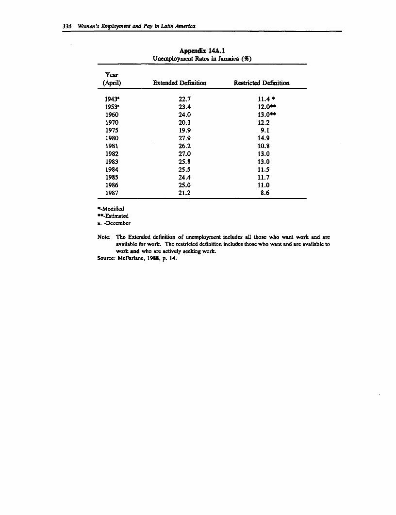
336 Women's Emplkyment and Pay in Lain America
Appendix 14A.1Unemployment Rates in Jamaica (%)
Year(April) Extended Definition Restricted Definition
1943' 22.7 11.4 *1953' 23.4 12.0**1960 24.0 13.0**1970 20.3 12.21975 19.9 9.11980 27.9 14.91981 26.2 10.81982 27.0 13.01983 25.8 13.01984 25.5 11.51985 24.4 11.71986 25.0 11.01987 21.2 8.6
*-Modified*-*-Estimateda. -Deccmber
Note: The Extended definition of unemployment includes all those who want work and areavailable for work. The restricted definition includes those who want and are available towork and who are actively seeking work.
Source: McFarlane, 1988, p. 14.
References
Anderson, P. "Levels of Poverty and Household Food Consumption in Jamaica in 1989." Paperpresented at the Workshop on Food and Nutrition Policies: Issues and Recommendationsfor the 1990s and Beyond. Jamaica: Jamaica and Caribbean Food and Nutrition Institute,1990.
Anker, R. and R.C. Knowles. "Female Labor Force Participation in Kenya" in G. Standing, andG. Sheehan (eds.). Labor Force Participation in Low-Income Countries. Geneva:International Labor Office, 1978.
Behrman, J. and B.L. Wolfe. "Labor Force Participation and Earnings Determinants for Womenin the Special Conditions of Developing Countries. " Journal of Development Economics,Vol. 15 (1984). pp. 259-288.
Doeringer, P. B. "Market Structure, Jobs and Productivity: Observations from Jamaica." ReportNo. DRD285. Washington, D.C.: World Bank, 1987.
Heckman, J. "Sample Selection Bias as a Specification Error." Econometrica, Vol. 47, no. 1(1979). pp. 153-161.
-==. "Shadow Prices, Market Wages, and Labor Supply." Econometrica, Vol. 42, no. 4 (1974).pp. 679-694.
International Labor Office. World Employment Review. Geneva: International Labor Office,1988.
-----."Employment and Economic Growth: Labor Force, Employment and Unemployment."Report No. II. Geneva: International Labor Office, 1982.
Klinov, R. "Costs and Returns to Liberalization: The Jamaican Case." Report No. DRD297.Washington, D.C.: World Bank, 1987.
Lisk, F. " An Action Programme for Jamaica, 1987/89, to Sustain the Incomes and LivingStandards of the Poor During Adjustment: Employment Policies and Programmes for theNon-Rural Poor." Port-of-Spain: International Labour Office, 1987.
McFarlane, C. "Measurement of Unemployment with Special Reference to the JamaicanExperience." Journal of the Statistical Institute of Jamaica, Vol. 1. (1988). pp. 43-59.
337
338 Women's Employment and Pay in Latin America
Oaxaca, R.L. "Male-female Wage Differentials in Urban Labor Markets." InternationalEconomic Review, Vol. 14, no. 1 (1973). pp. 693-709.
Powell, D. et al. "Women's Work, Social Support Resources and Infant Feeding Practices inJamaica". Mimeograph. Washington D.C.: International Center for Research on Women,1988.
Powell, D. "Female Labour Force Participation and Fertility: An Exploratory Study of JamaicanWomen." Social and Economic Studies, Vol. 25, no. 3 (1976). pp. 234-258.
Statistical Institute of Jamaica (STATIN). The Labour Force, October 1987. Kingston: StatisticalInstitute of Jamaica, 1989.
Statistical Institute of Jamaica. The Labour Force, April 1987. Kingston: Statistical Institute ofJamiaca, 1987.
Sinclair, P.A. "The Jamaican Situation." Vienna: United Nations Interregional Seminar onWomen and the Economic Crisis, 1988.
Tokeman, V.E. and A. Uphoff. " A Note of the Labour market in Jamaica, 1980-85." Kingston:PREALC, International Labor Office, 1986.
UNESCO. Jamaica: Development of Secondary Education. Paris: UNESCO, 1983.
Villarreal Gonda, R.I. "An Econometric Forecasting Model of Employment for Jamaica."Mimeograph. 1983.
World Bank. World Development Report, 1990. Washington, D.C.: World Bank, 1990.
World Bank. "Jamaica: A Survey of Female Headed Low Income Households." Washington,D.C.: Office of the Adviser on Women in Development, World Bank, 1985.
15
Women's Participation Decisions and Earnings inMexico
Diane Steele
1. Introduction
The purpose of this study is to examine the factors which influence women's decisions toparticipate in the labor force in Mexico. Using data from the 1984 Encuesta Nacional de Ingreso-Gasto de los Hogares, we focus on factors which have been shown in previous studies toinfluence the decision to enter the workforce such as age, education level, presence of youngchildren, marital status, and household wealth. The scope of the analysis is limited by the useof this survey since information on several key factors, including hours worked per week,participation in the public sector or the private sector, participation in the formal or informallabor market, and tenure on the job, is not available. Where possible, proxies for these variableshave been created using existing information.
Following a brief description of the Mexican labor market, we discuss, in Section 3, thecharacteristics of the sample used in this analysis. Section 4 examines factors influencingwomen's labor force participation. In Section 5 we derive earnings functions estimates forworking men and working women. Using the standard human capital model we also perform theanalyses controlling for selectivity bias in our sample of working women. Section 6 decomposesthe earnings differential and considers what proportion of this differential is attributable todiscrimination in the labor market.
2. The Mexican Economy
Mexico experienced high rates of economic growth between 1950 and 1974. Social welfare andgeneral standards of living improved substantially over these two decades. Welfare programsbrought about declines in infant mortality, malnutrition and morbidity, and the illiteracy rate fellfrom 40 percent in 1950 to 18 percent in 1980. Between 1960 and 1980, infant mortalitydeclined from 74 to about 50 deaths per 1,000 live births, and life expectancy at birth increasedalmost 10 years from 59 to 68 years.
The economy experienced a serious, albeit brief, financial crisis in 1976 which was terminatedby major oil discoveries in 1977. This prosperity, however, was short lived.
During the decades of economic growth, Mexico made great improvements in the quality of andaccess to public education. Primary education coverage increased from 17.6 percent to 79.8percent between 1950 and 1980. Nationwide, the number of schools tripled, the number of
339
340 Women 's Employment and Pay in Latin America
teachers quintupled, and school enrollment increased sevenfold. Since the crisis in 1982,provision of educational services has slowed.'
Since 1982, an economic crisis has existed in Mexico. The crisis, caused by rising interest ratesand falling oil prices, has caused severe hardships for the poor, and many of the gains of theprevious two decades have been threatened. Real wages have declined by 40 percent and socialsector spending has declined from 20 percent of total government expenditures in 1982 to around12 percent in 1991.
3. Data Characteristics
This analysis is based on data collected for the 1984 Encuesta Nacional de Ingreso-Gasto de losHogares. The survey data include 7,536 individuals in the third quarter of 1984. The datainclude information for all individuals aged 12 years and older.
In the survey, wage information was reported by quarter. In order to determine weekly wages,the quarterly wage was divided by 3 to give monthly wage, and the resulting monthly wage wasdivided by 4.3 to give weekly wages.
Although participation is commonly defined to include those currently employed and thoseseeking employment, these data do not permit the identification of job seekers. It was onlypossible to identify individuals as currently employed or not currently employed. In addition,income from wage information was not reported for all workers. The sample was limited torespondents between the ages of 15 and 65, and to workers reporting positive income. Thisresulted in a sample of 3,360 working men, 1,217 working women, and 450 non-workingwomen. Ninety-six percent of all men and 73 percent of all women in the sample were reportedto be working.
Because the survey variables were limited, it was necessary to construct variables for use in theanalyses. The amount of experience in the labor market was estimated as age minus years ofschooling minus six. This overestimates actual experience because it does not take into accountvoluntary or involuntary absences from the labor force. This is especially true for women whoare more likely to withdraw from the labor force for childrearing.
Most studies indicate that the presence in the household of young children influences the decisionto enter the labor market. The data did not, however, provide information on children agedunder 12 years. Consequently, we were only able to include a variable for children aged 12 to14 years.
Table 15.1 gives means and standard deviations of the sample variables by gender. Workingwomen are, on average, two and a half years younger than working men, but non-workingwomen are more than seven years older. Working women have one and a third years moreschooling than working men, and working men have almost two years more schooling than non-working women.
Women earn almost 86 percent of men's weekly wages. There is no information on the numberof hours worked, making it impossible to determine whether this difference is driven by numberof hours worked. The experience variable indicates that working women have almost four yearsless experience than men, but it should be remembered that this is a constructed variable.
I See Carlson and Prawda (1991).
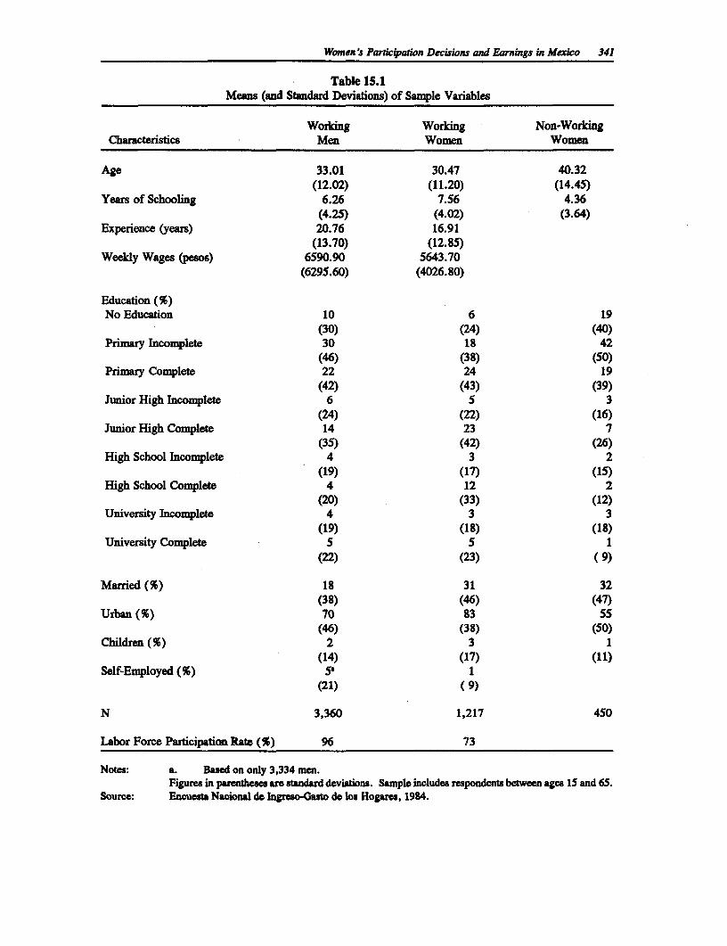
Women's Particiaton Decisions and Earnings in Mexico 341
Table 15.1Means (and Standard Deviations) of Sample Variables
Worling Working Non-WorkingCharacteristics Men Women Women
Age 33.01 30.47 40.32(12.02) (11.20) (14.45)
Years of Schooling 6.26 7.56 4.36(4.25) (4.02) (3.64)
Experience (years) 20.76 16.91(13.70) (12.85)
Weekly Wages (pesos) 6590.90 5643.70(6295.60) (4026.80)
Education (%)No Education 10 6 19
(30) (24) (40)Primary Incomplete 30 18 42
(46) (38) (50)Primary Complete 22 24 19
(42) (43) (39)Junior High Incomplete 6 5 3
(24) (22) (16)Junior High Complete 14 23 7
(35) (42) (26)High School Incomplete 4 3 2
(19) (17) (15)High School Complete 4 12 2
(20) (33) (12)University Incomplete 4 3 3
(19) (18) (18)University Complete 5 5 1
(22) (23) (9)
Married (%) 18 31 32(38) (46) (47)
Urban (%) 70 83 55(46) (38) (50)
Children (%) 2 3 1(14) (17) (11)
Self-Employed (%) 5 1(21) (9)
N 3,360 1,217 450
Labor Force Participation Rate (X) 96 73
Notes: a. Based on only 3,334 men.Figures in parenthes are sandard deviations. Sample includes respondents between ages 15 and 65.
Source: Encueta Nacional de Ingreso-Gasto dc los Hogares, 1984.
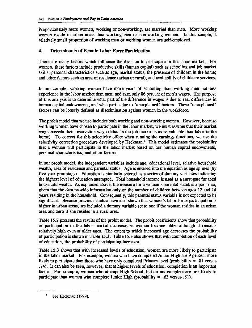
342 Women 's Emloyment and Pay in Latin America
Proportionately more women, working or non-working, are married than men. More workingwomen reside in urban areas than working men or non-working women. In this sample, arelatively small proportion of working men or working women are self-employed.
4. Determinants of Female Labor Force Participation
There are many factors which influence the decision to participate in the labor market. Forwomen, these factors include productive skills (human capital) such as schooling and job marketskills; personal characteristics such as age, marital status, the presence of children in the home;and other factors such as area of residence (urban or rural), and availability of childcare services.
In our sample, working women have more years of schooling than working men but lessexperience in the labor market than men, and earn only 86 percent of men's wages. The purposeof this analysis is to determine what part of the difference in wages is due to real differences inhuman capital endowments, and what part is due to "unexplained" factors. These 'unexplained'factors can be loosely defined as discrimination against women in the workforce.
The probit model that we use includes both working and non-working women. However, becauseworking women have chosen to participate in the labor market, we must assume that their marketwage exceeds their reservation wage Oabor in the job market is more valuable than labor in thehome). To correct for this selectivity effect when running the earnings functions, we use theselectivity correction procedure developed by Heckman.2 This model estimates the probabilitythat a woman will participate in the labor market based on her human capital endowments,personal characteristics, and other factors.
In our probit model, the independent variables include age, educational level, relative householdwealth, area of residence and parental status. Age is entered into the equation as age splines (byfive year groupings). Education is similarly entered as a series of dummy variables indicatingthe highest level of education attempted. Total household income is used as a surrogate for totalhousehold wealth. As explained above, the measure for a woman's parental status is a poor one,given that the data provide information only on the number of children between ages 12 and 14years residing in the household. Consequently, this parental status variable is not expected to besignificant. Because previous studies have also shown that women's labor force participation ishigher in urban areas, we included a dummy variable set to one if the woman resides in an urbanarea and zero if she resides in a rural area.
Table 15.2 presents the results of the probit model. The probit coefficients show that probabilityof participation in the labor market decreases as women become older although it remainsrelatively high even at older ages. The extent to which increased age decreases the probabilityof participation is shown in Table 15.3. Table 15.3 also shows that with completion of each levelof education, the probability of participating increases.
Table 15.3 shows that with increased levels of education, women are more likely to participatein the labor market. For example, women who have completed Junior High are 9 percent morelikely to participate than those who have only completed Primary level (probability = .81 versus.74). It can also be seen, however, that at higher levels of education, completion is an importantfactor. For example, women who attempt High School, but do not complete are less likely toparticipate than women who complete Junior High (probability = .62 versus .81).
2 See Heckman (1979).
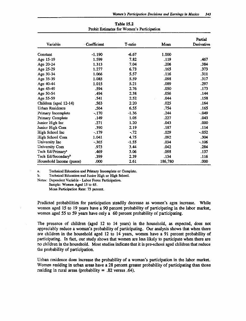
Women's Parlicipation Decisions and Earnings in Mexico 343
Table 15.2Probit Estimates for Women's Participation
PartialVariable Coefficient T-ratio Mean Derivative
Constant -1.190 -6.67 1.000Age 15-19 1.599 7.82 .119 .467Age 20-24 1.313 7.04 .206 .384Age 25-29 1.277 6.73 .165 .373Age 30-34 1.066 5.57 .116 .311Age 35-39 1.085 5.59 .098 .317Age 40-44 1.015 5.21 .089 .297Age 45-49 .594 2.76 .050 .173Age 50-54 .494 2.38 .056 .144Age 55-59 .541 2.52 .044 .158Children (aged 12-14) .563 2.20 .025 .164Urban Residence .564 6.55 .754 .165Primary Incomplete -.170 -1.36 .244 -.049Primary Complete .149 1.05 .227 .043Junior High Inc .271 1.20 .043 .000Junior High Com .390 2.19 .187 .114High School Inc -.179 -.72 .029 -.052High School Com 1.041 4.75 .092 .304University Inc -.365 -1.55 .034 -.106University Com .973 3.44 .042 .284Tech Ed/Primary' .469 3.06 .098 .137Tech Ed/Secondaryb .399 2.39 .134 .116Household Income (pesos) .000 2.61 186,780 .000
a. Technical Education and Primary Incomplete or Complete.b. Technical Education and Junior High or High School.Notes: Dependent Variable - Labor Force Participation.
Sample: Women Aged 15 to 65.Mean Participation Rate: 73 percent.
Predicted probabilities for participation steadily decrease as women's ages increase. Whilewomen aged 15 to 19 years have a 90 percent probability of participating in the labor market,women aged 55 to 59 years have only a 60 percent probability of participating.
The presence of children (aged 12 to 14 years) in the household, as expected, does notappreciably reduce a woman's probability of participating. Our analysis shows that when thereare children in the household aged 12 to 14 years, women have a 91 percent probability ofparticipating. In fact, our study shows that women are less likely to participate when there areno children in the household. Most studies indicate that it is pre-school aged children that reducethe probability of participation.
Urban residence does increase the probability of a woman's participation in the labor market.Women residing in urban areas have a 28 percent greater probability of participating than thoseresiding in rural areas (probability = .82 versus .64).
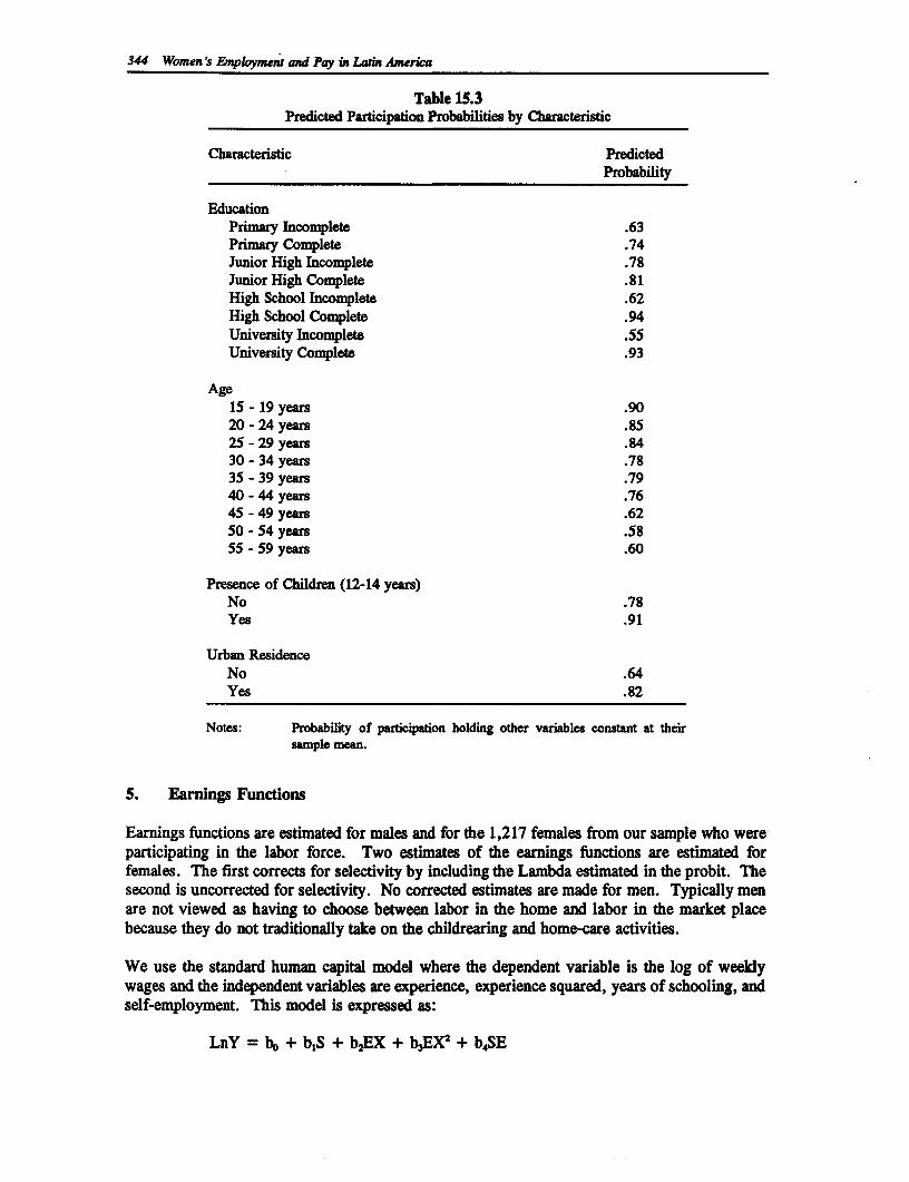
344 Women 's Employment and Pay in Latn America
Table 15.3Predicted Participation Probabilities by Characteristic
Characteristic PredictedProbability
EducationPrimry Incomplete .63Primary Complete .74Junior High Incomplete .78Junior High Complete .81High School Incomplete .62High School Complete .94University Incomplete .55University Complete .93
Age15 - 19 years .9020 - 24 years .8525 - 29 years .8430 - 34 years .7835 - 39 years .7940 - 44 years .7645 - 49 years .6250 - 54 years .5855 - 59 years .60
Presence of Children (12-14 years)No .78yes .91
Urban ResidenceNo .64Yes .82
Notes: Probability of participation holding other variables constant at theirsample mean.
5. Earnings Functions
Earnings functions are estimated for males and for the 1,217 females from our sample who wereparticipating in the labor force. Two estimates of the earmings functions are estimated forfemales. The first corrects for selectivity by including the Lambda estimated in the probit. Thesecond is uncorrected for selectivity. No corrected estimates are made for men. Typically menare not viewed as having to choose between labor in the home and labor in the market placebecause they do not traditionally take on the childrearing and home-care activities.
We use the standard human capital model where the dependent variable is the log of weeldywages and the independent variables are experience, experience squared, years of schooling, andself-employment. This model is expressed as:
LnY = bo + b,S + b2EX + b3EX2 + b4SE
Women 's Partcipaion Decisions and Earnings in Mexico 345
where:
LnY = the natural log of weekly wages,EX = experience (potential: defined as age-years of school-6),EX2 = experience squared,S = years of schooling, andSE = self-employed (one if self-employed).
A serious shortcoming in the estimation was the lack of information on the hours worked by eachworker. Lacking this information, we were forced to assume that all workers supplied the sameamount of labor. This assumption is clearly invalid, given existing knowledge about women'stypical work patterns, but there was no way to derive estimates from the existing data.3 A broadsurrogate for sector of employment, paid or self-employment, is also included as an independentvariable, but because so few of the survey respondents are self-employed, the results from thisvariable should be interpreted with caution. The survey did provide information on therespondents' occupation. However, when dummy variables indicating which occupational sectorthe respondent belonged to were added to the equation, they provided no additional information.
The results of these earnings functions are shown in Table 15.4. The first column presentsresults for the male sample. The rate of return to schooling for males is estimated to be 13percent. Log earnings increase with experience but, as expected in a normal age-earnings profile,they decrease with age. The broad occupational sector variable, self-employment, is highlysignificant and negative indicating that earnings are lower among the self-employed.
The correction for selectivity in the female earnings functions is shown to be important. Theequation which corrects for selectivity shows the rate of return to schooling to be close to 11percent, substantially below the 15 percent estimated in the uncorrected equation. Lambda itselfis significant and negative. Similarly, the experience variable in the corrected equation is belowthat in the uncorrected equation. In both cases the self-employment variable is significant andnegative showing that earnings are lower among the self-employed.
6. Discrimination
Working women in this survey earn 86 percent of male weekly wages. Using the Oaxaca methodwe are able to decompose this earnings differential into a component attributable to differencesin human capital endowments, and a component which is largely attributable to wagediscrimination. The difference between the mean Oog) wage rates of males and females in theOaxaca decomposition method is expressed as:
BmXm - BfXf = XI(bm7bf) + bm(X7Xf) (la)= X.(b.7bf) + bf(Xm-Xf) (lb)
There is always an index number problem experienced here. Theoretically, there is no advantageto estimating the results using male means or female means, so we present both. The first termin both equations is the part of the log earnings differential that can be ascribed to differences inthe wage structures between the sexes and the second term is that part of the log earningsdifferential that can be ascribed to differences in human capital endowments.
3 See Gronau (1988), pp 277-301. See also Ng, Scott, and Velez and Winter in this volume.
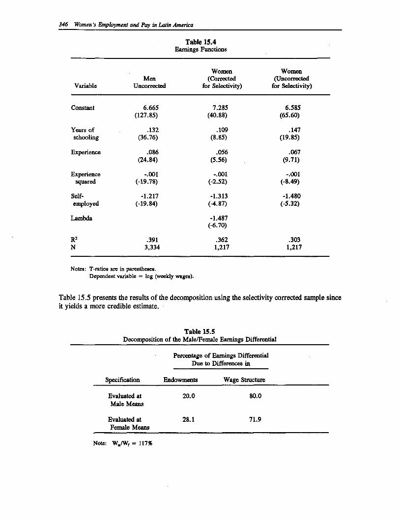
346 Women's Employment and Pay in Latin America
Table 15.4Earnings Functions
Women WomenMen (Corrected (Uncorrfected
Variable Uncorrected for Selectivity) for Selectivity)
Constant 6.665 7.285 6.585(127.85) (40.88) (65.60)
Years of .132 .109 .147schooling (36.76) (8.85) (19.85)
Experience .086 .056 .067(24.84) (5.56) (9.71)
Experience -.001 -.001 -.001squared (-19.78) (-2.52) (-8.49)
Self- -1.217 -1.313 -1.480employed (-19.84) (-4.87) (-5.32)
Lambda -1.487(-6.70)
R2 .391 .362 .303N 3,334 1,217 1,217
Notes: T-ratios are in parentheses.Dependent varable = log (weekly wages).
Table 15.5 presents the results of the decomposition using the selectivity corrected sample sinceit yields a more credible estimate.
Table 15.5Decomposition of the Male/Female Eamings Differential
Percentage of Earnings DifferentialDue to Differences in
Specification Endowments Wage Structure
Evaluated at 20.0 80.0Male Means
Evaluated at 28.1 71.9Female Means
Note: W,.,/Wf = 117%
Women's Parikpation Decisions and Earnings in Mexico 347
Using the equation evaluated at the male means we see that only 20 percent of the differential isdue to differences in human capital endowments, and 80 percent is due to unobservable factors.The equation evaluated at the female means shows that approximately 28 percent of thedifferential is due to differences in human capital endowments and 72 percent due to differencesin the way men and women are rewarded in the labor market.
7. Discussion
As has been shown, women's participation rates are positively influenced by the amount ofeducation. Urban residence has a positive effect on participation, and the presence of teenagedchildren in the household does not appear to influence women's decision to work.
A wage differential of 14 percent is low in comparison with other Latin American countries, andwith some industrialized countries.4 This may be explained in part by our inability to identifyseveral of the important factors in the decision making process, such as hours worked, publicversus private sector and formal versus informal sector.
The small differential may also be due to several factors that we can identify in the existing data.Working women have, on average, one and a third more years of schooling than working men.Working women are also more likely to complete higher levels of education than working men.Twenty-eight percent of the working women attempted Junior High with 23 percent completing,compared to only 20 percent of working men who attempted Junior High with 14 percentcompleting. Similarly, 15 percent of working women attempted High School with 12 percentcompleting, compared to 8 percent of working men who attempted with 4 percent completing.
Despite the low earnings differential between men and women, this study has shown that onlya small proportion of the differential can be explained by differences in human capitalendowments. The "upper bound" estimate of discrimination is 72 or 80 percent, depending onthe equation used. Given the nature of the survey data used in these analyses, males may havehad endowments which were superior to women's but of which we are not aware. If this is thecase, the lack of information will bias the estimate of the component due to wage discriminationupwards.
Clearly, further research into the factors influencing women's participation decisions needs to bedone. Further research should include those human capital factors that were missing or had tobe estimated in this study. Especially important are hours worked per week and tenure in the jobmarket.
4 In Britain, women earn 74 percent of men's wages. Khandker reports women's wages as beingabout two-thirds of men's in Peru while Chu Ng found women's wages in Argentina to be 65 percent ofmen's (both in this volume). See also Gunderson (1989), Tzannatos (1987), Zabalza and Tzannatos (1985),and Gregory and Duncan (1982).
References
Carlson, S. and J. Prawda. Basic Education in Mexico: Trends, Issues and PolicyRecommendations. Washington, D.C.: World Bank, June 1991.
Gregory, R.G. and R.C. Duncan. "Segmented Labour Market Theories and the AustralianExperience of Equal Pay for Women." Journal of Post-Keynesian Economics. Vol.3(1982). pp. 403-428.
Gronau, R. "Sex-Related Wage Differentials and Women's Interrupted Labor Careers: TheChicken and Egg Question." Journal of Labor Economics. Vol. 6, no. 1 (1988). pp 277-301.
Gunderson, M. "Male-Female Wage Differentials and Policy Responses." Journal of EconomicLiterature. Vol. 21, no.1 (1989). pp 46-72.
Heckman, J. "Sample Selection Bias as a Specification Error." Econometrica. Vol. 47, no. 1(1979). pp. 153-161.
Tzannatos, Z. "Equal Pay in Greece and Britain." Industrial Relations Journal. Vol. 18, no.4 (1987). pp. 275-283.
World Bank. Mexico, Selected Policy Papers. Washington, D.C.: World Bank, June 20, 1989.
World Bank. Staff Appraisal Report, Mexico, Water, Women and Development Project.Washington, D.C.: World Bank, May 24, 1989.
Zabalza, A. and Z. Tzannatos. Women and Equal Pay: The Effects of Legislation on FemaleEmployment and Wages in Britain. Cambridge: Cambridge University Press, 1985.
348
16
Female Labor Force Participation and Wages:A Case Study of Panama
Mary Arends
1. Introduction
This chapter examines the differential in earnings between males and females in Panama. In thesample, female wages are 85 percent of male wages, a very high percentage for Latin America.What are the reasons for this high percentage? How does Panama's low participation rate forwomen affect female earnings? The country is also interesting because of its extensive LaborCode, which has many sections pertaining specifically to women. Because of long standingstructural problems in the labor market, Panama has a high unemployment rate, especially forwomen.
n Section 2, the economic and labor market situation in Panama are discussed. Section 3pertains to the data and includes descriptive statistics. Section 4 presents the results of aunivariate probit model for both men and women that attempts to determine which characteristicsmake an individual likely to be observed in the work force. The results of the probit are usedto correct for selectivity in earnings regressions. Section 5 discusses the results of earningsregressions for men and women, both correcting for selectivity and without correcting forselectivity. A decomposition of the earnings differential is calculated to estimate how much ofthe differential is due to differences in endowments and how much could be attributed to labormarket discrimination. Lastly, there is a discussion of the policy implications of the findings.
2. The Panamanian Economy and Labor Market
The population growth rate was 2.2 percent from 1980 to 1989, which is average for LatinAmerica as a whole. Thirty-five percent of the population was aged from 0 to 14 years in 1989,while 60 percent of the population was aged from 15 to 64 years, about average for LatinAmerica. The labor force growth rate was 2.9 percent in the 1980s, averaging 3.3 percent forwomen.'
Panama had a GNP of $1,760 per capita in 1989. Growth was high from 1965 to 1980 at 5.5percent, but the economic problems of Latin America in the 1980s affected Panama also, and
Economist Intelligence Unit (1991), p.SS.
349
350 Women's Employment and Pay in Latin America
growth was only .5 percent from 1980 to 1989. The economy was very heavily oriented towardsservices, which accounted for 74 percent of GDP in 1989, while industry accounted for 15percent and agriculture for 11 percent.2 Recent political problems strongly impacted theeconomy. In 1988, United States' sanctions and massive capital flight led to 16 percentcontraction of GDP. In 1989, the economy did not recover and GDP fell again by .9 percent.3
However, the most chronic problem in Panama is persistent unemployment. A 1985 World Bankcountry study stated that unemployment was, without a doubt, the gravest economic and socialproblem.4 In the study, the 1983 unemployment rate was estimated at 9.5 percent. The situationsteadily worsened during the 1980s. Unemployment estimates for 1989 ranged from 16.0 percentto 20.1 percent.5 In the sample used in this study, the male and female unemployment rateswere 14 percent and 22 percent, respectively.
To confront Panama's unemployment problem, one strategy was to increase the public sector.The Torrijos regime, which governed from 1969 to 1981, used this strategy throughout its tenure,and enacted the Emergency Employment Program in 1977. When the Emergency Program endedin 1980, 25 percent of workers were in the public sector.6 Because of budget constraints, thepublic sector could not continue to provide employment, and the percentage of workers in thepublic sector steadily declined throughout the 1980s. However, the percentage of workers in thepublic sector remained high at 21.9 percent in 1989.7
The participation rate declined from over 60 percent in early 1970s to just over 50 percent in1982 and 1983. This happened because of greatly increased enrollment in secondary and tertiaryeducation, a reduction in the voluntary retirement age from 62 to 55, and a falling femaleparticipation rate.' However, according to one official source, female participation rates roseduring the 1980s from 17.8 percent in 1980 to 20.8 percent in 1989.9 The total labor forceparticipation rate was estimated at 58 percent in 1989.10
An important contributing factor to unemployment was Panama's labor code. Instituted in 1972,it substantially increased the cost of hiring labor for employers. Workers were given more jobsecurity, benefits, and bargaining power. It required employers to pay high severance pay whichincreases with the length of service, discouraging temporary hires. The total burden on
2 World Bank (1991), Tables 1 and 3.
3 Economist Intelligence Unit (1991), p. 54.
4 World Bank (1985), p.9 .
S The estimates come from the Economist Intelligence Unit and the World Bank Panama OperationsDesk respectively.
6 World Bank (1985), p. 19.
7 World Bank, Latin America and the Caribbean, Country Department II, unpublished table, (1991).
s World Bank (1985), p. 11.
9 World Bank (1990), p. 238-239.
10 The Economist Country Profile, 1991-92.
Female Labor Force Pardcyaton and Wages: A Case Stu of Panama 351
employers including a thirteen-month bonus and paid vacations was estimated by the World Bankto be 40 percent.1" Employers could not reduce a worker's salary, so piecework could not bepaid on the basis of productivity. As a result of these regulations, Panama's labor costs wereamong the highest in the Caribbean Basin. The World Bank recommended changes in 1985 asconditions for a structural adjustment loan. The reforms were finally accepted in March 1986,despite a ten-day work stoppage by the unions and fierce political opposition. The modificationspermitted piecework, encouraged rewards for productivity, and rationalized overtime provisionsfor some firms."2 Whether these changes have had a great impact remains to be seen.
Many aspects of Panamanian law apply directly to women in the labor force. There areprovisions in Panama's Constitution (Article 62) and in the Labor Code (Section 10) thatemployers must provide equal pay for equal work. Legal redress is available, but the burden ofproof is on the employee. No real attempt has been made in Panama to address the issue throughthe courts. Low female labor force participation rates and women's willingness to be self-employed are two explanations why this is so.13
There are provisions in the Labor Code which may add to the female unemployment problem.Employers are required to provide 14 weeks of maternity leave, with the employer making upthe difference between regular pay and social security payments. It is unlawful to dismiss awoman during pregnancy and five months thereafter without judicial approval. New mothers areentitled to a paid hour break each day in order to breast feed their babies. If a company employsover 20 females, it is required to provide a nursery. Also, the Code forbids women fromworking in dangerous occupations, such as mines and civil construction. In a Labor Codesurvey, Spinanger interviewed employers in various sectors of the economy. Two-thirds said thatmaternity protection laws discouraged them from hiring women. Employers were willing toincrease wages by 25 percent to have more flexible maternity arrangements.14 Such laws mayencourage employers to discriminate against all women, including those who have no intentionto have a child or older women who do not plan to have more children.
Another characteristic of Panama's labor market is regional disparity in earnings. Heckman andHotz (1986) found evidence that the Panamanian labor market was segmented by regions, withless developed regions showing higher rates of return to education than developed regions. Ruralregions such as Darien, Veraguas, and Cocle had high rates of return, while the Canal Zone andPanama City showed rates of return comparable to the United States.15 Also, in the CanalZone, wages are about three times higher than in the rest of the country.1" Only 2.6 percentof workers are employed in the Canal Zone, but their salaries, which are raised in real terms inaccordance with United States cost of living changes, may have prevented other wages in the
" World Bank (1985), p. 17.
12 Tollefson (1989), p. 135.
13 Spinanger (1984), p. 21.
14 Spinanger (1984), p. 29.
15 Heckman and Hotz (1986), p. 540.
16 Because of the Panama Canal treaty, former Canal Zone employees who became employees inPanama were guaranteed wages and conditions similar to those their position had commanded whenemployed by the U.S. (see Tollefson, p. 142).
352 Women's Enployment and Pay un Latin America
Canal areas of Colon and Panama from falling, which would help solve the unemploymentproblem.'7
Panama has a long-standing, strong commitment to education. Adult illiteracy was 12 percentin 1989. Schooling is compulsory for 9 years, and begins at age 5. Enrollments were higherthan average for Latin America, given Panama's per capita income. Primary school enrollmentsas a percentage of the relevant age group were 102 percent in 1965 and 106 percent in 1988.Secondary school enrollments were 34 percent in 1965 and 59 percent in 1988, compared to anaverage in Latin America of 48 percent in 1988. Twenty-eight percent of the relevant age groupwas enrolled in tertiary education in that year, a percentage that was only surpassed by threeLatin American countries, all with higher per capita income-Argentina, Venezuela, andUruguay.18
3. Data Characteristics
The data for this study were taken from the Encuesta de Hogares-Mano de Obra of August 1989,by the Office of Statistics and Census of Panama (DEC). The survey consisted of 8,817households, comprised of 38,416 individuals. Out of this sample, the individuals of economicallyactive age (ages 15 to 65) were selected, giving a sample of 23,196 individuals. The surveycovered both urban and rural households, and the data were weighted to give an accuraterepresentation of the population.
One limitation of the data was that about 30 percent of employed males had no hours and/or noincome reported. Over 90 percent of the males that were recorded as "employed" but had nohours or no income were either family workers or self-employed workers in agriculture. Table16.1 summarizes the problem. Labor force participation includes employed and unemployedworkers. Work force participation includes only those who were recorded as "employed" in thesurvey. The third column labelled "+Hours, +Income" consists only of workers who reportedpositive hours and positive income. The table breaks down these rates by province. Overall, awage rate could be calculated for only 71 percent of the male workers. The problem is severestfor the rural provinces of Darien and Bocas del Toro. Because of the low percentages of maleworkers with positive hours and positive income, there is a selectivity problem when examiningthe male wage functions. The males for whom hours and income are available are a specialsubset of the male workers. Therefore, in Section 4, the results of separate probit equations forboth the males and females are presented.
For females, most rural women were classified as "housewives" and therefore inactive. It islikely that many of them are actually unremunerated family workers. Unfortunately, there is noway to determine the kind of work these women do.
In Table 16.2, the means of the sample variables for the working and non-working samples ofmales and females are shown. For the table and the subsequent regressions, working was definedas having positive hours and positive income. About 50 percent of the men and 30 percent ofthe women in the sample of individuals aged 15 to 65 were classified as working. Schooling wascalculated by taking the number of years completed at the highest level and adding the numberof years required to finish preceding levels. Because it was not known if the individual
17 World Bank (1985), p. 19.
1 World Bank, (1990), pp. 238-239, and World Bank (1991), Table 29.
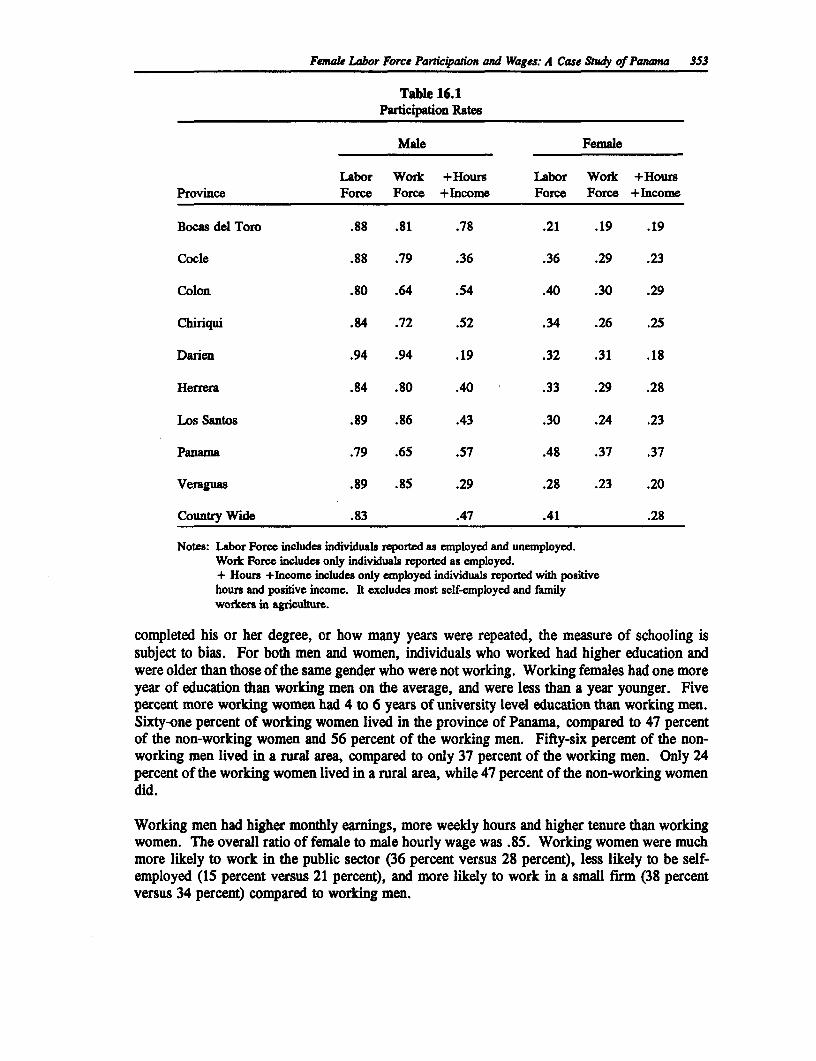
Female Labor Force Particaopatn and Wages: A Case Study of Panana 353
Table 16.1Participation Rates
Male Female
Labor Work +Hours Labor Work +HoursProvince Force Force + income Force Force +Income
Bocas del Toro .88 .81 .78 .21 .19 .19
Cocle .88 .79 .36 .36 .29 .23
Colon .80 .64 .54 .40 .30 .29
Chiriqui .84 .72 .52 .34 .26 .25
Darien .94 .94 .19 .32 .31 .18
Herrera .84 .80 .40 .33 .29 .28
Los Santos .89 .86 .43 .30 .24 .23
Panama .79 .65 .57 .48 .37 .37
Veraguas .89 .85 .29 .28 .23 .20
Country Wide .83 .47 .41 .28
Notes: Labor Force includes individuals reported as employed and unemployed.Work Force includes only individuals reported as employed.+ Hours +Income includes only employed individuals reported with positivehours and positive income. It excludes most self-employed and familyworkers in agriculture.
completed his or her degree, or how many years were repeated, the measure of schooling issubject to bias. For both men and women, individuals who worked had higher education andwere older than those of the same gender who were not working. Working females had one moreyear of education than working men on the average, and were less than a year younger. Fivepercent more working women had 4 to 6 years of university level education than working men.Sixty-one percent of working women lived in the province of Panama, compared to 47 percentof the non-working women and 56 percent of the working men. Fifty-six percent of the non-working men lived in a rural area, compared to only 37 percent of the working men. Only 24percent of the working women lived in a rural area, while 47 percent of the non-working womendid.
Working men had higher monthly earnings, more weekly hours and higher tenure than workingwomen. The overall ratio of female to male hourly wage was .85. Working women were muchmore likely to work in the public sector (36 percent versus 28 percent), less likely to be self-employed (15 percent versus 21 percent), and more likely to work in a small firm (38 percentversus 34 percent) compared to working men.
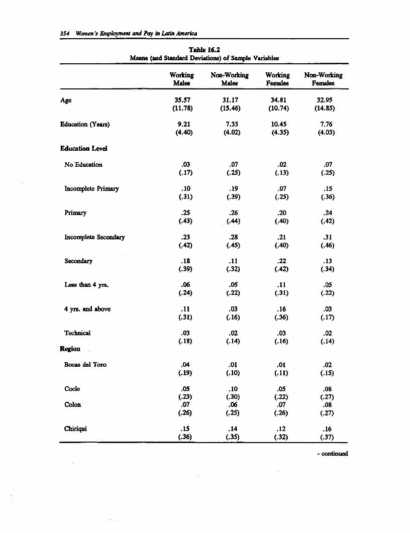
354 Women's Enployntent and Pay in Lain America
Table 16.2Means (and Standard Deviations) of Sample Variables
Worldng Non-Working Working Non-WorkingMales Males Females Females
Age 35.57 31.17 34.81 32.95(11.78) (15.46) (10.74) (14.85)
Education (Years) 9.21 7.33 10.45 7.76(4.40) (4.02) (4.35) (4.03)
Education Level
No Education .03 .07 .02 .07(.17) (.25) (.13) (.25)
Incomplete Primay .10 .19 .07 .15(.31) (.39) (.25) (.36)
Primary .25 .26 .20 .24(.43) (.44) (.40) (.42)
Incomplete Secondary .23 .28 .21 .31(.42) (.45) (.40) (.46)
Secondary .18 .11 .22 .13(.39) (.32) (.42) (.34)
Lessthan 4 yrs. .06 .05 .11 .05(.24) (.22) (.31) (.22)
4 yrs. and above .11 .03 .16 .03(.31) (.16) (.36) (.17)
Technical .03 .02 .03 .02(.18) (.14) (.16) (.14)
Region
Bocas del Toro .04 .01 .01 .02(.19) (.10) (.11) (.15)
Cocle .05 .10 .05 .08(.23) (.30) (.22) (.27)
Colon .07 .06 .07 .08(.26) (.25) (.26) (.27)
Chiriqui .15 .14 .12 .16(.36) (.35) (.32) (.37)
- continued
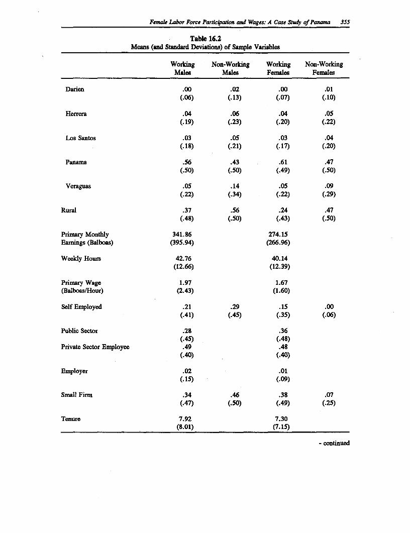
Female Labor Force Particpatwion and Wages: A Case Study of Panama 355
Table 16.2Means (and Standard Deviations) of Sample Variables
Working Non-Working Worling Non-WorkingMales Males Females Females
Darien .00 .02 .00 .01(.06) (.13) (.07) (.10)
Herrera .04 .06 .04 .05(.19) (.23) (.20) (.22)
Los Santos .03 .05 .03 .04(.18) (.21) (.17) (.20)
Panama .56 .43 .61 .47(.50) (.50) (.49) (.50)
Veraguas .05 .14 .05 .09(.22) (.34) (.22) (.29)
Rumal .37 .56 .24 .47(.48) (.50) (.43) (.50)
Primary Monthly 341.86 274.15Earnings (Balboas) (395.94) (266.96)
Weekly Hours 42.76 40.14(12.66) (12.39)
Primary Wage 1.97 1.67(Balboas/Hour) (2.43) (1.60)
Self Employed .21 .29 .15 .00(.41) (.45) (.35) (.06)
Public Sector .28 .36(.45) (.48)
Private Sector Employee .49 .48(.40) (.40)
Employer .02 .01(.15) (.09)
Small Firm .34 .46 .38 .07(.47) (.50) (.49) (.25)
Tenure 7.92 7.30(8.01) (7.15)
- continued
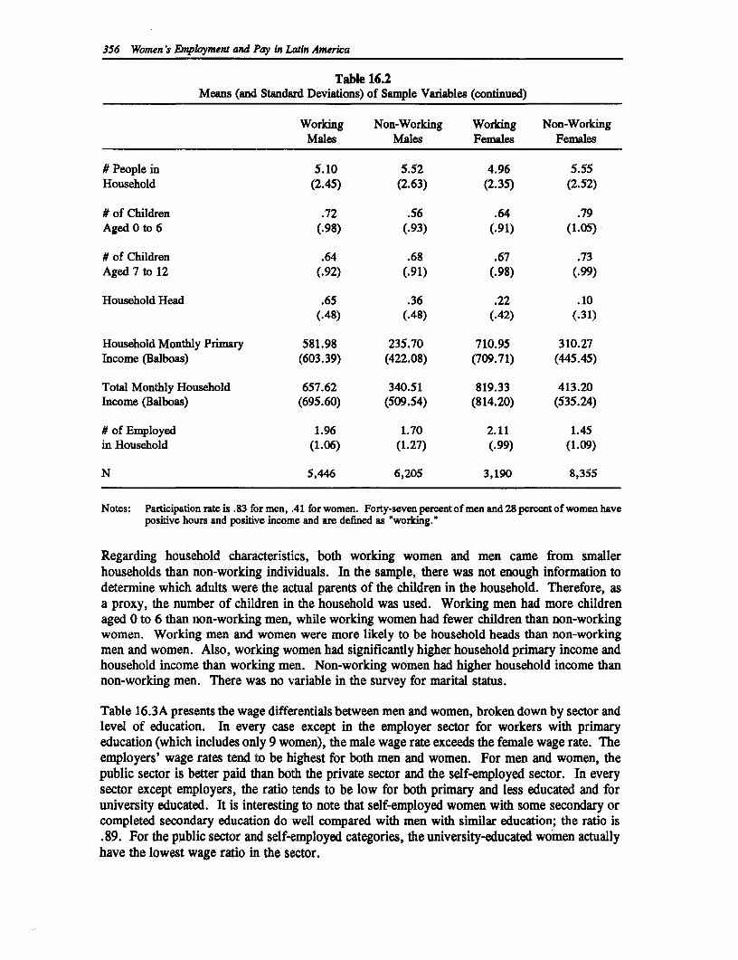
356 Women's Employment and Pay in Latin America
Table 16.2Means (and Standard Deviations) of Sample Variables (continued)
Working Non-Working Working Non-WorkingMales Males Females Females
# People in 5.10 5.52 4.96 5.55Household (2.45) (2.63) (2.35) (2.52)
# of Children .72 .56 .64 .79Aged 0 to 6 (.98) (.93) (.91) (1.05)
# of Children .64 .68 .67 .73Aged 7 to 12 (.92) (.91) (.98) (.99)
Household Head .65 .36 .22 .10(.48) (.48) (.42) (.31)
Household Monthly Primary 581.98 235.70 710.95 310.27Income (Balboas) (603.39) (422.08) (709.71) (445.45)
Total Monthly Household 657.62 340.51 819.33 413.20Income (Balboas) (695.60) (509.54) (814.20) (535.24)
# of Employed 1.96 1.70 2.11 1.45in Household (1.06) (1.27) (.99) (1.09)
N 5,446 6,205 3,190 8,355
Notes: Participation rate is .83 for men, .41 for women. Forty-seven percent of men and 28 percent of women havepositive hours and positive income and are defined as "working."
Regarding household characteristics, both working women and men came from smallerhouseholds than non-working individuals. In the sample, there was not enough information todetermine which adults were the actual parents of the children in the household. Therefore, asa proxy, the number of children in the household was used. Working men had more childrenaged 0 to 6 than non-working men, while working women had fewer children than non-workingwomen. Working men and women were more likely to be household heads than non-workingmen and women. Also, working women had significantly higher household primary income andhousehold income than working men. Non-working women had higher household income thannon-working men. There was no variable in the survey for marital status.
Table 16.3A presents the wage differentials between men and women, broken down by sector andlevel of education. In every case except in the employer sector for workers with primaryeducation (which includes only 9 women), the male wage rate exceeds the female wage rate. Theemployers' wage rates tend to be highest for both men and women. For men and women, thepublic sector is better paid than both the private sector and the self-employed sector. In everysector except employers, the ratio tends to be low for both primary and less educated and foruniversity educated. It is interesting to note that self-employed women with some secondary orcompleted secondary education do well compared with men with similar education; the ratio is.89. For the ppablic sector and self-employed categories, the university-educated women actuallyhave the lowest wage ratio in the sector.
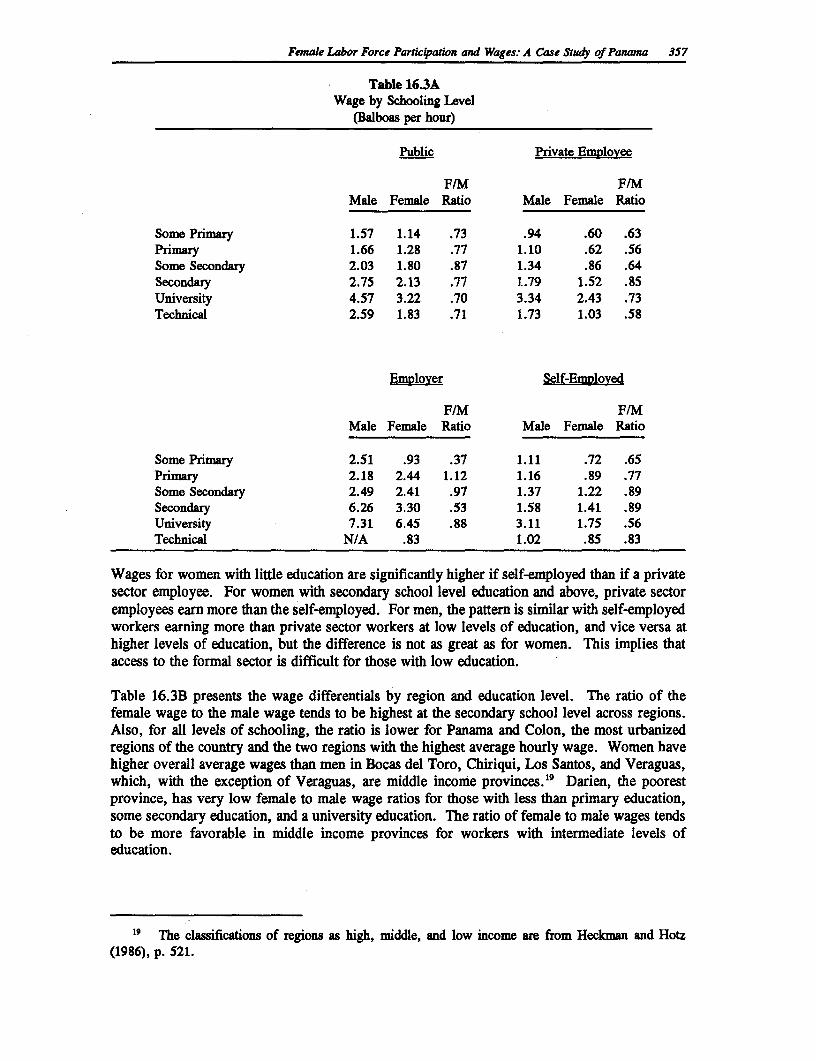
Femak Labor Force Paricipation and Wages: A Case Study of Panama 357
Table 16.3AWage by Schooling Level
(Balboas per hour)
Public Private Employee
F/M F/MMale Female Ratio Male Female Ratio
Some Primary 1.57 1.14 .73 .94 .60 .63Primary 1.66 1.28 .77 1.10 .62 .56Some Secondary 2.03 1.80 .87 1.34 .86 .64Secondary 2.75 2.13 .77 1.79 1.52 .85University 4.57 3.22 .70 3.34 2.43 .73Technical 2.59 1.83 .71 1.73 1.03 .58
Emplover Self-Employed
F/M F/MMale Female Ratio Male Female Ratio
Some Primary 2.51 .93 .37 1.11 .72 .65Primary 2.18 2.44 1.12 1.16 .89 .77Some Secondary 2.49 2.41 .97 1.37 1.22 .89Secondary 6.26 3.30 .53 1.58 1.41 .89University 7.31 6.45 .88 3.11 1.75 .56Technical N/A .83 1.02 .85 .83
Wages for women with little education are significantly higher if self-employed than if a privatesector employee. For women with secondary school level education and above, private sectoremployees earn more than the self-employed. For men, the pattern is similar with self-employedworkers earning more than private sector workers at low levels of education, and vice versa athigher levels of education, but the difference is not as great as for women. This implies thataccess to the formal sector is difficult for those with low education.
Table 16.3B presents the wage differentials by region and education level. The ratio of thefemale wage to the male wage tends to be highest at the secondary school level across regions.Also, for all levels of schooling, the ratio is lower for Panama and Colon, the most urbanizedregions of the country and the two regions with the highest average hourly wage. Women havehigher overall average wages than men in Bocas del Toro, Chiriqui, Los Santos, and Veraguas,which, with the exception of Veraguas, are middle income provinces."9 Darien, the poorestprovince, has very low female to male wage ratios for those with less than primary education,some secondary education, and a university education. The ratio of female to male wages tendsto be more favorable in middle income provinces for workers with intermediate levels ofeducation.
19 The classifications of regions as high, middle, and low income are from Heckman and Hotz(1986), p. 521.
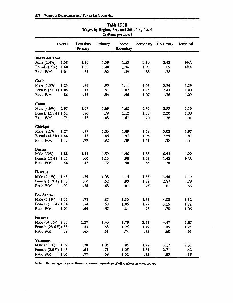
358 Women's Emnployment and Pay in Latin America
Table 16.3BWages by Region, Sex, and Schooling Level
(Balboas per hour)
Overall Less than Primary Some Secondary University TechnicalPrimary Secondary
Bocas del ToroMale (2.4%) 1.58 1.30 1.53 1.53 2.19 2.43 N/AFemale (.5%) 1.60 1.08 1.40 1.36 1.93 1.89 N/ARatio F/M 1.01 .83 .92 .89 .88 .78
CocleMale (3.3%) 1.23 .86 .95 1.11 1.63 3.24 1.29Female (2.0%) 1.06 .48 .51 1.07 1.75 2.47 1.40Ratio F/M .86 .56 .54 .96 1.07 .76 1.09
ColonMale (4.6%) 2.07 1.07 1.65 1.68 2.69 2.82 1.19Female (2.8%) 1.52 .56 .79 1.12 1.88 2.20 1.08Ratio F/M .73 .52 .48 .67 .70 .78 .91
ChiriquiMale (9.1%) 1.27 .97 1.05 1.09 1.38 3.03 1.97Female (4.6%) 1.44 .77 .86 .97 1.96 2.59 .87Ratio F/M 1.13 .79 .82 .89 1.42 .85 .44
DarienMale (.3%) 1.88 1.43 1.59 1.96 1.86 5.54 1.22Female (.2%) 1.21 .60 1.15 .98 1.59 1.45 N/ARatio F/M .64 .42 .72 .50 .85 .26
HerreraMale (2.4%) 1.43 .79 1.08 1.15 1.83 3.54 1.19Female (1.7 %) 1.33 .60 .52 .93 1.73 2.87 .79Ratio FIM .93 .76 .48 .81 .95 .81 .66
Los SantosMale (2.1%) 1.26 .78 .87 1.30 1.86 4.03 1.62Female (1.1%) 1.34 .54 .58 1.05 1.79 3.16 1.72Ratio F/M 1.06 .69 .67 .81 .96 .78 1.06
PanamaMale (34.3%) 2.35 1.27 1.40 1.70 2.38 4.47 1.87Female (23.6%)1.83 .83 .88 1.25 1.79 3.05 1.23Ratio F/M .78 .65 .63 .74 .75 .68 .66
VeraguasMale (3.3%) 1.39 .70 1.05 .95 1.78 3.17 2.37Female (2.0%) 1.48 .54 .71 1.25 1.63 2.71 .42Ratio F/M 1.06 .77 .68 1.32 .92 .85 .18
Note: Percentages in parentheses represent percentage of all workers in each group.
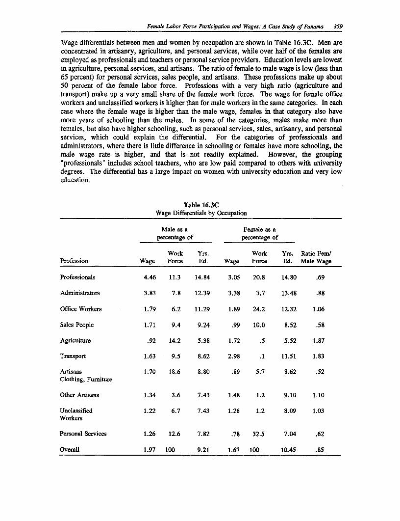
Female Labor Force Participation and Wages: A Case Study of Panama 359
Wage differentials between men and women by occupation are shown in Table 16.3C. Men areconcentrated in artisanry, agriculture, and personal services, while over half of the females areemployed as professionals and teachers or personal service providers. Education levels are lowestin agriculture, personal services, and artisans. The ratio of female to male wage is low Oess than65 percent) for personal services, sales people, and artisans. These professions make up about50 percent of the female labor force. Professions with a very high ratio (agriculture andtransport) make up a very small share of the female work force. The wage for female officeworkers and unclassified workers is higher than for male workers in the same categories. In eachcase where the female wage is higher than the male wage, females in that category also havemore years of schooling than the males. In some of the categories, males make more thanfemales, but also have higher schooling, such as personal services, sales, artisanry, and personalservices, which could explain the differential. For the categories of professionals andadministrators, where there is little difference in schooling or females have more schooling, themale wage rate is higher, and that is not readily explained. However, the grouping"professionals" includes school teachers, who are low paid compared to others with universitydegrees. The differential has a large impact on women with university education and very loweducation.
Table 16.3CWage Differentials by Occupation
Male as a Female as apercentage of percentage of
Work Yrs. Work Yrs. Ratio Fem/Profession Wage Force Ed. Wage Force Ed. Male Wage
Professionals 4.46 11.3 14.84 3.05 20.8 14.80 .69
Administrators 3.83 7.8 12.39 3.38 3.7 13.48 .88
Office Workers 1.79 6.2 11.29 1.89 24.2 12.32 1.06
Sales People 1.71 9.4 9.24 .99 10.0 8.52 .58
Agriculture .92 14.2 5.38 1.72 .5 5.52 1.87
Transport 1.63 9.5 8.62 2.98 .1 11.51 1.83
Artisans 1.70 18.6 8.80 .89 5.7 8.62 .52Clothing, Furniture
Other Artisans 1.34 3.6 7.43 1.48 1.2 9.10 1.10
Unclassified 1.22 6.7 7.43 1.26 1.2 8.09 1.03Workers
Personal Services 1.26 12.6 7.82 .78 32.5 7.04 .62
Overall 1.97 100 9.21 1.67 100 10.45 .85
360 Women's Employment and Pay in Latin America
4. Determinants of Work Force Participation
In this section, the results of a univariate probit regression are discussed. The probit wasestimated separately for men and women. The need to estimate the probits arises because theworking men and women are a selected subset of all men and women. They are people whoobtained wage offers higher than their reservation wage. Reservation wages are affected bytastes, age, and schooling. For example, an individual with high education would have a higherreservation wage because of raised expectations and would be less willing to take a lower payingjob than someone with low education. A woman who has young children would be less likelyto work than a woman who has no children because her time in the household is more valuableto her. An individual in his or her teens would be less likely to be in the work force because ofopportunities for schooling, and a long work life ahead to earn a return on schooling. A manin an urban area may have a lower reservation wage than a man in a rural area because in urbanareas, goods that may have been readily available from a small plot of land in a rural area mustbe bought. For example, an urban worker may have to buy the fruits, subsistence food orfirewood which he could gather or cultivate easily if he lived in the countryside.
In order to obtain unbiased estimates for the return to schooling, experience, hours, and tenure,it is necessary to correct for selectivity. This is done using Heckman's (1979) two-stepprocedure. The probit includes as independent variables schooling levels, age levels, regions,and variables that represent the structure of the household. The inverse Mill's ratio (Lambda)is computed in order to account for the unseen variables that affect the decision to work. Then,Lambda can be included as a regressor in an ordinary least squares (OLS) regression. A positivevalue of the Lambda coefficient implies that characteristics that make an individual more likelyto be in the work force also lead to higher earnings, while a negative value means thatcharacteristics associated with staying out of the work force imply higher earnings. An exampleof a characteristic that would explain a negative Lambda coefficient is higher education, becauseit increases the reservation wage, decreasing the probability of work force participation, whilehigher schooling also earns a compensating differential in earnings.
Because such a high percentage of men do not have hours or income reported, a probit regressionis estimated for men as well as women. The probit for men includes the same independentvariables as the probit for women in order to make comparisons between them. A priori, theresearcher would expect that the number of children would have a strong negative effect on thefemale participation decision, because females traditionally carry more responsibility in thehousehold for child care. Living in a rural area would be likely to decrease participation for bothmales and females. One would expect the age group to have less of an effect on maleparticipation rates than female rates because male participation rates are consistently high, whilefemales have more elastic labor supply.
Tables 16.4A and 16.4B present the results for the probits for men and women. Table 16.5presents a simulation where the effect of each characteristic on the probability of work forceparticipation is examined. All other values are held at the sample mean, so that the effect of onlythe relevant characteristic can be determined. First, it is evident for every characteristic that theprobability of a given male being in the work force is higher than for a given female. Lookingat education levels, for females the likelihood of working increases with higher education levels.In Table 16.5, participation rates increase from 10 percent for those with no education to 48percent for those with over 4 years of university education. These results contrast with theresults for males, where those with technical education have the highest likelihood of participation
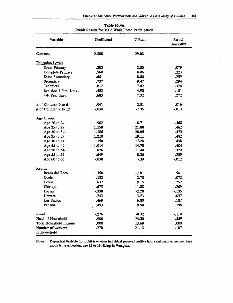
Female Labor Force Partictpation and Wages. A Case Study of Panama 361
Table 16.4AProbit Results for Male Work Force Participation
Variable Coefficient T-Ratio PartialDerivative
Constant -2.808 -29.08
Education LevelsSome Primary .200 2.80 .079Complete Primary .560 8.06 .223Some Secondary .651 8.80 .259Secondary .737 9.47 .294Technical .812 7.42 .324less than 4 Yrs. Univ. .453 4.93 .1814+ Yrs. Univ. .683 7.32 .272
# of Children 0 to 6 .041 2.81 .016# of Children 7 to 12 -.034 -2.35 -.013
Age GroupAge 20 to 24 .902 18.71 .360Age 25 to 29 1.158 21.88 .462Age 30 to 34 1.186 20.05 .473Age 35 to 39 1.210 19.11 .482Age 40 to 44 1.150 17.28 .458Age 45 to 49 1.014 14.70 .404Age 50 to 54 .826 11.44 .329Age 55 to 59 .649 8.26 .259Age 60 to 65 -.030 -.39 -.012
RegionBocas del Toro 1.358 12.81 .541Cocle .182 2.78 .072Colon .632 9.15 .252Chiriqui .675 11.88 .269Darien -.338 -2.28 -.135Herrera .243 3.23 .097Los Santos .469 6.00 .187Panama .493 9.54 .196
Rural -.276 -8.32 -. 110Head of Household .900 23.30 .359Total Household Income .000 13.69 .000Number of workers .270 21.13 .107in Household
Notes: Dependent Variable for probit is whether individual reported positive hours and positive income. Basegroup is no education, age 15 to 19, living in Veraguas.
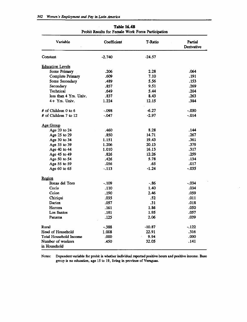
362 Women's Employment and Pay in Latin America
Table 16.4BProbit Results for Female Work Force Participation
Variable Coefficient T-Ratio PartialDerivative
Constant -2.740 -24.57
Education LevelsSome Primary .206 2.28 .064Complete Primary .609 7.10 .191Some Secondary .489 5.56 .153Secondary .857 9.51 .269Technical .649 5.44 .204less than 4 Yrs. Univ. .837 8.43 .2634+ Yrs. Univ. 1.224 12.15 .384
#of Children 0 to 6 -.098 -6.27 -.030# of Children 7 to 12 -.047 -2.97 -.014
Age GrounAge 20 to 24 .460 8.28 .144Age 25 to 29 .850 14.71 .267Age 30 to 34 1.151 19.43 .361Age 35 to 39 1.206 20.13 .379Age 40 to 44 1.010 16.13 .317Age 45 to 49 .826 12.26 .259Age 50 to 54 .426 5.78 .134Age 55 to 59 .056 .65 .017Age 60 to 65 -.113 -1.24 -.035
RgionBocas del Toro -.109 -.86 -.034Cocle .110 1.40 .034Colon .190 2.46 .059Chiriqui .035 .52 .011Darien .057 .31 .018Herrera .161 1.86 .050Los Santos .181 1.95 .057Panama .125 2.06 .039
Rural -.388 -10.87 -.122Head of Household 1.008 22.91 .316Total Household Income .000 9.94 .000Number of workers .450 32.05 .141in Household
Notes: Dependent variable for probit is whether individual reported positive hours and positive income. Basegroup is no education, age 15 to 19, living in province of Veraguas.
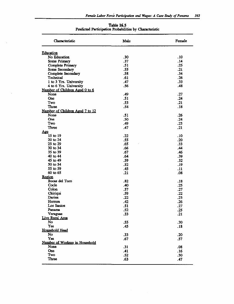
Female Labor Force Paricipation and Wages: A Case Study of Panama 363
Table 16.5Predicted Participation Probabilities by Characteristic
Characteristic Male Fenale
EducationNo Education .30 .10Some Primary .37 .14Complete Primary .51 .25Some Secondary .55 .21Complete Secondary .58 .34Technical .61 .26I to 3 Yrs. University .47 .334 to 6 Yrs. University .56 .48
Number of Children AFed 0 to 6None .49 .27One .51 .24Two .53 .21Three .54 .18
Number of Children Aged 7 to 12None .51 .26One .50 .24Two .49 .23Three .47 .21
Age15 to 19 .22 .1020 to 24 .55 .2025 to 29 .65 .3330 to 34 .66 .4435 to 39 .67 .4640 to 44 .64 .3945 to 49 .59 .3250 to 54 .52 .1955 to 59 .45 .1160 to 65 .21 .08
ReRionBocas del Toro .82 .18Cocle .40 .25Colon .57 .27Chiriqui .59 .22Darien .22 .23Herrera .42 .26Los Santos .51 .27Panama .52 .25Veraguas .33 .21
Live Rural AreaNo .55 .30Yes .45 .18
Household HeadNo .33 .20Yes .67 .57
Number of Workers in HouseholdNone .31 .08One .41 .16Two .52 .30Three .63 .47
364 Women's Employment and Pay in Latin America
at 61 percent. For men, this could reflect very high reservation wages for those who attendedthe university due to raised expectations, while women with university education have a lowreservation wage due to a strong preference to work outside the home.
Another contrast is the effect of the number of children on work force participation. Womenwith children aged 0 to 6 are less likely to be in the labor force than women with no children,while men with young children are more likely to be in the labor force than men withoutchildren. The probability of participation for females drops from 27 percent for women with nochildren aged 0 to 6 to 18 percent for women with three children in that age group. For men,the probability increases as the number of young children increases from 49 percent with noneto 54 percent with three small children. Women are caring for children in the home, while menare earning outside the home to support the family financially. The number of children aged 7to 12 affects men and women about equally. The effect is small; for both men and women theprobability drops about 4 percent when the number of older children is raised from none to three.
As for the effects of age, both men and women have peak work force participation rates between35 and 39 years of age. The female pattern is more concave than the male pattern, with femaleparticipation rates dropping at a younger age than male participation. The probability for womendrops from 32 percent to 19 percent between the 45 to 49 and the 50 to 54 age groups. For men,a drop of this magnitude occurs between the 55 to 59 and 60 to 65 age group, where theparticipation drops 14 percentage points. This is expected given the discussion above, and giveneconometric labor supply studies, which find that female labor supply is more elastic than malelabor supply.'
The regional variables affect male participation rates strongly, while for females, only 2 of the8 regional variables are significant at the 5 percent level. The two significant variables, Panamaand Colon, are the most urbanized provinces in Panama. For males, every regional variable issignificant at the 5 percent level, with probability of participation the highest at 82 percent inBocas del Toro, a middle income province, and the lowest at 22 percent in Darien, a low incomeprovince. This can be explained by the fact that men in the poorer regions are more likely to beself-employed agricultural workers, and therefore excluded from the sample of working men.Both male and female participation is affected by whether the individual lives in an urban or ruralarea; for both the coefficient is negative and significant, and the effect is larger for women.Living in an urban area implies for men an 11 percent greater probability of working and forfemales, a 12 percent greater probability of working than living in a rural area. This is consistentwith the prediction made above.
The variables which proxy household structure, total household income, whether the individualis the head of the household, and the number of occupied people in the household, are all positiveand significant determinants of both male and female participation rates. For women, theprobability of working increases from 20 percent to 57 percent if she is a household head. Formales, the corresponding percentages are 33 percent and 67 percent. For both men and women,with more workers in the household, the probability of the individual working increases, and theincrease is more for women than men.
What effect do these variables representing household structure have on labor force participation?A member of a richer household is more likely to be working than a member of a poorerhousehold. The richer have greater access to the formal labor market. Once again, this could
M See Killingsworth and Heckman, (1986).
Female Labor Force Participation and Wages: A Case Study of Panama 365
be due to the missing data for poorer farmers and their families. As for the females, there areprobably interactions between high education level and high household income, since well-educated women tend to marry well-educated men with high earning potential. Householdheadship is an important determinant because household heads bear more of the financialresponsibilities in the family. Lastly, it is not self-evident why the number of occupied peoplein the household has a positive effect. With more employed members of the household, a givenindividual has less need to work, but families with many workers may be poorer families thatmust send children and women into the work force in order to maintain their living standard.It could also mean that there is a family "work ethic" with members preferring to work outsidethe home.
There are important differences between men and women in how characteristics affect work forceparticipation. The differences are greatest with respect to number of small children, educationlevels, and regions. In the next section, the results of these probit regressions are used inearnings functions to correct for selectivity.
5. Earnings Functions
In Mincer's (1974) model to estimate earnings regressions, the log of earnings is regressed onschooling, experience, and experience squared. The earnings function is concave and increasingin schooling and experience. In this section, the model is used to estimate separate male andfemale earnings functions, both correcting for selectivity and using the most basic model.
In the case of Panama, it is possible to use tenure instead of potential experience as the regressor.The latter experience variable is usually calculated by taking age, subtracting the years ofschooling and subtracting six, which is the age when schooling is assumed to begin. This proxyis likely to be upwardly biased, especially for women, because it does not take into account yearsspent out of the work force since the completion of schooling, nor the deterioration of experiencewhen a person stops working for an extended period of time. Women are likely to haveinterrupted careers if they have had children. For this reason, tenure, which is the amount oftime spent at the present job, is a better proxy for women of human capital acquired on the jobthan the estimate of experience. The drawback of using tenure is that if workers change jobsfrequently, it discounts accumulated experience which transfers between jobs. In Panama thispresents less of a problem than in the United States where workers are mobile and change jobsreadily. There is a high unemployment problem, which makes workers less likely to quit jobsand search for better ones.
Log of monthly earnings is the dependent variable, while years of schooling, tenure, tenuresquared, and the log of monthly hours are the independent variables. Including the log of hourson the right hand side of the equation rather than using the log of hourly wage as the left handside variable allows the value of the elasticity of earnings to hours to differ from one. To correctfor selectivity, according to the Heckman procedure, the inverse Mill's ratio (Lambda) is includedas an independent variable in the earnings regression. Table 16.6 presents the results of theregressions for males and females, both including Lambda and excluding Lambda.
From the table, it is evident in the uncorrected regressions that females earn a higher return toschooling and tenure, while men have a higher elasticity of log earnings to log hours. Bothexhibit a concave earnings profile, with decreasing returns to tenure. The rate of return toeducation for females is almost 3 percent higher than for males, and the rate of return to tenure
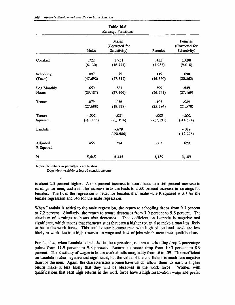
366 Women's Employment and Pay in Latin America
Table 16.6Earnings Functions
Males Females(Corrected for (Corrected for
Males Selectivity) Females Selectivity)
Constant .722 1.951 .455 1.098(6.130) (16.771) (3.982) (9.018)
Schooling .097 .072 .119 .098(Years) (47.692) (27.312) (46.360) (30.363)
Log Monthly .659 .561 .599 .589Hours (29.187) (27.366) (26.741) (27.169)
Tenure .079 .056 .103 .089(27.688) (19.729) (25.384) (21.578)
Tenure -.002 -.001 -.003 -.002Squared (-16.866) (-11.016) (-17.131) (-14.594)
Lambda -.679 -.389(-20.586) (-12.276)
Adjusted .456 .524 .605 .629R-Squared
N 5,445 5,445 3,189 3,189
Notes: Numbers in parenthesis are t-ratios.Dependent variable is log of monthly income.
is about 2.5 percent higher. A one percent increase in hours leads to a .66 percent increase inearnings for men, and a similar increase in hours leads to a .60 percent increase in earnings forfemales. The fit of the regression is better for females than males-the R squared is .61 for thefemale regression and .46 for the male regression.
When Lambda is added to the male regression, the return to schooling drops from 9.7 percentto 7.2 percent. Similarly, the return to tenure decreases from 7.9 percent to 5.6 percent. Theelasticity of earnings to hours also decreases. The coefficient on Lambda is negative andsignificant, which means that characteristics that earn a higher return also make a man less likelyto be in the work force. This could occur because men with high educational levels are lesslikely to work due to a high reservation wage and lack of jobs which meet their qualifications.
For females, when Lambda is included in the regression, returns to schooling drop 2 percentagepoints from 11.9 percent to 9.8 percent. Returns to tenure drop from 10.3 percent to 8.9percent. The elasticity of wages to hours worked falls marginally from .6 to .59. The coefficienton Lambda is also negative and significant, but the value of the coefficient is much less negativethan for the men. Again, the characteristics women have which allow them to earn a higherreturn make it less likely that they will be observed in the work force. Women withqualifications that earn high returns in the work force have a high reservation wage and prefer
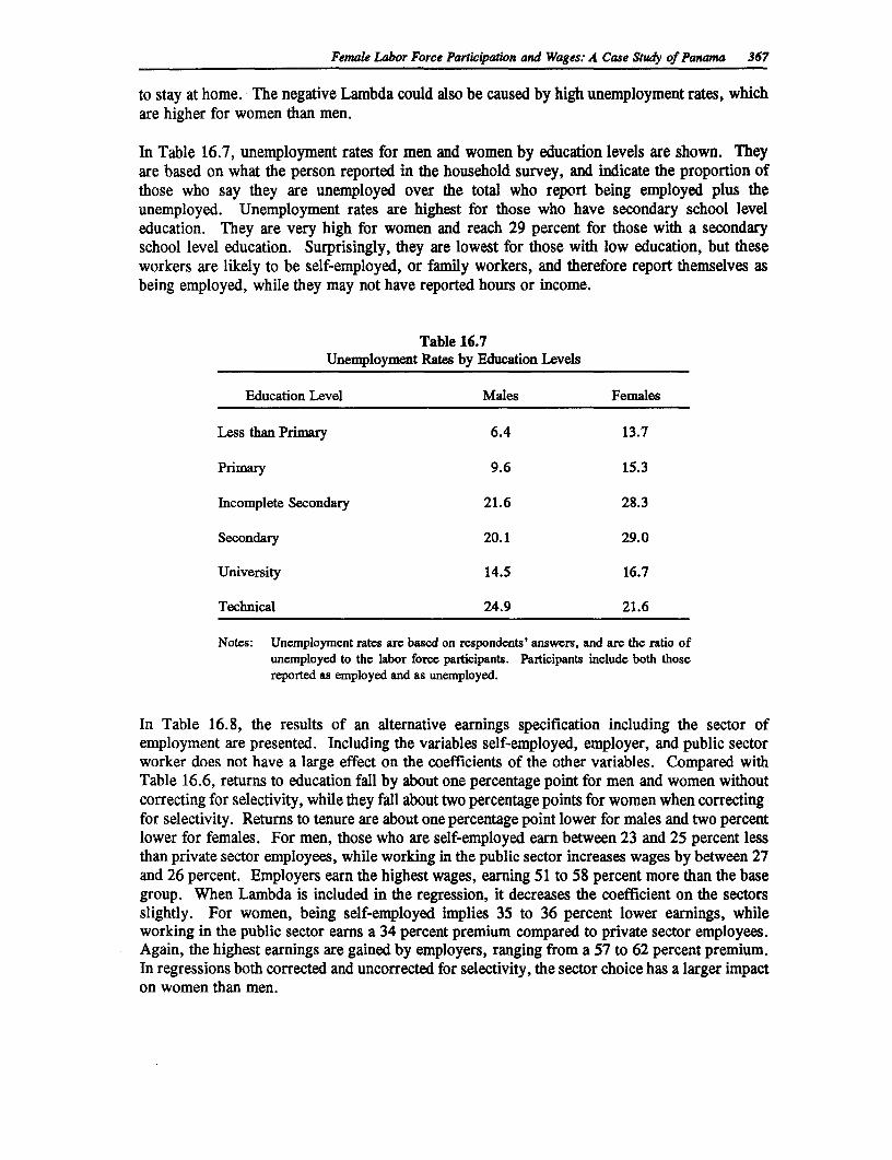
Femak Labor Force Parricwation and Wages: A Case Study of Panama 367
to stay at home. The negative Lambda could also be caused by high unemployment rates, whichare higher for women than men.
In Table 16.7, unemployment rates for men and women by education levels are shown. Theyare based on what the person reported in the household survey, and indicate the proportion ofthose who say they are unemployed over the total who report being employed plus theunemployed. Unemployment rates are highest for those who have secondary school leveleducation. They are very high for women and reach 29 percent for those with a secondaryschool level education. Surprisingly, they are lowest for those with low education, but theseworkers are likely to be self-employed, or family workers, and therefore report themselves asbeing employed, while they may not have reported hours or income.
Table 16.7Unemployment Rates by Education Levels
Education Level Males Females
Less than Primary 6.4 13.7
Primary 9.6 15.3
Incomplete Secondary 21.6 28.3
Secondary 20.1 29.0
University 14.5 16.7
Technical 24.9 21.6
Notes: Unemployment rates are based on respondents' answers, and are the ratio ofunemployed to the labor force participants. Participants include both thosereported as employed and as unemployed.
In Table 16.8, the results of an alternative earnings specification including the sector ofemployment are presented. Including the variables self-employed, employer, and public sectorworker does not have a large effect on the coefficients of the other variables. Compared withTable 16.6, returns to education fall by about one percentage point for men and women withoutcorrecting for selectivity, while they fall about two percentage points for women when correctingfor selectivity. Returns to tenure are about one percentage point lower for males and two percentlower for females. For men, those who are self-employed earn between 23 and 25 percent lessthan private sector employees, while working in the public sector increases wages by between 27and 26 percent. Employers earn the highest wages, earning 51 to 58 percent more than the basegroup. When Lambda is included in the regression, it decreases the coefficient on the sectorsslightly. For women, being self-employed implies 35 to 36 percent lower earnings, whileworking in the public sector earns a 34 percent premium compared to private sector employees.Again, the highest earnings are gained by employers, ranging from a 57 to 62 percent premium.In regressions both corrected and uncorrected for selectivity, the sector choice has a larger impacton women than men.
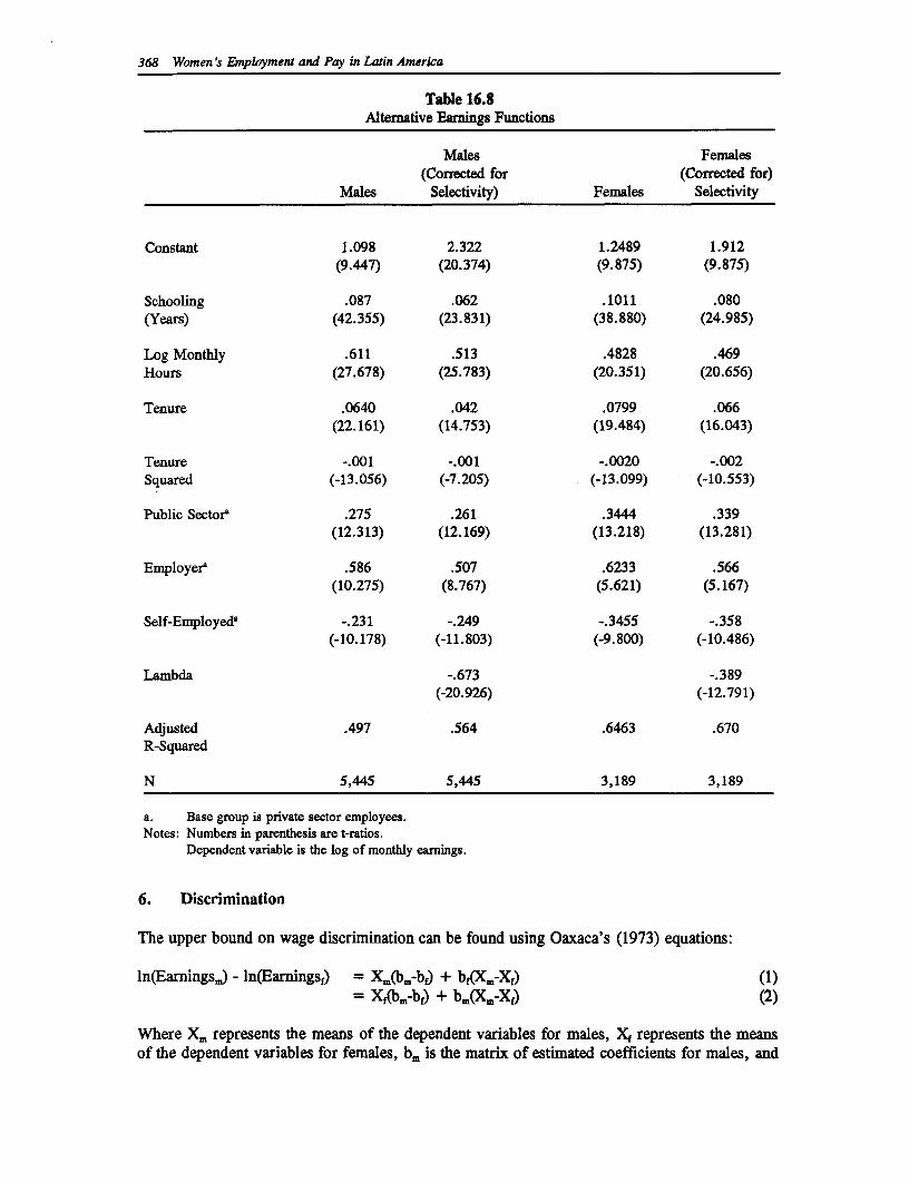
368 Women's Employment and Pay in Latin America
Table 16.8Alternative Eanings Functions
Males Females(Corrected for (Corrected for)
Males Selectivity) Females Selectivity
Constant 1.098 2.322 1.2489 1.912(9.447) (20.374) (9.875) (9.875)
Schooling .087 .062 .1011 .080(Years) (42.355) (23.831) (38.880) (24.985)
Log Monthly .611 .513 .4828 .469Hours (27.678) (25.783) (20.351) (20.656)
Tenure .0640 .042 .0799 .066(22.161) (14.753) (19.484) (16.043)
Tenure -.001 -.001 -.0020 -.002Squared (-13.056) (-7.205) (-13.099) (-10.553)
Public Sector' .275 .261 .3444 .339(12.313) (12.169) (13.218) (13.281)
Employer" .586 .507 .6233 .566(10.275) (8.767) (5.621) (5.167)
Self-Employeda -.231 -.249 -.3455 -.358(-10.178) (-11.803) (-9.800) (-10.486)
Lambda -.673 -.389(-20.926) (-12.791)
Adjusted .497 .564 .6463 .670R-Squared
N 5,445 5,445 3,189 3,189
a. Base group is private sector employees.Notes: Numbers in parenthesis are t-ratios.
Dependent variable is the log of monthly earnings.
6. Discrimination
The upper bound on wage discrimination can be found using Oaxaca's (1973) equations:
ln(Earnings.) - ln(Earningsf) = Xm(bmjbf) + bf(Xm-Xf) (1)= XA(bm-bf) + bm(Xm-Xf) (2)
Where Xm represents the means of the dependent variables for males, Xf represents the meansof the dependent variables for females, bm is the matrix of estimated coefficients for males, and
Female Labor Force Parlicipalion and Wages: A Case Study of Panama 369
bf is the matrix of estimated coefficients for females. Both equations give the differential betweenthe predicted values of earnings for males and females, bmXm-bfXf. The first term on the righthand side in equation 1 gives the part of the differential that is explained by differences in howmale and female human capital endowments are rewarded in the labor market (wage structure)evaluated at the male means. The second term calculates the part of the differential due todifferences in the means of the dependent variables of men and women (endowments), multipliedby the female coefficients. Equation 2 is the same breakdown, but calculated at the female meansrather than the male means. There is an index number problem with the two equations.However, it makes more sense to evaluate the differential at the male means, since this paper isexamining potential discrimination against women.
In calculating the percentage of the differential due to endowments and to wage structure, themeans of the entire sample of men and women are used for schooling, and the means of workingmen and women are used for log hours and tenure. Both working and non-working individualshave reported schooling, but only working men and women have positive hours and years oftenure. Neither the Mill's ratio terms (Lambda) nor their coefficients are included in the equationbecause the parameter of interest is the mean for the whole sample, not just working men andwomen. 2
1
Table 16.9 shows the calculations of the Oaxaca decomposition using the regression coefficientscorrecting for selectivity. There is not a large difference between the calculations evaluated atthe male means (equation 1) and at the female means (equation 2). From 14 to 15 percent of thedifferential between male and female wages can be explained by endowments, while 85 to 86percent are explained by the wage structure.
However, it should be noted that the differential due to wage structure is an upper bound ondiscrimination. If there are attributes not measured here that are valuable in the labor market,and men have these attributes in greater quantity or quality than women, the upper bound ondiscrimination will be upwardly biased. However, if there are societal characteristics that are notmeasured here preventing women from entering the labor force or inhibiting women fromacquiring human capital, the measure of discrimination will be underestimated.
Table 16.9
Decomnposition of Sex Earnings Differential
Percentage of the Differential Due to Differences in
Specification Endowments Wage Structure Total
Corrected forSelectivity
Equation 1 14.7 85.3 37Equation 2 13.9 86.1 37
Note: The decomposition is based on the results of Table 16.6.
21 See the chapter in this volume by Psacharopoulos on Venezuela.
370 Women 's Employment and Pay in Latin America
7. Discussion
Despite high educational attainments for women, Panama's female participation rate is low. Avery important impediment to equality is difficulty in finding a job indicated by the incrediblyhigh unemployment rate women face. This is especially a problem for women with secondarylevel education.
The overall ratio of female to male wage in Panama is favorable compared with other LatinAmerican countries, such as Uruguay, Venezuela and Peru.' However, at the minimum 85percent of the differential cannot be explained by differences in endowments between men andwomen, and can be attributed to wage structure discrimination.
A topic of further study would be whether the Labor Code has impacted female wages favorably.The evidence presented here indicates that for women who have jobs, the wage gap is smallrelative to other countries, but that the labor code also discourages employers from hiring womenbecause they must provide benefits that are specific to women. Employers perceive that it ischeaper to hire men. The code could be reformed to provide more flexibility to employers forproviding maternity benefits. Laws designed to help women may actually hurt them.
The choice to work as an employee or to be self-employed has an important implication forearnings for both men and women. Individuals with lower levels of education seem to earnhigher wages as self-employed workers than as employees. To alleviate high unemployment,credit could be extended to women who would like to be self-employed. However, in the longrun, sound economic growth would provide private sector jobs. In the sample, only a smallpercentage of working women are self-employed (15 percent) and with a big increase in thenumber of self-employed women, undoubtedly their wages would decrease. With high enougheconomic growth, employment in the private sector would increase and wages would increase toreflect productivity growth.
Labor market discrimination seems to be more of a factor for women with very low educationallevels and relatively high educational levels. This could be because given the high unemploymentrates for women with secondary education, only very qualified or determined women can getjobs, and, therefore, their wages are a higher percentage of men's wages. Better enforcementof anti-discrimination laws would help those women that are private and public sector employeesearn a wage more equal to male employees.
2 See Khandker, Arends, and Winter (in this volume) who report the ratio to be about .67, .75 and.78 in Peru, Uruguay, and Venezuela, respectively.
References
Economist Intelligence Unit. Nicaragua, Costa Rica, Panama: Country Profile 1991-92. London:Economist Intelligence Unit Limited, 1991.
Heckman, J.J. "Sample Selection Bias as a Specification Error." Econometrica, Vol. 47, no. 1(1979). pp. 153-161.
Heckman, J.J. and V.J. Hotz, "An Investigation of the Labor Market Earnings of PanamanianMales: Evaluating the Sources of Inequality." Journal of Human Resources, Vol. 21 (1986)pp. 507-42.
Killingsworth, M.R. and J.J. Heckman, "Female Labor Supply: A Survey" in 0. Ashenfelter andR. Layard (eds.) Handbook of Labor Economics. Amsterdam: North Holland, 1986, pp.103-204.
Mincer, J. Schooling, Experience, and Earnings. New York: Columbia University Press, 1974.
Oaxaca, R. "Male-female Wage Differentials in Urban Labor Markets." International EconomicReview, Vol. 14, no. 1 (1973). pp. 693-701.
Spinanger, D. "Labor Market in Panama: an Analysis of the Employment Impact of the LaborCode." Kiel Working Papers, No. 221, December 1984.
Tollefson, S. "The Economy" in S. Meditz and D. Hanratty (eds.) Panama: a Country Study.Washington, DC: United States Government, Department of the Army, 1989. pp. 123-171.
World Bank. Panama: Structural Change and Growth Prospects. Washington, DC: World Bank,1985.
World Bank. Second Structural Adjustment Project--Panama. Latin America Division, PanamaDesk, 1986.
World Bank. Social Indicators of Development 1990. Baltimore, MD: Johns Hopkins UniversityPress, 1990. p. 238-9.
World Bank. World Development Report. New York: Oxford University Press, 1991.
371

17
Women's Labor Market Participation andMale-Female Wage Differences in Peru
Shahidur R. Khandker'
1. Introduction
This study uses Peruvian Living Standard Survey (PLSS) data to estimate women's labor market(i.e., wage) participation, and male-female differences in productivity (measured by wages). Thepurpose is to (1) identify those characteristics that enable some women, though not as many men,to participate in the wage sector, (2) determine the private economic returns to education bygender, and (3) evaluate how much of the male-female wage gap is due to differences in humancapital. Identifying the constraints to women's labor market participation and productivity is animportant policy exercise in Peru where female participation rates are below the average for theregion (Suarez-Berenguela, 1987).
Results indicate that gender differences in human capital, such as education and experience,account for some of the observed differences in labor market participation and productivity.Estimates of the returns to education show the private rate to be generally higher for women,especially for secondary school level and rural areas. However, school enrollment rates forfemales are lower than for males, indicating that parents invest less in female than male children.
The study uses a household model framework (Becker, 1965) that provides an estimable labormarket participation equation. This equation can help estimate the relative effect of individual,household, and market factors in influencing an individual's labor market participation. Thestudy uses, in addition, a human capital model as per Becker (1964) and Mincer (1974) to analyzewages in the wage sector. The focus here is on human capital variables such as education andexperience as determinants of productivity. Wage estimates provide measures of the private ratesof returns to education for men and women and can be used to identify how much variation inmale-female wages is due to gender differences in education and other job-related characteristics.
The human capital model, however, may not satisfactorily explain variations in wages sinceproductivity is likely to be determined by a number of factors including, but not limited to,human capital variables. A satisfactory analysis, therefore, requires identifying potentially
I Comments on an earlier draft by George Psacharopoulos, Zafiris Tzannatos, and Indermit Gill aregratefully acknowledged. I am also indebted to Jorge Castillo who provided excellent assistance inanalyzing the data. The usual disclaimer applies.
373
374 Women's Employment and Pay in Latin America
observable characteristics other than human capital that can affect an individual's wage.Unfortunately, these are not clearly understood and are thus difficult to incorporate in theanalysis. There are, however, ways to reduce the impact of unobserved characteristics. Thisstudy uses a sample selection correction technique to estimate the severity of sample selection biasin the wage estimates that may arise because the analysis is restricted to wage earners. Thisprocedure determines whether sample selection correction significantly alters the wage estimatesand hence the estimates of the returns to education and gender differences in productivity.
The chapter is structured as follows. Section 2 briefly describes the Peruvian economy and labormarket to illustrate women's position in the overall economy. Section 3 discusses the data andhighlights the differences between males and females in terms of wage-related characteristics.Section 4 discusses the determinants of female labor force participation and Section 5 the wagedeterminants and returns to education. Section 6 discusses the extent to which male/femaleearnings differentials can be attributed to differences in the way the market structure rewardsmale and female workers. Policy implications are in the concluding section.
2. Peru: Economic Background and Women's Status in the Labor Market
Peru is a middle income country with a per capita income of US$1300 in 1988. The economyis heavily dependent on mineral resources which are its major export goods. It also hasconsiderable potential for fishing and hydrocarbon resource development. The country isgeographically divided by the Andean mountains into three regions--the highlands (Sierra), therain forest (Selva) and the coast regions. About half of Peru's 20 million (1987 estimates)population lives in the coastal regions, 40 percent in the Andean highlands, and the remainderin the Selva (i.e., Amazon) region.
Table 17.1 presents data relating to employment, unemployment, and labor productivity in Peruduring the period 1970-85. Between 1970 and 1985 the labor force increased from 4.2 millionto 6.6 million, of which about 88 percent were employed. During this time the employed laborforce increased by 46 percent with 28 percent of that increase being employed in agriculture.Unemployment increased by about 7 percentage points over the same period.
Column 4 in Table 17.1 gives figures on adequate employment for the labor force who areemployed. According to these figures, the rates of underemployment in Peru ranged between 46and 54 percent of the labor force in 1970 and 1985, respectively. Thus, underemployment ismore serious than open unemployment in Peru. Labor productivity, defined as value added peremployed person, is also a problem in Peru. As column 5 indicates, labor productivity declinedin Peru between 1981 and 1985. Increasing labor productivity and adequate employmentopportunities are significant problems in Peru.
In Peru women's labor force participation rates are below those in many Latin Americancountries (Suarez-Berenguela, 1987), but it has increased between 1970 and 1985. For example,women's labor force participation increased from 34 to 43 percent in urban Peru.2 Women'sall-Peru participation rate is 57 percent for 1985 (Schafgans, 1990), their participation beingmuch higher in rural than urban areas. Of all economically active women, about 18 percent workin the wage sector, 55 percent are farmers, and 27 percent work in the informal (non-farm)activities. Women are thus predominantly in agriculture and self-employed non-farm activities.Table 17.2 shows that women are predominantly employed in the informal sector; in 1985 about
2 See Table 23.2. The figures are calculated as: Column 3 x Column 1/100.
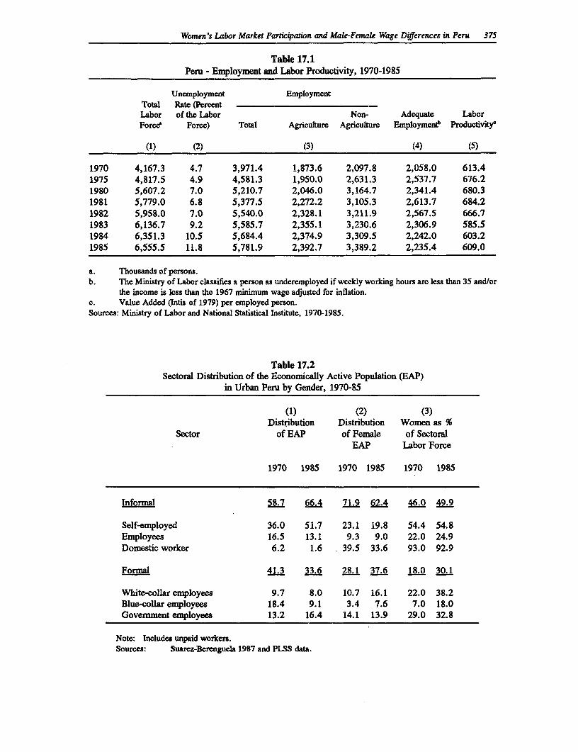
Women's Labor Market Participation and Male-Female Wage Diferences in Peru 375
Table 17.1Peru - Employment and Labor Productivity, 1970-1985
Unemployment EmploymentTotal Rate (PercentLabor of the Labor Non- Adequate LaborForces Force) Total Agriculture Agriculture EmploymenP Productivity'
(1) (2) (3) (4) (5)
1970 4,167.3 4.7 3,971.4 1,873.6 2,097.8 2,058.0 613.41975 4,817.5 4.9 4,581.3 1,950.0 2,631.3 2,537.7 676.21980 5,607.2 7.0 5,210.7 2,046.0 3,164.7 2,341.4 680.31981 5,779.0 6.8 5,377.5 2,272.2 3,105.3 2,613.7 684.21982 5,958.0 7.0 5,540.0 2,328.1 3,211.9 2,567.5 666.71983 6,136.7 9.2 5,585.7 2,355.1 3,230.6 2,306.9 585.51984 6,351.3 10.5 5,684.4 2,374.9 3,309.5 2,242.0 603.21985 6,555.5 11.8 5,781.9 2,392.7 3,389.2 2,235.4 609.0
a. Thousands of persons.b. The Ministry of Labor classifies a person as underemployed if weekly working hours are less than 35 and/or
the income is less than the 1967 minimum wage adjusted for inflation.c. Value Added (Intis of 1979) per employed person.Sources: Ministry of Labor and National Statistical Institute, 1970-1985.
Table 17.2Sectoral Distribution of the Economically Active Population (EAP)
in Urban Peru by Gender, 1970-85
(1) (2) (3)Distribution Distribution Women as %
Sector of EAP of Female of SectoralEAP Labor Force
1970 1985 1970 1985 1970 1985
Informal 58.7 66.4 71.9 62.4 46.0 49.9
Self-employed 36.0 51.7 23.1 19.8 54.4 54.8Employees 16.5 13.1 9.3 9.0 22.0 24.9Domestic worker 6.2 1.6 39.5 33.6 93.0 92.9
Formal 41.3 33.6 28.1 37.6 18.0 30.1
White-collar employees 9.7 8.0 10.7 16.1 22.0 38.2Blue-collar employees 18.4 9.1 3.4 7.6 7.0 18.0Government employees 13.2 16.4 14.1 13.9 29.0 32.8
Note: Includes unpaid workers.Sources: Suarez-Berenguela 1987 and PLSS data.
376 Women's Employment and Pay in Latin America
33 percent of the economically active population in urban Peru were women employed in theinformal sector compared to 10 percent in the formal sector.
Women's wages in the formal sector are lower than men's. Women's employment options andproductivity perhaps reflect their low education and employment opportunities. Peruvian womenhave about five years of schooling on average compared to seven years for men. Only 8 percentof men did not attend school compared to 25 percent of women (King and Bellew, 1990). Thispaper attempts to account for differences in women's labor market participation and wages usinghousehold survey data from Peru.
3. Data Characteristics
The data are drawn from the Peruvian Living Standard Survey (PLSS) household data collectedjointly by the World Bank and the Peruvian Instituto Nacional de Estadistica (INE). These dataprovide detailed socio-economic information on over 5,100 households and 26,000 individuals.The samples were drawn from a self-weighted national probability sample of Peruvian householdsand represent an approximate 1/100 sample of the population. The sampling frame is based ona 1984 National Health and Nutrition Survey. About 25 percent of the households in the PLSSwere in metropolitan Lima, 28 percent in other urban areas, and 47 percent in rural areas. Thedata were collected between June 1985 and July 1986 (see Grootaert and Arriagada, 1986).
The sample includes workers aged 14 to 60. The wage earner participation equation is estimatedusing information for all potential workers. The wage equation in Section 5, however, isestimated only for men and women reporting wage and remuneration and hours worked and wholist this as their main occupation in the week prior to data collection. Self-employed and unpaidfamily workers are thus excluded. This reduced sample consists of 2,255 men from 1,856households and 898 women from 783 households, drawn from a total of 6,429 men from 4,142households and 6,942 women from 4,387 households. The wage labor market participation rateis 13 percent for women and 35 percent for men. Table 17.3 gives the means and standarddeviations of the variables by gender.
Women wage earners have one more year of education on average than men wage earners.Employed women also have more vocational training -- 52 percent of women have trainingcompared to 31 percent of men. Despite this, women receive about half of men's wages.3 Thissuggests that there are significant differences in wage structures between men and women.Occupational segregation may cause this male-female wage gap. Women also come fromrelatively wealthier households (in terms of landholding and unearned income). The data suggestthat more married (or cohabiting) men participate in the labor market than married (or cohabiting)women. Employed women are also younger on average than employed men.
4. Determinants of Female Labor Force Participation
What influences women's participation in the labor market? Do women differ from men inresponding to labor market opportunities? Does human capital (for instance, education) helpwomen, more than men, to participate in the wage sector? Do women face different market
3 The real hourly wage rate, i.e., nominal hourly wages deflated at 1985 consumer price indices(RHW) is defined as RHW = AC/AH where: AC = annual compensation = monthly pay x monthsworked in the past year; AH = annual hours = weekly hours x months worked in the past year x 4.33.Note that the above male-female wage difference is adjusted for male-female sample differences.
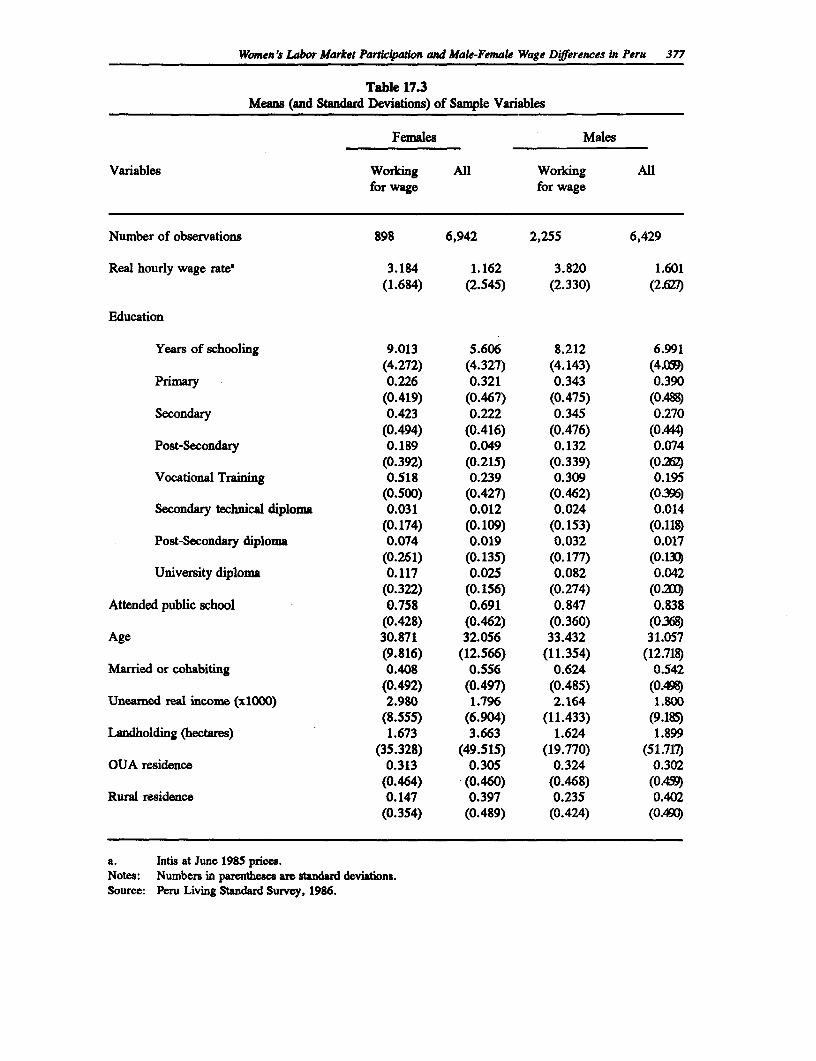
Women 's Labor Market Participaton and Male-Female Wage Differences in Peru 377
Table 17.3Means (and Standard Deviations) of Sample Variables
Females Males
Variables Working All Working Allfor wage for wage
Number of observations 898 6,942 2,255 6,429
Real hourly wage rate 3.184 1.162 3.820 1.601(1.684) (2.545) (2.330) (2.6)
Education
Years of schooling 9.013 5.606 8.212 6.991(4.272) (4.327) (4.143) (4.(5)
Primary 0.226 0.321 0.343 0.390(0.419) (0.467) (0.475) (0.48"
Secondary 0.423 0.222 0.345 0.270(0.494) (0.416) (0.476) (0.444)
Post-Secondary 0.189 0.049 0.132 0.074(0.392) (0.215) (0.339) (0.262)
Vocational Training 0.518 0.239 0.309 0.195(0.500) (0.427) (0.462) (0396)
Secondary technical diploma 0.031 0.012 0.024 0.014(0.174) (0.109) (0.153) (0.118)
Post-Secondary diploma 0.074 0.019 0.032 0.017(0.261) (0.135) (0.177) (0.130)
University diploma 0.117 0.025 0.082 0.042(0.322) (0.156) (0.274) (0m
Attended public school 0.758 0.691 0.847 0.838(0.428) (0.462) (0.360) (0368)
Age 30.871 32.056 33.432 31.057(9.816) (12.566) (11.354) (12.718)
Married or cohabiting 0.408 0.556 0.624 0.542(0.492) (0.497) (0.485) (0.498)
Unearned real income (x1000) 2.980 1.796 2.164 1.800(8.555) (6.904) (11.433) (9.185)
Landholding (hectares) 1.673 3.663 1.624 1.899(35.328) (49.515) (19.770) (51.717)
OUA residence 0.313 0.305 0.324 0.302(0.464) (0.460) (0.468) (0.45w)
Rural residence 0.147 0.397 0.235 0.402(0.354) (0.489) (0.424) (0.490
a. Intis at June 1985 prices.Notes: Numbers in parentheses are standard deviations.Source: Peru Living Standard Survey, 1986.
378 Women's Employment and Pay in Lain America
structures than men? Answers to these questions will help policy makers promote women'sparticipation in the labor market.
This section outlines a theoretical framework to address women's labor market participation andreports the results from Peru.
The decision to join in the labor market, given the constraints, is based on an individual'sincome-leisure trade-off. A household model framework can help identify the constraints thataffect an individual's allocation of time (Becker, 1965). This model identifies individualcharacteristics such as education and experience, household characteristics, including landholdingand unearned income, and market conditions, such as wages, which may influence an individual'sallocation of time. Thus the time allocated to different activities, including leisure, can be writtenas a function of individual, household, and market characteristics. The time allocation data canproduce a discrete choice structure of whether or not individuals participate in the wage market.The decision can be estimated using a probability function independently for males and femalesas follows:
Ym =T. + X.,Tlm + ZmT2m + em (1)Yf Tf + XfTlf + Zft2 + ef (2)
where: Yi(i=m,f) are binary dependent variables with 1 if the ith individual participates in thewage labor market and 0 otherwise; X is a vector of individual characteristics that influences anindividual's time allocation; Z is a vector of household and market factors which also explainswhy an individual participates in the labor market; T is the vector of coefficients to be estimated,and e is an error term.4
Different reasons can justify the inclusion of individual (X), and household and market (Z) factorsas explanatory variables in labor market participation equations 1 and 2. An individualcharacteristic, such as the level of education, can be treated as an explanatory variable that mayindicate the potential productivity of an individual at home and in market production. Holdingmarket wages constant, an increase in the level of an individual's education can increase his orher probability of labor market participation if it increases the opportunity costs of staying athome. The household's constraints include such household asset variables as landholding, whichmay act as a proxy for productive household assets. The productive assets exert a price effectand an income effect on an individual's labor market participation. The price effect would raisethe marginal product or "shadow price" of an individual's labor, while the income effect wouldencourage an individual to consume more of his or her leisure - even at its given opportunitycost. The household's unearned income - another household characteristic - can influence labormarket participation via a pure income effect. Market factors such as market wages exert anincome and a substitution effect on an individual's time allocation. These factors may alsoinclude community variables, such as the household's proximity to community services(schooling, health, and banking services). These variables measure the impact on time allocation
4 Y; equal to zero includes individuals who are either self-employed in family business and farmingor exclusively engaged in non-market home production. Including self-employment and home productionin one category assumes that the degree of independence between participation in these two activities isalmost zero (Khandker, 1987). No test is done to assess the validity of this assumption, but for simplicitywe assume that these activities can be jointly undertaken with low transactions cost for switching from onejob to the other and hence in this sense, the participation decisions are not independent.
Women 's Labor Market Paricopation and Male-Female Wage Differences in Peru 379
of implicit prices of many goods and services the household uses for production andconsumption.5
How do we estimate the labor market participation equation? Because the dependent variabletakes the value of 1 or 0 in both equations 1 and 2, the error structures yield heteroscedasticity;hence ordinary least squares produces inconsistent estimates. A maximum likelihood methodsuch as the probit technique which takes care of heteroscedasticity problem can produce efficientestimates (Maddala, 1983). I shall use this technique to estimate both equations, 1 and 2.6
Table 17.4 reports probit equation results that examine the probability that a woman will join thewage labor market. A similar probit equation is run for the male sample and is also reported inTable 17.4 for comparing the response pattern between men and women in Peru. Based on theLikelihood Ratio test, the hypothesis that marital status has no effect on the participation of menor women is rejected. Table 17.4 is then based on the preferred specification that includes maritalstatus, landholding and unearned income as identifying variables in the labor market participationequation.
Consider first a woman's decision to join the labor market. Both general and technical educationaffect her decision just like they affect a man's participation decision. However, the responsecoefficient differs between men and women. Vocational training and secondary educationincrease women's labor market participation more than men's. In Peru as a whole, theprobability that a woman will join the wage market is about 10 percent higher if both men andwomen have vocational training. Additionally, the probability that a woman will join the wagemarket is at least 5 percent higher if both women and men complete secondary school. Thissuggests that improving women's education can increase their labor market participation fasterthan a similar increase in men's education would affect their participation. Public schoolattendance seems to be an important determinant of both women's and men's labor marketparticipation. Both unearned income and landholding (which measure the income effect onleisure) generally decrease the probability of being in the labor market for men and women.Landholding significantly reduces men's participation in the wage market, but only affectswomen's participation in rural areas. Labor market participation for both genders is loweroutside Lima, 32 and 53 percent lower for women and 33 and 74 percent lower for men,respectively, in other urban areas and rural areas. There is a higher probability that women willwork for wages than men in rural Peru.
Using the above probit results, we predict the effect of changing certain characteristics onwomen's labor market participation. Two types of predictions are made, one using the women'sprobit equation and the other using the men's probit equation. The second predicted category
5 No information on any of these market factors is available except for nrual areas. Thus Z variablesinclude only household-level variables.
6 A single probit which estimates separately 1 and 2 may produce inefficient estimates if the errorse, and ef are correlated. The errors are likely to be correlated if men and women participate in the wagemarket from the same household. A bivariate probit is necessary to estimate the labor market participationequations, 1 and 2, to obtain efficient estimates. However, for our sample of 898 women and 2,255 men,only 6 percent of men and women belong to the same household that participate in the labor market. Weassume, therefore, that the correlation between errors is zero.
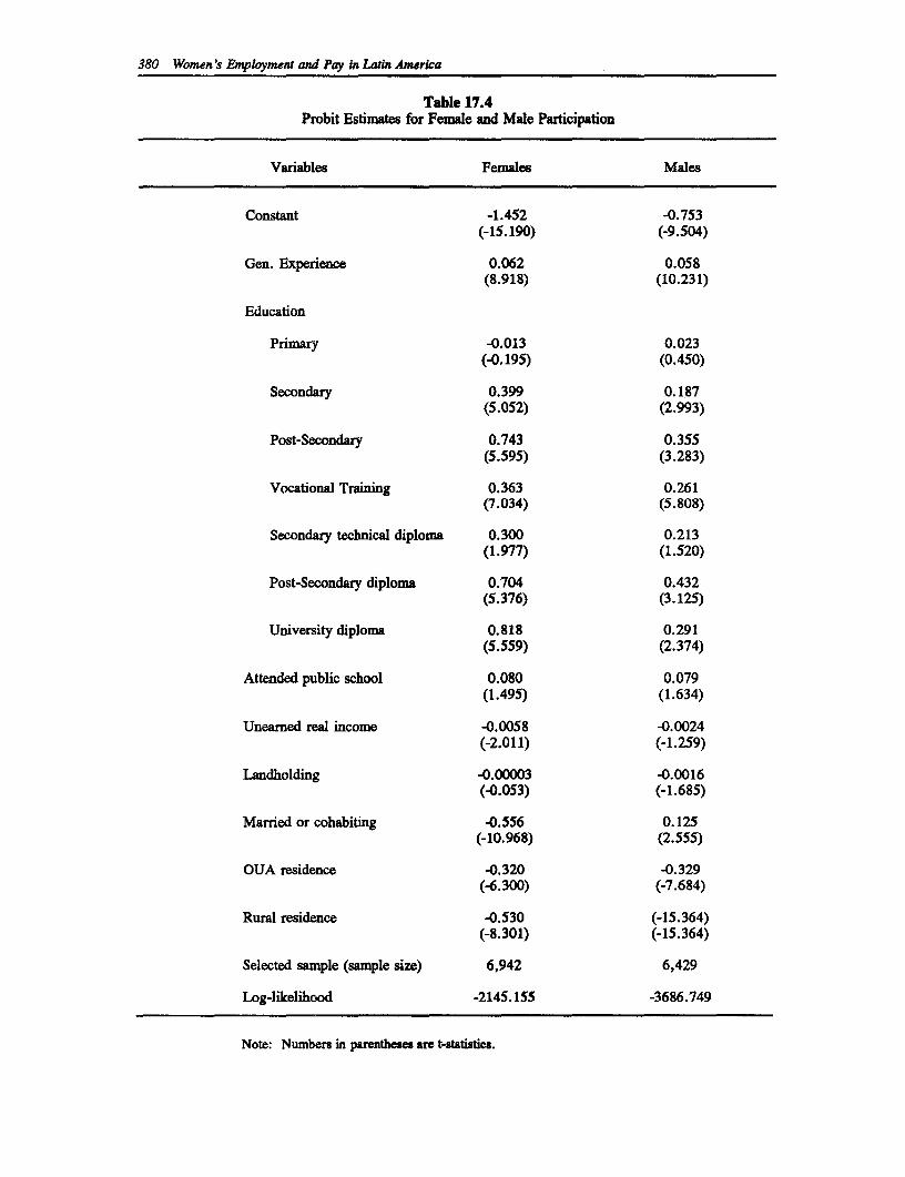
380 Women's Employment and Pay in Latin America
Table 17.4Probit Estimates for Female and Male Participation
Variables Females Males
Constant -1.452 -0.753(-15.190) (-9.504)
Gen. Experience 0.062 0.058(8.918) (10.231)
Education
Primary -0.013 0.023(-0.195) (0.450)
Secondary 0.399 0.187(5.052) (2.993)
Post-Secondary 0.743 0.355(5.595) (3.283)
Vocational Training 0.363 0.261(7.034) (5.808)
Secondary technical diploma 0.300 0.213(1.977) (1.520)
Post-Secondary diploma 0.704 0.432(5.376) (3.125)
University diploma 0.818 0.291(5.559) (2.374)
Attended public school 0.080 0.079(1.495) (1.634)
Unearned real income -0.0058 -0.0024(-2.011) (-1.259)
Landholding -0.00003 -0.0016(-0.053) (-1.685)
Married or cohabiting -0.556 0.125(-10.968) (2.555)
OUA residence -0.320 -0.329(-6.300) (-7.684)
Rural residence -0.530 (-15.364)(-8.301) (-15.364)
Selected sample (sample size) 6,942 6,429
Log-likelihood -2145.155 -3686.749
Note: Numbers in parentheses are t-statistics.
Women's Labor Market Participaon and Mak-Femak Wage Differences in Peru 381
explains women's predicted probability of being in the wage sector if women behave in the sameway as men in responding to market incentives to participate in the wage market. With othersample characteristics remaining the same, we predict the probability of women's labor marketparticipation for different educational levels (including general and technical education), public-private school attendance, marital status and regions where they live. The information is givenin Table 17.5. The mean predicted probability of women's being in the wage sector is 9 percentagainst a 13 percent actual participation. This suggests that the participation model works wellin explaining variations in women's labor market participation decision. However, the meanpredicted probability of women's market participation almost quadruples if women behave thesame way as men in responding to market incentives (column B). This is an interesting findingthat suggests that the labor market response pattern is different for women than men in Peru. Inparticular, there may be structural differences in men's and women's job specialization whichmay produce these large variations in their response behavior.
The predicted probability for changing an individual job characteristic is given by the predictedindividual probability for each characteristic. As expected, an increase in educational attainmentleads to an increase in women's labor market participation. Note that women's participation doesnot change substantially if women have primary instead of less than primary education.However, women's participation increases more as women attain higher education and the gainis the highest if they attain post-secondary level of education. It is interesting to note that theincreases in labor market participation are even much higher for the same level of education ifwomen were to respond in the same way as men to changes in market incentives. For instance,a woman with secondary education increases her probability of participation by an additional 23points if she follows men's response behavior rather than women's response pattern. Womenwith vocational training have a 6 percent higher probability of being in the wage market thanwomen with no vocational training. However, women with vocational training can do even betterif they follow men's response behavior. Thus, a woman with vocational training has a 26 percenthigher probability if she follows a man's response pattern. Women gain substantially in laborforce participation if they have a university rather than secondary or post-secondary diploma.
However, the gain is only marginal if they attended public rather than private school. Awoman's gain does not vary by whether or not she follows women's or men's response patternsin this respect. Single women participate more by about 9 percent compared to married womenand their probability is 15 percent higher if they follow single men's response pattern. Incontrast, a married woman's participation rate is 29 percent higher if she follows a married man'sresponse behavior. The predicted participation rate for women is highest in Lima (15 percent)followed by other urban areas (9 percent) and rural areas (6 percent). The predicted probabilityof being in the wage market increases if women follow men's response pattern: 48 percent inLima, 35 percent in other urban areas, and 21 percent in rural areas.
5. Wage Determinants and Returns to Education
Following Becker (1964) and Mincer (1974), assume that variations in wages arise fromdifferences in the stock of human capital such as schooling and experience. This assumption canbe formally represented in an estimable equation form 3 below:
InWi = %_ + ,liSi + ftl,K; + #XV. + e. (3)
where InW; is the natural log of the hourly wage rate of the ith individual (i=m for male, i=ffor female wage worker); S is the individual's years of schooling, K is the individual's postschool
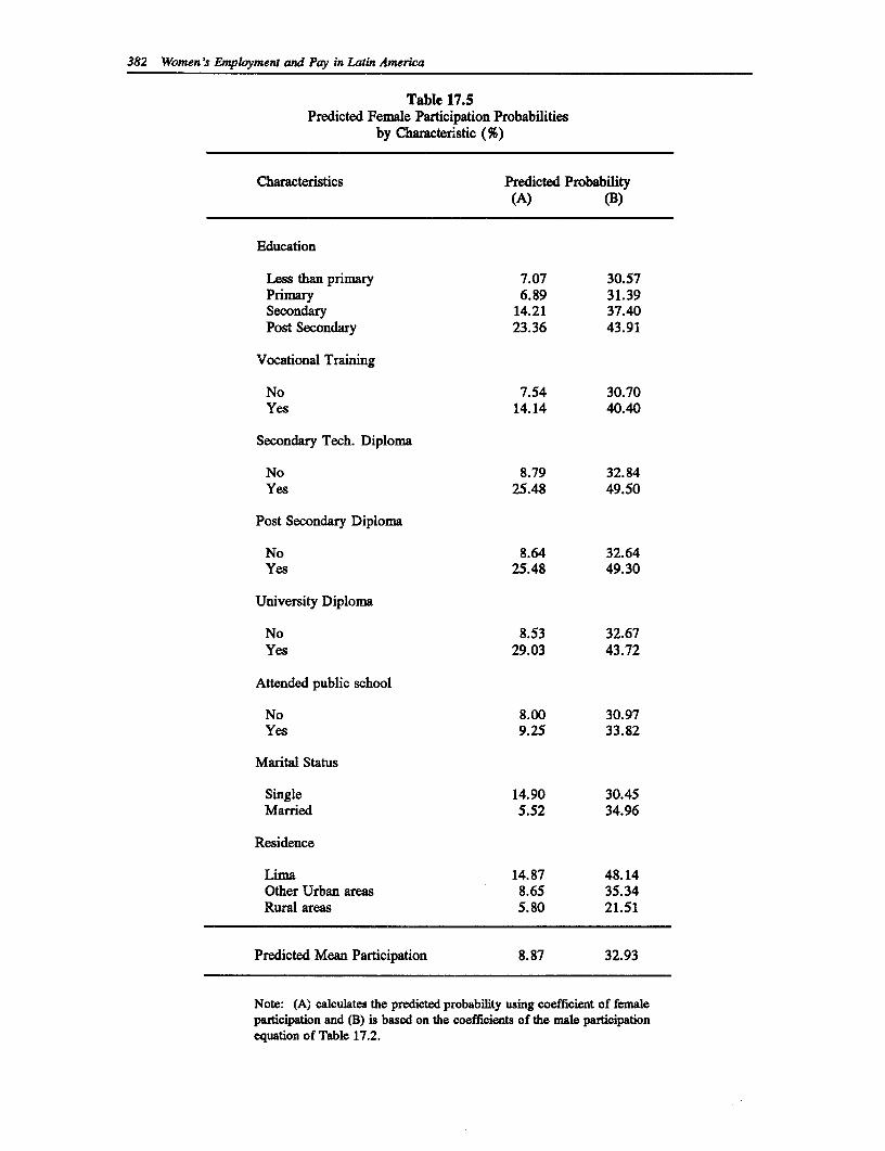
382 Women's Employment and Pay in Latin America
Table 17.5Predicted Female Participation Probabilities
by Characteristic (%)
Characteristics Predicted Probability(A) (B)
Education
Less than primary 7.07 30.57Primary 6.89 31.39Secondary 14.21 37.40Post Secondary 23.36 43.91
Vocational Training
No 7.54 30.70Yes 14.14 40.40
Secondary Tech. Diploma
No 8.79 32.84yes 25.48 49.50
Post Secondary Diploma
No 8.64 32.64Yes 25.48 49.30
University Diploma
No 8.53 32.67Yes 29.03 43.72
Attended public school
No 8.00 30.97Yes 9.25 33.82
Marital Status
Single 14.90 30.45Married 5.52 34.96
Residence
Lima 14.87 48.14Other Urban areas 8.65 35.34Rural areas 5.80 21.51
Predicted Mean Participation 8.87 32.93
Note: (A) calculates the predicted probability using coefficient of femaleparticipation and (B) is based on the coefficients of the male participationequation of Table 17.2.
Women's Labor Market Particyation and Male-Female Wage Differences in Peru 383
experience (defined as age - S - school entry age, say, 6); K2 is the individual's experiencesquared; ca and f j 0=1,2,3) are, respectively, the intercept and slope coefficients to beestimated; and e; is the individual specific unobserved error. If the error is normally andindependently distributed, an ordinary least squares (OLS) technique can be applied to estimatethe wage equation. The estimated coefficient #I measures the proportional increase in the wagesassociated with each additional year of education.
As postschool experience increases, productivity and wages tend to rise. But further increasesin postschool experience may lead to a decline in wages and productivity because of diminishingmarginal returns. The concavity of the wage profile is thus captured by the quadratic experienceterms.7 According to human capital theory, education and experience are likely to have majoreffects on productivity.
Two possible interpretations of wage equation 3 are found in the literature. The first is due toRosen (1974) who interprets the equation as an hedonic index on characteristics which affect theprice of the individual's time. The more dominant interpretation is given by Mincer (1974) whoviews equation 3 as a generalization of the equilibrium relation between wages and education,where the coefficient fB, is the estimate of the private rate of return to the time spent in schoolinstead of in the labor market. Mincer's interpretation is widely applied in the empiricalliterature and is derived as follows. Assume that: (1) the only cost of schooling for an individualis his or her forgone earnings; (2) individuals enter the labor force immediately after completionof schooling; and (3) each individual's working life of N years is independent of his years ofeducation. Given the additional assumption of a steady state with no productivity growth, onecan write the present value of the life earnings of an individual with S years of schooling as:
N 1 1 -_-NV(S) = I W(S) - e7rt = W(S)-(ep-"erN) (4)S r r
where r is the rate of discount indicating people's time preference. If r is the same for everyone(and N is large), the equation becomes:
1V(S) = W(S)-e- = V. for all S; (5)
r
and the present value of income streams are equalized among individuals. The above can thenbe rewritten as:
W(S) = W0e", where W. = V0r. (6)
Taking log on both sides, we have:
InW = W. + rS, (7)
where W. may be interpreted as the permanent labor income of a worker. Individuals facing agiven market interest rate, r, choose that level of schooling that maximizes the present value of
7 Although information on job-specific experience is available, we cannot include it in the wageequation because it is an endogenous variable. In contrast, post-school experience is exogenous to theextent that the individual's education is parentally determined and hence predetermined.
384 Women's Employment and Pay in Latin America
their lifetime earnings. Thus r also represents the internal rate of return. Specification 7 thenjustifies using a semilogarithmic wage function, as in equation 3 to estimate the economic returnsto education, (the estimated coefficient of S). Note that as Mincer's assumptions may not holdin the real world, the estimated schooling coefficient, 8l in equation 3, is only an approximationof the internal rate of return. Thus, if S takes the value of years of schooling in 3, then itscoefficient ,B measures an average economic rate of return to an additional year of schooling.
Equation 3 may be too simple to estimate an individual's productivity in the wage market whenfactors other than human capital influence the wages and hence the economic returns to education.Moreover, education quality may not be homogenous as assumed in equation 3. Thus, the basicwage model needs to be adjusted to reflect reality. Three adjustmnents in the functional form ofequation 3 are undertaken in this paper.' First, there is a possibility that regional labor marketsmay behave differently and hence yield quite different estimates. Three distinct markets(metropolitan Lima, other urban areas, and rural areas) have already been identified (Stelcner et.al., 1988). The wage rate and labor market participation equations are thus estimated separatelyfor men and women in these three regions. While this method is preferred where there is nointerregional migration, such migration does occur as educated workers move to higher wagemarkets.
But interregional migration may bias estimates of the returns to education as well as to labormarket participation. In Latin American countries, as much as half the life-cycle returns toschooling of rural residents result from migrating to urban centers (Schultz, 1988). This biascould not be reduced even if the migrants' original location were known, because migration isa self-selection process. Using regional "shifters" in the wage equation fitted for the country asa whole, one can illustrate the potential severity of interregional migration on the estimatedreturns to schooling and labor market participation. In particular, because high-wage urbanregions have more and better schooling, introducing regional shift variables in the wage orparticipation equations reduces the estimated returns to schooling, or the influence of schoolingon participation in the labor market.
Second, since different levels of schooling impart different skills and wages, an adjustment isnecessary to quantify the effect of the quality of different categories of education on wages.There are at least three ways one can quantify the effect of heterogenous quality of education.The first method is by including schooling squared, S2, as an additional variable. In this case thederivative of the dependent variable Oog wage) with respect to S gives us an estimate of (1 +2pS), where p is the estimated coefficient of S2. By inserting different values of schooling levels,say, 5 for primary level, 10 for secondary, and 14 for post-secondary education in thisexpression, we can estimate the private rate of return for each category of schooling. Thedrawback of this method is that it gives equal weight to each category of education in the sensethat only the incremental return varies by the level of education, but not the basic return toeducation. The second method requires an introduction of different education dummies fordifferent levels of schooling where an education dummy is defined as a value of 1 if theindividual belongs to a particular schooling level and 0 otherwise. In this second case, theeducational-level-specific economic rate of return is calculated by deflating the estimatedcoefficient of a particular schooling dummy with the difference in years of schooling between thisparticular schooling level and the reference or control school group. The problem with thisapproach is that it understates the returns to primary education (Psacharopoulos, 1981). The third
8 Note that these adjustments are also applied to the labor market participation equations 1 and 2.
Women 's Labor Market ParticOpation and Mae-Femakc Wage D&iferences in Peru 385
method is a more direct way of estimating the economic returns to various categories ofeducation, and it involves using splines of schooling years in the wage equation 3. For example,if an individual has 9 years of schooling, the value for his or her education takes 5 years inprimary schooling, 4 years in secondary and 0 years in post-secondary education. This methodis better in the sense that it estimates directly the economic returns to different quality education.This paper employs all three methods to estimate and compare the school returns for threecategories of education - primary, secondary, and post-secondary.
Third, an adjustment is necessary to control for the effect on wages of the quality of educationacross schools, particularly between private and public schools. Attendance or non-attendancein public school is included in the wage and participation functions to control for the influenceof unobserved school quality. Parental characteristics also often contribute to children'sunobserved ability by giving them a better education (Schultz, 1988). Thus, by including thisschool quality variable in the wage function, we may reduce the impact of parental characteristicson an individual's productivity and hence returns to education.9
With these three adjustments in equation 3, the extended wage equation can be written as:
3 2InWi = a0 + Ef3iji + 21 + 3; + 6JREGh + PIPUBSCL + fi (8)
j=1 h=1
where Sji is the jth-level education of the ith individual, REG represents regional dummies suchas Lima, other urban areas, and rural areas, and PUBSCL indicates whether or not an individualattended a public school. Again, like equation 3, we may assume that the errors areindependently and normally distributed in which case an OLS can yield unbiased estimates.
An adjustment is, however, essential in our OLS strategy to estimate either model 3 or 8 freefrom sample selection bias. The sample selection bias arises for endogeneity if the decision toparticipate in the labor market is conditioned by the worker's labor-leisure choice. Thus theestimates of either equation will be biased if it is estimated by including only wage-earners - thusexcluding persons not reporting a wage yet who are part of the potential labor force. Thedecision to join the labor market influences wages because the characteristics that affect labormarket participation may also interact with wages. Thus the wage estimates need to beindependent of the possible impact of these characteristics.
Estimating model 3 or 8 in conjunction with labor market participation equation 1 or 2 mayreduce sample selection bias from the wage estimates. Heckman (1979) has suggested a two-stepprocedure to estimate the wage and labor market participation equations. In the first stage theexpected values of the residuals of equation 3 or 8 that are truncated are obtained by estimatingthe labor market participation equation 1 or 2 by the probit method. By introducing the estimatedvalues of residuals from the participation equation into wage equation 3 or 8, we can use ordinary
9 One may include parents' characteristics directly in the wage regression. But parents may influencechildren's eamings only via children's school attainment. Thus, by including parental characteristics inthe wage equation one would only reduce the returns to individual's education (see Stelcner et.al., 1988.)
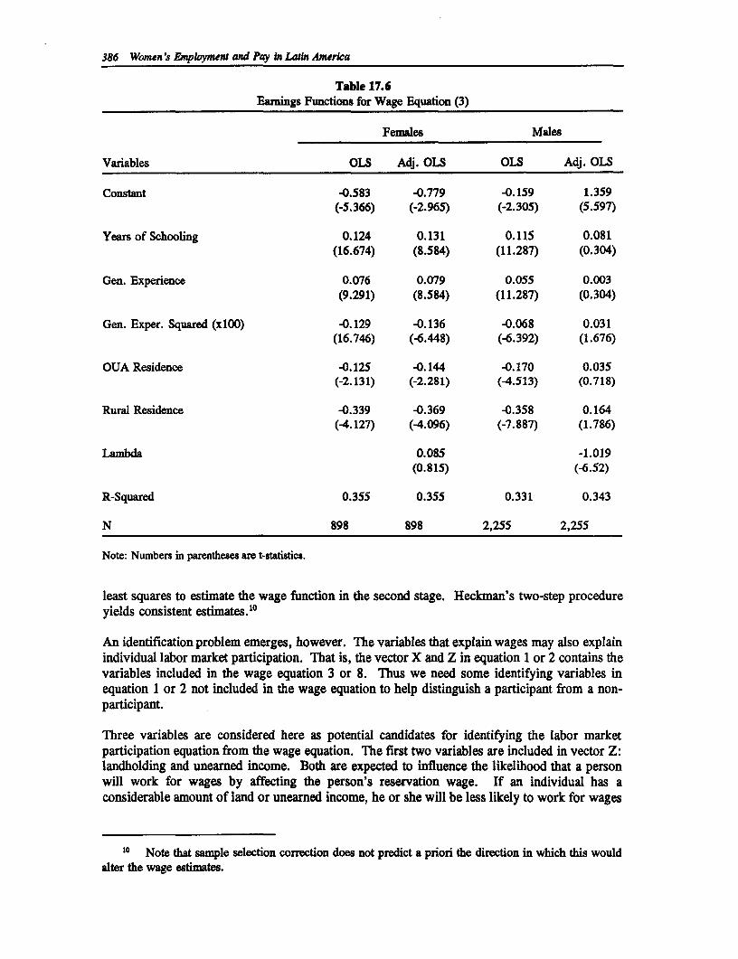
386 Women's Employment and Pay in Latin America
Table 17.6Eamings Functions for Wage Equation (3)
Females Males
Variables OLS Adj. OLS OLS Adj. OLS
Constant -0.583 -0.779 -0.159 1.359(-5.366) (-2.965) (-2.305) (5.597)
Years of Schooling 0.124 0.131 0.115 0.081(16.674) (8.584) (11.287) (0.304)
Gen. Experience 0.076 0.079 0.055 0.003(9.291) (8.584) (11.287) (0.304)
Gen. Exper. Squared (xlOO) -0.129 -0.136 -0.068 0.031(16.746) (-6.448) (-6.392) (1.676)
OUA Residence -0.125 -0.144 -0.170 0.035(-2.131) (-2.281) (4.513) (0.718)
Rural Residence -0.339 -0.369 -0.358 0.164(-4.127) (-4.096) (-7.887) (1.786)
Lambda 0.085 -1.019(0.815) (-6.52)
R-Squared 0.355 0.355 0.331 0.343
N 898 898 2,255 2,255
Note: Numbers in parentheses are t-statistics.
least squares to estimate the wage function in the second stage. Heckman's two-step procedure
yields consistent estimates.' 0
An identification problem emerges, however. The variables that explain wages may also explain
individual labor market participation. That is, the vector X and Z in equation 1 or 2 contains the
variables included in the wage equation 3 or 8. Thus we need some identifying variables in
equation 1 or 2 not included in the wage equation to help distinguish a participant from a non-
participant.
Three variables are considered here as potential candidates for identifying the labor market
participation equation from the wage equation. The first two variables are included in vector Z:
landholding and unearned income. Both are expected to influence the likelihood that a person
will work for wages by affecting the person's reservation wage. If an individual has a
considerable amount of land or unearned income, he or she will be less likely to work for wages
10 Note that sample selection correction does not predict a priori the direction in which this wouldalter the wage estimates.
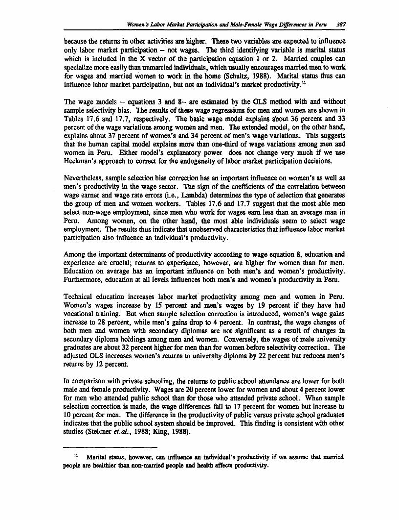
Women's Labor Market Parlicipation and Male-Female Wage Differences in Peru 387
because the returns in other activities are higher. These two variables are expected to influenceonly labor market participation - not wages. The third identifying variable is marital statuswhich is included in the X vector of the participation equation 1 or 2. Married couples canspecialize more easily than unmarried individuals, which usually encourages married men to workfor wages and married women to work in the home (Schultz, 1988). Marital status thus caninfluence labor market participation, but not an individual's market productivity."
The wage models - equations 3 and 8- are estimated by the OLS method with and withoutsample selectivity bias. The results of these wage regressions for men and women are shown inTables 17.6 and 17.7, respectively. The basic wage model explains about 36 percent and 33percent of the wage variations among women and men. The extended model, on the other hand,explains about 37 percent of women's and 34 percent of men's wage variations. This suggeststhat the human capital model explains more than one-third of wage variations among men andwomen in Peru. Either model's explanatory power does not change very much if we useHeckman's approach to correct for the endogeneity of labor market participation decisions.
Nevertheless, sample selection bias correction has an important influence on women's as well asmen's productivity in the wage sector. The sign of the coefficients of the correlation betweenwage earner and wage rate errors (i.e., Lambda) determines the type of selection that generatesthe group of men and women workers. Tables 17.6 and 17.7 suggest that the most able menselect non-wage employment, since men who work for wages earn less than an average man inPeru. Among women, on the other hand, the most able individuals seem to select wageemployment. The results thus indicate that unobserved characteristics that influence labor marketparticipation also influence an individual's productivity.
Among the important determinants of productivity according to wage equation 8, education andexperience are crucial; returns to experience, however, are higher for women than for men.Education on average has an important influence on both men's and women's productivity.Furthermore, education at all levels influences both men's and women's productivity in Peru.
Technical education increases labor market productivity among men and women in Peru.Women's wages increase by 15 percent and men's wages by 19 percent if they have hadvocational training. But when sample selection correction is introduced, women's wage gainsincrease to 28 percent, while men's gains drop to 4 percent. In contrast, the wage changes ofboth men and women with secondary diplomas are not significant as a result of changes insecondary diploma holdings among men and women. Conversely, the wages of male universitygraduates are about 32 percent higher for men than for women before selectivity correction. Theadjusted OLS increases women's returns to university diploma by 22 percent but reduces men'sreturns by 12 percent.
In comparison with private schooling, the returns to public school attendance are lower for bothmale and female productivity. Wages are 20 percent lower for women and about 4 percent lowerfor men who attended public school than for those who attended private school. When sampleselection correction is made, the wage differences fall to 17 percent for women but increase to10 percent for men. The difference in the productivity of public versus private school graduatesindicates that the public school system should be improved. This finding is consistent with otherstudies (Stelcner et.al., 1988; King, 1988).
11 Mrital status, however, can influence an individual's productivity if we assume that marriedpeople are healthier than non-married people and health affects productivity.
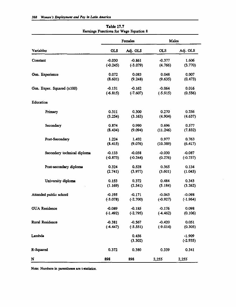
388 Women's Employment and Pay in Latin America
Table 17.7Earnings Functions for Wage Equation 8
Females Males
Variables OLS Adj. OLS OLS Adj. OLS
Constant -0.030 -0.861 -0.377 1.606(-0.245) (-3.079) (4.766) (3.770)
Gen. Experience 0.072 0.083 0.048 0.007(8.601) (9.248) (9.635) (0.473)
Gen. Exper. Squared (x1OO) -0.131 -0.162 -0.064 0.016(-6.815) (-7.607) (-5.915) (0.556)
Education
Primary 0.311 0.300 0.270 0.256(3.254) (3.163) (4.904) (4.637)
Secondary 0.874 0.990 0.696 0.577(8.434) (9.094) (11.246) (7.832)
Post-Secondary 1.224 1.432 0.977 0.763(8.415) (9.076) (10.389) (6.417)
Secondary technical diploma -0.133 -0.038 -0.030 -0.087(-0.873) (-0.244) (0.276) (-0.757)
Post-secondary diploma 0.324 0.528 0.365 0.134(2.741) (3.977) (3.601) (1.043)
University diploma 0.153 0.372 0.484 0.343(1.169) (2.541) (5.184) (3.262)
Attended public school -0.195 -0.171 -0.043 -0.098(-3.078) (-2.700) (-0.927) (-1.964)
OUA Residence -0.089 -0.185 -0.176 0.098(-1.492) (-2.795) (-4.462) (0.106)
Rural Residence -0.381 -0.567 -0.420 0.051(-4.447) (-5.551) (-9.014) (0.305)
Lambda 0.456 -1.909(3.302) (-2.935)
R-Squared 0.372 0.380 0.339 0.341
N 898 898 2,255 2,255
Note: Numbers in parentheses are t-statistics.
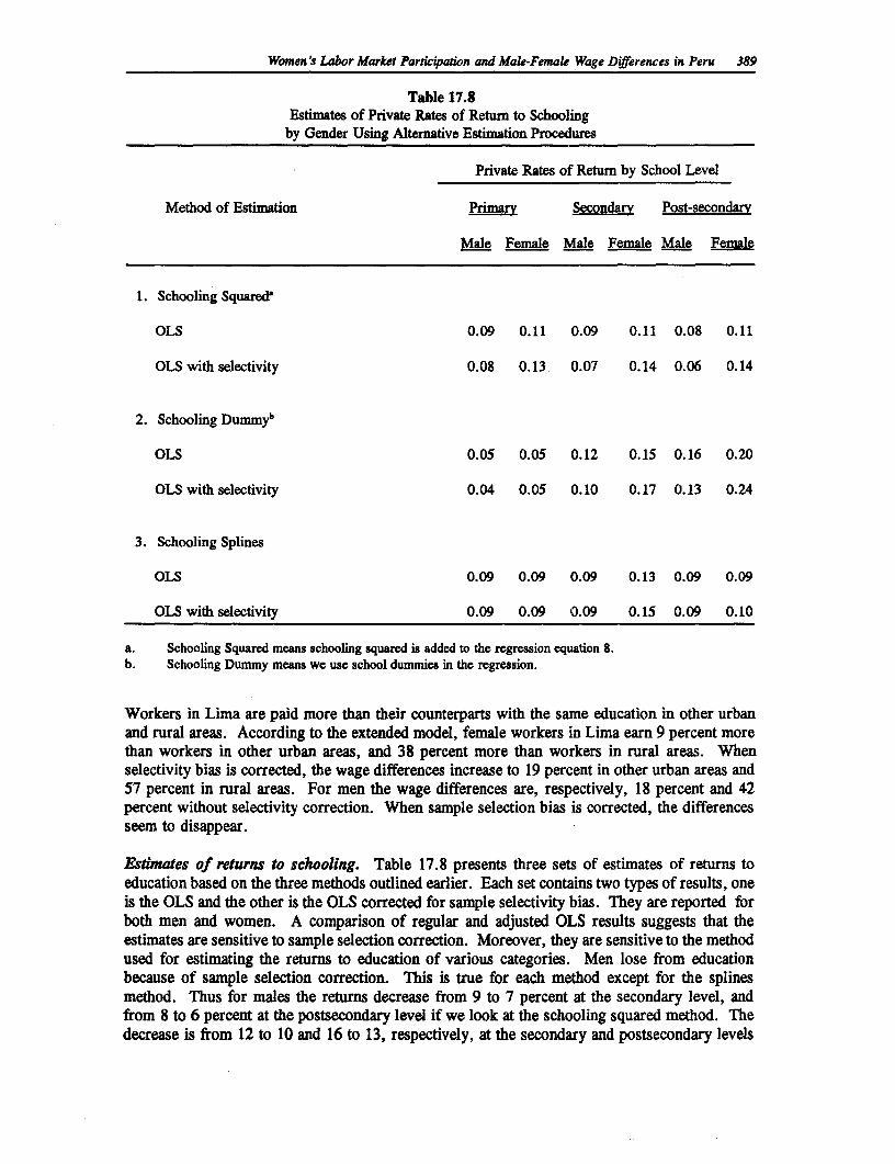
Women's Labor Market Partic4ation and Male-Female Wage Differences in Peru 389
Table 17.8Estimates of Private Rates of Return to Schooling
by Gender Using Alternative Estimation Procedures
Private Rates of Return by School Level
Method of Estimation Primrv Secondarv Post-secondary
Male Female Male Female Male Female
1. Schooling Squared"
OLS 0.09 0.11 0.09 0.11 0.08 0.11
OLS with selectivity 0.08 0.13. 0.07 0.14 0.06 0.14
2. Schooling Dummyb
OLS 0.05 0.05 0.12 0.15 0.16 0.20
OLS with selectivity 0.04 0.05 0.10 0.17 0.13 0.24
3. Schooling Splines
OLS 0.09 0.09 0.09 0.13 0.09 0.09
OLS with selectivity 0.09 0.09 0.09 0.15 0.09 0.10
a. Schooling Squared means schooling squared is added to the regression equation 8.b. Schooling Dummy means we use school dummies in the regression.
Workers in Lima are paid more than their counterparts with the same education in other urbanand rural areas. According to the extended model, female workers in Lima earn 9 percent morethan workers in other urban areas, and 38 percent more than workers in rural areas. Whenselectivity bias is corrected, the wage differences increase to 19 percent in other urban areas and57 percent in rural areas. For men the wage differences are, respectively, 18 percent and 42percent without selectivity correction. When sample selection bias is corrected, the differencesseem to disappear.
Estimates of returns to schooling. Table 17.8 presents three sets of estimates of returns toeducation based on the three methods outlined earlier. Each set contains two types of results, oneis the OLS and the other is the OLS corrected for sample selectivity bias. They are reported forboth men and women. A comparison of regular and adjusted OLS results suggests that theestimates are sensitive to sample selection correction. Moreover, they are sensitive to the methodused for estimating the returns to education of various categories. Men lose from educationbecause of sample selection correction. This is true for each method except for the splinesmethod. Thus for males the returns decrease from 9 to 7 percent at the secondary level, andfrom 8 to 6 percent at the postsecondary level if we look at the schooling squared method. Thedecrease is from 12 to 10 and 16 to 13, respectively, at the secondary and postsecondary levels
390 Women's Employment and Pay in Latin America
with the schooling dummy approach. Women, on the other hand, gain in almost all approachesused for calculating the school returns. For women the returns increase from 11 to 14 both atsecondary and postsecondary levels when the schooling squared technique is used. For womenthe gain is the largest at the postsecondary level under the dummy schooling method, i.e., theincrease is from 20 to 24 percent when sample selection correction is made.
The differences among three alternative methods for calculating the returns to education ofdifferent categories are substantial. As expected, the return to schooling is biased downward atthe primary level with the dummy variable method. The OLS estimate of the returns to primaryeducation is 5 percent for both men and women under the dummy schooling method, while it is9 percent for both men and women with the splines method. In contrast, the returns are 9percent for men and 11 percent for women using the schooling squared method. As the schoolingsquared method gives equal weight to both primary and post-primary education it seems tooverestimate the returns to primary education. The schooling dummy method registers a muchhigher return for both secondary and postsecondary education than any other method for bothmen and women. Thus the return to postsecondary education for women is 24 percent comparedto 14 and 10 percent under squared and splines methods, respectively. The results, therefore,show that the estimates of the returns to education vary remarkably with the kind of method usedfor calculating these estimates.
T'he differences in returns to schooling for men and women are also worth noting. The returnsto schooling are higher for women than for men, especially at the secondary and postsecondarylevel. This is true for all three methods used for calculating the returns to schooling. Thisfinding contrasts with studies from other countries that suggest that the returns to schooling aresimilar for men and women (Schultz, 1989). The return to schooling is higher for women at thesecondary level than at any other level with the splines method, a result which is consistent withother Latin American and Asian countries (Schultz, 1988; Mohan, 1986). However, with thedummy and squared methods, the return to schooling is higher for women at the postsecondarylevel than at any other level.
6. Male-Female Wage Differences
A large number of studies based on United States' data and a few studies from developingcountries attempt to identify the extent of male-female wage differences that is explained bydifferences in human capital and other observed job-related characteristics (Becker, 1985; Birdsalland Fox, 1985; Gronau, 1988; Mincer and Polachek, 1974; Oaxaca, 1973; Gannicott, 1986). Onestandard procedure to measure the male-female wage gap is to fit equation 3 or 8 by ordinaryleast squares separately to a sample of male (m) and female (f) workers as follows:
lnWm = B.m & + e(9)and
InWf = Xf Bf + ef (10)
where: B. and Bf are the vectors of unknown coefficients, including the intercepts; X. and Xfwhich are, respectively, the vector of males' and females' observed characteristics; and em andef are, respectively, the males' and females' individual specific error. A property of ordinaryleast squares is that the regression lines pass through the mean values of the variables so that:
lnW, = Xm B. (11)
InW= X, if (12)
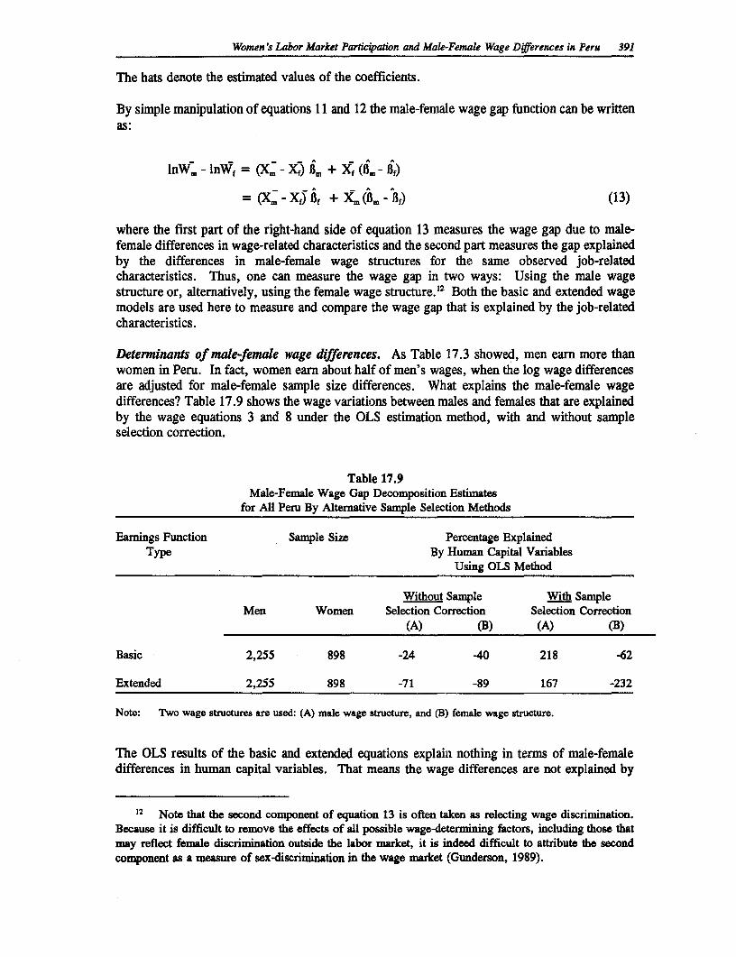
Women's Labor Market Participation and Male-Female Wage Differences in Peru 391
The hats denote the estimated values of the coefficients.
By simple manipulation of equations 11 and 12 the male-female wage gap function can be writtenas:
InW 1 - In-Wf = (X - Xf) ir + Xf (im - f)
(Xm Xf) f + X,, (B. -"if) (13)
where the first part of the right-hand side of equation 13 measures the wage gap due to male-female differences in wage-related characteristics and the second part measures the gap explainedby the differences in male-female wage structures for the same observed job-relatedcharacteristics. Thus, one can measure the wage gap in two ways: Using the male wagestructure or, alternatively, using the female wage structure."2 Both the basic and extended wagemodels are used here to measure and compare the wage gap that is explained by the job-relatedcharacteristics.
Determinants of mate-female wage differences. As Table 17.3 showed, men earn more thanwomen in Peru. In fact, women earn about half of men's wages, when the log wage differencesare adjusted for male-female sample size differences. What explains the male-female wagedifferences? Table 17.9 shows the wage variations between males and females that are explainedby the wage equations 3 and 8 under the OLS estimation method, with and without sampleselection correction.
Table 17.9Male-Female Wage Gap Decomposition Estimates
for All Peru By Alternative Sample Selection Methods
Earnings Function Sample Size Percentage ExplainedType By Human Capital Variables
Using OLS Method
Without Sample With SampleMen Women Selection Correction Selection Correction
(A) (B) (A) (B)
Basic 2,255 898 -24 -40 218 -62
Extended 2,255 898 -71 -89 167 -232
Note: Two wage structures are used: (A) male wage structure, and (B) female wage structure.
The OLS results of the basic and extended equations explain nothing in terms of male-femaledifferences in human capital variables. That means the wage differences are not explained by
12 Note that the second component of equation 13 is often taken as relecting wage discrimination.Because it is difficult to remove the effects of all possible wage-determining factors, including those thatmay reflect female discrimination outside the labor market, it is indeed difficult to attribute the secondcomponent as a measure of sex-discrimination in the wage market (Gunderson, 1989).
392 Women's Employment and Pay in Latin America
male-female differences in job-related characteristics, but by differences in the wage structures.In fact, wage structures for men and women are so different that women are not paid consistentlyaccording to their human capital endowment. Thus, human capital differences produce evennegative contributions in the calculation of male-female wage differences. However, when thesample selection correction is applied and male wage structure is used to calculate the wage gap,the model explains more than 100 percent of the differences in wages in terms of the differencesin job-related characteristics. This method includes, in addition with the standard variables, acorrelation factor that measures the relationship between the errors of the wage equation and thelabor market participation. This result suggests that the unobserved characteristics that influenceboth the labor market participation and productivity explain fully the male-female wagedifferences in Peru."3 However, when female wage structure is used to calculate the wage gap,even sample selection correction does not help the human capital model to explain the wage gapthat exists in Peru. If the unobserved characteristics explain the wage gap, it follows that weneed to identify more observable characteristics of a worker other than his or her human capitalvariables to explain the male-female wage differences that exist in Peru."4
7. Discussion
This paper addresses four critical questions. First, what influences men and women to participatein the labor market? Although education and training raise labor market participation of bothmen and women, vocational training and secondary school increase the labor market participationof women more than that of men. Thus, improving education for women can increase theirparticipation faster than a similar increase in men's education would affect the participation ofmen. Unearned income and landholding reduce the participation of both men and women. Theprobability of being in the wage sector is high for married men and low for married women,indicating an expected job specialization after marriage.
Second, what determines the productivity of men and women in the wage market? Experience,education, and training are all effective. The quality of education is also significant: Thoseemployees educated in private schools are more productive than those with a public schooleducation. Moreover there are sharp regional differences in productivity. Men and women fromother urban areas and rural areas are paid less than their counterparts in Lima. The extent ofmale-female differences in productivity depends on the impact of sample selectivity bias.
Third, is there any systematic gender bias in the estimated returns to schooling if we ignore thepossible sample selection rule of who is a wage earner? The results suggest that sample selectioncorrection decreases the returns to schooling for men but increases them for women. Sampleselection bias is substantial for both men and women, showing that the selected wage earners arenot a random sample. The magnitude and direction of the bias, however, vary by method used
13 This is an interesting finding because it does not include any controversial control variable suchas occupational status in the wage regression. The wage function includes an additional variable--thesample selection correction factor--that accounts for the unobserved characteristics influencing labor marketparticipation.
14 Even controlling the wage equation for occupational differences which may imply some variationsin unobserved characteristics does not solve the puzzle of why men earn more than women in Peru.Although occupational status is a choice variable, we control for it's effect in the wage equation byincluding a number of occupational dummies. This method still does not alter the conclusion of this study.
Women's Labor Market Partication and Male-Female Wage Differences in Peru 393
for the calculation of these returns. The returns to schooling are higher for women at theprimary school level. The results confirm that sample selection bias is an important factor inlabor market participation. The most able men select non-wage employment, while the most ablewomen select wage employment.
And finally, why do men earn more than women? Although there are some differences in humancapital, the extent to which these differences explain the wage gap depends critically on sampleselection correction factors and the wage structure used to calculate the wage gap. Thus whensample selection correction is not included in the wage regression of a random sample of malesand females, the human capital model does not explain any portion of the wage gap that existsin Peru. This is true no matter whether we use the male or female wage structure to calculatethe wage gap. When the correction factor is included and the male wage structure is used, themodel explains 100 percent of the wage gap. This suggests that the unobserved characteristicsthat influence labor market participation and productivity also affects the productivity differencesbetween males and females. Clearly it would be useful to identify other observable characteristicsthat affect wage differences.
Two policy implications that result from our answers to these questions should be mentioned.First, since public schools are less effective than private schools in raising productivity andreducing the wage gap, policymakers should take steps to make the public school system moreeffective.
Second, as the school returns are higher for women than for men, parents should invest equally,if not more, in female education. However, the PLSS survey data indicate that parents enrollmore male than female children in schools, especially at the secondary level (Schafgans, 1990).This clearly supports the notion that school investment in children is not gender neutral, nor isit governed by the private rate of returns to schooling for men and women. Apart from equityreasons, there is a strong case for an efficiency-based argument for investing more equally inmale and female children. The results of this paper indicate that investments in education andtraining for women raise their participation and productivity in the labor market more than asimilar investment in men's education. In addition, these investments reduce fertility, improvingthe education of children and the health and nutrition of all family members. Thus human capitalinvestment in women is a high return activity and at least as good as an equivalent investmentin men. The government, therefore, must identify ways to channel more resources towardwomen's education.
References
Becker, G.S. Human Capital. New York: Columbia University Press, 1964.
"A Theory of the Allocation of Time." Economic Journal, Vol. 75 (1965). pp. 493-517.
----. "Human Capital, Effort and the Sexual Division of Labor." Journal of Labor Economics,Vol. 3 (1985). pp. 533-558.
Behrman, J.R. and N. Birdsall. "The Quality of Schooling." American Economic Review, Vol.73, no. 5 (1983). pp. 928-946.
Birdsall, N. and M.L. Fox. "Why Males Earn More." Economic Development and CulturalChange, Vol. 33, no. 3 (1985). pp. 533-556.
Dagsvik, J. and Aaberge, R. 1990. "Household Production, Time Allocation, and Welfare inPeru." PRE Working Paper No. 503. Washington, D.C.: World Bank, 1990.
Gannicott, K. "Women, Wages and Discrimination: Some Evidence from Taiwan." EconomicDevelopment and Cultural Change, Vol. 39, no. 4 (1986). pp. 721-730.
Grootaert, C. and A.M. Arriagada. "The Peruvian Livings Standards Survey: An AnnotatedQuestionnaire." Washington, D.C.: World Bank, 1986.
Griliches, Z. "Estimating Returns to Schooling: Some Econometric Problems." Econometrica,Vol. 45, no.1 (1977). pp. 1-22.
Gronau, R. "Sex-related Wage Differentials and Women's Interrupted Labor Careers - TheChicken or the Egg." Journal of Labor Economics, Vol. 6 (1988). pp. 277-301.
Gunderson, M. "Male-female Wage Differentials and Policy Responses." Journal of EconomicLiterature, Vol. 27 (1989). pp. 46-72.
Heckman, J. "Sample Selection Bias as a Specification Error." Econometrica, Vol. 47, January(1979). pp. 153-161.
Khandker, S.R. "Labor Market Participation of Married Women in Bangladesh." Review ofEconomics and Statistics, Vol. 71 (1987). pp. 536-541.
394
Women's Labor Market Participation and Male-Female Wage Differences in Peru 395
King, E.M. "Does Education Pay in the Labor Force." PHREE Working Paper. Washington,D.C.: World Bank, 1988.
King, E.M. and R. Bellew. "Gains in the Education of Peruvian Women, 1940 to 1980." PREWorking Paper No. 472. Washington, D.C.: World Bank, 1990.
Maddala, G.S. Limited-dependent and Qualitative Variables in Econometrics. New York:Cambridge University Press, 1983.
Mincer, J. Schooling, Experience and Earnings. New York: Columbia University Press, 1974.
Mincer, J. and S. Polachek. "Family Investments in Human Capital: Earnings of Women."Journal of Political Economy, Vol. 82 (1974). pp. S76-S108.
Mohan, R. Work, Wages and Welfare in a Developing Metropolis. New York: Oxford UniversityPress, 1986.
Newman, J. "Labor Market Activitiy in Cote d'Ivoire and Peru." LSMS Working Paper No. 36.Washington, D.C.: World Bank, 1987.
Oaxaca, R. "Male-female Wage Differentials in Urban Labor Markets." International EconomicReview, Vol. 14, no. 1 (1973). pp. 693-709.
Psacharopoulos, G. "Returns to Education: An Updated International Comparison." ComparativeEducation, Vol. 11, no. 3 (1981). pp. 321-341.
Robb, R. "Earnings Differentials between Males and Females in Ontario, 1971." CanadianJournal of Economics, Vol. 11, no. 2 (1978). pp. 350-359.
Rosen, S. "Hedonic Functions and Implicit Markets." Journal of Political Economy, Vol. 82(1974). pp. 34-55.
Schafgans, M.M.A. "A Comparison of Men and Women in the Labor Force in Peru." in B. Herzand S. Khander (eds.). Women's Work, Education and Welfare in Peru. Forthcoming.
Schultz, T.P. "Women and Development: Objectives, Framework, and Policy Interventions."PHR Working Paper. Washington, D.C.: World Bank, 1989.
-. "Educational Investment and Returns." in H. Chenery and T.N. Srinivasan (eds.).Handbook of Development Economics, Vol. 1. Amsterdam: North Holland, 1988.
Stelcner, M., A.M. Arriagada, and P. Mook. "Wage Determinants and School AttainmentAmong Men in Peru." LSMS Working Paper No. 41. Washington, D.C.: World Bank,1988.
Suarez-Berenguela, R. "Peru Informal Sector, Labor Markets, and Returns to Education." LSMSWorking Paper No. 32. Washington, D.C.: World Bank, 1987.
World Bank. "Peru, Politices to Stop Hyperinflation and Initiate Economic Recovery."Mimeograph. Country Study Series. Washington, D.C.: World Bank, 1989.

18
Is there Sex Discrimination in Peru?Evidence from the 1990 Lima Living Standards
Survey
Indennit A. GiMl
1. Introduction
Allegations of imperfectly functioning labor markets have been commonplace in the literature formany years. Researchers have struggled to provide reliable estimates of discrimination againstwomen, racial and ethnic minorities, of the degree of segmentation in labor markets byoccupation and location, and the effects of government intervention on these 'market failures."For example, it has been argued that while the government often creates jobs that are protectedfrom market forces, it also -- sometimes simultaneously - serves as an employer for "unfairly"disadvantaged groups such as women.
This chapter readdresses these issues using a somewhat novel approach: It combines analysis ofone form of alleged labor market failure - gender discrimination - with the examination ofanother facet - segmentation of the labor market by type of employer. More precisely, I examineif the degree to which similar observed skills of men and women are differentially rewardeddepends upon whether an individual works in the wage sector or as a self-employed worker. Thisprovides crude indicators of two forms of market imperfection: First, it throws up first-roundestimates of the differences in returns to human capital (schooling, general work experience, andjob-specific skills) of the self-employed and wage workers. Since in Peru these classes roughlycorrespond to the informal and formal sector, respectively, the results can be used to determinewhether the pecuniary rewards to human capital differ across sectors, i.e., whether the labormarket is occupationally segmented. Second, it provides a preliminary measure of gender biasesin remuneration under differing employment regimes, indicating whether the gender gap inearnings is driven by market structure or skill differentials.
Uncovering differences by employment type and gender is just the first step, though. There aregood reasons to believe that while self-employment is often harder to initiate than paidemployment (because it may require high startup costs), it provides workers with relativelyflexible work schedules. Married and cohabiting women (who, facts indicate, often balance two
397
398 Women's Employment and Pay in Latin America
careers - household and market work) are very likely to benefit from this flexibility.' Theupshot of the discussion is that while married women are better suited for self-employment orinformal market work, single women and men constitute relatively 'fungible' human capital.Standard measures of skills must be augmented by considerations of gender and marital status instudying the effectiveness of skill accumulation (investment in human capital) as a welfareenhancing device. Not realizing this will lead to inefficient policy design.
A number of studies have been written on the Peruvian labor market in the years since the1985-86 Peruvian Living Standards Survey results were made available. Labor marketparticipation of Peruvian men and women, their schooling decisions and earnings determinants,and other forms of market segmentation have been examined by a battery of capable researchers.In other words, all the favorite areas of labor economists have been explored. Why another studyon Peru? While repetition in scientific inquiry rarely needs to be justified, this study more thanjust duplicates past efforts: First, while human capital effects on work participation and earningshave been repeatedly explored for men (e.g., Stelcner, Arriagada, and Moock, 1988) and forwomen (e.g., King, 1990; Khandker, 1992), explicit gender comparisons of these phenomena arerelatively rare. This study does just that. Second, as discussed above, while allegations of marketimperfection (referred to as "labor market segmentation," "duality" or "sex discrimination") areimplicit in many studies of labor markets in Latin America, there has been no comprehensiveexamination of these aspects of market failure in a unified analytical setting. Finally, since thisstudy uses the 1990 Living Standards Survey, it is worthwhile examining whether the marketstructure revealed by these data differs substantially from that indicated by the 1985-86 survey.
To sharpen the discussion, consider the following facts:
i . While about half of the women who worked in the market were self-employed, onlyabout a third of men were self-employed.
2. Both wage and self-employed males worked about 48 hours per week, while self-employed women worked about 7 hours less than wage and salaried women (35 and42 hours respectively).
3. The variance of hours worked in the salaried sector is less than half the value of thevariance of hours worked per week by the self-employed for both men and women.
4. About 62 percenit of self-employed women were married or cohabiting, as comparedwith 37 percent of wage and salaried women. For men, the ratio is 62 percent forboth classes.
5. While the female-male ratio of monthly earnings is roughly the same for wageworkers and the self-employed (about 0.62 and 0.66 respectively), the ratio forhourly earnings is much lower in the wage sector than among the self-employed(0.71 and 0.92 respectively).
The other main beneficiaries from this hours flexibility are likely to be workers with large marketskills. Wage and salaried employment generally have hour restrictions, and able workers (who have a highmarginal cost of leisure) may be forced into comer solutions. It is likely that men with unusually largeentrepreneurial skills will choose self-employment for this reason, and work longer than the medianworker.
Is There Sex Discrnmi,uton in Peru? Ewdencefrom the 1990 Lina Liwng Standards Survey 399
Using standard techniques, this study tries to explain these facts. First, the determinants of thedecision to work in the market are examined using simple univariate probit procedures.2 Theaim of the exercise is two-fold: To obtain an understanding of gender differences in the decisionto work, and to obtain a summary measure of the difference in unobserved work-choice relatedcharacteristics of workers and non-workers by computing the Mill's ratio. Then the factorsaffecting sector choice (wage work or self-employment) are examined, again using univariateprobit procedures. The aims of this exercise are to isolate the effects of marital status on sectorchoice, and to obtain summary measures differences in sector-choice related unobserved attributesof working women and men.
Second, Mincerian human capital earnings functions are estimated for all workers with andwithout sample selectivity corrections proposed by Heckman (1979), using the results of workparticipation probit regressions. Also, separate earnings functions are estimated for wage andsalaried workers and for the self-employed using a simple two-step sample selectivity correctionbased on the results of both work participation and sector choice probit procedures.
Third, using Oaxaca's (1973) technique, the explained gender gap in earnings is decomposed intotwo parts: The gap in earnings due to observed skill differences, and the differential due to agender gap in returns to similar observed skills, which constitutes the theoretical upper bound tosex discrimination in the marketplace. I also briefly examine whether industrial and occupationalsegregation by sex explains some of the observed earnings differential.
Finally, I examine the key policy implications of the analysis. The main policy implication thatemerges is that, given the nature of female work histories, policies that increase access toeducation for women may not be adequate to improve the welfare of women. These measuresmust be supplemented by encouraging female entrepreneurship (e.g, by credit subsidization),which allows women to obtain gainful employment which is more compatible with theirtraditional roles as homemakers. This does not mean that education subsidization is useless,because schooling fundamentally changes the occupations that women choose for themselves: Itincreases participation in market activities, especially in the wage sector.
2. Background
Summary statistics are presented (Table 18.1) separately for wage and salaried workers and forthe self-employed. There are compelling reasons to expect differences in levels of earnings, effortand human capital across sectors. First, self-employed earnings confound the returns of non-human capital - for which the data are poor - and the returns to human capital -which are theprimary concern of this paper. Second, differences in levels of earnings for equally skilled maleand female workers may exist in the wage sector if employers discriminate against women - asis commonly alleged --but not in the self-employed sector. Third, schooling as a signal of work-related ability is valuable only in the wage sector. If returns to schooling are higher in the wageand salaried sector than among the self-employed, this would be evidence consistent with the viewthat schooling serves at least in part as a signalling device.
2 Henceforth, for the sake of brevity, *work* refers to work other than household activities suchas housekeeping, childbearing and childcare, and nursing relatives. The intention is not to minimize theimportance of these functions, but simply to keep sentences short.
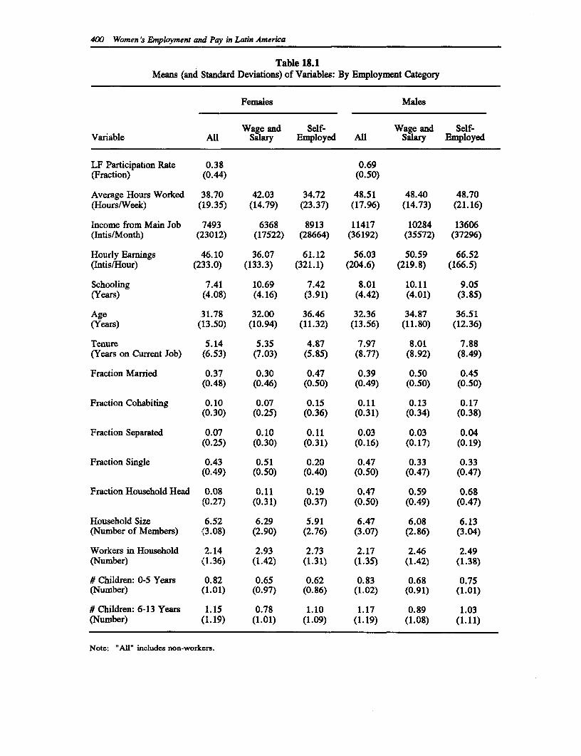
400 Women's Employment and Pay in Latin America
Table 18.1Means (and Standard Deviations) of Variables: By Emnployment Category
Females Males
Wage and Self- Wage and Self-
Variable All Salary Emnployed All Salary Emaployed
LF Participation Rate 0.38 0.69
(Fraction) (0.44) (0.50)
Average Hours Worked 38.70 42.03 34.72 48.51 48.40 48.70(Hours/Week) (19.35) (14.79) (23.37) (17.96) (14.73) (21.16)
Income from Main Job 7493 6368 8913 11417 10284 13606(Intis/Month) (23012) (17522) (28664) (36192) (35572) (37296)
Hourly Earnings 46.10 36.07 61.12 56.03 50.59 66.52(Intis/Hour) (233.0) (133.3) (321.1) (204.6) (219.8) (166.5)
Schooling 7.41 10.69 7.42 8.01 10.11 9.05(Years) (4.08) (4.16) (3.91) (4.42) (4.01) (3.85)
Age 31.78 32.00 36.46 32.36 34.87 36.51(Years) (13.50) (10.94) (11.32) (13.56) (11.80) (12.36)
Tenure 5.14 5.35 4.87 7.97 8.01 7.88(Years on Current Job) (6.53) (7.03) (5.85) (8.77) (8.92) (8.49)
Fraction Married 0.37 0.30 0.47 0.39 0.50 0.45(0.48) (0.46) (0.50) (0.49) (0.50) (0.50)
Fraction Cohabiting 0.10 0.07 0.15 0.11 0.13 0.17(0.30) (0.25) (0.36) (0.31) (0.34) (0.38)
Fraction Separated 0.07 0.10 0.11 0.03 0.03 0.04(0.25) (0.30) (0.31) (0.16) (0.17) (0. 19)
Fraction Single 0.43 0.51 0.20 0.47 0.33 0.33(0.49) (0.50) (0.40) (0.50) (0.47) (0.47)
Fraction Household Head 0.08 0.11 0.19 0.47 0.59 0.68(0.27) (0.31) (0.37) (0.50) (0.49) (0.47)
Household Size 6.52 6.29 5.91 6.47 6.08 6.13(Number of Members) (3.08) (2.90) (2.76) (3.07) (2.86) (3.04)
Workers in Household 2.14 2.93 2.73 2.17 2.46 2.49(Number) (1.36) (1.42) (1.31) (1.35) (1.42) (1.38)
# Children: 0-5 Years 0.82 0.65 0.62 0.83 0.68 0.75(Number) (1.01) (0.97) (0.86) (1.02) (0.91) (1.01)
# Children: 6-13 Years 1.15s 0.78 1.10 1.17 0.89 1.03(Number) (1. 19) (1.01) (1.09) (1. 19) (1.08) (1. 11)
Note: 'All" includes non-workers.
Is There Sex Discramination in Peru? Evidence from the 1990 Lima Living Standards Survey 401
The numbers in Table 18.1 indicate that:
1. Female labor force participation is about half of the rate for men: 38 percent to 69percent. The average hours worked per week by women are about 10 hours less thanmen. The male-female difference is about 6 hours per week for wage and salariedworkers, but about 14 hours for the self-employed. The coefficient of variation(standard deviation divided by the mean) for hours worked by self-employed womenis 0.67, compared with 0.45 for self-employed men.3 This seems to indicategreater flexibility in terms of hours of self-employment, which could be especiallyvaluable for married and cohabiting women.
2. This last inference is confirmed by the observation that while only about 35 percentof working men were self-employed, 45 percent of working women are self-employed. While 62 percent of self-employed women were married or cohabiting,61 percent of wage and salaried women were single or separated.
3. The level of schooling among the self-employed is lower for both males and femalesthan for wage sector workers. The gender gap in schooling among the self-employedis greater (1.6 years, favoring men) than for the wage sector (0.6 years, favoringwomen).
4. Self-employed workers are generally older than wage workers, but the intersectoraldifferences in tenure (years at current job) are insignificant. Men have been at theircurrent jobs about 3 years more than their female counterparts.
5. The male-female gap in average hourly earnings is greater in the wage sector (14intis per hour) than among the self-employed (5 intis per hour). Hourly earnings arehigher in the self-employed sector, even though schooling and tenure levels arehigher among salaried workers. Since part of self-employed workers' earnings arethe returns to non-human capital, this finding is not surprising.
3. Occupational Choice Decisions
The aim of this section is to analyze the determinants of the decision to choose market work, andto obtain a measure of sample selectivity that can be used (in the next section) to study thedeterminants of earnings. The central concerns are the existence and interpretation of reportedwages. For these purposes, the occupational choice of men and women can be classified intothree categories:
1. Non-market activities (household work, investment in non-job-specific humancapital, or leisure),
2. Wage and salaried employment, and
3. Self-employed market activities.
3 The coefficient of variation is 0.35 and 0.31 for wage and salaried women and men respectively.
402 Women's Employment and Pay in Latin America
This classification allows us to study two aspects of gender difference in work histories: Thedecision whether or not to participate in market work, and the choice of occupation when hoursflexibility is a desirable attribute of a job.'
The detenmnnants of work paricipahaon. The decision to participate in market work dependsupon the offered market wage, W, and the reservation wage, W. The market wage depends uponstocks of human capital (schooling, training, job-specific skills, etc.). Reservation wages dependupon the productivity of labor at home (in bearing and rearing children, looking after olderrelatives, etc.), or returns to pre-employment investment in human capital (e.g., earning adiploma) or the taste for leisure (which could depend upon the age and unearned income of theperson). Thus we can write:
P=P(W,W) (1)
where P equals 1 if the person works in the market, and 0 if the person does not. We can writethis as:
P = P (E, X, T; R, A, D; others) (2)
where E is the education level, X is previous work experience, T is job training - factorsaffecting market wage, R is unearned income, A is age, and D is the number of dependents(young children and old or infirm relatives) - factors affecting reservation wage. The signs ofthe derivatives PE, PXI PT, PR, PA and PD can be inferred from standard consumer theory.
The choice of market sector. The choice of occupation in the market sector - wage employmentor self-employment - is generally made simultaneously with the decision whether or not to workin the market sector. That is, some of the factors affecting the work participation decision alsoaffect the choice of sector of employment. Represent the sector choice decision as:
T = T (Ws, Ww) (3)
where T equals 1 if the person is self-employed, and 0 if the person is a wage worker, Ws is self-employed sector earnings, and ww is the wage sector earnings.
If employment in the wage sector requires more, or relatively rigid, hours, workers who valuehours flexibility more will prefer self-employment. Married women tend to fall into this category.But self-employment also usually requires greater non-human capital than wage employment. Soage will, in general, be positively correlated with the decision to be self-employed, both becauseof its obvious association with marital status, and because older workers have more accumulatedwealth.
The role of education in the choice of type of employment is relatively less clearcut. If schoolingserves only as a signal of innate ability to potential employers, then schooling will be more
4 It is not necessary that only one altemnative be chosen. In fact, it is likely that household workis combined with self-employment by many women.
Is There Sex Discrbninajion in Peru? Evidence from the 1990 Lima Living Standards Survey 403
valued in the wage sector. Education levels among the self-employed will be lower than amongwage and salaried workers.5
Estimation technique. In any case, variables such as education, marital status and age, whichinfluence P, also may influence T. If there are common observable influences, it is reasonableto expect that there are common unobserved variables that affect both P and T. That is, ifequations 1 and 3 are written as:
P = #,BZ, + e, (4)T= # 2Z 2 + E2 (5)
then, e, and e2 are likely to be correlated, so that probit or ordinary least squares (OLS)estimators of #, and #2 are inefficient. The solution is to estimate equations 4 and 5 using abivariate probit regression procedure. On the other hand, if the covariance between e1 and e2 iszero, then a stepwise probit procedure (in which equation 4 is estimated using data on bothworkers and non-workers, and then the sector choice probit equation is estimated using data onlyon workers) yields reliable estimates of #, and #2 .
To see whether a stepwise probit procedure is adequate, i.e., to test if:
Correlation (et, e2) = 0 (6)
I estimated equations 4 and 5 separately, and tested the hypothesis that:
Correlation (6, 4) = 0. (7)
This is not a rigorous test for deciding that a bivariate probit estimation yields the same resultsas a stepwise probit procedure. If correlation (e,, e2) is not equal to zero, then end e2computed by estimating equations 4 and 5 separately are not reliable. But if equation 7 holds, thestepwise probit provides a good approximation to the bivariate probit results without any of theadditional distributional restrictions required by this procedure.
The results showed that correlation (e;, e) was .0056 for females, and -0.0044 for males, so thehypothesis that correlation (e1, e2) = 0 cannot be rejected. In this paper, then, I report the resultsof stepwise probit estimations.6 It should not be surprising, though, to find that thesecorrelations are insignificant, even though there are (observed) common influences. If all thecommon influences are observable, then the error terms of the two equations will be uncorrelated.There are good reasons to believe that education, age, and marital status are (or closely proxy)the common factors in both the work participation and the sector choice decision.
5 There may be other reasons for this differential in schooling levels: Self-employed sector workmay require job-specific skills more than general human capital (schooling), while wage sector jobs valuegeneral skills more due to relatively rapid changes in the nature of jobs in the wage sector.
6 For bivariate probit estimations of work participation and sector choice equations for Santiago(Chile) in 1987 and Lima (Peru) in 1990, see Gill (1991b).
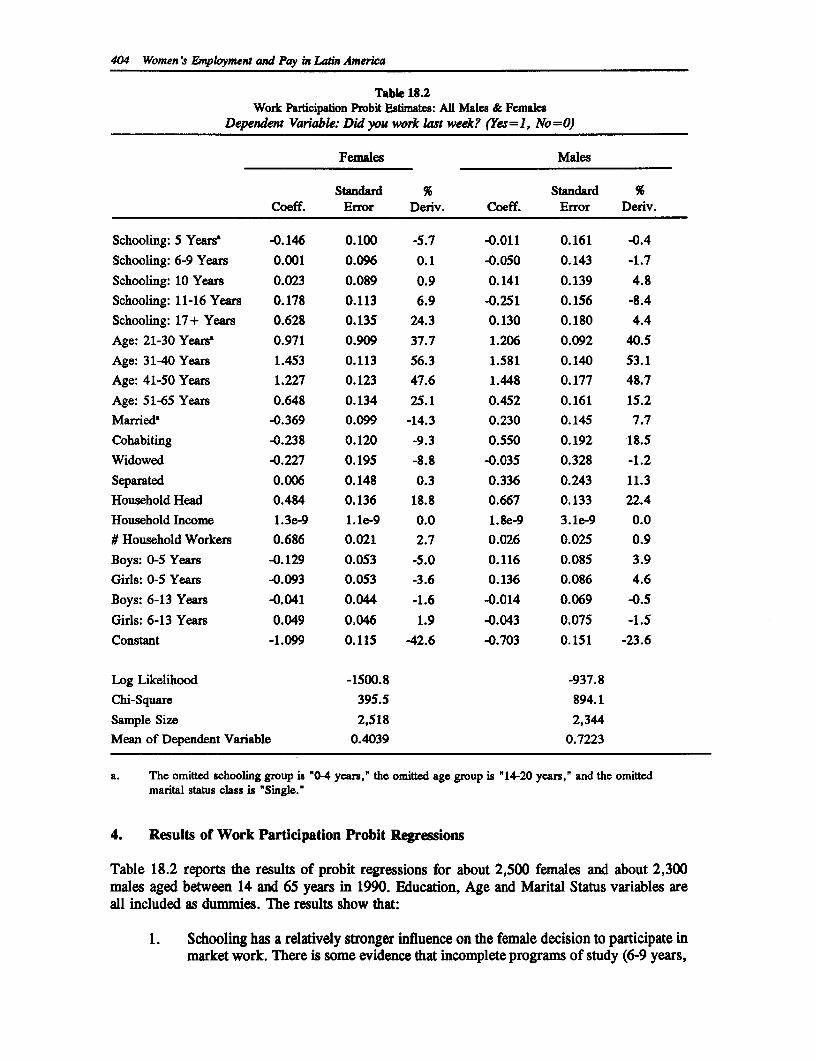
404 Women's Employment and Pay us Latin America
Table 18.2Work Participation Probit Estimatea: All Males & Females
Dependent Variable: Did you work last week? (Yes=1, No =0)
Females Males
Standard % Standard %Coeff. Error Deriv. Coeff. Error Deriv.
Schooling: 5 Years -0.146 0.100 -5.7 -0.011 0.161 -0.4
Schooling: 6-9 Years 0.001 0.096 0.1 -0.050 0.143 -1.7
Schooling: 10 Years 0.023 0.089 0.9 0.141 0.139 4.8
Schooling: 11-16 Years 0.178 0.113 6.9 -0.251 0.156 -8.4
Schooling: 17+ Years 0.628 0.135 24.3 0.130 0.180 4.4
Age: 21-30 Years 0.971 0.909 37.7 1.206 0.092 40.5
Age: 31-40 Years 1.453 0.113 56.3 1.581 0.140 53.1
Age: 41-50 Years 1.227 0.123 47.6 1.448 0.177 48.7
Age: 51-65 Years 0.648 0.134 25.1 0.452 0.161 15.2
Married^ -0.369 0.099 -14.3 0.230 0.145 7.7
Cohabiting -0.238 0.120 -9.3 0.550 0.192 18.5
Widowed -0.227 0.195 -8.8 -0.035 0.328 -1.2
Separated 0.006 0.148 0.3 0.336 0.243 11.3
Household Head 0.484 0.136 18.8 0.667 0.133 22.4
Household Income 1.3e-9 1.le-9 0.0 1.8e-9 3.le-9 0.0
# Household Workers 0.686 0.021 2.7 0.026 0.025 0.9
Boys: 0-5 Years -0.129 0.053 -5.0 0.116 0.085 3.9
Girls: 0-5 Years -0.093 0.053 -3.6 0.136 0.086 4.6
Boys: 6-13 Years -0.041 0.044 -1.6 -0.014 0.069 -0.5
Girls: 6-13 Years 0.049 0.046 1.9 -0.043 0.075 -1.5
Constant -1.099 0.115 -42.6 -0.703 0.151 -23.6
Log Likelihood -1500.8 -937.8
Chi-Square 395.5 894.1
Sample Size 2,518 2,344
Mean of Dependent Variable 0.4039 0.7223
a. The omitted schooling group is "04 years," the omitted age group is "14-20 years," and the omittedmarital status class is "Single."
4. Results of Work Participation Probit Regressions
Table 18.2 reports the results of probit regressions for about 2,500 females and about 2,300males aged between 14 and 65 years in 1990. Education, Age and Marital Status variables areall included as dummies. The results show that:
1. Schooling has a relatively stronger influence on the female decision to participate inmarket work. There is some evidence that incomplete programs of study (6-9 years,
Is There Sex Discrimination in Peru? Evidence from the 1990 Lima Living Standards Survey 405
and 11-16 years) are associated with lower male participation, probablybecause the reservation wage is increased by the expected wage gains obtained byacquiring a diploma. This result is also found for Chile (Gill, 1991a).
2. The age profile of work participation is inverse U-shaped, with women entering themarket later and staying longer. Late entry of women into the labor market isprobably due to childbirth and childrearing. Late departure may be because of thelower retirement benefits in jobs traditionally held by women, the pure income effectof lower lifetime savings of women relative to men, or the longer lifespans ofwomen.7
3. Married and cohabiting women have a labor force participation rate of about 33percent compared to a rate of 47 percent for single women (see Table 18.3). Otherthings equal, married and cohabiting men are more likely to be working in themarket than single men. Being a household head significantly increases thelikelihood of being a labor market participant for both women and men.
4. The number of workers in the household marginally, but significantly, raises theprobability of working outside the home for women. This is the opposite of what weexpected to find. The influence of household income (other than the individual's)is also inexplicably positive but insignificant. The number of young children (aged0-5 years) - conditional upon the person being married or cohabiting - is negativelyassociated with work participation for women. There is some evidence that thepresence of older girls (potential substitutes for adult females in household work)increases the probability of female market participation.
Reasonsfor not working. Table 18.4 and Appendix Table A24. 1 report reasons for not workingby marital status. Married women who are not working cite "household work" and "physicallyunable to work" as the main reasons, single women cite "studying" and "household work."Married men who don't work list "retired," "sick" or "unable to work", or 'job-related factors"as the reason. Single non-working men are generally attending school.
The sample of working men therefore differs from the male population: Male workers arerelatively old, or more experienced, and more likely to be married or cohabiting than male non-workers. The sample of working women differs from the female population: Ceteris paribus,working women are older, more likely to be unmarried, and are likely to have more educationthan non-working women.
Heckman's (1979) sample selectivity correction uses a measure of the covariance of errors in thework participation regressions and the earnings regressions to adjust for differences in unobservedcharacteristics of workers and non-workers. Working men seem to be relatively more able toacquire job experience (finding and holding onto jobs), and working women are more able thannon-workers in acquiring schooling. In analyzing the determinants of male and female earnings,it is likely that the sample selectivity correction for men will affect the coefficients measuring thereturns to experience, while for women it is likely to alter the returns to schooling.
7 This last reason is unlikely because, even though life expectancy at birth in 1988 was 65 and 61for Peruvian women and men respectively, it is very likely that life expectancy at age 14 is relativelyuniform (and considerably higher than 65 years) for the two sexes.
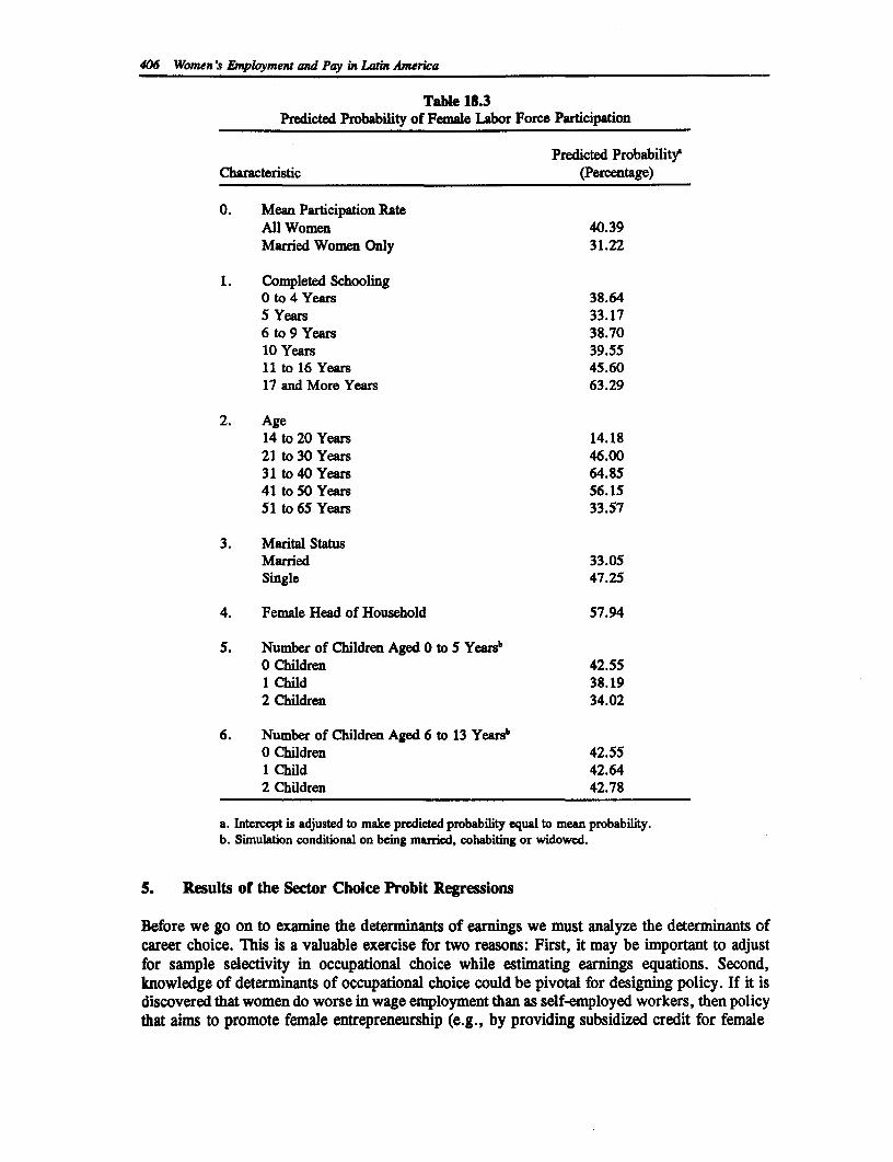
406 Women's Employment and Pay in Latin America
Table 18.3Predicted Probability of Female Labor Force Participation
Predicted Probability'Characteristic (Percentage)
0. Mean Participation RateAll Women 40.39Married Women Only 31.22
1. Completed Schooling0 to 4 Years 38.645 Years 33.176 to 9 Years 38.7010 Years 39.5511 to 16 Years 45.6017 and More Years 63.29
2. Age14 to 20 Years 14.1821 to 30 Years 46.0031 to 40 Years 64.8541 to 50 Years 56.1551 to 65 Years 33.57
3. Marital StatusMarried 33.05Single 47.25
4. Female Head of Household 57.94
5. Number of Children Aged 0 to 5 Yearsb0 Children 42.551 Child 38.192 Children 34.02
6. Number of Children Aged 6 to 13 Yearb0 Children 42.551 Child 42.642 Children 42.78
a. Intercept is adjusted to make predicted probability equal to mean probability.b. Simulation conditional on being married, cohabiting or widowed.
5. Results of the Sector Choice Probit Regressions
Before we go on to examine the determinants of earnings we must analyze the determinants ofcareer choice. This is a valuable exercise for two reasons: First, it may be important to adjustfor sample selectivity in occupational choice while estimating earnings equations. Second,knowledge of determinants of occupational choice could be pivotal for designing policy. If it isdiscovered that women do worse in wage employment than as self-employed workers, then policythat aims to promote female entrepreneurship (e.g., by providing subsidized credit for female
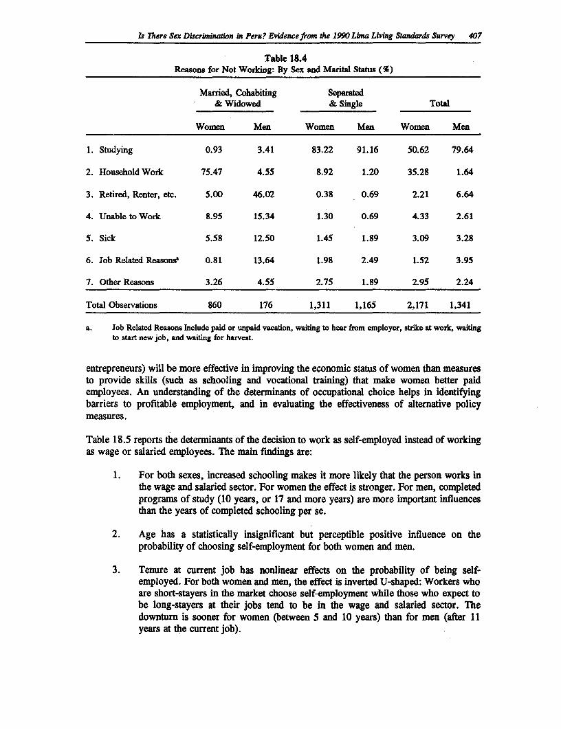
ls There Sex Discrimination in Peru? Evidencefrom the 1990Lima LivWng Standards Survey 407
Table 18.4Reasons for Not Woring: By Sex and Marital Ststus (%)
Married, Cohabiting Separtd& Widowed & Single Total
Women Men Women Men Women Men
1. Studying 0.93 3.41 83.22 91.16 50.62 79.64
2. Household Work 75.47 4.55 8.92 1.20 35.28 1.64
3. Retired, Renter, etc. 5.00 46.02 0.38 0.69 2.21 6.64
4. Unable to Work 8.95 15.34 1.30 0.69 4.33 2.61
5. Sick 5.58 12.50 1.45 1.89 3.09 3.28
6. Job Related Reasonse 0.81 13.64 1.98 2.49 1.52 3.95
7. Other Reasons 3.26 4.55 2.75 1.89 2.95 2.24
Total Observations 860 176 1,311 1,165 2,171 1,341
a. Job Related Reasons Include paid or unpaid vacation, waiting to hear from employer, strike at work, waitingto start new job, and waiting for harvest.
entrepreneurs) will be more effective in improving the economic status of women than measuresto provide skills (such as schooling and vocational training) that make women better paidemployees. An understanding of the determinants of occupational choice helps in identifyingbarriers to profitable employment, and in evaluating the effectiveness of alternative policymeasures.
Table 18.5 reports the determinants of the decision to work as self-employed instead of workingas wage or salaried employees. The main findings are:
1. For both sexes, increased schooling makes it more likely that the person works inthe wage and salaried sector. For women the effect is stronger. For men, completedprograms of study (10 years, or 17 and more years) are more important influencesthan the years of completed schooling per se.
2. Age has a statistically insignificant but perceptible positive influence on theprobability of choosing self-employment for both women and men.
3. Tenure at current job has nonlinear effects on the probability of being self-employed. For both women and men, the effect is inverted U-shaped: Workers whoare short-stayers in the market choose self-employment while those who expect tobe long-stayers at their jobs tend to be in the wage and salaried sector. Thedownturn is sooner for women (between 5 and 10 years) than for men (after 11years at the current job).
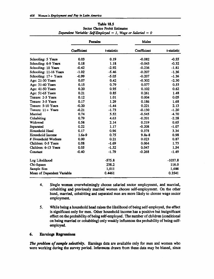
408 Women's Enmplyment and Pay in Latin America
Table 18.5Sector Choice Probit Estimates
Dependent Variabk: Sef-Employed = 1, Wage or Salaried = 0
Females Males
Coefficient t-statistic Coefficient t-statistic
Schooling: 5 Years 0.03 0.19 -0.082 -0.55Schooling: 6-9 Years 0.18 1.18 -0.043 -0.32Schooling: 10 Years -0.42 -2.92 -0.236 -1.81Schooling: 11-16 Years -1.02 -5.46 -0.207 -1.36Schooling: 17+ Years -0.99 -5.05 -0.207 -1.36Age: 21-30 Years 0.07 0.42 -0.302 -2.30Age: 31-40 Years 0.15 0.79 0.077 0.53Age: 41-50 Years 0.20 0.95 0.102 0.62Age: 51-65 Years 0.21 0.85 0.261 1.48Tenure: 2-3 Years 0.12 1.01 0.004 0.05Tenure: 3-5 Years 0.17 1.29 0.186 1.68Tenure: 5-10 Years -0.20 -1.44 0.221 2.13Tenure: 11+ Years -0.21 -1.73 -0.130 -1.20Married 0.74 5.52 -0.545 -4.70Cohabiting 0.79 4.63 -0.201 -2.28Widowed 0.58 2.14 0.219 0.65Separated 0.22 1.17 -0.208 -1.07Household Head 0.17 0.96 0.378 3.34Household Income 1.6e-9 0.75 9.8e-8 0.98# Household Workers 0.00 0.21 0.023 0.87Children: 0-5 Years 0.08 -1.69 0.064 1.73Children: 6-13 Years 0.05 -1.32 0.047 1.54Constant -0.40 -1.79 -0.268 -1.49
Log Likelihood -575.8 -1037.8Chi-Square 238.2 116.0Sample Size 1,011 1,686Mean of Dependent Variable 0.4461 0.3541
4. Single women overwhelmingly choose salaried sector employment, and married,cohabiting and previously married women choose self-employment. On the otherhand, married, cohabiting and separated men are more likely to choose wage sectoremployment.
5. While being a household head raises the likelihood of being self-employed, the effectis significant only for men. Other household income has a positive but insignificanteffect on the probability of being self-employed. The number of children (conditionalon being married or cohabiting) only weakly influences the probability of being self-employed.
6. Earnings Regressions
7he problem of sample seklivity. Earnings data are available only for men and women whowere working during the survey period. Inferences drawn from these data may be biased, since
Is There Sex Discrimination in Peru? Evidencefrom the 1990 Lima Living Standards Survey 409
the sample (working women and men) may not be randomly drawn from the population (allwomen and men). For example, we know that the average woman who works is more educatedthan a woman who does not. If women are being sorted (into workers/non-workers) on the basisof observable attributes such as education, then it is likely that they are also sorted by unobservedcharacteristics. Because of this nonrepresentativeness of the studied sample, the earnings equation:
W = a + aE + a2 X + C 3X2 + C4T + Cx5V + #D + e (8)
(where E is education, X is potential work experience, T is tenure at current job, and D is amarital status variable) yields biased estimates of the coefficients.
Heckman (1979) has proposed that estimating equation 9 below instead of the above earningsfunction at least partially corrects for this sampling bias.
W = co + E + a2 X + c 3 X2 + a4T + a5 T2 + ,D +-yXI + e (9)
Equation 9 includes a new variable, XI, which is called the selectivity correction factor.Heuristically, this is a summary measure of the comparative advantage of workers over non-workers in market activities. Theory cannot ex ante tell us what sign y should be, though it isrelatively easy to interpret the coefficient. If y is negative, this implies that the unobservedattributes that make workers earn more (than their observed skills would justify) are the sameattributes that make it less likely that the person would work in the first place. Put another way,market wage offers are positively correlated with reservation wages. If y is positive, then thesample of workers have a comparative advantage in market work.
Estimates of returns to human capital based on equation 9 above are more reliable for policypurposes. To illustrate this point, consider proposals to subsidize training as a welfare increasingdevice. These proposals are of necessity based on data for workers, which show that trainedworkers earn more than untrained workers who seem otherwise identical. Using simple statisticalmethods to evaluate that returns to training may result in biased estimators of the effectivenessof training for not just for non-workers, but even for workers. The reason is that there may betrained workers who do not participate in market work, so that the earnings data are truncated.'Sample selectivity correction is required to obtain a reliable evaluation of the effectiveness of thispolicy.
VWhile on this subject of policy effectiveness and non-random assignment, it is worthwhile todistinguish between three questions listed by Heckman and Robb (1985):
1. What would be the impact of a proposed policy on earnings if people were randomly chosen tobe its beneficiaries?
2. How do the post-policy earnings of the beneficiaries compare to what they would have been inthe absence of the policy measure?
3. What would be the effect of this policy on the earnings of the beneficiaries if the future selectionrule differs from the past selection rule?
Question 1 is a special case of question 3. Both these questions are much harder to answer than question2, because they ask to forecast the increment in the eanings of beneficiaries over their prepolicy eaningswhen no selection bias characterizes enrollment while selection bias characterizes the available data.
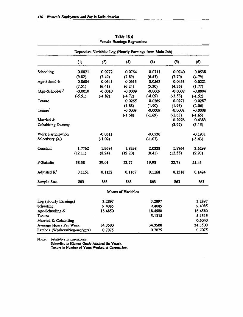
410 Women 's Employment and Pay in Latin America
Table 18.6Female Earnings Regressions
Dependent Variable: Log (Hourly Earnings from Main Job)
(1) (2) (3) (4) (5) (6)
Schooling 0.0821 0.0772 0.0764 0.0711 0.0740 0.0538(9.02) (7.49) (7.89) (6.53) (7.70) (4.79)
Age-School-6 0.0684 0.0641 0.0613 0.0568 0.0458 0.0221(7.51) (6.41) (6.24) (5.30) (4.35) (1.77)
(Age-School-6)2 -0.0010 -0.0010 -0.0009 -0.0009 -0.0007 -0.0004(-5.51) (-4.82) (-4.72) (-4.09) (-3.53) (-1.52)
Tenure 0.0265 0.0269 0.0271 0.0287(1.88) (1.90) (1.93) (2.06)
Tenure2 -0.0009 -0.0009 -0.0008 -0.0008(-1.68) (-1.69) (-1.63) (-1.65)
Married & 0.2976 0.4383Cohabiting Dummy (3.97) (5.15)
Work Participation -0.0511 -0.0536 -0.1931Selectivity (Xi) (-1.02) (-1.07) (-3.43)
Constant 1.7762 1.9684 1.8298 2.0328 1.8764 2.6299(12.11) (8.24) (12.20) (8.41) (12.58) (9.93)
F-Statistic 38.38 29.01 23.77 19.98 22.78 21.43
Adjusted R2 0.1151 0.1152 0.1167 0.1168 0.1316 0.1424
Sample Size 863 863 863 863 863 863
Means of Variables
Log (Hourly Earnings) 3.2897 3.2897 3.2897Schooling 9.4085 9.4085 9.4085Age-Schooling-6 18.4850 18.4580 18.4580Tenure 5.1315 5.1315Married & Cohabiting 0.5040Average Hours Per Week 34.3500 34.3500 34.3500Lambda (Workers/Non-workers) 0.7075 0.7075 0.7075
Notes: t-statistics in parenthesis.Schooling is Highest Grade Attained (in Years).Tenure is Number of Years Worked at Current Job.
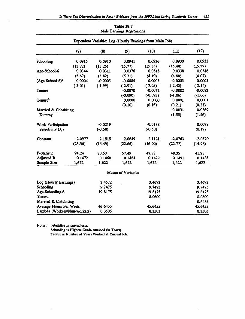
Is There Sex Discrumnaion in Peru? Evidence from the 1990 Lima Living Standards Survey 411
Table 18.7Male Earnings Regressions
Dependent Variable: Log (Hourly Eanings from Main Job)
(7) (8) (9) (10) (11) (12)
Schooling 0.0915 0.0910 0.0941 0.0936 0.0930 0.0933(15.72) (15.26) (15.77) (15.33) (15.48) (15.27)
Age-School-6 0.0344 0.0311 0.0376 0.0348 0.0338 0.0346(5.67) (3.82) (5.71) (4.10) (4.80) (4.07)
(Age-School-6)2 -0.0004 -0.0003 -0.0004 -0.0003 -0.0003 -0.0003(-3.01) (-1.99) (-2.91) (-2.05) (-2.45) (-2.14)
Tenure -0.0070 -0.0072 -0.0082 -0.0082(-0.090) (-0.093) (-1.06) (-1.06)
Tenure2 0.0000 0.0000 0.0001 0.0001(0.10) (0.15) (0.21) (0.21)
Married & Cohabiting 0.0831 0.0869Dummy (1.55) (1.46)
Work Participation -0.0219 -0.0188 0.0078Selectivity Qk) (-0.58) (-0.50) (0.19)
Constant 2.0977 2.1515 2.0649 2.1121 -2.0763 -2.0570(23.36) (16.49) (22.66) (16.00) (22.72) (14.98)
F-Statistic 94.24 70.53 57.49 47.77 48.35 41.28Adjusted R 0.1472 0.1468 0.1484 0.1479 0.1491 0.1485Sample Size 1,622 1,622 1,622 1,622 1,622 1,622
Means of Variables
Log (Hourly Eamings) 3.4672 3.4672 3.4672Schooling 9.7475 9.7475 9.7475Age-Schooling-6 19.8175 19.8175 19.8175Tenure 8.0600 8.0600Married & Cohabiting 0.6485Average Hours Per Week 46.6455 45.6455 45.6455Lambda (Workers/Non-workers) 0.3505 0.3505 0.3505
Notes: t-statistics in parenthesis.Schooling is Highest Grade Attained (in Years).Tenure is Number of Years Worked at Current Job.
412 Women's Employment and Pay in Latin America
Results of earnings regressions. This subsection discusses the results of fitting equations 8 and9 to the data for about 863 women and 1,622 men aged 15 to 65. Ideally, hourly earnings shouldbe used as the dependent variable, since it is earnings "potential" that the human capital earningsfunction tries to explain. Since hourly earnings are obtained by deflating monthly earnings byhours worked per month (actually, average hours worked per week multiplied by 4.3), andbecause the assumption of a constant wage-elasticity of hours supplied may not necessarily belegitimate, I experimented with both hourly and monthly earnings.9
Table 18.6 presents the results of hourly earnings regressions for all women, and Table 18.7 forall men. Odd-numbered columns are results of fitting equation 8, and even-numbered columnsare estimations of selectivity corrected equation 9. Monthly earnings regressions are reported inAppendix Tables A24.2 and A24.3.
The main results are:
1. The return to schooling in Lima is about 1 to 3 percentage points higher for menthan for women. While the sample selectivity correction affects the return toschooling for women, it leaves the return to schooling for men unaltered. Hourlyand monthly earnings regressions yield roughly the same rate of return to schooling.
2. The return to potential work experience (age - schooling - 6 years) is generallyhigher for women, being higher for men only when tenure at current job and maritalstatus are included as independent variables. For women, the rate of return topotential experience falls when tenure at current job is included. For men, it remainsunchanged. Sample selectivity correction lowers the returns to experience for bothmen and women.
3. Tenure at current job is always insignificant for men when potential experience isincluded in the regression, but is always significant for women, especially in themonthly wage regressions. This is because, while for men potential experience is agood continuous, interrupted careers make potential experience a poor proxy of jobskills for women. Tenure at current job contains information on job skills forwomen, but for men it is redundant when potential experience is included in theregression.
4. Married and cohabiting women and, to a lesser extent, men, are paid more thansingle and separated women and men. This result is consistent with the hypothesis
9 Suppose that the monthly earnings equation to be fitted is:
Log W = a + ,Z + ry Log H + 8 X + e
where W is monthly earnings, Z is the set of human capital variables, H is the number of hours workedper month, and 1 is the sample selectivity correction factor. Then the estimated hourly equation is:
LogW/H = a + ,BZ + dX + c, or
Log W - Log H = a + ,BZ + d X + %l.
This roughly amounts to assuming that -y = 8W/1H = 1. That is, the inverse of the supply elasticity ofhours of work is one.
Is There Scx Discruninaton in Peru? Evidencefrom the 1990 Lima Living Standards Survey 413
that unobserved social ability is positively associated with unobserved professionalability.10 Including a marital status variable reduces the coefficient on potentialexperience considerably for women; for men it does not alter this coefficient at all.
5. The coefficient for sample selectivity is negative for women, but insignificant formen in the hourly earnings regressions. For monthly earnings, the sample selectivitycoefficient is negative for both women and men, but more important for women.This implies that sample selectivity is a more severe problem when studying femaleearnings and labor supply than for males. The negative sign of this coefficientimplies that the unobserved attributes that make women more prolific in marketwork also make them less likely to be in the market (and stay at home or be inschool). For men, it implies that the unobserved characteristics that make men betterpaid also make it more likely that the worker be in school or retired.
6. The coefficient of logarithm of average hours worked per week is close to 0.4 forwomen, and about 0.3 for men. But this estimate is not reliable, since hours workedare jointly determined with wages, and this endogeneity implies that the ordinaryleast equares (OLS) estimator is biased."1
Wage workers versus the self employed. Tables 18.8 and 18.9 report the results of hourly wageequations for self-employed and waged and salaried women and men respectively, and AppendixTables A24.4 and A24.5 report the results of monthly wage regressions. These are the results offitting the equation:
W = at + aE + ot2X + a3V + 4tJ + ot5T + ,BD + yX1 + BX2 + e (10)
where E is education, X is potential work experience, T is tenure at current job, D is a maritalstatus dummy that takes the value 1 if the worker is married or cohabiting, XA is the sampleselectivity index (inverse of Mill's ratio) obtained from the work participation probit regression,and X2 is the sector choice selectivity correction factor (inverse of Mill's ratio obtained from thesector choice probit estimation).
The main results are:
1. The return to schooling for self-employed women is about 4-6 percent, considerablylower than the 8-10 percent return for salaried women. The return to schooling formen is about 9-10 percent. It seems that self-employed women operate in a relativelysegmented market.
2. The return to general experience (age adjusted by years of schooling) for men isabout 2 percent per year in both the self-employed and the wage sector. For women,the rate of return to experience (in both sectors) drops considerably when a marital
10 That is, the ability to find and sustain a relationship with a mate is positively correlated with theability to find and keep a job.
11 To correct for the endogenous nature of hours worked, I used nstumental Variables techniques.Hours worked are instrumented by using schooling, age, marital status, and number of children anddependent relatives. Since the numbers of children and old or sick relatives are likely to affect hoursworked but not wages, the equations are identifiable. The results will be reported in future work.
414 Women's Employment and Pay in Latin America
status variable is included in the regression. The likely reason is that marital statuscontains information about the work history of women (apart from potentialexperience and current tenure), since it may be correlated with frequency andduration of absence from the labor market. Since men generally participate in themarket work continuously, marital status will not add to the information onaccumulated job skills already provided by work experience and tenure.
3. The return coefficients for tenure are generally insignificant. The only exception isthe case of self-employed women, for whom the coefficient is about 4 percent butstatistically insignificant in the hourly wage regression, and 7 percent and significantin the monthly wage regression. Again, salaried women and men display similarcharacteristics, while self-employed women seem to be in a relatively distinctmarket.
4. Married and cohabiting women earn significantly higher hourly wages than womenwho are single or separated, especially in the self-employed sector. This evidenceis consistent with the argument that being married provides a source of financing forself-employment among women. In the wage sector, the premium to being marriedmay be due to the greater specialization afforded by marriage. However, it ispuzzling that married and cohabiting men earn higher wages in the wage sector,while there is no premium to being married for self-employed men.
5. Firm size, included in the estimations for self-employed workers as a proxy for theamount of non-human capital, always has a positive coefficient. The effect of firmsize on earnings is larger for women than for men.
6. Unionization has a statistically insignificant effect on wages for women and for menthe effect is positive but weak. The magnitude of the union coefficient is larger forwomen than men, indicating that collective bargaining raises women's wages morethan men's. But the statistical insignificance of the union coefficient refutes claimsthat unionization systematically raises the earnings of workers, and that the declineof unionization has worsened the position of the working class.
7. Work participation selectivity is negative for both men and women. This implies thatthe unobserved attributes that make some workers earn higher wages than theirobserved human capital would justify, are also the attributes that make it less likelythat the female or male worker works. For women, this can be interpreted to meanthat the unobserved characteristics that make women better earners in the market(relative to what their observed skills would lead us to expect) also make them moreproductive in household work or in accumulating pre-job human capital. For men,it can be interpreted to mean that attributes associated with high earnings are likelyto make them attend more school and retire earlier.
8. Sector choice selectivity is generally insignificant, which means that while self-employed and wage workers differ in their earnings-related observed attributes suchas schooling, age and marital status, they do not differ in their earnings-relatedunobserved characteristics.
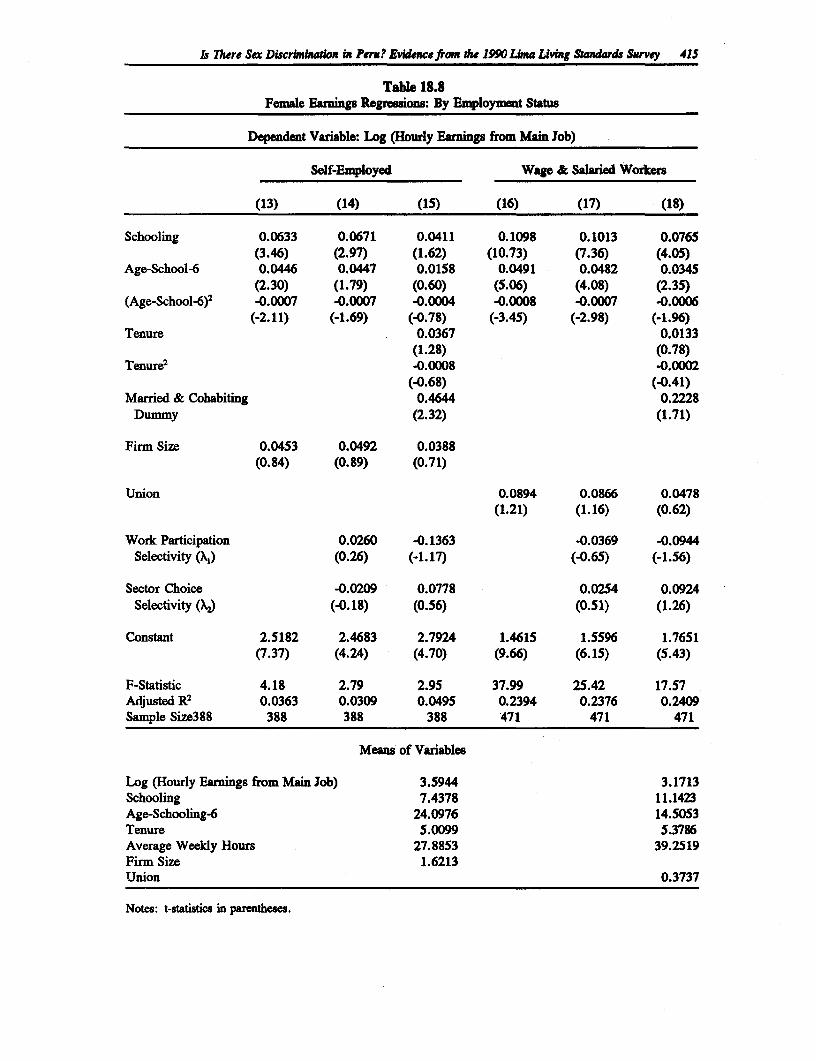
Is There Sex Discri,niution in Perm? Evidence from the 1990 ;ina Living Standardw Survey 415
Table 18.8Female Earnings Regressions: By Employment Stahts
Depdent Variable: Log (Hourly Earnings from Main Job)
Self-Employed Wage & Salaried Workers
(13) (14) (15) (16) (17) (18)
Schooling 0.0633 0.0671 0.0411 0.1098 0.1013 0.0765(3.46) (2.97) (1.62) (10.73) (7.36) (4.05)
Age-School-6 0.0446 0.0447 0.0158 0.0491 0.0482 0.0345(2.30) (1.79) (0.60) (5.06) (4.08) (2.35)
(Age-School-6)2 -0.0007 -0.0007 -0.0004 -0.0008 -0.0007 -0.0006(-2.11) (-1.69) (-0.78) (-3.45) (-2.98) (-1.96)
Tenure 0.0367 0.0133(1.28) (0.78)
Tenure2 -0.0008 -0.0002(-0.68) (-0.41)
Married & Cohabiting 0.4644 0.2228Dummy (2.32) (1.71)
Firm Size 0.0453 0.0492 0.0388(0.84) (0.89) (0.71)
Union 0.0894 0.0866 0.0478(1.21) (1.16) (0.62)
Work Participation 0.0260 -0.1363 -0.0369 -0.0944Selectivity (XA) (0.26) (-1.17) (-0.65) (-1.56)
Sector Choice -0.0209 0.0778 0.0254 0.0924Selectivity (X1) (-0.18) (0.56) (0.51) (1.26)
Constant 2.5182 2.4683 2.7924 1.4615 1.5596 1.7651(7.37) (4.24) (4.70) (9.66) (6.15) (5.43)
F-Statistic 4.18 2.79 2.95 37.99 25.42 17.57Adjusted R2 0.0363 0.0309 0.0495 0.2394 0.2376 0.2409Sample Size388 388 388 388 471 471 471
Means of Variables
Log (Hourly Earnings from Main Job) 3.5944 3.1713Schooling 7.4378 11.1423Age-Schooling-6 24.0976 14.5053Tenure 5.0099 5.3786Average Weekly Hours 27.8853 39.2519Firm Size 1.6213Union 0.3737
Notes: t-statistics in parentheses.
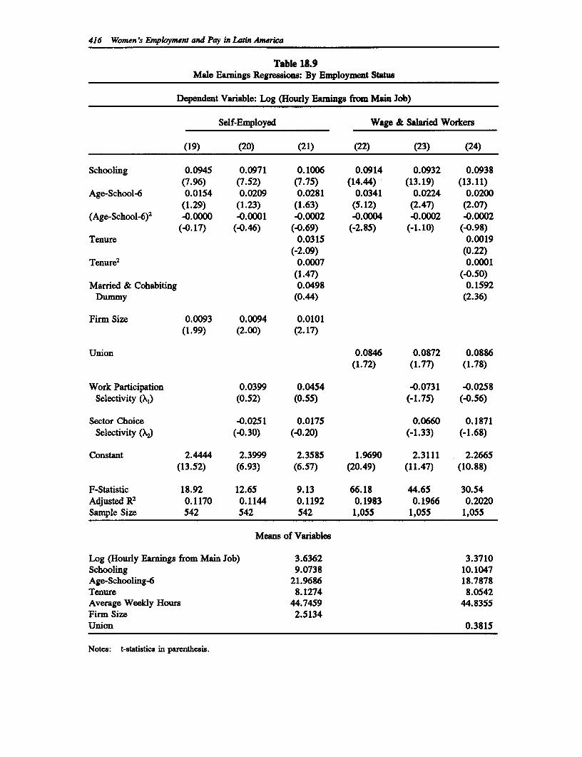
416 Women 's Employment and Pay in Latin America
Table 18.9Male Earnings Regressions: By Employment Status
Dependent Vanable: Log (Hourly Earnings from Main Job)
Self-Employed Wage & Salaried Workers
(19) (20) (21) (22) (23) (24)
Schooling 0.0945 0.0971 0.1006 0.0914 0.0932 0.0938(7.96) (7.52) (7.75) (14.44) (13.19) (13.11)
Age-School-6 0.0154 0.0209 0.0281 0.0341 0.0224 0.0200(1.29) (1.23) (1.63) (5.12) (2.47) (2.07)
(Age-School-6)2 -0.0000 -0.0001 -0.0002 -0.0004 -0.0002 -0.0002(-0.17) (-0.46) (-0.69) (-2.85) (-1.10) (-0.98)
Tenure 0.0315 0.0019(-2.09) (0.22)
Tenure2 0.0007 0.0001(1.47) (-0.50)
Married & Cohabiting 0.0498 0.1592Dummy (0.44) (2.36)
Firm Size 0.0093 0.0094 0.0101(1.99) (2.00) (2.17)
Union 0.0846 0.0872 0.0886(1.72) (1.77) (1.78)
Work Participation 0.0399 0.0454 -0.0731 -0.0258Selectivity (X1) (0.52) (0.55) (-1.75) (-0.56)
Sector Choice -0.0251 0.0175 0.0660 0.1871Selectivity (X2) (-0.30) (-0.20) (-1.33) (-1.68)
Constant 2.4444 2.3999 2.3585 1.9690 2.3111 2.2665(13.52) (6.93) (6.57) (20.49) (11.47) (10.88)
F-Statistic 18.92 12.65 9.13 66.18 44.65 30.54Adjusted R2 0.1170 0.1144 0.1192 0.1983 0.1966 0.2020Sample Size 542 542 542 1,055 1,055 1,055
Means of Variables
Log (Hourly Earnings from Main Job) 3.6362 3.3710Schooling 9.0738 10.1047Age-Schooling-6 21.9686 18.7878Tenure 8.1274 8.0542Average Weekly Hours 44.7459 44.8355Firm Size 2.5134Union 0.3815
Notes: t-statistics in parenthesis.
Is There Sex Discrimination in Peru? Evidencefrom the 1990 Lbna Living Standards Survey 417
5. Accounting for the Earnings Differential
The Oaxaca decomposition. Table 18.10 below provides the results of the Oaxacadecomposition of earnings into the part due to endowed skill differences and the part due todifferences in the returns to these skills. The evidence broadly indicates that much of the earningsdifferences are because of the latter. That is, skill differences between men and women explainonly about 10 to 15 percent of the difference in earnings; the rest is attributable to differentialrewards to human capital. The choice of index type does not seem to affect this result very much.
The results for salaried sector decomposition need clarification. The estimated intercept for menis much larger than that for women, so that wage offers calculated by netting out the intercept(and selectivity bias) from mean wages yield a negative discrimination against women, ordiscrimination against men. This indicates poor choice of functional form or omission of stronglyrelevant variables. Experimenting with variables such as firm size, occupation and industrydummies did not eliminate this problem. Fortunately, this changes when marital status is includedin the regression, and the results are then consistent with the results for all men and women.
Possible explanations. Before the earnings differential between men and women is specificallyattributed to labor market discrimination, it is useful to examine the labor market further. Oneargument against the discrimination view is that having the same amount of market skills is notsufficient to result in the same earnings for men and women; women may choose low wage workfor several reasons. The criterion that immediately comes to mind is hours flexibility. To examinethis question, the non-pecuniary characteristics of jobs need to be examined. A preliminarysolution is to study gender differences in the industrial and occupational composition ofemployment.
Table 18.11 lists the industrial composition of female and male employment and their meanearnings. Lima's women are concentrated in non-government services, retail and non-retailcommerce. Services are the only extraordinarily low paying sectors, but these sectors aregenerally thought to afford greater hours flexibility. Males are relatively more dispersed acrossindustries, though about a quarter of males in Lima work in manufacturing. Except in industrieswhere they are scantily represented (transportation, government services, and construction),females earn less than their male counterparts in all sectors, with the largest differentials existingin household services and manufacturing (one dominated by women and the other by men). Theseresults are very similar to the ones obtained in Gill (1991a) for Chile.
Table 18.12 lists industry means of schooling, tenure at current job and age. Working womenare marginally less schooled than men, they have considerably less tenure at their current job,and are about a year and a half younger. Given the differences in levels of human capital acrosssectors, the large earning differentials in manufacturing, finance and real estate, services and non-retail commerce seem to be reasonable: These sectors also have the largest gender gaps inschooling, tenure and age.
The occupational distribution of female and male employment ratios and earnings (Table 18.13)clearly shows the occupations in which women are concentrated (office workers, service workers,self-employed traders, and professionals). Among these occupations, only professionals and self-employed traders are also those that have unusually low female-to-male earnings ratios. Table18.14 shows that these occupations have the largest differences in schooling, tenure and/or age.Much of the lower wages of women in Lima can therefore be attributed to segregation (unequalwork), not discrimination (unequal pay for the same work).
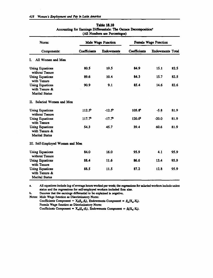
418 Women's Enpkoyment and Pay ui Ladn Amrica
Tabl 18.10Accounting for Eamings Differentials: The Oaxu Decomposition'
(Alll Numbem are Percentages)
Norm: Male Wae Function Female Wage Function
Components: Coefficients Endowments Coefficients Endowments Total
I. All Women and Men
Using Equations 80.5 19.5 84.9 15.1 82.5without Tenure
Using Equations 89.6 10.4 84.3 15.7 82.5with Tenure
Using Equations 90.9 9.1 85.4 14.6 82.6with Tenure &Martal Status
II. Salaried Women and Men
Using Equations 112.5b -12.5" 105.8" -5.8 81.9without Tenure
Using Equations 117.7b -17.7b 120.0' -20.0 81.9with Tenure
Using Equations 54.3 45.7 39.4 60.6 81.9with Tenure &Marital Status
m. Self-Employed Women and Men
Using Equations 84.0 16.0 95.9 4.1 95.9without Tenure
Using Equations 88.4 11.6 86.6 13.4 95.9with Tenure
Using Equations 88.5 11.5 87.2 12.8 95.9with Tenure &Marital Status
a. All equations include log of average hours worked per week; the regresions for ularied workers include unionstatus and the regressions for self-employed worker included firn size.
b. Denotes that the eaniings differential to be explained is negative.Notes: Male Wage function as Discriminatory Norm:
Coefficients Component = XA0$*-0f), Endowments Component = .(X,-Xf).Pemale Wage function as Discriminatory Norm:Coefficients Component = XJ0.-Ar), Endowments Component = A(X.-Xf).
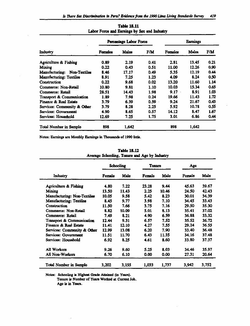
IS There Six DCrbAn bi Per? EWdewefro the 1990 Lima Livag Standards Survey 419
Table 18.11Labor Force and Earnings by Sex and Industry
PeCentage IAbor Force Eanings
Industry Females Males F/M Females Males F/M
Agriculture & Fishing 0.89 2.19 0.41 2.81 13.45 0.21Mining 0.22 0.43 0.51 11.00 12.26 0.90Manufacturing: Non-Textiles 8.46 17.17 0.49 5.35 12.19 0.44Manufacturing: Textiles 8.91 7.25 1.23 4.09 8.24 0.50Construction 0.22 9.68 0.02 13.20 11.60 1.14Commerce: Non-Retail 10.80 9.81 1.10 10.03 15.34 0.65Commerce: Retail 28.51 14.43 1.98 9.17 8.91 1.03Transport & Communication 1.89 7.98 0.24 19.66 11.43 1.72Finance & Real Estate 3.79 6.39 0.59 9.24 21.67 0.43Services: Community & Other 3.79 8.28 2.25 5.92 10.78 0.55Services: Government 4.90 8.65 0.57 14.12 8.47 1.67Services: Household 12.69 7.25 1.75 3.01 6.86 0.44
Total Number in Sample 898 1,642 898 1,642
Notes: Earnings are Monthly Earnings in Thouand. of 1990 Inti.
Table 18.12Average Schooling, Tenure and Age by Industry
Schooling Tenure Age
Industry Female Male Female Male Female Male
Agriculture & Fishing 4.80 7.22 23.28 9.44 45.63 39.67Mining 13.50 11.43 2.25 10.46 24.50 42.43Manufacturing: Non-Textiles 10.05 9.58 5.42 8.23 30.01 34.39Manufacturing: Textiles 8.45 9.77 3.98 7.10 34.45 33.43Construction 11.50 7.66 3.75 7.16 29.50 35.30Commerce: Non-Retil 8.82 10.09 5.01 8.13 35.41 37.02Commerce: Retail 7.49 8.21 4.90 6.59 36.88 33.32Transport & Communication 12.44 9.31 6.57 7.52 35.52 36.72Finance & Real Estate 11.41 12.10 4.27 7.55 29.24 36.55Services: Community & Other 12.99 13.08 6.20 7.90 33.40 36.48Services: Government 11.51 11.70 6.43 11.35 34.16 37.48Services: Household 6.92 8.25 4.61 8.60 33.80 37.37
All Workers 9.26 9.60 5.25 8.03 34.46 35.97All Non-Workers 6.70 6.10 0.00 0.00 27.31 20.64
Total Number in Sample 3,202 3,155 1,033 1,737 3,942 3,752
Notes: Schooling is Highet Grade Atained (in Year.).Tenure is Number of Yea Worked at Curent Job.Age is in Years.
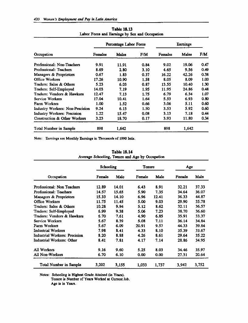
420 Women's Employment and Pay in Latin America
Table 18.13Labor Force and Earnings by Sex and Occupation
Percentage Labor Force Earnings
Occupation Females Males F/M Females Males F/M
Professional: Non-Teachers 9.91 11.91 0.84 9.02 19.06 0.47Professional: Teachers 8.69 2.80 3.10 4.65 9.56 0.49Managers & Proprietors 0.67 1.83 0.37 16.22 42.26 0.38Office Workers 17.26 10.90 1.58 8.05 8.09 1.00Traders: Sales & Others 5.23 6.03 0.87 13.55 10.40 1.30Traders: Self-Employed 14.03 7.19 1.95 11.95 24.86 0.48Traders: Vendors & Hawkers 12.47 7.13 1.75 6.79 6.34 1.07Service Workers 17.04 10.41 1.64 5.53 6.93 0.80Farm Workers 1.00 1.52 0.66 3.06 5.11 0.60Industry Workers: Non-Precision 9.24 6.15 1.50 3.53 5.92 0.60Industry Workers: Precision 1.22 15.47 0.08 3.13 7.18 0.44Construction & Other Workers 3.23 18.70 0.17 3.93 11.80 0.34
Total Number in Sample 898 1,642 898 1,642
Note: Earnings are Monthly Earnings in Thousands of 1990 Intis.
Table 18.14Average Schooling, Tenure and Age by Occupation
Schooling Tenure Age
Occupation Female Male Female Male Female Male
Professional: Non Teachers 12.89 14.01 6.43 8.91 32.21 37.33Professional: Teachers 14.57 15.65 5.90 7.35 34.64 36.07Managers & Proprietors 15.33 14.10 6.96 12.41 36.33 44.87Office Workers 11.75 11.45 5.00 9.03 29.90 35.78Traders: Sales & Others 10.28 9.94 5.12 8.62 32.11 36.57Traders: Self-Employed 6.99 9.38 5.06 7.23 38.70 36.60Traders: Vendors & Hawkers 6.70 7.61 4.90 6.85 35.91 33.37Service Workers 5.67 8.39 5.08 7.11 36.14 34.84Farm Workers 5.67 6.09 20.91 9.57 44.33 39.84Industrial Workers 7.98 8.41 4.33 8.10 35.39 33.67Industrial Workers: Precision 8.20 8.88 4.26 8.61 29.64 35.22Industrial Workers: Other 8.41 7.81 4.17 7.14 28.86 34.95
All Workers 9.16 9.60 5.25 8.03 34.46 35.97All Non-Workers 6.70 6.10 0.00 0.00 27.31 20.64
Total Number in Sample 3,202 3,155 1,033 1,737 3,942 3,752
Notes: Schooling is Highest Grade Attained (in Years).Tenure is Number of Years Worked at Current Job.Age is in Years.
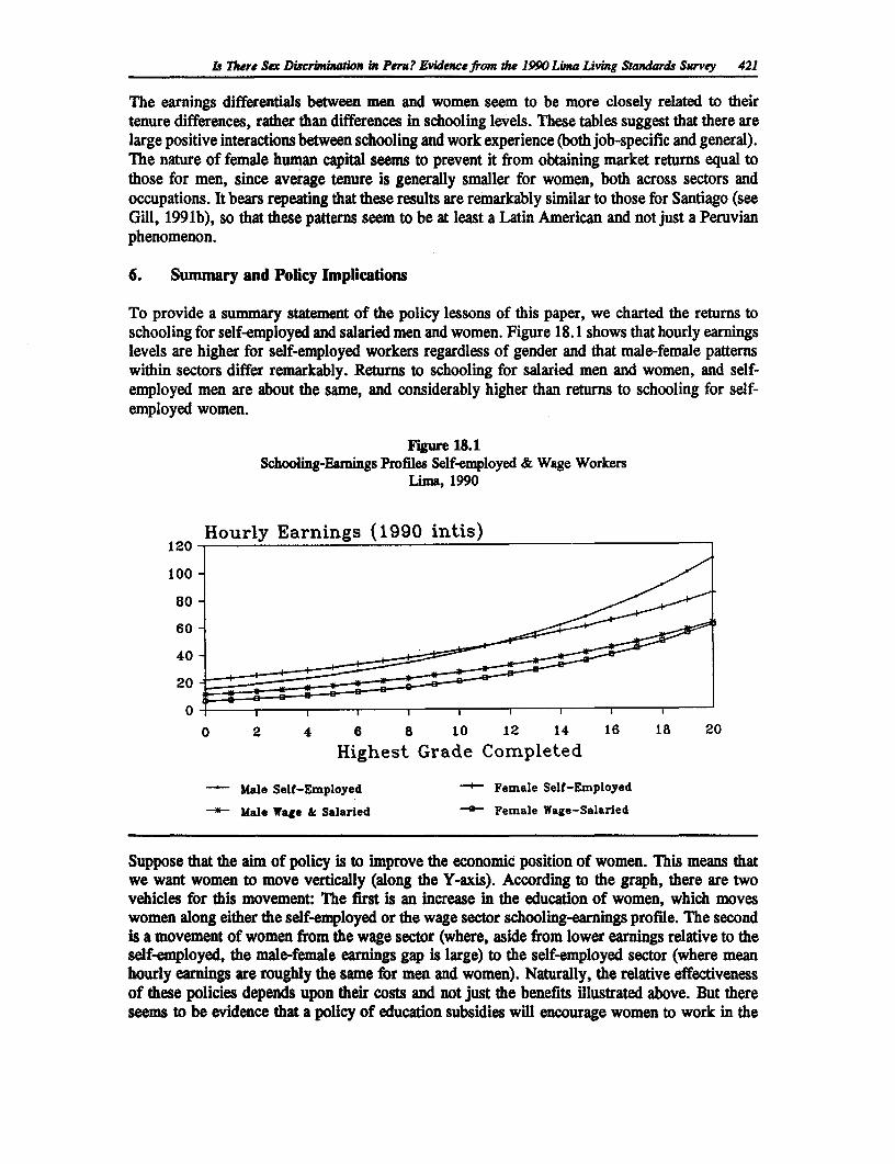
Is There Six Discriminaion i Peru? Evidene from *e 1990 Lina Living Standards Survey 421
The earnings differentials between men and women seem to be more closely related to theirtenure differences, rather than differences in schooling levels. These tables suggest that there arelarge positive interactions between schooling and work experience (both job-specific and general).The nature of female human capital seems to prevent it from obtaining market returns equal tothose for men, since average tenure is generally smaller for women, both across sectors andoccupations. It bears repeating that these results are remarkably similar to those for Santiago (seeGill, 199 lb), so that these patterns seem to be at least a Latin American and not just a Peruvianphenomenon.
6. Summary and Policy Inplications
To provide a summary statement of the policy lessons of this paper, we charted the returns toschooling for self-employed and salaried men and women. Figure 18.1 shows that hourly earningslevels are higher for self-employed workers regardless of gender and that male-female patternswithin sectors differ remarkably. Returns to schooling for salaried men and women, and self-employed men are about the same, and considerably higher than returns to schooling for self-employed women.
Figure 18.1Schooling-Earnings Profiles Self-employed & Wage Workers
Lima, 1990
H-ourly Earnings (1990 intis)
100 -
80
60-
40-
20
o 2 4 6 8 10 12 14 16 18 20
Highest Grade Completed
- Male Self-Employed - Female Self-Employed
" Male Wage & Salaried - Female Wage-Salaried
Suppose that the aim of policy is to improve the economic position of women. This means thatwe want women to move vertically (along the Y-axis). According to the graph, there are twovehicles for this movement: The first is an increase in the education of women, which moveswomen along either the self-employed or the wage sector schooling-earnings profile. The secondis a movement of women from the wage sector (where, aside from lower earnings relative to theself-employed, the male-female earnings gap is large) to the self-employed sector (where meanhourly earnings are roughly the same for men and women). Naturally, the relative effectivenessof these policies depends upon their costs and not just the benefits illustrated above. But thereseems to be evidence that a policy of education subsidies will encourage women to work in the
422 Women 's Emplyment and Pay in Latn America
wage sector, where there are higher returns to schooling but where average earnings are lowerthan in the self-employed sector.
Given the difference in levels, there are clearly obstacles to being self-employed. One likelyobstacle is startup capital. Improving access to credit would help to remove this barrier. If women(especially mothers) obtain greater overall benefits from flexibility in work schedules, a policyof credit subsidization would be more compatible with the objective of improving the economicstatus of women than education subsidies. There are probably still good arguments for schoolingsubsidies. However, this paper provides some evidence that increased schooling, by loweringfertility, can make women choose work patterns similar to those of males only up to a point.Women will always choose to have some children, and childcare will always remain a relativelyfemale-intensive activity. Policy design must recognize that women need more flexibility in workschedules than men.
If there are positive externalities associated with the improved status of women, creditsubsidization for women may be the more effective instrument in attaining these benefits, at leastin urban areas where schooling has already reached reasonable levels. The discussion aboveseems to justify subsidization of work schedule flexibility primarily for women with children.This creates a targeting problem, because a policy of credit subsidization for mothers will leadto fertility that is higher than optimal as women try to qualify for this subsidy. Subsidized creditfor women without children (younger, unmarried women) can be rationalized if returns to sector-specific experience among the self-employed are high, so that there are advantages to early entry.
The evidence in this study indicates high returns to sector-specific experience for self-employedwomen. A simpler policy implication emerges as a result of this: Education policy must besupplemented by a policy that facilitates the transition of women from the wage to the self-employed sector, for example, through credit subsidization.
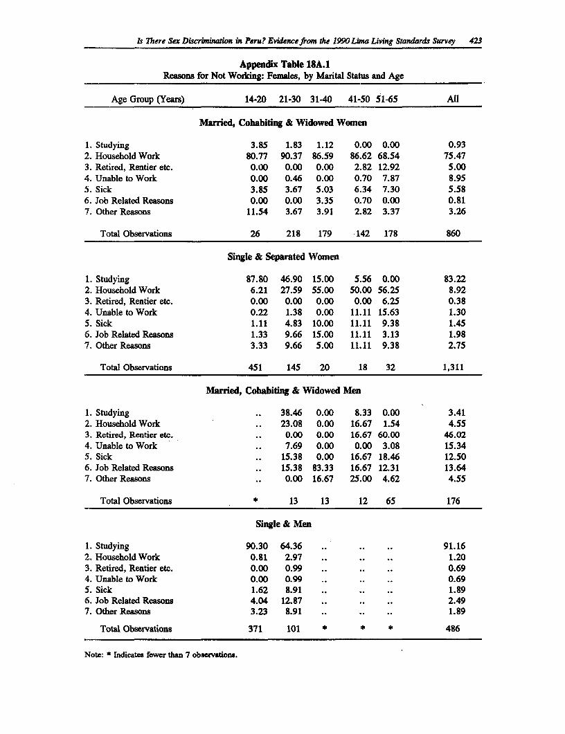
Is There Sex Discrbnion in Peru? Evidence from the 1990 Lina Liwng Standards Survey 423
Appendix Table 18A.1Reasons for Not Woring: Females, by Marital Status and Age
Age Group (Years) 14-20 21-30 31-40 41-50 51-65 All
Mbarried, Cohabiting & Widowed Women
1. Studying 3.85 1.83 1.12 0.00 0.00 0.932. Household Work 80.77 90.37 86.59 86.62 68.54 75.473. Retired, Rentier etc. 0.00 0.00 0.00 2.82 12.92 5.004. Unable to Work 0.00 0.46 0.00 0.70 7.87 8.955. Sick 3.85 3.67 5.03 6.34 7.30 5.586. Job Related Reasons 0.00 0.00 3.35 0.70 0.00 0.817. Other Reasons 11.54 3.67 3.91 2.82 3.37 3.26
Total Observations 26 218 179 142 178 860
Single & Separated Women
1. Studying 87.80 46.90 15.00 5.56 0.00 83.222. Household Work 6.21 27.59 55.00 50.00 56.25 8.923. Retired, Rentier etc. 0.00 0.00 0.00 0.00 6.25 0.384. Unable to Work 0.22 1.38 0.00 11.11 15.63 1.305. Sick 1.11 4.83 10.00 11.11 9.38 1.456. Job Related Reasons 1.33 9.66 15.00 11.11 3.13 1.987. Other Reasons 3.33 9.66 5.00 11.11 9.38 2.75
Total Observations 451 145 20 18 32 1,311
Married, Cohabiting & Widowed Men
1. Studying .. 38.46 0.00 8.33 0.00 3.412. Household Work .. 23.08 0.00 16.67 1.54 4.553. Retired, Rentier etc. .. 0.00 0.00 16.67 60.00 46.024. Unable to Work .. 7.69 0.00 0.00 3.08 15.345. Sick .. 15.38 0.00 16.67 18.46 12.506. Job Related Reasons .. 15.38 83.33 16.67 12.31 13.647. Other Reasons .. 0.00 16.67 25.00 4.62 4.55
Total Observations * 13 13 12 65 176
Single & Men
1. Studying 90.30 64.36 .. .. .. 91.162. Household Work 0.81 2.97 .. .. .. 1.203. Retired, Rentier etc. 0.00 0.99 .. .. .. 0.694. Unable to Work 0.00 0.99 .. .. .. 0.695. Sick 1.62 8.91 .. .. .. 1.896. Job Related Reasons 4.04 12.87 .. .. .. 2.497. Other Reasons 3.23 8.91 .. .. .. 1.89
Total Observations 371 101 * * * 486
Note: * Indicates fewer than 7 observadons.
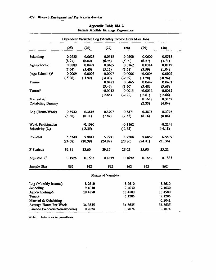
424 Women's Employnent and Pay in Lain America
Appendix Table 18A.2Female Monthly Earnings Regressions
Dependent Vanable: Log (Monthly Income from Main Job)
(25) (26) (27) (28) (29) (30)
Schooling 0.0733 0.0628 0.0618 0.0500 0.0609 0.0383(8.77) (6.62) (6.95) (5.00) (6.87) (3.71)
Age-School-6 0.0589 0.0497 0.0465 0.0362 0.0384 0.0119(7.04) (5.40) (5.15) (3.68) (3.99) (1.04)
(Age-School-6)2 -0.0009 -0.0007 -0.0007 -0.0006 -0.0006 -0.0002(-5.08) (-3.92) (-4.00) (-2.89) (-3.28) (-0.94)
Tenure 0.0451 0.0465 0.0449 0.0471(3.49) (3.60) (3.48) (3.68)
Tenure2 -0.0012 -0.0013 -0.0012 -0.0012(-2.66) (-2.72) (-2.61) (-2.66)
Married & 0.1618 0.3157Cohabiting Dummy (2.33) (4.04)
Log (Hours/Week) 0.3932 0.3816 0.3707 0.3571 0.3875 0.3798(8.38) (8.11) (7.87) (7.57) (8.16) (8.06)
Work Participation -0.1080 -0.1162 -0.2145Selectivity (XI) (-2.35) (-2.55) (-4.18)
Constant 5.5340 5.9845 5.7271 6.2208 5.6869 6.5539(24.68) (20.39) (24.99) (20.86) (24.81) (21.36)
F-Statistic 39.81 33.00 29.17 26.02 25.90 25.21
Adjusted R2 0.1526 0.1567 0.1639 0.1690 0.1682 0.1837
Sample Size 862 862 862 862 862 862
Means of Variables
Log (Monthly Income) 8.2610 8.2610 8.2610Schooling 9.4030 9.4030 9.4030Age-Schooling-6 18.4850 18.4580 18.4580Tenure 5.1286 5.1286Married & Cohabiting 0.5041Average Hours Per Week 34.3635 34.3635 34.3635Lambda (Workers/Non-workers) 0.7074 0.7074 0.7074
Note: t-statiatics in parentheuis.
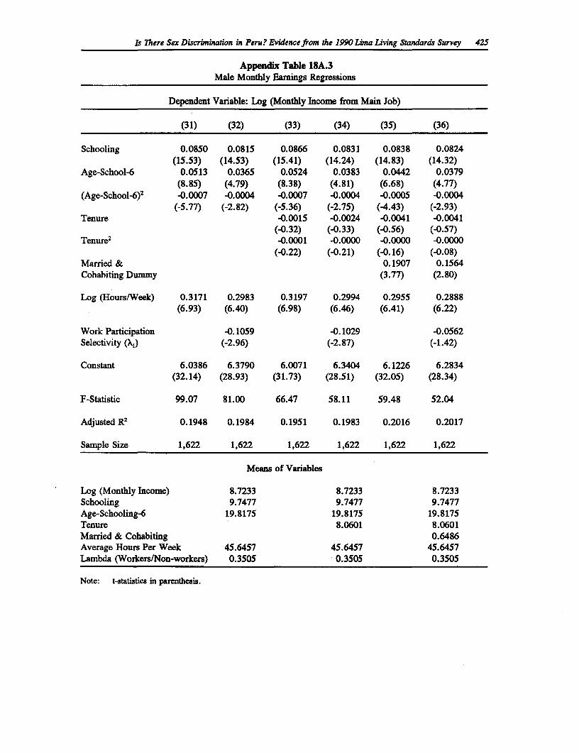
Is There Sex Discrimination in Peru? Evidence from the 1990 Lima Living Standards Survey 425
Appendix Table 18A.3Male Monthly Earnings Regressions
Dependent Variable: Log (Monthly Income from Main Job)
(31) (32) (33) (34) (35) (36)
Schooling 0.0850 0.0815 0.0866 0.0831 0.0838 0.0824(15.53) (14.53) (15.41) (14.24) (14.83) (14.32)
Age-School-6 0.0513 0.0365 0.0524 0.0383 0.0442 0.0379(8.85) (4.79) (8.38) (4.81) (6.68) (4.77)
(Age-School-6)2 -0.0007 -0.0004 -0.0007 -0.0004 -0.0005 -0.0004(-5.77) (-2.82) (-5.36) (-2.75) (-4.43) (-2.93)
Tenure -0.0015 -0.0024 -0.0041 -0.0041(-0.32) (-0.33) (-0.56) (-0.57)
Tenure2 -0.0001 -0.0000 -0.0000 -0.0000(-0.22) (-0.21) (-0.16) (-0.08)
Married & 0.1907 0.1564Cohabiting Dummy (3.77) (2.80)
Log (Hours/Week) 0.3171 0.2983 0.3197 0.2994 0.2955 0.2888(6.93) (6.40) (6.98) (6.46) (6.41) (6.22)
Work Participation -0.1059 -0.1029 -0.0562Selectivity (X,) (-2.96) (-2.87) (-1.42)
Constant 6.0386 6.3790 6.0071 6.3404 6.1226 6.2834(32.14) (28.93) (31.73) (28.51) (32.05) (28.34)
F-Statistic 99.07 81.00 66.47 58.11 59.48 52.04
Adjusted R2 0.1948 0.1984 0.1951 0.1983 0.2016 0.2017
Sample Size 1,622 1,622 1,622 1,622 1,622 1,622
Means of Variables
Log (Monthly Income) 8.7233 8.7233 8.7233Schooling 9.7477 9.7477 9.7477Age-Schooling-6 19.8175 19.8175 19.8175Tenure 8.0601 8.0601Married & Cohabiting 0.6486Average Hours Per Week 45.6457 45.6457 45.6457Lambda (Workers/Non-workers) 0.3505 0.3505 0.3505
Note: t-statistics in parenthesis.
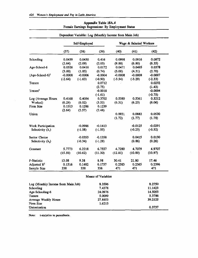
426 Women's Employment and Pay in Latin America
Appendix Table 18A.4Female Earnings Regressions: By Employment Status
Dependent Variable: Log (Monthly Income from Main Job)
Self-Employed Wage & Salaried Workers
(37) (38) (39) (40) (41) (42)
Schooling 0.0439 0.0430 0.416 0.0998 0.0916 0.0872(2.64) (2.09) (2.03) (9.88) (6.80) (6.35)
Age-School-6 0.0526 0.0416 0.0172 0.0471 0.0495 0.0378(3.00) (1.85) (0.74) (5.00) (4.31) (2.70)
(Age-School-6)2 -0.0008 -0.0006 -0.0004 -0.0008 -0.0008 -0.0007(-2.64) (-1.63) (-0.90) (-3.54) (-3.29) (-2.33)
Tenure 0.0712 0.0232(2.75) (1.43)
Tenure2 -0.0018 -0.0004(-1.61) (-0.75)
Log (Average Hours 0.4168 0.4054 0.3702 0.5380 0.5361 0.5212Worked) (6.29) (6.02) (5.53) (6.31) (6.25) (6.06)
Firm Size 0.1313 0.1286 0.1239(2.64) (2.57) (2.48)
Union 0.0931 0.0882 0.0530(1.72) (1.77) (1.78)
Work Participation -0.0986 -0.1413 -0.0125 -0.0291Selectivity (X1) (-1.08) (-1.55) (-0.23) (-0.52)
Sector Choice -0.0353 -0.1358 0.0415 0.0130Selectivity (X2) (-0.34) (-1.28) (0.86) (0.26)
Constant 5.7773 6.2218 6.7557 4.7280 4.7079 4.9707(15.56) (10.62) (11.30) (12.81) (10.89) (10.97)
F-Statistic 13.08 9.38 8.98 30.41 21.80 17.46Adjusted R2 0.1516 0.1482 0.1757 0.2383 0.2365 0.2396Sample Size 338 338 338 471 471 471
Means of Variables
Log (Monthly Income from Main Job) 8.3596 8.2750Schooling 7.4378 11.1423Age-Schooling-6 24.0976 14.5053Tenure 5.0099 5.3786Average Weekly Hours 27.8853 39.2125Firm Size 1.6213Unionization 0.3737
Note: t-statistics in parenthesis.
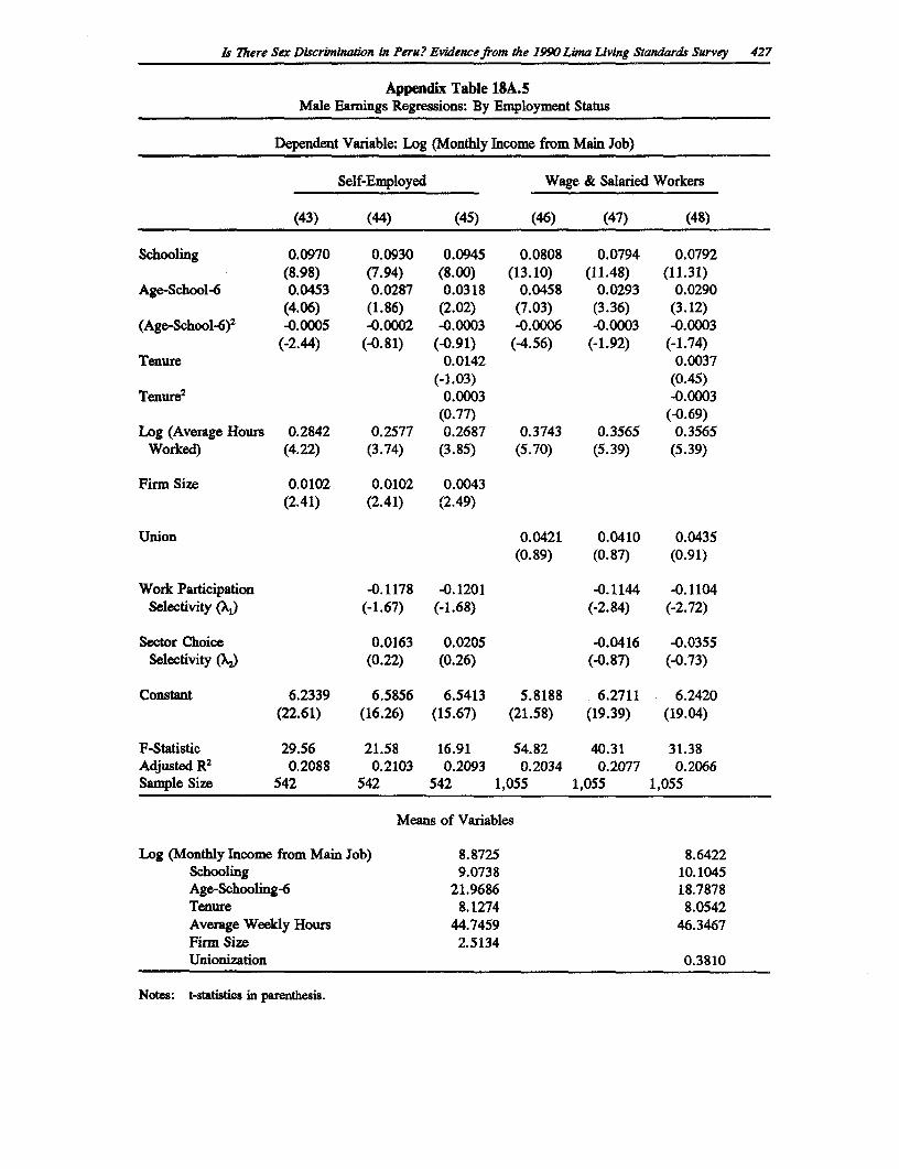
Is Zhere Sex Discrimination in Peru? Evidence from the 1990 Lima Living Standards Survey 427
Appendix Table 18A.5Male Earnings Regressions: By Employment Status
Dependent Variable: Log (Monthly Income from Main Job)
Self-Employed Wage & Salaried Workers
(43) (44) (45) (46) (47) (48)
Schooling 0.0970 0.0930 0.0945 0.0808 0.0794 0.0792(8.98) (7.94) (8.00) (13.10) (11.48) (11.31)
Age-School-6 0.0453 0.0287 0.0318 0.0458 0.0293 0.0290(4.06) (1.86) (2.02) (7.03) (3.36) (3.12)
(Age-School-6)2 -0.0005 -0.0002 -0.0003 -0.0006 -0.0003 -0.0003(-2.44) (-0.81) (-0.91) (-4.56) (-1.92) (-1.74)
Tenure 0.0142 0.0037(-1.03) (0.45)
Tenure2 0.0003 -0.0003(0.77) (-0.69)
Log (Average Hours 0.2842 0.2577 0.2687 0.3743 0.3565 0.3565Worked) (4.22) (3.74) (3.85) (5.70) (5.39) (5.39)
Firm Size 0.0102 0.0102 0.0043(2.41) (2.41) (2.49)
Union 0.0421 0.0410 0.0435(0.89) (0.87) (0.91)
Work Participation -0.1178 -0.1201 -0.1144 -0.1104Selectivity (XA) (-1.67) (-1.68) (-2.84) (-2.72)
Sector Choice 0.0163 0.0205 -0.0416 -0.0355Selectivity (X,) (0.22) (0.26) (-0.87) (-0.73)
Constant 6.2339 6.5856 6.5413 5.8188 6.2711 6.2420(22.61) (16.26) (15.67) (21.58) (19.39) (19.04)
F-Statistic 29.56 21.58 16.91 54.82 40.31 31.38Adjusted R2 0.2088 0.2103 0.2093 0.2034 0.2077 0.2066Sample Size 542 542 542 1,055 1,055 1,055
Means of Variables
Log (Monthly Income from Main Job) 8.8725 8.6422Schooling 9.0738 10.1045Age-Schooling-6 21.9686 18.7878Tenure 8.1274 8.0542Average Weeldy Hours 44.7459 46.3467Firm Size 2.5134Unionization 0.3810
Notes: t-statistics in parenthesis.
References
Cornwell, Christopher and Peter Rupert. "Unobservable Individual Effects, Marriage and theEarnings of Young Men," working paper, State University of New York at Buffalo, 1990.
Gill, Indermit. "Is there Sex Discrimination in Chile? Evidence from the CASEN Survey," inFemale Employment and Pay in Latin America, A Regional Study, edited by GeorgePsacharopoulos, Human Resources Division, Technical Department, Latin America andthe Caribbean Region, The World Bank, 1991a.
Gill, Indermit. "Gender, Occupational Choice, and Earnings in Latin America: The Cases ofLima and Santiago," Human Resources Division, Technical Department, Latin Americaand the Caribbean Region, The World Bank, 1991b.
Glewwe, Paul. "The Distribution of Welfare in Peru in 1985-86," Living Standards MeasurementStudy Working Paper No. 42, The World Bank, 1988.
Heckman, James J. "Sample Selection Bias as a Specification Error," Econometrica, Volume 47:pages 153-161, 1979.
Heckman, James J. and Richard Robb. "Alternative Methods for Evaluating the Impact ofInterventions," in Longitudinal Analysis of Labor Market Data, edited by J. Heckman andB. Singer. Cambridge University Press: pages 156- 245, 1985.
Killingsworth, Mark R. and James J. Heckman. "Female Labor Supply: A Survey," in Handbookof Labor Economics, Volume 1, edited by 0. Ashenfelter and R. Layard. Elsevier SciencePublishers: pages 103-204, 1986.
Khandker, Shahidur. "Women's Labor Force Participation and Male-Female Wage Differencesin Peru." This volume, 1992.
King, Elizabeth M. "Does Education Pay in the Labor Market? The Labor Force Participation,Occupation, and Earnings of Peruvian Women," Living Standards Measurement StudyWorking Paper No. 67, The World Bank, 1990.
Mincer, Jacob. Schooling, Experience and Earnings. Columbia University Press, New York,1974.
428
Is There Sex Discrbnination in Peru? Evidence from the 1990 L;ma Living Standards Survey 429
Moock, Peter, Philip Musgrove and Morton Stelcner. "Education and Earnings in Peru'sInformal Nonfarm Family Enterprises," Living Standards Measurement Study WorkingPaper No. 64, The World Bank, 1990.
Oaxaca, Ronald."Male-female Wage Differentials in Urban Labor Markets," InternationalEconomic Review: pages 693-709, 1973.
Stelcner, Morton, Ana-Maria Arriagada, and Peter Moock. "Wage Determinants and SchoolAttainment among Men in Peru," Living Standards Measurement Study Working PaperNo. 38, The World Bank, 1988.
United Nations Development Programme. Hwnan Development Report, New York: OxfordUniversity Press, 1990.
World Bank. World Development Report. Washington, D.C. Oxford University Press, 1990.

19
Women's Labor Force Participation and Earnings:The Case of Uruguay
Mary Arends
1. Introduction
Women's wages are about 75 percent of men's wages in Uruguay. This study investigates thisdifferential using econometric analysis. Uruguay is an interesting country to study because ofits high female labor force participation rate (about 50 percent of females between the ages of 14and 65 participate) and because of a long-standing commitment to public education. There is awide scope for investigation of human capital characteristics and their effect on female earnings.
A description of the Uruguayan labor market is given in the next section. Section 3 discussesthe sample used in the analysis. Section 4 looks at the characteristics that influence a woman'sdecision to participate in the labor force. It examines the selectivity problem, which arisesbecause working women are a self-selected group out of the entire female sample. Section 5 usesa Mincerian earnings function to estimate returns to human capital endowments in the labormarket and considers how returns differ between men and women, taking into account theselectivity problem. Section 6 breaks down the earnings differential to determine how much canbe explained by differences in endowments and what is the upper bound of possible labor marketdiscrimination.
2. The Uruguayan Economy and Labor Market
Uruguay's demographics are characterized by low growth rates, a high emigration rate, an agingpopulation, and a high degree of urbanization. The average annual population growth rate from1965 to 1980 was .4 percent, and was .6 percent from 1980 to 1988. Of the total population in1988, 26.2 percent was aged 0 to 14, 62.7 percent was aged 15 to 64, and 11.1 percent was over65. Eighty-five percent of the population lived in an urban area, and about 52 percent lived inMontevideo. Due to higher emigration rates among men, in 1989, 53 percent of the populationof 2,747,800 people were women. Considering the population aged 14 to 65 the disparity waseven greater; 55 percent of a total of 2,116,200 people in this age group were female.
Economically, although Uruguay has one of the highest GNP per capita in Latin America atUS$2,620 in 1989, the country has experienced stagnation since the mid-1950s due to import-substitution policies in the fifties and sixties, and stabilization policies in the late seventies andeighties. The annual growth rate was 1.3 percent from 1965 to 1988, and -.4 percent from 1980to 1988. The share of industry in the economy has declined from 32 percent in 1965 to 29percent in 1988. Sixty percent of the country's GNP in 1988 came from the service sector. Inaddition, the country has suffered political upheaval. In 1973, there was a military coup, and a
431
432 Women's Empkoyment and Pay in Latin America
dictatorship ruled the country until March 1, 1985. This period coincided with a fall in realwages, which had fallen to 62 percent of their 1968 level by 1984.'
The stagnation, coupled with the recent military regime, has led to high emigration rates asUruguayans move to Brazil and Argentina. Emigration was concentrated in the years 1973 to1977 and reached its peak in 1974, when 62,400 people left the country. There wereapproximately 300,000 emigrants from 1963 to 1981, which represents about 10 percent of thecurrent Uruguayan population. Emigrants tended to be males, in their early or late twenties, andmarried. They also tended to be workers in the private industrial sector. Because of the age andeducational attainment of emigrants, the impact of the emigration on the labor market was strongand lasting. For example, Aguiar (1984) estimates that Uruguay lost 20.7 percent of itspopulation between the ages of 20 and 29, 10.8 percent of its economically active population, 20percent of its salaried workers, 22.6 percent of its artisans and day workers, and 27.9 percentof its employees in industry.2
This has provided opportunities for women to enter the labor force, as the female economicallyactive population has grown relative to the male population. In addition to the decrease inqualified males in the work force, declining family living standards have encouraged a high levelof female labor force participation. Sending women and young people into the paid labor forcewho would otherwise be at home is a survival strategy to maintain family living standards.3
Fortuna and Prates (1989) report evidence that between 1971 and 1979 real wages fell 45 percent,and between 1973 and 1979 90 percent of the population in Montevideo maintained its level offamily earnings due to the incorporation of more of its members into the labor force.4 Women'sparticipation rate increased from 27 percent in 1967 to 36.9 percent in 1979.5 The growth infemale participation has continued throughout the 1980s. In 1989, it reached 47 percent.
Another characteristic of the Uruguayan labor market is the long hours worked. Besidesincreasing the number of workers in the family to maintain living standards, workers increasetheir hours, especially in the public sector, and take on extra jobs, often in the informal sector.In the sample, 10 percent of the workers reported having more than one job. Labor supplyincreases because hours increase and participation levels increase even though real wages havedeclined. Apparently the income effect of lower wages (which makes leisure less affordable)outweighs the substitution effect (which would decrease labor supply because leisure is lessexpensive). These responses, which represent a shift in the labor supply curve outward, will tendto decrease real wages further, holding the labor demand curve constant.6
The work week also tends to be long because of expensive labor market laws requiring employersto pay a one month bonus, social security benefits, health insurance, accident insurance, and two
I Weinstein (1988), p. 94.
2 Aguiar (1984), p. 22.
3 Taglioretti (1983), p. 30.
4 Fortuna and Prates (1989), p. 81.
5 Aguiar (1984), p. 38.
6 Aguiar (1984), p. 34.
Women's Labor Force Participation and Earnings: The Case of Uruguay 433
weeks' leave to each employee. Employers who face an upturn in demand are likely to requireexisting hires to work more hours, rather than expand the labor pool. Another consequence ofthe laws is the expansion of the informal sector in the Uruguayan labor market. By World Bankestimates, from 16 to 28 percent of the labor force was employed in the informal sector in1987.' Employers may subcontract tasks to the informal sector, and women play a role as anexpendable labor force, as documented by Fortuna and Prates (1989) in the textile and recyclingsectors.'
Uruguay has traditionally had an extensive public schooling system. Enrollments in secondaryschool, as a percentage of the relevant age group, was higher than for any other Latin Americancountry in 1965 at 44 percent, and in 1987 it was 73 percent, second only to Argentina. Tertiaryenrollments were also the highest in Latin America in 1987 at 42 percent. The economicallyactive population with incomplete primary education has declined from 20.1 percent in 1969 to10.1 percent in 1989, while the percentage with secondary and university education has increasedfrom 31.2 percent to 58.5 percent.9 The system includes teaching schools, a "labor university"which provides secondary technical education, and one national university. However, theUruguayan economy has had difficulties finding suitable employment for highly educatedgraduates with raised expectations, and consequently, unemployment rates are higher than averageamong college graduates.'0
3. Data Characteristics
The data used in this study are drawn from the 1989 Encuesta Nacional de Hogares conductedby the General Administration of Statistics and the Census (DGEC) in Uruguay. It is a householdsurvey of 31,766 individuals in 9,648 households. The survey only includes urban households,and thus excludes the 15 percent of the population in rural areas. For the analysis in this chapter,only individuals aged 14 to 65 were included, providing a sample of 20,502 individuals.
An individual was classified as working if he or she reported positive earnings and positive hoursworked in a primary occupation. Excluded were those who reported no hours because they wereon vacation or sick because no regular hours could be estimated for them. An individual wasclassified as a labor force participant if he or she was classified as employed (whetherremunerated or not), laid off, looking for work for the first time, or on strike.
Descriptive statistics for the working male, working female, and non-working female samples arepresented in Table 19.1. The female participation rate is 52 percent. Working females have ahigher level of education than working men. Schooling was calculated using information aboutthe highest level of education attained and the number of years completed at that level, addingthe number of years in each previous level to the number of years at the highest level. For someindividuals, the schooling in years could not be estimated because the level was unknown. Sincethe schooling system was changed in 1977, the measure for schooling is an estimate, and subjectto inaccuracies. Experience was estimated using the proxy of age minus years of schooling minus6. This measure is very likely to overestimate experience because there is no way to measure
7 World Bank (1991), p. 33.
s Fortuna and Prates (1989), pp. 82-93.
9 World Bank (1991), p. 34.
10 World Bank (1991), p. 39.
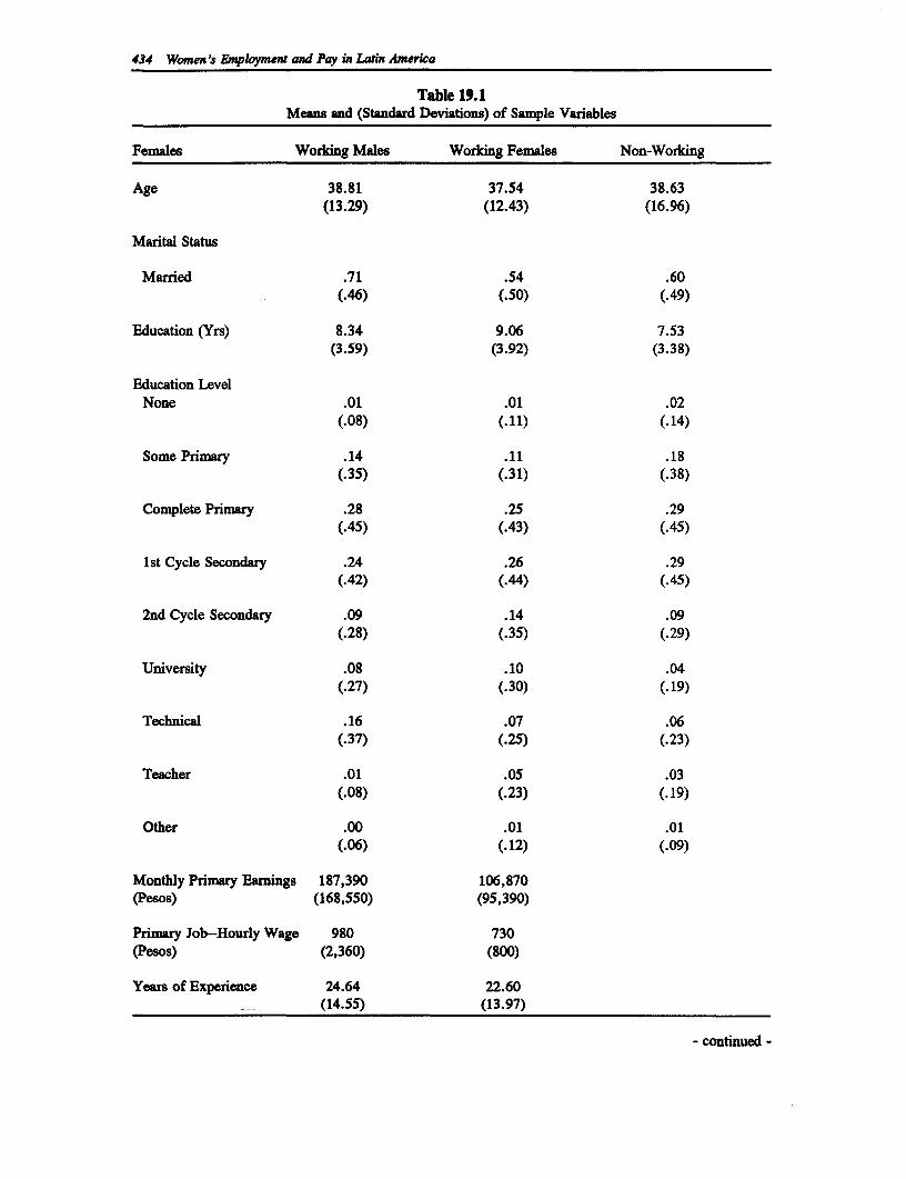
434 Women's Enpoymet and Pay in Latin Amerca
Table 19.1Means and (Standard Deviations) of Sample Variables
Females Working Males Working Females Non-Working
Age 38.81 37.54 38.63(13.29) (12.43) (16.96)
Marital Status
Married .71 .54 .60(.46) (.50) (.49)
Education (Yrs) 8.34 9.06 7.53(3.59) (3.92) (3.38)
Education LevelNone .01 .01 .02
(.08) (.11) (.14)
Some Primary .14 .11 .18(.35) (.31) (.38)
Complete Primary .28 .25 .29(.45) (.43) (.45)
1st Cycle Secondary .24 .26 .29(.42) (.44) (.45)
2nd Cycle Secondary .09 .14 .09(.28) (.35) (.29)
University .08 .10 .04(.27) (.30) (.19)
Technical .16 .07 .06(.37) (.25) (.23)
Teacher .01 .05 .03(.08) (.23) (.19)
Other .00 .01 .01(.06) (.12) (.09)
Monthly Primary Earnings 187,390 106,870(Pesos) (168,550) (95,390)
Primary Job-Hourly Wage 980 730(Pesos) (2,360) (800)
Years of Experience 24.64 22.60(14.55) (13.97)
- continued -
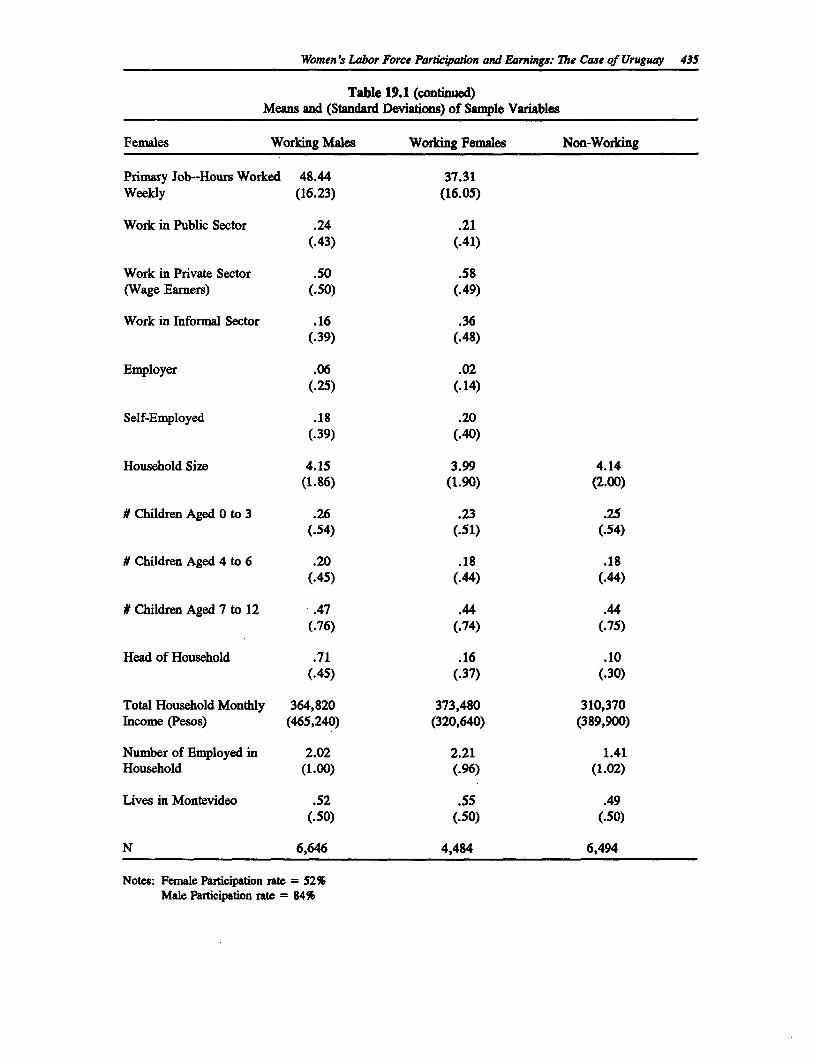
Women's Labor Force Participaton and Earnings: The Case of Uruguay 435
Table 19.1 (continued)Means and (Standard Deviations) of Sample Variables
Females Working Males Working Females Non-Working
Primary Job-Hours Worked 48.44 37.31Weekly (16.23) (16.05)
Work in Public Sector .24 .21(.43) (.41)
Work in Private Sector .50 .58(Wage Earners) (.50) (.49)
Work in Informal Sector .16 .36(.39) (.48)
Employer .06 .02(.25) (.14)
Self-Employed .18 .20(.39) (.40)
Household Size 4.15 3.99 4.14(1.86) (1.90) (2.00)
# Children Aged 0 to 3 .26 .23 .25(-54) (.51) (.54)
# Children Aged 4 to 6 .20 .18 .18(.45) (.44) (.44)
# Children Aged 7 to 12 .47 .44 .44(.76) (.74) (.75)
Head of Household .71 .16 .10(.45) (.37) (.30)
Total Household Monthly 364,820 373,480 310,370Income (Pesos) (465,240) (320,640) (389,900)
Number of Employed in 2.02 2.21 1.41Household (1.00) (.96) (1.02)
Lives in Montevideo .52 .55 .49(.50) (.50) (.50)
N 6,646 4,484 6,494
Notes: Female Participation rate = 52%Male Participation rate = 84%
436 Women's Employment and Pay in Latin America
the time individuals may have spent out of the labor force. The bias is likely to be greater forfemales, who typically interrupt their working lives during childbearing years. Working maleson average have more experience and work longer hours than working females.
All female observations were included in the probit regression, while only those females classifiedas working, and for whom schooling and experience could be calculated with some accuracy,were included in the wage regression.
Wages were calculated by taking the monthly income in the participant's primary job, anddividing it by the hours worked in a week times 4.3 to approximate monthly hours.
Unemployment rates in the sample are much higher for women than men (10 percent versus 5.7percent)." The unemployment rate is higher for those who have a university education--8percent for men and 11 percent for women. For both sexes, about half of the unemployed witha university education are first time job seekers.
One question in examining wage differentials between men and women is whether the two groupschoose different occupations, with women either choosing or being forced by lack of opportunityinto the lower paid occupations. Table 19.2A presents the distribution of occupations by gender;17 percent of the females working are professionals, technicians and teachers, while only 7percent of the men are in this category. Thirty-two percent of working women work in personalservices and 18 percent in office work (corresponding figures for men are 1 percent and 13percent). For each occupation except transport, females make considerably less than males. Thelowest paid occupation is agriculture, but a very small percentage of either males and females areemployed in this sector. The next lowest paid group is personal services and 32 percent of thewomen are employed in this occupation. Men are more heavily represented in artisan and non-classified occupations which are also low paying. Taglioretti (1983) notes that most of theincrease in women's labor supply has been absorbed by state and social services. Personalservices have also played a large role in absorbing the increase."2
In Table 19.2B, the breakdown of employment by sector is shown. Males are more likely towork in the public sector or to be employers than females. Females tend to work in the informalsector; 36 percent of working females and 19 percent of working males are employed there. Theinformal sector is defined here as including the self-employed who either have or do not have aregular work place in firms of less than five people. Self-employed professionals and techniciansare considered to be formal sector workers. The informal sector also includes workers receivinga regular wage in the private sector providing personal services, while working for enterprisesof less than five people. It includes most domestics, thus the high female participation rate inthis sector. Looking at average education levels, employers, public sector workers, and formalsector workers tend to have the most years of schooling. In every sector, women have moreeducation than men, with the exception of the informal sector.
11 Unemployment rates are defined as the percentage of the labor force categorized as laid offworkers or first time job seekers.
12 Taglioretti (1983), p. 49.
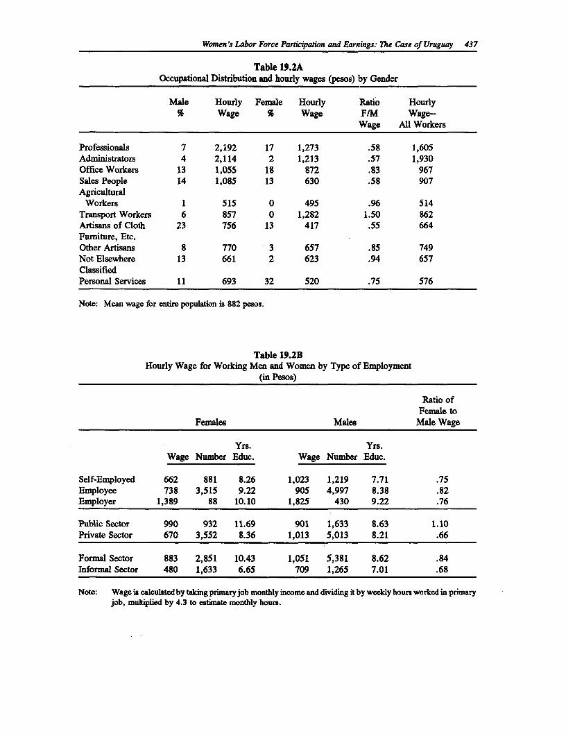
Women's Labor Force Parickoation and Earnings: The Case of Uruguay 437
Table 19.2AOccupational Distribution and hourly wages (pesos) by Gender
Male Hourly Female Hourly Ratio Hourly% Wage % Wage F/M Wage-
Wage All Workers
Professionals 7 2,192 17 1,273 .58 1,605Administrators 4 2,114 2 1,213 .57 1,930Office Workers 13 1,055 18 872 .83 967Sales People 14 1,085 13 630 .58 907Agricultural
Workers 1 515 0 495 .96 514Transport Workers 6 857 0 1,282 1.50 862Artisans of Cloth 23 756 13 417 .55 664Furniture, Etc.Other Artisans 8 770 3 657 .85 749Not Elsewhere 13 661 2 623 .94 657ClassifiedPersonal Services 11 693 32 520 .75 576
Note: Mean wage for entire population is 882 pesos.
Table 19.2BHourly Wage for Working Men and Women by Type of Employment
(in Pesos)
Ratio ofFemale to
Females Males Male Wage
Yrs. Yrs.Wage Number Educ. Wage Number Educ.
Self-Employed 662 881 8.26 1,023 1,219 7.71 .75Employee 738 3,515 9.22 905 4,997 8.38 .82Employer 1,389 88 10.10 1,825 430 9.22 .76
Public Sector 990 932 11.69 901 1,633 8.63 1.10Private Sector 670 3,552 8.36 1,013 5,013 8.21 .66
Formal Sector 883 2,851 10.43 1,051 5,381 8.62 .84Informal Sector 480 1,633 6.65 709 1,265 7.01 .68
Note: Wage is calculated by taking primary job monthly income and dividing it by weekly hours worked in primaryjob, multiplied by 4.3 to estimate monthly hours.
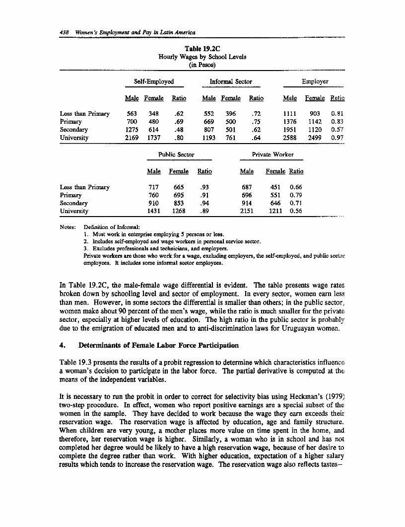
438 Women's Employment and Pay in Latin America
Table 19.2CHourly Wages by School Levels
(in Pesos)
Self-Employed Informal Sector Employer
Male Female Ratio Male Female Ratio Male Female Ratio
Less than Prirnary 563 348 .62 552 396 .72 1111 903 0.81Primary 700 480 .69 669 500 .75 1376 1142 0.83Secondary 1275 614 .48 807 501 .62 1951 1120 0.57University 2169 1737 .80 1193 761 .64 2588 2499 0.97
Public Sector Private Worker
Male Female Ratio Male Female Ratio
Less than Primary 717 665 .93 687 451 0.66Primary 760 695 .91 696 551 0.79Secondary 910 853 .94 914 646 0.71University 1431 1268 .89 2151 1211 0.56
Notes: Definition of Informal:1. Must work in enterprise employing 5 persons or less.2. Includes self-employed and wage workers in personal service sector.3. Excludes professionals and technicians, and employers.Private workers are those who work for a wage, excluding employers, the self-employed, and public sectoremployees. It includes some informal sector employees.
In Table 19.2C, the male-female wage differential is evident. The table presents wage ratesbroken down by schooling level and sector of employment. In every sector, women earn lessthan men. However, in some sectors the differential is smaller than others; in the public sector,women make about 90 percent of the men's wage, while the ratio is much smaller for the privatesector, especially at higher levels of education. The high ratio in the public sector is probablydue to the emigration of educated men and to anti-discrimination laws for Uruguayan women.
4. Determinants of Female Labor Force Participation
Table 19.3 presents the results of a probit regression to determine which characteristics influencea woman's decision to participate in the labor force. The partial derivative is computed at themeans of the independent variables.
It is necessary to run the probit in order to correct for selectivity bias using Heckman's (1979)two-step procedure. In effect, women who report positive earnings are a special subset of thewomen in the sample. They have decided to work because the wage they earn exceeds theirreservation wage. The reservation wage is affected by education, age and family structure.When children are very young, a mother places more value on time spent in the home, andtherefore, her reservation wage is higher. Similarly, a woman who is in school and has notcompleted her degree would be likely to have a high reservation wage, because of her desire tocomplete the degree rather than work. With higher education, expectation of a higher salaryresults which tends to increase the reservation wage. The reservation wage also reflects tastes--
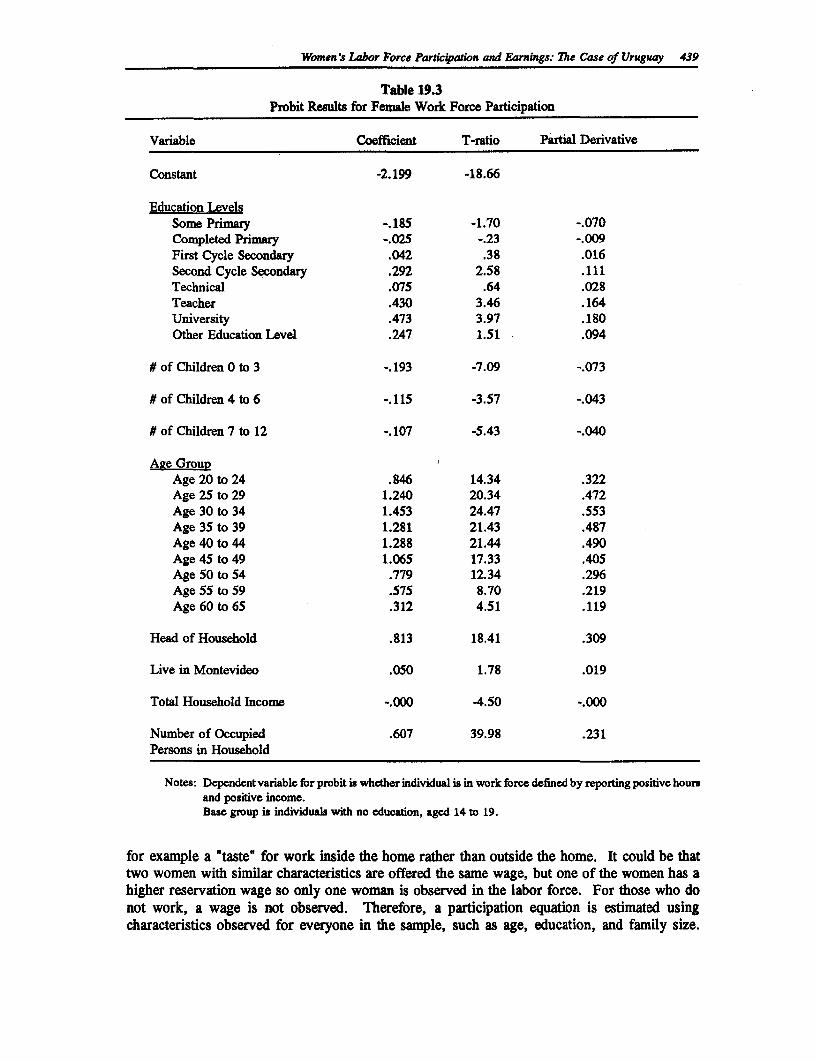
Women's Labor Force Partic@adon and Earnings: 7he Case of Uruguay 439
Table 19.3Probit Results for Female Work Force Participation
Variable Coefficient T-ratio Partial Derivative
Constant -2.199 -18.66
Education LevelsSome Primary -.185 -1.70 -.070Completed Primary -.025 -.23 -.009First Cycle Secondary .042 .38 .016Second Cycle Secondary .292 2.58 .111Technical .075 .64 .028Teacher .430 3.46 .164University .473 3.97 .180Other Education Level .247 1.51 .094
#of Children 0 to 3 -.193 -7.09 -.073
# of Children 4 to 6 -.115 -3.57 -.043
#of Children 7 to 12 -.107 -5.43 -.040
Ae GroupAge 20 to 24 .846 14.34 .322Age 25 to 29 1.240 20.34 .472Age 30 to 34 1.453 24.47 .553Age 35 to 39 1.281 21.43 .487Age 40 to 44 1.288 21.44 .490Age 45 to 49 1.065 17.33 .405Age 50 to 54 .779 12.34 .296Age 55 to 59 .575 8.70 .219Age 60 to 65 .312 4.51 .119
Head of Household .813 18.41 .309
Live in Montevideo .050 1.78 .019
Total Household Income -.000 -4.50 -.000
Number of Occupied .607 39.98 .231Persons in Household
Notes: Dependentvariable for probit is whether individual is in work force defined by reporting positive hoursand positive income.Base group is individuals with no education, aged 14 to 19.
for example a "taste" for work inside the home rather than outside the home. It could be thattwo women with similar characteristics are offered the same wage, but one of the women has ahigher reservation wage so only one woman is observed in the labor force. For those who donot work, a wage is not observed. Therefore, a participation equation is estimated usingcharacteristics observed for everyone in the sample, such as age, education, and family size.
440 Women's Employment and Pay in Latin America
This equation is used to determine work. When this ratio, or Lambda, is included in the earningsfunction it eliminates the bias due to selectivity.
A factor tending to decrease the reservation wage is the need for income. Standing (1982)explained how having a higher need for income would tend to increase labor forceparticipation."3 For example, in the probit the number of people employed, the total householdincome, and whether the woman is the head of the household are all proxies for the need forincome. If many household members are employed, that would reduce the need for a female towork outside the home. Likewise, higher household income would be expected to have anegative effect on labor force participation. On the other hand, if a woman is the head of thehousehold, this increases her responsibility to earn money.
The dependent variable in the probit is a dummy variable equal to 1 if the woman is working andif she reports positive earnings and positive hours worked for the previous week and equal to 0otherwise. Dummy variables are used to represent various levels of schooling and age splines.Other dummy variables include whether the woman is the head of the household and whether thewoman lives in Montevideo. Variables that proxy the structure of the household include thenumber of children aged 0 to 3, 4 to 6, and 7 to 12, and the number of employed people in thehousehold. It was not possible to determine in every case which children belonged to whichfemale in each household, so the number of children in the household is used as a proxy. Thenumber of children were grouped in this manner because Uruguay has a very well developedpreschool program and primary school begins at age 6. Preschool education covers about 40percent of children aged 3-5; 75 percent of 5 year olds attend school. Sixty-nine percent of thechildren in the sample aged 4 to 6 attend school. This would help women with their childcareduties, and therefore enable them to participate in the labor force when the children reach ayounger age than in other Latin American countries, where schooling might begin at age six.However, about 60 percent of children without access to preschool education are from the pooresthouseholds. Women that have more of a need for income may not have the opportunity to sendtheir young children to school. The other variables used in the probit are total household incomeand the number of working people in the household."4
Table 19.4 presents the results of a simulation testing for each characteristic while holding allother characteristics at the value of their sample mean. It is apparent that education plays a rolein predicting whether a female works. For example, the probability ranged from .28 for womenwith some primary education to .54 for women with university level education. Also, at lowerlevels of education the effect is not as significant as for higher levels; looking at the t-statistics,they are insignificant at the 5 percent level for all education levels except the second cycle ofsecondary school, the university, and teacher school. Apparently, the opportunity cost of stayingout of the labor market is higher for women with more education, and the opportunity cost effectoutweighs the positive effect that education has on the reservation wage. The net effect is thathigher education is associated with higher participation rates in the labor force.
13 Standing, (1982), p. 55.
W As shown in the other chapters in this book, being married had a significant negative effect on theprobability of working in an earlier equation, but was left out in the final probit equation because ofcorrelation effects with the number of children.
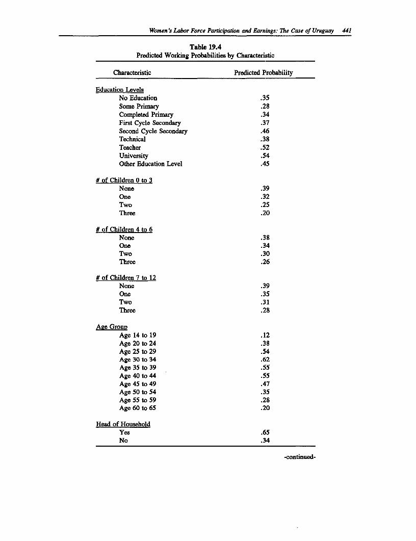
Women's Labor Force Partcipation and Earnings: The Case of Uruguay 441
Table 19.4Predicted Worldng Probabilities by Characteristic
Characteristic Predicted Probability
Education LevelsNo Education .35Some Primary .28Completed Primary .34First Cycle Secondary .37Second Cycle Secondary .46Technical .38Teacher .52University .54Other Education Level .45
# of Children 0 to 3None .39One .32Two .25Three .20
# of Children 4 to 6None .38One .34Two .30Three .26
# of Children 7 to 12None .39One .35Two .31Three .28
Age Group,Age 14 to 19 .12Age 20 to 24 .38Age 25 to 29 .54Age 30 to 34 .62Age 35 to 39 .55Age 40 to 44 .55Age 45 to 49 .47Age 50 to 54 .35Age 55 to 59 .28Age 60 to 65 .20
Head of HouseholdYes .65No .34
-continued-
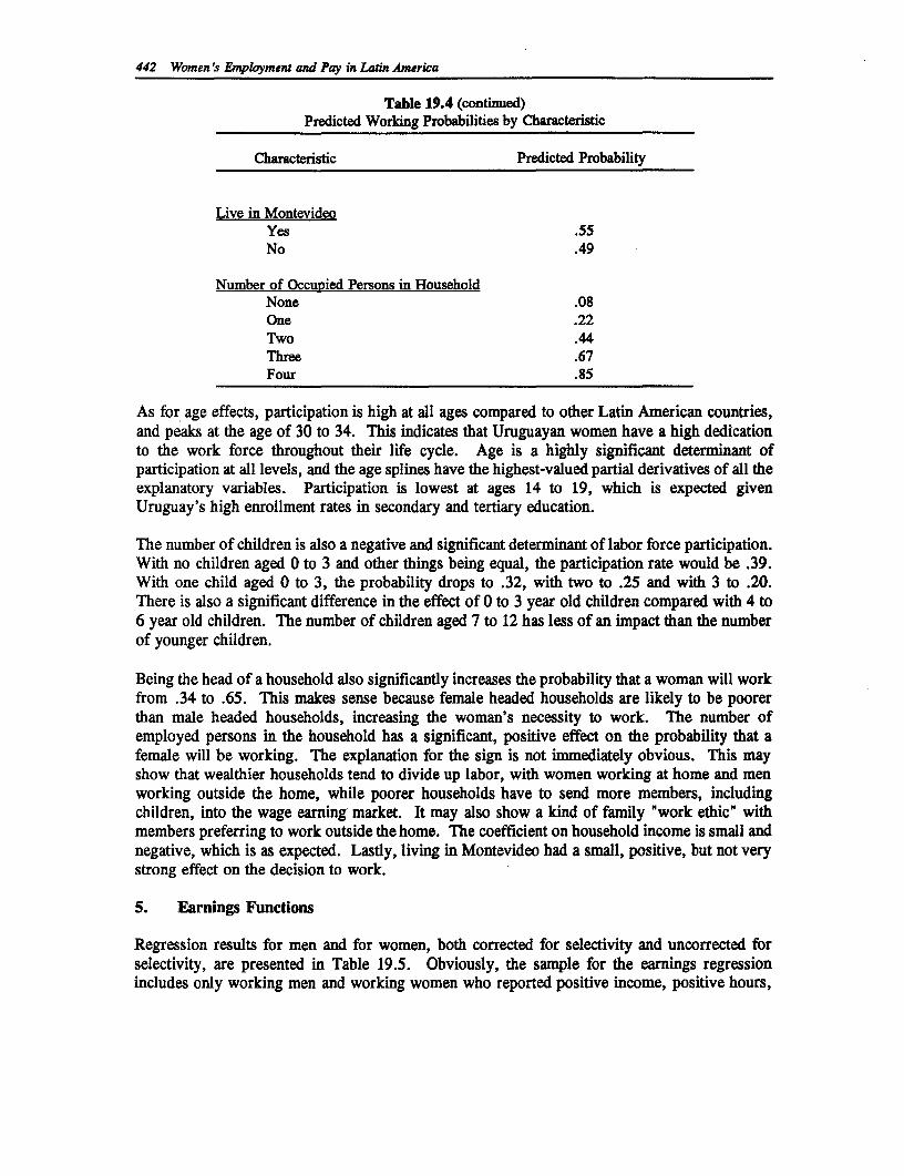
442 Women's Employment and Pay in Latin America
Table 19.4 (continued)Predicted Working Probabilities by Characteristic
Characteristic Predicted Probability
Live in MontevideoYes .55No .49
Number of Occupied Persons in HouseholdNone .08One .22Two .44Three .67Four .85
As for age effects, participation is high at all ages compared to other Latin American countries,and peaks at the age of 30 to 34. This indicates that Uruguayan women have a high dedicationto the work force throughout their life cycle. Age is a highly significant determinant ofparticipation at all levels, and the age splines have the highest-valued partial derivatives of all theexplanatory variables. Participation is lowest at ages 14 to 19, which is expected givenUruguay's high enrollment rates in secondary and tertiary education.
T'he number of children is also a negative and significant determinant of labor force participation.With no children aged 0 to 3 and other things being equal, the participation rate would be .39.With one child aged 0 to 3, the probability drops to .32, with two to .25 and with 3 to .20.There is also a significant difference in the effect of 0 to 3 year old children compared with 4 to6 year old children. The number of children aged 7 to 12 has less of an impact than the numberof younger children.
Being the head of a household also significantly increases the probability that a woman will workfrom .34 to .65. This makes sense because female headed households are likely to be poorerthan male headed households, increasing the woman's necessity to work. The number ofemployed persons in the household has a significant, positive effect on the probability that afemale will be working. The explanation for the sign is not immediately obvious. This mayshow that wealthier households tend to divide up labor, with women working at home and menworking outside the home, while poorer households have to send more members, includingchildren, into the wage earning market. It may also show a kind of family "work ethic" withmembers preferring to work outside the home. The coefficient on household income is small andnegative, which is as expected. Lastly, living in Montevideo had a small, positive, but not verystrong effect on the decision to work.
5. Earnings Functions
Regression results for men and for women, both corrected for selectivity and uncorrected forselectivity, are presented in Table 19.5. Obviously, the sample for the earnings regressionincludes only working men and working women who reported positive income, positive hours,
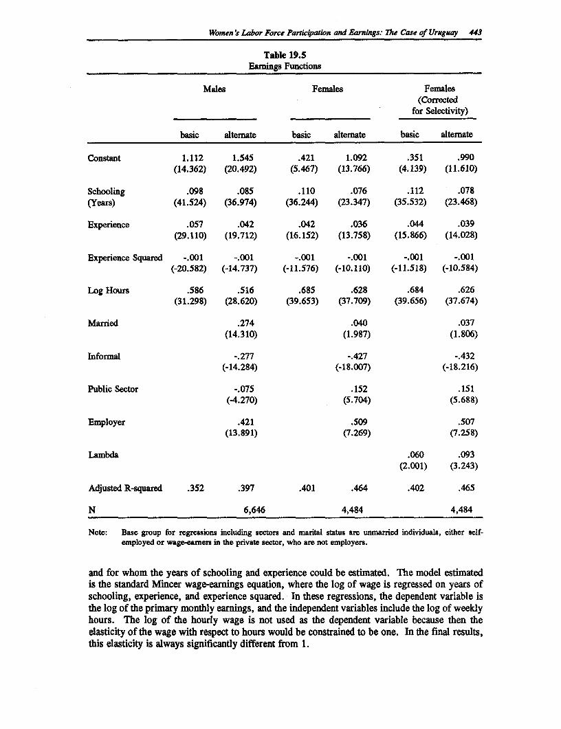
Women's Labor Force Pardcypadon and Earnings. The Case of Urmgay 443
Table 19.5Earnings Functions
Males Females Females(Corrected
for Selectivity)
basic alternate basic alternate basic alternate
Constant 1.112 1.545 .421 1.092 .351 .990(14.362) (20.492) (5.467) (13.766) (4.139) (11.610)
Schooling .098 .085 .110 .076 .112 .078(Years) (41.524) (36.974) (36.244) (23.347) (35.532) (23.468)
Experience .057 .042 .042 .036 .044 .039(29.110) (19.712) (16.152) (13.758) (15.866) (14.028)
Experience Squared -.001 -.001 -.001 -.001 -.001 -.001(-20.582) (-14.737) (-11.576) (-10.110) (-11.518) (-10.584)
Log Hours .586 .516 .685 .628 .684 .626(31.298) (28.620) (39.653) (37.709) (39.656) (37.674)
Married .274 .040 .037(14.310) (1.987) (1.806)
Informal -.277 -.427 -.432(-14.284) (-18.007) (-18.216)
Public Sector -.075 .152 .151(-4.270) (5.704) (5.688)
Employer .421 .509 .507(13.891) (7.269) (7.258)
Lambda .060 .093(2.001) (3.243)
Adjusted R-squared .352 .397 .401 .464 .402 .465
N 6,646 4,484 4,484
Note: Base group for regressions including sectors and marital status are unmarried individuals, either self-employed or wage-earners in the private sector, who are not employers.
and for whom the years of schooling and experience could be estimated. The model estimatedis the standard Mincer wage-earnings equation, where the log of wage is regressed on years ofschooling, experience, and experience squared. In these regressions, the dependent variable isthe log of the primary monthly earnings, and the independent variables include the log of weeklyhours. The log of the hourly wage is not used as the dependent variable because then theelasticity of the wage with respect to hours would be constrained to be one. In the final results,this elasticity is always significantly different from 1.
444 Women 's Employment and Pay in Latin America
The earnings functions are corrected for selectivity using Heckman's two-stage procedure (1979).By computing the probit equation, it is possible to compute the inverse Mill's ratio (Lambda) foreach working woman in the sample. The Lambda is then included in the explanatory variablesfor the female regression, and the results are compared with the uncorrected regression.
In the uncorrected regression, the return on education for women is seen to be about 11.1percent. A one percent increase in weekly hours worked is associated with a .7 percent increasein monthly earnings. The return on experience is 4 percent, and the sign on experience squaredis negative, implying a concave earnings function. When Lambda is added to the regressiondetermining women's earnings, the return to schooling increases very slighdy to 11.2 percent anda one percent increase in hours worked is still associated with a .7 percent increase in wages.There is very little difference in the results when Lambda is included. Lambda is positive andbarely significant at the 5 percent level. This indicates that those characteristics that areassociated with high earnings also increase the probability that the woman will be in the laborforce. Another way of saying this is that working women have a comparative advantage in workoutside the home. Those women who earn higher wages are also likely to have lower reservationwages.
The return to schooling is higher for women than men (11.1 percent versus 9.9 percent), but menhave a higher return to experience at about 5.8 percent. The elasticity of earnings to hoursworked is about the same for both groups. There is no selectivity correction for men becausetheir participation rate is high at 84 percent.
Interesting results occur when dummy variables representing sectors and marital status are addedto the wage equation. The rate of return for education to women declines to 7.7 percent from11.1 percent in the uncorrected regression, and the return to experience also declines to 3.7percent. The increase in adjusted R-squared implies that these variables were omitted variablesin the first regression and perhaps some of the return to education should be attributed to sectoralchoice. It is apparent that working in the informal sector is associated with a 43 percent declinein earnings when compared to the reference group of those employed in the private formal sector,while working in the public sector or being an employer implies earnings premiums of 15 percentand 51 percent, respectively, compared to the reference group. The sector effects are significant.When Lambda is added to the equation, its coefficient is larger and more significant than whenthe sectors are not included in the regression. There must be interactions between the decisionto work and the choice of sector. Again, the other coefficients are not affected much whenLambda is added to the right hand side of the equation, although the returns to schooling andexperience increase slightly. Being married, ceterisparabis increases wages by about 4 percent,but the effect is barely significant at the 5 percent level when Lambda is not in the equation, andis insignificant when correcting for selectivity.
For men, adding the marital status and sectoral dummies decreases the return to schooling byabout 1.3 percent and reduces the return to experience by about 1.5 percent. The return toschooling becomes higher for men than women. For the men, working in the informal sector orthe public sector is associated with lower wages than the reference group by 28 percent and 8percent respectively, while employers earn a 42 percent premium. This implies that the sectoralchoice is more important in determining female earnings than male earnings. However, marriedmales earn approximately 27 percent more than single men, and the effect is significant. Therationale for including marital status in the regression is that it is often observed that marriedpeople earn more than single people across countries. One explanation could be that skills valuedin the household are also beneficial in the work place. Another explanation is that marriage
Women's Labor Force Particpation and Earnings: The Case of Uruguay 445
allows male workers to increase their efficiency through specialization of labor, with the femaleconcentrating on household tasks and the men concentrating on outside work.
The experience profile for all specifications peaks later for men than women. For the women'sregressions with selectivity, it peaks at about 35 years of age; for women's regressions withoutselectivity, it peaks at about 36 years of age; and for men, the profile peaks at about 38 years ofage.
6. Discrimination
Having estimated the coefficients for males and females, the Oaxaca decomposition can bedetermined. Oaxaca (1973) devised a method to break down the earnings differential into twoparts; differences explained by differentials in human capital endowments (endowments) anddifferences caused by variations in returns to human capital in the labor market (the wagestructure). The latter represents the upper bound to discrimination.
In symbols, the difference between males and females is the following:
In (Earnings=) - In (Earningsf) = Xbbm - Xfbf
Xi represents the means of the sample parameters, and b. their corresponding coefficients. Thereare two equations that can be used to do the decomposition, and they will give different results.One equation measures the differential using the female means and the other measures it usingthe male means.
Xbbm - Xfbf = Xf(bm - bf) + bm(Xm - Xf) (l)Xbbm - Xfbf = Xm(bm - bf) + bf(Xm - Xf) (2)
The first term in both equations on the right side refer to the differences in earnings due todifference in wage structure, while the second term refers to the differences due to the differencesin endowments. The two equations present a base number problem, and there is no economicreason to use one of the two equations over the other. Table 19.6 includes the results using bothequations.
Using the earnings coefficients from the selectivity corrected ordinary least squares (OLS)estimates for the regression including only experience, schooling and log hours, 23 percent ofthe difference in earnings can be attributed to differences in endowments and 77 percent to thedifference in wage structure between men and women. The percentages are coincidentally thesame whether evaluated at the male or female means. The OLS estimates uncorrected forselectivity imply that a higher percentage of the difference can be explained by the differencesin endowments. For the regressions with the dummy variables for sectors and marital statusincluded, the percentage explained by endowments is higher, whether the estimates are correctedfor selectivity or not. A higher percentage is explained by endowments with the uncorrected OLSequations than the corrected OLS equations. The upper bound on discrimination is estimated atabout 55 to 60 percent for the equations including the sectoral and marital status dummyvariables.
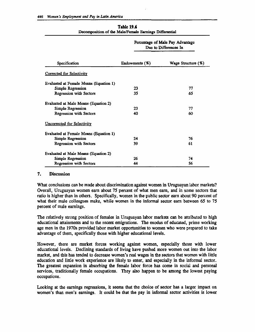
446 Women's Employment and Pay in Latn America
Table 19.6Decomposition of the Male/Female Earnings Differential
Percentage of Male Pay AdvantageDue to Differences In
Specification Endowments (%) Wage Structure (%)
Corrected for Selectivity
Evaluated at Female Means (Equation 1)Simple Regression 23 77Regression with Sectors 35 65
Evaluated at Male Means (Equation 2)Simple Regression 23 77Regression with Sectors 40 60
Uncorrected for Selectivity
Evaluated at Female Means (Equation 1)Simple Regression 24 76Regression with Sectors 39 61
Evaluated at Male Means (Equation 2)Simple Regression 26 74Regression with Sectors 44 56
7. Discussion
What conclusions can be made about discrimination against women in Uruguayan labor markets?Overall, Uruguayan women earn about 75 percent of what men earn, and in some sectors thatratio is higher than in others. Specifically, women in the public sector earn about 90 percent ofwhat their male colleagues make, while women in the informal sector earn between 65 to 75percent of male earnings.
The relatively strong position of females in Uruguayan labor markets can be attributed to higheducational attainments and to the recent emigrations. The exodus of educated, prime workingage men in the 1970s provided labor market opportunities to women who were prepared to takeadvantage of them, specifically those with higher educational levels.
However, there are market forces working against women, especially those with lowereducational levels. Declining standards of living have pushed more women out into the labormarket, and this has tended to decrease women's real wages in the sectors that women with littleeducation and little work experience are likely to enter, and especially in the informal sector.The greatest expansion in absorbing the female labor force has come in social and personalservices, traditionally female occupations. They also happen to be among the lowest payingoccupations.
Looking at the earnings regressions, it seems that the choice of sector has a larger impact onwomen's than men's earnings. It could be that the pay in informal sector activities is lower
Women's Labor Force Parcwipation and Earnings: The Case of Uruguay 447
because of non-pecuniary advantages, such as proximity to the home or flexible working hours,in which case there would not be labor market discrimination, but lower wages as the result oftrade-offs made by working women.
From the decomposition, it is true that in every case differences in wage structure are moreimportant in explaining the differential than differences in endowments. However, the differencein coefficients could be biased upwards. For example, the proxy for experience in the femaleregression is likely to be overestimated, because women typically have interrupted careers inorder to raise children. This will bias the return to experience downward, since the wageexperience profile is concave. This will also increase the percentage of the differential attributedto wage structure, and therefore, discrimination. Also, it would be helpful to have measurementsof job tenure, or uninterrupted time in the labor force. This is a proxy for dedication to labormarket activities, and could be a missing variable that is higher for men than women and whichis desirable to employers. It is important to note also that adding the sectoral variables increasesthe percentage attributable to endowments; the choice of sector is obviously an important factorin examining discrimination.
Uruguayan women could benefit from policies that would make it easier to combine householdwork and work in the formal sector, such as expanded provision of daycare. Coverage of thealready-existing preschool program could be expanded to poorer families. Pay is low in theinformal sector, and the ratio of female to male wage is also low. The same is true of the self-employed sector. The state has already done much in the area of preschool education. Also,further work should be done to determine why the wage structure is different between men andwomen, and whether women are constrained by custom or habit from more highly paidoccupations.
References
Aguiar, C. El Impacto de las Migraciones Internacionales en el Mercado de Empleo del Pais deOrigen: El Caso Uruguayo. Montevideo: Centro Interdisciplinario de Estudios Sobre elDesarrollo Uruguay, 1984.
Aldrich-Langen, C. The Admission and Academic Placement of Students from Selected SouthAmerican Countries. Washington, DC: National Association for Foreign Student Affairs,1978.
Fortuna, J. C. and S. Prates, "Informal Sector versus Informalized Labor Relations in Uruguay.'in A. Portes, M. Castells, and L. Benton (eds.) The Informal Economy: Studies inAdvanced and Less Developed Countries. Baltimore: The Johns Hopkins UniversityPress, 1989.
Heckman, J. "Sample Selection Bias as a Specification Error." Econometrica, Vol. 47 (1979).pp. 153-161.
Lubell, H. The Informal Sector in the 1980s and 1990s. Paris: Development Centre of theOrganisation for Economic Co-operation and Development, 1991.
Mann, A. and C. Sanchez, "Labor Market Responses to Southern Cone Stabilization Policies:The Cases of Argentina, Chile, Uruguay." Inter-American Economic Affairs, Vol. 38(Spring 1985) pp. 19-39.
Mincer, J. Schooling, Experience and Earnings. New York: Columbia University Press, 1974.
Oaxaca, R. "Male-female Wage Differentials in Urban Labor Markets." International EconomicReview. Vol. 14, no. 1 (1973) pp. 693-701.
Portes, A., S. Blitzer, and J. Curtis, "The Urban Informal Sector in Uruguay: Its InternalStructure, Characteristics, and Effects." World Development, Vol. 14, no. 6 (1986) pp727-741.
Solari, A. "Analysis of Educational Financing and Administration in a Context of Austerity: theCase of Uruguay." Major Project in the Field of Education in Latin America and theCaribbean (Chile). No. 21, April 1990, pp. 34-56.
448
Women's Labor Force Parnkation and Earnings: The Case of Uruguay 449
Standing, G. Labor Force Participation and Development. Geneva: International LaborOrganization, 1982.
Taglioretti, G. Women and Work in Uruguay. Paris: UNESCO, 1983.
Weil, T. Area Handbookfor Uruguay. Washington, DC: American University, 1971, pp. 117-144.
Weinstein, M. Uruguay: Democracy at the Crossroads. Boulder, CO: Westview Press, 1988.
World Bank, "Uruguay: Employment and Wages." Country Operations, Division 4. Report No.9608-UR, May 1991.

20
Female Participation and Earnings, Venezuela 1987
Donald Cox and George Psacharopoulos
1. Introduction
In 1987, the average earnings of Venezuelan working women were 70 percent of the averageearnings of Venezuelan working men. What accounts for the pay gap? Are human capitalindicators lower for women? Or is the gap due in part to labor market discrimination? Thischapter sheds some light on these questions by analyzing Venezuelan household survey microdata.
Simple comparisons of differences in average earnings can be misleading when making inferencesabout possible discrimination because skill indicators can differ between men and women. Sowe seek to estimate earnings differences while controlling for earnings determinants.
2. The Venezuelan Labor Market
Modernization, improved access to education, the growth of the public sector, and long termdeclines in fertility rates have all contributed to significant increases in female labor forceparticipation rates in Venezuela and by 1989, women accounted for 30 percent of the labor force.Women's participation rates have increased in both public and private sectors, although theincrease has been most pronounced in the public sector.
A number of studies (World Bank, 1990) show that women earn lower wages than men inVenezuela. While the wage differentials are partly explained by women's concentrations inlower-paying industries and in the informal sector, there is some evidence suggesting that womenearn less than men even when they have similar levels of education, years of experience in thelabor force, and when they hold similar jobs. This study uses 1987 Household Survey data todetermine what proportion of the male/female earnings differential is due to differences in humancapital endowments and how much of the differential can be attributed to differences in the wayemployers value male and female labor.
3. Data Characteristics
We use data from the Encuesta de Hogares, a survey covering a representative cross-section ofhouseholds in Venezuela. The survey was conducted by the Oficina Central de Estadistica eInformatica (OCEI) in the second semester of 1987. The data set contains observations from131,032 households covering 681,328 persons and contains information about labor marketearnings and individual characteristics such as age, schooling, gender, and place of residence.
451
452 Women's Employment and Pay in Latin America
From the large data set we selected a random sample of 10 percent of the individuals. Since weare interested in the behavior of prime-age individuals, we restricted our sub-sample toindividuals aged between 20 and 55 years. Further, we dropped persons with inconsistent labor-market information: Those who reported having earnings but no hours worked or vice versa.These sample-selection criteria result in an aggregate sample of 17,725 individuals: 8,375working males, 4,131 working females and 5,219 non-working females. (M'e reasons forincluding non-working females in our analysis is explained in a later section.)
Table 20.1 displays means and standard deviations (S.D.) of selected variables from the sample.The average age of working men and women is about the same, but average schooling amongworking women exceeds that of working men by almost a year. Eleven percent of workingwomen attended university, compared with 8 percent of men. And half of the working womenattended secondary school compared with 41 percent of men.
A higher proportion of men were self-employed-28 percent compared to 22 percent for workingwomen. But female workers were better represented in the public sector than men-31 versus17 percent. The earnings of women are 70 percent those of men (2,700/3,827).
Non-working women are slightly older than their working counterparts, and have approximately2 years less schooling. The variable "years of experience" is computed in the standard way bysubtracting years of schooling plus 6 from age. Note that we do not have measures of actuallabor market experience in our data set. So we must use potential years of labor marketexperience as a proxy. We recognize, of course, that women frequently experience interruptionsin their careers, so that our experience measure is an imperfect proxy for actual years spentworking.
4. Determinants of Female Labor Force Participation
We seek to estimate earnings functions for men and women, but our analysis for women posesa special problem because of the intermittency of female labor force participation. Hence we areestimating earnings functions for self-selected samples of women. That is, we estimate earningsfunctions for women whose market wage exceeds the value of time spent at home.
Our analysis is based on the occupational choice model of Roy (1951) that has been explored byHeckman (1979), Lee (1978), Willis and Rosen (1979), Borjas (1987) and others.
Suppose the market wage of woman HjY is given by the equation:
w(m) = bX + e(m), (1)
where X denotes a vector of wage determinants, b measures the returns to those determinants,and e(m) is the error term for woman I." (The subscript Vi" applies to the terms w(m), X, ande(m) and is suppressed for convenience.) The value of time spent at home for woman "i" isexpressed as:
w(h) = aZ + e(h). (2)
The vector Z denotes the determinants of the woman's productivity at home. We assume thevector Z contains all of the elements of X, plus other determinants. This assumption makes sensesince variables such as being a household head would affect productivity at home but not in the
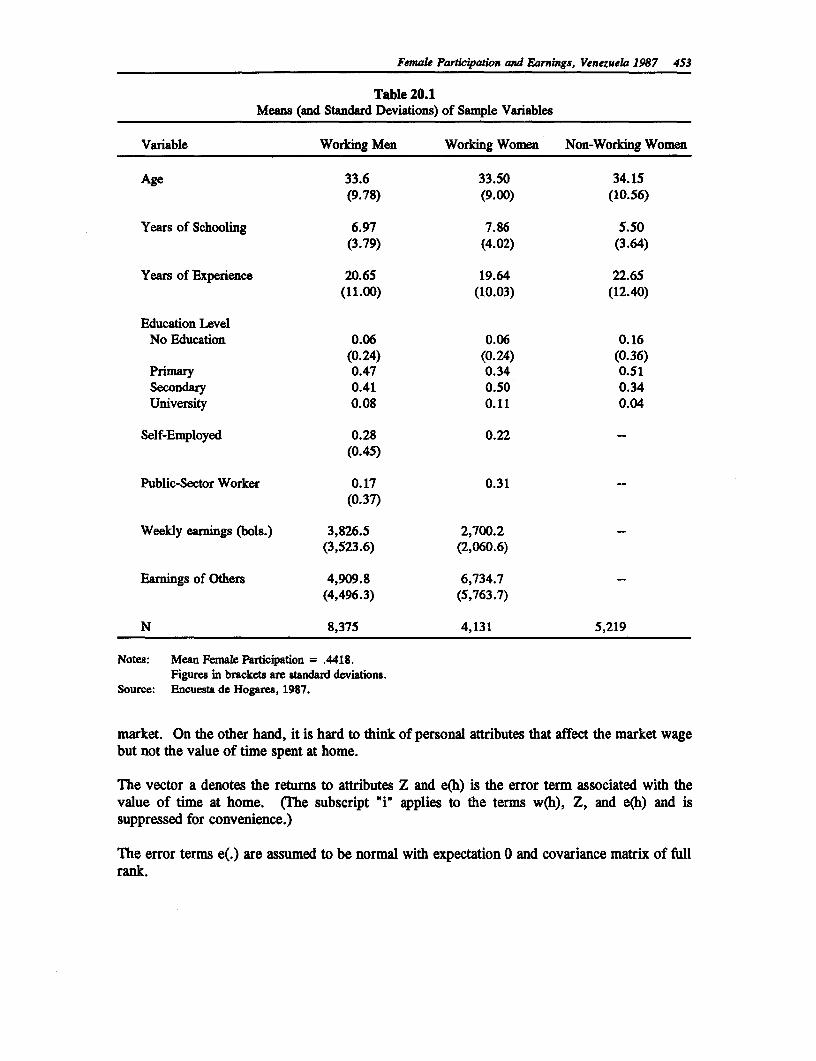
Female Participation and Earnings, Venezuela 1987 453
Table 20.1Means (and Standard Deviations) of Sample Variables
Variable Working Men Worldng Women Non-Working Women
Age 33.6 33.50 34.15(9.78) (9.00) (10.56)
Years of Schooling 6.97 7.86 5.50(3.79) (4.02) (3.64)
Years of Experience 20.65 19.64 22.65(11.00) (10.03) (12.40)
Education LevelNo Education 0.06 0.06 0.16
(0.24) (0.24) (0.36)Primary 0.47 0.34 0.51Secondary 0.41 0.50 0.34University 0.08 0.11 0.04
Self-Employed 0.28 0.22(0.45)
Public-Sector Worker 0.17 0.31(0.37)
Weekly earnings (bols.) 3,826.5 2,700.2(3,523.6) (2,060.6)
Earnings of Others 4,909.8 6,734.7(4,496.3) (5,763.7)
N 8,375 4,131 5,219
Notes: Mean Female Participation = .4418.Figures in brackets are standard deviations.
Source: Encuesta de Hogares, 1987.
market. On the other hand, it is hard to think of personal attributes that affect the market wagebut not the value of time spent at home.
The vector a denotes the returns to attributes Z and e(h) is the error term associated with thevalue of time at home. (The subscript "i" applies to the terms w(h), Z, and e(h) and issuppressed for convenience.)
The error terms e(.) are assumed to be normal with expectation 0 and covariance matrix of fullrank.
454 Women 's Employment and Pay in Latin America
A woman chooses to work if, and only if:
I = w(m) - w(h) = bX - aZ + e(m) - e(h) > 0, (3)
where I denotes an index of labor force participation. The variable I, which differs for eachindividual in the cross-section, is a continuous variable that indexes the propensity for a womanto enter the labor force. If the variable I crosses a certain threshold, the woman enters the laborforce (otherwise she does not). We do not lose anything essential by normalizing this thresholdto 0, as in expression (3).
Consider the expected value of women's wages, conditional on working in the market and on X.
E(w(m)) = bX + E(e(m)II > 0). (4)
"E" denotes the expectations operator. This is the standard sample-selection problem consideredby Heckman (1974, 1979). The expected value of the wage is conditional on the sample-selectionrule, which in this case is that the women work (I > 0). Focus on the last term in 4, theexpectation of the error term. That expression can be written as:
E(e(m) II > 0) = c(f(I)/F()) = cL, (5)
where f(I) denotes the ordinate of the standard normal density evaluated at the index I, F(I) thestandard normal distribution function evaluated at (I), and the ratio of the two (rewritten as L)is the inverse Mill's ratio term.
It can be shown that the variable c can be written as:
c = s(h)(s(m)/s(h) - r(m,h)), (6)
where s(.) denotes the standard deviation of e(.), (e.g., s(m) is the standard deviation of the errorterm associated with market wage offers) and r(m,h) is the correlation between e(m) and e(h)(-1 <= r <= 1).
The derivation in equation 6 is useful for determining the sign of the coefficient of the Mill'sratio, or selectivity term. The sign of c can be positive, negative, or zero, depending on thedispersion and covariance of the error terms e(.). For example, if e(m) and e(f) are inverselycorrelated (r < 0), so that unobserved characteristics that raise market productivity (e.g.,aggressiveness) lower productivity in the home, and the dispersion of market wages (captured bys(m)) is low relative to that of home production (s(h)), then the coefficient of the selection termwill be positive. In this case positive self-selection will occur; women sort themselves into thesectors in which they are most productive.
On the other hand, if s(m) and s(h) are roughly equal and r is approximately 1, the coefficientc will be close to zero. In this case, there is a strong positive correlation between unobservedmarket and home traits and the dispersion in the market and home error terms is the same. Itmakes sense that self-selection effects are minimal in this case because unobservables in eachsector are strongly correlated and their dispersion is the same.
Now consider the case in which r = 1 but s(h) > s(m). Unobservables that help boost thepayoff to home production boost the payoff to market work as well. And the dispersion of
Female Participation and Earnings, Venezuela 1987 455
rewards in the home sector is higher than that of the market. The most productive women willbe attracted to the sector with the greater dispersion. The reason is that if they are going to beat the top, they might as well be at the top of a wide distribution-this strategy maximizes thereward from sector choice. On the other hand, women whose e(.) terms are lowest will beattracted to the sector with the lesser dispersion (in this case the market sector). The reason isthat if they are going to be at the bottom of the distribution, they might as well choose the sectorwith the smaller dispersion so that their reward, which will be smallest, will at least not be toosmall. In this instance, then, the market sector attracts the women who are least productive interms of their unobservables, so that the selection effects in the market wage equation arenegative.
The first step in estimating selectivity-adjusted earnings functions is to estimate the index function3 using probit. The vector Z contains age dummies, schooling dummies, dummies for regionof residence, dummies for whether the woman was a wife or partner of the household head, andearnings of other household members, and a rural residence dummy.
The dependent variable in the probit analysis is labor force participation, which is defined asearning at least 200 bolivares per month in 1987. This definition is not strictly comparable withthe official one, which counts both the unemployed and employed as members of the labor force.But the concept of unemployment is complicated; experts disagree on exactly who is unemployed.The concept of employment is unambiguous; it is easy to identify those who have earned overa threshold amount.
The estimation results are presented in Tables 20.2 and 20.3. The probability of participatingin the labor force steadily rises with age until women reach their late forties, then it declines.The age effects are large. For example, the probit coefficients indicate that, controlling for otherfactors, the probability of participation is about 30 percentage points higher for women in theirearly 40's than for those in their early 20's. Education has powerful effects on participation too.All else being equal, secondary school graduates have an estimated participation probability thatis 30 percentage points higher than primary school graduates. University graduates have aparticipation probability 70 percentage points higher than primary school graduates. Butgraduating from a technical secondary school results in a lower participation probability thangraduating from an academic secondary school. This result is puzzling, but also likely to beimprecise-less than 2 percent of the sample attended technical school. Those with someuniversity education are less likely to participate in the labor force than secondary schoolgraduates. Part of the reason might be that attending a university raises reservation wagesleading to longer spells of unemployment. The marital status and headship variables are verylarge, precisely estimated and have the anticipated sign in the participation probit. Being a wifeor partner reduces the probability of participation by 22 percentage points, so familyresponsibilities compete for time spent in the market. Being a household head raises theparticipation probability by 23 percentage points. Income of other family members reduces theprobability of working. This is most likely due to income effects which raise the demand fortime spent at home (Mincer, 1962). A 15,000 bolivare increase in other income reduces theprobability of working by 4 percentage points.
Finally, participation probabilities follow distinct regional patterns. Women from Caracas aremore likely to work than those from Guayana. A 9 percentage point difference in participationprobabilities exists between the two regions. And living in a rural area reduces the probabilityof participating by 13 percentage points.
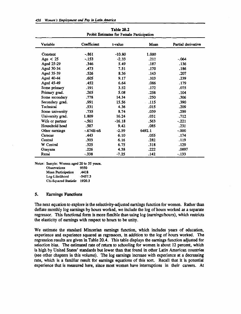
456 Women's Employment and Pay in Latin America
Table 20.2Probit Estimates for Female Participation
Variable Coefficient t-value Mean Partial derivative
Constant -.861 -10.80 1.000Age < 25 -.153 -2.33 .211 -.064Aged 25-29 .346 5.49 .187 .136Aged 30-34 .473 7.51 .170 .186Aged 35-39 .526 8.36 .143 .207Aged 40-44 .605 9.17 .103 .239Aged 45-49 .452 6.64 .086 .179Some primary .191 3.52 .172 .075Primary grad. .265 5.08 .258 .104Some secondary .778 14.34 .250 .306Secondary grad. .991 15.56 .115 .390Technical .531 4.36 .015 .209Some university .735 8.74 .039 .289University grad. 1.809 16.24 .031 .712Wife or partner -.561 -16.18 .563 -.221Household head .587 9.42 .085 .231Other earnings -.674E-oS -2.59 6492.1 -.000Caracas .443 6.10 .055 .174Central .303 6.16 .282 .119W Central .325 6.75 .318 .129Guayana .226 4.38 .222 .0897Rural -.338 -7.25 .142 -.133
Notes: Sample: Women aged 20 to 55 years.Observations 9350Mean Participation .4418Log-Likelihood -5457.3Chi-Squared Statistic 1920.3
5. Earnings Functions
The next equation to explore is the selectivity-adjusted earnings function for women. Rather thandeflate monthly log earnings by hours worked, we include the log of hours worked as a separateregressor. This functional form is more flexible than using log (earnings/hours), which restrictsthe elasticity of earnings with respect to hours to be unity.
We estimate the standard Mincerian earnings function, which includes years of education,experience and experience squared as regressors, in addition to the log of hours worked. Theregression results are given in Table 20.4. This table displays the earnings function adjusted forselection bias. The estimated rate of return to schooling for women is about 12 percent, whichis high by United States' standards but lower than that found in other Latin American countries(see other chapters in this volume). The log earnings increase with experience at a decreasingrate, which is a familiar result for earnings equations of this sort. Recall that it is potentialexperience that is measured here, since most women have interruptions in their careers. At
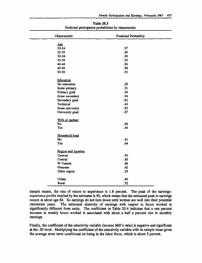
Female Particpation and Earnings, Venezuela 1987 457
Table 20.3Predicted participation probabilities by characteristic
Characteristic Predicted Probability
Age20-24 .2725-29 .4530-34 .5035-39 .5340-44 .5645-49 .5050-55 .32
EducationNo education .25Some primary .31Primary grad .34Some secondary .54Secondary grad .62Technical .44Some university .52University grad .87
Wife or partnerNo .56Yes .34
Household headNo .41Yes .64
Region and locationCaracas .50Central .45W Central .46Guayana .42Other region .33
Urban .45Rural .32
sample means, the rate of return to experience is 1.8 percent. The peak of the earnings-experience profile implied by the estimates is 50, which means that the estimated peak in earningsoccurs at about age 64. So earnings do not turn down until women are well into their potentialretirement years. The estimated elasticity of earnings with respect to hours worked issignificantly different from unity. The coefficient in Table 20.4 indicates that a one percentincrease in weekly hours worked is associated with about a half a percent rise in monthlyearnings.
Finally, the coefficient of the selectivity variable (inverse Mill's ratio) is negative and significantat the .05 level. Multiplying the coefficient of the selectivity variable with its sample mean givesthe average error term conditional on being in the labor force, which is about 5 percent.
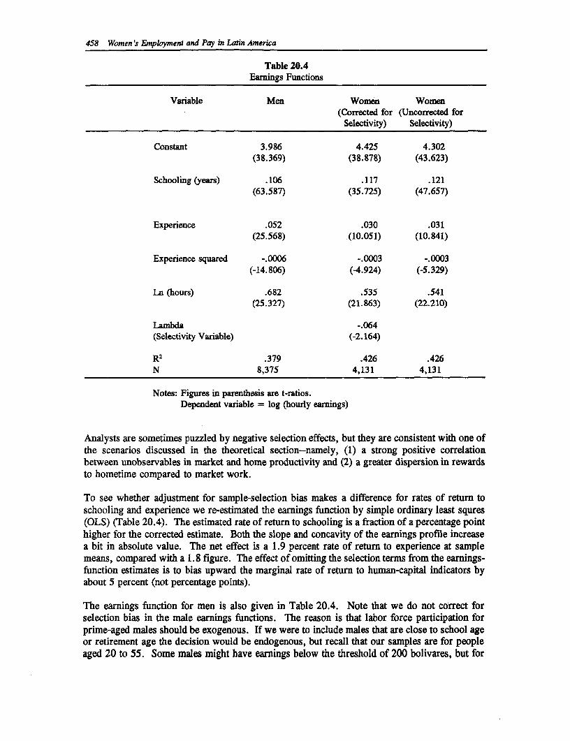
458 Women's Employment and Pay in Latin America
Table 20.4Earnings Functions
Variable Men Women Women(Corrected for (Uncorrected for
Selectivity) Selectivity)
Constant 3.986 4.425 4.302(38.369) (38.878) (43.623)
Schooling (years) .106 .117 .121(63.587) (35.725) (47.657)
Experience .052 .030 .031(25.568) (10.051) (10.841)
Experience squared -.0006 -.0003 -.0003(-14.806) (-4.924) (-5.329)
Ln (hours) .682 .535 .541(25.327) (21.863) (22.210)
Lambda -.064(Selectivity Variable) (-2.164)
R2 .379 .426 .426N 8,375 4,131 4,131
Notes: Figures in parenthesis are t-ratios.Dependent variable = log (hourly earnings)
Analysts are sometimes puzzled by negative selection effects, but they are consistent with one ofthe scenarios discussed in the theoretical section--namely, (1) a strong positive correlationbetween unobservables in market and home productivity and (2) a greater dispersion in rewardsto hometime compared to market work.
To see whether adjustment for sample-selection bias makes a difference for rates of return toschooling and experience we re-estimated the earnings function by simple ordinary least squres(OLS) (Table 20.4). The estimated rate of return to schooling is a fraction of a percentage pointhigher for the corrected estimate. Both the slope and concavity of the earnings profile increasea bit in absolute value. The net effect is a 1.9 percent rate of return to experience at samplemeans, compared with a 1.8 figure. The effect of omitting the selection terms from the earnings-function estimates is to bias upward the marginal rate of return to human-capital indicators byabout 5 percent (not percentage points).
The earnings function for men is also given in Table 20.4. Note that we do not correct forselection bias in the male earnings functions. The reason is that labor force participation forprime-aged males should be exogenous. If we were to include males that are close to school ageor retirement age the decision would be endogenous, but recall that our samples are for peopleaged 20 to 55. Some males might have earnings below the threshold of 200 bolivares, but for
Femak Participation and Earnings, Venezuela 1987 459
reasons that are likely to be exogenous to the model; illness, unemployment caused by deficientdemand, or search unemployment.
The estimated rate of return for schooling is slightly lower for males than females. But thereturns from labor market experience are a lot higher for men than women. At sample means therate of return to experience is 2.4 percent for men, a third higher than the comparable figure forwomen. This result is consistent with human-capital-investment theory, which predicts thatworkers with long horizons will invest in skills more than those with short ones. And men arelikely to have much longer horizons than women who drop out of the labor force to raisechildren.
How is the investment effect reflected in the experience-earnings profile? Investing a lot earlyin the career entails foregone earnings, which lowers starting wages. But as skills accumulatewith experience investment declines. The latter occurs because it pays to invest the most whenyoung. The two effects combine to steepen the earnings profile.
6. Discrimination
Now that we have estimated earnings functions for men and women, we can address the questionposed at the beginning: how much of the male-female earnings differential can be explained byobserved factors? How much might be caused by discrimination?
The technique used to answer this question is the widely-used Oaxaca (1973) decomposition. Theidea is to split the difference in log wages into that accounted for by differences in observedvariables, and that accounted for by differences in the way those variables are rewarded. We canwrite the difference in log earnings of men and women as:
BmXm - BfXf = (B. - Bf)X. + Bf(Xm - Xf) (7a)= (B. - Bf)Xf + Bm(Xi - Xf), (7b)
where Bi i = m,f are the estimated coefficients of the earnings functions and Xi i = m,f are theaverages of the explanatory variables in the earnings functions. Focus on expression 7a. Thefirst term is the difference in rewards, for those having mean attributes of men. The second termis the differential due to differences in attributes, weighted by the vector of female coefficients.Expression 7b does the same job as 7a, but the weights are different. (We discuss this below.)
Before we proceed further in calculating the 'explained" component of the wage gap, we needto address three further issues. First, what sample means should we use for women--workersonly or the entire sample? The answer is that we should use the entire sample, because theselectivity corrected equations gives us an estimate of the population regression function whenwe base our predictions on the estimate of b in equation 1. Second, we do not include the Mill'sratio terms or their coefficients in making our predictions because we seek to measure theconditional mean for the population, not just the sample of working women. Third, though weuse entire-sample means for female schooling and experience, we use the working-sample meanfor log hours, since hours for non-working women equal zero because they do not participate inthe labor force.
Second, note that the Oaxaca-decomposition can be done two ways, hence expressions 7a and 7b.Which way is best? Economic theory gives little guidance; this is an example of the index-
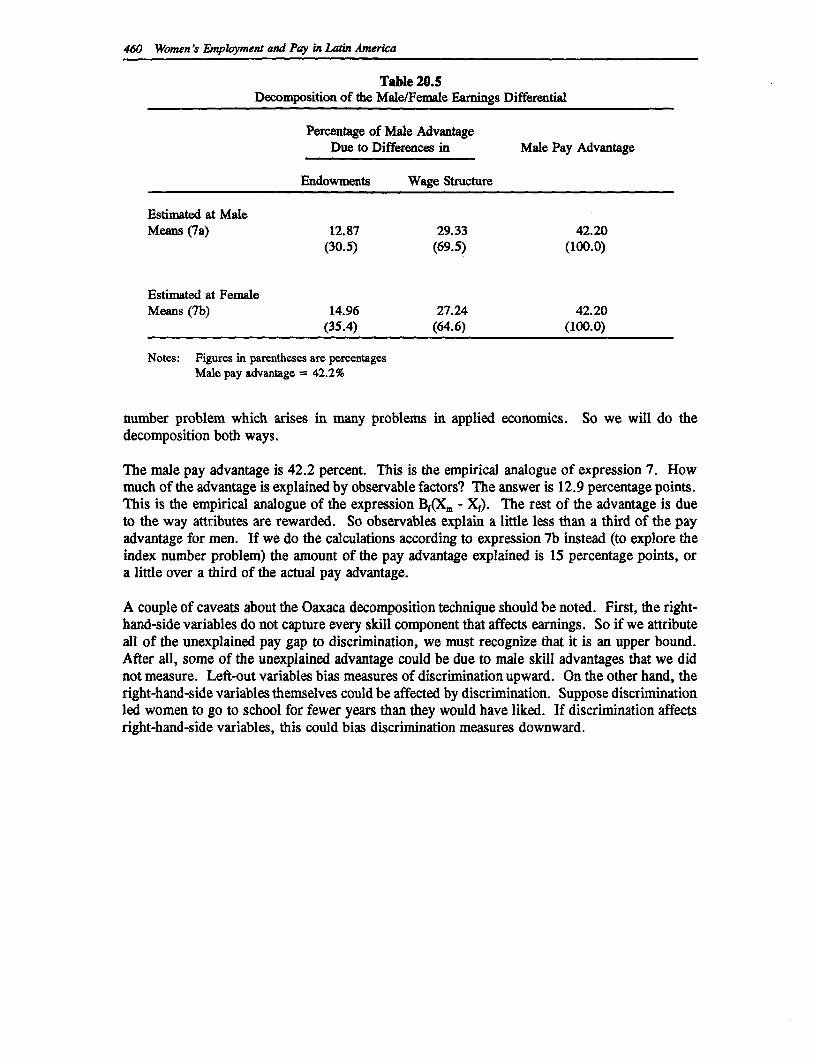
4W Women 's Employment and Pay in Latin America
Table 20.5Decomposition of the Male/Female Earnings Differential
Percentage of Male AdvantageDue to Differences in Male Pay Advantage
Endowments Wage Structure
Estimated at MaleMeans (7a) 12.87 29.33 42.20
(30.5) (69.5) (100.0)
Estimated at FemaleMeans (7b) 14.96 27.24 42.20
(35.4) (64.6) (100.0)
Notes: Figures in parentheses are percentagesMale pay advantage = 42.2%
number problem which arises in many problems in applied economics. So we will do thedecomposition both ways.
The male pay advantage is 42.2 percent. This is the empirical analogue of expression 7. Howmuch of the advantage is explained by observable factors? The answer is 12.9 percentage points.This is the empirical analogue of the expression Bf(X3 - Xf). The rest of the advantage is dueto the way attributes are rewarded. So observables explain a little less than a third of the payadvantage for men. If we do the calculations according to expression 7b instead (to explore theindex number problem) the amount of the pay advantage explained is 15 percentage points, ora little over a third of the actual pay advantage.
A couple of caveats about the Oaxaca decomposition technique should be noted. First, the right-hand-side variables do not capture every skill component that affects earnings. So if we attributeall of the unexplained pay gap to discrimination, we must recognize that it is an upper bound.After all, some of the unexplained advantage could be due to male skill advantages that we didnot measure. Left-out variables bias measures of discrimination upward. On the other hand, theright-hand-side variables themselves could be affected by discrimination. Suppose discriminationled women to go to school for fewer years than they would have liked. If discrimination affectsright-hand-side variables, this could bias discrimination measures downward.
References
Borjas, G.J. "Self-selection and the Earnings of Immigrants." American Economic Review, Vol.77 (1987). pp. 531-555.
Heckman, J. "Sample Selection as a Specification Error." Econometrica, Vol. 47, no. 1 (1979).pp. 153-161.
---. "Shadow Prices, Market Wages, and Labor Supply." Econometrica, Vol. 42, no. 4 (1974).pp. 679-694.
Lee, L. "Unionism and Wage Rates: A Similtaneous Equations Model with Qualitative andLimited Dependent Variables. " International Economic Review, Vol. 19 (1978). pp. 415-433.
Mincer, J. "Labor Force Participation of Married Women: A Study of Labor Supply" in NationalBureau of Economic Research. Aspects of Labor Economics. Princeton, New Jersey:Princeton University Press, 1962.
Oaxaca, R.L. "Male-female Wage Differentials in Urban Labor Markets." InternationalEconomic Review, Vol. 14. no. 1 (1973). pp. 693-709.
Roy, A.D. "Some Thoughts on the Distribution of Earnings." Oxford Economic Papers, Vol. 3(1951). pp. 135-146.
Willis, R. and S. Rosen. "Education and Self-selection." Journal of Political Economy, Vol. 87,no. 5, part 2 (1979). pp. S7-S36.
World Bank. "Venezuela: A Country Assessment on the Role of Women in Development."Mimeograph. Washington, D.C.: Latin American and Caribbean Region, World Bank.1990.
461

21
Female Earnings, Labor Force Participation andDiscrimination in Venezuela, 1989
Carolyn Winter
1. Introduction
In this chapter we try to determnine (1) what factors are most likely to influence female labor forceparticipation and (2) what factors account for existing male-female wage differentials inVenezuela. The 1989 household survey data show working female monthly earnings to beapproximately 78 percent of male earnings. Although this differential is not as large as thatreported in many other Latin American countries, it is still substantial.' It is important todetermine whether this differential is the result of different endowments in productivity-relatedcharacteristics between the sexes, such as education and work experience, or whether it is aconsequence of labor market discrimination. If men and women in Venezuela are paid accordingto the same wage structure differences in endowments should account for all the observedearnings differentials. If, however, we adjust for differences in endowments between the sexesand we continue to find a wage gap, this can be interpreted as evidence of wage discriminationbetween the sexes. Following Oaxaca's (1973) approach, we decompose sex-specific earningsinto an "endowment" component and a "discrimination" component and attempt to estimate theextent to which wage differentials result from discrimination.
The following section provides a brief description of the Venezuelan labor market, its fluctuatingfortunes since the end of the "oil boom," and general factors affecting women's labor forceparticipation. Section 3 describes the data base used in the analysis and some basic features ofthe data. In Section 4 we present probit estimates showing the determinants of women's laborforce participation and in Section 5 we consider earnings functions estimates for working malesand females and include corrections for possible selectivity bias among women. Section 6presents the estimate of the extent to which earnings differentials can be explained bydiscrimination.
2. The Setting: The Venezuelan Economy and Labor Market
The discovery and widespread exploitation of oil meant that Venezuela changed rapidly from anagriculture-based economy to one of the largest oil exporters by mid-century. Although the oilindustry itself has never been a large employer of labor (in 1989 it employed only 0.7 percent
i Many of the other studies reported in this volume (Brazil and Peru, for example), report women'searmings to be about two-thirds of men's. BirdsalU & Fox (1985) report that female teachers in Brazil earnless than 55 percent of male teacher's earnings.
463
464 Women's Employment and Pay in Latin America
of the labor force) it fueled the growth and expansion of the economy which is nowpredominantly urban-based. In 1989 approximately 82 percent of the population lived in urbanareas, principally in the northern industrialized states.
The rapidly growing population and the economic windfalls of the "oil boom" during the sixtiesand seventies prompted the government to give priority to the expansion of education, particularlytertiary education where enrollments increased by 9.1 percent per annum between 1975 and 1984(Psacharopoulos and Steier, 1988). Improved access to schooling has especially benefittedfemales who now have, on average, 1.6 years more schooling than males.
Increased access to education has meant that women's labor force participation has increasedsignificantly, from 22 percent in the 1970s, to 29 percent in 1982, and to 38 percent in 1989 (dePlanchart, 1988; Psacharopoulos and Alam, 1991). The proportion of women holdingprofessional and technical jobs grew from 15.2 percent in 1961, to 22.1 percent in 1987, and21.1 percent in 1989 (de Planchart, 1988). In terms of earnings, however, women continue tobe concentrated in lower paying occupations. The proportion of women in the highest payingcategory, managerial occupations, has changed little over the past two decades (see Appendixtable) and in professional occupations, women are predominantly found in the lower paying areas,such as nursing and teaching.
Economic growth halted abruptly in 1979 with the end of the "oil boom" and labor shortageswere replaced by rising unemployment which peaked at 14 percent in early 1985, stabilizedaround 6.9 percent in 1988 and began to rise sharply again in 1989. Workers in low-paid, lowskills jobs have been most immediately affected and women are often heavily represented amongthese groups.
Women's labor force participation has also been affected by "protective" labor legislation lawsintroduced in the seventies which inadvertently work to exclude women from certain sectors ofthe labor market. These laws prohibit employers from hiring women for "physically andmorally" dangerous work, for night work, or in industries with numerous daily shifts. It is alsoillegal for women to work in most occupations in the mining sector. In addition, legislationstipulating generous maternal leave privileges at full pay makes female labor potentially morecostly to employers than male labor.
Recorded incidents of discrimination against female workers are few, but there is evidence thatemployers seek not to hire women and actively discriminate against hiring married women(Rakowski, 1985). Clauses supporting equal pay for equal work have really only been enforcedin the public sector which possibly accounts for the high proportion of women (more than twiceas many women as men) employed in this sector.
Venezuela's rapid population growth rate, averaging 3.5 percent in the previous two decades and2.8 percent in the 1980s, means that 40 percent of the population is now under 15 years of age.To keep unemployment at its current levels, a real annual growth rate in the GDP of 5 percentwould have to be achieved and maintained. This is not expected (Economist Intelligence Unit,1989). Changes in women's labor force participation and the extent to which discriminationaffects their earnings will thus be a real concern in any poverty alleviation efforts; women aremore heavily represented among lower income groups than men and the proportion of femaleheaded households, already accounting for over 20 percent of all households, is continuing toincrease.
Female Earnings, Labor Force Participation and Discrimination in Venezuela, 1989 465
3. Data Characteristics
The analysis is based on data from the 1989 Venezuela Household Survey conducted by theOficina Central de Estadisticas e Informatica (OCEI). Such Household Surveys were conductedtwice yearly between 1968 and 1983, and quarterly from 1984. The survey covers nine politicaladministrative regions, Caracas Metropolitan area, Capital, Central, West-central, Zuliana, LosAndes, Southern, Non-eastern, and Guyana. Data from the Guyana region were collectedindependently in the 1989 survey and technical difficulties with the data prevented its inclusionin this analysis. The available survey data included 159,818 individual observations from whicha 10 percent random sample was drawn for use in this analysis.
The survey provides detailed information on labor issues including employment status, weeklyhours worked, occupation and industry category, and monthly income. Data on socio-economiccharacteristics such as age, educational attainment, marital status, number of children andhousehold size is also available.
Labor participation, as commonly defined, includes those employed and those seekingemployment. However, because a large informal sector exists in Venezuela, it was difficult toidentify individuals as unemployed or as being employed in the formal sector in the data base.Consequently, only actively employed individuals, identified by their positive responses toquestions concerning employment status, weekly hours worked and monthly income, were definedas participating in the labor force. Individuals with incomplete or inconsistent labor marketinformation were excluded from the sample. This included unpaid family workers and workerswho did not report hours worked. Income was reported erratically by younger and olderrespondents. Consequently the sample was restricted to prime-age working males (20-60 years)and prime-age females (20-55 years). Within the samples of working males and females,individuals who reported earning less than 10 percent of the mean hourly wage for their sex ormore than 15 times the mean hourly wage were excluded. Fifteen cases, reporting eitherextremely high or low earnings, were excluded in this way. This resulted in a sample of 2,408working males and 3,143 females, of whom 1,181 were working in either the public or privatesector. The proportion of employed men and women were 76 and 38 percent respectively.
A proxy for labor force experience was constructed as age minus years of schooling minus sixyears. This proxy measure will almost certainly overstate experience since no adjustments canbe made for periodic absences from the labor force. Overestimates will be most severe forwomen since they are more likely to withdraw during childrearing.
Table 21.1 gives means and standard deviations of the sample variables by gender. Workingwomen earn approximately 78 percent of men's weekly earnings but, on average, work fewerhours per week (38.48 compared to 43.71 hours). After adjusting for differences in weekly hoursworked, women's hourly earnings are 12 percent less than men's. The proxy measure for laborforce experience is lower for women.
As in most Latin American countries, female workers in Venezuela have, on average,approximately one and one half years more schooling than male workers. This educationaladvantage holds true at all education levels beyond primary school, even at tertiary levels.Working women are also more likely than men to be studying while they are working.Married/cohabiting women are less likely to participate than married/cohabiting men.
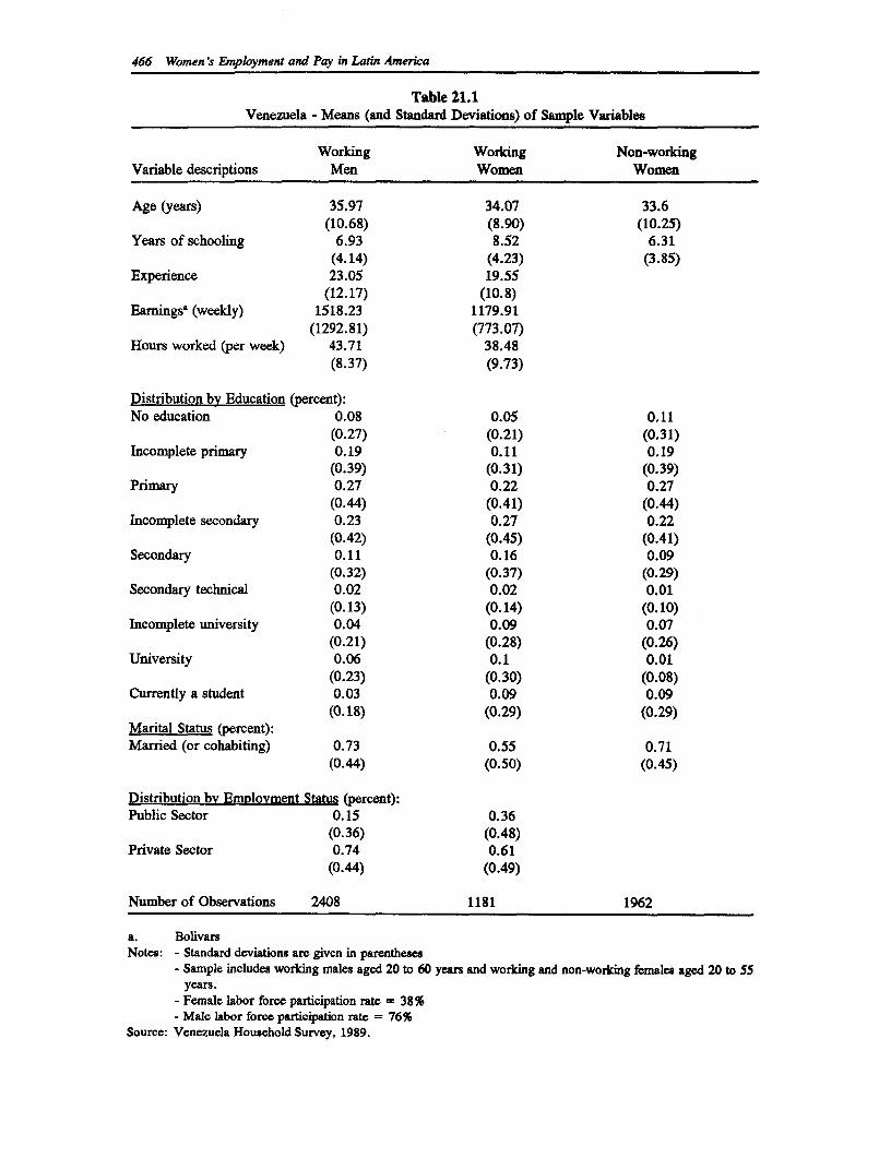
466 Women's Emaployment and Pay in Latin America
Table 21.1Venezuela - Means (and Standard Deviations) of Sample Variables
Working Working Non-workingVariable descriptions Men Women Women
Age (years) 35.97 34.07 33.6(10.68) (8.90) (10.25)
Years of schooling 6.93 8.52 6.31(4.14) (4.23) (3.85)
Experience 23.05 19.55(12.17) (10.8)
Earningse (weekly) 1518.23 1179.91(1292.81) (773.07)
Hours worked (per week) 43.71 38.48(8.37) (9.73)
Distribution by Education (percent):No education 0.08 0.05 0.11
(0.27) (0.21) (0.31)Incomplete primary 0.19 0.11 0.19
(0.39) (0.31) (0.39)Primary 0.27 0.22 0.27
(0.44) (0.41) (0.44)Incomplete secondary 0.23 0.27 0.22
(0.42) (0.45) (0.41)Secondary 0.11 0.16 0.09
(0.32) (0.37) (0.29)Secondary technical 0.02 0.02 0.01
(0.13) (0.14) (0.10)Incomplete university 0.04 0.09 0.07
(0.21) (0.28) (0.26)University 0.06 0.1 0.01
(0.23) (0.30) (0.08)Currently a student 0.03 0.09 0.09
(0.18) (0.29) (0.29)Marital Status (percent):Married (or cohabiting) 0.73 0.55 0.71
(0.44) (0.50) (0.45)
Distribution by Emplovment Status (percent):Public Sector 0.15 0.36
(0.36) (0.48)Private Sector 0.74 0.61
(0.44) (0.49)
Number of Observations 2408 1181 1962
a. BolivarsNotes: - Standard deviations are given in parentheses
- Sample includes worldng males aged 20 to 60 years and working and non-working females aged 20 to 55years.
- Female labor force participation rate = 38%- Male labor force participation rate = 76%
Source: Venezuela Household Survey, 1989.
Female Earnings, Labor Force Participation and Discrimination in Venezuela, 1989 467
4. Determinants of Female Labor Force Participation
Numerous factors influence a woman's decision to participate in the labor market -- herinvestments in human capital, personal characteristics such as her marital status and whether shehas young children, and other factors such as the availability of suitable childcare options.Ultimately, her decision to participate will rest upon the comparison of her market wage with thevalue of her time in the home (i.e., her reservation wage).
This means that if we estimate earnings functions using data from our sample of working women,the sample will include only women whose market wage exceeds their reservation wage.Consequently, we will be estimating earnings functions for a self-selected sample of women.
To correct for this we follow Heckman's (1979) widely adopted procedure and estimate a probitequation for the full sample of women (working and non-working) in which the probability thata woman will participate is estimated given various conditions, in this case whether she has youngdependent children, her age, region of residence and educational attainment. The dependentvariable in this model is a dummy variable for labor force participation (1 if a participant and 0if not). The inverse Mill's ratio (Lambda) is estimated in this equation and entered in theearnings equations to adjust for the possible selectivity bias inherent in our sample of workingwomen. The probit estimates are shown in Table 21.2. Table 21.3 estimates predictedparticipation rates for each characteristic while the values of other characteristics is held at theirsample mean.
In line with the general human capital literature, education is found to have a powerful effect onparticipation. The probit coefficients in Table 21.2 show that the probability of participating risessteadily with each successive level of education. The predicted probabilities in Table 21.3 makesthis very evident. A woman with mean values of all other characteristics and completeduniversity education has a predicted probability of labor force participation 37 percentage pointshigher than a woman with completed secondary education (probability = .87 versus .50).Similarly, a woman with completed secondary education has a predicted probability ofparticipation 21 percentage points higher than a woman who has only completed primaryeducation (probability = .50 versus .29).
The effects of age on participation are as expected, with women's probability of workingincreasing steadily from their mid-twenties and peaking between ages 41 and 45. Lowparticipation rates among women in their early twenties are consistent with the high enrollment(44 percent) of women in this age group in higher education.
It is widely posited that being the mother of young children (under 6 years of age) significantlyincreases the opportunity costs of women's labor force participation and increases the probabilitythat they will withdraw from the labor force.2 Our estimates support this finding. Table 21.3shows that a woman has a predicted probability of participation of .32 if she has young childrenand .41 if she does not.
2 See Behrman and Wolfe (1984) and Gronau (1988).
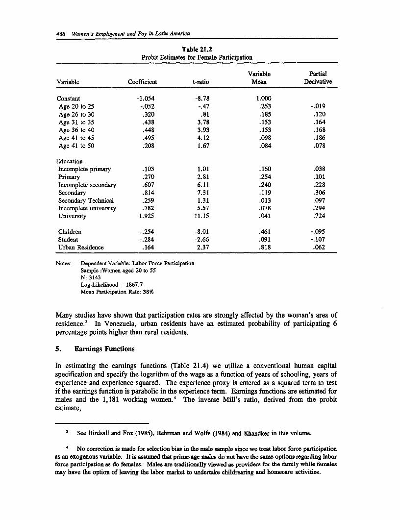
468 Women's Employment and Pay in Latin America
Table 21.2Probit Estimates for Female Participation
Variable PartialVariable Coefficient t-ratio Mean Derivative
Constant -1.054 -8.78 1.000Age 20 to 25 -.052 -.47 .253 -.019Age 26 to 30 .320 .81 .185 .120Age 31 to 35 .438 3.78 .153 .164Age 36 to 40 .448 3.93 .153 .168Age 41 to 45 .495 4.12 .098 .186Age 41 to 50 .208 1.67 .084 .078
EducationIncomplete primary .103 1.01 .160 .038Primary .270 2.81 .254 .101Incomplete secondary .607 6.11 .240 .228Secondary .814 7.31 .119 .306Secondary Technical .259 1.31 .013 .097Incomplete university .782 5.57 .078 .294University 1.925 11.15 .041 .724
Children -.254 -8.01 .461 -.095Student -.284 -2.66 .091 -.107Urban Residence .164 2.37 .818 .062
Notes: Dependent Variable: Labor Force ParticipationSample :Women aged 20 to 55N: 3143Log-Likelihood -1867.7Mean Participation Rate: 38%
Many studies have shown that participation rates are strongly affected by the woman's area ofresidence.3 In Venezuela, urban residents have an estimated probability of participating 6percentage points higher than rural residents.
5. Earnings Functions
In estimating the earnings functions (Table 21.4) we utilize a conventional human capitalspecification and specify the logarithm of the wage as a function of years of schooling, years ofexperience and experience squared. The experience proxy is entered as a squared term to testif the earnings function is parabolic in the experience term. Earnings functions are estimated formales and the 1,181 working women.4 The inverse Mill's ratio, derived from the probitestimate,
3 See Birdsall and Fox (1985), Behrman and Wolfe (1984) and Khandker in this volume.
4 No correction is made for selection bias in the male sample since we treat labor force participationas an exogenous variable. It is assumed that prime-age males do not have the same options regarding laborforce participation as do females. Males are traditionally viewed as providers for the family while femalesmay have the option of leaving the labor market to undertake childrearing and homecare activities.
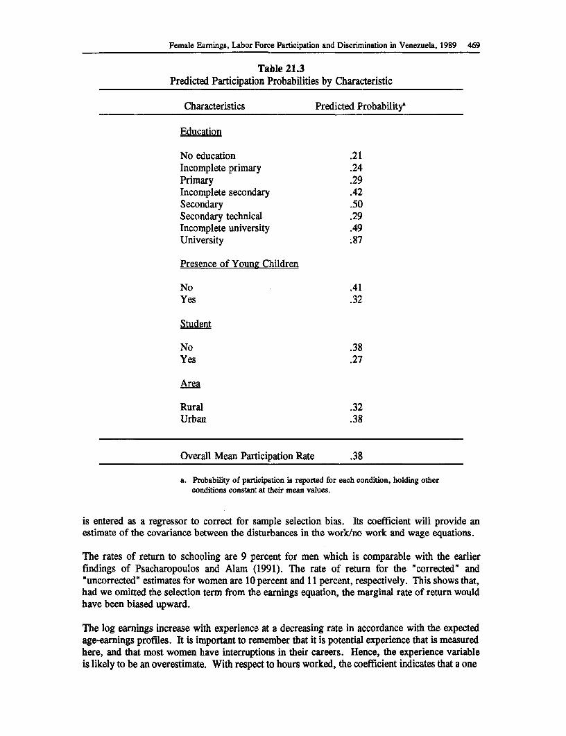
Female Earnings, Labor Force Participation and Discrimination in Venezuela, 1989 469
Table 21.3Predicted Participation Probabilities by Characteristic
Characteristics Predicted Probabilitya
Education
No education .21Incomplete primary .24Primary .29Incomplete secondary .42Secondary .50Secondary technical .29Incomplete university .49University .87
Presence of Young Children
No .41Yes .32
Student
No .38Yes .27
Area
Rural .32Urban .38
Overall Mean Participation Rate .38
a. Probability of participation is reported for each condition, holding otherconditions constant at their mean values.
is entered as a regressor to correct for sample selection bias. Its coefficient will provide anestimate of the covariance between the disturbances in the work/no work and wage equations.
The rates of return to schooling are 9 percent for men which is comparable with the earlierfindings of Psacharopoulos and Alam (1991). The rate of return for the "corrected" and"uncorrected" estimates for women are 10 percent and 11 percent, respectively. This shows that,had we omitted the selection term from the earnings equation, the marginal rate of return wouldhave been biased upward.
The log earnings increase with experience at a decreasing rate in accordance with the expectedage-earnings profiles. It is important to remember that it is potential experience that is measuredhere, and that most women have interruptions in their careers. Hence, the experience variableis likely to be an overestimate. With respect to hours worked, the coefficient indicates that a one
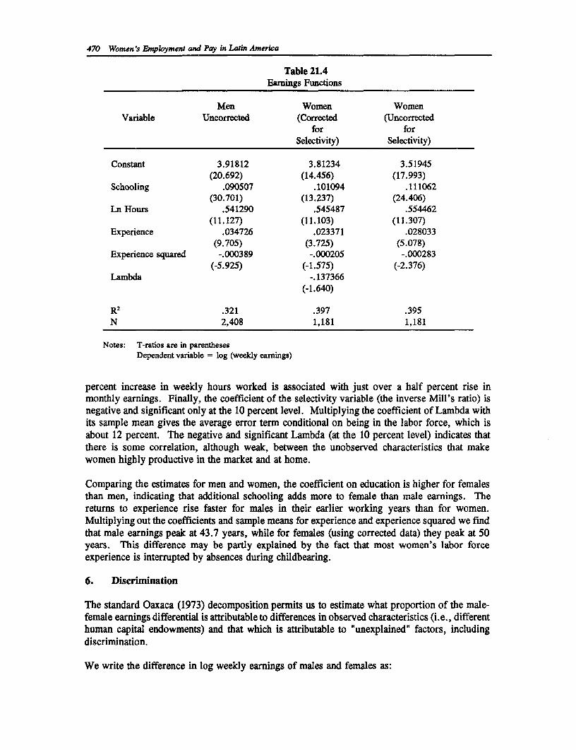
470 Women's Employment and Pay in Latin America
Table 21.4Earmings Functions
Men Women WomenVariable Uncorrected (Corrected (Uncorrected
for forSelectivity) Selectivity)
Constant 3.91812 3.81234 3.51945(20.692) (14.456) (17.993)
Schooling .090507 .101094 .111062(30.701) (13.237) (24.406)
Ln Hours .541290 .545487 .554462(11.127) (11.103) (11.307)
Experience .034726 .023371 .028033(9.705) (3.725) (5.078)
Experience squared -.000389 -.000205 -.000283(-5.925) (-1.575) (-2.376)
Lambda -.137366(-1.640)
R2 .321 .397 .395N 2,408 1,181 1,181
Notes: T-ratios are in parenthesesDependent variable = log (weekly earnings)
percent increase in weekly hours worked is associated with just over a half percent rise inmonthly earnings. Finally, the coefficient of the selectivity variable (the inverse Mill's ratio) isnegative and significant only at the 10 percent level. Multiplying the coefficient of Lambda withits sample mean gives the average error term conditional on being in the labor force, which isabout 12 percent. The negative and significant Lambda (at the 10 percent level) indicates thatthere is some correlation, although weak, between the unobserved characteristics that makewomen highly productive in the market and at home.
Comparing the estimates for men and women, the coefficient on education is higher for femalesthan men, indicating that additional schooling adds more to female than male earnings. Thereturns to experience rise faster for males in their earlier working years than for women.Multiplying out the coefficients and sample means for experience and experience squared we findthat male earnings peak at 43.7 years, while for females (using corrected data) they peak at 50years. This difference may be partly explained by the fact that most women's labor forceexperience is interrupted by absences during childbearing.
6. Discrimination
The standard Oaxaca (1973) decomposition permits us to estimate what proportion of the male-female earnings differential is attributable to differences in observed characteristics (i.e., differenthuman capital endowments) and that which is attributable to "unexplained" factors, includingdiscrimination.
We write the difference in log weekly earnings of males and females as:
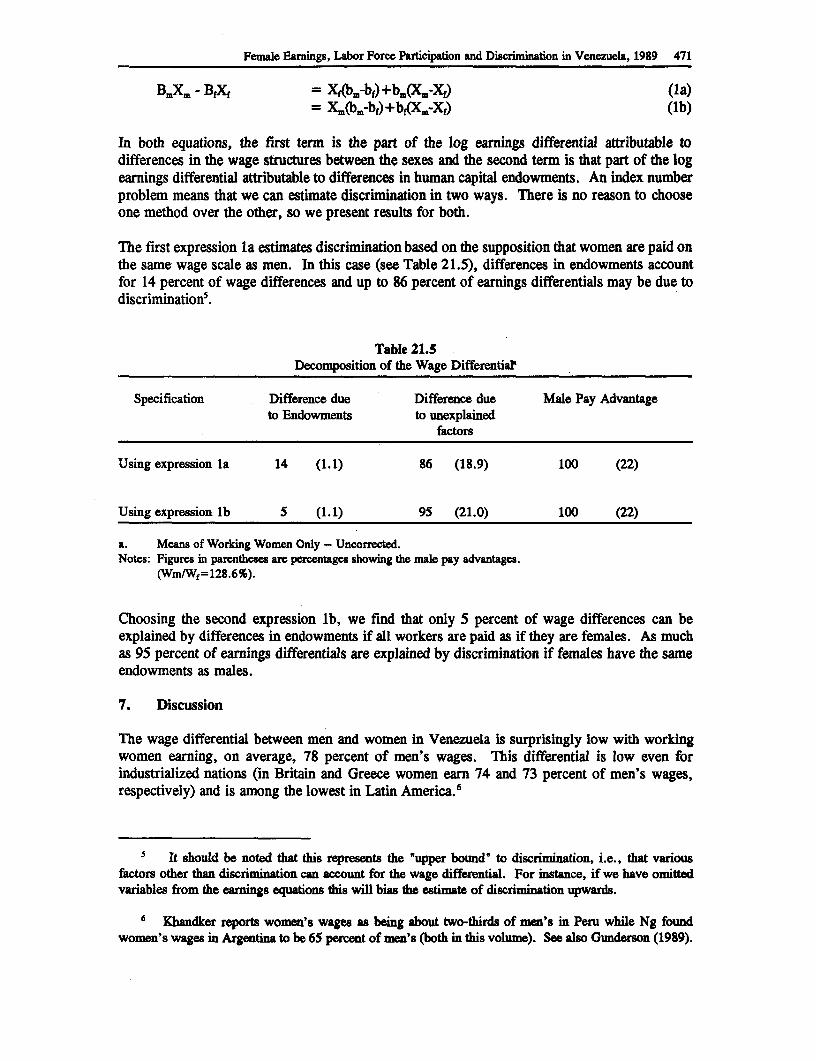
Female Earnings, Labor Force Participation and Discrimination in Venezuela, 1989 471
BmXm - BfXf = XAbmbf)+bm(X,-Xf) (la)= Xm(bm7bf)+bf(Xm-Xf) (lb)
In both equations, the first term is the part of the log earnings differential attributable todifferences in the wage structures between the sexes and the second term is that part of the logearnings differential attributable to differences in human capital endowments. An index numberproblem means that we can estimate discrimination in two ways. There is no reason to chooseone method over the other, so we present results for both.
The first expression la estimates discrimination based on the supposition that women are paid onthe same wage scale as men. In this case (see Table 21.5), differences in endowments accountfor 14 percent of wage differences and up to 86 percent of earnings differentials may be due todiscrimination5.
Table 21.5Decomposition of the Wage Differentia?
Specification Difference due Difference due Male Pay Advantageto Endowments to unexplained
factors
Using expression la 14 (1.1) 86 (18.9) 100 (22)
Using expression lb 5 (1.1) 95 (21.0) 100 (22)
a. Means of Workdng Women Only - Uncorrected.Notes: Figures in parentheses are percentages showing tfie male pay advantages.
(Wmi/Wf=128.6%).
Choosing the second expression lb, we find that only 5 percent of wage differences can beexplained by differences in endowments if all workers are paid as if they are females. As muchas 95 percent of earnings differentials are explained by discrimination if females have the sameendowments as males.
7. Discussion
The wage differential between men and women in Venezuela is surprisingly low with workingwomen earning, on average, 78 percent of men's wages. This differential is low even forindustrialized nations (in Britain and Greece women earn 74 and 73 percent of men's wages,respectively) and is among the lowest in Latin America.6
5 It should be noted that this represents the *upper bound" to discrimination, i.e., that variousfactors other than discrimination can account for the wage differential. For instance, if we have omittedvariables from the earnings equations this will bias the estimate of discrimination upwards.
6 Khandker reports women's wages as being about two-thirds of men's in Peru while Ng foundwomen's wages in Argentina to be 65 percent of men's (both in this volume). See also Gunderson (1989).
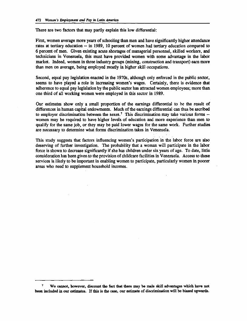
472 Women's Employment and Pay in Lain America
There are two factors that may partly explain this low differential:
First, women average more years of schooling than men and have significantly higher attendancerates at tertiary education - in 1989, 10 percent of women had tertiary education compared to6 percent of men. Given existing acute shortages of managerial personnel, skilled workers, andtechnicians in Venezuela, this must have provided women with some advantage in the labormarket. Indeed, women in three industry groups (mining, construction and transport) earn morethan men on average, being employed mostly in higher skill occupations.
Second, equal pay legislation enacted in the 1970s, although only enforced in the public sector,seems to have played a role in increasing women's wages. Certainly, there is evidence thatadherence to equal pay legislation by the public sector has attracted women employees; more thanone third of all working women were employed in this sector in 1989.
Our estimates show only a small proportion of the earnings differential to be the result ofdifferences in human capital endowments. Much of the earnings differential can thus be ascribedto employer discrimination between the sexes.7 This discrimination may take various forms -women may be required to have higher levels of education and more experience than men toqualify for the same job, or they may be paid lower wages for the same work. Further studiesare necessary to determine what forms discrimination takes in Venezuela.
This study suggests that factors influencing women's participation in the labor force are alsodeserving of further investigation. The probability that a woman will participate in the laborforce is shown to decrease significantly if she has children under six years of age. To date, littleconsideration has been given to the provision of childcare facilities in Venezuela. Access to theseservices is likely to be important in enabling women to participate, particularly women in poorerareas who need to supplement household incomes.
7 We cannot, however, discount the fact that there may be male skill advantages which have notbeen included in our estimates. If this is the case, our estimate of discrimination will be biased upwards.
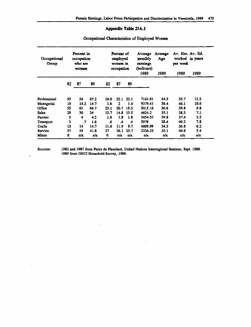
PFmale Earnings, Labor Force Participation and Discrimination in Venezucla, 1989 473
Appendix Table 21A.1
Occupational Characteristics of Employed Women
Percent in Percent of Average Average Av. Hrs. Av. Ed.Occupational occupation employed monthly Age worked in years
Group who are women in earnings per weekwomen occupation (bolivars)
1989 1989 1989 1989
82 87 89 82 87 89
Professional 55 54 67.2 19.8 22.1 22.1 7161.81 34.5 35.7 12.2Managerial 10 14.2 14.7 1.6 2 1.4 9379.41 . 36.4 46.1 10.6Office 55 61 64.7 23.1 20.7 19.5 5015.16 30.8 39.8 9.8Sales 29 30 34 13.7 14.8 13.5 4624.2 35.1 38.3 7.1Farmer 3 4 4.2 1.6 1.8 1.8 3454.52 39.8 37.6 2.2Transport 2 .7 1.6 .6 .4 .4 5978 28.4 40.2 7.8Crafts 13 14 14.7 11.6 11.9 9.7 4009.99 34.3 36.8 6.2service 57 54 41.8 27 26.1 25.7 3226.35 35.1 40.8 5.4Miner 0 n/a n/a 0 n/a n/a n/a n/a n/a n/a
Sources: 1982 and 1987 from Perez de Planchart, United Nations Interregional Seminar, Sept. 1988.1989 from OECI Household Survey, 1989.
References
Birdsall, N. and N. Fox. "Why Males Earn More: Location and Training of BrazilianSchoolteachers." Economic Development and Cultural Change, Vol. 33, no. 3 (1985). pp.533-556.
Behrman, J. R. and B. L. Wolfe. "Labor Force Participation and Earnings Determinants forWomen in the Special Conditions of Developing Countries." Journal of DevelopmentEconomics, Vol. 15 (1984). pp. 259-288.
Gannicott, K. "Women, Wages and Discrimination: Some Evidence from Taiwan." EconomicDevelopment and Cultural Change, Vol. 39, no.4 (1986) pp. 721-730.
Gronau, R. "Sex-Related Wage Differentials and Women's Interrupted Labor Careers: TheChicken and Egg Question." Journal of Labor Economics, Vol.6, no. 3 (1988). pp. 277-301.
Gunderson, M. "Male-female Wage Differentials and Policy Responses." Journal of EconomicLiterature, Vol. 21, no. 1 (1989). pp. 46-72.
Heckman, J.J. "Sample Selection Bias as a Specification Error." Econometrica, Vol. 47, no. 1(1979).pp. 53-161.
Khandker, S.R. "Labor Market Participation, Returns to Education, and Male-Female WageDifferences in Peru." In this volume.
Knight, J.B. and R.H. Sabot. "Labor Market Discrimination in a Poor Urban Economy." TheJournal of Development Studies, Vol. 19, no. 1 (1982). pp. 67-87.
McCoy, J.L. "The Politics of Adjustment: Labor and the Debt Crisis." Journal of InterAmericanStudies and World Affairs, Vol. 28 (1986/87). pp. 103-38.
Oaxaca, R.L. "Sex Earning Differentials" in G. Psacharopoulos (ed.). Economics of Education:Research and Studies. New York: Pergamon Press, 1987.
Oaxaca, R.L. "Male-female Wage Differentials in Urban Labor Markets." InternationalEconomic Review, Vol. 14, no.1 (1973). pp. 693-709.
Perez de Planchart, M.C. Case Study of Venezuela: Women and the Economic Crisis. Vienna:United National Interregional Seminar on Women and the Economic Crisis, 1988.
474
Female Earnings, Labor Force Participation and Discrimination in Venezuela, 1989 475
Psacharopoulos, G. and A. Alam. "Earnings and Education in Venezuela: An Update from the1987 Household Survey." Economics of Education Review, Vol. 10, No. 1 (1991).
Psacharopoulos, G. and F. Steier. "Education and the Labor Market in Venezuela, 1975-1984."Economics of Education Review, Vol. 7, no. 3 (1988). pp. 321-332.
Psacharopoulos, G. and E. Velez. "Does Training Pay Independent of Education? SomeEvidence from Colombia.' International Journal of Educational Research, forthcoming,1991.
Rakowski, C.A. Women in Nontraditional Industry: The Case of Steel in Ciudad Guayana,Venezuela. Working Paper No. 104. Michigan: Michigan State University, 1985.
Rakowski, C.A. Production and Reproduction in a Planned Industrial City: The Working- andLower-Class Households of Ciudad Guayana, Venezuela. Working Paper No. 61.Michigan: Michigan State University, 1984.
The Economist Intelligence Unit. Venezuela to 1993. A Change in Direction? Special Report No.2003. London: The Economist Intelligence Unit, 1989.
United Nations. Five Studies on the Situation of Women in Latin America. Santiago: UnitedNations,1983.
Urdaneta, L. Participation Economica de la Mujer YLa Distribucion del Ingreso. 1986. Caracas:Banco Central de Venezuela, 1986.

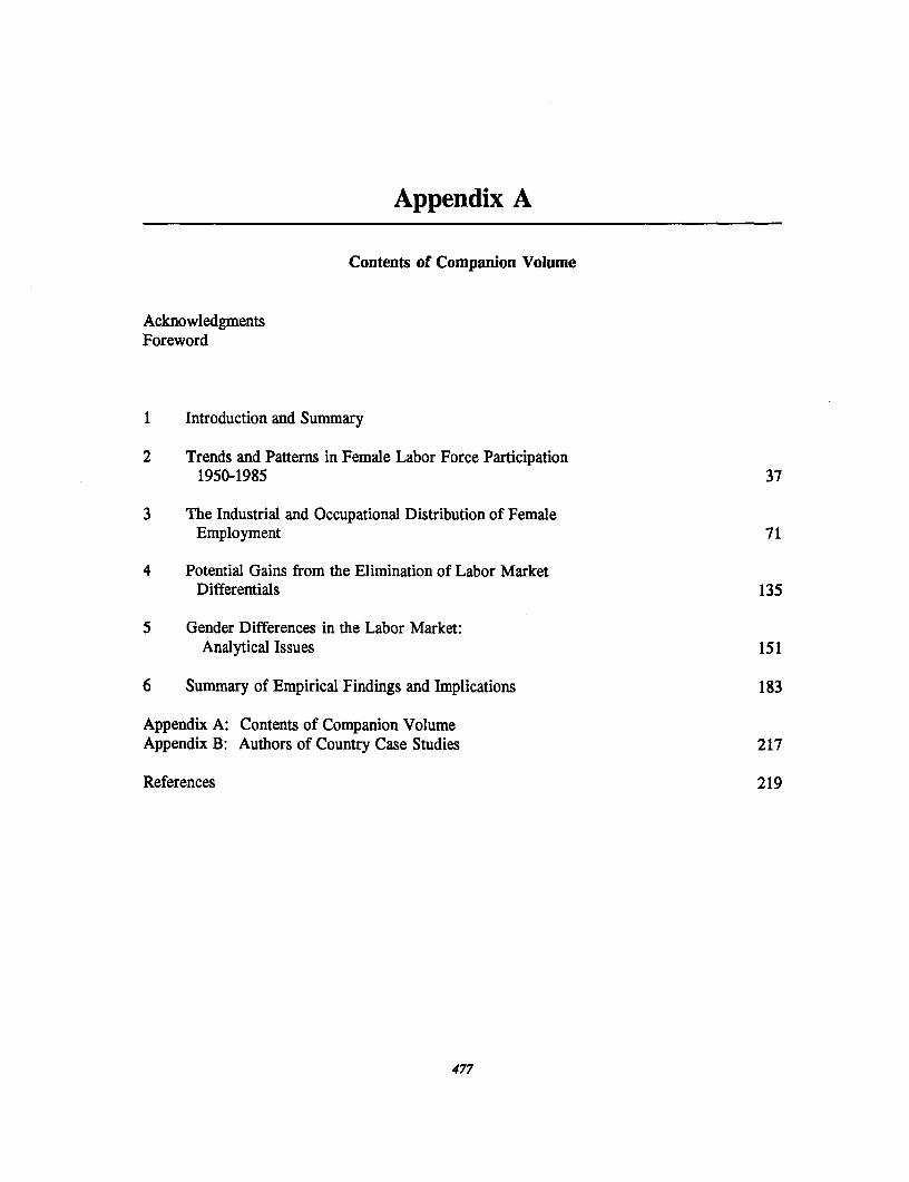
Appendix A
Contents of Companion Volume
AcknowledgmentsForeword
1 Introduction and Summary
2 Trends and Patterns in Female Labor Force Participation1950-1985 37
3 The Industrial and Occupational Distribution of FemaleEmployment 71
4 Potential Gains from the Elimination of Labor MarketDifferentials 135
5 Gender Differences in the Labor Market:Analytical Issues 151
6 Summary of Empirical Findings and Implications 183
Appendix A: Contents of Companion VolumeAppendix B: Authors of Country Case Studies 217
References 219
477

Appendix B
The Authors
Mary Arends is a Consultant for the World Bank's Latin America and Caribbean TechnicalDepartment, Human Resources Division.
Jon A. Breslaw is Associate Professor in the Department of Economics, Concordia University,Montreal.
Donald Cox is Associate Professor of Economics, Economics Department, Boston College atChesnut Hill, Massachusetts.
Indermit Gill is Assistant Professor in the School of Management at the State University of NewYork at Buffalo.
T.H. Gindling is Assistant Professor in the Department of Economics, University of Maryland,Baltimore County.
George Jakubson is Associate Professor in the School of Industrial Labor Relations at CornellUniversity.
Shahidur Khandker is a Research Economist in the Women in Development Division,Population and Human Resources Department, The World Bank.
Thierry Magnac is associated with INRA, ESR Paris, France and the Department of Economics,University College of London, United Kingdom.
Georges Monette is Associate Professor in the Department of Mathematics, York University,Toronto.
Ying Chu Ng is Assistant Professor at Hong Kong Baptist College.
George Psacharopoulos is Senior Human Resources Advisor, Technical Department, LatinAmerica and the Caribbean Region, The World Bank.
Katherine Scott is a Consultant for the World Bank's Latin America and Caribbean TechnicalDepartment, Human Resources Division.
J. Barry Smith is Associate Professor in the Department of Economics, York University,Toronto.
479
480 Women's Employment and Pay in Lain America
Diane Steele is an Analyst at the American Institutes for Research, Washington D.C.
Morton Stelcner is a Professor in the Department of Economics at Concordia University,Montreal.
Jaime Tenjo is Assistant Professor in the Department of Management and Economics at theUniversity of Toronto, Scarborough Campus.
Jill Tiefenthaler is Assistant Professor in the Department of Economics at Colgate University.
Zafiris Tzannatos is a Labor Economist in the Education and Employment Division, Populationand Human Resources Department of the World Bank.
Eduardo Velez is an Education Specialist in the Human Resources Division of the LatinAmerican and Caribbean Region of the World Bank.
Carolyn Winter is a Human Resources Specialist in the Women and Development Division,Population and Human Resources Department of the World Bank.
Hongyu Yang is a Consultant in the Human Resources Division of the Latin American andCaribbean Region of the World Bank.

T H E W O R L D B A N K
World Bank Regional and Sectoral Studies
Nongovernmental Organizations and the World Bank:
Cooperation for Development, edited by Samuel Paul
and Arturo Israel
Unfair Advantage: Labor Market Discrimination in DevelopinEg
Countries, edited by Nancy Birdsall and Richard Sabot
Education in Asia: A Comparative Study of Cost and Financing,
Jee-Peng Tan and Alain Mingat
Health Care in Asia: A Comparative Study of Cost
and Financing, Charles C. Griffin
Bolivia's Answer to Poverty, Economic Crisis, and Adjustment:
The Emergency Social Fund, edited by Steen Jorgensen,
Margaret Grosh, and Mark Schacter
Crop-Livestock Interaction in Sub-Saharan Africa,
John McIntire, Daniel Bourzat, and Prabhu Pingali
Commodity Price Stabilization and Policy Reform: An Approach
to the Evaluation of the Brazilian Price Band Proposals,
Avishay Braverman and others
The Transition from Socialism in Eastern Europe: Domestic
Restructuring and Foreign Trade, edited by Arye L. Hillman and
Branko Milanovic
Women's Employment and Pay in Latin America: Overview andMethodology, George Psacharopoulos and Zafiris Tzannatos
Related Documents