Carstensen 2007a

STATISTICS IN MEDICINEStatist. Med. 2007; 26:3018–3045Published online 18 December 2006 in Wiley InterScience(www.interscience.wiley.com) DOI: 10.1002/sim.2764

Age–period–cohort models for the Lexis diagram

B. Carstensen∗,†

Steno Diabetes Center, Niels Steensens Vej 2, DK 2820 Gentofte, Denmark

SUMMARY

Analysis of rates from disease registers are often reported inadequately because of too coarse tabulationof data and because of confusion about the mechanics of the age–period–cohort model used for analysis.Rates should be considered as observations in a Lexis diagram, and tabulation a necessary reduction ofdata, which should be as small as possible, and age, period and cohort should be treated as continuousvariables. Reporting should include the absolute level of the rates as part of the age-effects.

This paper gives a guide to analysis of rates from a Lexis diagram by the age–period–cohort model.Three aspects are considered separately: (1) tabulation of cases and person-years; (2) modelling of age,period and cohort effects; and (3) parametrization and reporting of the estimated effects. It is argued thatmost of the confusion in the literature comes from failure to make a clear distinction between these threeaspects. A set of recommendations for the practitioner is given and a package for R that implements therecommendations is introduced. Copyright q 2006 John Wiley & Sons, Ltd.

KEY WORDS: age–period–cohort model; Lexis diagram; follow-up studies; Poisson model;parametrization; epidemiology; demography

1. INTRODUCTION

Disease registries collect information on disease occurrence in populations by recording new casesby diagnosis, sex, age and date of diagnosis, etc. Description of disease rates by age and time isbest conceptualized by regarding the observations in a Lexis-diagram.

The age–period–cohort model is a descriptive tool for observations from a Lexis diagram,typically from cancer registries or other disease registers. The model describes rates as a productof an age-effect, a period effect and a cohort effect. The aim is to give an overview of (1) themagnitude of the rates, (2) the variation by age and (3) time trends in the rates.

The database used as basis for the descriptive analysis is a tabulation of events (deaths, diagnosesof disease) and population size over a certain time period and age span, possibly restricted to certainbirth cohorts.

∗Correspondence to: B. Carstensen, Steno Diabetes Center, Niels Steensens Vej 2, DK 2820 Gentofte, Denmark.†E-mail: [email protected], URL: http://www.biostat.ku.dk/˜bxc

Received 17 May 2006Copyright q 2006 John Wiley & Sons, Ltd. Accepted 11 October 2006

AGE–PERIOD–COHORT MODELS FOR THE LEXIS DIAGRAM 3019

The classical age–period–cohort model has been formulated as a model for this table where theeffect of age, period and cohort are modelled as factors, i.e. with one parameter per level in thetabulation. In order to keep the number of parameters at a manageable level and to obtain reasonablysmooth curves for the effects, the tabulation has usually been by 5-year age and period intervals.

Since the date of diagnosis is the sum of the date of birth and the age at diagnosis, there will bea constraint in any model which includes these three variables on a linear scale. The literature isabundant with attempts to overcome this so-called identifiability problem. It is of course futile toovercome the problem of having two variables as well as their sum in the same linear model. Theidentifiability problem is not much different from any other problem that arises from convenienceformulation of models by over-parametrization as is, for example, often the case with the two-wayANOVA model. As such it cannot be solved properly without a view to the subject matter.

In this paper I formulate the age–period–cohort model as a general model for observation in theLexis diagram. Clayton and Schifflers [1, 2] gave a careful exposition of the modelling problemsin this setting, in particular, advice on what functions of the rates that could be (meaningfully)estimated. Keiding [3] gave an exposition of the analysis of rates in the Lexis diagram in continuoustime, under various observation schemes.

In this paper I will focus on practical aspects of analysis of data where events are derived fromdisease registers and population risk time from census data, typically from national statistical offices.

The main points of the paper are (1) the tabulation of data should be part of the data analysis andas little information as possible should be thrown away by tabulation, (2) age, period and cohortshould be regarded as continuous variables and (3) the absolute levels of the rates should be a partof the reporting. This requires a formulation that allows any kind of tabulation of data, not onlyby age and date of event, but also by date of birth, and not necessarily in intervals of the samelength. I will separate the issues of the tabulation of the data, the model for the age, period andcohort effects and the parametrization of these. These three issues are mixed up in many papersdiscussing the models, mainly because the tabulation of data has been taken for granted, and thedefault model has been a factor model.

Section 2 gives a brief overview of the initial steps of an analysis of the observations ina Lexis diagram, Section 3 discusses tabulation of cases and person-years by age, period andcohort, and the implications for analysis. In Section 4 the Poisson model for rates is brieflyreviewed and the options for modelling the underlying rates from the Lexis diagram dis-cussed. The core of the paper is in Sections 5 and 6, where the parametrization of the age–period–cohort model is discussed without reference to tabulation of data and the particular parametricform chosen for the three effects. Finally, I give a few remarks about graphical display of resultsin Section 8 and in Section 9 I use data on testis cancer incidence in Denmark to illustrate theoptions given. In the discussion in Section 10, a set of recommendations are given for practicalanalysis and reporting of rates observed in a Lexis diagram. Two appendices address technicaldetails for person-years calculation and matrix algebra for construction of parameter estimates.

2. DESCRIPTION OF RATES

2.1. Initial plots

Prior to analysis by age–period–cohort models one should always plot the observed rates. Thiswill of course require that cases and person-years be tabulated in classes that are sufficiently large

Copyright q 2006 John Wiley & Sons, Ltd. Statist. Med. 2007; 26:3018–3045DOI: 10.1002/sim

3020 B. CARSTENSEN

to produce fairly stable rates. There are four classical plots that should be made.

1. Rates versus age, observations within each period connected, i.e. cross-sectional age-specificrates.

2. Rates versus age, observations within each birth cohort connected, i.e. longitudinal age-specific rates.

3. Rates versus period, observations within each age-class connected.4. Rates versus cohort, observations within each age-class connected.

These four plots are initial explorations of whether rates are proportional between periods orcohorts. If rates are plotted on a log scale the first and third will exhibit parallel lines if age-specific rates are proportional between periods (i.e. follow an age–period model), the second andfourth if they are proportional between cohorts (i.e. follow an age–cohort model).

These plots require a reasonably coarse tabulation to be informative. But the tabulation used fora first simple overview of data need not be the basis for the entire analysis.

An example of these four plots are given in Figure 1 for rates of testis cancer in Denmark. Animportant feature of these plots is the recognition of the absolute level of the rates.

The numbers used as basis for the plots are in Table I.

2.2. Modelling rates

There are three separate issues to consider when using a statistical model to describe rates from adisease register (observations in a Lexis diagram):

Data: How should data be tabulated: should we use 1-year intervals or 5-year intervals? Shouldthe tabulation be by age and period, by age and cohort, by period and cohort or should it be byall three: age, period and cohort?

Model: How should we model the effects of age, period and cohort: use a factor model (oneparameter per level) or smooth functions of the three variables? Should the smoothing be parametricor non-parametric?

Parametrization: How should we parametrize the estimated effects: what constraints should beused and how is it made clear which ones we have used? What is a sensible graphical display?

Note that I have separated the model and the parametrization of it. A (linear) model in myterminology is synonymous with the linear subspace spanned by the columns of the design matrix.Some authors (e.g. Clayton and Schifflers [1, 2]) have referred to different parametrizations of thesame model as different models.

3. DATA

In principle the entire population could be regarded as a cohort, and data analysed in continuoustime. However, this will rarely be feasible, so in practise data will be tabulated. The analysis dataset will have one record per subset of the Lexis diagram, with number of events and risk time asoutcome variables, and mean age, period and cohort as explanatory variables.

Any tabulation of data represents an information loss (rounding of age and date of diagnosis),so the tabulation should be as detailed as possible, it should only be limited by the availability ofpopulation figures. Cells with 0 events (cases) will not invalidate the analysis, so there is no lowerlimit to the tabulation intervals (except for computing capacity).



20 30 40 50 60

0.5

1.0

2.0

5.0

10.0

Age at diagnosis

1945.5 1955.5

1965.5

1975.5 1985.5

1995.5

20 30 40 50 60

0.5

1.0

2.0

5.0

10.0

Age at diagnosis

1898

1908 1918

1928

1938 1948

1958

1968

1978

1950 1960 1970 1980 1990 2000

0.5

1.0

2.0

5.0

10.0

Date of diagnosis

17.5

27.5 37.5

47.5

57.5

1880 1900 1920 1940 1960 1980

0.5

1.0

2.0

5.0

10.0

Date of birth

17.5

27.5 37.5

47.5

57.5

Figure 1. The classical four plots for rates observed in a Lexis diagram. Rates of testis cancer (per100 000 person-years) in Denmark 1943–1997 in ages 15–64 years. Top left: age-specific rates by periodof diagnosis. Top right: age-specific rates by date of birth. Bottom left: period-specific rates by age. Bottom

right: cohort-specific rates by age.

3.1. Cases

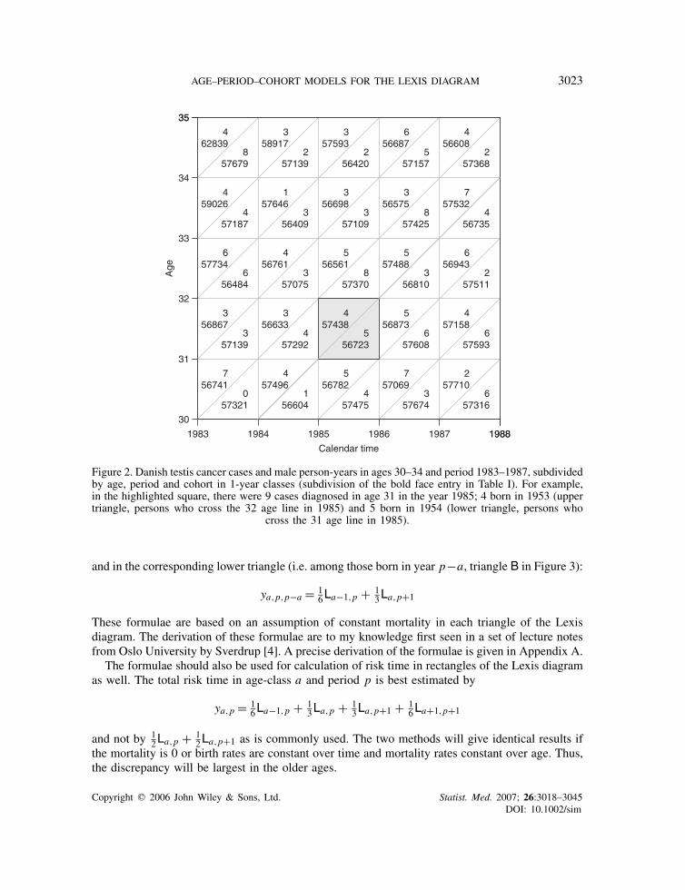
If disease cases are taken from a register, cases can be tabulated arbitrarily by age at diagnosis,date of diagnosis (period) and date of birth (cohort). It will for example be possible to enumeratecases for each 1× 1× 1-year triangle of the Lexis diagram as illustrated for Danish testis cancercases in Figure 2. In principle, it would even be possible to produce a tabulation of data by singlemonths as well.


3022 B. CARSTENSEN

Table I. Cases of testis cancer and male person-years in Denmark 1943–1996 in 5-year classes.

Mean period

Mean age 1945.5 1950.5 1955.5 1960.5 1965.5 1970.5 1975.5 1980.5 1985.5 1990.5 1995.0

Cases17.5 10 7 13 13 15 33 35 37 49 51 4122.5 30 31 46 49 55 85 110 140 151 150 11227.5 55 62 63 82 87 103 153 201 214 268 19432.5 56 66 82 88 103 124 164 207 209 258 25137.5 53 56 56 67 99 124 142 152 188 209 19942.5 35 47 65 64 67 85 103 119 121 155 12647.5 29 30 37 54 45 64 63 66 92 86 9652.5 16 28 22 27 46 36 50 49 61 64 5157.5 6 14 16 25 26 29 28 43 42 34 4562.5 9 12 11 13 20 18 28 23 26 15 10

Person-years (in 1000s)17.5 2321 2233 2382 2919 3155 2883 2858 3033 3015 2789 201122.5 2439 2234 2165 2313 2881 3162 2902 2859 3059 3052 228327.5 2372 2345 2169 2096 2294 2888 3168 2883 2869 3095 250732.5 2398 2324 2308 2135 2100 2310 2881 3136 2865 2871 246437.5 2308 2349 2281 2281 2135 2107 2302 2856 3107 2846 229242.5 2082 2263 2305 2250 2270 2129 2090 2273 2821 3071 226447.5 1866 2030 2214 2260 2214 2239 2095 2047 2229 2770 245352.5 1618 1801 1962 2146 2198 2155 2173 2027 1982 2163 210557.5 1413 1538 1713 1868 2042 2095 2051 2059 1923 1883 163462.5 1210 1305 1424 1584 1720 1880 1930 1884 1890 1772 1392

Note: The mean date in the period 1943–1947 is 1945.5, etc. The last period 1993–1996 is only 4 years, sothe mean date is here 1995.0. The bold-face entry in the table is further subdivided in 50 subsets by one-yearclasses of age, period and cohort in Figure 1.

3.2. Person-years

Population figures are needed to produce rates, and the availability of these will normally bethe limiting factor. In most countries, population figures in 1-year age classes for each calendaryear are available. Such figures of population prevalence can be used to compute the risk time(person-years) in triangular subsets of the Lexis diagram.

For the sake of simplicity, the following formulae are given for one-year age classes and one-year periods.‡ Specifically, let La,p be the population size in age a, at beginning of year p, see theleft part of Figure 3, where a = 61 and p= 1980. The risk time in age class a − 1, during year p,among those aged a− 1 at the beginning of year p (i.e. born in year p−a, triangle A in Figure 3)is estimated as

ya−1,p,p−a = 13La−1,p + 1

6La,p+1

‡Strictly speaking these formulae are wrong as they give number of cases rather than risk time. In order to makethem correct all quantities must be multiplied by the interval length, in this case 1 year.



Calendar time

Age

1983 1984 1985 1986 1987 1988

30

31

32

33

34

35

057321

156604

457475

357674

657316

756741

457496

556782

757069

257710

357139

457292

556723

657608

657593

356867

356633

457438

556873

457158

656484

357075

857370

356810

257511

657734

456761

556561

557488

656943

457187

356409

357109

857425

456735

459026

157646

356698

356575

757532

857679

257139

256420

557157

257368

462839

358917

357593

656687

456608

1988

35

Figure 2. Danish testis cancer cases and male person-years in ages 30–34 and period 1983–1987, subdividedby age, period and cohort in 1-year classes (subdivision of the bold face entry in Table I). For example,in the highlighted square, there were 9 cases diagnosed in age 31 in the year 1985; 4 born in 1953 (uppertriangle, persons who cross the 32 age line in 1985) and 5 born in 1954 (lower triangle, persons who

cross the 31 age line in 1985).

and in the corresponding lower triangle (i.e. among those born in year p−a, triangle B in Figure 3):

ya,p,p−a = 16La−1,p + 1

3La,p+1

These formulae are based on an assumption of constant mortality in each triangle of the Lexisdiagram. The derivation of these formulae are to my knowledge first seen in a set of lecture notesfrom Oslo University by Sverdrup [4]. A precise derivation of the formulae is given in Appendix A.

The formulae should also be used for calculation of risk time in rectangles of the Lexis diagramas well. The total risk time in age-class a and period p is best estimated by

ya,p = 16La−1,p + 1

3La,p + 13La,p+1 + 1

6La+1,p+1

and not by 12La,p + 1

2La,p+1 as is commonly used. The two methods will give identical results ifthe mortality is 0 or birth rates are constant over time and mortality rates constant over age. Thus,the discrepancy will be largest in the older ages.


3024 B. CARSTENSEN

1980 1981 1982 198360

61

62

63

Age

Calendar time

1920 1921 1982 1982

A

B

L62,1981

L61,1981

L60,1980

L61,1980

Figure 3. Lexis diagram. The thick lines in the left part show the population figures at the beginning of1980 and 1981 necessary to estimate the population risk time in the triangles A and B. The right part ofthe diagram shows the mean age, period and cohort in the triangular subsets of a Lexis diagram. Note theconnection between age, period and cohort: p=c+ a: 19821

3 = 192023 + 612

3 and 198223 = 19211

3 + 6113 .

3.3. Mean age, period and cohort in triangular subsets

If a tabulation is by age and period (A-sets: ), by period and cohort (B-sets: �� ) or by age

and cohort (C-sets: �� ), the mean age, period and cohort in each set is simply the mean for thecorresponding tabulation intervals for each of the two tabulation variables. The mean for the thirdvariable is obtained using the relation a = p − c.

But when subdividing the Lexis diagram in triangles, the mean age, period and cohort in a givenset is not equal to the mean of the classes chosen for tabulation. The means are offset by 1

6 of thetabulation interval, as shown in the right part of Figure 3, see e.g. [5]; a formal derivation of thisgiven in [6]. These values should be used when modelling rates based on a tabulation in triangles.Note in particular that the relationship a = p − c must hold for all subsets of the Lexis diagram(and hence for all units in the data set).

In the following there will be no assumptions about the particular shape of the subsets of theLexis diagram used for tabulation, neither w.r.t. the number of tabulation variables, whether thetabulation intervals are equally long for different variables nor whether all subsets have the sameshape. Thus, we consider rates observed as (D, Y ) in arbitrary subsets of a Lexis diagram, whereD is number of cases and Y the amount of risk time. The associated covariates are mean age a,mean period p, and mean cohort c= p − a for the subsets.



4. MODELS

The general form of a multiplicative age–period–cohort model for rates �(a, p) at age a in periodp for persons in birth cohort c= p − a is

log[�(a, p)] = f (a) + g(p) + h(c) (1)

Here it is assumed that a, p and c represent the mean age, period and cohort for the observationalunits. The model allows the effects of each of the three variables to be non-linear (on the log ratescale). The particular parametric form chosen for the functions f , g and h is immaterial at thispoint.

4.1. ‘Poisson’ model

For tabulated data, one must assume that the rate is constant within each tabulation category (subsetof Lexis diagram). The log likelihood contribution from observation of the random quantity (D, Y )

in one subset is

l(�|D, Y ) = D log(�) − �Y

Except for a constant (D log(Y )) not involving the rate parameter this is the same as the loglikelihood for an observation of a random variable D from a Poisson distribution with mean �Y .The log likelihood for the entire table of (D, Y ) is the sum of such terms, because individualsare assumed to be independent, and the contributions to different cells from one individual areconditionally independent. Hence, models for � can be fitted using a programme for Poissonregression for independent observations, that allows for an offset term to separate the person-yearsfrom the rate in the expression for the mean.

However, the fact that the Poisson model and the constant rate model has the same likelihooddoes not mean that the number of cases is Poisson distributed, and in particular not that the amountof risk time is fixed. The Poisson machinery should only be used for making likelihood basedinference. Inference based on the distributional properties of the Poisson is not necessarily correct.

The information about � = log(�) is computed as minus the second derivative of the log likeli-hood evaluated at the ML-estimate:

l(�|D, Y ) = D� − e�Y, l ′�(�|D, Y ) = D − e�Y, l ′′� (�|D, Y ) =−e�Y

so I (�) = e�Y = �Y = D. Note that this is the observed information not the Fisher informationwhich is the expected information. In the Poisson model the expected information is �Y (becauseY is assumed known in the Poisson model), but in the constant rate model further assumptionsabout the observation plan is required to compute the expected value of D. A discussion of this inmore depth is found in Keiding [3], who also gives references for the more probabilistic literature.

4.2. Submodels

One may argue that test of the terms in model (1) is irrelevant as it is a descriptive model. However,it has been customary to make formal tests of the effects.

The relevant submodels can conveniently be arranged in a sequence which gives all the relevanttests as comparisons between adjacent lines.


3026 B. CARSTENSEN

Model log[�(a, p)]Age f (a)

Age-drift f (a) + �cAge–cohort f (a) + h(c)Age–period–cohort f (a) + g(p) + h(c)Age–period f (a) + g(p)Age-drift f (a) + �p

Note that the two drift models (i.e. with a log linear trend in period respective cohort) areidentical: since p= a + c, a term �a can be separated from �p and absorbed into f (a) givingthe cohort drift model. Thus, the age-drift model is the intersection of the age–period and theage–cohort model, as pointed out by Clayton and Schifflers [1].

The deviance as output from most programmes can be used to derive the likelihood-ratio test forthe model reductions. The deviance statistic is also commonly used in isolation to judge whether aparticular model provides an adequate fit to the data. The deviance statistic is the likelihood-ratiotest against the model with a completely freely varying interaction between age and period (orcohort). This is a meaningful test if the data represent a meaningful tabulation of the underlyingprocess, but since any tabulation used for observations in a Lexis diagram is arbitrary so is theinteraction model. Thus, the formal goodness of fit tests does not have an interpretation in termsof the original model for the rates as function of age, period and cohort in continuous time, andso is largely meaningless. If the analysis is based on coarsely tabulated data (5× 5-year classes,say) it may be argued that the full model is the only natural extension of the age–period–cohortfactor model, and thus provide a sensible test.

However, if data are tabulated in very small intervals the number of units in the analysis willincrease to thousands and even if the modelling of age, period and cohort effects are fairly detailed,the degrees of freedom of the goodness of fit tests will increase dramatically, and thus more easilyproduce a significant statistic even if the average deviance contribution from each cell is more orless constant. Hence, the deviance statistic is a quantity depending on the chosen tabulation ratherthan on the adequacy of the model in describing the rates.

4.3. Classical approach to modelling effects

As an extreme way of accommodating the non-linearity of the effects of age, period and cohort,the usual approach to modelling effects uses one parameter per distinct value of a, p and c, bydefining the variables as ‘factors’ (class variables).

As the tabulation of data becomes finer, the age–period–cohort modelling by one factor levelfor each distinct value of the three factors becomes unfeasible. This problem in age–period–cohortmodelling emerges because the ‘factor’ approach insists that effects be modelled by one separateparameter for each distinct value of the tabulation factors age, period and cohort. The factor modelsare thus effectively models that let the tabulation induce the model.

The classical approach (which has largely emerged from cancer epidemiology) has been todefine a tabulation sufficiently coarse to avoid an excess amount of parameters in the modelling;keeping the number of parameters of the models at a reasonable level has lead to a coarse tabulationof data, typically in 5-year intervals. Thus, there has been a feed-back loop between the tabulationof data and the modelling approach based on the concept of piecewise constant rates—the ‘factor’-



modelling approach. This may have been induced by limited availability of population figures orby limited computing capacity (initially the need to compute standardized rates by hand beforethe advent of proper modelling hard- and software).

4.3.1. Three-way tabulated data and the factor model. If data are tabulated by age, period andcohort, and the factor coding of effects is used, the model will fall into two disjoint parts, in thesense that the likelihood function will be a product of two terms, one only involving data fromupper triangles ( � ) and one only involving data from lower triangles (� ), with separate sets ofparameters. This was pointed out by Osmond and Gardner [7], but to my knowledge no one hassuggested a way to remedy this problem, other than pooling the triangular subsets to quadrangular.The following section provides a solution.

4.4. Smoothing with parametric functions

Since the three variables age, period and cohort are originally continuous variables it seems naturalto model their effects by parametric smooth functions of the class means, for example:

• Splines, i.e. 1st, 2nd or 3rd degree polynomials in predefined intervals, constrained to haveidentical values and derivatives at interval boundaries (knots).

• Natural splines, 3rd degree splines constrained to be linear beyond the outermost knots.• Fractional polynomials, combination of polynomials of various powers, including non-integer

powers.

Any of these approaches gives columns of the design matrix for age, period and cohort effects,and as such are just (generalized) linear models.

If sufficient data are available there will be little difference between these approaches, the majorquestion to address is the number of parameters to use for modelling each time-scale. Moreover,all the standard paraphernalia of penalizing the roughness of the effects is available for fine tuningthe number of parameters and the location of knots. However, penalizing the roughness is notnecessarily desirable in a descriptive demographic model where sudden changes in effects may beperfectly sensible, for example, due to changes in diagnostic practice.

Parametric smoothing avoids the problem of two separate models when using a factor modelfor data tabulated by age, period and cohort. Any factor model uses one parameter per co-hort, even for the youngest and oldest where usually little data are present. With a parametricfunction of cohort it is possible to let the model reflect the information available in differentcohorts.

If the number of parameters in the terms describing an effect equals the number of categories,then the model will be the same as the factor model, albeit parametrized differently. Hence, theparametric models are submodels of the classical ‘factor’ model.

Heuer [8] suggested to use restricted B-splines (natural splines) to model age, period andcohort effects in finely tabulated data. The point I suggest here is to use the class meansdirectly as continuous variables to construct the splines, apparently similar to Holford’s [9]approach. Essentially, that is what Heuer ends up with too, albeit only for rectangularsubsets.

Heuer [8] suggested as a rule of thumb to use one knot per five years of the timescale. I findthis suggestion too rigorous, certainly the number of events (= amount of information) must berelevant in deciding how many knots can be accommodated. Even if the cohort scale has a length


3028 B. CARSTENSEN

which is the sum of the lengths for age and period, I would suggest that approximately the samenumber of knots be used for all three timescales. If there is a special interest in age-effects, say, thenumber of knots on this scale could be increased. Furthermore it should be considered to place theknots so that the (marginal) number of events is the same between them, rather than equidistantly,as the information is proportional to the number of events.

4.4.1. Non-parametric smoothers. If a non-parametric smoothing is used it is difficult to keepstrict control over the parametrization. From the next sections it will be clear that access to thedesign matrix is essential for handling the parametrization of the effects of age, period and cohort.In particular, it is important to be able to access and manipulate the design matrix when predictionsare made for rate-ratios relative to a specified point. Therefore, the non-parametric option is notconsidered further in this paper.

5. IDENTIFIABLE LINEAR TREND?

Holford [10] suggested extracting the linear trends from the age-, period- and cohort-parametersfrom a factor model by regressing age-parameters on age, period parameters on period and cohortparameters on cohort, and then report the residuals as age, period and cohort effects. This wouldgive a display of the identifiable quantities on a recognizable scale. The three remaining parameterswould then be the age-slope and the period/cohort slope and the intercept. The intercept woulddepend on the choice of reference point for the age and period or cohort. Holford also showedhow this could be incorporated directly in the modelling by making a projection of the columnsof parts of the design matrix.

Regression of the estimates for the age, period and cohort classes on age, period and cohortand extraction of the linear trend produces a set of parameters (functions) f , g and h that are 0on average with 0 trend and are connected to the original parameters by

f (a) = f (a) + �a + �aa

g(p) = g(p) + �p + �p p

h(c) = h(c) + �c + �cc

Holford notes that �a + �p and �p + �c are invariants in the sense that regardless of the initialparametrization of f , g and h, they will have the same values, because any other parametrization( f , g, h) can be obtained by a suitable choice of �a , �c and � as

f (a) = f (a) − �a − �a

g(p) = g(p) + �a + �c + �p

h(c) = h(c) − �c − �c

It is easily verified that f (a)+ g(p)+ h(p) = f (a)+g(p)+h(c) for any value of (a, p, c= p−a),and that the regression slopes of f , g and h differ from those for f , g and h with the same numericalquantity (�), but that the quantities �a + �p and �p + �c are the same.



As Holford showed, the ‘detrended’ period estimates can be obtained directly in the modelfitting by replacing the part of the design matrix corresponding to period by a matrix with columnsorthogonal to the intercept column and the (period) drift column. This matrix is found by takingthe original columns and projecting them on the orthogonal complement to the space spanned bythe constant and the drift.

However, the uniqueness of the overall secular trend �p + �c depends on the definition of‘orthogonal’ or ‘0 on average with 0 slope’. The formulae devised by Holford are based onorthogonality with respect to the usual inner product

〈x|y〉= ∑xi yi

However, this is not the only way of defining the drift, instead we could use an inner product ofthe type

〈x|y〉= ∑xiwi yi

with some pre-defined weights. One obvious choice would be to take the wi s proportional to thenumber of cases in each record (tabulation cell), i.e. using the observed information about thelog rate as weights. One might argue that this choice depends on data and as such would rendercomparisons of trends across populations or regions invalid. However, the choice of the tabulationunit for the weighting is equally arbitrary; recall that the basic data unit after all is the follow-upof single persons in the population. With this in mind a choice would obviously be to choose theperson-years as weights for the inner product. In most data sets these are options that put more orless weight in the older age-classes.

Hence, the linear components (�a + �p and �p + �c) devised by Holford are just as arbitrary asany other set of extracted linear trends. The size of extracted linear trends are not a feature of themodel; they are a feature of the model and the (arbitrarily) chosen method for extracting the lineartrends, hence it is largely a matter of taste which inner product to use when extracting the trends.

6. PARAMETRIZATION OF THE AGE–PERIOD–COHORT MODEL

Since the aim is to model rates as a function of age, period and cohort, the logical approach toparametrization is to formulate the problem in continuous time, i.e. by a model for the rate at anypoint (a, p) in the Lexis diagram. A general formulation of the model is

log[�(a, p)] = f (a) + g(p) + h(c) (2)

for three functions, f , g and h. The model predicts the rates at any point in the Lexis diagram.Applied to tabulated data the rates are assumed to be constant in each of the subsets in the Lexisdiagram. The general form of the model makes parametric assumptions about the rates in thesesubsets. Note that the classical factor approach to modelling also falls under this formulation—thefunctions are just assumed piecewise constant in larger intervals.

The challenge is to choose a parametrization of these three functions in a way that:

1. is meaningful,2. is understandable and recognizable,


3030 B. CARSTENSEN

3. is practically estimable by standard software,4. allows reconstruction of the fitted rates from the reported values.

Little attention has been paid to the last point, for example both Heuer [8] and Holford [9],present graphs for relative effects without considering the absolute level of the rates.

As noted by Holford [10] and later by Clayton and Schifflers [2], the only components of themodel (2) that can be uniquely determined are the second derivatives of the three functions, andyet the relevant representation of the model is by graphs of three functions f , g and h that sumto the predicted log rates. The first derivatives as well as the absolute levels can be moved aroundbetween the functions. One choice is only to show the second derivatives, but as the scale forthese is not easily understandable this is not an option in practise, although it has been used [11].

6.1. Choice of parametrization

For the sake of the argument, consider first the age–cohort model

log[�(a, c)]= f (a) + h(c)

In this model only the first derivatives (contrasts) of f and h are identifiable. This is tradition-ally fixed by choosing a reference cohort c0, say, and constrain h(c0) = 0. This will make f (a)

interpretable as the age-specific log rates in cohort c0 and h(c) as the log rate ratio of cohort ccompared to cohort c0.

The formalism behind this is to write

log[�(a, c)]= f (a) + h(c)= ( f (a) + �) + (h(c) − �)

and by choosing �= h(c0) we get the desired functions as

f (a)= f (a) − h(c0), h(c)= h(c) − h(c0)

which indeed has the property that f (a) + h(c)= f (a) + h(c) and h(c0) = 0. In practise this canbe implemented by choosing the parametrization of the model carefully. In the case of a factormodel for the effect of cohort, this is known as choosing the reference cohort to be c0. This isa standard procedure when fitting linear models, but it is rarely recognized as the solution to anidentifiability problem.

A similar machinery can be invoked to explicitly move the three unidentifiables in an age–period–cohort model around between f , g and h by choosing �a , �c and � so that the resultingfunctions, f (a), g(p) and h(c) meet some desired constraints:

log[�(a, p)] = f (a) + g(p) + h(c) = f (a) −�a −�a

+ g(p) +�a +�c +�p

+ h(c) −�c −�c

In the age–period–cohort model with three terms and where only the second derivatives of theeffects are identifiable, two levels and one value of the first derivative must be fixed. This isfrequently done by fixing one value on the cohort scale to be 0 and two points on the period scale



to be 0, thereby fixing the overall slope of the period parameters, but a less technical principle forthe choice of parametrization is desirable.

6.2. A principle for parametrization

Any parametrization of the age–period–cohort model fixes two levels and a slope among the threefunctions, but different principles can be invoked to accomplish this.

One principle for choice of parametrization is based on an extension of the assumptions behindway the age–cohort model was parametrized:

1. The age-function should be interpretable as log age-specific rates in cohort c0 after adjustmentfor the period effect.

2. The cohort function is 0 at a reference cohort c0, interpretable as log RR relative to cohortc0.

3. The period function is 0 on average with 0 slope, interpretable as log RR relative to theage–cohort prediction (residual log RR).Alternatively, the period function could be constrained to be 0 at a reference date, p0. In

this case the age-effects at a0 = p0 − c0 would equal the fitted rate for period p0 (and cohortc0), and the period effects would be residual log RRs relative to p0.

The first choice fixes one constant (0 at c0), and the third fixes a level (0 on average or 0 at p0)and a slope (0 slope for the period function). The inclusion of the slope (drift) with the cohorteffect makes the age-effects interpretable as cohort-specific rates of disease (longitudinal rates).Depending on the subject matter, the role of cohort and period could be interchanged, in whichcase the age-effects would be cross-sectional rates for the reference period. Heuer [8] also discussthese two interpretations of the age-effects depending on whether the drift is allocated with periodor cohort.

In practise this can be implemented as follows. The point is to choose the columns of thedesign matrix in such a way that desired functions are simple linear combinations of the estimatedparameters, which will give a simple calculation of standard errors and hence confidence intervals.This is detailed in Section 6.3.

Suppose functions f , g and h have been estimated from data. Then we fix a reference cohortc0, and extract the linear part from g, for example, by regressing the values of g(p) on p

g(p) = g(p) − (� + �p)

where � is chosen to make g(p) equal to 0 on average. The log rates can then be expressed inthree new terms

log[�(a, p)] = f (a) + g(p) + h(c)

where

f (a) = f (a) +� +�a +h(c0) +�c0

g(p) = g(p) −� −�p

h(c) = h(c) +�c −h(c0) −�c0

The functions f (a), g(p) and h(c) defined this way fulfils the requirements above; g(p) is 0on average with 0 overall slope, h(c) is 0 for c= c0, and f (a) has the dimension of log rates,


3032 B. CARSTENSEN

referring to cohort c0. If we prefer to fix the period function to 0 at a given date p0, we just use� = g(p0) − �p0, instead of using the estimated � from the regression.

Note that in the derivation above, we made no assumptions about the algorithm used to extractthe linear trends. It was only assumed that it was possible to de-trend g and h in some way.

6.2.1. Explicit drift parameter. A variant of the above approach is to extract the drift entirely andreport it as a separate parameter and then report both cohort and period effects as ‘residuals’. Thiswould correspond to the partitioning of the model into terms:

log(�(a, p)) = fc(a) + �(c − c0) + g(p) + h(c)

= f p(a) + �(p − p0) + g(p) + h(c)

where g(p) and h(c) are ‘de-trended’, i.e. have 0 slope. fc(a) are the age-specific rates in thereference cohort c0 and f p(a) the age-specific rates in the reference period p0. Thus, age-specificrates can be chosen to refer to either a specific cohort (longitudinal rates) or a specific period(cross-sectional rates). Note that fc(a)= f p(a) + �(a − (p0 − c0)), so if there is a positive drift(�>0) the cohort (longitudinal) age-curve will be steeper than the period (cross-sectional) agecurve.

6.3. Parametric models in practise

The goal of the parametrization is to produce estimates of three functions showing the age, theperiod and the cohort effects constrained in a sensible way. We also want confidence intervalsfor these. This section details how the design matrix for the model can be set up in such a waythat derivation of these functions is done by simple linear functions of three separate subsets ofparameters.

Consider first a simple age–cohort model with say cohort c0 as reference. If a factor model isused we would set up a design matrix with one indicator column per age class and one indicatorcolumn for each cohort except for c0. The estimated parameters would then be the log rates ineach age class for cohort c0, and log RRs relative to this.

If we instead model the age-specific log rates as quadratic in age we replace the age-columnswith the three columns [1|a|a2] where a is the midpoint in each age-category. If the estimatesfor these three columns are (�0, �1, �2), then the estimated log rate for age a in cohort c0, is�0 + �1a + �2a2, or in matrix notation

(1 a a2 )

⎛⎜⎝

�0

�1

�2

⎞⎟⎠

If the estimated variance–covariance matrix of (�0, �1, �2) is R (a 3× 3 matrix), then the varianceof the log rate at age a is

(1 a a2 )R

⎛⎜⎝

1

a

a2

⎞⎟⎠



This rather tedious approach is an advantage if we simultaneously want to compute the estimatedrates at several ages a1, a2, . . . , an . The estimates and the variance covariance of these are then

⎛⎜⎜⎜⎜⎜⎝

1 a1 a21

1 a2 a22...

......

1 an a2n

⎞⎟⎟⎟⎟⎟⎠

⎛⎜⎝

�0

�1

�2

⎞⎟⎠ and

⎛⎜⎜⎜⎜⎜⎝

1 a1 a21

1 a2 a22...

......

1 · · · a2n

⎞⎟⎟⎟⎟⎟⎠R

⎛⎜⎝

1 1 · · · 1

a1 a2 · · · a3

a21 a22 · · · a23

⎞⎟⎠

The matrix we use to multiply with the parameter estimates is the age-part of the design matrix wewould have if observations were for ages a1, a2, . . . , an . The product of this piece of the designmatrix and the parameter vector represents the function f (a) evaluated in the ages a1, a2, . . . , an .

If a spline model for the age effect is used, the age-part of the design matrix will be columnsof base vectors for the splines. If cubic splines are used and knots k1 and k2 are used the columnsof the design matrix corresponding to age will be:

1, a, a2, a3, (a − k1)3+, (a − k2)

3+

with the notation x+ = max(0, x). These functions of a1, a2, . . . , an will be multiplied with thesix parameters �0, �1, . . . , �5 in the spline model to give estimates of the log rates as �0 + �1a +�2a2 + �3a3 + �4(a − k1)3+ + �5(a − k2)3+.

Now suppose that the cohort effect is modelled by a cubic spline as well, i.e. we use the columns

c c2 c3 (c − k1)3+ (c − k2)

3+

This will not assure that the estimated effect of cohort is 0 for cohort c0; if the parameter estimatesfor the splines for cohort effect are �0, �1, . . . the estimated cohort effect at c0 will be

�0 + �1c0 + �2c20 + �3c

30 + �4(c0 − k1)

3+ + �5(c0 − k2)3+

Therefore, if we replace the cohort-columns in the design matrix with the columns

c − c0, c2 − c20, c3 − c30, (c − k1)3+ − (c0 − k1)

3+, (c − k2)3+ − (c0 − k2)

3+

we get an estimated cohort effect which is 0 at c0. What we have done is just to subtract adifferent constant from each column, which does not influence the model, it only changes theintercept parameter, which is a part of the age-effects. This way we automatically also get theage-parameters to refer to the log rates for cohort c0.

A similar approach to parametrization fulfilling the requirements above can be implemented forthe age–period–cohort model as follows. The idea is that we want to end up with three sets ofcolumns that directly allows to compute age, period and cohort effects at any set of points we wish.

1. Set up model matrices for age, period and cohort, Ma , Mp and Mc, each including theintercept term. If a factor model is used these are just columns of indicators, one for eachlevel of age, period and cohort. If a spline model is used the matrices will be columns of basevectors for the splines, as in the example above, or generated as a B-spline basis (see e.g. [8]).

2. Extract the linear trend from Mp and Mc, by projecting their columns onto the orthogonalcomplement of [1|p] and [1|c], respectively. Estimates for period and cohort effects derived


3034 B. CARSTENSEN

using these matrices will be 0 on average and with 0 overall slope. This projection is anon-trivial matrix operation, that is further detailed in Appendix II.The resulting matrices Mp and Mc have two fewer columns than the original Mp and Mc.

This was in essence the proposal that Holford [10] made, also providing the projection matrix.3. Centre the cohort effect around c0: First take a row from Mc corresponding to c0. Form a

matrix of the same dimension as Mc with all rows equal to this, and subtract it from Mc toform Mc0 .

4. The desired parametrization can now be obtained by using the Ma for the age-effects, Mp

for the period effects and [c − c0|Mc0] for the cohort effects.Since the intercept is assumed to be included in Ma , the age-effects are automatically

adjusted for the centring of the cohort-effect around c0, so they represent log rates for thecohort c0.

5. The extracted drift is estimated separately by considering the estimated coefficient to thecolumn c−c0, and the standard error of it. If the drift is taken out as a separate parameter, bothcohort and period effects will be residual effects constrained to be 0 on average with 0 slope.

6. Suppose the subsets of the estimated parameter vector corresponding to Ma , Mp and

[c− c0|Mc0] are �a , �p and �c. The value of f (a) at the as actually present in the data set is

Ma �a . The variance of it is found by MTa RaMa , where Ra is the variance–covariance matrix

of �a . In practical situations one would shave Ma down to a matrix with unique rows, eachrepresenting an observed point on the age-scale.The same machinery is used to derive effects for the other two effects at the observed points.

It is clear from the above that it will be convenient to have tools that can generate model matricesfor the type of model used, as well as have facilities for matrix operations. These tools are availablein Stata and SAS, but not directly integrated in the language as is the case with S-plus and R, wherematrices may be entered directly in the fitting functions. A publicly available implementation ofthe methods given here is available in the function apc.fit in the Epi package for R. The Epipackage also contain functions for matrix projection.

7. FITTING MODELS SEQUENTIALLY

It is possible to obtain an approximation to the parametrization outlined above using a small trick:first fit the age–cohort model. By omitting an explicit intercept and choosing a suitable referencefor the cohort, the age-effect will be log rates for the reference cohort and the cohort effect willbe log RRs relative to this. f (a) and h(c) are then used as age and cohort effects.

The log of the fitted values from this model is then used as offset variable in a model withperiod-effect

log[�(a, p)] = [ f (a) + h(c)] + g(p)

The period effects from this model (also omitting an explicit intercept) are then used as the residuallog RRs by period.

The estimates obtained by this sequential procedure are not the ML-estimates from the age–period–cohort model, they are marginal age–cohort estimates and period estimates conditional



on the estimates from the age–cohort model, but in practise they will be very similar to theML-estimates.

If one has an a priori assumption that mainly cohort-effects drive the change in rates, then thiswould the best way to model the rates, because the period effects would then only be residualsconditional on the estimated age and cohort effects.

Usually, the estimates from this approach will be close to the ML estimates, and the advantageis that the parametrization is very simple, no special manipulations are required to reparametrizeand obtain standard errors. There are obvious extensions of this trick: first fit the age-drift model,and then sequentially cohort and period as ‘residual’ effects.

A variant of this procedure has been used by some authors as a way of fixing the age-effectsto obtain identifiability [12]. The procedure is also implemented in the function apc.fit in theEpi package for R too.

8. GRAPHICAL DISPLAY OF EFFECTS

For any chosen constraints there will be three estimated functions, f (a), g(p) and h(c) whichsum to the fitted log rates. These effects should be shown in one figure, with same equidistance

20 40 60 1880 1900 1920 1940 1960 1980 2000

Age Calendar time

0.5

1

2

5

10

0.25

0.5

11

2.5

5

Rat

e ra

tio

Figure 4. The estimated effects using the weighted and the naive approach to extracting the drift. Forboth approaches the drift is included with the cohort effect. The fit to the data is the same. The marginaldrift is the drift estimate from the age-drift model. The inside tickmarks at the bottom and top indicatethe placement of the knots for the natural splines. The cohort curve is the leftmost and longest of the two

curves on the calendar time scale, the period curve the rightmost and shorter.


3036 B. CARSTENSEN

for the horizontal scale for age, period and cohort. Also the relative extent for the rate-scale forage-effects and relative risk scale for period and cohort effects should be the same. This will putall three effects on a directly comparable scale and allow the slopes of the effects to be compared.

The figure must have the horizontal scale divided in two; one for age and one for cohort/period;the latter two will often cover overlapping calendar periods. The vertical scale will be a rate scalefor the age-effect and a relative risk scale for the period and cohort effects. If a reference cohortor period is chosen a dot should be placed at (c0, 1) or at (p0, 1) to indicate this.

This is shown in Figure 4 for the Danish testis cancer data.

9. ANALYSIS OF DANISH TESTIS CANCER DATA

An annotated R-file and the Danish testis cancer data are available on my homepagehttp://www.biostat.ku.dk/˜bxc/APC/SiM-ex.

The classical displays shown in Figure 1 produced with the function rateplot, which is thenatural first step of the analysis, in this case based on data in 5 by 5 year classes. There is a cleartendency that cohort born around 1940–1945 show lower rates than those born earlier and later.

20 40 60 1880 1900 1920 1940 1960 1980 2000

Age Calendar time

0.5

1

2

5

10

0.25

0.5

11

2.5

5

Rat

e ra

tio

Figure 5. The estimated effects using the weighted approach to extracting the drift (full lines), contrastedwith the sequential approach by first fitting the age–cohort model and then the period model to the residuals(broken lines). The age-effect refers to the 1940 cohort. The fit to the data is the not same for the two setsof estimates. In the sequential approach the age and cohort effects are from the age–cohort model, andsome confounding of the cohort effect by period seems to be present. The cohort curve is the leftmost and

longest of the two curves on the calendar time scale, the period curve the rightmost and shorter.



20 40 60 1880 1900 1920 1940 1960 1980 2000

Age Calendar time

0.5

1

2

5

10

0.25

0.5

11

2.5

5

Rat

e ra

tio

Figure 6. The estimated effects using the weighted approach to extracting the drift (black) andallocating it with the cohort, and using the 1940 cohort and 1975 period as references. Curves withadded annual period drifts of −2,−1, 1, 2% are shown as well. The rates predicted from curves oflike colours are the same. The cohort curve is the leftmost and longest of the two curves on thecalendar time scale, the period curve the rightmost and shorter. A film-like version can be found at

www.biostat.ku.dk/˜bxc/APC/Testis-film.pdf.

Testis cancer cases in Denmark 1943–1996 were tabulated in 1-year classes by age, periodand cohort. Population figures in 1-year age-classes at 1 January each year were obtained fromStatistics Denmark. The risk time was computed as outlined in Section 3. The analysis is restrictedto the age-classes 15–64 years.

The age–period–cohort model was fitted with apc.fit, which allows various models (linearsplines, cubic splines, factors) and parametrizations to be used. The displays in Figures 4–6 showsa model where natural splines with 15 parameters for each of the effects were used, these wereplotted with the functions apc.frame and apc.lines.

From the curves it is clear that there is a ‘dip’ in rates for the birth cohorts born during the firstand second world wars. Such a dip is a second order feature of the curve and is therefore not anartefact of the parametrization. These two dips in the cohort effects are brought out clearly by acombination of the detailed tabulation of data, and the detailed parametrization of the cohort effect.Modelling the effects with fewer parameters would overlook the dip around the first world war.

10. DISCUSSION

Age–period–cohort models are descriptive tools for rates observed in a Lexis diagram. Properanalysis of rates should use the maximally available information. Therefore, tabulation in very


3038 B. CARSTENSEN

coarse groups of age, period and cohort should be avoided. Whenever possible tabulation by allthree variables should be done.

Overly coarse tabulation of data is abundant in the epidemiological literature, rates of child-hood diabetes (ages 0–14 years) is for example commonly modelled using three 5-year ageclasses! [13–16].

At least for countries in western Europe, data on population size in 1-year age-classes willusually be available. The SEER programme in U.S.A. have made population data in one-yearclasses available at state level (see http://seer.cancer.gov/popdata/).

Large parts of the literature on the age–period–cohort models is difficult to read because ofoverly complicated notation, e.g. use of indexing of age, period and cohort groups by i , j and krunning from 1 to I , J and K , giving rise to complicated indexing formulae, involving the totalnumber of categories that are otherwise only relevant when specifying computer code. It seemsmore straightforward to use mnemonics like a, p and c and letting the indices be the mean ofthese continuous variable in each cell of the tabulation, even if takes much of the magic out of thesubject. The use of the notational tradition from abstract mathematics has presumably distractedmany readers from realizing that age–period–cohort analysis is about having two timescales (ageand period) and their difference in the same model. Certainly, some authors seem to have beenmisled in this aspect, see e.g. [17, 18].

Effectively, only the factor model induced by the tabulation of data have been used in appliedage–period–cohort modelling and it is also the predominant model addressed in the theoreticalpapers. Therefore, the parametrization problems have mostly been addressed in the framework ofthe factor model. This has led to a plethora of suggestions for parametrizations with little view tothe principal aspects of the subject matter, see e.g. [19].

Heuer [8] suggested using splines in modelling the effects for rectangular subsets of the Lexisdiagram, and although his formulation is tantamount to the use of the mean age, period and cohortfor the subsets of the Lexis diagram, this point was not used in his exposition. Heuer also proposedthe direct use of a projection (albeit only with respect to the common inner product) to generalizeHolford’s method to spline models; Holford [9] used spline modelling for rectangular subsets ofthe Lexis diagram too, but none of these authors included the rate dimension in the reporting ofthe models.

The tools available for age–period–cohort modelling have by and large been Poisson-modellingby programmes that produce a standard parametrization of factors such as proc genmod fromSAS or the glm command from Stata. In most applied papers the authors have shied awayfrom graphical reporting of the estimates [14, 15, 20]. This may be an indication of the technicalproblems associated with transforming the default parametrization from the statistical packages toa useful parametrization. Particularly, the derivation of standard errors of estimated curves can bea complicated task with older software as Stata and SAS, where the concept of the data set as thebasic analytical unit hampers manipulation with model matrices and estimates.

In this paper I reiterated the basic fact for the parametrization of the age–period–cohort model:arbitrary decisions on the allocation of two absolute levels and one drift must be taken in orderto report the estimated effects. Arbitrary in this context means unrelated to the model, impossibleto derive from data or design. Choice of parametrization should of course not be unrelated to thesubject matter.

Since the substance is description of disease rates in populations over time, the major variable isage. Therefore, the reporting of the models should be based on age-specific rates. It is impossibleto give universal guidelines as to whether they should be reported as cohort-rates (longitudinal) in



which case the drift should be included with the cohort-effect, or as period-rates (cross-sectional)in which case the drift should be included with the period effect.

10.1. Recommendations

In summary, the following steps should be taken when describing rates based on observations froma Lexis diagram:

1. Tabulate cases and person-years as detailed as possible, preferably by age, period and cohort.2. Compute risk time from population data using the formulae for risk time in triangles.3. Use the mean age, period and cohort in each cell of the table as continuous covariates.

a = p − c must be met for all analysis units.4. Use parametric functions to describe the effects. Choose the parametrization (allocation of

knots, etc.) carefully, so that relevant features can be captured, but modelling of randomnoise is avoided.

5. Report estimates of three effects that can be combined to the predicted rates.6. Age should be the primary variable, report age-specific rates, i.e. include the absolute level

with the age-parameters.7. Make an informed choice of the other aspects of parametrization, and state it clearly. This

will include:

(a) How is the drift extracted.(b) Where is the drift allocated.(c) How are the RRs for period and cohort fixed.(d) What is the interpretation of the age-specific rates.

8. Report estimates as line-graphs with confidence limits.9. Be careful with firm interpretation of formal tests for period and cohort effects—significant

effects may represent clinically irrelevant effects.10. Do not report goodness of fit tests—they are largely meaningless.

The possible options for parametrization of the model are summarized in Table II.

Table II. Parametrizations for the age–period–cohort model.

Drift extraction: 1: Orthogonal projection (a) All units the same weight(b) Weights ∝ observed informa-

tion (D)(c) Weights ∝ original data (Y )

2: Equation of two points on period and cohort scales

Interpretation of effects:Age Period Cohort

Longitudinal rates for cohort c0 Residual RR RR relative to cohort c0Cross-sectional rates for period p0 RR relative to period p0 Residual RRLongitudinal rates for cohort c0.Fitted rates at a0 = p0 − c0

Residual RR relative to p0 RR relative to cohort c0

Cross-sectional rates for period p0.Fitted rates at a0 = p0 − c0

RR relative to period p0 Residual RR relative to c0

Note: Two steps are needed: fixing the drift parameter, and fixing the reference values.


3040 B. CARSTENSEN

The options for model fitting, parametrization and graphical reporting mentioned above areall implemented in the R-package Epi, in functions apc.fit, apc.frame and apc.lines.Projections of model matrices is implemented in the function detrend. The package is availablethrough CRAN (The Comprehensive R Archive Network, http://cran.r-project.org)or at the package home page http://www.biostat.ku.dk/˜bxc/Epi.

APPENDIX A: PERSON-YEARS IN LEXIS TRIANGLES

The following is based on material from lecture notes by Sverdrup [4]. To my knowledge thishas not been published elsewhere, despite its obvious relevance in descriptive epidemiology.The paper by Hoem [21] and the correction note [22] has a reference to a similar result from anearlier version of Sverdrup’s notes.

A.1. Census data

First, consider for the sake of simplicity the division of the Lexis-diagram in 1-year classes byage, calendar time and date of birth, and suppose that population figures are available in 1-yearclasses each year, as will be the situation for most areas where regular censuses are done. Thesituation is illustrated in Figure 3. The target is to construct estimates of population risk time foreach of the areas A and B.

In the following we let a refer to age, p to calendar time (period), and c to date of birth (cohort),and we let La,p represent the population size in age a at the beginning of the year p.

If no deaths or migrations occurred in the population, we would have that La,p = La+1,p+1.In presence of mortality§ we can at least infer that the survivors La+1,p+1 have been at risk

throughout the year p. Assuming that the persons are uniformly distributed within the age-classes,the average risk time contribution of a survivor will be 1

2 year to each of the triangles A and B.In order to work out the contribution of risk time of those dying during the year p, we assume

that the deaths are uniformly distributed over A and B.¶ This means that the total amount of risktime contributed to A and B by those dying in A and B is (La,p − La+1,p+1) × 1

2y.Those who die in A contribute no risk time to B. In A their average contribution can be computed

by integration over the triangle A. The mean contribution must be calculated as an average w.r.t.to the uniform measure on A. The area of A is 1

2 (=∫ p=1p=0

∫ a=1a=p 1 da dp), so the density of the

uniform measure is 2.For simplicity of notation it is assumed that age and date range from 0 to 1 in all of the

calculations below. A person dying in age a at date p in A contributes p risk time, so the averageis found by integration of the function f (a, p) = p with respect to the uniform measure withdensity 2 over A, letting a vary from p to 1 and p from 0 to 1

∫ p=1

p=0

∫ a=1

a=p2p da dp=

∫ p=1

p=02p(1 − p) dp=

[p2 − 2

3p3

]p=1

p=0= 1

3

§ Immigration and emigration can be treated as negative and positive mortality respectively, and does not alter theresults derived here, provided the assumptions made for the mortality pattern also holds for the migration patternsin the population.¶Note that this may a unrealistic assumption for age-classes of length 5 years or more.



Those who die in B contribute risk time in both A and B. If death occurs in age a at date p theperson has contributed p − a person-years in A and a person-years in B.

Hence, the average amount contributed in A is∫ p=1

p=0

∫ a=p

a=02(p − a) da dp=

∫ p=1

p=0[2pa − a2]a=p

a=0 dp=∫ p=1

p=0p2 dp= 1

3

and in B ∫ p=1

p=0

∫ a=p

a=02a da dp=

∫ p=1

p=0p2 dp= 1

3

Under the assumption that the deaths in A ∪ B, (La,p − La+1,p+1) are uniformly distributed, wetherefore have the following risk time in A and B

A B

Survivors La+1,p+1 × 12y La+1,p+1 × 1

2y

Dead in A 12 (La,p − La+1,p+1) × 1

3y

Dead in B 12 (La,p − La+1,p+1) × 1

3y12 (La,p − La+1,p+1) × 1

3y∑( 13La,p + 1

6La+1,p+1) × 1y ( 16La,p + 13La+1,p+1) × 1y

The risk among 0-year olds in year p, born in year p can be computed by requiring that thetotal risk time among 0-year olds in year p should equal 1y× the average of the population sizesin age 0 at the beginning and end of year p, i.e. we should use

12 (L0,p + L0,p+1) × 1y − ( 13L0,p + 1

6L1,p+1) × 1y= ( 16L0,p + 12L0,p+1 − 1

6L1,p+1) × 1y

Another possible estimate is 12L0,p+1 for those born in year p, disregarding those dead in the

year born. Yet another alternative is to take a weighted average of 12L0,p+1 and half the number

of births in the year, 12bp. Since the mortality is largest in early months, bp should be given the

smallest weight, but the actual weights to use is matter of taste.A similar procedure can be applied in the last non-open age-class (usually 89). It has little

meaning to try to subdivide open age-classes by date of birth.

APPENDIX B: PRACTICALITIES OF PROJECTION

In order to get an estimate of the extracted drift with confidence intervals we need a functionthat takes P columns of the design matrix produce and a set of P − 2 columns orthogonal to theconstant and the drift w.r.t. some defined inner product.

So let M be a design matrix, and define the relevant inner product between two columns as

〈m j |mk〉 = ∑imi jwimik


3042 B. CARSTENSEN

where we would use either wi = 1, wi = Di or wi = Yi , the total number of cases or person-yearsobserved in unit i of the data set. The task is now to produce a projection of the columns of Mon the orthogonal complement to the two column matrix of the constant and the drift, [1|p] (or[1|c] for the cohort effect).

B.1. Projections in matrix formulation

The projection of a vector v on the column space of the matrix X with respect to the usual innerproduct, is Pv where

P=X(XTX)−1XT

and the projection on the orthogonal complement is (I − P)v.For a general inner product

〈x|y〉= ∑ixiwi yi = xTWy

with W= diag(wi ), the projection matrix on the column space of X w.r.t. this inner product is

PW =X(XTWX)−1XTW (B1)

and the projection on the orthogonal complement is (I − PW)v.

B.2. Implementation in R

In the parametrization of the linear trend from the cohort and period effects we use R functions(ns, bs, . . .) to generate model matrices using e.g. natural splines. Let this be M.

Then we project the columns ofM on the orthogonal complement of [1|p] w.r.t. a weighted innerproduct. This is done using the function proj.ip, which is just a translation of the formula (B1)to R (X is here playing the role of [1|p])

proj.ip <-function( X, M, orth = FALSE, weight=rep(1,nrow(X)) ){Pp <- solve( crossprod( X * sqrt(weight) ), t( X * weight ) ) %*% MPM <- X %*% Ppif (orth) PM <- M - PMelse PM}

When using tabulation of data in very small intervals the resulting data sets can be quite large;for example the example data set with testis cancer in ages 15–65 for the period 1943–1997has 50 age classes and 54 periods, i.e. 50× 54× 2= 5400 observations for triangles in the Lexisdiagram. Therefore, the multiplication XW is done by multiplying with the vector w (weight),using the R-feature of recycling and the column-major storage of matrices. If it had been codedX %*% diag(weight), it would require a square matrix of dimension n (the number ofunits), which is very large (54002 = 2 916 000 entries). By the same token, the projection ma-trix X(XTWX)−1XTW is not computed as it would also have this huge dimension. Instead the last



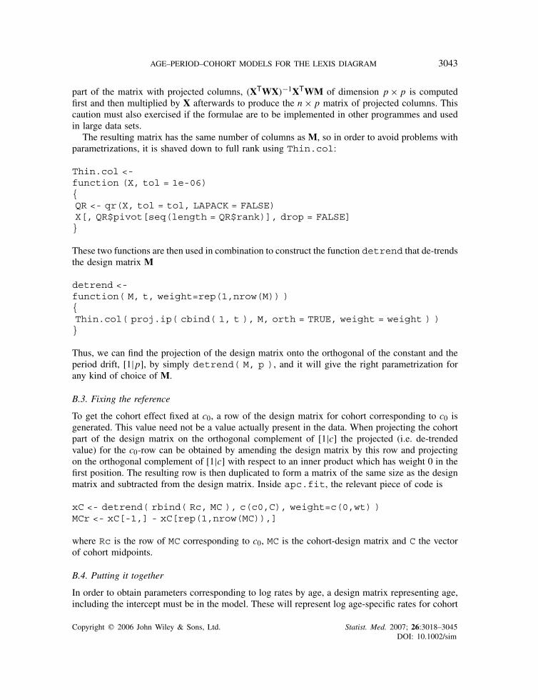
part of the matrix with projected columns, (XTWX)−1XTWM of dimension p× p is computedfirst and then multiplied by X afterwards to produce the n × p matrix of projected columns. Thiscaution must also exercised if the formulae are to be implemented in other programmes and usedin large data sets.

The resulting matrix has the same number of columns as M, so in order to avoid problems withparametrizations, it is shaved down to full rank using Thin.col:

Thin.col <-function (X, tol = 1e-06){QR <- qr(X, tol = tol, LAPACK = FALSE)X[, QR$pivot[seq(length = QR$rank)], drop = FALSE]}

These two functions are then used in combination to construct the function detrend that de-trendsthe design matrix M

detrend <-function( M, t, weight=rep(1,nrow(M)) ){Thin.col( proj.ip( cbind( 1, t ), M, orth = TRUE, weight = weight ) )}

Thus, we can find the projection of the design matrix onto the orthogonal of the constant and theperiod drift, [1|p], by simply detrend( M, p ), and it will give the right parametrization forany kind of choice of M.

B.3. Fixing the reference

To get the cohort effect fixed at c0, a row of the design matrix for cohort corresponding to c0 isgenerated. This value need not be a value actually present in the data. When projecting the cohortpart of the design matrix on the orthogonal complement of [1|c] the projected (i.e. de-trendedvalue) for the c0-row can be obtained by amending the design matrix by this row and projectingon the orthogonal complement of [1|c] with respect to an inner product which has weight 0 in thefirst position. The resulting row is then duplicated to form a matrix of the same size as the designmatrix and subtracted from the design matrix. Inside apc.fit, the relevant piece of code is

xC <- detrend( rbind( Rc, MC ), c(c0,C), weight=c(0,wt) )MCr <- xC[-1,] - xC[rep(1,nrow(MC)),]

where Rc is the row of MC corresponding to c0, MC is the cohort-design matrix and C the vectorof cohort midpoints.

B.4. Putting it together

In order to obtain parameters corresponding to log rates by age, a design matrix representing age,including the intercept must be in the model. These will represent log age-specific rates for cohort


3044 B. CARSTENSEN

c0 if the variable c − c0 is put in the model. If the column c − c0 is merged with the de-trendedand c0-centred cohort effect design matrix, this will represent the log RR relative to cohort c0.Finally, the de-trended period matrix will represent the residual log RR by period.

The estimated age-curve is found by taking the unique rows of the age-part of the design matrixwhere each row corresponds to an observed age in data. This is then multiplied with the vector ofage-parameters to give the curve of estimated log rates. Pre- and post-multiplication on the variancecovariance matrix of the age-parameters gives the variances needed to construct confidence limitsfor the log rates. Finally the log rates are transformed to the rate scale.

The same procedure is used to obtain the RR curves for period and cohort.

REFERENCES

1. Clayton D, Schifflers E. Models for temporal variation in cancer rates. I: Age–period and age–cohort models.Statistics in Medicine 1987; 6:449–467.

2. Clayton D, Schifflers E. Models for temporal variation in cancer rates. II: Age–period–cohort models. Statisticsin Medicine 1987; 6:469–481.

3. Keiding N. Statistical inference in the Lexis diagram. Philosophical Transactions of the Royal Society of London,Series A 1990; 332:487–509.

4. Sverdrup E. Statistiske metoder ved dødelikhetsundersøkelser. Statistical Memoirs. Institute of Mathematics,University of Oslo, 1967 (in Norwegian).

5. Tango T. Re: Statistical modelling of lung cancer laryngeal cancer incidence in Scotland 1960–1979. AmericanJournal of Epidemiology 1988; 127(3):677–678.

6. Carstensen B, Keiding N. Age–Period–Cohort Models: Statistical Inference in the Lexis Diagram. Lecture Notes.Department of Biostatistics, University of Copenhagen, 2004 (http://www.biostat.ku.dk/˜bxc/APC/notes.pdf).

7. Osmond C, Gardner MJ. Age, period, and cohort models. Non-overlapping cohorts don’t resolve the identificationproblem. American Journal of Epidemiology 1989; 129(1):31–35.

8. Heuer C. Modelling of time trends and interactions in vital rates using restricted regression splines. Biometrics1997; 53(1):161–177.

9. Holford TR. Approaches to fitting age–period–cohort models with unequal intervals. Statistics in Medicine 2006;25:977–993.

10. Holford TR. The estimation of age, period and cohort effects for vital rates. Biometrics 1983; 39:311–324.11. Richiardi L, Bellocco R, H-Adami O, Torrang A, Barlow L, Hakulinen T, Rahu M, Stengrevics A, Storm H,

Tretli S, Kurtinaitis J, Tyczynski JE, Akre O. Testicular cancer incidence in eight northern European countries:secular and recent trends. Cancer Epidemiology Biomarkers and Prevention 2004; 13(12):2157–2166.

12. Ajdacic-Gross V, Bopp M, Gostynski M, Lauber G, Gutzwiller F, Rossler W. Age–period–cohort analysisof Swiss suicide data 1881–2000. European Archives of Psychiatry and Clinical Neuroscience 2005; 256(4):207–214.

13. Bruno G, Merletti F, Biggeri A, Cerutti F, Grosso N, De Salvia A, Vitali E, Pagano G. Increasing trend of typeI diabetes in children young adults in the province of Turin (Italy). Analysis of age, period and birth cohorteffects from 1984 to 1996. Diabetologia 2001; 44(1):22–25.

14. Feltbower RG, McKinney PA, Parslow RC, Stephenson CR, Bodansky HJ. Type 1 diabetes in Yorkshire, U.K.:Time trends in 0–14 and 15–29-year-olds, age at onset and age–period–cohort modelling. Diabetic Medicine2003; 20(6):437–441.

15. Pundziute-Lycka A, Dahlquist G, Nystrom L, Arnqvist H, Bjork E, Blohme E, Bolinder J, Eriksson JW,Sundkvist G, Ostman J, Swedish Childhood Diabetes Group Study. The incidence of type I diabetes has notincreased but shifted to a younger age at diagnosis in the 0–34 years group in Sweden 1983 to 1998. Diabetologia2002; 45:773–791.

16. Rewers M, Stone RA, La Porte RE, Drash AL, Becker DJ, Walczak M, Kuller LH. Poisson regression modelling oftemporal variation in incidence of childhood insulin-dependent diabetes mellitus in Allegheny county, Pennsylvaniaand Wielkopolska, Poland, 1970–1985. American Journal of Epidemiology 1989; 129(3):569–581.

17. Boyle P, Robertson C. Statistical modelling of lung cancer and laryngeal cancer incidence in Scotland1960–1979. American Journal of Epidemiology 1987; 125(4):731–744.



18. Robertson C, Boyle P. Age, period and cohort models: the use of individual records. Statistics in Medicine 1986;5:527–538.

19. Robertson C, Boyle P. Age–period–cohort analysis of chronic disease rates. I: Modelling approach. Statistics inMedicine 1998; 17:1305–1323.

20. Tyczynski JE, Hill TD, Berkel HJ. Why do postmenopausal African-American women not benefit from overallbreast cancer mortality decline? Annals of Epidemiology 2005; 16(3):180–190.

21. Hoem JM. Fertility rates and reproduction rates in a probabilistic setting. Biometrie-Praximetrie 1969; 10:38–66.

22. Hoem JM. Correction note. Biometrie-Praximetrie 1970; 11:20.


Carstensen 2007a

Documents