Carrier Phase Ambiguity Resolution for the Global Positioning

JOURNAL OF GEOPHYSICAL RESEARCH, VOL. 94, NO. B8, PAGES 10,187-10,203, AUGUST 10, 1989

Carrier Phase Ambiguity Resolution for the Global Positioning System Applied to Geodetic Baselines up to 2000 km

GEOFFREY BLEWITT

Jet Propulsion Laboratory, California Institute of Technology, Pasadena

The Global Positioning System {GPS) carrier phase data are biased by an integer number of cycles. A successful strategy has been developed and demonstrated for resolving these integer ambiguities for geodetic baselines of up to 2000 km in length, resulting in a factor of 3 improvement in baseline accuracy, and giving centimeter-level agreement with coordinates inferred by very long baseline interferometry in the western United States. For this experiment, a method using pseudorange data is shown to be more reliable than one using ionospheric constraints for baselines longer than 200 km. An automated algorithm exploits the correlations between the many phase biases of a GPS receiver network to enable the resolution of ambiguities for very long baselines. A method called bias optimizing has been developed, which, unlike traditional bias fixing, does not require an arbitrary confidence test. Bias optimizing is expected to be preferable to bias fixing for poorly configured networks. In order to enable ambiguity resolution for long baselines, it is recommended that future GPS networks have a wide spectrum of baseline lengths ranging from < 100 to > 1000 km and that GPS receivers be used which can acquire aluM-frequency P code data.

INTRODUCTION

The use of carrier phase data from the Global Positioning System (GPS) has already yielded geodetic baseline estimates with precisions of 1 part in 107 to 1 part in l0 s [e.g., Book et al., 1986; Beutler et al., 1987; LieMen and Border, 1987; Tralli et al., 1988]. However, carrier phase data are biased by an integer number of wavelengths which must be estimated from the data [Remondi, 1985]. Unless a scheme is implemented which invokes this integer nature, the solutions of geodetic parameters are considerably weakened through their correlation with the phase biases. For example, except in regions of high latitude, the phase biases are more correlated with the east component of baselines than with the north; consequently, the precision to which the east component can be estimated is degraded by factors of 2 to 5. The reason for this asymmetry relates to the north-south ground tracks of GPS satellites at the equator in the Earth- fixed reference frame [Melbourne, 1985].

The GPS P code pseudorange data type, which is a ranging measurement using known modulations on the carrier signal, does not have this weakness. However, presently available pseudorange data are contaminated by multipath signatures with amplitudes two orders of magnitude greater than for carrier phase, and therefore they must be weighted accordingly for parameter estimation. Lichten and Border [1987] have shown that the phase bias solutions can be constrained by processing pseudorange data simultaneously with carrier phase data, resulting in a factor of 2 improvement in precision of the east component of the baselines. Even so, the estimation of carrier phase biases still con- tributes significantly to the error in baseline components.

Resolving the integer ambiguity in carrier phase biases effectively converts carrier phase data into an ultraprecise pseudorange data. The problem of resolving these ambigu-

Copyright 1989 by the American Geophysical Union.

Paper number 89JB00484. 0148-0227/89 / 89 J B-00484 $05.00

ities, often under the names ambiguity resolution and bias fixing, has received theoretical attention by Bender and Lar- den [1985], Goad [1985], Melbourne [1985], Wabbena [1985], and others. Some of the ideas expressed in these papers serve as a starting point for this work.

Results presented by Bocket al. [1985, 1986] and Abbot and Counselman [1987] show improved baseline precision due to bias fixing. Dong and Book [1989] have demonstrated ambiguity resolution for baseline lengths up to a few hundred kilometers. One method of ambiguity resolution, which has been implemented in various forms by these and other investigators, starts by imposing a priori constraints on the differential ionospheric delay to reduce the correlation of ionospheric parameters with the carrier phase biases. An excellent example of this method is described by Dong and Book [1989]. As explained by Bender and Larden [1985], this method fails at some baseline length which depends on the local horizontal gradient in the vertical ionospheric electron content. Maximum ionospheric gradients occur at the peak of the 11-year solar sunspot cycle (the next peak occurs around 1991); the annual maximum is during the spring equinox, and the diurnal maximum at 1400 hours local time. Tropical regions are worst affected, although ionospheric scintillations at high latitudes (> 60 ø) can be problematic even for short ((50km) baselines [Rothacher et al., 1988]. From this point of view, GPS data sets acquired over the last few years in North America should be almost optimal for the application of ionospheric constraints for ambiguity resolution.

This paper emphasizes a method for resolving the carrier phase ambiguities which is insensitive to the ionosphere [Melbourne, 1985; W•bbena, 1985] and which is applied to baselines up to 2000 km in length. This technique applies to dual-frequency P code receivers. A straightforward method for applying ionospheric constraints is also described, since P code receivers are not always available.

It is shown that ambiguity resolution results in about a factor of 3 improvement in the agreement of baselines with very long baseline interferometry (VLBI). The treatment of

10,187

10,188 BLEWITT' GPS AMBIGUITY RESOLUTION UP TO 2000 KM

geodetic networks is addressed, where ambiguities may be sequentially resolved over successively longer baselines. The concept of bias optimizing is introduced, which is an alternative approach to traditional bias fixing. Finally, recommen- dations are given for the design of GPS receiver networks.

• P s OBSERVABLES

Observable Types

GPS receivers extract phase observables from carrier sig- nms transmitted by the GPS satellites at two L band frequencies [Rernondi, 1985]. These observables precisely track changes in electromagnetic phase delay with subcentimeter precision. Measurements at two frequencies allow for a first- order calibration of the dispersive ionospheric delay with subcentimeter precision [Spilker, 1980].

A certain class of receiver (of which the Texas Instruments TI-4100 is the most common), also extracts two pseudorange observables by correlating modulations on both carriers with a known code (P code) [Spilker, 1980]. P code pseudorange observables are measurements of satellite to receiver range plus timing offsets. With the TI-4100, the pseudorange precision is about 70 cm in 30 s. Recent tests of the prototype Rogue receiver [Thomas, 1988] with various antenna con- figurations [Meehan et al., 1987] suggest that precisions least an order of magnitude better than this will soon be routinely available [Blewitt et al., 1988].

Many receivers cannot acquire the P code, and instead extract a less precise single-frequency pseudorange observable by acquiring the C/A code. A third class of receiver is codeless, providing carrier phase measurements only. Important variations on these receiver types are being developed but are not presently in general use. This point will be addressed later.

Observable Equations

Consider the following model for the duM-band GPS carrier phase and P code pseudorange observables acquired by receiver k from satellite i. All observables have the dimen-

sions of length. Terms due to noise and multipath are not explicitly shown, and higher-order ionospheric terms which are assumed to be subcentimeter are ignored:

= - _ +

---- p} -- I• 112/(112 -- 122) q- •262• - Ap} (lb) = + = + _

where (I>1•: and (I>2•: are the raw carrier phases, L• and are the carrier phase ranges, P• and P2• are the P code pseudoranges, c is the conventional speed of light, and the GPS system constants are

fl - 154 x 10.23MHz (2a) f2 - 120 x 10.23 MHz (2b) •1 = ½/fl """ 19.0cm (2c) hi = ½/f2 •-- 24.4 cm (2d)

The term I• in (1) is by definition the difference in ionospheric delay between the L1 and L2 channels and is propor- tional to N,i, the path integral of the ionospheric electron

density [Spilker, 1980] between satellite i and receiver k: ß 15 ar i / --2

__ x ) (s)

The term p]: is the nondispersive delay, lumping together the effects of geometric delay, tropospheric delay, clock signatures, and any other delay which affects all four observables identically. The geometrical calibration term lXp accounts for the differential delay between the L1 and L2 phase cen- ters and is calculated using relatively crude values for satellite elevation t•} and azimuth •b•:, and the differential phase center vector (Ar,,Ar,,,Aro, which is defined (in local coordinates) as going from L2 to

Api(•}, •i ) = -- cost•}(Ar, sin •i + Ar,• cos •i) -- Aresin 0} (4)

The phase biases b•: and b2•: are initialization constants. These biases are composed of three terms'

ß i

= + - (5) The terms n• and n2• are integer numbers of cycles and are present because the receiver can only measure the fractional phase of the first measurement. The receiver can thereafter keep track of the total phase relative to the initial measurement. However, the integer associated with the first measurement is arbitrary, and hence the need for these integer parameters in the model. The terms 5(I)lk and 5(I)2k are un- calibrated components of phase delay originating in the re-

ceiver (assu. reed to be common to all satellite channels); the terms 5(I)•' and •(I)2 i originate in the satellite transmitter. Empirically (by plotting appropriate linear combinations of the data), it is known that these offsets are stable to better than a nanosecond; however, their presence prevents the resolution of the integer cycle biases n lk and n2}.

Double-Diff erenced Phase Ambiguity

Double differencing of the phase biases between two receivers (k, l) and two satellites (i, j) results in an integer bias [Goad, 1985]:

where the band subscript (1 or 2) has been dropped from the notation because this equation applies to either band, or any linear combination of bands. Hence it is the double- differenced integer cycle ambiguity that can be resolved.

Some investigators process double-differenced data, thus their carrier phase biases are naturally integer parameters. The approach taken here is to process undifferenced data and then form double-differenced estimates. The covariance

matrix of the estimated parameters is used to select the set of double-differenced biases which are theoretically best determined (as will be explained in later sections and in Appendix B).

BLEWITT: GPS AMBIGUITY RESOLUTION UP TO 2000 KM 10,189

This method is preferable since, for example, it uses the extra information available from a receiver when there

are data outages, or outlying data points, at the other receiver. In addition, the analysis is simplified by not requiring complicated double-differencing algorithms at the data processing stage; for example, measurement residuals can be inspected for individual station-satellite channels which greatly enhances troubleshooting when a particular channel has a problem.

PHASE BIAS ESTIMATION STRATEGY

The Ionosphere-Free Combination

The problem of how to estimate the phase bias b• is now ß

addressed. The term p•, can in principle be modeled very accurately [$overs and Border, 1987]; however, the ionospheric parameter I• is generally unpredictable, though can some- times be constrained within reasonable limits. The standard

ionosphere-free observable combination can be formed from

. - iap/(n -

where the phase bias term

This direct approach has been suggested by Melbourne [1985] and W•bbena [1985]. Typical TI-4100 pseudorange has root- mean-square multipath delays of around 70 cm for 30 s data points, giving an error contribution of roughly 50 cm to (12). This contribution needs to be time-averaged to below half of the 86 cm ambiguity in the wide-lane phase observable; for TI-4100's, 20 minutes of data are usually sufficient. Tests by Meehan et al. [1988] using the prototype Rogue receiver show that 1 minute of data is more than sufficient.

From (10) and (12) we can write

(13)

where Apl is given by (4). The coefficient multiplying Apl is -,, 4/(86cm), showing that if the length of the differential phase center vector, (Ar• + ar• + aro) is no more than 1 or 2 cm, we may safely neglect this term. (This is particularly useful for applications with moving antennas). For routine static positioning, this term can easily be calculated. The linear combination in (13) is computed for each data point, and a time-averaged (real) value is taken. The'estimates are subsequently double-differenced, and (6) is used to give an estimate of the integer constant

can be estimated as a real-valued parameter using a Kalman filter [Lichten and Border, 1987] or an equivalent weighted least squares approach. Double differencing these estimates, then applying (6) gives

iy is computed as A formal error for the estimate of • follows:

,2 .2 .2 2)1/2 where we define

Although the problem of eliminating the ionospheric delay parameter has been solved,..(9) alone does not give us in-

,• ii This will now be dependent estimates of • and •2•. addressed.

Resolving the Wide-Lane Bias: Pseudorange Approach

From (1) we can form the following linear combination of the carrier phase data, which is often called the wide-lane combination because of the relatively large wavelength of ,Xa -- c/(/x - f2) • 80.2 cm:

(10)

where the wide-lane bias

To solve for bs •, we can calibrate the carrier phase data with the following pseudorange combination:

•si - • ((bs}2>- (bsi> (16) and Nj is the number of points used in the time averag- ing. Points bai are automatically excluded as outliers from the above computations if they lie more than 3•ra} from the running value of

Using this technique, wide-laning is independent of our knowledge of orbits, station locations, etc., and so can be applied to baselines of any length provided there is sufficient common visibility of the satellites. Pseudorange multipath errors (< 20cm) originating at the GPS satellites would tend to cancel less between receivers with increasing baseline length, thus giving a small baseline length dependence to wide-laning accuracy. The differential measurement error would be ,-, 1 part in l0 s of baseline length and is therefore negligible for purposes of wide-laning. For practical reasons, we can therefore call the pseudorange wide-laning method "baseline length independent."

Resolving the Wide-lane Bias: Ionospheric Approach

The pseudorange approach is not applicable to non-P code receivers. For completeness, an alternative approach to wide-laning is presented here. Let us define the ionospheric combination of carrier phase data:

i i

ß P•/c = (flPlk "[- f2P2•)/(fl -[- f2) (12) -- Pl + I• flf2/(fl 2 -- f•2) _ Api f2/(fl -[" f2) = g + lbll - 2621 + (17)

10,190 BLEWITT: GPS AMBIGUITY RESOLUTION UP TO 2000 KM

where (1) was used. This equation can be rewritten in terms of the biases bs• of (11), and Bc• of (8)'

L,•: - I• -4-[(f•2 _ f2•)!f•f•](:ksbs• - B½•) -4- Ap• (18)

Double differencing this equation and using (6) gives the wide-lane bias:

iy is the double-differenced ionosphere-free bias de- where B•t rived from the Kalman filter solution. Since the precision of

B•t is typically much better than 10 cm, its contribution to the error in the wide-lane bias is usually insignificant.

The largest error usually comes from the unknown value of the differential ionospheric delay I•{ which is nominally assumed to be zero. A value of II•{I > 21.7cm will give the wrong integer value for the wide-lane bias. The time at which (19) is evaluated should be when Ig{I i• expected to be at a minimum. We may reasonably expect this time to be approximately when the undifferenced ionospheric delay I• is at a minimum. From (19), this necessarily occurs when Lz} is at a minimum (assuming system noise on the measurement is negligib!e). Following this line of reasoning, the single difference L,i:t -= (Lz} - L•) is evaluated when (L• q- L•) is at a minimum, and similarly for L•. Hence the following approximation is made:

kl - Ill) r,• (Lz•llm|n[LI i __ k-{-LI •1 m|n[L/k +Lit]

and this expression is substituted into (19) to resolve iy Note that the above double-differenced combination is f'•S kl.

formed from single differences taken at different times, which is more optimal than the traditional double-differencing approach because the ionospheric delay is not generally at a minimum simultaneously for both satellites.

;J is computed as The formal error in this estimate of ns•t follows:

ii is the formal error in B•,t from the ionosphere- where •r•l •i is an estimate of the error free filter covariance, and •rz•

in the approximation used in (20). We assume that this error scales with baseline length l and is the following simple function of satellite elevation angle 8'

,• sl (22) o'zz:• = s•n-•

where O is taken from the lowest satellite in the sky. The term 1/sin8 adequately accounts for the increased slant depth at lower elevations. For example, at 30 ø elevation,

iY which is a factor of 2 larger than (22) gives a value for •r•t at zenith (an approximation which is good to about 10%).

The term s is a constant scaling coefficient, which can be input by the analyst based on the expected ionospheric gradients, or adjusted empirically so that the deviation of wide-lane bias estimates from the nearest integer values are consistent with the expected systematic errors. This model assumes that s adequately applies for any baseline orientation. It should be noted, however, that there are few sig-

nificant minima/maxima in vertical electron content around the globe; therefore there will usually be a preferred baseline orientation for which the differential ionospheric delay is negligible (i.e., along the contours of constant vertical electron content). Perhaps this could be used to significant advantage in the baseline selection algorithm for ambiguity resolution.

Under excellent ionospheric conditions we may expect vertical electron content to deviate on the order of l0 is m -•

per 100 km in geographical location. Using (3) and (22), this corresponds to values of s ,-, 10 -7. This will allow for reliable wide-laning for baselines up to I ,,0 1000 kin. The ionospheric gradient can be at least an order of magnitude worse than this [e.g., Bender and Larden, 1985], reducing the effectiveness of this method under such conditions to

baselines I ,,0 100 kin.

Resolving the Ionosphere-Free Bias

q has been resolved (using either (14) or (lS)), Once ns •t we can use (9) to solve for nx•t a•t independently. For example, using (2), (9) can be rewritten as

" ii

" _ 'i (23) = +

where the narrow-lane wavelength Xc = c/(fx + f2) •- 10.7 cm. Given the value of •, we must be able to estimate the ionosphere-free bias B•, iy with an accuracy of better than kl

5.4 cm in order to adjust n2u• to the correct integer value, and with a preclsion of better than 2 cm to have 99% con-

iy iy back substitution fidenee. Having resolved ns•t and n•t , ..

in (23) gives the exact value of B• '• As will be described, kl'

the adjustment to this bias can be used to perturb the estimates of all the other parameters which constitute py of (1), resulting in improved estimates of station locations, satellite states, clocks, and tropospheric delay.

Use of Non-P Code Receivers

For presently available non-P code receivers, an ionospheric wide-laning approach must be applied. Moreover, as a result of the codeless technique, the La carrier phase ambiguity wavelength is exactly ,Xa/2, and this has the effect of reducing the wide-lane wavelength by a factor of 2 as well. Hence the tolerable error due to differential ionospheric delay is one half of the tolerable error than when using a P code receiver. This in turn reduces the maximum baseline

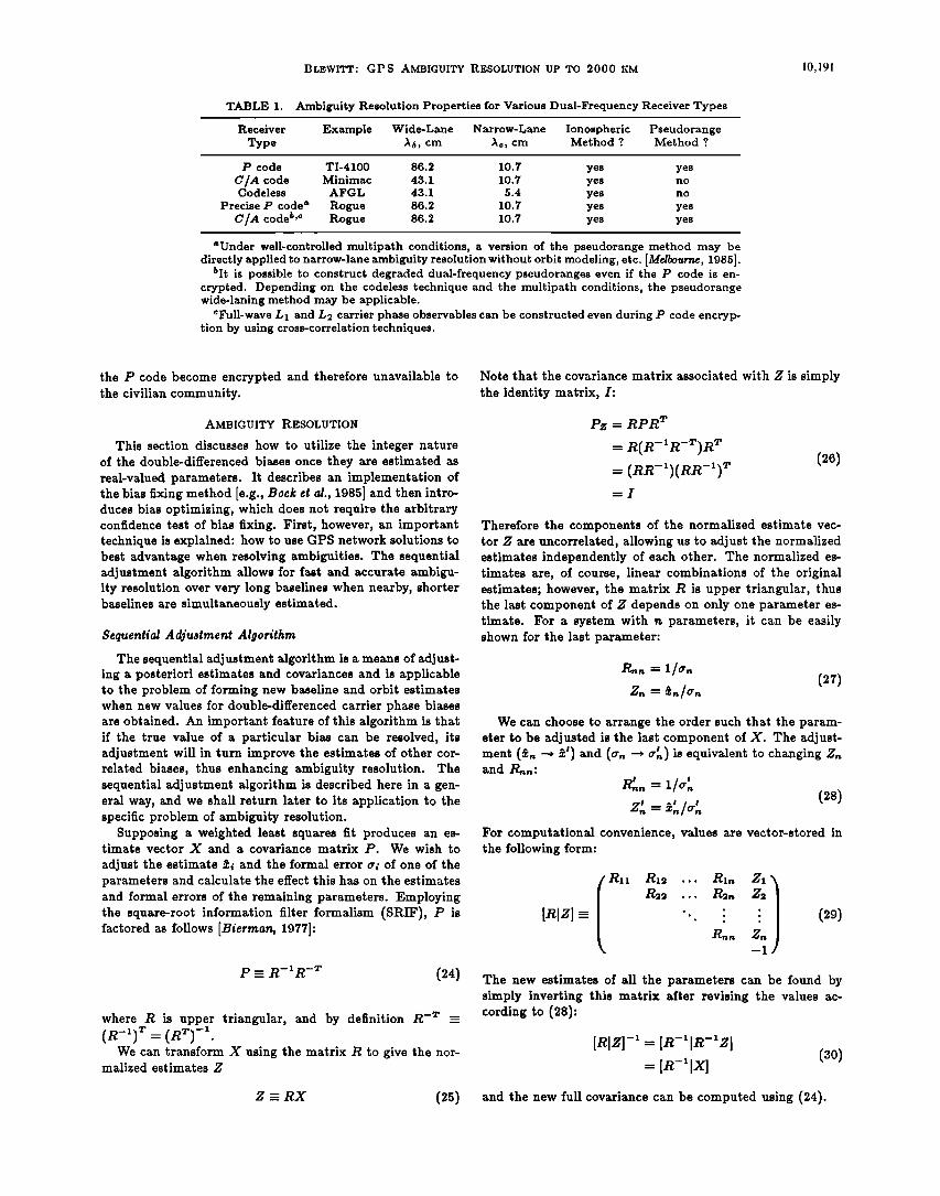
length for wide-lane ambiguity resolution by a factor of 2. The narrow-lane wavelength for C/A code receivers is 10.7 cm, the same as for P code receivers. However, for completely codeless receivers, the narrow-lane wavelength is 5.4 cm. A summary of these differences is given in Table 1.

Looking to the near future, there may soon be new receivers generally available, which can construct the full-wave carrier phases at both frequencies without explicit knowledge of the P code. Cross-correlating techniques implemented by the prototype Rogue receiver can be used to extract (P•- Pa) pseudorange observables without explicit knowledge of the P code, hence giving an absolute measurement of the ionospheric delay. An alternative pseudorange wide-laning method could then be applied in which -(Px-Pa)•{ substitutes the term Ii{ in (19). This technique would be effective with good multipath control at the antenna. These codeless capabilities will be important should


TABLE 1. Ambiguity Resolution Properties for Various Dual-Frequency Receiver Types

Receiver Example Wide-Lane Narrow-Lane Ionospheric Pseudorange Type :•, cm :kc, cm Method ? Method ?

P code TI-4100 86.2 10.7 yes yes C/A code Minimac 43.1 10.7 yes no Codeless AFGL 43.1 5.4 yes no

Precise P code a Rogue 86.2 10.7 yes yes C/A code •,c Rogue 86.2 10.7 yes yes

aUnder well-controlled multipath conditions, a version of the pseudorange method may be directly applied to narrow-lane ambiguity resolution without orbit modeling, etc. [Melbourne, 1985].

•It is possible to construct degraded dual-frequency pseudoranges even if the P code is encrypted. Depending on the codeless technique and the multipath conditions, the pseudorange wide-laning method may be applicable.

CFull-wave L1 and L2 carrier phase observables can be constructed even during P code encryp- tion by using cross-correlation techniques.

the P code become encrypted and therefore unavailable to the civilian community.

AMBIGUITY RESOLUTION

This section discusses how to utilize the integer nature of the double-differenced biases once they are estimated as real-valued parameters. It describes an implementation of the bias fixing method [e.g., Bocket al., 1985] and then intro- duces bias optimizing, which does not require the arbitrary confidence test of bias fixing. First, however, an important technique is explained: how to use GPS network solutions to best advantage when resolving ambiguities. The sequential adjustment algorithm allows for fast and accurate ambiguity resolution over very long baselines when nearby, shorter baselines are simultaneously estimated.

Sequential Adjustment Algorithm

The sequential adjustment algorithm is a means of adjusting a posteriori estimates and covariances and is applicable to the problem of forming new baseline and orbit estimates when new values for double-differenced carrier phase biases are obtained. An important feature of this algorithm is that if the true value of a particular bias can be resolved, its adjustment will in turn improve the estimates of other correlated biases, thus enhancing ambiguity resolution. The sequential adjustment algorithm is described here in a general way, and we shall return later to its application to the specific problem of ambiguity resolution.

Supposing a weighted least squares fit produces an estimate vector X and a covariance matrix P. We wish to

adjust the estimate •i and the formal error (•i of one of the parameters and calculate the effect this has on the estimates and formal errors of the remaining parameters. Employing the square-root information filter formalism (SRIF), P is factored as follows [Bierman, 1977]:

P • R-IR -• (24)

where R is upper triangular, and by definition R -•" = =

We can transform X using the matrix R to give the normalized estimates g

Note that the covariance matrix associated with Z is simply the identity matrix, I:

Pz = RPR T

= R(R- •R-•)R • = -I

(26)

Therefore the components of the normalized estimate vector g are uncorrelated, allowing us to adjust the normalized estimates independently of each other. The normalized estimates are, of course, linear combinations of the original estimates; however, the matrix R is upper triangular, thus the last component of g depends on only one parameter estimate. For a system with n parameters, it can be easily shown for the last parameter:

We can choose to arrange the order such that the parameter to be adjusted is the last component of X. The adjustment (•, -* •') and ((•, -* (•) is equivalent to changing g• and P•.:

= z.' '

For computational convenience, values are vector-stored in the following form'

The new estimates of all the parameters can be found by simply inverting this matrix after revising the values ac- cording to (28)'

[elzl- = 1 = [R_lx] (so)

Z =_ RX (25) and the new full covariance can be computed using (24).

10,192 BLEWITT' GPS AMBIGUITY 'RESOLUTION UP TO 2000 KM

Note that the inversion expressed in (30) only needs to be computed after all bias parameters have been adjusted. This algorithm is very fast and numerically stable because it operates on vector-stored, upper triangular matrices.

Sequential Bias Fizing Method

Bias fixing refers to constraining the phase biases to integer values and effectively removing the biases as parameters from the solution. It is generally a poor strategy to indis- criminately fix every bias to the nearest integer value; this may degrade the geodetic solutions if there is a significant chance of fixing a bias to the wrong value. The method used here is to calculate the cumulative probability that all the fixed biases (wide-lane and ionosphere free) have the correct value and to subsequently fix another bias only if the cumulative probability stays greater than 99%. The order of bias fixing, which here is uniquely determined, is decided by always choosing the next wide-lane/ionosphere-free bias pair most likely to be fixed correctly (i.e., by sequentially maxi- mizing the cumulative probability). The estimates and uncertainties of the remaining unfixed biases are continuously updated by the sequential adjustment algorithm to reflect the progressively improving solution as biases become fixed to their true values.

The probability for fixing a bias correctly is derived from its distance to the nearest integer and its formal error. For wide-laning, the formal errors are given by (15) or (21), depending on the method used. For resolving the ionosphere- free bias, (9), the covariance matrix calculated during the weighted least squares fit provides the formal error. In the latter case, the formal errors scale with the assumed data noise. For TI-4100 data, which our preprocessing software smooths to 6 min normal points, we conservatively use I cm for carrier phase data and 250cm for pseudorange data. These values provide good agreement of the formal errors with baseline repeatability, and the reduced chi-square of the least squares fit is close to unity.

This bias fixing method for a system with r• phase ambiguities is summarized mathematically in the following equations:

j=integer

t:•i- k, Qi > 0.99 (31a) • -- •i Qi _• 0.99 (3lb)

cri- 0 q, > 0.99 (31c) •i = •i Qi • 0.99 (31d)

where

i = (1,3,5,...,n- 1) wide-lane bias index; i = (2, 4,6,..., a) ionosphere-free bias index; qi = cumulative probability (Qo ---- 1); •i = adjusted estimate of phase bias, i; ki = nearest integer to 5i; cri = formal error of •i; zi = new estimate of cri = formal error of z•.

Given that i- 1 biases have been fixed, the next wide- lane/ionosphere-free pair (i, i + 1) is selected such that is maximized. For computational purposes, the summation in (31) is carried out over integers within the window 10 •. In calculating the probability, the precaution is taken

of setting cri =[ii - ki[/2 if it is initially smaller than this value. This provides a safety net in case a bias estimate is inconsistent with its formal error (which, fortunately, rarely happens). It is to be understood in these equations that it is not in general the initial estimate of the phase bias, but that it has been sequentially adjusted from its initial value due to its correlation with the biases (1,2,...,i- 1) that have already been resolved.

For comparison with other bias fixing algorithms [e.g., Dong and Dock, 1989], Figure I shows contours of constant probability Q that the nearest integer is the correct one in the two-dimensional space defined by the formal error cr and the distance to the nearest integer, [i- k[. Note that the interpretation of this figure is slightly different to the one of Dong and Dock [1989], since it is understood that the cumulative probability be computed when deciding whether to round the next bias to the nearest integer. Dong and Dock [1989] appear to be more conservative in their acceptable values of or, and less conservative for [i- k I. A comparison of the two techniques at an analytical level is rather difficult, however, since our respective softwares implement different measurement models and estimation strategies. We generally find the formal errors for the biases to be very consistent with the estimated distance to the nearest integer provided a realistic estimation strategy is selected.

Bias fixing is a perfectly adequate means of using the integer nature of the biases provided almost all the biases can be constrained at the integer value with very high confidence. However, we may have a situation where, for a given set of biases, the cumulative probability is too low to justify bias fixing, even though individual biases are quite likely to have the nearest integer value. There may also be the problem that the final solution is sensitive to an arbitrarily chosen confidence test. The bias optimizing method addresses these problems.

Sequential Bias Optimizing Method Let us define the expectation value as the weighted-mean

value of all possible global solutions in a linear system, where the weights are determined by the formal errors derived from a fit in which the parameters are estimated as real-valued. In the case of systems where all the parameters can intrinsically take on any real value, the expectation value corresponds to

o rY rY

o

99%

99.9%

..... 99.99%

o

0 0.1 0.2 0.5 0.4 0.5

DEVIATION, I•-'•1 (CYCLES)

Fig. 1. For a given formal error and an estimated distance of a bias to the nearest integer, the contours show the probability that the true value of the bias is the nearest integer.


the initial fit value. It is shown in Appendix A that if the parameters are intrinsically integers, the expectation value is a minimum variance solution. The question of a confidence test never arises, and the implementation is automatic and requires no subjective decisions.

In the limit that the initial solution has very small formal errors for all the biases, this approach becomes equivalent to bias fixing. In the opposite limit of very large formal errors, the initial solution is left unchanged. In between these limits, the expectation value approach gives a baseline solution which continuously varies from the initial to the ideal, bias-fixed solution.

Using the same notation as in (31), the following equations summarize the bias optimizing method (see also (A6) and (A8)):

., I • (i-•,)'/z,,•' (32) ./=integer

j=integer

where

j=integer

Since they are so well determined, each wide-lane ambiguity is first bias fixed before bias optimizing its corresponding ionosphere-free ambiguity. The same order of adjustment is used as was defined for bias fixing.

Global Estimate/Covariance Adjustment

The above descriptions of bias fixing and bias optimizing apply to double-differenced bias estimates, which must first be computed from the undifferenced estimates. The double- differenced biases are adjusted, then transformed back to undifferenced estimates before globally adjusting the parameters of interest, including station locations.

The initial weighted least squares estimate X and covariance P are used to compute JR]Z] as defined by (24), (25) and (29) (or alternatively, JR]Z] can be obtained directly from the data using a SRIF algorithm). The parameters are ordered such that the undifferenced ionosphere-free bias parameters of (8) appear as the last components of X, so that [R]Z] can be partitioned as follows:

--1 (33)

where the subscript b refers to the ionosphere-free bias parameters, and a to any other parameters (e.g., station locations). The lower partition [RsIZs] is then extracted:

Rs Zs ) (34) --1

As described in Appendix B, an operator D is used to transform the undifferenced bias estimates into an optimal set of double-differenced bias estimates. Equation (B6) gives the appropriate computation

= m[R•D-•IZs] (35)

where Hs is a series of Householder transformations which

puts Ra into upper triangular form, and D is a regular square matrix. The derived set of double-differenced bias estimates is optimal in the sense that it is the linearly independent set with the smallest formal errors.

Having computed the SRIF array [RalZa], the sequential adjustment algorithm can now be applied to the double- differenced bias parameters. Equation (28) is applied using either the bias fixing or bias optimizing methods described in (31) and (32). It is to be understood that the double- differenced ionosphere-free biases have been calibrated into units of cycles by substituting the resolved wide-lane biases n•l into (23). In the case of the bias fixing method, •r i cannot be set to zero in (28), so a value is chosen which is physically very small (e.g., 10 -ø cycles), yet not too small to induce numerical instability.

As previously explained, the next bias pair selected for adjustment maximizes the cumulative probability in (31), and so an iterative reordering scheme is needed because our defined order of ambiguity resolution is not known beyond the next iteration. The procedure given in (28) can be sequentially applied for the adjustment of several parameters by reordering R such that each bias is in turn represented by the last component. For computational efficiency, this is achieved by permuting the columns of the matrix R, then applying a series of Householder orthogonal transformations H to put R back into upper triangular form [Bierman, 1977]. Note that we choose not to use a (slightly more efficient) scheme which explicitly eliminates the fixed bias parameters, because it is convenient for purposes of bookkeeping to keep the fixed bias parameters attached to the solutions. For example, it allows the analyst to easily determine, after the fact, which biases on a particular baseline were fixed, even if that baseline's biases were not explicitly represented.

Let us denote the sequentially adjusted SRIF array with primes:

[R,•IZ, 4 --• [R•,IZ• ] (36)

Once all biases have been adjusted, the SRIF array is ar- ranged into its original order and is transformed in order to recover the undifferenced biases:

= Ha[R•DIZ•] (37)

where the orthogonal transformation Ha ensures R• is upper triangular. The new estimates of station locations, orbital parameters, etc., can now be computed by substituting [R•IZg] in place of [RslZs] in (33) and inverting the full at-

[R'-ix'i = [R, iz,]

R• R•s =

-1

(38)

The following equation explicitly relates the change •X,• = (X: - X,) in the remaining parameters (e.g., station locations) caused by adjustments 6Xa in the double-differenced bias estimates, and similarly for the associated covariance matrices P• and Pa:

6X,• = S 5Xa (39)

&P,• = S &PaS :r

10,194 BLEWITT: GPS AMBIGUITY RESOLUTION UP TO 2000 KM

where the sensitivity matrix is given by

S = -R•'iR•bD -x (40)

Equation (39) is only shown for completeness; the computations are implicit in (33)-(38), which allow for a convenient and numerically stable implementation.

Using the algorithms described in this section, ambiguity resolution of a 6 satellite, 14 receiver network requires 10 rain of processing time on the Digital MicroVAX II computer.

Sequential Ambiguity Resolution of Networks

The sequential adjustment algorithm automatically ensures that the best determined biases are resolved first, thus improving the resolution of the remaining biases. Formal errors in station locations as computed by the Kalman filter tend to be correlated, since a random error in a satellite orbit parameter maps into a station location error in almost the same direction for nearby stations. Therefore longer baselines tend to have larger formal errors. Since the ionosphere-free biases are correlated with the baseline and orbit parameters, the shorter baselines in a network are usually the first to be selected for ambiguity resolution.

There are two major factors which strengthen ambiguity resolution for networks in comparison to individual baselines: (1) ambiguities for longer baselines are often resolved as the linear combination of ambiguities for shorter baselines and (2) ambiguities are correlated, so by first resolving the best determined ambiguities, solutions for the remaining ambiguities are strengthened. Ambiguity correlations will always exist in a system with either station specific parameters or satellite specific parameters, for example, station locations, zenith tropospheric delay, or satellite orbital elements. Intuitively, reason 2 can be explained in terms of the successive improvement in station locations, GPS orbits, tropospheric delay, etc., as biases are sequentially adjusted.

It should be pointed out that wide-lane ambiguities are generally not as strongly correlated with each other as the ionosphere-free ambiguities, and so sequential adjustment is of lesser importance for wide-laning. The reason for this is that the ionosphere-free ambiguities are strongly correlated with the baseline and orbit parameters which are sequentially improved; however, the wide-lane ambiguities are independent of these parameters using the pseudorange method, and are only weakly dependent on them using the ionospheric method (through Bc• of (19)). It is likely that the ionospheric method could be significantly enhanced by sequential adjustment of a network if the term I• in (19) were modeled and estimated as a function of time, longitude, and latitude over the area of interest. Another approach to enhancing the sequential adjustment of wide-lane ambiguities is to introduce ionospheric correlations a priori, a framework for which is described by Schaffrin and Bock [1988].

Of course, reason 1 given above still applies to wide- laning. For the pseudorange method this is of no conse- quence, since it is independent of baseline length; for the ionospheric method it is an important consideration for the design of non-P code receiver networks.

Multidimensional Generalization

The cumulative probability function used for bias fixing, (31), is an approximation of the more general function which considers all possible combinations of integers. If we arrange

our initial bias estimates into a column vector X and con-

sider that a possible value of this vector can be any one with integer components J, then we can write the probability that K is the correct combination

exp [-•(K- X)•rP-X(K- X)] Q(K,X,P) = E exp [-•(J- X)wP-i(J- X)] (41)

J

where P is the covariance matrix, and the summation is to be carried out over integer lattice points in d dimensions, where d is the number of biases in the system.

Similarly, the expectation value given by (32) can be easily generalized to the multidimensional case where there are many biases

J

P'= - - J

(42)

where P* is the new bias covariance matrix, and Q( J, X, P) is defined by (41). If these expressions could be computed, all available information could be used, and sequential adjustment would not be necessary. However, on inspection of (41) and (42) we see that there is a problem: the number of lattice points in the summation grows as N a, where N is a search window. The multidimensional case becomes im-

practical to implement unless the search space is limited in some way. A realistic approach would be to devise an algorithm which finds a subset of all J which are good candidates for correct integer combination. Such an algorithm, based on the sequential adjustment algorithm, is under develop- ment. (Another approach, used by Dong and Bock [1989], is to sequentially fix biases in batches using a five-dimensional search.)

The analysis presented in this paper successfully uses the one-dimensional sequential adjustment technique. For sparse networks, where this type of bootstrapping may not be successfully initiated, a multidimensional search is clearly preferable. However, it is exactly this kind of network which is expected to benefit from the bias optimizing method, so a multidimensional scheme is recommended to fully test the relative merit of bias optimizing.

DATA ANALYSIS AND RESULTS

Software

The GIPSY software (GPS-Inferred Positioning System), which was developed at the Jet Propulsion Laboratory, has already been used to analyze GPS carrier phase and pseudorange data, yielding baseline precisions at the level of a few parts in l0 s or better [Lichten and Border, 1987; Tralli et al., 1988]. The software automatically corrects for integer-cycle discontinuities (cycle slips) in the carrier phase data when a receiver loses lock on the signal. The module TurboEdit, which will not be described in detail here, automatically detects and corrects for wide-lane cycle slips using equation (13) and corrects for the narrow-lane cycle slip using a polynomial model of ionospheric variations in the data over a few minutes spanning each side of the cycle slip. A study using thousands of station-satellite data arcs shows that TurboEdit makes an error on less than 1% of the arcs

using pseudorange of TI-4100 quality. Any remaining, un-

BLEWITT' GPS AMBIGUITY R, ESOLUTION UP TO 2000 KM 10,195

resolved cycle slips are treated as additional parameters in the least squares process.

A new module, A_MBIGON, implements the ideas expressed in this paper for resolving carrier phase ambiguities and unresolved cycle slips and has been incorporated into GIPSY for routine data processsing. AMBIGON operates on an initial global estimate vector and factored covariance matrix from a filter run and produces a new global estimate and covariance. All the parameters in the filter run are adjusted, including the GPS satellite states and station locations. Low elevation data can be excluded when (14) is applied if large multipath signatures are a problem. This analysis nominally excludes GPS data from below 15 degrees of elevation. The user can run A_K4BIGON in either a bias

fixing or bias optimizing mode, and batches of stations can be selected for ambiguity resolution. AMBIGON is designed to work naturally in network mode, using the algorithms described in this paper. A_ mixed network of P code receivers, C•A code receivers, and codeless receivers can be processed for ambiguity resolution. One strategy available is the automatic application of either the pseudorange or ionospheric method for each wide-lane bias, the decision being based on receiver type, baseline length, and the formal errors as computed by (15) and (21). The program is fully automatic, requiring no user intervention.

Data

The GPS data presented here were taken during the June 1986 southern California campaign, in which up to 16 dual- frequency TI-4100 receivers acquired carrier phase and pseudorange data from the 6 available GPS satellites for four daily sessions. The receiver deployment schedule is shown in Table 2. In addition to 16 sites in southern Califor-

nia, receivers were deployed at Hat Creek (northern Cali- fornia), Yuma (Arizona), and at the International Radio In-

TABLE 2. Deployment of TI-4100 Receivers for the June 1986 Southern California Experiment

Station June 17 June 18 June 19 June 20

Fort Davis a X X X X

Haystack a X X X X Richmond a X X X X

Boucher X X

Catalina c X X X X

Cuyamaca X Hat Creek b X

La Jolla X X

Mojave b,c X X X X Monument Peak •,• X X X X

Niguel X X Otay X X

Palos Vetdes • X X X X

Pinyon Flats • X X San Clemente {1) X X San Clemente {2) X X

San Nicholas • X X X X

Santiago X Soledad X X

Vandenberg •,e X X X Yuma •,c X X X X

aThese fiducial sites were held fixed at their VLBI-inferred coordinates.

bThese sites were used in the comparison of GPS and VLBI solutions.

øSites occupied for 3 or 4 days used for the daily repeatability study.

20

18

16

• 14 -

• 12 -

,, 10 -

• 8-

'• 6 -

4 -

2 -

I I I I I I I

6 8 10 12 14

BASELINE LENGTH (x100 km)

I I I

16 18 20

Fig. 2. lengths in the western United States on June 20, 1986.

Histogram showing the distribution of G PS baseline

terferometric Surveying (IRIS) sites at Fort Davis (Texas), Haystack (Massachusetts), and Richmond (Florida).

The baselines in the western United States ranged in length from 18 to 1933km (Hat Creek-Fort Davis). This network was especially suitable for testing network mode ambiguity resolution because of the wide spectrum of baseline lengths, which is shown in Figure 2 for June 20, 1986. Even though data were acquired for only a few days at each site, the daily repeatability of baseline estimates provides a strong statistical test for evaluating analysis techniques because of the large number of baselines.

Baseline accuracy was assessed by comparing GPS with very long baseline interferometry (VLBI) solutions. Histo- ries VLBI solutions for baseline coordinates are available

from Hat Creek, Mojave, Monument Peak, Pinyon Flats, Vandenberg, Yuma, and the IRIS sites [Ryan and Ma, 1987]. The analysis presented here used the latest available God- dard global VLBI solution GLB223 evaluated at the epoch of June 1986 (3. W. Ryan, C. Ma and E. Himwich, God- dard Space Flight Center VLBI Group, unpublished results, 1988). This provided (1) a priori values for the fixed fiducial coordinates at the IRIS stations and (2) ground truth baseline coordinates in the western United States from which

GPS accuracy could be assessed both with and without ambiguity resolution.

Parameter Estimation Strategy

The analysis employed a parameter estimation strategy which basically follows Lichten and Border [1987], except that the parameters were estimated independently for each day. The use of independent data sets strengthens daily repeatability as a test of the improvement in precision.

Undifferenced, ionospherically calibrated carrier phase and pseudorange data were processed simultaneously using a U-D factorized batch sequential filter with process noise capabilities. The receiver and satellite clock biases were constrained to be identical for the two data types and were estimated as white noise processes. Unlike techniques which prefit polynomials to the system clocks using the pseudo-

10,196 BLEWITT: GPS AMBIGUITY P•ESOLUTION UP TO 2000 KM

range, this method is completely insensitive to discontinuities and other problematic behavior in the clock signatures. This technique can be shown to be identical to using the pseudorange to prefit the station satellite carrier phase biases (rather than the clocks), and subsequently using only carrier phase data to estimate the undifferenced biases with tight constraints at the level of a few nanoseconds (S.C. Wu, Jet Propulsion Laboratory, unpublished work, 1987).

In order to accurately estimate the GPS orbits, and to establish solutions in the VLBI reference frame, the fiducial network concept was implemented, as described by Davidson et M. [1985]. Three fiducial sites (Fort Davis, Haystack, and Richmond) were fixed at their VLBI-inferred coordinates, and the other station locations were estimated simultane-

ously with the GPS satellite states using loose constraints of 2 km on the a priori station locations. In the absence of water vapor radiometers (WVR's), surface meteorological data were used to calibrate the tropospheric delay, and the residual zenith tropospheric delay at each site was modeled as a random walk process with a characteristic constant of 2.0 x !0 -? km/sec x/2 [œichten and Border, 1987]. This strategy allows the estimated zenith troposphere to wander from the calibrated values by about 5 cm over a 24-hour period. WVR data were available at the fiducial sites and Palos

Verdes for some of the days. In these cases, a constant residual zenith delay was estimated.

Arabiguity Resolution

Ambiguity resolution techniques were applied to the western United States network for all 4 days using both the sequential bias fixing method of (31) and the sequential bias optimizing method of (32). For the entire experiment, a total of 262 linearly independent, observable double- differenced phase biases were formed. Figure 3 shows the distribution of wide-lane bias estimates (equation (14)) about their nearest integer value using the pseudorange method. Since only those biases with a formal error less than 0.2 cycles are shown, we would expect to see a sharply peaked distribution about the nearest integer value. Fig- ure 4 shows a similar distribution for the ionosphere-free

160 -

140 -

• 120 -

,,, 100 -

fl. 80 -

o

n- 60 -

:• 40 -

20 -

0.1 0.2 0.3 0.4 0.5

CYCLES FROM NEAREST INTEGER

Fig. 3. Histogram showing the distribution of wide-lane bias estimates about the nearest integer values. Only biases with formal errors less than 0.2 cycles are shown.

140

u• 120

,,, 100 -'

o. 80 -

o

o:: 60 -

• 40 -

0.1 0.2 0.3 0.4 0.5

CYCLES FROM NEAREST INTEGER

Fig. 4. Histogram showing the distribution of ionosphere-free bias estimates about the nearest discrete values. The scale has been normalized so that the 10.7 cm distance between discrete

values is defined to be 1 cycle. Only biases with formal errors less than 0.2 cycles are shown.

biases (equation (23)) which was derived from the filter solutions (i.e., before sequential adjustment) assuming that the wide-lane biases were correctly resolved. In both Figures 3 and 4, we clearly see the quantized nature of these biases and the characteristic half-Gaussian shape of the distributions. These distributions indicate that systematic effects were small compared to the predicted random errors.

Using the bias fixing method, 94% of the ionosphere-free ambiguities were resolved with a cumulative confidence of greater than 99% for each daily solution. The remaining ambiguities failed the confidence test primarily because ex- cessive pseudorange multipath prevented wide-laning. Even so, 97% of the wide-lane biases could be resolved with an individual confidence of greater than 99%, showing that TI- 4100 receivers are adequate for the direct wide-laning approach.

When bias optimizing was applied, the baseline solutions agreed at the millimeter level with bias fixing. The reason for this is that the expectation values derived by (32) dif- fered at the submillimeter level with the values of the bias

fixing approach derived by (31). This should be typical for well-configured networks. Since the solutions were so similar, baseline results in the following sections apply to both approaches.

A comparison of wide-lane bias estimates derived by the pseudorange and ionospheric methods is given in Figure 5 for June 20, 1986. (Please note that in Figure 5 slight adjustments to the baseline length (+10km) were made for a few overlapping points in order to enhance graphical clarity). The integer used to compute the deviation of the estimate was determined as follows: (1) in 64 out of 72 cases, the rounded integer agreed for both methods and was assumed to be correct and (2) in 5 cases, the rounded integer disagreed, but the estimates disagreed by less than one cycle; in these cases the integer closer to one of the estimates was taken.

In the remaining 3 cases, the estimates disagreed by more than one cycle for the longest 1003 km baseline. For this baseline, it was noted that 5 of the 7 estimates using the pseudorange method were within 0.12 cycles of the nearest integer, and the other 2 were 0.23 cycles from the near-

BLEWITT: GPS AMBIGUITY t•ESOLUTION UP TO 2000 KM 10,197

.-. 3.0

• 2.5

z 2.0 O

• 1.5

1.0

m 0.5

0.0 0

ß . , ! . . . ! . , . ! .

(a) PSEUDORANGE METHOD

200 400 600 800 1000 1200

BASELINE LENGTH (KM)

3.0

2.5

2.0

1.5

1.0

0.5

0.0 0

(b) IONOSPHERIC METHOD o

o

o o

.o o -ff o

.... i , . . i . , i . . . i . ,

200 400 600 800 1000 1200


Fig. 5. Distance of wide-lane bias estimates from correct integer as a function of baseline length on June 20, 1986. Determination of the correct integer is described in the text. (a) Pseudorange method. (b) Ionospheric method.

est integer. However, the integers associated with the ionospheric method were not obvious. Moreover, the pseudorange method is independent of baseline length, and based on statistics from shorter baselines, we expect only 0.6 of these 7 estimates to have the incorrect integer. The integers derived from the pseudorange method were therefore assumed to be correct for this baseline.

If this reasoning is correct, Figure 5 shows a breakdown of the ionospheric approach to wide-laning for the 1003 km baseline (Yuma-Fort Davis), using P code receivers. As mentioned previously, this translates to • 500 km for codeless receivers. While the ionospheric approach looks superior for baselines of around 100 km, at 200 km the pseudorange method gives more precise wide-lane estimates. At 699 km (Vandenberg-Hat Creek), despite the fact that the ionosphere method gave correct integer estimates, little confidence could have been placed in the estimates were it not for the verification provided by the pseudorange method. The large difference in ionospheric wide-laning precision between the 699 and 1003 km baselines may be attributed to differences in both baseline length and orientation. Since wide-laning using the pseudorange was more successful, the results that follow pertain to this technique.

Baseline Repeatabilit•t Improvement

The daily repeatability of a component of a baseline is defined here as follows'

$= N 1' (R/-- (R))• 1 (43) i:1 O'i --

where N is the number of days the baseline was occupied, /L' and cri are the estimate and formal error of the baseline

component on the ith day, and the angled brackets denote a weighted mean. For this experiment, data outages were minimal and so the daily weights were approximately equal.

Figure 6 plots the baseline repeatability for the east, north, and vertical components versus baseline length, before and after applying bias fixing. Only baselines which were occupied for 3 or 4 days are shown. After bias fixing, the largest observed horizontal baseline repeatability was only 1.4 cm (Vandenberg-Yuma: 620 km). Baselines occupied for only 2 days show the same pattern, showing subcentimeter repeatability with no outliers, demonstrating the remarkable robustness of this data set and these analysis techniques. (Two-day repeatabilities have not been included in Figure 6 for purposes of graphical clarity).

Table 3 shows the baseline repeatability averaged over all baselines in Figure 6, for each baseline component both before and after bias fixing. Consistent with the prediction by Melbourne [1985], ambiguity resolution improves the east baseline component by a factor of 2.4, the north by a factor of 1.9, and the vertical is not significantly improved. These improvement factors are consistent with the reduction in the formal errors as computed by (39). The negligible improve-

• • BEFORE BIAS FIXING ?• 7 O AFTER BIAS FIXING _• 6 ; 5

• 4

m 3 •' 2

03 1 A {• O '• 0 QO 0 I•1 0 ' ' ' ' ' ' ' ' 0 100 200 300 400 500


i ß

(a)

ß

600 700

•' 8

•-- 6

m 5

• 4

,,, 3

3: 2 •c 1 O z 0

0

BEFORE BIAS FIXING AFTER BIAS FIXING

i i i

(b)

100 200 300 400 500 600


700

8 Z• BEFORE BIAS FIXING 7 O AFTER BIAS FIXING

I ß i ß i ß

6

1 0 100

A

•o • Oo9

• oo o

200 300 400 500

Q

600 700


Fig. 6. Daily baseline repeatability versus baseline length, before and after bias fixing, for those baselines occupied for at least 3 days: (a) east component, (b) north component, and (½) vertical component.

10,198 BLEWITT' GPS AMBIGUITY P•ESOLUTION UP TO 2000 KM

TABLE 3. Mean Daily Repeatability for Baselines Occupied for 3 or 4 Days, Before and After Bias Fixing the Solutions

Baseline

Component RMS RMS Improvement

Before, cm After, cm Factor

2.0 0.82 2.4

0.74 0.40 1.9

3.2 2.9 1.1

East

North Vertical

Also shown is the improvement factor due to bias fixing.

ment in the vertical component can be understood in terms of its relatively small correlation with the carrier phase biases.

Baseline Accuracy Improvement

The accuracy of a given baseline component solution is defined here as the magnitude of the difference between the GPS-inferred coordinate and the VLBI-inferred coordinate.

This approach is conservative, since it neglects possible errors in the antenna eccentricities, local monument surveys, and the VLBI solutions. The GPS-inferred coordinate is

taken to be the weighted mean of the daily solutions. GPS baselines between all sites collocated with VLBI were ana-

lyzed, except for those involving the IRIS sites (which were held fixed). The longest of these baselines is Hat Creek- Yuma (1086 km).

Using the above definition, baseline accuracy for the east, north and vertical components is plotted versus baseline length in Figure 7. Table 4 shows the accuracy of each baseline component averaged over all baselines collocated with VLBI. We see an improvement in accuracy for the horizontal baseline components after bias fixing. The east component is improved by a factor of 2.8, and the north component by a factor of 1.25. As expected, no improvement is seen for the vertical component. The mean vertical accuracy for baselines less than 500km is also shown. GPS and VLBI

baseline lengths agree on average to better than a centimeter. In fact, the Hat Creek-Yuma baseline (1086 km) agrees to 0.88cm, which corresponds to 8 parts in 109. The accuracy improvement factors are similar to those for daily repeatability; thus where no independent verification (such as from VLBI) is available, daily repeatability may be a good indicator as to the accuracy improvement due to ambiguity resolution.

Discussion on Network Design

The carrier phase bias parameters can be expressed in terms of linear combinations of the biases which were ex-

plicitly resolved. Figure 8 shows all the baselines for which biases were explicitly resolved on June 20, 1986. Sequential ambiguity resolution tends to take a path of least resistance, i.e., biases tend to be resolved between nearest neighbor station pairs. When the neighbors are approximately equidis- tant from a given station, the automatic selection of biases also depends on more subtle factors such as network geometry, satellite geometry, and data scheduling (for example, look at La Jolla in Figure 8). Figure 9 shows the distribution of nearest neighbor distances, which is almost identical to the distribution of lengths from Figure 8. It is recommended that networks be designed with a similar distribution of nearest neighbor distances, starting with baseline lengths of around 100 km.

8

o o


200 400 600 800


(a)

1000 1200

8

7

6

5

4

3

2

1 -

0 0


A A ,•^. . O .• ,

200 400 600 800


!

(b)

O

1000 1200

•- 8

> o o

BEFORE BIAS FIXING AFTER BIAS FIXING (c)

O

.

A ß

,40 200 400

o

600

! . ! .

800 1000 1200


Fig. 7. Magnitude of difference between GPS and VLBI baseline solutions versus baseline length, before and after bias fixing: (a) east component, (b) north component, and (½) vertical component.

Figure 8 can be used to infer a linear combination of biases associated with a particular baseline. For example, each resolved bias associated with the Vandenberg-Fort Davis baseline (1618 km) can be expressed as a linear combination of 8 or 9 resolved biases associated with shorter baselines

(depending on the associated satellites). By performing a linear decomposition, the percentage of resolved biases for any given baseline or subnetwork can be calculated. For example, 23 out of a total of 26 ionosphere-free biases (88%) were resolved for the 1618-km Vandenberg-Fort Davis base-

TABLE 4. Mean RMS Difference Between GPS and VLBI

Solutions for Baselines Between Nonfiducial Stations, Before and After Bias Fixing

Baseline RMS RMS Improvement Component Before, cm After, cm Factor

East 2.7 0.97 2.8

North 1.0 0.80 1.25

Vertical* 3.6 4.0 0.90

Also shown is the improvement factor due to bias fixing. *Mean vertical RMS for baselines • 500 km is 2.8 cm before and

2.6 cm after.

BLEWITT' GPS AMBIGUITY RESOLUTION UP TO 2000 KM 10,199

HATC

0 200 400 I , I , I ,

100 300 500 k rn

MOJA

VAND

NICH

PALO •ANT

BOUC YUMA

CLBVI LAJO MONU

FORT

Fig. 8. Receiver deployment on June 20, 1986. Baselines for which biases which were explicitly resolved are shown. Other baselines had their biases resolved by linear combinations of the shown baselines. This illustrates a major strength that networks bring to ambiguity resolution for long baselines.

line. The remaining 3 biases could not be resolved due to wide-laning failures; however, their formal errors were better than 6 mm, which is almost as good as having them resolved. The reason that these formal errors are so small is

that the network was almost completely bias fixed and that the unresolved ambiguities are really associated with baselines much shorter than 1618 kin. This study shows some of the inherent strengths that networks provide for long baseline ambiguity resolution.

The mechanism of sequential adjustment is just one important consideration when designing networks for long baseline ambiguity resolution. Of course, sequential adjustment will only succeed if the initial (preadjusted) ambiguity estimates are sufficiently accurate. With this in mind, the network designer should also consider (1) the selection of fiducial sites for precise orbit determination, (2) the spatial extent of the network and the number of receivers used in

order to improve the local fit to the orbits over the region of interest, (3) the use of high precision P code receivers for more precise solutions before the ambiguities are resolved, and (4) the ability to resolve wide-lane ambiguities.

6 w

2 •

I I I I I I

2 4 6 8 10 12

BASELINE LENGTH (x100 kin)

Fig. 9. Histogram showing the distribution of nearest neighbor distances on June 20, 1986.

Since the pseudorange wide-laning method is baseline length independent, wide-laning need not be considered for the design of P code receiver networks. For the ionospheric method, however, the minimum distance between nearest neighboring stations required for wide-lane ambiguity resolution should be anywhere from N 100 to > 1000 km depending on the local time of day, the month of the year, the phase of the solar sunspot cycle, and the geographical location. These conditions are important considerations when deciding on the placement of non-P receivers in a network.

Analltsis of a Well-Configured, Sparse Network

A similar analysis to the one which has been described here in detail was conducted using a subset of the data acquired during the global CASA UNO experiment of January 1988 [Neilan et al., 1988; Blewitt et al., 1988]. The network for this study comprised 4 stations in California: Mammoth, Owens Valley Radio Observatory (OVRO), Mojave, and Hat Creek. The fiducial network consisted of Haystack, Fort Davis and Hat Creek. (The other IRIS site, Richmond, had a receiver which was malfunctioning during this experiment.) The California network, shown in Figure 10, is clearly sparse, but based on the previous discussion is theoretically well-configured because of the wide spectrum of baseline lengths. Figure 10 also illustrates the proximity of the fiducial baseline Hat Creek-Fort Davis to the California network: covariance studies show that this fiducial geometry is very strong for surveys in this region.

Ambiguity resolution over the Hat Creek-Mojave baseline (723 km) was consistently applied to five single-day solutions by resolving the ambiguities on the Mammoth-OVRO baseline (71 km), the OVRO-Mojave baseline (245 km), and the Mammoth-Hat Creek baseline (416 km). All ambiguities were resolved, resulting in similar improvements in daily repeatability and accuracy as for the June 1986 southern California experiment. This was a more stringent test of the sequential adjustment algorithm since the network was much more sparse. Hence complete ambiguity resolution

10,200 I•LEWITT' GPS AMBIGUITY P•ESOLUTION UP TO 2000 KM

HATC

o 200 400 I i , I

'•" 100 300 500 km '•.

"•..

'•,.

MOdA (FIDUCIAL BASELINE) "•..

'•,. •,.

',•,.

-x.F. oRT Fig. 10. California network of January 1989, for which all biases were resolved. Also shown is one of the fiducial baselines: Fort Davis-Hat Creek. The third fiducial site at Haystack, Massachusetts, is not shown.

can be achieved for 700 km baselines with a good fiducial network and as few as two additional, strategically located, •phase-connector"stations.

Comparison of Bias Optimizing and Bias Fixing

In its present implementation using (32), bias optimizing gave baseline solutions within I mm of bias fixing for 3 station subsets of the June 1986 southern California network

for which the shortest baseline lengths were about 200 km or less. In these cases, both techniques were almost maximally effective (i.e., all but a few ambiguities could be fixed with very high confidence). Submillimeter agreement was found when the shortest baseline was about 400 km or more, but for a different reason: the uncertainties in the phase biases were large enough that neither bias optimizing nor bias fixing changed the initial filter solution significantly (if at all).

In the intermediate regime, several three-station networks were investigated, for example, the Vandenberg-Mojave- Monument Peak triangle, for which the shortest baseline is 274 km. The following general observations can be made about these networks for this particular experiment: (1) a significant number of biases (20-100%) could not be fixed if the shortest baseline length were greater than 200 km, (2) both bias fixing and bias optimizing gave improved baseline accuracies and repeatabilities, especially on the shortest of the three baselines, and (3) most baseline solutions using bias optimizing and bias fixing agreed to better than a centimeter, and neither approach as it stands appears preferable to the other.

In order to better test the hypothesis that bias optimizing is better than fixing for certain sparse networks, a multidimensional search algorithm is currently being developed which should provide a more meaningful realization of the probability function, (41), and the expectation value, (42).

CONCLUSIONS

This analysis shows that using pseudorange for wide-lane ambiguity resolution is a powerful technique, in this case

with a success rate of 97% when using a 99% confidence level, and rather poor quality pseudorange data. This technique is important because it is applicable to baselines of any length and requires no assumptions about the ionosphere. Using receivers and antennas which will shortly be commercially available, a 99.9% success rate is certainly possible.

The application of ionospheric constraints appears to be reliable for baselines up to a few hundred kilometers when using P code receivers during good ionospheric conditions (at Californian latitudes, and near the solar sunspot minimum). The pseudorange wide-laning approach appears to be more precise above 200 km. The results of Wu and Ben- der [1988] tend to support this conclusion. With receivers which do not acquire the P code, apart from the obvious problems that can be encountered under less desirable conditions, the baseline length over which the ionospheric con- straint method works is reduced by a factor of 2.

For the ionosphere-free biases, ambiguities were successfully resolved for baselines ranging up to 1933 km in length. The precision of the east baseline component improved on average by a factor of 2.4, and the agreement of the east component with VLBI improved by a factor of 2.8. Vertical accuracy is not significantly affected, because of the small correlation of the vertical component with carrier phase biases. The comparison of GP$ with VLBI suggests that centimeter-level accuracy for the horizontal baseline components has been achieved, corresponding to about 1 part in l0 s for the longer baselines.

l•esults using the bias optimizing method indicate that it is a promising approach, giving baseline accuracies compa- rable to bias fixing. A multidimensional algorithm for com- puting the expectation value (and also for bias fixing) would more rigorously test the hypothesis that bias optimizing is superior to bias fixing for poorly configured networks.

The importance of ambiguity resolution for high precision geodesy cannot be overstated, and attention should be paid to this in the design of GP$ experiments. These studies show that if 1000 km baselines are to be resolved, the network should also contain baseline lengths as small as 100 km. The

BLEWITT' GPS AMBIGUITY [•ESOLUTION UP TO 2000 KM 10,201

results of Cou.selm•. [1987] and Do,g •nd Bock [1989] tend to support this conclusion. Ambiguity resolution software should then exploit the correlations between the biases for baselines of different lengths. The extra expense incurred by deploying extra receivers to ensure ambiguity resolution may be more than offset by the reduced dwell time needed to achieve the required accuracy for a particular baseline. Followlng these guidelines, ambiguity resolution could be routinely applied to baselines spanning entire continents.

APPENDIX A' DERIVATION OF THE

EXPECTATION VALUE

The expectation value is derived using Bayesean considerations. Let us define p(zl• ) to be the likelihood function that a bias has a value z, given that it was estimated to have the (real)value •. Let p(z) be the a priori probability density that the bias has a value z. Let p(•lz) be the probability density of obtaining the weighted least squares estimate •, given that the true value of the bias was z. Us- ing Bayes' theorem [Mathews and Walker, 1970, p. 387] we can write

P(•!x)P(x) (A1) =

If an experiment were repeated an infinite number of times, and the experimental conditions were identical each time except for random white data noise, estimates • would obey the Gaussian probability distribution:

1 _(•_•)2/2•2 (A2) = where z is the true value of the bias, and •r is the formal error.

Now, if we assume a priori that any integer value is equally likely for a given bias in some large range (-N, ..., +N), then we can write the a priori probability density'

1 •6(x--j) v(,) = (2N + (AS)

Substituting (A2) and (A3)into (A1) and performing the integration gives

where

pCzl): -

+N

C = • e -(•-•)2/2'r2

(A4)

Equation (A4) represents our best estimate of the probability distribution for the correct value of the bias. We can now ask what value of the bias we should take. The bias fix-

ing approach is to take the maximum likelihood value only if it is more probably correct than some confidence level, otherwise use the originally estimated value •. In contrast, the expectation value is a minimum variance estimate.

Suppose we took some real value z' for our new estimate of the bias. The variance of this value is defined in the usual

way by the following integral [Mathews and Walker, 1970, p. 388]'

=/;: (z - z') 2 v(zl)dz Substituting (A4) into (AS) and integrating, we find

+N

1 z,)2 (AO)

Let us find the value of z' when the variance is minimized. Let us define •':

as(z') az, =o

3:1 --•1

therefore from (A6) and (A7),

-I-N

L:' = 1 e_(i_•)2/2•2 (AS)

But as can be seen, •' is simply the weighted sum of all possible integer values that the bias can take; hence •* is called the expectation value. The standard error on •* is given by

cr'= V/s($ ') (A9)

where s(i')is calculated using (A6). Equations (AS) and (A9) are the actual formulas used

in the bias optimizing approach. The original estimate i and formal error cr are replaced with the values • and cr '. Subsequently, the estimates and covariance for all the other parameters in the problem are updated.

Equations (AS) and (A9) can be used to illustrate some interesting and desirable qualities of the expectation value. One can easily show the following limits:

lim $' = (nearest integer to •)

lim cr' = 0 o'---• 0

(A10)

which is, of course, the same as bias fixing with 100% confidence, and

lim • -- •

'-• (All) lim •" = o'

which states that if the initial resolution of bias is much

worse than a single spacing between the possible values, then we approach the continuum limit, and our initial real-valued estimates cannot be improved.

These two limits correspond to the two possible choices that can be made when using the bias fixing approach. How- ever, we have a smooth transition between the limits when the initial a is finite, and we have a means to account for the improvement in the formal errors.

APPENDIX B' AN OPTIMAL DOUBLE-DIFFERENOING TRANSFORMATION

A matrix D is found which maps the set of undifferenced bias estimates Xb, with covariance Pb, into an optimal set

10,202 BLBWITT' GPS AMBIGUITY RBSOLUTION UP TO 2000 KM

(in the sense of being best determined) of double-differenced bias estimates Xd, with covariance Pd:

X• = DX•

P• = DP•D •

where Pb = R•-XR• -r. The transformation matrix O is chosen as follows. First,

let us define T as the matrix which transforms Xb into a vector whose components constitute a redundant set of all mathematically allowed double-differenced bias estimates. Hence each row of T has two elements which have a value + 1, two which are -1, and the rest are zero. The formal errors of the double-differenced biases can be rapidly computed as follows:

• = T• • B2

where n is the number of undifferenced biases. (Note •he subscripts •, j, and k simply refer to ms•rix elements and do not refer to particular stations or satellites).

The matrix D is constructed by selecting rows of T which correspond to the transformed biases with the smallest ues of •;. A row of T is not used if it is $ linear combination

of previously selected rows; this is tested by attempting to form an orthogonal vector to the selected set of rows using the candidate row (via the Gram-Schmidt procedure). Thus O defines a unique, linearly independent, theoretically best- determined set of double-differenced biases. The dimension

• of O so constructed would be less than a. A complete n-dimensional set is formed by arbitrarily selecting (n- undifferenced biases which p•s the Gram-Schmidt test and appending the appropriate (n- m) rows to D. Hence D becomes an n-dimensional, regular square matrix and can be inverted for use in (35).

Let us now consider the application of the transformation D in the SRIF formalism. Using an orthogonal matrix Hs = (H•) • • H• •, (B1) can be written

Pd= R• X R• T = DR•(H•Hjr)R•D • = ( H• R• D - • ) - • ( H• R• D - X ) - T

hence

Rd = H•RbD -• (B4) where for convenience, Hs is chosen such that Rd is upper triangular. Substituting (B1)into (25), and using (B4),

Zd ---- RdXd

= RdDXb

= ••D-•DX• (•$) = H•R•X•

=H•Zb

Hence in the SRIF notation of (29), (B4) and (B5) are represented as follows:

[nlz] = m[nm-l&]

which also appears as (35).

Acknowledgements. The research in this publication was carried out by the Jet Propulsion Laboratory (JPL), California In- stitute of Technology, under a contract with the National Aero- nautics and Space Administration. The data analyzed here were processed using the GIPSY software at JPL by many of my col- leagues, with special thanks to Lisa L. Skrumeda and Peter M. Kroger. I am grateful to John M. Davidson for his advice during the course of this work, and to William G. Melbourne for his pi- oneering work on this topic. Catherine L. Thornton, Steven M. Lichten, David M. Tralli, and Thomas P. Yunck provided good suggestions which were incorporated into this paper. I thank Larry E. Young, Thomas P. Yunck, and J. Brooks Thomas for information on the Rogue receiver, and codeless receiver algorithms. I am grateful to Yehuda Bock and Gerhard Beutler for critical reviews of this work and for their excellent comments.

Essential parts of the software written for this research rely on SRIF matrix manipulation techniques which were explained to me by the late Gerald J. Bierman. I would especially like to thank collaborators from JPL, Scripps Institute of Oceanogra- phy, the Caltech Division of Geological and Planetary Sciences, the National Geodetic Survey, and the U.S. Geological Survey for producing a very valuable and reliable data set from the June 1986 southern California G PS experiment.

REFERENCES

Abbot, R. I., and C. C. Counselman III, Demonstration of GPS orbit-determination enhancement by resolution of carrier phase ambiguity, Eos Trans. AGU, 68, (44), 1238, 1987.

Bender, P. L., and D. R. Larden, GPS carrier phase ambiguity resolution over long baselines, in Proceedings of the First Symposium on Precise Positioning with the Global Positioning System, Positioning with GPS-1985, pp. 357-362, U.S. Department of Commerce, Rockville, Md., 1985.

Beutler, G., I. Bauersima, W. Gurtner, M. Rothacher, and T. Schildknecht, Evaluation of the 1984 Alaska Global Position- ing campaign with the Bernese G PS software, J. Geophys. Res., 9œ, (B2), 1295-1303, 1987.

Bierman, G. J., Factorization Methods for Discrete Sequential Estima- tion, Academic, San Diego, Calif., 1977.

Blewitt, G., et el., GPS geodesy with centimeter accuracy, in teetare Notes in Earth Sciences, vol. 19, pp. 30-40, edited by E. Groten and R. Strauss, Springer-Verlag, New York, 1988.

Bock, Y., R. I. Abbot, C. C. Councelman III, S. A. Gourevitch, and R. W. King, Establishment of three-dimensional geodetic control by interferometry with the Global Positioning System, J. Geophys. Res., 90, 7689-7703, 1985.

Bock, Y., R. I. Abbot, C. C. Counselman III, and R. W. King, A demonstration of one to two parts in 10 7 accuracy using GPS, Bull. Geod., 60, 241-254, 1986.

Counselman III, C. C., Resolving carrier phase ambiguity in GPS orbit determination, Eos Trans. AGU, 65, (44), 1238, 1987

Davidson, J. M., C. L. Thornton, C. J. Vegos, L. E. Young, and T. P. Yunck, The March 1985 demonstration of the fiducial network concept for GPS geodesy: A preliminary report, in Proceedings of the First Symposium on Precise Positioning with the Global Positioning Systerr• Positioning with GPS-1955, pp. 603-611, U.S. Department of Commerce, Rockville, Md., 1985.

Dong, D., and Y. Bock, GPS network analysis with phase ambiguity resolution applied to crustal deformation studies in Cal- ifornia, J. Geophys. Res., 94, (B4), 3949-3966, 1989.

Goad, C. C., Precise relative position determination using Global Positioning System carrier phase measurements in nondiffer- ence mode, in Proceech'ngs of the First Symposium on Precise Po- sitioning with the Global Positioning Systerrb Positioning with GP8- 1985, pp. 347-356, U.S. Department of Commerce, Rockville, Md., 1985.

Lichten, S. M., and J. S. Border, Strategies for high precision GPS orbit determination, J. Geophys. Res., 9œ, (B12), 12,751-12,762, 1987.

Mathews, J., and R. L. Walker, Mathematical Methods of Physics, 2nd ed., Benjamin/Cummings, Menlo Park, Calif., 1970.

Meehan, T. K., G. Blewitt, K. Larson, and R. E. Neilan, Baseline results of the Rogue GPS receiver from CASA UNO, Eos Trans. AGU, 69, (44), 1150, 1988.

Meehan, T. K., et el., GPS multipath reduction using absorbing backplanes, Eos Trans. AGU, 68, (44), 1238, 1987.

Melbourne, W. G., The case for ranging in GPS based geodetic


systems, in Proceedings of the First Symposium on P•c•se Po•t•o•ng •th •e Glo• Podtio• $yste• PoMffo•ng • GP8-1985, pp. 373-386, U.S. Departmen• of Commerce, Rockville, Md., 1985.

Neilan, R. E., e• al., CASA UNO GPS--A summaw of •he Jan- ua• '88 Campaign, Eos •. AG• 69, (16), 323, 1988.

Remondi, B. W., Global Positioning System carrier phase, De- scription and use, B•L Ge•., 59, 361-377, 1985.

Rothacher, M., G. Beutler, G. Foulger, R. Bilham, C. Rocken, and J. Beaven, Iceland 1986 GPS campaign: A complete network solution with fixed ambiguities, Eos •a•. AG• 69, (44), 1151, 1988.

Ryan, J. W., and C. Ms, Crustal Dynamics Project data analysis- 1987, NASA T•K me•. 10068• a• 100689, NASA, Goddard Space Flight Center, Greenbelt, Md., 1987.

Schaffrin, B., and Y. Bock, A unified scheme for processing GPS phase obse•ations, B•l. G•, 6•, 142-160, 1988.

Sovers, O. J., and J. S. Border, Obse•ation model and parameter partials for JPL geodetic modeling software, "GPSOMC," JPL P•. 87-•1, Jet Propulsion Lab., Pasadena, Calif., 1987.

Spilker, Jr., J. J., GPS signal structure and performance charac- teristics, in Glo• PoMtio•ng System, Pa•rs P•lish• in Na•ga- ffo• vol. 1, p. 29, edited by P.M. Janiczek, The Institute of Navigation, Washington, D.C., 1980.

Thomas, J. B., Functional description of signal processing in the Rogue GPS receiver, JPL Pub. $$-15, Jet Propulsion Lab., Pasadena, Calif., 1988.

Tralli, D. M., T. H. Dixon, and S. A. Stephens, The effect of wet tropospheric path delays on estimation of geodetic baselines in the Gulf of California using the Global Positioning System, J. Geophys. Res., 93, (B6), 6545-6557, 1988.

Wu, X., and P. L. Bender, Carrier phase ambiguity resolution and recovery of Kauai-Maui baseline, Eos ff•ns. AGU, 69, (44), 1151, 1988.

Wiibbena, G., Software developments for geodetic positioning with GPS using TI-4100 code and carrier measurements, in P•o- ceedings of the First Symposium on P•ecise Positioning with the Global Positioning Systerr• Positioning with GP$-1955, pp. 403-412, U.S. Department of Commerce, Rockville, Md., 1985.

G. Blewitt, MS 238-601, Jet Propulsion Laboratory, 4800 Oak Grove Drive, Pasadena, CA 91109.

(Received August 22, 1988; revised March 4, 1989;

accepted March 9, 1989.)

Carrier Phase Ambiguity Resolution for the Global Positioning

Documents